Estimation 2: 1

Estimation – MoreApplications

Estimation 2: 2

So far …

• defined appropriate confidence interval estimates for a single population mean, .

• Confidence interval estimators are valuable because they provide:

• Indicate the width of the central (1-alpha)% of the sampling distribution of the estimator

• Provide an idea of how much the estimator might differ if another study was done.

Estimation 2: 3

Next step:

• extend the principles of confidence interval estimation to develop CI estimates for other parameters.

The important things to keep track of FOR EACH PARAMETER:

• What is the appropriate probability distribution to describe the spread of the point estimator of the parameter?

• What underlying assumptions about the data are necessary?

• How is the confidence interval calculated?

Estimation 2: 4

The confidence interval estimates of interest are:

1. Confidence Interval calculation for the difference between two means, 1 – 2 , for comparing two

independent groups.

2. Confidence Interval calculation for the mean difference, d , for paired data.

3. Population variance, 2, when the underlying distribution is Normal. We will introduce the 2 (Chi-square) distribution.

4. The ratio of two variances for comparing variances of 2 independent groups:

– introducing the F-distribution.

2122

Estimation 2: 5

Confidence Interval Estimation for:

5. Population proportion, , using the Normal approximation for a Binomial proportion.

6. The difference between two proportions, 1 – 2 two independent groups.

Estimation 2: 6

1. Confidence Interval calculation for the

difference between two means, 1 – 2,

for Two Independent groups

We are often interested in comparing two groups:

1. What is the difference in mean blood pressure between males and females?

2. What is the difference in body mass index (BMI) between breast cancer cases versus non-cancer patients?

3. How different is the length of stay (LOS) for CABG patients at hospital A compared to hospital B?

We are interested in the similarity of the two groups.

Estimation 2: 7

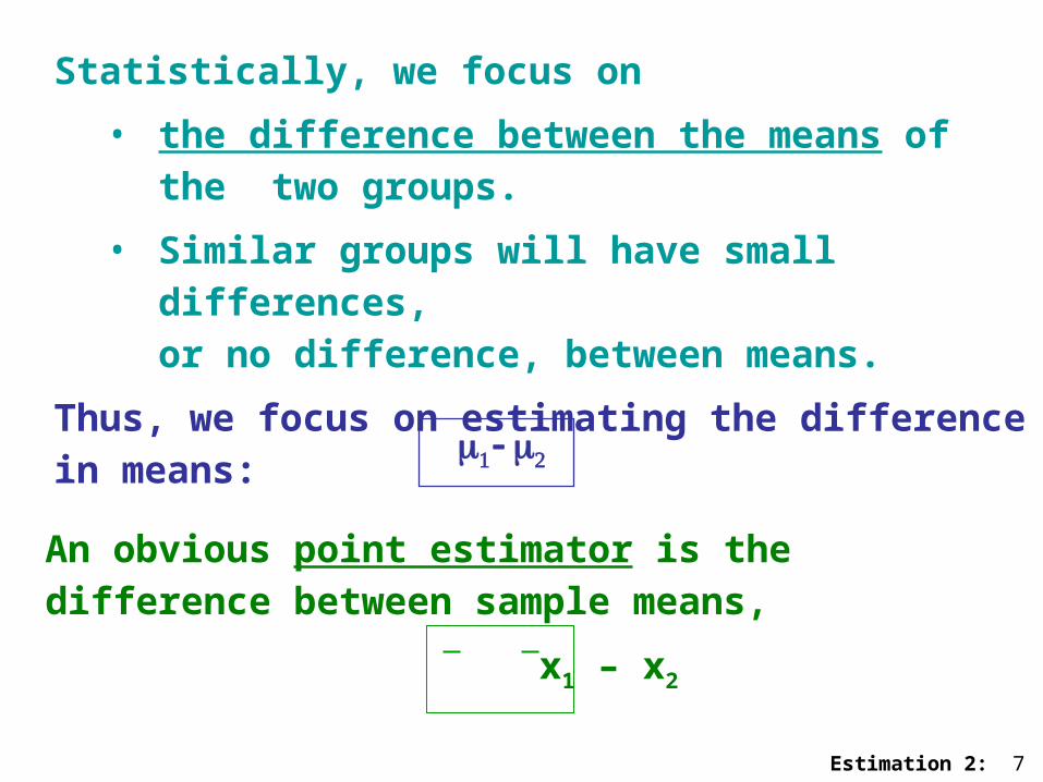
Statistically, we focus on

• the difference between the means of the two groups.

• Similar groups will have small differences, or no difference, between means.

Thus, we focus on estimating the difference in means:

An obvious point estimator is the difference between sample means,

x1 – x2

Estimation 2: 8

To compute a confidence interval for this difference,

we need to know the standard error of the difference.

Suppose we take independent random samples from two different groups:

We know the sampling distribution of the mean for each group:

21 1 1~ ( , )x N 2

2 2 2~ ( , )x N

21

1 11

~ ( , )x Nn

22

2 22

~ ( , )x Nn

Estimation 2: 9

What is the distribution of the difference between the

sample means, (x1 – x2) ?

• The sum (or difference) of normal RVs will be normal. What will be the mean and variance?

• This is a linear combination of two independent random variables. As a result,

1 2 1 2

1 2 1 2var var var

E X X E X E X

X X X X

Estimation 2: 10

In general, for any constants a and b, :

2 22 21 2

1 2 1 21 2

~ ,ax bx N a b a bn n

That is, the distribution of the sum of ax1 and bx2,

• The mean is the sum of a1 and b2

• The variance is the sum of (a2)(var of

sampling distribution of x1) and

(b2)(var of sampling distribution of x2)

Estimation 2: 11

Letting a = 1, and b = -1, we have:

2 21 2

1 2 1 21 2

( ) ~ ,x x Nn n

Thus, the standard error of the difference between means:

1 2

2 21 2

1 2x x n n

Estimation 2: 12

Once we have

• a point estimate

• its standard error,

→ we know how to compute a confidence interval estimate.

ConfidenceInterval

Estimate

PointEstimate

ConfidenceCoefficient

StdError

x1 – x2 Percentile From N(0,1)

2 21 2

1 2n n

Percentile from tdf

Est. of std errors2 estimated from samples

2 known

Estimation 2: 13

Example: Data are available on the weight gain of weanling rats fed either of two diets. The weight gain in grams was recorded for each rat, and the mean for each group computed:

Diet Group #1 Diet Group #2

n1 = 12 rats n2 = 7 rats

x1 = 120 gms x2 = 101 gms

What is the difference in weight gain between rats fed on the 2 diets, and a 99% CI for the difference?

Estimation 2: 14

We will assume a. The rats were selected via independent simple random samples

from two populations.

b. the variance of weight gain of weanling rats is known, and is the same for both diet groups:

12 = 2

2 = 400

Construct a 99% confidence interval estimate of the difference in mean weight gain, 1 – 2

1. Point Estimate: x1 – x2 = 120 – 101 = 19 gms

2. Std error of point estimate:

1 2

2 21 2

1 2

400 4009.51

12 7x x n n

Estimation 2: 15

3. With known variance, use a percentile of N(0,1):

For (1 – = .99, z.995 = 2.576

4. The 99% CI for 1 – 2 is:

= (–5.5, 43.5) gms

2 21 2

1 2 1 / 21 2

( ) ( ) 19 (2.576)(9.51)x x zn n

Estimation 2: 16

How do we interpret this interval? (–5.5, 43.5) gms

With different samples, we will have different estimates of the true difference in gains. The endpoints of the confidence interval indicate how wide the difference in estimates is expected to be 99% of the time.

Alternatively, if we repeatedly selected samples and computed a CI, then for 99% of the intervals computed would include the true difference in gains.

Estimation 2: 17

How do we compute a confidence interval when • we don’t “know” the population variance(s), • but must estimate them from our samples?

If 12 and 2

2 are UNknown:

Is it reasonable to assume that the variances of the two groups are the same?

That is, is it OK to assume unknown 12 2

2 ?

Questions to consider:• Do data arise from the same measurement

process?• Have we have sampled from the same population?• Does difference in groups lead us to expect

different variability as well as different mean levels?

Estimation 2: 18

If OK to assume variances equal: 12 = 2

2 = 2

• We have 2 estimates of same parameter, 2

• One from each sample: s12 and s2

2

We can create a pooled estimate: sp2

• This is a weighted average of the 2 estimates of the variance

• Weighting by (ni–1) for the ith sample

2 22 1 1 2 2

1 2

( 1) ( 1)

( 1) ( 1)p

n s n ss

n n

Estimation 2: 19

The standard error of the difference in means, x1 – x2

is then:

That is,

Sp2 is used as an estimator of the variance of x1

and of x2 rather than the two sample estimates

2 2

1 21 2

( ) p ps sse x x

n n

Estimation 2: 20

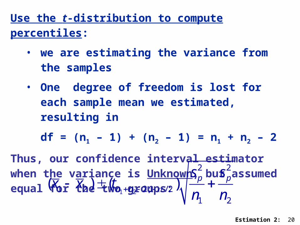
Use the t-distribution to compute percentiles:

• we are estimating the variance from the samples

• One degree of freedom is lost for each sample mean we estimated, resulting in

df = (n1 – 1) + (n2 – 1) = n1 + n2 – 2

Thus, our confidence interval estimator when the variance is Unknown, but assumed equal for the two groups:

1 2

2 2

1 2 2;1 / 21 2

( ) ( ) p pn n

s sx x t

n n

Estimation 2: 21

Example: Weanling Rats Revisited

Diet Group #1 Diet Group #2

n1 = 12 rats n2 = 7 rats

x1 = 120 gms x2 = 101 gms

s12 = 457.25 g2 s2

2 = 425.33 g2

Is there a difference in mean weight gain among rats fed on the 2 diets?

• Use sample estimates of the variance• Assume that the variances are equal since

• the rats in each group come from the same breed

• were fed the same number of calories on their different diets

• Used same scale in weighing.

Estimation 2: 22

Assuming 12 2

2, equal but unknown, construct a

99% CI for the difference in means, 1 – 2 .

1. Point Estimate: x1 – x2 = 120 – 101 = 19 gms

2. Std error of point estimate:Step 1: sp

2

2 22 1 1 2 2

1 2

( 1) ( 1)

( 1) ( 1)p

n s n ss

n n

2(12 1)(457.25) (7 1)(425.33)445.98

12 7 2gm

Estimation 2: 23

Step 2: SE of point estimate:

3. Confidence Coefficient for 99% CI:

df = n1+n2 – 2 = 12 + 7 – 2 = 17

1 = .99 /2 = .005 1 – /2=.995

t17;.995= 2.898

2 2

1 21 2

445.98 445.98( ) 10.04

12 7p ps s

se x xn n

Estimation 2: 24

3. Confidence interval estimate of (1 – 2):

(-10.1, 48.1)

Again, we can conclude that if we repeated the study many times, and looked at how widely the sample mean differences were spread out (99% of the time), then the width would be equal to the confidence interval width.

Notice that the width is wider than when we know the variance.

1 2 17;.995 1 2( ) ( ) ( ) 19 (2.898)(10.04)x x t se x x

Estimation 2: 25

What if it is not reasonable to assume that the variances of the two groups are the same?

When it seems likely that 12 2

2

For example

• we have used a different measuring process

• we have other reasons to believe both the mean level and variability are different between the two populations

Then

• Use separate estimates of the variance from each sample, s1

2 and s22

• Compute Satterthwaite’s df – and appropriate t-value

Estimation 2: 26

Satterthwaite’s Formula for Degrees of freedom:22 2

1 2

1 22 22 2

1 2

1 2

1 21 1

s sn n

fs sn n

n n

horrible … avoid computing by hand!

Note • it is a function both of the sample sizes and the

variance estimates. • When in fact the variances and sample sizes are

similar – the df will be similar to the pooled variance df.

Estimation 2: 27

Putting it all together yields

the CI estimator when UNknown 12 2

2 :

Note: use separate estimates of standard error of sample means for each sample

2 21 2

1 2 ;1 / 21 2

( ) ( )f

s sx x t

n n

Estimation 2: 28

Example: Weanling Rats Once Again!

Assume that the population variances are not equal –

12 2

2 .

Diet Group #1 Diet Group #2

n1 = 12 rats n2 = 7 rats

x1 = 120 gms x2 = 101 gms

s12 = 457.25 g2 s2

2 = 425.33 g2

Is there a difference in mean weight gain among rats

fed on the 2 diets?

Compute at 99% CI for the difference in the group

means, assuming 12 2

2 .

Estimation 2: 29

1. Point Estimate: x1 – x2 = 120 – 101 = 19 gms

2. Std error of point estimate:

3. Confidence Coefficient for 99% CI:

df = f = … = 13.08 use 13

1 = .99 /2 = .005 1 – /2=.995

t13;.995= 3.012

2 21 2

1 21 2

457.25 425.33( ) 9.94

12 7

s sse x x

n n

Estimation 2: 30

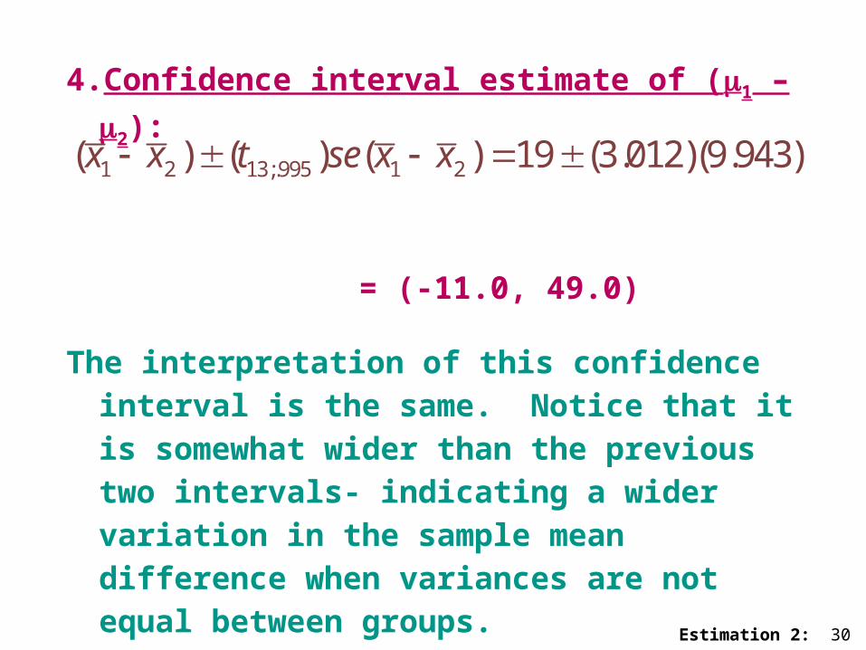
4. Confidence interval estimate of (1 – 2):

= (-11.0, 49.0)

The interpretation of this confidence interval is the same. Notice that it is somewhat wider than the previous two intervals- indicating a wider variation in the sample mean difference when variances are not equal between groups.

1 2 13;.995 1 2( ) ( ) ( ) 19 (3.012)(9.943)x x t se x x

Estimation 2: 31

Since the unit is common to the two measures, we

expect

• the two responses to the unit to be similar in

some respects

• We expect the 1st and 2nd responses within a

unit to be related.

Studies use this design to reduce the effects of

subject-to-subject variability

• This variability can be reduced by subtracting

the common part out.

• We do this by taking the difference between the

2 measures, on the same subject or unit.

Estimation 2: 32

Analysis of Paired Data Focuses on:

difference = Response 2 – Response 1

for each subject, or paired unit.

Work with the differences –

• as if never saw the individual paired responses

• and see only the differences as our data set

• The data set comprised of differences has been

reduced to a one sample set of data.

• We already know how to work with this.

Estimation 2: 33

1st Response Difference2nd – 1st

1 x1 = 10

… xi

n

2nd Response

y1 = 12 d1 = 12–10 = 2

yi di = xi – yi

xn = 14 y1 = 11 dn = 11–14 = -3

Note:• The order in which you take differences is

arbitrary, but it must be consistent. If you choose

yi – xi , then compute that way for all pairs.

• Direction is important. Keep track of positive and

negative differences.

Estimation 2: 34

Confidence Interval Calculations for the mean difference, d

Preliminaries:

1. Compute sample of differences, d1, …, dn , where

n = # of paired measures.

2. Obtain sample mean and sample variance of the differences

3. Treat like any other 1-sample case for estimating a mean, , (here a mean difference.)

1

1 n

ii

d dn

2 2

1

1( )

1

n

d ii

s d dn

Estimation 2: 35

Example: Reaction times in seconds to 2 different stimuli are given below for 8 individuals. Estimate the average difference in reaction time, with a 95% CI. Does there appear to be a difference in reaction time to the 2 stimuli?

Subject X1 X2 Difference (X2 – X1)

1 1 4 3

2 3 2 -1

3 2 3 1

4 1 3 2

5 2 1 -1

6 1 2 1

7 3 3 0

8 2 3 1

Estimation 2: 36

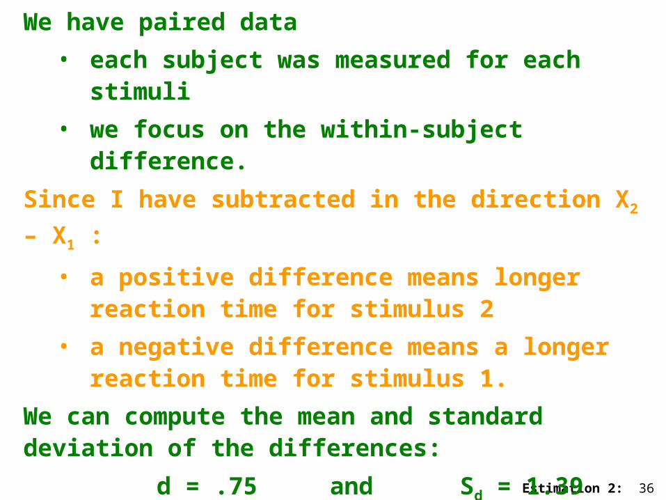
We have paired data

• each subject was measured for each stimuli

• we focus on the within-subject difference.

Since I have subtracted in the direction X2 – X1 :

• a positive difference means longer reaction time for stimulus 2

• a negative difference means a longer reaction time for stimulus 1.

We can compute the mean and standard deviation of the differences:

d = .75 and Sd = 1.39

Estimation 2: 37

• For a 95% confidence interval,

• using my sample estimate of standard error,

• use the t-distribution.

The confidence interval is:

d ± tn-1; .1-/2(sd/n) = .75 ± t 7; .975(sd/8)

= .75 ± 2.36 (1.39/8)

95% CI is (-0.41, 1.91)

The results indicate that repeating the study may produce an estimate quite different from that observed, and even possibly a negative estimate.

Estimation 2: 38

Notes:

• It is a common error to fail to recognize paired data, and therefore fail to compute the appropriate confidence interval.

• The mean difference d is equal to the difference

in means, 2 – 1 if we ignore pairs – your point

estimate will be correct.

• However, the variance of the mean difference does NOT equal the variance of the difference in means – so the confidence interval will not be correctly estimated if you neglect to use a paired data approach.

Sd2/n = (S1

2/n) + (S22/n)-2Cov/n

Estimation 2: 39

Confidence Interval Estimation

of the Variance, 2

Standard Deviation,

and Ratio of Variances of 2 groups

Estimation 2: 40

3. Confidence Interval for the variance, 2:Introducing the 2 Distribution

What if our interest lies in estimation of the variance, 2 ?

Some common examples are:• Standardization of equipment

– repeated measurement of a standard should have small variability

• Evaluation of technicians – are the results from person i “too variable”

• Comparison of measurement techniques – is a new method more variable than a standard method?

Estimation 2: 41

We have an obvious point estimator of 2 s2, which we have shown earlier is an unbiased estimator (when using Simple random with replacement sampling).

How do we get a confidence interval?

We will define a new standardized variable, based upon the way in which s2 is computed:

That is, [(n-1)s2 / 2] follows a chi-square distribution with n-1 degrees of freedom

22 2

12

( 1)~ n

n s

Estimation 2: 42

A quick and dirty derivation:

We defined the sample variance as:

Multiplying each side by (n-1):

2 2

1

1( )

1

n

ii

s x xn

2 2

1

( 1) ( )n

ii

n s x x

Note this is the numerator from the 2 variable.

This side is the sum of squared deviations from the mean.

Estimation 2: 43

Recall, for X ~ N(, 2)

We can standardize as: ~ (0,1)X

N

If we square this, we have a squared standard normal variable:

221~

X

That is, a squared standard normal variable follows

a chi- square distribution, with 1 degree of freedom

– this is the definition of a chi-square, df=1

Estimation 2: 44

If we sum n such random variables, we define a chi-square distribution with n degrees of freedom:

However, if we first estimate from the data: x, we reduce the degrees of freedom:

22

21

( )~

ni

ni

x

2 2212 2

1

( ) ( 1)~

ni

ni

x n sx

Estimation 2: 45

Features of the Chi Square Distribution

• Chi-squared variables are sums of squared Normally distributed variables.

• Chi-squared random variables are always positive. (Why? –square is always positive)

• The distribution is NOT symmetric. A typical shape is:

0

Estimation 2: 46

• Each degree of freedom defines a different distribution.

• The shape is less skewed as n increases.

df = 1df = 2

df = 4df = 6

df =10df = 100

Features of the Chi Square Distribution

Estimation 2: 47

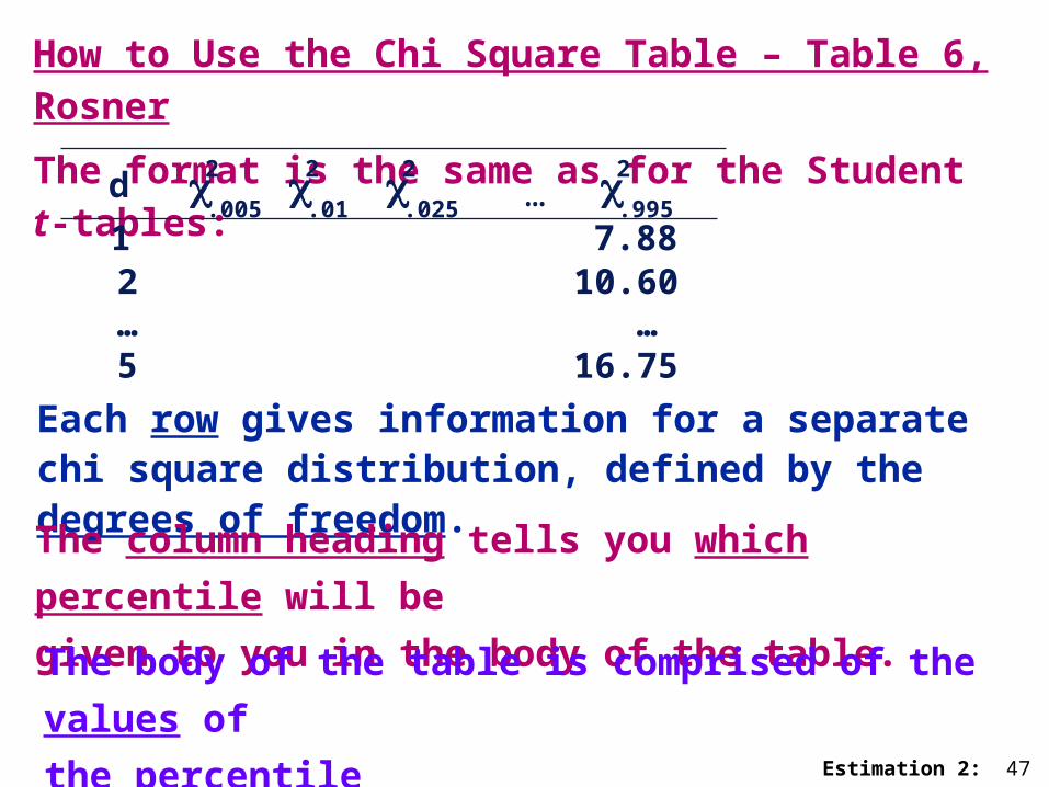
How to Use the Chi Square Table – Table 6, Rosner

The format is the same as for the Student t-tables:

d .005

2…

1 7.882…5

10.60 …16.75

.995

2.01

2

Each row gives information for a separate chi square distribution, defined by the degrees of freedom.

The column heading tells you which percentile will be

given to you in the body of the table.

The body of the table is comprised of the values of

the percentile

.025

2

Estimation 2: 48

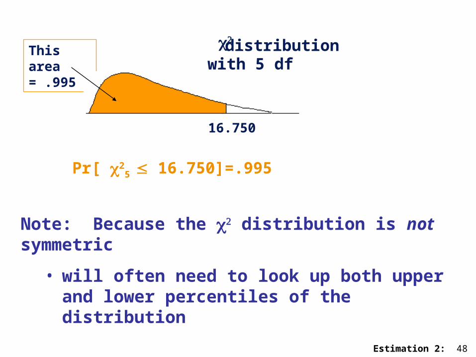
This area= .995

16.750

distributionwith 5 df

Pr[ 25

16.750]=.995

Note: Because the distribution is not symmetric

• will often need to look up both upper and lower percentiles of the distribution

Estimation 2: 49

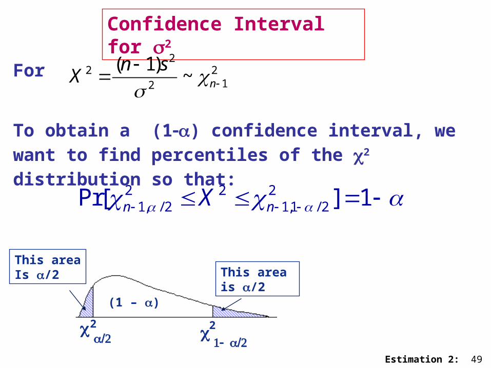
Confidence Interval for 2

2

2

(1 – )

This area is /2

This areaIs /2

For

To obtain a (1) confidence interval, we want to find percentiles of the 2 distribution so that:

22 2

12

( 1)~ n

n sX

2 2 21, / 2 1,1 / 2Pr[ ] 1n nX

Estimation 2: 50

Substitute for X2 in the middle of the inequality:

2 2 21, / 2 1,1 / 2Pr[ ] 1n nX

22 21, / 2 1,1 / 22

( 1)Pr[ ] 1n n

n s

A little algebra yields the confidence interval formula:

2 22

2 21,1 / 2 1, / 2

( 1) ( 1)Pr 1

n n

n s n s

Estimation 2: 51

Lower limit ofthe (1– ) CI:

Upper limit ofthe (1– ) CI:

2

21,1 / 2

( 1)

n

n s

2

21, / 2

( 1)

n

n s

Confidence Interval for 2

Estimation 2: 52

Exercise

A precision instrument is guaranteed to read accurately to within 2 units.

A sample of 4 readings on the same object yield 353, 351, 351, and 355.

Find a 95% confidence interval estimate for the population variance, 2 and also for the population standard deviation, .

Estimation 2: 53

Solution

1. Point Estimate: We must first estimate the mean,x = 352.5, and then the variance, s2 = 3.67

2. Since n=4, the correct chi-square distribution has df = n-1 = 3.

.95This area = .025 This area = .025

3. For a (1) = .95 CI

= .05 /2 = .025 and 1/2 = .975

We want 23;.025 and 2

3;.975

23;.025 2

3;.975

Estimation 2: 54

4. Using Table 6 in Rosner (page 758) :

(i) Using column labeled .025 read down to

df= 3 row

23;.025 = .216

(ii)Using column labeled .975 read down to

df= 3 row

23,.925 = 9.35

(or use Minitab or other program…)

Estimation 2: 55

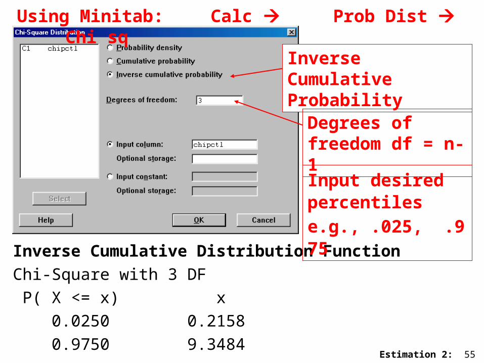
Inverse Cumulative Distribution Function

Chi-Square with 3 DF

P( X <= x) x

0.0250 0.2158

0.9750 9.3484

Using Minitab: Calc Prob Dist Chi sq

Inverse Cumulative Probability

Degrees of freedom df = n-1

Input desired percentiles e.g., .025, .975

Estimation 2: 56

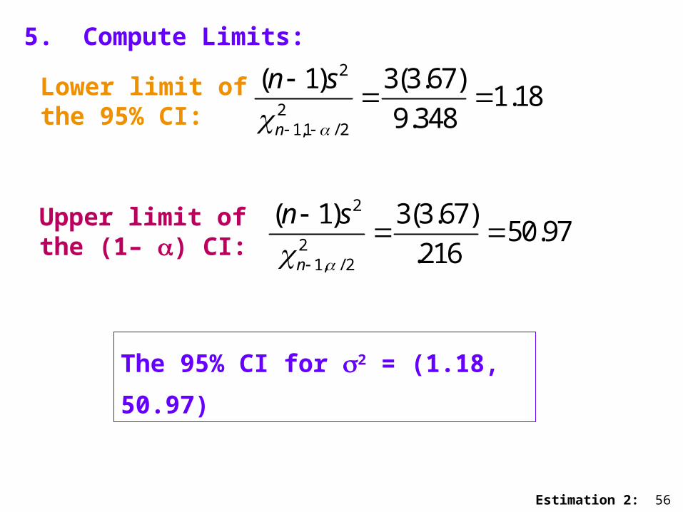
5. Compute Limits:

Lower limit ofthe 95% CI:

Upper limit ofthe (1– ) CI:

2

21,1 / 2

( 1) 3(3.67)1.18

9.348n

n s

2

21, / 2

( 1) 3(3.67)50.97

.216n

n s

The 95% CI for 2 = (1.18, 50.97)

Estimation 2: 57

6. To compute a confidence interval for the standard deviation,

• always compute a CI for the variance

• then take the square root of the upper and lower limits:

95% CI for : ( 1.18, 50.97 ) = (1.09, 7.14)

Point estimate for = 3.67 = 1.92

Does this precision instrument meet its ‘guarantee’ to accuracy within 2 units?

Estimation 2: 58

Note that the confidence intervals for

• are wide

• are not symmetric about the point estimate

• Only with very large n

• will you find relatively narrow confidence interval estimates for the variance and standard deviation.

1.09 1.92 7.14

LL s UL

Estimation 2: 59

Confidence Interval calculation for the ratio of two variances – introducing the F-distribution

We are often interested in comparing the variances of 2 groups.

• This may be the primary question of interest:

I have a new measurement procedure – are the results more variable than the standard

procedure?

• Comparison of variances may also be a preliminary analysis to determine whether it is appropriate to compute a pooled variance estimate or not, when the goal is comparing the mean levels of two groups.

Estimation 2: 60

For comparing variances, we use a RATIO rather than a difference.

• We look at the ratio of variances: x2/y

2

• If this ratio is 1 the variances are the same

• If it is far from 1 the variances differ.

In order to

• make probability statements about ratios of variances

• to compute confidence intervals

we need to introduce another distribution, known as the

F-distribution

Estimation 2: 61

A Definition of the F Distribution

IF x1, … xnx are each independent Normal (x, x2)

and y1, … yny are each independent Normal (y, y2)

and if we calculate sample variances in the usual way

2 2

1

1( )

1

xn

x iix

s x xn

2 2

1

1( )

1

yn

y iiy

s y yn

Estimation 2: 62

The ratio follows an F-distribution with two degree of

freedom specifications – for the numerator and for

the denominator.

numerator df = nx – 1

denominator df = ny – 1

THEN2 2

1; 12 2

/~

/ x y

x xn n

y y

sF

s

Estimation 2: 63

Percentiles of the F-distribution are tabulated, as in the Appendix of Rosner, Table 9, pages 762-764.

Using the Table:

• Each row defines a different percentile distribution for a given denominator df.

• Each column defines a different numerator df.

• The body of the table gives values of the F-distribution.

• Only the upper-tail percentiles (.90, …, .999) of the distribution are tabulated.

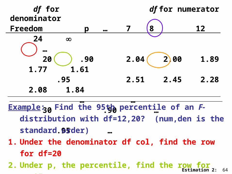
Estimation 2: 64

df for df for numeratordenominatorFreedom p … 7 8 12 24 … 20 .90 2.04 2.00 1.89 1.77 1.61

.95 2.51 2.45 2.28 2.08 1.84 … … 30 .90 …

.95 …

Example: Find the 95th percentile of an F-distribution with

df=12,20? (num,den is the standard order)

1. Under the denominator df col, find the row for df=20

2. Under p, the percentile, find the row for p=.95

3. Find the column headed by numerator df=12.

4. Read the value at their intersection: F12,20; .95 = 2.28 .

Estimation 2: 65

For lower-tail percentiles (.005, …, .10) which are not

tabulated, we use the fact that:

The percentiles of an F with numerator df=a

denominator df=b

are related to

The percentiles of an F with numerator df=b

denominator df=a

as:

, ;( ), ;(1 )

1a b

b a

FF

Estimation 2: 66

Example: What is the 5th percentile of an F-

distribution with df=12,20?

We have already looked up this value.

20,12;(.05)12,20;(.95)

1 1.439

2.28F

F

Lower and upper tail percentiles can be computed

directly using Minitab – no need to invert.

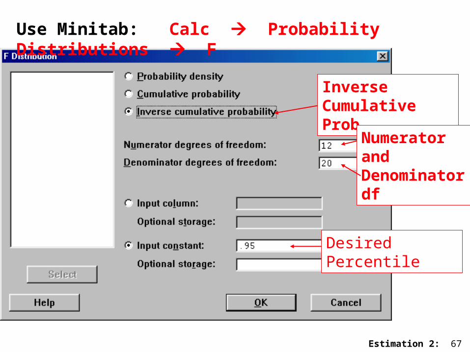
Estimation 2: 67

Use Minitab: Calc Probability Distributions F

Inverse Cumulative Prob

Numerator and Denominator df

Desired Percentile

Estimation 2: 68

Inverse Cumulative Distribution Function

F distribution with 12 DF in numerator and 20 DF in denominator

P( X <= x) x

0.9500 2.2776

Estimation 2: 69

Confidence Interval for the ratio of 2 Variances: x2/y

2

IF x1, … xnx are each independent Normal (x, x2)

and y1, … yny are each independent Normal (y, y2)

A point estimate of x2/y

2 is

sx2/sy

2

Estimation 2: 70

A (1) Confidence Interval Estimate has:

2

21, 1;(1 / 2)

1:

x y

x

y n n

sLL

s F

2

21, 1;( / 2)

1:

x y

x

y n n

sUL

s F

2

1, 1;(1 / 2)2 y x

xn n

y

sF

s

Estimation 2: 71

Example:

Pelicans were exposed to DDT. Is there a difference in variability of residue found in juveniles and nestling birds?

Juvenile Pelicans Nestling Pelicans

n1 = 10 n2 = 13

s1 = .017 s2 = .006

Compute a 95% Confidence Interval for the ratio of true variances, s1

2/s22 .

Estimation 2: 72

1. Point estimate:

s12/s2

2 = (.017)2 / (.006)2 = 8.03

2. Percentiles of F:

F9,12;.975 = 3.44

F9,12;.025 = .286

3. Confidence Limits:2

21, 1;(1 / 2)

1 1: 8.03 2.33

3.44x y

x

y n n

sLL

s F

Estimation 2: 73

2

21, 1;( / 2)

1 1: 8.03 31.07

.286x y

x

y n n

sUL

s F

A 95% CI for the variance ratio is (2.33, 31.07) .

Notice that the width of the sampling distribution of variance ratios is very broad. Since 1 is not in the interval, it appears that the variances of the groups are different, with juvenile pelicans having a greater variability in DDT residue.

Note: always work with variances, not standard deviations.