Centre forEconomicand FinancialResearchatNew Economic School

Estimation of IndividualDemand for Alcohol

Y. AndrienkoA. Nemtsov

Working Paper No 89

CEFIR / NES Working Paper series

January 2006

Abstract

Using individual data from RLMS, the longitudinal survey of the representative sample

of the Russian population, we study static and dynamic models of demand for alcohol. We show

the demand curve has traditional negative slope for any type of alcoholic drink: vodka, beer, and

wine. We find substitution of moonshine for vodka with higher price on vodka and between

vodka&beer with higher price on one of them. As a result of substitution vodka price has no

impact on total ethanol consumption, while higher price on beer and wine reduce demand for

ethanol. We also demonstrate that income has important effect on demand for alcoholic drinks.

Risk to be drinker is rising with individual income. Higher income results in lower consumption

of moonshine and in higher consumption of vodka, beer, and wine.

JEL classification: I1; I18

Keywords: alcohol; demand; Russia

Non-technical summary Alcohol like cigarettes should be treated differently from other consumer goods due to its

serious negative outcomes for health. In Russia a number of indicators linked to alcohol abuse,

such as personal violence (homicides and suicides), mortality (from alcohol poisoning and

accidents), and life expectancy are among the worst in the world. Public regulation of alcohol

branch should not only aim to bring maximum budget revenues from highly profitable

production but ideally minimize harm.

As it was shown by two prohibition campaigns in Russian history in XX century,

regulation is able to affect public health in great degree. One of the common and accessible

mechanisms of alcohol market regulation is taxation which is reflected in price formation.

Decreasing demand curve is a common empirical result in economic literature on alcohol

consumption and smoking in developed countries. WHO has even a recommendation for lower

income countries to increase prices on tobacco which immediately brings positive effect on

public health.

In this project we consider economic model of rational addictive behavior. From the

model one can derive a dynamic empirical model of alcohol consumption. For empirical

investigation of the demand curve slope we explore mostly available individual data from

RLMS, the longitudinal survey of a representative sample of Russian population. Due to a large

number of censored (zero) observations we use Tobit model. We show the demand curve has a

traditional negative slope for any type of alcoholic drink: vodka, beer, and wine. We find

substitution of moonshine for vodka with higher price on vodka and between vodka&beer with

higher price on one of them. As a result of substitution vodka price has no impact on total

ethanol consumption, while higher price on beer and wine reduce demand for ethanol. We also

demonstrate that income has important effect on demand for alcoholic drinks. Risk to be drinker

is rising with individual income. Higher income results in lower consumption of moonshine and

in higher consumption of vodka, beer, and wine.

Introduction Alcohol is not an ordinary consumer good because of negative consequences linked to its

consumption, the cardinal of which is the ability to cause dependence and even death. Degree of

harm connected to alcoholic drinks depends on the level and structure of alcohol consumption. In

their turn, the levels of alcohol consumption and abuse are determined by several factors such as

availability, income, retail process, public policy and individual factors including genetic,

psychological, ecological, and other (World Bank, 2003).

Public alcohol policy should aim at harm minimization. Among the first priority tasks,

countries should seek to significantly decrease alcohol consumption (Edwards et al, 1994). This

does not mean that there is a need in alcohol prohibition since the Soviet and international

practices show it is all but impossible. Significant reduction of production ultimately leads to

dire consequences due to consumption of low-quality drinks, in particular moonshine. There

should be right balance between the need in alcohol and its availability, between industrial and

domestic production. There are a number of instruments, economic and political, which have

impact on the size of both markets. No doubt that development of preventive measures should be

focused on certain groups (teenagers, women, and hard drinkers) and circumstances of

consumption (drunken driving, drinking on job, on street, and in public places).

From an economic standpoint demand for alcohol can be studied as for ordinary

consumer good. On the first glance higher prices on alcohol after raised taxation on production

and distribution should lead to lower alcohol consumption due to lower available income. But it

is indubitably for many that such policy in Russia is accompanied by substitution of illegal

alcohol, in particular moonshine (samogon in Russian), for legal drinks. Anti-alcohol campaign

in the former Soviet Union showed that it took a mere five years to compensate the reduction in

legal production. But many important details of this process are unknown.

Also, it is not clear what happens with alcohol consumption when income becomes

higher. Country aggregate panel data for alcohol consumption from WHO shows positive

dependence on GDP per capita1. However in higher income countries alcohol consumption has

been gradually declining since 70 or 80-es. In fact this seems to occur due to different restrictive

policies and reasonable alcohol policy.

It is quite within reason to suggest, that higher personal income as well as lower relative

price of alcohol may lead to higher availability of alcohol and consumption of better quality

drinks. Therefore, risk to be drinker, the level of consumption and its structure may change with

income and price. If these hypotheses are true, then stable or decreasing real prices on alcohol

1 This result is obtained by Y. Andrienko for spirits consumption and total ethanol consumption on the sample of 150 countries for time period from 1975 to 2000 controlling for country (fixed) effect.

may not lead to the desired result, the reduction of alcohol related harm during the period of

economic growth.

If alcohol is a luxury good then rich people spent higher proportion of income on

alcohol. It is known from household budget surveys that a family from higher income group has

higher expenditures on alcohol and even higher its proportion in total expenditures (Goskomstat,

2003). However, traditional alcohol consumption–income curve has U- or J-shape. Therefore,

one can expect that consumption of alcohol by one category can be higher with income but lower

for another.

One of the major distinctions of alcohol is that it is a habit forming good. This fact may

indicate that demand is more stable for particular category of population and consumption is less

sensitive to change in price. Therefore, alcohol policy has long-run effect which overweighs

often invisible short-run changes. Any policy other than shock therapy such as notorious

Gorbachev’s anti-alcohol campaign in 1985 is not expected to provide immediate results.

Another attribute of alcohol, indicated by psychologists and sociologists, is that its

consumption is usually collective process which serves to facilitate contacts (so called

“communicative dope”). Due to social interaction the style of alcohol consumption is often

unified (“social diffusion”). As a result, the more people around drink, the more a given

individual drinks. In this project we test the hypothesis about influence of drinkers in a

household on individual alcohol consumption.

Beside to the recognized negative influence of alcohol, it has several pharmacological

properties such as to distress, boost spirits and rouse from the depression. Also, alcoholic drinks

and especially red wine lower risk of male cardio-vascular disease when drinking is moderate.

The Soviet Russia has seen the serious socio-economic and medical consequences of

immoderate drinking since the end of 50-es in XX century. The anti-alcohol campaign during the

mid of 80-es was aimed to solve these problems drastically. Though poorly organized, it was

quite successful in the short run. It led to reduction of the legal alcohol production, to higher

prices on alcohol beverages and as a result to decreased availability of alcohol and significant

fall in consumption. However, by the period of the market reforms alcohol consumption had

approached level that was before the campaign due to underground production. Low labor

productivity and especially high level of industrial injuries were the direct consequences of hard

alcohol consumption for the economy during transition period. Mortality rates from injuries,

poisoning, and accidents closely connected with alcohol abuse, became even more dramatic.

By these indicators the Russian Federation is among the most unfavorable countries in

the world. Among 74 countries Russian homicide rate is the forth highest after that in Columbia,

El Salvador, and Brazil and suicide rate is the second highest after Lithuanian one (WHO, 2002).

It was recently estimated that 30 percent of all deaths in Russia are directly or indirectly

connected with alcohol (Nemtsov, 2002). The similar estimates for other countries are

substantially lower. Not surprisingly life expectancy of males is extremely low, 58.5 years in

20022. Labor force is gradually decreasing thereby bringing long term economic problem.

Therefore, there is an urgent need of reduction in alcohol related harm and losses in Russia,

especially among vulnerable groups.

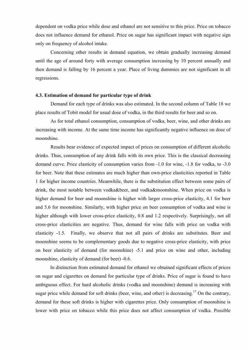
Figure 1.

Alcohol consumption, real income and relative price of alcohol

11

12

13

14

15

16

1990 1991 1992 1993 1994 1995 1996 1997 1998 1999 2000 20010

0.2

0.4

0.6

0.8

1Alcohol consumption, litres of ethanol (left scale) Real income, 1991=1 (right scale) Relative price of alcohol, 1990=1 (right scale)

Sources: Nemtsov (2003a), Goskomstat (2003) A question arises: what economic mechanisms affect alcohol consumption? At present

alcohol supply is not restricted; it is competitive market, half of which is not regulated by the

state in the past two decades (according to Chamber of Counting only 34 percent of consumed

hard drinks are legal). This means that political decision has low efficiency in the near future.

Real alcohol consumption has been fluctuating during the transition period. It grew until 1994,

then fell until 1998 and again has been rising to date. What factors determine the fluctuations of

alcohol consumption when availability of alcoholic drinks is not restricted? As we may see on

Figure 1, alcohol consumption rise in 1990-94 was accompanied with sharp fall in alcohol

prices. Then period of reduction in consumption 1995-97 coincided with somewhat dearer

alcohol. Finally, since 1999 consumption has been increasing while prices are relatively stable

since 1998. At the same time, there is no any unequivocal link with average income. Thus, there

were periods of both unidirectional changes (93-95, 98, 00-01) and changes in the opposite

2 It is not to be compared with life expectancy of males in Europe, 74-77 and even with Russian females’ 72, thereby achieving 14 years the maximum gender difference in the world.

direction (92, 97, and 99). Does this mean that alcohol consumption is not correlated with

income?

All of the above-mentioned approaches us to the main problem: what determines alcohol

consumption during the last decade? We are going to concentrate our efforts on the partial

problem: what is important in this process on the individual level? Thus, the main goal of the

project is to estimate individual demand for alcohol in Russia.

Main hypothesis. First of all, we are going to check whether alcohol is a normal good

that is individual demand for alcohol of better quality is increasing with income. Also we test

whether alcohol has a classical negative slope of the demand curve. Under individual demand

for alcohol in this project we mean not only total ethanol3 consumption but also decision to drink

or not, frequency of alcohol consumption, accustomed doses of different alcoholic drinks. The

generalized hypothesis states that individual demand depends on economic characteristics,

individual and aggregate (such as household income and prices on different alcoholic drinks),

and other individual characteristics (such as gender, age, and environment).

The empirical part is based on the estimation of a generalized demand equation, which is

the level of individual consumption of alcohol as a function of income, prices on alcohol drinks

and other individual and household characteristics. This model can be in the dynamic form.

Therefore, not only short-term effects can be estimated in the demand equation but also long-

term effects. The stationary and dynamic demand equations are estimated by Tobit model since

the data contains some proportion of censored (zero) observations.

Data to be used in the project comes from Russian Longitudinal Monitoring Survey

(RLMS). This survey is regularly conducted during ten-year period, except to 1997 and 1999, on

the representative sample of population. Every round includes about 4000 households. The

standardized interview contains numerous questions on health, nutrition, and economic status. In

addition, a number of questions about consumption of addictive goods, such as cigarettes and

different types of alcoholic drinks are asked. In the empirical part of the project a model of

consumption will be estimated on the individual panel data from 5-11 rounds of RLMS covering

period 1994-2002.4

3 Hereafter, under ethanol we mean pure (100%) alcohol. We use conventional measure of ethanol consumption in liters and milliliters (ml) but not in grams and kilograms since density of ethanol is less than that of water. In order to imagine the volume of ethanol reported throughout this paper, 1 litre of ethanol is contained in 5 half-litre bottles of vodka. 4 There was another sample of population in rounds 1-4 in 1992-94, which organizers gave up.

The structure of this report is following. In the first chapter literature review on the

subject of the project is done. In the second we present theoretical models of addictive behavior.

The third chapter contains methodology and data description. The forth demonstrates obtained

results of econometric model estimation. The last one comprises conclusions.

1. Literature Addictive behavior is quite popular topic of economic research at present. How far the

economic science goes forward one may judge, for example, looking at two surveys in

Handbook of Health Economics, dedicated to the most popular addictive goods, cigarettes and

alcohol. The volumes and references of those articles show that number of papers on alcohol

consumption (Cook and Moore, 1999) is two-three times less than on smoking (Chaloupka and

Warner, 1999). Economic research in these fields spreads out from study of consumer behavior

(in particular includes its reaction to change of supply and price, advertisement and its ban) to

efficiency estimation of state interventions.

During the last years research in this field becomes politically motivated problem in

many countries because of necessity in state regulation and restructure into publicly acceptable

market of addictive goods and approaching the adequate level of their consumption. The

difficulty of studying this problem is explained by two facts. Hard alcohol consumption and

smoking have on the one hand, long term negative consequences to health and hence to economy

and on the other hand, are very profitable for producers, provide valuable budget revenues and

create jobs.

Beside recognized negative consequences of alcohol on health, there is evidence of lower

risk of cardio-vascular disease when drinking, especially of red wine, is moderate. However, this

result has no support in economic literature so far, possibly, due to other causes of lower risk,

including unobserved ones. In other sciences this fact is demonstrated, for example, by means of

one factor analysis for Russian senior males (see Aleksandri et al, 2003). As Finnish authors

show, this and other positive effects prevail over negative effect only for the level of ethanol

consumption below 2 litres per year.5 However, negative consequences such as high risk of

traumatism, in particular on the road, problems with health, within family or at work strongly

dominate beginning with this low level.

Not so much the level of alcohol consumption per capita is important as the composition

of consumption, which includes frequency, dose (how much a consumer drinks at a time), and

types of drinks. In the paper (Bobak et al, 2003) based on cross sectional survey of drinking in

one Russian, one Polish, and one Czech city authors show that while Russians have low mean

drinking frequency, they consume the highest dose of ethanol per drinking session and have

more individual problems related to drinking (see Table 8 in Appendix). In view of this fact

individual demand for alcohol should be thoroughly investigated, including finding what

determines the decision to drink, what to drink, how often and how much.

The major contribution of economic profession in the study of alcohol problems is in the

use of the standard model of consumer choice with intertemporary effects and social impact. The

most stable result in economic literature is repeatedly demonstrated fact that alcohol

consumption and problems related to it fell when prices on alcohol rise. Moreover, economic

literature shows decreasing demand curve for different types of alcohol (beer, wine, spirit) and

that increase in price on one type leads to reduction in total alcohol consumption. In Table 1 we

show the estimated price effect for a number of higher income countries. As a result of higher

prices share of hard drinking population decreases. At the same time, it is possible that

sensitivity to price change differs for diverse categories of population (Cook and Moore, 1999).

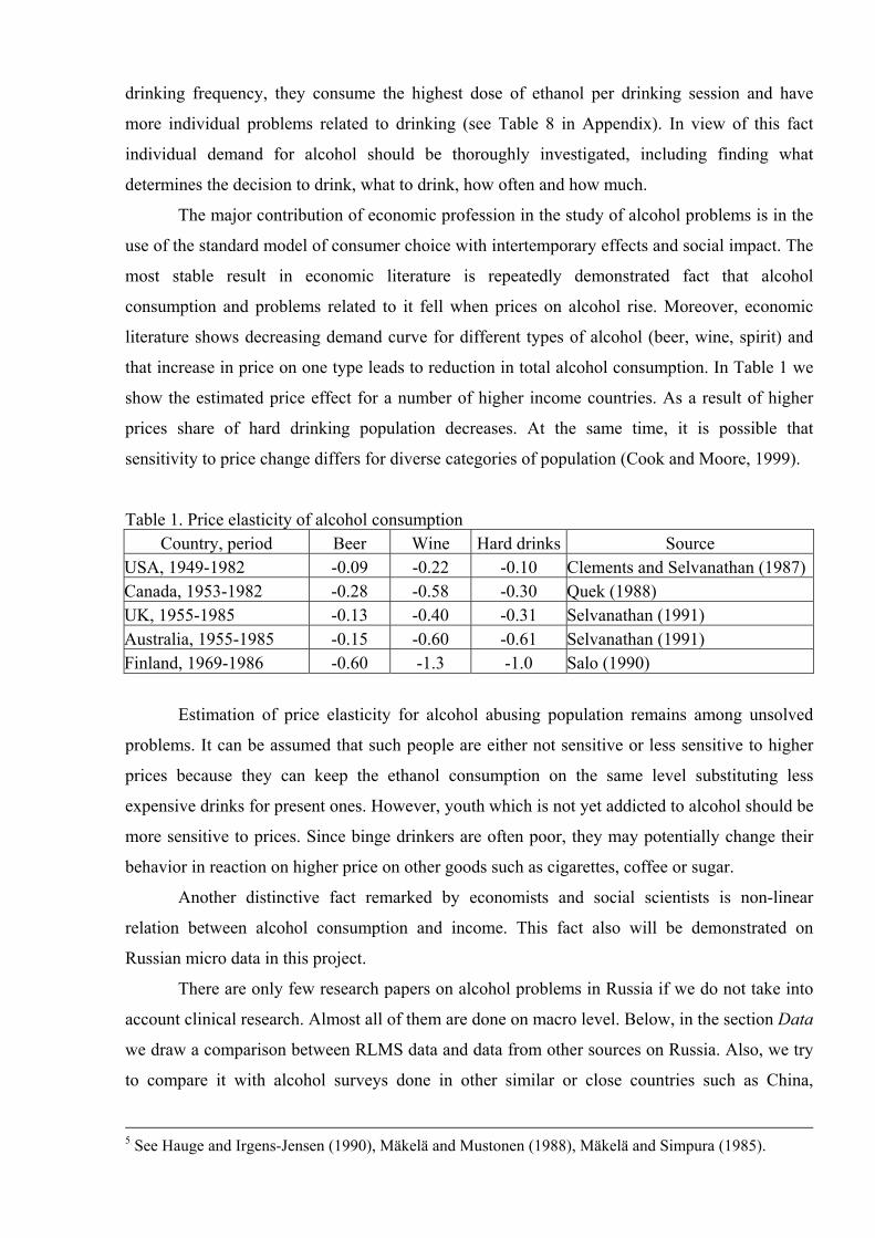
Table 1. Price elasticity of alcohol consumption Country, period Beer Wine Hard drinks Source

USA, 1949-1982 -0.09 -0.22 -0.10 Clements and Selvanathan (1987)Canada, 1953-1982 -0.28 -0.58 -0.30 Quek (1988) UK, 1955-1985 -0.13 -0.40 -0.31 Selvanathan (1991) Australia, 1955-1985 -0.15 -0.60 -0.61 Selvanathan (1991) Finland, 1969-1986 -0.60 -1.3 -1.0 Salo (1990)

Estimation of price elasticity for alcohol abusing population remains among unsolved

problems. It can be assumed that such people are either not sensitive or less sensitive to higher

prices because they can keep the ethanol consumption on the same level substituting less

expensive drinks for present ones. However, youth which is not yet addicted to alcohol should be

more sensitive to prices. Since binge drinkers are often poor, they may potentially change their

behavior in reaction on higher price on other goods such as cigarettes, coffee or sugar.

Another distinctive fact remarked by economists and social scientists is non-linear

relation between alcohol consumption and income. This fact also will be demonstrated on

Russian micro data in this project.

There are only few research papers on alcohol problems in Russia if we do not take into

account clinical research. Almost all of them are done on macro level. Below, in the section Data

we draw a comparison between RLMS data and data from other sources on Russia. Also, we try

to compare it with alcohol surveys done in other similar or close countries such as China,

5 See Hauge and Irgens-Jensen (1990), Mäkelä and Mustonen (1988), Mäkelä and Simpura (1985).

Nigeria, Poland, and Czech Republic. Official statistics reports data which does not reflect real

consumption (see Figure 8). Probably some estimates of alcohol consumption in Russia on

macro level are closer to reality such as in Treml (1997) and Nemtsov (2000), including scale of

alcohol related mortality (Nemtsov, 2002) and other high consequences of alcohol consumption

(Nemtsov, 2000). It was already noted that individual data from RLMS, the country

representative survey, significantly underestimate actual distribution of alcohol consumption

(Nemtsov, 2003).

There is no unanimity in estimation of economic consequences of high alcohol

consumption in Russia. Thus, analysis of employment and income based on RLMS shows

surprising result that the level of alcohol consumption has a positive impact on wage both for

males and females (Tekin, 2002), though the endogeneity problem is not accounted for properly.

Empirical results for other countries also confirm the result that abstainers earn less than drinkers

(e.g. Bryant et al, 1992, Zarkin et al, 1998). It is likely, that impact of alcohol on labor

productivity is indirect, affecting through the human capital accumulation (Cook and Moore,

1999).

While the most estimated demand equations for alcohol are done on macro level using

country or state level data only few studies explore micro data. None of them consider censored

nature of individual alcohol consumption data. Without dealing with this problem estimated

coefficients are biased. Economic literature on smoking is more progressive in this sense. It

provides models and results entertaining the censoring problem.

2. Model of alcohol consumption The common economic model of rational addiction (Becker and Murphy, 1988) is

considered in the theoretical basis of the project. In this model past and future consumption play

the primary role as it reflects the addictive effect.

We start with a model of demand for addictive good presented by Cook and Moor

(1995), which assumes “myopic” formation of addiction. Myopia assumption means that agent

recognizes that present consumption depends on past consumption but does not foresee that

future consumption is determined by past and present ones. The agent’s utility is a function of

the addictive good past and present consumption and consumption of a composite good with unit

price6. The following optimization problem is solved:

(1) ( ) max,, 1 →= − tttt YCCUU , under the budget constraint

6 For simplicity of the model exposition other variables in the utility function, such as gender, age, education, marital status etc, are not considered.

(2) tttt IYCP =+⋅

Notations include: U - utility, tC - consumption of the addictive good at period t, tY -

consumption of the composite good, tP - price of the addictive good, tI - income. Assuming the

constant marginal utility of income and quadratic utility function, the following empirical model

of demand for the addictive good is derived:

(3) ttttt IPСcС εγβα +⋅+⋅+⋅+= −1 ,

where tε is error term of the model.

The signs of parameters in the empirical model are determined by parameters of

quadratic utility function. Our basic hypotheses about these signs are that 0,0,0 ><> γβα .

In more general model of rational addiction an individual decides how much to consume

in present period taking into account not only past consumption but also future consumption

(Becker et al, 1994). Rationality in contrast to myopia means that the consumer foresees future

consumption of the addictive good. The consumer maximizes the discounted sum of the utilities:

(4) ( )tttt

t YCCUU ,, 10

−

∞

=⋅= ∑ β ,

where β is discount factor, given the budget constraint with the present value of income:

(5) ( )∑∞

==+⋅⋅

0tttt

t IYCPβ

For quadratic utility function and constant marginal utility of income and full

depreciation of the addictive stock the empirical model for consumption is the next:

(6) tttttt IPССcС εγβδα +⋅+⋅+⋅+⋅+= +− 11

Coefficient β is negative under the assumption of the concave utility function.

Coefficients α and δ are positive in case of rational addiction. In this case consumption in past

and present periods are complements as in present and future periods.

Econometric theory does not provide good methods of estimation for this model on

aggregate panel data. However, Becker et al (1994) have found an elegant solution. As the model

assumes that present consumption does not depend on price in past and future periods, then using

these prices as instruments for past and future consumption one get unbiased estimates of α and

δ . In their and series of other papers cigarettes and alcohol consumption are shown to follow

this empirical model and therefore, conform to the theory of rational addiction. This is done, in

particular, for alcohol consumption in USA (Becker et al 1994), for smoking in USA

(Chaloupka, 1991), Australia (Bardsley and Olekans, 1998), and Finland (Pekurinen, 1991).

Rational and myopic addiction models are analyzed in economic literature mostly on

aggregate level data. Micro level analysis meets with obstacles the major of which is presence of

zero observations. Econometric treatment of nondrinkers can be proposed in several ways.

Estimation of an individual demand for alcohol needs limited dependent variable models. In

general individual data on consumption of alcohol are censored like consumption of durable

goods because they are not purchased every week and therefore zero outcomes are frequent. The

nature of zeros is double: one wants to drink alcohol but can not afford it while another does not

like to drink at all.

In addition to considered models it is possible to derive the model on censored data with

separated participation and consumption decisions. One approach of dealing with censoring is

double-hurdle model of Jones (1989), suggested for cigarette consumption. The panel version of

this model was developed by Labeaga (1999) who estimated the model of rational addiction on

individual smoking data. He considered the trivariate model has the four equations:

1) Start equation { }01 >+⋅′= nhk γ

2) Quit equation { }01 >+⋅′= vzd α

3) Observed consumption *cdkc ⋅⋅=

4) Consumption equation { }uyc +⋅′= β,0max* , *c is called a latent variable, since

it is not observed in censored cases.

This model is more difficult to estimate than the bivariate model, which excludes the quit

equation. In the case of alcohol consumption we are not sure that any drinker or abstainer who

has zero alcohol consumption at present will not drink in future, therefore, quit equation does not

play the leading role.

The double-hurdle model means that the first hurdle is a decision of participation and the

second hurdle is a choice of non-zero consumption (non corner solution of utility maximization

problem). In this case the following method of estimation on panel data is applied. At the first

stage the binary dependent variable of participation is regressed on some independent variables

which may be different from those in consumption model. Then T cross-section regressions are

estimated for latent consumption in each period. At the second stage the model of consumption

is estimated on the panel entertaining the results from the first stage which correct estimates on

censoring bias (see methodology in Labeaga, 1999).

There are three alternatives to double-hurdle model. First, one could apply the panel

Heckman model which is the first hurdle dominance. The program is supplied on the Web with

paper of Kyriazidou (1999). It may be possible that this model can be applied in case of

moonshine consumption and category of other drinks which exclude the most popular drinks like

vodka, beer, and wine. Another option is to use complete first hurdle dominance model applying

probit for participation and OLS for consumption. However, one may expect that not all zeros

are explained by the first hurdle. The third model which we apply in the empirical part is

standard selection mechanism implied by panel Tobit model assuming that participation decision

is not as important as consumption decision and zeros are generated mostly by rare frequency of

alcohol consumption. This model seems to be preferable for consumption of ethanol, vodka,

beer, and wine.

The model of addictive behavior will be estimated by means of the following models

beginning with Heckman model. The first step in Heckman model is participation equation:

(7) iiii IPcD εγβ +⋅+⋅+= ,

where iD is dummy for participation decision. This equation can be estimated by probit model

on cross-section data. The second step in Heckman model is OLS model for consumption

equation which includes inverse Mills ratio iMills obtained from the participation equation:

(8) iiiii MillsIPcС εγβ ++⋅+⋅+=

In order to identify participation equation, it should include at least one additional

identifying variable which is not in the consumption equation.

We suggest estimating the following static model on panel data using combination of

Tobit and Heckman models. In Tobit model which is the standard model in case of censored data

in addition to price and income the list of independent variables includes individual Mills inverse

ratio, which allows correcting biased estimates.

(9) itiititit uMillsIPcС εδγβ ++⋅+⋅+⋅+= ,

where u is random effect7. Also we estimate dynamic model of consumption with lagged

consumption, myopic addiction model:

(10) itiitititit uMillsIPСcС εδγβα ++⋅+⋅+⋅+⋅+= −1 ,

and with both lagged and leaded consumption, rational addiction model:

(11) itiititititit uMillsIPССcС εδγβγα ++⋅+⋅+⋅+⋅+⋅+= +− 11 ,

3. Methodology and data In the empirical part the models of demand for alcohol (7)-(11), i.e. static model and

dynamic model with autoregressive terms (lag and lead) and including correction for censoring

bias. Independent variables in the model are real income per head in a household, average prices

for different types of alcoholic drinks, sugar, and tobacco, and other individual characteristics,

including age, gender, and place of living (rural village, urban village, urban, and regional

capital).

Participation equation is estimated by probit cross-section regression with binary

dependent variable equal to 0 if an individual never drank during the survey period and

participated at least in four surveys out of seven (in order to distinguish real abstainers from rare

drinkers), and equal to 1 if an individual drank at least in one round. The list of independent

variables is average individual income, average price of alcoholic drinks, sugar, and tobacco,

gender, age. Then, consumption equation in a simple case is OLS on means with additional

variable correcting censoring bias, inverse Mills ratio. This ratio can be calculated within

heckman procedure in statistical software program STATA which also estimates both

participation and consumption equations. Another way to estimate consumption equation is to

explore a model on censored panel data such as Tobit model. Estimation of Tobit regression on

panel data is obtained by means of procedure xttobit in STATA.

As dependent variable in consumption equation we take not only daily average ethanol

consumption but also frequency of alcohol intake, usual dose of ethanol in one drinking day and

usual dose of ethanol consumption for different types of alcoholic drinks: vodka, wine, beer,

moonshine (home-made liquor in RLMS), and other drinks. 8

Among independent variables in consumption equation we explore price on different

alcoholic drinks (vodka, beer, wine and other drinks). As an alternative price on moonshine we

use price on sugar, the main ingredient of its production. Since drinkers often smoke cigarettes,

we also include price on tobacco. Below we discuss in details how dependent variables are

constructed.

3.1. Data

The informational base of the project is Russian Longitudinal Monitoring Survey

(RLMS), which began in 1992 on the national sample of population, and serves to study various

aspects of economic situation and health condition. This survey is designed to cover

representative regions and groups of population. It includes dynamic of wide range of socio-

economic indicators during transition period for more than 4000 households and about 10000

respondents.

The standardized interview contains numerous questions on the structure of household,

household budget, living conditions, health, nutrition, etc. The survey is almost annually

7 Tobit model with individual fixed effect can not be consistently estimated. 8 Average ethanol consumption is equal to the frequency time usual dose. Usual dose of ethanol is the sum of usual doses of ethanol for different types of alcoholic drinks.

conducted on the current sample since 1994 except to 1997 and 1999 by specially trained

interviewers.

Data on alcohol can be extracted from two questionnaires for family and adult, see Table

15 with questions in Appendix. In family questionnaire the head of household reports the

quantity of purchased alcoholic drinks (vodka, wine, and beer) by household and expenditures on

them during the last week. In individual questionnaire every adult is asked about frequency and

usual consumption of alcoholic drinks (vodka, beer, dry wine, fortified wine9, moonshine, and

other drinks) in the last 30 days. After data processing RLMS reports the daily average volume

of ethanol for each drinker and usual ethanol dose for each type of alcoholic drinks. We have

recalculated all individual data on consumption using more accurate Goskomstat data on ethanol

content in beer (0.0285 before 1995, 0.0337 in 1995-99, and 0.0389 beginning in 2000); keeping

the other data the same as in RLMS (dry wine 0.144, fortified wine 0.18, moonshine 0.39, vodka

0.4, other drinks 0.228. Note in original RLMS data they used factor 0.028 for beer). As a result

of recalculation, total alcohol consumption increased up to 6 percent depending on the round.

Knowing ethanol content in drinks we are able to recalculate nominal price, which is

expenditures divided by quality, into price for litre of ethanol.

There are few remarks concerning quality of data. Reported individual data on alcohol

consumption is regarded as understated. Analysis of general population surveys in different

countries shows that they capture only 40-60 percent of total consumption (Midanik, 1982). The

explanation of this discrepancy is that respondents lessen the actual consumption because of

negative attitude towards drinking. However, the survey sample can be biased because it

excludes some hard drinking groups of population which either underrepresented or refused to

participate (Cook and Moore, 1999). It was already noted that RLMS sample of drinking

population is also biased. There are no migrants, servicemen, inmates, homeless people and other

marginal groups in the sample (Nemtsov, 2003b). Some of these groups consist of binge

drinkers. They are not in the sample since the object of the survey is a household.

There are a number of additional drawbacks which we noted while working with RLMS

data. The survey reports only general frequency of alcohol use but frequency of drinking varies

for different types of drinks (see, e.g. CINDI, 2001 and NOBUS, 2003). Hence total daily

average ethanol consumption is estimated with errors for people who consume several types of

alcoholic drinks. We find in Tobit regression analysis that marginal effect of being drinker of

hard drinks (vodka or moonshine) on frequency is statistically higher than that of soft drinks

(beer or wine) controlling for gender. Therefore, if a drinker consumes the two most popular

types of alcoholic beverages, vodka and beer, his total ethanol consumption is generally

somewhat overestimated. In order to escape this type of error we do not use daily average

consumption of particular drink as dependent variable but explore only usual dose of that drink.

Another drawback, respondents are asked about usual dose of alcohol without any information

about cases of hard drinking. In this case alcohol consumption is underestimated.

3.2. Comparison with other sources

In order to understand how representative RLMS cohort by alcohol attributes one may

compare RLMS with data collected in other surveys in Russia within the last decade (see Table

24 and Figure 6 in Appendix). We came to a conclusion that RLMS provides average volume

and frequency of alcohol consumption as compared to other sources. Being on the first glance an

outlier but in essence the most accurate data on consumption of alcohol, basically moonshine, in

countryside is the figure reported in a survey of 75 typical families in three typical rural areas in

Voronezh, Nizhni Novgorod, and Omsk regions (Zaigraev, 2004)10. In international comparison

Russian data does not looking as outstanding. Table 8 says that although males and females in

Russia drink significantly less than in Poland and Czech Republic, this is due to low frequency

of alcohol use whereas dose is much higher. In its turn, the comparison with alcohol surveys in

Nigeria and China also show higher frequency of alcohol consumption there than in Russia

(Table 9 in Appendix). Distribution of drinking frequency in Russia is closer to that in China

both for males and females. Distribution in Nigeria indicates existence of two poles where every

day drinkers and abstainers are allocated.

3.3. Data description

At the first stage and in accordance with the problems of the project the general

description of RLMS information is done. Its structure is presented in Table 2 below. Only 1

percent of respondents do not report their current drinking status. In each round slightly above

half of respondents were drinkers. One may note that dynamics of alcohol consumption

corresponds to other available data on alcohol consumption in Russia, see Figure 8.

Table 2. General characteristics of RLMS data on alcohol*

Round, year

Total num. obs.

Known alcohol status

Unknown alcohol status

Share of drinkers,

%

Alcohol consumption per capita, ml of ethanol a

day

Alcohol consumption per capita, litres of

ethanol a year (litres of vodka

equivalent)

9 In the analysis below under wine we mean combined dry wine and fortified wine. 10 Data from Zaigraev (2004) does not seem to connect with the other data in Table 24 probably because only rural places were investigated. Nevertheless, the lack of abstainers is impressive.

5, 1994 8893 8781 112 54.6 14.4 5.2 (13.1) 6, 1995 8402 8281 121 53.2 14.4 5.2 (13.1) 7, 1996 8342 8219 123 51.7 13.0 4.7 (11.8) 8, 1998 8701 8596 105 50.7 10.8 3.9 (9.8) 9, 2000 9074 9000 74 51.5 14.0 5.1 (12.8) 10, 2001 10098 10022 76 58.6 13.7 5 (12.5) 11, 2002 10499 10373 126 57.4 14.6 5.3 (13.3)

* Alcohol consumption is reported for respondents above 14 years of age

Females dominate in the sample of respondents. Their share is 56-57 percent, which is

approximately the true gender structure of adult population in Russia. Females’ dominance is

even more notable among permanent survey participants, with ratio higher than 3:2 (see Tables 7

and 20).

In Table 3 we show distribution of population by drinking status between 1994 and 2002.

There were a fifth of females who never reported to be drinker during the month preceding the

survey, but only 5 percent of males were abstainers. About two thirds of males and females have

been occasional drinkers. 40 percent of males which is ten times as much as females have been

hard drinkers at least one month during eight-year period. One may also note from this table very

low number of males participated in all rounds.

Table 3. Distribution of the sample by drinking status, percent (only respondents participated in 5-11 rounds)

Males FemalesAbstainers 5 22 Occasional drinkers* 64 67 Permanent drinkers 31 11 Total 100 100

Never hard drinkers** 55 74 Occasional hard drinkers*** 40 4 Number of individuals 1272 2154

* Respondents reported drinking during the last 30 days not in every round. ** Consumption is less than 400 ml of ethanol (1000 ml of vodka) a week. *** Note, there are the only permanent hard drinker among males and none among females.

On Figure 2 in Appendix we plotted histogram with distribution of the sample by the

volume of alcohol consumption in 11 round, 2002 for males and females. Log of consumption

has normal distribution. This is in accordance to results obtained both on Russian data (Simpura

et al, 1997), and other data (Skog, 1985). Note, 20 percent of drinking males and 5 percent of

drinking females consume more than a litre of vodka equivalent a week. At the same time about

half of males and three quarters of females in the cohort observed during eight-year period have

never consumed such amount of ethanol (Table 3).

Volume of consumption by age groups is shown on Figure 3 in Appendix, separately for

males and females. Not surprisingly, there is large gender difference in the level of consumption.

The ratio is 5:1 in favor of males. Maximum consumption is achieved at 44 and 33 years of age

for males and females respectively. After the pick reduction in consumption for females is much

faster than for males. By 65 females drink on average 0.5 litre of ethanol per year while males

reduce consumption to 1 litre only by 90.

Gender difference is observed for frequency of drinking as well (see Figure 4). In

addition to higher volume of drinking an average male slowly increases frequency by 45-50

years of age and then does not change it (remember his life expectancy is 59 in 2002). That

means the fall of his level of consumption is mostly because of lower dose of ethanol (compare

Figures 3 and 4). Gradual reduction in frequency of drinking by average female occurs after 30.

It goes more slowly than fall of her level of consumption which is also an evidence of decreasing

dose with age. However this process begins 20 years earlier than for males.

RLMS allows us to estimate structure of ethanol consumption, that is how many people

drink different types of alcoholic drinks (Table 4) and how much ethanol they drink for types of

drinks (Table 5). It is possible to conclude from Table 4 that there is a dramatic increase of beer

consumers in Russia together with comparable drop of vodka drinkers. The largest change is in

share of beer drinkers, from 26 to 58 percent during eight-year period. We suppose that part of

hard drinks users have switched consumption over to soft drinks (vodka-beer), and some small

part remained but substituted cheaper moonshine for vodka.

Table 4. Share of drinkers by types of drink, percent (drinkers only) Round, year Vodka Beer Wine Moonshine Other

5, 1994 75 26 42 6 6 8, 1998 68 37 32 13 4 11, 2002 54 58 30 15 6

The next table shows very surprising fact for Russia that share of vodka reduced until

half of ethanol consumption, but share of beer and moonshine grew.

Table 5. Structure of alcohol consumption by types of drink, percent of ethanol Round, year Vodka Beer Wine Moonshine Other

5, 1994 69 6 14 10 2 8, 1998 63 10 8 16 3 11, 2002 49 15 10 22 4

Then, it is possible to calculate from data in Tables 2, 4 and 5 how much alcohol is

consumed by average drinker for each type of alcoholic drinks measured both in terms of ethanol

and vodka equivalent (Table 6). As expected, users of hard beverages drink more ethanol while

minimum consumption is observed for beer and wine drinkers. Especially high volume of

consumption is among moonshine drinkers.

Table 6. Average consumption of ethanol by types of drinks, litres of ethanol a year (vodka equivalent), drinkers only

Round, year Vodka Beer Wine Moonshine Other

5, 1994 9 (22) 2 (5) 3 (8) 15 (38) 3 (8) 8, 1998 7 (18) 2 (5) 2 (5) 9 (22) 5 (13)11, 2002 8 (21) 2 (6) 3 (8) 14 (34) 5 (13)

3.4. Independent variable construction

In this section we describe how core independent variables are constructed. Consult the

survey questions in Table 15.

Prices on different types of drinks were calculated as average in a given site (usually it is

a city or a village) using information about household expenditures on vodka, beer, wine and

other drinks and number of purchased drinks in last 7 days. This information is available for

about half of households which have a drinker, therefore, for about a quarter of the entire sample.

Moreover, we calculated for each individual his average price on ethanol using his structure of

consumption and average prices on different drinks. For respondent not reported drinking we

assigned average price of ethanol in its site. Average price for two other goods, sugar and

tobacco, were constructed in similar way. For them there are considerably more observations

among households.

The logical question arises. What is quality of prices on alcohol reported by households

and how different average price in RLMS from official Goskomstat price? The comparison can

be done on country average data. Among data reported by the survey respondents on alcohol,

price of purchased alcohol is probably the most accurate since average prices are quite close to

real prices on alcohol market. Average prices are reported by Goskomstat, which obtains them

using registered prices in many retail places located in largest cities. Mean prices on vodka and

beer with comparison to Goskomstat data can be found in Tables 13 and 14 in Appendix. Price

on beer reported by RLMS and Goskomstat differ not more than in 16 percent (in 1995), that

means coincidence is satisfactory. Slightly worse is the situation with vodka price. The largest

overestimation by Goskomstat was almost 1.5 times in 1996. In other years the difference does

not exceed 23 percent (in 1995). However, three latest surveys actually show practically the

same average price as Goskomstat one. Considerably higher discrepancy in price of vodka in

mid of 90-es is linked with the fact that Goskomstat registered only legal sales whereas RLMS

respondents could purchased illegally produced and therefore cheap vodka. Economic

inexpediency and difficulty to falsify beer explains better coincidence of beer prices.

After making comparison, we constructed real prices on alcohol, sugar, and tobacco in

the following way. Since regions presented in RLMS differ in price levels for comparable goods

and in order to escape influence of inflation, all prices were divided by price on basket of 25

basic foods in a region which is published by Goskomstat11. In Table 12 we show distribution of

nominal prices on vodka and beer for each round. In particular we plotted distribution of price on

vodka in 11 round on Figure 7. According to it more than 60 percent of purchases were done in

price interval 100± 20 roubles.

In its turn, income per head is equal to total household expenditures in last 30 days

divided by the number of household members. Real income used in the analysis is also obtained

by division of income per head by price on basket of 25 basic foods. In Table 7 we present

average frequency and level of alcohol consumption, as well as real income and alcohol prices in

RLMS 5-11 rounds. As may be noted, in spite of hard problems related to alcohol in Russia,

price on basic drinks is even falling and going back to the minimum level in mid of 90-es, when

Russia achieved maximum levels of average alcohol consumption, abuse, and alcohol related

problems. Note minimum level of real income and price on alcohol achieved immediately after

financial crisis in 1998 according to RLMS correspond to minimum frequency and level of

alcohol consumption.

Table 7. Descriptive statistics (drinkers only)*

Round, year

Frequency, times a day

Ethanol consumption,

ml a day (vodka

equivalent)

Income per

head

Price on

vodka

Price on

beer

Price on wine and

other

Price on

sugar

Price on tobacco

5, 1994 0.15 26 (65) 3.2 0.22 0.81 0.53 0.022 0.0074 6, 1995 0.16 27 (67) 2.9 0.21 0.92 0.49 0.022 0.0083 7, 1996 0.15 25 (62) 3.1 0.28 1.03 0.62 0.016 0.0093 8, 1998 0.13 21 (52) 2.3 0.25 0.69 0.49 0.020 0.0099 9, 2000 0.16 27 (68) 3.1 0.32 0.77 0.52 0.025 0.0090 10, 2001 0.16 23 (59) 3.5 0.31 0.72 0.61 0.019 0.0086 11, 2002 0.17 25 (63) 3.6 0.29 0.69 0.63 0.019 0.0087

On average 0.16 25 (62) 3.1 0.26 0.77 0.55 0.020 0.0088 * Income and prices are expressed in food baskets, that is divided by price on basket of 25 basic foods; price of alcohol is for litre of ethanol

Figure 5.

11 This basket is elaborated on the base of norms conformable to minimum consumption and borders of nutrition adopted in international practice (Goskomstat, 1996).

Structure of alcoholic drinks consumption by income of respondents, (11 round, 2002)

0

5

10

15

20

25

30

35

40

1 2 3 4 5 6 7 8 9 10

Deciles

ml o

f eth

anol

a d

ay

OtherHome-made liquorWineBeerVodka

Figure 5 presents the link between the structure of alcohol consumption (only for

drinkers) and income per head. On the X-axis are income deciles and on Y-axis is daily average

consumption of alcoholic drinks in millilitres of ethanol. Consumption of vodka and ethanol in

general have traditional U-shape with minimum in the sixth decile12. Interestingly, frequency of

alcohol consumption has similar distribution. Maximum level of ethanol consumption among

drinkers together with maximum frequency belongs to the poorest fifth of population (first and

second deciles)13. There is no clear relation between consumption of beer and income what

makes beer the most democratic drink. In contrast with beer, consumption of wine is higher with

income. The most dramatic changes occur with consumption of moonshine, which falls with

income, especially fast between the first and the second deciles. The general shape of

distribution and its conformity with foreign investigations are indirect verifiers of relative

accurateness of alcohol related information reported by RLMS respondents.

4. Empirical part We start the empirical part with participation equation estimation. First of all we study

determinants of decision to be drinker vs. abstainer. We will try to identify participation equation

exploring data for each individual about drinking status among the rest of the family. Inverse

Mills ratio is calculated for every individual from probit regression and explored on the second

stage. Then, we continue with consumption equation estimation entertaining information

12 Reduction of consumption in highest decile occurs due to higher than usual proportion of females. 13 Meantime, one should bear in mind that the poorest group does not consume the most of alcohol because according to RLMS data there are less drinkers among poor. As we suppose, hard drinkers, who are mostly poor, are underrepresented in RLMS. At the same time the sample is biased towards poor. Therefore, both tendencies may counterweigh the sample.

obtained from the participation equation. Static consumption equation is estimated on cross-

section data using Heckman model and on panel data using Tobit model.14 After that we study

the two models of addiction, myopic and rational, by means of dynamic Tobit model on panel

data. We finish our empirical part with estimation of the static Tobit model on subsamles and

with robustness check.

Inasmuch as income and alcohol consumption have lognormal distribution they are taken

in logarithms as well as prices. Therefore the corresponding coefficients in consumption

equations are either income or price elasticity of consumption. In order to estimate model on the

entire sample, we decided to assign minimal volume of ethanol consumption to be equal to 0.1

ml a day for each non-drinker meaning that all data equal to or below this level are assumed to

be censored.15 The same was done with usual dose in the regressions for particular type of drink.

Similarly, minimum frequency of alcohol consumption was assumed to be 0.01 time a day.

4.1. Participation and average consumption equations

On the first stage we estimate probit model for drinkers vs. abstainers on mean values of

price, income and other variables. We explored in the model constructed for each individual a

dummy variable for a drinker among the rest of household members. Results of the regressions

are reported in Table 13 in Appendix. Dummy is statistically different from zero and has

expected sign in probit regression (column 2). In consumption equation estimated by Heckman

model, which is OLS with inverse Mills ratio, dummy of another drinker is not significant

(column 4)16. Hence, participation equation is identified. Risk to be drinker is higher for any

person who lives in household which has a drinker. However, presence of a drinker among the

rest has no impact on average alcohol consumption. Therefore, we estimate model for

consumption without that dummy variable using OLS (column 3). In the last three columns of

the table we show results of regressions with price on types of alcoholic drinks.

Price on ethanol and income are found to be significant determinants of risk to be drinker

and volume of consumption. This risk is more sensitive to income than to price of ethanol, since

magnitude of elasticity is higher, but for consumption of ethanol the opposite is true. It is more

sensitive to price than to income. Prices on particular type of alcohol are only marginally

14 Unfortunately, there is no good program to estimate Heckman model on panel data. Available program (see Kyriazidou, 1997) for two-step estimation procedure, which 'differences out' the sample selection effect and the unobservable individual effect from the equation of interest does not provide stable results. 15 It is known, that organism generates alcohol in small doses. Moreover, alcohol is contained in medicaments and confectioneries. 16 In participation equation dummy for a drinker among the rest is endogenous variable. Coefficient obtained for it is biased to zero, that is does not loose statistical significance. We do not know whether this dummy is endogenous in consumption equation. Instrumental variable is not found yet.

significant. Price on cigarettes negatively affects risk to be drinker in contrast with consumption

which is positively affected.

Obtained coefficients for other dummies indicate risk and consumption to be lower in

rural areas and higher in a regional capital as compared to other urban areas. The negative sign

for rural dummy in combination with lower income in rural areas in demand model may cause

doubt either in adequacy of RLMS data or in Zaigraev (2004) data which are in accordance with

common perception of incidence of hard drinking among rural population. However, controlling

prices on types of drinks, we get insignificant rural dummy in consumption equations (columns 6

and 7).

In addition to simple probit on means we estimated participation equation on panel data

using random effect probit model. It is not exactly analogous participation equation since almost

half of observations are zero because of rare drinking. In contrast to this case in probit model

estimated on cross-section data only abstainers had zero observations. Panel regressions show

quite similar results (see Table 14). While income elasticity of risk is only slightly lower than in

cross-section probit for participation, ethanol price elasticity is thrice as much but gender dummy

is only half as much. Dummies for village, urban village, and regional capital are not significant

in this model.

4.2. Estimation of total demand for ethanol

Descriptive statistics of variables in the demand models estimated on panel data is

located in Table 16 in Appendix. All core empirical results obtained in regression analysis of the

model (9) are placed in Table 17. In the first column you see the names of independent variables.

Results of Tobit regression for usual daily dose in millilitres of ethanol are in the second and

third columns. The forth column contains results for frequency of alcohol consumption (number

of occasions in last 30 days divided by 30, varying between 0 and 1). In the fifth column we

report results for usual dose of ethanol.

Since coefficient for inverse Mills ratio is significantly negative in all cases, this is an

indicator that OLS estimate without dealing with censored data problem has bias towards zero

appearing due to abstainers.

We find that income has significantly positive impact on frequency, usual dose and as a

consequence, total ethanol consumption. We came to the conclusion about aggregate positive

effect of income on alcohol consumption. Out of the two components of total consumption,

frequency and dose, the latter is twice more sensitive to change in income than the former.

Price elasticities of ethanol consumption, frequency and dose are significantly negative

with respect to price on ethanol, beer, and wine. However, frequency is found to be positively

dependent on vodka price while dose and ethanol are not sensitive to this price. Price on tobacco

does not influence demand for ethanol. Price on sugar has significant impact with negative sign

only on frequency of alcohol intake.

Concerning other results in demand equation, we obtain gradually increasing demand

until the age of around forty with average consumption increasing by 10 percent annually and

then demand is falling by 16 percent a year. Place of living dummies are not significant in all

regressions.

4.3. Estimation of demand for particular type of drink

Demand for each type of drinks was also estimated. In the second column of Table 18 we

place results of Tobit model for usual dose of vodka, in the third results for beer and so on.

As for total ethanol consumption, consumption of vodka, beer, wine, and other drinks are

increasing with income. At the same time income has significantly negative influence on dose of

moonshine.

Results bear evidence of expected impact of prices on consumption of different alcoholic

drinks. Thus, consumption of any drink falls with its own price. This is the classical decreasing

demand curve. Price elasticity of consumption varies from -1.0 for wine, -1.8 for vodka, to -3.0

for beer. Note that these estimates are much higher than own-price elasticities reported in Table

1 for higher income countries. Meanwhile, there is the substitution effect between some pairs of

drink, the most notable between vodka&beer, and vodka&moonshine. When price on vodka is

higher demand for beer and moonshine is higher with larger cross-price elasticity, 4.1 for beer

and 5.6 for moonshine. Similarly, with higher price on beer consumption of vodka and wine is

higher although with lower cross-price elasticity, 0.8 and 1.2 respectively. Surprisingly, not all

cross-price elasticities are negative. Thus, demand for wine falls with price on vodka with

elasticity -1.5. Finally, we observe that not all pairs of drinks are substitutes. Beer and

moonshine seems to be complementary goods due to negative cross-price elasticity, with price

on beer elasticity of demand (for moonshine) -5.1 and price on wine and other, including

moonshine, elasticity of demand (for beer) -0.6.

In distinction from estimated demand for ethanol we obtained significant effects of prices

on sugar and cigarettes on demand for particular type of drinks. Price of sugar is found to have

ambiguous effect. For hard alcoholic drinks (vodka and moonshine) demand is increasing with

sugar price while demand for soft drinks (beer, wine, and other) is decreasing.17 On the contrary,

demand for these soft drinks is higher with cigarettes price. Only consumption of moonshine is

lower with price on tobacco while this price does not affect consumption of vodka. Possible

explanation: in contrast to vodka moonshine is chiefly consumed by poorest people who are

more sensitive to price on another addiction good, cigarettes.

As it was many times shown, there is evidence of gender difference in alcohol

consumption. Frequency, dose, and level of consumption for females are substantially lower than

for males, except to wine, which females prefer the most.

Finally, results identify different age profile for types of alcoholic drinks. Thus, not only

for total demand for ethanol, but also for hard drinks, vodka and moonshine, one may observe

slowly rising demand by approximately forty years of age and then gradual decline with the

similar angle. In distinction from that, demands for beer and wine are falling beginning with

young ages.

4.4. Myopic and rational addiction models

In this section we test whether alcohol consumption follows myopic or rational addiction

model. Both hypotheses need to estimate dynamic model. In Table 19 we report results of

models (10) and (11) estimation. In the first and third columns we show results of regression

with lag and lead of total alcohol consumption explored as independent variables. In the second

and forth regressions we use fitted values of the consumption from the static model (9). That

means likewise Becker et al (1994) we use past and future prices as instruments for past and

future consumption respectively in order to receive unbiased estimates. As results of the

regressions demonstrate, uninstrumented lag and lead have much larger coefficients.

Both models, myopic and rational, with instrumented lag and lead provide similar

estimated parameters. In contrast to static model (column two in Table 17) dynamic models

(columns two and four in Table 19) show significantly positive vodka price elasticity while

prices on beer and wine have similar to the static case value of elasticity. Also, in myopic and

rational addiction models gender and age have slightly lower effect in their magnitude as

compared to the static case.

4.5. Estimation of demand for total alcohol on subsamples

Finally, we estimated static demand for ethanol on different subsamples. First of all, we

started with estimation of demand separately for males and females. Results are reported in

Table 20. Both regressions differ only in price effect. While for males the only significant price

out of five is price of beer, for females all three alcohol prices are significant but price on vodka

has the positive sign. Another distinction, women in regional centers drink greater by 17 percent

than women residing in other urban places. Males living in an urban village consume 40 percent

17 Nonetheless we expected negative impact of sugar price on moonshine consumption.

less ethanol than males in cities (compare with the case for poorest below). Other rural and urban

dummies are not significant for females and males.

Then we divided the sample into three equally sized subsamples using 33 and 67

percentiles of real income. Three regressions on each subsample are located in Table 21. On the

one hand, results obtained indicate high sensitivity of the lower income group of respondents to

prices on beer, and wine. On another hand, the middle group is sensitive only to beer price and

higher income population is not sensitive to changes in price of alcohol. With respect to income

all income groups have positive effect on total alcohol consumption. In the middle income group

this effect of income is three times larger than in the richest group but twice as much as in the

poorest group. Finally, the first regression for the poorest part indicates that a rural citizen

consumes ethanol greater by 40 percent than an individual from urban area. But rural dummy in

the results for the higher income group demonstrates that rich persons in rural place consume 25

percent less than similar people from cities. Sugar and tobacco prices are insignificant.

As robustness check we have estimated consumption equations assuming 10 times higher

volume of minimal ethanol consumption that is not 0.1 ml but 1 ml a day which is more than a

bottle of beer in a month. This level seems to be unrealistically high for left censoring point.

Results of these regressions can be found in Tables 22 and 23. We observe that almost all

income and price elasticities are about 40 percent less than in the core case. This result may

indicate that real drinkers are more sensitive to core variables in the demand equation, income

and price.

5. Conclusions In this project we have studied demand for alcohol by means of econometric analysis

based on individual data from RLMS, the longitudinal survey of the representative sample of

Russian population.

1. We have shown that alcohol has an ordinary demand as many other consumer goods. The

only distinction, it is the addictive good which follows rational addiction model.

2. Raised price for any type of alcoholic drinks dominating in official production (in

diminishing order: vodka, beer, and wine) leads to reduction in its consumption. This

conclusion is of critical importance for the public policy. Own-price elasticities are found

to be much higher than those obtained in time-series analysis for higher income

countries.

3. There is strong substitution effect by another type of drink, in particular substitution of

moonshine for vodka when price of vodka grows and between vodka&beer with higher

price on one of them. As a result of substitution vodka price has no impact on total

ethanol consumption.

Income growth has important effect on demand for alcoholic drinks.

4. Risk to be drinker is rising with individual income. Risk is higher if there are drinkers

among the rest of household members.

5. Higher income results in lower consumption of lower quality, hence, more toxic

moonshine, and at the same time in higher consumption of vodka, beer, and wine. Also,

growing income leads to higher frequency and usual dose which totals in higher

consumption of ethanol.

6. While total ethanol consumption rises with income, it has more “soft” structure and could

have less harm than that from lower level consumption corresponding to lower income.

7. We also find that poorest people in rural areas consume ethanol 40 percent greater than

similar people in urban places.

8. Our findings with respect to income and price do not fully explain those huge changes in

the structure of ethanol consumption which occurred during the period of observation

1994-2002 such as falling number of vodka drinkers and rising number of people

consuming beer and moonshine. Additional investigation is needed. One could study

participation decision for hard and soft drinks which may provide solution to the task.

Bibliography Aleksandri et al (2003) А.Л. Александры, В.В. Константинов, А.Д. Деев, А.В.

Капустина, Д.Б. Шестов Потребление алкоголя и его связь со смертностью от сердечно-сосудистых заболеваний мужчин 40-59 лет: Данные проспективного наблюдения за 21,5 года // Терапевтический архив.12. С. 8-12.

Arellano M. and S. Bond (1991) “Some tests of specification for panel data: Monte Carlo evidence and an application to employment equations.” Review of Economic Studies 58. PP. 277-97.

Bardsley P., Olekans N. (1998) “Cigarette and tobacco consumption: Have anti-smoking policies made a difference?” Working paper, Department of Economics, the University of Melbourne.

Becker G.S., M. Grossman, and K.M. Murphy (1994) “An empirical analysis of cigarette addiction”, American Economic Review 84(3). PP. 396-418.

Becker G.S. and K.M. Murphy (1988) “A theory of rational addiction”, Journal of Political Economy 96(4). PP. 675-700.

Bobak M., McKee M., Rose R., Marmot M. (1999) “Alcohol consumption in a natural sample of the Russian population”. Addiction. 94: 857-866.

Bobak M., Murphy M., Rose R., Marmot M. (2003) “Determinants of adult mortality in Russia. A study based on siblings' survival”. Epidemiology. 14: 603-611.

Bobak M., Room R., Pikhart H., Kubinova R., Malyutina S., Pajak A., Kurilovich S., Topor R., Nikitin Y. (2004) “Contribution of drinking pattern to differences in rates of alcohol related problems between three urban populations”, Journal of Epidemiology and Community Health, 58: 238-242.

Bryant R.R., V.A. Sumaranayake, and A. Wilhite (1992) “Alcohol use and wages of young men: Whites vs. nonwhites”, International Review of Applied Economics 6(2). PP. 184-202.

CINDI (Countrywide Integrated Noncommunicable Desease Intervention) (2001) Изучение поведенческих факторов риска НИЗ среди населения Москвы www.cindi.ru

Cook P.J. and M.J. Moore (1999) “Alcohol”, NBER WP No. 6905. Cook P.J. and M.J. Moore (1995) “Habit and heterogeneity in the youthful demand for

alcohol”, NBER WP No. 5152. Chaloupka F.J. (1991) “Rational addictive behavior and cigarette smoking”, Journal of

political Economy, 99 (4): 722-42. Chaloupka F.J. and K.E. Warner (1999) “The economics of smoking”, NBER WP No.

7047. Chamberlain G. (1980) “Analysis of covariance with qualitative data”, Review of

Economic Studies 47. PP. 225-238. Clements K.W. and Selvanathan E.A. (1987) Alcohol consumption, pp.185-264 in Thiel H. and Clements K. (eds.) Applied Demand Analysis: Results from System-Wide Approaches. Cambridge, Mass: Ballinger Publishing Company.

Edwards G., Anderson P., Babor Th.F., Casswell S., Ferrence R., Giesbrecht N., Godfrey Ch., Holder H.D., Lemmens P., Mäkelä K., Midanik L.T., Norström Th., Osterberg E., Romelsjo A., Room R., Simpura J., Skog O.-J. (1994) Alcohol policy and the public good. Oxford-NY-Tokyo. Oxford Univ. Press.

Goskomstat (1996) Методологические положения по статистике. Вып.1, Госкомстат России. - M., 674 c.

Goskomstat (2003) Российский статистический ежегодник. 2003: Стат.сб./Госкомстат России. – М., 705 с.

Hauge R., Irgens-Jensen O. (1990) “The experiencing of positive consequence of drinking in four Scandinavian countries” British Journal of Addiction. 85. 645-653.

Kyriazidou E. (1997) “Estimation of A Panel Data Sample Selection Model” Econometrica, Vol. 65, No 6, pp. 1335-1364.

Laatikainen T., Alho H., Vartiainen E., Jousilahti P., Sillanaukee P., Puska P. (2002) “Self-reported alcohol consumption and association to carbohydrate-deficient transferring and gamma-glutamyl transferring in random sample of general population in the Republic of Karelia, Russia and in North Karelia, Finland”. Alcohol and Alcoholism. 37: 282-288.

Mäkelä K., Mustonen H. (1988) Positive and negative experiences related to drinking as a function of annual intake. British Journal of Addiction. 83. 403-408.

Mäkelä K., Simpura J. (1985) Experiences related to drinking as a function of annual intake and by sex and age. Drug and Alcohol Dependence. 15. 389-404.

Malyutina S., Bobak M., Kurilovich S., Gafarov V., Simonova G., Nikitin Y., Marmot M. (2002) “Relation between heavy and binge drinking and all-cause and cardiovascular mortality in Novosibirsk, Russia: a prospective cohort study”. Lancet. 360: 1448-1452.

Malyutina S., Bobak M., Kurilovich S., Ryizova E., Nikitin Y., Marmot M. (2001) “Alcohol consumption and binge drinking in Novosibirsk, Russia, 1985-95”. Addiction. 96: 987-995.

Midanik L. (1982) “The validity of self-reported alcohol consumption and alcohol problems: A literature review”, British Journal of Addiction 77. PP. 357-382.

Nemtsov A. (2000) “Estimates of total alcohol consumption in Russia, 1980-1994”, Drug and Alcohol Dependence 58. PP. 133-142.

Nemtsov А. (2001) Немцов А.В. Алкогольная смертность в России, 1980-90-е годы. М.

Nemtsov A. (2002) “Alcohol-related harm losses in Russia in the 1980s and 1990s”, Addiction 97. PP. 1413-1425.

Nemtsov А. (2003a) Немцов А.В. Алкогольный урон России. М., NALEX.

Nemtsov А. (2003b) “Alcohol consumption level in Russia: a viewpoint on monitoring health conditions in the Russian Federation (RLMS)”, Addiction 98, pp. 369-370.

Obot, Isidore S. (2001) “Household survey of alcohol use in Nigeria: The Middle belt study” in “Survey of drinking patterns and problems in seven developing countries”, World Health Organization.

Pekurinen M. (1991) “Economic aspects of smoking: Is there a case for government intervention in Finland?” Helsinki: Vapk-Publishing. Quek K.E. (1988) The demand for Alcohol in Canada: An econometric Study. Discussion Paper No.88.08, Department of Economics, The University of Western Australia. Salo M. (1990) Alkoholijuomien vähittäskulutuksen analyysi vuosilta 1969-1988 (An analysis of off-premises retail sales of alcoholic beverages, 1969-1988) Helsinki, Alco. Selvanathan E.A. (1991) Cross-country consumption in the UK, 1955-1985: a system-wide analysis. Applied economics 20, 1071-86.

Simpura J., Levin B., Mustonen H. (1997) “Russian drinking in the 1990's: patterns and trends in international comparison”. In: “Demystifying Russian drinking” Eds. Simpura J., Levin B.: 79-107.

Skog O.-J. (1985) “The collectivity of drinking culture. A theory of the distribution of alcohol consumption” British Journal of Addiction. 80. 83-99.

Tekin (2002) “Employment, wages, and alcohol consumption in Russia: Evidence from panel data”, Discussion Paper No. 432, The Institute for the Study of Labor (IZA), Bonn, Feb. 2002.

Wei H., Derson Y., Shuiyuan X., Lingjiang L. (2001) “Drinking patterns and related problems in a large general population sample in China” in “Survey of drinking patterns and problems in seven developing countries”, World Health Organization.

WHO (2002) “World Report on Violence and Health”, World Health Organization. World Bank (2003) “Alcohol at a glance”, www.worldbank.org/hnp Zaigraev G. (2004) “The Russian model of noncommercial alcohol consumption”. In:

“Moonshine Markets”. Eds. A.Haworth & R.Simpson. N-Y & Hove: 211-234. Zarkin G.A. et al (1998) “Alcohol use and wages: New results from the National

Household Survey on Drug Abuse”, Journal of Health Economics 17(1). PP. 53-68. Data sources RLMS, The Russian Longitudinal Monitoring Survey, 1992—2002 http://www.cpc.unc.edu/rlms NOBUS, National household welfare survey, 2003 http://www.worldbank.org.ru/ECA/Russia.nsf FPO, Fund of Public Opinion http://bd.fom.ru/cat/humdrum/problems/alkohol

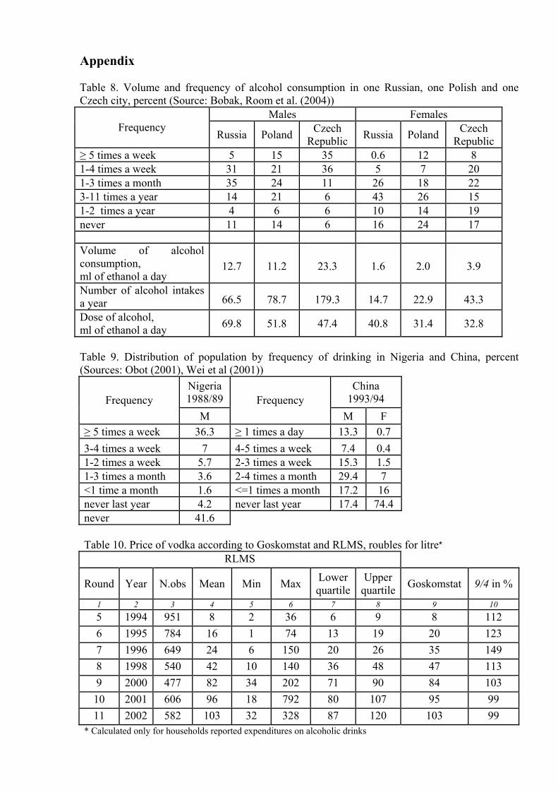
Appendix Table 8. Volume and frequency of alcohol consumption in one Russian, one Polish and one Czech city, percent (Source: Bobak, Room et al. (2004))

Males Females Frequency

Russia Poland Czech Republic Russia Poland Czech

Republic ≥ 5 times a week 5 15 35 0.6 12 8 1-4 times a week 31 21 36 5 7 20 1-3 times a month 35 24 11 26 18 22 3-11 times a year 14 21 6 43 26 15 1-2 times a year 4 6 6 10 14 19 never 11 14 6 16 24 17

Volume of alcohol consumption, ml of ethanol a day

12.7 11.2 23.3 1.6 2.0 3.9

Number of alcohol intakes a year 66.5 78.7 179.3 14.7 22.9 43.3 Dose of alcohol, ml of ethanol a day 69.8 51.8 47.4 40.8 31.4 32.8

Table 9. Distribution of population by frequency of drinking in Nigeria and China, percent (Sources: Obot (2001), Wei et al (2001))

Nigeria 1988/89

China 1993/94 Frequency

М Frequency

М F ≥ 5 times a week 36.3 ≥ 1 times a day 13.3 0.7 3-4 times a week 7 4-5 times a week 7.4 0.4 1-2 times a week 5.7 2-3 times a week 15.3 1.5 1-3 times a month 3.6 2-4 times a month 29.4 7 <1 time a month 1.6 <=1 times a month 17.2 16 never last year 4.2 never last year 17.4 74.4 never 41.6 Table 10. Price of vodka according to Goskomstat and RLMS, roubles for litre*

RLMS

Round Year N.obs Mean Min Max Lower quartile

Upper quartile Goskomstat 9/4 in %

1 2 3 4 5 6 7 8 9 10 5 1994 951 8 2 36 6 9 8 112 6 1995 784 16 1 74 13 19 20 123 7 1996 649 24 6 150 20 26 35 149 8 1998 540 42 10 140 36 48 47 113 9 2000 477 82 34 202 71 90 84 103 10 2001 606 96 18 792 80 107 95 99 11 2002 582 103 32 328 87 120 103 99

* Calculated only for households reported expenditures on alcoholic drinks

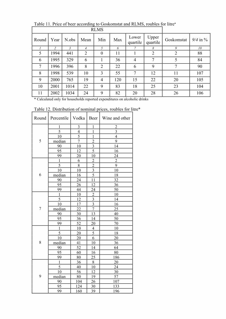
Table 11. Price of beer according to Goskomstat and RLMS, roubles for litre* RLMS

Round Year N.obs Mean Min Max Lower quartile

Upper quartile Goskomstat 9/4 in %

1 2 3 4 5 6 7 8 9 10 5 1994 441 2 0 11 1 2 2 88 6 1995 329 6 1 36 4 7 5 84 7 1996 396 8 2 22 6 9 7 90 8 1998 539 10 3 55 7 12 11 107 9 2000 765 19 4 120 15 22 20 105 10 2001 1014 22 9 83 18 25 23 104 11 2002 1034 24 9 82 20 28 26 106

* Calculated only for households reported expenditures on alcoholic drinks Table 12. Distribution of nominal prices, roubles for litre*

Round Percentile Vodka Beer Wine and other

1 3 1 25 4 1 3

10 5 1 4median 7 2 9

90 10 3 1495 12 5 16

5

99 20 10 241 6 2 25 8 2 9

10 10 3 10median 16 5 18

90 24 11 3295 26 12 36

6

99 44 24 501 10 2 105 12 3 14

10 17 3 16median 22 7 25

90 30 13 4095 36 14 50

7

99 52 20 701 10 4 105 20 5 18

10 20 6 20median 41 10 36

90 52 14 6495 60 16 80

8

99 80 25 1861 36 8 205 40 10 24

10 56 12 30median 80 19 57

90 104 26 10795 124 30 133

9

99 160 39 196

1 26 10 165 40 12 32

10 50 14 40median 90 20 86

90 130 30 15095 150 32 200

10

99 210 50 4001 40 11 305 50 13 36

10 65 15 43median 100 23 100

90 140 34 18395 156 38 286

11

99 198 50 600* Calculated only for households reported expenditures on alcoholic drinks Table 13. Participation and consumption equations♦, probit and Heckman models

Dependent variable

method

Drinker (0/1), probit

Consump-tion, log Heckman

Consump-tion, log Heckman

Drinker (0/1), probit

Consump-tion, log Heckman

Consump-tion, log Heckman

Drinker among rest (0/1) 0.356*** 0.054 0.355*** 0.033 Income per head, log 0.266*** 0.09*** 0.096*** 0.285*** 0.074*** 0.078*** Price on ethanol, log -0.074*** -0.142*** -0.145*** Price on vodka, log -0.005 -0.172* -0.174* Price on beer, log -0.036 -0.007 -0.008 Price on wine and other, log 0.195** 0.064 0.066 Price on sugar, log -0.644*** -0.106 -0.114 Price on tobacco, log -0.332*** 0.129** 0.123** Age 0.018*** 0.038*** 0.039*** 0.018*** 0.041*** 0.041*** (Age-40)*1{Age>40} -0.057*** -0.08*** -0.082*** -0.057*** -0.083*** -0.084***Gender (m-0, f-1) -0.724*** -1.626*** -1.646*** -0.734*** -1.663*** -1.675***Village (0/1) -0.297*** -0.09** -0.099** -0.332*** -0.05 -0.056 Urban village (0/1) -0.455*** -0.147** -0.16** -0.373*** -0.167** -0.173** Regional center♦♦ (0/1) 0.211*** 0.112*** 0.117*** 0.21*** 0.079** 0.082** Const 2.257*** 3.789*** 3.753*** -2.138*** 3.059*** 2.965*** Number of obs 13369 13369 13369 13372 13372 13372 Censored obs 1308 1308 1308 1308 1308 1308 Uncensored obs 12061 12061 12061 12064 12064 12064 ♦ The sample consists of drinkers at least in one round no matter how many rounds they are observed and abstainers defined as respondents participated at least in 4 rounds out of 7 and never drank. Here and below stars mean significance levels: *- 10%, **- 5%, ***- 1%. ♦♦ Here and below cities other than regional capitals are taken as base in a regression.

Table 14. Participation equation, probit model with random effect

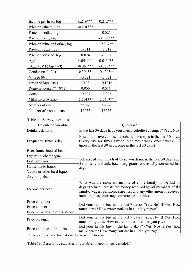
Income per head, log 0.216*** 0.212*** Price on ethanol, log -0.201*** Price on vodka, log 0.025 Price on beer, log -0.086*** Price on wine and other, log -0.047** Price on sugar, log -0.011 -0.018 Price on tobacco, log 0.024 -0.008 Age 0.041*** 0.043*** (Age-40)*1{Age>40} -0.063*** -0.067*** Gender (m-0, f-1) -0.394*** -0.429*** Village (0/1) -0.021 -0.024 Urban village (0/1) -0.08 -0.101* Regional center** (0/1) 0.006 0.010 Const -0.209 -0.228 Mills inverse ratio -2.191*** -2.069*** Number of obs 55686 55686 Number of respondents 16277 16277

Table 15. Survey questions Calculated variable Question*

Drinker, dummy In the last 30 days have you used alcoholic beverages? (Yes, No)

Frequency, times a day How often have you used alcoholic beverages in the last 30 days?(Every day, 4-6 times a week, 2-3 times a week, once a week, 2-3 times in the last 30 days, once in the last 30 days)

Beer, home-brewed beer Dry wine, champagne Fortified wine Home-made liquor Vodka or other hard liquor Anything else

Tell me, please, which of these you drank in the last 30 days and,for those, you drank, how many grams you usually consumed in aday?

Income per head

What was the monetary income of entire family in the last 30days? Include here all the money received by all members of thefamily: wages, pensions, stipends, and any other money received,including hard currency converted into rubles.

Price on vodka Price on beer Price on wine and other alcohol

Did your family buy in the last 7 days? (Yes, No) If Yes: Howmuch litres? How many roubles in all did you pay?

Price on sugar Did your family buy in the last 7 days? (Yes, No) If Yes: Howmuch kilograms? How many roubles in all did you pay?

Price on tobacco products Did your family buy in the last 7 days? (Yes, No) If Yes: howmany packs? How many roubles in all did you pay?

* Every answer has options: doesn’t know, refused to answer Table 16. Descriptive statistics of variables in econometric models*

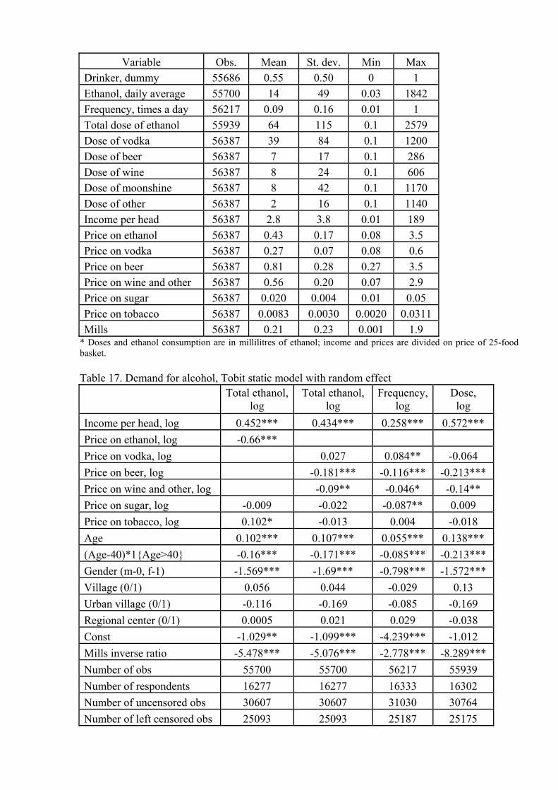
Variable Obs. Mean St. dev. Min Max Drinker, dummy 55686 0.55 0.50 0 1 Ethanol, daily average 55700 14 49 0.03 1842 Frequency, times a day 56217 0.09 0.16 0.01 1 Total dose of ethanol 55939 64 115 0.1 2579 Dose of vodka 56387 39 84 0.1 1200 Dose of beer 56387 7 17 0.1 286 Dose of wine 56387 8 24 0.1 606 Dose of moonshine 56387 8 42 0.1 1170 Dose of other 56387 2 16 0.1 1140 Income per head 56387 2.8 3.8 0.01 189 Price on ethanol 56387 0.43 0.17 0.08 3.5 Price on vodka 56387 0.27 0.07 0.08 0.6 Price on beer 56387 0.81 0.28 0.27 3.5 Price on wine and other 56387 0.56 0.20 0.07 2.9 Price on sugar 56387 0.020 0.004 0.01 0.05 Price on tobacco 56387 0.0083 0.0030 0.0020 0.0311 Mills 56387 0.21 0.23 0.001 1.9

* Doses and ethanol consumption are in millilitres of ethanol; income and prices are divided on price of 25-food basket. Table 17. Demand for alcohol, Tobit static model with random effect

Total ethanol,

log Total ethanol,

log Frequency,

log Dose,

log Income per head, log 0.452*** 0.434*** 0.258*** 0.572*** Price on ethanol, log -0.66*** Price on vodka, log 0.027 0.084** -0.064 Price on beer, log -0.181*** -0.116*** -0.213*** Price on wine and other, log -0.09** -0.046* -0.14** Price on sugar, log -0.009 -0.022 -0.087** 0.009 Price on tobacco, log 0.102* -0.013 0.004 -0.018 Age 0.102*** 0.107*** 0.055*** 0.138*** (Age-40)*1{Age>40} -0.16*** -0.171*** -0.085*** -0.213*** Gender (m-0, f-1) -1.569*** -1.69*** -0.798*** -1.572*** Village (0/1) 0.056 0.044 -0.029 0.13 Urban village (0/1) -0.116 -0.169 -0.085 -0.169 Regional center (0/1) 0.0005 0.021 0.029 -0.038 Const -1.029** -1.099*** -4.239*** -1.012 Mills inverse ratio -5.478*** -5.076*** -2.778*** -8.289*** Number of obs 55700 55700 56217 55939 Number of respondents 16277 16277 16333 16302 Number of uncensored obs 30607 30607 31030 30764 Number of left censored obs 25093 25093 25187 25175

Table 18. Demand for alcohol by types of drink, Tobit static model with random effect

Dose of vodka,

log

Dose of beer, log

Dose of wine, log

Dose of moonshine,

log

Dose of other,

log

Income per head, log 0.524*** 1.114*** 1.304*** -1.049*** 2.415*** Price on vodka, log -1.774*** 4.132*** -1.537*** 5.598*** 0.465 Price on beer, log 0.785*** -3.017*** 1.195*** -5.076*** 0.186 Price on wine and other, log 0.293*** -0.567*** -1.045*** -0.949*** -0.246 Price on sugar, log 0.802*** -1.005*** -0.644** 2.126*** -2.874***Price on tobacco, log 0.152 0.957*** 0.318* -1.804*** 1.345** Age 0.25*** -0.003 -0.004 0.262*** -0.035 (Age-40)*1{Age>40} -0.36*** -0.154*** -0.082*** -0.213*** -0.102** Gender (m-0, f-1) -4.075*** -3.085*** 4.629*** -5.522*** 1.503*** Village (0/1) -0.059 -0.765*** -1.047*** 4.218*** -2.226***Urban village (0/1) -0.844*** -1.285*** 0.39 2.888*** -1.265 Regional center (0/1) 0.277** 0.265*** 1.111*** -5.14*** 0.99*** Const -2.743*** 4.54*** -18.52*** -14.39*** -33.61***Mills inverse ratio -6.695*** -6.66*** -11.64*** -12.97*** -5.036** Number of obs 56387 56387 56387 56387 56387 Number of respondents 16348 16348 16348 16348 16348 Number of uncensored obs 20304 12817 10305 3569 1556 Number of left censored obs 36083 43570 46082 52818 54831

Table 19. Myopic and rational addiction Tobit models

Myopic Myopic♦ Rational Rational♦ Lag of consumption, log 0.645*** 0.123** 0.487*** 0.167*** Lead of consumption, log 0.522*** 0.181*** Income per head, log 0.315*** 0.432*** 0.272*** 0.415*** Price on vodka, log 0.177** 0.16** 0.114 0.221** Price on beer, log -0.222*** -0.21*** -0.152** -0.221*** Price on wine and other, log -0.175*** -0.209*** -0.07 -0.198*** Price on sugar, log 0.21** -0.067 -0.179* -0.145 Price on tobacco, log 0.049 0.099 0.079 0.258*** Age 0.016*** 0.06*** 0.012*** 0.035*** (Age-40)*1{Age>40} -0.041*** -0.111*** -0.022*** -0.069*** Gender (m-0, f-1) -0.794*** -1.504*** -0.234*** -1.187*** Village (0/1) 0.056 0.171** 0.058 0.132 Urban village (0/1) 0.001 0.029 0.055 0.259 Regional center (0/1) -0.029 -0.065 -0.082* -0.098 Const 1.492*** 0.628 -0.875* 1.442** Mills inverse ratio -3.585*** -4.139*** -2.846*** -2.915*** Number of obs 40215 37729 28269 25710

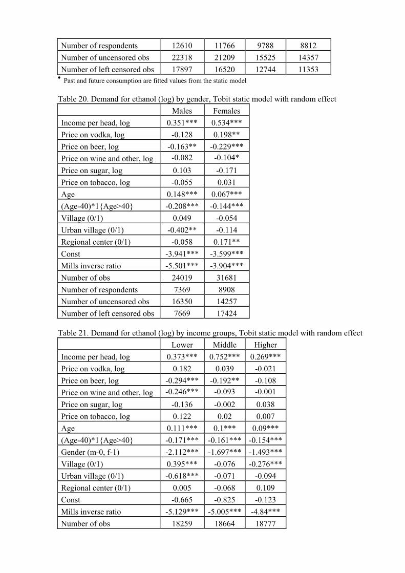
Number of respondents 12610 11766 9788 8812 Number of uncensored obs 22318 21209 15525 14357 Number of left censored obs 17897 16520 12744 11353

♦ Past and future consumption are fitted values from the static model Table 20. Demand for ethanol (log) by gender, Tobit static model with random effect

Males Females Income per head, log 0.351*** 0.534*** Price on vodka, log -0.128 0.198** Price on beer, log -0.163** -0.229*** Price on wine and other, log -0.082 -0.104* Price on sugar, log 0.103 -0.171 Price on tobacco, log -0.055 0.031 Age 0.148*** 0.067*** (Age-40)*1{Age>40} -0.208*** -0.144*** Village (0/1) 0.049 -0.054 Urban village (0/1) -0.402** -0.114 Regional center (0/1) -0.058 0.171** Const -3.941*** -3.599*** Mills inverse ratio -5.501*** -3.904*** Number of obs 24019 31681 Number of respondents 7369 8908 Number of uncensored obs 16350 14257 Number of left censored obs 7669 17424

Table 21. Demand for ethanol (log) by income groups, Tobit static model with random effect

Lower Middle Higher Income per head, log 0.373*** 0.752*** 0.269*** Price on vodka, log 0.182 0.039 -0.021 Price on beer, log -0.294*** -0.192** -0.108 Price on wine and other, log -0.246*** -0.093 -0.001 Price on sugar, log -0.136 -0.002 0.038 Price on tobacco, log 0.122 0.02 0.007 Age 0.111*** 0.1*** 0.09*** (Age-40)*1{Age>40} -0.171*** -0.161*** -0.154***Gender (m-0, f-1) -2.112*** -1.697*** -1.493***Village (0/1) 0.395*** -0.076 -0.276***Urban village (0/1) -0.618*** -0.071 -0.094 Regional center (0/1) 0.005 -0.068 0.109 Const -0.665 -0.825 -0.123 Mills inverse ratio -5.129*** -5.005*** -4.84*** Number of obs 18259 18664 18777

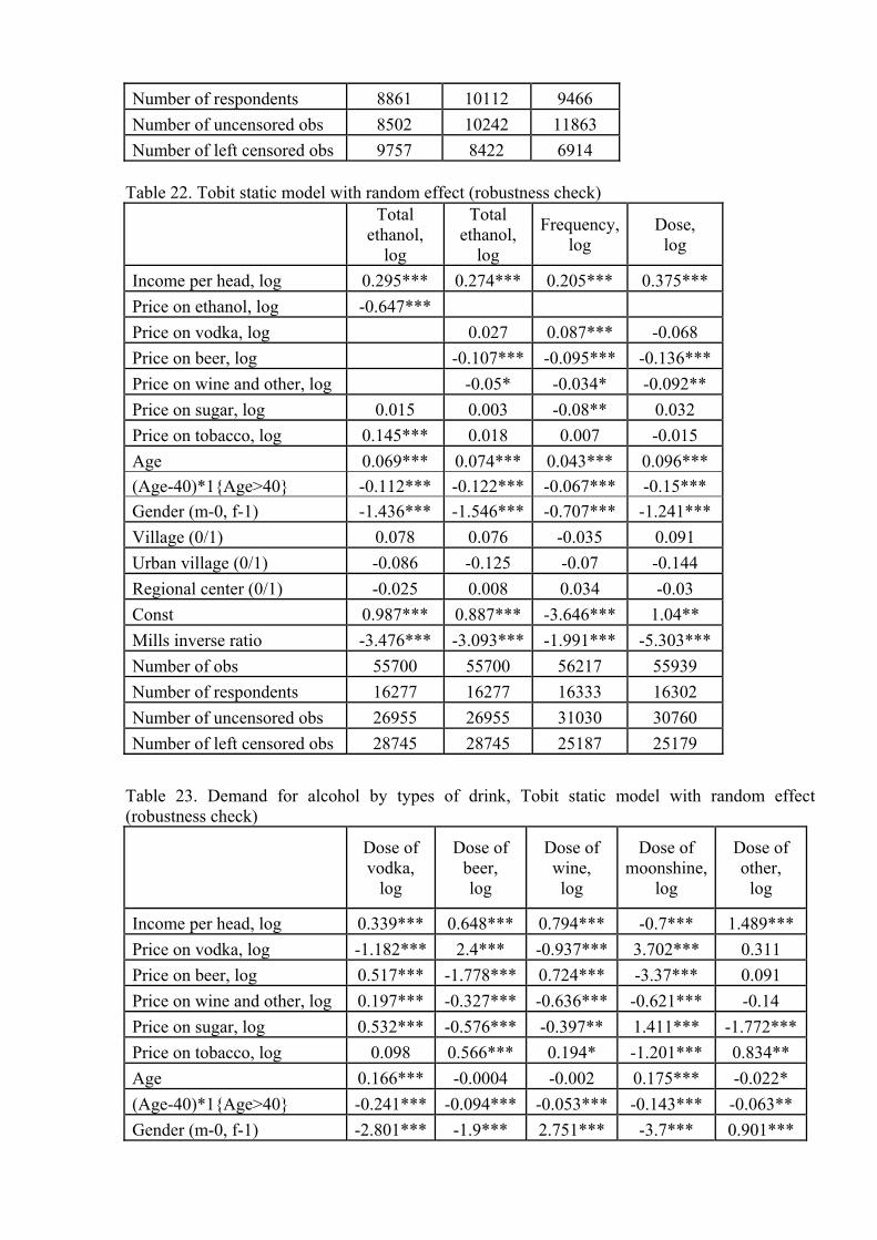
Number of respondents 8861 10112 9466 Number of uncensored obs 8502 10242 11863 Number of left censored obs 9757 8422 6914

Table 22. Tobit static model with random effect (robustness check)

Total ethanol,

log

Total ethanol,

log

Frequency,log

Dose, log

Income per head, log 0.295*** 0.274*** 0.205*** 0.375*** Price on ethanol, log -0.647*** Price on vodka, log 0.027 0.087*** -0.068 Price on beer, log -0.107*** -0.095*** -0.136*** Price on wine and other, log -0.05* -0.034* -0.092** Price on sugar, log 0.015 0.003 -0.08** 0.032 Price on tobacco, log 0.145*** 0.018 0.007 -0.015 Age 0.069*** 0.074*** 0.043*** 0.096*** (Age-40)*1{Age>40} -0.112*** -0.122*** -0.067*** -0.15*** Gender (m-0, f-1) -1.436*** -1.546*** -0.707*** -1.241*** Village (0/1) 0.078 0.076 -0.035 0.091 Urban village (0/1) -0.086 -0.125 -0.07 -0.144 Regional center (0/1) -0.025 0.008 0.034 -0.03 Const 0.987*** 0.887*** -3.646*** 1.04** Mills inverse ratio -3.476*** -3.093*** -1.991*** -5.303*** Number of obs 55700 55700 56217 55939 Number of respondents 16277 16277 16333 16302 Number of uncensored obs 26955 26955 31030 30760 Number of left censored obs 28745 28745 25187 25179

Table 23. Demand for alcohol by types of drink, Tobit static model with random effect (robustness check)

Dose of vodka,

log

Dose of beer, log

Dose of wine, log

Dose of moonshine,

log

Dose of other,

log

Income per head, log 0.339*** 0.648*** 0.794*** -0.7*** 1.489*** Price on vodka, log -1.182*** 2.4*** -0.937*** 3.702*** 0.311 Price on beer, log 0.517*** -1.778*** 0.724*** -3.37*** 0.091 Price on wine and other, log 0.197*** -0.327*** -0.636*** -0.621*** -0.14 Price on sugar, log 0.532*** -0.576*** -0.397** 1.411*** -1.772***Price on tobacco, log 0.098 0.566*** 0.194* -1.201*** 0.834** Age 0.166*** -0.0004 -0.002 0.175*** -0.022* (Age-40)*1{Age>40} -0.241*** -0.094*** -0.053*** -0.143*** -0.063** Gender (m-0, f-1) -2.801*** -1.9*** 2.751*** -3.7*** 0.901***

Village (0/1) -0.041 -0.446*** -0.635*** 2.796*** -1.377***Urban village (0/1) -0.58*** -0.783*** 0.214 1.912*** -0.791 Regional center (0/1) 0.171** 0.159*** 0.678*** -3.404*** 0.596** Const -0.138 4.148*** -9.809*** -7.994*** -19.21***Mills inverse ratio -4.288*** -3.663*** -7.039*** -8.566*** -3.118** Number of obs 56387 56387 56387 56387 56387 Number of respondents 16348 16348 16348 16348 16348 Number of uncensored obs 20304 12806 10305 3569 1556 Number of left censored obs 36083 43581 46082 52818 54831

Figure 2.

0-5 10-15 20-25 30-35 40-45 >50

Litres per capita a year, vodka equivalent

0

20

40

60D

rinke

rs, %

males females

11-th round (4505 males, 5994 females)

Figure 3.

14-20 30-40 50-60 70-80

Age

0

10

20

30

40

Alc

ohol

con

sum

ptio

n, li

ters

per

cap

ita a

yea

r,vo

dka

equi

vale

nt

males females

Figure 4.

15-20 26-30 36-40 46-50 56-60 66-70 76-80 86-90

Age

0

1

2

3

4

5

6Nu

mbe

r of a

lcoh

ol in

take

s pe

r a

mon

th males females

Figure 6.

RLM

S-9

5

RLM

S-0

2

Sim

pura

-94

Mal

yutin

.85

Mal

yutin

.95

Laat

kain

.92

Laat

kain

.97

Bob

ak-0

0

Zaig

raev

FPO

CIN

DI0

5

10

15

20

25

30

35

Alc

ohol

con

sum

ptio

n, li

tres

per c

apita

a y

ear

males females

Figure 7.

0 20 40 60 80 100 120 140 160 180 200

Price of vodka, roubles per litre

0%

5%

10%

15%

20%

25%

30%

35%

40%O

bser

vatio

ns

11 round (2002) n=582

Figure 8.

Alc

ohol

con

sum

ptio

n, li

ters

per

cap

ita a

yea

r

1994 1995 1996 1997 1998 1999 2000 2001 20020

3

6

9

12

15

18

RLMS

Nemtsov (2003)

Goskomstat RF

* RLMS data were calculated per adult above 14 years of age.

Table 24. Quantity and frequency of alcohol consumption in Russia (continuation see below)

RLMS, >10,000*

Malyutina et al (2001), Novosibirsk, >4500

Laatkainen et al (2002), Karelia, >1500** Source,

region, size,

year of survey

6th round 1995

11th round 2002

Simpura et al (1997), Moscow,

>900, 1994

Bobak et al (1999), >1500*,

1996 1985-86 1994-95

Mal

yutin

a et

al

(200

2),

>630

0, 8

4-95

1992 1997

Bobak et al♦ (2003), >2000*,

2001

Bobak et al (2004), >900,

1999-2000

Zaigraev (2004), 3 rural areas,

>200, 2001

No. 1 2 3 4 5 6 7 8 9 10 11 12

Gender M F M F М F M F M F M F M M F M F M F M F M F Ethanol, ml a day 27.7 3.6 27.4 4.9 ***

29.9 ***2.7 n/a 17.1 4.4 2.3 5.9 n/a 6.2 1.0 10.1 1.3 n/a 12.9 1.6 85.5 35.1

Frequency of intake, % Every day 2.3 0.3 3.3 0.5 1 5 0.6 65 23 20 times a month 2.9 0.4 3.7 0.6 1

8

10 times a month 12.3 2.4 15.2 3.3 6

10

2 n/a 9 2

26 36

4 times a month 17.0 6.5 19.2 9.7 7 27 0.6 38 6.5

23 8 1

31 5

2 times a month 21.3 16.1 18.0 17.6 4

40 10 15 3 35 26

9 37

1 time a month 11.4 17.9 9.2 17.2 7 21 18

57 16 5 14 43 0 4

Less or never 32.8 56.5 30.5 51.2 74

n/a

29 71

n/a

12

n/a

41 83 14 26 0 0

♦ In Bobak et al (2003) the share "unknown" is equal to 11% for males and 6% for females. In other cases it does not exceed 1%. * National sample. ** The first method of estimation out of two explored by the authors. *** Our recalculation. Table 24. Quantity and frequency of alcohol consumption in Russia (continued)

Source, region,

size, year of survey

NOBUS >100,000*,

2003

FPO 1500*, 2002

CINDI (2001) Moscow, >1600,

2000-2001

No. 13 14 15

Gender M F М F М F

Ethanol, ml a day n/a

*** litres per capita

a year (see Figure 6)

*** litres per

capita a year (see Figure 6)

Frequency of intake, % Every day 3.1 0.4 6 0 20 times a month 10 times a month

9.0 1.6 16 2

4 times a month 17.1 5.3 23 9 2 times a month 18.1 9.9 20 17 1 time a month 23.0 35.6 22 51

Strong drinks time per 7 days

Beer time per 4 days

Strong drinks time

per 40 days

Beer time per 4 days

Less or never 29.8 47.3 12 20 13.5 20.5

* National sample *** Recalculation of the authors