estimation of solvation entropy and enthalpy via …...2015/10/21 · estimation of solvation...

Estimation of Solvation Entropy and Enthalpy via Analysis of WaterOxygen−Hydrogen CorrelationsCamilo Velez-Vega,*,† Daniel J. J. McKay,*,† Tom Kurtzman,*,‡,§ Vibhas Aravamuthan,†

Robert A. Pearlstein,† and Jose S. Duca†

†Computer-Aided Drug Discovery, Global Discovery Chemistry, Novartis Institutes for BioMedical Research, 100 TechnologySquare, Cambridge, Massachusetts 02139, United States‡Department of Chemistry, Lehman College, The City University of New York, 250 Bedford Park Boulevard West, Bronx, New York10468, United States§Ph.D. Program in Chemistry, The Graduate Center of the City University of New York, New York, New York 10016, United States

*S Supporting Information

ABSTRACT: A statistical-mechanical framework for estima-tion of solvation entropies and enthalpies is proposed, which isbased on the analysis of water as a mixture of correlated wateroxygens and water hydrogens. Entropic contributions ofincreasing order are cast in terms of a Mutual InformationExpansion that is evaluated to pairwise interactions. In turn,the enthalpy is computed directly from a distance-basedhydrogen bonding energy algorithm. The resulting expressionsare employed for grid-based analyses of Molecular Dynamicssimulations. In this first assessment of the methodology, we obtained global estimates of the excess entropy and enthalpy of waterthat are in good agreement with experiment and examined the method’s ability to enable detailed elucidation of solvationthermodynamic structures, which can provide valuable knowledge toward molecular design.

■ INTRODUCTION

In silico approaches aimed at the analysis of structural andthermodynamic properties of water have in recent years shownpromise as tools to aid ligand design. The palpable interest inthese methods is naturally linked to the key role that waterplays in most biophysical processes, which can in principle beelucidated through information extracted from solventstructural dynamics. Indeed, we have previously developedand reported1 a novel approach yielding detailed time-averagedsolute and solvent structures that have been used to revealrelevant insights pertaining to biomolecular mechanisms and,more importantly, have facilitated rational ligand design. Yet,further development of this approach, aimed at bridging the gapbetween structure-free energy relationships within the contextof solvation-based analyses, is a necessary advancement towardmore efficient drug discovery.Several methods have been proposed for estimation of

thermodynamic quantities from solvation dynamics, which areeither rooted in Inhomogeneous Solvation Theory (IST)2−8

(GIST,9,10 STOW,11 WaterMap,12,13 and others14,15) oralternate statistical mechanical fundamentals (3D-RISM,16

GCT,17 SZMAP,18 and WATsite19). Although these ap-proaches show great potential for expediting ligand design,their systematic use has been largely hampered by the limitedaccuracy of the resulting solvation thermodynamic quantities.The latter may be in part due to the apparent drawbacks ofsome of these methodologies, which include the following:

1) The use of fixed-solute simulations to study solvationdynamics,2−9,12,17 which may lead to nonrepresentativesolvation structures for flexible systems, and can maskinconsistencies in the system/simulation setup.2) The study of high-occupancy hydration sites only,12,14,19,20

disregarding low-occupancy solvation and its correspondingsolvation thermodynamics; the latter contribution can havecritical impact on ligand design and optimization.3) The demanding computational effort required to properly

evaluate second order solvation entropy terms (e.g., forimplementations derived from IST2−9,11), difficulty thatescalates upon estimation of third and higher ordercorrelations.This work is part of an ongoing effort aimed at further

developing solvation dynamics-based methodologies towardincreasingly dependable and efficient tools for drug design.We present here a new theoretical platform for calculating

water entropy, in which increasing order contributions areexpressed in terms of a Mutual Information Expansion21

(MIE). This treatment allows for the straightforwarddiscretization of space, leading to an efficient, grid-based, all-density occupancy algorithm for analysis of solvent structuresextracted from flexible solute simulations. The proposedentropy formulation is centered on the breakdown of water

Received: May 12, 2015

Article

pubs.acs.org/JCTC

© XXXX American Chemical Society A DOI: 10.1021/acs.jctc.5b00439J. Chem. Theory Comput. XXXX, XXX, XXX−XXX

pubs.acs.org/JCTC

http://dx.doi.org/10.1021/acs.jctc.5b00439

into a mixture of correlated oxygens and hydrogens, aperspective initially prompted by the mobile nature of water’sconstituent atoms. This approach entails handling only relativeatomic positions, thus offering a more tractable way to computesolvation entropies relative to the practice (as in ISTimplementations) of estimating distinct terms for the transla-tional and orientational entropy of water molecules.Water enthalpy values are also computed within this grid-

based analysis protocol. In brief, nonbonded interactionsbetween waters are approximated by their correspondinghydrogen bonding energies. Free energies are then calculatedas the sum of entropic cost and the enthalpic contributions.Overall, the methodology introduced provides both a global

estimate and a detailed structural description of the solvationentropy, enthalpy, and free energy of a system.As a key validation step, the proposed thermodynamics

expressions were used to compute global estimates of theexcess enthalpy and entropy of pure water under physiologicalconditions. The ability of our method to portray local solvationstructures is then illustrated via analysis of pure water systemswhose perturbed solvent fields (generated upon fixing theposition of two water molecules) are either interacting ornoninteracting.

■ METHODSTheoretical Formulations. Solvation Entropy − Integral

Expressions. The total entropy S of a solvated system can beexpressed in terms of the joint probability density (ρ) of thedegrees of freedom describing the solute (A) and the solvent(B)22

∫ ∫ ρ ρ= − * +A B A B A BS k d d k C( , ) ln( ( , )) ln( )B B

(1)

where kB is the Boltzmann constant, and the last term is aconstant that eliminates the units of the probability densityinside the logarithm and cancels out exactly upon computingdifferences in entropy.By virtue of the conditional probability law, ρ(A,B) =

ρ(A)ρ(B|A) = ρ(B)ρ(A|B), eq 1 can be denoted as

∫ ∫ ∫ρ ρ ρ ρ

ρ

= − * − |

* | +

A A A A A B A

B A B

S k d k d

d k C

( ) ln( ( )) ( ) ( )

ln( ( )) ln( )

B B

B (2)

The first term corresponds to the entropy of the solute degreesof freedom, whereas the second term has been elegantlyinterpreted by Zhou and Gilson22 as the entropy of the solventdegrees of freedom (B) averaged over the equilibriumdistribution of the solute degrees of freedom (A). Thus, eq 2can be further cast as the sum of separate contributions to theentropy arising from motions of the solute molecules (Ssolute)and from motions of the solvent (Ssolv) due to the presence ofsolute:

= +S S Ssolute solv (3)

The first and second terms in eq 2 are entirely included in Ssoluteand Ssolv, respectively. This work does not consider theestimation of Ssolute in eq 3. For that purpose, the reader isreferred to previous research21,23−26 relevant to the estimationof configurational entropies.We are primarily concerned with computing solvation

entropy differences (ΔSsolv) relative to the bulk solvent atconditions relevant to biological systems. To this end, we

propose ΔSsolv expressions that are cast in terms of normalizedprobability densities (relative to bulk), denoted by ρ (asdescribed in Appendix A, Supporting Information). Note againthat calculation of solvation entropy differences ensurescancellation of the constant contribution to Ssolv arising fromthe last term in eq 2.Below, we derive expressions for ΔSsolv in which water is

considered as a mixture of N oxygens (x) and 2N correlatedhydrogens (y), whose reference state corresponds to a uniformdistribution of oxygens and hydrogens. For this case

∫ ∫ρ

ρ

ρ

Δ = −

*

*

r p r p r p r p

r p r p r p r p

r p r p r p r p r p r p

r p r p

S k

d d d d

d d d d

( , , , , ..., , , , )

... ( , , , , ..., , , , )

ln( ( , , , , ..., , , , ))

...

solv bulk x x y y xN xN y N y N

x x y y xN xN y N y N

x x y y xN xN y N y N x x y y

xN xN y N y N

B 1 1 1 1 2 2

1 1 1 1 2 2

1 1 1 1 2 2 1 1 1 1

2 2 (4)

where r and p, respectively, correspond to the Cartesiancoordinates and momenta of all oxygens (x) and hydrogens (y)in the system. The normalized joint probability density ρ is afunction of all degrees of freedom of the solvent atoms, whereasρbulk can be computed as the product of the marginal bulkprobability density of all such quantities.When the dynamics of a system is modeled via a

Hamiltonian in Cartesian coordinates (as is usually the casefor MD simulations), the momentum and spatial contributionsare uncorrelated; i.e., the kinetic and potential energy termsdepend only on the momenta and the spatial coordinates,respectively. Therefore, eq 4 can be separated into

∫ ∫

∫ ∫

ρ ρ

ρ

ρ ρ

ρ

Δ = −

*

−

*

r r r r r r r r

r r r r r r r r

p p p p p p p p

p p p p p p p p

S k

d d d d

k

d d d d

( , , ..., , ) ... ( , , ..., , )

ln( ( , , ..., , )) ...

( , , ..., , ) ... ( , , ..., , )

ln( ( , , ..., , )) ...

solv bulk x y xN y N x y xN y N

x y xN y N x y xN y N

bulk x y xN y N x y xN y N

x y xN y N x y xN y N

B 1 1 2 1 1 2

1 1 2 1 1 2

B 1 1 2 1 1 2

1 1 2 1 1 2 (5)

Furthermore, given that the momentum term depends only ontemperature and the weighted atomic mass m = (∏i=1

S mi)1/s

computed from all s atoms in the system (which is invariant tochanges in the number of waters),27 the last term in eq 5 isnegligible for thermostated simulations. Moreover, this termcancels out when taking differences relative to the referencebulk state. Thus, with rx = {rx1,...,rxN} and ry = {ry1,...,ry2N}, weobtain

∬ρ ρ ρΔ = − * r r r r r r r r r rS k d d( , ) ( , ) ( , ) ln( ( , ))x y x y x y x y x ysolv bulkB

(6)

In this work, we estimate the solvation entropy defined by eq 6in terms of increasingly higher order terms of the MutualInformation Expansion for this quantity, as adopted from theformulation proposed by Matsuda28 and Killian et al.21

∑ ∑

∑ ∑

α α α α α

α α α α α α α

= −

+ − +

=S S I

I I

( , ..., ) ( ) ( , )

( , , ) ( , , , ) ...

Dm

i

m

iC

i j

Ci j k

Ci j k l

( )1

11 2

3 4

m

m m

2

3 4 (7)

where D is the order of the truncation in the entropyexpansion, I is the mutual information (MI), variables α are thedegrees of freedom defining the probability density functions(e.g., positions, angles, torsions), and Cd

m are all distinct order d≤ D combinations of m degrees of freedom.

Journal of Chemical Theory and Computation Article

DOI: 10.1021/acs.jctc.5b00439J. Chem. Theory Comput. XXXX, XXX, XXX−XXX

B

http://pubs.acs.org/doi/suppl/10.1021/acs.jctc.5b00439/suppl_file/ct5b00439_si_001.pdf


Expansion of eq 6 based on eq 7 leads to

∑ ∑

∑ ∑

∑

Δ ≡ = +

− +

+ + +

= =

⎡⎣⎢⎢

⎤⎦⎥⎥

r r r r

r r r r

r r

S S S S

I I

I O

( , ) ( ) ( )

( , )12

( , )

12

( , ) (3) ...

solvD

xi yii

N

xii

N

yi

Cxi yj

Cxi xj

Cyi yj

( )

11

1

2

1

2 2

2

N N

N

22

2

22

(8)

The first and second summations of eq 8 correspond to themarginal (S1) entropies, which collectively represent an upperbound for the entropy.21 The 1/2 factor preceding the secondand third pairwise MI (I2) summations prevents doublecounting of correlations of the same species.Eq 8 can be directly expanded in terms involving joint

probability distributions:

∫∫ ∫

∫

∫

∫

∫

∫ ∫

∫

∫

∫

∫

∫

∫

ρ ρ ρ

ρ ρ ρ ρ

ρ ρ ρ

ρ ρρ

ρ ρ

ρρ

ρ ρ

ρρ

ρ ρ

ρρ

ρ ρρ

ρρ

ρ ρρ

ρρ ρ

ρ

ρρ ρ

ρ

ρρ ρ

ρ

ρρ

ρ ρ

ρρ

ρ ρ

ρρ

ρ ρ

ρρ

ρ ρ

Δ ≡ = − * +

+ * −

* + + *

− × *

+ +

*

+

+ *

+ +

+ *

−

× *

+ +

*

+ +

*

+ +

*

−

× *

+ +

*

+

+ *

+ + *

+ +

−

−

−−

−−

−−

⎡⎣⎢⎢

⎛⎝⎜⎜

⎞⎠⎟⎟

⎛⎝⎜⎜

⎞⎠⎟⎟

⎛⎝⎜⎜

⎞⎠⎟⎟

⎛⎝⎜⎜

⎞⎠⎟⎟

⎤⎦⎥⎥

⎡⎣⎢⎢

⎛⎝⎜

⎞⎠⎟

⎛⎝⎜

⎞⎠⎟

⎛⎝⎜

⎞⎠⎟

⎛⎝⎜

⎞⎠⎟

⎤⎦⎥⎥

⎡⎣⎢⎢

⎛⎝⎜⎜

⎞⎠⎟⎟

⎛⎝⎜⎜

⎞⎠⎟⎟

⎛⎝⎜⎜

⎞⎠⎟⎟

⎛⎝⎜⎜

⎞⎠⎟⎟

⎤⎦⎥⎥

r r r r r r

r r r r r

r r r r r

r r r rr r

r rr r

r rr r

r rr r

r rr r

r rr r

r rr r

r rr r r r

r rr r

r rr r r r

r rr r

r r r r

r rr r

r r r r

r rr r

r r r r

r rr r

r rr r

r rr r

r rr r

r rr r

r rr r

r rr r

r rr r

S S k d

d k

d d

k d d

d d

d d

d d k

d d

d d

d d

d d k

d d

d d

d d

d d

O

( , ) ( )[ ( ) ln( ( ))

... ( ) ln( ( )) ] ( )[ ( )

ln( ( )) ... ( ) ln( ( )) ]

( , ) ( , ) ln( , )

( ) ( )...

( , ) ln( , )

( ) ( )

... ( , ) ln( , )

( ) ( )...

... ( , ) ln( , )

( ) ( )12

( , )

( , ) ln( , )

( ) ( )... ( , )

ln( , )

( ) ( )... ( , )

ln( , )

( ) ( )... ( , )

ln( , )

( ) ( )12

( , )

( , ) ln( , )

( ) ( )...

( , ) ln( , )

( ) ( )

... ( , ) ln( , )

( ) ( )

... ( , ) ln( , )

( ) ( )

(3) ...

solvD

xi yi bulk x x x x

xN xN xN bulk y y

y y y N y N y N

bulk x y x yx y

x yx y

x y Nx y N

x y Nx y N

xN yxN y

xN yxN y

xN y NxN y N

xN y NxN y N bulk x x

x xx x

x xx x x xN

x xN

x xNx xN xN x

xN x

xN xxN x xN xN

xN xN

xN xNxN xN bulk y y

y yy y

y yy y

y y Ny y N

y y Ny y N

y N yy N y

y N yy N y

y N y Ny N y N

y N y Ny N y N

( )B 1 1 1

B 1

1 1 2 2 2

B 1 11 1

1 11 1

1 21 2

1 21 2

11

11

22

22 B

1 21 2

1 21 2 1

1

11 1

1

11 1

1

11 B

1 21 2

1 21 2

1 21 2

1 21 2

2 12 1

2 12 1

2 2 12 2 1

2 2 12 2 1

(9)

Eq 9 is a general expression for calculation of ΔSsolv referencedto water as a mixture of two monatomic fluids. Forcompleteness, Appendix B, Supporting Information offers aMIE-based formulation akin to the one presented in eq 9,resulting from considering water as a polyatomic molecule. The

latter may be of interest to researchers studying implementa-tions derived from or related to IST. Moreover, it is anticipatedthat further exploration of the derivation shown in Appendix B,Supporting Information will lead to entropy formulationsclosely reminiscent of those proposed by IST.We now formulate discrete expressions that allow estimation

of ΔSsolv from eq 9, via analysis of MD simulations.Solvation Entropy − Discrete Expressions. Capitalizing on

the indistinguishable nature of the oxygen and hydrogen atomscomprising the solvent, it is recognized that the marginalcontribution to the solvation entropy, computed as the sum ofthe integrals over phase space of all individual particles (e.g., Nparticles for oxygen; see term 1 in eq 9), can be computed viathe Riemann sum of the solvation entropy contributions of allindividual volume elements (e.g., voxels) used to discretize thesimulation space. For instance, the term corresponding to theoxygen marginal translational solvation entropy in eq 9 can bedenoted as

∫ ∫

∫∑

ρ ρ ρ ρ ρ

ρ ρ ρ

− * + + *

= − * =

r r r r r r r

r r r r

k d d

k d

( )[ ( ) ln( ( )) ... ( ) ln( ( )) ]

( ) ( ) ln( ( ))

bulk x x x x xN xN xN

bulk xk

K

Vx k x k x k

B 1 1 1

B0

1, , ,

k (10)

where k is the voxel index, K is the total number of voxels,ρbulk0 (rx,k) is the bulk density of oxygen in Å−3, V is the voxel

volume (in this work, it is equal for all voxels) in Å3, and ρ(rx,k)is the normalized probability density of finding an oxygen atom(x) at position r within voxel k.For small voxel sizes such as the one employed in this work

(i.e., [0.5 Å]3), it is reasonable to assume that the variation inthe probability density within each of these subregions is small.9

As a result, the integral over each voxel can be represented byits average value, and the right-hand side of eq 10 is thenexpressed as

∫∑

∑

ρ ρ ρ

ρ ρ ρ

− *

≈ − *

=

=

r r r r

r r r

k d

k V

( ) ( ) ln( ( ))

( ) ( ) ln( ( ))

bulk xk

K

Vx k x k x k

bulk xk

K

x k x k

B0

1, , ,

B0

1, ,

k

(11)

The pairwise correlation integrals can be discretized in ananalogous fashion; e.g., the first pairwise MI term in eq 9 wouldbe expressed as

∫

∫

∫

∫

∑ ∑

ρ ρρ

ρ ρ

ρρ

ρ ρ

ρρ

ρ ρ

ρρ

ρ ρ

ρ ρρ

ρ ρ

*

+

+ *

+

+ *

+

+ *

≈ * = ≠

⎡⎣⎢⎢

⎛⎝⎜⎜

⎞⎠⎟⎟

⎛⎝⎜⎜

⎞⎠⎟⎟

⎛⎝⎜⎜

⎞⎠⎟⎟

⎛⎝⎜⎜

⎞⎠⎟⎟

⎤⎦⎥⎥

⎡⎣⎢⎢

⎛⎝⎜⎜

⎞⎠⎟⎟⎤⎦⎥⎥

r r r rr r

r rr r

r rr r

r rr r

r rr r

r rr r

r rr r

r rr r

r r r rr r

r r

k d d

d d

d d

d d

k V

( , ) ( , ) ln( , )

( ) ( )

... ( , ) ln( , )

( ) ( )

... ( , ) ln( , )

( ) ( )

... ( , ) ln( , )

( ) ( )

( , ) ( , ) ln( , )

( ) ( )

bulk x y x yx y

x yx y

x y Nx y N

x y Nx y N

xN yxN y

xN yxN y

xN y NxN y N

xN y NxN y N

bulk x yk

K

n k

K

x k y nx k y n

x k y n

B 1 11 1

1 11 1

1 21 2

1 21 2

11

11

22

22

B0 2

1, ,

, ,

, , (12)

where n is the index for all voxels around the central voxel k.Incorporating all discretized terms into eq 9, we obtain



C




∑

∑

∑ ∑

∑ ∑

∑ ∑

ρ ρ ρ

ρ ρ ρ

ρ ρρ

ρ ρ

ρ ρρ

ρ ρ

ρ ρρ

ρ ρ

Δ ≈ −

−

− *

− *

− *

+ +

≠

≠

≠

⎡⎣⎢⎢

⎛⎝⎜⎜

⎞⎠⎟⎟⎤⎦⎥⎥

⎡⎣⎢⎢

⎛⎝⎜⎜

⎞⎠⎟⎟⎤⎦⎥⎥

⎡⎣⎢⎢

⎛⎝⎜⎜

⎞⎠⎟⎟⎤⎦⎥⎥

r r r

r r r

r r r rr r

r r

r r r rr r

r r

r r r rr r

r r

S k V

k V

k V

k V

k V

O

( ) ( )ln( ( ))

( ) ( )ln( ( ))

( , ) ( , ) ln( , )

( ) ( )

12

( , ) ( , ) ln( , )

( ) ( )

12

( , ) ( , ) ln( , )

( ) ( )

(3) ...

solv bulk xk

x k x k

bulk yk

y k y k

bulk x yk n k

K

x k y nx k y n

x k y n

bulk x xk n k

K

x k x nx k x n

x k x n

bulk y yk n k

K

y k y ny k y n

y k y n

B0

, ,

B0

, ,

B0 2

, ,, ,

, ,

B0 2

, ,, ,

, ,

B0 2

, ,, ,

, ,

(13)

Finally, casting eq 13 in terms of quantities computed insimulation leads to

∑

∑

∑ ∑

∑ ∑

∑ ∑

ρρ ρ

ρρ ρ

ρ ρρ ρ ρ ρ

ρ

ρρ

ρ ρ

ρ ρρ

ρ

ρ

ρ ρ

Δ ≈ −

−

− * *

* −

* * −

* * * + +

≠

≠

≠

⎛⎝⎜⎜

⎞⎠⎟⎟

⎛⎝⎜⎜

⎞⎠⎟⎟

⎛⎝⎜⎜

⎞⎠⎟⎟

⎛⎝⎜⎜

⎞⎠⎟⎟

⎡

⎣⎢⎢

⎛⎝⎜⎜

⎞⎠⎟⎟⎤

⎦⎥⎥

⎡⎣⎢⎢

⎛⎝⎜⎜

⎞⎠⎟⎟⎤⎦⎥⎥

⎡

⎣⎢⎢⎢

⎛

⎝⎜⎜

⎞

⎠⎟⎟⎤

⎦⎥⎥⎥

S k VN

VNN

VN

k VN

VN

N

VN

k VN

V N

N

V N

VN

N

VN

Nk V

N

V N

N

V N

VN

N

VN

Nk V

N

V N

N

V N

VN

N

VN

NO

ln

ln

ln

12

( )( )

ln( )

12

( )( )

ln( )

(3) ...

solv bulkox

k

kox

bulkox

f

kox

bulkox

f

bulkhy

k

khy

bulkhy

f

khy

bulkhy

f

bulkox

bulkhy

k n k

n khy

bulkox

bulkhy

f

n khy

bulkox

bulkhy

f

bulkhy

f

nhy

bulkox

f

kox bulk

ox

k n k

n kox

bulkox

f

n kox

bulkox

f

bulkox

f

nox

bulkox

f

kox bulk

hy

k n k

n khy

bulkhy

f

n khy

bulkhy

f

bulkhy

f

nhy

bulkhy

f

khy

B

B

B2 ,

2,

2

B2 ,

2,

2

B2 ,

2

,

2

ox ox

ox ox

hy

hy

(14)

where Nf is the total number of frames in the simulation, Nkox(hy)

is the number of frames with an O or H in voxel k, and Nn,kox(hy)ox(hy)

is the number of frames for which voxel n is occupied by an Oor H given that an O or H is found in voxel k.Note that second-plus order contributions depend on the

joint probability between particles (i.e., the probability offinding these particles at specific positions at the same time/frame); therefore, the per-voxel evaluation of Nn,kox(hy)

ox(hy) in eq 14requires a frame-by-frame analysis. It is also important to keepin mind that the space should be divided into voxels whosevolume is sufficiently small to harbor only one particle persimulation frame (i.e., side ≤0.55 Å, based on a 0.96 Å covalentOH bond). This ensures that the mutual information is zerowithin each voxel, given that there are no intravoxelcorrelations.Solvation Enthalpy. The total enthalpy H of a solvated

system can be expressed in terms of the pairwise contributionsarising from solute−solute, water−water, and solute−waternonbonded interactions:

= + +− − −H H H Hsol sol wat wat sol wat (15)

Defining the enthalpy difference with respect to a referencestate comprised of pure (bulk) water and each of the solutesisolated in vacuum leads to

Δ = − + −

+− − − −

−

H H H H H

H

( ) ( )sol solsolvated

sol solvacuum

wat watsolvated

wat watbulk

sol wat (16)

In this work, we focus on the estimation of water−waterenthalpy differences (i.e., second parentheses in eq 16,henceforth called ΔHsolv). Yet, solute−solute and solute−water enthalpies can in principle be estimated in a wayanalogous to that presented here for the water−watercontributions.Specifically, given that the dominant contribution to ΔHsolv

comes from short-range nonbonded interactions betweenoxygen and hydrogen atoms, we can approximate this quantityas the hydrogen bonding (henceforth, H-bonding) energy ofthe system. For this purpose, we capitalize on the grid-basednature of the methodology introduced to compute ΔHsolv as thedeviation from bulk water, of the sum of the per-voxelensemble-averaged H-bonding energy. We compute this energyfor every frame in which a water oxygen is in voxel k (kox) andan H-bonding partner is within a spherical ring volume (VHbond

kox )of 1.4−2.4 Å around the exact position of that water oxygen.Restated in mathematical terms

∑ ∑Δ ≈ ⟨ ⟩ −∈

H f r H( )solvk hy V

frames solvbulk

Hbondkox (17)

Hsolvbulk is the reference value, corresponding to the total enthalpy

of a bulk water simulation at the same temperature and density,and can be computed by setting ΔHsolv = 0 in eq 17. f(r) is anenergy function that is dependent upon the distance r betweeneach donor−acceptor pair, and whose parameters wereobtained by fitting to water−water interaction energiescomputed from quantum mechanical (QM) calculations atvarying water−water distances.In brief, a two-water-molecule potential curve was computed

in gas phase via the counter-poise corrected MP2/6-311++G(d,p) formalism. We restrained the distance between one ofthe water’s O atom and an H atom on the other water, allowingthe waters to adopt the lowest energy conformation at each ofthe fixed distances studied. Nine pairwise potentials wereobtained and collapsed into a single potential curve thatreached 0 kcal/mol at a separation of 13.95 Å. This curve wasthen fit to a standard Morse potential

= − −− −⎡⎣ ⎤⎦f r D e C( ) (1 )ea r r

w( [ ]) 2e

(18)

where Cw = 5.7642, De = 5.3441, a = 1.4952, and re = 1.9070.Note that re corresponds to the average O−H H-bondingdistance for bulk water, which changes depending on the watermodel. A very good fit to the QM calculations was achieved (R2

= 0.9995) for the distance range of interest.This simple potential exploits the cancellation of errors due

to the overestimation of interactions at short-range and theneglect of interactions longer than the H-bond cutoff, toprovide a fast, yet accurate, estimate of the solvation enthalpy(see Results).

Considerations toward Practical Implementation ofthe Proposed Expressions. Solvation Entropy - Approx-imations. The evaluation of all contributions to the solvationentropy is currently a very challenging computational task. Thiscomplexity calls for the use of practical implementations thatcan still maintain accuracy. Accordingly, we identify approx-imate solutions by neglecting the third-and-higher order termsin eq 8. The adequacy of this approximation is supported byrelated work,6 which within the context of entropy calculationsconcludes that third-and-higher order terms appear to accountonly for ∼10% of the thermodynamic properties of water.



D


Furthermore, calculation of the discretized pairwise MIcontributions (see eq 12) can readily become intractable withthe current computational capabilities. Therefore, the summa-tion on the right-hand side of eq 12 (as well as thosecorresponding to the remaining I2 terms) is limited here to thevicinity of each voxel

∑ ∑

∑ ∑

ρ ρρ

ρ ρ

ρ ρρ

ρ ρ

*

≈ *

= ≠

= ∈

⎡⎣⎢⎢

⎛⎝⎜⎜

⎞⎠⎟⎟⎤⎦⎥⎥

⎡⎣⎢⎢

⎛⎝⎜⎜

⎞⎠⎟⎟⎤⎦⎥⎥

r r r rr r

r r

r r r rr r

r r

k V

k V

( , ) ( , ) ln( , )

( ) ( )

( , ) ( , ) ln( , )

( ) ( )

bulk x yk

K

n k

K

x k y nx k y n

x k y n

bulk x yk

K

n Wx k y n

x k y n

x k y n

B0 2

1, ,

, ,

, ,

B0 2

1, ,

, ,

, ,

(19)

where W is a voxel subspace of the entire space comprised by Kvoxels. The optimal value of W is that which provides asatisfactory approximation to the exact per-voxel entropy at areasonable computational cost. This is contingent upon the rateat which the correlations decay as W is extended, which candiffer for each entropy contribution.Accordingly, eq 14 is reduced to

∑

∑

∑ ∑

∑ ∑

∑ ∑

ρρ ρ

ρρ ρ

ρ ρρ ρ ρ ρ

ρ

ρρ

ρ

ρ

ρ ρ

ρρ ρ

ρ

ρ

Δ ≈ −

−

− *

* −

* * *

− *

*

∈

∈

∈

⎛⎝⎜⎜

⎞⎠⎟⎟

⎛⎝⎜⎜

⎞⎠⎟⎟

⎛⎝⎜⎜

⎞⎠⎟⎟

⎛⎝⎜⎜

⎞⎠⎟⎟

⎡

⎣⎢⎢

⎛⎝⎜⎜

⎞⎠⎟⎟⎤

⎦⎥⎥

⎡⎣⎢⎢

⎛⎝⎜⎜

⎞⎠⎟⎟⎤⎦⎥⎥

⎡

⎣⎢⎢⎢

⎛

⎝⎜⎜

⎞

⎠⎟⎟⎤

⎦⎥⎥⎥

S k VN

VNN

VN

k VN

VN

N

VN

k VN

V N

N

V N

VN

N

VN

Nk V

N

V N

N

V N

VN

N

VN

N

k VN

V N

N

V N

VN

N

VN

N

ln

ln

ln

12

( )( )

ln( )

12

( )( )

ln( )

solv bulkox

k

kox

bulkox

f

kox

bulkox

f

bulkhy

k

khy

bulkhy

f

khy

bulkhy

f

bulkox

bulkhy

k n W

n khy

bulkox

bulkhy

f

n khy

bulkox

bulkhy

f

bulkhy

f

nhy

bulkox

f

kox bulk

ox

k n W

n kox

bulkox

f

n kox

bulkox

f

bulkox

f

nox

bulkox

f

kox

bulkhy

k n W

n khy

bulkhy

f

n khy

bulkhy

f

bulkhy

f

nhy

bulkhy

f

khy

B

B

B2 ,

2,

2

B2 ,

2

,2

B2 ,

2

,

2

ox ox

ox

ox

hy hy

(20)

Pairwise MI calculations are limited here to a subspace Wcomprised of n = 15,624 voxels, namely, those that are fully orpartially encompassed by a sphere of 6 Å radius around centervoxel k (i.e., rdist = 6 Å). The adequacy of this cutoff (afterwhich pairwise correlations are assumed to be negligible) issupported by the marked dampening observed for radialdistribution functions of pure water (herein RDFs), gOO,gOH, and gHH, at such distance from the center particle.Figure 1 shows plots of these RDFs, resolved experimentally29

at 298 K; the corresponding RDFs from simulations at 300 K,carried out using the same water model employed in this work,have been reported by Huggins30 in Figures 3−5 of the citedpublication. Ensuing studies involving solutes might requireadjustment of this value.Reduction in the Uncertainty of Calculations. The noise

introduced as a result of deficient sampling leads tofluctuations/deviations from the actual thermodynamic valuesfor bulk and nonbulk solvation. The concomitant uncertaintycan both hamper the identification of hot spots and swamp theoverall values obtained upon summation over the millions of

small voxels comprising the entire grid for a solvated proteinsystem. The latter effect is related to the well-known challengeof accurately computing small differences between largenumbers (e.g., when carrying out free energy calculations ofbiomolecular systems) and encourages the use of approaches toincrease the signal-to-noise ratio of our calculations.We have developed a “filtering” scheme in which we isolate

the signal from higher-than-bulk and lower-than-bulk solvationby zeroing out bulk-like entropy and enthalpy contributions.Two alternatives have been evaluated toward this end. In thefirst, we1. Carry out a reference unrestrained bulk water simulation.2. Calculate per-voxel solvation entropies and enthalpies

across the whole grid, via eqs 20 and 17, respectively.3. Fit a Gaussian distribution to the solvation entropy data

and another one to the solvation enthalpy data.4. For each case, identify a minimum cutoff of the standard

deviation (expressed as the normalized quantity over the

absolute standard deviation; i.e., σcutΔSsolv

bulk

= (σcutΔSsolv

bulk

)/(σΔSsolvbulk

) and

σcutΔHsolv

bulk

= (σcutΔHsolv

bulk

)/(σΔHsolvbulk

) for which the summation of thevalues that lie outside of such cutoff is effectively zero (<10−2

kcal/mol).5. Perform a simulation of interest under the same conditions

as the reference bulk water run.6. Calculate the per-voxel solvation entropies and enthalpies

of this new simulation, via eqs 20 and 17.7. Use the bulk-water cutoffs obtained on step 4 to filter the

solvation entropy and enthalpy data computed on step 6, byneglecting the contribution of those voxels whose ΔSsolv andΔHsolv fall within the range delimited by σcut

ΔSsolvbulk

and σcutΔHsolv

bulk

,respectively.

As a second more efficient alternative, we extract σcutΔSsolv

bulk

and

σcutΔHsolv

bulk

directly from the simulation of interest and use thesecutoffs to zero out the bulk-like solvation of that samesimulation. For this scheme, the box size should be sufficientlylarge so that the majority of the waters have bulk-likethermodynamic properties (ensuring that the dominant peakfor each term, to which a Gaussian distribution is fit,corresponds to bulk). Indeed, the latter requirement is naturallyfulfilled when considering a volume of voxel subspace (W) such

Figure 1. Radial distribution functions of pure water at 298 K, asresolved by Soper.29



E


that second order entropic correlations are captured withsatisfactory accuracy.Both filtering schemes were compared via preliminary

analyses of enthalpies and first and second order entropiesobtained from 100 ns MD simulations (results not shown). Thelatter led to excellent agreement between both alternatives,readily suggesting the use of the second one as the standardchoice for all ensuing calculations. The previous analysis also

led to the selection of σcutΔHsolv

bulk

= 6 and σcutΔSsolv

bulk

= 5 as suitable valuesfor the present study.It is important to mention that filtering should be carried out

separately for each entropy term (e.g., first order O entropy,second order O−H entropy, and so forth), prior to addingthese quantities to obtain a value of the total entropy. This isbecause straight summation of the “unfiltered” terms, each ofwhich contains a considerable amount of bulk-like noise, willlead to loss of the nonbulk-like signal contributed by eachindividual term, resulting in an inaccurate value of total entropy.Altogether, the practice described above filters out the

contribution from voxels where the signal is indistinguishablefrom the noise (i.e., singles-out those voxels that are statisticallysignificant relative to bulk solvent), allowing not only for easiervisualization of the effectively relevant solvent regions withinthe grid but also improving the accuracy of the global ΔSsolv andΔHsolv estimates (i.e., those obtained by summation of all per-voxel quantities). The effect of filtering thermodynamicsdistributions is discussed in the Results section.Computational Details. Systems of 10,012 TIP3P water

molecules with 0, 1, or 2 water oxygens restrained by means ofa stiff force constant k = 100 kcal/mol/Å2 (for all cases) werearranged into a cubic periodic box, minimized, and equilibratedat 300 K for 500 ps. These were used as starting points forproduction MD simulations at 300 K within the NPTensemble, which were run for either 50 or 100 ns. All MDsimulations were performed using the Amber1231,32 softwarepackage, with a frame rate of 0.1 ps and a time step of 2 fs.Constant temperature and pressure were, respectively,maintained by means of the Berendsen thermostat and theBerendsen barostat with isotropic position scaling. The timeconstant for heat bath coupling and the pressure relaxation timewere both set to 2 ps.The resulting MD trajectories were used to compute

solvation entropies and enthalpies via eqs 20 and 17,respectively. For this purpose, we developed algorithms forefficient extraction of the required probability distributions,which we integrated into an in-house software package calledWATMD. This package is customarily employed in our lab tocharacterize solute−solvent dynamics and has proven useful forligand design and elucidation of mechanistic insights ofbiophysical processes. Details on WATMD can be found inref1.Our thermodynamic calculations were carried out on MD

trajectories representing a single image of the periodic solventbox. Hence, those voxels located near the edges of the boxexhibit occupancies (both marginal and joint) that are distortedby the absence of contiguous images. Accordingly, to ensureproper calculation of the quantities of interest, we focus ouranalysis on a subvolume of the solvent box, corresponding inthis work to those voxels at least 14 Å away from any box edge;this amounts to 2,570 waters. Complementary analyses (datanot shown) confirmed that the filtering procedure leads toestimates that are highly robust to changes in the size of this

subvolume, granted that the cutoff is larger than 10 Å from anybox edge. MATLAB33 was used to isolate and filter thesubvolume, yielding the results reported in the followingsection.

■ RESULTSThe current work focuses on the estimation of ΔSsolv fromwater-only simulations.To assess the accuracy of the approach presented above, we

initially calculate overall values of the excess enthalpy andentropy of pure water and obtain an estimate of the solvationfree energy of a water molecule in bulk. This is achieved bymeans of sets of simulations with one stiffly restrained wateroxygen or without restraints.Subsequently, we study two systems (each with two

restrained water oxygens) whose solvation fields are eithercorrelated or uncorrelated, to highlight the wealth ofinformation contained in their detailed solvation structures,which for the general case can be critical to improve the efficacyof drug design.

Excess Enthalpy and Entropy of Pure Water. An excessproperty represents the difference between the value of athermodynamic property M of a real solution at a specified T,P, and composition and that of an ideal solution underanalogous conditions:

= −M M ME ideal (21)

The excess entropy, SE, is equivalent to

= − ≈S S S SE ideal (2) (22)

We approximate SE as the second-order truncation of thesolvation entropy (i.e., D = 2 in eq 8).Theoretical estimates of SE for pure water have previously

been obtained by integration of the RDFs.6,30,34 In theseanalyses, the change in entropy relative to the ideal molecularfluid is computed based on the order established upon fixingthe position of a single water molecule of the system.Accordingly, in this work we compute the per-water SE as thefiltered value (see Methods) of the solvation entropy extractedfrom pure water simulations in which a single water oxygen hasbeen restrained via a stiff harmonic potential. Specifically, a 100ns run was used to obtain the statistics up to 1 million frames(0.1 ps frame rate), and 20 50 ns simulations were used togather data up to 10 million frames. The use of multiple shorter(in this case 50 ns) simulations, each of which is assigned adifferent seed for the initial velocities at the production stage,can lead to better sampling1 and improved computationalefficiency. In the present case, the value of SE at 1 millionframes extracted from the 100 ns simulation coincides with thatobtained from two 50 ns simulations, suggesting that samplingis comparable in both instances (such that the latter strategyprimarily aids computational efficiency).Our calculations are referenced to a uniform distribution of

uncorrelated oxygens and hydrogens, which we believe providesa more comprehensive standpoint relative to other methods,given that it inherently accounts for intramolecular entropy(see Discussion). Yet, direct comparison between our estimateof SE and available experimental values35,36 requires theexclusion of the entropic cost of forming all water molecules,which corresponds to the difference between our higherentropy reference state and an ideal fluid of uniformlydistributed water molecules. We account for this difference byneglecting the following: 1) the first order H contribution of



F


those voxels that are one or two voxels away from the voxelcontaining the restrained particle and 2) the O−H and H−HMI terms of those voxels that are at most two or three voxelsaway from the central voxel, respectively. Each voxel is eitherincluded or excluded in the calculation, leading to a cubicexclusion volume around the central voxel. This procedureeffectively excludes the translational entropic cost of formingthe two O−H bonds and the orientational entropic cost arisingfrom the H−O−H angle; i.e., the first peak of the O−H and theH−H RDFs (see Figure 1). Note that the number of voxels tobe disregarded depends on the voxel size employed (in thiscase, [0.5 Å]3) and involves an added approximation to ourcalculation. Appendix C, Supporting Information presents ananalysis from which we obtained a rough estimate of the errorin SE resulting from ignoring the aforementioned entropiccontributions of neighboring voxels; we estimate the error to bearound 0.3 kcal/mol.In addition, comparison with the experimental SE requires

that the entropic cost attributable to fixing the reference particleis also omitted from the calculation. For a stiff restraint, thelatter corresponds predominantly to the marginal entropy of avery small number of voxels that are visited by the restrainedatom.Figure 2 displays convergence plots of the marginal entropies

and mutual information terms, as well as the sum of all such

quantities to obtain an estimate of the excess entropy (TSE).The result at 10 million frames, −3.76 kcal/mol, is in goodagreement with the corresponding experimental value of −4.22kcal/mol (i.e., −14.05 cal/mol/K) at 300 K.35 This outcomesupports the validity of the proposed formulations forestimation of ΔSsolv. Note also that all of the pairwise MIterms are non-negative after sufficient sampling, as required bya corollary of Mutual Information Theory. We highlight thatour calculations correspond to the solvation entropy of theentire system in response to fixing a water oxygen, which acts asa solute immersed in pure water. Thus, the uncertainty in thisquantity upon solvating other solutes is anticipated to be similarto the one reported above.

The entropic contributions to SE (i.e., Sox, Shy, I(ox,hy), I(ox,ox),and I(hy,hy)) converge at a varying pace. Figure 2 shows that by 2million frames the faster converging first order entropies andthe H−H MI term have stabilized within 90% of the value at 10million frames. In contrast, the O−H and O−O MI terms havereached 75% and 81% of the corresponding values at 10 millionframes. Potential ways to improve convergence are discussedlater in this work. Yet, we highlight here the benefit of thefiltering approach relative to an “unfiltered” case in which SE issimply calculated as the difference with respect to a bulk watersimulation, i.e. SE ≈ ΔSsolv − ΔSsolvbulk. Figure 3 shows that this

choice leads to a value of TSE that by 2 million frames is already3.7 kcal/mol lower than the experimental value, and whose O−O MI term is still negative. As expected, the effect of filtering isless dramatic for faster-converging quantities, such as marginalentropies.The excess enthalpy, HE, is in turn equal to

= −H H HE ideal (23)

The enthalpy of the real solution (H) is equivalent to HE

since all energetic interactions are zero in an ideal solution.Thus, for pure water under physiological conditions, HE shouldcorrespond to the value extracted from bulk water simulationsat 300 K. We initially computed this quantity via brute force(i.e., no filtering) estimation of Hsolv

bulk via eq 17. We thennormalized the result by the amount of waters in thesubvolume analyzed to enable comparison with the exper-imental per-water value reported by Wagner and Pruβ.35 Figure4 shows fast and accurate convergence of our HE estimate tothe target value of −10.51 kcal/mol;35 the equilibrium valuefrom simulation is −10.54 kcal/mol.Alternatively, a more stringent calculation of HE can be

performed to test the ability of our approach to filter out bulk-like enthalpy contributions. To accomplish this, we analyzedthe trajectories with one fixed water oxygen that were used forcalculation of SE. The filtered enthalpy in this case should stillbe equal to HE, since bulk-like enthalpy (and thus zerocontribution to HE) is expected for all but the translationallyfixed water. We note that fixing a water oxygen is equivalent toaligning all frames with respect to that particle, a practice thatclearly does not alter the per-frame enthalpy of the system (i.e.,the restraining work is solely entropic in nature). Figure 5illustrates the convergence of HE for this scenario, which by 10

Figure 2. Convergence of the filtered marginal (Sox and Shy) andpairwise (I(ox,hy), I(ox,ox), and I(hy,hy)) contributions to SE and the totalvalue of SE = Sox + Shy − I(ox,hy) − I(ox,ox) − I(hy,hy) as a function ofnumber of frames. Sox, Shy, I(ox,hy), I(ox,ox), and I(hy,hy) correspond,respectively, to the 1st, 2nd, 3rd, 4th, and 5th terms in eq 20. Theexperimental value of SE is also included for reference.

Figure 3. Convergence of the unfiltered marginal and pairwisecontributions to SE and total value of SE, as a function of number offrames. The scale of the y-axis has been matched to Figure 2 tofacilitate comparison.



G



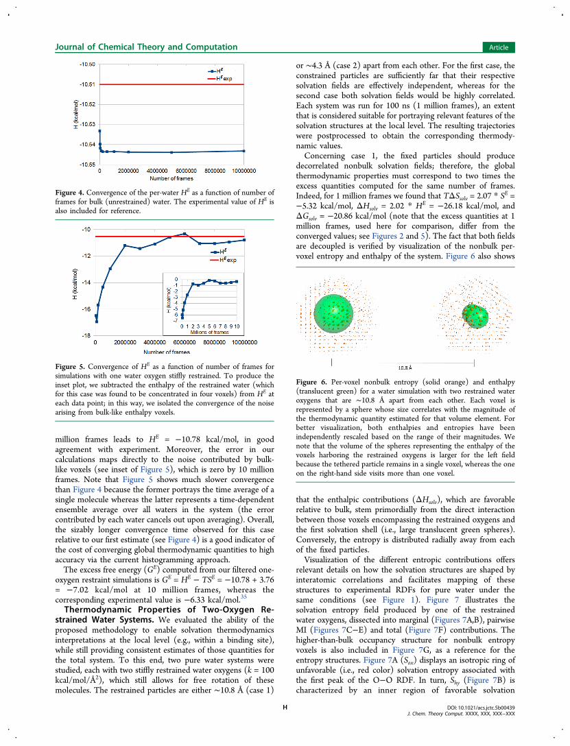
million frames leads to HE = −10.78 kcal/mol, in goodagreement with experiment. Moreover, the error in ourcalculations maps directly to the noise contributed by bulk-like voxels (see inset of Figure 5), which is zero by 10 millionframes. Note that Figure 5 shows much slower convergencethan Figure 4 because the former portrays the time average of asingle molecule whereas the latter represents a time-dependentensemble average over all waters in the system (the errorcontributed by each water cancels out upon averaging). Overall,the sizably longer convergence time observed for this caserelative to our first estimate (see Figure 4) is a good indicator ofthe cost of converging global thermodynamic quantities to highaccuracy via the current histogramming approach.The excess free energy (GE) computed from our filtered one-

oxygen restraint simulations is GE = HE − TSE = −10.78 + 3.76= −7.02 kcal/mol at 10 million frames, whereas thecorresponding experimental value is −6.33 kcal/mol.35

Thermodynamic Properties of Two-Oxygen Re-strained Water Systems. We evaluated the ability of theproposed methodology to enable solvation thermodynamicsinterpretations at the local level (e.g., within a binding site),while still providing consistent estimates of those quantities forthe total system. To this end, two pure water systems werestudied, each with two stiffly restrained water oxygens (k = 100kcal/mol/Å2), which still allows for free rotation of thesemolecules. The restrained particles are either ∼10.8 Å (case 1)

or ∼4.3 Å (case 2) apart from each other. For the first case, theconstrained particles are sufficiently far that their respectivesolvation fields are effectively independent, whereas for thesecond case both solvation fields would be highly correlated.Each system was run for 100 ns (1 million frames), an extentthat is considered suitable for portraying relevant features of thesolvation structures at the local level. The resulting trajectorieswere postprocessed to obtain the corresponding thermody-namic values.Concerning case 1, the fixed particles should produce

decorrelated nonbulk solvation fields; therefore, the globalthermodynamic properties must correspond to two times theexcess quantities computed for the same number of frames.Indeed, for 1 million frames we found that TΔSsolv = 2.07 * SE =−5.32 kcal/mol, ΔHsolv = 2.02 * HE = −26.18 kcal/mol, andΔGsolv = −20.86 kcal/mol (note that the excess quantities at 1million frames, used here for comparison, differ from theconverged values; see Figures 2 and 5). The fact that both fieldsare decoupled is verified by visualization of the nonbulk per-voxel entropy and enthalpy of the system. Figure 6 also shows

that the enthalpic contributions (ΔHsolv), which are favorablerelative to bulk, stem primordially from the direct interactionbetween those voxels encompassing the restrained oxygens andthe first solvation shell (i.e., large translucent green spheres).Conversely, the entropy is distributed radially away from eachof the fixed particles.Visualization of the different entropic contributions offers

relevant details on how the solvation structures are shaped byinteratomic correlations and facilitates mapping of thesestructures to experimental RDFs for pure water under thesame conditions (see Figure 1). Figure 7 illustrates thesolvation entropy field produced by one of the restrainedwater oxygens, dissected into marginal (Figures 7A,B), pairwiseMI (Figures 7C−E) and total (Figure 7F) contributions. Thehigher-than-bulk occupancy structure for nonbulk entropyvoxels is also included in Figure 7G, as a reference for theentropy structures. Figure 7A (Sox) displays an isotropic ring ofunfavorable (i.e., red color) solvation entropy associated withthe first peak of the O−O RDF. In turn, Shy (Figure 7B) ischaracterized by an inner region of favorable solvation

Figure 4. Convergence of the per-water HE as a function of number offrames for bulk (unrestrained) water. The experimental value of HE isalso included for reference.

Figure 5. Convergence of HE as a function of number of frames forsimulations with one water oxygen stiffly restrained. To produce theinset plot, we subtracted the enthalpy of the restrained water (whichfor this case was found to be concentrated in four voxels) from HE ateach data point; in this way, we isolated the convergence of the noisearising from bulk-like enthalpy voxels.

Figure 6. Per-voxel nonbulk entropy (solid orange) and enthalpy(translucent green) for a water simulation with two restrained wateroxygens that are ∼10.8 Å apart from each other. Each voxel isrepresented by a sphere whose size correlates with the magnitude ofthe thermodynamic quantity estimated for that volume element. Forbetter visualization, both enthalpies and entropies have beenindependently rescaled based on the range of their magnitudes. Wenote that the volume of the spheres representing the enthalpy of thevoxels harboring the restrained oxygens is larger for the left fieldbecause the tethered particle remains in a single voxel, whereas the oneon the right-hand side visits more than one voxel.



H


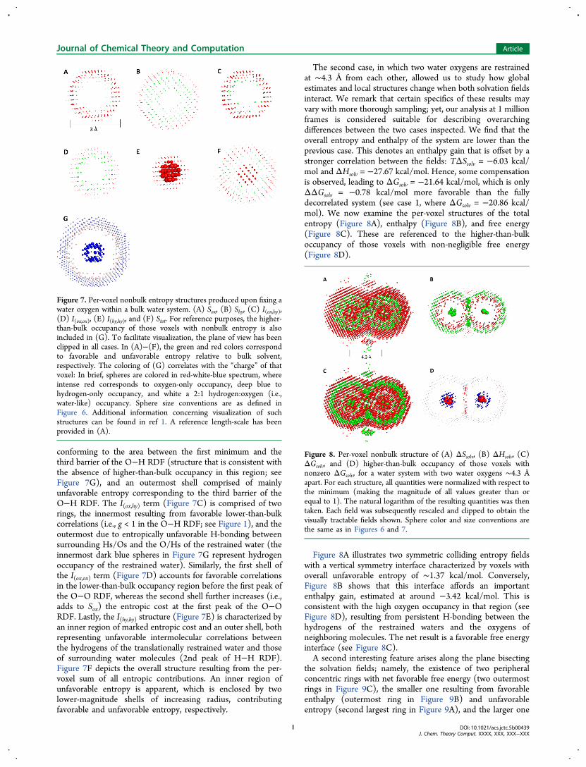
conforming to the area between the first minimum and thethird barrier of the O−H RDF (structure that is consistent withthe absence of higher-than-bulk occupancy in this region; seeFigure 7G), and an outermost shell comprised of mainlyunfavorable entropy corresponding to the third barrier of theO−H RDF. The I(ox,hy) term (Figure 7C) is comprised of tworings, the innermost resulting from favorable lower-than-bulkcorrelations (i.e., g < 1 in the O−H RDF; see Figure 1), and theoutermost due to entropically unfavorable H-bonding betweensurrounding Hs/Os and the O/Hs of the restrained water (theinnermost dark blue spheres in Figure 7G represent hydrogenoccupancy of the restrained water). Similarly, the first shell ofthe I(ox,ox) term (Figure 7D) accounts for favorable correlationsin the lower-than-bulk occupancy region before the first peak ofthe O−O RDF, whereas the second shell further increases (i.e.,adds to Sox) the entropic cost at the first peak of the O−ORDF. Lastly, the I(hy,hy) structure (Figure 7E) is characterized byan inner region of marked entropic cost and an outer shell, bothrepresenting unfavorable intermolecular correlations betweenthe hydrogens of the translationally restrained water and thoseof surrounding water molecules (2nd peak of H−H RDF).Figure 7F depicts the overall structure resulting from the per-voxel sum of all entropic contributions. An inner region ofunfavorable entropy is apparent, which is enclosed by twolower-magnitude shells of increasing radius, contributingfavorable and unfavorable entropy, respectively.

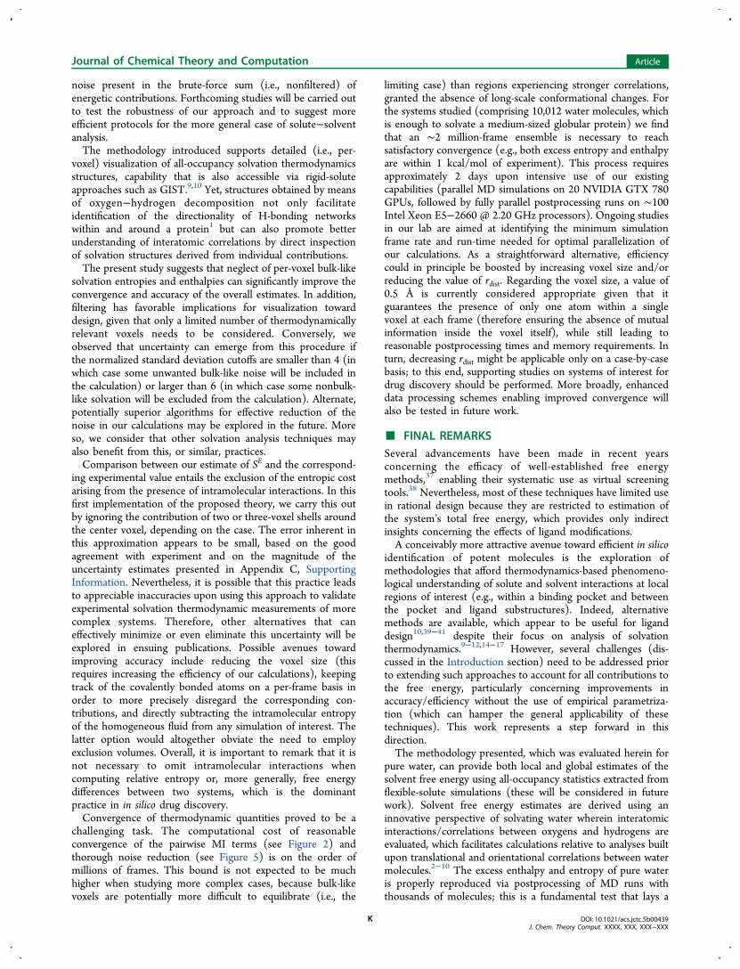
The second case, in which two water oxygens are restrainedat ∼4.3 Å from each other, allowed us to study how globalestimates and local structures change when both solvation fieldsinteract. We remark that certain specifics of these results mayvary with more thorough sampling; yet, our analysis at 1 millionframes is considered suitable for describing overarchingdifferences between the two cases inspected. We find that theoverall entropy and enthalpy of the system are lower than theprevious case. This denotes an enthalpy gain that is offset by astronger correlation between the fields: TΔSsolv = −6.03 kcal/mol and ΔHsolv = −27.67 kcal/mol. Hence, some compensationis observed, leading to ΔGsolv = −21.64 kcal/mol, which is onlyΔΔGsolv = −0.78 kcal/mol more favorable than the fullydecorrelated system (see case 1, where ΔGsolv = −20.86 kcal/mol). We now examine the per-voxel structures of the totalentropy (Figure 8A), enthalpy (Figure 8B), and free energy(Figure 8C). These are referenced to the higher-than-bulkoccupancy of those voxels with non-negligible free energy(Figure 8D).

Figure 8A illustrates two symmetric colliding entropy fieldswith a vertical symmetry interface characterized by voxels withoverall unfavorable entropy of ∼1.37 kcal/mol. Conversely,Figure 8B shows that this interface affords an importantenthalpy gain, estimated at around −3.42 kcal/mol. This isconsistent with the high oxygen occupancy in that region (seeFigure 8D), resulting from persistent H-bonding between thehydrogens of the restrained waters and the oxygens ofneighboring molecules. The net result is a favorable free energyinterface (see Figure 8C).A second interesting feature arises along the plane bisecting

the solvation fields; namely, the existence of two peripheralconcentric rings with net favorable free energy (two outermostrings in Figure 9C), the smaller one resulting from favorableenthalpy (outermost ring in Figure 9B) and unfavorableentropy (second largest ring in Figure 9A), and the larger one

Figure 7. Per-voxel nonbulk entropy structures produced upon fixing awater oxygen within a bulk water system. (A) Sox, (B) Shy, (C) I(ox,hy),(D) I(ox,ox), (E) I(hy,hy), and (F) Stot. For reference purposes, the higher-than-bulk occupancy of those voxels with nonbulk entropy is alsoincluded in (G). To facilitate visualization, the plane of view has beenclipped in all cases. In (A)−(F), the green and red colors correspondto favorable and unfavorable entropy relative to bulk solvent,respectively. The coloring of (G) correlates with the “charge” of thatvoxel: In brief, spheres are colored in red-white-blue spectrum, whereintense red corresponds to oxygen-only occupancy, deep blue tohydrogen-only occupancy, and white a 2:1 hydrogen:oxygen (i.e.,water-like) occupancy. Sphere size conventions are as defined inFigure 6. Additional information concerning visualization of suchstructures can be found in ref 1. A reference length-scale has beenprovided in (A).

Figure 8. Per-voxel nonbulk structure of (A) ΔSsolv, (B) ΔHsolv, (C)ΔGsolv, and (D) higher-than-bulk occupancy of those voxels withnonzero ΔGsolv, for a water system with two water oxygens ∼4.3 Åapart. For each structure, all quantities were normalized with respect tothe minimum (making the magnitude of all values greater than orequal to 1). The natural logarithm of the resulting quantities was thentaken. Each field was subsequently rescaled and clipped to obtain thevisually tractable fields shown. Sphere color and size conventions arethe same as in Figures 6 and 7.



I


solely from favorable entropy (outermost ring in Figure 9A).These can also be discerned in Figures 8A−C as clusters ofspheres directly above and below the vertical interface discussedin the previous paragraph. These rings represent thepropagation of nonbulk correlations/interactions into thesecond solvation shell, effects that are nearly absent when thefields are decorrelated (e.g., case 1). Note that Figures 8 and 9display the logarithm of each quantity; thus, it can be inferredfrom these figures that the two second-shell rings provide amarkedly lower contribution to the overall free energy, relativeto the enthalpy of the fixed particles or the enthalpy of thedirect interface between the fields. Nevertheless, in the generalcase, second and higher-shell effects that disseminate to largeportions of space may have a sizable impact on ligand designand should therefore be carefully scrutinized.As a final observation, the phenomenon of entropy-enthalpy

compensation is suggested in Figure 9 by the palpablesuperposition of shells of favorable enthalpy and unfavorableentropy, which offset each other with the concomitant effect onthe free energy.

■ DISCUSSIONWe have introduced a methodology for calculating solvationentropies, enthalpies, and free energies, which is rooted in thestudy of water oxygen and hydrogen correlations/interactions.Our results suggest that the discretized expressions derivedfrom our postulates are suitable for estimation of thesethermodynamic quantities, both globally and around localregions of interest. Furthermore, for the general case, theviewpoint introduced offers particular advantages over relatedgrid-based or site-based techniques. These include thefollowing:1) A more tractable algorithm for calculation of second and

higher-order solvation entropies, relative to those based on theanalysis of molecular positions and orientations.2−8,16 Inparticular, potential inaccuracies resulting from the summationof entropies that are computed via two distinct distance metrics(e.g., positional and orientational) are avoided. Moreover, weanticipate that convergence of ΔSsolv for large systems will befaster when circumventing the highly complex process ofcomputing accurate probability densities from relativeorientations between waters. In general, the derived thermody-namics expressions can also be employed to postprocess wateroxygen−hydrogen density data obtained from other techniques(e.g., 3D-RISM16).

2) The entropy expressions derived in this work are notfounded on (but are naturally related to) IST; more explicitly,our derivation is not conceptually built around the use of radialdistribution functions. Thus, future attempts to extend ourtheory to the estimation of solute−solvent free energies(ongoing work) would likely be independent of the fixed-solute requirement inherent in IST. In general, allowing solutemotions should lead to a more representative solute−solventstructural ensemble relative to the use of fixed solute. Inaddition, flexible-solute simulations can expedite recognition ofincorrect solvent structures (arising, for instance, frominappropriate charge assignments) given that the resultingensemble-averaged structures should overlay satisfactorily ontothe corresponding high-resolution crystals, when available.More laborious fixed-solute schemes in which variousrepresentative states are sampled in parallel might be anappealing alternative to flexible-solute analyses. Nevertheless,these involve costly preliminary steps including initial samplingruns, clustering toward identification of a representativestructure for each state, and proper weighting of the probabilitydensity of each state. It may be argued that a single flexible-solute simulation affords deficient sampling of solvent statesrelative to multiple fixed-solute analyses of diverse conforma-tions. To overcome this potential limitation, our standardprotocol includes running multiple parallel simulations withperturbed initial velocities, as implemented in this work andelsewhere.1

3) The ability to capture relative differences in intramolecularentropy resulting from molecular vibrations, which are directlylinked to the first peak of the O−H and H−H RDFs. This isonly relevant when using flexible-water models (which shouldlead to more detailed results due to their ability to captureintramolecular motions), given that intramolecular contribu-tions cancel out when using rigid-water models to computeΔΔSsolv. Note that the use of our approach to compute ΔΔGsolvfrom flexible-water simulations would require both retaining theunfavorable entropic cost of covalently forming all watermolecules and including all favorable covalent bonding energies(formation of a water molecule is an exothermic process),which are not encompassed by eq 17.The value of the excess entropy computed for pure water,

resulting from the sum of two marginal and three pairwiseterms, exhibits good agreement with experiment. Our resultssupport the notion that third-plus order terms do notcontribute significantly to the overall entropy estimate; yet,plausible scenarios for which higher order terms are relevantshould not be discounted, and follow-up efforts to characterizethese circumstances may be advantageous. Note that the lowerentropic cost observed in our calculations is likely due to thefact that for voxel sizes of 0.5 Å the actual probability density ofeach voxel is still smoothed out. A simple analysis of theexperimental RDFs of pure water, in which the one-dimensional data is binned into distances of varying magnitude,suggests that highly uniform probability densities will beachieved only for voxel sizes that are ≤0.1 Å. The use of such ahigh-resolution grid is, however, not feasible in light of ourcurrent computational capabilities.Concerning the excess enthalpy, it is encouraging to find that

a simplified H-bonding distance algorithm leads to values thatare in good agreement with experiment. Interestingly, otherapproaches encompassing the full spectrum of interactionenergies9,30 can potentially lead to higher uncertainty, due totheir direct dependence on force field energies and/or due to

Figure 9. Per-voxel nonbulk structure of (A) ΔSsolv, (B) ΔHsolv, and(C) ΔGsolv. These views correspond to a 90-degree rotation of Figures8A−C, along the x-axis. The enthalpy has been scaled by a smallerfactor relative to Figure 8B, to allow visualization of the outermostring. In accordance with this rescaling, the enthalpically favorable innerring in (B) corresponds to the enthalpically favorable outer rings inFigure 8B. Sphere color and size is the same as in Figures 6 and 7. Areference length-scale has been provided in (A).



J


noise present in the brute-force sum (i.e., nonfiltered) ofenergetic contributions. Forthcoming studies will be carried outto test the robustness of our approach and to suggest moreefficient protocols for the more general case of solute−solventanalysis.The methodology introduced supports detailed (i.e., per-

voxel) visualization of all-occupancy solvation thermodynamicsstructures, capability that is also accessible via rigid-soluteapproaches such as GIST.9,10 Yet, structures obtained by meansof oxygen−hydrogen decomposition not only facilitateidentification of the directionality of H-bonding networkswithin and around a protein1 but can also promote betterunderstanding of interatomic correlations by direct inspectionof solvation structures derived from individual contributions.The present study suggests that neglect of per-voxel bulk-like

solvation entropies and enthalpies can significantly improve theconvergence and accuracy of the overall estimates. In addition,filtering has favorable implications for visualization towarddesign, given that only a limited number of thermodynamicallyrelevant voxels needs to be considered. Conversely, weobserved that uncertainty can emerge from this procedure ifthe normalized standard deviation cutoffs are smaller than 4 (inwhich case some unwanted bulk-like noise will be included inthe calculation) or larger than 6 (in which case some nonbulk-like solvation will be excluded from the calculation). Alternate,potentially superior algorithms for effective reduction of thenoise in our calculations may be explored in the future. Moreso, we consider that other solvation analysis techniques mayalso benefit from this, or similar, practices.Comparison between our estimate of SE and the correspond-

ing experimental value entails the exclusion of the entropic costarising from the presence of intramolecular interactions. In thisfirst implementation of the proposed theory, we carry this outby ignoring the contribution of two or three-voxel shells aroundthe center voxel, depending on the case. The error inherent inthis approximation appears to be small, based on the goodagreement with experiment and on the magnitude of theuncertainty estimates presented in Appendix C, SupportingInformation. Nevertheless, it is possible that this practice leadsto appreciable inaccuracies upon using this approach to validateexperimental solvation thermodynamic measurements of morecomplex systems. Therefore, other alternatives that caneffectively minimize or even eliminate this uncertainty will beexplored in ensuing publications. Possible avenues towardimproving accuracy include reducing the voxel size (thisrequires increasing the efficiency of our calculations), keepingtrack of the covalently bonded atoms on a per-frame basis inorder to more precisely disregard the corresponding con-tributions, and directly subtracting the intramolecular entropyof the homogeneous fluid from any simulation of interest. Thelatter option would altogether obviate the need to employexclusion volumes. Overall, it is important to remark that it isnot necessary to omit intramolecular interactions whencomputing relative entropy or, more generally, free energydifferences between two systems, which is the dominantpractice in in silico drug discovery.Convergence of thermodynamic quantities proved to be a

challenging task. The computational cost of reasonableconvergence of the pairwise MI terms (see Figure 2) andthorough noise reduction (see Figure 5) is on the order ofmillions of frames. This bound is not expected to be muchhigher when studying more complex cases, because bulk-likevoxels are potentially more difficult to equilibrate (i.e., the

limiting case) than regions experiencing stronger correlations,granted the absence of long-scale conformational changes. Forthe systems studied (comprising 10,012 water molecules, whichis enough to solvate a medium-sized globular protein) we findthat an ∼2 million-frame ensemble is necessary to reachsatisfactory convergence (e.g., both excess entropy and enthalpyare within 1 kcal/mol of experiment). This process requiresapproximately 2 days upon intensive use of our existingcapabilities (parallel MD simulations on 20 NVIDIA GTX 780GPUs, followed by fully parallel postprocessing runs on ∼100Intel Xeon E5−2660 @ 2.20 GHz processors). Ongoing studiesin our lab are aimed at identifying the minimum simulationframe rate and run-time needed for optimal parallelization ofour calculations. As a straightforward alternative, efficiencycould in principle be boosted by increasing voxel size and/orreducing the value of rdist. Regarding the voxel size, a value of0.5 Å is currently considered appropriate given that itguarantees the presence of only one atom within a singlevoxel at each frame (therefore ensuring the absence of mutualinformation inside the voxel itself), while still leading toreasonable postprocessing times and memory requirements. Inturn, decreasing rdist might be applicable only on a case-by-casebasis; to this end, supporting studies on systems of interest fordrug discovery should be performed. More broadly, enhanceddata processing schemes enabling improved convergence willalso be tested in future work.

■ FINAL REMARKSSeveral advancements have been made in recent yearsconcerning the efficacy of well-established free energymethods,37 enabling their systematic use as virtual screeningtools.38 Nevertheless, most of these techniques have limited usein rational design because they are restricted to estimation ofthe system’s total free energy, which provides only indirectinsights concerning the effects of ligand modifications.A conceivably more attractive avenue toward efficient in silico

identification of potent molecules is the exploration ofmethodologies that afford thermodynamics-based phenomeno-logical understanding of solute and solvent interactions at localregions of interest (e.g., within a binding pocket and betweenthe pocket and ligand substructures). Indeed, alternativemethods are available, which appear to be useful for liganddesign10,39−41 despite their focus on analysis of solvationthermodynamics.9−12,14−17 However, several challenges (dis-cussed in the Introduction section) need to be addressed priorto extending such approaches to account for all contributions tothe free energy, particularly concerning improvements inaccuracy/efficiency without the use of empirical parametriza-tion (which can hamper the general applicability of thesetechniques). This work represents a step forward in thisdirection.The methodology presented, which was evaluated herein for

pure water, can provide both local and global estimates of thesolvent free energy using all-occupancy statistics extracted fromflexible-solute simulations (these will be considered in futurework). Solvent free energy estimates are derived using aninnovative perspective of solvating water wherein interatomicinteractions/correlations between oxygens and hydrogens areevaluated, which facilitates calculations relative to analyses builtupon translational and orientational correlations between watermolecules.2−10 The excess enthalpy and entropy of pure wateris properly reproduced via postprocessing of MD runs withthousands of molecules; this is a fundamental test that lays a



K




solid foundation for the efficacious study of solvated systemsrelevant to drug discovery. Variations in the local and globalenthalpy, entropy, and free energy between water systems withcorrelated versus decorrelated inhomogeneous solvationstructures were also examined. The ability of our approach toisolate the contributions of individual solvating water moleculesand networks thereof provides, in the general case, the basis fordetailed structural and mechanistic studies essential forunderstanding flexible protein−ligand binding.The expressions proposed herein will be adopted as a basis

for iterative design practices, in which local solvationthermodynamic quantities are used to guide changes in thesolute/ligand (e.g., aimed at displacing free energeticallyunfavorable or avoiding favorable solvation), whose effect isassessed by means of iterative simulations/analysis, design(based on solute−solvent reorganization), synthesis, andexperimental testing. This process, when carried out until asatisfactory solute−solvent structure has been attained, cannoticeably improve the chance of identifying promisingcandidates.Looking forward, additional work is necessary to further

assess the accuracy of the proposed methodology in its currentstate. This involves exploring improved filtering protocols aswell as practices that would allow us to relax some of theassumptions/approximations that are presently in place. Inaddition, the computational cost required for convergence ofthermodynamic quantities via the current histogrammingprotocol may, to some extent, hinder the systematic use ofour methodology for virtual screening. Therefore, research inprogress includes exploration of alternate statistical analysistechniques, such as the k-Nearest-Neighbors algorithm whichhas been previously evaluated within the framework of IST-derived approaches.9,42

Prospective research also includes the estimation of solvationenthalpies and entropies of small solutes, host−guestcomplexes, and protein−ligand systems, with the primary goalof partitioning the relative contributions of solvation freeenergies into the association and dissociation barriers (i.e., tokon and koff). Related efforts have been previously carried out byour group,13,40,43 suggesting that water−water interactions playa dominant role (as a “free energy reservoir”) during thebinding process. More general theoretical inquiries, such as thedegree of coupling between solute and solvent entropies andentropy-enthalpy compensation, can also be explored bycomplementing the proposed methodology with techniquessuch as alchemical or PMF free energy methods or algorithmsfor estimation of configurational entropies and energies.Overall, we believe that this type of structure-free energy

analyses can enhance the role of computational chemistry in thepharmaceutical industry, with the potential to more consistentlydeliver drug-like ligand designs than those efforts supported bymore traditional molecular modeling techniques.

■ ASSOCIATED CONTENT

*S Supporting InformationThe Supporting Information is available free of charge on theACS Publications website at DOI: 10.1021/acs.jctc.5b00439.

Appendix A: Normalization of the solvation entropydifferences relative to bulk solvent, Appendix B:Solvation entropy: Water as a polyatomic fluid, AppendixC: Estimation of the error in the entropy calculations

upon disregarding contributions of voxels around thecenter voxel (PDF)

■ AUTHOR INFORMATIONCorresponding Authors*E-mail: [email protected] (C.V.-V.).*E-mail: [email protected] (D.J.J.M.).*E-mail: [email protected] (T.K.).NotesThe authors declare no competing financial interest.

■ ACKNOWLEDGMENTSThe authors thank Prof. Mike Gilson, Dr. Viktor Hornak, andDr. Mitsunori Kato for fruitful discussions leading to the workpresented in this document. Tom Kurtzman's contribution wasfunded, in part, by NIH grant GM095417.

■ REFERENCES(1) Velez-Vega, C.; McKay, D. J. J.; Aravamuthan, V.; Pearlstein, R.;Duca, J. S. Time-Averaged Distributions of Solute and SolventMotions: Exploring Proton Wires of GFP and PfM2DH. J. Chem. Inf.Model. 2014, 54 (12), 3344−3361.(2) Wallace, D. C. On the Role of Density Fluctuations in theEntropy of a Fluid. J. Chem. Phys. 1987, 87 (4), 2282−2284.(3) Ashbaugh, H. S.; Paulaitis, M. E. Entropy of HydrophobicHydration: Extension to Hydrophobic Chains. J. Phys. Chem. 1996,100 (5), 1900−1913.(4) Lazaridis, T. Inhomogeneous Fluid Approach to SolvationThermodynamics. 1. Theory. J. Phys. Chem. B 1998, 102 (18), 3531−3541.(5) Morita, T.; Hiroike, K. A New Approach to the Theory ofClassical Fluids. III General Treatment of Classical Systems. Prog.Theor. Phys. 1961, 25 (4), 537−578.(6) Lazaridis, T.; Karplus, M. Orientational Correlations and Entropyin Liquid Water. J. Chem. Phys. 1996, 105 (10), 4294−4316.(7) Baranyai, A.; Evans, D. J. Direct Entropy Calculation fromComputer Simulation of Liquids. Phys. Rev. A: At., Mol., Opt. Phys.1989, 40 (7), 3817−3822.(8) Huggins, D. J. Quantifying the Entropy of Binding for WaterMolecules in Protein Cavities by Computing Correlations. Biophys. J.2015, 108 (4), 928−936.(9) Nguyen, C. N.; Young, T. K.; Gilson, M. K. Grid InhomogeneousSolvation Theory: Hydration Structure and Thermodynamics of theMiniature Receptor cucurbit[7]uril. J. Chem. Phys. 2012, 137 (4),044101.(10) Nguyen, C. N.; Cruz, A.; Gilson, M. K.; Kurtzman, T.Thermodynamics of Water in an Enzyme Active Site: Grid-BasedHydration Analysis of Coagulation Factor Xa. J. Chem. Theory Comput.2014, 10 (7), 2769−2780.(11) Li, Z.; Lazaridis, T. Computing the ThermodynamicContributions of Interfacial Water. Methods Mol. Biol. 2012, 819,393−404.(12) Young, T.; Abel, R.; Kim, B.; Berne, B. J.; Friesner, R. A. Motifsfor Molecular Recognition Exploiting Hydrophobic Enclosure inProtein−ligand Binding. Proc. Natl. Acad. Sci. U. S. A. 2007, 104 (3),808−813.(13) Pearlstein, R. A.; Hu, Q.-Y.; Zhou, J.; Yowe, D.; Levell, J.; Dale,B.; Kaushik, V. K.; Daniels, D.; Hanrahan, S.; Sherman, W.; Abel, R.New Hypotheses about the Structure-Function of ProproteinConvertase Subtilisin/kexin Type 9: Analysis of the Epidermal GrowthFactor-like Repeat A Docking Site Using WaterMap. Proteins: Struct.,Funct., Genet. 2010, 78 (12), 2571−2586.(14) Huggins, D. J. Application of Inhomogeneous Fluid SolvationTheory to Model the Distribution and Thermodynamics of WaterMolecules around Biomolecules. Phys. Chem. Chem. Phys. 2012, 14(43), 15106−15117.



L

http://pubs.acs.org

http://pubs.acs.org/doi/abs/10.1021/acs.jctc.5b00439


mailto:[email protected]




(15) Haider, K.; Huggins, D. J. Combining Solvent ThermodynamicProfiles with Functionality Maps of the Hsp90 Binding Site to Predictthe Displacement of Water Molecules. J. Chem. Inf. Model. 2013, 53(10), 2571−2586.(16) Sindhikara, D. J.; Hirata, F. Analysis of Biomolecular SolvationSites by 3D-RISM Theory. J. Phys. Chem. B 2013, 117 (22), 6718−6723.(17) Gerogiokas, G.; Calabro, G.; Henchman, R. H.; Southey, M. W.Y.; Law, R. J.; Michel, J. Prediction of Small Molecule HydrationThermodynamics with Grid Cell Theory. J. Chem. Theory Comput.2014, 10 (1), 35−48.(18) Grant, J. A.; Pickup, B. T.; Nicholls, A. A Smooth PermittivityFunction for Poisson−Boltzmann Solvation Methods. J. Comput.Chem. 2001, 22 (6), 608−640.(19) Hu, B.; Lill, M. A. WATsite: Hydration Site Prediction Programwith PyMOL Interface. J. Comput. Chem. 2014, 35 (16), 1255−1260.(20) Abel, R.; Young, T.; Farid, R.; Berne, B. J.; Friesner, R. A. Roleof the Active-Site Solvent in the Thermodynamics of Factor Xa LigandBinding. J. Am. Chem. Soc. 2008, 130 (9), 2817−2831.(21) Killian, B. J.; Kravitz, J. Y.; Gilson, M. K. Extraction ofConfigurational Entropy from Molecular Simulations via an ExpansionApproximation. J. Chem. Phys. 2007, 127 (2), 024107.(22) Zhou, H.-X.; Gilson, M. K. Theory of Free Energy and Entropyin Noncovalent Binding. Chem. Rev. 2009, 109 (9), 4092−4107.(23) Head, M. S.; Given, J. A.; Gilson, M. K. Mining Minima”: DirectComputation of Conformational Free Energy. J. Phys. Chem. A 1997,101 (8), 1609−1618.(24) Hnizdo, V.; Darian, E.; Fedorowicz, A.; Demchuk, E.; Li, S.;Singh, H. Nearest-Neighbor Nonparametric Method for Estimatingthe Configurational Entropy of Complex Molecules. J. Comput. Chem.2007, 28 (3), 655−668.(25) King, B. M.; Silver, N. W.; Tidor, B. Efficient Calculation ofMolecular Configurational Entropies Using an Information TheoreticApproximation. J. Phys. Chem. B 2012, 116 (9), 2891−2904.(26) Karplus, M.; Kushick, J. N. Method for Estimating theConfigurational Entropy of Macromolecules. Macromolecules 1981,14 (2), 325−332.(27) Hnizdo, V.; Gilson, M. K. Thermodynamic and DifferentialEntropy under a Change of Variables. Entropy 2010, 12 (3), 578−590.(28) Matsuda, H. Physical Nature of Higher-Order MutualInformation: Intrinsic Correlations and Frustration. Phys. Rev. E:Stat. Phys., Plasmas, Fluids, Relat. Interdiscip. Top. 2000, 62 (3), 3096−3102.(29) Soper, A. K. The Radial Distribution Functions of Water and Icefrom 220 to 673 K and at Pressures up to 400 MPa. Chem. Phys. 2000,258 (2−3), 121−137.(30) Huggins, D. J. Correlations in Liquid Water for the TIP3P-Ewald, TIP4P-2005, TIP5P-Ewald, and SWM4-NDP Models. J. Chem.Phys. 2012, 136 (6), 064518.(31) Case, D.; Darden, T.; Cheatham, T.; Simmerling, C.; Wang, J.;Duke, R.; Luo, R.; Walker, R.; Zhang, W.; Merz, K.; Roberts, B.; Hayik,S.; Roitberg, A.; Seabra, G.; Kolossvary, I.; Wong, K.; Paesani, F.;Vanicek, J.; Wolf, R.; Liu, J.; Wu, X.; Brozell, S.; Steinbrecher, T.;Gohlke, H.; Cai, Q.; Ye, X.; Wang, J.; Hsieh, M.-J.; Cui, G.; Roe, D.;Mathews, D.; Seetin, M.; Salomon-Ferrer, R.; Sagui, C.; Babin, V.;Luchko, T.; Gusarov, S.; Kovalenko, A.; Kollman, P. Amber 12.(32) Salomon-Ferrer, R.; Gotz, A. W.; Poole, D.; Le Grand, S.;Walker, R. C. Routine Microsecond Molecular Dynamics Simulationswith AMBER on GPUs. 2. Explicit Solvent Particle Mesh Ewald. J.Chem. Theory Comput. 2013, 9 (9), 3878−3888.(33) MATLAB and Statistics Toolbox Release 2007b; The MathWorks,Inc.: Natick, Massachusetts, United States, 2007.(34) Rosenfeld, Y. Relation between the Transport Coefficients andthe Internal Entropy of Simple Systems. Phys. Rev. A: At., Mol., Opt.Phys. 1977, 15 (6), 2545−2549.(35) Wagner, W.; Pruß, A. The IAPWS Formulation 1995 for theThermodynamic Properties of Ordinary Water Substance for Generaland Scientific Use. J. Phys. Chem. Ref. Data 2002, 31 (2), 387−535.

(36) Wertz, D. H. Relationship between the Gas-Phase Entropies ofMolecules and Their Entropies of Solvation in Water and 1-Octanol. J.Am. Chem. Soc. 1980, 102 (16), 5316−5322.(37) Hansen, N.; van Gunsteren, W. F. Practical Aspects of Free-Energy Calculations: A Review. J. Chem. Theory Comput. 2014, 10 (7),2632−2647.(38) Christ, C. D.; Fox, T. Accuracy Assessment and Automation ofFree Energy Calculations for Drug Design. J. Chem. Inf. Model. 2014,54 (1), 108−120.(39) Weldon, D. J.; Shah, F.; Chittiboyina, A. G.; Sheri, A.; Chada, R.R.; Gut, J.; Rosenthal, P. J.; Shivakumar, D.; Sherman, W.; Desai, P.;Jung, J.-C.; Avery, M. A. Synthesis, Biological Evaluation, HydrationSite Thermodynamics, and Chemical Reactivity Analysis of α-KetoSubstituted Peptidomimetics for the Inhibition of PlasmodiumFalciparum. Bioorg. Med. Chem. Lett. 2014, 24 (5), 1274−1279.(40) Pearlstein, R. A.; Sherman, W.; Abel, R. Contributions of WaterTransfer Energy to Protein-Ligand Association and DissociationBarriers: Watermap Analysis of a Series of p38α MAP KinaseInhibitors. Proteins: Struct., Funct., Genet. 2013, 81 (9), 1509−1526.(41) Mondal, J.; Friesner, R. A.; Berne, B. J. Role of Desolvation inThermodynamics and Kinetics of Ligand Binding to a Kinase. J. Chem.Theory Comput. 2014, 10 (12), 5696−5705.(42) Huggins, D. J. Estimating Translational and OrientationalEntropies Using the K-Nearest Neighbors Algorithm. J. Chem. TheoryComput. 2014, 10 (9), 3617−3625.(43) Tran, Q.-T.; Williams, S.; Farid, R.; Erdemli, G.; Pearlstein, R.The Translocation Kinetics of Antibiotics through Porin OmpC:Insights from Structure-Based Solvation Mapping Using WaterMap.Proteins: Struct., Funct., Genet. 2013, 81 (2), 291−299.



M


estimation of solvation entropy and enthalpy via …...2015/10/21 · estimation of solvation...

Documents