eswarmurthi gopalakrishnan
TRANSCRIPT
MASTER THESIS
Luleå University of Technology
Czech Technical University
Faculty of Electrical Engineering
Department of Control Engineering
QUADCOPTER FLIGHT MECHANICS MODEL AND
CONTROL ALGORITHMS
Eswarmurthi Gopalakrishnan
Prague, May 2017
Supervisor: Prof. Dr. Martin Hromčík
Abstract In this thesis I am working on designing the controller for the non-linear Quadcopter model.
I have designed two controllers for the model and have used the simulation to check the
performance of the model.
In the beginning of my work, the fundamental equations of motion and forces of the
Quadcopter are derived and the design parameters for the given Quadcopter are chosen. I
have created a non-linear model for the Quadcopter based on the equation of motion and
forces of moment. Then, I designed a nonlinear dynamics DC motor and have implemented
it in the Simulink. The nonlinear model is then linearized at a given point using the Jacobian
method. For a given set of inputs, the response of the linear and non-linear model is
validated. First, the PID controller for the non-linear model is designed and the results are
analysed. The performance of the Quadcopter model with the optimal PID controller values
are studied by analysing the Angular velocity and Angular displacement of the model. Later
LQR controller is designed for the linear model, which is then implemented to the nonlinear
model to check the performance. The model’s performance is validated by implementing
the DC motor as the source of input. The motor as input is given to study the behaviour of
the model in real life scenario. Finally, I studied the performance of the model with the
controller when a disturbance is given to the model by means of step input and change in
initial condition.
Proclamation I hereby declare that I have developed and written the enclosed Master Thesis
completely by myself, and have not used sources or means without declaration in the
text. Any thoughts from others or literal quotations are clearly marked. The Master
Thesis was not used in the same or in a similar version to achieve an academic grading or
is being published elsewhere.
In Prague, May 26, 2017
………………………………………........
Eswarmurthi Gopalakrishnan
Acknowledgment Firstly, I would like to express my sincere thanks to my supervisor in Czech Technical
University Dr. Prof. Martin Hromčík, who gave me the opportunity to work on this
interesting project, for his guidance over the period of time.
I would like to dedicate this Master Thesis work to my late Mother Thriveni Gopalakrishnan.
Also, I would like to thank my wife, my parents, my sister and my friends who stood by my
side during hard time and gave me mental strength to complete my thesis successfully. Next
I would like to thank Mr. Sanjeev Kubakaddi for his guidance throughout the thesis work.
Lastly, I would like to thank Mr. Sauradep Roy for his help in clearing my doubts whenever I
approached them.
Eswarmurthi Gopalakrishnan May 2017
1
Table of Contents List of Figures ................................................................................................................................................3
Chapter 1 Introduction .................................................................................................................................4
1.1 Quadcopter .........................................................................................................................................4
1.1.1 Indoor Quadcopter ......................................................................................................................5
1.1.2 Outdoor Quadcopter ...................................................................................................................5
1.2 Advantages of Quadcopter over comparably scaled Helicopters .......................................................6
1.3 Uses of Quadcopter ............................................................................................................................6
Chapter 2 Objectives of the thesis ................................................................................................................7
Chapter 3 Dynamic Quadcopter and DC Motor Modelling ..........................................................................8
3.1 Quadcopter Modelling ........................................................................................................................8
3.1.1 General Moments and Forces ......................................................................................................9
3.1.2 Equations of Motion ................................................................................................................. 10
3.2 DC Motor .......................................................................................................................................... 13
3.2.1 Working Principle ...................................................................................................................... 13
3.2.2 Vehicle Dynamics ...................................................................................................................... 15
3.2.3 Aerodynamic Effects ................................................................................................................. 17
3.2.4 Blade Flapping ........................................................................................................................... 19
3.2.5 Coning ....................................................................................................................................... 20
3.2.6 Static Thrust .............................................................................................................................. 22
3.2.7 Thrust through Dynamics Modelling ........................................................................................ 26
3.2.8 Motor Specification ................................................................................................................... 28
3.2.9 Speed Control Using the Armature Current Control ................................................................. 30
Chapter 4 Linearization of the model ........................................................................................................ 33
4.1 Uses of linearization in Stability analysis ......................................................................................... 33
4.1.1 Stability Analysis ....................................................................................................................... 33
4.2 Jacobian Method .............................................................................................................................. 33
4.3 Linearization of the model ............................................................................................................... 34
4.4 Validation of Non-linear and Linear model for the given input ....................................................... 35
4.5 Analysis of the Linearized model ..................................................................................................... 37
4.5.1 Analysis using Controllability and the Observability ................................................................. 37
Chapter 5 Controller .................................................................................................................................. 40
5.1 SISO approach .................................................................................................................................. 40
Eswarmurthi Gopalakrishnan May 2017
2
5.2 PID Controller ................................................................................................................................... 40
5.2.1 Effect of each parameter .......................................................................................................... 42
5.2.2 The characteristics of P, I and D controllers ............................................................................. 43
5.2.3 How to tune Quadcopter PID Gains .......................................................................................... 43
5.2.4 Proportional Controller ............................................................................................................. 44
5.2.5 Proportional Derivative Controller ........................................................................................... 44
5.2.6 Proportional Integral Controller ............................................................................................... 44
5.2.7 Proportional Integral and Derivative Controller ....................................................................... 44
5.3 LQR ................................................................................................................................................... 45
Chapter 6 Simulation ................................................................................................................................. 51
6.1 Simulation ........................................................................................................................................ 51
6.2 Control ............................................................................................................................................. 51
6.3 PD Control ........................................................................................................................................ 52
6.4 PID Control ....................................................................................................................................... 55
6.5 LQR ................................................................................................................................................... 56
Chapter 7 Conclusion ................................................................................................................................. 62
7.1 Comparison of the work .................................................................................................................. 62
7.2 Conclusion ........................................................................................................................................ 63
References ................................................................................................................................................. 64
Eswarmurthi Gopalakrishnan May 2017
3
List of Figures 1. UDI U839- An Indoor Quadcopter
2. Phantom 2 Vision+ - An Outdoor Quadcopter
3. Basic Flight Movements of a Quadcopter
4. Quadcopter Coordinate system
5. Basic components of DC motor
6. Fleming’s left hand rule
7. Movement of forces in a DC motor
8. Electric circuit of a DC motor
9. Response of the DC motor with no controller 10. Response of the DC motor with Drag force
11. Response for the manually tuned Speed and Current controller for DC motor 12. Response of the non-linear and linear model for the given Pitch command
13. Response of the nonlinear and linear model for the given Roll command
14. Simulink structure of PID Controller
15. Controller-Plant Simulink Structure
16. Linear model response for step reference
17. Non-linear model response of 0.5 phi initial condition
18. Response of Quadcopter for the Proportional Derivative controller
19. Response of the Quadcopter due to the Proportional Integral and Derivative Controller
20. Input Signal fed to the model for the forward movement action 21. Non-linear model response for the given step signal
22. Response of motor for the given step reference signal 23. Non-linear model response for the DC motor 24. Nonlinear model response for step signal disturbance 25. Nonlinear model response for change in initial condition for Pitch Angle
Eswarmurthi Gopalakrishnan May 2017
4
Chapter 1 Introduction The aim of this work is to design a linearized simulation model for a dynamics Quadcopter
model and design a controller for the Quadcopter model for a stabilized motion. The work
progresses as follows, in the beginning a detailed introduction is given about the UAVs, their
dynamics and applications. In Chapter 2, the objectives of the thesis work is given and the
guidelines of the thesis work is given. In Chapter 3, the equations of motion for the
Quadcopter model are designed and the model is created in the simulink. Then, equations for
the DC motor are given and the motor is designed in the simulink, later the Angular Velocity
of the motor is controlled through a feed-back controller and then the armature current is
controlled through Armature current controller, which is also a feed-back controller in this
case. In Chapter 4, the non-linear model is linearized using Jacobian Matrix method assigning
operating points for the Quadcopter. Then the controllability, observability of the linearized
model is determined. In chapter 5, a brief note on the PID controller is given. The effect of
each parameters of the PID controller is defined using a table. Then, an introduction to the
LQR controller and the procedure to determine the values of the LQR gain is discussed along
with the benefits of using the LQR controller. In chapter 6, the simulation of the model for the
PD and PID controller is done and the performance of the system for the controller is studied.
After designing the PID controller for the model, the LQR controller is determined by using the
linearized model and then the gain is fed to the non-linear model and the performance of the
model with the gain value is observed. Later simulation is run on the model for different
inputs with and without disturbances. Finally in the Chapter 7, the comparison of the
objectives of the thesis work and the result obtained are compared briefly and a detailed
conclusion of the report and the controller chosen for the model is explained.
1.1 Quadcopter Quadcopter also known as Quad rotor Helicopter, Quad rotor is a multi-rotor helicopter that
is lifted and propelled by four rotors. Quadcopter are classified as rotorcraft, as opposed to
fixed-wing aircraft, because their lift is generated by a set of rotors (vertically oriented
propellers).
Unlike most helicopters, Quadcopter uses two set of identical fixed pitched propellers: tow
clock wise and two counters- clockwise. These use variation of RPM to control loft and torque.
Control of the Quadcopter is achieved by altering the rotation rate of one or more rotor discs,
thereby changing it torque load and thrust/lift characteristics.
A number of manned designs appeared in the 1920s and 1920s. These vehicles were among
the first successful heavier- than- air vertical take-off and landing (VTOL) vehicles [1].
However, early prototypes suffered from poor performance [1], and latter prototypes
required too much pilot work load, due to poor stability augmentation and limited control
authority.
More recently Quadcopter designs have become popular in unmanned aerial vehicle (UAV)
research. These vehicles use an electronic control system and electronic sensors to stabilize
Eswarmurthi Gopalakrishnan May 2017
5
the aircraft. With their small size and agile manoeuvrability, these Quadcopter can be flown
indoors as well as outdoors.
A typical Quadcopter is equipped with an inertial navigation unit (3 accelerometers, 3
gyroscopes and 3 magnetometers) for attitude determination, a barometer (outdoor) or an
ultrasonic proximity sensor (indoor) for altitude measurements and optionally they come with
a camera or GPS receiver.
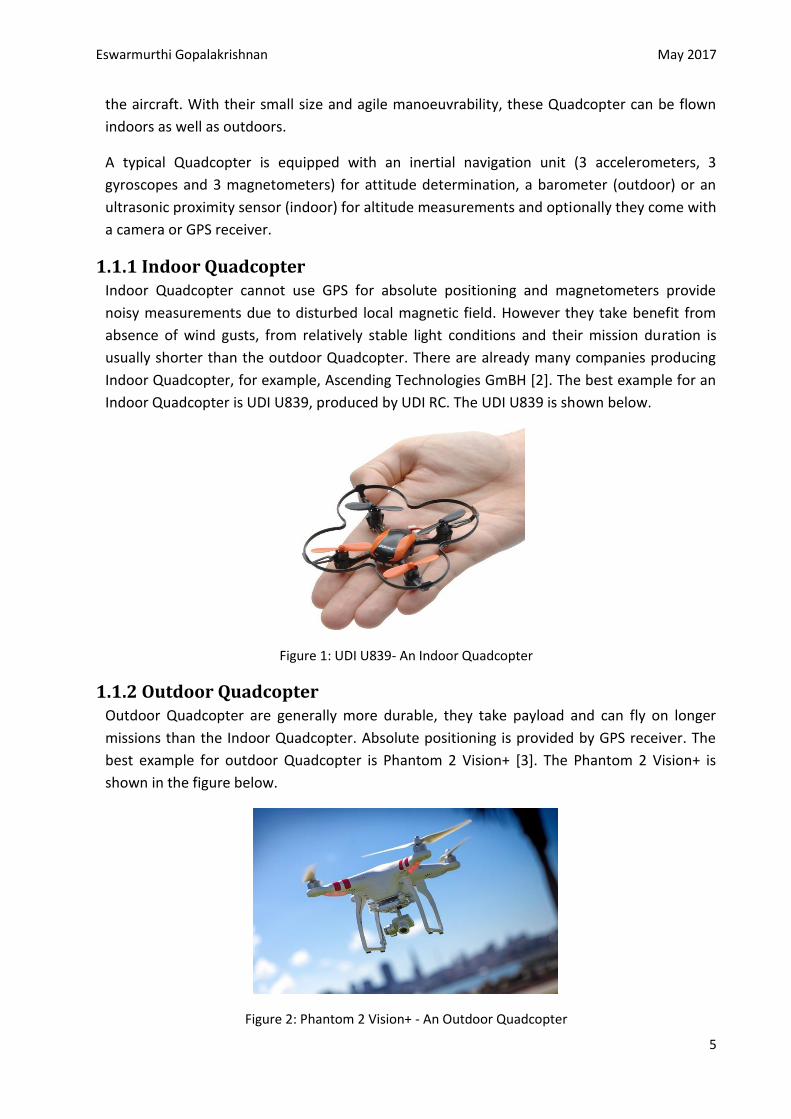
1.1.1 Indoor Quadcopter Indoor Quadcopter cannot use GPS for absolute positioning and magnetometers provide
noisy measurements due to disturbed local magnetic field. However they take benefit from
absence of wind gusts, from relatively stable light conditions and their mission duration is
usually shorter than the outdoor Quadcopter. There are already many companies producing
Indoor Quadcopter, for example, Ascending Technologies GmBH [2]. The best example for an
Indoor Quadcopter is UDI U839, produced by UDI RC. The UDI U839 is shown below.
Figure 1: UDI U839- An Indoor Quadcopter
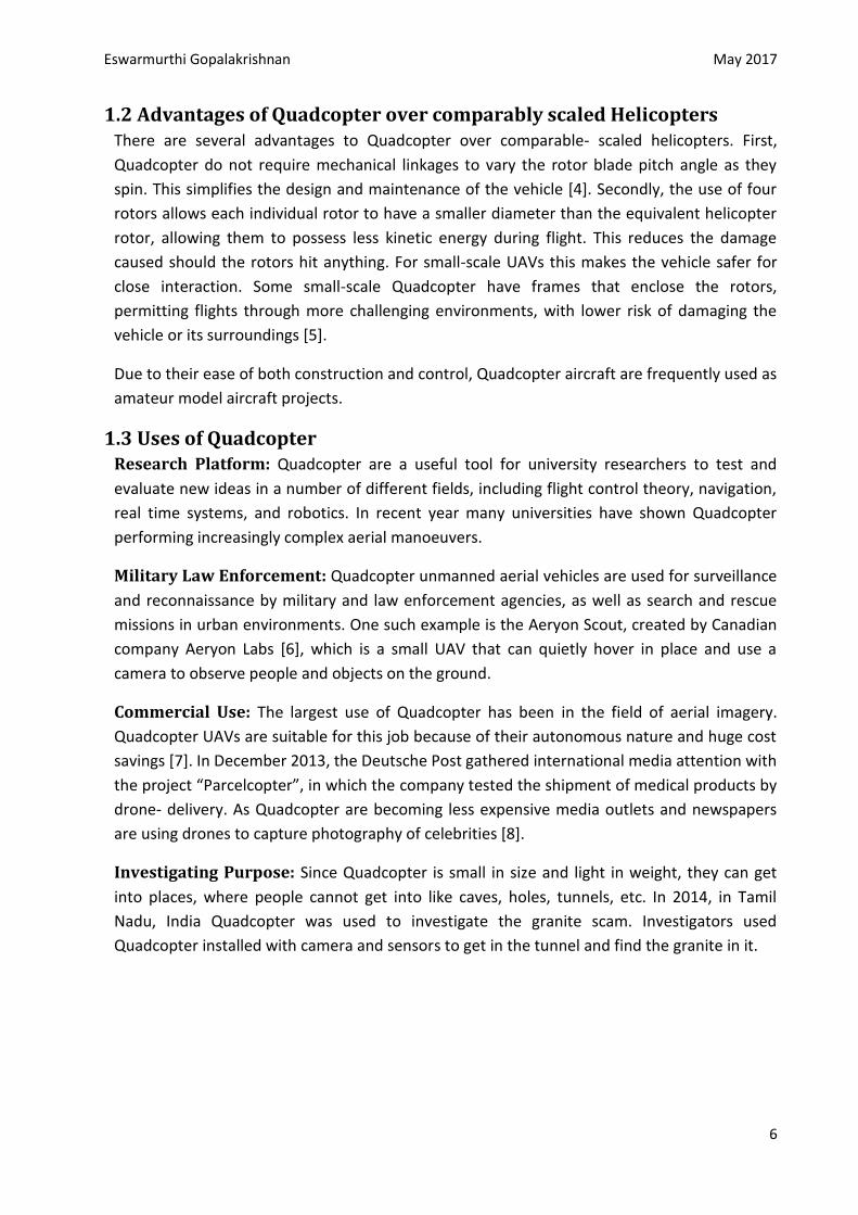
1.1.2 Outdoor Quadcopter Outdoor Quadcopter are generally more durable, they take payload and can fly on longer
missions than the Indoor Quadcopter. Absolute positioning is provided by GPS receiver. The
best example for outdoor Quadcopter is Phantom 2 Vision+ [3]. The Phantom 2 Vision+ is
shown in the figure below.
Figure 2: Phantom 2 Vision+ - An Outdoor Quadcopter
Eswarmurthi Gopalakrishnan May 2017
6
1.2 Advantages of Quadcopter over comparably scaled Helicopters There are several advantages to Quadcopter over comparable- scaled helicopters. First,
Quadcopter do not require mechanical linkages to vary the rotor blade pitch angle as they
spin. This simplifies the design and maintenance of the vehicle [4]. Secondly, the use of four
rotors allows each individual rotor to have a smaller diameter than the equivalent helicopter
rotor, allowing them to possess less kinetic energy during flight. This reduces the damage
caused should the rotors hit anything. For small-scale UAVs this makes the vehicle safer for
close interaction. Some small-scale Quadcopter have frames that enclose the rotors,
permitting flights through more challenging environments, with lower risk of damaging the
vehicle or its surroundings [5].
Due to their ease of both construction and control, Quadcopter aircraft are frequently used as
amateur model aircraft projects.
1.3 Uses of Quadcopter Research Platform: Quadcopter are a useful tool for university researchers to test and
evaluate new ideas in a number of different fields, including flight control theory, navigation,
real time systems, and robotics. In recent year many universities have shown Quadcopter
performing increasingly complex aerial manoeuvers.
Military Law Enforcement: Quadcopter unmanned aerial vehicles are used for surveillance
and reconnaissance by military and law enforcement agencies, as well as search and rescue
missions in urban environments. One such example is the Aeryon Scout, created by Canadian
company Aeryon Labs [6], which is a small UAV that can quietly hover in place and use a
camera to observe people and objects on the ground.
Commercial Use: The largest use of Quadcopter has been in the field of aerial imagery.
Quadcopter UAVs are suitable for this job because of their autonomous nature and huge cost
savings [7]. In December 2013, the Deutsche Post gathered international media attention with
the project “Parcelcopter”, in which the company tested the shipment of medical products by
drone- delivery. As Quadcopter are becoming less expensive media outlets and newspapers
are using drones to capture photography of celebrities [8].
Investigating Purpose: Since Quadcopter is small in size and light in weight, they can get
into places, where people cannot get into like caves, holes, tunnels, etc. In 2014, in Tamil
Nadu, India Quadcopter was used to investigate the granite scam. Investigators used
Quadcopter installed with camera and sensors to get in the tunnel and find the granite in it.
Eswarmurthi Gopalakrishnan May 2017
7
Chapter 2 Objectives of the thesis The objective of my thesis work is to design a mathematical dynamic Quadcopter model and a
controller for a stabilized flight motion for the given input to it. The model is to be analysed
through simulation in real life time scenario. I have decided to design a dynamic model of a DC
motor as the input source for the model and also to check the performance of the model with
the controller with disturbance given to it to check the performance. The objective of the thesis
is to develop a Quadcopter flight mechanics nonlinear model in Simulink and check the
performance based on a controller for its guidance and stabilization. The Guidelines of the
thesis work is as follows:
Deliver a literature survey related to the modelling, control law
Implement the mathematical Quadcopter model in the simulink
Linearize the nonlinear model
Design, implement and validate controller on the model for the stabilization
Design, implement and validate controller on the model for the automatic guidance
This thesis submission is my second approach towards this topic; I have made some
improvements to my previous work and have submitted a detailed report about it at the end of
the report. I have compared both of the controllers designed as well as I have compared my
works from both the attempts and have highlighted the changes from my previous work.
Eswarmurthi Gopalakrishnan May 2017
8
Chapter 3 Dynamic Quadcopter and DC Motor Modelling
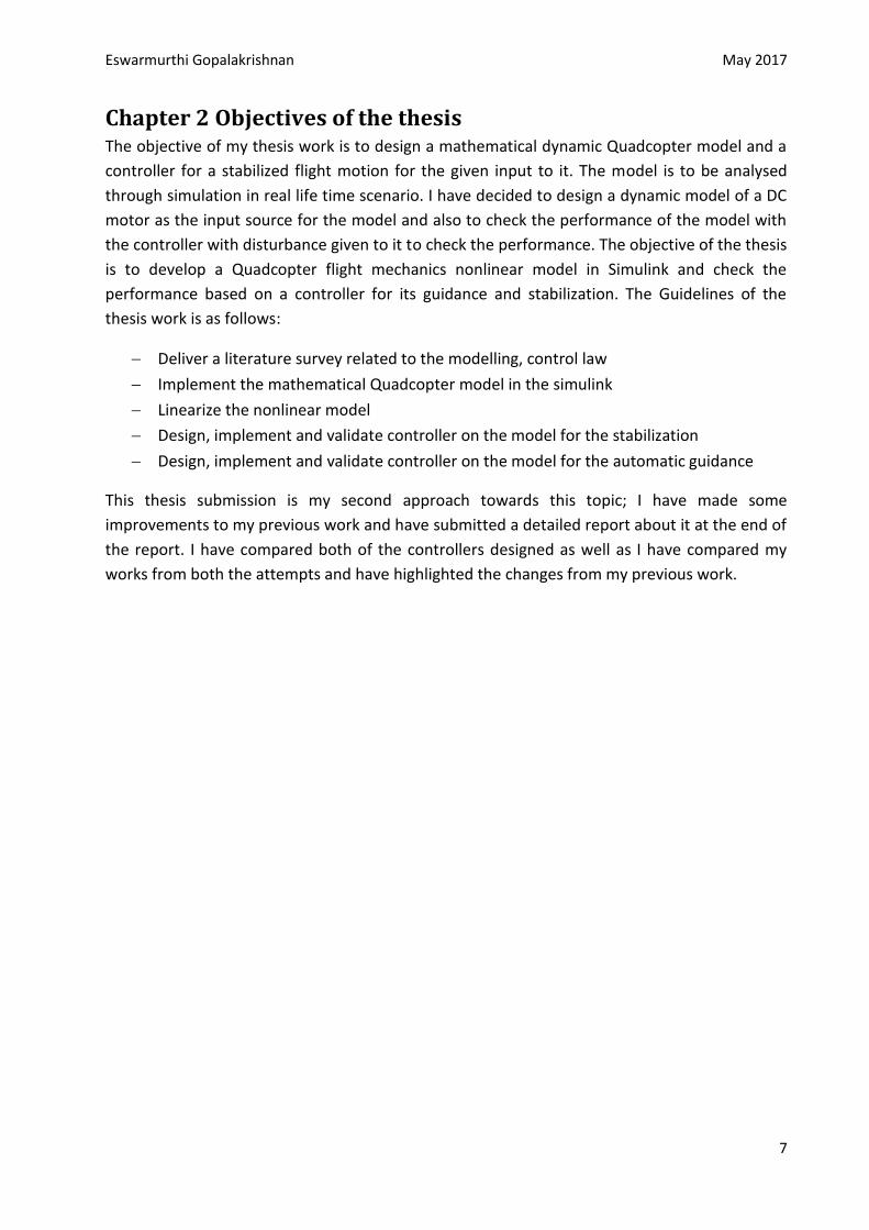
3.1 Quadcopter Modelling This section presents the basic Quadcopter dynamics, as well as control concept. It is based
on [9] and [10]. The basic idea of the movement of the Quadcopter is shown in the following
figure. It can be seen from the figure that the Quadcopter is simple in mechanical design
compared to helicopters. Movement in horizontal frame is achieved by tilting the platform
whereas vertical movement is achieved by changing the total thrust of the motors. But,
Quadcopter arise certain difficulties with the control design.
Figure 3: Basic Flight movements of a Quadcopter
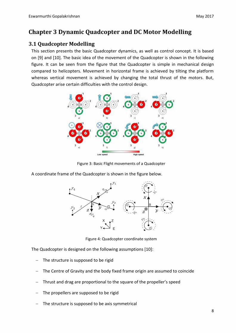
A coordinate frame of the Quadcopter is shown in the figure below.
Figure 4: Quadcopter coordinate system
The Quadcopter is designed on the following assumptions [10]:
The structure is supposed to be rigid
The Centre of Gravity and the body fixed frame origin are assumed to coincide
Thrust and drag are proportional to the square of the propeller’s speed
The propellers are supposed to be rigid
The structure is supposed to be axis symmetrical
Eswarmurthi Gopalakrishnan May 2017
9
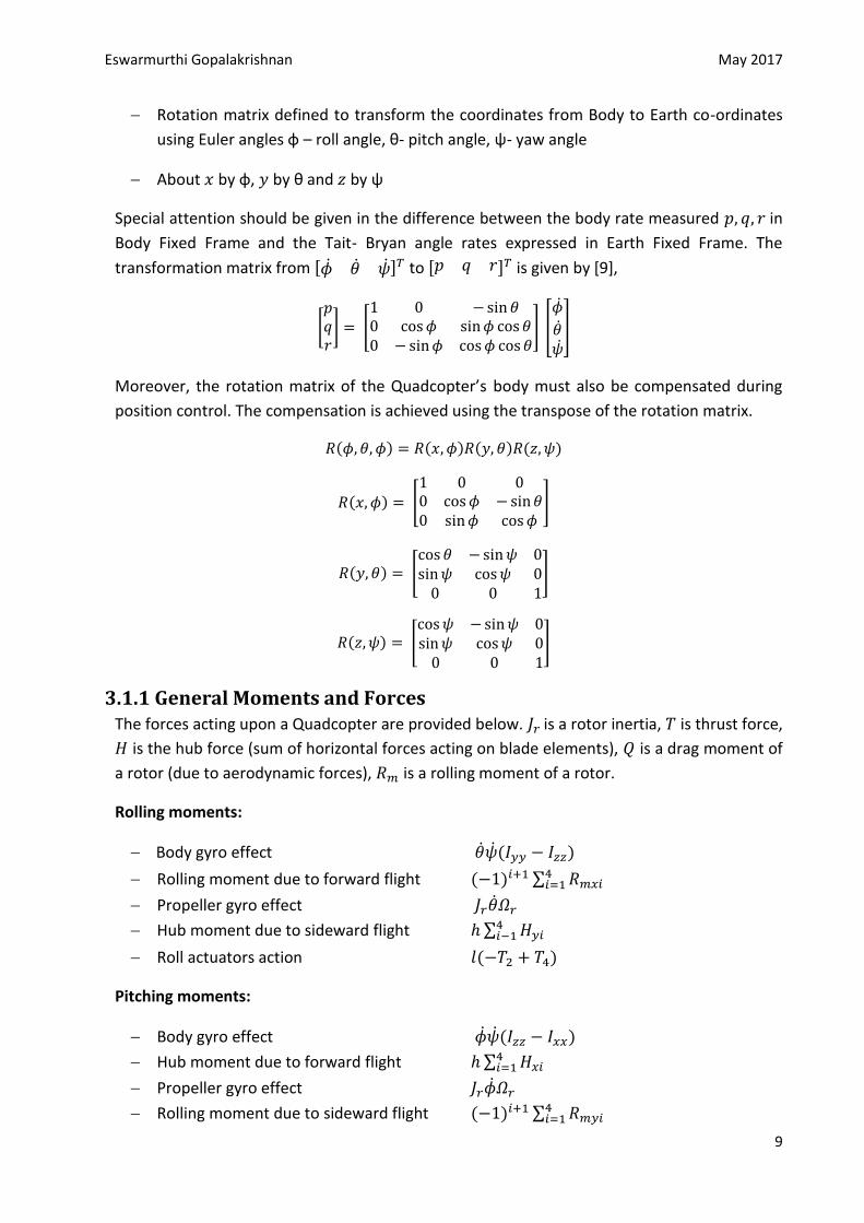
Rotation matrix defined to transform the coordinates from Body to Earth co-ordinates
using Euler angles φ – roll angle, θ- pitch angle, ψ- yaw angle
About by φ, by θ and by ψ
Special attention should be given in the difference between the body rate measured in
Body Fixed Frame and the Tait- Bryan angle rates expressed in Earth Fixed Frame. The
transformation matrix from [ ] to [ ] is given by [9],
[ ] [
] [
]
Moreover, the rotation matrix of the Quadcopter’s body must also be compensated during
position control. The compensation is achieved using the transpose of the rotation matrix.
( ) ( ) ( ) ( )
( ) [
]
( ) [
]
( ) [
]
3.1.1 General Moments and Forces The forces acting upon a Quadcopter are provided below. is a rotor inertia, is thrust force,
is the hub force (sum of horizontal forces acting on blade elements), is a drag moment of
a rotor (due to aerodynamic forces), is a rolling moment of a rotor.
Rolling moments:
Body gyro effect ( )
Rolling moment due to forward flight ( ) ∑
Propeller gyro effect
Hub moment due to sideward flight ∑
Roll actuators action ( )
Pitching moments:
Body gyro effect ( )
Hub moment due to forward flight ∑
Propeller gyro effect
Rolling moment due to sideward flight ( ) ∑
Eswarmurthi Gopalakrishnan May 2017
10
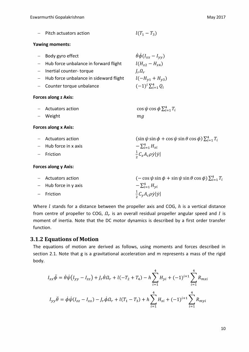
Pitch actuators action ( )
Yawing moments:
Body gyro effect ( )
Hub force unbalance in forward flight ( )
Inertial counter- torque
Hub force unbalance in sideward flight ( )
Counter torque unbalance ( ) ∑
Forces along z Axis:
Actuators action ∑
Weight
Forces along x Axis:
Actuators action ( )∑
Hub force in x axis ∑
Friction
| |
Forces along y Axis:
Actuators action ( )∑
Hub force in y axis ∑
Friction
| |
Where stands for a distance between the propeller axis and COG, is a vertical distance
from centre of propeller to COG, is an overall residual propeller angular speed and is
moment of inertia. Note that the DC motor dynamics is described by a first order transfer
function.
3.1.2 Equations of Motion The equations of motion are derived as follows, using moments and forces described in
section 2.1. Note that g is a gravitational acceleration and m represents a mass of the rigid
body.
( ) ( ) ∑
( ) ∑
( ) ( ) ∑
( ) ∑
Eswarmurthi Gopalakrishnan May 2017
11
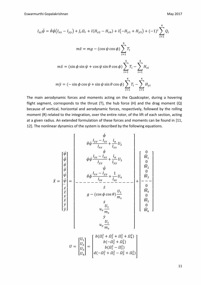
( ) ( ) ( ) ( ) ∑
( )∑
( )∑ ∑
( )∑ ∑
The main aerodynamic forces and moments acting on the Quadcopter, during a hovering
flight segment, corresponds to the thrust (T), the hub force (H) and the drag moment (Q)
because of vertical, horizontal and aerodynamic forces, respectively, followed by the rolling
moment (R) related to the integration, over the entire rotor, of the lift of each section, acting
at a given radius. An extended formulation of these forces and moments can be found in [11,
12]. The nonlinear dynamics of the system is described by the following equations.
[
]
[
( )
]
[
]
[
]
[
(
)
(
)
(
)
(
) ]
Eswarmurthi Gopalakrishnan May 2017
12
[
] [
]
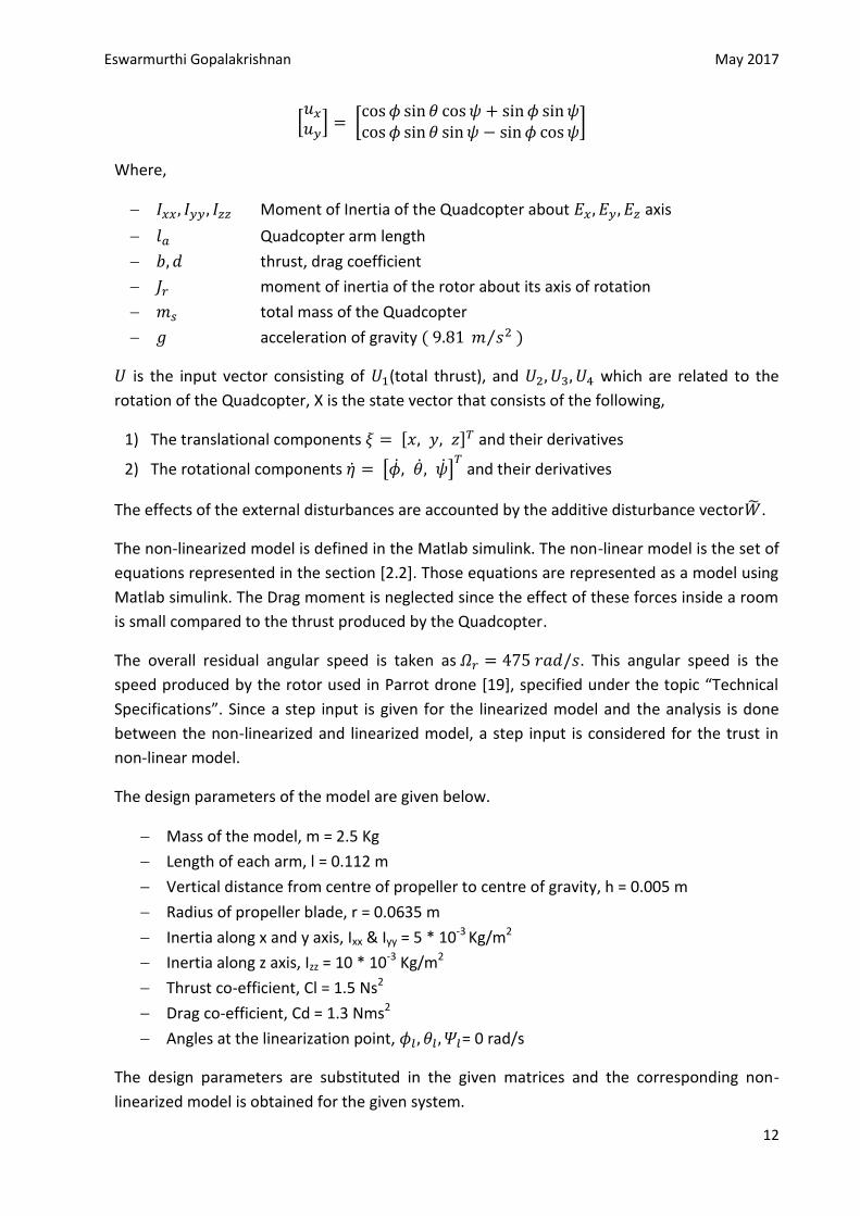
Where,
Moment of Inertia of the Quadcopter about axis
Quadcopter arm length
thrust, drag coefficient
moment of inertia of the rotor about its axis of rotation
total mass of the Quadcopter
acceleration of gravity ( ⁄ )
is the input vector consisting of (total thrust), and which are related to the
rotation of the Quadcopter, X is the state vector that consists of the following,
1) The translational components [ ] and their derivatives
2) The rotational components [ ]
and their derivatives
The effects of the external disturbances are accounted by the additive disturbance vector .
The non-linearized model is defined in the Matlab simulink. The non-linear model is the set of
equations represented in the section [2.2]. Those equations are represented as a model using
Matlab simulink. The Drag moment is neglected since the effect of these forces inside a room
is small compared to the thrust produced by the Quadcopter.
The overall residual angular speed is taken as . This angular speed is the
speed produced by the rotor used in Parrot drone [19], specified under the topic “Technical
Specifications”. Since a step input is given for the linearized model and the analysis is done
between the non-linearized and linearized model, a step input is considered for the trust in
non-linear model.
The design parameters of the model are given below.
Mass of the model, m = 2.5 Kg
Length of each arm, l = 0.112 m
Vertical distance from centre of propeller to centre of gravity, h = 0.005 m
Radius of propeller blade, r = 0.0635 m
Inertia along x and y axis, Ixx & Iyy = 5 * 10-3 Kg/m2
Inertia along z axis, Izz = 10 * 10-3 Kg/m2
Thrust co-efficient, Cl = 1.5 Ns2
Drag co-efficient, Cd = 1.3 Nms2
Angles at the linearization point, = 0 rad/s
The design parameters are substituted in the given matrices and the corresponding non-
linearized model is obtained for the given system.
Eswarmurthi Gopalakrishnan May 2017
13
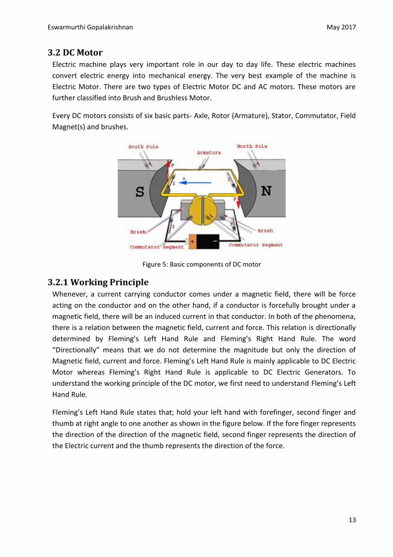
3.2 DC Motor Electric machine plays very important role in our day to day life. These electric machines
convert electric energy into mechanical energy. The very best example of the machine is
Electric Motor. There are two types of Electric Motor DC and AC motors. These motors are
further classified into Brush and Brushless Motor.
Every DC motors consists of six basic parts- Axle, Rotor (Armature), Stator, Commutator, Field
Magnet(s) and brushes.
Figure 5: Basic components of DC motor
3.2.1 Working Principle Whenever, a current carrying conductor comes under a magnetic field, there will be force
acting on the conductor and on the other hand, if a conductor is forcefully brought under a
magnetic field, there will be an induced current in that conductor. In both of the phenomena,
there is a relation between the magnetic field, current and force. This relation is directionally
determined by Fleming’s Left Hand Rule and Fleming’s Right Hand Rule. The word
“Directionally” means that we do not determine the magnitude but only the direction of
Magnetic field, current and force. Fleming’s Left Hand Rule is mainly applicable to DC Electric
Motor whereas Fleming’s Right Hand Rule is applicable to DC Electric Generators. To
understand the working principle of the DC motor, we first need to understand Fleming’s Left
Hand Rule.
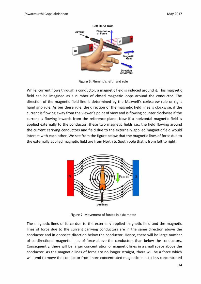
Fleming’s Left Hand Rule states that; hold your left hand with forefinger, second finger and
thumb at right angle to one another as shown in the figure below. If the fore finger represents
the direction of the direction of the magnetic field, second finger represents the direction of
the Electric current and the thumb represents the direction of the force.
Eswarmurthi Gopalakrishnan May 2017
14
Figure 6: Fleming’s left hand rule
While, current flows through a conductor, a magnetic field is induced around it. This magnetic
field can be imagined as a number of closed magnetic loops around the conductor. The
direction of the magnetic field line is determined by the Maxwell’s corkscrew rule or right
hand grip rule. As per these rule, the direction of the magnetic field lines is clockwise, if the
current is flowing away from the viewer’s point of view and is flowing counter clockwise if the
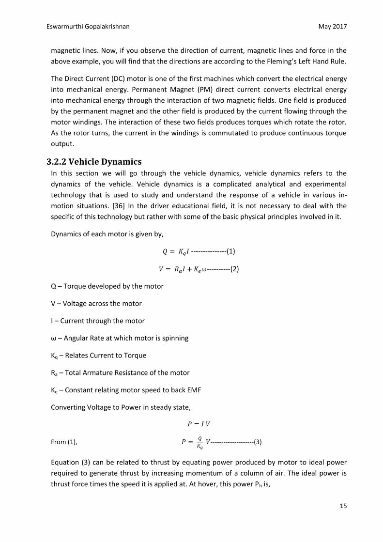
current is flowing inwards from the reference plane. Now if a horizontal magnetic field is
applied externally to the conductor, these two magnetic fields i.e., the field flowing around
the current carrying conductors and field due to the externally applied magnetic field would
interact with each other. We see from the figure below that the magnetic lines of force due to
the externally applied magnetic field are from North to South pole that is from left to right.
Figure 7: Movement of forces in a dc motor
The magnetic lines of force due to the externally applied magnetic field and the magnetic
lines of force due to the current carrying conductors are in the same direction above the
conductor and in opposite direction below the conductor. Hence, there will be large number
of co-directional magnetic lines of force above the conductors than below the conductors.
Consequently, there will be larger concentration of magnetic lines in a small space above the
conductor. As the magnetic lines of force are no longer straight, there will be a force which
will tend to move the conductor from more concentrated magnetic lines to less concentrated
Eswarmurthi Gopalakrishnan May 2017
15
magnetic lines. Now, if you observe the direction of current, magnetic lines and force in the
above example, you will find that the directions are according to the Fleming’s Left Hand Rule.
The Direct Current (DC) motor is one of the first machines which convert the electrical energy
into mechanical energy. Permanent Magnet (PM) direct current converts electrical energy
into mechanical energy through the interaction of two magnetic fields. One field is produced
by the permanent magnet and the other field is produced by the current flowing through the
motor windings. The interaction of these two fields produces torques which rotate the rotor.
As the rotor turns, the current in the windings is commutated to produce continuous torque
output.
3.2.2 Vehicle Dynamics In this section we will go through the vehicle dynamics, vehicle dynamics refers to the
dynamics of the vehicle. Vehicle dynamics is a complicated analytical and experimental
technology that is used to study and understand the response of a vehicle in various in-
motion situations. [36] In the driver educational field, it is not necessary to deal with the
specific of this technology but rather with some of the basic physical principles involved in it.
Dynamics of each motor is given by,
---------------(1)
----------(2)
Q – Torque developed by the motor
V – Voltage across the motor
I – Current through the motor
ω – Angular Rate at which motor is spinning
Kq – Relates Current to Torque
Ra – Total Armature Resistance of the motor
Ke – Constant relating motor speed to back EMF
Converting Voltage to Power in steady state,
From (1),
--------------------(3)
Equation (3) can be related to thrust by equating power produced by motor to ideal power
required to generate thrust by increasing momentum of a column of air. The ideal power is
thrust force times the speed it is applied at. At hover, this power Ph is,
Eswarmurthi Gopalakrishnan May 2017
16
----------------(4)
Where, induced velocity at hover Vh, is change in air speed induced by rotor blades with
respect to the free stream velocity . For the analysis for wind free hover condition.
Using momentum theory,
√
-----------(5)
T – Thrust produced by rotor to remain in hover
A - area swept out by the rotor
ρ – Density of the air
R – Radius of the rotor
For quadrotor helicopter, this is equal to
Tnom – Weight of the vehicle.
The Torque is proportional to the thrust, with a constant ratio Kt that depend on the blade
geometry.
The relation between applied voltage (V) and thrust (T) is found by equating the power
produced (P) with ideal power consumed at hover (Ph) and combining (4) and (5)
√
⁄
√ ---------(6)
⁄
√
-------------(7)
Thrust produced by rotor is proportional to the square of the voltage applied across the
motor. Total force F is given by,
∑ ( ) --------(8)
Db – Drag force of vehicle body
ev – Current velocity direction unit vector
m – Vehicle mass
Eswarmurthi Gopalakrishnan May 2017
17
g – Acceleration due to gravity
eD – Unit vector along D-direction in NED
Ti – Thrust produced by i-th rotor
- Rotation matrix from the plane of i-th rotor to inertial coordinates
ZR,I – Rotor plane axis along which the thrust of the i-th rotor acts
Similarly, the total moment, M is,
∑ ( ( )) -----------(9)
- Rotation matrix from plane of rotor I to body co ordinates
Note that, Db is neglected while calculating the moment. Because, this force was found to
cause a negligible disturbance on M. The full non-linear dynamics can be described as,
---------------------(10)
--------------------(11)
– Angular Velocity of aircraft along body frame
Using M is considered zero as the momentum from the counter-rotating pairs cancels when
yaw is held steady.
3.2.3 Aerodynamic Effects Although vehicle dynamics are modelled accurately as linear for attitude and altitude control,
this is acceptable only for low velocity. Even for moderate velocity, the impact of aerodynamic
effects resulting from variation in air speed is significant.
There are four main effects, 3 of which are quantifiable and are incorporated into the non-
linear model of the vehicle for estimation and control. The other one which results in
unsteady airflow and can therefore be mitigated through structural redesign. The types of
aerodynamic effects are Unsteady Airflow, Total Thrust, Inflow Velocity “Blade Flapping” and
Unsteady Thrust [37].
Total Thrust: The total thrust varies not only with the power input but also with the free
stream velocity and the angle of attack with respect to the free stream. It is further more
complicated by a flight regime, called Vortex Ring State, in which there is no analytical
solution for thrust and experimental data shows that the thrust is extremely stochastic. The
induced power is the required power input to create the induced velocity. When the
rotorcraft undergoes translational motion, or changes the angle of attack, the induced power
requirement of a rotorcraft changes.
Eswarmurthi Gopalakrishnan May 2017
18
To derive the effect of free stream velocity on induced power, from conservation of
momentum, the induced velocity is Vi is found by the solving the following (4m)
√( ) ( ) ---------(12)
- Total free stream speed, including translational velocity and ambient wind velocity
α- Angle of attack; positive – pitching forward
This equation is less accurate for large angle of attack and is not valid during Vortex Ring
State. Nonetheless, it provides an accurate result for much of the useful flight envelope.
Using Vi , ideal thrust per power input can be computed, using
---------(13)
The denominator corresponds to the air speed across the rotor. At low speed, the α has
vanishingly little effect on ⁄ is more sensitive to α.
Similar to aircraft, pitching up increases lift force. The α for which Th increases with forward
speed. For level flight, the power required to retain altitude increases with forward speed. In
extreme region of α, where the flight is close to vertical, rotorcraft have 3 operational mode
for climb velocity Vc.
Nominal Working State :
Windmill Brake State :
Vortex Ring State :
In Normal Working State, air is flowing down through the rotor. In Windmill Brake State, air is
flowing up through the rotor due to rapid descent. For these 2 states, conservation of
momentum can be used to derive induced velocity.
For Normal State,
√(
)
-----------------(14)
For Windmill State,
√(
)
--------------(15)
In VRS, the air recirculates through the blades in a periodic and somewhat random fashion. As
a result, induced velocity varies greatly, particularly over the domain
reducing aerodynamic damping. An empirical model of induced velocity in VRS is,
Eswarmurthi Gopalakrishnan May 2017
19
( (
) (
) (
)
(
)
(
)
) ( )
Where,
To model the dynamics during climb, the power is thrust times the speed it is applied at,
( )
Ignoring Profile power loss,
T * Vc – Power consumed by the climbing motion
T * Vi – Power transferred to air
Vortex Ring State is avoided by maintaining a substantial forward speed while descending.
The thrust achieved for a given input can be computed as a function of climb velocity by
substituting (14), (15) and (16) into (17)
3.2.4 Blade Flapping
In translational flight, advancing blade of a rotor sees a higher effective velocity relative to the
air, while the retreating blade sees a lower effective velocity. This results in a difference in lift
between the two rotors, causing the rotor blades to flap up and down once per revolution.
The backward tilt of the rotor plane generated a longitudinal thrust which is given below,
a1s – angle by which the thrust vector is tilted or deflected
If centre of gravity of the vehicle is not aligned with the rotor plane, it creates a moment
about the centre of gravity,
( )
rcg – Vertical distance from rotor plane to the C.G. of the vehicle
Since stiff rotors are generally used in all quad-rotors, the tilt of the blades generated a
moment along the rotor hub,
( )
Kβ – Stiffness of rotor in Nm/rad
Eswarmurthi Gopalakrishnan May 2017
20
3.2.5 Coning
The upward flexure of the rotor blades from the lift force on each blade. It also causes the
impinging airflow to have unbalanced forcing of the blades which causes a lateral tilt of the
rotor plane. This lateral tilt generates moments at right angles to the velocity vector, but
because of counter-rotating pairs of quad-rotor rotors, the lateral effect cancels.
A distinction must also be noted in the terminology of flap angle β and the deflection angle
a1s. The flap angle β is generally defined as the total deflection of a rotor blade away from the
horizontal in body coordinates in any point in the rotation and is calculated as,
( )
a0s – Blade deflection due to coning
a1s, b1s – Longitudinal and Lateral blade deflection, respectively due to flapping
Ψ – Azimuth angle of the blade and is zero at the rear
The equation of deflection angle of a flapping rotor with the hinged blades is,
(
) ( )
a0 – Slope of lift curve per radian
μlong – Longitudinal rotor advance ratio. Defined as ratio of the longitudinal to blade tip speed
γ – Non-dimensional lock number
( )
( )
Ib – Moment of Inertia of blade about the hinge
C- Chord of the blade
R – Rotor radius
σ – Solidity Ratio of the rotor
( )
Eswarmurthi Gopalakrishnan May 2017
21
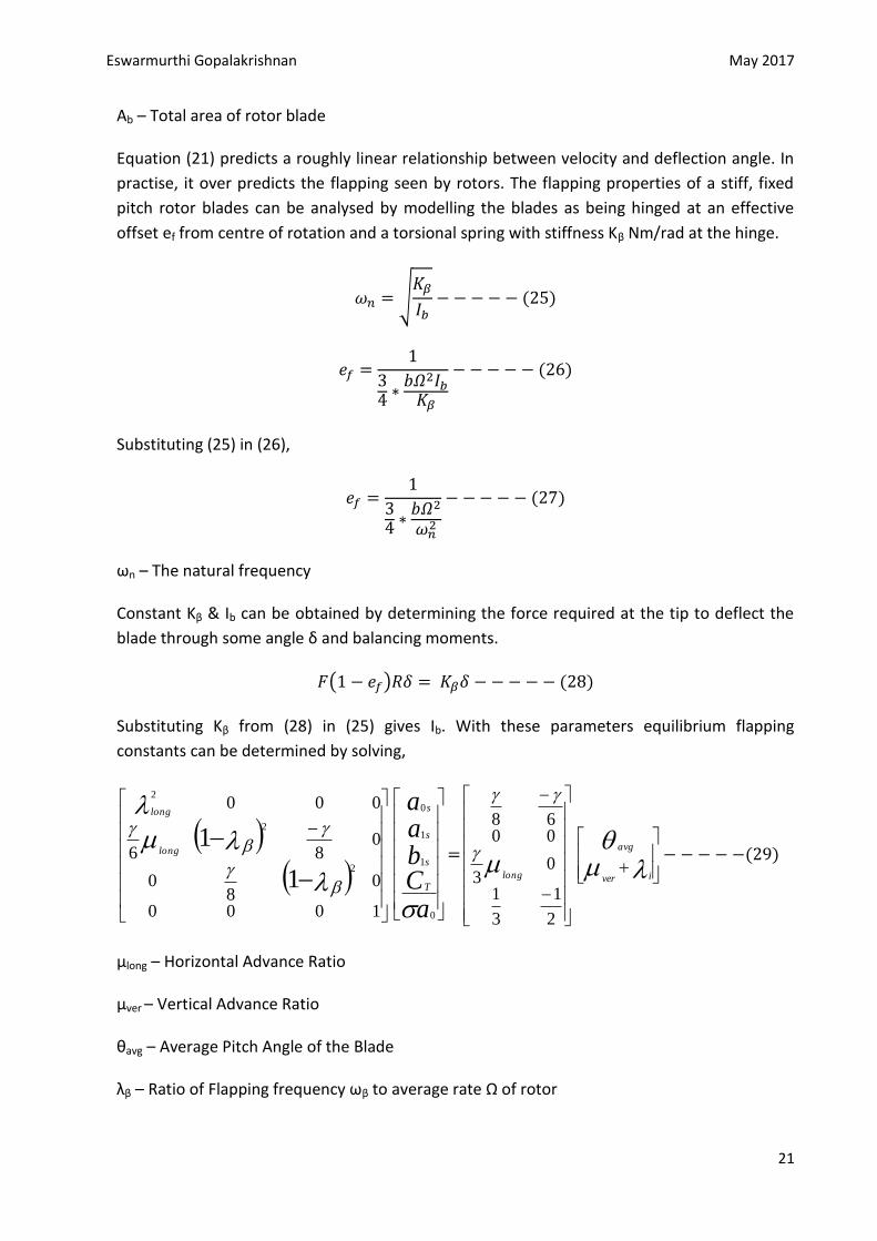
Ab – Total area of rotor blade
Equation (21) predicts a roughly linear relationship between velocity and deflection angle. In
practise, it over predicts the flapping seen by rotors. The flapping properties of a stiff, fixed
pitch rotor blades can be analysed by modelling the blades as being hinged at an effective
offset ef from centre of rotation and a torsional spring with stiffness Kβ Nm/rad at the hinge.
√
( )
( )
Substituting (25) in (26),
( )
ωn – The natural frequency
Constant Kβ & Ib can be obtained by determining the force required at the tip to deflect the
blade through some angle δ and balancing moments.
( ) ( )
Substituting Kβ from (28) in (25) gives Ib. With these parameters equilibrium flapping
constants can be determined by solving,
1000
08
0
086
000
1
12
2
2
long
long
aCbaa
T
s
s
s
0
1
1
0
=
2
1
3
1
03
0068
long
iver
avg ( )
μlong – Horizontal Advance Ratio
μver – Vertical Advance Ratio
θavg – Average Pitch Angle of the Blade
λβ – Ratio of Flapping frequency ωβ to average rate Ω of rotor
Eswarmurthi Gopalakrishnan May 2017
22
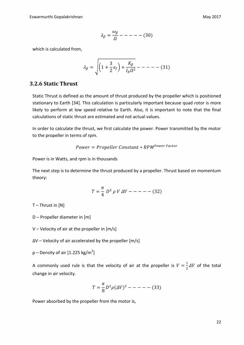
( )
which is calculated from,
√(
)
( )
3.2.6 Static Thrust
Static Thrust is defined as the amount of thrust produced by the propeller which is positioned
stationary to Earth [34]. This calculation is particularly important because quad rotor is more
likely to perform at low speed relative to Earth. Also, it is important to note that the final
calculations of static thrust are estimated and not actual values.
In order to calculate the thrust, we first calculate the power. Power transmitted by the motor
to the propeller in terms of rpm.
Power is in Watts, and rpm is in thousands
The next step is to determine the thrust produced by a propeller. Thrust based on momentum
theory:
( )
T – Thrust in [N]
D – Propeller diameter in [m]
V – Velocity of air at the propeller in [m/s]
ΔV – Velocity of air accelerated by the propeller [m/s]
ρ – Density of air [1.225 kg/m3]
A commonly used rule is that the velocity of air at the propeller is
of the total
change in air velocity.
( ) ( )
Power absorbed by the propeller from the motor is,
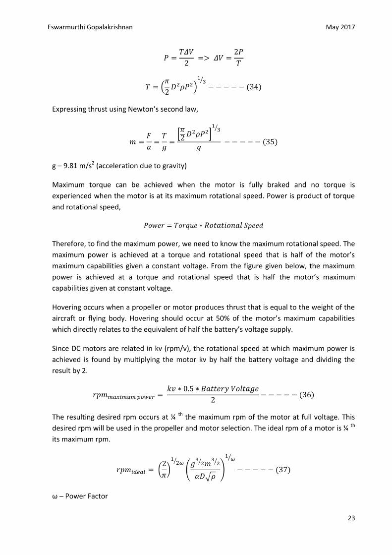
Eswarmurthi Gopalakrishnan May 2017
23
(
)
⁄
( )
Expressing thrust using Newton’s second law,
[ ]
⁄
( )
g – 9.81 m/s2 (acceleration due to gravity)
Maximum torque can be achieved when the motor is fully braked and no torque is
experienced when the motor is at its maximum rotational speed. Power is product of torque
and rotational speed,
Therefore, to find the maximum power, we need to know the maximum rotational speed. The
maximum power is achieved at a torque and rotational speed that is half of the motor’s
maximum capabilities given a constant voltage. From the figure given below, the maximum
power is achieved at a torque and rotational speed that is half the motor’s maximum
capabilities given at constant voltage.
Hovering occurs when a propeller or motor produces thrust that is equal to the weight of the
aircraft or flying body. Hovering should occur at 50% of the motor’s maximum capabilities
which directly relates to the equivalent of half the battery’s voltage supply.
Since DC motors are related in kv (rpm/v), the rotational speed at which maximum power is
achieved is found by multiplying the motor kv by half the battery voltage and dividing the
result by 2.
( )
The resulting desired rpm occurs at ¼ th the maximum rpm of the motor at full voltage. This
desired rpm will be used in the propeller and motor selection. The ideal rpm of a motor is ¼ th
its maximum rpm.
(
)
⁄
(
⁄
⁄
√ )
⁄
( )
ω – Power Factor
Eswarmurthi Gopalakrishnan May 2017
24
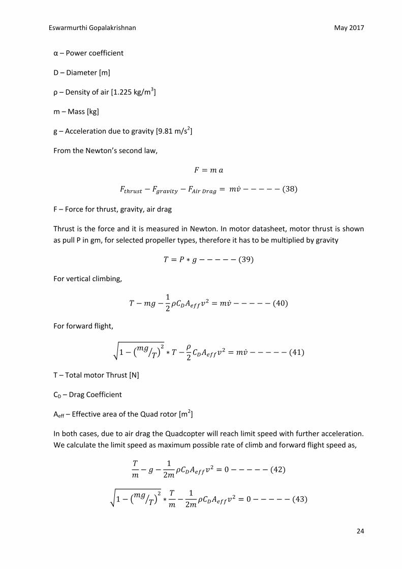
α – Power coefficient
D – Diameter [m]
ρ – Density of air [1.225 kg/m3]
m – Mass [kg]
g – Acceleration due to gravity [9.81 m/s2]
From the Newton’s second law,
( )
F – Force for thrust, gravity, air drag
Thrust is the force and it is measured in Newton. In motor datasheet, motor thrust is shown
as pull P in gm, for selected propeller types, therefore it has to be multiplied by gravity
( )
For vertical climbing,
( )
For forward flight,
√ (
⁄ )
( )
T – Total motor Thrust [N]
CD – Drag Coefficient
Aeff – Effective area of the Quad rotor [m2]
In both cases, due to air drag the Quadcopter will reach limit speed with further acceleration.
We calculate the limit speed as maximum possible rate of climb and forward flight speed as,
( )
√ (
⁄ )
( )
Eswarmurthi Gopalakrishnan May 2017
25
The square root term reflects that a certain fraction of the thrust is needed to keep the
Quadcopter at constant altitude. The vertical component of the motor thrust has to
compensate the gravitational force mg.
The copter flies with a forward pitch angle α,
(
)
Maximum Rate of Climb,
√
( )
A – Top Area of Quadcopter [m2]
Thrust ratio, ⁄ substituting thrust ratio in the above equation,
√
√( ) ( )
The thrust ratio, TR must be always greater than 1.
For maximum forward flight,
√ √ (
⁄ )
( )
In terms of TR,
√ ⁄
√
√ ( )
The effective area Aeff is a function of the forward pitch angle α. To simplify the calculation we
only take into account the vertical projection of the Quadcopter top area.
⁄
⁄
⁄
√ ⁄
√
√ ( )
Eswarmurthi Gopalakrishnan May 2017
26
√ ⁄
√
( )
For practical, TR around 2 or higher the factor under the double square root is close to 1. As
for the maximum rate of climb, maximum forward flight speed depends on the weight, size
and aerodynamic form of the Quadcopter, but the main factor is the thrust of weight ratio. An
increase will directly increase into forward speed.
3.2.7 Thrust through Dynamics Modelling
The goal of this section is to relate the voltage applied to the velocity of the motor. Two
balancing equation can be developed by considering the electrical and mechanical
characteristics of the system. The DC model consists of two inputs Input Armature Voltage
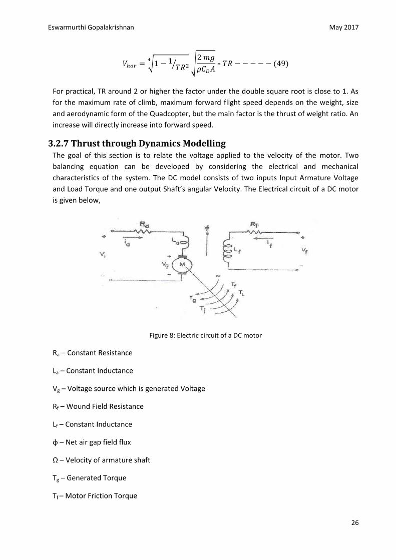
and Load Torque and one output Shaft’s angular Velocity. The Electrical circuit of a DC motor
is given below,
Figure 8: Electric circuit of a DC motor
Ra – Constant Resistance
La – Constant Inductance
Vg – Voltage source which is generated Voltage
Rf – Wound Field Resistance
Lf – Constant Inductance
φ – Net air gap field flux
Ω – Velocity of armature shaft
Tg – Generated Torque
Tf – Motor Friction Torque
Eswarmurthi Gopalakrishnan May 2017
27
TJ – Motor Inertial Torque
TL – Load Torque
An idea of how to obtain the equations for the dynamics modelling of DC motor is obtained
from the reference report [31] & [33].
Applying Kirchhoff’s Law to Armature Circuit,
( ) ( )
( )
( ) ( )
Vg(t) is generated voltage resulting due to movement of the conductors of the armature
through the field flux established by the field current if.
( ) ( ) ( )
( ) ( ) ( )
Assuming constant field current and ignoring flux changes due to the armature reaction and
other second order effects,
( ) ( ) ( )
The generated electromagnetic torque Tg is proportional to the armature current, assuming
field flux to constant. Thus,
( ) ( )
Kt – Torque constant of the motor
At any given time, the developed torque must be equal and opposite to the sum of torques
necessary to overcome friction, inertia and load. Thus,
( ) [ ( ) ( )] ( ) ( )
( )
Equation (50), (51), (52), (53) are the basic set of equation that model the DC motor. Applying
Laplace transform and rearranging the terms,
( ) ( ) ( )
( )
( )
( ) ( ) ( ) ( )
( ) ( ) ( ) ( ) ( )
( ) ( ) ( )
( ) ( ) ( )
Eswarmurthi Gopalakrishnan May 2017
28
( ) ( ) ( )
( ) ( ) ( )
( ) ( ) [ ( ) ( )] ( ) ( )
( ) ( ) ( ) ( ) ( )
( ) ( ) ( ) ( ) ( ) ( )
The equations (50), (51), (52) and (53) are used to design a block diagram which is given
below, here we consider the no load condition; . For my work, I have used the
basic equations of the DC motor to design the motor and analyse it. For a given voltage input,
the angular velocity and the angular position response is analysed.
3.2.8 Motor Specification For my design analysis, I have chosen ES040A- 2 (4412) Brushless DC motor, the details of the
specific DC motor is given below:
Weight = 454 g
Voltage = 19.1 V
Kt = 0.031 Nm/A
Ke = 0.031 V/rad/s
La = 0.16 mH
Ra = 0.82 ohms
J = 5.65 * 10-6 Kg-m2
B = 1.81 * 10-6 Nms/rad
These motor specifications are mentioned in the motor dynamic model in Simulink. The
Simulink is run and the Angular Velocity and the Angular Position of the model is obtained
from the scope. The Angular Velocity, Angular position and Armature current for the model
with no Controller and disturbance is given below.
Eswarmurthi Gopalakrishnan May 2017
29
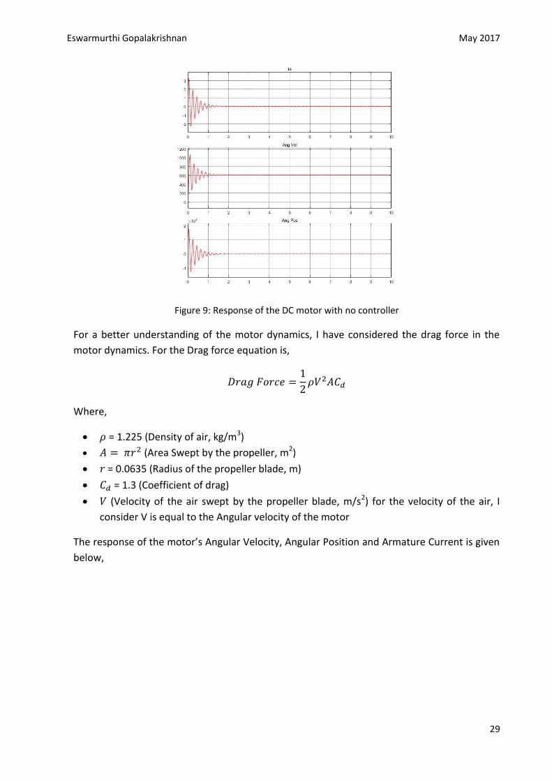
Figure 9: Response of the DC motor with no controller
For a better understanding of the motor dynamics, I have considered the drag force in the
motor dynamics. For the Drag force equation is,
Where,
= 1.225 (Density of air, kg/m3)
(Area Swept by the propeller, m2)
= 0.0635 (Radius of the propeller blade, m)
= 1.3 (Coefficient of drag)
(Velocity of the air swept by the propeller blade, m/s2) for the velocity of the air, I
consider V is equal to the Angular velocity of the motor
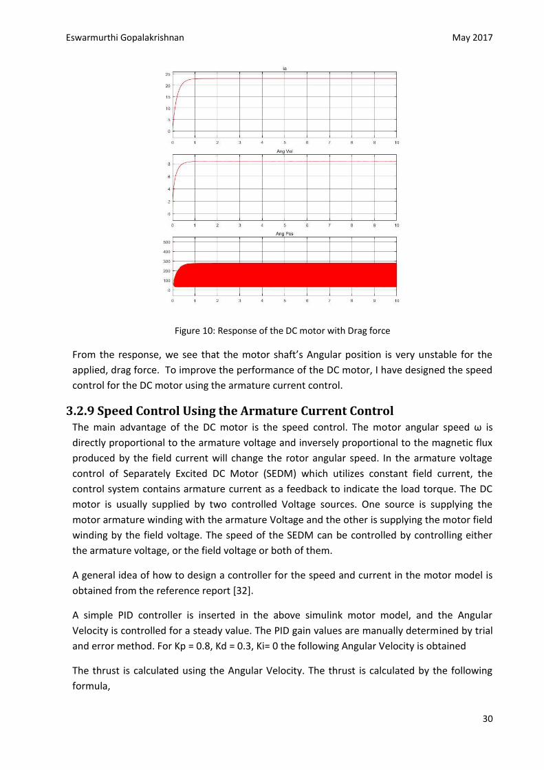
The response of the motor’s Angular Velocity, Angular Position and Armature Current is given
below,
Eswarmurthi Gopalakrishnan May 2017
30
Figure 10: Response of the DC motor with Drag force
From the response, we see that the motor shaft’s Angular position is very unstable for the
applied, drag force. To improve the performance of the DC motor, I have designed the speed
control for the DC motor using the armature current control.
3.2.9 Speed Control Using the Armature Current Control The main advantage of the DC motor is the speed control. The motor angular speed ω is
directly proportional to the armature voltage and inversely proportional to the magnetic flux
produced by the field current will change the rotor angular speed. In the armature voltage
control of Separately Excited DC Motor (SEDM) which utilizes constant field current, the
control system contains armature current as a feedback to indicate the load torque. The DC
motor is usually supplied by two controlled Voltage sources. One source is supplying the
motor armature winding with the armature Voltage and the other is supplying the motor field
winding by the field voltage. The speed of the SEDM can be controlled by controlling either
the armature voltage, or the field voltage or both of them.
A general idea of how to design a controller for the speed and current in the motor model is
obtained from the reference report [32].
A simple PID controller is inserted in the above simulink motor model, and the Angular
Velocity is controlled for a steady value. The PID gain values are manually determined by trial
and error method. For Kp = 0.8, Kd = 0.3, Ki= 0 the following Angular Velocity is obtained
The thrust is calculated using the Angular Velocity. The thrust is calculated by the following
formula,
Eswarmurthi Gopalakrishnan May 2017
31
ρ – 1.225 * 103 g/m3 (density of air)
CD – 1.3 (Drag Coefficient)
V – Angular Velocity of the model, determined from the motor dynamics
A – Top Area of the Quadcopter, the formula is given below
( )
MTM – Motor to Motor Distance
Rprop – Radius of Propeller
Using the 250 FPV Racing Quad, MTM = 0.255 m
When we use 5 inch propeller, r = 0.0635 m
Using the above values, the area of the Quadcopter is determined. The thrust is calculated in
the Matlab Simulink. For the motor angular speed controller, the motor angular speed is fed
back to a proportional controller gain with a reference signal. The obtained controlled signal is
fed to the armature current controller as the reference signal. The armature current produced
from the electrical component of the DC motor is fed back to a proportional controller with
the reference signal from the angular speed controller. The obtained controlled output from
the armature current controller is fed as the input voltage for the DC motor. For the angular
speed controller and armature current controller, I have used a simple Proportional controller
gain. The motor angular speed controller is first tuned manually for the given reference signal.
Once, the angular speed is controlled, the armature current is then tuned manually for the
stabilization of the armature current.
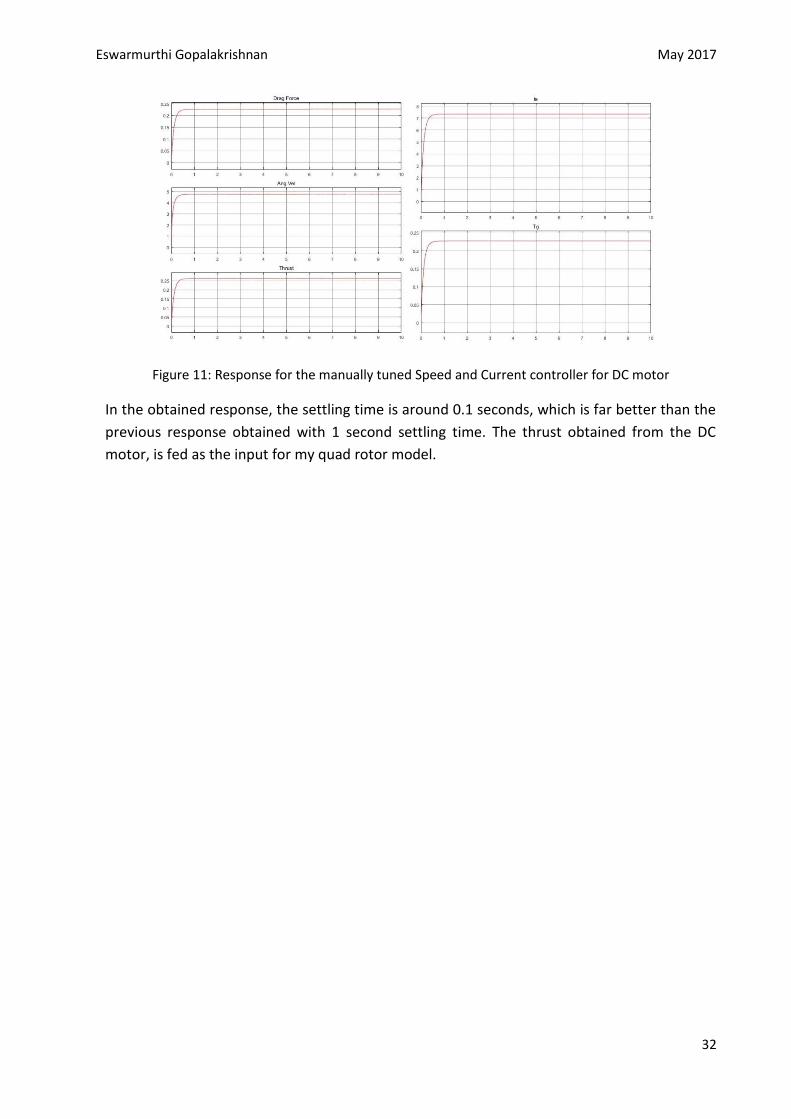
The tuned proportional gain value for the motor angular speed is 129.992110649462 and the
tuned proportional gain value for the armature current is 0.0127870036171011. For the
tuned gain value, the obtained Thrust, Drag force, Angular Velocity, Armature current, Torque
of the motor is given below,
Eswarmurthi Gopalakrishnan May 2017
32
Figure 11: Response for the manually tuned Speed and Current controller for DC motor
In the obtained response, the settling time is around 0.1 seconds, which is far better than the
previous response obtained with 1 second settling time. The thrust obtained from the DC
motor, is fed as the input for my quad rotor model.
Eswarmurthi Gopalakrishnan May 2017
33
Chapter 4 Linearization of the model In mathematics, linearization refers to finding the linear approximation to a function at a
given point. In the study of dynamical systems, linearization is a method for assessing the
local stability of an equilibrium point of a system of nonlinear differential equations or
discrete dynamical systems [13]. A set of nonlinear ODE’s (forces equations, moments
equations) are parameterized by mass characteristics of the system as well as aerodynamics.
The nonlinear equations are directly useful for simulations like computer games, flight
trainers, flight simulators and validation of control law. They are not directly useable for
development of control laws as the design methods rely on the linear systems and control
theory. The nonlinear equations come from the geometric transformations and describing
functions of aerodynamic coefficient. For this reason, the linearized system and control tools
are attractive and viable options for FCS design. In order to design a controller for a
Quadcopter it is suggested to have a linearized model of the system to have a precise
controller [14]. In this chapter the nonlinear model of the Quadcopter is linearized using the
Jacobian method.
4.1 Uses of linearization in Stability analysis Linearization makes it possible to use tools for studying linear systems to analyse the
behaviour of a non-linear function near a given point. The linearization function is the first
order term of its Taylor expansion around the point of interest. For a system defined by the
equation
( )
The Linearized systems can be written as
( ) ( ) ( )
Where is the point of interest and ( ) is the Jacobian of ( ) evaluated at
4.1.1 Stability Analysis In stability analysis of autonomous systems, one can use the eigenvalues of the Jacobian
matrix evaluated at a hyperbolic equilibrium point to determine the nature of that
equilibrium. This is the content of Linearization theorem. For time-varying systems, the
linearization requires additional justification [15].
4.2 Jacobian Method The Jacobian generalizes the gradient of a scalar- valued function of multiple variables, which
itself generalizes the derivative of a scalar- valued function of a single variable. In other
words, the Jacobian for a scalar- valued function of single variable is simply its derivative [16].
An example of how to solve a function using Jacobian method is given below,
Consider a system with ‘2’ equations and ‘2’ variables as given below,
Eswarmurthi Gopalakrishnan May 2017
34
( )
( )
( )
[
]
( ) [
]
A similar method is used to linearize the nonlinear model of the system. Firstly, the operating
points for the system to be linearized are given and the Jacobian method is implemented to
linearize the equation.
4.3 Linearization of the model In order to derive the linearized representation of the Quadcopter’s linearized attitude
dynamics, small attitude perturbations , with , around the operating points
[ ]
are considered.
[ ]
[ ]
[ ]
The resulting linearized dynamics is an extension of the state space matrices represented in
the following equations.
[
]
Eswarmurthi Gopalakrishnan May 2017
35
[
]
[
]
[
]
The above mentioned
matrices are the linearized matrices for the given system.
Where are the pitch, roll and yaw rate at the linearization point.
The design parameters given in the previous section are substituted in the matrices above and
obtained matrices are the linearized state space model for the system. The linearized model
can be used to design the controller.
4.4 Validation of Non-linear and Linear model for the given input In this section, we shall see how both the non-linear and linear system react to the given input
or command. The input for the non-linearized as well as the linearized model is the propeller
thrusts. For my validation, I have combined a set of step signals to perform a specific task.
The output depends on the model we observe, for the non-linearized model; the outputs are
as follows- Roll angle, Roll rate, Pitch angle, Pitch rate, Yaw angle, Yaw rate, Velocity along
direction, Velocity along direction, Velocity along direction. Whereas the output from
the linearized model; depends on the parameter we require for designing the controller. In
my case, the output from the linearized model is as follows- Roll angle, Roll rate, Pitch angle,
Pitch rate, Yaw angle, Yaw rate.
First, I have implemented an input signal to perform the Pitch action. The input signal is
designed such that from 0 to 3 seconds the Quad-rotor is stable in the ground, from 3 to 6
seconds, the Quad-rotor lifts from the ground, from 6 to 9 seconds the Quad-rotor performs
Eswarmurthi Gopalakrishnan May 2017
36
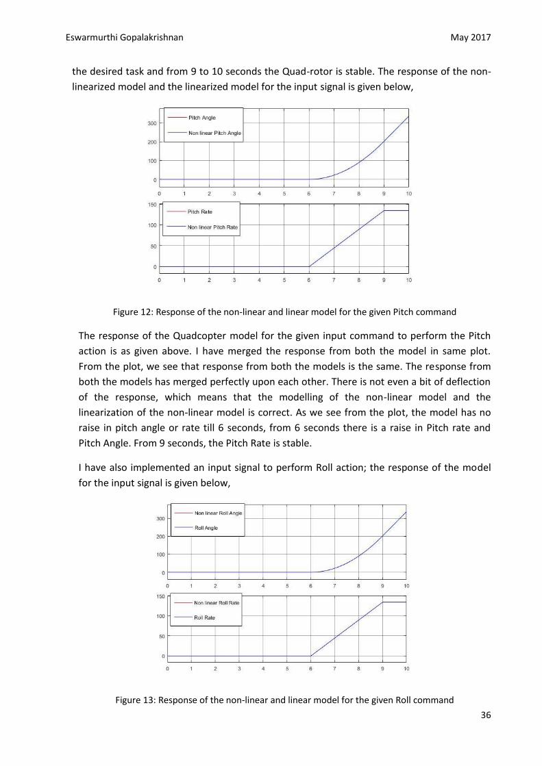
the desired task and from 9 to 10 seconds the Quad-rotor is stable. The response of the non-
linearized model and the linearized model for the input signal is given below,
Figure 12: Response of the non-linear and linear model for the given Pitch command
The response of the Quadcopter model for the given input command to perform the Pitch
action is as given above. I have merged the response from both the model in same plot.
From the plot, we see that response from both the models is the same. The response from
both the models has merged perfectly upon each other. There is not even a bit of deflection
of the response, which means that the modelling of the non-linear model and the
linearization of the non-linear model is correct. As we see from the plot, the model has no
raise in pitch angle or rate till 6 seconds, from 6 seconds there is a raise in Pitch rate and
Pitch Angle. From 9 seconds, the Pitch Rate is stable.
I have also implemented an input signal to perform Roll action; the response of the model
for the input signal is given below,
Figure 13: Response of the non-linear and linear model for the given Roll command
Eswarmurthi Gopalakrishnan May 2017
37
The response of the Quadcopter model for the given input command to perform the Roll
action is as given above. As we see from the plot, the model has no raise in roll angle or rate
till 6 seconds, from 6 seconds there is a raise in Roll rate and Roll Angle. From 9 seconds, the
Roll Rate is stable.
4.5 Analysis of the Linearized model In this section, we analyse the linearized model of the quad copter for the given input. The
model is analysed based on the input given to the model. The response of the model is as
follows- Roll angle, Roll rate, Pitch angle, Pitch rate, Yaw angle and Yaw rate. The model is
analysed as, the Roll angel response for the different inputs given to the model, later the roll
rate for the given inputs and so on. 5 different inputs are considered for the model, they are-
Thrust from rotor 1, rotor 2, rotor 3 and rotor 4 lastly the overall angular rotor speed. The
overall angular speed is nothing but the speed at which the rotor rotates. The overall residual
angular speed is directly proportional to the thrust produced by the rotor. The response of
the linearized model is studied based on the input given to the system. Hence, there are a
total of 6 analysis studies, one for each degree of freedom of the system. A system is
considered unstable if the poles are placed on the right half plane. The response of the model
for the input is given below in the following figure.
4.5.1 Analysis using Controllability and the Observability The controllability and observability represents 2 major concepts of modern control system
theory. It was introduced by R. Kalman in 1960 [17]. They can be roughly defined as follows:
Controllability; In order to be able to do whatever we want with the given dynamic system
under control input, the system must be controllable.
Observability; In order to see what is going on inside the system under observation, the
system must be observable.
Controllability of a Linear Time Invariant system
Before determining the controllability of a LTI system, first let us understanding the
Reachability of a system. A particular state X1 is called reachable if there exists an input that
transfers the state of the system from the initial state X0 to X1 in some finite time interval [t0,
t]. A system is reachable at time t1, if every state X1 in the state- space is reachable at time t1.
Similarly, a system is controllable at time t0 if every state X0 in the state- space is controllable
at time t0.
For the LTI system, a system is reachable if and only if its controllability matrix ζ has a full rank
of p, where p is the dimension of matrix A and is the dimension of B matrix. The
controllability matrix is given by,
[ ]
Eswarmurthi Gopalakrishnan May 2017
38
A system is controllable or “Controllable to the origin” when any state X1 can be driven to the
zero state X=0 in a finite number of steps. A system is controllable when the rank of the
system matrix A is p and the rank of the controllability matrix is equal to:
( ) ( )
If the second equation is not satisfied, then the system is not controllable. If ( ) ,
then the controllability does not imply Reachability [18].
Reachability always implies controllability
Controllability only implies reachability when the transition matrix is non-singular.
Matlab allows one to create a controllability matrix with the command.
( )
Then in order to find if the system is controllable or not we use the command to
determine if it has full rank.
( )
Observability of Linear Time Invariant system
The observability of the system is dependant only on the system state and system output. The
state space equation of a system is given by,
( ) ( ) ( )
( ) ( ) ( )
Therefore, we can show that observability of the system is dependant only on the co-efficient
matrices . We can show precisely how to determine whether the system is observable,
using only these two matrices. The observability matrix Q is given by,
[ ]
We can show that the system is observable if and only if the Q matrix has a rank of p. Notice
that the Q matrix has the dimension .
Matlab allows one to create the observability matrix with the command as,
( )
Then in order to determine if the system is observable or not, we can use the rank command
to determine if it has full rank.
( )

Eswarmurthi Gopalakrishnan May 2017
39
Controllability and Observability of my model
My model was checked for the controllability and observability using the same technique as
above. The controllable and observable matrix has full rank that is 6. Hence the system is
considered to be controllable and Observable.
Eswarmurthi Gopalakrishnan May 2017
40
Chapter 5 Controller In this section we will learn about two types of controllers, Proportional-Integral-Derivative
(PID) controller and Linear Quadratic Regulator (LQR).
Proportional-integral-derivative controller is a control loop feedback mechanism widely used
in industrial control systems. A PID controller calculates an error value as the difference
between a measured process variable and a desired set-point. The controller attempts to
minimize the error by adjusting the process through use of a manipulated variable. The PID
controller algorithm involves three separate constant parameters and is accordingly: the
proportional, the integral and the derivative values, denoted by P, I, D [22].
One of the standard controllers in basic control theory is the Linear Quadratic Regulator. The
theory of optimal control is concerned with operating a dynamic system at minimum cost.
The case where the system dynamics are described by a set of linear differential equations
and the cost is defined by the quadratic function called LQ problem. One of the main results
in the theory is that the solution is provided by the linear-quadratic regulator (LQR), a
feedback controller whose equations are discussed in detail below [30].
5.1 SISO approach A single-input and single-output (SISO) system is a simple single variable control system with
one input and one output. As the linear model of the Quadcopter shows, it is possible to use
SISO approach for controlling attitude components. SISO systems are typically less complex
compared to MIMO systems [23]. Hence a SISO approach is advised for designing a PID
controller for the system.
5.2 PID Controller PID (Proportional- Integral- Derivative) is a closed loop control system that tries to get the
actual result closer to the desired result by adjusting the input. Quadcopter or multicopters
use PID to achieve stability. Tuning of the PID controllers has been attracting interest for six
decades. Numerous methods have been suggested so far try to accomplish the task by making
use of different representations of the essential aspects of the process behaviour [24]. Among
the well- known formulas are the Ziegler- Nicolas rule, the Cohen-Coon method, IAE, ITAE,
and the internal model control. Control parameters are usually tuned so that the closed- loop
system meets the following three objectives:
1. Stability and stability robustness, usually measured in frequency domain.
2. Transient response, including rise time, overshoot, and settling time.
3. Steady state accuracy [25].
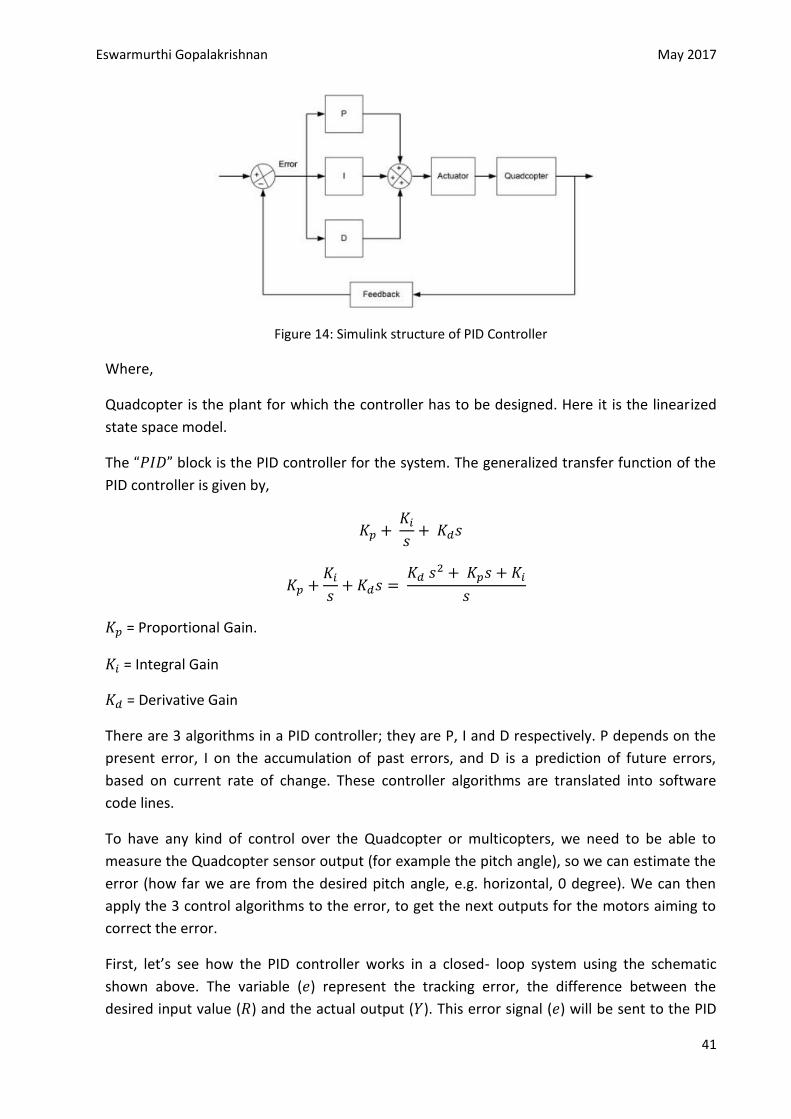
The figure [29] below shows control block diagram that can be used for each one of
components. As shown in the figure, one controller should be designed for each one
of .
Eswarmurthi Gopalakrishnan May 2017
41
Figure 14: Simulink structure of PID Controller
Where,
Quadcopter is the plant for which the controller has to be designed. Here it is the linearized
state space model.
The block is the PID controller for the system. The generalized transfer function of the
PID controller is given by,
= Proportional Gain.
= Integral Gain
= Derivative Gain
There are 3 algorithms in a PID controller; they are P, I and D respectively. P depends on the
present error, I on the accumulation of past errors, and D is a prediction of future errors,
based on current rate of change. These controller algorithms are translated into software
code lines.
To have any kind of control over the Quadcopter or multicopters, we need to be able to
measure the Quadcopter sensor output (for example the pitch angle), so we can estimate the
error (how far we are from the desired pitch angle, e.g. horizontal, 0 degree). We can then
apply the 3 control algorithms to the error, to get the next outputs for the motors aiming to
correct the error.
First, let’s see how the PID controller works in a closed- loop system using the schematic
shown above. The variable ( ) represent the tracking error, the difference between the
desired input value ( ) and the actual output ( ). This error signal ( ) will be sent to the PID
Eswarmurthi Gopalakrishnan May 2017
42
controller, and the controller computes both the derivative and the integral of this error
signal. The signal ( ) just past the controller is now equal to the proportional gain ( ) ties
the magnitude f the error plus the integral gain ( ) times the integral of the error plus the
derivative gain ( ) times the derivative of the error.
∫
This signal ( ) will be sent to the plant, and the new output ( ) will be obtained. This new
output ( ) will be sent back to the sensor again to find the new error signal ( ). The controller
takes this new error signal and computed its derivative and it is integral again. This process
goes on and on.
5.2.1 Effect of each parameter The variation of each of these parameters alters the effectiveness of the stabilization.
Generally there are 3 PID loops with their own coefficients, one per axis, so you will have
to set P, I and D values for each axis ( ).
To a Quadcopter, these parameters can cause this behaviour.
Proportional Gain coefficient – Your Quadcopter can fly relatively stable without
other parameters but this one. This coefficient determines which is more important,
human control or the values measured by the gyroscopes. The higher the coefficient,
the higher the Quadcopter seems more sensitive and reactive to angular change. If it is
too low, the Quadcopter will appear sluggish and will be harder to keep steady. You
might find the Quadcopter starts to oscillate with a high frequency when P gain is too
high.
Integral Gain coefficient – This coefficient can increase the precision of the angular
position. For example, when the Quadcopter is disturbed and its angle changes from
, in theory it remembers how much the angle has changed and will return . In
practise if you make your Quadcopter go forward and the force it to stop, the
Quadcopter will continue for some time to counteract the action. Without this term,
the opposition does not last as long. This term is especially useful with irregular wind,
and ground effect (turbulence from motors). However, when the I value get too high
your Quadcopter might begin to have slow reaction and a decrease effect of the
proportional gain as consequence, it will also start to oscillate like having high P gain,
but with a lower frequency.
Derivative Gain coefficient – This coefficient allows the Quadcopter to reach more
quickly the desired attitude. Some people call it the accelerator parameter because it
amplifies the user input. It also decrease control action fast when the error is
decreasing fast. In particle it will increase the reaction speed and in certain cases an
increase the effect of the P gains.
Eswarmurthi Gopalakrishnan May 2017
43
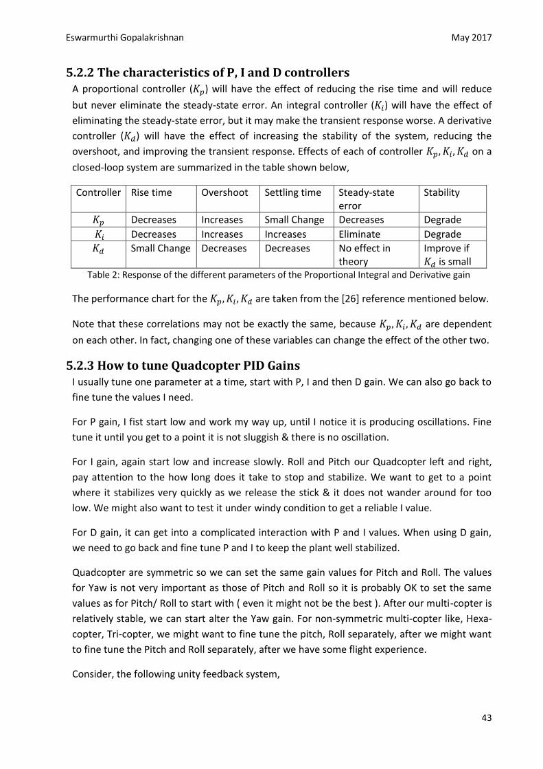
5.2.2 The characteristics of P, I and D controllers A proportional controller ( ) will have the effect of reducing the rise time and will reduce
but never eliminate the steady-state error. An integral controller ( ) will have the effect of
eliminating the steady-state error, but it may make the transient response worse. A derivative
controller ( ) will have the effect of increasing the stability of the system, reducing the
overshoot, and improving the transient response. Effects of each of controller on a
closed-loop system are summarized in the table shown below,
Controller Rise time Overshoot Settling time Steady-state error
Stability
Decreases Increases Small Change Decreases Degrade
Decreases Increases Increases Eliminate Degrade
Small Change Decreases Decreases No effect in theory
Improve if is small
Table 2: Response of the different parameters of the Proportional Integral and Derivative gain
The performance chart for the are taken from the [26] reference mentioned below.
Note that these correlations may not be exactly the same, because are dependent
on each other. In fact, changing one of these variables can change the effect of the other two.
5.2.3 How to tune Quadcopter PID Gains I usually tune one parameter at a time, start with P, I and then D gain. We can also go back to
fine tune the values I need.
For P gain, I fist start low and work my way up, until I notice it is producing oscillations. Fine
tune it until you get to a point it is not sluggish & there is no oscillation.
For I gain, again start low and increase slowly. Roll and Pitch our Quadcopter left and right,
pay attention to the how long does it take to stop and stabilize. We want to get to a point
where it stabilizes very quickly as we release the stick & it does not wander around for too
low. We might also want to test it under windy condition to get a reliable I value.
For D gain, it can get into a complicated interaction with P and I values. When using D gain,
we need to go back and fine tune P and I to keep the plant well stabilized.
Quadcopter are symmetric so we can set the same gain values for Pitch and Roll. The values
for Yaw is not very important as those of Pitch and Roll so it is probably OK to set the same
values as for Pitch/ Roll to start with ( even it might not be the best ). After our multi-copter is
relatively stable, we can start alter the Yaw gain. For non-symmetric multi-copter like, Hexa-
copter, Tri-copter, we might want to fine tune the pitch, Roll separately, after we might want
to fine tune the Pitch and Roll separately, after we have some flight experience.
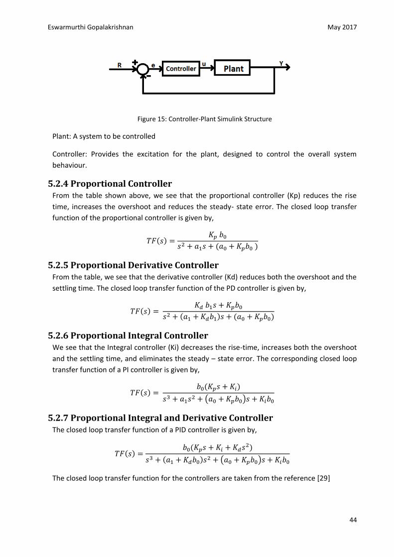
Consider, the following unity feedback system,
Eswarmurthi Gopalakrishnan May 2017
44
Figure 15: Controller-Plant Simulink Structure
Plant: A system to be controlled
Controller: Provides the excitation for the plant, designed to control the overall system
behaviour.
5.2.4 Proportional Controller From the table shown above, we see that the proportional controller (Kp) reduces the rise
time, increases the overshoot and reduces the steady- state error. The closed loop transfer
function of the proportional controller is given by,
( )
( )
5.2.5 Proportional Derivative Controller From the table, we see that the derivative controller (Kd) reduces both the overshoot and the
settling time. The closed loop transfer function of the PD controller is given by,
( )
( ) ( )
5.2.6 Proportional Integral Controller We see that the Integral controller (Ki) decreases the rise-time, increases both the overshoot
and the settling time, and eliminates the steady – state error. The corresponding closed loop
transfer function of a PI controller is given by,
( ) ( )
( )
5.2.7 Proportional Integral and Derivative Controller The closed loop transfer function of a PID controller is given by,
( ) ( )
( ) ( )
The closed loop transfer function for the controllers are taken from the reference [29]
Eswarmurthi Gopalakrishnan May 2017
45
5.3 LQR Linear Quadratic Regulator is one of the most efficient optimal controllers; this method is
used to derive the feedback gain for a system. LQR is a powerful tool for calculating the
feedback gains. Consider a system,
Suppose we want to design a state feedback control to stabilize the system. We can
make a new system that looks like,
( )
This system is without a reference input. Suppose we have a command input ( ), the closed
loop system using this input becomes
( ) ( )
Where Ac is closed loop plant matrix.
We have a rule that if ( ) is controllable, then we can place the Eigenvalues of the closed
loop system anywhere we want. This method is very powerful but in practice, it would be
sometimes not useful. There are few problems associated with this.
The first problem is supposed we have a second order system without any zeros, whose
transfer function looks like,
With, being the Natural Frequency, being the Damping Ratio and c being a constant. If
the system is given a step input of magnitude 1, the system dynamics can be either critically
damped or under damped or over damper. But, most of the system does not react like this,
even if we add a small disturbance to the system as given below,
( )
When we give in a step input for this system, we would expect the system to be critically
damped, but the system would respond with an overshoot even though the denominator is
critically damped.
The other problem is, even though we can place the system’s Eigenvalues wherever we want,
we do not have the great sense of the input required to place the Eigenvalues. That is if the
system has poles at -1 which is considered to be stable, we would think why we don’t place
the poles at -10 or any other place more left to the origin so that the system would be more
stable. The problem is we would require a much greater value of an input to place the poles
Eswarmurthi Gopalakrishnan May 2017
46
at -10 rather than -1. This is one of the purposes of the LQR that is to find the value of K a
little bit more intuitive to the designer.
So, here is how we find it, we are going to design a cost function J, which is a one by one
scalar. We call it Performance Index; we take the integral from zero to infinity so it is called as
an infinite horizon problem. We have the time limit to infinity because we want the controller
to work well all time and not for a particular period of time. So, we are going to integrate the
state vector of the system in time with a weighted matrix Q and input vector of the system in
time with another weighted matrix R over the infinite period of time. So, this Performance
Index would look like,
∫ ( ( ) ( ) ( ) ( )
) ( )
The dimensions of the PI are, the ( ) is of the order nx1, the ( ) is of the order 1xn so the
Q is a positive semi-definite matrix of the order nxn. Similarly, the ( ) is of the order px1 and
( ) is of the order 1xp and the R is a positive definite matrix of the order pxp. So, the first
part of the PI is a 1x1 scalar which we are adding to another 1x1 scalar (second part of the PI).
It means that J is a constant value of the order 1x1.
NOTE:
Positive-definite matrix- It says that if A is a positive definite matrix, then will always be
greater than zero, for every possible .
Positive semi-definite matrix- If A is a positive semi-definite matrix, then will always be
greater than or equal to zero, for every possible .
From the PI formula, we can see that the cost function is directly proportional to the state and
the input of the system. Since this is a regulator problem, we want to bring all the states to
zero as early as possible. That is to bring the state ( )to zero as time goes to infinity. So, we
want the states to be really small, this is achieved by making the cost J as small as possible.
This is achieved by varying the weighted matrices Q and R.
Let us consider a simple a second order system to see how Q and R look like.
Let, the state ( ) be a real matrix of the order 2, Q be a symmetric matrix of order 2,
[
] [
]
From the last equation we see that the term q1 basically penalizes the state 1 which is the
square term, so it does not matter if it is positive or negative similarly, the term q2 penalizes
the state 2. We can understand from this that all the individual diagonal terms penalize the
Eswarmurthi Gopalakrishnan May 2017
47
stated individually. The off-diagonal terms (in our case q3) penalizes the combination of the
states.
So, let us consider the first state as position and second state as velocity. If we want a system
for example not to go too fast, in this case, we could alter the term q2 either by making it large
or small depending on the system’s response.
NOTE:
The state term ( ) ( ) in J must always be a positive number. If the term is a negative
number then we would end up with J being negative and pushing the system to be more
unstable.
Now, let us take the Q matrix, I have q1 and q2 equal to 1 and q3 is equal to a very small value,
say for example 0.0001 in this case, Q matrix remains positive semi-definite matrix, but in
some scenario, we will have a certain q3 value, where the Q matrix is not positive semi-
definite. So, it is much better to consider the weighted matrices Q and R a diagonal matrix.
This is the basic idea of the LQR controller. Now, let us see how to derive the gain K from the
LQR controller. We are going to implement the control function ( ) ( ).
Substituting the State Variable feedback Control into the cost function, that is (59) in (58).
∫ ( ( ) )
( )
We assume v(t) = 0; since our only concern is the internal stability. The main objective is to
find K that minimizes the cost function J. To find the optimal feedback gain K we proceed as
follows. Suppose there exists a constant matrix P,
( ) ( ( ) ) ( )
Substituting (61) in (60),
∫
( ) ( ) ( )
( )
From (62) we see that J is a constant independent of K and depends only on auxiliary matrix P
and the initial conditions. We find K so that (61) holds, to find such a K, we differentiate (61)
and then substitute from (58) to see that (61) is equivalent to,
( )
Eswarmurthi Gopalakrishnan May 2017
48
Since v(t) is equal to zero, the last equation holds for every x(t). Therefore, the terms in the
bracket must be individually equal to zero.
( ) ( )
This is Matrix Quadratic Equation. As for the scalar case,
( )
( ) ( ) ( ) ( )
( )
This equation is known as the algebraic Riccatti Equation (ARE). This equation is solved for P
given A,B,Q,R. Then, the State Variable Feedback gain (K) is calculated using (63). The minimal
value of PI using this gain by (62), which only depends on the initial condition. This means that
the cost of using the State Variable Feed Back (63) can be computed from the initial
conditions before the control is ever applied to the system. The procedure for finding the LQR
feedback gain K is,
Selecting the weighted matrices Q and R
Solve the ARE for P
Find K using
There are numerical ways to compute the gain by paper. To calculate the gain through Matlab
we use the command ( ). The LQR design procedure is guaranteed to
produce a feedback gain that stabilized the system as long as some basic properties hold.
LQR Theorem 1: Let the system (A,B) be reachable. Let R be positive definite and Q be
positive definite. Then the closed loop system (A-BK) is asymptotically stable.
Note that this holds regardless of the stability of the open loop system. Recall that
reachability can be verified by checking that the reachability matrix
[ ] has full rank n [38].
LQR Theorem 2: Let the system (A, B) be stabilizable. Let R be positive definite, Q be positive
semi-definite and ( √ ) be observable. Then the closed loop system (A-BK) is
asymptotically stable [38].
It is important to realize that this modern control approach to feedback design is very
different from the philosophy of classical control. It is characterized by,
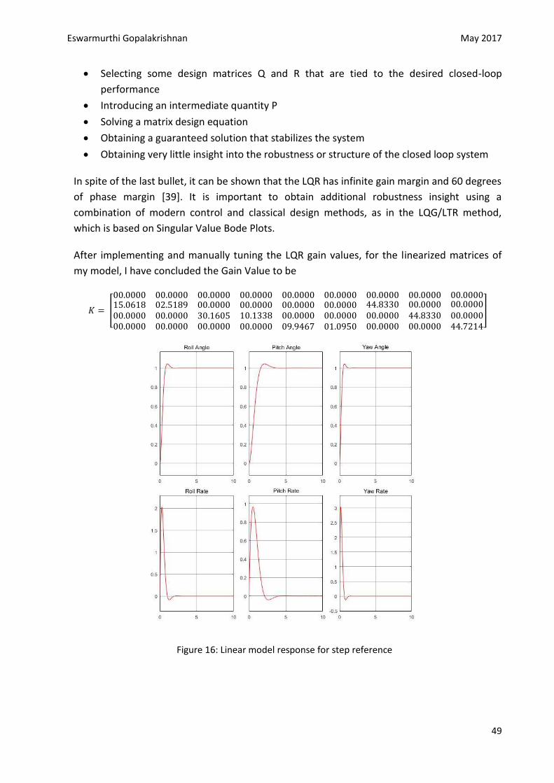
Eswarmurthi Gopalakrishnan May 2017
49
Selecting some design matrices Q and R that are tied to the desired closed-loop
performance
Introducing an intermediate quantity P
Solving a matrix design equation
Obtaining a guaranteed solution that stabilizes the system
Obtaining very little insight into the robustness or structure of the closed loop system
In spite of the last bullet, it can be shown that the LQR has infinite gain margin and 60 degrees
of phase margin [39]. It is important to obtain additional robustness insight using a
combination of modern control and classical design methods, as in the LQG/LTR method,
which is based on Singular Value Bode Plots.
After implementing and manually tuning the LQR gain values, for the linearized matrices of
my model, I have concluded the Gain Value to be
[
]
Figure 16: Linear model response for step reference
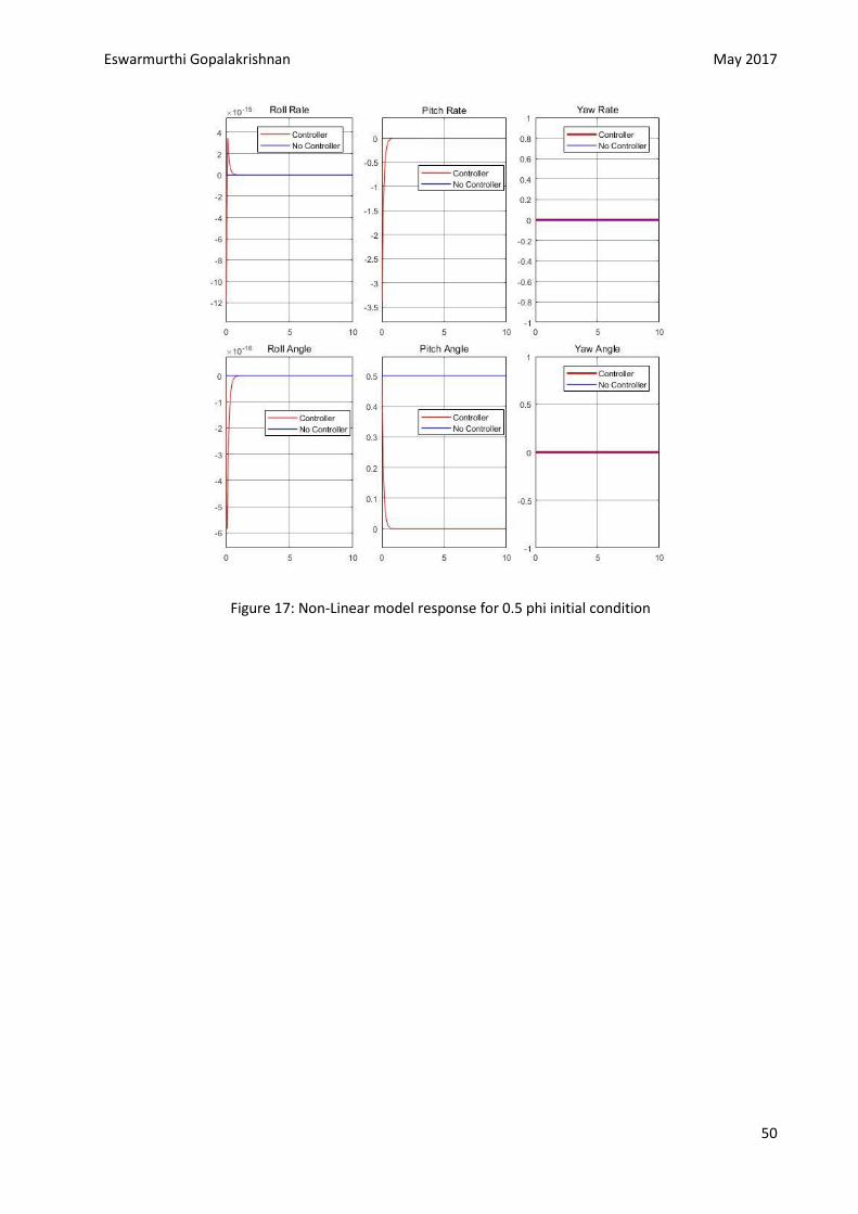
Eswarmurthi Gopalakrishnan May 2017
50
Figure 17: Non-Linear model response for 0.5 phi initial condition
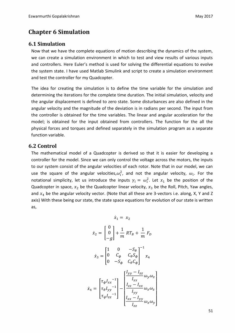
Eswarmurthi Gopalakrishnan May 2017
51
Chapter 6 Simulation
6.1 Simulation Now that we have the complete equations of motion describing the dynamics of the system,
we can create a simulation environment in which to test and view results of various inputs
and controllers. Here Euler’s method is used for solving the differential equations to evolve
the system state. I have used Matlab Simulink and script to create a simulation environment
and test the controller for my Quadcopter.
The idea for creating the simulation is to define the time variable for the simulation and
determining the iterations for the complete time duration. The initial simulation, velocity and
the angular displacement is defined to zero state. Some disturbances are also defined in the
angular velocity and the magnitude of the deviation is in radians per second. The input from
the controller is obtained for the time variables. The linear and angular acceleration for the
model; is obtained for the input obtained from controllers. The function for the all the
physical forces and torques and defined separately in the simulation program as a separate
function variable.
6.2 Control The mathematical model of a Quadcopter is derived so that it is easier for developing a
controller for the model. Since we can only control the voltage across the motors, the inputs
to our system consist of the angular velocities of each rotor. Note that in our model, we can
use the square of the angular velocities, , and not the angular velocity, . For the
notational simplicity, let us introduce the inputs . Let be the position of the
Quadcopter in space, be the Quadcopter linear velocity, be the Roll, Pitch, Yaw angles,
and be the angular velocity vector. (Note that all these are 3-vectors i.e. along, X, Y and Z
axis) With these being our state, the state space equations for evolution of our state is written
as,
[
]
[
]
[
]
[
]
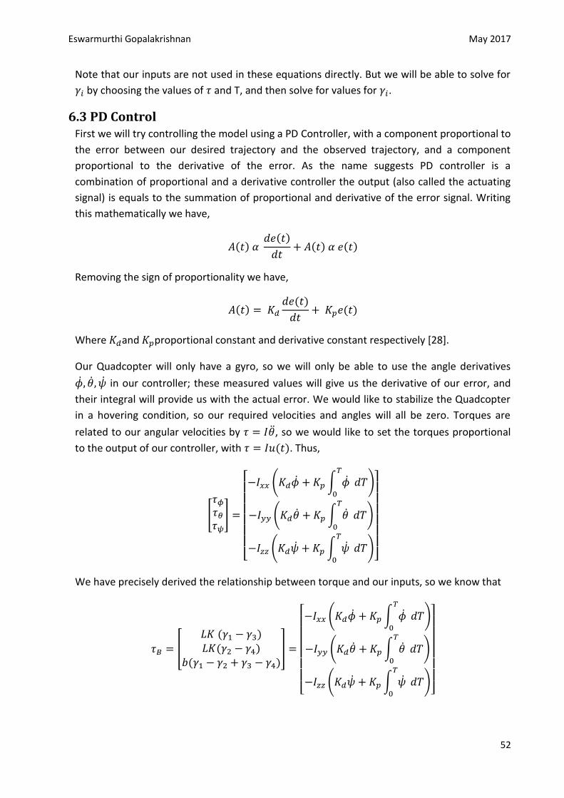
Eswarmurthi Gopalakrishnan May 2017
52
Note that our inputs are not used in these equations directly. But we will be able to solve for
by choosing the values of and T, and then solve for values for .
6.3 PD Control First we will try controlling the model using a PD Controller, with a component proportional to
the error between our desired trajectory and the observed trajectory, and a component
proportional to the derivative of the error. As the name suggests PD controller is a
combination of proportional and a derivative controller the output (also called the actuating
signal) is equals to the summation of proportional and derivative of the error signal. Writing
this mathematically we have,
( ) ( )
( ) ( )
Removing the sign of proportionality we have,
( )
( )
( )
Where and proportional constant and derivative constant respectively [28].
Our Quadcopter will only have a gyro, so we will only be able to use the angle derivatives
in our controller; these measured values will give us the derivative of our error, and
their integral will provide us with the actual error. We would like to stabilize the Quadcopter
in a hovering condition, so our required velocities and angles will all be zero. Torques are
related to our angular velocities by , so we would like to set the torques proportional
to the output of our controller, with ( ). Thus,
[
]
[ ( ∫
)
( ∫
)
( ∫
)]
We have precisely derived the relationship between torque and our inputs, so we know that
[
( ) ( )
( )]
[ ( ∫
)
( ∫
)
( ∫
)]
Eswarmurthi Gopalakrishnan May 2017
53
This gives us a set of three equations with four unknowns. We can constraint this by enforcing
the constraint that our input must keep the Quadcopter loft:
Note that this equation ignores the fact that the thrust will not be pointed directly up. This
will limit the applicability of our controller, but should not cause major problems for small
deviations from stability. If we had a way of determining the current angle accurately, we
could compensate. If our gyro is precise enough, we can integrate the values obtained from
the gyro to get the angles . In this case, we can calculate the thrust necessary to keep
the Quadcopter aloft by projecting the thrust onto the inertial z axis. We find that,
Therefore, with a precise angle measurement, we can instead enforce the requirement that
the thrust be equal to
In which case the component of the thrust pointing along the positive z axis will be equal to
mg. We know that the thrust is proportional to a weighted sum of the inputs:
∑ ∑
With this extra constraint, we have a set of four linear equations with four unknowns . We
can simulate this controller using our simulation environment. The controller drives the
angular velocities and angles to zero.
The response of my model for the PD controller is given below. Here we are analysing the
Angular Velocity and the Angular Displacement of the model for the given input and the
Proportional and Derivative controller.
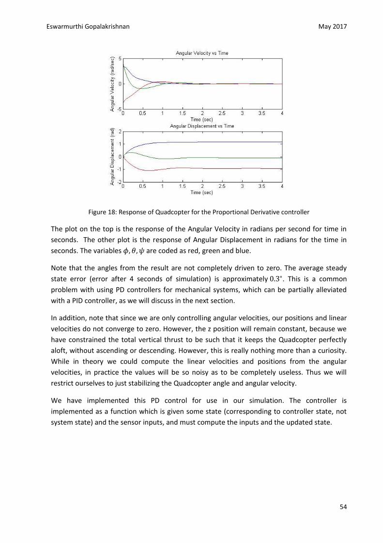
Eswarmurthi Gopalakrishnan May 2017
54
Figure 18: Response of Quadcopter for the Proportional Derivative controller
The plot on the top is the response of the Angular Velocity in radians per second for time in
seconds. The other plot is the response of Angular Displacement in radians for the time in
seconds. The variables are coded as red, green and blue.
Note that the angles from the result are not completely driven to zero. The average steady
state error (error after 4 seconds of simulation) is approximately . This is a common
problem with using PD controllers for mechanical systems, which can be partially alleviated
with a PID controller, as we will discuss in the next section.
In addition, note that since we are only controlling angular velocities, our positions and linear
velocities do not converge to zero. However, the z position will remain constant, because we
have constrained the total vertical thrust to be such that it keeps the Quadcopter perfectly
aloft, without ascending or descending. However, this is really nothing more than a curiosity.
While in theory we could compute the linear velocities and positions from the angular
velocities, in practice the values will be so noisy as to be completely useless. Thus we will
restrict ourselves to just stabilizing the Quadcopter angle and angular velocity.
We have implemented this PD control for use in our simulation. The controller is
implemented as a function which is given some state (corresponding to controller state, not
system state) and the sensor inputs, and must compute the inputs and the updated state.
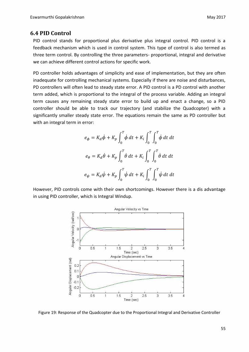
Eswarmurthi Gopalakrishnan May 2017
55
6.4 PID Control PID control stands for proportional plus derivative plus integral control. PID control is a
feedback mechanism which is used in control system. This type of control is also termed as
three term control. By controlling the three parameters- proportional, integral and derivative
we can achieve different control actions for specific work.
PD controller holds advantages of simplicity and ease of implementation, but they are often
inadequate for controlling mechanical systems. Especially if there are noise and disturbances,
PD controllers will often lead to steady state error. A PID control is a PD control with another
term added, which is proportional to the integral of the process variable. Adding an integral
term causes any remaining steady state error to build up and enact a change, so a PID
controller should be able to track our trajectory (and stabilize the Quadcopter) with a
significantly smaller steady state error. The equations remain the same as PD controller but
with an integral term in error:
∫
∫ ∫
∫
∫ ∫
∫
∫ ∫
However, PID controls come with their own shortcomings. However there is a dis advantage
in using PID controller, which is Integral Windup.
Figure 19: Response of the Quadcopter due to the Proportional Integral and Derivative Controller
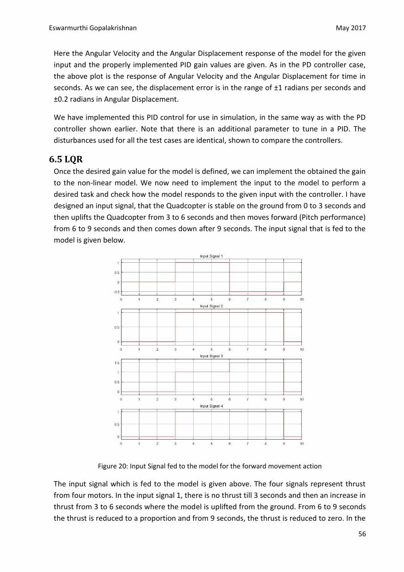
Eswarmurthi Gopalakrishnan May 2017
56
Here the Angular Velocity and the Angular Displacement response of the model for the given
input and the properly implemented PID gain values are given. As in the PD controller case,
the above plot is the response of Angular Velocity and the Angular Displacement for time in
seconds. As we can see, the displacement error is in the range of ±1 radians per seconds and
±0.2 radians in Angular Displacement.
We have implemented this PID control for use in simulation, in the same way as with the PD
controller shown earlier. Note that there is an additional parameter to tune in a PID. The
disturbances used for all the test cases are identical, shown to compare the controllers.
6.5 LQR Once the desired gain value for the model is defined, we can implement the obtained the gain
to the non-linear model. We now need to implement the input to the model to perform a
desired task and check how the model responds to the given input with the controller. I have
designed an input signal, that the Quadcopter is stable on the ground from 0 to 3 seconds and
then uplifts the Quadcopter from 3 to 6 seconds and then moves forward (Pitch performance)
from 6 to 9 seconds and then comes down after 9 seconds. The input signal that is fed to the
model is given below.
Figure 20: Input Signal fed to the model for the forward movement action
The input signal which is fed to the model is given above. The four signals represent thrust
from four motors. In the input signal 1, there is no thrust till 3 seconds and then an increase in
thrust from 3 to 6 seconds where the model is uplifted from the ground. From 6 to 9 seconds
the thrust is reduced to a proportion and from 9 seconds, the thrust is reduced to zero. In the
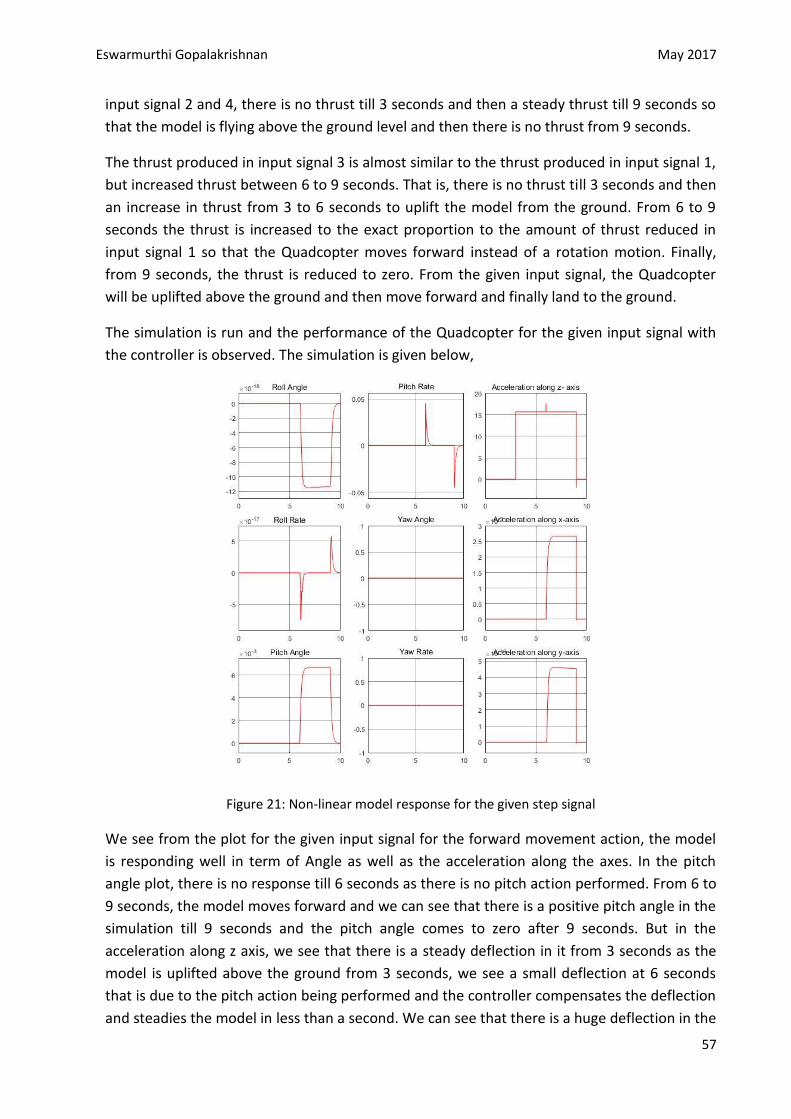
Eswarmurthi Gopalakrishnan May 2017
57
input signal 2 and 4, there is no thrust till 3 seconds and then a steady thrust till 9 seconds so
that the model is flying above the ground level and then there is no thrust from 9 seconds.
The thrust produced in input signal 3 is almost similar to the thrust produced in input signal 1,
but increased thrust between 6 to 9 seconds. That is, there is no thrust till 3 seconds and then
an increase in thrust from 3 to 6 seconds to uplift the model from the ground. From 6 to 9
seconds the thrust is increased to the exact proportion to the amount of thrust reduced in
input signal 1 so that the Quadcopter moves forward instead of a rotation motion. Finally,
from 9 seconds, the thrust is reduced to zero. From the given input signal, the Quadcopter
will be uplifted above the ground and then move forward and finally land to the ground.
The simulation is run and the performance of the Quadcopter for the given input signal with
the controller is observed. The simulation is given below,
Figure 21: Non-linear model response for the given step signal
We see from the plot for the given input signal for the forward movement action, the model
is responding well in term of Angle as well as the acceleration along the axes. In the pitch
angle plot, there is no response till 6 seconds as there is no pitch action performed. From 6 to
9 seconds, the model moves forward and we can see that there is a positive pitch angle in the
simulation till 9 seconds and the pitch angle comes to zero after 9 seconds. But in the
acceleration along z axis, we see that there is a steady deflection in it from 3 seconds as the
model is uplifted above the ground from 3 seconds, we see a small deflection at 6 seconds
that is due to the pitch action being performed and the controller compensates the deflection
and steadies the model in less than a second. We can see that there is a huge deflection in the
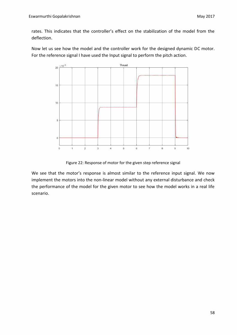
Eswarmurthi Gopalakrishnan May 2017
58
rates. This indicates that the controller’s effect on the stabilization of the model from the
deflection.
Now let us see how the model and the controller work for the designed dynamic DC motor.
For the reference signal I have used the Input signal to perform the pitch action.
Figure 22: Response of motor for the given step reference signal
We see that the motor’s response is almost similar to the reference input signal. We now
implement the motors into the non-linear model without any external disturbance and check
the performance of the model for the given motor to see how the model works in a real life
scenario.
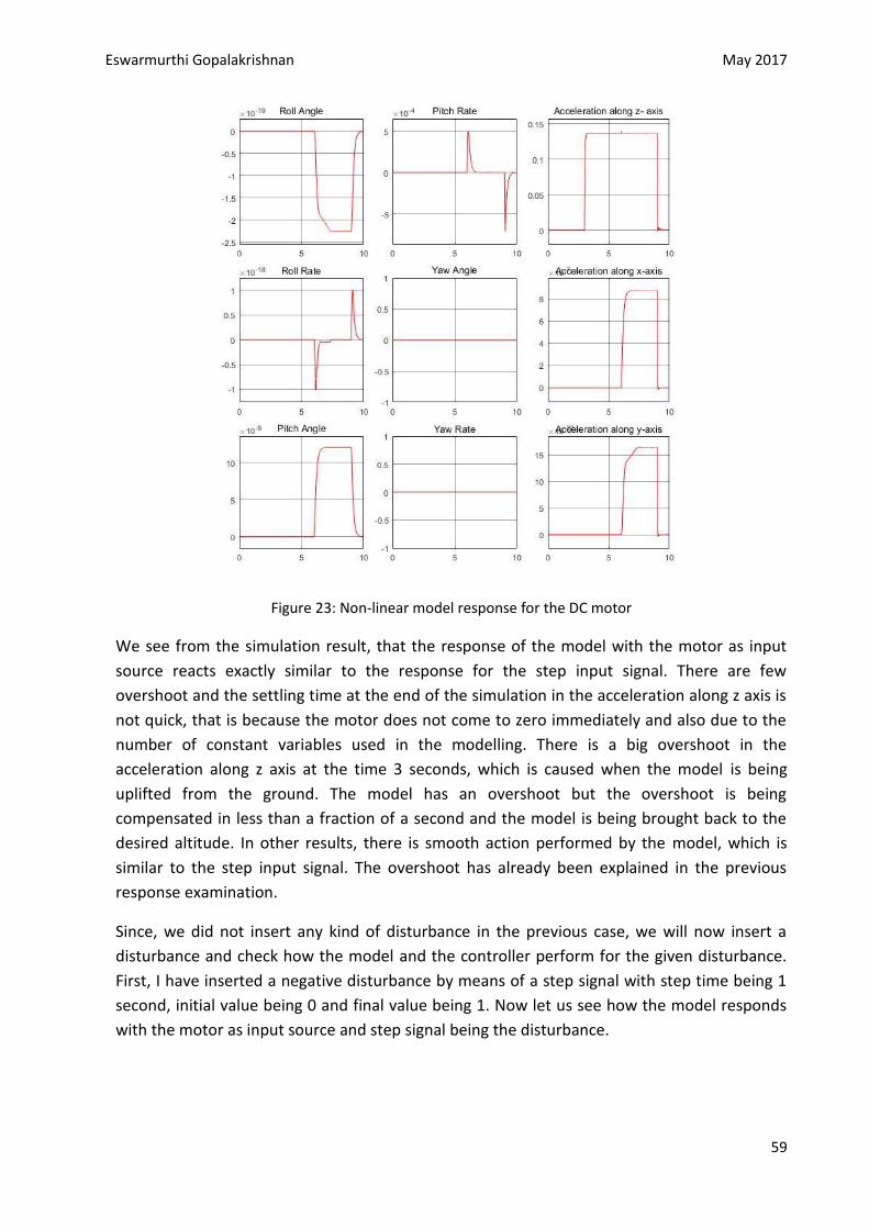
Eswarmurthi Gopalakrishnan May 2017
59
Figure 23: Non-linear model response for the DC motor
We see from the simulation result, that the response of the model with the motor as input
source reacts exactly similar to the response for the step input signal. There are few
overshoot and the settling time at the end of the simulation in the acceleration along z axis is
not quick, that is because the motor does not come to zero immediately and also due to the
number of constant variables used in the modelling. There is a big overshoot in the
acceleration along z axis at the time 3 seconds, which is caused when the model is being
uplifted from the ground. The model has an overshoot but the overshoot is being
compensated in less than a fraction of a second and the model is being brought back to the
desired altitude. In other results, there is smooth action performed by the model, which is
similar to the step input signal. The overshoot has already been explained in the previous
response examination.
Since, we did not insert any kind of disturbance in the previous case, we will now insert a
disturbance and check how the model and the controller perform for the given disturbance.
First, I have inserted a negative disturbance by means of a step signal with step time being 1
second, initial value being 0 and final value being 1. Now let us see how the model responds
with the motor as input source and step signal being the disturbance.
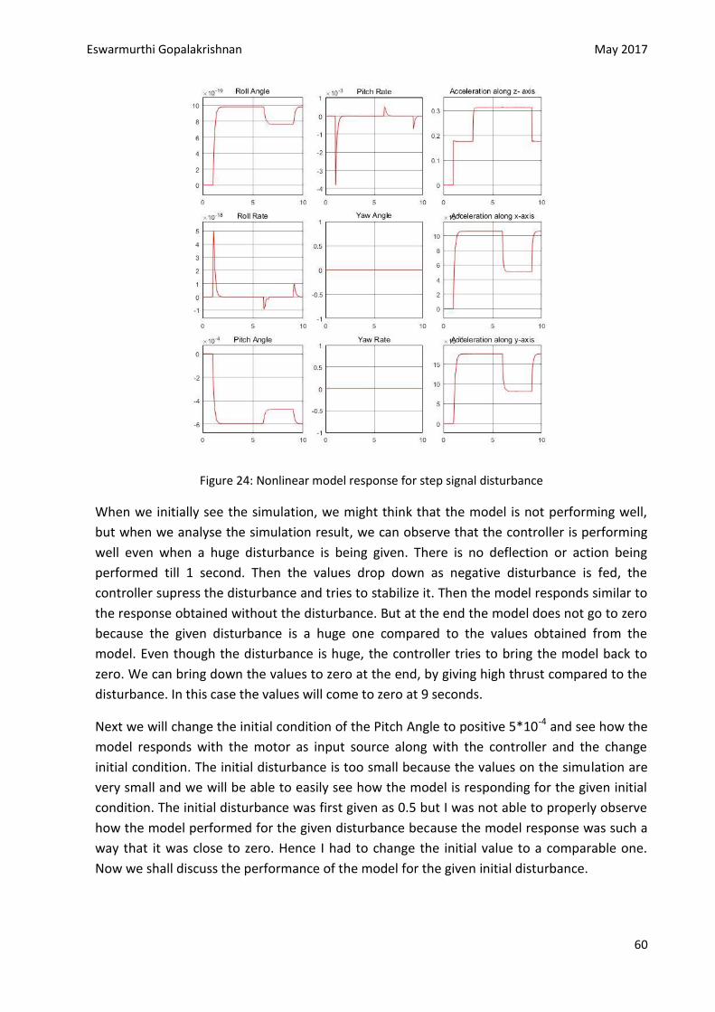
Eswarmurthi Gopalakrishnan May 2017
60
Figure 24: Nonlinear model response for step signal disturbance
When we initially see the simulation, we might think that the model is not performing well,
but when we analyse the simulation result, we can observe that the controller is performing
well even when a huge disturbance is being given. There is no deflection or action being
performed till 1 second. Then the values drop down as negative disturbance is fed, the
controller supress the disturbance and tries to stabilize it. Then the model responds similar to
the response obtained without the disturbance. But at the end the model does not go to zero
because the given disturbance is a huge one compared to the values obtained from the
model. Even though the disturbance is huge, the controller tries to bring the model back to
zero. We can bring down the values to zero at the end, by giving high thrust compared to the
disturbance. In this case the values will come to zero at 9 seconds.
Next we will change the initial condition of the Pitch Angle to positive 5*10-4 and see how the
model responds with the motor as input source along with the controller and the change
initial condition. The initial disturbance is too small because the values on the simulation are
very small and we will be able to easily see how the model is responding for the given initial
condition. The initial disturbance was first given as 0.5 but I was not able to properly observe
how the model performed for the given disturbance because the model response was such a
way that it was close to zero. Hence I had to change the initial value to a comparable one.
Now we shall discuss the performance of the model for the given initial disturbance.
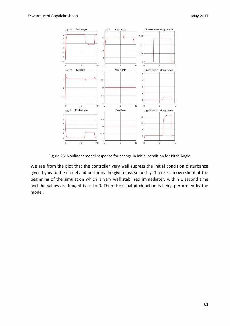
Eswarmurthi Gopalakrishnan May 2017
61
Figure 25: Nonlinear model response for change in initial condition for Pitch Angle
We see from the plot that the controller very well supress the initial condition disturbance
given by us to the model and performs the given task smoothly. There is an overshoot at the
beginning of the simulation which is very well stabilized immediately within 1 second time
and the values are bought back to 0. Then the usual pitch action is being performed by the
model.
Eswarmurthi Gopalakrishnan May 2017
62
Chapter 7 Conclusion
7.1 Comparison of the work As I mentioned earlier, this is my second approach towards the topic handled in this thesis. In
the previous work, I designed a dynamic Quadcopter model and linearized it at a given
linearization point. Later, I designed a PID controller for the linearized model. But, in the
objective of the thesis it was clearly mentioned that an advanced control law has to be
designed and validated, which could not be completed along with the simulation of the model
in the previous approach. I have been able to achieve the advanced control law as well as the
guidance of the model. I have listed down the work from the previous approach.
A literature survey related to the topic was given
Designed a nonlinear dynamic Quadcopter model and implemented it in the Simulink
Performed linearization on the nonlinear model
Designed a PID controller for the model and also designed automated PID tuning for
the model.
In this approach, I have designed the dynamic model for the Quadcopter, and then linearized
the model for the linearization point. Next, I have designed a dynamic model of a DC motor as
a source of input to the model. I designed a controller for the speed of the motor along with
the armature current controller for the motor. This motor was used by me to validate the
performance of the model in real life scenario. Later, I designed a LQR controller using the
linearized model of the Quadcopter. The tuned LQR gain was fed to the nonlinear model and
the performance of the model was verified. Finally, an input signal was given to the nonlinear
model, so that it performs a specific task along with the disturbance given to the model. I
have also listed down the tasks completed from the second approach of the work for
comparison purpose.
Delivered a brief literature survey on Quadcopter, their purpose in day to day life, DC
motors is given and finally Control law used in the thesis
Designed a nonlinear dynamic Quadcopter model and implemented it in the Simulink
Designed a dynamic DC motor model and implemented it in the Simulink along with
the speed control and armature current control
Performed linearization on the nonlinear model
Validated the linear and nonlinear model to check the linearization of the model
Designed a PID controller for the model and also designed automated PID tuning for
the model
Designed a LQR controller for the linearized model and implemented it to the
nonlinear model
The nonlinear model’s performance along with the LQR controller was studied for the
input from the DC motor to perform a specific action
Eswarmurthi Gopalakrishnan May 2017
63
Finally, the model was studied for the disturbance given to the model to check for
stability of the model in real life scenario
7.2 Conclusion In my thesis work, I was able to successfully design a nonlinear dynamic Quadcopter model
and linearize the model for the given linearization point. The linear and nonlinear model was
validated and the result was more than satisfactory. I designed a dynamic DC motor with the
speed controller with the armature current controller. Later, a PID controller was designed
and validated. The LQR controller for the linear model was designed, which was later fed to
the linear model. The performance was verified and the DC motor was introduced as the
input source. The output from the DC motor was the thrust produced by the motor. The
thrust was designed in such a way that the model was supposed to perform a specific action.
The result was better and the model was performing the task with more stability. Then some
disturbance was introduced to the model. Firstly, a step input was given as a negative
disturbance and the designed LQR controller was able to overcome the disturbance and then
the initial condition was altered. The controller was able to overcome even this condition and
performed the given task with more stability. I hereby conclude that the LQR controller
performed well both cases where the input source was a step signal as well as when the DC
motor was introduced to the model.
Eswarmurthi Gopalakrishnan May 2017
64
References 1. Leishman, J.G. (2000). Principles of Helicopter Aerosynamics. New Yorl, NY: Cambridge
University Press.
2. www.asctec.de
3. http://www.dji.com/product/phantom-2-vision-plus
4. Pounds, P.;Mahony, R,; Corke, P. (December 2006). "In the Proceedings of the Australasian
Conference on Robotics and Automation". Auckland, New Zealand.
5. Hoffman, G,; Haung, H.; Waslander, S.L.; Tomlin, C.J. (20-23 August 2007). "In the
Conference of the Anerican Institute of Aeronautics and Astronautics". Head Hilton, South
California.
6. "Aeryon Labs Inc."
7. Illumin- The Quadcoptor's Coming of Age"
8. "Paparazzi Agency - We've Used Drones For A Long Time". www.tmz.com
9. Model Predictive quadrotor control: attitude, altitude and position experimental studies by
K. Alexis, G. Nikolakopoulos and A. Tzes
10. Design and Control of Quadrotors with application to Autonomous Flying by Samir
Bouabdallah.
11. "Full control of a Quadrotor" by Bouabdallah, S, Siegwart, R.
12. "Design and control of quadrotors with application to autonomous flying" by Bouabdallah,
19. http://ardrone2.parrot.com/
13. http://www.scholarpedia.org/article/Siegel_disks/Linearization - The Linearization
problem in complex dimension one dynamical systems
14. CSAS_flightmechanics1 lecture slides in CVUT by Martin Xhromcik- department of control
Engineering.
15. G.A. Leonov, N.V. Kuznetsov, Time-Varying Linearization and the Perron effects,
International Journal of Bifurcation and Chaos, Vol. 17, No. 4, 2007
16. http://en.wikipedia.org/wiki/Jacobian_matrix_and_determinant
17. http://www.ece.rutgers.edu/~gajic/psfiles/chap5traCO.pdf
18. https://en.wikibooks.org/wiki/Control_Systems/Controllability_and_Observability
Eswarmurthi Gopalakrishnan May 2017
65
19. Understanding Poles and Zeros by Massachusetts Institute of Technology, Department of
Mechanical Engineering
20. http://www.mathworks.com/matlabcentral/answers/82408-the-advantages-of-matlab-
over-other-programing-languges-for-image-processing
21. Simulink Getting Started Tutorial by Mathworks
22. http://en.wikipedia.org/wiki/PID_controller
23. http://en.wikipedia.org/wiki/Single-input_single-output_system
24. "Improving Disturbance Rejection of PID controllers by Means of the Magnitude Optimum
Method", D. Vrancic, S. Strmcnik, J. Kocijan and P. B. M. Oliveira
25. "On stabilizing PI Controller Ranges for Multi- variable Systems" pp. 620- 625 by, C. Lin,
Q.G. Wang, Y. He, G. Wen, X. Han and G. Z. H. Z. Li.
26. https://en.wikipedia.org/wiki/PID_controller
27. https://courses.engr.illinois.edu/ece486/documents/lecture_notes/pid.pdf
28.http://www.electrical4u.com/types-of-controllers-proportional-integral-derivative-
controllers/
29. https://oscarliang.com/quadcopter-pid-explained-tuning/
30. https://en.wikipedia.org/wiki/Linear%E2%80%93quadratic_regulator
31. Dynamic Modelling of DC Motor and Simulation by Defence Research and Development
Organisation, Chandipur, India.
32. DC motors: Dynamic model and control techniques, by Luca Zaccarian
33. http://www.profjrwhite.com/system_dynamics/sdyn/s6/s6fmathm/s6fmathm.html
34. https://quadcopterproject.wordpress.com/static-thrust-calculation/
35. https://www.wired.com/2014/05/modeling-the-thrust-from-a-quadcopter/
36. http://ritzel.siu.edu/courses/302s/vehicle/vehicledynamics.htm
37. Quadrotor Helicopter Flight Dynamics and Control: Theory and Experiment, by Gabriel M.
Hoffmann, Haomiao Huang, Steven L. Waslander, Claire J. Tomlin
38. http://www.uta.edu/utari/acs/Lectures/lqr.pdf
39. https://ocw.mit.edu/courses/mechanical-engineering/2-154-maneuvering-and-control-of-surface-
and-underwater-vehicles-13-49-fall-2004/lecture-notes/lec19.pdf