eupdate - agronomy | kansas state university · 1. gramoxone (paraquat) drift on corn the dry...

eUpdate

08/02/2013

These e-Updates are a regular weekly item from K-State Extension Agronomy and Steve Watson, Agronomy e-Update Editor. All of the Research and Extension faculty in Agronomy will be involved as sources from time to time. If you have any questions or suggestions for topics you'd like to have us address in this weekly update, contact Steve Watson, 785-532-7105 [email protected], Jim Shroyer, Crop Production Specialist 785-532-0397 [email protected], or Curtis Thompson, Extension Agronomy State Leader and Weed Management Specialist 785-532-3444 [email protected].

415

Extension Agronomy

2 Kansas State University Department of Agronomy

2004 Throckmorton Plant Sciences Center | Manhattan, KS 66506 www.agronomy.ksu.edu | www.facebook.com/KState.Agron | www.twitter.com/KStateAgron

eUpdate Table of Contents | 08/02/2013| Issue 415

1. Gramoxone (paraquat) drift on corn ......................................................................................................................... 3

2. Control weeds in wheat stubble before they set seed ....................................................................................... 5

3. Volunteer wheat emerging rapidly where it has rained .................................................................................... 7

4. Estimating corn yield potential ................................................................................................................................... 8

5. Check terraces now for needed repairs and maintenance ............................................................................ 14

6. New K-State video on terrace maintenance ........................................................................................................ 18

7. Canola meeting in Harper County, August 15 .................................................................................................... 19

8. Comparative Vegetation Condition Report: July 16 – 29 ................................................................................ 20



1. Gramoxone (paraquat) drift on corn

The dry conditions in western Kansas have resulted in increased use of Gramoxone for weed control on fallow acres. As a result, Gramoxone drift complaints have increased during the last couple of weeks. Sometimes these symptoms can be observed great distances from the treated field.

The active ingredient in Gramoxone is paraquat. This chemistry has contact activity only, which means the herbicide is not translocated in the plant and only kills the cells it contacts. Depending on the quantity of chemical drift onto the plant, minor to severe symptoms will become evident very quickly -- often within 24 hours.

Figure 1. Paraquat drift injury to corn. Photo by Curtis Thompson, K-State Research and Extension.



Figure 1 shows a corn plant injured by paraquat drift in the V12 to V13 stage. V13 is often the ear leaf. In this photo, approximately 75 to 80% of the exposed leaf tissue exposed was destroyed by the paraquat drift. Following application, the corn continued to grow, thus the green tissue above the desiccated corn leaves.

What is the effect on grain yield? Assuming adequate moisture is received, yield loss from paraquat drift is directly related to foliage lost. Using a chart showing potential yield loss from leaf defoliation caused by hail damage can greatly assist the evaluation of potential yield loss from leaf area damage caused by drift from contact herbicides. The chart, which is specific to different corn stages, is in a publication titled Assessing Hail Damage to Corn by James V. Vorst at Purdue University, available on the web at: http://www.extension.iastate.edu/Publications/NCH1.pdf

In this publication, scroll all the way down to Table 3. To assess the potential yield loss from the situation described above, go to the row in the table for 13-leaf stage, then across to 80% defoliation. The estimated yield loss in this situation is 22%, which would correspond to the damage on the corn plant in the above photo.

Further into the corn field, less destruction was observed and expected yield loss would be significantly less. When leaves simply have a scattering of small circular spots of desiccated tissue from paraquat droplets, the actual percentage of leaf area lost is small. In that case, grain yield will not be affected although visually symptoms are very obvious and appear damaging.

Curtis Thompson, Extension Agronomy State Leader and Weed Management Specialist [email protected]



2. Control weeds in wheat stubble before they set seed

Some areas in Kansas have received just enough rainfall to have rather large broadleaf and grassy weeds actively growing in harvested wheat stubble at this time. These weeds are utilizing moisture and nutrients that would be available for a subsequent crop. It is a good idea to control these weeds before they set seed.

Kochia and Russian thistle are daylength sensitive and are currently beginning to flower, thus will be setting seed shortly. Controlling kochia and Russian thistle now is very important to prevent seed production.

Weeds growing now in wheat stubble fields, without crop competition, set ample seed -- which will be likely to cause a problem in following crops. It is especially important to prevent seed production from happening on fields that will be planted to crops with limited options for weed control, such as grain sorghum, sunflower, or annual forages. It is especially difficult to control broadleaf weeds in sunflower and grassy weeds in sorghum that emerge after crop emergence. Preventing weed seed production ahead of these crops is essential. Seed of some weed species can remain viable for several years so allowing weeds to produce seed can create weed problems for multiple years.

If the field will be planted to Roundup Ready corn or soybeans, producers may decide they can just wait and control any weed and grass seed that form now and emerge next season with a postemergence application of glyphosate in the corn or soybeans. However, with the concerns over the development of glyphosate-resistant weeds, it would be far better to control these weeds and grasses now in wheat stubble. That way, other herbicides with a different mode of action can be tank-mixed with glyphosate to ensure adequate control.

Producers should control weeds in wheat stubble fields by applying the full labeled rate of glyphosate with the proper rate of ammonium sulfate additive. As mentioned, it is also a good idea to add 2,4-D or dicamba (unless there is cotton in the area) to the glyphosate. Do not apply the growth regulator herbicides around cotton. Tank mixes of glyphosate and either 2,4-D or dicamba will help control weeds that are difficult to control with glyphosate alone, and will help reduce the chances that glyphosate-tolerant weed populations will develop.

Dicamba or 2,4-D tankmixes with glyphosate may not perform well under the drier conditions of western Kansas, especially on kochia and Russian thistle. Utilizing Gramoxone with atrazine (atrazine is synergistic with Gramoxone) has been a more effective treatment than glyphosate/dicamba or glyphosate/2,4-D under dry conditions.

Several have asked about the addition of atrazine for residual weed control in fallow. Although atrazine provides residual control of weeds, it is best applied later in the fall. At this time of year, atrazine residual is quite short and will not provide adequate control of fall emerged weeds/winter annuals. An application of atrazine needs to be made in the fall (early October into November), depending on the weeds being targeted. Also, keep in mind that atrazine antagonizes glyphosate. Do not apply atrazine with reduced rates of glyphosate.



Curtis Thompson, Extension Agronomy State Leader and Weed Management Specialist [email protected]



3. Volunteer wheat emerging rapidly where it has rained

Volunteer wheat has germinated rapidly in almost every wheat field in Kansas that has received significant rain in the last week or two. Some of these fields look like lush lawns with this flush of volunteer (see photo below). More rain is predicted for the next week so this is going to continue.

This sets up an ideal situation for many of our wheat pests. All of these pests, both insects and pathogens, utilize this “green bridge” as a host until planted wheat emerges in the fall. These pests include Hessian flies, wheat curl mites (infestations of which occurred well into central Kansas last season), the wheat aphids (greenbugs/bird cherry oat aphid/English grain aphid), brown wheat mites, false wireworms, and a few other less common pests.

One of the best management tools to avoid significant infestations from these pests is to make sure volunteer wheat destruction occurs at least two weeks prior to planting this fall.

Jeff Whitworth, Extension Entomologist [email protected]

Holly Davis, Entomology Diagnostician [email protected]



4. Estimating corn yield potential

Recent rains have brought welcome relief to much of Kansas. Unfortunately, dryland corn in many areas had been under such severe drought stress until recently that the rains came too late. In those cases, the dryland corn may not be worth harvesting for grain. Thus, the question to be asked is: Should I use the corn for a different final purpose than grain production? The alternatives uses are: for silage or for grazing the residues.

In the article published in July 19, 2013 Agronomy e-Update (No. 413), we briefly discussed the concept of determining the corn yield potential. Firstly, if no ear was formed within a week or two after pollination, then that specific corn plant will remain “barren” till the end of the season. Thus, the decision is in that situation is pretty much straightforward. You only need to choose whether to harvest it for silage or leave it in place for grazing the residue.

The number of potential kernels per ear can be adversely affected before silking time (Figures 1 and 2) if no potential ovule develops. Kernel formation can also be adversely affected by conditions after silking. At that stage, kernel numbers are reduced under any or all of the following conditions:

• If the fertilization was not effective (unpollinated ovules). • If there is abortion of the fertilized ovules. • If there is early abortion of developing kernels (before or at milk stage, R3 stage).

Figures 1 and 2. Determination of the potential kernel number in corn ears as seen under a microscope (left) and magnifying glass (right). The tip kernels are the first one to start the abortion process under any environmental (abiotic) stress. Photos by Ignacio Ciampitti, K-State Research and Extension.

If ears are present a week or two after silking, a judgment call has to be made on whether to leave it for grain harvest or utilize it for forage – depending on the estimated grain yield potential. Producers



can get a reasonable yield estimate by the time the kernels are at the milk or dough stages. Before the milk stage, it is difficult to tell which kernels will develop and which ones will be aborted. The milk stage take place about 15-25 days after flowering time (depending on the environmental conditions), and we can easily recognize this stage by opening the husk. In the milk stage, a milky white fluid will be evident when the kernels are punctured with a thumbnail.

Farmers can get some estimate of the failure or success of the pollination process by examining several corn ear silks. Pollination is successful when silks turn to brown (R2 stage, kernel blister stage) and when they can be easily detached from the ear structure when husks are removed. If the silks remain green, growing several inches in length, pollination has failed (Figure 3). In this situation, the ovules will not be fertilized, and kernels will not develop.

Figure 3. Unpollinated silks have grown in several inches in length. Photo by Kraig Roozeboom, K-State Research and Extension.

The concept of estimating yields using the “yield component method” has advantages and disadvantages. The primary advantage is that can be used early enough in the crop growing season (milk stage, R3) and involves the assumption that the kernel weight is “constant.” The method only estimates the “potential” yield because the kernel weight component is still unknown until the maturity of the crop (R6 stage).

Estimating potential corn yield using yield components is calculated using the following elements:

1) Total number of ears (ears per acre): This is determined by counting the number of ears in a known area (Figure 4). With 30-inch rows, 17.4 feet of row = one-thousandth of an acre. This is probably the minimum area that should be used. The number of ears in 17.4 feet of row x 1,000 = the number of ears per acre. Counting a longer length of row is fine, just be sure to convert it to the correct portion of an acre. Make ear counts in 10 to 15 representative parts of the field or management zone to get a good average estimate (in order to fairly represent the field variation). The more ear



counts you make (if they are representative of the rest of the field), the more confidence you have in your yield estimate.

Figure 4. Total number of corn ear per unit area. Photo by Ignacio Ciampitti, K-State Research and Extension.

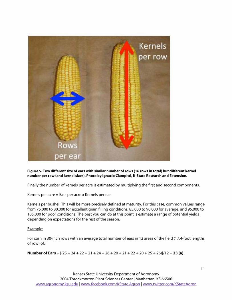
2) Final kernel number per ear: Count the number of rows within each ear and the number of kernels in each row (Figure 5). The final number of kernels per ear is calculated by multiplying the number of rows by the number of kernels within each row. This is just a quick estimation of the potential yield. The number of kernels within each row is not standard and can vary from row to row (more if a large proportion of kernels aborted, “abnormal ears”). Do not count aborted kernels or the kernels on the tip of the ear; count only kernels that are in complete rings around the ear. Do this for every 5th

or 6th

plant in each of your ear count areas (but as the more you can count, the more precise

will be the estimation). Avoid odd, non-representative ears.



Figure 5. Two different size of ears with similar number of rows (16 rows in total) but different kernel number per row (and kernel sizes). Photo by Ignacio Ciampitti, K-State Research and Extension.

Finally the number of kernels per acre is estimated by multiplying the first and second components.

Kernels per acre = Ears per acre x Kernels per ear

Kernels per bushel: This will be more precisely defined at maturity. For this case, common values range from 75,000 to 80,000 for excellent grain filling conditions, 85,000 to 90,000 for average, and 95,000 to 105,000 for poor conditions. The best you can do at this point is estimate a range of potential yields depending on expectations for the rest of the season.

Example:

For corn in 30-inch rows with an average total number of ears in 12 areas of the field (17.4-foot lengths of row) of:

Number of Ears = [(25 + 24 + 22 + 21 + 24 + 26 + 20 + 21 + 22 + 20 + 25 + 26)]/12 = 23 (a)



An average of 23 ears were counted within the 17.4-foot lengths. This can be scaling up to an acre basis by multiplying the number of ears by 1,000 (constant factor if the counts were taken in a 17.4-foot length).

Ears per acre = 23 x 1000 = 23,000 (b)

From those 23 ears, we will take between 2 and 5 ears to calculate the rows per ear and the kernels per row. The average number of rows was 14 with 27 kernels per row.

Kernel number per ear = 14 rows per ear x 27 kernels per row = 378 (c)

The final number of kernels per acre is the outcome of the multiplication of (b) ears per acre and (c) kernel number per ear.

Kernels per acre = 23,000 ears per acre x 378 kernels per ear = 8,694,000 (d)

Kernels per bushel

Under hot, dry conditions, grain filling duration and biomass translocation from the whole plant to the ear (kernels) can be severely affected. Otherwise, a reasonable value to use is about 105,000 kernels per bushel (e).

The final number of kernels per bushel is affected by diverse factors such as genotype, management practices (for example, plant density), and the environment. Plant density can strongly affect the kernel weight and the number of kernels per bushel. Lower plant densities (if growing conditions are optimum) will result in lower values for kernel number per bushel. Also, expect a lower kernel number per bushel as N is more deficient. More information regarding the influence of these management practices on the kernel weight and the number of kernels per bushel is available from an article titled “Corn Grain Yield Estimation: The Kernel Weight Factor” from Dr. Tony Vyn, Purdue University, at: http://extension.entm.purdue.edu/pestcrop/2010/issue22/index.html#corn

Final yield: Calculation of bushels per acre

The final calculation of the potential yield to be obtained at the end of the season is simply the outcome of dividing the component (d) by (e).

Bushels per acre = 8,694,000 kernels per acre ÷ 105,000 kernels per bushel = ~83

In this example, if projected conditions prove to be accurate, the corn should obviously be kept and harvested for grain. From previous experiences, the yield component method of estimating yields often seems to provide optimistic outcomes (slightly overestimation). If the conditions during the reproductive period are predicted to worsen (severe heat stress and lack of precipitation); then the kernel weight can be reduced, and the number estimated for component (e), kernels per bushel, should be higher. That will reduce the yield expectations in amore “pessimistic” scenario.

Links with further discussions on the potential yield estimation and an online tool that will assist you on all the previous calculations can be found at:



http://corn.osu.edu/newsletters/2010/2010-25/201cpredicting201d-corn-yields-prior-to-harvest The Ohio State University

http://www.ca.uky.edu/agc/pubs/agr/agr187/agr187.pdf University of Kentucky

http://www.agry.purdue.edu/ext/corn/news/timeless/yldestmethod.html Purdue University

http://corn.agronomy.wisc.edu/AA/pdfs/A033.pdf University of Wisconsin

http://www.conservfs.com/ProdServ/AgCalc/Calc1.html Online calculator tool

Ignacio Ciampitti, Cropping Systems and Crop Production Specialist [email protected]

Kraig Roozeboom, Cropping Systems Agronomist [email protected]



5. Check terraces now for needed repairs and maintenance

Mid-summer is a good time to evaluate and perform maintenance on terraces if fields are in wheat stubble. In Kansas, over 9 million acres of land is protected by more than 290,000 miles of terraces, making Kansas No. 2 in the U.S. for this soil and water conservation practice. To accomplish their purpose for erosion control and water savings, terraces must have adequate capacity, ridge height and channel width.

Without adequate capacity to carry water, terraces will be overtopped by runoff in a heavy storm. Overtopping causes erosion of the terrace ridge, terrace back slope, and lower terraces and may result in severe gullies. Terraces are typically designed to handle runoff from a 1-in-10-year storm. The rainfall amounts for such a storm are approximately 5 inches for eastern Kansas, 4 inches for central, and 3 inches for western Kansas during a 24-hour period.

Terraces need regular maintenance to function for a long life. Erosion by water, wind, and tillage wears the ridge down and deposits sediment in the channel, decreasing the effective ridge height, and channel capacity. The amount of capacity loss depends on the type and number of tillage operations, topography, soil properties, crop residue, and precipitation. Terrace maintenance restores capacity by removing sediment from the channel and rebuilding ridge height.

Typically, more frequent maintenance is required for steep slopes and/or highly erodible soils. Annual maintenance is necessary for intense tillage operations and heavy rainfall runoff. Less frequent maintenance is often adequate with high residue levels or where lower rainfall occurs and runoff intensity is low.

Check for needed repairs

Terraces degrade naturally by erosion and sediment, and can be damaged by machinery, animals, settling, and erosion. Check terraces and terrace outlets regularly (at least annually) for needed repairs. The best time to check is after rains, when erosion, sedimentation, and unevenness in elevation are easiest to spot. Specific items to note are overtopping, low or narrow terrace ridges, water ponding in the channel, terrace outlets, erosion, and sediment clogging near waterway or pipe outlets.

Reshaping the terrace

Terrace maintenance can been done with virtually any equipment that efficiently moves soil. Common tools include those that turn soil laterally, such as a moldboard plow, disk plow, one-way, terracing blade (pull-type grader), or 3-point ridging disk (terracing disk, etc.); those that convey or throw soil (belt terracer, scraper, whirlwind terracer, etc.); and those that push or drag soil (dozer blade, straight-wheeled blade, 3-point blade, etc.).

This article discusses procedures for the common plow. For other equipment, get advice from manufacturers, other users (contractor), or experiment to find what works best.

The primary objective in reshaping the terrace is to move soil from the channel to the ridge. Work done on the terrace back slope or cut slope above the channel may help maintain or improve shape,



but does little to add significant ridge height or channel capacity. Because of improved efficiency, a two-way (rollover) plow is ideal for terrace maintenance. It can usually achieve the desired shape with fewer passes than the conventional plow. Turn the soil in one direction to counteract erosion or turn it in either direction to clear the channel or raise and widen the terrace ridge.

The number of passes required for maintenance depends on the size of the tool, the depth of operation, travel speed (which controls distance of throw), and the amount of soil moved. The plow throws soil further at higher speeds, so a minimum ground speed of 5 mph in loose soil is suggested, but 6 mph or more is better.

Maintenance controls terrace shape. Assess what needs to be done before beginning maintenance. Compare the existing cross-section shape with the desired shape and size, and determine where soil should be removed and where it should be placed for the desired result. Back furrows are placed where more soil is needed, while dead furrows are located where soil needs to be removed. In this way, passes or sets of passes with the equipment are located to achieve the desired results.

Terrace dimensions can be changed by carefully planned placement of back furrows and dead furrows. Large changes in dimension and shape require several sets of passes with the tools or earth-moving equipment. Plan the terrace cross-section shape and size and terrace slope segment length to fit current and future tillage, planting, and harvesting equipment size.

The number of rounds or passes with maintenance equipment depends on the beginning shape of the terrace, size of equipment, and the desired size and shape. If in doubt, make more passes rather than stop too soon. Remember, the loose soil will settle a lot.

Plowing the ridge. The terrace ridge is raised and widened by plowing up from both sides as shown in Figure 1. When a 2-way plow is used, plow just the front slope from the channel to the ridge. Plowing the backslope makes it steeper.

Figure 1. Double back furrow. Arrow indicates the two back furrows meeting on the top of the ridge.

The back furrows are placed on top of the ridge, and the dead furrows are placed at the desired center of the channel and at the toe or beyond on the backslope. Avoid making a depression on the back-slope by varying where the dead furrow is placed. Plowing the ridge is recommended for maintaining



or adding ridge height. To make the ridge wider and not so sharply peaked, the back furrows should come together, but not overlap and make additional rounds. Correct a narrow peaked ridge resulting from too few passes by moving the plow over only one or two bottom widths with each pass. This process requires many more rounds.

To make the terraces slopes long enough to fit equipment, always leave dead furrow the desired distance from the ridge. For the three-segment shape, locate the back and dead furrows in the same place each year, keeping the cross-section uniform in size and shape. Vary the back furrow and dead furrow locations each time to maintain the rounded shape of the channel and ridge for the large smooth section.

Plowing the channel. Sometimes even when the ridge is large enough, the channel can have inad-equate capacity. To enlarge and widen the terrace channel, plow out to both sides as shown in Figure 2.

Figure 2. Enlarging and widening the terrace channel. Arrow indicates the two dead furrows meeting at the center of the channel.

Back furrows are placed on the ridge and on the uphill cut-slope side the same distance from the desired center of the channel. Begin at a distance equal to that from ridge to desired channel center. A double side-by-side dead furrow should result at the desired channel center. Locate the plow back furrow on the ridge and the dead furrows in the desired channel bottom to achieve and maintain the desired shape. Vary the back furrow location to avoid leaving a large ridge on the cut slope.

Plowing out the channel periodically is recommended for steeper slopes to help maintain adequate channel capacity. Alternating between plowing the channel out and plowing the up from one time to the next is a good practice.

Consider making changes to increase terrace life

When silt bars and sediment deposits accumulate frequently in a terrace channel, excessive erosion is the cause. A change in tillage and cropping practices is needed to correct this cause. Conservation tillage and crop rotations that retain crop residue will reduce erosion substantially. This will reduce the frequency of terrace maintenance needs. Many no-till producers find terrace systems require little maintenance. Although runoff still occurs, there is very little soil movement in a no-till system. Terraces prevent gullies and are only a part of an overall erosion control plan. Conservation farming



methods, especially residue, compliments erosion control structures and has been shown to be both economically and environmentally sound.

For more information, refer to publication Terrace Maintenance, C-709 available online at: http://www.ksre.ksu.edu/bookstore/pubs/C709.pdf Additional sources for technical information include local USDA-Natural Resources Conservation Service and County Conservation District offices.

DeAnn Presley, Soil and Water Conservation and Management Specialist [email protected]



6. New K-State video on terrace maintenance

A new video from K-State Research and Extension’s Agriculture Today, titled Basics of Terrace Maintenance, is available now on the web at: http://youtu.be/CcoITeP9QRA

This video is 3 minutes and 42 seconds long, and features Todd Whitney, formerly River Valley District agronomist. In the video, Whitney discusses the need for terraces, even on no-till ground.

DeAnn Presley, Soil and Water Conservation and Management Specialist [email protected]



7. Canola meeting in Harper County, August 15

A Winter Canola Production School will be held August 15, from 10 a.m. to 2 p.m. at the K of C Hall in Danville, Kansas. This will be a good opportunity for producers to learn from university agronomists and industry experts about this new crop, and how it can fit into cropping systems in south central Kansas.

Winter canola faced the same challenges as wheat last season, and came through extremely well in most cases.

Winter canola did a good job of weathering the elements this year, from drought to late freezes to hail. At the meeting in Danville, we’ll discuss variety performance and selection, and establishment strategies for the fall.

Specific topics of discussion include:

• Canola varieties • Winter canola establishment strategies • Pest management in fall and winter • Update on winter canola crop insurance • Update on marketing strategies

The school is free, with a lunch provided. Please preregister for the school by Tuesday, August 13 by contacting Jenni Carr, agriculture agent with the Harper County Extension Office, at [email protected] or 620-842-5445.

Sponsors of the school include the Bank of Kansas, Danville Coop Association, Dupont Pioneer Hi-Bred, the Great Plains Canola Association, Anthony Farmers Cooperative, and Horsch/Harper Industries.

Mike Stamm, Canola Breeder [email protected]



8. Comparative Vegetation Condition Report: July 16 – 29

K-State’s Ecology and Agriculture Spatial Analysis Laboratory (EASAL) produces weekly Vegetation Condition Report maps. These maps can be a valuable tool for making crop selection and marketing decisions.

Two short videos of Dr. Kevin Price explaining the development of these maps can be viewed on YouTube at: http://www.youtube.com/watch?v=CRP3Y5NIggw http://www.youtube.com/watch?v=tUdOK94efxc

The objective of these reports is to provide users with a means of assessing the relative condition of crops and grassland. The maps can be used to assess current plant growth rates, as well as comparisons to the previous year and relative to the 24-year average. The report is used by individual farmers and ranchers, the commodities market, and political leaders for assessing factors such as production potential and drought impact across their state.

NOTE TO READERS: The maps below represent a subset of the maps available from the EASAL group. If you’d like digital copies of the entire map series please contact Kevin Price at [email protected] and we can place you on our email list to receive the entire dataset each week as they are produced. The maps are normally first available on Wednesday of each week, unless there is a delay in the posting of the data by EROS Data Center where we obtain the raw data used to make the maps. These maps are provided for free as a service of the Department of Agronomy and K-State Research and Extension.

The maps in this issue of the newsletter show the current state of photosynthetic activity in Kansas, the Corn Belt, and the continental U.S., with comments from Mary Knapp, state climatologist:



Figure 1. The Vegetation Condition Report for Kansas for July 16 – 29 from K-State’s Ecology and Agriculture Spatial Analysis Laboratory shows that NDVI values are highest in the northeastern counties, and along the Republican River Valley in north central Kansas. Favorable temperature and moisture has allowed greater biomass production. There is alsoincreased photosynthetic activity in parts of southwest Kansas.



Figure 2. Compared to the previous year at this time for Kansas, the current Vegetation Condition Report for July 16 – 29 from K-State’s Ecology and Agriculture Spatial Analysis Laboratory shows that greatest differences are in the Central division and along the Flint Hills. Compared to the poor productivity that dominated last year’s conditions, the NDVI values this year are higher for much of the state. In the western regions, this signals only a marginal improvement in conditions.



Figure 3. Compared to the 24-year average at this time for Kansas, this year’s Vegetation Condition Report for July 16 – 29 from K-State’s Ecology and Agriculture Spatial Analysis Laboratory shows that, despite cooler temperatures, much of the state continues to have below-average plant productivity. Rains at the end of July may translate to higher productivity in the next several weeks, but are too recent to have had an impact yet on this two-week composite map. Also, excess moisture may continue to limit productivity in the southeast. Parts of Crawford and Cherokee counties ended the month with more than 14 inches of rainfall, most of which fell in the last week.



Figure 4. The Vegetation Condition Report for the Corn Belt for July 16 – 29 from K-State’s Ecology and Agriculture Spatial Analysis Laboratory shows that high photosynthetic activity dominates much of the region. In Illinois, many of the crops are averaging more than 60 percent in good to excellent condition. Corn is reported at 64% good to excellent, while 75 % of the alfalfa is in good to excellent condition.



Figure 5. The comparison to last year in the Corn Belt for the period July 16 – 29 from K-State’s Ecology and Agriculture Spatial Analysis Laboratory shows that the production is much higher for a good portion of the region. From Indiana through eastern Kansas, biomass production is higher. While extreme drought conditions remain in the western areas of the Corn Belt, biomass productivity is higher than last year. Temperatures this year have been much closer to normal, allowing for more benefit from the available water.



Figure 6. Compared to the 24-year average at this time for the Corn Belt, this year’s Vegetation Condition Report for July 16 – 29 from K-State’s Ecology and Agriculture Spatial Analysis Laboratory shows only a small portion of the region has above-average NDVI values. The biggest region of above-average productivity is in eastern South Dakota, which has avoided some of the excess moisture issues that have hampered production in North Dakota and parts of Minnesota and Iowa.



Figure 7. The Vegetation Condition Report for the U.S. for July 16 – 29 from K-State’s Ecology and Agriculture Spatial Analysis Laboratory shows that the east/west divide in biomass production continues. Highest NDVI values are in parts of the Appalachians and also in the Cascades. Lowest NDVI values are in the region from Montana down through West Texas. The biggest areas of exceptional drought continue be concentrated from western Nebraska, through the High Plains into Western Texas and New Mexico.



Figure 8. The U.S. comparison to last year at this time for the period July 16 – 29 from K-State’s Ecology and Agriculture Spatial Analysis Laboratory shows that the biggest improvement in biomass productivity is in the center of the country. Conditions were poor in this area last year.



Figure 9. The U.S. comparison to the 24-year average for the period July 16 – 29 from K-State’s Ecology and Agriculture Spatial Analysis Laboratory shows that the lingering effects of drought continue. Below-average productivity is most notable in the Southern and Central Plains. New England, particularly in New Hampshire, Vermont, and Maine, also show reduced productivity. National Agricultural Statistics reports indicate that this region has continued to have much-cooler-than-average temperatures and continued rainfall. Temperatures in these areas dipped to the lower 30s.

Mary Knapp, State Climatologist [email protected]

Kevin Price, Agronomy and Geography, Remote Sensing, Natural Resources, GIS [email protected]

Nan An, Graduate Research Assistant, Ecology & Agriculture Spatial Analysis Laboratory (EASAL) [email protected]

eupdate - agronomy | kansas state university · 1. gramoxone (paraquat) drift on corn the dry...

Documents