eurostat regional year book
TRANSCRIPT

KS-HA
-10-001-EN-C
Eurostat regional yearbook 2010
ISSN 1830-9674
Eurostat regional yearbook 2010Eurostat regional yearbook 2010 gives a detailed picture of a large number of statistical fields in the 27 Member States of the European Union, as well as in candidate and EFTA countries. If you would like to take a closer look at social and economic trends in Europe’s regions, this publication is for you! The texts are written by specialists in statistics and are accompanied by maps, figures and tables on each subject. There is a broad set of regional indicators for the following 15 subjects: population, European cities, labour market, gross domestic product, household accounts, structural business statistics, information society, science, technology and innovation, education, transport, tourism, health, agriculture, coastal regions and, last but not least, a study on a new urban-rural typology. This publication is available in German, English and French.
http://ec.europa.eu/eurostat
Eurostat regional yearbook 2010
S t a t i s t i c a l b o o k s
Price (excluding VAT) in Luxembourg: EUR 20

How to obtain EU publicationsFree publications:
• viaEUBookshop(http://bookshop.europa.eu);
• attheEuropeanUnion’srepresentationsordelegations.YoucanobtaintheircontactdetailsontheInternet(http://ec.europa.eu)orbysendingafax to +352 2929-42758.
Priced publications:
• viaEUBookshop(http://bookshop.europa.eu).
Priced subscriptions (e.g. annual series of the Official Journal of the European Union and reports of cases before the Court of Justice of the European Union):
• viaoneofthesalesagentsofthePublicationsOfficeoftheEuropeanUnion (http://publications.europa.eu/others/agents/index_en.htm).
Eurostat regional yearbook 2010
S t a t i s t i c a l b o o k s
Europe Direct is a service to help you find answers to your questions about the European Union
Freephone number (*):
00 800 6 7 8 9 10 11(*) Certain mobile telephone operators do not allow access
to 00 800 numbers or these calls may be billed.
More information on the European Union is available on the Internet (http://europa.eu).
Cataloguing data can be found at the end of this publication.
Luxembourg: Publications Office of the European Union, 2010
ISBN 978-92-79-14565-0ISSN 1830-9674doi:10.2785/40203Cat. No: KS-HA-10-001-EN-C
Theme: General and regional statisticsCollection: Statistical books
© European Union, 2010© Copyright for the photos: cover: © Ferenc Kálmándy and ‘European cities’: © József Kéméndy; the two photos are from Pécs in Hungary, European Capital of Culture 2010 (see: http://pecs2u.eu); the chapters ‘Introduction’, ‘Population’, ‘Household accounts’, ‘Information society’, ‘Education’, ‘Tourism’ and ‘A revised urban-rural typology’: © Phovoir.com; the chapters ‘Labour market’, ‘Gross domestic product’, ‘Structural business statistics’, ‘Science, technology and innova-tion’, ‘Transport’, ‘Health’ and ‘Agriculture’: © Digital Photo Library of the Directorate-General for Regional Policy of the European Commission; the chapter ‘Coastal regions’: © Teodóra Brandmüller.
For reproduction or use of these photos, permission must be sought directly from the copyright holder.
Printed in Belgium
PRINTED ON ELEMENTAL CHLORINE-FREE BLEACHED PAPER (ECF)

3Eurostat regional yearbook 2010eurostat
Preface
Dear readers,
The Eurostat regional yearbook is a rich source of information about Europeans’ everyday life. What happens in the regions has an immediate impact on the conditions citizens face. The effects of European and national policies are felt directly at regional level.
For many years tangible progress has been made in economic and social conditions in the vast majority of European regions, with an increasing trend towards stronger cohesion. The European Union is continuing to apply its regional and urban policies to consolidate these achievements, a task which is even more difficult in current times.
The 15 chapters of this regional yearbook investigate interesting regional similarities and differences in the 27 Member States and in the candidate and EFTA countries. We are pleased to include two entirely new topics in this issue: coastal regions and a revised urban-rural typology. The chapters on transport and on health appeared in earlier issues, but have been reintroduced this year.
Beyond being a source of information, the regional yearbook also aims to tempt readers to dig deeper into the Eurostat website, which contains far more regional data. For many indicators, the electronic tables and the databases available from Eurostat go into a degree of detail beyond the scope of this regional yearbook.
Eurostat is constantly updating the range of regional indicators available and cooperates closely with the Member States of the European Union, the candidate countries and EFTA countries to improve their quality.
I wish you an enjoyable reading experience!
Walter RadermacherDirector-General, Eurostat

4 Eurostat regional yearbook 2010 eurostat
AbstractEurostat regional yearbook 2010 gives a detailed picture of a large number of statistical fields in the 27 Member States of the European Union, as well as in candidate and EFTA countries. If you would like to take a closer look at social and economic trends in Europe’s regions, this publication is for you! The texts are written by specialists in statistics and are accompanied by maps, figures and tables on each subject. There is a broad set of regional indicators for the following 15 subjects: population, European cities, labour market, gross domestic product, household accounts, structural business statistics, information society, science, technology and innovation, education, transport, tourism, health, agriculture, coastal regions, and last but not least, a study on a new urban-rural typology. This publication is available in German, English and French.
Editor-in-chiefBerthold Feldmann
Eurostat, Head of section, Unit E.4, Regional statistics and geographical information
EditorÅsa Önnerfors
Eurostat, Unit E.4, Regional statistics and geographical information
Map productionBaudouin Quennery
Eurostat, Unit E.4, Regional statistics and geographical information
DisseminationPetra Rusinova
Eurostat, Unit D.4, Dissemination
Contact detailsEurostat
Statistical Office of the European Union
Bâtiment Joseph Bech
5, rue Alphonse Weicker
2721 LUxEMBOURG
E-mail: [email protected]
For more information please consultInternet: http://ec.europa.eu/eurostat
Data extractedMarch 2010

5Eurostat regional yearbook 2010eurostat
Acknowledgements
The editor-in-chief and the editor of the Eurostat regional yearbook 2010 would like to thank all of the colleagues who contributed. We would particularly like to thank those who were involved in each specific chapter:
• Population: Veronica Corsini, Konstantinos Giannakouris and Monica Marcu (Eurostat, Unit F.1, Population)• European cities: Teodóra Brandmüller (Eurostat, Unit E.4, Regional statistics and geographical in-formation)• Labour market: Pedro Ferreira (Eurostat, Unit E.4, Regional statistics and geographical informa-tion) for the first part on the Labour Force Survey (LFS) and Simone Casali (Eurostat, Unit F.2, Labour market) for the second part on the Structure of Earnings Survey (SES)• Gross domestic product: Andreas Krüger (Eurostat, Unit C.2, National accounts — Production)• Household accounts: Andreas Krüger (Eurostat, Unit C.2, National accounts — Production)• Structural business statistics: Aleksandra Stawińska (Eurostat, Unit G.2, Structural business sta-tistics)• Information society: Anna Lööf and Albrecht Wirthmann (Eurostat, Unit F.6, Information society; Tourism)• Science, technology and innovation: Daniela Silvia Crintea, Bernard Félix, Dominique Groenez, Reni Petkova and Håkan Wilén (Eurostat, Unit F.4, Education, science and culture)• Education: Sorin-Florin Gheorghiu, Dominique Groenez, Emmanuel Kailis and Paolo Turchetti (Eurostat, Unit F.4, Education, science and culture)• Transport: Anna Bialas-Motyl (Eurostat, Unit E.6, Transport)• Tourism: Christophe Demunter, Giuseppe Di Giacomo and Pavel Vancura (Eurostat, Unit F.6, In-formation society; Tourism)• Health: Marta Carvalhido, Elodie Cayotte and Jean-Marc Schaefer (Eurostat, Unit F.5, Health and food safety; Crime)• Agriculture: Ole Olsen (Eurostat, Unit E.2, Agriculture and fisheries)• Coastal regions: Isabelle Collet and Catherine Coyette (Eurostat, Unit E.1, Farms, agro-environ-ment and rural development)• A revised urban-rural typology: Lewis Dijkstra and Hugo Poelman (Directorate-General for Re-gional Policy, Unit C.3, Economic and quantitative analysis; Additionality)
Thanks also to:
the Directorate-General for Translation of the European Commission, particularly the German, English and French translation units, and the Editing Unit;
the Publications Office of the European Union, and in particular Bernard Jenkins in Unit B.1, Cross-media publishing, and the proofreaders in Unit B.2, Editorial services.
6 Eurostat regional yearbook 2010 eurostat
Contents
INTRODUCTION . . . . . . . . . . . . . . . . . . . . . . . . . . . . . . . . . . . . . . . . . . . . . . . . . . . . . . . . . . . . . . . . . . . . . . . . . . . . . . . . . . . . . . . . . . . . . . . . . . . . . . . . . . . . . . . . . . . . . . . . . . . 11
Statistics on regions and cities . . . . . . . . . . . . . . . . . . . . . . . . . . . . . . . . . . . . . . . . . . . . . . . . . . . . . . . . . . . . . . . . . . . . . . . . . . . . . . . . . . . . . . . . . . . . . . . . . . . . . . . . . . . . 12Historically speaking . . . . . . . . . . . . . . . . . . . . . . . . . . . . . . . . . . . . . . . . . . . . . . . . . . . . . . . . . . . . . . . . . . . . . . . . . . . . . . . . . . . . . . . . . . . . . . . . . . . . . . . . . . . . . . . . . . . . . . . . 12Core content and news in the 2010 edition . . . . . . . . . . . . . . . . . . . . . . . . . . . . . . . . . . . . . . . . . . . . . . . . . . . . . . . . . . . . . . . . . . . . . . . . . . . . . . . . . . . . . . . . . . . . . 12The NUTS classification . . . . . . . . . . . . . . . . . . . . . . . . . . . . . . . . . . . . . . . . . . . . . . . . . . . . . . . . . . . . . . . . . . . . . . . . . . . . . . . . . . . . . . . . . . . . . . . . . . . . . . . . . . . . . . . . . . . . . 13Coverage . . . . . . . . . . . . . . . . . . . . . . . . . . . . . . . . . . . . . . . . . . . . . . . . . . . . . . . . . . . . . . . . . . . . . . . . . . . . . . . . . . . . . . . . . . . . . . . . . . . . . . . . . . . . . . . . . . . . . . . . . . . . . . . . . . . . . . 14More regional information . . . . . . . . . . . . . . . . . . . . . . . . . . . . . . . . . . . . . . . . . . . . . . . . . . . . . . . . . . . . . . . . . . . . . . . . . . . . . . . . . . . . . . . . . . . . . . . . . . . . . . . . . . . . . . . . . 14
1 POPULATION . . . . . . . . . . . . . . . . . . . . . . . . . . . . . . . . . . . . . . . . . . . . . . . . . . . . . . . . . . . . . . . . . . . . . . . . . . . . . . . . . . . . . . . . . . . . . . . . . . . . . . . . . . . . . . . . . . . . . . . . . . . . 17
Unveiling the regional pattern of demography . . . . . . . . . . . . . . . . . . . . . . . . . . . . . . . . . . . . . . . . . . . . . . . . . . . . . . . . . . . . . . . . . . . . . . . . . . . . . . . . . . . . . . . . 18Population density . . . . . . . . . . . . . . . . . . . . . . . . . . . . . . . . . . . . . . . . . . . . . . . . . . . . . . . . . . . . . . . . . . . . . . . . . . . . . . . . . . . . . . . . . . . . . . . . . . . . . . . . . . . . . . . . . . . . . . . . . . . 18Population change . . . . . . . . . . . . . . . . . . . . . . . . . . . . . . . . . . . . . . . . . . . . . . . . . . . . . . . . . . . . . . . . . . . . . . . . . . . . . . . . . . . . . . . . . . . . . . . . . . . . . . . . . . . . . . . . . . . . . . . . . . 18Regional population projections . . . . . . . . . . . . . . . . . . . . . . . . . . . . . . . . . . . . . . . . . . . . . . . . . . . . . . . . . . . . . . . . . . . . . . . . . . . . . . . . . . . . . . . . . . . . . . . . . . . . . . . . . . 27Conclusion . . . . . . . . . . . . . . . . . . . . . . . . . . . . . . . . . . . . . . . . . . . . . . . . . . . . . . . . . . . . . . . . . . . . . . . . . . . . . . . . . . . . . . . . . . . . . . . . . . . . . . . . . . . . . . . . . . . . . . . . . . . . . . . . . . . . 32Methodological notes . . . . . . . . . . . . . . . . . . . . . . . . . . . . . . . . . . . . . . . . . . . . . . . . . . . . . . . . . . . . . . . . . . . . . . . . . . . . . . . . . . . . . . . . . . . . . . . . . . . . . . . . . . . . . . . . . . . . . . . 33
2 EUROPEAN CITIES . . . . . . . . . . . . . . . . . . . . . . . . . . . . . . . . . . . . . . . . . . . . . . . . . . . . . . . . . . . . . . . . . . . . . . . . . . . . . . . . . . . . . . . . . . . . . . . . . . . . . . . . . . . . . . . . . . . . . 35
Introduction . . . . . . . . . . . . . . . . . . . . . . . . . . . . . . . . . . . . . . . . . . . . . . . . . . . . . . . . . . . . . . . . . . . . . . . . . . . . . . . . . . . . . . . . . . . . . . . . . . . . . . . . . . . . . . . . . . . . . . . . . . . . . . . . . . 36
The topics . . . . . . . . . . . . . . . . . . . . . . . . . . . . . . . . . . . . . . . . . . . . . . . . . . . . . . . . . . . . . . . . . . . . . . . . . . . . . . . . . . . . . . . . . . . . . . . . . . . . . . . . . . . . . . . . . . . . . . . . . . . . . . . . . . 36
The time frame . . . . . . . . . . . . . . . . . . . . . . . . . . . . . . . . . . . . . . . . . . . . . . . . . . . . . . . . . . . . . . . . . . . . . . . . . . . . . . . . . . . . . . . . . . . . . . . . . . . . . . . . . . . . . . . . . . . . . . . . . . . . 36
The spatial dimension . . . . . . . . . . . . . . . . . . . . . . . . . . . . . . . . . . . . . . . . . . . . . . . . . . . . . . . . . . . . . . . . . . . . . . . . . . . . . . . . . . . . . . . . . . . . . . . . . . . . . . . . . . . . . . . . . . . . 36Urbanisation . . . . . . . . . . . . . . . . . . . . . . . . . . . . . . . . . . . . . . . . . . . . . . . . . . . . . . . . . . . . . . . . . . . . . . . . . . . . . . . . . . . . . . . . . . . . . . . . . . . . . . . . . . . . . . . . . . . . . . . . . . . . . . . . . . 36Present and future generations — the demographic challenge . . . . . . . . . . . . . . . . . . . . . . . . . . . . . . . . . . . . . . . . . . . . . . . . . . . . . . . . . . . . . . . . . . . . 37Conclusion . . . . . . . . . . . . . . . . . . . . . . . . . . . . . . . . . . . . . . . . . . . . . . . . . . . . . . . . . . . . . . . . . . . . . . . . . . . . . . . . . . . . . . . . . . . . . . . . . . . . . . . . . . . . . . . . . . . . . . . . . . . . . . . . . . . . 43
3 LABOUR MARKET . . . . . . . . . . . . . . . . . . . . . . . . . . . . . . . . . . . . . . . . . . . . . . . . . . . . . . . . . . . . . . . . . . . . . . . . . . . . . . . . . . . . . . . . . . . . . . . . . . . . . . . . . . . . . . . . . . . . . . 49
Introduction . . . . . . . . . . . . . . . . . . . . . . . . . . . . . . . . . . . . . . . . . . . . . . . . . . . . . . . . . . . . . . . . . . . . . . . . . . . . . . . . . . . . . . . . . . . . . . . . . . . . . . . . . . . . . . . . . . . . . . . . . . . . . . . . . . 50Regional sector specialisation . . . . . . . . . . . . . . . . . . . . . . . . . . . . . . . . . . . . . . . . . . . . . . . . . . . . . . . . . . . . . . . . . . . . . . . . . . . . . . . . . . . . . . . . . . . . . . . . . . . . . . . . . . . . . 50Brief overview of 2008 . . . . . . . . . . . . . . . . . . . . . . . . . . . . . . . . . . . . . . . . . . . . . . . . . . . . . . . . . . . . . . . . . . . . . . . . . . . . . . . . . . . . . . . . . . . . . . . . . . . . . . . . . . . . . . . . . . . . . . 50Regional sector specialisation . . . . . . . . . . . . . . . . . . . . . . . . . . . . . . . . . . . . . . . . . . . . . . . . . . . . . . . . . . . . . . . . . . . . . . . . . . . . . . . . . . . . . . . . . . . . . . . . . . . . . . . . . . . . . 57High education levels in the regional labour market . . . . . . . . . . . . . . . . . . . . . . . . . . . . . . . . . . . . . . . . . . . . . . . . . . . . . . . . . . . . . . . . . . . . . . . . . . . . . . . . . 58Conclusion . . . . . . . . . . . . . . . . . . . . . . . . . . . . . . . . . . . . . . . . . . . . . . . . . . . . . . . . . . . . . . . . . . . . . . . . . . . . . . . . . . . . . . . . . . . . . . . . . . . . . . . . . . . . . . . . . . . . . . . . . . . . . . . . . . . . 60Structure of Earnings Survey. . . . . . . . . . . . . . . . . . . . . . . . . . . . . . . . . . . . . . . . . . . . . . . . . . . . . . . . . . . . . . . . . . . . . . . . . . . . . . . . . . . . . . . . . . . . . . . . . . . . . . . . . . . . . . . 63Gross hourly earnings . . . . . . . . . . . . . . . . . . . . . . . . . . . . . . . . . . . . . . . . . . . . . . . . . . . . . . . . . . . . . . . . . . . . . . . . . . . . . . . . . . . . . . . . . . . . . . . . . . . . . . . . . . . . . . . . . . . . . . . 63Gross annual earnings . . . . . . . . . . . . . . . . . . . . . . . . . . . . . . . . . . . . . . . . . . . . . . . . . . . . . . . . . . . . . . . . . . . . . . . . . . . . . . . . . . . . . . . . . . . . . . . . . . . . . . . . . . . . . . . . . . . . . . 65Annual bonuses as a percentage of annual earnings . . . . . . . . . . . . . . . . . . . . . . . . . . . . . . . . . . . . . . . . . . . . . . . . . . . . . . . . . . . . . . . . . . . . . . . . . . . . . . . . 65Conclusion . . . . . . . . . . . . . . . . . . . . . . . . . . . . . . . . . . . . . . . . . . . . . . . . . . . . . . . . . . . . . . . . . . . . . . . . . . . . . . . . . . . . . . . . . . . . . . . . . . . . . . . . . . . . . . . . . . . . . . . . . . . . . . . . . . . . 68Methodological notes . . . . . . . . . . . . . . . . . . . . . . . . . . . . . . . . . . . . . . . . . . . . . . . . . . . . . . . . . . . . . . . . . . . . . . . . . . . . . . . . . . . . . . . . . . . . . . . . . . . . . . . . . . . . . . . . . . . . . . . 69
Labour Force Survey . . . . . . . . . . . . . . . . . . . . . . . . . . . . . . . . . . . . . . . . . . . . . . . . . . . . . . . . . . . . . . . . . . . . . . . . . . . . . . . . . . . . . . . . . . . . . . . . . . . . . . . . . . . . . . . . . . . . . . 69
Structure of Earnings Survey . . . . . . . . . . . . . . . . . . . . . . . . . . . . . . . . . . . . . . . . . . . . . . . . . . . . . . . . . . . . . . . . . . . . . . . . . . . . . . . . . . . . . . . . . . . . . . . . . . . . . . . . . . . . 69Definitions . . . . . . . . . . . . . . . . . . . . . . . . . . . . . . . . . . . . . . . . . . . . . . . . . . . . . . . . . . . . . . . . . . . . . . . . . . . . . . . . . . . . . . . . . . . . . . . . . . . . . . . . . . . . . . . . . . . . . . . . . . . . . . . . . . . . . 70
Labour Force Survey . . . . . . . . . . . . . . . . . . . . . . . . . . . . . . . . . . . . . . . . . . . . . . . . . . . . . . . . . . . . . . . . . . . . . . . . . . . . . . . . . . . . . . . . . . . . . . . . . . . . . . . . . . . . . . . . . . . . . . 70
Structure of Earnings Survey . . . . . . . . . . . . . . . . . . . . . . . . . . . . . . . . . . . . . . . . . . . . . . . . . . . . . . . . . . . . . . . . . . . . . . . . . . . . . . . . . . . . . . . . . . . . . . . . . . . . . . . . . . . . 71
7Eurostat regional yearbook 2010eurostat
4 GROSS DOMESTIC PRODUCT . . . . . . . . . . . . . . . . . . . . . . . . . . . . . . . . . . . . . . . . . . . . . . . . . . . . . . . . . . . . . . . . . . . . . . . . . . . . . . . . . . . . . . . . . . . . . . . . . . . . . . 73
What is regional gross domestic product? . . . . . . . . . . . . . . . . . . . . . . . . . . . . . . . . . . . . . . . . . . . . . . . . . . . . . . . . . . . . . . . . . . . . . . . . . . . . . . . . . . . . . . . . . . . . . . 74Regional GDP in 2007 . . . . . . . . . . . . . . . . . . . . . . . . . . . . . . . . . . . . . . . . . . . . . . . . . . . . . . . . . . . . . . . . . . . . . . . . . . . . . . . . . . . . . . . . . . . . . . . . . . . . . . . . . . . . . . . . . . . . . . . 74Major regional differences even within the countries themselves . . . . . . . . . . . . . . . . . . . . . . . . . . . . . . . . . . . . . . . . . . . . . . . . . . . . . . . . . . . . . . . . . 77Dynamic catch-up process on the periphery . . . . . . . . . . . . . . . . . . . . . . . . . . . . . . . . . . . . . . . . . . . . . . . . . . . . . . . . . . . . . . . . . . . . . . . . . . . . . . . . . . . . . . . . . . . 77Different trends even within the countries themselves . . . . . . . . . . . . . . . . . . . . . . . . . . . . . . . . . . . . . . . . . . . . . . . . . . . . . . . . . . . . . . . . . . . . . . . . . . . . . . 80Convergence makes progress . . . . . . . . . . . . . . . . . . . . . . . . . . . . . . . . . . . . . . . . . . . . . . . . . . . . . . . . . . . . . . . . . . . . . . . . . . . . . . . . . . . . . . . . . . . . . . . . . . . . . . . . . . . . . 81Conclusion . . . . . . . . . . . . . . . . . . . . . . . . . . . . . . . . . . . . . . . . . . . . . . . . . . . . . . . . . . . . . . . . . . . . . . . . . . . . . . . . . . . . . . . . . . . . . . . . . . . . . . . . . . . . . . . . . . . . . . . . . . . . . . . . . . . . 84Methodological notes . . . . . . . . . . . . . . . . . . . . . . . . . . . . . . . . . . . . . . . . . . . . . . . . . . . . . . . . . . . . . . . . . . . . . . . . . . . . . . . . . . . . . . . . . . . . . . . . . . . . . . . . . . . . . . . . . . . . . . . 86
Purchasing power parities and international volume comparisons . . . . . . . . . . . . . . . . . . . . . . . . . . . . . . . . . . . . . . . . . . . . . . . . . . . . . . . . . . . . . 86
Dispersion of per inhabitant GDP . . . . . . . . . . . . . . . . . . . . . . . . . . . . . . . . . . . . . . . . . . . . . . . . . . . . . . . . . . . . . . . . . . . . . . . . . . . . . . . . . . . . . . . . . . . . . . . . . . . . . . 86
5 HOUSEHOLD ACCOUNTS . . . . . . . . . . . . . . . . . . . . . . . . . . . . . . . . . . . . . . . . . . . . . . . . . . . . . . . . . . . . . . . . . . . . . . . . . . . . . . . . . . . . . . . . . . . . . . . . . . . . . . . . . . . 89
Introduction: Measuring wealth . . . . . . . . . . . . . . . . . . . . . . . . . . . . . . . . . . . . . . . . . . . . . . . . . . . . . . . . . . . . . . . . . . . . . . . . . . . . . . . . . . . . . . . . . . . . . . . . . . . . . . . . . . 90Private household income . . . . . . . . . . . . . . . . . . . . . . . . . . . . . . . . . . . . . . . . . . . . . . . . . . . . . . . . . . . . . . . . . . . . . . . . . . . . . . . . . . . . . . . . . . . . . . . . . . . . . . . . . . . . . . . . . 90Results for 2007 . . . . . . . . . . . . . . . . . . . . . . . . . . . . . . . . . . . . . . . . . . . . . . . . . . . . . . . . . . . . . . . . . . . . . . . . . . . . . . . . . . . . . . . . . . . . . . . . . . . . . . . . . . . . . . . . . . . . . . . . . . . . . . 91
Primary income . . . . . . . . . . . . . . . . . . . . . . . . . . . . . . . . . . . . . . . . . . . . . . . . . . . . . . . . . . . . . . . . . . . . . . . . . . . . . . . . . . . . . . . . . . . . . . . . . . . . . . . . . . . . . . . . . . . . . . . . . . . 91
Disposable income . . . . . . . . . . . . . . . . . . . . . . . . . . . . . . . . . . . . . . . . . . . . . . . . . . . . . . . . . . . . . . . . . . . . . . . . . . . . . . . . . . . . . . . . . . . . . . . . . . . . . . . . . . . . . . . . . . . . . . . 91Dynamic developments at the edges of the Union . . . . . . . . . . . . . . . . . . . . . . . . . . . . . . . . . . . . . . . . . . . . . . . . . . . . . . . . . . . . . . . . . . . . . . . . . . . . . . . . . . . 95Conclusion . . . . . . . . . . . . . . . . . . . . . . . . . . . . . . . . . . . . . . . . . . . . . . . . . . . . . . . . . . . . . . . . . . . . . . . . . . . . . . . . . . . . . . . . . . . . . . . . . . . . . . . . . . . . . . . . . . . . . . . . . . . . . . . . . . . . 97Methodological notes . . . . . . . . . . . . . . . . . . . . . . . . . . . . . . . . . . . . . . . . . . . . . . . . . . . . . . . . . . . . . . . . . . . . . . . . . . . . . . . . . . . . . . . . . . . . . . . . . . . . . . . . . . . . . . . . . . . . . . . 99
6 STRUCTURAL BUSINESS STATISTICS . . . . . . . . . . . . . . . . . . . . . . . . . . . . . . . . . . . . . . . . . . . . . . . . . . . . . . . . . . . . . . . . . . . . . . . . . . . . . . . . . . . . . . . . . . . 101
Introduction . . . . . . . . . . . . . . . . . . . . . . . . . . . . . . . . . . . . . . . . . . . . . . . . . . . . . . . . . . . . . . . . . . . . . . . . . . . . . . . . . . . . . . . . . . . . . . . . . . . . . . . . . . . . . . . . . . . . . . . . . . . . . . . . . 102Regional specialisation and business concentration . . . . . . . . . . . . . . . . . . . . . . . . . . . . . . . . . . . . . . . . . . . . . . . . . . . . . . . . . . . . . . . . . . . . . . . . . . . . . . . . . 102Specialisation in business services. . . . . . . . . . . . . . . . . . . . . . . . . . . . . . . . . . . . . . . . . . . . . . . . . . . . . . . . . . . . . . . . . . . . . . . . . . . . . . . . . . . . . . . . . . . . . . . . . . . . . . . 108Employment growth in business services . . . . . . . . . . . . . . . . . . . . . . . . . . . . . . . . . . . . . . . . . . . . . . . . . . . . . . . . . . . . . . . . . . . . . . . . . . . . . . . . . . . . . . . . . . . . . . 110Characteristics of the top 30 most specialised regions in business services . . . . . . . . . . . . . . . . . . . . . . . . . . . . . . . . . . . . . . . . . . . . . . . . . . . . . 111Methodological notes . . . . . . . . . . . . . . . . . . . . . . . . . . . . . . . . . . . . . . . . . . . . . . . . . . . . . . . . . . . . . . . . . . . . . . . . . . . . . . . . . . . . . . . . . . . . . . . . . . . . . . . . . . . . . . . . . . . . . . 116
7 INFORMATION SOCIETy . . . . . . . . . . . . . . . . . . . . . . . . . . . . . . . . . . . . . . . . . . . . . . . . . . . . . . . . . . . . . . . . . . . . . . . . . . . . . . . . . . . . . . . . . . . . . . . . . . . . . . . . . . . . 119
Introduction . . . . . . . . . . . . . . . . . . . . . . . . . . . . . . . . . . . . . . . . . . . . . . . . . . . . . . . . . . . . . . . . . . . . . . . . . . . . . . . . . . . . . . . . . . . . . . . . . . . . . . . . . . . . . . . . . . . . . . . . . . . . . . . . . 120Access to information and communication technologies . . . . . . . . . . . . . . . . . . . . . . . . . . . . . . . . . . . . . . . . . . . . . . . . . . . . . . . . . . . . . . . . . . . . . . . . . . 120Regular use of the Internet . . . . . . . . . . . . . . . . . . . . . . . . . . . . . . . . . . . . . . . . . . . . . . . . . . . . . . . . . . . . . . . . . . . . . . . . . . . . . . . . . . . . . . . . . . . . . . . . . . . . . . . . . . . . . . . . 123Online shopping: e-commerce attracts customers . . . . . . . . . . . . . . . . . . . . . . . . . . . . . . . . . . . . . . . . . . . . . . . . . . . . . . . . . . . . . . . . . . . . . . . . . . . . . . . . . . . 123Non-users of the Internet . . . . . . . . . . . . . . . . . . . . . . . . . . . . . . . . . . . . . . . . . . . . . . . . . . . . . . . . . . . . . . . . . . . . . . . . . . . . . . . . . . . . . . . . . . . . . . . . . . . . . . . . . . . . . . . . . . 129Conclusion . . . . . . . . . . . . . . . . . . . . . . . . . . . . . . . . . . . . . . . . . . . . . . . . . . . . . . . . . . . . . . . . . . . . . . . . . . . . . . . . . . . . . . . . . . . . . . . . . . . . . . . . . . . . . . . . . . . . . . . . . . . . . . . . . . . 130Methodological notes . . . . . . . . . . . . . . . . . . . . . . . . . . . . . . . . . . . . . . . . . . . . . . . . . . . . . . . . . . . . . . . . . . . . . . . . . . . . . . . . . . . . . . . . . . . . . . . . . . . . . . . . . . . . . . . . . . . . . . 132
8 SCIENCE, TECHNOLOGy, AND INNOvATION . . . . . . . . . . . . . . . . . . . . . . . . . . . . . . . . . . . . . . . . . . . . . . . . . . . . . . . . . . . . . . . . . . . . . . . . . . . . . . . . . 135
Introduction . . . . . . . . . . . . . . . . . . . . . . . . . . . . . . . . . . . . . . . . . . . . . . . . . . . . . . . . . . . . . . . . . . . . . . . . . . . . . . . . . . . . . . . . . . . . . . . . . . . . . . . . . . . . . . . . . . . . . . . . . . . . . . . . . 136Research and development . . . . . . . . . . . . . . . . . . . . . . . . . . . . . . . . . . . . . . . . . . . . . . . . . . . . . . . . . . . . . . . . . . . . . . . . . . . . . . . . . . . . . . . . . . . . . . . . . . . . . . . . . . . . . . . 136Human resources in science and technology. . . . . . . . . . . . . . . . . . . . . . . . . . . . . . . . . . . . . . . . . . . . . . . . . . . . . . . . . . . . . . . . . . . . . . . . . . . . . . . . . . . . . . . . . . 138Patents . . . . . . . . . . . . . . . . . . . . . . . . . . . . . . . . . . . . . . . . . . . . . . . . . . . . . . . . . . . . . . . . . . . . . . . . . . . . . . . . . . . . . . . . . . . . . . . . . . . . . . . . . . . . . . . . . . . . . . . . . . . . . . . . . . . . . . . . 142Conclusion . . . . . . . . . . . . . . . . . . . . . . . . . . . . . . . . . . . . . . . . . . . . . . . . . . . . . . . . . . . . . . . . . . . . . . . . . . . . . . . . . . . . . . . . . . . . . . . . . . . . . . . . . . . . . . . . . . . . . . . . . . . . . . . . . . . 143Methodological notes . . . . . . . . . . . . . . . . . . . . . . . . . . . . . . . . . . . . . . . . . . . . . . . . . . . . . . . . . . . . . . . . . . . . . . . . . . . . . . . . . . . . . . . . . . . . . . . . . . . . . . . . . . . . . . . . . . . . . . 147
8 Eurostat regional yearbook 2010 eurostat
9 EDUCATION . . . . . . . . . . . . . . . . . . . . . . . . . . . . . . . . . . . . . . . . . . . . . . . . . . . . . . . . . . . . . . . . . . . . . . . . . . . . . . . . . . . . . . . . . . . . . . . . . . . . . . . . . . . . . . . . . . . . . . . . . . . . . 149
Introduction . . . . . . . . . . . . . . . . . . . . . . . . . . . . . . . . . . . . . . . . . . . . . . . . . . . . . . . . . . . . . . . . . . . . . . . . . . . . . . . . . . . . . . . . . . . . . . . . . . . . . . . . . . . . . . . . . . . . . . . . . . . . . . . . . 150Students in tertiary education . . . . . . . . . . . . . . . . . . . . . . . . . . . . . . . . . . . . . . . . . . . . . . . . . . . . . . . . . . . . . . . . . . . . . . . . . . . . . . . . . . . . . . . . . . . . . . . . . . . . . . . . . . . . 150Students aged 17 in education . . . . . . . . . . . . . . . . . . . . . . . . . . . . . . . . . . . . . . . . . . . . . . . . . . . . . . . . . . . . . . . . . . . . . . . . . . . . . . . . . . . . . . . . . . . . . . . . . . . . . . . . . . . 151Participation of 4-year-olds in education . . . . . . . . . . . . . . . . . . . . . . . . . . . . . . . . . . . . . . . . . . . . . . . . . . . . . . . . . . . . . . . . . . . . . . . . . . . . . . . . . . . . . . . . . . . . . . . 151Pupils in primary or lower-secondary education . . . . . . . . . . . . . . . . . . . . . . . . . . . . . . . . . . . . . . . . . . . . . . . . . . . . . . . . . . . . . . . . . . . . . . . . . . . . . . . . . . . . . 153Tertiary educational attainment . . . . . . . . . . . . . . . . . . . . . . . . . . . . . . . . . . . . . . . . . . . . . . . . . . . . . . . . . . . . . . . . . . . . . . . . . . . . . . . . . . . . . . . . . . . . . . . . . . . . . . . . . 153Lifelong learning . . . . . . . . . . . . . . . . . . . . . . . . . . . . . . . . . . . . . . . . . . . . . . . . . . . . . . . . . . . . . . . . . . . . . . . . . . . . . . . . . . . . . . . . . . . . . . . . . . . . . . . . . . . . . . . . . . . . . . . . . . . . 158Conclusion . . . . . . . . . . . . . . . . . . . . . . . . . . . . . . . . . . . . . . . . . . . . . . . . . . . . . . . . . . . . . . . . . . . . . . . . . . . . . . . . . . . . . . . . . . . . . . . . . . . . . . . . . . . . . . . . . . . . . . . . . . . . . . . . . . . 158Methodological notes . . . . . . . . . . . . . . . . . . . . . . . . . . . . . . . . . . . . . . . . . . . . . . . . . . . . . . . . . . . . . . . . . . . . . . . . . . . . . . . . . . . . . . . . . . . . . . . . . . . . . . . . . . . . . . . . . . . . . . 161
10 TRANSPORT . . . . . . . . . . . . . . . . . . . . . . . . . . . . . . . . . . . . . . . . . . . . . . . . . . . . . . . . . . . . . . . . . . . . . . . . . . . . . . . . . . . . . . . . . . . . . . . . . . . . . . . . . . . . . . . . . . . . . . . . . . . 163
Introduction . . . . . . . . . . . . . . . . . . . . . . . . . . . . . . . . . . . . . . . . . . . . . . . . . . . . . . . . . . . . . . . . . . . . . . . . . . . . . . . . . . . . . . . . . . . . . . . . . . . . . . . . . . . . . . . . . . . . . . . . . . . . . . . . . 164Transport infrastructure . . . . . . . . . . . . . . . . . . . . . . . . . . . . . . . . . . . . . . . . . . . . . . . . . . . . . . . . . . . . . . . . . . . . . . . . . . . . . . . . . . . . . . . . . . . . . . . . . . . . . . . . . . . . . . . . . . . 164Road safety . . . . . . . . . . . . . . . . . . . . . . . . . . . . . . . . . . . . . . . . . . . . . . . . . . . . . . . . . . . . . . . . . . . . . . . . . . . . . . . . . . . . . . . . . . . . . . . . . . . . . . . . . . . . . . . . . . . . . . . . . . . . . . . . . . . 169Air transport . . . . . . . . . . . . . . . . . . . . . . . . . . . . . . . . . . . . . . . . . . . . . . . . . . . . . . . . . . . . . . . . . . . . . . . . . . . . . . . . . . . . . . . . . . . . . . . . . . . . . . . . . . . . . . . . . . . . . . . . . . . . . . . . . 171Maritime transport. . . . . . . . . . . . . . . . . . . . . . . . . . . . . . . . . . . . . . . . . . . . . . . . . . . . . . . . . . . . . . . . . . . . . . . . . . . . . . . . . . . . . . . . . . . . . . . . . . . . . . . . . . . . . . . . . . . . . . . . . . 172Conclusion . . . . . . . . . . . . . . . . . . . . . . . . . . . . . . . . . . . . . . . . . . . . . . . . . . . . . . . . . . . . . . . . . . . . . . . . . . . . . . . . . . . . . . . . . . . . . . . . . . . . . . . . . . . . . . . . . . . . . . . . . . . . . . . . . . . 175Methodological notes . . . . . . . . . . . . . . . . . . . . . . . . . . . . . . . . . . . . . . . . . . . . . . . . . . . . . . . . . . . . . . . . . . . . . . . . . . . . . . . . . . . . . . . . . . . . . . . . . . . . . . . . . . . . . . . . . . . . . . 181
11 TOURISM . . . . . . . . . . . . . . . . . . . . . . . . . . . . . . . . . . . . . . . . . . . . . . . . . . . . . . . . . . . . . . . . . . . . . . . . . . . . . . . . . . . . . . . . . . . . . . . . . . . . . . . . . . . . . . . . . . . . . . . . . . . . . . . 183
Introduction . . . . . . . . . . . . . . . . . . . . . . . . . . . . . . . . . . . . . . . . . . . . . . . . . . . . . . . . . . . . . . . . . . . . . . . . . . . . . . . . . . . . . . . . . . . . . . . . . . . . . . . . . . . . . . . . . . . . . . . . . . . . . . . . . 184Top 20 tourist regions in the EU-27 . . . . . . . . . . . . . . . . . . . . . . . . . . . . . . . . . . . . . . . . . . . . . . . . . . . . . . . . . . . . . . . . . . . . . . . . . . . . . . . . . . . . . . . . . . . . . . . . . . . . . . 184Regions with over 8 million overnight stays . . . . . . . . . . . . . . . . . . . . . . . . . . . . . . . . . . . . . . . . . . . . . . . . . . . . . . . . . . . . . . . . . . . . . . . . . . . . . . . . . . . . . . . . . . . 185Regions popular with tourists from the same country . . . . . . . . . . . . . . . . . . . . . . . . . . . . . . . . . . . . . . . . . . . . . . . . . . . . . . . . . . . . . . . . . . . . . . . . . . . . . . . 185Tourism intensity (carrying capacity) . . . . . . . . . . . . . . . . . . . . . . . . . . . . . . . . . . . . . . . . . . . . . . . . . . . . . . . . . . . . . . . . . . . . . . . . . . . . . . . . . . . . . . . . . . . . . . . . . . . . 186Tourism density . . . . . . . . . . . . . . . . . . . . . . . . . . . . . . . . . . . . . . . . . . . . . . . . . . . . . . . . . . . . . . . . . . . . . . . . . . . . . . . . . . . . . . . . . . . . . . . . . . . . . . . . . . . . . . . . . . . . . . . . . . . . . 189Average length of stay . . . . . . . . . . . . . . . . . . . . . . . . . . . . . . . . . . . . . . . . . . . . . . . . . . . . . . . . . . . . . . . . . . . . . . . . . . . . . . . . . . . . . . . . . . . . . . . . . . . . . . . . . . . . . . . . . . . . . 189Trends in tourism . . . . . . . . . . . . . . . . . . . . . . . . . . . . . . . . . . . . . . . . . . . . . . . . . . . . . . . . . . . . . . . . . . . . . . . . . . . . . . . . . . . . . . . . . . . . . . . . . . . . . . . . . . . . . . . . . . . . . . . . . . . 189Inbound tourism . . . . . . . . . . . . . . . . . . . . . . . . . . . . . . . . . . . . . . . . . . . . . . . . . . . . . . . . . . . . . . . . . . . . . . . . . . . . . . . . . . . . . . . . . . . . . . . . . . . . . . . . . . . . . . . . . . . . . . . . . . . . 189Conclusion . . . . . . . . . . . . . . . . . . . . . . . . . . . . . . . . . . . . . . . . . . . . . . . . . . . . . . . . . . . . . . . . . . . . . . . . . . . . . . . . . . . . . . . . . . . . . . . . . . . . . . . . . . . . . . . . . . . . . . . . . . . . . . . . . . . 193Methodological notes . . . . . . . . . . . . . . . . . . . . . . . . . . . . . . . . . . . . . . . . . . . . . . . . . . . . . . . . . . . . . . . . . . . . . . . . . . . . . . . . . . . . . . . . . . . . . . . . . . . . . . . . . . . . . . . . . . . . . 197
12 HEALTH . . . . . . . . . . . . . . . . . . . . . . . . . . . . . . . . . . . . . . . . . . . . . . . . . . . . . . . . . . . . . . . . . . . . . . . . . . . . . . . . . . . . . . . . . . . . . . . . . . . . . . . . . . . . . . . . . . . . . . . . . . . . . . . . . 199
Introduction . . . . . . . . . . . . . . . . . . . . . . . . . . . . . . . . . . . . . . . . . . . . . . . . . . . . . . . . . . . . . . . . . . . . . . . . . . . . . . . . . . . . . . . . . . . . . . . . . . . . . . . . . . . . . . . . . . . . . . . . . . . . . . . . . 200Causes of death . . . . . . . . . . . . . . . . . . . . . . . . . . . . . . . . . . . . . . . . . . . . . . . . . . . . . . . . . . . . . . . . . . . . . . . . . . . . . . . . . . . . . . . . . . . . . . . . . . . . . . . . . . . . . . . . . . . . . . . . . . . . . 200
Respiratory diseases . . . . . . . . . . . . . . . . . . . . . . . . . . . . . . . . . . . . . . . . . . . . . . . . . . . . . . . . . . . . . . . . . . . . . . . . . . . . . . . . . . . . . . . . . . . . . . . . . . . . . . . . . . . . . . . . . . . . . 200
Chronic lower respiratory diseases . . . . . . . . . . . . . . . . . . . . . . . . . . . . . . . . . . . . . . . . . . . . . . . . . . . . . . . . . . . . . . . . . . . . . . . . . . . . . . . . . . . . . . . . . . . . . . . . . . . 201Hospital discharges . . . . . . . . . . . . . . . . . . . . . . . . . . . . . . . . . . . . . . . . . . . . . . . . . . . . . . . . . . . . . . . . . . . . . . . . . . . . . . . . . . . . . . . . . . . . . . . . . . . . . . . . . . . . . . . . . . . . . . . . . 201Nurses and midwives . . . . . . . . . . . . . . . . . . . . . . . . . . . . . . . . . . . . . . . . . . . . . . . . . . . . . . . . . . . . . . . . . . . . . . . . . . . . . . . . . . . . . . . . . . . . . . . . . . . . . . . . . . . . . . . . . . . . . . . 201Conclusion . . . . . . . . . . . . . . . . . . . . . . . . . . . . . . . . . . . . . . . . . . . . . . . . . . . . . . . . . . . . . . . . . . . . . . . . . . . . . . . . . . . . . . . . . . . . . . . . . . . . . . . . . . . . . . . . . . . . . . . . . . . . . . . . . . . 207Methodological notes . . . . . . . . . . . . . . . . . . . . . . . . . . . . . . . . . . . . . . . . . . . . . . . . . . . . . . . . . . . . . . . . . . . . . . . . . . . . . . . . . . . . . . . . . . . . . . . . . . . . . . . . . . . . . . . . . . . . . . 209
13 AGRICULTURE . . . . . . . . . . . . . . . . . . . . . . . . . . . . . . . . . . . . . . . . . . . . . . . . . . . . . . . . . . . . . . . . . . . . . . . . . . . . . . . . . . . . . . . . . . . . . . . . . . . . . . . . . . . . . . . . . . . . . . . . 211
Introduction . . . . . . . . . . . . . . . . . . . . . . . . . . . . . . . . . . . . . . . . . . . . . . . . . . . . . . . . . . . . . . . . . . . . . . . . . . . . . . . . . . . . . . . . . . . . . . . . . . . . . . . . . . . . . . . . . . . . . . . . . . . . . . . . . 212Contribution of agriculture to GvA . . . . . . . . . . . . . . . . . . . . . . . . . . . . . . . . . . . . . . . . . . . . . . . . . . . . . . . . . . . . . . . . . . . . . . . . . . . . . . . . . . . . . . . . . . . . . . . . . . . . . . 212Labour productivity of agriculture. . . . . . . . . . . . . . . . . . . . . . . . . . . . . . . . . . . . . . . . . . . . . . . . . . . . . . . . . . . . . . . . . . . . . . . . . . . . . . . . . . . . . . . . . . . . . . . . . . . . . . . 212
9Eurostat regional yearbook 2010eurostat
Importance of crop production . . . . . . . . . . . . . . . . . . . . . . . . . . . . . . . . . . . . . . . . . . . . . . . . . . . . . . . . . . . . . . . . . . . . . . . . . . . . . . . . . . . . . . . . . . . . . . . . . . . . . . . . . . 214Agricultural productivity . . . . . . . . . . . . . . . . . . . . . . . . . . . . . . . . . . . . . . . . . . . . . . . . . . . . . . . . . . . . . . . . . . . . . . . . . . . . . . . . . . . . . . . . . . . . . . . . . . . . . . . . . . . . . . . . . . 214Energy costs in agriculture . . . . . . . . . . . . . . . . . . . . . . . . . . . . . . . . . . . . . . . . . . . . . . . . . . . . . . . . . . . . . . . . . . . . . . . . . . . . . . . . . . . . . . . . . . . . . . . . . . . . . . . . . . . . . . . . 217Conclusion . . . . . . . . . . . . . . . . . . . . . . . . . . . . . . . . . . . . . . . . . . . . . . . . . . . . . . . . . . . . . . . . . . . . . . . . . . . . . . . . . . . . . . . . . . . . . . . . . . . . . . . . . . . . . . . . . . . . . . . . . . . . . . . . . . . 217Methodological notes . . . . . . . . . . . . . . . . . . . . . . . . . . . . . . . . . . . . . . . . . . . . . . . . . . . . . . . . . . . . . . . . . . . . . . . . . . . . . . . . . . . . . . . . . . . . . . . . . . . . . . . . . . . . . . . . . . . . . . 221
14 COASTAL REGIONS . . . . . . . . . . . . . . . . . . . . . . . . . . . . . . . . . . . . . . . . . . . . . . . . . . . . . . . . . . . . . . . . . . . . . . . . . . . . . . . . . . . . . . . . . . . . . . . . . . . . . . . . . . . . . . . . . 223
Introduction . . . . . . . . . . . . . . . . . . . . . . . . . . . . . . . . . . . . . . . . . . . . . . . . . . . . . . . . . . . . . . . . . . . . . . . . . . . . . . . . . . . . . . . . . . . . . . . . . . . . . . . . . . . . . . . . . . . . . . . . . . . . . . . . . 224Europeans attracted by the coast . . . . . . . . . . . . . . . . . . . . . . . . . . . . . . . . . . . . . . . . . . . . . . . . . . . . . . . . . . . . . . . . . . . . . . . . . . . . . . . . . . . . . . . . . . . . . . . . . . . . . . . . 224Growing old or retiring on the coast . . . . . . . . . . . . . . . . . . . . . . . . . . . . . . . . . . . . . . . . . . . . . . . . . . . . . . . . . . . . . . . . . . . . . . . . . . . . . . . . . . . . . . . . . . . . . . . . . . . . 224Ebb and flow of the active population . . . . . . . . . . . . . . . . . . . . . . . . . . . . . . . . . . . . . . . . . . . . . . . . . . . . . . . . . . . . . . . . . . . . . . . . . . . . . . . . . . . . . . . . . . . . . . . . . . 226Unemployment in the coastal regions . . . . . . . . . . . . . . . . . . . . . . . . . . . . . . . . . . . . . . . . . . . . . . . . . . . . . . . . . . . . . . . . . . . . . . . . . . . . . . . . . . . . . . . . . . . . . . . . . . 226Services well-established in the coastal regions . . . . . . . . . . . . . . . . . . . . . . . . . . . . . . . . . . . . . . . . . . . . . . . . . . . . . . . . . . . . . . . . . . . . . . . . . . . . . . . . . . . . . . 229High gross domestic product in the capital regions . . . . . . . . . . . . . . . . . . . . . . . . . . . . . . . . . . . . . . . . . . . . . . . . . . . . . . . . . . . . . . . . . . . . . . . . . . . . . . . . . 229High density of tourism in the southern regions . . . . . . . . . . . . . . . . . . . . . . . . . . . . . . . . . . . . . . . . . . . . . . . . . . . . . . . . . . . . . . . . . . . . . . . . . . . . . . . . . . . . . 229Users of sea transport . . . . . . . . . . . . . . . . . . . . . . . . . . . . . . . . . . . . . . . . . . . . . . . . . . . . . . . . . . . . . . . . . . . . . . . . . . . . . . . . . . . . . . . . . . . . . . . . . . . . . . . . . . . . . . . . . . . . . . 229Conclusion . . . . . . . . . . . . . . . . . . . . . . . . . . . . . . . . . . . . . . . . . . . . . . . . . . . . . . . . . . . . . . . . . . . . . . . . . . . . . . . . . . . . . . . . . . . . . . . . . . . . . . . . . . . . . . . . . . . . . . . . . . . . . . . . . . . 234Methodological notes . . . . . . . . . . . . . . . . . . . . . . . . . . . . . . . . . . . . . . . . . . . . . . . . . . . . . . . . . . . . . . . . . . . . . . . . . . . . . . . . . . . . . . . . . . . . . . . . . . . . . . . . . . . . . . . . . . . . . . 236
15 A REvISED URBAN-RURAL TyPOLOGy . . . . . . . . . . . . . . . . . . . . . . . . . . . . . . . . . . . . . . . . . . . . . . . . . . . . . . . . . . . . . . . . . . . . . . . . . . . . . . . . . . . . . . . 239
Introduction . . . . . . . . . . . . . . . . . . . . . . . . . . . . . . . . . . . . . . . . . . . . . . . . . . . . . . . . . . . . . . . . . . . . . . . . . . . . . . . . . . . . . . . . . . . . . . . . . . . . . . . . . . . . . . . . . . . . . . . . . . . . . . . . . 240Why a new typology? . . . . . . . . . . . . . . . . . . . . . . . . . . . . . . . . . . . . . . . . . . . . . . . . . . . . . . . . . . . . . . . . . . . . . . . . . . . . . . . . . . . . . . . . . . . . . . . . . . . . . . . . . . . . . . . . . . . . . . 240The OECD methodology . . . . . . . . . . . . . . . . . . . . . . . . . . . . . . . . . . . . . . . . . . . . . . . . . . . . . . . . . . . . . . . . . . . . . . . . . . . . . . . . . . . . . . . . . . . . . . . . . . . . . . . . . . . . . . . . . . . 240
Identifying rural local administrative units level 2 . . . . . . . . . . . . . . . . . . . . . . . . . . . . . . . . . . . . . . . . . . . . . . . . . . . . . . . . . . . . . . . . . . . . . . . . . . . . . . . . . 240
Classifying the regional level . . . . . . . . . . . . . . . . . . . . . . . . . . . . . . . . . . . . . . . . . . . . . . . . . . . . . . . . . . . . . . . . . . . . . . . . . . . . . . . . . . . . . . . . . . . . . . . . . . . . . . . . . . 240The new typology . . . . . . . . . . . . . . . . . . . . . . . . . . . . . . . . . . . . . . . . . . . . . . . . . . . . . . . . . . . . . . . . . . . . . . . . . . . . . . . . . . . . . . . . . . . . . . . . . . . . . . . . . . . . . . . . . . . . . . . . . . . 242
Definition based on a population grid . . . . . . . . . . . . . . . . . . . . . . . . . . . . . . . . . . . . . . . . . . . . . . . . . . . . . . . . . . . . . . . . . . . . . . . . . . . . . . . . . . . . . . . . . . . . . . . 242
Definition at the regional level . . . . . . . . . . . . . . . . . . . . . . . . . . . . . . . . . . . . . . . . . . . . . . . . . . . . . . . . . . . . . . . . . . . . . . . . . . . . . . . . . . . . . . . . . . . . . . . . . . . . . . . . 245
Other regional levels . . . . . . . . . . . . . . . . . . . . . . . . . . . . . . . . . . . . . . . . . . . . . . . . . . . . . . . . . . . . . . . . . . . . . . . . . . . . . . . . . . . . . . . . . . . . . . . . . . . . . . . . . . . . . . . . . . . . 249Conclusion . . . . . . . . . . . . . . . . . . . . . . . . . . . . . . . . . . . . . . . . . . . . . . . . . . . . . . . . . . . . . . . . . . . . . . . . . . . . . . . . . . . . . . . . . . . . . . . . . . . . . . . . . . . . . . . . . . . . . . . . . . . . . . . . . . . 249
ANNEx 1 — NUTS (nomenclature of territorial units for statistics) . . . . . . . . . . . . . . . . . . . . . . . . . . . . . . . . . . . . . . . . . . . . . . . . . . . . . . . . . . . . . . 255European Union: NUTS 2 regions . . . . . . . . . . . . . . . . . . . . . . . . . . . . . . . . . . . . . . . . . . . . . . . . . . . . . . . . . . . . . . . . . . . . . . . . . . . . . . . . . . . . . . . . . . . . . . . . . . . . . . . . 255Candidate countries: Statistical regions at level 2 . . . . . . . . . . . . . . . . . . . . . . . . . . . . . . . . . . . . . . . . . . . . . . . . . . . . . . . . . . . . . . . . . . . . . . . . . . . . . . . . . . . . 258EFTA countries: Statistical regions at level 2 . . . . . . . . . . . . . . . . . . . . . . . . . . . . . . . . . . . . . . . . . . . . . . . . . . . . . . . . . . . . . . . . . . . . . . . . . . . . . . . . . . . . . . . . . . . 259
ANNEx 2 — Cities participating in the Urban Audit data collection . . . . . . . . . . . . . . . . . . . . . . . . . . . . . . . . . . . . . . . . . . . . . . . . . . . . . . . . . . . . 260European Union: Urban Audit cities . . . . . . . . . . . . . . . . . . . . . . . . . . . . . . . . . . . . . . . . . . . . . . . . . . . . . . . . . . . . . . . . . . . . . . . . . . . . . . . . . . . . . . . . . . . . . . . . . . . . . 260Candidate countries: Urban Audit cities . . . . . . . . . . . . . . . . . . . . . . . . . . . . . . . . . . . . . . . . . . . . . . . . . . . . . . . . . . . . . . . . . . . . . . . . . . . . . . . . . . . . . . . . . . . . . . . . 263EFTA countries: Urban Audit cities . . . . . . . . . . . . . . . . . . . . . . . . . . . . . . . . . . . . . . . . . . . . . . . . . . . . . . . . . . . . . . . . . . . . . . . . . . . . . . . . . . . . . . . . . . . . . . . . . . . . . . . 264


Introduction
Introduction
12 Eurostat regional yearbook 2010 eurostat
Statistics on regions and cities
Statistical information is an important tool for understanding and quantifying the impact of political decisions on citizens in a specific territory or area. Eurostat, the Statistical Office of the European Union, is responsible for collecting and disseminating data at European level, not just from the 27 Member States of the European Union, but also from the three candidate countries, Croatia, the former Yugoslav Republic of Macedonia and Turkey, and the four EFTA countries, Iceland, Liechtenstein, Norway and Switzerland.
The aim of this publication, the Eurostat regional yearbook 2010, is to give a flavour of some of the statistics on regions and cities that Eurostat collects from these countries. Statistics on regions make it possible to identify patterns and trends in more detail than in national data. Because there are 271 NUTS 2 regions in the EU-27, 30 statistical regions on level 2 in the candidate countries, and 16 statistical regions on level 2 in the EFTA countries, the volume of data is so large that there has to be a sorting principle to make it understandable and meaningful.
Statistical maps are one way of presenting large amounts of statistical data in a user-friendly way. That is why this year’s Eurostat regional yearbook, like previous editions, contains many maps in which the data are sorted into different statistical classes represented by colour shades. Some chapters also make use of graphs and tables to present the data, selected and sorted according to principles to make the results more apparent.
Historically speaking
This year marks the 10th anniversary of the extended version of the Eurostat regional yearbook. It first came out in 2000, under the title Regions: Statistical yearbook. It was — and still is — published in German, English and French. The publication itself has existed since 1971, under several titles and in all the official languages of the time. It started life as a publication gathering together a large number of tables with regional data and a couple of statistical maps, but no real text commenting on the data in the tables. Still, publishing the tables did have a very important purpose before the Eurostat database became freely available on the Internet, as it is now.
By 2000, it was time to include more maps and graphs in the publication, as well as longer texts explaining and commenting on the statistics presented in each chapter. The PDF version of all previous editions dating back to 2000 is available for downloading from the Eurostat website. Go to the following link:
http://epp.eurostat.ec.europa.eu/portal/page/por t a l /publ ic at ions/reg iona l _yea rbook /previous_editions_sub
The first extended version of the Eurostat regional yearbook, published in 2000, had eight chapters, and it is interesting to see that all the subjects published then remain in the publication today: agriculture, population, gross domestic product, labour market (divided into two chapters on the Labour Force Survey and regional unemployment), research and development (now a part of the chapter on science, technology and innovation), tourism and transport. The publication has been enlarged with additional chapters almost every year since then. This year, the Eurostat regional yearbook has 15 chapters, an all-time high so far!
Core content and news in the 2010 edition
This year’s edition has a mix of core subjects and some new or recurring topics. Chapter 1, on population, presents some basic demographic indicators, such as population density, population growth, fertility rates and migration, and also shows some newly-calculated population projections that can be described as ‘what-if ’ scenarios to provide information about the likely size and structure of the population in the near future. This chapter can be considered as a key to all the others, since the other topics all more or less depend on the composition of the population.
Chapter 2, on European cities, highlights some aspects of urbanisation. It focuses on sustainability, particularly the demographic challenge of an ageing society. This phenomenon is shown on a series of maps depicting cities at European level, and it includes some individual examples. A novelty in the chapter is the use of annual data. Eurostat started to collect annual data from cities last year, and is now publishing this material for the first time.

13Eurostat regional yearbook 2010eurostat
Introduction
The chapter on the labour market is this year divided into two parts, referring to two separate data collections: the Labour Force Survey (LFS) and the Structure of Earnings Survey. The first part of the labour market chapter also contains a cluster analysis based on a classification of the predominant sector of employment for each NUTS 2 region, which suggests a model that will enable analysis of the labour market data in more detail.
The three economic chapters on gross domestic product, household accounts and structural business statistics are also essential for understanding the general economic situation in regions, private households and different sectors of the business economy.
For the second year in a row, there is a set of data on the information society. This chapter describes the use of information and communication technologies (ICT) among private persons and households in the European regions. This chapter measures, for example, how many households use the Internet regularly and how many people have access to broadband connections.
The two chapters about science, technology and innovation and education represent two interlinked subjects that are very important for measuring the future competitiveness of the European economy on a global scale. The chapter on transport gives a detailed picture on a number of different indicators: transport infrastructure, road safety, as well as air and maritime transport. Closely related to transport are statistics on tourism, which not only give a picture of our general travel behaviour within Europe, but also of the impact of tourism on the local (regional) economy.
The chapter on health focuses on three issues: causes of death, hospital discharges and healthcare staff, especially nurses and midwives. The chapter on agriculture focuses broadly on several economic aspects of agriculture, based on the Economic Accounts for Agriculture (EAA), and also on energy costs in agriculture.
Finally, there are two new chapters, broadening and deepening the regional picture. The chapter on coastal regions presents a number of statistical subjects with data for NUTS 3 regions on the coastal borders of the EU’s Member States. It is therefore more detailed (NUTS 3 instead of NUTS 2) and more specialised (only coastal regions) than the other chapters.
The final chapter is of particular interest for analytical work: it deals with the categorisation of NUTS 3 regions into ‘predominantly urban’, ‘intermediate’ or ‘predominantly rural’. A revised urban-rural typology for categorising the NUTS 3 regions is suggested.
The NUTS classification
Europe stands for diversity. What is trivial on a national level is even more so with regard to regions. In addition, there are many more regions than countries, which results in a very complex picture when comparing data. That is why Eurostat has developed a regional classification for Europe that provides a harmonised hierarchy of regions on three levels.
NUTS (nomenclature of territorial units for statistics) subdivides each Member State into a number of NUTS 1 regions, each of which is in turn subdivided into a number of NUTS 2 regions and so on. If available, administrative structures are used for the different NUTS levels. Where there is no administrative layer for a given level, artificial regions are created by aggregating smaller administrative regions.
It should be noted that some Member States have a relatively small population and are therefore not divided into more than one NUTS 2 region. Thus, for these countries, the NUTS 2 value is identical to the national value. Following the latest revision of the NUTS classification in 2006, this now applies to six Member States, Estonia, Cyprus, Latvia, Lithuania, Luxembourg and Malta, to one candidate country, the former Yugoslav Republic of Macedonia, and to two EFTA countries, Iceland and Liechtenstein. In each case, the whole country consists of one single NUTS 2 region.
A folding map inside the cover accompanies this publication. It shows all NUTS level 2 regions in the 27 Member States of the European Union (EU-27) and the corresponding level 2 statistical regions in the candidate and EFTA countries, and it has a full list of codes and names of these regions. The map is to help readers locate the name and NUTS code of a specific region on the other statistical maps in the publication.
The NUTS classification has been used for regional statistics for many decades, and has always formed the basis for regional funding
Introduction
14 Eurostat regional yearbook 2010 eurostat
policy. However, it was only in 2003 that NUTS acquired a legal basis, when the Parliament and Council adopted the NUTS regulation (1).
The NUTS regulation states that the regional classification can be amended to take into account new administrative divisions or boundary changes, but only at a minimum of three-year intervals. This is to ensure stability for the sake of historical statistics. In 2010, a second review took place, but the results of these changes will not come into force before 1 January 2012.
Coverage
The Eurostat regional yearbook 2010 contains statistics on the 27 Member States of the European Union and, where available, data are also given on the three candidate countries, Croatia, the former Yugoslav Republic of Macedonia and Turkey, and the four EFTA countries, Iceland, Liechtenstein, Norway and Switzerland.
Regions in the candidate and EFTA countries are called ‘statistical regions’ and follow the same rules as the NUTS regions in the European Union, except that there is no legal base. A full set of data from the candidate and EFTA countries is not yet available in the Eurostat database for some of the policy areas, but the situation is systematically improving, and the next edition of the yearbook should provide even better coverage for these countries.
More regional information
In the subject area ‘Regions and cities’ under the heading ‘General and regional statistics’ on the Eurostat website, there are tables with statistics on both ‘Regions’ and the ‘Urban Audit’, with more detailed time series. A number of indicators at NUTS level 3 (mainly for land area, demography, gross domestic product and labour market data) are also available on this public database. This is important, since some of the countries covered are not divided into NUTS 2 regions, as mentioned above.
Another innovation in this year’s edition is the inclusion of source links, which enable readers to obtain up-to-date figures. These links can be found under each map, table and graph in this publication. In the PDF version of the publication, there are hyperlinks to the corresponding data set in the Eurostat database.
It is also possible to download Excel tables containing the specific data used to produce the maps and other illustrations for each chapter in this publication. These can be found on the Eurostat website under the product page of the Eurostat regional yearbook.
There is also a complete listing of the content of the regional and urban databases. This is available in the Eurostat publication European regional and urban statistics — Reference guide — 2010 edition, which can be downloaded free of charge from the Eurostat website. We hope readers will find this publication both interesting and useful. Feedback is always welcome.
(1) More information on the NUTS classification can be found at: http://epp.eurostat.ec.europa.eu/portal/page/portal/nuts_nomenclature/introduction


Population

1 Population
18 Eurostat regional yearbook 2010 eurostat
Unveiling the regional pattern of demography
Demographic trends have a strong impact on the societies of the European Union. Consistently low fertility levels, combined with extended longevity and the fact that the baby boomers are reaching retirement age, result in demographic ageing of the EU population. The number of people of working age is decreasing, while the number of older people is on the rise.
The social and economic changes associated with population ageing are likely to have profound implications for the EU, both at national and regional levels. They stretch across a wide range of policy areas, with impacts on the school-age population, healthcare, participation in the labour force, social protection, social security issues, government finances and so on.
Demographic trends vary across the EU’s regions, with certain phenomena showing a stronger impact in some regions than in others. This chapter presents the regional pattern of demographic phenomena as it stands today.
Population density
On 1 January 2008, 587 million people inhabited the 27 Member States of the European Union, the three candidate countries and the four EFTA countries.
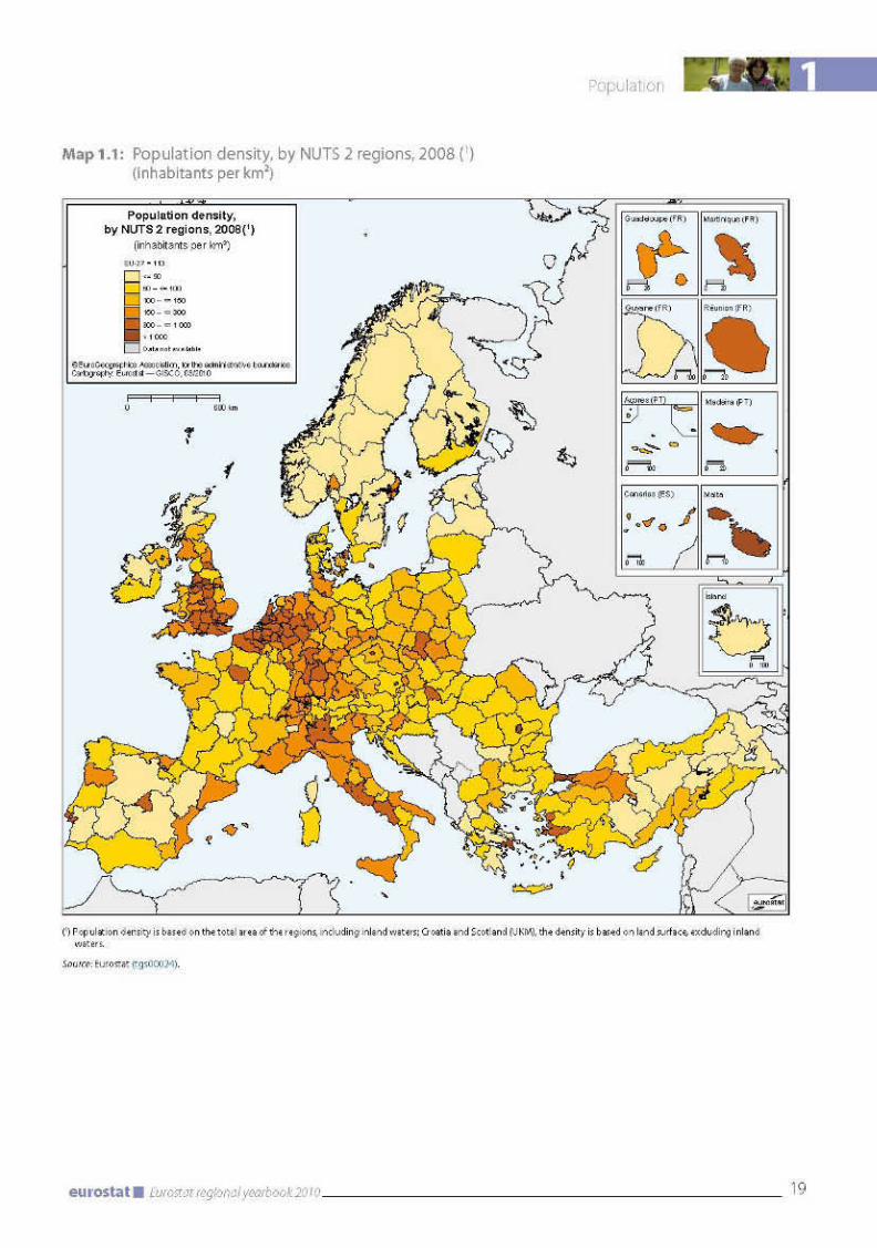
Map 1.1 shows population density on 1 January 2008. The population density of a region is the ratio of the population of a territory to its size. Generally, regions that include the capital city of the country are among the most densely populated, as the map shows. Inner London was by far the most densely populated, but the Brussels, Wien, Berlin, Praha, İstanbul, Bucureşti – Ilfov and Attiki (Greece) regions also have densities above 1 000 inhabitants per km². The least densely populated region was Guyane (France). Next, with fewer than 10 inhabitants per km², were regions in Sweden, Finland, Iceland and Norway. By comparison, the European Union has, on average, a population density of 113 inhabitants per km².
Population change
During the last four and a half decades, the population of the 27 countries that make up today’s European Union has grown from around 400 million (1960) to almost 500 million (499.7
million on 1 January 2009). Including candidate countries and EFTA countries, the total population has grown from under 450 million to 590 million over the same period.
The population growth has two components: so-called ‘natural growth’ or ‘natural change’, defined as the difference between the numbers of live births and deaths, and net migration, which ideally represents the difference between inward and outward migration flows (see ‘Methodological notes’). Changes in the size of a population are the result of the number of births, the number of deaths, and the number of people who migrate inwards and outwards.
Up to the end of the 1980s, natural growth was by far the major component of population growth. However, there has been a sustained decline in natural growth since the early 1960s. On the other hand, international migration has gained importance and became the driving force of population growth from the beginning of the 1990s onwards.
The analysis on the following pages is based mainly on demographic trends observed from 1 January 2004 to 1 January 2009. Five-year averages have been calculated of annual population growth and its components. Given that demographic trends are long-term developments, the five-year averages provide a stable and accurate picture. They help to identify regional clusters, which often stretch well beyond national borders. For the sake of comparability, population growth and its components are presented in relative terms, calculating the so-called crude rates, i.e. they relate to the size of the total population (see ‘Methodological notes’). Maps 1.2, 1.3 and 1.4 present population growth and its components.
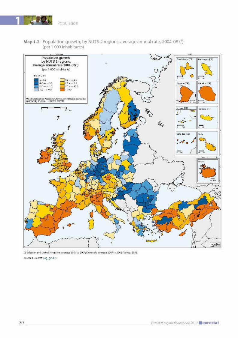
In most of the north-east, east and part of the south-east of the area made up by the European Union, the candidate and EFTA countries, the population is decreasing. Map 1.2 shows a clear division between the regions there and in the rest of the EU. The countries most affected by this trend are Germany (in particular the former East Germany), Poland, Bulgaria, Slovakia, Hungary and Romania; and to the north, the three Baltic States, the northern parts of Sweden, and the Finnish region of Itä-Suomi. Decreasing population trends are also evident in many regions of Greece. On the other hand, to the east, the population growth is positive in Cyprus and, to a lesser extent, in the former Yugoslav Republic of Macedonia, and in Turkey.
1 Population
22 Eurostat regional yearbook 2010 eurostat
In nearly all western and south-western regions of the EU, the population increased over the period 2003–08. This is particularly evident in Ireland and in almost all regions of the United Kingdom, Italy, Spain, France, Portugal, including the French overseas departments and the Spanish and Portuguese islands in the Atlantic Ocean. Positive population growth was registered also in Austria, Switzerland, Belgium, Luxembourg and the Netherlands.
The picture provided by Map 1.2 can be refined by analysing the two components of total population growth, namely natural growth and net migration.
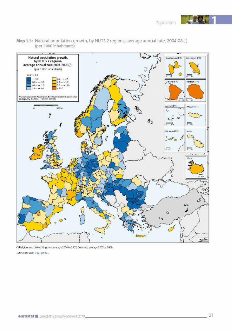
Map 1.3 shows that, in many regions of the EU, more people died than were born in the
period 2004–08. The resulting negative natural population growth is widespread and affects almost half the EU’s regions.
A single extended cross-border region showing a positive natural change in its population can be identified, made up of Ireland, central United Kingdom, most regions in France, Belgium, Luxembourg, the Netherlands, Switzerland, Iceland, Liechtenstein, Denmark and Norway. In these regions, there were more live births than deaths in the period 2004–08.
Deaths were more numerous than births in most regions of Germany, Hungary, Croatia, Romania and Bulgaria, as well as in the Baltic States in the north, and Greece and Italy in the south. Other countries had a more balanced pattern overall.
Figure 1.1: Total fertility rate, by NUTS 2 regions, 2008 (1)
(children per woman)
National average Capital region
0.0 0.5 1.0 1.5 2.0 2.5 3.0 3.5 4.0
BelgiumBulgaria
Czech RepublicDenmarkGermany
EstoniaIrelandGreece
SpainFrance
ItalyCyprusLatvia
LithuaniaLuxembourg
HungaryMalta
NetherlandsAustriaPoland
PortugalRomaniaSloveniaSlovakiaFinland
SwedenUnited Kingdom
CroatiaFormer Yugoslav
Republic of MacedoniaTurkeyIceland
LiechtensteinNorway
Switzerland
Prov. Limburg (B)Severen tsentralen
PrahaHovedstaden
Southern and Eastern
Hamburg
IpeirosPrincipado de Asturias
CorseSardegna
Nyugat-Dunántúl
Limburg (NL)Burgenland (A)Opolskie
Centro (P)Sud-Vest Oltenia
Vzhodna SlovenijaZápadné Slovensko
Etelä-SuomiÖvre Norrland
Highlands and IslandsJadranska Hrvatska
Oslo og Akershus
Bati Marmara
Ticino
Région de Bruxelles-Capitale/Brussels Hoofdstedelijk GewestYugoiztochen
Střední Čechy
Weser-Ems
Border, Midland and WesternKriti
Ciudad Autónoma de Ceuta
Észak-Magyarország
FlevolandOberösterreich
PomorskieAlgarve
Nord-EstZahodna Slovenija
Východné SlovenskoPohjois-Suomi
Mellersta NorrlandWest Midlands
Agder og RogalandZentralschweiz
Središnja i Istočna (Panonska) Hrvatska
Güneydogu Anadolu
Provincia Autonoma Bolzano/BozenGuyane
Sjælland
(1) Belgium, 2006; Ireland, Spain, France, Italy and United Kingdom, 2007; Turkey, by NUTS 1 regions.
Source: Eurostat (reg_frate2).

1
23Eurostat regional yearbook 2010eurostat
Population
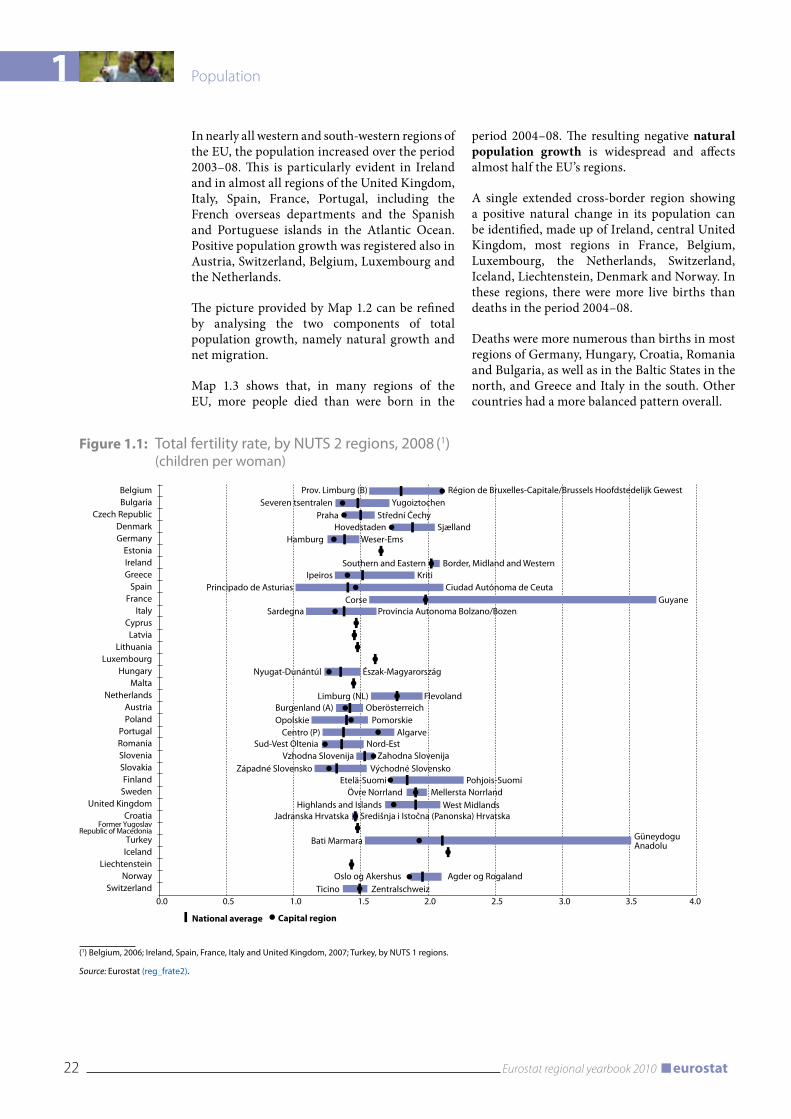
A major reason for the slowdown in the natural growth of the population is the fact that the EU’s inhabitants have fewer children than they used to. At aggregated level, in the 27 countries that form the EU today, the total fertility rate has declined from a level of around 2.5 children per woman in the early 1960s to about 1.5 in 1993. It has remained around that level since then. (For the definition of the total fertility rate, see the ‘Methodological notes’.)
At country level, in 2008, a total fertility rate lower than 1.5 children per woman was observed in 15 of the 27 Member States. In the more developed parts of the world today, a total fertility rate of around 2.1 children per woman is considered to be the replacement level, i.e. the level at which the population would remain stable in the long run if there were no inward or outward migration. At present (2008 data), practically all of the EU, candidate and EFTA countries, with the exception of Turkey and Iceland, are still well below replacement level.
Figure 1.1 shows the range of the European regions’ total fertility rate for each country. Additionally, between the highest and lowest values, the bars illustrate the national level of the fertility rate, and the value registered in the region that includes the capital of the country. Among the 317 NUTS 2 regions covered in this analysis, in 2008, the total fertility rate ranges from one child per woman registered in the region Principado de Asturias in Spain to 3.7 children per woman in the French region Guyane.
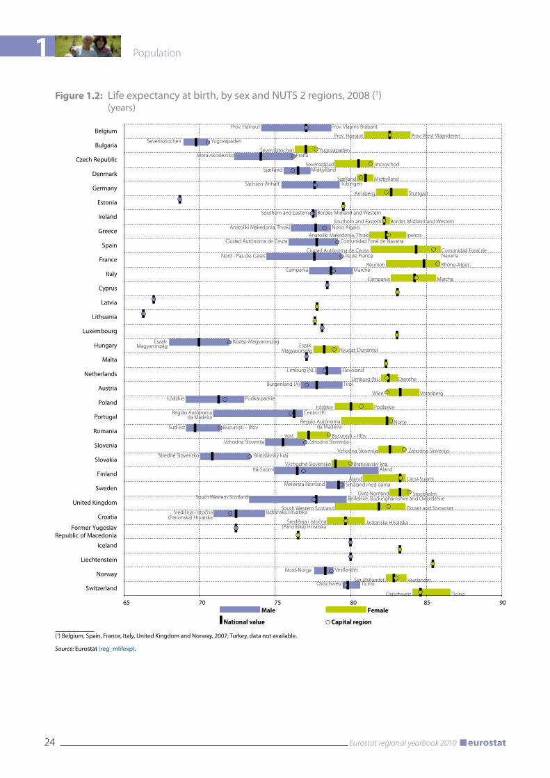
Life expectancy at birth has risen by about 10 years over the last 50 years, due to improved socioeconomic and environmental conditions and better medical treatment and care.
Figure 1.2 is based on Eurostat’s calculations on life expectancy at birth at national and regional level available for the years 2007–08. The figure shows the range of life expectancy at birth for men and women by region for each country. Between the highest and lowest values, the bars illustrate the value at national level, as well as the value registered by the region including the capital of the country.
In 2007, life expectancy at birth of women in the EU-27 was 82.0 years, and 75.8 years for men, showing a gender gap of 6.2 years. In all 27 Member States, Croatia, the former Yugoslav Republic of Macedonia, and the four EFTA countries, women live longer than men. The gender gap ranges from about four years in Cyprus, the Netherlands, the
United Kingdom and Sweden to about 11 or 12 years in the three Baltic States.
Across the 317 NUTS 2 regions covered in this analysis, considerable differences can be observed. Life expectancy at birth for men ranged from 66.3 years in Lithuania to about 81.8 years in Finland’s Åland region. For women, it ranged from around 76.3 years in the Bulgarian region of Severoiztochen to 86.6 years in the Ticino region of Switzerland. In most Member States, life expectancy in the region including the capital is higher than that at national level. This is more often observed in the case of women.
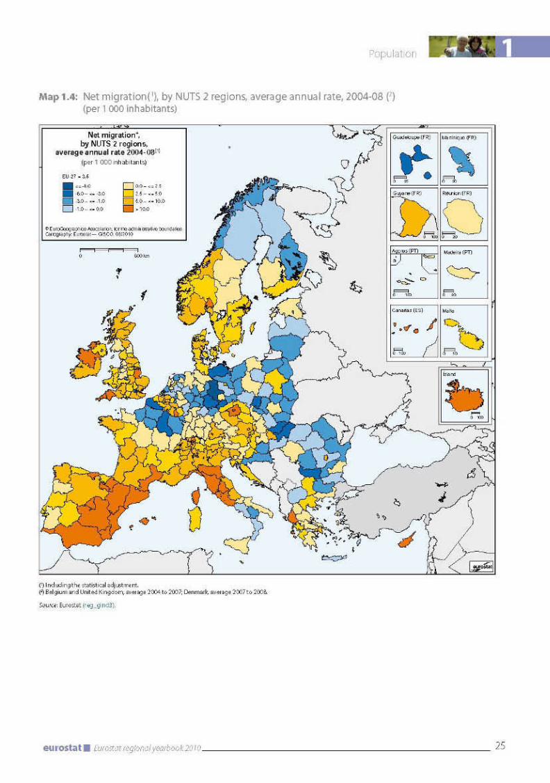
The third determinant of population growth (after fertility and mortality) is net migration. As many countries in the EU are currently at a point in the demographic cycle where natural population change is close to being balanced or negative, net migration becomes more significant when it comes to maintaining the size of the population. Moreover, migration also contributes indirectly to natural growth, given that migrants have children. Migrants are also usually younger and have not yet reached the age at which the probability of dying is higher.
In some EU regions, negative natural change has been offset by positive net migration. This is at its most striking in Austria, the United Kingdom, Spain, the northern and central regions of Italy, and in some regions of western Germany, Slovenia, southern Sweden, Portugal and Greece, as can be seen in Map 1.4. The opposite is much rarer: in only a few regions has positive natural change been cancelled out by negative net migration. This is the case in the northern regions of Poland and of Finland.
Four cross-border regions where more people have left than arrived (negative net migration) can be identified on Map 1.4:
the northern regions of Norway, Sweden and •Finland;a cross-Europe area, starting in the north-west •and going south-east, comprising most of the regions in the Netherlands, eastern Germany, Poland, Lithuania and Latvia, and most parts of Slovakia, Hungary, Romania and Bulgaria;regions in the north-east of France, as well •as Guadeloupe and Martinique in the French overseas departments;a few regions in the south of Italy and in the •United Kingdom.
1 Population
24 Eurostat regional yearbook 2010 eurostat
Figure 1.2: Life expectancy at birth, by sex and NUTS 2 regions, 2008 (1)
(years)
Male Female
National value Capital region
65 70 75 80 85 90
Belgium
Bulgaria
Czech Republic
Denmark
Germany
Estonia
Ireland
Greece
Spain
France
Italy
Cyprus
Latvia
Lithuania
Luxembourg
Hungary
Malta
Netherlands
Austria
Poland
Portugal
Romania
Slovenia
Slovakia
Finland
Sweden
United Kingdom
Croatia
Former YugoslavRepublic of Macedonia
Iceland
Liechtenstein
Norway
Switzerland
Prov. Hainaut
Prov. HainautSeveroiztochen
SeveroiztochenMoravskoslezsko
SeverozápadSjælland
SjællandSachsen-Anhalt
Arnsberg
Southern and Eastern
Southern and EasternAnatoliki Makedonia, Thraki
Anatoliki Makedonia, ThrakiCiudad Autónoma de Ceuta
Ciudad Autónoma de Ceuta Nord - Pas-de-Calais
RéunionCampania
Campania
Limburg (NL)
Limburg (NL)
Wien
Burgenland (A)
Łódzkie
Łódzkie
Stredné Slovensko
Východné SlovenskoItä-Suomi
Åland
Nord-Norge
Sør-ØstlandetOstschweiz
Ostschweiz
Sud-Est
Vest
South Western Scotland
South Western ScotlandSredišnja i Istočna
(Panonska) HrvatskaSredišnja i Istočna
(Panonska) Hrvatska
Mellersta Norrland
Övre Norrland
Vzhodna Slovenija
Vzhodna Slovenija
Região Autónomada Madeira
Região Autónoma da Madeira
Észak-Magyarország Észak-
Magyarország
Prov. Vlaams-Brabant
Prov. West-Vlaanderen
Yugozapaden
Yugozapaden
Praha
JihovýchodMidtjylland
MidtjyllandTübingen
Stuttgart
Notio Aigaio
Ipeiros
Île de France
Rhône-AlpesMarche
Marche
Flevoland
Drenthe
Vorarlberg
Tirol
Podkarpackie
Podlaskie
Közép-Magyarország
Nyugat-Dunántúl
Bucureşti – Ilfov
Bucureşti – Ilfov
Bratislavský kraj
Bratislavský kraj
Centro (P)
Norte
Zahodna Slovenija
Zahodna Slovenija
Åland
Länsi-Suomi
Stockholm
Jadranska Hrvatska
Jadranska Hrvatska
Vestlandet
Ticino
Ticino
Vestlandet
Berkshire, Buckinghamshire and Oxfordshire
Dorset and Somerset
Småland med öarna
Comunidad Foral de Navarra
Comunidad Foral de Navarra
Border, Midland and Western
Border, Midland and Western
(1) Belgium, Spain, France, Italy, United Kingdom and Norway, 2007; Turkey, data not available.
Source: Eurostat (reg_mlifexp).
1
27Eurostat regional yearbook 2010eurostat
Population
There are regions where the two components of population change (positive/negative natural change, positive/negative net migration) have both moved in the same direction.
In Ireland, Luxembourg, Belgium, Malta, Cyprus, Switzerland, Iceland, many regions in France and in Norway, and some regions in Spain, the United Kingdom and the Netherlands, a positive natural change has been accompanied by positive net migration, hence a rise in their populations.
However, in eastern Germany, Lithuania and Latvia, and in some regions in Poland, Slovakia, Hungary, Bulgaria and Romania, both components of population change have moved in a negative direction, as can be seen also from Map 1.2. This trend has led to sustained population loss.
Regional population projections
Population projections are ‘what-if ’ scenarios that aim to provide information about the likely future size and structure of the population. EUROPOP2008 regional population projections produced by Eurostat present one of several possible population change scenarios at NUTS level 2, based on assumptions for fertility, mortality and migration for the period 2008–30. The 2008-based (EUROPOP2008) population projections at national level cover all the EU Member States, Norway and Switzerland, in total 281 regions.
Two highlights of the EUROPOP2008 regional population projections are presented in this chapter:
most of the European regions are projected to •have a larger population by 2030; the process of population ageing is projected to •occur in almost all regions.
The population of the EU as a whole is projected to rise by 5 % between 2008 and 2030, but there is considerable variation among regions in the Member States, Norway and Switzerland.
In fact, as shown in Map 1.6, the population may increase in Cyprus, Luxembourg and Malta, and in all regions in Belgium, Denmark, Ireland, the United Kingdom, Norway and Switzerland by 2030. The most densely inhabited regions of Austria, the Czech Republic, Spain, Finland, France, Greece, Italy, the Netherlands, Portugal,
Sweden and Slovenia are also likely to see rises in their populations.
Estonia, Latvia and Lithuania and most regions in Bulgaria, Romania, Germany, Hungary, Poland and Slovakia are expected to have a lower population by 2030.
The population profile is projected to become older in almost all regions. This is likely to happen due to the combined effect of three factors — the existing population structure, fertility lower than replacement levels, and the steadily rising numbers of people living longer.
In the coming decades, the high number of ageing baby boomers will swell the number of elderly people. As a result, the proportion of the population aged 65 or over is projected to increase considerably over the period 2008–30 (see Map 1.7).
For the EU-27, the share of the total population aged 65 years or over is projected to increase to 23.5 % in 2030, from 17.1 % in 2008. In 2030, for the 281 regions, the proportion of the population aged 65 or over is projected to range between 10.4 % for Inner London in the United Kingdom, and 37.3 % in the German region of Chemnitz on the border with the Czech Republic (see Figure 1.4). For comparison, in 2008, the range was between 9.1 % in the region of Flevoland (Netherlands) and 26.8 % in the coastal region of Liguria in north-west Italy.
The old-age dependency ratio is used as an indicator of the extent to which the population aged 65 or over must be supported by people of working age, conventionally 15–64 years old. In 2030, the ratio may be pushed much higher than currently registered, due to a combination of a rise in the proportion of the projected population aged 65 or over, and a fall in the population of working age for most regions.
For the EU-27, the old-age dependency ratio in 2030 is expected to rise to 38.0 % from a registered value of 25.4 % in 2008. This means that, on average, 100 people of working age are projected to support 38 people aged 65 or over in 2030, whereas the 2008 figures were 100 per 25 (see Map 1.5). The range across all regions is projected to be between 14.8 % and 70.2 %.
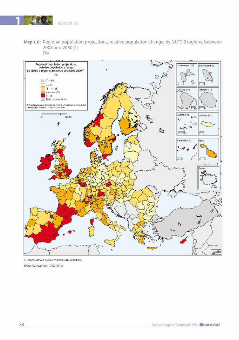
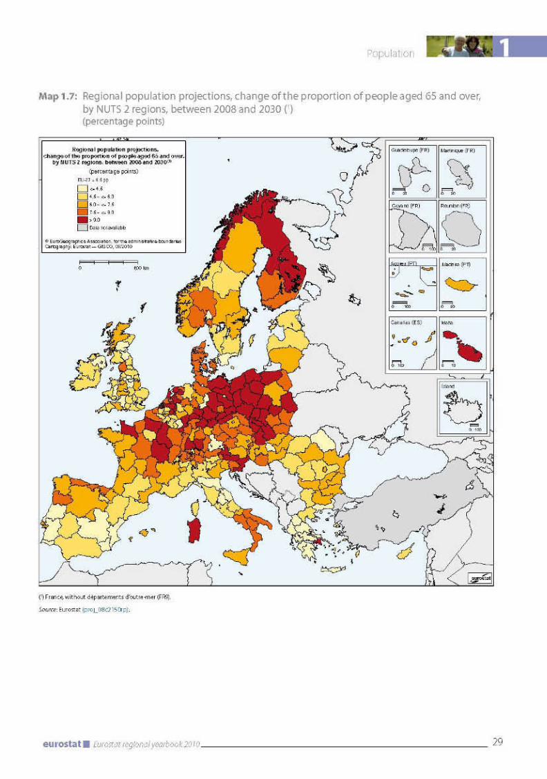

1 Population
30 Eurostat regional yearbook 2010 eurostat
Figure 1.3: Regional population projections, NUTS 2 regions with the highest/lowest proportion of people aged 65 and over in the total population in 2030 (1) (%)
% 5% 10% 15% 20% 25% 30% 35% 40% 45%
Belgium Région de Bruxelles-Capitale / Brussels Hoofdstedelijk Gewest
Yugozapaden
Praha
Hovedstaden
Hamburg
Southern and Eastern
Sterea Ellada
Ciudad Autónoma de Melilla
Île de France
Provincia Autonoma Bolzano/Bozen
Közep-Magyarország
Flevoland
Wien
Małopolskie
Região Autónoma dos Açores
Nord-Est
Zahodna Slovenija
Východné Slovensko
Etelä-Suomi
Stockholm
Inner London
Oslo og Akershus
Zürich
Świętokrzyskie
Alentejo
Vzhodna Slovenija
Západné Slovensko
Itä-Suomi
Norra Mellansverige
Dorset and Somerset
Hedmark og Oppland
Ticino
Sud-Vest Oltenia
Prov. West-Vlaanderen
Severozapaden
Střední Morava
Sjælland
Chemnitz
Border, Midland and Western
Attiki
Principado de Asturias
Bourgogne
Liguria
Dél-Dunántúl
Zeeland
Kärnten
Bulgaria
Czech Republic
Denmark
Germany
Estonia
Ireland
Greece
Spain
France
Italy
Cyprus
Latvia
Lithuania
Luxembourg
Hungary
Malta
Netherlands
Austria
Poland
Portugal
Romania
Slovenia
Slovakia
Finland
Sweden
United Kingdom
Norway
Switzerland
National value Capital region
(1) France, without départements d’outre-mer (FR9).
Source: Eurostat (proj_08c2150rp).


32 Eurostat regional yearbook 2010 eurostat
Population1
Conclusion
This chapter highlights selected features of trends in regional population in the area made up by the EU-27 Member States, candidate countries and EFTA countries over the period from 1 January 2004 to 1 January 2009. As far as possible, typologies of regions with phenomena spreading across national boundaries have been identified. While population decline is evident in several regions, at aggregated level, the EU-27 population still increased by around 2 million people every year over the period examined. The main driver
of population growth is net migration, which counterbalanced the negative natural change of the population in many regions.
The current regional demographic profile is com-plemented by the scenario proposed by the re-gional demographic projections EUROPOP2008. Most European regions are projected to have a larger population in 2030. According to the pop-ulation projections, elderly people would account for an increasing share of the population, due to a rise in longevity in past and future decades. The process of population ageing is widespread in most regions.

33Eurostat regional yearbook 2010eurostat
1Population
Methodological notes
Sources: Eurostat — Population statistics. For more information, please consult the Eurostat website at http://epp.eurostat.ec.europa.eu/portal/page/portal/population/introduction
Population growth, or population change, is the difference between the size of the population at the end and the beginning of the period. It is equal to the algebraic sum of natural population growth and net migration (including the statistical adjustment). There is negative population growth when both of these components are negative or when one is negative and has a higher absolute value than the other.
Natural population growth, or natural change, is the difference between the number of live births and the number of deaths.
Migration can be extremely difficult to measure. A variety of different data sources and definitions are used in the Member States, meaning that direct comparisons between national statistics can be difficult or misleading. The net migration figures here are not directly calculated from immigration and emigration flow figures. Since many countries either do not have accurate, reliable and comparable figures on immigration and emigration flows or have no figures at all, net migration is generally estimated on the basis of the difference between total population growth and natural population growth between two dates (in Eurostat data, this is then called net migration including statistical adjustment). The statistics on net migration are therefore affected by all the statistical inaccuracies in the two components of this equation, especially population growth. In effect, net migration equals all changes in total population that cannot be attributed to births and deaths.
Crude rate of population growth is the ratio of the total population growth during the year to the average population of the area in question in that year. The value is expressed per 1 000 inhabitants.
Crude rate of natural population growth is the ratio of natural population growth over a period to the average population of the area in question during that period. The value is expressed per 1 000 inhabitants.
Crude rate of net migration is the ratio of net migration during the year to the average population in that year. The value is expressed per 1 000 inhabitants. As said above, the crude rate of net migration is equal to the difference between the crude rate of population growth and the crude rate of natural population growth (i.e. net migration is considered as the part of population growth not attributable to births and deaths).
Total fertility rate is defined as the average number of children that would be born to a woman during her lifetime if she were to pass through her childbearing years conforming to the age-specific fertility rates that have been measured in a given year.
Life expectancy at birth is the mean number of years that a newborn child can expect to live if subjected throughout his or her life to current mortality conditions.
Population density is the ratio of the population of a territory to the total size of the territory (including inland waters), as measured on 1 January.
Old-age dependency ratio is the ratio of the number of elderly persons of an age when they are generally economically inactive (age 65 and over in this publication) to the number of persons of working age (conventionally 15–64 years old).
33Eurostat regional yearbook 2010eurostat

European cities
2 European cities
36 Eurostat regional yearbook 2010 eurostat
Introduction
The Treaty of Lisbon states that the European Union ‘shall work for the sustainable develop-ment of Europe’. The EU’s sustainable develop-ment strategy (1) aims at ‘continuous improve-ment of the quality of life and well-being on Earth for present and future generations’. To improve the quality of life in cities, governments must work at local, national and international levels to come up with policy responses and ef-fective measures to deal with environmental, economic and social vulnerabilities. To assist policymakers in their efforts, data on European cities were collected in the Urban Audit project. The ultimate goal of the project is to contribute to improving the quality of urban life. It supports exchanges of experience between cities, helps to identify best practices, facilitates benchmarking at European level and provides information on the dynamics within cities and their surround-ings. How? This can be explained by looking at the topics, the time frame and the spatial dimen-sion of the Urban Audit.
The topics
The EU’s sustainable development strategy brings together many strands of economic, social and environmental policy under one overarching objective (2). To capture the complexity of the sustainable development of cities, a wide range of topics have to be looked at. The topics covered by the Urban Audit include demography, housing, health, crime, the labour market, income disparity, local administration, educational qualifications, the environment, climate, travel patterns, the information society and cultural infrastructure. For each topic several indicators are defined. These are derived from the variables collected by the European Statistical System. Data availability differs widely. Demographic data, for instance, are available for almost every city, whereas environmental data are available for fewer than half.
The time frame
Sustainable development, as mentioned in the introduction, meets the needs of the present without compromising the ability of future generations to meet their own needs (3). This definition imposes requirements on the time frame of the statistics. Data must be available
on the present situation but the time series must be long enough to allow projections. The Urban Audit tries to meet both these requirements. The oldest data are for 1991, the latest for 2008. Figures 2.1 and 2.2 display some of these long time series from 1991 to 2008. Collecting ‘historical’ data or the most recent data is always more difficult, so for these years only figures on key indicators are available. Most of the data are for 2001 and 2004. If data for these years were not available, data from adjacent years are provided.
The spatial dimension
Sustainable development policy is, first and foremost, targeted on people. However, most people in Europe have addresses, i.e. they live in places, and many of them live in cities. To provide information on these addresses, places and cities, the Urban Audit has a multilayered spatial dimension.
Most of the data are collected at core city level, i.e. the city as delimited by its administrative or political boundaries. However, economic activity, labour flows, air pollution, etc. do not stop at the administrative boundaries of a city nor are workplaces, labour force and air pollutants evenly distributed within the boundaries of a city. To make it easier to analyse the interaction between a city and its surroundings, for each city participating a second level called the larger urban zone was delineated. The larger urban zone is an approximation of the functional urban area centred on the core city. To provide information on internal disparities within the core city’s boundaries, a third spatial level, the sub-city district, was introduced. The data used to produce Maps 2.1 and 2.2 refer to the core city, whereas Map 2.3 presents information at sub-city district level.
Urbanisation
The declared geographical scope of the EU’s sustainable development strategy covers well-being ‘on Earth’, so it is appropriate to take a brief look at global trends. One of these is urbanisation, ‘the world goes to town’ (4). The industrial revolution in the late 18th century triggered one of the greatest human migrations in history. The mass exodus from rural areas to cities swept through Europe and North America first and is still in the process of transforming Asia. Europe
(1) Council of the European Union, ‘Review of the EU sustainable development strategy (EU SDS) — Re-newed strategy’, 10117/06.
(2) Eurostat, Sustainable de-velopment in the European Union — 2009 monitoring report on the EU sustain-able development strategy, Luxembourg, Office for Official Publications of the European Communi-ties, 2009.
(3) United Nations, 1987, ‘Report of the World Commission on Environ-ment and Development’, General Assembly Resolu-tion 42/187, 11 December 1987.
(4) The Economist, ‘The world goes to town’, The Econo-mist Newspaper Limited, 3 May 2007.
2
37Eurostat regional yearbook 2010eurostat
European cities
is considered to be at the advanced stage of urbanisation. Asia is still at the middle stage, but nevertheless 11 of the 19 largest cities in the world were in Asia in 2007 (5). The two most populous cities in the European Union were London (UK) and Paris (FR) in 2007. The larger urban zones of both these cities had more than 10 million inhabitants, that is more than several of the countries in the European Union. Nevertheless, these cities account for a small share of the urban population in Europe, in contrast to the United States, where 80 % of the country’s population are classified as living in a metropolitan area and one third of them live in large cities with populations of over 5 million.
In Europe the distribution of urban-dwellers across cities of different sizes is more even, as illustrated in Map 2.1. Each circle on the map represents an Urban Audit city. At present, the Urban Audit data collection includes more than 300 cities from the EU-27, plus 26 Turkish, five Croatian, six Norwegian and four Swiss cities. In the near future, the number of Swiss cities participating in the Urban Audit will increase to 10. The size of the circle reflects the number of inhabitants in the core city. Six cities in the Urban Audit have more than 3 million inhabitants: Berlin (DE), Madrid (ES), Paris (FR), London (UK), Ankara (TR) and İstanbul (TR). Another 20 have fewer than 3 million but more than 1 million inhabitants. They are spread all over Europe, from northern to western, southern and central Europe. Smaller cities, with fewer than 1 million but more than half a million inhabitants, are considerably more numerous. The next tier, made up of cities with populations ranging from 250 000 to just under half a million, numbers 80. One noteworthy point is that the total population in each size category mentioned so far is about the same, approximately 30 million, underlining the balanced distribu-tion of the urban population in Europe. However, the Urban Audit does not include every city in Europe. Several, especially in the smaller size groups, i.e. with fewer than 250 000 inhabitants, are not included. To fill this gap in the Urban Audit data collection, the ‘Large City Audit’ was launched. It includes all ‘non-Urban Audit cities’ with more than 100 000 inhabitants in the EU-27. For these cities a smaller set of 50 variables is collected. The data set including all Urban Audit and Large City Audit cities is available in Eurostat’s databases.
Present and future generations — the demographic challenge
The sustainable development strategy identi-fies seven key challenges: climate change and clean energy; sustainable transport; sustainable consumption and production; conservation and management of natural resources; social inclu-sion; demography and migration; public health and global poverty. Building on the Urban Audit, it is possible to take a closer look at the demo-graphic challenge.
One major challenge facing socioeconomic development is the ageing population. This is reflected in the growing old-age dependency ratio. As shown by Map 2.2, in most Urban Audit cities the old-age dependency ratio stands at between 22 % and 26 %. For example, in the Maltese capital Valetta the value is 25 %, meaning that for every person aged 65 or over there are four of working age. Besides the two largest cities in Europe, smaller cities in most of the ‘new’ Member States and Greece stand out as having a low old-age dependency ratio. Irish and Turkish cities also fall into this group, irrespective of their size. Cities located in the core of Europe, i.e. in Belgium, Germany, Switzerland, Austria and Italy, tend to have higher old-age dependency ratios, as do most Spanish and Portuguese cities.
Looking at the indicator value for a city tells only part of the story. Even in a city with a low value, like Amsterdam (17 %), neighbourhoods can be found with exceptionally high old-age dependency ratios (above 30 %), as shown in Map 2.3. The map also confirms that differences between neighbourhoods within the same city can be much larger than between cities. In some cities certain spatial patterns can be observed: in Berlin (DE) or Zürich (CH) there is a big difference between the city centre and the surrounding districts, whereas in Budapest (HU) there is an east/west divide along the River Danube. Analysing the spread of indicator values within individual cities makes it possible to paint a detailed picture of an ageing society.
Another way to examine the phenomenon of ageing cities is to focus on the time dimension. Figure 2.1 focuses on two cities, Madrid and Milano, and shows how the age structure of the population changed between 1991 and 2008. ‘Population pyramids’ are commonly used to illustrate the distribution of age groups in a
(5) UN, Habitat, State of the world’s cities 2008/2009, Harmonious cities, Lon-don, 2008.

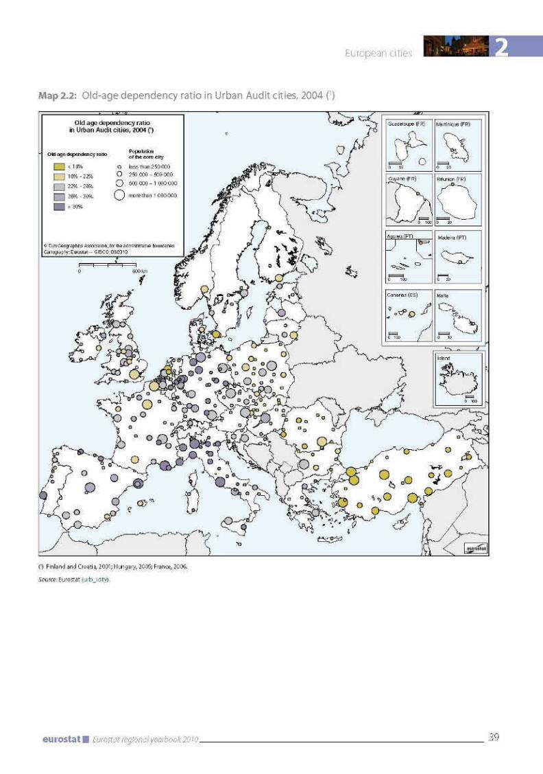
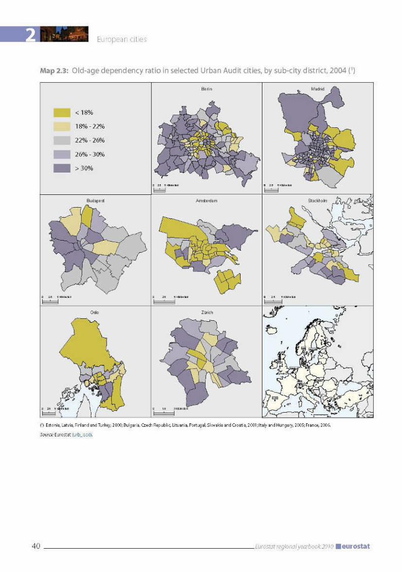
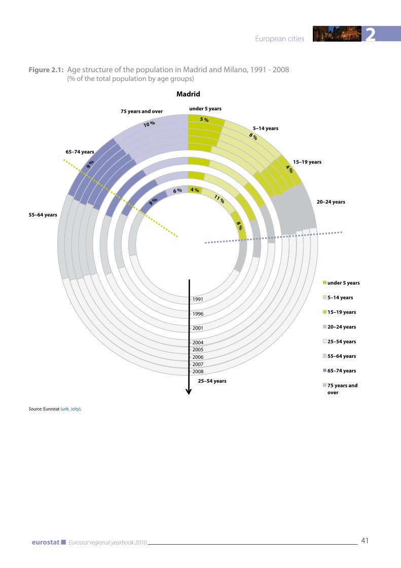
2
41Eurostat regional yearbook 2010eurostat
European cities
Figure 2.1: Age structure of the population in Madrid and Milano, 1991 - 2008 (% of the total population by age groups)
5–14 years
65–74 years
55–64 years
25–54 years
5–14 years
15–19 years
20–24 years
25–54 years
55–64 years
65–74 years
75 years andover
15–19 years
under 5 years75 years and over
20–24 years
under 5 years
Madrid
- 1991
- 1996
- 2001
- 2004- 2005- 2006- 2007- 2008
10 %
9 %
5 %
8 %
4 %
8 %
11 %
4 %6 %
9 %
Source: Eurostat (urb_icity).
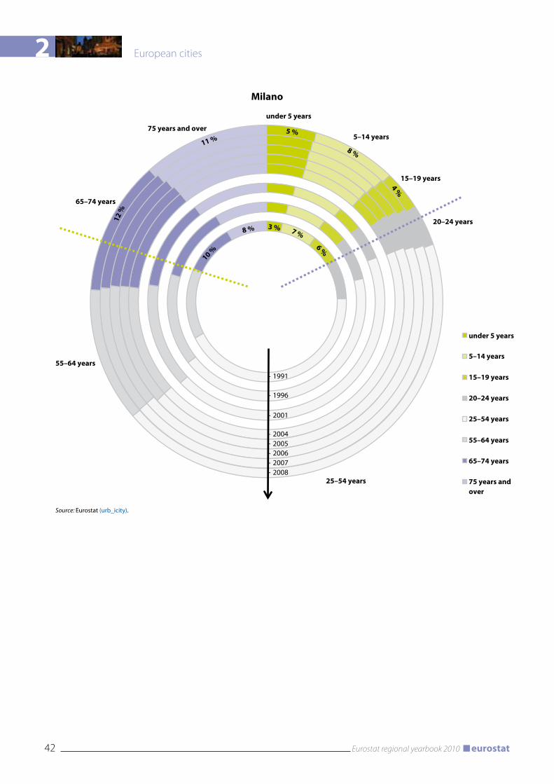
2 European cities
42 Eurostat regional yearbook 2010 eurostat
5–14 years
15–19 years
20–24 years
25–54 years
55–64 years
65–74 years
75 years andover
under 5 years
Milano
- 1991
- 1996
- 2001
- 2004- 2005- 2006- 2007- 2008
5–14 years
15–19 years
20–24 years
25–54 years
55–64 years
65–74 years
75 years and over
under 5 years
7 %6 %
3 %8 %
10 %
11 %
12 %
5 %
8 %4 %
Source: Eurostat (urb_icity).
2
43Eurostat regional yearbook 2010eurostat
European cities
country or city. However, population pyramids show the proportion of population in age cohorts at one point in time. In Figure 2.1 each ring depicts one year, like the growth rings of a tree. The different colours indicate the different age groups. In 1991 in Madrid almost a quarter of the population were in the under-20 age group. This proportion shrank gradually to approximately 17 % in 2008. The decrease in the young slice of the population was counterbalanced by an increase in the proportion of elderly residents. A similar trend can be observed in Milano, but starting from a slightly different position. In Milano, over-65s already outnumbered under-20s in 1991, when the opposite was the case in Madrid.
A society’s ability to cope with an ageing population does not depend directly on the old-age dependency ratio. The question is how many inactive people have to be supported by the active population. Attracting nationals from other countries is one way of preventing labour-force shortages (6). Map 2.4 provides an overview of the proportion of nationals in Urban Audit cities. Most cities in the ‘new’ Member States, candidate countries and eastern Germany have a very small or no foreign population, except Tallinn (EE) and Berlin (DE). In southern Europe the big cities, for example Madrid (ES), Barcelona (ES), Milano (IT) and Athina (EL), all have a large share of non-national population. The same pattern can be observed in Ireland, Denmark, France, the Netherlands and Norway, where foreigners are concentrated in the biggest city in the country. On the other hand, in German-speaking countries (Germany, Austria and Switzerland), the overwhelming majority
of cities, irrespective of their size, have a large share of non-nationals.
After looking at the spatial dimension, this indicator can be analysed along the time line as well. This can be illustrated by two very different capitals, Roma (IT) and Luxembourg (LU). Of all European cities, Luxembourg (LU) had the lowest proportion of nationals in 2007. Over the last two decades this proportion has been decreasing steadily, from more than 50 % in 1991 to less than 40 % in 2008, as shown in Figure 2.2. This means that the majority of residents in the city of Luxembourg are foreigners. By contrast, almost all residents of Roma were Italian. The proportion has decreased since 1991, but is still over 90 % (7).
Conclusion
This chapter presented a few indicators reflecting the demographic challenge facing cities, looking back at longer and shorter periods and focusing on different spatial levels. Besides these indicators, there are many more, just as besides the demographic challenge there are also many more challenges. Cities are focal points of consumption of energy and materials; they are hubs of transport networks, bringing together polluters and protectors of the environment, skilled workers and unemployed, homeless and wealthy, culture and crime. Are they sustainable? Eurostat invites everyone to formulate their own assumptions in response to this question and to test, quantify or reject them themselves after looking at the figures in the various domains of the Urban Audit data collection available on the Eurostat website.
(6) European Commission, Demography Report 2008: Meeting Social Needs in an Ageing Society, Brussels, 2008.
(7) United Nations Population Division, ‘An Overview of Urbanisa-tion, Internal Migration, Population Distribution and Development in the World’, United Nations Secretariat, New York, 21–23 January 2008.
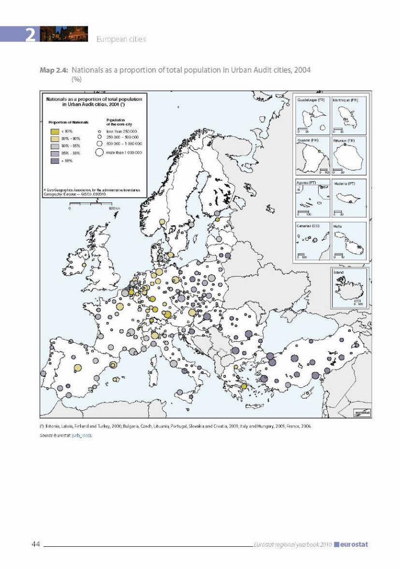
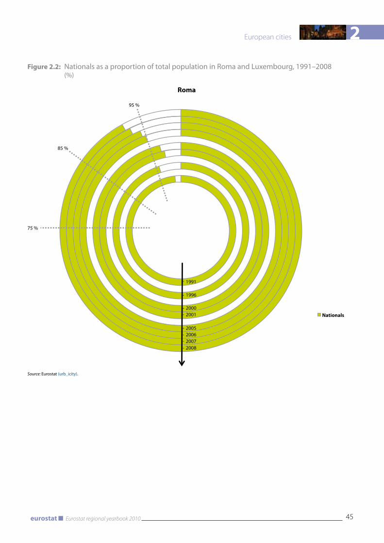
2
45Eurostat regional yearbook 2010eurostat
European cities
Figure 2.2: Nationals as a proportion of total population in Roma and Luxembourg, 1991–2008 (%)
Roma
Nationals
- 1991
- 1996
- 2000- 2001
- 2005- 2006- 2007- 2008
75 %
85 %
95 %
Source: Eurostat (urb_icity).
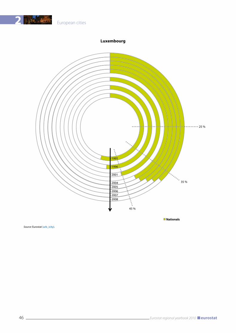
2 European cities
46 Eurostat regional yearbook 2010 eurostat
Luxembourg
Nationals
-
-1996
-2001
-2004-2005-2006-2007-2008
25 %
45 %
35 %
1991
Source: Eurostat (urb_icity).


Labour market
3 Labour market
50 Eurostat regional yearbook 2010 eurostat
Introduction
This chapter looks at two very different aspects of the regional labour market. The first part describes the recent changes in employment and unemployment at regional level, and carries out a cluster analysis based on the predominant economic sectors, using the latest results from the Labour Force Survey.
The second part presents some of the results of the Structure of Earnings Survey, for which the most recent reference year available is 2006. This part will focus mainly on hourly earnings, annual earnings and bonuses.
Regional sector specialisation
A period of several years of economic growth and job creation has been followed by the biggest economic downturn since World War II. The EU has responded by adopting the European economic recovery plan, along with other measures to moderate the effects of this unprecedented crisis. Securing existing jobs and putting people back into employment as quickly as possible was and remains a priority.
Although all of the measures taken have helped to reduce the negative impact of this crisis, they have been unable to halt job losses or rising unemployment entirely. At the time of writing, unemployment is currently 10 % in the euro area and only slightly lower in the EU-27.
Regions now have to face the huge challenge of pick-ing themselves up and getting back on track, which will certainly present them with a whole range of difficulties. Regions have been affected in different ways and they display different characteristics.
Understanding that some regions are in fact different from others, and that they are therefore likely to be confronted by different challenges, is a first step towards becoming more policy efficient, by taking measures that are tailored to the different needs.
This text takes a closer look at employment and unemployment. Regions will be clustered into different groups according to the main sector of activity and we will show that taking this factor into account is a useful and meaningful way to complement the analysis of the regional labour market.
Brief overview of 2008
The EU-27 employment rate rose from an average of 65.4 % in 2007 to 65.9 % in 2008. The Lisbon employment target is set to 70 %, to be achieved in 2010. The full impact of the economic recession on employment levels has not yet been reflected in 2008 because labour markets usually take some time to respond to economic recession. In addition, regional labour market data are based on yearly averages and the recent crisis did not begin until late 2008.
Map 3.1 shows the regional employment rates for the 15–64 age group, by NUTS 2 regions in 2008.
In 2008, only 94 of the 271 NUTS 2 regions in the EU-27 had already achieved the Lisbon target for 2010, while 50 regions were still 10 percentage points below the overall employment target.
Relatively low employment rates were recorded in the south of Spain, the south of Italy, Greece, Poland, Slovakia, Hungary, Bulgaria and Romania, whereas in the northern EU regions, including regions in the Netherlands, the United Kingdom, Denmark, Sweden and Finland recorded relatively high employment rates.
A significant margin of 40.0 percentage points separated the lowest and highest regional employment rates in 2008, with Campania (Italy) on 42.5 % at one extreme, and Åland (Finland) on 82.5 % at the other.
The degrees of rise or fall in employment levels between 2007 and 2008 in most of the regions more or less reflected those in the respective country as a whole. However, there are some exceptions. For example, in Spain, where the employment rate fell by 1.3 percentage points, there were regions where employment showed relatively bigger falls, such as Canarias which fell 4.8 percentage points, while other regions, such as Ciudad Autónoma de Ceuta or Principado de Asturias, recorded significant increases of 5.1 and 2.5 percentage points respectively.
In the EFTA regions, all employment rates were above 70 %. In the candidate countries, employ-ment rates ranged from 27.1 % in Mardin (Turkey) to 62.4 % in Sjeverozapadna Hrvatska (Croatia).
The female employment rate in the EU-27 rose in 2008 by 0.7 percentage points to 59.0 %. More

3 Labour market
52 Eurostat regional yearbook 2010 eurostat
than half of the regions have already achieved the Lisbon target for female employment, which is set at 60 %.
There is a strong correlation between the level of female employment and the level of overall employment, with the result that the geographical distribution of female employment is similar to that shown in Map 3.1. Regional female employment rates covered a wide range in 2008, from a minimum of 27.3 % in Campania (Italy) to a maximum of 78.6 % in Åland (Finland).
Regional male employment rates were higher than female employment rates in all EU regions. Over the last five years, female employment rates have been rising faster than male employment rates, thereby closing the gender gap. However, in 2008 this gap was still 13.7 percentage points.
Older workers, i.e. employed persons aged from 55 to 64, had an employment rate in 2008 of 45.6 %, which is 1 percentage point higher than in 2007. The Lisbon employment target for this age group was set at 50 %, and 113 regions have already achieved this target.
Relatively higher old-age employment rates were to be found mainly in northern regions — the United Kingdom, the Netherlands and Germany. At a regional level, employment rates of older workers ranged from a minimum of 21.9 % in Dél-Dunántúl (Hungary) to a maximum of 75.9 % in Åland (Finland).
Map 3.2 also shows that levels of old-age employment are relatively similar within each country. The levels of old-age employment at regional level are strongly influenced by the national level, which may be due to the different legislation governing retirement age in the various Member States. Romania and Slovakia differ somewhat from the main trend, owing to the substantial regional differences within these countries. The difference between the highest and lowest old-age employment rates was 26.2 percentage points in Slovakia and 24.3 percentage points in Romania.
Unemployment rates continued to fall in 2008, but to a lesser extent than in 2007. Due to the economic crisis in late 2008 and the customary time lag between economic contraction and the rise in unemployment, the impact on the yearly averages is still not significant. Consequently, unemployment levels are expected to worsen
next year. However, some regions have already experienced significant rises in unemployment. Map 3.3 shows the distribution of unemployment rates by NUTS 2 regions in 2008.
The regional unemployment rates in 2008 range from 1.9 % in Praha (Czech Republic) to 24.8 % in Réunion (France). The highest unemployment rates were recorded in the French overseas departments, the south of Spain and the region of Canarias and Spain’s two autonomous cities, Ceuta and Melilla, plus the regions of Berlin and Brussels (Bruxelles-Capitale/Brussels Hoofdstedelijk Gewest), all of which had unemployment rates above 15 %. The lowest unemployment rates were to be found mainly in the Netherlands, Austria and the Praha region of the Czech Republic.
Most of the Spanish regions recorded big changes in their unemployment rate. The region of Canarias — an outermost region — recorded the highest annual change in unemployment, with an increase of 7 percentage points in a single year. Significant increases were also recorded in the Border, Midland and Western regions (Ireland) and in Sardegna (Italy).
In Germany, there seem to be three distinct levels of unemployment: it is highest in the north-east regions, at an intermediate level in the north-west regions and relatively low in the southern regions. Italy showed a marked difference between north and south.
The share of long-term unemployment stood at 37.2 %, which was a significant fall of 5.8 percentage points from the 2007 level.
In the EFTA regions, all unemployment rates were below 5 %. In the candidate countries, unemployment rates ranged from 4.9 % in Kastamonu (Turkey) to 15.8 % in Mardin (also in Turkey).
To close this very short review of regional labour market performance in 2008, a brief word on the cohesion of labour markets is called for. Although the dispersion of employment and unemployment rates — which measures the regional differences in employment and unemployment levels — has been decreasing over time (Tables 3.1 and 3.2), the impact of the economic crisis on labour market cohesion has yet to make itself felt. It is possible that cohesion will not be too seriously affected, since the impact of the crisis is generalised
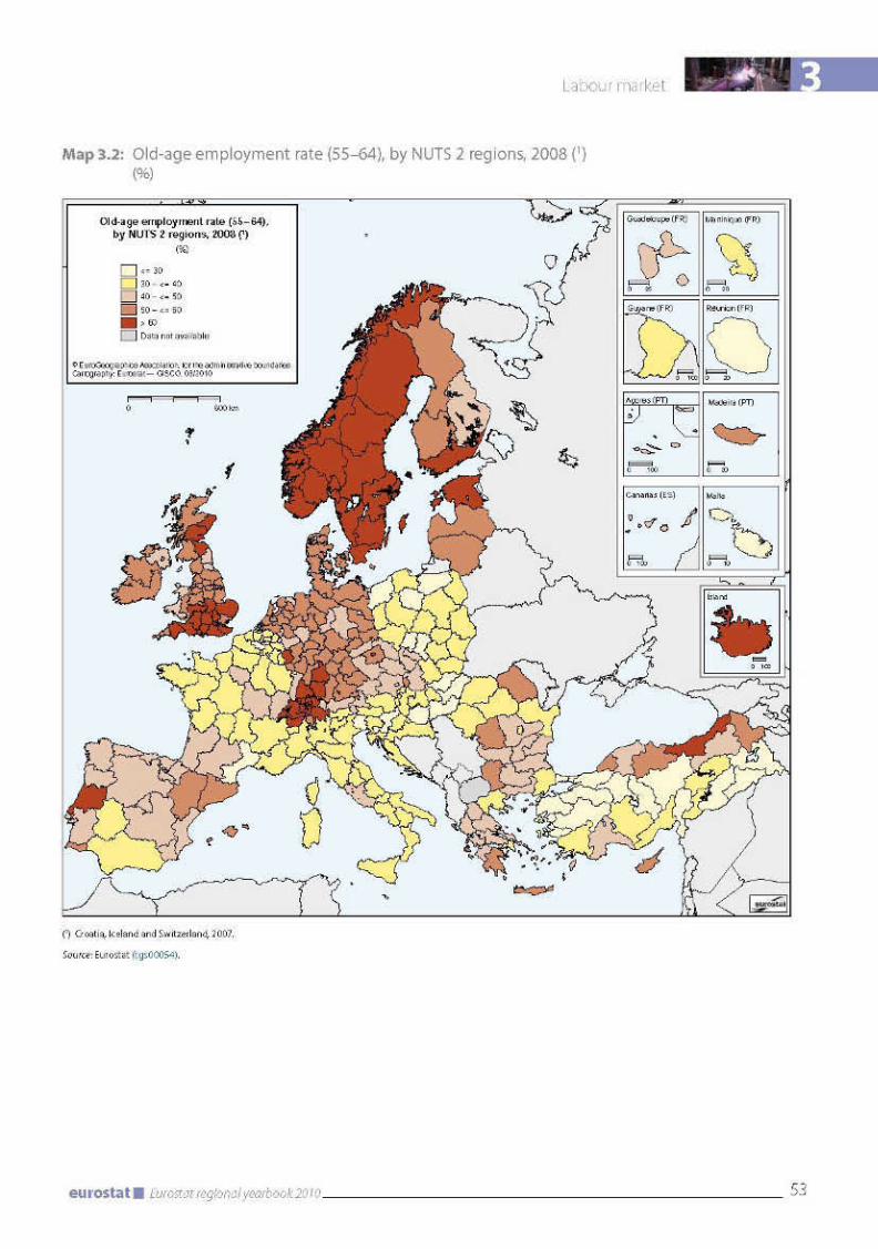
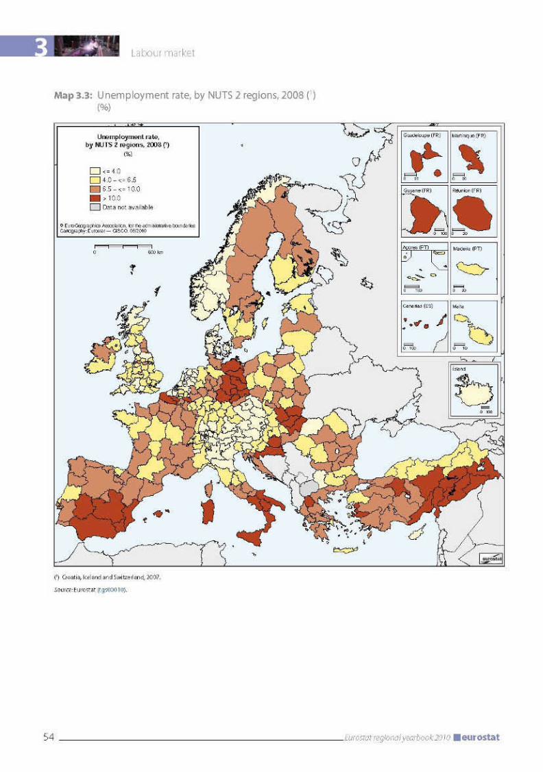
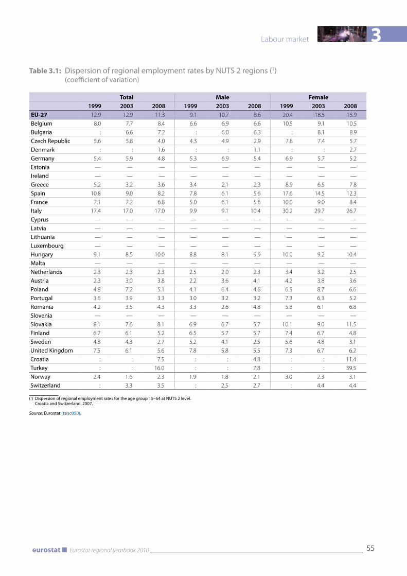
3
55Eurostat regional yearbook 2010eurostat
Labour market
Table 3.1: Dispersion of regional employment rates by NUTS 2 regions (1) (coefficient of variation)
Total Male Female1999 2003 2008 1999 2003 2008 1999 2003 2008
EU-27 12.9 12.9 11.3 9.1 10.7 8.6 20.4 18.5 15.9
Belgium 8.0 7.7 8.4 6.6 6.9 6.6 10.5 9.1 10.5
Bulgaria : 6.6 7.2 : 6.0 6.3 : 8.1 8.9
Czech Republic 5.6 5.8 4.0 4.3 4.9 2.9 7.8 7.4 5.7
Denmark : : 1.6 : : 1.1 : : 2.7
Germany 5.4 5.9 4.8 5.3 6.9 5.4 6.9 5.7 5.2
Estonia — — — — — — — — —
Ireland — — — — — — — — —
Greece 5.2 3.2 3.6 3.4 2.1 2.3 8.9 6.5 7.8
Spain 10.8 9.0 8.2 7.8 6.1 5.6 17.6 14.5 12.3
France 7.1 7.2 6.8 5.0 6.1 5.6 10.0 9.0 8.4
Italy 17.4 17.0 17.0 9.9 9.1 10.4 30.2 29.7 26.7
Cyprus — — — — — — — — —
Latvia — — — — — — — — —
Lithuania — — — — — — — — —
Luxembourg — — — — — — — — —
Hungary 9.1 8.5 10.0 8.8 8.1 9.9 10.0 9.2 10.4
Malta — — — — — — — — —
Netherlands 2.3 2.3 2.3 2.5 2.0 2.3 3.4 3.2 2.5
Austria 2.3 3.0 3.8 2.2 3.6 4.1 4.2 3.8 3.6
Poland 4.8 7.2 5.1 4.1 6.4 4.6 6.5 8.7 6.6
Portugal 3.6 3.9 3.3 3.0 3.2 3.2 7.3 6.3 5.2
Romania 4.2 3.5 4.3 3.3 2.6 4.8 5.8 6.1 6.8
Slovenia — — — — — — — — —
Slovakia 8.1 7.6 8.1 6.9 6.7 5.7 10.1 9.0 11.5
Finland 6.7 6.1 5.2 6.5 5.7 5.7 7.4 6.7 4.8
Sweden 4.8 4.3 2.7 5.2 4.1 2.5 5.6 4.8 3.1
United Kingdom 7.5 6.1 5.6 7.8 5.8 5.5 7.3 6.7 6.2
Croatia : : 7.5 : : 4.8 : : 11.4
Turkey : : 16.0 : : 7.8 : : 39.5
Norway 2.4 1.6 2.3 1.9 1.8 2.1 3.0 2.3 3.1
Switzerland : 3.3 3.5 : 2.5 2.7 : 4.4 4.4
(1) Dispersion of regional employment rates for the age group 15–64 at NUTS 2 level. Croatia and Switzerland, 2007.
Source: Eurostat (tsisc050).
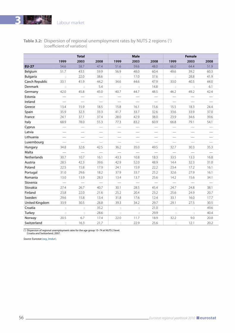
3 Labour market
56 Eurostat regional yearbook 2010 eurostat
Table 3.2: Dispersion of regional unemployment rates by NUTS 2 regions (1) (coefficient of variation)
Total Male Female1999 2003 2008 1999 2003 2008 1999 2003 2008
EU-27 54.6 58.7 47.4 51.6 59.6 48.0 66.0 64.4 51.9
Belgium 51.7 43.5 59.9 56.9 48.0 60.4 49.6 39.2 60.3
Bulgaria : 22.0 38.6 : 17.0 37.6 : 28.8 41.9
Czech Republic 33.1 41.9 44.2 34.6 44.6 47.9 33.0 40.5 44.0
Denmark : : 5.4 : : 14.8 : : 6.1
Germany 42.0 45.8 45.0 40.7 44.7 48.5 46.2 49.2 42.4
Estonia — — — — — — — — —
Ireland — — — — — — — — —
Greece 13.4 15.9 18.5 15.8 16.1 15.6 15.5 18.3 24.4
Spain 35.9 32.3 33.3 41.7 33.7 32.6 33.6 33.9 37.0
France 24.1 37.1 37.4 28.0 42.9 38.0 23.9 34.6 39.6
Italy 68.9 78.0 55.3 77.3 83.2 60.9 66.8 79.1 54.1
Cyprus — — — — — — — — —
Latvia — — — — — — — — —
Lithuania — — — — — — — — —
Luxembourg — — — — — — — — —
Hungary 34.8 32.6 42.5 36.2 35.0 49.5 32.7 30.3 35.3
Malta — — — — — — — — —
Netherlands 30.7 10.7 16.1 43.3 10.8 18.3 33.5 13.3 16.8
Austria 28.5 42.3 39.6 42.9 52.0 48.9 14.4 32.3 31.0
Poland 22.5 15.8 17.9 24.1 15.9 22.2 23.4 17.2 16.1
Portugal 31.0 29.6 18.2 37.9 33.7 25.2 32.6 27.9 16.1
Romania 13.0 13.9 28.3 13.4 13.7 25.6 14.2 15.6 34.1
Slovenia — — — — — — — — —
Slovakia 27.4 26.7 40.7 30.1 28.5 45.4 24.7 24.8 38.1
Finland 23.8 22.0 21.6 25.2 20.4 23.2 25.6 24.9 20.7
Sweden 29.6 15.8 13.4 31.8 17.6 12.4 33.1 16.0 17.7
United Kingdom 33.9 30.5 28.8 39.3 34.2 29.7 29.1 27.5 30.5
Croatia : : 35.2 : : 21.0 : : 49.6
Turkey : : 28.6 : : 29.9 : : 40.4
Norway 20.5 6.7 17.4 22.0 11.7 18.9 32.2 9.0 20.8
Switzerland : 16.3 21.7 : 22.9 25.6 : 12.1 20.2
(1) Dispersion of regional unemployment rates for the age group 15–74 at NUTS 2 level. Croatia and Switzerland, 2007.
Source: Eurostat (reg_lmdur).
3
57Eurostat regional yearbook 2010eurostat
Labour market
and also because it is still the country’s actual performance that mainly determines the levels of employment and unemployment. Ultimately, however, the outcome will depend on the ability of the regions to respond to the crisis and on their ability to take advantage, at a local level, of the various measures already put in place to curb the economic downturn.
Regional sector specialisation
Regional sector specialisation is broadly under-stood to be the extent to which particular eco-nomic sectors attract larger shares of employ-ment or output in one region as compared with another.
The sectoral composition of the regional economy affects employment patterns in several ways. For example, sectors have different rates of growth in production and demand, different employment intensities, different regulations and policies, different capital intensity or different patterns of technological change. All of these factors will influence employment in each sector differently.
Two regions belonging to the same country with similar macroeconomic conditions can have different employment patterns which can be partly explained by their degree of specialisation in the different sectors.
Regions have differing degrees of sector specialisation and, therefore, a comparison of regional labour markets which takes into account their sector composition can shed some light on the analysis.
In order to take into account the degree of sector specialisation, the first question to answer is about how this factor can be measured in a given region.
Several approaches are found in the literature, but probably the most widely used is the location quotient approach, which compares the local economy with a reference economy, in an attempt to identify specialisations in the former. The location quotient is defined as the ratio between the share of regional employment in one sector and the share of employment in that same sector in the reference economy.
The reference economy could be either the EU as a whole or the national economy of which
that region is part. In this text, each region is compared with its respective country, since there are different levels of technology in the various Member States, which entail different employment intensities for the same sector in different countries. As such, comparing regions with the EU average would take precedence over the different levels of technology. This choice between EU economy and national economy inevitably gave rise to a new problem, namely that it is impossible to compute the location quotients for Member States with a single NUTS 2 region, like Luxembourg or Malta. Further on in the text, we will postulate a different approach to deal with these Member States.
The location quotient for a specific sector and a specific region is greater than 1.0 when employ-ment in that sector tends to be over-represented in that region, and is therefore regarded as being specialised in that sector. If the location quotient is less than 1.0, local employment is less than is expected for that given sector. Therefore, that sector is not even meeting the local demands for the particular goods or services.
The underlying data used to cluster regions according the degree of specialisation are data on employment by economic activity, at NUTS levels 1 and 2 according to NACE Rev. 1.1. This is not the most recent version of NACE (the statistical classification of economic activities in the European Community), but since only three sectors were used (agriculture and fisheries, industry and services) there are no significant changes to the most recent version. In addition, longer time series are available in the old NACE classification at regional level.
The Labour Force Survey measures resident employment. For regions with high levels of commuters, i.e. employed persons who work in a different region from where they live, the location quotient based on resident employment may be quite different from the one obtained using domestic employment. Nevertheless, three things attenuate this difference in the analysis that is being carried out. First, there is, in general, a very high share of persons who work in the same NUTS 2 region as that in which they live. Second, only three sectors are taken into account (a more detailed analysis would be more exposed to the fact that resident employment is being used instead of domestic employment). Third, the purpose of the exercise is to create only a rough and approximate classification that should not be taken as a definitive indicator of sector specialisation.

3 Labour market
58 Eurostat regional yearbook 2010 eurostat
Given the share of employed persons working in agriculture and fisheries, industry and services, location quotients for each of these sectors were computed for each NUTS 2 region.
Several model-based statistical clustering techniques were used and the number of clusters was chosen according to the Bayesian Information Criteria. Five clusters were identified as the best choice for this data set. Each of the five clusters was characterised according to its main characteristics and this classification has been used as the starting point for grouping the NUTS 2 regions in different clusters.
Another alternative approach was to look at each region’s location quotients for agriculture, industry and services, and to decide on the minimum threshold at which a region was to be considered as specialised in a particular sector. The chosen threshold was 1.1, which means that if a region has, for example, a location quotient in agriculture of 1.1 or higher, it is labelled as being specialised in agriculture, since the relative share of employment in agriculture is at least 10 % higher than the country average. If that location quotient was less than 0.9, the region was considered as being under-represented in agriculture, while regions with location quotients between 0.9 and 1.1 were considered to be ‘balanced’.
Since the most suitable number of clusters identified for this data set was five, regions have been classified into one of the following five categories:
• specialised in services: location quotient of services greater than 1.1 and location quotients of agriculture and industry below 0.9; • specialised in industry: location quotient of industry greater than 1.1 and location quotients in agriculture and services below 1.1; • specialised in agriculture and industry: lo-cation quotients of agriculture and industry greater than 1.1 and location quotient of ser-vices below 1.1; • specialised in agriculture: location quotient of agriculture greater than 1.1 and location quo-tients of industry and services below 1.1; • balanced: all the remaining regions, i.e. no location quotients on agriculture, industry or services below 1.1.
The classification described above bears some similarity to the classification obtained using the model-based clustering technique described above.
Since this latter approach for clustering gives similar results to the clusters obtained using the more complex model-based cluster techniques, the first approach was chosen. The classification rules are easy to understand and the results are similar to those obtained using more advanced cluster techniques.
Finally, countries with only one or two NUTS 2 regions, such as Luxembourg or Ireland, were included in the most similar cluster, i.e. the one which has the closest distance between the region’s location quotients to be classified and the cluster average.
The classification resulting from this method is presented in Map 3.4.
As expected, the majority of the NUTS 2 regions in which the capital city of the respective country is located were classified as specialised in services. A closer examination of how sector specialisation is distributed geographically enables us to identify a well-defined distribution of sectors in some Member States. Hungary is divided in half, with the south-east regions specialising in agriculture and the north-west regions specialising in industry; the exception is the region of Közép-Magyarország, which includes the capital city of Budapest and specialises in services.
Italy also shows a well-defined distribution of sector specialisation, with the southern regions specialised in agriculture, and the northern regions mainly dominated by industry. Eastern Germany is basically dominated by agriculture, except for the region of Berlin, which is specialised in services; western Germany, on the other hand, is mainly dominated by services and industry.
Clustering regions according to the type of sector specialisation can now be used in regional labour market analysis. As mentioned previously, the composition of the sector can have a significant influence on regional employment patterns, and taking this factor into account will provide an additional perspective for the analysis.
High education levels in the regional labour market
To demonstrate more clearly the usefulness and relevance of taking account of sector specialisation in regional labour markets, this section will look
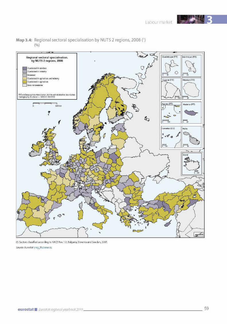
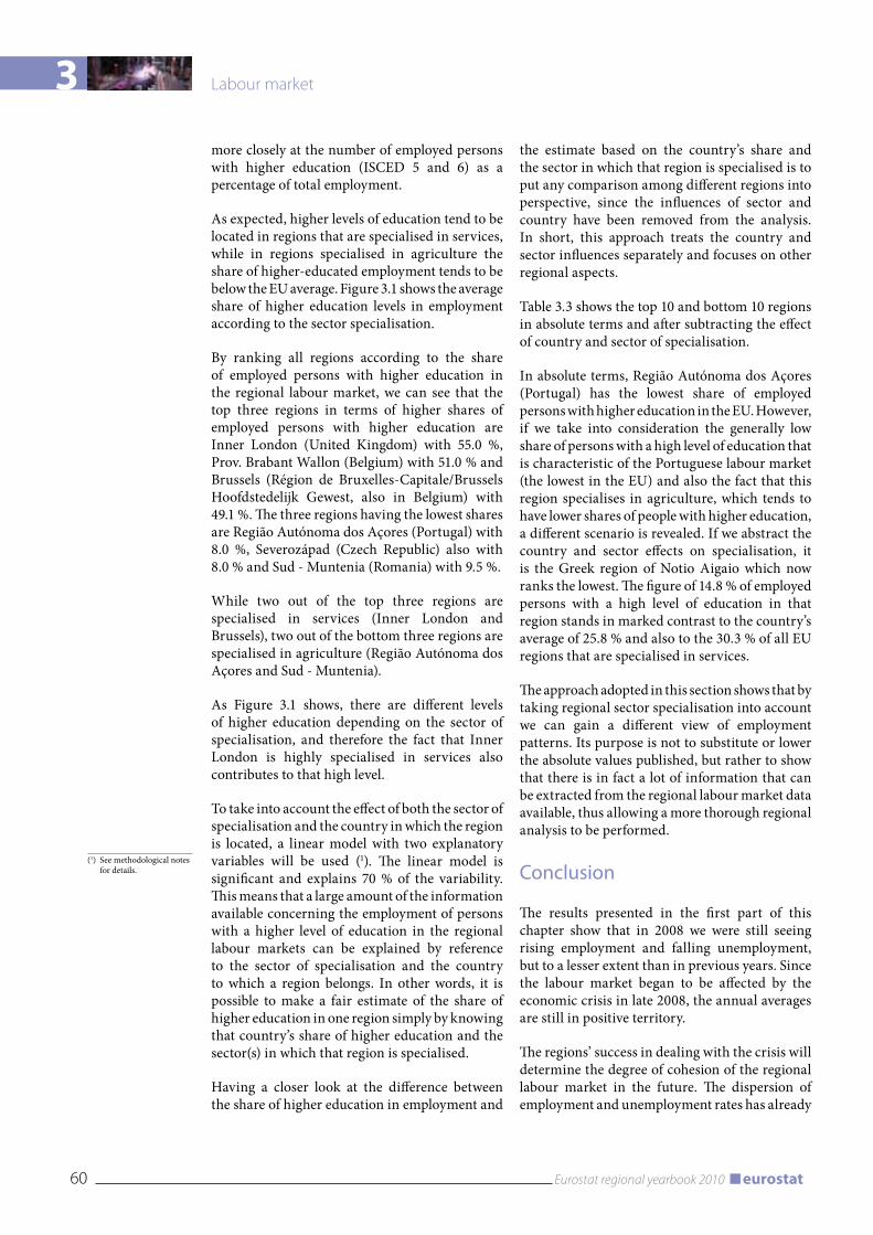
3 Labour market
60 Eurostat regional yearbook 2010 eurostat
more closely at the number of employed persons with higher education (ISCED 5 and 6) as a percentage of total employment.
As expected, higher levels of education tend to be located in regions that are specialised in services, while in regions specialised in agriculture the share of higher-educated employment tends to be below the EU average. Figure 3.1 shows the average share of higher education levels in employment according to the sector specialisation.
By ranking all regions according to the share of employed persons with higher education in the regional labour market, we can see that the top three regions in terms of higher shares of employed persons with higher education are Inner London (United Kingdom) with 55.0 %, Prov. Brabant Wallon (Belgium) with 51.0 % and Brussels (Région de Bruxelles-Capitale/Brussels Hoofdstedelijk Gewest, also in Belgium) with 49.1 %. The three regions having the lowest shares are Região Autónoma dos Açores (Portugal) with 8.0 %, Severozápad (Czech Republic) also with 8.0 % and Sud - Muntenia (Romania) with 9.5 %.
While two out of the top three regions are specialised in services (Inner London and Brussels), two out of the bottom three regions are specialised in agriculture (Região Autónoma dos Açores and Sud - Muntenia).
As Figure 3.1 shows, there are different levels of higher education depending on the sector of specialisation, and therefore the fact that Inner London is highly specialised in services also contributes to that high level.
To take into account the effect of both the sector of specialisation and the country in which the region is located, a linear model with two explanatory variables will be used (1). The linear model is significant and explains 70 % of the variability. This means that a large amount of the information available concerning the employment of persons with a higher level of education in the regional labour markets can be explained by reference to the sector of specialisation and the country to which a region belongs. In other words, it is possible to make a fair estimate of the share of higher education in one region simply by knowing that country’s share of higher education and the sector(s) in which that region is specialised.
Having a closer look at the difference between the share of higher education in employment and
the estimate based on the country’s share and the sector in which that region is specialised is to put any comparison among different regions into perspective, since the influences of sector and country have been removed from the analysis. In short, this approach treats the country and sector influences separately and focuses on other regional aspects.
Table 3.3 shows the top 10 and bottom 10 regions in absolute terms and after subtracting the effect of country and sector of specialisation.
In absolute terms, Região Autónoma dos Açores (Portugal) has the lowest share of employed persons with higher education in the EU. However, if we take into consideration the generally low share of persons with a high level of education that is characteristic of the Portuguese labour market (the lowest in the EU) and also the fact that this region specialises in agriculture, which tends to have lower shares of people with higher education, a different scenario is revealed. If we abstract the country and sector effects on specialisation, it is the Greek region of Notio Aigaio which now ranks the lowest. The figure of 14.8 % of employed persons with a high level of education in that region stands in marked contrast to the country’s average of 25.8 % and also to the 30.3 % of all EU regions that are specialised in services.
The approach adopted in this section shows that by taking regional sector specialisation into account we can gain a different view of employment patterns. Its purpose is not to substitute or lower the absolute values published, but rather to show that there is in fact a lot of information that can be extracted from the regional labour market data available, thus allowing a more thorough regional analysis to be performed.
Conclusion
The results presented in the first part of this chapter show that in 2008 we were still seeing rising employment and falling unemployment, but to a lesser extent than in previous years. Since the labour market began to be affected by the economic crisis in late 2008, the annual averages are still in positive territory.
The regions’ success in dealing with the crisis will determine the degree of cohesion of the regional labour market in the future. The dispersion of employment and unemployment rates has already
(1) See methodological notes for details.
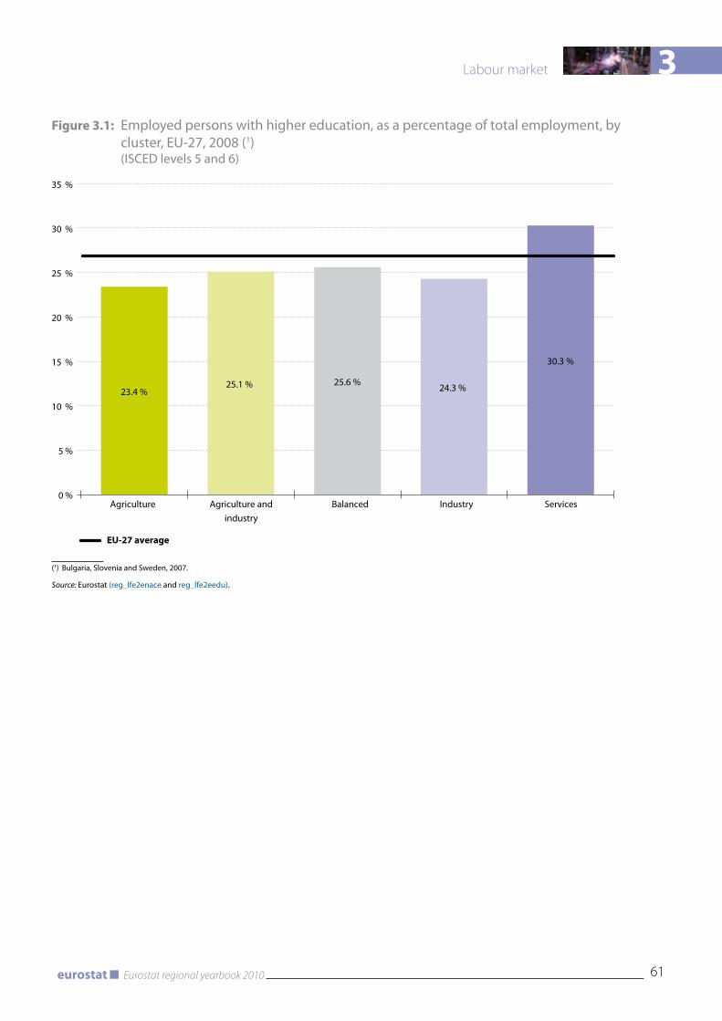
3
61Eurostat regional yearbook 2010eurostat
Labour market
Figure 3.1: Employed persons with higher education, as a percentage of total employment, by cluster, EU-27, 2008 (1) (ISCED levels 5 and 6)
23.4 %25.1 % 25.6 % 24.3 %
30.3 %
0 %
5 %
10 %
15 %
20 %
25 %
30 %
35 %
Agriculture
EU-27 average
Agriculture andindustry
Balanced Industry Services
(1) Bulgaria, Slovenia and Sweden, 2007.
Source: Eurostat (reg_lfe2enace and reg_lfe2eedu).
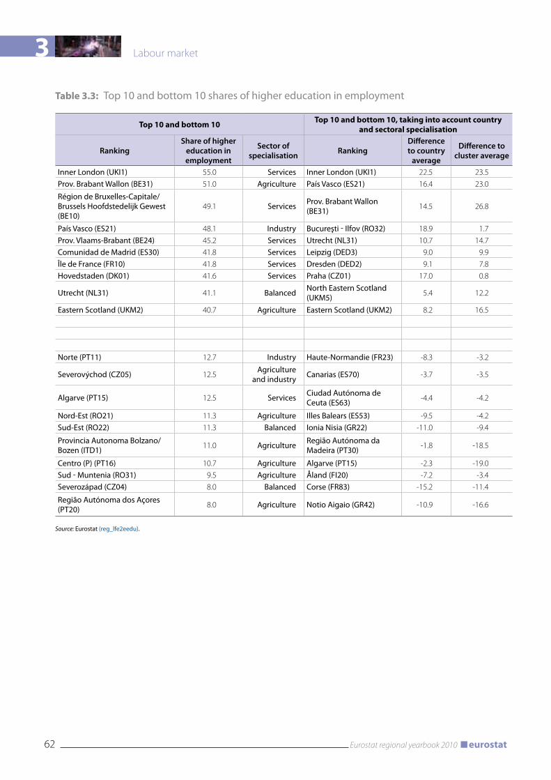
3 Labour market
62 Eurostat regional yearbook 2010 eurostat
Table 3.3: Top 10 and bottom 10 shares of higher education in employment
Top 10 and bottom 10 Top 10 and bottom 10, taking into account country and sectoral specialisation
RankingShare of higher
education in employment
Sector of specialisation Ranking
Difference to country
average
Difference to cluster average
Inner London (UKI1) 55.0 Services Inner London (UKI1) 22.5 23.5
Prov. Brabant Wallon (BE31) 51.0 Agriculture País vasco (ES21) 16.4 23.0
Région de Bruxelles-Capitale/ Brussels Hoofdstedelijk Gewest (BE10)
49.1 Services Prov. Brabant Wallon (BE31) 14.5 26.8
País vasco (ES21) 48.1 Industry Bucureşti - Ilfov (RO32) 18.9 1.7
Prov. vlaams-Brabant (BE24) 45.2 Services Utrecht (NL31) 10.7 14.7
Comunidad de Madrid (ES30) 41.8 Services Leipzig (DED3) 9.0 9.9
Île de France (FR10) 41.8 Services Dresden (DED2) 9.1 7.8
Hovedstaden (DK01) 41.6 Services Praha (CZ01) 17.0 0.8
Utrecht (NL31) 41.1 Balanced North Eastern Scotland (UKM5) 5.4 12.2
Eastern Scotland (UKM2) 40.7 Agriculture Eastern Scotland (UKM2) 8.2 16.5
Norte (PT11) 12.7 Industry Haute-Normandie (FR23) -8.3 -3.2
Severovýchod (CZ05) 12.5Agriculture
and industry Canarias (ES70) -3.7 -3.5
Algarve (PT15) 12.5 Services Ciudad Autónoma de Ceuta (ES63) -4.4 -4.2
Nord-Est (RO21) 11.3 Agriculture Illes Balears (ES53) -9.5 -4.2
Sud-Est (RO22) 11.3 Balanced Ionia Nisia (GR22) -11.0 -9.4
Provincia Autonoma Bolzano/Bozen (ITD1) 11.0 Agriculture Região Autónoma da
Madeira (PT30) -1.8 -18.5
Centro (P) (PT16) 10.7 Agriculture Algarve (PT15) -2.3 -19.0
Sud - Muntenia (RO31) 9.5 Agriculture Åland (FI20) -7.2 -3.4
Severozápad (CZ04) 8.0 Balanced Corse (FR83) -15.2 -11.4
Região Autónoma dos Açores (PT20) 8.0 Agriculture Notio Aigaio (GR42) -10.9 -16.6
Source: Eurostat (reg_lfe2eedu).
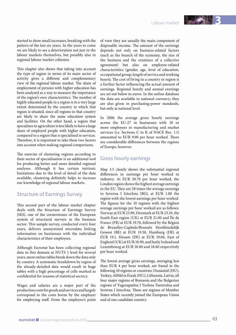
3
63Eurostat regional yearbook 2010eurostat
Labour market
started to show small increases, breaking with the pattern of the last six years. In the years to come we are likely to see a deterioration not just in the labour markets themselves, but possibly also in regional labour market cohesion.
This chapter also shows that taking into account the type of region in terms of its main sector of activity gives a different and complementary view of the regional labour market. The share of employment of persons with higher education has been analysed as a way to measure the importance of the region’s own characteristics. The number of highly educated people in a region is to a very large extent determined by the country in which that region is situated, since all regions in that country are likely to share the same education system and facilities. On the other hand, a region that specialises in agriculture is less likely to have a large share of employed people with higher education, compared to a region that is specialised in services. Therefore, it is important to take these two factors into account when making regional comparisons.
The exercise of clustering regions according to their sector of specialisation is an additional tool for producing better and more detailed regional analyses. Although it has certain intrinsic limitations due to the level of detail of the data available, clustering definitely helps to increase our knowledge of regional labour markets.
Structure of Earnings Survey
This second part of the labour market chapter deals with the Structure of Earnings Survey (SES), one of the cornerstones of the European system of structural surveys in the business sector. This sample survey, conducted every four years, delivers anonymised microdata linking information on businesses with the individual characteristics of their employees.
Although Eurostat has been collecting regional data in this domain at NUTS 1 level for several years, most online tables break down the data only by country. A systematic breakdown by region of the already-detailed data would result in huge tables with a high percentage of cells marked as confidential for reasons of statistical secrecy.
Wages and salaries are a major part of the production costs for goods and services and largely correspond to the costs borne by the employer for employing staff. From the employee’s point
of view they are usually the main component of disposable income. The amount of the earnings depends not only on business-related factors (such as the branch of the economy, the size of the business and the existence of a collective agreement) but also on employee-related characteristics (gender, age, level of education, occupational group, length of service and working hours). The cost of living in a country or region is a further factor influencing the actual amount of earnings. Regional hourly and annual earnings are set out below in euros. In the online database the data are available in national currency; they are also given in purchasing-power standards, but only at national level.
In 2006 the average gross hourly earnings across the EU-27 in businesses with 10 or more employees in manufacturing and market services (i.e. Sections C to K of NACE Rev. 1.1) amounted to EUR 9.90 per hour worked. There are considerable differences between the regions of Europe, however.
Gross hourly earnings
Map 3.5 clearly shows the substantial regional differences in earnings per hour worked in industry. At EUR 28.70 per hour worked, the London region shows the highest average earnings in the EU. They are 28 times the average earnings in Severna I Iztochna (BG), at EUR 1.00 the region with the lowest earnings per hour worked. The figures for the 10 regions with the highest average earnings per hour worked are as follows: Norway at EUR 23.90, Denmark at EUR 23.10, the South-East region (UK) at EUR 21.00 and Île de France (FR) at EUR 19.70, followed by the Région de Bruxelles-Capitale/Brussels Hoofdstedelijk Gewest (BE) at EUR 19.50, Hamburg (DE) at EUR 19.1, Hessen (DE) at EUR 19.00, East of England (UK) at EUR 18.90, and lastly Ireland and Luxembourg at EUR 18.80 and 18.60 respectively per hour worked.
The lowest average gross earnings, averaging less than EUR 4 per hour worked, are found in the following 10 regions or countries: Dunántúl (HU), Turkey, Alföld és Észak (HU), Lithuania, Latvia, all four major regions of Romania and the Bulgarian regions of Yugozapadna I Yuzhna Tsentralna and Severna I Iztochna. These are regions of Member States which recently joined the European Union and of one candidate country.
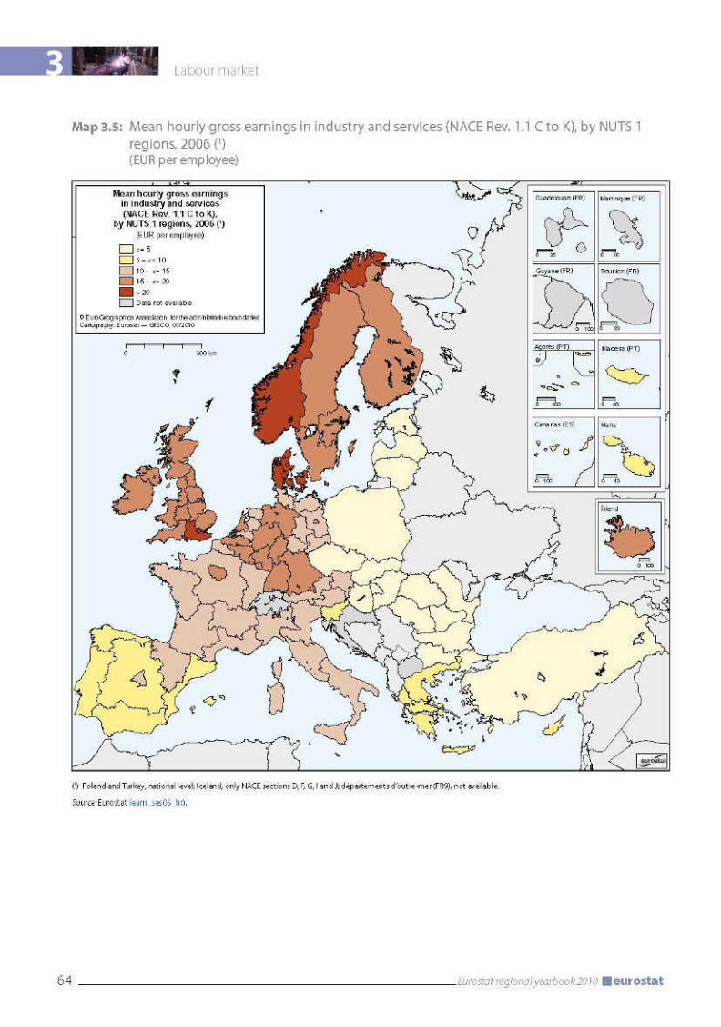

3
65Eurostat regional yearbook 2010eurostat
Labour market
Gross annual earnings
In 2006 the average gross annual earnings across the EU-27 amounted to EUR 29 400, but there were significant regional differences. Map 3.6 shows the regional differences in average gross annual earnings per employee in manufacturing and market services within the European Union. It should be noted that gross annual earnings include extraordinary payments, which are not included in the hourly earnings described above. Annual earnings include, for example, 13th and 14th month wages and salaries, productivity bonuses, profit shares and payments in kind. The regions or countries with the highest hourly earnings, in descending order, are London, Iceland, Norway and Région de Bruxelles-Capitale/Brussels Hoofdstedelijk Gewest (BE), whereas those with the highest annual earnings are London, Norway, Denmark and the South East (UK). A comparison of Maps 3.5 and 3.6 clearly illustrates this difference where certain regions are concerned. In 2006 the London region (UK) was the absolute leader with an average gross annual earnings rate of EUR 72 000, followed by the Belgian regions of Bruxelles-Capitale/Brussels Hoofdstedelijk Gewest and Vlaams Gewest, Luxembourg, the three German Länder Baden-Württemberg, Hessen and Hamburg, Denmark, the regions of Île de France (FR), West-Nederland (NL) and East of England (UK) and Ireland, all showing figures of over EUR 40 000. Average gross annual earnings in the Nordic countries of Iceland and Norway amount to more than EUR 47 000.
At the other end of the scale, average earnings are less than EUR 10 000 per year in the Bulgarian regions of Severna I Iztochna and Yugozapadna I Yuzhna Tsentralna, in all regions of Romania, in Lithuania and Latvia, in the Hungarian regions of Alföld és Észak and Dunántúl, and in Estonia, Poland, the Czech Republic and Turkey.
Living costs, national legislation and national and regional customs concerning working time, which can also vary from one sector of activity (hotels and restaurants, transport, construction) to another, are disregarded here, as are the average annual hours worked, which are also affected by the prevailing economic situation (full order books on the one hand, or short-time working and plant closures on the other).
Annual bonuses as a percentage of annual earnings
Map 3.7 gives an idea of the shares of bonuses and extraordinary allowances in gross annual earnings in industry and services in the various regions in 2006. This comparison too must be seen against the background of the specific economic, social and cultural circumstances. There is a fairly obvious north–south divide. The average shares of bonuses in annual earnings are relatively low in the northern Member States, at 7.5 %, for example in Scandinavia (Sweden, Denmark, Norway and the Ǻland region of Finland) and in Iceland, Mecklenburg-Vorpommern (DE), Poland and Estonia. In the south, only Malta and the Macroregiunea doi region of Romania show relatively low average bonus percentages.
The 10 regions with the highest shares of bonuses and extraordinary allowances (over 15.0 %) in gross annual earnings within the EU include all seven regions of Spain, above all the Comunidad de Madrid (17.9 %), the Portuguese region of Continente, the Greek region of Attiki and all three regions of Austria.
Figure 3.1 allows a more differentiated view of regional shares of bonuses in gross annual earnings by economic activity. Here, for example, the energy and water supply sector, mining and quarrying and specialist service companies in the financial sector, with relatively high bonus and allowance shares, and economic activities such as construction and hotels and restaurants, which are known to have relatively low bonus and allowance shares, are shown separately. Most of the 10 highest bonus share percentages (between 21 % and 29 %) are found in the financial intermediation branch and in the southern European regions (all seven regions of Spain and the Continente (PT), Alföld és Észak (HU) and London (UK) regions). When expressed in absolute values, however, the highest annual bonuses in this branch tend to be awarded in regions and countries which also have significant financial centres (all at more than EUR 13 000 per year). This is especially true of London (UK) at an average of over EUR 60 000, Hessen (DE), Ostösterreich (AT), Luxembourg and Iceland and the Comunidad de Madrid region (ES3).
The online database also shows multidimensional tables on earnings at national level (hourly and annual earnings, overtime payments, bonuses and
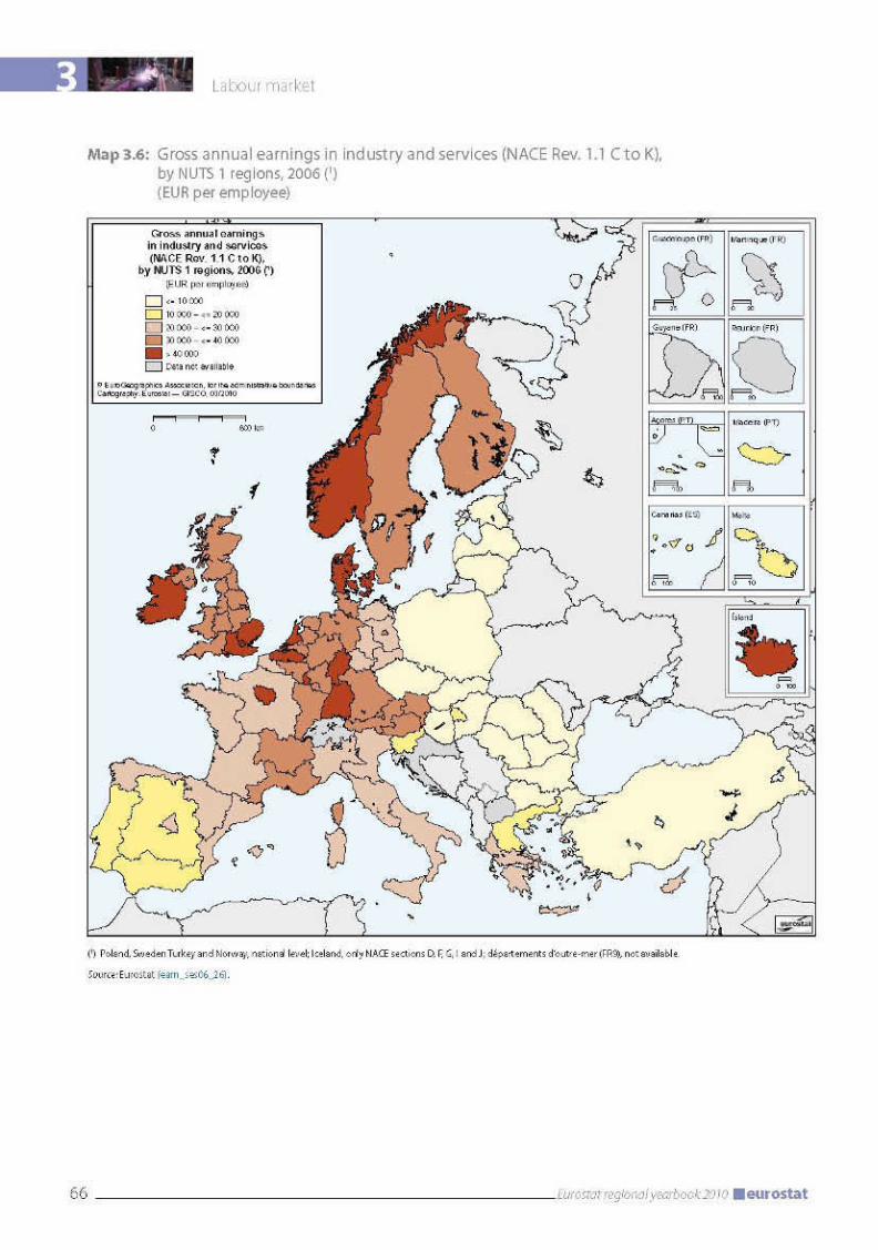

3 Labour market
68 Eurostat regional yearbook 2010 eurostat
allowances) broken down by further employee-related characteristics (e.g. occupational group, age group, gender, length of service, contractual working hours, employment contract, collective agreement) and by economic branch, size of company and economic control over the business.
Conclusion
The above description gives no more than an initial insight into the Structure of Earnings Survey. No attempt is made here to interpret the data using the many explanatory variables in the Eurostat online database. Interested readers may, however, wish to search through Eurostat’s extensive database according to their field of interest.
Figure 3.2: Regional divergences of annual bonuses as % of annual earnings, EU-27, 2006 (1)
0 % 5 %10 %15 % 20 % 25 % 30 % 35 % 40 % 45 % 50 % 55 % 60 % 65 %
NACE C-K: Industry and services Åland (FI2) Comunidad de Madrid (ES3)
NACE C: Mining and quarrying Polska (PL) North East (England) (UKC)
NACE D: Manufacturing Danmark (DK) Canarias (ES7)
NACE E: Electricity, gas and water supply Åland (FI2) Canarias (ES7)
Continente (PT1)
Polska (PL) Comunidad de Madrid (ES3)
NACE F: Construction Mecklenburg-Vorpommern (DE8)
NACE G: Wholesale and retail trade; repair of motorvehicles, motorcycles and personal and household goods
NACE H: Hotels and restaurants Nord - Pas-de-Calais (FR3) Sur (ES6)
NACE I: Transport, storage and communication Slovenská republika (SK) Comunidad de Madrid (ES3)
NACE J: Financial intermediation Danmark (DK) Centro (E) (ES4)
NACE K: Real estate, renting and business activities Danmark (DK) Canarias (ES7)
EU-27 average
(1) The graph shows the NUTS 1 region with the lowest and the highest annual bonuses (as % of annual earnings) by economic activity. Poland and Sweden, national level; départements d’outre-mer (FR9), not available.
Source: Eurostat (earn_ses06_rbns).
3
69Eurostat regional yearbook 2010eurostat
Labour market
Methodological notes
Labour Force Survey
The source for regional labour market information down to NUTS level 2 is the EU Labour Force Survey (LFS). This is a quarterly household sample survey conducted in the Member States of the European Union.
The LFS target population is made up of all members of private households aged 15 or over. The survey follows the definitions and recommendations of the International Labour Organisation (ILO). To achieve further harmonisation, the Member States also adhere to common principles on the construction of questionnaires.
All regional results presented here concern NUTS 2 regions and all regional figures are annual averages of the quarterly surveys.
For further information about regional labour market statistics, see the metadata on the Eurostat website (http://ec.europa.eu/eurostat).
Cluster analysis was conducted using model-based clustering techniques based on the Bayesian Information Criterion (BIC) in comprehensive strategies for clustering, density estimation and discriminant analysis.
A linear regression was used to check the amount of variability in regional higher education in the labour markets that is due to the country which that region belongs to and the predominant sector of activity. The dependent variable is the regional share of higher education and the independent variables are the country’s share of higher education and the cluster to which that region was assigned. The regression is significant with an adjusted R-squared of 70 %.
Structure of Earnings Survey
The source of information on regional earnings down to NUTS Level 1 is the EU Structure of Earnings Survey (SES). This survey is conducted every four years on the basis of Council Regulation (EC) No 530/1999 and Commission Regulation (EC) No 1738/2005.
The aim of this legislation is to make exact and comparable data on earnings in the EU Member States, the EFTA countries and the candidate countries available for policy and scientific purposes. The SES is a large-scale sample survey of businesses yielding detailed information on the relationships between the level of earnings (hourly and annual earnings, overtime payments, annual bonuses), the individual characteristics of employees (gender, age, length of service, occupation, level of education, contractual working hours, etc.) and the employer (branch of the economy, size and location of the business, etc.).
The survey’s population comprises all enterprises with 10 or more employees. Although in 2002 the scope of the survey was extended for the first time to the sectors M (Education), N (Health and social work) and O (Other community, social and personal service activities), we have confined ourselves here to sectors C to K, i.e. manufacturing and ‘market’ services, in the statistical classification of economic activities in the European Community (NACE Rev. 1.1).
It should be noted that earnings data are available only at national level for Poland, Sweden (data on annual earnings and bonuses only), Turkey and Norway. The same goes for a number of smaller Member States, where the NUTS 1 level corresponds to the whole country: Cyprus, the Czech Republic, Denmark, Estonia, Ireland, Latvia, Lithuania, Luxembourg, Malta, Slovakia and Slovenia. No earnings data are reported for France’s overseas departments. Data for Iceland and Norway are also available (here, too, the statistical region at NUTS 1 Level corresponds to the whole country).

3 Labour market
70 Eurostat regional yearbook 2010 eurostat
Eurostat publishes the most important data from the 2006 Structure of Earnings Survey in tabular form on the Eurostat website in the Labour Market Statistics section
http://epp.eurostat.ec.europa.eu/portal/page/portal/labour_market/earnings
under the Structure of Earnings Survey 2006 (earn_ses06) heading http://epp.eurostat.ec.europa.eu/ portal/page/portal/labour_market/earnings/database. Eurostat also provides anonymised microdata sets from the Structure of Earnings Survey in its ‘Safe Centre’:
http://epp.eurostat.ec.europa.eu/portal/page/portal/microdata/ses
It should be stressed here that the current legal framework allows access to the anonymised SES microdata available at Eurostat only for scientific purposes under special conditions and with due regard for statistical secrecy (cf: ‘Access to microdata’ http://epp.eurostat.ec.europa.eu/portal/page/portal/microdata/introduction).
Definitions
Labour Force Survey
Population covers persons aged 15 and over, living in private households (persons living in collective households, such as residential homes, boarding houses, hospitals, religious institutions and workers’ hostels, are therefore not included). This category comprises all persons living in the households surveyed during the reference week. The definition also includes persons who are absent from the households for short periods due to studies, holidays, illness, business trips, etc. (but who have maintained a link with the private household). Persons on compulsory military service are not included.
Employed persons are persons aged 15 years and over (16 years and over in Spain, United Kingdom and Sweden (1995–2001); 15–74 years in Denmark, Estonia, Hungary, Latvia, Finland, Sweden and Norway (from 2001 onwards); 16–74 years in Iceland) who during the reference week performed work, even for just one hour a week, for pay, profit or family gain or were not at work but had a job or business from which they were temporarily absent for example due to illness, holidays, industrial dispute and education and training.
Unemployed persons are persons aged 15–74 (in Spain, Sweden and Norway 1995–2000), and aged 16–74 in the United Kingdom and Iceland, who were without work during the reference week, were currently available for work and were either actively seeking work in the past four weeks or had already found a job to start within the next three months.
Employment rate represents employed persons as a percentage of the population.
Old-age employment rate represents employed persons aged 55–64 as a percentage of the population aged 55–64.
Unemployment rate represents unemployed persons as a percentage of the economically active population. The unemployment rate can be broken down further by age and sex. The youth unemployment rate relates to persons aged 15–24.
Dispersion of employment (unemployment) rates is the coefficient of variation of regional employment (unemployment) rates in a country, weighted by the absolute population (active population) of each region.
Location quotient expresses the relationship between an area’s share of a particular industry or sector and the national share.

3
71Eurostat regional yearbook 2010eurostat
Labour market
Structure of Earnings Survey
Average gross hourly earnings are equivalent to the gross earnings recorded in the reporting month divided by the corresponding number of paid working hours. Gross monthly earnings cover remuneration in cash paid by the employer in the reporting month before tax deductions and social security contributions payable by wage earners and retained by the employer. The following elements are included: all payments relating to this period (even if actually paid outside the representative month), including any overtime pay, shift premiums, overtime bonuses, allowances for teamwork, night work and weekend work, commissions, etc., bonuses and allowances paid regularly in each pay period, even if the amount varies from month to month, payments for periods of absence and work stoppages paid for entirely by the employer, family allowances and other gratuities in cash fixed by collective agreements or voluntarily agreed, and payments to employees’ saving schemes.
Gross annual earnings: Annual and monthly earnings differ primarily in that annual earnings are more than the sum of the direct remuneration, bonuses and allowances paid at every pay period. Thus they are usually more than the monthly standard pay package multiplied by 12. Annual earnings also include bonuses and allowances not paid at every pay period and payments in kind.
Annual bonuses and allowances: These are cash contributions not paid at every pay period, such as 13th or 14th month pay, holiday bonuses, quarterly or annual premiums, productivity bonuses linked to established targets, employee recognition awards, recruitment incentives, leaving or retirement bonuses and backdated arrears.


Gross domestic product

4 Gross domestic product
74 Eurostat regional yearbook 2010 eurostat
What is regional gross domestic product?
The economic development of a region is, as a rule, expressed in terms of its gross domestic product (GDP). This indicator is also frequently used as a basis for comparisons between regions. But what exactly does it mean? And how can comparability be established between regions of different sizes and with different currencies?
Regions of different sizes achieve different levels of regional GDP. However, a real comparison can be made only by comparing the regional GDP with the population of the region in question. This is where the distinction between place of work and place of residence becomes significant: GDP measures the economic output achieved within national or regional boundaries, regardless of whether this was attributable to resident or non-resident employed persons. The use of per inhabitant GDP is therefore only straightforward if all employed persons involved in generating GDP are also residents of the region in question.
In areas with a high proportion of commuters, regional per inhabitant GDP can be extremely high, particularly in business centres such as London or Luxembourg but also in Hamburg, Praha or Wien, and relatively low in the surrounding regions, even if households’ primary income in these regions is very high. Regional per inhabitant GDP should therefore not be equated with regional primary income.
Regional GDP is calculated in the currency of the country in question. In order to make GDP com-parable between countries, it is converted into eu-ros, using the official average exchange rate for the given calendar year. However, not all differences in price levels between countries are reflected by ex-change rates. To compensate for this, GDP is con-verted using conversion factors, known as purchas-ing power parities (PPPs), to an artificial common currency called the purchasing power standard (PPS). This makes it possible to compare the pur-chasing power of different national currencies (see methodological notes at the end of the chapter).
Regional GDP in 2007
Maps 4.1 and 4.2 provide an overview of the regional distribution of per inhabitant GDP (as a percentage of the EU-27 average of 24 900 PPS) for
the European Union, Croatia, the former Yugoslav Republic of Macedonia and Turkey which has, after a lengthy interruption, once again provided data (for reference years 2004–06) for the first time in line with the ESA transmission programme. The regions with the highest per inhabitant GDP are in southern Germany, in the south of the UK, in northern Italy and in Belgium, Luxembourg, the Netherlands, Austria, Ireland and Scandinavia. The capital regions Madrid, Paris and Praha also fall into this category. The weaker regions are concentrated at the southern, western and south-eastern periphery of the Union, in eastern Germany and the new Member States, Croatia, the former Yugoslav Republic of Macedonia and Turkey.
Within the EU-27, per inhabitant GDP ranges from 26 % of the EU-27 average (6 400 PPS) in Severozapaden in Bulgaria to 334 % (83 200 PPS) in the capital region of Inner London in the UK. The factor between the two ends of the distribution is therefore 13.1:1. Luxembourg at 275 % (68 500 PPS) and Brussels at 221 % (55 000 PPS) are in positions 2 and 3, followed by Hamburg at 192 % (47 800 PPS) and Praha at 172 % (42 800 PPS) in positions 4 and 5.
Praha (Czech Republic) thus remains by an increasing margin the region with the highest per inhabitant GDP in the new Member States; Bratislavský kraj (Slovakia) follows with 160 % (39 900 PPS) in position 12 of the 271 NUTS level 2 regions in the EU-27. However, these two regions must be regarded as exceptions among the regions in the new Member States which joined in 2004, since the next most prosperous regions in the new Member States are a long way behind: Zahodna Slovenija (Slovenia) at 107 % (26 600 PPS) in position 94, Közép-Magyarország (Hungary) at 103 % (25 600 PPS) in position 111 and Cyprus at 94 % (23 300 PPS) in position 146. With the exception of four other regions (Bucureşti–Ilfov in Romania, Mazowieckie in Poland, Malta and Střední Čechy in the Czech Republic), all the other regions of the new Member States have a per inhabitant GDP in PPS of less than 75 % of the EU-27 average.
Map 4.2 classifies the 271 EU regions according to their level of per inhabitant GDP (in PPS) in relation to the EU-27 average of 24 900 PPS per inhabitant. As a result, in 2007, GDP in 67 regions was less than 75 % of the EU-27 average. Some 24.4 % of the EU population live in these 67 regions, three quarters of them in new Member States and one quarter in EU-15 countries.
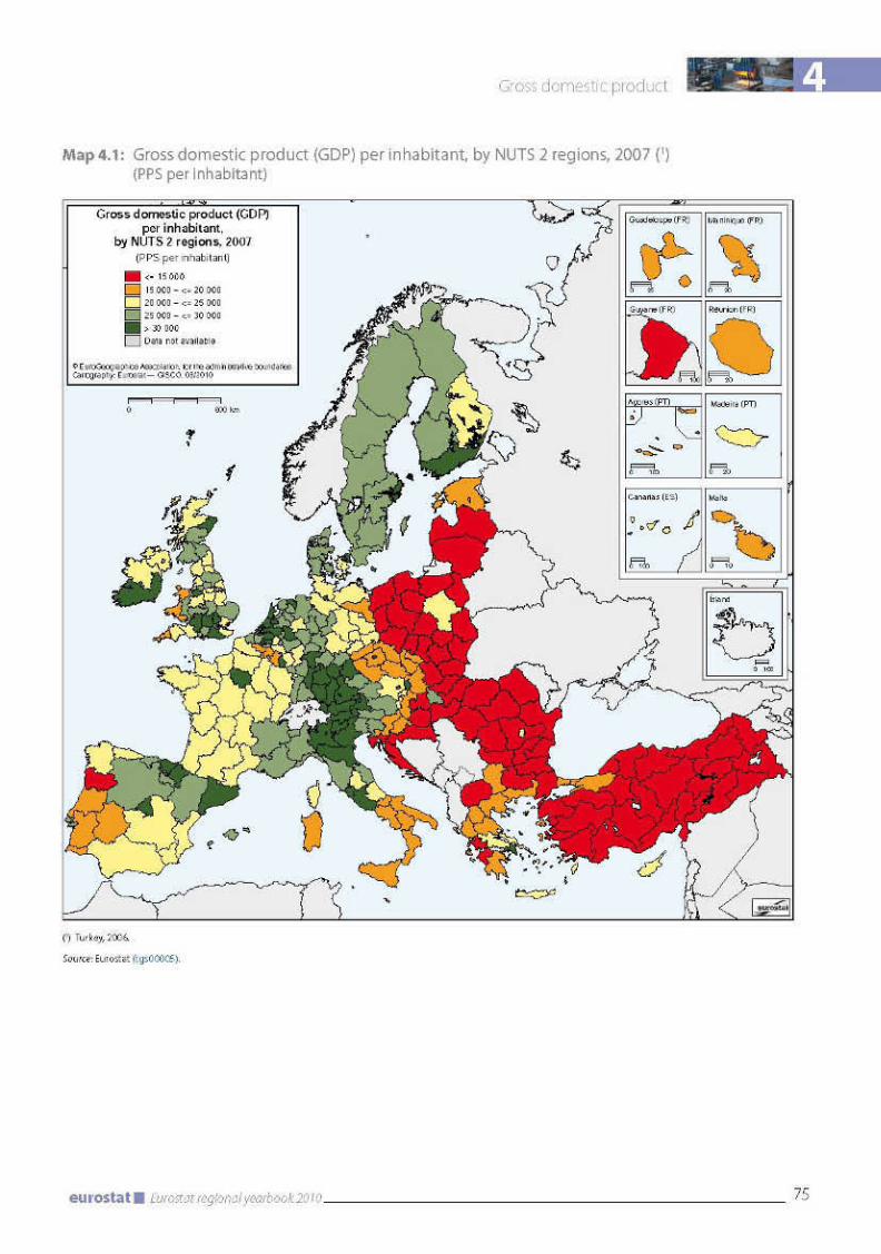

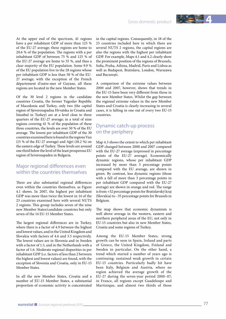
4
77Eurostat regional yearbook 2010eurostat
Gross domestic product
At the upper end of the spectrum, 41 regions have a per inhabitant GDP of more than 125 % of the EU-27 average; these regions are home to 20.6 % of the population. The regions with a per inhabitant GDP of between 75 % and 125 % of the EU-27 average are home to 55 %, and thus a clear majority of the EU population. Some 9.9 % of the EU population live in the 28 regions whose per inhabitant GDP is less than 50 % of the EU-27 average; with the exception of the French département d’outre-mer of Guyane, all these regions are located in the new Member States.
Of the 30 level 2 regions in the candidate countries Croatia, the former Yugoslav Republic of Macedonia and Turkey, only two (the capital region of Sjeverozapadna Hrvatska in Croatia and İstanbul in Turkey) are at a level close to three quarters of the EU-27 average; in a total of nine regions covering 41 % of the population of these three countries, the levels are over 50 % of the EU average. The lowest per inhabitant GDP of the 30 countries examined here is found in the regions Van (15 % of the EU-27 average) and Ağri (18.2 %) on the eastern edge of Turkey. These levels are around one third below the level of the least prosperous EU region of Severozapaden in Bulgaria.
Major regional differences even within the countries themselves
There are also substantial regional differences even within the countries themselves, as Figure 4.1 shows. In 2007, the highest per inhabitant GDP was more than twice the lowest in 14 of the 23 countries examined here with several NUTS 2 regions. This group includes seven of the nine new Member States/candidate countries but only seven of the 14 EU-15 Member States.
The largest regional differences are in Turkey, where there is a factor of 4.9 between the highest and lowest values, and in the United Kingdom and Slovakia with factors of 4.6 and 3.5 respectively. The lowest values are in Slovenia and in Sweden with a factor of 1.5, and in the Netherlands with a factor of 1.6. Moderate regional disparities in per inhabitant GDP (i.e. factors of less than 2 between the highest and lowest values) are found, with the exception of Slovenia and Croatia, only in EU-15 Member States.
In all the new Member States, Croatia and a number of EU-15 Member States, a substantial proportion of economic activity is concentrated
in the capital regions. Consequently, in 18 of the 23 countries included here in which there are several NUTS 2 regions, the capital regions are also the regions with the highest per inhabitant GDP. For example, Maps 4.1 and 4.2 clearly show the prominent position of the regions of Brussels, Sofia, Praha, Athina, Madrid, Paris and Lisboa as well as Budapest, Bratislava, London, Warszawa and Bucureşti.
A comparison of the extreme values between 2000 and 2007, however, shows that trends in the EU-15 have been very different from those in the new Member States. Whilst the gap between the regional extreme values in the new Member States and Croatia is clearly increasing in several cases, it is falling in one out of every two EU-15 countries.
Dynamic catch-up process on the periphery
Map 4.3 shows the extent to which per inhabitant GDP changed between 2000 and 2007 compared with the EU-27 average (expressed in percentage points of the EU-27 average). Economically dynamic regions, whose per inhabitant GDP increased by more than 3 percentage points compared with the EU average, are shown in green. By contrast, less dynamic regions (those with a fall of more than 3 percentage points in per inhabitant GDP compared with the EU-27 average) are shown in orange and red. The range is from +52 percentage points for Bratislavský kraj (Slovakia) to –35 percentage points for Brussels in Belgium.
The map shows that economic dynamism is well above average in the western, eastern and northern peripheral areas of the EU, not only in EU-15 countries but also in new Member States, Croatia and some regions of Turkey.
Among the EU-15 Member States, strong growth can be seen in Spain, Ireland and parts of Greece, the United Kingdom, Finland and Sweden in particular. On the other hand, a trend which started a number of years ago is continuing: sustained weak growth in certain EU-15 countries. Particularly badly hit have been Italy, Belgium and Austria, where no region achieved the average growth of the EU-27 during the seven-year period 2000–07; in France, all regions except Guadeloupe and Martinique, and almost two thirds of those
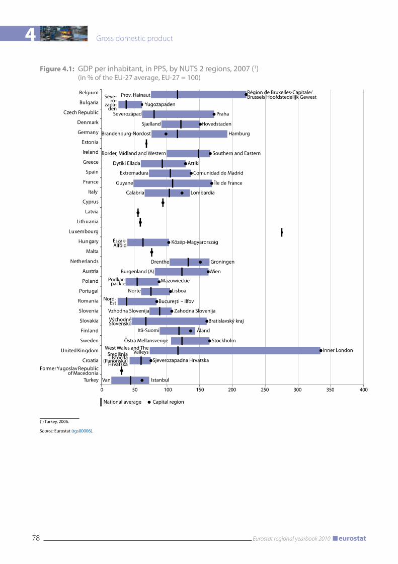
4 Gross domestic product
78 Eurostat regional yearbook 2010 eurostat
Figure 4.1: GDP per inhabitant, in PPS, by NUTS 2 regions, 2007 (1) (in % of the EU-27 average, EU-27 = 100)
0 50 100 150 200 250 300 350 400
Belgium
Bulgaria
Czech Republic
Denmark
Germany
Estonia
Ireland
Greece
Spain
France
Italy
Cyprus
Latvia
Lithuania
Luxembourg
Hungary
Malta
Netherlands
Austria
Poland
Portugal
Romania
Slovenia
Slovakia
Finland
Sweden
United Kingdom
CroatiaFormer Yugoslav Republic
of MacedoniaTurkey
National average Capital region
Prov. Hainaut Région de Bruxelles-Capitale/Brussels Hoofdstedelijk Gewest
Yugozapaden
Severozápad Praha
Sjælland Hovedstaden
Brandenburg-Nordost Hamburg
Border, Midland and Western
Dytiki Ellada Attiki
Southern and Eastern
Extremadura Comunidad de Madrid
Guyane Île de France
Calabria Lombardia
Észak-Alföld
Közép-Magyarország
Drenthe
Burgenland (A)
Groningen
Wien
Mazowieckie
Norte Lisboa
Bucureşti – Ilfov
Vzhodna Slovenija Zahodna Slovenija
Bratislavský kraj
Itä-Suomi Åland
Van Istanbul
Središnja i Istočna
(Panonska) Hrvatska
Östra Mellansverige Stockholm
Inner London
Sjeverozapadna Hrvatska
West Wales and The Valleys
Východné Slovensko
Nord-Est
Podkar-packie
Seve-ro-
zapa-den
(1) Turkey, 2006.
Source: Eurostat (tgs00006).


4 Gross domestic product
80 Eurostat regional yearbook 2010 eurostat
in Germany, fell against the EU average. In Portugal, only Alentejo and the islands achieved growth above the EU average.
Of the new Member States, apart from the very dynamic capital regions, the Baltic countries, Romania, the Czech Republic, Slovakia and most regions of Poland in particular have seen markedly above-average growth. Croatia, the former Yugoslav Republic of Macedonia and most of the Turkish regions also reveal above-average economic growth for the seven-year period 2000–07.
Closer analysis of the most dynamic regions shows that 36 EU regions have outperformed the EU average by more than 10 percentage points; of these, 20 are in the new Member States.
The 10 fastest-growing regions are spread over nine EU Member States. It is striking, however, that the capital regions continue to have an above-average rate of growth not only in the EU-15 countries but also in the new Member States. The non-capital region with the strongest growth in the new Member States was Vest (Romania), where per inhabitant GDP (in PPS) increased by 21.4 percentage points of the EU-27 average between 2000 and 2007.
A clear concentration in certain Member States is, on the other hand, apparent at the lower end of the distribution curve: of the 31 regions which fell by more than 10 percentage points below the EU-27 average, 15 are in Italy, four in Belgium and three in France.
Closer examination of the new Member States yields the pleasing result that, between 2000 and 2007, only three regions fell back compared with the EU-27 average: these are Malta (–7.2 percentage points), Nyugat-Dunántúl in Hungary (–1.3 percentage points) and Zachodniopomorskie in Poland (–0.2).
The trend in Turkey (2006 compared with 2000) was, on the other hand, fairly heterogeneous: by comparison with the EU, the catching-up process in certain western regions of Turkey was, as expected, particularly dynamic (specifically in İstanbul and Bursa); however, progress in individual regions in inland areas and in the east, such as in Kayseri and Ağri, has been above average. By contrast, other regions, particularly Adana on the eastern coast of the Mediterranean, have in some cases fallen substantially.
The catch-up process in the new Member States was of the order of 1.5 percentage points per year between 2000 and 2007 compared to the EU average, and therefore considerably faster than in the 1990s. Per inhabitant GDP (in PPS) in these 12 countries thus rose from 45 % of the EU-27 average in 2000 to 56 % in 2007. It is feared, however, that owing to the severe economic crisis of 2008 and 2009 this rate of growth will slow towards the end of the decade. However, the initial data available on certain Member States for 2008 and 2009 would suggest that the recession in rural regions and areas lagging behind in terms of economic development was less severe than in regions with a high per inhabitant GDP or with a high level of dependence on exports.
Different trends even within the countries themselves
A more detailed analysis of trends within the countries between 2000 and 2007 shows that the economic development of regions even within a country can be extremely divergent.
The greatest differences were seen in Slovakia, Greece, the Czech Republic and Belgium, where there was a difference of some 30 percentage points relative to the EU-27 average for per inhabitant GDP between the fastest- and slowest-growing regions. Slovenia and Denmark are at the lower end of the scale with 6 and 8 percentage points respectively. The highest and lowest values in the 26 regions of Turkey show a difference of 27 percentage points and thus fall within the upper fifth for the EU Member States.
In both new Member States and EU-15 countries, this significant divergence was the result mainly of dynamic growth in capital regions. However, as the relatively low values for Poland and Croatia in particular show, the data available do not confirm the assumption that such regional growth disparities are a typical feature of new Member States or accession countries.
The available data also show that even the least economically dynamic regions in 12 Member States attained levels of growth above the EU-27 average. It is pleasing to note that this was the case in all seven new Member States with at least two NUTS 2 regions. The same positive trend can be observed in Croatia and Turkey.
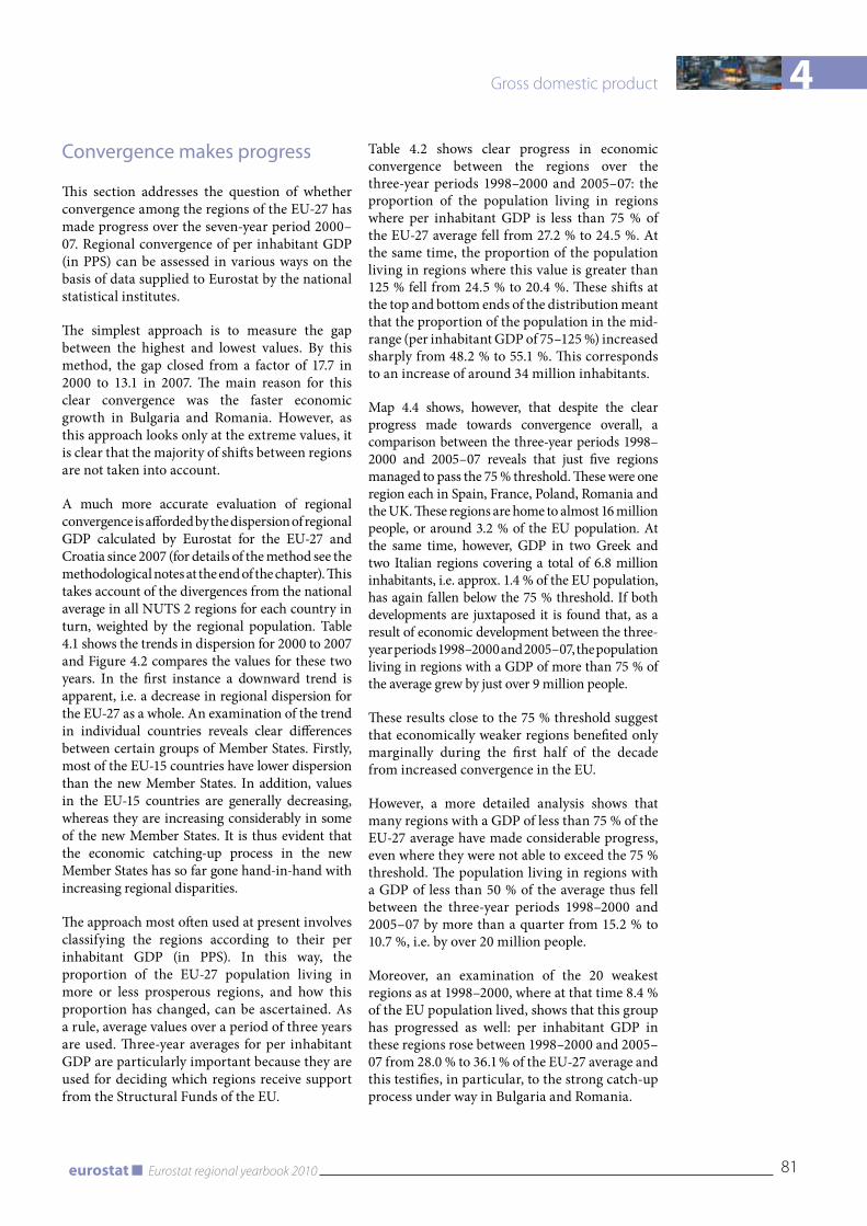
4
81Eurostat regional yearbook 2010eurostat
Gross domestic product
Convergence makes progress
This section addresses the question of whether convergence among the regions of the EU-27 has made progress over the seven-year period 2000–07. Regional convergence of per inhabitant GDP (in PPS) can be assessed in various ways on the basis of data supplied to Eurostat by the national statistical institutes.
The simplest approach is to measure the gap between the highest and lowest values. By this method, the gap closed from a factor of 17.7 in 2000 to 13.1 in 2007. The main reason for this clear convergence was the faster economic growth in Bulgaria and Romania. However, as this approach looks only at the extreme values, it is clear that the majority of shifts between regions are not taken into account.
A much more accurate evaluation of regional convergence is afforded by the dispersion of regional GDP calculated by Eurostat for the EU-27 and Croatia since 2007 (for details of the method see the methodological notes at the end of the chapter). This takes account of the divergences from the national average in all NUTS 2 regions for each country in turn, weighted by the regional population. Table 4.1 shows the trends in dispersion for 2000 to 2007 and Figure 4.2 compares the values for these two years. In the first instance a downward trend is apparent, i.e. a decrease in regional dispersion for the EU-27 as a whole. An examination of the trend in individual countries reveals clear differences between certain groups of Member States. Firstly, most of the EU-15 countries have lower dispersion than the new Member States. In addition, values in the EU-15 countries are generally decreasing, whereas they are increasing considerably in some of the new Member States. It is thus evident that the economic catching-up process in the new Member States has so far gone hand-in-hand with increasing regional disparities.
The approach most often used at present involves classifying the regions according to their per inhabitant GDP (in PPS). In this way, the proportion of the EU-27 population living in more or less prosperous regions, and how this proportion has changed, can be ascertained. As a rule, average values over a period of three years are used. Three-year averages for per inhabitant GDP are particularly important because they are used for deciding which regions receive support from the Structural Funds of the EU.
Table 4.2 shows clear progress in economic convergence between the regions over the three-year periods 1998–2000 and 2005–07: the proportion of the population living in regions where per inhabitant GDP is less than 75 % of the EU-27 average fell from 27.2 % to 24.5 %. At the same time, the proportion of the population living in regions where this value is greater than 125 % fell from 24.5 % to 20.4 %. These shifts at the top and bottom ends of the distribution meant that the proportion of the population in the mid-range (per inhabitant GDP of 75–125 %) increased sharply from 48.2 % to 55.1 %. This corresponds to an increase of around 34 million inhabitants.
Map 4.4 shows, however, that despite the clear progress made towards convergence overall, a comparison between the three-year periods 1998–2000 and 2005–07 reveals that just five regions managed to pass the 75 % threshold. These were one region each in Spain, France, Poland, Romania and the UK. These regions are home to almost 16 million people, or around 3.2 % of the EU population. At the same time, however, GDP in two Greek and two Italian regions covering a total of 6.8 million inhabitants, i.e. approx. 1.4 % of the EU population, has again fallen below the 75 % threshold. If both developments are juxtaposed it is found that, as a result of economic development between the three-year periods 1998–2000 and 2005–07, the population living in regions with a GDP of more than 75 % of the average grew by just over 9 million people.
These results close to the 75 % threshold suggest that economically weaker regions benefited only marginally during the first half of the decade from increased convergence in the EU.
However, a more detailed analysis shows that many regions with a GDP of less than 75 % of the EU-27 average have made considerable progress, even where they were not able to exceed the 75 % threshold. The population living in regions with a GDP of less than 50 % of the average thus fell between the three-year periods 1998–2000 and 2005–07 by more than a quarter from 15.2 % to 10.7 %, i.e. by over 20 million people.
Moreover, an examination of the 20 weakest regions as at 1998–2000, where at that time 8.4 % of the EU population lived, shows that this group has progressed as well: per inhabitant GDP in these regions rose between 1998–2000 and 2005–07 from 28.0 % to 36.1 % of the EU-27 average and this testifies, in particular, to the strong catch-up process under way in Bulgaria and Romania.
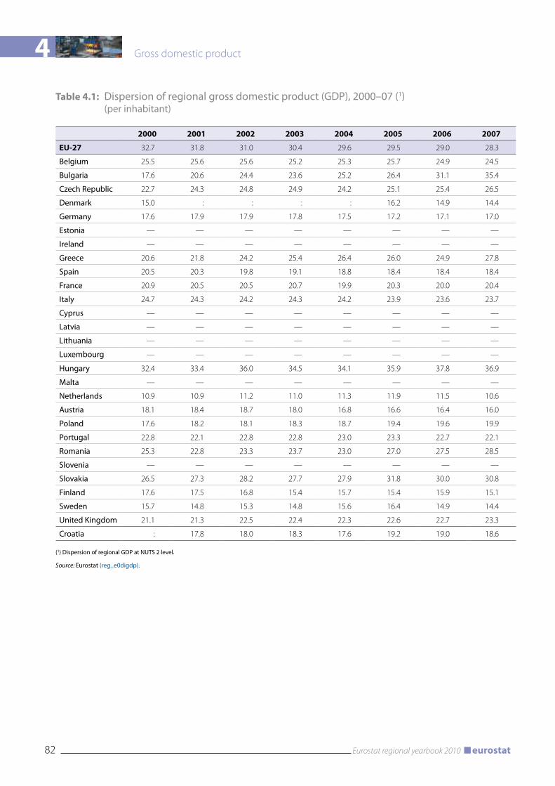
4 Gross domestic product
82 Eurostat regional yearbook 2010 eurostat
Table 4.1: Dispersion of regional gross domestic product (GDP), 2000–07 (1) (per inhabitant)
2000 2001 2002 2003 2004 2005 2006 2007
EU-27 32.7 31.8 31.0 30.4 29.6 29.5 29.0 28.3
Belgium 25.5 25.6 25.6 25.2 25.3 25.7 24.9 24.5
Bulgaria 17.6 20.6 24.4 23.6 25.2 26.4 31.1 35.4
Czech Republic 22.7 24.3 24.8 24.9 24.2 25.1 25.4 26.5
Denmark 15.0 : : : : 16.2 14.9 14.4
Germany 17.6 17.9 17.9 17.8 17.5 17.2 17.1 17.0
Estonia — — — — — — — —
Ireland — — — — — — — —
Greece 20.6 21.8 24.2 25.4 26.4 26.0 24.9 27.8
Spain 20.5 20.3 19.8 19.1 18.8 18.4 18.4 18.4
France 20.9 20.5 20.5 20.7 19.9 20.3 20.0 20.4
Italy 24.7 24.3 24.2 24.3 24.2 23.9 23.6 23.7
Cyprus — — — — — — — —
Latvia — — — — — — — —
Lithuania — — — — — — — —
Luxembourg — — — — — — — —
Hungary 32.4 33.4 36.0 34.5 34.1 35.9 37.8 36.9
Malta — — — — — — — —
Netherlands 10.9 10.9 11.2 11.0 11.3 11.9 11.5 10.6
Austria 18.1 18.4 18.7 18.0 16.8 16.6 16.4 16.0
Poland 17.6 18.2 18.1 18.3 18.7 19.4 19.6 19.9
Portugal 22.8 22.1 22.8 22.8 23.0 23.3 22.7 22.1
Romania 25.3 22.8 23.3 23.7 23.0 27.0 27.5 28.5
Slovenia — — — — — — — —
Slovakia 26.5 27.3 28.2 27.7 27.9 31.8 30.0 30.8
Finland 17.6 17.5 16.8 15.4 15.7 15.4 15.9 15.1
Sweden 15.7 14.8 15.3 14.8 15.6 16.4 14.9 14.4
United Kingdom 21.1 21.3 22.5 22.4 22.3 22.6 22.7 23.3
Croatia : 17.8 18.0 18.3 17.6 19.2 19.0 18.6
(1) Dispersion of regional GDP at NUTS 2 level.
Source: Eurostat (reg_e0digdp).
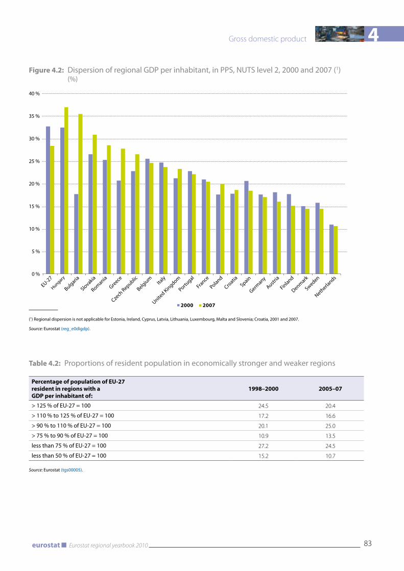
4
83Eurostat regional yearbook 2010eurostat
Gross domestic product
Figure 4.2: Dispersion of regional GDP per inhabitant, in PPS, NUTS level 2, 2000 and 2007 (1) (%)
0 %
5 %
10 %
15 %
20 %
25 %
30 %
35 %
40 %
2000 2007
EU-27
Hungary
Bulgaria
Slovakia
Romania
Greece
Czech
Republic
BelgiumIta
ly
United Kingdom
Portugal
France
Poland
Croatia
Spain
Germany
Austria
Finland
Denmark
Sweden
Netherla
nds
(1) Regional dispersion is not applicable for Estonia, Ireland, Cyprus, Latvia, Lithuania, Luxembourg, Malta and Slovenia; Croatia, 2001 and 2007.
Source: Eurostat (reg_e0digdp).
Table 4.2: Proportions of resident population in economically stronger and weaker regions
Percentage of population of EU-27 resident in regions with a GDP per inhabitant of:
1998–2000 2005–07
> 125 % of EU-27 = 100 24.5 20.4
> 110 % to 125 % of EU-27 = 100 17.2 16.6
> 90 % to 110 % of EU-27 = 100 20.1 25.0
> 75 % to 90 % of EU-27 = 100 10.9 13.5
less than 75 % of EU-27 = 100 27.2 24.5
less than 50 % of EU-27 = 100 15.2 10.7
Source: Eurostat (tgs00005).
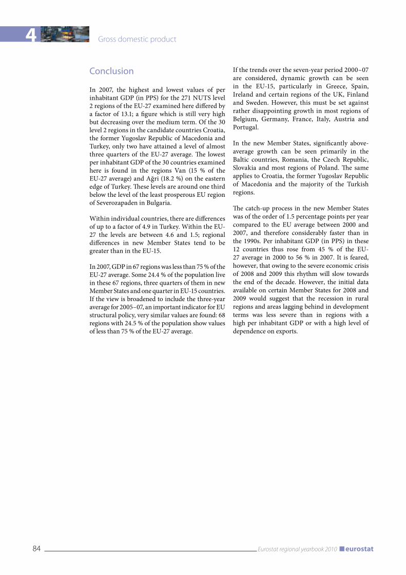
4 Gross domestic product
84 Eurostat regional yearbook 2010 eurostat
Conclusion
In 2007, the highest and lowest values of per inhabitant GDP (in PPS) for the 271 NUTS level 2 regions of the EU-27 examined here differed by a factor of 13.1; a figure which is still very high but decreasing over the medium term. Of the 30 level 2 regions in the candidate countries Croatia, the former Yugoslav Republic of Macedonia and Turkey, only two have attained a level of almost three quarters of the EU-27 average. The lowest per inhabitant GDP of the 30 countries examined here is found in the regions Van (15 % of the EU-27 average) and Ağri (18.2 %) on the eastern edge of Turkey. These levels are around one third below the level of the least prosperous EU region of Severozapaden in Bulgaria.
Within individual countries, there are differences of up to a factor of 4.9 in Turkey. Within the EU-27 the levels are between 4.6 and 1.5; regional differences in new Member States tend to be greater than in the EU-15.
In 2007, GDP in 67 regions was less than 75 % of the EU-27 average. Some 24.4 % of the population live in these 67 regions, three quarters of them in new Member States and one quarter in EU-15 countries. If the view is broadened to include the three-year average for 2005–07, an important indicator for EU structural policy, very similar values are found: 68 regions with 24.5 % of the population show values of less than 75 % of the EU-27 average.
If the trends over the seven-year period 2000–07 are considered, dynamic growth can be seen in the EU-15, particularly in Greece, Spain, Ireland and certain regions of the UK, Finland and Sweden. However, this must be set against rather disappointing growth in most regions of Belgium, Germany, France, Italy, Austria and Portugal.
In the new Member States, significantly above-average growth can be seen primarily in the Baltic countries, Romania, the Czech Republic, Slovakia and most regions of Poland. The same applies to Croatia, the former Yugoslav Republic of Macedonia and the majority of the Turkish regions.
The catch-up process in the new Member States was of the order of 1.5 percentage points per year compared to the EU average between 2000 and 2007, and therefore considerably faster than in the 1990s. Per inhabitant GDP (in PPS) in these 12 countries thus rose from 45 % of the EU-27 average in 2000 to 56 % in 2007. It is feared, however, that owing to the severe economic crisis of 2008 and 2009 this rhythm will slow towards the end of the decade. However, the initial data available on certain Member States for 2008 and 2009 would suggest that the recession in rural regions and areas lagging behind in development terms was less severe than in regions with a high per inhabitant GDP or with a high level of dependence on exports.
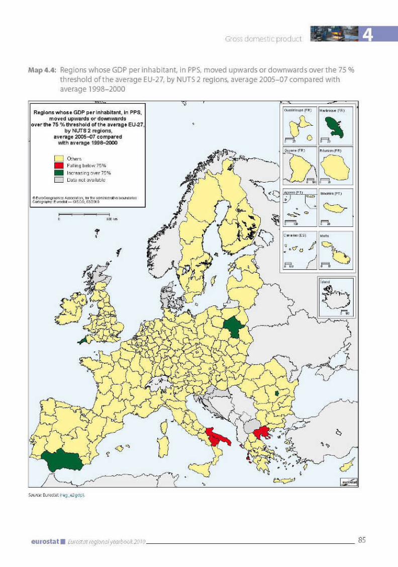
4 Gross domestic product
86 Eurostat regional yearbook 2010 eurostat
Methodological notes
Purchasing power parities and international volume comparisons
The differences in GDP values between countries, even after conversion by means of exchange rates to a common currency, cannot be attributed solely to differing volumes of goods and services. The ‘level of prices’ component is also a major contributory factor. Exchange rates are determined by many factors related to demand and supply in the currency markets, such as international trade, inflation forecasts and interest rate differentials. Conversions using exchange rates are therefore of only limited relevance for international comparisons. To obtain a more precise comparison, it is essential to use special conversion rates which eliminate the effect of price-level differences between countries. Purchasing power parities (PPPs) are conversion factors of this kind which convert economic indicators from national currencies into an artificial common currency, called the purchasing power standard (PPS). PPPs are therefore used to convert GDP and other economic aggregates (e.g. consumption expenditure on certain product groups) of various countries into comparable volumes of expenditure, expressed in purchasing power standards.
With the introduction of the euro, prices can now, for the first time, be compared directly between countries in the euro area. However, the euro has different purchasing power in the different countries of the euro area, depending on the national price level. PPPs must therefore also continue to be used to calculate pure volume aggregates in PPS for the Member States within the euro area.
In their simplest form, PPPs are a set of price ratios between the prices in national currency of the same good or service in different countries (e.g. a loaf of bread costs EUR 2.30 in France, EUR 1.90 in Germany, GBP 2.40 in the UK, etc.). A basket of comparable goods and services is used for price surveys. These are selected so as to represent the whole range of goods and services, taking account of the consumption structures in the various countries. The simple price ratios at product level are then aggregated to PPPs for product groups, then for overall consumption and finally for GDP. In order to have a reference value for the calculation of PPPs, one country is usually chosen and used as the reference country, and set to 1. For the European Union, the selection of a single country as a base is inappropriate. Therefore, PPS is the artificial common reference currency unit used in the European Union to express the volume of economic aggregates for the purpose of spatial comparisons in real terms.
Unfortunately, for reasons of cost, it will not be possible in the foreseeable future to calculate regional conversion factors. If such regional PPPs were available, the GDP in PPS for numerous peripheral or rural regions of the EU would probably be higher than that calculated using national PPPs.
The regions may be ranked differently when calculating in PPS instead of euros. For example, in 2007 the Swedish region of Östra Mellansverige had a per inhabitant GDP of EUR 31 300, putting it well ahead of Madrid at EUR 30 600. However, in PPS, Madrid at 34 100 PPS per inhabitant is ahead of Östra Mellansverige at 26 500 PPS per inhabitant.
In terms of distribution, the use of PPS rather than the euro has a levelling effect, as countries with a very high per inhabitant GDP also generally have relatively high price levels. The range of per inhabitant GDP in NUTS level 2 regions in the EU-27 thus falls from 93 400 in euros to 76 900 in PPS.
Per inhabitant GDP in PPS is the key variable for determining the eligibility of NUTS level 2 regions under the European Union’s structural policy.
Dispersion of per inhabitant GDP
Since 2007, Eurostat has been calculating a derived indicator which records the differences between regional per inhabitant GDP and the national average and makes them comparable between countries.

4
87Eurostat regional yearbook 2010eurostat
Gross domestic product
For a given country the dispersion D of regional GDP of the level 2 or 3 regions is defined as the sum of the absolute differences between regional and national GDP per inhabitant, weighted with the regional share of population and expressed as a percentage of national per inhabitant GDP:
D = 100 ¦ (yi - Y) ¦ (pi / P)
where:
y• i is the regional per inhabitant GDP of region i; Y is the national average per inhabitant GDP; •p• i is the population of region i;P is the population of the country;•n• is the number of regions of the country.
The value of the dispersion of per inhabitant GDP is equal to zero, if regional GDP values are identical in all regions of the country or economic area (such as the EU-27 or the euro area), and it will show, ceteris paribus, an increase if the differences between the regional per inhabitant GDP values among regions are rising. For example, a value of 20 % means that the per inhabitant GDP of all regions of a given country, weighted on the basis of the regional population, differs from the national value by an average of 20 %.
The EU-27 value is calculated by treating the EU-27 as a single country, i.e. only the level 2 or 3 regions are taken into account in each case. The corresponding NUTS level 2, level 1 or national values are thus not used in the calculation in order to avoid them being taken into account twice.
GDP dispersion figures published on the Eurostat website are based on per inhabitant GDP in purchasing power standards (PPS).


Household accounts

5 Household accounts
90 Eurostat regional yearbook 2010 eurostat
Introduction: Measuring wealth
One of the primary aims of regional statistics is to measure the wealth of regions. This is of particular relevance as a basis for policy measures which aim to provide support for less well-off regions.
The indicator most frequently used to measure the wealth of a region is regional gross domestic product (GDP). GDP is usually expressed in purchasing power standards (PPS) per inhabitant to make the data comparable between regions of differing size and purchasing power.
GDP is the total value of goods and services produced in a region by the persons employed in that region, minus the necessary inputs. However, owing to a multitude of interregional linkages and state interventions, the GDP generated in a given region does not tally with the income actually available to the inhabitants of the region.
One drawback of regional GDP per inhabitant as an indicator of wealth is that a ‘place-of-work’ figure (the GDP produced in the region) is divided by a ‘place-of-residence’ figure (the population living in the region). This inconsistency is of relevance wherever there are net commuter flows — i.e. more or fewer people working in a region than living in it. The most obvious example is the Inner London region of the UK, which has by far the highest GDP per inhabitant in the EU. Yet this by no means translates into a correspondingly high income level for the inhabitants of the same region, as thousands of commuters travel to London every day to work there but live in the neighbouring regions. Hamburg, Wien, Luxembourg, Praha and Bratislava are other examples of this phenomenon.
Apart from commuter flows, other factors can also cause the regional distribution of actual income not to correspond to the distribution of GDP. These include, for example, income from rent, interest or dividends received by the residents of a certain region, but paid by residents of other regions.
This being the case, a more accurate picture of a region’s economic situation can be obtained only by adding the figures for net income accruing to private households to GDP.
Private household income
In market economies with state redistribution mechanisms, a distinction is made between two stages of income distribution.
The primary distribution of income shows the income of private households generated directly from market transactions, i.e. the purchase and sale of factors of production and goods. These include in particular the compensation of employees, i.e. income from the sale of labour as a factor of production. Private households can also receive income on assets, particularly interest, dividends and rents. Then there is also income from operating surplus and self-employment. Interest and rents payable are recorded as negative items for households in the initial distribution stage. The balance of all these transactions is known as the primary income of private households.
Primary income is the point of departure for the secondary distribution of income, which means the state redistribution mechanism. All social benefits and transfers other than in kind (monetary transfers) are now added to primary income. From their income, households have to pay taxes on income and wealth, pay their social contributions and effect transfers. The balance remaining after these transactions have been carried out is called the disposable income of private households.
For an analysis of household income, a decision must first be made about the unit in which data are to be expressed if comparisons between regions are to be meaningful.
For the purposes of making comparisons between regions, regional GDP is generally expressed in PPS so that meaningful volume comparisons can be made. The same process should therefore be applied to the income parameters of private households. These are therefore converted with specific purchasing power standards for final consumption expenditure called PPCS (purchasing power consumption standards).

5
91Eurostat regional yearbook 2010eurostat
Household accounts
Results for 2007
Primary income
Map 5.1 gives an overview of primary income in the NUTS - 2 regions of the 24 countries examined here. Centres of wealth are clearly evident in southern England, Paris, northern Italy, Austria, Madrid and north-east Spain, Vlaams Gewest, the western Netherlands, Stockholm, Nordrhein-Westfalen, Hessen, Baden-Württemberg and Bayern. Also, there is a clear north–south divide in Italy and a west–east divide in Germany, whereas in France income distribution is relatively uniform between regions. The United Kingdom, too, has a north–south divide, although less marked than the divides in Italy and Germany.
In the new Member States, most of the regions with relatively high primary incomes are capital regions, in particular Bratislava (105 % of the EU-27 average) and Praha (98 %). Zahodna Slovenija and Közép-Magyarország (Budapest) also have primary incomes higher than 75 % of the EU average. All the regions of the Czech Republic, apart from Praha, and 13 other regions in the new Member States have primary incomes of private households higher than half of the EU average. The figure is below 50 % in the other regions of the new Member States.
The regional values range from 3 406 PPCS per inhabitant in Severozapaden (Bulgaria) to 34 842 PPCS in the UK region of Inner London. The 10 regions with the highest income per inhabitant include five regions in the UK, three in Germany and one each in France and Belgium. This clear concentration of regions with the highest incomes in the United Kingdom and Germany is also evident when the ranking is extended to the top 30 regions: this group contains 11 German and six UK regions, along with three regions each in Italy and Austria, two each in Belgium and the Netherlands, and one each in France, Spain and Sweden.
It is no surprise that the 30 regions at the tail end of the ranking are all located in the new Member States; they are 12 of the 16 Polish regions, all six Bulgarian regions, seven of the eight Romanian regions, four Hungarian regions and one Slovakian region.
In 2007, the highest and lowest primary incomes in the EU regions differed by a factor of 10.2.
Seven years earlier, in 2000, this factor had been 14.7. There was therefore a considerable narrowing of the gap between the opposite ends of the distribution over the period 2000–07. This positive development can be attributed partly to the Romanian and Bulgarian economies catching up compared to the rest of the EU.
Disposable income
A comparison of primary income with disposable income (Map 5.2) shows the levelling influence of state intervention. This particularly increases the relative income level in some regions of Italy and Spain, in the west of the United Kingdom and in parts of eastern Germany. Similar effects can be observed in the new Member States, particularly in Hungary, Romania, Bulgaria and Poland. However, the levelling out of private income levels in the new Member States is generally less pronounced than in the EU-15. Despite state redistribution and other transfers, most capital regions maintain their prominent position with the highest disposable incomes of the country in question.
The regional values range from 3 575 PPCS per inhabitant in Severozapaden (Bulgaria) to 24 733 PPCS in the UK region of Inner London.
Of the 10 regions with the highest per inhabitant disposable income, four each are in the UK and in Germany, and one each in France and Italy. The region with the highest disposable income in the new Member States is Bratislavský kraj with 13 749 PPCS per inhabitant (93 % of the EU-27 average), followed by the Praha region with 13 180 PPCS (90 %).
A clear regional concentration is also evident when the ranking is extended to the top 30 regions: this group contains 12 German and six UK regions, along with five regions in Austria, three in Italy, two in Spain and one each in Belgium and France.
The tail end of the distribution is very similar to the ranking for primary income. The bottom 30 include nine Polish and seven Romanian regions, six Bulgarian regions, five Hungarian regions, one Slovakian region and Estonia and Latvia.
State activity and other transfers significantly reduce the difference between the highest and lowest regional values in the 24 countries dealt with here from a factor of around 10.2 to 6.9.
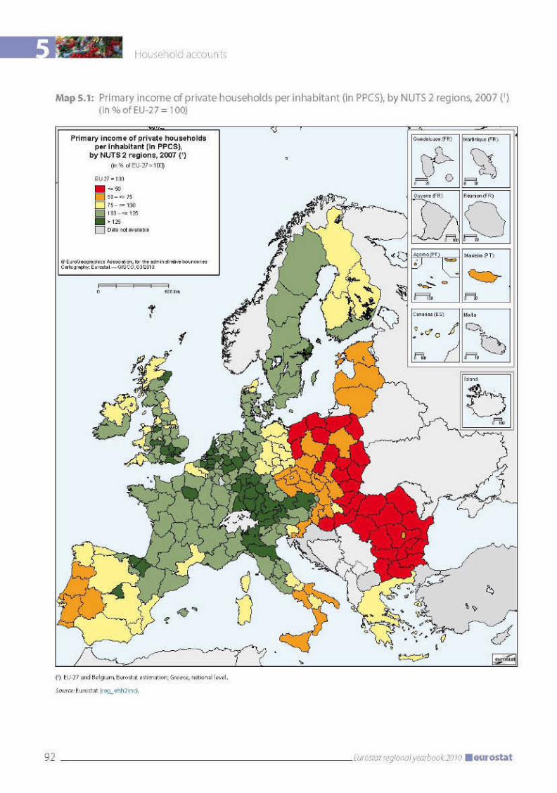

5 Household accounts
94 Eurostat regional yearbook 2010 eurostat
For disposable income there has been a significant trend towards a narrower spread in regional values over recent years: between 2000 and 2007 the difference between the highest and lowest values fell from a factor of 11.1 to 6.9. Like primary income, this positive development is partly the result of the economic catch-up process in Romania and Bulgaria.
To summarise, between 2000 and 2007, there was a clear narrowing of the difference between the highest and lowest regional values for both primary income and disposable income (influenced by state interventions and other transfers).
The regional spread in disposable income within the individual countries is naturally much lower than for the EU as a whole, but varies considerably from one country to another. Graph 5.1 gives an overview of the spread of disposable income per inhabitant between the regions with the highest and the lowest values for each country. It can be seen that, with a factor of almost 3, the regional disparity is greatest in Romania. This means that available income per inhabitant in Bucureşti - Ilfov is almost three times higher than in the Nord-Est region. Slovakia, the UK and Italy also have high regional differences with factors of between 1.7 and 1.9. In Hungary, Spain, Poland and Germany the highest values are, in each case, between 60 and 67 % above the lowest.
The regional differences tend to be higher in the new Member States than in the EU-15. Of the new Member States, Slovenia with 12 % has the smallest spread between the highest and lowest values and thus comes close to Denmark (5 %) and Austria (8 %), which have the lowest regional income disparities. Ireland, Finland, the Netherlands and Sweden also have only moderate regional disparities, with the highest values between 15 % and 25 % above the lowest values.
Figure 5.1 also shows that the capital city regions of 13 of the 20 countries with more than one NUTS 2 region where data are available also have the highest income values. All seven new Member States with at least two NUTS - 2 regions belong to this group.
The economic dominance of the capital regions is also evident when their income values are compared with the national averages. In four countries (the Czech Republic, Romania, Slovakia and the United Kingdom), the capital city regions
exceed the national values by more than a third. Only in Belgium and Germany are the values for the capital lower than the national average.
To assess the economic situation in individual regions, it is important to know not just the levels of primary and disposable income but also their relationship to each other. Map 5.3 shows this quotient, which gives an idea of the effect of state activity and of other transfer payments. On average, disposable income in the EU-27 amounts to 86.4 % of primary income. The figure was 86.4 % in 2000 too, so over this seven-year period the scale of state intervention and other transfers has not changed.
The lowest values are to be found in the capital regions of the more affluent Member States, in particular Hovedstaden (Denmark) at 65.7 % and Stockholm (Sweden) at 68.3 %; the highest values are found in rural regions away from economic centres, such as Lubelskie (Poland) at 105.9 % and Alentejo (Portugal) at 105.8 %.
In general, the EU-15 Member States have somewhat lower values than the new Member States. On closer inspection, typical differences can be seen between the regions of the Member States. Disposable income in the capital cities and other prosperous regions of the EU-15 is generally less than 80 % of primary income.
Correspondingly higher percentages can be observed in all the Member States in the less affluent areas, in particular on the southern and south-western peripheries of the EU, in the west of the United Kingdom and in eastern Germany.
The reason for this is that, in regions with relatively high income levels, a larger share of primary income is transferred to the state in the form of taxes. At the same time, state social benefits amount to less than in regions with relatively low income levels.
The regional redistribution of wealth is generally less significant in the new Member States than in the EU-15. For the capital regions the values are mostly between 75 % and 85 % and are almost without exception at the bottom end of the ranking within each country. This shows that incomes in these regions require much less support through social benefits than elsewhere. The difference between the capital region and the rest of the country is particularly large in Slovakia, at around 15 percentage points.

5
95Eurostat regional yearbook 2010eurostat
Household accounts
Figure 5.1: Disposable income of private households per inhabitant (in PPCS), by NUTS 2 regions, 2007 (1)
0 5 000 10 000 15 000 20 000 25 000 30 000
Belgium
Bulgaria
Czech Republic
Denmark
Germany
Estonia
Ireland
Greece
Spain
France
Italy
Latvia
Lithuania
Hungary
Netherlands
Austria
Poland
Portugal
Romania
Slovenia
Slovakia
Finland
Sweden
United Kingdom
National region Capital region
Prov. Hainaut Prov. Vlaams-Brabant
Severozapaden
Severozápad
Yugozapaden
Syddanmark
Praha
Mecklenburg-Vorpommern HamburgHovestaden
Border, Midland and Western Southern and Eastern
Extremadura País Vasco
Nord - Pas-de-Calais Île de France
Campania Emilia-Romagna
Észak-Alföld Közép-Magyarország
Groningen UtrechtKärnten Niederösterreich
Podkarpackie MazowieckieNorte Lisboa
Nord-Est Bucureşti – IlfovVzhodna Slovenija Zahodna Slovenija
Východné Slovensko Bratislavský krajPohjois-Suomi Åland
Norra Mellansverige StockholmWest Midlands Inner London
(1) Belgium, Eurostat estimation; Greece, national level; départements d’outre-mer (FR9), Cyprus, Luxembourg and Malta, data not available.
Source: Eurostat (reg_ehh2inc).
In the 24 EU Member States examined here, disposable income exceeds primary income in a total of 24 regions. These are nine Polish regions, four German, three regions each in Bulgaria and Portugal, two each in Romania and the UK and one in Italy. Map 5.3 clearly shows that these are particularly poor regions of the Member States in question. The highest value is to be found in Lubelskie (Poland), where disposable income exceeds primary income by 5.9 %. No clear differences in support for the incomes of private households between the new Member States and the EU-15 countries were found.
When interpreting these results, however, it should be borne in mind that it is not just monetary social benefits from the state which may cause disposable income to exceed primary income. Other transfer payments (e.g. transfers from people temporarily working in other regions) can play a role in some cases.
Dynamic developments at the edges of the Union
The focus finally turns to an overview of medium-term trends in the regions compared with the EU-27 average. Map 5.4 uses a seven-year comparison to show how disposable income per inhabitant (in PPCS) in the NUTS - 2 regions changed between 2000 and 2007 compared to the average for the EU-27.
It shows, first of all, dynamic processes at work at the edges of the Union, particularly in Spain and Ireland, the Czech Republic, Slovakia, Romania, the Baltic States and Finland.
On the other hand, incomes have grown at a below-average rate in most of the EU’s founding Member States. Belgium, Germany and Italy have been particularly hard hit; there, incomes fell

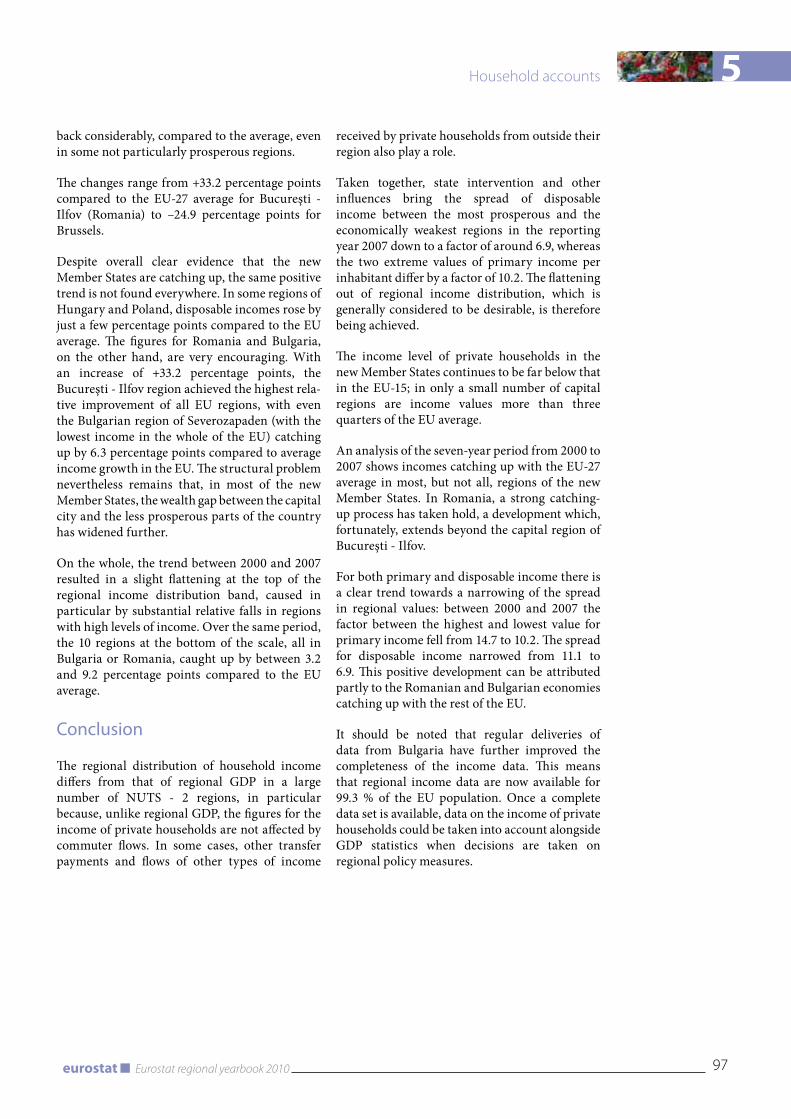
5
97Eurostat regional yearbook 2010eurostat
Household accounts
back considerably, compared to the average, even in some not particularly prosperous regions.
The changes range from +33.2 percentage points compared to the EU-27 average for Bucureşti - Ilfov (Romania) to –24.9 percentage points for Brussels.
Despite overall clear evidence that the new Member States are catching up, the same positive trend is not found everywhere. In some regions of Hungary and Poland, disposable incomes rose by just a few percentage points compared to the EU average. The figures for Romania and Bulgaria, on the other hand, are very encouraging. With an increase of +33.2 percentage points, the Bucureşti - Ilfov region achieved the highest rela-tive improvement of all EU regions, with even the Bulgarian region of Severozapaden (with the lowest income in the whole of the EU) catching up by 6.3 percentage points compared to average income growth in the EU. The structural problem nevertheless remains that, in most of the new Member States, the wealth gap between the capital city and the less prosperous parts of the country has widened further.
On the whole, the trend between 2000 and 2007 resulted in a slight flattening at the top of the regional income distribution band, caused in particular by substantial relative falls in regions with high levels of income. Over the same period, the 10 regions at the bottom of the scale, all in Bulgaria or Romania, caught up by between 3.2 and 9.2 percentage points compared to the EU average.
Conclusion
The regional distribution of household income differs from that of regional GDP in a large number of NUTS - 2 regions, in particular because, unlike regional GDP, the figures for the income of private households are not affected by commuter flows. In some cases, other transfer payments and flows of other types of income
received by private households from outside their region also play a role.
Taken together, state intervention and other influences bring the spread of disposable income between the most prosperous and the economically weakest regions in the reporting year 2007 down to a factor of around 6.9, whereas the two extreme values of primary income per inhabitant differ by a factor of 10.2. The flattening out of regional income distribution, which is generally considered to be desirable, is therefore being achieved.
The income level of private households in the new Member States continues to be far below that in the EU-15; in only a small number of capital regions are income values more than three quarters of the EU average.
An analysis of the seven-year period from 2000 to 2007 shows incomes catching up with the EU-27 average in most, but not all, regions of the new Member States. In Romania, a strong catching-up process has taken hold, a development which, fortunately, extends beyond the capital region of Bucureşti - Ilfov.
For both primary and disposable income there is a clear trend towards a narrowing of the spread in regional values: between 2000 and 2007 the factor between the highest and lowest value for primary income fell from 14.7 to 10.2. The spread for disposable income narrowed from 11.1 to 6.9. This positive development can be attributed partly to the Romanian and Bulgarian economies catching up with the rest of the EU.
It should be noted that regular deliveries of data from Bulgaria have further improved the completeness of the income data. This means that regional income data are now available for 99.3 % of the EU population. Once a complete data set is available, data on the income of private households could be taken into account alongside GDP statistics when decisions are taken on regional policy measures.

5
99Eurostat regional yearbook 2010eurostat
Household accounts
99Eurostat regional yearbook 2010eurostat
Methodological notes
Eurostat has had regional data on the income categories of private households for a number of years. The data are collected for the purposes of the regional accounts at NUTS - 2 level.
There are still no data available at NUTS - 2 level for the following regions: départements d’outre-mer (France), Cyprus, Luxembourg and Malta.
The text in this chapter therefore relates to only 24 Member States, or 264 NUTS - 2 regions. Three of these 24 Member States consist of only one NUTS - 2 region, namely Estonia, Latvia and Lithuania. For Greece, only data at national level are used. In the context of the collection of data for 2009, Bulgaria supplied data for the reference years 2000–07 for the first time. For Belgium, the figures for 2007 were estimated on the basis of the 2006 regional structure. The same nominal growth rate as for GDP was assumed for the national levels.
Because of the limited availability of data, the EU-27 values for the regional household accounts had to be estimated. For this purpose it was assumed that the share of the missing Member States in household income (in PPCS) for the EU-27 was the same as for GDP (in PPS). For the reference year 2007 this share was 0.5 %.
Data reaching Eurostat after 4 March 2010 were not taken into account in this chapter of the yearbook.


Structural business statistics
6 Structural business statistics
102 Eurostat regional yearbook 2010 eurostat
Introduction
What effects do the European Union’s economic and regional policies have on the business structure of the regions? What sectors are growing, what sectors are contracting and what regions are likely to be most affected? A detailed analysis of the structure of the European economy can only be made at regional level. Regional structural business statistics (SBS) provide data with a detailed activity breakdown that can be used for this kind of analysis. The first part of this chapter looks at regional specialisation and business concentration within the EU’s business economy. The second part analyses the activity of the business services sector in detail.
Regional specialisation and business concentration
There are significant disparities between European regions in terms of the importance of different activities within the business economy. While some activities are distributed relatively evenly across most regions, many others exhibit a considerable variation in the level of regional specialisation, often with a few regions having a particularly high degree of specialisation.
The share of a particular activity within the business economy gives an idea of which regions are the most or least specialised in that activity, regardless of whether the region or the activity considered is large or small. There are various reasons for relative specialisation. Depending on the type of activity, these can include availability of natural resources, availability of skilled employees, culture and tradition, cost levels, infrastructure, legislation, climatic and topographic conditions and proximity to markets.
Figure 6.1 shows that, on an aggregate activity level (NACE sections), the widest spread in the relative importance of an activity in each region’s non-financial business economy (NACE sections C to I and K) workforce was in manufacturing (NACE section D). Manufacturing accounted for only 3.7 % of persons employed in Ciudad Autónoma de Melilla (Spain) and under 10 % in a further 13 regions, including the capital regions of Belgium, Spain and the United Kingdom. The distribution of the remaining regions was relatively symmetrical, from 10 % to almost half of the workforce in one Bulgarian
and two Czech regions: Severen tsentralen (BG) — 48.4 %, Střední Morava (CZ) — 48.1 %, and Severovýchod (CZ) — 48.2 %. Západné Slovensko (SK) was the only region where the share of employment in manufacturing exceeded half the non-financial business economy workforce (56.1 %). In contrast, the spread of employment was much narrower in distributive trades (NACE section G), which was the activity displaying the highest median employment, present in all regions and serving more local clients. Shares ranged from 11.6 % in Észak-Alföld (Hungary) and less than 17 % in Åland and Länsi-Suomi (Finland), Comunidad Foral de Navarra (Spain), Vzhodna Slovenija (Slovenia) and Severozápad (the Czech Republic) to around 40 % in Kentriki Makedonia, Peloponnisos, Voreio Aigaio, Dytiki Ellada (Greece) and Ciudad Autónoma de Melilla (Spain) and over 45 % in Kriti (Greece).
On the other hand, transport, storage and communication (NACE section I) and mining and quarrying (NACE section C) are two activities with a similar relative size in most regions, but where there are a few strong outlier regions that are highly specialised. Transport, storage and communication accounted for not more than 6.9 % in a quarter of the regions and less than 9.8 % in three quarters of the regions. These narrow ranges are mainly due to the fact that road transport and post and telecommunications account for a large share of employment in this sector and that these activities tend to be of relatively equal importance across most regions. In fact, there were only four regions where the share of employment in transport, storage and communication exceeded 20 %. The highest specialisation of the Finnish island region of Åland, where almost half of the workforce (45.0 %) was employed in this sector, is due almost exclusively to the importance of water transport. Åland was far ahead of Köln in Germany (30.1 %) and Bourgogne in France (22.6 %), where post and telecommunications was particularly important, and Bratislavský kraj (22.3 %), the capital region of Slovakia, owing to the importance of road and other land transport. Natural endowments play an important role in activities of mining and quarrying. Many regions record little or no such activity, with only very few regions being highly specialised on account of deposits of metallic ores, coal, oil or gas. Mining and quarrying accounted for less than 0.2 % of persons employed in a quarter of all regions, and between 0.2 % and 0.5 % in half of the regions. However, this sector accounted for over 5 % in five regions and as much as a 10th of the total
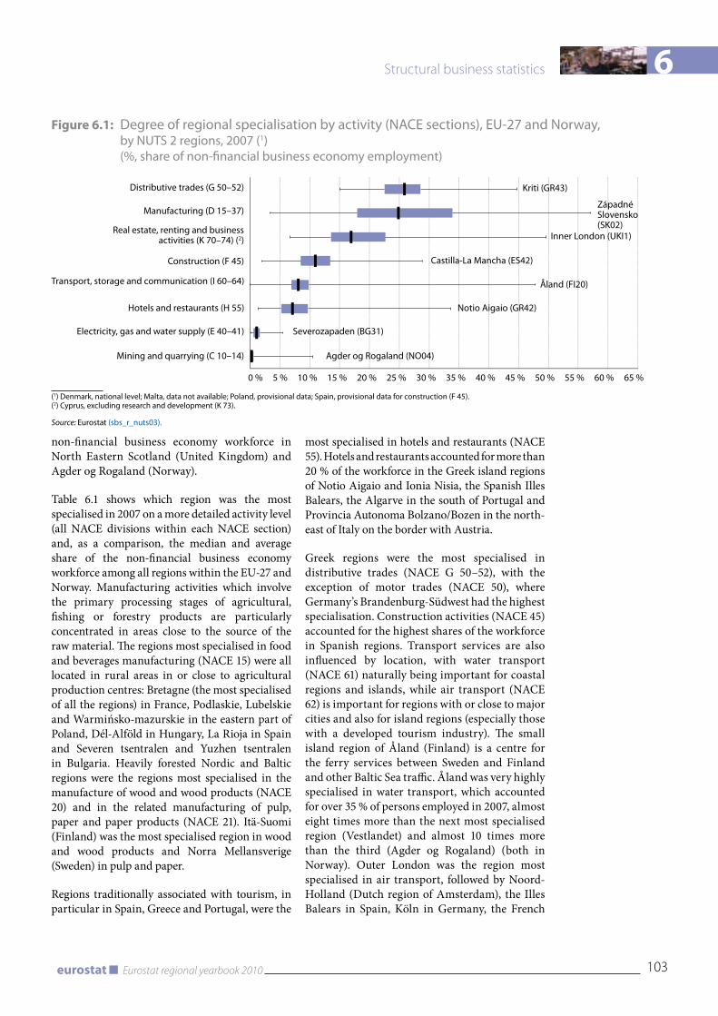
6
103Eurostat regional yearbook 2010eurostat
Structural business statistics
Figure 6.1: Degree of regional specialisation by activity (NACE sections), EU-27 and Norway, by NUTS 2 regions, 2007 (1) (%, share of non-financial business economy employment)
0 % 5 % 10 % 15 % 20 % 25 % 30 % 35 % 40 % 45 % 50 % 55 % 60 % 65 %
Distributive trades (G 50–52)
Manufacturing (D 15–37)
Real estate, renting and businessactivities (K 70–74) (2)
Construction (F 45)
Transport, storage and communication (I 60–64)
Hotels and restaurants (H 55)
Electricity, gas and water supply (E 40–41)
Mining and quarrying (C 10–14)
Západné Slovensko (SK02)
Severozapaden (BG31)
Castilla-La Mancha (ES42)
Kriti (GR43)
Notio Aigaio (GR42)
Åland (FI20)
Inner London (UKI1)
Agder og Rogaland (NO04)
(1) Denmark, national level; Malta, data not available; Poland, provisional data; Spain, provisional data for construction (F 45).(2) Cyprus, excluding research and development (K 73).
Source: Eurostat (sbs_r_nuts03).
non-financial business economy workforce in North Eastern Scotland (United Kingdom) and Agder og Rogaland (Norway).
Table 6.1 shows which region was the most specialised in 2007 on a more detailed activity level (all NACE divisions within each NACE section) and, as a comparison, the median and average share of the non-financial business economy workforce among all regions within the EU-27 and Norway. Manufacturing activities which involve the primary processing stages of agricultural, fishing or forestry products are particularly concentrated in areas close to the source of the raw material. The regions most specialised in food and beverages manufacturing (NACE 15) were all located in rural areas in or close to agricultural production centres: Bretagne (the most specialised of all the regions) in France, Podlaskie, Lubelskie and Warmińsko-mazurskie in the eastern part of Poland, Dél-Alföld in Hungary, La Rioja in Spain and Severen tsentralen and Yuzhen tsentralen in Bulgaria. Heavily forested Nordic and Baltic regions were the regions most specialised in the manufacture of wood and wood products (NACE 20) and in the related manufacturing of pulp, paper and paper products (NACE 21). Itä-Suomi (Finland) was the most specialised region in wood and wood products and Norra Mellansverige (Sweden) in pulp and paper.
Regions traditionally associated with tourism, in particular in Spain, Greece and Portugal, were the
most specialised in hotels and restaurants (NACE 55). Hotels and restaurants accounted for more than 20 % of the workforce in the Greek island regions of Notio Aigaio and Ionia Nisia, the Spanish Illes Balears, the Algarve in the south of Portugal and Provincia Autonoma Bolzano/Bozen in the north-east of Italy on the border with Austria.
Greek regions were the most specialised in distributive trades (NACE G 50–52), with the exception of motor trades (NACE 50), where Germany’s Brandenburg-Südwest had the highest specialisation. Construction activities (NACE 45) accounted for the highest shares of the workforce in Spanish regions. Transport services are also influenced by location, with water transport (NACE 61) naturally being important for coastal regions and islands, while air transport (NACE 62) is important for regions with or close to major cities and also for island regions (especially those with a developed tourism industry). The small island region of Åland (Finland) is a centre for the ferry services between Sweden and Finland and other Baltic Sea traffic. Åland was very highly specialised in water transport, which accounted for over 35 % of persons employed in 2007, almost eight times more than the next most specialised region (Vestlandet) and almost 10 times more than the third (Agder og Rogaland) (both in Norway). Outer London was the region most specialised in air transport, followed by Noord-Holland (Dutch region of Amsterdam), the Illes Balears in Spain, Köln in Germany, the French
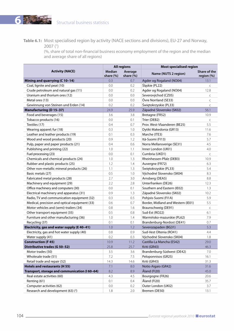
6 Structural business statistics
104 Eurostat regional yearbook 2010 eurostat
Table 6.1: Most specialised region by activity (NACE sections and divisions), EU-27 and Norway, 2007 (1) (%, share of total non-financial business economy employment of the region and the median and average share of all regions)
Activity (NACE)All regions Most specialised region
Median share (%)
Average share (%) Name (NUTS 2 region) Share of the
region (%) Mining and quarrying (C 10–14) 0.3 0.7 Agder og Rogaland (NO04) 13.1
Coal, lignite and peat (10) 0.0 0.2 Śląskie (PL22) cCrude petroleum and natural gas (11) 0.0 0.2 Agder og Rogaland (NO04) 12.8Uranium and thorium ores (12) 0.0 0.0 Severovýchod (CZ05) cMetal ores (13) 0.0 0.0 Övre Norrland (SE33) cGewinnung von Steinen und Erden (14) 0.2 0.2 Świętokrzyskie (PL33) c
Manufacturing (D 15–37) 24.9 25.9 Západné Slovensko (SK02) 56.1Food and beverages (15) 3.6 3.8 Bretagne (FR52) 10.9Tobacco products (16) 0.0 0.1 Trier (DEB2) cTextiles (17) 0.4 0.7 Prov. West-vlaanderen (BE25) 5.5Wearing apparel; fur (18) 0.3 1.0 Dytiki Makedonia (GR13) 11.6Leather and leather products (19) 0.1 0.3 Marche (ITE3) 7.6Wood and wood products (20) 0.9 1.2 Itä-Suomi (FI13) 5.7Pulp, paper and paper products (21) 0.4 0.6 Norra Mellansverige (SE31) 4.5Publishing and printing (22) 1.0 1.1 Inner London (UKI1) 4.0Fuel processing (23) 0.0 0.1 Cumbria (UKD1) cChemicals and chemical products (24) 1.0 1.3 Rheinhessen-Pfalz (DEB3) 10.9Rubber and plastic products (25) 1.2 1.4 Auvergne (FR72) 6.3Other non-metallic mineral products (26) 1.1 1.3 Świętokrzyskie (PL33) 5.4Basic metals (27) 0.5 1.0 východné Slovensko (SK04) 8.3Fabricated metal products (28) 2.7 3.0 Arnsberg (DEA5) 8.8Machinery and equipment (29) 2.2 2.8 Unterfranken (DE26) 12.3Office machinery and computers (30) 0.0 0.1 Southern and Eastern (IE02) 1.3Electrical machinery and apparatus (31) 0.9 1.3 Západné Slovensko (SK02) 10.2Radio, Tv and communication equipment (32) 0.3 0.5 Pohjois-Suomi (FI1A) 5.9Medical, precision and optical equipment (33) 0.6 0.7 Border, Midland and Western (IE01) 5.5Motor vehicles and (semi)-trailers (34) 0.8 1.6 Braunschweig (DE91) cOther transport equipment (35) 0.5 0.8 Sud-Est (RO22) 6.1Furniture and other manufacturing (36) 1.0 1.4 Warmińsko-mazurskie (PL62) 7.9Recycling (37) 0.1 0.1 Brandenburg-Nordost (DE41) 0.7
Electricity, gas and water supply (E 40–41) 1.0 1.2 Severozapaden (BG31) 5.3Electricity, gas and hot water supply (40) 0.8 0.9 Sud-vest Oltenia (RO41) 4.4Water supply (41) 0.2 0.3 východné Slovensko (SK04) 1.8
Construction (F 45) 10.9 11.2 Castilla-La Mancha (ES42) 29.0Distributive trades (G 50–52) 25.8 25.7 Kriti (GR43) 46.3
Motor trades (50) 3.5 3.6 Brandenburg-Südwest (DE42) 7.0Wholesale trade (51) 7.2 7.5 Peloponnisos (GR25) 16.1Retail trade and repair (52) 14.3 14.6 Kriti (GR43) 31.3
Hotels and restaurants (H 55) 7.1 8.0 Notio Aigaio (GR42) 31.6Transport, storage and communication (I 60–64) 8.2 8.9 Åland (FI20) 45.0
Real estate activities (60) 4.3 4.5 Bourgogne (FR26) 20.6Renting (61) 0.1 0.4 Åland (FI20) 35.7Computer activities (62) 0.0 0.2 Outer London (UKI2) 3.7Research and development (63) (2) 1.8 2.0 Bremen (DE50) 13.1
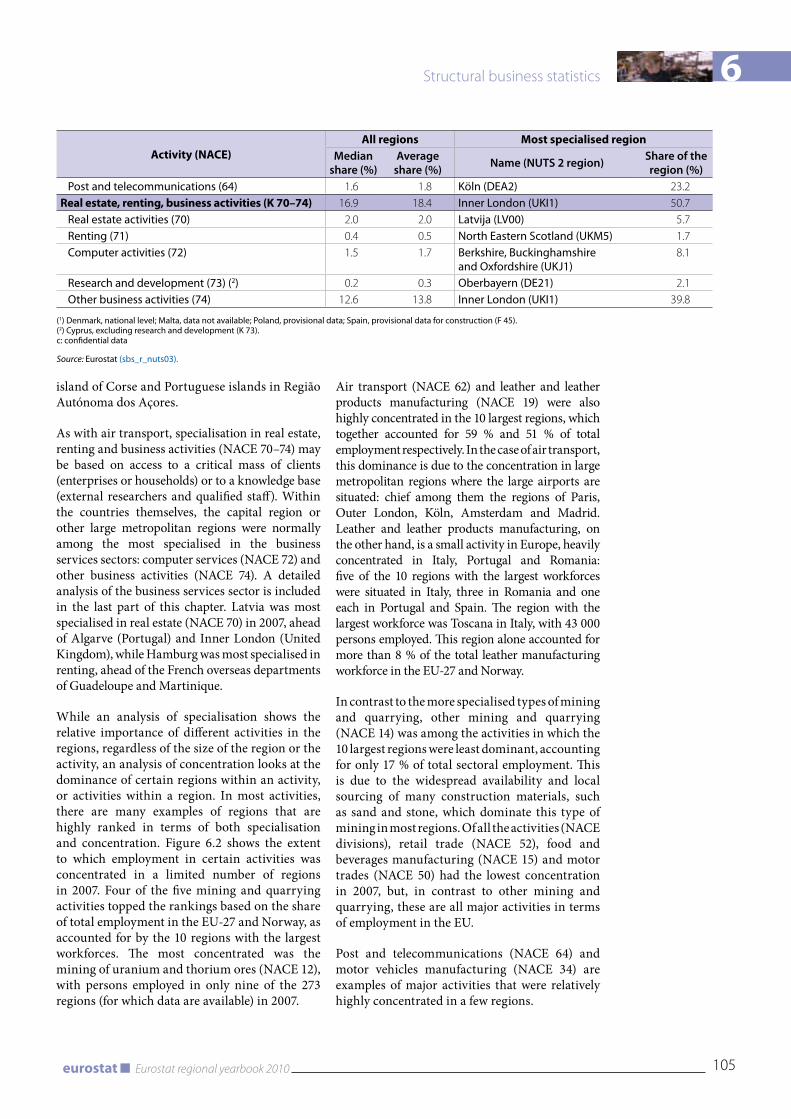
6
105Eurostat regional yearbook 2010eurostat
Structural business statistics
Activity (NACE)All regions Most specialised region
Median share (%)
Average share (%) Name (NUTS 2 region) Share of the
region (%) Post and telecommunications (64) 1.6 1.8 Köln (DEA2) 23.2
Real estate, renting, business activities (K 70–74) 16.9 18.4 Inner London (UKI1) 50.7Real estate activities (70) 2.0 2.0 Latvija (Lv00) 5.7Renting (71) 0.4 0.5 North Eastern Scotland (UKM5) 1.7Computer activities (72) 1.5 1.7 Berkshire, Buckinghamshire
and Oxfordshire (UKJ1)8.1
Research and development (73) (2) 0.2 0.3 Oberbayern (DE21) 2.1Other business activities (74) 12.6 13.8 Inner London (UKI1) 39.8
(1) Denmark, national level; Malta, data not available; Poland, provisional data; Spain, provisional data for construction (F 45).(2) Cyprus, excluding research and development (K 73).c: confidential data
Source: Eurostat (sbs_r_nuts03).
island of Corse and Portuguese islands in Região Autónoma dos Açores.
As with air transport, specialisation in real estate, renting and business activities (NACE 70–74) may be based on access to a critical mass of clients (enterprises or households) or to a knowledge base (external researchers and qualified staff). Within the countries themselves, the capital region or other large metropolitan regions were normally among the most specialised in the business services sectors: computer services (NACE 72) and other business activities (NACE 74). A detailed analysis of the business services sector is included in the last part of this chapter. Latvia was most specialised in real estate (NACE 70) in 2007, ahead of Algarve (Portugal) and Inner London (United Kingdom), while Hamburg was most specialised in renting, ahead of the French overseas departments of Guadeloupe and Martinique.
While an analysis of specialisation shows the relative importance of different activities in the regions, regardless of the size of the region or the activity, an analysis of concentration looks at the dominance of certain regions within an activity, or activities within a region. In most activities, there are many examples of regions that are highly ranked in terms of both specialisation and concentration. Figure 6.2 shows the extent to which employment in certain activities was concentrated in a limited number of regions in 2007. Four of the five mining and quarrying activities topped the rankings based on the share of total employment in the EU-27 and Norway, as accounted for by the 10 regions with the largest workforces. The most concentrated was the mining of uranium and thorium ores (NACE 12), with persons employed in only nine of the 273 regions (for which data are available) in 2007.
Air transport (NACE 62) and leather and leather products manufacturing (NACE 19) were also highly concentrated in the 10 largest regions, which together accounted for 59 % and 51 % of total employment respectively. In the case of air transport, this dominance is due to the concentration in large metropolitan regions where the large airports are situated: chief among them the regions of Paris, Outer London, Köln, Amsterdam and Madrid. Leather and leather products manufacturing, on the other hand, is a small activity in Europe, heavily concentrated in Italy, Portugal and Romania: five of the 10 regions with the largest workforces were situated in Italy, three in Romania and one each in Portugal and Spain. The region with the largest workforce was Toscana in Italy, with 43 000 persons employed. This region alone accounted for more than 8 % of the total leather manufacturing workforce in the EU-27 and Norway.
In contrast to the more specialised types of mining and quarrying, other mining and quarrying (NACE 14) was among the activities in which the 10 largest regions were least dominant, accounting for only 17 % of total sectoral employment. This is due to the widespread availability and local sourcing of many construction materials, such as sand and stone, which dominate this type of mining in most regions. Of all the activities (NACE divisions), retail trade (NACE 52), food and beverages manufacturing (NACE 15) and motor trades (NACE 50) had the lowest concentration in 2007, but, in contrast to other mining and quarrying, these are all major activities in terms of employment in the EU.
Post and telecommunications (NACE 64) and motor vehicles manufacturing (NACE 34) are examples of major activities that were relatively highly concentrated in a few regions.
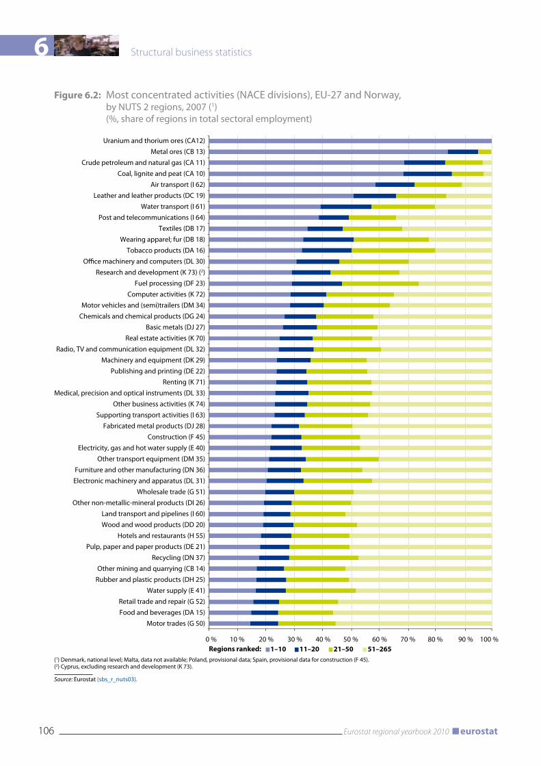
6 Structural business statistics
106 Eurostat regional yearbook 2010 eurostat
Figure 6.2: Most concentrated activities (NACE divisions), EU-27 and Norway, by NUTS 2 regions, 2007 (1) (%, share of regions in total sectoral employment)
0 % 20 % 30 %10 % 40 % 50 % 70 %60 % 80 % 90 % 100 %
Motor trades (G 50)
Food and beverages (DA 15)
Retail trade and repair (G 52)
Water supply (E 41)
Rubber and plastic products (DH 25)
Other mining and quarrying (CB 14)
Recycling (DN 37)
Pulp, paper and paper products (DE 21)
Hotels and restaurants (H 55)
Wood and wood products (DD 20)
Land transport and pipelines (I 60)
Other non-metallic-mineral products (DI 26)
Wholesale trade (G 51)
Electronic machinery and apparatus (DL 31)
Furniture and other manufacturing (DN 36)
Other transport equipment (DM 35)
Electricity, gas and hot water supply (E 40)
Construction (F 45)
Fabricated metal products (DJ 28)
Supporting transport activities (I 63)
Other business activities (K 74)
Medical, precision and optical instruments (DL 33)
Renting (K 71)
Publishing and printing (DE 22)
Machinery and equipment (DK 29)
Radio, TV and communication equipment (DL 32)
Real estate activities (K 70)
Basic metals (DJ 27)
Chemicals and chemical products (DG 24)
Motor vehicles and (semi)trailers (DM 34)
Computer activities (K 72)
Fuel processing (DF 23)
Research and development (K 73) (2)
Office machinery and computers (DL 30)
Tobacco products (DA 16)
Wearing apparel; fur (DB 18)
Textiles (DB 17)
Post and telecommunications (I 64)
Water transport (I 61)
Leather and leather products (DC 19)
Air transport (I 62)
Coal, lignite and peat (CA 10)
Crude petroleum and natural gas (CA 11)
Metal ores (CB 13)
Uranium and thorium ores (CA12)
1–10 11–20 21–50 51–265Regions ranked:(1) Denmark, national level; Malta, data not available; Poland, provisional data; Spain, provisional data for construction (F 45).(2) Cyprus, excluding research and development (K 73).
Source: Eurostat (sbs_r_nuts03).
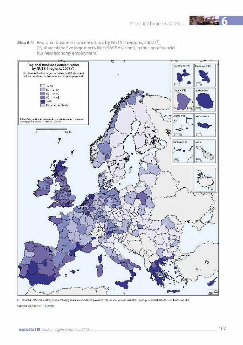
6 Structural business statistics
108 Eurostat regional yearbook 2010 eurostat
Map 6.1 gives an indication of how concentrated or diversified the regional business economy was in 2007, measured as the share of the five largest activities (NACE divisions) in the total non-financial business economy workforce. The level of concentration tends to be highest in regions where trade and services dominate the business economy, as industrial activities are more fragmented. By this measure, the most concentrated regions were generally in countries traditionally associated with tourism (in particular Spain, Greece and Portugal), underlining the importance of construction, trade, and hotels and restaurants in tourism-oriented regions.
However, high concentrations were also recorded in several densely populated areas, such as most parts of the Netherlands, and also the capital region in most countries (at least relative to the national average). The situation was similar in most countries — the capital region was usually among the regions with the highest business concentration and was often top of the list.
In contrast, the lowest business concentrations were recorded mainly in regions with a relatively small services sector and a large manufacturing sector in eastern Europe (in particular in Slovakia, the Czech Republic, Hungary, Romania and Bulgaria), although low shares were also recorded in Sweden (except the capital region) and Finland (except the island region of Åland). The five largest activities accounted for less than 40 % of total employment in Západné Slovensko (Slovakia) and Severovýchod (Czech Republic).
Figure 6.3 provides a more detailed analysis of the most specialised regions. Among the top 10 regions, Inner London stands apart as the only large metropolitan region with a fundamentally different business profile. Here, other business activities dominate, accounting for 40 % of total employment, which is much higher than in all the other regions shown. In addition, real estate activities (NACE division 70) are among the top five activities in Inner London (and not construction), whereas in all other regions shown the top five activities in terms of employment were retail trade, construction, hotels and restaurants, other business activities and wholesale trade. In fact, looking at all regions for which data are available, retail trade is among the five largest activities (NACE divisions) in every region (except Észak-Alföld in Hungary), other business activities is among the five largest in more than 95 % of the regions, construction in more than 85 % of the regions, wholesale trade
in more than 80 % of the regions and hotels and restaurants in more than 65 % of the regions.
Specialisation in business services
The services sector is an important and growing area of the EU economy which in recent years has attracted increasing political and economic interest. In real estate, renting and business activities (NACE section K) made up a third of this sector in terms of employment, and was second by only 6 percentage points to distributive trades.
The importance of this sector, measured as the share in the total workforce of the non-financial business economy, has been seen to increase in recent years. The structure of employment in this sector is shown in Figure 6.4.
It can be observed that three quarters of the workforce in 2007 was divided between other business services (NACE 74), which include many highly specialised knowledge-intensive activities such as legal, accounting and management services, architectural and engineering activities, advertising and the supply of personnel and placement services provided by labour recruitment agencies. Security and industrial cleaning services are also included, as are secretarial, translation, packaging and other professional business services. A significant share of just over 10 % was taken up by computer activities (NACE 72), which cover consultancy activities for hardware and software, data processing activities, database activities and the maintenance and repair of office and information technology machinery. This sector is at the forefront of the information society, with enterprises that support clients in a broad range of areas, in almost all economic activities. It is quite common for enterprises to outsource their requirements for hardware and software to specialist providers. The possibility to trade such services across borders has been increased by improved telecommunications, notably growing access to broadband Internet. Those two divisions together (NACE 72 and 74) make up the business services sector.
All the divisions within the section of real estate, renting and business activities noted positive growth rates of employment in 2007 (see Figure 6.5) and all the rates were significant. The growth rate for computer activities reached 6.9 % and for other business activities 5.8 %. The business services sector was quite clearly one of the most
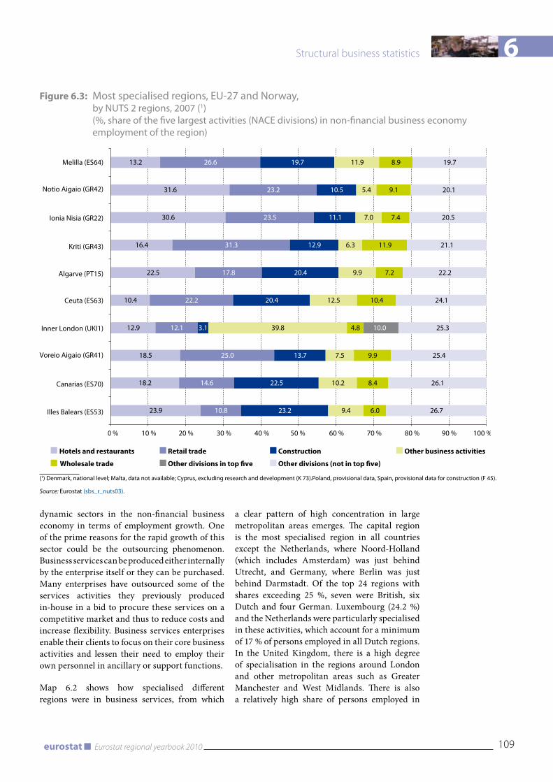
6
109Eurostat regional yearbook 2010eurostat
Structural business statistics
Figure 6.3: Most specialised regions, EU-27 and Norway, by NUTS 2 regions, 2007 (1) (%, share of the five largest activities (NACE divisions) in non-financial business economy employment of the region)
10,0
-23.9
0 % 10 % 20 % 30 % 40 % 50 % 60 % 70 % 80 % 90 % 100 %
18.2
18.5
12.9
10.4
22.5
16.4
30.6
31.6
13.2
10.8
14.6
25.0
12.1
22.2
17.8
31.3
23.5
23.2
26.6
23.2
22.5
13.7
3.1
20.4
20.4
12.9
11.1
10.5
19.7
9.4
10.2
7.5
39.8
12.5
9.9
6.3
7.0
5.4
11.9
6.0
8.4
9.9
4.8
10.4
7.2
11.9
7.4
9.1
8.9
10.0
26.7
26.1
25.4
25.3
24.1
22.2
21.1
20.5
20.1
19.7Melilla (ES64)
Notio Aigaio (GR42)
Ionia Nisia (GR22)
Kriti (GR43)
Algarve (PT15)
Ceuta (ES63)
Inner London (UKI1)
Voreio Aigaio (GR41)
Canarias (ES70)
Illes Balears (ES53)
Retail trade Construction Other business activities
Wholesale trade Other divisions in top �ve Other divisions (not in top �ve)
Hotels and restaurants
(1) Denmark, national level; Malta, data not available; Cyprus, excluding research and development (K 73).Poland, provisional data, Spain, provisional data for construction (F 45).
Source: Eurostat (sbs_r_nuts03).
dynamic sectors in the non-financial business economy in terms of employment growth. One of the prime reasons for the rapid growth of this sector could be the outsourcing phenomenon. Business services can be produced either internally by the enterprise itself or they can be purchased. Many enterprises have outsourced some of the services activities they previously produced in-house in a bid to procure these services on a competitive market and thus to reduce costs and increase flexibility. Business services enterprises enable their clients to focus on their core business activities and lessen their need to employ their own personnel in ancillary or support functions.
Map 6.2 shows how specialised different regions were in business services, from which
a clear pattern of high concentration in large metropolitan areas emerges. The capital region is the most specialised region in all countries except the Netherlands, where Noord-Holland (which includes Amsterdam) was just behind Utrecht, and Germany, where Berlin was just behind Darmstadt. Of the top 24 regions with shares exceeding 25 %, seven were British, six Dutch and four German. Luxembourg (24.2 %) and the Netherlands were particularly specialised in these activities, which account for a minimum of 17 % of persons employed in all Dutch regions. In the United Kingdom, there is a high degree of specialisation in the regions around London and other metropolitan areas such as Greater Manchester and West Midlands. There is also a relatively high share of persons employed in
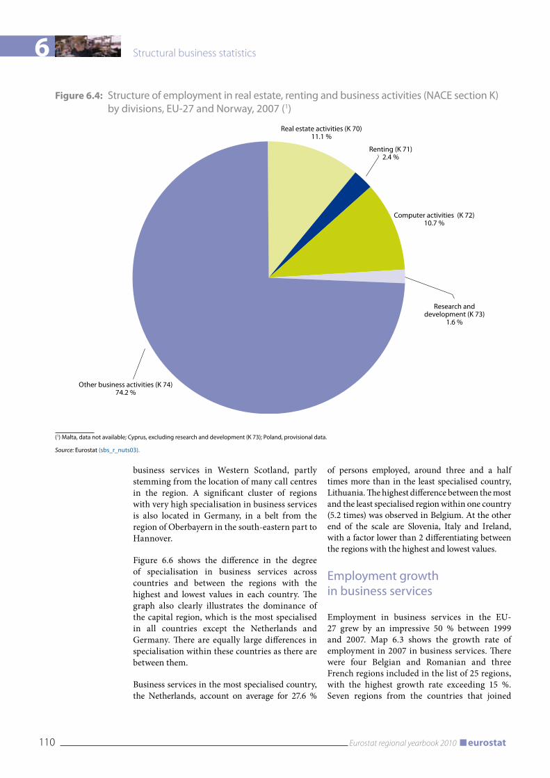
6 Structural business statistics
110 Eurostat regional yearbook 2010 eurostat
Figure 6.4: Structure of employment in real estate, renting and business activities (NACE section K) by divisions, EU-27 and Norway, 2007 (1)
Other business activities (K 74)74.2 %
Research and development (K 73)
1.6 %
Computer activities (K 72)10.7 %
Renting (K 71)2.4 %
Real estate activities (K 70)11.1 %
(1) Malta, data not available; Cyprus, excluding research and development (K 73); Poland, provisional data.
Source: Eurostat (sbs_r_nuts03).
business services in Western Scotland, partly stemming from the location of many call centres in the region. A significant cluster of regions with very high specialisation in business services is also located in Germany, in a belt from the region of Oberbayern in the south-eastern part to Hannover.
Figure 6.6 shows the difference in the degree of specialisation in business services across countries and between the regions with the highest and lowest values in each country. The graph also clearly illustrates the dominance of the capital region, which is the most specialised in all countries except the Netherlands and Germany. There are equally large differences in specialisation within these countries as there are between them.
Business services in the most specialised country, the Netherlands, account on average for 27.6 %
of persons employed, around three and a half times more than in the least specialised country, Lithuania. The highest difference between the most and the least specialised region within one country (5.2 times) was observed in Belgium. At the other end of the scale are Slovenia, Italy and Ireland, with a factor lower than 2 differentiating between the regions with the highest and lowest values.
Employment growth in business services
Employment in business services in the EU-27 grew by an impressive 50 % between 1999 and 2007. Map 6.3 shows the growth rate of employment in 2007 in business services. There were four Belgian and Romanian and three French regions included in the list of 25 regions, with the highest growth rate exceeding 15 %. Seven regions from the countries that joined
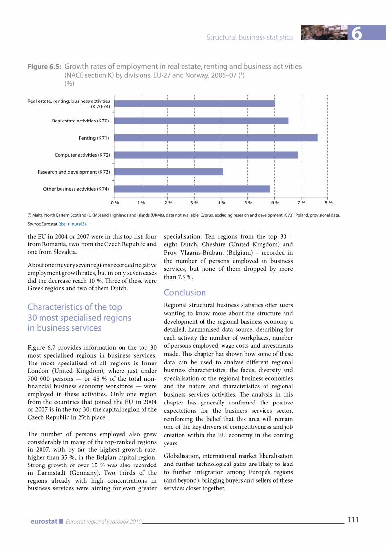
6
111Eurostat regional yearbook 2010eurostat
Structural business statistics
Figure 6.5: Growth rates of employment in real estate, renting and business activities (NACE section K) by divisions, EU-27 and Norway, 2006–07 (1) (%)
Other business activities (K 74)
Research and development (K 73)
Computer activities (K 72)
Renting (K 71)
Real estate activities (K 70)
Real estate, renting, business activities(K 70-74)
0 % 1 % 2 % 3 % 4 % 5 % 6 % 7 % 8 %
(1) Malta, North Eastern Scotland (UKM5) and Highlands and Islands (UKM6), data not available; Cyprus, excluding research and development (K 73); Poland, provisional data.
Source: Eurostat (sbs_r_nuts03).
the EU in 2004 or 2007 were in this top list: four from Romania, two from the Czech Republic and one from Slovakia.
About one in every seven regions recorded negative employment growth rates, but in only seven cases did the decrease reach 10 %. Three of these were Greek regions and two of them Dutch.
Characteristics of the top 30 most specialised regions in business services
Figure 6.7 provides information on the top 30 most specialised regions in business services. The most specialised of all regions is Inner London (United Kingdom), where just under 700 000 persons — or 45 % of the total non-financial business economy workforce — were employed in these activities. Only one region from the countries that joined the EU in 2004 or 2007 is in the top 30: the capital region of the Czech Republic in 25th place.
The number of persons employed also grew considerably in many of the top-ranked regions in 2007, with by far the highest growth rate, higher than 35 %, in the Belgian capital region. Strong growth of over 15 % was also recorded in Darmstadt (Germany). Two thirds of the regions already with high concentrations in business services were aiming for even greater
specialisation. Ten regions from the top 30 – eight Dutch, Cheshire (United Kingdom) and Prov. Vlaams-Brabant (Belgium) – recorded in the number of persons employed in business services, but none of them dropped by more than 7.5 %.
ConclusionRegional structural business statistics offer users wanting to know more about the structure and development of the regional business economy a detailed, harmonised data source, describing for each activity the number of workplaces, number of persons employed, wage costs and investments made. This chapter has shown how some of these data can be used to analyse different regional business characteristics: the focus, diversity and specialisation of the regional business economies and the nature and characteristics of regional business services activities. The analysis in this chapter has generally confirmed the positive expectations for the business services sector, reinforcing the belief that this area will remain one of the key drivers of competitiveness and job creation within the EU economy in the coming years.
Globalisation, international market liberalisation and further technological gains are likely to lead to further integration among Europe’s regions (and beyond), bringing buyers and sellers of these services closer together.
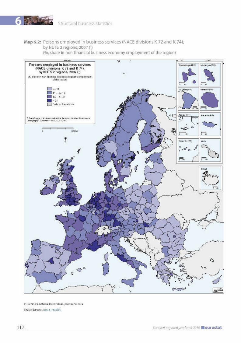
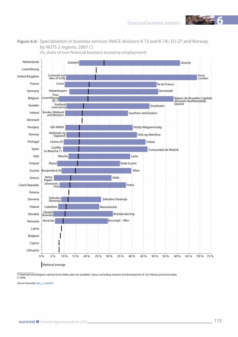
6
113Eurostat regional yearbook 2010eurostat
Structural business statistics
Figure 6.6: Specialisation in business services (NACE divisions K 72 and K 74), EU-27 and Norway, by NUTS 2 regions, 2007 (1) (%, share of non-financial business economy employment)
0 % 5 % 10 % 15 % 20 % 25 % 30 % 35 % 40 % 45 % 50 % 55 % 60 % 65 % 70 % 75 %
Netherlands
Luxembourg
United Kingdom
France
Germany
Belgium
Sweden
Ireland
Denmark
Hungary
Norway
Portugal
Spain
Italy
Finland
Austria
Greece
Czech Republic
Estonia
Slovenia
Poland
Slovakia
Romania
Latvia
Bulgaria
Cyprus
Lithuania
National average
Zeeland Utrecht
Île de France
Inner London
Corse
Småland med öarna Stockholm
Border, Midland and Western
Southern and Eastern
Dél-Alföld Közép-Magyarország
Oslo og Akershus
Centro (P) Lisboa
Castilla-La Mancha (2) Comunidad de Madrid
Marche Lazio
Åland Etelä-Suomi
Notio Aigaio
Attiki
Burgenland (A) Wien
Severovýc-hod Praha
Vzhodna Slovenija Zahodna Slovenija
Lubelskie Mazowieckie
Bratislavský kraj
Bucureşti – IlfovNord-Est
Západné Slovensko
Hedmark ogOppland
Niederbayern Darmstadt
Région de Bruxelles-Capitale /Brussels Hoofdstedelijk Gewest
Prov. Luxembourg
(B) (2)
Cornwall and Isles of Scilly
(1) Denmark and Bulgaria, national level; Malta, data not available; Cyprus, excluding research and development (K 73); Poland, provisional data.(2) 2006.
Source: Eurostat (sbs_r_nuts03).
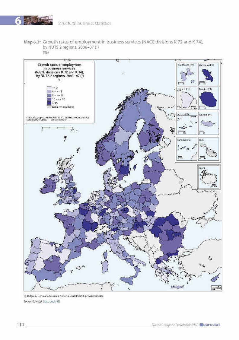
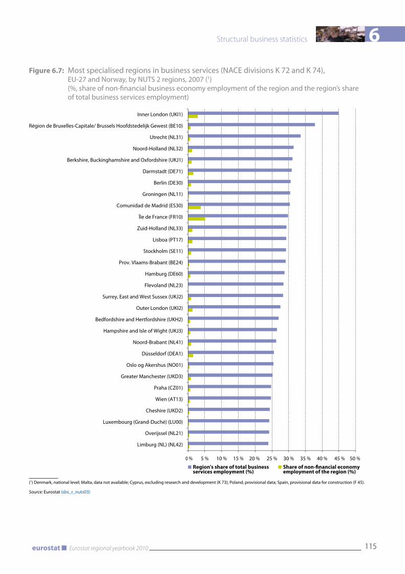
6
115Eurostat regional yearbook 2010eurostat
Structural business statistics
Figure 6.7: Most specialised regions in business services (NACE divisions K 72 and K 74), EU-27 and Norway, by NUTS 2 regions, 2007 (1) (%, share of non-financial business economy employment of the region and the region’s share of total business services employment)
0 % 5 % 10 % 15 % 20 % 25 % 30 % 35 % 40 % 45 % 50 %
Limburg (NL) (NL42)
Region's share of total businessservices employment (%)
Share of non-�nancial economyemployment of the region (%)
Overijssel (NL21)
Luxembourg (Grand-Duché) (LU00)
Cheshire (UKD2)
Wien (AT13)
Praha (CZ01)
Greater Manchester (UKD3)
Oslo og Akershus (NO01)
Düsseldorf (DEA1)
Noord-Brabant (NL41)
Hampshire and Isle of Wight (UKJ3)
Bedfordshire and Hertfordshire (UKH2)
Outer London (UKI2)
Surrey, East and West Sussex (UKJ2)
Flevoland (NL23)
Hamburg (DE60)
Prov. Vlaams-Brabant (BE24)
Stockholm (SE11)
Lisboa (PT17)
Zuid-Holland (NL33)
Île de France (FR10)
Comunidad de Madrid (ES30)
Groningen (NL11)
Berlin (DE30)
Darmstadt (DE71)
Berkshire, Buckinghamshire and Oxfordshire (UKJ1)
Noord-Holland (NL32)
Utrecht (NL31)
Région de Bruxelles-Capitale/ Brussels Hoofdstedelijk Gewest (BE10)
Inner London (UKI1)
(1) Denmark, national level; Malta, data not available; Cyprus, excluding research and development (K 73); Poland, provisional data; Spain, provisional data for construction (F 45).
Source: Eurostat (sbs_r_nuts03)

6 Structural business statistics
116 Eurostat regional yearbook 2010 eurostat
Methodological notes
Regional structural business statistics (SBS) are collected within the framework of a Council and Parliament regulation, in accordance with the definitions and breakdowns specified in the Commission regulations implementing it. Data for the reference year 2007, presented in the chapter, have been collected within the legal framework provided by Council Regulation (EC, Euratom) No 58/97 of 20 December 1996 concerning structural business statistics. The data cover all the EU Member States and Norway. Data at NUTS 2 level in the 2006 classification were unavailable for Denmark. These and other SBS data sets are available on Eurostat’s website (www.ec.europa.eu/eurostat) on the tag ‘Statistics’, under the theme ‘Industry, trade and services’/‘Structural Business Statistics’. Selected publications, data and background information are available in this section of the Eurostat website dedicated to European business — see the special topic on regional structural business statistics. Most data series are continuously updated and revised where necessary. This chapter reflects the data situation in March 2010.
Structural business statistics are presented by sectors of activity according to the NACE Rev. 1.1 classification, with a breakdown to two-digit level (NACE divisions). The data presented here are restricted to the non-financial business economy. The non-financial business economy includes sections C (Mining and quarrying), D (Manufacturing), E (Electricity, gas and water supply), F (Construction), G (Wholesale and retail trade), H (Hotels and restaurants), I (Transport, storage and communication) and K (Real estate, renting and business activities). It excludes agricultural, forestry and fishing activities and public administration and other non-market services (such as education and health, which are currently not covered by the SBS), as well as financial services (NACE section J).
The observation unit for regional SBS data is the local unit, which is an enterprise or part of an enterprise situated in a geographically identified place. Local units are classified into sectors (by NACE) according to their main activity. At national level, the statistical unit is the enterprise. An enterprise can consist of several local units. It is possible for the principal activity of a local unit to differ from that of the enterprise to which it belongs. Hence, national and regional structural business statistics are not entirely comparable. It should be noted that in some countries the activity code assigned is based on the principal activity of the enterprise in question.
Regional data are available at NUTS 2 level for a limited set of variables: the number of local units, wages and salaries, the number of persons employed and investments in tangible goods. The latter variable is collected on an optional basis, except for Industry (NACE sections C to E), which has more limited availability of data than for the other variables.
Structural business statistics define number of persons employed as the total number of persons who work (paid or unpaid) in the observation unit, as well as persons who work outside the unit who belong to it and are paid by it. It includes working proprietors, unpaid family workers, part-time workers and seasonal workers, etc.


Information society
7 Information society
120 Eurostat regional yearbook 2010 eurostat
Introduction
Information and communication technologies (ICTs) have now penetrated all areas of economic and social life. ICTs account for a significant increase in productivity and growth of GDP, and are transforming our societies in profound and unprecedented ways. The introduction of the Internet and the World Wide Web have led the development of the so-called information society. With access to the Internet, it is very easy to obtain information on almost anything. Search engines provide fast, easy access to websites and information sources on the World Wide Web. Many activities such as communicating, and selling or buying goods and services, can be done online. These developments have created new ways for people, individually or collectively, to take part in economic, social or political life. Because these activities are not bound to any specific geographical place, they can potentially bridge large distances. Basically, people can carry out these activities anywhere, as long as there is a connection to the Internet. Nowadays, it is possible to keep in touch with family members or friends via social networking sites, to share holiday pictures on the web, or make a video call with a friend via the Internet. Electronic shopping sites enable bargain hunters to buy or sell items via the Internet. ICTs support working from home or from other places outside the office, enabling more flexibility in the way in which work is organised, with benefits for both employers and employees. The ubiquitous presence of information and communication technologies carries the potential for completely new ways of participating in the economy and society.
The basic essential for benefiting from the information society, whether as a private individual, an employer or an employee, is access to information and communication technologies, i.e. electronic devices such as computers, and fast connections to the Internet. The term ‘digital divide’ refers to the difference between those who have access to the Internet and are able to make use of new services offered on the World Wide Web, and those excluded. The term explicitly includes access to information and communication technologies, as well as the skills needed to take part in the information society. The digital divide can be classified according to criteria that describe differences in participation according to gender, age, education, income, social groups or geographic location. This chapter puts emphasis on geographical aspects of the digital divide.
Policies within the European Union at national and European level have recognised the importance of bridging the digital divide to give citizens equal access to information and communication technologies and to enable them to take part in the information society. The Digital Agenda for Europe outlines a number of actions concerning very fast Internet access and a sustainable digital society. The key benchmarking indicators are defined in the European Commission’s framework for ‘Benchmarking Digital Europe 2011–15’ (1). This will monitor the development of the European information society and success in achieving the policy objectives set out in the Digital Agenda for Europe, which is a flagship initiative under the Europe 2020 strategy for smart, sustainable and inclusive growth (2), to further develop an economy based on knowledge and innovation.
The benchmarking framework distinguishes between annual indicators that monitor:
basic aspects of the development of the Euro-•pean information society;special modules that focus on specific aspects. •
The special modules change on an annual basis. For 2009, e-commerce is the topic of a special module on the use of information and communication technologies in households and by individuals. As well as basic indicators of the digital divide, the chapter presents selected results related to e-commerce.
Access to information and communication technologies
Access to information and communication technologies is at the heart of the digital divide. Geographical location are one aspect of that divide. Regional statistical data are available at European level on access to the Internet within households and on availability of broadband for going online. The Digital Agenda for Europe specifies fast Internet access as a specific area for action. New, innovative developments in electronic services need fast wired and wireless Internet access. That is why it is essential to foster and monitor the development of fast Internet access as part of the benchmarking framework.
In contrast to supply-side statistics, the Eurostat figures show the actual uptake of ICTs in households. In 2009, on average, almost two thirds (65 %) of households in Europe with members aged
(1) http://ec.europa.eu/ information_society/ eeurope/i2010/docs/benchmarking/ benchmarking_digital_europe_2011-2015.pdf
(2) http://eur-lex.europa.eu/LexUriServ/LexUriServ.do?uri=COM:2010:2020: FIN:EN:PDF
7
121Eurostat regional yearbook 2010eurostat
Information society
between 16 and 74 had access to the Internet at home and more than half (56 %) had access to the Internet via broadband. These figures have grown rapidly in recent years, at an annual growth rate of 10 % for Internet access and 30 % for broadband access between 2004 and 2009.
Access to the Internet makes it possible to take part in the information society, but broadband connections enable Internet users to exploit the potential of the Internet to the full. In fact, a broadband connection is essential for many advanced Internet services, such as social networking sites, uploading and downloading of media content (video and audio files) or the use of online maps and satellite images.
Websites are getting richer in content, boosting demand for traffic volumes constantly, even for less advanced services such as e-mail.
There are wide regional differences in broadband access. They range from 84 % in Stockholm (SE11), Utrecht (NL31) and Noord-Holland (NL32) to 20 % in Kentriki Ellada (GR2). The leading regions are in Sweden, the Netherlands, the United Kingdom, Denmark and Finland. At the other end of the spectrum are regions with the lowest share of households with broadband access, in Italy, the Czech Republic, Bulgaria, Romania and Greece.
It is also possible to analyse regional differences in broadband access within a country. This enables consumers within a country to evaluate how ‘connected’ their region is relative to others, irrespective of the picture at European level. The lowest interregional differences at national level can be observed in Romania, Slovakia, Poland and Sweden, with differences of less than 10 percentage points. The highest differences are in Germany, Greece, the Czech Republic, Spain and the United Kingdom.
Map 7.1 shows the share of households with broadband connections in Europe. A closer look at the map reveals three different patterns of digital divide. First, there is a north–south gradient. The regions with the highest share of households benefiting from broadband access are in the Nordic countries, the United Kingdom and the Netherlands, while regions in southern Europe tend to have lower penetration rates.
The second pattern is longitudinal. Regions in the west and east of the European Union have lower Internet penetration rates than regions in its centre.
Lastly, households in urban regions tend to have higher broadband access rates than those in rural regions. At EU-27 level, 61 % of households in densely populated areas have access to the Internet via broadband, while only 46 % of households in thinly populated areas have a broadband connection. Depending on the structure and size of the regions within a country, this is the pattern for some regions on Map 7.1. In general, regions with big cities, e.g. Lisboa (PT17), Madrid (ES30) and Barcelona (ES51), Île de France (FR01), Wien (AT13), Attiki (GR3), Praha (CZ01) or Berlin (DE3), show up as islands within their regions because of their higher levels of broadband access. The effect is even more pronounced if the region is covered entirely by the conurbation. Exceptions to this rule are Brussels (BE10) and Bratislavský kraj (SK01), where neighbouring regions have higher broadband Internet access rates than the cities.
Figure 7.1 illustrates differences in the share of households with Internet access and broadband connections. Instead of showing divergences in percentage shares, they show how far a country is ahead or behind the average in the EU-27 in terms of time. So, for instance, the level of Internet access in Hungary for 2009 corresponds to the average the EU reached in 2007. In other words, Hungary is lagging two years behind. Denmark, on the other hand, is four years ahead of the EU average. The general trend of Internet and broadband access at EU level is calculated, including a forecast based on the current trend. The national figures are then compared to the European trend. In general, time lags for Internet access are higher than those for broadband connections. This is because take-up of broadband connections has shown an average increase of 30 % over the last five years, while the average increase in Internet access has been 10 % over the same time span.
In terms of Internet access, the Netherlands, Luxembourg, Sweden and Denmark are more than four years ahead of the EU average, while Greece, Romania and Bulgaria are more than four years behind. The maximum time difference between the slowest and fastest EU country amounts to 13 years. For household broadband connections, the leaders are Sweden, the Netherlands, Denmark and Finland with an advantage of more than two years, whereas Italy, Greece, Bulgaria and Romania are lagging behind the EU average by more than two years. The maximum time lag between EU countries for broadband connections is 4.5 years.

7
123Eurostat regional yearbook 2010eurostat
Information society
Regular use of the Internet
The share of households with Internet access or broadband connections shows the potential for private use of the Internet from home. Map 7.2 provides an overview of the geographic distribution of regions according to actual use of the Internet in 2009. Regular users of the Internet are defined as those who use it at least once a week, regardless of location. For 2009, the average share of regular Internet users is 60 % of the target population. Access is correlated to regular use. More than 70 % of the population in regions in Scandinavia, Germany, the Netherlands, the United Kingdom and Luxembourg use the Internet at least once a week.
More people living in densely populated areas (66 %) regularly use the Internet compared to those living in thinly populated areas (51 %). As in Map 7.1, there is a latitudinal gradient in the share of regular Internet users. Regions in the east and west of the EU-27 have lower shares. For 2009, the share of regular users in almost all regions in Portugal, southern Italy, Greece, Bulgaria and Romania was below 40 %.
So far, the regional trends, i.e. the north–south trend and the latitudinal trend from centre to west and east, have been expressed in qualitative terms. To quantify this subjective observation, two approximation lines were calculated to express the level of regular Internet users depending on location. The location of each region is represented by its geographic centre. As statistics are based on population, the centres were calculated, taking into account the distribution of the population within each region. The trend in Figure 7.2 illustrates the latitudinal trend. To express a linear trend, a centre line has been assumed, passing through the Netherlands, close to the German–French and French–Italian borders. Distances are expressed in km from the assumed centre to the east and west.
Figure 7.3 shows the meridional, i.e. the south–north trend. Again, distances are expressed in km from south to north. Figures 7.2 and 7.3 show both statistically significant linear trends. Going from south to north, a distance of 100 km coincides with an increase of 1.9 % points in regular Internet usage. For the latitudinal trend, with every 100 km distance from the centre, the share of regular Internet users decreases by 2.5 % points. These trends describe an existing spatial
phenomenon in a quantitative way, but do not necessarily describe a causal relationship between the location of a region and the percentage of regular Internet users. Further analysis would be needed to describe and analyse suitable explanatory variables for these phenomena.
Online shopping: e-commerce attracts customers
One of the most popular Internet activities is online shopping. The percentage of Internet users doing some shopping online has more than doubled over the last five years, and reached 43 % in 2009 for the EU-27. The advantages of e-commerce as compared to traditional shopping are that clients can order goods or services irrespective of the location of the shop. Opening hours do not apply, shopping is possible 24 hours a day, seven days a week. The Internet provides ample opportunities to get information about products in user forums or on other websites. It is very easy to compare the prices of selected goods or services, especially when using specialised price comparison websites. Shoppers are able to order products that are not normally offered where they live. For vendors, Internet shopping gives them opportunities to enlarge their potential client base. Competition is fierce, as competitors are only a few mouse clicks away. Trust is crucial for e-commerce, as seller and buyer do not have direct personal contact. Credit card details might be used fraudulently, or ordered goods might not be delivered properly, or, indeed, at all. It might take more effort to return goods if they do not meet the client’s expectations. And some people might miss personal contact and advice while shopping online.
The most popular goods or services among Internet shoppers are travel and accommodation services (51 %), followed by clothes and sports goods (46 %) and household goods (37 %). These have shown the most dynamic growth between 2005 and 2009. Travel and accommodation services have grown by 17 % points and clothes and sports goods by 14 % points over the last five years. On the other hand, only 18 % of Internet shoppers buy computer hardware and 29 % order or download software.
Regional differences for e-commerce are shown on Map 7.3. Again, all regions in Norway, Sweden and Denmark, most of the United Kingdom, the Netherlands and Luxembourg have more

7 Information society
124 Eurostat regional yearbook 2010 eurostat
Figure 7.1: Time distance of Internet and broadband access of households, 2009 (computed distance in number of years as compared to the EU-27 average in 2009)
–8 –6 –4 –2 0 2 4 6 8
Bulgaria
Romania
Greece
Portugal
Italy
Cyprus
Czech Republic
Spain
Hungary
Latvia
Poland
Lithuania
Slovakia
France
Estonia
Slovenia
Malta
Ireland
Belgium
Austria
United Kingdom
Finland
Germany
Denmark
Sweden
Norway
Luxembourg
Netherlands
Iceland
Internet access Broadband access
Source: Eurostat (isoc_si_broad and isoc_si_lia).
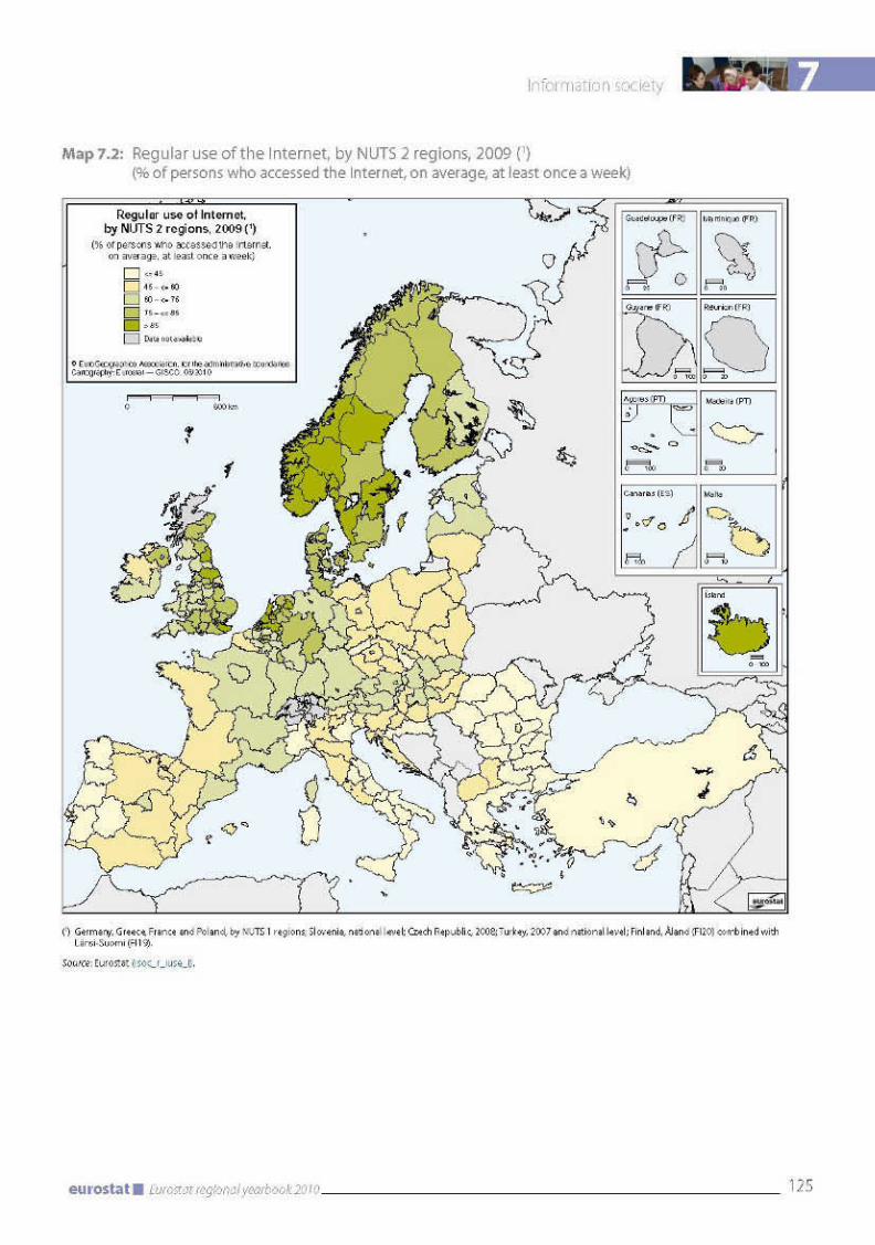
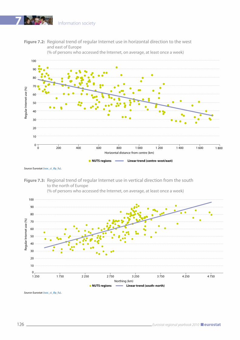
7 Information society
126 Eurostat regional yearbook 2010 eurostat
Figure 7.2: Regional trend of regular Internet use in horizontal direction to the west and east of Europe (% of persons who accessed the Internet, on average, at least once a week)
0
10
20
30
40
50
60
70
80
90
100
0 200 400 600 800 1 000 1 200 1 400 1 600 1 800
Regu
lar I
nter
net u
se (%
)
Horizontal distance from centre (km)
NUTS regions Linear trend (centre–west/east)
Source: Eurostat (isoc_ci_ifp_fu).
Figure 7.3: Regional trend of regular Internet use in vertical direction from the south to the north of Europe (% of persons who accessed the Internet, on average, at least once a week)
0
10
20
30
40
50
60
70
80
90
100
1 250 1 750 2 250 2 750 3 250 3 750 4 250 4 750
Regu
lar I
nter
net u
se (%
)
NUTS regions Linear trend (south–north) Northing (km)
Source: Eurostat (isoc_ci_ifp_fu).
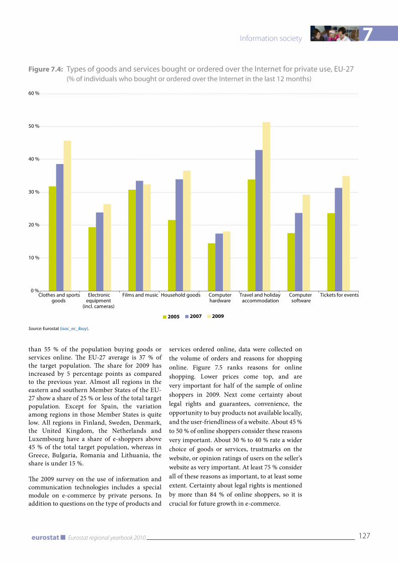
7
127Eurostat regional yearbook 2010eurostat
Information society
than 55 % of the population buying goods or services online. The EU-27 average is 37 % of the target population. The share for 2009 has increased by 5 percentage points as compared to the previous year. Almost all regions in the eastern and southern Member States of the EU-27 show a share of 25 % or less of the total target population. Except for Spain, the variation among regions in those Member States is quite low. All regions in Finland, Sweden, Denmark, the United Kingdom, the Netherlands and Luxembourg have a share of e-shoppers above 45 % of the total target population, whereas in Greece, Bulgaria, Romania and Lithuania, the share is under 15 %.
The 2009 survey on the use of information and communication technologies includes a special module on e-commerce by private persons. In addition to questions on the type of products and
services ordered online, data were collected on the volume of orders and reasons for shopping online. Figure 7.5 ranks reasons for online shopping. Lower prices come top, and are very important for half of the sample of online shoppers in 2009. Next come certainty about legal rights and guarantees, convenience, the opportunity to buy products not available locally, and the user-friendliness of a website. About 45 % to 50 % of online shoppers consider these reasons very important. About 30 % to 40 % rate a wider choice of goods or services, trustmarks on the website, or opinion ratings of users on the seller’s website as very important. At least 75 % consider all of these reasons as important, to at least some extent. Certainty about legal rights is mentioned by more than 84 % of online shoppers, so it is crucial for future growth in e-commerce.
Figure 7.4: Types of goods and services bought or ordered over the Internet for private use, EU-27 (% of individuals who bought or ordered over the Internet in the last 12 months)
0 %
10 %
20 %
30 %
40 %
50 %
60 %
Clothes and sportsgoods
Electronicequipment
(incl. cameras)
Films and music Household goods Computerhardware
Travel and holiday accommodation
Computer software
Tickets for events
2005 2007 2009
Source: Eurostat (isoc_ec_ibuy).
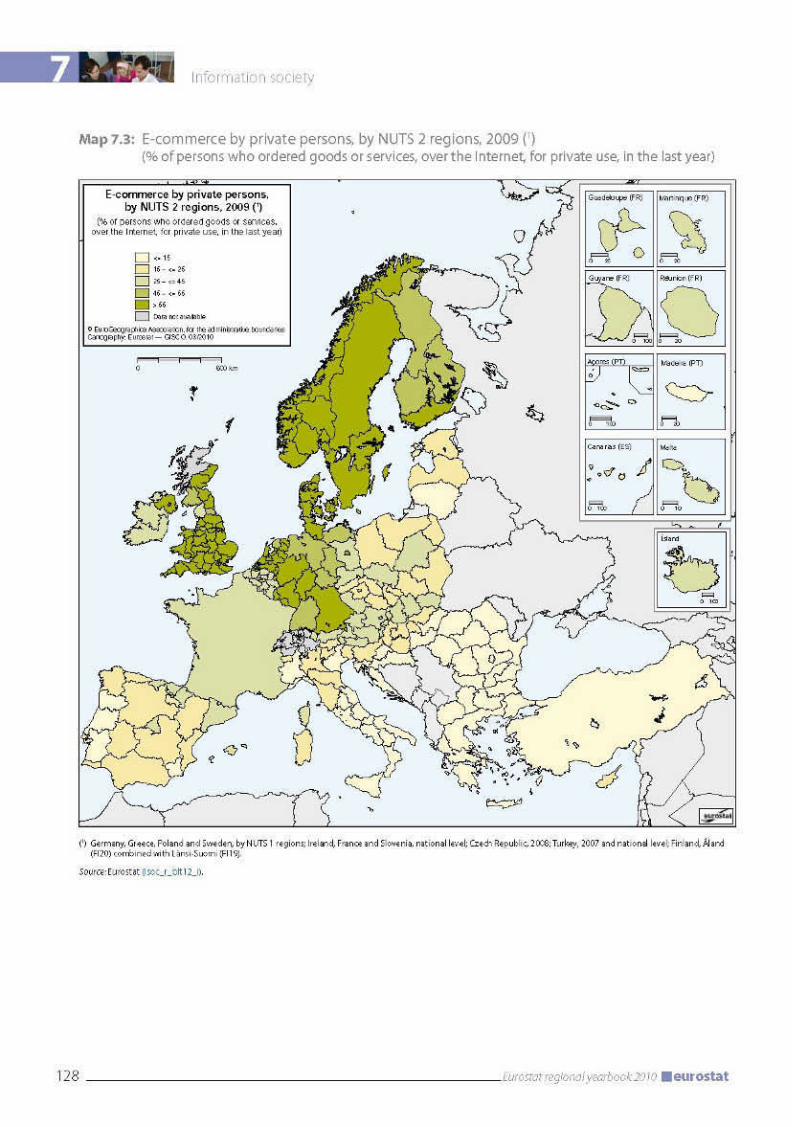
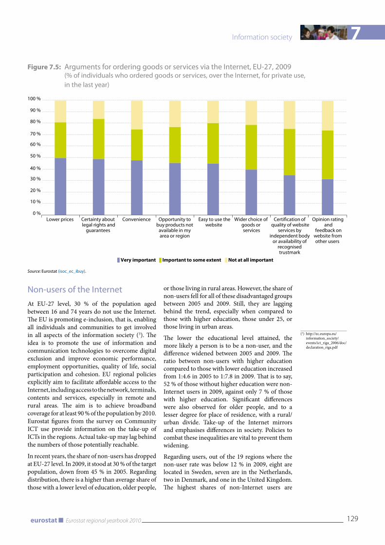
7
129Eurostat regional yearbook 2010eurostat
Information society
Figure 7.5: Arguments for ordering goods or services via the Internet, EU-27, 2009 (% of individuals who ordered goods or services, over the Internet, for private use, in the last year)
0 %
10 %
20 %
30 %
40 %
50 %
60 %
70 %
80 %
90 %
100 %
Lower prices Certainty about legal rights and
guarantees
Convenience Opportunity to buy products not
available in my area or region
Easy to use thewebsite
Wider choice of goods or services
Certification of quality of website
services by independent body
or availability of recognised trustmark
Opinion rating and
feedback onwebsite from other users
Very important Important to some extent Not at all important
Source: Eurostat (isoc_ec_ibuy).
Non-users of the InternetAt EU-27 level, 30 % of the population aged between 16 and 74 years do not use the Internet. The EU is promoting e-inclusion, that is, enabling all individuals and communities to get involved in all aspects of the information society (3). The idea is to promote the use of information and communication technologies to overcome digital exclusion and improve economic performance, employment opportunities, quality of life, social participation and cohesion. EU regional policies explicitly aim to facilitate affordable access to the Internet, including access to the network, terminals, contents and services, especially in remote and rural areas. The aim is to achieve broadband coverage for at least 90 % of the population by 2010. Eurostat figures from the survey on Community ICT use provide information on the take-up of ICTs in the regions. Actual take-up may lag behind the numbers of those potentially reachable.
In recent years, the share of non-users has dropped at EU-27 level. In 2009, it stood at 30 % of the target population, down from 45 % in 2005. Regarding distribution, there is a higher than average share of those with a lower level of education, older people,
or those living in rural areas. However, the share of non-users fell for all of these disadvantaged groups between 2005 and 2009. Still, they are lagging behind the trend, especially when compared to those with higher education, those under 25, or those living in urban areas.
The lower the educational level attained, the more likely a person is to be a non-user, and the difference widened between 2005 and 2009. The ratio between non-users with higher education compared to those with lower education increased from 1:4.6 in 2005 to 1:7.8 in 2009. That is to say, 52 % of those without higher education were non-Internet users in 2009, against only 7 % of those with higher education. Significant differences were also observed for older people, and to a lesser degree for place of residence, with a rural/urban divide. Take-up of the Internet mirrors and emphasises differences in society. Policies to combat these inequalities are vital to prevent them widening.
Regarding users, out of the 19 regions where the non-user rate was below 12 % in 2009, eight are located in Sweden, seven are in the Netherlands, two in Denmark, and one in the United Kingdom. The highest shares of non-Internet users are
(3) http://ec.europa.eu/information_society/events/ict_riga_2006/doc/declaration_riga.pdf
7 Information society
130 Eurostat regional yearbook 2010 eurostat
located in Italy (one region), Portugal and Greece (both three regions), Bulgaria (four regions) and Romania (seven regions). The regions with the highest share of non-users, with two thirds of the target population, are Sud-Muntenia (RO31) and Sud-Vest Oltenia (RO41).
Map 7.4 shows the distribution of regions according to the share of persons who have never used the Internet as a deviation from the EU-27 average. Regions in green have fewer non-users than the EU-27 average, while regions in yellow and orange are above the EU-27 average. The geographical distribution shows similar patterns to those described above. All regions in the Scandinavian countries, Finland, Sweden, Denmark as well as the Netherlands, the United Kingdom, Slovakia and Luxembourg are below 25 % of the target population, while the share of non-users in almost all regions in Bulgaria, Greece, Portugal, Romania, southern Italy and Cyprus is above 45 %. As seen above, regions in the east and west of the EU-27 tend to have higher shares of non-users as compared to the EU-27 average. Urban regions with higher population density tend to be below the EU-27 average. This tendency is visible, for example, for Athina, Lisboa, Madrid, Paris, Wien, Praha or Berlin.
Conclusion
Statistics on use of information and communica-tion technologies in households and by indivi-duals are collected annually at level 1 of NUTS. Some EU Member States additionally provide information at NUTS 2 level. The statistics illustrate that there are considerable differences regarding access and use of information and communication technologies among the regions
of the EU-27. Within the last few years, all Member States have increased access to and use of ICTs. However, differences in society regarding education, age and population density also appear in the pattern for the introduction of Internet and related services, and may reinforce these inequalities. To overcome this, the European Union has set explicit policy targets to achieve an inclusive information society. This includes the geographical dimension of the digital divide. The policies are benchmarked according to the ‘Benchmarking Digital Europe’ framework.
The maps in this chapter reveal specific spatial patterns that are visible for all indicators. There is a clear north–south gradient, with higher values of Internet access and use in northern Member States. The second pattern is a latitudinal pattern. Regions in the west and east of the European Union tend to have lower shares of Internet access and use than regions in the centre. Finally, urban or densely populated regions have a higher share of the population accessing and using the Internet than thinly populated areas. To achieve policy goals on participation in the information society, keeping up efforts to provide affordable access to the Internet via broadband, and educating people to equip them with the skills to access and benefit from Internet use will be essential. The new European 2020 strategy for smart, sustainable and inclusive growth (4), and the related flagship initiative ‘Digital Agenda for Europe’ will emphasise measures extending very fast Internet access, in achieving a single digital market, and ensuring a sustainable digital society.
(4) http://eur-lex.europa.eu/LexUriServ/LexUriServ.do?uri=COM:2010:2020: FIN:EN:PDF


7 Information society
132 Eurostat regional yearbook 2010 eurostat
Methodological notes
European statistical data on use of information and communication technologies have been available since 2003. Harmonised data have been published since 2006, based on Regulation (EC) No 808/2004 of 21 April 2004, concerning Community statistics on the information society. The regulation describes two modules or areas of statistical data production: statistics on the use of ICT in enterprises, and statistics on ICT use in households and by individuals. Annual Commission regulations define the set of indicators for which data are collected by the EU Member States. Regional data on a limited list of indicators have been available at the level of NUTS 1 since 2006 as a voluntary contribution by the Member States, and since 2008 on a mandatory basis. Some Member States provide regional data at NUTS 2 level on a voluntary basis. The data collection for each module is divided into a core part, i.e. access to ICT, and general use of ICT. Questions on access to ICT are addressed to the household, while questions on the use of ICT are answered by individuals within the household. Following the principles of the i2010 benchmarking framework, the model questionnaire includes an annual topic of special focus, i.e. e-government (2006), e-skills (2007), advanced services (2008), e-commerce (2009) and security (2010).
The survey covers individuals aged between 16 and 74, and households with at least one member within this age range. The reference period is the first three months of the calendar year.
The presentation of statistics on ICT use is restricted to a number of core indicators for which regional data are available. These regional indicators are ‘access to the Internet at home by household’, ‘access to the Internet via broadband by household’, ‘Regular Internet users’, ‘Persons who have never used the Internet’ and ‘E-commerce by individuals’.
The term ‘access’ does not refer to ‘connectivity’, i.e. whether connections can be provided in the household’s area or street, but to whether anyone in the household was able to use the Internet at home.
The term ‘broadband connection’ refers to the speed of data transfer for uploading and downloading data. Broadband requires a data transfer speed of more than 144 kbit/s. The technologies most widely used for broadband access to the Internet are Digital Subscriber Line (DSL) or cable modem.
Internet users are persons who have used the Internet within the last three months. Regular Internet users have used the Internet at least once a week within the reference period of three months.
For the purpose of the households’ module, e-commerce via the Internet is defined as placing orders for goods or services via the Internet. Purchases of financial investments, e.g. shares, confirmed reservations for accommodation and travel, participation in lotteries and betting, and obtaining payable information services from the Internet or purchases via online auctions, are included in the definition. Orders via manually typed e-mails are excluded. Delivery or payment via electronic means is not a requirement for an e-commerce transaction.


Science, technologyand innovation
8 Science, technology and innovation
136 Eurostat regional yearbook 2010 eurostat
Introduction
The Lisbon strategy launched in March 2000 and covering a period of 10 years emphasised the importance of research and development (R & D) and innovation in the European Union. Five years later, the Lisbon strategy was renewed by the initiative on ‘Working together for growth and jobs’, which put science, technology and innovation back at the heart of EU, national and regional policies in order to take targeted action in the main area of ‘Knowledge and innovation for growth’.
After the end of the Lisbon strategy and the recent economic crisis, a new strategy for the EU was called for. Based on the Commission communication entitled ‘Europe 2020: a strategy for smart, sustainable and inclusive growth’, in March 2010 the European Council agreed on the following components of this new strategy, which will be formally adopted in June 2010.
Europe 2020 sets three mutually reinforcing priorities:
smart growth: developing an economy based •on knowledge and innovation;sustainable growth: promoting a more re-•source-efficient, greener and more competitive economy;inclusive growth: fostering a high-employment •economy delivering social and territorial cohe-sion.
Seven flagship initiatives have also been proposed to support these priorities. One of them — the ‘Innovation Union’ initiative — aims to re-focus R & D and innovation policy on the challenges facing society, such as climate change, energy and resource efficiency, health and demographic change.
Based on a number of data sources available at Eurostat, this chapter presents statistics and indicators designed to compare trends in, and the structure of, science, technology and innovation (STI) in European regions and their position relative to other regions. The domains covered are: R & D; patents; high technology; human resources in science and technology (HRST). More regional indicators on science, technology and innovation are available on the Eurostat website under ‘Science and technology’.
Research and development
Twenty-seven of the 260 regions shown on Map 8.1 spend the equivalent of more than 3 % of their GDP on R & D. These regions are thus above the R & D-intensity target set by the Barcelona Council in 2002 and maintained in the Europe 2020 strategy. More than 40 % of the EU’s total R & D expenditure is generated in these, the most R & D-intensive, regions.
A cluster of four research-intensive regions can be found in south-western Germany: Stuttgart (5.85 %), Karlsruhe (3.72 %), Tübingen (3.80 %) and Darmstadt (3.11 %). These regions are also very important in absolute terms, as together they generate around 8 % of the total R & D expenditure in the EU. Another leading region in terms of R & D is Oberbayern (4.32 %), to the east of the four-region cluster, which contributes another 3 % to the EU total. Further north, Braunschweig (6.77 %), in the middle of Germany, is the most R & D-intensive region on the map. East of Braunschweig, two more major R & D regions are located: Dresden (4.12 %) and Berlin (3.36 %).
East Anglia (5.72 %), in the most eastern part of England, and Essex (4.66 %), just south of it, are the third and seventh most R & D-intensive regions in the UK. Together these two regions generate around 3 % of the EU total. Other R & D-intensive regions in the UK are, starting from the south, Hampshire and the Isle of Wight (3.41 %), Berkshire, Buckinghamshire and Oxfordshire (3.3 %), Cheshire (4.55 %), Lancashire (3.2 %) and North Eastern Scotland (3.11 %), which is also the only one of the 27 most R & D-intensive regions where the higher education sector generates more R & D expenditure than the business enterprise sector.
Eight of the most R & D-intensive regions are located in the Nordic countries. These regions are, starting from the south, Hovedstaden (the region surrounding the capital København) in Denmark (5.09 %), Sydsverige (4.91 %), Västsverige (4.47 %), Östra Mellansverige (3.79 %) and Stockholm (4.19 %) in Sweden, and Etelä-Suomi (3.39 %), Länsi-Suomi (3.68 %) and, finally, Pohjois-Suomi (5.38 %) in Finland which is the fourth most R & D-intensive region on the map.
In France the most R & D-intensive region is Midi-Pyrénées (4.15 %), just north of the Iberian Peninsula. In absolute terms, Île de France

8 Science, technology and innovation
138 Eurostat regional yearbook 2010 eurostat
(3.11 %), which includes the French capital, is the leading region in the EU with almost 8 % of the EU’s total expenditure on R & D. Two more regions with relatively high R & D intensity are located in Austria: Steiermark (3.77 %) and Wien (3.62 %).
Between 2003 and 2007 nine of the regions for which data are available increased their R & D intensity by more than half a percentage point: Praha (up by 0.68) in the Czech Republic, Stuttgart (1.17), Dresden (1.01) and Detmold (0.52) in Germany, La Rioja (0.54) and Comunidad Foral de Navarra (0.54) in Spain, Lisboa (0.72) in Portugal, Pohjois-Suomi (0.65) in Finland and Sydsverige (0.68) in Sweden.
Map 8.2 provides an overview of the regional distribution of the share of researchers in total employment (measured in headcount). Researchers are the core category directly employed on R & D activities. They are defined as ‘professionals engaged in the conception or creation of new knowledge, products, processes, methods and systems and in the management of the projects concerned’. The highest intensity of researchers (share of researchers out of all persons employed), more than 1.8 %, was found in 25 of the regions shown on Map 8.2. With six regions in this group of front-runners, the United Kingdom was the leading country, followed by Germany with five regions, Finland with three and Sweden and Norway with two each. Austria, Belgium, the Czech Republic, France, Portugal, Slovakia and Iceland each had one top region.
In 2007, North Eastern Scotland (United Kingdom) was the region with the highest share of researchers in total employment, with 4.58 %, well above the EU-27 average (0.99 %). Intensity of researchers was more than three times higher than the EU-27 average in four other regions: Inner London (United Kingdom) with 3.40 %, Wien (Austria) with 3.07 %, Trøndelag (Norway) with 3.05 % and Praha (Czech Republic) with 3.03 %. Fifteen out of the 25 regions performing well in terms of share of researchers also had the highest R & D intensity, with above 3 %, as shown on Map 8.1. The regions with relatively high concentrations of both researchers and R & D expenditure were North Eastern Scotland (United Kingdom), Wien (Austria) and Pohjois-Suomi (Finland).
Intensity of researchers ranged between 1.2 % and 1.8 % in 39 European regions. Again, most
of them were located in the United Kingdom (11), followed by another nine regions in Germany. In the vast majority of European regions the share of researchers did not exceed 0.6 % of all persons employed. Nineteen EU Member States and Norway reported at least one region with intensity of researchers below 0.6 %.
Looking at national differences, the spread between the regions with the highest and lowest proportions of researchers in total employment was particularly wide in the United Kingdom (4.47 percentage points between North Eastern Scotland and Highlands and Islands) and the Czech Republic (2.88 percentage points between Praha and Severozápad). Ireland was the country with the narrowest regional disparities in intensity of researchers (0.16 percentage points).
Human resources in science and technology
Science and technology have been recognised as key fields for European development. It is therefore extremely important for policymakers at regional level (and also at EU and national levels) to analyse the stock of highly qualified people who are actively participating in science and technology activities and technological innovation.
One way to measure the concentration of highly qualified people in the regions is by looking at human resources in science and technology (HRST). HRST includes persons who have completed tertiary (i.e. university) education (HRSTE) and/or are employed in a science and technology occupation (HRSTO). The stock of HRSTO can be used as an indicator of development of the knowledge-based economy in the EU.
As Map 8.3 shows, HRSTO are mostly concentrated in urban regions, in particular around the capitals. In 2008, 12 of the 25 leading regions were capital regions, where there is often a high concentration of highly qualified jobs, for example due to the presence of the head offices of companies and government institutions. Capitals are often big cities with large higher education facilities and a large number of highly educated people. This makes these and the surrounding regions attractive places to open science- and technology-related businesses. At the same time,
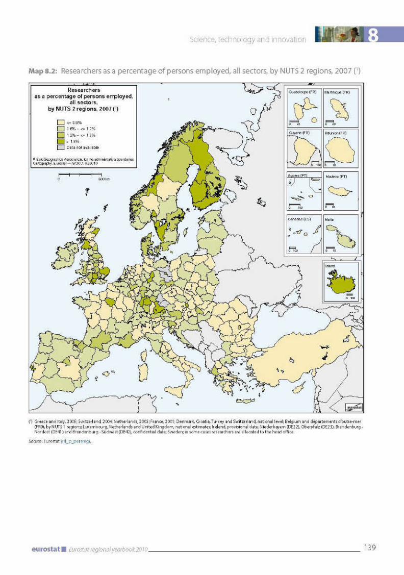
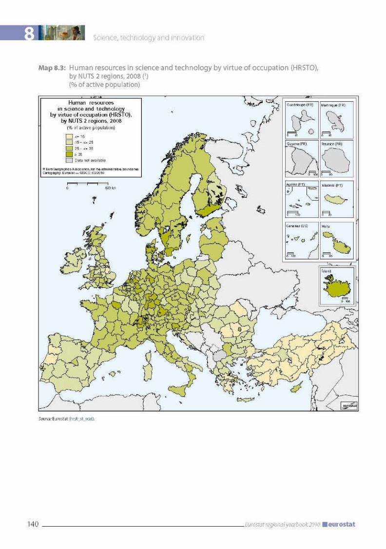
8
141Eurostat regional yearbook 2010eurostat
Science, technology and innovation
highly skilled people are often attracted to larger cities, as they are more likely to find a job that meets their requirements in a region where there are many companies.
This urban concentration of human resources employed in science and technology can also be seen by looking at two of the three large regional clusters with shares of HRSTO exceeding 35 % in 2008. The first of these clusters stretches from Switzerland into central and south-eastern Germany. In general, the regions in this cluster are very densely populated. This also applies to the regions in the second distinct cluster, which spans the Benelux countries and the western border regions of Germany. The third cluster is in the Scandinavian countries, where the regions — apart from the capital regions — are very sparsely populated. The regions with the second-, third- and fourth-highest shares of HRSTO are also found in Scandinavia: they are Stockholm in Sweden (48 %), Hovedstaden (København) in Denmark (47 %) and Oslo og Akershus in Norway (47 %). The highest share, however, is reported in Praha (Czech Republic), where 53 % of the labour force are HRSTO. For comparison, HRSTO made up 28 % of the active population in the EU in 2008. Amongst the top 10 regions, the share of HRSTO in the active population increased most in Bratislavský kraj (Slovakia) (by 6.0 percentage points from 2004 to 2008), Nordwestschweiz in Switzerland (5.1), Oberbayern in Germany (4.8) and Praha in the Czech Republic (4.7).
Based on R & D intensity, sectors of economic activity can be subdivided into more specific sub-sectors for the purposes of analysing employment in science and technology. For manufacturing industries, four groups have been identified, depending on the level of R & D intensity: high, medium-high, medium-low and low-technology sectors. Similarly, services were also classified into knowledge-intensive and less knowledge-intensive services. Within both these groups the following breakdowns are used: high-tech knowledge-intensive services, market high-tech and low-tech knowledge-intensive services, knowledge-intensive financial services and others.
High-tech knowledge-intensive services and high-tech manufacturing are the two subsectors of greatest importance for science and technology in terms of generating relatively high added value, providing new jobs and contributing to
competitive growth. Consequently, these two sectors are often analysed jointly as high-tech sectors. The NACE Rev. 2 classification defines high-tech knowledge-intensive services as including motion picture, video and television programme production, sound recording and music publishing activities, programming and broadcasting, telecommunications, computer programming and related activities, information service activities and research and development. High-tech manufacturing covers manufacture of pharmaceutical products and pharmaceutical preparations and of computers and electronic and optical products.
Some 68.0 % of the labour force in the EU in 2008 were employed in the services sector as a whole, but only 2.6 % in high-tech knowledge-intensive services. In addition, 16.9 % were employed in manufacturing, but only 1.1 % in high-tech manufacturing. Together, the high-tech sectors generated 3.7 % of total employment, with two thirds working in high-tech knowledge-intensive services and the other third in high-tech manufacturing.
Figure 8.1 shows the regional disparities in high-tech sectors as a share of total employment. It indicates the national average for each country and the regions with the lowest and highest shares of employment in high-tech sectors.
As can be seen from the figure, the highest and lowest national and regional shares vary significantly from one country to another. Moreover, significant disparities can be observed at regional level within and between countries.
With regard to the national averages, 15 of the 33 countries observed recorded values higher than the EU-27 average (3.7 %), with rates of more than 5.0 % in Malta, Finland, Switzerland, Denmark and Hungary. At the other end of the scale, the lowest national shares of high-tech sectors in total employment (below 2.5 %) were reported in Latvia, Portugal, Greece, Lithuania and Romania.
Note that six European Union countries (Estonia, Cyprus, Latvia, Lithuania, Luxembourg and Malta), one candidate country (the former Yugoslav Republic of Macedonia) and two EFTA countries (Iceland and Liechtenstein) are each classified as a single NUTS 2 region covering the entire country. Consequently, their national and regional figures at NUTS level 2 are identical.
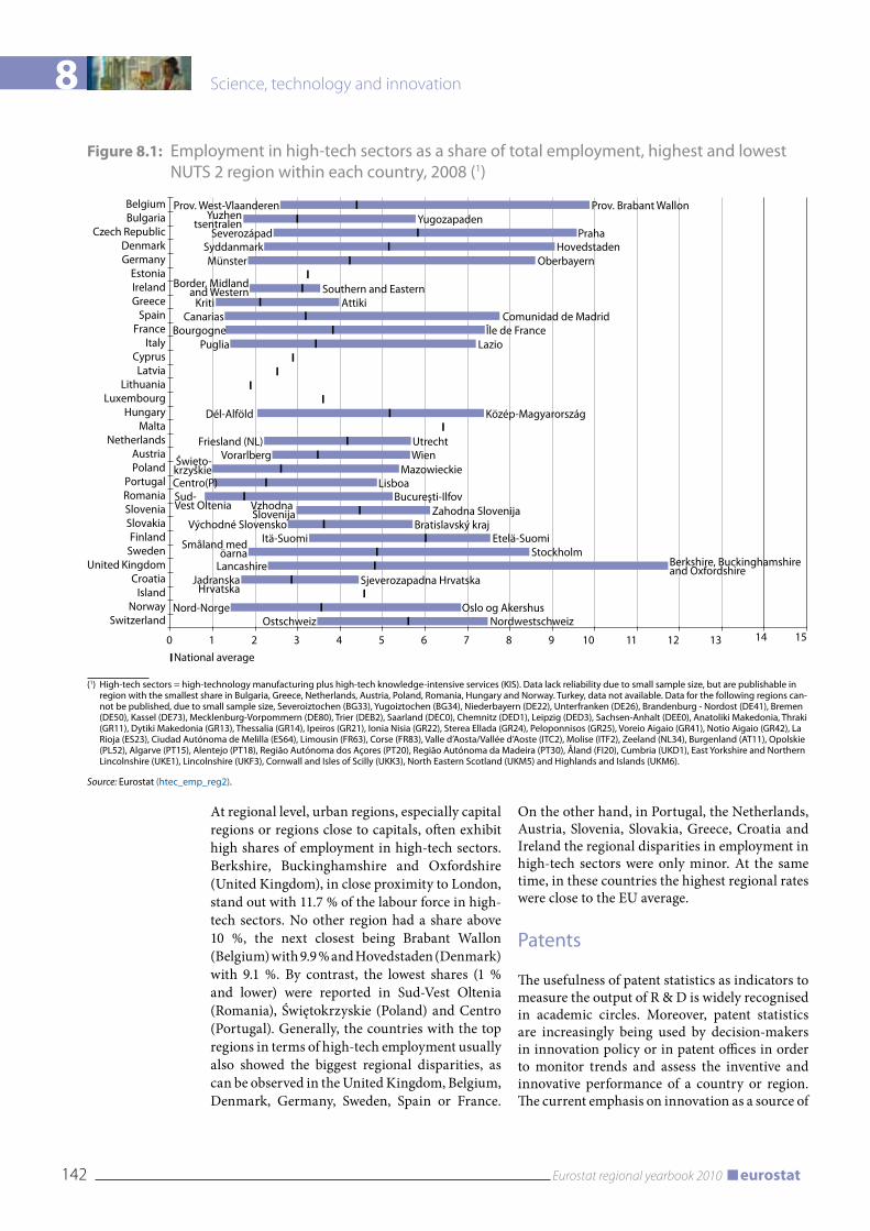
8 Science, technology and innovation
142 Eurostat regional yearbook 2010 eurostat
Figure 8.1: Employment in high-tech sectors as a share of total employment, highest and lowest NUTS 2 region within each country, 2008 (1)
0 1 2 3 4 5 6 7 8 9 10 11 12 13 14 15
BelgiumBulgaria
Czech RepublicDenmarkGermany
EstoniaIrelandGreece
SpainFrance
ItalyCyprusLatvia
LithuaniaLuxembourg
HungaryMalta
NetherlandsAustriaPoland
PortugalRomaniaSloveniaSlovakiaFinland
SwedenUnited Kingdom
CroatiaIsland
NorwaySwitzerland
Prov. West-Vlaanderen Prov. Brabant WallonYugozapaden
Severozápad PrahaSyddanmark HovedstadenMünster Oberbayern
Southern and EasternKriti Attiki
Canarias Comunidad de MadridBourgogne Île de France
Puglia Lazio
Dél-Alföld Közép-Magyarország
Centro(P)
Východné SlovenskoItä-Suomi Etelä-Suomi
Stockholm
Sjeverozapadna HrvatskaLancashire Berkshire, Buckinghamshire
and Oxfordshire
Nord-Norge
National average
Oslo og AkershusOstschweiz Nordwestschweiz
Jadranska Hrvatska
Småland medöarna
Sud-Vest Oltenia
Friesland (NL) UtrechtVorarlberg Wien
MazowieckieLisboa
Bucureşti-IlfovZahodna Slovenija
Bratislavský kraj
Vzhodna Slovenija
Święto-krzyskie
Border, Midlandand Western
Yuzhentsentralen
(1) High-tech sectors = high-technology manufacturing plus high-tech knowledge-intensive services (KIS). Data lack reliability due to small sample size, but are publishable in region with the smallest share in Bulgaria, Greece, Netherlands, Austria, Poland, Romania, Hungary and Norway. Turkey, data not available. Data for the following regions can-not be published, due to small sample size, Severoiztochen (BG33), yugoiztochen (BG34), Niederbayern (DE22), Unterfranken (DE26), Brandenburg - Nordost (DE41), Bremen (DE50), Kassel (DE73), Mecklenburg-vorpommern (DE80), Trier (DEB2), Saarland (DEC0), Chemnitz (DED1), Leipzig (DED3), Sachsen-Anhalt (DEE0), Anatoliki Makedonia, Thraki (GR11), Dytiki Makedonia (GR13), Thessalia (GR14), Ipeiros (GR21), Ionia Nisia (GR22), Sterea Ellada (GR24), Peloponnisos (GR25), voreio Aigaio (GR41), Notio Aigaio (GR42), La Rioja (ES23), Ciudad Autónoma de Melilla (ES64), Limousin (FR63), Corse (FR83), valle d’Aosta/vallée d’Aoste (ITC2), Molise (ITF2), Zeeland (NL34), Burgenland (AT11), Opolskie (PL52), Algarve (PT15), Alentejo (PT18), Região Autónoma dos Açores (PT20), Região Autónoma da Madeira (PT30), Åland (FI20), Cumbria (UKD1), East yorkshire and Northern Lincolnshire (UKE1), Lincolnshire (UKF3), Cornwall and Isles of Scilly (UKK3), North Eastern Scotland (UKM5) and Highlands and Islands (UKM6).
Source: Eurostat (htec_emp_reg2).
At regional level, urban regions, especially capital regions or regions close to capitals, often exhibit high shares of employment in high-tech sectors. Berkshire, Buckinghamshire and Oxfordshire (United Kingdom), in close proximity to London, stand out with 11.7 % of the labour force in high-tech sectors. No other region had a share above 10 %, the next closest being Brabant Wallon (Belgium) with 9.9 % and Hovedstaden (Denmark) with 9.1 %. By contrast, the lowest shares (1 % and lower) were reported in Sud-Vest Oltenia (Romania), Świętokrzyskie (Poland) and Centro (Portugal). Generally, the countries with the top regions in terms of high-tech employment usually also showed the biggest regional disparities, as can be observed in the United Kingdom, Belgium, Denmark, Germany, Sweden, Spain or France.
On the other hand, in Portugal, the Netherlands, Austria, Slovenia, Slovakia, Greece, Croatia and Ireland the regional disparities in employment in high-tech sectors were only minor. At the same time, in these countries the highest regional rates were close to the EU average.
Patents
The usefulness of patent statistics as indicators to measure the output of R & D is widely recognised in academic circles. Moreover, patent statistics are increasingly being used by decision-makers in innovation policy or in patent offices in order to monitor trends and assess the inventive and innovative performance of a country or region. The current emphasis on innovation as a source of
8
143Eurostat regional yearbook 2010eurostat
Science, technology and innovation
industrial competitiveness has raised awareness of patenting. The aim of patents is to protect R & D output, but they are just as significant as a source of technical information, which can help to avoid unnecessarily reinventing and redeveloping ideas.
Patent statistics at regional level are based on applications to the European Patent Office (EPO). The data are regionalised by linking postcodes or city names to the nomenclature of territorial units for statistics (NUTS).
However, any analysis of patent statistics should also take into consideration the limitations of such indicators. For instance, not all inventions are systematically patented. Moreover, a patent is an intellectual property right for inventions of a technical nature and there are other ways to protect intellectual property. Another drawback is that not all patents have the same intrinsic value and that only a small proportion of them lead to technological breakthroughs.
Another aspect can also skew interpretation of regional patent statistics: the place of residence of the inventor — which is used by the major producers of patent statistics for the distribution of patent applications — and the place where the invention took place (e.g. research institute) are not necessarily in the same NUTS region. Figure 8.2 shows regional disparities in patent applications to the EPO per million inhabitants by country and the national average. In Germany significant disparities were observed in 2005 between the leading region of Stuttgart in the south and the lowest-ranked region of Mecklenburg-Vorpommern in the east. Regional discrepancies were even wider in the Netherlands between the regions of Noord-Brabant and Zeeland. By contrast, discrepancies between regions were much smaller in Finland and Sweden, where the national averages were much closer to the top regions in terms of patent applications than in countries such as the Netherlands, Germany or Austria.
Map 8.4 illustrates regional patenting activity in high technology in the EU and provides an overview of regional performance in high-tech patent applications. In most European countries, national patenting is concentrated in specific regions. Regions that are active in patenting are often bunched close together to form economic clusters. This is the case, for example, in the southern part of Germany, the south-east of France
and the north-west of Italy. In general, the most active patenting regions are situated in the Nordic countries and at the centre of the EU-27.
In the field of high technology, however, patenting clusters are more difficult to detect, as very few regions recorded more than 100 high-tech patent applications to the EPO per million inhabitants. Finland is the only EU Member State where more than two regions submitted over 100 patent applications to the EPO per million inhabitants.
As shown in Figure 8.3, biotechnology patenting can also be measured at regional level. Seven of the top 15 regions in biotech patenting in the EU were in Germany, two in France, two in the United Kingdom and one each in the Netherlands, Denmark, Italy and Spain. The Danish capital region of Hovedstaden led the field in 2005, with 138 biotech patent applications, followed by Île de France with 127 and Oberbayern (Germany) with 104.
Conclusion
The economic crisis has been largely to blame for blowing some European regions off course away from growth and economic sustainability. This fact underlines the need for relevant and meaningful indicators on science, technology and innovation. Such indicators are of paramount importance for informing policymakers about where European regions stand and can help them take the measures necessary to put all regions back on the path towards greater knowledge and growth. This information also helps to draw clear comparisons of how regions are evolving, both at European level and worldwide.
Based on the relevant statistics and indicators, this yearbook spotlights which European regions are performing better than others in research and development activities and those that need support.
Data on high-tech industries and knowledge-intensive services, patents and human resources in science and technology were also used extensively to complete this regional picture.
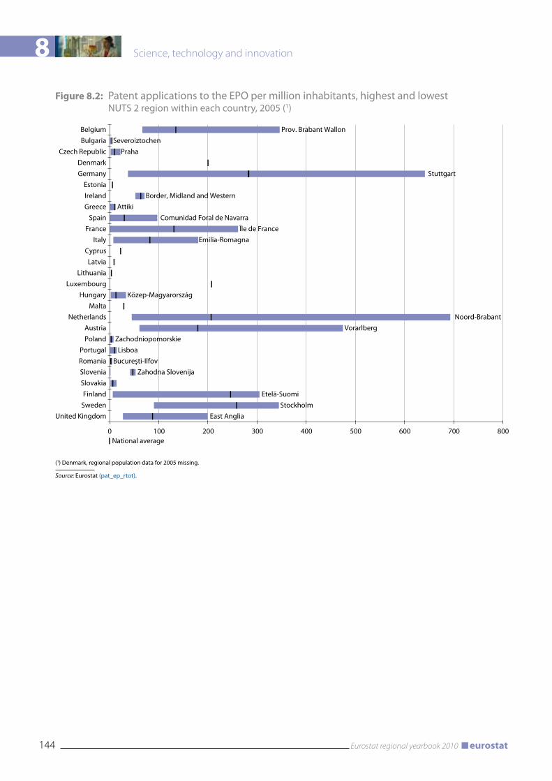
8 Science, technology and innovation
144 Eurostat regional yearbook 2010 eurostat
Figure 8.2: Patent applications to the EPO per million inhabitants, highest and lowest NUTS 2 region within each country, 2005 (1)
0 100 200 300 400 500 600 700 800
Belgium Prov. Brabant Wallon Bulgaria Severoiztochen
Czech Republic PrahaDenmarkGermany Stuttgart
EstoniaIreland Border, Midland and WesternGreece Attiki
Spain Comunidad Foral de NavarraFrance Île de France
Italy Emilia-RomagnaCyprusLatvia
LithuaniaLuxembourg
Hungary Közep-MagyarországMalta
Netherlands Noord-BrabantAustria VorarlbergPoland Zachodniopomorskie
Portugal LisboaRomania Bucureşti-IlfovSlovenia Zahodna SlovenijaSlovakia
National average
Finland Etelä-SuomiSweden Stockholm
United Kingdom East Anglia
(1) Denmark, regional population data for 2005 missing.
Source: Eurostat (pat_ep_rtot).
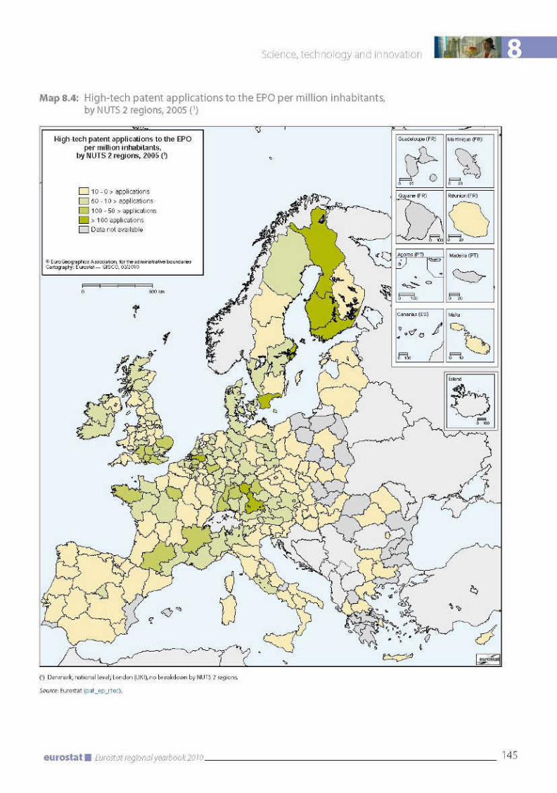
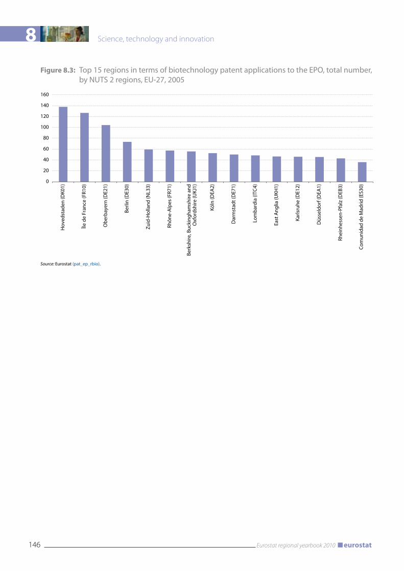
8 Science, technology and innovation
146 Eurostat regional yearbook 2010 eurostat
Figure 8.3: Top 15 regions in terms of biotechnology patent applications to the EPO, total number, by NUTS 2 regions, EU-27, 2005
0
20
40
60
80
100
120
140
160
Hov
edst
aden
(DK0
1)
Île d
e Fr
ance
(FR1
0)
Obe
rbay
ern
(DE2
1)
Berli
n (D
E30)
Zuid
-Hol
land
(NL3
3)
Rhôn
e-A
lpes
(FR7
1)
Berk
shire
, Buc
king
ham
shire
and
Oxf
ords
hire
(UKJ
1)
Köln
(DEA
2)
Dar
mst
adt (
DE7
1)
Lom
bard
ia (I
TC4)
East
Ang
lia (U
KH1)
Karls
ruhe
(DE1
2)
Düs
seld
orf (
DEA
1)
Rhei
nhes
sen-
Pfal
z (D
EB3)
Com
unid
ad d
e M
adrid
(ES3
0)
Source: Eurostat (pat_ep_rbio).

8
147Eurostat regional yearbook 2010eurostat
Science, technology and innovation
Methodological notes
The data in the maps and tables in this chapter are, wherever possible, broken down by NUTS 2 regions. Data are extracted from the ‘Science, technology and innovation’ domain and, more specifically, from the sub-domains ‘Research and development’, ‘Human resources in science and technology’, ‘High- technology industries and knowledge-intensive services’ and ‘Patents’.
Statistics on research and development are collected by Eurostat to meet the requirements of Commission Regulation (EC) No 753/2004, which specifies the data sets, breakdowns, frequency and transmission deadlines. The method for national R & D statistics is defined in further detail in the Frascati manual: proposed standard practice for surveys on research and experimental development (OECD, 2002), which is also used by many non-European countries.
The statistics on human resources in science and technology (HRST) are compiled annually, based on microdata extracted from the EU Labour Force Survey (EU LFS). The basic method employed for these statistics is laid down in the Canberra manual, which covers all HRST concepts.
The data on high-technology industries and knowledge-intensive services are compiled annually, based on data collected from a number of official sources (EU LFS, structural business statistics, etc.). The high-technology employment aggregates are defined in terms of R & D intensity, calculated as the ratio of R & D expenditure on the relevant economic activity to its value added, and based on the statistical classification of economic activities in the European Community (NACE). Revision of the NACE from Rev. 1.1 to Rev. 2 led to changes in the definitions of high-technology and knowledge-intensive sectors. The statistics in this chapter are based on NACE Rev. 2.
Finally, the data on patent applications to the EPO are compiled on the basis of microdata received from the European Patent Office (EPO). The data reported include the patent applications filed at the EPO during the reference year, classified by the inventor’s region of residence and in accordance with the international patents classification of applications. Patent data are regionalised using procedures linking postcodes and/or place names to NUTS 2 regions. Patent statistics published by Eurostat are almost exclusively based on the EPO’s Worldwide Statistical Patent Database (Patstat) developed by the EPO in 2005, using its patent data collection and its knowledge of patent data. The data are largely taken from the EPO’s master bibliographic database (DocDB), also known as the ‘EPO Patent Information Resource’. It includes bibliographic details on patents filed at 73 patent offices worldwide and contains more than 50 million documents. It covers a large number of fields included in patent documents, such as application details (claimed priorities, application and publication), categories of technology, inventors and applicants, titles and abstracts, patent citations and texts of non-patent literature.


Education

9 Education
150 Eurostat regional yearbook 2010 eurostat
Introduction
Education, vocational training and lifelong learning play a vital role in the economic and social strategy of the European Union. The relaunched Lisbon process, implemented by the ‘Education and training 2010’ programme, cannot be completed without efficient use of resources, improvements in the quality of education and training systems and implementation of a coherent lifelong learning strategy at national level. Secu-ring education and lifelong learning opportunities in every region and for every inhabitant, wherever they live, is one of the cornerstones of the national strategies to achieve this goal. Eurostat’s regional statistics on enrolment in education, educational attainment and participation in lifelong learning make it possible to measure progress at regional level and monitor regions lagging behind.
Comparable regional data on enrolment in education from 1998 onwards are available from Eurostat’s website, while data on educational attainment and on participation in lifelong learning are available for the period since 1999.
The Eurostat website contains region-by-region information on the total number of enrolments by level of education and sex, and by age and sex, plus indicators relating enrolments in education to the total population. Data on enrolments in education are generally available for the 15 ‘old’ Member States for the period since 1998 and for the 12 ‘new’ Member States plus Norway since 2000 or 2001. Information on the educational attainment of the population and on participation in lifelong learning is available for all the Member States and also for Norway.
Students in tertiary education
‘Tertiary education’ means levels of education that are offered by universities, vocational universities, institutes of technology and other institutions that award academic degrees or professional certificates. Access to tertiary-level courses typically requires successful completion of an upper-secondary and/or post-secondary non-tertiary level programme.
Tertiary-level education can be classified on the basis of its purpose:
ISCED (• 1) level 5A is, for the most part, theoreti-cally based and is intended to provide adequate
qualifications for entry into advanced research programmes and professions with high skills requirements;ISCED level 5B is more practical, technical and •employment oriented;ISCED level 6 (PhD-like studies) leads to an ad-•vanced research qualification.
Currently several goals and benchmarks for higher education have to be achieved in the EU. Amongst these, the most relevant aims are to increase the number of mathematics, science and technology graduates, to increase the number of Erasmus students, to raise more investment in higher education and, finally, to foster the mobility of students across Europe.
To give further pointers to the mobility of students, a tertiary education indicator is presented here. In 2008, the number of students in tertiary education in the EU-27 countries stood at nearly 19 million.
Map 9.1 shows the number of students who were enrolled in tertiary education (ISCED levels 5 and 6) in 2008 (2007/08 academic year) as a percentage of the corresponding regional population aged 20 to 24. This indicator is a function of the number of students in the region and of the number of residents aged 20 to 24 in the same region and gives an idea of how attractive the region is to tertiary students. Actually, since this indicator is based on data on the area where the students are studying, and not the area where they come from or live, it is likely that some of the students are not resident in the region where they are studying. Hence, regions which show high values for this indicator host big universities or other tertiary education institutions and, as a consequence, attract large numbers of students from outside the region.
Some of the factors that have to be explored when interpreting this indicator are related to the age-group structures of the population within regions and to the corresponding structures of the tertiary education system between regions. In spite of these limitations, the indicator gives a rough picture of the concentration or spread of tertiary education institutions across regions.
This indicator is high in regions such as Praha (Czech Republic), Wien (Austria), Lisboa (Portugal), Bucureşti - Ilfov (Romania), Bratislavský kraj (Slovakia), Brussels, Brabant Wallon and Oost-Vlaanderen (Belgium), Zahodna Slovenija
(1) ISCED: International Standard Classification of Education.

9
151Eurostat regional yearbook 2010eurostat
Education
(Slovenia), Hovedstaden (the region surrounding the capital København in Denmark), Övre Norrland (Sweden), Groningen (the Netherlands), Małopolskie (Poland), Közép-Magyarország (Hungary), Oslo og Akershus and Trøndelag (Norway), regions in the centre of Italy and most of Greece and Finland, because most of these regions are in fact around capital cities. Relatively few regions have a tertiary-level student population below 30 % of the 20- to 24-years age group.
Together with Map 9.1, Figure 9.1 gives an overview of the percentage of regions presenting different performance levels for this indicator. Regions showing 100 % of the indicator host big tertiary institutions and, as a consequence, attract large numbers of students from outside the region. As can be seen in this graph, when roughly 35 % of the regions have been considered, the proportion of the population aged 20 to 24 enrolled in tertiary education is about 60 %, whereas 20 % of regions have less than 40 % of this section of the population in tertiary education.
Students aged 17 in education
Compulsory education, along with the age when compulsory education ends, varies greatly between the EU Member States. In most countries, compulsory education ends at the age of 15 or 16, which is typically the end of lower-secondary education. Moreover, by the age of 17 it is possible to have finished secondary education in some countries, whereas in others pupils might have just started upper-secondary level. In spite of this, at the age of 17 most young people in the European Union are still in education.
At the age of 17, young people are faced with the choice of whether to remain in education, go into training or look for a job. Even if compulsory education ends before 17, over the last decade young people have become more likely to continue with their education.
Map 9.2 depicts students aged 17 (at all levels of education) as a percentage of the corresponding age group in each region. The highest figures for this indicator are in Sweden, Finland, Poland and other regions spread out across many states in the north of Europe, the United Kingdom, Iceland and Denmark. Looking at the candidate countries, Greece, Portugal, parts of Spain and parts of Italy, the indicator shows that in these regions the percentage of 17-year-olds who are
still in education is lower than in others. Almost everywhere in Europe this indicator gives a result of more than 75 %. That means that, for one reason or another, the younger generation are still in the education system even after the compulsory schooling age.
Participation of 4-year-olds in education
Learning begins at birth. The period from birth to the start of primary education is a critical formative stage for the growth and development of children. The learning outcomes and the knowledge and skills acquired during primary education are stronger when children learn and develop appropriately in the years preceding regular schooling.
The purpose of pre-primary education is to prepare children physically, emotionally, socially and mentally to enter grade 1 of primary school, giving them the ability and skills to enter the first level of the education system. This preparation is considered the foundation for further psychological development.
To bear out this theory, in December 2008 the European Commission proposed a new benchmark, with the aim that 90 % of 4-year-olds should participate in pre-primary education by 2020. The aim of this proposal is to underpin progress towards the target set at the 2002 Barcelona summit of increasing participation in pre-primary education to 90 % of all children between 3 years of age and the beginning of compulsory education.
The indicator shown here reflects participation in early childhood education by NUTS 2 region, by measuring the percentage of 4-year-olds who are in either pre-primary or primary school. By far the majority of 4-year-olds attend pre-primary school (non-compulsory). A 4-year-old child can be enrolled either in pre-primary or in primary school. The data highlight that most 4-year-olds attend pre-primary school. Ireland and the United Kingdom are the only countries where a significant proportion of 4-year-olds are in primary education.
At the age of 4 most children in the European Union are therefore in pre-primary education, which is generally available from at least 3 to 4 years of age in the EU Member States. Enrolment

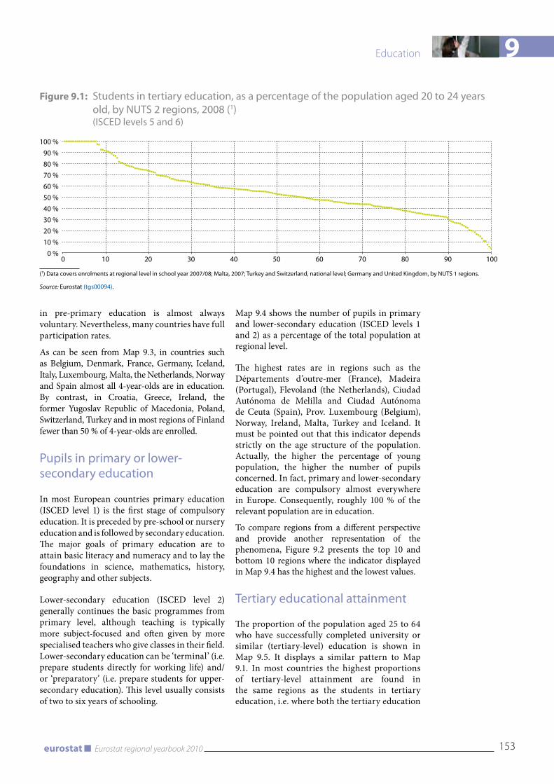
9
153Eurostat regional yearbook 2010eurostat
Education
in pre-primary education is almost always voluntary. Nevertheless, many countries have full participation rates.
As can be seen from Map 9.3, in countries such as Belgium, Denmark, France, Germany, Iceland, Italy, Luxembourg, Malta, the Netherlands, Norway and Spain almost all 4-year-olds are in education. By contrast, in Croatia, Greece, Ireland, the former Yugoslav Republic of Macedonia, Poland, Switzerland, Turkey and in most regions of Finland fewer than 50 % of 4-year-olds are enrolled.
Pupils in primary or lower-secondary education
In most European countries primary education (ISCED level 1) is the first stage of compulsory education. It is preceded by pre-school or nursery education and is followed by secondary education. The major goals of primary education are to attain basic literacy and numeracy and to lay the foundations in science, mathematics, history, geography and other subjects.
Lower-secondary education (ISCED level 2) generally continues the basic programmes from primary level, although teaching is typically more subject-focused and often given by more specialised teachers who give classes in their field. Lower-secondary education can be ‘terminal’ (i.e. prepare students directly for working life) and/or ‘preparatory’ (i.e. prepare students for upper-secondary education). This level usually consists of two to six years of schooling.
Map 9.4 shows the number of pupils in primary and lower-secondary education (ISCED levels 1 and 2) as a percentage of the total population at regional level.
The highest rates are in regions such as the Départements d’outre-mer (France), Madeira (Portugal), Flevoland (the Netherlands), Ciudad Autónoma de Melilla and Ciudad Autónoma de Ceuta (Spain), Prov. Luxembourg (Belgium), Norway, Ireland, Malta, Turkey and Iceland. It must be pointed out that this indicator depends strictly on the age structure of the population. Actually, the higher the percentage of young population, the higher the number of pupils concerned. In fact, primary and lower-secondary education are compulsory almost everywhere in Europe. Consequently, roughly 100 % of the relevant population are in education.
To compare regions from a different perspective and provide another representation of the phenomena, Figure 9.2 presents the top 10 and bottom 10 regions where the indicator displayed in Map 9.4 has the highest and the lowest values.
Tertiary educational attainment
The proportion of the population aged 25 to 64 who have successfully completed university or similar (tertiary-level) education is shown in Map 9.5. It displays a similar pattern to Map 9.1. In most countries the highest proportions of tertiary-level attainment are found in the same regions as the students in tertiary education, i.e. where both the tertiary education
Figure 9.1: Students in tertiary education, as a percentage of the population aged 20 to 24 years old, by NUTS 2 regions, 2008 (1) (ISCED levels 5 and 6)
0 %10 %20 %30 %40 %50 %60 %70 %80 %90 %
100 %
0 10 20 30 40 50 60 70 80 90 100
(1) Data covers enrolments at regional level in school year 2007/08; Malta, 2007; Turkey and Switzerland, national level; Germany and United Kingdom, by NUTS 1 regions.
Source: Eurostat (tgs00094).
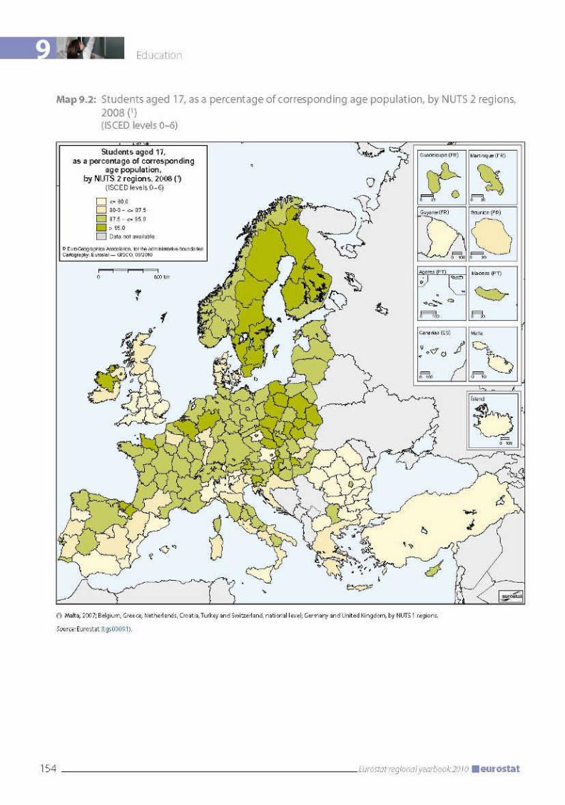
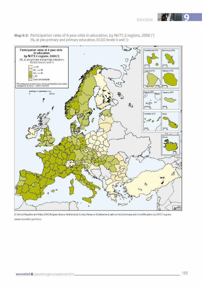
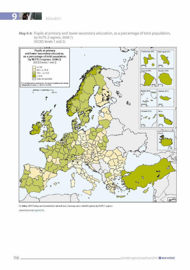
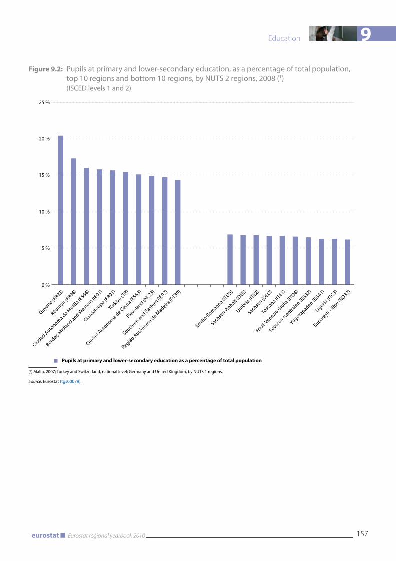
9
157Eurostat regional yearbook 2010eurostat
Education
Figure 9.2: Pupils at primary and lower-secondary education, as a percentage of total population, top 10 regions and bottom 10 regions, by NUTS 2 regions, 2008 (1) (ISCED levels 1 and 2)
0 %
5 %
10 %
15 %
20 %
25 %
Pupils at primary and lower-secondary education as a percentage of total population
Guyane (FR93)
Réunion (FR94)
Ciudad Autónoma de M
elilla (E
S64)
Border, M
idland and Weste
rn (IE
01)
Guadeloupe (FR91)
Türkiye (TR)
Ciudad Autonoma de Ceuta (E
S63)
Flevoland (NL23)
Southern
and Eastern
(IE02)
Região Autónoma da M
adeira (P
T30)
Emilia-Romagna (IT
D5)
Sachse
n-Anhalt (
DEE)
Umbria (IT
E2)
Sachse
n (DED)
Tosca
na (ITE1)
Friuli-V
enezia G
iulia (IT
D4)
Severen tsentra
len (BG32)
Yugozapaden (B
G41)
Liguria (IT
C3)
Bucureşti
- Ilfo
v (RO32)
(1) Malta, 2007; Turkey and Switzerland, national level; Germany and United Kingdom, by NUTS 1 regions.
Source: Eurostat (tgs00079).
9 Education
158 Eurostat regional yearbook 2010 eurostat
institutions and the largest enterprises and institutions and their suppliers are located. The demographic profile of a region also has some influence on educational attainment, as younger generations tend to achieve higher levels than older generations. In 2008 only 26 regions in the EU recorded a proportion of persons with higher education above 35 %. These include large cities such as Brussels, London, Paris, Helsinki, Stockholm and Madrid plus Utrecht in the Netherlands. Oslo (Norway) and Geneva and Zürich (Switzerland) also fall into this category. In EU Member States such as Ireland, Sweden, Finland, the Netherlands, Belgium and Germany educational attainment levels are generally high across the whole country. The regions with the lowest percentages of people with tertiary education are largely concentrated in the rural parts of nine EU countries, in marked contrast to their larger cities. This is the case in Portugal and Romania in particular, and also in Croatia, Turkey and, to a lesser extent, in Bulgaria, the Czech Republic, Greece, Italy, Hungary, Poland and Slovakia. This also applies to some islands such as Sardegna and Sicilia (Italy), Açores and Madeira (Portugal) and Malta.
Lifelong learning
Continuously refreshing the skills of the labour force by means of lifelong learning has repeatedly been underlined in EU policies following up the Lisbon objectives. This is reflected in the EU’s ‘Education and training 2010’ programme and in the European employment strategy, which emphasises the need for comprehensive lifelong learning strategies to keep workers continuously adaptable and employable. Adult learning can be measured in the Labour Force Survey by specific
questions on participation in education or training activities during the four weeks preceding the survey. The data concern the 25–64 age group for all education or vocational training, whether or not relevant to the participants’ current or future employment. As Map 9.6 shows, participation in education and training shows a largely national profile. In fact, this is the education indicator showing the smallest regional variation compared with the others discussed earlier in this chapter. Participation is high in every region of Denmark, the Netherlands, Slovenia, Finland, Sweden and the United Kingdom and also in Iceland, Norway and Switzerland. Within countries, the highest rates of participation in education and training are often found around the largest cities, which are usually also the regions with the highest levels of educational attainment (see previous section) and where the range of education and training offered is widest and continuing vocational training activities are most frequent (e.g. in large enterprises). On the other hand, EU Member States on the fringes of the continent, such as Greece, Hungary, Malta, Poland, Portugal, Romania and Slovakia, generally have low participation rates in education and training for the 25–64 age group, as do Croatia and Turkey.
Conclusion
The examples given above are intended merely to highlight a few of the many possible ways of analysing education and lifelong learning in the regions of the EU and should not be considered a detailed analysis. However, Eurostat hopes that they will encourage readers to probe deeper into all the data on education available free of charge on the Eurostat website and to make many further interesting discoveries.
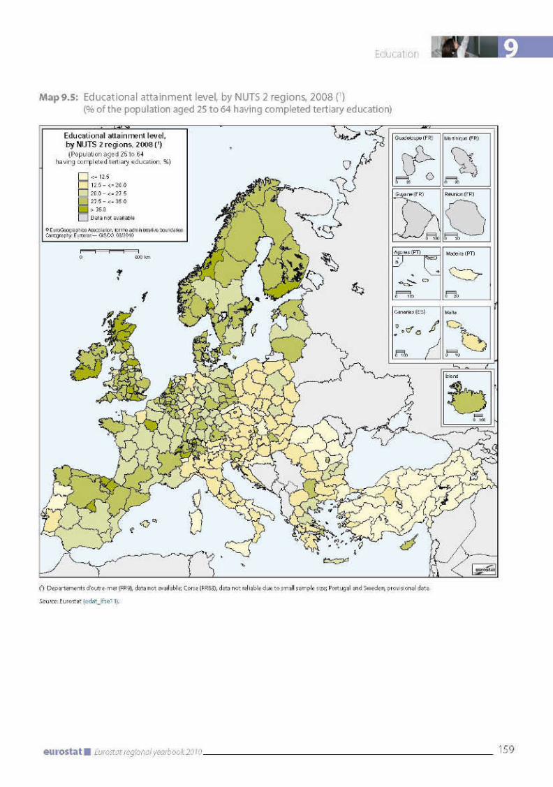
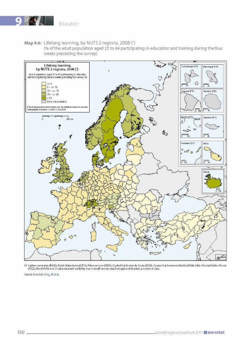

9
161Eurostat regional yearbook 2010eurostat
Education
Methodological notes
The maps are presented at NUTS 2 level, except the educational enrolment indicators for Germany and the United Kingdom, where data are available at NUTS 1 level only. In Croatia, Switzerland and Turkey no data on enrolments by age are available at regional level. Consequently, only national figures have been shown for these countries.
As the structure of education systems varies widely from one country to another, a framework for assembling, compiling and presenting both national and international education statistics and indicators is a prerequisite for international comparability. The International Standard Classification of Education (ISCED) provides the basic classification for collecting data on education. ISCED-97, the current version of the classification introduced in 1997, is built to classify each educational programme by field of education and by level.
ISCED-97 presents standard concepts, definitions and classifications. A full description of ISCED-97 is available on the Unesco Institute of Statistics website (http://www.uis.unesco.org/ev.php?ID=3813_201&ID2=DO_TOPIC).
Qualitative information about school systems in the EU Member States is organised and disseminated by Eurydice (http://www.eurydice.org), for example on compulsory school attendance ages and numerous issues relating to organisation of school life in the Member States (decision-making, curricula, school hours, etc.).
The statistics on enrolments in education include all regular education programmes and all adult education with content similar to regular education programmes or leading to qualifications similar to the corresponding regular programmes. Apprenticeship programmes are included, except those which are entirely work-based and which are not supervised by any formal education authority. The data sources for Maps 9.1 to 9.4 are two specific Eurostat tables which form part of the ‘UOE’ (UIS-UNESCO, OECD and Eurostat) data collection on education systems. Information about the UOE data collection can be found at: http://circa.europa.eu/Public/irc/dsis/edtcs/library?l=/public/unesco_collection&vm=detailed&sb=Title.
The statistics on educational attainment and on participation in lifelong learning are based on the EU Labour Force Survey (LFS), which is a quarterly sample survey. The indicators refer to the annual average of the quarterly data for 2007. The educational attainment level reported is based on ISCED-97. Lifelong learning includes participation in any kind of education and training activities during the four weeks prior to the survey.

Transport

10 Transport
164 Eurostat regional yearbook 2010 eurostat
Introduction
Roads, railway lines, inland waterways, seaports, airports and railway stations form the backbone of transport infrastructure in Europe. Modern transport infrastructure of a high standard is the basic means of moving goods and passengers and, as such, essential both for regional economic development and for creating an internal European market.
In keeping with the high importance of inland transport infrastructure for the economic development of Europe’s regions, investment in road and rail infrastructure accounts for a large share of the Union’s regional budgets.
Another aspect of transport policies is the aim of reducing the impact of transport activities on the global climate, by means of a more efficient transport system and a switch to transport modes with lower emissions of CO2 and other substances detrimental to the climate.
The aim of regional transport statistics is to describe regions in terms of a set of transport indicators and to quantify the flows of goods and passengers between, within and through regions. In this 2010 issue of the Eurostat regional yearbook, the analysis of regional transport infrastructure is followed by a look at the regional distribution of road fatalities and a sharper focus on the top European regions with respect to the dynamic growth of air and maritime transport.
This chapter is divided into four main sections. The first deals with the regional distribution of motorways and railway lines within Europe, thus helping to identify the regions with comparatively high or low infrastructure density. It reveals regional patterns of infrastructure provision and differences between EU Member States and peripheral and central countries. The second section investigates the regional distribution of road fatalities. While the total number of fatal road accidents in the European Union has fallen since 1991, significant regional disparities remain, providing insight into the conditions that favour low road fatality rates. The third and fourth sections review the top 20 European regions in passenger and freight transport by air and sea and transport growth in these regions between 2003 and 2008.
Transport infrastructure
The major importance for economic integration in Europe of modern high-capacity transport links and hubs for all modes of transport has been recognised by the Union and its Member States. This has led them to define major trans-European transport corridors forming part of the trans-European networks (TENs). These have been a key component for developing the single market and promoting economic and social cohesion within the EU.
Constructing these priority transport corridors involves enhancing and extending existing regional transport infrastructure to include the trans-European corridors identified. However, removing transport bottlenecks, particularly on cross-border sections of the networks, is also important for improving access to regions. The capacity of cross-border links has not always been a priority in national transport planning. However, the cross-border capacity is important for the free flow of freight and passengers within the single market, across national borders. The EU is therefore putting particular emphasis on future development of such cross-border links. In many cases transport bottlenecks are caused not only by insufficient provision of physical infrastructure, but also by organisational constraints. This is especially true of rail transport, where the inherited organisation of the national railway companies, each with their own technical standards, hampers international traffic flows. However, in recent years, progress has been made. Extension of the Schengen area to include the eastern European countries in 2007 was a major step towards improving the mobility of goods and passengers on the roads.
From the regional perspective, an extensive network of roads, motorways and railway links is a prerequisite for economic development and interregional competitiveness.
Map 10.1 shows the density of the motorway network in the NUTS 2 regions in Europe in 2008, expressed as kilometres of motorway per 1 000 km² of land area.
In general, the density of the motorway network is closely correlated with population density and, thus, with the degree of urbanisation. The densest motorway networks can therefore be found in the Netherlands, Belgium, the western regions of
10
165Eurostat regional yearbook 2010eurostat
Transport
Germany and the United Kingdom. At country level, the Netherlands has the highest motorway infrastructure density with 77 km/1 000 km², followed by Belgium (58 km/1 000 km²) and Luxembourg (57 km/1 000 km²). Trailing some distance behind Luxembourg, Germany comes fourth with 35 km/1 000 km², followed by Slovenia, Cyprus and Spain. The countries with the lowest motorway density are Romania (1 km/1 000 km²) and Estonia, Finland and Poland (2 km/1 000 km²). Bulgaria, Sweden, Lithuania, Ireland, Slovakia and the Czech Republic also all have motorway densities below 10 km/1 000 km².
A closer look reveals that the highest motorway density is found around European capitals and other big cities, in large industrial conurbations and around major seaports. It is fair to say that, historically, the motorway infrastructure in these specific regions was a product of regional development rather than the driving force behind it.
Major industrialised areas with high motorway density include the north-western part of England (Greater Manchester: 138 km/1 000 km² and Merseyside: 100 km/1 000 km²) and, in Germany, the Ruhrgebiet (Düsseldorf: 121 km/1 000 km²) and the Rhein-Main region (Köln: 76 km/1 000 km²; Darmstadt: 64 km/1 000 km²).
Most European capitals and large cities are surrounded by a ring of motorways in order to meet the high demand for road transport originating from these metropolitan areas. Dense motorway networks can be found around the capitals: Wien (107 km/1 000 km²), Amsterdam (Noord-Holland: 106 km/1 000 km²), Madrid (94 km/1 000 km²), Berlin (86 km/1 000 km²), København (Hovedstaden: 61 km/1 000 km²), Luxembourg (57 km/1 000 km²) and Paris (Île de France: 51 km/1 000 km²). Since the motorways are concentrated in a ring close to the cities, the reported density decreases as the area of the NUTS 2 region concerned increases. As a result, the motorway density reported for the small NUTS 2 region of Wien is higher than for the much larger NUTS 2 region of Île de France, even though the motorway network of Paris is actually larger.
Other densely populated regions with high motorway density include the Randstad region in the western part of the Netherlands (Utrecht: 128 km/1 000 km², Zuid-Holland:
125 km/1 000 km² and Noord-Holland: 106 km/1 000 km²) and the area around Birmingham in the United Kingdom (West Midlands: 90 km/1 000 km²).
High motorway density is also found around the major seaports of northern Europe: the motorway density of the NUTS 2 regions of Bremen (186 km/1 000 km²) with the port of Bremerhaven, of Zuid-Holland with the port of Rotterdam (125 km/1 000 km²) and of Hamburg (107 km/1 000 km²) is among the highest of all European regions.
Another reason for the high density of the motorway network in central European countries (such as Germany) is the proportionately high and growing volume of transit freight traffic.
In addition to the regional structure described above, coastal regions with a thriving tourism industry have noticeably denser motorway networks than other peripheral regions. This is especially true of the País Vasco in Spain (71 km/1 000 km²) and of Liguria in Italy (70 km/1 000 km²), the two peripheral coastal regions with the densest motorway networks in Europe. Unsurprisingly, the density of motorways on islands is generally low, since islands cannot be reached directly by road but rely on sea or air for access. However, the motorway density of the Canarias is still relatively high at 29 km/1 000 km².
While ready accessibility for goods and passengers may be an important factor in shaping a region’s ability to compete, this does not mean that all regions with a high GDP necessarily have a high motorway density. While high accessibility is generally a prerequisite for a region’s economic performance, this can be achieved by means of transport other than road, such as air or rail. The regional distribution of railway infrastructure is shaped by economic development, specific historical developments and the geographical characteristics of the regions. As a legacy from the socialist era, the countries in central and eastern Europe have been left with a more concentrated rail network than their western neighbours, but at the same time with a substantially less developed motorway network. Although these countries have made substantial changes to their transport policy since the beginning of the 1990s — with the support of the EU (e.g. under the Phare programme and the Structural Funds) in addition to their national efforts — their infrastructure

10
167Eurostat regional yearbook 2010eurostat
Transport
still reveals differences. Map 10.2 illustrates the density of railway lines per 1 000 km² of territory in Europe.
In general, the national network-to-area ratio for railway lines is high in western and central parts of Europe (including the Benelux countries, Germany, the Czech Republic and Hungary) and lower in the peripheral countries (including Scandinavia, the Iberian peninsula, Greece, the Baltic countries, Turkey and Bulgaria). The highest network density can be found in the Czech Republic, Belgium, Luxembourg and Germany (above 100 km/1 000 km²), followed by the Netherlands, Hungary, Austria, Slovakia, the United Kingdom and Poland (65 to 86 km/1 000 km²). At the lower end of the range are Turkey, Norway, Finland and Greece, with values of 20 km/1 000 km² and below.
While the significant differences in population density account for most of the differences observed between the individual countries, the relatively high values for the Czech Republic, Slovakia, Hungary and Poland exemplify the persisting strong influence of the socialist heritage on Europe’s infrastructure today. Measuring rail network density by population instead of territory changes the overall picture. The highest density of railway infrastructure per inhabitant is in the Scandinavian countries, Latvia and the Czech Republic. The new Member States in central Europe follow some way behind, while by far the lowest values are found in Turkey, the Netherlands and the United Kingdom. In Scandinavia, the sheer vastness of the countries requires high levels of investment per inhabitant in railway lines in order to ensure sufficient accessibility by rail for their population. Another point which has to be remembered is that the way in which the railways are operated differs significantly between countries with low and high population density. While the level of service is comparatively low in countries with high rail infrastructure density per inhabitant, countries with a high population density, like the Netherlands and Germany, use highly complex rail traffic management systems to operate their rail infrastructure in order to meet the high level of demand on their heavily used railway network.
There are also other differences between rail transport systems that are due to the spatial distribution of population within countries. For example, the French system can be described as a ‘hub-and-spoke’ system, with Paris at its
centre, while in Germany the proportion of direct connections between population centres is significantly higher, reflecting Germany’s more even population distribution. This results in a more complex railway network.
In many central and eastern European countries, there has been a significant drop in rail freight since 1990, in terms of both total volume and of modal share. By contrast, road transport volumes have soared. This development can be regarded as part of the economic and social transformation undergone by the countries which joined the EU in the last two enlargements. As a result, the density of the railway network decreased in some countries — a phenomenon not seen in any national motorway network. A particularly striking reduction in rail infrastructure was seen in Poland, where the railway density dropped from 84 km/1 000 km² in 1990 to 74 km/1 000 km² in 1998 and then to 65 km /1 000 km² in 2008. Data on regional rail infrastructure in Poland have been available since 1998. The most striking reductions between 1998 and 2008 were in Dolnośląskie (down by 14 % to 88 km/1 000 km² in 2008), Lubelskie (down by 24 % to 43 km/1 000 km²), Warmińsko-Mazurskie (down by 70 % to 50 km/1 000 km²) and Wielkopolskie (down by 46 % to 69 km/1 000 km²), compared with a decline of 13 % for Poland as a whole over the same period. Most of these regions had high-density networks in 1990. One exception is the Śląskie region, where the high-density rail network inherited has actually been significantly extended since 1998 (up by 16 % to 174 km/1 000 km² in 2008).
In the case of passenger transport, the most significant recent development is the continuing expansion of the high-speed rail network. While this is not reflected in the railway density indicator, it does account for major recent investment in railway infrastructure.
Turning to the individual regions, the densest rail networks are in the capital regions: Berlin (708 km/1 000 km²) and Praha (507 km/1 000 km²). While these central European capitals have indeed had traditionally strong railway infrastructure, the strikingly high values are due to the small size of these regions within the NUTS 2 classification and the fact that the density of urban infrastructure tends to be much higher than the density of inter-urban roads and railway lines. Other capital regions with relatively dense rail networks are Bucureşti
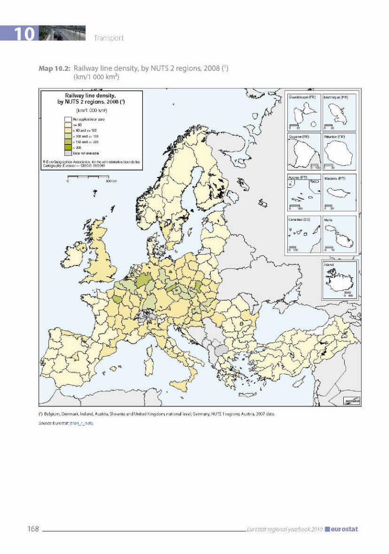

10
169Eurostat regional yearbook 2010eurostat
Transport
(Bucureşti - Ilfov: 159 km/1 000 km²), Paris (Île-de-France: 154 km/1 000 km²) and Amsterdam (Noord-Holland: 134 km/1 000 km²).
Next in the ranking come Bremen (423 km/ 1 000 km²) and Hamburg (373 km/1 000 km²), two smaller NUTS 2 regions where extensive freight lines to and from the seaports contribute to the high density. Like the capital cities mentioned above, these two hanseatic cities, which are also German federal states, are much smaller than regions like Zuid-Holland and Antwerpen, with their competing ports of Rotterdam and Antwerpen. These differences make it hard to draw direct comparisons with the infrastructure at the North Sea ports.
Freight lines also play a leading role in some regions with traditional coal and steel industries, like the Saarland in western Germany (135 km/1 000 km²) and Śląskie in south-west Poland (174 km/1 000 km²). Interestingly, Śląskie is, as mentioned above, also the only Polish region with significant recent net additions to its rail network. Consequently, the development of rail infrastructure in Śląskie bucks the general trend in Poland, although this can probably be attributed to the strong economic development in this region. Further regions with high railway density are Severozápad and Severovýchod in the Czech Republic and the regions making up Randstad in the western part of the Netherlands: Utrecht, Zuid-Holland (with the port of Rotterdam) and Noord-Holland (with Amsterdam).
Road safety
Road mobility comes at a high price in terms of lives lost. In 2008, just under 39 000 people lost their lives in road accidents within the EU-27, continuing the steady decrease in the number of fatalities on Europe’s roads. However, this number is still more than 20 times the total fatalities in rail and air transport combined. In response to the growing concern shown by European citizens over road safety, the European Union made this issue a priority of its common transport policy set out in the 2001 White Paper on transport ‘Time to decide’ and its mid-term review in 2006 (‘Keep Europe moving — Sustainable mobility for our continent’). In that White Paper, the European Commission set the target of halving the number of road fatalities between 2000 and 2010. To achieve this objective, a number of steps have been taken, including introducing higher
vehicle safety standards, improving the quality of road infrastructure, extending the traffic regulations combined with enforcing the existing regulations and improving driver education. As a result, despite the strong growth in road traffic in Europe, the total road death toll was cut by 48 % between 1991 and 2008 and has fallen by 31 % since the year 2000. While this positive trend can be seen across every country in Europe, there are significant variations between individual regions in the relative risk of fatal road accidents. Map 10.3 shows the number of deaths in road traffic accidents per million inhabitants by NUTS 2 region in 2008.
National totals of fatal road accidents are taken from the CARE database (see the methodological notes). Apart from Liechtenstein and Malta, both very small and therefore difficult to compare with other countries, the lowest numbers of road fatalities per million inhabitants were recorded by Sweden (43) and most regions in the United Kingdom (43 at national level). They are followed by the Netherlands (46), Switzerland (47), Norway (54) and most German regions, especially the federal states in the west (54 at national level). Furthermore, the relative number of fatal road accidents at regional level is comparatively low in major conglomerations and European capitals such as Wien (16 fatalities per million inhabitants), Berlin (16), Bremen (18), Oslo (Oslo og Akershus: 22), Stockholm (23), Birmingham (West Midlands: 23), Hamburg (23), Greater Manchester (24), Istanbul (25), Amsterdam (Zuid-Holland: 27), Outer London (27) and Inner London (28). The fatality rates in the more rural areas surrounding the conglomerations are always significantly higher.
With the exception of the candidate country Croatia (150 fatalities per million inhabitants), the highest rates of road deaths are found in the eastern and south-eastern European countries. Among these Lithuania has the highest fatality rate (148), followed by Poland (143), Romania (142), Latvia (139), Bulgaria (139), Greece (138), Slovakia (112) and Slovenia (106). Given the lower level of vehicle ownership still seen in most of these countries, these high figures — compared with western Europe — might partly be explained by the quality of the infrastructure and partly by the age, size and security standards of the vehicles.
Statistically, the numbers of road deaths are particularly low for many regions with high traffic volumes. This is true especially of many
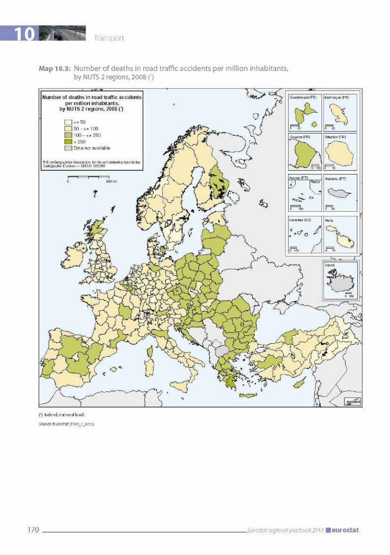
10
171Eurostat regional yearbook 2010eurostat
Transport
regions in western Germany and England, in particular around major cities, and of most parts of the Netherlands. Especially around major cities and transport hubs (e.g. seaports), high traffic volumes cause congestion, which reduces average speeds and, therefore, also the likelihood of fatalities when accidents do occur. A closer look at this phenomenon also reveals that many of these regions tend to have high motorway density. In general, motorways are much safer than secondary roads. Furthermore, mainly transit traffic uses existing motorways, thus keeping the number of road fatalities in these regions relatively low, despite high total traffic volumes. In fact, the quality of the roads in these countries is especially high, contributing to the low number of accidents.
By contrast, fatality rates are high in regions with low motorway density, such as all of Romania, Hungary and the Czech Republic except their capitals, the whole of Bulgaria, Poland, the Baltic countries, some of the eastern federal states of Germany and many rural areas in France and Spain. These data strongly suggest that the high proportion of traffic using motorways is an important factor behind the low number of road fatalities in many regions.
In addition to the share of the total road network accounted for by motorways, the significant reductions in the number of road deaths are also due to a combination of high in-vehicle and out-of-vehicle safety standards, speed limits and a general ‘safety culture’, including the quality of the emergency and healthcare systems.
The relatively low number of fatal road accidents in most major European cities can also be explained by the higher proportion of public transport and other modes, such as cycling and walking. While road accidents in general are more frequent in city traffic, driving at lower speed reduces the probability of serious injuries. However, an increase in the number of accidents involving non-motorised travellers could also lead to an increase in the number of serious injuries. Consequently, the combined effect of lower speeds and of more accidents involving more vulnerable travellers is not clear-cut.
Physical geography might be another reason for the differences in per-inhabitant fatality levels. Driving in mountainous regions like the Alps, the Pyrénées and the Carpathians is often more dangerous than in flat areas and therefore leads to a higher number
of accidents and fatalities. In addition, these regions attract a high volume of tourist traffic, thus adding to local traffic and, hence, the number of accidents reported per inhabitant.
Air transport
The rapid growth of air transport has been one of the most significant developments in the transport sector, both in Europe and all over the world. Intra-EU air transport (including domestic flights) more than doubled between 1995 and 2008. After the events of 11 September 2001 led to a decline in 2002, growth rates then bounced back. There is no doubt that completion of liberalisation of the air transport market in the European Union contributed significantly to this development, most noticeably in the form of the massive expansion of low-cost airlines, which also led to remarkable growth of smaller regional airports, which are less congested and charge lower landing fees than large airports in the capital regions.
Eurostat’s databases contain regional air transport statistics for passengers and freight. These series show passenger and freight movements by NUTS 2 region, measured in thousand passengers and tonnes respectively. The passenger data are divided into passengers embarking, disembarking and in transit. The freight statistics are divided into tonnes of freight and mail loaded and unloaded. Two series are available on air freight, based on different methods. The series going back to 1978 ended with reference year 1998 and was replaced by a new time series with different definitions as from 1999.
Currently, data on air transport are collected under Regulation (EC) No 437/2003 of the European Parliament and of the Council on statistical returns in respect of the carriage of passengers, freight and mail by air. This regulation provides detailed monthly data for airports handling more than 150 000 passengers a year. The data collected at airport level are then aggregated at NUTS 2 regional level.
This section on air transport focuses on the total number of passengers and the total number of tonnes loaded and unloaded in NUTS 2 regions in Europe. Tables 10.1 and 10.2 show the top 20 regions with the highest number of air passengers and highest volume of air freight in 2008.
10 Transport
172 Eurostat regional yearbook 2010 eurostat
The top-ranking regions in terms of the total number of air passengers are the capital regions of western Europe. The list is headed by Île de France, with a total of 86.7 million passengers for Paris-Charles de Gaulle and Paris-Orly airports, followed by Outer London (Heathrow) with 66.9 million passengers, Darmstadt with Frankfurt/Main airport (53.2 million), Comunidad de Madrid (50.4 million), Noord-Holland (Amsterdam/Schiphol: 47.4 million) and Lazio with Roma/Fiumicino and Roma/Ciampino airports (39.6 million).
The big airports in and around western Europe’s capitals also serve as central hubs for intercontinental air traffic. This is especially true for Heathrow (London), Charles de Gaulle (Paris), Frankfurt/Main and Schiphol (Amsterdam) airports.
In addition to these capital regions, high air passenger transport volumes can also be observed in Cataluña (Barcelona), Lombardia (Milano) and Oberbayern (München). The high passenger volumes for the south of Spain can be explained to a large extent by tourist traffic.
Although this is not visible from Table 10.1, a significant number of smaller regional airports are among the fastest growing, due to the success of low-cost carriers using them as their main hubs.
Among the top 20 airports for passenger transport, the Niederösterreich region with Wien shows the strongest growth (+55 %) over the five-year period from 2003 to 2008, followed by Cataluña with Barcelona (+50 %), southern and eastern Ireland with Dublin, Cork and Shannon (+47 %), Lazio with Roma (+45 %), Oberbayern with München (+44 %) and Comunidad de Madrid (+42 %). It is not surprising that the biggest airports do not show the fastest growth, since they are starting from a high base and are often already operating near to maximum capacity.
For air freight, Darmstadt (Frankfurt/Main) leads the top 20 European regions with 2.10 million tonnes, followed by Noord-Holland (Amsterdam/Schiphol: 1.59 million tonnes), Outer London (Heathrow: 1.48 million tonnes) and Île de France (Paris: 1.46 million tonnes). Volumes at other European airports are significantly lower, indicating that the biggest European airports serve as the main European hubs for air freight. Relatively high volumes can also be observed in four other regions: Luxembourg (0.79 million
tonnes), Vlaams-Brabant (Brussels: 0.61 million tonnes), Lombardia (Milano/Bergamo/Brescia: 0.59 million tonnes) and Köln (Köln-Bonn: 0.57 million tonnes).
While the total volume of air freight is limited in comparison with the much higher volumes of freight transported by road, rail, inland waterway and especially sea, air freight is important and growing steadily for articles with high added value, perishable goods (especially food) and express parcels.
Air freight is clearly dominated by the big airports, such as Frankfurt/Main, Amsterdam/Schiphol, London Heathrow and Paris-Charles de Gaulle and Paris-Orly. However, as with passenger transport, the most dynamic growth over the five-year period from 2003 to 2008 was at smaller airports with relatively low volumes, such as Leipzig/Halle in Germany and at the airports in the Etelä-Suomi region of Finland (including Helsinki and Turku), in Oberbayern (München) and in Niederösterreich (Wien).
Maritime transport
While the number of passengers embarking or disembarking in EU ports has remained stable since 2004, volumes of freight handled in EU ports increased by almost 20 % between 2002 and 2008. This increase highlights the important role that maritime transport plays in transport of goods in extra-EU trade. The landlocked Member States (the Czech Republic, Luxembourg, Hungary, Austria and Slovakia) do not report activity in this sector.
Eurostat’s databases contain regional maritime transport statistics for passengers and freight. These series show passenger and freight movements by NUTS 2 region, measured in thousand passengers and tonnes respectively. The passenger data are divided into passengers embarking and disembarking. The freight statistics are divided into tonnes of freight loaded and unloaded. Two series are available on maritime passenger transport, based on different methods. The series going back to 1997 ended with reference year 2003 and was replaced by a new time series with different definitions as from 2004 (now excluding passengers on cruises).
Currently, data on maritime transport are collected under Directive 2009/42/EC on
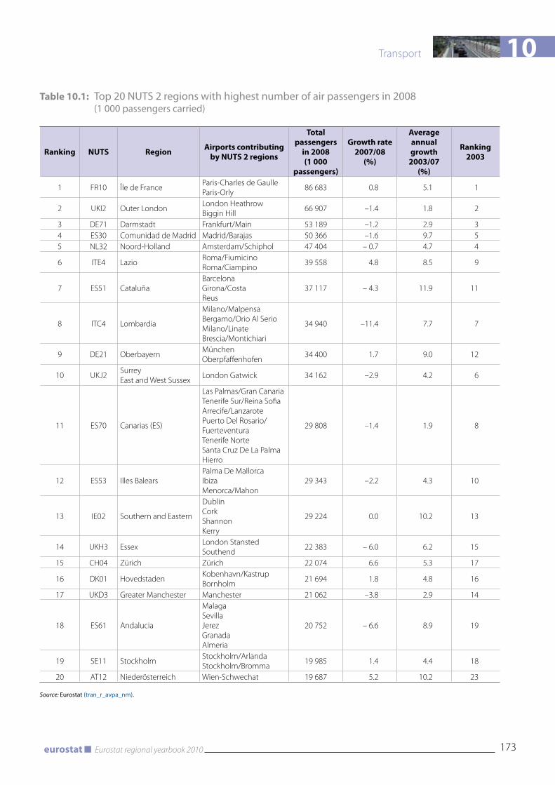
10
173Eurostat regional yearbook 2010eurostat
Transport
Table 10.1: Top 20 NUTS 2 regions with highest number of air passengers in 2008 (1 000 passengers carried)
Ranking NUTS Region Airports contributing by NUTS 2 regions
Total passengers
in 2008 (1 000
passengers)
Growth rate 2007/08
(%)
Average annual growth
2003/07(%)
Ranking 2003
1 FR10 Île de FranceParis-Charles de Gaulle Paris-Orly
86 683 0.8 5.1 1
2 UKI2 Outer LondonLondon Heathrow Biggin Hill
66 907 –1.4 1.8 2
3 DE71 Darmstadt Frankfurt/Main 53 189 –1.2 2.9 34 ES30 Comunidad de Madrid Madrid/Barajas 50 366 –1.6 9.7 55 NL32 Noord-Holland Amsterdam/Schiphol 47 404 – 0.7 4.7 4
6 ITE4 LazioRoma/Fiumicino Roma/Ciampino
39 558 4.8 8.5 9
7 ES51 CataluñaBarcelona Girona/Costa Reus
37 117 – 4.3 11.9 11
8 ITC4 Lombardia
Milano/Malpensa Bergamo/Orio Al Serio Milano/Linate Brescia/Montichiari
34 940 –11.4 7.7 7
9 DE21 OberbayernMünchen Oberpfaffenhofen
34 400 1.7 9.0 12
10 UKJ2Surrey East and West Sussex
London Gatwick 34 162 –2.9 4.2 6
11 ES70 Canarias (ES)
Las Palmas/Gran Canaria Tenerife Sur/Reina Sofia Arrecife/Lanzarote Puerto Del Rosario/Fuerteventura Tenerife Norte Santa Cruz De La Palma Hierro
29 808 –1.4 1.9 8
12 ES53 Illes BalearsPalma De Mallorca Ibiza Menorca/Mahon
29 343 –2.2 4.3 10
13 IE02 Southern and Eastern
Dublin Cork Shannon Kerry
29 224 0.0 10.2 13
14 UKH3 EssexLondon Stansted Southend
22 383 – 6.0 6.2 15
15 CH04 Zürich Zürich 22 074 6.6 5.3 17
16 DK01 HovedstadenKobenhavn/Kastrup Bornholm
21 694 1.8 4.8 16
17 UKD3 Greater Manchester Manchester 21 062 –3.8 2.9 14
18 ES61 Andalucia
Malaga Sevilla Jerez Granada Almeria
20 752 – 6.6 8.9 19
19 SE11 StockholmStockholm/Arlanda Stockholm/Bromma
19 985 1.4 4.4 18
20 AT12 Niederösterreich Wien-Schwechat 19 687 5.2 10.2 23
Source: Eurostat (tran_r_avpa_nm).
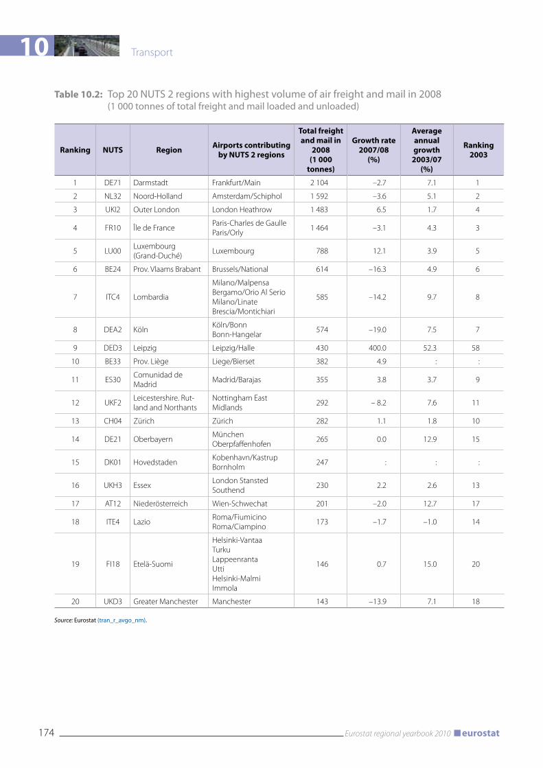
10 Transport
174 Eurostat regional yearbook 2010 eurostat
Table 10.2: Top 20 NUTS 2 regions with highest volume of air freight and mail in 2008 (1 000 tonnes of total freight and mail loaded and unloaded)
Ranking NUTS Region Airports contributing by NUTS 2 regions
Total freight and mail in
2008 (1 000
tonnes)
Growth rate 2007/08
(%)
Average annual growth
2003/07(%)
Ranking 2003
1 DE71 Darmstadt Frankfurt/Main 2 104 –2.7 7.1 1
2 NL32 Noord-Holland Amsterdam/Schiphol 1 592 –3.6 5.1 2
3 UKI2 Outer London London Heathrow 1 483 6.5 1.7 4
4 FR10 Île de FranceParis-Charles de Gaulle Paris/Orly
1 464 –3.1 4.3 3
5 LU00Luxembourg (Grand-Duché)
Luxembourg 788 12.1 3.9 5
6 BE24 Prov. Vlaams Brabant Brussels/National 614 –16.3 4.9 6
7 ITC4 Lombardia
Milano/Malpensa Bergamo/Orio Al Serio Milano/Linate Brescia/Montichiari
585 –14.2 9.7 8
8 DEA2 KölnKöln/Bonn Bonn-Hangelar
574 –19.0 7.5 7
9 DED3 Leipzig Leipzig/Halle 430 400.0 52.3 58
10 BE33 Prov. Liège Liege/Bierset 382 4.9 : :
11 ES30Comunidad de Madrid
Madrid/Barajas 355 3.8 3.7 9
12 UKF2Leicestershire. Rut-land and Northants
Nottingham East Midlands
292 – 8.2 7.6 11
13 CH04 Zürich Zürich 282 1.1 1.8 10
14 DE21 OberbayernMünchen Oberpfaffenhofen
265 0.0 12.9 15
15 DK01 HovedstadenKobenhavn/Kastrup Bornholm
247 : : :
16 UKH3 EssexLondon Stansted Southend
230 2.2 2.6 13
17 AT12 Niederösterreich Wien-Schwechat 201 –2.0 12.7 17
18 ITE4 LazioRoma/Fiumicino Roma/Ciampino
173 –1.7 –1.0 14
19 FI18 Etelä-Suomi
Helsinki-Vantaa Turku Lappeenranta Utti Helsinki-Malmi Immola
146 0.7 15.0 20
20 UKD3 Greater Manchester Manchester 143 –13.9 7.1 18
Source: Eurostat (tran_r_avgo_nm).
10
175Eurostat regional yearbook 2010eurostat
Transport
statistical returns in respect of carriage of goods and passengers by sea. This regulation provides detailed quarterly data for ports handling more than 1 million tonnes of goods or recording more than 200 000 passenger movements a year. The data collected at port level are then aggregated at NUTS 2 regional level.
This section on maritime transport focuses on the total number of passengers and the total number of tonnes loaded and unloaded in NUTS 2 regions in Europe. Tables 10.3 and 10.4 show the top 20 regions with the highest number of sea passengers and highest volume of sea freight in 2008.
Not surprisingly, maritime passenger transport is dominated by regions with a sea-faring tradition. By far the largest number of passengers transported by sea (31.5 million) is recorded by the Attiki region, where the port of Piraeus is the main gateway for passengers to the Greek islands. The second highest number of passengers was recorded in Sydsverige in Sweden, although the passenger count of 15.0 million was less than half that of Attiki. The ports of the Sydsverige region service a large number of ferry connections to the other countries around the Baltic Sea. Next comes Sicilia, with 14.9 million passengers. Sicilia services several ferry connections to the mainland of Italy, with Messina the busiest passenger port in Italy, but there are also ferry routes to Malta and Tunisia. The high passenger counts in Kent (14.0 million) and Nord - Pas-de-Calais (13.8 million) reflect the close ties across the English Channel, with the ports of Dover, Medway and Ramsgate on the English side and Calais and Dunkerque on the French side.
From 2004 to 2008, the growth in passenger numbers varied greatly between the top 20 European regions in terms of maritime passenger transport. In particular, the smaller port regions in the top 20 recorded rises in passenger numbers, whereas the numbers fell in several of the largest regions in the top 20. The highest growth rate over this period (+49 %) was recorded for Toscana with the ports of Livorno, Marina Di Carrara and Piombino. Other regions with strong increases in passenger numbers were Notio Aigaio (+21 %) and Sardegna (+12 %).
Several leading maritime regions reported falls in the number of passengers transported from 2004 to 2008. This was the case not only in the largest region, Attiki (down by 13 %), but also in regions
around the Baltic Sea, namely Nordjylland in Denmark, with its traditional ties with western Sweden and southern Norway (down by 16 %), and Sydsverige in Sweden (down by 5 %). The regions on both sides of the English Channel also reported slightly lower passenger numbers: down by 3 % in Kent and by 0.4% in Nord - Pas-de-Calais.
For maritime freight, Zuid-Holland with the port of Rotterdam is far in the lead. It handled 391 million tonnes of freight, more than twice the volume of the second of the top 20 European regions, Antwerpen (171 million tonnes). They are followed by Hamburg in Germany (119 million tonnes), Haute Normandie in France (99 million tonnes), Noord-Holland in the Netherlands and Andalucía in Spain (both 98 million tonnes), Provence-Alpes-Côte d’Azur in France (93 million tonnes) and East Yorkshire and Northern Lincolnshire in the United Kingdom (91 million tonnes). These volumes are far higher than those recorded for other modes of transport and clearly illustrate the key role maritime freight plays in the European economy. The geographical spread of the main seaports also illustrates the flexibility of maritime transport, which allows large volumes to be loaded and unloaded close to the main recipients and producers.
Despite the decline in volumes at several key seaports from 2007 to 2008, the freight volumes handled increased in all the top 20 European regions over the five-year period 2003–08, with the exceptions of Sicilia in Italy and Vestlandet in Norway. Noord-Holland in the Netherlands recorded the highest growth in freight volumes over this period (up by 65 %), followed by some of the ‘smaller’ top 20 regions in terms of freight volumes handled: Comunidad Valenciana in Spain (up by 51 %) and Bremen in Germany (up by 49 %).
Conclusion
The data presented in the three maps and four tables in this chapter show a number of interrelationships between regions’ economic and geographical characteristics and the structure of the European transport system. They indicate a close relationship between the availability of motorways and road safety. They also provide basic figures on the regional distribution of air and maritime transport. However, the data presented in this chapter are only part of the
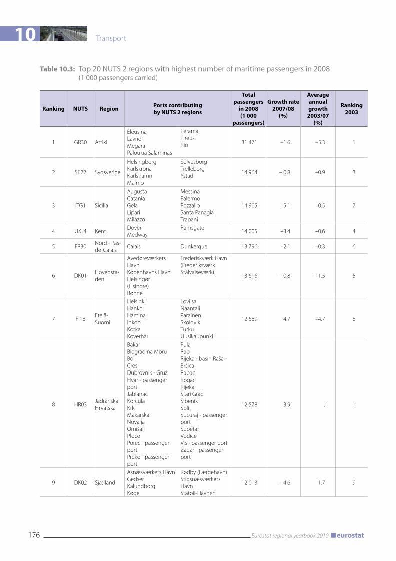
10 Transport
176 Eurostat regional yearbook 2010 eurostat
Table 10.3: Top 20 NUTS 2 regions with highest number of maritime passengers in 2008 (1 000 passengers carried)
Ranking NUTS Region Ports contributing by NUTS 2 regions
Total passengers
in 2008 (1 000
passengers)
Growth rate 2007/08
(%)
Average annual growth
2003/07(%)
Ranking 2003
1 GR30 Attiki
Eleusina Lavrio Megara Paloukia Salaminas
Perama Pireus Rio 31 471 –1.6 –5.3 1
2 SE22 Sydsverige
Helsingborg Karlskrona Karlshamn Malmö
Sölvesborg Trelleborg Ystad
14 964 – 0.8 –0.9 3
3 ITG1 Sicilia
Augusta Catania Gela Lipari Milazzo
Messina Palermo Pozzallo Santa Panagia Trapani
14 905 5.1 0.5 7
4 UKJ4 KentDover Medway
Ramsgate14 005 –3.4 –0.6 4
5 FR30Nord - Pas-de-Calais
Calais Dunkerque 13 796 –2.1 –0.3 6
6 DK01Hovedsta-den
Avedøreværkets Havn Københavns Havn Helsingør (Elsinore) Rønne
Frederiskværk Havn (Frederiksværk Stålvalseværk)
13 616 – 0.8 –1.5 5
7 FI18Etelä-Suomi
Helsinki Hanko Hamina Inkoo Kotka Koverhar
Loviisa Naantali Parainen Sköldvik Turku Uusikaupunki
12 589 4.7 –4.7 8
8 HR03Jadranska Hrvatska
Bakar Biograd na Moru Bol Cres Dubrovnik - Gruž Hvar - passenger port Jablanac Korcula Krk Makarska Novalja Omišalj Ploce Porec - passenger port Preko - passenger port
Pula Rab Rijeka - basin Raša - Bršica Rabac Rogac Rijeka Stari Grad Šibenik Split Sucuraj - passenger port Supetar Vodice Vis - passenger port Zadar - passenger port
12 578 3.9 : :
9 DK02 Sjælland
Asnæsværkets Havn Gedser Kalundborg Køge
Rødby (Færgehavn) Stigsnæsværkets Havn Statoil-Havnen
12 013 – 4.6 1.7 9
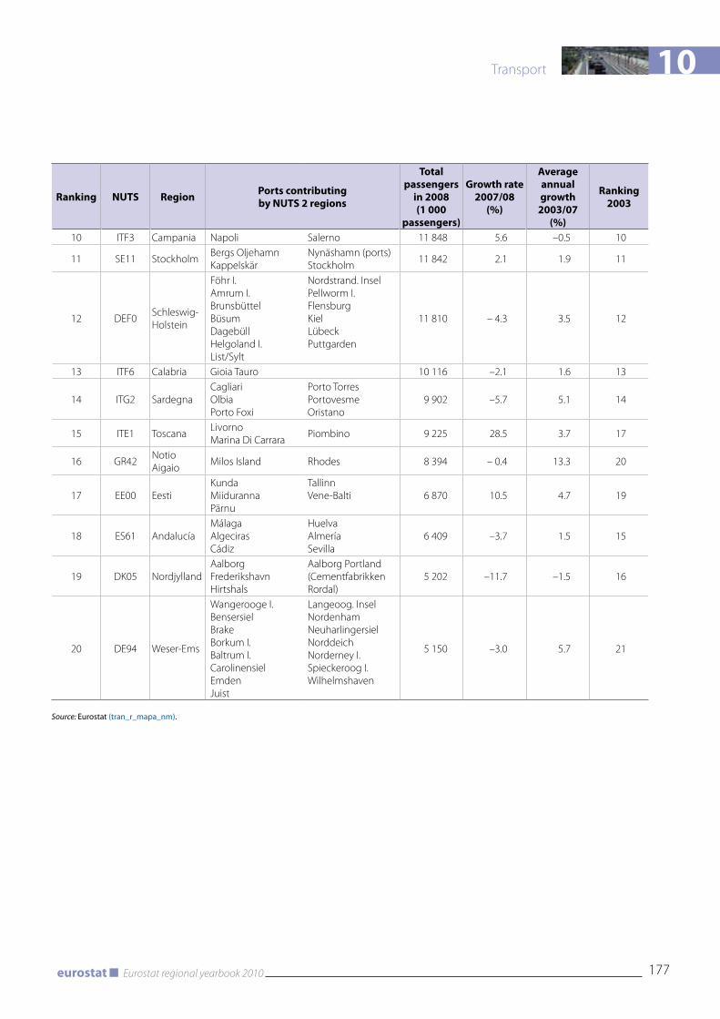
10
177Eurostat regional yearbook 2010eurostat
Transport
Ranking NUTS Region Ports contributing by NUTS 2 regions
Total passengers
in 2008 (1 000
passengers)
Growth rate 2007/08
(%)
Average annual growth
2003/07(%)
Ranking 2003
10 ITF3 Campania Napoli Salerno 11 848 5.6 –0.5 10
11 SE11 StockholmBergs Oljehamn Kappelskär
Nynäshamn (ports) Stockholm
11 842 2.1 1.9 11
12 DEF0Schleswig-Holstein
Föhr I. Amrum I. Brunsbüttel Büsum Dagebüll Helgoland I. List/Sylt
Nordstrand. Insel Pellworm I. Flensburg Kiel Lübeck Puttgarden
11 810 – 4.3 3.5 12
13 ITF6 Calabria Gioia Tauro 10 116 –2.1 1.6 13
14 ITG2 SardegnaCagliari Olbia Porto Foxi
Porto Torres Portovesme Oristano
9 902 –5.7 5.1 14
15 ITE1 ToscanaLivorno Marina Di Carrara
Piombino 9 225 28.5 3.7 17
16 GR42Notio Aigaio
Milos Island Rhodes 8 394 – 0.4 13.3 20
17 EE00 EestiKunda Miiduranna Pärnu
Tallinn Vene-Balti 6 870 10.5 4.7 19
18 ES61 AndalucíaMálaga Algeciras Cádiz
Huelva Almería Sevilla
6 409 –3.7 1.5 15
19 DK05 NordjyllandAalborg Frederikshavn Hirtshals
Aalborg Portland (Cementfabrikken Rordal)
5 202 –11.7 –1.5 16
20 DE94 Weser-Ems
Wangerooge I. Bensersiel Brake Borkum I. Baltrum I. Carolinensiel Emden Juist
Langeoog. Insel Nordenham Neuharlingersiel Norddeich Norderney I. Spieckeroog I. Wilhelmshaven
5 150 –3.0 5.7 21
Source: Eurostat (tran_r_mapa_nm).
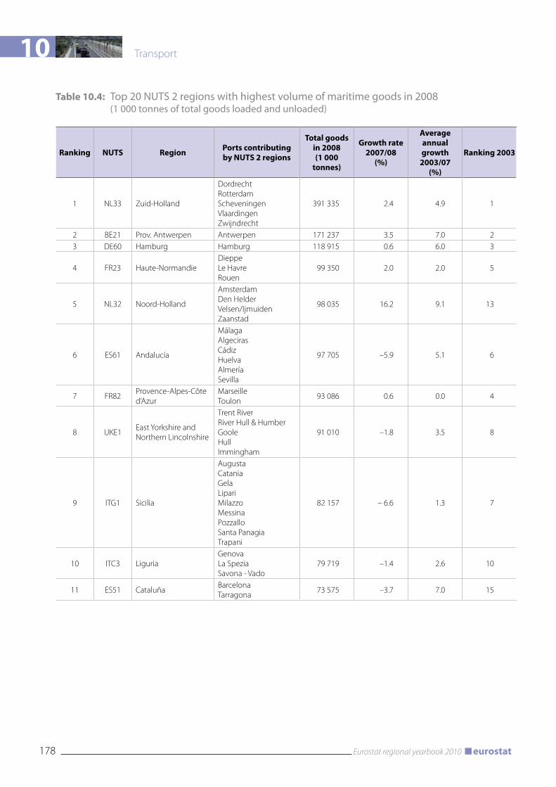
10 Transport
178 Eurostat regional yearbook 2010 eurostat
Table 10.4: Top 20 NUTS 2 regions with highest volume of maritime goods in 2008 (1 000 tonnes of total goods loaded and unloaded)
Ranking NUTS Region Ports contributing by NUTS 2 regions
Total goods in 2008 (1 000
tonnes)
Growth rate 2007/08
(%)
Average annual growth
2003/07(%)
Ranking 2003
1 NL33 Zuid-Holland
Dordrecht Rotterdam Scheveningen Vlaardingen Zwijndrecht
391 335 2.4 4.9 1
2 BE21 Prov. Antwerpen Antwerpen 171 237 3.5 7.0 23 DE60 Hamburg Hamburg 118 915 0.6 6.0 3
4 FR23 Haute-NormandieDieppe Le Havre Rouen
99 350 2.0 2.0 5
5 NL32 Noord-Holland
Amsterdam Den Helder Velsen/Ijmuiden Zaanstad
98 035 16.2 9.1 13
6 ES61 Andalucía
Málaga Algeciras Cádiz Huelva Almería Sevilla
97 705 –5.9 5.1 6
7 FR82Provence-Alpes-Côte d’Azur
Marseille Toulon
93 086 0.6 0.0 4
8 UKE1East Yorkshire and Northern Lincolnshire
Trent River River Hull & Humber Goole Hull Immingham
91 010 –1.8 3.5 8
9 ITG1 Sicilia
Augusta Catania Gela Lipari Milazzo Messina Pozzallo Santa Panagia Trapani
82 157 – 6.6 1.3 7
10 ITC3 LiguriaGenova La Spezia Savona - Vado
79 719 –1.4 2.6 10
11 ES51 CataluñaBarcelona Tarragona
73 575 –3.7 7.0 15
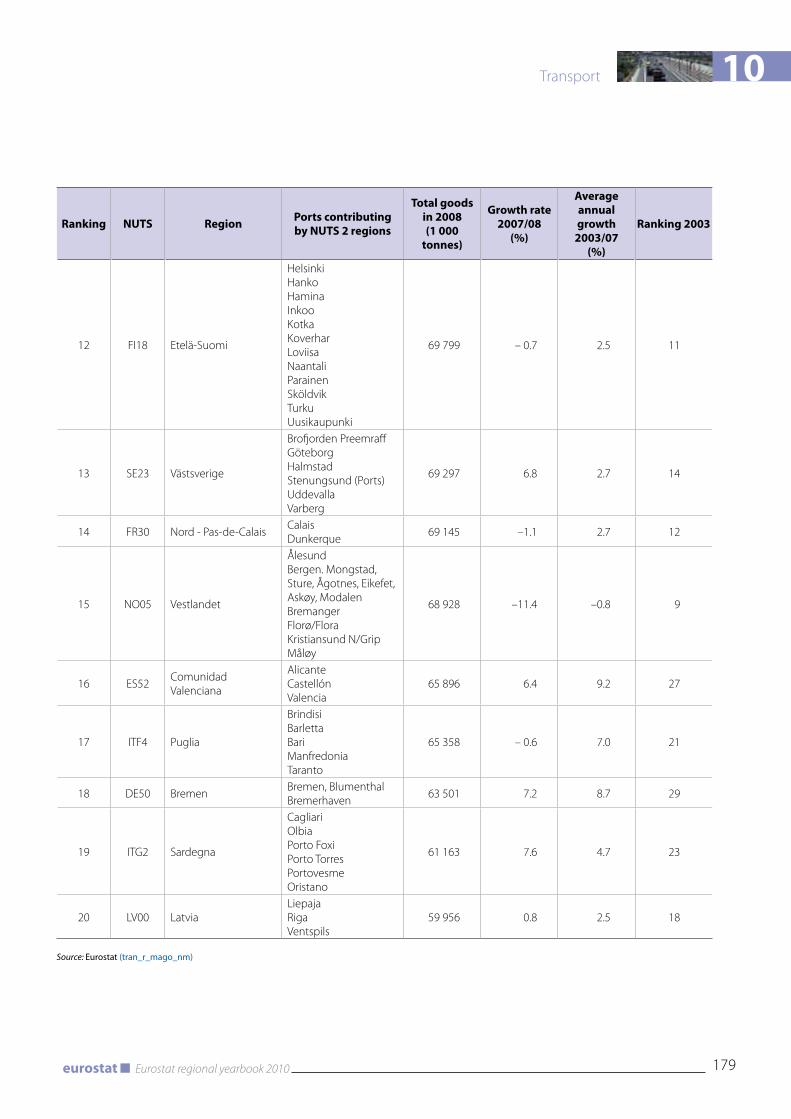
10
179Eurostat regional yearbook 2010eurostat
Transport
Ranking NUTS Region Ports contributing by NUTS 2 regions
Total goods in 2008 (1 000
tonnes)
Growth rate 2007/08
(%)
Average annual growth
2003/07(%)
Ranking 2003
12 FI18 Etelä-Suomi
Helsinki Hanko Hamina Inkoo Kotka Koverhar Loviisa Naantali Parainen Sköldvik Turku Uusikaupunki
69 799 – 0.7 2.5 11
13 SE23 Västsverige
Brofjorden Preemraff Göteborg Halmstad Stenungsund (Ports) Uddevalla Varberg
69 297 6.8 2.7 14
14 FR30 Nord - Pas-de-CalaisCalais Dunkerque
69 145 –1.1 2.7 12
15 NO05 Vestlandet
Ålesund Bergen. Mongstad, Sture, Ågotnes, Eikefet, Askøy, Modalen Bremanger Florø/Flora Kristiansund N/Grip Måløy
68 928 –11.4 –0.8 9
16 ES52Comunidad Valenciana
Alicante Castellón Valencia
65 896 6.4 9.2 27
17 ITF4 Puglia
Brindisi Barletta Bari Manfredonia Taranto
65 358 – 0.6 7.0 21
18 DE50 BremenBremen, Blumenthal Bremerhaven
63 501 7.2 8.7 29
19 ITG2 Sardegna
Cagliari Olbia Porto Foxi Porto Torres Portovesme Oristano
61 163 7.6 4.7 23
20 LV00 LatviaLiepaja Riga Ventspils
59 956 0.8 2.5 18
Source: Eurostat (tran_r_mago_nm)

10 Transport
180 Eurostat regional yearbook 2010 eurostat
wider set of regional transport statistics available in Eurostat’s databases. Regional transport statistics show patterns of variation across regions, where transport-related variables are often closely related to levels of economic activity. As mentioned earlier, transport policies are at the very heart of efforts to reduce regional inequality and improve regional cohesion. In the enlarged European Union, economic and infrastructure disparities are now more evident than before.
Furthermore, European transport policies seek to reduce the emission of CO2 and other substances detrimental to the global climate, through a more intelligent transport system and a better mix of transport modes. One of Eurostat’s long-term objectives is to expand the current regional transport indicators in order to provide a better understanding of the impact of transport policies on economic growth, transport needs and the environment.

10
181Eurostat regional yearbook 2010eurostat
Transport
Methodological notes
Eurostat collects, compiles and disseminates a variety of regional indicators. Data on road and railway infrastructure, inland waterways, vehicle stocks and road accidents are currently collected by Member States and candidate countries on a voluntary basis via annual questionnaires. Data on road transport of goods as well as maritime and air transport for passengers and goods are derived directly from the data collection required by law. In addition, data on journeys made by vehicles are derived from a specific study of road transport data.
Eurostat’s statistical database contains information on the road, railway and inland waterway infrastructure at NUTS 2 regional level. The road network is divided into motorways and other roads. Railway links are classified on the basis of two criteria: the number of tracks and whether or not they are electrified. Inland waterways include navigable rivers and canals, plus lakes. However, up until now, the varying performance of these transport links (e.g. the capacity per link) has not been reflected in the data Eurostat receives from the Member States.
Regional transport indicators are available on Eurostat’s website under ‘Transport’ and are mirrored in the ‘General and regional statistics’. In addition to the full data sets, 16 main tables are currently available for transport data, covering infrastructure, the vehicle fleet, journeys by road, rail, sea and air, and road safety (numbers of deaths and injuries in road accidents). All the data are annual, with time series going back to the reference year 1978 for transport infrastructure, air transport and maritime transport. For road safety data, the series starts from 1988.
Due to the intrinsic nature of transport, a spatial breakdown is built into most legislation calling for collection of transport flow statistics, which makes it possible to derive regional indicators for maritime and air transport directly. Other indicators on regional transport flows can be found under the separate areas of ‘Transport’, namely ‘Road transport’, ‘Railway transport’ and ‘Inland waterway transport’. Further information on transport flows between airports and ports can also be obtained under ‘Maritime transport’ and ‘Air transport’.
To demonstrate the potential of transport statistics for analysing regional patterns, this chapter focuses on the data on regional transport infrastructure, road safety, air transport and maritime transport. The latter are derived from the data collection required by law. The regional infrastructure is expressed by a density indicator which divides the total length of the motorway and railway network within a region by the region’s land area. Regional road safety is assessed by dividing the number of road fatalities by the number of inhabitants per region. In contrast to the data on persons injured, the data on road casualties are comparable across Europe. Regional air transport volumes are expressed as the total number of air passengers embarking, disembarking and in transit and as tonnes of freight loaded and unloaded at airports in the regions. The data are derived from those provided by the countries at airport level. Precise definitions of all the variables used can be found in the glossary for transport statistics (http://www.internationaltransportforum.org/Pub/pdf/09GloStat.pdf).
The basic data used in the maps and tables were extracted from Eurostat’s website, although not all the derived indicators are directly available there. The aim is to provide added value over and above the data already available to the public on the website. Further information can be found in Eurostat’s Statistics in focus on transport issues, in the 2009 Panorama of transport publications and in CARE, a Community database on road accidents resulting in death or injury, which contains detailed data on individual accidents collected by the Member States (http://ec.europa.eu/transport/road_safety/specialist/statistics/care_reports_graphics/index_en.htm).


Tourism
11 Tourism
184 Eurostat regional yearbook 2010 eurostat
Introduction
Tourism is an important and fast-evolving economic activity with social, cultural and environmental implications. It occupies large numbers of small and medium-sized businesses and its contribution to growth and employment varies widely from one region of the EU to another. In rural regions in particular, usually remote from the economic centres of their countries, tourism is often one of the main sources of income for the population and a prominent factor in securing an adequate level of employment.
The crucial role that tourism plays in generating growth and jobs, its growing importance and its impact on other policy areas ranging from regional policy, diversification of rural economies, maritime policy, employment, sustainability and competitiveness to social policy and inclusion (‘tourism for all’) are widely acknowledged all over the European Union. Therefore, tourism is reflected in EU policy as well as in national policies.
Tourism is a typical cross-cutting industry. Services to tourists involve a variety of branches of the economy: hotels and other accommodation, gastronomy (restaurants, cafés, etc.), various transport operators and also a wide range of cultural and recreational facilities (theatres, museums, leisure parks, swimming pools, etc.). In many regions geared to tourism the retail and services sectors also benefit considerably from the demand generated by tourists in addition to that from the resident population.
Eurostat has been collecting data on trends in, and the structure of, tourism since 1995, based on Council Directive 95/57/EC on the collection of statistical information in the field of tourism. This includes data both on accommodation capacity and occupancy and on tourist behaviour. The tourist behaviour data are, however, only available at national level. By contrast, the data on accommodation capacity and occupancy are also available by region.
The regional data on occupancy of tourist accommodation from different perspectives are summed up in this chapter. Since the number of overnight stays, which reflects both the length of stay and the number of visitors, is the central indicator for accommodation services, this chapter will concentrate exclusively on this variable.
Top 20 tourist regions in the EU-27
Figure 11.1 shows the 20 regions in the European Union with the highest number of overnight stays, broken down by hotels and campsites. These regions account for 36 % of the total number of overnight stays in all 271 regions of the EU-27 for which data are available.
The dominance of European tourism by Spain, Italy and France is clearly visible. Tirol in Austria (11th place) and Oberbayern in Germany (16th place), which includes the Bavarian metropolitan area of München, are the only regions in the top 20 that are not in one of those three leading tourism countries.
With 67.5 million overnight stays, the Île de France region, which includes the French capital Paris, is well in the lead, followed by four Spanish regions: Cataluña (56.0 million), Illes Balears (49.8 million), Canarias (49.6 million) and Andalucía (47.9 million).
In 18 of the 20 regions more nights are spent in hotels and similar establishments (from 100 % to 61 %) than on campsites. In two French regions, Languedoc-Roussillon and Aquitaine, however, this is not the case. They attract more tourists to campsites than to other types of accommodation. Only 31 % of overnight stays are spent in hotels as opposed to campsites in Languedoc-Roussillon and 39 % in Aquitaine, whereas in all 271 regions in the EU-27 the share of overnight stays spent in hotels is 81 %.
Figure 11.2 shows the top 20 EU regions recording the highest number of total overnight stays in hotels and on campsites by foreign tourists. These top 20 regions account for 49 % of all overnight stays by non-residents across the EU-27. Within the top 20, the first six regions (Illes Baleares, Canarias, Île de France, Cataluña, Veneto and Tirol) together recorded as many nights as the next 14. Hotels clearly play a dominant role compared with accommodation on campsites for non-resident tourists. The share of overnight stays by foreign tourists taken by hotels ranges from 100 % to 58 %. Nevertheless, in two of the top 20 regions, campsites take almost the same share as hotels: the French region of Provence-Alpes-Côte d’Azur, where the share of campsites is 42 %, and the Italian region of Veneto with 40 %. In absolute figures,
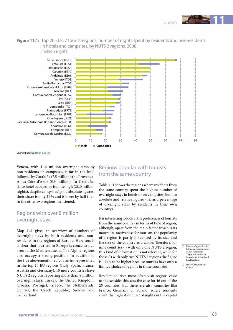
11
185Eurostat regional yearbook 2010eurostat
Tourism
Veneto, with 11.4 million overnight stays by non-residents on campsites, is far in the lead, followed by Cataluña (7.5 million) and Provence-Alpes-Côte d’Azur (5.9 million). In Cataluña, since hotel occupancy is quite high (28.0 million nights), despite campsites’ good absolute figures, their share is only 21 % and is lower by half than in the other two regions mentioned.
Regions with over 8 million overnight stays
Map 11.1 gives an overview of numbers of overnight stays by both residents and non-residents in the regions of Europe. Here too, it is clear that tourism in Europe is concentrated around the Mediterranean. The Alpine regions also occupy a strong position. In addition to the five abovementioned countries represented in the top 20 EU regions (Italy, Spain, France, Austria and Germany), 10 more countries have NUTS 2 regions reporting more than 8 million overnight stays: Turkey, the United Kingdom, Croatia, Portugal, Greece, the Netherlands, Cyprus, the Czech Republic, Sweden and Switzerland.
Regions popular with tourists from the same country
Table 11.1 shows the regions where residents from the same country spent the highest number of overnight stays in hotels or on campsites, both in absolute and relative figures (i.e. as a percentage of overnight stays by residents in their own country).
It is interesting to look at the preferences of tourists from the same country in terms of type of region, although, apart from the main factor which is its natural attractiveness for tourism, the popularity of a region is partly influenced by its size and the size of the country as a whole. Therefore, for nine countries (1) with only one NUTS 2 region, this kind of information is not relevant, while for those (2) with only two NUTS 2 regions the figure is likely to be higher because tourists have only a limited choice of regions in those countries.
Resident tourists most often visit regions close to the seaside; this was the case for 16 out of the 25 countries. But there are also countries like France, Germany or Poland, where residents spent the highest number of nights in the capital
Figure 11.1: Top 20 EU-27 tourist regions, number of nights spent by residents and non-residents in hotels and campsites, by NUTS 2 regions, 2008 (million nights)
0 10 20 30 40 50 60 70 80
Île de France (FR10)Cataluña (ES51)
Illes Balears (ES53)Canarias (ES70)
Andalucía (ES61)Veneto (ITD3)
Emilia-Romagna (ITD5)Provence-Alpes-Côte d'Azur (FR82)
Toscana (ITE1)Comunidad Valenciana (ES52)
Tirol (AT33)Lazio (ITE4)
Lombardia (ITC4)Rhône-Alpes (FR71)
Languedoc-Roussillon (FR81)Oberbayern (DE21)
Provincia Autonoma Bolzano/Bozen (ITD1)Aquitaine (FR61)Campania (ITF3)
Comunidad de Madrid (ES30)
Hotels Campsites
Source: Eurostat (tour_occ_n).
(1) Estonia, Cyprus, Latvia, Lithuania, Luxembourg, Malta, the former Yugoslav Republic of Macedonia, Iceland and Liechtenstein.
(2) Ireland, Slovenia and Croatia.
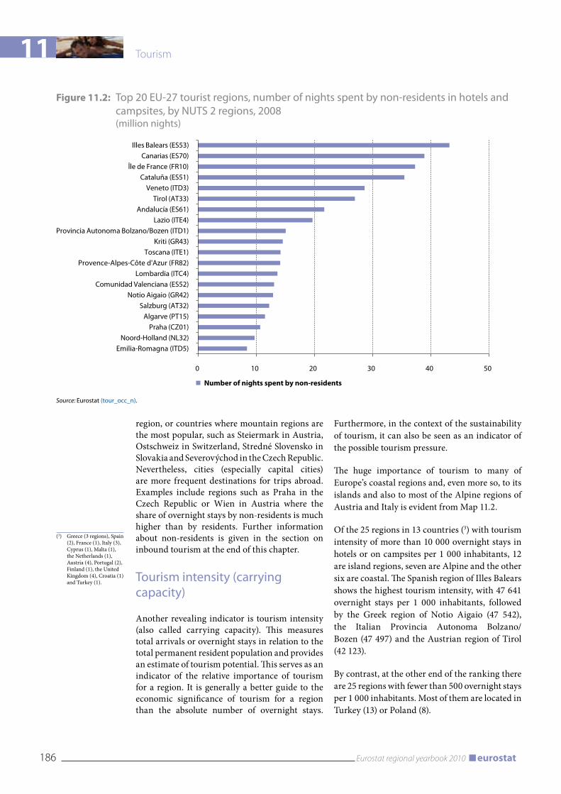
11 Tourism
186 Eurostat regional yearbook 2010 eurostat
Figure 11.2: Top 20 EU-27 tourist regions, number of nights spent by non-residents in hotels and campsites, by NUTS 2 regions, 2008 (million nights)
0 10 20 30 40 50
Illes Balears (ES53)Canarias (ES70)
Île de France (FR10)Cataluña (ES51)
Veneto (ITD3)Tirol (AT33)
Andalucía (ES61)Lazio (ITE4)
Provincia Autonoma Bolzano/Bozen (ITD1)Kriti (GR43)
Toscana (ITE1)Provence-Alpes-Côte d'Azur (FR82)
Lombardia (ITC4)Comunidad Valenciana (ES52)
Notio Aigaio (GR42)Salzburg (AT32)
Algarve (PT15)Praha (CZ01)
Noord-Holland (NL32)Emilia-Romagna (ITD5)
Number of nights spent by non-residents
Source: Eurostat (tour_occ_n).
region, or countries where mountain regions are the most popular, such as Steiermark in Austria, Ostschweiz in Switzerland, Stredné Slovensko in Slovakia and Severovýchod in the Czech Republic. Nevertheless, cities (especially capital cities) are more frequent destinations for trips abroad. Examples include regions such as Praha in the Czech Republic or Wien in Austria where the share of overnight stays by non-residents is much higher than by residents. Further information about non-residents is given in the section on inbound tourism at the end of this chapter.
Tourism intensity (carrying capacity)
Another revealing indicator is tourism intensity (also called carrying capacity). This measures total arrivals or overnight stays in relation to the total permanent resident population and provides an estimate of tourism potential. This serves as an indicator of the relative importance of tourism for a region. It is generally a better guide to the economic significance of tourism for a region than the absolute number of overnight stays.
Furthermore, in the context of the sustainability of tourism, it can also be seen as an indicator of the possible tourism pressure.
The huge importance of tourism to many of Europe’s coastal regions and, even more so, to its islands and also to most of the Alpine regions of Austria and Italy is evident from Map 11.2.
Of the 25 regions in 13 countries (3) with tourism intensity of more than 10 000 overnight stays in hotels or on campsites per 1 000 inhabitants, 12 are island regions, seven are Alpine and the other six are coastal. The Spanish region of Illes Balears shows the highest tourism intensity, with 47 641 overnight stays per 1 000 inhabitants, followed by the Greek region of Notio Aigaio (47 542), the Italian Provincia Autonoma Bolzano/Bozen (47 497) and the Austrian region of Tirol (42 123).
By contrast, at the other end of the ranking there are 25 regions with fewer than 500 overnight stays per 1 000 inhabitants. Most of them are located in Turkey (13) or Poland (8).
(3) Greece (3 regions), Spain (2), France (1), Italy (3), Cyprus (1), Malta (1), the Netherlands (1), Austria (4), Portugal (2), Finland (1), the United Kingdom (4), Croatia (1) and Turkey (1).
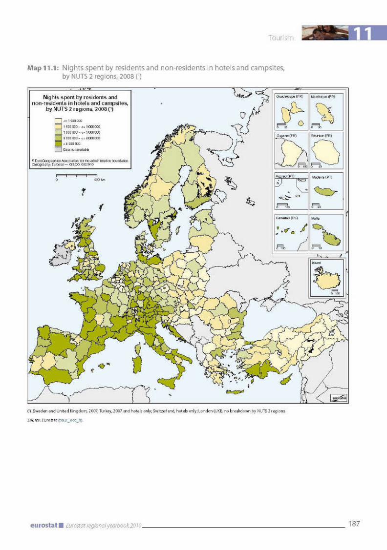
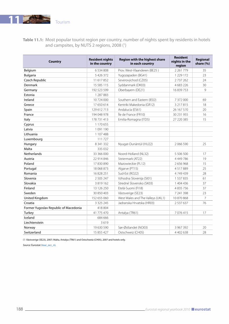
11 Tourism
188 Eurostat regional yearbook 2010 eurostat
Table 11.1: Most popular tourist region per country, number of nights spent by residents in hotels and campsites, by NUTS 2 regions, 2008 (1)
Country Resident nights in the country
Region with the highest share in each country
Resident nights in the
region
Regional share (%)
Belgium 6 534 808 Prov. West-Vlaanderen (BE25 ) 2 261 779 35
Bulgaria 5 426 372 Yugozapaden (BG41) 1 229 172 23
Czech Republic 11 617 852 Severovýchod (CZ05) 2 737 262 24
Denmark 15 585 115 Syddanmark (DK03) 4 683 226 30
Germany 192 523 599 Oberbayern (DE21) 16 839 753 9
Estonia 1 287 883
Ireland 10 724 000 Southern and Eastern (IE02) 7 372 000 69
Greece 17 650 614 Kentriki Makedonia (GR12) 3 217 815 18
Spain 129 612 713 Andalucía (ES61) 26 167 570 20
France 194 048 978 Île de France (FR10) 30 231 955 16
Italy 178 731 413 Emilia-Romagna (ITD5) 27 220 385 15
Cyprus 1 170 655
Latvia 1 091 190
Lithuania 1 107 488
Luxembourg 111 727
Hungary 8 341 332 Nyugat-Dunántúl (HU22) 2 066 590 25
Malta 335 032
Netherlands 33 366 000 Noord-Holland (NL32) 5 506 500 17
Austria 22 914 846 Steiermark (AT22) 4 449 786 19
Poland 17 830 890 Mazowieckie (PL12) 2 656 968 15
Portugal 18 068 873 Algarve (PT15) 4 517 889 25
Romania 16 828 251 Sud-Est (RO22) 4 749 439 28
Slovenia 2 505 247 Vzhodna Slovenija (SI01) 1 537 835 61
Slovakia 3 819 162 Stredné Slovensko (SK03) 1 404 436 37
Finland 13 126 250 Etelä-Suomi (FI18) 4 835 756 37
Sweden 30 850 403 Västsverige (SE23) 7 241 398 23
United Kingdom 152 655 060 West Wales and The Valleys (UKL1) 10 870 868 7
Croatia 3 325 245 Jadranska Hrvatska (HR03) 2 537 637 76
Former yugoslav Republic of Macedonia 418 804
Turkey 41 775 470 Antalya (TR61) 7 076 415 17
Iceland 684 666
Liechtenstein 3 619
Norway 19 630 590 Sør-Østlandet (NO03) 3 967 392 20
Switzerland 15 855 427 Ostschweiz (CH05) 4 402 638 28
(1) västsverige (SE23), 2007; Malta, Antalya (TR61) and Ostschweiz (CH05), 2007 and hotels only.
Source: Eurostat (tour_occ_n).
11
189Eurostat regional yearbook 2010eurostat
Tourism
Tourism density
This variable is modelled on population statistics and tries to show the ratio of the overnight stays by tourists to the size of the territory, in the same way as population density does. This indicator aims at improving comparability between regions which differ in size across Europe. Generally, capital city regions are among the most ‘densely visited’, as Map 11.3 shows.
Brussels is in the lead in terms of tourism den-sity (31 113 nights per km2), followed by five other capital city regions which have a density above 16 000 nights per km2: Inner London (27 331), Malta (24 559), Wien (23 374), Praha (23 293) and Berlin (16 455).
Average length of stay
The number of overnight stays in a region is the product of the number of visitors and their average length of stay. The importance of each of the two factors depends on the nature of the region. For example, urban regions frequently have very large numbers of visitors, but they tend to stay for only a few days. A large proportion of visitors to these regions are often there for professional reasons. But even tourists staying for private reasons tend to opt for short stays. By contrast, stays are generally substantially longer in the typical holiday regions visited chiefly for recreational purposes. To that extent, average lengths of stay can also indicate the tourist nature of a region.
Map 11.4 shows the NUTS 2 regions in Europe by average length of stay of visitors. Once again, it can be seen that the typical holiday areas in the European Union with the longest average visitor stays are very often coastal regions. They either have long coastlines or are islands and therefore encircled by the sea. None of the 21 NUTS 2 regions where the average length of stay of visitors is five nights or more is completely landlocked: they are either island regions or have long coastlines.
Trends in tourism
Tourism in the European Union increased overall from 2000 to 2008, as shown in Figure 11.3. After 2000 and 2001, each with 1.75 billion overnight stays in hotels or on campsites, tourism declined
in 2002 and 2003, due partly to the economic slowdown but also certainly to the 9/11 attacks. The number of overnight stays decreased to 1.73 billion in 2003 but then increased markedly from 2004 to 2007. In 2008 the number of overnight stays in hotels or on campsites in the EU Member States went down again slightly, to 1.92 billion.
Map 11.5 shows the trend in overnight stays over the period 2004–08. It shows that the main beneficiaries of the upswing in tourism over this period were the regions in the Baltic States, Poland, Bulgaria, Turkey, the United Kingdom and Greece. With a 64 % increase, the Dutch region of Overijssel is far in the lead, followed by the Turkish region of Hatay (up by 23 %) and the English region of Tees Valley and Durham (up by 21 %).
Figure 11.4 shows the performance of each Member State over the period from 2004 to 2008. It displays the same information as Map 11.5 but at country level. Therefore it is not surprising that Baltic States (in particular Lithuania and Latvia) recorded the highest increase with over 12 %. Poland, Greece and Bulgaria gradually became more attractive for tourists, with average annual growth above 5 %. Two Member States nevertheless showed an average annual fall from 2004 to 2008. They are Luxembourg with a decrease of 3 % and Cyprus with 1 %.
Inbound tourism
Inbound tourism, i.e. visits from abroad, is of particular interest to most analyses of tourism in a given region. The statistically important factor here is the usual place of residence of the visitors, not their nationality. Foreign visitors, particularly from far-away countries, usually spend more per day than visitors from the same country during their stays and thus generate greater demand for the local economy. Their expenditure also contributes to the balance of payments of the country visited. They therefore help to offset foreign trade deficits.
Map 11.6 shows overnight stays by foreign visitors as a percentage of total overnight stays in the various regions. The values differ very widely from region to region: from under 2 % to well over 90 %. Europe’s island regions, or at least those in the south, show particularly high figures for foreign visitors as a percentage of total overnight
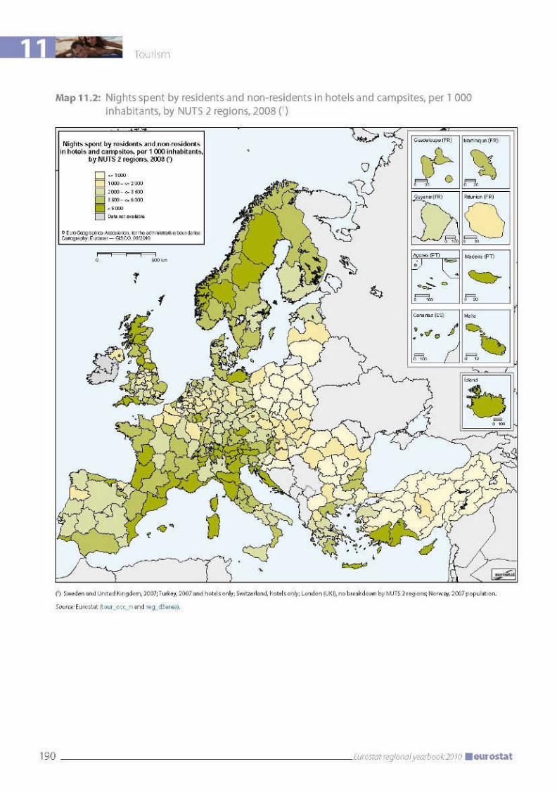
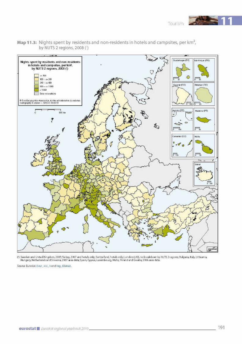
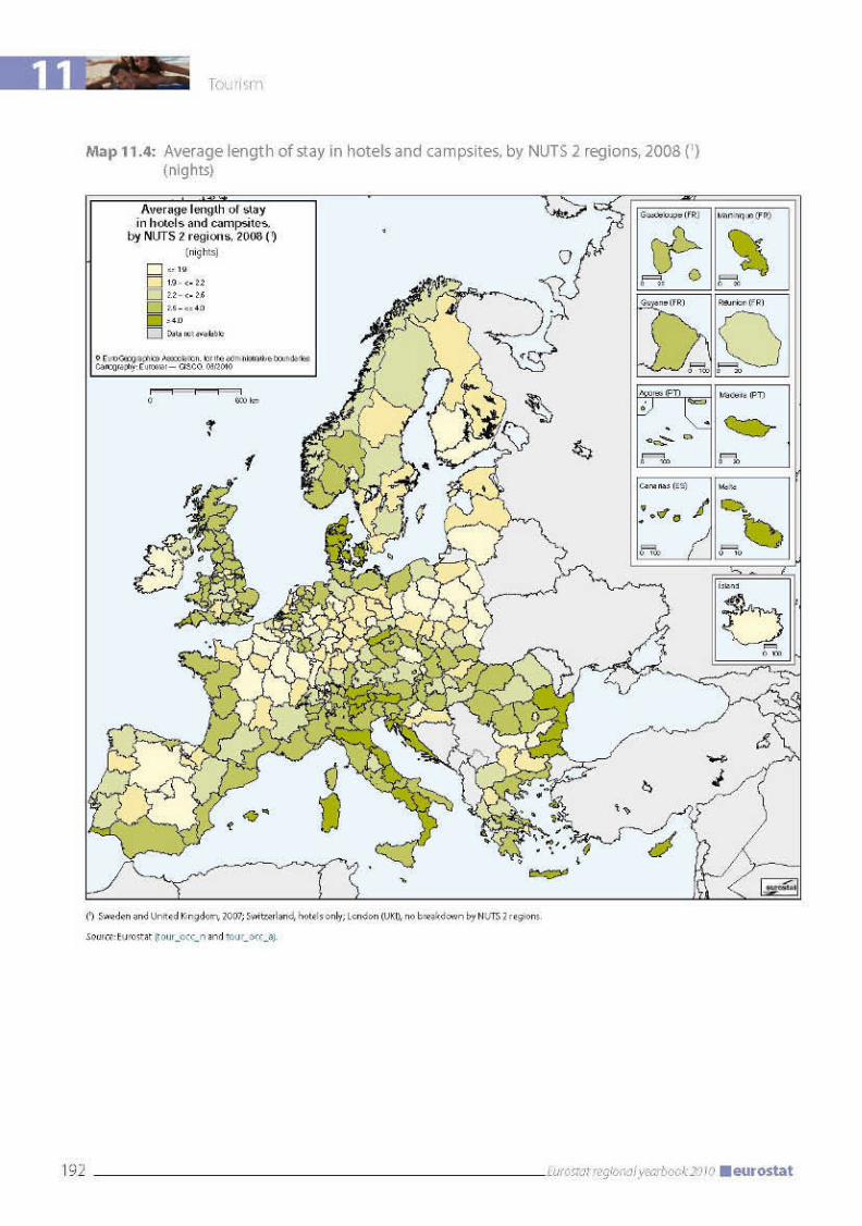
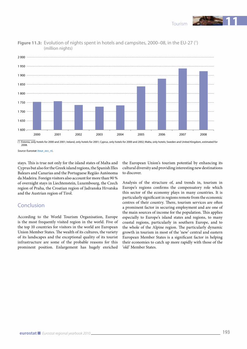
11
193Eurostat regional yearbook 2010eurostat
Tourism
stays. This is true not only for the island states of Malta and Cyprus but also for the Greek island regions, the Spanish Illes Balears and Canarias and the Portuguese Região Autónoma da Madeira. Foreign visitors also account for more than 90 % of overnight stays in Liechtenstein, Luxembourg, the Czech region of Praha, the Croatian region of Jadranska Hrvatska and the Austrian region of Tirol.
Conclusion
According to the World Tourism Organisation, Europe is the most frequently visited region in the world. Five of the top 10 countries for visitors in the world are European Union Member States. The wealth of its cultures, the variety of its landscapes and the exceptional quality of its tourist infrastructure are some of the probable reasons for this prominent position. Enlargement has hugely enriched
the European Union’s tourism potential by enhancing its cultural diversity and providing interesting new destinations to discover.
Analysis of the structure of, and trends in, tourism in Europe’s regions confirms the compensatory role which this sector of the economy plays in many countries. It is particularly significant in regions remote from the economic centres of their country. There, tourism services are often a prominent factor in securing employment and are one of the main sources of income for the population. This applies especially to Europe’s island states and regions, to many coastal regions, particularly in southern Europe, and to the whole of the Alpine region. The particularly dynamic growth in tourism in most of the ‘new’ central and eastern European Member States is a significant factor in helping their economies to catch up more rapidly with those of the ‘old’ Member States.
Figure 11.3: Evolution of nights spent in hotels and campsites, 2000–08, in the EU-27 (1) (million nights)
1 600
1 650
1 700
1 750
1 800
1 850
1 900
1 950
2 000
2000 2001 2002 2003 2004 2005 2006 2007 2008
(1) Estonia, only hotels for 2000 and 2001; Ireland, only hotels for 2001; Cyprus, only hotels for 2000 and 2002; Malta, only hotels; Sweden and United Kingdom, estimated for 2008.
Source: Eurostat (tour_occ_n).
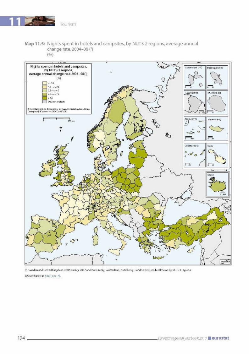
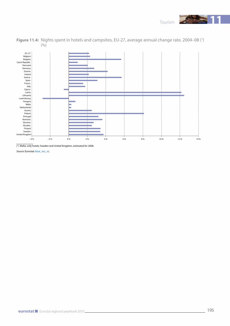
11
195Eurostat regional yearbook 2010eurostat
Tourism
Figure 11.4: Nights spent in hotels and campsites, EU-27, average annual change rate, 2004–08 (1) (%)
– 4 % –2 % 0 % 2 % 4 % 6 % 8 % 10 % 12 % 14 %
EU -27BelgiumBulgaria
Czech RepublicDenmarkGermany
EstoniaIrelandGreece
SpainFrance
ItalyCyprus
LatviaLithuania
Luxembourg Hungary
MaltaNetherlands
AustriaPoland
PortugalRomaniaSloveniaSlovakia
FinlandSweden
United Kingdom
(1) Malta, only hotels; Sweden and United Kingdom, estimated for 2008.
Source: Eurostat (tour_occ_n).
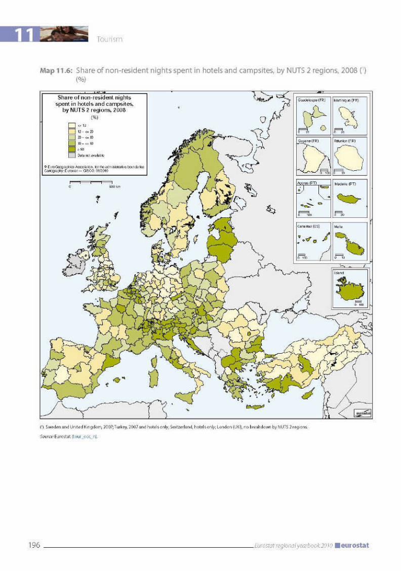

11
197Eurostat regional yearbook 2010eurostat
Tourism
Methodological notes
Harmonised statistical data on tourism have been collected since 1996 in the Member States of the European Union on the basis of Council Directive 95/57/EC of 23 November 1995 on the collection of statistical information in the field of tourism. The programme covers both the supply side, i.e. data on available accommodation capacity (establishments, rooms and bedplaces) and its occupancy (number of visitor arrivals and overnight stays), and the demand side, i.e. the travel behaviour of the population. Results by region below Member State level are available only for the supply side, however.
The tourism statistics presented in this chapter relate only to ‘hotels and similar establishments’ and ‘tourist campsites’. Statistics for ‘holiday dwellings’ and ‘other collective accommodation’, on which data are also collected under the tourism statistics directive, are not included in this analysis since their comparability must still be regarded as limited, particularly at regional level.
One important thing to point out is that the statistical definition of ‘tourism’ is broader than the common, everyday definition. It encompasses not only private trips but also business trips. This is primarily because it views tourism from an economic perspective. Private visitors and business visitors have broadly similar consumption patterns. They both make significant demands on transport, accommodation and restaurant services. To providers of these services, it is of secondary interest whether their customers are private tourists or on business. Tourism promotion departments, on the other hand, are keen to combine the two aspects by emphasising the attractiveness of conference locations as tourist destinations in their own right and give particular prominence to this in their marketing activities.


Health

12 Health
200 Eurostat regional yearbook 2010 eurostat
Introduction
Health is a top priority for Europeans, who expect to be protected against illness and disease — at home, at work and when travelling. The issue cuts across a range of topics from consumer protection (food safety) to safety at work and environmental and social policies.
Establishment of comparable EU-wide data on public health and the factors determining it is closely linked to one of the priorities of the Com-munity action programme in the field of public health for 2008–13, namely to generate and dis-seminate information and knowledge on health.
This enables Eurostat to contribute to achieving other objectives of the action programme, by col-lecting and disseminating statistics and health indicators which help policymakers to identify health risks, improve public health security and promote health, including reducing health in-equalities.
Causes of death
Mortality patterns differ significantly, depend-ing on age and gender, but also between coun-tries and regions. Three types of factor determine mortality patterns: intrinsic factors, such as age and gender; extrinsic factors, such as biological or collective social factors, living or working con-ditions; and individual factors, such as lifestyle, smoking, alcohol consumption, driving and sex-ual behaviour.
As a general rule, the mortality rate is higher among men than among women in all age groups. Although there are signs that the mortality gap is narrowing in some Member States, there are still significant differences between genders.
Variations in mortality patterns reveal signifi-cant differences in causes of death, depending on the age group of the population. Since nowadays people tend to live longer, diseases of the cir-culatory system are the main cause of death in the European Union. Malignant neoplasms follow as the second most frequent cause, af-fecting mainly the middle-aged or elderly. In the younger age groups, however, the larg-est share of deaths is down to external causes (including transport accidents). The distribu-tion of causes of death also depends on geo-graphical location. For example, most of the
new Member States have high death rates due to diseases of the circulatory system, with the Baltic States also recording above-average mor-tality from external causes.
These are all good reasons to take a closer look at mortality rates at both national and regional levels, distinguishing between men and women and between different age groups.
Respiratory diseases
Respiratory diseases include infectious acute re-spiratory diseases (influenza and pneumonia) and chronic obstructive diseases. They are the third most frequent cause of death in the European Union, accounting for 8 % of all deaths. Respira-tory diseases mainly affect older people: nine out of 10 deaths from them occur after the age of 65.
There are considerable differences in the pat-terns of deaths from respiratory diseases within Europe. The rates vary between 82 deaths per 100 000 men and 69 deaths per 100 000 women, of all ages in both cases.
Looking at people over 65, the mortality rates from respiratory diseases are higher for men in almost every region, except for four regions in the United Kingdom (Lincolnshire, East An-glia, Kent, and Cornwall and Isles of Scilly) and in Iceland, where more female deaths were re-corded (437.4 per 100 000 inhabitants compared with 385.2). For other regions within the EU-27 the variation can be quite high, ranging from a male/female ratio of 1 in Berkshire, Bucking-hamshire and Oxfordshire (UK) to more than 3.0 in Pohjois-Suomi (Finland), Estonia, Lubel-skie (Poland) and as much as 4.1 in Lithuania.
The regional pattern for mortality from respirato-ry diseases emerges very clearly. In the regions of Spain, Norway, the United Kingdom and Portu-gal, high mortality can be observed. The highest crude death rates for citizens over 65 years old are reported in Região Autónoma da Madeira (Portu-gal — 1 653.3 deaths per 100 000 males and 940.1 deaths per 100 000 females), Merseyside (UK — 945.6 for males and 819.3 for females), Greater Manchester (UK — 942.5 for males and 902.1 for females) and Lancashire (UK — 918.4 for males and 867.1 for females). The national values of these two countries are 37 % (for Portugal) and 70 % (for the UK) higher than the EU-27 average and account for 24 % of all deaths of Europeans
12
201Eurostat regional yearbook 2010eurostat
Health
over 65 years old from respiratory diseases. At the other end of the scale, the regions with the low-est rates differ, depending on gender, except for Latvia. For males, these regions are Guadeloupe in France (193.8), Sachsen-Anhalt in Germany (234.8) and Latvia (240.5), whereas for females the regions with the lowest rates are Latvia (66.2) and Estonia (76.8).
Chronic lower respiratory diseases
Chronic lower respiratory diseases (chronic pul-monary diseases, emphysema and asthma) are the main group of respiratory diseases and ac-count for 3.9 % of male deaths and 2.6 % of female deaths in the EU-27. Of these, chronic obstructive pulmonary diseases (COPD) are the most com-mon, accounting for 31 % of deaths from respira-tory diseases. Most of these deaths occur after the age of 65 but even so, just as in the case of respira-tory diseases as a whole, the national and regional distributions of deaths due to chronic lower respi-ratory diseases differ.
For chronic lower respiratory diseases the highest national crude death rates per 100 000 inhabit-ants for males aged 65 and over are found in Hun-gary (382.4), Belgium (373.1), Denmark (314.0) and Lithuania (341.4).
Female mortality rates, on the other hand, are high in Denmark (314.2), Iceland (254.3), Ireland (253.5) and the United Kingdom (237.3).
The lowest national values for males are in France (116.4) and Greece (131.2). For females Latvia (28.9) and Malta (49.1) are at the bottom of the table.
The data reveal marked differences between the lowest values for males and females.
Comparing regional values, the highest crude death rates for males aged 65 and over are report-ed in Észak-Magyarország (Hungary) with 531.6 and Principado de Asturias (Spain) with 504.0 and the lowest in Guadeloupe (France) with 29.4 and Kentriki Makedonia (Greece) with 92.7.
For females, Merseyside (UK) with 341.1 and Oslo og Akershus (Norway) with 268.9 report the highest regional rates. Just as for males, Guade-loupe (France) shows the lowest mortality rate for women (16.2), followed by Yugoiztochen (Bulga-ria) with 38.4.
Hospital discharges
Hospitalisation statistics give a broad picture of healthcare treatment of the population and also of general public health. Around 16 760 persons per 100 000 were discharged from hospitals in the EU-27 in 2007. However, even between countries, there is a wide range for this indicator, from fewer than 7 500 in Cyprus and Malta to over 27 000 in Austria. These differences possibly partly reflect differences in the organisation of healthcare ser-vices.
Regional data on hospital discharges of inpatients were not available until quite recently and not all countries are yet in a position to provide data on this subject at subnational level. Amongst the countries with subnational data, the Czech Repub-lic, Germany and France show the greatest varia-tion within the country for the number of hospital discharges per 100 000 inhabitants aged 65 and over after a respiratory disease, the same category as analysed above for causes of death. In France, around four times as many people over 65 are dis-charged from hospitals after a respiratory disease in Réunion as in Guadeloupe. In metropolitan France, this spread falls to 1.7. In Germany and the Czech Republic hospital discharges within the country vary by a factor of around 1.5.
Looking at the gender gap, Iceland shows almost perfect equality for hospital discharges (3 389.4 males over 65 discharged after a respiratory dis-ease per 100 000 and 3 333.9 females). The biggest differences are found in Spain: in Asturias 2.5 times more males were discharged than females in 2007 and in Ciudad Autónoma de Melilla 2.6 times more.
Nurses and midwives
Regional data on healthcare staff give a broad picture of the human resources available to pro-vide healthcare for the population. Eurostat’s information on healthcare staff is largely based on administrative sources. The definitions used possibly vary from one country to another and, to a large degree, reflect countries’ specific ways of organising healthcare, so the data collected are not always completely comparable.
The data presented on human resources available to provide healthcare services take no account of the sector of employment (i.e. whether the staff are independent or are employed by a hospital or
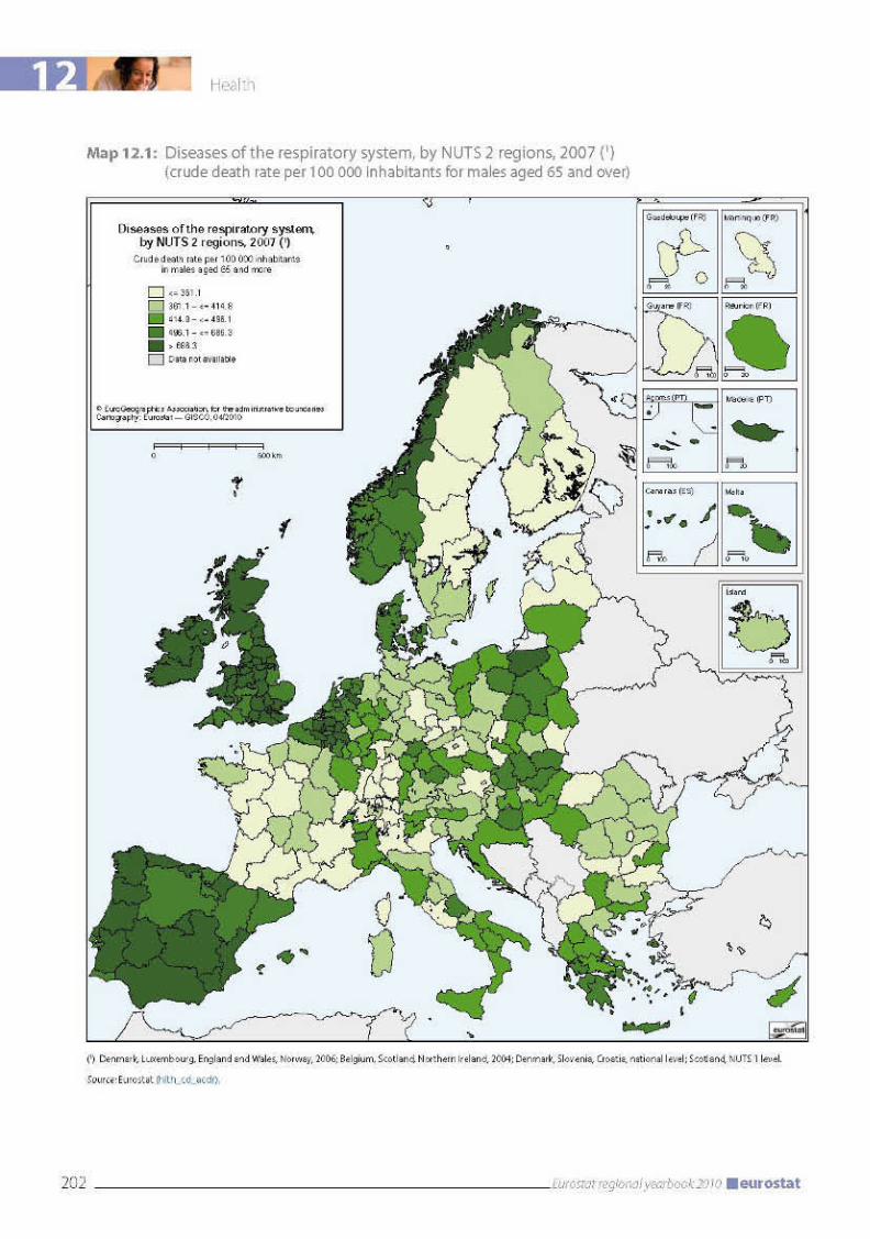
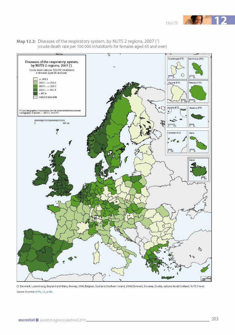
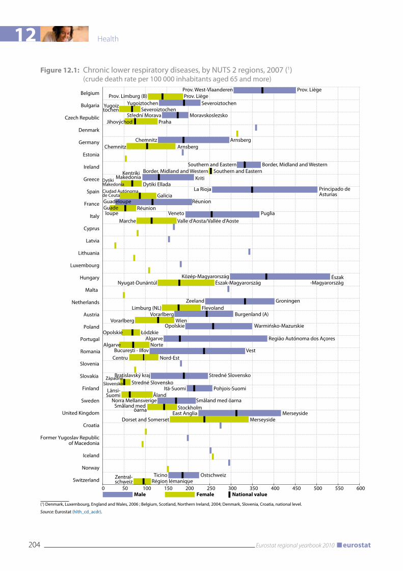
12 Health
204 Eurostat regional yearbook 2010 eurostat
Figure 12.1: Chronic lower respiratory diseases, by NUTS 2 regions, 2007 (1) (crude death rate per 100 000 inhabitants aged 65 and more)
Male Female National value0 50 100 150 200 250 300 350 400 450 500 550 600
Belgium
Bulgaria
Czech Republic
Denmark
Germany
Estonia
Ireland
Greece
Spain
France
Italy
Cyprus
Latvia
Lithuania
Luxembourg
Hungary
Malta
Netherlands
Austria
Poland
Portugal
Romania
Slovenia
Slovakia
Finland
Sweden
United Kingdom
Croatia
Former Yugoslav Republicof Macedonia
Iceland
Norway
Switzerland
Prov. West-Vlaanderen Prov. LiègeProv. Limburg (B) Prov. Liège
Severoiztochen
Chemnitz Arnsberg
Ciudad Autónomade Ceuta Galicia
Réunion
Dytiki Makedonia
Yugoiztochen SeveroiztochenYugoiztochen
Střední Morava Moravskoslezsko
Kriti
Jihovýchod Praha
Chemnitz Arnsberg
Marche Valle d'Aosta/Vallée d'Aoste
Nyugat-Dunántúl Észak-Magyarország
Limburg (NL) Flevoland
Vorarlberg Wien
Centru Nord-Est
Länsi-Suomi Åland
ZápadnéSlovensko
Småland med öarna Stockholm
Dorset and Somerset Merseyside
Opolskie Łódzkie
Algarve Norte
Kentriki Makedonia
Southern and Eastern Border, Midland and WesternBorder, Midland and Western Southern and Eastern
Dytiki ElladaLa Rioja Principado de
Asturias
Veneto Puglia
Közép-Magyarország Észak-Magyarország
Zeeland Groningen
Vorarlberg Burgenland (A)
Opolskie Warmińsko-Mazurskie
Vest
Algarve Região Autónoma dos Açores
Bucureşti - Ilfov
Bratislavský kraj Stredné SlovenskoStredné Slovensko
Itä-Suomi Pohjois-Suomi
Norra Mellansverige Småland med öarna
East Anglia Merseyside
Ticino OstschweizZentral-schweiz Région lémanique
Guadeloupe RéunionGuadeloupe
(1) Denmark, Luxembourg, England and Wales, 2006 ; Belgium, Scotland, Northern Ireland, 2004; Denmark, Slovenia, Croatia, national level.
Source: Eurostat (hlth_cd_acdr).
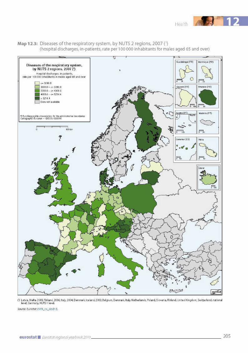
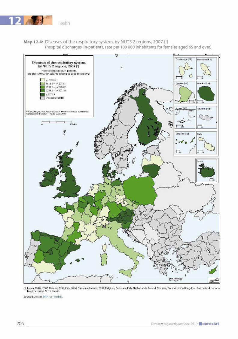
12
207Eurostat regional yearbook 2010eurostat
Health
any other provider). For the purpose of compar-ing healthcare services across Member States, Eurostat prefers the concept of ‘practising profes-sionals’, as this gives the best picture of the avail-ability of healthcare resources (although this was not always possible to achieve).
At EU level, Europe can roughly be divided into two distinct areas by drawing a line from Finland to Italy. West of this line, healthcare systems can generally count on between 667 and 1 096 nursing professionals per 100 000 inhabitants, with the notable exception of Portugal, whereas regions in the east often have an indicator of below 667 per 100 000 inhabitants, with some even below 554.
In 2007 the average number of nurses and mid-wives per 100 000 inhabitants was around 882 for the EU-27. The highest concentration of practising nurses and midwives per 100 000 inhabitants was reported by Luxembourg (1 571.5), followed by the Netherlands (1 500.7), Switzerland (1 485.7), Iceland (1 460.1) and Denmark (1 459.3), whereas in Bulgaria the figure of 466.4 was around 53 % lower than the EU average.
In other words, considerable variations can be observed at regional level.
Across all regions the density ranges from fewer than 300 in several regions of Portugal (Algarve, Alentejo and Norte) to higher than 1 600 in the Netherlands (Gelderland, Zeeland, Groningen, Friesland and Drenthe). Not surprisingly, in most countries the highest concentration is often found in the capital region, for example Praha (Prague) or Bucureşti - Ilfov (Bucharest). However, in a number of countries non-capital regions also have a high proportion of nurses and midwives,
for example, Limousin in France, Prov. West-Vlaanderen in Belgium or Comunidad Foral de Navarra and Aragón in Spain.
When interpreting the map, special attention has to be paid to the fact that the regional data for France, Italy, Slovakia and the former Yugoslav Republic of Macedonia are for ‘professionally ac-tive’ nurses and midwives (which include prac-tising and other (non-practising) midwives and nurses for whom their training is a prerequisite for the job), and could therefore be overesti-mated.
Conclusion
Information about healthcare systems and, ul-timately, about the health of a population is a prerequisite for monitoring the performance of health policy.
The regional indicators currently available for health provide an insight into similarities, partic-ularities and contrasts across regions in Europe. As explained above, there can be big differences between regions in the same country, while re-gions in different countries may be very similar. Thorough analysis of trends and variations in health indicators at regional level is therefore in-dispensable for planning and monitoring action and programmes, formulating new policies, de-veloping new strategies and, all in all, contribut-ing to ‘evidence-based health policy’.
Eurostat’s work on health statistics is focusing mainly on further improvements in the quality, comparability and completeness of the data and further extension of the regional coverage.
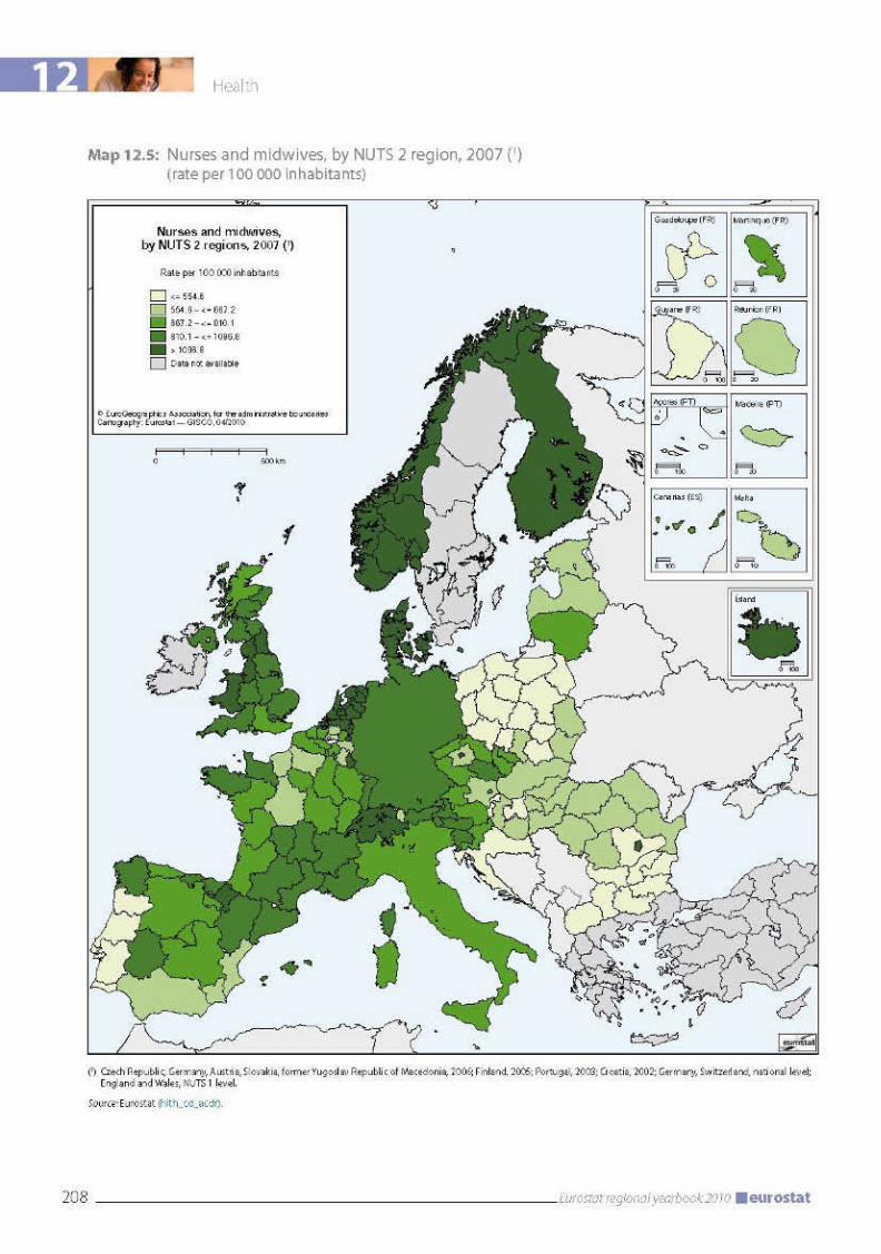
12
209Eurostat regional yearbook 2010eurostat
Health
Methodological notes
Cause of death (COD) statistics are based on information from death certificates. COD statis-tics record the underlying cause of death, i.e. to quote the definition adopted by the World Health Assembly, ‘the disease or injury which initiated the train of morbid events leading directly to death, or the circumstances of the accident or violence which produced the fatal injury’.
In addition to absolute numbers, crude death rates and standardised death rates for COD are provided at national and regional levels. Regional-level data are provided in the form of three-year averages, along with yearly crude death rates for some age groups. The crude death rate indicates mortality in relation to the total population. It is expressed per 100 000 inhabitants, i.e. calculated as the number of deaths recorded in the population over a given period divided by the population in the same period and then multiplied by 100 000. Crude death rates are calculated for five-year age groups. At this level of detail, comparisons between countries and regions are meaningful. The crude death rate for the total population (all ages) by gender and age, however, is a weighted average of the age-specific mortal-ity rates. The weighting factor is the age distribution of the population whose mortality is being ob-served. Consequently, the population structure strongly influences this indicator for broad age groups. In a relatively ‘old’ population there will be more deaths than in a ‘young’ one because mortality is higher in older age groups. For comparisons, the age effect can be taken into account by using a stan-dard population. The standardised death rate (SDR) is a weighted average of age-specific mortality rates. The weighting factor is the age distribution of a standard reference population. The ‘standard European population’ defined by the World Health Organisation (WHO) is used for this purpose. Standardised death rates are expressed per 100 000 inhabitants and calculated for the 0–64 age group (‘premature death’), 65+ and for all ages. Causes of death are classified into the 65 on the ‘European shortlist’, which is based on the international statistical classification of diseases and related health problems (ICD) developed and maintained by the WHO.
Eurostat collects regional-level statistics on healthcare staff (numbers of doctors, dentists, pharmacists, nursing professionals and physiotherapists), on hospital beds and on hospital discharges of inpatients. In addition to absolute numbers, density rates are used to indicate the availability of resources or the frequency of services rendered, expressed per 100 000 inhabitants. They are calculated by dividing the absolute number of healthcare resources available or services rendered in a given period by the popula-tion covered in the same period and then multiplying by 100 000.
Data on nurses and midwives should indicate those ‘immediately serving patients’, i.e. nurses and midwives who have direct contact with patients as consumers of healthcare services. In the context of comparing healthcare services across Member States, Eurostat considers that this is the concept which gives the best picture of the availability of healthcare resources. However, Member States use differ-ent concepts when they report the number of healthcare professionals — both for national purposes and for international comparisons. Therefore the data for some countries might refer to nurses and midwives who are ‘professionally active’ (i.e. including practising and other (non-practising) midwives and nurses for whom their education is a prerequisite for the execution of the job) or ‘licensed to prac-tice’ (i.e. registered and entitled to practice as healthcare professionals , irrespective whether they see patients or not).


Agriculture
13 Agriculture
212 Eurostat regional yearbook 2010 eurostat
Introduction
The Economic Accounts for Agriculture (EAA) are a satellite account of the European System of Accounts (ESA 1995), providing detailed monetary data on agriculture. The main purpose of the EAA is to analyse the production process and the primary income which it generates. They integrate a wide range of statistics and administrative information on agriculture. The maps in this publication are based on the regional EAA and show some of the ways in which these data can be used for analyses and be combined with agricultural statistics from other domains (Farm Structure Survey, etc.).
Eurostat has been collecting, processing and publishing data on the EAA in the form of a regional breakdown for more than 15 years. Eurostat’s free dissemination database contains detailed information on the EAA in a NUTS 2 regional breakdown, covering the period from 1990 to 2008. The regional data, which also cover candidate countries and EFTA countries, are not complete for the time being. Where necessary, data at country or NUTS 1 level have been used in the analyses instead.
Contribution of agriculture to GvA
In national accounts’ terminology, gross value added (GVA) at market prices is a main final result of the production activity of various branches (‘resident producer units’) of an economy. Comparison of the GVA of a given branch with the overall GVA therefore gives a rough measure of its economic importance. It is only a rough measure. Given the close economic relationships between individual branches, it would be somewhat short-sighted to consider each in isolation. Map 13.1 shows that agriculture’s contribution to GVA is generally quite low. However, since the EU underwent enlargement, there is now more diversity.
Looking at the EU-27 average, agriculture’s contribution to total GVA was only around 1.4 % in 2007. But the economic importance of agriculture is generally much greater in the east and south than in the west and north. Its share in GVA is higher than 6.0 % in 23 out of the 223 regional entities shown: 7 (out of 8) regions in Romania, 7 in Greece, 5 in Bulgaria, 2 in Hungary, 1 in France (Champagne-Ardenne), and also in the former Yugoslav Republic of Macedonia.
The regions showing a contribution of between 3 % and 6 % from agriculture include six regions in Italy, five in France, four in Greece, four in the Netherlands, three in Hungary, two each in Poland and Portugal, and one in Austria.
The regions with the lowest share for agriculture are mainly located in the United Kingdom and Germany. Furthermore, the share of agricultural activity is typically very low in regions around big cities, and this applies to eastern and central Europe too. Bratislava and Bucureşti are examples, as are the Île de France (the region including Paris), and the German cities Berlin, Bremen and Hamburg in western Europe.
Labour productivity of agriculture
Productivity indicators are ratios of measures of output to measures of input. They can be used to measure and compare levels and rates of growth in productivity between Member States and industries. Agriculture is a highly labour-intensive sector. It is revealing to compile a partial productivity indicator from the gross value added data from the EAA and the corresponding agricultural labour input data, broken down using the latest Farm Structure Survey (FSS). This indicator is also used in the statistics on rural areas.
To take account of part-time and seasonal work, agricultural labour is measured in annual work units (AWU). One AWU corresponds to the input, measured in working time, of one person engaged in agricultural activities in an agricultural unit on a full-time basis over an entire year. Map 13.2 shows the gross value added in agriculture per AWU. When comparing levels between Member States and regions, it should be borne in mind that these data are not adjusted by purchasing power parities (PPP). In other words, they do not reflect general differences in price levels.
On average for the EU, the gross value added per annual work unit is about EUR 13 000. In 27 regions, mainly in Denmark, France, Germany, the Netherlands and the United Kingdom, the gross value added per annual work unit is higher than EUR 40 000 in 2007.
Map 13.2 clearly shows a big difference between the western and eastern parts of Europe. Only regions in central and eastern Europe, plus three regions in Portugal (Norte, Centro and Madeira) show results lower than EUR 5 000 per annual work
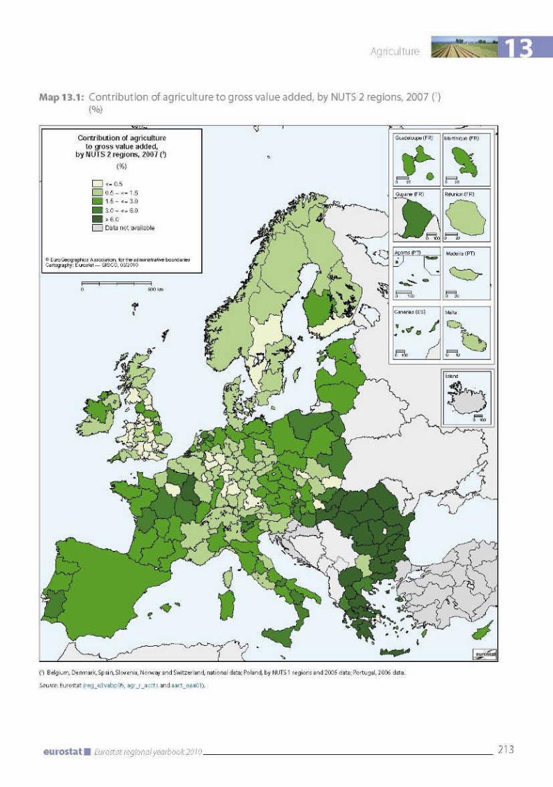

13 Agriculture
214 Eurostat regional yearbook 2010 eurostat
unit. Labour productivity is strongly influenced by farm structures. In most of the eastern (and also in some southern) Member States, average farm sizes are small, the level of mechanisation is low, and a significant part of production is for on-farm consumption. The influence of farm structures on labour productivity can, for example, be noted in the Czech Republic, a Member State with many large cooperatives. Two regions in the Czech Republic (Střední Čechy and Severozápad) show results over EUR 10 000 per annual work unit.
Another factor which influences the comparability of productivity of agricultural labour is the structure of production. For example, production of fruit and vegetables requires more labour than production of arable crops, while capital costs are relatively lower. Therefore, the GVA per annual work unit cannot be taken as the only indicator for productivity.
Importance of crop production
An important content of the EAA is information on the value of output, which also makes it possible to show how the composition of output differs between regions. Map 13.3 shows the significance of crop output compared to total agricultural goods output, monitored in basic prices. At the same time, the map also shows the significance of animal output, as crop output plus animal output amounts to total agricultural goods output. The regions with light colours are, therefore, regions with high animal production. The total area of arable land, soil quality, climate conditions and consumer demand may influence the composition of output.
On average, crop output is about 55 % and animal output about 45 % of total agricultural goods output. Regions with the highest share from crop output are found mainly in the southern part of Europe, with their high production of, for example, wine, fruits, olive oil and vegetables, but for some regions, intensive production of cereals is of high importance.
Regions with high levels of animal production are to be found in many parts of Europe, depending on local conditions. Cattle and milk production is often linked to large areas of grassland, as found, for example, in Ireland and the western part of the UK, but also in mountainous areas of central Europe. In other regions, for example in the north-west of Germany (Weser-Ems and
Münster) and in western France (Bretagne and Basse-Normandie), very intensive pig production is one of the main reasons for the high level of animal production.
In the new Member States, there are few differences among regions within a country, though Bulgaria is an exception, as its six regions comprise four different categories of importance for crop and animal production. At country level, Poland (where the figures are for NUTS 1 regions) and Malta show high levels of animal production among the new Member States.
Agricultural productivity
Map 13.4 shows the value of crop output per hectare of agricultural area. However, it focuses on intensive crop production, so output of forage plants and the area they cover are excluded from the calculation. The value of crop output per hectare, which on average is about EUR 1 800, depends mainly on the type of crop. Vegetables, wine, fruit-growing and olive oil production can generate a value over 10 times higher per hectare than, for example, cereal production. Furthermore, growing under glass or plastic means high output on a limited area of land, which explains why most regions in the Netherlands show very high output per hectare. Other regions with more than EUR 8 000 per hectare are found in Switzerland and Austria, where the amount of land suitable for intensive production is low, and is used for vegetables, fruits, flowers, etc. The overseas departments of France (Guadeloupe, Martinique and Guyane) plus Madeira and Açores (Portugal) show very high productivity for crop production.
Low crop production values per hectare (less than EUR 1 000 per hectare) are predominantly found in eastern and northern Europe. Regarding eastern Europe, low figures are explained by a combination of lower yields and lower prices. In the case of Poland, the use of data from 2005 may impact the result, as crop prices increased by about 20 % in real terms from 2005 to 2007.
The big difference in crop output per hectare between Norway and neighbouring regions in northern Europe seems to be explained mainly by the way in which subsidies are granted. In Norway a larger proportion of subsidies are included in basic prices than in EU Member States, where subsidies are predominantly granted to support income, and not as product-related subsidies.
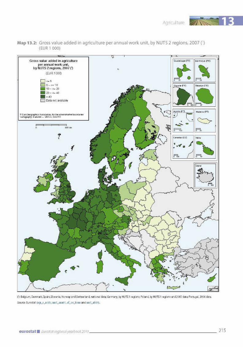
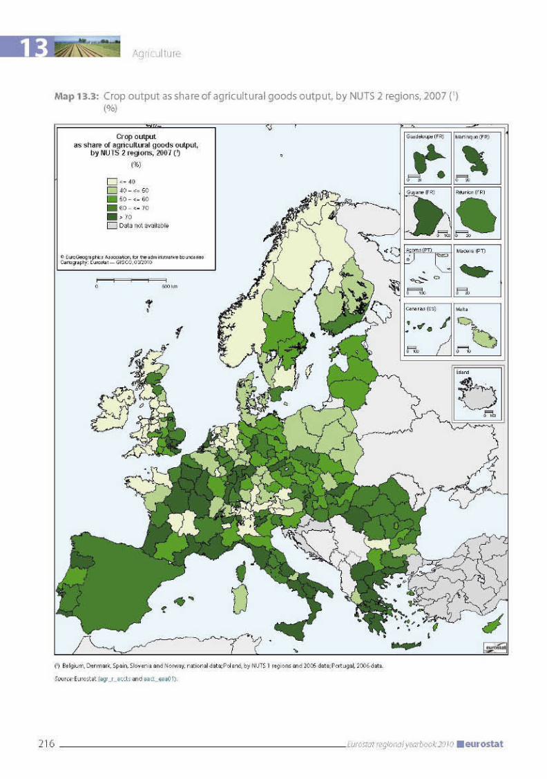
13
217Eurostat regional yearbook 2010eurostat
Agriculture
Map 13.5 shows the value of animal output in basic prices per livestock unit, that is, the value of output of live animals and animal products per 500 kilograms of live animals. The value depends, among other factors, on the balance between meat and livestock production and the production of animal products (such as milk and eggs), as animal products generate higher income per livestock unit than the production of meat. On average the output per livestock unit is about EUR 1 000.
The picture for EU and EFTA countries is mixed. Many regions in eastern Europe show low productivity using this indicator. Ireland and several regions in northern and western parts of the United Kingdom are in the lowest group, too. In eastern Europe, prices below the EU average can explain this, while low-intensity beef production seems to explain the results for Ireland and the United Kingdom.
Regarding high output per unit of livestock in the north, this is partly due to special subsidies in less favoured areas, while high figures for Norway and Switzerland are due to subsidy systems that differ from those in the EU. The high results in many regions in central Italy seem to be explained by high product prices.
Energy costs in agriculture
Map 13.6 shows the costs of energy and lubricants compared to the value of output. The share of energy costs can be considered as an agro-environmental indicator, as energy consumption is a core element in policies related to environment and climate. Energy costs are — generally speaking — expected to be highest where mechanisation is very developed. Cross-country comparison of figures can be affected by differences in prices and taxes on energy, and by the products in the agricultural basket.
The picture presented by Map 13.6 shows high energy costs in particular in regions in eastern Europe, despite the fact that the level of mechanisation in most of these countries is low. The high figures in eastern Europe, therefore, are to be explained by other factors, for example lower productivity and lower prices for output. In the case of Poland, relatively high energy costs are not explained by use of data from 2005, as prices for output and for energy increased by almost the same percentage between 2005 and 2007.
The high figures for regions in the Netherlands (in particular Zuid-Holland) and in regions such as Essex, Outer London and Inner London are most probably explained by intensive production in greenhouses, with high energy consumption for heating. The relatively high costs in Norway, Sweden and Finland can — apart from the high demand for heating for some kinds of agricultural production because of the cold climate — be explained by high transport costs in regions with low population density.
Low energy costs are mainly found in south-western parts of Europe, which most probably can be explained by higher output prices (compared to eastern Europe) and by more efficient use of energy.
Conclusion
The regional EAA are an appropriate source of information for analysing agricultural production, input and income. Since they are a synthesis of a wide range of statistics and administrative data on agriculture, they can be connected with any other agricultural information systems and data on other branches of the national economy. Recent developments and new demands for data for rural development statistics and for more information on environment-related information have added to their importance. Current gaps in the data are expected to be filled in the near future.
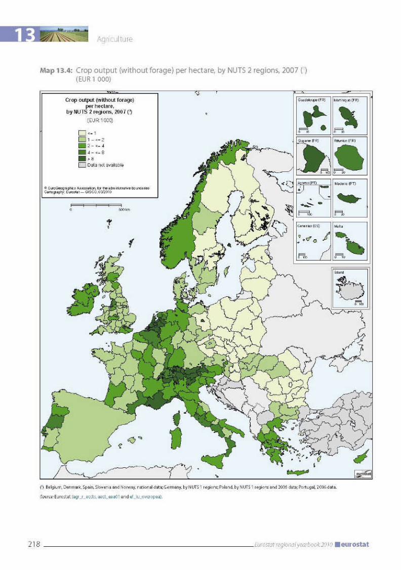
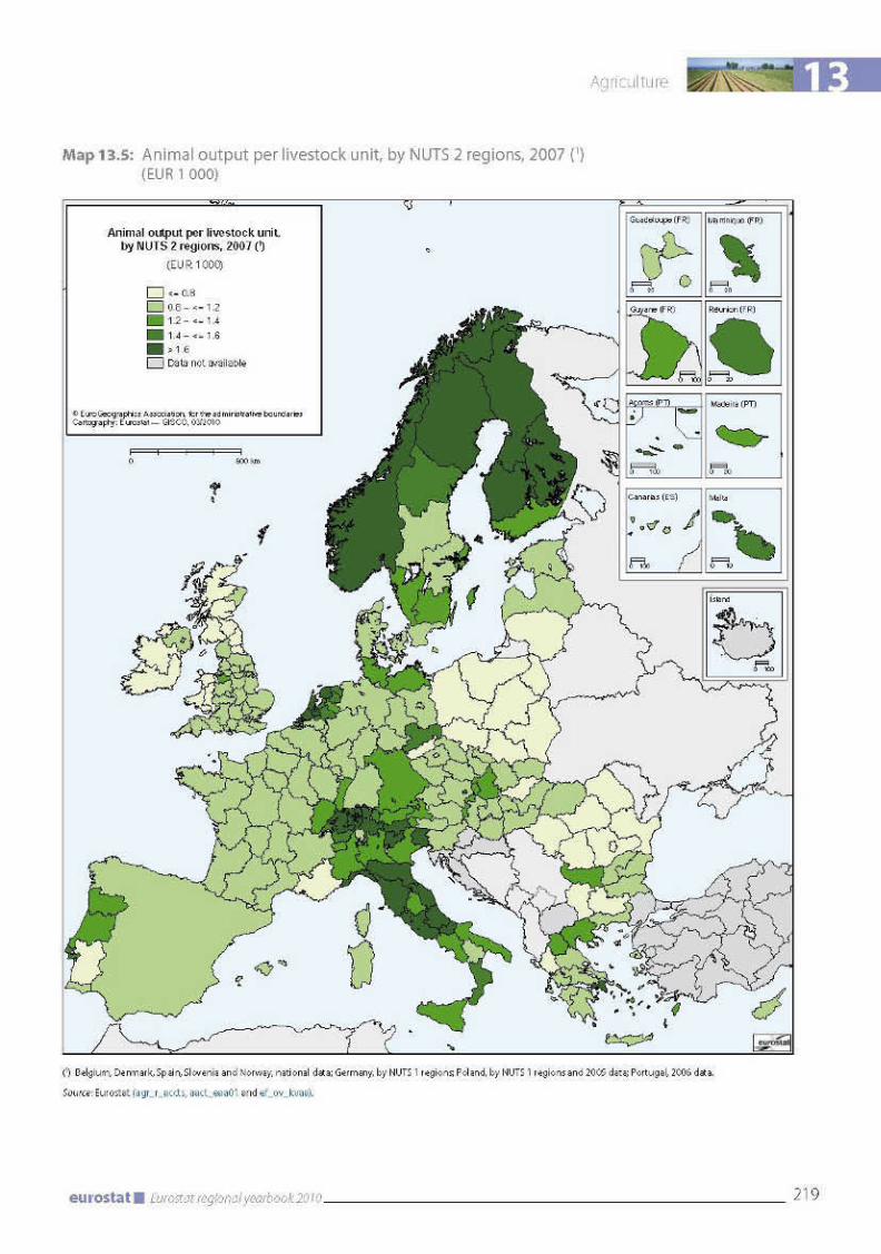
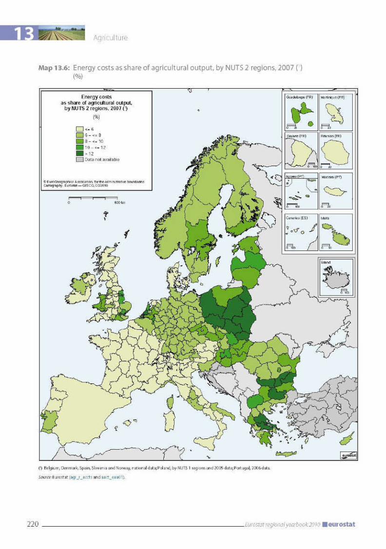

13
221Eurostat regional yearbook 2010eurostat
Agriculture
Methodological notes
The agricultural accounts data at regional level are compiled in the same context as the Economic Accounts for Agriculture (EAA) at national level. The regional data are for output items which are often building blocks for the result at national level, while the regional data for intermediate consumption (direct input of goods and services in the production) are often broken down from national results using other information, using a top-down approach. The regional results are, therefore, often less accurate than data at national level.
The output of the agricultural sector is the sum of the output of agricultural products and of the goods and services produced in inseparable non-agricultural secondary activities. Output of agricultural products comprises the total value of sales (except trade in animals between agricultural holdings), changes in stocks held by producers, on-farm final consumption (of agricultural products), processing of agricultural products by producers (in the form of separable activities) and the value of intra-unit consumption of crop products used in animal feed.
Gross value added (GVA) is the difference in basic prices between the value of output and the value of intermediate consumption.
The crop area is based on data from the Farm Structure Survey (FSS), which covers slightly less than the production covered by the EAA, as the FSS excludes the smallest farms. The area used in Map 13.4. includes utilised arable land (for crops other than forage) and land under permanent crops, while the exclusion of forage land (including permanent grassland) is partly due to a wish to refine the analyses, and partly due to quality problems in the values for forage.
For certain purposes, various categories of livestock need to be aggregated, e.g. piglets, breeding sows and other pigs. By using coefficients, all animals are converted into a common measurement unit, named livestock units (LU). The LU is compiled in the context of the FSS.
To take into account the very large proportion of part-time work in agriculture and opportunities for part-time work in other sectors of the economy, information on employment in agriculture is expressed in annual work units (AWU). One AWU corresponds to the work performed by one person performing agricultural work on a holding over a 12-month period on a full-time basis. The yearly working time of each such worker is 1 800 hours (225 working days of 8 hours per day), unless national provisions governing contracts of employment specify otherwise. The number of persons working (full-time or part-time) in agriculture is shown in the FSS statistics.


Coastal regions
14 Coastal regions
224 Eurostat regional yearbook 2010 eurostat
Introduction
On 10 October 2007, the Commission adopted the Blue Paper launching an integrated maritime policy for the European Union. The aims of this policy are to maximise the sustainable use of the oceans and seas, enhance Europe’s knowledge and innovation potential in maritime affairs, ensure development and sustainable growth in the coastal regions, strengthen Europe’s maritime leadership and raise the profile of maritime Europe. For the sake of greater coherence, this policy gives preference to a holistic approach, i.e. all areas or sectors concerned are taken into account. For example, the economic issues must incorporate environmental aspects and vice versa. Similarly, the development of a sector of activity will have to take account of all the sectors developed on the same territory or using the same maritime areas.
As natural boundaries between the land and the sea, the coastal regions of Europe fall quite naturally under this policy. These regions are, in fact, attractive places to live for their inhabitants and tourists, prime business areas for sectors with links to the sea and obligatory points of transit for goods and passengers transported by sea. It is therefore not surprising that these regions constitute a major focal point and are very much involved in the introduction and follow-up of this integrated maritime policy at local, national and European levels.
The purpose of this chapter is to paint a portrait of these regions and to present some of their demographic, social and economic features. For the sake of consistency, most of the data relate to 2007. The indicators chosen will attempt to highlight the specific features of these regions, comparing them with those of the country as a whole.
Europeans attracted by the coast
In 2007, a total of 196 million (1) people lived in the 446 coastal regions of the European Union, i.e. 43 % of the population of the 22 EU countries which have a coastline.
As Map 14.1 shows, in 97 % of these regions more than 50 % of the inhabitants live less than 50 km from the sea. The population concentration in this coastal strip exceeds 75 % of the region’s population in the case of 88 % of these regions. Some 194 cities with more than 100 000
inhabitants are also located less than 50 km from the sea. These major conurbations are home to 38 % of these regions’ inhabitants. The biggest of them are London, Athina, Napoli and Roma.
The proportion of the national population living in a coastal region depends to a great extent on the country’s geographical characteristics, such as the length and shape of its coastline. Thus, in the case of the island states, such as Cyprus or Malta, or peninsular states, such as Denmark, this proportion is 100 %, because all the regions in these countries are regarded as coastal. In contrast, the inhabitants of coastal regions represent only 4 % of the population in Romania and 9 % in Germany.
It should be noted that the area of the geographical units included in the definition of coastal regions varies considerably from one country to another. This may result in the population of the coastal regions being overestimated for certain countries, such as Sweden and Finland. However, this overestimation is fairly limited. Indeed, even if a large proportion of the area of a coastal region is far from the coast, in most cases the inhabitants and the economic activities are located close to it.
Growing old or retiring on the coast
In 2007, some 41 % of persons over the age of 65 belonging to the 22 Member States with a coastline lived in a coastal region. On average, the ageing of the population in the coastal regions is not therefore more pronounced than in these Member States as a whole. However, the proportion of elderly persons (over the age of 65) compared to the national average differs appreciably from region to region. As shown by Map 14.2, in almost 48 % of coastal regions there was a greater proportion of elderly people than in the country as a whole and in 30 % of these regions the proportion was lower. For example, the coastal regions of the United Kingdom, such as East Sussex or the Isle of Wight, were home to around 1.4 times more elderly people than the national average. This is also the case in the Arrondissement of Veurne on the Belgian coast. This phenomenon may be more marked, as on the northern coast of Spain in the Lugo region, where there were proportionally 1.6 times more elderly people than in the country as a whole. On the other hand, in the Romanian coastal region
(1) Excluding Northern Ireland and Scotland, for which no data are available.
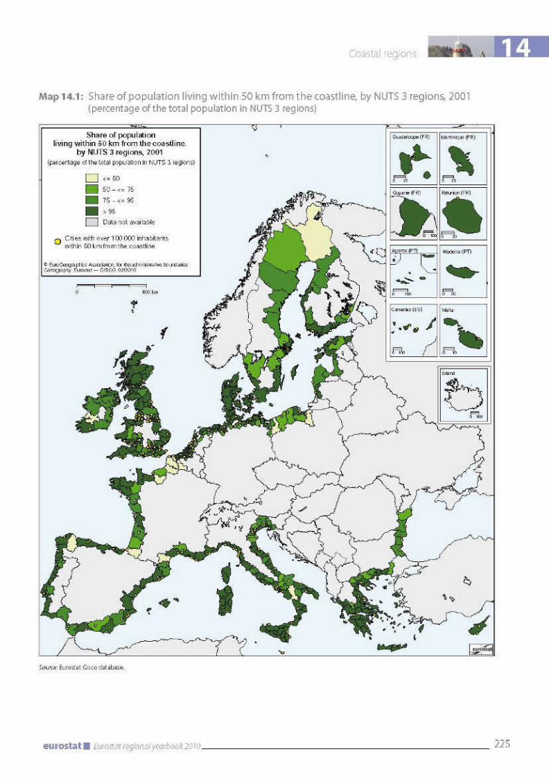
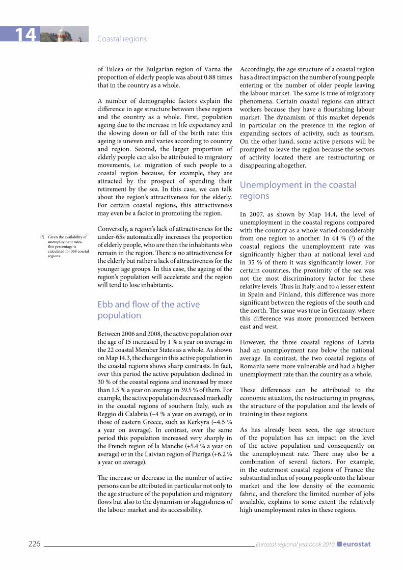
14 Coastal regions
226 Eurostat regional yearbook 2010 eurostat
of Tulcea or the Bulgarian region of Varna the proportion of elderly people was about 0.88 times that in the country as a whole.
A number of demographic factors explain the difference in age structure between these regions and the country as a whole. First, population ageing due to the increase in life expectancy and the slowing down or fall of the birth rate: this ageing is uneven and varies according to country and region. Second, the larger proportion of elderly people can also be attributed to migratory movements, i.e. migration of such people to a coastal region because, for example, they are attracted by the prospect of spending their retirement by the sea. In this case, we can talk about the region’s attractiveness for the elderly. For certain coastal regions, this attractiveness may even be a factor in promoting the region.
Conversely, a region’s lack of attractiveness for the under-65s automatically increases the proportion of elderly people, who are then the inhabitants who remain in the region. There is no attractiveness for the elderly but rather a lack of attractiveness for the younger age groups. In this case, the ageing of the region’s population will accelerate and the region will tend to lose inhabitants.
Ebb and flow of the active population
Between 2006 and 2008, the active population over the age of 15 increased by 1 % a year on average in the 22 coastal Member States as a whole. As shown on Map 14.3, the change in this active population in the coastal regions shows sharp contrasts. In fact, over this period the active population declined in 30 % of the coastal regions and increased by more than 1.5 % a year on average in 39.5 % of them. For example, the active population decreased markedly in the coastal regions of southern Italy, such as Reggio di Calabria (–4 % a year on average), or in those of eastern Greece, such as Kerkyra (–4.5 % a year on average). In contrast, over the same period this population increased very sharply in the French region of la Manche (+5.4 % a year on average) or in the Latvian region of Pierīga (+6.2 % a year on average).
The increase or decrease in the number of active persons can be attributed in particular not only to the age structure of the population and migratory flows but also to the dynamism or sluggishness of the labour market and its accessibility.
Accordingly, the age structure of a coastal region has a direct impact on the number of young people entering or the number of older people leaving the labour market. The same is true of migratory phenomena. Certain coastal regions can attract workers because they have a flourishing labour market. The dynamism of this market depends in particular on the presence in the region of expanding sectors of activity, such as tourism. On the other hand, some active persons will be prompted to leave the region because the sectors of activity located there are restructuring or disappearing altogether.
Unemployment in the coastal regions
In 2007, as shown by Map 14.4, the level of unemployment in the coastal regions compared with the country as a whole varied considerably from one region to another. In 44 % (2) of the coastal regions the unemployment rate was significantly higher than at national level and in 35 % of them it was significantly lower. For certain countries, the proximity of the sea was not the most discriminatory factor for these relative levels. Thus in Italy, and to a lesser extent in Spain and Finland, this difference was more significant between the regions of the south and the north. The same was true in Germany, where this difference was more pronounced between east and west.
However, the three coastal regions of Latvia had an unemployment rate below the national average. In contrast, the two coastal regions of Romania were more vulnerable and had a higher unemployment rate than the country as a whole.
These differences can be attributed to the economic situation, the restructuring in progress, the structure of the population and the levels of training in these regions.
As has already been seen, the age structure of the population has an impact on the level of the active population and consequently on the unemployment rate. There may also be a combination of several factors. For example, in the outermost coastal regions of France the substantial influx of young people onto the labour market and the low density of the economic fabric, and therefore the limited number of jobs available, explains to some extent the relatively high unemployment rates in these regions.
(2) Given the availability of unemployment rates, this percentage is calculated for 368 coastal regions.
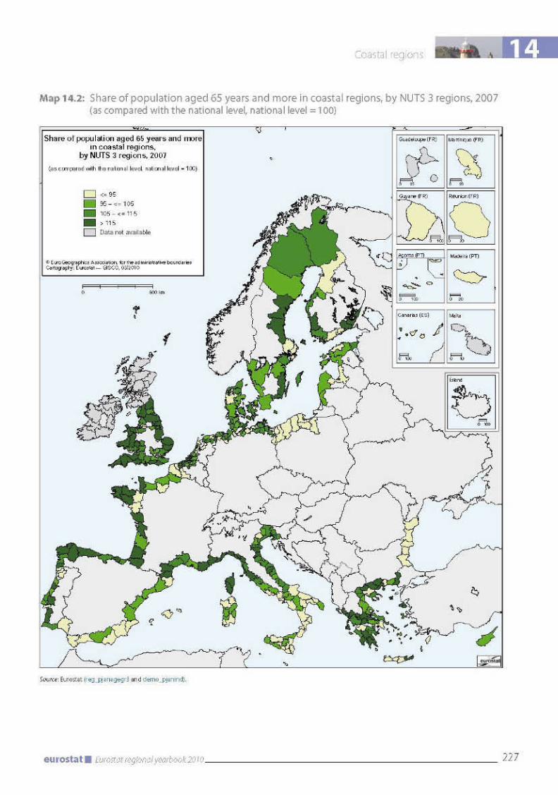
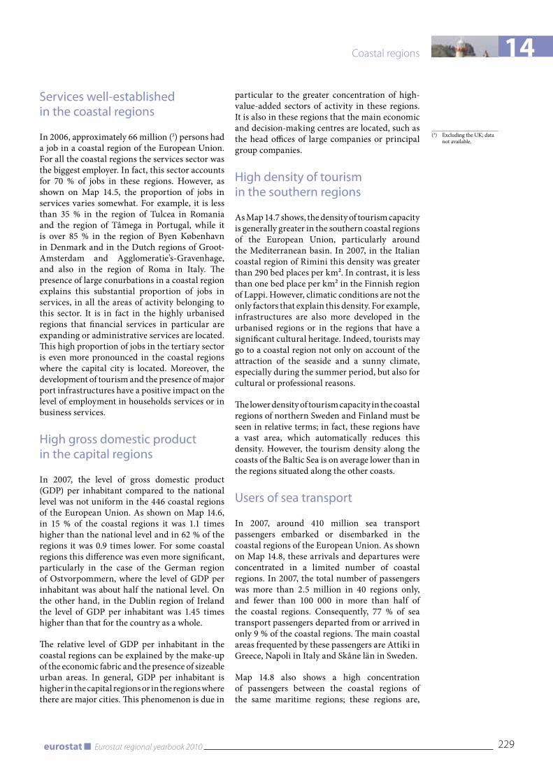
14
229Eurostat regional yearbook 2010eurostat
Coastal regions
Services well-established in the coastal regions
In 2006, approximately 66 million (3) persons had a job in a coastal region of the European Union. For all the coastal regions the services sector was the biggest employer. In fact, this sector accounts for 70 % of jobs in these regions. However, as shown on Map 14.5, the proportion of jobs in services varies somewhat. For example, it is less than 35 % in the region of Tulcea in Romania and the region of Tâmega in Portugal, while it is over 85 % in the region of Byen København in Denmark and in the Dutch regions of Groot-Amsterdam and Agglomeratie’s-Gravenhage, and also in the region of Roma in Italy. The presence of large conurbations in a coastal region explains this substantial proportion of jobs in services, in all the areas of activity belonging to this sector. It is in fact in the highly urbanised regions that financial services in particular are expanding or administrative services are located. This high proportion of jobs in the tertiary sector is even more pronounced in the coastal regions where the capital city is located. Moreover, the development of tourism and the presence of major port infrastructures have a positive impact on the level of employment in households services or in business services.
High gross domestic product in the capital regions
In 2007, the level of gross domestic product (GDP) per inhabitant compared to the national level was not uniform in the 446 coastal regions of the European Union. As shown on Map 14.6, in 15 % of the coastal regions it was 1.1 times higher than the national level and in 62 % of the regions it was 0.9 times lower. For some coastal regions this difference was even more significant, particularly in the case of the German region of Ostvorpommern, where the level of GDP per inhabitant was about half the national level. On the other hand, in the Dublin region of Ireland the level of GDP per inhabitant was 1.45 times higher than that for the country as a whole.
The relative level of GDP per inhabitant in the coastal regions can be explained by the make-up of the economic fabric and the presence of sizeable urban areas. In general, GDP per inhabitant is higher in the capital regions or in the regions where there are major cities. This phenomenon is due in
particular to the greater concentration of high-value-added sectors of activity in these regions. It is also in these regions that the main economic and decision-making centres are located, such as the head offices of large companies or principal group companies.
High density of tourism in the southern regions
As Map 14.7 shows, the density of tourism capacity is generally greater in the southern coastal regions of the European Union, particularly around the Mediterranean basin. In 2007, in the Italian coastal region of Rimini this density was greater than 290 bed places per km². In contrast, it is less than one bed place per km² in the Finnish region of Lappi. However, climatic conditions are not the only factors that explain this density. For example, infrastructures are also more developed in the urbanised regions or in the regions that have a significant cultural heritage. Indeed, tourists may go to a coastal region not only on account of the attraction of the seaside and a sunny climate, especially during the summer period, but also for cultural or professional reasons.
The lower density of tourism capacity in the coastal regions of northern Sweden and Finland must be seen in relative terms; in fact, these regions have a vast area, which automatically reduces this density. However, the tourism density along the coasts of the Baltic Sea is on average lower than in the regions situated along the other coasts.
Users of sea transport
In 2007, around 410 million sea transport passengers embarked or disembarked in the coastal regions of the European Union. As shown on Map 14.8, these arrivals and departures were concentrated in a limited number of coastal regions. In 2007, the total number of passengers was more than 2.5 million in 40 regions only, and fewer than 100 000 in more than half of the coastal regions. Consequently, 77 % of sea transport passengers departed from or arrived in only 9 % of the coastal regions. The main coastal areas frequented by these passengers are Attiki in Greece, Napoli in Italy and Skåne län in Sweden.
Map 14.8 also shows a high concentration of passengers between the coastal regions of the same maritime regions; these regions are,
(3) Excluding the UK; data not available.

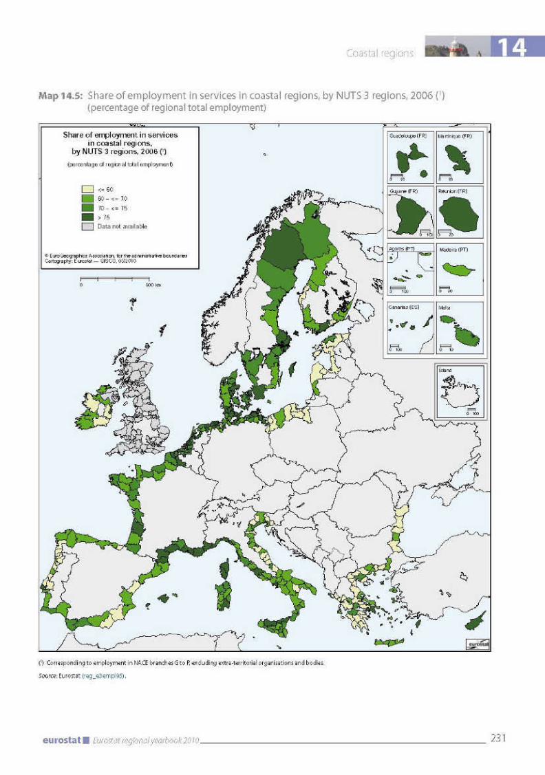
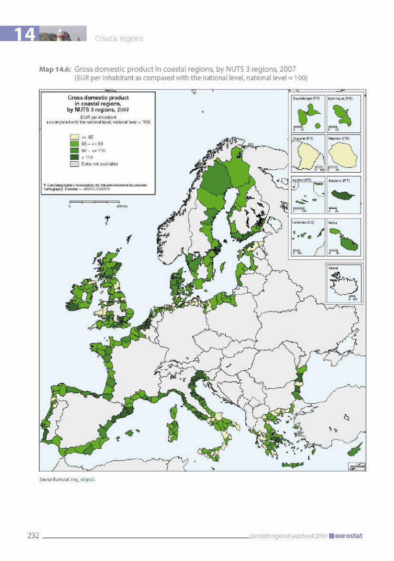
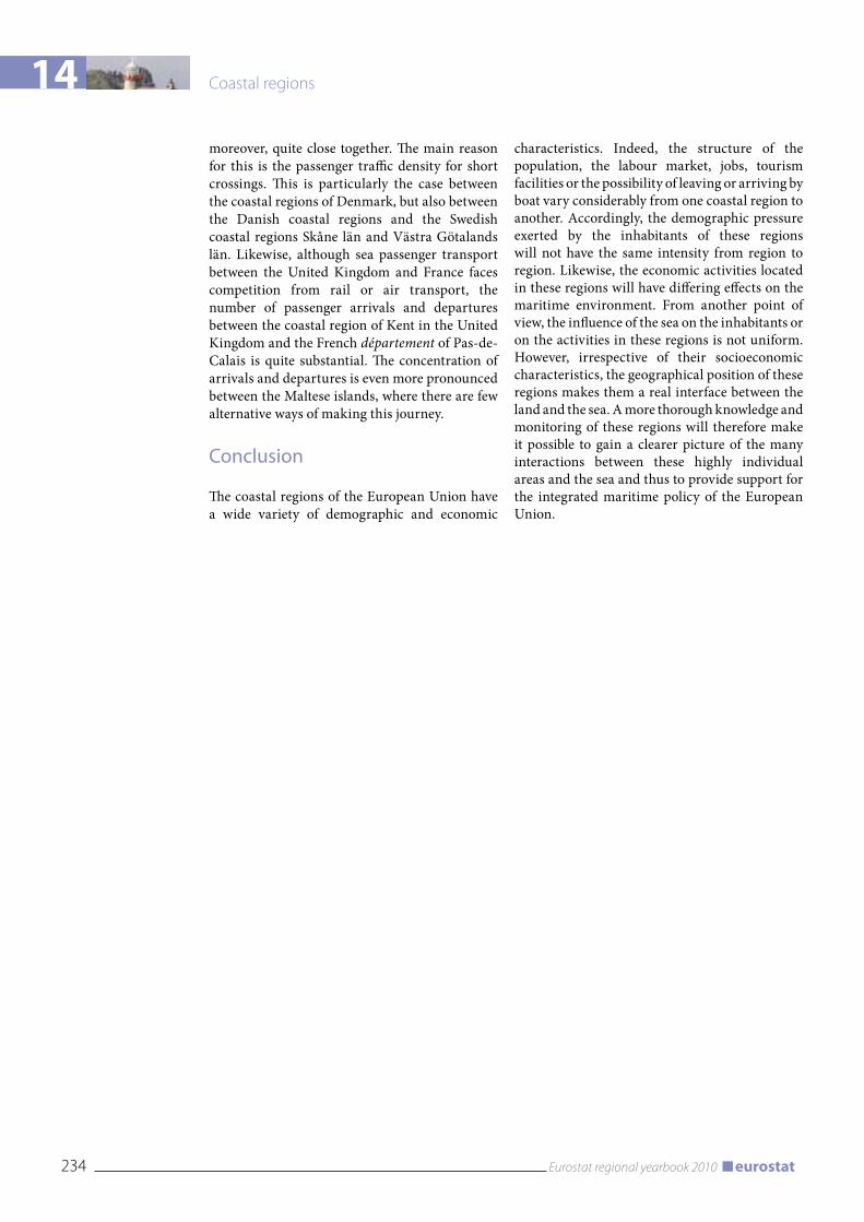
14 Coastal regions
234 Eurostat regional yearbook 2010 eurostat
moreover, quite close together. The main reason for this is the passenger traffic density for short crossings. This is particularly the case between the coastal regions of Denmark, but also between the Danish coastal regions and the Swedish coastal regions Skåne län and Västra Götalands län. Likewise, although sea passenger transport between the United Kingdom and France faces competition from rail or air transport, the number of passenger arrivals and departures between the coastal region of Kent in the United Kingdom and the French département of Pas-de-Calais is quite substantial. The concentration of arrivals and departures is even more pronounced between the Maltese islands, where there are few alternative ways of making this journey.
Conclusion
The coastal regions of the European Union have a wide variety of demographic and economic
characteristics. Indeed, the structure of the population, the labour market, jobs, tourism facilities or the possibility of leaving or arriving by boat vary considerably from one coastal region to another. Accordingly, the demographic pressure exerted by the inhabitants of these regions will not have the same intensity from region to region. Likewise, the economic activities located in these regions will have differing effects on the maritime environment. From another point of view, the influence of the sea on the inhabitants or on the activities in these regions is not uniform. However, irrespective of their socioeconomic characteristics, the geographical position of these regions makes them a real interface between the land and the sea. A more thorough knowledge and monitoring of these regions will therefore make it possible to gain a clearer picture of the many interactions between these highly individual areas and the sea and thus to provide support for the integrated maritime policy of the European Union.

14 Coastal regions
236 Eurostat regional yearbook 2010 eurostat
Methodological notes
A coastal region of the European Union is a statistical region defined at NUTS3 level of the geographical nomenclature, having a coastline or with more than half of its population living less than 50 km from the sea. In the EU as a whole there are 446 such regions, belonging to the 22 Member States which have a coastline. Of these 446 coastal regions, 372 have a coastline, while 73 do not but meet the second criterion. Lastly, the German region of Hamburg has been added to the list, given the strong influence of the sea there.
The 22 Member States which have a coastline are: Belgium, Bulgaria, Cyprus, Denmark, Estonia, Finland, France, Germany, Greece, Ireland, Italy, Latvia, Lithuania, Malta, the Netherlands, Poland, Portugal, Romania, Slovenia, Spain, Sweden and the United Kingdom.
Map 14.2: The data used for the age structure of the population are the population figures as at 1 January. The proportion of persons over the age of 65 in a coastal region is compared with the proportion of this age group at national level. The elderly are said to be overrepresented when this relative level is higher than 105 and underrepresented when it is lower than 95.
On Map 14.3 the active population comprises the population in employment plus the population of unemployed. On Maps 14.3 and 14.4 the definitions and references relating to the active population and unemployment correspond to those used in the labour force survey.
Map 14.4: The unemployment rate in a coastal region is compared to the national unemployment rate. This rate is significantly higher when this relative level is higher than 110 and significantly lower when it is lower than 90.
Map 14.5: The data on employment are taken from the branch accounts in the national accounts. They relate to total employment, the number of wage- and salary-earners and the number of self-employed.
Map 14.6: The regional gross domestic product (GDP) per inhabitant is compared to the national GDP per inhabitant.
Map 14.8: The maritime transport data are collected by port. Here, they have been aggregated by coastal region. The data for ports outside the coastal regions and for groups of ports have not been taken into account.
The number of passengers relates to passengers embarking and disembarking, including cruise passengers. As regards the latter, the cruise stages are not taken into account.


A revised urban-rural typology
15 A revised urban-rural typology
240 Eurostat regional yearbook 2010 eurostat
Introduction
This chapter presents a new typology of pre-dominantly rural, intermediate and predomi-nantly urban regions based on a variation of the OECD methodology (see Map 15.1). The aim of this new typology is to provide a consistent basis for the description of predominantly rural, in-termediate and predominantly urban regions in all Commission communications, reports and publications.
This typology has been developed jointly by the following four different Directorates-General within the European Commission over the past two years: the Directorate-General for Agriculture and Rural Development, Eurostat, the Joint Research Centre (JRC) and the Directorate-General for Regional Policy. The authors would like to acknowledge in particular the contribution of Guido Castellano, Josefine Loriz-Hoffmann, Christine Mason, Lorenzo Orlandini, Rob Peters and Thierry Vard from the Agriculture and Rural Development DG, Berthold Feldmann and Oliver Heiden from Eurostat, Javier Gallego from the JRC, and Nicola De Michelis, Lewis Dijkstra and Hugo Poelman from the Regional Policy DG.
Why a new typology?
Using the current OECD methodology to classify NUTS 3 regions in the EU creates two types of distortions that undermine its comparability within the EU. The first distortion is due to the large variation in the area of local administrative units level 2 (LAU2). The second distortion is due to the large variation in the surface area of NUTS 3 regions and the practice in some countries to separate a (small) city centre from the surrounding region. This chapter first describes the OECD methodology briefly. Secondly it shows how this new typology seeks to remediate these two issues with the existing OECD approach.
The OECD methodology
The OECD methodology (1) for defining the typology involves two main steps:
defining rural local administrative units level 2;•
based on the population share in rural LAU2s, •classifying regions.
Identifying rural local administrative units level 2
The OECD methodology classifies LAU2s with a population density below 150 inhabitants per km² as rural. Due to heterogeneity of the size in area of LAU2s, some LAU2s will be incorrectly classified.
Small villages which are very tightly circum-•scribed by their administrative boundary have a sufficiently high density and therefore will be classified as urban despite having a very small total population. For example, Aldea de Trujillo in Spain is classified as urban despite having a population of only 439 inhabitants.Cities or towns in very large LAU2s will be clas-•sified as rural due to a low population density, even when the city is fairly large and the vast majority of the population of the LAU2 lives in that city. For example, Badajoz and Cáceres in Spain and Uppsala in Sweden are classified as rural despite all three having a population of 150 000 or more.
Classifying the regional level
The OECD approach classifies regions as predom-inantly urban, intermediate or predominantly rural based on the percentage of population liv-ing in local rural units.
A NUTS 3 region is classified as:
predominantly urban (PU), if the share of pop-•ulation living in rural LAU2 is below 15 %;intermediate (IN), if the share of population liv-•ing in rural LAU2 is between 15 % and 50 %;predominantly rural (PR), if the share of popula-•tion living in rural LAU2 is higher than 50 %.
In a third step, the size of the urban centres in the region is considered.
A region classified as predominantly rural by •steps 1 and 2 becomes intermediate if it con-tains an urban centre of more than 200 000 inhabitants representing at least 25 % of the re-gional population.A region classified as intermediate by steps 1 •and 2 becomes predominantly urban if it con-tains an urban centre of more than 500 000 inhabitants representing at least 25 % of the re-gional population.
The result of this approach can be seen on Map 15.2.
(1) See OECD Regional Typology, GOV/TDPC/TI(2007)8, 2007, Paris, OECD.
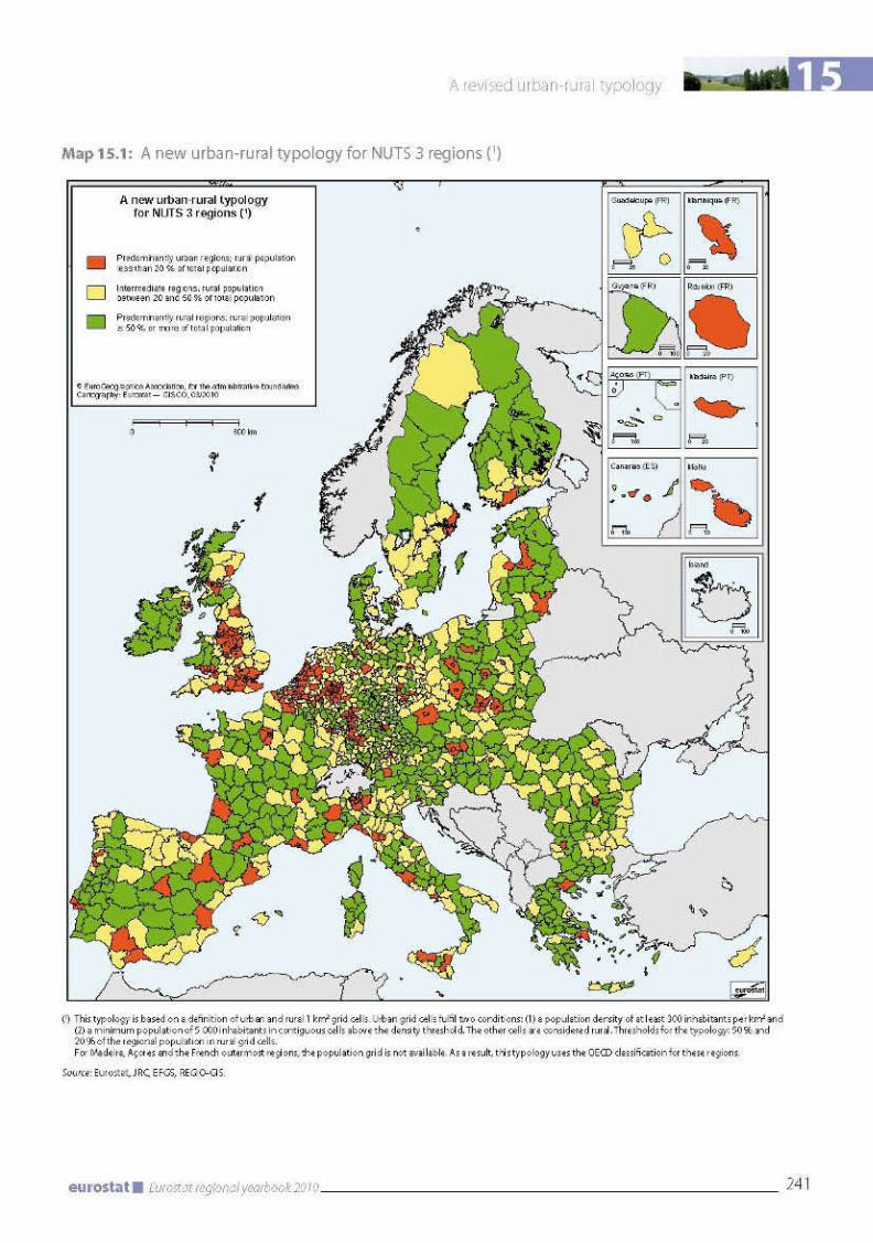
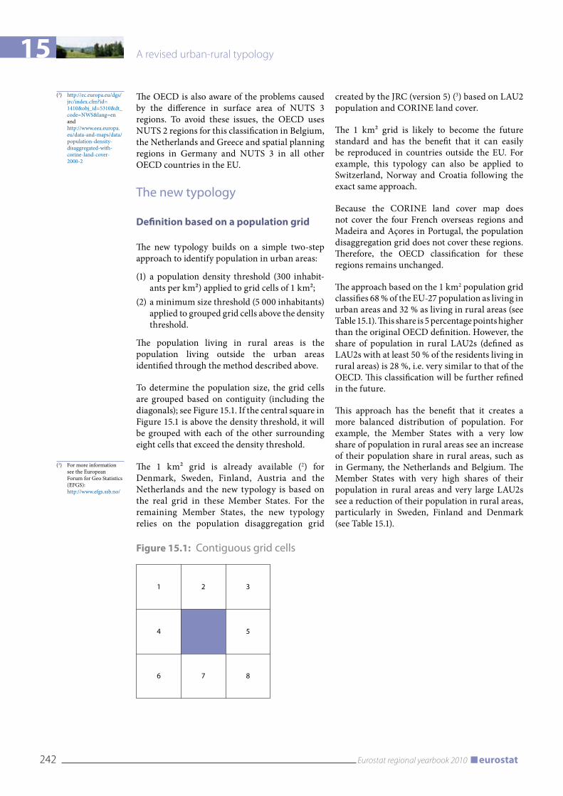
15 A revised urban-rural typology
242 Eurostat regional yearbook 2010 eurostat
The OECD is also aware of the problems caused by the difference in surface area of NUTS 3 regions. To avoid these issues, the OECD uses NUTS 2 regions for this classification in Belgium, the Netherlands and Greece and spatial planning regions in Germany and NUTS 3 in all other OECD countries in the EU.
The new typology
Definition based on a population grid
The new typology builds on a simple two-step approach to identify population in urban areas:
(1) a population density threshold (300 inhabit-ants per km²) applied to grid cells of 1 km²;
(2) a minimum size threshold (5 000 inhabitants) applied to grouped grid cells above the density threshold.
The population living in rural areas is the population living outside the urban areas identified through the method described above.
To determine the population size, the grid cells are grouped based on contiguity (including the diagonals); see Figure 15.1. If the central square in Figure 15.1 is above the density threshold, it will be grouped with each of the other surrounding eight cells that exceed the density threshold.
The 1 km² grid is already available (2) for Denmark, Sweden, Finland, Austria and the Netherlands and the new typology is based on the real grid in these Member States. For the remaining Member States, the new typology relies on the population disaggregation grid
created by the JRC (version 5) (3) based on LAU2 population and CORINE land cover.
The 1 km² grid is likely to become the future standard and has the benefit that it can easily be reproduced in countries outside the EU. For example, this typology can also be applied to Switzerland, Norway and Croatia following the exact same approach.
Because the CORINE land cover map does not cover the four French overseas regions and Madeira and Açores in Portugal, the population disaggregation grid does not cover these regions. Therefore, the OECD classification for these regions remains unchanged.
The approach based on the 1 km2 population grid classifies 68 % of the EU-27 population as living in urban areas and 32 % as living in rural areas (see Table 15.1). This share is 5 percentage points higher than the original OECD definition. However, the share of population in rural LAU2s (defined as LAU2s with at least 50 % of the residents living in rural areas) is 28 %, i.e. very similar to that of the OECD. This classification will be further refined in the future.
This approach has the benefit that it creates a more balanced distribution of population. For example, the Member States with a very low share of population in rural areas see an increase of their population share in rural areas, such as in Germany, the Netherlands and Belgium. The Member States with very high shares of their population in rural areas and very large LAU2s see a reduction of their population in rural areas, particularly in Sweden, Finland and Denmark (see Table 15.1).
(2) For more information see the European Forum for Geo Statistics (EFGS): http://www.efgs.ssb.no/
Figure 15.1: Contiguous grid cells
1 2 3
4 5
6 7 8
(3) http://ec.europa.eu/dgs/ jrc/index.cfm?id= 1410&obj_id=5310&dt_code=NWS&lang=en and http://www.eea.europa.eu/data-and-maps/data/population-density-disaggregated-with-corine-land-cover-2000-2
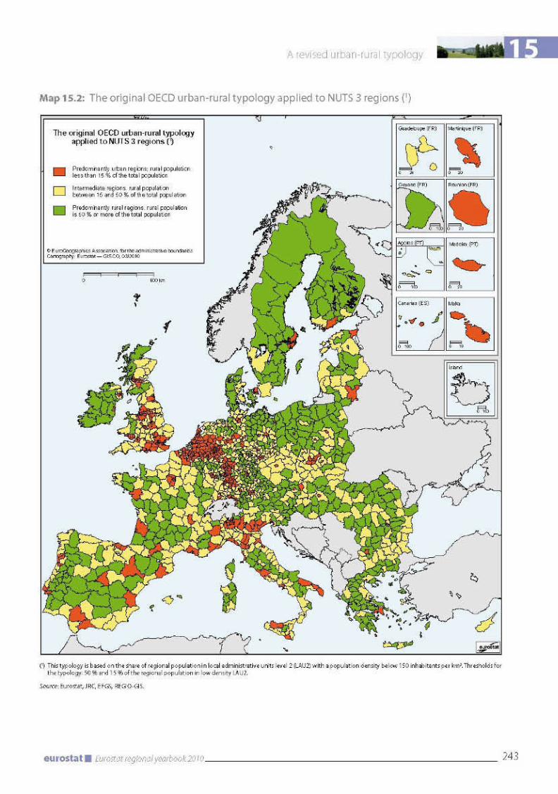
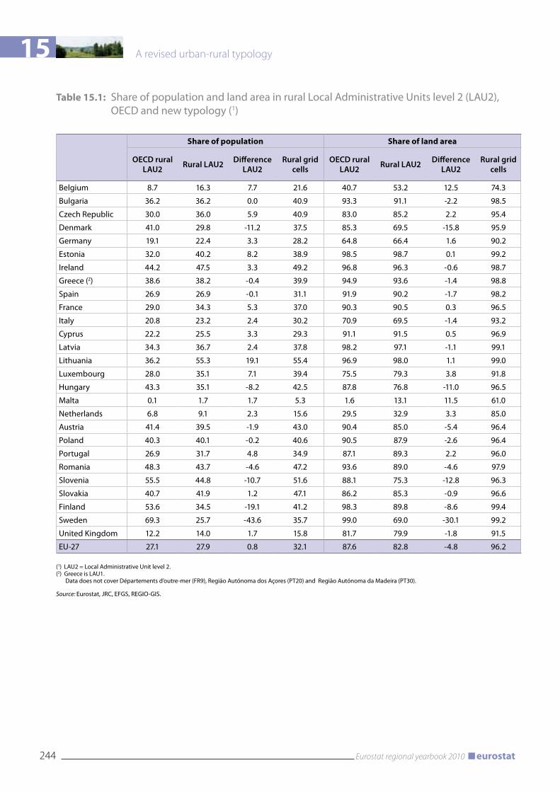
15 A revised urban-rural typology
244 Eurostat regional yearbook 2010 eurostat
Table 15.1: Share of population and land area in rural Local Administrative Units level 2 (LAU2), OECD and new typology (1)
Share of population Share of land area
OECD rural LAU2 Rural LAU2 Difference
LAU2Rural grid
cellsOECD rural
LAU2 Rural LAU2 Difference LAU2
Rural grid cells
Belgium 8.7 16.3 7.7 21.6 40.7 53.2 12.5 74.3
Bulgaria 36.2 36.2 0.0 40.9 93.3 91.1 -2.2 98.5
Czech Republic 30.0 36.0 5.9 40.9 83.0 85.2 2.2 95.4
Denmark 41.0 29.8 -11.2 37.5 85.3 69.5 -15.8 95.9
Germany 19.1 22.4 3.3 28.2 64.8 66.4 1.6 90.2
Estonia 32.0 40.2 8.2 38.9 98.5 98.7 0.1 99.2
Ireland 44.2 47.5 3.3 49.2 96.8 96.3 -0.6 98.7
Greece (2) 38.6 38.2 -0.4 39.9 94.9 93.6 -1.4 98.8
Spain 26.9 26.9 -0.1 31.1 91.9 90.2 -1.7 98.2
France 29.0 34.3 5.3 37.0 90.3 90.5 0.3 96.5
Italy 20.8 23.2 2.4 30.2 70.9 69.5 -1.4 93.2
Cyprus 22.2 25.5 3.3 29.3 91.1 91.5 0.5 96.9
Latvia 34.3 36.7 2.4 37.8 98.2 97.1 -1.1 99.1
Lithuania 36.2 55.3 19.1 55.4 96.9 98.0 1.1 99.0
Luxembourg 28.0 35.1 7.1 39.4 75.5 79.3 3.8 91.8
Hungary 43.3 35.1 -8.2 42.5 87.8 76.8 -11.0 96.5
Malta 0.1 1.7 1.7 5.3 1.6 13.1 11.5 61.0
Netherlands 6.8 9.1 2.3 15.6 29.5 32.9 3.3 85.0
Austria 41.4 39.5 -1.9 43.0 90.4 85.0 -5.4 96.4
Poland 40.3 40.1 -0.2 40.6 90.5 87.9 -2.6 96.4
Portugal 26.9 31.7 4.8 34.9 87.1 89.3 2.2 96.0
Romania 48.3 43.7 -4.6 47.2 93.6 89.0 -4.6 97.9
Slovenia 55.5 44.8 -10.7 51.6 88.1 75.3 -12.8 96.3
Slovakia 40.7 41.9 1.2 47.1 86.2 85.3 -0.9 96.6
Finland 53.6 34.5 -19.1 41.2 98.3 89.8 -8.6 99.4
Sweden 69.3 25.7 -43.6 35.7 99.0 69.0 -30.1 99.2
United Kingdom 12.2 14.0 1.7 15.8 81.7 79.9 -1.8 91.5
EU-27 27.1 27.9 0.8 32.1 87.6 82.8 -4.8 96.2
(1) LAU2 = Local Administrative Unit level 2.(2) Greece is LAU1.
Data does not cover Départements d’outre-mer (FR9), Região Autónoma dos Açores (PT20) and Região Autónoma da Madeira (PT30).
Source: Eurostat, JRC, EFGS, REGIO-GIS.
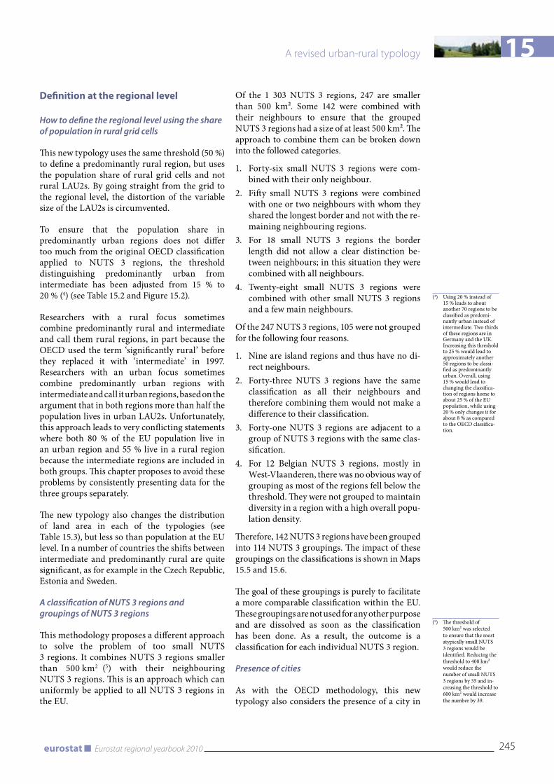
15
245Eurostat regional yearbook 2010eurostat
A revised urban-rural typology
Definition at the regional level
How to define the regional level using the share of population in rural grid cells
This new typology uses the same threshold (50 %) to define a predominantly rural region, but uses the population share of rural grid cells and not rural LAU2s. By going straight from the grid to the regional level, the distortion of the variable size of the LAU2s is circumvented.
To ensure that the population share in predominantly urban regions does not differ too much from the original OECD classification applied to NUTS 3 regions, the threshold distinguishing predominantly urban from intermediate has been adjusted from 15 % to 20 % (4) (see Table 15.2 and Figure 15.2).
Researchers with a rural focus sometimes combine predominantly rural and intermediate and call them rural regions, in part because the OECD used the term ‘significantly rural’ before they replaced it with ‘intermediate’ in 1997. Researchers with an urban focus sometimes combine predominantly urban regions with intermediate and call it urban regions, based on the argument that in both regions more than half the population lives in urban LAU2s. Unfortunately, this approach leads to very conflicting statements where both 80 % of the EU population live in an urban region and 55 % live in a rural region because the intermediate regions are included in both groups. This chapter proposes to avoid these problems by consistently presenting data for the three groups separately.
The new typology also changes the distribution of land area in each of the typologies (see Table 15.3), but less so than population at the EU level. In a number of countries the shifts between intermediate and predominantly rural are quite significant, as for example in the Czech Republic, Estonia and Sweden.
A classification of NUTS 3 regions and groupings of NUTS 3 regions
This methodology proposes a different approach to solve the problem of too small NUTS 3 regions. It combines NUTS 3 regions smaller than 500 km2 (5) with their neighbouring NUTS 3 regions. This is an approach which can uniformly be applied to all NUTS 3 regions in the EU.
Of the 1 303 NUTS 3 regions, 247 are smaller than 500 km². Some 142 were combined with their neighbours to ensure that the grouped NUTS 3 regions had a size of at least 500 km². The approach to combine them can be broken down into the followed categories.
1. Forty-six small NUTS 3 regions were com-bined with their only neighbour.
2. Fifty small NUTS 3 regions were combined with one or two neighbours with whom they shared the longest border and not with the re-maining neighbouring regions.
3. For 18 small NUTS 3 regions the border length did not allow a clear distinction be-tween neighbours; in this situation they were combined with all neighbours.
4. Twenty-eight small NUTS 3 regions were combined with other small NUTS 3 regions and a few main neighbours.
Of the 247 NUTS 3 regions, 105 were not grouped for the following four reasons.
1. Nine are island regions and thus have no di-rect neighbours.
2. Forty-three NUTS 3 regions have the same classification as all their neighbours and therefore combining them would not make a difference to their classification.
3. Forty-one NUTS 3 regions are adjacent to a group of NUTS 3 regions with the same clas-sification.
4. For 12 Belgian NUTS 3 regions, mostly in West-Vlaanderen, there was no obvious way of grouping as most of the regions fell below the threshold. They were not grouped to maintain diversity in a region with a high overall popu-lation density.
Therefore, 142 NUTS 3 regions have been grouped into 114 NUTS 3 groupings. The impact of these groupings on the classifications is shown in Maps 15.5 and 15.6.
The goal of these groupings is purely to facilitate a more comparable classification within the EU. These groupings are not used for any other purpose and are dissolved as soon as the classification has been done. As a result, the outcome is a classification for each individual NUTS 3 region.
Presence of cities
As with the OECD methodology, this new typology also considers the presence of a city in
(5) The threshold of 500 km² was selected to ensure that the most atypically small NUTS 3 regions would be identified. Reducing the threshold to 400 km² would reduce the number of small NUTS 3 regions by 35 and in-creasing the threshold to 600 km² would increase the number by 39.
(4) Using 20 % instead of 15 % leads to about another 70 regions to be classified as predomi-nantly urban instead of intermediate. Two thirds of these regions are in Germany and the UK. Increasing this threshold to 25 % would lead to approximately another 50 regions to be classi-fied as predominantly urban. Overall, using 15 % would lead to changing the classifica-tion of regions home to about 25 % of the EU population, while using 20 % only changes it for about 8 % as compared to the OECD classifica-tion.
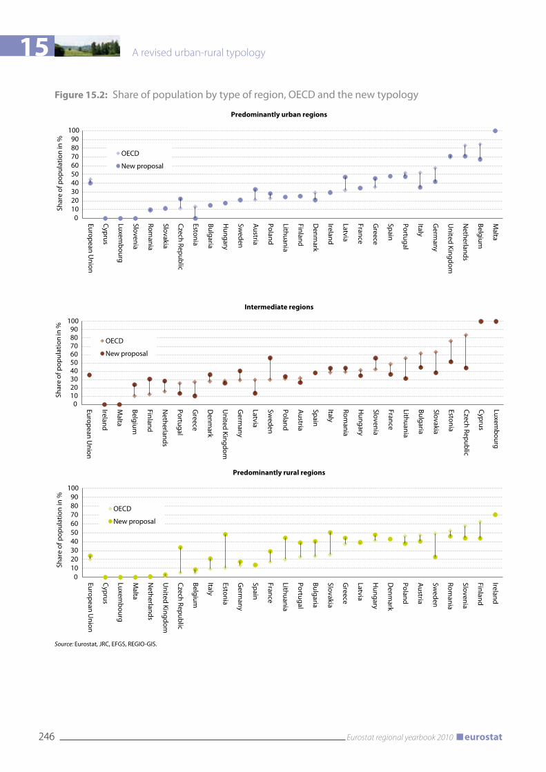
15 A revised urban-rural typology
246 Eurostat regional yearbook 2010 eurostat
Figure 15.2: Share of population by type of region, OECD and the new typology
0102030405060708090
100
European Union
Cyprus
Luxembourg
Slovenia
Romania
Slovakia
Czech Republic
Estonia
Bulgaria
Hungary
Sweden
Austria
Poland
Lithuania
Finland
Denm
ark
Ireland
Latvia
France
Greece
Spain
Portugal
Italy
Germ
any
United Kingdom
Netherlands
Belgium
Malta
Shar
e of
pop
ulat
ion
in %
Predominantly urban regions
OECD
New proposal
0102030405060708090
100
European Union
Cyprus
Luxembourg
Malta
Netherlands
United Kingdom
Czech Republic
Belgium
Italy
Estonia
Germ
any
Spain
France
Lithuania
Portugal
Bulgaria
Slovakia
Greece
Latvia
Hungary
Denm
ark
Poland
Austria
Sweden
Romania
Slovenia
Finland
IrelandSh
are
of p
opul
atio
n in
%
Predominantly rural regions
OECD
New proposal
0102030405060708090
100
European Union
Ireland
Malta
Belgium
Finland
Netherlands
Portugal
Greece
Denm
ark
United Kingdom
Germ
any
Latvia
Sweden
Poland
Austria
Spain
Italy
Romania
Hungary
Slovenia
France
Lithuania
Bulgaria
Slovakia
Estonia
Czech Republic
Cyprus
Luxembourg
Shar
e of
pop
ulat
ion
in %
Intermediate regions
OECD
New proposal
Source: Eurostat, JRC, EFGS, REGIO-GIS.
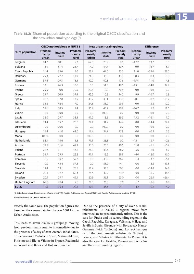
15
247Eurostat regional yearbook 2010eurostat
A revised urban-rural typology
Table 15.2: Share of population according to the original OECD classification and the new urban-rural typology (1)
% of population
OECD methodology at NUTS 3 New urban-rural typology DifferencePredomi-
nantly urban
Interme-diate
Predomi-nantly rural
Predomi-nantly urban
Interme-diate
Predomi-nantly rural
Predomi-nantly urban
Interme-diate
Predomi-nantly rural
Belgium 84.7 10.1 5.2 67.5 23.9 8.6 –17.2 13.7 3.5
Bulgaria 14.9 61.4 23.7 14.9 44.7 40.4 0.0 –16.7 16.7
Czech Republic 11.4 83.6 5.0 22.4 44.0 33.6 11.0 –39.6 28.6
Denmark 29.3 27.7 43.0 21.0 36.0 43.0 –8.3 8.3 0.0
Germany 57.4 29.3 13.3 42.0 40.3 17.6 –15.4 11.0 4.3
Estonia 13.1 76.3 10.6 0.0 51.5 48.5 –13.1 –24.8 37.9
Ireland 29.5 0.0 70.5 29.5 0.0 70.5 0.0 0.0 0.0
Greece 35.7 26.9 37.4 45.5 10.3 44.2 9.9 –16.7 6.8
Spain 48.2 37.8 13.9 48.2 38.1 13.8 –0.1 0.2 –0.2
France 34.5 48.4 17.0 34.6 36.2 29.3 0.0 –12.3 12.2
Italy 52.1 38.5 9.4 35.4 43.7 20.9 –16.7 5.2 11.5
Cyprus 0.0 100.0 0.0 0.0 100.0 0.0 0.0 0.0 0.0
Latvia 32.0 29.7 38.3 47.2 13.5 39.3 15.2 –16.1 1.0
Lithuania 24.4 55.7 20.0 24.4 31.2 44.4 0.0 –24.4 24.4
Luxembourg 0.0 100.0 0.0 0.0 100.0 0.0 0.0 0.0 0.0
Hungary 17.4 41.0 41.6 17.4 34.7 47.9 0.0 –6.3 6.3
Malta 100.0 0.0 0.0 100.0 0.0 0.0 0.0 0.0 0.0
Netherlands 83.1 15.6 1.3 71.1 28.3 0.7 –12.1 12.7 –0.6
Austria 21.2 31.6 47.1 33.0 26.5 40.5 11.8 –5.1 –6.7
Poland 22.7 31.1 46.2 28.3 33.6 38.0 5.6 2.6 –8.2
Portugal 51.7 25.5 22.8 47.7 13.5 38.8 –4.0 –12.0 16.0
Romania 8.5 39.2 52.3 9.9 43.9 46.2 1.4 4.7 –6.1
Slovenia 0.0 42.4 57.6 0.0 55.9 44.1 0.0 13.5 –13.5
Slovakia 11.4 63.1 25.5 11.4 38.3 50.3 0.0 –24.8 24.8
Finland 25.4 12.2 62.4 25.4 30.7 43.9 0.0 18.5 –18.5
Sweden 20.9 29.7 49.4 20.9 56.1 23.0 0.0 26.4 –26.4
United Kingdom 69.6 28.4 2.0 71.3 25.8 2.9 1.7 –2.6 0.9
EU-27 44.5 35.4 20.1 40.3 35.6 24.1 -4.2 0.2 4.0
(1) Data do not cover départements d’outre-mer (FR9), Região Autónoma dos Açores (PT20) and Região Autónoma da Madeira (PT30).
Source: Eurostat, JRC, EFGS, REGIO-GIS.
exactly the same way. The population figures are based on the census data for the year 2001 for the Urban Audit cities.
This leads to seven NUTS 3 groupings moving from predominantly rural to intermediate due to the presence of a city of over 200 000 inhabitants. This concerns: Córdoba in Spain, Maine-et-Loire, Finistère and Ille-et-Vilaine in France, Radomski in Poland, and Bihor and Dolj in Romania.
Due to the presence of a city of over 500 000 inhabitants, 16 NUTS 3 regions move from intermediate to predominantly urban. This is the case for: Praha and its surrounding region in the Czech Republic, Zaragoza, València, Málaga and Sevilla in Spain, Gironde (with Bordeaux), Haute-Garonne (with Toulouse) and Loire-Atlantique (with the communauté urbaine de Nantes) in France, and Vilnius in Lithuania. In Poland it is also the case for Kraków, Poznań and Wrocław and their surrounding region.
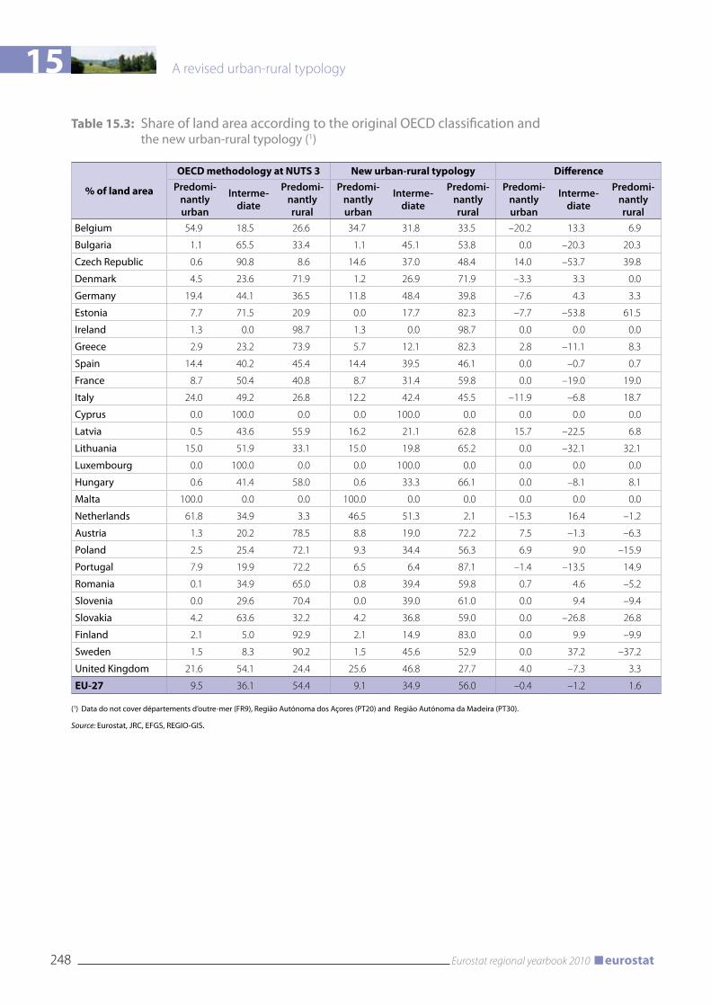
15 A revised urban-rural typology
248 Eurostat regional yearbook 2010 eurostat
Table 15.3: Share of land area according to the original OECD classification and the new urban-rural typology (1)
% of land area
OECD methodology at NUTS 3 New urban-rural typology DifferencePredomi-
nantly urban
Interme-diate
Predomi-nantly rural
Predomi-nantly urban
Interme-diate
Predomi-nantly rural
Predomi-nantly urban
Interme-diate
Predomi-nantly rural
Belgium 54.9 18.5 26.6 34.7 31.8 33.5 –20.2 13.3 6.9
Bulgaria 1.1 65.5 33.4 1.1 45.1 53.8 0.0 –20.3 20.3
Czech Republic 0.6 90.8 8.6 14.6 37.0 48.4 14.0 –53.7 39.8
Denmark 4.5 23.6 71.9 1.2 26.9 71.9 –3.3 3.3 0.0
Germany 19.4 44.1 36.5 11.8 48.4 39.8 –7.6 4.3 3.3
Estonia 7.7 71.5 20.9 0.0 17.7 82.3 –7.7 –53.8 61.5
Ireland 1.3 0.0 98.7 1.3 0.0 98.7 0.0 0.0 0.0
Greece 2.9 23.2 73.9 5.7 12.1 82.3 2.8 –11.1 8.3
Spain 14.4 40.2 45.4 14.4 39.5 46.1 0.0 –0.7 0.7
France 8.7 50.4 40.8 8.7 31.4 59.8 0.0 –19.0 19.0
Italy 24.0 49.2 26.8 12.2 42.4 45.5 –11.9 –6.8 18.7
Cyprus 0.0 100.0 0.0 0.0 100.0 0.0 0.0 0.0 0.0
Latvia 0.5 43.6 55.9 16.2 21.1 62.8 15.7 –22.5 6.8
Lithuania 15.0 51.9 33.1 15.0 19.8 65.2 0.0 –32.1 32.1
Luxembourg 0.0 100.0 0.0 0.0 100.0 0.0 0.0 0.0 0.0
Hungary 0.6 41.4 58.0 0.6 33.3 66.1 0.0 –8.1 8.1
Malta 100.0 0.0 0.0 100.0 0.0 0.0 0.0 0.0 0.0
Netherlands 61.8 34.9 3.3 46.5 51.3 2.1 –15.3 16.4 –1.2
Austria 1.3 20.2 78.5 8.8 19.0 72.2 7.5 –1.3 –6.3
Poland 2.5 25.4 72.1 9.3 34.4 56.3 6.9 9.0 –15.9
Portugal 7.9 19.9 72.2 6.5 6.4 87.1 –1.4 –13.5 14.9
Romania 0.1 34.9 65.0 0.8 39.4 59.8 0.7 4.6 –5.2
Slovenia 0.0 29.6 70.4 0.0 39.0 61.0 0.0 9.4 –9.4
Slovakia 4.2 63.6 32.2 4.2 36.8 59.0 0.0 –26.8 26.8
Finland 2.1 5.0 92.9 2.1 14.9 83.0 0.0 9.9 –9.9
Sweden 1.5 8.3 90.2 1.5 45.6 52.9 0.0 37.2 –37.2
United Kingdom 21.6 54.1 24.4 25.6 46.8 27.7 4.0 –7.3 3.3
EU-27 9.5 36.1 54.4 9.1 34.9 56.0 –0.4 –1.2 1.6
(1) Data do not cover départements d’outre-mer (FR9), Região Autónoma dos Açores (PT20) and Região Autónoma da Madeira (PT30).
Source: Eurostat, JRC, EFGS, REGIO-GIS.
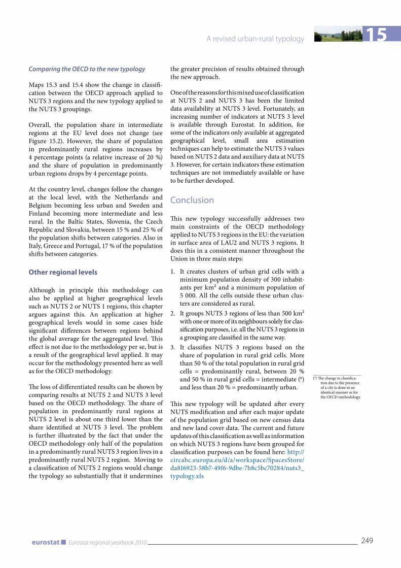
15
249Eurostat regional yearbook 2010eurostat
A revised urban-rural typology
(6) The change in classifica-tion due to the presence of a city is done in an identical manner as for the OECD methodology.
Comparing the OECD to the new typology
Maps 15.3 and 15.4 show the change in classifi-cation between the OECD approach applied to NUTS 3 regions and the new typology applied to the NUTS 3 groupings.
Overall, the population share in intermediate regions at the EU level does not change (see Figure 15.2). However, the share of population in predominantly rural regions increases by 4 percentage points (a relative increase of 20 %) and the share of population in predominantly urban regions drops by 4 percentage points.
At the country level, changes follow the changes at the local level, with the Netherlands and Belgium becoming less urban and Sweden and Finland becoming more intermediate and less rural. In the Baltic States, Slovenia, the Czech Republic and Slovakia, between 15 % and 25 % of the population shifts between categories. Also in Italy, Greece and Portugal, 17 % of the population shifts between categories.
Other regional levels
Although in principle this methodology can also be applied at higher geographical levels such as NUTS 2 or NUTS 1 regions, this chapter argues against this. An application at higher geographical levels would in some cases hide significant differences between regions behind the global average for the aggregated level. This effect is not due to the methodology per se, but is a result of the geographical level applied. It may occur for the methodology presented here as well as for the OECD methodology.
The loss of differentiated results can be shown by comparing results at NUTS 2 and NUTS 3 level based on the OECD methodology. The share of population in predominantly rural regions at NUTS 2 level is about one third lower than the share identified at NUTS 3 level. The problem is further illustrated by the fact that under the OECD methodology only half of the population in a predominantly rural NUTS 3 region lives in a predominantly rural NUTS 2 region. Moving to a classification of NUTS 2 regions would change the typology so substantially that it undermines
the greater precision of results obtained through the new approach.
One of the reasons for this mixed use of classification at NUTS 2 and NUTS 3 has been the limited data availability at NUTS 3 level. Fortunately, an increasing number of indicators at NUTS 3 level is available through Eurostat. In addition, for some of the indicators only available at aggregated geographical level, small area estimation techniques can help to estimate the NUTS 3 values based on NUTS 2 data and auxiliary data at NUTS 3. However, for certain indicators these estimation techniques are not immediately available or have to be further developed.
Conclusion
This new typology successfully addresses two main constraints of the OECD methodology applied to NUTS 3 regions in the EU: the variation in surface area of LAU2 and NUTS 3 regions. It does this in a consistent manner throughout the Union in three main steps:
1. It creates clusters of urban grid cells with a minimum population density of 300 inhabit-ants per km² and a minimum population of 5 000. All the cells outside these urban clus-ters are considered as rural.
2. It groups NUTS 3 regions of less than 500 km² with one or more of its neighbours solely for clas-sification purposes, i.e. all the NUTS 3 regions in a grouping are classified in the same way.
3. It classifies NUTS 3 regions based on the share of population in rural grid cells. More than 50 % of the total population in rural grid cells = predominantly rural, between 20 % and 50 % in rural grid cells = intermediate (6) and less than 20 % = predominantly urban.
This new typology will be updated after every NUTS modification and after each major update of the population grid based on new census data and new land cover data. The current and future updates of this classification as well as information on which NUTS 3 regions have been grouped for classification purposes can be found here: http://circabc.europa.eu/d/a/workspace/SpacesStore/da816923-58b7-49f6-9dbe-7b8c5bc70284/nuts3_typology.xls
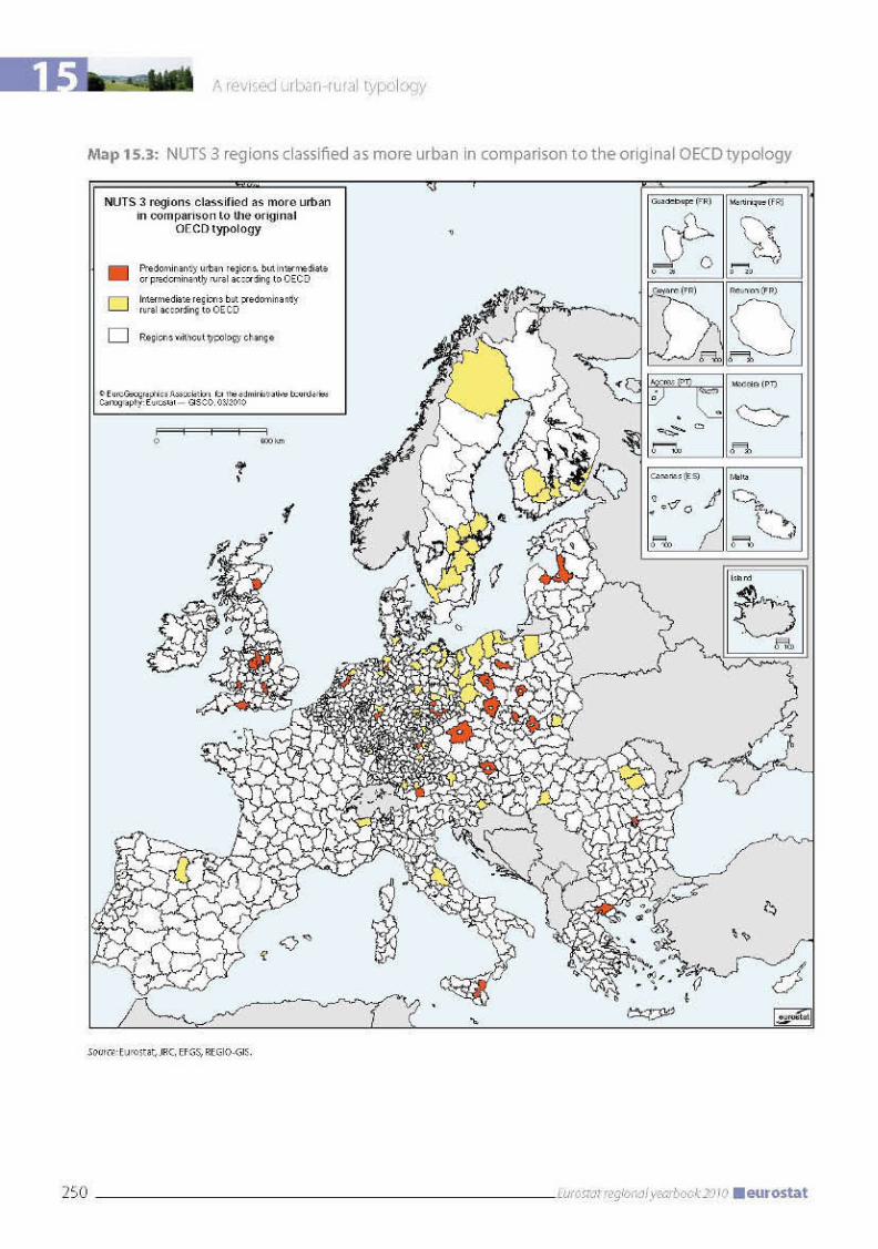
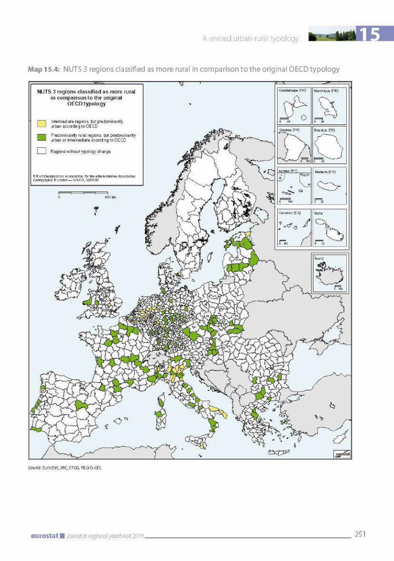
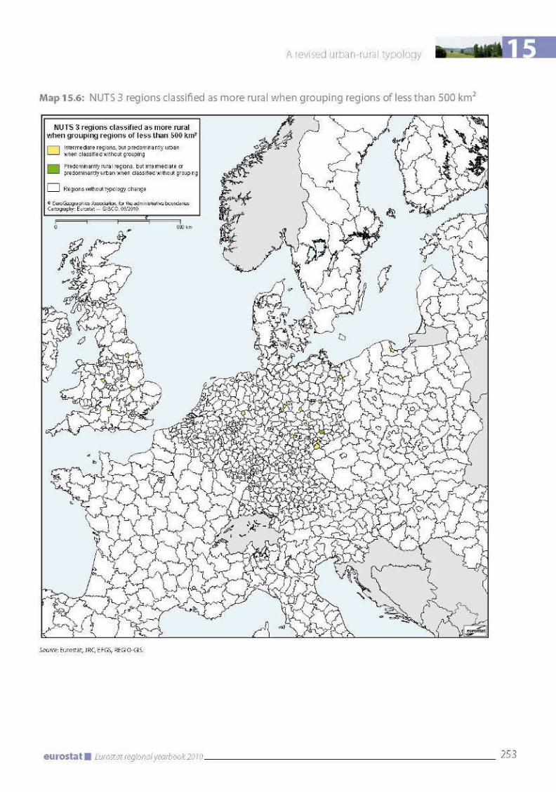

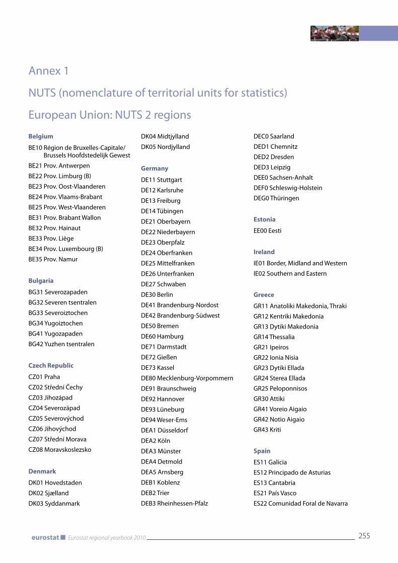
255Eurostat regional yearbook 2010eurostat
Annex 1
NUTS (nomenclature of territorial units for statistics)
European Union: NUTS 2 regions
Belgium
BE10 Région de Bruxelles-Capitale/Brussels Hoofdstedelijk Gewest
BE21 Prov. Antwerpen
BE22 Prov. Limburg (B)
BE23 Prov. Oost-vlaanderen
BE24 Prov. vlaams-Brabant
BE25 Prov. West-vlaanderen
BE31 Prov. Brabant Wallon
BE32 Prov. Hainaut
BE33 Prov. Liège
BE34 Prov. Luxembourg (B)
BE35 Prov. Namur
Bulgaria
BG31 Severozapaden
BG32 Severen tsentralen
BG33 Severoiztochen
BG34 yugoiztochen
BG41 yugozapaden
BG42 yuzhen tsentralen
Czech Republic
CZ01 Praha
CZ02 Střední Čechy
CZ03 Jihozápad
CZ04 Severozápad
CZ05 Severovýchod
CZ06 Jihovýchod
CZ07 Střední Morava
CZ08 Moravskoslezsko
Denmark
DK01 Hovedstaden
DK02 Sjælland
DK03 Syddanmark
DK04 Midtjylland
DK05 Nordjylland
Germany
DE11 Stuttgart
DE12 Karlsruhe
DE13 Freiburg
DE14 Tübingen
DE21 Oberbayern
DE22 Niederbayern
DE23 Oberpfalz
DE24 Oberfranken
DE25 Mittelfranken
DE26 Unterfranken
DE27 Schwaben
DE30 Berlin
DE41 Brandenburg-Nordost
DE42 Brandenburg-Südwest
DE50 Bremen
DE60 Hamburg
DE71 Darmstadt
DE72 Gießen
DE73 Kassel
DE80 Mecklenburg-vorpommern
DE91 Braunschweig
DE92 Hannover
DE93 Lüneburg
DE94 Weser-Ems
DEA1 Düsseldorf
DEA2 Köln
DEA3 Münster
DEA4 Detmold
DEA5 Arnsberg
DEB1 Koblenz
DEB2 Trier
DEB3 Rheinhessen-Pfalz
DEC0 Saarland
DED1 Chemnitz
DED2 Dresden
DED3 Leipzig
DEE0 Sachsen-Anhalt
DEF0 Schleswig-Holstein
DEG0 Thüringen
Estonia
EE00 Eesti
Ireland
IE01 Border, Midland and Western
IE02 Southern and Eastern
Greece
GR11 Anatoliki Makedonia, Thraki
GR12 Kentriki Makedonia
GR13 Dytiki Makedonia
GR14 Thessalia
GR21 Ipeiros
GR22 Ionia Nisia
GR23 Dytiki Ellada
GR24 Sterea Ellada
GR25 Peloponnisos
GR30 Attiki
GR41 voreio Aigaio
GR42 Notio Aigaio
GR43 Kriti
Spain
ES11 Galicia
ES12 Principado de Asturias
ES13 Cantabria
ES21 País vasco
ES22 Comunidad Foral de Navarra

256 Eurostat regional yearbook 2010 eurostat
ES23 La Rioja
ES24 Aragón
ES30 Comunidad de Madrid
ES41 Castilla y León
ES42 Castilla-La Mancha
ES43 Extremadura
ES51 Cataluña
ES52 Comunidad valenciana
ES53 Illes Balears
ES61 Andalucía
ES62 Región de Murcia
ES63 Ciudad Autónoma de Ceuta
ES64 Ciudad Autónoma de Melilla
ES70 Canarias
France
FR10 Île de France
FR21 Champagne-Ardenne
FR22 Picardie
FR23 Haute-Normandie
FR24 Centre
FR25 Basse-Normandie
FR26 Bourgogne
FR30 Nord - Pas-de-Calais
FR41 Lorraine
FR42 Alsace
FR43 Franche-Comté
FR51 Pays de la Loire
FR52 Bretagne
FR53 Poitou-Charentes
FR61 Aquitaine
FR62 Midi-Pyrénées
FR63 Limousin
FR71 Rhône-Alpes
FR72 Auvergne
FR81 Languedoc-Roussillon
FR82 Provence-Alpes-Côte d’Azur
FR83 Corse
FR91 Guadeloupe
FR92 Martinique
FR93 Guyane
FR94 Réunion
Italy
ITC1 Piemonte
ITC2 valle d’Aosta/vallée d’Aoste
ITC3 Liguria
ITC4 Lombardia
ITD1 Provincia Autonoma Bolzano/Bozen
ITD2 Provincia Autonoma Trento
ITD3 veneto
ITD4 Friuli-venezia Giulia
ITD5 Emilia-Romagna
ITE1 Toscana
ITE2 Umbria
ITE3 Marche
ITE4 Lazio
ITF1 Abruzzo
ITF2 Molise
ITF3 Campania
ITF4 Puglia
ITF5 Basilicata
ITF6 Calabria
ITG1 Sicilia
ITG2 Sardegna
Cyprus
Cy00 Kýpros/Kıbrıs
Latvia
Lv00 Latvija
Lithuania
LT00 Lietuva
Luxembourg
LU00 Luxembourg (Grand-Duché)
Hungary
HU10 Közép-Magyarország
HU21 Közép-Dunántúl
HU22 Nyugat-Dunántúl
HU23 Dél-Dunántúl
HU31 Észak-Magyarország
HU32 Észak-Alföld
HU33 Dél-Alföld
Malta
MT00 Malta
Netherlands
NL11 Groningen
NL12 Friesland (NL)
NL13 Drenthe
NL21 Overijssel
NL22 Gelderland
NL23 Flevoland
NL31 Utrecht
NL32 Noord-Holland
NL33 Zuid-Holland
NL34 Zeeland
NL41 Noord-Brabant
NL42 Limburg (NL)
Austria
AT11 Burgenland (A)
AT12 Niederösterreich
AT13 Wien
AT21 Kärnten
AT22 Steiermark
AT31 Oberösterreich
AT32 Salzburg
AT33 Tirol
AT34 vorarlberg
Poland
PL11 Łódzkie
PL12 Mazowieckie
PL21 Małopolskie
PL22 Śląskie
PL31 Lubelskie
PL32 Podkarpackie
PL33 Świętokrzyskie
PL34 Podlaskie
PL41 Wielkopolskie
PL42 Zachodniopomorskie
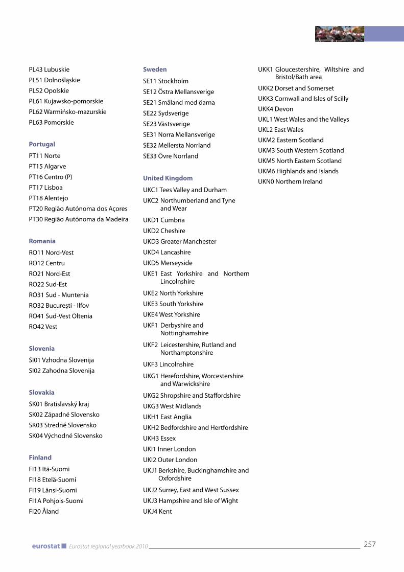
257Eurostat regional yearbook 2010eurostat
PL43 Lubuskie
PL51 Dolnośląskie
PL52 Opolskie
PL61 Kujawsko-pomorskie
PL62 Warmińsko-mazurskie
PL63 Pomorskie
Portugal
PT11 Norte
PT15 Algarve
PT16 Centro (P)
PT17 Lisboa
PT18 Alentejo
PT20 Região Autónoma dos Açores
PT30 Região Autónoma da Madeira
Romania
RO11 Nord-vest
RO12 Centru
RO21 Nord-Est
RO22 Sud-Est
RO31 Sud - Muntenia
RO32 Bucureşti - Ilfov
RO41 Sud-vest Oltenia
RO42 vest
Slovenia
SI01 vzhodna Slovenija
SI02 Zahodna Slovenija
Slovakia
SK01 Bratislavský kraj
SK02 Západné Slovensko
SK03 Stredné Slovensko
SK04 východné Slovensko
Finland
FI13 Itä-Suomi
FI18 Etelä-Suomi
FI19 Länsi-Suomi
FI1A Pohjois-Suomi
FI20 Åland
Sweden
SE11 Stockholm
SE12 Östra Mellansverige
SE21 Småland med öarna
SE22 Sydsverige
SE23 västsverige
SE31 Norra Mellansverige
SE32 Mellersta Norrland
SE33 Övre Norrland
United Kingdom
UKC1 Tees valley and Durham
UKC2 Northumberland and Tyne and Wear
UKD1 Cumbria
UKD2 Cheshire
UKD3 Greater Manchester
UKD4 Lancashire
UKD5 Merseyside
UKE1 East yorkshire and Northern Lincolnshire
UKE2 North yorkshire
UKE3 South yorkshire
UKE4 West yorkshire
UKF1 Derbyshire and Nottinghamshire
UKF2 Leicestershire, Rutland and Northamptonshire
UKF3 Lincolnshire
UKG1 Herefordshire, Worcestershire and Warwickshire
UKG2 Shropshire and Staffordshire
UKG3 West Midlands
UKH1 East Anglia
UKH2 Bedfordshire and Hertfordshire
UKH3 Essex
UKI1 Inner London
UKI2 Outer London
UKJ1 Berkshire, Buckinghamshire and Oxfordshire
UKJ2 Surrey, East and West Sussex
UKJ3 Hampshire and Isle of Wight
UKJ4 Kent
UKK1 Gloucestershire, Wiltshire and Bristol/Bath area
UKK2 Dorset and Somerset
UKK3 Cornwall and Isles of Scilly
UKK4 Devon
UKL1 West Wales and the valleys
UKL2 East Wales
UKM2 Eastern Scotland
UKM3 South Western Scotland
UKM5 North Eastern Scotland
UKM6 Highlands and Islands
UKN0 Northern Ireland
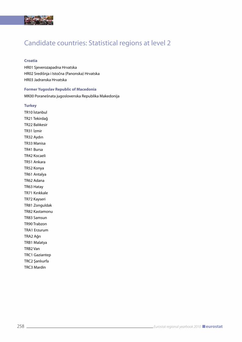
258 Eurostat regional yearbook 2010 eurostat
Candidate countries: Statistical regions at level 2
Croatia
HR01 Sjeverozapadna Hrvatska
HR02 Središnja i Istočna (Panonska) Hrvatska
HR03 Jadranska Hrvatska
Former Yugoslav Republic of Macedonia
MK00 Poranešnata jugoslovenska Republika Makedonija
Turkey
TR10 İstanbul
TR21 Tekirdağ
TR22 Balıkesir
TR31 İzmir
TR32 Aydın
TR33 Manisa
TR41 Bursa
TR42 Kocaeli
TR51 Ankara
TR52 Konya
TR61 Antalya
TR62 Adana
TR63 Hatay
TR71 Kırıkkale
TR72 Kayseri
TR81 Zonguldak
TR82 Kastamonu
TR83 Samsun
TR90 Trabzon
TRA1 Erzurum
TRA2 Ağrı
TRB1 Malatya
TRB2 van
TRC1 Gaziantep
TRC2 Şanlıurfa
TRC3 Mardin
259Eurostat regional yearbook 2010eurostat
EFTA countries: Statistical regions at level 2
Iceland
IS00 Ísland
Liechtenstein
LI00 Liechtenstein
Norway
NO01 Oslo og Akershus
NO02 Hedmark og Oppland
NO03 Sør-Østlandet
NO04 Agder og Rogaland
NO05 vestlandet
NO06 Trøndelag
NO07 Nord-Norge
Switzerland
CH01 Région lémanique
CH02 Espace Mittelland
CH03 Nordwestschweiz
CH04 Zürich
CH05 Ostschweiz
CH06 Zentralschweiz
CH07 Ticino

260 Eurostat regional yearbook 2010 eurostat
BelgiumBE001C Bruxelles/Brussel BE002C Antwerpen
BE003C Gent
BE004C Charleroi
BE005C Liège
BE006C Brugge
BE007C Namur
BulgariaBG001C SofiaBG002C Plovdiv
BG003C varna
BG004C Burgas
BG005C Pleven
BG006C Ruse
BG007C vidin
BG008C Stara Zagora
Czech RepublicCZ001C PrahaCZ002C Brno
CZ003C Ostrava
CZ004C Plzeň
CZ005C Ústí nad Labem
CZ006C Olomouc
CZ007C Liberec
CZ008C České Budějovice
CZ009C Hradec Králové
CZ010C Pardubice
CZ011C Zlín
CZ012C Kladno
CZ013C Karlovy vary
CZ014C Jihlava
DenmarkDK001C København
DK002C Aarhus
DK003C Odense
DK004C Aalborg
GermanyDE001C BerlinDE002C Hamburg
DE003C München
DE004C Köln
DE005C Frankfurt am Main
DE006C Essen
DE007C Stuttgart
DE008C Leipzig
DE009C Dresden
DE010C Dortmund
DE011C Düsseldorf
DE012C Bremen
DE013C Hannover
DE014C Nürnberg
DE015C Bochum
DE017C Bielefeld
DE018C Halle an der Saale
DE019C Magdeburg
DE020C Wiesbaden
DE021C Göttingen
DE022C Mülheim an der Ruhr
DE023C Moers
DE025C Darmstadt
DE026C Trier
DE027C Freiburg im Breisgau
DE028C Regensburg
DE029C Frankfurt (Oder)
DE030C Weimar
DE031C Schwerin
DE032C Erfurt
DE033C Augsburg
DE034C Bonn
DE035C Karlsruhe
DE036C Mönchengladbach
DE037C Mainz
DE039C Kiel
DE040C Saarbrücken
DE041C Potsdam
DE042C Koblenz
DE043C Rostock
EstoniaEE001C TallinnEE002C Tartu
IrelandIE001C DublinIE002C Cork
IE003C Limerick
IE004C Galway
IE005C Waterford
GreeceGR001C AthinaGR002C Thessaloniki
GR003C Pátra
GR004C Iraklio
GR005C Larisa
GR006C volos
GR007C Ioannina
GR008C Kavala
GR009C Kalamata
SpainES001C MadridES002C Barcelona
ES003C valencia
ES004C Sevilla
ES005C Zaragoza
(1) Cities in bold are capitals
Annex 2
Cities participating in the Urban Audit data collection (1)
European Union: Urban Audit cities

261Eurostat regional yearbook 2010eurostat
ES006C Málaga
ES007C Murcia
ES008C Las Palmas
ES009C valladolid
ES010C Palma de Mallorca
ES011C Santiago de Compostela
ES012C vitoria-Gasteiz
ES013C Oviedo
ES014C Pamplona/Iruña
ES015C Santander
ES016C Toledo
ES017C Badajoz
ES018C Logroño
ES019C Bilbao
ES020C Córdoba
ES021C Alicante/Alacant
ES022C vigo
ES023C Gijón
ES024C L’Hospitalet de Llobregat
ES025C Santa Cruz de Tenerife
FranceFR001C ParisFR203C Marseille
FR003C Lyon
FR004C Toulouse
FR205C Nice
FR006C Strasbourg
FR007C Bordeaux
FR008C Nantes
FR009C Lille
FR010C Montpellier
FR011C Saint-Étienne
FR012C Le Havre
FR013C Rennes
FR014C Amiens
FR015C Rouen
FR016C Nancy
FR017C Metz
FR018C Reims
FR019C Orléans
FR020C Dijon
FR021C Poitiers
FR022C Clermont-Ferrand
FR023C Caen
FR024C Limoges
FR025C Besançon
FR026C Grenoble
FR027C Ajaccio
FR028C Saint Denis
FR029C Pointe-à-Pitre
FR030C Fort-de-France
FR031C Cayenne
FR032C Toulon
FR035C Tours
FR202C Aix-en-Provence
FR207C Lens-Liévin
ItalyIT001C RomaIT002C Milano
IT003C Napoli
IT004C Torino
IT005C Palermo
IT006C Genova
IT007C Firenze
IT008C Bari
IT009C Bologna
IT010C Catania
IT011C venezia
IT012C verona
IT013C Cremona
IT014C Trento
IT015C Trieste
IT016C Perugia
IT017C Ancona
IT018C l’Aquila
IT019C Pescara
IT020C Campobasso
IT021C Caserta
IT022C Taranto
IT023C Potenza
IT024C Catanzaro
IT025C Reggio di Calabria
IT026C Sassari
IT027C Cagliari
IT028C Padova
IT029C Brescia
IT030C Modena
IT031C Foggia
IT032C Salerno
CyprusCy001C Lefkosia
LatviaLv001C RīgaLv002C Liepāja
LithuaniaLT001C VilniusLT002C Kaunas
LT003C Panevėžys
LuxembourgLU001C Luxembourg
HungaryHU001C BudapestHU002C Miskolc
HU003C Nyíregyháza
HU004C Pécs
HU005C Debrecen
HU006C Szeged
HU007C Győr
HU008C Kecskemét
HU009C Székesfehérvár
MaltaMT001C VallettaMT002C Gozo
NetherlandsNL001C ’s-Gravenhage
NL002C AmsterdamNL003C Rotterdam
NL004C Utrecht
NL005C Eindhoven
NL006C Tilburg
NL007C Groningen
NL008C Enschede

262 Eurostat regional yearbook 2010 eurostat
NL009C ArnhemNL010C HeerlenNL011C AlmereNL012C BredaNL013C NijmegenNL014C ApeldoornNL015C Leeuwarden
AustriaAT001C WienAT002C GrazAT003C LinzAT004C SalzburgAT005C Innsbruck
PolandPL001C WarszawaPL002C ŁódźPL003C KrakówPL004C WrocławPL005C PoznańPL006C GdańskPL007C SzczecinPL008C BydgoszczPL009C LublinPL010C KatowicePL011C BiałystokPL012C KielcePL013C ToruńPL014C OlsztynPL015C RzeszówPL016C OpolePL017C Gorzów WielkopolskiPL018C Zielona GóraPL019C Jelenia GóraPL020C Nowy SączPL021C SuwałkiPL022C KoninPL023C ŻoryPL024C CzęstochowaPL025C RadomPL026C PłockPL027C KaliszPL028C Koszalin
PortugalPT001C LisboaPT002C Porto
PT003C Braga
PT004C Funchal
PT005C Coimbra
PT006C Setúbal
PT007C Ponta Delgada
PT008C Aveiro
PT009C Faro
RomaniaRO001C BucureştiRO002C Cluj-Napoca
RO003C Timişoara
RO004C Craiova
RO005C Brăila
RO006C Oradea
RO007C Bacău
RO008C Arad
RO009C Sibiu
RO010C Târgu Mureş
RO011C Piatra Neamţ
RO012C Călăraşi
RO013C Giurgiu
RO014C Alba Iulia
SloveniaSI001C LjubljanaSI002C Maribor
SlovakiaSK001C BratislavaSK002C Košice
SK003C Banská Bystrica
SK004C Nitra
SK005C Prešov
SK006C Žilina
SK007C Trnava
SK008C Trenčín
FinlandFI001C HelsinkiFI002C Tampere
FI003C Turku
FI004C Oulu
SwedenSE001C StockholmSE002C Göteborg
SE003C Malmö
SE004C Jönköping
SE005C Umeå
SE006C Uppsala
SE007C Linköping
SE008C Örebro
United KingdomUK001C LondonUK002C Birmingham
UK003C Leeds
UK004C Glasgow
UK005C Bradford
UK006C Liverpool
UK007C Edinburgh
UK008C Manchester
UK009C Cardiff
UK010C Sheffield
UK011C Bristol
UK012C Belfast
UK013C Newcastle upon Tyne
UK014C Leicester
UK015C Derry
UK016C Aberdeen
UK017C Cambridge
UK018C Exeter
UK019C Lincoln
UK020C Gravesham
UK021C Stevenage
UK022C Wrexham
UK023C Portsmouth
UK024C Worcester
UK025C Coventry
UK026C Kingston-upon-Hull
UK027C Stoke-on-Trent
UK028C Wolverhampton
UK029C Nottingham
UK030C Wirral
263Eurostat regional yearbook 2010eurostat
Candidate countries: Urban Audit cities
Croatia
HR001C ZagrebHR002C Rijeka
HR003C Slavonski Brod
HR004C Osijek
HR005C Split
Turkey
TR001C AnkaraTR002C Adana
TR003C Antalya
TR004C Balıkesir
TR005C Bursa
TR006C Denizli
TR007C Diyarbakır
TR008C Edirne
TR009C Erzurum
TR010C Gaziantep
TR011C Hatay
TR012C İstanbul
TR013C İzmir
TR014C Kars
TR015C Kastamonu
TR016C Kayseri
TR017C Kocaeli
TR018C Konya
TR019C Malatya
TR020C Manisa
TR021C Nevşehir
TR022C Samsun
TR023C Siirt
TR024C Trabzon
TR025C van
TR026C Zonguldak

264 Eurostat regional yearbook 2010 eurostat
EFTA countries: Urban Audit cities
Norway
NO001C OsloNO002C Bergen
NO003C Trondheim
NO004C Stavanger
NO005C Kristiansand
NO006C Tromsø
Switzerland
CH001C Zürich
CH002C Genève
CH003C Basel
CH004C BernCH005C Lausanne
CH006C Winterthur
CH007C St Gallen
CH008C Luzern
CH009C Lugano
CH010C Biel/Bienne

European Commission
Eurostat regional yearbook 2010
Luxembourg: Publications Office of the European Union
2010 — 264 pp. — 21 x 29.7 cm
Theme: General and regional statisticsCollection: Statistical books
ISBN 978-92-79-14565-0ISSN 1830-9674doi:10.2785/40203Cat. No: KS-HA-10-001-EN-C
Price (excluding VAT) in Luxembourg: EUR 20
How to obtain EU publicationsFree publications:
• viaEUBookshop(http://bookshop.europa.eu);
• attheEuropeanUnion’srepresentationsordelegations.YoucanobtaintheircontactdetailsontheInternet(http://ec.europa.eu)orbysendingafax to +352 2929-42758.
Priced publications:
• viaEUBookshop(http://bookshop.europa.eu).
Priced subscriptions (e.g. annual series of the Official Journal of the European Union and reports of cases before the Court of Justice of the European Union):
• viaoneofthesalesagentsofthePublicationsOfficeoftheEuropeanUnion (http://publications.europa.eu/others/agents/index_en.htm).
KS-HA
-10-001-EN-C
Eurostat regional yearbook 2010
ISSN 1830-9674
Eurostat regional yearbook 2010Eurostat regional yearbook 2010 gives a detailed picture of a large number of statistical fields in the 27 Member States of the European Union, as well as in candidate and EFTA countries. If you would like to take a closer look at social and economic trends in Europe’s regions, this publication is for you! The texts are written by specialists in statistics and are accompanied by maps, figures and tables on each subject. There is a broad set of regional indicators for the following 15 subjects: population, European cities, labour market, gross domestic product, household accounts, structural business statistics, information society, science, technology and innovation, education, transport, tourism, health, agriculture, coastal regions and, last but not least, a study on a new urban-rural typology. This publication is available in German, English and French.
http://ec.europa.eu/eurostat
Eurostat regional yearbook 2010
S t a t i s t i c a l b o o k s
Price (excluding VAT) in Luxembourg: EUR 20