evaluating homogeneity of monsoon rainfall in saraswati

Evaluating homogeneity of monsoon rainfallin Saraswati River basin of Gujarat, India

DEEPESH MACHIWAL1,* , B S PARMAR

2, SANJAY KUMAR3,4, HARI MOHAN MEENA

1

and B S DEORA2

1Division of Natural Resources, ICAR-Central Arid Zone Research Institute, Jodhpur, Rajasthan 342 003, India.

2Sardarkrushinagar Dantiwada Agricultural University, Dantiwada, Gujarat, India.

3Krishi Vigyan Kendra, ICAR-Central Arid Zone Research Institute, Bhuj, Gujarat 370 105, India.4Present address: College of Forestry, Banda University of Agriculture and Technology, Uttar Pradesh, Banda,India.*Corresponding author. e-mail: [email protected]

MS received 22 September 2020; revised 9 April 2021; accepted 30 April 2021

This study investigates presence/absence of homogeneity in 32-yr (1981–2012) rainfall record of fourindividual monsoon months (June–September) and monsoon season (JJAS) for 16 stations in SaraswatiRiver basin, Gujarat, India. Temporal homogeneity is examined by Hartley, Link-Wallace, Bartlett, andTukey tests, and spatial homogeneity is tested by Levene’s and Tukey tests. CoefBcient of variation forrainfall in June (72–163%), July (48–100%), August (78–114%) and September (93–127%) indicate a largevariability in comparison to that in JJAS period (45–60%). Correlation coefBcient (r) Bnds moderatelysignificant (r C 0.7) to highly significant (0.7[r C 0.3) relationships in rainfall for 68 (57%), 120 (100%),120 (100%), 109 (91%), and 120 (100%) pairs of stations in June, July, August, September, and JJAS,respectively. Distribution of rainfall is uniform and stable in July, and hence, kharif crops may be sown inJuly to mitigate impact of uncertain rainfall on agriculture. Dissimilar results of four homogeneity testsjustify approach of adopting multiple statistical tests. Considering the likely Bndings of Link–Wallace andTukey tests, both are recommended for testing homogeneity. Non-homogeneity is found at Paswadal(June, September, and JJAS), Navawas (August and JJAS), Palanpur (JJAS), and Pilucha (September)stations. The Levene’s test reveals spatial homogeneity in July, August, September, and JJAS; and non-homogeneity in June. Hierarchical cluster analysis delineates four clusters of rainfall stations in fourmonths and JJAS with their geographically distinct locations and a remarkable difference in inter-annualrainfall dynamics.

Keywords. Box–whisker plots; correlation analysis; hierarchical cluster analysis; multiple homogeneitytests; rainfall variability; homogeneity.

1. Introduction

Rainfall is a vital component of hydrologic cycle,which plays a major role in identifying impacts ofclimate change and variability in meteorology,hydrology, climatology and other Belds (Ghosh

et al. 2012; Bintanja 2018; Li et al. 2019). Thus,rainfall is treated as an indicator for determiningoverall impact of climate variability/change (Frichet al. 2002). Evaluating rainfall variability bothspatially as well as temporally has been a primefocus of several studies all over the world in the

J. Earth Syst. Sci. (2021) 130:181 � Indian Academy of Scienceshttps://doi.org/10.1007/s12040-021-01671-6 (0123456789().,-volV)(0123456789().,-volV)

http://orcid.org/0000-0002-5659-9783

http://crossmark.crossref.org/dialog/?doi=10.1007/s12040-021-01671-6&domain=pdf

https://doi.org/10.1007/s12040-021-01671-6

recent past (Zhang et al. 2009, 2010; Deka et al.2013; Gupta et al. 2017; Meena et al. 2019).Knowledge about rainfall variability is essential forplanning and management of available waterresources sustainably in agriculture sector, espe-cially under the scenario of climate variability(Haigh 2004). Exploring rainfall pattern and eval-uating its variability are important in areasreceiving low rainfall, especially under hyper-arid,arid, semi-arid and dry sub-humid regions thatencompass about 41% (62 million km2) of theglobal lands (Huang et al. 2016).A large proportion of annual rainfall in India is

received during a conBned period of 4 months(June–September) from south-west monsoon,resulting in large rainfall variability within a year.Further, it varies spatially in different areas due touneven distribution of rainfall over the space,which prompts water scarcity as well as waterabundance conditions both temporally as well asspatially. Climate change and variability are pos-ing a serious threat to changing rainfall patterns.Perhaps, this is the reason that a large number ofrecent studies focus on assessing rainfall variabilityin different parts of the country (e.g., Ahmed et al.2019; Meena et al. 2019; Panda and Sahu 2019;Pradhan et al. 2019). Prior to prediction of futureclimate and assessment of climate change throughmodelling, there is a need to have accurate, con-sistent and continuous rainfall data. In addition, arainfall time-series is tested for the salient time-series properties such as shifts or homogeneity,trends, stationarity, persistence, among others(Machiwal et al. 2016). However, it is observedfrom a literature review that mainly rainfall trendsand variability are explored, while other time-series properties such as homogeneity that havean equal importance as trend are neglected.Homogeneous rainfall records are essential for

climate and hydrological modelling studies asinhomogeneous rainfall does not provide reliableresults in many statistical analyses (Arikan andKahya 2019). Recently, there has been anincreasing interest of the researchers in testinghomogeneity of the rainfall records (CheRos et al.2016; Arikan and Kahya 2019; Meena et al. 2019;Ay 2020; Kocsis et al. 2020; Praveenkumar andJothiprakash 2020). CheRos et al. (2016) investi-gated homogeneity in 1948–2011 period rainfallrecords of 50 stations in Kelantan River basin ofMalaysia by four tests of Buishand test, standardnormal homogeneity test (SNHT), Pettitt test,and von Neumann test. The results indicate 46

homogeneous rainfall stations, and four stationsare inhomogeneous at 99% conBdence level. Arikanand Kahya (2019) characterize homogeneity ofrainfall from 160 stations across Turkey for theperiod 1974–2014 by four tests of SNHT, Buishand,von Neumann and Pettitt test. The results indicatethat 44 of 160 stations show non-homogeneity ofrainfall as they fail by at least one of the four testsat 5% significance level. In arid region of westernRajasthan, Meena et al. (2019) explore homo-geneity in monthly, seasonal and annual rainfall of62 stations by four tests of Tukey, Link–Wallace,Bartlett and Hartley tests using 55-yr (1957–2011)data. It is concluded that Link–Wallace and Tukeytests are superior to Hartley and Bartlett tests dueto relatively more sensitivity of the latter teststowards deviation of data distribution from nor-mality, and non-homogeneity at a few stations innorth-east and eastern portions is attributed tosignificantly rising amount of rainfall. Praveenku-mar and Jothiprakash (2020) analyse homogeneityin rainfall series over Indravati River basin (a sub-basin of Godavari River, India) by Pettitt andSNHT tests. The study uses three types of rainfalldatasets: (i) gridded datasets of 79 grids acquiredfrom India Meteorological Department (IMD), (ii)an advanced version of Tropical Rainfall Measur-ing Mission (TRMM) that is TRMM Multi-satel-lite Precipitation Analysis (TMPA), and (iii)observed IMD rainfall of 10 stations. The resultsshow that rainfall is homogeneous at more numberof grids and stations of IMD, and non-homogeneityis largely associated with TMPA rainfall data.Rainfall variability in arid and semi-arid regions

of Gujarat, India has been analysed in a few stud-ies. Khandelwal et al. (2013) studied variations inblock-level monthly and annual rainfall of Kachchhdistrict by coefBcient of variation (CV). Resultsindicate large rainfall variability with CV rangingfrom 57 to 80%. Priyan (2015) computes CV ofannual rainfall for eight talukas of Anand district,and results reveal high rainfall variability. Machi-wal et al. (2016) characterize homogeneity ofannual rainfall for 10 stations of Kachchh districtby time-series modelling. Results reveal non-homogeneity in the rainfall of Rapar station due tothe presence of a significant trend. Dave and James(2017) study spatio-temporal variations and trendsof intense/extreme rainfall over Gujarat byMann–Kendall test, and observe significantlyincreasing trends. Pisal et al. (2017) analyse long-term trends in monthly, seasonal, and annualrainfall using 102-yr data of Navsari and Bharuch

181 of 19 J. Earth Syst. Sci. (2021) 130:181

districts by Mann–Kendall test. Results indicateincreasing trends [(+) 2.72 mm.year–1] in annualrainfall of Navsari, and decreasing trends [(–) 0.36mm.year–1] in Bharuch. It is apparent from theabove literature review that presence/absenceof homogeneity in rainfall time-series is rarelyexamined in any part of Gujarat until now.Reviews indicate that studies on testing of

rainfall homogeneity in semi-arid zone of India, andparticularly in Saraswati River basin in Gujarat,have not been taken up yet. Saraswati River basinis located alongside of ‘white desert’ of Kachchh,Gujarat that counts among the driest areas of thecountry where water scarcity is a common phe-nomenon and water supplies remain inadequate tomeet domestic and agricultural water demandsespecially during dry periods (Kumar et al. 2019).In Saraswati River basin, annual rainfall depicts adecreasing temporal trend (India-WRIS 2014). It isneeded to evaluate rainfall distribution over spaceand time in order to manage the precious rainwaterquantities in the area. Therefore, this study isundertaken with two objectives: (i) to understandtemporal distribution of monthly and seasonalmonsoon rainfall, and (ii) to examine presence/absence of temporal and spatial homogeneity inmonthly and seasonal monsoon rainfall series of 16stations in Saraswati River basin, Gujarat, India.Unlike many earlier worldwide studies examiningrainfall homogeneity, this study employs multiplestatistical tests, as recommended in literature(Sonali and Kumar 2013).

2. Materials and methods

2.1 Study area and data

Saraswati River basin (study area) encompassesan area of 1725.3 km2, and is located in thenorthern part of Gujarat State of India. Thebasin partly covers Banaskantha, Patan, andMehsana districts of Gujarat. Location coordi-nates of the basin are 71�45026.8400–72�5009.2800Elongitudes and 23�44027.3200–24�18039.0400N lati-tudes (Bgure 1).Saraswati River originates from the north-east

direction in Banaskantha, and runs towards thesouth-west direction up to the Little Rann ofKachchh with a total length of 182.8 km. Catch-ment of the Saraswati River basin is a sub-basin ofthe west-Cowing rivers in Kachchh and Saurashtraregions, including Luni basin that Cows towards

the Arabian Sea. Climate of the study area ischaracterized by four seasons of monsoon(June–September, JJAS), post-monsoon (Octo-ber–December), winter (January–February), andsummer (March–May). January is the coldestmonth of year, and winds mostly blow from north-west to south-east direction. The mean annualrainfall is 640 mm (1981–2012), and more than 90%of annual rainfall is received during south-westmonsoon season (India-WRIS 2014). Topographicelevation ranges from 32 to 783 m from the meansea level (m MSL), and the land is generally Catwith 0–1% slope, except in some area in theextreme eastern side where steep slopes are pre-sent. Soil texture is mixed Bne, coarse-rocky withmajority of clay.In this study, 32-yr (1981–2012) monthly rainfall

data of monsoon season (June–September) arecollected for all available stations (16) of the studyarea from the India Meteorological Department(IMD), Pune. The procured data are checked formissing data and data regularity. This study con-siders four individual monsoon months (June–September) as well as monsoon season (JJAS) forevaluating temporal variability of monthly andseasonal rainfall and for testing homogeneity, as amajor portion (90%) of the 32-yr (1981–2012)annual rainfall in the study area is received duringmonsoon season only.

2.2 Computation of basic statistics of rainfallseries

Basic statistics of monthly and seasonal rainfallfor 16 stations are examined by computing themean, standard deviation, coefBcient of variation,skewness and kurtosis. The mean and standarddeviation values help understanding representa-tive rainfall at a station, and its dispersion fromthe mean over years. On the other hand, skew-ness and kurtosis values provide knowledge aboutdistribution of annual data in individual monthsand season and deviation, if any, from the nor-mal probability distribution (Machiwal and Jha2012).

2.3 Exploration of temporal patterns in rainfallseries

Box–whisker plots of monthly and seasonal rainfallseries with sample size of 32 years’ data are plottedduring monsoon season (June, July, August and

J. Earth Syst. Sci. (2021) 130:181 of 19 181

September, and JJAS) for 16 individual rainfallstations. The box–whisker plot depicts informationabout the Bve important statistical properties of atime-series, i.e., maximum, minimum, 25th per-centile, 50th percentile (median) and 75th percentile(Machiwal and Jha 2012). Multiple box–whiskerplots are drawn together for 16 stations to comparetheir temporal patterns, and to enable spatial com-parison. In addition, presence/absence of normalityinmonthly and seasonal rainfall series is examinedby drawing histograms. Also, normality of rainfallis tested by applying three tests, i.e., Shapiro–Wilk test, Kolmogorov–Smirnov test, and Lil-liefors test using STATISTICA software (StatSoftInc. 2004).

2.4 Analysis of rainfall correlationsamong stations

Similar/dissimilar rainfall patterns at two or morestations indicate comparative variability of rainfallas well as diversity of factors responsible for vari-ability of rainfall. Understanding similarity/dis-similarity of rainfall patterns is also important foreDcient rainwater management. Therefore, corre-lation analyses are performed for monthly andseasonal rainfall series consisting of 32-yr data ofJune, July, August and September months andJJAS season for all possible pairs of 16 stations. Inthis study, linear relationships between differentpairs of rainfall stations are explored by the

Figure 1. Location map of the study area showing location and altitude of 16 rainfall stations.


Pearson correlation coefBcient (r). Thus, monthlyand seasonal rainfall series of 120 pairs of 16 rain-fall stations are correlated.The pairs of stations are classiBed into three

groups of linear relationships based on value of cor-relation coefBcient (r): (i) strongly positive (1[ r C0.7), (ii) moderately positive (0.7[r C 0.3), and (iii)weakly positive (0.3[ r[ 0) following the criterionsuggested by Ratner (2009). Moreover, the signifi-cance of correlation coefBcient values is examined bycomputing p-value using STATISTICA software.

2.5 Evaluation of rainfall homogeneity

In this study, homogeneity of monthly and seasonalrainfall series consisting of 32-yr data is investi-gated in both temporal and spatial contexts.Temporal homogeneity of rainfall is tested byapplying four tests of Hartley test, Link–Wallacetest, Bartlett test, and Tukey test. Spatial homo-geneity is examined by applying Levene’s spatialhomogeneity test and Tukey test.

2.5.1 Hartley test

This parametric test is applied by dividing wholerainfall series xt (t = 1, 2, …, n) into two subseriesof equal size. Sample variances of both thesubseries are calculated.The test-statistic (F) is deBned as (Kanji 2001):

Fmax ¼s2max

s2min

; ð1Þ

where s2max is the largest of the two subseries’

variances (mm2), and s2min is the smallest of the twosubseries’ variances (mm2).The critical values of F test-statistic are taken

from Kanji (2001). If computed value of the test-statistic exceeds its critical value, the nullhypothesis of equal variances is rejected.

2.5.2 Link–Wallace test

This parametric test is applied to all monthly andseasonal rainfall series after dividing the wholeseries into two subseries (k = 2) of equal samplesizes (nk).The test-statistic (KL) is deBned as (Kanji 2001):

KL ¼ nk wð�xÞPk

i¼1 wiðxÞ; ð2Þ

where wi(x) is the range of x values for ith sample(mm), and wð�xÞ is the range of sample means(mm).Critical values of the test-statistic are taken

from Kanji (2001). If computed values of the test-statistic are greater than the critical values, thenull hypothesis of equal variances is rejected at 5%significance level.

2.5.3 Bartlett test

This parametric test is applied to rainfall time-series after fragmenting the whole series into twosubseries with n1 and n2 sizes. A null hypothesisthat variances of all subseries are equal is set withan alternative hypothesis of unequal variances.

Sample variance (s2i ) of each subseries is computedand used to compute the overall variance

ðs2 ¼P2

i¼1 ðni � 1Þ s2i =P2

i¼1 ðni � 1ÞÞ(Kanji 2001).The test-statistic (B) is calculated as (Kanji

2001):

B ¼ 2:30259

C

�X2

i¼1

ni � 1ð Þ log s2�X2

i¼1

ni � 1ð Þ log s2i

" #

;

ð3Þ

where C is a bias correction factor, expressed as:

C ¼ 1þ ð1=3ð2� 1ÞÞ

�X2

i¼1

1.ðni � 1Þ � 1

.X2

i¼1

ðni � 1Þ !( )

.

For ni[6, critical values of the test-statistic ‘B’are obtained from the standard tables of v2-distri-bution with ‘1’ degree of freedom. The nullhypothesis of equal variances is rejected whencomputed test-statistic is found greater than itscritical value.

2.5.4 Tukey test

This parametric test is applied to monthly andseasonal rainfall series after dividing the wholeseries into two subseries (K=2) of equal samplesizes. Total variance of the samples,

s2 ¼XK

i¼1

ni � 1ð Þ s2i = n �Kð Þ

is calculated (Kanji 2001), where, si2 is variance of

the ith sample, and ‘n’ is the total sample size.


The test-statistic is computed as (Kanji 2001):

W ¼ q s

n1=2t

; ð4Þ

where q is the studentized range, nt ¼2= 1=n1ð Þ þ 1=n2ð Þ½ �, and s is the standard deviation(mm).The critical values for ‘q’ are obtained at degrees

of freedom ðm ¼ n1 þ n2Þ from the standardtable (Kanji 2001). If the absolute differencebetween two sample means exceed the limit (W), itsuggests that the corresponding population meansdiffer significantly.In this study, Tukey test is employed to deter-

mine temporal as well as spatial homogeneity ofmonthly and seasonal rainfall of monsoon seasonfor 16 stations.

2.5.5 Levene’s spatial homogeneity test

In contrast to earlier tests used for testing temporalhomogeneity of monthly and seasonal rainfall ser-ies, Levene’s test of equal variances is used to testspatial homogeneity. For applying the test, it isconsidered that 32-yr monthly and seasonal rainfallseries of 16 stations are samples of a single popu-lation. Thus, total sample size (n) is 16 9 32 = 512.The test-statistic is computed as (Levene 1960):

WL ¼ n � kð Þk � 1

Pki¼1 ni Zis � Zom

� �2

Pki¼1

Pnij¼1 Zij � Zis

� �2

2

4

3

5; ð5Þ

where Zij ¼ xij � �xi��

��, xij is the rainfall data of ith

station and jth place (mm), �xi = mean of ith sta-

tion (mm), Zis= group means of Zij (mm), Zom =overall mean of Zij (mm), k = number of stations,n = sum of sample size of all stations, and ni =sample size of ith station.Observed value of the WL is compared with its

critical value taken from F-distribution with k�1and n�k degrees of freedom at 5% significance level.

2.6 Delineation of homogeneous rainfall clusters

In order to further explore dynamics of rainfalltemporally with respect to homogeneity, rainfallstations are grouped into clusters using 32 years’monthly and seasonal data of 16 stations by per-forming analysis for four individual months as wellas JJAS period. Clustering of rainfall stations isdone following hierarchical cluster analysis (HCA)

technique in such a manner that homogeneousrainfall stations depicting similar behaviour and/orpatterns are grouped into a single cluster. TheHCA is a proven unsupervised pattern recognitiontechnique that uncovers intrinsic structure orunderlying behaviour of a dataset without makinga priori assumption about data, in order to classifyobjects of a system into clusters based on theirsimilarities (Otto 1998).In addition, monthly and seasonal rainfall values

are averaged for the delineated clusters in indi-vidual four months (June–September) and JJASperiod. Furthermore, box–whisker plots of themean monthly and seasonal cluster-based rainfalldata are plotted for individual four months andJJAS period to understand distribution of rainfallpatterns within and among the clusters.

3. Results and discussion

3.1 Basic statistics of rainfall series

Basic statistics for four months’ and JJAS rainfallseries of 16 stations are provided in table 1. It isseen that monthly rainfall is relatively low in themonth of June (38–103 mm), and high (173–316mm) in the month of July. However, standarddeviation is relatively high for the month of July(144–215 mm). The lowest mean monthly rainfallin June, July, August, and September months isrecorded at Navawas (38 mm), Raphu (173 mm),Raphu (125 mm), and Raphu (74 mm), respec-tively. Similarly, the highest mean monthly rainfallis 103 mm (Sami), 316 mm (Ambaji), 277 mm(Ratanpur), and 115 mm (Ambaji) in June, July,August and September, respectively. During JJAS,the mean rainfall is the lowest at Raphu (434 mm)and the highest at Ambaji (748 mm) followed byDanta (743 mm). Values of coefBcient of variation(CV) range from 72 to 163%, 48–100%, 78–114%and 93–127% in June, July, August, and Septem-ber months, respectively, which indicate a veryhigh temporal variability of the rainfall. The CVvalues are lowest for July (48–100%), and highestfor September (93–127%). However, rainfall istemporally less variable during JJAS with CVvalues ranging from 45 to 60%. Thus, rainfalldepicts less and less temporal variation withincreasing rainfall amounts. Skewness values inJune, July, August, September and JJAS rangefrom 0.39 to 4.25, 0–2.02, 0.86–3.11, 1.11–2.01, and0.43–1.56, respectively. Positive values of skewness


Table

1.Basic

statistics

for32

-yr(198

1–20

12)mon

thly

andseason

alrainfallof

16stationsin

SaraswatiRiver

basin,India.

Statistic

Ambaji

Baspa

Danta

Kan

ador

Mukteshwar

Navawas

Palanpur

Pasw

adal

Patan

Pilucha

Rap

hu

Ratanpur

Sami

Siddhapur

Vadgaam

Wagdod

(a)June

Mean(m

m)

70

54

83

75

73

38

74

69

54

45

72

51

103

50

77

59

Std.dev.(m

m)

76

57

79

80

88

27

85

112

61

40

83

46

139

49

94

84

CV

(%)

107

105

95

107

121

72

115

163

113

89

116

90

136

98

122

143

Skew

ness

2.18

1.32

1.40

3.10

2.65

0.39

2.69

4.25

1.31

1.11

1.30

1.51

2.73

1.74

3.37

2.91

Kurtosis

4.24

1.36

2.35

12.69

8.09

–1.21

8.56

20.93

0.76

0.20

0.80

2.23

7.64

4.36

14.42

11.05

(b)July

Mean(m

m)

316

189

301

263

243

203

224

256

227

226

173

286

187

213

238

221

Std.dev.(m

m)

152

162

160

199

176

203

194

190

154

144

153

180

146

149

175

215

CV

(%)

48

86

53

76

73

100

87

74

68

64

89

63

78

70

73

97

Skew

ness

0.00

1.14

0.00

2.02

1.00

1.26

1.93

1.72

0.52

1.08

1.25

1.29

0.82

1.24

0.72

1.44

Kurtosis

–0.66

0.36

–0.77

5.74

0.93

1.03

6.58

4.30

–0.31

1.91

0.99

2.37

–0.05

2.80

0.75

1.30

(c)August

Mean(m

m)

247

143

261

183

204

183

224

247

193

183

125

277

135

240

217

184

Std.dev.(m

m)

207

111

240

200

176

208

202

221

194

196

115

220

149

191

204

162

CV

(%)

84

78

92

109

86

114

90

89

101

107

92

80

110

80

94

88

Skew

ness

1.00

0.86

2.70

2.46

1.57

3.11

2.14

1.89

2.10

2.45

1.09

1.20

1.30

1.54

2.00

1.15

Kurtosis

–0.15

–0.02

10.39

7.42

2.84

11.77

7.08

4.55

6.53

8.46

0.34

0.69

0.74

3.14

5.73

0.92

(d)September

Mean(m

m)

115

74

98

80

82

95

86

92

95

81

64

107

77

91

75

81

Std.dev.(m

m)

135

90

116

99

97

89

103

94

99

86

81

131

90

96

82

102

CV

(%)

117

121

118

124

118

93

120

103

105

105

127

123

118

105

108

126

Skew

ness

2.01

1.12

1.72

1.67

1.74

1.27

1.80

1.19

1.32

1.11

1.44

1.87

1.32

1.38

1.16

1.89

Kurtosis

4.39

0.74

2.68

1.98

3.71

0.90

2.65

0.48

1.01

0.22

1.22

3.03

1.20

1.04

0.53

4.99

(e)JJAS

Mean(m

m)

748

460

743

601

602

519

607

664

569

535

434

713

502

594

607

544

Std.dev.(m

m)

359

218

362

350

268

374

365

396

327

304

238

360

251

313

361

310

CV

(%)

48

47

49

58

45

72

60

60

58

57

55

51

50

53

59

57

Skew

ness

0.55

0.44

1.12

1.21

0.43

1.29

0.79

0.79

1.42

1.56

0.69

0.52

0.48

0.68

0.45

0.49

Kurtosis

–0.30

–0.73

2.79

0.60

0.08

1.51

0.57

0.10

3.64

4.51

–0.29

–0.19

–0.09

0.45

0.00

–0.60

Std.dev.=

Standard

deviation;CV

=CoefBcientofvariation.


indicate that the distribution of rainfall data isskewed towards right. Similar Bnding has beenreported by Machiwal and Jha (2017) for Udaipurdistrict situated in semi-arid region of the country.The skewness is markedly\1 for Navawas stationin June, Bve stations (Ambaji, Danta, Patan, Samiand Vadgaam) in July, Baspa station in August,none of the stations in September, and 11 stationsin JJAS. Likewise, kurtosis varies from (–)1.21to 20.93, (–)0.77 to 6.58, (–)0.15 to 11.77, 0.22 to4.99, and (–)0.73 to 4.51 in June, July, August,September, and JJAS, respectively. Positive kur-tosis values indicate that the data distribution isheavy-tailed with a sharper peak in comparison tothe normal distribution curve. On the other hand,negative kurtosis suggests that rainfall distributionis light-tailed with a Catter peak in comparison tothe normal distribution curve. The heavy-taileddistributions tend to have outliers with very highvalues.

3.2 Temporal distribution of rainfall

Box–whisker plots of monthly and seasonal rainfallplotted for 16 stations are depicted in Bgure 2. It isseen that length of the lower whisker is lesser incomparison to that of the upper whisker for almostall stations in all months and JJAS, although thelength of lower whiskers is the largest in July com-pared to the other months. This indicates that dis-tribution of rainfall in July is more uniform incomparison to that in June, August and September,which suggests that rainfall in July follows normaldistributionmore closely than that followed in June,August and September. It is further evident that themedian of rainfall is situated in the lower-half of thebox at most of stations in June (11 stations), August(13 stations), September (13 stations), and JJAS (10stations), and the same is located either at themiddle or upper-half of the box for a relatively largenumber of stations in July (nine stations) comparedto other months (Bgure 2). This indicated thatrainfalls in June, August, September, and JJAS aremostly concentrated over a small range compared torainfall in July when the rainfall distribution is moreuniform in comparison to other three months andJJAS (Meena et al. 2019).Number of extreme rainfall events is highest

during June (13 extremes) in comparison to thatduring July (2 extremes), August (5 extremes) andSeptember (4 extremes) (Bgure 2). Similarly,numbers of outliers are 8, 18, 16, 27, and 10 in

June, July, August, September, and JJAS,respectively. In this study, a data point is consid-ered as an outlier when its value is found outsidethe range [upper value ± –outlier coefBcient 9 boxlength˝] and an extreme when its value crosses therange [upper value ± –29outlier coefBcient 9 boxlength˝], where, box length is difference of theupper (0.75 percentile) and lower (0.25 percentile)values of the box. The box–whisker plots are drawnin this study using STATISTICA software, whichuses default value of 1.5 for the outlier coefBcient.Presence of the extremes and outliers makes therainfall series right-skewed. These Bndings suggestthat rainfall has a right-skewed distribution in allmonths, except in July and JJAS when the rainfalldistribution of a few stations seems to follow thenormal distribution. Similar Bnding is reportedby Machiwal and Jha (2017) for Udaipur districtsituated in semi-arid region of the country.Shape of histograms of rainfall do not resemble

normal distribution curve for any station in June,August, and September. However, histograms forrainfall in July show coherence to normal distri-bution curve for 10 stations in July and 13 stationsin JJAS. Histograms for four selected stations (i.e.,Siddhapur, Mukteshwar, Danta, and Ambaji)along with results of Shapiro–Wilk test, Kol-mogorov–Smirnov test, and Lilliefors test areshown for rainfall in June (Bgure 3a–d), July(Bgure 3e–h), August (Bgure 3i–l), September(Bgure 3m–p), and JJAS (Bgure 3q–t). Results ofShapiro–Wilk test further support the Bndingsobtained from the box–whisker plots, and revealthat rainfall of none of the stations follows a normalprobability distribution (at 5% significance level)in June, August, and September (Bgure 2). How-ever, normality in rainfall series is present at fourstations (Ambaji, Danta, Patan, and Vadgaam) inJuly and 12 stations in JJAS. Results of histogramsand all the three statistical tests conBrm that therainfall distribution in July and JJAS is moreuniform than that in June, August, and Septembermainly due to relatively less number of outliersand/or extremes in the former and positivelyskewed distribution of the latter (Bgure 3a–t).

3.3 Rainfall correlations among stations

Results of the correlation matrices computed formonthly and seasonal rainfall are summarized intable 2. It is seen that correlation coefBcient(r) values of total 120 pairs of stations are strongly


positive (1 [ r C 0.7) for 17 (14%), 49 (41%),49 (41%), 52 (43%), and 56 (47%) pairs of stationsin June, July, August, September, and JJAS,respectively. On the other hand, r-values aremoderately positive (0.7[r C 0.3) for 51 (43%), 71(59%), 71 (59%), 57 (48%), and 64 (53%) pairs ofstations in June, July, August, September, andJJAS, respectively. Further, only 52 (43%), 0, 0, 11(9%), and 0 pairs of stations reveal weakly positive(0.3[ r C 0.0) correlations in June, July, August,September, and JJAS, respectively. The signifi-cance for strong positive correlations among allmonthly and seasonal rainfall series is statisticallyveriBed (p\0.05) at 5% significance level (table 2).

Likewise, the weakly positive correlations arefound to be insignificant (p[0.05) in all 120 pairsof stations in all months. Similarly, moderate cor-relations are revealed statistically-significant foralmost all pairs of stations, except for 5, 2, and 8pairs in June, August, and September months.These Bndings justify the classiBcation criterionadopted in this study for grouping of rainfall sta-tions according to correlation coefBcient. Thus, it isevident that strong to moderately positive rainfallcorrelations are statistically significant among aconsiderable number of stations. Also, the corre-lations are strong to moderately positive among100% pairs of stations in two high rainfall months

Median 25%-75% Non-Outlier Range Outliers Extremes

Am

baji*

Bas

pa*

Dan

ta*

Kan

ador

*M

ukte

shw

ar*

Nav

awas

*Pa

lanp

ur*

Pasw

adal

*Pa

tan*

Pilu

cha*

Rap

hu*

Rat

anpu

r*Sa

mi*

Sidd

hapu

r*V

adga

am*

Wag

dod*

0100200300400500600700

Mon

thly

rain

fall,

mm (a) June


Am

baji

Bas

pa*

Dan

taK

anad

or*

Muk

tesh

war

*N

avaw

as*

Pala

npur

*Pa

swad

al*

Pata

nPi

luch

a*R

aphu

*R

atan

pur*

Sam

i*Si

ddha

pur*

Vad

gaam

Wag

dod*

0200400600800

100012001400

Mon

thly

rain

fall,

mm (b) July


Am

baji*

Bas

pa*

Dan

ta*

Kan

ador

*M

ukte

shw

ar*

Nav

awas

*Pa

lanp

ur*

Pasw

adal

*Pa

tan*

Pilu

cha*

Rap

hu*

Rat

anpu

r*Sa

mi*

Sidd

hapu

r*V

adga

am*

Wag

dod*

0200400600800

100012001400

Mon

thly

rain

fall,

mm (c) August


Am

baji*

Bas

pa*

Dan

ta*

Kan

ador

*M

ukte

shw

ar*

Nav

awas

*Pa

lanp

ur*

Pasw

adal

*Pa

tan*

Pilu

cha*

Rap

hu*

Rat

anpu

r*Sa

mi*

Sidd

hapu

r*V

adga

am*

Wag

dod*

0100200300400500600700

Mon

thly

rain

fall,

mm (d) September

Median 25%-75% Non-Outlier Range Outliers

Am

baji

Bas

paD

anta

Kan

ador

*M

ukte

shw

arN

avaw

as*

Pala

npur

Pasw

adal

Pata

n*Pi

luch

a*R

aphu

Rat

anpu

rSa

mi

Sidd

hapu

rV

adga

amW

agdo

d0300600900

1200150018002100

Mon

soon

rain

fall,

mm (e) JJAS

Figure 2. Box–whisker plots of monthly rainfall in (a) June, (b) July, (c) August, (d) September, and (e) JJAS for 16 stations.(* after name of station indicates deviation from normality in rainfall by Shapiro–Wilk test at 5% significance level).


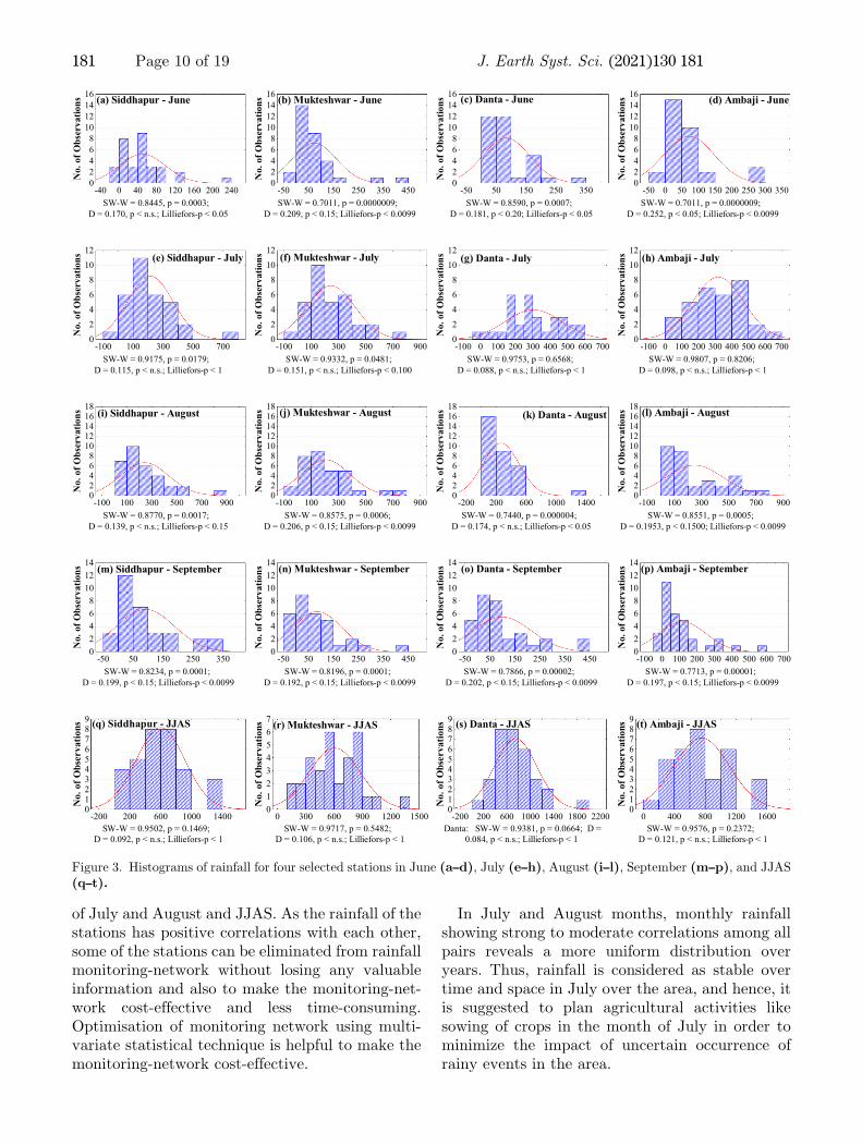
of July and August and JJAS. As the rainfall of thestations has positive correlations with each other,some of the stations can be eliminated from rainfallmonitoring-network without losing any valuableinformation and also to make the monitoring-net-work cost-effective and less time-consuming.Optimisation of monitoring network using multi-variate statistical technique is helpful to make themonitoring-network cost-effective.

In July and August months, monthly rainfallshowing strong to moderate correlations among allpairs reveals a more uniform distribution overyears. Thus, rainfall is considered as stable overtime and space in July over the area, and hence, itis suggested to plan agricultural activities likesowing of crops in the month of July in order tominimize the impact of uncertain occurrence ofrainy events in the area.

SW-W = 0.8445, p = 0.0003; D = 0.170, p < n.s.; Lilliefors-p < 0.05

-40 0 40 80 120 160 200 24002468

10121416

No.

of O

bser

vatio

ns (a) Siddhapur - June

SW-W = 0.7011, p = 0.0000009; D = 0.209, p < 0.15; Lilliefors-p < 0.0099

-50 50 150 250 350 45002468

10121416

No.

of O

bser

vatio

ns (b) Mukteshwar - June


-50 50 150 250 35002468

10121416

No.

of O

bser

vatio

ns (c) Danta - June


-50 0 50 100 150 200 250 300 35002468

10121416

No.

of O

bser

vatio

ns (d) Ambaji - June

SW-W = 0.9175, p = 0.0179; D = 0.115, p < n.s.; Lilliefors-p < 1

-100 100 300 500 70002468

1012

No.

of O

bser

vatio

ns (e) Siddhapur - July


-100 100 300 500 700 90002468

1012

No.

of O

bser

vatio

ns (f) Mukteshwar - July


-100 0 100 200 300 400 500 600 70002468

1012

No.

of O

bser

vatio

ns (g) Danta - July


-100 0 100 200 300 400 500 600 70002468

1012

No.

of O

bser

vatio

ns (h) Ambaji - July


-100 100 300 500 700 90002468

1012141618

No.

of O

bser

vatio

ns (i) Siddhapur - August


-100 100 300 500 700 90002468

1012141618

No.

of O

bser

vatio

ns (j) Mukteshwar - August


-200 200 600 1000 140002468

1012141618

No.

of O

bser

vatio

ns (k) Danta - August


-100 100 300 500 700 90002468

1012141618

No.

of O

bser

vatio

ns (l) Ambaji - August


-50 50 150 250 35002468

101214

No.

of O

bser

vatio

ns (m) Siddhapur - September


-50 50 150 250 350 45002468

101214

No.

of O

bser

vatio

ns (n) Mukteshwar - September


-50 50 150 250 350 45002468

101214

No.

of O

bser

vatio

ns (o) Danta - September


-100 0 100 200 300 400 500 600 70002468

101214

No.

of O

bser

vatio

ns (p) Ambaji - September


-200 200 600 1000 14000123456789

No.

of O

bser

vatio

ns (q) Siddhapur - JJAS


0 300 600 900 1200 150001234567

No.

of O

bser

vatio

ns (r) Mukteshwar - JJAS

Danta: SW-W = 0.9381, p = 0.0664; D =0.084, p < n.s.; Lilliefors-p < 1

-200 200 600 1000 1400 1800 22000123456789

No.

of O

bser

vatio

ns (s) Danta - JJAS


0 400 800 1200 16000123456789

No.

of O

bser

vatio

ns (t) Ambaji - JJAS

Figure 3. Histograms of rainfall for four selected stations in June (a–d), July (e–h), August (i–l), September (m–p), and JJAS(q–t).


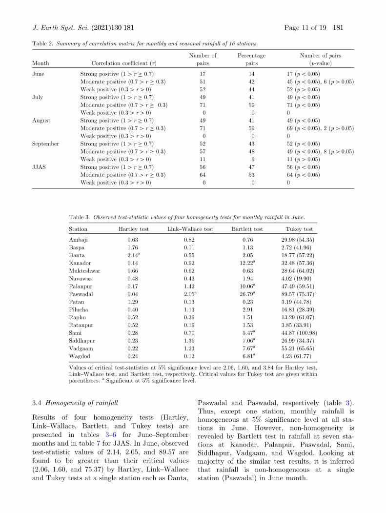
3.4 Homogeneity of rainfall

Results of four homogeneity tests (Hartley,Link–Wallace, Bartlett, and Tukey tests) arepresented in tables 3–6 for June–Septembermonths and in table 7 for JJAS. In June, observedtest-statistic values of 2.14, 2.05, and 89.57 arefound to be greater than their critical values(2.06, 1.60, and 75.37) by Hartley, Link–Wallaceand Tukey tests at a single station each as Danta,

Paswadal and Paswadal, respectively (table 3).Thus, except one station, monthly rainfall ishomogeneous at 5% significance level at all sta-tions in June. However, non-homogeneity isrevealed by Bartlett test in rainfall at seven sta-tions at Kanodar, Palanpur, Paswadal, Sami,Siddhapur, Vadgaam, and Wagdod. Looking atmajority of the similar test results, it is inferredthat rainfall is non-homogeneous at a singlestation (Paswadal) in June month.

Table 2. Summary of correlation matrix for monthly and seasonal rainfall of 16 stations.

Month Correlation coefBcient (r)

Number of

pairs

Percentage

pairs

Number of pairs

(p-value)

June Strong positive (1[ r C 0.7) 17 14 17 (p\ 0.05)

Moderate positive (0.7[ r C 0.3) 51 42 45 (p\ 0.05), 6 (p[ 0.05)

Weak positive (0.3[ r[ 0) 52 44 52 (p[ 0.05)

July Strong positive (1[ r C 0.7) 49 41 49 (p\ 0.05)

Moderate positive (0.7[ r C 0.3) 71 59 71 (p\ 0.05)

Weak positive (0.3[ r[ 0) 0 0 0

August Strong positive (1[ r C 0.7) 49 41 49 (p\ 0.05)



September Strong positive (1[ r C 0.7) 52 43 52 (p\ 0.05)


Weak positive (0.3[ r[ 0) 11 9 11 (p[ 0.05)

JJAS Strong positive (1[ r C 0.7) 56 47 56 (p\ 0.05)

Moderate positive (0.7[ r C 0.3) 64 53 64 (p\ 0.05)


Table 3. Observed test-statistic values of four homogeneity tests for monthly rainfall in June.

Station Hartley test Link–Wallace test Bartlett test Tukey test

Ambaji 0.63 0.82 0.76 29.98 (54.35)

Baspa 1.76 0.11 1.13 2.72 (41.96)

Danta 2.14a 0.55 2.05 18.77 (57.22)

Kanador 0.14 0.92 12.22a 32.48 (57.36)

Mukteshwar 0.66 0.62 0.63 28.64 (64.02)

Navawas 0.48 0.43 1.94 4.02 (19.90)

Palanpur 0.17 1.42 10.06a 47.49 (59.51)

Paswadal 0.04 2.05a 26.79a 89.57 (75.37)a

Patan 1.29 0.13 0.23 3.19 (44.78)

Pilucha 0.40 1.13 2.91 16.81 (28.39)

Raphu 0.52 0.39 1.51 13.29 (61.07)

Ratanpur 0.52 0.19 1.53 3.85 (33.91)

Sami 0.28 0.70 5.47a 44.87 (100.98)

Siddhapur 0.23 1.36 7.06a 26.99 (34.37)

Vadgaam 0.22 1.23 7.67a 55.21 (65.65)

Wagdod 0.24 0.12 6.81a 4.23 (61.77)

Values of critical test-statistics at 5% significance level are 2.06, 1.60, and 3.84 for Hartley test,Link–Wallace test, and Bartlett test, respectively. Critical values for Tukey test are given withinparentheses. a Significant at 5% significance level.


In July, three tests (Hartley, Link–Wallace,and Tukey) do not reveal non-homogeneousrainfall at any station at 5% significance level(table 4). However, results of Bartlett testindicate significantly non-homogeneous rainfall

at four stations, i.e., Baspa, Palanpur, Piluchaand Raphu. Considering the results of the mul-tiple tests, it is concluded that there was nosignificant non-homogeneous rainfall time-seriesin July.

Table 4. Observed and critical test-statistic values of four homogeneity tests for monthly rainfall inJuly.


Ambaji 0.53 0.05 1.43 3.63 (111.39)

Baspa 0.31 1.30 4.66a 78.43 (115.27)

Danta 1.08 0.24 0.02 17.32 (116.93)

Kanador 0.36 0.01 3.58 1.27 (146.04)

Mukteshwar 1.28 0.02 0.22 1.85 (129.54)

Navawas 1.29 0.90 0.24 78.60 (146.16)

Palanpur 0.31 1.22 4.71a 104.34 (136.84)

Paswadal 0.60 0.99 0.96 93.78 (134.95)

Patan 0.84 0.08 0.11 5.28 (113.00)

Pilucha 0.35 0.20 3.82 13.27 (105.54)

Raphu 0.31 0.87 4.64a 51.11 (110.90)

Ratanpur 0.38 0.24 3.23 19.34 (134.99)

Sami 0.87 0.03 0.07 1.80 (106.83)

Siddhapur 0.38 0.003 3.34 0.21 (109.52)

Vadgaam 0.66 0.63 0.64 48.20 (126.95)

Wagdod 1.03 0.22 0.002 19.94 (157.54)

Values of critical test-statistics at 5% significance level are 2.06, 1.60, and 3.84 for Hartley test,Link-Wallace test, and Bartlett test, respectively. Critical values for Tukey test are given withinparentheses.a significant at 5% significance level.

Table 5. Observed and critical test-statistic values of four homogeneity tests for monthly rainfall inAugust.


Ambaji 1.25 0.38 0.18 32.18 (151.77)

Baspa 2.26a 0.14 2.36 6.64 (81.75)

Danta 0.33 0.62 4.23a 69.00 (174.53)

Kanador 0.68 0.69 0.55 68.27 (144.68)

Mukteshwar 0.99 0.24 0.001 20.54 (128.83)

Navawas 0.06 2.03a 21.48a 159.80 (140.95)a

Palanpur 0.46 0.55 2.14 52.46 (147.07)

Paswadal 0.90 0.82 0.04 89.83 (158.36)

Patan 0.42 1.17 2.63 104.56 (137.14)

Pilucha 0.36 0.91 3.70 82.57 (140.78)

Raphu 1.23 0.80 0.15 39.07 (83.20)

Ratanpur 1.36 1.30 0.35 123.94 (155.08)

Sami 2.55a 0.25 3.08 13.44 (109.25)

Siddhapur 0.91 0.27 0.04 24.95 (139.96)

Vadgaam 0.56 0.68 1.23 60.89 (148.24)

Wagdod 2.18a 0.06 2.16 4.48 (118.69)

Values of critical test-statistics at 5% significance level are 2.06, 1.60, and 3.84 for Hartley test,Link–Wallace test, and Bartlett test, respectively. Critical values for Tukey test are given withinparentheses. a Significant at 5% significance level.


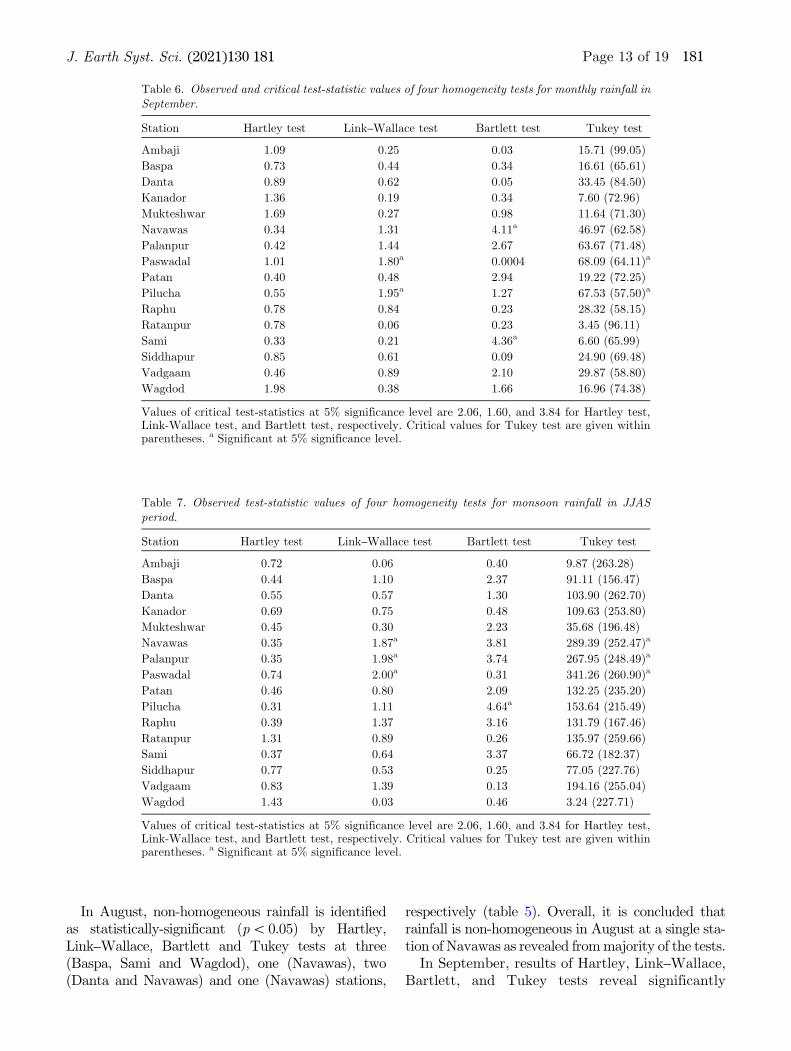
In August, non-homogeneous rainfall is identiBedas statistically-significant (p\0.05) by Hartley,Link–Wallace, Bartlett and Tukey tests at three(Baspa, Sami and Wagdod), one (Navawas), two(Danta and Navawas) and one (Navawas) stations,

respectively (table 5). Overall, it is concluded thatrainfall is non-homogeneous in August at a single sta-tion of Navawas as revealed frommajority of the tests.In September, results of Hartley, Link–Wallace,

Bartlett, and Tukey tests reveal significantly

Table 6. Observed and critical test-statistic values of four homogeneity tests for monthly rainfall inSeptember.


Ambaji 1.09 0.25 0.03 15.71 (99.05)

Baspa 0.73 0.44 0.34 16.61 (65.61)

Danta 0.89 0.62 0.05 33.45 (84.50)

Kanador 1.36 0.19 0.34 7.60 (72.96)

Mukteshwar 1.69 0.27 0.98 11.64 (71.30)

Navawas 0.34 1.31 4.11a 46.97 (62.58)

Palanpur 0.42 1.44 2.67 63.67 (71.48)

Paswadal 1.01 1.80a 0.0004 68.09 (64.11)a

Patan 0.40 0.48 2.94 19.22 (72.25)

Pilucha 0.55 1.95a 1.27 67.53 (57.50)a

Raphu 0.78 0.84 0.23 28.32 (58.15)

Ratanpur 0.78 0.06 0.23 3.45 (96.11)

Sami 0.33 0.21 4.36a 6.60 (65.99)

Siddhapur 0.85 0.61 0.09 24.90 (69.48)

Vadgaam 0.46 0.89 2.10 29.87 (58.80)

Wagdod 1.98 0.38 1.66 16.96 (74.38)

Values of critical test-statistics at 5% significance level are 2.06, 1.60, and 3.84 for Hartley test,Link-Wallace test, and Bartlett test, respectively. Critical values for Tukey test are given withinparentheses. a Significant at 5% significance level.

Table 7. Observed test-statistic values of four homogeneity tests for monsoon rainfall in JJASperiod.


Ambaji 0.72 0.06 0.40 9.87 (263.28)

Baspa 0.44 1.10 2.37 91.11 (156.47)

Danta 0.55 0.57 1.30 103.90 (262.70)

Kanador 0.69 0.75 0.48 109.63 (253.80)

Mukteshwar 0.45 0.30 2.23 35.68 (196.48)

Navawas 0.35 1.87a 3.81 289.39 (252.47)a

Palanpur 0.35 1.98a 3.74 267.95 (248.49)a

Paswadal 0.74 2.00a 0.31 341.26 (260.90)a

Patan 0.46 0.80 2.09 132.25 (235.20)

Pilucha 0.31 1.11 4.64a 153.64 (215.49)

Raphu 0.39 1.37 3.16 131.79 (167.46)

Ratanpur 1.31 0.89 0.26 135.97 (259.66)

Sami 0.37 0.64 3.37 66.72 (182.37)

Siddhapur 0.77 0.53 0.25 77.05 (227.76)

Vadgaam 0.83 1.39 0.13 194.16 (255.04)

Wagdod 1.43 0.03 0.46 3.24 (227.71)

Values of critical test-statistics at 5% significance level are 2.06, 1.60, and 3.84 for Hartley test,Link-Wallace test, and Bartlett test, respectively. Critical values for Tukey test are given withinparentheses. a Significant at 5% significance level.


non-homogeneous rainfall at zero, two (Paswadal andPilucha), two (Navawas and Sami) and two (Pas-wadal and Pilucha) stations, respectively (table 6).Thus, it is clear that rainfall is non-homogeneous inSeptember at 5% significance level at Paswadal andPilucha stations by two statistical tests.In JJAS, Hartley, Link–Wallace, Bartlett, and

Tukey tests detect significantly non-homogeneousrainfall (p\ 0.05) at zero, three (Navawas,Palanpur, and Paswadal), one (Pilucha), and three(Navawas, Palanpur, and Paswadal) stations,respectively (table 7). Based on comparative eval-uation of all tests’ results, it is conBrmed thatrainfall during JJAS is homogeneous at 13 stationsand non-homogeneous at Navawas, Palanpur, andPilucha stations.Disagreement among the results of homogeneity

tests in months of June, July, August andSeptember and JJAS justiBes the approach ofadopting multiple statistical tests (Machiwal et al.2016). Overall, 12 of total 16 stations have homo-geneous monthly and seasonal rainfall in the studyarea, and only four stations (Navawas, Paswadal,Palanpur, and Pilucha) have non-homogeneousrainfall during monsoon season. Thus, it is con-cluded that monthly monsoon rainfall is temporallyhomogeneous in the area, and hence, the rainfalldata may be used for studies dealing with trendidentiBcation, climate modelling and prediction offuture climate (CheRos et al. 2016). It is observedthat results of Bartlett test mostly differ from otherthree homogeneity tests, which is also observed byMachiwal et al. (2016). Presence of homogeneity inrainfall series ensures that trends, if any present inrainfall series, are related to climate change andvariability and not due to non-homogeneity in theseries (H€ansel et al. 2016). It is not straightforwardto decide preference of a homogeneity test over the

others, and is also not the motive of this study.However, it is observed that results of two tests ofLink–Wallace and Tukey are in harmony to eachother. Also, Hartley and Bartlett tests Bnd non-homogeneous rainfall at relatively more number ofstations in comparison to Link–Wallace and Tukeytests. These results are corroborated with Bndingsof Meena et al. (2019) who reported thatLink–Wallace and Tukey tests detect presence andabsence of homogeneity at almost similar stationsin four monsoon months. On the other hand,Hartley and Bartlett tests might be more sensitivein examining homogeneity due to deviation of datafrom normality (Meena et al. 2019). Hence,Link–Wallace and Tukey tests might be preferredfor homogeneity testing in rainfall series. Non-homogeneity in rainfall is mainly caused by chan-ges in the method of data collection and/or theenvironment, and can cause the incorrect inter-pretation of extreme events (Rahman et al. 2017).This study could not Bnd any speciBc reasons forpresence of non-homogeneous rainfall at four sta-tions (Navawas, Paswadal, Palanpur, and Pilu-cha); however, meta-data and historicalbackground information of the rainfall measure-ments at the stations may be examined to under-stand the possible climatic and non-climatic causesof shift in the mean values of rainfall (Kocsis et al.2020). Non-homogeneity generally results in abruptchanges in rainfall time-series, and in future, abruptchanges may also be explored in rainfall time-series ofstations where non-homogeneity is revealed.Results of Levene’s test and Tukey test for

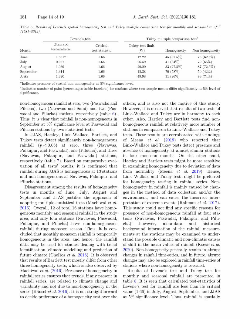
monthly and seasonal rainfall are presented intable 8. It is seen that calculated test-statistics ofLevene’s test for rainfall are less than its criticalvalue (1.66) in July, August, September, and JJASat 5% significance level. Thus, rainfall is spatially

Table 8. Results of Levene’s spatial homogeneity test and Tukey multiple comparison test for monthly and seasonal rainfall(1981–2012).

Month

Levene’s test Tukey multiple comparison testa

Observed

test-statisticCritical

test-statistic

Tukey test-limit

(W) Homogeneity Non-homogeneity

June 1.851* 1.66 12.22 45 (37.5%) 75 (62.5%)

July 0.957 1.66 26.59 41 (34%) 79 (66%)

August 1.039 1.66 29.20 33 (27.5%) 87 (72.5%)

September 1.314 1.66 15.38 70 (58%) 50 (42%)

JJAS 1.320 1.66 49.98 31 (26%) 89 (74%)

*Indicates presence of spatial non-homogeneity at 5% significance level.aIndicates number of pairs (percentages inside brackets) for stations where two sample means differ significantly at 5% level ofsignificance.


homogeneous in these three months as well as overJJAS period. However, the rainfall is not foundspatially homogeneous in June, where calculatedtest-statistic value of Levene’s test is more than itscritical value. In contrast, results of Tukey testindicates presence of a large number of stationpairs where the two means of rainfall significantlydiffer at 5% level of significance. It is seen that thenumber of pairs showing non-homogeneous rainfallare 75 (62.5%), 79 (66%), 87 (72.5%), 50 (42%) and89 (74%) in June, July, August, September, and

JJAS, respectively. Therefore, Tukey test clearlysuggests presence of considerable non-homoge-neous rainfalls over the space in four monsoonmonths as well as monsoon season. Overall, non-homogeneous rainfall in June is conBrmed fromresults of both the tests; however, results of twotests are not found coherent regarding presence/absence of spatially homogeneous rainfall in othermonths and JJAS period. Limits (W) of Tukey testfor rainfall in four months and JJAS period are alsopresented in table 8, which might be treated as

0 20 40 60 80 100 120(Dlink/Dmax)*100

SamiVadgaamPaswadal

MukteshwarPalanpurWagdodKanador

SiddhapurPatan

PiluchaNavawasRatanpur

BaspaDanta

RaphuAmbaji (a) June

10 20 30 40 50 60 70 80 90 100 110(Dlink/Dmax)*100

WagdodNavawas

MukteshwarRatanpurKanador

SiddhapurPilucha

PatanPaswadalVadgaamPalanpur

SamiRaphuBaspaDanta

Ambaji (b) July

0 20 40 60 80 100 120(Dlink/Dmax)*100

SamiRaphuBaspa

NavawasPilucha

PatanKanadorRatanpurPaswadal

DantaWagdod

SiddhapurMukteshwar

VadgaamPalanpur

Ambaji (c) August

0 10 20 30 40 50 60 70 80 90 100 110(Dlink/Dmax)*100

WagdodRaphuPatan

BaspaSami

VadgaamPilucha

PalanpurMukteshwar

NavawasPaswadal

SiddhapurKanadorRatanpur

DantaAmbaji (d) September

10 20 30 40 50 60 70 80 90 100 110(Dlink/Dmax)*100

SamiRaphuBaspa

VadgaamPalanpur

MukteshwarSiddhapur

PiluchaPatan

NavawasWagdod

PaswadalKanadorRatanpur

DantaAmbaji (e) JJAS

Figure 4. Dendrograms showing cluster formation of 16 rainfall stations for rainfall in (a) June, (b) July, (c) August,(d) September, and (e) JJAS.


critical difference, and be linked to the meanrainfall values of the stations given in table 1.

3.5 Clusters of rainfall stations

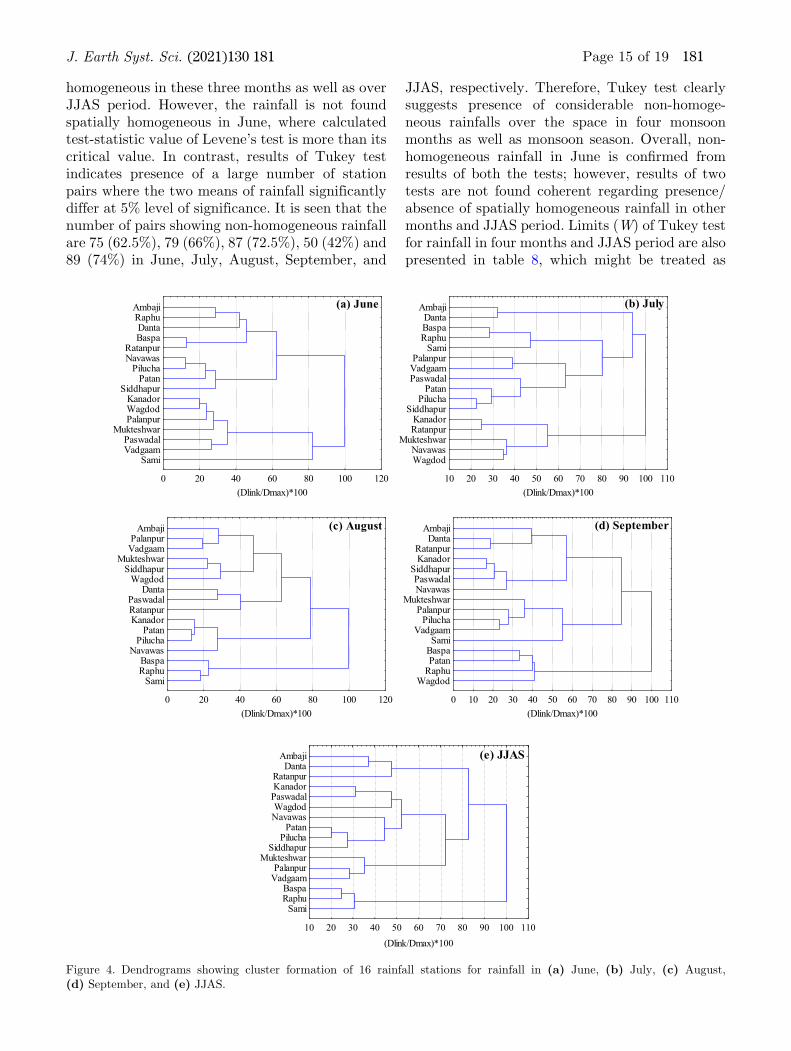
Dendrograms illustrating cluster formation processbased on 32-yr rainfall data of 16 stations in fourindividual months (June–September) as well asJJAS period are presented in Bgure 4. Number ofrainfall clusters in June, July, August, September,and JJAS are chosen at a linkage distance (Dlink/Dmax) of 55, 65, 55, 55, and 55%, respectively, thatdelineates four clusters of rainfall stations in eachmonth and JJAS. The linkage distance in July is

chosen slightly greater than that selected in otherthree months and JJAS in order to have equalnumber of clusters in each month, and their easycomparative evaluations. In the month of June, thenumber of rainfall stations in clusters I, II, III andIV are 5, 4, 6 and 1, respectively. In July, clusters I,II, III and IV consist of 2, 3, 6 and 5 stations,respectively. On the other hand, in August, rainfallstations grouped in clusters I, II, III and IV are 6, 3,4 and 3, respectively; and rainfall in SeptemberclassiBes 3, 4, 5 and 4 stations in clusters I, II, IIIand IV, respectively. In JJAS, rainfall stations inclusters I, II, III and IV are 3, 7, 3 and 3, respec-tively. Four clusters of the rainfall stations for fourmonths and JJAS are geographically located in

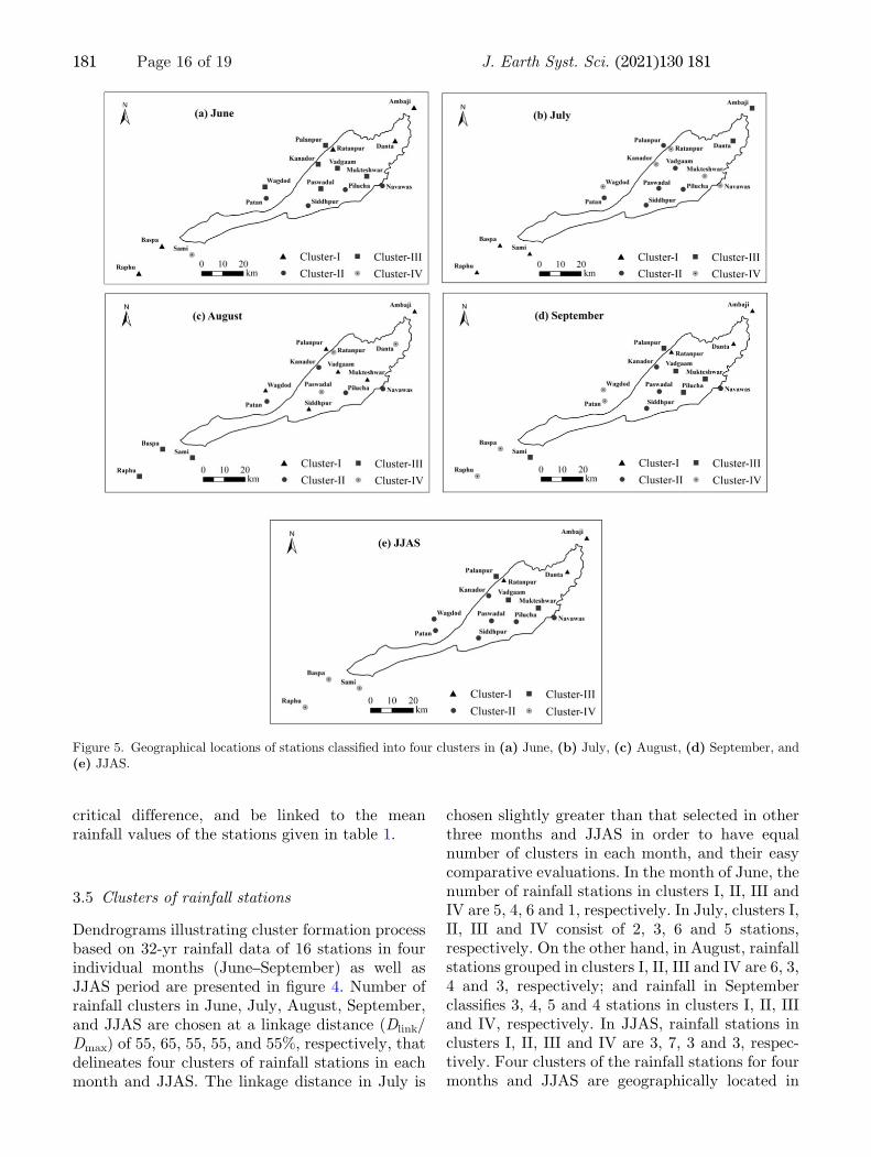
Figure 5. Geographical locations of stations classiBed into four clusters in (a) June, (b) July, (c) August, (d) September, and(e) JJAS.


Bgure 5. It is apparent that stations grouped inCluster I are mainly located on relatively high landelevation (195–455 m MSL) towards the northeastboundary of the basin in June, August, September,and JJAS. Similarly, stations of Cluster II are sit-uated towards the south-central portion in all themonths and JJAS and stations of Cluster III existin the central and north-central portion of thebasin in the months of June, August, September,and JJAS. Stations of Cluster IV are present in thesouth-west extreme (13–34 m MSL) of the basin inJune, September, and JJAS. It is seen that rainfallstations varied from cluster to cluster for differ-ent months. This Bnding indicates inter-annual

changes in temporal distributions of rainfall atdifferent stations among different months. Thus, itis emphasized here to consider monthly scalerainfall data for evaluating rainfall variability.Monthly and seasonal rainfall of the stations

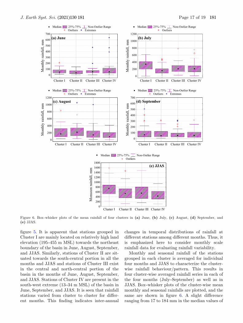
grouped in each cluster is averaged for individualfour months and JJAS to characterize the cluster-wise rainfall behaviour/pattern. This results infour cluster-wise averaged rainfall series in each ofthe four months (July–September) as well as inJJAS. Box–whisker plots of the cluster-wise meanmonthly and seasonal rainfalls are plotted, and thesame are shown in Bgure 6. A slight differenceranging from 17 to 184 mm in the median values of


Cluster I Cluster II Cluster III Cluster IV

0

100

200

300

400

500

600

700

Mon

thly

rain

fall,

mm

(a) June


Cluster I Cluster II Cluster III Cluster IV0

200

400

600

800

1000

1200

Mon

thly

rain

fall,

mm

(b) July



200

400

600

800

1000

1200

Mon

thly

rain

fall,

mm

(c) August


Cluster I Cluster II Cluster III Cluster IV

0

100

200

300

400

500

600

700

Mon

thly

rain

fall,

mm

(d) September



200400600800

10001200140016001800

Mon

soon

rain

fall,

mm

(e) JJAS

Figure 6. Box–whisker plots of the mean rainfall of four clusters in (a) June, (b) July, (c) August, (d) September, and(e) JJAS.


the average rainfall is seen among the four clustersin every month (Bgure 6a–d), which is moreapparent in July (difference of 184 mm) andAugust (difference of 126 mm) months when thereis abundance of rainfall (235 mm in July and 203mm in August) (Bgure 6b, c). Less difference in themedian values during June (17 mm) and Septem-ber (17 mm) months is due to relatively lessamount of the monthly rainfall in June (65 mm)and September (87 mm) months. In JJAS, differ-ence in the median rainfall values varies from 11 to308 mm among the four clusters (Bgure 6e). Themedian rainfall values of 39, 154, and 47 mm inCluster II always remain lowest compared to otherclusters in June (47–56 mm), July (207–338 mm)and September (54–64 mm). However, the medianrainfall value of 214 mm in Cluster II is signifi-cantly higher than that in other clusters (88–166mm) in August (Bgure 6c). On the other hand, themedian rainfall value of 737 mm in Cluster I isconsiderably higher than that in other clusters(429–543 mm) during JJAS. Overall, it is apparentthat the four clusters identiBed through dendro-grams have distinct geographical locations in thearea. However, stations and rainfall statistics foreach cluster vary slightly.

4. Conclusions

This study examines rainfall homogeneity at 16stations for June–September months and JJASperiod. CoefBcient of variation (CV) for June(72–163%), July (48–100%), August (78–114%) andSeptember (93–127%) indicate high rainfall vari-ability in comparison to JJAS period (CV *45–60%).Monthly and seasonal rainfalls have right-skewed distribution and strong to moderate linearrelationships among a large number of pairs. Hence,there exists a scope for optimization of rainfallmonitoring-network by retaining one station fromeach pair depicting a strong linear relationship, andthereby, reducing time and manpower involved inrainfall monitoring and making it cost-effective.Sowing of kharif crops is suggested in July month toget advantage of uniformand stable rainfall. Diverseresults justify approach of multiple homogeneitytests adopted in this study.Rainfall is temporally homogeneous except at

Paswadal (June, September, and JJAS), Navawas(August and JJAS), Palanpur (JJAS) and Pilucha(September) stations. Homogeneous rainfall-records may be used in climate-modelling studies

for getting reliable predictions. Use of Link–Wal-lace and Tukey tests is preferred for homogeneity.Levene’s test reveals spatial homogeneity in rain-fall of July, August, September, and JJAS. Den-drograms delineate four rainfall clusters withstations varying among clusters; their distinctgeographical positions and box–whisker plotsevidence inter-annual rainfall changes.

Acknowledgements

First author acknowledges all facilities provided bythe Director, ICAR-Central Arid Zone ResearchInstitute, Jodhpur, India for carrying out thisstudy. The authors are grateful to the anonymousreviewer for their constructive suggestions, whichgreatly enhanced the quality of an earlier version ofthis paper.

Author statement

Deepesh Machiwal: Conceptualization, methodol-ogy, formal analysis, investigation, interpretationof results, writing and editing manuscript. B SParmar: Data and resources. Sanjay Kumar:Resources and GIS Bgures. Hari Mohan Meena:Review, methodology. B S Deora: Supervision.

References

Ahmed A, Deb D and Mondal S 2019 Assessment of rainfallvariability and its impact on groundnut yield in Bun-delkhand region of India; Curr. Sci. 117(5) 794–803.

Arikan B B and Kahya E 2019 Homogeneity revisited:Analysis of updated precipitation series in Turkey; Theor.Appl. Climatol. 135 211–220.

Ay M 2020 Trend and homogeneity analysis in temperatureand rainfall series in western Black Sea region, Turkey;Theor. Appl. Climatol. 139 837–848.

Bintanja R 2018 The impact of Arctic warming on increasedrainfall; Sci. Rep. 8 16001, https://doi.org/10.1038/s41598-018-34450-3.

CheRos F, Tosaka H, Sidek L M and Basri H 2016Homogeneity and trends in long-term rainfall data, Kelan-tan River Basin, Malaysia; Int. J. River Basin Manag.14(2) 151–163.

Dave H and James M E 2017 Characteristics of intense rainfallover Gujarat state (India) based on percentile criteria;Hydrol. Sci. J. 62(12) 2035–2048.

Deka R L, Mahanta C, Pathak H, Nath K K and Das S 2013Trends and Cuctuations of rainfall regime in the Brahma-putra and Barak basins of Assam, India; Theor. Appl.Climatol. 114(1–2) 61–71.


https://doi.org/10.1038/s41598-018-34450-3

https://doi.org/10.1038/s41598-018-34450-3

Frich P, Alexander L V, Della-Marta P, Gleason B, HaylockM, Klein Tank A M G and Peterson T 2002 Observedcoherent changes in climatic extremes during the secondhalf of twentieth century; Clim. Res. 19 193–212.

Ghosh S, Das D, Kao S-C and Ganguly A R 2012 Lack ofuniform trends but increasing spatial variability inobserved Indian rainfall extremes; Nat. Clim. Change 286–91.

Gupta A, Kamble T and Machiwal D 2017 Comparison ofordinary and Bayesian kriging techniques in depictingrainfall variability in arid and semi-arid regions of north-west India; Environ. Earth Sci. 76 512, https://doi.org/10.1007/s12665-017-6814-3.

Haigh M J 2004 Sustainable management of head waterresources: The Nairobi head water declaration (2002)and beyond; Asian J. Water, Environ. Pollut. 1(1–2) 17–28.

H€ansel S, Medeiros D M, Matschullat J, Petta R A and deMendonc�a Silva I 2016 Assessing homogeneity and climatevariability of temperature and precipitation series in thecapitals of north-eastern Brazil; Front. Earth Sci. 4 29,https://doi.org/10.3389/feart.2016.00029.

Huang J, Ji M, Xie Y, Wang S, He Y and Ran J 2016 Globalsemi-arid climate change over last 60 years; Clim. Dyn. 461131–1150.

India-WRIS 2014 West Flowing Rivers of Kutch andSaurashtra including Luni Basin; Version 2.0, Report ofJoint Project of Central Water Commission; Ministry ofWater Resources, New Delhi and National RemoteSensing Centre, Indian Space Research Organization,Hyderabad, Government of India on Generation ofDatabase and Implementation of Web enabled WaterResources Information System in the Country (India-WRISWebGIS), 135p.

Kanji G K 2001 100 Statistical tests; Sage Publication, NewDelhi, India.

Khandelwal M K, Arora S and Raju K C B 2013 Spatial andtemporal variations in rainfall and rainwater harvestingpotential for Kutch district, Gujarat; J. Soil Water Con-serv. 12(2) 117–122.

Kocsis T, Kov�acs-Sz�ekely I and Anda A 2020 Homogeneitytests and non-parametric analyses of tendencies in precip-itation time series in Keszthely, Western Hungary; Theor.Appl. Climatol. 139 849–859.

Kumar S, Machiwal D and Parmar B S 2019 Parsimoniousapproach to delineate groundwater potential zones usinggeospatial modeling and MCDA techniques under limiteddata availability condition; Eng. Rep. 1(5) e12073, https://doi.org/10.1002/eng2.12073.

Levene H 1960 Robust tests for equality of variances; In:Contributions to Probability and Statistics: Essays inHonour of Harold Hotelling (eds) Olkin I, Ghurye S G,HoeAding W, Madow W G and Mann H B, StanfordUniversity Press, Palo Alto, California, pp. 278–292.

Li Z, Li X, Wang Y and Quiring S M 2019 Impact of climatechange on precipitation patterns in Houston, Texas, USA;Anthropocene 25 100193, https://doi.org/10.1016/j.ancene.2019.100193.

Machiwal D and Jha M K 2012 Hydrologic Time SeriesAnalysis: Theory and Practice; Springer, Netherlands andCapital Publishing Company, New Delhi, India, 303p.

Machiwal D and Jha M K 2017 Evaluating persistence, andidentifying trends and abrupt changes in monthly andannual rainfalls of a semi-arid region in western India;Theor. Appl. Climatol. 128(3–4) 689–708.

Machiwal D, Kumar S and Dayal D 2016 Characterizingrainfall of hot arid region by using time-series modeling andsustainability approaches: A case study from Gujarat,India; Theor. Appl. Climatol. 124 593–607.

Meena H M, Machiwal D, Santra P, Moharana P C and SinghD V 2019 Trends and homogeneity of monthly, seasonal,and annual rainfall over arid region of Rajasthan, India;Theor. Appl. Climatol. 136(3–4) 795–811.

Otto M 1998 Multivariate methods; In: Analytical Chemistry(eds) Kellner R, Mermet J M, Otto M and Widmer H M,Wiley VCH, Weinheim, Germany, 916p.

Panda A and Sahu N 2019 Trend analysis of seasonal rainfalland temperature pattern in Kalahandi, Bolangir andKoraput districts of Odisha India; Atmos. Sci. Lett.20(10) e932, https://doi.org/10.1002/asl.932.

Pisal R R, Kumar N and Shukla S P 2017 Long term trendanalysis of rainfall at heavy rainfall zone of South Gujarat,India; Indian J. Soil Conserv. 45(2) 168–175.

Pradhan R K, Sharma D, Panda S K and Sharma A 2019Changes of precipitation regime and its indices overRajasthan state of India: Impact of climate change scenar-ios experiments; Clim. Dyn. 5(5–6) 3405–3420.

Praveenkumar Ch and Jothiprakash V 2020 Spatio-temporaltrend and homogeneity analysis of gridded and gaugeprecipitation in Indravati River basin, India; J. WaterClim. Change 11(1) 178–199.

Priyan K 2015 Spatial and temporal variability of rainfall inAnand district of Gujarat state. International Conferenceon Water Resources, Coastal and Ocean Engineering(ICWRCOE 2015); Aquat. Procedia 4 713–720.

Rahman M A, Yunsheng L and Sultana N 2017 Analysis andprediction of rainfall trends over Bangladesh using Mann-Kendall, Spearman’s rho tests and ARIMA model; Meteor.Atmos. Phys. 129(4) 409–424.

Ratner B 2009 The correlation coefBcient: Its values rangebetween +1/�1, or do they?; J. Target. Meas. Anal.Market. 17(2) 139–142.

Sonali P and Kumar D N 2013 Review of trend detectionmethods and their application to detect temperaturechanges in India; J. Hydrol. 476 212–227.

StatSoft Inc 2004 STATISTICA (Data Analysis SoftwareSystem); version 6, www.statsoft.com.

Zhang Q, Xu C-Y, Becker S, Zhang Z X, Chen Y D andCoulibaly M 2009 Trends and abrupt changes of precipita-tion maxima in the Pearl River Basin, China; Atmos. Sci.Lett. 10 132–144.

Zhang Q, Xu C-Y, Zhang Z, Chen X and Han Z 2010Precipitation extremes in a karst region: A case study in theGuizhou Province, southwest China; Theor. Appl. Climatol.101 53–65.

Corresponding editor: KAVIRAJAN RAJENDRAN


https://doi.org/10.1007/s12665-017-6814-3

https://doi.org/10.1007/s12665-017-6814-3

https://doi.org/10.3389/feart.2016.00029

https://doi.org/10.1002/eng2.12073

https://doi.org/10.1002/eng2.12073

https://doi.org/10.1016/j.ancene.2019.100193

https://doi.org/10.1016/j.ancene.2019.100193

https://doi.org/10.1002/asl.932

http://www.statsoft.com

evaluating homogeneity of monsoon rainfall in saraswati

Documents