UNIVERSITY OFILLINOIS LIBRARY

AT URBANA-CHAMPAIGNBOOKSTACKS

Digitized by the Internet Archive

in 2011 with funding from

University of Illinois Urbana-Champaign

http://www.archive.org/details/evaluatingperfor1571gent

BEBRFACULTY WORKINGPAPER NO. 89-1571

Evaluating the Performance of

Receivable and Inventory Strategies

James A. Gentry

Paid Newbcld

David T. Whitford

Jesus De La Garza

"» <00f)

Y Of ILLINOIS

r-MAMPAIG!"

College of Commerce and Business Administration

Bureau of Economic and Business Research

University of Illinois Urbana-Champaign

BEBR

FACULTY WORKING PAPER NO. 89-1571

College of Commerce and Business Administration

University of Illinois at Urbana- Champaign

May 1989

Evaluating the Performance of Receivableand Inventory Strategies

James A. Gentry, ProfessorDepartment of Finance

Paul Newbold, ProfessorDepartment of Economics

David T. Whitford, Associate ProfessorDepartment of Finance

Jesue De La GarzaVirginia Polytechnic Institute and State University

EVALUATING THE PERFORMANCE OF RECEIVABLEAND INVENTORY STRATEGIES

ABSTRACT

The primary objective of this paper is to present a methodology

for evaluating the long-run performance of receivable and inventory

management. The methodology is based on a conceptual idea and a time

series technique. The model develops nine sets of conditions involved

in determining the cause of changes in accounts receivables and inven-

tories. It shows the trend of sales patterns and collection exper-

ience are responsible for changes in receivables. Also the trend of

production costs and inventory controls are the causes of changes in

inventories. The model ranks the nine sets of conditions according to

the present value that is created because of management decisions

and/or economic factors related to receivables and/or inventories.

The best strategy for receivables management improvement is to speed

up the inflow of cash, which occurs when the rate of change in

receivables is below the rate of change in sales. The best strategy

for Inventory management improvement is to improve control and reduce

inventory levels, which occurs when the rate of change in inventories

is lower than the rate of change in production cost patterns, and vice

versa. The Box, Pierce and Newbold ARIMA model determines a time

series trend of sales, receivables, production costs and inventories.

The estimated trends are used to rank the performance of a company's

receivable and/or inventory management. The methodology is tested

empirically in a recession and a post recession period. Finally,

insights from the methodology are presented.

EVALUATING THE PERFORMANCE OF RECEIVABLEAND INVENTORY STRATEGIES 1

Changes in Che amount and turnover of receivables and inventories

are directly related to the level and timing of a firm's cash inflows

and outflows. Therefore, changes in the long-run performance of

receivable and inventory management directly affects the value of a

firm [25, 26]. For example, shortening the time period involved in

collecting cash from customers without decreasing demand results in an

increase in the present value of the net cash flows, which in turn

creates shareholder value. Likewise the overall reduction in the com-

mitment to inventories without decreasing demand creates shareholder

value. When analyzing the causes of changes in the level and speed of

cash inflows and outflows, changes in accounts receivable and inven-

tory are compared to changes in sales and production, respectively.

Therefore, a model that determines the causes of changes in

receivables and inventories provides valuable information to manage-

ment, boards of directors and analysts. There are numerous finance

oriented models that focus on the control of accounts receivable,

e.g., [1, 4, 5, 6, 7, 8, 9, 10, 13, 14, 15, 17, 18, 27]. However,

models for controlling inventories are generally found in the

accounting literature, e.g., [16, 20] or in the management science

literature.

The systems used to monitor receivables and inventories provide a

wealth of information for estimating trends and evaluating the per-

formance of receivable and inventory strategies. The performance of

receivable management has not been previously studied because, until

-2-

recently, the cause of changes in receivables had not been fully

developed. The causes of changes in inventories are developed in this

paper. In 1985 Gentry and De La Garza (GD) [10] extended the work of

Carpenter and Miller [4] and showed there are nine possible sets of

conditions that underlie the causes of changes in accounts receivable.

GD concluded the primary causes of changes in receivables are

attributed to changes in sales patterns, collection experiences and

joint effects. Gallinger and Ifflander [9] also observed these three

effects in a variance model designed to control accounts receivables.

The overall objective of the study is to create a methodology for

evaluating the performance of receivable and inventory management.

The remaining objectives are to review briefly the GD model for

monitoring accounts receivable; to develop a model for explaining the

causes of changes in inventories; to present a methodology for ranking

the performance of receivable and inventory management; to use the

Box, Pierce and Newbold [3] ARIMA model to evaluate the receivable and

inventory management performance of 119 industrial companies; and to

analyze the performance rankings and the contribution receivable and

inventory strategies make in the creation of shareholder value.

I. MONITORING MODELS

Overview

GD identified nine sets of conditions that were needed in order

to analyze changes in accounts receivable. These conditions were

conceptualized in a 3x3 matrix based on the trend of sales patterns

(S) and collection experience (CE). Exhibit 1 is a similar 3x3 matrix

used to identify the conditions that cause changes in receivables and

-3-

inventories . The horizontal axis shows changes in receivables are

caused by changes in sales patterns and changes in inventories are

associated with changes in production cost patterns. Changes in sales

and production are in turn related to changes in the demand for a

firm's products and changes in production schedules, respectively.

The vertical axis reflects that changes in receivables are also re-

lated to collection experience. Additionally, changes in inventories

are also related to inventory control. These changes in collection

experience are in turn related to changes in a firm's credit policies

and the changes in inventory control are related to changes in inven-

tory management and/or production policies.

Changes in sales or production cost patterns refer to monthly

changes in the level of sales or production. The pattern and trend in

sales and production can change because of seasonal, cyclical or random

events. The collection experience reflects the payment behavior of a

firm's customers and is related to a firm's credit administration

actions. Collection experience is characterized by the fraction of

credit purchases in a month that remain outstanding at the end of a

subsequent month. Inventory control exemplifies the performance of

the internal control system and the efficiency of inventory manage-

ment. Inventory control experience reflects the fraction of a firm's

production costs in a month that remain outstanding at the end of each

subsequent month. For example, if the inventory control pattern for

June is 80-50-20, it means 80% of June's production costs are embedded

in the June 30th inventory value; 50% of May's production costs are

-4-

present in the inventory value on June 30, and 20% of April's produc-

tion costs are still outstanding in the inventory value on June 30.

The nine conditions shown in Exhibit 1 reflect the interaction

that exists between sales experience and collection pattern behavior

and between production costs and inventory control experiences. The

algorithms for taking into account these interaction effects for re-

ceivables are presented in GD [10, p. 31], and the algorithm for

2inventories are presented in Exhibit 2. The algorithms determine the

relative amount that each component contributes to either the change

in receivables or inventories. Because receivables and inventories

are current assets, the only difference between the two algorithms is

the explanation of the variables that cause receivables or inventories

to change. The interactive relationships developed in the algorithm

are manifested in the trend of sales and receivables, as shown in

Exhibit 3, or in the trend of production costs and inventories, as

shown in Exhibit 4.

Inventory Model

Exhibit 4 provides the conceptual framework for understanding the

logic embedded in the inventory management algorithms. The relation-

ships that cause changes in receivables were developed in GD [10, p.

30], therefore, a brief overview of the conditions that cause changes

in inventories follows. The parallel lines of production cost and

inventories shown in Condition 1 of Exhibit 4 indicate there was no

change in production costs, or in inventory control for the time

period presented, therefore, there was no change in inventories.

-5-

Under Conditions 2 and 2' there is no change in production costs,

but in Condition 2 inventory control is deteriorating while in

Condition 2' it is improving. Because inventory control is deterior-

ating in Condition 2 inventories are increasing more rapidly than the

stable production costs. Under Condition 2' the opposite set of

circumstances prevail which cause inventories to decrease while pro-

duction remains constant.

Under Condition 3 inventories change only because of changes in

production cost patterns and inventory control performance is neutral

and has no affect on inventories. In Condition 3 inventories increase

because of an increase in production costs and in Condition 3' the

decrease in inventories is caused by a decline in production costs.

Condition 4 in Exhibit 4 illustrates the case where lax inventory

controls cause raw material or goods-in-process inventories to in-

crease more rapidly than production costs. For example, a change in a

policy to carry more raw materials because of a forecasted shortage

may be an explanation for this inventory build up. Additionally, an

increase in sales can cause an increase in production costs. Like-

wise a forecasted increase in sales can create an expansion in raw

material goods-in-process or finished goods inventories. Thus an

increase in inventories may be caused by a pure production effect,

a pure inventory control effect and/or an interaction effect between

production costs and inventory control, referred to as a joint effect.

Scenario 5 expresses an opposite set of conditions. Tightened

inventory control can cause raw materials, goods-in-process or

finished goods to decline more rapidly than the declining production

-6-

costs. Likewise a cut in production costs can result In a tightening

of inventory controls, which can cause inventories to decline more

rapidly than the production costs. Also a policy to hold less raw

materials, goods-in-process or finished goods can be carried over into

production efficiency, thereby causing production costs to decline.

Under Condition 5 inventories can be smaller because of a decline in

production costs, a production effect, an improvement in inventory

control, or a combination of the two, a joint interaction effect.

Under Conditions 6 and 7, there are opposite forces at play that

affect the change in inventories. For example, under Condition 6,

lenient inventory control practices result in an inventory build up,

simultaneously, a decline in demand causes production costs to be

reduced. The decline in demand is a countervailing force that pro-

duces an overall decline in inventories. Under Condition 7, improved

inventory control practices and policies cause inventories to decline

while increased demand causes production costs to rise. In this

circumstance, the improved inventory control practices more than

offset the increase in inventories caused by rising demand. The re-

sult is inventories increase less rapidly than production costs.

II. RANKING PERFORMANCE

The model makes it possible to analyze the long-run performance of

receivable and inventory management and, thereby, determine the effec-

tiveness of the operating strategies pursued by a company. The moni-

toring model provides a tool to rank the operating performance of

receivable and inventory management.

-7-

Objectives of top management are to analyze and judge the per-

formance record of receivable and inventory management. Exhibit 3

shows graphically that annual changes in accounts receivable (AAR)

were related to long-run trends in sales (AS) and in collection ex-

perience (ACE). Exhibit 4 graphically shows that annual changes in

inventories (AINV) are associated with long-run trends in production

costs (AP) and in inventory control experience (AIC). Exhibits 3 and

4, respectively, provide operating frameworks for financial managers,

analysts and academic researchers to identify quickly the sets of con-

ditions and variables used in measuring the performance of receivable

and inventory management. Using the present value model as a bench-

mark, Exhibits 3 and 4, respectively, highlight from the best to the

worst set of conditions that exist in creating firm value through cash

collection or inventory control strategies. The ranking methodology

is based on the principle of creating present value for shareholders.

Receivables

The best strategy for receivable management improvement is to

speed up the inflow of cash without causing demand to decline. That

would occur when the rate of change in receivables is below the rate

of change in sales. The receivable management strategies that would

speed up the inflow of cash are strategies 7, 2' and 5 in Exhibit 3.

The worst strategy for receivable management is to slow down the

inflow of cash. That occurs when the rate of change in receivables is

greater than the rate of change in sales. These worst receivable

management strategies are in cells 6, 2 and 4 as shown in Exhibit 3.

-8-

Finally strategies 3, 1 and 3' reflect a neutral receivables strategy

where the change in receivables is equal to the change in sales.

Inventories

The best strategy for inventory management improvement is to

improve control and reduce inventory levels without causing stockouts

and shortages. That occurs when the rate of change in inventories is

below the rate of change in production costs. The inventory strate-

gies that reduce inventory levels are strategies 7, 2' and 5 in

Exhibit 4. The worst strategy for management is to lose control of

its inventories and experience an unexpected build up in its inven-

tories. That happens when the rate of change in inventories is

greater than the rate of change in production costs. These worst

inventory management strategies are in cells 6, 2 and 4 as shown in

Exhibit 4. Finally, strategies 3, 1 and 3' reflect a neutral inven-

tory strategy, where the change in inventories is equal to a change in

production costs.

Benefits

The performance ranking system can be used by top management to

accomplish several important tasks. First, if top management observed

that receivables management was in the worst ranking performance

cells, credit policies and collection procedures could be designed to

speed up the inflow of cash, causing receivables to become a smaller

proportion of sales.

Second, top management may wish to create a hierarchy of rewards

if the performance record is deserving and creates shareholder value.

For example, Exhibit 5 shows the highest award would occur when

-9-

consistent performance is achieved over time, which would be in cell 7

for both receivable and inventory management. The second highest

award would be for performance achievement that is consistently in the

top three strategies over time, which would be cells 7, 2' and 5 as

reflected in Exhibit 5.

Third, the performance ranking system provides top management the

information needed to track longitudinally the performance of receiv-

able and inventory management. Assuming the objective of top manage-

ment is to maximize owner's wealth, the performance ranking system

makes it possible to determine if receivable and inventory management

consistently produce results that are in the cells with the highest

ranking. If the results are not consistently in the highest ranking

cells, management is also concerned that performance is improving as

evidenced in the longer run performance trend results.

The first step in determining the performance ranking is to esti-

mate the trends of sales, receivables, production and inventories.

An explanation of the Box, Jenkins and Newbold ARIMA model follows.

III. ESTIMATING TRENDS

A frequently studied problem in time series analysis, notably in

the literature on seasonal adjustment, concerns the decomposition of

an observed series into trend, seasonal, and irregular components.

Often this decomposition is taken to be additive. Alternatively, a

multiplicative components model can be considered through the additive

decomposition of the logarithms of the observed series. A great dif-

ficulty that is faced is that, given just the observed series, the

-10-

individual components are not uniquely Identified, unless somewhat

arbitrary assumptions about their behavior are imposed. Given a

generating process for an observed time series, there typically exists

a large number of plausible decompositions whose components can rea-

sonably be viewed as representing trend, seasonal, and irregular para-

meters. This large number of alternatives can create problems in

analyzing seasonal adjustment problem. However, Box, Pierce and

Newbold [3] have recently shown that, for a wide class of time series

generating models, although the problem of estimating components over

the sample period has no unique solution, there is a unique solution

to the problem of forecasting future values of these components. In

short, all of the observationally equivalent components' models lead

to identical forecasts for the constituent components. Thus, while

there is some ambiguity in defining and estimating trend over the

sample period, there is no ambiguity in the estimation of projected

trend . This is encouraging, since for many purposes it is precisely

this forward looking version of trend that is most relevant. For

example, if a manager is presented with a historical record of data on

sales and receivables it is reasonable to ask what these data suggest

about future trends. It is precisely this problem for which the ana-

lysis of Box, Pierce and Newbold demonstrates that a unique solution

is available.

Box, Pierce and Newbold consider a time series X ,generated by a

member of the class of seasonal ARIMA models of Box and Jenkins [2].

If a member of this class of models admits a decomposition into trend,

seasonal, and irregular components, then the optimal components

-11-

forecasts, based on observations of X , are unique. For example, one

particular member of this class which has been found to well represent

a wide array of actual series is the (0 , 1 , 1)(0 , 1, 1) model—sometimes

called the "airline model." This is

(l-B)(l-BS)X

t= (l-e,B)(l-6

sBS)e

t

where s is the seasonal period, B the back shift operator, and e is

zero-mean white noise. As Box, Pierce and Newbold note, forecasts of

future values of series generated by this model can be written as a

linear time trend, plus seasonal dummy variables. Viewing the process

X as the sura of trend, seasonal and irregular components, the linear

trend in the forecast function constitutes the optimal prediction of

the trend component, and the dummies are the optimal predictors of the

seasonal component. (The optimal forecast of the irregular component

is zero.) Since the airline model can be fitted to observed data, and

forecasts of future values of X readily computed from the fitted

model, it is straightforward to separate out the components forecasts.

If an airline model is fitted to the logarithms of a time series, the

slope of the linear trend in the forecasts of the logarithms repre-

sents projected growth rate in the original series.

When analyzing a large number of time series on the same phenome-

non, such as corporate sales or receivables, it is common practice to

see if it is reasonable to impose the same ARIMA model structure on

every series. The model parameters are then separately estimated for

each series. We carefully examined the time series properties of a

subset of our sales and receivables series, and found in both cases

-12-

that the airline model appeared to provide a good description of the

behavior of the logarithms of these data. Accordingly, this model was

fitted to the logarithms of all of our series on sales and receivables.

The forecasts from these fitted models were then used to estimate pro-

jected growth rates. These projected growth rates should give an

accurate picture of what management could reasonably expect about

future trends, based on recent past history of these time series.

Company Selection

In order to use the Box, Pierce and Newbold ARIMA model to measure

a time series trend of sales, receivables, production and inventories,

a sample of 119 industrial companies was selected from the quarterly

3Compustat file. The time period of the analysis was IVQ 1975 to the

IIQ 1987. To be included in the sample it was necessary to have 47

4quarters of continuous sales, receivables, production and inventory

observations for the period IVQ 1975 to TIQ 1987. A list of the 119

companies is presented in Exhibit 6.

IV. PERFORMANCE ANALYSIS

There are models designed to control accounts receivable and in-

ventories, however, there are no empirical studies that analyze the

performance of receivable or inventory management. Neither are there

any studies that determine the receivable or inventory strategy

pursued by a company in a recession or post recession environment.

One objective of this paper is to analyze the long-run (vis-a-vis

seasonal) performance of receivable and inventory management and the

strategies pursued in a recession and in a post recession period. The

-13-

overall objective is to create a modei that evaluates receivable and

inventory performance. Additional objectives are to test the model

with empirical data, to interpret management performance and strate-

gies pursued in managing receivables and inventories in a recession

and post recession period.

Quarterly data for 119 industrial companies are used to estimate

the trend of sales, receivables, production and inventories in a

recession and a post recession period. There were 2 5 quarters of time

series data, 1VQ 1975 to IVQ 1981, used in the Box, Pierce and Newbold

model to estimate the trend of sales, receivables, production and

inventories for the subsequent eight quarters, i.e., 1Q 1982 to IVQ

1983. Likewise, 47 quarters, IVQ 1975 to IIQ 1987, of sales,

receivables, production and inventory data were used to estimate their

respective trends for the subsequent eight quarters, 1110 1987 to IIQ

1989. The projected two-year trends are used to assign each sample

company to the appropriate receivable or inventory performance cell in

Exhibit 1.

Receivables

If the theoretical objective of a firm is to maximize owners'

wealth and, if the firm's managers are successful in implementing a

receivable strategy to achieve that task in the face of powerful macro

economic and industry forces, the receivable performance would be

expected to be located in cells with the highest rankings in Exhibit

5. The top ranked cells are in the bottom row of Exhibit 1, where the

projected trend of receivables is always lower than the respective

sales trend. Thus if sales are increasing, the best strategy is for

-14-

the trend in receivables to be below the sales growth, which is cell 7

in Exhibit 1. If sales are flat or declining, cells 2' and 5, respec-

tively, reflect the best strategy. The estimated trends of sales and

receivables are reported in Exhibit 6 for each of the 119 sample com-

panies.

A transition matrix is used to present the performance rankings of

the 119 companies. The vertical axis represents the receivable per-

formance ranking for the recession period. The highest rank is a 1

and the lowest is a 9. The cell location from Exhibit 1 is associated

with its appropriate performance ranking. That is cell 7 has the

highest performance rank, a 1. Cell 6 has the lowest performance rank,

a 9. The horizontal axis represents the receivable performance rankiag

for the post recession period.

The following example illustrates how to interpret the information

in Exhibit 7. The northwest corner of the matrix shows 35.7 percent

of companies that were located in cell 7 for the recession period were

also located in cell 7 in the post recession period. That is, of the

42 companies that had the highest receivable performance ranking in

the recession, where sales were increasing more rapidly than receiv-

ables, 35.7 percent (15/42) continued to have the highest receivable

performance ranking in the post recession period. In the same row of

Exhibit 7 we observe that 19 percent (8/42) of the companies that had

the highest receivable performance rank in the recession had declined

to the fourth ranked cell 3, where the trend of sales and receivables

were increasing at the same rate. Finally, in the same row we observe

that receivable performance declined for two companies (2/42=4.3%)

-15-

froni the highest to the lowest level hetween the recession and the

post recession period. Using the principle developed in the above

examples, it is possible to determine the probability of a company

changing its receivable performance between a recession and a post

recession period. For example, using cell 4, there was a 27.5 percent

probability of a company having below average performance in the

recession, but improving to the highest rank, cell 7, in the post

recession period. Or there was a 40 percent chance that the

receivable performance of a company starting in cell 4 would remain

unchanged in the post recession period.

There are several significant observations related to Exhibit 7,

the transition matrix. There is not a clustering of the companies in

the highest performance rankings. By inspection one can observe that

cells 7, 3, 4, and 6 are most widely pursued strategies in the reces-

sion. That is 42 companies started in cell 7, 20 in cell 3, 40 in

cell 4 and 12 in cell 6, which represents over 95 percent (114/119) of

the sample companies. For the post recession period five strategies

were most widely pursued. That is 38 of the companies were in cell 7,

six in cell 5, 21 in cell 3, 47 in cell 4, and five in cell 6.

Exhibit 8 summarizes the number of companies that experienced

either an improvement or a decline in their receivable performance

between the two periods. There were 41 companies that had an improve-

ment in performance and 41 companies that experienced a decline.

There were 37 companies that experienced no change in their performance

between the two periods. This equal distribution among the three per-

formance nodes suggests a rather random performance pattern for the

-16-

119 companies In the sample. Exhibit 8 also shows the number of

levels that the performance rank either improved or declined. For

example, five companies improved eight levels, that is from the worst

to the best, and 11 companies improved six levels, i.e., from cell 4

to 7. Exhibits 7 and 8 show there were five companies that started in

the worst performing cell, 6, and ended up in cell 7, the best per-

forming cell. In summary, the information in Exhibit 8 is taken from

Exhibit 7.

The mean and standard deviation of the forecasted trends of sales

and receivables for the major performance cells are presented in

Exhibit 9. The summarized information is subdivided into the reces-

sion and post recession period. These summary data provide an over-

view of the trends for each performance ranking.

Inventories

Assuming the objective of management is to create shareholder

wealth, the best possible inventory management strategy is to reduce

the level of inventories and simultaneously avoid a shortage or

excessive handling or ordering costs. However, in the presence of

powerful economic and industry influences, this is at best a difficult

assignment. If management is successful in implementing an inventory

strategy that achieves this task, inventory performance would be

expected to be located in the higher ranking cells in Exhibits 1 and

4. As in the case of receivables performance, the top ranked cells

are in the bottom row of Exhibits 1 and 4 where the projected trend of

inventories is always lower than its production cost trend. That is

when production costs are increasing, the best strategy is for the

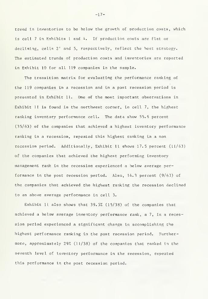
-17-

trend in inventories to be below the growth of production costs, which

is cell 7 in Exhibits 1 and U. If production costs are flat or

declining, cells 2' and 5, respectively, reflect the best strategy.

The estimated trends of production costs and inventories are reported

in Exhibit 10 for all 119 companies in the sample.

The transition matrix for evaluating the performance ranking of

the 119 companies in a recession and in a post recession period is

presented in Exhibit 11. One of the most important observations in

Exhibit 11 is found in the northwest corner, in cell 7, the highest

ranking inventory performance cell. The data show 55.6 percent

(35/63) of the companies that achieved a highest inventory performance

ranking in a recession, repeated this highest ranking in a non

recession period. Additionally, Exhibit 11 shows 17.5 percent (11/63)

of the companies that achieved the highest performing inventory

management rank in the recession experienced a below average per-

formance in the post recession period. Also, 14.3 percent (9/63) of

the companies that achieved the highest ranking the recession declined

to an above average performance in cell 3.

Exhibit 11 also shows that 39.5% (15/38) of the companies that

achieved a below average inventory performance rank, a 7, in a reces-

sion period experienced a significant change in accomplishing the

highest performance ranking in the post recession period. Further-

more, approximately 29% (11/38) of the companies that ranked in the

seventh level of inventory performance in the recession, repeated

this performance in the post recession period.

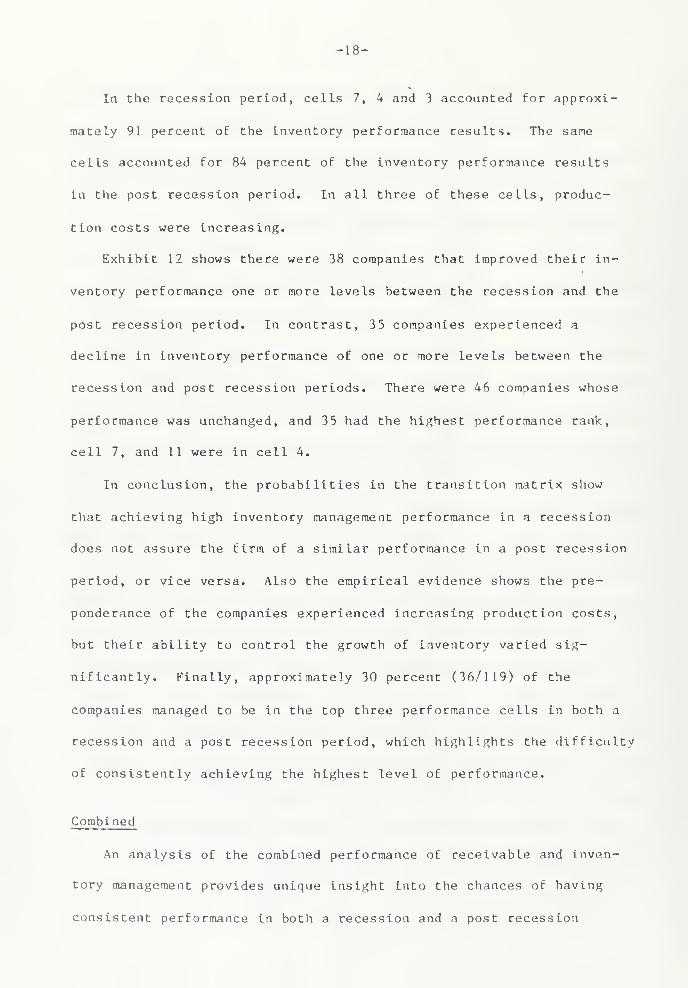
-18-

In the recession period, cells 7, 4 and 3 accounted for approxi-

mately 91 percent of the inventory performance results. The same

cells accounted for 84 percent of the inventory performance results

in the post recession period. In all three of these cells, produc-

tion costs were increasing.

Exhibit 12 shows there were 38 companies that improved their in-

ventory performance one or more levels between the recession and the

post recession period. In contrast, 35 companies experienced a

decline in inventory performance of one or more levels between the

recession and post recession periods. There were 46 companies whose

performance was unchanged, and 35 had the highest performance rank,

cell 7, and 11 were in cell 4.

In conclusion, the probabilities in the transition matrix show

that achieving high inventory management performance in a recession

does not assure the firm of a similar performance in a post recession

period, or vice versa. Also the empirical evidence shows the pre-

ponderance of the companies experienced increasing production costs,

but their ability to control the growth of inventory varied sig-

nificantly. Finally, approximately 30 percent (36/119) of the

companies managed to be in the top three performance cells in both a

recession and a post recession period, which highlights the difficulty

of consistently achieving the highest level of performance.

Combined

An analysis of the combined performance of receivable and inven-

tory management provides unique insight into the chances of having

consistent performance in both a recession and a post recession

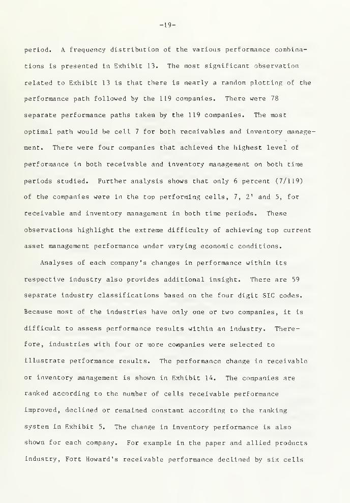
-19-

period. A frequency distribution of the various performance combina-

tions is presented in Exhibit 13. The most significant observation

related to Exhibit 13 is that there is nearly a random plotting of the

performance path followed by the 119 companies. There were 78

separate performance paths taken by the 119 companies. The most

optimal path would be cell 7 for both receivables and inventory manage-

ment. There were four companies that achieved the highest level of

performance in both receivable and inventory management on both time

periods studied. Further analysis shows that only 6 percent (7/119)

of the companies were in the top performing cells, 7, 2' and 5, for

receivable and inventory management in both time periods. These

observations highlight the extreme difficulty of achieving top current

asset management performance under varying economic conditions.

Analyses of each company's changes in performance within its

respective industry also provides additional insight. There are 59

separate industry classifications based on the four digit SIC codes.

Because most of the industries have only one or two companies, it is

difficult to assess performance results within an industry. There-

fore, industries with four or more co«panies were selected to

illustrate performance results. The performance change in receivable

or inventory management is shown in Exhibit 14. The companies are

ranked according to the number of cells receivable performance

improved, declined or remained constant according to the ranking

system in Exhibit 5. The change in inventory performance is also

shown for each company. For example in the paper and allied products

industry, Fort Howard's receivable performance declined by six cells

-20-

between the recession and post recession periods, while the inventory

performance was unchanged. Likewise, International Paper's

receivables and inventory performance improved the maximum of eight

cells, i.e., it went from the worst to best performance between the

two periods.

A casual study of the changes in receivables and inventory perfor-

mance within an industry shows the results vary widely among the

several companies. The joint performance of receivable and inventory

management for companies within an industry is mixed. There are no

performance patterns that arise from this small sample of companies

within the five industries.

V. CONCLUSIONS

A methodology was presented that ranked the performance of

receivable and inventory management. The receivable strategies pur-

sued by a company can be evaluated on the basis of the relative trends

of sales and receivables. Likewise, the trends of production costs

and inventories provide the information needed to evaluate the inven-

tory strategies followed by a company. The methodology makes it

possible to determine the probability of a firm changing its re-

ceivables of inventory performance between two comparative periods.

Also it shows the stability of receivable or inventory strategies

among firms and/or across industries. The contribution of the

methodology is that it provides management, analysts and academic

researchers a tool for better evaluating the contribution of re-

ceivable and inventory management to the value of the firm.

-21-

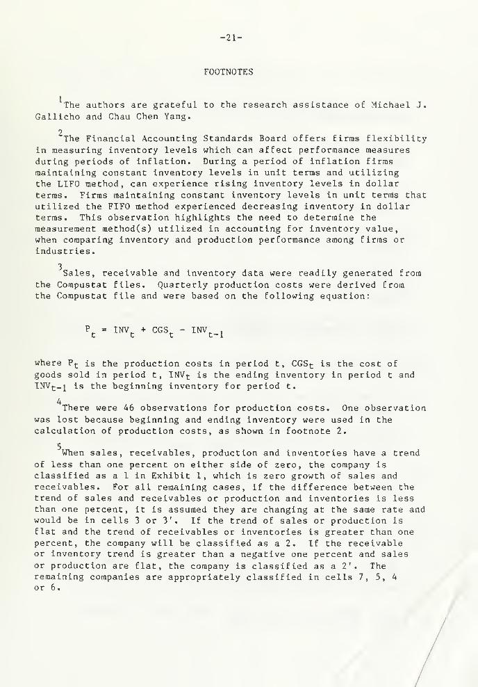
FOOTNOTES

The authors are grateful to the research assistance of Michael J.

Gallicho and Chau Chen Yang.

2The Financial Accounting Standards Board offers firms flexibility

in measuring inventory levels which can affect performance measuresduring periods of inflation. During a period of inflation firmsmaintaining constant inventory levels in unit terms and utilizingthe LIFO method, can experience rising inventory levels in dollarterras. Firms maintaining constant inventory levels in unit ternls that

utilized the FIFO method experienced decreasing inventory in dollarterras. This observation highlights the need to determine the

measurement method(s) utilized in accounting for inventory value,when comparing inventory and production performance among firms or

industries.

3Sales, receivable and inventory data were readily generated from

the Corapustat files. Quarterly production costs were derived fromthe Corapustat file and were based on the following equation:

Pfc

- INV + CGSt

- INVt_j

where P t is the production costs in period t, CGSt i- s tne cost of

goods sold in period t, INV^ is the ending inventory in period t andINV t_i is the beginning inventory for period t.

4There were 46 observations for production costs. One observation

was lost because beginning and ending inventory were used in thecalculation of production costs, as shown in footnote 2.

When sales, receivables, production and inventories have a trend

of less than one percent on either side of zero, the company is

classified as a 1 in Exhibit 1, which is zero growth of sales andreceivables. For all remaining cases, if the difference between thetrend of sales and receivables or production and inventories is lessthan one percent, it is assumed they are changing at the same rate andwould be in cells 3 or 3'. If the trend of sales or production is

flat and the trend of receivables or inventories is greater than onepercent, the company will be classified as a 2. If the receivableor inventory trend is greater than a negative one percent and salesor production are flat, the company is classified as a 2'. Theremaining companies are appropriately classified in cells 7, 5, 4

or 6.

-22-

REFERENCES

1. W. Beranek, Analysis for Financial Decisions , Homewood, IL,

Richard D. Irwin, 1963.

2. George E. P. Box and Gwilym M. Jenkins, Time Series Analysis, Fore -

casting and Control , San Francisco: Holden Day, 1970, revised ed.

1976.

3. George E. P. Box, David A. Pierce and Paul Newbold, "EstimatingTrend and Growth Rates in Seasonal Time Series," Journal of the

American Statistical Association , Vol. 82 (March 1987), pp. 276-282.

4. Michael D. Carpenter and Jack E. Miller, "A Reliable Framework for

Monitoring Accounts Receivable," Financial Management , Vol. 9 (Winter

1979), pp. 37-40.

5. R. M. Cyert, H. J. Davidson, and G. L. Thompson, "Estimation of

Allowance for Doubtful Accounts by Markov Chains," ManagementScience (April 1962), pp. 287-303.

6. R. M. Cyert and G. L. Thompson, "Selecting a Portfolio of CreditRisks by Markov Chains," Journal of Business (January 1968), pp.

39-46.

7. L. P. Freitas, "Monitoring Accounts Receivable," ManagementAccounting (September 1973), pp. 18-21.

8. G. W. Gallinger and P. B. Healey, Liquidity Analysis and

Management , Reading, MA, Addison-Wesley Publishing Company, 1987.

9. George Gallinger and James Ifflander, "Monitoring Accounts Receiv-

able Using Variance Analysis," Financial Management , Vol. 15 (Winter1986), pp. 69-76.

10. James A. Gentry and Jesus M. De La Garza, "A Generalized Model for

Monitoring Accounts Receivable," Financial Management , Vol. 14

(Winter 1985), pp. 28-38.

11. , "Monitoring Payables and Receivables," Working Paper,January 1988, 32 pages.

12.,

"Monitoring Payables and Receivables," Faculty WorkingPaper No. 1358, College of Commerce and Business Administration,Bureau of Economic and Business Research, University of Illinois,May 1987, Revised October 1987.

13. J. J. Hampton and C. L. Wagner, Working Capital Management , NewYork, John Wiley & Sons, 1989.

-23-

14. N. C. Hill and K. D. Riener, "Determining the Cash Discount in the

Firm's Credit Policy," Financial Management (Spring 1979), pp.

68-73.

15. N. C. Hill and W. L. Sartoris, Short-Term Financial Management ,

New York, Macmillan Publishing Company, 1988.

16. H. C. Hunt, "Potential Determinants of Corporate Inventory

Accounting Decisions," Journal of Accounting Research (Autumn

1985), pp. 448-467.

17. J. D. Kallberg and A. Saunders, "Markov Chain Approaches to

Analysis of Payment Behavior of Retail Credit Customers,"Financial Management (Summer 1983), pp. 5-14.

18. Y. H. Kim (editor) and V. Srinivasan (collaborator), Advances in

Working Capital Management , Volum 1, Greenwich, CT , JAI Press

Inc. 1988.

19. G. H. Lawson, "The Mechanics, Determinants and Management of

Working Capital," Managerial Finance (No. 3/4 1984), pp. 12-25.

20. C. J. Lee and D. A. Hsieh, "Choice of Inventory AccountingMethods: Comparative Analyses of Alternate Hypotheses," Journalof Accounting Research (Autumn 1985), pp. 468-485.

21. W. D. Lewellen and R. W. Johnson, "Better Way to Monitor AccountsReceivables," Harvard Business Review (May-June 1972), pp. 101-109.

22. W. D. Lewellen and R. 0. Edmister, "A General Model for AccountsReceivable Analysis and Control," Journal of Financial andQuantitative Analysis (March 1973), pp. 195-206.

23. M. E. Porter, Competitive Strategy: Techniques for AnalyzingIndustries and Competitors , New York, The Free Press, 1980.

24. , Competitive Advantage , New York, The Fress Press, 1985.

25. Alfred Rappaport, Creating Shareholder Value , New York, The FreePress, 1987.

26. William Sartoris and Ned C. Hill, "A Generalized Cash Flow Approachto Short-Term Financial Decisions," Journal of Finance , Vol. 38

(May 1983), pp. 349-360.

27. B. K. Stone, "The Payment Pattern Approach to Forecasting andControl of Accounts Receivable," Financial Management (Autumn

1976), pp. 65-82.

D/496

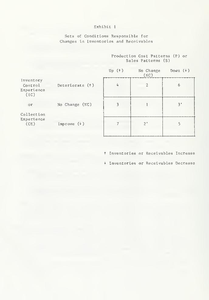
Exhibit 1

Sets of Conditions Responsible for

Changes in Inventories and Receivables

Inventory

ControlExperience

(IC)

or

CollectionExperience

(CE)

Deteriorate (+

)

No Change (NC)

Improve (+

)

Production Cost Patterns (P) orSales Patterns (S)

Up (+) No Change(NC)

Down (+)

4 2 6

3 1 3*

7 V 5

t Inventories or Receivables Increase

+ Inventories or Receivables Decrease

Exhibit 2

Algorithms for Measuring the Pattern EffectsThat Cause a Change in Inventories

Condition Description

1 NC in IC or PC

2 & 2' t or + in IC andNC in PC

( PC .= PC . )

J i

3 & 3' t or 4 in PC and

NC in IU

4 t in IC and 4- in PC

4 in IC and t in PC

t in IC and 4 in PC

4 in IC and t in PC

PatternEffects Algorithm

None

ICE AIC x PC.

'

l

PCPE

PCPE

ICE

JE

PCPE

ICE

JE

PCPE

ICE

PCPE

ICE

A PC X IC.1

A PC X IC.i

AIC X PE.l

A PC X AIC

A PC X AIC

AIC X PC.J

-APC X AIC

APC X AIC

AIC X PC.J

APC X IU.J

AIC X PC.

Legend

PC = production cost patterns

IC = inventory control patterns

NC = no change

t or 4 = see Exhibit I

i = oldest month

j = current month

PCPE = production cost pattern

effect

ICE = inventory control effect

JE = joint effect

Exhibit 3

Examples of Relationships that CauseChanges in Receivables

$

Up(|)

(Best)

4

1?$

Sales Patterns

No Change

(Neutral)

2

Deteriorating( |

)

(Worst)

Down (|)

(Worst)

6

Collection

ExperiencePatterns

No Change

(Neutral)

Improving( \

)

(Best)

Slope of sales in period t

Slope of receivables in period t

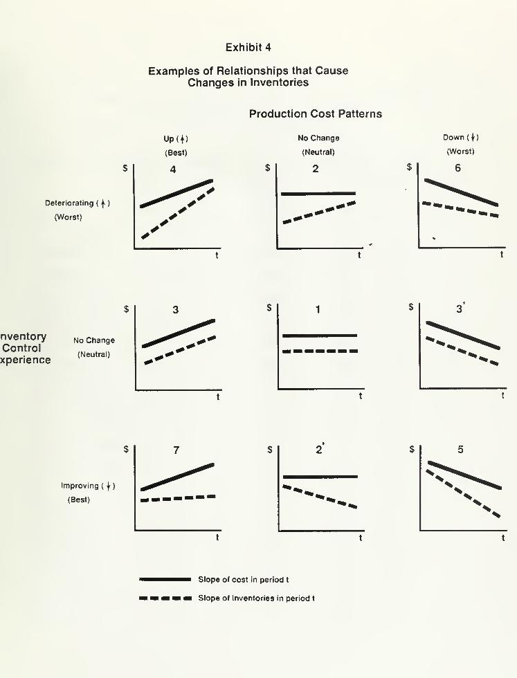
Exhibit 4

Examples of Relationships that CauseChanges in Inventories

Production Cost Patterns

$

Up(|)

(Best)

4 $

No Change

(Neutral)

2

Deteriorating( f

)

(Worst)^~~~~~

Down (f

)

(Worst)

6

nventoryControlxperience

No Change

(Neutral)

Improving( |

)

(Best)

Slope of cost in period t

Slope of inventories in period t

Exhibit 5

Ranking the Performance of Receivable and Inventory Management

Receivables Inventory

Cell in Production Control Cell in Sales CollectionRank Exhibit 4 Performance Performance Exhibit 3 Performance Performance

1 7 best best 7 best best

2 V neutral best 2' neutral best

3 5 worst best 5 worst best

4 3 best neutral 3 best neutral

5 1 neutral neutral 1 neutral neutral

6 3' worst neutral 3' worst neutral

7 4 best worst 4 best worst

8 2 neutral worst 2 neutral worst

9 6 worst worst & worst worst

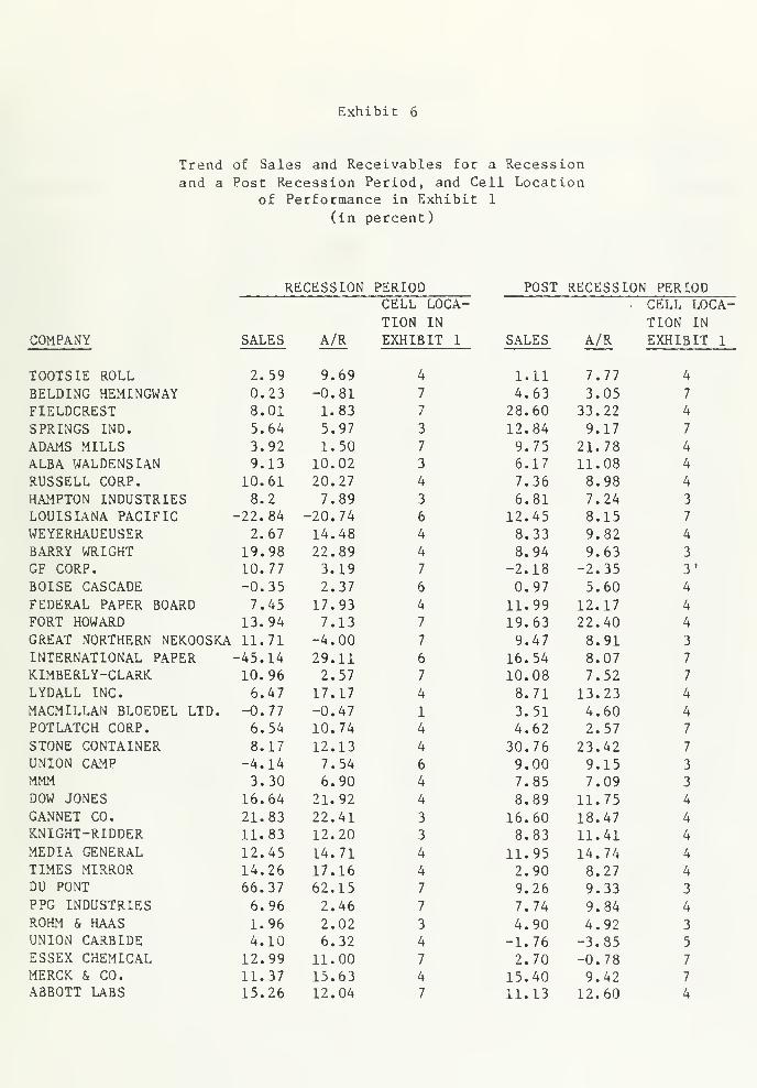
Exhibit 6

Trend of Sales and Receivables for a Recessionand a Post Recession Period, and Cell Location

of Performance in Exhibit 1

(in percent)

RECESSION PERIOD POST RECESSION PERIODCELL LOCA- CELL LOCA-TION IN TION IN

COMPANY SALES A/R EXHIBIT 1 SALES A/R EXHIBIT 1

TOOTS IE ROLL 2.59 9.69 4 1.11 7.77 4

BELDING HEMINGWAY 0.23 -0.81 7 4.63 3.05 7

FIELDCREST 8.01 1.83 7 28.60 33.22 4

SPRINGS IND. 5.64 5.97 3 12.84 9.17 7

ADAMS MILLS 3.92 1.50 7 9.75 21.78 4

ALBA WALDENSIAN 9.13 10.02 3 6.17 11.08 4

RUSSELL CORP. 10.61 20.27 4 7.36 8.98 4

HAMPTON INDUSTRIES 8.2 7.89 3 6.81 7.24 3

LOUISIANA PACIFIC -22.84 -20.74 6 12.45 8.15 7

WEYERHAUEUSER 2.67 14.48 4 8.33 9.82 4

BARRY WRIGHT 19.98 22.89 4 8.94 9.63 3

GF CORP. 10.77 3.19 7 -2.18 -2.35 3'

BOISE CASCADE -0.35 2.37 6 0.97 5.60 4

FEDERAL PAPER BOARD 7.45 17.93 4 11.99 12.17 4

FORT HOWARD 13.94 7.13 7 19.63 22.40 4

GREAT NORTHERN NEKOOSKA 11.71 -4.00 7 9.47 8.91 3

INTERNATIONAL PAPER -45.14 29.11 6 16.54 8.07 7

KIMBERLY-CLARK 10.96 2.57 7 10.08 7.52 7

LYDALL INC. 6.47 17.17 4 8.71 13.23 4

MACMILLAN BLOEDEL LTD. -0.77 -0.47 1 3.51 4.60 4

POTLATCH CORP. 6.54 10.74 4 4.62 2.57 7

STONE CONTAINER 8.17 12.13 4 30.76 23.42 7

UNION CAMP -4.14 7.54 6 9.00 9.15 3

MMM 3.30 6.90 4 7.85 7.09 3

DOW JONES 16.64 21.92 4 8.89 11.75 4

GANNET CO. 21.83 22.41 3 16.60 18.47 4

KNIGHT-RIDDER 11.83 12.20 3 8.83 11.41 4

MEDIA GENERAL 12.45 14.71 4 11.95 14.74 4

TIMES MIRROR 14.26 17.16 4 2.90 8.27 4

DU PONT 66.37 62.15 7 9.26 9.33 3

PPG INDUSTRIES 6.96 2.46 7 7.74 9.84 4

ROHM & HAAS 1.96 2.02 3 4.90 4.92 3

UNION CARBIDE 4.10 6.32 4 -1.76 -3.85 5

ESSEX CHEMICAL 12.99 11.00 7 2.70 -0.78 7

MERCK & CO. 11.37 15.63 4 15.40 9.42 7

ABBOTT LABS 15.26 12.04 7 11.13 12.60 4

Exhibit 6 (continued)

RECESSION PERIOD POST RECESSION PERIODCELL LOCA- CELL LOCA-TION IN TION IN

COMPANY SALES A/R EXHIBIT 1 SALES A/R EXHIBIT 1

BRISTOL-MYERS 10.76 13.35 4 8.87 9.00 3

SMITHK.LINE BECKMAN 30.67 24.15 7 12.21 16.73 4

LAMAUR INC. 31.63 24.09 7 11.47 14.68 4

GUARDSMAN PRODUCTS 7.15 7.32 3 11.64 9.83 7

PRATT & LAMBERT 21.46 14.85 7 9.55 8.65 3

CROMPTON & KNOWLES -1.51 -10.28 5 4.59 21.01 7

FAIRMOUNT CHEMICAL 8.01 9.51 4 -1.58 -4.36 5

DEXTER CORP. -4.44 2.95 6 16.67 8.88 7

FERRO CORP. -2.05 10.69 6 11.31 7.46 7

LUBRIZOL CORP. 11.00 2.70 7 2.18 4.13 4

NALCO CHEMICAL 9.4 14.4 4 6.63 6.49 3

AMERICAN PETROFINA 10.42 10.57 3 7.15 8.36 4

AMOCO CORP. 17.14 15.89 7 4.45 2.13 7

ATLANTIC RICHFIELD 21.4 11.63 4 -2.24 -4.05 5

CHEVRON 17.07 7.52 7 2.77 0.53 7

IMPERIAL OIL 8.7 -23.69 7 -1.15 -0.81 6

KERR-MCGEE 15.94 -4.52 7 -1.47 -4.48 5

MURPHY OIL 20.46 12.43 7 -0.42 -0.55 1

TEXACO 9.54 -7.53 7 2.12 0.85 7

TOSCO CORP. 31.91 31.29 3 -4.60 -15.26 5

UNOCAL 12.37 -15.74 7 3.60 0.92 7

BANDAG INC. 10.01 10.28 3 7.25 7.63 3

CARLISLE 14.94 21.8 4 7.00 7.29 3

COOPER TIRE & RUBBER 12.07 6.78 7 10.98 9.97 7

PANTASOTE 3.83 -2.95 7 2.50 23.94 4

VOPLEX 14.64 14.77 3 9.19 13.88 4

WOLVERINE WORLD WIDE -10.11 20.46 6 -6.05 -2.34 6

BROCKWAY INC. 11.83 9.68 7 6.84 5.23 7

IDEAL BASIC IND. 4.73 10.10 4 -11.37 -23.05 5

LONE STAR IND. 4.89 6.55 4 0.27 -8.55 7

USG CORP. -1.69 -0.93 3' 10.11 3.44 7

NORTON CO. 13.72 2.12 7 3.36 2.91 3

LUKENS INC. 10.27 7.89 7 7.32 7.28 3

ALCAN ALUMINUM 2.71 -3.09 7 6.46 6.36 3

ALUMINUM CO. OF

AMERICA -24.57 -6.53 6 3.59 6.13 4

ARMANDA CORP. 6.44 16.94 7 4.78 2.80 7

VAN DORN CO. 9.70 12.77 4 6.25 7.45 4

SNAPON TOOLS 7.44 12.71 4 7.88 13.80 4

GENERAL HOUSEWARES 11.52 17.27 4 -0.54 1.89 6

HEXCEL CORP. 15.39 13.92 7 16.67 18.54 4

CRANE CO. 5.16 6.12 3 2.59 1.67 3

CUMMINS ENGINE 12.06 13.19 4 9.89 10.26 3

CATERPILLAR 11.51 12.64 4 3.54 8.75 4

SAFE GUARD SCIEN. -17.74 -4.82 6 2.41 3.76 4

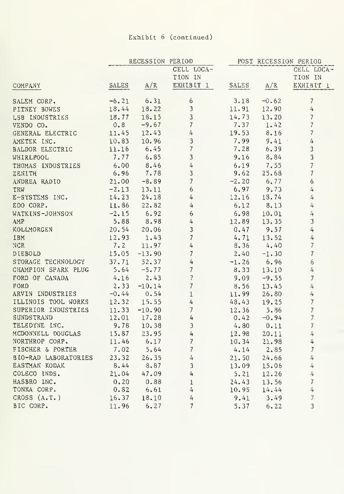
Exhibit 6 (continued)

RECESSION PERIOD POST RECESSION PERIODCELL LOCA- CELL LOCA-TION IN TION IN

COMPANY SALES A/R EXHIBIT 1 SALES A/R EXHIBIT 1

SALEM CORP. -6.21 6.31 6 3.18 -0.62 7

PITNEY BOWES 18.44 18.22 3 11.91 12.90 4

LSB INDUSTRIES 18.77 18.15 3 14.73 13.20 7

VENDO CO. 0.8 -9.67 7 7.37 1.42 7

GENERAL ELECTRIC 11.45 12.43 4 19.53 8.16 7

AMETEK INC. 10.83 10.96 3 7.99 9.41 '

4

BALDOR ELECTRIC 11.16 6.45 7 7.28 6.39 3

WHIRLPOOL 7.77 6.85 3 9.16 8.84 3

THOMAS INDUSTRIES 6.00 8.46 4 6.19 7.55 7

ZENITH 6.96 7.78 3 9.62 25.68 7

ANDREA RADIO 21.00 -8.89 7 -2.20 6.77 6

TRW -2.13 13.11 6 6.97 9.73 4

E-SYSTEMS INC. 14.23 24.18 4 12.16 13.74 4

EDO CORP. 11.86 22.82 4 6.12 8.13 4

WATKINS-JOHNSON -2.15 6.92 6 6.98 10.01 4

AMP 5.88 8.98 4 12.89 13.35 3

KOLLMORGEN 20.54 20.06 3 0.47 9.57 4

IBM 12.93 1.43 7 4.71 13.52 4

NCR 7.2 11.97 4 8.36 4.40 7

DIEBOLD 15.05 -13.90 7 2.40 -1.30 7

STORAGE TECHNOLOGY 37.71 52.37 4 -1.26 6.96 6

CHAMPION SPARK PLUG 5.64 -5.77 7 8.33 13.10 4

FORD OF CANADA 4.16 2.43 7 9.09 -9.55 7

FORD 2.33 -10.14 7 8.56 13.45 4

ARVIN INDUSTRIES -0.44 0.54 1 11.99 26.80 4

ILLINOIS TOOL WORKS 12.32 15.55 4 48.43 19.25 7

SUPERIOR INDUSTRIES 11.33 -10.90 7 12.36 5.86 7

SUNDSTRAND 12.01 17.28 4 0.42 -0.94 7

TELEDYNE INC. 9.78 10.38 3 4.80 0.11 7

MCDONNELL DOUGLAS 15.87 23.95 4 12.98 20.11 4

NORTHROP CORP. 11.46 6.17 7 10.34 21.98 4

FISCHER & PORTER 7.02 5.64 7 4.14 2.85 7

BIO-RAD LABORATORIES 23.32 26.35 4 21.50 24.66 4

EASTMAN KODAK 8.44 8.87 3 13.09 15.06 4

COLECO INDS. 21.04 47.09 4 5.21 12.26 4

HASBRO INC. 0.20 0.88 1 24.43 13.56 7

TONKA CORP. 0.82 6.61 4 10.95 14.44 4

CROSS (A.T.

)

16.37 18.10 4 9.41 3.49 7

BIC CORP. 11.96 6.27 7 5.37 6.22 3

Rank1/Cell

2

1/7

2/2'

3/5

4/3

5/1

eginning 6/3'

eriod -

ecession 7/4

8/2

9/6

%

Exhibit 7

Receivable Performance Matrix of 119 CompaniesDuring a Recession and Post Recession Period

(in percent)

Ending Period - Post RecessionT0TA1

1/7 2/2' 3/5 4/3 5/1 6/3 7/4 8/2 9/6 %

35.7 — 2.4 19.0 2.4 2.4 33.3 — 4.8 100.0

100.0 -- — — — — — — -- 100.0

20.0 — 5.0 25.0 — — 50.0 — — 100.0

33.3 — — — ~ — 56.7 — ~ 100.0

100.0 — -- — — — — — — 100.0

27.5 — 10.0 17.5 — -- 40.0 — 5.0 100.0

41.7 — — 8.3 — — 41.7 — 3.3 100.0

31.9 — 5.0 17.6 .84 .84 39.5 — 4.2 100.0

38 — 6 21 1 1 47 — 5

Performance rank, from Exhibit 5.

Cell location from Exhibit 1.

Exhibit 8

Distribution of Companies Whose Receivable PerformanceImproved, Declined or was Unchanged

Between A Recession and A Post Recession Period

Performance Improved Performance Declined

Number of

Companies •

in the

Number of Number of Sample that Number of

Companies in Levels in Experienced Levels in

the Sample that in Exhibit 5 a Decline Exhibit 5

Improved their that the in their that the

Receivable Performance Receivable PerformancePerformance Improved Performance Declined

1 1 — 1

7 2 5 2

11 3 18 3

5 4 1 4

2 5 1 5

11 6 14 6— 7 — 7

5 8 2 8

TOTAL 41 TOTAL 41

Number of

Sample Companiesthat ExperiencedNo Change in

ReceivablePerformance

Location of

the PerformanceCell in Exhibit 1

16

15

5

1

37

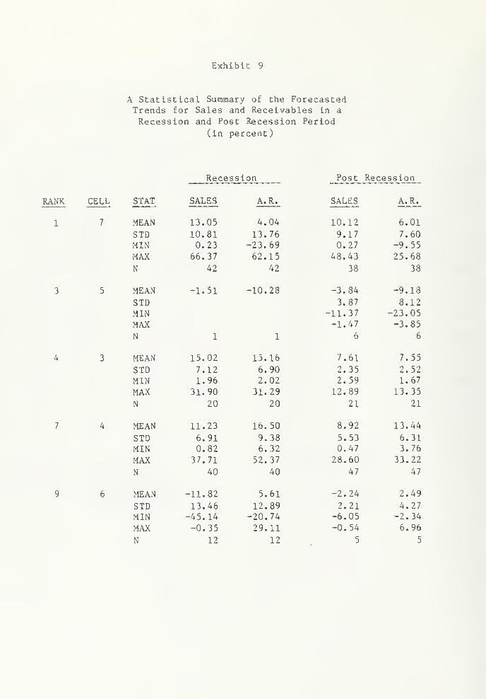
Exhibit 9

A Statistical Summary of the ForecastedTrends for Sales and Receivables in a

Recession and Post Recession Period

(in percent)

Post Recession

RANK CELL STAT SALES A.R. SALES A.R.

Recession

STAT SALES A.R.

MEAN 13.05 4.04

STD 10.81 13.76MIN 0.23 -23.69

MAX 66.37 62.15

N 42 42

MEAN -1.51 -10.28

STDMINMAXN 1 1

MEAN 15.02 15.16

STD 7.12 6.90MIN 1.96 2.02

MAX 31.90 31.29

N 20 20

MEAN 11.23 16.50

STD 6.91 9.38MIN 0.82 6.32MAX 37.71 52.37

N 40 40

MEAN -11.82 5.61

STD 13.46 12.89MIN -45.14 -20.74

MAX -0.35 29.11

N 12 12

10. 12

9. 17

0. 27

48. 43

38

-3. 84

3. 87

11..37-1. 47

6

7,,61

2.,35

2. 59

12.,89

21

8.,92

5.,53

0.,47

28.,60

47

-2.,24

2,,21-6.,05

-0,,54

5

6. 01

7. 60-9. 55

25. 68

38

-9. 18

8. 12

23. 05-3. 85

6

7.,55

2.,52

1.,67

13. 35

21

13.,44

6.,31

3.,76

33.,22

47

2.,49

4.,27

-2.,34

6,.96

5

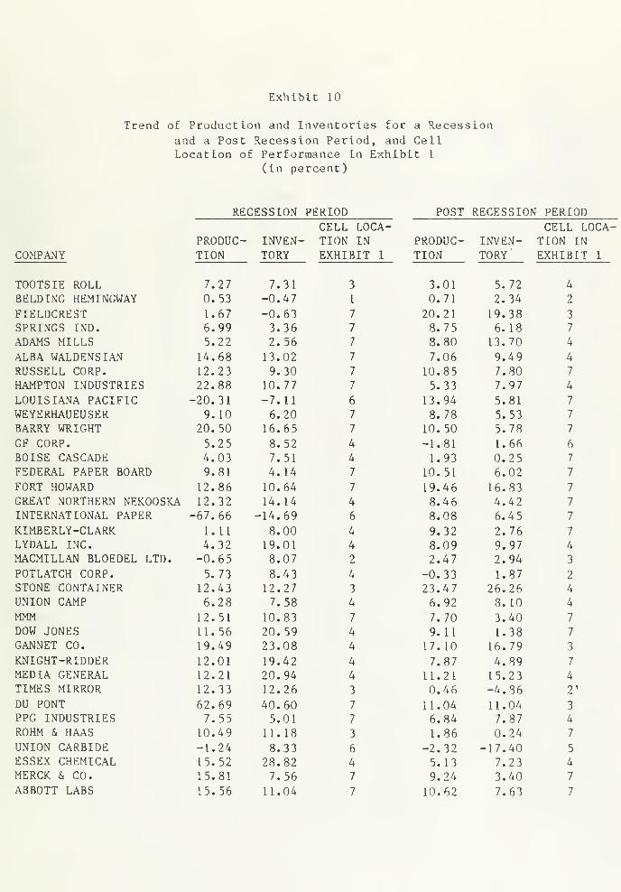
Exhibit 10

Trend of Production and Inventories for a Recessionand a Post Recession Period, and CellLocation of Performance in Exhibit 1

(in percent)

RECESSION PERIOD POST RECESSION PERIODCELL LOCA- CELL LOCA-

PRODUC- INVEN- TION IN PRODUC- INVEN- TION IN

COMPANY TION TORY EXHIBIT 1 TION TORY' EXHIBIT 1

TOOTS IE ROLL 7.27 7.31 3 3.01 5.72 4

BELDING HEMINGWAY 0.53 -0.47 1 0.71 2.34 2

FIELDCREST 1.67 -0.63 7 20.21 19.38 3

SPRINGS IND. 6.99 3.36 7 8.75 6.18 7

ADAMS MILLS 5.22 2.56 7 8.80 13.70 4

ALBA WALDENSIAN 14.68 13.02 7 7.06 9.49 4

RUSSELL CORP. 12.23 9.30 7 10.85 7.80 7

HAMPTON INDUSTRIES 22.88 10.77 7 5.33 7.97 4

LOUISIANA PACIFIC -20.31 -7.11 6 13.94 5.81 7

WEYERHAUEUSER 9.10 6.20 7 8.78 5.53 7

BARRY WRIGHT 20.50 16.65 7 10.50 5.78 7

GF CORP. 5.25 8.52 4 -1.81 1.66 6

BOISE CASCADE 4.03 7.51 4 1.93 0.25 7

FEDERAL PAPER BOARD 9.81 4.14 7 10.51 6.02 7

FORT HOWARD 12.86 10.64 7 19.46 16.83 7

GREAT NORTHERN NEKOOSKA 12.32 14.14 4 8.46 4.42 7

INTERNATIONAL PAPER -67.66 -14.69 6 8.08 6.4 5 7

KIMBERLY-CLARK L. 11 8.00 4 9.32 2.76 7

LYDALL INC. 4.32 19.01 4 8.09 9.97 4

MACMILLAN BLOEDEL LTD. -0.65 8.07 2 2.47 2.94 3

POTLATCH CORP. 5.73 8.43 4 -0.33 1.87 2

STONE CONTAINER 12.43 12.27 3 23.47 26.26 4

UNION CAMP 6.28 7.58 4 6.92 8.10 4

MMM 12.51 10.83 7 7.70 3.40 7

DOW JONES 11.56 20.59 4 9.11 1.38 7

GANNET CO. 19.49 23.08 4 17.10 16.79 3

KNIGHT-RIDDER 12.01 19.42 4 7.87 4.89 7

MEDIA GENERAL 12.21 20.94 4 11.21 15.23 4

TIMES MIRROR 12.33 12.26 3 0.46 -4.86 2'

DU PONT 62.69 40.60 7 11.04 11.04 3

PPG INDUSTRIES 7.55 5.01 7 6.84 7.87 4

ROHM & HAAS 10.49 11.18 3 1.86 0.24 7

UNION CARBIDE -1.24 8.33 6 -2.32 -17.40 5

ESSEX CHEMICAL 15.52 28.82 4 5.13 7.23 4

MERCK & CO. 15.81 7.56 7 9.24 3.40 7

ABBOTT LABS 15.56 11.04 7 10.62 7.63 7

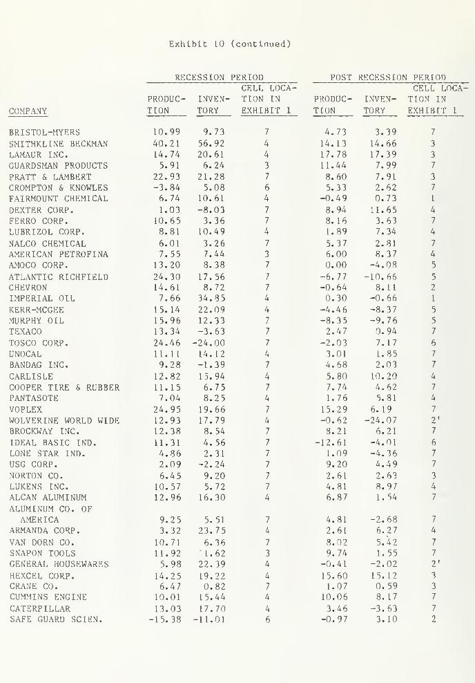
Exhibit 10 (continued)

RECESSION PERIODCELL LOCA-

POST RECESSION PERIODCELL LOCA-

PRODUC- INVEN- TION IN PRODUC- INVEN- TION IN

COMPANY TION TORY EXHIBIT 1 TION TORY EXHIBIT 1

BRISTOL-MYERS 10.99 9.73 7 4.73 3.39 7

SMITHKLINE BECKMAN 40.21 56.92 4 14.13 14.66 3

LAMAUR INC. 14.74 20.61 4 17.78 17.39 3

GUARDSMAN PRODUCTS 5.91 6.24 3 11.44 7.99 7

PRATT & LAMBERT 22.93 21.28 7 8.60 7.91 3

CROMPTON & KNOWLES -3.84 5.08 6 5.33 2.62 7

FAIRMOUNT CHEMICAL 6.74 10.61 4 -0.49 0.73 I

DEXTER CORP. 1.03 -8.03 7 8.94 11.65 4

FERRO CORP. 10.65 3.36 7 8.16 3.63 7

LUBRIZOL CORP. 8.81 10.49 4 1.89 7.34 4

NALCO CHEMICAL 6.01 3.26 7 5.37 2.81 7

AMERICAN PETROFINA 7.55 7.44 3 6.00 8.37 4

AMOCO CORP. 13.20 8.38 7 0.00 -4.08 5

ATLANTIC RICHFIELD 24.30 17.56 7 -6.77 -10.66 5

CHEVRON 14.61 8.72 7 -0.64 8. LI 2

IMPERIAL OIL 7.66 34.85 4 0.30 -0.66 1

KERR-MCGEE 15. 14 22.09 4 -4.46 -8.37 5

MURPHY OIL 15.96 12.33 7 -8.35 -9.76 5

TEXACO 13.34 -3.63 7 2.47 0.94 7

TOSCO CORP. 24.46 -24.00 7 -2.03 7.17 6

UNOCAL 11.11 14. 12 4 3.01 1.85 7

BANDAG INC. 9.28 -1.39 7 4.68 2.03 7

CARLISLE 12.82 15.94 4 5.80 10.20 4

COOPER TIRE & RUBBER 11.15 6.75 7 7.74 4.62 7

PANTASOTE 7.04 8.25 4 1.76 5.81 4

VOPLEX 24.95 19.66 7 15.29 6.19 7

WOLVERINE WORLD WIDE 12.93 17.79 4 -0.62 -24.07 2*

BROCKWAY INC. 12.38 8.54 7 8.21 6.21 7

IDEAL BASIC IND. 11.31 4.56 7 -12.61 -4.01 6

LONE STAR IND. 4.86 2.31 7 1.09 -4.36 7

USG CORP. 2.09 -2.24 7 9.20 4.49 7

NORTON CO. 6.45 9.20 7 2.61 2.63 3

LUKENS INC. 10.57 5.72 7 4.81 8.97 4

ALCAN ALUMINUM 12.96 16.30 4 6.87 1.54 7

ALUMINUM CO. OFAMERICA 9.25 5.51 7 4.81 -2.68 7

ARMANDA CORP. 3.32 23.75 4 2.61 6.27 4

VAN DORN CO. 10.71 6.36 7 8.02 5.42 7

SNAPON TOOLS 11.92 ' 1.62 3 9.74 1.55 7

GENERAL HOUSEWARES 5.98 22.39 4 -0.41 -2.02 2'

HEXCEL CORP. 14.25 19.22 4 15.60 15.12 3

CRANE CO. 6.47 0.82 7 1.07 0.59 3

CUMMINS ENGINE 10.01 15.44 4 10.06 8. 17 7

CATERPILLAR 13.03 17.70 4 3.46 -3.63 7

SAFE GUARD SCIEN. -15.38 -11.01 6 -0.97 3. 10 2

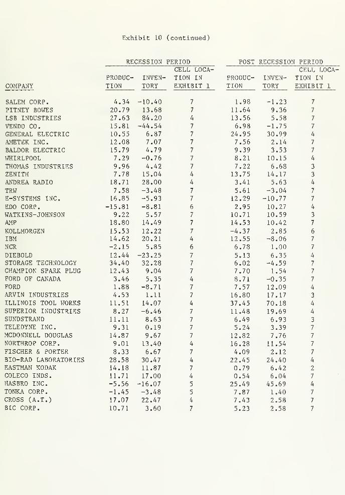
Exhibit 10 (continued)

RECESSION PERIOD POST RECESSION PERIODCELL LOCA- CELL LOCA-

PRODUC- INVEN- TION IN PRODUC- INVEN- TION IN

COMPANY TION TORY EXHIBIT 1 TION TORY— EXHIBIT 1

SALEM CORP. 4.34 -10.40 7 1.98 -1.23 7

PITNEY BOWES 20.79 13.68 7 11.64 9.36 7

LSB INDUSTRIES 27.63 84.20 4 13.56 5.58 7

VENDO CO. 15.81 -44.54 7 6.98 -1.75 7

GENERAL ELECTRIC 10.55 6.87 7 24.95 30.99 4

AMETEK INC. 12.08 7.07 7 7.56 2.14 7

BALDOR ELECTRIC 15.79 4.79 7 9.39 3.53 7

WHIRLPOOL 7.29 -0.76 7 8.21 10.15 4

THOMAS INDUSTRIES 9.96 4.42 7 7.22 6.68 3

ZENITH 7.78 15.04 4 13.75 14.17 3

ANDREA RADIO 18.71 28.00 4 3.41 5.63 4

TRW 7.58 -3.48 7 5.61 -3.04 7

E-SYSTEMS INC. 16.85 -5.93 7 12.29 -10.77 7

EDO CORP. -15.81 -8.81 6 2.95 10.27 4

WATKINS-JOHNSON 9.22 5.57 7 10.71 10.59 3

AMP 18.80 14.49 7 14.53 10.42 7

KOLLMORGEN 15.53 12.22 7 -4.37 2.85 6

IBM 14.62 20.21 4 12.55 -8.06 7

NCR -2.15 5.85 6 6.78 1.00 7

DIEBOLD 12.44 -23.25 7 5.13 6.35 4

STORAGE TECHNOLOGY 34.40 32.28 7 6.02 -4.59 7

CHAMPION SPARK PLUG 12.43 9.04 7 7.70 1.54 7

FORD OF CANADA 3.46 5.35 4 8.71 -0.35 7

FORD 1.88 -8.71 7 7.57 12.09 4

ARVIN INDUSTRIES 4.53 1.11 7 16.80 17.17 3

ILLINOIS TOOL WORKS 11.51 14.07 4 37.45 70.18 4

SUPERIOR INDUSTRIES 8.27 -6.46 7 11.48 19.69 4

SUNDSTRAND 11.11 8.63 7 6.49 6.93 3

TELEDYNE INC. 9.31 0.19 7 5.24 3.39 7

MCDONNELL DOUGLAS 14.87 9.67 7 12.82 7.76 7

NORTHROP CORP. 9.01 13.40 4 16.28 11.54 7

FISCHER & PORTER 8.33 6.67 7 4.09 2.12 7

BIO-RAD LABORATORIES 28.58 30.47 4 22.45 24.40 4

EASTMAN KODAK 14.18 11.87 7 0.79 6.42 2

COLECO INDS. 11.71 17.00 4 0.54 6.04 7

HASBRO INC. -5.56 -16.07 5 25.49 45.69 4

TONKA CORP. -1.45 -3.48 5 7.87 1.40 7

CROSS (A.T.) 17.07 22.47 4 7.43 2.58 7

BIC CORP. 10.71 3.60 7 5.23 2.58 7

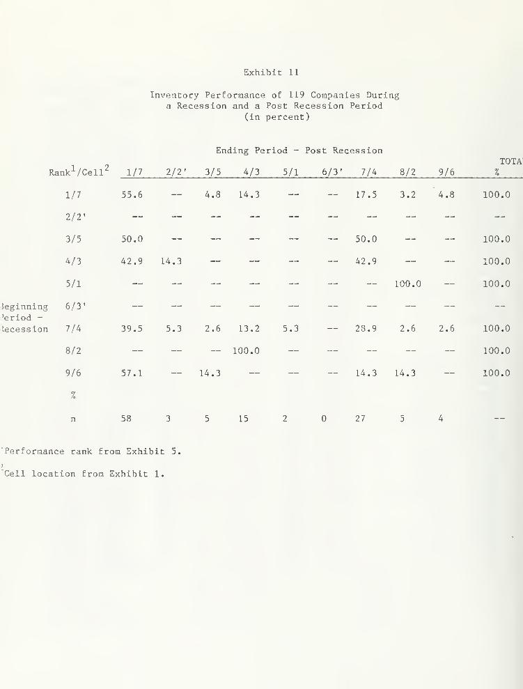
Exhibit 11

Inventory Performance of 119 Companies Duringa Recession and a Post Recession Period

(in percent)

Ending Period - Post Recessiontota:

Rank1 /Cell2

1/7 2/2' 3/5 4/3 5/1 6/3' 7/4 8/2 9/6 %

1/7 55.6 — 4.8 14.3 — — 17.5 3.2 4.8 100.0

3/5 50.0 — — -- — — 50.0 — — 100.0

4/3 42.9 14.3 — -- — — 42.9 -- — 100.0

5/1 — — — — — — ~ 100.0 — 100.0

beginning 6/3' — — — — —'eriod -

lecession 7/4 39.5 5.3 2.6 13.2 5.3 — 28.9 2.6 2.6 100.0

8/2 — — -- 100.0 — — — — — 100.0

9/6 57.1 -- 14.3 — -- — 14.3 14.3 — 100.0

%

n 58 3 5 15 2 27 5 4

"Performance rank from Exhibit 5.

"Cell location from Exhibit 1.

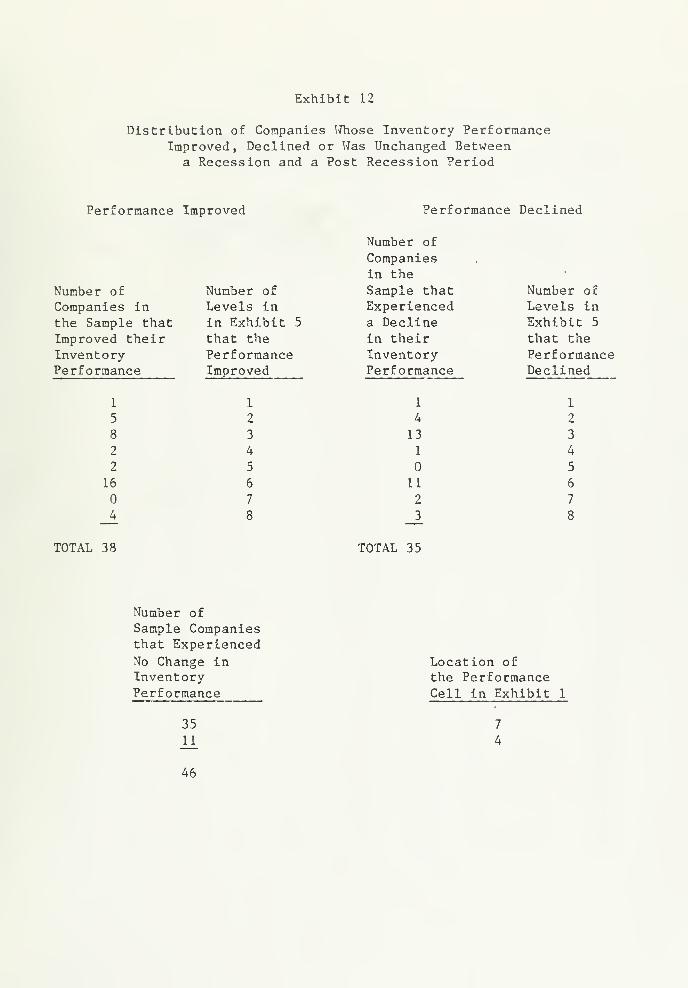
Exhibit 12

Distribution of Companies Whose Inventory PerformanceImproved, Declined or Was Unchanged Between

a Recession and a Post Recession Period

Performance Improved Performance Declined

Number of Number of

Companies in Leve Is in

the Sample that in Exhibit 5

Improved their that the

Inventory PerfiormancePerformance Improved

1 1

5 2

8 3

2 4

2 5

16 6

7

4 8

Number of

Companiesin the

Sample thatExperienceda Declinein theirInventoryPerformance

1

4

13

1

11

2

3

Number of

Levels inExhibit 5

that the

PerformanceDeclined

1

2

3

4

5

6

7

8

TOTAL 38 TOTAL 35

Number ofSample Companiesthat Experienced

No Change inInventoryPerformance

Location ofthe PerformanceCell in Exhibit 1

35

11

46

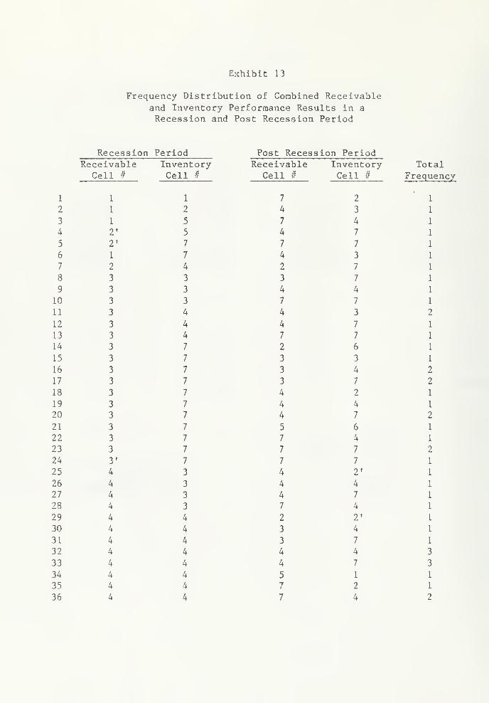
Exhibit 13

Frequency Distribution of Combined Receivableand Inventory Performance Results in a

Recession and Post Recession Period

Recession Period Post Recession PeriodReceivable Inventory

Cell # Cell #

1 1 1

2 1 2

3 1 5

4 2' 5

5 2' 7

6 1 7

7 2 4

8 3 3

9 3 3

10 3 3

11 3 4

12 3 4

13 3 4

14 3 7

15 3 7

16 3 7

17 3 7

18 3 7

19 3 7

20 3 7

21 3 7

22 3 7

23 3 7

24 3' 7

25 4 3

26 4 3

27 4 3

28 4 3

29 4 4

30 4 4

31 4 4

32 4 4

33 4 4

34 4 4

35 4 4

36 4 4

Receivable Inventory TotalCell # Cell #

2

Frequency

7

4 3

7 4

4 7

7 7

4 3

2 7

3 7

4 4

7 7

4 3

4 7

7 7

2 6

3 3

3 4

3 7

4 2

4 4

4 7

5 6

7 4

7 7

7 7

4 2'

4 4

4 7

7 4

2 2'

3 4

3 7

4 4

4 7 3

5 1

7 2

7 4 2

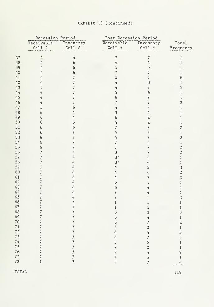
Exhibit 13 (continued)

Recession Period Post Recession PeriodReceivable Inventory Receivable Inventory Total

Cell # Cell //

4

Cell # Cell #

7

Frequency

37 4 7 1

38 4 6 4 4 1

39 4 6 5 5 1

40 4 6 7 7 1

41 4 7 3 7 6

42 4 7 4 3 1

43 4 7 4 7 5

44 4 7 5 6 1

45 4 7 6 7 1

46 4 7 7 7 2

47 5 6 4 7 1

48 6 4 3 4 1

49 6 4 6 2' 1

50 6 6 4 2 1

51 6 6 7 7 2

52 6 7 4 3 1

53 6 7 4 7 2

54 6 7 7 4 1

55 6 7 7 7 2

56 7 4 3 7 2

57 7 4 3' 4 1

58 7 4 3' 6 1

59 7 4 4 3 3

60 7 4 4 4 2

61 7 4 4 7 2

62 7 4 5 5 1

63 7 4 6 4 1

64 7 4 7 4 1

65 7 4 7 7 3

66 7 7 1 3 1

67 7 7 1 5 1

68 7 7 3 3 3

69 7 7 3 4 1

70 7 7 3 7 2

71 7 7 4 3 1

72 7 7 4 4 3

73 7 7 4 7 3

74 7 7 5 5 1

75 7 7 7 2 1

76 7 7 7 4 2

77 7 7 7 5 1

78 7 7 7 7 4

TOTAL 119

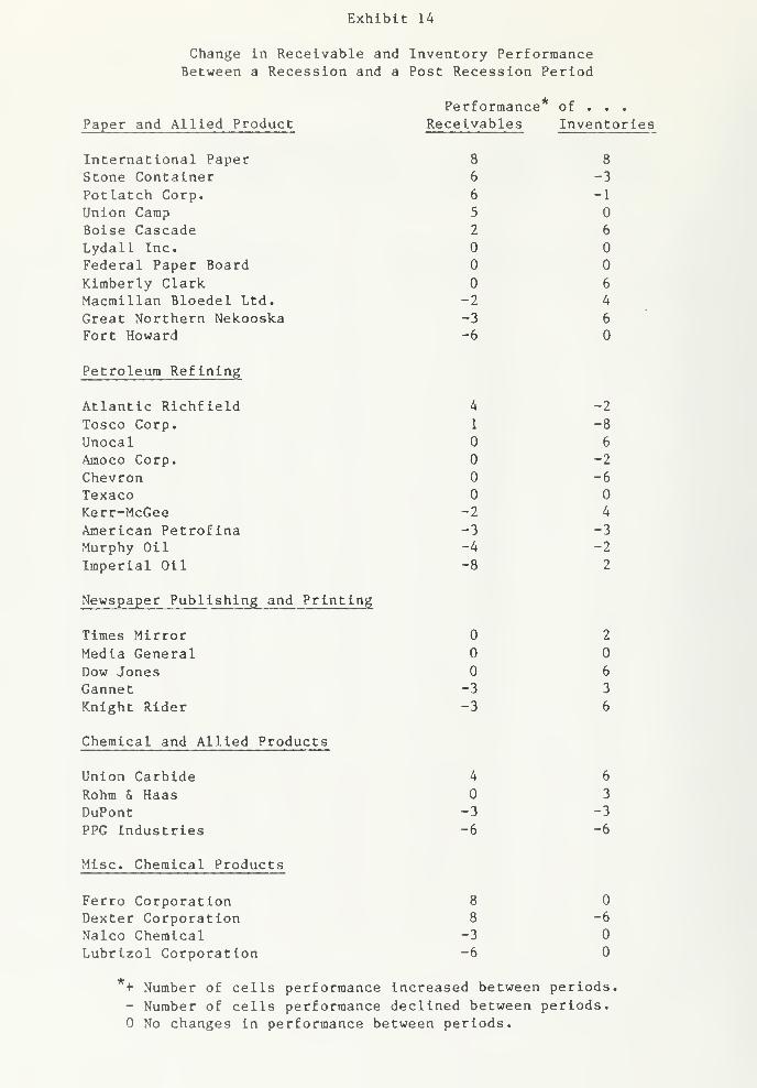
Exhibit 14

Change in Receivable and Inventory PerformanceBetween a Recession and a Post Recession Period

Paper and Allied Product

International PaperStone ContainerPotlatch Corp.

Union CampBoise CascadeLydall Inc.

Federal Paper Board

Kimberly ClarkMacraillan Bloedel Ltd.

Great Northern NekooskaFort Howard

Performance of • • •

Receiva bles Inventories

8 8

6 -3

6 -1

5

2 6

6

-2 4

-3 6

-6

Petroleum Refining

Atlantic RichfieldTosco Corp.

UnocalAmoco Corp.

ChevronTexacoKerr-McGeeAmerican PetrofinaMurphy OilImperial Oil

Newspaper Publishing and Printing

Times MirrorMedia GeneralDow JonesGannetKnight Rider

Chemical and Allied Products

Union CarbideRohm & HaasDuPontPPG Industries

Misc. Chemical Products

Ferro CorporationDexter CorporationNalco ChemicalLubrlzol Corporation

8

8

-3

-6

-6

'+ Number of cells performance Increased between periods- Number of cells performance declined between periods.

No changes In performance between periods.

HECKMANBINDERY

inc.

JUN95'^-To-Pf,^ N. MANCHESTFR

I