evaluation of circumferential indications in …summary report on evaluation of circumferential...

Summary Report

on

Evaluation of Circumferential Indications in Pressurizer Nozzle Dissimilar Metal Welds

at the Wolf Creek Power Plant

to

Nuclear Regulatory Commission Washington DC

by

D. Rudland, D.-J. Shim, H. Xu, and G. Wilkowski

Engineering Mechanics Corporation of Columbus 3518 Riverside Drive

Suite 202 Columbus, OH 43221

Phone/Fax (614) 459-3200/-6800

April 2007

ii

Table of Contents Table of Contents............................................................................................................................ ii List of Figures ................................................................................................................................ iii List of Tables .................................................................................................................................. v 1. Introduction............................................................................................................................ 1 2. Geometry and Loads from Wolf Creek ................................................................................. 1 3. Analysis Methodologies and Assumptions............................................................................ 5

3.1 Loads................................................................................................................................ 5 3.1.1 Operating loads .................................................................................................... 5 3.1.2 Welding residual stress ........................................................................................ 6

3.2 K-solutions..................................................................................................................... 11 3.2.1 Circumferential surface cracks .......................................................................... 13 3.2.2 Circumferential through-wall cracks ................................................................. 15

3.3 Subcritical surface crack growth.................................................................................... 17 3.4 Transition to circumferential through-wall crack .......................................................... 18 3.5 Subcritical through-wall-crack growth .......................................................................... 19 3.6 Critical crack size determination ................................................................................... 19

3.6.1 Determination of appropriate stress-stain curve for dissimilar metal weld analyses .............................................................................................................. 19

3.6.2 Critical circumferential crack size calculations ................................................. 27 3.7 Leak rate analyses .......................................................................................................... 31

3.7.1 The Henry-Fauske flow model in SQUIRT....................................................... 31 3.7.2 Other thermodynamic flow models ................................................................... 31 3.7.3 Crack morphology parameters........................................................................... 33 3.7.4 Other assumptions.............................................................................................. 33

4. Analyses Results .................................................................................................................. 34 4.1 Surge, relief and safety nozzle ....................................................................................... 34 4.2 Hot-leg nozzle................................................................................................................ 37 4.3 Discussion on time to leakage and rupture .................................................................... 38 4.4 Leak rate results ............................................................................................................. 41

5. Comparison to Industry Results........................................................................................... 45 6. Summary .............................................................................................................................. 50 7. References............................................................................................................................ 52

iii

List of Figures Figure 1 Wolf Creek surge nozzle geometry ............................................................................. 3 Figure 2 Wolf Creek safety/relief nozzle geometry................................................................... 3 Figure 3 Normal operating stress from LBB database .............................................................. 5 Figure 4 Welding residual stress for dissimilar welds ............................................................... 7 Figure 5 Prescribed residual stress field from ASME Section XI IWB-3640 analyses ............ 8 Figure 6 Development of 3rd order approximation from ASME welding stress data................ 9 Figure 7 Stress-strain curves for Alloy 182 weld metal at 288C (550F) from Reference 3 ...... 9 Figure 8 Comparison of welding residual stresses for the relief/safety line............................ 10 Figure 9 Application of superposition showing stress intensity simplification....................... 11 Figure 10 Definition of crack-front angle.................................................................................. 13 Figure 11 Comparison of curve fit and FE solutions for influence function G0 at the deepest

point of a circumferential surface crack in pipe with R/t=20.................................... 14 Figure 12 Comparison of Influence functions for smaller diameter pipe.................................. 14 Figure 13 Comparison of Anderson solution and the fir through Sanders solution in

NUREG/CR-4572 for circumferential through-wall cracks. Note G0 is for axial membranes loading only. .......................................................................................... 16

Figure 14 Schematic representation of surface crack evolution ................................................ 18 Figure 15 Definition of effective through-wall crack length..................................................... 19 Figure 16 Stress-strain curves for TP304 at 550F and SA508 at 600F ..................................... 20 Figure 17 Stress-strain curves for Alloy 182 at 550F in as-welded condition .......................... 21 Figure 18 Stress-strain curves for A516Gr70 at 550F............................................................... 21 Figure 19 Case 1 model: Butt weld and focused mesh at the crack front, with a crack at the

center of weld and buttering...................................................................................... 22 Figure 20 Case 2 model: Butt weld and focused mesh at the crack front, with a crack at the

center of the main weld (excluding buttering) .......................................................... 22 Figure 21 Case 3 model: Weld and focused mesh at the crack front, with a crack in the weld,

but very close to the SA508 ...................................................................................... 23 Figure 22 Comparison of J-integral values obtained from LBB.ENG2 and finite element

analysis ...................................................................................................................... 24 Figure 23 Stress-stain curves for the three different materials. Equivalent stress-stain curve is

also shown for comparison........................................................................................ 25 Figure 24 Comparison of J-integral values obtained from NRCPIPE and finite element analysis

considering crack location......................................................................................... 26 Figure 25 Comparison of stress-stain curves for equivalent materials considering crack

location ...................................................................................................................... 26 Figure 26 J-R curve for as-welded Alloy 182 at 550F .............................................................. 27 Figure 27 Critical crack size for surge line nozzle: (a) through-wall crack, (b) surface crack.. 28 Figure 28 Critical crack size for safety/relief nozzles: (a) through-wall crack, (b) surface

crack .......................................................................................................................... 29 Figure 29 Critical crack size for hot-leg nozzle: (a) through-wall crack, (b) surface crack ...... 30 Figure 30 Plot of critical pressure ratio as a function of crack depth to hydraulic diameter ratio

showing when the leak rate models in SQUIRT are valid [19]................................. 32 Figure 31 Time to leakage for surge, relief and safety nozzle................................................... 34 Figure 32 Time from leakage to rupture for surge, relief and safety nozzle assuming through-

wall crack length equal to surface crack length ........................................................ 35

iv

Figure 33 Time from leakage to rupture for surge, relief and safety nozzle assuming through-wall crack area equal to surface crack area ............................................................... 36

Figure 34 Evolution of relief nozzle crack ................................................................................ 36 Figure 35 Time to leakage for assumed flaws in hot-leg nozzle ............................................... 37 Figure 36 Time from leakage to rupture for assumed laws in hot leg nozzle............................ 38 Figure 37 Hoop weld residual stresses for steepest sidehill CRDM nozzle case ...................... 40 Figure 38 Keq versus crack-front angle for an internal crack with a/t=0.25 and 2c=45mm in a

CRDM nozzle............................................................................................................ 40 Figure 39 Cracking predictions for the surge nozzle................................................................. 41 Figure 40 Leak rate versus through-wall crack length for the surge nozzle.............................. 42 Figure 41 Leak rate versus through-wall crack length for the surge nozzle – smaller leak rates

only............................................................................................................................ 43 Figure 42 Leak rate versus through-wall crack length for the safety/relief nozzle ................... 44 Figure 43 Evolution of relief line crack..................................................................................... 48 Figure 44 Comparison of K-solutions for NRC and Industry results ........................................ 49 Figure 45 Investigation of G5 influence function....................................................................... 50

v

List of Tables Table 1 Wolf Creek Indications .................................................................................................... 2 Table 2 Wolf Creek Nozzle geometry .......................................................................................... 4 Table 3 Operating pressure and temperature for Wolf Creek pressurizer nozzles ....................... 4 Table 4 Loads for Wolf Creek pressurizer nozzles....................................................................... 4 Table 5 Stresses for Wolf Creek analyses..................................................................................... 6 Table 6 Material properties for the three different materials and the equivalent material.......... 24 Table 7 Material properties for the four different materials and the equivalent materials ......... 25 Table 8 Critical through-wall crack lengths (inches) for Wolf Creek nozzles ........................... 30 Table 9 Mean values of crack morphology parameters used in SQUIRT (from Refs. 18 and

19 ) ................................................................................................................................. 33 Table 10 Leaking through-wall crack length calculations for the surge nozzle .......................... 42 Table 11 Leaking through-wall crack length calculations for the safety/relief nozzle................ 43 Table 12 Leakage rates for equivalent through-wall crack sizes at first leakage ........................ 44

1

1. Introduction In October 2006, NRC-RES informed Emc2 of circumferential indications that had be located by UT in three of the pressurizer nozzle dissimilar welds at the Wolf Creek power plant. Using Subtask 8.3 in the existing “Alloy 600 Cracking” contract, Emc2 was tasked with analyzing these defects. The purpose of the analyses was to estimate the times to both leakage and rupture for each indication. In addition, the time from crack initiation to the current size was also calculated. This report summaries the Emc2 effort for NRC-RES on the analysis of the Wolf Creek pressurizer nozzle circumferential indications. These scoping analyses were conducted over a very short period of time and were refined several times as the industry provided the technical information required to conduct and refine these analyses. The results presented in this report are from the final scoping analyses. After this introduction, Section 2 presents the geometry and loads given to NRC-RES and Emc2 for the Wolf Creek pressurizer nozzles that contained the circumferential indications. The data given in this section was supplied by either the Wolf Creek plant or EPRI. Section 3 presents the analysis methodologies and assumptions used in conducting these calculations. Section 4 presents the results of the analyses. Section 5 presents a comparison of the results generated in this effort with the results presented by EPRI. Finally, Section 6 presents a summary of this effort.

2. Geometry and Loads from Wolf Creek All of the data given in this section of the report was supplied to Emc2 through Al Csontos (NRC-RES). Prior to conducting the analyses presented in this report, Emc2 was provided several documents from the industry that described the geometry of pressurizer nozzles, the circumferential indications, and the operating loads of interest. Some of these documents contain proprietary information. These documents are listed below:

1.) Draft document, “Docket No. 50-482: Response to Request to Confirm Information Relating to Examination of Pressurizer Nozzle-to-Safe End Dissimilar Metal Welds,” by Terry Garrett. This document included seven enclosures:

a. Enclosure I, LTR-MRCDA-06-198, Rev. 2, “Wolf Creek Information on Pressurizer Nozzles Requested by the NRC,” provides additional information requested by the NRC staff for the performance of flaw evaluations. This was considered a proprietary document.

b. Enclosure II is the non-proprietary version of Enclosure I. c. Enclosure III is Westinghouse’s affidavit on proprietary information entitled,

“Application for Withholding Proprietary Information from Public Disclosure.” d. Enclosure IV contains the “Non-Destructive Examination (NDE) Reports for the

Pre-Weld Overlay Examinations of the Relief Nozzle DM Weld, the “C” Safety Nozzle DM Weld, and the Surge Nozzle DM Weld.”

e. Enclosure V contains “Radiograph Repair Maps for the Surge nozzle DM Weld, the “C” Safety nozzle DM Weld and the Relief nozzle DM Weld.”

2.) A set of NRC slides (PowerPoint format) entitled, “Wolf Creek Pressurizer Weld Cracks.”

2

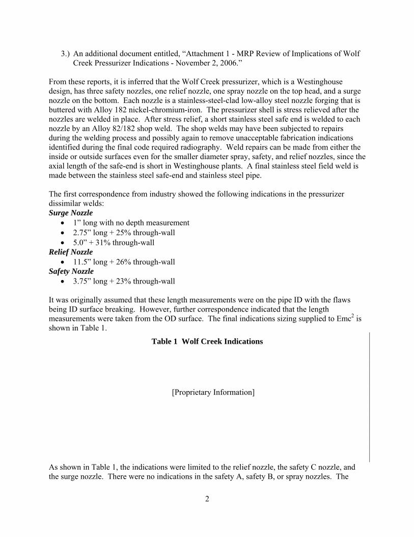
3.) An additional document entitled, “Attachment 1 - MRP Review of Implications of Wolf Creek Pressurizer Indications - November 2, 2006.”

From these reports, it is inferred that the Wolf Creek pressurizer, which is a Westinghouse design, has three safety nozzles, one relief nozzle, one spray nozzle on the top head, and a surge nozzle on the bottom. Each nozzle is a stainless-steel-clad low-alloy steel nozzle forging that is buttered with Alloy 182 nickel-chromium-iron. The pressurizer shell is stress relieved after the nozzles are welded in place. After stress relief, a short stainless steel safe end is welded to each nozzle by an Alloy 82/182 shop weld. The shop welds may have been subjected to repairs during the welding process and possibly again to remove unacceptable fabrication indications identified during the final code required radiography. Weld repairs can be made from either the inside or outside surfaces even for the smaller diameter spray, safety, and relief nozzles, since the axial length of the safe-end is short in Westinghouse plants. A final stainless steel field weld is made between the stainless steel safe-end and stainless steel pipe. The first correspondence from industry showed the following indications in the pressurizer dissimilar welds: Surge Nozzle

• 1” long with no depth measurement • 2.75” long + 25% through-wall • 5.0” + 31% through-wall

Relief Nozzle • 11.5” long + 26% through-wall

Safety Nozzle • 3.75” long + 23% through-wall

It was originally assumed that these length measurements were on the pipe ID with the flaws being ID surface breaking. However, further correspondence indicated that the length measurements were taken from the OD surface. The final indications sizing supplied to Emc2 is shown in Table 1.

Table 1 Wolf Creek Indications

[Proprietary Information]

As shown in Table 1, the indications were limited to the relief nozzle, the safety C nozzle, and the surge nozzle. There were no indications in the safety A, safety B, or spray nozzles. The

3

geometries for the surge and safety/relief nozzles are given in Figure 1 and Figure 2, respectively.


Figure 1 Wolf Creek surge nozzle geometry


Figure 2 Wolf Creek safety/relief nozzle geometry In addition to the figures, the documents listed above gave a table of the overall geometries of the affected nozzles, see Table 2. As shown in this table and Figure 2, the OD of the relief/safety nozzle is not constant across the weld, therefore the average was assumed in the Emc2 analyses. Also note that the wall thickness of the relief/safety nozzles is not consistent between Table 1 and Table 2. The value in Table 1 is listed as nominal; therefore, the calculated value from Table 2 was used in the analyses.

4

Table 2 Wolf Creek Nozzle geometry


In addition to the geometry, the normal operating and faulted loads were supplied to Emc2. Table 3 gives the nominal pressure and temperature for each of the nozzles and Table 4 gives all of the other relevant loads. For the Wolf Creek pressurizer, all of the safety nozzles and the relief nozzle have the same geometry and are designed to the same loads.

Table 3 Operating pressure and temperature for Wolf Creek pressurizer nozzles


Table 4 Loads for Wolf Creek pressurizer nozzles


[

Proprietary Information

5


]

The loads for the Wolf Creek hot-leg nozzle are near the upper bound of the loads found in the LBB database. As shown in Figure 3, for all of the diameters considered in the LBB database, the Wolf Creek hot-leg nozzle loads are relatively high. The same trend holds true for the N+SSE stresses.


Figure 3 Normal operating stress from LBB database

3. Analysis Methodologies and Assumptions In this section of the report, the analysis methodologies and assumptions used in the Emc2 scoping analyses of the Wolf Creek circumferential indications are presented. With the limited time available to perform these analyses, new analysis procedures were not developed, only procedures that existed prior to conducting these analyses were used.

3.1 Loads The loads used in the analyses were taken directly from Table 3 and Table 4 as given in the previous section.

3.1.1 Operating loads The normal operating loads considered included deadweight, thermal and pressure loads. The faulted conditions included the normal loads plus the SSE load. In the case of the surge line, the start-up thermal loads are sometimes higher than the SSE load; however, in this case the SSE loads were higher so they were included in the faulted loads. The SEE loads were not added to the start-up loads due to the low probability of those two transient events happening at the same time. Several assumptions were made in handling the loads:

6

• Pressure stresses were calculated per NB-3652 of ASME code. • The moments and torques were combined into an effective moment per NUREG-6229

and the following equation - 2

22

23

⎟⎟⎠

⎞⎜⎜⎝

⎛++= TMMM yxeff .

• Outer fiber bending stresses were calculated since the K-solutions were defined using this stress, see Section 3.2.

• The loads were assumed to be additive.

The stresses calculated from the loads are given in Table 5.

Table 5 Stresses for Wolf Creek analyses


3.1.2 Welding residual stress Due to the limited time to conduct these scoping analyses, welding residual stresses were not calculated for this effort. A combination of results generated in the past, and modification of the welding stresses in the ASME code were used. Through the LBLOCA contract and for inclusion in PRO-LOCA, a series of welding residual stress solutions were developed [1]. These solutions were developed using standard piping geometries and welding procedures. The details of the analyses are given in Reference 1. From these welding residual stresses, 4th-order polynomial curve fits were used to represent the results. The curve fits are shown in Figure 4. Several piping sizes were assumed in the analyses in Reference 1:

• Hot Leg – 918 mm (36.1 inch) OD with a wall thickness of 86.4mm (3.4 inch) • Surge line – 340 mm (13.4 inch) OD with a wall thickness of 42 mm (1.65 inches) • Spray line – 180.4 mm (7.1 inch) OD with a wall thickness of 26.2 mm (1.03

inches)

The hot-leg analyses were performed with and without a 15% deep, 360 degree ID weld repair. The surge line analysis was only conducted with the 15% deep, 360 degree ID weld repair, and the spray line was only conducted without a weld repair. The 360-degree weld repair, i.e., last–pass ID weld, in the surge line may be representative of the normal welding practice. There has been conflicting information from industry on whether last pass ID welding is standard practice for butt welds. The effects of the fillet weld attaching the thermal sleeve in the surge line weld (see Area 5 in Figure 1) were not included, and would have the tendency to increase the tensile residual stresses on the ID surface. In addition, the proximity of the stainless steel weld is fairly

7

close to the DM weld due to the shorter safe end and could affect the residual stresses in the DMW.

-40

-30

-20

-10

0

10

20

30

40

50

60

0 0.2 0.4 0.6 0.8 1

Nomalized Distance from ID Surface

Res

idua

l Stre

ss, k

si

Hot leg - no repairHot Leg - 360 ID repairSurge - 360 ID repairSpray - no repair

Figure 4 Welding residual stress for dissimilar welds

For use in the Wolf Creek scoping analyses, several assumptions were made regarding welding residual stresses:

• For the surge nozzle, even though the weld stresses assumed were for a slightly different geometry, they were used in analyzing the Wolf Creek surge nozzle. However, analyses were not completed without the 360-degree weld repair*; therefore, since the surge nozzle and hot-leg nozzle result with repair were very similar, the hot-leg nozzle results without repair were used to simulate the surge nozzle stresses without repair.

• The effects of the filler and fillet weld for the thermal sleeve in the surge line nozzle were not included in the analysis. This assumption could lead to non-conservative results since this weld procedure may increase the ID stresses.

• The welding residual stresses for the safety/relief line were based on the ASME Section XI IWB-3460† approximation.

The geometry for the analyzed spray nozzle from Reference 1 is very close to the Wolf Creek safety/relief lines; therefore, this weld residual stress field was initially considered as a candidate to be used in the analyses. The main issue with the spray line welding residual stresses given in Figure 4 is that the ID stresses are compressive, which does not promote PWSCC initiation and * This type of repair, i.e., a 360-deg last pass ID weld, may be typical for this type of butt weld. There is conflicting information from industry on whether this practice is typical or not. † This WRS was for BWR piping and was actually measured from the sensitized HAZ of the lower strength stainless steel pipe and not the higher strength weld material.

8

growth. However, the largest flaw found was in the relief line. It is suspected that the extensive ID welding repairs on the relief nozzle caused this cracking. However, for this size nozzle, welding residual stresses with ID repairs have not been calculated. In fact, until full details of the relief and safety nozzle welding repairs were made available to Emc2, we were unaware that ID repairs could be made on this size pipe. Therefore since there was not enough time to conduct full numerical analyses, the welding residual stresses in the safety/relief lines had to be approximated. The basis of the welding residual stresses for the safety/relief line was the ASME Section XI IWB-3640 approximation as shown in Figure 5. This approximation was developed from a series of experimental measurements [2] of residual stresses in the HAZ of stainless steel welds (not in the weld as per the PWSCC concerns). These measurements were plotted and normalized by the base metal yield strength to give the representations shown in Figure 5. The actual weld metal strength is considerably higher than the base metal strength.

Figure 5 Prescribed residual stress field from ASME Section XI IWB-3640 analyses

The actual experimental data from Reference 2 is normalized and plotted with the representation from Figure 5 in Figure 6. Also shown in Figure 6 is a 3rd order approximation of these results for use in these analyses.

9

-2

-1.5

-1

-0.5

0

0.5

1

1.5

2

0 0.2 0.4 0.6 0.8 1

Distance/Thickness

WR

S/Yi

eld

DataASME >0.75inch3rd order fit >0.75inchLinear <0.75inch

Figure 6 Development of 3rd order approximation from ASME welding stress data

In order to take the trends given in Figure 6 and develop actual stresses relative to the nozzle in question, a corresponding material yield strength had to be chosen. From the EPRI documentation, the assumed yield strength for Alloy 182 weld at temperature was 30 ksi. This value was determined from code values of Alloy 600 base metal at 600F. However, work conducted by Battelle for the NRC [3] has shown that the actual yield strength is much higher for as-welded Alloy 182 weld metal, see Figure 7. Similar strength values for the Alloy 82/182 weld metal are also found in Table 3-1 of MRP-140.

Figure 7 Stress-strain curves for Alloy 182 weld metal at 288C (550F) from Reference 3

10

Figure 7 illustrates that the yield strength of Alloy 182 weld at 288C is approximately 54 ksi. Therefore, for the analyses conducted, a yield strength of 30 ksi (per EPRI) was chosen as one option, and as a second option, a yield strength of 40 ksi was chosen so that the stresses on the ID surface would equal the true yield strength of the weld metal (54 ksi). These adjusted welding stresses are shown in Figure 8. Also shown in this figure are the welding stresses for the surge nozzle with a 15% deep, 360 degree ID weld repair. The comparison shows these trends are similar and add confidence to the assumptions made for the welding stresses in the relief/safety line.

-30

-20

-10

0

10

20

30

40

50

60

0 0.2 0.4 0.6 0.8 1

Nomalized Distance from ID Surface

Wel

d re

sidu

al s

tres

s, k

si

ASME 30ksi yield

ASME 40ksi yield

Surge with 360deg ID repair

ASME Thick section fit to 3rd order polynomial

Figure 8 Comparison of welding residual stresses for the relief/safety line

A couple of points/assumptions about these welding residual stresses: • All of the welding stresses were from axisymmetric analyses and are assumed to constant

around the circumference. • As mentioned earlier, the residual stresses used as a basis for the safety/relief line were

taken experimentally from the HAZ of stainless steel welds. Welding stresses in the weld or butter from dissimilar metal welds may be different.

• The wall thickness of the nozzles in question are greater than 1 inch, therefore the 3rd order fit is more appropriate than the linear fit.

• Due to the limited time for conducting these analyses, no welding analyses were conducted for the Wolf Creek nozzle geometries. Therefore, it is assumed that the results presented are representative for the Wolf Creek nozzles. It is understood that the actual repair history and welding sequence will have a large impact on the welding stresses and the corresponding leakage/rupture results, but the assumptions made here (with the exception of not including the thermal sleeve fillet weld in the surge line) are most likely conservative.

11

3.2 K-solutions In order to make proper crack growth predictions, accurate stress intensity factor solutions are needed. Over the years, many researchers have developed K-solutions for circumferential and axial surface and through-wall cracks in cylindrical vessels based on finite element parametric analyses. Researchers such as Atluri and Kathiresan [4], McGowan and Raymond [5], Raju and Newman [6], Chapuliot and Lacire [7], Bergman [8], and Anderson et al. [9] have all used three-dimensional finite element analyses to infer stress-intensity factor solutions along a semi-elliptical crack front in cylindrical vessels. In all cases, the K-solutions were developed using the principle of superposition. The principle of superposition states that the solution for a multiple load case is equal to the sum of the results from the individual load cases. If one considers an arbitrary body subjected to a far-field normal stress, a traction at the desired crack plane exists. If a crack was present at that location, superposition could be used, as shown in Figure 9, to calculate the stress intensity factor. In short, the stress intensity factor for a far-field load is equal to the stress intensity with a crack-face load equal to the normal stress at the crack location in absence of the crack.

Figure 9 Application of superposition showing stress intensity simplification

In all cases, researchers have run parametric finite element analyses using power-law crack-face pressure to infer stress intensity factors from far-field arbitrary loading. The form of the crack-face pressure is as follows:

n

n axpxp ⎥⎦

⎤⎢⎣⎡=)( (1)

where x is the local coordinate measured from the mouth of the crack, a is the crack depth, and pn is the stress at x = a. If a through-wall stress distribution in an uncracked cylinder can be represented by a polynomial of the form

4

4

3

3

2

210)( ⎥⎦⎤

⎢⎣⎡+⎥⎦

⎤⎢⎣⎡+⎥⎦

⎤⎢⎣⎡+⎥⎦

⎤⎢⎣⎡+=

tx

tx

tx

txx σσσσσσ (2)

and if σ5 represents the global in-plane bending stress at the outer fiber, then when a crack is introduced into this stress field,

12

QaG

taG

taG

taG

taGGK oI

πσσσσσσ ⎟⎟⎠

⎞⎜⎜⎝

⎛+⎥⎦

⎤⎢⎣⎡+⎥⎦

⎤⎢⎣⎡+⎥⎦

⎤⎢⎣⎡+⎥⎦

⎤⎢⎣⎡+= 55

4

44

3

33

2

22110 (3)

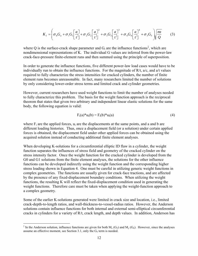
where Q is the surface-crack shape parameter and Gi are the influence functions‡, which are nondimensional representations of K. The individual G values are inferred from the power-law crack-face-pressure finite-element runs and then summed using the principle of superposition. In order to generate the influence functions, five different power-law load cases would have to be individually run to obtain the influence functions. For the magnitude of R/t, a/c, and a/t values required to fully characterize the stress intensities for cracked cylinders, the number of finite element runs becomes unreasonable. In fact, many researchers limited the number of solutions by only considering lower-order stress terms and limited crack and cylinder geometries. However, current researchers have used weight functions to limit the number of analyses needed to fully characterize this problem. The basis for the weight function approach is the reciprocal theorem that states that given two arbitrary and independent linear elastic solutions for the same body, the following equation is valid:

Fi(a)*ui(b) = Fi(b)*ui(a) (4)

where Fi are the applied forces, ui are the displacements at the same points, and a and b are different loading histories. Thus, once a displacement field (or a solution) under certain applied forces is obtained, the displacement field under other applied forces can be obtained using the acquired solution instead of conducting additional finite element analyses. When developing K-solutions for a circumferential elliptic ID flaw in a cylinder, the weight function separates the influences of stress field and geometry of the cracked cylinder on the stress intensity factor. Once the weight function for the cracked cylinder is developed from the G0 and G1 solutions from the finite element analyses, the solutions for the other influence functions can be developed indirectly using the weight function and the corresponding higher stress loading shown in Equation 4. One must be careful in utilizing generic weight functions in complex geometries. The functions are usually given for crack-face tractions, and are affected by the presence of any fixed-displacement boundary conditions. When utilizing the weight functions, the resulting K will reflect the fixed-displacement condition used in generating the weight functions. Therefore care must be taken when applying the weight-function approach to a complex geometry. Some of the earlier K-solutions generated were limited in crack size and location, i.e., limited crack-depth-to-length ratios, and wall-thickness-to-vessel-radius ratios. However, the Anderson solutions contain influence functions for both internal and external semi-elliptical circumferential cracks in cylinders for a variety of R/t, crack length, and depth values. In addition, Anderson has

‡ In the Anderson solution, influence functions are given for both Mx (G5) and My (G6). However, since the analyses assume an effective moment, see Section 3.1, only the G5 term is needed.

13

circumferential through-wall-crack solutions for similar pipe geometries. The Anderson solutions were used in this effort.

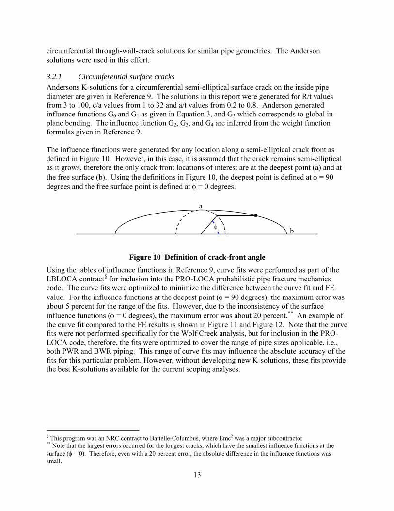
3.2.1 Circumferential surface cracks Andersons K-solutions for a circumferential semi-elliptical surface crack on the inside pipe diameter are given in Reference 9. The solutions in this report were generated for R/t values from 3 to 100, c/a values from 1 to 32 and a/t values from 0.2 to 0.8. Anderson generated influence functions G0 and G1 as given in Equation 3, and G5 which corresponds to global in-plane bending. The influence function G2, G3, and G4 are inferred from the weight function formulas given in Reference 9. The influence functions were generated for any location along a semi-elliptical crack front as defined in Figure 10. However, in this case, it is assumed that the crack remains semi-elliptical as it grows, therefore the only crack front locations of interest are at the deepest point (a) and at the free surface (b). Using the definitions in Figure 10, the deepest point is defined at φ = 90 degrees and the free surface point is defined at φ = 0 degrees.

Figure 10 Definition of crack-front angle

Using the tables of influence functions in Reference 9, curve fits were performed as part of the LBLOCA contract§ for inclusion into the PRO-LOCA probabilistic pipe fracture mechanics code. The curve fits were optimized to minimize the difference between the curve fit and FE value. For the influence functions at the deepest point (φ = 90 degrees), the maximum error was about 5 percent for the range of the fits. However, due to the inconsistency of the surface influence functions (φ = 0 degrees), the maximum error was about 20 percent.** An example of the curve fit compared to the FE results is shown in Figure 11 and Figure 12. Note that the curve fits were not performed specifically for the Wolf Creek analysis, but for inclusion in the PRO-LOCA code, therefore, the fits were optimized to cover the range of pipe sizes applicable, i.e., both PWR and BWR piping. This range of curve fits may influence the absolute accuracy of the fits for this particular problem. However, without developing new K-solutions, these fits provide the best K-solutions available for the current scoping analyses.

§ This program was an NRC contract to Battelle-Columbus, where Emc2 was a major subcontractor ** Note that the largest errors occurred for the longest cracks, which have the smallest influence functions at the surface (φ = 0). Therefore, even with a 20 percent error, the absolute difference in the influence functions was small.

φ

a

b

14

1

1.5

2

2.5

3

3.5

0 0.2 0.4 0.6 0.8 1a/t

G0(

90)

Curve fitc/a=1c/a=2c/a=4c/a=8c/a=16c/a=32

R/t=20

Figure 11 Comparison of curve fit and FE solutions for influence function G0 at the

deepest point of a circumferential surface crack in pipe with R/t=20

0

0.5

1

1.5

2

2.5

3

3.5

0 0.5 1 1.5 2 2.5 3 3.5Fit

Act

ual

G0 r/t=3G5 r/t=3G0 r/t=5G5 r/t=5

Figure 12 Comparison of Influence functions for smaller diameter pipe

As shown in Figure 11, there are several shortcomings of the Anderson solutions. First, the influence functions were only generated for a/t values from 0.2 to 0.8. This becomes a problem when trying to predict crack behavior from initiation to failure. Therefore, several assumptions were made. First, if the cracks grow beyond 80 percent of the wall thickness, it is assumed that the K-solutions can be extrapolated to 100 percent through wall. Secondly, a solution by Chapuliot (Ref. 7) was developed for a/t = 0. These results were incorporated and linear interpolation was used between these values and Anderson’s results at a/t = 0.2.

15

In addition to the semi-elliptical surface crack results, Anderson also generated K solutions for a/c = 0 (360-degree surface crack). Since long surface crack K-solutions are currently not available (c/a>32), it was assumed that for surface cracks with c/a greater than 32, the K solution at the free surface is equal to the K-solution at c/a = 32 and for the deepest point, the K-solution equals that of the K-solution for a/c = 0. This assumption is conservative in the length direction, because as the crack length gets longer, the influence functions (hence the K-solution) at the free surface tends toward zero. By using the K-solution at the free surface equal to c/a = 32, slightly larger crack growths will occur, producing conservative leak times. Finally, Anderson did not generate solutions for Ri/t less than 3. For the relief/safety line, the Ri/t is approximately 2; therefore it was assumed that the curve fits generated could be extrapolated for these smaller Ri/t values. It should also be noted that all the surface crack solutions assume an ideal semi-elliptical shape. Very limited work by Emc2, as presented to the ASME Section XI committee WGPFE, showed that as the surface flaw shape changes to more of a constant depth with semi-circular ends, the K values at the center do not change significantly, but the K-values at the ends of the surface flaw can increase by a factor of 10. Real flaws may be somewhere between elliptical and constant depth flaws with semi-circular ends. Hence the semi-elliptical flaw shape assumption could underestimate the growth in the length direction.

3.2.2 Circumferential through-wall cracks The Anderson K-solutions for an idealized circumferential through-wall crack in a pipe are given in Reference 10. These solutions were generated for R/t values from 1 to 100 and to crack lengths of about 66 percent of the circumference. The solutions were generated for both the inside and outside surface of the through-wall crack, however; only the G0, G1 and G5 influence functions are available. At this time, the weight function solutions for a TWC are not available. Similar through-wall-crack solutions were generated for circumferential through-wall cracks in pipes in Reference 11. These solutions are similar to those generated from Sanders (Ref.12), however, the curve fit used by Sanders forced a G0 value of 1 at a zero crack length. A comparison of the NUREG/CR-4572 results with the Anderson solutions is shown in Figure 13. In this figure, the Anderson solution is averaged though-wall, and is shown to be slightly higher than the solution in NUREG/CR-4572.

16

0

1

2

3

4

5

6

0 20 40 60 80 100

Crack angle, theta

G0

R/t=10R/t=5R/t=3R/t=10R/t=5R/t=3

Symbol - AndersonLine - NUREG/CR-4572

Figure 13 Comparison of Anderson solution and the fir through Sanders solution in

NUREG/CR-4572 for circumferential through-wall cracks. Note G0 is for axial membranes loading only.

The Anderson solution was programmed into the PRO-LOCA code because of the larger range of R/t values available. In Reference 10, the circumferential through-wall-crack K solutions were curve fit and the coefficients were presented for R/t values of 1, 3, 5, 10, 20, 60, and 100. These coefficients were programmed in PRO-LOCA and linear interpolation was used to predict the coefficients for other R/t values. The influence functions on both the inside and outside surface of the through-wall crack are calculated, and then averaged to get the K-solution for circumferential through-wall-crack growth. The subroutine for conducting these calculations in PRO-LOCA was extracted and used in analyzing the Wolf Creek indications. In summary, some of the assumptions for the use of K-solutions include:

• The surface flaws are assumed to be semi-elliptical in shape. It is also assumed that the surface flaws will not change from the elliptical shape during its evolution.

• The use of the K-solution approach is based on the principle of superposition, and all of the loads considered are additive. Redistribution due to plasticity is not accounted for in this analysis.

• The solutions used in this effort are a combination of results from Anderson and Chapuliot that were curve fit over a wide range of R/t and c/a values for inclusion in the PRO-LOCA probabilistic code. It is assumed that the curve fits chosen (exponential and logarithmic) can be used to extrapolate the solutions beyond the range in which they were developed. Some uncertainty exists for pipe geometries and crack sizes not used in the development of the curve fitting.

• The development of the influence and weight functions assumes that the loads applied are not a function of distance from the crack plane and the boundary conditions are consistent with the case being analyzed. Varying from these assumptions can produce incorrect K-solutions. Using this type of analyses with residual stress fields that vary from the crack

plane may produce artificially high K-values due to the redistribution of stresses that may occur as the crack develops in the complex welding residual stress field.

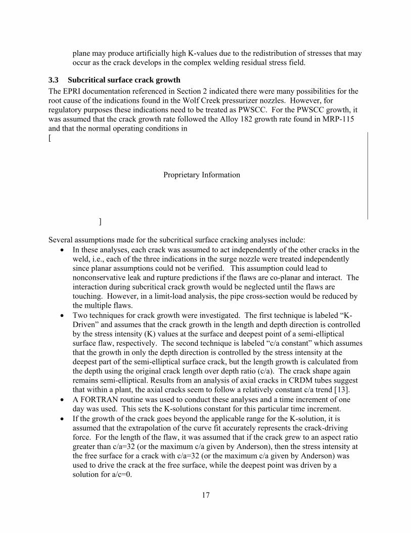
3.3 Subcritical surface crack growth The EPRI documentation referenced in Section 2 indicated there were many possibilities for the root cause of the indications found in the Wolf Creek pressurizer nozzles. However, for regulatory purposes these indications need to be treated as PWSCC. For the PWSCC growth, it was assumed that the crack growth rate followed the Alloy 182 growth rate found in MRP-115 and that the normal operating conditions in [

Severa

•

•

•

•

17


]

l assumptions made for the subcritical surface cracking analyses include: In these analyses, each crack was assumed to act independently of the other cracks in the weld, i.e., each of the three indications in the surge nozzle were treated independently since planar assumptions could not be verified. This assumption could lead to nonconservative leak and rupture predictions if the flaws are co-planar and interact. The interaction during subcritical crack growth would be neglected until the flaws are touching. However, in a limit-load analysis, the pipe cross-section would be reduced by the multiple flaws. Two techniques for crack growth were investigated. The first technique is labeled “K-Driven” and assumes that the crack growth in the length and depth direction is controlled by the stress intensity (K) values at the surface and deepest point of a semi-elliptical surface flaw, respectively. The second technique is labeled “c/a constant” which assumes that the growth in only the depth direction is controlled by the stress intensity at the deepest part of the semi-elliptical surface crack, but the length growth is calculated from the depth using the original crack length over depth ratio (c/a). The crack shape again remains semi-elliptical. Results from an analysis of axial cracks in CRDM tubes suggest that within a plant, the axial cracks seem to follow a relatively constant c/a trend [13]. A FORTRAN routine was used to conduct these analyses and a time increment of one day was used. This sets the K-solutions constant for this particular time increment. If the growth of the crack goes beyond the applicable range for the K-solution, it is assumed that the extrapolation of the curve fit accurately represents the crack-driving force. For the length of the flaw, it was assumed that if the crack grew to an aspect ratio greater than c/a=32 (or the maximum c/a given by Anderson), then the stress intensity at the free surface for a crack with c/a=32 (or the maximum c/a given by Anderson) was used to drive the crack at the free surface, while the deepest point was driven by a solution for a/c=0.

18

3.4 Transition to circumferential through-wall crack Assuming the growing circumferential surface crack does not reach a critical size, when the surface crack penetrates the wall thickness, it will become a circumferential through-wall crack. At first, this crack will have a very small length on the OD (for an ID initiating crack), and a length equal to the surface crack length on the ID. The through-wall crack front will have the shape of the final surface crack. Assuming semi-elliptical shape, the evolution of a surface crack is shown schematically in Figure 14.

Figure 14 Schematic representation of surface crack evolution

There will be a finite time when the crack is growing from Time 2 to Time 3, but it is suspected that this time will be extremely short due to the reduced ligament along the crack front. Unfortunately, the K-solutions for this type of flaw are not readily available, so some approximations need to be made. For these analyses, the following approximations were made.

• When the circumferential surface crack first extends through the wall thickness, the resulting circumferential through-wall crack will be idealized and have an ID length equal to the ID surface crack length. This is the most conservative assumption and provides no time between Time 2 and Time 3 in Figure 14.

• When the circumferential surface crack first extends through the wall thickness, the resulting circumferential through-wall crack will be idealized and have a crack area equal to the final surface crack area at penetration, see Figure 15. Therefore, the idealized ID length of the through-wall will be shorter than the ID length of the surface crack. This approximation may give a better estimate of the time between Time 2 and Time 3.

• If the surface crack reached the critical surface crack size, the surface crack ligament fails and the resulting ID length of the through-wall crack was equal to the ID length of the surface crack.

Time 1

Time 2

Time 3

19

Figure 15 Definition of effective through-wall crack length

3.5 Subcritical through-wall-crack growth The resulting through-wall crack is grown with the same set of loads and assumptions as the surface crack with the following exceptions:

• Due to the limitation of the through-thickness behavior of the Anderson circumferential through-wall crack K-solutions, only the membrane and global bending normal operating loads were used to drive the cracks. Because of this limitation, the higher order through-thickness stress terms were eliminated from the subcritical through-wall crack growth calculations.

• Even though the thermal expansion stresses may be relieved for large through-wall crack growth, these stresses were assumed to subcritically drive the through-wall crack until it reaches critical size. This assumption was based on the results from past efforts in the IPIRG and BINP piping fracture programs.

3.6 Critical crack size determination The critical crack size was determined for both a surface crack and an idealized through-wall crack. The critical crack sizes were calculated using appropriate J-estimation scheme developed for the NRC through programs funded at Battelle [14]. For a surface crack, it has been shown that the most accurate J-estimation scheme for maximum load carrying capacity is SC.TNP, while for a through-wall crack, the most accurate J-estimation scheme is LBB.ENG2. The details of these estimation schemes can be found in Reference 14. These estimation schemes were developed from different analytical approaches and validated by comparisons to numerous full-scale experiments for piping and similar metal welds. The procedures used for the validation were to use the base-metal tensile-strength properties and the weld-metal toughness properties. In the case of Wolf Creek, the cracks reside in the dissimilar metal weld. The difficulty in using these estimation schemes with a dissimilar weld is the determination of the appropriate stress-strain curve necessary for an accurate prediction of the load carrying capacity since there are different strength base metals on each side of the weld. A series of 3D FE analyses were conducted to determine the appropriate stress-strain curve to use in making critical crack size predictions for the DMW flaw evaluations.

3.6.1 Determination of appropriate stress-stain curve for dissimilar metal weld analyses In order to make this assessment, detailed finite element analyses were conducted and compared to the J-estimation scheme results. Due to the limited time for conducting these FE analyses,

20

only one pipe size and one crack type was investigated. The FE analysis results were then used to determine the effective stress-strain curve to use in the J-estimation schemes. The surge nozzle was chosen for the FE study. A 3D FE analysis was carried out to calculate the J-integral for the cracked surge nozzle with 14-inch outer diameter and 1.246-inch wall thickness, subject to an internal pressure of 2,250 psi and various levels of bending moments from 1,000 in-kips to 6,000 in-kips. Four materials were involved in this case study: TP304 stainless steel for the low strength end and the cladding on the ferritic pipe, either SA508 or A516G70 for the ferritic steel end, and Alloy 182 weld metal was used to join the two ends. The stress-strain curves for TP304 and SA508 are shown in Figure 16. The weld metal stress-strain curve was obtained from the pipe fracture mechanics database (PIFRAC), as shown in Figure 17. In the same way, the A516Gr70 stress-strain curve was obtained as the average of three stress-strain curves as shown in Figure 18. The test temperatures were close to but slightly below the pressurizer nozzle. The actual temperature properties would be slightly lower.

0.0

20.0

40.0

60.0

80.0

100.0

120.0

0.00 0.02 0.04 0.06 0.08 0.10 0.12 0.14 0.16 0.18 0.20

Strain, in/in

Stre

ss, k

si

SS304 Abaqus Input: True Stress-Plastic Strain curve

SA508 Abaqus Input: True Stress-Plastic Strain curve

Figure 16 Stress-strain curves for TP304 at 550F and SA508 at 600F

Taking into consideration the symmetry of the geometry and loading, a half pipe was modeled with a circumferential through-wall crack with a half length of 3 inches. Three cases were analyzed. For the first case, the crack was located in the center of the weld metal including the main weld and buttering, as shown in Figure 19. For this case, the safe-end pipe and cladding material was TP304, and the ferritic nozzle was SA508. In the second case, the crack was located in the center of the main weld, excluding the buttering, which is closer to the TP304 as shown in Figure 20. The ferritic nozzle end was SA508. For the third case, the cracking occurred in the weld, but very close (0.1 inch) to the ferritic nozzle end as shown in Figure 21. The safe end was TP304. Both SA508 and A516Gr70 were considered for the ferritic nozzle end. For DMWs in Westinghouse plants, the ferritic steel would be the 508 nozzle material, whereas in CE and B&W the DMWs would contain A516 Gr70 or A106C for the nozzle. For the first two cases, a bevel angle of 22.5 degree was applied. For all three cases, the pipe length

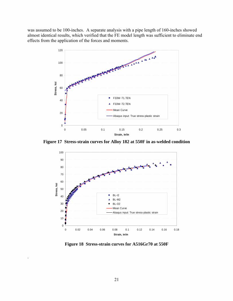
21

was assumed to be 100-inches. A separate analysis with a pipe length of 160-inches showed almost identical results, which verified that the FE model length was sufficient to eliminate end effects from the application of the forces and moments.

0

20

40

60

80

100

120

0 0.05 0.1 0.15 0.2 0.25 0.3

Strain, in/in

Stre

ss, k

si

F33W -T1.TEN

F33W -T2.TEN

Mean Curve

Abaqus input: True stress-plastic strain

Figure 17 Stress-strain curves for Alloy 182 at 550F in as-welded condition

0

10

20

30

40

50

60

70

80

90

100

0 0.02 0.04 0.06 0.08 0.1 0.12 0.14 0.16 0.18

Strain, in/in

Stre

ss, k

si

BL-I2BL-M2BL-O2Mean CurveAbaqus input: True stress-plastic strain

Figure 18 Stress-strain curves for A516Gr70 at 550F

.

22

Figure 19 Case 1 model: Butt weld and focused mesh at the crack front, with a crack at

the center of weld and buttering

Figure 20 Case 2 model: Butt weld and focused mesh at the crack front, with a crack at

the center of the main weld (excluding buttering)

SA508 AL182

TP304

TP304 AL182

SA508

23

Figure 21 Case 3 model: Weld and focused mesh at the crack front, with a crack in the

weld, but very close to the SA508†† In order to determine the stress-strain curve that should be used to make accurate predictions of the crack-driving force, J-integral versus moment curves were obtained for each material using the LBB.ENG2 J-estimation scheme and were compared with the FE result as shown in Figure 22. Note that in this first case, the crack was assumed to be located in the center of the weld. As shown in Figure 22, the J-moment curve obtained from the FE analysis is in between the curves of TP304 and Alloy 182 and is approximately 1/4 of the way from the TP304 curve. Based on these results, the equivalent material properties‡‡, i.e., σy, σu, E, α and n, were determined by weighted average of the material properties of TP304 and Alloy 182 (AL182): Equivalent = TP304*0.75 + AL182*0.25 The equivalent material properties are listed in Table 6 and the corresponding stress-strain curve is plotted in Figure 23. As expected, the stress-strain curve for the equivalent material is slightly higher than the TP304 curve. Using these material properties as input to LBB.ENG2 J-estimation scheme, a J-moment curve was obtained for the equivalent material. As demonstrated in Figure 22, the J-moment curve for the equivalent material is almost identical with the FE result.

†† Limitations with the FE mesh generator prevented this case from having a normal Vee-weld groove. ‡‡ These properties were determined by matching the results from the LBB.ENG2 J-estimation scheme to the detailed FE results.

TP304

SA508 AL182

24

Table 6 Material properties for the three different materials and the equivalent material

Material σy (ksi) σu (ksi) E (ksi) α n TP304 25.33 65.88 24937 7.56 4.07 SA508 34.52 87.17 27023 0.22 6.21 AL182 55.48 84.63 29500 6.54 7.04

Equivalent* 32.87 70.57 26078 7.31 4.81 * Equivalent = TP304*0.75 + AL182*0.25

0

1

2

3

4

0 2000 4000 6000 8000 10000Moment (in-kips)

J (k

ips/

in)

TP304SA508AL182FEA: Crack at weld centerEquivalent

Figure 22 Comparison of J-integral values obtained from LBB.ENG2 and finite element

analysis

To investigate the effect of crack location (within the dissimilar weld) on the equivalent material properties, three additional cases were considered;

- Crack located near TP304 in TP304/AL182/SA508 dissimilar weld - Crack located near SA508 in TP304/AL182/SA508 dissimilar weld - Crack located near A516Gr70 in TP304/AL182/A516Gr70 dissimilar weld

To determine the equivalent material properties for the above three cases, the actual J-integral versus moment curves were obtained from FE analyses. By weighted average of the material properties, i.e., σy, σu, E, α and n, of the two base metals and using these values as inputs to the LBB.ENG2 J-estimation scheme, J-integral versus moment curves were obtained for the equivalent materials as shown in Figure 24. The corresponding material properties are summarized in Table 7. When the crack is located near the TP304 in TP304/AL182/SA508 dissimilar weld, the material properties for TP304 should be used as the equivalent material properties in the J-estimation scheme. When the crack is located near the higher strength base metal (SA508 or A516Gr70) in

25

the dissimilar weld, the equivalent material properties are the average values of the two base metals: Equivalent = TP304*0.5 + SA508 *0.5 or TP304*0.5 + A516Gr70 *0.5 The case with the crack in the center of the TP304/AL182/SA508 dissimilar weld was reanalyzed using the two base metal properties. The equivalent material properties are given as:

Equivalent = TP304*0.6 + SA508 *0.4

0

20

40

60

80

100

120

0 0.1 0.2 0.3 0.4 0.5

Strain

Stre

ss, k

si

TP304SA508AL182Equivalent

Figure 23 Stress-stain curves for the three different materials. Equivalent stress-stain

curve is also shown for comparison. Figure 25 shows the comparison of stress-strain curves for all the equivalent materials along with the original base and weld materials.

Table 7 Material properties for the four different materials and the equivalent materials

Material σy (ksi) σu (ksi) α n E (ksi) Crack location

TP304 25.330 65.880 7.560 4.070 24937 crack close to TP304 (1.0*304)

SA508 34.520 87.170 0.220 6.210 27023

A516Gr70 33.360 69.970 2.170 4.810 26992

AL182 55.480 84.630 6.540 7.040 29500

Eq01 29.006 74.396 4.624 4.926 25771 crack in weld center (0.6*304+0.4*508)

Eq02 29.925 76.525 3.890 5.140 25980 crack close to SA508 (0.5*304+0.5*508)

Eq03 29.345 67.925 4.865 4.440 25965 crack close to A516Gr70 (0.5*304+0.5*516)

26

0

1

2

3

4

0 2000 4000 6000 8000 10000

Moment (in-kips)

J (k

ips/

in)

TP304 SA508A516 AL182FEA: Crack in weld center FEA: Crack close to TP304FEA: Crack close to SA508 FEA: Crack close to A516Eq01: Crack in weld center (0.6*304+0.4*508) Eq02: Crack close to SA508 (0.5*304+0.5*508)Eq03: Crack close to A516 (0.5*304+0.5*516)

Figure 24 Comparison of J-integral values obtained from NRCPIPE and finite element analysis considering crack location

0

20

40

60

80

100

0 0.02 0.04 0.06 0.08 0.1

Strain

Stre

ss, k

si

TP304SA508A516AL182Eq01: Crack in weld center (0.6*304+0.4*508)Eq02: Crack close to SA508 (0.5*304+0.5*508)Eq03: Crack close to A516 (0.5*304+0.5*516)

Figure 25 Comparison of stress-stain curves for equivalent materials considering crack

location

27

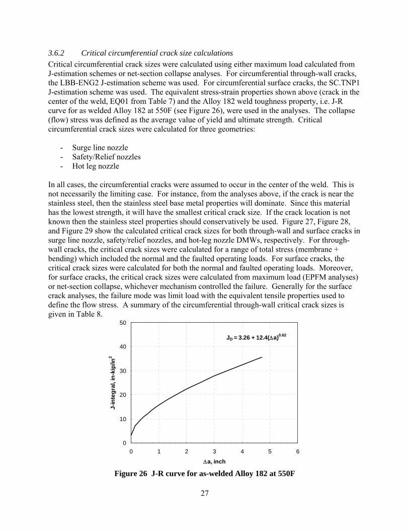
3.6.2 Critical circumferential crack size calculations Critical circumferential crack sizes were calculated using either maximum load calculated from J-estimation schemes or net-section collapse analyses. For circumferential through-wall cracks, the LBB-ENG2 J-estimation scheme was used. For circumferential surface cracks, the SC.TNP1 J-estimation scheme was used. The equivalent stress-strain properties shown above (crack in the center of the weld, EQ01 from Table 7) and the Alloy 182 weld toughness property, i.e. J-R curve for as welded Alloy 182 at 550F (see Figure 26), were used in the analyses. The collapse (flow) stress was defined as the average value of yield and ultimate strength. Critical circumferential crack sizes were calculated for three geometries:

- Surge line nozzle - Safety/Relief nozzles - Hot leg nozzle

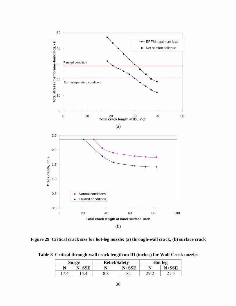
In all cases, the circumferential cracks were assumed to occur in the center of the weld. This is not necessarily the limiting case. For instance, from the analyses above, if the crack is near the stainless steel, then the stainless steel base metal properties will dominate. Since this material has the lowest strength, it will have the smallest critical crack size. If the crack location is not known then the stainless steel properties should conservatively be used. Figure 27, Figure 28, and Figure 29 show the calculated critical crack sizes for both through-wall and surface cracks in surge line nozzle, safety/relief nozzles, and hot-leg nozzle DMWs, respectively. For through-wall cracks, the critical crack sizes were calculated for a range of total stress (membrane + bending) which included the normal and the faulted operating loads. For surface cracks, the critical crack sizes were calculated for both the normal and faulted operating loads. Moreover, for surface cracks, the critical crack sizes were calculated from maximum load (EPFM analyses) or net-section collapse, whichever mechanism controlled the failure. Generally for the surface crack analyses, the failure mode was limit load with the equivalent tensile properties used to define the flow stress. A summary of the circumferential through-wall critical crack sizes is given in Table 8.

0

10

20

30

40

50

0 1 2 3 4 5 6

Δa, inch

J-in

tegr

al, i

n-ki

p/in

2

JD = 3.26 + 12.4(Δa)0.62

Figure 26 J-R curve for as-welded Alloy 182 at 550F

28

0

10

20

30

40

0 5 10 15 20 25Total crack length at ID, inch

Tota

l stre

ss (m

embr

ane+

bend

ing)

, ksi EPFM maximum load

Net section collapse

Normal operating condition

Faulted conditions

(a)

0.0

0.5

1.0

1.5

2.0

0 5 10 15 20 25 30 35 40

Total crack length at inner surface, inch

Cra

ck d

epth

, inc

h

Normal conditionsFaulted conditions

(b)

Figure 27 Critical crack size for surge line nozzle: (a) through-wall crack, (b) surface crack

29

0

10

20

30

40

50

0 2 4 6 8 10 12 14Total crack length at ID, inch

Tota

l stre

ss (m

embr

ane+

bend

ing)




Faulted conditions

(a)

0.0

0.5

1.0

1.5

0.00 4.00 8.00 12.00 16.00


Cra

ck d

epth

, inc

h


(b)

Figure 28 Critical crack size for safety/relief nozzles: (a) through-wall crack, (b) surface crack

30

0

10

20

30

40

50

0 10 20 30 40 50Total crack length at ID, inch

Tota

l stre

ss (m

embr

ane+

bend

ing)



Faulted condition


(a)

0.0

0.5

1.0

1.5

2.0

2.5

0 20 40 60 80 100


Cra

ck d

epth

, inc

h


(b)

Figure 29 Critical crack size for hot-leg nozzle: (a) through-wall crack, (b) surface crack

Table 8 Critical through-wall crack length on ID (inches) for Wolf Creek nozzles

Surge Relief/Safety Hot leg N N+SSE N N+SSE N N+SSE

17.4 14.4 8.8 8.1 29.2 21.5

31

3.7 Leak rate analyses As part of this initial scoping study, two sets of leakage calculations were performed. First, the NRC requested that leaking through-wall crack sizes be calculated for each of the Wolf Creek pressurizer nozzles with indications for leak rates of 0.1, 0.5, 1, 5, 10, 20, and 50 gpm. In addition, leakage calculations were conducted to determine the order of magnitude leakage that would occur from the indications found in the Wolf Creek pressurizer nozzles at the point of first leakage. The leak rates were calculated using the SQUIRT computer code [15,16] developed for the NRC. SQUIRT, which stands for Seepage Quantification of Upsets In Reactor Tubes, is a computer program that predicts the leakage rate for cracked pipes in nuclear power plants. The development of the SQUIRT computer model enables licensing authorities and industry users to conduct the leak-rate evaluations for leak-before-break applications in a more efficient manner. The SQUIRT code also includes technical advances that are not available in other computer codes currently used for leak-rate estimation. The SQUIRT code has been benchmarked against other leak rate codes and validated against experimental results [16,17].

3.7.1 The Henry-Fauske flow model in SQUIRT A review [15] of existing thermal-hydraulic models indicated that the Henry-Fauske model was the best currently available representation of two-phase fluid flow through tight cracks in a piping system. This model allows for non-equilibrium vapor generation rates as the fluid flows through the crack. The rate at which vapor is formed approaches the equilibrium value using an exponential relaxation correlation, with the correlation coefficients determined from the experimental data of Henry. In addition to the uncertainty associated with specifying the non-equilibrium vapor generation rate, other uncertainties in the analysis arise due to incomplete knowledge of the flow path losses, the friction factors for tight cracks, and the potential for particulate plugging.

3.7.2 Other thermodynamic flow models The SQUIRT code has three different thermal-hydraulic flow models depending on the thermodynamic state of the fluid inside the pipe. The default model is the Henry-Fauske two phase model for tight cracks for subcooled liquid as described above. The other two models are as follows.

1. Single-phase liquid model. A model was added to predict the leakage rate through a pipe crack when the fluid inside the pipe is under pressure, but the fluid temperature is below the saturation temperature corresponding to the ambient pressure outside of the pipe. In this case the fluid remains a liquid as it flows through the pipe crack and as it is discharged. This model solves the flow equations associated with non-compressible fluid flow.

2. Superheated single-phase steam model. A model was added to predict the leakage rate

through a pipe crack when the fluid inside the pipe is superheated steam. By definition, superheated steam has a steam quality of 100%. In this case, the fluid remains a gas as it flows through the pipe crack and as it is discharged. This module solves the flow equations associated with compressible gas flow.

32

If the temperature of the fluid inside the pipe is less than or equal to the saturation temperature of the fluid at the ambient pressure, then the single-phase liquid flow model can be used to calculate a leakage rate. Alternatively, if the crack depth (pipe wall thickness) to hydraulic diameter ratio is less than 0.5, then the single-phase liquid model can also be used because the fluid is assumed to pass through the crack as a liquid before it has time to flash to a two-phase mixture. If the temperature of the fluid inside the pipe is greater than the saturation temperature of water at the pipe operating pressure, then the superheated steam fluid flow model may be used to calculate the leakage rate. Under these circumstances, the steam quality is assumed to be 100 percent throughout the crack depth, and the fluid is modeled as a single-phase compressible flow. Finally, if the crack depth (pipe wall thickness) to hydraulic-diameter ratio is greater than 15 (tight crack) and the fluid inside the pipe is a liquid, the fluid will flash to a two-phase mixture at the ambient pressure, and the Henry-Fauske two-phase flow model in SQUIRT may be used to calculate the flow rate. Figure 30 shows the critical pressure ratio as a function of the crack depth (pipe wall thickness) to hydraulic diameter ratio for two-phase flow. This figure also shows the region on the plot where the Henry-Fauske model is valid. Likewise, the figure also shows the region on the plot where the single-phase liquid model may be used to approximate the leakage rate. Finally, the current version of SQUIRT does not have a transitional two-phase flow model to handle pipe cracks with depth (pipe wall thickness) to hydraulic diameter ratios between 0.5 and 15. A sensitivity study was done in a previous study [17] and it was determined that at L/D=15, the single-phase model overpredicted the two-phase flow model by 30% for both large and small leak rates. This is within the normal scatter of leak rate data where the scatter was a factor of 2 (except at very low leak rates). Therefore, it was decided that for conditions where L/D<15, the all-liquid model should be used but the results should be scaled by a factor that would range linearly from 0.7 (at L/D=15) to 1 (at L/D=1).

0

0.1

0.2

0.3

0.4

0.5

0.6

0 5 10 15 20Crack Depth to Hydraulic Diameter Ratio

Henry/Fauske Two-Phase Flow Model for Tight Cracks

Orifice Flow -- Can be approximated with single-phase liquid model

SQUIRT currently does not have a two-phase flow model to simulate this region

Figure 30 Plot of critical pressure ratio as a function of crack depth to hydraulic diameter

ratio showing when the leak rate models in SQUIRT are valid [18]

33

3.7.3 Crack morphology parameters The SQUIRT uses a COD-dependent crack morphology model for leak-rate calculations. This model is described in detail in Reference19. The key crack morphology parameters are:

μL - Local roughness, μG - Global roughness, ntL - Number of turns in flow path when the crack is tight (δ/μG <0.1), KG - Global path deviation factor, ratio of flow path to pipe thickness, and KG+L - Local path deviation factor, ratio of flow path to pipe thickness. The SQUIRT code has three types of cracking mechanisms: IGSCC - Intergranular stress corrosion crack, Fatigue - Fatigue crack, and PWSCC - Primary water stress corrosion crack. Table 9 gives the mean values of the crack morphology parameters for the three different crack mechanisms as determined from cracks removed from service.

Table 9 Mean values of crack morphology parameters used in SQUIRT (from Refs. 18 and 20 )

Crack Morphology Variable IGSCC Fatigue PWSCC§§ μL, μm 4.699 8.814 16.86 μG, μm 80.010 40.513 113.9

ntL, mm-1 28.2 6.73 5.94 KG 1.07 1.017 1.009

KG+L 1.33 1.06 1.243 The effects of the crack-opening displacement on the crack morphology parameters are fully discussed in References 19 and 21.

3.7.4 Other assumptions For these analyses, the following assumptions were necessary in order to make the SQUIRT predictions:

• The equivalent, idealized through-wall crack length was used in all leak-rate predictions, see Figure 15. The K-driven analyses were used in generating the leakage crack lengths.

• Subcooled water was assumed for the surge nozzle analyses, while 100% quality steam was assumed for the relief and safety analyses.

• GE/EPRI analyses [22] was used to calculate the COD in all cases. For the 100% quality steam cases, the current version of SQUIRT does not allow for the calculation of COD (SQUIRT4 module) within the code. Therefore, for these cases, COD was calculated using the NRCPIPE code [23] offline of SQUIRT, then the leak rates were calculated with the SQUIRT2 module.

§§ For PWSCC these values are for cracks that are traveling parallel to the dendritic grain structure, see Reference 20

34

• The COD dependence on crack morphology parameters [19, 21] was used in these analyses.

• The welding residual stress would not affect the COD. • Restraint of pressure induced bending [24] was not accounted for in these analyses.

4. Analyses Results Using the details and assumptions in the previous sections, crack growth analyses were conducted to predict the time to leakage, rupture and the time from initiation to current crack size for all cases. The tables that contain the detailed results of these analyses are given in Appendix A. In addition, leak rate calculations were conducted to predict the leakage from the Wolf Creek indications at through-wall penetration.

4.1 Surge, relief and safety nozzle The times to leakage for all of the cases (except for the hot leg) are shown in Figure 31. As shown in this figure, for every welding residual stress case assumed, there is a significant time until leakage. The minimum case is for the surge nozzle flaw with the 360-degree repair weld assuming constant c/a growth. Even for this case, the time to leakage is over one year. Interestingly, even if no welding residual stress is considered, the surge nozzle flaw will leak after about 1.5 years. For the relief nozzle, the times to leakage range from 2 years to 2.5 years, while for the safety nozzle, the times to leakage range from about 3 years to 8 years.

0.0

1.0

2.0

3.0

4.0

5.0

6.0

7.0

8.0

K-driven c/a constant

Tim

e to

leak

age,

yea

rs

Surge Nozzle with Surge+repair WRSSurge Nozzle with Surge+no repair WRSSurge Nozzle with no WRSRelief Nozzle with ASME WRS - 30ksiRelief Nozzle with ASME WRS - 54ksiRelief Nozzle no WRSSafety Nozzle with ASME WRS - 30ksiSafety Nozzle with ASME WRS - 54ksiSafety Nozzle no WRS

Surge Relief Safety

Surge Relief Safety

Figure 31 Time to leakage for surge, relief and safety nozzle

35

Looking at the time from leakage to rupture, the results are shown in Figure 32. In this figure, the data is plotted for the case that the through-wall crack length at leakage is set equal to the ID surface crack length immediately before the leakage. As shown in this figure, there are many cases where there is no time between leakage and rupture. For instance, for the safety and relief lines, leakage and rupture occur simultaneously when constant c/a crack growth is considered. However, on the other hand, for every case considered, the surge nozzle flaws will leak before rupture.

0.0

1.0

2.0

3.0

4.0

5.0

6.0

7.0

8.0


Tim

e be

twee

n le

akag

e an

d ru

ptur

e, y

ears

Surge Nozzle with Surge+repair WRSSurge Nozzle with Surge+no repair WRSSurge Nozzle with no WRSRelief Nozzle with ASME WRS - 30ksiRelief Nozzle with ASME WRS - 54ksiRelief Nozzle no WRSSafety Nozzle with ASME WRS - 30ksiSafety Nozzle with ASME WRS - 54ksiSafety Nozzle no WRS

Surge Relief Safety Surge Relief Safety

Figure 32 Time from leakage to rupture for surge, relief and safety nozzle assuming

through-wall crack length equal to surface crack length If it is assumed that the through-wall crack area at leakage is identical to the surface crack area at first leakage, the results change slightly, see Figure 33. In this case, for the safety nozzle results, all cases show some time between leakage and rupture. However, for the relief nozzle, no time between leakage and rupture is predicted if welding residual stresses are considered. However, for the relief nozzle, only the K-driven case with no welding residual stress gave margin between leakage and rupture. The relief line can be investigated further by looking at the history of the cracking as shown in Figure 34. In this figure, the size of the original indication in the relief nozzle is shown. The surface crack growth is shown in this figure for all of the welding residual stress fields assumed. Also included in this figure are the critical surface crack sizes at operating conditions, and the critical through-wall crack length. This figure illustrates that for the relief nozzle crack, if residual stresses are considered, the surface flaw will become critical before growing through wall by PWSCC. Since the critical surface crack length is longer than the critical through-wall crack length, the pipe will rupture at first leakage.

36

0.0

1.0

2.0

3.0

4.0

5.0

6.0

7.0

8.0


Tim

e be

twee

n le

akag

e an

d ru

ptur

e, y

ears

Relief Nozzle with ASME WRS - 30ksiRelief Nozzle with ASME WRS - 54ksiRelief Nozzle no WRSSafety Nozzle with ASME WRS - 30ksiSafety Nozzle with ASME WRS - 54ksiSafety Nozzle no WRS

Relief Safety Relief Safety

Figure 33 Time from leakage to rupture for surge, relief and safety nozzle assuming

through-wall crack area equal to surface crack area

0.0

0.5

1.0

0.00 4.00 8.00 12.00 16.00Total crack length at inner surface, inch

a/t

Critical SurfaceCritical TWC30 ksi yield WRS40 ksi yield WRSno WRS

Relief line

Initial flaw size

Figure 34 Evolution of relief nozzle crack

Break Leak

37

The time from initiation to current crack size for all cases are given in Appendix A, but are not discussed here. For these calculations, all of the same inputs and assumptions were used.

4.2 Hot-leg nozzle Even though there were no indications found in the hot-leg nozzle at the Wolf Creek power plant, the NRC wanted to determine the times to leak and rupture for a flaw in the hot leg that was similar to the long flaw found in the relief line. Therefore this hypothetical situation was assessed. Two cases were investigated:

• Assumed flaw #1 - absolute size of Wolf Creek relief flaw - ID Length = 7.7 inch, depth = 0.34 inch

• Assumed flaw #2 - same relative size of Wolf Creek - Length = 47% of circ, depth = 26% of thickness

In all cases in this section, the equivalent through-wall flaw length was assumed at leakage, i.e., the through-wall crack area at leakage is equal to the surface crack area at leakage. Using the loads and critical crack sizes given above, predictions of time to leak and rupture were estimated. The detailed results are given in Appendix A. The times to leakage for the two assumed flaws are given in Figure 35. The results in this figure illustrate that there is at least a one year time period for leakage for even the very long flaw. Interestingly, the results with the hot-leg welding residual stress without the weld repair have slightly longer times than the case without considering welding residual stress, due to the compressive stresses in the residual stress.

0.0

0.5

1.0

1.5

2.0

2.5

3.0

3.5

4.0

4.5

5.0


Tim

e to

leak

age,

yea

rs

Hot leg Nozzle with repair WRS

Hot leg Nozzle with no repair WRSHot leg Nozzle with no WRS

Flaw #1

Flaw #1

Flaw #2Flaw #2

Figure 35 Time to leakage for assumed flaws in hot-leg nozzle

The times between leakage and rupture for the two assumed flaws in the hot-leg nozzle are given in Figure 36. For the case of the analysis assuming PWSCC growth with a constant c/a, there were no cases where leak before break will occur. For the K-driven analyses with the semi-

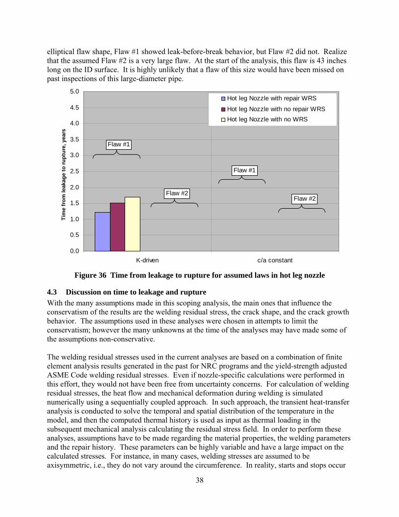
38

elliptical flaw shape, Flaw #1 showed leak-before-break behavior, but Flaw #2 did not. Realize that the assumed Flaw #2 is a very large flaw. At the start of the analysis, this flaw is 43 inches long on the ID surface. It is highly unlikely that a flaw of this size would have been missed on past inspections of this large-diameter pipe.

0.0

0.5

1.0

1.5

2.0

2.5

3.0

3.5

4.0

4.5

5.0


Tim

e fr

om le

akag

e to

rupt

ure,

yea

rs

Hot leg Nozzle with repair WRS

Hot leg Nozzle with no repair WRSHot leg Nozzle with no WRS

Flaw #1

Flaw #1

Flaw #2Flaw #2

Figure 36 Time from leakage to rupture for assumed laws in hot leg nozzle

4.3 Discussion on time to leakage and rupture With the many assumptions made in this scoping analysis, the main ones that influence the conservatism of the results are the welding residual stress, the crack shape, and the crack growth behavior. The assumptions used in these analyses were chosen in attempts to limit the conservatism; however the many unknowns at the time of the analyses may have made some of the assumptions non-conservative. The welding residual stresses used in the current analyses are based on a combination of finite element analysis results generated in the past for NRC programs and the yield-strength adjusted ASME Code welding residual stresses. Even if nozzle-specific calculations were performed in this effort, they would not have been free from uncertainty concerns. For calculation of welding residual stresses, the heat flow and mechanical deformation during welding is simulated numerically using a sequentially coupled approach. In such approach, the transient heat-transfer analysis is conducted to solve the temporal and spatial distribution of the temperature in the model, and then the computed thermal history is used as input as thermal loading in the subsequent mechanical analysis calculating the residual stress field. In order to perform these analyses, assumptions have to be made regarding the material properties, the welding parameters and the repair history. These parameters can be highly variable and have a large impact on the calculated stresses. For instance, in many cases, welding stresses are assumed to be axisymmetric, i.e., they do not vary around the circumference. In reality, starts and stops occur

39

in the welding process as the welder finishes one partial arc pass and starts another. These locations can contain higher stresses than the stresses developed in other parts of the weld. Therefore, cracks in these stress fields may grow more localized than calculated in an axisymmetric stress field, i.e., they may leak before break. On the other hand, it is clear from welding analyses that ID weld repairs (or ID last pass weld procedures) increase the stresses on the ID surface, which promotes PWSCC initiation and growth. In these studies, 15% deep, 360-degree ID weld repairs were assumed; however, typically, partial arc weld repairs and not full circumferential repairs are made. However, there are conflicting opinions from the industry on whether 360-degree, ID, last pass welds are typical for these butt welds. If they are not typical, it can be argued that partial arc weld repairs may lead to leaking flaws in that the length of the flaw will not be much greater than the length of the repair. However, if the last pass ID welds are typical, additional extensive ID repairs can make the assumptions in this analyses non-conservative. For instance, the surge line has a thermal sleeve that is welded to the ID of the nozzle. Since the ID of the dissimilar weld is uneven due to the bevel, the ID is evened out by the addition of Alloy 182 weld metal before the insertion of the thermal sleeve. The addition of this weld metal may radically change the welding stresses. In addition, in some cases, the ID of the safe end did not meet specification, so after welding the dissimilar metal weld, additional stainless steel weld metal was deposited to the ID of the safe end. Again, this will alter the residual stress and may make them worse than the assumptions used in this study. These changes can lead to non-conservative leak and rupture predictions. Also, the crack shape and growth behavior assumptions are very important to the leakage and rupture calculations. Assuming a semi-elliptical crack shape was necessary since the standard solutions generated were all based on this crack shape. However, in these complex stress fields, the cracks will not grow with an elliptical shape. For example, in CRDM analyses conducted by Emc2 for the NRC [25], axial cracks were embedded into complex welding residual stress fields, see Figure 37. Using numerical analysis and standard K-solutions, a comparison of the crack driving force was completed. A sample of these results is shown in Figure 38 and illustrates that the driving force along the semi-elliptical crack front is highest at the point of highest through-thickness stress. Even though the Anderson solutions bounds the results if the highest through thickness stress field is chosen, the shape of the flaw will be far from semi-elliptical and will probably leak before becoming critical.

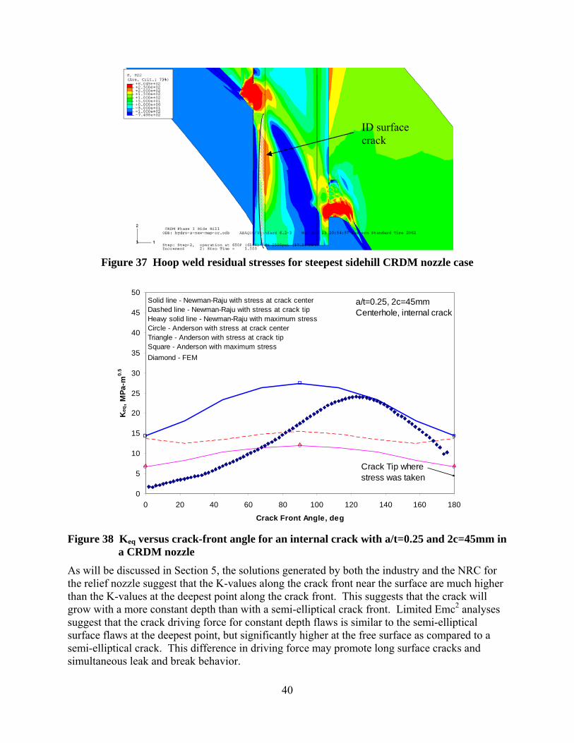
40

Figure 37 Hoop weld residual stresses for steepest sidehill CRDM nozzle case

0

5

10

15

20

25

30

35

40

45

50

0 20 40 60 80 100 120 140 160 180

Crack Front Angle, deg

Keq

, MPa

-m0.

5

a/t=0.25, 2c=45mmCenterhole, internal crack

Crack Tip where stress was taken

Solid line - Newman-Raju with stress at crack centerDashed line - Newman-Raju with stress at crack tipHeavy solid line - Newman-Raju with maximum stressCircle - Anderson with stress at crack centerTriangle - Anderson with stress at crack tipSquare - Anderson with maximum stressDiamond - FEM

Figure 38 Keq versus crack-front angle for an internal crack with a/t=0.25 and 2c=45mm in

a CRDM nozzle As will be discussed in Section 5, the solutions generated by both the industry and the NRC for the relief nozzle suggest that the K-values along the crack front near the surface are much higher than the K-values at the deepest point along the crack front. This suggests that the crack will grow with a more constant depth than with a semi-elliptical crack front. Limited Emc2 analyses suggest that the crack driving force for constant depth flaws is similar to the semi-elliptical surface flaws at the deepest point, but significantly higher at the free surface as compared to a semi-elliptical crack. This difference in driving force may promote long surface cracks and simultaneous leak and break behavior.

ID surface crack

41

In addition, the assumptions of K-driven and constant c/a crack growth analyses may not be appropriate. For instance, if the length and depth of the three surge nozzle cracks are plotted together, an exponential trend can be fit between the data as shown in Figure 39. This trend can be extrapolated back to an initiation size flaw as shown in the figure. Using both the K-driven and constant c/a assumptions***, predictions of the cracking history for one crack can be made. If it assumed that the conditions are similar around the circumference, then each of the three cracks in the surge nozzle would have the same cracking history. From the results shown in Figure 39, the K-driven analysis under predicts the cracking behavior, while the constant c/a over predicts the cracking behavior. If it is assumed that the length of the surface crack grows faster than the rate driven by the crack tip K-solution, better predictions are made. For instance, an acceleration factor of about 5 on the crack length growth makes the best predictions of the surge nozzle cracks. However, as shown in Figure 39, the trend does not appear constant with crack depth, i.e., the length growth appears faster for deeper cracks. Clearly the behavior for the pressurizer nozzle cracks is bound by the K-driven and constant c/a analyses. Overall, the assumptions made for this quick scoping analysis is believed to have reasonable bounds and were selected to reasonably limit the conservatisms in the analyses.

y = 0.3691e4.9914x

0

1

2

3

4

5

6

0 0.1 0.2 0.3 0.4 0.5 0.6

Crack Depth, inch

Cra

ck L

engt

h, in

ch

Surge cracksK-driven2 on length7 on lengthc/a=6

Figure 39 Cracking predictions for the surge nozzle

4.4 Leak rate results Calculations of through-wall crack length were made for each nozzle geometry and loading conditions for leakages ranging from 0.1 to 50 gpm. Since the NRC requested leaking crack

*** Assuming semi-elliptical shape

42

sizes at certain leak rates, the SQUIRT4††† module was used to generate the crack lengths in the surge nozzle for a variety of leakage rates as shown in Table 10.

Table 10 Leaking through-wall crack length calculations for the surge nozzle

Leak Rate, gpm 0.1 0.5 1 5 10 20 50 Through-wall crack length, inch 2.1 3.8 5.0 8.8 10.8 12.2 13.5

These results are shown graphically in Figure 40. Also shown in this figure are two curve fits to these results. The solid line represents the best curve fit for all of the data, while the dashed line represents the best fit for the crack length data less than 10 inches. Limiting the data to a crack length of 10 inches and a leak rate of 6 gpm, a comparison of the two curve fits for the lower leak rates is shown in Figure 41. Clearly, the curve fit represented by the dashed line fits the data better for the smaller crack lengths.

0

2

4

6

8

10

12

14

0 10 20 30 40 50 60

Leak Rate, gpm

Cra

ck L

engt

h, in

ch

Surge NozzleSubcooled Water

Figure 40 Leak rate versus through-wall crack length for the surge nozzle

††† SQUIRT4 module is used to make predictions of crack length given a leak rate. Using the GE/EPRI scheme and the input loads, it iterates on crack length until the requested leak rate is calculated. This module is only available for two-phase flow conditions.

43

0

1

2

3

4

5

6

7

8

9

10

0 1 2 3 4 5 6

Leak Rate, gpm

Cra

ck L

engt

h, in

ch

Surge NozzleSubcooled Water

Figure 41 Leak rate versus through-wall crack length for the surge nozzle – smaller leak

rates only

For the safety and relief nozzle cases, the SQUIRT2‡‡‡ module was used since the SQUIRT4 module is unavailable for 100% quality steam. In this case, the COD was calculated using the NRCPIPE code and the GE/EPRI estimation scheme. Since it is extremely labor intensive to calculate the crack length at a particular leak rate using the SQUIRT2 module, several arbitrary crack lengths were chosen, leak rates were calculated and a curve fit was used to interpolate the results. The results from this effort are shown in Table 11 and Figure 42.

Table 11 Leaking through-wall crack length calculations for the safety/relief nozzle

Leak Rate, gpm 0.1 0.5 1 5 10 20 50 Through-wall crack length, inch 2.4 4.6 5.5 7.7 8.6 9.5 10.7

‡‡‡ The SQUIRT2 module is used when the COD and crack length are known. The COD must be calculated from the loads in a separate calculation.

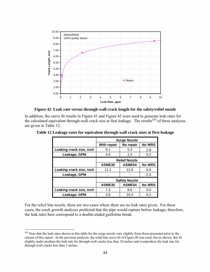
44

0.00

1.00

2.00

3.00

4.00

5.00

6.00

7.00

8.00

9.00

10.00

0 1 2 3 4 5 6 7 8 9 10

Leak Rate, gpm

Cra

ck L

engt

h, in

ch

Steam

Safety/Relief100% quality Steam

Figure 42 Leak rate versus through-wall crack length for the safety/relief nozzle

In addition, the curve fit results in Figure 41 and Figure 42 were used to generate leak rates for the calculated equivalent through-wall crack size at first leakage. The results§§§ of these analyses are given in Table 12.

Table 12 Leakage rates for equivalent through-wall crack sizes at first leakage

Surge Nozzle With repair No repair No WRS

Leaking crack size, inch 8.1 5.3 2.8 Leakage, GPM 4.0 1.2 0.2

Relief Nozzle ASME30 ASME54 No WRS

Leaking crack size, inch 11.1 12.6 6.6 Leakage, GPM - - 2.3

Safety Nozzle ASME30 ASME54 No WRS

Leaking crack size, inch 7.3 8.6 3.0 Leakage, GPM 3.8 10.4 0.2

For the relief line nozzle, there are two cases where there are no leak rates given. For these cases, the crack growth analyses predicted that the pipe would rupture before leakage; therefore, the leak rates here correspond to a double-ended guillotine break.

§§§ Note that the leak rates shown in this table for the surge nozzle vary slightly from those presented prior to the release of this report. In the previous analyses, the solid line curve fit of Figure 40 was used, but as shown, this fit slightly under predicts the leak rate for through-wall cracks less than 10 inches and overpredicts the leak rate for through-wall cracks less than 3 inches.

45

It should be noted that these results do not account for a couple of factors that may decrease the leakage from these cracks. The first factor is the restraint of pressure-induced bending. In piping systems, the restraint of the piping due to other structures, i.e., hangers, the vessel, etc., may limit the amount of rotation that could occur due to a through-wall crack in a pressurized pipe. This limit of the rotation will also limit the crack-opening displacement and thus the leakage. As mentioned earlier, the analyses used to calculate COD was the GE-EPRI scheme, which assumes that the crack pipe is free to rotate, and thus maximizes the COD. In Reference 24, detailed finite element analyses were conducted with different degrees of pipe restraint to quantify its affect on the COD. From these efforts, analytical expressions were developed with correction factors on the COD as a function of the location of restraints from the crack plane. However, in order to use these analyses, detailed knowledge of the pipe system layout is needed. In addition, the through-thickness welding residual stresses may also limit the COD. As discussed in Reference 24, welding residual stresses calculated for a stainless steel weld rotate the crack faces and limited the leakage. This effect was a function of not only the residual stress, but also the geometry and total stress level. The severity of this effect was small, but if its effect is neglected, the results could lead to non-conservative leakage predictions.

5. Comparison to Industry Results After presenting the results of these analyses to the industry at a public meeting, the industry completed a series of analyses aimed at refining the scoping analysis presented in this report. Those results are summarized in a draft white paper document submitted to the NRC [26]. The purpose of this section of the report is to compare the results generated in this scoping analysis to the refined results generated by the industry. This section is not meant to be a comprehensive review of the white paper and its conclusions. Therefore, the main focus of this comparison will be on Section 5 of the white paper. However, a few comments on other relevant sections will also be made. Section 3 – Review of Wolf Creek inspection and root cause analysis findings This was a very informative section about the actual inspection findings and the detailed repair history of these nozzles. This data was not available to the NRC or Emc2 during this scoping analysis. What was interesting was the number of repairs that had been performed on these smaller diameter nozzles. For instance, the surge nozzle weld had five weld repairs with one being a full grind out of the internal thermal sleeve due to the omission of an inspection after completion of the 4th repair. For the relief nozzle, ten weld repairs were completed with five of those repairs being conducted on the ID surface after the post-weld heat treatment. These repairs included both buttering and welding repairs, as well as this deposition of stainless steel on the ID of the safe end. Clearly these nozzles had highly complex welding residual stress fields due to the number of repairs. Section 4 – Predicted growth of Wolf Creek flaws without mitigation In this section of the white paper, analyses were conducted with 5% deep, 360-degree surface flaws using the residual stresses presented in this report. The purpose of these analyses was to show that the driving force for a long surface crack is not constant along the crack front and will be highest at the point of maximum moment. The argument is that this behavior will lead to a leaking flaw before rupture. However, the authors failed to consider the criticality of these

46

surface cracks. If the bending moment dominates, then a long surface crack will tend to grow more at the point of maximum moment than minimum moment, however, the criticality of that flaw can not be judged until the critical surface crack size is calculated. These types of calculations need to be conducted numerically, since the estimation schemes for making critical crack size predictions are based on either constant depth flaws, or semi-elliptical flaws [14]. Section 6 Critical flaw size and leakage detection before risk of rupture This section investigates the calculation of the critical flaw sizes for the Wolf Creek pressurizer nozzles. The presented critical through-wall flaws from the analyses in MRP-113 for similar nozzles were about 30% less than those calculated in this effort. This is a reasonable comparison since MRP-113 assumed a lower yield strength for the Alloy 182 material (actually code minimum for alloy 600 at operating temperatures) and worst case loading for the critical crack sizes, i.e., dead weight, pressure, thermal expansion, thermal stratification, and SSE loads, while in the Emc2 analyses, only normal operating loads were used for the critical crack size and time to leakage calculations. However, for the specific calculations of critical flaw size in the white paper, a thick-walled limit-load solution, the same material properties and the Wolf Creek specific load-controlled stresses were assumed. In this case, as shown in Figure 6.1a of the white paper, the critical through-wall sizes were reasonable close to the results from the Emc2 analyses. Since different loads, material properties and limit-load solutions were used, the good agreement in the critical crack sizes may be fortuitous. This section of the white paper did not address the stability of long surface cracks. It did attempt to look at the stability of 360 degree surface cracks, but claimed they would leak before becoming critical, and the resulting complex crack would produce a great amount of leakage before rupture. While this is true, the criticality of long surface cracks will play a role in determining leak-rupture boundaries. As explained earlier, as the surface crack grows longer and deeper, there is a family of surface flaws that are critical at the operating conditions. If the surface flaw reaches this critical value before leaking, the ligament will fail, and the resulting through-wall crack will have the same length as the ID surface crack. If this length is longer than the critical through-wall crack length, the pipe will rupture upon leakage. This idea was never considered in this white paper since critical surface crack sizes were never calculated. Section 7 Update of MRP-109 calculations for larger aspect ratio cracks This update to the MRP-109 calculations only looked at larger aspect ratios and the impact of those ratios on the time from a 1 gpm leakage to failure. It is difficult to make comparisons of the results since there were many major differences in the analyses. Some of the differences include;

• Section 7 did not use Wolf Creek specific loads, where this study by Emc2 did. • Section 7 used residual stresses directly from ASME code and did not adjust for

differences in yield strength, where the welding stresses were adjusted for the material yield strength in the Emc2 effort.

• Section 7 calculated time to leakage from a flaw resulting in a stress intensity of 9 MPa-m0.5 and not the initial defect size of the Wolf Creek cracks as was used in this report.

• Section 7 calculated rupture times from a 1 gpm flaw and did not take into account the size of the flaw at leakage, which was accounted for in the analyses in this report.

47

These differences create such a large discrepancy between the analyses that a comparison of the absolute results would not be useful. Section 5 Review and refinement of NRC crack growth calculation for relief nozzle This section of the white paper focused on a detailed review and refinement of the scoping calculations presented in this report. The main focus of this section is on the relief nozzle analyses since those were the most critical of all cases. The purpose of the analyses was to investigate two of the assumptions made in this report:

• Anderson K-solutions – Anderson developed his solutions only for Ri/t values greater than 3 with c/a values less than 8. For the relief line, the Ri/t is about 2, and the c/a may be greater than 8. The uncertainties that come from extrapolation of these results were investigated.

• Elastic superposition for semi-elliptical flaws. As explained earlier, in these complex welding residual stress fields, the stresses on the crack plane are different from the far field stresses. Therefore, the stress redistribution and relaxation of the stress intensity factor may occur, which would affect the time to leakage and rupture.

The analyses conducted in the white paper used the same basis as the results presented in this report, i.e., geometry, loads, welding residual stresses were identical. However, they made several good observations:

• In this report, the pressure stresses were calculated per NB-3652 of ASME code. This is a thin-walled formula and may overestimate the stresses in a thick-walled shell.

• The effects of crack-face pressure were not included in the analyses in this report.

These are very good points and obvious omissions from the analyses presented in this report. However, correcting for the thick-walled shell formula decreases the axial stress by about 2ksi, while accounting for the crack-face pressure increases the axial stress by 2.25 ksi (based on superposition). The net result is only a change of 0.25 ksi, which would not significantly impact the leak/rupture times. EPRI addressed the effects of the two assumptions shown above by developing a detailed finite element model of the relief nozzle geometry. They ran several cases with a larger diameter to verify that their fracture model was calibrated correctly and gave results similar to the Anderson solution. They ran cases without residual stress and with a “simulated” residual stress that gave them a crack plane stress identical to the 40 ksi yield strength case analyzed in this effort. They used an imposed thermal stress to simulate this stress loading and allowed the residual stresses to dissipate to zero about 1.5-inches from the crack plane. This procedure will not produce an accurate welding residual stress field, but is sufficient for investigating the effects of stress redistribution. The major findings from their analysis are:

• A time to leakage of 4.4 years was calculated as compared to the 2.5 years shown in this report.

• The crack length at leakage was similar to the analysis presented in this report. • Using the same crack shape assumptions, EPRI also predicted leak and rupture at the

same time. However, they suggest that the semi-elliptical crack assumption is too constrictive, and the actual growth of the crack will be such that the center of the flaw

48

will grow much deeper than the semi-elliptical assumption, and the ends of the flaw will grow slower than the semi-elliptical assumption. This difference will lead to a leak before rupture.

The first finding can be investigated by studying the difference in the crack evolution for each case, see Figure 43. In this figure, the aspect ratio is plotted as a function of time. From this plot, it is clear that the analysis generated in this report shows a much higher depth-than-length growth rate as compared to the industry results.

0

5

10

15

20

25

30

0 1 2 3 4 5

Time, years

2c/a

Figure 43 Evolution of relief line crack

This difference is further confirmed when the stress intensities are compared as shown in Figure 44. As shown in this figure, the stress intensities for both the deepest and free surface locations are compared as a function of a/t. The K-solution values on the free surface are very similar, which supports the finding that the final crack lengths were similar between the analyses. However, the K-solutions at the deepest location were significantly different. In fact, the industry minimum K-value was about 50% of the value calculated in this work. The difference has to be related to the extrapolation of the Anderson solutions to the smaller Ri/t values with the longer cracks assumed in this effort. The industry conducted FE analyses of actual cracks in a cylinder with Ri/t=2 and compared that with a local extrapolation of the Anderson solutions. They conducted these comparisons to verify their finite element analyses. Since the actual influence functions generated by the industry’s FE analyses was not made available to Emc2, a comparison between the Emc2 extrapolated influence functions and the industry’s extrapolated influence function can add insight into the differences observed. In comparing the influence functions generated by industry with the extrapolated values used in this effort, the G0, and G1 influence functions (see Equation 3) showed a maximum difference of only 7%. However, the G5 (global bending) solution showed a much larger difference. This difference can be further investigated as shown in Figure 45. In this figure there are several comparison shown which all pertain to the G5 influence function. First, a comparison of the extrapolated Ri/t=2 values by

This report

Industry

49

industry are compared to the Anderson Ri/t=3 results. These results show differences from 5% to 20%. Second are the similar comparisons for the results generated in this report. These results show differences from 1% to 9%. Third are the comparison of the extrapolated Ri/t=2 results from both industry and from this report. These results range from 2% to 25%, which are very similar to the first comparison. Finally, the curve fits used in this report are checked by the fourth comparison which shows the difference between the Emc2 Ri/t=3 curve fit to the actual Anderson Ri/t=3 solution. These results range from about 1% to 6%. Clearly, the issue in the G5 function is with the extrapolation which is causing these differences. It is suggested that further investigations be carried out to determine why the industry has such a large difference between the Ri/t=2 and 3 G5 values, when the difference in the results presented here is much smaller.

0

5

10

15

20

25

30

35

40

45

0 0.1 0.2 0.3 0.4 0.5 0.6 0.7 0.8 0.9 1

a/t

K-ks

i-in0.

5

Kdeep - Kdriven

Ksurf - Kdriven

DEI - Kdeep-Kdriven

DEI - Ksurf-Kdriven

Relief nozzle

Figure 44 Comparison of K-solutions for NRC and Industry results

The industry also investigated the effects of redistribution of the welding residual stresses and found that for the case analyzed, the benefits are minimal. This is to be expected since the largest gradient of stresses occurs close to the ID surface. It is expected that more redistribution would occur for deeper cracks in welding residual stress fields that are more tensile near the OD surface of the pipe. There is some service experience that shows there can be a redistribution of weld residual stresses with very deep cracks. Consider the PWSCC examples of the Tsuruga 2 and VC Summer axial cracks that barely leaked. Even though only a small portion of the crack leaked, a great portion of the crack was at least 95% deep. The concern is that such redistribution for the very deep circumferential cracks under low normal operating stresses will prevent leakage, while the crack continues to grow around the circumference due to higher surface stresses. In this case, an upset load may cause failure in this ligament by developing a break before leak scenario.

50

-15.0%

-10.0%

-5.0%

0.0%

5.0%

10.0%

15.0%

20.0%

25.0%

30.0%

0.2 0.4 0.6 0.8 0.2 0.4 0.6 0.8 0.2 0.4 0.6 0.8 0.2 0.4 0.6 0.8

c/a and a/t

Diff

eren

ce in

G5

Industry R/t=2 versus R/t=3Emc2 R/t=2 versus R/t=3R/t=2 industry versus NRCEmc2 R/t=3 actual versus fit

c/a=1 c/a=2 c/a=4 c/a=8

Figure 45 Investigation of G5 influence function

The argument made by the industry about the non-elliptical crack shape evolution is a valid one and is probably worth further investigation. If each point along a surface crack front is allowed to grow by the driving force at that location, the shape of the growing crack will not be semi-elliptical in these complex stress fields. This was shown in the results presented in Figure 38. Also, Figure 44 suggests that for the relief nozzle, the crack growth through thickness near the surface will be higher than the crack growth at the deepest point for almost all a/t values. This suggests that the crack would likely grow more constant depth than semi-elliptically. The constant depth flaw has been shown to have higher K-solutions near the free surface as compared to a semi-elliptical flaw; therefore the predictions of leakage and rupture using semi-elliptical assumptions may be non-conservative. However, the calculation of the actual evolution of a non-uniform crack in a Wolf Creek nozzle would be very difficult to conduct and require adaptive finite element meshing techniques and numerous numerical analyses. In addition to the elastic crack growth analyses, elastic plastic analyses are needed to check the criticality of the surface crack as it evolves as well as to check the redistribution of stresses if the superimposed stresses are above yield. This is an extensive effort and beyond the scope of the analyses presented here.

6. Summary In this report, the scoping analyses conducted by Emc2 for the NRC on predictions of leakage and rupture for the circumferential indications found in the Wolf Creek pressurizer were

51

presented. These analyses were conducted with a variety of assumptions and analysis procedures chosen to provide reasonable results that tended towards conservatism. Loads and geometries from the industry and welding residual stresses generated in other efforts were utilized in making these predictions. Utilizing the principle of superposition, published K-solutions for semi-elliptical cracks and idealized through-wall cracks were used with the MRP-115 crack growth law to make predictions of leakage and rupture. Analyses were conducted to predict the critical surface and through-wall crack sizes based on FE modeling and pre-existing J-estimation schemes. The results of the analyses suggested that for all geometries and indications, there was at least one year before leakage. In some cases up to 8 years was predicted until leakage. Leak-before-break behavior was observed for the surge nozzle and safety nozzle if certain assumptions were used. However, the relief nozzle only showed leak-before-break behavior when no residual stress and the K-driven growth in the length and depth direction was assumed. The size of the flaw in the relief nozzle and the extensive repair history suggests a detailed residual stress field. Therefore, this nozzle location is a safety concern. If this size flaw was found in a hot-leg nozzle, it may leak before rupture. However, if the same relative size (percent of circumference and wall thickness) flaw was found in a hot-leg nozzle, leak-before-break would not be satisfied. As pointed out, the many assumptions used in these analyses were chosen to produce results that tended toward conservatism. The assumptions that may lead to non-conservative leak and rupture predictions include:

• The three flaws in the surge nozzle were assumed to act independently. If these flaws are coplanar, they may interact, which would decrease the leak and rupture times.

• The crack growth rates used corresponded to the 75 percentile for the distributions of growth rates due to weld wire/stick material heat processing and weld fabrication variability. There could be crack growth rates that exceed this value, which would decrease the times to leakage and rupture

• The welding residual stresses used were estimates. If a 360-degree last pass ID weld is typical for these butt welds, and ID welding repairs occurred, the stresses may be higher than assumed in these analyses.

• The cracks are semi-elliptical in shape and remain that way during growth. PWSCC will not grow with a semi-elliptical crack front. The result presented suggest that the crack may grow more constant depth, i.e., K-solution are much higher at the surface than at the deepest point. Limited analyses suggest that the driving force is higher at the surface of a constant depth flaw as compared to an elliptical flaw. This difference may lead to non-conservative leak and rupture predictions.

• The welding stresses do not redistribute due to the presence of the crack. The industry result suggests that the redistribution of stresses due to the presence of the crack did not affect the results. However, the stress distribution used was very steep on the ID surface and not highly variable on the OD surface. For deeper cracks and higher stresses closer to the OD, the stresses may redistribute more and retard the through thickness growth, which would increase the leakage times. However, the length would continue to grow due to the high surface stresses, which could lead to long, deep surface cracks and

52

significantly decrease the time between leak and rupture, and possibly cause simultaneous leak and rupture.

• The crack location within the weld affects the critical flaw size. In these analyses it was assumed that the crack was in the center of the weld, but if it was closer to the safe end, the effective flow stress is lower. For a given load, the critical flaw size would be smaller in this case.

Leakage analyses were conducted using an NRC leak-rate code (SQUIRT) and several assumptions including the GE/EPRI estimation of crack-opening displacement, PWSCC crack morphology parameters, COD dependence of crack morphology parameters, and either subcooled water or 100% quality steam as required. The results of the analyses suggest that the leakage rate is highly dependent on the welding residual stress assumption (which controlled the crack growth but did not affect the COD) and can range from low leakage (0.2 gpm), to rather large leakage (10.4 gpm). In the case of the relief line, the crack growth analyses suggested rupture before leak, so the leak rate would correspond to a double-ended break. These results did not take into account pipe system restraint of bending due to pressure loading on cracked pipe, or the rotation of the crack faces due to welding residual stresses. Each of these cases may decrease the calculated leakage. In comparing the relief nozzle results in this report to those from the refinement analyses conducted by the industry, it was shown that if the same assumptions were made, the only significant difference was in the time to leakage. This difference was attributed to the extrapolation of the standard K-solutions for smaller Ri/t values and larger crack lengths. The industry made several arguments regarding the possibility of leak-before-break for situations like the large flaw in the relief nozzle. These arguments included non-elliptical flaw shape evolution and the redistribution of stresses. As discussed earlier, the redistribution of stresses may actually cause a more critical condition for cases where the depth growth is retarded by the redistribution, while the length growth continues due to the high surface stresses. This scenario may produce a long deep surface crack, whose ligament may fail during a faulted load history. The non-elliptical flaw shape assumption is valid, but may or may not be more conservative than the elliptical assumption. This point requires further investigation since qualitative analyses illustrating this effect do not exist. These analyses would require adaptive finite element meshing techniques and numerous numerical analyses. In addition to the elastic subcritical crack growth analyses, elastic-plastic analyses would be needed to check the criticality of the surface crack as it evolves. This is an extensive effort and beyond the scope of the analyses presented here.

7. References 1 Rudland, D., Xu, H., Wilkowski, G., Scott, P., Ghadiali, N., and Brust, F., “Evaluation of

Loss-of-Coolant Accident (LOCA) Frequencies using the PRO-LOCA Code,” Report to U.S. Nuclear Regulatory Commission, December 2005.

2 “Evaluations of Flaws in Austenitic Steel Piping,” Section XI Task Group on Piping Flaw Evaluation, ASME code, Journal of Pressure Vessel Technology, Volume 108, August 1986, pp. 352-366.

53

3 Scott, P., Francini, R., Rahman, S., Rosenfield, A., and Wilkowski, G., “Fracture

Evaluation of Fusion Line Cracks in Nuclear Pipe Bimetallic Welds,” NUREG/CR-6297, BMI-2182, April 1995.

4 Atluri, S.N., and Kathiresan, K., “Outer and Inner Surface Flaws in Thin-Walled Pressure Vessels,” Transactions of the Fourth International Conference on Structural Mechanics in Reactor Technology, San Francisco, Cal. 1977.

5 McGowan, J.J., and Raymond, M., “Stress Intensity Factor Solutions For Internal Semi-Elliptical Surface Flaws in a Cylinder Under Arbitrary Loading,” Fracture Mechanics, ASTM STP 677, American Society for Testing and Materials, 1979, pp. 365-380.

6 Raju, I.S., and Newman, J.C., “Stress-Intensity Factors for Internal and External Surface Cracks in Cylindrical Vessels,” Journal of Pressure Vessel Technology, Vol. 104, pp 293-298, November 1982.

7 Chapuliot, S., Lacire, M.H and Le Delliou P., “Stress Intensity Factors for Internal Circumferential Cracks in Tubes Over a Wide Range of Radius over Thickness Ratios,” PVP-Vol. 365, Fatigue, Fracture and High Temperature Design Methods in Pressure Vessels and Piping, American Society of Mechanical Engineering, 1998.

8 Bergman, M., “Stress Intensity Factors for Circumferential Surface Cracks in Pipes,” Final Report SA/FoU – Report 95/01, The Swedish Plant Inspectorate, January 1995.

9 Anderson, T.L., Thornwald, G., Revelle, D.A., and Lanaud, C., “Stress Intensity Solutions for Surface Cracks and Buried Cracks in Cylinders, Spheres, and Flat Plates,” Structural Reliability Technology final report to The Materials Property Council, Inc., March 14, 2000.

10 Anderson, T.L., “Stress Intensity and Crack Opening Area Solutions for Through-wall Cracks in Cylinders, and Spheres,” Structural Reliability Technology final report to The Materials Property Council, Inc., January 29, 2003.

11 Klecker, R., Brust, F., and Wilkowski, G., “NRC Leak-Before-Break (LBB.NRC) Analysis Method for Circumferentially Through-Wall Cracked Pipes Under Axial Plus Bending Loads,” NUREG/CR-4572, BMI-2134, May 1986.

12 Sanders, J.L., Jr. “Circumferential Through-Crack in a Cylindrical Shell Under Combined Bending and Tension,” Journal of Applied Mechanics, March 1983, Vol. 50, p.221.

13 Wilkowski, G., Xu, H., and Rudland, D., “Examination of Service Cracks in CRDM Nozzles and Relevance to Flaw Evaluation Procedures,” PVP2006-ICPVT11-93995, Proceedings of the 2006 ASME Pressure Vessels and Piping Division Conference, July 23-27, 2006, Vancouver, BC, Canada.

14 Wilkowski, G. M., Olson, R. J., and Scott, P. M., “State-of-the-Art Report on Piping Fracture Mechanics,” U.S. Nuclear Regulatory Commission report NUREG/CR-6540, BMI-2196, February 1998.

15 Paul, D., and others, “Evaluation and Refinement of Leak-Rate Estimation Models,” NUREG/CR-5128, Rev. 1, June 1994.

16 “User’s Guide for SQUIRT (Windows Version 1.1),” Battelle Memorial Institute, March 2003.

17 Scott, P.M., Ghadiali,N., Paul,D., Morbitzer, R., Rudland, D., and Wilkowski, G., “Technical Development of Loss of Coolant Accident Frequency Distribution Program, Subtask 1a: Finalize and QA SQUIRT Code,” Final report to Nuclear Regulatory Commission, March 2003.

54

18 El-Wakil, M., M., Nuclear Heat Transport, International Text Book Company, Copyright

1971, Page 362, Figure 12-21. 19 Rahman, S., Ghadiali, N., Paul, D., and Wilkowski, G., “Probabilistic Pipe Fracture

Evaluations for Leak-Rate Detection Applications,” NUREG/CR-6004, April 1995. 20 Rudland D., Wolterman, R. and Wilkowski, G., “ Impact of PWSCC and Current Leak

Detection on Leak-Before-Break,” Emc2 final report to NRC, January 31, 2003. 21 Rudland D.L., Wilkowski, G., and Scott, P., “Effects of Crack Morphology Parameters on

Leak-rate Calculations in LBB Evaluations,” International Journal of Pressure Vessels and Piping, 79 (2002), pp. 99-102.

22 Kumar, V., “An Engineering Approach for Elastic-Plastic Fracture Analyses,” EPRI report NP-1931, July 1981.

23 “User’s Guide for NRCPIPE (Windows Version 3.0),” Battelle Memorial Institute, April 1996.

24 Scott, P, et al., “The Battelle Integrity of Nuclear Piping (BINP) Program Report, Appendix D, Analytical Expressions Incorporating Restraint of Pressure-Induced Bending in Crack-Opening Displacement Calculations,” NUREG/CR-6837, Vol. 2 , June 2005.

25 Rudland, D., and Wilkowski, G., “Development of Axial Surface Crack K-Solutions for Control Rod Drive Mechanism,” final report to the U.S. Nuclear Regulatory Commission, January 2004.

26 “Implications of Wolf Creek Pressurizer Butt Weld Indications Relative to Safety Assessment and Inspection Requirements,” Draft Report, Electric Power Research Institute, December 2006.

Appendix A – Detailed results from Emc2 analyses of Wolf Creek pressurizer indications

Table 1 Time1 to leak and rupture for surge nozzle

Time, years Surge Nozzle with Surge+ repair WRS

Leak Break - N Break - N+SSE K-driven c/a constant K-driven c/a constant K-driven c/a constant

Flaw#1 1.3 1.0 2.6 1.7 2.2 1.3 Flaw#2 1.6 1.7 3.0 3.6 2.6 3.2 Flaw#3 1.9 2.1 3.3 4.4 3.0 4.0

Surge Nozzle with Surge+ no repair WRS Leak Break - N Break - N

K-driven c/a constant K-driven c/a constant K-driven c/a constant Flaw#1 2.2 2.0 5.1 2.6 4.8 2.2 Flaw#2 3.0 2.9 6.4 4.8 6.0 4.4 Flaw#3 4.3 4.1 7.7 6.3 7.3 5.9

Surge Nozzle with no WRS Leak Break - N Break - N+SSE

K-driven c/a constant K-driven c/a constant K-driven c/a constant Flaw#1 1.8 1.4 5.8 2.0 5.4 1.7 Flaw#2 2.6 2.0 7.9 3.9 7.5 3.5 Flaw#3 4.9 3.4 10.9 5.7 10.5 5.3

Table 2 Time from initiation for the surge nozzle

Time from Initiation, years Surge Nozzle with Surge+repair WRS

Surge Nozzle with Surge+no repair WRS Surge Nozzle with no WRS

K-driven c/a constant K-driven c/a constant K-driven c/a constant

Flaw#1 0.3 0.3 1.5 1.7 2.4 2.7 Flaw#2 0.3 0.3 1.3 1.5 2.3 2.7 Flaw#3 0.1 0.1 0.4 0.5 1.3 1.5

1 For Tables 1, 3, 5 and 7, the time shown is the total time from when the indications were found, i.e., the time to rupture is not the time between leakage and rupture, it is the time from the inspection to rupture.

A-2

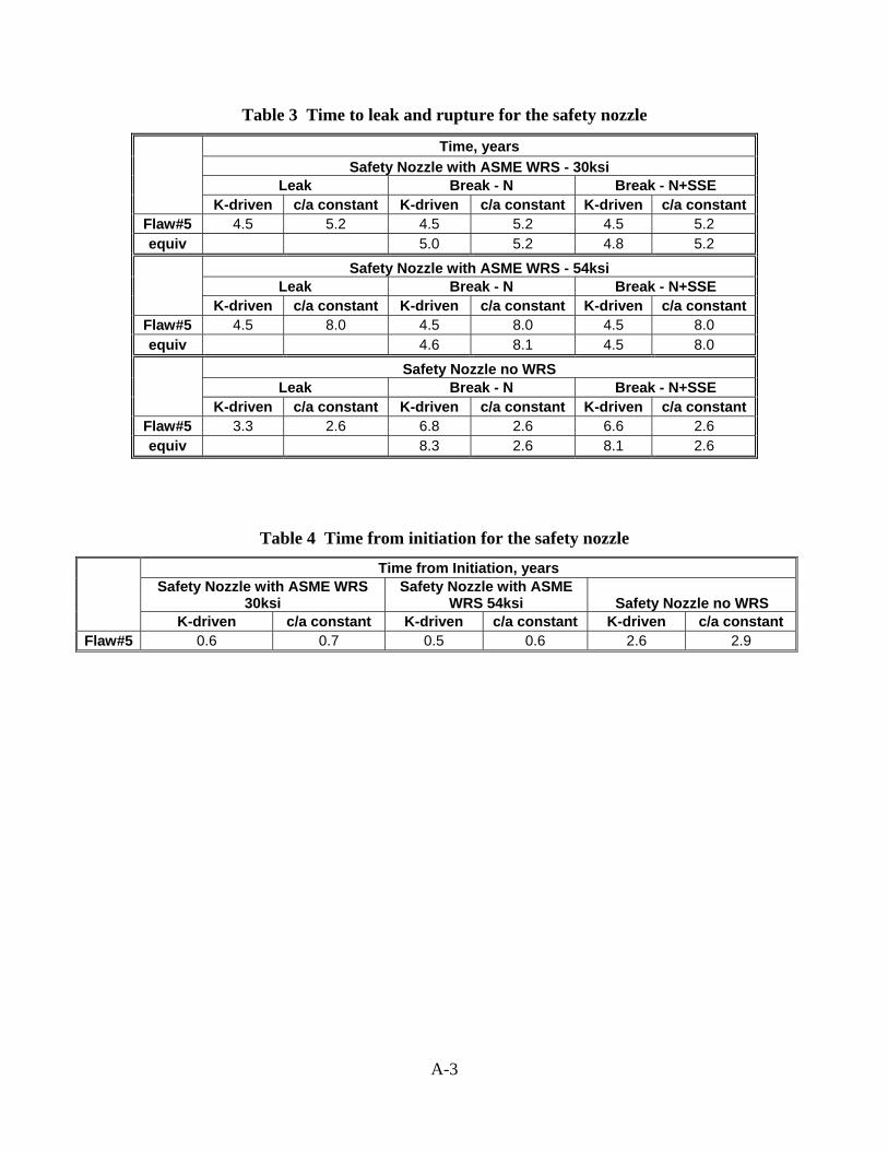
Table 3 Time to leak and rupture for the safety nozzle

Time, years Safety Nozzle with ASME WRS - 30ksi

Leak Break - N Break - N+SSE


Flaw#5 4.5 5.2 4.5 5.2 4.5 5.2 equiv 5.0 5.2 4.8 5.2

Safety Nozzle with ASME WRS - 54ksi Leak Break - N Break - N+SSE

K-driven c/a constant K-driven c/a constant K-driven c/a constant Flaw#5 4.5 8.0 4.5 8.0 4.5 8.0 equiv 4.6 8.1 4.5 8.0

Safety Nozzle no WRS Leak Break - N Break - N+SSE

K-driven c/a constant K-driven c/a constant K-driven c/a constant Flaw#5 3.3 2.6 6.8 2.6 6.6 2.6 equiv 8.3 2.6 8.1 2.6

Table 4 Time from initiation for the safety nozzle

Time from Initiation, years Safety Nozzle with ASME WRS

30ksi Safety Nozzle with ASME

WRS 54ksi Safety Nozzle no WRS K-driven c/a constant K-driven c/a constant K-driven c/a constant

Flaw#5 0.6 0.7 0.5 0.6 2.6 2.9

A-3

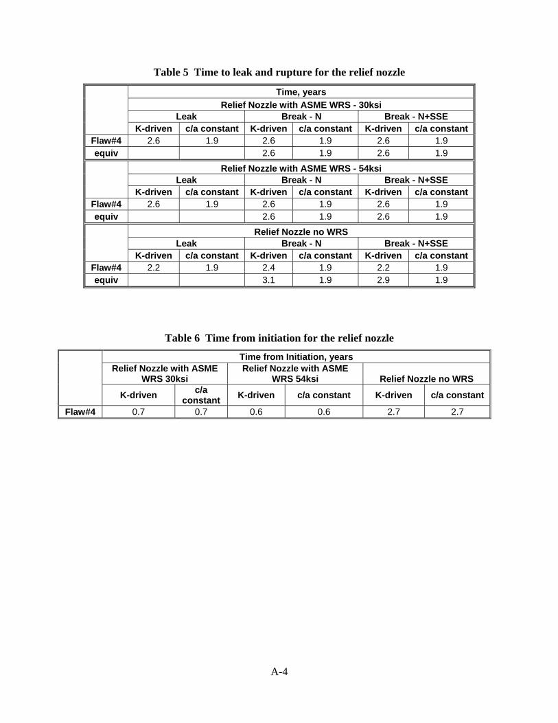
Table 5 Time to leak and rupture for the relief nozzle

Time, years Relief Nozzle with ASME WRS - 30ksi



Flaw#4 2.6 1.9 2.6 1.9 2.6 1.9 equiv 2.6 1.9 2.6 1.9

Relief Nozzle with ASME WRS - 54ksi Leak Break - N Break - N+SSE


Flaw#4 2.6 1.9 2.6 1.9 2.6 1.9 equiv 2.6 1.9 2.6 1.9

Relief Nozzle no WRS Leak Break - N Break - N+SSE


Flaw#4 2.2 1.9 2.4 1.9 2.2 1.9 equiv 3.1 1.9 2.9 1.9

Table 6 Time from initiation for the relief nozzle

Time from Initiation, years Relief Nozzle with ASME

WRS 30ksi Relief Nozzle with ASME

WRS 54ksi Relief Nozzle no WRS K-driven c/a

constant K-driven c/a constant K-driven c/a constant

Flaw#4 0.7 0.7 0.6 0.6 2.7 2.7

A-4

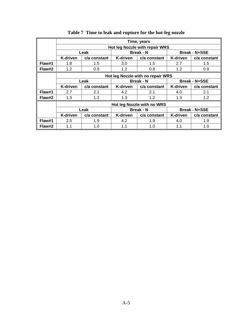
Table 7 Time to leak and rupture for the hot-leg nozzle

Time, years Hot leg Nozzle with repair WRS



Flaw#1 1.8 1.5 3.0 1.5 2.7 1.5 Flaw#2 1.2 0.9 1.2 0.9 1.2 0.9

Hot leg Nozzle with no repair WRS Leak Break - N Break - N+SSE

K-driven c/a constant K-driven c/a constant K-driven c/a constant Flaw#1 2.7 2.1 4.2 2.1 4.0 2.1 Flaw#2 1.3 1.2 1.3 1.2 1.3 1.2

Hot leg Nozzle with no WRS Leak Break - N Break - N+SSE

K-driven c/a constant K-driven c/a constant K-driven c/a constant Flaw#1 2.5 1.9 4.2 1.9 4.0 1.9 Flaw#2 1.1 1.0 1.1 1.0 1.1 1.0

A-5

evaluation of circumferential indications in …summary report on evaluation of circumferential...

Documents