fuzzy control applied to nuclear power plant pressurizer

2011 International Nuclear Atlantic Conference - INAC 2011 Belo Horizonte,MG, Brazil, October 24-28, 2011 ASSOCIAÇÃO BRASILEIRA DE ENERGIA NUCLEAR - ABEN ISBN: 978-85-99141-04-5

FUZZY CONTROL APPLIED TO NUCLEAR POWER PLANT PRESSURIZER SYSTEM

Mauro V. Oliveira and José C. S. Almeida

Instituto de Engenharia Nuclear (IEN / CNEN - RJ) Rua Hélio de Almeida 75

21941-906 Rio de Janeiro, RJ [email protected]; [email protected]

ABSTRACT In a pressurized water reactor (PWR) nuclear power plants (NPPs) the pressure control in the primary loop is very important for keeping the reactor in a safety condition and improve the generation process efficiency. The main component responsible for this task is the pressurizer. The pressurizer pressure control system (PPCS) utilizes heaters and spray valves to maintain the pressure within an operating band during steady state conditions, and limits the pressure changes, during transient conditions. Relief and safety valves provide overpressure protection for the reactor coolant system (RCS) to ensure system integrity. Various protective reactor trips are generated if the system parameters exceed safe bounds. Historically, a proportional-integral-derivative (PID) controller is used in PWRs to keep the pressure in the set point, during those operation conditions. The purpose of this study has two main goals: first is to develop a pressurizer model based on artificial neural networks (ANNs); second is to develop a fuzzy controller for the PWR pressurizer pressure, and compare its performance with the P controller. Data from a simulator PWR plant was used to test the ANN and the controllers as well. The reference simulator is a Westinghouse 3-loop PWR plant with a total thermal output of 2785 MWth. The simulation results show that the pressurizer ANN model response are in reasonable agreement with the simulated power plant, and the fuzzy controller built in this study has better performance compared to the P controller.

1. INTRODUCTION Nuclear power plants are in nature nonlinear systems with various components and are difficult to model due to their parameters vary with time as a function of power level. Many diverse models have been developed to model the dynamic response of such systems. Computer simulation of the behavior of complex systems and components, whose requires the solution of many equations and extensive use of closure relations, has become very important in modern design. This way of proceeding is used particularly in the nuclear industry where safety rules are rather rigid and impose to closely examine any possible situation and mode of operation of the system. In the phase of implementation of the physical-mathematical model, the discretization of the differential systems can be complicated by issues of stability and convergence. Artificial neural networks (ANNs) can be used in this context to overcome this problem thanks to their reliability in performing functional mappings. Akkurt and Çolak [1] have modeled several components of a PWR reactor using feedforward neural network. Masini et al. [2] have applied feedforward ANNs to model a steam generator based on superposition scheme in which a set of networks are individually trained, each one to respond to a different input forcing function.

INAC 2011, Belo Horizonte, MG, Brazil.

Likewise, the control of the nuclear power plants systems are difficult due to their complex, time varying and insufficiently known parameters. The application of intelligent systems including fuzzy logic in the control of large-scale complex nonlinear systems as nuclear plants are very promissory. Fuzzy control scheme has been applied by Bhatt et al. [3] for generating regulating signals to feed and bleed control valves, which are used in Liquid Zone Control System for maintaining constant pressure difference between gas outlet header and delay tank. Liu et al. [4] have applied a fuzzy proportional-integral-derivative (fuzzy-PID) in the nuclear reactor power control system tuned by genetic algorithm (GA). The purpose of this work has two main goals: first is to develop a pressurizer pressure model based on artificial neural networks for a PWR plant; and second is to develop a fuzzy controller for the ANN developed model and compare its performance with the plant proportional controller.

2. OVERVIEW OF THE NUCLEAR POWER PLANT SYSTEMS The nuclear power plant simulator used in this work is a Westinghouse 3-loops PWR plant with a total thermal output of 2785 MWth. Fig. 1 presents the main components of the plant, where only one of the 3 loops is showed in the figure. The plant can be divided into two circuits: the primary circuit (or primary side) and the secondary circuit (or secondary side).

Figure 1. Simplified flow of the nuclear power plant. On the primary side there are the reactor vessel, the pressurizer (PZR), the steam generator (primary side), the control rods system, and the chemical and volume control system (CVCS). The reactor is the main component of the primary circuit (or primary loop) and is responsible for heat the circulating water, pumped by the reactor coolant pump (RCP), throughout the fission process. The fission process is controlled by the control rods system. The pressurizer controls the primary pressure. The primary pressure must be kept high enough to guarantee the primary water in the liquid phase. Pressure is increased with heaters increasing steam bubble temperature in the pressurizer. Pressure is decreased using spray-cooling water in the steam in the pressurizer. The output water from the reactor goes through the hot leg to the steam generator (primary side), that transfer the heat of the water to the steam generator


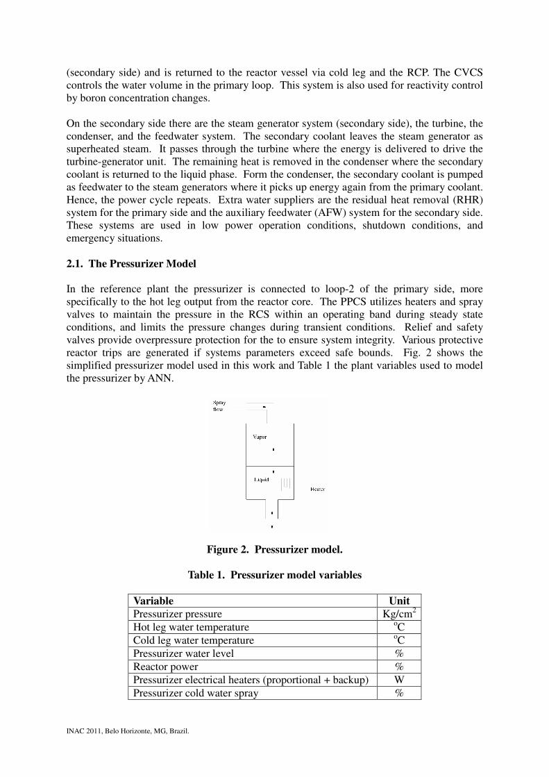
(secondary side) and is returned to the reactor vessel via cold leg and the RCP. The CVCS controls the water volume in the primary loop. This system is also used for reactivity control by boron concentration changes. On the secondary side there are the steam generator system (secondary side), the turbine, the condenser, and the feedwater system. The secondary coolant leaves the steam generator as superheated steam. It passes through the turbine where the energy is delivered to drive the turbine-generator unit. The remaining heat is removed in the condenser where the secondary coolant is returned to the liquid phase. Form the condenser, the secondary coolant is pumped as feedwater to the steam generators where it picks up energy again from the primary coolant. Hence, the power cycle repeats. Extra water suppliers are the residual heat removal (RHR) system for the primary side and the auxiliary feedwater (AFW) system for the secondary side. These systems are used in low power operation conditions, shutdown conditions, and emergency situations. 2.1. The Pressurizer Model In the reference plant the pressurizer is connected to loop-2 of the primary side, more specifically to the hot leg output from the reactor core. The PPCS utilizes heaters and spray valves to maintain the pressure in the RCS within an operating band during steady state conditions, and limits the pressure changes during transient conditions. Relief and safety valves provide overpressure protection for the to ensure system integrity. Various protective reactor trips are generated if systems parameters exceed safe bounds. Fig. 2 shows the simplified pressurizer model used in this work and Table 1 the plant variables used to model the pressurizer by ANN.

Figure 2. Pressurizer model.

Table 1. Pressurizer model variables

Variable Unit

Pressurizer pressure Kg/cm2 Hot leg water temperature oC Cold leg water temperature oC Pressurizer water level % Reactor power % Pressurizer electrical heaters (proportional + backup) W Pressurizer cold water spray %


2.2. The Pressurizer Pressure Control System Program

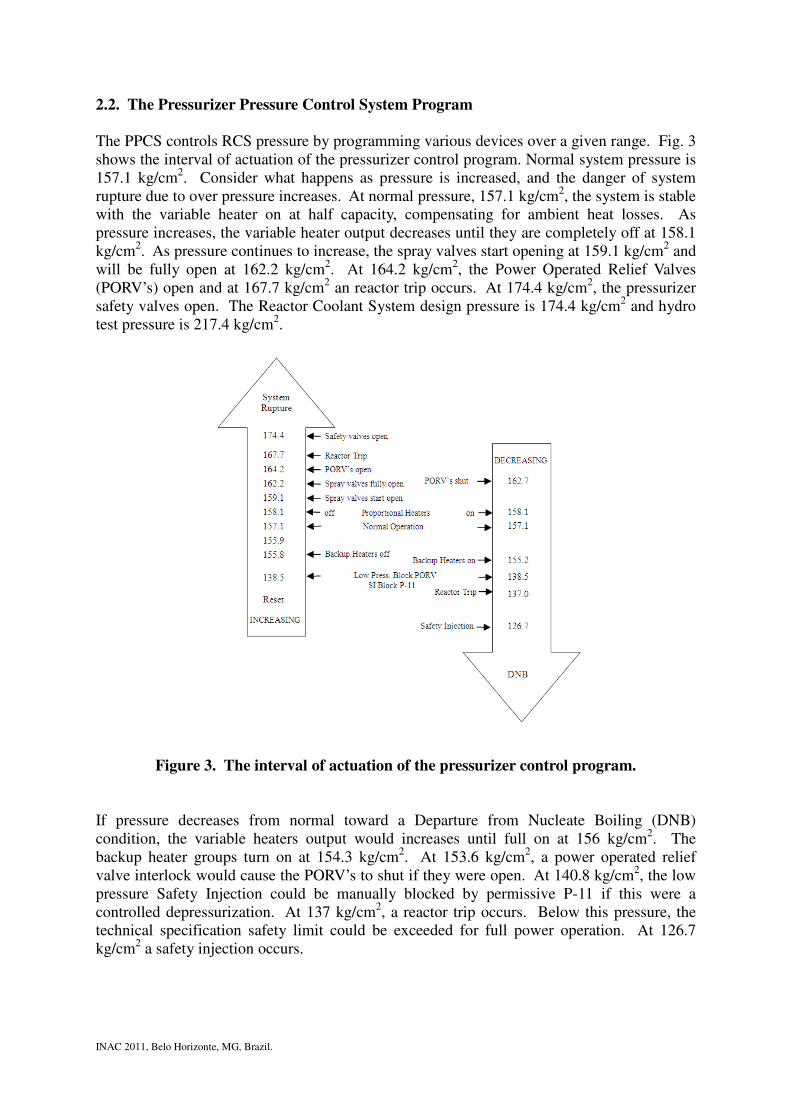
The PPCS controls RCS pressure by programming various devices over a given range. Fig. 3 shows the interval of actuation of the pressurizer control program. Normal system pressure is 157.1 kg/cm2. Consider what happens as pressure is increased, and the danger of system rupture due to over pressure increases. At normal pressure, 157.1 kg/cm2, the system is stable with the variable heater on at half capacity, compensating for ambient heat losses. As pressure increases, the variable heater output decreases until they are completely off at 158.1 kg/cm2. As pressure continues to increase, the spray valves start opening at 159.1 kg/cm2 and will be fully open at 162.2 kg/cm2. At 164.2 kg/cm2, the Power Operated Relief Valves (PORV’s) open and at 167.7 kg/cm2 an reactor trip occurs. At 174.4 kg/cm2, the pressurizer safety valves open. The Reactor Coolant System design pressure is 174.4 kg/cm2 and hydro test pressure is 217.4 kg/cm2.

Figure 3. The interval of actuation of the pressurizer control program. If pressure decreases from normal toward a Departure from Nucleate Boiling (DNB) condition, the variable heaters output would increases until full on at 156 kg/cm2. The backup heater groups turn on at 154.3 kg/cm2. At 153.6 kg/cm2, a power operated relief valve interlock would cause the PORV’s to shut if they were open. At 140.8 kg/cm2, the low pressure Safety Injection could be manually blocked by permissive P-11 if this were a controlled depressurization. At 137 kg/cm2, a reactor trip occurs. Below this pressure, the technical specification safety limit could be exceeded for full power operation. At 126.7 kg/cm2 a safety injection occurs.


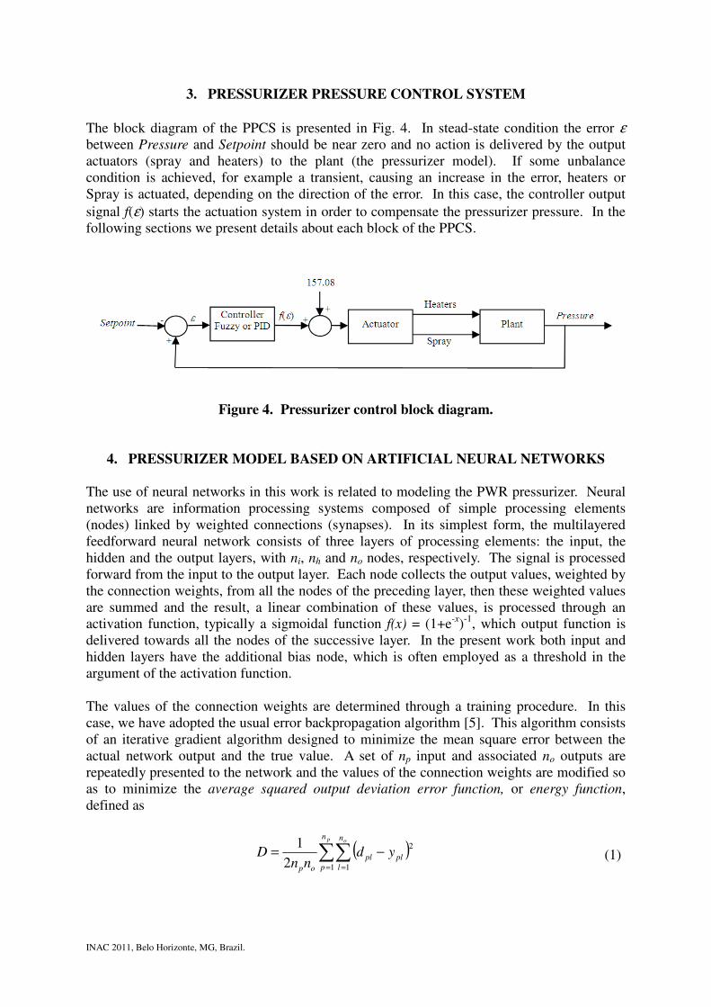
3. PRESSURIZER PRESSURE CONTROL SYSTEM The block diagram of the PPCS is presented in Fig. 4. In stead-state condition the error ε between Pressure and Setpoint should be near zero and no action is delivered by the output actuators (spray and heaters) to the plant (the pressurizer model). If some unbalance condition is achieved, for example a transient, causing an increase in the error, heaters or Spray is actuated, depending on the direction of the error. In this case, the controller output signal f(ε) starts the actuation system in order to compensate the pressurizer pressure. In the following sections we present details about each block of the PPCS.

Figure 4. Pressurizer control block diagram.

4. PRESSURIZER MODEL BASED ON ARTIFICIAL NEURAL NETWORKS The use of neural networks in this work is related to modeling the PWR pressurizer. Neural networks are information processing systems composed of simple processing elements (nodes) linked by weighted connections (synapses). In its simplest form, the multilayered feedforward neural network consists of three layers of processing elements: the input, the hidden and the output layers, with ni, nh and no nodes, respectively. The signal is processed forward from the input to the output layer. Each node collects the output values, weighted by the connection weights, from all the nodes of the preceding layer, then these weighted values are summed and the result, a linear combination of these values, is processed through an activation function, typically a sigmoidal function f(x) = (1+e-x)-1, which output function is delivered towards all the nodes of the successive layer. In the present work both input and hidden layers have the additional bias node, which is often employed as a threshold in the argument of the activation function. The values of the connection weights are determined through a training procedure. In this case, we have adopted the usual error backpropagation algorithm [5]. This algorithm consists of an iterative gradient algorithm designed to minimize the mean square error between the actual network output and the true value. A set of np input and associated no outputs are repeatedly presented to the network and the values of the connection weights are modified so as to minimize the average squared output deviation error function, or energy function, defined as

( )∑∑= =

−=p o

n

p

n

lplpl

op

ydnn

D1 1

2

2

1

(1)


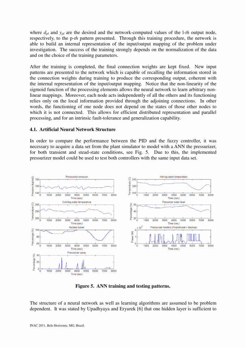
where dpl and ypl are the desired and the network-computed values of the l-th output node, respectively, to the p-th pattern presented. Through this training procedure, the network is able to build an internal representation of the input/output mapping of the problem under investigation. The success of the training strongly depends on the normalization of the data and on the choice of the training parameters. After the training is completed, the final connection weights are kept fixed. New input patterns are presented to the network which is capable of recalling the information stored in the connection weights during training to produce the corresponding output, coherent with the internal representation of the input/output mapping. Notice that the non-linearity of the sigmoid function of the processing elements allows the neural network to learn arbitrary non-linear mappings. Moreover, each node acts independently of all the others and its functioning relies only on the local information provided through the adjoining connections. In other words, the functioning of one node does not depend on the states of those other nodes to which it is not connected. This allows for efficient distributed representation and parallel processing, and for an intrinsic fault-tolerance and generalization capability. 4.1. Artificial Neural Network Structure In order to compare the performance between the PID and the fuzzy controller, it was necessary to acquire a data set from the plant simulator to model with a ANN the pressurizer, for both transient and stead-state conditions, see Fig. 5. Due to this, the implemented pressurizer model could be used to test both controllers with the same input data set.

Figure 5. ANN training and testing patterns. The structure of a neural network as well as learning algorithms are assumed to be problem dependent. It was stated by Upadhyaya and Eryurek [6] that one hidden layer is sufficient to


solve problems in several areas, including parameter estimation, as in the case of this study, and the minimum number of hidden layer nodes, H, in a neural network with N training patterns is given by the empirical relation

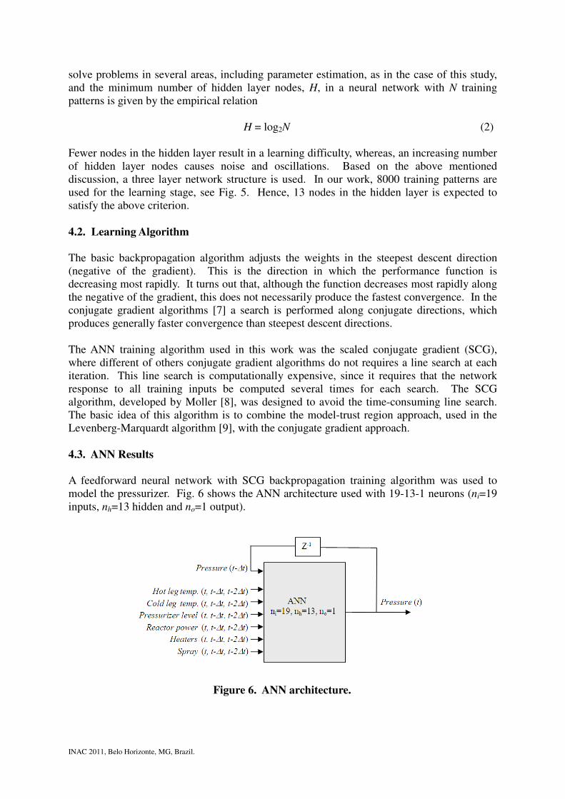
H = log2N (2) Fewer nodes in the hidden layer result in a learning difficulty, whereas, an increasing number of hidden layer nodes causes noise and oscillations. Based on the above mentioned discussion, a three layer network structure is used. In our work, 8000 training patterns are used for the learning stage, see Fig. 5. Hence, 13 nodes in the hidden layer is expected to satisfy the above criterion. 4.2. Learning Algorithm The basic backpropagation algorithm adjusts the weights in the steepest descent direction (negative of the gradient). This is the direction in which the performance function is decreasing most rapidly. It turns out that, although the function decreases most rapidly along the negative of the gradient, this does not necessarily produce the fastest convergence. In the conjugate gradient algorithms [7] a search is performed along conjugate directions, which produces generally faster convergence than steepest descent directions. The ANN training algorithm used in this work was the scaled conjugate gradient (SCG), where different of others conjugate gradient algorithms do not requires a line search at each iteration. This line search is computationally expensive, since it requires that the network response to all training inputs be computed several times for each search. The SCG algorithm, developed by Moller [8], was designed to avoid the time-consuming line search. The basic idea of this algorithm is to combine the model-trust region approach, used in the Levenberg-Marquardt algorithm [9], with the conjugate gradient approach. 4.3. ANN Results A feedforward neural network with SCG backpropagation training algorithm was used to model the pressurizer. Fig. 6 shows the ANN architecture used with 19-13-1 neurons (ni=19 inputs, nh=13 hidden and no=1 output).

Figure 6. ANN architecture.


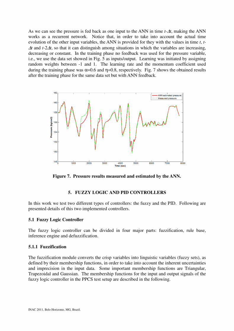
As we can see the pressure is fed back as one input to the ANN in time t-∆t, making the ANN works as a recurrent network. Notice that, in order to take into account the actual time evolution of the other input variables, the ANN is provided for they with the values in time t, t-∆t and t-2∆t, so that it can distinguish among situations in which the variables are increasing, decreasing or constant. In the training phase no feedback was used for the pressure variable, i.e., we use the data set showed in Fig. 5 as inputs/output. Learning was initiated by assigning random weights between -1 and 1. The learning rate and the momentum coefficient used during the training phase was α=0.6 and η=0.8, respectively. Fig. 7 shows the obtained results after the training phase for the same data set but with ANN feedback.

Figure 7. Pressure results measured and estimated by the ANN.

5. FUZZY LOGIC AND PID CONTROLLERS In this work we test two different types of controllers: the fuzzy and the PID. Following are presented details of this two implemented controllers. 5.1 Fuzzy Logic Controller The fuzzy logic controller can be divided in four major parts: fuzzification, rule base, inference engine and defuzzification. 5.1.1 Fuzzification The fuzzification module converts the crisp variables into linguistic variables (fuzzy sets), as defined by their membership functions, in order to take into account the inherent uncertainties and imprecision in the input data. Some important membership functions are Triangular, Trapezoidal and Gaussian. The membership functions for the input and output signals of the fuzzy logic controller in the PPCS test setup are described in the following.


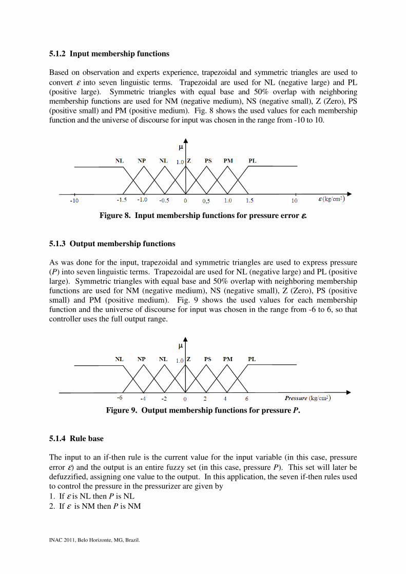
5.1.2 Input membership functions Based on observation and experts experience, trapezoidal and symmetric triangles are used to convert ε into seven linguistic terms. Trapezoidal are used for NL (negative large) and PL (positive large). Symmetric triangles with equal base and 50% overlap with neighboring membership functions are used for NM (negative medium), NS (negative small), Z (Zero), PS (positive small) and PM (positive medium). Fig. 8 shows the used values for each membership function and the universe of discourse for input was chosen in the range from -10 to 10.

Figure 8. Input membership functions for pressure error εεεε.

5.1.3 Output membership functions

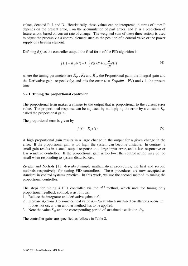
As was done for the input, trapezoidal and symmetric triangles are used to express pressure (P) into seven linguistic terms. Trapezoidal are used for NL (negative large) and PL (positive large). Symmetric triangles with equal base and 50% overlap with neighboring membership functions are used for NM (negative medium), NS (negative small), Z (Zero), PS (positive small) and PM (positive medium). Fig. 9 shows the used values for each membership function and the universe of discourse for input was chosen in the range from -6 to 6, so that controller uses the full output range.

Figure 9. Output membership functions for pressure P.

5.1.4 Rule base The input to an if-then rule is the current value for the input variable (in this case, pressure error ε) and the output is an entire fuzzy set (in this case, pressure P). This set will later be defuzzified, assigning one value to the output. In this application, the seven if-then rules used to control the pressure in the pressurizer are given by 1. If ε is NL then P is NL 2. If ε is NM then P is NM


3. If ε is NS then P is NS 4. If ε is Z then P is Z 5. If ε is PS then P is PS 6. If ε is PM then P is PM 7. If ε is PL then P is PL 5.1.5 Inference engine The inference engine is the process of formulating the mapping from a given input to an output using fuzzy sets based on fuzzy if-then rules stored in the rule base. The mapping then provides a basis from which decisions can be made, or patterns discerned. The process of fuzzy inference involves three steps as explained below. In the first step, the fuzzy inputs to the inference mechanism are compared with the premises of all the fuzzy if-then rules in the rule base to determine the rules that apply to the current situation. In the second step, using the fuzzy implication, a fuzzy decision is made by reshaping the fuzzy output sets in the consequent parts of all currently relevant rules using a function associated with the respective antecedent parts. In the final step, sometimes called aggregation, the modified fuzzy output sets from all the rules are unified in an appropriate manner to have a single fuzzy conclusion. In this work Mamdani implication [10] with union aggregation is used to infer the output contribution from each rule. Hence max operation is performed to aggregate the control outputs obtained as a result of firing several rules. 5.1.6 Defuzzification The process of finding the crisp value that best represents the fuzzy decision is called defuzzification. There are several methods of defuzzification available, but the most commonly used defuzzification method is the center of gravity (centroid) technique. The centroid equation for aggregation using max is given by

∑∑

=

== N

i i

N

i iiyy

1

1*

µ

µ (3)

where y* is the output of the defuzzification operation, N is the number of rules, yi is the center of fuzzy output set implied in the ith rule and µi is the degree of relevance of the ith rule. 5.2 PID Controller A proportional-integral-derivative controller (PID controller) is a generic control loop feedback mechanism (controller) widely used in industrial control systems. A PID controller calculates an error value ε as the difference between a measured process variable (PV) and a desired Setpoint. The controller attempts to minimize the error by adjusting the process control inputs. The PID controller calculation (algorithm) involves three separate constant parameters, and is accordingly sometimes called three-term control: the proportional, the integral and derivative


values, denoted P, I, and D. Heuristically, these values can be interpreted in terms of time: P depends on the present error, I on the accumulation of past errors, and D is a prediction of future errors, based on current rate of change. The weighted sum of these three actions is used to adjust the process via a control element such as the position of a control valve or the power supply of a heating element.

Defining f(t) as the controller output, the final form of the PID algorithm is

)()()()(0

tdt

dkdttktKtf

t

dip εεε ∫ ++= (4)

where the tuning parameters are Kp , Ki and Kd, the Proportional gain, the Integral gain and

the Derivative gain, respectively; and ε is the error (ε = Setpoint - PV) and t is the present time. 5.2.1 Tuning the proportional controller

The proportional term makes a change to the output that is proportional to the current error value. The proportional response can be adjusted by multiplying the error by a constant Kp, called the proportional gain.

The proportional term is given by

)()( tKtf pε= (5)

A high proportional gain results in a large change in the output for a given change in the error. If the proportional gain is too high, the system can become unstable. In contrast, a small gain results in a small output response to a large input error, and a less responsive or less sensitive controller. If the proportional gain is too low, the control action may be too small when responding to system disturbances. Ziegler and Nichols [11] described simple mathematical procedures, the first and second methods respectively, for tuning PID controllers. These procedures are now accepted as standard in control systems practice. In this work, we use the second method to tuning the proportional controller. The steps for tuning a PID controller via the 2nd

method, which uses for tuning only proportional feedback control, is as follows: 1. Reduce the integrator and derivative gains to 0. 2. Increase Kp from 0 to some critical value Kp=Kcr at which sustained oscillations occur. If

it does not occur then another method has to be applied. 3. Note the value Kcr and the corresponding period of sustained oscillation, Pcr. The controller gains are specified as follows in Table 2.


Table 2. Ziegler-Nichols recipe - second method

PID Type Kp Ti Td P 0.5 kcr ∞ 0 PI 0.45 kcr

2.1crP

0

PID 0.6 kcr

2crP

8crP

After applying the Ziegler-Nichols method we obtain kcr= 7.0 and Pcr = 5. Table 3 shows the correspondents gain values obtained. In the application, was selected for the controller a proportional gain of kP = 3.5.

Table 3. Obtained values for Ziegler-Nichols second method

PID Type Kp Ti Td P 3.5 ∞ 0 PI 3.15 4.17 0

PID 4.2 2.5 0.625 To compare the proportional controller with the fuzzy controller the span for the input variable and output variable for the proportional controller are limited to -10 to 10 and -6 to 6, respectively. Out of these span the controller system is consider saturated.

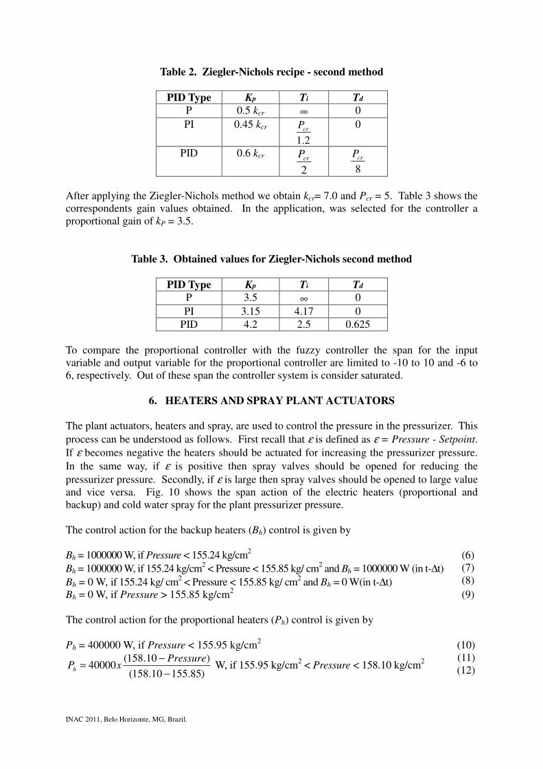
6. HEATERS AND SPRAY PLANT ACTUATORS The plant actuators, heaters and spray, are used to control the pressure in the pressurizer. This process can be understood as follows. First recall that ε is defined as ε = Pressure - Setpoint. If ε becomes negative the heaters should be actuated for increasing the pressurizer pressure. In the same way, if ε is positive then spray valves should be opened for reducing the pressurizer pressure. Secondly, if ε is large then spray valves should be opened to large value and vice versa. Fig. 10 shows the span action of the electric heaters (proportional and backup) and cold water spray for the plant pressurizer pressure. The control action for the backup heaters (Bh) control is given by Bh = 1000000 W, if Pressure < 155.24 kg/cm2 (6) Bh = 1000000 W, if 155.24 kg/cm2 < Pressure < 155.85 kg/ cm2 and Bh = 1000000 W (in t-∆t) Bh = 0 W, if 155.24 kg/ cm2 < Pressure < 155.85 kg/ cm2 and Bh = 0 W(in t-∆t)

(7) (8)

Bh = 0 W, if Pressure > 155.85 kg/cm2 (9) The control action for the proportional heaters (Ph) control is given by Ph = 400000 W, if Pressure < 155.95 kg/cm2 (10)

)85.15510.158(

)10.158(40000

−

−=

PressurexPh W, if 155.95 kg/cm2 < Pressure < 158.10 kg/cm2

(11) (12)


Ph = 0 W, if Pressure > 158.10 kg/cm2 (13) The control action for the cold water spray (S) control is given by S = 0 %, if Pressure < 159.12 kg/cm2 (14)

)12.15918.162(

)12.159(100

−

−=

PressurexS %, if 159.12 kg/cm2 < Pressure < 162.18 kg/cm2 (15)

S = 100 %, if Pressure > 158.10 kg/cm2 (16)

Figure 10. Controls action interval according with pressure P.

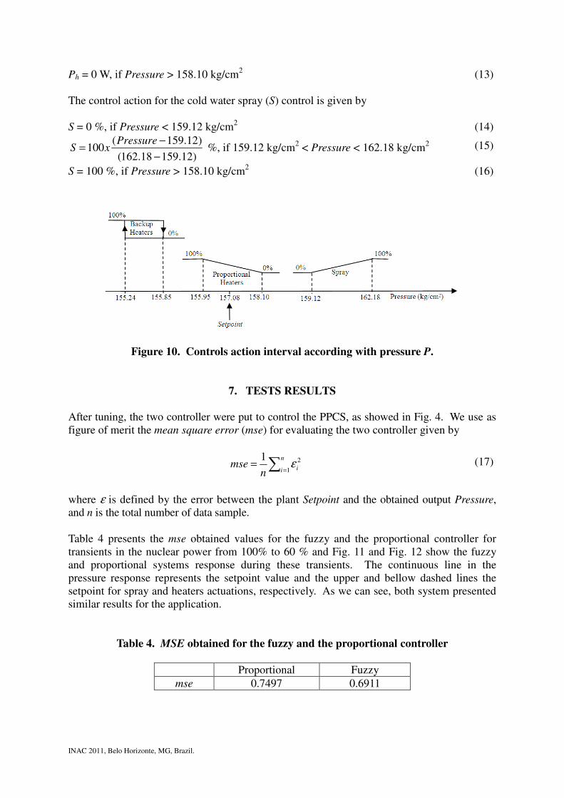
7. TESTS RESULTS After tuning, the two controller were put to control the PPCS, as showed in Fig. 4. We use as figure of merit the mean square error (mse) for evaluating the two controller given by

∑ ==

n

i in

mse1

21ε (17)

where ε is defined by the error between the plant Setpoint and the obtained output Pressure, and n is the total number of data sample. Table 4 presents the mse obtained values for the fuzzy and the proportional controller for transients in the nuclear power from 100% to 60 % and Fig. 11 and Fig. 12 show the fuzzy and proportional systems response during these transients. The continuous line in the pressure response represents the setpoint value and the upper and bellow dashed lines the setpoint for spray and heaters actuations, respectively. As we can see, both system presented similar results for the application.

Table 4. MSE obtained for the fuzzy and the proportional controller

Proportional Fuzzy mse 0.7497 0.6911


Pressurizer pressure

Heaters actuation

Spray actuation

Figure 11. Fuzzy controller response.

Pressurizer pressure

Heaters actuation

Spray actuation

Figure 12. Proportional controller response.


8. CONCLUSIONS This work has two main goals: first is to develop a pressurizer model based on artificial neural networks (ANNs) and second is to develop a fuzzy controller for the PWR pressurizer pressure, and compare its performance with the proportional controller. A feedforward backpropagation ANN with SCG training algorithm and architecture 19-13-1 neurons was used to model the pressurizer. The ANN output pressure is fed back as one input to the ANN in previous time, making the ANN works as a recurrent network. In order to take into account the actual time evolution of the other input variables, the ANN is provided for them with the values in present and two previous time steps, making it possible distinguish among situations in which the variables are increasing, decreasing or constant. Besides the nonlinear characteristic of the pressurizer system the developed ANN model showed similar response to the numeric model for a wide range of transients in the nuclear power of the simulated plant, as we can see in Fig. 7. A Mamdani type architecture was used to model the fuzzy controller with a total of seven trapezoidal and triangular membership functions for divide the input and output space. Seven fuzzy rules were used for mapping input/output space and aggregation using max for defuzzication. For the proportional controller was selected a gain of kP = 3.5. Both controller were tested for transients in the nuclear power and, as we can see in Table 4 and Fig. 12 and Fig. 13, the systems presented similar results for the application, with little advantage to the fuzzy controller. In the near future, we plain to compare the fuzzy controller with classical PI and PID and also to use genetic algorithm to tuning the membership functions partition of the fuzzy controller.

REFERENCES 1. H. Akkurt and Ü. Çolak, “PWR system simulation and parameter estimation with neural

networks”, Annals of Nuclear Energy, Vol. 29, pp.2087-2103 (2002). 2. R. Masini, E. Padovani, M.E. Ricotti and E. Zio, “Dynamic simulation of a steam generator by

neural networks”, Nuclear Engineering and Design, Vol. 187, pp.197-213 (1999). 3. T.U. Bhatt, K.C. Madala, S.R. Shimjith and A.P. Tiwari, “Application of fuzzy logic control

system for regulation of differential pressure in Liquid Zone Control System”, Annals of Nuclear Energy, Vol. 36, pp.1412-1423 (2009).

4. C. Liu, J.F. Peng, F.Y. Zhao and C. Li, “Design and optimization of fuzzy-PID controller for the nuclear reactor power control”, Nuclear Engineering and Design, Vol. 239, pp.2311-2316 (2009).

5. B. Müller and J. Reinhardt, Neural Networks - An Introduction, Springer-Verlag, New York & USA (1991). 6. B.R. Upadhyaya and E. Eryurek, “Application of neural networks for sensor validation

and plant monitoring”, Nuclear Technology, Vol. 97 (2), pp.170-176 (1992). 7. M.T. Hagan, H.B. Demuth and M.H. Beale, Neural Network Design, PWS Publishing,

Boston & USA (1996). 8. M.F. Moller, “A scaled conjugate gradient algorithm for fast supervised learning,” Neural

Networks, Vol. 6, pp.525-533 (1993). 9. M.T. Hagan and M. Menhaj, “Training feedforward networks with the Marquardt

algorithm,” IEEE Transactions on Neural Networks, Vol. 5 (6), pp.989-993 (1994). 10. E.H. Mamdani and S. Assilian, “An experiment in linguistic synthesis with a fuzzy logic

controller,” International Journal of Man-Machine Studies, Vol. 7 (1), pp.1-13 (1975). 11. J.G. Ziegler and N.B. Nichols, “Optimum settings for automatic controllers”,

Transactions of the ASME, Vol. 64, pp.759-768 (1942).

fuzzy control applied to nuclear power plant pressurizer

Documents