Evaluation of Fire Models for Nuclear Power Plant Applications

Benchamrk Exercise No. 4: Fuel Pool Fire Inside A Compartment

International Panel Report

GRS - 213

Gesellschaft für Anlagen- und Reaktorsicherheit (GRS) mbH

Evaluation of Fire Models for Nuclear Power Plant Applications

Benchmark Exercise No. 4: Fuel Pool Fire Inside A Compartment

International Panel Report

Compiled by:Walter Klein-Heßling (GRS)Marina Roewekamp (GRS)Olaf Riese (iBMB)

November 2006

Remark:

This report was prepared under con-tract No. 02 SR 2491 “Übergreifen-de Bewertung des Brandschutzes bei Kernkraftwerken - Auswertung von spezifi schen Brandereignissen, Mitarbeit in internationalen Gremien, Entscheidungshilfe bei der Verwen-dung von Brandsimulationsprogram-men“ with the German Bundesmin-sterium für Umwelt, Naturschutz und Reaktorsicherheit (BMU) durchge-führt.

The work was conducted by the Ge-sellschaft für Anlagen- und Reaktor-sicherheit (GRS) mbH together with the Institut für Baustoffe, Massivbau und Brandschutz (iBMB).

The authors are responsible for the content of this report.

Gesellschaft für Anlagen-

und Reaktorsicherheit(GRS) mbH

GRS - 213

ISBN 978-3-931995-80-5

Deskriptoren:

Ausbreitung, Auswirkung, Brand, Brandgefährdung, Brandschutz, Brandverhalten, Druck, Gas, Kohlendioxid, Öl, Reaktor, Rechenverfahren, Sauerstoff, Simulation, Temperatur, Verbrennung

I

Abstract

Fire simulations as well as their analytical validation procedures have gained more and

more significance, particularly in the context of the fire safety analysis for operating

nuclear power plants. Meanwhile, fire simulation models have been adapted as analyti-

cal tools for a risk oriented fire safety assessment.

Calculated predictions can be used, on the one hand, for the improvements and up-

grades of fire protection in nuclear power plants by the licensees and, on the other

hand, as a tool for reproducible and clearly understandable estimations in assessing

the available and/or foreseen fire protection measures by the authorities and their ex-

perts. For consideration of such aspects in the context of implementing new nuclear fire

protection standards or of updating existing ones, an “International Collaborative Pro-

ject to Evaluate Fire Models for Nuclear Power Plant Applications” also known as the

“International Collaborative Fire Model Project” (ICFMP) was started in 1999. It has

made use of the experience and knowledge of a variety of worldwide expert institutions

in this field to assess and improve, if necessary, the state-of-the-art with respect to

modeling fires in nuclear power plants and other nuclear installations.

This document contains the results of the ICFMP Benchmark Exercise No. 4, where

two fuel pool fire experiments in an enclosure with two different natural vent sizes have

been considered. Analyzing the results of different fire simulation codes and code types

provides some indications with respect to the uncertainty of the results. This informa-

tion is especially important in setting uncertainty parameters in probabilistic risk studies

and to provide general insights concerning the applicability and limitations in the appli-

cation of different types of fire simulation codes for this type of fire scenario and

boundary conditions.

During the benchmark procedure the participants performed different types of calcula-

tions. These included totally blind simulations without knowledge of the pyrolysis rate,

semi-blind calculations with knowledge of this rate only, and completely open post-

calculations with knowledge of all experimental measurements. It has been demon-

strated, as expected, that the pyrolysis rate has a strong influence on the calculation

results. This could be derived from the large differences in the quality of results be-

tween the few blind and ‘semi-blind’ or open calculations. The range of the results is

much larger for the blind simulations compared to the semi-blind ones. This reduces

II

the reliability of the results in the event of fire simulation codes being applied e.g. in the

frame of probabilistic risk analyses.

The Benchmark Exercise has furthermore shown that the simulation of under-ventilated

fires is more difficult for the fire simulation codes and that a highly transient fire behav-

ior leads to a wider range of the code simulation results. Compared to typical fire sce-

narios analyzed in the fire PSA the considered Benchmark Exercise is extreme in

terms of thermal loads. This has to be considered for the assessment of the deviations

between the simulation results and the experimental data.

III

Kurzfassung

Brandsimulationen sowie deren analytische Validierung erhalten mehr und mehr Be-

deutung im Rahmen von Brandsicherheitsanalysen in Betrieb befindlicher Kernkraft-

werke. Mittlerweile sind Brandsimulationsmodelle als analytische Werkzeuge, welche

sich insbesondere für risikoorientierte Brandsicherheitsbewertungen eignen, anerkannt.

Die Verwendung rechnerischer Vorhersagen kann zum einen die Verbesserungen und

Nachrüstungen des Brandschutzes durch die Betreiber aufzeigen, zum anderen aber

auch als ein Hilfsmittel für reproduzierbare und klar verständliche Abschätzungen im

Rahmen der Bewertung vorhandener bzw. geplanter Brandschutzmaßnahmen seitens

der Genehmigungs- und Aufsichtsbehörden und deren Gutachter genutzt werden. Zur

Berücksichtigung derartiger Aspekte auch bei der Umsetzung neuer oder der Erweite-

rung kerntechnischer Brandschutzregelwerke wurde ein so genanntes ’International

Collaborative Project to Evaluate Fire Models for Nuclear Power Plant Applications

auch bekannt unter ’International Collaborative Fire Model Project (ICFMP)’ im Jahr

1999 initiiert, in welchem Erfahrungen und Kenntnisse einer Vielzahl von Experteninsti-

tutionen auf diesem Fachgebiet dazu genutzt werden sollen, den Stand von Wissen-

schaft und Technik auf dem Gebiet der Modellierung von Bränden für Anwendungen in

Kernkraftwerken und anderen kerntechnischen Einrichtungen zu bewerten und, falls

erforderlich, zu verbessern.

Der nachfolgende Bericht beinhaltet die Ergebnisse des ICFMP Benchmark Exercise

Nr. 4, bei welchem zwei Versuche zum Treibstofflachenbrand in einem Brandraum mit

unterschiedlicher natürlicher Ventilation betrachtet werden. Die Analyse der Ergebnisse

von Simulationsrechnungen mit unterschiedlichen Brandsimulationscodes und -

codearten gibt Hinweise in Bezug auf die Unsicherheiten der Resultate. Dies ist zum

einen von Bedeutung für die Auswahl von Unsicherheitsparametern in probabilisti-

schen Sicherheitsanalysen. Zum anderen ergeben sich daraus Erkenntnisse hinsicht-

lich der Anwendbarkeit und Anwendungsgrenzen verschiedener Arten von Brandsimu-

lationscodes für solche Brandszenarien und die entsprechenden Randbedingungen.

Im Verlauf des Benchmarks werden von den Teilnehmern unterschiedliche Arten von

Simulationsrechnungen durchgeführt. Dabei handelt es sich um so genannte ’blinde’

Vorausrechnungen ohne Kenntnis der Pyrolyserate, um ’semi-blinde’ Rechnungen, bei

welchen nur die Pyrolyserate bekannt ist, und um vollständig offene Nachrechnungen

unter Kenntnis der Versuchsdaten. Wie erwartet, zeigte sich, dass die Pyrolyserate

IV

einen erheblichen Einfluss auf die rechnerischen Ergebnisse hat. Dies zeigte sich ins-

besondere an den doch erheblichen Qualitätsunterschieden der Rechenergebnisse

von den wenigen blinden im Vergleich zu den ‚semi-blinden’ bzw. offenen Rechnun-

gen. Die Bandbreite der Ergebnisse ist bei den blinden Vorausrechnungen erheblich

größer als bei den semi-blinden, was zu höheren Ergebnisunsicherheiten bei Nutzung

von Brandsimulationsrechnungen bei z.B. probabilistischen Analysen führt. Es zeigt

sich weiterhin, dass die Simulation unterventilierter Brände für die Brandsimulationsco-

des erheblich schwieriger ist. Ein sehr instationäres Brandverhalten führt zu einer grö-

ßeren Bandbreite der Ergebnisse. Die betrachtete Benchmarkaufgabe ist in Bezug auf

die thermischen Belastungen extrem im Vergleich zu den in Rahmen von Brand PSA

betrachteten Szenarien. Dies ist bei der Betrachtung der Abweichungen der Simulati-

onsergebnisse von den experimentellen Werten zu berücksichtigen.

V

Table of Contents

Abstract....................................................................................................... I

Kurzfassung ............................................................................................. III

1 Introduction ............................................................................................... 1

2 Specification of Benchmark Exercise No. 4 ........................................... 3

2.1 Review of Previous Related Work within the ICFMP Project ...................... 3

2.2 Specification of the Experiments ................................................................. 5 2.2.1 Description of the Test Facility .................................................................... 5 2.2.2 Measurements Performed......................................................................... 15 2.2.3 Experimental Procedure............................................................................ 21

3 Experimental Results.............................................................................. 29

3.1 Summary of Test 1.................................................................................... 30

3.2 Summary of Test 3.................................................................................... 34

3.3 Conclusions............................................................................................... 37

4 Input Parameters and Assumptions...................................................... 39

5 Comparison of Code Simulations and Experimental Results............ 43

5.1 Blind Calculations...................................................................................... 44 5.1.1 FDS (CFD Code) Applied by K. McGrattan (NIST, USA).......................... 44 5.1.2 JASMINE (CFD Code) Applied by S. Miles (BRE, UK) ............................. 47

5.2 Semi-blind Calculations............................................................................. 52 5.2.1 FDS (CFD Code) Applied by K. McGrattan (NIST, USA).......................... 52 5.2.2 FDS (CFD Code) and CFST (Zone Model) Applied by M. Dey

(USNRC, USA).......................................................................................... 55 5.2.3 CFAST (Zone Model) and JASMINE (CFD CODE) Applied by S. Miles

(BRE, UK) ................................................................................................. 61

5.3 Open Calculations..................................................................................... 70 5.3.1 FATE (Zone Model) Applied by T. Elicson (Fauske & Associates LLC,

USA).......................................................................................................... 70 5.3.2 FLAMME-S (Zone Model) Applied by L. Rigollet (IRSN, France) ............. 75

VI

5.3.3 CFX (CFD Code) Applied by M. Heitsch (GRS, Germany) ....................... 78 5.3.4 FDS (CFD Code) Applied by W. Brücher (GRS, Germany) ...................... 81 5.3.5 COCOSYS (Lumped Parameter Code) Applied by B. Schramm (GRS,

Germany) .................................................................................................. 87 5.3.6 VULCAN (CFD Code) Applied by V.F. Nicolette (SNL, USA) ................... 91 5.3.7 MAGIC (zone code) Applied by B. Gautier (EDF, France)........................ 95

6 Code to Code Comparison..................................................................... 97

6.1 Test 1 ........................................................................................................ 97 6.1.1 Plume Temperatures (M1 to M6) .............................................................. 97 6.1.2 Temperatures inside the Fire Compartment ............................................. 99 6.1.3 Layer Height and Upper Layer Temperature .......................................... 106 6.1.4 Gas Concentration inside the Fire Compartment .................................... 108 6.1.5 Probe Temperatures ............................................................................... 113

6.2 Test 3 ...................................................................................................... 116 6.2.1 Plume Temperatures (M1 to M6) ............................................................ 116 6.2.2 Temperatures inside the Fire Compartment ........................................... 119 6.2.3 Layer Height and Upper Layer Temperature .......................................... 126 6.2.4 Gas Concentrations inside the Fire Compartment .................................. 129 6.2.5 Probe Temperatures ............................................................................... 134

7 General Conclusions and Recommendations.................................... 137

7.1 General Conclusions............................................................................... 137

7.2 Recommendations .................................................................................. 138

8 Summary................................................................................................ 139

9 References............................................................................................. 141

List of Figures ....................................................................................... 143

List of Tables ......................................................................................... 147

List of Appendices:............................................................................... 149

Appendices A – J on CD

1

1 Introduction

Fire simulations as well as analytical validation procedures have gained more and

more significance, particularly in the context of fire safety analysis for operating nuclear

power plants (NPPs). Fire simulation models have been developed as analytical tools

for a risk oriented fire safety assessment.

The use of calculated predictions could be considered, on the one hand, for improve-

ments and upgrades of the fire protection by the licensees and, on the other hand as a

tool for reproducible and clearly understandable estimations in assessing the available

and/or foreseen fire protection measures by the authorities and their experts. For con-

sideration of such aspects even in the frame of implementing new nuclear fire protec-

tion standards or upgrading existing ones, an “International Collaborative Project to

Evaluate Fire Models for Nuclear Power Plant Applications” also known as the “Interna-

tional Collaborative Fire Model Project” (ICFMP)” was started in 1999, to make use of

the experience and knowledge of a variety of expert institutions in this field worldwide

to assess and improve, where necessary, the state-of-the-art with respect to modeling

fires for application to nuclear installations/plants.

Within the ICFMP project the following Benchmark Exercises have been performed:

– Benchmark Exercise No. 1: Cable fire and thermal load on cables in a cable

spreading room (theoretical) /DEY 02/;

– Benchmark Exercise No. 2: Heptane pool fire in a large hall (experiment) and large

oil fire in a turbine hall with 2 floor levels and horizontal openings /MIL 04/;

– Benchmark Exercise No. 3: Heptane spray fire in a cable room to investigate ther-

mal loads on cables and cable trays (experiments) /MCG 06/;

– Benchmark Exercise No. 4: Relatively large fuel pool fire with two variations of the

door cross section area (experiments);

– Benchmark Exercise No. 5: Fire spreading on vertical cable trays with variations on

the pre-heating and cable material (experiments) /RIE 06/.

In this Panel Report, Benchmark Exercise No. 4 will be discussed and the results of the

different participants will be evaluated. The individual reports of the participants are

presented as attachments.

2

The main objective of the experiments for Benchmark Exercise No. 4 was to analyze

the thermal load on the structures surrounding a fire relatively large compared to the

floor area and volume of the fire compartment. In several experiments the natural and

forced ventilation has been changed to investigate the influence of oxygen depleted

conditions on the fire. Both the thermal loads and the oxygen depleted conditions are

somewhat difficult aspects to calculate. Therefore these experiments can contribute to

the further improvement of fire codes. Additionally, the results give some insight con-

cerning the uncertainties of fire simulations of pool fires in an enclosure under the given

boundary conditions. This information is important for the definition of uncertainty input

parameters for PSA studies.

3

2 Specification of Benchmark Exercise No. 4

At iBMB (Institut für Baustoffe, Massivbau und Brandschutz) of Braunschweig Univer-

sity of Technology, a set of nine real scale fuel pool fire experiments has been per-

formed. The objective of these experiments was to systematically vary the major influ-

encing parameters on the burning behavior to derive standard fire curves (time de-

pendence of temperatures and heat flow densities at different distances from the fire

source, burning rates, energy release rates and temperature loads) and to examine the

dependence on the pool surface area, the fuel filling level and the ventilation condi-

tions.

The fire compartment OSKAR of iBMB, an enclosure with a compartment floor size of

3.6 m x 3.6 m = 12.96 m2 and a height of 5.7 m, was used for the pool fire test series.

This facility has 3 possible openings for the natural ventilation of the fire compartment.

At the ceiling, the hot gases and smoke can be extracted and cleaned by a fan system

with filters. During the experiments gas and surface temperatures, gas composition,

velocities and heat flux densities were measured.

2.1 Review of Previous Related Work within the ICFMP Project

In this section, the relation of Benchmark Exercise No. 4 to the previous Benchmark

Exercises is discussed.

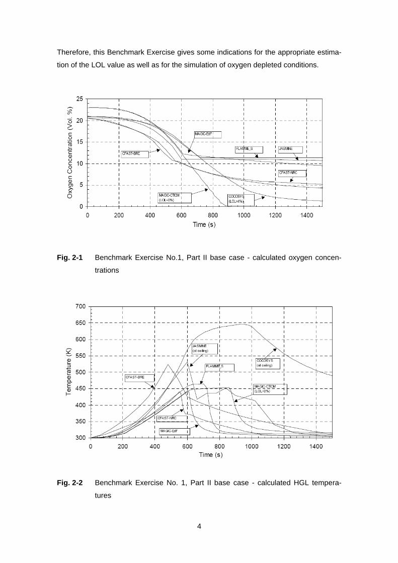
Looking to Benchmark Exercise No. 1, one result was the strong influence of the as-

sumed lower oxygen limit (LOL) on the calculated results /DEY 02/. Fig. 2-1 presents

the calculated oxygen concentrations for the Benchmark Exercise No. 1, Part II base

case. The results depend on the assumed parameter of LOL. The range of this pa-

rameter varied between 0 and 10 Vol.-%. The difference between calculations with the

zone model MAGIC by different users, MAGIC-EDF (with 10 Vol.-%) and MAGIC-

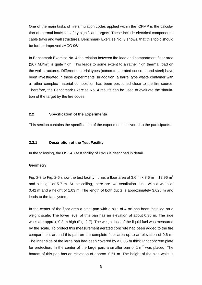
CTICM (with 0 Vol.-%) are of special interest. The consequences of this parameter on

the hot gas layer temperature (HGL) are shown in Fig. 2-2. In particular, the fire dura-

tion is predicted quite differently.

The main difference between Test 1 and Test 3 in Benchmark Exercise No. 4 is the

ventilation opening at the front wall, leading to oxygen depleted conditions in Test 3.

4

Therefore, this Benchmark Exercise gives some indications for the appropriate estima-

tion of the LOL value as well as for the simulation of oxygen depleted conditions.

Fig. 2-1 Benchmark Exercise No.1, Part II base case - calculated oxygen concen-

trations

Fig. 2-2 Benchmark Exercise No. 1, Part II base case - calculated HGL tempera-

tures

5

One of the main tasks of fire simulation codes applied within the ICFMP is the calcula-

tion of thermal loads to safety significant targets. These include electrical components,

cable trays and wall structures. Benchmark Exercise No. 3 shows, that this topic should

be further improved /MCG 06/.

In Benchmark Exercise No. 4 the relation between fire load and compartment floor area

(267 MJ/m2) is quite high. This leads to some extent to a rather high thermal load on

the wall structures. Different material types (concrete, aerated concrete and steel) have

been investigated in these experiments. In addition, a barrel type waste container with

a rather complex material composition has been positioned close to the fire source.

Therefore, the Benchmark Exercise No. 4 results can be used to evaluate the simula-

tion of the target by the fire codes.

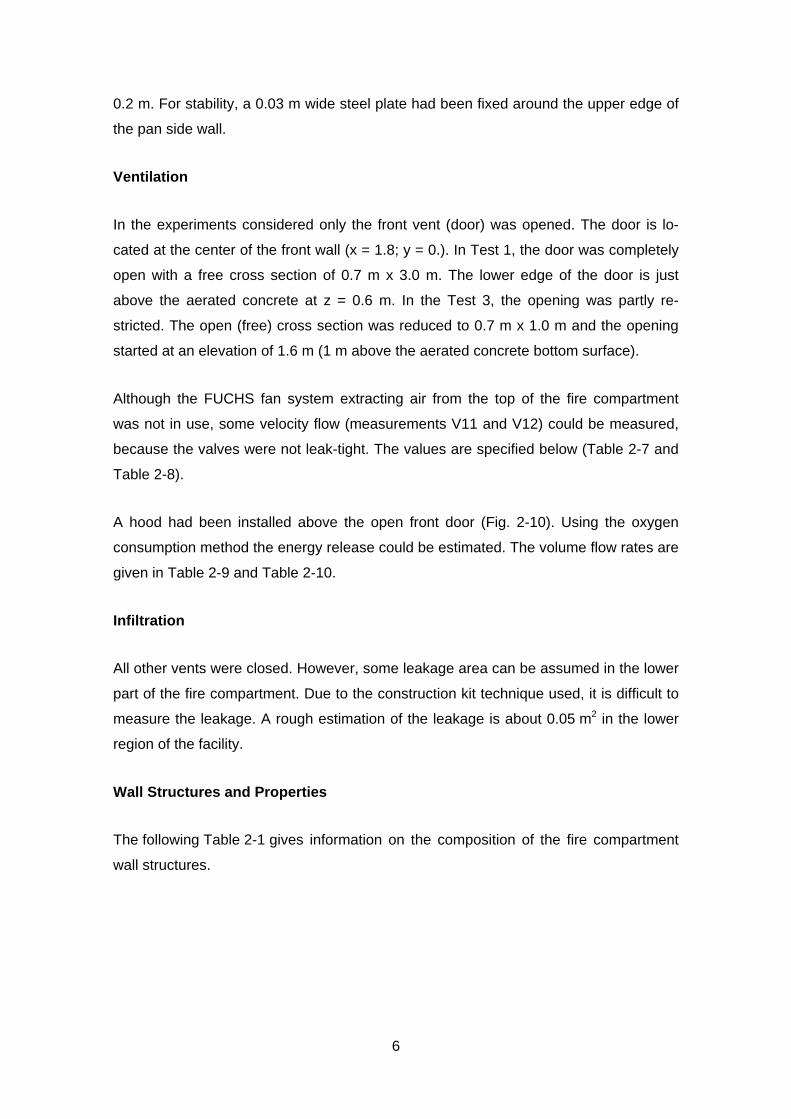
2.2 Specification of the Experiments

This section contains the specification of the experiments delivered to the participants.

2.2.1 Description of the Test Facility

In the following, the OSKAR test facility of iBMB is described in detail.

Geometry

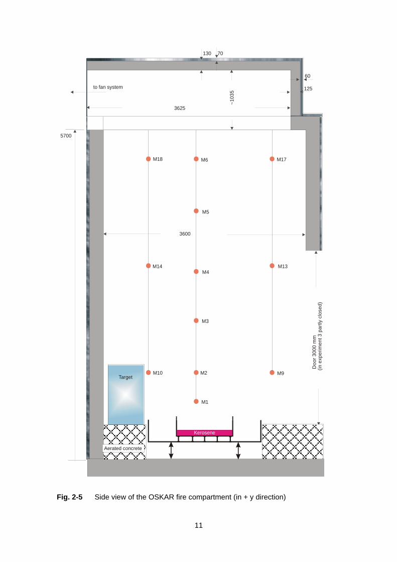
Fig. 2-3 to Fig. 2-6 show the test facility. It has a floor area of 3.6 m x 3.6 m = 12.96 m2

and a height of 5.7 m. At the ceiling, there are two ventilation ducts with a width of

0.42 m and a height of 1.03 m. The length of both ducts is approximately 3.625 m and

leads to the fan system.

In the center of the floor area a steel pan with a size of 4 m2 has been installed on a

weight scale. The lower level of this pan has an elevation of about 0.36 m. The side

walls are approx. 0.3 m high (Fig. 2-7). The weight loss of the liquid fuel was measured

by the scale. To protect this measurement aerated concrete had been added to the fire

compartment around this pan on the complete floor area up to an elevation of 0.6 m.

The inner side of the large pan had been covered by a 0.05 m thick light concrete plate

for protection. In the center of the large pan, a smaller pan of 1 m2 was placed. The

bottom of this pan has an elevation of approx. 0.51 m. The height of the side walls is

6

0.2 m. For stability, a 0.03 m wide steel plate had been fixed around the upper edge of

the pan side wall.

Ventilation

In the experiments considered only the front vent (door) was opened. The door is lo-

cated at the center of the front wall (x = 1.8; y = 0.). In Test 1, the door was completely

open with a free cross section of 0.7 m x 3.0 m. The lower edge of the door is just

above the aerated concrete at z = 0.6 m. In the Test 3, the opening was partly re-

stricted. The open (free) cross section was reduced to 0.7 m x 1.0 m and the opening

started at an elevation of 1.6 m (1 m above the aerated concrete bottom surface).

Although the FUCHS fan system extracting air from the top of the fire compartment

was not in use, some velocity flow (measurements V11 and V12) could be measured,

because the valves were not leak-tight. The values are specified below (Table 2-7 and

Table 2-8).

A hood had been installed above the open front door (Fig. 2-10). Using the oxygen

consumption method the energy release could be estimated. The volume flow rates are

given in Table 2-9 and Table 2-10.

Infiltration

All other vents were closed. However, some leakage area can be assumed in the lower

part of the fire compartment. Due to the construction kit technique used, it is difficult to

measure the leakage. A rough estimation of the leakage is about 0.05 m2 in the lower

region of the facility.

Wall Structures and Properties

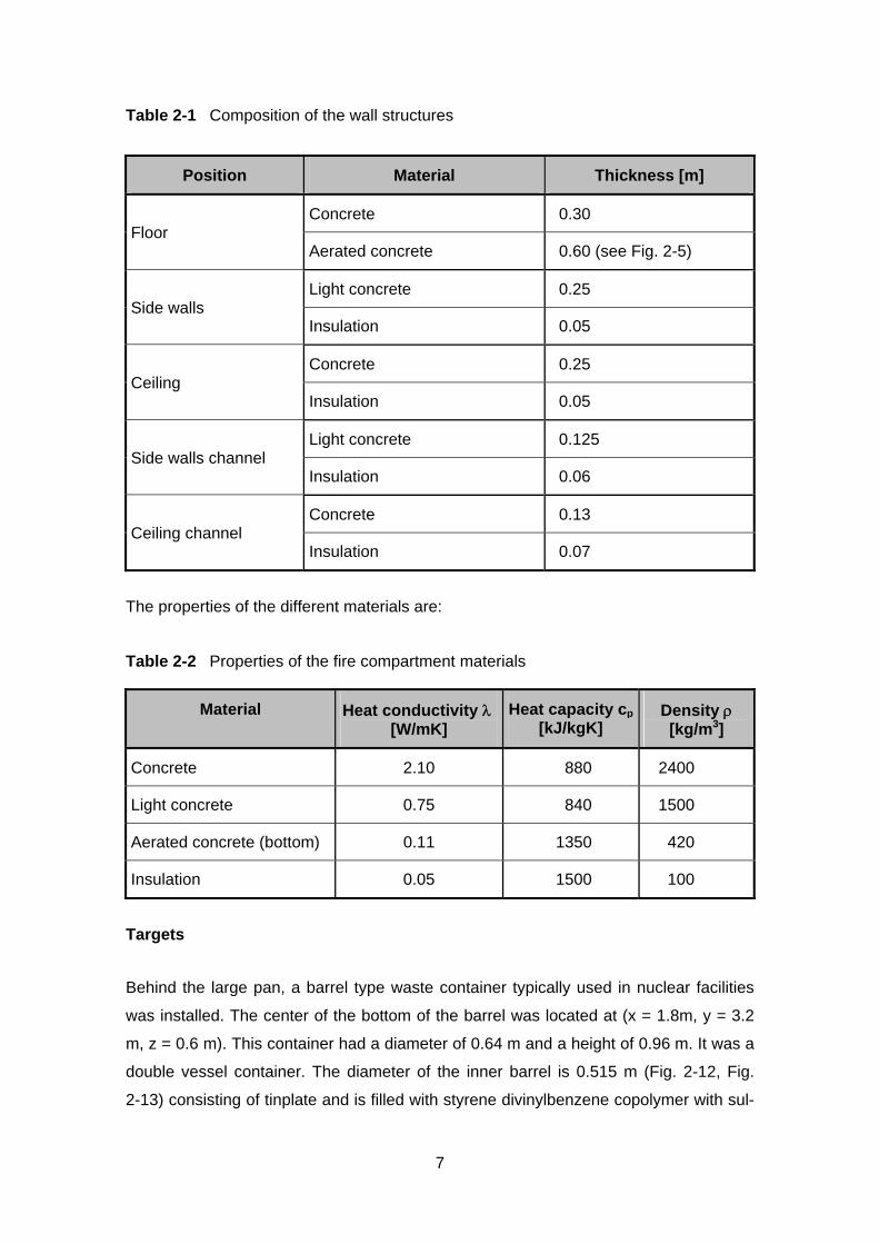
The following Table 2-1 gives information on the composition of the fire compartment

wall structures.

7

Table 2-1 Composition of the wall structures

Position Material Thickness [m]

Concrete 0.30 Floor

Aerated concrete 0.60 (see Fig. 2-5)

Light concrete 0.25 Side walls

Insulation 0.05

Concrete 0.25 Ceiling

Insulation 0.05

Light concrete 0.125 Side walls channel

Insulation 0.06

Concrete 0.13 Ceiling channel

Insulation 0.07

The properties of the different materials are:

Table 2-2 Properties of the fire compartment materials

Material Heat conductivity λ [W/mK]

Heat capacity cp [kJ/kgK]

Density ρ [kg/m3]

Concrete 2.10 880 2400

Light concrete 0.75 840 1500

Aerated concrete (bottom) 0.11 1350 420

Insulation 0.05 1500 100

Targets

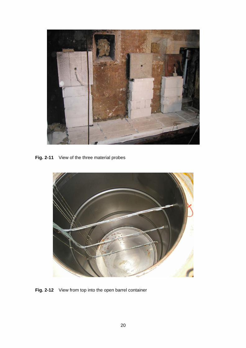
Behind the large pan, a barrel type waste container typically used in nuclear facilities

was installed. The center of the bottom of the barrel was located at (x = 1.8m, y = 3.2

m, z = 0.6 m). This container had a diameter of 0.64 m and a height of 0.96 m. It was a

double vessel container. The diameter of the inner barrel is 0.515 m (Fig. 2-12, Fig.

2-13) consisting of tinplate and is filled with styrene divinylbenzene copolymer with sul-

8

fur acid groups. The gap between the inner and outer steel barrel was filled with con-

crete (Table 2-3) and equipped with six (2 at each of three levels) thermocouples for

measurements.

Three different types of material probes were positioned on the right side of the fire

compartment (x = 0 m). The materials are "aerated concrete", concrete and steel. The

size of these elements is 0.3 m x 0.3 m (Fig. 2-11). For the concrete probes, the thick-

ness is 0.1 m, for the steel plate it is 0.02 m. The properties of the materials used are

given in Table 2-3. The location of the center surface is given in Table 2-4.

Table 2-3 Properties of the target materials

Material Heat conductivity λ [W/mK]

Heat capacity cp [J/kgK]

Density ρ [kg/m3]

Granulate (styrene) 0.233 1600 1000

Tin plate 63 230 7280

Concrete (between barrels) 2.1 880 2400

Steel 44.5 480 7743

Concrete (probe) 2.1 880 2400

Aerated concrete 0.11 1350 420

Table 2-4 Location of the material probes

Material probe x [cm] y [cm] z [cm]

Aerated concrete 8 65 170

Concrete 8 190 170

Steel 2 280 170

Hood

To measure the oxygen consumption of the fire, a hood in front of the front door was

installed. The cross section of the hood is 2.9 m × 2.9 m = 8.41 m2 and the hood was

positioned at the center of the front door just at the upper edge (at z = 3.6 m). A flexible

soot apron of 1 m height was fixed at the hood inlet. Therefore, the lower edge of the

hood apron is at z = 2.6 m. The scheme of the hood is shown in Fig. 2-9.

9

Fig. 2-3 3D view of the OSKAR fire compartment

door

10

TargetM8,12,16

M19,20,22,23

M10,14,18

M1-6

M7,11,15

M9,13,17WS 4M26-29

WS 3M30-33

WS 2M34,35

WS 1

Kersosene 1m2

Outer pan 4m2

Door 700mm

y

x

250

mm

50 m

m

to fan systemM62, V11

to fan systemM63, V12

M64, V13, GA2

3600

3600

Hood

Fig. 2-4 Top view of the OSKAR fire compartment

11

M1

M2

M3

M4

M5

M6M18

M14

M10

M17

M13

M9

Kerosene

Aerated concrete

Target

Doo

r 300

0 m

m(in

exp

erim

ent 3

par

tly c

lose

d)

to fan system

3625

125

60

130 70

3600

5700

~103

5

Fig. 2-5 Side view of the OSKAR fire compartment (in + y direction)

12

M1

M2

M3

M4

M5

M6M18

M14

M10

M17

M13

M9

Kerosene

Light concrete

Target

Doo

r 300

0 m

m(in

exp

erim

ent 3

par

tly c

lose

d)

to fan system

3625

125

60

130 70

3600

5700

~103

5

Fig. 2-6 Side view of the OSKAR fire compartment (in + x direction)

13

600

6050

200

50

100

100

30

300

~360~5

10

Fig. 2-7 Height of the fuel pan side walls and its elevations

Fig. 2-8 View of the fire compartment through the front door

14

Connection to fan system

Measurement positionwith afterwards buffle plates

Intermediate pipe withbuffle plates before

Hood cap with twobuffle plate

Hood

Soot apron

Fig. 2-9 Scheme of the hood above the front door

Fig. 2-10 View onto the hood installed above the front door

15

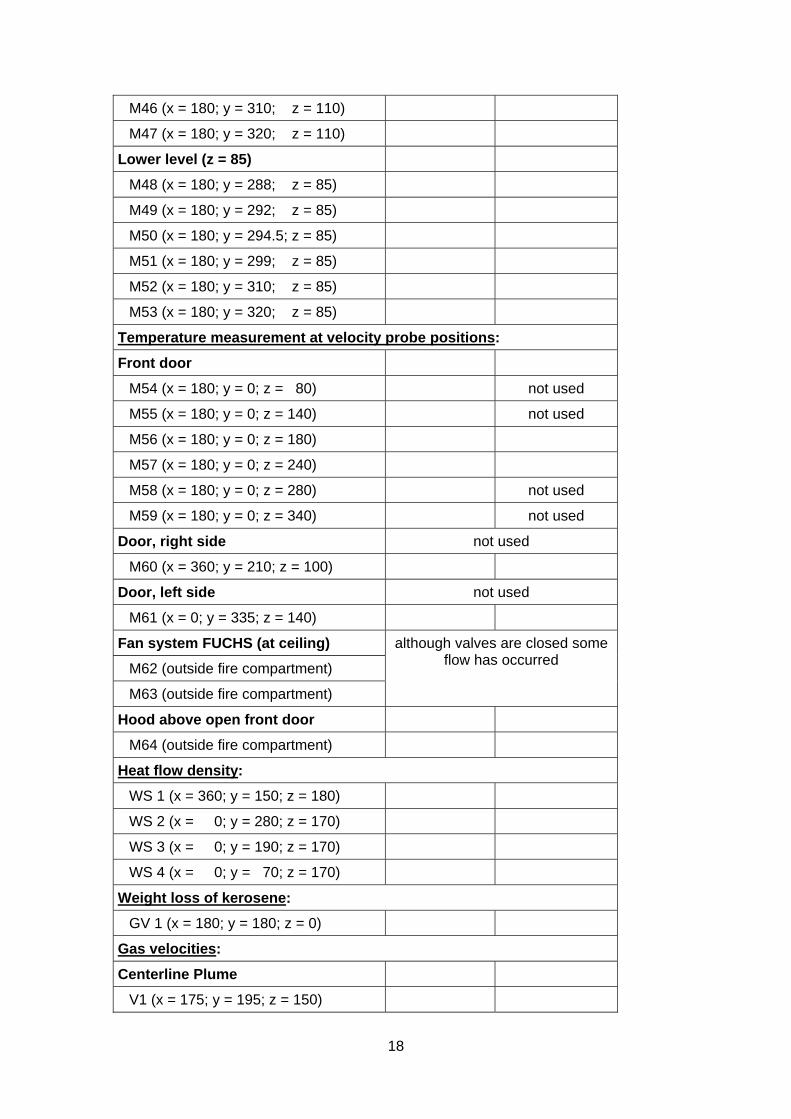
2.2.2 Measurements Performed

For measuring the temperatures inside the fire compartment, 3 mm-thick thermocou-

ples were used. These were not protected against flame radiation. The position of the

thermocouples was fixed on a grid.

To measure the surface temperatures, the measuring point was fixed with a 5 mm thick

thermo-wire. In parallel, “coated thermocouples” with a diameter of 3 mm were used.

To measure the temperatures of typical materials used at NPPs, three different types of

material probes (concrete, aerated concrete, steel) were inserted into the fire compart-

ment (Fig. 2-11). The convective and radiative heat flow into the material probes were

measured by water cooled heat transfer blocks. The coolant temperature was approxi-

mately 10 °C.

Along three lines, the temperatures inside the barrel container were measured (M36 to

M53). The location of these measurements is shown in Fig. 2-13.

The velocity inside the plume, at the door and inside the fan systems were measured

using bi-directional probes. The cross section area at the measurement positions V11

and V12 is 0.4 m x 0.8 m, and at the velocity measurement position V13 inside the

hood the diameter of the pipe was 0.4 m.

To measure the gas concentrations and pressure, open pipes were routed to the out-

side of the fire compartment and connected to the measurement systems. The posi-

tions and nomenclature of the different measurements are shown in Fig. 2-3 to Fig. 2-6

and in Table 2-5.

16

Table 2-5 List of measurements performed

Nomenclature

WS = Heat flow density measurement M = Temperature measurement GA = Measurement of gas composition V = Gas velocity measurement P = Measurement of total pressure GV = Measurement of weight loss

Measurement position Comment for Test 1

Comment for Test 3

Plume-temperature (x = 175, y = 195):

M 1 (z = 100 cm)

M 2 (z = 150 cm)

M 3 (z = 240 cm)

M 4 (z = 335 cm)

M 5 (z = 430 cm)

M 6 (z = 520 cm)

Temperature inside fire compartment:

Level 1: (z = 150 cm)

M 7 (x = 275; y = 85)

M 8 (x = 245; y = 345)

M 9 (x = 95; y = 60)

M 10 (x = 90; y = 280)

Level 2: (z = 335 cm)

M 11 (x = 275; y = 85)

M 12 (x = 245; y = 345)

M 13 (x = 95; y = 60)

M 14 (x = 90; y = 280)

Level 3: (z = 520 cm)

M 15 (x = 275; y = 85)

M 16 (x = 245; y = 345)

M 17 (x = 95; y = 60)

M 18 (x = 90; y = 280)

Surface temperature

Plates on the surface

M 19 (x = 245; y = 360; z = 150)

M 20 (x = 245; y = 360; z = 335)

17

M 21 (x = 0; y = 190; z = 170)

"Coated thermocouples" on the surface:

M 22 (x = 245; y = 360; z = 150)

M 23 (x = 245; y = 360; z = 335)

M 24 (x = 0; y = 190; z = 170)

Fuel temperature:

M25 (x = 175; y = 195; z = 33)

Material probes:

“Aerated concrete” (plate 10 cm thickness)

M26 (x = 2; y = 65; z =.170) *)

M27 (x = 5; y = 65; z = 170)

M28 (x = 8; y = 65; z = 170) *)

M29 (x = 10; y = 65; z = 170)

Concrete (plate 10 cm thickness)

M30 (x = 2; y = 190; z = 170) *)

M31 (x = 5; y = 190; z = 170)

M32 (x = 8; y = 190; z = 170) *)

M33 (x = 10; y = 190; z = 170)

Steel (plate 2 cm thickness)

M34 (x = 2; y = 280; z = 170)

M35 (x = 0; y = 280; z = 170)

Barrel type target (waste package):

Upper level (z = 140)

M36 (x = 180; y = 288; z = 140)

M37 (x = 180; y = 292; z = 140)

M38 (x = 180; y = 294.5; z = 140)

M39 (x = 180; y = 299; z = 140)

M40 (x = 180; y = 310; z = 140)

M41 (x = 180; y = 320; z = 140)

Center level (z = 110)

M42 (x = 180; y = 288; z = 110)

M43 (x = 180; y = 292; z = 110)

M44 (x = 180; y = 294.5; z = 110)

M45 (x = 180; y = 299; z = 110)

18

M46 (x = 180; y = 310; z = 110)

M47 (x = 180; y = 320; z = 110)

Lower level (z = 85)

M48 (x = 180; y = 288; z = 85)

M49 (x = 180; y = 292; z = 85)

M50 (x = 180; y = 294.5; z = 85)

M51 (x = 180; y = 299; z = 85)

M52 (x = 180; y = 310; z = 85)

M53 (x = 180; y = 320; z = 85)

Temperature measurement at velocity probe positions:

Front door

M54 (x = 180; y = 0; z = 80) not used

M55 (x = 180; y = 0; z = 140) not used

M56 (x = 180; y = 0; z = 180)

M57 (x = 180; y = 0; z = 240)

M58 (x = 180; y = 0; z = 280) not used

M59 (x = 180; y = 0; z = 340) not used

Door, right side not used

M60 (x = 360; y = 210; z = 100)

Door, left side not used

M61 (x = 0; y = 335; z = 140)

Fan system FUCHS (at ceiling)

M62 (outside fire compartment)

M63 (outside fire compartment)

although valves are closed some flow has occurred

Hood above open front door

M64 (outside fire compartment)

Heat flow density:

WS 1 (x = 360; y = 150; z = 180)

WS 2 (x = 0; y = 280; z = 170)

WS 3 (x = 0; y = 190; z = 170)

WS 4 (x = 0; y = 70; z = 170)

Weight loss of kerosene:

GV 1 (x = 180; y = 180; z = 0)

Gas velocities:

Centerline Plume

V1 (x = 175; y = 195; z = 150)

19

V2 (x = 175; y = 195; z = 335)

Door

V3 (x = 180; y = 0; z = 80)

V4 (x = 180; y = 0; z = 140)

V5 (x = 180; y = 0; z = 180)

V6 (x = 180; y = 0; z = 240)

V7 (x = 180; y = 0; z = 280)

V8 (x = 180; y = 0; z = 340)

Door, right side not used, door closed

V9 (x = 360; y = 210; z = 100)

Door, left side not used, door closed

V10 (x = 0; y = 335; z = 140)

Fan system FUCHS

V11 (outside fire compartment)

V12 (outside fire compartment)

Hood above open front door

V13 (outside fire compartment)

Gas composition:

Fire compartment

GA1 (x = 10; y = 190; z = 380)

Hood above front door

GA2 (outside fire compartment)

Fan system FUCHS not used

GA3 (outside fire compartment)

Pressure:

P1 (x = 110; y = 240; z = 540)

P2 (x = 30; y = 200; z = 280)

*) corrected after performance of calculations and documentation

20

Fig. 2-11 View of the three material probes

Fig. 2-12 View from top into the open barrel container

21

Fig. 2-13 Measurement positions inside barrel

2.2.3 Experimental Procedure

Procedure

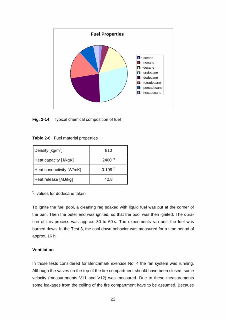
At the beginning of the experiments the pan was filled with fuel. In all experiments the

fuel level was 0.1 m. Fig. 2-14 shows a typical composition of the fuel used with the

chemical summary formula C11.64H25.29. Other fuel characteristics are outlined in Table

2-6.

22

Fuel Properties

n-octanen-nonanen-decanen-undecanen-dodecanen-tetradecanen-pentadecanen-hexadecane

Fig. 2-14 Typical chemical composition of fuel

Table 2-6 Fuel material properties

Density [kg/m3] 810

Heat capacity [J/kgK] 2400 *)

Heat conductivity [W/mK] 0.109 *)

Heat release [MJ/kg] 42.8

*): values for dodecane taken

To ignite the fuel pool, a cleaning rag soaked with liquid fuel was put at the corner of

the pan. Then the outer end was ignited, so that the pool was then ignited. The dura-

tion of this process was approx. 30 to 60 s. The experiments ran until the fuel was

burned down. In the Test 3, the cool-down behavior was measured for a time period of

approx. 16 h.

Ventilation

In those tests considered for Benchmark exercise No. 4 the fan system was running.

Although the valves on the top of the fire compartment should have been closed, some

velocity (measurements V11 and V12) was measured. Due to these measurements

some leakages from the ceiling of the fire compartment have to be assumed. Because

23

negative values were measured part of the time, the resulting volume flow through fan

system is assumed to be

( )[ ]12V11V vv.,0max8.04.0V +⋅⋅=& . (3-1)

Table 2-7 and Table 2-8 contain the smoothed volume flow and velocity values for

each experiment.

Table 2-7 Smoothed values for the total volume flow and velocity through the FUCHS

fan system (measurements V11 and V12) for Test 1

Test 1 (V11 and V12)

Time [s] Velocity v [m/s] Volume flow V& [m3/s]

0.00 0.00 0.00

150.00 0.00 0.00

165.00 0.26 0.08

180.00 1.38 0.44

195.00 2.59 0.83

210.00 4.12 1.32

225.00 4.41 1.41

551.00 6.82 2.18

615.00 6.78 2.17

666.00 6.64 2.13

720.00 7.03 2.25

859.00 6.01 1.92

1011.00 4.92 1.57

1245.00 3.41 1.09

1405.00 1.36 0.43

1650.00 0.45 0.14

1800.00 0.19 0.06

24

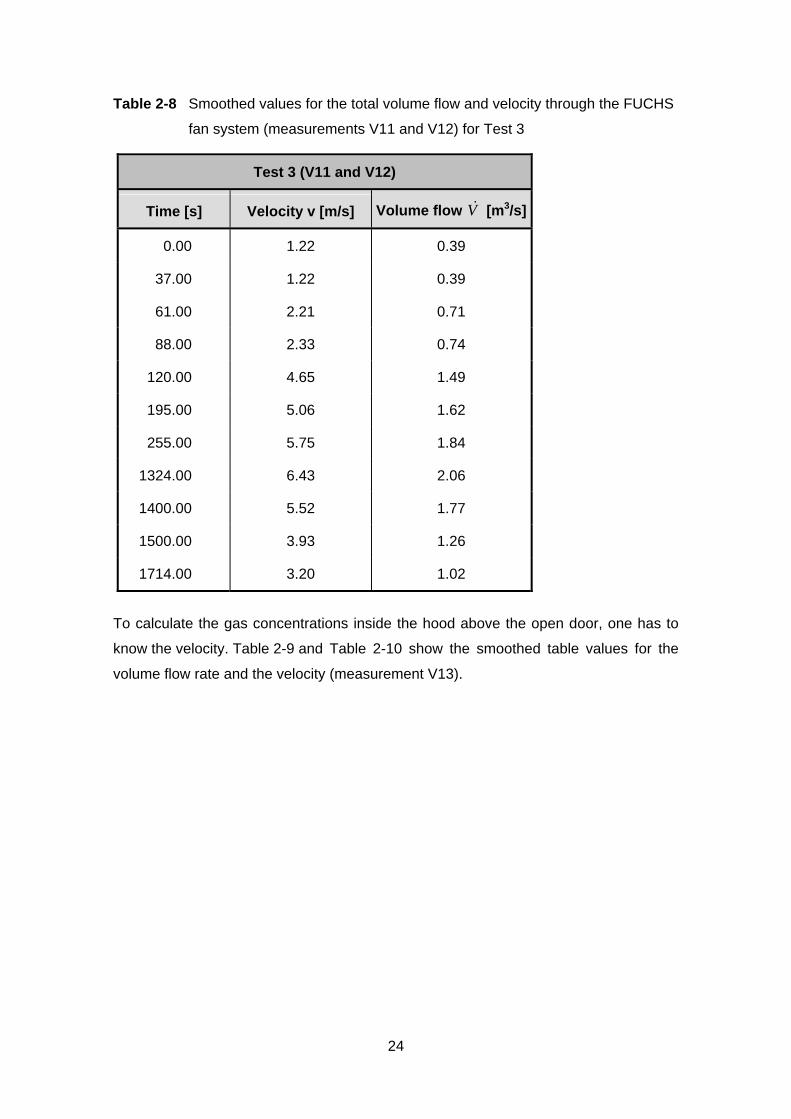
Table 2-8 Smoothed values for the total volume flow and velocity through the FUCHS

fan system (measurements V11 and V12) for Test 3

Test 3 (V11 and V12)

Time [s] Velocity v [m/s] Volume flow V& [m3/s]

0.00 1.22 0.39

37.00 1.22 0.39

61.00 2.21 0.71

88.00 2.33 0.74

120.00 4.65 1.49

195.00 5.06 1.62

255.00 5.75 1.84

1324.00 6.43 2.06

1400.00 5.52 1.77

1500.00 3.93 1.26

1714.00 3.20 1.02

To calculate the gas concentrations inside the hood above the open door, one has to

know the velocity. Table 2-9 and Table 2-10 show the smoothed table values for the

volume flow rate and the velocity (measurement V13).

25

Table 2-9 Smoothed values for the total volume flow and velocity through the hood

(measurement V13) for Test 1

Test 1 (V13)

Time [s] Velocity v [m/s] Volume flow V& [m3/s]

0.00 0.37 2.12

15.00 0.39 2.24

30.00 0.42 2.41

45.00 0.39 2.26

195.00 0.44 2.55

210.00 0.55 3.20

225.00 0.53 3.08

240.00 0.55 3.20

255.00 0.56 3.26

405.00 0.57 3.30

886.00 0.61 3.51

1449.00 0.63 3.66

1711.00 0.46 2.65

1755.00 0.52 3.03

1770.00 0.46 2.68

1785.00 0.49 2.86

1800.00 0.49 2.82

26

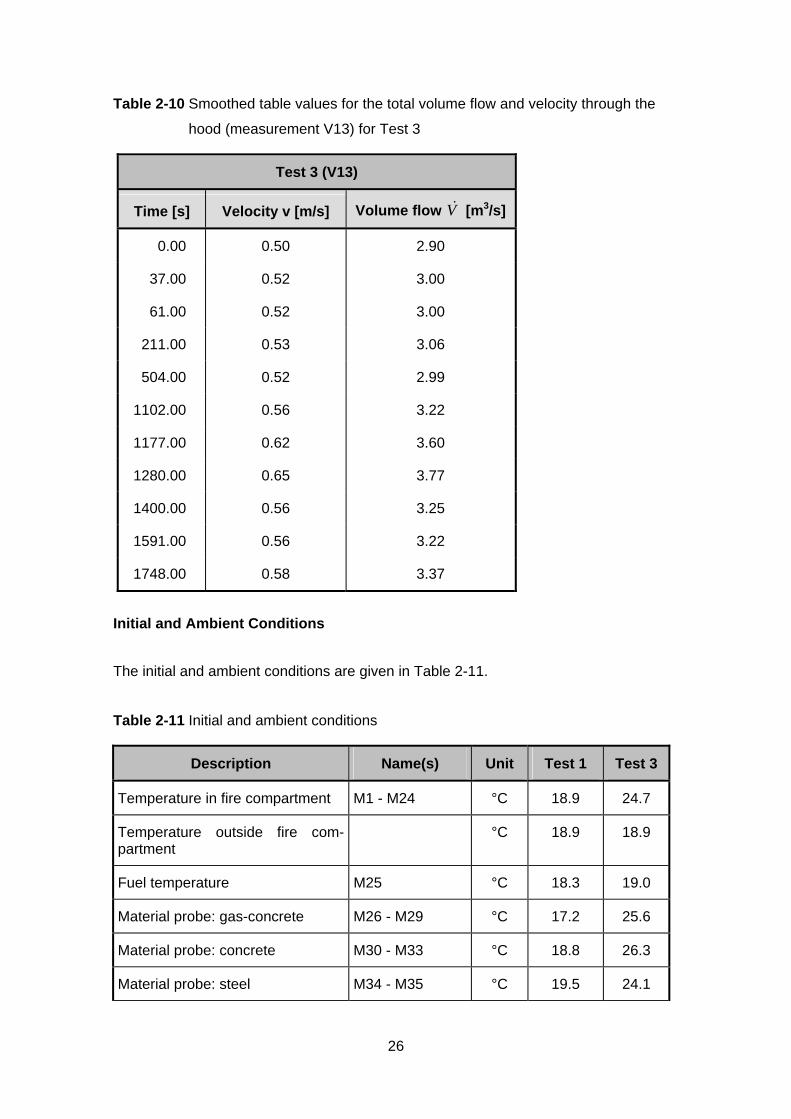
Table 2-10 Smoothed table values for the total volume flow and velocity through the

hood (measurement V13) for Test 3

Test 3 (V13)

Time [s] Velocity v [m/s] Volume flow V& [m3/s]

0.00 0.50 2.90

37.00 0.52 3.00

61.00 0.52 3.00

211.00 0.53 3.06

504.00 0.52 2.99

1102.00 0.56 3.22

1177.00 0.62 3.60

1280.00 0.65 3.77

1400.00 0.56 3.25

1591.00 0.56 3.22

1748.00 0.58 3.37

Initial and Ambient Conditions

The initial and ambient conditions are given in Table 2-11.

Table 2-11 Initial and ambient conditions

Description Name(s) Unit Test 1 Test 3

Temperature in fire compartment M1 - M24 °C 18.9 24.7

Temperature outside fire com-partment

°C 18.9 18.9

Fuel temperature M25 °C 18.3 19.0

Material probe: gas-concrete M26 - M29 °C 17.2 25.6

Material probe: concrete M30 - M33 °C 18.8 26.3

Material probe: steel M34 - M35 °C 19.5 24.1

27

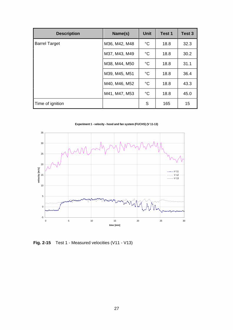
Description Name(s) Unit Test 1 Test 3

M36, M42, M48 °C 18.8 32.3

M37, M43, M49 °C 18.8 30.2

M38, M44, M50 °C 18.8 31.1

M39, M45, M51 °C 18.8 36.4

M40, M46, M52 °C 18.8 43.3

Barrel Target

M41, M47, M53 °C 18.8 45.0

Time of ignition S 165 15

Experiment 1 - velocity - hood and fan system (FUCHS) (V 11-13)

-5

0

5

10

15

20

25

30

35

0 5 10 15 20 25 30

time [min]

velo

city

[m/s

]

V 11V 12V 13

Fig. 2-15 Test 1 - Measured velocities (V11 - V13)

28

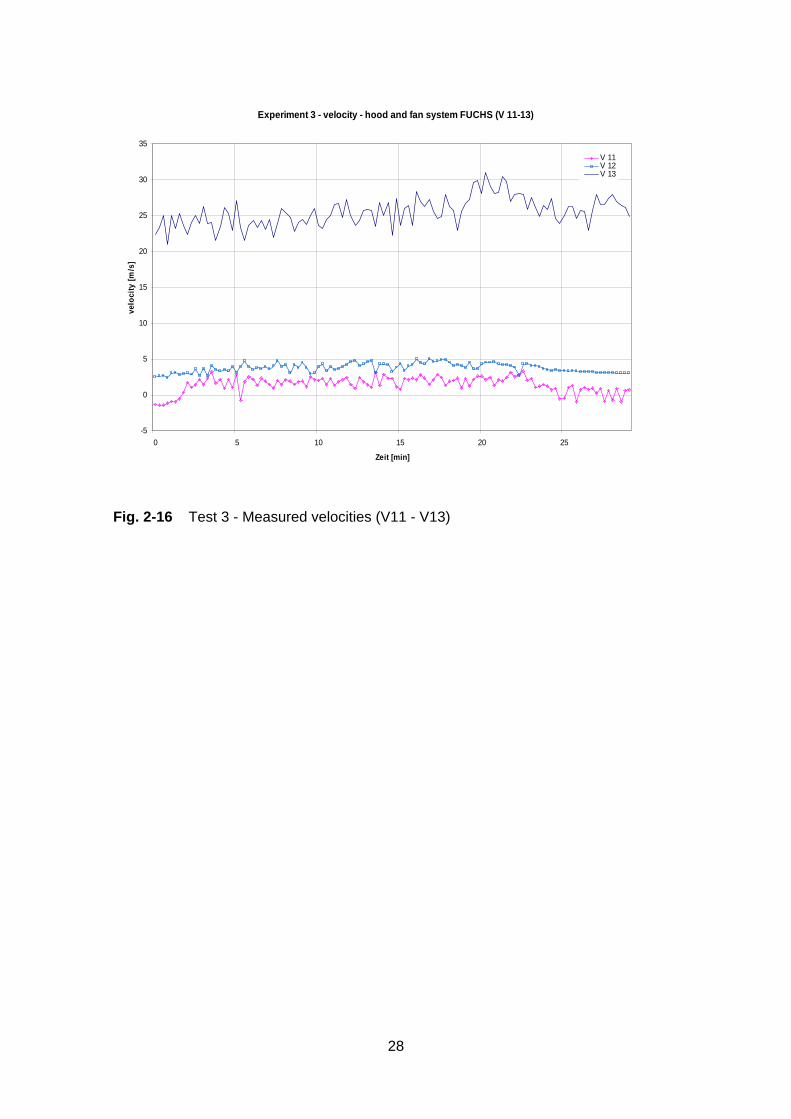
Experiment 3 - velocity - hood and fan system FUCHS (V 11-13)

-5

0

5

10

15

20

25

30

35

0 5 10 15 20 25

Zeit [min]

velo

city

[m/s

]

V 11V 12V 13

Fig. 2-16 Test 3 - Measured velocities (V11 - V13)

29

3 Experimental Results

The following section provides data and results from both experiments of the ICFMP

Benchmark Exercise No. 4. The results have been made available to the participants of

ICFMP in two steps. In April 2004, the pyrolysis rates of the fuel pool fires were re-

leased. Most of the results were delivered in May 2004. These results were presented

during the 8th ICFMP Meeting at VTT in Finland /KLE 04/.

The tests 1 and 3 are part of a total of 9 fuel pool fire tests at iBMB. Table 3-1 shows

the test matrix. In the frame of these tests, the influence of openings as well as of the

forced ventilation and the pool size on the thermal load has been investigated. In some

tests large pool sizes compared to the fire compartment volume were used, leading to

rather high temperature loads.

Table 3-1 Test matrix of the iBMB fuel pool fire tests

Test Pool area [m2] Openings [m2] Ventilation

1 1 door: 3 x 0.7 no

2 1 door: 2 x 0.7 no

3 1 door: 1 x 0.7 (1 m above floor) no

4 1 door: 1 x 0.7 (2 m above floor) no

5 1 door: 2 x 0.7 (1 m above floor) sides: 0.6 x 0.7 and 0.6 x 1.2

yes

6 1 door: 2 x 0.3 (1 m above floor) sides: 0.3 x 0.7 and 0.4 x 1.2

yes

7 2 door: 3 x 0.7 sides: 0.6* x 0.7 and 0.6 x 1.2

yes

8 2 door: 2 x 0.7 (1 m above floor) yes

9 4 door: 2 x 0.7 (1 m above floor) yes

30

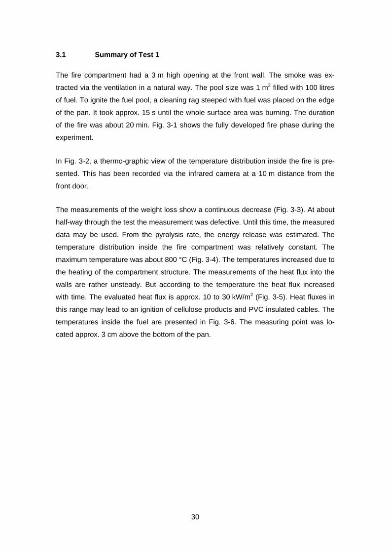
3.1 Summary of Test 1

The fire compartment had a 3 m high opening at the front wall. The smoke was ex-

tracted via the ventilation in a natural way. The pool size was 1 m2 filled with 100 litres

of fuel. To ignite the fuel pool, a cleaning rag steeped with fuel was placed on the edge

of the pan. It took approx. 15 s until the whole surface area was burning. The duration

of the fire was about 20 min. Fig. 3-1 shows the fully developed fire phase during the

experiment.

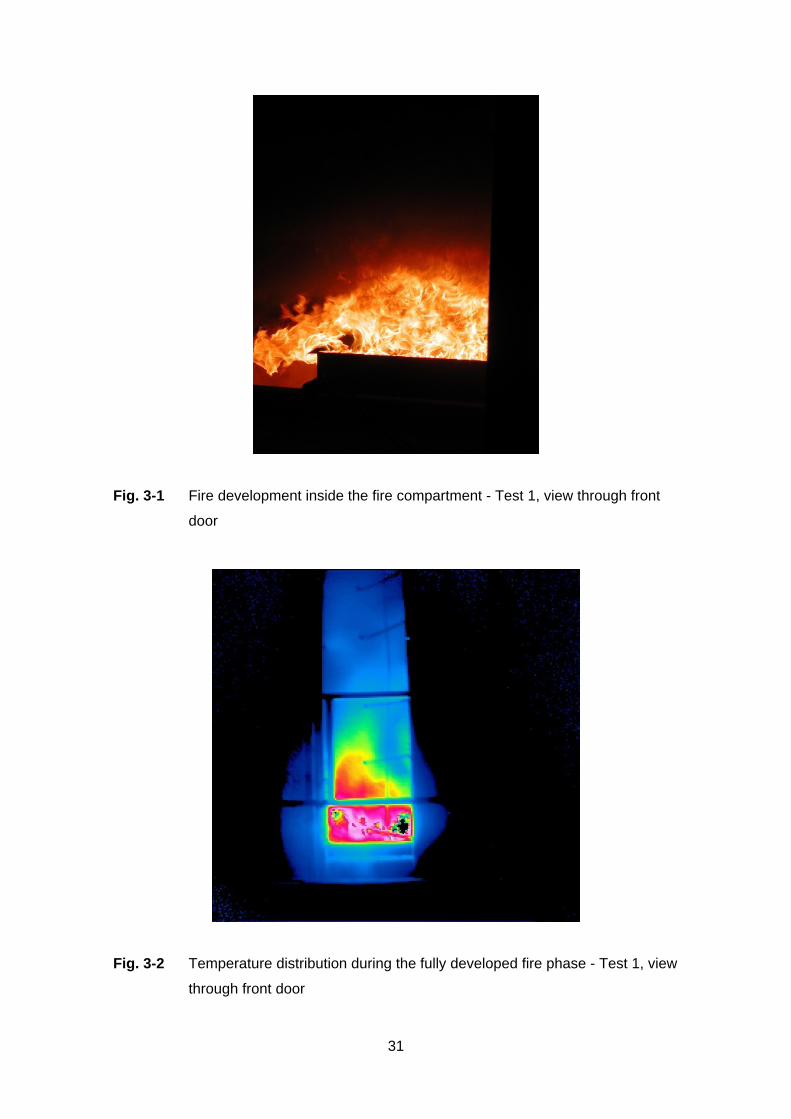
In Fig. 3-2, a thermo-graphic view of the temperature distribution inside the fire is pre-

sented. This has been recorded via the infrared camera at a 10 m distance from the

front door.

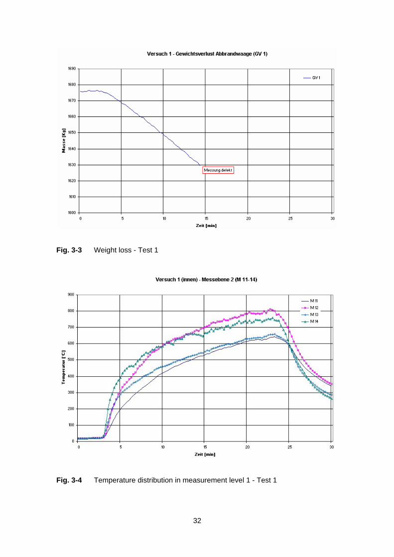
The measurements of the weight loss show a continuous decrease (Fig. 3-3). At about

half-way through the test the measurement was defective. Until this time, the measured

data may be used. From the pyrolysis rate, the energy release was estimated. The

temperature distribution inside the fire compartment was relatively constant. The

maximum temperature was about 800 °C (Fig. 3-4). The temperatures increased due to

the heating of the compartment structure. The measurements of the heat flux into the

walls are rather unsteady. But according to the temperature the heat flux increased

with time. The evaluated heat flux is approx. 10 to 30 kW/m2 (Fig. 3-5). Heat fluxes in

this range may lead to an ignition of cellulose products and PVC insulated cables. The

temperatures inside the fuel are presented in Fig. 3-6. The measuring point was lo-

cated approx. 3 cm above the bottom of the pan.

31

Fig. 3-1 Fire development inside the fire compartment - Test 1, view through front

door

Fig. 3-2 Temperature distribution during the fully developed fire phase - Test 1, view

through front door

32

Fig. 3-3 Weight loss - Test 1

Fig. 3-4 Temperature distribution in measurement level 1 - Test 1

33

Fig. 3-5 Heat flux into material probes - Test 1

Fig. 3-6 Measured fuel temperature 3 cm above pan bottom - Test 1

34

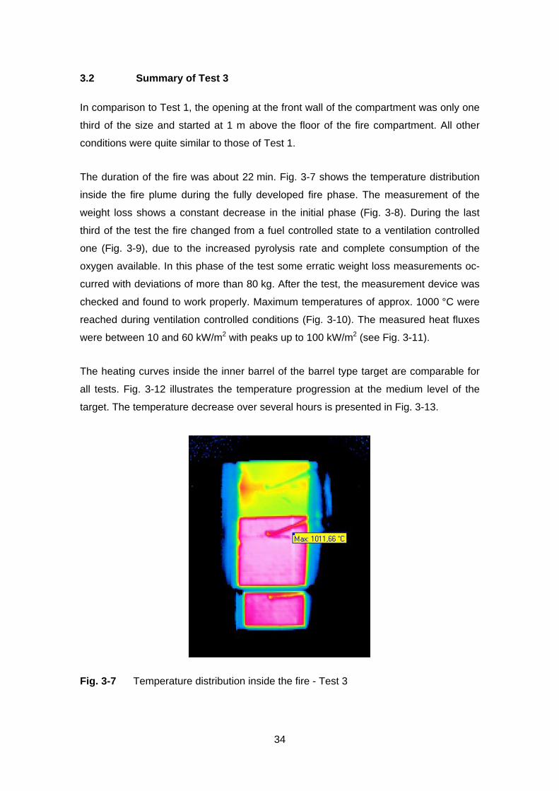
3.2 Summary of Test 3

In comparison to Test 1, the opening at the front wall of the compartment was only one

third of the size and started at 1 m above the floor of the fire compartment. All other

conditions were quite similar to those of Test 1.

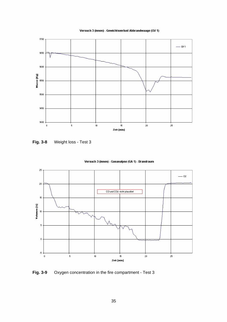
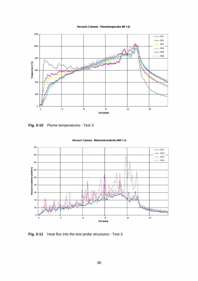
The duration of the fire was about 22 min. Fig. 3-7 shows the temperature distribution

inside the fire plume during the fully developed fire phase. The measurement of the

weight loss shows a constant decrease in the initial phase (Fig. 3-8). During the last

third of the test the fire changed from a fuel controlled state to a ventilation controlled

one (Fig. 3-9), due to the increased pyrolysis rate and complete consumption of the

oxygen available. In this phase of the test some erratic weight loss measurements oc-

curred with deviations of more than 80 kg. After the test, the measurement device was

checked and found to work properly. Maximum temperatures of approx. 1000 °C were

reached during ventilation controlled conditions (Fig. 3-10). The measured heat fluxes

were between 10 and 60 kW/m2 with peaks up to 100 kW/m2 (see Fig. 3-11).

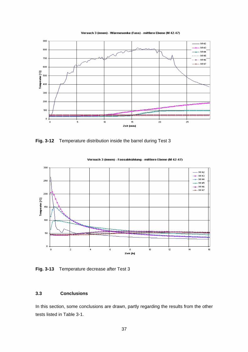
The heating curves inside the inner barrel of the barrel type target are comparable for

all tests. Fig. 3-12 illustrates the temperature progression at the medium level of the

target. The temperature decrease over several hours is presented in Fig. 3-13.

Fig. 3-7 Temperature distribution inside the fire - Test 3

35

Fig. 3-8 Weight loss - Test 3

Fig. 3-9 Oxygen concentration in the fire compartment - Test 3

36

Fig. 3-10 Plume temperatures - Test 3

Fig. 3-11 Heat flux into the test probe structures - Test 3

37

Fig. 3-12 Temperature distribution inside the barrel during Test 3

Fig. 3-13 Temperature decrease after Test 3

3.3 Conclusions

In this section, some conclusions are drawn, partly regarding the results from the other

tests listed in Table 3-1.

38

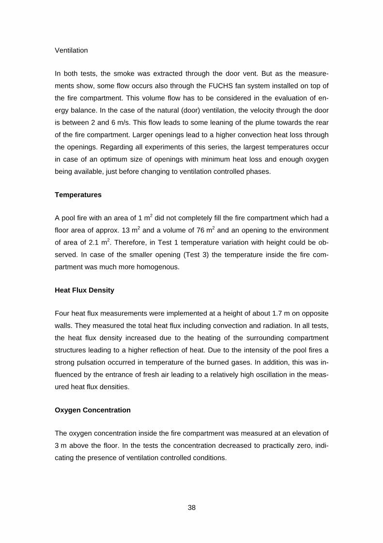
Ventilation

In both tests, the smoke was extracted through the door vent. But as the measure-

ments show, some flow occurs also through the FUCHS fan system installed on top of

the fire compartment. This volume flow has to be considered in the evaluation of en-

ergy balance. In the case of the natural (door) ventilation, the velocity through the door

is between 2 and 6 m/s. This flow leads to some leaning of the plume towards the rear

of the fire compartment. Larger openings lead to a higher convection heat loss through

the openings. Regarding all experiments of this series, the largest temperatures occur

in case of an optimum size of openings with minimum heat loss and enough oxygen

being available, just before changing to ventilation controlled phases.

Temperatures

A pool fire with an area of 1 m2 did not completely fill the fire compartment which had a

floor area of approx. 13 m2 and a volume of 76 m2 and an opening to the environment

of area of 2.1 m2. Therefore, in Test 1 temperature variation with height could be ob-

served. In case of the smaller opening (Test 3) the temperature inside the fire com-

partment was much more homogenous.

Heat Flux Density

Four heat flux measurements were implemented at a height of about 1.7 m on opposite

walls. They measured the total heat flux including convection and radiation. In all tests,

the heat flux density increased due to the heating of the surrounding compartment

structures leading to a higher reflection of heat. Due to the intensity of the pool fires a

strong pulsation occurred in temperature of the burned gases. In addition, this was in-

fluenced by the entrance of fresh air leading to a relatively high oscillation in the meas-

ured heat flux densities.

Oxygen Concentration

The oxygen concentration inside the fire compartment was measured at an elevation of

3 m above the floor. In the tests the concentration decreased to practically zero, indi-

cating the presence of ventilation controlled conditions.

39

4 Input Parameters and Assumptions

For the Benchmark Exercise No. 4, it was intended to perform blind calculations with-

out knowing the pyrolysis rate or the other experimental results, semi-blind calculations

(knowing only the pyrolysis rate) and open calculations with all data being available to

the modelers. From the beginning, it was clear that performing blind calculations is a

challenging task. But, on the other hand, this is a typical situation for real applications

in nuclear power plants and installations. The deviations of the calculated results from

the measured data provides some insights into the uncertainties of the results for such

(somewhat extreme) situations, particularly due to the high heat release rate compared

to the volume of the fire compartment.

In the following section the major assumptions employed in performing the calculations

are listed and discussed:

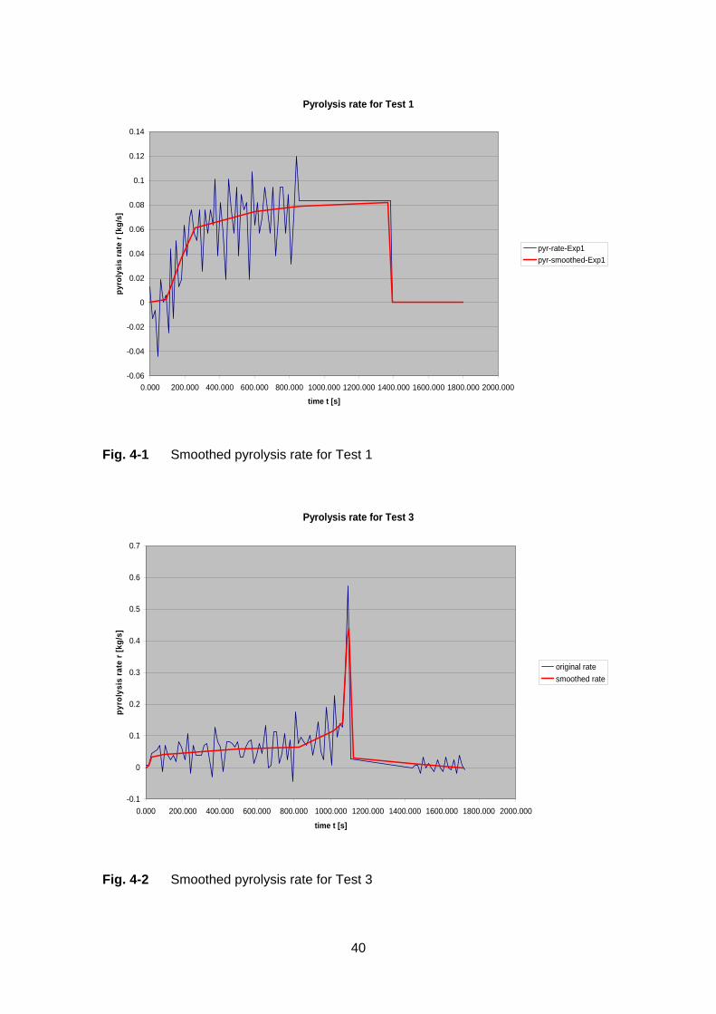
Heat Release Rate

The specified pyrolysis rate (used in the semi-blind and open calculations) is based on

the measurement of the weight loss, which had some problems for Test 1 (weight loss

data available until 850 s only) and Test 3 (containing positive gradients leading to

negative pyrolysis rates). Therefore, some approximations and assumptions have been

made influencing the results to some extent. Fig. 4-1 and Fig. 4-2 show the proposed

smoothed pyrolysis rates compared to the raw measured data.

LOL Value

Main difference between the two tests is the cross section of the door opening. This

leads to under-ventilated conditions in Test 3. Some codes have to specify the LOL

value or it is fixed inside the program. A too high value for LOL reduces the accuracy of

the predictions for Test 3. In case of high temperatures the entrained oxygen seems to

be completely consumed by the combustion process.

40

Pyrolysis rate for Test 1

-0.06

-0.04

-0.02

0

0.02

0.04

0.06

0.08

0.1

0.12

0.14

0.000 200.000 400.000 600.000 800.000 1000.000 1200.000 1400.000 1600.000 1800.000 2000.000

time t [s]

pyro

lysi

s ra

te r

[kg/

s]

pyr-rate-Exp1pyr-smoothed-Exp1

Fig. 4-1 Smoothed pyrolysis rate for Test 1

Pyrolysis rate for Test 3

-0.1

0

0.1

0.2

0.3

0.4

0.5

0.6

0.7

0.000 200.000 400.000 600.000 800.000 1000.000 1200.000 1400.000 1600.000 1800.000 2000.000

time t [s]

pyro

lysi

s ra

te r

[kg/

s]

original ratesmoothed rate

Fig. 4-2 Smoothed pyrolysis rate for Test 3

41

Ventilation

In most cases, the ventilation was defined as it was described in the specification.

Some participants decided not to simulate the ventilation system and the hood.

Radiation Fraction

The radiation fraction has to be defined by the user. Values about 40% have been

used. In some calculations the radiation fraction is assumed to be released from the

pan, possibly leading to different temperature loads on the targets.

Targets

The targets (three material probes) and the barrel type container are not always con-

sidered in the calculations. For the material probes (particularly for steel) one problem

was the thickness. Furthermore, a backward heating was possible, which was not (and

could not be) considered in any of the calculations. With respect to the barrel, the cy-

lindrical shape could not be modeled with some of the codes. In addition, the multi-

layer material composition could not be considered in all codes.

Combustion Scheme and Yields

The composition of the fuel was specified, but not the chemical reaction itself. There-

fore, the user had to specify the yields and to decide if the combustion is complete or

not. In particular for Test 3, the input may have an impact on the results, due to the

under-ventilated condition and production of CO and soot.

Grid Size

For CFD (computational fluid dynamics) codes the user has to specify the grid size.

The cell size used in FDS /MCG 04/ with a width of approx. 10 cm is somewhat larger

than the cell size used in CFX-5.7 /CFX 04/. The choice of suitable grid size will de-

pend on the type of CFD model (e.g. RANS of LES) and the numerical schemes em-

ployed.

Air Entrainment

For zone models, the simulation of the air entrainment (the plume mode) seems to be a

key parameter, as this effects the available oxygen for the combustion.

43

5 Comparison of Code Simulations and Experimental Results

For Benchmark Exercise No. 4 full blind calculations (without knowing the pyrolysis

rate), semi-blind calculations (knowing pyrolysis rate) and full open calculations have

been performed. Table 5-1 lists the participants for this Benchmark Exercise, the fire

codes used, type of analysis and the reference to the Appendix provided by the partici-

pant. A summary of the performed calculations is provided below.

Table 5-1 List of fire simulations performed within Benchmark Exercise No. 4

Participant Fire Code Code Type Tests Type of Analysis

Appen-dix

K. McGrattan, NIST

FDS zone 1 & 3 blind, semi-blind

A

S. Miles, BRE JASMINE CFD 1 & 3 blind, semi-blind,

open (3 only)

B

CFAST zone 1 & 3 semi-blind B

M. Dey, USNRC FDS CFD 1 & 3 semi-blind C

CFAST zone 1 & 3 semi-blind C

T. Elicson (Fauske) FATE zone 1 & 3 open D

L. Rigollet (IRSN) FLAMME-S zone 1 & 3 open E

M. Heitsch (GRS) CFX CFD 1 & 3 open F

W. Brücher (GRS) FDS CFD 3 open G

B. Schramm (GRS) COCOSYS LP 1 & 3 open H

V. Nicolette (SNL) VULCAN CFD 3 open I

B. Gautier (EdF) MAGIC zone 1 & 3 open J

44

5.1 Blind Calculations

5.1.1 FDS (CFD Code) Applied by K. McGrattan (NIST, USA)

FDS Code Description and Input

In cooperation with the fire protection engineering community, a computational fire mo-

del, Fire Dynamics Simulator (FDS) /MCG 04/, has been developed at the National

Institute of Standards and Technology (NIST) in the USA to study fire behavior and to

evaluate the performance of fire protection systems in buildings. The software was re-

leased into the public domain in 2000, and since then has been used for a wide variety

of analyses by fire protection engineers. Briefly, FDS is a computational fluid dynamics

code that solves the Navier-Stokes equations in low Mach number, or thermally ex-

pandable, form. The transport algorithm is based on large eddy simulation techniques,

radiation is modeled using a gray gas approximation and a finite-volume method is

used to solve the radiation transport equation. Combustion is modeled using a mixture

fraction approach, in which a single transport equation is solved for a scalar variable

representing the fraction of gas originating in the fuel stream.

The dimensions of the grid were 36 by 72 by 56, and the cells were exactly 10 cm in

size throughout. All objects within the computational domain were approximated to the

nearest 10 cm. The decision to use a 10 cm grid was based on the observation that the

ratio of the fire’s characteristic diameter D* to the size of the grid cell dx is an indicator

of the degree of resolution achieved by the simulation. D* is given by the expres-

sion 5/2)/( gTcQ p ∞∞

•

ρ , and was about 1 m for this series of fires. Past experience has

shown that a ratio of 10 produces favorable results at a moderate computational cost.

FDS performs a one-dimensional heat transfer calculation into an assumed homoge-

nous material of given thickness and (temperature-dependent) thermal properties. The

compartment walls and ceiling were made of various types of concrete, the thermal

properties of which were input directly into the model. It was assumed that the target

slabs of concrete, aerated concrete, and steel were only exposed at the front surface,

although the internal temperature measurements suggested otherwise. No attempt was

made to model the barrel container at the rear of the compartment, due to its cylinder

geometry and composition of different materials.

45

Some of the properties of the liquid fuel used in the tests were provided. For kerosene,

the fuel properties of “dodecane” (C11.64H25.29) were input into the model with assumed

soot and CO yields of 0.042 and 0.012, respectively. The current version of FDS did

not adjust the soot or CO yield as a consequence of reduced compartment ventilation

or combustion efficiency. The assumed heat of vaporization and boiling temperature:

256 kJ/kg and 216 °C, respectively, were important input values for the simulation. For

the blind calculations the fire was simulated by including in the simulation a small, hot

block that heated up the surface of the pool until the fire was self-sustaining, after

which the block literally disappeared from the calculation. FDS predicted the radiative

and convective heat flux from the fire to the fuel surface, and the evaporation of the fuel

according to the Clausius-Clapeyron equilibrium pressure of the fuel vapors above the

pan.

FDS uses a finite volume method to solve the radiation transport equation in the gray

gas limit. By default, the radiation from the fire and hot gases is tracked in 100 direc-

tions, which is adequate to predict the radiation heat flux to nearby targets.

The ventilation rates for all the compartment fans and hood were input directly into the

model.

Code Results

For blind calculations only the heat release has been discussed. For Test 1, the pre-

dicted heat release rate (HRR) rose very quickly to about 3 MW following ignition, fol-

lowed by a gradual rise over 15 min as the compartment heated up and the increased

thermal radiation from the hot upper layer led to an increased burning rate (Fig. 5-1).

The measured HRR did not exhibit the rapid rise, taking several minutes to grow to 3

MW and then gradually increasing at a rate comparable to the prediction. The reason

for the discrepancy is that FDS uses a mixture fraction model of combustion. Briefly,

the evaporated fuel burns readily with oxygen when mixed to the appropriate ratio, re-

gardless of temperature. Thus, FDS did not simulate properly the spreading of the fire

across the pan; rather it predicted an almost instantaneous involvement of the entire

fuel surface.

In Test 3, FDS over-emphasized the effect of the small compartment opening (Fig.

5-1). Initially, it predicted the same rapid growth as it had in Test 1, but then the fire

consumed the available oxygen, and the fire died down, decreasing the burning rate.

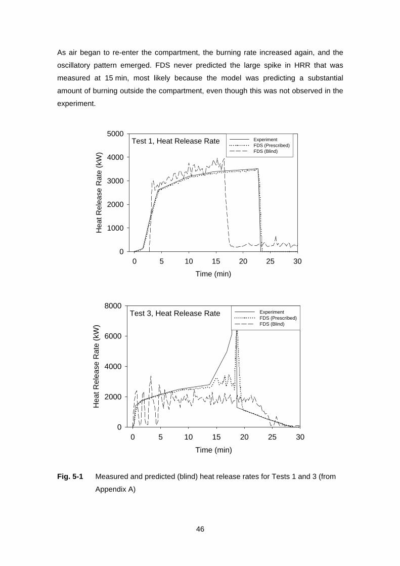
46

As air began to re-enter the compartment, the burning rate increased again, and the

oscillatory pattern emerged. FDS never predicted the large spike in HRR that was

measured at 15 min, most likely because the model was predicting a substantial

amount of burning outside the compartment, even though this was not observed in the

experiment.

Test 1, Heat Release Rate

Time (min)

0 5 10 15 20 25 30

Hea

t Rel

ease

Rat

e (k

W)

0

1000

2000

3000

4000

5000ExperimentFDS (Prescribed)FDS (Blind)

Test 3, Heat Release Rate

Time (min)

0 5 10 15 20 25 30

Hea

t Rel

ease

Rat

e (k

W)

0

2000

4000

6000

8000ExperimentFDS (Prescribed)FDS (Blind)

Fig. 5-1 Measured and predicted (blind) heat release rates for Tests 1 and 3 (from

Appendix A)

47

5.1.2 JASMINE (CFD Code) Applied by S. Miles (BRE, UK)

Blind calculations (prior to the dissemination of the experimentally measured fuel mass

release rate) were conducted for Tests 1 and 3 with JASMINE Version 3.2.3 /COX 87/.

One important purpose of these blind simulations was to examine how realistic predic-

tions could be made for gas temperatures, fluxes etc using a simple, empirical expres-

sion for fuel pyrolysis rate.

JASMINE Code Description and Input Assumptions

JASMINE solves the Reynolds-Averaged Navier Stokes (RANS) equations of fluid flow

on a single-block Cartesian grid. The coupled set of equations for each of the three

Cartesian velocity components, enthalpy (heat) and other scalars required by the vari-

ous sub-models (e.g. fuel mass and mixture fractions for combustion) is approximated

as a system of algebraic equations that are solved numerically on a discrete grid. This

generates a solution value for each variable at each grid location. JASMINE uses the

finite volume method, where the differential equations are first transformed into an inte-

gral form and then discreticizsed on the control volumes (or cells) defined by the nu-

merical grid. This solution procedure is coupled with a variant of the SIMPLE pressure-

correction scheme. Transient solutions are generated by a first-order, fully-implicit

scheme. A standard κ-ε turbulence model with additional buoyancy source terms was

used. Standard wall functions for enthalpy and momentum describe the turbulent

boundary layer adjacent to solid surfaces.

In the benchmark exercise combustion was modeled using the eddy break-up sub-

model in which the fuel pyrolysis rate is specified as an input boundary condition. Re-

action (oxidation) is calculated at all control volumes as a function of fuel concentration,

oxygen concentration and the local turbulent time-scale. A simple one-step, infinitely

fast chemical reaction is assumed. Complete oxidation of the fuel is assumed where

sufficient oxygen is available. The effect of oxygen concentration on the local rate of

burning may be incorporated by setting oxygen and temperature limits which define

'burn' and 'no burn' regions. For the blind simulations no oxygen concentration limit was

specified, i.e. there was only a 'burn' region.

A fuel source area of 1 m2 and a heat of combustion of 4.28 x 107 J kg-1 were used in

all calculations. For the blind calculations a fixed fuel pyrolysis rate was assumed from

60 s after ignition (increasing linearly to this value over the first 60 s). A value of

48

0.039 kg s-1 was chosen, based upon published engineering information. The sensitiv-

ity to reducing this value to 0.0234 kg s-1 was investigated.

Radiant heat transfer is modeled with either the six-flux model, which assumes that

radiant transfer is normal to the co-ordinate directions, or the potentially more accurate

discrete transfer method. All blind calculations were performed using the six-flux radia-

tion model. Local absorption-emission properties are computed using a mixed grey-gas

model, which calculates the local absorption coefficient as a function of temperature

and gas species concentrations. As soot was not modeled in this benchmark exercise,

only CO2 and H2O acted as participating media in the radiation calculations.

Where soot is not explicitly modeled, its influence on the overall energy budget may be

incorporated, somewhat crudely, by reducing the heat release rate of the fire, i.e. either

the pyrolysis rate or the effective heat of combustion, by a fixed fraction. This is akin to

the radiative fraction employed in zone models such as CFAST. The amount of heat

then removed represents what could be expected to be 'lost' by radiation from the

sooty flame region above the fuel source. The remainder of this heat is assumed to be

convected into the rest of the compartment or, as a relatively small fraction, by radia-

tion from the plume region due to CO2 and H2O. Note also that of the heat convected

into the compartment (from the fire source), some of this is subsequently radiated from

the ‘smoke gases’ (due to CO2 and H2O).

Thermal conduction into solid boundaries may be included by means of a quasi-steady,

semi-infinite, one-dimensional assumption, which is appropriate for many smoke mo-

vement applications. Alternatively, the solution of the one-dimensional heat conduction

equation into the solid is also available. The quasi-steady, one-dimensional assumption

was employed in the blind calculations. The thermal properties of the concrete walls,

floor and ceiling were included as specified.

The dimensions of the compartment, doorway opening and exhaust ventilation duct

were modeled exactly as in the problem specification. Only half the compartment was

modeled, imposing symmetry at the x = 1.8 m plane, and using a numerical mesh of

approximately 80,000 cells. A fixed numerical time-step of 2.5 s was employed in all

simulations.

Ventilation through the fan system was modeled as a time-dependent mass sink, set to

a value corresponding to the experimentally measured volumetric flow rate.

49

The thermal response of the material probe targets and the heat flow densities (WS2,

WS3 & WS4) was included in the JASMINE calculations. Furthermore, the wall surface

temperatures at the locations of the plates/thermocouples (M19 etc) were calculated.

While the blockage due to the barrel target was included, its thermal response was not

modeled and so no comparisons were made with the barrel temperature measure-

ments.

Further general information on JASMINE is provided in the Appendix B to this report.

JASMINE Code Results

Two sets of blind predictions were made for each of Test 1 and Test 3, one using a

fixed fuel pyrolysis rate of 0.039 kg s-1 and the other a rate of 0.0234 kg s-1. These cal-

culations were performed only for the first ten minutes of the experiments.

Comparisons between prediction and measurement were made for gas temperatures,

oxygen concentration, door/wall vent velocities and compartment surface tempera-

tures. The blind predictions made with the higher value of the pyrolysis rate were closer

to the experimental measurements than those made with the lower pyrolysis rate.

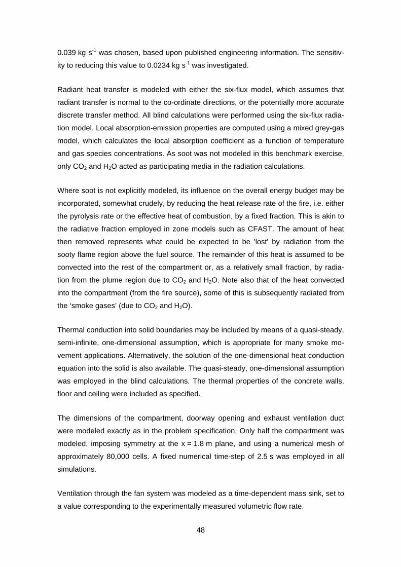
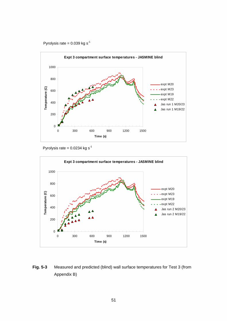
Fig. 5-2 and Fig. 5-3 (from the Appendix B) show the gas phase and wall surface tem-

perature calculations for Test 3 using the two fuel pyrolysis specifications.

The blind calculations using the higher fuel pyrolysis rate of 0.039 kg s-1 were quite

encouraging considering the complexity of the physics involved. A simple engineering

estimate of the pyrolysis rate was in this case sufficient to capture the main gas phase

properties of the experiments. It was noted, however, that the transient effects due to

changes in the pyrolysis rate due to the development of conditions inside the enclosure

were not captured. Effects due to the feedback of radiation from soot particulates and

the compartment walls are likely to be highly transient.

A main discrepancy between the blind calculations and the measurements was in the

doorway vent flow in Test 3, where in contrast to the flow being predominantly into the

compartment as indicated in the predictions, the measurements suggest a more dis-

tinct two-way flow at the wall vent. This discrepancy may be due, in part at least, to the

imposed exhaust flow at the mechanical ventilation duct in the JASMINE calculations

forcing a significant amount of air into the compartment through the wall vent.

50

Fig. 5-2 Measured and predicted (blind) gas temperatures for Test 3 (from Appendix

B)

Expt 3 compartment temperatures - JASMINE blind

0

200

400

600

800

1000

0 300 600 900 1200 1500

Time (s)

Tem

pera

ture

(C)

expt M16expt M12expt M11expt M7Jas run 2 M16Jas run 2 M12Jas run 2 M11Jas run 2 M7

Pyrolysis rate = 0.0234 kg s-1

Expt 3 compartment temperatures - JASMINE blind

0

200

400

600

800

1000

0 300 600 900 1200 1500

Time (s)

Tem

pera

ture

(C)

expt M16expt M12expt M11expt M7Jas run 1 M16Jas run 1 M12Jas run 1 M11Jas run 1 M7

Pyrolysis rate = 0.039 kg s-1

51

Fig. 5-3 Measured and predicted (blind) wall surface temperatures for Test 3 (from

Appendix B)

Expt 3 compartment surface temperatures - JASMINE blind

0

200

400

600

800

1000

0 300 600 900 1200 1500

Time (s)

Tem

pera

ture

(C) expt M20

expt M23expt M19expt M22Jas run 1 M20/23Jas run 1 M19/22

Pyrolysis rate = 0.039 kg s-1

Expt 3 compartment surface temperatures - JASMINE blind

0

200

400

600

800

1000

0 300 600 900 1200 1500

Time (s)

Tem

pera

ture

(C) expt M20

expt M23expt M19expt M22Jas run 2 M20/23Jas run 2 M19/22

Pyrolysis rate = 0.0234 kg s-1

52

5.2 Semi-blind Calculations

5.2.1 FDS (CFD Code) Applied by K. McGrattan (NIST, USA)

FDS Code Description and Input

(See paragraph 5.1.1)

Code Results

Assuming an uncertainty of 15 % for the heat release rate (HRR) an uncertainty of

temperatures about 10 % can be concluded. In general, the difference between meas-

ured and predicted compartment temperatures in Tests 1 and 3 was within the uncer-

tainty bounds established by the prescribed HRR, but there were some exceptions,

especially in Test 3. In making comparisons between model and experiment, the tem-

peratures were compared from 10 min onwards. Earlier in the tests, the measured

temperatures exhibited a delay relative to the predictions, probably due to the thermal

inertia of the thermocouples.

Three plates were positioned on the side wall of the compartment, about 1.7 m above

the floor. FDS did compute the inner temperatures of the slabs, and the temperatures

decreased monotonically with depth since FDS considered the slab to back up to an

ambient temperature environment. However, the measured temperatures did not de-

crease monotonically, either because of a measurement error or the slab might have

been heated from behind. Sometimes the comparison of surface temperatures and

heat flux with the experimental data was somewhat inconsistent. In some situations,

the predicted surface temperature was more accurate than the predicted heat flux,

suggesting either that the heat flux measurement was inaccurate, or that the model

benefited from “two wrongs making a right”; that is, an under- or over-prediction in the

heat flux was compensated by a comparable error in the surface properties or solid

phase heat transfer calculation.

FDS uses a mixture fraction combustion model, meaning that all gas species within the

compartment are assumed to be functions of a single scalar variable. For the major

species, like carbon dioxide and oxygen, the predictions are essentially an indicator of

how well FDS is predicting the bulk transport of combustion products throughout the

53

space. For minor species, like carbon monoxide, FDS at the present time did not ac-

count for changes in combustion efficiency, relying only on a fixed yield of CO from the

combustion product. In reality, the generation rate of CO changes depending on the

ventilation conditions in the compartment.

The quality of the calculated velocity depends strongly on the grid resolution at the door

opening. The model used 10 cm grid cells, fine enough to compute the bulk tempera-

tures and flows within the compartment, but not fine enough to capture the steep gradi-

ent in horizontal velocity over the height of the doorway, especially in Test 3 where the

door was resolved by just a few cells spanning the vertical dimension.

Sensitivity studies have been performed using a double grid size. In general, there we-

re no significant degradations of the results using the 20 cm grid. Indeed, it appeared

that the heat fluxes and surfaces temperatures were predicted more accurately with the

coarse grid. The coarse grid tends to “smooth out” the temperature and heat flux fields,

sometimes resulting in lower predicted values that are closer to the measured values.

However, this “smoothing” of the temperature field more often leads to less accurate

predictions. For example, consider the plume temperature predictions. The upper layer

temperature predictions (M-3 and M-6) were not degraded on the 20 cm grid, but the

lower level prediction (M-1) was significantly degraded due to the “smoothing” of high

temperatures near the base of the fire.

54

Test 3, Front Room Temperatures

Time (min)

0 5 10 15 20 25 30

Tem

pera

ture

(C)

0

200

400

600

800

1000

1200

Exp Time vs M 17 Exp Time vs M 13 Exp Time vs M 9 FDS Time vs M17 FDS Time vs M13 FDS Time vs M9

Test 3, Back Room Temperatures

Time (min)

0 5 10 15 20 25 30

Tem

pera

ture

(C)

0

200

400

600

800

1000

1200

Exp Time vs M 16 Exp Time vs M 12 Exp Time vs M 8 FDS Time vs M16 FDS Time vs M12 FDS Time vs M8

Fig. 5-4 Gas temperature comparisons for Test 3 (from Appendix A)

55

5.2.2 FDS (CFD Code) and CFST (Zone Model) Applied by M. Dey (USNRC,

USA)

The following paragraph provides a comparison of semi-blind predictions by CFAST

and FDS for the tests conducted for ICFMP Benchmark Exercise No. 4. CFAST Ver-

sion 3.1.7 and FDS Version 3.1.5 were used for the computations.

The FDS code simulated Tests 1 and 3 successfully. The CFAST code simulated Test

1 to the end of the specified transient, however, instabilities were noted. There were

convergence issues in the CFAST simulation of Test 3. The simulation halted at about

14 % to completion. CFAST is sensitive in cases with a high heat flux. The penetration

of the thermal wave in the compartment floor and in less dense materials with low

thermal conductivity poses numerical challenges for the CFAST code.

CFAST Code Description

CFAST is a widely used zone model, available from the National Institute of Standards

and Technology (NIST), USA. It is a multi -room zone model, with the capability to

model multiple fires and targets /JON 04/. Fuel pyrolysis rate is a pre-defined input, and

the burning in the compartment is then modeled to generate heat release and allow

species concentrations to be calculated. CFAST was used as a conventional two-zone

model, whereby each compartment is divided into a hot gas upper layer and a cold

lower layer. In the presence of fire, a plume sub-model (zone) transports heat and

mass from the lower to upper layer making use of an empirical correlation. Flows

through vents and doorways are determined from correlations derived from the Ber-

noulli equation. Radiation heat transfer between the fire plume, upper and lower layers

and the compartment boundaries is included using an algorithm derived from other

published work. Other features of CFAST relevant to the benchmark exercise include a

one-dimensional solid phase heat conduction algorithm employed at compartment

walls and targets and a network flow model for mechanical ventilation.

FDS Code Description

(See paragraph 5.1.1)

56

Input Assumptions for FDS and CFAST

For both codes the pre-defined heat release rate was used. The use of prescribed heat

release rates neglects the feedback effect between the fire and the compartment condi-

tions. Therefore, the use of prescribed HRRs will include some uncertainty due to the

lack of complete simulation of the fire phenomena in the compartment. The given peak

in the heat release rate for Test 3 and the assumptions made for Test 1 may lead to a

larger source of uncertainty in the predicted results.

The lower oxygen limit needs to be input to the CFAST code for the simplistic sub-

model for predicting the extinction of the fire. There was no value for LOL included in

the specifications, allowing judgment from users to define the most appropriate value

for the experiments. The specification of this parameter has a large effect on the pre-

diction of extinction and could be a large source of user effects, especially for under-

ventilated conditions. In FDS internal values are used, generally eliminating the need

for user intervention.

The barrel was not simulated in FDS or CFAST, due to its cylindrical geometry and

multi-material configuration which cannot be modeled in the codes. Standard material

properties have been used elsewhere.

The radiative fraction of the fuel was not specified. The value of the radiative fraction

available in the literature for n-dodecane was assumed for the analysis. This parameter

was identified as a key parameter effecting fire compartment conditions in ICFMP

Benchmark Exercise No. 2.

The FUCHS fan system was simply modeled in CFAST and FDS with prescribed flow

rates, without accounting for any feedback effects between the ventilation system and

the compartment. Furthermore, the flow through the FUCHS system was assumed to

be constant for the CFAST calculations as there is no direct means for providing input

for varying ventilation flow rates in the code. The exhaust hood was not simulated in

CFAST.

Code Results of FDS and CFAST for Test 1

The initial development of the HGL based on measured data seems erratic and may be

due to discrepancies in the offset in the initiation of the transient. The measured data

57

shows the hot gas layer (HGL) interface reaches approx. 1.5 m at about 600 s. Both

CFAST and FDS under-predict the steady state HGL interface height by 19 %.

Both CFAST and FDS predictions follow the same trend of temperature increase of

HGL as the experimental data, but with CFAST over-predicting the increase by a larger

amount. Once reaching the end of the rapid increase at approx. 360 s, the increase in

temperature is greater in the experiment than that predicted by both CFAST and FDS.

This discrepancy may be due to smaller heat loss in the experiments due to the pres-

ence of insulation that was ignored in the code calculations.

The O2 level at GA1-O2, located at 3.8 m above the floor in the HGL (top of door is at

3.0 m), predicted by CFAST and FDS at the end of the transient phase is 8.9 % and

5.7 %, respectively. The measured O2 level at the end of the transient is 13.5 %. Since

the measured O2 level does not decrease much after approx. 465 s, there is potentially

an error in the measured O2 level.

FDS predicts peaks in the plume temperature at approx. 50 s. These peaks are ex-

plained by the plume development predicted by FDS. Observations of the plume pre-

dicted by FDS indicate a steady vertical plume until approx. 50 s when the plume is

pushed to the rear wall by flow into the compartment through the door. This causes

peaks in the thermocouples, M2, M4, and M6 which are located directly above the fuel

pan. The experimental measurements do not indicate this extensive movement of the

fire plume. The measured temperatures M7 to M10 of measurement level 1 show a

rapid increase in temperature followed by a more gradual increase until the end of the

transient. The temperature measured at M10 is much higher than that measured at M7,

M8, and M9. This is due to the tilting of the fire plume toward M10. FDS also shows a

rapid increase in temperature followed by large oscillations and unexpected trends.

These oscillations may be caused by oscillations in the flow through the door predicted

by FDS. The temperature predicted at M8 by FDS is highest since the code predicts

the fire plume to be pushed more toward the rear wall. For higher levels the effect of

plume tilt is not evident.

The comparison of heat flux prediction with measured data poses several challenges. It

is important that equivalent measures of flux are used in the comparison. The flux

gauges in the experiments were cooled and maintained at a constant temperature (10

°C). The CFAST and FDS codes normally output the net heat flux on targets based on

the target temperature. These fluxes were reformulated to give to the incident radiative

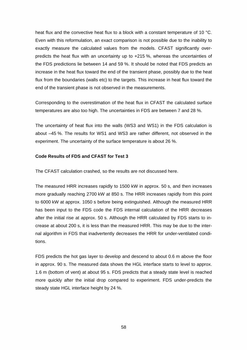
58

heat flux and the convective heat flux to a block with a constant temperature of 10 °C.

Even with this reformulation, an exact comparison is not possible due to the inability to

exactly measure the calculated values from the models. CFAST significantly over-

predicts the heat flux with an uncertainty up to +215 %, whereas the uncertainties of

the FDS predictions lie between 14 and 59 %. It should be noted that FDS predicts an

increase in the heat flux toward the end of the transient phase, possibly due to the heat

flux from the boundaries (walls etc) to the targets. This increase in heat flux toward the

end of the transient phase is not observed in the measurements.

Corresponding to the overestimation of the heat flux in CFAST the calculated surface

temperatures are also too high. The uncertainties in FDS are between 7 and 28 %.

The uncertainty of heat flux into the walls (WS3 and WS1) in the FDS calculation is

about –45 %. The results for WS1 and WS3 are rather different, not observed in the

experiment. The uncertainty of the surface temperature is about 26 %.

Code Results of FDS and CFAST for Test 3

The CFAST calculation crashed, so the results are not discussed here.

The measured HRR increases rapidly to 1500 kW in approx. 50 s, and then increases

more gradually reaching 2700 kW at 850 s. The HRR increases rapidly from this point

to 6000 kW at approx. 1050 s before being extinguished. Although the measured HRR

has been input to the FDS code the FDS internal calculation of the HRR decreases

after the initial rise at approx. 50 s. Although the HRR calculated by FDS starts to in-

crease at about 200 s, it is less than the measured HRR. This may be due to the inter-

nal algorithm in FDS that inadvertently decreases the HRR for under-ventilated condi-

tions.

FDS predicts the hot gas layer to develop and descend to about 0.6 m above the floor

in approx. 90 s. The measured data shows the HGL interface starts to level to approx.

1.6 m (bottom of vent) at about 95 s. FDS predicts that a steady state level is reached

more quickly after the initial drop compared to experiment. FDS under-predicts the

steady state HGL interface height by 24 %.

59

The FDS prediction is similar to experimental observation until 840 s at which point

FDS predicts a rapid reduction in O2 level to 0 %, while experimental observation indi-

cates the O2 level reaches 0 % more gradually at approx. 1095 s.

FDS predicts again that the flame is pushed significantly towards the rear wall by the

flow of ambient air into the compartment through the door. Observations of the tem-

perature fields show that FDS predicts that the flow through the door pulsates with a

period of approx. 2 s. This pulsating behavior was noted during the experiments. The

pulsating flow through the door provides sufficient oxygen to the fire and prevents it

from being under-ventilated.

The plume temperature behavior is similar to Test 1 with an intermediate peak at about

50 s. These peaks are explained by plume development predicted by FDS. But the

experimental measurements do not indicate this extensive movement of the fire plume.

The measured data shows the plume to be fully developed at approx. 180 s after which

the plume temperatures increase to approx. 1000 OC without any intermediate peaks.

The measured temperatures in the compartment at Level 1 for M7, M8, M9, and M10

show a rapid increase followed by a more gradual increase until the end of the tran-

sient phase. The temperature measured at M10 and M8 is higher than that measured

at M7 and M9. This is due to the tilting of the fire plume toward the back wall. The

plume temperature at M10 is higher than at M8 indicating that the tilt is more toward

M10, but not as far as M8. FDS also shows a rapid increase in temperature followed by

oscillations and a gradual increase in plume temperature, caused by flow oscillations at

door opening.

The temperatures at higher levels (elevations) show a notable peak due to increased

HRR at about 800 s. This was not simulated in the FDS calculations. The uncertainty

was about 24 % to 33 %.

The uncertainty and the problem in comparing the heat flux and surface temperature

for the material blocks are similar to those reported for Test 1. The uncertainty values

are about 70 % for the heat flux and 35 % for the temperatures.

60

Fig. 5-5 View of flame sheet output from FDS - Test 1 (from Appendix C)

Fig. 5-6 Plume temperature (from Appendix C)

61

5.2.3 CFAST (Zone Model) and JASMINE (CFD CODE) Applied by S. Miles

(BRE, UK)

Semi-blind calculations were made for Tests 1 and 3 with CFAST Version 3.1.6 and

JASMINE Version 3.2.3. The main difference with the blind calculations was that the

fuel mass loss measurement data were available, from which the fuel pyrolysis rates

had been derived, allowing a more accurate fuel source term to be specified in the cal-

culations. While most calculations had been conducted prior to the release of the other

experimental measurements, some further calculations had then been conducted to

explore various issues. The results of all these calculations are presented in detail in

the Appendix B, and summarized below.

CFAST Code Description and Input Assumptions

CFAST is described above in paragraph 5.2.2. Version 3.1.6, without the FAST graphi-

cal user interface, was employed in all calculations. Additional information relevant to

the application of CFAST to this Benchmark Exercise No. 4 is given below.

The dimensions of the OSKAR fire compartment and the doorway ventilation openings

were modeled as in the problem specification. The thermal properties of the walls, floor

and ceiling were included by creating new user defined materials with the required

(concrete) properties. Conduction losses to the room walls, ceiling and floor were in-

cluded, using the one-dimensional heat conduction sub-model.

The ventilation through the fan system was modeled using a mechanical exhaust vent.

A limitation was that a fixed value for the volume flow rate was required, i.e. the time-

dependent measured profile was not followed.

The fire was treated as a constrained fire (i.e. oxygen controlled) with an area 1 m2,

located at the center of the compartment at floor level. The fuel was modeled as kero-

sene, using a heat of combustion of 4.28 x 107 J kg-1. The time-dependent pyrolysis

rate was set to that measured experimentally for the initial calculations, and was then

adjusted in subsequent parametric calculations. For Test 1 two calculations were con-

ducted using a fixed fuel pyrolysis rate of 0.039 kg s-1, based upon published engineer-

ing information. This provided a comparison with the blind JASMINE calculations where

the same pyrolysis specification had been used.

62

In all calculations a two-layer gas assumption was assumed inside the room, but the

'ceiling jet' option was inactive. The radiative fraction was set to 0.3 in most calculations

(0.6 was also investigated). While in most calculations the lower oxygen limit (LOL)

was set to 0 %, it was adjusted to 10 % in some parametric calculations.

A required approximation in CFAST is that targets are treated as rectangular slabs.

Furthermore, heat conduction is modeled in one-dimension, i.e. in the direction of the

surface normal. The surface temperature of the three material probes was calculated,

with the target surface normal directed into the compartment (x-direction). The re-

sponse of the barrel target was not included in the CFAST calculations.

JASMINE Code Description and Input Assumptions

JASMINE is described above in 5.1.2. It was applied as described for the blind calcula-

tions with the main exception that the measured, transient fuel pyrolysis (or a fixed frac-

tion thereof) was used to specify the fuel source term. In addition the effect of employ-

ing the discrete transfer radiation model was investigated. The influence of applying an

oxygen concentration limiter on the combustion process was also investigated for Test

3. Furthermore, for Test 3 the consequence of reducing the imposed exhaust flow rate

at the mechanical (FUCHS) duct by 50 % was explored.

CFAST Code Results

Appendix B presents details of the scenarios, for which converged CFAST simulations

were achieved. Other parametric combinations were attempted for which a converged

solution was not achieved, which is perhaps a consequence of the complex physics of

the two experiments. The main observations and findings are summarized below:

For Test 1, the choice of a radiative fraction of 0.6, coupled to the measured fuel pyro-

lysis rate, resulted in an upper gas layer temperature reasonably close to that meas-

ured. The layer height predictions, with the layer dropping to approximately 1 m, were

perhaps less representative of the actual experiment. For Test 3, the upper gas layer

temperature predictions were less encouraging, with an over-prediction in all paramet-

ric calculations undertaken. This was observed, in particular, in the earlier stage of the

experiment. It should be noted that radiative fractions higher than 0.3, and up to 0.6,

were attempted but that converged solutions were not then obtained. Fig. 5-7 (from

63

Appendix B) illustrates gas temperature calculations for Test 1 using the measured and

fixed (0.039 kg s-1) fuel pyrolysis specifications.

For Test 1, the calculated oxygen concentration appears reasonable. For Test 3, the

calculated oxygen concentration, while dropping to zero, does so much more quickly

than suggested by the experimental measurement. This is most likely coupled to the

fact that too much burning, and associated gas temperature rise, was predicted in the

calculation compared to the actual experiment. For Test 3, where the oxygen concen-

tration dropped to zero, whether the lower oxygen limit was set to 10 % or zero had

very little influence on the calculated values.

Surface temperatures and incident fluxes for Test 1 were reasonable for the two calcu-

lations using a fixed fuel pyrolysis rate of 0.039 kg s-1, but for the calculation using the

measured pyrolysis rate they were notable higher than the measured values. Fig. 5-8

(from Appendix B) illustrates wall surface temperature calculations for Test 1 using the

measured and fixed (0.039 kg s-1) fuel pyrolysis specifications.

Test 3 calculations for wall surface temperature were reasonably close to the experi-

mental measurements for all the parametric runs. Material probe surface temperatures

and the heat flux densities were, however, over-predicted compared to measurement in

all parametric runs. This may be due, in part at least, to three-dimensional geometry

effects that cannot be captured using a zone model such as CFAST.

The limitation that the flow rate through the mechanical exhaust was fixed in value, and

did not vary according to the measurement data, probably had only a small conse-

quence.

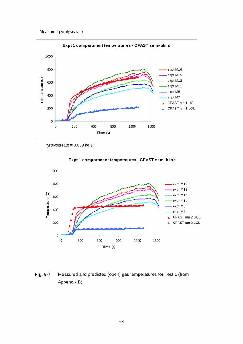
64

Expt 1 compartment temperatures - CFAST semi-blind

0

200

400

600

800

1000

0 300 600 900 1200 1500

Time (s)

Tem

pera

ture

(C)

expt M16expt M15expt M12expt M11expt M8expt M7CFAST run 2 UGLCFAST run 2 LGL

Pyrolysis rate = 0.039 kg s-1

Fig. 5-7 Measured and predicted (open) gas temperatures for Test 1 (from

Appendix B)

Measured pyrolysis rate

Expt 1 compartment temperatures - CFAST semi-blind

0

200

400

600

800

1000

0 300 600 900 1200 1500

Time (s)

Tem

pera

ture

(C)

expt M16expt M15expt M12expt M11expt M8expt M7CFAST run 1 UGLCFAST run 1 LGL

65

Fig. 5-8 Measured and predicted (open) wall surface temperatures for Test 1 (from

Appendix B)

Expt 1 compartment surface temperatures - CFAST semi-blind

0

200

400

600

800

1000

0 300 600 900 1200 1500

Time (s)

Tem

pera

ture

(C) expt M20

expt M23expt M19expt M22CFAST run 2 UGL wallCFAST run2 LGL wall

Pyrolysis rate = 0.039 kg s-1

Expt 1 compartment surface temperatures - CFAST semi-blind

0

200

400

600

800

1000

0 300 600 900 1200 1500

Time (s)

Tem

pera

ture

(C) expt M20

expt M23expt M19expt M22CFAST run 1 UGL wallCFAST run1 LGL wall

Measured pyrolysis rate

66

JASMINE Code Results

Appendix B presents details of the JASMINE calculations. These were conducted for

the first 18 to 20 minutes of both experiments, after which time convergence problems

were encountered. The main observations and findings from the JASMINE calculations

are summarized below:

The calculations for Test 1, using the fuel pyrolysis rate derived from the experimental

measurements (actually 75% of the measured pyrolysis rate - to account for radiation

losses due to soot), were judged encouraging. The main features of the gas tempera-

tures, doorway flows and radiation fluxes were captured quite well. The compartment

temperature was arguably calculated to rise too quickly. Fig. 5-9 (from the Appendix B)

compares gas temperature and doorway velocity predictions and calculations for

Test 1.

While for Test 3 the calculations were generally considered quite reasonable, there

was however greater discrepancy with the measured data compared to Test 1. In par-

ticular, the direction of the wall vent flow was predicted to be predominantly into the

compartment compared to the actual experiment which exhibited a more pronounced

two-way flow. Simulations using 75 % of the measured fuel pyrolysis rate generated,

on average, results closer to the measurements compared to using the full pyrolysis

rate or 50 % of the rate. Recall here that the justification for adjusting the pyrolysis rate

is to account, in the overall energy balance, the heat lost from radiating soot particu-

lates (not modeled in the JASMINE calculations), i.e. akin to the radiative fraction in a

zone model such as CFAST.

It had been suggested that the level of the imposed exhaust in Test 3 might be the pri-

mary reason for the JASMINE calculations indicating less outflow from the wall vent

compared to that suggested by the experimental measurements. However, while in a

parametric simulation to investigate the effect of reducing the imposed exhaust rate by

50% the wall vent flow was then marginally more bi-directional, the overall effect was to

reduce the level of agreement between predicted and measured temperatures and

fluxes.

For both experiments the calculated flux densities at WS2 and WS3 were judged over-

all to be, qualitatively at least, quite reasonable. However, as illustrated in Fig. 5-10

(from Appendix B), the predicted flux density at WS4 (towards the front of the com-

67

partment) was significantly lower than that measured. This was initially attributed per-

haps to the use of the six-flux radiation model, which misses some of the important

angular radiant intensity information. However, further simulations using the more ac-

curate discrete transfer also exhibited the same discrepancy in flux density at WS4.

There was no significant influence on the calculated variables when invoking the addi-

tional oxygen limitation mechanism on the combustion sub-model. It is perhaps not too

surprising that little difference was observed due to the high compartment tempera-

tures, as even with the additional oxygen limitation mechanism combustion still occurs

if the local gas temperature is sufficiently high.

The energy ‘budget’ has been calculated in the JASMINE simulations, and is quite in-

formative. Fig. 5-11 (from Appendix B) shows the energy budget for one of the Test 3

calculations, and illustrates that both heat losses to the solid boundaries and heat con-

vected through the mechanical ventilation duct are significant.

A general note from the JASMINE work is that the presence of soot, and the subse-

quent radiation absorption and emission, may have an important bearing on the gas

temperatures predicted. This in turn influences the radiation fluxes significantly (bearing

in mind the T4 dependency on radiant intensity), which then has a major influence on

the conduction into the walls and targets and their temperature rise.

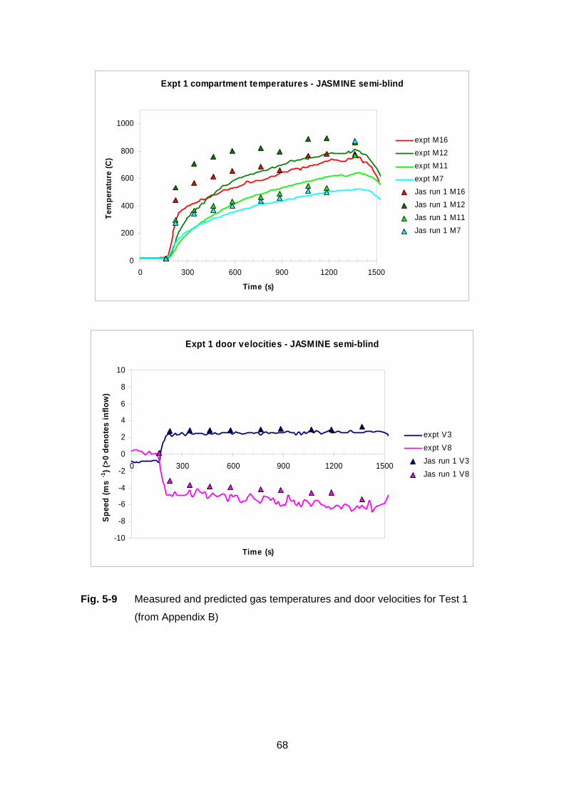
68

Expt 1 compartment temperatures - JASMINE semi-blind

0

200

400

600

800

1000

0 300 600 900 1200 1500

Time (s)

Tem

pera

ture

(C)

expt M16expt M12expt M11expt M7Jas run 1 M16Jas run 1 M12Jas run 1 M11Jas run 1 M7

Expt 1 door velocities - JASMINE semi-blind

-10

-8

-6

-4

-2

0

2

4

6

8

10

0 300 600 900 1200 1500

Time (s)

Spee

d (m

s-1

) (>0

den

otes

inflo

w)

expt V3expt V8Jas run 1 V3Jas run 1 V8

Fig. 5-9 Measured and predicted gas temperatures and door velocities for Test 1

(from Appendix B)

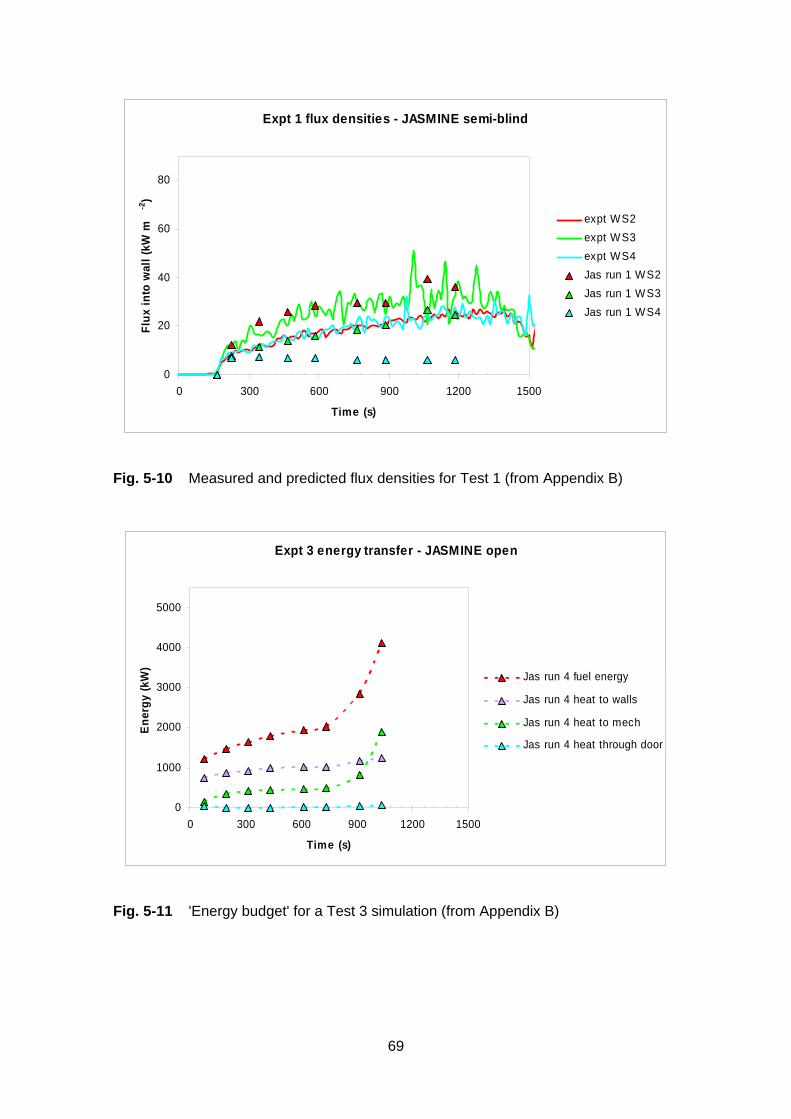
69

Expt 1 flux densities - JASMINE semi-blind

0

20

40

60

80

0 300 600 900 1200 1500

Time (s)

Flux

into

wal

l (kW

m-2

)

expt WS2expt WS3expt WS4Jas run 1 WS2Jas run 1 WS3Jas run 1 WS4

Fig. 5-10 Measured and predicted flux densities for Test 1 (from Appendix B)

Expt 3 energy transfer - JASMINE open

0

1000

2000

3000

4000

5000

0 300 600 900 1200 1500

Time (s)

Ene

rgy

(kW

)

Jas run 4 fuel energy

Jas run 4 heat to walls

Jas run 4 heat to mech

Jas run 4 heat through door

Fig. 5-11 'Energy budget' for a Test 3 simulation (from Appendix B)

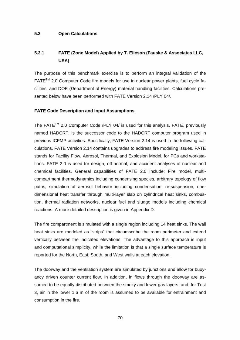
70

5.3 Open Calculations

5.3.1 FATE (Zone Model) Applied by T. Elicson (Fauske & Associates LLC,

USA)

The purpose of this benchmark exercise is to perform an integral validation of the

FATETM 2.0 Computer Code fire models for use in nuclear power plants, fuel cycle fa-

cilities, and DOE (Department of Energy) material handling facilities. Calculations pre-

sented below have been performed with FATE Version 2.14 /PLY 04/.

FATE Code Description and Input Assumptions

The FATETM 2.0 Computer Code /PLY 04/ is used for this analysis. FATE, previously

named HADCRT, is the successor code to the HADCRT computer program used in

previous ICFMP activities. Specifically, FATE Version 2.14 is used in the following cal-

culations. FATE Version 2.14 contains upgrades to address fire modeling issues. FATE

stands for Facility Flow, Aerosol, Thermal, and Explosion Model, for PCs and worksta-

tions. FATE 2.0 is used for design, off-normal, and accident analyses of nuclear and

chemical facilities. General capabilities of FATE 2.0 include: Fire model, multi-

compartment thermodynamics including condensing species, arbitrary topology of flow

paths, simulation of aerosol behavior including condensation, re-suspension, one-

dimensional heat transfer through multi-layer slab on cylindrical heat sinks, combus-

tion, thermal radiation networks, nuclear fuel and sludge models including chemical

reactions. A more detailed description is given in Appendix D.

The fire compartment is simulated with a single region including 14 heat sinks. The wall

heat sinks are modeled as “strips” that circumscribe the room perimeter and extend

vertically between the indicated elevations. The advantage to this approach is input

and computational simplicity, while the limitation is that a single surface temperature is

reported for the North, East, South, and West walls at each elevation.

The doorway and the ventilation system are simulated by junctions and allow for buoy-

ancy driven counter current flow. In addition, in flows through the doorway are as-

sumed to be equally distributed between the smoky and lower gas layers, and, for Test

3, air in the lower 1.6 m of the room is assumed to be available for entrainment and

consumption in the fire.

71

Two targets are included in the FATE model. The first target is the concrete material

probe with lower corner coordinates of x = 0.0 m, y = 1.9 m, and z = 1.7 m. The probe

is modeled with a single vertical rectangular heat sink, heat sink 16, with dimensions

0.3 m x 0.3 m x 0.1 m thick. This heat sink is divided into 20 nodes through the thick-

ness to allow one-dimensional conduction through the probe. In addition, the heat sink

is included in the radiation heat transfer network; therefore the heat sink surface is sub-

jected to convective and radiative boundary conditions. The second target is the more

complex barrel-type waste container. This target is divided azimuthally into four seg-

ments. The first three segments cover the cylinder half facing the fire, while the fourth

segment is the entire back half side of the barrel facing away from the fire. Each seg-

ment height is equal to the height of the barrel. In addition, each of the four segments is

represented as a composite heat sink consisting of three layers: an outer metal layer (5

radial nodes), a middle concrete layer (20 radial nodes), and an inner styrene granulate

fill layer (20 radial nodes). The tinplate that makes up the inner barrel is defined as a

contact resistance between the concrete and styrene. Radial conduction is allowed

between the layers, while azimuthal conduction is modeled only in the outer most steel

layer. The outer metal surfaces are also included in the radiation heat transfer network.

The given HHR were adjusted based on a 5-point moving average of the raw data and

a delay based on the fuel ignition time. The fuel ignition time is taken as the time at

which the heat sink temperatures begin to increase (160 s for Test 1 and 15 s for Test

3). FATE input also requires specification of the combustion products yield. The com-

bustion yields used for input are based on real yields for high molecular

weight/temperature hydrocarbons for well ventilated flaming fires.

Code Results

Test 1 is characterized by a kerosene fire with a steady state power in the range of 3 to

3.5 MW, peak fan vent flows of 2 m3/sec, a doorway opening of 0.7 m by 3.0 m, and a

multi-layer target in close proximity to the fire source. These conditions result in a flame

that extends well into the smoky region and significant variation in temperatures across

the x-y plane. As with other benchmark tests, the Benchmark Exercise No. 4 demon-

strates that the two most influential aspects of the input are the fire power and the room

ventilation behavior. To follow the measured ventilation flow rates, which are decreas-

ing at the end of the experiment, the flow area as been adjusted from 0.176 m2 to

0.0353 m2.

72

The measured flows were estimated by reducing the reported velocities from doorway

velocity probes V3 though V8. A volumetric flow rate was assigned to each measure-

ment by taking the product of the reported velocity and 1/6 of the door area (0.35 m2).

The net volumetric flow was then taken as the sum of the individual volumetric flows

and is assumed to represent the unidirectional flow rate. Even though the doorway a-

rea input to FATE is computed as 100 % of the geometric areas with no reductions

taken for entrance and exit losses, the FATE unidirectional flow rate calculation under-

predicts the estimated doorway flow rates.

For this particular geometry – a high powered fire in a relatively small and under-

ventilated compartment – the measured gas concentration may be a better measure of

room conditions rather than the smoky layer height. Reasonable agreement is indi-

cated between the calculated and measured gas concentrations.

The temperature variation inside the fire compartment along the x-y plane is promoted

by the room geometry in which the fire essentially blocks free inflow from the door (fire

pan width is larger than the narrow doorway width). The FATE smoky layer calculations

provide reasonable estimates of the average gas temperatures.

The peak wall temperatures in the back of the room are consistent with the peak gas

temperatures, while the side wall temperatures are about 100 K lower. This may be

influenced by air circulation which may be diminished toward the back of the room. The

FATE wall strip heat sink model presents an average temperature of all four side walls

at a particular elevation; therefore it is not surprising that peak wall temperatures are

not predicted. The under-prediction of wall temperatures at upper elevations is a result

of the overall lower predicted smoky layer gas temperature.

The container surface temperature is reasonably predicted, while the concrete probe

temperatures are somewhat under-estimated. The under-estimation of the concrete

probe temperature occurs because the probe remains in the lower gas layer in the

FATE calculation, while test data indicates the probe is submerged in the smoky layer.

Sensitivity calculations for which the probe is submerged in the smoky layer show good

agreement with the test data. The significant heat up of the can surface, even though

the waste can is located in the lower gas layer, is an indication of the radiative power

received from the fire.

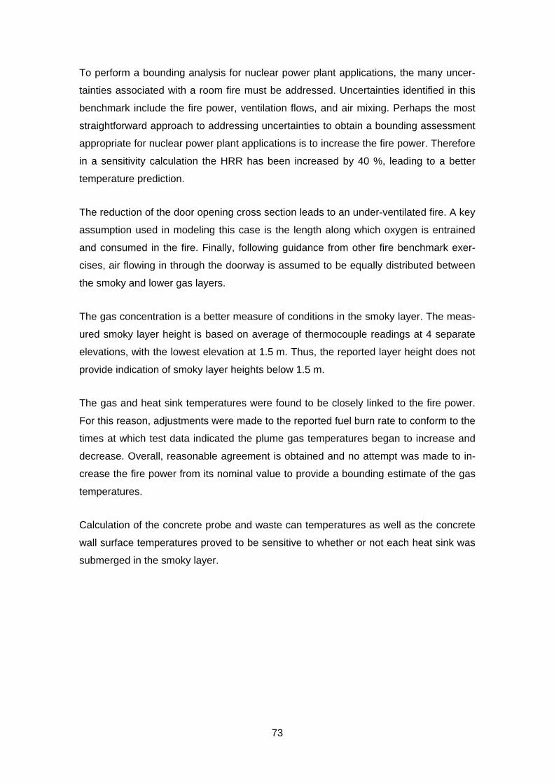
73

To perform a bounding analysis for nuclear power plant applications, the many uncer-

tainties associated with a room fire must be addressed. Uncertainties identified in this

benchmark include the fire power, ventilation flows, and air mixing. Perhaps the most

straightforward approach to addressing uncertainties to obtain a bounding assessment

appropriate for nuclear power plant applications is to increase the fire power. Therefore

in a sensitivity calculation the HRR has been increased by 40 %, leading to a better

temperature prediction.

The reduction of the door opening cross section leads to an under-ventilated fire. A key

assumption used in modeling this case is the length along which oxygen is entrained

and consumed in the fire. Finally, following guidance from other fire benchmark exer-

cises, air flowing in through the doorway is assumed to be equally distributed between

the smoky and lower gas layers.

The gas concentration is a better measure of conditions in the smoky layer. The meas-

ured smoky layer height is based on average of thermocouple readings at 4 separate

elevations, with the lowest elevation at 1.5 m. Thus, the reported layer height does not

provide indication of smoky layer heights below 1.5 m.

The gas and heat sink temperatures were found to be closely linked to the fire power.

For this reason, adjustments were made to the reported fuel burn rate to conform to the

times at which test data indicated the plume gas temperatures began to increase and

decrease. Overall, reasonable agreement is obtained and no attempt was made to in-

crease the fire power from its nominal value to provide a bounding estimate of the gas

temperatures.

Calculation of the concrete probe and waste can temperatures as well as the concrete

wall surface temperatures proved to be sensitive to whether or not each heat sink was

submerged in the smoky layer.

74

Fig. 5-12 Benchmark Exercise No. 4, Test 3 smoky layer gas concentrations (from

Appendix C)

75

5.3.2 FLAMME-S (Zone Model) Applied by L. Rigollet (IRSN, France)

Tests 1 and 3 have been simulated with the two-zone model code FLAMME-S, Ver-

sion.2.3.2 /BOU 02/, developed by IRSN. In this context, a remark must be made con-

cerning the fact that the studied cases are outside the validation domain of FLAMME-S,

specifically in respect to the two following conditions:

– The ratio of the pool surface area to the floor area of the facility is less than 5 %,

– The ratio of the heat release rate to the volume of the facility is less than 5 kWm-3.

FLAMME-S Code Description and Input Assumptions

The FLAMME-S code is similar to the CFAST code described above. The fuel pyrolysis

rate is a pre-defined input, and the burning in the compartment is then modeled to gen-

erate heat release and allow species concentrations to be calculated. FLAMME-S is a

two-zone model, whereby each compartment is divided into a hot gas upper layer and

a cold gas lower layer. In the presence of fire, the sub-model transports heat and mass

from the lower to the upper layer making use of an empirical correlation. A notable dif-

ference in this context is that FLAMME-S uses the Heskestad correlation for the plume

flow, whereas the McCaffrey correlation is utilized in CFAST. Flows through vents and

doorways are determined in both codes from correlations derived from the Bernoulli

equation. Radiation heat transfer between the fire plume, upper and lower layers, and

the compartment boundaries is also included.

The side walls of the fire compartment are constructed from 25 cm of light concrete and

5 cm of insulation. The ceiling is made of a 25 cm concrete layer and a 5 cm insulation

layer. For the floor, only 30 cm of concrete are taken into account: the aerated concrete

implemented in the experiments in order to protect the mass loss measurement is not

modeled. Two material probes, concrete and aerated concrete, are modeled.

In Test 1, the door is completely opened, with a free cross section of 0.7 m x 3 m. In

the Test 3, the opening is partly closed, with a free cross section of 0.7 m x 1 m. The

fan system, which is not used in the experiments, and the hood above the open front

door are not modeled.

The energy released by radiation represents 32 % of the total heat released. A com-

plete combustion reaction is assumed.

76

Two types of calculations have been performed: In a first step a constant pyrolysis rate

has been assumed (Test 1: 65 g/m2s; Test 3: 50 g/m2s) and in a second step the

measured rate was used. The LOL value was then reduced from 11.5 % to 0 %.

FLAMME-S Code Results

The layer height calculated by FLAMME-S is lower than that determined from the ex-

perimental data. The experimental interface height is determined from thermocouples

located at three elevations: 1.5 m, 3.35 m and 5.2 m. Thus, in the experiment, the layer

height never decreases under the elevation of the first thermocouple, i.e. 1.5 m. Tour-

niaire and al. /TOU 00/ have shown that the data reduction method is weakly depend-

ant on the number of thermocouples except in the case of three thermocouples where

the interface height does not reach the floor.

The gas temperatures calculated for the upper layer are in good agreement with the

experimental results of Test 1. As the layer height calculated by the code is lower than

the experimental interface, the calculated temperature of the lower layer is colder than

the gas temperatures measured.

The oxygen concentrations calculated with the code in the upper layer are lower than

those measured in the experiment; however, the comparison is difficult because the

sensor GA2-O2 seems to be saturated.

In the experiment, total heat fluxes were measured at one elevation, i.e. 1.7 m. At the

upper layer, the FLAMME-S code calculates slightly lower total heat fluxes.

The wall temperatures are not compared, because the FLAMME-S code calculates an

average temperature for the first mesh of a wall and thus cannot be compared with a

surface temperature measured experimentally.

However, the temperatures of two material probes (concrete and aerated concrete) are

compared. Experimentally, the sensors seem to be reversed: M 28 and M 26 for the

aerated concrete slab and M 32 and M 30 for the concrete slab. The calculated results

are in good agreement with the measurements, if the four sensors mentioned above

are indeed reversed.

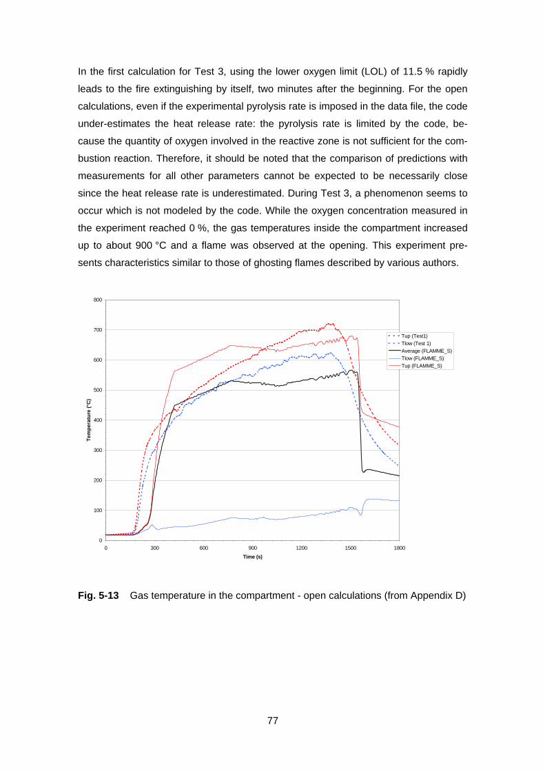
77

In the first calculation for Test 3, using the lower oxygen limit (LOL) of 11.5 % rapidly

leads to the fire extinguishing by itself, two minutes after the beginning. For the open

calculations, even if the experimental pyrolysis rate is imposed in the data file, the code

under-estimates the heat release rate: the pyrolysis rate is limited by the code, be-

cause the quantity of oxygen involved in the reactive zone is not sufficient for the com-

bustion reaction. Therefore, it should be noted that the comparison of predictions with

measurements for all other parameters cannot be expected to be necessarily close

since the heat release rate is underestimated. During Test 3, a phenomenon seems to

occur which is not modeled by the code. While the oxygen concentration measured in

the experiment reached 0 %, the gas temperatures inside the compartment increased

up to about 900 °C and a flame was observed at the opening. This experiment pre-

sents characteristics similar to those of ghosting flames described by various authors.

0

100

200

300

400

500

600

700

800

0 300 600 900 1200 1500 1800

Time (s)

Tem

pera

ture

(°C

)

Tup (Test1)Tlow (Test 1)Average (FLAMME_S)Tlow (FLAMME_S)Tup (FLAMME_S)

Fig. 5-13 Gas temperature in the compartment - open calculations (from Appendix D)

78

5.3.3 CFX (CFD Code) Applied by M. Heitsch (GRS, Germany)

Calculations with the CFD code CFX 5.7 have been carried out for Benchmark Exer-

cise No.4 within the frame of the International Collaborative to Evaluate Fire Models for

NPP Applications (ICFMP). Version 5 of the CFX family /CFX 04/ represents a com-

pletely new code structure compared with previous versions and offers new features.

CFX Code Description and Input Assumptions

CFX /CFX 04/ is a commercial Computational Fluid Dynamics (CFD) multi-purpose

code. The latest generation is named version 5. The current release is 5.7. The main

features which demonstrate the progress since the previous version 4 are the coupled

solver and the ability to handle structured and unstructured meshes. CFX-5 is capable

of modeling steady-state and transient flows, laminar and turbulent flows, subsonic,

transonic and supersonic flows, heat transfer and thermal radiation, buoyancy, non-

Newtonian flows, transport of non-reacting scalar components, multiphase flows, com-

bustion, flows in multiple frames of reference, and particle tracking.

Thanks to the regular geometry of the test arrangement, the computational mesh was

decided to be built exclusively with structured cells. The mesh has a total of 115700

cells in the fluid domain of the modeled test volume. Another 2548 cells are in the bar-

rel target (inner and outer part) to describe heat conduction. It reveals that the horizon-

tal resolution chosen may not be fine enough.

The gas mixture of air, fuel (kerosene) and combustion products is modeled by tracking

the individual species, which are kerosene, oxygen, nitrogen, carbon-dioxide and

steam. Soot is also created according to the Magnusson soot model implemented in

CFX. In this model, a number of constants are used, which were not further investi-

gated in this exercise. Nitrogen represents a background fluid, not participating in any

reaction. The chemical reaction itself is represented by a single-step mixing controlled

reaction within the Eddy Dissipation model. A complete combustion is assumed.

A predefined share of the reaction heat (40 %) is emitted from the surface of the fire

pan as radiation flux and distributed by the P1 radiation model in CFX. This radiation

model solves an extra transport equation and assumes direction independent radiation

transport. It allows heating of the fluid due to radiation from a boundary (here the fuel

pan). The radiation is not release from volume cells where the reaction takes place.

79

Flows through the venting (fan) system “FUCHS” and the hood are specified by flow

velocities given in the specification of the tests.

A simplification was made concerning the heat flow into the surrounding walls. These

walls are not included in the mesh and hence the heat flow calculated at constant wall

temperature. This overestimates the removal of energy from the fluid.

CFX Code Results

The history of the fuel release corresponds exactly to the fuel consumption curve from

the experiment. A total amount of 80.7 kg kerosene was added. The temperature dis-

tribution is affected by the inflow of cold air through the door and the hottest part of the

gas plume is pushed towards the back of the room. The temperatures in the front loca-

tion show a good correspondence to the measurements up to about 400 s but then

change little up to the time when the fire intensity passes its peak. In the simulation this

is expressed by a slight reduction of gas temperatures. Then the fire intensity remains

constant for a long while and reduces to zero after about 1400 s. The measured tem-

peratures however increase continuously up to the end of fuel combustion. A similar

tendency can be observed for temperatures in the back part of the facility. Here, how-

ever, measurement and simulation show different trends. During the test the highest

temperature was observed at the bottom of the room and decreased towards the ceil-

ing. The simulation predicts the opposite. This was true for all columns of thermocou-

ples.

The measured data for oxygen at GA1 are captured quite well. Only at the beginning

and the end of the fire scenario are some differences seen. This may be related to the

kerosene release curve, which was specified as an input. The measured CO2 mole

fraction is lower than the values predicted by CFX. This may be due to the fact that the

modeled chemical reaction does not include any production of CO and assumes only

CO2 and H2O.

In the door opening a number of flow sensors recorded the flow speeds in a vertical

line. In the upper locations the predictions compare quite well with the measurement, in

the lower probe locations however the flow is underestimated.

The barrel inside the fire compartment is built as a cylindrical double vessel container.

The inner section was filled by a type of granulate and the outer cylinder by concrete.

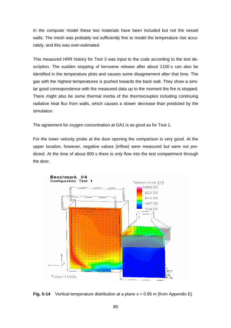
80

In the computer model these two materials have been included but not the vessel

walls. The mesh was probably not sufficiently fine to model the temperature rise accu-

rately, and this was over-estimated.

This measured HRR history for Test 3 was input to the code according to the test de-

scription. The sudden stopping of kerosene release after about 1100 s can also be

identified in the temperature plots and causes some disagreement after that time. The

gas with the highest temperatures is pushed towards the back wall. They show a simi-

lar good correspondence with the measured data up to the moment the fire is stopped.

There might also be some thermal inertia of the thermocouples including continuing

radiative heat flux from walls, which causes a slower decrease than predicted by the

simulation.

The agreement for oxygen concentration at GA1 is as good as for Test 1.

For the lower velocity probe at the door opening the comparison is very good. At the

upper location, however, negative values (inflow) were measured but were not pre-

dicted. At the time of about 800 s there is only flow into the test compartment through

the door.

Fig. 5-14 Vertical temperature distribution at a plane x = 0.95 m (from Appendix E)

81

0 400 800 1200 1600 2000Time [s]

200

400

600

800

1000Te

mpe

ratu

re [K

]

Sensor:M9 (0.95, 0.60, 1.5m)CFX (0.95, 0.60, 1.5m)M13 (0.95, 0.60, 3.35m)CFX (0.95, 0.60, 3.35m)M17 (0.95, 0.60, 5.2m)CFX (0.95, 0.60, 5.2m)

Benchmark #4: Kerosene Pool Fire

Test 1

Temperatures M9, M13, M17- Room front side -

Fig. 5-15 Comparison of selected gas temperatures close to the front of the test

facility for Test 1 (from Appendix E)

5.3.4 FDS (CFD Code) Applied by W. Brücher (GRS, Germany)

As an extension to earlier calculations with FDS2 and FDS3 within a project outside the

ICFMP, open calculations have now been performed with FDS3 and FDS4 to investi-

gate the influence of different FDS versions and the differences due to the chosen grid.

82

FDS Code Description and Input Assumptions

The FDS code has already been described in chapter 5.2.1. One major difference be-

tween FDS3 and FDS4, with some influence on the results is a different default LOL

condition, where the ‘no burn’ area in under-ventilated conditions is extended to higher

temperatures.

FDS Code Results

Actual heat release rates differ from the heat release rate obtained from the prescribed

pool mass loss data. Fig. 5-16 shows all heat release rates calculated with different

model configurations. Depending on the model configuration not all released fuel is

burnt immediately or in some cases it is only partly burnt. The mass release peak in

particular is not accompanied by an equivalent strong increase of the heat release due

to the under-ventilated conditions in Test 3.

Both calculations with FDS3 use exactly the same set of parameters except for the grid

cell size. Temperatures are generally slightly underestimated by the model for most of

the time (Fig. 5-17 to Fig. 5-19). The temperature peak appears too early compared to

the measurements, which is partly due to the mass loss rate of the benchmark specifi-

cation. A different (smoothed) interpolation of the questionable weight scale data in

former calculations resulted in a better agreement of the temperature development.

However, peak temperatures are also underestimated in that case. No obvious in-

crease in the simulation quality of the temperatures is found, although this effect would

be expected as a consequence of a better resolution of the flame area. A possible ex-

planation for the slightly worse overall performance with the fine grid may be the miss-

ing extension of the fine grid to the whole door area which is crucial for the develop-

ment of the fire inside. The calculated fine grid gas flow into the compartment is higher

than the measured one, resulting in lower gas temperatures inside the compartment.

This effect is also found in the calculation for oxygen concentration inside the fire com-

partment, which is over-estimated.

Due to the modification of the default temperature dependent LOL limit in FDS4, lower

heat releases are found in FDS4 compared to FDS3, also including lower gas tempera-

tures and surface heat fluxes. The default LOL definition seems to be a major problem

in under-ventilated conditions for both model versions.

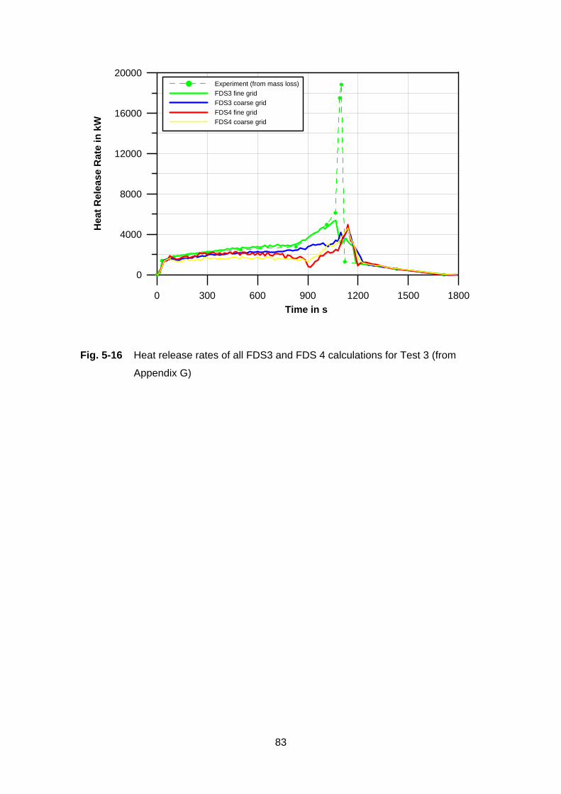
83

0 300 600 900 1200 1500 1800Time in s

0

4000

8000

12000

16000

20000

Hea

t Rel

ease

Rat

e in

kW

Experiment (from mass loss)FDS3 fine gridFDS3 coarse gridFDS4 fine gridFDS4 coarse grid

Fig. 5-16 Heat release rates of all FDS3 and FDS 4 calculations for Test 3 (from

Appendix G)

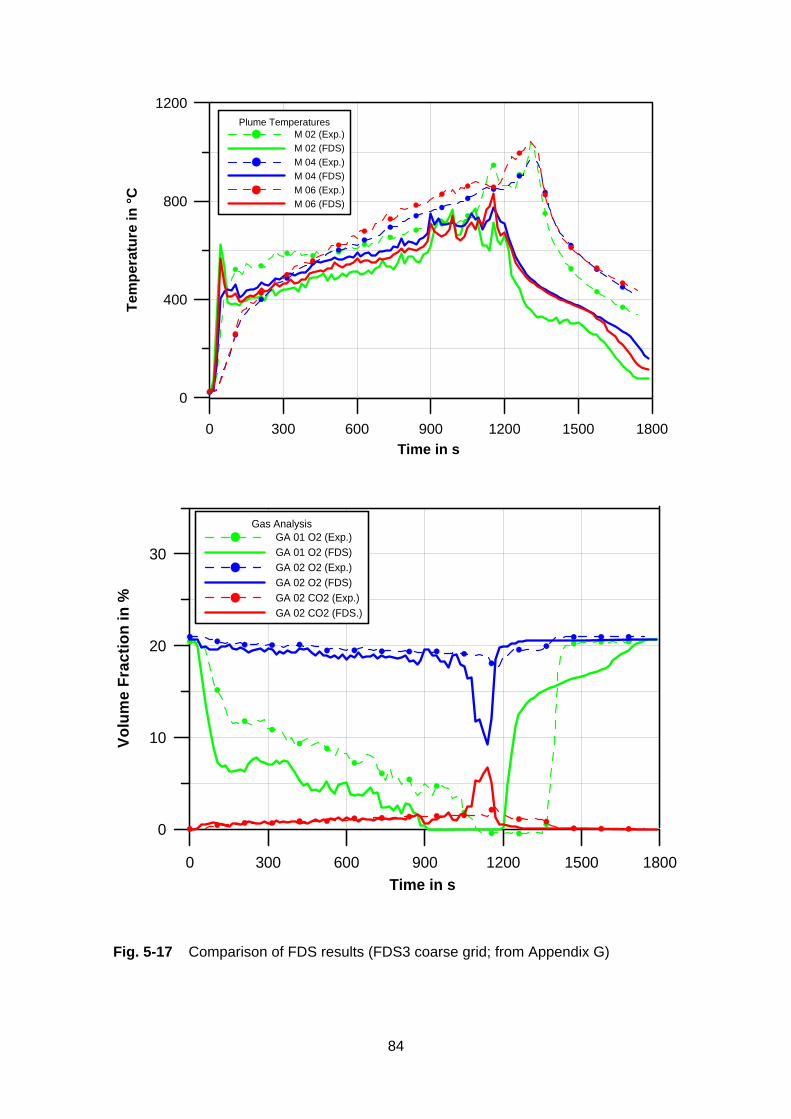
84

0 300 600 900 1200 1500 1800Time in s

0

400

800

1200

Tem

pera

ture

in °C

Plume TemperaturesM 02 (Exp.)M 02 (FDS)M 04 (Exp.)M 04 (FDS)M 06 (Exp.)M 06 (FDS)

0 300 600 900 1200 1500 1800Time in s

0

10

20

30

Volu

me

Frac

tion

in %

Gas AnalysisGA 01 O2 (Exp.)GA 01 O2 (FDS)GA 02 O2 (Exp.)GA 02 O2 (FDS)GA 02 CO2 (Exp.)GA 02 CO2 (FDS.)

Fig. 5-17 Comparison of FDS results (FDS3 coarse grid; from Appendix G)

85

0 300 600 900 1200 1500 1800Time in s

0

400

800

1200

Tem

pera

ture

in °C

Plume TemperaturesM 02 (Exp.)M 02 (FDS)M 04 (Exp.)M 04 (FDS)M 06 (Exp.)M 06 (FDS)

0 300 600 900 1200 1500 1800Time in s

0

10

20

30

Volu

me

Frac

tion

in %

Gas AnalysisGA 01 O2 (Exp.)GA 01 O2 (FDS)GA 02 O2 (Exp.)GA 02 O2 (FDS)GA 02 CO2 (Exp.)GA 02 CO2 (FDS.)

Fig. 5-18 Comparison of FDS results (FDS3 fine grid; from Appendix G)

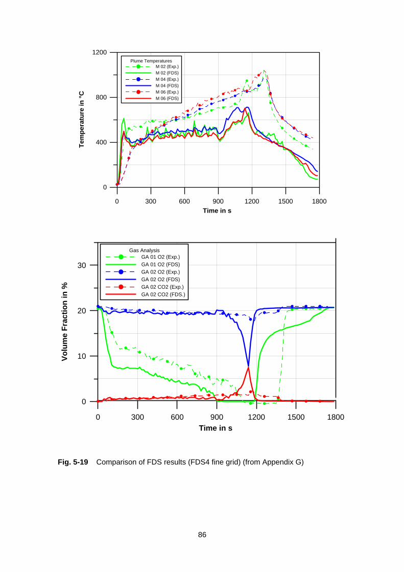
86

0 300 600 900 1200 1500 1800Time in s

0

400

800

1200

Tem

pera

ture

in °C

Plume TemperaturesM 02 (Exp.)M 02 (FDS)M 04 (Exp.)M 04 (FDS)M 06 (Exp.)M 06 (FDS)

0 300 600 900 1200 1500 1800Time in s

0

10

20

30

Volu

me

Frac

tion

in %

Gas AnalysisGA 01 O2 (Exp.)GA 01 O2 (FDS)GA 02 O2 (Exp.)GA 02 O2 (FDS)GA 02 CO2 (Exp.)GA 02 CO2 (FDS.)

Fig. 5-19 Comparison of FDS results (FDS4 fine grid) (from Appendix G)

87

5.3.5 COCOSYS (Lumped Parameter Code) Applied by B. Schramm (GRS,

Germany)

Both experiments of Benchmark Exercise No. 4 have been simulated with COCOSYS

with knowledge of the experimental results. Because of the flame being extinguished

due to oxygen depletion in Test 3, the pyrolysis rate has been modified in some para-

metric calculations.

COCOSYS Code Description and Input Assumptions

The lumped parameter (LP) code COCOSYS /ALL 05/ has been developed and vali-

dated for the comprehensive simulation of severe accident progression in light water

reactor containments. This code system is to allow the simulation of all relevant phe-

nomena, containment systems and conditions during the course of design basis acci-

dents and severe accidents. In COCOSYS, mechanistic models are used as far as

possible for analyzing the physical and chemical processes inside reactor contain-

ments. Essential interactions between the individual processes, e.g. feedback from

fission product decay heat on thermal hydraulics, are treated in a thorough way. With

such a detailed approach, COCOSYS is not restricted only to relevant severe accident

phenomena, but will also be able to demonstrate interactions between these phenom-

ena as well as the overall behavior of the containment.

For the simulation of oil and cable fires, pyrolysis and burning models have been im-

plemented in the thermal hydraulic module of COCOSYS. This process is divided into

two steps: first the release of pyrolysed species from the oil or cable surface and sec-

ond the burning processes inside the atmosphere and on the surface of the burning

material itself. Two different types of concepts have been implemented in COCOSYS:

a very detailed one simulating the combustible materials (oil and cables) with a 1D heat

flow model and a simplified concept to handle user specified pyrolysis rates including in

some way the feedback from the thermal hydraulic boundary conditions.

In the oil fire model, the material to be burned is represented by a usual structure sub-

divided into several layers for the calculation of temperature profiles in the material

(Fig. 5-20).The surface temperature is calculated by a spline interpolation using all

layer temperatures. The heat flux on the surface (e.g. reaction heat, convective heat

transfer, radiation) is distributed into the uppermost layer and the second layer accord-

ing to the volume fraction of the uppermost layer. The released CHX fractions are

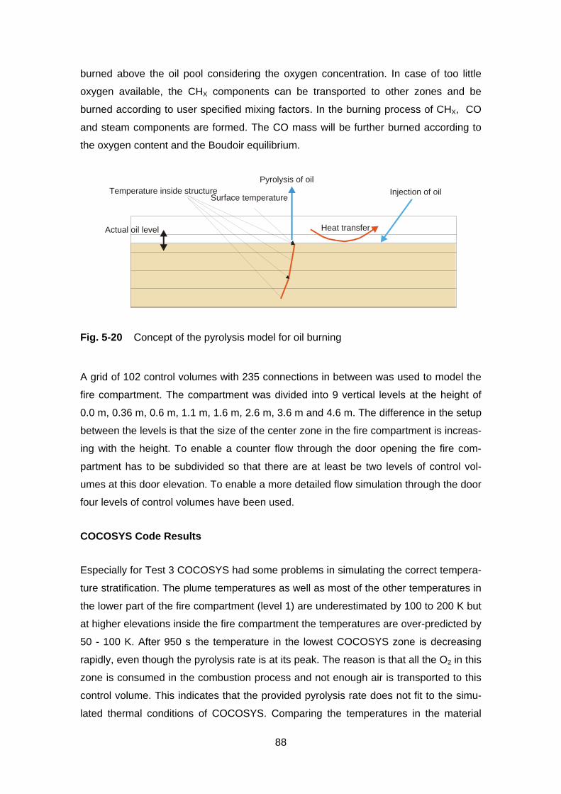
88

burned above the oil pool considering the oxygen concentration. In case of too little

oxygen available, the CHX components can be transported to other zones and be

burned according to user specified mixing factors. In the burning process of CHX, CO

and steam components are formed. The CO mass will be further burned according to

the oxygen content and the Boudoir equilibrium.

Temperature inside structureSurface temperature

Pyrolysis of oilInjection of oil

Heat transferActual oil level

Fig. 5-20 Concept of the pyrolysis model for oil burning

A grid of 102 control volumes with 235 connections in between was used to model the

fire compartment. The compartment was divided into 9 vertical levels at the height of

0.0 m, 0.36 m, 0.6 m, 1.1 m, 1.6 m, 2.6 m, 3.6 m and 4.6 m. The difference in the setup

between the levels is that the size of the center zone in the fire compartment is increas-

ing with the height. To enable a counter flow through the door opening the fire com-

partment has to be subdivided so that there are at least be two levels of control vol-

umes at this door elevation. To enable a more detailed flow simulation through the door

four levels of control volumes have been used.

COCOSYS Code Results

Especially for Test 3 COCOSYS had some problems in simulating the correct tempera-

ture stratification. The plume temperatures as well as most of the other temperatures in

the lower part of the fire compartment (level 1) are underestimated by 100 to 200 K but

at higher elevations inside the fire compartment the temperatures are over-predicted by

50 - 100 K. After 950 s the temperature in the lowest COCOSYS zone is decreasing

rapidly, even though the pyrolysis rate is at its peak. The reason is that all the O2 in this

zone is consumed in the combustion process and not enough air is transported to this

control volume. This indicates that the provided pyrolysis rate does not fit to the simu-

lated thermal conditions of COCOSYS. Comparing the temperatures in the material

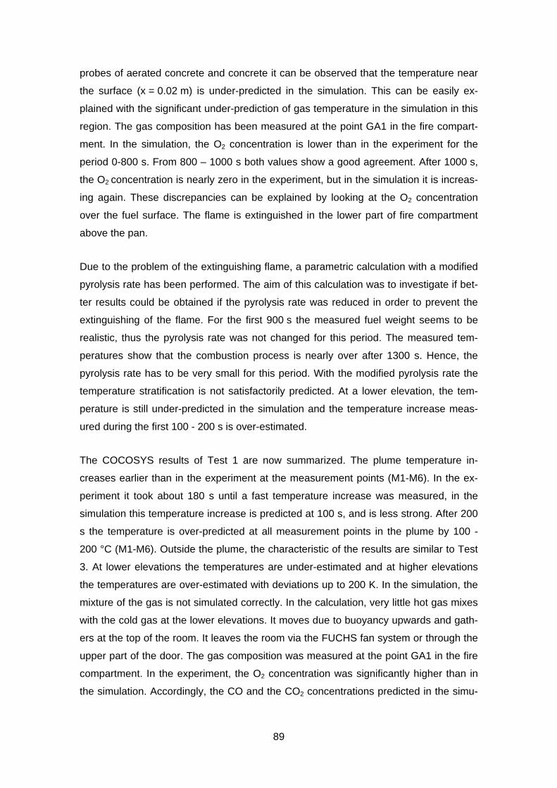
89

probes of aerated concrete and concrete it can be observed that the temperature near

the surface (x = 0.02 m) is under-predicted in the simulation. This can be easily ex-

plained with the significant under-prediction of gas temperature in the simulation in this

region. The gas composition has been measured at the point GA1 in the fire compart-

ment. In the simulation, the O2 concentration is lower than in the experiment for the

period 0-800 s. From 800 – 1000 s both values show a good agreement. After 1000 s,

the O2 concentration is nearly zero in the experiment, but in the simulation it is increas-

ing again. These discrepancies can be explained by looking at the O2 concentration

over the fuel surface. The flame is extinguished in the lower part of fire compartment

above the pan.

Due to the problem of the extinguishing flame, a parametric calculation with a modified

pyrolysis rate has been performed. The aim of this calculation was to investigate if bet-

ter results could be obtained if the pyrolysis rate was reduced in order to prevent the

extinguishing of the flame. For the first 900 s the measured fuel weight seems to be

realistic, thus the pyrolysis rate was not changed for this period. The measured tem-

peratures show that the combustion process is nearly over after 1300 s. Hence, the

pyrolysis rate has to be very small for this period. With the modified pyrolysis rate the

temperature stratification is not satisfactorily predicted. At a lower elevation, the tem-

perature is still under-predicted in the simulation and the temperature increase meas-

ured during the first 100 - 200 s is over-estimated.

The COCOSYS results of Test 1 are now summarized. The plume temperature in-

creases earlier than in the experiment at the measurement points (M1-M6). In the ex-

periment it took about 180 s until a fast temperature increase was measured, in the

simulation this temperature increase is predicted at 100 s, and is less strong. After 200

s the temperature is over-predicted at all measurement points in the plume by 100 -

200 °C (M1-M6). Outside the plume, the characteristic of the results are similar to Test

3. At lower elevations the temperatures are under-estimated and at higher elevations

the temperatures are over-estimated with deviations up to 200 K. In the simulation, the

mixture of the gas is not simulated correctly. In the calculation, very little hot gas mixes

with the cold gas at the lower elevations. It moves due to buoyancy upwards and gath-

ers at the top of the room. It leaves the room via the FUCHS fan system or through the

upper part of the door. The gas composition was measured at the point GA1 in the fire

compartment. In the experiment, the O2 concentration was significantly higher than in

the simulation. Accordingly, the CO and the CO2 concentrations predicted in the simu-

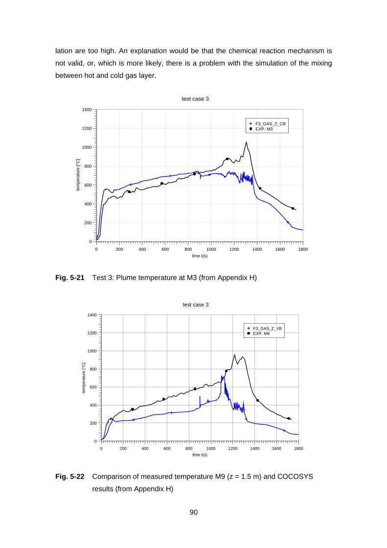
90

lation are too high. An explanation would be that the chemical reaction mechanism is

not valid, or, which is more likely, there is a problem with the simulation of the mixing

between hot and cold gas layer.

test case 3

0 200 400 600 800 1000 1200 1400 1600 1800

time t(s)

0

200

400

600

800

1000

1200

1400

tem

pera

ture

[°C

]

F3_GAS_Z_CBEXP. M3

Fig. 5-21 Test 3: Plume temperature at M3 (from Appendix H)

test case 3

0 200 400 600 800 1000 1200 1400 1600 1800

time t(s)

0

200

400

600

800

1000

1200

1400

tem

pera

ture

[°C

]

F3_GAS_Z_VBEXP. M9

Fig. 5-22 Comparison of measured temperature M9 (z = 1.5 m) and COCOSYS

results (from Appendix H)

91

5.3.6 VULCAN (CFD Code) Applied by V.F. Nicolette (SNL, USA)

The CFD code VULCAN has been used for open calculations of Test 3. However, the

results have not been optimized to match the available experimental data.

VULCAN Code Description and Input Assumptions

VULCAN is derived from the Kameleon Fire code /HOL 90/. It models the transport and

burning of vaporized fuel, as well as the transport of combustion by-products and their

thermal impact on targets. Conservation equations are solved for mass, species, mo-

mentum, energy (enthalpy), turbulence quantities, and radiation intensity. Convective

and radiative heat transfers to targets are included in the code, as well as the subse-

quent thermal response of the targets. VULCAN contains the following sub-models

(algorithms):

– A fuel vaporization sub-model for the estimation of the rate, at which the fuel is

transferred from the liquid phase (for liquid fuels) to the vapor phase.

- A k-ε turbulence model;

- Eddy Dissipation Concept (EDC) combustion model. Reactions are modeled as

either 1-step or 2-step reactions, with irreversible, infinitely fast chemistry (relative

to the mixing process);

- A soot generation and transport model;

- Discrete Transfer Method (DTM) of Shah and Lockwood is employed to solve the

thermal radiation;

- VULCAN uses an extension of the SIMPLEC method of Patankar and Spalding,

1972, to solve the conservation equations using a control volume formulation. A

structured three-dimensional Cartesian grid is used. First- and second-order accu-

rate upwind schemes can be used for the convective terms.

A non-uniform grid of 38 x 55 x 46 (y direction is from the front door to the back of

room) control volumes was used for the majority of simulations, and was developed

based on previous modeling experience. Additionally, a refined mesh simulation was

performed using 74 x 104 x 84 control volumes (essentially dividing the physical length

of each control volume side by a factor of 2). This yielded a control volume length scale

of order 0.07 – 0.15 m in the x and y directions. The control volumes in the z direction

92

were somewhat larger in the upper regions of the room, where gradients were ex-

pected to be small. The computational domain was taken as the fire compartment plus

some reservoir space outside of the fire compartment.

For some simulations, the measured fuel evaporation rate was specified for the code.

For other simulations, the fuel evaporation rate was calculated by the code based on

the thermal response of the fuel. The chemical reaction was modeled as a two-step

reaction with production of intermediate species. In the first step of the chemical reac-

tion, the fuel is assumed to combust to form carbon monoxide and hydrogen. The sec-

ond step of the reaction converts the intermediate species to water vapor and carbon

dioxide.

VULCAN Code Results

A simulation was performed in which the experimentally measured mass loss rate was

directly calculated based on the thermal response of the fuel pool (Fig. 5-23).

Oxygen depletion was observed to occur significantly sooner in the simulations than in

the experiment. The agreement between simulation and experiment is best discussed

when separated into 2 time periods: pre-oxygen depletion, and post-oxygen depletion

of the room. Prior to oxygen depletion, very good agreement was obtained for the pool

mass loss rate and the majority of heat fluxes to targets. The agreement was not as

good for thermocouple temperatures, target thermal response, and doorway velocities.

For times that are post-oxygen depletion, the agreement is generally not as good as for

the pre-depletion period. This is understandable since the post-oxygen depletion envi-

ronment is highly dependent upon the locations and amounts of leakage into the com-

partment. A fine mesh simulation produced essentially the same results as with the

coarse mesh, suggesting the coarse mesh results were adequate. The inclusion of

buoyancy generated turbulence in the simulations did not change the results substan-

tially, but did improve the prediction of temperature low in the plume and the lower

doorway velocity, while resulting in even faster oxygen consumption (relative to the

standard k-ε model).

The sources of discrepancies between the predictions and data could not be defini-

tively resolved due to uncertainties in the experiment and documentation. These dis-

crepancies are believed to be primarily due to inputs to the code being significantly

different than existed in the experiment. In that context, this experiment is not recom-

93

mended for code validation purposes, but does provide useful information regarding

the potential uncertainties in code predictions when key inputs (e.g., leakage paths) are

not accurately specified.

Fig. 5-23 Mass loss rate (smoothed) versus experiment (from Appendix I)

94

Fig. 5-24 Front room temperatures and oxygen concentration (from Appendix I)

95

5.3.7 MAGIC (zone code) Applied by B. Gautier (EDF, France)

The zone model MAGIC has been used for open calculations of Tests 1 and 3. Some

additional parameter studies concerning the heat release and the effect of light con-

crete floor have been performed.

MAGIC code description and input assumptions

The calculations presented here were performed with MAGIC V4.1.1b /GAY 06/. The

code is used in its standard version using input variables corresponding to a normal

risk study approach. MAGIC uses a two-zone model including most of the classic fea-

tures, like gaseous phase combustion, governed by the properties of emitted products

and the air supply attributable to the plume flow, smoke production and transport of

unburned products, heat exchange, natural flows and forced ventilation, simulation of

targets and sprinkler systems.

The shape of fire compartment has been simplified, and has conserved the total vol-

ume. The distances between targets or openings and fuel surface are conserved. The

hood in front of the door is not modeled. The ventilation has been simplified to one glo-

bal exhaust vent at the ceiling. The lower oxygen limit is fixed to 0 % which is the EDF

recommended value. The radiation fraction is set to 0.35.

MAGIC code results

MAGIC results appear more realistic in Test 1 (open door) than in Test 3 (semi-closed

door). In Test 1 the gas temperature are realistic while target temperature and flux are

significantly over-estimated. In Test 3 gas layer temperature is little under-estimated,

while the target predicitions are in good agreement.

In Test 3, the configuration induces more complex phenomena: the reduction of the

opening cross section produces under-ventilated conditions. It seems that the flame

was inclined to the door in the experiment. These phenomena are not represented in

MAGIC.

Some experimental data appears to be questionable, especially the HRR in Test 3 and

the interface height (due to the low number of thermocouples used in the interface

height calculation).

96

More information on the vent system would have allowed it to be modelled and permit-

ted a more realistic "fire risk study" type of approach to the test. Especially in Test 3,

the ventilation due to the vent is comparable to the one due to the door (in calculation

and probably also in the actual test). It seems that the door flow is under estimated in

the calculation, maybe due to the hood effect.

0

100

200

300

400

500

600

700

800

0 5 10 15 20 25 30 35Time (min)

Tem

pera

ture

(C)

MAGIC Fire : Upper layer temperatureTupMAGIC Fire: Lower layer temperatureTlow

Fig. 5-25 Upper and lower temperature in Test 1 (from Appendix J)

0

200

400

600

800

1000

1200

0 10 20 30 40

Time (min)

Tem

pera

ture

(C)

M AGIC Fire: Upper layer temperatureTupM AGIC Fire: Lower layer temperatureTlow

Fig. 5-26 Upper and lower temperature in Test 3 (from Appendix J)

97

6 Code to Code Comparison

In this chapter the results of the different codes and types of codes are compared to

each other. It is clear that the results of simulation tools depend on the quality and ca-

pabilities of the models themselves as well as on the experience of the users. Further-

more, it is obvious that this comparison is specific to the Benchmark Exercise consid-

ered, with partly oxygen depleted conditions and a relative strong fire.

The objective of this chapter is to look at the overall results of fire simulation tools for:

– characterization of deviations from the experimental results to give some

indications on uncertainties, particularly for PSA studies;

– identification of minimum and maximum values of code results;

– characterization of user effects as well as differences between blind and open

calculations;

– characterization of potential uncertainties of the experiment itself and the

experimental results.

Due to the limited number of participants and calculations it is quite difficult to identify

the real causes of deviations of the calculated values from the experimental measure-

ments. Nevertheless, this Benchmark Exercise does give some view on the possible

uncertainties of fire simulations.

6.1 Test 1

6.1.1 Plume Temperatures (M1 to M6)

Fig. 6-1 and Fig. 6-2 compare the results for blind and open calculations of the plume

temperatures at positions M2 and M6. In comparison to the blind simulations, the re-

sults of the semi-blind FDS calculations are much better, having used the pre-defined

pyrolysis rate. Larger deviations between semi-blind FDS simulations occur for tem-

peratures closer to the fire surface (like M2). It seems that the user has to be careful to

get good results at positions close to the fuel surface. The blind simulations of

JASMINE also show an underestimation of the temperatures. This underestimation

was not so significant in the semi-blind simulations of JASMINE. The open COCOSYS

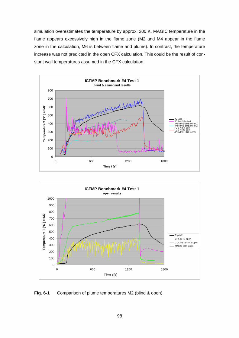
98

simulation overestimates the temperature by approx. 200 K. MAGIC temperature in the

flame appears excessively high in the flame zone (M2 and M4 appear in the flame

zone in the calculation, M6 is between flame and plume). In contrast, the temperature

increase was not predicted in the open CFX calculation. This could be the result of con-

stant wall temperatures assumed in the CFX calculation.

ICFMP Benchmark #4 Test 1blind & semi-blind results

0

100

200

300

400

500

600

700

800

0 600 1200 1800

Time t [s]

Tem

pera

ture

T [°

C ]

at M

2

Exp-M2FDS-NIST-blindJASMINE-BRE-blind(1)JASMINE-BRE-blind(2)FDS-NIST-semiFDS-NRC-semiJASMINE-BRE-semi

ICFMP Benchmark #4 Test 1open results

0

100

200

300

400

500

600

700

800

900

1000

0 600 1200 1800

Time t [s]

Tem

pera

ture

T [°

C ]

at M

2

Exp-M2CFX-GRS-openCOCOSYS-GRS-openMAGIC-EDF-open

Fig. 6-1 Comparison of plume temperatures M2 (blind & open)

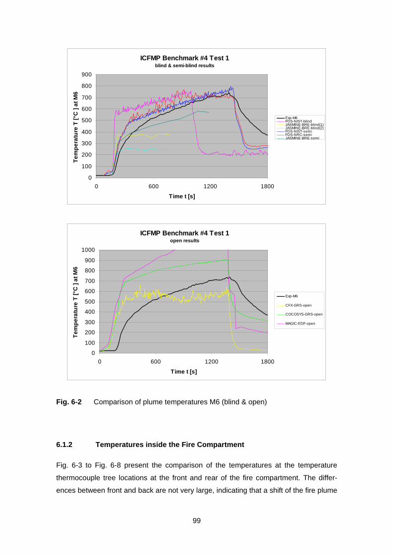
99

ICFMP Benchmark #4 Test 1blind & semi-blind results

0

100

200

300

400

500

600

700

800

900

0 600 1200 1800

Time t [s]

Tem

pera

ture

T [°

C ]

at M

6

Exp-M6FDS-NIST-blindJASMINE-BRE-blind(1)JASMINE-BRE-blind(2)FDS-NIST-semiFDS-NRC-semiJASMINE-BRE-semi

ICFMP Benchmark #4 Test 1open results

0

100

200

300

400

500

600

700

800

900

1000

0 600 1200 1800

Time t [s]

Tem

pera

ture

T [°

C ]

at M

6

Exp-M6

CFX-GRS-open

COCOSYS-GRS-open

MAGIC-EDF-open

Fig. 6-2 Comparison of plume temperatures M6 (blind & open)

6.1.2 Temperatures inside the Fire Compartment

Fig. 6-3 to Fig. 6-8 present the comparison of the temperatures at the temperature

thermocouple tree locations at the front and rear of the fire compartment. The differ-

ences between front and back are not very large, indicating that a shift of the fire plume

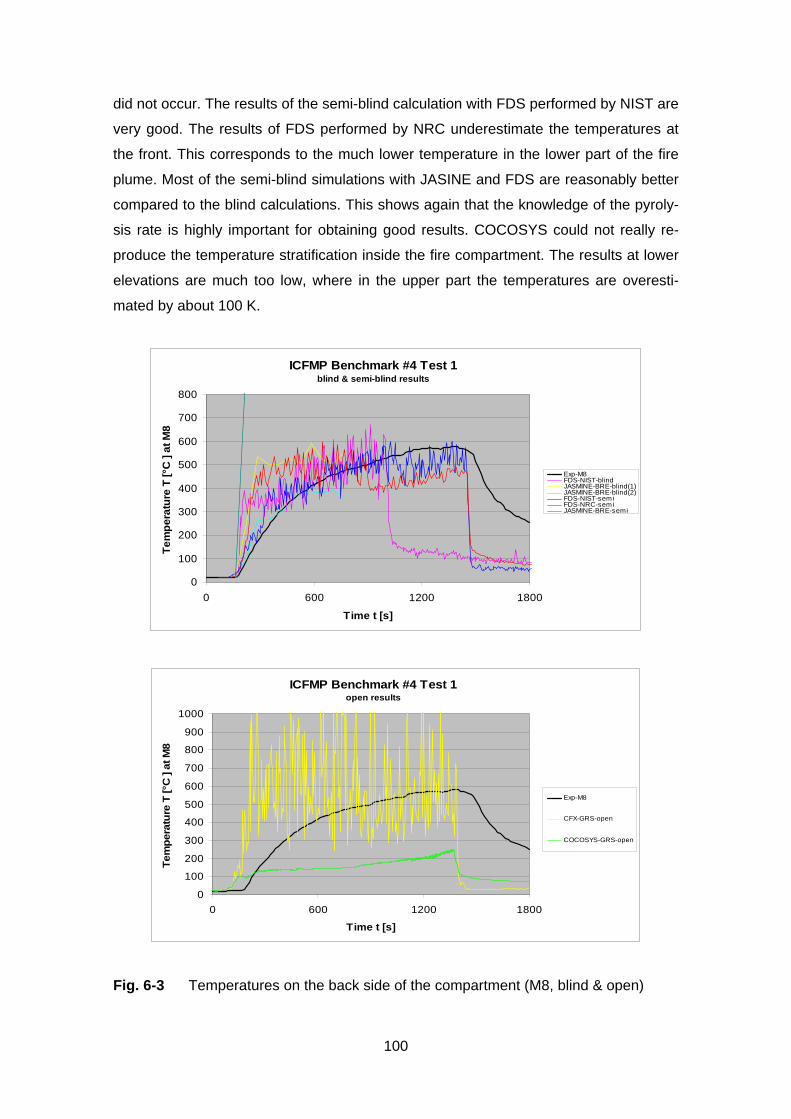
100

did not occur. The results of the semi-blind calculation with FDS performed by NIST are

very good. The results of FDS performed by NRC underestimate the temperatures at

the front. This corresponds to the much lower temperature in the lower part of the fire

plume. Most of the semi-blind simulations with JASINE and FDS are reasonably better

compared to the blind calculations. This shows again that the knowledge of the pyroly-

sis rate is highly important for obtaining good results. COCOSYS could not really re-

produce the temperature stratification inside the fire compartment. The results at lower

elevations are much too low, where in the upper part the temperatures are overesti-

mated by about 100 K.

ICFMP Benchmark #4 Test 1blind & semi-blind results

0

100

200

300

400

500

600

700

800

0 600 1200 1800

Time t [s]

Tem

pera

ture

T [°

C ]

at M

8

Exp-M8FDS-NIST-blindJASMINE-BRE-blind(1)JASMINE-BRE-blind(2)FDS-NIST-semiFDS-NRC-semiJASMINE-BRE-semi

ICFMP Benchmark #4 Test 1open results

0

100

200

300

400

500

600

700

800

900

1000

0 600 1200 1800

Time t [s]

Tem

pera

ture

T [°

C ]

at M

8

Exp-M8

CFX-GRS-open

COCOSYS-GRS-open

Fig. 6-3 Temperatures on the back side of the compartment (M8, blind & open)

101

ICFMP Benchmark #4 Test 1blind & semi-blind results

0

100

200

300

400

500

600

700

800

900

1000

0 600 1200 1800

Time t [s]

Tem

pera

ture

T [°

C ]

at M

12

Exp-M12FDS-NIST-blindJASMINE-BRE-blind(1)JASMINE-BRE-blind(2)FDS-NIST-semiFDS-NRC-semiJASMINE-BRE-semi

ICFMP Benchmark #4 Test 1open results

0

100

200

300

400

500

600

700

800

900

1000

0 600 1200 1800

Time t [s]

Tem

pera

ture

T [°

C ]

at M

12

Exp-M12

CFX-GRS-open

COCOSYS-GRS-open

Fig. 6-4 Temperatures on the back side of the compartment (M12, blind & open)

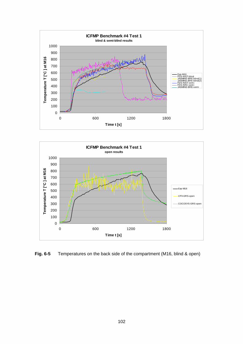
102

ICFMP Benchmark #4 Test 1blind & semi-blind results

0

100

200

300

400

500

600

700

800

900

1000

0 600 1200 1800

Time t [s]

Tem

pera

ture

T [°

C ]

at M

16

Exp-M16FDS-NIST-blindJASMINE-BRE-blind(1)JASMINE-BRE-blind(2)FDS-NIST-semiFDS-NRC-semiJASMINE-BRE-semi

ICFMP Benchmark #4 Test 1open results

0

100

200

300

400

500

600

700

800

900

1000

0 600 1200 1800

Time t [s]

Tem

pera

ture

T [°

C ]

at M

16

Exp-M16

CFX-GRS-open

COCOSYS-GRS-open

Fig. 6-5 Temperatures on the back side of the compartment (M16, blind & open)

103

ICFMP Benchmark #4 Test 1blind & semi-blind results

0

100

200

300

400

500

600

700

800

0 600 1200 1800

Time t [s]

Tem

pera

ture

T [°

C ]

at M

9

Exp-M9FDS-NIST-blindJASMINE-BRE-blind(1)JASMINE-BRE-blind(2)FDS-NIST-semiFDS-NRC-semiJASMINE-BRE-semi

ICFMP Benchmark #4 Test 1open results

0

100

200

300

400

500

600

700

800

900

1000

0 600 1200 1800

Time t [s]

Tem

pera

ture

T [°

C ]

at M

9

Exp-M9

CFX-GRS-open

COCOSYS-GRS-open

Fig. 6-6 Temperatures on the front side of the compartment (M9, blind & open)

104

ICFMP Benchmark #4 Test 1blind & semi-blind results

0

100

200

300

400

500

600

700

800

900

1000

0 600 1200 1800

Time t [s]

Tem

pera

ture

T [°

C ]

at M

13

Exp-M13FDS-NIST-blindJASMINE-BRE-blind(1)JASMINE-BRE-blind(2)FDS-NIST-semiFDS-NRC-semiJASMINE-BRE-semi

ICFMP Benchmark #4 Test 1open results

0

100

200

300

400

500

600

700

800

900

1000

0 600 1200 1800

Time t [s]

Tem

pera

ture

T [°

C ]

at M

13

Exp-M13

CFX-GRS-open

COCOSYS-GRS-open

Fig. 6-7 Temperatures on the front side of the compartment (M13, blind & open)

105

ICFMP Benchmark #4 Test 1blind & semi-blind results

0

100

200

300

400

500

600

700

800

900

1000

0 600 1200 1800

Time t [s]

Tem

pera

ture

T [°

C ]

at M

17

Exp-M17FDS-NIST-blindJASMINE-BRE-blind(1)JASMINE-BRE-blind(2)FDS-NIST-semiFDS-NRC-semiJASMINE-BRE-semi

ICFMP Benchmark #4 Test 1open results

0

100

200

300

400

500

600

700

800

900

1000

0 600 1200 1800

Time t [s]

Tem

pera

ture

T [°

C ]

at M

17

Exp-M17

CFX-GRS-open

COCOSYS-GRS-open

Fig. 6-8 Temperatures on the front side of the compartment (M17, blind & open)

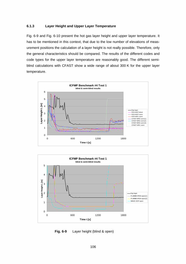
106

6.1.3 Layer Height and Upper Layer Temperature

Fig. 6-9 and Fig. 6-10 present the hot gas layer height and upper layer temperature. It

has to be mentioned in this context, that due to the low number of elevations of meas-

urement positions the calculation of a layer height is not really possible. Therefore, only

the general characteristics should be compared. The results of the different codes and

code types for the upper layer temperature are reasonably good. The different semi-

blind calculations with CFAST show a wide range of about 300 K for the upper layer

temperature.

ICFMP Benchmark #4 Test 1blind & semi-blind results

0

1

2

3

4

5

6

0 600 1200 1800

Time t [s]

Laye

r Hei

ght L

[m]

Exp-layerFDS-NIST-blindFDS-NIST-semiFDS-NRC-semiCFAST-BRE-semi(1)CFAST-BRE-semi(2)CFAST-BRE-semi(3)CFAST-NRC-semi

ICFMP Benchmark #4 Test 1blind & semi-blind results

0

1

2

3

4

5

0 600 1200 1800

Time t [s]

Laye

r Hei

ght L

[m]

Exp-layer

FLAMME-IRSN-open(1)

FLAMME-IRSN-open(2)MAGIC-EDF-open

Fig. 6-9 Layer height (blind & open)

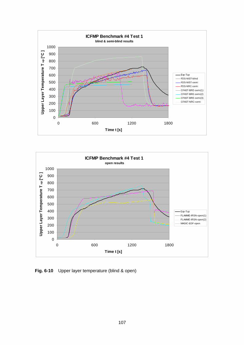
107

ICFMP Benchmark #4 Test 1blind & semi-blind results

0

100

200

300

400

500

600

700

800

900

1000

0 600 1200 1800

Time t [s]

Upp

er L

ayer

Tem

pera

ture

Tup

[°C

]

Exp-TupFDS-NIST-blindFDS-NIST-semiFDS-NRC-semi

CFAST-BRE-semi(1)CFAST-BRE-semi(2)CFAST-BRE-semi(3)CFAST-NRC-semi

ICFMP Benchmark #4 Test 1 open results

0

100

200

300

400

500

600

700

800

900

1000

0 600 1200 1800

Time t [s]

Upp

er L

ayer

Tem

pera

ture

Tup

[°C

]

Exp-Tup

FLAMME-IRSN-open(1)

FLAMME-IRSN-open(2)MAGIC-EDF-open

Fig. 6-10 Upper layer temperature (blind & open)

108

6.1.4 Gas Concentration inside the Fire Compartment

The main difference between Test 1 and Test 3 is the ventilation condition leading to

oxygen rich conditions for Test 1. Fig. 6-11 to Fig. 6-14 show the comparison for the

gas concentrations of O2 and CO2 inside and outside the fire compartment. All codes

except CFX underestimate the oxygen concentration inside the fire compartment.

Since the experimental values at the measurement position GA1 are quite constant in

contradiction to the values at the position GA2, the measurement at GA1 seems to be

somewhat questionable. The results of the semi-blind FDS calculation performed by

NIST outside the fire compartment are very good. In addition, the measured CO2 con-

centration at GA1 does not seem to be reasonable. The value is lower compared to the

value at the position GA2.

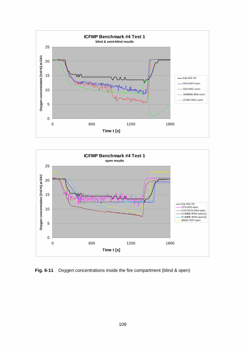
109

ICFMP Benchmark #4 Test 1blind & semi-blind results

0

5

10

15

20

25

0 600 1200 1800

Time t [s]

Oxy

gen

conc

entra

tion

[Vol

-%] a

t GA

1

Exp-GA1-O2

FDS-NIST-semi

FDS-NRC-semi

JASMINE-BRE-semi

CFAST-NRC-semi

ICFMP Benchmark #4 Test 1open results

0

5

10

15

20

25

0 600 1200 1800

Time t [s]

Oxy

gen

conc

entra

tion

[Vol

-%] a

t GA

1

Exp-GA1-O2CFX-GRS-openCOCOSYS-GRS-openFLAMME-IRSN-open(1)FLAMME-IRSN-open(2)MAGIC-EDF-open

Fig. 6-11 Oxygen concentrations inside the fire compartment (blind & open)

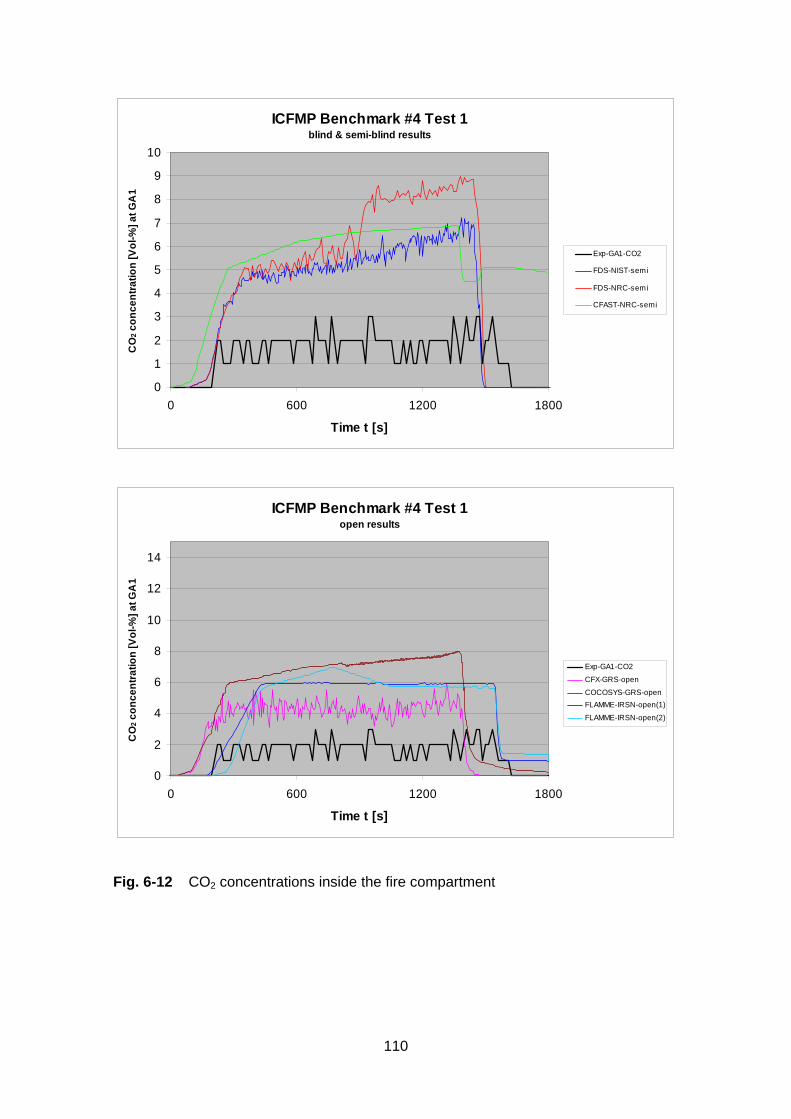
110

ICFMP Benchmark #4 Test 1blind & semi-blind results

0

1

2

3

4

5

6

7

8

9

10

0 600 1200 1800

Time t [s]

CO

2 con

cent

ratio

n [V

ol-%

] at G

A1

Exp-GA1-CO2

FDS-NIST-semi

FDS-NRC-semi

CFAST-NRC-semi

ICFMP Benchmark #4 Test 1open results

0

2

4

6

8

10

12

14

0 600 1200 1800

Time t [s]

CO

2 con

cent

ratio

n [V

ol-%

] at G

A1

Exp-GA1-CO2

CFX-GRS-open

COCOSYS-GRS-openFLAMME-IRSN-open(1)

FLAMME-IRSN-open(2)

Fig. 6-12 CO2 concentrations inside the fire compartment

111

ICFMP Benchmark #4 Test 1blind & semi-blind results

0

5

10

15

20

25

0 600 1200 1800

Time t [s]

Oxy

gen

conc

entra

tion

[Vol

-%] a

t GA

2

Exp-GA2-O2

FDS-NIST-semi

ICFMP Benchmark #4 Test 1open results

0

5

10

15

20

25

0 600 1200 1800

Time t [s]

Oxy

gen

conc

entra

tion

[Vol

-%] a

t GA

2

Exp-GA1-O2

CFX-GRS-open

Fig. 6-13 Oxygen concentration outside the fire compartment (blind & open)

112

ICFMP Benchmark #4 Test 1blind & semi-blind results

0

1

2

3

4

5

6

7

8

9

10

0 600 1200 1800

Time t [s]

CO

2 con

cent

ratio

n [V

ol-%

] at G

A2

Exp-GA2-CO2

FDS-NIST-semi

ICFMP Benchmark #4 Test 1open results

0

2

4

6

8

10

12

14

0 600 1200 1800

Time t [s]

CO

2 con

cent

ratio

n [V

ol-%

] at G

A2

Exp-GA2-CO2

CFX-GRS-open

Fig. 6-14 CO2 concentration outside the fire compartment

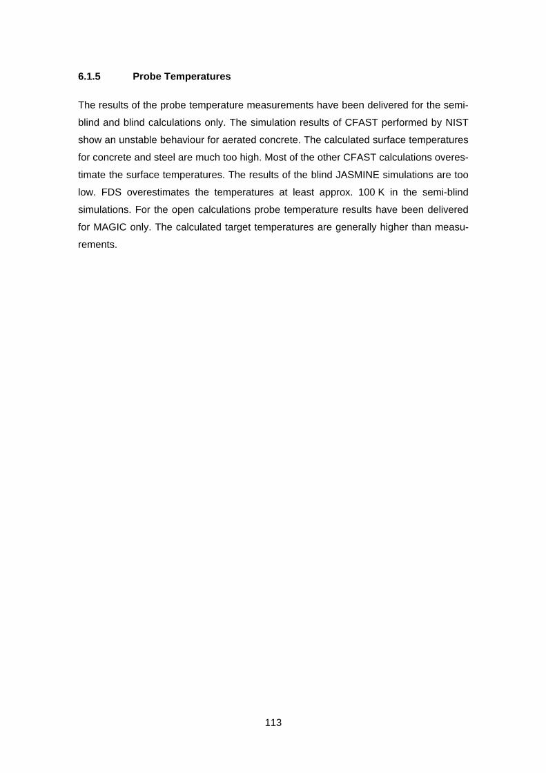
113

6.1.5 Probe Temperatures

The results of the probe temperature measurements have been delivered for the semi-

blind and blind calculations only. The simulation results of CFAST performed by NIST

show an unstable behaviour for aerated concrete. The calculated surface temperatures

for concrete and steel are much too high. Most of the other CFAST calculations overes-

timate the surface temperatures. The results of the blind JASMINE simulations are too

low. FDS overestimates the temperatures at least approx. 100 K in the semi-blind

simulations. For the open calculations probe temperature results have been delivered

for MAGIC only. The calculated target temperatures are generally higher than measu-

rements.

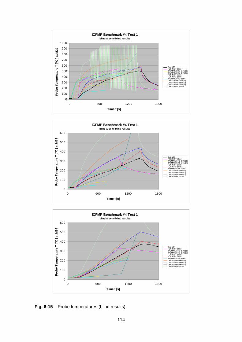
114

ICFMP Benchmark #4 Test 1blind & semi-blind results

0

100

200

300

400

500

600

700

800

900

1000

0 600 1200 1800

Time t [s]

Prob

e Te

mpe

ratu

re T

[°C

] at

M29

Exp-M29FDS-NIST-blindJASMINE-BRE-blind(1)JASMINE-BRE-blind(2)FDS-NIST-semiFDS-NRC-semiJASMINE-BRE-semiCFAST-BRE-semi(1)CFAST-BRE-semi(2)CFAST-BRE-semi(3)CFAST-NRC-semi

ICFMP Benchmark #4 Test 1blind & semi-blind results

0

100

200

300

400

500

600

0 600 1200 1800

Time t [s]

Prob

e Te

mpe

ratu

re T

[°C

] at

M33

Exp-M33FDS-NIST-blindJASMINE-BRE-blind(1)JASMINE-BRE-blind(2)FDS-NIST-semiFDS-NRC-semiJASMINE-BRE-semiCFAST-BRE-semi(1)CFAST-BRE-semi(2)CFAST-BRE-semi(3)CFAST-NRC-semi

ICFMP Benchmark #4 Test 1blind & semi-blind results

0

100

200

300

400

500

600

0 600 1200 1800

Time t [s]

Prob

e Te

mpe

ratu

re T

[°C

] at

M34

Exp-M34FDS-NIST-blindJASMINE-BRE-blind(1)JASMINE-BRE-blind(2)FDS-NIST-semiFDS-NRC-semiJASMINE-BRE-semiCFAST-BRE-semi(1)CFAST-BRE-semi(2)CFAST-BRE-semi(3)CFAST-NRC-semi

Fig. 6-15 Probe temperatures (blind results)

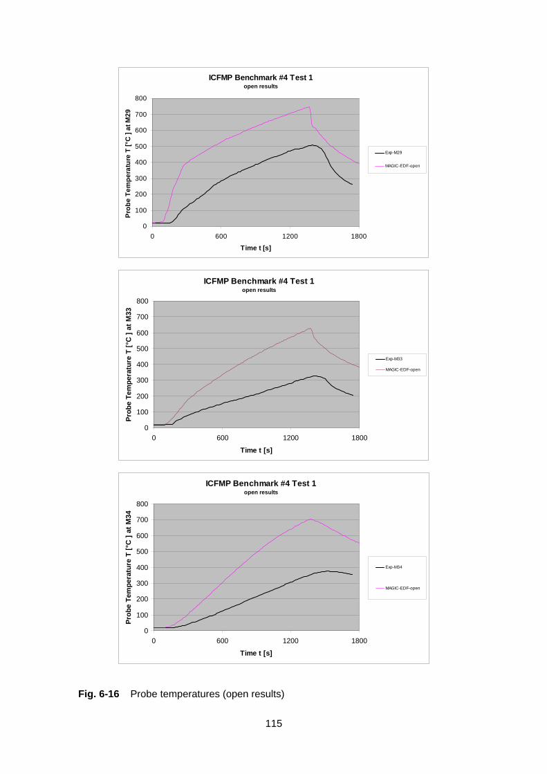
115

ICFMP Benchmark #4 Test 1open results

0

100

200

300

400

500

600

700

800

0 600 1200 1800

Time t [s]

Prob

e Te

mpe

ratu

re T

[°C

] at

M29

Exp-M29

MAGIC-EDF-open

ICFMP Benchmark #4 Test 1open results

0

100

200

300

400

500

600

700

800

0 600 1200 1800

Time t [s]

Prob

e Te

mpe

ratu

re T

[°C

] at

M33

Exp-M33

MAGIC-EDF-open

ICFMP Benchmark #4 Test 1open results

0

100

200

300

400

500

600

700

800

0 600 1200 1800

Time t [s]

Prob

e Te

mpe

ratu

re T

[°C

] at

M34

Exp-M34

MAGIC-EDF-open

Fig. 6-16 Probe temperatures (open results)

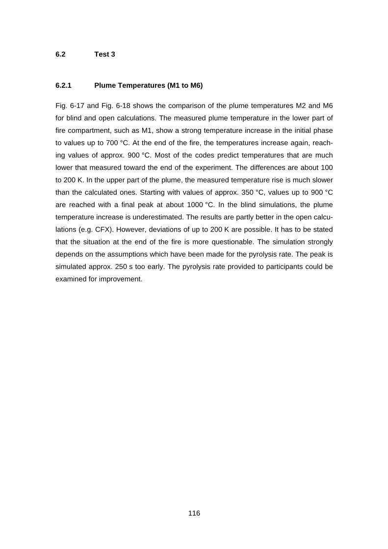
116

6.2 Test 3

6.2.1 Plume Temperatures (M1 to M6)

Fig. 6-17 and Fig. 6-18 shows the comparison of the plume temperatures M2 and M6

for blind and open calculations. The measured plume temperature in the lower part of

fire compartment, such as M1, show a strong temperature increase in the initial phase

to values up to 700 °C. At the end of the fire, the temperatures increase again, reach-

ing values of approx. 900 °C. Most of the codes predict temperatures that are much

lower that measured toward the end of the experiment. The differences are about 100

to 200 K. In the upper part of the plume, the measured temperature rise is much slower

than the calculated ones. Starting with values of approx. 350 °C, values up to 900 °C

are reached with a final peak at about 1000 °C. In the blind simulations, the plume

temperature increase is underestimated. The results are partly better in the open calcu-

lations (e.g. CFX). However, deviations of up to 200 K are possible. It has to be stated

that the situation at the end of the fire is more questionable. The simulation strongly

depends on the assumptions which have been made for the pyrolysis rate. The peak is

simulated approx. 250 s too early. The pyrolysis rate provided to participants could be

examined for improvement.

117

ICFMP Benchmark #4 Test 3blind & semi-blind results

0

100

200

300

400

500

600

700

800

900

1000

0 600 1200 1800

Time t [s]

Tem

pera

ture

T [°

C ]

at M

2

Exp-M2FDS-NIST-blindJASMINE-BRE-blind(1)JASMINE-BRE-blind(2)JASMINE-BRE-blind(3)FDS-NIST-semiFDS-NRC-semiJASMINE-BRE-semiJASMINE-BRE-semi(2)

ICFMP Benchmark #4 Test 3open results

0

100

200

300

400

500

600

700

800

900

1000

0 600 1200 1800

Time t [s]

Tem

pera

ture

T [°

C ]

at M

2

Exp-M2VULCAN-SAND-openCFX-GRS-openFDS-GRS-open(1)FDS-GRS-open(2)FDS-GRS-open(3)COCOSYS-GRS-openMAGIC-EDF-open

Fig. 6-17 Comparison of plume temperatures M2 (blind & open)

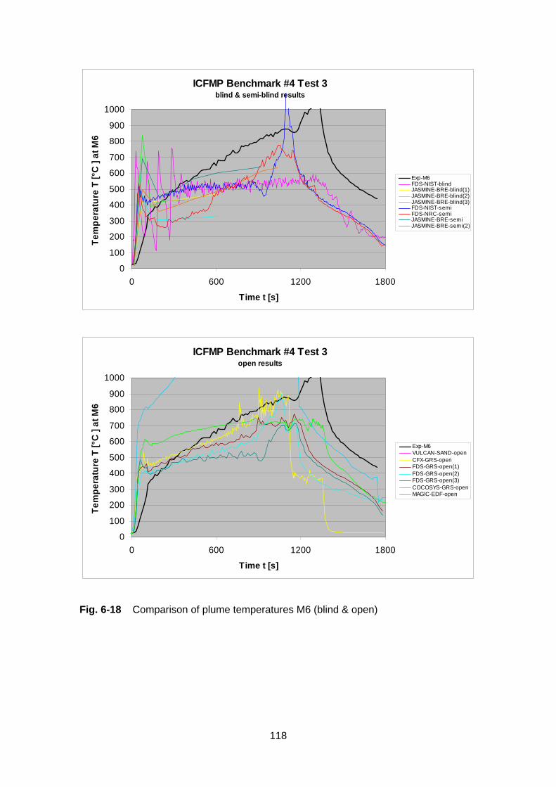
118

ICFMP Benchmark #4 Test 3blind & semi-blind results

0

100

200

300

400

500

600

700

800

900

1000

0 600 1200 1800

Time t [s]

Tem

pera

ture

T [°

C ]

at M

6

Exp-M6FDS-NIST-blindJASMINE-BRE-blind(1)JASMINE-BRE-blind(2)JASMINE-BRE-blind(3)FDS-NIST-semiFDS-NRC-semiJASMINE-BRE-semiJASMINE-BRE-semi(2)

ICFMP Benchmark #4 Test 3open results

0

100

200

300

400

500

600

700

800

900

1000

0 600 1200 1800

Time t [s]

Tem

pera

ture

T [°

C ]

at M

6

Exp-M6VULCAN-SAND-openCFX-GRS-openFDS-GRS-open(1)FDS-GRS-open(2)FDS-GRS-open(3)COCOSYS-GRS-openMAGIC-EDF-open

Fig. 6-18 Comparison of plume temperatures M6 (blind & open)

119

6.2.2 Temperatures inside the Fire Compartment

Fig. 6-19 to Fig. 6-24 present the comparison of blind and open calculations for two

temperature trees. These are the measurement positions M8, M12 and M16 at the rear

of the fire compartment close to the wall and the positions M9, M13 and M17 at the

front. The deviations between the code results are partly quite high with approx. up to

500 K. JASMINE calculates very high temperatures at the rear (position M8), while the

results are much better at the front. A possible reason is that a strong shift of the fire

plume was calculated in the simulation. Similar to the plume temperatures, the tem-

perature gradient is underestimated by most of the codes. The open CFX calculation

shows a somewhat better simulation of the temperature gradient. But, similar to the

plume temperature, the measured temperature peak was not calculated. At about

550 s the VULCAN simulation shows a temperature decrease, which was not observed

in the experiment. COCOSYS does not solve the momentum balance. Therefore, a

plume shift can not be calculated and the results for back and front side are very simi-

lar. A temperature peak was also not simulated.

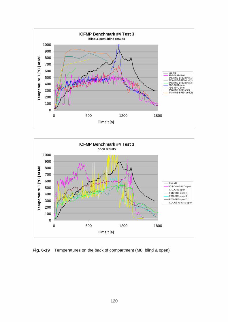
120

ICFMP Benchmark #4 Test 3blind & semi-blind results

0

100

200

300

400

500

600

700

800

900

1000

0 600 1200 1800

Time t [s]

Tem

pera

ture

T [°

C ]

at M

8

Exp-M8FDS-NIST-blindJASMINE-BRE-blind(1)JASMINE-BRE-blind(2)JASMINE-BRE-blind(3)FDS-NIST-semiFDS-NRC-semiJASMINE-BRE-semiJASMINE-BRE-semi(2)

ICFMP Benchmark #4 Test 3open results

0

100

200

300

400

500

600

700

800

900

1000

0 600 1200 1800

Time t [s]

Tem

pera

ture

T [°

C ]

at M

8

Exp-M8VULCAN-SAND-openCFX-GRS-openFDS-GRS-open(1)FDS-GRS-open(2)FDS-GRS-open(3)COCOSYS-GRS-open

Fig. 6-19 Temperatures on the back of compartment (M8, blind & open)

121

ICFMP Benchmark #4 Test 3blind & semi-blind results

0

100

200

300

400

500

600

700

800

900

1000

0 600 1200 1800

Time t [s]

Tem

pera

ture

T [°

C ]

at M

12

Exp-M12FDS-NIST-blindJASMINE-BRE-blind(1)JASMINE-BRE-blind(2)JASMINE-BRE-blind(3)FDS-NIST-semiFDS-NRC-semiJASMINE-BRE-semiJASMINE-BRE-semi(2)

ICFMP Benchmark #4 Test 3open results

0

100

200

300

400

500

600

700

800

900

1000

0 600 1200 1800

Time t [s]

Tem

pera

ture

T [°

C ]

at M

12

Exp-M12VULCAN-SAND-openCFX-GRS-openFDS-GRS-open(1)FDS-GRS-open(2)FDS-GRS-open(3)COCOSYS-GRS-open

Fig. 6-20 Temperatures on the back of compartment (M12, blind & open)

122

ICFMP Benchmark #4 Test 3blind & semi-blind results

0

100

200

300

400

500

600

700

800

900

1000

0 600 1200 1800

Time t [s]

Tem

pera

ture

T [°

C ]

at M

16

Exp-M16FDS-NIST-blindJASMINE-BRE-blind(1)JASMINE-BRE-blind(2)JASMINE-BRE-blind(3)FDS-NIST-semiFDS-NRC-semiJASMINE-BRE-semiJASMINE-BRE-semi(2)

ICFMP Benchmark #4 Test 3open results

0

100

200

300

400

500

600

700

800

900

1000

0 600 1200 1800

Time t [s]

Tem

pera

ture

T [°

C ]

at M

16

Exp-M16VULCAN-SAND-openCFX-GRS-openFDS-GRS-open(1)FDS-GRS-open(2)FDS-GRS-open(3)COCOSYS-GRS-open

Fig. 6-21 Temperatures on the back of compartment (M16, blind & open)

123

ICFMP Benchmark #4 Test 3blind & semi-blind results

0

100

200

300

400

500

600

700

800

900

1000

0 600 1200 1800

Time t [s]

Tem

pera

ture

T [°

C ]

at M

9

Exp-M9FDS-NIST-blindJASMINE-BRE-blind(1)JASMINE-BRE-blind(2)JASMINE-BRE-blind(3)FDS-NIST-semiFDS-NRC-semiJASMINE-BRE-semiJASMINE-BRE-semi(2)

ICFMP Benchmark #4 Test 3open results

0

100

200

300

400

500

600

700

800

900

1000

0 600 1200 1800

Time t [s]

Tem

pera

ture

T [°

C ]

at M

9

Exp-M9VULCAN-SAND-openCFX-GRS-openFDS-GRS-open(1)FDS-GRS-open(2)FDS-GRS-open(3)COCOSYS-GRS-open

Fig. 6-22 Temperatures on the front side of compartment (M9, blind & open)

124

ICFMP Benchmark #4 Test 3blind & semi-blind results

0

100

200

300

400

500

600

700

800

900

1000

0 600 1200 1800

Time t [s]

Tem

pera

ture

T [°

C ]

at M

13

Exp-M13FDS-NIST-blindJASMINE-BRE-blind(1)JASMINE-BRE-blind(2)JASMINE-BRE-blind(3)FDS-NIST-semiFDS-NRC-semiJASMINE-BRE-semiJASMINE-BRE-semi(2)

ICFMP Benchmark #4 Test 3open results

0

100

200

300

400

500

600

700

800

900

1000

0 600 1200 1800

Time t [s]

Tem

pera

ture

T [°

C ]

at M

13

Exp-M13VULCAN-SAND-openCFX-GRS-openFDS-GRS-open(1)FDS-GRS-open(2)FDS-GRS-open(3)COCOSYS-GRS-open

Fig. 6-23 Temperatures on the front of compartment (M13, blind & open)

125

ICFMP Benchmark #4 Test 3blind & semi-blind results

0

100

200

300

400

500

600

700

800

900

1000

0 600 1200 1800

Time t [s]

Tem

pera

ture

T [°

C ]

at M

17

Exp-M17FDS-NIST-blindJASMINE-BRE-blind(1)JASMINE-BRE-blind(2)JASMINE-BRE-blind(3)FDS-NIST-semiFDS-NRC-semiJASMINE-BRE-semiJASMINE-BRE-semi(2)

ICFMP Benchmark #4 Test 3open results

0

100

200

300

400

500

600

700

800

900

1000

0 600 1200 1800

Time t [s]

Tem

pera

ture

T [°

C ]

at M

17

Exp-M17VULCAN-SAND-openCFX-GRS-openFDS-GRS-open(1)FDS-GRS-open(2)FDS-GRS-open(3)COCOSYS-GRS-open

Fig. 6-24 Temperatures on the front of compartment (M17, blind & open)

126

6.2.3 Layer Height and Upper Layer Temperature

Only three levels of measurements are available inside the fire compartment. Therefore

the calculation of the upper layer temperature and the hot gas layer height is question-

able. Fig. 6-25 and Fig. 6-26 present the comparison between the results of zone mod-

els and experimental results. The calculated layer heights are lower compared to the

experiment, In particular close to the floor level. Because the lowest elevation of the

measurement is located at 1.5 m, the experimental result cannot be lower.

The semi-blind CFAST calculations performed by different users show a strong devia-

tion of 300 K for the upper layer temperature. Results from open calculations are pro-

vided by the code FLAMME-S and MAGIC. The results of MAGIC are quite close to

the experimental results. Concerning FLAMME-S it has to be pointed out that this

Benchmark Exercise is out of the validated range of this code. The simulated tempera-

tures are too low in comparison to the experimental data.

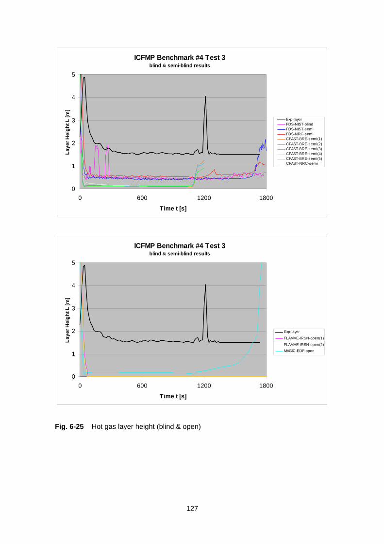
127

ICFMP Benchmark #4 Test 3blind & semi-blind results

0

1

2

3

4

5

0 600 1200 1800

Time t [s]

Laye

r Hei

ght L

[m]

Exp-layerFDS-NIST-blindFDS-NIST-semiFDS-NRC-semiCFAST-BRE-semi(1)CFAST-BRE-semi(2)CFAST-BRE-semi(3)CFAST-BRE-semi(4)CFAST-BRE-semi(5)CFAST-NRC-semi

ICFMP Benchmark #4 Test 3blind & semi-blind results

0

1

2

3

4

5

0 600 1200 1800

Time t [s]

Laye

r Hei

ght L

[m]

Exp-layer

FLAMME-IRSN-open(1)FLAMME-IRSN-open(2)MAGIC-EDF-open

Fig. 6-25 Hot gas layer height (blind & open)

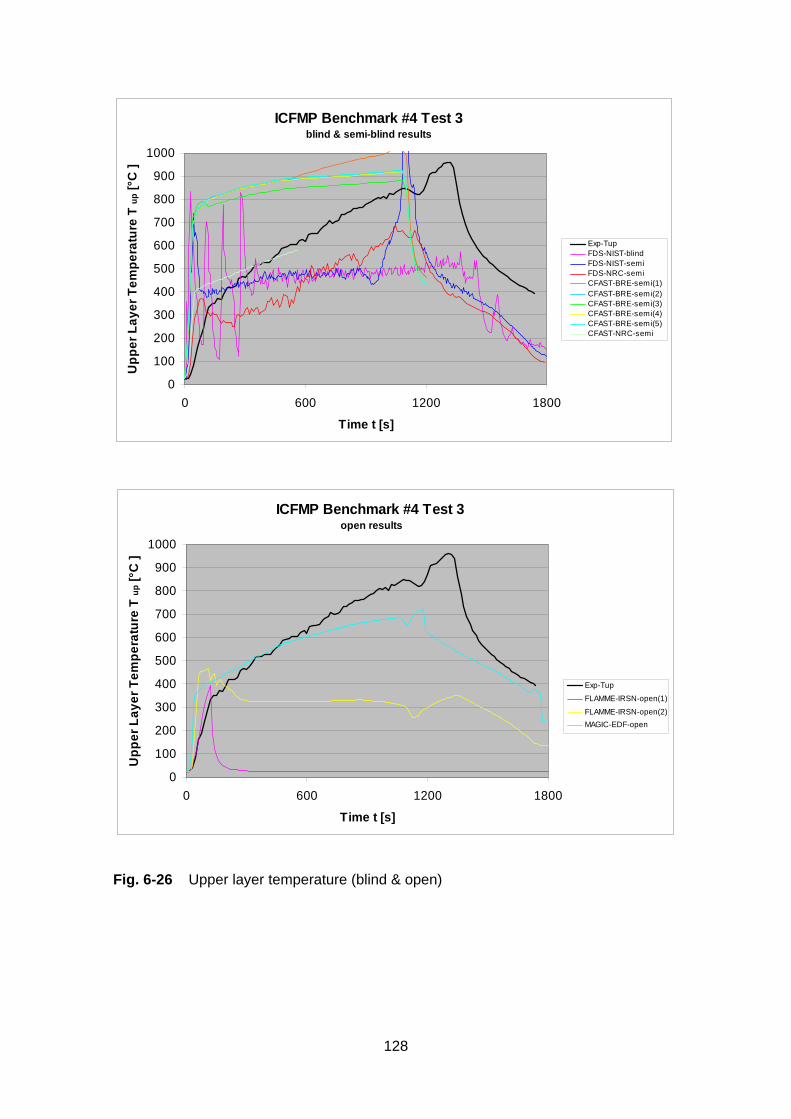
128

ICFMP Benchmark #4 Test 3blind & semi-blind results

0

100

200

300

400

500

600

700

800

900

1000

0 600 1200 1800

Time t [s]

Upp

er L

ayer

Tem

pera

ture

Tup

[°C

]

Exp-TupFDS-NIST-blindFDS-NIST-semiFDS-NRC-semiCFAST-BRE-semi(1)CFAST-BRE-semi(2)CFAST-BRE-semi(3)CFAST-BRE-semi(4)CFAST-BRE-semi(5)CFAST-NRC-semi

ICFMP Benchmark #4 Test 3 open results

0

100

200

300

400

500

600

700

800

900

1000

0 600 1200 1800

Time t [s]

Upp

er L

ayer

Tem

pera

ture

Tup

[°C

]

Exp-TupFLAMME-IRSN-open(1)

FLAMME-IRSN-open(2)MAGIC-EDF-open

Fig. 6-26 Upper layer temperature (blind & open)

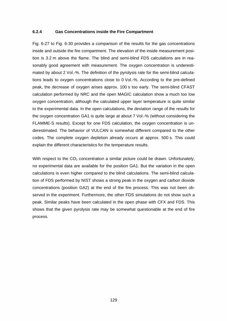
129

6.2.4 Gas Concentrations inside the Fire Compartment

Fig. 6-27 to Fig. 6-30 provides a comparison of the results for the gas concentrations

inside and outside the fire compartment. The elevation of the inside measurement posi-

tion is 3.2 m above the flame. The blind and semi-blind FDS calculations are in rea-

sonably good agreement with measurement. The oxygen concentration is underesti-

mated by about 2 Vol.-%. The definition of the pyrolysis rate for the semi-blind calcula-

tions leads to oxygen concentrations close to 0 Vol.-%. According to the pre-defined

peak, the decrease of oxygen arises approx. 100 s too early. The semi-blind CFAST

calculation performed by NRC and the open MAGIC calculation show a much too low

oxygen concentration, although the calculated upper layer temperature is quite similar

to the experimental data. In the open calculations, the deviation range of the results for

the oxygen concentration GA1 is quite large at about 7 Vol.-% (without considering the

FLAMME-S results). Except for one FDS calculation, the oxygen concentration is un-

derestimated. The behavior of VULCAN is somewhat different compared to the other

codes. The complete oxygen depletion already occurs at approx. 500 s. This could

explain the different characteristics for the temperature results.

With respect to the CO2 concentration a similar picture could be drawn. Unfortunately,

no experimental data are available for the position GA1. But the variation in the open

calculations is even higher compared to the blind calculations. The semi-blind calcula-

tion of FDS performed by NIST shows a strong peak in the oxygen and carbon dioxide

concentrations (position GA2) at the end of the fire process. This was not been ob-

served in the experiment. Furthermore, the other FDS simulations do not show such a

peak. Similar peaks have been calculated in the open phase with CFX and FDS. This

shows that the given pyrolysis rate may be somewhat questionable at the end of fire

process.

130

ICFMP Benchmark #4 Test 3blind & semi-blind results

0

5

10

15

20

25

0 600 1200 1800

Time t [s]

Oxy

gen

conc

entra

tion

[Vol

-%] a

t GA

1

Exp-GA1-O2

FDS-NIST-blind

FDS-NIST-semiFDS-NRC-semi

CFAST-NRC-semi

ICFMP Benchmark #4 Test 3open results

0

5

10

15

20

25

0 600 1200 1800

Time t [s]

Oxy

gen

conc

entra

tion

[Vol

-%] a

t GA

1

Exp-GA1-O2CFX-GRS-open

FDS-GRS-open(1)FDS-GRS-open(2)FDS-GRS-open(3)COCOSYS-GRS-open

VULCAN-SAND-openFLAMME-IRSN-open(1)FLAMME-IRSN-open(2)

MAGIC-EDF-open

Fig. 6-27 Oxygen concentration inside fire compartment (blind & open)

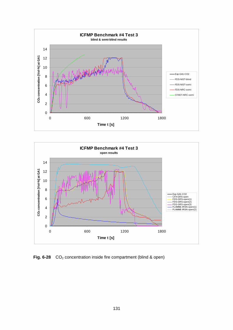
131

ICFMP Benchmark #4 Test 3blind & semi-blind results

0

2

4

6

8

10

12

14

0 600 1200 1800

Time t [s]

CO

2 con

cent

ratio

n [V

ol-%

] at G

A1

Exp-GA1-CO2

FDS-NIST-blind

FDS-NIST-semi

FDS-NRC-semi

CFAST-NRC-semi

ICFMP Benchmark #4 Test 3open results

0

2

4

6

8

10

12

14

0 600 1200 1800

Time t [s]

CO

2 con

cent

ratio

n [V

ol-%

] at G

A1

Exp-GA1-CO2CFX-GRS-openFDS-GRS-open(1)FDS-GRS-open(2)FDS-GRS-open(3)FLAMME-IRSN-open(1)FLAMME-IRSN-open(2)

Fig. 6-28 CO2 concentration inside fire compartment (blind & open)

132

ICFMP Benchmark #4 Test 3blind & semi-blind results

0

5

10

15

20

25

0 600 1200 1800

Time t [s]

Oxy

gen

conc

entra

tion

[Vol

-%] a

t GA

2

Exp-GA2-O2

FDS-NIST-blind

FDS-NIST-semi

FDS-NRC-semi

CFAST-NRC-semi

ICFMP Benchmark #4 Test 3open results

0

5

10

15

20

25

0 600 1200 1800

Time t [s]

Oxy

gen

conc

entra

tion

[Vol

-%] a

t GA

2

Exp-GA1-O2CFX-GRS-open

FDS-GRS-open(1)FDS-GRS-open(2)FDS-GRS-open(3)

Fig. 6-29 Oxygen concentration outside fire compartment (blind & open)

133

ICFMP Benchmark #4 Test 3blind & semi-blind results

0

1

2

3

4

5

6

7

8

9

10

0 600 1200 1800

Time t [s]

CO

2 con

cent

ratio

n [V

ol-%

] at G

A2

Exp-GA2-CO2

FDS-NIST-blind

FDS-NIST-semi

ICFMP Benchmark #4 Test 3open results

0

2

4

6

8

10

12

14

0 600 1200 1800

Time t [s]

CO

2 con

cent

ratio

n [V

ol-%

] at G

A2

Exp-GA2-CO2CFX-GRS-open

FDS-GRS-open(1)FDS-GRS-open(2)

FDS-GRS-open(3)

Fig. 6-30 CO2 concentration outside the fire compartment (blind & open)

134

6.2.5 Probe Temperatures

One of the main objectives of fire simulations codes for NPP applications is the estima-

tion of thermal loads on different type of targets. On the left wall of the compartment

three material probes of different material types, concrete, aerated concrete and steel

have been installed. Fig. 6-31 and Fig. 6-32 compare the calculated and experimental

temperatures close to the material surface. The results of the blind calculations show a

wide range of deviations. The semi-blind CFAST calculation performed by BRE overes-

timates the temperatures by about 300 K while most of the CFD codes underestimate

the temperature by up to 300 K. The strong temperature peak simulated by some CFD

codes as a result of the peak in the pyrolysis rate was not observed in the temperature

measurements. The results of FDS for the open calculations are comparable to those

for the blind simulations. The temperatures are underestimated by approx. 100 K. The

results of VULCAN are on the one hand in a very good agreement with the experimen-

tal data, except the strong peak for aerated concrete. On the other hand the calculated

temperature decrease at the end of the fire process is much too strong, indicating that

the thermal heat conduction or heat transfer is not simulated correctly. The results of

the open MAGIC calculation are reasonable and better compared to Test 1.

135

ICFMP Benchmark #4 Test 3blind & semi-blind results

0

100

200

300

400

500

600

700

800

900

1000

0 600 1200 1800

Time t [s]

Prob

e Te

mpe

ratu

re T

[°C

] at

M29

Exp-M29FDS-NIST-blindJASMINE-BRE-blind(1)JASMINE-BRE-blind(2)JASMINE-BRE-blind(3)FDS-NIST-semiFDS-NRC-semiJASMINE-BRE-semiCFAST-BRE-semi(1)CFAST-BRE-semi(2)CFAST-BRE-semi(3)CFAST-NRC-semi

ICFMP Benchmark #4 Test 3blind & semi-blind results

0

100

200

300

400

500

600

700

800

0 600 1200 1800

Time t [s]

Prob

e Te

mpe

ratu

re T

[°C

] at

M33

Exp-M33FDS-NIST-blindJASMINE-BRE-blind(1)JASMINE-BRE-blind(2)JASMINE-BRE-blind(3)FDS-NIST-semiFDS-NRC-semiJASMINE-BRE-semiCFAST-BRE-semi(1)CFAST-BRE-semi(2)CFAST-BRE-semi(3)CFAST-NRC-semi

ICFMP Benchmark #4 Test 3blind & semi-blind results

0

100

200

300

400

500

600

0 600 1200 1800

Time t [s]

Prob

e Te

mpe

ratu

re T

[°C

] at

M34

Exp-M34FDS-NIST-blindJASMINE-BRE-blind(1)JASMINE-BRE-blind(2)JAMSINE-BRE-blind(3)FDS-NIST-semiFDS-NRC-semiJASMINE-BRE-semiCFAST-BRE-semi(1)CFAST-BRE-semi(2)CFAST-BRE-semi(3)CFAST-NRC-semi

Fig. 6-31 Comparison of the probe surface temperatures (blind simulations)

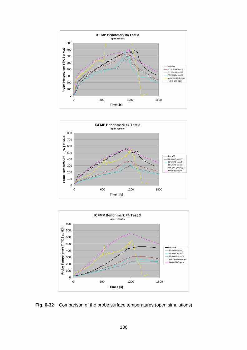
136

ICFMP Benchmark #4 Test 3open results

0

100

200

300

400

500

600

700

800

0 600 1200 1800

Time t [s]

Prob

e Te

mpe

ratu

re T

[°C

] at

M29

Exp-M29FDS-GRS-open(1)FDS-GRS-open(2)FDS-GRS-open(3)

VULCAN-SAND-openMAGIC-EDF-open

ICFMP Benchmark #4 Test 3open results

0

100

200

300

400

500

600

700

800

0 600 1200 1800

Time t [s]

Prob

e Te

mpe

ratu

re T

[°C

] at

M33

Exp-M33

FDS-GRS-open(1)FDS-GRS-open(2)

FDS-GRS-open(3)

VULCAN-SAND-openMAGIC-EDF-open

ICFMP Benchmark #4 Test 3open results

0

100

200

300

400

500

600

700

800

0 600 1200 1800

Time t [s]

Prob

e Te

mpe

ratu

re T

[°C

] at

M34

Exp-M34FDS-GRS-open(1)FDS-GRS-open(2)

FDS-GRS-open(3)

VULCAN-SAND-openMAGIC-EDF-open

Fig. 6-32 Comparison of the probe surface temperatures (open simulations)

137

7 General Conclusions and Recommendations

7.1 General Conclusions

This section provides a discussion of the general conclusions derived from Benchmark

Exercise No. 4.

Heat Release Rate

The pyrolysis rate and the resulting heat release rate have a great impact on the ther-

mo-fluid conditions inside the fire compartment. The specified (measured) rate for Test

1 seems to be satisfactory, because reasonable temperatures were calculated. The

rate for Test 3 is more questionable, because the temperature peak at the end of the

experiment is not simulated and the calculated temperature decrease starts too early.

On the other hand, due to the under-ventilated conditions, the combustion usually is

incomplete and possibly under-estimated.

Blind calculations show that the models to calculate pyrolysis rates are still limited. The

results of these calculations show significant deviations from the experimental results.

Gas Temperatures

The overall gas temperatures could be reasonably well simulated by zone models as

well as by the more complex CFD codes, although the differences for Test 3 are larger.

The CFD codes were able to simulate the drift of the flame to the rear wall due to the

fresh air entrainment through the door. However, in comparing the lower temperatures

at the measurement locations M8 and M10 at the rear of fire compartment, this effect

seems to be over-estimated in the simulations. Particularly for targets close to the fire,

these effects may be more important.

Oxygen Concentration

Key parameters for the oxygen concentration inside the fire compartment are the com-

bustion efficiency, the ventilation conditions, and the reaction schemes modeled, par-

ticularly for CO and soot production. Here, Test 3 gives some answers for the specifi-

cation of the LOL value, which should be set to 0 Vol.-%. FDS with only one single

transport equation shows some principal limitations in this range.

138

Wall Temperatures

Wall temperatures are partly influenced by the flame shifting to the back wall. This ef-

fect could be simulated, in principle, by CFD codes only. Zone codes assume homoge-

neous boundary conditions.

Ventilation – Air Entrainment

For zone models the handling of the air entrainment for under-ventilated conditions is

important, particularly in Test 3. Here, specific assumptions have been made in some

zone model calculations.

Target Simulation

The ability to simulate the targets is restricted in the various codes. Some problems

result from the cylindrical shape of the barrel target as well as from the multi-layer ma-

terial configuration. Radiation has an important influence on the thermal loading, and

this has to be partly specified by the user.

7.2 Recommendations

The strong differences between calculations and experiments, in particular for the blind

simulations, indicates that models to predict pyrolysis rates are strongly needed. Unfor-

tunately, there is a strong positive feedback from the thermal environment back to fuel

surface which then influences the pyrolysis rate. Further local effects, such as edges to

the pan, may also have an influence on the pyrolysis rate. The consequences for the

estimation of uncertainties should be discussed in more detail. In this context, further

blind calculations (for new experiments) will be helpful.

Scenarios with under-ventilated fires are still difficult to simulate. It has to be kept in

mind that such scenarios are typical for NPPs, as most of the fire compartments in a

NPP can be assumed more or less closed during a fire.

The simulation of targets should be further improved and investigated. This is highly

important, because potential failures (e.g. short circuits) may occur much earlier than

the ignition of the target itself.

139

8 Summary

The fuel pool fire Tests 1 and 3, performed in the OSKAR test facility at iBMB of Braun-

schweig University of Technology at the end of 2003, have been included in the bench-

marking and validation exercises of the International Collaborative Fire Model Project

(ICFMP) as Exercise No. 4. The objective of the collaborative project is to share the

knowledge and resources of various organizations to evaluate and improve the state of

the art of fire models for the use in nuclear power plant fire safety assessments, cover-

ing deterministic fire hazard analysis (FHA) as well as fire probabilistic safety assess-

ment (PSA) studies.

The main difference between the two experiments carried out is the size of the door

area. Both experiments give first indications on the effects of ventilation and fuel con-

trolled fires as well as on the thermal loading on different types of targets. Previous

benchmark exercises within the ICFMP had shown that the simulation of these two

phenomena should be improved.

During the benchmark procedure, the participants performed different types of calcula-

tions. These were totally blind simulations without knowledge of the measurements,

semi-blind calculations with knowledge of the pyrolysis rate only, and completely open

calculations. It has been demonstrated that the pyrolysis rate has a strong influence on

the calculation results. Limited information on the pyrolysis rate affects the results to

some extent. This finding was supported from the comparison of the (admittedly few)

blind and semi-blind simulations. The range of the results (e. g. JASMINE and FDS) is

much larger for the blind simulations compared to the semi-blind ones. This overall

result of Benchmark Exercise No. 4 should be somehow considered in the estimation

of uncertainty parameters as an input in, for example PSA studies.

The simulation of under-ventilated fires is more difficult for the fire codes. In particular,

the high transient behavior at the final phase of Test 3 leads to a wide range of simula-

tion results. Unfortunately, the measured pyrolysis rate is no longer valid in this phase,

and so the ‘specified’ pyrolysis rate may not be very reliable at this time. It should be

mentioned, however, that many of the possible fire scenarios in real nuclear power

plants will lead to under-ventilated conditions. Therefore, this issue should be further

investigated and the models should be further improved.

140

Some codes have difficulties to simulate more complex targets. Most of the codes are

able to simulate the material probes. The range of the results is larger compared to that

for the gas temperatures. As this information is significant for estimating failures of

safety related equipment, the models should be further developed and improved.

141

9 References

/ALL 05/ Allelein, H.-J. et al.:

Weiterentwicklung der Rechenprogramme COCOSYS und ASTEC,

Abschlussbericht, GRS-A-3266, Gesellschaft für Anlagen- und

Reaktorsicherheit, April 2005

/BOU 02/ Bouton, E.,

Overview of the FLAMME-S code validation matrix, Technical Note

SESHP/GME/IPS/FLS/C40/NT/02.337, 2002

/CFX 04/ CFX-5.7, User Documentation, ANSYS Inc., USA, 2004

/COX 87/ Cox, G., and S. Kumar:

Field modelling of fire in forced ventilated enclosures, Combustion Science

and Technology, Vol. 52, pp. 7-23, 1987

/DEY 02/ Dey M.:

Evaluation of Fire Models for Nuclear Power Plant Applications: Cable Tray

Fires, NISTIR 6872, National Institute of Standard and Technology, USA,

June 2002

/GAY 06/ L. GAY, B. GAUTIER

"Magic Software Version 4.1.1: Mathematical Model"

HI-82/04/024/B - March 2006

/HOL 90/ Holen, J., M. Brostrom, and B.F. Magnusson:

Finite Difference Calculation of Pool Fires, 23rd Symposium on Combustion,

Combustion Institute, pp. 1677-1683, 1990

/JON 04/ Jones, W.W., et al.:

CFAST - Consolidated Model of Fire Growth and Smoke Transport ,

(Version 5): Technical Reference Guide. NIST Special Publication 1030,

October 2004

/KLE 04/ Klein-Heßling, W.:

Website: http://techconf.llnl.gov/cgi-fire/topics

142

/MCG 04/ McGrattan, K.B. (ed.):

Fire Dynamics Simulator (Version 4), Technical Reference Guide, NIST

Special Publication 1018, National Institute of Standards and Technology,

Gaithersburg, Maryland, USA, 2004

/MCG 06/ McGrattan, K.B.:

Evaluation of Fire Models for Nuclear Power Plant Applications: Benchmark

Exercise #3, International Panel Report, NISTIR 7338, to be published

January 2007

/MIL 04/ Miles, S.:

International Panel Report: Benchmark Exercise # 2 - Pool Fires in Large

Halls. May 2004

/PLY 04/ Plys, M.G., and J.L. Sung:

FATETM 2.0: Facility Flow, Aerosol, Thermal, and Explosion Model

(Improved and Combined HANSF and HADCRT Models), FAI/04-71,

SNF-23281, Two Volumes, November 2004

/RIE 06/ Riese, O., D. Hosser, M. Röwekamp:

Evaluation of Fire Models for Nuclear Power Plant Applications: Flame

Spread in Cable Tray Fires, International Panel Report on Benchmark

Exercise No. 5, Gesellschaft für Anlagen- und Reaktorsicherheit (GRS)

Report Number GRS-214, ISBN-Nr.: 978-3-931995-81-2, in publication,

2006

/TOU 00/ Tourniaire, B., and L. Audouin:

Sensitivity analysis of a data reduction method estimating the interface

height, the lower and upper temperatures in fire room, Proceedings of the

International Seminar of Fire and Explosion Hazard, 2000

143

List of Figures

Fig. 2-1 Benchmark Exercise No.1, Part II base case - calculated oxygen

concentrations............................................................................................. 4 Fig. 2-2 Benchmark Exercise No. 1, Part II base case - calculated HGL

temperatures ............................................................................................... 4 Fig. 2-3 3D view of the OSKAR fire compartment .................................................... 9 Fig. 2-4 Top view of the OSKAR fire compartment ................................................ 10 Fig. 2-5 Side view of the OSKAR fire compartment (in + y direction)..................... 11 Fig. 2-6 Side view of the OSKAR fire compartment (in + x direction)..................... 12 Fig. 2-7 Height of the fuel pan side walls and its elevations................................... 13 Fig. 2-8 View of the fire compartment through the front door ................................. 13 Fig. 2-9 Scheme of the hood above the front door ................................................. 14 Fig. 2-10 View onto the hood installed above the front door .................................... 14 Fig. 2-11 View of the three material probes ............................................................. 20 Fig. 2-12 View from top into the open barrel container ............................................ 20 Fig. 2-13 Measurement positions inside barrel ........................................................ 21 Fig. 2-14 Typical chemical composition of fuel......................................................... 22 Fig. 2-15 Test 1 - Measured velocities (V11 - V13) .................................................. 27 Fig. 2-16 Test 3 - Measured velocities (V11 - V13) .................................................. 28 Fig. 3-1 Fire development inside the fire compartment - Test 1, view through

front door................................................................................................... 31 Fig. 3-2 Temperature distribution during the fully developed fire phase - Test 1,

view through front door ............................................................................. 31 Fig. 3-3 Weight loss - Test 1 .................................................................................. 32 Fig. 3-4 Temperature distribution in measurement level 1 - Test 1 ........................ 32 Fig. 3-5 Heat flux into material probes - Test 1 ...................................................... 33 Fig. 3-6 Measured fuel temperature 3 cm above pan bottom - Test 1 ................... 33 Fig. 3-7 Temperature distribution inside the fire - Test 3........................................ 34 Fig. 3-8 Weight loss - Test 3 .................................................................................. 35 Fig. 3-9 Oxygen concentration in the fire compartment - Test 3 ............................ 35 Fig. 3-10 Plume temperatures - Test 3..................................................................... 36 Fig. 3-11 Heat flux into the test probe structures - Test 3 ........................................ 36 Fig. 3-12 Temperature distribution inside the barrel during Test 3........................... 37 Fig. 3-13 Temperature decrease after Test 3........................................................... 37

144

Fig. 4-1 Smoothed pyrolysis rate for Test 1 ........................................................... 40 Fig. 4-2 Smoothed pyrolysis rate for Test 3 ........................................................... 40 Fig. 5-1 Measured and predicted (blind) heat release rates for Tests 1 and 3

(from Appendix A) ..................................................................................... 46 Fig. 5-2 Measured and predicted (blind) gas temperatures for Test 3 (from

Appendix B)............................................................................................... 50 Fig. 5-3 Measured and predicted (blind) wall surface temperatures for Test 3

(from Appendix B) ..................................................................................... 51 Fig. 5-4 Gas temperature comparisons for Test 3 (from Appendix A).................... 54 Fig. 5-5 View of flame sheet output from FDS - Test 1 (from Appendix C) ............ 60 Fig. 5-6 Plume temperature (from Appendix C)...................................................... 60 Fig. 5-7 Measured and predicted (open) gas temperatures for Test 1 (from

Appendix B)............................................................................................... 64 Fig. 5-8 Measured and predicted (open) wall surface temperatures for Test 1

(from Appendix B) ..................................................................................... 65 Fig. 5-9 Measured and predicted gas temperatures and door velocities for Test

1 (from Appendix B) .................................................................................. 68 Fig. 5-10 Measured and predicted flux densities for Test 1 (from Appendix B)........ 69 Fig. 5-11 'Energy budget' for a Test 3 simulation (from Appendix B) ....................... 69 Fig. 5-12 Benchmark Exercise No. 4, Test 3 smoky layer gas concentrations

(from Appendix C) ..................................................................................... 74 Fig. 5-13 Gas temperature in the compartment - open calculations (from

Appendix D) .............................................................................................. 77 Fig. 5-14 Vertical temperature distribution at a plane x = 0.95 m (from Appendix

E)............................................................................................................... 80 Fig. 5-15 Comparison of selected gas temperatures close to the front of the test

facility for Test 1 (from Appendix E) .......................................................... 81 Fig. 5-16 Heat release rates of all FDS3 and FDS 4 calculations for Test 3 (from

Appendix G) .............................................................................................. 83 Fig. 5-17 Comparison of FDS results (FDS3 coarse grid; from Appendix G)........... 84 Fig. 5-18 Comparison of FDS results (FDS3 fine grid; from Appendix G)................ 85 Fig. 5-19 Comparison of FDS results (FDS4 fine grid) (from Appendix G) .............. 86 Fig. 5-20 Concept of the pyrolysis model for oil burning .......................................... 88 Fig. 5-21 Test 3: Plume temperature at M3 (from Appendix H)................................ 90 Fig. 5-22 Comparison of measured temperature M9 (z = 1.5 m) and COCOSYS

results (from Appendix H) ......................................................................... 90

145

Fig. 5-23 Mass loss rate (smoothed) versus experiment (from Appendix I) ............. 93 Fig. 5-24 Front room temperatures and oxygen concentration (from Appendix I).... 94 Fig. 5-25 Upper and lower temperature in Test 1 (from Appendix J) ....................... 96 Fig. 5-26 Upper and lower temperature in Test 3 (from Appendix J) ....................... 96 Fig. 6-1 Comparison of plume temperatures M2 (blind & open)............................. 98 Fig. 6-2 Comparison of plume temperatures M6 (blind & open)............................. 99 Fig. 6-3 Temperatures on the back side of the compartment (M8, blind & open) 100 Fig. 6-4 Temperatures on the back side of the compartment (M12, blind &

open) ....................................................................................................... 101 Fig. 6-5 Temperatures on the back side of the compartment (M16, blind &

open) ....................................................................................................... 102 Fig. 6-6 Temperatures on the front side of the compartment (M9, blind & open). 103 Fig. 6-7 Temperatures on the front side of the compartment (M13, blind &

open) ....................................................................................................... 104 Fig. 6-8 Temperatures on the front side of the compartment (M17, blind &

open) ....................................................................................................... 105 Fig. 6-9 Layer height (blind & open) ..................................................................... 106 Fig. 6-10 Upper layer temperature (blind & open) .................................................. 107 Fig. 6-11 Oxygen concentrations inside the fire compartment (blind & open)........ 109 Fig. 6-12 CO2 concentrations inside the fire compartment..................................... 110 Fig. 6-13 Oxygen concentration outside the fire compartment (blind & open) ....... 111 Fig. 6-14 CO2 concentration outside the fire compartment .................................... 112 Fig. 6-15 Probe temperatures (blind results) .......................................................... 114 Fig. 6-16 Probe temperatures (open results) ......................................................... 115 Fig. 6-17 Comparison of plume temperatures M2 (blind & open)........................... 117 Fig. 6-18 Comparison of plume temperatures M6 (blind & open)........................... 118 Fig. 6-19 Temperatures on the back of compartment (M8, blind & open) .............. 120 Fig. 6-20 Temperatures on the back of compartment (M12, blind & open) ............ 121 Fig. 6-21 Temperatures on the back of compartment (M16, blind & open) ............ 122 Fig. 6-22 Temperatures on the front side of compartment (M9, blind & open)....... 123 Fig. 6-23 Temperatures on the front of compartment (M13, blind & open) ............ 124 Fig. 6-24 Temperatures on the front of compartment (M17, blind & open) ............ 125 Fig. 6-25 Hot gas layer height (blind & open)......................................................... 127 Fig. 6-26 Upper layer temperature (blind & open) .................................................. 128 Fig. 6-27 Oxygen concentration inside fire compartment (blind & open)................ 130 Fig. 6-28 CO2 concentration inside fire compartment (blind & open) ..................... 131

146

Fig. 6-29 Oxygen concentration outside fire compartment (blind & open) ............. 132 Fig. 6-30 CO2 concentration outside the fire compartment (blind & open) ............. 133 Fig. 6-31 Comparison of the probe surface temperatures (blind simulations)........ 135 Fig. 6-32 Comparison of the probe surface temperatures (open simulations) ....... 136

147

List of Tables

Table 2-1 Composition of the wall structures ............................................................. 7 Table 2-2 Properties of the fire compartment materials .............................................. 7 Table 2-3 Properties of the target materials ................................................................ 8 Table 2-4 Location of the material probes................................................................... 8 Table 2-5 List of measurements performed ............................................................. 16 Table 2-6 Fuel material properties ............................................................................ 22 Table 2-7 Smoothed values for the total volume flow and velocity through the

FUCHS fan system (measurements V11 and V12) for Test 1 .................. 23 Table 2-8 Smoothed values for the total volume flow and velocity through the

FUCHS fan system (measurements V11 and V12) for Test 3 .................. 24 Table 2-9 Smoothed values for the total volume flow and velocity through the

hood (measurement V13) for Test 1 ......................................................... 25 Table 2-10 Smoothed table values for the total volume flow and velocity through

the hood (measurement V13) for Test 3 ................................................... 26 Table 2-11 Initial and ambient conditions.................................................................... 26 Table 3-1 Test matrix of the iBMB fuel pool fire tests................................................ 29 Table 5-1 List of fire simulations performed within Benchmark Exercise No. 4......... 43

149

List of Appendices:

Appendix A: Benchmark Exercise No. 4 Simulations with FDS

Appendix B: Benchmark Exercise No. 4 Simulations with JAMINE and CFAST

Appendix C: Validation of the CFAST and FDS Fire Models with Large Fire

Experiments in a Compartment

Appendix D: FATETM 2.0 Computer Code Calculations for Benchmark

Exercise No. 4

Appendix E: Benchmark Exercise No. 4: Kerosene Pool Fire Inside A

Compartment

Appendix F: CFX5 Simulations for Benchmark Exercise No. 4

Appendix G: FDS Simulations for Benchmark Exercise No. 4

Appendix H: CCOCOSYS Simulations for Benchmark Exercise No. 4

Appendix I: Vulcan Simulations of ICFMP Benchmark Exercise No. 4, Test 3

Appendix J: Kerosene pool fire inside a compartment Simulation with MAGIC

Gesellschaft für Anlagen- und Reaktorsicherheit (GRS) mbH

Schwertnergasse 150667 Köln

Telefon +49 221 2068-0Telefax +49 221 2068-888

Forschungsinstitute85748 Garching b.München

Telefon +49 89 32004-0Telefax +49 89 32004-300

Kurfürstendamm 200 10719 Berlin

Telefon +49 30 88589-0Telefax +49 30 88589-111

Theodor-Heuss-Straße 438122 Braunschweig

Telefon +49 531 8012-0Telefax +49 531 8012-200

www.grs.de

ISBN 978-3-931995-80-5