evaluation of iec 61850 process bus architecture and
TRANSCRIPT
EVALUATION OF IEC 61850 PROCESS BUS ARCHITECTURE AND RELIABILITY
A thesis submitted to The University of Manchester for the degree ofDoctor of Philosophy
in the Faculty of Engineering and Physical Sciences
2012
UZOAMAKA BENITA ANOMBEM
SCHOOL OF ELECTRICAL AND ELECTRONIC ENGINEERING

Table of ContentsLIST OF ABBREVIATIONS USED.....................................................................14LIST OF PUBLICATIONS...................................................................................16ABSTRACT.........................................................................................................17DECLARATION..................................................................................................18COPYRIGHT STATEMENT...............................................................................19ACKNOWLEDGEMENT.....................................................................................20CHAPTER 1INTRODUCTION............................................................................21
1.1. SUBSTATION AUTOMATION..................................................................................211.2. ISSUES AFFECTING THE SUBSTATION..............................................................211.3. COMMUNICATION PROTOCOLS...........................................................................241.4. MOTIVATION............................................................................................................271.5. OBJECTIVES .........................................................................................................281.6. THESIS STRUCTURE.............................................................................................29
CHAPTER 2 LITERATURE REVIEW................................................................312.1. INTRODUCTION......................................................................................................312.2. IEC 61850 DESIGN PROCESS ..............................................................................312.3. IEC 61850 SITE IMPLEMENTATIONS AND TRIALS..............................................322.4. PROPOSED PROCESS BUS ARCHITECTURES..................................................342.4.1. Keeping the Process Bus and Station Bus separate............................................352.4.1.1. Star Topology (Process Bus and Station Bus separate)....................................352.4.1.2. Ring Topology (Process Bus and Station Bus separate)...................................362.4.1.3. Point to point Topology (Process Bus and Station Bus separate).....................372.4.1.4. Parallel Redundancy Protocol, PRP (Process Bus and Station Bus separate).372.4.1.5. High-availability Seamless Redundancy (HSR) (Process Bus and Station Bus separate)..........................................................................................................................382.4.2. Merging the Process Bus and Station Bus ...........................................................392.4.2.1. Star Topology (Merging the Process Bus and Station Bus)...............................392.4.2.2. Ring and Star Topology (Merging the Process Bus and Station Bus)...............402.5. IEC 61850 COMMUNICATION BUS RELIABILITY ANALYSIS METHODS ..........412.5.1. Interface Tables .................................................................................................412.5.2. The Markov state model........................................................................................432.5.3. Fault trees Analysis...............................................................................................452.5.4. Tie sets method.....................................................................................................462.6. SUBSTATION LIFE CYCLE COST ANALYSIS ......................................................472.7. MERGING UNIT TESTS..........................................................................................492.7.1. Interoperability Tests.............................................................................................492.7.2. Merging Unit Accuracy Tests.................................................................................502.7.3. Commercially Available Merging Unit Testing Product - Omicron SV Scout......512.8. SUMMARY................................................................................................................52
CHAPTER 3 FUNDAMENTALS.........................................................................543.1. INTRODUCTION .....................................................................................................54
2

3.2. POWER SYSTEM ...................................................................................................543.3. SMART GRID...........................................................................................................553.4. SUBSTATION...........................................................................................................553.5. IEC 61850 ................................................................................................................583.5.1. Summary of The Parts Making up IEC 61850.......................................................593.5.2. IEC 61850 “Light Edition” (LE)...............................................................................613.5.3. IEC 61850 Edition 2...............................................................................................613.6. BENEFITS OF IEC 61850........................................................................................623.7. IEC 61850 STATION BUS .......................................................................................633.8. IEC 61850 PROCESS BUS .....................................................................................633.9. COMPARISON OF IEC 61850 WITH LEGACY PROTOCOLS...............................643.10. SUMMARY..............................................................................................................66
CHAPTER 4 PROPOSED PROCESS BUS ARCHITECTURE DESIGN..........674.1. INTRODUCTION......................................................................................................674.2. GOLDEN RULES AND ADDITIONAL CRITERIA....................................................674.3. SYSTEM DESCRIPTION.........................................................................................694.3.1. Basic Architecture Concept...................................................................................694.3.1.1. Data Flow (One Bay, Two Bays)........................................................................694.3.1.2. Interbay Process Bus Link .................................................................................714.3.2. High Level Application of Generic Architecture.....................................................714.3.2.1. Generic Architecture Diagram ...........................................................................714.3.2.2. Double Busbar Generic Diagram.......................................................................724.3.2.3. Mesh Substation Generic Diagram....................................................................734.4. DETAILED PROCESS BUS APPLICATIONS.........................................................744.4.1. Double Busbar Applications..................................................................................754.4.1.1. Double Bus Bar Arrangement ............................................................................754.4.1.2. Detailed Double Bus Bar Application ................................................................754.4.2. Mesh Corner Application.......................................................................................814.4.2.1. Mesh Corner Substation Arrangement ..............................................................814.4.2.2. Detailed Mesh Corner Application......................................................................824.5. ARCHITECTURE COMPLIANCE WITH GOLDEN RULES....................................864.6. SUMMARY................................................................................................................88
CHAPTER 5 DETERMINATION OF ARCHITECTURE RELIABILITY..............895.1. INTRODUCTION......................................................................................................895.2. RELIABILITY ANALYSIS METHODOLOGY............................................................895.2.1. Component reliability.............................................................................................895.2.2. System reliability....................................................................................................895.2.2.1. Reliability block diagram (RBD)..........................................................................905.2.2.2. Event Trees.........................................................................................................905.2.2.3. Component Availability.......................................................................................935.2.2.4. System Availability..............................................................................................935.3. RELIABILITY ANALYSIS: CASE STUDY ...............................................................935.3.1. Process Bus Architecture Scenarios.....................................................................935.3.2. Reliability Analysis.................................................................................................975.3.2.1. Component reliability and availability.................................................................975.3.2.2. System reliability and availability........................................................................975.4. ARCHITECTURE RELIABILITY: RESULTS AND DISCUSSION..........................1015.4.1. System Reliability and Availability Comparison..................................................101
3

5.4.2. Sensitivity Analysis - Effects of Device Reliability on System Reliability ..........1065.4.2.1. Double Busbar Feeder Bay (Double Busbar Bus Coupler Bay, Double Busbar Section Bay and Mesh Corner Feeder Bay) Process Bus (Star)..................................1065.4.2.2. Double Busbar Feeder Bay (Double Busbar Bus Coupler Bay, Double Busbar Section Bay and Mesh Corner Feeder Bay) Process Bus (Ring).................................1095.4.2.3. Double Busbar Transformer Bay Process Bus (Star)......................................1115.4.2.4. Double Busbar Transformer Bay Process Bus (Ring).....................................1145.4.2.5. Mesh Corner Mesh Corner Bay Process Bus (Star)........................................1155.4.2.6. Mesh Corner Transformer Bay Process Bus (Star).........................................1175.4.2.7. Mesh Corner Transformer Bay Process Bus (Ring).........................................1195.5. SUMMARY..............................................................................................................121
CHAPTER 6 DETERMINATION OF OPTIMUM ARCHITECTURE ................1236.1.INTRODUCTION.....................................................................................................1236.2. LIFE CYCLE COST ANALYSIS METHODOLOGY................................................1236.3. LIFE CYCLE COST ANALYSIS: CASE STUDY....................................................1266.4. OPTIMUM ARCHITECTURE: RESULTS AND DISCUSSION ............................1296.4.1. Life Cycle Cost Comparison - Double Busbar Feeder Bay (Star)......................1296.5. SUMMARY .............................................................................................................133
CHAPTER 7 DESIGN AND IMPLEMENTATION OF MERGING UNIT PERFORMANCE TEST BED ..........................................................................134
7.1. INTRODUCTION....................................................................................................1347.2. PROTOTYPE AND COMMERCIALLY AVAILABLE MERGING UNITS ...............1347.2.1. Locamation .........................................................................................................1347.2.2. GE .......................................................................................................................1357.2.3. Siemens .............................................................................................................1367.2.4. Mitsubishi.............................................................................................................1377.2.5. Alstom..................................................................................................................1387.2.6. ABB......................................................................................................................1387.3. MERGING UNIT PERFORMANCE TEST BED ....................................................1407.3.1. Real Time Digital Simulator (RTDS)...................................................................1417.3.2. Amplifiers – Omicron Amplifier and Isolation Amplifier.......................................1437.3.2.1. Isolation Amplifier Calibration...........................................................................1437.3.3. National Instruments Digital Acquisition System (DAS)......................................1477.3.4. Endace Network Monitoring Card (NMC)............................................................1487.3.5. Personal Computer (PC).....................................................................................1487.3.6. Fibre optic Ethernet Switch..................................................................................1487.4. DESCRIPTION OF MU PERFORMANCE TESTS................................................1497.4.1. Ethernet Frame Format Check and Sampled Values Recovery Test.................1497.4.2. MU GPS Timestamping Delay Test...................................................................1577.4.3. MU Process Delay Test.......................................................................................1597.4.4. Arrival Time Uniformity Test................................................................................1607.4.5. MU Conversion Error Test...................................................................................1617.4.6. MU Filter Performance Test................................................................................1637.5. DESCRIPTION OF RTDS MODELLING AND MERGING UNIT TEST PROGRAMS .......................................................................................................................................1687.5.1. RTDS Modelling...................................................................................................1687.5.2. Sampled Values Recovery Test Program...........................................................1717.5.3. Data Retrieval program for GPS Timestamping Delay.......................................172
4

7.5.4. Process Delay Test and Arrival Time Uniformity Test Program.........................1747.5.5. Data Retrieval Program for MU Error Test and MU Filter Test...........................1767.6. MERGING UNIT PERFORMANCE TESTS RESULTS.........................................1787.6.1. Ethernet Frame Format Check And Sampled Values Recovery Test................1787.6.2. GPS Timestamping Delay Test...........................................................................1797.6.3. Process Delay Test..............................................................................................1807.6.4. Arrival Time Uniformity Test................................................................................1837.6.5. Conversion Error Test..........................................................................................1867.6.5.1. Voltage Injection...............................................................................................1867.6.5.2. Current Injection...............................................................................................1887.6.6. Filter Performance Test.......................................................................................1917.6.6.1. Voltage Injection...............................................................................................1917.6.6.2. Current Injection...............................................................................................1967.7. SUMMARY..............................................................................................................200
CHAPTER 8 CONCLUSION AND FUTURE WORK........................................2028.1. CONCLUSION........................................................................................................2028.2. KNOWLEDGE CONTRIBUTIONS TO RESEARCH AREA ..................................2068.3. FUTURE WORK.....................................................................................................207
REFERENCES.................................................................................................240
5

Final Word Count: 51339
6

Index of TablesTable 2.1: Interface table for Integration scenario of Fig. 2.11 [58].....................................43Table 3.1:Comparison of IEC 61850 with 2 major protocols: IEC 60870-5 and DNP [21]. .64Table 5.1: Numerical representation of event tree model ...................................................92Table 5.2: Number of Devices in each Scenario (Double Busbar Feeder Bay (Star))........96Table 5.3: Component MTBF, Reliability and Availability....................................................97Table 5.4: Numerical Representation Of Event Tree Model ............................................100Table 5.5 :Process Bus Scenarios (Reliability).................................................................102Table 5.6: Process Bus Scenarios (Availability)................................................................104Table 5.7: Reliability of Different Scenarios For The DBB Feeder Bay (Based On Estimated Reliability figures From Table 5.5)......................................................................................106Table 6.1: Component Investment Cost And Lifetime Data ..............................................126Table 6.2: Investment Cost for Scenario 4 ........................................................................127Table 6.3: Renewal Cost for Scenario 4.............................................................................127Table 6.4: Maintenance Cost for Scenario 4......................................................................127Table 6.5: Replacement Cost for Scenario 4....................................................................128Table 6.6: Penalty Cost for Scenario 4 (Penalty Cost Factor = 0)....................................128Table 6.7: Reliability And Cost Data For Mesh Corner Bay Process Bus Scenarios (Penalty Cost Factor = 0)....................................................................................................129Table 6.8: Reliability And Cost Data For Mesh Corner Bay Process Bus Scenarios (Penalty Cost Factor = 400000).........................................................................................130Table 6.9: Reliability And Cost Data For Mesh Corner Bay Process Bus Scenarios (Penalty Cost Factor = 21000)..........................................................................................................132Table 7.1: Isolation Amplifier Current Calibration..............................................................144Table 7.2: Isolation Amplifier Voltage Calibration..............................................................144Table 7.3: PhsMeas1 Values.............................................................................................154Table 7.4: MX attributes from Table 7.3.............................................................................155Table 7.5: Quality Attribute Type definition........................................................................155Table 7.6: GPS Timestamping Delay (GTD) Test Results...............................................180Table 7.7: Process Delay (PD) Test Results.....................................................................182Table 7.8: Merging Unit Arrival Time Uniformity (ATU) Test Results..............................185Table 7.9: MU Filter Performance Test Results (Voltage).................................................195Table 7.10: MU Filter Performance Test Results (Current)...............................................200Table A.1: Number of Devices in each Scenario (Double Busbar Feeder Bay (Ring)).....210Table A.2: Number of Devices in each Scenario (Double Busbar Transformer Bay (Star))............................................................................................................................................211Table A.3: Number of Devices in each Scenario (Double Busbar Transformer Bay (Ring))............................................................................................................................................211Table A.4: Number of Devices in each Scenario (Mesh Corner Mesh Corner Bay (Star))211Table A.5: Number of Devices in each Scenario (Mesh Corner Transformer Bay (Star)).212Table A.6: Number of Devices in each Scenario(Mesh Corner Transformer Bay (Ring)).212Table B.1: Availability of Different Scenarios For The Double Busbar Feeder Bay (Star) (Based On Estimated Availability figures)..........................................................................213Table B.2: Reliability of Different Scenarios For The Double Busbar Feeder Bay (Star) (Based On Initial Component Reliability Set To 0.999)......................................................213Table B.3: Reliability of Different Scenarios For The Double Busbar Feeder Bay (Ring) (Based On Estimated Reliability figures)............................................................................213
7

Table B.4: Availability of Different Scenarios For The Double Busbar Feeder Bay (Ring) (Based On Estimated Availability figures)..........................................................................214Table B.5: Reliability of Different Scenarios For The Double Busbar Feeder Bay (Ring) (Based On Initial Component Reliability Set To 0.999)......................................................214Table B.6: Reliability of Different Scenarios For The Double Busbar Transformer Bay (Star) (Based On Estimated Reliability figures)..................................................................214Table B.7: Availability of Different Scenarios For The Double Busbar Transformer Bay (Star) (Based On Estimated Availability figures)................................................................214Table B.8: Reliability of Different Scenarios For The Double Busbar Transformer Bay (Star) (Based On Initial Component Reliability Set To 0.999)............................................215Table B.9: Reliability of Different Scenarios For The Double Busbar Transformer Bay (Ring) (Based On Estimated Reliability figures).................................................................215Table B.10: Availability of Different Scenarios For The Double Busbar Transformer (Ring) (Based On Estimated Availability figures)..........................................................................216Table B.11: Reliability of Different Scenarios For The Double Busbar Transformer Bay (Ring) (Based On Initial Component Reliability Set To 0.999)...........................................216Table B.12: Reliability of Different Scenarios For The Mesh Corner Mesh Corner Bay (Star) (Based On Estimated Reliability figures)..................................................................216Table B.13: Availability of Different Scenarios For The Mesh Corner Mesh Corner Bay(Star) (Based On Estimated Availability figures)..........................................................217Table B.14: Reliability of Different Scenarios For The Mesh Corner Mesh Corner Bay (Star) (Based On Initial Component Reliability Set To 0.999)............................................217Table B.15: Reliability of Different Scenarios For The Mesh Corner Transformer Bay (Star) (Based On Estimated Reliability figures)............................................................................218Table B.16: Availability of Different Scenarios For The Mesh Corner Transformer Bay(Star) (Based On Estimated Availability figures)..........................................................218Table B.17: Reliability of Different Scenarios For The Mesh Corner Transformer Bay (Star) (Based On Initial Component Reliability Set To 0.999)............................................218Table B.18: Reliability of Different Scenarios For The Mesh Corner Transformer Bay (Ring) (Based On Estimated Reliability figures).................................................................218Table B.19: Availability of Different Scenarios For The Mesh Corner Transformer Bay(Ring) (Based On Estimated Availability figures).........................................................219Table B.20: Reliability of Different Scenarios For The Mesh Corner Transformer Bay (Ring) (Based On Initial Component Reliability Set To 0.999)...........................................219Table C.1: Reliability And Cost Data For Double Busbar Feeder Bay (Ring) Process Bus Scenarios (Penalty Cost Factor = 0)................................................................................220Table C.2: Reliability And Cost Data For Double Busbar Feeder Bay (Ring) Process Bus Scenarios (Penalty Cost Factor = 400000)......................................................................220Table C.3: Reliability And Cost Data For Double Busbar Feeder Bay (Ring) Process Bus Scenarios (Penalty Cost Factor = 21000)..........................................................................221Table C.4: Reliability And Cost Data For Double Busbar Transformer Bay (Star) Process Bus Scenarios (Penalty Cost Factor = 0).........................................................................222Table C.5: Reliability And Cost Data For Double Busbar Transformer Bay (Star) Process Bus Scenarios (Penalty Cost Factor = 400000)...............................................................222Table C.6: Reliability And Cost Data For Double Busbar Transformer Bay (Star) Process Bus Scenarios (Penalty Cost Factor = 21000)...................................................................223Table C.7: Reliability And Cost Data For Double Busbar Transformer Bay (Ring) Process Bus Scenarios (Penalty Cost Factor = 0).........................................................................224
8
Table C.8: Reliability And Cost Data For Double Busbar Transformer Bay (Ring) Process Bus Scenarios (Penalty Cost Factor = 400000)...............................................................225Table C.9: Reliability And Cost Data For Double Busbar Transformer Bay (Ring) Process Bus Scenarios (Penalty Cost Factor = 21000)...................................................................226Table C.10: Reliability And Cost Data For Mesh Corner Mesh Corner Bay (Star) Process Bus Scenarios (Penalty Cost Factor = 0).........................................................................227Table C.11: Reliability And Cost Data For Mesh Corner Mesh Corner Bay (Star) Process Bus Scenarios (Penalty Cost Factor = 400000)...............................................................228Table C.12: Reliability And Cost Data For Mesh Corner Mesh Corner Bay (Star) Process Bus Scenarios (Penalty Cost Factor = 21000)...................................................................229Table C.13: Reliability And Cost Data For Mesh Corner Transformer Bay (Star) Process Bus Scenarios (Penalty Cost Factor = 0).........................................................................230Table C.14: Reliability And Cost Data For Mesh Corner Transformer Bay (Star) Process Bus Scenarios (Penalty Cost Factor = 400000)...............................................................231Table C.15: Reliability And Cost Data For Mesh Corner Transformer Bay (Star) Process Bus Scenarios (Penalty Cost Factor = 21000)...................................................................232Table C.16: Reliability And Cost Data For Mesh Corner Transformer Bay (Ring) Process Bus Scenarios (Penalty Cost Factor = 0).........................................................................233Table C.17: Reliability And Cost Data For Mesh Corner Transformer Bay (Ring) Process Bus Scenarios (Penalty Cost Factor = 400000)...............................................................233Table C.18: Reliability And Cost Data For Mesh Corner Transformer Bay (Ring) Process Bus Scenarios (Penalty Cost Factor = 21000)...................................................................234Table D.1: Process Delay (PD) and Arrival Time Results (40 Ethernet Packets)............235Table D.2: GPS Timestamp Delays (5 Injections).............................................................236Table D.3: MU1 Conversion Error Measures of Dispersion based on repeated 50Hz Voltage Injections ranging from 10V – 120V......................................................................236Table D.4: MU2 Conversion Error Measures of Dispersion based on repeated 50Hz Voltage Injections ranging from 10V – 120V......................................................................236Table D.5: MU3 Conversion Error Measures of Dispersion based on repeated 50Hz Voltage Injections ranging from 10V – 120V......................................................................237Table D.6: MU1 Conversion Error Measures of Dispersion based on repeated 50Hz Current Injections ranging from 1A – 5A............................................................................237Table D.7: MU2 Conversion Error Measures of Dispersion based on repeated 50Hz Current Injections ranging from 1A – 5A............................................................................237Table D.8: MU3 Conversion Error Measures of Dispersion based on repeated 50Hz Current Injections ranging from 1A – 5A............................................................................237Table D.9: MU1 Filter Analysis Measures of Dispersion based on repeated 50V Injections at frequencies ranging from 50Hz to 1950z.......................................................................238Table D.10: MU2 Filter Analysis Measures of Dispersion based on repeated 50V Injections at frequencies ranging from 50Hz to 1950z.......................................................238Table D.11: MU3 Filter Analysis Measures of Dispersion based on repeated 50V Injections at frequencies ranging from 50Hz to 1950z.......................................................238Table D.12: MU1 Filter Analysis Measures of Dispersion based on repeated 2A Injections at frequencies ranging from 50Hz to 1950z.......................................................................238Table D.13: MU2 Filter Analysis Measures of Dispersion based on repeated 2A Injections at frequencies ranging from 50Hz to 1950z.......................................................................239Table D.14: MU3 Filter Analysis Measures of Dispersion based on repeated 2A Injections at frequencies ranging from 50Hz to 1950z.......................................................................239
9
List of FiguresFig. 2.1 : Alternative Process Bus Architectures [4].............................................................34Fig. 2.2: Station Bus and Process Bus separate (Star Topology) [30].................................35Fig. 2.3: Station Bus and Process Bus separate (Process Bus Ring Topology).................36Fig. 2.4: Station Bus and Process Bus separate (Process Bus Point to point Topology) [37]..............................................................................................................................................37Fig. 2.5: Station Bus and Process Bus separate (PRP Process Bus) [37]..........................38Fig. 2.6: Station Bus and Process Bus separate (HSR Process Bus) [37]..........................38Fig. 2.7: Station Bus and Process Bus Merged (Star Topology) [30]..................................39Fig. 2.8: Station Bus and Process Bus Merged (Ring Topology) [39]..................................40Fig. 2.9: Hardware model of a computer system [58]..........................................................41Fig. 2.10: Event tree for circuit breaker closure [58].............................................................42Fig. 2.11: Integration scenario containing some circuit breaker closure functions [58].......42Fig. 2.12: Markov modelling - State transition diagram for a restorable one-element system [54] .......................................................................................................................................44Fig. 2.13: Fault tree modelling example...............................................................................46Fig. 2.14: Reliability block diagram, Series – parallel system..............................................46Fig. 2.15: Tie sets for series-parallel system in Fig. 2.14.....................................................47Fig. 2.16 Life Cycle Costing [53].........................................................................................48Fig. 2.17: Relationship between reliability and life cycle cost..............................................49Fig. 2.18: Interoperability Test ABB and Siemens [48]........................................................50Fig. 2.19: Merging unit Accuracy Test [51] ..........................................................................51Fig. 2.20: Validity of sampling accuracy and content test [52] ............................................51Fig. 2.21: Omicron SV Scout Test Arrangement [55]...........................................................52Fig. 3.1: Power System.........................................................................................................54Fig. 3.2: Substations within a power system........................................................................56Fig. 3.3: Part of Double Busbar Transmission Substation...................................................57Fig. 3.4: IEC 61850 modelling [4].........................................................................................58Fig. 4.1: Standard interface applied to a substation.............................................................68Fig. 4.2: Proposed Generic Process Bus Architecture applied to a generic substation bay69Fig. 4.3: Proposed Generic Process Bus Architecture applied across 2 generic bays (Data Flow).....................................................................................................................................70Fig. 4.4: Filter Switch Mechanism........................................................................................71Fig. 4.5: Proposed Generic Process Bus Architecture ........................................................72Fig. 4.6: High-level view of Double Bus Bar Substation Process Bus Architecture ............73Fig. 4.7: High-level view of Mesh Substation Process Bus Architecture .............................74Fig. 4.8: Double Bus Single Breaker with Bus Tie Arrangement ........................................75Fig. 4.9: Feeder Bay for 400 kV Double Busbar Substation with Non-Unit Feeder Protections [65].....................................................................................................................76Fig. 4.10: Bus Section or Bus Coupler Bay for 400 kV Double Busbar Substation (Numbering shown for a bus coupler bay) [65]....................................................................76Fig. 4.11: Transformer Bay for 400 kV Double Busbar Substation With LV........................77Fig. 4.12: Detailed Double Busbar Substation Application..................................................78Fig. 4.13: Detailed Double Busbar Substation Application – Bus Coupler Bay..................79Fig. 4.14: Detailed Double Busbar Substation Application – Bus Section Bay...................79Fig. 4.15: Detailed Double Busbar Substation Application – Feeder Bay...........................80Fig. 4.16: Detailed Double Busbar Substation Application – Transformer Bay..................81Fig. 4.17: Mesh Corner Substation with four independent mesh corner protection scheme arrangements........................................................................................................................81
10
Fig. 4.18: 400kV Mesh corner with feeder and transformer [65]..........................................83Fig. 4.19: Detailed Mesh Corner Substation Application (Filter Switch Shunt Connection) 84Fig. 4.20 : Detailed Mesh Corner Substation Application – Mesh Corner Bay...................85Fig. 4.21: Detailed Mesh Corner Substation Application – Feeder Bay..............................85Fig. 4.22: Detailed Mesh Corner Substation Application – Transformer Bay.....................86Fig. 5.1: Reliability Block Diagram - Series Methodology....................................................90Fig. 5.2: Series Parallel System [58]....................................................................................91Fig. 5.3: Event Tree Model for System shown in Fig. 5.2 [58].............................................91Fig. 5.4: Detailed Double Busbar Application – Feeder Bay................................................94Fig. 5.5: Scenario 1, Introducing the Process Bus, Star Topology......................................95Fig. 5.6: Scenario 1 Feeder Bay 1........................................................................................95Fig. 5.7: Scenario 2 Feeder Bay 1........................................................................................96Fig. 5.8: Scenario 3 Feeder Bay 1........................................................................................96Fig. 5.9: Scenario 4 Feeder Bay 1........................................................................................98Fig. 5.10: Scenario 4 Series-parallel Reliability Block Diagram...........................................99Fig. 5.11: System Reliability ..............................................................................................103Fig. 5.12: System Availability.............................................................................................105Fig. 5.13: Sensitivity analysis of the different scenarios (based on initial estimated component reliability)..........................................................................................................107Fig. 5.14: Sensitivity analysis of the different scenarios (based on initial estimated component availability).......................................................................................................107Fig. 5.15: Sensitivity analysis of the different scenarios (based on all component reliability set to 0.999)........................................................................................................................109Fig. 5.16: Sensitivity analysis of the different scenarios ....................................................111Fig. 5.17: Reliability comparison of the different scenarios................................................113Fig. 5.18: Sensitivity analysis (Double Busbar Transformer Bay)......................................115Fig. 5.19: Reliability comparison of the different scenarios (each component reliability set to 0.999)..............................................................................................................................117Fig. 5.20: Reliability comparison of the different scenarios (each component reliability set to 0.999)..............................................................................................................................119Fig. 5.21: Reliability comparison of the different scenarios (each component reliability set to 0.999)..............................................................................................................................121Fig. 6.1: Life Cycle Cost Determination..............................................................................124Fig. 6.2: Cost Versus Reliability with Penalty Cost factor 0...............................................130Fig. 6.3: Cost Versus Reliability with Penalty Cost factor 400000.....................................131Fig. 6.4: Cost Versus Reliability with Penalty Cost factor 21000.......................................132Fig. 7.1: Locamation Arrangement - Analogue Merging Unit Function..............................135Fig. 7.2: Locamation Arrangement - Digital Merging Unit Function...................................135Fig. 7.3: GE Process Bus Architecture...............................................................................136Fig. 7.4: Siemens Merging Unit Set-Up..............................................................................137Fig. 7.5: Mitsubishi Merging Unit .......................................................................................138Fig. 7.6: Mitsubishi Merging Unit........................................................................................138Fig. 7.7: Mitsubishi Merging Unit........................................................................................138Fig. 7.8: ABB Redundant system for revenue metering using Merging unit for Metering (CP-MUM)...........................................................................................................................139Fig. 7.9: ABB Merging unit for Protection(CP-MUP)..........................................................139Fig. 7.10: Merging unit Test Bed Layout............................................................................140Fig. 7.11: Merging Unit Test Bed Block Diagram...............................................................141Fig. 7.12: RTDS..................................................................................................................141
11

Fig. 7.13: Mesh Corner Substation.....................................................................................142Fig. 7.14: Amplifiers used for merging unit Test Bed.........................................................143Fig. 7.15: Calibration Results for Isolation Amplifier (2A injection)....................................146Fig. 7.16: Calibration Results for Isolation Amplifier (6V injection)....................................147Fig. 7.17: National Instruments Digital Acquisition System................................................147Fig. 7.18: Endace Network Monitoring Card (NMC)...........................................................148 Fig. 7.19: GE Fibre Optic Ethernet Switch........................................................................148Fig. 7.20: Contents of an Ethernet Frame .........................................................................150Fig. 7.21: Structure of the Header MAC.............................................................................150Fig. 7.22: Structure of the tag header ................................................................................151Fig. 7.23: Structure of the Ethertype PDU..........................................................................152Fig. 7.24: Application Protocol Data Unit (APDU), Application Service Data Units (ASDU) and Dataset........................................................................................................................153Fig. 7.25: PhsMeas1 Dataset.............................................................................................154Fig. 7.26: Merging unit GPS Timestamping Delay Test and Process Delay Test.............158Fig. 7.27: Merging unit GPS Timestamping Delay Test.....................................................159Fig. 7.28: Arrival Time Uniformity Plot................................................................................160Fig. 7.29: Merging Unit Conversion Error Test (Voltage) ..................................................162Fig. 7.30: MU Filter Performance Test (Voltage)...............................................................165Fig. 7.31: Squarewave Injection Test: Filter Analysis Curve (MU Magnitude / DAS Magnitude)..........................................................................................................................166Fig. 7.32: Sinewave Injection Test (MU Magnitude / DAS Magnitude)..............................167Fig. 7.33: DAQ Voltage Output based on 50V 50Hz injection...........................................168Fig. 7.34: DAQ and merging unit Voltage Output based on 50V 50Hz injection...............170Fig. 7.35: DAQ and merging unit Current Output based on 3AV 50Hz injection...............171Fig. 7.36: Program flow of sampled values recovery test program...................................172Fig. 7.37: Program flow of data retrieval program for GPS Timestamping Delay.............173Fig. 7.38: Program flow of Process Delay Test and Arrival Time Uniformity Test Program............................................................................................................................................175Fig. 7.39: Program flow of Data Retrieval Program for MU Error Test and MU Filter Test............................................................................................................................................177Fig. 7.40: Ethernet Frame Format Check...........................................................................179Fig. 7.41: MU1 GPS Timestamping Delay Test (400 packets)..........................................181Fig. 7.42: MU2 GPS Timestamping Delay Test (400 packets)..........................................181Fig. 7.43: MU3 GPS Timestamping Delay Test (400 packets)..........................................182Fig. 7.44: Arrival Time Uniformity Plot (400 packets) MU1................................................184Fig. 7.45: Arrival Time Uniformity Plot (400 packets) MU2................................................184Fig. 7.46: Arrival Time Uniformity Plot (400 packets) MU3................................................185Fig. 7.47: MU1 Conversion Error (Voltage)........................................................................186Fig. 7.48: MU2 Conversion Error (Voltage).......................................................................187Fig. 7.49: MU3 Conversion Error (Voltage)........................................................................187Fig. 7.50: MU1, MU2 and MU3 Conversion Error (Voltage)..............................................188Fig. 7.51: MU1 Conversion Error (Current)........................................................................189Fig. 7.52: MU2 Conversion Error (Current)........................................................................189Fig. 7.53: MU3 Conversion Error (Current) .......................................................................190Fig. 7.54: MU1, MU2 and MU3 Conversion Error (Current)...............................................190Fig. 7.55: MU and DAS output from 50V 50Hz square wave injection..............................192Fig. 7.56: MU1 Filter Performance (Voltage)....................................................................193Fig. 7.57: MU2 Filter Performance (Voltage)....................................................................194
12
Fig. 7.58: MU3 Filter Performance (Voltage)....................................................................195Fig. 7.59: MU and DAS output from 1A 50Hz square wave injection ..............................196Fig. 7.60: MU1 Filter Performance (Current)......................................................................197Fig. 7.61: MU2 Filter Performance (Current)......................................................................198Fig. 7.62: MU3 Filter Performance (Current).....................................................................199Fig. A.1: Scenario 4 - Double Busbar Feeder Bay...........................................................209Fig. A.2: Scenario 5 - Double Busbar Feeder Bay...........................................................209Fig. A.3: Scenario 6 - Double Busbar Feeder Bay...........................................................209Fig. A.4: Scenario 7 - Double Busbar Feeder Bay...........................................................209Fig. A.5: Scenario 8 - Double Busbar Feeder Bay...........................................................210Fig. A.6: Scenario 9 - Double Busbar Feeder Bay...........................................................210Fig. A.7: Scenario 10 - Double Busbar Feeder Bay,........................................................210Fig. C.1: Cost Versus Reliability with Penalty Cost factor 0...............................................220Fig. C.2: Cost Versus Reliability with Penalty Cost factor 400000.....................................221Fig. C.3: Cost Versus Reliability with Penalty Cost factor 21000.......................................221Fig. C.4: Cost Versus Reliability with Penalty Cost factor 0...............................................222Fig. C.5: Cost Versus Reliability with Penalty Cost factor 400000.....................................223Fig. C.6: Cost Versus Reliability with Penalty Cost factor 21000.......................................224Fig. C.7: Cost Versus Reliability with Penalty Cost factor 0...............................................225Fig. C.8: Cost Versus Reliability with Penalty Cost factor 400000.....................................226Fig. C.9: Cost Versus Reliability with Penalty Cost factor 21000.......................................227Fig. C.10: Cost Versus Reliability with Penalty Cost factor 0.............................................228Fig. C.11: Cost Versus Reliability with Penalty Cost factor 400000...................................229Fig. C.12: Cost Versus Reliability with Penalty Cost factor 21000.....................................230Fig. C.13: Cost Versus Reliability with Penalty Cost factor 0.............................................231Fig. C.14: Cost Versus Reliability with Penalty Cost factor 400000...................................232Fig. C.15: Cost Versus Reliability with Penalty Cost factor 21000.....................................232Fig. C.16: Cost Versus Reliability with Penalty Cost factor 0.............................................233Fig. C.17: Cost Versus Reliability with Penalty Cost factor 400000...................................234Fig. C.18: Cost Versus Reliability with Penalty Cost factor 21000.....................................234
13

LIST OF ABBREVIATIONS USED1. PB - Process Bus2. M - Metering 3. CBC - Circuit Breaker Control - CB/Disconnector Control Outputs +
Indications/Alarm Inputs4. AMU - Merging Unit - Analogues5. MMU - Merging Unit - Metering High Accuracy6. MP - Main Protection 7. BCU - Bay Control Unit – Substation Control System8. GPS - Global Positioning System9. BP - Backup Protection10. PMU - Phasor Measurement Unit/Substation Monitoring Unit11. WAN - Wide Area Network12. CVT - Capacitive Voltage Transformer 13. CT - Current Transformer14. VT - Voltage Transformer15. SCADA - Supervisory Control and Data Acquisition16. SICAP - Substation Information, Control and Protection17. NICAP - National scheme for Integrated Control and Protection18. CB - circuit breaker 19. IED - Intelligent Electronic Device20. AS3 - Architecture of Substation Secondary System 21. DBB - Double Busbar22. SAS - substation automation system23. SSD - System specification Description24. SCL - Substation Configuration Language25. VLAN - Virtual Local Area Network26. CFE - Comisión Federal de Electricidad27. TVA - Tennessee Valley Authority28. NCIT - Non-Conventional Instrument Transformer29. AEP - American Electric Power30. GE - General Electric31. PRP - Parallel Redundancy Protocol32. HSR - High-availability Seamless Redundancy33. AIS - air insulated substation34. GIS - Gas Insulated Substation35. LCC - Life cycle cost36. EPRI - Electric Power Research Institute
14

37. UCA - Utility Communication Architecture38. IEC TC - International Electrotechnical Commission Technical Committee39. MMS - Manufacturing Message Specification40. ASCI - Abstract Service Communication Interface41. SCSM - Service Communication Service Mapping 42. DER - Distributed Energy Resources43. IRIG-B - Inter-Range Instrumentation Group B44. PTP - Precision Time Protocol45. RMS - Root Mean Square46. RTU - Remote Terminal Unit47. DNP - Distributed Network Protocol48. ASDU - Application Service Data Unit
15

LIST OF PUBLICATIONS
Conferences
1. ANOMBEM, U. B. , LI, H. , CROSSLEY, P. , ZHANG, R., McTAGGART, C., "Flexible IEC 61850 Process Bus Architecture Designs to Support Life-Time Maintenance Strategy of Substation Automation Systems", CIGRE Study Committee B5 Colloquium, Jeju Korea, October 2009.
2. ANOMBEM, U. B. , LI, H. , CROSSLEY, P. , ZHANG, R. , McTAGGART, C. , "IEC 61850 Process bus architecture design and optimisation analysis", International Conference on Advanced Power System Automation and Protection, APAP, Jeju, Korea, October 2009.
3. U.B. ANOMBEM, H.Y. LI, P. CROSSLEY, R. ZHANG and C. McTAGGART; “Process Bus Architectures For Substation Automation With Consideration of Life Cycle Cost”, 10th IET DPSP Conference 2010, Manchester, UK, March 29 - April 1 2010.
4. ANOMBEM, U. B., LI, H., CROSSLEY, P., AN, W., ZHANG, R., McTAGGART, C. , “Merging Unit Interoperability Performance Testing and Assessment Tool”, CIGRE Study Committee B5 Colloquium Lausanne, Switzerland, September 12-17, 2011.
5. ANOMBEM Uzoamaka, LI Haiyu, CROSSLEY Peter, AN Wen, ZHANG Ray & MCTAGGART Craig, “Performance Testing and Assessment of Merging Units using IEC 61850”, International Conference on Advanced Power System Automation and Protection, APAP, Beijing, China October 16- 20, 2011.
Journal
1. Uzoamaka B. Anombem, Haiyu Li, Peter A. Crossley, Wen An, Ray Zhang, Craig McTaggart and David MacLeman , "Process Bus Architecture Design and Optimisation Analysis based on Life Cycle Cost Evaluation", IEEE Trans. on Smart Grid, (1st Revision Submitted May 2012).
16
ABSTRACT
As the use of renewable energy and the implementation of smart grids become more prevalent in Europe, there will be a need to ensure that the quality of power supply is not compromised during the integration of distributed generation to the main grid. Europe’s electricity networks should be flexible, accessible, reliable and economic. In the UK, National Grid has standardised its substation protection and control equipment commissioning and replacement policies, yet issues affecting system long life availability remain, one reason being long outage periods during substation secondary equipment installation, commissioning and maintenance. The present use of direct hardwired point to point connections between the primary power system plant equipment and substation secondary system protection and control devices does not allow for easy upgrading or replacement of these substation secondary devices without an outage of the primary plant or substation.
Outage and the consequent availability problems associated with secondary equipment can be addressed by the open utility communication architecture standard IEC 61850. A well-designed simple, highly reliable, secure, flexible and long-life communication IEC 61850-based architecture can help mitigate the impact of using protection and control IEDs (Intelligent Electronic Devices). Faulty IEDs can be replaced with little or no interruption to the overall operation of the substation. Interoperability is a key feature of the adoption of IEC 61850 in substations. IEC 61850-compliant protection and control devices can communicate with one another, even if they are made by different manufacturers.
This thesis has proposed a simple, long life IEC 61850 based communication architecture which is expected to be flexible and robust enough to cope with both growth and outages. Reliability analyses have been carried out on various hypothetical applications of the proposed process bus architecture to National Grid substation bays. A detailed description of how to determine the optimal process bus architecture using the life cycle cost evaluation technique has been provided. The design and implementation of a test bed used for evaluating the performance characteristics of merging units has been presented. The results of the tests have been fed back to National Grid and the manufacturers, who may then use the data to assist with the drafting of a Merging Unit Test Bed Specification, and also to help the manufacturers to make refinements to the merging units in order to make interoperability more readily achievable.
17

DECLARATION
No portion of the work referred to in the thesis has been submitted in support of an
application for another degree or qualification of this or any other university or other
institute of learning.
18

COPYRIGHT STATEMENT
i. The author of this thesis (including any appendices and/or schedules to this thesis)
owns certain copyright or related rights in it (the “Copyright”) and s/he has given
The University of Manchester certain rights to use such Copyright, including for
administrative purposes.
ii. Copies of this thesis, either in full or in extracts and whether in hard or electronic
copy, may be made only in accordance with the Copyright, Designs and Patents
Act 1988 (as amended) and regulations issued under it or, where appropriate, in
accordance with licensing agreements which the University has from time to time.
This page must form part of any such copies made.
iii. The ownership of certain Copyright, patents, designs, trade marks and other
intellectual property (the “Intellectual Property”) and any reproductions of copyright
works in the thesis, for example graphs and tables (“Reproductions”), which may
be described in this thesis, may not be owned by the author and may be owned by
third parties. Such Intellectual Property and Reproductions cannot and must not be
made available for use without the prior written permission of the owner(s) of the
relevant Intellectual Property and/or Reproductions.
iv. Further information on the conditions under which disclosure, publication and
commercialisation of this thesis, the Copyright and any Intellectual Property and/or
Reproductions described in it may take place is available in the University IP Policy
(see http://www.campus.manchester.ac.uk/medialibrary/policies/intellectual-
property.pdf), in any relevant Thesis restriction declarations deposited in the
University Library, The University Library’s regulations (see
http://www.manchester.ac.uk/library/aboutus/regulations) and in The University’s
policy on presentation of Theses.
19

ACKNOWLEDGEMENT
I would like to thank God for everything He has done for me.
I would like to acknowledge the great advice, guidance and support that my supervisor,
Dr. Haiyu Li has provided me throughout this project.
I would also like to thank Wen An, Ray Zhang, John Fitch, Peter Holliday (from National
Grid), Craig McTaggart (from Scottish Power), Zheng Luo, Feng Zhang and Senpeng Zhao
and my advisor Prof. Peter Crossley (from the University of Manchester) for all the help
they provided me with at different stages of the project.
To my parents, brothers, sisters, Felix and everyone who has had a positive impact on my
life, I say thank you.
I am very grateful to National Grid, Scottish Power and SSE (Scottish and Southern
Energy) for their financial support.
20
CHAPTER 1 INTRODUCTION
1.1. SUBSTATION AUTOMATIONA digital substation is an electrical substation which is managed by distributed Intelligent
Electronic Devices (IEDs) interconnected by communication networks [1]. It is the result of
technological changes made in substation communication. Substation devices were made
to incorporate the use of microprocessors, thus providing increased functionality of the
devices, and improving their accuracy and stability. Also, as substation communication
capabilities were improved it became possible to connect the substation devices to
Supervisory Control and Data Acquisition (SCADA) equipment. Substation personnel
could have access to relevant information via user interfaces using specialized software
running on personal computers. As computing power became greater and cheaper, it
became possible to use fewer devices to carry out the same functions as before. Due to
the integration of functions and communications within the devices, the traditional divisions
between protection, monitoring and control have become blurred and these three areas
now fall within one broad area called substation automation.
1.2. ISSUES AFFECTING THE SUBSTATIONOne of the main challenges facing the energy Industry over the coming years will be the
need to meet the global demand for electric services, which shall grow significantly, while
players in the industry seek to produce more and more energy using environmentally
sensitive and sustainable sources, and in an efficient and cost-effective manner. This is
because the global demand for energy services shall increase primarily due to population
growth, and climate change will still be a very important factor to be considered. There will
need to be an emphasis on cutting down greenhouse gas emissions arising from
generation utilising traditional fossil fuel sources, while making renewable energy
technologies more competitive. In addition, as the use of renewable energy and the
implementation of smart grids become more prevalent, there shall be more instances of
decentralised (distributed) means of power generation. The effects of distributed
21

Chapter 1 - Introduction
generation will thus play a more important role during power system planning – as the
model continues to move away from the purely central power generation, there will be a
need to ensure that the quality of power supply is not compromised during the integration
of the distributed generation model to the main grid. In the UK, a number of power stations
are scheduled to close within the next 10 years and 20GW of generation will be needed by
2020 to meet the continued demand; however, the UK must also meet the targets of
reducing greenhouse gas emissions and addressing climate change. In response to these
needs, the UK Government has adopted an energy policy promoting energy efficiency, and
a range of energy sources, including renewable energy and gas. The consequent activities
include replacements and upgrades of ageing assets, as well as construction of new
overhead power lines and substations.
In order to adapt to these activities it is thus becoming increasingly necessary to ensure
that they can be carried out with minimum outage in order to maintain life system
availability.
Substation equipment can be broadly classified into 2 categories - the primary equipment
(for example, transformers and circuit breakers), and secondary equipment (for example,
protection and control devices). National Grid has standardised its substation protection
and control equipment commissioning and replacement policies by adopting the SICAP
(Substation Information, Control and Protection) and NICAP (National scheme for
Integrated Control and Protection) philosophies. However, the issues affecting system long
life availability remain due to the following reasons:
a) Long outage periods during substation secondary equipment installation,
commissioning and maintenance
Key substation secondary equipment includes relays and control devices. Traditionally
electromechanical relays have been used in substations to gather analogue data from
Current and Voltage Transformers (CTs and VTs). An electomechanical relay is highly
reliable with a long useful lifetime (about 30 years [2] but requires one or two long outage
periods during which costly, high-risk maintenance would be carried out. It also requires
long outage periods for installation and commissioning. Advances in electronics allowed for
the advent of microprocessor-based relays, which are types of IEDs capable of performing
22
Chapter 1 - Introduction
more protection and monitoring functions than the traditional electromechanical relay. Also,
an IED, unlike an electromechanical relay, is capable of undergoing software upgrades, so
that additional functions and features can be programmed into the IED, thus keeping it up
to date without having to replace it. These software upgrades however take place every 3-
5 years, thus still leading to frequent outages involving costly, risky maintenance.
b) High cost, high risk and long outage time during hardware I/O interface
replacement
A complex network of copper cables links the CTs/VTs to the relays. The relays would
then be able to use this information provided via the cables to determine whether or not to
trip the relevant circuit breakers (CBs). Replacement of any of these cables is an
expensive risky process which would require long outage periods.
c) Short life and replacement cycle in microprocessor based electronic devices
One disadvantage of IED-type relays is that they have a shorter useful lifetime than
electromechanical relays [3]. This implies that they would require more frequent
replacements than the traditional electromechanical relays.
d) Risk of equipment spare part obsolescence and unavailability of equipment
technical support
By the time a piece of substation equipment requires the replacement of spare parts, the
company producing those types of spare parts may no longer be producing them or
providing technical support for them. Newer models of those spare parts may not be
compatible with the original substation equipment. The manufacturer may not even be in
business anymore.
In order to address the issues hindering long-term system availability, the National Grid
Architecture of Substation Secondary System (AS3) project was commissioned. The aims
of the project are to form a new policy for substation light current systems aimed at
maintaining high availability and reliability of the transmission network by balancing the
whole life-cycle risk, performance and cost of assets and develop a new architecture for
substation secondary system targeting a quicker, safer and easier approach for the
23

Chapter 1 - Introduction
installation and replacement of protection and control equipment beyond 2011. This new
architecture may be realisable if it is implemented in accordance with IEC 61850.
1.3. COMMUNICATION PROTOCOLSCommunication protocols are necessary for proper communications and data exchange
between IEDs. A communication protocol is a set of conventions governing the treatment
and especially the formatting of data in an electronic communications system [4]. These
protocols provide the translation or common language for IEDs to communicate and
exchange data with one another. There are many protocols that one can use in integration
applications, ranging from vendor-specific (proprietary) to standard protocols. Some major
power system automation protocols are IEC 60870-5 and DNP3. Others include Modbus,
Profibus and Profinet.
IEC 60870-5 IEC 60870-5 is part 5 of the IEC 60870 set of standards [5] which define systems used for
telecontrol (supervisory control and data acquisition or SCADA) in power system
automation applications. IEC 60870-5 itself has many parts such as IEC 60870-5-101
(which defines the most important user functions and actual communication functions for
the telecontrol equipment, and also defines Application Service Data Units, or ASDUs, with
time tags which could be applied in scenarios such as the temporary failure of a network),
IEC 60870-5-103 (which presents specifications for the informative interface of protection
equipment and describes 2 methods of information exchange - one based on explicitly
specified ASDUs and application procedures for transmission of “standardized” messages,
and the second which uses generic services for transmission of nearly all possible
information) and IEC 60870-5-104 (which applies to telecontrol equipment and systems
with coded bit serial data transmission for monitoring and controlling geographically
widespread processes and which enables interoperability among compatible telecontrol
equipment). The specifications of IEC 60870-5-104 present a combination of the
application layer of IEC 60870-5-101 and the transport functions provided by a TCP/IP
(Transmission Control Protocol/Internet Protocol). Within TCP/IP, various network types
can be utilized, including X.25, FR (Frame Relay), ATM (Asynchronous Transfer Mode)
and ISDN (Integrated Service Data Network). Using the same definitions, alternative
24
Chapter 1 - Introduction
ASDUs specified in other IEC 60870-5 companion standards may be combined with
TCP/IP.
DNP3 DNP [6] stands for Distributed Network Protocol. DNP3 has been adopted as an IEEE
standard (IEEE 1815).
It was developed between 1992 and 1994 by Westronic Incorporated (now GE-Harris
Canada) based on the early parts of IEC 60870-5. It is an open, non-proprietary protocol
maintained by the DNP Users Group (a users group of vendors and end users), rather than
a proprietary protocol maintained by just one vendor.
DNP was specifically developed for use in electrical utility SCADA Applications. Although a
primary focus for DNP3 was on the electric utility industry, other industries that deliver
energy, transportation services and water are also using DNP3.
DNP3 is an intelligent, robust, and efficient modern SCADA protocol which can [7]
• request and respond with multiple data types in single messages,
• segment messages into multiple frames to ensure excellent error detection and
recovery,
• include only changed data in response messages,
• assign priorities to data items and request data items periodically based on their
priority,
• respond without request (unsolicited),
• support time synchronization and a standard time format,
• allow multiple masters and peer-to-peer operations,
• and allow user definable objects including file transfer.
Modbus Modbus [8] is a messaging structure developed by Modicon (now Schneider Electric) in
1979. It is used to establish master-slave/client-server communication between intelligent
devices as well as seniors and instruments. It is also used to monitor devices using HMIs
and also to program them. Modbus is also used in RTU applications where wireless
25
Chapter 1 - Introduction
communication is required, such as in gas and oil and substation applications. It has also
been used for building, infrastructure and transportation applications. It has been
implemented by hundreds of vendors on thousands of different devices to transfer
discrete/analog I/O and register data between control devices.
Different transmission protocols exist for implementing the Modbus protocol [9]:
• Asynchronous Serial Transmission: for serial connections (over wire RS-232, 422 or 485,
fibber or radio). Two different transmission modes exist, Modbus RTU, a compact, binary
representation of the data, which is faster and is used for normal operation (hex); and
Modbus ASCII, which is human readable, and more verbose, and is used for testing
purposes.
• TCP/IP over Ethernet
• Modbus Plus: also referred to as Modbus+ or MB+ which is currently proprietary to
Modicon (Schneider Electric).
The major advantage of Modbus is its simplicity for small devices as well as the very large
range of devices that have some sort of Modbus interface. Modbus does not however
support time-stamped data.
Profibus and ProfinetProfibus (Process Fieldbus) is the fieldbus-based automation standard for Profibus and
Profinet International (PI). Profibus [10] is currently available in two forms: Profibus DP
(Decentralized Periphery) and Profibus PA (Process Automation). Profibus DP
incorporates a master-slave based polling system. The mater (for instance a PC) sends a
request message to each of the connected slaves (for example input/output devices) and
then each slave answers the prompting master with a response message. Profibus is
standardized in accordance with the IEC 61158 and IEC 61784 standards. Profibus is not
as widely used as Profibus DP. It is used for the transmission of data and power in
accordance with the IEC 61158-2 standard.
26
Chapter 1 - Introduction
Profinet [11] is the communication standard for Profibus and Profinet International (PI).
Profinet is also standardized in accordance with IEC the IEC 61158 and IEC 61784
standards. It is an open standard for Industrial Ethernet. The Profinet concept has two
perspectives: Profinet CBA (Component Based Automation) and Profinet IO (Input Output).
Profinet CBA is used for component-based machine to machine communication via
TCP/IP. It is also used for real-time communication and is applicable to modular plant
design. Profinet IO is used for real-time and isochronous real time communication between
distributed IO devices. Profinet IO follows a provider/consumer model for data exchange. A
plant implements at least one IO Controller and one or more IO Devices. The IO Controller
is usually a Programmable Logic Controller or PLC and serves as a provider of output data
to the IO Devices and serves as a consumer of input data provided by the IO Devices. The
IO Device is usually a distributed IO device. Data can be exchange in a cyclic or acyclic
manner.
1.4. MOTIVATIONOutage and the consequent availability problems associated with secondary equipment
can to an extent be addressed by the open utility communication architecture set of
standards for communication networks, IEC 61850 [5]. With the traditional protection
scheme arrangement, replacing a relay or copper cable would lead to a considerable
interruption to the substation. One of the key advantages of IEC 61850 is that it makes it
possible to replace the faulty devices without relatively little or no interruption to the overall
operation of the substation. With IEC 61850, a well-designed simple, highly reliable,
secure, flexible and long-life process bus architecture can thus help mitigate the impact of
using IEDs which have a shorter lifetime than traditional electomechanical relays. IEDs can
be linked to CTs/VTs through a 'plug and play' arrangement as described below.
An IED is connected to a device called a merging unit (MU) via a process bus. The MU,
which is hardwired to the CTs/VTs, digitizes the analogue current/voltage signals from the
CT/VTs, and sends this digitized data in a standard format to the IED through the process
bus. The use of fibre optic cables for the process bus eliminates the cost of providing
electromagnetic interference shielding for these cables. The IED can also trip a circuit
breaker via a circuit breaker Controller (CBC) connected to both the IED and CB. Some
IEDs may require information from multiple CTs/VTs. Replacing the intricate connections
27
Chapter 1 - Introduction
from such IEDs to each individual CT/VT with simpler connections to a process bus leads
to an overall use of fewer cables. The use of fewer cables means that IED disconnection
and reconnection time is reduced. IEC 61850 also supports interoperability meaning that
IEC 61850-compliant IEDs from different manufacturers would be able to communicate
with the MU, CBC, and each other, without needing any protocol converter. Utilities will not
then be restricted to using protection and devices from only one manufacturer in a
substation, and a 'plug and play' environment can be more readily achieved. The use of a
modular process bus means that it will be easier to add a new relay during expansion of
the bay.
Although some initial work has been carried out in terms of proposing different process bus
architectures and evaluating process bus reliability/availability, there is still need for a
process bus architecture that can cope with the data requirements within a bay while still
simultaneously catering for the data requirements between bays. There is a need to be
able to select an optimum process bus architecture based on specified criteria when faced
with a range of possible process bus architectures. Finally, although some previous work
on merging unit testing has been carried out, there are some additional characteristics not
currently being tested for that need to be addressed, in order to further facilitate
interoperability between relays and merging units from different manufacturers. One key
characteristic for example is the bandwidth of the Merging Unit. This characteristic is
important because the data sent tot he relay needs to be accurate enough even when the
input frequency of the analogue voltage/current signal is of the order of many kilohertz.
1.5. OBJECTIVES The objectives of this thesis are
1. To propose a simple, long life process bus architecture and to carry out detailed
reliability analyses on detailed applications of process bus architectures on the
bays of different types of substations: Double Busbar (DBB) and Mesh Corner (MC)
Substations.
28

Chapter 1 - Introduction
2. To propose an initial optimum process bus architecture based on reliability and life
cycle costing.
3. To develop a merging unit test platform that is able to evaluate the performance of
IEC 61850-9-2 Light Edition (LE) merging units made by different manufacturers.
1.6. THESIS STRUCTUREChapter 1 provides the background for the research topic as well as the motivation and
objectives.
Chapter 2 presents a description of IEC 61850-related and in particular process bus-
related work that has been carried out by others. It provides a detailed description of
reliability analysis methods currently being used to determine IEC 61850 communication
bus reliability and in particular the process bus reliability. Existing merging unit test
methodologies are also described.
Chapter 3 presents a detailed description of power systems, the smart grid and the IEC
61850 standard.
In Chapter 4, a proposed process bus architecture and its hypothetical applications to both
National Grid double busbar and mesh corner substations are described. The architecture
has been proposed based on a set of golden rules for substation protection and control
systems.
In Chapter 5, the methodology for evaluating the reliability of the individual devices making
up the process bus system, and the system as a whole is introduced. This methodology is
then applied to a case study and the results are discussed for different types of bays in the
double busbar and mesh corner substations.
In Chapter 6, the methodology for evaluating the optimum process bus architecture using
the life cycle cost methodology is discussed. This methodology is then applied to a case
29

Chapter 1 - Introduction
study and the results are discussed. The methodology is also applied to the different
double busbar and mesh corner substation bays.
Chapter 7 presents the design and implementation of a test bed used for evaluating the
performance characteristics of merging units. The currently available vendor merging units
shall be described. The results of performance tests carried out on merging units from 3
different vendors are discussed.
In Chapter 8, the conclusions, contributions and suggestions for future work are presented.
30
CHAPTER 2 LITERATURE REVIEW
2.1. INTRODUCTIONThis chapter presents a detailed description of reliability analysis methods currently being
used to determine IEC 61850 communication bus reliability and in particular the process
bus reliability. These methods include reliability block modelling, the Markov state model,
event trees, interface tables tie sets and fault tree analysis. The concept of life cycle
costing is also introduced in this chapter. Existing merging unit test methodologies are
also discussed.
2.2. IEC 61850 DESIGN PROCESS In [13], a recommended process of designing IEC 61850 substation automation systems
(SASs) is described. The design process may begin with the functional specification in the
form of a System specification Description (SSD). The next step is to select IEDs which
support the required functions. Factors such as safety, reliability and availability should be
taken into account when designing the communication architecture. To address the
problem of single point of failure for the process bus, redundancy is provided – for
instance, one process bus is connected to the Main 1 protection while a separate process
bus is connected to the Main 2 protection. The IEDs will be able to provide a Substation
Configuration Language (SCL) based description in a standardized file which can be read
and written using the appropriate system engineering tools. IEC 61850 leads to open
communication across devices [14] and this makes a robust system design even more
important. The robustness of the system can be improved by decoupling IED critical
functions from distributed functions, storing redundant configuration databases in each
IED, and using system management tools that can automatically update separate IEDs.
Recommendations are made in [15] for selecting IEC 61850 compliant equipment and
service vendors. These can be useful for utilities when designing new highly integrated
protection and control systems. In [16] it is suggested that a single network using the IEEE
1588 Precision Time Synchronisation Protocol can provide clock synchronisation.
31
Chapter 2 - Literature Review
According to [15], time-synchronized devices, if used, are typically isolated from other
zones of protection. This is to ensure that their failure or maintenance will have limited
impact on the overall substation protection system. It is possible for IEDs to provide backup
protection for other protection zones. Redundant IEDs may be assigned to the same zone.
Using redundant IEDs means it is possible for one IED to undergo maintenance while the
other IED is protecting the primary equipment. The optimum design also depends on the
geography of the substation and the cost of resulting communication equipment such as
switches, cables and plugs [17]. In [18], the use of a Virtual Local Area Network (VLAN) at
the process bus level is mentioned. A VLAN makes it possible for an Ethernet switch to
deliver data to only those switch ports/IEDs that have subscribed to the data.
2.3. IEC 61850 SITE IMPLEMENTATIONS AND TRIALSIn November 2004, the world’s first IEC 61850-based substation was installed [23] and
since then numerous installations have been carried out in different parts of the world. For
instance, in Switzerland the successful refurbishment of a 380kV Laufenburg substation
was carried out, based on IEC 61850 [24]. A stepwise (bay by bay) approach was used to
retrofit a number of bays within the substation. The IEC 61850 Main 1 and Main 2
protection devices were supplied by different manufacturers. The Main 2 protection was
installed and integrated with the existing substation automation system (SAS). There were
a few bugs discovered in the first two months of implementation, but these were eventually
resolved. In [25] the successful implementation of IEC 61850 in Mexico on a Comisión
Federal de Electricidad (CFE) integrated transmission protection and control network is
described. Use was made of IEC 61850 devices from different vendors. Suggestions were
made about points which could be considered at the different project stages (design,
communication interface testing, and functional testing). The first IEC 61850-based multi-
vendor project in the United States was carried out at a Tennessee Valley Authority (TVA)
substation [26]. In this multi-vendor project, GOOSE interoperability was successfully
achieved between IEDs from different vendors.
The previous installations mentioned above have been station bus based implementations,
mainly involving IEC 61850 based protection and control IEDs located in bays
communicating with the station control centre devices. Process bus based
implementations are not as prevalent, but more and more trials are being carried out. In the
32
Chapter 2 - Literature Review
UK, for instance, at least two ‘piggy-back’ trials [27] have been installed and commissioned
at National Grid substations. A piggy-back trial is one in which a trial system is installed in
parallel with the existing protection and control system. The controls and trips of the trial
system are however disabled. In the Areva (now Alstom) piggy back trial, a Non-
Conventional Instrument Transformer (NCIT) was installed in one substation (Osbaldwick)
and a conventional instrument transformer was installed in the other remote substation
(Thornton). Metering and Feeder protection devices were connected to these instrument
transformers according to IEC 61850 9-2 ”Light Edition” (LE) via merging units. Another set
of metering and feeder protection devices was installed using conventional connections for
reference purposes. In the Siemens piggy back trial, switchboxes (used for isolation
purposes), feeder distance and backup protection devices were installed at the National
Grid 400kV Radcliffe substation for 3 main reasons. The first reason was to assess the
performance of process IEDs with IEC 61850-9-2 LE, and investigate switchbox installation
issues. The second reason was to explore the implementation of different Ethernet
switches, using the switchbox for simulated replacement to investigate outage reduction.
The third reason was to examine the Siemens time synchronized Ethernet, again using the
switchbox for simulated replacement to confirm outage reduction benefits.
[28] describes the installation in China of a smart 110/10kV Air Insulated Substation which
included the process bus implementation together with synchronization based on IEEE
1588 time synchronization. [69] describes a pilot process bus installation commissioned in
2009, running in parallel with a conventional control and protection system in order to
enable the collection of long-term real-life experience as well as comparison of behaviour.
On the primary side a combined and fully redundant ABB CP-3 current and voltage sensor
(with merging units for protection and metering) was installed. On the secondary side were
an ABB line distance protection IED, an energy meter and an ABB busbar protection
system with three bay units. For supervision and easy access, a station bus was also
installed. [68] describes ABB's proposed refurbishment of a substation first commissioned
in 1999 in Queensland, Australia an upgrade that would include the world’s first
commercial implementation of IEC 61850-9-2 LE. The ABB merging units for the project
are tailor-made for a specific type of Non-Conventional Instrument Transformer (NCIT)
and hence are not designed to be used with other types of transformers, including
conventional Current Transformers and Voltage Transformers. [29] describes the
33
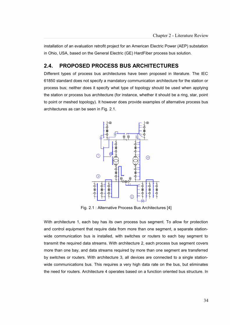
Chapter 2 - Literature Review
installation of an evaluation retrofit project for an American Electric Power (AEP) substation
in Ohio, USA, based on the General Electric (GE) HardFiber process bus solution.
2.4. PROPOSED PROCESS BUS ARCHITECTURESDifferent types of process bus architectures have been proposed in literature. The IEC
61850 standard does not specify a mandatory communication architecture for the station or
process bus; neither does it specify what type of topology should be used when applying
the station or process bus architecture (for instance, whether it should be a ring, star, point
to point or meshed topology). It however does provide examples of alternative process bus
architectures as can be seen in Fig. 2.1.
Fig. 2.1 : Alternative Process Bus Architectures [4]
With architecture 1, each bay has its own process bus segment. To allow for protection
and control equipment that require data from more than one segment, a separate station-
wide communication bus is installed, with switches or routers to each bay segment to
transmit the required data streams. With architecture 2, each process bus segment covers
more than one bay, and data streams required by more than one segment are transferred
by switches or routers. With architecture 3, all devices are connected to a single station-
wide communications bus. This requires a very high data rate on the bus, but eliminates
the need for routers. Architecture 4 operates based on a function oriented bus structure. In
34
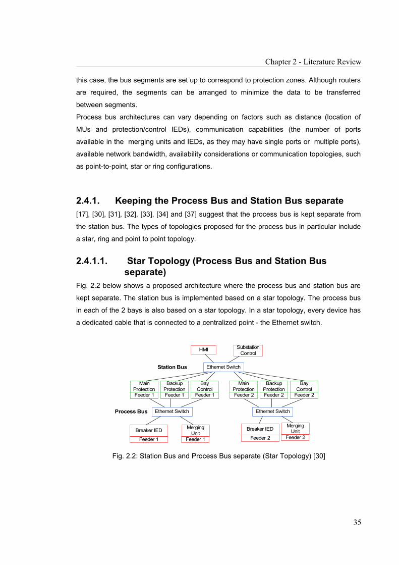
Chapter 2 - Literature Review
this case, the bus segments are set up to correspond to protection zones. Although routers
are required, the segments can be arranged to minimize the data to be transferred
between segments.
Process bus architectures can vary depending on factors such as distance (location of
MUs and protection/control IEDs), communication capabilities (the number of ports
available in the merging units and IEDs, as they may have single ports or multiple ports),
available network bandwidth, availability considerations or communication topologies, such
as point-to-point, star or ring configurations.
2.4.1. Keeping the Process Bus and Station Bus separate[17], [30], [31], [32], [33], [34] and [37] suggest that the process bus is kept separate from
the station bus. The types of topologies proposed for the process bus in particular include
a star, ring and point to point topology.
2.4.1.1. Star Topology (Process Bus and Station Bus separate)
Fig. 2.2 below shows a proposed architecture where the process bus and station bus are
kept separate. The station bus is implemented based on a star topology. The process bus
in each of the 2 bays is also based on a star topology. In a star topology, every device has
a dedicated cable that is connected to a centralized point - the Ethernet switch.
HMI
Main Protection
Ethernet Switch
Substation Control
Backup Protection
Bay Control
Main Protection
Backup Protection
Bay Control
Ethernet Switch
Feeder 2 Feeder 2 Feeder 2Feeder 1 Feeder 1 Feeder 1
Ethernet Switch
Merging Unit
Feeder 1
Breaker IED Merging Unit
Feeder 2 Feeder 2Breaker IED
Feeder 1
Station Bus
Process Bus
Fig. 2.2: Station Bus and Process Bus separate (Star Topology) [30]
35

Chapter 2 - Literature Review
A network based on a star topology is straightforward and easy to maintain. It is also easy
to carry out troubleshooting and fault isolation tasks within a star topology. A fault may be
detected by a switch that incorporates management software, and it will be possible to spot
errors at the port level. Take the example shown in Fig. 2.2. If the Feeder 1 merging unit
fails, the switch port that it is connected to on the Ethernet Switch will indicate that
connection to the device has been lost. A star topology based network is a flexible one. A
device may be added without necessarily requiring the entire substation to be shut down.
In terms of data transfer between the merging unit and the bay level IED(s) (also
connected to the switch) , the destination device is no more than two nodes away from the
sending device - for data to reach its intended device it just passes through the switch and
then reaches the destination device, it does not go to any other device.
2.4.1.2. Ring Topology (Process Bus and Station Bus separate)
Fig. 2.3 below shows an example of a process bus implemented based on a ring topology.
Each Ethernet Switch is connected to the next and the last one is connected back again to
the first to form a ring. There is a logical gap maintained between two switches to ensure
that the data does not flow continuously in a ring. If a single cable fault occurs, the logical
gap will be closed to ensure network continuity.
Fig. 2.3: Station Bus and Process Bus separate (Process Bus Ring Topology)
A ring topology can allow for a single cable or device failure. Ring networks are relatively
easy to troubleshoot. This is because a device will become aware that a connection has
36
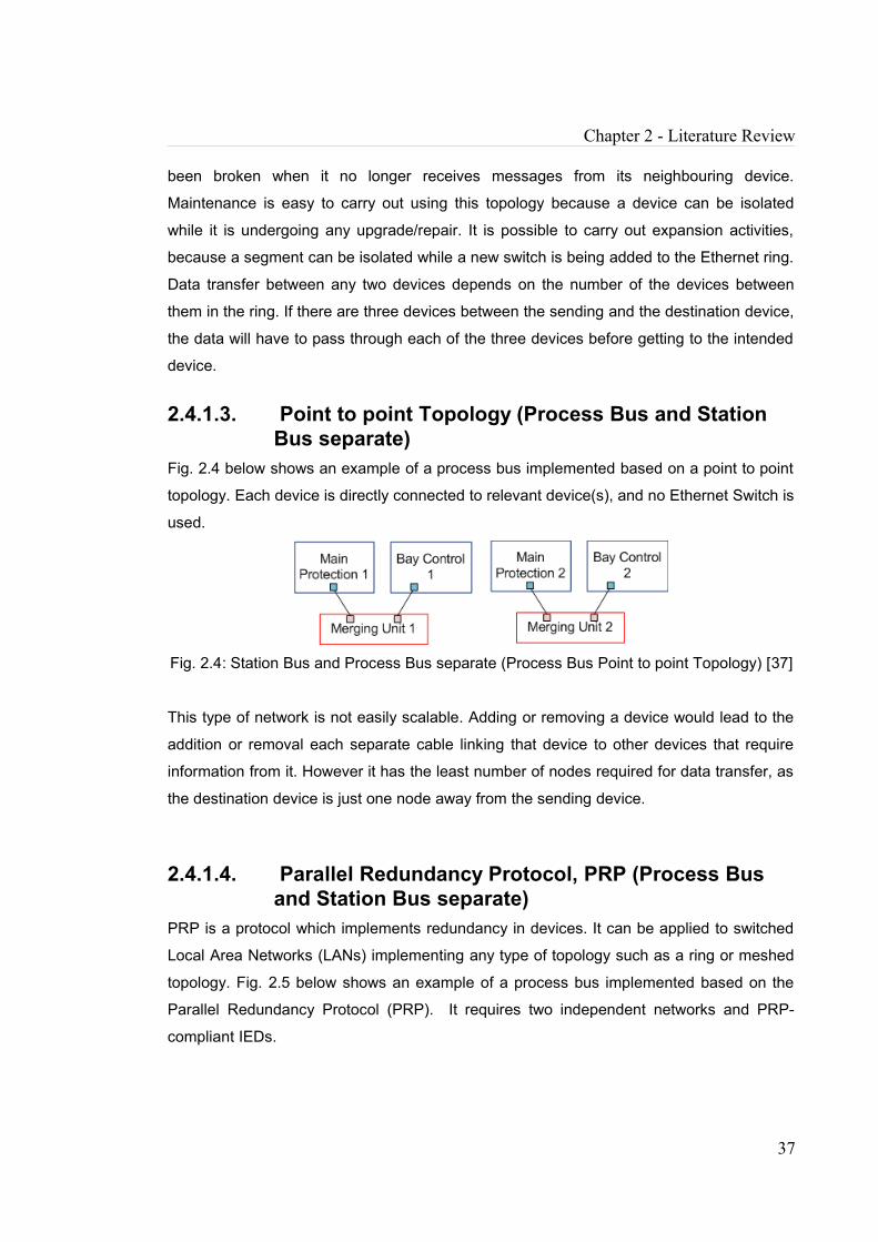
Chapter 2 - Literature Review
been broken when it no longer receives messages from its neighbouring device.
Maintenance is easy to carry out using this topology because a device can be isolated
while it is undergoing any upgrade/repair. It is possible to carry out expansion activities,
because a segment can be isolated while a new switch is being added to the Ethernet ring.
Data transfer between any two devices depends on the number of the devices between
them in the ring. If there are three devices between the sending and the destination device,
the data will have to pass through each of the three devices before getting to the intended
device.
2.4.1.3. Point to point Topology (Process Bus and Station Bus separate)
Fig. 2.4 below shows an example of a process bus implemented based on a point to point
topology. Each device is directly connected to relevant device(s), and no Ethernet Switch is
used.
Fig. 2.4: Station Bus and Process Bus separate (Process Bus Point to point Topology) [37]
This type of network is not easily scalable. Adding or removing a device would lead to the
addition or removal each separate cable linking that device to other devices that require
information from it. However it has the least number of nodes required for data transfer, as
the destination device is just one node away from the sending device.
2.4.1.4. Parallel Redundancy Protocol, PRP (Process Bus and Station Bus separate)
PRP is a protocol which implements redundancy in devices. It can be applied to switched
Local Area Networks (LANs) implementing any type of topology such as a ring or meshed
topology. Fig. 2.5 below shows an example of a process bus implemented based on the
Parallel Redundancy Protocol (PRP). It requires two independent networks and PRP-
compliant IEDs.
37

Chapter 2 - Literature Review
Fig. 2.5: Station Bus and Process Bus separate (PRP Process Bus) [37]
Merging Unit 1 multicasts sampled values frames to both networks. Relays 1 and 2 are
connected to both networks. Every time the Merging Unit sends a sampled value frame,
each Relay receives the same sampled value frame from both networks and discards one
of the frames. This type of connection ensures lossless transmission of critical data over
the network.
2.4.1.5. High-availability Seamless Redundancy (HSR) (Process Bus and Station Bus separate)
HSR is an application of PRP which allows for the approximate halving of the network
infrastructure or bandwidth depending on the initial protocol used (for instance if it was
PRP or RSTP (Rapid Spanning Tree Protocol) that was initially used). It is in particular
applicable to the topologies made up of rings, or rings of rings. Fig. 2.6 below shows an
example of a process bus implemented based on High-availability Seamless Redundancy
(HSR). Each device is connected to the next and the last one is connected back again to
the first to form a ring.
Fig. 2.6: Station Bus and Process Bus separate (HSR Process Bus) [37]
38

Chapter 2 - Literature Review
A sending device (for instance Merging Unit 1) sends sampled value frames over each of
its 2 ports. Every time the Merging Unit sends a sampled value frame, a destination device
(for instance Relay1) receives two identical frames from each its own 2 ports within a
certain interval and discards one of the frames. If Merging Unit 1 receives the frame that it
injected into the ring, it will not forward it. This type of connection also ensures lossless
transmission of critical data over the network.
2.4.2. Merging the Process Bus and Station BusMerging the station and process bus has been suggested in [16], [17], [30], [35], [36], [38],
and [39]. The types of topologies proposed for the merged station and process bus include
star and ring topologies.
2.4.2.1. Star Topology (Merging the Process Bus and Station Bus)
Fig. 2.7 shows an architecture similar to the one shown above in Fig. 2.2 where the station
bus is implemented based on a star topology, and the process bus in each of the 2 bays is
also based on a star topology. However, in this case [30], the station bus has been
connected to each of the bay process buses.
Fig. 2.7: Station Bus and Process Bus Merged (Star Topology) [30]
39
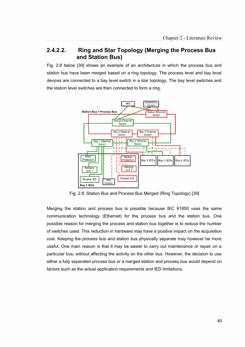
Chapter 2 - Literature Review
2.4.2.2. Ring and Star Topology (Merging the Process Bus and Station Bus)
Fig. 2.8 below [39] shows an example of an architecture in which the process bus and
station bus have been merged based on a ring topology. The process level and bay level
devices are connected to a bay level switch in a star topology. The bay level switches and
the station level switches are then connected to form a ring.
Fig. 2.8: Station Bus and Process Bus Merged (Ring Topology) [39]
Merging the station and process bus is possible because IEC 61850 uses the same
communication technology (Ethernet) for the process bus and the station bus. One
possible reason for merging the process and station bus together is to reduce the number
of switches used. This reduction in hardware may have a positive impact on the acquisition
cost. Keeping the process bus and station bus physically separate may however be more
useful. One main reason is that it may be easier to carry out maintenance or repair on a
particular bus, without affecting the activity on the other bus. However, the decision to use
either a fully separated process bus or a merged station and process bus would depend on
factors such as the actual application requirements and IED limitations.
40
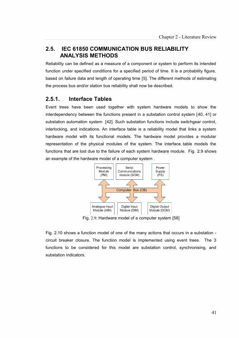
Chapter 2 - Literature Review
2.5. IEC 61850 COMMUNICATION BUS RELIABILITY ANALYSIS METHODS
Reliability can be defined as a measure of a component or system to perform its intended
function under specified conditions for a specified period of time. It is a probability figure,
based on failure data and length of operating time [5]. The different methods of estimating
the process bus and/or station bus reliability shall now be described.
2.5.1. Interface Tables Event trees have been used together with system hardware models to show the
interdependency between the functions present in a substation control system [40, 41] or
substation automation system [42]. Such substation functions include switchgear control,
interlocking, and indications. An interface table is a reliability model that links a system
hardware model with its functional models. The hardware model provides a modular
representation of the physical modules of the system. The interface table models the
functions that are lost due to the failure of each system hardware module. Fig. 2.9 shows
an example of the hardware model of a computer system .
Fig. 2.9: Hardware model of a computer system [58]
Fig. 2.10 shows a function model of one of the many actions that occurs in a substation -
circuit breaker closure. The function model is implemented using event trees. The 3
functions to be considered for this model are substation control, synchronising, and
substation indicators.
41
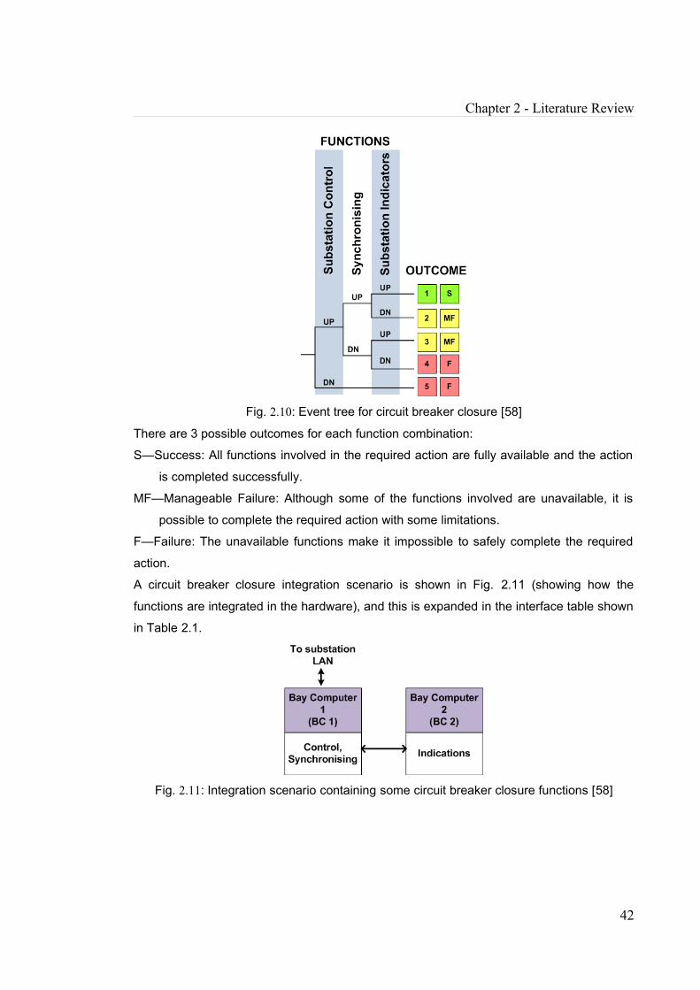
Chapter 2 - Literature Review
Fig. 2.10: Event tree for circuit breaker closure [58]
There are 3 possible outcomes for each function combination:
S—Success: All functions involved in the required action are fully available and the action
is completed successfully.
MF—Manageable Failure: Although some of the functions involved are unavailable, it is
possible to complete the required action with some limitations.
F—Failure: The unavailable functions make it impossible to safely complete the required
action.
A circuit breaker closure integration scenario is shown in Fig. 2.11 (showing how the
functions are integrated in the hardware), and this is expanded in the interface table shown
in Table 2.1.
Fig. 2.11: Integration scenario containing some circuit breaker closure functions [58]
42

Chapter 2 - Literature Review
Table 2.1: Interface table for Integration scenario of Fig. 2.11 [58]
In order to determine the system reliability based on this interface table:
1. The hardware modules are represented from a reliability point of view by their
availability.
2 All possible combinations of hardware module failures are considered. For each
hardware failure combination:
a) the probability of its occurrence is calculated
b) the resulting failed functions will be obtained from the interface table.
c) The event tree then shows the system outcome (S, MF, F) resulting from
the failed functions and the probability calculated in (a) is assigned to that
outcome.
3 The system reliability is the sum of the successful outcome probabilities obtained in
2c above.
2.5.2. The Markov state modelReference [17] proposes different architectures at the station level and at the process level
and some reliability analysis is carried out on these architectures, based on the Markov
43
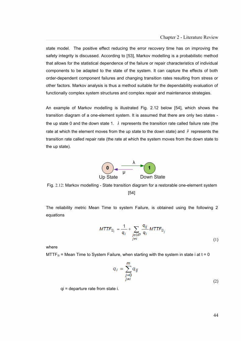
Chapter 2 - Literature Review
state model. The positive effect reducing the error recovery time has on improving the
safety integrity is discussed. According to [53], Markov modelling is a probabilistic method
that allows for the statistical dependence of the failure or repair characteristics of individual
components to be adapted to the state of the system. It can capture the effects of both
order-dependent component failures and changing transition rates resulting from stress or
other factors. Markov analysis is thus a method suitable for the dependability evaluation of
functionally complex system structures and complex repair and maintenance strategies.
An example of Markov modelling is illustrated Fig. 2.12 below [54], which shows the
transition diagram of a one-element system. It is assumed that there are only two states -
the up state 0 and the down state 1. λ represents the transition rate called failure rate (the
rate at which the element moves from the up state to the down state) and µ represents the
transition rate called repair rate (the rate at which the system moves from the down state to
the up state).
Fig. 2.12: Markov modelling - State transition diagram for a restorable one-element system
[54]
The reliability metric Mean Time to system Failure, is obtained using the following 2
equations
(1)
where
MTTFSi = Mean Time to System Failure, when starting with the system in state i at t = 0
(2)
qi = departure rate from state i.
44
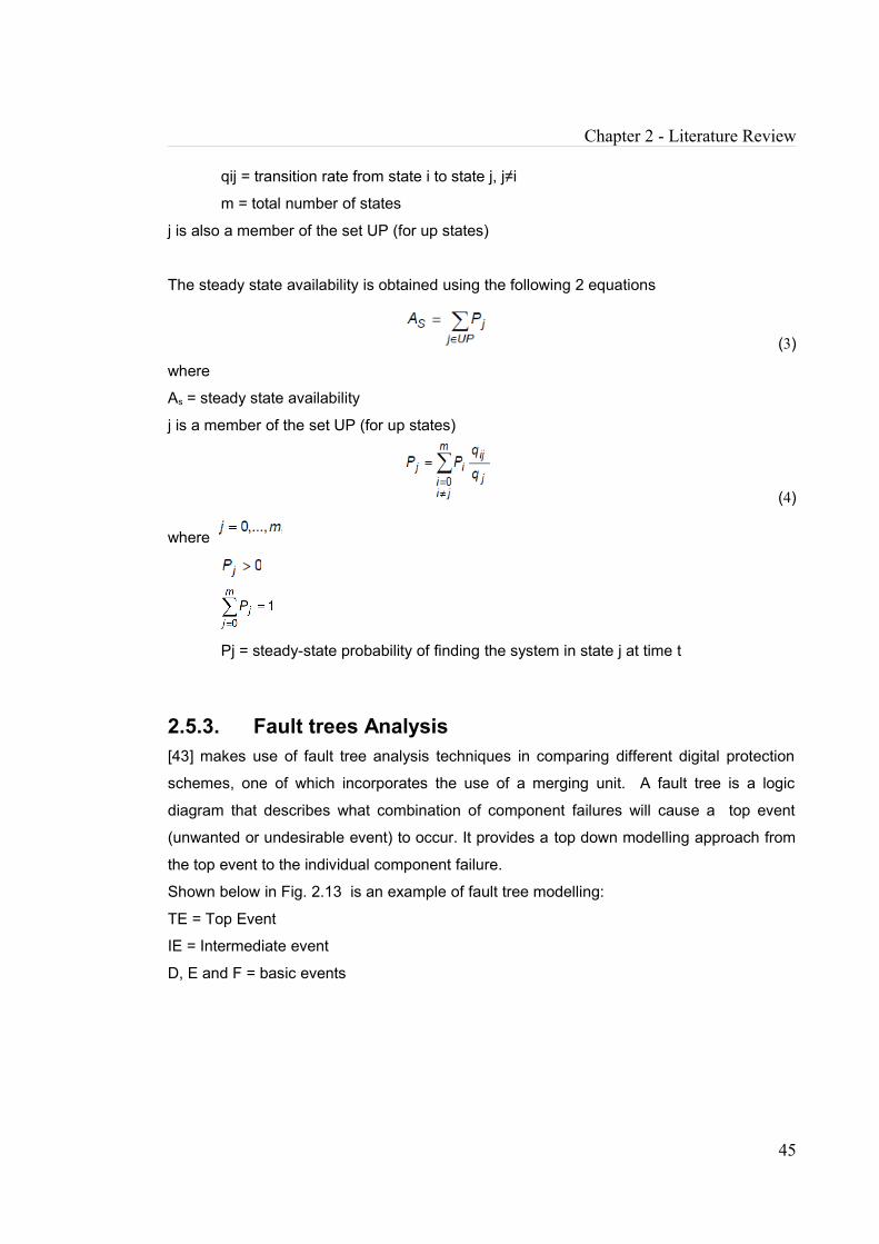
Chapter 2 - Literature Review
qij = transition rate from state i to state j, j≠i
m = total number of states
j is also a member of the set UP (for up states)
The steady state availability is obtained using the following 2 equations
(3)
where
As = steady state availability
j is a member of the set UP (for up states)
(4)
where
Pj = steady-state probability of finding the system in state j at time t
2.5.3. Fault trees Analysis[43] makes use of fault tree analysis techniques in comparing different digital protection
schemes, one of which incorporates the use of a merging unit. A fault tree is a logic
diagram that describes what combination of component failures will cause a top event
(unwanted or undesirable event) to occur. It provides a top down modelling approach from
the top event to the individual component failure.
Shown below in Fig. 2.13 is an example of fault tree modelling:
TE = Top Event
IE = Intermediate event
D, E and F = basic events
45
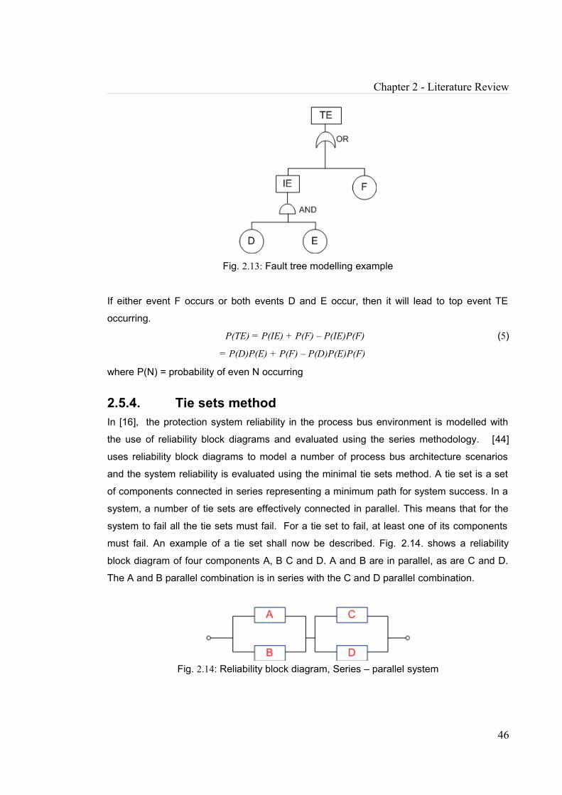
Chapter 2 - Literature Review
Fig. 2.13: Fault tree modelling example
If either event F occurs or both events D and E occur, then it will lead to top event TE
occurring.
P(TE) = P(IE) + P(F) – P(IE)P(F) (5)
= P(D)P(E) + P(F) – P(D)P(E)P(F) where P(N) = probability of even N occurring
2.5.4. Tie sets methodIn [16], the protection system reliability in the process bus environment is modelled with
the use of reliability block diagrams and evaluated using the series methodology. [44]
uses reliability block diagrams to model a number of process bus architecture scenarios
and the system reliability is evaluated using the minimal tie sets method. A tie set is a set
of components connected in series representing a minimum path for system success. In a
system, a number of tie sets are effectively connected in parallel. This means that for the
system to fail all the tie sets must fail. For a tie set to fail, at least one of its components
must fail. An example of a tie set shall now be described. Fig. 2.14. shows a reliability
block diagram of four components A, B C and D. A and B are in parallel, as are C and D.
The A and B parallel combination is in series with the C and D parallel combination.
Fig. 2.14: Reliability block diagram, Series – parallel system
46

Chapter 2 - Literature Review
It can be seen from the above Fig. 2.14 that for the system to fail either A and B must both
fail, or C and D must both fail. Hence there are two tie sets. In tie set 1, T1, A and B are
modelled in series since they both need to fail for system failure. Similarly, C and D are
modelled in series since they also need to both fail for the system to fail and are
represented in tie set T2. This is illustrated in Fig. 2.15 below.
Fig. 2.15: Tie sets for series-parallel system in Fig. 2.14
The system reliability, Rs is obtained using the following equation
Rs = P(T1 …..U Tn ) (6)
where Tn = nth tie set
P(Tn) = the probability of the occurrence of Tn
2.6. SUBSTATION LIFE CYCLE COST ANALYSIS Life Cycle Costing is a useful tool in determining the optimum configuration when faced
with a range of configurations to choose from. [45], [46] and [47], apply different models
for estimating the Life Cycle Costs in substations. However, the common costs that feature
among them are the investment cost, maintenance cost and failure cost. In [45], the life
cycle costs (LCCs) are determined for an overhead transmission grid with air insulated
substations. The genetic algorithm is applied in order to minimize the LCC of a substation.
The algorithm iteratively changes the components making up the substation layout, varying
both the technology and the type of redundancy used. In each iteration step the algorithm
calculates the LCC for the current substation layout and for the next iteration step the
algorithm improves the substation layout. Every component is defined with its LCC
parameters, and then put in a component specific file card. After a certain number of
iteration steps the algorithm provides the optimal composition of the substation layout.
In [46], life cycle costing is applied as part of distribution network planning. The studied
network is 110 kV fed by a 380 kV system via 380/110 kV transformers, and consists of air
insulated substations (AIS) and is assumed to be newly built. It was seen from a study of
accumulated non delivered energy for all loads that overhead lines were responsible for 39
47
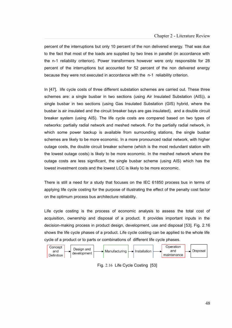
Chapter 2 - Literature Review
percent of the interruptions but only 10 percent of the non delivered energy. That was due
to the fact that most of the loads are supplied by two lines in parallel (in accordance with
the n-1 reliability criterion). Power transformers however were only responsible for 28
percent of the interruptions but accounted for 52 percent of the non delivered energy
because they were not executed in accordance with the n-1 reliability criterion.
In [47], life cycle costs of three different substation schemes are carried out. These three
schemes are: a single busbar in two sections (using Air Insulated Substation (AIS)), a
single busbar in two sections (using Gas Insulated Substation (GIS) hybrid, where the
busbar is air insulated and the circuit breaker bays are gas insulated), and a double circuit
breaker system (using AIS). The life cycle costs are compared based on two types of
networks: partially radial network and meshed network. For the partially radial network, in
which some power backup is available from surrounding stations, the single busbar
schemes are likely to be more economic. In a more pronounced radial network, with higher
outage costs, the double circuit breaker scheme (which is the most redundant station with
the lowest outage costs) is likely to be more economic. In the meshed network where the
outage costs are less significant, the single busbar scheme (using AIS) which has the
lowest investment costs and the lowest LCC is likely to be more economic.
There is still a need for a study that focuses on the IEC 61850 process bus in terms of
applying life cycle costing for the purpose of illustrating the effect of the penalty cost factor
on the optimum process bus architecture reliability.
Life cycle costing is the process of economic analysis to assess the total cost of
acquisition, ownership and disposal of a product. It provides important inputs in the
decision-making process in product design, development, use and disposal [53]. Fig. 2.16
shows the life cycle phases of a product. Life cycle costing can be applied to the whole life
cycle of a product or to parts or combinations of different life cycle phases.
Fig. 2.16 Life Cycle Costing [53]
48
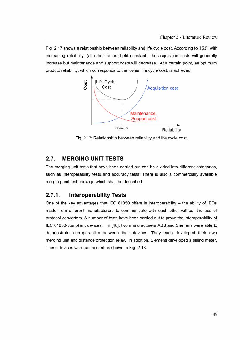
Chapter 2 - Literature Review
Fig. 2.17 shows a relationship between reliability and life cycle cost. According to [53], with
increasing reliability, (all other factors held constant), the acquisition costs will generally
increase but maintenance and support costs will decrease. At a certain point, an optimum
product reliability, which corresponds to the lowest life cycle cost, is achieved.
Fig. 2.17: Relationship between reliability and life cycle cost.
2.7. MERGING UNIT TESTSThe merging unit tests that have been carried out can be divided into different categories,
such as interoperability tests and accuracy tests. There is also a commercially available
merging unit test package which shall be described.
2.7.1. Interoperability TestsOne of the key advantages that IEC 61850 offers is interoperability – the ability of IEDs
made from different manufacturers to communicate with each other without the use of
protocol converters. A number of tests have been carried out to prove the interoperability of
IEC 61850-compliant devices. In [48], two manufacturers ABB and Siemens were able to
demonstrate interoperability between their devices. They each developed their own
merging unit and distance protection relay. In addition, Siemens developed a billing meter.
These devices were connected as shown in Fig. 2.18.
49

Chapter 2 - Literature Review
Fig. 2.18: Interoperability Test ABB and Siemens [48]
The current/voltage signals from an Omicron Test Set were fed to the merging units via
sensor simulators. The MUs then converted these signals to IEC 61850 9-1 messages
which were delivered to the protection devices and meter via an Ethernet Switch. The ABB
relay received the messages from the Siemens MU while the Siemens meter and relay
both received data from the ABB MU. The Omicron Test set simulated a single phase short
circuit which led to both the ABB and Siemens relays tripping. This communication was
however based on the IEC 61850 9-1 standard.
[49] describes interoperability evaluation tests performed on three different all digital
protection systems based on an IEC-61850-9-2 process bus. These protection systems
were assembled in the Texas A&M Protection and Control Lab. A compatibility index was
applied as a means of quantifying the level of interoperability. The tested protection
systems were seen to be compatible and interoperable.
2.7.2. Merging Unit Accuracy TestsSome work on merging unit accuracy testing has also been carried out. [51] proposes a
test bed that is able to test for the accuracy of up to 2 merging units simultaneously. Fig.
2.19 shows the MU accuracy test bed setup. A GPS receiver provides synchronization to
all required devices. A signal generator generates the test scenarios. Amplifiers produce
realistic voltage/current signals. Instrument transformers step down the realistic
50
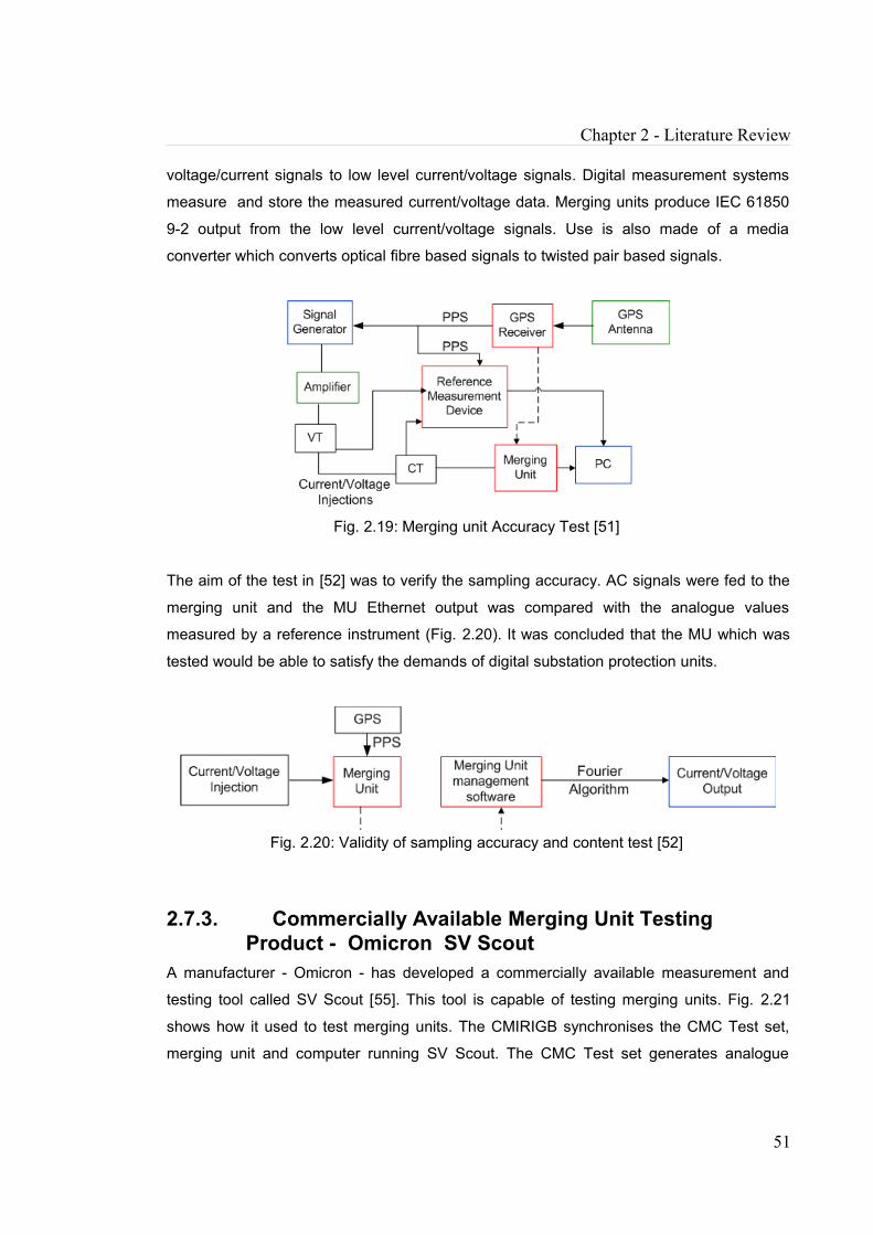
Chapter 2 - Literature Review
voltage/current signals to low level current/voltage signals. Digital measurement systems
measure and store the measured current/voltage data. Merging units produce IEC 61850
9-2 output from the low level current/voltage signals. Use is also made of a media
converter which converts optical fibre based signals to twisted pair based signals.
Fig. 2.19: Merging unit Accuracy Test [51]
The aim of the test in [52] was to verify the sampling accuracy. AC signals were fed to the
merging unit and the MU Ethernet output was compared with the analogue values
measured by a reference instrument (Fig. 2.20). It was concluded that the MU which was
tested would be able to satisfy the demands of digital substation protection units.
Fig. 2.20: Validity of sampling accuracy and content test [52]
2.7.3. Commercially Available Merging Unit Testing Product - Omicron SV Scout
A manufacturer - Omicron - has developed a commercially available measurement and
testing tool called SV Scout [55]. This tool is capable of testing merging units. Fig. 2.21
shows how it used to test merging units. The CMIRIGB synchronises the CMC Test set,
merging unit and computer running SV Scout. The CMC Test set generates analogue
51
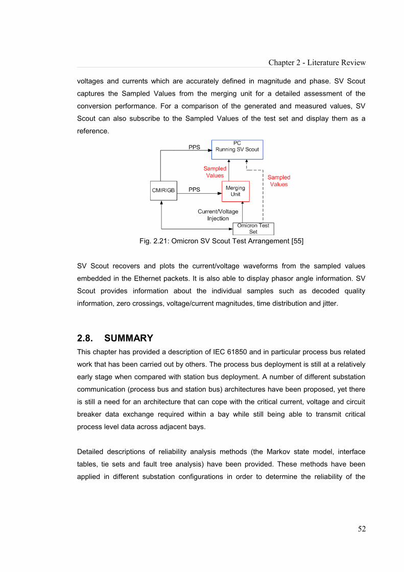
Chapter 2 - Literature Review
voltages and currents which are accurately defined in magnitude and phase. SV Scout
captures the Sampled Values from the merging unit for a detailed assessment of the
conversion performance. For a comparison of the generated and measured values, SV
Scout can also subscribe to the Sampled Values of the test set and display them as a
reference.
Fig. 2.21: Omicron SV Scout Test Arrangement [55]
SV Scout recovers and plots the current/voltage waveforms from the sampled values
embedded in the Ethernet packets. It is also able to display phasor angle information. SV
Scout provides information about the individual samples such as decoded quality
information, zero crossings, voltage/current magnitudes, time distribution and jitter.
2.8. SUMMARYThis chapter has provided a description of IEC 61850 and in particular process bus related
work that has been carried out by others. The process bus deployment is still at a relatively
early stage when compared with station bus deployment. A number of different substation
communication (process bus and station bus) architectures have been proposed, yet there
is still a need for an architecture that can cope with the critical current, voltage and circuit
breaker data exchange required within a bay while still being able to transmit critical
process level data across adjacent bays.
Detailed descriptions of reliability analysis methods (the Markov state model, interface
tables, tie sets and fault tree analysis) have been provided. These methods have been
applied in different substation configurations in order to determine the reliability of the
52

Chapter 2 - Literature Review
station bus, process bus or a combination of both. Out of the existing methodologies,
reliability block diagram modelling together with event trees (which are described in more
detail in Chapter 5) shall be used to evaluate the reliability for the process bus architecture
scenarios introduced in this thesis. Varying levels of redundancy shall be introduced until a
process bus architecture scenario where there is full topology duplication, and the reliability
of all the architecture scenarios will be compared.
There is also still a need to be able to compare process bus architecture scenarios with the
goal of determining an optimum one. Thus, the life cycle costs of different hypothetical
process bus architecture scenarios shall also be obtained for the architecture scenarios
introduced in this thesis. The architecture with the lowest life cycle cost shall be deemed
the optimal architecture.
There is a need to test merging units prior to when they are connected to a relay, a need
for a test system that can independently assess the performance characteristics of the
merging units, as this can help promote interoperability among relays and merging units
from different manufacturers. It would also be beneficial to be able to carry out additional
tests not currently being carried out on merging units. Such tests include the GPS
Timestamping delay test (which would determine the delay that occurs when the MU
timestamps the digitized signal) and Filter performance assessment (which would check
how much of the original signal the MU is able to recover at different frequencies). In this
thesis, the design and development of a merging unit test bed which can be used to carry
out these additional tests shall be discussed.
53

CHAPTER 3 FUNDAMENTALS
3.1. INTRODUCTION
This chapter presents a description of fundamental topics, most of which shall be
periodically referred to in subsequent chapters. The topics to be described are power
systems, smart grids, the IEC 61850 standard, the station bus and the process bus.
3.2. POWER SYSTEM A power system serves to generate and deliver electrical energy to consumers and it is
expected to do so in a reliable, safe and economic manner. Fig. 3.1 shows a high level
example depicting the UK power system.
Fig. 3.1: Power System
In the example depicted above, electrical energy is produced at 22kV by generators
located in a generating station (G). Step up transformers are then used to increase the
energy voltage level to 400kV for onward transmission via transmission lines. Busbars
connect different parts of the system together. For example large industrial consumers
(such as steel mills) can be served directly via the transmission busbars. In addition, the
54
Chapter 3 - Fundamentals
22kV/400kV step up transformer is connected to the 400kV transmission lines via the
transmission busbars. The 400kV part of the power system falls under national
transmission. When the voltage is stepped down to 132kV it then falls under regional
substransmission. The voltage is stepped down to 33kV and then the distribution system is
used to connect to large commercial customers (at 11kV) or domestic and commercial
customers (400V).
3.3. SMART GRIDA smart grid is an electricity network that can intelligently integrate the actions of all users
connected to it – generators, consumers and those that do both – in order to efficiently
deliver sustainable, economic and secure electricity supplies [50]. It is a power grid which
has incorporated connectivity and automation between the different parts making up the
grid. Implementation of smart grids include the transmission and distribution grids that
undergo modernization such as increased use of variable energy resources (for example
renewable energy sources) as well as automation are monitoring capabilities for
continental bulk transmission. Advanced sensors and distributed computing technology are
expected to improve the efficiency, reliability and safety of power delivery and use, while
new or improved services can be implemented such as fire monitoring and alarms which
can automatically shut off power and constant emergency services. Analogue meters are
replaced with digital 'smart' meters which can record power usage in real time.
3.4. SUBSTATIONA substation is a node in the power system. Substations play many roles in the ultimate
delivery of power to end users [66]. The roles could include switching generators,
equipment, and AC voltages form one level to another, and/or changing AC to DC or DC to
AC. Substations vary in size, construction, cost and complexity according to voltage,
location and function. Two types of substations, the transmission substation and
distribution substation are highlighted in Fig. 3.2 below.
55

Chapter 3 - Fundamentals
Fig. 3.2: Substations within a power system
Some substations may be small, with little more than a transformer and associated
switches. Other substations may be large, with several transformers and dozens of
switches and other equipment. Although not all substations are designed to function
exactly alike, most substations perform the following functions:
• Change the voltage from one level to another
• Regulate voltage to compensate for system voltage changes
• Switch transmission and distribution circuits into and out of the grid system
• Measure electric power qualities flowing in the circuits
• Connect communication signals to the circuits
• Eliminate lightning and other electrical surges from the system
• Connect electric generation plants to the system
• Make interconnections between the electric systems of more than one utility
• Control reactive kilovolt-amperes supplied and the flow of reactive kilovolt-amperes
in the circuits
The functions above broadly fall within 2 main substation functions, protection and control.
Protection is required to identify and remove from the power system any item of plant that
suffers a fault. This ensures that a fault does not adversely affect the secure and economic
operation of the power system. Protection is typically implemented using relays. Protection
56
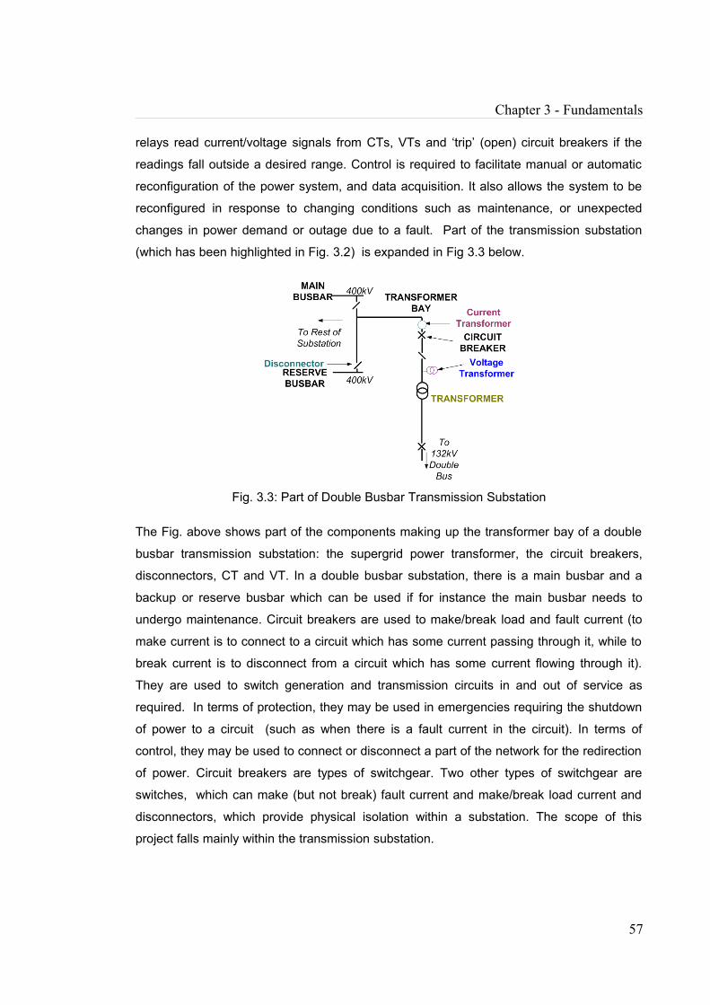
Chapter 3 - Fundamentals
relays read current/voltage signals from CTs, VTs and ‘trip’ (open) circuit breakers if the
readings fall outside a desired range. Control is required to facilitate manual or automatic
reconfiguration of the power system, and data acquisition. It also allows the system to be
reconfigured in response to changing conditions such as maintenance, or unexpected
changes in power demand or outage due to a fault. Part of the transmission substation
(which has been highlighted in Fig. 3.2) is expanded in Fig 3.3 below.
Fig. 3.3: Part of Double Busbar Transmission Substation
The Fig. above shows part of the components making up the transformer bay of a double
busbar transmission substation: the supergrid power transformer, the circuit breakers,
disconnectors, CT and VT. In a double busbar substation, there is a main busbar and a
backup or reserve busbar which can be used if for instance the main busbar needs to
undergo maintenance. Circuit breakers are used to make/break load and fault current (to
make current is to connect to a circuit which has some current passing through it, while to
break current is to disconnect from a circuit which has some current flowing through it).
They are used to switch generation and transmission circuits in and out of service as
required. In terms of protection, they may be used in emergencies requiring the shutdown
of power to a circuit (such as when there is a fault current in the circuit). In terms of
control, they may be used to connect or disconnect a part of the network for the redirection
of power. Circuit breakers are types of switchgear. Two other types of switchgear are
switches, which can make (but not break) fault current and make/break load current and
disconnectors, which provide physical isolation within a substation. The scope of this
project falls mainly within the transmission substation.
57

Chapter 3 - Fundamentals
3.5. IEC 61850 IEC 6I850 is a set of standards developed with the main goal of providing interoperability
between all devices in substations. Interoperability means that devices from different
manufacturers are able to effectively communicate with one another, without the need for
complex and costly protocol converters. IEC 61850 is designed to support any allocation of
functions to substation automation system devices. The flexibility in the allocation of
functions is necessary to cater for different user requirements and advances in
communication technology. The Electric Power Research Institute (EPRI) began work on a
Utility Communication Architecture (UCA) Version 1 in the early 1990s. The UCA was
developed in order to produce a consensus in the industry about device interoperability.
This work was developed further to UCA Version 2 which showed that interoperability was
indeed achievable. The UCA2 was developed further by International Electrotechnical
Commission Technical Committee (IEC TC) 57, and as a result IEC 61850 was produced.
Fig. 3.4 provides an example of how IEC 6150 is used to model substation equipment.
Fig. 3.4: IEC 61850 modelling [4]
58
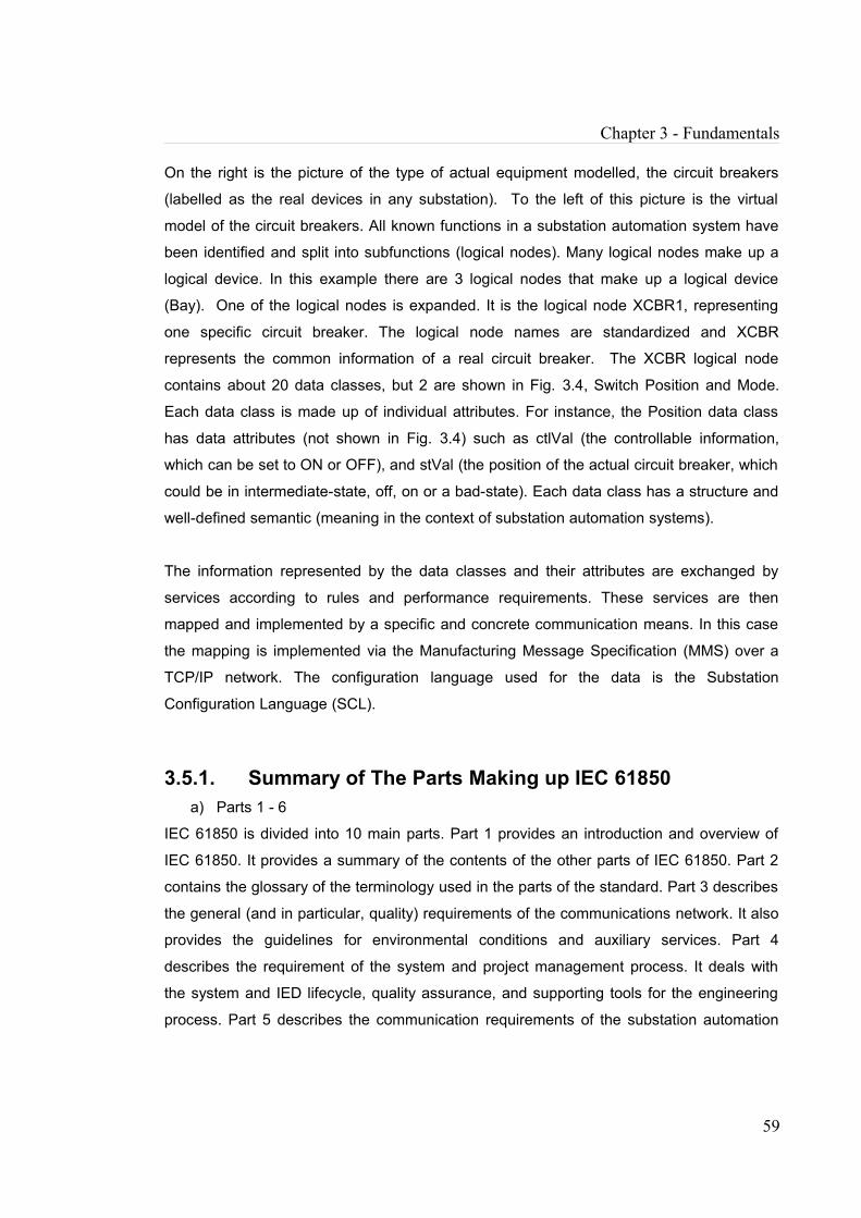
Chapter 3 - Fundamentals
On the right is the picture of the type of actual equipment modelled, the circuit breakers
(labelled as the real devices in any substation). To the left of this picture is the virtual
model of the circuit breakers. All known functions in a substation automation system have
been identified and split into subfunctions (logical nodes). Many logical nodes make up a
logical device. In this example there are 3 logical nodes that make up a logical device
(Bay). One of the logical nodes is expanded. It is the logical node XCBR1, representing
one specific circuit breaker. The logical node names are standardized and XCBR
represents the common information of a real circuit breaker. The XCBR logical node
contains about 20 data classes, but 2 are shown in Fig. 3.4, Switch Position and Mode.
Each data class is made up of individual attributes. For instance, the Position data class
has data attributes (not shown in Fig. 3.4) such as ctlVal (the controllable information,
which can be set to ON or OFF), and stVal (the position of the actual circuit breaker, which
could be in intermediate-state, off, on or a bad-state). Each data class has a structure and
well-defined semantic (meaning in the context of substation automation systems).
The information represented by the data classes and their attributes are exchanged by
services according to rules and performance requirements. These services are then
mapped and implemented by a specific and concrete communication means. In this case
the mapping is implemented via the Manufacturing Message Specification (MMS) over a
TCP/IP network. The configuration language used for the data is the Substation
Configuration Language (SCL).
3.5.1. Summary of The Parts Making up IEC 61850a) Parts 1 - 6
IEC 61850 is divided into 10 main parts. Part 1 provides an introduction and overview of
IEC 61850. It provides a summary of the contents of the other parts of IEC 61850. Part 2
contains the glossary of the terminology used in the parts of the standard. Part 3 describes
the general (and in particular, quality) requirements of the communications network. It also
provides the guidelines for environmental conditions and auxiliary services. Part 4
describes the requirement of the system and project management process. It deals with
the system and IED lifecycle, quality assurance, and supporting tools for the engineering
process. Part 5 describes the communication requirements of the substation automation
59
Chapter 3 - Fundamentals
system functions. The emphasis is on identifying the communication requirements
between technical services and the substation. Part 6 specifies a Substation Configuration
Language (SCL), which is to be used for the configuration of IEDs.
b) Parts 7 - 8
Part 7 is itself made up of 4 parts. Part 7-1 provides an introduction of modelling methods,
communication principles, and information models. Part 7-2 describes the services used
for the exchange of information for different kinds of functions. It describes the Abstract
Communication Service Interface (ACSI), a virtual interface which provides abstract
information modelling methods. This interface is independent of the actual underlying
protocol stacks used. Part 7-3 deals with the abstract definitions of Common Data Classes
(CDCs) related to substation applications. It provides a list of commonly used information.
Part 7-4 makes use of the CDCs defined in part 7-3 to specify compatible data classes for
communication between IEDs. It defines specific information models for substation
automation functions.
Part 8-1 describes the Specific Communication Service Mapping (SCSM) of the ACSI
defined in IEC 61850-7-2 to Manufacturing Message Specification (MMS) and ISO/IEC
8802-3 (Ethernet) frames. It specifies a method of exchanging time-critical and non-time-
critical data through local area networks by mapping the ACSI to MMS and Ethernet
frames.
c) Parts 9- 10
Part 9 is further divided into 2 parts. Part 9-1 introduces the connection of current and
voltage transformers with a merging unit. Part 9-2 defines the Specific Communication
Service Mapping (SCSM) for the transmission of Sampled Values over Ethernet. It is an
extended mapping specification of IEC 61850-9-1 and IEC 61850-8-1 to cover sampled
value transmission over ISO/IEC 8802-3.
Part 10 defines the methods and abstract test cases for conformance testing of devices
used in substation automation systems, and the metrics to be measured within devices
according to the requirements defined in Part 5.
60

Chapter 3 - Fundamentals
3.5.2. IEC 61850 “Light Edition” (LE)A document called “Implementation Guideline for Digital Interface to Instrument
Transformers Using IEC 61850-9-2” (popularly referred to as IEC 61850 9-2 “Light Edition”
(LE) [16]) was prepared in order to support a fast market introduction and implementation
of IEC 61850 9-2. IEC 61850 does not specify logical devices, but allows for logical
devices to be described using the Substation Configuration Language (SCL). In order to
reduce the first implementations to a minimum of required services without losing
interoperability, IEC 61850 9-2 LE defines a merging unit logical device which includes a
dataset used for the transmission of sampled values. It specifies operation modes: “ON”
(when the merging unit is in normal operation mode and transmits the Ethernet packets),
“TEST” (where the merging unit transmits the Ethernet packets, but these packets are
flagged with a test indicator bit), and “OFF” (when the merging unit does not transmit any
Ethernet packet). IEC 61850 9-2 LE also provides recommendations for synchronisation
accuracy, and how the merging unit should behave when it is synchronised or if it has lost
its synchronisation signal.
3.5.3. IEC 61850 Edition 2Many parts of IEC 61850 (parts 4, 6, 7-1 to 7-4, 8-1 and 9-2) have been revised. The
revisions [20] include new concepts, models, functional extensions, clarifications,
corrections and enlarging the scope from substation automation systems to all utility
automation systems. The name of the IEC 61850 series has also been changed. It had
previously been “Communication networks and systems in substations”. The new name of
the series is “Communication networks and systems for power utility automation”, since the
scope of IEC 61850 is no longer limited to substations. IEC 61850 has been updated so
that it is also applicable to other areas such as wind turbines and hydro power plants and
distributed energy resources. The new series includes 4 new parts: parts 7-410, 7-420, 80-
1 and 90-1.
Part 7-410 specifies additional common data classes, logical nodes and data objects
required for the use of IEC 61850 in a hydro power plant.
61

Chapter 3 - Fundamentals
Part 7-420 defines IEC 61850 information models to be used in the exchange of
information with distributed energy resources (DER), which comprise dispersed generation
devices and dispersed storage devices, including reciprocating engines, fuel cells,
microturbines, photovoltaics, combined heat and power, and energy storage.
Part 80-1 is a technical specification which provides a guideline on how to exchange
information from a Common Data Class based data model using IEC 60870-5-101 or IEC
60870-5-104 between substation(s) and control centre(s).
Part 90-1 is a technical report which provides a comprehensive overview on the different
aspects that need to be considered while using IEC 61850 for information exchange
between substations.
3.6. BENEFITS OF IEC 61850IEC 61850 offers several benefits, some of which are described below:
• Devices are able to communicate with one another without the need for costly
protocol converters, hence reducing the cost of procuring such converters. In
addition, utilities are not restricted to using devices from only one manufacturer.
• Previously, for an IED to have been able to communicate with two other IEDs, a
dedicated connection between that IED and each of the other IEDs would have
been required. With IEC 61850, IEDs can be connected to different IEDs via a
single connection to a Local Area Network (LAN). It reduces the complexity of such
connections as well as installation costs associated with wiring, trenching and
ducting.
• A current or voltage transducer (via a merging unit and process bus) can
communicate with more IEDs than before, leading to reduced transducer costs. [1]
• Since naming conventions are standardized, it will be easier to migrate to new
equipment. Also, IEC 61850 makes it possible for new applications to be
developed and implemented since all the main data required for such application is
readily available and this data is presented in a standard form
62
Chapter 3 - Fundamentals
• IEC 61850 is flexible enough to allow for easy expansion, so if the network grows
and requires more IEDs, this will have little impact on the existing devices. Faulty
devices can be replaced without little or no interruption to the overall operation of
the substation. This leads to a reduction of maintenance and expansion costs.
3.7. IEC 61850 STATION BUS
The station bus is used for the complete information exchange between the station and
bay levels in a substation. At the station level, the following devices may be located – a
gateway (such as a router) which enables remote access/control, and the Station
Computer which provides the Human Machine Interface (HMI) functionality. The HMI is a
graphic screen showing alarms and switch positions, and which logs historical data that
can be used for future analysis. At the bay level, the following devices may be located - a
bay controller IED (for forwarding information and control commands between the station
and bay level), and main and backup protection devices (for sending trip commands to
open the required circuit breaker).
3.8. IEC 61850 PROCESS BUS
The process bus is used for the complete information exchange between the process and
bay levels. As mentioned above, the following devices may be located at the bay level - a
bay controller IED (for forwarding information and control commands between the station
and bay level), main and backup protection devices (for sending trip commands to open
the required circuit breaker). At the process level, the following devices may be located -
the Current Transformer (CT), Voltage Transformer (VT), merging unit (MU), Breaker IED,
and circuit breaker (CB). The MU samples the analogue signals from the CT and VT and
sends these sampled signals in a standardized format via the process bus to the protection
and control IED(s). When needed, the Protection or Control IED(s) send(s) trip commands
via the process bus to the Breaker IED which then trips the circuit breaker. The
connections between the CT, VT and the MU are proprietary; they are specific to the MU
manufacturer. Similarly, the connections between the Breaker IED and the circuit breaker
are proprietary.
A common time reference, such as a GPS, is required in order to ensure that the sampling
carried out by every merging unit located throughout the substation is synchronised. This
63

Chapter 3 - Fundamentals
will ensure that protection and control devices will have accurately timestamped
information about the voltage and current in different parts of the substation, important
when the protection and control device algorithms that are fed these current/voltage
sampled values need to determine whether or not the measured magnitude and/or phase
values are outside prescribed limits. According to [22], interpolation can also be used to
predict what the value of a sample would be at a particular time based on known time
delays.
The maturity of the process bus is not considered to be at the same level as the station
bus. A possible reason for this is that the process bus requires time critical digitized data,
whereas the station bus can cope with a delayed response time.
3.9. COMPARISON OF IEC 61850 WITH LEGACY PROTOCOLS
IEC 61850 is often referred to as a more advanced communication protocol However it
tends to be more than just a protocol in the traditional sense. IEC 61850 defines an
interface (Application Communication Service Interface - ASCI) which is independent of
the communication protocols. The ACSI services and objects can then be mapped onto a
particular protocol stack. IEC 61850 references existing protocols (such as MMS, TCP, IP
and Ethernet).
The table below shows a comparison of IEC 61850 with 2 major protocols IEC 61870-5
and DNP:
Table 3.1:Comparison of IEC 61850 with 2 major protocols: IEC 60870-5 and DNP [21]
IEC 61850 IEC 60870-5 DNPSCADA Applications:Standardized file transfer of data including quality information and timestamp data
Supported Supported
The process bussignificantly reduces wiring and EMC by connecting Circuit Breakers and
Relies on analog data which is not digitized close to source with more EMC requirements.
Relies on analog data which is not digitized close to source with more EMC
64
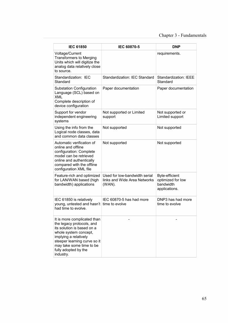
Chapter 3 - Fundamentals
IEC 61850 IEC 60870-5 DNPVoltage/Current Transformers to Merging Units which will digitize the analog data relatively close to source.
requirements.
Standardization: IEC Standard
Standardization: IEC Standard Standardization: IEEE Standard
Substation Configuration Language (SCL) based on XMLComplete description of device configuration
Paper documentation Paper documentation
Support for vendor independent engineering systems
Not supported or Limited support
Not supported or Limited support
Using the info from the Logical node classes, data and common data classes
Not supported Not supported
Automatic verification of online and offline configuration: Complete model can be retrieved online and authentically compared with the offline configuration XML file
Not supported Not supported
Feature-rich and optimized for LAN/WAN based (high bandwidth) applications
Used for low-bandwidth serial links and Wide Area Networks (WAN).
Byte-efficient optimized for low bandwidth applications.
IEC 61850 is relatively young, untested and hasn’t had time to evolve.
IEC 60870-5 has had more time to evolve
DNP3 has had more time to evolve
It is more complicated than the legacy protocols, and its solution is based on a whole system concept, implying a relatively steeper learning curve so it may take some time to be fully adopted by the industry.
- -
65

Chapter 3 - Fundamentals
3.10. SUMMARYIn this chapter an overview of power systems, substations, smart grids, the IEC 61850
standard, the station bus and the process bus has been provided. The crucial nature of
power grid cannot be overemphasized. Whether it is to a small or large extent, the model
of the power grid will change and the many benefits of IEC61850 over other previous
substation communication implementations (using solutions such as DNP3 for instance)
along with its 'future proof' nature should make it suitable for use at the substation and
even beyond, where there opportunities for the standard to be used in wind turbine, hydro
power, and distributed energy resource applications.
IEC 61850 is increasingly being adopted in substations at the region connecting the
secondary equipment (such the Human Machine Interface and IEDs) for critical monitoring
and control purposes, but is yet to be as extensively adopted at the extremely critical
region where the primary equipment is directly connected to the secondary equipment
using complex analogue copper cable connections. The proposed replacement of most of
these existing analogue cable connections with a fibre optic network based on IEC 61850
shall be described in the following chapter. This project mainly focuses on the connections
between the Current Transformers, Voltage Transformers, disconnectors, Circuit breakers
and the Protection and Control Intelligent Electronic Devices in a transmission substation.
66

CHAPTER 4 PROPOSED PROCESS BUS ARCHITECTURE DESIGN
4.1. INTRODUCTIONIn this chapter, a proposed IEC 61850 process bus architecture and its applications to both
the double busbar and mesh corner substation are described. The proposed architecture
was largely based on a set of golden rules for substation protection and control systems,
which any potential process bus architecture is expected to comply with.
4.2. GOLDEN RULES AND ADDITIONAL CRITERIAThe aims of designing the National Grid Architecture of Substation Secondary System
(AS3) Architectures are to:
1. Allow for the replacement of faulty IED(s) with minimum outage requirements
2. Allow for secondary bay refurbishment with minimum outage requirement
3. Simplify isolation procedures between primary and secondary systems
4. Reduce risk of maloperation
In response to this, a process bus architecture which can be applied to different types of
substations such as the double busbar and mesh corner shall be proposed. A set of
golden rules for substation protection and control systems were taken into consideration
during the design of this architecture. These golden rules were agreed on by National Gird
experts from the fields of protection, control, equipment commissioning/decommissioning,
and also by relay manufacturers including Alstom and Siemens. Although the architecture
is for National Grid, it is generic and should be readily adaptable to Scottish Power and
SSE requirements). These golden rules are:
1. All trip signals shall be received by the breakers within 10ms excluding inter-trip
send.
2. No single activity on the main 1 system shall affect the main 2 system.
3. No single failure shall result in the loss of control of more than one bay.
4. Physical facilities shall be available to isolate a bay for testing (Protection &
Control).
5. The Protection and Control application/philosophy shall be functionally identical to
the current solution.
67

Chapter 4 - Proposed Process Bus Architecture Design
6. Design of AS3 scheme standard for all bays – DBB feeder, DBB Bus Section, DBB
Bus Coupler, MC Mesh Corner, MC Transformer and MC Feeder.
7. The switching box should be located as close as possible to the primary
equipment.
The AS3 project was divided into different streams each with different objectives. One of
the objectives of AS3 Stream 1 was to develop simple, long life, reliable and standard
interfaces between the primary equipment and the secondary equipment. The standard
interfaces in substation secondary systems may be divided into critical (Station Bus and
Control bus) and extremely critical (Process Bus and GOOSE Messages). In view of this,
the following IEC 61850 architecture design rules were suggested (Fig. 4.1):
8. These interfaces connecting the station level to the bay level, (as well as the bay
level to the process level) of the substation should be vendor independent
solutions. For example, standard Ethernet switches or hubs shall be used to
configure the standard interface without the need for any special software.
IED: Intelligent Electronic Device MU: merging unit CBC: circuit breaker Controller SB: Switch Box
Fig. 4.1: Standard interface applied to a substation
9. Due to critical and extremely critical requirements, as well as security
implementation issues, the separation between the station/control buses and
process buses is necessary.
68

Chapter 4 - Proposed Process Bus Architecture Design
4.3. SYSTEM DESCRIPTION
4.3.1. Basic Architecture Concept
4.3.1.1. Data Flow (One Bay, Two Bays)Based on the above golden rules (1-7) and standard interface design rules (8-9), Fig. 4.2
shows the proposed generic architecture applied to a generic substation bay where the
• Station Bus is mainly used for the configuration, monitoring and control of the
substation secondary system equipment.
• Control Bus is mainly used for high accuracy measurement equipment, such as
metering equipment and high resolution voltage sample values across bays for
busbar protection and the
• Duplicate Interbay Process Buses are mainly used for protection equipment IEDs.
Fig. 4.2: Proposed Generic Process Bus Architecture applied to a generic substation bay
69

Chapter 4 - Proposed Process Bus Architecture Design
Each CT and VT is connected to a merging unit (MU) while each circuit breaker (CB) is
connected to a circuit breaker Controller (CBC). The CBCs and MUs are connected to the
bay process buses (PB1 and PB2). Between each CT/VT and MU (and between each CB
and CBC) is a Switch Box (SB), which is used for isolation purposes. The protection
devices (Main Protection - MP1, MP2 and Backup protection BP) are connected to the
process bus and the station bus. The dashed arrows show the bay level IED process bus
connections which are not dedicated. The Bay Control Unit (BCU) and Metering (M)
devices are connected to the control bus and station bus, while the Phasor Measurement
Unit (PMU) is connected to the Wide Area Network (WAN), as well as the control bus. The
interfaces connecting the station level to the bay level, (as well as the bay level to the
process level) are expected to be fixed, while the deployment of the bay level IEDs,
merging units and the CBC can depend on the manufacturer.
Fig. 4.3 shows the concept applied to 2 basic bays (with 1 bay highlighted), with only 1 bay
process bus (PB) in each bay. The PBs in the different bays are connected to each other
with an optional interbay process bus link. The process bus link is used within an Interbay
Process Bus to connect or isolate bays wherever necessary .
Fig. 4.3: Proposed Generic Process Bus Architecture applied across 2 generic bays (Data Flow)
70

Chapter 4 - Proposed Process Bus Architecture Design
4.3.1.2. Interbay Process Bus Link The interbay process bus link can be implemented by using a filter switch mechanism. This
filter switch mechanism is further illustrated in Fig. 4.4 below:
PB1PB1Process Bus Link
a - Series Connection
Process Bus Link
PB1PB1
b - Shunt Connection
Fig. 4.4: Filter Switch Mechanism
In Fig. 4.4a, the filter switches are connected in a series manner. The filter switch located
at the end of a bay process bus is connected to the filter switch at the beginning of the next
bay process bus. 8-1 GOOSE messaging traffic is allowed to pass through to
neighbouring bay process buses. In Fig. 4.4b, the filter switch is connected to the interbay
process bus in a shunt manner.
4.3.2. High Level Application of Generic Architecture
4.3.2.1. Generic Architecture Diagram Fig. 4.5 shows the proposed generic architecture applied to “n” number of bays.
71
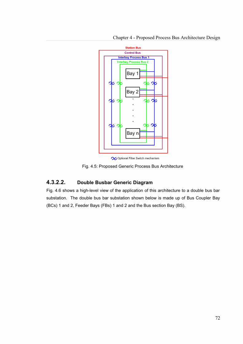
Chapter 4 - Proposed Process Bus Architecture Design
Fig. 4.5: Proposed Generic Process Bus Architecture
4.3.2.2. Double Busbar Generic DiagramFig. 4.6 shows a high-level view of the application of this architecture to a double bus bar
substation. The double bus bar substation shown below is made up of Bus Coupler Bay
(BCs) 1 and 2, Feeder Bays (FBs) 1 and 2 and the Bus section Bay (BS).
72

Chapter 4 - Proposed Process Bus Architecture Design
Fig. 4.6: High-level view of Double Bus Bar Substation Process Bus Architecture
It can be seen that the bays are decoupled - the protection scheme for each bay operates
independently. The protection devices in one bay do not require voltage/current information
from another bay, neither do they need to be able to trip circuit breakers located in other
bays. The filter switches are therefore not used to link bays together.
4.3.2.3. Mesh Substation Generic DiagramFig. 4.7 shows a high-level view of the application of this architecture to a mesh substation.
The mesh substation consists of four independent mesh corners. Each mesh corner has
three or more bays (such as mesh corner bay, transformer bay and feeder bay).
73

Chapter 4 - Proposed Process Bus Architecture Design
Fig. 4.7: High-level view of Mesh Substation Process Bus Architecture
Within each mesh corner the protection devices in one bay may need to be able to trip
circuit breakers located in other bays. The bays are thus linked by the filter switches. If any
refurbishment in a single bay is required, the other bays making up the mesh corner will
still be able to communicate with one another.
4.4. DETAILED PROCESS BUS APPLICATIONSAs mentioned in Section 4.1., CTs and VTs are connected to merging units (MUs), while
circuit breakers are connected to circuit breaker Controllers (CBCs). These connections to
MUs and CBCs are all made via Switch Boxes. The detailed applications below also
include disconnectors which are also connected to CBCs. Most of the CTs are connected
to a merging unit each, while there are some CTs that are connected to 2 merging units.
Most of the VTs are connected to 3 merging units each, and these merging units are
usually also connected to CTs. Each merging unit is then connected to either PB1, PB2 or
the Control Bus. Each circuit breaker is connected to 4 CBCs. 2 CBCs are connected to
PB1 and PB2 and the other 2 are connected to the Control Bus. Each disconnector is
74

Chapter 4 - Proposed Process Bus Architecture Design
connected to 2 CBCs. Each of these CBCs is then connected to either PB1 or the Control
Bus. In the different bays, MP1 is connected to PB1, while BP is connected to PB2. In the
case of the feeder bay, which has 3 projection IEDs (MP1, MP2 and BP), MP1 and BP are
connected to PB1, while MP2 is connected to PB2. The dashed arrows show the bay level
IED process bus connections which are not dedicated.
4.4.1. Double Busbar Applications
4.4.1.1. Double Bus Bar Arrangement A typical double bus bar substation with single breaker bus tie arrangement is shown in
Fig. 4.8 below. According to the high-level view of double busbar substation process bus
architecture in Fig. 7.6, no filter switches are required between neighbouring bays. This is
because the protection schemes for the bus coupler bay, bus section bay, feeder bay and
transformer bay are independent of one another.
Fig. 4.8: Double Bus Single Breaker with Bus Tie Arrangement
4.4.1.2. Detailed Double Bus Bar Application Figs. 4.9 - 4.11 [65] show the Feeder Bay, Bus Section, Bus Coupler Bay and Transformer
Bay of a National Grid 400kV substation prior to the introduction of the process bus. The
Figs. show the original copper connections between the current transformers, voltage
transformers and their corresponding protection and control devices.
75
Bus section
Reserve bar disconnector
Bus coupler
Feeder
Tranformer
Source
Bus coupler

Chapter 4 - Proposed Process Bus Architecture Design
Fig. 4.9: Feeder Bay for 400 kV Double Busbar Substation with Non-Unit Feeder
Protections [65]
It can be seen in Fig. 4.10, that there is no VT used in the bus coupler and bus section
bays, and thus the merging units for these bays will only receive current signal inputs.
Fig. 4.10: Bus Section or Bus Coupler Bay for 400 kV Double Busbar Substation
(Numbering shown for a bus coupler bay) [65]
76
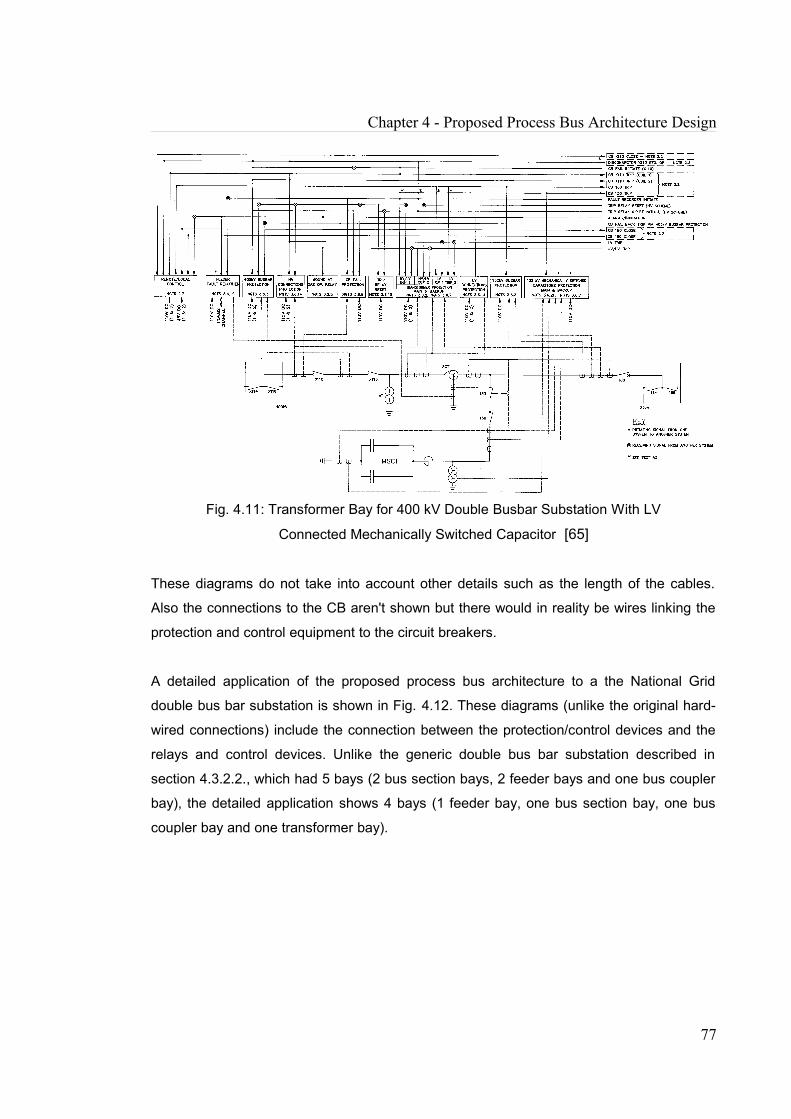
Chapter 4 - Proposed Process Bus Architecture Design
Fig. 4.11: Transformer Bay for 400 kV Double Busbar Substation With LV
Connected Mechanically Switched Capacitor [65]
These diagrams do not take into account other details such as the length of the cables.
Also the connections to the CB aren't shown but there would in reality be wires linking the
protection and control equipment to the circuit breakers.
A detailed application of the proposed process bus architecture to a the National Grid
double bus bar substation is shown in Fig. 4.12. These diagrams (unlike the original hard-
wired connections) include the connection between the protection/control devices and the
relays and control devices. Unlike the generic double bus bar substation described in
section 4.3.2.2., which had 5 bays (2 bus section bays, 2 feeder bays and one bus coupler
bay), the detailed application shows 4 bays (1 feeder bay, one bus section bay, one bus
coupler bay and one transformer bay).
77
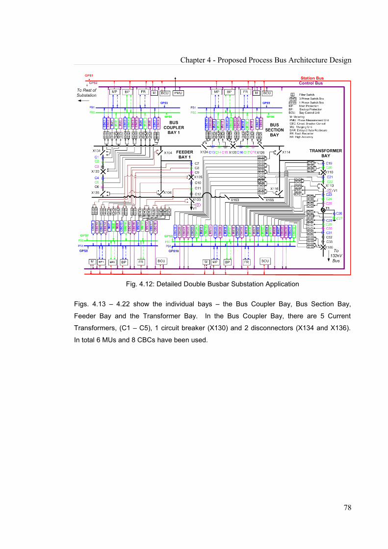
Chapter 4 - Proposed Process Bus Architecture Design
Fig. 4.12: Detailed Double Busbar Substation Application
Figs. 4.13 – 4.22 show the individual bays – the Bus Coupler Bay, Bus Section Bay,
Feeder Bay and the Transformer Bay. In the Bus Coupler Bay, there are 5 Current
Transformers, (C1 – C5), 1 circuit breaker (X130) and 2 disconnectors (X134 and X136).
In total 6 MUs and 8 CBCs have been used.
78
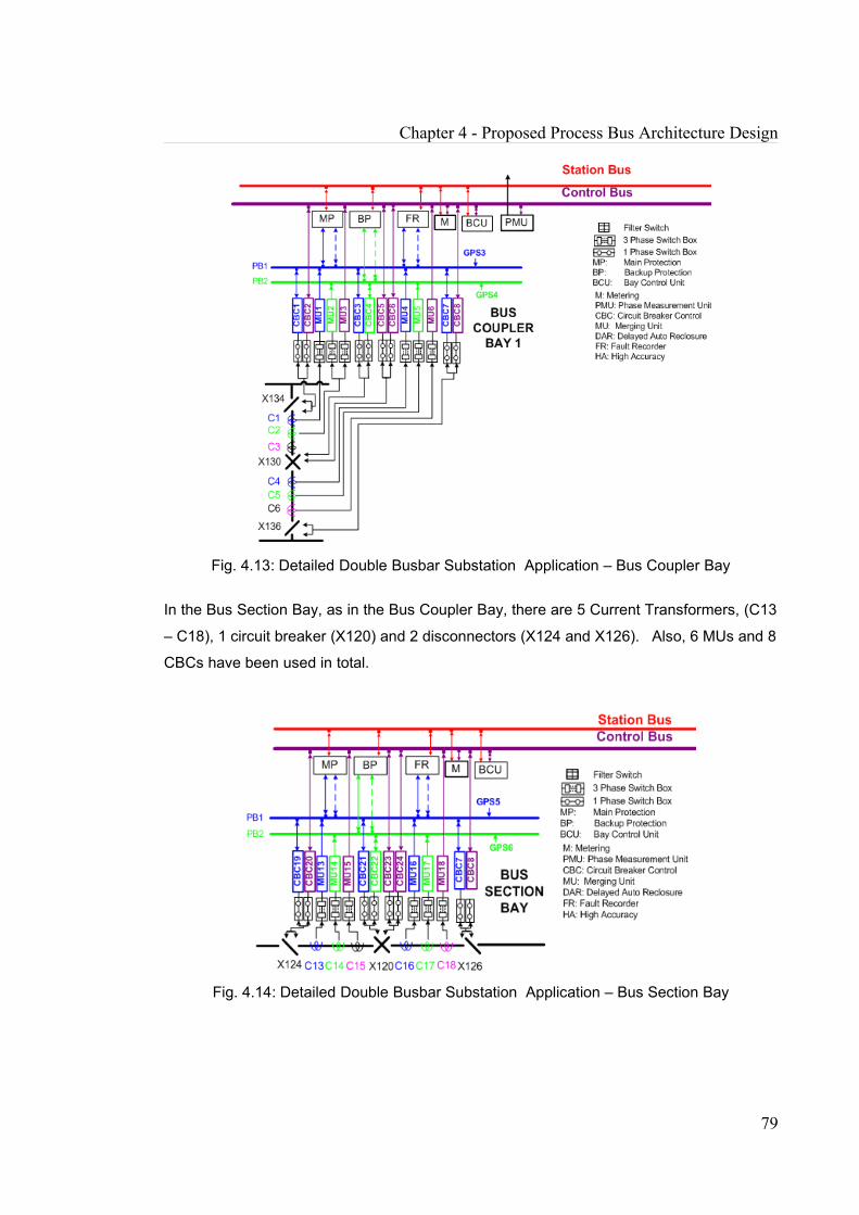
Chapter 4 - Proposed Process Bus Architecture Design
Fig. 4.13: Detailed Double Busbar Substation Application – Bus Coupler Bay
In the Bus Section Bay, as in the Bus Coupler Bay, there are 5 Current Transformers, (C13
– C18), 1 circuit breaker (X120) and 2 disconnectors (X124 and X126). Also, 6 MUs and 8
CBCs have been used in total.
Fig. 4.14: Detailed Double Busbar Substation Application – Bus Section Bay
79
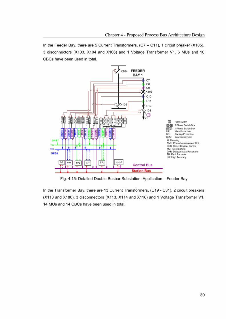
Chapter 4 - Proposed Process Bus Architecture Design
In the Feeder Bay, there are 5 Current Transformers, (C7 – C11), 1 circuit breaker (X105),
3 disconnectors (X103, X104 and X106) and 1 Voltage Transformer V1. 6 MUs and 10
CBCs have been used in total.
Fig. 4.15: Detailed Double Busbar Substation Application – Feeder Bay
In the Transformer Bay, there are 13 Current Transformers, (C19 - C31), 2 circuit breakers
(X110 and X180), 3 disconnectors (X113, X114 and X116) and 1 Voltage Transformer V1.
14 MUs and 14 CBCs have been used in total.
80
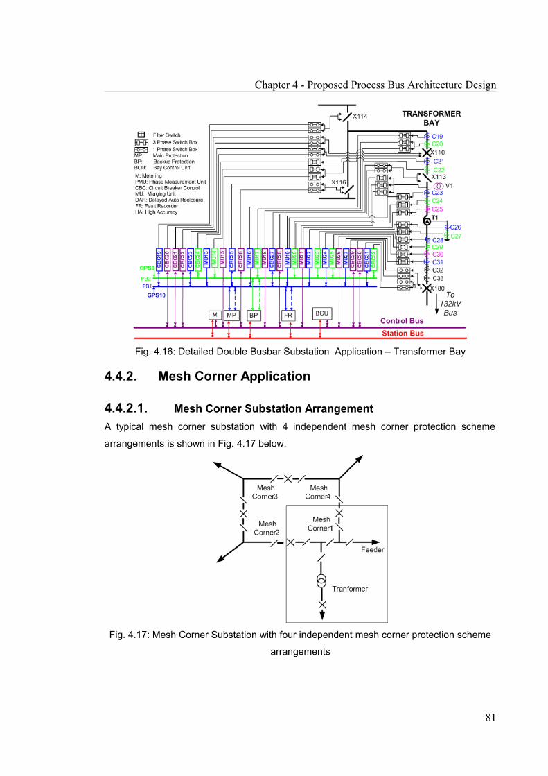
Chapter 4 - Proposed Process Bus Architecture Design
Fig. 4.16: Detailed Double Busbar Substation Application – Transformer Bay
4.4.2. Mesh Corner Application
4.4.2.1. Mesh Corner Substation Arrangement A typical mesh corner substation with 4 independent mesh corner protection scheme
arrangements is shown in Fig. 4.17 below.
Fig. 4.17: Mesh Corner Substation with four independent mesh corner protection scheme
arrangements
81

Chapter 4 - Proposed Process Bus Architecture Design
According to the high-level overview of Mesh Corner substation Architecture in Fig. 4.7, no
filtering switches are required between neighbouring mesh corner protection schemes.
Hence, each mesh corner application is considered independently. It is assumed that each
mesh corner is identical.
4.4.2.2. Detailed Mesh Corner ApplicationIn the feeder, mesh corner and transformer bays, the hard wired connections between the
CTs, VT and the Protection devices shall be replaced with process bus connections.
There will be a hard wired connection between the CT/VT and the merging unit, and an
Ethernet connection between the MU and the Switch (SW). Finally there will be an
Ethernet connection between the SW and the protection device. It is assumed that the
circuit breaker is hardwired to a circuit breaker Controller (CBC). Fig. 4.18 [65] shows the
detailed 400kV Mesh Corner substation with the mesh corner, feeder and transformer bay.
82

Fig. 4.18: 400kV Mesh corner with feeder and transformer [65]
83

Chapter 4 - Proposed Process Bus Architecture Design
A detailed application of the proposed process bus architecture to the 400kV National Grid
Mesh corner substation is shown in Fig. 4.19. It shows that the filter switch mechanism is
applied in a shunt manner to the each of bays making up the mesh corner.
Fig. 4.19: Detailed Mesh Corner Substation Application (Filter Switch Shunt Connection)
Figs. 4.20 – 4.22 show the individual bays – the Mesh Corner Bay, Feeder Bay, and the
Transformer Bay. In the Mesh Corner Bay, there are 6 Current Transformers, 2 circuit
breakers (X120 and X420), and 3 disconnectors (X124, X126 and X428). 106 MUs and 14
CBCs have been used in total.
84

Chapter 4 - Proposed Process Bus Architecture Design
Fig. 4.20 : Detailed Mesh Corner Substation Application – Mesh Corner Bay
In the Mesh Corner Feeder Bay, there are 3 Current Transformers, 1 disconnector and 1
Voltage Transformer V1. 5 MUs and 2 CBCs have been used in total.
Fig. 4.21: Detailed Mesh Corner Substation Application – Feeder Bay
85
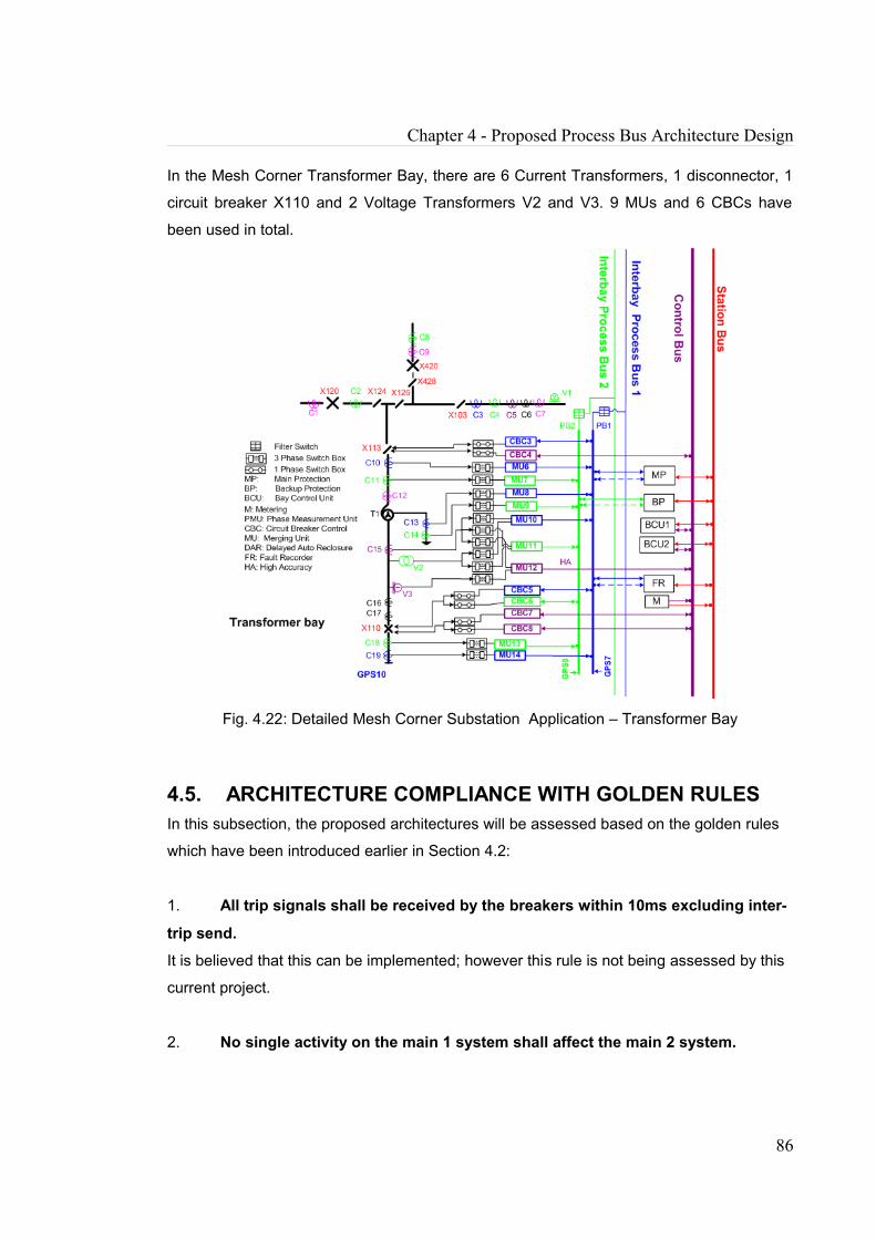
Chapter 4 - Proposed Process Bus Architecture Design
In the Mesh Corner Transformer Bay, there are 6 Current Transformers, 1 disconnector, 1
circuit breaker X110 and 2 Voltage Transformers V2 and V3. 9 MUs and 6 CBCs have
been used in total.
Fig. 4.22: Detailed Mesh Corner Substation Application – Transformer Bay
4.5. ARCHITECTURE COMPLIANCE WITH GOLDEN RULESIn this subsection, the proposed architectures will be assessed based on the golden rules
which have been introduced earlier in Section 4.2:
1. All trip signals shall be received by the breakers within 10ms excluding inter-
trip send.
It is believed that this can be implemented; however this rule is not being assessed by this
current project.
2. No single activity on the main 1 system shall affect the main 2 system.
86

Chapter 4 - Proposed Process Bus Architecture Design
This is the case with the proposed architecture. The Main 1 and Main 2 systems have links
to both process buses, however the back up links are non-dedicated. Main 1 and Main 2
are thus sufficiently isolated from one another.
3. No single failure shall result in the loss of control of more than one bay.
In the Double Busbar Substation, the bays are already decoupled, therefore the failure in
one bay will not affect the operation of other bays.
In the Mesh Corner substation, a single BCU failure will not result in the loss of control of
more than one bay. In addition, a fault-tolerant Control Bus will ensure that no single failure
results in the loss of control of more than one bay.
4. Physical facilities shall be available to isolate a bay for testing (Protection &
Control).
The filter switches and Switch boxes are able to isolate a bay for testing
5. The Protection and Control application/philosophy shall be functionally
identical to the current solution.
The Protection and Control IEDs will be able to gather the same required CT and VT data
as the current solution. They will also have access to the same required circuit breakers as
they are currently to. To prevent common mode failure, the merging units/circuit breaker
controllers used for Main 1 and Main 2 may be supplied by different manufacturers, and as
mentioned in Rule 2 above, they are sufficiently isolated from one another.
6. Design of AS3 scheme standard for all bays – DBB feeder, DBB Bus Section,
DBB Bus Coupler, MC Mesh Corner, MC Transformer, MC Feeder.
As can be seen in the previous sections, the generic architecture has been consistently
applied to a DBB Feeder, DBB Bus Section, DBB Bus Coupler, MC Mesh Corner, MC
Transformer, and MC Feeder.
7. The switching box should be located as close as possible to the primary
equipment.
It is believed that this can be implemented during installation.
87

Chapter 4 - Proposed Process Bus Architecture Design
4.6. SUMMARY
A generic process bus architecture has been introduced based on National Grid protection
and control equipment application golden rules and proposed standard interface design
rules. The architecture has been largely seen to comply with these golden rules and
interface design rules. The proposed architecture has been applied to different types of
bays that may be found in double busbar and mesh corner substations. The outcomes of
these applications indicate that although the proposed generic architecture concept is quite
simple and basic, its application ranges from simple to very complex substation
arrangements. The architecture has thus been seen to be adaptable to different types of
substation configurations. The use of switchboxes provide a means of completely
separating the primary equipment from the secondary equipment and the use of filter
switches make it possible to isolate one bay from another bay. Another important point is
that the Circuit Breaker Controllers, Merging Units, Protection and Control IEDs do not all
have to be produced by the same manufacturer.
These different characteristics help ensure that there is less overall interruption to the
substation operation if maintenance work needs to be carried out, or during an expansion
of a bay.
88
CHAPTER 5 DETERMINATION OF ARCHITECTURE RELIABILITY
5.1. INTRODUCTIONThe methodology for evaluating the reliability of the individual devices/components making
up the process bus system, and then of the system as a whole shall be introduced in this
chapter. This methodology is then applied to a case study and the results are discussed
for different types of bays in the double busbar and mesh corner substations.
5.2. RELIABILITY ANALYSIS METHODOLOGY
5.2.1. Component reliabilityComponent (or device) reliability, r, is estimated using the following equation [56].
( ) exp tr tMTBF
− = ÷ (7)
where
MTBF= Mean Time Between Failure (years). MTBF is the Mean Time Between Failure
(years). It is the reciprocal of the failure rate, when it is assumed that the failure rate is
constant. For example, an MTBF of 400 years is the reciprocal of the failure rate, 1/400
failures/year [57]. It means that in a statistical population of 400 components, on average
one component is expected to fail each year.
It is assumed that the period under consideration is the 1st year, thus t = 1.
5.2.2. System reliabilityParts of the system will be modelled using a reliability block diagram. Other parts will be
modelled using an event tree.
89
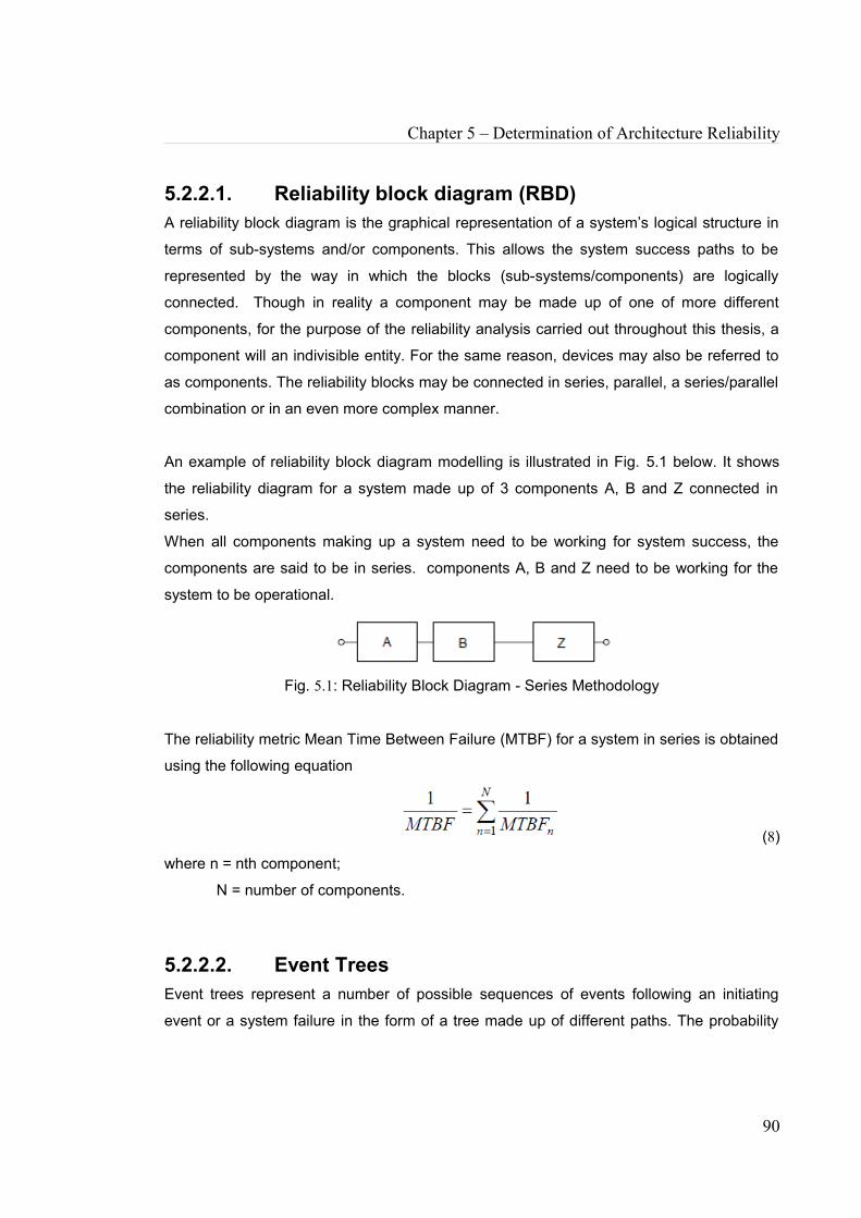
Chapter 5 – Determination of Architecture Reliability
5.2.2.1. Reliability block diagram (RBD)A reliability block diagram is the graphical representation of a system’s logical structure in
terms of sub-systems and/or components. This allows the system success paths to be
represented by the way in which the blocks (sub-systems/components) are logically
connected. Though in reality a component may be made up of one of more different
components, for the purpose of the reliability analysis carried out throughout this thesis, a
component will an indivisible entity. For the same reason, devices may also be referred to
as components. The reliability blocks may be connected in series, parallel, a series/parallel
combination or in an even more complex manner.
An example of reliability block diagram modelling is illustrated in Fig. 5.1 below. It shows
the reliability diagram for a system made up of 3 components A, B and Z connected in
series.
When all components making up a system need to be working for system success, the
components are said to be in series. components A, B and Z need to be working for the
system to be operational.
Fig. 5.1: Reliability Block Diagram - Series Methodology
The reliability metric Mean Time Between Failure (MTBF) for a system in series is obtained
using the following equation
(8)
where n = nth component;
N = number of components.
5.2.2.2. Event TreesEvent trees represent a number of possible sequences of events following an initiating
event or a system failure in the form of a tree made up of different paths. The probability
90
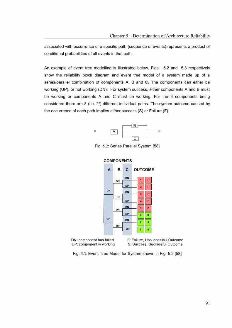
Chapter 5 – Determination of Architecture Reliability
associated with occurrence of a specific path (sequence of events) represents a product of
conditional probabilities of all events in that path.
An example of event tree modelling is illustrated below. Figs. 5.2 and 5.3 respectively
show the reliability block diagram and event tree model of a system made up of a
series/parallel combination of components A, B and C. The components can either be
working (UP), or not working (DN). For system success, either components A and B must
be working or components A and C must be working. For the 3 components being
considered there are 8 (i.e. 23) different individual paths. The system outcome caused by
the occurrence of each path implies either success (S) or Failure (F).
Fig. 5.2: Series Parallel System [58]
DN: component has failed F: Failure, Unsuccessful OutcomeUP: component is working S: Success, Successful Outcome
Fig. 5.3: Event Tree Model for System shown in Fig. 5.2 [58]
91

Chapter 5 – Determination of Architecture Reliability
There may also be an outcome implying a degree of manageable failure (MF), but for the
example below, only outcomes implying success or failure are illustrated. The system
reliability is the sum of all the successful outcomes.
Table 5.1 below is the mathematical representation of the event tree model shown in Fig.
5.3. For each outcome, the component failure (DN) has been replaced by the probability of
competent failure q, while the component working (UP) has been replaced by the
probability that the component is working, r.
reliability of component N, rN, is the probability that component N is working
unreliability of component N, qN, is the probability that component N has failed.
rN and qN are related by the following equation
qN = 1 – rN (9)
P(Oi) is the probability of occurrence of Outcome i
Table 5.1: Numerical representation of event tree model
OutcomeNumber A B C
Outcome :Success (S)
or Failure (F)
Probability of
Outcome1 qA qB qC F P(O1)2 qA qB rC F P(O2)3 qA rB qC F P(O3)4 qA rB rC F P(O4)5 rA qB qC F P(O5)6 rA qB rC S P(O6)7 rA rB qC S P(O7)8 rA rB rC S P(O8)
System Reliability, R is the sum of successful outcome probabilities
From Table 5.1,
R = P(O6)+ P(O7) + P(O8) = (rA x qB x rC) + (rA x rB x qC) x (rA x rB x rC) (10)
92

Chapter 5 – Determination of Architecture Reliability
5.2.2.3. Component AvailabilityThe component availability a, is the probability that a component will be functioning at any
point in time [59]. It is estimated using the following equation [60].
a =1 - MTTRMTBF
(11)
where
MTTR = Mean Time to Repair, the time taken to detect and repair each component failure.
It is the average downtime per failure (years)
MTBF is as described above (in the component reliability section)
5.2.2.4. System AvailabilityBy replacing the figures for component reliability with the corresponding figures for
component availability, the system availability will be estimated using event trees and
reliability block diagrams.
5.3. RELIABILITY ANALYSIS: CASE STUDY The reliability analysis for the proposed double bus bar process bus architecture
applications shall be carried out. A combination of reliability block diagram and event tree
modelling methods shall be applied. An introductory reliability analysis has also been
carried out in [61].
5.3.1. Process Bus Architecture ScenariosFig. 5.4 shows the architecture that will be used for the case study. It is the detailed
process bus architecture applied to the feeder bay of a double busbar substation as
previously described in Chapter 4.
93

Chapter 5 – Determination of Architecture Reliability
Fig. 5.4: Detailed Double Busbar Application – Feeder Bay
Fig. 5.4 is redrawn (Fig. 5.5) to show the primary equipment connections that are
considered for this analysis. Fig. 5.5 is the first architecture scenario and includes the
Ethernet switches that are used to implement the process bus. Ethernet Switch 1(SW1)
represents Process Bus 1, Ethernet Switch 2 (SW2) represents Process Bus 2 while
Ethernet Switch 3 (SW3) represents the Control Bus. The bay level IEDs are shown – their
connections to the process bus (the fibre optic cables) are included in the reliability
analysis, but not the bay level IEDs themselves. The IED P1 incorporates the functions of
Main Protection device. P2 incorporates the functions of Main Protection 2 and the backup
protection. Control IED C incorporates control functions such as Fault recording, and
delayed auto reclosure. Each current and voltage transformer is connected to a merging
unit (MU) and each circuit breaker is connected to a circuit breaker Controller (CBC). The
merging units and circuit breaker Controllers are connected to the Ethernet Switches. The
copper cables connecting the merging units to the CTs/VT and the circuit breaker
Controllers to the circuit breakers are not considered in this reliability analysis.
94
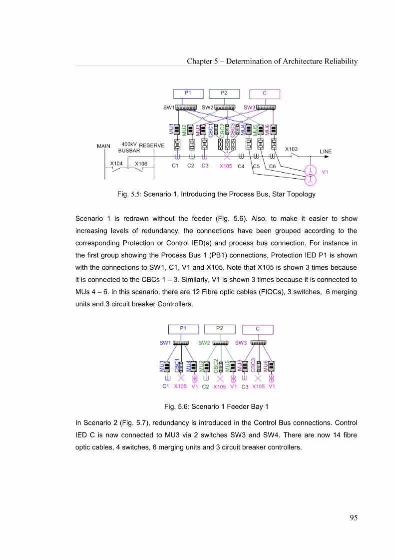
Chapter 5 – Determination of Architecture Reliability
Fig. 5.5: Scenario 1, Introducing the Process Bus, Star Topology
Scenario 1 is redrawn without the feeder (Fig. 5.6). Also, to make it easier to show
increasing levels of redundancy, the connections have been grouped according to the
corresponding Protection or Control IED(s) and process bus connection. For instance in
the first group showing the Process Bus 1 (PB1) connections, Protection IED P1 is shown
with the connections to SW1, C1, V1 and X105. Note that X105 is shown 3 times because
it is connected to the CBCs 1 – 3. Similarly, V1 is shown 3 times because it is connected to
MUs 4 – 6. In this scenario, there are 12 Fibre optic cables (FIOCs), 3 switches, 6 merging
units and 3 circuit breaker Controllers.
Fig. 5.6: Scenario 1 Feeder Bay 1
In Scenario 2 (Fig. 5.7), redundancy is introduced in the Control Bus connections. Control
IED C is now connected to MU3 via 2 switches SW3 and SW4. There are now 14 fibre
optic cables, 4 switches, 6 merging units and 3 circuit breaker controllers.
95

Chapter 5 – Determination of Architecture Reliability
Fig. 5.7: Scenario 2 Feeder Bay 1
In order to increase the redundancy, C is also connected via the 2 switches to CBC3 in
Scenario 3 ((Fig. 5.8). This redundancy is gradually increased until each process bus has 2
Ethernet Switches, and each IED, MU and CBC is connected to the 2 Ethernet Switches in
the corresponding process bus connection group.
Fig. 5.8: Scenario 3 Feeder Bay 1
There are in total 10 scenarios, and Scenario 4 is shown below in the subsequent
subsection, and Scenarios 5-10 can be seen in APPENDIX A. In Scenario 4, there is full
star topology duplication for the control bus. In Scenarios 5 - 7, varying levels of
redundancy are further added until there is a full star topology duplication in bay process
bus 1, and in Scenarios 8 - 10, varying levels of redundancy are further added until there is
a full star topology duplication in bay process bus 2. Table 5.2 lists the number of
components used for each architecture scenario:
Table 5.2: Number of Devices in each Scenario (Double Busbar Feeder Bay (Star))
Scenario Number of DevicesSW MU CBC FIOC
1 3 6 3 122 4 6 3 143 4 6 3 154 4 6 3 16
96
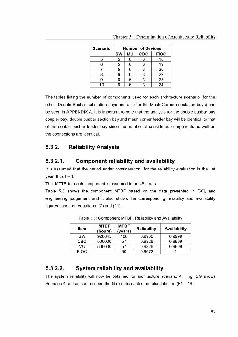
Chapter 5 – Determination of Architecture Reliability
Scenario Number of DevicesSW MU CBC FIOC
5 5 6 3 186 5 6 3 197 5 6 3 208 6 6 3 229 6 6 3 2310 6 6 3 24
The tables listing the number of components used for each architecture scenario (for the
other Double Busbar substation bays and also for the Mesh Corner substation bays) can
be seen in APPENDIX A. It is important to note that the analysis for the double busbar bus
coupler bay, double busbar section bay and mesh corner feeder bay will be identical to that
of the double busbar feeder bay since the number of considered components as well as
the connections are identical.
5.3.2. Reliability Analysis
5.3.2.1. Component reliability and availabilityIt is assumed that the period under consideration for the reliability evaluation is the 1st
year, thus t = 1.
The MTTR for each component is assumed to be 48 hours
Table 5.3 shows the component MTBF based on the data presented in [60], and
engineering judgement and it also shows the corresponding reliability and availability
figures based on equations (7) and (11).
Table 5.3: Component MTBF, Reliability and Availability
Item MTBF (hours)
MTBF (years) Reliability Availability
SW 928845 106 0.9906 0.9999CBC 500000 57 0.9826 0.9999MU 500000 57 0.9826 0.9999
FIOC 30 0.9672 1
5.3.2.2. System reliability and availabilityThe system reliability will now be obtained for architecture scenario 4. Fig. 5.9 shows
Scenario 4 and as can be seen the fibre optic cables are also labelled (F1 – 16).
97
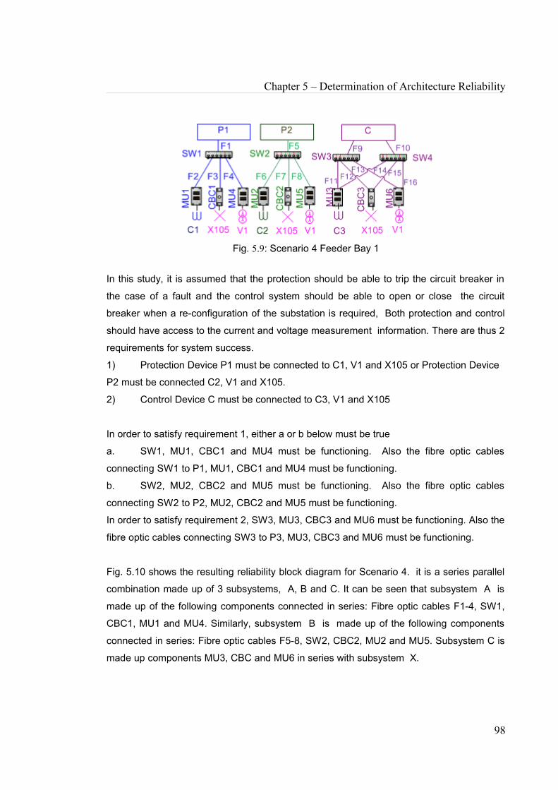
Chapter 5 – Determination of Architecture Reliability
Fig. 5.9: Scenario 4 Feeder Bay 1
In this study, it is assumed that the protection should be able to trip the circuit breaker in
the case of a fault and the control system should be able to open or close the circuit
breaker when a re-configuration of the substation is required, Both protection and control
should have access to the current and voltage measurement information. There are thus 2
requirements for system success.
1) Protection Device P1 must be connected to C1, V1 and X105 or Protection Device
P2 must be connected C2, V1 and X105.
2) Control Device C must be connected to C3, V1 and X105
In order to satisfy requirement 1, either a or b below must be true
a. SW1, MU1, CBC1 and MU4 must be functioning. Also the fibre optic cables
connecting SW1 to P1, MU1, CBC1 and MU4 must be functioning.
b. SW2, MU2, CBC2 and MU5 must be functioning. Also the fibre optic cables
connecting SW2 to P2, MU2, CBC2 and MU5 must be functioning.
In order to satisfy requirement 2, SW3, MU3, CBC3 and MU6 must be functioning. Also the
fibre optic cables connecting SW3 to P3, MU3, CBC3 and MU6 must be functioning.
Fig. 5.10 shows the resulting reliability block diagram for Scenario 4. it is a series parallel
combination made up of 3 subsystems, A, B and C. It can be seen that subsystem A is
made up of the following components connected in series: Fibre optic cables F1-4, SW1,
CBC1, MU1 and MU4. Similarly, subsystem B is made up of the following components
connected in series: Fibre optic cables F5-8, SW2, CBC2, MU2 and MU5. Subsystem C is
made up components MU3, CBC and MU6 in series with subsystem X.
98

Chapter 5 – Determination of Architecture Reliability
Fig. 5.10: Scenario 4 Series-parallel Reliability Block Diagram
The components making up subsystem A are in series, thus based on equation (I) and the
data in Table 5.3, the reliability of A is
0.9672 x 0.9906 x 0.9672 x 0.9826 x 0.9672 x 0.9826 x 0.9672 x 0.9826 ≈ 0.8225 (12)
Since B has identical components connected in an identical manner, the reliability of this
subsystem ≈ 0.8225.
Subsystem X is made up of the following components
SW1, F1, F3, F4, F5, SW2, F2, F6, F7 and F8,
SW1 and FI are in series and be replaced by a subsystem SW1*
Similarly, SW2 and F2 are in series and be replaced by a subsystem SW2*
For the system success of subsystem X, at least one of the following groups of
components/subsystems must be functioning:
1. SW1* F3 F4 F5 2. SW1* F4 F5 SW2* F6 3. SW1* F3 F5 SW2* F7 4. SW1* F3 F4 SW2* F8 5. SW1* F5 SW2* F6 F7 6. SW1* F4 SW2* F6 F8
99

Chapter 5 – Determination of Architecture Reliability
7. SW1* F3 SW2* F7 F8 8. SW2* F6 F7 F8 9. SW1* F3 SW2* F7 F8 10. SW1* F4 SW2* F6 F8 11. SW1* F5 SW2* F6 F7 12. SW1* F4 F5 SW2* F6 13. SW1* F3 F5 SW2* F7 14. SW1* F3 F4 SW2* F8
For the 8 components/subsystems being considered there are 256 (i.e. 28) different
individual paths. These paths are numerically (partially) represented in part in Table 5.4.
Table 5.4: Numerical Representation Of Event Tree Model
(O/C : Outcome; O/C Prob: Outcome Probability)
O/C
No. SW1* F3 F4 F5 SW2* F6 F7 F8
Outcome:Success (S) or
Failure (F)
O/C
Prob.
1 qSW1* qF3 qF4 qF5 qSW2* qF6 qF7 qF8 F 02 qSW1* qF3 rF4 qF5 qSW2* qF6 qF7 rF8 F 03 qSW1* qF3 qF4 qF5 qSW2* qF6 rF7 qF8 F 04 qSW1* qF3 qF4 qF5 qSW2* qF6 rF7 rF8 F 0....
.
.
.
.
.
.
.
.
.
.
.
.
.
.
.
.
.
.
.
.
.
.
.
.
.
.
.
.
.
.
.
.
.
.
.
.
.
.
.
.254 rSW1* rF3 rF4 rF5 rSW2* rF6 qF7 rF8 S 0.0255255 rSW1* rF3 rF4 rF5 rSW2* rF6 rF7 qF8 S 0.0255256 rSW1* rF3 rF4 rF5 rSW2* rF6 rF7 rF8 S 0.7515
Based on the data in Table 5.4
rSW1* = 0.9906 x 0.9672= 0.9581rF3 = 0.9672rF4 = 0.9672rF5 = 0.9672rSW2* = 0.9906 x 0.9672 = 0.9581rF6 = 0.9672rF7 = 0.9672rF8 = 0.9672
Reliability of subsystem X is the sum of successful outcome probabilities. Use was made
of an event tree program developed in Java to derive the reliability of subsystem X.
100
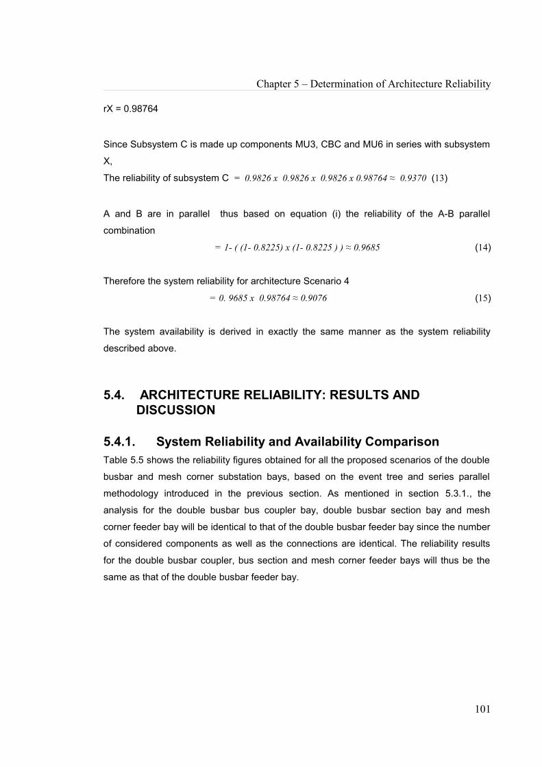
Chapter 5 – Determination of Architecture Reliability
rX = 0.98764
Since Subsystem C is made up components MU3, CBC and MU6 in series with subsystem
X,
The reliability of subsystem C = 0.9826 x 0.9826 x 0.9826 x 0.98764 ≈ 0.9370 (13)
A and B are in parallel thus based on equation (i) the reliability of the A-B parallel
combination
= 1- ( (1- 0.8225) x (1- 0.8225 ) ) ≈ 0.9685 (14)
Therefore the system reliability for architecture Scenario 4
= 0. 9685 x 0.98764 ≈ 0.9076 (15)
The system availability is derived in exactly the same manner as the system reliability
described above.
5.4. ARCHITECTURE RELIABILITY: RESULTS AND DISCUSSION
5.4.1. System Reliability and Availability ComparisonTable 5.5 shows the reliability figures obtained for all the proposed scenarios of the double
busbar and mesh corner substation bays, based on the event tree and series parallel
methodology introduced in the previous section. As mentioned in section 5.3.1., the
analysis for the double busbar bus coupler bay, double busbar section bay and mesh
corner feeder bay will be identical to that of the double busbar feeder bay since the number
of considered components as well as the connections are identical. The reliability results
for the double busbar coupler, bus section and mesh corner feeder bays will thus be the
same as that of the double busbar feeder bay.
101
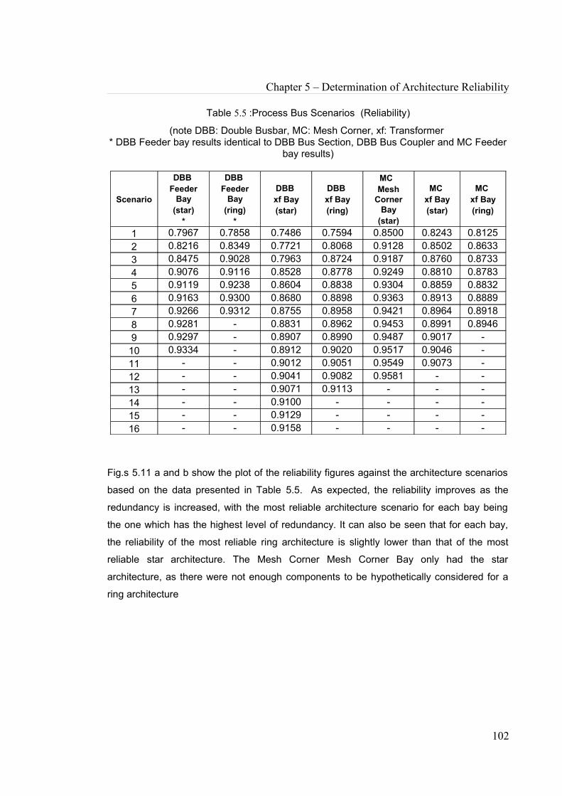
Chapter 5 – Determination of Architecture Reliability
Table 5.5 :Process Bus Scenarios (Reliability)
(note DBB: Double Busbar, MC: Mesh Corner, xf: Transformer * DBB Feeder bay results identical to DBB Bus Section, DBB Bus Coupler and MC Feeder
bay results)
Scenario
DBB Feeder
Bay(star)
*
DBB Feeder
Bay(ring)
*
DBB xf Bay(star)
DBB xf Bay(ring)
MC Mesh
Corner Bay
(star)
MC xf Bay(star)
MC xf Bay(ring)
1 0.7967 0.7858 0.7486 0.7594 0.8500 0.8243 0.81252 0.8216 0.8349 0.7721 0.8068 0.9128 0.8502 0.86333 0.8475 0.9028 0.7963 0.8724 0.9187 0.8760 0.87334 0.9076 0.9116 0.8528 0.8778 0.9249 0.8810 0.87835 0.9119 0.9238 0.8604 0.8838 0.9304 0.8859 0.88326 0.9163 0.9300 0.8680 0.8898 0.9363 0.8913 0.88897 0.9266 0.9312 0.8755 0.8958 0.9421 0.8964 0.89188 0.9281 - 0.8831 0.8962 0.9453 0.8991 0.89469 0.9297 - 0.8907 0.8990 0.9487 0.9017 -10 0.9334 - 0.8912 0.9020 0.9517 0.9046 -11 - - 0.9012 0.9051 0.9549 0.9073 -12 - - 0.9041 0.9082 0.9581 - -13 - - 0.9071 0.9113 - - -14 - - 0.9100 - - - -15 - - 0.9129 - - - -16 - - 0.9158 - - - -
Fig.s 5.11 a and b show the plot of the reliability figures against the architecture scenarios
based on the data presented in Table 5.5. As expected, the reliability improves as the
redundancy is increased, with the most reliable architecture scenario for each bay being
the one which has the highest level of redundancy. It can also be seen that for each bay,
the reliability of the most reliable ring architecture is slightly lower than that of the most
reliable star architecture. The Mesh Corner Mesh Corner Bay only had the star
architecture, as there were not enough components to be hypothetically considered for a
ring architecture
102
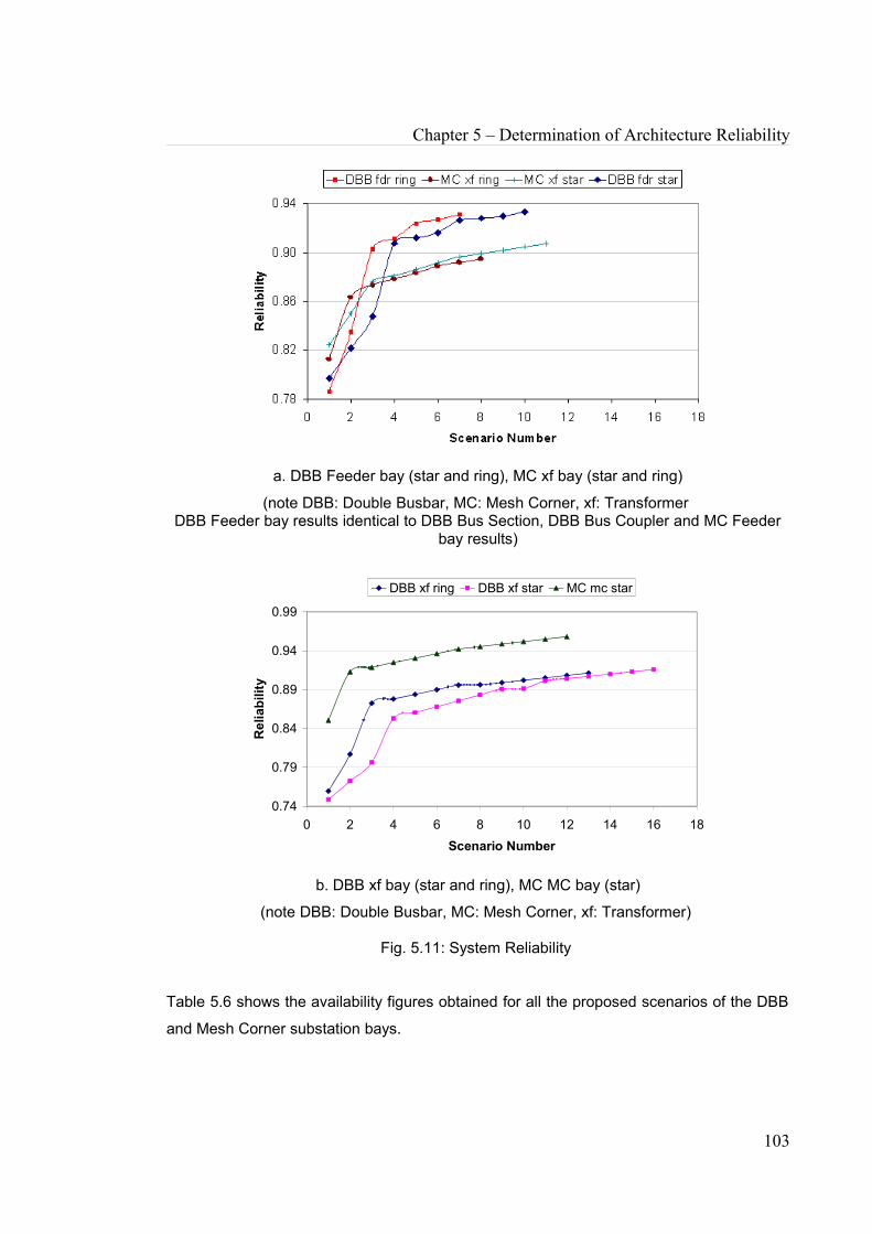
Chapter 5 – Determination of Architecture Reliability
a. DBB Feeder bay (star and ring), MC xf bay (star and ring)
(note DBB: Double Busbar, MC: Mesh Corner, xf: Transformer DBB Feeder bay results identical to DBB Bus Section, DBB Bus Coupler and MC Feeder
bay results)
0.74
0.79
0.84
0.89
0.94
0.99
0 2 4 6 8 10 12 14 16 18Scenario Number
Rel
iabi
lity
DBB xf ring DBB xf star MC mc star
b. DBB xf bay (star and ring), MC MC bay (star)
(note DBB: Double Busbar, MC: Mesh Corner, xf: Transformer)
Fig. 5.11: System Reliability
Table 5.6 shows the availability figures obtained for all the proposed scenarios of the DBB
and Mesh Corner substation bays.
103

Chapter 5 – Determination of Architecture Reliability
Table 5.6: Process Bus Scenarios (Availability)(note MC: DBB: Double Busbar, Mesh Corner, xf: Transformer
* DBB Feeder bay results identical to DBB Bus Section, DBB Bus Coupler and MC Feeder bay results)
Scenario
DBB Feeder
Bay(star)
*
DBB Feeder
Bay(ring)
*
DBB xf Bay(star)
DBB xf Bay(ring)
MC Mesh
Corner Bay
(star)
MC xf Bay(star)
MC xf Bay(ring)
1 0.99893 0.99888 0.99893 0.99888 0.99948 0.99921 0.999162 0.99911 0.99924 0.99911 0.99924 0.99990 0.99939 0.999523 0.99929 0.99971 0.99929 0.99971 0.99990 0.99957 0.999524 0.99971 0.99971 0.99971 0.99971 0.99990 0.99957 0.999525 0.99971 0.99971 0.99971 0.99971 0.99990 0.99957 0.999526 0.99971 0.99971 0.99971 0.99971 0.99990 0.99957 0.999527 0.99971 0.99971 0.99971 0.99971 0.99990 0.99957 0.999528 0.99971 - 0.99971 0.99971 0.99990 0.99957 0.999529 0.99971 - 0.99971 0.99971 0.99990 0.9995710 0.99971 - 0.99971 0.99971 0.99990 0.9995711 - - 0.99971 0.99971 0.99990 0.9995712 - - 0.99971 0.99971 0.9999013 - - 0.99971 0.99971 - - -14 - - 0.99971 - - - -15 - - 0.99971 - - - -16 - - 0.99971 - - - -
Fig.s 5.12 a and b show the plot of the availability figures against the architecture
scenarios based on the data presented in Table 5.6. Again the system availability
improves across the bays as the redundancy is increased, although it gets to a point where
the increase in availability is not as steep when compared with reliability. Also, especially
for the double busbar feeder bay and transformer bay, the difference in availability
between the most available ring and the star is much less than that seen in the case of
reliability.
104

Chapter 5 – Determination of Architecture Reliability
0.9988
0.9990
0.9992
0.9994
0.9996
0.9998
0 2 4 6 8 10 12 14 16 18
Scenario Number
Ava
ilabi
lity
DBB fdr ring MC xf ring MC xf star DBB fdr star
a. DBB Feeder bay (star and ring), MC xf bay (star and ring)
(note MC: DBB: Double Busbar, Mesh Corner, xf: Transformer DBB Feeder bay results identical to DBB Bus Section, DBB Bus Coupler and MC Feeder
bay results)
0.99880
0.99900
0.99920
0.99940
0.99960
0.99980
1.00000
0 2 4 6 8 10 12 14 16 18
Scenario Number
Ava
ilabi
lity
DBB xf ring DBB xf star MC mc star
b. DBB xf bay (star and ring), MC MC bay (star)
(note MC: DBB: Double Busbar, Mesh Corner, xf: Transformer)
Fig. 5.12: System Availability
The reliability of the feeder bay process bus architecture has however been seen to be less
than that of the hardwired copper-based connections (prior to the introduction of the
process bus). Taking the double busbar feeder bay as an example, the estimated reliability
of the most reliable feeder bay process bus architecture was 0.9334. The reliability of the
105
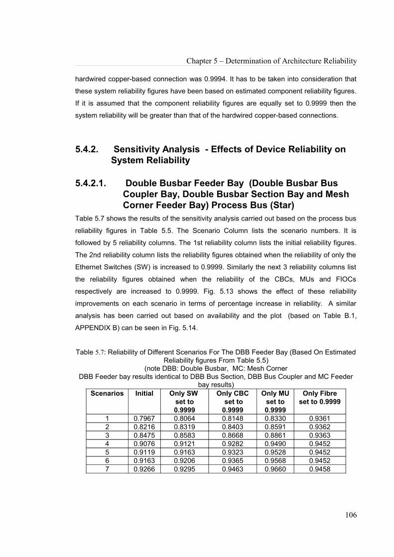
Chapter 5 – Determination of Architecture Reliability
hardwired copper-based connection was 0.9994. It has to be taken into consideration that
these system reliability figures have been based on estimated component reliability figures.
If it is assumed that the component reliability figures are equally set to 0.9999 then the
system reliability will be greater than that of the hardwired copper-based connections.
5.4.2. Sensitivity Analysis - Effects of Device Reliability on System Reliability
5.4.2.1. Double Busbar Feeder Bay (Double Busbar Bus Coupler Bay, Double Busbar Section Bay and Mesh Corner Feeder Bay) Process Bus (Star)
Table 5.7 shows the results of the sensitivity analysis carried out based on the process bus
reliability figures in Table 5.5. The Scenario Column lists the scenario numbers. It is
followed by 5 reliability columns. The 1st reliability column lists the initial reliability figures.
The 2nd reliability column lists the reliability figures obtained when the reliability of only the
Ethernet Switches (SW) is increased to 0.9999. Similarly the next 3 reliability columns list
the reliability figures obtained when the reliability of the CBCs, MUs and FIOCs
respectively are increased to 0.9999. Fig. 5.13 shows the effect of these reliability
improvements on each scenario in terms of percentage increase in reliability. A similar
analysis has been carried out based on availability and the plot (based on Table B.1,
APPENDIX B) can be seen in Fig. 5.14.
Table 5.7: Reliability of Different Scenarios For The DBB Feeder Bay (Based On Estimated Reliability figures From Table 5.5)
(note DBB: Double Busbar, MC: Mesh CornerDBB Feeder bay results identical to DBB Bus Section, DBB Bus Coupler and MC Feeder
bay results)Scenarios Initial Only SW
set to 0.9999
Only CBC set to 0.9999
Only MU set to 0.9999
Only Fibre set to 0.9999
1 0.7967 0.8064 0.8148 0.8330 0.93612 0.8216 0.8319 0.8403 0.8591 0.93623 0.8475 0.8583 0.8668 0.8861 0.93634 0.9076 0.9121 0.9282 0.9490 0.94525 0.9119 0.9163 0.9323 0.9528 0.94526 0.9163 0.9206 0.9365 0.9568 0.94527 0.9266 0.9295 0.9463 0.9660 0.9458
106

Chapter 5 – Determination of Architecture Reliability
Scenarios Initial Only SW set to 0.9999
Only CBC set to 0.9999
Only MU set to 0.9999
Only Fibre set to 0.9999
8 0.9281 0.9310 0.9475 0.9668 0.94589 0.9297 0.9325 0.9487 0.9676 0.9458
10 0.9334 0.9357 0.9515 0.9694 0.9462
Fig. 5.13: Sensitivity analysis of the different scenarios (based on initial estimated component reliability)
(note DBB: Double Busbar, MC: Mesh CornerResults identical to DBB Bus Section, DBB Bus Coupler and MC Feeder bay results)
Fig. 5.14: Sensitivity analysis of the different scenarios (based on initial estimated component availability)
(note DBB: Double Busbar, MC: Mesh CornerResults identical to DBB Bus Section, DBB Bus Coupler and MC Feeder bay results)
107

Chapter 5 – Determination of Architecture Reliability
It can be seen that increasing the reliability of the fibre optic cables in the first 3 scenarios
leads to the highest increases in system reliability. With each subsequent scenario, as the
system reliability increases, the impact of the fibre optic cables on reliability improvement is
reduced. The same can be said of the Ethernet Switches, though the reduction of the
impact on reliability is not as steep as that of the fibre optic cables. The increase in system
reliability is higher in MUs than that of the CBCs. Also the system reliability improvement
due to the increase in MU and CBC reliability are almost constant throughout all scenarios.
The latter can be attributed to the fact that in all scenarios, it is only the MUs and CBCs
which do not vary in number. The same is true of the availability analysis in Fig. 5.14.
However the influence due to improvements in the individual component categories is
much less, indeed the highest impact seen is in Scenario 1 where the improvement is
approximately 0.07% when compared with approximately 18% in the reliability analysis.
This is due to the fact that the initial availability of the components is already much higher
than the initial reliability of the components. The trends are still similar as the impact of
fibre is much higher for the less available scenarios (1 – 3) and then tends to be negligible
for the more available scenarios (4 - 10). The MUs and CBCs had a consistent impact
across all the scenarios and finally the improvements in switch reliability had the least
impact overall.
The results in Table 5.5 do not take into account the fact that apart from the MUs and
CBCs, the reliability of the devices are different. Increasing the reliability of a device to
0.9999 would increase the reliability of that device by a higher percentage than for another
device, and hence affect their relative increase in system reliability. Also these reliability
figures are estimates and the actual reliability may be higher than what was estimated. For
these reasons mentioned above, the sensitivity analysis was repeated, this time with the
reliability of all devices set to 0.999 after which the reliability of each device category was
in turn increased to 0.9999 (Table B.2, APPENDIX B). Fig. 5.15 shows the new plot based
on the new analysis.
108

Chapter 5 – Determination of Architecture Reliability
Fig. 5.15: Sensitivity analysis of the different scenarios (based on all component reliability set to 0.999)
(note DBB: Double Busbar, MC: Mesh CornerResults identical to DBB Bus Section, DBB Bus Coupler and MC Feeder bay results)
It is seen that the actual percentage increases have generally dropped when compared
with Fig. 5.13, but there are still similarities between Figs 5.13 and 5.15. The impact of the
fibre cable is still the greatest in the 1st 3 scenarios and this impact drops steeply in
subsequent scenarios. Also the MU and CBC reliability increase still have a constant
impact on the system reliability improvement, with the MUs’ still being higher than that of
the CBCs’.
The sensitivity analysis for the other bays shall now be discussed and the tables used for
the plots can be found in APPENDIX B.
5.4.2.2. Double Busbar Feeder Bay (Double Busbar Bus Coupler Bay, Double Busbar Section Bay and Mesh Corner Feeder Bay) Process Bus (Ring)
Fig. 5.16a-c show the effect of system reliability (or availability) improvements on each
scenario in terms of percentage increase in reliability, availability and the reliability (when
the reliability of all individual devices is set to the same value) respectively for the Ring-
topology based Process Bus architecture applied to the Double Busbar Feeder Bay. The
109

Chapter 5 – Determination of Architecture Reliability
results are identical to the Double Busbar Bus Coupler Bay, Double Busbar Section Bay
and Mesh Corner Feeder Bay .
a. Comparison of percentage increase in system reliability due to increase in component category reliability (based on initial estimated component reliability)
(note DBB: Double Busbar, MC: Mesh CornerResults identical to DBB Bus Section, DBB Bus Coupler and MC Feeder bay results)
b. Comparison of percentage increase in system availability due to increase in component category availability (based on initial estimated component availability)
(note DBB: Double Busbar, MC: Mesh CornerResults identical to DBB Bus Section, DBB Bus Coupler and MC Feeder bay results)
110

Chapter 5 – Determination of Architecture Reliability
c. Comparison of percentage increase in system reliability due to increase in component category reliability (each component reliability set to 0.999)
(note DBB: Double Busbar, MC: Mesh CornerResults identical to DBB Bus Section, DBB Bus Coupler and MC Feeder bay results)
Fig. 5.16: Sensitivity analysis of the different scenarios
There are fewer proposed scenarios (7) than for the star based architecture. However the
trend is the same as that of the star based architecture: the fibre has the highest impact for
the less reliable scenarios and then this impact drastically reduces as the architecture
becomes more reliable. Both the MU and CBC have a consistent impact across all
scenarios and the Ethernet switch has the lowest overall impact on system reliability. With
the reliability of all components set to 0.999 (c), the impact of the switches and the fibre is
seen to be negligible for more reliable scenarios. The same can be said of the availability
(b). In terms of consistency, an increase in the MU reliability is seen to have the greatest
impact on the system reliability.
5.4.2.3. Double Busbar Transformer Bay Process Bus (Star)Fig. 5.17a-c show the effect of reliability (or availability) improvements on each scenario in
terms of percentage increase in reliability, availability and the reliability (when the reliability
of all individual devices is set to the same value) respectively for the double busbar bay
(star based architecture).
111

Chapter 5 – Determination of Architecture Reliability
a. Comparison of percentage increase in system reliability due to increase in component category reliability (based on initial estimated component reliability)
b. Comparison of percentage increase in system availability due to increase in component category availability (based on initial estimated component availability)
112
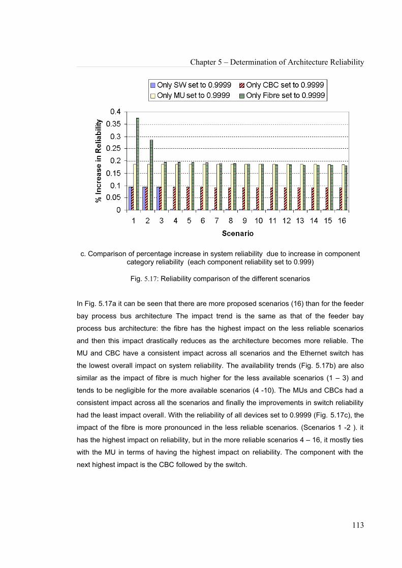
Chapter 5 – Determination of Architecture Reliability
c. Comparison of percentage increase in system reliability due to increase in component category reliability (each component reliability set to 0.999)
Fig. 5.17: Reliability comparison of the different scenarios
In Fig. 5.17a it can be seen that there are more proposed scenarios (16) than for the feeder
bay process bus architecture The impact trend is the same as that of the feeder bay
process bus architecture: the fibre has the highest impact on the less reliable scenarios
and then this impact drastically reduces as the architecture becomes more reliable. The
MU and CBC have a consistent impact across all scenarios and the Ethernet switch has
the lowest overall impact on system reliability. The availability trends (Fig. 5.17b) are also
similar as the impact of fibre is much higher for the less available scenarios (1 – 3) and
tends to be negligible for the more available scenarios (4 -10). The MUs and CBCs had a
consistent impact across all the scenarios and finally the improvements in switch reliability
had the least impact overall. With the reliability of all devices set to 0.9999 (Fig. 5.17c), the
impact of the fibre is more pronounced in the less reliable scenarios. (Scenarios 1 -2 ). it
has the highest impact on reliability, but in the more reliable scenarios 4 – 16, it mostly ties
with the MU in terms of having the highest impact on reliability. The component with the
next highest impact is the CBC followed by the switch.
113

Chapter 5 – Determination of Architecture Reliability
5.4.2.4. Double Busbar Transformer Bay Process Bus (Ring)
Fig. 5.18a-c show the effect of reliability (or availability) improvements on each scenario in
terms of percentage increase in reliability, availability and the reliability (when the reliability
of all individual devices is set to the same value) respectively for the double busbar
transformer bay (ring based architecture).
a. Comparison of percentage increase in system reliability due to increase in component category reliability (based on initial estimated component reliability)
114

Chapter 5 – Determination of Architecture Reliability
b. Comparison of percentage increase in system availability due to increase in component category availability (based on initial estimated component availability)
c. Comparison of percentage increase in system reliability due to increase in component category reliability (each component reliability set to 0.999)
Fig. 5.18: Sensitivity analysis (Double Busbar Transformer Bay)
It can be seen from Fig.s 5.18a-c the SWs make their highest impact on only the 1st 2
scenarios, after which their impact reduces, even in Fig. 5.18a and even more drastically
so in Fig. 5.18b and c. the same trend is also seen with the fibre. As usual, the impact of
MU and CBC on the reliability is steady throughout. The MU has the highest overall impact
on the availability and reliability, followed by the CBC, fibre and finally the switches.
5.4.2.5. Mesh Corner Mesh Corner Bay Process Bus (Star)Fig. 5.19a-c show the effect of reliability (or availability) improvements on each scenario in
terms of percentage increase in reliability, availability and the reliability (when the reliability
of all individual devices is set to the same value) respectively for the mesh corner mesh
corner bay (star based architecture).
115

Chapter 5 – Determination of Architecture Reliability
a. Comparison of percentage increase in system reliability due to increase in component
category reliability
b. Comparison of percentage increase in system availability due to increase in component
category availability
116
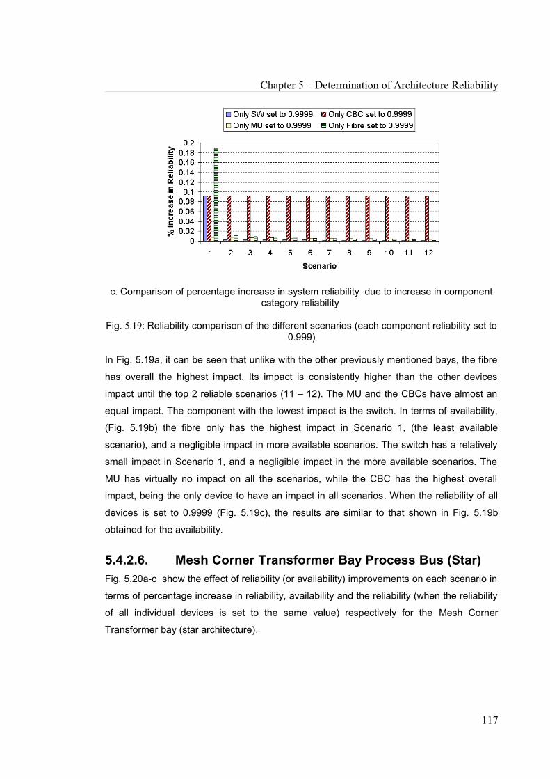
Chapter 5 – Determination of Architecture Reliability
c. Comparison of percentage increase in system reliability due to increase in component category reliability
Fig. 5.19: Reliability comparison of the different scenarios (each component reliability set to 0.999)
In Fig. 5.19a, it can be seen that unlike with the other previously mentioned bays, the fibre
has overall the highest impact. Its impact is consistently higher than the other devices
impact until the top 2 reliable scenarios (11 – 12). The MU and the CBCs have almost an
equal impact. The component with the lowest impact is the switch. In terms of availability,
(Fig. 5.19b) the fibre only has the highest impact in Scenario 1, (the least available
scenario), and a negligible impact in more available scenarios. The switch has a relatively
small impact in Scenario 1, and a negligible impact in the more available scenarios. The
MU has virtually no impact on all the scenarios, while the CBC has the highest overall
impact, being the only device to have an impact in all scenarios. When the reliability of all
devices is set to 0.9999 (Fig. 5.19c), the results are similar to that shown in Fig. 5.19b
obtained for the availability.
5.4.2.6. Mesh Corner Transformer Bay Process Bus (Star)Fig. 5.20a-c show the effect of reliability (or availability) improvements on each scenario in
terms of percentage increase in reliability, availability and the reliability (when the reliability
of all individual devices is set to the same value) respectively for the Mesh Corner
Transformer bay (star architecture).
117

Chapter 5 – Determination of Architecture Reliability
a. Comparison of percentage increase in system reliability due to increase in component
category reliability
b. Comparison of percentage increase in system availability due to increase in component
category availability
118
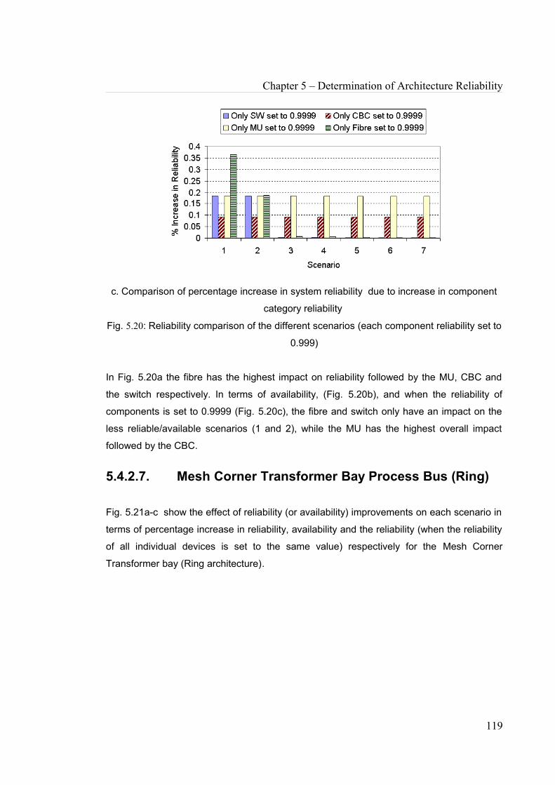
Chapter 5 – Determination of Architecture Reliability
c. Comparison of percentage increase in system reliability due to increase in component
category reliability
Fig. 5.20: Reliability comparison of the different scenarios (each component reliability set to
0.999)
In Fig. 5.20a the fibre has the highest impact on reliability followed by the MU, CBC and
the switch respectively. In terms of availability, (Fig. 5.20b), and when the reliability of
components is set to 0.9999 (Fig. 5.20c), the fibre and switch only have an impact on the
less reliable/available scenarios (1 and 2), while the MU has the highest overall impact
followed by the CBC.
5.4.2.7. Mesh Corner Transformer Bay Process Bus (Ring)
Fig. 5.21a-c show the effect of reliability (or availability) improvements on each scenario in
terms of percentage increase in reliability, availability and the reliability (when the reliability
of all individual devices is set to the same value) respectively for the Mesh Corner
Transformer bay (Ring architecture).
119

Chapter 5 – Determination of Architecture Reliability
a. Comparison of percentage increase in system reliability due to increase in component
category reliability
b. Comparison of percentage increase in system availability due to increase in component
category availability
120

Chapter 5 – Determination of Architecture Reliability
c. Comparison of percentage increase in system reliability due to increase in component
category reliability
Fig. 5.21: Reliability comparison of the different scenarios (each component reliability set to
0.999)
For the Mesh Corner Transformer bay (ring architecture), the fibre (Fig. 5.21a) has the
highest impact on reliability followed by the MU, the switch and the CBC respectively. In
terms of availability, (Fig. 5.21b), the fibre also has the highest impact, but this time the
switch, MU and CBC are tied for the next highest impact on availability. Finally when the
reliability is set to 0.9999, the switch now has the overall highest impact on system
reliability while the CBC, MU and fibre are tied for the next highest impact except Scenario
1, while the fibre has the highest impact.
5.5. SUMMARYIn this chapter, the methodology for evaluating the reliability of the process bus has been
described. A combination of reliability block diagram and event tree modelling methods
have been applied to the proposed double bus bar and mesh corner process bus
architecture scenarios. By using estimated component reliability and cost data, the
reliability, availability of these architecture scenarios have been evaluated and compared.
The impact of certain types of devices on the process bus system reliability has been
studied. It has been seen that in all bays with a star or ring alternative (the mesh corner
mesh corner bay had the sole option of using a star based architecture, but other bays
could incorporate either a star based or ring based architecture) the reliability figure of the
121

Chapter 5 – Determination of Architecture Reliability
most reliable star architecture scenario was higher than that of the most reliable ring based
architecture scenario.
From the sensitivity analysis carried out, it could be seen that the system reliability was
overall most likely to improve when the merging units' reliability was increased, although
there were a few times when the greatest system reliability improvement was due to an
improvement in the reliability of the fibre optic cables, switches or the circuit breaker
controllers. Also it was seen that on most occasions, in the first one or two scenarios when
the system was less reliable/available, the fibre optic cables had a higher impact on system
reliability.
122
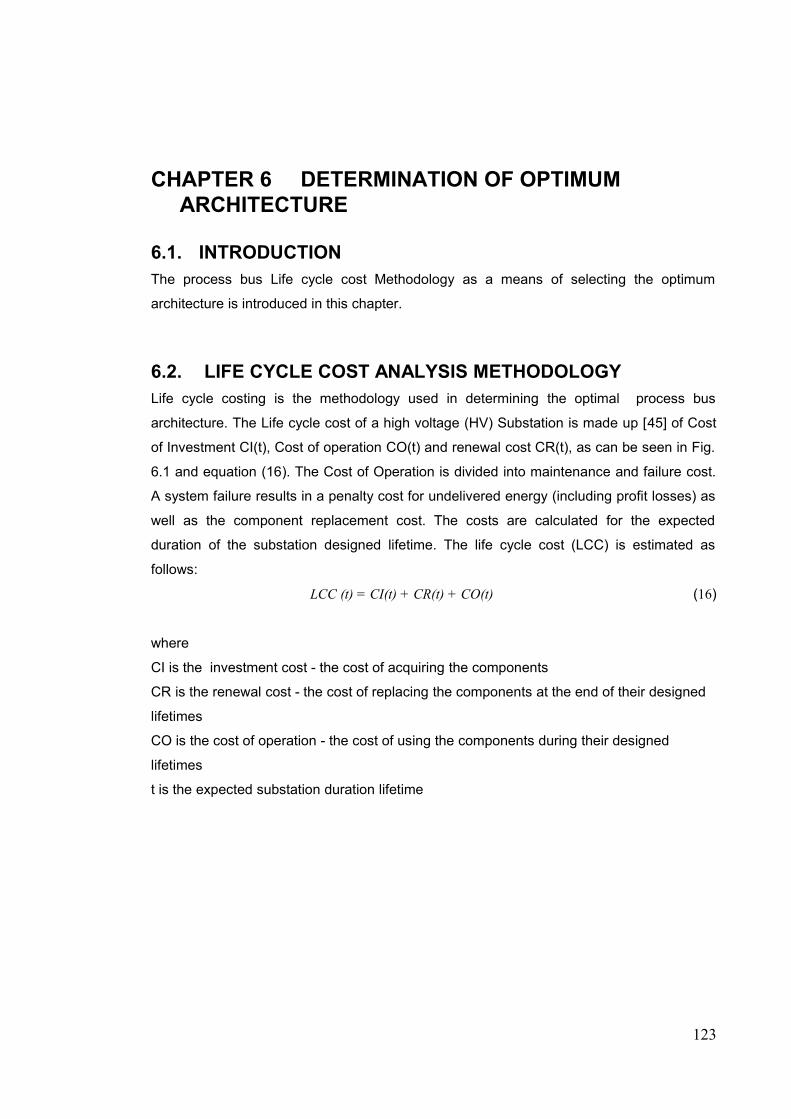
CHAPTER 6 DETERMINATION OF OPTIMUM ARCHITECTURE
6.1. INTRODUCTIONThe process bus Life cycle cost Methodology as a means of selecting the optimum
architecture is introduced in this chapter.
6.2. LIFE CYCLE COST ANALYSIS METHODOLOGYLife cycle costing is the methodology used in determining the optimal process bus
architecture. The Life cycle cost of a high voltage (HV) Substation is made up [45] of Cost
of Investment CI(t), Cost of operation CO(t) and renewal cost CR(t), as can be seen in Fig.
6.1 and equation (16). The Cost of Operation is divided into maintenance and failure cost.
A system failure results in a penalty cost for undelivered energy (including profit losses) as
well as the component replacement cost. The costs are calculated for the expected
duration of the substation designed lifetime. The life cycle cost (LCC) is estimated as
follows:
LCC (t) = CI(t) + CR(t) + CO(t) (16)
where
CI is the investment cost - the cost of acquiring the components
CR is the renewal cost - the cost of replacing the components at the end of their designed
lifetimes
CO is the cost of operation - the cost of using the components during their designed
lifetimes
t is the expected substation duration lifetime
123

Chapter 6 - Determination Of Optimum Architecture
Fig. 6.1: Life Cycle Cost Determination
The investment cost CI is estimated as follows
1 =
n
ii
CI(t) Inv=
∑ (17)
where
n = number of components
Invi = investment cost of the ith component
The renewal cost CR is estimated as follows
CR(t) = 1
n
i ii
Nren Inv=
×∑ (18)
where
n = number of components
Invi = investment cost of the ith component
Nreni = number of times the ith component will be renewed
The operation cost CO is estimated as follows
124

Chapter 6 - Determination Of Optimum Architecture
CO(t) = CM(t) + CF(t) (19)
where
CM = maintenance cost
CF = failure cost
The maintenance cost CM is estimated as follows
CM(t) = 1 1
n m
iji j
C= =
∑ ∑ (20)
where
n = number of components
m = number of maintenance activities for a particular component
Cij = cost of carrying out the jth maintenance activity on the ith component.
The failure cost CF is estimated as follows
CF(t) = CCR(t) + CP(t) (21)
where
CCR = replacement cost - the cost of replacing the components in the event of a failure
CP = penalty cost - the cost of undelivered service as a result of the downtime
The replacement cost CCR is estimated as follows
CCR(t) = 1
* ( )n
iCrepi Fi t
=∑ (22)
where
Crepi = component replacement price
Fi = ith component failure probability
The penalty cost CP is estimated as follows
CP (t) = kp * Fs * tsRep (23)
where
125

Chapter 6 - Determination Of Optimum Architecture
kp = penalty cost factor
Fs = system failure probability
tsRep = system repair time
Some assumptions were made during the estimation of the life cycle cost:
a) All component prices are estimated and relative.
b) All component designed lifetimes are estimated.
c) System repair time tsRep = Period of consideration * system unavailability.
d) Reliability and availability figures are constant during the useful lifetime of the
components.
e) Net Present Value is not considered.
6.3. LIFE CYCLE COST ANALYSIS: CASE STUDYIn the previous chapter, Section 5.3. described how the reliability analysis methodology
was applied to a process bus architecture scenario which served as a case study. The life
cycle cost will now be obtained for that same architecture scenario. Introductory life cycle
cost analyses have also been carried out in [70] and [71].
Some assumptions were made during the estimation of the life cycle cost:
• Maintenance cost is 1% of investment cost
• Maintenance is carried out every 5 years
• Penalty cost factor is applied in factors of 24hrs
• Period under consideration = 40 years
• Maintenance is carried out every 5 years
Table 6.1 shows the component Investment Cost and lifetime estimates.
Table 6.1: Component Investment Cost And Lifetime Data
Device Investment Cost Lifetime (Years)SW 1000 15MU 3500 15
CBC 3500 15
126

Chapter 6 - Determination Of Optimum Architecture
Device Investment Cost Lifetime (Years)FIOC 200 25
Investment cost CI has been estimated based in equation 17 and the results are shown
in Table 6.2
Table 6.2: Investment Cost for Scenario 4
Component Unit Investment
Cost
Quantity Inv[Unit Investment Cost x Quantity]
SW 1000 4 4000MU 3500 6 21000
CBC 3500 3 10500FIOC 200 16 3200
System Investment cost 38700
The renewal cost CR has been estimated based in equation 18 and the results are
shown in Table 6.3.
Table 6.3: Renewal Cost for Scenario 4
Component Npur: No. of times component will be
purchased over 40yr period
Nren: No. of times component will be
renewed[Npur - 1]
Nren x Inv[Nren x Unit
Investment Cost x Quantity]
SW 8 7 28000MU 3 2 42000
CBC 3 2 21000FIOC 2 1 3200
System Renewal cost 94200
The maintenance cost CM has been estimated based in equation 20 and the results are shown in Table 6.4.
Table 6.4: Maintenance Cost for Scenario 4
Component Uman: Unit Maintenance
Cost
Nman: No. of maintenance
activities
Component Maintenance Cost [Quantity x Uman x
Nman]SW 10 0 0MU 35 5 1050
127
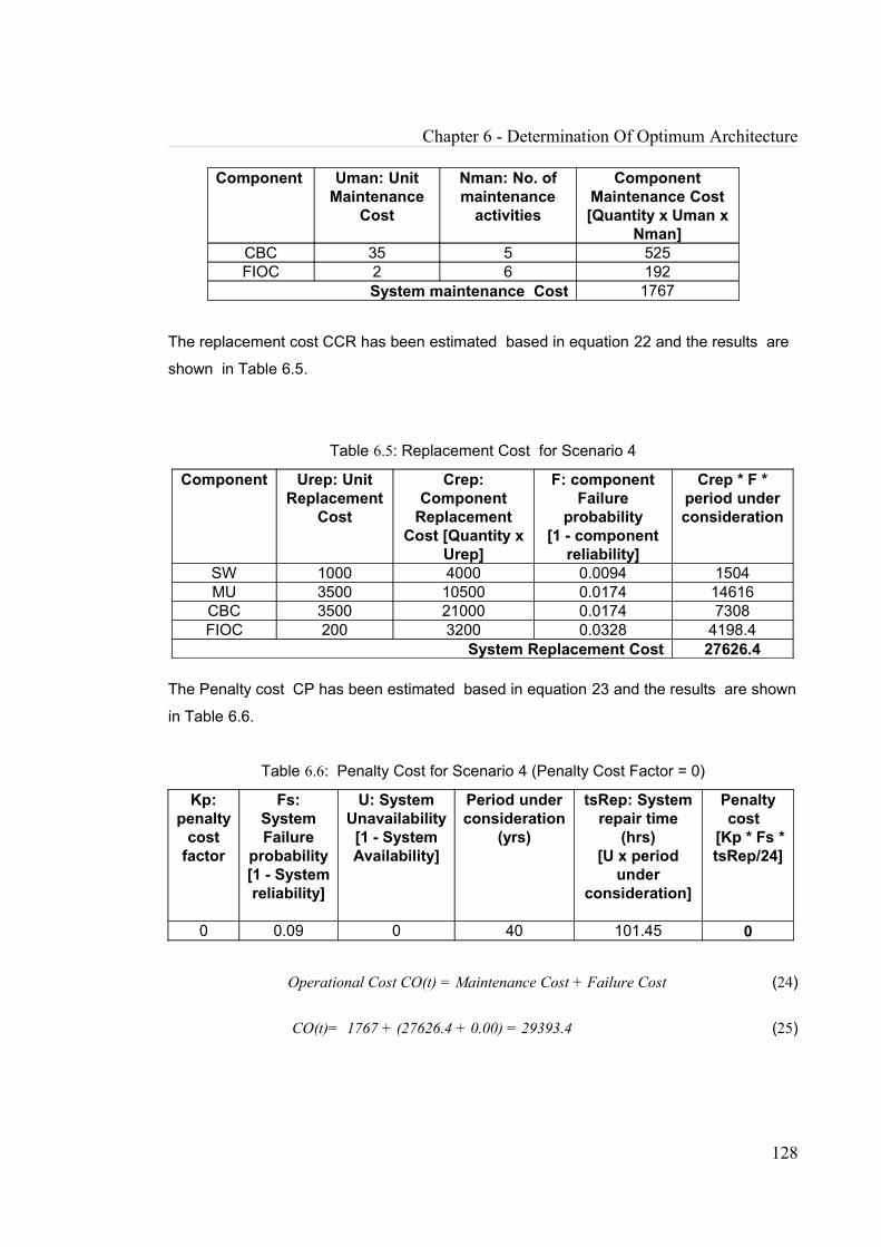
Chapter 6 - Determination Of Optimum Architecture
Component Uman: Unit Maintenance
Cost
Nman: No. of maintenance
activities
Component Maintenance Cost [Quantity x Uman x
Nman]CBC 35 5 525FIOC 2 6 192
System maintenance Cost 1767
The replacement cost CCR has been estimated based in equation 22 and the results are
shown in Table 6.5.
Table 6.5: Replacement Cost for Scenario 4
Component Urep: Unit Replacement
Cost
Crep: Component
Replacement Cost [Quantity x
Urep]
F: component Failure
probability[1 - component
reliability]
Crep * F * period under consideration
SW 1000 4000 0.0094 1504MU 3500 10500 0.0174 14616
CBC 3500 21000 0.0174 7308FIOC 200 3200 0.0328 4198.4
System Replacement Cost 27626.4
The Penalty cost CP has been estimated based in equation 23 and the results are shown
in Table 6.6.
Table 6.6: Penalty Cost for Scenario 4 (Penalty Cost Factor = 0)
Kp: penalty
cost factor
Fs: System Failure
probability[1 - System reliability]
U: System Unavailability
[1 - System Availability]
Period under consideration
(yrs)
tsRep: System repair time
(hrs)[U x period
under consideration]
Penalty cost
[Kp * Fs * tsRep/24]
0 0.09 0 40 101.45 0
Operational Cost CO(t) = Maintenance Cost + Failure Cost (24)
CO(t)= 1767 + (27626.4 + 0.00) = 29393.4 (25)
128

Chapter 6 - Determination Of Optimum Architecture
Life Cycle Cost for Scenario 4 = CI(t) + CR(t) + CO(t)
= 38700 + 94200 + 29393.4 ≈ 162293.4 (26)
Alternatively,Life Cycle Cost for Scenario 4 = CIRM (t) + CF(t) (27)
where CIRM(t) is the sum of CI(t), CR(t) and CM(t)
LCC = ( 38700 + 94200 + 1767) + 27626.4 ≈ 162293.4 (28)
6.4. OPTIMUM ARCHITECTURE: RESULTS AND DISCUSSION The results of the process bus reliability analysis carried on the double bus bar feeder bay
shall now be discussed. As noted in the reliability analysis, the results for the double
busbar feeder, DBB Feeder bay, DBB Bus Section, DBB Bus Coupler and MC Feeder bay
are identical. The effects of device reliability on the process bus system reliability are also
studied. The penalty cost factor is varied and its impact on the life cycle cost and
subsequent optimum process bus architecture reliability is discussed.
6.4.1. Life Cycle Cost Comparison - Double Busbar Feeder Bay (Star)
Table 6.7 shows the (investment, failure and life cycle) costs for each process bus scenario
for the feeder bay, using a penalty cost factor of 0. As the penalty is 0, the resulting failure
cost is low and it can be seen (Fig. 6.2) that the failure cost has little or no impact on the
life cycle cost and naturally the life cycle cost will increase as reliability increases. In this
situation the optimum will automatically be the scenario which had the lowest investment
cost, which is Scenario 1. The optimum process bus architecture reliability is 0.797.
Table 6.7: Reliability And Cost Data For Mesh Corner Bay Process Bus Scenarios
(Penalty Cost Factor = 0)
129
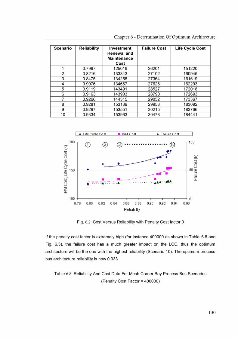
Chapter 6 - Determination Of Optimum Architecture
Scenario Reliability Investment Renewal andMaintenance
Cost
Failure Cost Life Cycle Cost
1 0.7967 125019 26201 1512202 0.8216 133843 27102 1609453 0.8475 134255 27364 1616194 0.9076 134667 27626 1622935 0.9119 143491 28527 1720186 0.9163 143903 28790 1726937 0.9266 144315 29052 1733678 0.9281 153139 29953 1830929 0.9297 153551 30215 18376610 0.9334 153963 30478 184441
Fig. 6.2: Cost Versus Reliability with Penalty Cost factor 0
If the penalty cost factor is extremely high (for instance 400000 as shown in Table 6.8 and
Fig. 6.3), the failure cost has a much greater impact on the LCC, thus the optimum
architecture will be the one with the highest reliability (Scenario 10). The optimum process
bus architecture reliability is now 0.933
Table 6.8: Reliability And Cost Data For Mesh Corner Bay Process Bus Scenarios
(Penalty Cost Factor = 400000)
130
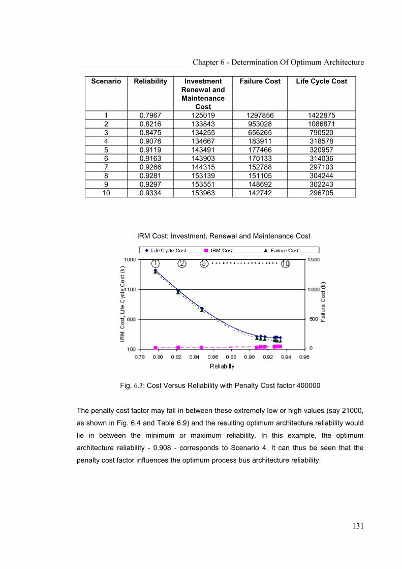
Chapter 6 - Determination Of Optimum Architecture
Scenario Reliability Investment Renewal andMaintenance
Cost
Failure Cost Life Cycle Cost
1 0.7967 125019 1297856 14228752 0.8216 133843 953028 10868713 0.8475 134255 656265 7905204 0.9076 134667 183911 3185785 0.9119 143491 177466 3209576 0.9163 143903 170133 3140367 0.9266 144315 152788 2971038 0.9281 153139 151105 3042449 0.9297 153551 148692 30224310 0.9334 153963 142742 296705
IRM Cost: Investment, Renewal and Maintenance Cost
Fig. 6.3: Cost Versus Reliability with Penalty Cost factor 400000
The penalty cost factor may fall in between these extremely low or high values (say 21000,
as shown in Fig. 6.4 and Table 6.9) and the resulting optimum architecture reliability would
lie in between the minimum or maximum reliability. In this example, the optimum
architecture reliability - 0.908 - corresponds to Scenario 4. It can thus be seen that the
penalty cost factor influences the optimum process bus architecture reliability.
131
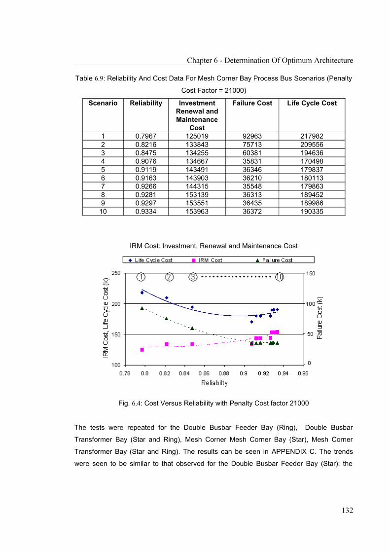
Chapter 6 - Determination Of Optimum Architecture
Table 6.9: Reliability And Cost Data For Mesh Corner Bay Process Bus Scenarios (Penalty
Cost Factor = 21000)
Scenario Reliability Investment Renewal andMaintenance
Cost
Failure Cost Life Cycle Cost
1 0.7967 125019 92963 2179822 0.8216 133843 75713 2095563 0.8475 134255 60381 1946364 0.9076 134667 35831 1704985 0.9119 143491 36346 1798376 0.9163 143903 36210 1801137 0.9266 144315 35548 1798638 0.9281 153139 36313 1894529 0.9297 153551 36435 18998610 0.9334 153963 36372 190335
IRM Cost: Investment, Renewal and Maintenance Cost
Fig. 6.4: Cost Versus Reliability with Penalty Cost factor 21000
The tests were repeated for the Double Busbar Feeder Bay (Ring), Double Busbar
Transformer Bay (Star and Ring), Mesh Corner Mesh Corner Bay (Star), Mesh Corner
Transformer Bay (Star and Ring). The results can be seen in APPENDIX C. The trends
were seen to be similar to that observed for the Double Busbar Feeder Bay (Star): the
132

Chapter 6 - Determination Of Optimum Architecture
higher the penalty cost factor, the higher the impact that failure cost has on the Life cycle
cost. In addition, the higher the penalty cost factor, the higher the optimum process bus
architecture scenario reliability.
6.5. SUMMARYIn this chapter the process bus Life cycle cost methodology has been introduced and
applied to different process bus architecture scenarios. It has been shown how Life Cycle
Costing can be used as an optimum process bus architecture selection methodology. As
the quantities which have been used in determining the Life Cycle Cost are estimates, it
may be better utilized as one of many tools that can be used in the decision making
process. It has also been suggested that the reliability increases as the architecture
becomes more redundant. It is important to note that this is not always the case, as there
would be occasions where increasing the redundancy may adversely affect reliability.
There also has to be a good balance between redundancy and simplicity so that in an
effort to make the system more reliable by introducing redundancy, the system does not
end up becoming too complex.
It has also been shown how the penalty cost factor (for outage periods) influences the
optimum process bus architecture reliability. It was seen that when the penalty cost factor
was extremely high, then the optimum architecture reliability was that of the most reliable
architecture. When the penalty was extremely low, the optimum architecture reliability was
that of the least reliable architecture. This has shown that although it is always desirable to
select the most reliable architecture, that architecture may not be the optimum one when
other factors (such as the penalty for outage) are taken into account.
133
CHAPTER 7 DESIGN AND IMPLEMENTATION OF MERGING UNIT PERFORMANCE TEST BED
7.1. INTRODUCTIONThere are a number of prototype and commercially available merging units currently
available. Merging units from different manufacturers though capable of producing
Ethernet packets that are IEC 61850-compliant, may vary in their performance
characteristics, such as delay, dynamic range and conversion error. Presently there is no
particular MU specification; hence, there is a need to test MU performance characteristics,
as this may be useful in promoting interoperability.
In this chapter, the design and implementation of a MU performance test bed shall be
discussed. This test bed can be used for carrying out performance tests such as the
sampled values recovery test, process delay test, GPS Timestamping delay test, arrival
time uniformity test, conversion error test and filter performance assessment. It is able to
test up to 4 MUs simultaneously.
7.2. PROTOTYPE AND COMMERCIALLY AVAILABLE MERGING UNITS
7.2.1. Locamation Figs. 7.1 and 7.2 illustrate how the Locamation MU606 Merging unit functions as an
Analogue Merging Unit (AMU) and Digital Merging Unit (DMU) [72].
Analogue Merging Unit (AMU) functionCurrent and Voltage transformers are connected to a Current Interface Module (CIM) and
Voltage Interface Module (VIM) respectively. The CIM and VIM deliver the raw data of
measured current and voltage samples respectively to the MU. The resulting sampled
values (based on IEC 61850-9-2 LE) are then sent to the external Protection device by
134

Chapter 7 - Design and Implementation of Merging Unit Performance Test Bed
using 100Base-FX (optical fibre based) Ethernet communication. The merging unit can be
synchronised by an external GPS system based on Pulse per second (PPS) signals.
Fig. 7.1: Locamation Arrangement - Analogue Merging Unit Function
Digital Merging Unit (DMU)GOOSE control messages are sent from the external Protection device to the MU, which is
then able to trip a circuit breaker via the Breaker Interface Module (BIM).
Fig. 7.2: Locamation Arrangement - Digital Merging Unit Function
7.2.2. GE Fig. 7.3 shows the Process Bus system Architecture for the GE HardFiber solution [63].
The Bricks convert copper signals to and from digital optical signals. Copper signals
include CTs, VTs, contact inputs, and contact outputs. Bricks implement the concept of an
IEC 61850 merging unit, expanded to optically connect relays with all types of input and
output signals in the switchyard, not just instrument transformers. A relay can also work
with duplicated bricks. The Brick receives a GOOSE Ethernet frame sent by a relay. It then
uses the GOOSE message to sample the measured (CT, VT) values. Each brick can work
with different relays.
135

Chapter 7 - Design and Implementation of Merging Unit Performance Test Bed
STATIONLAN
RELAY 1 RELAY 2 RELAY 3
21 65
CROSSCONNECTPANEL 1
CROSSCONNECTPANEL 2
3
4
BrickL-1
CT-1 CT-2CB-1 CT-3 CB-2
VT-1
CT-4
Outdoor Fibrecables
Indoor Fibrecables
Control House
Fig. 7.3: GE Process Bus Architecture
Copper cables (not shown in Fig. 7.3) make the connections between the copper
terminals inside the power equipment to the Bricks mounted in the switchyard, typically on
the outside of the equipment. Outdoor fibre cables make the optical connection between
the Bricks in the switchyard and the Cross Connect Panels in the control house. They are
also used to supply power to the Brick internal electronics via an embedded copper wire
pair. Cross Connect Panels are where individual fibres in the outdoor cables are
patchcorded to individual fibres of indoor cables, completing the associations between the
relays and the Bricks for a given station topology. Also, the panels distribute DC to the
Bricks via the outdoor fibre cables. Indoor fibre cables make the optical connection
between the process bus ports of the relays and the Cross Connect Panel.
The GE HardFiber System does not require external clocks. Components called Process
Cards convert Brick digital optical signals so they can be used by GE relays.
7.2.3. Siemens A prototype Siemens merging unit setup [73] is shown in Fig. 7.4. A conventional current
transformer (CT) and a conventional voltage transformer (VT) are connected to the
136

Chapter 7 - Design and Implementation of Merging Unit Performance Test Bed
merging unit. An interphase open/Interphase close (IPO/IPC) relay is connected to a circuit
breaker IED. The merging unit and circuit breaker controller are connected via a process
bus to a feeder protection IED and Gateway switch. A data logger is connected to the
process bus via the gateway switch. The setup also incorporates an isolation scheme. If
procedures such as testing, maintenance or commissioning need to be carried out, an
isolation box is used in conjunction with the merging unit. The merging unit can be
synchronised by an external GPS system using fibre-optic based Pulse per second (PPS)
signals.
Fig. 7.4: Siemens Merging Unit Set-Up
7.2.4. MitsubishiThe Mitsubishi MMU-H100A prototype merging unit [74] is shown in Fig. 7.5. A current
transformer (CT) and a voltage transformer (VT) are connected to the merging unit which
broadcasts the output Ethernet packets according to IEC 61850 9-2 LE. The merging unit
can be synchronised by an external GPS system based on Inter-Range Instrumentation
Group B (IRIG -B) signals.
137
CT VT IPO/IPCRELAY
ISOLATION BOXNORMAL
MERGING UNIT
IEC 61850 9-2 LE BUS
FEEDERPROTECTION
DATALOGGER
9-2 GATEWAYSWITCH
CIRCUIT BREAKER IED

Chapter 7 - Design and Implementation of Merging Unit Performance Test Bed
Fig. 7.5: Mitsubishi Merging Unit
7.2.5. AlstomThe Alstom COSI-NXMU commercially available merging unit is shown in Fig. 7.6 [75]. It
accepts optical CT and analogue VT signals and is able to sample signals based on 80
and 256 samples/cycle. The output can be sent to metering and protection devices.
Fig. 7.6: Mitsubishi Merging Unit
There is also the Alstom IMU prototype merging unit which accepts conventional CT and
VT signals (Fig. 7.7).
Fig. 7.7: Mitsubishi Merging Unit
7.2.6. ABBABB has 2 different types of merging units. They are the Merging unit for Measurement
(CP-MUM) [67] and the Merging unit for Protection (CP-MUP) [68]. These merging units
are designed to be used in conjunction with an ABB product, ELK-CP3, which is a
Combined Non-Conventional Instrument Transformer (NCIT) for current and voltage.
Figure 7.8 shows how the ELK-CP3 is connected to 2 merging units for Metering thus
providing 2 independent measuring systems. A CP-MUM has one sensor input (one sensor
138

Chapter 7 - Design and Implementation of Merging Unit Performance Test Bed
input means three individual phases). It provides 1 Pulse Per Second (PPS) output. The
Ethernet output stream from the merging unit is IEC 61850 9-1 transmitted using 10BaseT.
Fig. 7.8: ABB Redundant system for revenue metering using Merging unit for Metering
(CP-MUM)
The ABB Merging unit for Protection (CP-MUP) (Fig. 7.9) is a Merging unit with three
sensor inputs, five Ethernet ports based on IEC 61850 9-2 LE and a freely configurable
Ethernet switch. It can be synchronized by a 1 PPS signal and provides 5 1PPS outputs. It
provides 5 Ethernet streams transmitted using 100BaseFX.
Fig. 7.9: ABB Merging unit for Protection(CP-MUP)
139

Chapter 7 - Design and Implementation of Merging Unit Performance Test Bed
7.3. MERGING UNIT PERFORMANCE TEST BED The MU test bed basic layout is illustrated in Fig. 7.10 and introductory descriptions of the
test bed have been provided in [76] and [77]. A Real Time Digital Simulator (RTDS) shall
be used to model instrument transformers within a substation. The RTDS output is then
amplified using an Omicron amplifier, producing analogue signals which mirror the voltage
and current signals from instrument transformers. Further amplification is required by an
isolation amplifier before the signal is fed to the DAS. Throughout the chapter, voltage
signals will be mentioned more often, but a similar analysis would apply to current signals.
Two analogue voltage signals of equal magnitude, phase and frequency shall be
simultaneously fed into the merging unit (MU), and the National Instruments Digital
Acquisition System (DAS). The MU samples its input analogue voltage signal and sends
the output in the form of Ethernet packets (also referred to as Ethernet frames). The DAS
also samples its analogue voltage signals. The sampling of the MU and DAS is
synchronized by GPS signals connected to both of them. A PC is able to capture the output
from the A/D converter and also receive the Ethernet packets from the MU via an Ethernet
Switch (not shown). The output is stored and analysed. The MU test bed is able to test up
to 4 MUs simultaneously. The MU generic Test bed block diagram is shown in Fig. 7.11.
Fig. 7.10: Merging unit Test Bed Layout
140

Chapter 7 - Design and Implementation of Merging Unit Performance Test Bed
RTDS: Real Time Digital SimulatorDAS: National Instruments Digital Acquisition SystemNMC: Endace Network Monitoring CardPC: ComputerMU: Merging UnitIs Amp: Isolation Amplifier
Fig. 7.11: Merging Unit Test Bed Block Diagram
7.3.1. Real Time Digital Simulator (RTDS)RTDS software is used to model the circuits which provide the current and voltage injection
signals for the merging unit. The RTDS device is shown below in Fig. 7.12.
Fig. 7.12: RTDS
For instance RTDS can be used to model one of the mesh corner substations highlighted
in Fig. 7.13a. The mesh corner substation is made up of 3 circuit breakers (CB1, CB4, and
CB5) and a transformer (T1). T1 is a 400kV/132kV step-down transformer, CB5 is a 132kV
141
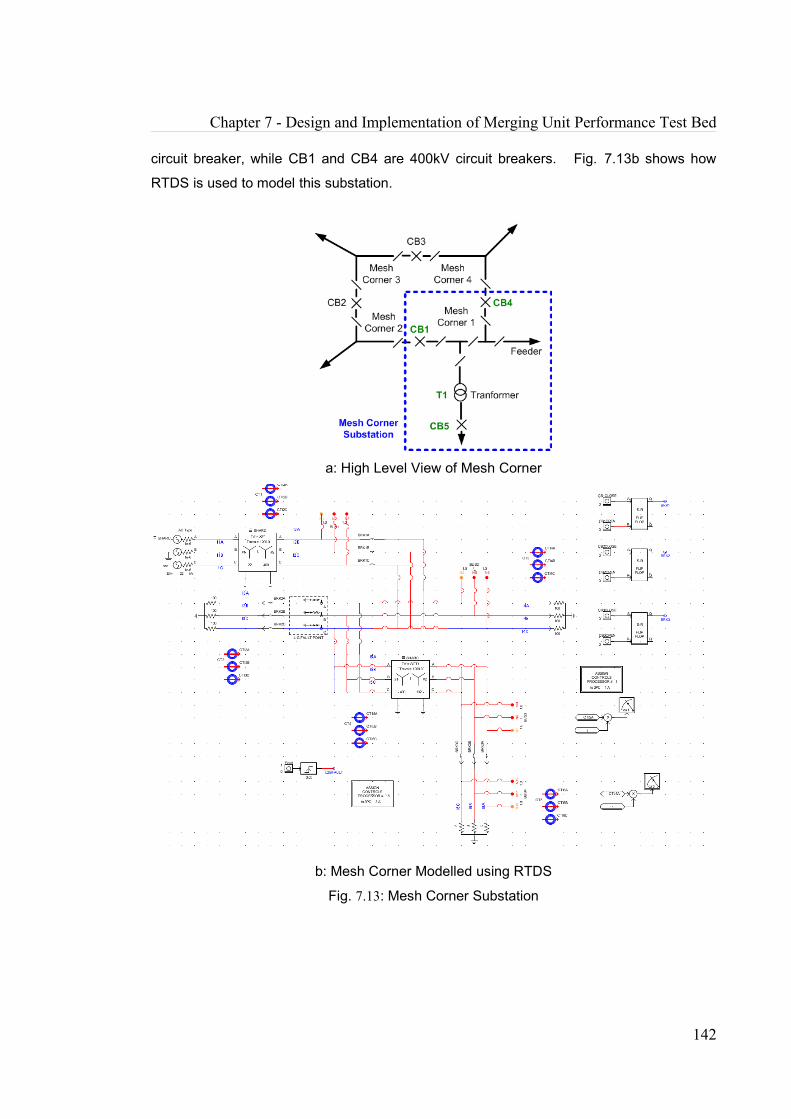
Chapter 7 - Design and Implementation of Merging Unit Performance Test Bed
circuit breaker, while CB1 and CB4 are 400kV circuit breakers. Fig. 7.13b shows how
RTDS is used to model this substation.
a: High Level View of Mesh Corner
b: Mesh Corner Modelled using RTDS
Fig. 7.13: Mesh Corner Substation
142

Chapter 7 - Design and Implementation of Merging Unit Performance Test Bed
7.3.2. Amplifiers – Omicron Amplifier and Isolation AmplifierThe Omicron amplifier (shown in Fig 7.14a together with an oscilloscope measuring its
output voltage) amplifies the analogue signals produced by RTDS and produces output
analogue signals that mirror the output of voltage (and current) instrument transformers.
This output is then simultaneously fed to the MU directly and to the Digital Acquisition
System via the Isolation Amplifier (Fig. 7.14b). The Omicron analogue output is scaled
down with the isolation amplifier before it is fed to the DAS.
a. Omicron Amplifier b. Isolation Amplifier
Fig. 7.14: Amplifiers used for merging unit Test Bed
The Omicron amplifier produces 50V for every 1V input it receives, while it produces 5A for
every 1V input it receives. The isolation amplifier provides 20V for every 1V input, and 1V
for every 1A input it receives from the Omicron amplifier. The Digital Acquisition System
(DAS) samples the analogue voltage outputs from the isolation amplifier and then rescales
the digital output so that this output represents the original voltage (and current) signals
produced by the Omicron Amplifier. The input and output voltages are measured using the
oscilloscope.
7.3.2.1. Isolation Amplifier CalibrationThe methodology for the calibration of the isolation amplifier is as follows. For the current
calibration, 2A(RMS) signals ranging from 50Hz to 5kHz are fed into the current ports of
the amplifier. The input current is measured by:
143

Chapter 7 - Design and Implementation of Merging Unit Performance Test Bed
a) using a clamp placed across the incoming input cable (this cable is connected to
the incoming input port. The other input cable, the outgoing input cable, is connected to the
outgoing input port). The output of the current clamp is a voltage output which is measured
by using the oscilloscope;
b) using an ammeter as part of the connections;
c) measuring the voltage across the current input ports, using the oscilloscope.
The output of the amplifier is a voltage signal which has a 1:1 ratio with the current input.
This output is measured using an oscilloscope.
For the voltage calibration, 6V (RMS) signals are fed into the voltage ports of the amplifier.
Only the voltage across the input voltage ports are used for comparison with the output
voltage (measured using the oscilloscope).
Tables 7.1 and 7.2 show the isolation amplifier calibration data for the voltage and current.
Table 7.1: Isolation Amplifier Current Calibration
Freq(Hz)
Input current
(ammeter) (A)
Input voltage(clamp)
(mV)
VIPR = Input
voltage(parallel resistor across input
terminals)
(mV)
Input voltage (parallel resistor)normalized/converted to Amps (A)
(VIPR x 2/60)
Output voltage
(oscilloscope)
converted to Amps
(1V represents
1A)
Current Ratio
Error (%)
50 2 201 60 2 2.02 1.010 11000 1.96 205 460 2 2.02 1.010 12000 1.89 199 452 1.965 1.99 1.013 1.2615000 1.46 164 390 1.696 1.70 1.003 0.200
Table 7.2: Isolation Amplifier Voltage Calibration
144
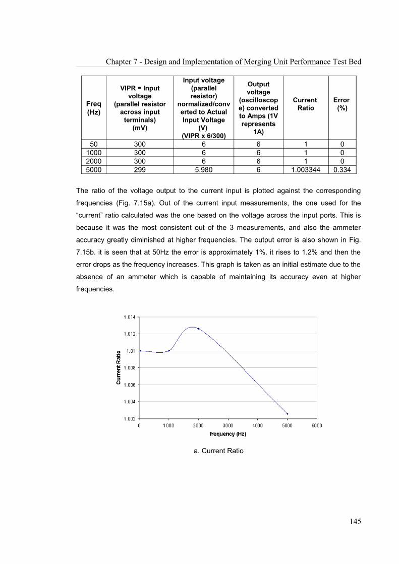
Chapter 7 - Design and Implementation of Merging Unit Performance Test Bed
Freq(Hz)
VIPR = Input voltage
(parallel resistor across input
terminals)(mV)
Input voltage (parallel resistor)
normalized/converted to Actual Input Voltage
(V) (VIPR x 6/300)
Output voltage
(oscilloscope) converted to Amps (1V represents
1A)
Current Ratio
Error (%)
50 300 6 6 1 01000 300 6 6 1 02000 300 6 6 1 05000 299 5.980 6 1.003344 0.334
The ratio of the voltage output to the current input is plotted against the corresponding
frequencies (Fig. 7.15a). Out of the current input measurements, the one used for the
“current” ratio calculated was the one based on the voltage across the input ports. This is
because it was the most consistent out of the 3 measurements, and also the ammeter
accuracy greatly diminished at higher frequencies. The output error is also shown in Fig.
7.15b. it is seen that at 50Hz the error is approximately 1%. it rises to 1.2% and then the
error drops as the frequency increases. This graph is taken as an initial estimate due to the
absence of an ammeter which is capable of maintaining its accuracy even at higher
frequencies.
a. Current Ratio
145

Chapter 7 - Design and Implementation of Merging Unit Performance Test Bed
b. Current Error
Fig. 7.15: Calibration Results for Isolation Amplifier (2A injection)
The voltage ratio and error can be seen in Fig. 7.16. The error is seen to be approximately
zero percent while it gets to 0.33% when the input frequency is 5kHz.
a. Voltage Ratio
146
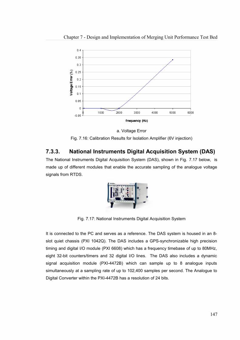
Chapter 7 - Design and Implementation of Merging Unit Performance Test Bed
a. Voltage Error
Fig. 7.16: Calibration Results for Isolation Amplifier (6V injection)
7.3.3. National Instruments Digital Acquisition System (DAS)The National Instruments Digital Acquisition System (DAS), shown in Fig. 7.17 below, is
made up of different modules that enable the accurate sampling of the analogue voltage
signals from RTDS.
Fig. 7.17: National Instruments Digital Acquisition System
It is connected to the PC and serves as a reference. The DAS system is housed in an 8-
slot quiet chassis (PXI 1042Q). The DAS includes a GPS-synchronizable high precision
timing and digital I/O module (PXI 6608) which has a frequency timebase of up to 80MHz,
eight 32-bit counters/timers and 32 digital I/O lines. The DAS also includes a dynamic
signal acquisition module (PXI-4472B) which can sample up to 8 analogue inputs
simultaneously at a sampling rate of up to 102,400 samples per second. The Analogue to
Digital Converter within the PXI-4472B has a resolution of 24 bits.
147

Chapter 7 - Design and Implementation of Merging Unit Performance Test Bed
7.3.4. Endace Network Monitoring Card (NMC)The Endace Network Monitoring Card (NMC) shown in Fig. 7.18 below, timestamps the
arrival of the incoming Ethernet packets sent from the MU. It has a resolution of 7.5ns.
Fig. 7.18: Endace Network Monitoring Card (NMC)
It is installed in the PC. It provides precise packet stamping, 100% packet capture
capability and can be synchronized with a GPS.
7.3.5. Personal Computer (PC)The DAS is connected to the Personal Computer (PC). The NMC is installed in the PC. A
program running on the PC has been developed based on Wireshark, (network analysis
software). At the desired time, the program triggers the simultaneous capture of Ethernet
packets sent by the MU, and the sampling of the analogue signals by the DAS saves and
analyses the stored data.
7.3.6. Fibre optic Ethernet SwitchThe GE MultiLink Fibre Optic Ethernet Switch illustrated in Fig. 7.19 below has fibre optic
ports and RJ45 Ethernet ports.
Fig. 7.19: GE Fibre Optic Ethernet Switch
148
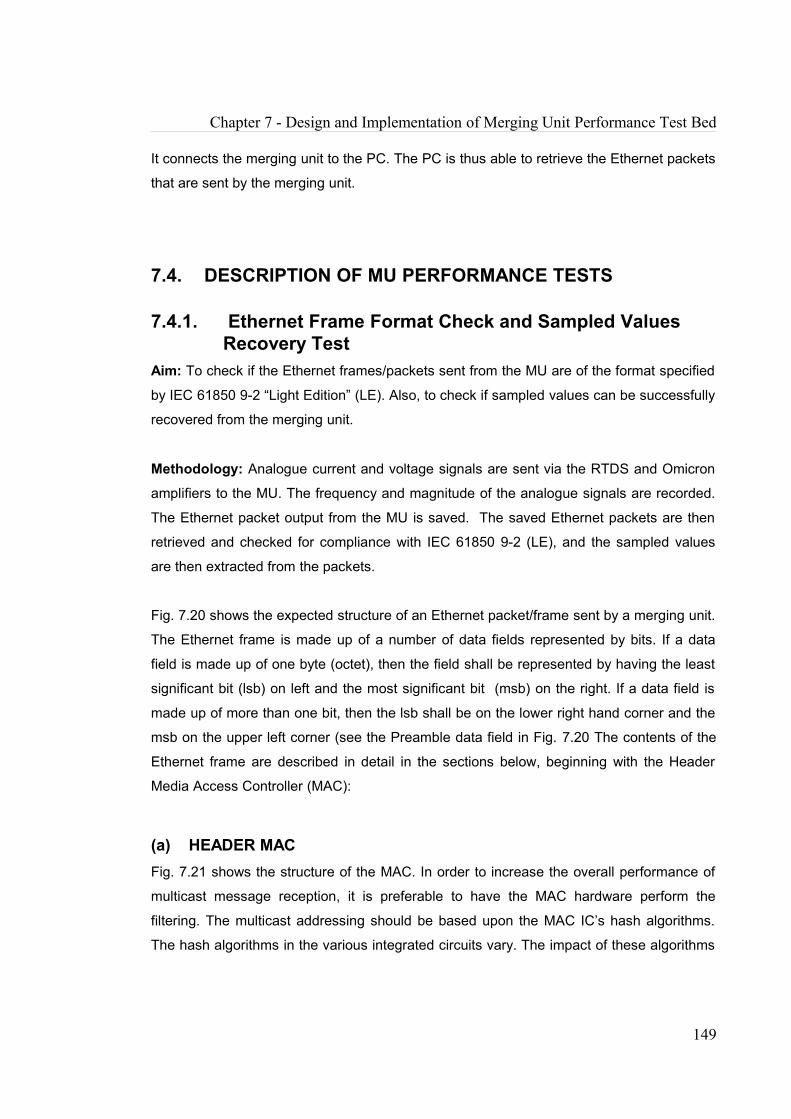
Chapter 7 - Design and Implementation of Merging Unit Performance Test Bed
It connects the merging unit to the PC. The PC is thus able to retrieve the Ethernet packets
that are sent by the merging unit.
7.4. DESCRIPTION OF MU PERFORMANCE TESTS
7.4.1. Ethernet Frame Format Check and Sampled Values Recovery Test
Aim: To check if the Ethernet frames/packets sent from the MU are of the format specified
by IEC 61850 9-2 “Light Edition” (LE). Also, to check if sampled values can be successfully
recovered from the merging unit.
Methodology: Analogue current and voltage signals are sent via the RTDS and Omicron
amplifiers to the MU. The frequency and magnitude of the analogue signals are recorded.
The Ethernet packet output from the MU is saved. The saved Ethernet packets are then
retrieved and checked for compliance with IEC 61850 9-2 (LE), and the sampled values
are then extracted from the packets.
Fig. 7.20 shows the expected structure of an Ethernet packet/frame sent by a merging unit.
The Ethernet frame is made up of a number of data fields represented by bits. If a data
field is made up of one byte (octet), then the field shall be represented by having the least
significant bit (lsb) on left and the most significant bit (msb) on the right. If a data field is
made up of more than one bit, then the lsb shall be on the lower right hand corner and the
msb on the upper left corner (see the Preamble data field in Fig. 7.20 The contents of the
Ethernet frame are described in detail in the sections below, beginning with the Header
Media Access Controller (MAC):
(a) HEADER MAC Fig. 7.21 shows the structure of the MAC. In order to increase the overall performance of
multicast message reception, it is preferable to have the MAC hardware perform the
filtering. The multicast addressing should be based upon the MAC IC’s hash algorithms.
The hash algorithms in the various integrated circuits vary. The impact of these algorithms
149

Chapter 7 - Design and Implementation of Merging Unit Performance Test Bed
need to evaluated when destination multicast addresses are being assigned. A unique
ISO/IEC 8802-3 source address shall be used. One recommended addressing scheme for
the destination address is outlined below:
The multicast addresses (octet string of size 6) used will have the following structure:
• The first three octets are assigned by IEEE with 01-0C-CD.
• The fourth octet will be 04 for multicast sampled values.
• The last two octets will be used as individual addresses assigned by range 00-00 to
01-FF.
Octets123456789
101112131415161718192021222324252627282930313233343536......
8 7 6 5 4 3 2 1
Preamble
Start of Frame
HeaderMAC
Priority Tagged
EthertypePDU
Pad bytes if neededFrame check
sequence
lsb
msb
Octets123456789
101112
8 7 6 5 4 3 2 1
HeaderMAC
Destination Address
Source Address
Fig. 7.20: Contents of an Ethernet Frame Fig. 7.21: Structure of the Header MAC
(b) PRIORITY TAGGING/VIRTUAL LAN
150
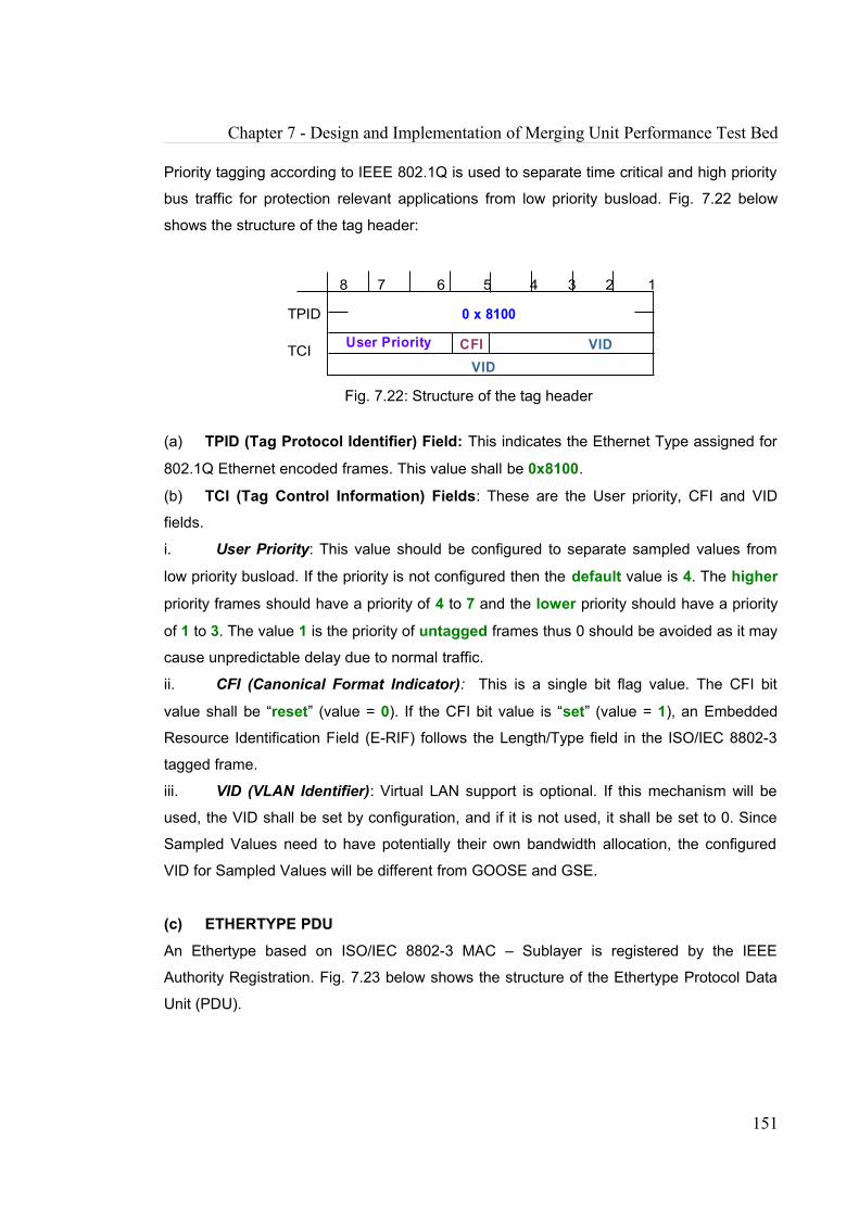
Chapter 7 - Design and Implementation of Merging Unit Performance Test Bed
Priority tagging according to IEEE 802.1Q is used to separate time critical and high priority
bus traffic for protection relevant applications from low priority busload. Fig. 7.22 below
shows the structure of the tag header:
8 7 6 5 4 3 2 1
TPID 0 x 8100
VIDTCI VIDCFIUser Priority
Fig. 7.22: Structure of the tag header
(a) TPID (Tag Protocol Identifier) Field: This indicates the Ethernet Type assigned for
802.1Q Ethernet encoded frames. This value shall be 0x8100.
(b) TCI (Tag Control Information) Fields: These are the User priority, CFI and VID
fields.
i. User Priority: This value should be configured to separate sampled values from
low priority busload. If the priority is not configured then the default value is 4. The higher
priority frames should have a priority of 4 to 7 and the lower priority should have a priority
of 1 to 3. The value 1 is the priority of untagged frames thus 0 should be avoided as it may
cause unpredictable delay due to normal traffic.
ii. CFI (Canonical Format Indicator): This is a single bit flag value. The CFI bit
value shall be “reset” (value = 0). If the CFI bit value is “set” (value = 1), an Embedded
Resource Identification Field (E-RIF) follows the Length/Type field in the ISO/IEC 8802-3
tagged frame.
iii. VID (VLAN Identifier): Virtual LAN support is optional. If this mechanism will be
used, the VID shall be set by configuration, and if it is not used, it shall be set to 0. Since
Sampled Values need to have potentially their own bandwidth allocation, the configured
VID for Sampled Values will be different from GOOSE and GSE.
(c) ETHERTYPE PDU
An Ethertype based on ISO/IEC 8802-3 MAC – Sublayer is registered by the IEEE
Authority Registration. Fig. 7.23 below shows the structure of the Ethertype Protocol Data
Unit (PDU).
151

Chapter 7 - Design and Implementation of Merging Unit Performance Test Bed
Octets123456789
10
. . . . . . . . .m + 10
Ethertype
APDU
APPIDLength
Reserved 1Reserved 2
Eth
erty
pe
PDU
Fig. 7.23: Structure of the Ethertype PDU
i. Ethertype - The registered Ethertype value is 88-BA (hexadecimal). The sampled
analogue value buffer update is directly mapped to the reserved Ethertype and the
Ethertype PDU.
ii. APPID (Application identifier): The APPID is used to select ISO/IEC 8802-3
frames containing sampled value (SV) messages and to distinguish the application
association. The value of APPID is the combination of the APPID type, defined as the two
most significant bits of the value (“01” for sampled values), and the actual ID. The reserved
value range for sampled values is 0x4000 to 0x7FFF. If no APPID is configured, the
default value shall be 0x4000. The default value is reserved to indicate lack of
configuration. It is strongly recommended to have unique, source orientated SV APPID
within a system. This should be enforced by the configuration system.
iii. Length: This is the number of octets including the Ethertype PDU header starting
at APPID, and the length of the APDU (Application Protocol Data Unit). Therefore, the
value of Length shall be m+8, where m is the length of the APDU and m is less than
1492. Frames with inconsistent or invalid length field shall be discarded.
iv. Reserved1, Reserved2: These are reserved for future standardized applications
and shall be set to 0 as default.
v. APDU (Application Protocol Data Unit): An APDU is made up of one or more
Application Service Data Units (ASDUs). It is possible to concatenate “n” number of
ASDUs into one APDU before the APDU is posted into the transmission buffer. The
number of ASDUs which will be concatenated into one ASDU is defined with a
configuration parameter and related to the sample rate. The concatenation of ASDUs is not
dynamically changeable in order to reduce the implementation complexity. When
152
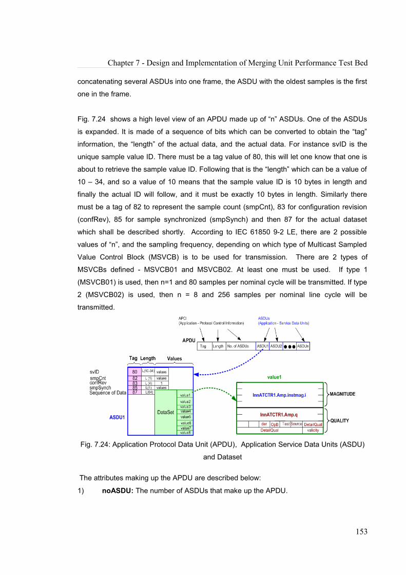
Chapter 7 - Design and Implementation of Merging Unit Performance Test Bed
concatenating several ASDUs into one frame, the ASDU with the oldest samples is the first
one in the frame.
Fig. 7.24 shows a high level view of an APDU made up of “n” ASDUs. One of the ASDUs
is expanded. It is made of a sequence of bits which can be converted to obtain the “tag”
information, the “length” of the actual data, and the actual data. For instance svID is the
unique sample value ID. There must be a tag value of 80, this will let one know that one is
about to retrieve the sample value ID. Following that is the “length” which can be a value of
10 – 34, and so a value of 10 means that the sample value ID is 10 bytes in length and
finally the actual ID will follow, and it must be exactly 10 bytes in length. Similarly there
must be a tag of 82 to represent the sample count (smpCnt), 83 for configuration revision
(confRev), 85 for sample synchronized (smpSynch) and then 87 for the actual dataset
which shall be described shortly. According to IEC 61850 9-2 LE, there are 2 possible
values of “n”, and the sampling frequency, depending on which type of Multicast Sampled
Value Control Block (MSVCB) is to be used for transmission. There are 2 types of
MSVCBs defined - MSVCB01 and MSVCB02. At least one must be used. If type 1
(MSVCB01) is used, then n=1 and 80 samples per nominal cycle will be transmitted. If type
2 (MSVCB02) is used, then n = 8 and 256 samples per nominal line cycle will be
transmitted.
Fig. 7.24: Application Protocol Data Unit (APDU), Application Service Data Units (ASDU)
and Dataset
The attributes making up the APDU are described below:
1) noASDU: The number of ASDUs that make up the APDU.
153

Chapter 7 - Design and Implementation of Merging Unit Performance Test Bed
2) svID: The attribute svID shall be a unique identification of the sampled value buffer
related to the update of the sampled values.
3) smpCnt: The parameter smpCnt contains the values of a counter, which is
incremented each time a new sample of the analogue value is taken. The sample values
shall be kept in the right order. If the counter is used to indicate time consistency of various
sampled values, the counter shall be reset by an external synchronization event.
4) ConfRev: The attribute ConfRev represents a count of the number of times that the
datset configuration has been changed. However, the datasets used for the transmission
of sampled values have been defined. The MSVCB has also been defined. Hence, this
attribute has a fixed value of 1.
5) smpSynch: The parameter smpSynch indicates whether the sampled analogue
values sent by the MSVCB are synchronized by clock signals. It shall be set to TRUE if the
merging unit is synchronized.
6) DataSet: Within each ASDU is a dataset. The dataset contains the data to be
transmitted. The name of the dataset for IEC 61850 9-2 LE is “PhsMeas1”. The section
“value1” within the “PhsMeas1” dataset is expanded in Fig. 7.24. The expected format of
this DataSet is shown in Fig. 7.25 and the relevant values are shown in the Table 1. The
MX attributes are listed in Table 7.5.
Fig. 7.25: PhsMeas1 Dataset
Table 7.3: PhsMeas1 Values
No Attribute name Value Comment1 DSMemberRef InnATCTR1.Amp[MX]
InnBTCTR2.Amp[MX]Inn and TCTR(1 - 4) are for the identification of the Current Sensors;
154

Chapter 7 - Design and Implementation of Merging Unit Performance Test Bed
No Attribute name Value CommentInnCTCTR3.Amp[MX]InnNTCTR4.Amp[MX]UnnATVTR1.Vol[MX]UnnBTVTR2.Vol[MX]UnnCTVTR3.Vol[MX]UnnNTVTR4.Vol[MX]
Unn and TVTR(1 - 4) are for the identification of the Voltage Sensors;
A, B C and N are for phase identification.
Amp/Vol are the Current/Voltage sampled values. The MX attributes of these sampled values are listed in the table below.
Table 7.4: MX attributes from Table 7.3
No. Attribute name Attribute Type1. instmag.i IINT322. q Quality3. sVC.scaleFactor FLOAT324. sVC.offset FLOAT32
The MX attributes listed in the table above are described below:
1) instmag.i : This is the magnitude of the instantaneous value of a measured value.
“.i” means that the value returned would be an integer.
2) q (Quality): This provides more information about the sampled value that was just
obtained. It includes an indication of whether the value is derived or based on a real
sensor, if further update of the value has been blocked by an operator, if it is a test flag, the
nature of the source or origin of the value, data validity information (and for invalid or
questionable data, the reasons for the questionability/invalidity).
For example, InnATCTR1.Amp.instmag.q.derived = 1 means that phase A current sampled
value has been calculated, and not actually measured. The quality type attributes are listed
in the table below and then the attributes are further described.
Table 7.5: Quality Attribute Type definition
(Note: M = mandatory; O = optional; C = conditional)
No. Attribute Name Attribute Type Value/Value Range M/O/CPACKED LIST
I. validity CODED ENUM good | invalid | questionable MII. detailQual PACKED LIST M
a overflow BOOLEAN Mb outOfRange BOOLEAN Mc badReference BOOLEAN Md oscillatory BOOLEAN M
155

Chapter 7 - Design and Implementation of Merging Unit Performance Test Bed
No. Attribute Name Attribute Type Value/Value Range M/O/Ce failure BOOLEAN Mf oldData BOOLEAN Mg inconsistent BOOLEAN Mh inaccurate BOOLEAN M
III. source CODED ENUM process | substitutedDEFAULT process
M
IV. test BOOLEAN DEFAULT FALSE MV. operatorBlocked BOOLEAN DEFAULT FALSE MVI. derived BOOLEAN DEFAULT FALSE M
I validity: The validity is either good, questionable or invalid:
• good: This is when no abnormal condition of the acquisition function or the
information source is detected.
• invalid: This is when an abnormal condition of the acquisition function or
the information source (missing or non-operating updating devices) is
detected. It is used to indicate to the client that the value may be incorrect
and shall not be used.
• questionable: This is when a supervision function detects an abnormal
behaviour, however the value could still be valid. The client shall be
responsible for determining whether or not values marked "questionable"
should be used.
II detailQual: This represents the detailed quality identifiers. The reason for an
invalid or questionable value of an attribute may be specified in more detail with further
quality identifiers. If one of these identifiers is set then validity shall be set to invalid or
questionable. The 8 detailed quality identifiers are described below:
• overflow: The value of the attribute to which the quality has been
associated is beyond the capability of being represented properly.
• outOfRange :The attribute to which the quality has been associated is
beyond a predefined range of values. The server shall decide if validity
shall be set to invalid or questionable.
• badReference: The value may not be a correct value due to a reference
being out of calibration. The server shall decide if validity shall be set to
invalid or questionable.
• oscillatory : A signal oscillation has occurred : the signal has changed in a
defined time twice in the same direction.
156
Chapter 7 - Design and Implementation of Merging Unit Performance Test Bed
• failure : A supervision function has detected an internal or external failure.
• oldData: An update has not been made during a specific time interval.
• inconsistent : An evaluation function has detected an inconsistency.
• inaccurate : The value does not meet the stated accuracy of the source.
III source: This gives information related to the origin of a value. The value may be
acquired from the process or be a substituted value.
• process: the value is provided by an input function from the process
input/output (I/O) or is calculated from some application function.
• substituted: the value is provided by input of an operator or by an automatic
source.
IV test : This may be used to classify a value being a test value and not to be used for
operational purposes.
V operatorBlocked: This is set if further update of the value has been blocked by an
operator.
VI derived: This is TRUE if the value is not based on a real sensor, but is derived
from the values of other real sensors. It is set to FALSE if the value is based on a real
sensor.
3) sVC.scaleFactor and sVC.offset : These are used to convert the integer value of
instmag.i to a floating point value. sVC.scaleFactor is 0.001 for current, and 0.01 for
voltage. sVC.offset is 0. This implies a fixed scaling. (sVC stands for ScaledValueConfig).
For the current, the scale has been fixed so that each bit stands for 0.001A = 1mA.
The length of instmag.i is 32 bits (4 bytes). Take for instance InnATCTR1.Amp.instmag.i
A value of “1” in the InnATCTR1.Amp.instmag.i field means the current is 1mA.
A value of “11” means the current is 3 x 1mA. = 3mA.
For the voltage, the scale has been fixed so that each bit stands for 0.01V = 10mV.
A value of “1” in the UnnATVTR1.Vol.instmag.i field means the voltage is 10mV.
A value of “11” means the voltage is 3 x 10mV = 30mV.
7.4.2. MU GPS Timestamping Delay Test
157

Chapter 7 - Design and Implementation of Merging Unit Performance Test Bed
Aim: The aim of the MU GPS Timestamping Delay Test is to determine the delay that
occurs when the MU timestamps the digitized signal.
Methodology: A voltage signal is sent to both the MU and the DAS (See Fig. 7.26). timeA
reflects the timestamp of a voltage value, part of analogue voltage signal produced by the
signal generator. timeB corresponds to the time when the MU sampled and timestamped
the analogue voltage value produced at timeA. That sample is called dataA1. timeC
corresponds to the time that a similar value (dataB1) was obtained by the DAS. The
dataA1 is then converted to an Ethernet packet pcktA1 and sent to the PC. pcktA1 arrives
at timeD.
Fig. 7.26: Merging unit GPS Timestamping Delay Test and Process Delay Test
Fig. 7.27 below provides a further description of how timeA, timeB and timeC are
measured. timeA is measured by the oscilloscope as the time between a GPS pulse input,
and the end of a voltage dip period. timeB is calculated based on the MU GPS sample
count attached to the sampled value of the point indicated by the oscilloscope at timeA.
The sample count ranges from 0 to 3999, and the sample count value is divided by 4000 to
get the sub second timestamp for that sampled value. Similarly, timeC is the sub second
timestamp value extracted from the DAS. The GPS Timestamping delay is estimated using
the following equation:
Estimated GPS Timestamping Delay = GTD = T0 = timeB – timeA. (29)
158
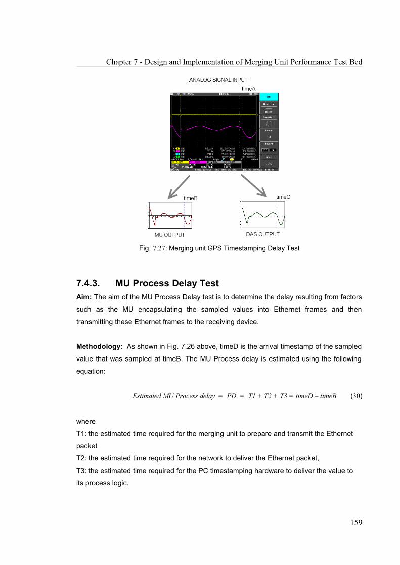
Chapter 7 - Design and Implementation of Merging Unit Performance Test Bed
Fig. 7.27: Merging unit GPS Timestamping Delay Test
7.4.3. MU Process Delay TestAim: The aim of the MU Process Delay test is to determine the delay resulting from factors
such as the MU encapsulating the sampled values into Ethernet frames and then
transmitting these Ethernet frames to the receiving device.
Methodology: As shown in Fig. 7.26 above, timeD is the arrival timestamp of the sampled
value that was sampled at timeB. The MU Process delay is estimated using the following
equation:
Estimated MU Process delay = PD = T1 + T2 + T3 = timeD – timeB (30)
where
T1: the estimated time required for the merging unit to prepare and transmit the Ethernet
packet
T2: the estimated time required for the network to deliver the Ethernet packet,
T3: the estimated time required for the PC timestamping hardware to deliver the value to
its process logic.
159
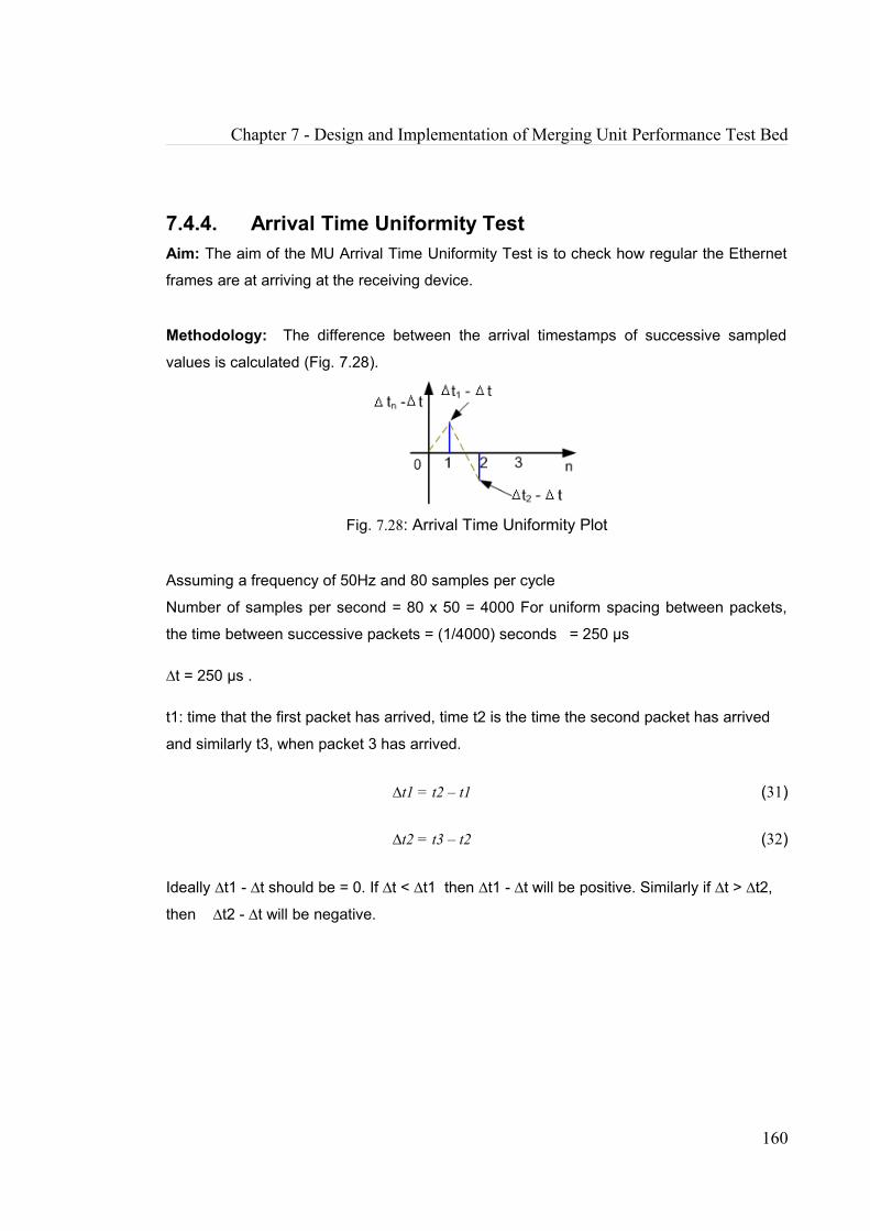
Chapter 7 - Design and Implementation of Merging Unit Performance Test Bed
7.4.4. Arrival Time Uniformity TestAim: The aim of the MU Arrival Time Uniformity Test is to check how regular the Ethernet
frames are at arriving at the receiving device.
Methodology: The difference between the arrival timestamps of successive sampled
values is calculated (Fig. 7.28).
Fig. 7.28: Arrival Time Uniformity Plot
Assuming a frequency of 50Hz and 80 samples per cycle
Number of samples per second = 80 x 50 = 4000 For uniform spacing between packets,
the time between successive packets = (1/4000) seconds = 250 μs
∆t = 250 μs .
t1: time that the first packet has arrived, time t2 is the time the second packet has arrived
and similarly t3, when packet 3 has arrived.
∆t1 = t2 – t1 (31)
∆t2 = t3 – t2 (32)
Ideally ∆t1 - ∆t should be = 0. If ∆t < ∆t1 then ∆t1 - ∆t will be positive. Similarly if ∆t > ∆t2,
then ∆t2 - ∆t will be negative.
160
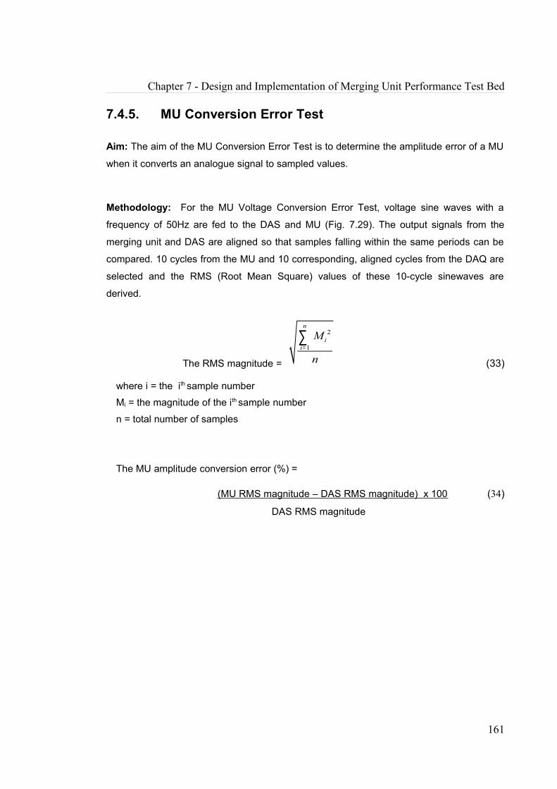
Chapter 7 - Design and Implementation of Merging Unit Performance Test Bed
7.4.5. MU Conversion Error Test
Aim: The aim of the MU Conversion Error Test is to determine the amplitude error of a MU
when it converts an analogue signal to sampled values.
Methodology: For the MU Voltage Conversion Error Test, voltage sine waves with a
frequency of 50Hz are fed to the DAS and MU (Fig. 7.29). The output signals from the
merging unit and DAS are aligned so that samples falling within the same periods can be
compared. 10 cycles from the MU and 10 corresponding, aligned cycles from the DAQ are
selected and the RMS (Root Mean Square) values of these 10-cycle sinewaves are
derived.
The RMS magnitude =
2
1
n
ii
M
n=
∑ (33)
where i = the ith sample number
Mi = the magnitude of the ith sample number
n = total number of samples
The MU amplitude conversion error (%) =
(MU RMS magnitude – DAS RMS magnitude) x 100 (34)
DAS RMS magnitude
161
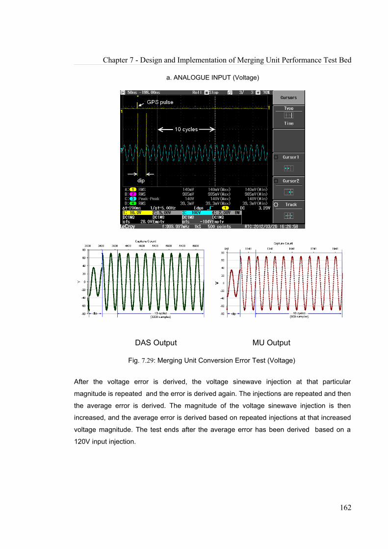
Chapter 7 - Design and Implementation of Merging Unit Performance Test Bed
a. ANALOGUE INPUT (Voltage)
DAS Output MU Output
Fig. 7.29: Merging Unit Conversion Error Test (Voltage)
After the voltage error is derived, the voltage sinewave injection at that particular
magnitude is repeated and the error is derived again. The injections are repeated and then
the average error is derived. The magnitude of the voltage sinewave injection is then
increased, and the average error is derived based on repeated injections at that increased
voltage magnitude. The test ends after the average error has been derived based on a
120V input injection.
162
Chapter 7 - Design and Implementation of Merging Unit Performance Test Bed
The methodology for the current conversion error is exactly the same as that for the
voltage conversion error test, only this time, current injections are used instead of voltage
injections.
7.4.6. MU Filter Performance Test
Aim: The aim of the MU Filter Performance Test is to check how much of the original
signal the MU is able to recover at different frequencies. A square wave has been initially
used because theoretically it is a sum of an infinite number of sine wave signals at different
frequencies. Since a MU samples at 4kHz, ideally it should be able to recover the original
signal up to 2kHz, if there is an antialiaisng filter.
However, there were cases where the cut-off frequency point did not appear within the
2kHz frequency range. It may have been due to one or more reasons such as FFT
leakage, or the MU may not be using a filter, or the filter may not be attenuating signals at
more than 2kHz (half the 4kHz assumed sample rate), leading to aliasing. To reduce or
rule out errors due to FFT leakage, a sine wave injection test was carried out.
Methodology: The DAS serves as a reference, since it has been set to have a sampling
rate of 16kHz (4 times that of the MU). It has also been calibrated by the manufacturer, and
has an Analogue to Digital Converter with a resolution of 24 bits. The DAS can thus be
assumed to accurately represent the input analogue signals.
The initial methodology for the filter performance was based on a Fourier Analysis. For the
voltage square wave test, a Fourier Analysis was carried out on the DAS and MU output
after both had simultaneously received 50V, 50Hz, square wave input signals (Fig. 7.30a
-c) . A square wave is theoretically a sum of an infinite number of sine wave signals at
different frequencies. The frequencies selected for the Fourier analysis plot were based on
odd harmonics of the fundamental input frequency, 50Hz (odd harmonics starting from
50Hz, and including 150Hz, 250Hz, up to 1950Hz) (Fig. 7.30 d-e). For each selected
frequency, the derived MU Fourier magnitude output was divided by the corresponding
DAS Fourier magnitude output. The results of these calculations were then plotted (Fig.
7.30 f).
163

Chapter 7 - Design and Implementation of Merging Unit Performance Test Bed
The cut-off frequency is the frequency at which the merging unit output divided by the
reference = √2 /2
Cut-off frequency = freq (MU magnitude/ DAS magnitude = √2 /2 = 0.707) (35)
a. 50V, 50Hz Square Wave Injection
b. DAS Output c. MU Output
d. DAS Fourier Analysis (16kHz sampling) e. MU Fourier Analysis (4kHz sampling)
164

Chapter 7 - Design and Implementation of Merging Unit Performance Test Bed
0
0.1
0.2
0.3
0.4
0.5
0.6
0.7
0.8
0.9
1
1.1
0 200 400 600 800 1000 1200 1400 1600 1800 2000
freq f (Hz)
MU
/DA
S
CUT-OFF FREQUENCY
f. Filter Analysis Curve (MU Magnitude / DAS Magnitude)
Fig. 7.30: MU Filter Performance Test (Voltage).
Fig. 7.30f is the filter analysis curve for the merging unit from one manufacturer. The Fig.
shows a clear cut-off frequency of approximately 250Hz to the nearest 50Hz.
These results were consistent when repeated. However Fig. 7.31 shows the result of a
square wave injection test carried out on the merging unit from a different manufacturer. It
can be seen that the cut-off frequency point does not appear within the 2kHz frequency
range. In addition to this, the results were not consistent when the test was repeated.
There were instances when the cut-off frequency would appear within the 2kHz. The
inconsistent results may have been due to one or more reasons: FFT leakage, or the MU
may not be using a filter, or the filter may not be attenuating signals at more than 2kHz
(half the 4kHz assumed sample rate), leading to aliasing, or the MU and DAS samples
used for comparison had not been aligned.
165

Chapter 7 - Design and Implementation of Merging Unit Performance Test Bed
Fig. 7.31: Squarewave Injection Test: Filter Analysis Curve (MU Magnitude / DAS
Magnitude)
In order to reduce or rule out errors due to FFT leakage and non-alignment, a data capture
methodology similar to that used for the MU Conversion Error (section 7.4.5.) was applied.
For the Filter Performance Voltage test, voltage sine waves with an initial frequency of
50Hz were fed to the DAS and MU (Fig. 7.29). The output signals from the merging unit
and DAS were aligned so that samples falling within the same periods could be compared.
10 cycles from the MU and 10 corresponding, aligned cycles from the DAS were selected
and the RMS values of these 10-cycle sinewaves were derived. The voltage ratio was
derived using the following equation:
Voltage ratio, Vout/Vin = merging unit Output Voltage Magnitude/DAS Output Voltage
Magnitude (36)
After the voltage ratio had been derived, the voltage sinewave injection at that particular
frequency was repeated and the voltage ratio was derived again. The injections were
repeated and then the average ratio was derived. The frequency of the voltage sinewave
injection was then increased, and the average ratio was derived based on repeated
injections at that increased frequency. The frequencies used for the voltage sinewave
injections were the same as those initially used for the Fourier analysis (50Hz, 150Hz,
250Hz, up to 1950Hz).
166

Chapter 7 - Design and Implementation of Merging Unit Performance Test Bed
The output can be seen in Fig 7.32. The test results were consistent when repeated and
are discussed in detail in Section 7.6.6..
Fig. 7.32: Sinewave Injection Test (MU Magnitude / DAS Magnitude)
For the Filter Performance current test the methodology is identical to that used for the
voltage test, but it is based on 2A injections rather than 50V injections.
According to [78], most protection functions need to filter the fundamental components of the
analogue values and analyses of current and voltages at frequencies of up to 1kHz is
considered sufficient. For evaluation of power quality, frequencies up to the 50th harmonic are
expected to be measured and for a 50Hz system, this corresponds to 2.5kHz. IEC 61850
specifies a sampling rate of 4kHz or 12.8kHz for a 50Hz system, which means that the Merging
Unit will be only able to correctly sample signals with frequencies up to 2kHz or 6.4kHz based on
the Nyquist theorem. The Merging Unit is thus limited by its sampling frequencies and will not
be able to be correctly used for transient earth fault current detection which may require input
frequencies of up to 12kHz. MU may also not be able to correctly detect higher frequency
transient signals relevant to transient based protection for Extremely High Voltage (EHV)
transmission lines, which are of the magnitude of hundreds of many kHz or higher
167
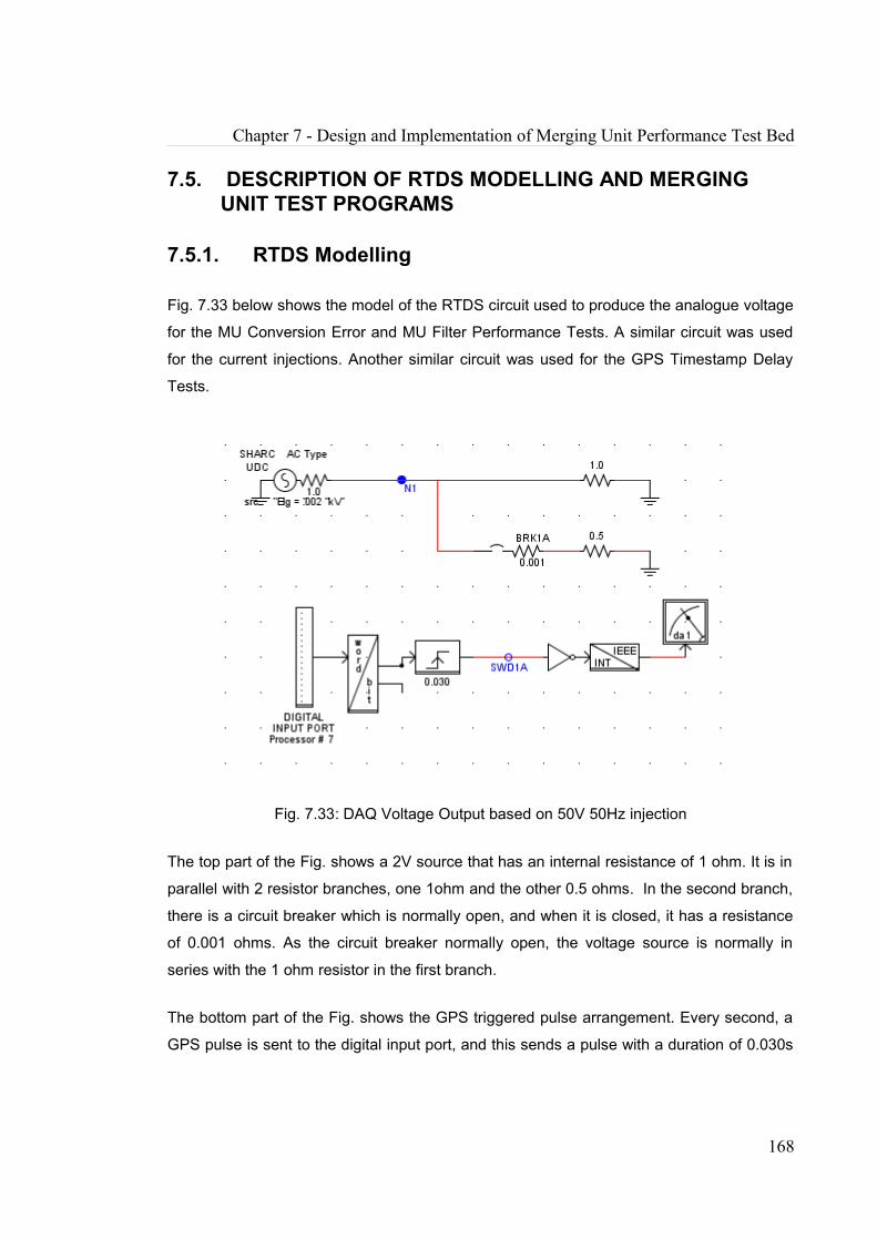
Chapter 7 - Design and Implementation of Merging Unit Performance Test Bed
7.5. DESCRIPTION OF RTDS MODELLING AND MERGING UNIT TEST PROGRAMS
7.5.1. RTDS Modelling
Fig. 7.33 below shows the model of the RTDS circuit used to produce the analogue voltage
for the MU Conversion Error and MU Filter Performance Tests. A similar circuit was used
for the current injections. Another similar circuit was used for the GPS Timestamp Delay
Tests.
Fig. 7.33: DAQ Voltage Output based on 50V 50Hz injection
The top part of the Fig. shows a 2V source that has an internal resistance of 1 ohm. It is in
parallel with 2 resistor branches, one 1ohm and the other 0.5 ohms. In the second branch,
there is a circuit breaker which is normally open, and when it is closed, it has a resistance
of 0.001 ohms. As the circuit breaker normally open, the voltage source is normally in
series with the 1 ohm resistor in the first branch.
The bottom part of the Fig. shows the GPS triggered pulse arrangement. Every second, a
GPS pulse is sent to the digital input port, and this sends a pulse with a duration of 0.030s
168

Chapter 7 - Design and Implementation of Merging Unit Performance Test Bed
or 30ms to the circuit, breaker, thus triggering the circuit breaker and causing it to close for
approximately 30ms. During that period, the 0.5 ohm resistor in the second branch will then
be connected in parallel with the source and the 1 ohm resistor. This connection will cause
a voltage dip across the measurement node (N1) for approximately 30ms. This has been
displayed in the oscilloscope output window shown in Fig. 7.29a in the previous section.
The dip is introduced in order to assist with the alignment of the MU and DAQ output (Fig.
7.34). The beginning of the dip occurs around the time that the GPS pulse has been
received by RTDS and since the DAQ and MU are both GPS synchronized, they will
capture the dip at roughly the same period, (when their GPS subsecond timestamp
counters have been reset to zero by the GPS pulse). From there a point is selected,
usually the second instance when the sampled value changes from a negative value to a
positive value (capture count 4028 in the DAQ, Fig. 7.34a and capture count 1204 in the
MU, Fig. 7.34b ). Beginning from that point, 10 cycles are then selected and then the RMS
value of the cycles is obtained and used for further analysis. (Note that as stated in section
7.3.2., the Omicron Amplifier amplified the RTDS output signals in order to provide the
actual signals that were sent to the MU and DAQ (the latter via the isolation amplifier) ).
a. DAQ Voltage Output
169

Chapter 7 - Design and Implementation of Merging Unit Performance Test Bed
b. Merging Unit Voltage Output
Fig. 7.34: DAQ and merging unit Voltage Output based on 50V 50Hz injection
This alignment was seen to be especially useful when comparing the current output (Fig.
7.35).
a. DAQ Current Output
170
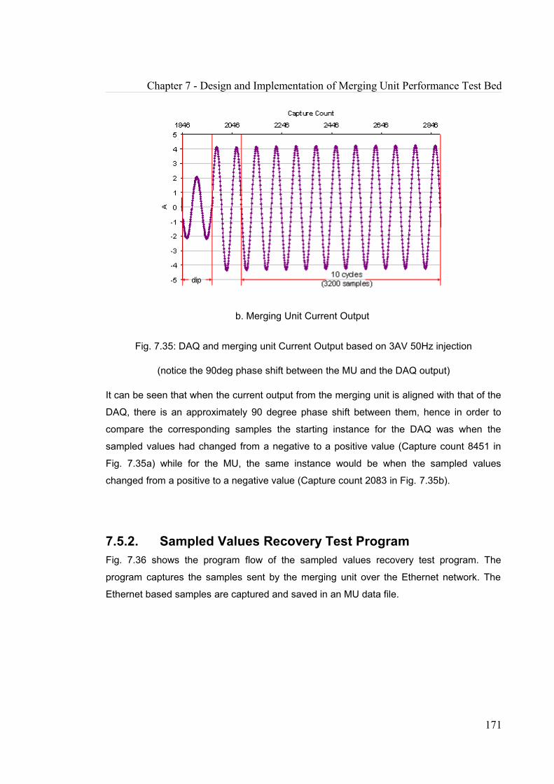
Chapter 7 - Design and Implementation of Merging Unit Performance Test Bed
b. Merging Unit Current Output
Fig. 7.35: DAQ and merging unit Current Output based on 3AV 50Hz injection
(notice the 90deg phase shift between the MU and the DAQ output)
It can be seen that when the current output from the merging unit is aligned with that of the
DAQ, there is an approximately 90 degree phase shift between them, hence in order to
compare the corresponding samples the starting instance for the DAQ was when the
sampled values had changed from a negative to a positive value (Capture count 8451 in
Fig. 7.35a) while for the MU, the same instance would be when the sampled values
changed from a positive to a negative value (Capture count 2083 in Fig. 7.35b).
7.5.2. Sampled Values Recovery Test ProgramFig. 7.36 shows the program flow of the sampled values recovery test program. The
program captures the samples sent by the merging unit over the Ethernet network. The
Ethernet based samples are captured and saved in an MU data file.
171

Chapter 7 - Design and Implementation of Merging Unit Performance Test Bed
Fig. 7.36: Program flow of sampled values recovery test program
The phase voltage (or current if it the current test) is extracted from the MU data file and
plotted on the program window. A new set of samples and then captured, processed and
plotted and this continues until the user clicks stop or the steps have been repeated a
predetermined number of times.
7.5.3. Data Retrieval program for GPS Timestamping Delay
Fig. 7.37 shows the program flow of the data retrieval program for GPS Timestamping
Delay. The program captures the samples sent by the merging unit over the Ethernet
network. The Ethernet based samples are captured an saved in an MU data file. The user
is then prompted to view the captured data and if selected, an Excel file is then opened
172

Chapter 7 - Design and Implementation of Merging Unit Performance Test Bed
and when updated, it retrieves the latest voltage/current sampled values and plots these
values. The user can then refocus the plot so that the event of interest is within view.
Fig. 7.37: Program flow of data retrieval program for GPS Timestamping Delay
In order to complete the analysis, the user locates the MU samplecount data
corresponding to the event of interest and then this samplecount is converted to seconds
by dividing it by 4000. this result is the timestamp of the event in the form of a decimal
number (timeB). The GPS timestamping delay is then deduced by subtracting timeB from
timeA which is the oscilloscope timestamp of the same event.
173

Chapter 7 - Design and Implementation of Merging Unit Performance Test Bed
7.5.4. Process Delay Test and Arrival Time Uniformity Test Program
Fig. 7.38 shows the program flow of the Process Delay Test and Arrival Time Uniformity
Test Program. The program captures the samples sent by the merging unit over the
Ethernet network. When each sample arrives it is timestamped by the high accuracy
Endace Network Monitoring Card. The Ethernet based samples are saved together with
the accurate and corresponding arrival timestamp data in an MU data file. The MU
current/voltage and samplecount data is retrieved from the MU data file and saved in a 2 nd
MU data file. The MU arrival timestamp data represents the time the sample arrived at the
network Monitoring card. It is retrieved from the 1st MU data file and saved in a 3rd MU data
file. It is then extracted from the 3rd MU data file and the time is converted into seconds. It
is now in the form of a large number made up of integers and decimals and it is the
decimal part that is used for comparison with the MU samplecount. For this reason, the
decimal part of the arrival timestamp number is separated from the integer part of the
number and saved in a 4th MU data file.
The user is then presented with the option of viewing the process delay, and if this is
selected, an Excel file is then opened, and when it is updated, the MU samplecount is
extracted from the 2nd MU data file and converted into seconds in the form a decimal
number (timeB) by dividing it by 4000. The corresponding arrival timestamp second data is
(in the form of a decimal) is designated as timeD. The MU process delay is then deduced
by subtracting timeB from timeD (as described in equation 31).
After the MU Process Delay test has been carried out, the user is also able to carry out the
Arrival Time Uniformity test and is presented with the option to view the Arrival Time
Uniformity. If this option is selected, an Excel file is opened and when it is updated, the
arrival timestamp data for is extracted and the arrival time uniformity difference is derived
as described in Section 7.4.4.. The uniformity difference is then plotted.
174

Chapter 7 - Design and Implementation of Merging Unit Performance Test Bed
Fig. 7.38: Program flow of Process Delay Test and Arrival Time Uniformity Test Program
175
Chapter 7 - Design and Implementation of Merging Unit Performance Test Bed
7.5.5. Data Retrieval Program for MU Error Test and MU Filter Test
Fig. 7.39 shows the program flow of the data retrieval program for MU Error Test and MU
Filter Test. The program captures the samples sent by the merging unit over the Ethernet
network. The Ethernet based samples are captured an saved in an MU data file. Almost
simultaneously, the DAQ begins sampling the same analogue voltage/current signals as
the MU and it also acquires the corresponding timestamp for each sample. The samples
and corresponding timestamps are saved in a DAQ data file. The user is then presented
with an option of viewing the captured data and if this is selected, an Excel file is then
opened and when updated, it retrieves the latest voltage/current sampled values for both
the MU and DAQ and plots these values. The user can then refocus the plots so that the
event of interest is within view in both the MU and DAQ window.
The user then specifies where the MU voltage/current RMS analysis should begin, as well
the number of samples that will be used for the RMS analysis. The same is done for the
DAQ. The beginning point should coincide with the point that was specified for the MU.
Also the number of samples should be consistent with the number of samples specified for
the MU. The MU samples at 4kHz and for a 50Hz signal the MU would thus have 4000/50
samples per cycle or 80 samples per cycle. For this analysis, the equivalent 10 cycles for
a 50Hz input signal were specified. 10 cycles for a 50 Hz signal equals 80 x 10 or 800
samples (Fig. 7.34a). Since the DAQ was set to capture at 16kHz, the equivalent of 10
cycles for a 50Hz input signal equals 800 x 4 or 3200 samples(Fig. 7.34b).
176

Chapter 7 - Design and Implementation of Merging Unit Performance Test Bed
Fig. 7.39: Program flow of Data Retrieval Program for MU Error Test and MU Filter Test
177

Chapter 7 - Design and Implementation of Merging Unit Performance Test Bed
For the MU conversion error, the frequency of all input signals was 50Hz. The Filter
performance however involved input signals of varying frequencies, up to 1950Hz. At
50Hz, 10 cycles correspond to a 200ms window. This 200ms window was consistently
used for all frequencies, hence an 800 sample RMS analysis was maintained for the MU
while a 3200 sample RMS analysis was maintained for the DAQ.
7.6. MERGING UNIT PERFORMANCE TESTS RESULTSThe results of the performance tests carried out on merging units from 3 different
manufacturers shall be discussed. These tests include the sampled values recovery test,
process delay test, GPS Timestamping delay test, arrival time uniformity test, conversion
error test and filter performance assessment. More of the merging unit performance test
result data can be seen in APPENDIX D.
7.6.1. Ethernet Frame Format Check And Sampled Values Recovery Test
Ethernet Frames of MUs 1- 3 adhere to the IEC 61850 9-2 (LE) format. Fig. 7.40 shows
part of an Ethernet frame that has been recovered from a merging unit. This part is the
Application Protocol Data Unit (APDU).
178
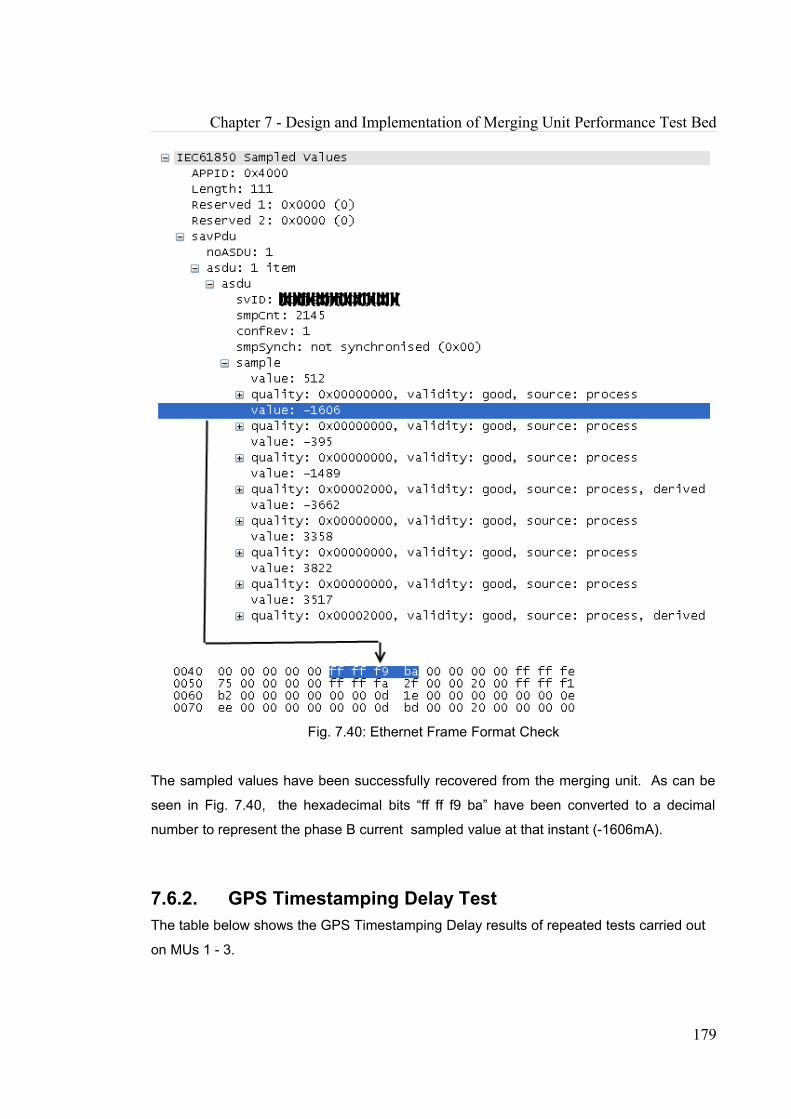
Chapter 7 - Design and Implementation of Merging Unit Performance Test Bed
Fig. 7.40: Ethernet Frame Format Check
The sampled values have been successfully recovered from the merging unit. As can be
seen in Fig. 7.40, the hexadecimal bits “ff ff f9 ba” have been converted to a decimal
number to represent the phase B current sampled value at that instant (-1606mA).
7.6.2. GPS Timestamping Delay TestThe table below shows the GPS Timestamping Delay results of repeated tests carried out
on MUs 1 - 3.
179

Chapter 7 - Design and Implementation of Merging Unit Performance Test Bed
Table 7.6: GPS Timestamping Delay (GTD) Test Results
Measure of Dispersion
Result (microseconds)MU1 MU2 MU3
Average 410 -70 131Standard Deviation 65.19 83.67 81.73Variance 4.25E-003 7.00E-003 6.68E-003Maximum 500 0 200Minimum 350 -200 5Range 150 200 195
It is seen from Table 7.6 that in the case of MU2, the average GTD is negative, which
would imply that the MU timestamped the analogue signal before the analogue signal was
sent, and this is not expected to be the case. The accuracy of the results depends on a
number of different factors. The timestamp timeA from the oscilloscope was measured to
the nearest 10th of a millisecond (100μs). The timestamp timeB from a merging unit is
measured to the nearest 250μs (that is 1/4000 s). Also, it is possible that MU2 possesses a
method of determining exactly when the analogue signal was sent, and then time-stamping
the corresponding sampled value using that time. Thus, MU2 may be able to compensate
for any actual delay when timestamping the sampled values, while MU1 and MU3 may not
presently be able to compensate for such a delay. Another factor to take into account is the
possible reading error that may occur while taking measurements from the oscilloscope.
7.6.3. Process Delay TestFig. 7.41 below shows the process delay in microseconds for 400 packets captured from
MU1.
180

Chapter 7 - Design and Implementation of Merging Unit Performance Test Bed
405
410
415
420
425
430
435
440
445
450
455
400 450 500 550 600 650 700 750 800
Capture Count
Del
ay (μ
s)
Fig. 7.41: MU1 GPS Timestamping Delay Test (400 packets)
It can be seen from Fig. 7.41 that the delay pattern is quite steady and after approximately
every 50 samples, the delay sharply increases and then reduces until it gets to being
relatively steady again.
Fig. 7.42 below shows the process delay in microseconds for 400 packets captured from MU2.
Fig. 7.42: MU2 GPS Timestamping Delay Test (400 packets)
181

Chapter 7 - Design and Implementation of Merging Unit Performance Test Bed
It can be seen from Fig. 7.42 that the delay pattern for MU2 is relatively inconsistent and
rises and falls sharply throughout the sample view. The lowest delay is higher than the
higher than the highest delay observed in MU1.
Fig. 7.43 below shows the process delay in microseconds for 400 packets captured from
MU3.
Fig. 7.43: MU3 GPS Timestamping Delay Test (400 packets)
It can be seen from Fig. 7.43 that the delay pattern in MU3 falls in between that of MU1
and MU2. Its lowest value is still higher than the highest value of MU1, but its highest value
is still lower that the lowest value of MU2. The pattern is not as steady as that of MU1, yet
the delays do not rise and fall as sharply as that of MU2.
The table below shows the MUs 1-3 Process Delay results after repeated Ethernet packet
captures.
Table 7.7: Process Delay (PD) Test Results
Measure of Dispersion
Result (microseconds)MU1 MU2 MU3
Average 416.85 1170.49 521.71Standard Deviation 5.67 271.57 6.49Variance 3.21E-005 7.38E-002 0.00Maximum 474.00 2254.00 561.00Minimum 411.00 633.00 501.00
182

Chapter 7 - Design and Implementation of Merging Unit Performance Test Bed
Measure of Dispersion
Result (microseconds)MU1 MU2 MU3
Range 63.00 1621.00 60.00
Based on these results MU1 has the lowest process delay of 417µs followed by MU3
(522µs) and then MU2 (1170µs). It is seen that the overall average process delay for MU2
is about 2.8 times as much as that of MU1, while the process delay of MU3 is 1.25 times
as much as that of MU1. The standard deviation of MU1 is the lowest (5.7 μs) followed by
MU3 (6.5 μs) and with that of MU2 being much (271.6 μs). MU1 and MU3 have roughly the
same range of 60 μs while MU2 also has a much larger range of 1620 μs.
As in section 7.6.2., a number of factors need to be taken into account when considering
the accuracy of the results shown in Table 7.7. The previously discussed accuracy of the
MU is to the nearest 0.250ms (or 250µs) and the Ethernet packet arrival timestamp timeD
has a resolution of 7.5ns and also depends on the accuracy of the supplied GPS used for
synchronizing the Endace Network Monitoring Card. The GE Fibre Optic Ethernet switch
also introduces a very small delay. The GE switch has a latency of 5 μs + the packet time.
The packet time for an IEC 61850 9-2 LE packet is approximately 13.12 μs, hence the total
latency due to the Ethernet Switch is = 5 μs + 13.12 μs = 18.12 μs.
7.6.4. Arrival Time Uniformity Test
The results below show the difference between the arrival timestamps of successive
packets differ from 250 μs. Due to the fact that the Arrival Time Uniformity is directly
derived from the Process Delay, the patterns obtained for the ATU are very similar to that
observed in the Process Delay patterns.
Fig. 7.44 below shows the arrival time uniformity test results for 400 packets captured from
MU1.
183
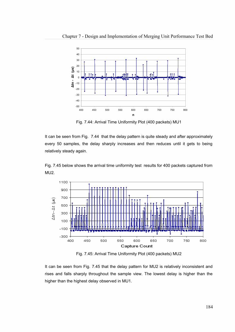
Chapter 7 - Design and Implementation of Merging Unit Performance Test Bed
-50
-40
-30
-20
-10
0
10
20
30
40
50
400 450 500 550 600 650 700 750 800
n
Δtn
- Δ
t (μ
s)
Fig. 7.44: Arrival Time Uniformity Plot (400 packets) MU1
It can be seen from Fig. 7.44 that the delay pattern is quite steady and after approximately
every 50 samples, the delay sharply increases and then reduces until it gets to being
relatively steady again.
Fig. 7.45 below shows the arrival time uniformity test results for 400 packets captured from
MU2.
Fig. 7.45: Arrival Time Uniformity Plot (400 packets) MU2
It can be seen from Fig. 7.45 that the delay pattern for MU2 is relatively inconsistent and
rises and falls sharply throughout the sample view. The lowest delay is higher than the
higher than the highest delay observed in MU1.
184

Chapter 7 - Design and Implementation of Merging Unit Performance Test Bed
Fig. 7.46 below shows the arrival time uniformity test results for 400 packets captured from
MU3.
Fig. 7.46: Arrival Time Uniformity Plot (400 packets) MU3
It can be seen from Fig. 7.46 that the delay pattern in MU3 falls in between that of MU1
and MU2. Its lowest value is still higher than the highest value of MU1, but its highest value
is still lower that the lowest value of MU2. The pattern is not as steady as that of MU1, yet
the delays do not rise and fall as sharply as that of MU2.
The table below shows the MUs 1-3 Process Delay results after repeated Ethernet packet
captures.
Table 7.8: Merging Unit Arrival Time Uniformity (ATU) Test Results
Measure of Dispersion
Result (microseconds)MU1 MU2 MU3
Average 0.00 0.22 0.01Standard Deviation 6.76 270.33 6.91Variance 4.57E-005 7.31E-002 4.77E-005Maximum 57.00 1045.00 28.00Minimum -55.00 -238.00 -32.00Range 112.00 1283.00 60.00
185

Chapter 7 - Design and Implementation of Merging Unit Performance Test Bed
Based on these results MU1 and MU3 can be said to be on average extremely uniform
with an overall Arrival Time Uniformity (ATU) difference of 0 μs and 0.01 μs respectively.
They both have a standard deviation of less than 7 μs, but the range of MU1 is almost
twice (112 μs ) that of MU3 (60 μs). The ATU of MU2 is on average very uniform with an
ATU of 0.22μs . Its standard deviation is the highest (270 μs) as is the range (1283 μs).
7.6.5. Conversion Error Test
The results of the conversion error tests shall now be shown. It may be important to note
that for the current and voltage outputs provided by RTDS, the GPS synchronized dip
duration varied slightly each second, and the actual magnitude provided by RTDS may
also have changed slightly each second. This provided an even stronger reason to repeat
the tests and derive the average error values for each approximate magnitude injection
(10V – 120V for voltage and 1A – 5A for current). For each MU conversion error plot, the
overall average error is displayed, as is the range.
7.6.5.1. Voltage Injection
Fig. 7.47 shows the MU1 Conversion Error (%) plotted against the input voltages ranging
from 10V to 120V.
Fig. 7.47: MU1 Conversion Error (Voltage)
186
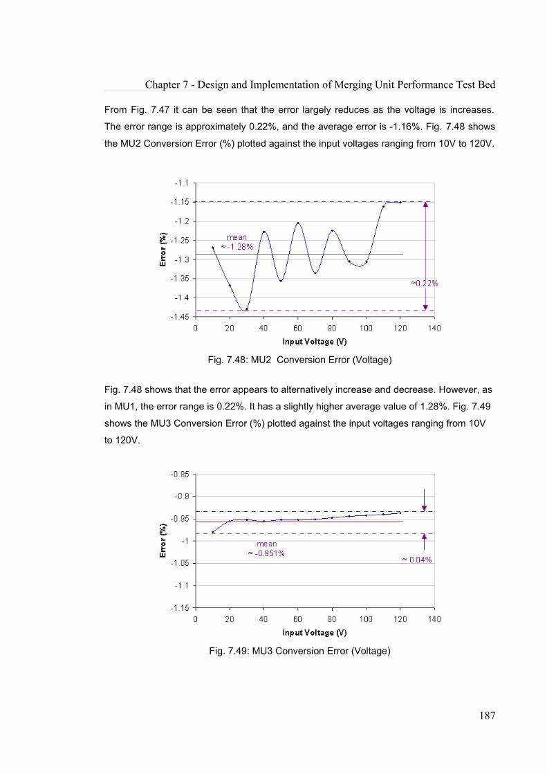
Chapter 7 - Design and Implementation of Merging Unit Performance Test Bed
From Fig. 7.47 it can be seen that the error largely reduces as the voltage is increases.
The error range is approximately 0.22%, and the average error is -1.16%. Fig. 7.48 shows
the MU2 Conversion Error (%) plotted against the input voltages ranging from 10V to 120V.
Fig. 7.48: MU2 Conversion Error (Voltage)
Fig. 7.48 shows that the error appears to alternatively increase and decrease. However, as
in MU1, the error range is 0.22%. It has a slightly higher average value of 1.28%. Fig. 7.49
shows the MU3 Conversion Error (%) plotted against the input voltages ranging from 10V
to 120V.
Fig. 7.49: MU3 Conversion Error (Voltage)
187
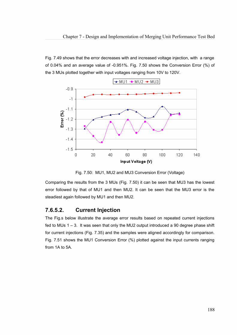
Chapter 7 - Design and Implementation of Merging Unit Performance Test Bed
Fig. 7.49 shows that the error decreases with and increased voltage injection, with a range
of 0.04% and an average value of -0.951%. Fig. 7.50 shows the Conversion Error (%) of
the 3 MUs plotted together with input voltages ranging from 10V to 120V.
Fig. 7.50: MU1, MU2 and MU3 Conversion Error (Voltage)
Comparing the results from the 3 MUs (Fig. 7.50) it can be seen that MU3 has the lowest
error followed by that of MU1 and then MU2. It can be seen that the MU3 error is the
steadiest again followed by MU1 and then MU2.
7.6.5.2. Current InjectionThe Fig.s below illustrate the average error results based on repeated current injections
fed to MUs 1 – 3. It was seen that only the MU2 output introduced a 90 degree phase shift
for current injections (Fig. 7.35) and the samples were aligned accordingly for comparison.
Fig. 7.51 shows the MU1 Conversion Error (%) plotted against the input currents ranging
from 1A to 5A.
188
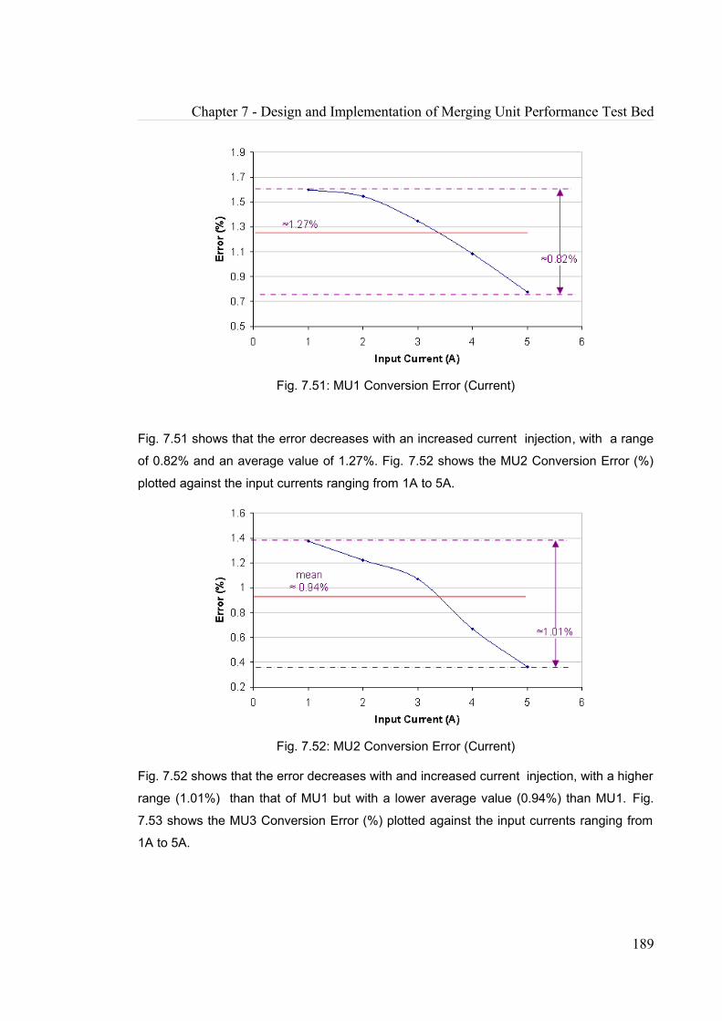
Chapter 7 - Design and Implementation of Merging Unit Performance Test Bed
Fig. 7.51: MU1 Conversion Error (Current)
Fig. 7.51 shows that the error decreases with an increased current injection, with a range
of 0.82% and an average value of 1.27%. Fig. 7.52 shows the MU2 Conversion Error (%)
plotted against the input currents ranging from 1A to 5A.
Fig. 7.52: MU2 Conversion Error (Current)
Fig. 7.52 shows that the error decreases with and increased current injection, with a higher
range (1.01%) than that of MU1 but with a lower average value (0.94%) than MU1. Fig.
7.53 shows the MU3 Conversion Error (%) plotted against the input currents ranging from
1A to 5A.
189
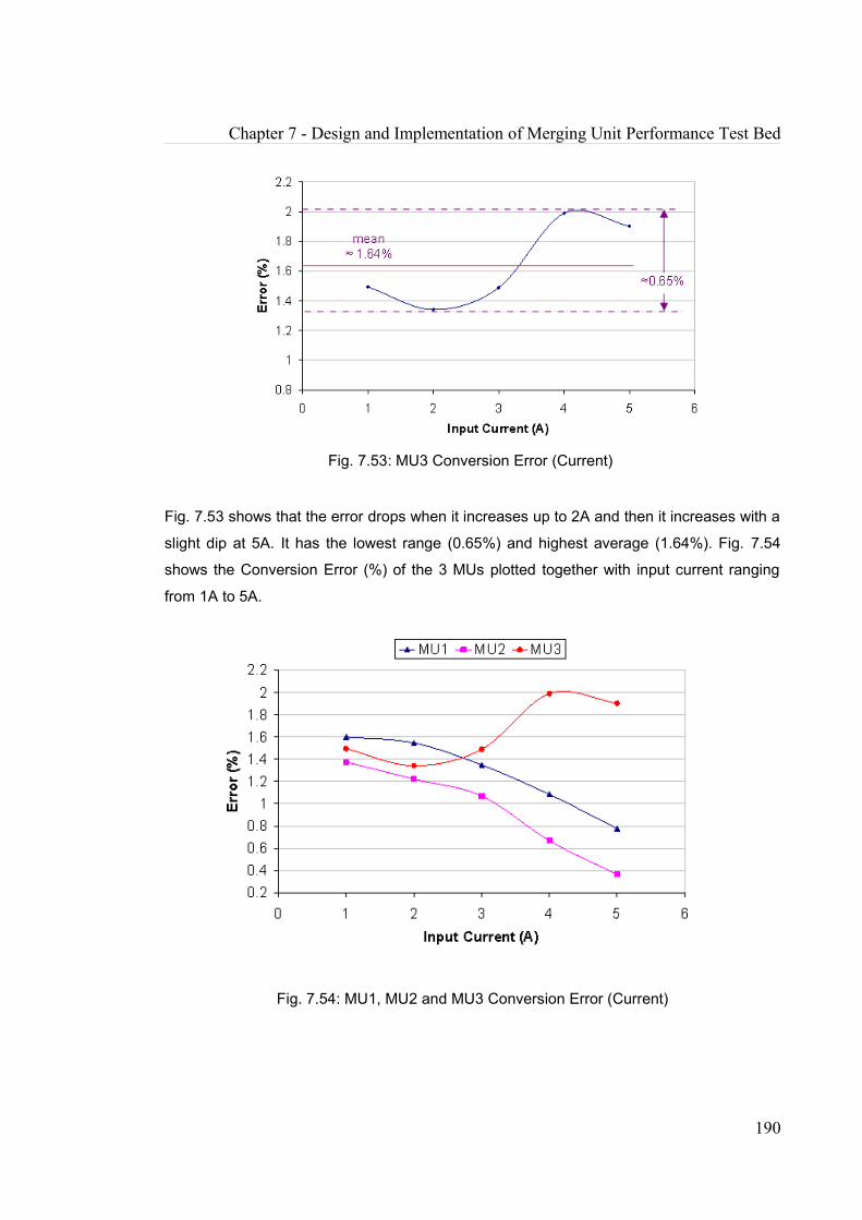
Chapter 7 - Design and Implementation of Merging Unit Performance Test Bed
Fig. 7.53: MU3 Conversion Error (Current)
Fig. 7.53 shows that the error drops when it increases up to 2A and then it increases with a
slight dip at 5A. It has the lowest range (0.65%) and highest average (1.64%). Fig. 7.54
shows the Conversion Error (%) of the 3 MUs plotted together with input current ranging
from 1A to 5A.
Fig. 7.54: MU1, MU2 and MU3 Conversion Error (Current)
190
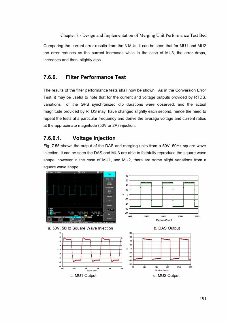
Chapter 7 - Design and Implementation of Merging Unit Performance Test Bed
Comparing the current error results from the 3 MUs, it can be seen that for MU1 and MU2
the error reduces as the current increases while in the case of MU3, the error drops,
increases and then slightly dips.
7.6.6. Filter Performance Test
The results of the filter performance tests shall now be shown. As in the Conversion Error
Test, it may be useful to note that for the current and voltage outputs provided by RTDS,
variations of the GPS synchronized dip durations were observed, and the actual
magnitude provided by RTDS may have changed slightly each second, hence the need to
repeat the tests at a particular frequency and derive the average voltage and current ratios
at the approximate magnitude (50V or 2A) injection.
7.6.6.1. Voltage InjectionFig. 7.55 shows the output of the DAS and merging units from a 50V, 50Hz square wave
injection. It can be seen the DAS and MU3 are able to faithfully reproduce the square wave
shape, however in the case of MU1, and MU2, there are some slight variations from a
square wave shape.
a. 50V, 50Hz Square Wave Injection b. DAS Output
c. MU1 Output d. MU2 Output
191

Chapter 7 - Design and Implementation of Merging Unit Performance Test Bed
e. MU3 Output
Fig. 7.55: MU and DAS output from 50V 50Hz square wave injection
Fig. 7.56 shows one MU1 Filter Analysis curve after a 50V 50Hz square wave injection. It
can be seen from Fig. 7.56 that the cut-off frequency is well below 2kHz. The test was
repeated using the sinewave injection test and the average of the voltage ratios obtained at
different frequencies can be seen in Fig. 7.56 b below. The cut-off frequencies were seen
on average to be consistent after repeated square wave and sinewave voltage injections.
0
0.1
0.2
0.3
0.4
0.5
0.6
0.7
0.8
0.9
1
1.1
0 200 400 600 800 1000 1200 1400 1600 1800 2000freq f (Hz)
MU
/DA
S
CUT-OFF FREQUENCY
a. Filter Analysis Curve, square wave injection, MU1
192

Chapter 7 - Design and Implementation of Merging Unit Performance Test Bed
b. Filter Analysis Curve, sine wave injection, MU1
Fig. 7.56: MU1 Filter Performance (Voltage)
It can also be seen that the result of the sinewave injection test is largely consistent with
the result of the square wave injection test. The results for MU2 were quite different. Fig.
7.57a shows the MU2 Filter Analysis curve after a 50V 50Hz square wave injection. It can
be seen that the cut-off frequency point does not appear within the 2kHz frequency range,
and though it is not shown, there were instances where the cut-off would appear within the
2kHz range. The 50V sine wave is thus injected at different frequencies and the voltage
ratio is plotted as can be seen in Fig. 7.57b.
a. Filter Analysis Curve, square wave injection, MU2
193

Chapter 7 - Design and Implementation of Merging Unit Performance Test Bed
b. Filter Analysis Curve, sine wave injection, MU2
Fig. 7.57: MU2 Filter Performance (Voltage)
It can be seen that even with repeated sinewave injection tests, the cut-off frequency
appears to be greater than 2000Hz. This bandwidth is higher than anticipated, since if the
sampling rate is 4kHz, then the maximum bandwidth is expected to be no more than half of
that frequency.
Fig. 7.58a shows the MU3 Filter Analysis curve after a 50V 50Hz square wave injection,
and the cut-off frequency point also does not appear within the 2kHz frequency range, and
as with MU2, the results varied during different square wave voltage injections. A 50V
sine wave is then injected at different frequencies and the voltage ratio is plotted as can be
seen in Fig. 7.58b.
0
0.2
0.4
0.6
0.8
1
1.2
0 200 400 600 800 1000 1200 1400 1600 1800 2000freq f (Hz)
MU
/DA
S
194

Chapter 7 - Design and Implementation of Merging Unit Performance Test Bed
a. Filter Analysis Curve, square wave injection, MU3
b. Filter Analysis Curve, sine wave injection, MU3
Fig. 7.58: MU3 Filter Performance (Voltage)
It can be seen that this time the cut-off frequency point does appear within the 2kHz
frequency and it is approximately 1700Hz.
Table 7.9 lists the cut-off frequencies based on the voltage injection tests carried out on
MUs1-3 (accurate to the nearest 50Hz).
Table 7.9: MU Filter Performance Test Results (Voltage)
merging unit
Average cut-off Freq
(Hz)MU1 250MU2 >2000MU3 1700
The results show that MU3 has a cut-off frequency (1700Hz) which is greater than that of
MU1 (250Hz). MU2 on the other hand, appears to have a cut-off frequency which is greater
than 2000Hz.
195
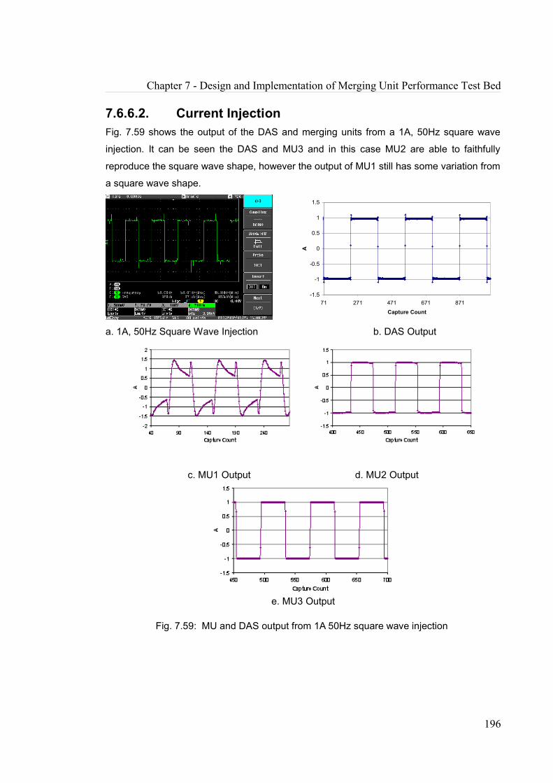
Chapter 7 - Design and Implementation of Merging Unit Performance Test Bed
7.6.6.2. Current InjectionFig. 7.59 shows the output of the DAS and merging units from a 1A, 50Hz square wave
injection. It can be seen the DAS and MU3 and in this case MU2 are able to faithfully
reproduce the square wave shape, however the output of MU1 still has some variation from
a square wave shape.
-1.5
-1
-0.5
0
0.5
1
1.5
71 271 471 671 871
Capture CountA
a. 1A, 50Hz Square Wave Injection b. DAS Output
c. MU1 Output d. MU2 Output
e. MU3 Output
Fig. 7.59: MU and DAS output from 1A 50Hz square wave injection
196

Chapter 7 - Design and Implementation of Merging Unit Performance Test Bed
Fig. 7.60a shows one of the MU1 Filter Analysis curves after a 1A 50Hz square wave
injection, while Fig. 7.60b shows the MU1 Filter Analysis curve, based on the average of
repeated 2A sine wave injections at different frequencies. The cut-off frequencies were
seen on average to be consistent after repeated square wave and sinewave current
injections.
00.10.20.30.40.50.60.70.80.9
11.11.21.31.4
0 200 400 600 800 1000 1200 1400 1600 1800 2000
freq f (Hz)
MU
/DA
S
CUTOFF FREQUENCY
a. Filter Analysis Curve, square wave injection, MU1
b. Filter Analysis Curve, sine wave injection, MU1
Fig. 7.60: MU1 Filter Performance (Current)
197
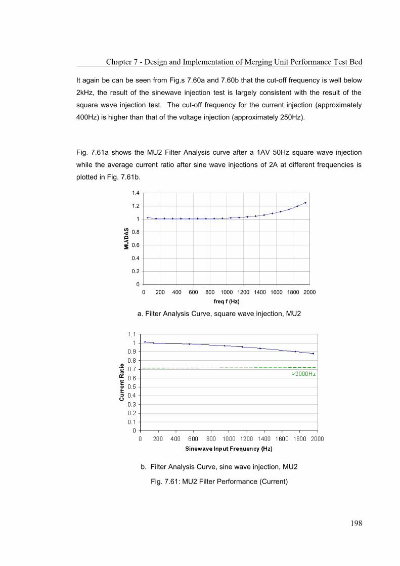
Chapter 7 - Design and Implementation of Merging Unit Performance Test Bed
It again be can be seen from Fig.s 7.60a and 7.60b that the cut-off frequency is well below
2kHz, the result of the sinewave injection test is largely consistent with the result of the
square wave injection test. The cut-off frequency for the current injection (approximately
400Hz) is higher than that of the voltage injection (approximately 250Hz).
Fig. 7.61a shows the MU2 Filter Analysis curve after a 1AV 50Hz square wave injection
while the average current ratio after sine wave injections of 2A at different frequencies is
plotted in Fig. 7.61b.
0
0.2
0.4
0.6
0.8
1
1.2
1.4
0 200 400 600 800 1000 1200 1400 1600 1800 2000
freq f (Hz)
MU
/DA
S
a. Filter Analysis Curve, square wave injection, MU2
b. Filter Analysis Curve, sine wave injection, MU2
Fig. 7.61: MU2 Filter Performance (Current)
198
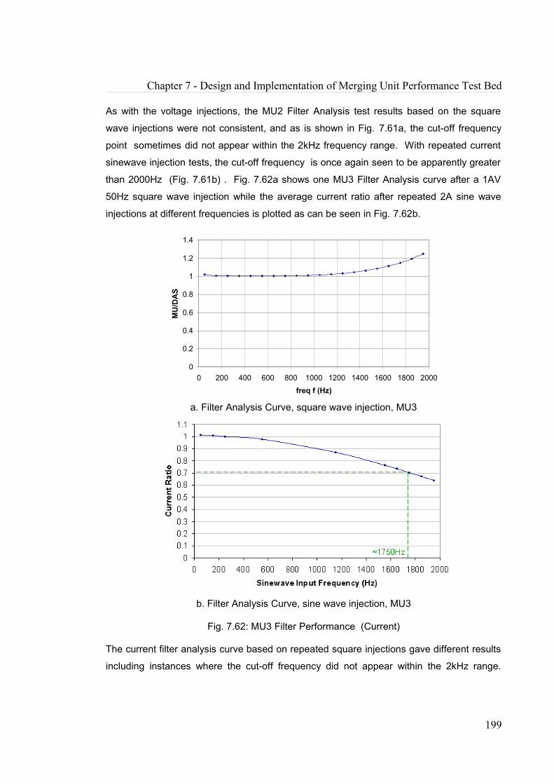
Chapter 7 - Design and Implementation of Merging Unit Performance Test Bed
As with the voltage injections, the MU2 Filter Analysis test results based on the square
wave injections were not consistent, and as is shown in Fig. 7.61a, the cut-off frequency
point sometimes did not appear within the 2kHz frequency range. With repeated current
sinewave injection tests, the cut-off frequency is once again seen to be apparently greater
than 2000Hz (Fig. 7.61b) . Fig. 7.62a shows one MU3 Filter Analysis curve after a 1AV
50Hz square wave injection while the average current ratio after repeated 2A sine wave
injections at different frequencies is plotted as can be seen in Fig. 7.62b.
0
0.2
0.4
0.6
0.8
1
1.2
1.4
0 200 400 600 800 1000 1200 1400 1600 1800 2000
freq f (Hz)
MU
/DA
S
a. Filter Analysis Curve, square wave injection, MU3
b. Filter Analysis Curve, sine wave injection, MU3
Fig. 7.62: MU3 Filter Performance (Current)
The current filter analysis curve based on repeated square injections gave different results
including instances where the cut-off frequency did not appear within the 2kHz range.
199
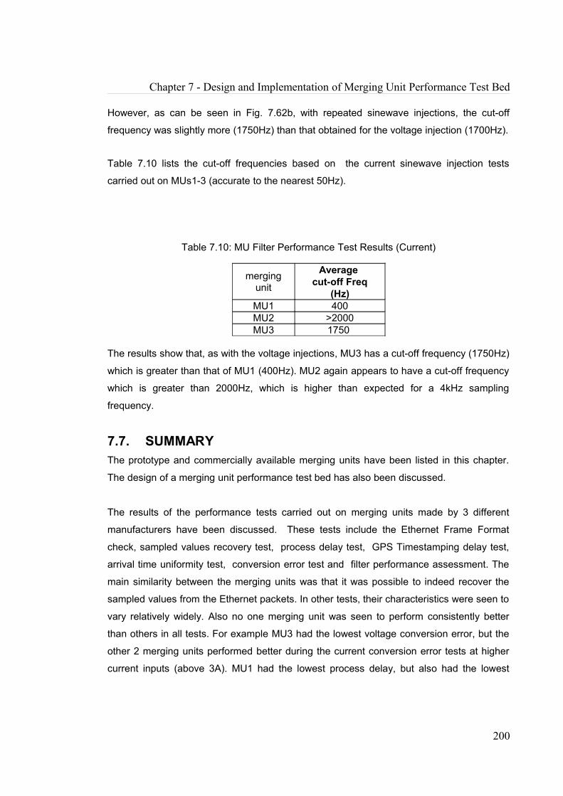
Chapter 7 - Design and Implementation of Merging Unit Performance Test Bed
However, as can be seen in Fig. 7.62b, with repeated sinewave injections, the cut-off
frequency was slightly more (1750Hz) than that obtained for the voltage injection (1700Hz).
Table 7.10 lists the cut-off frequencies based on the current sinewave injection tests
carried out on MUs1-3 (accurate to the nearest 50Hz).
Table 7.10: MU Filter Performance Test Results (Current)
merging unit
Average cut-off Freq
(Hz)MU1 400MU2 >2000MU3 1750
The results show that, as with the voltage injections, MU3 has a cut-off frequency (1750Hz)
which is greater than that of MU1 (400Hz). MU2 again appears to have a cut-off frequency
which is greater than 2000Hz, which is higher than expected for a 4kHz sampling
frequency.
7.7. SUMMARYThe prototype and commercially available merging units have been listed in this chapter.
The design of a merging unit performance test bed has also been discussed.
The results of the performance tests carried out on merging units made by 3 different
manufacturers have been discussed. These tests include the Ethernet Frame Format
check, sampled values recovery test, process delay test, GPS Timestamping delay test,
arrival time uniformity test, conversion error test and filter performance assessment. The
main similarity between the merging units was that it was possible to indeed recover the
sampled values from the Ethernet packets. In other tests, their characteristics were seen to
vary relatively widely. Also no one merging unit was seen to perform consistently better
than others in all tests. For example MU3 had the lowest voltage conversion error, but the
other 2 merging units performed better during the current conversion error tests at higher
current inputs (above 3A). MU1 had the lowest process delay, but also had the lowest
200

Chapter 7 - Design and Implementation of Merging Unit Performance Test Bed
bandwidth in both voltage and current injection tests. MU1 had the lowest GPS
timestamping delay but had the highest process delay.
As these merging units are mostly prototypes being developed and there is not yet a
merging unit specification, the merging units may need to be modified to meet the utility
requirement (for instance, if the utility specifies that the merging unit should be able to
recover samples up to 2kHz, or if the GPS Timestamping delay must be less than 250 μs,
or if the conversion error must be less than +/- 1 %, or the desired bandwidth). The results
of each individual merging unit set of tests have been fed back to the corresponding
vendor, as well as to National Grid.
201

CHAPTER 8 CONCLUSION AND FUTURE WORK
8.1. CONCLUSIONThe IEC 61850 standard has been implemented in varying degrees in substations around
the world, and has the potential to extend its impact beyond substations. While there is a
need for some refinement so that a major goal of interoperability among different devices
can be achieved, the immediate and long term benefits of IEC 61850 are not in question.
The immediate benefits of an IEC 61850 based architecture include the flexibility to adapt
to changes as the technology and processes associated with smart grids and renewable
energy systems mature. Such changes include growth in the communication network due
to the addition of a new substation bay, or upgrades of existing bays to ensure that they
can keep up with the latest technology advances. In the long term, the architecture the
technology and processes associated with renewable energy and smart grids are expected
to have matured, but maintenance would still need to be carried out, and it would still be
important to be able to continue to provide the communication services to the other bays in
the substation while one part of the substation has to be taken out in order to undergo
maintenance.
In response to these needs, the design of a simple, long life IEC 61850 based
communication architecture has been presented in this Thesis. The architecture is
expected to be modular, flexible and robust enough to cope with growth, outages and even
shrinkage that may occur in transmission substations. This architecture design has taken
into account golden rules which have been outlined by protection and control experts from
National Grid and device manufacturers. As part of the architecture design, the security
implementation issues were also taken into account and as a result of this, it was proposed
that the critical substation wide information should be kept separate from the extremely
critical relatively fast information concentrated within the bay. The process bus architecture
has been applied to the following bays within a Double Busbar (DBB) substation: DBB
Feeder bay, DBB transformer bay, DBB Bus coupler/Bus coupler bay. The architecture
has also been applied to the following bays within a Mesh Corner (MC) substation: MC MC
bay, MC feeder bay and MC transformer bay. It has been seen that the architecture
202
Chapter 8 - Conclusion and Future Work
concept is simple and basic, yet adaptable to complex situations, such as can be found in
the Mesh Corner substation.
Extensive reliability analyses have been carried out on various scenarios which are
detailed applications of this proposed process bus architecture to the bays of different
Double Busbar and Mesh Corner substation bays. The reliability block diagram (RBD) was
useful because it provided an overall model of the system in terms of components and
subsystems and the RBD was used to represent the high level success path of the system
from which the system reliability was derived. For the less complex scenarios, subsystems
could be readily broken down into basic series/parallel combinations from which the
subsystem and resulting system reliability could be derived. For the more complex
scenarios, event trees were used to model the subsystems which could not readily be
broken down into basic series/parallel combinations. The event tree allowed for the
specification of requirements for the successful operation of the subsystem and based on
this list of requirements, the subsystem reliability could then be derived. This resulting
subsystem reliability could then be fed into the reliability block diagram and the system
reliability could be derived using a series/parallel combination. From the analyses carried
out on the different bays it was seen that the system was more likely to be reliable when
based on a star architecture than when based on a ring architecture. The most reliable
architecture scenarios were duplicated star connections. From the sensitivity analysis
carried out, it could be seen that the system reliability was overall most likely to improve
when the merging units' reliability was increased. However this was seen to depend on
how reliable the system was because on most occasions, during the first one or two
scenarios when the system was less reliable/available, the fibre optic cables had a higher
impact on system reliability. After the Merging Unit, the Circuit Breaker Controllers had the
next highest overall reliability impact followed by the fibre optic cables and finally the
Ethernet switch. These results were based on estimated reliability figures and in practice
the devices may be more reliable than initially estimated.
Life cycle costing has been used to illustrate how an optimum architecture scenario can be
selected from a range of architecture scenarios. As the reliability, availability and life cycle
cost parameters have been estimated, the methodology has been essentially used to
illustrate how the optimum architecture can be determined. The penalty factor has been
203
Chapter 8 - Conclusion and Future Work
varied between extremely low and high values, and the actual penalty is most likely to fall
in between these 2 extremes. The penalty factor has been varied to show its impact on the
resulting optimum architecture and the corresponding optimum reliability.
Security means the security against “unwanted commands“. It is a measure of the degree
of certainty that a relay will not operate incorrectly”, Dependability is a measure of the
degree of certainty that a relay system will operate correctly
The primary focus of this project has been on the dependability, in particular the
dependability of the communication architecture itself. The dependability assessment has
been in the form of estimating the probability that the protection and control devices would
be able to receive adequate information form the current/voltage transformers and circuit
breakers via this communication architecture, and in turn send trip commands to the circuit
breakers when required.
The reliability (in terms of dependability) of the architecture, based on the analysis that has
been carried out, has been seen to be somewhat reduced, compared with the original
hardwired configuration, or indeed when compared the other communication protocols.
This may be in some measure be attributed to the overall increased part count, and the
use of components/devices which are not as reliable as the copper cables. This decrease
can be mitigated by improving the reliability of the individual components/devices and
applying proper redundancy. However, the use of a Merging Unit to send digital data to the
relay would make it possible to incorporate additional features in the relay which would
improve the security and availability. Features such as continuous internal self testing and
data-integrity mechanisms will make it possible for personnel to solve faults with more
precision and with less down time. Failures which may have been undetected in traditional
hardwired configurations may now be detected more easily as a result of this digital
communication. The rectification of these failures would ensure that the protection
equipment operates properly when required, thus enhancing its security. The continuous
self monitoring may also reduce the human errors which could cause the maloperation of
the protection systems during testing and maintenance tasks.
The use of fibre optic cables for the process bus means that personnel would not be
exposed to potentially lethal voltage/current when they need to replace the relays, hence
204

Chapter 8 - Conclusion and Future Work
this is expected to reduce the downtime and have a positive impact on availability. In terms
of Life Cycle Cost depending on the penalty for downtime, the LCC for the new architecture
may prove less as a result of the overall downtime that may occur during maintenance of
upgrades.
Finally, a Merging Unit performance test bed has been developed for testing these crucial
devices which send current and voltage data to the protection and control devices. The
results of the tests have been fed back to National Grid and the manufacturers, who may
then use the data to assist with the drafting of a merging unit Test Bed Specification, and
also to help the manufacturers to make refinements to the merging units in order to make
interoperability more readily achievable.
This test bed has been used to test the following features of merging units:
• Ethernet frame format check and sampled values recovery test (To check if the
Ethernet frames/packets sent from the MU are of the format specified by IEC
61850 9-2 “Light Edition” (LE). Also, to check if sampled values can be successfully
recovered from the merging unit)
• MU GPS Timestamping Delay (To determine the delay that occurs when the MU
timestamps the digitized signal)
• Process Delay (To determine the delay resulting from factors such as the MU
encapsulating the sampled values into Ethernet frames and then transmitting these
Ethernet frames to the receiving device)
• Arrival Time Uniformity (To check how regularly the Ethernet frames arrive at the
receiving device).
• MU Conversion Error Test (To determine the amplitude error of a MU when it
converts an analogue signal to sampled values) and
• MU Filter Performance (To check how much of the original signal the MU is able to
recover at different frequencies)
The main similarity between the merging units was seen in the Ethernet frame format
check and sampled values recovery test were it was possible to indeed recover the
sampled values from the Ethernet packets. In other tests, their characteristics were seen to
vary relatively widely. Also no one merging unit was seen to perform consistently better
205

Chapter 8 - Conclusion and Future Work
than others in all tests. For example MU1 had the lowest process delay and the highest
arrival time uniformity, but also had the lowest bandwidth in both voltage and current
injection tests. MU2 had the lowest GPS timestamping delay but had the highest process
delay. MU3 had the lowest voltage conversion error, but the other 2 merging units
performed better during the current conversion error tests at higher current inputs (above
3A). A key benefit of this test bed is that it has been used to show that it is flexible enough
to assess the performance of merging units irrespective of who manufactured them and as
a result, it has been able to provide a range of key performance metrics which can be
useful to both National Grid and the manufacturers in achieving a major goal of IEC 61850,
which is interoperability.
8.2. KNOWLEDGE CONTRIBUTIONS TO RESEARCH AREA Based on the conclusion described in the above section, the highlights of the contributions
made by this thesis are:
✔ The design of a simple, long life IEC 61850 based process bus architecture which
is modular, flexible and robust. This architecture has been designed to cope with
shrinkage, growth, or outages which may occur in transmission substations;
✔ The application of this architecture to different National Grid Double Busbar and
Mesh Corner Bays leading to a variety of process bus architecture scenarios;
✔ The application of existing reliability analysis methodologies in order to evaluate
the reliability of the process bus architecture scenarios;
✔ The application of existing life cycle costing methodologies in order to select an
optimum scenario from a range of process bus architecture scenarios;
✔ The design of a performance test bed for testing Merging Units, the crucial devices
which send sampled current and voltage data to the protection and control
devices; and
206

Chapter 8 - Conclusion and Future Work
✔ The implementation of the Merging Unit performance test bed. 3 actual Merging
Units made from different manufacturers have been tested, leading to the
generation of performance test data that can help facilitate interoperability.
8.3. FUTURE WORKIt may be useful to scale the reliability analysis so that it is carried out for the substation –
a combination of the different bays. Busbar Protection was not considered in this analysis
so it may be beneficial to incorporate busbar protection in the reliability analysis.
The proposed architecture has been applied hypothetically to a substation. Carrying out an
actual implementation of the architecture, even in a laboratory setting may help with the
identification of the quantifiable strengths and disadvantages of the architecture.
The merging unit performance test results shown in this thesis were based on tests that
were carried out separately on one merging unit at a time. It is however possible that
testing more merging units simultaneously may have an effect on characteristics such as
the MU process delay, since the presence of additional MUs on the network will increase
the traffic. It may thus be useful to explore this option of testing the merging units
simultaneously. Also the merging unit tests were based on only single phase injection.
There would be some benefits in carrying out the tests based on 3 phase injections. The
comparisons were made mainly based on magnitude of the current and voltage signals.
While the GPS timestamp delay has provided the delay in terms of microseconds, future
upgrades of the test bed may also be able to incorporate instantaneous conversions of the
delay results from seconds to phase angle differences.
The MU test analyses were based on cycles of pure sinewaves. Future work could
incorporate analysis of the signals generated under fault conditions.
The merging units tested so far have been able to accept an external synchronising signal
mostly based on a 1 pulse per second (pps) input which goes to the merging units' clocks.
One merging unit was synchronised using an external synchronizing signal based on IRIG-
B inputs. It is expected that the merging unit samples should be time stamped with an
207

Chapter 8 - Conclusion and Future Work
accuracy of +/- 4 microseconds. However, each timestamp based on the sample count
field located in the merging unit Ethernet packet had a resolution of 250 microseconds, and
the oscilloscope currently used for the project has a resolution of 100 microseconds, thus it
is not currently possible to test the accuracy of the synchronisation to the nearest
microsecond. However, it may become possible to do so if the refrTm Refresh Time field in
the Ethernet packet is used and if oscilloscopes used for future tests are accurate to the
nearest 0.5 microseconds. The Refresh Time field allows for extremely accurate
timestamps, much more accurate than 1 microsecond. The IEEE 1588 time
synchronization standard defines the Precision Time Protocol (PTP) and allows sub-
microsecond synchronization of real-time clocks becomes and is expected to be applicable
to local area networks supporting multicast communications (including but not limited to
Ethernet). It is being considered for time synchronization in future distributed recording
systems, including such applications as wide area monitoring and recording.
Synchronization based on IEEE 1588 may become more widely available and may
warrant more study.
208
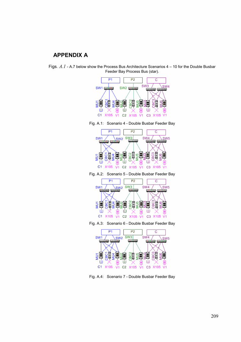
APPENDIX A
Figs. A.1 - A.7 below show the Process Bus Architecture Scenarios 4 – 10 for the Double Busbar Feeder Bay Process Bus (star).
Fig. A.1: Scenario 4 - Double Busbar Feeder Bay
Fig. A.2: Scenario 5 - Double Busbar Feeder Bay
Fig. A.3: Scenario 6 - Double Busbar Feeder Bay
Fig. A.4: Scenario 7 - Double Busbar Feeder Bay
209

Appendix A
Fig. A.5: Scenario 8 - Double Busbar Feeder Bay
Fig. A.6: Scenario 9 - Double Busbar Feeder Bay
Fig. A.7: Scenario 10 - Double Busbar Feeder Bay,
Table A.1: Number of Devices in each Scenario (Double Busbar Feeder Bay (Ring))
Scenario Number of DevicesSW MU CBC FIOC
1 6 6 3 182 8 6 3 233 8 6 3 244 10 6 3 295 10 6 3 306 12 6 3 357 12 6 3 36
210
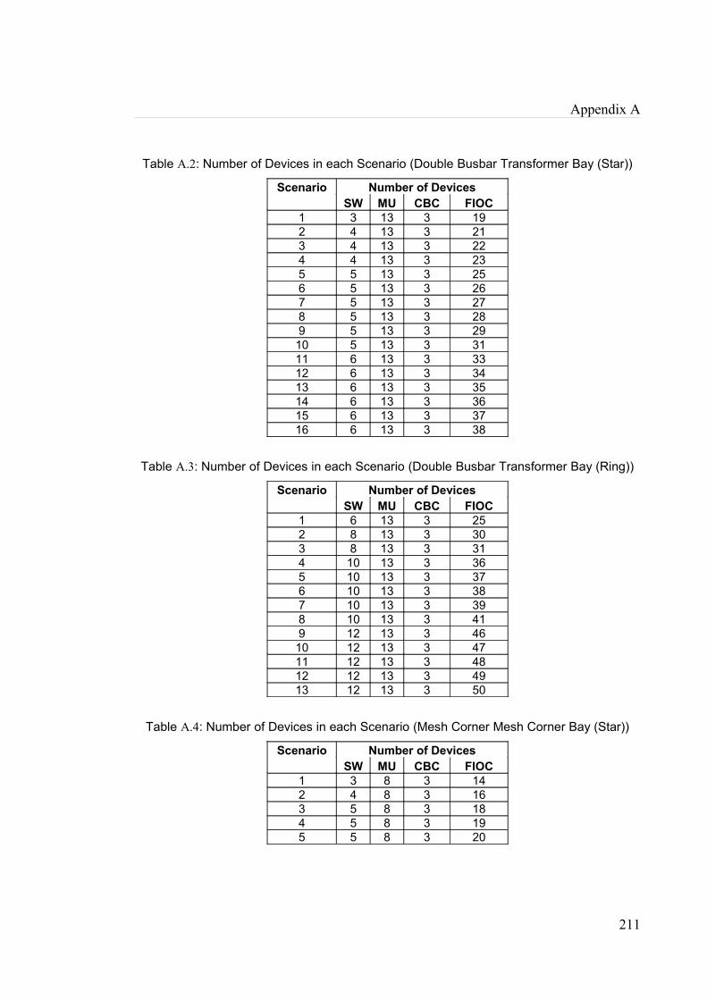
Appendix A
Table A.2: Number of Devices in each Scenario (Double Busbar Transformer Bay (Star))
Scenario Number of DevicesSW MU CBC FIOC
1 3 13 3 192 4 13 3 213 4 13 3 224 4 13 3 235 5 13 3 256 5 13 3 267 5 13 3 278 5 13 3 289 5 13 3 2910 5 13 3 3111 6 13 3 3312 6 13 3 3413 6 13 3 3514 6 13 3 3615 6 13 3 3716 6 13 3 38
Table A.3: Number of Devices in each Scenario (Double Busbar Transformer Bay (Ring))
Scenario Number of DevicesSW MU CBC FIOC
1 6 13 3 252 8 13 3 303 8 13 3 314 10 13 3 365 10 13 3 376 10 13 3 387 10 13 3 398 10 13 3 419 12 13 3 4610 12 13 3 4711 12 13 3 4812 12 13 3 4913 12 13 3 50
Table A.4: Number of Devices in each Scenario (Mesh Corner Mesh Corner Bay (Star))
Scenario Number of DevicesSW MU CBC FIOC
1 3 8 3 142 4 8 3 163 5 8 3 184 5 8 3 195 5 8 3 20
211
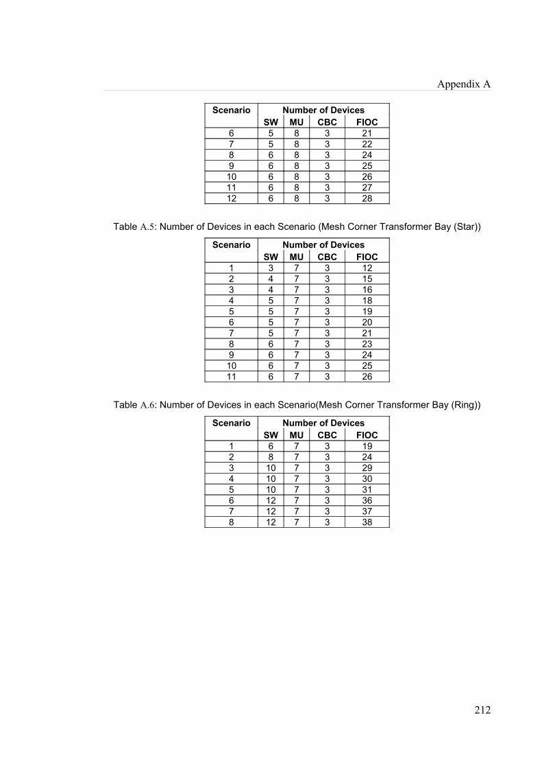
Appendix A
Scenario Number of DevicesSW MU CBC FIOC
6 5 8 3 217 5 8 3 228 6 8 3 249 6 8 3 2510 6 8 3 2611 6 8 3 2712 6 8 3 28
Table A.5: Number of Devices in each Scenario (Mesh Corner Transformer Bay (Star))
Scenario Number of DevicesSW MU CBC FIOC
1 3 7 3 122 4 7 3 153 4 7 3 164 5 7 3 185 5 7 3 196 5 7 3 207 5 7 3 218 6 7 3 239 6 7 3 2410 6 7 3 2511 6 7 3 26
Table A.6: Number of Devices in each Scenario(Mesh Corner Transformer Bay (Ring))
Scenario Number of DevicesSW MU CBC FIOC
1 6 7 3 192 8 7 3 243 10 7 3 294 10 7 3 305 10 7 3 316 12 7 3 367 12 7 3 378 12 7 3 38
212
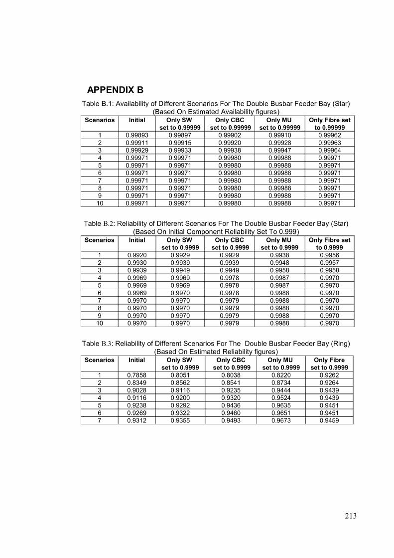
APPENDIX BTable B.1: Availability of Different Scenarios For The Double Busbar Feeder Bay (Star)
(Based On Estimated Availability figures)Scenarios Initial Only SW
set to 0.99999Only CBC
set to 0.99999Only MU
set to 0.99999Only Fibre set
to 0.999991 0.99893 0.99897 0.99902 0.99910 0.999622 0.99911 0.99915 0.99920 0.99928 0.999633 0.99929 0.99933 0.99938 0.99947 0.999644 0.99971 0.99971 0.99980 0.99988 0.999715 0.99971 0.99971 0.99980 0.99988 0.999716 0.99971 0.99971 0.99980 0.99988 0.999717 0.99971 0.99971 0.99980 0.99988 0.999718 0.99971 0.99971 0.99980 0.99988 0.999719 0.99971 0.99971 0.99980 0.99988 0.99971
10 0.99971 0.99971 0.99980 0.99988 0.99971
Table B.2: Reliability of Different Scenarios For The Double Busbar Feeder Bay (Star) (Based On Initial Component Reliability Set To 0.999)
Scenarios Initial Only SW set to 0.9999
Only CBC set to 0.9999
Only MU set to 0.9999
Only Fibre set to 0.9999
1 0.9920 0.9929 0.9929 0.9938 0.99562 0.9930 0.9939 0.9939 0.9948 0.99573 0.9939 0.9949 0.9949 0.9958 0.99584 0.9969 0.9969 0.9978 0.9987 0.99705 0.9969 0.9969 0.9978 0.9987 0.99706 0.9969 0.9970 0.9978 0.9988 0.99707 0.9970 0.9970 0.9979 0.9988 0.99708 0.9970 0.9970 0.9979 0.9988 0.99709 0.9970 0.9970 0.9979 0.9988 0.997010 0.9970 0.9970 0.9979 0.9988 0.9970
Table B.3: Reliability of Different Scenarios For The Double Busbar Feeder Bay (Ring) (Based On Estimated Reliability figures)
Scenarios Initial Only SW set to 0.9999
Only CBC set to 0.9999
Only MU set to 0.9999
Only Fibre set to 0.9999
1 0.7858 0.8051 0.8038 0.8220 0.92622 0.8349 0.8562 0.8541 0.8734 0.92643 0.9028 0.9116 0.9235 0.9444 0.94394 0.9116 0.9200 0.9320 0.9524 0.94395 0.9238 0.9292 0.9436 0.9635 0.94516 0.9269 0.9322 0.9460 0.9651 0.94517 0.9312 0.9355 0.9493 0.9673 0.9459
213
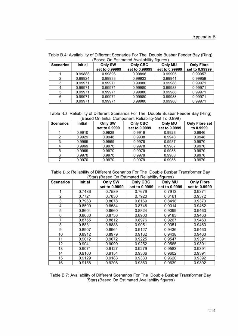
Appendix B
Table B.4: Availability of Different Scenarios For The Double Busbar Feeder Bay (Ring) (Based On Estimated Availability figures)
Scenarios Initial Only SW set to 0.99999
Only CBC set to 0.99999
Only MU set to 0.99999
Only Fibre set to 0.99999
1 0.99888 0.99896 0.99896 0.99905 0.999572 0.99924 0.99933 0.99933 0.99941 0.999593 0.99971 0.99971 0.99980 0.99988 0.999714 0.99971 0.99971 0.99980 0.99988 0.999715 0.99971 0.99971 0.99980 0.99988 0.999716 0.99971 0.99971 0.99980 0.99988 0.999717 0.99971 0.99971 0.99980 0.99988 0.99971
Table B.5: Reliability of Different Scenarios For The Double Busbar Feeder Bay (Ring) (Based On Initial Component Reliability Set To 0.999)
Scenarios Initial Only SW set to 0.9999
Only CBC set to 0.9999
Only MU set to 0.9999
Only Fibre set to 0.9999
1 0.9910 0.9928 0.9919 0.9928 0.99462 0.9929 0.9948 0.9938 0.9948 0.99483 0.9969 0.9969 0.9978 0.9987 0.99704 0.9969 0.9970 0.9978 0.9987 0.99705 0.9969 0.9970 0.9979 0.9988 0.99706 0.9970 0.9970 0.9979 0.9988 0.99707 0.9970 0.9970 0.9979 0.9988 0.9970
Table B.6: Reliability of Different Scenarios For The Double Busbar Transformer Bay (Star) (Based On Estimated Reliability figures)
Scenarios Initial Only SW set to 0.9999
Only CBC set to 0.9999
Only MU set to 0.9999
Only Fibre set to 0.9999
1 0.7486 0.7589 0.7679 0.7913 0.93712 0.7721 0.7830 0.7920 0.8161 0.93723 0.7963 0.8078 0.8169 0.8418 0.93734 0.8500 0.8584 0.8748 0.9014 0.94625 0.8604 0.8660 0.8824 0.9099 0.94636 0.8680 0.8736 0.8900 0.9183 0.94637 0.8755 0.8812 0.8976 0.9267 0.94638 0.8831 0.8888 0.9051 0.9351 0.94639 0.8907 0.8964 0.9127 0.9436 0.946310 0.8912 0.8979 0.9132 0.9438 0.946311 0.9012 0.9072 0.9225 0.9547 0.939112 0.9041 0.9099 0.9252 0.9565 0.939113 0.9071 0.9127 0.9279 0.9583 0.939114 0.9100 0.9154 0.9306 0.9602 0.939115 0.9129 0.9183 0.9333 0.9620 0.939216 0.9158 0.9208 0.9360 0.9639 0.9392
Table B.7: Availability of Different Scenarios For The Double Busbar Transformer Bay (Star) (Based On Estimated Availability figures)
214

Appendix B
Scenarios Initial Only SW set to 0.99999
Only CBC set to 0.99999
Only MU set to 0.99999
Only Fibre set to 0.99999
1 0.99893 0.99897 0.99901 0.99910 0.999622 0.99911 0.99915 0.99920 0.99928 0.999633 0.99929 0.99933 0.99938 0.99946 0.999644 0.99971 0.99971 0.99979 0.99988 0.999715 0.99971 0.99971 0.99979 0.99988 0.999716 0.99971 0.99971 0.99979 0.99988 0.999717 0.99971 0.99971 0.99980 0.99988 0.999718 0.99971 0.99971 0.99980 0.99988 0.999719 0.99971 0.99971 0.99980 0.99988 0.9997110 0.99971 0.99971 0.99980 0.99988 0.9997111 0.99971 0.99971 0.99980 0.99988 0.9997112 0.99971 0.99971 0.99980 0.99988 0.9997113 0.99971 0.99971 0.99980 0.99988 0.9997114 0.99971 0.99971 0.99980 0.99988 0.9997115 0.99971 0.99971 0.99980 0.99988 0.9997116 0.99971 0.99971 0.99980 0.99988 0.99971
Table B.8: Reliability of Different Scenarios For The Double Busbar Transformer Bay (Star) (Based On Initial Component Reliability Set To 0.999)
Scenarios Initial Only SW set to 0.9999
Only CBC set to 0.9999
Only MU set to 0.9999
Only Fibre set to 0.9999
1 0.9919 0.9928 0.9928 0.9937 0.99562 0.9929 0.9938 0.9938 0.9947 0.99573 0.9938 0.9948 0.9948 0.9957 0.99584 0.9968 0.9968 0.9977 0.9987 0.99885 0.9968 0.9969 0.9978 0.9987 0.99886 0.9968 0.9969 0.9978 0.9987 0.99887 0.9969 0.9969 0.9978 0.9987 0.99888 0.9969 0.9969 0.9978 0.9987 0.99889 0.9969 0.9969 0.9978 0.9987 0.9988
10 0.9969 0.9969 0.9978 0.9987 0.998811 0.9969 0.9969 0.9978 0.9988 0.998712 0.9969 0.9969 0.9978 0.9988 0.998713 0.9969 0.9969 0.9978 0.9988 0.998714 0.9969 0.9969 0.9978 0.9988 0.998715 0.9969 0.9969 0.9978 0.9988 0.998716 0.9969 0.9969 0.9978 0.9988 0.9987
Table B.9: Reliability of Different Scenarios For The Double Busbar Transformer Bay (Ring) (Based On Estimated Reliability figures)
Scenarios Initial Only SW set to 0.9999
Only CBC set to 0.9999
Only MU set to 0.9999
Only Fibre set to 0.9999
1 0.7594 0.7795 0.7782 0.8097 0.91962 0.8068 0.8289 0.8268 0.8603 0.91983 0.8724 0.8826 0.8940 0.9302 0.93724 0.8778 0.8881 0.8994 0.9348 0.93725 0.8838 0.8939 0.9053 0.9399 0.9372
215
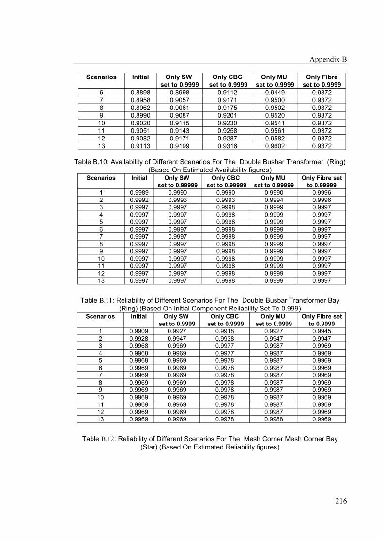
Appendix B
Scenarios Initial Only SW set to 0.9999
Only CBC set to 0.9999
Only MU set to 0.9999
Only Fibre set to 0.9999
6 0.8898 0.8998 0.9112 0.9449 0.93727 0.8958 0.9057 0.9171 0.9500 0.93728 0.8962 0.9061 0.9175 0.9502 0.93729 0.8990 0.9087 0.9201 0.9520 0.9372
10 0.9020 0.9115 0.9230 0.9541 0.937211 0.9051 0.9143 0.9258 0.9561 0.937212 0.9082 0.9171 0.9287 0.9582 0.937213 0.9113 0.9199 0.9316 0.9602 0.9372
Table B.10: Availability of Different Scenarios For The Double Busbar Transformer (Ring) (Based On Estimated Availability figures)
Scenarios Initial Only SW set to 0.99999
Only CBC set to 0.99999
Only MU set to 0.99999
Only Fibre set to 0.99999
1 0.9989 0.9990 0.9990 0.9990 0.99962 0.9992 0.9993 0.9993 0.9994 0.99963 0.9997 0.9997 0.9998 0.9999 0.99974 0.9997 0.9997 0.9998 0.9999 0.99975 0.9997 0.9997 0.9998 0.9999 0.99976 0.9997 0.9997 0.9998 0.9999 0.99977 0.9997 0.9997 0.9998 0.9999 0.99978 0.9997 0.9997 0.9998 0.9999 0.99979 0.9997 0.9997 0.9998 0.9999 0.999710 0.9997 0.9997 0.9998 0.9999 0.999711 0.9997 0.9997 0.9998 0.9999 0.999712 0.9997 0.9997 0.9998 0.9999 0.999713 0.9997 0.9997 0.9998 0.9999 0.9997
Table B.11: Reliability of Different Scenarios For The Double Busbar Transformer Bay (Ring) (Based On Initial Component Reliability Set To 0.999)
Scenarios Initial Only SW set to 0.9999
Only CBC set to 0.9999
Only MU set to 0.9999
Only Fibre set to 0.9999
1 0.9909 0.9927 0.9918 0.9927 0.99452 0.9928 0.9947 0.9938 0.9947 0.99473 0.9968 0.9969 0.9977 0.9987 0.99694 0.9968 0.9969 0.9977 0.9987 0.99695 0.9968 0.9969 0.9978 0.9987 0.99696 0.9969 0.9969 0.9978 0.9987 0.99697 0.9969 0.9969 0.9978 0.9987 0.99698 0.9969 0.9969 0.9978 0.9987 0.99699 0.9969 0.9969 0.9978 0.9987 0.996910 0.9969 0.9969 0.9978 0.9987 0.996911 0.9969 0.9969 0.9978 0.9987 0.996912 0.9969 0.9969 0.9978 0.9987 0.996913 0.9969 0.9969 0.9978 0.9988 0.9969
Table B.12: Reliability of Different Scenarios For The Mesh Corner Mesh Corner Bay (Star) (Based On Estimated Reliability figures)
216
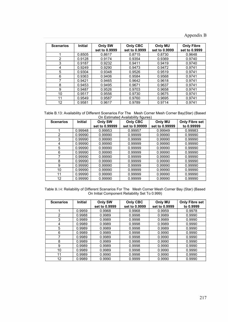
Appendix B
Scenarios Initial Only SW set to 0.9999
Only CBC set to 0.9999
Only MU set to 0.9999
Only Fibre set to 0.9999
1 0.8505 0.8617 0.8715 0.8730 0.96482 0.9128 0.9174 0.9354 0.9369 0.97403 0.9187 0.9232 0.9411 0.9419 0.97404 0.9249 0.9290 0.9473 0.9472 0.97415 0.9304 0.9348 0.9526 0.9519 0.97416 0.9363 0.9406 0.9584 0.9568 0.97417 0.9421 0.9465 0.9642 0.9618 0.97418 0.9453 0.9495 0.9671 0.9637 0.97419 0.9487 0.9526 0.9703 0.9658 0.9741
10 0.9517 0.9556 0.9730 0.9675 0.974111 0.9549 0.9587 0.9760 0.9695 0.974112 0.9581 0.9617 0.9789 0.9714 0.9741
Table B.13: Availability of Different Scenarios For The Mesh Corner Mesh Corner Bay(Star) (Based On Estimated Availability figures)
Scenarios Initial Only SW set to 0.99999
Only CBC set to 0.99999
Only MU set to 0.99999
Only Fibre set to 0.99999
1 0.99948 0.99953 0.99957 0.99949 0.999832 0.99990 0.99990 0.99999 0.99990 0.999903 0.99990 0.99990 0.99999 0.99990 0.999904 0.99990 0.99990 0.99999 0.99990 0.999905 0.99990 0.99990 0.99999 0.99990 0.999906 0.99990 0.99990 0.99999 0.99990 0.999907 0.99990 0.99990 0.99999 0.99990 0.999908 0.99990 0.99990 0.99999 0.99990 0.999909 0.99990 0.99990 0.99999 0.99990 0.9999010 0.99990 0.99990 0.99999 0.99990 0.9999011 0.99990 0.99990 0.99999 0.99990 0.9999012 0.99990 0.99990 0.99999 0.99990 0.99990
Table B.14: Reliability of Different Scenarios For The Mesh Corner Mesh Corner Bay (Star) (Based On Initial Component Reliability Set To 0.999)
Scenarios Initial Only SW set to 0.9999
Only CBC set to 0.9999
Only MU set to 0.9999
Only Fibre set to 0.9999
1 0.9959 0.9968 0.9968 0.9959 0.99782 0.9988 0.9989 0.9998 0.9989 0.99903 0.9989 0.9989 0.9998 0.9989 0.99904 0.9989 0.9989 0.9998 0.9989 0.99905 0.9989 0.9989 0.9998 0.9989 0.99906 0.9989 0.9989 0.9998 0.9990 0.99907 0.9989 0.9989 0.9998 0.9990 0.99908 0.9989 0.9989 0.9998 0.9990 0.99909 0.9989 0.9989 0.9998 0.9990 0.999010 0.9989 0.9989 0.9998 0.9990 0.999011 0.9989 0.9990 0.9998 0.9990 0.999012 0.9989 0.9990 0.9999 0.9990 0.9990
217

Appendix B
Table B.15: Reliability of Different Scenarios For The Mesh Corner Transformer Bay (Star) (Based On Estimated Reliability figures)
Scenarios Initial Only SW set to 0.9999
Only CBC set to 0.9999
Only MU set to 0.9999
Only Fibre set to 0.9999
1 0.8243 0.8347 0.8439 0.8533 0.95062 0.8502 0.8612 0.8704 0.8801 0.95073 0.8760 0.8877 0.8969 0.9069 0.95084 0.8810 0.8926 0.9017 0.9112 0.95085 0.8859 0.8975 0.9064 0.9155 0.95086 0.8913 0.9029 0.9117 0.9202 0.95087 0.8964 0.9079 0.9167 0.9246 0.95088 0.8991 0.9104 0.9190 0.9263 0.95089 0.9017 0.9129 0.9214 0.9279 0.950810 0.9046 0.9157 0.9240 0.9298 0.950811 0.9073 0.9183 0.9264 0.9315 0.9508
Table B.16: Availability of Different Scenarios For The Mesh Corner Transformer Bay(Star) (Based On Estimated Availability figures)
Scenarios Initial Only SW set to 0.99999
Only CBC set to 0.99999
Only MU set to 0.99999
Only Fibre set to 0.99999
1 0.99921 0.99925 0.99929 0.99929 0.999732 0.99939 0.99943 0.99948 0.99948 0.999743 0.99957 0.99961 0.99966 0.99966 0.999754 0.99957 0.99961 0.99966 0.99966 0.999755 0.99957 0.99961 0.99966 0.99966 0.999756 0.99957 0.99961 0.99966 0.99966 0.999757 0.99957 0.99961 0.99966 0.99966 0.999758 0.99957 0.99961 0.99966 0.99966 0.999759 0.99957 0.99961 0.99966 0.99966 0.9997510 0.99957 0.99961 0.99966 0.99966 0.9997511 0.99957 0.99961 0.99966 0.99966 0.99975
Table B.17: Reliability of Different Scenarios For The Mesh Corner Transformer Bay (Star) (Based On Initial Component Reliability Set To 0.999)
Scenarios Initial Only SW set to 0.9999
Only CBC set to 0.9999
Only MU set to 0.9999
Only Fibre set to 0.9999
1 0.9939 0.9948 0.9948 0.9949 0.99672 0.9949 0.9958 0.9958 0.9959 0.99683 0.9959 0.9968 0.9968 0.9968 0.99694 0.9959 0.9968 0.9968 0.9969 0.99695 0.9959 0.9968 0.9968 0.9969 0.99696 0.9959 0.9968 0.9968 0.9969 0.99697 0.9959 0.9969 0.9969 0.9969 0.99698 0.9959 0.9969 0.9969 0.9969 0.99699 0.9960 0.9969 0.9969 0.9969 0.996910 0.9960 0.9969 0.9969 0.9969 0.996911 0.9960 0.9969 0.9969 0.9969 0.9969
Table B.18: Reliability of Different Scenarios For The Mesh Corner Transformer Bay (Ring) (Based On Estimated Reliability figures)
218
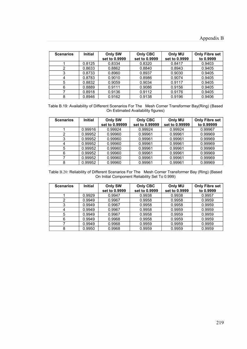
Appendix B
Scenarios Initial Only SW set to 0.9999
Only CBC set to 0.9999
Only MU set to 0.9999
Only Fibre set to 0.9999
1 0.8125 0.8334 0.8320 0.8417 0.94032 0.8633 0.8862 0.8840 0.8943 0.94053 0.8733 0.8960 0.8937 0.9030 0.94054 0.8783 0.9010 0.8986 0.9074 0.94055 0.8832 0.9059 0.9034 0.9117 0.94056 0.8889 0.9111 0.9086 0.9156 0.94057 0.8918 0.9136 0.9112 0.9176 0.94058 0.8946 0.9162 0.9138 0.9196 0.9406
Table B.19: Availability of Different Scenarios For The Mesh Corner Transformer Bay(Ring) (Based On Estimated Availability figures)
Scenarios Initial Only SW set to 0.99999
Only CBC set to 0.99999
Only MU set to 0.99999
Only Fibre set to 0.99999
1 0.99916 0.99924 0.99924 0.99924 0.999672 0.99952 0.99960 0.99961 0.99961 0.999693 0.99952 0.99960 0.99961 0.99961 0.999694 0.99952 0.99960 0.99961 0.99961 0.999695 0.99952 0.99960 0.99961 0.99961 0.999696 0.99952 0.99960 0.99961 0.99961 0.999697 0.99952 0.99960 0.99961 0.99961 0.999698 0.99952 0.99960 0.99961 0.99961 0.99969
Table B.20: Reliability of Different Scenarios For The Mesh Corner Transformer Bay (Ring) (Based On Initial Component Reliability Set To 0.999)
Scenarios Initial Only SW set to 0.9999
Only CBC set to 0.9999
Only MU set to 0.9999
Only Fibre set to 0.9999
1 0.9929 0.9947 0.9938 0.9938 0.99572 0.9949 0.9967 0.9958 0.9958 0.99593 0.9949 0.9967 0.9958 0.9958 0.99594 0.9949 0.9967 0.9958 0.9959 0.99595 0.9949 0.9967 0.9958 0.9959 0.99596 0.9949 0.9968 0.9958 0.9959 0.99597 0.9949 0.9968 0.9959 0.9959 0.99598 0.9950 0.9968 0.9959 0.9959 0.9959
219
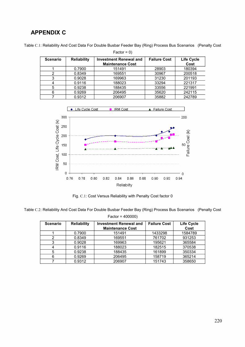
APPENDIX C
Table C.1: Reliability And Cost Data For Double Busbar Feeder Bay (Ring) Process Bus Scenarios (Penalty Cost
Factor = 0)
Scenario Reliability Investment Renewal andMaintenance Cost
Failure Cost Life Cycle Cost
1 0.7900 151491 28903 1803942 0.8349 169551 30967 2005183 0.9028 169963 31230 2011934 0.9116 188023 33294 2213175 0.9238 188435 33556 2219916 0.9269 206495 35620 2421157 0.9312 206907 35882 242789
Fig. C.1: Cost Versus Reliability with Penalty Cost factor 0
Table C.2: Reliability And Cost Data For Double Busbar Feeder Bay (Ring) Process Bus Scenarios (Penalty Cost
Factor = 400000)
Scenario Reliability Investment Renewal andMaintenance Cost
Failure Cost Life Cycle Cost
1 0.7900 151491 1433298 15847892 0.8349 169551 761702 9312533 0.9028 169963 195621 3655844 0.9116 188023 182515 3705385 0.9238 188435 161899 3503346 0.9269 206495 158719 3652147 0.9312 206907 151743 358650
220

Appendix C
Fig. C.2: Cost Versus Reliability with Penalty Cost factor 400000
Table C.3: Reliability And Cost Data For Double Busbar Feeder Bay (Ring) Process Bus Scenarios (Penalty Cost Factor = 21000)
Scenario Reliability Investment Renewal andMaintenance Cost
Failure Cost
Life Cycle Cost
1 0.7900 151491 102634 2541252 0.8349 169551 69331 2388823 0.9028 169963 39860 2098234 0.9116 188023 41128 2291515 0.9238 188435 40294 2287296 0.9269 206495 42083 2485787 0.9312 206907 41965 248872
Fig. C.3: Cost Versus Reliability with Penalty Cost factor 21000
221

Appendix C
Table C.4: Reliability And Cost Data For Double Busbar Transformer Bay (Star) Process Bus Scenarios (Penalty Cost Factor = 0)
Scenario Reliability Investment Renewal andMaintenance Cost
Failure Cost Life Cycle Cost
1 0.7486 202628 45090 2477182 0.7721 211452 45990 2574423 0.7963 211864 46253 2581174 0.8528 212276 46515 2587915 0.8604 221100 47416 2685166 0.8680 221512 47678 2691907 0.8755 221924 47941 2698658 0.8831 222336 48203 2705399 0.8907 222748 48466 27121410 0.8912 223572 48990 27256211 0.9012 232396 49891 28228712 0.9041 232808 50154 28296213 0.9071 233220 50416 28363614 0.9100 233632 50678 28431015 0.9129 234044 50941 28498516 0.9158 234456 51203 285659
Fig. C.4: Cost Versus Reliability with Penalty Cost factor 0
Table C.5: Reliability And Cost Data For Double Busbar Transformer Bay (Star) Process Bus Scenarios (Penalty Cost Factor = 400000)
Scenario Reliability Investment Renewal andMaintenance Cost
Failure Cost Life Cycle Cost
1 0.7486 202628 1621357 18239852 0.7721 211452 1232059 14435113 0.7963 211864 889234 11010984 0.8528 212276 297700 5099765 0.8604 221100 285317 5064176 0.8680 221512 272336 4938487 0.8755 221924 259392 4813168 0.8831 222336 246486 4688229 0.8907 222748 233618 456366
222
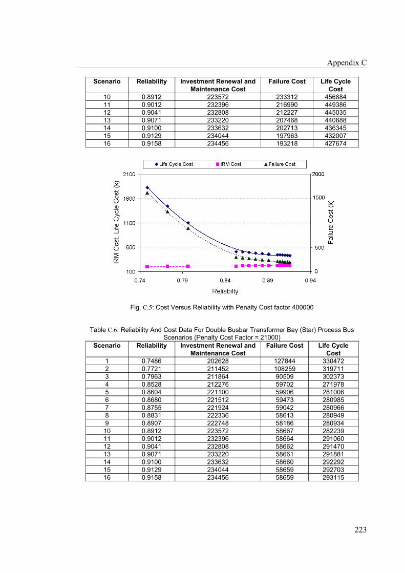
Appendix C
Scenario Reliability Investment Renewal andMaintenance Cost
Failure Cost Life Cycle Cost
10 0.8912 223572 233312 45688411 0.9012 232396 216990 44938612 0.9041 232808 212227 44503513 0.9071 233220 207468 44068814 0.9100 233632 202713 43634515 0.9129 234044 197963 43200716 0.9158 234456 193218 427674
Fig. C.5: Cost Versus Reliability with Penalty Cost factor 400000
Table C.6: Reliability And Cost Data For Double Busbar Transformer Bay (Star) Process Bus Scenarios (Penalty Cost Factor = 21000)
Scenario Reliability Investment Renewal andMaintenance Cost
Failure Cost Life Cycle Cost
1 0.7486 202628 127844 3304722 0.7721 211452 108259 3197113 0.7963 211864 90509 3023734 0.8528 212276 59702 2719785 0.8604 221100 59906 2810066 0.8680 221512 59473 2809857 0.8755 221924 59042 2809668 0.8831 222336 58613 2809499 0.8907 222748 58186 28093410 0.8912 223572 58667 28223911 0.9012 232396 58664 29106012 0.9041 232808 58662 29147013 0.9071 233220 58661 29188114 0.9100 233632 58660 29229215 0.9129 234044 58659 29270316 0.9158 234456 58659 293115
223
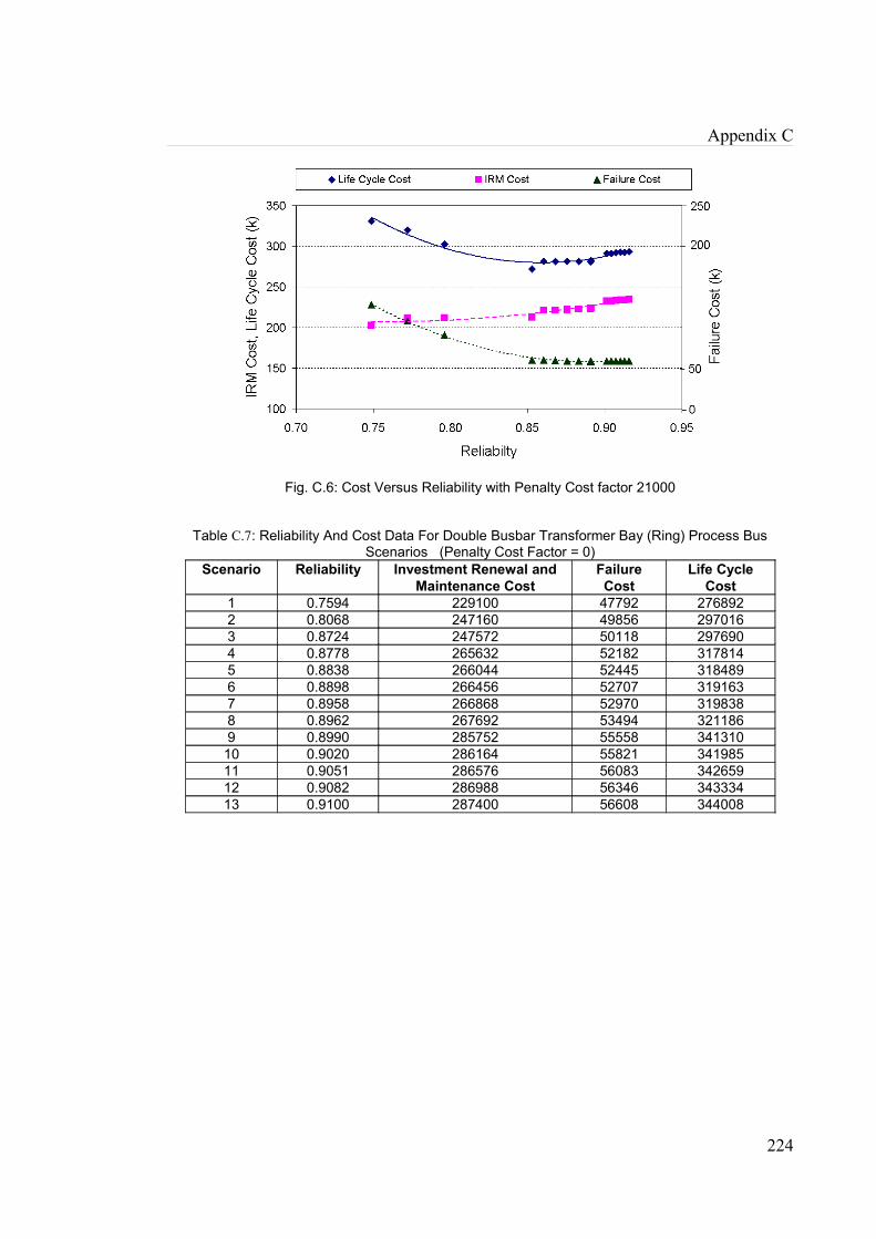
Appendix C
Fig. C.6: Cost Versus Reliability with Penalty Cost factor 21000
Table C.7: Reliability And Cost Data For Double Busbar Transformer Bay (Ring) Process Bus Scenarios (Penalty Cost Factor = 0)
Scenario Reliability Investment Renewal andMaintenance Cost
Failure Cost
Life Cycle Cost
1 0.7594 229100 47792 2768922 0.8068 247160 49856 2970163 0.8724 247572 50118 2976904 0.8778 265632 52182 3178145 0.8838 266044 52445 3184896 0.8898 266456 52707 3191637 0.8958 266868 52970 3198388 0.8962 267692 53494 3211869 0.8990 285752 55558 34131010 0.9020 286164 55821 34198511 0.9051 286576 56083 34265912 0.9082 286988 56346 34333413 0.9100 287400 56608 344008
224

Appendix C
Fig. C.7: Cost Versus Reliability with Penalty Cost factor 0
Table C.8: Reliability And Cost Data For Double Busbar Transformer Bay (Ring) Process Bus Scenarios (Penalty Cost Factor = 400000)
Scenario Reliability Investment Renewal andMaintenance Cost
Failure Cost Life Cycle Cost
1 0.7594 229100 1627410 18565102 0.8068 247160 906440 11536003 0.8724 247572 266877 5144494 0.8778 265632 259465 5250975 0.8838 266044 249364 5154086 0.8898 266456 239286 5057427 0.8958 266868 229231 4960998 0.8962 267692 229109 4968019 0.8990 285752 226346 51209810 0.9020 286164 221320 50748411 0.9051 286576 216299 50287512 0.9082 286988 211283 49827113 0.9100 287400 206326 493726
225

Appendix C
Fig. C.8: Cost Versus Reliability with Penalty Cost factor 400000
Table C.9: Reliability And Cost Data For Double Busbar Transformer Bay (Ring) Process Bus Scenarios (Penalty Cost Factor = 21000)
Scenario Reliability Investment Renewal andMaintenance Cost
Failure Cost
Life Cycle Cost
1 0.7594 229100 130722 3598222 0.8068 247160 94827 3419873 0.8724 247572 61498 3090704 0.8778 265632 63065 3286975 0.8838 266044 62783 3288276 0.8898 266456 62503 3289597 0.8958 266868 62223 3290918 0.8962 267692 62714 3304069 0.8990 285752 64525 35027710 0.9020 286164 64509 35067311 0.9051 286576 64495 35107112 0.9082 286988 64480 35146813 0.9100 287400 64468 351868
226

Appendix C
Fig. C.9: Cost Versus Reliability with Penalty Cost factor 21000
Table C.10: Reliability And Cost Data For Mesh Corner Mesh Corner Bay (Star) Process Bus Scenarios (Penalty Cost Factor = 0)
Scenario Reliability Investment Renewal andMaintenance Cost
Failure Cost Life Cycle Cost
1 0.85049 148017 32122 1801392 0.91281 156017 32498 1885153 0.91868 164841 33399 1982404 0.92493 165253 33662 1989155 0.93040 165665 33924 1995896 0.93626 166077 34186 2002637 0.94212 166489 34449 2009388 0.94532 175313 35350 2106639 0.94873 175725 35612 21133710 0.95172 176137 35874 21201111 0.95492 176549 36137 21268612 0.95812 176961 36399 213360
227

Appendix C
Fig. C.10: Cost Versus Reliability with Penalty Cost factor 0
Table C.11: Reliability And Cost Data For Mesh Corner Mesh Corner Bay (Star) Process Bus Scenarios (Penalty Cost Factor = 400000)
Scenario Reliability Investment Renewal andMaintenance Cost
Failure Cost Life Cycle Cost
1 0.85049 148017 482234 6302512 0.91281 156017 82814 2388313 0.91868 164841 80191 2450324 0.92493 165253 76726 2419795 0.93040 165665 73730 2393956 0.93626 166077 70530 2366077 0.94212 166489 67351 2338408 0.94532 175313 66391 2417049 0.94873 175725 64677 24040210 0.95172 176137 63209 23934611 0.95492 176549 61626 23817512 0.95812 176961 60047 237008
228

Appendix C
Fig. C.11: Cost Versus Reliability with Penalty Cost factor 400000
Table C.12: Reliability And Cost Data For Mesh Corner Mesh Corner Bay (Star) Process Bus Scenarios (Penalty Cost Factor = 21000)
Scenario Reliability Investment Renewal andMaintenance Cost
Failure Cost Life Cycle Cost
1 0.85049 148017 55753 2037702 0.91281 156017 35140 1911573 0.91868 164841 35856 2006974 0.92493 165253 35922 2011755 0.93040 165665 36014 2016796 0.93626 166077 36094 2021717 0.94212 166489 36176 2026658 0.94532 175313 36979 2122929 0.94873 175725 37138 21286310 0.95172 176137 37309 21344611 0.95492 176549 37475 21402412 0.95812 176961 37641 214602
229
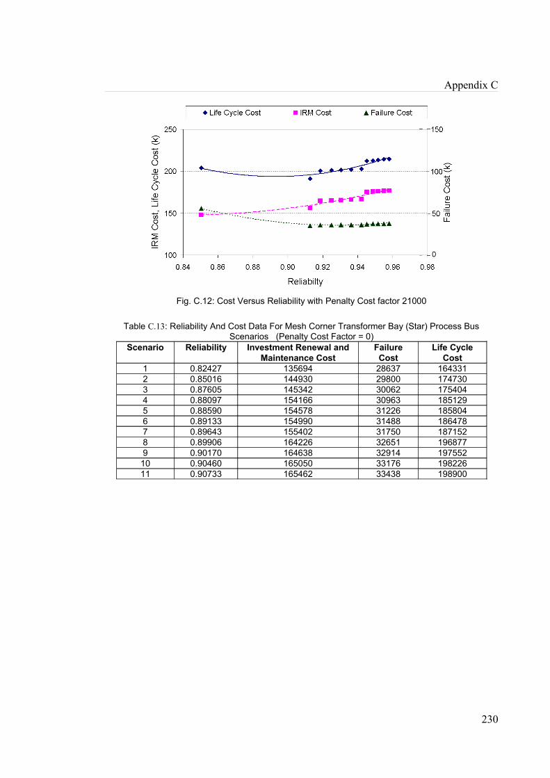
Appendix C
Fig. C.12: Cost Versus Reliability with Penalty Cost factor 21000
Table C.13: Reliability And Cost Data For Mesh Corner Transformer Bay (Star) Process Bus Scenarios (Penalty Cost Factor = 0)
Scenario Reliability Investment Renewal andMaintenance Cost
Failure Cost
Life Cycle Cost
1 0.82427 135694 28637 1643312 0.85016 144930 29800 1747303 0.87605 145342 30062 1754044 0.88097 154166 30963 1851295 0.88590 154578 31226 1858046 0.89133 154990 31488 1864787 0.89643 155402 31750 1871528 0.89906 164226 32651 1968779 0.90170 164638 32914 19755210 0.90460 165050 33176 19822611 0.90733 165462 33438 198900
230

Appendix C
Fig. C.13: Cost Versus Reliability with Penalty Cost factor 0
Table C.14: Reliability And Cost Data For Mesh Corner Transformer Bay (Star) Process Bus Scenarios (Penalty Cost Factor = 400000)
Scenario Reliability Investment Renewal andMaintenance Cost
Failure Cost
Life Cycle Cost
1 0.82427 135694 842668 9783622 0.85016 144930 564230 7091603 0.87605 145342 340083 4854254 0.88097 154166 328485 4826515 0.88590 154578 316265 4708436 0.89133 154990 302805 4577957 0.89643 155402 290197 4455998 0.89906 164226 284455 4486819 0.90170 164638 278080 44271810 0.90460 165050 271038 43608811 0.90733 165462 264447 429909
231

Appendix C
Fig. C.14: Cost Versus Reliability with Penalty Cost factor 400000
Table C.15: Reliability And Cost Data For Mesh Corner Transformer Bay (Star) Process Bus Scenarios (Penalty Cost Factor = 21000)
Scenario Reliability Investment Renewal andMaintenance Cost
Failure Cost
Life Cycle Cost
1 0.82427 135694 71373 2070672 0.85016 144930 57858 2027883 0.87605 145342 46338 1916804 0.88097 154166 46583 2007495 0.88590 154578 46190 2007686 0.89133 154990 45732 2007227 0.89643 155402 45319 2007218 0.89906 164226 45871 2100979 0.90170 164638 45785 21042310 0.90460 165050 45664 21071411 0.90733 165462 45566 211028
Fig. C.15: Cost Versus Reliability with Penalty Cost factor 21000
232
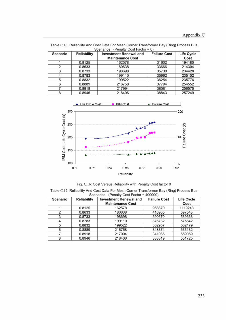
Appendix C
Table C.16: Reliability And Cost Data For Mesh Corner Transformer Bay (Ring) Process Bus Scenarios (Penalty Cost Factor = 0)
Scenario Reliability Investment Renewal andMaintenance Cost
Failure Cost Life Cycle Cost
1 0.8125 162578 31602 1941802 0.8633 180638 33666 2143043 0.8733 198698 35730 2344284 0.8783 199110 35992 2351025 0.8832 199522 36254 2357766 0.8889 216758 37794 2545527 0.8918 217994 38581 2565758 0.8946 218406 38843 257249
Fig. C.16: Cost Versus Reliability with Penalty Cost factor 0
Table C.17: Reliability And Cost Data For Mesh Corner Transformer Bay (Ring) Process Bus Scenarios (Penalty Cost Factor = 400000)
Scenario Reliability Investment Renewal andMaintenance Cost
Failure Cost Life Cycle Cost
1 0.8125 162578 956670 11192482 0.8633 180638 416905 5975433 0.8733 198698 390670 5893684 0.8783 199110 376732 5758425 0.8832 199522 362957 5624796 0.8889 216758 348374 5651327 0.8918 217994 341065 5590598 0.8946 218406 333319 551725
233

Appendix C
Fig. C.17: Cost Versus Reliability with Penalty Cost factor 400000
Table C.18: Reliability And Cost Data For Mesh Corner Transformer Bay (Ring) Process Bus Scenarios (Penalty Cost Factor = 21000)
Scenario Reliability Investment Renewal andMaintenance Cost
Failure Cost Life Cycle Cost
1 0.8125 162578 80168 2427462 0.8633 180638 53786 2344243 0.8733 198698 54364 2530624 0.8783 199110 53881 2529915 0.8832 199522 53406 2529286 0.8889 216758 54099 2708577 0.8918 217994 54461 2724558 0.8946 218406 54303 272709
Fig. C.18: Cost Versus Reliability with Penalty Cost factor 21000
234
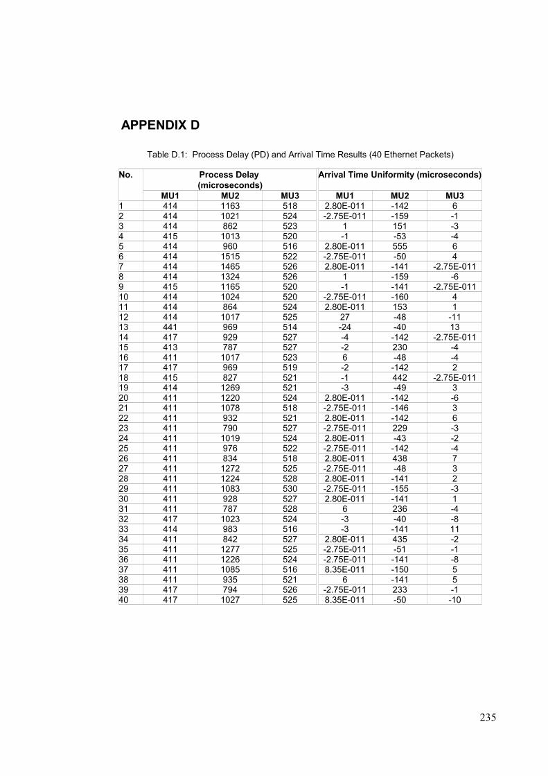
APPENDIX D
Table D.1: Process Delay (PD) and Arrival Time Results (40 Ethernet Packets)
No. Process Delay (microseconds)
Arrival Time Uniformity (microseconds)
MU1 MU2 MU3 MU1 MU2 MU31 414 1163 518 2.80E-011 -142 62 414 1021 524 -2.75E-011 -159 -13 414 862 523 1 151 -34 415 1013 520 -1 -53 -45 414 960 516 2.80E-011 555 66 414 1515 522 -2.75E-011 -50 47 414 1465 526 2.80E-011 -141 -2.75E-0118 414 1324 526 1 -159 -69 415 1165 520 -1 -141 -2.75E-01110 414 1024 520 -2.75E-011 -160 411 414 864 524 2.80E-011 153 112 414 1017 525 27 -48 -1113 441 969 514 -24 -40 1314 417 929 527 -4 -142 -2.75E-01115 413 787 527 -2 230 -416 411 1017 523 6 -48 -417 417 969 519 -2 -142 218 415 827 521 -1 442 -2.75E-01119 414 1269 521 -3 -49 320 411 1220 524 2.80E-011 -142 -621 411 1078 518 -2.75E-011 -146 322 411 932 521 2.80E-011 -142 623 411 790 527 -2.75E-011 229 -324 411 1019 524 2.80E-011 -43 -225 411 976 522 -2.75E-011 -142 -426 411 834 518 2.80E-011 438 727 411 1272 525 -2.75E-011 -48 328 411 1224 528 2.80E-011 -141 229 411 1083 530 -2.75E-011 -155 -330 411 928 527 2.80E-011 -141 131 411 787 528 6 236 -432 417 1023 524 -3 -40 -833 414 983 516 -3 -141 1134 411 842 527 2.80E-011 435 -235 411 1277 525 -2.75E-011 -51 -136 411 1226 524 -2.75E-011 -141 -837 411 1085 516 8.35E-011 -150 538 411 935 521 6 -141 539 417 794 526 -2.75E-011 233 -140 417 1027 525 8.35E-011 -50 -10
235
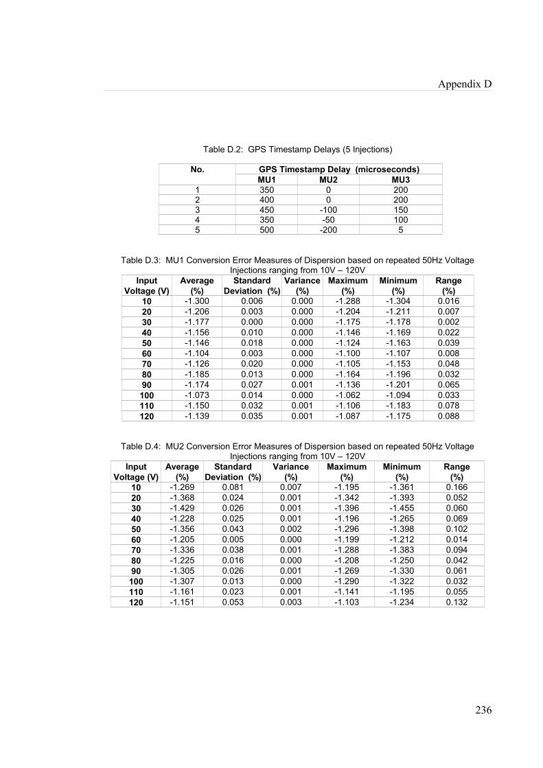
Appendix D
Table D.2: GPS Timestamp Delays (5 Injections)
No. GPS Timestamp Delay (microseconds)MU1 MU2 MU3
1 350 0 2002 400 0 2003 450 -100 1504 350 -50 1005 500 -200 5
Table D.3: MU1 Conversion Error Measures of Dispersion based on repeated 50Hz Voltage
Injections ranging from 10V – 120VInput
Voltage (V)Average
(%)Standard
Deviation (%)Variance
(%)Maximum
(%)Minimum
(%)Range
(%)10 -1.300 0.006 0.000 -1.288 -1.304 0.01620 -1.206 0.003 0.000 -1.204 -1.211 0.00730 -1.177 0.000 0.000 -1.175 -1.178 0.00240 -1.156 0.010 0.000 -1.146 -1.169 0.02250 -1.146 0.018 0.000 -1.124 -1.163 0.03960 -1.104 0.003 0.000 -1.100 -1.107 0.00870 -1.126 0.020 0.000 -1.105 -1.153 0.04880 -1.185 0.013 0.000 -1.164 -1.196 0.03290 -1.174 0.027 0.001 -1.136 -1.201 0.065100 -1.073 0.014 0.000 -1.062 -1.094 0.033110 -1.150 0.032 0.001 -1.106 -1.183 0.078120 -1.139 0.035 0.001 -1.087 -1.175 0.088
Table D.4: MU2 Conversion Error Measures of Dispersion based on repeated 50Hz Voltage Injections ranging from 10V – 120V
Input Voltage (V)
Average(%)
Standard Deviation (%)
Variance(%)
Maximum(%)
Minimum(%)
Range(%)
10 -1.269 0.081 0.007 -1.195 -1.361 0.16620 -1.368 0.024 0.001 -1.342 -1.393 0.05230 -1.429 0.026 0.001 -1.396 -1.455 0.06040 -1.228 0.025 0.001 -1.196 -1.265 0.06950 -1.356 0.043 0.002 -1.296 -1.398 0.10260 -1.205 0.005 0.000 -1.199 -1.212 0.01470 -1.336 0.038 0.001 -1.288 -1.383 0.09480 -1.225 0.016 0.000 -1.208 -1.250 0.04290 -1.305 0.026 0.001 -1.269 -1.330 0.061100 -1.307 0.013 0.000 -1.290 -1.322 0.032110 -1.161 0.023 0.001 -1.141 -1.195 0.055120 -1.151 0.053 0.003 -1.103 -1.234 0.132
236
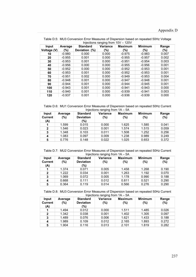
Appendix D
Table D.5: MU3 Conversion Error Measures of Dispersion based on repeated 50Hz Voltage Injections ranging from 10V – 120V
Input Voltage (V)
Average(%)
Standard Deviation (%)
Variance(%)
Maximum(%)
Minimum(%)
Range(%)
10 -0.980 0.000 0.000 -0.975 -0.983 0.00720 -0.955 0.001 0.000 -0.955 -0.957 0.00230 -0.953 0.001 0.000 -0.951 -0.954 0.00340 -0.956 0.000 0.000 -0.955 -0.956 0.00150 -0.952 0.000 0.000 -0.952 -0.953 0.00160 -0.953 0.001 0.000 -0.952 -0.953 0.00170 -0.951 0.002 0.000 -0.949 -0.953 0.00480 -0.948 0.001 0.000 -0.947 -0.948 0.00190 -0.944 0.001 0.000 -0.944 -0.945 0.001
100 -0.943 0.001 0.000 -0.941 -0.943 0.000110 -0.940 0.001 0.000 -0.939 -0.941 0.003120 -0.937 0.001 0.000 -0.936 -0.939 0.000
Table D.6: MU1 Conversion Error Measures of Dispersion based on repeated 50Hz Current Injections ranging from 1A – 5A
Input Current
(A)
Average(%)
Standard Deviation
(%)
Variance(%)
Maximum(%)
Minimum(%)
Range(%)
1 1.599 0.015 0.000 1.625 1.585 0.0412 1.546 0.023 0.001 1.574 1.515 0.0593 1.348 0.103 0.011 1.508 1.252 0.2564 1.083 0.097 0.009 1.238 0.989 0.2495 0.776 0.148 0.022 1.025 0.653 0.372
Table D.7: MU2 Conversion Error Measures of Dispersion based on repeated 50Hz Current Injections ranging from 1A – 5A
Input Current
(A)
Average(%)
Standard Deviation
(%)
Variance(%)
Maximum(%)
Minimum(%)
Range(%)
1 1.374 0.071 0.005 1.458 1.268 0.1902 1.222 0.034 0.001 1.263 1.192 0.0703 1.069 0.072 0.005 1.178 0.990 0.1884 0.668 0.111 0.012 0.811 0.521 0.2905 0.364 0.119 0.014 0.566 0.276 0.290
Table D.8: MU3 Conversion Error Measures of Dispersion based on repeated 50Hz Current Injections ranging from 1A – 5A
Input Current
(A)
Average(%)
Standard Deviation
(%)
Variance(%)
Maximum(%)
Minimum(%)
Range(%)
1 1.494 0.012 0.000 1.511 1.485 0.0262 1.342 0.038 0.001 1.402 1.305 0.0973 1.489 0.076 0.006 1.621 1.433 0.1884 1.989 0.109 0.012 2.165 1.893 0.2725 1.904 0.116 0.013 2.101 1.819 0.282
237

Appendix D
Table D.9: MU1 Filter Analysis Measures of Dispersion based on repeated 50V Injections at frequencies ranging from 50Hz to 1950z
Input Frequency
(Hz)
Average(%)
Standard Deviation
(%)
Variance(%)
Maximum(%)
Minimum(%)
Range(%)
50 0.989 0.00 0.00 0.989 0.988 0.00150 0.941 3.48E-005 1.21E-009 0.941 0.941 8.20E-005250 0.671 1.26E-005 1.60E-010 0.671 0.671 2.59E-005350 0.407 1.46E-005 2.14E-010 0.407 0.407 3.83E-005550 0.173 6.09E-006 3.71E-011 0.173 0.173 1.52E-005
1150 0.040 3.45E-005 1.19E-009 0.040 0.040 7.04E-0051950 0.014 2.36E-005 5.57E-010 0.014 0.014 6.35E-005
Table D.10: MU2 Filter Analysis Measures of Dispersion based on repeated 50V Injections at frequencies ranging from 50Hz to 1950z
Input Frequency
(Hz)
Average(%)
Standard Deviation
(%)
Variance(%)
Maximum(%)
Minimum(%)
Range(%)
50 0.986 0 1.86E-007 0.987 0.986 0150 0.983 9.73E-005 9.46E-009 0.983 0.983 0550 0.974 9.56E-005 9.15E-009 0.974 0.974 0950 0.954 3.62E-005 1.31E-009 0.954 0.954 8.46E-005
1150 0.939 9.77E-005 9.55E-009 0.939 0.939 01350 0.922 1.67E-005 2.78E-010 0.922 0.922 3.91E-0051750 0.882 0 2.83E-008 0.882 0.882 01950 0.859 0 9.48E-006 0.863 0.860 0.01
Table D.11: MU3 Filter Analysis Measures of Dispersion based on repeated 50V Injections at frequencies ranging from 50Hz to 1950z
Input Frequency
(Hz)
Average(%)
Standard Deviation
(%)
Variance(%)
Maximum(%)
Minimum(%)
Range(%)
50 0.990 3.70E-006 1.37E-011 0.990 0.990 8.89E-006150 0.988 5.00E-006 2.50E-011 0.988 0.988 1.01E-005250 0.959 6.67E-005 4.45E-009 0.959 0.959 0550 0.898 3.24E-005 1.05E-009 0.898 0.897 7.78E-005
1150 0.856 4.59E-005 2.11E-009 0.856 0.856 01550 0.754 0 1.36E-005 0.755 0.747 0.011650 0.727 8.65E-005 7.48E-009 0.727 0.727 01750 0.697 0 3.63E-008 0.698 0.697 01850 0.667 6.79E-005 4.60E-009 0.667 0.667 01950 0.635 0 1.99E-008 0.636 0.635 0
Table D.12: MU1 Filter Analysis Measures of Dispersion based on repeated 2A Injections at frequencies ranging from 50Hz to 1950z
Input Frequency
(Hz)
Average(%)
Standard Deviation
(%)
Variance(%)
Maximum(%)
Minimum(%)
Range(%)
50 1.020 0.000 5.41E-008 1.016 1.015 0.001150 1.314 0.001 4.92E-007 1.316 1.314 0.002250 1.267 0.000 1.72E-007 1.268 1.267 0.001350 0.797 0.445 0.2 0.997 0.001 0.996
238

Appendix D
Input Frequency
(Hz)
Average(%)
Standard Deviation
(%)
Variance(%)
Maximum(%)
Minimum(%)
Range(%)
550 0.624 0.000 8.73E-008 0.625 0.624 0.0011150 0.261 0.000 2.76E-008 0.262 0.261 0.0001950 0.115 0.000 1.72E-007 0.116 0.115 0.001
Table D.13: MU2 Filter Analysis Measures of Dispersion based on repeated 2A Injections at frequencies ranging from 50Hz to 1950z
Input Frequency
(Hz)
Average(%)
Standard Deviation
(%)
Variance(%)
Maximum(%)
Minimum(%)
Range(%)
50 1.012 0.000 1.15E-007 1.013 1.012 0.001150 1.000 0.000 1.31E-007 1.001 1.000 0.001550 0.989 0.000 5.16E-008 0.989 0.989 0.001950 0.969 0.000 6.72E-008 0.970 0.969 0.001
1150 0.956 0.000 1.85E-007 0.956 0.955 0.0011350 0.940 0.000 7.01E-008 0.940 0.940 0.0011750 0.902 0.000 1.28E-007 0.903 0.902 0.0011950 0.881 0.002 6.06E-006 0.883 0.878 0.005
Table D.14: MU3 Filter Analysis Measures of Dispersion based on repeated 2A Injections at frequencies ranging from 50Hz to 1950z
Input Frequency
(Hz)
Average(%)
Standard Deviation
(%)
Variance(%)
Maximum(%)
Minimum(%)
Range(%)
50 1.013 0.000 1.46E-007 1.014 1.013 0.001150 1.010 5.93E-005 3.52E-009 1.010 1.010 0.000250 1.000 0.013 0 1.006 0.977 0.029550 0.979 0.000 4.89E-008 0.980 0.979 0.001
1150 0.871 0.000 1.67E-008 0.871 0.871 0.0001550 0.765 0.000 6.03E-008 0.766 0.765 0.0011650 0.735 0.000 8.35E-008 0.736 0.735 0.0011750 0.704 0.001 3.44E-007 0.705 0.703 0.0021850 0.672 0.000 4.35E-008 0.673 0.672 0.0011950 0.640 0.000 2.03E-007 0.640 0.639 0.001
239
REFERENCES
1 Alstom Grid, “Network Protection & Automation Guide”, Edition May 2011.
2 D. Novosel, “Upgrading and Retrofitting Utility Protective Relaying Systems
Benefits of Upgrading Protective Relaying Systems”, Power Systems Conference
and Exposition, PSCE, October 29, 2006 - November 1, 2006.
3 P. Montignies, P. Basu, F. Gruffaz, “Digital Protective Relays Are Designed For
Long Life”, 4th European Conference on Electrical and Instrumentation
Applications in the Petroleum & Chemical Industry, PCIC Europe, June 2007.
4 Merriam-Webster Dictionary, “http://www.merriam-webster.com”.
5 IEC 60870 Standard, “Telecontrol equipment and systems”.
6 IEEE Standard for Electric Power Systems Communications-Distributed Network
Protocol (DNP3), IEEE Std 1815.
7 DNP3 Overview - Triangle MicroWorks, “http://www.trianglemicroworks.com”.
8 The Modbus Organization, “http://www.modbus.org”.
9 S. Mohagheghi, J. Stoupis and Z. Wang, "Communication protocols and networks
for power systems-current status and future trends," Power Systems Conference
and Exposition, 2009. PSCE '09. IEEE/PES , vol., no., pp.1-9, 15-18 March 2009.
10 PROFIBUS System Description Technology and Application,
“http://www.profibus.com”.
11 PROFINET System Description Technology and Application, www.profibus.com.
12 Communication networks and systems in substations, IEC Standard 61850 Parts 1
- 10, first parts published in 2002.
13 K.P. Brand, C. Brunner, W. Wimmer, “Design Of IEC 61850 Based Substation
Automation Systems According To Customer Requirements”, CIGRE Study
Committee B5 - 103, Paris, August - September 2004.
14 L. Hossenlopp, “Engineering perspectives on IEC 61850”, IEEE Power and Energy
Magazine, May/June 2007, pages 45– 50.
15 Bogdan Kasztenny, James Whatley, Eric A. Udren, John Burger, Dale Finney and
Mark Adamiak; “IEC 61850 Practical Application Primer for Protection Engineers”,
Annual Georgia Tech Protective Relaying Conference, Atlanta, Georgia, May 2006
240
16 V. Skendzic, I. Ender and G. Zweigle, Schweitzer Engineering Laboratories, Inc.,
“IEC 61850-9-2 Process Bus and Its Impact on Power System Protection and
Control Reliability”, 9th Annual Western Power Delivery Automation Conference,
Spokane, Washington, April 2007.
17 Andersson, K.-P. Brand, C. Brunner, and W. Wimmer, “Reliability investigations for
SA communication architectures based on IEC 61850”, in Conf. Rec. Power Tech,
IEEE Russia, 2005, pp. 1 - 7.
18 D. Baigent, M. Adamiak and R. Mackiewicz, “IEC 61850 Communication Networks
and Systems in Substations: An Overview for Users”, SIPSEP, Monterrey, Mexico,
November 2004.
19 IEC 61850 9-2 “Light Edition” - “Implementation Guideline for Digital Interface to
Instrument Transformers using IEC 61850 9-2”.
20 Communication networks and systems for power utility automation, IEC Standard
61850.
21 K. Schwartz, “Comparison of IEC 60870-5-101/-103/-104, DNP3, and IEC 60870-6-
TASE.2 with IEC 61850”, version 3, 2008-10-03.
22 IEC 60044 Standard, “Instrument transformers”, Part 8.
23 Siemens Press Release, “Siemens commissions the world’s first substation control
system based on IEC 61850”, Reference number: PTD EA 200412.357 e, Siemens
AG 2002.
24 S. Laederach, W. Baass, K.P. Brand and P. Reinhardt, “Experience with IEC
61850 in the refurbishment of an important European 380 kV substation”, CIGRE
B5-109, Paris, 2006.
25 V.M. Flores, D. Espinosa, J. Alzate, D. Dolezilek, “Case Study: Design and
Implementation of IEC 61850 From Multiple Vendors at CFE La Venta II” 60th
Annual Conference for Protective Relay Engineers, March 2007.
26 J. Holbach, C. Wester, L. Frisk, S. Kunsman, L. Hossenlopp , “Status On The First
IEC 61850 Based Protection And Control, Multi-Vendor Project In The United
States”, 60th Annual Conference for Protective Relay Engineers, March 2007.
27 R. Zhang and B. Gwyn, “Architecture of Substation Secondary Systems,
Protection, Automation and Control (PAC) World Magazine”, September 2010.
241

28 J. McGhee and M. Goraj, “Smart High Voltage Substation based on IEC 61850
Process Bus and IEEE 1588 Time Synchronization”, First IEEE International
Conference on Smart Grid Communications (SmartGridComm), 2010.
29 J. F. Burger, D. A. Krummen and J. R. Abele, “AEP Process Bus Replaces
Copper”, Transmission & Distribution World magazine, March 2009.
30 D. Dolezilek, “IEC 61850: What you Need to Know about Functionality and
Practical Implementation”, Power Systems Conference: Advanced Metering,
Protection, Control, Communication, and Distributed Resources, 2006.
31 J.-C.Tournier and T. Werner, “A quantitative evaluation of IEC 61850 process bus
architectures”, in Conf. Rec. IEEE Power and Energy Society General Meeting,
2010, pp. 1 - 8.
32 M. Schumacher, “Process bus communication in High Voltage Substations based
on IEC 61850”, CIGRE Study Committee B3 Colloquium, Berlin, September 2007,
Presentation PS1-105.
33 R.E. Mackiewicz, “Overview of IEC 61850 and benefits”, Power Engineering
Society General Meeting, IEEE, June 2006.
34 A. Apostolov and D. Tholomier, “Impact of IEC 61850 on Power System
Protection”, Power Systems Conference and Exposition, IEEE PES
October/November 2006, pages 1053 – 1058.
35 L. Andersson, C. Brunner and F. Engler, “Substation Automation based on IEC
61850 with new process-close Technologies”, Power Tech Conference
Proceedings, IEEE Bologna June 2003.
36 K. Brand and W. Wimmer, "Investigations of different Function Allocations in SA
Systems enabled by IEC 61850", IEEE Lausanne PowerTech Conference,
Lausanne, July 2007, pages 720 – 725.
37 J. Mo, J. C. TAN, P. A. Crossley, Z. Q. Bo and A. Klimek, “Evaluation of Process
Bus Reliability”, in Conf. Rec. Managing the Change, 10th IET Int. Conf. on
Developments in Power System Protection (DPSP), 2010, pp. 1 - 5.
38 R. Midence and D. Iadonisi, “Ethernet Networks Redundancy with Focus on IEC
61850 Applications”, in Conf. Rec. 20th Int. Conf. on Electricity Distribution, 2009,
pp. 1 - 4.
242

39 M.S. Thomas and I. Ali, “Reliable, Fast, and Deterministic Substation
Communication Network Architecture and its Performance Simulation,” IEEE
Trans. on Power Delivery, vol. 25, no. 4, pp. 2364 - 2370, Oct. 2010.
40 L. R. Castro Ferreira, P. A. Crossley and R.N. Allan , “The impact of functional
integration on the reliability of substation protection and control systems,” IEEE
Trans. on Power Delivery, vol. 16, no. 1, pp. 83-88, Jan. 2001.
41 L. R. Castro Ferreira, P. A. Crossley and R.N. Allan , “Reliability evaluation of
substation control systems,” in IEE Proc. Generation, Transmission and
Distribution, vol. 146, no. 6, pp. 626-632.
42 H. Hajian-Hoseinabadi, “Impacts of Automated Control Systems on Substation
Reliability,” IEEE Trans. on Power Delivery, vol. 26, no. 3, pp. 1681 -1691, Jul.
2011.
43 B. Morris, R. Moxley, and C. Kusch, Then Versus Now: A Comparison of Total
Scheme Complexity, 62nd Annual Conference for Protective Relay Engineers,
2009.
44 L. Yang, P. A. Crossley, J. Zhao, H. Li, and W. An, Impact Evaluation of IEC 61850
Process Bus Architecture on Numerical Protection Systems, International
Conference on Sustainable Power Generation and Supply, SUPERGEN 2009.
45 M. Hinow, M. Waldron, L. Müller, H. Aeschbach and K. Pohlink, “Substation Life
Cycle Cost Management Supported by Stochastic Optimization Algorithm”, in Conf.
Rec. CIGRÉ Session 42, paper no. B3-103, Paris 2008.
46 I. Jeromin, G. Balzer, J. Backes and R. Huber, “Life cycle cost analysis of
transmission and distribution systems” , in Conf. Rec. Power Tech, IEEE
Bucharest, 2009, pp. 1 - 6.
47 D. Karlsson, L. Wallin, H.-E. Olovsson and C.-E.Solver, “Reliability and life cycle
cost estimates of 400 kV substation layouts ” , IEEE Transactions on Power
Delivery, Oct 1997 Volume 12, Issue 4, pp : 1486 - 1492.
48 P. Erni, “Successful demo of IEC 61850-9-1”, “http://www.nettedautomation.com”,
2002.
49 Z. Djekic, L. Portillo and M. Kezunovic, “Compatibility and Interoperability
Evaluation of All-digital Protection Systems Based on IEC 61850-9-2
Communication Standard”, IEEE Power and Energy Society General Meeting -
Conversion and Delivery of Electrical Energy in the 21st Century, 2008.
243

50 IET smart grids briefing July 2010 www.iet.org.
51 M. Gurbiel, P. Komarnicki, Z. A. Styczynski, F.W. Gatzen,. C. Dzienis, “merging
unit Accuracy Testing”, IEEE Power & Energy Society General Meeting, PES,
2009.
52 L. Xiaobin, Z. Jie, Y. Yongbiao, S. Jian, X, L1, Z. Bin, “Development of New Kind of
merging unit Based on IEC 61850”, International Conference on Electricity
Distribution CICED, 2008, China.
53 IEC 60300 Standard, “Dependability management”.
54 IEC 61165 Standard, “Application of Markov techniques”.
55 Omicron SVScout Product Brochure, September 2011.
56 C. M. Torres-Ortolaza and A. A. Irizany-Rivera, “Reliability of Intelligent Power
Routers”, presented at the 8th Int. Conf. On Probabilistic Methods Applied to Power
Systems, Iowa, September 2004.
57 E. O. Schweitzer III, B. Fleming, T.J. Lee and P. M. Anderson, “Reliability Analysis
of Transmission Protection Using Fault Tree Methods”, presented at the 24th
Annual Western Protective Relay, Spokane, Washington, 1997.
58 L. Rafael de Castro Ferreira, “Reliability Assessment of Integrated Protection and
Control System”, Ph.D. Thesis, University of Manchester, May 1999.
59 M. L. Shooman, “Reliability of computer systems and networks: fault tolerance,
analysis and design,” John Wiley and Sons, 2002, pp. 14.
60 G. W. Scheer and R. E. Moxley, “Digital Communications Improve Contact I/O
Reliability,” presented at the Power Systems Conf. Advanced Metering, Protection,
Control, Communication, and Distributed Resources, March 2006.
61 U.B. Anombem, H. Li, P. Crossley, R. Zhang and C. McTaggart, “Flexible IEC
61850 Process Bus Architecture Designs to Support Life-Time Maintenance
Strategy of Substation Automation Systems”, CIGRÉ Study Committee B5
Colloquium paper no. 102, Jeju 2009.
62 S. Robinson. “Total Value Concepts in the Contract Definition Phase”, IEEE
Transactions on Aerospace and Electronic Systems, pp. 402-408 (1966).
63 GE, “Hard Fiber Process Bus System”, GE HardFiber Reference Manual, 2008.
64 IEEE 1588 Standard, “Standard for a Precision Clock Synchronization Protocol for
Networked Measurement and Control Systems”.
65 National Grid Technical Specification NGTS 2.6 Issue 3, November, 2008.
244
66 D. Warkentin-Glenn, “Electric Power Industry In Nontechnical Language”, 2006
PennWell Corporation.
67 “Experiences with Non-Conventional Instrument Transformers (NCITs)”, D.
Füchsle, M. Stanek, GCC Power Conference 2009.
68 S. Meier, “Sharing Values”, ABB Review Issue 1/2011.
69 “IEC 61850 at work”, ABB Review Special Report IEC 61850, August 2010.
70 U. B. Anombem, H. Li, P. Crossley, R. Zhang and C. McTaggart, “IEC 61850
Process Bus Architecture Design and Optimisation Analysis” , presented at the Int.
Conf. on Advanced Power System Automation and Protection (APAP), Jeju 2009,
Paper APAP2009-P151.
71 U. B. Anombem, H. Li, P. Crossley, R. Zhang and C. McTaggart, “Process bus
architectures for substation automation with life cycle cost consideration”, in Conf.
Rec. Managing the Change, 10th IET Int. Conf. on Developments in Power System
Protection (DPSP), Manchester, 2010, pp. 1 – 5.
72 Locamation MU606 merging unit Series Manual Release 5.9, version 01, 2010.
73 D. Meadows, "WG13 Siemens Trial Proposal", National Grid AS3 Project, October
2008.
74 Mitsubishi MMU-H100A Merging Unit Manual, 2008.
75 Alstom COSI-MU merging unit Product Brochure, 2012.
76 U.B. Anombem, H. Li, P. Crossley, W. An, R. Zhang, C. McTaggart, “Merging Unit
Interoperability Performance Testing and Assessment Tool“ CIGRE Study
Committee B5 Annual Meeting and Colloquium, Lausanne, Switzerland,
September 2011.
77 U.B. Anombem, H. Li, P. Crossley, W. An, R. Zhang, C. McTaggart, “Performance
Testing and Assessment of Merging Units using IEC 61850”, The International
Conference on Advanced Power System Automation and Protection (APAP),
Beijing, October 2011.
78 M. Kleemann,. K. Gorner, and C. Rehtanz, “Concept and requirements of a
simulator for substation automation systems”, Innovative Smart Grid Technologies
Conference Europe (ISGT Europe), 2010 IEEE PES.
245