EVALUATION OF MODEL PREDICTIVE CONTROL METHOD FOR

COLLISION AVOIDANCE OF AUTOMATED VEHICLES

A Thesis

Submitted to the Faculty

of

Purdue University

by

Hikmet D. Ozdemir

In Partial Fulfillment of the

Requirements for the Degree

of

Master of Science in Electrical and Computer Engineering

August 2020

Purdue University

Indianapolis, Indiana

ii

THE PURDUE UNIVERSITY GRADUATE SCHOOL

STATEMENT OF THESIS APPROVAL

Dr. Lingxi Li, Chair

Department of Electrical and Computer Engineering

Dr. Sarah Koskie

Department of Electrical and Computer Engineering

Dr. Brian King

Department of Electrical and Computer Engineering

Approved by:

Dr. Brian King

Head of Graduate Program

iii

This work is dedicated to my parents, my siblings,

my husband and my sweet Arel.

iv

ACKNOWLEDGMENTS

I would like to dedicate this work to my parents Dr. Siddik Sener and Mrs. Sulun

Sener, who believed in my dreams, told me I am more than what I am and encouraged

me to fly. Special thanks to my husband Bergil being there for me unconditionally

with love and support, thanks to my sweet boy Arel holding my hand through this

journey to a new life, we have built a new life my dear son. My siblings Can and

Cansu, my life mentors, I am so blessed to have you; whenever I fail, without your

guide, I could not continue. My dear Omar, your hopeful way of looking into the

life and being there for years whenever I needed is precious, I will never forget. My

dear Zeynep, teaching me the optimistic way of looking into life. My cutie pie Elisa,

never forget every success starts with the decision to try. Thanks to Dr. Lingxi Li, my

thesis advisor, he imparted his knowledge and supported me under any circumstances.

Without him, this research could not have been possible. I also would like to thank my

committee members, Dr. Brian King, for guiding me at almost all steps in my career

with wise advice and kindness. Dr. Sarah Koskie, I appreciate your understanding

for letting us in your classes, without your patience, I could not have completed the

course. My angel, Sherrie Tucker, who brings joy, pleasure, and bliss wherever she

is. She always cheers me on and reminds me I can do it. Special thanks to Jennifer

Watson and all my friends for their support and encouragements. This thesis has

been written during the Covid-19 pandemic with hope.

v

TABLE OF CONTENTS

Page

LIST OF TABLES . . . . . . . . . . . . . . . . . . . . . . . . . . . . . . . . . . vii

LIST OF FIGURES . . . . . . . . . . . . . . . . . . . . . . . . . . . . . . . . . viii

SYMBOLS . . . . . . . . . . . . . . . . . . . . . . . . . . . . . . . . . . . . . . ix

ABBREVIATIONS . . . . . . . . . . . . . . . . . . . . . . . . . . . . . . . . . . x

ABSTRACT . . . . . . . . . . . . . . . . . . . . . . . . . . . . . . . . . . . . . xi

1 INTRODUCTION . . . . . . . . . . . . . . . . . . . . . . . . . . . . . . . . 1

1.1 Thesis Background . . . . . . . . . . . . . . . . . . . . . . . . . . . . . 1

1.2 Literature Review . . . . . . . . . . . . . . . . . . . . . . . . . . . . . . 2

1.3 Thesis Organization . . . . . . . . . . . . . . . . . . . . . . . . . . . . . 14

1.4 Thesis Contributions . . . . . . . . . . . . . . . . . . . . . . . . . . . . 14

2 VEHICLE MODEL . . . . . . . . . . . . . . . . . . . . . . . . . . . . . . . . 16

2.1 Kinematic Vehicle Model . . . . . . . . . . . . . . . . . . . . . . . . . . 16

2.2 Dynamic Vehicle Model . . . . . . . . . . . . . . . . . . . . . . . . . . 19

3 CONTROL METHODS FOR AUTOMATED VEHICLES . . . . . . . . . . 22

3.1 Model Predictive Control Theory . . . . . . . . . . . . . . . . . . . . . 22

3.1.1 Receding Horizon Concept . . . . . . . . . . . . . . . . . . . . . 23

3.1.2 The Structure of Model Predictive Control . . . . . . . . . . . . 27

3.1.3 Models for Model Predictive Control . . . . . . . . . . . . . . . 30

3.1.3.1 Finite Step Response Model . . . . . . . . . . . . . . . 31

3.1.3.2 Finite Impulse Response Model . . . . . . . . . . . . . 31

3.1.3.3 Transfer Function Model . . . . . . . . . . . . . . . . . 32

3.1.3.4 State Space Model . . . . . . . . . . . . . . . . . . . . 32

3.1.4 Single-Input and Single-Output Systems . . . . . . . . . . . . . 33

3.1.5 Multi-Input and Multi-Output Systems . . . . . . . . . . . . . . 33

vi

Page

3.1.6 Continuous-Time to Discrete-Time Models . . . . . . . . . . . . 35

3.2 Simple Sliding Mode Controller . . . . . . . . . . . . . . . . . . . . . . 35

3.3 Fuzzy Logic Controller . . . . . . . . . . . . . . . . . . . . . . . . . . . 36

4 MODELING . . . . . . . . . . . . . . . . . . . . . . . . . . . . . . . . . . . . 40

4.1 Collision Avoidance Design by Adaptive MPC . . . . . . . . . . . . . . 41

4.1.1 Plant Model . . . . . . . . . . . . . . . . . . . . . . . . . . . . . 41

4.1.2 Adaptive Model Predictive Controller . . . . . . . . . . . . . . . 42

4.1.3 Reference Trajectory Design . . . . . . . . . . . . . . . . . . . . 47

4.2 Simulations and Results . . . . . . . . . . . . . . . . . . . . . . . . . . 48

5 CONCLUSION . . . . . . . . . . . . . . . . . . . . . . . . . . . . . . . . . . 53

6 FUTURE WORK . . . . . . . . . . . . . . . . . . . . . . . . . . . . . . . . . 54

REFERENCES . . . . . . . . . . . . . . . . . . . . . . . . . . . . . . . . . . . . 55

vii

LIST OF TABLES

Table Page

1.1 Levels of Driving Automation . . . . . . . . . . . . . . . . . . . . . . . . . 2

1.2 State of the Art on Different Control Methods for Collision Avoidance. . . 9

3.1 Advantages and Disadvantages of Control Methods . . . . . . . . . . . . . 38

4.1 Values of Dynamic Bicycle Model Parameters . . . . . . . . . . . . . . . . 43

viii

LIST OF FIGURES

Figure Page

2.1 Kinematic Bicycle Model . . . . . . . . . . . . . . . . . . . . . . . . . . . . 17

2.2 Dynamic Bicycle Model . . . . . . . . . . . . . . . . . . . . . . . . . . . . 19

3.1 The MPC Action Structure [40] . . . . . . . . . . . . . . . . . . . . . . . . 25

3.2 Model Predictive Control . . . . . . . . . . . . . . . . . . . . . . . . . . . . 26

3.3 State Feedback Model of the MPC [40] . . . . . . . . . . . . . . . . . . . . 28

3.4 Sampling Time . . . . . . . . . . . . . . . . . . . . . . . . . . . . . . . . . 29

3.5 Step Response . . . . . . . . . . . . . . . . . . . . . . . . . . . . . . . . . . 31

3.6 Single-Input and Single-Output Systems . . . . . . . . . . . . . . . . . . . 34

3.7 Multi-Input and Multi-Output Systems . . . . . . . . . . . . . . . . . . . . 34

3.8 An Example of a Multi-Input and Multi-Output Systems. . . . . . . . . . 35

3.9 Sample and ZOH Conversion [40] . . . . . . . . . . . . . . . . . . . . . . . 36

3.10 Closed-loop System with a Fuzzy Logic Controller . . . . . . . . . . . . . . 37

4.1 Structure Inside the MPC Designer . . . . . . . . . . . . . . . . . . . . . . 44

4.2 Collision Avoidance Simulink Design Using Adaptive MPC . . . . . . . . . 46

4.3 Lateral Vehicle Dynamics . . . . . . . . . . . . . . . . . . . . . . . . . . . 47

4.4 Lateral Position . . . . . . . . . . . . . . . . . . . . . . . . . . . . . . . . . 48

4.5 Reported Lateral Position [4] . . . . . . . . . . . . . . . . . . . . . . . . . 49

4.6 Lateral Error . . . . . . . . . . . . . . . . . . . . . . . . . . . . . . . . . . 50

4.7 Steering Angle . . . . . . . . . . . . . . . . . . . . . . . . . . . . . . . . . 51

4.8 Steering Angle Reported [4] . . . . . . . . . . . . . . . . . . . . . . . . . . 51

4.9 Yaw Angle . . . . . . . . . . . . . . . . . . . . . . . . . . . . . . . . . . . . 52

4.10 Lateral Position and Yaw Angle Comparison . . . . . . . . . . . . . . . . . 52

ix

SYMBOLS

m mass

v velocity

δf front steering angle

δr rear steering angle

lf front axle to the center of the mass

lr rear axle to the center of the mass

ψ yaw angle

x, y local coordinates

vx longitudinal velocity

vy lateral velocity

Iz moment of inertia

ψ yaw rate

ψ yaw acceleration

X, Y global position

cf , cr cornering stiffness of the front and rear tires

αf , αr front and rear tires slip angles

Ts sampling time

t time

y lateral velocity

x

ABBREVIATIONS

MPC Model Predictive Control

SMC Sliding Mode Controller

FLC Fuzzy Logic Controller

CAS Collision Avoidance System

ADAS Advanced Driver Assistance System

MMPC Multi-Constrained Model Predictive Control

CPU Central Processing Unit

LTV Linear Time-Varying

DOF Degree of Freedom

MIMO Multi-Input Multi-Output

QP Quadratic Program

SISO Single-Input Single-Output

ZOH Zero-Order Hold

MV Manipulated Variables

OV Output Variables

TSCC Lines of Time-Scaled Collision Cone

xi

ABSTRACT

Ozdemir, Hikmet D. M.S.E.C.E., Purdue University, August 2020. Evaluation ofModel Predictive Control Method for Collision Avoidance of Automated Vehicles.Major Professor: Lingxi Li.

Collision avoidance design plays an essential role in autonomous vehicle technol-

ogy. It’s an attractive research area that will need much experimentation in the

future. This research area is very important for providing the maximum safety to au-

tomated vehicles, which have to be tested several times under different circumstances

for safety before use in real life.

This thesis proposes a method for designing and presenting a collision avoidance

maneuver by using a model predictive controller with a moving obstacle for automated

vehicles. It consists of a plant model, an adaptive MPC controller, and a reference

trajectory. The proposed strategy applies a dynamic bicycle model as the plant

model, adaptive model predictive controller for the lateral control, and a custom

reference trajectory for the scenario design. The model was developed using the

Model Predictive Control Toolbox and Automated Driving Toolbox in Matlab. Built-

in tools available in Matlab/Simulink were used to verify the modeling approach and

analyze the performance of the system.

The major contribution of this thesis work was implementing a novel dynamic

obstacle avoidance control method for automated vehicles. The study used validated

parameters obtained from previous research. The novelty of this research was per-

forming the studies using a MPC based controller instead of a sliding mode controller,

that was primarily used in other studies. The results obtained from the study are com-

pared with the validated models. The comparisons consisted of the lateral overlap,

lateral error, and steering angle simulation results between the models. Additionally,

xii

this study also included outcomes for the yaw angle. The comparisons and other out-

comes obtained in this study indicated that the developed control model produced

reasonably acceptable results and recommendations for future studies.

1

1. INTRODUCTION

1.1 Thesis Background

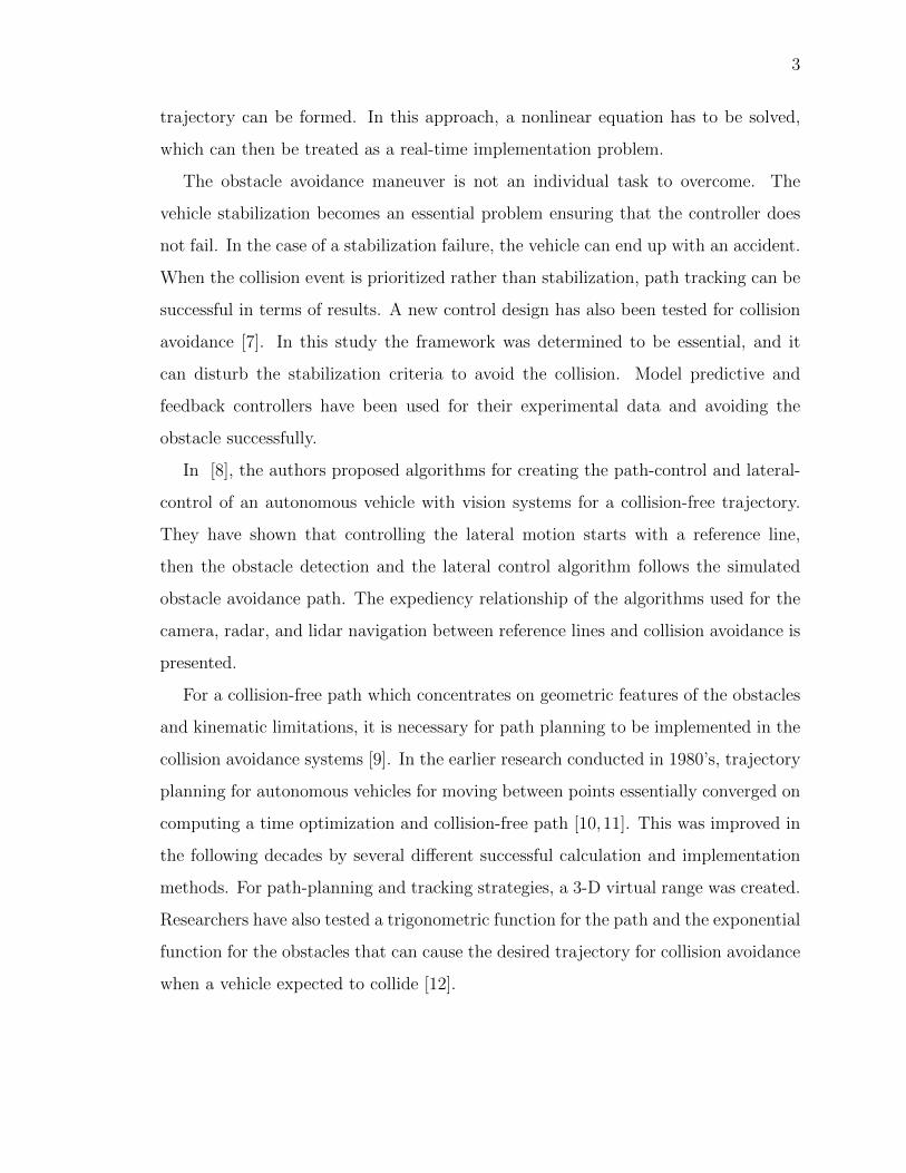
After the fast development of automated vehicle technology in the last decade,

many collision avoidance approaches have been proposed to improve driving safety.

Collision avoidance system (CAS), was firstly proposed in the 1950’s. Cadillac devel-

oped a prototype by using a radar that detects the objects in front of the car. They

decided not to manufacture due to the associated high cost [1]. In 1977, Toyota intro-

duced the adaptive cruise control system on their cars only in Japan. In 1995, they

first tested the collision avoidance system based on radar sensors in a research lab in

California, which was never implemented. Nowadays, we have many different types

of advanced driver-assistance systems such as maneuver control systems, adaptive

cruise control, lane change assistance, and collision avoidance systems.

All these systems are using technology to minimize human error through various

type of warnings [2]. The standards established by the Society of Automotive Engi-

neers indicate that the driving automation or the advanced driver-assistance systems

(ADAS) can be categorized at six-levels, starting from no to full driving automation.

Table 1.1 shows the details of the driving automation criteria. Level 0 encompasses

the manual control of all tasks of driving done by a human. Level 1 includes some

basic functions of driving assistance, such as cruise control, which supports the vehicle

driver to reduce or increase the speed. Level 2 is the partial automation by ADAS.

The driver allows the function to act and is responsible for the result’ so the vehicle

can perform steering and acceleration in this level of automation. In Level 3, the au-

tomated system is in charge and performs the primary driving tasks. There have been

fatalities of on-road testing of prototypes for vehicles at Level 2 and Level 3 [2]. At

Level 4 automation, the vehicle can perform all driving tasks under specific circum-

2

stances. Full automation is referred to as Level 5, and these vehicles can complete all

driving responsibilities under all circumstances without the need for human attention

or cooperation. Algorithms for ADAS and autonomous driving for automated driving

cars have been further discussed and analyzed in [3].

Table 1.1.: Levels of Driving Automation

Past Past 2018 2020 2020-2025 2025-2030

Level 0 1 2 3 4 5

No

Automation

Driver

Assistance

Partial

Automation

Conditional

Automation

High

Automation

Full

Automation

1.2 Literature Review

Automated driving technology consists of sensing, understanding, preparation,

and action. Technology has a fast journey, and a large amount of research has been

conducted in the field. However, it is challenging to understand the whole spectrum

of the technology. Most of the analyses describe problems under several boundary

circumstances. Researchers can examine many issues under a specific condition, but

it’s not feasible to estimate solutions for the whole autonomous driving system all at

once.

In the compared research, for the lateral motion, the desired trajectory has been

designed as a sinusoidal or exponential trajectory. A sliding mode controller was

created to ensure that the vehicle tracks the desired path [4]. Reichardt and Schick [5]

provided an electrical field analysis of the obstacles and examined the autonomous

vehicle as an electrical charge in this field. Forces managed in that charge determined

the vehicle’s path. Brandt et al. [6] suggested an automatic collision prevention

system based on the theory of elastic band. In this method, the desired trajectory

of the autonomous vehicle is called the elastic band, resembling links connected to

springs. There is a force applied on the links by the obstacle. Accordingly, a secure

3

trajectory can be formed. In this approach, a nonlinear equation has to be solved,

which can then be treated as a real-time implementation problem.

The obstacle avoidance maneuver is not an individual task to overcome. The

vehicle stabilization becomes an essential problem ensuring that the controller does

not fail. In the case of a stabilization failure, the vehicle can end up with an accident.

When the collision event is prioritized rather than stabilization, path tracking can be

successful in terms of results. A new control design has also been tested for collision

avoidance [7]. In this study the framework was determined to be essential, and it

can disturb the stabilization criteria to avoid the collision. Model predictive and

feedback controllers have been used for their experimental data and avoiding the

obstacle successfully.

In [8], the authors proposed algorithms for creating the path-control and lateral-

control of an autonomous vehicle with vision systems for a collision-free trajectory.

They have shown that controlling the lateral motion starts with a reference line,

then the obstacle detection and the lateral control algorithm follows the simulated

obstacle avoidance path. The expediency relationship of the algorithms used for the

camera, radar, and lidar navigation between reference lines and collision avoidance is

presented.

For a collision-free path which concentrates on geometric features of the obstacles

and kinematic limitations, it is necessary for path planning to be implemented in the

collision avoidance systems [9]. In the earlier research conducted in 1980’s, trajectory

planning for autonomous vehicles for moving between points essentially converged on

computing a time optimization and collision-free path [10,11]. This was improved in

the following decades by several different successful calculation and implementation

methods. For path-planning and tracking strategies, a 3-D virtual range was created.

Researchers have also tested a trigonometric function for the path and the exponential

function for the obstacles that can cause the desired trajectory for collision avoidance

when a vehicle expected to collide [12].

4

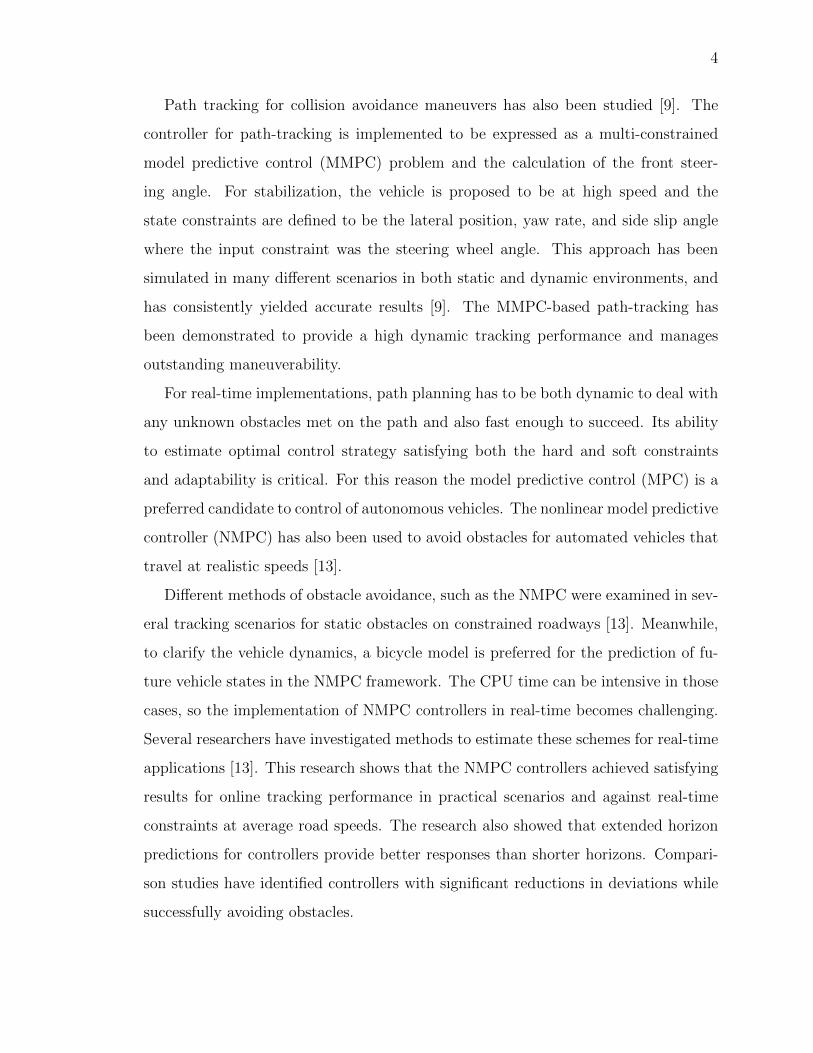
Path tracking for collision avoidance maneuvers has also been studied [9]. The

controller for path-tracking is implemented to be expressed as a multi-constrained

model predictive control (MMPC) problem and the calculation of the front steer-

ing angle. For stabilization, the vehicle is proposed to be at high speed and the

state constraints are defined to be the lateral position, yaw rate, and side slip angle

where the input constraint was the steering wheel angle. This approach has been

simulated in many different scenarios in both static and dynamic environments, and

has consistently yielded accurate results [9]. The MMPC-based path-tracking has

been demonstrated to provide a high dynamic tracking performance and manages

outstanding maneuverability.

For real-time implementations, path planning has to be both dynamic to deal with

any unknown obstacles met on the path and also fast enough to succeed. Its ability

to estimate optimal control strategy satisfying both the hard and soft constraints

and adaptability is critical. For this reason the model predictive control (MPC) is a

preferred candidate to control of autonomous vehicles. The nonlinear model predictive

controller (NMPC) has also been used to avoid obstacles for automated vehicles that

travel at realistic speeds [13].

Different methods of obstacle avoidance, such as the NMPC were examined in sev-

eral tracking scenarios for static obstacles on constrained roadways [13]. Meanwhile,

to clarify the vehicle dynamics, a bicycle model is preferred for the prediction of fu-

ture vehicle states in the NMPC framework. The CPU time can be intensive in those

cases, so the implementation of NMPC controllers in real-time becomes challenging.

Several researchers have investigated methods to estimate these schemes for real-time

applications [13]. This research shows that the NMPC controllers achieved satisfying

results for online tracking performance in practical scenarios and against real-time

constraints at average road speeds. The research also showed that extended horizon

predictions for controllers provide better responses than shorter horizons. Compari-

son studies have identified controllers with significant reductions in deviations while

successfully avoiding obstacles.

5

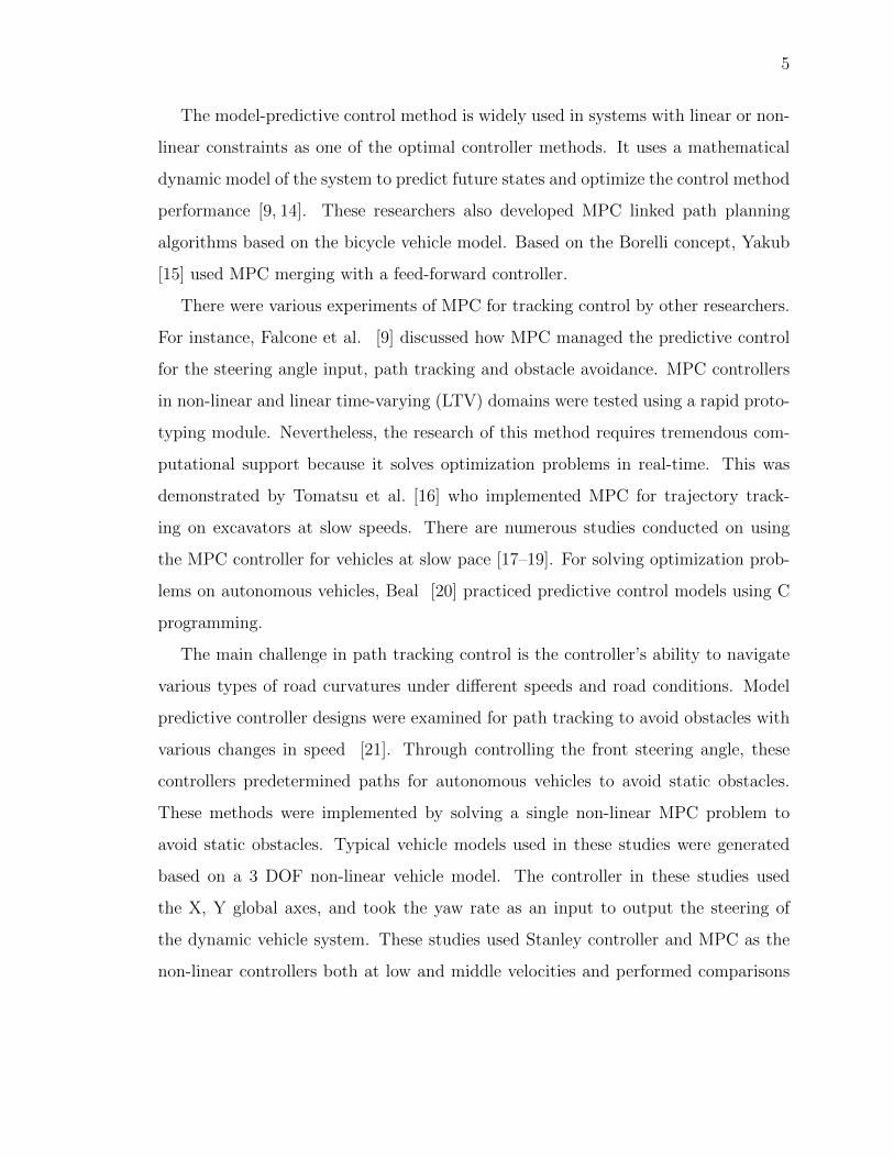
The model-predictive control method is widely used in systems with linear or non-

linear constraints as one of the optimal controller methods. It uses a mathematical

dynamic model of the system to predict future states and optimize the control method

performance [9, 14]. These researchers also developed MPC linked path planning

algorithms based on the bicycle vehicle model. Based on the Borelli concept, Yakub

[15] used MPC merging with a feed-forward controller.

There were various experiments of MPC for tracking control by other researchers.

For instance, Falcone et al. [9] discussed how MPC managed the predictive control

for the steering angle input, path tracking and obstacle avoidance. MPC controllers

in non-linear and linear time-varying (LTV) domains were tested using a rapid proto-

typing module. Nevertheless, the research of this method requires tremendous com-

putational support because it solves optimization problems in real-time. This was

demonstrated by Tomatsu et al. [16] who implemented MPC for trajectory track-

ing on excavators at slow speeds. There are numerous studies conducted on using

the MPC controller for vehicles at slow pace [17–19]. For solving optimization prob-

lems on autonomous vehicles, Beal [20] practiced predictive control models using C

programming.

The main challenge in path tracking control is the controller’s ability to navigate

various types of road curvatures under different speeds and road conditions. Model

predictive controller designs were examined for path tracking to avoid obstacles with

various changes in speed [21]. Through controlling the front steering angle, these

controllers predetermined paths for autonomous vehicles to avoid static obstacles.

These methods were implemented by solving a single non-linear MPC problem to

avoid static obstacles. Typical vehicle models used in these studies were generated

based on a 3 DOF non-linear vehicle model. The controller in these studies used

the X, Y global axes, and took the yaw rate as an input to output the steering of

the dynamic vehicle system. These studies used Stanley controller and MPC as the

non-linear controllers both at low and middle velocities and performed comparisons

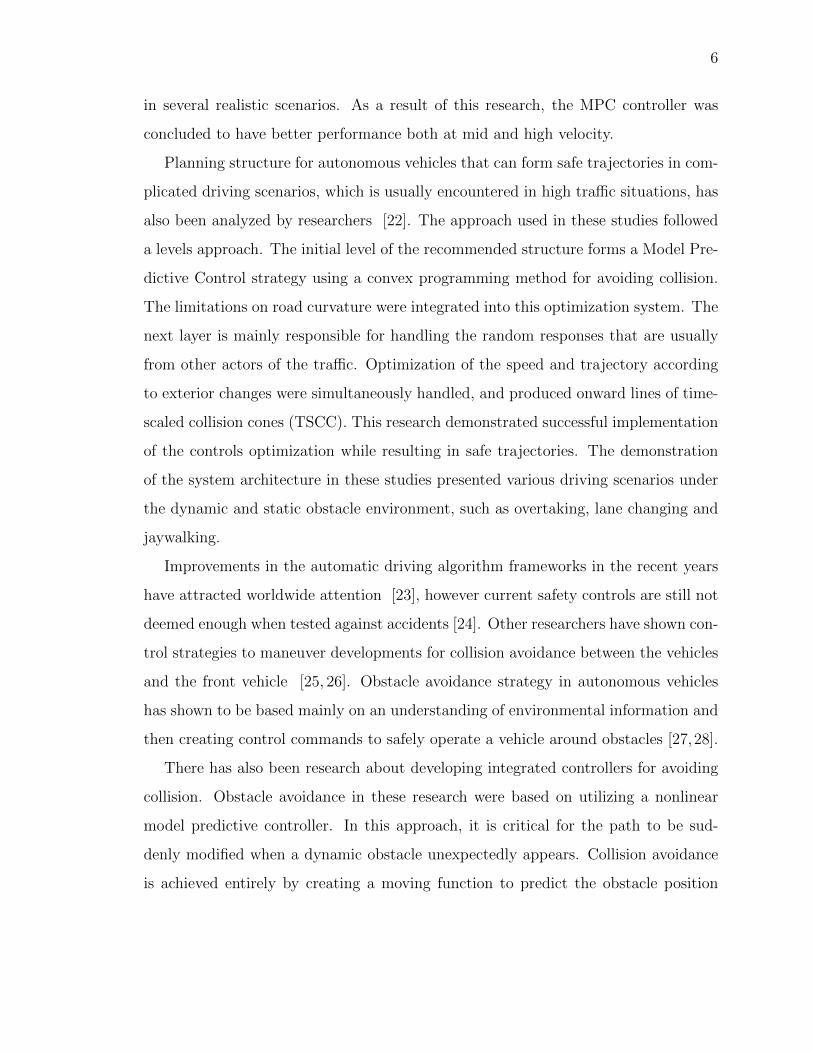
6

in several realistic scenarios. As a result of this research, the MPC controller was

concluded to have better performance both at mid and high velocity.

Planning structure for autonomous vehicles that can form safe trajectories in com-

plicated driving scenarios, which is usually encountered in high traffic situations, has

also been analyzed by researchers [22]. The approach used in these studies followed

a levels approach. The initial level of the recommended structure forms a Model Pre-

dictive Control strategy using a convex programming method for avoiding collision.

The limitations on road curvature were integrated into this optimization system. The

next layer is mainly responsible for handling the random responses that are usually

from other actors of the traffic. Optimization of the speed and trajectory according

to exterior changes were simultaneously handled, and produced onward lines of time-

scaled collision cones (TSCC). This research demonstrated successful implementation

of the controls optimization while resulting in safe trajectories. The demonstration

of the system architecture in these studies presented various driving scenarios under

the dynamic and static obstacle environment, such as overtaking, lane changing and

jaywalking.

Improvements in the automatic driving algorithm frameworks in the recent years

have attracted worldwide attention [23], however current safety controls are still not

deemed enough when tested against accidents [24]. Other researchers have shown con-

trol strategies to maneuver developments for collision avoidance between the vehicles

and the front vehicle [25, 26]. Obstacle avoidance strategy in autonomous vehicles

has shown to be based mainly on an understanding of environmental information and

then creating control commands to safely operate a vehicle around obstacles [27,28].

There has also been research about developing integrated controllers for avoiding

collision. Obstacle avoidance in these research were based on utilizing a nonlinear

model predictive controller. In this approach, it is critical for the path to be sud-

denly modified when a dynamic obstacle unexpectedly appears. Collision avoidance

is achieved entirely by creating a moving function to predict the obstacle position

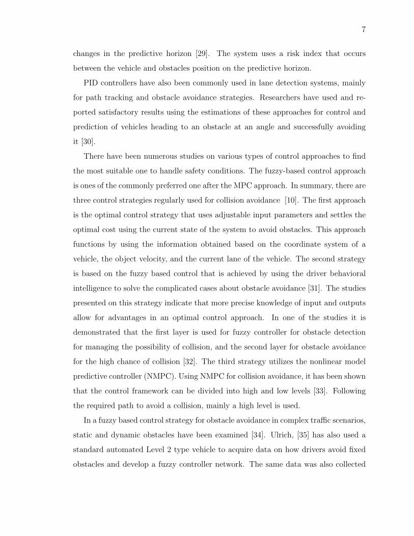
7

changes in the predictive horizon [29]. The system uses a risk index that occurs

between the vehicle and obstacles position on the predictive horizon.

PID controllers have also been commonly used in lane detection systems, mainly

for path tracking and obstacle avoidance strategies. Researchers have used and re-

ported satisfactory results using the estimations of these approaches for control and

prediction of vehicles heading to an obstacle at an angle and successfully avoiding

it [30].

There have been numerous studies on various types of control approaches to find

the most suitable one to handle safety conditions. The fuzzy-based control approach

is ones of the commonly preferred one after the MPC approach. In summary, there are

three control strategies regularly used for collision avoidance [10]. The first approach

is the optimal control strategy that uses adjustable input parameters and settles the

optimal cost using the current state of the system to avoid obstacles. This approach

functions by using the information obtained based on the coordinate system of a

vehicle, the object velocity, and the current lane of the vehicle. The second strategy

is based on the fuzzy based control that is achieved by using the driver behavioral

intelligence to solve the complicated cases about obstacle avoidance [31]. The studies

presented on this strategy indicate that more precise knowledge of input and outputs

allow for advantages in an optimal control approach. In one of the studies it is

demonstrated that the first layer is used for fuzzy controller for obstacle detection

for managing the possibility of collision, and the second layer for obstacle avoidance

for the high chance of collision [32]. The third strategy utilizes the nonlinear model

predictive controller (NMPC). Using NMPC for collision avoidance, it has been shown

that the control framework can be divided into high and low levels [33]. Following

the required path to avoid a collision, mainly a high level is used.

In a fuzzy based control strategy for obstacle avoidance in complex traffic scenarios,

static and dynamic obstacles have been examined [34]. Ulrich, [35] has also used a

standard automated Level 2 type vehicle to acquire data on how drivers avoid fixed

obstacles and develop a fuzzy controller network. The same data was also collected

8

by a robot driver and compared with the initial driver. The success and quality of

the control strategy have been demonstrated by examining 300 fuzzy rules, where

only two have failed. It was also shown that using a single fuzzy controller was

not efficient due to the large number of input and output variables [36]. This has

also resulted in the controller not being able to handle the rules separated in detail,

hence the amount of fuzzy rules increased rapidly. The number of fuzzy rules is only

in linear growth instead of exponential, and hierarchical fuzzy controller is required

to meet the real-time control specifications. These issues have led to research to

develop an algorithm that avoids obstacles on autonomous vehicles in a shorter time.

An electric three-wheeled vehicle was tested for avoiding obstacles by using a fuzzy

logic controller [37], where the considerations derived from a popular bicycle model.

The study examined many different road conditions and successfully reached the set

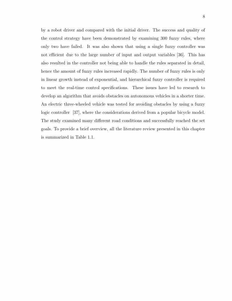
goals. To provide a brief overview, all the literature review presented in this chapter

is summarized in Table 1.1.

9

Table 1.2.: State of the Art on Different Control Methods

for Collision Avoidance.

Controller Research Title Features Results

MPC

Collision

Avoidance and

Stabilization for

Autonomous

Vehicles in

Emergency

Scenarios [7]

A single controller for

collision avoidance,

vehicle stabilization,

and path tracking

used.

The performance,

ability of the

controller and the

convenience of this

prioritization

approach for avoiding

collision and

stabilization was

successful.

MPC

Visual

Navigation

along Reference

Lines and

Collision

Avoidance for

Autonomous

Vehicles [8]

Visual navigation

algorithms including

image processing for

reference lines and

obstacles, and lateral

control with reference

lines and for obstacle

avoidance is

proposed.

The feasibility of the

algorithms for visual

navigation along

reference lines and

collision avoidance is

tested.

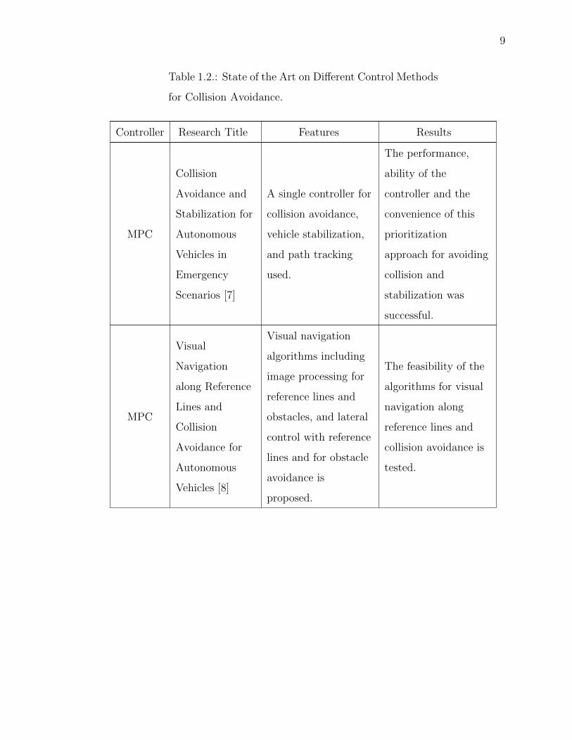
10

Table 1.2.: continued

MPC

Path Planning

and Tracking for

Vehicle Collision

Avoidance

Based on Model

Predictive

Control With

Multi-

constraints [12]

A framework for path

planning built on a

3-D potential field

based on the data of

road and obstacles.

The results

demonstrate that the

controller was able to

stabilize the vehicle

on a

low-friction-coefficient

road with a moving

obstacle and satisfy

the tracking

performance.

MPC

Obstacle

Avoidance in

Real Time With

Nonlinear

Model

Predictive

Control of

Autonomous

Vehicles [13]

The NMPC system

uses a simplified

bicycle model within

the controller, in

realistic road

conditions.

The NMPC method

handled dynamic

trajectory changes

and unanticipated

obstacles at normal

road speeds.

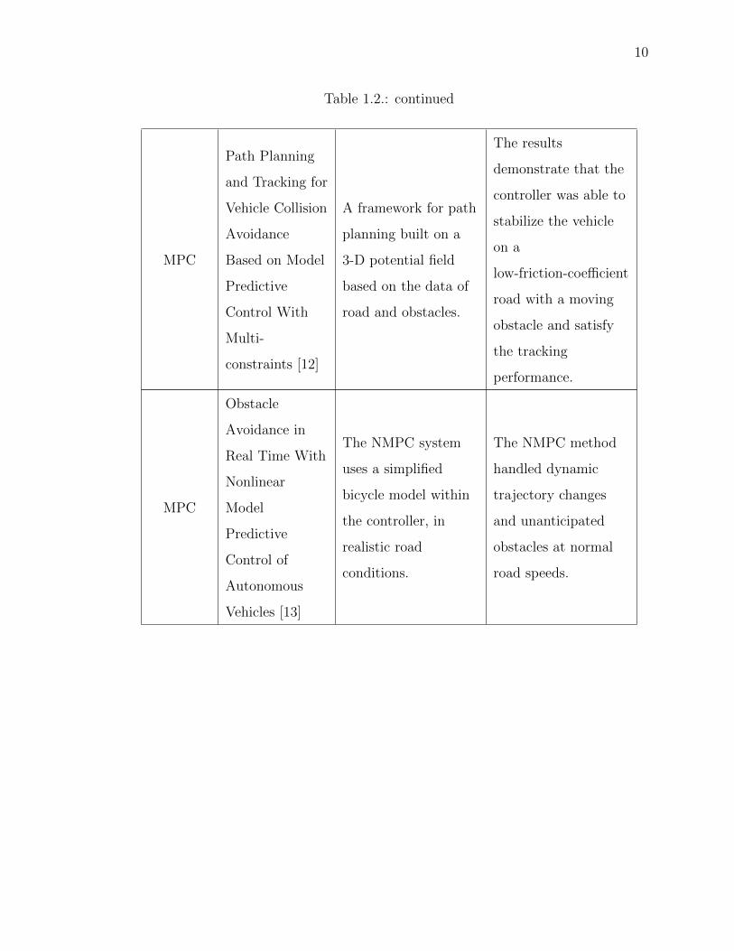
11

Table 1.2.: continued

MPC

Model

Predictive

Controller for

Path Tracking

and Obstacle

Avoidance

Manoeuvre on

Autonomous

Vehicle [21]

This paper proposed

a path tracking MPC

controller for an 3

DOF non-linear

autonomous vehicle

at various speed on

avoidance obstacle.

It was showed that

the small lateral

position error at small

speed and at large

speed large error at

yaw rate observed.

MPC

Motion

Planning

Framework for

Autonomous

Vehicles: A

Time Scaled

Collision Cone

Interleaved

Model

Predictive

Control

Approach [22]

A framework

generated a global

plan with complex

constraints for a

realistic planning

horizon.

The framework is

compared with

standalone MPC

validated in different

scenarios including

pedestrian

jaywalking, merging

and overtaking.

12

Table 1.2.: continued

MPC

Dynamic

Trajectory

Planning and

Tracking for

Autonomous

Vehicle With

Obstacle

Avoidance

Based on Model

Predictive

Control [29]

Simultaneous

trajectory for

dynamic path

planning and tracking

are integrated as a

single-level NPMC

controller, when

dynamic obstacle

suddenly appears, the

trajectory should be

adjusted respectively.

Moving a function to

predict the position of

the obstacle changes

in the predictive

horizon has designed.

FLC

Fuzzy-based

Collision

Avoidance

System for

Autonomous

Driving in

Complicated

Traffic Scenarios

[34]

The Fuzzy controller

has both the lane

change and adaptive

cruise control with

optimal rules to

enable effective

collision avoidance

when there are both

static and dynamic

obstacles.

The results shows

that the vehicle could

change lane, slow

down or stop

depending on the

traffic situation.

13

Table 1.2.: continued

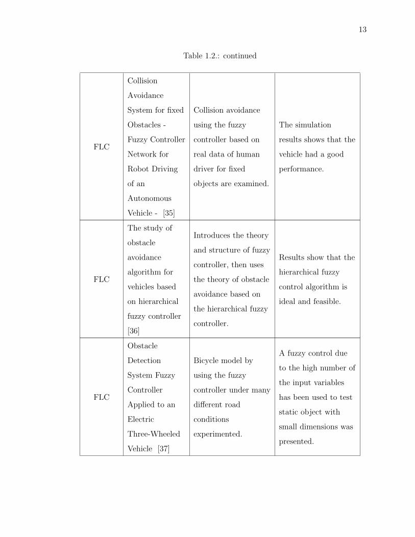
FLC

Collision

Avoidance

System for fixed

Obstacles -

Fuzzy Controller

Network for

Robot Driving

of an

Autonomous

Vehicle - [35]

Collision avoidance

using the fuzzy

controller based on

real data of human

driver for fixed

objects are examined.

The simulation

results shows that the

vehicle had a good

performance.

FLC

The study of

obstacle

avoidance

algorithm for

vehicles based

on hierarchical

fuzzy controller

[36]

Introduces the theory

and structure of fuzzy

controller, then uses

the theory of obstacle

avoidance based on

the hierarchical fuzzy

controller.

Results show that the

hierarchical fuzzy

control algorithm is

ideal and feasible.

FLC

Obstacle

Detection

System Fuzzy

Controller

Applied to an

Electric

Three-Wheeled

Vehicle [37]

Bicycle model by

using the fuzzy

controller under many

different road

conditions

experimented.

A fuzzy control due

to the high number of

the input variables

has been used to test

static object with

small dimensions was

presented.

14

Table 1.2.: continued

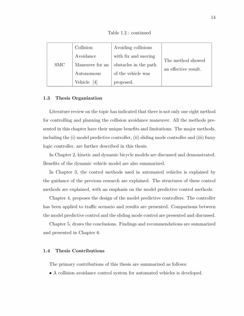
SMC

Collision

Avoidance

Maneuver for an

Autonomous

Vehicle [4]

Avoiding collisions

with fix and moving

obstacles in the path

of the vehicle was

proposed.

The method showed

an effective result.

1.3 Thesis Organization

Literature review on the topic has indicated that there is not only one right method

for controlling and planning the collision avoidance maneuver. All the methods pre-

sented in this chapter have their unique benefits and limitations. The major methods,

including the (i) model predictive controller, (ii) sliding mode controller and (iii) fuzzy

logic controller, are further described in this thesis.

In Chapter 2, kinetic and dynamic bicycle models are discussed and demonstrated.

Benefits of the dynamic vehicle model are also summarized.

In Chapter 3, the control methods used in automated vehicles is explained by

the guidance of the previous research are explained. The structures of these control

methods are explained, with an emphasis on the model predictive control methods.

Chapter 4, proposes the design of the model predictive controllers. The controller

has been applied to traffic scenario and results are presented. Comparisons between

the model predictive control and the sliding mode control are presented and discussed.

Chapter 5, draws the conclusions. Findings and recommendations are summarized

and presented in Chapter 6.

1.4 Thesis Contributions

The primary contributions of this thesis are summarized as follows:

• A collision avoidance control system for automated vehicles is developed.

15

• The properties of the proposed control model are discussed in detail.

• A MPC controller is demonstrated based on built-in Simulink toolboxes to con-

trol the lateral position and yaw angle.

• The model predictive controller is tuned to control the lateral maneuver success-

fully.

• The collision avoidance system results are verified by comparing against a val-

idated study having similar scenarios and parameters but using a different type of

controller.

16

2. VEHICLE MODEL

This chapter gives information about the vehicle dynamics models and under which

circumstances they are used. Advantages and disadvantages of the models are briefly

explained. In vehicle dynamics, there are various types of degrees of freedom. The

most manageable dynamic model is the two-degree-of-freedom bicycle model which is

used in this thesis. It represents the lateral motion and yaw angle. This model doesn’t

include the longitudinal direction because it does not have any impact on lateral

motion and yaw angle. The steering angle maneuver delivers a vehicle direction on

the road. In this research, the vehicle is doing an automated lane-change maneuver.

For that reason, the longitudinal velocity is considered constant. In experiments to

control the lane-change maneuver, kinematic or dynamic models is preferred.

2.1 Kinematic Vehicle Model

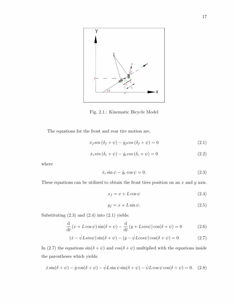
The kinematic vehicle model represents the geometry of vehicle motion [38]. Figure

2.1, represents the bicycle vehicle model, front two tires are modelled as one tire, and

the rear two tires modelled as one. The control input for the front steering angle is

δf , and that for the rear steering angle is δr. We assume δr = 0 and that there is a no

slip condition generally because many vehicles are front wheel drive. We ignored the

force effects to the motion in this model. The advantage of this model is that there

are only two parameters to identify. The distance from the front axle to the center of

the mass Lf and the distance from the rear axle to the center of the mass of a vehicle

is defined by Lr. The length of the vehicle can be calculated by Lf + Lr = L.

X and Y are the global position of the vehicle where x and y are used for to

represent the local coordinates [39]. The yaw angle of the vehicle is ψ and velocity is

denoted as v.

17

Fig. 2.1.: Kinematic Bicycle Model

The equations for the front and rear tire motion are,

xfsin (δf + ψ)− yfcos (δf + ψ) = 0 (2.1)

xrsin (δr + ψ)− yrcos (δr + ψ) = 0 (2.2)

where

xr sinψ − yr cosψ = 0. (2.3)

These equations can be utilized to obtain the front tires position on an x and y axis.

xf = x+ L cosψ (2.4)

yf = x+ L sinψ. (2.5)

Substituting (2.3) and (2.4) into (2.1) yields:

d

dt(x+ L cosψ) sin(δ + ψ)− d

dt(y + Lsinψ) cos(δ + ψ) = 0 (2.6)

(x− ψLsinψ) sin(δ + ψ)− (y − ψLcosψ) cos(δ + ψ) = 0 (2.7)

In (2.7) the equations sin(δ + ψ) and cos(δ + ψ) multiplied with the equations inside

the parentheses which yields:

x sin(δ + ψ)− y cos(δ + ψ)− ψL sinψ sin(δ + ψ)− ψL cosψ cos(δ + ψ) = 0. (2.8)

18

Using trigonometric identities to expand the last two terms on the left hand side, we

obtain the equation below,

x sin(δ + ψ)− y cos(δ + ψ)− ψL sinψ(sinψ cos δ + sin δ cosψ)−

ψL cosψ(cos δ cosψ − sin δ sinψ) = 0. (2.9)

Then expanding and recombining terms we obtain successively,

x sin(δ + ψ)− y cos(δ + ψ)− ψL(sin2 ψ cos δ + sin δ sinψ cosψ)−

ψL(cos2 ψ cos δ − cosψ sin δ sinψ) = 0, (2.10)

x sin(δ + ψ)− ψL cos δ(sin2 ψ + cos2 ψ)− y cos(δ + ψ) = 0, (2.11)

and

x sin(δ + ψ)− ψL cos δ − y cos(δ + ψ) = 0. (2.12)

Then, solving for the yaw rate ψ yields

ψ =x sin(δ + ψ)− y cos(δ + ψ)

L cos δ. (2.13)

The local coordinates for x and y are given. Plugging that back into (2.13) and

simplifying yields:

ψ =vx((cos2 ψ + sin2 ψ) sin δ)

L cos δ. (2.14)

By using the Pythagorean trigonometric identity theorem cos2 ψ + sin2 ψ = 1 we

obtain the equation below,

ψ =vx sin δ

L cos δ. (2.15)

The Equation (2.16) gives the yaw rate of the kinematic vehicle.

ψ =vx tan δ

L. (2.16)

The kinematic vehicle model commonly introduced in smaller velocity analyses

due to the loss of the forces on the tire. It is simple to use and can get fast results.

It gives similar results on the comparison with the real vehicle model.

19

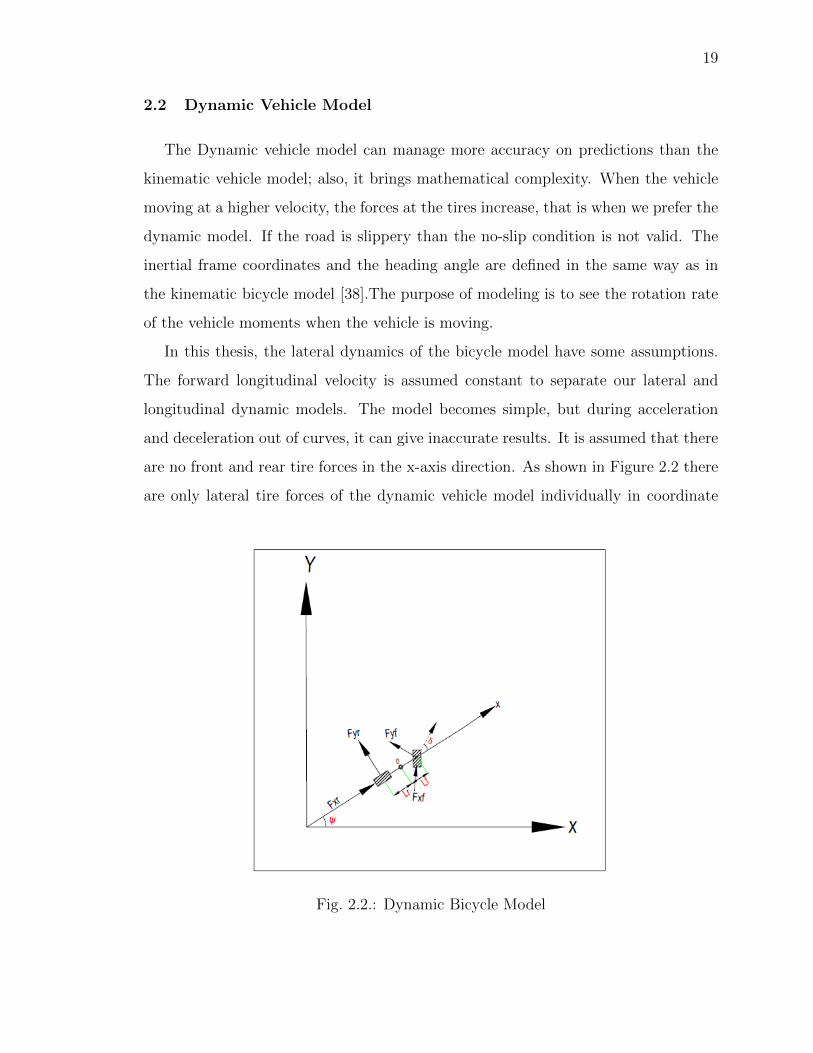
2.2 Dynamic Vehicle Model

The Dynamic vehicle model can manage more accuracy on predictions than the

kinematic vehicle model; also, it brings mathematical complexity. When the vehicle

moving at a higher velocity, the forces at the tires increase, that is when we prefer the

dynamic model. If the road is slippery than the no-slip condition is not valid. The

inertial frame coordinates and the heading angle are defined in the same way as in

the kinematic bicycle model [38].The purpose of modeling is to see the rotation rate

of the vehicle moments when the vehicle is moving.

In this thesis, the lateral dynamics of the bicycle model have some assumptions.

The forward longitudinal velocity is assumed constant to separate our lateral and

longitudinal dynamic models. The model becomes simple, but during acceleration

and deceleration out of curves, it can give inaccurate results. It is assumed that there

are no front and rear tire forces in the x-axis direction. As shown in Figure 2.2 there

are only lateral tire forces of the dynamic vehicle model individually in coordinate

Fig. 2.2.: Dynamic Bicycle Model

20

frames followed by the wheels. Lastly, the nonlinear effects such as aerodynamic

forces, suspension movement, and road inclination are assumed.

The vehicle’s center of gravity will be the reference point for calculating Newton’s

law. The longitudinal velocity is a constant and vx = 0, as a result of this the force

Fxf = 0.

The equations below are relevant to the lateral position and yaw angle, where the

yaw angle is calculated with respect to the x-axis on the global coordinate.

mvx = −mvyψ + Fxf cos δ + Fxr − Fyf sin δ, (2.17)

mvy = mvxψ + Fxf sin δ + Fyr + Fyf cos δ, (2.18)

Izψ = LfFyf cos δ + LfFxf sin δ − LrFyr. (2.19)

The variables in the equation are, vx is the longitudinal velocity and vy is the lateral

velocity of the vehicle, m is the vehicle mass, and Iz is the vehicle’s moment of inertia.

After substituting the assumptions the differential equations are given by:

mvy = mvxψ + Fyr + Fyf cos δ (2.20)

Izψ = LfFyf cos δ − LrFyr. (2.21)

ψ represents the angular acceleration in the z direction which combines with yaw

inertia to get the equation of the moments as shown at (2.25). Front and rear tires

slip angles given by,

αf = tan−1

(vy + Lf ψ

vx

)− δ (2.22)

αr = tan−1

(vy − Lrψ

vx

). (2.23)

For small tire slip angles front and rear tire forces are varying linearly. The forces

are defined as,

Fyf = −Cfαf (2.24)

Fyr = −Crαr, (2.25)

21

where cf and cr are the cornering stiffness of the front and rear tires. Substituting

Fyf and Fyr from Equations (2.24) and (2.25) as shown,

mvy = mvxψ − Cf

(tan−1 vy + Lf ψ

vx− δ

)cos δ − Cr

(tan−1 vy + Lrψ

vx

)(2.26)

Izψ = LrCr

(tan−1 vy − Lrψ

vx

)− LrCf

(tan−1 vy + Lf ψ

vx− δ

)cos δ. (2.27)

After rearranging the Equations the position of the vehicle is defined as (2.32) and

(2.33). These are nonlinear equations.

x = vx cosψ − vy sinψ (2.28)

y = vx sinψ + vy cosψ (2.29)

The linearized equations are shown as,

mvy =−Cfvy − CfLf ψ

vx+ Cfδ +

−Crvy + CrLrψ

vx−mvxψ (2.30)

Izψ =LrCrvy − L2

rCrψ

vx+LfCfvy − L2

fCf ψ

vx+ LfCfδ (2.31)

These can be written as,

vy =− (Cf + Cr)

mvxvy +

Cf

mvxδ +

(CrLr − CfLf

mv2x

− 1

)ψ (2.32)

and

ψ =LrCr − CfLf

Izvxvy +

LfCf

Izδ −

L2rCr + CfL

2f ψ

Izvxψ. (2.33)

Mass of the vehicle, cornering stiffness of the front and rear wheels, moment of

inertia of the vehicle around center of the mass, the distance between the front axle

and the rear axle to the center of the mass values can be seen. The kinematic and

dynamic bicycle models are compared in context of MPC controller design in [39].

22

3. CONTROL METHODS FOR AUTOMATED VEHICLES

In recent years, advanced control strategies’ importance has rapidly increased in vari-

ous industries. When we focus on the control methods, we observe various constraints

are affecting the control strategy. Traditional control methods address all constraints

separately. It is challenging when the system is multi input multi output (MIMO),

and the ideal method is to have a single controller that can handle multiple variables.

The literature shows that the MPC method is much more beneficial than the other

control methods due to its strengths such as the constraints. The parameters have

constraints and MPC tries to satisfy it as close as possible.

3.1 Model Predictive Control Theory

Because it can predict future travel based on the current state and can handle

multiple constraints MPC became one of the most commonly used controllers. In

this thesis, structure and working principles of the model predictive control method

are briefly described.

In a model-based control method, the system of the process model is estimated,

and control action performed. This control method makes estimates and controls

based on time. At every time step, an optimization problem has been solved by

the controller, and at sample time tries to find the control signals that give optimal

performance. Model predictive control, is an improved control method with feedback.

The MPC structure uses control and optimization tools [40]. The purpose of this

controller is to get the target control signal for the plant model. Key features are

calculation of the plant’s input and output measurements at each sampling instant and

current state over a finite horizon. Controller optimizes the performance and satisfies

the constraints on each control action. In predictive control, parameter settings are

compared to other control methods are easier. It can be used to control various type

23

of dynamic systems, unstable systems to more complex ones. One of the important

aspects, it is easily used in the control of multi-variable systems. The result is a linear

control rule that can be easy to implement. MPC has fundamental principles that

are entirely open for development.

The model predictive control method has many applications today; it provides

easy application even in cases with limited system information. The system’s easy

adjustment of parameters is one of the advantages. It can handle multiple variables

easily and have a prediction on upcoming sample time. Plant dynamics can be ex-

ploited. It improves steady-state response by a decrease in offset error and transient

response by a decrease in rise time, peak time, and settling time. To control a slow-

moving process, it is preferred to use time delay situations. On the other hand, the

system requires a plant model to control and has a high computational load with a

high algorithmic complexity.

Different types of MPC controller use different methods to deal with errors due

to operation outside the linear region. The most popular ones are Adaptive, Gain-

Scheduled, and Nonlinear MPC strategy. When the system constraints, and the

cost function are nonlinear, the nonlinear MPC controller is preferred. It’s the most

reliable but, at the same time, the most challenging to implement due to the non-

convex optimization problem. If the system is nonlinear and it has linear constraints,

and a quadratic cost function then one of the linear MPC options can be used, such

as Adaptive and Gain-Scheduled. If the optimization problem structure changes,

gain scheduled MPC is preferred, if not, Adaptive MPC can handle the system. The

adaptive MPC is going to be described briefly during Chapter 4 of the design model.

3.1.1 Receding Horizon Concept

In this section, the technology behind the MPC control algorithm is presented and

briefly compared with similar and different approaches. The purposes of the MPC

controller are limiting violation of the input and output constraints, optimizing the

24

input variables and output variables to stay in the assigned limits, and also can handle

multiple variables when there are not many sensors controlling the variables [41]. The

concept behind it, is that, while the driver looks at the road ahead, he judges the

present status, and the previous response. He predicts his response up to a horizon

ahead, As shown in Figure 3.1 where it is called prediction horizon. Depending on the

prediction horizon, the driver proceeds to the direction. MPC presents a structure

that can substitute a simple path tracking control law with continuously introduced

in the constraints of the parameters which has an optimization attempting to reduce

the errors of path tracking. MPC can calculate non-linearity, future predictions,

and operating constraints of the control system framework. MPC working principle

depends on the prediction states and the present states of the output. The purpose of

the MPC control calculations is to determine the prediction of the control movements

of the response as close as possible to the set-points.

The control of the single-input single-output plant discussed in this chapter. The

current time is represented as time step k in a discrete-time setting. At that moment,

the plant output is y(k), also in the Figure 3.1, the previous output trajectory is

shown. The output should follow the set-point trajectory s(t/k). Np is the prediction

horizon that shows how far the MPC looks into the future and represents the number

of future time steps. MPC controller aims to find the most suitable predictive path

closest to the reference. Control signal u(k+ i) is the predicted control action at k+ i

given u(k), likewise y(k+ i) is the predicted output at k+ i at given y(k). Figure 3.2

shows the model-based predictive control approach.

The reference trajectory represents an essential perspective of closed-loop perfor-

mance and starts at output y(k). The reference trajectory could be also a linear

function as shown in Figure 3.2. For instance, it determines a trajectory where the

plant returns to the set-point trajectory even though there is a disturbance. It is con-

sidered that the reference trajectory accesses the set-point and the systems response

speed expressed as Tref .

ε(k) = s(k)− y(k) (3.1)

25

Fig. 3.1.: The MPC Action Structure [40]

ε(k + i) = e−iTs/Tref ε(k) (3.2)

= λiε(k) (3.3)

The error is calculated at Equation 3.1 and the reference trajectory is picked i

step later and the output is represented above where the Ts is denoted as sampling

time [42]. The reference trajectory defined as follows,

r(k + i|k) = s(k + i)− ε(k + i) = s(k + i)− e−iTs/Tref ε(k) (3.4)

Predictive control starts from the current time and has an internal model to predict

the behavior of the system throughout the Np. The internal model assumed linear

for simplicity of the calculation. Predicted system behavior relies on the measured

input trajectory u(k+ i). The aim is to choose the input that gives the most suitable

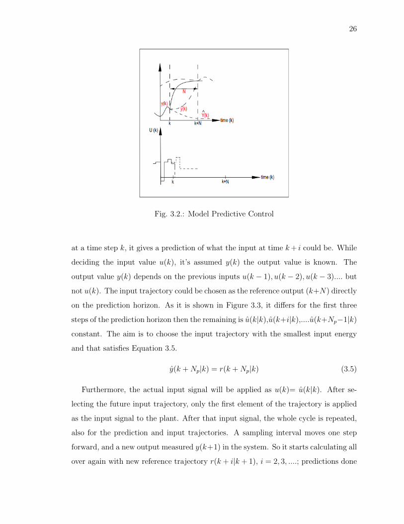
predictive behavior. In the representation u has been preferred rather than u, because

26

Fig. 3.2.: Model Predictive Control

at a time step k, it gives a prediction of what the input at time k+ i could be. While

deciding the input value u(k), it’s assumed y(k) the output value is known. The

output value y(k) depends on the previous inputs u(k − 1), u(k − 2), u(k − 3).... but

not u(k). The input trajectory could be chosen as the reference output (k+N) directly

on the prediction horizon. As it is shown in Figure 3.3, it differs for the first three

steps of the prediction horizon then the remaining is u(k|k),u(k+i|k),....u(k+Np−1|k)

constant. The aim is to choose the input trajectory with the smallest input energy

and that satisfies Equation 3.5.

y(k +Np|k) = r(k +Np|k) (3.5)

Furthermore, the actual input signal will be applied as u(k)= u(k|k). After se-

lecting the future input trajectory, only the first element of the trajectory is applied

as the input signal to the plant. After that input signal, the whole cycle is repeated,

also for the prediction and input trajectories. A sampling interval moves one step

forward, and a new output measured y(k+1) in the system. So it starts calculating all

over again with new reference trajectory r(k + i|k + 1), i = 2, 3, ....; predictions done

27

through the horizon k+ 1 + i, i = 1, 2, 3, ....; new trajectory chosen u(k+ 1 + i|k+ 1),

i = 0, 1, 2, ....,Np−1 and the input signal applied u(k+1)=u(k+1|k+1). The length

of the prediction horizon stays same but it shifts forward one sampling interval at

each time step to control the plant where it’s called the receding horizon control.

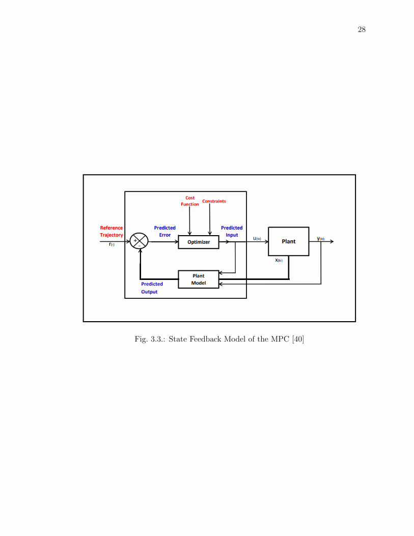
3.1.2 The Structure of Model Predictive Control

The general structure of the state feedback strategy of MPC is presented in Figure

3.4. In here r(.) is reference trajectory, the output signal of the plant is y(kj), u(kj)

is the plant input signal, x(kj) is the state at time kj from the plant which can be

measured in some cases. If it cannot be measured then a state estimator has to be used

and feedback to the MPC controller. The MPC uses a model of the plant to predict

the future behavior of the output and optimizer to make sure the output matches

as close as possible the expected reference. The aim of the optimization is to reach

the most suitable value for the best result despite the unmeasured disturbance such

as wind. Optimizer tries to satisfy constraints while solving an online optimization

problem at each time step, and the controller attempts to reduce the error between

the predicted path and the reference. Additionally, the controller minimizes the input

signal for immediate changes at each time step. By using the control input u, the

optimization algorithm decreases the cost function J . The cost function is,

J =

p∑i=1

wee2k+i +

p−1∑i=0

w∆u∆u2k+i, (3.6)

where, we and w4u are the weighting coefficients, the square of ∆uk+i is the ma-

nipulated variable, p is the prediction horizon, and the square of ek+i is the error

obtained by subtracting the reference variable from the controlled variable. There

are some constraints that MPC tries to stay inside the boundaries for the most de-

sirable outcome, which gives the optimal solution and the automated car moves as

close as possible to the reference.

28

Fig. 3.3.: State Feedback Model of the MPC [40]

29

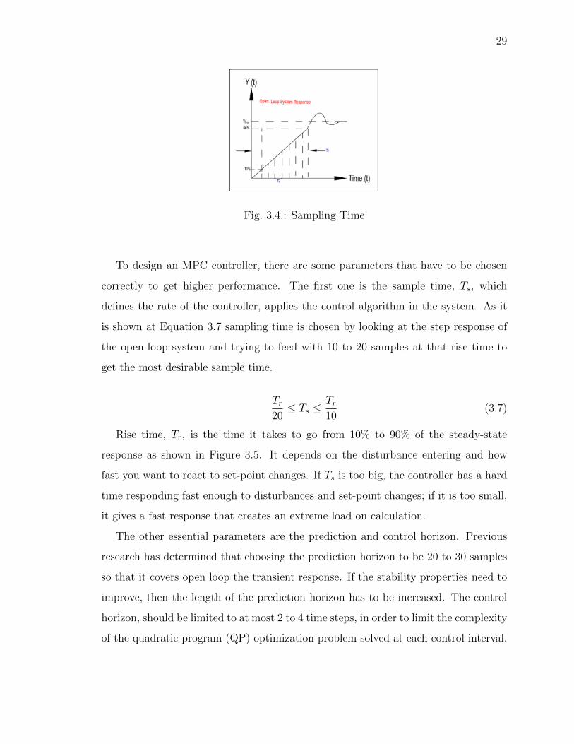
Fig. 3.4.: Sampling Time

To design an MPC controller, there are some parameters that have to be chosen

correctly to get higher performance. The first one is the sample time, Ts, which

defines the rate of the controller, applies the control algorithm in the system. As it

is shown at Equation 3.7 sampling time is chosen by looking at the step response of

the open-loop system and trying to feed with 10 to 20 samples at that rise time to

get the most desirable sample time.

Tr20≤ Ts ≤

Tr10

(3.7)

Rise time, Tr, is the time it takes to go from 10% to 90% of the steady-state

response as shown in Figure 3.5. It depends on the disturbance entering and how

fast you want to react to set-point changes. If Ts is too big, the controller has a hard

time responding fast enough to disturbances and set-point changes; if it is too small,

it gives a fast response that creates an extreme load on calculation.

The other essential parameters are the prediction and control horizon. Previous

research has determined that choosing the prediction horizon to be 20 to 30 samples

so that it covers open loop the transient response. If the stability properties need to

improve, then the length of the prediction horizon has to be increased. The control

horizon, should be limited to at most 2 to 4 time steps, in order to limit the complexity

of the quadratic program (QP) optimization problem solved at each control interval.

30

As seen in Equation 3.8 the control horizon m, has to be set to 10% to 20% of the

prediction horizon. If the control horizon is smaller than the calculation load, and

only the first few moves has a important effect on the predicted output, the rest is

constant and doesn’t have any insignificant effect. So if the control horizon is chosen

as same as the prediction horizon, it causes a complexity on the optimization problem.

Thus we must have,

P

10≤ m ≤ 2P

10(3.8)

Plant manipulated variables, MV; constraints are the limits you have in actuators.

Plant output variables, OV, are the constraints that limit the outputs controlled

for the physical system. The most important part of the constraints is when more

constraints are added; then, the optimization problem is more complex to solve. They

are classified as hard and soft constraints depending on whether they can be violated

or not. For the optimization problem to be solvable, it is not wise to give hard

constraints to both input and output; they can conflict with each other. The most

common use is to set the output constrains soft. The ratio between the output and

input weights are the last essential parameters. If the ratio is high, the controller

is more competitive but weak. If the controller needs to be robust, then the input

weights have to increase. For balanced performance is to weight the ratio of input

and output correlated with each other.

3.1.3 Models for Model Predictive Control

In this section, there will be a brief description of the models used for the MPC

algorithms. There are different types of discrete models used to calculate the predicted

outputs. The impulse and step response are the most common models used in MPC

algorithms.

31

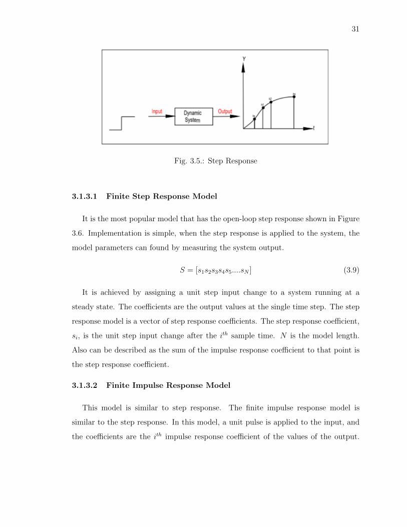
Fig. 3.5.: Step Response

3.1.3.1 Finite Step Response Model

It is the most popular model that has the open-loop step response shown in Figure

3.6. Implementation is simple, when the step response is applied to the system, the

model parameters can found by measuring the system output.

S = [s1s2s3s4s5....sN ] (3.9)

It is achieved by assigning a unit step input change to a system running at a

steady state. The coefficients are the output values at the single time step. The step

response model is a vector of step response coefficients. The step response coefficient,

si, is the unit step input change after the ith sample time. N is the model length.

Also can be described as the sum of the impulse response coefficient to that point is

the step response coefficient.

3.1.3.2 Finite Impulse Response Model

This model is similar to step response. The finite impulse response model is

similar to the step response. In this model, a unit pulse is applied to the input, and

the coefficients are the ith impulse response coefficient of the values of the output.

32

There is a close connection between the step response Si and impulse response Hi

shown in Equation 3.10.

Hi = Si − Si−1 (3.10)

Si =n∑

i=1

hj (3.11)

. in which {hj}ni=1 are the impulse response coefficients (Markov parameters) are

differences at the step response coefficient at each time step. Overall there are two

significant constraints for both of these response models.

3.1.3.3 Transfer Function Model

The transfer function model requires fewer parameters. The input signal is u(t),

and the output signal is y(t). The model can be represented as (3.14) where,

A(z−1) = 1 + a1z−1 + a2z

−2 + .....+ ana.z−na, (3.12)

B(z−1) = b0 + b1z−1 + b2z

−2 + .....+ bnb.z−nb, (3.13)

A(z−1)y(t) = B(z−1)u(t− 1). (3.14)

The predicted output using this model is,

y

(t+

k

t

)=Bz−1

Az−1u

(t+

k

t

). (3.15)

3.1.3.4 State Space Model

The state-space equation is mostly preferred for multivariate systems. It is often

used in predictive functional control algorithms. The state space equation is,

x(k + 1) = Ax(k) +Bu(k), (3.16)

The output equation is,

y(k) = Cyx(k) (3.17)

33

and the estimator state is,

z(k) = Czx(k). (3.18)

Here x is the n-dimensional state vector, u is the one-dimensional input vector, y

is dimensional measured outputs, z is the outputs to be controlled at mz dimensional

vector. The variables at y and z often overlapped with a broad scope, and generally,

they are the same. So all controlled outputs are continuously measured. In the

equation k represents the time step, often y is accepted as z, C applied as Cy and Cz.

This model can be generalized to include the measured and not-measured errors

and the measurement noise. Measurement values are taken y(k). The required input

values calculated u(k) applied to the system There is always a delay between the

measured y(k) to u(k), so the measured output doesn’t have direct feed between u(k)

to y(k). The controlled output z(k) can be related to u(k),

z(k) = z(k) +Dzu(k). (3.19)

3.1.4 Single-Input and Single-Output Systems

A single output controlled by a single manipulated variable is called single input

single output systems [43]. Heating control and air conditioning control systems are

examples of SISO systems.

The controlled system is a set of elements put together for a specific function as

represented in Figure 3.7. The control of the set of elements calculates the model;

therefore, there is a single input and single output at the model.

3.1.5 Multi-Input and Multi-Output Systems

If the systems have more than one cycle it is called Multi-input multi-output

systems [43]. There are some applications such as manufacturing that can not be

controlled by single input single output. It is challenging to tune many controller

gains. The MPC can also handle constraints. An example is given for multivariate

34

Fig. 3.6.: Single-Input and Single-Output Systems

system analysis for two input, and two output in Figure 3.8. Any input at MIMO

systems effected by the other output and the outputs are effected by the other input.

Fig. 3.7.: Multi-Input and Multi-Output Systems

The system variables can be represented with the equations by using the transfer

functions relation.

Yi(s) = Gii(s)Ri(s) +Gij(s)Rj(s) (3.20)

Y1(s) = G11(s)R1(s) +G12(s)R2(s) (3.21)

Y2(s) = G21(s)R1(s) +G22(s)R2(s) (3.22)

In these equations, the Gij transfer function is the relation between the i, output

variable with j, input variable. The block diagram of the equation set shown in Figure

3.9.

35

Fig. 3.8.: An Example of a Multi-Input and Multi-Output Systems.

3.1.6 Continuous-Time to Discrete-Time Models

In the MPC strategy, linearization is important. A method is presented to trans-

forms linear continuous-time models to linear discrete-time in this section. The dis-

crete models perform calculations to produce control commands. A sample and zero-

order hold (ZOH) operation is used to convert a continuous signal to a discrete signal

where h is the sampling period shown in Figure [40].

f(kh), kh ≤ t < (k + 1)h, (3.23)

3.2 Simple Sliding Mode Controller

In this section, a single input single output sliding mode controller overview given.

It is a nonlinear control strategy that has easy tuning and gives accurate results. The

structure of a sliding mode controller has two phases. The first phase is to obtain

36

Fig. 3.9.: Sample and ZOH Conversion [40]

the desired system behavior with a custom-made surface design. The second phase

is to make sure the closed-loop system is stable to the sliding surface; the feedback

gains of the controller have to be selected [40]. The sliding surface is a derivative

of state space. On the sliding surface, the controller keeps the states on the close

neighborhood of the sliding surface. The advantages and disadvantages are described

at the most common controller comparison Table 3.1 at the end of the chapter.

3.3 Fuzzy Logic Controller

In this section, a closed-loop system with a fuzzy controller presented. The fuzzy

logic controller has common use in the industry as much as a model predictive con-

troller due to efficiency, reliability, and it’s success at the control application. Many

products have a fuzzy logic controller, such as control on traffic lights, washing ma-

chines, and room temperatures. The fuzzy logic control has rules which is used in

controller design. The closed-loop fuzzy logic architecture utilizes the control error

37

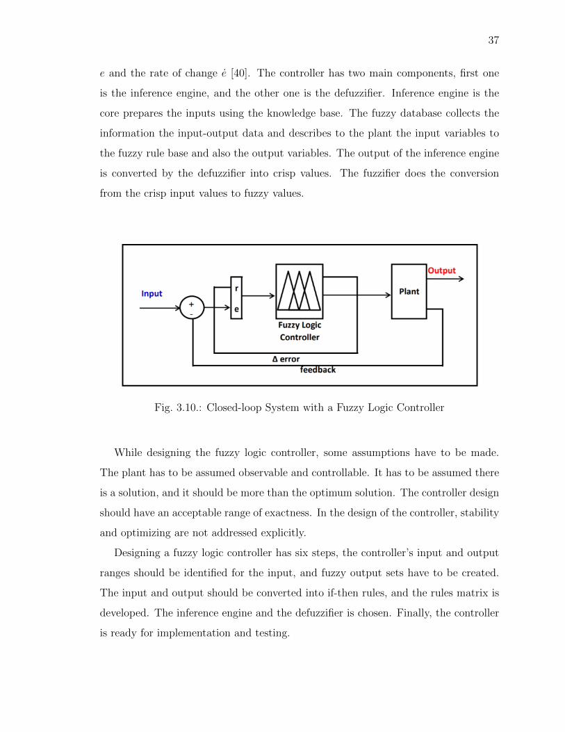
e and the rate of change e [40]. The controller has two main components, first one

is the inference engine, and the other one is the defuzzifier. Inference engine is the

core prepares the inputs using the knowledge base. The fuzzy database collects the

information the input-output data and describes to the plant the input variables to

the fuzzy rule base and also the output variables. The output of the inference engine

is converted by the defuzzifier into crisp values. The fuzzifier does the conversion

from the crisp input values to fuzzy values.

Fig. 3.10.: Closed-loop System with a Fuzzy Logic Controller

While designing the fuzzy logic controller, some assumptions have to be made.

The plant has to be assumed observable and controllable. It has to be assumed there

is a solution, and it should be more than the optimum solution. The controller design

should have an acceptable range of exactness. In the design of the controller, stability

and optimizing are not addressed explicitly.

Designing a fuzzy logic controller has six steps, the controller’s input and output

ranges should be identified for the input, and fuzzy output sets have to be created.

The input and output should be converted into if-then rules, and the rules matrix is

developed. The inference engine and the defuzzifier is chosen. Finally, the controller

is ready for implementation and testing.

38

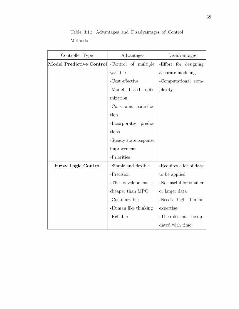
Table 3.1.: Advantages and Disadvantages of Control

Methods

Controller Type Advantages Disadvantages

Model Predictive Control -Control of multiple

variables

-Cost effective

-Model based opti-

mization

-Constraint satisfac-

tion

-Incorporates predic-

tions

-Steady state response

improvement

-Priorities

-Effort for designing

accurate modeling

-Computational com-

plexity

Fuzzy Logic Control -Simple and flexible

-Precision

-The development is

cheaper than MPC

-Customizable

-Human like thinking

-Reliable

-Requires a lot of data

to be applied

-Not useful for smaller

or larger data

-Needs high human

expertise

-The rules must be up-

dated with time

39

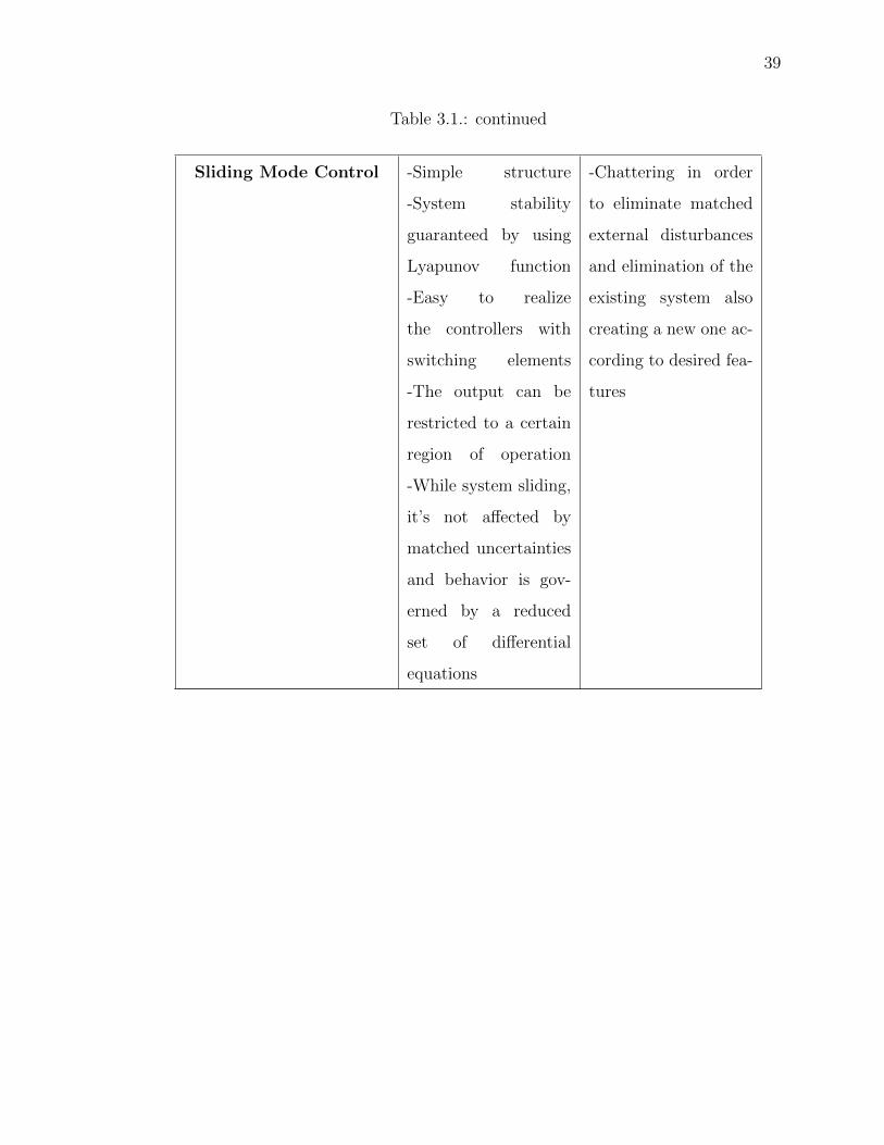
Table 3.1.: continued

Sliding Mode Control -Simple structure

-System stability

guaranteed by using

Lyapunov function

-Easy to realize

the controllers with

switching elements

-The output can be

restricted to a certain

region of operation

-While system sliding,

it’s not affected by

matched uncertainties

and behavior is gov-

erned by a reduced

set of differential

equations

-Chattering in order

to eliminate matched

external disturbances

and elimination of the

existing system also

creating a new one ac-

cording to desired fea-

tures

40

4. MODELING

Several years ago, autonomous vehicles attracted intense awareness from the auto-

motive industry due to their potential for improving comfort and safety in driving.

Automated collusion avoidance control can reduce the number of accidents, fatali-

ties, and increase in traffic density moved safety in a critical position in intelligent

transportation systems. Due to the complex work environment, researchers applied

modern control theory and sensing technologies to control smart vehicles. Fully au-

tonomous driving is a remaining complicated task, hence generating a collision-free

trajectory is the key for the next level intelligent vehicles.

Autonomous vehicles are driven by artificial intelligence, which has a place in

everyday life. The vehicle applies the sensors and collects data of the environment

from them. The data collected is transmitted to the central computer system to

enable the vehicle to perform it is maneuvers, such as steering control, acceleration,

and deceleration accurately. The computer gives the best outcome for safe drive.

There are many industries in which autonomous vehicles will widely be used over

the next decades, such as professional driving, parking garages, military, and delivery

services.

There are many challenges to succeed. In some states, it is legal to test autonomous

vehicles on public roadways. To control the reliability in terms of fatalities and

accidents, the control strategy has to examine for several cases. After the fatality

of a pedestrian in Arizona in 2018, artificial intelligence was questioned. Following

that accident, there were nine confirmed Level 2 accidents in which the autopilot was

involved in the Florida area. It is mandatory to investigate, examine, and research

widely.

41

4.1 Collision Avoidance Design by Adaptive MPC

The collision avoidance design is presented at Figure 4.2. The strategy is designed

using Matlab/Simulink. For the controller design Simulink/ Model Predictive Control

Toolbox was used and the reference trajectory was designed using the Automated

Driving Toolbox. In the following, sections each block will be described in detail.

4.1.1 Plant Model

An MPC controller contains a dynamic plant model. It is briefly discussed in

Chapter 2, along with the kinematic and dynamic vehicle model parameters. Our

goal is to control the lateral position and yaw angle for passing the obstacle. In this

section, the parameters and the dynamic plant model will be explained.

The global position of the car is represented depending on the distance to the X

and Y axes. Vy is the lateral velocity; Vx is the longitudinal velocity. The MPC

controller needs a reference trajectory for the car to control. The reference values for

our goal are measured with respect to Vx. The car model is linearized in this thesis,

and the longitudinal velocity is constant during the vehicle travels. The steering angle

is δ, yaw angle is ψ, and reference yaw angle is ψref . It is created as state-space model

which shown in Equation 4.1 and 4.2. System dynamic matrices are A and B which

are time-invariant when longitudinal speed is constant. There are four states used

for calculation first lateral velocity Vy, second yaw angle represented as ψ, third yaw

rate ψ and last the lateral position y.

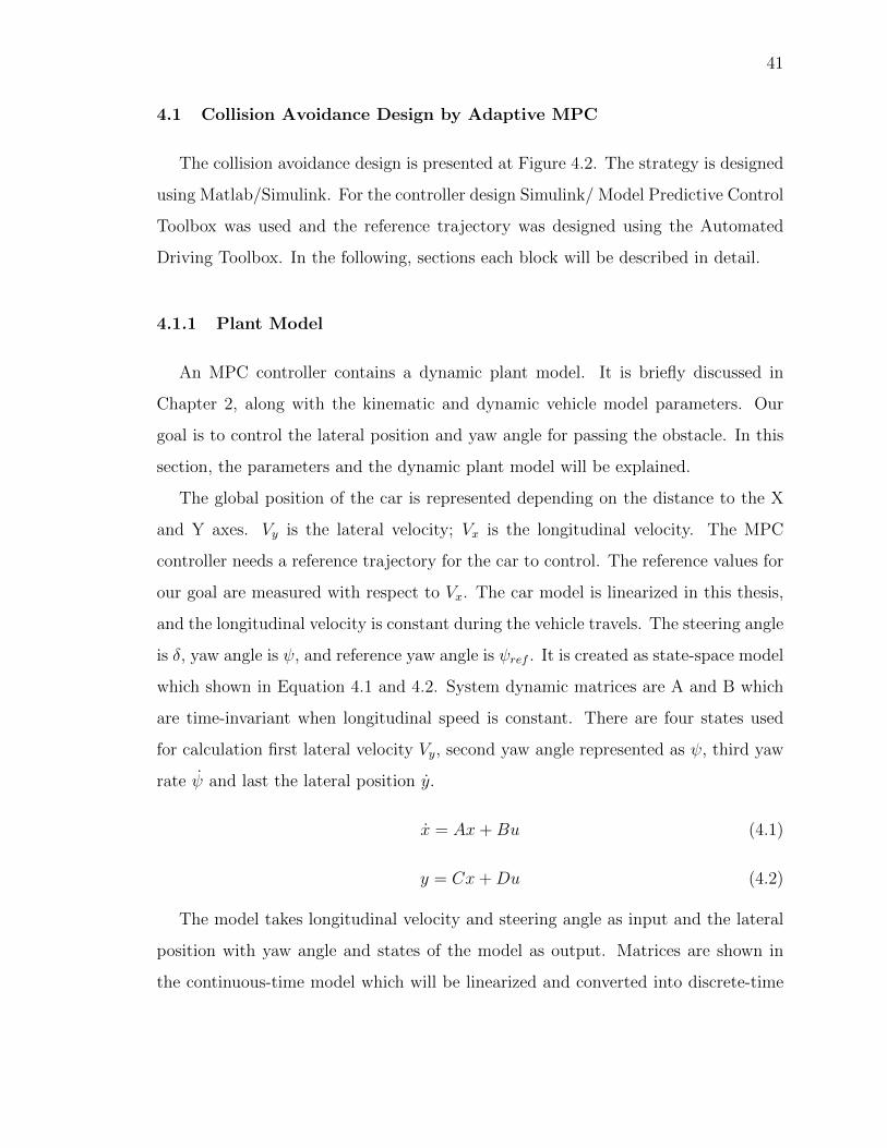
x = Ax+Bu (4.1)

y = Cx+Du (4.2)

The model takes longitudinal velocity and steering angle as input and the lateral

position with yaw angle and states of the model as output. Matrices are shown in

the continuous-time model which will be linearized and converted into discrete-time

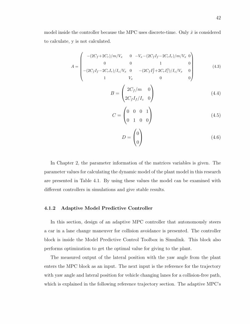
42

model inside the controller because the MPC uses discrete-time. Only x is considered

to calculate, y is not calculated.

A =

−(2Cf+2Cr)/m/Vx 0 −Vx−(2CfIf−2CrIr)/m/Vx 0

0 0 1 0

−(2CfIf−2CrIr)/Iz/Vx 0 −(2CfI2f+2CrI

2r )/Iz/Vx 0

1 Vx 0 0

(4.3)

B =

2Cf/m 0

2CfIf/Iz 0

(4.4)

C =

0 0 0 1

0 1 0 0

(4.5)

D =

0

0

(4.6)

In Chapter 2, the parameter information of the matrices variables is given. The

parameter values for calculating the dynamic model of the plant model in this research

are presented in Table 4.1. By using these values the model can be examined with

different controllers in simulations and give stable results.

4.1.2 Adaptive Model Predictive Controller

In this section, design of an adaptive MPC controller that autonomously steers

a car in a lane change maneuver for collision avoidance is presented. The controller

block is inside the Model Predictive Control Toolbox in Simulink. This block also

performs optimization to get the optimal value for giving to the plant.

The measured output of the lateral position with the yaw angle from the plant

enters the MPC block as an input. The next input is the reference for the trajectory

with yaw angle and lateral position for vehicle changing lanes for a collision-free path,

which is explained in the following reference trajectory section. The adaptive MPC’s

43

Table 4.1.: Values of Dynamic Bicycle Model Parameters

Parameter Value

m 976 kg

Cr 33000 N/deg

Cf 19000 N/deg

Iz 5400 kgm2

Lr 1.6 m

If 1.2 m

main difference from the regular MPC is that at each time step it presents a new

linear plant model for present operating conditions. In this research, it assumed that

there is no measured disturbance. The last is connecting controller output, which is

steering angle to the plant input. All these connections can be seen in Figure 4.2.

The MPC block has an optimizer and a plant model inside, which is shown in

Figure 3.3. The controller has constraints, weights, sample time, prediction, and

control horizons, which have to be specified in the controller and tuned for the most

reliable result the performance can be measured. Inside the MPC structure, there

is an MPC designer where we set the number of inputs and outputs. We set the

controller sample time to 0.1 sec and then linearize. For the predictions, MPC uses

an internal plant model and an optimizer to make sure it is the optimal control action.

While linearizing, it takes the plant model data and uses it as an internal plant. It

shows the input and output responses, so the next step will be finding the best control

action by changing the parameters.

The signal information, units, and also when there isn’t much magnitude difference

between the signals has been adjusted. The scale factor is used as one. The change

is made inside the I/O attributes. Then the parameters are saved inside the edit

scenario. In Figure 4.1 it is displayed.

44

Fig. 4.1.: Structure Inside the MPC Designer

The next part is the tuning, where we decide the prediction and control horizon.

For the prediction horizon, it preferred to be 10 when it is increased the response goes

slow. For the control horizon, it is raised and then decreased for the more desirable

result; it is preferred to be three. There are weights to be set to an amount other

than zero for the input and outputs to have a destination. The lateral position is the

most important, so it is set to one. There is a slider on top of the MPC designer user

interface. For aggressive control, it is slid to the right side.

The last part is assigning the constraint parameters. It mentioned in the previous

chapters that there are soft and hard constraints. The input constraints are hard in

this research, and the output constraints are soft. Earlier it is described that when we

are assuming constraints for the better result if the input is soft, the output should

be hard or vice versa. In this research, it was thought that the steering angle should

be a maximum of 30 degrees and the rate of change of steering angle 16 deg/sec to

get more solid results. The data is entered in radians then it will be converted into

45

degrees in the Simulink model. After all these adjusted parameters, the controller is

ready to compile and update the MPC block in our model.

The adaptive MPC uses an update plant model in which the output is the last

input to be connected to the controller. It updates the plant model at each time step

for current condition. Inside the block, it has the Matlab function of the state space

matrices of the state-space model. It has a conversion to the discrete-time model

from the continuous-time model and updates the nominal conditions. The inputs to

the blocks are longitudinal velocity, steering angle, and states.

46

Vₓ

u x

30

Lon

gatu

din

al

Ve

loci

ty

S

tate

s

Ste

eri

ng

An

gle

Mo

mV

ref

Late

ral P

osi

tio

n

Mo

del

Ad

apti

ve

MP

C

Up

dat

ed

Pla

nt

Mo

de

l

Sce

nar

io

Re

ade

r

Dyn

amic

Pla

nt

Mo

de

l

Fig

.4.

2.:

Col

lisi

onA

void

ance

Sim

ulink

Des

ign

Usi

ng

Adap

tive

MP

C

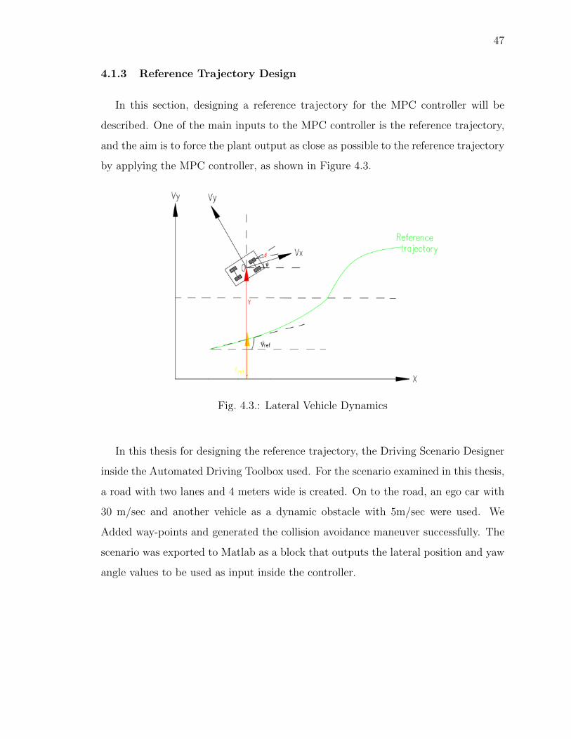
47

4.1.3 Reference Trajectory Design

In this section, designing a reference trajectory for the MPC controller will be

described. One of the main inputs to the MPC controller is the reference trajectory,

and the aim is to force the plant output as close as possible to the reference trajectory

by applying the MPC controller, as shown in Figure 4.3.

Fig. 4.3.: Lateral Vehicle Dynamics

In this thesis for designing the reference trajectory, the Driving Scenario Designer

inside the Automated Driving Toolbox used. For the scenario examined in this thesis,

a road with two lanes and 4 meters wide is created. On to the road, an ego car with

30 m/sec and another vehicle as a dynamic obstacle with 5m/sec were used. We

Added way-points and generated the collision avoidance maneuver successfully. The

scenario was exported to Matlab as a block that outputs the lateral position and yaw

angle values to be used as input inside the controller.

48

4.2 Simulations and Results

This research is about implementing a collision avoidance model controlling the

lateral maneuver and yaw angle for autonomous vehicles. The results are compared

with the scenario proposed in [4], which used a sliding mode controller for a collision-

free path. In the scenario, a vehicle moving at 5m/s is considered as the dynamic

obstacle. The following vehicle is at a speed of 30 m/s. The lateral overlap, lateral

error, tire steering angle comparisons are presented. Additionally, the yaw angle is

also displayed in the Simulink results.

Fig. 4.4.: Lateral Position

In the parameters considered for the study were the mass (m), sampling time and

moment of inertia of the vehicle (Iz) which were obtained from the research paper [4].

The simulation results for the lateral overlap scenario are shown in Figure 4.4, where

the controller followed the expected trajectory with a similar response having a time

discrepancy of less than a second. The discrepancy between the results is credited to

the difference in the input reference trajectory. In Figure 4.4 it is shown that the Lat-

Real proceeds slower than the reference. There is a time delay of 0.7 seconds. When

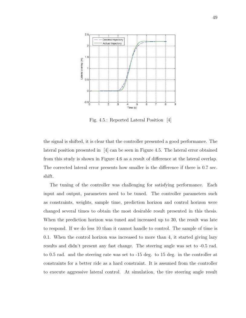
49

Fig. 4.5.: Reported Lateral Position [4]

the signal is shifted, it is clear that the controller presented a good performance. The

lateral position presented in [4] can be seen in Figure 4.5. The lateral error obtained

from this study is shown in Figure 4.6 as a result of difference at the lateral overlap.

The corrected lateral error presents how smaller is the difference if there is 0.7 sec.

shift.

The tuning of the controller was challenging for satisfying performance. Each

input and output, parameters need to be tuned. The controller parameters such

as constraints, weights, sample time, prediction horizon and control horizon were

changed several times to obtain the most desirable result presented in this thesis.

When the prediction horizon was tuned and increased up to 30, the result was late

to respond. If we do less 10 than it cannot handle to control. The sample of time is

0.1. When the control horizon was increased to more than 4, it started giving lazy

results and didn’t present any fast change. The steering angle was set to -0.5 rad.

to 0.5 rad. and the steering rate was set to -15 deg. to 15 deg. in the controller at

constraints for a better ride as a hard constraint. It is assumed from the controller

to execute aggressive lateral control. At simulation, the tire steering angle result

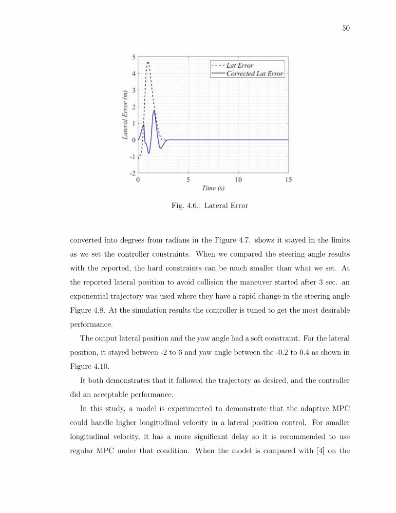
50

Fig. 4.6.: Lateral Error

converted into degrees from radians in the Figure 4.7. shows it stayed in the limits

as we set the controller constraints. When we compared the steering angle results

with the reported, the hard constraints can be much smaller than what we set. At

the reported lateral position to avoid collision the maneuver started after 3 sec. an

exponential trajectory was used where they have a rapid change in the steering angle

Figure 4.8. At the simulation results the controller is tuned to get the most desirable

performance.

The output lateral position and the yaw angle had a soft constraint. For the lateral

position, it stayed between -2 to 6 and yaw angle between the -0.2 to 0.4 as shown in

Figure 4.10.

It both demonstrates that it followed the trajectory as desired, and the controller

did an acceptable performance.

In this study, a model is experimented to demonstrate that the adaptive MPC

could handle higher longitudinal velocity in a lateral position control. For smaller

longitudinal velocity, it has a more significant delay so it is recommended to use

regular MPC under that condition. When the model is compared with [4] on the

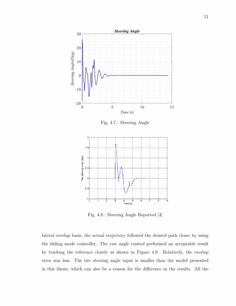
51

Fig. 4.7.: Steering Angle

Fig. 4.8.: Steering Angle Reported [4]

lateral overlap basis, the actual trajectory followed the desired path closer by using

the sliding mode controller. The yaw angle control performed an acceptable result

by tracking the reference closely as shown in Figure 4.9. Relatively, the overlap

error was less. The tire steering angle input is smaller than the model presented

in this thesis, which can also be a reason for the difference in the results. All the

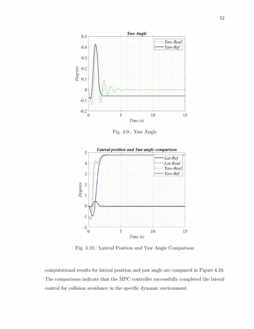
52

Fig. 4.9.: Yaw Angle

Fig. 4.10.: Lateral Position and Yaw Angle Comparison

computational results for lateral position and yaw angle are compared in Figure 4.10.

The comparisons indicate that the MPC controller successfully completed the lateral

control for collision avoidance in the specific dynamic environment.

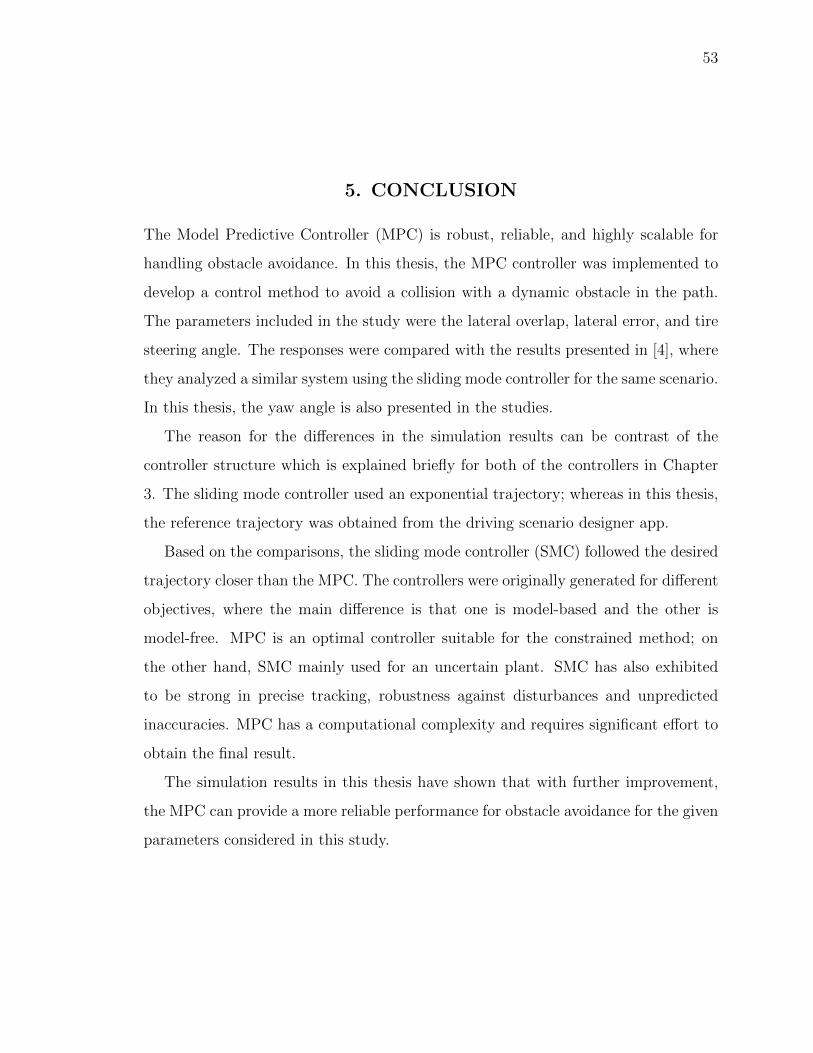
53

5. CONCLUSION

The Model Predictive Controller (MPC) is robust, reliable, and highly scalable for

handling obstacle avoidance. In this thesis, the MPC controller was implemented to

develop a control method to avoid a collision with a dynamic obstacle in the path.

The parameters included in the study were the lateral overlap, lateral error, and tire

steering angle. The responses were compared with the results presented in [4], where

they analyzed a similar system using the sliding mode controller for the same scenario.

In this thesis, the yaw angle is also presented in the studies.

The reason for the differences in the simulation results can be contrast of the

controller structure which is explained briefly for both of the controllers in Chapter

3. The sliding mode controller used an exponential trajectory; whereas in this thesis,

the reference trajectory was obtained from the driving scenario designer app.

Based on the comparisons, the sliding mode controller (SMC) followed the desired

trajectory closer than the MPC. The controllers were originally generated for different

objectives, where the main difference is that one is model-based and the other is

model-free. MPC is an optimal controller suitable for the constrained method; on

the other hand, SMC mainly used for an uncertain plant. SMC has also exhibited

to be strong in precise tracking, robustness against disturbances and unpredicted

inaccuracies. MPC has a computational complexity and requires significant effort to

obtain the final result.

The simulation results in this thesis have shown that with further improvement,

the MPC can provide a more reliable performance for obstacle avoidance for the given

parameters considered in this study.

54

6. FUTURE WORK

The results of the simulations introduced the idea that there are still challenges in

this model to explore and testing it with another popular method called fuzzy logic

controller. For this future research, a combination of radar, lidar and camera can be

implemented for testing real-time performance.

The lateral motion model was tested using Matlab/Simulink. In this research, the

longitudinal velocity was constant and can be tested with changing variables in the

future study. The most critical improvement to the controller tuning should be to

minimize the time delay obtained in the response by further tuning the controller

parameters.

In the future, more detailed scenarios with different constraints need to be con-

sidered. This can be done using an extended approach for dealing with disturbances

from the measurement where the disturbance can be measured before it enters the

system or could be rejected before entering the system.

REFERENCES

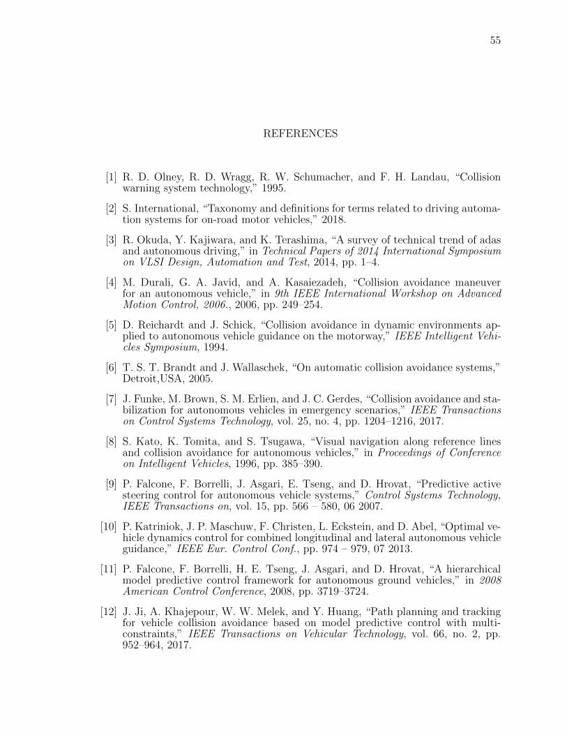
55

REFERENCES

[1] R. D. Olney, R. D. Wragg, R. W. Schumacher, and F. H. Landau, “Collisionwarning system technology,” 1995.

[2] S. International, “Taxonomy and definitions for terms related to driving automa-tion systems for on-road motor vehicles,” 2018.

[3] R. Okuda, Y. Kajiwara, and K. Terashima, “A survey of technical trend of adasand autonomous driving,” in Technical Papers of 2014 International Symposiumon VLSI Design, Automation and Test, 2014, pp. 1–4.

[4] M. Durali, G. A. Javid, and A. Kasaiezadeh, “Collision avoidance maneuverfor an autonomous vehicle,” in 9th IEEE International Workshop on AdvancedMotion Control, 2006., 2006, pp. 249–254.

[5] D. Reichardt and J. Schick, “Collision avoidance in dynamic environments ap-plied to autonomous vehicle guidance on the motorway,” IEEE Intelligent Vehi-cles Symposium, 1994.

[6] T. S. T. Brandt and J. Wallaschek, “On automatic collision avoidance systems,”Detroit,USA, 2005.

[7] J. Funke, M. Brown, S. M. Erlien, and J. C. Gerdes, “Collision avoidance and sta-bilization for autonomous vehicles in emergency scenarios,” IEEE Transactionson Control Systems Technology, vol. 25, no. 4, pp. 1204–1216, 2017.

[8] S. Kato, K. Tomita, and S. Tsugawa, “Visual navigation along reference linesand collision avoidance for autonomous vehicles,” in Proceedings of Conferenceon Intelligent Vehicles, 1996, pp. 385–390.

[9] P. Falcone, F. Borrelli, J. Asgari, E. Tseng, and D. Hrovat, “Predictive activesteering control for autonomous vehicle systems,” Control Systems Technology,IEEE Transactions on, vol. 15, pp. 566 – 580, 06 2007.

[10] P. Katriniok, J. P. Maschuw, F. Christen, L. Eckstein, and D. Abel, “Optimal ve-hicle dynamics control for combined longitudinal and lateral autonomous vehicleguidance,” IEEE Eur. Control Conf., pp. 974 – 979, 07 2013.

[11] P. Falcone, F. Borrelli, H. E. Tseng, J. Asgari, and D. Hrovat, “A hierarchicalmodel predictive control framework for autonomous ground vehicles,” in 2008American Control Conference, 2008, pp. 3719–3724.

[12] J. Ji, A. Khajepour, W. W. Melek, and Y. Huang, “Path planning and trackingfor vehicle collision avoidance based on model predictive control with multi-constraints,” IEEE Transactions on Vehicular Technology, vol. 66, no. 2, pp.952–964, 2017.

56

[13] M. A. Abbas, R. Milman, and J. M. Eklund, “Obstacle avoidance in real timewith nonlinear model predictive control of autonomous vehicles,” Canadian Jour-nal of Electrical and Computer Engineering, vol. 40, no. 1, pp. 12–22, 2017.

[14] G. Bayar, M. Bergerman, A. B. Koku, and E. Konukseven, “Localization andcontrol of an autonomous orchard vehicle,” Computers and Electronics in Agri-culture, vol. 115, pp. 118–128, 07 2015.

[15] F. Yakub and Y. Mori, “Comparative study of autonomous path following vehiclecontrol via model predictive control and linear quadratic control,” Proc. Inst.Mech. Eng. Part D J. Automob. Eng., vol. 229, pp. 1695–1714, 12 2015.

[16] T. Tomatsu, K. Nonaka, K. Sekiguchi, and K. Suzuki, “Model predictive trajec-tory tracking control for hydraulic excavator on digging operation,” 2015 IEEEConference on, 2015, pp. 1136–1141, 2015.

[17] A. S. Yamashita, P. M. Alexandre, A. C. Zanin, and D. Odloak, “Referencetrajectory tuning of model predictive control,” Control Engineering Practice,vol. 50, pp. 1–11, 2016.

[18] I. Prodan, S. Olaru, F. A. C. C. Fontes, F. L. Pereira, J. B. de Sousa, and C. S.Maniu, “Predictive control for path-following from trajectory generation to theparametrization of the discrete tracking sequences,” pp. 161–181, 2015.

[19] G. V. Raffo, G. K. Gomes, J. E. Rico, C. R. Kelber, and L. B. Becker, “A predic-tive controller MPC for autonomous vehicle path tracking,” IEEE Transactionson Intelligent Transportation Systems, vol. 10, pp. 92–102, 2009.

[20] C. E. Beal, “Applications of MPC to vehicle dynamics for active safety andstability,” Department of Mechanical Engineering, Stanford University, 2011.

[21] Z. A. Leman, M. Hatta Mohammad Ariff, H. Zamzuri, M. A. Abdul Rahman,and S. Amri Mazlan, “Model predictive controller for path tracking and obsta-cle avoidance manoeuvre on autonomous vehicle,” in 2019 12th Asian ControlConference (ASCC), 2019, pp. 1271–1276.

[22] R. R. Theerthala, A. V. S. S. B. Kumar, M. Babu, S. Phaniteja, and K. M.Krishna, “Motion planning framework for autonomous vehicles: A time scaledcollision cone interleaved model predictive control approach,” in 2019 IEEE In-telligent Vehicles Symposium (IV), 2019, pp. 1075–1080.

[23] M. A. Abbas, R. Milman, and J. M. Eklund, “Obstacle avoidance in real timewith nonlinear model predictive control of autonomous vehicles,” 2014 IEEE27th Canadian Conference on Electrical and Computer Engineering (CCECE),pp. 1–6, 2014.

[24] J. Su, J. Wu, P. Cheng, and J. Chen, “Autonomous vehicle control through thedynamics and controller learning,” IEEE Transactions on Vehicular Technology,pp. 1–1, 03 2018.

[25] S. He, M. Wang, S. Dai, and F. Luo, “Leader–follower formation control of usvswith prescribed performance and collision avoidance,” IEEE Transactions onIndustrial Informatics, vol. 15, pp. 572–581, 2019.

57

[26] T. L. Z. Peng, D. Wang and M. Han, “Output feedback cooperative formationmaneuvering of autonomous surface vehicles with connectivity preservation andcollision avoidance,” IEEE Trans. Cybern.

[27] J. Liu, P. Jayakumar, J. L. Stein, and T. Ersal, “An MPC algorithm with com-bined speed and steering control for obstacle avoidance in autonomous groundvehicles,” 2016.

[28] J. Liu, P. Jayakumar, J. L. Stein, and T. Ersal, “Combined speed and steeringcontrol in high-speed autonomous ground vehicles for obstacle avoidance usingmodel predictive control,” IEEE Transactions on Vehicular Technology, vol. 66,no. 10, pp. 8746–8763, 2017.

[29] S. Li, Z. Li, Z. Yu, B. Zhang, and N. Zhang, “Dynamic trajectory planningand tracking for autonomous vehicle with obstacle avoidance based on modelpredictive control,” IEEE Access, vol. 7, pp. 132 074–132 086, 2019.

[30] T. S. A. Al-Zaher, A. M. Bayoumy, A. M. Sharaf, and Y. H. H. El-din, “Lanetracking and obstacle avoidance for autonomous ground vehicles,” in 2012 9thFrance-Japan 7th Europe-Asia Congress on Mechatronics (MECATRONICS) /13th Int’l Workshop on Research and Education in Mechatronics (REM), 2012,pp. 264–271.

[31] T. Takeuchi, “An autonomous fuzzy mobile robot,” Advanced Robotics, vol. 5,no. 2, pp. 215–230, 1990.

[32] V. Kapse, B. Jharia, and S. S. Thakur, “Fpga based fuzzy control techniquefor obstacle avoidance,” in TENCON 2017 - 2017 IEEE Region 10 Conference,2017, pp. 1245–1250.

[33] C. Choi, Y. Kang, and Seangwock Lee, “Emergency collision avoidance maneu-ver based on nonlinear model predictive control,” in 2012 IEEE InternationalConference on Vehicular Electronics and Safety (ICVES 2012), 2012, pp. 393–398.

[34] A. S. Rashed, W. Faris, and S. Fatai, “Fuzzy-based collision avoidance system forautonomous driving in complicated traffic scenarios,” in 2018 IEEE InternationalConference on Automatic Control and Intelligent Systems (I2CACIS), 2018, pp.57–62.

[35] U. Lages, “Collision avoidance system for fixed obstacles-fuzzy controller networkfor robot driving of an autonomous vehicle,” in ITSC 2001. 2001 IEEE IntelligentTransportation Systems. Proceedings, 2001, pp. 489–491.

[36] Y. Zhenhe and W. Jianfeng, “The study of obstacle avoidance algorithm for ve-hicles based on hierarchical fuzzy controller,” in 2014 IEEE Workshop on Elec-tronics, Computer and Applications, 2014, pp. 182–185.

[37] J. G. Parada-Salado, M. Rodrıguez-Licea, F. J. Perez-Pinal, and A. I. Barranco-Gutierrez, “Obstacle detection system fuzzy controller applied to an electricthree-wheeled vehicle,” in 2017 IEEE International Autumn Meeting on Power,Electronics and Computing (ROPEC), 2017, pp. 1–6.

[38] R. Rajamani, Vehicle Dynamics and Control. Springer, 2011.

58

[39] J. Kong, M. Pfeiffer, G. Schildbach, and F. Borrelli, “Kinematic and dynamicvehicle models for autonomous driving control design,” in 2015 IEEE IntelligentVehicles Symposium (IV), 2015, pp. 1094–1099.

[40] S. H. Zak, Systems and control. Oxford University Press New York, 2003, vol.198.

[41] J. Qin and T. Badgwell, “A survey of industrial model predictive control tech-nology,” Control engineering practice, vol. 11, pp. 733–764, 07 2003.

[42] J. Maciejowski, Predictive control with constraints, J.M. Maciejowski. UnitedKingdom: Pearson Education Limited, 2002.

[43] M. T. Tham, “Multivariable control: An introduction to decoupling control,”1999.