evaluation of organic loading and hydraulic rest …

EVALUATION OF ORGANIC LOADING AND HYDRAULIC REST PERIOD OF FOOD

PROCESSING WASTEWATER IRRIGATION TO PREVENT MOBILIZATION OF

TRANSITION METALS

By

Ryan Julien

A THESIS

Submitted to

Michigan State University

in partial fulfillment of the requirements

for the degree of

Biosystems Engineering – Master of Science

2014

ABSTRACT

EVALUATION OF ORGANIC LOADING AND HYDRAULIC REST PERIOD OF FOOD

PROCESSING WASTEWATER IRRIGATION TO PREVENT MOBILIZATION OF

TRANSITION METALS

By

Ryan Julien

Wastewater generated during food processing is commonly treated using land-application

systems which primarily rely on microbes in the soil to treat wastewater by transforming

nutrients and organic compounds into benign byproducts. Naturally occurring metals in soil may

be chemically reduced via microbially mediated oxidation-reduction reactions as oxygen

becomes depleted. Metals such as manganese, iron, and arsenic are water soluble in their reduced

forms and may lead to contamination of groundwater.

A column study was conducted at Michigan State University to investigate impacts of land-

application of wastewater. Oxygen content and volumetric water data was collected via soil

sensors for the duration of the study. The pH, chemical oxygen demand, alkalinity, total iron, and

total manganese in the influent and effluent water for each column were evaluated. Average

organic loading, organic load per dose, and hydraulic rest period were shown to have statistically

significant impacts on effluent water quality using Spearman’s Rank Correlation Coefficient.

This study verifies that excessive organic loading of land application systems causes

mobilization of naturally occurring metals and ineffective wastewater treatment, but also

indicates the need for consideration of organic dose load and hydraulic rest period in treatment

system design. Findings from this study demonstrate application of water to soil twice daily may

encourage soil aeration and allow for increased organic loading while limiting metal

mobilization.

iii

ACKNOWLEDGEMENTS

I would like to thank Dr. Safferman, Leila Saber, my undergraduate research assistants,

Steve Miller, Steve Marquie, and my committee members for their assistance conducting this

research project. I would also like to thank my family and friends for their support. Finally, I

would to thank Ashley and my pack for the love and support they’ve shown me throughout this

stage of my life.

iv

TABLE OF CONTENTS

LIST OF TABLES ......................................................................................................................... vi

LIST OF FIGURES ...................................................................................................................... vii

KEY TO ABBREVIATIONS ...................................................................................................... viii

Introduction ..................................................................................................................................... 1

Literature Review............................................................................................................................ 3

Land Application of Wastewater................................................................................................. 4

Wastewater Treatment Technologies ...................................................................................... 4

Current and Historical Use ...................................................................................................... 5

Wastewater Characteristics ...................................................................................................... 6

Organic Loading .................................................................................................................. 7

Hydraulic Loading ............................................................................................................... 8

Nutrient Loading .................................................................................................................. 9

Impacts of Elevated Groundwater Concentrations of Selected Metals ..................................... 10

Health Risks and Toxicology ................................................................................................ 10

Nuisance Problems ................................................................................................................ 12

Metal Solubility ......................................................................................................................... 13

Soil Conditions ...................................................................................................................... 14

Microbially Mediated Redox Reactions ................................................................................ 15

Materials and Methods .................................................................................................................. 16

Wastewater Composition .......................................................................................................... 17

Column Construction ................................................................................................................ 18

Sensor Description .................................................................................................................... 20

Oxygen Sensors ..................................................................................................................... 23

Water Content Reflectometer ................................................................................................ 24

Thermistors ............................................................................................................................ 24

Experimental Operation ............................................................................................................ 25

Water application ................................................................................................................... 25

Analytical Data Collected ...................................................................................................... 27

Maintenance ........................................................................................................................... 28

Results and Discussion ................................................................................................................. 28

Methods of Analysis Considered .............................................................................................. 29

Principal Component Analysis .............................................................................................. 29

Multiple Linear Regression ................................................................................................... 29

Seasonal-Trend Decomposition Procedure Based on Loess ................................................. 30

Analysis Used to Identify Relationships ................................................................................... 30

Spearman’s Rank Order Correlation ..................................................................................... 31

Average Daily Organic Loading ........................................................................................ 36

Hydraulic Rest Period ........................................................................................................ 37

v

Organic Load per Dose ...................................................................................................... 39

Column Length .................................................................................................................. 40

Presence of Perched Groundwater Table ........................................................................... 41

Soil after Experiment ................................................................................................................ 41

Conclusions ................................................................................................................................... 42

Opportunities for Further Research ........................................................................................... 45

APPENDICES .............................................................................................................................. 48

APPENDIX A ........................................................................................................................... 49

APPENDIX B ........................................................................................................................... 58

APPENDIX C ........................................................................................................................... 67

APPENDIX D ......................................................................................................................... 108

APPENDIX E .......................................................................................................................... 112

REFERENCES ........................................................................................................................... 115

vi

LIST OF TABLES

Table 1 - Water Use and Effluent Characteristics for Selected Food Products (Mannapperuma,

Yates et al. 1993) ............................................................................................................................ 7

Table 2 - Synthetic Wastewater Composition for 10 mg Glucose/L Solution (Trulear and

Characklis 1982) ........................................................................................................................... 18

Table 3 - Column Sensor Depths .................................................................................................. 20

Table 4 - Column Loading Conditions ......................................................................................... 26

Table 5 - Spearman’s Rank Sample: Raw Example Data ............................................................. 32

Table 6 - Spearman’s Rank Sample: Data Rankings .................................................................... 32

Table 7 - Spearman's Rank for Selected Variables ....................................................................... 36

Table 8 - Percentage of Columns Meeting SMCL Criteria Organized by Average Daily Organic

Load .............................................................................................................................................. 37

Table 9 - Data Subset for Column Length Correlations ............................................................... 40

Table 10 - Column Loading Schedule .......................................................................................... 51

Table 11 - Weekly Checklist ......................................................................................................... 57

Table 12 - Raw Analytical Data.................................................................................................... 68

Table 13 - Results Including Ranks for Calculation of Spearman's Rank .................................. 109

Table 14 - Spearman's Rank Resulting Calculated Data ............................................................ 110

Table 15 - Spearman's Rank Excel Formulas Used .................................................................... 111

vii

LIST OF FIGURES

Figure 1 - Mineral Scale in Pipe ................................................................................................... 13

Figure 2 - Column Support Structure Sketch ................................................................................ 19

Figure 3 - Sensor Placement During Column Construction ......................................................... 21

Figure 4 - Sensor Data Collection Setup....................................................................................... 22

Figure 5 - Average Daily BOD Applied vs. Median Total Iron Effluent Concentration ............. 31

Figure 6 - Ranks of Average Daily Organic Load vs. Ranks of Median Effluent Iron

Concentration ................................................................................................................................ 34

Figure 7 - Rank of Hydraulic Rest Period and Column Water Content ....................................... 38

Figure 8 - Column 1 Soil Cores Illustrating Accumulation of Organic Matter Near Soil Surface42

Figure 9 - Pump Configuration ..................................................................................................... 50

Figure 10 - Column 1 Raw Data ................................................................................................... 59








Figure 18 - Photos of Soil Cores from Columns One Through Four.......................................... 113

Figure 19 - Photos of Soil Cores from Columns Five Through Eight ........................................ 114

viii

KEY TO ABBREVIATIONS

ac Acres

BOD Biological Oxygen Demand

COD Chemical Oxygen Demand

Eh Oxidation reduction potential, measured in mV

kg Kilograms

L Liters

lbs Pounds

m Meters

MDEQ Michigan Department of Environmental Quality

mg Milligrams

mL Milliliters

MSU Michigan State University

mV Millivolts

ORP Oxidation-Reduction Potential

ρ Spearman’s Rank Correlation Coefficient

s Seconds

SMCL Secondary Maximum Contaminant Level

STL Seasonal-Trend Decomposition Procedure Based On Loess

TSS Total Suspended Solids

USGS United States Geological Survey

USEPA United States Environmental Protection Agency

VWC Volumetric Water Content

1

Introduction

Land application as a wastewater treatment technology has been a common practice for many

years. This technology is especially common for rinse water from fruit and vegetable processing.

Wastewater is often used as irrigation water in this process when crops are active. Crops may be

cultivated on fields receiving wastewater as irrigation water and used as animal feed. Organic

matter from this waste is filtered by soil, degraded via microbially-mediated oxidation-reduction

(redox) reactions, and chemically adsorbed. Microbially-mediated redox reactions can occur in

either aerobic or anaerobic environments.

Wastewater composition and volume from food processors is highly variable. Biological oxygen

demand (BOD), nutrient content, and the volume of wastewater applied are of primary concern

in land application design. Microbes carry out redox reactions to achieve cellular respiration.

Both an electron donor and an electron acceptor are required to complete such reactions. Organic

matter in wastewater encourages microbial growth by acting as an electron donor. Microbial

populations will typically shift to utilize the most energetically favorable electron acceptor

available.

Naturally occurring transition metals in typical soil such as manganese, iron, and arsenic, exist in

oxidized (insoluble) and reduced (soluble) forms. The oxidized forms of these metals may serve

as electron acceptors in microbially mediated redox reactions as more favorable electron

acceptors such as oxygen become depleted. These metals are chemically reduced in the process

causing each to become more soluble in water and become mobilized, resulting in transport from

the soil matrix to local groundwater.

2

Groundwater impacted with high levels of metals resulting from land application sites can create

both nuisance and health problems. High concentrations of iron and manganese in drinking water

cause nuisance problems including staining of plumbing fixtures and clothing, as well as forming

deposits of metals on pipes leading to fouling and blockages. High concentrations of these metals

can also result in health problems. Conversely, arsenic is acutely toxic and elevated levels in

drinking water can cause cancer and other serious health problems.

There are currently few prescriptive criteria for land application operational strategies that

minimize mobilization of these metals. Research was conducted to determine relationships

between selected loading criteria and chemical reduction of naturally occurring transition metals.

3

Literature Review

Land application of wastewater has been utilized for many years and is an effective and

economic means of wastewater disposal.(Lance, Whisler et al. 1973, Leeson and Hinchee 1997,

Tchbanoglaus, Burton et al. 2003, Mokma 2006, Duan, Sheppard et al. 2010). These systems

rely on natural environments to degrade wastes (Leeson and Hinchee 1997, Crites and

Tchabanoglaus 1998, Tchbanoglaus, Burton et al. 2003, Duan, Sheppard et al. 2010).

Advantages of land application include economic waste disposal, return of water to a local

aquifer, and potential for growth and sale of crops (Beggs, Bold et al. 2007). Despite its

advantages, land application of wastewater has not been adequately studied (Mokma 2006).

Although nutrient requirements of specific crops are well understood, little is known about

hydraulic and organic loading rates that promote wastewater treatment without mobilization of

metals (Mokma 2006). Poorly managed land application sites have been shown to negatively

impact groundwater quality (McDaniel 2006, Beggs, Bold et al. 2007).

Limited scientific information regarding how to control aerobic and anaerobic zones has made

formulating guidance that is environmentally protective, yet fair to industry, difficult. Overly-

stringent regulations may increase wastewater treatment costs and unnecessarily inhibit business

growth. Poorly managed land application practices can cause environmental and health problems

(McDaniel 2006, Mokma 2006). Scientifically based data and an understanding of fundamental

mechanisms are essential for designing and regulating land application systems.

The goal of this literature review is to provide a comprehensive report regarding current and

historical land application systems, impacts of poor treatment system performance on the

mobilization of transition metals; namely manganese, iron, and arsenic, and review mechanisms

of mobilizing these metals from soil.

4

Land Application of Wastewater

Land application has been used as a treatment technology for domestic wastewater since before

1880 (Crites and Tchabanoglaus 1998). Wastewater generated from food processing is

commonly treated using land application systems (Tchbanoglaus, Burton et al. 2003, Duan,

Sheppard et al. 2010). Wastewater in these systems is degraded in the soil, where organic

compounds are broken down by physical, chemical, and biological mechanisms (Tchbanoglaus,

Burton et al. 2003).

Wastewater Treatment Technologies

Many treatment technologies may be utilized to treat food processing wastewater. Land

application offers several advantages including relative simplicity of systems results in increased

reliability, return of water to a local aquifer, and potential for growth and sale of crops (United

States Environmental Protection Agency Office of Wastewater Management 2004, Beggs, Bold

et al. 2007). Wastewater treatment using land application systems can offer significant economic

savings over activated sludge treatment plants. The United Nations Economic And Social

Commission For Western Asia (2003) estimated operation and maintenance treatment cost of

domestic wastewater in a typical activated sludge treatment system to be $0.22/m3 and a typical

land application system to be $0.10/m3 to $0.20/m

3. Land applications systems also require

significantly less maintenance and energy (Crites and Tchabanoglaus 1998), return treated water

to the local aquifer(O'Brien 2002, Beggs, Bold et al. 2007, Hillel 2008), and require less

infrastructure due to the decentralized nature of these systems(Crites and Tchabanoglaus 1998).

An estimated 70% of food processing wastewater in the United States is treated using land-

application systems (Beggs, Bold et al. 2007).

5

Current and Historical Use

Land application of food processing wastewater has been practiced since before 1956 (Mokma

2006). Elevated concentrations of iron, manganese, and arsenic have been identified in

groundwater near some treatment sites used by food processing plants since the 1970’s

(Safferman, Fernandez-Torres et al. 2011). This phenomenon has been identified in Michigan

(Mokma 2006).

The California League of Food Processors recently estimated that 70% of wastewater generated

by food processing is land applied (Beggs, Bold et al. 2007). Thus, improving understanding of

the environmental implications of this practice is critical.

Benefits of land application include inexpensive waste disposal, reduced water consumption for

agricultural crops, reduced fertilizer usage, and reduction in carbon emissions (Beggs, Bold et al.

2007, Duan, Sheppard et al. 2010). However, poorly managed land application systems can lead

to solubilization of compounds in soil (McDaniel 2006), destruction of crops (McDaniel 2006),

and odorous conditions (Beggs, Bold et al. 2007).

Discharge of wastes to surface waters is regulated by the Clean Water Act of 1972. However,

implementation of these regulations are generally delegated to individual states by the US

Environmental Protection Agency (USEPA) (Beggs, Bold et al. 2007). The Michigan

Department of Environmental Quality (MDEQ) regulates land application treatment systems

under Cleanup Criteria Requirements for Response Activity (formerly the part 201 Generic

Cleanup Criteria and Screening Levels).

6

Wastewater Characteristics

Site-specific hydraulic, organic, nitrogen, and salt loading rates of a land application treatment

system must be considered in the design phase to ensure proper operation (Beggs, Bold et al.

2007). Chemical constituents in food processing wastewater vary significantly depending on the

crop processed. These variations must also be considered in design of treatment systems.

Characteristics of food processing wastewater vary depending on the crop processed. Table 1

shows water examples of usage and effluent characteristics of a selection of food products

processed in California.

7

Table 1 - Water Use and Effluent Characteristics for Selected Food Products

(Mannapperuma, Yates et al. 1993)

Product

Water Usage

gallons per

ton

BOD

lbs per

ton

TSS

lbs per

ton

Apple Sauce 280

Apricots 3000 39 9.0

Artichokes 770 3.3 3.9

Asparagus 810

Brussel

Sprouts 810

Cheese 1700 1000 29

Cherries 12000 100 21

Frozen

Fruits 1800

Garlic 2800 1.8

Meat 4000

Mushrooms 1800 1.8 0.8

Mushrooms* 780

Onions 1000

Pears 4200 11 6.0

Pumpkins 3700

Raisins 2000 75 15

Seafood 2700 13 7.9

Seafood* 2700 4.0

Specialty 3500 13

Vegetable

Oils 2100 1.1 0.3

Yams 6900 8.0 3.0

Yams* 4200 40 22

Zucchini 8000 340 100

*data gathered from multiple processing plants

Organic Loading

Little is known regarding the impacts of organic loading from food processing wastewater

(Mokma 2006). Suggested maximum organic loading rates from past articles included 30-100 lbs

8

BOD ac-1

day-1

(Mannapperuma 2005), 150 lbs BOD ac-1

day-1

(Beggs, Bold et al. 2007), 200 lbs

BOD ac-1

day-1

(Carawan and Chambers 1979), 450 to 500 lbs BOD ac-1

day-1

, (Crites and

Tchabanoglaus 1998) and 500 lbs BOD ac-1

day-1

(Coody, Sommers et al. 1986).

Excessive organic loading can lead to depletion of oxygen in soil and anaerobic conditions

(Beggs, Bold et al. 2007). Anaerobic bacteria degrade organic material more slowly than aerobic

bacteria and may result in insufficient treatment (McDaniel 2006). Metals naturally occurring in

soil may be chemically reduced when subjected to anaerobic conditions for prolonged periods of

time and become mobilized (Hillel 2004). Local groundwater can become impacted with

inadequately treated wastewater constituents and metals as a result.

Wastewater is physically filtered by soil in land application systems (Crites and Tchabanoglaus

1998). Suspended solids in wastewater can be retained near the surface and limit oxygen

transport into the soil, promoting anaerobic conditions (Crites and Tchabanoglaus 1998, Beggs,

Bold et al. 2007). Over time the addition of organic matter, especially TSS, can cause a change

in soil type (McDaniel 2006). Anaerobic bacteria often produce slime that foul soil pore space,

retain water in soil, and reduce oxygen transport (McDaniel 2006).

Hydraulic Loading

Required crop irrigation rates are well studied and typically range from 0.25 to 1.5 cm per day

(Mokma 2006). However, the effects of hydraulic loading rates on land application systems are

not as well understood.

Controlling hydraulic loading is critical for keeping land application system soil aerobic because

anaerobic populations degrade organics at a slower rate (McDaniel 2006). Oxygen is delivered to

the soil matrix by gaseous diffusion into soil pore space, carried by water as dissolved oxygen, or

9

as mass transfer drawn in by hydrodynamic forces (McMichael, McKee et al. 1965). Lance,

Whisler et al. (1973) estimated that this mass transfer accounts for 30-40% of oxygen present in

soil during drainage periods.

Diffusion of oxygen into the soil diminishes as soil pores are flooded with water (Erickson and

Tyler 2000) and with depth (Lance, Whisler et al. 1973). Saturated soils are likely to become

anaerobic if organic matter and nutrients are present to permit cellular growth(Hillel 2008).

Many anaerobic organisms excrete material to form a biofilm that reduces infiltration and further

limits oxygen transfer into the soil (King 1986).

Previous column studies have indicated that only soil near the surface can remain aerobic. Lance,

Whisler et al. (1973) determined that anaerobic conditions are maintained at a depth of 140 cm.

Excessive hydraulic loading of soil can flush organic constituents in the water past this aerobic

zone leading to anaerobic degradation (Cook 1995, Beggs, Bold et al. 2007).

Nutrient Loading

Nutrients necessary for cellular growth and respiration must be available for microbially-

mediated degradation of organics. Nitrogen and phosphorus are the primary macronutrients

required for cellular growth (Chrzanowskil, Kyle et al. 1996, Levy, Fine et al. 2011). Food

processing wastewaters often have limited quantities of available nitrogen which can limit

bacterial growth and allow fungi to dominate (Mokma 2006). The minimum carbon to nitrogen

ratio required for bacterial domination of the soil has been identified as 20:1 (Mokma 2006) and

24:1 (Beggs, Bold et al. 2007). Micronutrients such as manganese, nickel, iron, sodium, sulfur,

magnesium, and chloride are also required for cellular growth (Cowan 2012). However, these

elements are required in far lower quantities.

10

Impacts of Elevated Groundwater Concentrations of Selected Metals

Elevated manganese, iron, and arsenic levels in groundwater have been linked to health problems

including damage to the neurological and circulatory systems, skin damage, and many forms of

cancer. These metals can also cause nuisance problems both in homes and in water distribution

systems by causing buildup to form in pipes, unpleasant-tasting water, and staining of piping,

fixtures or clothing. The following subsections provide additional detail.

Health Risks and Toxicology

Iron and manganese are necessary micronutrients for humans (Kazantzis 1981, Gurzau, Neagu et

al. 2003, Santamaria and Sulsky 2010). However, drinking water is not a primary source for

these nutrients.

Manganese, while essential to human health, can pose significant health risk when consumed in

high concentrations. Prolonged exposure to elevated doses has been shown to cause neurological

problems (World Health Organization 2004, World Health Organization 2006). Animal studies

have indicated symptoms including irritability and emotional instability. Prolonged exposure

produced muscular weakness, rigidity of lower limbs, and evidence of neural degeneration in

rhesus monkeys (World Health Organization 2006). However, assessing the toxic effects of

chronic overexposure to manganese on humans has been very difficult as different animals

respond differently to manganese (World Health Organization 2006). Case studies where humans

have been subjected to high manganese concentrations in drinking water have demonstrated

negative health effects such as lethargy, neurological impairment, and tremors (World Health

Organization 2004). The USEPA has established a Secondary Maximum Contaminant Level

(SMCL) of 0.05 mg/L for manganese in drinking water (United States Environmental Protection

Agency 2012).

11

Iron concentrations in the body are regulated by complex interactions primarily associated with

liver enzymes. These interactions are not yet well understood (Gurzau, Neagu et al. 2003).

Excessive amounts of iron can cause the production of free-radicals in the body and damage

tissue (Gurzau, Neagu et al. 2003). Acute iron overdose occurs with dosages greater than 40

mg/kg of body mass (Fawell, Lund et al. 2003). While acute iron poisoning is dangerous, chronic

overexposure is unlikely to cause adverse effects unless the person has another health issue

impacting iron uptake by the liver (Fawell, Lund et al. 2003). The USEPA has established a

SMCL of 0.3 mg/L for iron in drinking water (United States Environmental Protection Agency

2012).

While recent research indicates arsenic may also be an essential micronutrient (Uthus 2003,

Zeng, Uthus et al. 2005), it is dangerous at much lower concentrations than either manganese or

iron. Acute arsenic poisoning from drinking contaminated water has been shown to be between

1.2 and 21.0 mg of arsenic/kg body mass depending on redox state (Cotruvo, Fawell et al. 2011).

Health problems resulting from chronic exposure to arsenic contaminated water include skin

lesions, skin cancer, bladder and kidney cancer, neurological disease, hypertension, pulmonary

disease, peripheral vascular disease, and diabetes mellitus (Smith, Lingas et al. 2000). Chronic

exposure to arsenic has been shown to cause damage to the skin and circulatory system as well

as an increased risk of cancer (United States Environmental Protection Agency Updated

November 4th, 2010) and concentrations as low as 500 ppb in drinking water have shown to

cause death by cancer in 10% of people exposed (Smith, Lingas et al. 2000). The USEPA has

set the Maximum Contaminant Level (MCL) for arsenic at 0.01 ppm (United States

Environmental Protection Agency Updated November 4th, 2010). However, the MCL Goal for

12

arsenic is 0.00 mg/L (United States Environmental Protection Agency Updated November 4th,

2010).

Nuisance Problems

In addition to causing several health risks, manganese and iron cause nuisance problems when

used domestically. Cho (2005) estimated that chemical removal or prevention of mineral scale

formation costs the United States $25-$30 billion annually.

Manganese concentrations as low as 0.1 ppm can give water a foul taste and stain laundry and

plumbing fixtures (World Health Organization 2006). At concentrations higher than 0.2 ppm,

manganese can cause a black buildup in pipes that occasionally sloughs off (World Health

Organization 2006).

Iron concentrations in water of 0.3 ppm have been known to discolor water as well as stain

laundry and delivery pipes (World Health Organization 2006). Iron in water also promotes the

growth of iron-oxidizing bacteria which cause a slimy buildup in piping (World Health

Organization 2006). Iron scale can also be deposited in piping and result in blockages. A pipe

fouled with mineral, predominantly iron, scale is shown as Figure 1.

13

Figure 1 - Mineral Scale in Pipe

The nuisance effects of arsenic are not as thoroughly studied, since arsenic is toxic at

concentrations below those at which it would become a nuisance.

Metal Solubility

Manganese and iron are commonly found in soil in their oxidized states, Fe(III) and Mn(IV), and

have very low solubility when pH is neutral (Sposito 2008). Manganese is generally reduced at a

redox potential (denoted as Eh) of between 300 and 100 mV, whereas iron is reduced between

100 mV and -100 mV (Chen and Avnimelech 1986). As such, manganese is typically reduced

before iron and is depleted when soil is subjected to anaerobic conditions (Sposito 2008). Iron

and manganese content in soil vary significantly however, a study conducted by the United

States Geological Survey (USGS) found average soil concentrations to be 1.8 percent by mass

for iron and 330 ppm for manganese in the contiguous United States (Shacklette and Boerngen

1984).

14

Arsenic commonly exists in two generic forms in the soil; an oxidized form, As(V) (arsenate)

and a reduced form As(III) (arsenite). These ions are most often bound to other chemicals in the

soil. Arsenite complexes are four to ten times more soluble and are also more toxic than the

oxidized arsenate forms (McLean and Bledsoe 1992). Arsenate compounds replace phosphate in

many biological reactions. Arsenite compounds inhibit production of specific enzymes in the

body (Hughes 2002). Arsenic in soil is typically found in the arsenate form (Martin, De Burca et

al. 2009). A study conducted by the USGS found the average soil concentration of arsenic in the

contiguous United States to be 5.2 ppm (Shacklette and Boerngen 1984). Arsenite compounds

are rare in soil but can be found in reducing environments where they have been shown to

account for 91% of the total arsenic in the soil (Drahota and Filippi 2009).

While groundwater can be directly contaminated by the application of wastewater containing

high concentrations of metals, the goal of this review is to investigate the effect of organic

material on the solubility of metals found naturally in soil. The solubility of each of these metals

depends on complex interactions in the soil. Physical, chemical and biological mechanisms play

a role in whether manganese, iron and arsenic exist in either the oxidized (non-soluble) or

reduced (soluble) form. If soluble, this can cause the metal to leach into the groundwater. These

mechanisms are described in further detail in the following sections.

Soil Conditions

Soil type impacts diffusion rate of oxygen into the soil (McDaniel 2006, Beggs, Bold et al.

2007). Oxygen diffusion rate is limited in soils that are wet, tightly packed, or otherwise have

highly tortuous paths for gas diffusion (Moldrup, Olesen et al. 2000).

15

pH plays a role in metal speciation in soil. Manganese, iron, and arsenic will take their reduced

forms and become more soluble in water with a reduced pH even at higher redox levels. For

example, iron is insoluble as Fe(III) at pH 7 and oxidation-reduction potential (ORP) of 0 mV

but is soluble as Fe(II) at a pH of 4 and ORP of 400 mV (Masscheleyn, Delaune et al. 1991).

Microbially Mediated Redox Reactions

Land application relies primarily on microbial metabolism to chemically oxidize organic wastes

(Beggs, Bold et al. 2007). Microbes in soil use organic wastes as a source of carbon and electron

donor. Diatomic oxygen is the most common electron acceptor for microbial metabolism in

aerobic conditions (Rittman and McCarty 2001). However, other, lower energy, electron

acceptors are utilized as oxygen is depleted (Haggblom, Rivera Md Fau - Young et al. , Rittman

and McCarty 2001, Spalding 2002, McDaniel 2006, Beggs, Bold et al. 2007). Because

manganese and iron are higher energy electron acceptors than arsenic, elevated concentrations of

manganese and iron in groundwater near application sites can serve as a potential indicator that

arsenic contamination may follow.

Aerobic microorganisms are faster at breaking down organic wastes found in wastewater than

anaerobic microbes and typically dominate a population when oxygen in soil is sufficient

(Chambers, Willis et al. 1990, Jones, Beyer et al. 1992, McDaniel 2006). The oxygen content in

the soil matrix depends on a wide range of factors including soil type, moisture content, soil

depth, temperature, and vegetative cover (Craul 1992, Leeson and Hinchee 1997, Hillel 2004,

McDaniel 2006).

Excessive organic loading of soil increases oxygen demand and may lead to biofouling of soil

pore space, thus limiting oxygen transport into the soil (Hillel 2008). Excessive hydraulic

16

loading saturates the soil porosity limiting the diffusion of air (Hillel 2004, Safferman,

Fernandez-Torres et al. 2011). Both conditions may encourage anaerobic conditions and the

potential mobilization of metals (McDaniel 2006). Additionally, many anaerobic organisms

produce a biofilm that occupies pore space in soil, thus further limiting oxygen diffusion to soil

and perpetuating anaerobic conditions (King 1986).

Materials and Methods

A lab-scale experiment was conducted on the campus of Michigan State University (MSU) to

analyze the effects of wastewater application on soil on effluent water quality. Concentrations of

COD, manganese, and iron were used as specific indicators of water quality. Focus of the study

was directed specifically at the impacts of average daily organic load, hydraulic rest period, and

organic load per dose on the propensity of soil to mobilize metals, specifically iron and

manganese.

Hydraulic loading of each column was limited to 2.4 liters per day to simulate the need of a

treatment system to dispose of a constantly generated volume of wastewater. This application

volume correlates to an application rate of 1.5 cm/day which was chosen to simulate conditions

at field-scale treatment systems and is within the range of treatment systems evaluated by

Mokma (2006).

Hydraulic loading frequency of the columns was altered using pumps and timers to deliver a

desired volume of water on a desired interval. Average daily organic load was altered by

modifying wastewater composition. Combined, these changes modified the organic load per dose

delivered to the columns.

17

Wastewater Composition

Synthetic wastewater was prepared in the lab in accordance with literature (Trulear and

Characklis 1982). Table 2 shows ingredients for a solution containing 10 mg glucose/L. This

solution contained glucose as a carbon source and micronutrients necessary for microbial

growth. Buffer solutions (denoted on Table 2) were used to maintain a neutral pH. This solution

was scaled linearly to produce a desired concentration of oxygen demand in the column feed

water. Organic loading in the experiment was expressed in units of pounds of BOD per acre per

day (lbs BOD ac-1

day-1

).

18

Table 2 - Synthetic Wastewater Composition for 10 mg Glucose/L Solution (Trulear and

Characklis 1982)

Constituent Concentration

in Dilution

FeCl3 0.045 mg/L

MnCl2*4H2O 0.011 mg/L

ZnCl2 0.008 mg/L

CuCl2*2H2O 0.005 mg/L

CoCl2*6H2O 0.007 mg/L

(NH4)6Mo7O24*4H2O 0.005 mg/L

Na2B4O7*10H2O 0.003 mg/L

Na3Citrate 0.408 mg/L

NaH2PO4*H2O 0.575 mg/L

(NH4)2SO4 0.367 mg/L

NH4Cl 3.417 mg/L

CaCl2 0.308 mg/L

MgCl2*6H2O 0.565 mg/L

KH2PO4 (Buffer) 0.004 M

Na2HPO4 (Buffer) 0.004 M

C6H12O6 10.0 mg/L

Each column received 2.4 liters of prepared wastewater (1.5 cm) per day for the duration of the

experiment. Wastewater was delivered to each column via a peristaltic pump controlled by an

electronic timer. The timer and pump for each column were adjusted weekly to ensure delivery

of the intended volume of water at prescribed intervals.

Column Construction

The experiment was conducted using eight soil columns. Each column was constructed using 46

cm corrugated polyvinyl chloride (PVC) pipe, using a split PVC end cap as the bottom.

Corrugated pipe was used to minimize short-circuiting of water along the column wall. Columns

were supported by a wooden structure (Figure 2). The structure held each column 20 cm above

the floor. The structure included access beneath the column for drainage and maintenance.

19

Effluent from each column drained via eleven 3 mm diameter holes and water was collected

under the column in a 12 liter clear plastic tub.

Figure 2 - Column Support Structure Sketch

Pea gravel was added to the bottom of each column to a depth of 1.2 cm. Columns were filled to

a specified depth with play sand purchased from a local hardware store. Specifically, six columns

had a sand column height of 0.6 m. Two additional columns with a sand column height of 1.2 m

were added after the first phase of the experiment to assess effects of a longer treatment zone.

Four columns were modified after the first phase of the experiment to simulate a perched

groundwater table. This was accomplished by sealing the drainage holes on the underside of

these columns. Rubber patches and epoxy were used to accomplish this. A ½-inch nominal

diameter PVC pipe was installed in the side of each of these columns approximately 8 cm from

the bottom for drainage. This pipe was installed with a low spot to remain full of water. This

acted as an air lock to prevent aeration of the soil column.

20

Sensor Description

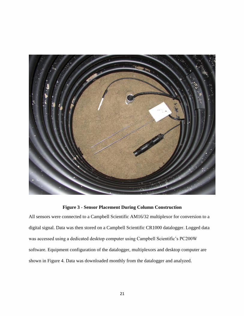
Three types of sensors were installed within the sand columns to monitor soil conditions,

described below. These sensors were installed in clusters at specified depths. Each of the sensor

clusters was assigned a letter. Table 3 shows depths at which sensors were installed. Figure 3

shows an example of a sensor cluster during construction. Note that only columns with sand 1.2

m deep included sensors at levels D, E, and F.

Table 3 - Column Sensor Depths

Sensor

Level

Depth Below

Surface

(cm)

A 10

B 30

C 51

D 71

E 91

F 112

21

Figure 3 - Sensor Placement During Column Construction

All sensors were connected to a Campbell Scientific AM16/32 multiplexor for conversion to a

digital signal. Data was then stored on a Campbell Scientific CR1000 datalogger. Logged data

was accessed using a dedicated desktop computer using Campbell Scientific’s PC200W

software. Equipment configuration of the datalogger, multiplexors and desktop computer are

shown in Figure 4. Data was downloaded monthly from the datalogger and analyzed.

22

Figure 4 - Sensor Data Collection Setup

23

Oxygen Sensors

Oxygen in the columns was measured using Apogee Model SO-110 sensors. These sensors

contain a fuel that reacts with gaseous oxygen in a galvanic cell. Voltage produced by this cell is

linearly proportional to the percentage of oxygen at the sensor. Fuel in the cell is consumed

faster when more oxygen is present. The galvanic cell sensor is shipped with enough fuel to last

up to 10 years operating continuously at atmospheric oxygen (20.95%). The manufacturer has

measured the oxygen consumed by the reaction in the sensor to be “2.2 μmol O2 per day when

the O2 concentration was 20.95% at 23 C”. Oxygen and cell fuel consumed are inversely

proportional to the concentration of gaseous oxygen at the sensor(Apogee 2014).

Each sensor requires a multiplier to convert measured voltage into a percent oxygen reading.

Output voltages of each sensor were measured in atmospheric conditions (20.95% oxygen) and

in a pure nitrogen environment (0% oxygen) as per the instructions in the owner’s manual to

determine each multiplier before installation in the soil column (Apogee 2014).

Some data collected from the oxygen sensors indicated a malfunction of the sensor. Potential

causes include loss of fuel at the sensor, failure of electromagnetic shielding in the sensor cable,

and damaged wiring. Sensor data collected was reviewed to identify errant readings. Data

gathered by oxygen sensors was excluded from analysis if it met any of the following conditions.

Oxygen concentrations above 23% or below -1%

Erratic behavior - likely causes include electrical connectivity issues or loss of fuel at

sensor

o Single points far away from norm (changes of >1% O2/10 minutes)

o Several points in a row (>0.5% O2/10min for more than 30 minutes)

24

o Known column operational problems, including nutrient feed not delivered to

column, column leaking, and sensor filled with chemical precipitate.

The Apogee SO-110 sensor is also equipped with a thermistor to measure ambient temperature.

However, this data is not included in this report.

Water Content Reflectometer

Water content reflectometers, which measured volumetric moisture content (VMC) in soil was

measured using a Campbell Scientific model CS616 water content reflectometer. This sensor

operates by emitting an electronic pulse at an electrode and measuring the transmission time for

the signal to travel through the soil matrix and be detected at an adjacent electrode. There is an

inverse relationship between moisture content and pulse travel time through the soil. This sensor

does not consume any materials and has no prescribed maintenance (Campbell Scientific 2014).

Volumetric water sensors did not experience many of the issues that the oxygen sensors had (no

consumable fuel and not susceptible to fouling). These sensors also displayed an error message if

the electrical signal was ever lost while a reading was taken. As such, only data with an explicit

error message was removed.

These sensors were factory calibrated. However, volumetric water content was measured of

column sand with known water content using the reflectometers to verify calibration.

Thermistors

Temperature was logged using Campbell Scientific model T108 thermistors. These sensors

measure the resistance of a thermally sensitive BetaTherm 100K6A. The instruction manual

provided by the manufacturer states that calibration and maintenance of these probes is not

necessary.

25

The experiment was conducted in a heated indoor space where temperature was held constant.

The data collected from these thermistors is therefore not presented in this report.

Experimental Operation

The sand assimilation experiment was carried out using a combination of standard operating

procedures (SOPs). These SOPs were conducted either on a routine or when criteria were met to

warrant maintenance. These procedures are described in further detail below and attached as

Appendix A - Standard Operating Procedure (SOP).

Water application

During all phases of this experiment each column received an average of 2.4 liters per day (15 L

day-1

m-2

) of synthetic wastewater to promote microbial growth. Composition of this wastewater

is described above and in Table 2. Loading conditions of columns are included in Table 4.

26

Table 4 - Column Loading Conditions

Unique

Identifie

r

Submerge

d Bottom?

Column

Length

(meters

)

Average Daily

Organic Load

(lbs BOD ac-

1day

-1)

Hydraulic Rest Period

(hours between doses)

Organic

Load per

Dose (mg)

C1-1 Yes 0.6 65 6 290

C1-2 Yes 0.6 500 6 2,200

C1-3 Yes 0.6 1000 3 2,200

C2-0 No 0.6 65 6 290

C2-1 No 0.6 65 6 290

C2-2 No 0.6 500 6 2,200

C2-3 No 0.6 1000 3 2,200

C3-1 Yes 0.6 250 12 2,200

C3-2 Yes 0.6 500 12 4,500

C3-3 Yes 0.6 500 24 9,000

C4-0 No 0.6 250 12 2,200

C4-1 No 0.6 250 12 2,200

C4-2 No 0.6 500 12 4,500

C4-3 No 0.6 500 24 9,000

C5-1 Yes 0.6 500 4 1,500

C5-2 Yes 0.6 1000 6 4,500

C5-3 Yes 0.6 1000 56 42,000

C6-0 No 0.6 500 24 9,000

C6-1 No 0.6 500 4 1,500

C6-2 No 0.6 1000 6 4,500

C6-3 No 0.6 1000 24 18,000

C7-1 Yes 1.2 250 12 2,200

C7-2 Yes 1.2 1000 12 9,000

C7-3 Yes 1.2 1000 56 42,000

C8-1 No 1.2 250 12 2,200

C8-2 No 1.2 1000 12 9,000

C8-3 No 1.2 1000 24 18,000

Synthetic wastewater was prepared every Monday, Wednesday and Friday to limit biological

growth, chemical degradation, and oxidation before application to the soil. Chemicals used in the

27

feed water were premeasured. Each delivery bucket received dry chemicals from sealed bags and

from a pre-mixed liquid stock solution.

Solution remaining in delivery buckets was discarded. Delivery buckets were thoroughly cleaned

with phosphate free soap and rinsed before new feed solution was prepared. Wastewater

application was automated using Masterflex 07553-80 peristaltic pumps. These pumps were

controlled by Cole-Parmer 5010CP digital electronic timers. Pump run times were calibrated

weekly to ensure correct wastewater volumes was delivered.

Analytical Data Collected

Influent and effluent water samples were collected from each column analyzed per the SOP for

pH, COD, alkalinity, total manganese and total iron. Additional details can be found in Appendix

A.

Chemical Oxygen Demand (COD) was measured according to USEPA Reactor Digestion

Method 8000 using high-range COD vials (100-1,000 mg/L) for influent water and low-range

COD vials (0-150 mg/L) for effluent water. Vials were manufactured by the HACH Corporation.

The pH of samples was measured using Denver Instrument Ultra Basic-10 pH probe. The probe

was calibrated before each use using a three-point calibration. Calibration solutions of 4, 7, and

10 were used. The pH probe was inserted into each sample. The reported pH value was recorded

after the instrument had reached equilibrium with the sample. The probe was rinsed with

deionized water after each reading was collected.

28

Alkalinity of each sampled was measured weekly using HACH Alkalinity Test Kit, Model AL-

DT. Test method 8203 was used. A standard and blank were each measured as a quality control

measure with each sampling event.

Influent and effluent samples from each column were collected weekly and analyzed for total

iron and manganese by the MSU Plant and Soil Sciences Laboratory using EPA method 6020A

via atomic adsorption spectrophotometer.

Maintenance

Soil surfaces were monitored weekly for excessive biological fouling. The columns were scraped

with a small garden cultivator when surface ponding persisted 30 minutes after water application

to encourage drainage. No soil or biological growth was removed during this process.

Drainage holes on the bottom of each column were visually inspected and mechanically cleaned

using a metal pin on a quarterly basis to discourage preferential flow through the end of the

columns.

Results and Discussion

Data collected during the study appeared to reveal basic trends between column loading

conditions and soil effluent characteristics. Generally speaking, it appeared that columns with

very high average daily organic loading led to poor wastewater treatment and excess metals in

column effluent. Columns with either the highest and lowest hydraulic rest period also resulted

in poor treatment.

Relationships between loading characteristics and treatment appeared to exhibit non-monotonic

characteristics. Figures depicting raw data collected for O2, VWC, effluent manganese

29

concentration, effluent iron concentration, and effluent COD concentration are included as

Appendix B - Selected Raw Data Figures. Note that the raw sensor data in these figures has not

been censored per the procedures described in the materials and method section of this report.

Analytical data collected for effluent manganese concentration, effluent iron concentration, and

effluent COD concentration during the study is included as Appendix C - Selected Raw

Analytical Data. An objective measure to quantify trends and relationships was required.

Methods of Analysis Considered

Methods initially identified as having potential to examine correlations, but ultimately rejected,

are listed below including reasoning for discontinuation of further evaluation.

Principal Component Analysis

Principal Component Analysis (PCA) assumes a linear relationship between each tested variable

and that data is normally distributed. A “minimally adequate” sample size of five times the

number of variables examined or 100, whichever is larger, is required (O'Rourke and Hatcher

2013). Initial observations of data collected indicated that many relationships were nonlinear.

Normality of collected sensor data was tested. Results indicated that data did not have a normal

distribution. Only 26 sample results were produced during the study. Therefore the “minimally

adequate” sample size was not realized. For these reasons further investigation of PCA was

terminated.

Multiple Linear Regression

Multiple Linear Regression (MLR) assumes the relationship between tested variables is linear

and that data is distributed normally. MLR also requires that data is homoscedastic, or of

constant variance (Greene 2011). Linear relationships between the variables to be tested were not

30

expected and data collected was not normally distributed. Additionally, collected data was not

heteroscedastic. Manuals from sensor manufacturers indicated that error varied with readings,

not full-scale measurement. Consequently, MLR as a means to analyze data collected during this

study was abandoned.

Seasonal-Trend Decomposition Procedure Based on Loess

Seasonal-Trend Decomposition based on Loess (STL) is a data filtering procedure used to

decompose a time series into three constituents: an overall trend, a cyclical trend that repeats

over a specified interval, and a remainder. The original data set is the sum of these three parts.

The “remainder” portion of the data signifies noise. This remainder is separated in STL, allowing

underlying trends to be identified in the “trend” and “seasonal” portions of the data. A function

for the STL procedure was developed in R, a computing program (Cleaveland, Cleaveland et al.

1990).

Soil sensor data was filtered using the STL function in R. Evaluation of decomposed data

revealed that the “remainder” portion of the data exhibited trends indicating that the model did

not identify all trend patterns in the data. This demonstrates that STL is likely an inappropriate

technique to filter the data set. Further investigation using STL was therefore discontinued.

Analysis Used to Identify Relationships

Censored data collected during the study exhibited visual trends. See appendix B. Figure 5 shows

the average daily BOD applied against median effluent total iron concentration. A positive non-

monotonic relationship appears to exist between these variables. A simple linear regression

through these points yields a low R2 value of 0.4. However, as discussed above, proving a

statistical relationship using conversional techniques has not been effective.

31

Figure 5 - Average Daily BOD Applied vs. Median Total Iron Effluent Concentration

Spearman’s Rank Order Correlation

Spearman’s rank order correlation is a modified version of the Pearson product-moment

correlation coefficient and is used to indicate whether a statistical correlation exists between two

variables. Correlations using Spearman’s rank reveal only monotonic relationships in data sets

and it does not require that the data be normally distributed or exhibit a linear relationship

(McDonald 2014). Spearman’s rank is a nonparametric statistical test that is used most

extensively in biological studies. The transformation into ranks used in this test limits the impact

of strong outliers but may still identify correlations in data.

Table 5 shows raw example data to complete an example Spearman’s rank calculation. Note that

this data is entirely fabricated. First, both variables must be numerically ranked. For example, the

R² = 0.4007

0.00

0.10

0.20

0.30

0.40

0.50

0.60

0 200 400 600 800 1000 1200

Me

dia

n T

ota

l Iro

n E

fflu

en

t C

on

cen

trat

ion

(m

g/L)

Average Daily BOD Applied (lbs ac-1 day-1)

32

lowest value within a set of one variable is assigned the rank of 1, the second largest 2, and so

on. If any values are equal, the ranks that would otherwise be assigned to those values are

averaged. See Table 6 for an example.

Table 5 - Spearman’s Rank Sample: Raw Example Data

x-values y-values

2 3

23 2

34 38

53 53

10 41

60 34

52 13

82 96

74 68

74 36

Table 6 - Spearman’s Rank Sample: Data Rankings

x-values y-values x-rank

(𝑥𝑖)

y-

rank

(𝑦𝑖)

(𝑥𝑖 − 𝑦𝑖)2

2 3 1 2 1

23 2 3 1 4

34 38 4 6 4

53 53 6 8 4

10 41 2 7 25

60 34 7 4 9

52 13 5 3 4

82 96 10 10 0

74 68 8.5 9 0.25

74 36 8.5 5 12.25

Sum 63.5

33

Spearman’s rank is denoted as ρ and is defined by the following equation.

𝜌 = 1 −6 Σ(𝑥𝑖 − 𝑦𝑖)

2

𝑛3 − 𝑛

Where:

𝑥𝑖 , 𝑦𝑖 = respective ranks of data pair

𝑛 = number of samples

Using the sample data in Table 5 and Table 6 the Spearman’s rank can be calculated for the

sample data as:

𝜌 = 1 −6 ∗ 63.5

103 − 10= 0.62

Spearman’s ρ is a relative correlation where -1 < ρ < 1, where ρ = 0 indicates no correlation and

|ρ| = 1 indicates a perfect correlation. As ρ approaches 0 the correlation is indicated as weaker.

Figure 6 is a plot of the ranks given to the data in Figure 5. Axes indicate the rank of each value

collected rather than the indicating the actual value of the data point. The difference between

each of the ranks is not necessarily linear. Figure 6 is included to assist to visualize the

transformation to Spearman’s rank.

34

Figure 6 - Ranks of Average Daily Organic Load vs. Ranks of Median Effluent Iron

Concentration

Analysis was conducted to determine whether correlations between loading characteristics and

treatment conditions existed. Five loading characteristics were studied: Average daily organic

load (expressed in lbs BOD ac-1

day-1

), hydraulic rest period (expressed in hours), organic load

per dose (expressed in mg BOD), column length (either 0.6 or 1.2 m), and presence of perched

groundwater table.

Because hydraulic loading was held constant during the study, variations in hydraulic rest period

caused variations in the volume of water in each application of wastewater. Organic load per

dose was calculated based on the concentration of water applied which depended on the average

0

5

10

15

20

25

30

0 5 10 15 20 25

Ran

ks o

f M

ed

ian

Eff

lue

nt

Iro

n

Co

nce

ntr

atio

n (

mg/

L)

Ranks of Average Daily BOD Applied (lbs BOD ac-1 day-1)

35

daily organic load, and the volume of wastewater applied per dose which depended on hydraulic

rest period.

Treatment conditions studied were total manganese in column effluent, total iron in column

effluent, COD in column effluent, oxygen concentration in the column, and volumetric water

content of soil in the column.

Spearman’s ρ was calculated for these comparisons using Microsoft Excel to determine whether

correlations between these parameters were statistically significant. Calculated data and formulas

are included as Appendix D - Calculation of Spearman’s Correlation Coefficient.

Loading conditions were compared with sensor and analytical data collected for each treatment.

Median values of each variable collected during each phase of the experiment were used to rank

analytical data to nullify the effect of strong outliers. Data was censored using the procedure

outlined in the materials and methods section of this report. Average values collected for O2 and

volumetric VWC were used for ranks.

Spearman’s ρ was calculated for comparisons between each of the selected dependent and

independent variables. Correlation of the pair was said to be statistically significant if the

absolute value of the calculated ρ exceeded the critical value (Zar 1972). A single-tailed

approach and p-value of <0.01 were used. Use of this p-value is common practice and indicates

that there is less than a 1% chance that the indicated correlation developed due to chance.

A matrix for Spearman’s ρ and p-value (if greater than 0.01) between the column loading

conditions and the collected data was developed and is shown as Table 7.

36

Table 7 - Spearman's Rank for Selected Variables

Spearman's Rank For Selected Variables

Mn Fe COD O2 VWC

ρ p-

value

ρ p-

value

ρ p-value ρ p-value ρ p-

value Average Daily

Organic Load

0.27 > 0.01 0.72 0.005 0.71 0.005 -0.46 0.010 0.59 0.005

Hydraulic

Rest Period

0.46 0.01 0.24 > 0.01 0.36 > 0.01 -0.27 > 0.01 -

0.10

> 0.01

Organic Load

per Dose

0.41 > 0.01 0.54 0.005 0.61 0.005 -0.52 0.005 0.28 > 0.01

Column

Length

0.88 0.01 0.21 > 0.01 0.40 > 0.01 0.31 > 0.01 -

0.36

> 0.01

Presence of

Perched

Groundwater

0.00 > 0.01 0.24 > 0.01 0.10 > 0.01 -0.20 > 0.01 0.29 > 0.01

Average Daily Organic Loading

Increased average daily organic load has a statistically significant positive correlation with

effluent iron concentration, effluent COD concentration, VWC in the soil columns, and a

negative correlation with oxygen concentration in the soil columns.

These correlations indicate that soil tends to become anaerobic and create iron reducing

conditions as organic loading of the soil increases (Crites and Tchabanoglaus 1998, McDaniel

2006, Beggs, Bold et al. 2007, Hillel 2008). Oxygen required to aerobically degrade organic

waste increases as organic application rate is increased. Anaerobic populations will dominate soil

if organic application rate exceeds oxygen flux into the soil.

37

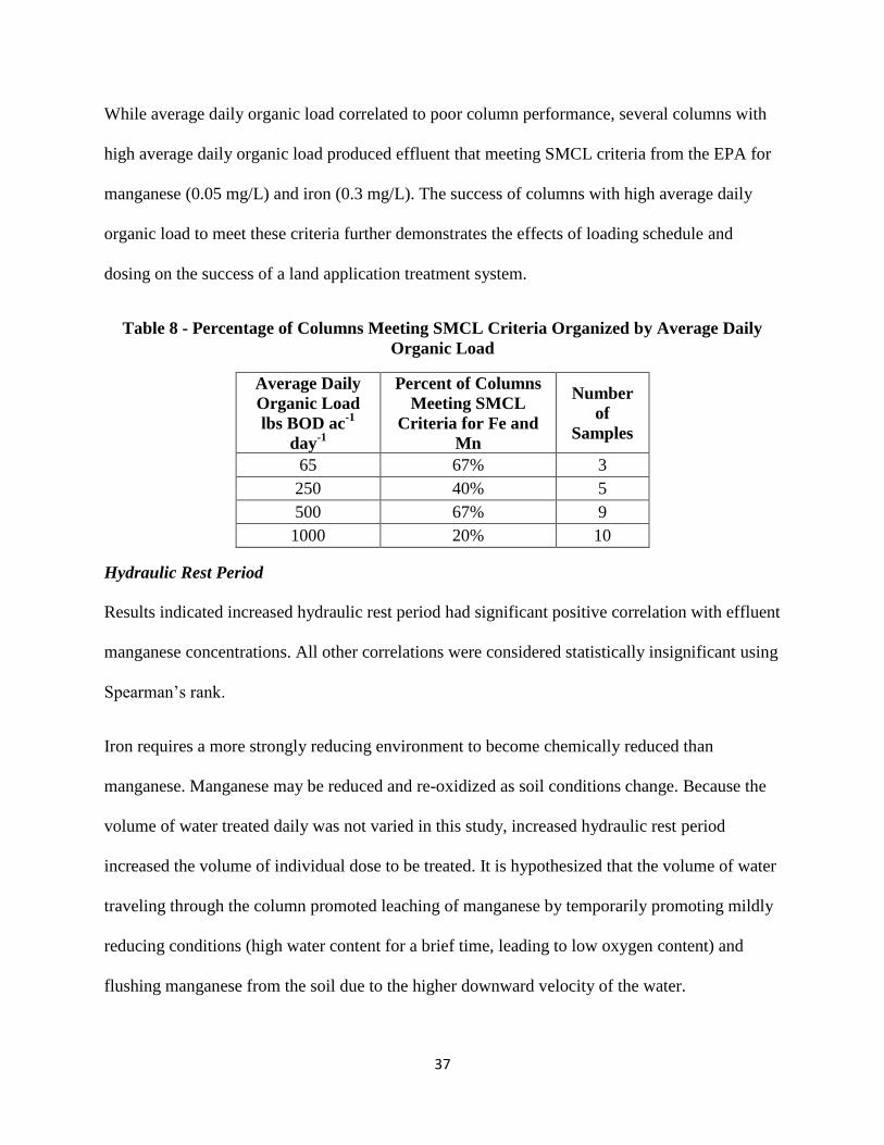
While average daily organic load correlated to poor column performance, several columns with

high average daily organic load produced effluent that meeting SMCL criteria from the EPA for

manganese (0.05 mg/L) and iron (0.3 mg/L). The success of columns with high average daily

organic load to meet these criteria further demonstrates the effects of loading schedule and

dosing on the success of a land application treatment system.

Table 8 - Percentage of Columns Meeting SMCL Criteria Organized by Average Daily

Organic Load

Average Daily

Organic Load

lbs BOD ac-1

day-1

Percent of Columns

Meeting SMCL

Criteria for Fe and

Mn

Number

of

Samples

65 67% 3

250 40% 5

500 67% 9

1000 20% 10


Results indicated increased hydraulic rest period had significant positive correlation with effluent

manganese concentrations. All other correlations were considered statistically insignificant using

Spearman’s rank.

Iron requires a more strongly reducing environment to become chemically reduced than

manganese. Manganese may be reduced and re-oxidized as soil conditions change. Because the

volume of water treated daily was not varied in this study, increased hydraulic rest period

increased the volume of individual dose to be treated. It is hypothesized that the volume of water

traveling through the column promoted leaching of manganese by temporarily promoting mildly

reducing conditions (high water content for a brief time, leading to low oxygen content) and

flushing manganese from the soil due to the higher downward velocity of the water.

38

However, each of the statistically insignificant data sets does not seem to follow a monotonic

function. For example, rank of VWC in soil during the study tended to be highest when water

applications were either more frequent or more infrequent. The lowest ranked VWC paired with

water application frequency between six and twelve hours. Effluent iron concentration and

effluent COD concentration follow this same pattern. Average oxygen concentration indicates an

inverted pattern. Figure 7 shows the paired rankings of the instantaneous volume of water

applied and the rank of VWC in the soil column. Visual inspection of this figure suggests the

monotonic requirements of Spearman’s rank have been violated. Analysis to objectively quantify

whether this relationship was monotonic was not conducted.

Figure 7 - Rank of Hydraulic Rest Period and Column Water Content

Frequent, low-volume hydraulic dosing may not give soil adequate time to drain, promoting a

more saturated soil. As the soil becomes more saturated, downward velocity of the water into the

soil decreases and the piston effect that draws oxygen into the soil via low pressure following a

substantial hydraulic dose described in previous literature (McMichael, McKee et al. 1965,

0

5

10

15

20

25

30

0 5 10 15 20 25 30

Ran

k o

f V

WC

in C

olu

mn


39

Lance, Whisler et al. 1973) becomes weaker. Small doses of water may also not draw enough air

into the soil to promote an aerobic environment. Conversely, infrequent, high-volume hydraulic

dosing draws air into the soil, but the large volume of water in the individual doses may

temporarily saturate the soil. This may allow a shift to a predominantly anaerobic microbial

population. Anaerobes maintain anaerobic conditions by producing slime in the soil pore space.

As such, an ideal dosing frequency appears to exist where soil is allowed to drain sufficiently

between water doses, but that provides a piston of air to the soil frequently enough to maintain

aerobic conditions. Data from this study suggests a hydraulic rest period of 12 hours will help to

maintain an aerobic soil environment. However, denitrification requires an anaerobic

environment. As such, denitrification requirements for a site should also be considered.

Organic Load per Dose

Increased instantaneous application of organic material had statistically significant positive

correlation with effluent iron concentration, effluent COD concentration, and a negative

correlation with oxygen concentration in the soil columns.

These correlations indicate that soil tends to become anaerobic and create iron reducing

conditions as organic load from individual dosing events increases. Oxygen demand of the

organic load in these doses has the potential to overwhelm oxygen flux into the soil. Anaerobic

microbially populations may dominate the soil if oxygen deficient environments are maintained

for a long enough period. Biofilms produced by anaerobic bacteria limit oxygen transport into

the soil. Aerobic populations will not recover if oxygen flux does not meet oxygen demand.

Wastewater treatment efficacy is decreased and potential for metals leaching is increased while

anaerobic conditions are maintained.

40

However, little research specifically investigating effects of individual applications of organic

matter on metal mobilization was found. Additionally, statistically significant positive

Spearman’s correlation between average daily organic load and organic load per dose existed

due to the experimental design of this study.

Column Length

Column length was biased by experimental design as long columns used in this study were

subjected to higher organic loading than the short columns. This is demonstrated by a significant

correlation between column length and average daily organic load.

Spearman’s rank for the effect of long columns on the dependent variables was recalculated

using a subset of eight loading conditions to nullify this effect. These eight conditions were a

combination of four pairs of long soil columns and short soil columns. Loading conditions were

duplicated between these pairs. This data subset is shown in Table 9.

Table 9 - Data Subset for Column Length Correlations

Unique

Identifier

Submerged

Bottom?

Column

Length

(meters)

Average Daily

Organic Load

(lbs BOD ac-

1day

-1)

Hydraulic Rest

Period

(hours between

doses)

Organic

Load

per

Dose

(mg)

C4-0 No 0.6 250 12 2,200

C4-1 No 0.6 250 12 2,200

C6-3 No 0.6 1000 24 18,000

C5-3 Yes 0.6 1000 56 42,000

C7-1 Yes 1.2 250 12 2,200

C8-1 No 1.2 250 12 2,200

C8-3 No 1.2 1000 24 18,000

C7-3 Yes 1.2 1000 56 42,000

41

Spearman’s rank calculated for these pairs indicated that increased column length had a

statistically significant positive correlation with effluent manganese concentration. Short

columns were used in the study prior to installation of the long columns. Iron requires a lower

redox potential than manganese to be mobilized and is more abundant in typical soils. It may be

possible that manganese was depleted from short columns during the initial phase of the

experiment. It is hypothesized that this measure is still biased because the long columns in this

study were operated for a shorter time than the short columns. No further conclusions were

drawn as a result.

Presence of Perched Groundwater Table

The presence of a perched groundwater table had no significant effects on the measured data.

This effect validates the experimental setup in that it demonstrates air did not enter the columns

from the bottom through drainage holes. It was initially hypothesized that submerged columns

would correlate to lower oxygen concentrations in the column if the bottom of unsubmerged

columns had allowed significant air to enter the column.

Soil after Experiment

Soil borings were taken of each column following the experiment. Note that soil cores illustrate

the changes to the soil due to the cumulative effect of the loading conditions applied to each

column. Photographs were taken and visual observations were noted.

Several columns had an organic sludge on the surface. However, because the columns without a

sludge layer may have recently been scraped to allow drainage, this sludge was not studied. Sand

throughout the columns appeared orange to brown in color. Soil 2.5 cm to 7.6 cm from the

surface in each column exhibited a dark band indicating that added organic mass had

42

accumulated in the top layer of soil. Buildup of organic matter in the top layer of the soil limits

diffusion rate of air into the soil and can promote anaerobic conditions. A photograph of soil

cores taken from one column is included as Figure 8. Organic layer on columns C7 and C8 is

less visible. These columns were operated for a shorter time than the other six columns. Photos

of all soil columns are included as Appendix E.

Figure 8 - Column 1 Soil Cores Illustrating Accumulation of Organic Matter Near Soil

Surface

Conclusions

Organic matter delivered to the soil matrix requires oxygen for aerobic degradation. Anaerobic

conditions, characterized by low oxidation-reduction potential, predominate without sufficient

oxygen. Naturally occurring metals in the soil may be reduced via microbially mediated redox

reactions under anaerobic conditions. Manganese, iron and, arsenic are common in soil and are

43

water soluble in their reduced states. These metals can leach into groundwater when reduced.

Additionally, anaerobic populations require more time than aerobic populations to fully degrade

organic compounds allowing organic waste to contaminate groundwater.

A lab-scale sand column experiment was conducted to assess impacts of land application of

wastewater. Specific goals of the study aimed to evaluate the impacts of several design and

operational parameters on groundwater with respect to mobilization of naturally occurring metals

from the soil matrix.

Results from the experiment indicated a statistically significant positive correlation between

average daily organic loading with effluent iron concentration, effluent COD concentration, and

column VWC. Negative correlations with gaseous O2 concentrations in column were observed.

Organic load per dose positively correlated with effluent iron concentration and effluent COD

concentration. Negative correlations with gaseous O2 concentrations in column were observed.

The results of this study concerning average daily organic load validate literature studied.

Excessive organic loading of land application systems may cause anaerobic soil conditions

resulting in groundwater contamination by metals and incompletely treated wastewater (Crites

and Tchabanoglaus 1998, McDaniel 2006, Beggs, Bold et al. 2007).

While the effects of average organic loading have been studied in depth, few studies focus on the

impact of organic load per dose as this project did. Results from this study indicate that total

oxygen demand of wastewater doses delivered to soil also impact soil conditions and can result

in incomplete wastewater treatment and metal mobilization from soil.

Findings from this lab-scale study revealed hydraulic rest period exhibited a statistically

significant positive correlation with effluent manganese concentration. Results also indicated that

44

hydraulic loading frequency did not exhibit statistically significant monotonic correlations with

effluent iron concentration, effluent COD concentration, soil VWC or soil O2 concentrations.

However, qualitative review of collected data suggests that a non-monotonic relationship with

these parameters may exist. Literature indicates water application to soil promotes soil aeration

by drawing in air via a hydrodynamic mass transfer “piston-like” effect (McMichael, McKee et

al. 1965, Lance, Whisler et al. 1973). Literature regarding effects of small, frequent, dosing of

wastewater to land application systems was not found.

The presence of a perched groundwater table was demonstrated to have a negligible effect on

effluent water quality and soil conditions during this study. p-values for all comparisons were

greater than 0.01.

Length of sand columns showed a statistically significant positive correlation to effluent

manganese concentration. However, this correlation is hypothesized to result from experimental

design and not necessarily from column length. No significant correlations to iron concentration,

COD concentration, oxygen concentration, or VWC were noted.

COD did not have a statistically significant correlation to column length but column effluent

typically contained measurable COD (see Appendix C for data). Oxygen concentrations in soil

diminish with depth (Lance, Whisler et al. 1973). Anaerobic treatment is slower than aerobic

treatment. Anaerobic portions of the soil columns will therefore offer little treatment but will

typically cause a reducing environment due to the presence of a carbon source and nutrients

(Hillel 2008). Manganese in the column effluent was thereby anticipated because of these

reducing conditions. The relatively low concentrations of COD in the lower portions of columns

may not have caused redox potential low enough to mobilize iron.

45

Visual inspect of soil after the experiment revealed deposition of organic matter in the top layer

of soil. This deposited organic matter may reduce the oxygen flux into the soil, promoting

anaerobic conditions. This layer likely developed over time and had a more significant effect on

the last phases of the study than the first. The accumulation of organic matter may introduce bias

by reducing oxygen flux into the soil; however, this effect was not specifically studied.

Overall trends indicate that increased average daily organic load and organic load per dose have

a negative impact on water quality. Other studies have attempted to determine an average daily

organic loading that prevents metal mobilization; however, findings from this study indicate

organic dose load and hydraulic rest period are important factors that should be considered in

design. General guidance from this study indicates that both organic load per dose and average

daily organic load be reduced to ensure a treatment system does not negatively impact

groundwater quality. Operational constraints should be considered during the design phase land

application treatment systems.

Hydraulic rest period is an important factor and may be used to help aerate soil. Results from this

study indicate that a rest period of approximately 12 hours using hydraulic loading events of 0.7

cm can be used to encourage aeration via hydrodynamic mass transfer.

Opportunities for Further Research

Wastewater land application systems offer many benefits. Land application of waste is

economical, relatively low-maintenance, and returns water to the local aquifer. Land applied

wastewater can serve as nutrient-rich irrigation water for crops. However, poorly managed

systems have resulted in crop failure, unpleasant odors, and contamination of soil and

groundwater.

46

Further research is required to gain a more complete understanding of wastewater land

application systems. Information acquired through this study can be utilized to further optimize

land application design and maintenance strategies as well as direct future research. Specific

recommendations developed following the completion of the lab-scale study are listed below.

1) Sample size of column conditions was relatively small in this study due to limited resources.

Conducting tests on a larger number of soil columns, including adequate duplication, may

allow for more comprehensive analysis using methods such as Multiple Liner Regression.

2) Consideration of soil type in this evaluation would help make this study more immediately

applicable to full-scale systems. Soil type plays an important role in available pore space,

VWC, and oxygen transfer into soil. Site specific pilot-scale systems may be an appropriate

means of assessing the quality of a site for a land application treatment system. Further study

using a variety of soil types and soil mixtures will provide a more robust understanding of

land application treatment systems and help to develop a prescriptive approach to operation

recommendations.

3) Further research is required to better understand the different impacts of average organic load

and organic load applied per dose. Land application requires optimization of several

competing factors including oxygen flux into soil, biokinetic rate of wastewater degradation

(with focus on aerobic versus anaerobic processes), and apparent velocity of water. Computer

modeling may prove useful and could be calibrated using data collected during previous

studies.

4) Organic material was deposited in the soil throughout the study. Past research has indicated

that deposition of organic material on soil limits oxygen transfer into soil. Land application

47

systems should consider maintenance strategies to reduce surface fouling due to

accumulation of organic matter at soil surface.

48

APPENDICES

49

APPENDIX A

Standard Operating Procedures

50

The following is the Standard Operating Procedure for the Sand Assimilation Project. This project is

aimed at determining the effect of carbon loading on soil on the leeching of metals from the soil.

The barn behind Farrall Hall houses the sand columns. These columns receive a mix of synthetic

wastewater from a system of pumps operated on timers. The pumps and timers allow for a more precise

delivery of the wastewater, both in terms of timing and volume, and help to reduce the amount of time

spent on the project. Below, in Figure 1, the pump configuration can be seen. This configuration was

planned out to keep the columns from the previous stage of the experiment in their current positions

and add Columns 7 and 8 with the smallest amount of confusion.

Figure 9 - Pump Configuration

Synthetic wastewater is produced by measuring out several chemicals to achieve a certain chemical

oxygen demand (COD) based on a well-respected article (Trulear, 1982). There are eight columns being

studied, each receiving a particular COD loading. Each column has a counterpart; one will allow water to

exit the column as it reaches the bottom and another with a closed bottom and a water trap to simulate

a high groundwater table. As such, wastewater will be prepared in four buckets, one for each pair of

conditions, and then split into eight buckets, one for each column. Conditions and bucket assignments

can be seen below in Table 1.

P4 P3 P2 P1

C4 C5 C6 C8

C1 C2 C3 C7

51

Table 10 - Column Loading Schedule

Organic Loading Hydraulic Loading

Loading Frequency Submerged Bucket

Column 1 65 lbs BOD/day 2.4 L/day 4x/day Submerged B1

Column 2 65 lbs BOD/day 2.4 L/day 4x/day Unsubmerged







Therefore, B1 will feed C1 and C2. However, both columns will have a separate bucket for influent. So,

B1 will be prepared, split evenly into F1 and F2 which will feed C1 and C2 respectively. Testing will be

done on B1-4 and not F1-8, as the samples would have the same concentrations and yield redundant

data.

Lab tests will be done to determine the pH, COD, Alkalinity and concentrations of manganese and iron of

both the influent and effluent water (from buckets and columns).

Data will be collected, input into a master spreadsheet and then analyzed.

52

Scheduled Operations Preparation and Sampling Prepare Sample Cups Clean sample cups can be found in a drawer labeled “Sample Cups” on the right-hand side of the fume

hood in Lab 128. For a typical day’s operation 12 cups will be needed; four for bucket samples, eight for

column samples. Be sure to grab the correct type of lid for each cup as there are two styles of threading.

Affix a small piece of painter’s tape to each cup and write the date and sample location on that tape.

Cups will be needed to sample each of the mixing buckets (B1-B4) and each of the columns (C1-C8).

Prepare Nutrient Solution Nutrient solution is stored in a 2L screw-cap bottle in a cupboard directly across from the door to lab

128. Also in this cupboard is a glass pipette and a sheet of paper explaining the necessary amount of

nutrients for each bucket/column. Use the pipette and the cordless pipetter normally found on the

countertop to fill the sample cups B1-B4 with the prescribed amount of the nutrient solution (indicated

on nutrient loading sheet). When finished clean the pipette tip out by flushing it with deionized (DI)

water. Place all materials back where they were found.

Measure Remaining Influent In order to complete a mass balance of metals and nutrients the amount of water actually applied to the

columns must be calculated. This is done by measuring the volume of influent water that is left over

after application and subtracting that from the volume of water prepared and using information about

the concentration of nutrients in the solution.

When first arriving in the barn each day, prepare an Influent/Effluent sheet. This is simply a large post-it

note (blank ones on the computer desk in the barn) with the date, time, temperature and volumes of

influent and effluent water recorded on it. The temperature should be recorded from the digital

thermometer located on top of the computer.

Measure the volume of influent remaining in each bucket either by using the graduations marked on the

sides of each feed bucket or by pouring the remaining influent into the graduated cylinder near the

columns. If using the graduated cylinder, make sure to keep it clean and avoid contaminating one bucket

with another’s nutrient solution. Record the volume on the Influent/Effluent sheet.

Clean Buckets After measuring the remaining effluent, each bucket must be cleaned thoroughly using phosphorus-free

soap and a sponge. Only use the sponge that has been labeled for this project as any other one could be

contaminated with chemicals that will interfere with the experiment. This will be done the easiest in the

shop sink (out the back door of Lab 129). A key into the shop can be found in the drawer where the

sample cups are stored.

53

Prepare Nutrient Buckets As stated previously, each column will be receiving water from its own bucket. This will allow a mass

balance to be done for each column. However, synthetic wastewater will be prepared for each pair of

buckets and need to be split into two different buckets. This saves time and makes measuring nutrients

easier.

To prepare each bucket, pour the nutrient solution measured earlier into the proper bucket as well as

the correct baggie of dry nutrients. These baggies will be stored in the same cupboard as the nutrient

solution.

Water must be added to each bucket. Each column will have 3000 mL available each day. Although they

are only meant to receive 2400 mL per day, the extra water allows for some error correction and makes

measuring the remaining influent easier. So, when preparing the nutrients, B1 (which feeds both C1 and

C2) will need 12 L of water on Mondays and Wednesdays. Because the columns will be left alone for an

extra day over the weekend, 18 L of water is needed.

After mixing the water and required nutrients together, carefully rinse out the B1-B4 sample cups to

reduce the residue left from the concentrated nutrient solution. Do this by scooping and pouring out

some of the solution to be sampled. This helps ensure that the bucket has all of the nutrients from the

sample cup and that the sample cup has a representative sample of the solution.

Each nutrient mixing bucket will then be split in half into the respective nutrient feed buckets.

Each bucket will then need to be placed on a shelf near its respective column in the barn. Wipe the hose

and PVC pipe connected to it with paper towel and replace the lid on each bucket. This helps prevent

bacterial growth in each bucket and helps ensure that nutrients are delivered to the columns instead of

consumed before application.

Measure/Sample Effluent The effluent from each column will also need to be measured to complete the mass balance. Under each

column there is a clear plastic tub. Take a sample of each of these tubs using the correctly labeled

sample cup. Again, rinse the sample cup with the sample by scooping up water and pouring it out (do

this three times for each sample). After sampling the water measure the effluent volume by pouring the

contents of the tub into the graduated cylinder. Be sure to account for the volume of the sample

(typically 50-100 mL). Record this on the Influent/Effluent Sheet (post-it note).

Cleaning Spray Nozzles Every week the spray nozzles that distribute the synthetic wastewater onto the soil columns must be

cleaned to ensure an even distribution and prevent clogs and buildup. Do this by pulling out the dirty

nozzles from their enclosure and allowing them to sit in an H2O2 solution. There is an extra set of nozzles

so that the clean ones can immediately be placed into the enclosure and the dirty nozzles can sit

overnight in the Hydrogen Peroxide solution.

54

The easiest way to do this has been to replace one nozzle each day of the week until all nozzles have

been cleaned. For example, replace C1 and C2 on Monday, C3 and C4 on Tuesday and so on. Do not

replace any nozzles on Friday.

Cleaning Effluent Tubs After measuring the volume of effluent produced take the empty effluent tubs to the sink in the shop to

wash. Wash them in the same way as the buckets. That is, scrub each out with phosphorus-free soap

using the sponge for this project.

Dry the tubs out by wiping the inside of each of them with paper towel and replace them under the

columns to continue catching effluent water.

Clean the Sink Each week the sink in the shop will need to be cleaned to prevent any bacterial buildup. To do this, use

the other sponge, not the one for the sand assimilation project, and the Comet cleaning powder to wipe

down the entire sink. Report any problems to Ryan Julien or Phil Hill.

Collect Sensor Data Once a week sensor data must be collected and input into the sensor data spreadsheet.

Observe Pumps Pumping of water onto columns should be observed once a week to ensure that the pumps are

operating properly and not leaking. This observation also serves to check that the columns are draining

properly. If all water has not infiltrated the soil surface 30 minutes after the water was applied, the top

of the column needs to be scraped. This can be done by running a small garden rake over the top of the

column to break up any bacterial growth and allow for proper drainage.

55

Lab Tests After collecting the samples and ensuring that the columns will have a continuous supply of water until

the next sampling period different laboratory tests must be run. All lab tests have Standard Operating

Procedures that can be found in the Sand Assimilation Project Book.

pH

pH of each sample must be tested as soon after collection as possible (within 1 hour). This will be done

using the pH meter in Lab 128. Follow the standard procedures for using the pH meter and be sure to

calibrate the meter before every test using the pH buffer solutions, found in the same cupboard as the

nutrient mixes.

COD Chemical oxygen demand is measured using HACH COD test kits. There are both high and low range test

kits for 1500mg O2/L and 150mg O2/L respectively. Typically the bucket samples will require the use of

the high range (HR) kits and the column samples can be measured using the low range (LR) kits. Both

types require 2mL of sample to be added to the prepared test tube. However, the HR kits will normally

be diluted with a 1 to 4 ratio. This means that 1.5mL of DI water and 0.5mL of sample water will be

added to each test tube. The LR tests are generally not diluted and simply receive 2mL of sample water.

Both the HR and LR tests will be run with a blank to calibrate the spectrophotometer that the tests are

read in. This blank is prepared by adding 2 mL of DI water to a prepared test tube.

A HR standard is also prepared. This is done using a standard 1000mg/L solution from the HACH

Company. Although this is a high range test, it is not meant to be diluted and 2mL of the solution is to be

added to a prepared vial.

Be sure to label each sample vial with the sample location (B1, HR Blank, Standard, etc.) and the date.

This is easiest to do before adding the sample to each vial as the reaction between the prepared

solution and the sample is exothermic and can be too hot to handle easily.

After preparing the solutions appropriately, overturn the vials 10 times to ensure the contents are

entirely mixed and place them in the oven under the fume hood for 2 hours at 150C as per the HACH

instructions. For any additional information see the HACH COD Kit SOP (Method 8000).

Alkalinity The alkalinity test is performed using pH indicator powder packets and a digital titrator. Follow the SOP

provided by HACH (method 8203).

Metals Metal testing will be done by the plant and soil sciences department. However, before a sample is

brought in for testing it must be acidified.

56

As-Needed Operations Several tasks do not adhere to a strict schedule and must be completed on an as-needed basis. Below

are the main tasks, but keep in mind this is not an exhaustive list.

Prepare Nutrient Baggies Nutrient baggies are to be prepared using the formulas on the nutrient mixing spreadsheet found in the

cupboard in Lab 128. Use the zip-top baggies (found on top of cabinets in Lab 128) and label each bag

with an appropriate label. This label includes the bucket number and whether the baggie is for two or

three days. It is best to have baggies in the cupboard for at least one week in advance to allow for any

changes in schedule that may occur.

Prepare Nutrient Solution As the concentrated nutrient solution runs out more will need to be prepared. There is another sheet

describing all of the chemicals included in this mixture in the cupboard and the Sand Assimilation Binder.

The 2L mixture generally lasts for about one month.

Prepare Clean H2O2 Solution The hydrogen peroxide solution used to clean the spray nozzles often gets dirty and becomes less

effective. When this happens it is time to prepare a clean solution.

In the cabinet under the computer in Lab 128 there is a bottle of 50% H2O2. This should be diluted to at

least 25% before being used to clean the nozzles. Pour an amount of 50% H2O2 into a sample cup and

add an equal volume of water. Use this as the new H2O2 solution.

Clean O2 Sensors Occasionally oxygen sensors in the sand columns get plugged up with crystals; presumably precipitates

from the nutrient solution. If sensor data shows that an oxygen sensor is reading 0% O2, it is likely that

the sensor has been overwhelmed with this precipitate.

To clean the sensors they must be carefully removed from the columns to reduce the influence of

opening the column to the atmosphere and cleaned according to the instructions provided by Apogee,

the producer of the sensors. These instructions can be found in the Apogee O2 sensor brochures in the

Sand Assimilation Book.

Checklist To ensure that each task is completed, a checklist has been developed. After completing a task initial the

corresponding box. This will allow all working on the project to easily see what tasks have been

completed and which, if any, need attention. See a copy of the weekly checklist below.

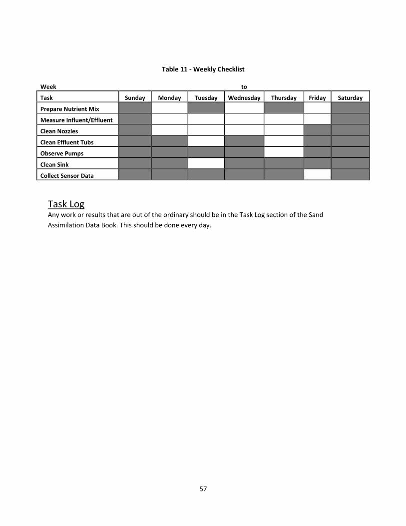
57

Table 11 - Weekly Checklist

Week to

Task Sunday Monday Tuesday Wednesday Thursday Friday Saturday

Prepare Nutrient Mix

Measure Influent/Effluent

Clean Nozzles

Clean Effluent Tubs

Observe Pumps

Clean Sink

Collect Sensor Data

Task Log Any work or results that are out of the ordinary should be in the Task Log section of the Sand

Assimilation Data Book. This should be done every day.

58

APPENDIX B

Selected Raw Data Figures

59

Figure 10 - Column 1 Raw Data

60


61


62


63


64


65


66


67

APPENDIX C

Raw Analytical Data

68

Table 12 - Raw Analytical Data

69

Table 12 (cont’d)

70

Table 12 (cont’d)

71

Table 12 (cont’d)

72

Table 12 (cont’d)

73

Table 12 (cont’d)

74

Table 12 (cont’d)

75

Table 12 (cont’d)

76

Table 12 (cont’d)

77

Table 12 (cont’d)

78

Table 12 (cont’d)

79

Table 12 (cont’d)

80

Table 12 (cont’d)

81

Table 12 (cont’d)

82

Table 12 (cont’d)

83

Table 12 (cont’d)

84

Table 12 (cont’d)

85

Table 12 (cont’d)

86

Table 12 (cont’d)

87

Table 12 (cont’d)

88

Table 12 (cont’d)

89

Table 12 (cont’d)

90

Table 12 (cont’d)

91

Table 12 (cont’d)

92

Table 12 (cont’d)

93

Table 12 (cont’d)

94

Table 12 (cont’d)

95

Table 12 (cont’d)

96

Table 12 (cont’d)

97

Table 12 (cont’d)

98

Table 12 (cont’d)

99

Table 12 (cont’d)

100

Table 12 (cont’d)

101

Table 12 (cont’d)

102

Table 12 (cont’d)

103

Table 12 (cont’d)

104

Table 12 (cont’d)

105

Table 12 (cont’d)

106

Table 12 (cont’d)

107

Table 12 (cont’d)

108

APPENDIX D

Calculation Of Spearman’s Correlation Coefficient

109

Table 13 - Results Including Ranks for Calculation of Spearman's Rank

110

Table 14 - Spearman's Rank Resulting Calculated Data

111

Table 15 - Spearman's Rank Excel Formulas Used

112

APPENDIX E

Photos Of Soil Column Cores Following Study

113

Figure 18 - Photos of Soil Cores from Columns One Through Four

114

Figure 19 - Photos of Soil Cores from Columns Five Through Eight

115

REFERENCES

116

REFERENCES

Apogee (2014). Apogee Instruments Owner's Manual - Oxygen Sensor: Models SO-110, SO-

120, SO-210, and SO-220. A. I. Inc.

Beggs, R., J. Bold, S. Melmon and G. Carlton (2007). Manual Of Good Practice For Land

Application Of Food Processing/Rinse Water Davis, CA, Kennedy/Jenks Consultants.

Campbell Scientific (2014). CS616 and CS625 Water Content Reflectometers I. Campbell

Scientific.

Carawan, R. E. and J. Chambers, V. (1979). Spinoff on Fruit and Vegetable Water and

Wastewater Management, North Carolina Agricultural Extension Service.

Chambers, C. D., J. Willis, S. Giti-Pour, J. L. Zieleniewski and J. F. Rickabaugh (1990).

Handbook on in situ treatment of hazardous waste-contaminated soils. U. S. E. P. Agency.

Cincinnati, OH, Risk Reduction Engineering Laboratory, Office of Research and Development,

U.S. Environmental Protection Agency.

Chen, Y. and Y. Avnimelech (1986). The Role of Organic Matter in Modern Agriculture,

Springer London, Limited.

Cho, D. (2005). "Scaling Back the Mineral Problem." Journal Of Environmental

Protection(11/01/2005).

Chrzanowskil, T. H., M. Kyle, J. J. Elser and R. W. Sterner (1996). "Element ratios and growth

dynamics of bacteria in an oligotrophic Canadian shield lake." Aquatic Microbial Ecology 11:

119-125.

Cleaveland, R. B., W. S. Cleaveland, J. E. McRae and I. Terpenning (1990). "STL: A Season-

Trend Decomposition Procedure Based on Loess." Journal of Official Statistics 6(1): 3-73.

Coody, P. N., L. E. Sommers and D. W. Nelson (1986). "Effects of glucose-imposed oxygen

demand on land treatment systems." Journal of Environmental Quality 15(1): 16-20.

Cook, F. J. (1995). "ONE-DIMENSIONAL OXYGEN DIFFUSION INTO SOIL WITH

EXPONENTIAL RESPIRATION - ANALYTICAL AND NUMERICAL-SOLUTIONS."

Ecological Modelling 78(3): 277-283.

Cotruvo, J., J. K. Fawell, M. Giddings, P. Jackson, Y. Magara, A. V. Festo and E. Ohanian

(2011). Arsenic in Drinking-water. W. H. Organization. Geneva, Switzerland, World Health

Organization.

117

Cowan, M. K. (2012). Microbiology : a systems approach. New York, McGraw-Hill.

Craul, P. J. (1992). Urban soil in landscape design, Wiley.

Crites, R. W. and G. Tchabanoglaus (1998). Small and Decentralized Wastewater Management

Systems, McGraw-Hill.

Drahota, P. and M. Filippi (2009). "Secondary arsenic minerals in the environment: A review."

Environment International 35(8): 1243-1255.

Duan, R. B., C. D. Sheppard and C. B. Fedler (2010). "Short-Term Effects of Wastewater Land

Application on Soil Chemical Properties." Water Air and Soil Pollution 211(1-4): 165-176.

Erickson, J. and E. J. Tyler (2000). Soil Oxygen Delivery to Wastewater Infiltration Surfaces.

National Onsite Wastewater Recycle Association, 632 Main Street, Laurel, MD 20707.

Fawell, J. K., U. Lund and B. Mintz (2003). Iron in Drinking-water. W. H. Organization.

Geneva, Switzerland, World Health Organization.

Greene, W. H. (2011). Econometric Analysis, Prentice Hall.

Gurzau, E. S., C. Neagu and A. E. Gurzau (2003). "Essential metals - case study on iron."

Ecotoxicology and Environmental Safety 56: 190-200.

Haggblom, M. M., L. Y. Rivera Md Fau - Young and L. Y. Young "Influence of alternative

electron acceptors on the anaerobic biodegradability of chlorinated phenols and benzoic acids."

(0099-2240 (Print)).

Hillel, D. (2004). Introduction to environmental soil physics. Amsterdam ; London, Elsevier

Academic Press.

Hillel, D. (2008). Soil in the environment : crucible of terrestrial life. London, Academic.

Hughes, M. F. (2002). "Arsenic toxicity and potential mechanisms of action." Toxicol Lett

133(1): 1-16.

Jones, A., L. Beyer, M. Rookwood, J. Pacenka and J. Bergin (1992). Technical Support

Document for Land Application of Sewage Sludge. U. S. E. P. Agency. Lexington, MA, The

Group.

118

Kazantzis, G. (1981). "ROLE OF COBALT, IRON, LEAD, MANGANESE, MERCURY,

PLATINUM, SELENIUM, AND TITANIUM IN CARCINOGENESIS." Environmental Health

Perspectives 40(AUG): 143-161.

King, L. D. (1986). Design and management considerations in applying minimally treated

wastewater to land. Utilization, Treatment, and Disposal of Waste on Land. E. C. A. Runge, Soil

Science Society of America: 15-26.

Lance, J. C., F. D. Whisler and H. Bouwer (1973). "Oxygen Utilization in Soils Flooded with

Sewage Water." J. Environ. Qual. 2(3): 345-350.

Leeson, A. and R. E. Hinchee (1997). Soil bioventing : principles and practice. Boca Raton ;

London, CRC/Lewis Publishers.

Levy, G. J., P. Fine and A. Bar-Tal (2011). Treated wastewater in agriculture : use and impacts

on the soil environment and crops. Chichester, Wiley-Blackwell.

Mannapperuma, J. D. (2005). Residual management in fruit processing plants. Processing Fruits:

Science and Technology. D. M. Barrett, L. Somogyi and H. Ramaswamy. Boca Raton, FL, CRC

Press.

Mannapperuma, J. D., E. D. Yates and P. R. Singh (1993). Survey of Water Use in the California

Food Processing Industry. Food Industry Environmental Conference, Atlanta, GA.

Martin, I., R. i. n. De Burca and H. White (2009). Soil guideline values for inorganic arsenic in

soil [author(s): Ian Martin, Róisín De Burca and Hannah Morgan]. Bristol, Environment Agency.

Masscheleyn, P. H., R. D. Delaune and W. H. Patrick (1991). "EFFECT OF REDOX

POTENTIAL AND PH ON ARSENIC SPECIATION AND SOLUBILITY IN A

CONTAMINATED SOIL." Environmental Science & Technology 25(8): 1414-1419.

McDaniel, P. A. (2006). Anaerobic Processes. Encyclopedia of Soil Science. R. Lal. Boca Raton,

FL, Taylor & Francis Group. 1: 97-100.

McDonald, J. H. (2014). Handbook of Biological Statistics. Baltimore, Maryland, Sparky House

Publishing.

McLean, J. E. and B. E. Bledsoe (1992). Ground Water Issue: Behavior of Metals in Soils.

McMichael, F. C., J. E. McKee, Keck (W. M.) Laboratory of Environmental Health Engineering.

and California. State Water Quality Control Board. (1965). Final report of research on

wastewater reclamation at Whittier Narrows. Pasadena,, W. M. Keck Laboratory of

Environmental Health Engineering, California Institute of Technology.

119

Mokma, D. M. (2006). Capacity of Soils to Assimilate Wastewaters from Food Processing

Facilities.

Moldrup, P., T. Olesen, J. Gamst, P. Schjønning, T. Yamaguchi and D. E. Rolston (2000).

"Predicting the Gas Diffusion Coefficient in Repacked Soil Water-Induced Linear Reduction

Model." Soil Sci. Soc. Am. J.(5): 1588-1594.

O'Brien, E. H. M. D. A. S. (2002). "Wastewater to wetlands opportunities for California

agriculture."

O'Rourke, N. and L. Hatcher (2013). A Step-by-Step Approach to Using SAS for Factor

Analysis and Structural Equation Modeling, SAS Institute Inc.

Rittman, B. E. and P. L. McCarty (2001). Environmental Biotechnology: Principles and

Applications. New York, NY, McGraw-Hill.

Safferman, S. I., I. Fernandez-Torres, S. M. Pfiffner, R. A. Larson and D. L. Mokma (2011).

"Predicting the Onset of Metal Leaching from Land Application of Wastewater Using Soil

Sensors and Microbial Community Analyses." Journal of Environmental Engineering-Asce

137(2): 97-107.

Santamaria, A. B. and S. I. Sulsky (2010). "Risk Assessment of an Essential Element:

Manganese." Journal of Toxicology and Environmental Health-Part a-Current Issues 73(2-3):

128-155.

Shacklette, H. T. and J. G. Boerngen (1984). Element concentrations in soils and other surficial

materials of the conterminous United States : an account of the concentrations of 50 chemical

elements in samples of soils and other regoliths. Washington, U.S. G.P.O.

Smith, A. H., E. O. Lingas and M. Rahman (2000). "Contamination of drinking-water by arsenic

in Bangladesh: a public health emergency." Bulletin of the World Health Organization 78(9):

1093-1103.

Spalding, R. F. (2002). Aquifer Denitrification. Groundwater Resources Association

6th

Symposium on Groundwater Contaminants - Nitrate in Groundwater: Sources, Impacts and

Solutions, Fresno, CA.

Sposito, G. (2008). The Chemistry of Soils. New York, NY, Oxford University Press.

Tchbanoglaus, G., F. L. Burton and H. D. Stensel (2003). Wastewater Engineering: Treatment

and Reuse. New York, NY, McGraw-Hill.

120

Trulear, M. G. and W. G. Characklis (1982). "Dynamics of Biofilm Processes." Water Pollution

Control Federation 54(9): 1288-1301.

United Nations - Economic and Social Commission for Western Asia (2003). Waste-water

Treatment Technologies: A General Review, United Nations, Economic and Social Commission

for Western Asia.

United States Environmental Protection Agency. (2012). "Secondary Drinking Water

Regulations: Guidance for Nuisance Chemicals." Retrieved February 16th, 2012.

United States Environmental Protection Agency. (Updated November 4th, 2010). "National

Primary Drinking Water Regulations." Retrieved November 11th, 2010, from

http://water.epa.gov/drink/contaminants/index.cfm#List.

United States Environmental Protection Agency Office of Wastewater Management (2004).

Primer for Municipal Wastewater Treatment Systems.

Uthus, E. O. (2003). "Arsenic essentiality: A role affecting methionine metabolism." Journal of

Trace Elements in Experimental Medicine 16(4): 345-355.

World Health Organization (2004). Manganese in Drinking-water.

World Health Organization (2006). Guidelines for Drinking-water Quality.

Zar, J. H. (1972). "Significance Testing of the Spearman Rank Correlation Coefficient." Journal

of the American Statistical Association 67(339): 578-580.

Zeng, H. W., E. O. Uthus and G. F. Combs (2005). "Mechanistic aspects of the interaction

between selenium and arsenic." Journal of Inorganic Biochemistry 99(6): 1269-1274.

http://water.epa.gov/drink/contaminants/index.cfm#List

evaluation of organic loading and hydraulic rest …

Documents