evaluation of the nutritional embedding evaluation programme neep... · evaluation of the...
TRANSCRIPT

1
1
EVALUATION OF THE NUTRITIONAL EMBEDDING EVALUATION PROGRAMME
AN INFORMATIONAL INTERVENTION IN WESTERN KENYA
INSTITUTE FOR FISCAL STUDIES SAM CROSSMAN
BANSI MALDE MARCOS VERA-HERNANDEZ
EVIDENCE ACTION PHILIP KOMO KAHUHO
DIKSHA RADHAKRISHNAN
SHADRACK OIYE HILDA CHAPOTA TAMBOSI PHIRI ESTHER KAINJA
This document was produced through support provided by UKaid from the Department for International Development and PATH. The opinions herein are those
of the author(s) and do not necessarily reflect the views of the Department for International Development or PATH.

2
Preface
Evidence Action scales proven solutions that improve the lives of millions. We implement cost-effective
interventions whose efficacy is backed by substantial rigorous evidence. Since Evidence Action’s inception
in 2013, the organization has operated two programmes at scale: Dispensers for Safe Water and The
Deworm the World Initiative. In 2014, Evidence Action set out to build new, evidence based programmes
with cost-effective impact at scale. We launched Evidence Action Beta - an in house incubator of potential
programmes - and assembled a dedicated team focused on our “global innovation” agenda. Since then, we
have been identifying and testing evidence based ideas to gauge their potential for implementation as cost-
effective programmes with impact at scale.
The Nutrition Embedded Evaluation Programme (NEEP) was a particularly interesting intervention. It
provided an opportunity to test an innovative idea that aimed at addressing the challenge of stunting and
below normal height-for-age, which is a manifestation of chronic undernutrition. It also gave us an
opportunity to explore an idea that could, conceivably, be implemented using the existing infrastructure of
one of our at-scale-programmes, Dispensers for Safe Water (DSW), and thus potentially maximise cost.
Evidence Action tested NEEP in Kenya where stunting remains a significant problem, with a reported 26
percent of children under the age of five stunted). Low levels of nutrition knowledge and poor feeding
practices among parents have long been cited as key causes for undernutrition. Any intervention that can
improve nutritional knowledge and induce behavioural change among parents has the potential to greatly
improve health outcomes among children under five.
NEEP was modelled on an intervention with proven impact. The MaiMwana intervention, conducted in
Malawi, provided information on nutritional practices to pregnant women and mothers, and was observed
to reduce infant mortality and improve growth outcomes. Indeed, multiple trials have shown that
informational education programmes can induce positive change in nutritional practices1.
However, informational programmes tend to be difficult to scale. They are costly, requiring heavy
investment towards building a network of workers to disseminate the information. NEEP was especially
attractive since it was able to use the existing platform of Evidence Action’s Dispenser for Safe Water
programme. Dispensers for Safe Water enlists a network of (volunteer) promoters to deliver safe water
messages to over 4.8 million people across Kenya, Uganda and Malawi. In NEEP, we saw an opportunity
to leverage this network of promoters to deliver additional nutritional information to households at a very
marginal cost.
Evaluating NEEP has been instructive for our team. Ultimately, the evaluation, is helping us make strategic
decisions on the intervention’s potential for scale-up. We believe the results will also be of interest to a
larger community of researchers, donors and policymakers seeking to learn more about what works to
improve nutritional outcomes.
Paul N. Byatta Monitoring, Learning and Information Systems | Africa Region Evidence Action
1All references given in the main text of the report
3
Table of Contents
Map of Study Area ........................................................................................................................................ 5
Acronyms ...................................................................................................................................................... 6
Acknowledgements ....................................................................................................................................... 7
Executive summary ....................................................................................................................................... 8
Structure and contents ................................................................................................................................. 10
1. Introduction ..................................................................................................................................... 11
1.1 Purpose, objectives, and questions .................................................................................................... 11
1.2 Background ....................................................................................................................................... 12
1.3 Logic and assumptions ...................................................................................................................... 13
2. Evaluation ....................................................................................................................................... 15
2.1 Evaluation purpose ............................................................................................................................ 15
2.2 Evaluation team ................................................................................................................................ 15
2.3 Programme design and target population .......................................................................................... 15
2.4 Evaluation design .............................................................................................................................. 16
2.5 Timeline of programme .................................................................................................................... 18
2.6 Objectives and questions ................................................................................................................... 19
2.7 Key Outcomes ................................................................................................................................... 19
2.8 Changes ............................................................................................................................................. 20
2.9 Ethical considerations ....................................................................................................................... 20
3. Methodology ................................................................................................................................... 21
3.1 Data sources and collection............................................................................................................... 21
3.2 Sample characteristics ....................................................................................................................... 22
3.3 Challenges ......................................................................................................................................... 23
3.4 Analytic methods .............................................................................................................................. 26
3.5 Limitations ........................................................................................................................................ 28
4. Findings........................................................................................................................................... 29
4.1 Intervention Delivery and Layering .................................................................................................. 29
4.2 Participant Outcomes, Main Results: ................................................................................................ 31
5. Conclusions ..................................................................................................................................... 35
5.1 Achievements .................................................................................................................................... 35
5.2 Results ............................................................................................................................................... 35
5.3 Strengths and Weaknesses ................................................................................................................ 37
6. Lessons ............................................................................................................................................ 39
7. Recommendations ........................................................................................................................... 40

4
References ................................................................................................................................................... 41
Appendix ....................................................................................................................................................... 1
Appendix A. Full Set of Outcome Variables ............................................................................................ 1
Appendix B. Evaluation team ................................................................................................................... 7
Appendix C.1: Tables Showing Balance of Baseline Sample .................................................................. 1
Appendix C.2: Tables Showing Balance of Endline Sample at Baseline ................................................. 2
Appendix C.3: Differences in attrition between study arms ..................................................................... 1
Appendix D: Results ................................................................................................................................. 2
Appendix E. Auxiliary Anthropometric Results ..................................................................................... 48
Appendix F: Other .................................................................................................................................. 55

5
Map of Study Area
Figure 1: Map of Study Area

6
Acronyms
DSW Dispensers for Safe Water
EDEPO Centre for the Evaluation of Development Policies
IFS Institute for Fiscal Studies
IYCN Infant & Young Child Nutrition (USAID project)
KDHS Kenya Demographic and Health Survey
NEEP Nutritional Embedding Evaluation programme
RCT Randomized Control Trial
WHO World Health Organization
MLIS Monitoring Learning & Information Systems

7
Acknowledgements
We are grateful to Evidence Action and, in particular, the Dispensers for Safe Water team led by Moses
Baraza and Samson Wakoli for their efforts in ensuring smooth implementation and monitoring of the
intervention. Tambosi Phiri, Hilda Chapota and Esther Kainja from Mai Mwana provided invaluable
assistance in developing the nutrition information intervention and materials. We also thank the data
collection team, led by Faridah Mwanamisi Mung’oni, for their very dedicated and careful work in finding
and interviewing study respondents. We also extend our gratitude to former Evidence Action colleagues
Evan Green-Lowe and Alexander Cosman for proposing the idea of this study. Divya Kumar provided
excellent research assistance.

8
Executive summary2
Undernutrition among children remains a significant challenge in Kenya with 26% of children under the
age of five registering low height-for-age ratios or, in other words, experiencing stunted growth. The
problem is often attributed to parents’ scant knowledge of optimal feeding practices. Augmenting this
knowledge by providing caregivers with information on nutrition has proven to be effective - inducing
positive changes in caregivers’ behavior and, in turn, improving health outcomes among children. Designed
to supply this critically needed information, NEEP was tested as a potentially impactful, cost-effective and
scalable innovation to reduce undernutrition and improve growth outcomes among children.
The programme leveraged the infrastructure of Evidence Action's Dispensers for Safe Water programme.
NEEP trained select DSW promoters on proper nutrition, and methods for delivering messages to target
groups through home visits. NEEP was evaluated through a randomized controlled trial involving two
treatment groups and a control group. In the first treatment group nutritional information was shared with
the child's mother only, while in the second treatment group the information was shared with both the
mother and the father of the child.
The information shared spanned several topics including what types of food are high in protein, best
practices for preparing and cooking food, hygiene practices etc. The information was delivered to
households with children 6-24 months old. The advice was provided through the dispenser promoters of
the DSW programme. Households in the control group, received normal visits from promoters - aimed at
sharing information related to safe water treatment only.
NEEP was implemented in select villages in Teso North and Nambale sub-counties of Busia County,
Western Province, Kenya, for a period of 18 months. A baseline survey of 1,671 households, across the
different sample water points, was conducted before initiating the programme. At baseline, information was
collected on nutritional and breastfeeding knowledge, food and non-food consumption at household level,
water practices (including a chlorine test of a drinking water sample) and anthropometric measurements of
the child. The same households were tracked again for the endline survey, with additional information being
captured on intervention delivery and other secondary outcomes.
The key question investigated through the evaluation was whether the delivery of nutritional information
to targeted households would lead to changes in nutritional knowledge, feeding practices and consumption,
or child growth outcomes.
In answering this question, the study faced a significant challenge, namely information spillover. During
the endline survey, a number of control households reported discussing nutritional information with
dispenser promoters during household visits. It is possible that high social interactions between dispenser
promoters related to different treatment arms led to the transmission of nutrition information to the
dispenser promoters serving the control group. These promoters may, in turn, have felt that the need to
include the new information in their household visits. The relative proximity of clusters in the study, and
apparent regularity of inter-village interaction, meant that messages were spread throughout study area
simply through word of mouth.
Efforts were made to account for this contamination in the analysis, by considering treatment not only in a
discrete way, i.e. did the household belong to a treatment group or control group, but also in a continuous
way i.e. what level of treatment might the household have received as a result of messages spreading
throughout the study area. Using this analysis, the study investigated the primary outcome of interest,
height-for-age and secondary outcomes of parental nutrition knowledge, child nutritional intake, and
2 All references are in the main text of the report

9
intervention delivery, which could help trace the causal chain through which the intervention’s impacts on
height.
The results reveal that NEEP had a mild positive impact on the primary outcome, once the indirect effects
resulting from the propagation of the nutritional messages across the study area are accounted for. The
findings on secondary outcomes, however, do not provide a clear picture of the mechanisms through which
the effects on anthropometrics were achieved. The study finds limited evidence on improvement in child
nutritional practices as a result of NEEP. However, given that we do not have a clear comparison group to
compare to the treatment group, it is difficult to say whether this is due to NEEP being ineffective or to the
difficulties in precisely controlling for contamination.
The evaluation, also shed light on the feasibility of using existing supply infrastructures available in the
DSW programme to deliver nutritional information. In particular, we have no evidence indicating that
NEEP undermined the safe water practices encouraged within the DSW programme. Promoters delivered
the water treatment messages along with the new nutritional messages and we found no differences in
household practices related to water treatment.
Based on these findings, a key recommendation that emerges at this point is to not scale NEEP in its current
form. The evidence is not conclusive and further testing is required.
Even with the challenges related to the evaluation, the programme was able to able to providing interesting
lessons for future endeavors on nutritional programmes. The first key lesson learned from NEEP is that
there is a need for a better understanding of how social interactions take place and to account for these in
the evaluation design. The dynamics of geographical and social networks are important components that
need to be considered during the planning and design of evaluations. The second lesson relates to the need
for similar interventions to include specific protocols for targeting and engaging the male members of
households effectively. Male members of the household are typically unavailable during working hours,
hence additional measures need to be taken to reach them. The third lesson is that there is potential to layer
additional programmes on top of existing ones without adversely affecting the initial programmes. NEEP
was delivered without any detrimental impact on DSW outcomes. However, further investigation is needed
to explore the potential of this avenue of service delivery.
Evidence Action and the Institute of Fiscal Studies (IFS) will be disseminating the results, lessons and
recommendations from the study to key stakeholders within and outside the organization. The findings will
also be shared with the larger community of policy makers through blogs, articles and presentations, to
share lessons and findings on the model and process followed for testing and delivery of the intervention.
Evidence Action will continue to investigate the potential of using the DSW platform for scaling other
service delivery programmes in a cost-effective manner.

10
Structure and contents
The report is divided into five main sections. Section one covers the motivation, design and logic behind
the evaluation; section two provides an overview of the programme and evaluation design; section three
provides, in greater detail, the methodology of the evaluation; section four presents the findings from the
evaluation; and section five provides a discussion of the findings. Section six and seven outline the key
lessons and recommendations inferred from the results of the evaluation.

11
1. Introduction
1.1 Purpose, objectives, and questions
It is now widely recognized that the early years of childhood are critical for children’s physical and
cognitive development. Nutritional deficits experienced during these years can influence later life outcomes
and spur medical conditions that, left untreated, become progressively less reversible. Poor maternal and
child nutritional, feeding, and hygiene practices are all major contributing factors to the high levels of
mortality, morbidity and undernutrition seen at early ages in low-and middle-income countries (LMICs),
particularly those across Sub-Saharan Africa (Black et al., 2008) (Hutton, Haller, & Bartram, 2007).
Education has been identified as a tool that can mitigate the impacts of these factors: if parents are better
informed about how they should feed and care for their child, they will adapt their behaviour accordingly
thereby improving child development outcomes. Educational interventions are advantageous since they are
relatively low cost, and could generate sustainable change by empowering households to make better
decisions, even after an intervention ends. This report evaluates the effectiveness of an intervention, the
Nutritional Embedding Evaluation Programme (NEEP), implemented in Western Kenya, which delivered
messages pertaining to infant feeding practices in inducing changes in knowledge, behaviour and child
health outcomes.
Although there is considerable evidence supporting the idea that nutritional interventions which provide
only information can induce positive changes in behaviour and affect health outcomes, this evidence
typically comes from small-scale efficacy trials, and there is still a relative dearth of evidence about how to
effectively administer these kinds of programmes at scale. NEEP’s strategy - leveraging an existing supply
of dispenser promoters to delivering nutrition messages to target groups through home visits - offers a
possible solution to the problem of how to deliver these types of programme at scale for a relatively low
cost. Home visits have already been proven to be an effective way of inducing positive changes in parental
behaviour along a number of dimensions, including the maintenance of exclusive breastfeeding (Morrow,
et al., 1999) (Haider, Ashworth, Iqbal, & Huttly, 2000) (Lewycka, et al., 2013) (Bhandari, et al., 2003) and
improving childrens’ psychosocial stimulation (Grantham-McGregor, Powell, Walker, & Himes, 1991)
(Yousafzai, Rasheed, Rizvi, Armstrong, & Bhutta, 2014).
Another question surrounding informational interventions is: who should this information be given to in
order to maximise impact? To date, relatively few studies in the LMIC context have explicitly sought to
assess the role fathers play in the success of nutritional interventions. NEEP set out to determine the relative
impact of engaging both parents when delivering nutritional messages, versus engaging the mother/primary
female caregiver alone. By splitting treatment into two arms - one in which only the mother was the target
of the messages, the other in which attempts were made to include both parents in the intervention delivery
process – we sought to isolate the additional impact that involving fathers can have on the effectiveness of
such interventions.
To prompt households in treatment groups to follow the messages delivered during home visits, a poster
summarizing the main pieces of advice was given to recipients to hang within the household - in close
proximity to areas of food preparation. This poster served as an added salience element to the messaging.
However, treatment households received different types of posters. Approximately half of the households
received a small, monochromatic poster while the other half received a larger, colourful poster. We sought
to evaluate the responsiveness of outcomes to these changes in salience.
The findings of the study will be used by Evidence Action to make strategic decisions regarding the
potential scale-up of the nutritional programme across Kenya and elsewhere. More generally, the results
are useful for institutions and donors attempting to cost-effectively improve nutritional outcomes using
community resources.

12
1.2 Background
In recent years, Kenya has registered tremendous improvements in child health outcomes. Between the last
two Kenyan Demographic and Health Surveys (2008/09-2014), the infant mortality rate fell from 52 to 39
per 1,000 live births. These declines have been driven by increases in antenatal and postnatal care, more
skilled attendance at childbirth, better use of mosquito nets, a decrease in unmet family planning needs, and
improvements in other factors such as education and access to water (Kenya Reproductive, Maternal,
Newborn, Child and Adolescent Health (RMNCAH) Investment Framework, 2016).
However, despite these positive trends undernutrition and malnutrition remain significant public health
problems. Stunting, or low height-for-age, is still prevalent, with 26 percent of children under the age of 5
stunted (2014 KHDS). Stunting rates are highest among children aged 18-23 months (36 percent) and
among children in rural areas (29 percent). Poor feeding practices and knowledge deficits partially account
for Kenya’s persistently high rates of undernutrition. As part of our baseline data collection we administered
a 25 question, true or false, quiz to female primary caregivers. The quiz contained questions related to best
practices - including feeding practices - for ensuring optimal child nutrition. The sample of caregivers
answered, on average, 15 questions correctly; fewer than 5% of respondents answered 20 or more questions
correctly. There were several widespread misconceptions: 90% of the sample believed that most of nutrients
in soup are in the broth rather than in the solids contained in the soup, 82% believed that a large range of
foods should be promptly introduced to children during the first stages of the weaning process, and 56%
believed that parents should force children to eat their food even if they do not want it.
A shorter nutritional quiz, containing an 11 question subset of the questions asked to the primary female
caregivers, was also administered to husbands/fathers who answered, on average, 5 questions correctly.
The belief that most of the nutrients in soups are in the broth was a common misperception for them too,
along with the perception that some chicken parts that are suitable for consumption by adults are not suitable
for consumption by children.
Other commonly cited drivers of undernutrition include poor maternal nutritional status, lack of access to
safe water and hygiene, malaria and HIV/AIDS. In addition, most Kenyans rely on diets that are
insufficiently diverse in micronutrients (Kenya Situation Analysis for Transform Nutrition, 2011).
To administer NEEP in a design with the potential for scale, we made use of an existing safe water supply
platform (Dispensers for Safe Water) that provides access to safe water and delivers water treatment
information to approximately 4.8 million people. Through this programme, Evidence Action has
established a robust and far-reaching supply chain that focuses on delivering chlorine to volunteer
promoters who refill dispensers and relay information to their community about the dangers of
contaminated water and how to treat water with chlorine. These promoters are members of their local
community and are elected by their peers. Our programme leveraged the existence of this service delivery
platform to provide promoters with additional training on proper nutrition (based on key indicators for
Infant and Young Child Nutrition) and methods for delivering these messages to target groups through
home visits.
The home visits were modelled on the “MaiMwana” infant feeding intervention (Lewycka, et al., 2013), a
home visiting programme in Mchinji District, Malawi, which provided information to pregnant women and
mothers of infants aged less than 6 months on how best to feed their infants. This intervention significantly
reduced infant mortality (by between 18% - 30%) and improved height-for-age by 0.27 standard deviations
(Fitzsimons, Malde, Mesnard, & Vera-Hernandez, 2016), (Lewycka et al., Effect of women's groups and
volunteer peer counselling on rate of mortality, morbidity, and health behaviours in mothers and child in
rural Malawi (MaiMwana): a factorial, cluster-randomised controlled trial, 2013). We worked with the
MaiMwana staff team in the design stage to adapt their intervention to the Kenyan context, and to target a
slightly older group of children (i.e. 6-24 months). This process was aided by qualitative research (including

13
focus group discussions and individual interviews with parents, village elders and community health
workers) which provided insight into existing feeding practices and constraints faced by households.
1.3 Logic and assumptions
Trials of this kind are typically administered by health workers, and most require beneficiaries to visit a
health facility. In developing countries, and particularly in rural areas, health services are geographically
dispersed, and are under extreme pressure due to a lack of qualified personnel and resources. Hence, health
worker home visits have rarely achieved significant coverage or effectiveness when taken to scale (Haines
et al., 2007). Programmes that require the beneficiary to visit a health facility can suffer from low uptake
(particularly in rural settings, where families may have to travel long distances to reach a facility), and are
likely to find that uptake is biased towards the less needy because children from poor families are less likely
to access health facilities than those from wealthier families (Schellenberg et al., 2003). The utilisation of
local volunteers helps to circumvent issues relating to the use of health workers for programme delivery at
scale.
The DSW promoters are seen as respected members of the local community; they are in close and regular
contact with the households that they are delivering the information to. These regular contact points with
community members should provide the necessary opportunities for repeated one-to-one interactions to
deliver nutritional messages, as well as creating ̀ nudges’ for households to abide by these messages through
the channels of peer influence and habit formation.
Further to this, a key logic behind the strategy of using the DSW promoters is that it provides a platform
that can easily and cost-effectively scale the nutritional information programme. The DSW programme
currently has close to 56,146 promoters spread across the regions of Uganda, Kenya and Malawi. The
nutritional educational programme has the potential to be taken to scale across these regions using the
promoter network, in a cost-effective manner.
Mothers are typically the main care-givers of children, particularly in the context of sub-Saharan Africa.
As such, programmes that seek to improve child health outcomes usually aim to induce a change in their
beliefs, knowledge and practices. However, in many developing countries, mothers often lack access to or
control over household resources. Indeed, in the context we work in, fathers are more likely to work to
generate income than mothers (85% vs. 55%), and they also earn more. Mothers may thus be limited in
their ability to act on new information that is delivered to them through educational interventions such as
NEEP. Involving fathers might be crucial to ensuring the success of such interventions. Existing research
has found that fathers may adjust their labour supply in response to information on nutrition (Fitzsimons,
Malde, Mesnard, & Vera-Hernandez, 2016).
The use of posters, containing some of NEEP’s key messages as an intervention material - and the decision
to split poster treatment between a large, colourful poster and a smaller, monochromatic poster – is driven
by recent findings in economics literature that salience may induce behavioural effects in consumer choice
(Bordalo, Gennaioli, & Shleifer, 2013), the pricing of assets (Bordalo, Gennaioli, & Shleifer, 2013) and
taxation (Chetty, 2009). Merely providing the poster, and encouraging the recipient to hang it in the area
where food is prepared, acts as a “prompt” to remind them to abide by the nutritional practices that are
being encouraged. Testing for heterogeneous effects across poster types allows us to assess the importance
of salience in the context of nutritional education.
This study focuses on two specific dimensions of the child health productive process – nutrition and
breastfeeding – for children between the ages of 6 and 24 months. This age range is widely recognised as a
“critical window” for the promotion of optimal growth, health and behavioural development: longitudinal
studies have consistently shown that this is the peak age for growth faltering, deficiencies of certain
micronutrients, and common childhood illnesses such as diarrhea (PAHO, 2003). Furthermore, after two
14
years of age, stunting becomes much harder to reverse, and some of the functional deficits brought on by
malnutrition are likely to be permanent (Dewey & Adu-Afarwuah, 2008). Short-term consequences of poor
nutrition during these formative years include increased morbidity and mortality risk; or delayed mental,
motor or social development. In the long-term, early nutritional deficits have been linked to impaired
intellectual performance, work capacity, reproductive outcomes and overall health during adolescence and
adulthood.

15
2. Evaluation
2.1 Evaluation purpose
Evidence Action scales proven development solutions to benefit millions of people around the world,
implementing effective interventions whose efficacy is backed by a substantial evidence base. In addition
to operating two at scale programmes (Dispensers for Safe Water and the Deworm the World Initiative),
Evidence Action prototypes and tests evidenced based interventions with the potential for cost-effective
impact at scale. As such, as well as making a general contribution to the evidence base in terms of delivering
nutritional information at scale in lower and middle income countries, the evaluation is an important tool
in allowing Evidence Action to test a nutrition information campaign that was found to have significant
positive impacts on child morbidity and growth in a new setting. These evaluation results will be used to
demonstrate the objective impact and cost-effectiveness of a programme that has been deliberately modified
from a different context (Malawi) to take into account local needs and on-the-ground practicalities of
scalable programmes. They will also provide guidance as to whether it is possible to “layer” two
programmes, which both make use of volunteers and local community resources, while still maintaining
the efficacy of both programmes. Evidence Action will use these evaluation results to determine whether
the impact and cost-effectiveness of the programme are sufficient to justify the scaling up of the programme
across the entire DSW network, which already serves 4.8 million people across 3 different countries; and
is currently being piloted in further locations.
2.2 Evaluation team
The NEEP evaluation team consists of researchers from the Institute for Fiscal Studies and members of
Evidence Action’s Monitoring Learning and Information System (MLIS) department. The study was led
by Dr. Marcos Vera-Hernandez, Reader in Economics at University College London, who provided
intellectual leadership for the evaluation. He designed the trial, and was involved in designing the data
collection instruments, analysis and interpretation of the data and findings. He was assisted by Dr. Bansi
Malde, Lecturer in Economics at the University of Kent, and Research Associate at IFS, who helped design
instruments, analyse and interpret the data and findings; and by Sam Crossman, Research Assistant who
managed and analysed the data. For the latter, two teams were involved in the NEEP study, data collection
team and data management and analysis team. The Data collection team was led by Faridah Mung’oni who
is the manager in charge of data collection and assisted by Jasper Otieno who is the associate in charge of
data collection. The main role of this team was recruiting, training, organizing and overseeing staff in
charge of all data for collection. The data management and analysis team was led by Evidence Action’s
manager for Design, Data processing and analysis assisted by Olive Mutai, the senior associate for data
analysis. This team lead data management of all NEEP and analysis of monitoring data as well as providing
guidelines on monitoring aspects of the intervention. The associate director of MLIS, Paul Byatta provided
budget management and project management oversight of evaluation activities.
2.3 Programme design and target population
The intervention was implemented as a cluster-randomized control trial in selected villages in Teso North
and Nambale sub-counties of Busia County, Western Province, Kenya. This is a primarily rural province,
with poor access to basic healthcare services. The main economic activity is agriculture, with agricultural
employment rates greater than the national average. Levels of diseases such as HIV, diarrhea, malaria and
16
TB remain high. This region was chosen as it was the immediate region where Dispensers for Safe Water
was expanding to during the planning stage.
Only households that belonged to the catchment area of study water points, and contained children aged 0
– 18 months at the time of baseline data collection, were chosen to participate in the programme. The
selected households were to receive visits from the trained promoters, only once the child was of 6 months
and were to continue till the child was 24 months of age. The intervention ran for a total of 18 months.
Children who were 0 months at baseline were 18 months at endline and benefitted from the intervention
while they were 6 to 18 months of age. Children who were 18 months at baseline were 36 months at endline.
These children will have directly benefitted from visits by the promoter while they were 18 to 24 months
of age. In addition, one would expect that the improvements in nutritional knowledge and practices during
the intervention period will remain in the household, and the benefits will accrue even when the promoter
is no longer visiting the household. In this sense, the evaluation is also capturing up to what extent the life
of the benefits extend beyond that of the household visits. The home visits by the promoter were only to
begin when the youngest child in the household reached 6 months of age, so as to avoid inadvertently
discouraging breastfeeding at very early ages. This is in line with WHO guidance that infants should be
exclusively breastfed throughout their first 6 months to achieve optimal growth, development and health
(WHO, 2011).
The intervention included information on the maintenance of breastfeeding, safe/hygienic preparation and
storage of complementary foods, the amount of complementary food needed, food consistency, meal
frequency and energy density, nutrient content of complementary foods, and feeding after illness. The
advice was formulated by a local nutritionist, and followed the Guiding Principles for Complementary
Feeding of the Breastfed Child (PAHO/WHO 2003). While consistent with WHO recommended best
practices, this advice was also simple enough for promoters to deliver directly to targeted households
without substantial training. Advice included examples of affordable foods with high protein content;
promotion of locally available nutritionally rich foods; tips to cook food to help children’s intake and
digestion; and hygienic measures in food preparation and consumption. Hence, the intervention followed a
food-based comprehensive approach, which is thought to be more cost-effective and sustainable than
interventions targeting individual nutrient deficiencies (Dewey & Adu-Afarwuah, 2008). The home visits
were modelled on the MaiMwana Infant Feeding intervention that has been taking place in Mchinji
(Malawi) since 2005.
The unit of cluster was the catchment area of (i.e. the households that collected their water from) a water
point/water-source with a DSW chlorine dispenser attached. At baseline, our study included a total of 1,671
households with children aged between 0-18 months, spread across 342 water points.
2.4 Evaluation design
The randomised design of the intervention is crucial in ensuring that any impacts we estimate are indeed
causal. Non-randomised study designs can detect associations between an intervention and an outcome, but
typically in these settings it is very hard to rule out the possibility that the association was caused by a third
factor linked to both intervention and outcome. Random allocation of treatment ensures no systematic
differences between study arms in characteristics, observable or unobservable, which may affect the
outcome. This allows us to attribute any estimated effect to the treatment alone.

17
Figure 2: Randomization Design
In the evaluation, each cluster was randomly allocated to one of three study arms:
1. Traditional, mother-only treatment: In this study arm, these home visits were targeted
specifically at the mother, with no attempts made to engage the father.
2. Couples treatment: The messages delivered in the home visits were identical to the `Mother
Only Treatment’, the only difference being that in this group promoters attempted to engage
both parents of the index child while delivering the messages. The `couples visit mode’ is
particularly innovative; recognizing that both husband and wife play an important role in
household decisions related to nutrition, including spending, labour supply and earnings.
Because the fathers weren’t necessarily present and willing to participate, this particular study
arm will be analysed on an intent-to-treat (ITT) basis.
3. Control: Promoters were trained to carry out home visits in which they delivered the same key
messages on safe water and hygiene practices that the treatment groups received (but with no
nutrition or infant feeding messages).
In addition, promoters in the two treatment arms were provided with posters displaying key messages from
the nutritional component of the home visits. These were disseminated to all households that were in a
treatment arm. Households were encouraged to hang the poster near the area where food is typically
prepared. Two types of poster were randomly allocated across the two treatment arms: a large, colourful,
and therefore salient poster; and a smaller, black and white, much less salient poster. Both posters carried
identical messages, the only difference being the manner in which these messages were presented.
Within the couples visit treatment arm, the possibility that the father would not be at home or would refuse
to participate in some nutritional education sessions with the promoter was considered. We sought to
maximise the proportion of time that the father participated by utilizing best practices from the field (such
as lessons learnt from UNICEF’s Male Champions programmes) for engaging males in household
consumption and child health decisions. In any case, the couples’ visits are analyzed on an intention-to-

18
treat (ITT) basis. That is, households allocated to the couples visit treatment arm are analyzed as members
of this treatment group regardless of whether the father was in fact present for all of the nutrition information
delivery visits. However, data were collected at endline (across all treatment arms) in order to assess the
extent of fathers’ participation in these visits.
It is feasible that simply receiving home visits from the promoter may be enough to induce changes in
household behaviour: if this is the case, then comparing treatments which consist of home visits, in which
households receive nutrition and breastfeeding guidance, to control groups in which no home visits were
made would thus result in the confounding of this visitation effect with the actual impact of the nutritional
component. Having both treatment and control arms receiving home visits in which safe water and hygiene
messages were relayed ensures that we can isolate the effect of the nutritional and breastfeeding messages
themselves.
The randomisation was implemented at the water point level, rather than at household level, in order to
minimise the potential for contamination. In our sample, the number of households per water point varied
from between 1 and 23, with mean 4.89. We expected that the majority of social network effects would
occur within the group of households that collect water from the same water point; this expectation was
based on Evidence Action’s field experience, and existing social network research conducted in Western
Kenya. By ensuring all households within one of these clusters receive the same treatment, we thus expected
to be able to minimise the potential for contamination bias. Beyond the water point, we expected some
interaction between households within the same village. Because some villages contain multiple water
points, efforts were made to ensure that only one water point per village was included in the study, but it
was the case that in some larger villages more than one water point was included in the study. There were
in total 7 cases in which water points in the same village were placed in different arms of the study, 3 of
which were such that one water point was assigned to the control arm and the other was assigned to one of
the treatment arms. At baseline, we expected that inter-household interaction beyond village level would
be minimal, due to limited and expensive transportation in the study area.
Cluster-randomised designs introduce dependence between individual units sampled, in the sense that two
individuals (or in our case, households) within a cluster are more likely to be similar (in terms of outcomes)
than two individuals/households sampled from different clusters. Indeed, this means that (relative to if
randomisation was at individual/household level), for a given sample size, the risk that the trials arms are
unbalanced according to some important characteristic is higher. To minimize the risk of yielding biased
estimates because of this, we used a large number of clusters (114) per study arm. To ensure that our
inference also takes into account this within-cluster correlation, standard errors will be clustered by water
point.
2.5 Timeline of programme
Figure 3: Timeline of Programme
The timeline of the intervention is described in figure 3 above.

19
To begin the intervention, the DSW programme team first conducted initial activities of water point
verification, chlorine dispenser installation and community sensitization meetings led by field officers. It is
in these community sensitization meetings that the community elects one of their members as a promoter.
Once the promoter was selected, they underwent training on the key messages of safe water and use of
chlorine dispensers. Promoters from treatment areas received additional training on the nutritional
information. Promoter training began in June 2015, with promoters in trial clusters receiving 1 day of
classroom instruction on the nutritional messages that they should be sharing, as well as the methods by
which they should be disseminating these messages. Evidence Action, in collaboration with other key
stakeholders, delivered the training. The intervention began in each water point as soon as the promoter for
that water point had been trained, and in all cases ran for a fixed term of 18 months. Throughout the trial
period, promoters in treatment areas were expected to relay advice on nutrition and food hygiene to target
households, along with messaging on safe water treatment. Promoters in control areas were also expected
to visits households on a monthly basis, but only to relay advice on safe water practices.
The collection of both the baseline and the endline waves of data accommodated this structure of rollout:
those households for which their promoters’ had an early training date were interviewed first at baseline to
ensure that had not yet received any form of treatment, and those households for which their promoters’
had a later training date were interviewed last at endline to ensure that they had received the full term of
treatment. Further description of the timeline for data collection can be found in the “Methodology” section.
2.6 Objectives and questions
The two key research questions that this evaluation aims to answer are:
Can existing chlorine dispenser platforms across rural East Africa (currently reaching 4.8 million
people) be used as a platform to distribute nutritional information campaigns?
Will the delivery of nutritional information to targeted households lead to changes in nutritional
knowledge, actual food consumption, nutrition behaviours, or child growth outcomes?
Is providing information on complementary feeding more effective when it is delivered to the
couple (father and mother) instead of only the mother?
A question of secondary interest is:
Do mechanisms that raise the salience of the nutrition information (i.e. salient posters showing
nutritional information) increase the impact of providing nutritional information?
2.7 Key Outcomes
The primary outcome of interest in the evaluation is the height-for-age z-score of the index child in the
study, at endline. The anthropometric measure of the child directly answers the question of improved
nutritional outcomes as a result of the study. Secondary outcomes of interest trace out the causal chain
through which the intervention impacts on height would be realized. These include parental nutrition
knowledge, child nutritional intake, the age at which the index child stops breastfeeding, and various other
anthropometric measures. Any improvement in these indicators, when compared with the control group,
would reveal a clear narrative of how the intervention impacted growth outcomes of the child. Other
outcomes that will be analysed include parental labour supply, aggregate household food consumption and
hygiene practices of household members. These indicators will track additional benefits that could be

20
gained from the intervention due to improved nutrition and knowledge. A full description of outcome
measures and how they were created is included in the Appendix.
2.8 Changes
The originally planned start date of the intervention was in April 2015, but delays in the commencement of
dispenser installations for Dispensers for Safe Water in the intervention area led to a 3 month delay that
affected the timeline of the programme.
We had also originally targeted 2,415 households from 345 water points, but were only able to get 1,671
households that had children of targeted age (0 to 18 months), across 342 water points. This was a result of
there being fewer children of the targeted age than we had expected in the study area. A request for approval
of this amendment was sent to the in-country ethic review and approval committee and the amendment
approved.
2.9 Ethical considerations
The only ethical issues relevant to the evaluation study were the choices of which informative health
messages the study participants were to receive. At comparison group water points, randomly selected
households with children aged 0 – 18 months at the time of baseline received targeted messaging about the
importance of water, sanitation and hygiene, including specific language about the value of using the
chlorine dispenser. In the treatment group, equivalent households also received targeted messages about
the importance of nutrition and tips on how to improve nutrition for infant children. Both sets of messages
are anticipated to provide health benefits (especially for young children) so neither groups is seen as
“missing out” on a valuable intervention.
When the baseline survey was administered, all potential participants were asked to provide consent for
their participation in the study before any data were collected about them. Two informed consent forms
were signed, with the respondent keeping one of the copies for their reference. These consent forms
included a rough outline of what their consent entailed; the expected length of the intervention; names of
the ethical review boards that had approved the study; contact details for a project manager at Evidence
Action; as well as a reiteration of the fact that they were free to withdraw from the trial at any point in time,
or refuse to answer any question while being surveyed, without giving any reason.
Interviews were only conducted after informed consent is obtained. Access to individually identifiable
private information is strictly limited to designated individuals in the organization or among the team
collecting the data. These persons, along with anyone else involved in the data collection, are bound by an
explicit confidentiality agreement. No such data are ever released for general research unless fully
anonymised. Anonymising entails removing any explicit household identifiers and the key to the link
between these identifiers is kept securely by the designated individuals mentioned above. In addition to the
anonymisation, data are never sent or transported unless encrypted safely and protected by a complex
password, which is communicated only in person. Any written and published information from the study
will be in aggregated form with no possibility of identifying the study participants.
Institutional review board approval was obtained from both the University College London Research Ethics
Committee (1827/006) and the Kenya Medical Research Institute (KEMRI/RES/7/3/1). The trail was also
registered with ClinicalTrials.gov (Identifier: NCT02427945).

21
3. Methodology
3.1 Data sources and collection
A total of four surveys were designed and administered by the evaluation team to act as the sources of data
for the evaluation. These were:
1. A household survey (administered only to the mother or primary care giver of the index
child): This questionnaire collected data about the socio-demographic characteristics of the
household in question, labour supply of various household members, food and non-food
consumption at household level, hygiene and water practices (including a chlorine test of a drinking
water sample), nutritional and breastfeeding knowledge, family networks, female empowerment,
time allocation, and finally maternal and child anthropometrics. At endline additional modules were
added to capture information on intra-household decision making on child nutrition, intervention
delivery, and marital relationships.
2. A “fathers” survey: This survey contained a subset of questions from the main household survey,
and was administered exclusively to the father of the index child. At baseline, data collected in this
survey captured information on time allocation, and nutritional and breastfeeding knowledge.
Additional modules were added to the endline iteration of the survey in order to capture information
pertaining to labour supply, decision making on child nutrition, intervention delivery and marital
relationship.
3. A promoter survey: This survey was designed to be asked to the promoters that were active in
each study area water point for any period of the trial. The promoter survey was only administered
at endline, because at the time of the baseline survey the final set of promoters that would take part
in the trial had not been selected. The idea behind surveying the promoters was that it would provide
data which would help to ascertain the characteristics of the promoters, how effectively the
programme was implemented by the promoters (and how this interacted with promoter
characteristics), and where there may be potential for improving intervention delivery. The
questions asked captured information on general household characteristics, promoter
responsibilities (including those outside their role as the promoter), promoter activities and
information delivery, knowledge on nutrition and breastfeeding issues, hygiene and safe water
practices, time allocation, personality, labour supply and assets. A module was also designed for
the promoter survey in order to capture whether or not the promoter for that water point had
changed over the study period, and if so, the training and handing over of responsibilities that had
taken place (if any) at the point of change. A shorter version of this questionnaire was also designed,
focusing only on intervention delivery, nutritional knowledge and promoter turnover, to be
administered over the phone in cases where the promoter could not be found or had migrated.
4. A market price survey: A group of surveyors were dispatched to the 20 main markets that were
used by study participants with the task of gathering data on local prices for the goods that made
up the household food consumption survey, as well as standardised measurements of non-standard
units for these goods (for instance, the weight in kg of a “heap” of onions, or the weight in kg of a
“kimbo” of omena). This was to assist in constructing a comparable-across-household metric of
household consumption expenditure from consumption quantities reported in the household
questionnaire, in cases where household purchasing data were missing or incomplete.
The same households that were interviewed at baseline were interviewed at endline. Although following
the same cohort across time isn’t strictly necessary for the estimation of treatment effects in a RCT setting,
such an approach maximizes the analytical possibilities of the evaluation. At baseline, we collected

22
information on children’s anthropometrics, nutritional practices, the mother and father’s knowledge of
nutrition, and women’s empowerment. Using the cohort approach, we will be able to analyze how the
impact of the intervention varies according to various baseline variables.
Baseline data collection ran from early May through to the end of July in 2015. In this period 1,671
household surveys were administered to the mother or primary caregiver of the index child in the
households that had been randomised into the study. 781 separate surveys were administered to the father
of the index child, in those cases where the mother/primary caregiver of the index child was married.
Finally, market surveys of the 20 main markets within the study area also took place to provide
supplementary data for constructing household consumption metrics (see the data sources section under
methodology for a more detailed description of the surveys administered).
Endline data collection began in early February 2017, and ended in May 2017. Attempts were made to
follow-up all households that were interviewed at baseline in both the endline household survey
(administered to mothers/primary caregivers), as well as for the separate spouse/father survey (in cases
where the mother/primary caregiver was married). In total, 1,427 of the main household surveys were
successfully administered, as were 1,014 of the separate spousal surveys. Up-to-date market data was also
collected for the same 20 markets as at baseline; and a survey of the promoters was also administered in
order to ascertain the characteristics of the promoters who worked on NEEP, as well as how well they
fulfilled their various responsibilities.
Data collection, management, quality assurance and quality control for the project were all managed by
Evidence Action’s MLIS team. A week long training course with the casual workers hired for data
collection. During the training the data collectors were first given a brief introduction to the study and
different field scenarios for NEEP and how to go about them. They were then taken through all the surveys
tools used for data collection in paper and electronic versions. On the last day of the training the data
collectors were taken through a practical section of how to use the relevant instruments for anthropometric
measurements; where a number of mothers and their children were invited and the data collector practiced
taking anthropometric measurement on them. A day before the start of data collection, the data
collectors went to water points which are not NEEP water points and collected dummy data for half a day
and then held a debrief session with the manager and associate in charge of data collection.
In the first days of data collection, the data management and analysis team performed checks on data
collected and gave feedback on areas that need to be improved on. In addition, back-checks were conducted
on 10% of the data collected where 2% of the households were visited physically by the associate directly
managing data collectors and 8% were back-checked by phone interview. The households to be back-
checked were randomly selected. In addition to these back-checks, the associate in charge of data collection
conducted infield supervision of the data collectors twice every week. The associate accompanied different
field officers every week and would sit in and observe as they administered the surveys.
3.2 Sample characteristics
The intervention took place across two sub-counties in Busia County, Western Kenya: Nambale and Teso
North. Households that lived in the catchment area of water points which had been randomly selected to
take part in the trial were interviewed at baseline, and those for which the youngest child was aged 0-18
months at baseline were selected to receive the intervention. In our sample, the number of eligible
households per water point varied between 1 and 23, with mean 4.89. The vast majority of households in
our baseline sample (84.0% & 82.8% respectively) had walls or floors made out of only natural materials
– sand, dirt, mud or plants. 33% of households in our baseline sample had an improved sanitation facility,
considerably higher than the rural-Kenya average from the DHS (21.6%). The mean number of household
member in our sample was 5.07, considerably below the corresponding average found for Western Kenya
in the DHS, which was 6.01.
23
The gender of children in our sample was roughly evenly split between boys (49.85%) and girls. The rates
of incidence for diarrhoeal disease in our baseline sample were 20.3% for children under 6 months and
23.2% for children 6 months and older. Of those children that, at baseline, had been introduced to semi-
solid or solid foods, 17.8% had been introduced at an age younger than the recommended 6 months.
Approximately 13% of children under the age of 12 months in our baseline sample were stunted (height-
for-age z-score < 2), while 6% were wasted (weight-for-age z-score < 2), and 6% were underweight
(weight-for-height z-score < 2). This compares to the respective figures of 13.9%, 7.9% and 6.3%
nationwide in the 2014 Kenya DHS; or 15.4%, 8.4% and 6.2% respectively for rural areas. The
corresponding figures for the province of Western Kenya given by the DHS data are 10.1%, 4.5% and 4.5%
respectively.
For children in our sample aged between 12 and 24 months at baseline, the rates of stunting, wasting, and
being underweight were, respectively, 29.3%, 13.1%, and 5.6%. The comparable figures from the 2014
DHS are 31.2%, 14.2%, and 6.3% at a nationwide level; 33.3%, 15.5%, and 7% for rural areas; and 25.9%,
6.8% and 3.9% for Western Province.
Educational attainment in Kenya, as in much of Sub-Saharan Africa, is low. In our baseline sample 12.3%
of mothers had completed secondary school or higher: this rate is slightly below that found for females in
the 2014 Kenya DHS in rural areas of Kenya (16.7%) and in Western Kenya specifically (21.9%). Spouses
in our survey were also quite poorly educated. 23. 6% had completed secondary education or higher, this
compares to the figures of 25.2% in rural areas and 26.3% in Western Kenya found for males in the DHS.
More than 50% of the mothers/primary caregivers, and 38.7% of spouses/fathers, in our sample had not
even completed their primary education.
In our sample, 59% of females and 86% of spouses were in employment at baseline. This compares to 65%
and 97% respectively which are the corresponding figures found in the Kenya DHS for married persons in
rural areas. Of those women that work, the majority are employed in agriculture (72%) and mostly on their
own or family land (67%). For the spouses, most employment is in either agriculture (38%), or self-
employment and work in the family business (34%).
Self-reported weekly household food consumption at baseline has an average of 952 KSHS (about $9).
Starch staples, such as rice, green maize, sorghum flour, cassava, and potato, make up the highest proportion
of average aggregate expenditure, around 250KSHS (about $2.50). Meats (including red meats, poultry,
and fish such as omena) are another significant component, with households spending on average just over
200KSHS (about $2) a week on them. Nuts and legumes, an example of a low-cost food group that is
typically high in nutritional value, showed relative low average consumption, the data suggests a value of
just under 30KSHS (about $0.30) a week.
3.3 Challenges
Attrition
Our endline data collection sought to survey as many of the index children as possible. To do so, we put in
place robust protocols to track and survey mothers (and their children) if they had migrated within or outside
the study area. Despite these efforts, we failed to survey almost 15% of all index children at endline. Of
these, 14 children had died, the mothers of 11 declined consent to interview at endline, while the rest had
moved out of the study area and their whereabouts were not known.
24
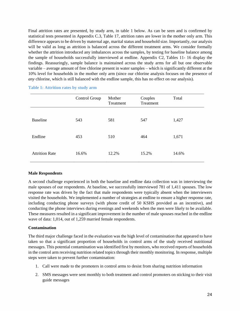
Final attrition rates are presented, by study arm, in table 1 below. As can be seen and is confirmed by
statistical tests presented in Appendix C.3, Table 17, attrition rates are lower in the mother only arm. This
difference appears to be driven by maternal age, marital status and household size. Importantly, our analysis
will be valid as long as attrition is balanced across the different treatment arms. We consider formally
whether the attrition introduced any imbalances across the samples, by testing for baseline balance among
the sample of households successfully interviewed at endline. Appendix C2, Tables 11- 16 display the
findings. Reassuringly, sample balance is maintained across the study arms for all but one observable
variable – average amount of free chlorine present in water samples – which is significantly different at the
10% level for households in the mother only arm (since our chlorine analysis focuses on the presence of
any chlorine, which is still balanced with the endline sample, this has no effect on our analysis).
Table 1: Attrition rates by study arm
Control Group Mother
Treatment Couples
Treatment Total
Baseline 543 581 547 1,427
Endline 453 510 464 1,671
Attrition Rate 16.6% 12.2% 15.2% 14.6%
Male Respondents
A second challenge experienced in both the baseline and endline data collection was in interviewing the
male spouses of our respondents. At baseline, we successfully interviewed 781 of 1,411 spouses. The low
response rate was driven by the fact that male respondents were typically absent when the interviewers
visited the households. We implemented a number of strategies at endline to ensure a higher response rate,
including conducting phone surveys (with phone credit of 50 KSHS provided as an incentive), and
conducting the phone interviews during evenings and weekends when the men were likely to be available.
These measures resulted in a significant improvement in the number of male spouses reached in the endline
wave of data: 1,014, out of 1,259 married female respondents.
Contamination
The third major challenge faced in the evaluation was the high level of contamination that appeared to have
taken so that a significant proportion of households in control arms of the study received nutritional
messages. This potential contamination was identified first by monitors, who received reports of households
in the control arm receiving nutrition related topics through their monthly monitoring. In response, multiple
steps were taken to prevent further contamination:
1. Call were made to the promoters in control arms to desist from sharing nutrition information
2. SMS messages were sent monthly to both treatment and control promoters on sticking to their visit
guide messages
25
3. The NEEP field officers, who were responsible for delivering chlorine to and training NEEP
promoters, were instructed to re-emphasize the messages above during field visits
Despite these measures, results from the intervention delivery module administered in the endline
household survey are suggestive of significant contamination across study arms. For instance, results from
a question in which respondents were asked whether they had discussed any nutritional messages with their
promoter show approximately 47% of respondents in the control arm claiming that they had discussed
nutrition with their promoters, only slightly less than the corresponding figure of 55% of respondents in
treatment arms.
A similar conclusion emerges when analyzing responses to a question (shown in Table 2) in which
respondents listed, without prompts, the specific nutritional messages they had discussed with their
promoters. The results indicate that control households received a similar number of nutrition messages as
treated households.
Answers to a question of whether the respondent ever received a poster carrying key nutritional messages
from their promoter, and whether they still had the poster at the time of the endline interview (which would
be verified by the interviewer), suggest that just over 50% of households in treatment arms received the
poster, and just below 50% still had the poster at the time of the endline interview. For control households,
the corresponding figures are 8.6% and 7%. This means that, in regards to the one physical object that was
delivered as part of NEEP, contamination was apparently fairly minimal, which potentially suggests that
the contamination was not a result of failings in the administration of NEEP.
One possibility is that interactions between promoters across different study arms led to the transmission
of the nutritional component of NEEP to control promoters, who in turn felt that they should be including
this information in their household visits too. Some descriptive statistics from the promoter survey provide
support for this hypothesis: 36% of all promoters interviewed at endline reported interacting with other
promoters at different water points in the 3 months prior to the interview (41% of control promoters); of
these promoters 81% (76% in control arms) reported discussing issues related to the programme specific
nutrition messages, in these interactions. Furthermore, the promoter survey also provided evidence of
promoters exhibiting pro-social behaviours. In the month prior to the interview: over 60% reported
participating in at least one community meeting; 68% reported being asked for advice by someone other
than a relative; and 38% reported working with others in their village to do something for the community
(for an average of 3.5 days) , without being paid. The relative lack of geographical dispersion of study
clusters (any given study-water point had on average 7 other water points within a 2km radius of itself; any
given control-arm water point had on average 5 treatment water points within a 2km radius of itself),
combined with the presence of these pro-social behaviours perhaps suggests that more care in the design
stage of the evaluation would have helped to ensure that such interactions wouldn’t have had such an effect
on the validity of the control group.
Another possibility is that the relative proximity of clusters in the study, and the apparently regularity with
which inter-village interaction took place (over half of our sample reported either visiting or being visited
by neighbouring villagers on a weekly basis), meant that these messages were spread throughout the study
area simply through word of mouth; by propagating in this way, these messages could potentially have
raised the salience of proper nutritional practices throughout the entire study area. It may also be the case
that both of these potential mechanisms worked simultaneously to drive spillovers between study clusters.

26
Table 2: Number of NEEP nutritional messages that respondent recalls discussing
Study Arm
No. of nutrition topics resp.
recalls discussing % Couples
(n = 452) Mothers
(n = 497) Control
(n = 441) Total
(n = 1390)
0 42.90 46.70 53.50 47.60
1-5 47.7 47.5 38 44.6
> 5 9.40 5.80 8.50 7.80
Total 100.00 100.00 100.00 100.00
3.4 Analytic methods
Statistical Methodology
The primary methodology used for determining whether NEEP had a significant impact on the outcomes
of interest is analysis of covariance (ANCOVA). In simple terms, ANCOVA evaluates whether the
population mean of a dependent variable of interest (for instance height-for-age z-score) is equal across
levels of a categorical independent variable (in our case, study arm), while controlling for other covariates
that are not of primary interest. This involves estimating regressions of the following form:
𝑌𝑖𝑘 = 𝛼 + 𝛽1𝑚𝑜𝑛𝑙𝑦𝑘 + 𝛽2𝑚𝑜𝑛𝑙𝑦𝑐𝑜𝑙𝑘 + 𝛽3𝑚𝑎𝑛𝑑𝑓𝑘 + 𝛽4𝑚𝑎𝑛𝑑𝑓𝑐𝑜𝑙𝑘 + 𝛾𝑌𝑖𝑘0 + 𝛿𝑋𝑖𝑘 + 휀𝑖𝑘
Here 𝑌𝑖𝑘 denotes the outcome of interest for individual i in cluster k. 𝑚𝑜𝑛𝑙𝑦𝑘, 𝑚𝑜𝑛𝑙𝑦𝑐𝑜𝑙𝑘, 𝑚𝑎𝑛𝑑𝑓𝑘, and
𝑚𝑎𝑛𝑑𝑓𝑐𝑜𝑙𝑘 are indicator variables that take a value of 1 if the individual’s cluster was assigned to mother-
only, black and white poster; mother-only colour poster; couples-visit black and white poster; or couples-
visit colour poster treatment respectively. 𝑌𝑖𝑘0 denotes the baseline value of the outcome variable; although
it is not necessary to control for this given the randomised nature of assignment to treatment (and the
relatively good balance of our baseline sample), we still do so where the data are available as this should
increase the precision of our estimates. 𝑋𝑖𝑘 is a vector of covariates, the inclusion of which reduces the
amount of unexplained within-group variance, and also controls for cases where covariates may not have
been totally balanced across study arms, which again should improve precision and statistical power of our
estimates. ANCOVA has been shown to perform as well as, or out-perform difference-in-differences
analysis (McKenzie, 2012).
Accounting for Contamination
As we describe in the preceding subsection, the primary challenge to our analysis is the level of
contamination, as evidenced by the reports from control households that they discussed nutritional topics
with their promoters. This forced us to consider treatment not only in a discrete way (i.e. did the household
belong to a treatment arm or a control arm), but also continuous (in the sense of: what level of treatment
might the household have received as a result of messages spreading throughout the study area).
To investigate this, we initially looked simply at how the number of treatment water points within a 1 or
2km radius of a household’s own water point affected outcomes. This provided some suggestive evidence
that those households which were surrounded by many treatment-arm water point (and thus were potentially
more likely to experience potential informational spillovers) did indeed show improved anthropometric
results at endline (results in Appendix E).

27
Following this, as a more nuanced measure of these potential spillover/network effects, we used the GPS
coordinates of study water points to devise a measure of “indirect treatment”, to act as a measure of the
level of inadvertent treatment that households may have received due to the propagation of messages due
to inter-water point promoter and/or participant interaction. This measure is based on the network theory
concept of Bonacich centrality (Bonacich, 1987), whereby the “centrality” (which measures the importance
of a vertex within a graph, a practical example of which could be the most influential person in a social
network) of a member of a network is a function of how many other members it is connected with (the
member’s ”neighbours”), and in turn the centrality of these neighbours (which in turn depends on the
centrality of their neighbours, which depends on the centrality of their neighbours, and so on and so forth);
as well as a parameter which weights the importance of a member’s more distant connections (i.e. the
centrality of one’s neighbours’ neighbours, and their neighbours, and so on and so forth).
Using the GPS coordinates of study water points, we were able to back out a measure of “total effective
treatment”, which for any given water point was a function of their actual treatment (i.e. whether they were
officially assigned to a treatment arm as part of NEEP); as well as their “indirect treatment”, the calculation
of which was based on the Bonacich centrality measure described above (but with extra weight given to
connections with treatment-arm clusters, to reflect that these clusters would have been the primary
propagators in the flow of information). This measure of indirect treatment was then included in the core
regressions to act as a control for any potential unintended treatment effects that may have spilled-over to
a given cluster.
In calculating this measure of “total effective treatment” we had to make a decision as to when to consider
two water points as being directly linked (in our case, if two water points are directly linked then
information can move between these water points without having to go through one or more intermediate
water points on the way). Our decision was informed by a question in the promoter survey which asked
promoters for the names and villages of other promoters that they had chatted to in the previous 3 months.
Using the GPS data, we found that promoters typically interact with other promoters whose water points
lie between 0 and 2km from their own. Thus, to show how sensitive our results are to the choice of this
threshold, our specifications in the results sections are presented with two separate direct-connections cut-
offs: one at 1km, and one at 2km.
In recognition of the potentially significant impacts that these indirect effects could have had on our
outcome variables, we will report “total treatment effects” (TTEs) for each of our main results in the
analysis. Three different TTEs will be reported: an average total treatment effect, a total treatment effect at
the 75th percentile of indirect treatment, and a total treatment effect at the 25th percentile of indirect
treatment. These TTEs will be calculated as the sum of the direct effect of treatment and the estimated total
indirect treatment effect, estimated at the relevant level (i.e. the mean, the 75th percentile or the 25th
percentile). These levels of indirect treatment will be calculated under the assumption of total coverage of
the programme (i.e. levels of indirect treatment that each household would have received had every
household been treated), which is simply the unscaled Bonacich centrality measure for each household,
minus 1 (the one representing direct treatment). Thus, what we report is a comparison of the expected
outcome for an individual with a given level of centrality, if the programme was implemented with full
coverage, and the counterfactual of no implementation whatsoever.
28
3.5 Limitations
The key limitation of our programme design lay in the lack of a distinct buffer zone between study clusters;
in the context of our trial there was no clear information on the level of inter-water point/-village interaction,
or on the kind of distances between which these interactions may take place. Hence there was no obvious
way to define what the buffer zone should be. Anecdotal evidence suggested that most social network
effects took place within the boundaries of the water point catchment area, and our prior was that inter-
village interaction would be minimal due to the high cost of transport within the study area, thus the focus
was on ensuring that water points within the same village received the same treatment (as described under
logic & assumptions in the previous section, there were 3 major violations of this). The difficulties in terms
of collecting data over a more dispersed geographical area meant that our ex ante belief was that the cost
of increasing the buffer zone beyond this were unlikely to outweigh the benefits. Ex post, it seems as though
the buffer zone was insufficient to ensure a clear distinction between treated and control households, as
described in the challenges subsection.
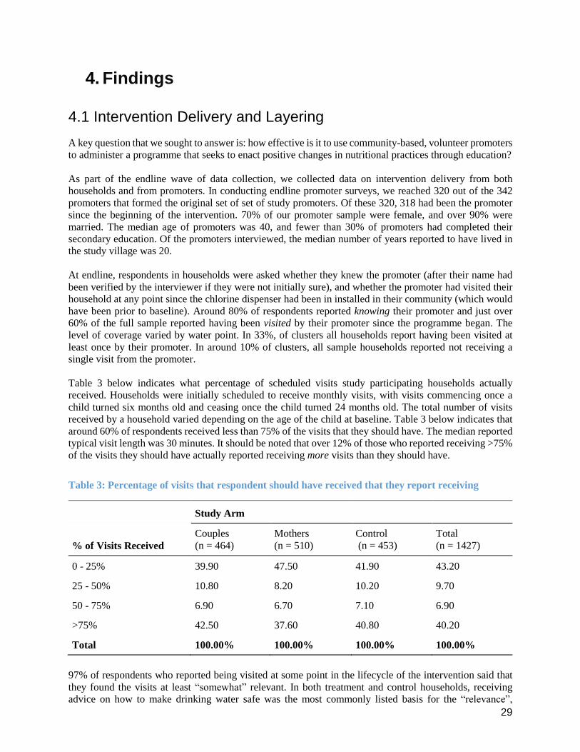
29
4. Findings
4.1 Intervention Delivery and Layering
A key question that we sought to answer is: how effective is it to use community-based, volunteer promoters
to administer a programme that seeks to enact positive changes in nutritional practices through education?
As part of the endline wave of data collection, we collected data on intervention delivery from both
households and from promoters. In conducting endline promoter surveys, we reached 320 out of the 342
promoters that formed the original set of set of study promoters. Of these 320, 318 had been the promoter
since the beginning of the intervention. 70% of our promoter sample were female, and over 90% were
married. The median age of promoters was 40, and fewer than 30% of promoters had completed their
secondary education. Of the promoters interviewed, the median number of years reported to have lived in
the study village was 20.
At endline, respondents in households were asked whether they knew the promoter (after their name had
been verified by the interviewer if they were not initially sure), and whether the promoter had visited their
household at any point since the chlorine dispenser had been in installed in their community (which would
have been prior to baseline). Around 80% of respondents reported knowing their promoter and just over
60% of the full sample reported having been visited by their promoter since the programme began. The
level of coverage varied by water point. In 33%, of clusters all households report having been visited at
least once by their promoter. In around 10% of clusters, all sample households reported not receiving a
single visit from the promoter.
Table 3 below indicates what percentage of scheduled visits study participating households actually
received. Households were initially scheduled to receive monthly visits, with visits commencing once a
child turned six months old and ceasing once the child turned 24 months old. The total number of visits
received by a household varied depending on the age of the child at baseline. Table 3 below indicates that
around 60% of respondents received less than 75% of the visits that they should have. The median reported
typical visit length was 30 minutes. It should be noted that over 12% of those who reported receiving >75%
of the visits they should have actually reported receiving more visits than they should have.
Table 3: Percentage of visits that respondent should have received that they report receiving
Study Arm
% of Visits Received Couples
(n = 464) Mothers
(n = 510) Control
(n = 453) Total
(n = 1427)
0 - 25% 39.90 47.50 41.90 43.20
25 - 50% 10.80 8.20 10.20 9.70
50 - 75% 6.90 6.70 7.10 6.90
>75% 42.50 37.60 40.80 40.20
Total 100.00% 100.00% 100.00% 100.00%
97% of respondents who reported being visited at some point in the lifecycle of the intervention said that
they found the visits at least “somewhat” relevant. In both treatment and control households, receiving
advice on how to make drinking water safe was the most commonly listed basis for the “relevance”,
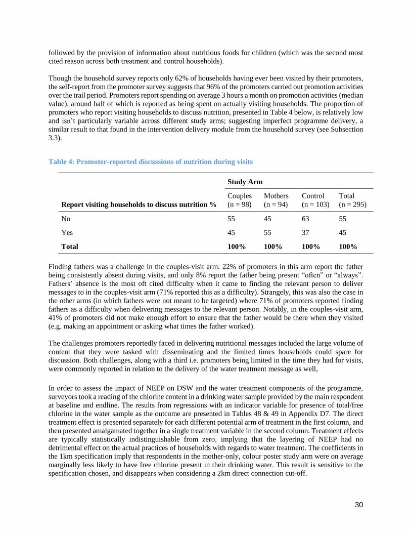
30
followed by the provision of information about nutritious foods for children (which was the second most
cited reason across both treatment and control households).
Though the household survey reports only 62% of households having ever been visited by their promoters,
the self-report from the promoter survey suggests that 96% of the promoters carried out promotion activities
over the trail period. Promoters report spending on average 3 hours a month on promotion activities (median
value), around half of which is reported as being spent on actually visiting households. The proportion of
promoters who report visiting households to discuss nutrition, presented in Table 4 below, is relatively low
and isn’t particularly variable across different study arms; suggesting imperfect programme delivery, a
similar result to that found in the intervention delivery module from the household survey (see Subsection
3.3).
Table 4: Promoter-reported discussions of nutrition during visits
Study Arm
Report visiting households to discuss nutrition % Couples
(n = 98) Mothers
(n = 94) Control
(n = 103) Total
(n = 295)
No 55 45 63 55
Yes 45 55 37 45
Total 100% 100% 100% 100%
Finding fathers was a challenge in the couples-visit arm: 22% of promoters in this arm report the father
being consistently absent during visits, and only 8% report the father being present “often” or “always”.
Fathers’ absence is the most oft cited difficulty when it came to finding the relevant person to deliver
messages to in the couples-visit arm (71% reported this as a difficulty). Strangely, this was also the case in
the other arms (in which fathers were not meant to be targeted) where 71% of promoters reported finding
fathers as a difficulty when delivering messages to the relevant person. Notably, in the couples-visit arm,
41% of promoters did not make enough effort to ensure that the father would be there when they visited
(e.g. making an appointment or asking what times the father worked).
The challenges promoters reportedly faced in delivering nutritional messages included the large volume of
content that they were tasked with disseminating and the limited times households could spare for
discussion. Both challenges, along with a third i.e. promoters being limited in the time they had for visits,
were commonly reported in relation to the delivery of the water treatment message as well,
In order to assess the impact of NEEP on DSW and the water treatment components of the programme,
surveyors took a reading of the chlorine content in a drinking water sample provided by the main respondent
at baseline and endline. The results from regressions with an indicator variable for presence of total/free
chlorine in the water sample as the outcome are presented in Tables 48 & 49 in Appendix D7. The direct
treatment effect is presented separately for each different potential arm of treatment in the first column, and
then presented amalgamated together in a single treatment variable in the second column. Treatment effects
are typically statistically indistinguishable from zero, implying that the layering of NEEP had no
detrimental effect on the actual practices of households with regards to water treatment. The coefficients in
the 1km specification imply that respondents in the mother-only, colour poster study arm were on average
marginally less likely to have free chlorine present in their drinking water. This result is sensitive to the
specification chosen, and disappears when considering a 2km direct connection cut-off.

31
4.2 Participant Outcomes, Main Results:
Primary Outcomes: Anthropometrics
Columns 1 and 2 in Tables 18 & 19 in Appendix D1 present the results for the regression containing height-
for-age z-score, the first table with the indirect treatment evaluated with a 1km direct-connection cut-off,
and for comparison the second table with a 2km cut-off. Throughout all specifications the coefficients on
direct treatment effects, whether split by treatment arm or combined into a single variable, imply no
statistically significant impact of NEEP on height-for-age. Looking at implied total (direct + indirect)
treatment effects, the specification with a 1km cut-off implies a positive total average treatment effect on
height-for-age z-score of just under 0.2 standard deviations. The total treatment effect at the 75th percentile
of indirect treatment effects (i.e. for households that are located around a very central water point) increases
in size to approximately 0.23 standard deviations. When looking at the results from the specification with
the 2km cut-off, implied total treatment effects increase in size across all levels of indirect treatment, but
the precision of these estimates drops off dramatically, meaning they are still indistinguishable from 0 with
any reasonable level of confidence.
Columns 3 and 4 in Tables 18 & 19 present the results of the regression containing a summary index
(Anderson, 2008) of the other z-scores that were created: weight-for-age, weight-for-height, bmi-for-age,
arm circumference-for-age and head circumference-for-age. Once again, we see no significant direct
treatment effects in any direction, in either specification. Total treatment effects in the summary index
regression are typically positive and significant across specifications, although this is driven entirely by
indirect effects.
Presence of bipedal oedema in our sample was so low - 13 children, or 0.78% of our sample at baseline;
and 29 children, 2.08% of our sample (of those children who were check for bipedal oedema) at endline –
that it was decided that it would not be possible to come to any meaningful conclusion on the effect of
NEEP on bipedal oedema, thus the impact of NEEP will not be evaluated on this dimension of child health.
Further analyses of the anthropometric results are contained within Appendix E.
Secondary Outcomes: Nutritional Knowledge & Food Intake
Tables 20 and 21 in Appendix D2 show the results obtained from the regressions looking at the results of
the nutrition and feeding quiz that was administered to the main female caregivers. In the first two columns
of each table the outcome variable is the proportion of questions that the respondent answered correctly,
and in the second two columns the outcome variable is the latent knowledge parameter that is outputted
from the IRT process mentioned previously.
The regression results imply no significant total treatment effects in either metric; there are significant direct
treatment effects in the couples visit, colour poster study arm – implying an increase in proportion correct
of around 2.5 percentage points, or an increase of 0.18-0.19 standard deviations in latent nutritional
knowledge – but these effects are entirely limited to this single arm. The median number of questions
correctly answered in our sample (15), did not change between baseline and endline.
In Tables 22 & 23 are the results from equivalent regressions run using the promoter data (although without
baseline controls, as no promoter data were collected at baseline); they show no effect whatsoever of
treatment on promoter knowledge. It should be noted that the median number of questions correctly
answered by promoters (16) is very similar to the equivalent figure for female primary caregivers.
Tables 24-29 in Appendix D3 present the results pertaining to the index child from the 7-day food frequency
section of the survey; the dependent variables represent the sum of days on which the index child was
reported as having consumed a food from that category in the 7 day period prior to the interview (e.g. if
32
they had consumed poultry on 3 days and omena on 2 days then the variable “meat” would take the value
5). The coefficients on the indicator variable for direct treatment indicate small, positive (but typically
statistically insignificant) increases in nutritional intake for the index child in three key, protein-rich groups
of food which were targeted by the intervention: meat, nuts and eggs. The coefficients for those study arms
where the more salient poster was dispensed are typically the most positive, which suggests that the regular
prompt provided by the poster may be driving this. Indirect effects and total treatment effects are typically
insignificant, although for groundnuts both are positive and highly significant in the specification with
network measures evaluated with a 2km cut-off; the sensitivity of this result to the choice of threshold for
direct connections casts doubt on its validity however.
There appear to also be some small (but again insignificant) direct effects of the programme on the
consumption of vitamin-A rich foods, and fruit. The results suggest a negative impact of the programme on
intake of green leafy vegetables (particularly in the mother only visit arm), but there do not appear to be
any clear patterns in other foods groups suggesting further modifications in behaviour.
Also in Appendix D3, Tables 30 & 31 show the results from regressions on whether the index child received
the minimum recommended number of meals in the 24 hour period preceding the interview. The
coefficients on the direct treatment effects are consistently positive, typically indicating a 2-3 percentage
point impact of direct treatment on the average likelihood of an index child meeting their 24-hour minimum
food frequency requirements; however they are statistically insignificant in all but one case. Implied indirect
effects are negative and insignificant in the 1km cut-off specification, and positive, small and insignificant
in the 2km specification.
Appendix D4i contains the results from the household food consumption questionnaire, with foods
categorised into relevant groups and total consumption expenditure on foods in these groups, in the 7 day
period prior to the interview, acting as the dependent variable.
The results of the expenditure regressions tell no consistent story as to whether NEEP had any impact by
this metric. Hence, as an alternative mode of analysis which should help to eliminate a certain amount of
measurement error coming from the potential for inaccurately reported or imputed prices, Appendix D4ii
presents results from regressions on quantities of some specific foods. When looking only at quantities, we
see small, consistently positive direct treatment effects of NEEP on household consumption of meat (in kg),
with these effects significant at the 10% level in the couples visit, colour poster study arm, and also in
column 2 when we consider all 4 separate treatment arms amalgamated into a single treatment variable.
The regressions for groundnuts imply no significant direct treatment effect of NEEP on household
consumption of groundnuts, but the indirect treatment effect is positive in both the 1km cut-off and 2km
cut-off specifications – and is quite large and significant in the 2km specification – which drives the positive
and significant total treatment effects which are visible in the specification with the 2km direct-connection
cut-off. The omena regression implies no significant impacts of NEEP on household consumption of this
food. For eggs (measured in pieces), we see negative, significant implied direct treatment effects in the
black and white poster arms, but these don’t translate into negative total treatment effects. Household
consumption of green leafy vegetables also appears to be unaffected by the programme. There is a small,
positive and significant direct treatment effect for the mother only, colour poster arms in the tomato
regression, but in the 2km specification this coefficient becomes insignificant and indirect effects are
sufficiently negative that they imply negative and significant total treatment effects. This does however
corroborate with the negative and significant total treatment effects that can be seen in the expenditure
regressions for fruit.
Tables 40 and 43 present the results for household consumption (in quantities) of maize flour, plain milk
and bananas, and the 1km and 2km cut-off respectively. Baseline controls are not included for these foods
because data were missing at baseline for them. Consistent with the results for starches when looking at
household expenditures, we see negative direct impacts of NEEP on consumption of maize flour, with these

33
impacts significant throughout the mother only treatment arms. House consumption of plain milk and
bananas appear to exhibit no significant adjustment according to the treatment received.
Non-food consumption & breastfeeding
Appendix D5 presents the results from the regressions containing household aggregate weekly non-food
consumption expenditure as the dependent variable. The coefficients on the direct treatment indicators
imply a quite large, negative direct treatment effect in the black and white poster arms; this effect is
significant at the 5% level in the couples visit arm. Indirect treatment effects are negative, quite large, but
insignificant in the specification with the 1km cut-off; and positive and insignificant in the specification
with the 2km cut-off.
At endline, a total of 1,080 of children in our sample were reported as having stopped breastfeeding. Thus,
tables 46 & 47 present the results of the regression where the outcome variable is the month at which these
children were reported as having stopped breastfeeding, where the data were available. These results show
no treatment effects – direct, indirect or total - of NEEP on this measure in the specification with a 1km
cut-off. There are some negative, significant total treatment effects in the 2km specification, but the
sensitivity of this result to the definition of the adjacency matrix reduces the strength of any conclusions
that may be drawn from this.
In all three of the main study arms – couples visit, mother visit, and control – the median age at which
breastfeeding stopped was 20 months, well above the WHO recommended minimum of 6 months. And for
those children who had stopped breastfeeding at baseline (n = 82) the median age in months at which they
were reported as having stopped was 12 months.
Other Outcomes of Interest
Tables 54 & 55 report the results from regressions of time spent cooking, and those for hours spent feeding
children, in the previous working day, for the 1km cut-off and 2km cut-off respectively. The 1km
specification implies no significant effects of NEEP on either of these measures. In the 2km specification
implied total treatment effects are negative and significant at 10% level, but this is driven entirely by the
indirect effect and the sensitivity of this result to the cut-off used means that the validity of this result may
be questionable.
The results from the regressions on indicator variables for the extensive margin labour supply (working or
not working) of primary female caregivers and spouses are contained within Appendix D8. The first two
columns in each specification look at the likelihood of the individual in question working, and the second
two columns look at the likelihood of the individual having a second job.
The results for the primary female caregivers typically imply no or even negative impact of NEEP on female
labour supply, particularly in the mother only, colour poster study arm for which the coefficient in both
specifications implies a significant, negative impact on the probability of working, and on the probability
of having a second job. The results for spousal labour supply are broadly similar, and suggest no impact of
NEEP on labour supply at the extensive margin (except, perhaps, in the mother only, colour poster treatment
arm, where like in the female case direct treatment effects are negative and significant, although this time
only in the 1km specification).
Probability of having a chat with a friend or acquaintance about food or nutrition
Tables 56 - 59 present that results for the regressions looking at self-reported chats about nutrition in the 3
days prior to the interviews; the outcome variable in columns 1 and 2 is an indicator for the respondent
reporting having a chat with family, and columns 3 and 4 for a chat with friends, about nutrition.

34
Table 56, which contains results for the specification with the 1km cut-off, implies no treatment effects of
NEEP on the probability of having a chat with a family member. In terms of chats with friends: in the
regression with separated treatment arms, implied direct treatment effects are consistently positive but
statistically indistinguishable from 0. When the treatment arms are amalgamated into a single treatment
arm, we do see a small but statistically significant direct impact of treatment on the probability of having a
chat with a friend about nutrition in the past 3 days: an increase in likelihood of about 5 percentage points,
significant at the 10% level. Accounting for both direct and indirect treatment effects, we see a significant
total treatment effect at the 25th percentile of indirect treatment; despite larger estimated effects at higher
levels of indirect treatment these effects are too imprecisely estimated to be statistically distinguishable
from 0.
In the 2km specification, indirect treatment effects increase considerably, which leads to positive and
significant treatment effects in the chats-with-family regression. These implied treatment effects are
strikingly large, and the sensitivity of this result to the direct connection cut-off used casts doubt on the
accuracy of these magnitudes. In terms of respondents’ chat with spouses, the regressions in tables 58 and
59 imply no significant impact of NEEP along this metric.
Probability of child suffering from diarrhea
To test for the impact of NEEP on the probability of the index child in the study suffering diarrhoea, tables
60 & 61 contain the regression results with outcome variable an indicator for whether the index child is
reported as having suffered from diarrhoea in the 7-day period prior to the interview.
For the specification with the 1km direct connection cut-off, direct treatment effects when treatment is
separated by arm are statistically insignificant. When looking at treatment as a single arm, the implied direct
treatment effect is positive (which suggests that NEEP lead to an increase in the probability that the index
child suffered from diarrhoea), but is very small and statistically insignificant. Indirect treatment effects are
negative and somewhat larger, but still indistinguishable from 0 at any reasonable level of confidence.
Reported total implied treatment effects are also negative, but again the null hypothesis of no total treatment
effect cannot be rejected using this specification. In table 61, with the 2km cut-off, direct treatment effects
are again entirely indistinguishable from 0 under both specifications. Indirect treatment effects grow in
magnitude compared to the specifications with a 1km cut-off, and become significant at the 5% level.
Implied total treatment effects are very large (the average total treatment effect implies an average reduction
in the likelihood of contracting diarrhoea of over 30 percentage points) and statistically significant.
Appendix D12 contains the results from regressions looking for programme impact in terms of hygiene
practices of study households; there are however no implied impacts of NEEP along this dimension.

35
5. Conclusions
5.1 Achievements
Our evaluation of NEEP shed light on the feasibility of using existing supply infrastructures such as those
available in the DSW programme to deliver nutritional information at low marginal cost. In particular, we
find no evidence indicating that NEEP undermined the practices encouraged within the DSW programme.
Promoters delivered the water treatment messages, along with the new nutritional messages and we found
no differences in household practices related to water treatment. However, further research is needed to
investigate how different types of programmes can be layered atop one another and what the best way to
operationalize this would be, given the varying needs that different interventions would have.
Our evaluation also investigated the difference in impact of providing information to a female caregivers
versus both parents. Unfortunately, the significant level of contamination experienced made it challenging
to answer these questions. However, preliminary findings applying a novel methodology developed to
account for this kind of contamination has revealed some interesting patterns. In particular, they point to
important indirect effects generated by the programme, which warrant further investigation in future work.
5.2 Results
The results on intervention delivery present a mixed picture on the success of NEEP in reaching the targeted
groups. In some respects, NEEP appears to perform well. Achieving a 60% home visitation rate is
significant for a programme making use of un-paid volunteers. Similarly, the fact that over 40% of
household reporting receiving at least 75% of their scheduled visits, with the median reported typical visit
time being 30 minutes, indicates that the promoters tried to follow the visit schedule and that the duration
was in line with programme design. The absence of any significant detrimental effect on DSW (e.g. the
tasks that promoters most often reported performing all pertained to water treatment, and the fact that
chlorine uptake appeared generally unaffected) can also be considered a success too.
In terms of the key outcome of interest, child height-for-age, the results imply that NEEP had a mild positive
impact, once the indirect effects resulting from the propagation of the nutritional messages across the study
area are accounted for. The total treatment effects are positive and quite large throughout all specifications
(see tables provided in Appendix D). A before-after analysis using DHS data provides further evidence
supporting this conclusion. We also find large, positive and statistically significant total treatment effects
in an index of other anthropometric outcomes (weight-for-age, BMI-for-age, weight-for-height, arm
circumference-for-age and head circumference-for-age), which provides further evidence suggestive of the
success of NEEP in improving child health outcomes.
There were no significant direct treatment effects in anthropometrics, even after controlling for the
estimated indirect treatment effect resulting from contamination. However, given that we do not have a
clear comparison group to compare to the treatment arms, it is hard to say whether this is due to NEEP
being ineffective or the difficulties in precisely controlling for contamination. The descriptive evidence of
interaction between promoters and trial participants across water points, combined with the finding that
NEEP increased the likelihood of participants discussing nutrition among their friends suggests that NEEP
may have raised the salience of nutrition issues in the study area.
Our analysis includes overall network centrality, which should soak up any spurious correlation emerging
for the spatial position of the water point in the study area. Thus, the centrality measure will capture effects
on our outcomes that are driven by, for example, the water point being positioned next to a road or market.
Thus, we can be relatively confident that NEEP is a key driver of the estimated indirect treatment effects.
36
Our findings on other outcomes, however, do not provide a clear picture on the mechanisms through which
the effects on anthropometrics were achieved. Although we found a consistently positive and significant
direct impact of NEEP on both the proportion of correct answers in the nutritional quiz, and on latent
nutritional knowledge measured using Item Response Theory, this impact was limited to a single treatment
arm in the study. And this translated to no significant total treatment effects overall. This could be a result
of the nutritional quiz not performing as well as expected in discerning respondents’ knowledge along
dimensions NEEP sought to influence. For instance, on review the authors identified some questions with
potentially ambiguous answers and others which were worded poorly (e.g. “Children should be given
chopped foods when they are 12 months old”, which was supposed to ask whether children can be given
adult foods when they are 12 months old), and others which didn’t appear to correspond to any of the
content in the intervention materials (e.g. “Some parts of a chicken should not be given to children”). A
second possibility is that the length of time taken to administer the female survey (the median survey took
over two hours to complete) led to inattention and lackadaisical answering on the part of the respondent.
Indeed, one possible explanation for our failure to find positive correlations between answers to the same
question at baseline and endline suggests that respondents might have been guessing the correct answer.
Some evidence for the first of these hypotheses is provided by the “item characteristics curves” (ICCs)
which are outputted from the IRT procedure. Item characteristic curves plot the relationship between
estimated latent knowledge and the probability of answering an item correctly, hence they are expected to
slope upwards if a question is a good metric for knowledge – there should be a higher probability that more
knowledgeable people answer a question correctly. Figures 4 & 5 in Appendix F present the item
characteristic curves for one of the questions identified as being ambiguous in its answer (“Children should
be given chopped foods when they are 12 months old”). We see that in the treated sample, at both baseline
and endline, the estimated ICC in fact has a slight downward slope, indicating that people who typically
performed better overall in the quiz in fact did a worse job at answering this question. There were several
other questions which exhibit either very flat or downward sloping ICCs, which suggests that the quiz we
used was a poor metric by which to judge nutritional knowledge.
We also find limited evidence of an improvement in child nutritional practices as a result of NEEP. In
particular, there appear to have been small improvements in consumption of nuts, eggs, dairy and vitamin-
A rich foods by the index child, but some of these results are statistically insignificant or sensitive to the
specification chosen. Further (although again limited) evidence supporting child nutritional intake as a
channel through which change may have taken place comes from the small apparent improvement in child
feed frequency shown by the results in Tables 30/31. We also find small increases in the quantities of nuts
and meats at the household level.
One possible explanation for why we detected significant effects in anthropometric results and not in those
pertaining to nutritional and food intake is that anthropometric measurements are likely to contain
considerably less measurement error – surveyors were provided were provided with the recommend
equipment and training, took multiple measurements, and were measuring something physical and not
prone to misreporting – than reported quantities such as consumption expenditures, or feeding frequency.
Given the difficulties in attaining our desired sample size, the statistical power that we have may be
insufficient to accurately determine changes in reported quantities such as these, but still detect changes in
anthropometric outcomes, which were more accurately measured and thus less prone to attenuation bias.
Another possible explanation is that practices did adjust in response to treatment, but that these adjustments
did not persist on the completion of the home visit schedule (around 50% of our sample were at least 30
months old at endline, and thus would not have received a visit for at least 6 months prior to the interview);
the time period over which behaviours did change may have been sufficient to drive the changes we see in
anthropometrics though.
Our evidence that NEEP increased chats about nutrition among family and friends, particularly in water
points which were more highly connected to treated water points. This lends credence to the idea that

37
salience of nutritional issues increased as a result of NEEP and this is a potentially important avenue through
which NEEP may have influenced and changed behaviours.
Other mechanisms that were originally posited as potential dimensions along which behaviour might
change were labour supply (which may increase for some family members to facilitate increased quality or
quantity of food purchases), time spent cooking (in order to implement the food preparation and storage
advice that formed a part of the information that NEEP disseminated), and household non-food
consumption (which may have decreased if households substituted non-food consumption for improved
food consumption as a result of their learning the potential benefits to doing so). None of these expected
changes were apparent in the results for these measures. The age at which the index child stopped
breastfeeding also appears to be unchanged by the trial, but the fact that most primary caregivers appear to
have already been following best practices here perhaps make this results not so surprising.
5.3 Strengths and Weaknesses
The first strength of the intervention is that it successfully contributed evidence towards the feasibility of
utilising the existing infrastructure of the DSW programme to administer new programmes simultaneously.
Whether this “layering” of programmes is successful is a question of the ability of both promoters and
recipients to absorb and act upon multiple streams of information. In order to answer this question we
collected data from both parties on how the various components of the intervention were delivered, and the
outcomes in terms of nutritional knowledge and chlorine uptake.
Another strength of NEEP comes from the extensive data that we collected in both survey waves. By
interviewing mothers, father, and promoters we were able to gain an extensive insight into the
characteristics and behaviours of all parties involved in the trial. A rich set of markers pertaining to
anthropometric outcomes, knowledge of nutritional issues, child nutritional intake, household consumption,
and water and hygiene practices allow for a detailed analysis of nutritional and health behaviours in our
sample. The data on promoter characteristics and intervention delivery will also prove valuable to Evidence
Action by giving them a more detailed picture of their promoters, the activities they perform, the social
interactions among them and their receptiveness to performing tasks outside of DSW.
The primary weakness of the intervention was the absence of a sufficiently large buffer zone to ensure that
there was a clear distinction between the treatment that treatment-arm and control-arm households received.
This was a result of a lack of information in the planning stage in both the extent of inter-village interactions,
and also in the lack of sufficiently detailed maps to allow for the inclusion of sufficiently large buffer zones
between study clusters. As a result, there was a significant level of contamination that took place across
study arms, as evidenced in reports in the monthly monitoring of discussions pertaining to nutritional
message taking place between promoters and participants in control arms, and in the distinct lack of
difference in the reported topics that respondents discussed with their promoters across treatment and
control arms at endline. These spillovers are likely to have come from two sources: interactions between
promoters from different study water points, and interactions within trial participants’ own social networks.
As a result of the contamination, it was very hard to distinguish between treatment-arm and control-arm
households in term of the actual level of treatment they received, and hence to it was challenging to draw
conclusions as to the effects NEEP had. In response to this challenge, we devised a measure of “effective
treatment” based on the centrality of clusters in the study-water point network in an attempt to create a
distinction between study households along this dimension. But even with these strategies we are unable to
report conclusively on the effect of NEEP.
Other weaknesses primarily related to data collection: in particular, the difficulty of reaching a sufficient
number of male respondents, and the relatively high levels of attrition at endline. The comparatively low
numbers of spouses reached (781 at baseline, 1014 at endline) was a result of males typically spending most
of their day outside of the household compound, and the difficulties that came with finding a reliable phone

38
number on which they could be reached for phone interview. The smaller, potentially selection-biased
sample of male respondent that resulted means that conclusions drawn from these data need to be interpreted
with caution. The level of attrition between the two waves of data collection (around 15%) was significantly
higher than the figure we had anticipated (around 7%), thus trying to ensure that our endline sample was
sufficiently large and balanced to facilitate a robust analysis was also a significant challenge. This attrition
further impacted statistical power to detect effects.

39
6. Lessons
The first key lesson learned from NEEP is that there is a need to better understand how interactions take
place in a setting prior to designing an evaluation. In this case, an understanding of the interactions between
promoters, as well as those between regular householders, should have been factored into evaluation design.
Developing such an understanding may, however, require further research into the structure of social
networks (e.g. in what way are families typically spread across a location), and also more extensive data
defining how village/locality boundaries are de facto defined (for instance through more extensive mapping
of areas of interest). Ensuring that this data is collected in the planning stage of future randomized controlled
trials aimed at testing informational interventions can reduce the likelihood of contamination across study
arms.
A second lesson relates to the difficulties associated with involving male family members, in the
intervention and evaluation. In evaluating NEEP, we found that the father of the child was mostly
unavailable during promoter visits, which were during the day. Most promoters reported that finding fathers
to receive messages was among the most difficult aspects of their role. This was also the case during both
evaluation survey rounds, where fathers were mostly absent during enumerator visits to the households,
leading to relatively high levels of attrition. Interventions that target the male members of the household,
should thus include specific protocols (like scheduling visits after working hours, scheduling appointments
etc.) which can effectively engage the male members. Similar processes should also be integrated in the
survey design for example phone surveys with incentive structures, which can help reduce multiple re-visits
to households and attrition in the sample.
A third lesson is that there is potential to layer additional programmes on top of DSW. The apparent absence
of detrimental impact on DSW as a result of the layering of the two programmes provides some support for
this as a method of delivering additional programmes at scale using existing infrastructure. However, the
lack of conclusive results, makes it difficult to definitively comment or provide explicit recommendations
on the process of layering. Further research is needed to identify the most sustainable and effective way to
operationalize a layered model on the DSW platform and to understand the best practices of engaging the
dispenser promoters in these additional activities.

40
7. Recommendations
Although there are some tentatively positive anthropometric results, the lack of a consistent message
presented by the results for outcomes that could be potential mechanisms for anthropometric changes casts
some doubt on the strength of any conclusions that can be drawn. However, the fact that contamination was
so pervasive means that NEEP could potentially still have been successful in enacting positive change, and
we simply lack a precise way of measuring this change. Thus, a primary recommendation is that further
investigation be pursued prior to making a decision about scaling NEEP, at least in its current form.
A second recommendation is that further care be taken in the planning stages of future informational
interventions, in order to ensure that there is sufficient understanding of geographic and social networks
which may impact on the reliability of the analysis. This may require investments in up to date mapping of
study areas to ensure that a complete and accurate picture of de facto boundaries is available when assigning
treatment, or pre-baseline surveys within study areas to facilitate an analysis of the structure of
family/friendship networks of potential study participants, to help ensure that spillovers of information are
negligible.
The data and results gained from the promoter survey may also prove a valuable tool in understanding who
the DSW promoters are and how they behave. Hence, sharing the evaluation findings with the DSW
programme team is recommended. This information may provide them with more nuanced insight into
promoters and the DSW operations in Busia county of Kenya.
Finally, given the tentatively positive results regarding the efficacy of layering different types of
complementary programmes on the DSW platform it is recommended that further research be undertaken
to investigate this avenue of service delivery, especially since different interventions will have different
needs. If feasible, layering holds tremendous prospects for improving the cost-effectiveness, and impact, of
DSW.
41
References
(n.d.). Retrieved from http://opendatakit.org/
Bhandari, N., Bahl, R., Mazumdar, S., Martines, J., Black, R. E., & Bhan, M. K. (2003). Effect of
Community-Based Promotion of Exclusive Breastfeeding on Diarrhoeal Illness and Growth: a
Cluster Randomised Controlled Trial. The Lancet, 1418 - 23.
Black, R. E., Allen, L. H., Bhutta, Z. A., Caulfield, L. E., de Onis, M., Ezzati, . . . Rivera, J. (2008). Maternal
and child undernutrition: global and regional exposures and health consequences. Lancet, 243-60.
Bordalo, P., Gennaioli, N., & Shleifer, A. (2013). Salience and Asset Prices. American Economic Review:
Papers & Proceedings, 623 - 628.
Bordalo, P., Gennaioli, N., & Shleifer, A. (2013). Salience and Consumer Choice. Journal of Political
Economy, 803 - 843.
Bourguignon, F., & Chiappori, P.-A. (1992). Collective Models of Household Behaviour: An Introduction.
European Economic Review, 355-364.
Chetty, R. (2009). The Simple Economics of Salience and Taxation. NBER Working Paper 15246.
Dewey, K. G., & Adu-Afarwuah, S. (2008). Systematic Review of the Efficacy and Effectiveness of
Complementary Feeding Interventions in Developing Countries. Maternal and Child Nutrition, 24
- 85.
Fitzsimons, E., Malde, B., Mesnard, A., & Vera-Hernandez, M. (2016). Nutrition, information and
household behavior: Experimental evidence from Malawi. Journal of Development Economics,
113-126.
Grantham-McGregor, S. G., Powell, C., Walker, S., & Himes, J. (1991). Nutritional Supplementation,
Psychosocial Stimulation, and Mental Development of Stunted Children: the Jamaican Study. The
Lancet, 1 - 5.
Haider, R., Ashworth, A., Iqbal, K., & Huttly, S. R. (2000). Effect of Community-based Peer Counsellors
on Exclusive Breastfeeding Practices in Dhaka, Bangladesh: a Randomised Controlled Trial. The
Lancet, 1643 - 47.
Haines, A., Sanders, D., Lehmann, U., Rowe, A. K., Lawn, J. E., Steve, J., . . . Bhutta, Z. (2007). Achieving
Child Survival Goals: Potential Contribution of Community Health Workers. The Lancet, 2121 -
31.
Hutton, G., Haller, L., & Bartram, J. (2007). Global cost-benefit analysis of water supply and sanitation
interventions. Journal of Water and Health, 481 - 502. Retrieved from
https://www.cdc.gov/healthywater/global/diarrhea-burden.html
Kang, Y., Kim, S., Sinamo, S., & Christian, P. (2016). Effectiveness of a community-based
nutritionprogramme to improve child growth in rural Ethiopia: a cluster randomized trial. Maternal
& Child Nutrition.

42
(2016). Kenya Reproductive, Maternal, Newborn, Child and Adolescent Health (RMNCAH) Investment
Framework. Ministry of Health, Government of Kenya.
(2011). KenyaL Situation Analysis for Transform Nutrition. Transform Nutrition
(http://www.transformnutrition.org/wp-
content/uploads/sites/3/2011/11/Kenya_situation_analysis.pdf).
Lewycka, S., Mwansambo, C., Rosato, M., Kazembe, P., Phiri, T., Mganga, A., . . . Costello, A. (2013).
Effect of women's groups and volunteer peer counselling on rate of mortality, morbidity, and health
behaviours in mothers and child in rural Malawi (MaiMwana): a factorial, cluster-randomised
controlled trial. Lancet, 1721-35.
Lewycka, S., Mwansambo, C., Rosato, M., Peter, K., Phiri, T., Mganga, A., . . . Costello, A. (2013). Effect
of Women's Groups and Volunteer Peer Counselling on Rates of Mortality, Morbidity, and Health
Behaviours in Mothers and Children in Rural Malawi (MaiMwana): a Factorial, Cluster-
Randomised Controlled Trial. The Lancet, 1721 - 35.
Ministry of Health, G. o. (2016). KENYA REPRODUCTIVE, MATERNAL, NEWBORN, CHILD AND
ADOLESCENT HEALTH (RMNCAH) INVESTMENT FRAMEWORK.
Morrow, A. L., Guerrero, M. L., Shults, J., Calva, J. J., Lutter, C., Bravo, J., . . . Butterfoss, F. D. (1999).
Efficacy of Home-based Peer Counselling to Promote Exclusive Breastfeeding: a Randomised
Controlled Trial. The Lancet, 1226 - 31.
PAHO. (2003). Guiding Principles for Complementary Feeding of the Breastfed Child. PAHO.
Prendergast, A. J., & Humphrey, J. H. (2014). The Stunting Syndrome in Developing Countries. Paediatrics
and International Child Health, 250 - 265.
Rosato, M., Mwansambo, C., Lewycka, S., Kazembem, P., Phiri, T., Malamba, F., . . . Costello, A. (2010).
MaiMwana women's groups: a community mobilisation intervention to improve mother and child
health and reduce mortality in rural Malawi. Malawi Medical Journal, 112-119.
Schellenberg, J. A., Victora, C. G., Mushi, A., de Savigny, D., Schellenberg, D., Mshinda, H., & Bryce, J.
(2003). Inequities Among the Very Poor: Health Care for Children in Rural Southern Tanzania.
The Lancet, 561 - 66.
Washington, U. o. (n.d.). Retrieved from http://opendatakit.org/
WHO, W. H. (2011, January 15). Retrieved from
http://www.who.int/mediacentre/news/statements/2011/breastfeeding_20110115/en/
Yousafzai, A. K., Rasheed, M. A., Rizvi, A., Armstrong, R., & Bhutta, Z. (2014). Effect of Integrated
Responsive Stimulation and Nutrition Interventions in the Lady Health Workerprogramme in
Pakistan on Child Development, Growth, and Health Outcomes: a Cluster-Randomised Factorial
Effectiveness Trial. The Lancet, 1282 - 93.

1
Appendix
Appendix A. Full Set of Outcome Variables
Primary
Height-for-age z-score of index child: This is a measure of the height of a child relative to the
height of a reference population (in this case, children that are in the same gender and month-age
group), divided by the standard deviation for the reference population. All z-scores were calculated
using the WHO Child Growth Standards Stata igrowup macro.
Secondary
Knowledge of child nutrition issues: Both parents were administered a short quiz, designed by
the nutritionist attached to the project, at both baseline and endline in order to test their knowledge
of key nutritional and feeding practices. As well as investigating whether there were any impacts
on the raw score of respondents, Item Response Theory was also used in order to construct a
potentially more nuanced measure of nutritional knowledge.
Child nutritional intake: In the survey administered to mothers, one module contained a 7-day
food frequency questionnaire which asked the respondent to recall how many times in the previous
7-days they had fed the index child a certain type of food (e.g. groundnuts, omena, mango, green
leafy vegetables). ). Child nutritional intake will also be evaluated through reported 24 hour feed
frequency.
Child’s age when breastfeeding stops: Mothers were asked to recall at what age the index child
stopped breastfeeding. This allows for the ascertainment of whether mothers maintained
breastfeeding until the recommended age, and also for the construction of an indicator for adequate
meal frequency for the index child (as this varies according to whether the child is still breastfed).
A composite index of other anthropometric indicators: Besides height, the index child’s weight,
mid-upper arm circumference and head circumference were also measured. These measurements
are then converted to z-scores in accordance with WHO Child Growth Standards and a summary
index is created using the methodology of Anderson, 2008.
Probability that a child suffers from bipedal oedema: Oedema arising from micronutrient
deficiencies (also known as Kwashiorkor. Prevalence of oedema was very low in our sample, and
hence this was dropped as an outcome.
Other
Household food consumption: A detailed survey of total household food purchases and
consumption over the 7-day period prior to the interview was taken for each of the interviewed
households at both baseline and endline.
Household consumption: As well as total food consumption in the household, data on the
consumption of other non-food goods including utilities, clothing, and healthcare were also
collected.
Total chlorine residual score: Surveyors were asked to measure chlorine levels in a typical glass
of drinking water provided by the main female respondent at both baseline and endline.
Labour supply: The main household survey collected data on typical weekly working hours for
mothers/main caregivers, spouses (if the main caregiver was married), and head of household (if
neither the main caregiver nor their spouse were household head). This recognised the previous
empirical findings (Fitzsimons, Malde, Mesnard, & Vera-Hernandez, 2016) that labour supply may

2
be an important dimension upon which households may need to adjust in order to facilitate their
uptake of a more nutritious diet. The male survey also collected information on the man’s own
labour supply.
Time cooking on the day prior to the survey: We asked both the main female respondent and her
spouse to report how much time they had spent on various activities, including cooking over the 24
hours prior to the survey.
Women’s empowerment: Both waves of the survey collected data on various dimensions of
domestic activities and decision making, to allow for the construction of an index based on the
Women’s Empowerment in Agriculture Index (WEAI). This will facilitate an analysis of whether
empowering caregivers to make better nutritional choices has an impact on their empowerment
more generally, and also whether this hypothesized impact varies depending on whether it is only
the main caregiver who receives the messages or both her and her spouse.
Probability of having a chat with a friend or acquaintance about food or nutrition: All female
respondents were asked separate questions as to whether they had spoken to their spouse, another
family member, or a friend or acquaintances about food or nutrition.
Probability of child suffering from diarrhoea: Data were collected on stool frequency and
consistency to gauge incidence of diarrhoea in children in the household over the 7 days prior to
the survey.
Hygiene practices: Data were collected on hand-washing, dish-washing, bathing of the index
child, and food-washing and storage.
Construction of Knowledge Score In the evaluation of the performance of respondents in the nutritional quiz, as well as looking at the simple
raw scores, we also created a more nuanced measure of “latent nutritional knowledge” using Item Response
Theory (IRT). This is in recognition of the fact that questions in our test typically did not have identical
characteristics: in particular, some were markedly harder than others, and some were more closely tied to
content contained within the intervention materials than others.
IRT models the probability of a correct response to a given question in the quiz (an “item”) by fitting a
logistic model to the data for each item, with parameters for its difficulty and discrimination (i.e. how well
a question can discriminate between high-and low-ability individuals). Performing this procedure on the
entire set of questions, one can obtain an overall estimate for the latent knowledge trait; also identified are
the difficulty and discrimination parameters for each item in the quiz, which will help us to determine which
parts of the quiz, if any, did a poor job of evaluating the knowledge of respondents.
Description of Constructed Anthropometric, Knowledge and Food/Nutrition
Variables
Anthropometrics
Height-for-age: Denotes height-for-age z-score. The z-score system expresses anthropometric
measurements as a number of standard deviations below or above the (age) reference median; z-
scores are widely considered to be the best system for analysis and presentation of anthropometric
data, and allow us to compare anthropometric results across children of different ages in our sample.
We calculate z-scores using the World Health Organization igrowup macro for STATA.
Summary Index: Denotes a summary index (Anderson, 2008) of the z-scores calculated (again
using the WHO igrowup macro) for the other anthropometric measures that we took in for our
survey. These other measures are: weight-for-height, bmi-for-age, arm-circumference-for-age, and
head-circumference-for-age. Summary index tests can be considered as having three advantages
over testing individual outcomes. Firstly, they are robust to overtesting (over rejection of the null

3
hypothesis because of multiple inference) because each index represents a single test. Secondly,
they provide a statistical test for whether a programme has a “general effect” on a set of outcomes;
since all of our anthropometric measures are essentially proxying for health status, this may be
more informative as to whether there was a positive impact than if one looks at the various measures
separately. Finally, they are potentially more powerful than individual-level tests – multiple
outcomes that approach marginal significance may aggregate into a single index that attains
statistical significance.
Knowledge of child nutrition issues
Prop_corr: The proportion of questions that the respondent answered correctly in the 25 question
nutritional quiz.
Latent Knowledge: The estimated latent knowledge parameter from the IRT procedure described
above.
Child’s age when breastfeeding stops
Age stopped breastfeeding (months): The age, in months, at which the primary female
caregiver/main respondent report the index child as having stopped breastfeeding.
Child nutritional intake
Foods: The variables labelled meat, nuts, eggs etc. in tables 24 – 29 denote a simple sum of the
number of days on which the index child is reported to have consumed foods falling under that
category in the week prior to interview. The categories are composed as follows
o Meat:
▪ Number of days on which child consumed any kind of meat (e.g.
cow/rabbit/sheep/goat/pig).
▪ Number of days on which child consumed any kind of poultry meat
(e.g. chicken/duck/turkey/birds).
▪ Number of days on which child consumed omena.
▪ Number of days on which child consumed any other fresh fish.
▪ Number of days on which child consumed any kind of dry fish.
▪ Number of days on which child consumed termites.
o Nuts:
▪ Number of days on which child consumed peanuts (groundnuts) and other nuts.
▪ Number of days on which child consumed beans, cowpeas, green grams and other
legumes.
o Eggs:
▪ Number of days on which child consumed eggs.
o Vit-A (Vitamin-A rich foods):
▪ Number of days on which child consumed orange fresh sweet potato.
▪ Number of days on which child consumed pumpkins, butternut or yellow squash.
▪ Number of days on which child consumed any red leafy vegetables.
o Green (Green vegetables):
▪ Number of days on which child consumed any dark green leafy vegetables.
o Fruit:
▪ Number of days on which child consumed mango.
▪ Number of days on which child consumed guava.

4
▪ Number of days on which child consumed pineapple.
▪ Number of days on which child consumed papaya
▪ Number of days on which child consumed banana.
▪ Number of days on which child consumed avocado.
o Dairy:
▪ Number of days on which child consumed milk
▪ Number of days on which child consumed yoghurt/home-made clotted milk
o Starch:
▪ Number of days on which child consumed any of rice, pasta, bread/cake/donuts,
sorghum, millet, maize, potato, cassava, sweet potato, or any other starchy staples
24 hour minimum feed frequency: food_min_freq is an indicator variable taking the value of 1 if
the child is reported as having received the minimum recommended number of meals (conditional
on their age and whether they are still breastfed) over the 24 hour period preceding the interview,
in accordance with IYCN guidelines.
Household food consumption
Consumption expenditures: The variables labelled meats, starch, veg. etc. in tables 32 – 37 denote
a sum of the reported consumption expenditure on foods that fall under that group in the week prior
to the interview. The categories are composed as follows:
o Meats:
▪ Consumption expenditure of any kind of meat (e.g.
cow/rabbit/sheep/goat/pig/poultry)
▪ Consumption expenditure on blood
▪ Consumption expenditure on termites
▪ Consumption expenditure on omena
▪ Consumption expenditure on dried fish (obambla)
▪ Consumption expenditure on other fish
o Legs (Legumes):
▪ Consumption expenditure on lentils
▪ Consumption expenditure on soybeans
▪ Consumption expenditure on peas
▪ Consumption expenditure on groundnuts
▪ Consumption expenditure on cow peas
▪ Consumption expenditure on green grams
o Eggs:
▪ Consumption expenditure on eggs
o Fruit:
▪ Consumption expenditure on tomatoes

5
▪ Consumption expenditure on mango
▪ Consumption expenditure on bananas
▪ Consumption expenditure on papaya
▪ Consumption expenditure on guava
▪ Consumption expenditure on avocado
o Veg. (Vegetables):
▪ Consumption expenditure on pumpkin/sweet potato
▪ Consumption expenditure on red leafy vegetables
▪ Consumption expenditure on green leafy vegetables
▪ Consumption expenditure on dark green leafy vegetables
▪ Consumption expenditure on onion
o Starch:
▪ Consumption expenditure on green maize
▪ Consumption expenditure on rice
▪ Consumption expenditure on millet flour
▪ Consumption expenditure on maize flour
▪ Consumption expenditure on sorghum flour
▪ Consumption expenditure on wheat flour
▪ Consumption expenditure on cassava
▪ Consumption expenditure on arrow root
▪ Consumption expenditure on pumpkin/sweet potato
▪ Consumption expenditure on potato
▪ Consumption expenditure on bread
o Dairy:
▪ Consumption expenditure on sour milk
▪ Consumption expenditure on plain milk
▪ Consumption expenditure on baby-formula milk
▪ Consumption expenditure on other milk
▪ Consumption expenditure on other dairy
o Other:
▪ Consumption expenditure on oil
▪ Consumption expenditure on sugar
▪ Consumption expenditure on salt

6
o Agg. (Aggregate):
▪ Consumption expenditure on all of the above
Consumption quantities: When looking at the quantities that households consumed, we focused on
a few key foods that were either specifically targeted by the intervention (e.g. groundnuts, omena),
or were likely to be a good source of the requisite nutrients to support growth (e.g. meat, eggs,
milk), along with a starch and a couple of staple fruits (maize flour, tomato and banana) to look for
broader effects. The foods chosen were as follows:
o Meat_qtty: Reported household consumption of any kind of meat (e.g.
cow/rabbit/sheep/goat/pig/poultry) in kg.
o Gn_qtty: Reported household consumption of groundnuts in kg.
o Omena_qtty: Reported household consumption of omena in kg.
o Eggs_qtty: Reported household consumption of eggs in pieces.
o Gl_qtty: Reported household consumption of green leaves in kg.
o Tom_qtty: Reported household consumption of tomatoes in pieces.
o Maizef_qtty: Reported household consumption of maize flour in kg.
o Pmilk_qtty: Reported household consumption of plain milk in litres.
o Ban_qtty: Reported household consumption bananas in pieces.
Household consumption
Nf_cons_agg: The non-food aggregate consumption measure is an agglomeration of reported
average weekly expenditure on a range of common household purchases; these are:
o Utilities (e.g. water, electricity)
o Firewood/charcoal
o Paraffin
o Matches/candles
o Grinding mill fees
Transport
o Clothing
o Medical expenses
o House improvements
o Household non-durables (pans, cups etc.)
o Education (including fees and related expenses such as uniform, stationary etc.)

7
Appendix B. Evaluation team
Paul Byatta is an associate director at Evidence Action. He leads the Monitoring, Learning and
Information Systems (MLIS) team. In this capacity, Paul is responsible for the overall strategy and
management of the MLIS team within the Africa region. Paul works with his team to support
Evidence Action’sprogramme outcomes through well-designed monitoring and analysis systems,
timely access to useful data and evidence-based decision making. Previously, he was a Senior
Research Associate for a large scale WASH and Nutrition research programme in Kenya run by
Innovations for Poverty Action (IPA). He also worked as a Policy Analyst at the Ministry of
Finance in Kenya. Paul has a B.A in Economics from Harvard University.
Philip Kahuho is the manager for Evidence Action’s Monitoring Design, Data Processing and
Analysis team. He oversees all measurement, sampling, survey strategy, and design forprogramme
monitoring and evaluation in Evidence Action’s programmes within the Africa region. Philip has
a background in Statistics (BSc) and Economics (MA) and has been working in the monitoring
and evaluation field for the last six years.
Farida Mung’oni is Evidence Action’s manager for Data Collection and Training. She is in charge
of all data collection within Africa and leads team dispersed across Kenya, Uganda, Malawi and
Ethiopia. She is a holder of Bachelor of Arts Degree in Project Planning and Management from
the University of Nairobi. She is highly skilled in Strategic planning, monitoring and evaluation,
data collection, team building and training. She has over 7 years’ experience working and
managing community projects.
Olive Mutai is the senior associate in charge of the analysis team and leads a team of two other
analysts who provide data analysis function for Evidence Action. She is highly skilled in statistical
analysis and data management. She is an expert in several analytical and geo-spatial software.
Olive holds a Bachelor of Science Degree in Mathematics majoring in Statistics. She has six years
of experience in analysis.
Jasper Otieno holds the position of Associate, Data Collection and Training. He is in charge of
charge the team that collects data for our programmes still under. He holds a Bachelor degree in
Science- Chemistry Major from Egerton University (2012) and has over two years of work
experience with Non-Governmental Organisation in data collection. He possesses data collection
skills, interviewing, planning, organisation and strong leadership skills.
Marcos Vera-Hernandez is a Senior Lecturer in the Economics Department at University College
London; and is also a research fellow at the Centre for the Evaluation of Development Polices
(EDePo), part of the Institute for Fiscal Studies (IFS). His primary research interests are in topics
relating to development and health economics. He holds a Ph.D. in Economics from Universitat
Autònoma de Barcelona.
Bansi Malde is an Assistant Professor of Economics at the University of Kent, and a Research
Associate at the Institute for Fiscal Studies. Her research focuses on the role on social networks in
developing country contexts, as well as on investigating the determinants of household investments
in health. She holds a Ph.D. in Economics from University College London.

8
Sam Crossman is a research assistant at the Institute for Fiscal Studies. He holds BSc and MSc
degrees Economics from University College London, where the focus of his studies was on
microeconomic and microeconometric theory, and empirical topics in development and health
economics.

1
1
Appendix C.1: Tables Showing Balance of Baseline Sample
Table 1: Baseline Characteristics of Index Children
Control Group
Mean
Difference:
Mother Visit -
Control
p-value Difference:
Couple Visit -
Control
p-value N
Age (months) 9.192 0.048 0.892 0.329 0.313 1671
(5.356) (0.351) (0.326)
Female 0.486 0.040 0.209 0.000 0.997 1671
(0.500) (0.032) (0.028)
Diarrhoea 0.199 0.039 0.176 0.033 0.217 1671
(0.400) (0.028) (0.027)
Height-for-age z-score -0.687 -0.060 0.580 -0.073 0.513 1635
(1.580) (0.109) (0.111)
Summary index of other
z-scores
0.034
(0.809)
-0.042
(0.049)
0.392 -0.058
(0.049)
0.238 1666
Age introduced to (semi-
)solids
5.749
(1.754)
-0.064
(0.140)
0.650 -0.033
(0.160)
0.839 1196
Age introduced to
liquids other than
breastmilk
4.753
(2.177)
0.247
(0.209)
0.239 0.206
(0.208)
0.322 1264
Still breastfed 0.944 0.018 0.182 -0.009 0.582 1655
(0.230) (0.013) (0.016)
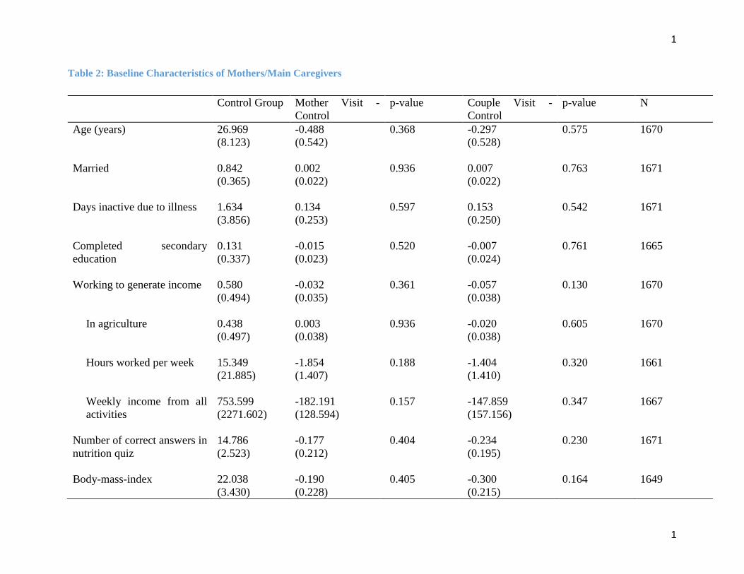
1
1
Table 2: Baseline Characteristics of Mothers/Main Caregivers
Control Group Mother Visit -
Control
p-value Couple Visit -
Control
p-value N
Age (years) 26.969 -0.488 0.368 -0.297 0.575 1670
(8.123) (0.542) (0.528)
Married 0.842 0.002 0.936 0.007 0.763 1671
(0.365) (0.022) (0.022)
Days inactive due to illness 1.634 0.134 0.597 0.153 0.542 1671
(3.856) (0.253) (0.250)
Completed secondary
education
0.131
(0.337)
-0.015
(0.023)
0.520 -0.007
(0.024)
0.761 1665
Working to generate income 0.580 -0.032 0.361 -0.057 0.130 1670
(0.494) (0.035) (0.038)
In agriculture 0.438 0.003 0.936 -0.020 0.605 1670
(0.497) (0.038) (0.038)
Hours worked per week 15.349 -1.854 0.188 -1.404 0.320 1661
(21.885) (1.407) (1.410)
Weekly income from all
activities
753.599
(2271.602)
-182.191
(128.594)
0.157 -147.859
(157.156)
0.347 1667
Number of correct answers in
nutrition quiz
14.786
(2.523)
-0.177
(0.212)
0.404 -0.234
(0.195)
0.230 1671
Body-mass-index 22.038 -0.190 0.405 -0.300 0.164 1649
(3.430) (0.228) (0.215)

1
1
Table 3: Baseline Characteristics of Spouse
Control Group
Mean
Difference:
Mother Visit -
Control
p-value Difference:
Couple Visit -
Control
p-value N
Age (years) 33.415 -0.866 0.198 -0.077 0.918 1278
(9.052) (0.671) (0.743)
Completed secondary
education
0.274 -0.022 0.537 -0.085** 0.011 1293
(0.447) (0.036) (0.033)
Days inactive in last month
due to illness
1.544
(4.996)
-0.642**
(0.304)
0.035 -0.498
(0.313)
0.113 1315
Working to generate income 0.892 -0.051** 0.047 -0.050** 0.042 1331
(0.310) (0.026) (0.024)
In agriculture 0.344 -0.011 0.808 -0.035 0.395 1100
(0.476) (0.045) (0.042)
Hours worked per week 41.166 0.756 0.701 3.271 0.113 1030
(23.416) (1.964) (2.058)
Weekly income from all
income generating
activities
2252.359
(3995.258)
-485.821**
(235.727)
0.040 -375.355
(241.360)
0.121 1321
Number of correct answers in
nutrition quiz
5.391
(1.863)
0.039
(0.187)
0.836 0.037
(0.187)
0.843 781

2
Table 4: Baseline Characteristics of Households
Control Group
Mean
Difference:
Mother Visit -
Control
p-value Difference:
Couple Visit -
Control
p-value N
No. of Household Members 5.193 -0.204 0.149 -0.146 0.274 1671
(2.067) (0.141) (0.133)
No. of Main Respondent's 0.904 0.087 0.513 0.026 0.820 1670
Family Living in Same Village (2.023) (0.133) (0.115)
No. of Spouse's Family Living 2.751 0.052 0.755 -0.219 0.179 1667
in Same Village (2.765) (0.166) (0.162)
Crowding 4.381 -0.185 0.183 -0.118 0.394 1614
(2.114) (0.139) (0.138)
Household has Electricity 0.131 -0.007 0.774 0.003 0.911 1671
(0.337) (0.024) (0.024)
Household Walls made of 0.197 -0.039 0.249 -0.071** 0.025 1671
Quality Material (0.398) (0.034) (0.032)
Household Floor made of 0.214 -0.055* 0.095 -0.071** 0.020 1671
Quality Material (0.410) (0.033) (0.030)
Household has Iron Roof 0.520 -0.025 0.484 0.033 0.375 1664
(0.500) (0.036) (0.037)
Land Owned by 1.389 -0.081 0.537 -0.003 0.982 1652
Household (Acres) (1.699) (0.130) (0.126)
Age of the Household Head 36.056 -0.449 0.554 -0.322 0.681 1585
(12.195) (0.758) (0.782)
Mother/Main Caregiver 0.118 -0.040** 0.046 -0.001 0.966 1671
Head of Household (0.323) (0.020) (0.020)
Spouse Head of 0.857 0.044* 0.061 0.004 0.853 1418
Household (0.351) (0.023) (0.023)
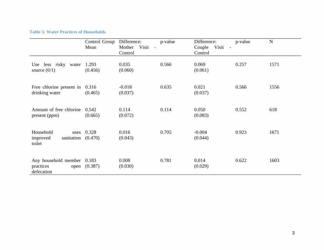
3
Table 5: Water Practices of Households
Control Group
Mean
Difference:
Mother Visit -
Control
p-value Difference:
Couple Visit -
Control
p-value N
Use less risky water
source (0/1)
1.293
(0.456)
0.035
(0.060)
0.566 0.069
(0.061)
0.257 1571
Free chlorine present in
drinking water
0.316
(0.465)
-0.018
(0.037)
0.635 0.021
(0.037)
0.566 1556
Amount of free chlorine
present (ppm)
0.542
(0.665)
0.114
(0.072)
0.114 0.050
(0.083)
0.552 618
Household uses
improved sanitation
toilet
0.328
(0.470)
0.016
(0.043)
0.705 -0.004
(0.044)
0.923 1671
Any household member
practices open
defecation
0.183
(0.387)
0.008
(0.030)
0.781 0.014
(0.029)
0.622 1603

1
1
Table 6: Household Weekly Food Consumption Expenditures
Control Group
Mean
Difference:
Mother Visit -
Control
p-value Difference:
Couple Visit -
Control
p-value N
Meat Goods 205.134 4.757 0.727 -8.053 0.546 1672
(208.923) (13.601) (13.323)
Nuts and Legumes 28.507 -0.440 0.897 -1.871 0.582 1672
(49.872) (3.388) (3.396)
Eggs 32.597 0.728 0.812 -3.874 0.154 1667
(37.198) (3.065) (2.711)
Fruits 101.371 -0.354 0.956 -11.139* 0.058 1672
(78.507) (6.394) (5.862)
Vegetables 101.162 8.250 0.154 -3.241 0.573 1672
(71.517) (5.767) (5.746)
Starchy Staples 279.266 -7.880 0.592 -14.823 0.296 1672
(202.046) (14.670) (14.159)
Dairy Goods 86.360 0.059 0.996 0.795 0.941 1672
(126.737) (10.777) (10.663)
Other Goods 178.520 11.322 0.123 -6.106 0.345 1672
(92.406) (7.318) (6.452)
Aggregate Consumption 964.216 12.822 0.729 -49.551 0.135 1672
(488.852) (37.020) (33.104)
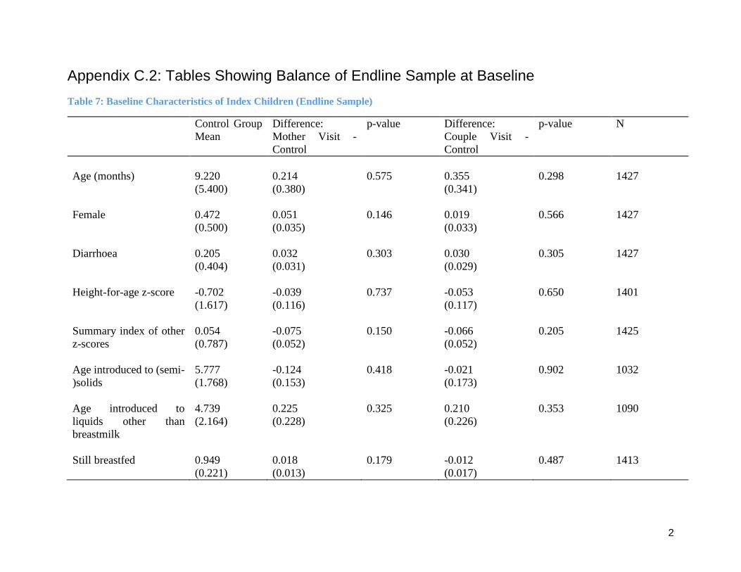
2
Appendix C.2: Tables Showing Balance of Endline Sample at Baseline
Table 7: Baseline Characteristics of Index Children (Endline Sample)
Control Group
Mean
Difference:
Mother Visit -
Control
p-value Difference:
Couple Visit -
Control
p-value N
Age (months) 9.220 0.214 0.575 0.355 0.298 1427
(5.400) (0.380) (0.341)
Female 0.472 0.051 0.146 0.019 0.566 1427
(0.500) (0.035) (0.033)
Diarrhoea 0.205 0.032 0.303 0.030 0.305 1427
(0.404) (0.031) (0.029)
Height-for-age z-score -0.702 -0.039 0.737 -0.053 0.650 1401
(1.617) (0.116) (0.117)
Summary index of other
z-scores
0.054
(0.787)
-0.075
(0.052)
0.150 -0.066
(0.052)
0.205 1425
Age introduced to (semi-
)solids
5.777
(1.768)
-0.124
(0.153)
0.418 -0.021
(0.173)
0.902 1032
Age introduced to
liquids other than
breastmilk
4.739
(2.164)
0.225
(0.228)
0.325 0.210
(0.226)
0.353 1090
Still breastfed 0.949 0.018 0.179 -0.012 0.487 1413
(0.221) (0.013) (0.017)
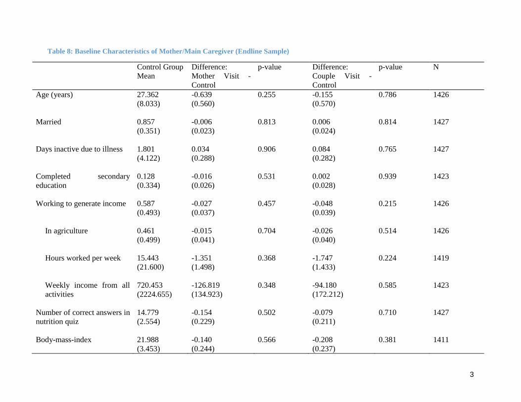
3
Table 8: Baseline Characteristics of Mother/Main Caregiver (Endline Sample)
Control Group
Mean
Difference:
Mother Visit -
Control
p-value Difference:
Couple Visit -
Control
p-value N
Age (years) 27.362 -0.639 0.255 -0.155 0.786 1426
(8.033) (0.560) (0.570)
Married 0.857 -0.006 0.813 0.006 0.814 1427
(0.351) (0.023) (0.024)
Days inactive due to illness 1.801 0.034 0.906 0.084 0.765 1427
(4.122) (0.288) (0.282)
Completed secondary
education
0.128
(0.334)
-0.016
(0.026)
0.531 0.002
(0.028)
0.939 1423
Working to generate income 0.587 -0.027 0.457 -0.048 0.215 1426
(0.493) (0.037) (0.039)
In agriculture 0.461 -0.015 0.704 -0.026 0.514 1426
(0.499) (0.041) (0.040)
Hours worked per week 15.443 -1.351 0.368 -1.747 0.224 1419
(21.600) (1.498) (1.433)
Weekly income from all
activities
720.453
(2224.655)
-126.819
(134.923)
0.348 -94.180
(172.212)
0.585 1423
Number of correct answers in
nutrition quiz
14.779
(2.554)
-0.154
(0.229)
0.502 -0.079
(0.211)
0.710 1427
Body-mass-index 21.988 -0.140 0.566 -0.208 0.381 1411
(3.453) (0.244) (0.237)

4
Table 9: Baseline Characteristics of Spouse (Endline Sample)
Control Group
Mean
Difference:
Mother Visit -
Control
p-value Difference:
Couple Visit -
Control
p-value N
Age (years) 33.949 -1.086 0.136 -0.012 0.989 1117
(8.865) (0.727) (0.823)
Completed secondary
education
0.284 -0.041 0.292 -0.093** 0.011 1133
(0.452) (0.039) (0.036)
Days inactive in last month
due to illness
1.429
(4.781)
-0.465
(0.310)
0.134 -0.325
(0.323)
0.316 1150
Working to generate income 0.899 -0.058** 0.028 -0.053** 0.048 1162
(0.301) (0.026) (0.027)
In agriculture 0.348 -0.007 0.892 -0.024 0.601 965
(0.477) (0.050) (0.046)
Hours worked per week 41.308 0.328 0.876 1.729 0.435 907
(23.487) (2.098) (2.213)
Weekly income from all
income generating
activities
2301.372
(4184.802)
-541.887**
(263.512)
0.041 -410.011
(265.926)
0.124 1153
Number of correct answers in
nutrition quiz
5.463
(1.851)
-0.007
(0.195)
0.972 -0.014
(0.203)
0.946 700

5
Table 10: Baseline Characteristics of Households (Endline Sample)
Control Group
Mean
Difference:
Mother Visit -
Control
p-value Difference:
Couple Visit -
Control
p-value N
No. of Household Members 5.331 -0.251 0.104 -0.135 0.355 1427
(2.072) (0.154) (0.146)
No. of Main Respondent's 0.857 0.130 0.355 0.046 0.712 1426
Family Living in Same Village (1.955) (0.140) (0.125)
No. of Spouse's Family Living 2.801 0.018 0.925 -0.260 0.140 1424
in Same Village (2.730) (0.192) (0.176)
Crowding 4.475 -0.207 0.183 -0.095 0.538 1377
(2.123) (0.155) (0.154)
Household has Electricity 0.135 -0.015 0.554 0.012 0.649 1427
(0.342) (0.025) (0.026)
Household Walls made of 0.201 -0.040 0.251 -0.065* 0.052 1427
Quality Material (0.401) (0.035) (0.033)
Household Floor made of 0.216 -0.063* 0.063 -0.070** 0.028 1427
Quality Material (0.412) (0.034) (0.032)
Household has Iron Roof 0.524 -0.028 0.468 0.041 0.310 1422
(0.500) (0.039) (0.040)
Land Owned by 1.397 -0.056 0.677 0.052 0.692 1412
Household (Acres) (1.678) (0.135) (0.132)
Age of the Household Head 36.354 -0.504 0.534 -0.734 0.381 1356
(11.936) (0.810) (0.837)
Mother/Main Caregiver 0.119 -0.049** 0.029 -0.003 0.900 1427
Head of Household (0.324) (0.022) (0.023)
Spouse Head of 0.859 0.048* 0.056 0.005 0.850 1230
Household (0.348) (0.025) (0.026)
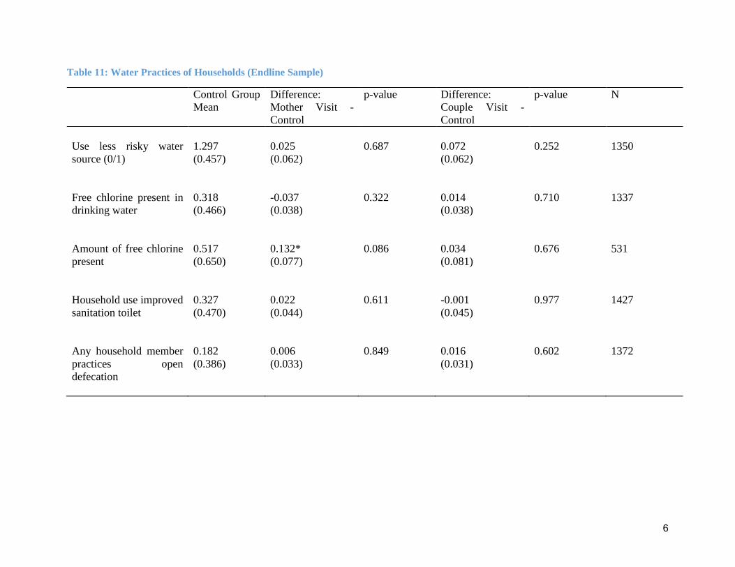
6
Table 11: Water Practices of Households (Endline Sample)
Control Group
Mean
Difference:
Mother Visit -
Control
p-value Difference:
Couple Visit -
Control
p-value N
Use less risky water
source (0/1)
1.297
(0.457)
0.025
(0.062)
0.687 0.072
(0.062)
0.252 1350
Free chlorine present in
drinking water
0.318
(0.466)
-0.037
(0.038)
0.322 0.014
(0.038)
0.710 1337
Amount of free chlorine
present
0.517
(0.650)
0.132*
(0.077)
0.086 0.034
(0.081)
0.676 531
Household use improved
sanitation toilet
0.327
(0.470)
0.022
(0.044)
0.611 -0.001
(0.045)
0.977 1427
Any household member
practices open
defecation
0.182
(0.386)
0.006
(0.033)
0.849 0.016
(0.031)
0.602 1372

7
Table 12: Household Weekly Food Consumption Expenditures (Endline Sample)
Control Group
Mean
Difference:
Mother Visit -
Control
p-value Difference:
Couple Visit -
Control
p-value N
Meat Goods 208.553 4.836 0.752 -11.614 0.409 1428
(211.211) (15.294) (14.054)
Nuts and Legumes 27.624 0.757 0.825 -1.867 0.556 1428
(48.619) (3.429) (3.169)
Eggs 33.103 -0.096 0.975 -3.512 0.220 1424
(37.011) (3.120) (2.858)
Fruits 103.162 -1.582 0.813 -11.811* 0.056 1428
(78.474) (6.696) (6.162)
Vegetables 103.221 6.305 0.302 -4.502 0.466 1428
(73.227) (6.102) (6.172)
Starchy Staples 282.936 -9.985 0.528 -11.953 0.441 1428
(202.548) (15.818) (15.506)
Dairy Goods 87.206 -0.285 0.980 1.617 0.882 1428
(128.040) (11.183) (10.896)
Other Goods 180.084 9.821 0.198 -5.853 0.406 1428
(92.558) (7.616) (7.039)
Aggregate Consumption 978.457 4.704 0.905 -52.735 0.122 1428
(491.127) (39.276) (34.002)

1
Appendix C.3: Differences in attrition between study arms
Table 13: Attrition rates by arm and characteristic
(1) (2) (3) (4)
Attrited Attrited Attrited Attrited
Mother -0.0435* -0.0474**
Only (0.076) (0.045)
Couples -0.0140 -0.0151
Visit (0.577) (0.526)
Mother Only –
Black & White
-0.0608**
(0.018)
-0.0627**
(0.012)
Mother Only –
Colour
-0.0218
(0.505)
-0.0278
(0.382)
Couples Visit –
Black & White
-0.0234
(0.414)
-0.0216
(0.439)
Couples Visit –
Colour
-0.00248
(0.937)
-0.00712
(0.807)
Mother’s age -0.00234** -0.00232**
(0.040) (0.042)
Mother married -0.0595** -0.0585**
(0.031) (0.035)
Mother sec. edu. -0.00139 -0.000802
(0.943) (0.967)
Household size -0.0233*** -0.0233***
(0.000) (0.000)
Index child gender 0.0188
(0.287)
0.0192
(0.275)
Index child age -0.00179 -0.00175
(0.287) (0.303)
Index child height
z-score
-0.00120
(0.806)
-0.000929
(0.850)
_cons 0.166*** 0.402*** 0.166*** 0.400***
(0.000) (0.000) (0.000) (0.000)
N 1671 1634 1671 1634 Standard errors clustered by waterpoint in parentheses. * p < 0.1, ** p < 0.05, *** p < 0.01

2
Appendix D: Results
D1. Anthropometrics
Table 14: Anthropometric Indicators (1km cut-off)
(1)
Height-for-age
(2)
Height-for-age
(3)
Summary index of
other z-scores
(4)
Summary index of
other z-scores
Mother Only - 0.019 -0.043
Black & White (0.092) (0.046)
Mother Only - -0.101 0.007
Colour Poster (0.101) (0.052)
Couples Visit - -0.020 0.045
Black & White (0.106) (0.047)
Couples Visit - -0.034 -0.067
Colour Poster (0.100) (0.051)
Treat -0.030 -0.012
(0.073) (0.035)
Indirect Effect - 0.265 0.269 0.192 0.183
1km (0.149)* (0.146)* (0.081)** (0.080)**
Bonacich Cent. - -0.265 -0.265 -0.147 -0.142
1km (0.114)** (0.114)** (0.061)** (0.060)**
Age 0.212 0.211 0.013 0.014
(0.057)*** (0.058)*** (0.026) (0.027)
Age Sqr. -0.004 -0.004 -0.000 -0.000
(0.001)*** (0.001)*** (0.000) (0.000)
Female 1.355 1.419 -0.029 -0.041
(1.505) (1.497) (0.629) (0.635)
Age*Female -0.081 -0.085 0.016 0.016
(0.099) (0.098) (0.041) (0.041)
Age Sqr.*Female 0.001 0.001 -0.001 -0.001
(0.002) (0.002) (0.001) (0.001)
zlen_bline 0.358 0.359
(0.023)*** (0.023)***
sum_index_othz_bline 0.502 0.503
(0.025)*** (0.025)***
TATE 0.188 0.136
(0.122) (0.065)**
TTE 75th Perc. 0.234 0.167
(0.143) (0.077)**
TTE 25th Perc. 0.037 0.033
(0.073) (0.035)
N 1,363 1,363 1,392 1,392 Standard errors clustered by waterpoint in parentheses. * p < 0.1, ** p < 0.05, *** p < 0.01
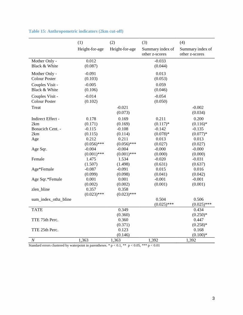
3
Table 15: Anthropometric indicators (2km cut-off)
Standard errors clustered by waterpoint in parentheses. * p < 0.1, ** p < 0.05, *** p < 0.01
(1)
Height-for-age
(2)
Height-for-age
(3)
Summary index of
other z-scores
(4)
Summary index of
other z-scores
Mother Only - 0.012 -0.033
Black & White (0.087) (0.044)
Mother Only - -0.091 0.013
Colour Poster (0.103) (0.053)
Couples Visit - -0.005 0.059
Black & White (0.106) (0.046)
Couples Visit - -0.014 -0.054
Colour Poster (0.102) (0.050)
Treat -0.021 -0.002
(0.073) (0.034)
Indirect Effect - 0.178 0.169 0.211 0.200
2km (0.171) (0.169) (0.117)* (0.116)*
Bonacich Cent. - -0.115 -0.108 -0.142 -0.135
2km (0.115) (0.114) (0.078)* (0.077)*
Age 0.212 0.211 0.013 0.013
(0.056)*** (0.056)*** (0.027) (0.027)
Age Sqr. -0.004 -0.004 -0.000 -0.000
(0.001)*** (0.001)*** (0.000) (0.000)
Female 1.475 1.534 -0.020 -0.031
(1.507) (1.498) (0.631) (0.637)
Age*Female -0.087 -0.091 0.015 0.016
(0.099) (0.098) (0.041) (0.042)
Age Sqr.*Female 0.001 0.001 -0.001 -0.001
(0.002) (0.002) (0.001) (0.001)
zlen_bline 0.357 0.358
(0.023)*** (0.023)***
sum_index_othz_bline 0.504 0.506
(0.025)*** (0.025)***
TATE 0.349 0.434
(0.360) (0.250)*
TTE 75th Perc. 0.360 0.447
(0.371) (0.258)*
TTE 25th Perc. 0.123 0.168
(0.146) (0.100)*
N 1,363 1,363 1,392 1,392

4
D2. Nutritional Knowledge
Table 16: Nutritional Quiz (1km cut-off)
Standard errors clustered by waterpoint in parentheses. * p < 0.1, ** p < 0.05, *** p < 0.01
(1)
Proportion
correct
(2)
Proportion
correct
(3)
Latent
knowledge
(4)
Latent
knowledge
Mother Only - 0.011 0.040
Black & White (0.009) (0.068)
Mother Only - -0.020 -0.126
Colour Poster (0.010)** (0.084)
Couples Visit - 0.005 -0.005
Black & White (0.010) (0.079)
Couples Visit - 0.019 0.186
Colour Poster (0.010)* (0.087)**
Treat 0.007 0.030
(0.008) (0.058)
Indirect Effect - -0.006 -0.008 0.007 -0.006
1km (0.017) (0.018) (0.133) (0.135)
Bonacich Cent. - -0.001 0.001 -0.052 -0.042
1km (0.013) (0.014) (0.104) (0.106)
Education level 0.011 0.011 0.081 0.081
(0.003)*** (0.003)*** (0.020)*** (0.020)***
prop_corr_bline 0.017 0.019
(0.028) (0.028)
lat_know_bline -0.034 -0.033
(0.029) (0.029)
TATE 0.002 0.026
(0.013) (0.105)
TTE 75th Perc. -0.001 0.024
(0.018) (0.144)
TTE 25th Perc. 0.005 0.028
(0.008) (0.064)
N 1,390 1,390 1,390 1,390

5
Table 17: Nutritional Quiz (2km cut-off)
Standard errors clustered by waterpoint in parentheses. * p < 0.1, ** p < 0.05, *** p < 0.01
(1)
Proportion
correct
(2)
Proportion
correct
(3)
Latent
knowledge
(4)
Latent
knowledge
Mother Only - 0.010 0.041
Black & White (0.009) (0.068)
Mother Only - -0.018 -0.117
Colour Poster (0.010)* (0.083)
Couples Visit - 0.004 -0.007
Black & White (0.009) (0.078)
Couples Visit - 0.022 0.205
Colour Poster (0.010)** (0.086)**
Treat 0.007 0.035
(0.007) (0.057)
Indirect Effect - -0.033 -0.037 -0.105 -0.126
2km (0.027) (0.028) (0.210) (0.218)
Bonacich Cent. - 0.016 0.020 0.012 0.029
2km (0.018) (0.019) (0.141) (0.147)
Education level 0.011 0.011 0.087 0.087
(0.003)*** (0.003)*** (0.020)*** (0.020)***
prop_corr_bline 0.018 0.020
(0.028) (0.029)
lat_know_bline -0.027 -0.026
(0.029) (0.029)
TATE -0.055 -0.177
(0.047) (0.372)
TTE 75th Perc. -0.074 -0.242
(0.061) (0.484)
TTE 25th Perc. -0.023 -0.069
(0.023) (0.188)
N 1,390 1,390 1,390 1,390

6
Table 18: Nutritional Quiz, Promoter (1km cut-off)
(1)
Proportion
correct
(2)
Proportion
correct
(3)
Latent knowledge
(4)
Latent knowledge
Mother Only - -0.012 -0.221
Black & White (0.019) (0.143)
Mother Only - -0.010 -0.056
Colour Poster (0.020) (0.155)
Couples Visit - 0.009 -0.029
Black & White (0.017) (0.137)
Couples Visit - -0.007 -0.107
Colour Poster (0.018) (0.143)
Treat -0.004 -0.099
(0.012) (0.093)
Indirect Effect - 0.038 0.033 0.256 0.216
2km (0.033) (0.033) (0.254) (0.253)
Bonacich Cent. - -0.025 -0.021 -0.187 -0.158
2km (0.023) (0.023) (0.178) (0.176)
Education level 0.004 0.004 0.033 0.031
(0.005) (0.005) (0.040) (0.040)
TATE 0.032 0.137
(0.036) (0.274)
TTE 75th Perc. 0.031 0.129
(0.034) (0.266)
TTE 25th Perc. 0.004 -0.045
(0.013) (0.102)
N 314 314 314 314 Standard errors in parentheses. * p < 0.1, ** p < 0.05, *** p < 0.01

7
Table 19: Nutritional Quiz, Promoter (2km cut-off)
(1)
Proportion
correct
(2)
Proportion
correct
(3)
Latent knowledge
(4)
Latent knowledge
Mother Only - -0.010 -0.200
Black & White (0.018) (0.141)
Mother Only - -0.008 -0.038
Colour Poster (0.020) (0.152)
Couples Visit - 0.011 -0.021
Black & White (0.017) (0.137)
Couples Visit - -0.003 -0.077
Colour Poster (0.017) (0.139)
Treat -0.002 -0.083
(0.012) (0.091)
Indirect Effect - 0.025 0.023 0.126 0.105
2km (0.026) (0.026) (0.223) (0.222)
Bonacich Cent. - -0.018 -0.017 -0.105 -0.090
2km (0.017) (0.017) (0.147) (0.145)
Education level 0.005 0.005 0.043 0.040
(0.005) (0.005) (0.040) (0.040)
TATE 0.058 0.186
(0.069) (0.576)
TTE 75th Perc. 0.051 0.158
(0.062) (0.517)
TTE 25th Perc. 0.016 -0.002
(0.024) (0.193)
N 314 314 314 314 Standard errors in parentheses. * p < 0.1, ** p < 0.05, *** p < 0.01

8
D3. Child Nutritional Intake
Table 20: Number of days that child consumed food, with foods grouped by type i (1km cut-off)
(1)
meat
(2)
meat
(3)
nuts
(4)
nuts
(5)
eggs
(6)
eggs
Mother Only - -0.103 -0.042 0.033
Black & White (0.230) (0.112) (0.086)
Mother Only - 0.166 0.048 0.167
Colour Poster (0.258) (0.124) (0.092)*
Couples Visit - 0.287 -0.021 -0.003
Black & White (0.245) (0.114) (0.090)
Couples Visit - 0.340 0.112 0.024
Colour Poster (0.235) (0.125) (0.103)
Treat 0.162 0.017 0.052
(0.168) (0.090) (0.069)
Indirect Effect -0.447 -0.501 -0.047 -0.053 0.104 0.109
- 1km (0.404) (0.392) (0.216) (0.213) (0.172) (0.172)
Bonacich Cent. 0.404 0.424 0.141 0.139 -0.043 -0.047
- 1km (0.300) (0.293) (0.165) (0.162) (0.127) (0.127)
Age 0.042 0.044 -0.090 -0.091 0.017 0.016
(0.054) (0.054) (0.044)** (0.044)** (0.021) (0.021)
Age Sqr. -0.002 -0.002 0.005 0.005 -0.001 -0.000
(0.003) (0.003) (0.002)** (0.002)** (0.001) (0.001)
Still Breastfed 0.114 0.113 -0.126 -0.125 -0.077 -0.074
(0.192) (0.191) (0.118) (0.117) (0.090) (0.090)
TATE -0.244 -0.026 0.141
(0.310) (0.182) (0.144)
TTE 75th Perc. -0.329
(0.369)
-0.035
(0.214)
0.159
(0.170)
TTE 25th Perc. 0.036
(0.167)
0.004
(0.097)
0.079
(0.074)
N 1,349 1,349 1,283 1,283 1,298 1,298 Standard errors clustered by waterpoint in parentheses. * p < 0.1, ** p < 0.05, *** p < 0.01

9
Table 21: Number of days that child consumed food, with foods grouped by type ii (1km cut-off)
(1)
vita
(2)
vita
(3)
green
(4)
green
(5)
fruit
(6)
fruit
Mother Only - 0.085 -0.370 0.041
Black & White (0.111) (0.207)* (0.463)
Mother Only - 0.140 -0.146 0.082
Colour Poster (0.143) (0.219) (0.431)
Couples Visit - 0.228 -0.074 0.034
Black & White (0.154) (0.226) (0.460)
Couples Visit - 0.021 -0.334 0.689
Colour Poster (0.107) (0.218) (0.418)
Treat 0.123 -0.229 0.188
(0.085) (0.161) (0.320)
Indirect Effect -0.006 -0.023 -0.124 -0.161 -0.035 -0.043
- 1km (0.222) (0.215) (0.462) (0.466) (0.669) (0.672)
Bonacich Cent. 0.037 0.049 0.167 0.188 0.049 0.036
- 1km (0.167) (0.162) (0.344) (0.349) (0.501) (0.505)
Age 0.020 0.021 0.093 0.095 0.141 0.141
(0.025) (0.025) (0.045)** (0.045)** (0.085) (0.084)*
Age Sqr. -0.001 -0.001 -0.005 -0.005 -0.006 -0.006
(0.001) (0.001) (0.002)** (0.002)** (0.004) (0.004)
Still Breastfed 0.002 0.004 0.104 0.109 -0.437 -0.447
(0.111) (0.111) (0.167) (0.166) (0.311) (0.309)
TATE 0.105 -0.359 0.153
(0.184) (0.374) (0.567)
TTE 75th Perc. 0.101
(0.217)
-0.387
(0.447)
0.146
(0.666)
TTE 25th Perc. 0.118
(0.095)
-0.270
(0.176)
0.177
(0.327)
N 1,349 1,349 1,324 1,324 1,349 1,349 Standard errors clustered by waterpoint in parentheses. * p < 0.1, ** p < 0.05, *** p < 0.01

10
Table 22: Number of days that child consumed food, with foods grouped by type iii (1km cut-off)
(1)
dairy
(2)
dairy
(3)
starch
(4)
starch
Mother Only - 0.021 -0.114
Black & White (0.348) (0.259)
Mother Only - 0.462 -0.369
Colour Poster (0.354) (0.277)
Couples Visit - 0.125 -0.314
Black & White (0.376) (0.263)
Couples Visit - -0.114 -0.208
Colour Poster (0.337) (0.276)
Treat 0.122 -0.247
(0.254) (0.197)
Indirect Effect 0.205 0.194 -0.343 -0.318
- 1km (0.705) (0.713) (0.533) (0.545)
Bonacich Cent. -0.178 -0.170 0.237 0.225
- 1km (0.522) (0.526) (0.404) (0.411)
Age -0.156 -0.157 0.017 0.017
(0.075)** (0.077)** (0.056) (0.056)
Age Sqr. 0.007 0.007 -0.002 -0.002
(0.004)* (0.004)* (0.003) (0.003)
Still Breastfed -0.639 -0.627 -0.453 -0.458
(0.259)** (0.259)** (0.225)** (0.225)**
TATE 0.279 -0.505
(0.593) (0.449)
TTE 75th Perc. 0.312 -0.559
(0.705) (0.535)
TTE 25th Perc. 0.171 -0.327
(0.287) (0.218)
N 1,349 1,349 1,307 1,307 Standard errors clustered by waterpoint in parentheses. * p < 0.1, ** p < 0.05, *** p < 0.01

11
Table 23: Number of days that child consumed food, with foods grouped by type i (2km cut-off)
(1)
meat
(2)
meat
(3)
nuts
(4)
nuts
(5)
eggs
(6)
eggs
Mother Only - -0.127 -0.034 0.048
Black & White (0.228) (0.118) (0.087)
Mother Only - 0.147 0.024 0.173
Colour Poster (0.256) (0.122) (0.091)*
Couples Visit - 0.252 -0.018 0.003
Black & White (0.240) (0.113) (0.089)
Couples Visit - 0.285 0.085 0.022
Colour Poster (0.231) (0.125) (0.102)
Treat 0.125 0.009 0.059
(0.162) (0.089) (0.068)
Indirect Effect -0.466 -0.530 0.443 0.442 0.023 0.052
- 2km (0.472) (0.461) (0.190)** (0.193)** (0.158) (0.157)
Bonacich Cent. 0.350 0.391 -0.286 -0.285 -0.004 -0.024
- 2km (0.317) (0.310) (0.126)** (0.128)** (0.105) (0.105)
Age 0.044 0.046 -0.088 -0.088 0.018 0.016
(0.054) (0.054) (0.044)** (0.044)** (0.022) (0.021)
Age Sqr. -0.002 -0.002 0.005 0.005 -0.001 -0.000
(0.003) (0.003) (0.002)** (0.002)** (0.001) (0.001)
Still Breastfed 0.109 0.111 -0.131 -0.130 -0.080 -0.077
(0.192) (0.191) (0.119) (0.118) (0.090) (0.090)
TATE -1.032 0.972 0.172
(1.003) (0.426)** (0.341)
TTE 75th Perc. -1.066
(1.033)
1.001
(0.439)**
0.176
(0.351)
TTE 25th Perc. -0.326
(0.411)
0.385
(0.184)**
0.103
(0.142)
N 1,349 1,349 1,283 1,283 1,298 1,298 Standard errors clustered by waterpoint in parentheses. * p < 0.1, ** p < 0.05, *** p < 0.01
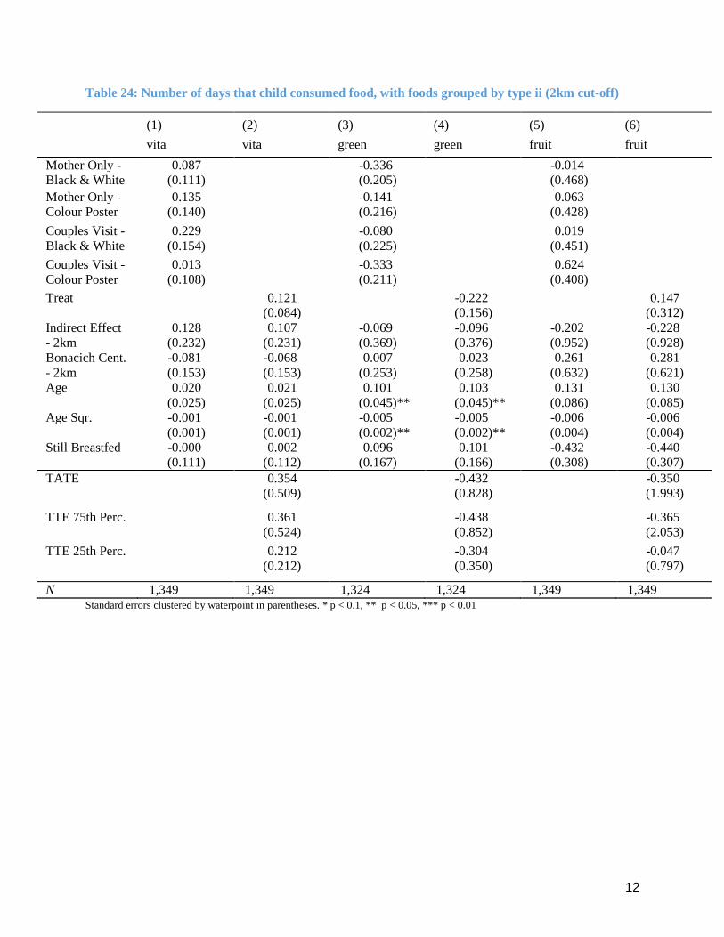
12
Table 24: Number of days that child consumed food, with foods grouped by type ii (2km cut-off)
(1)
vita
(2)
vita
(3)
green
(4)
green
(5)
fruit
(6)
fruit
Mother Only - 0.087 -0.336 -0.014
Black & White (0.111) (0.205) (0.468)
Mother Only - 0.135 -0.141 0.063
Colour Poster (0.140) (0.216) (0.428)
Couples Visit - 0.229 -0.080 0.019
Black & White (0.154) (0.225) (0.451)
Couples Visit - 0.013 -0.333 0.624
Colour Poster (0.108) (0.211) (0.408)
Treat 0.121 -0.222 0.147
(0.084) (0.156) (0.312)
Indirect Effect 0.128 0.107 -0.069 -0.096 -0.202 -0.228
- 2km (0.232) (0.231) (0.369) (0.376) (0.952) (0.928)
Bonacich Cent. -0.081 -0.068 0.007 0.023 0.261 0.281
- 2km (0.153) (0.153) (0.253) (0.258) (0.632) (0.621)
Age 0.020 0.021 0.101 0.103 0.131 0.130
(0.025) (0.025) (0.045)** (0.045)** (0.086) (0.085)
Age Sqr. -0.001 -0.001 -0.005 -0.005 -0.006 -0.006
(0.001) (0.001) (0.002)** (0.002)** (0.004) (0.004)
Still Breastfed -0.000 0.002 0.096 0.101 -0.432 -0.440
(0.111) (0.112) (0.167) (0.166) (0.308) (0.307)
TATE 0.354 -0.432 -0.350
(0.509) (0.828) (1.993)
TTE 75th Perc. 0.361
(0.524)
-0.438
(0.852)
-0.365
(2.053)
TTE 25th Perc. 0.212
(0.212)
-0.304
(0.350)
-0.047
(0.797)
N 1,349 1,349 1,324 1,324 1,349 1,349 Standard errors clustered by waterpoint in parentheses. * p < 0.1, ** p < 0.05, *** p < 0.01
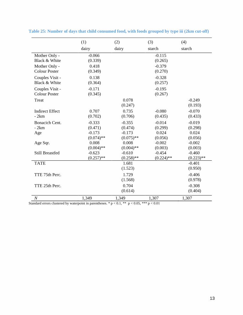
13
Table 25: Number of days that child consumed food, with foods grouped by type iii (2km cut-off)
(1)
dairy
(2)
dairy
(3)
starch
(4)
starch
Mother Only - -0.066 -0.115
Black & White (0.339) (0.265)
Mother Only - 0.418 -0.379
Colour Poster (0.349) (0.270)
Couples Visit - 0.138 -0.328
Black & White (0.364) (0.257)
Couples Visit - -0.171 -0.195
Colour Poster (0.345) (0.267)
Treat 0.078 -0.249
(0.247) (0.193)
Indirect Effect 0.707 0.735 -0.080 -0.070
- 2km (0.702) (0.706) (0.435) (0.433)
Bonacich Cent. -0.333 -0.355 -0.014 -0.019
- 2km (0.471) (0.474) (0.299) (0.298)
Age -0.173 -0.173 0.024 0.024
(0.074)** (0.075)** (0.056) (0.056)
Age Sqr. 0.008 0.008 -0.002 -0.002
(0.004)** (0.004)** (0.003) (0.003)
Still Breastfed -0.623 -0.610 -0.454 -0.460
(0.257)** (0.258)** (0.224)** (0.223)**
TATE 1.681 -0.401
(1.523) (0.950)
TTE 75th Perc. 1.729 -0.406
(1.568) (0.978)
TTE 25th Perc. 0.704 -0.308
(0.614) (0.404)
N 1,349 1,349 1,307 1,307 Standard errors clustered by waterpoint in parentheses. * p < 0.1, ** p < 0.05, *** p < 0.01

14
Table 26: Indicator for child meeting 24 hour minimum feed-frequency (1km cut-off)
(1)
food_min_freq
(2)
food_min_freq
Mother Only - 0.034
Black & White (0.033)
Mother Only - 0.021
Colour Poster (0.032)
Couples Visit - 0.032
Black & White (0.035)
Couples Visit - 0.067
Colour Poster (0.037)*
Treat 0.038
(0.026)
Indirect Effect -0.044 -0.045
- 1km (0.056) (0.056)
Bonacich Cent. 0.037 0.037
- 1km (0.042) (0.042)
Age -0.006 -0.006
(0.011) (0.011)
Age Sqr. -0.000 -0.000
(0.000) (0.001)
Female -0.004 -0.004
(0.021) (0.021)
Still Breastfed 0.176 0.175
(0.026)*** (0.026)***
food_min_freq_bline 0.035 0.036
(0.039) (0.039)
TATE 0.002
(0.048)
TTE 75th Perc. -0.006
(0.056)
TTE 25th Perc. 0.026
(0.027)
N 1,297 1,297 Standard errors clustered by waterpoint in parentheses. * p < 0.1, ** p < 0.05, *** p < 0.01

15
Table 27: Indicator for child meeting 24 hour minimum feed-frequency (2km cut-off)
(1)
food_min_freq
(2)
food_min_freq
Mother Only - 0.027
Black & White (0.032)
Mother Only - 0.016
Colour Poster (0.033)
Couples Visit - 0.029
Black & White (0.034)
Couples Visit - 0.060
Colour Poster (0.037)
Treat 0.032
(0.025)
Indirect Effect 0.005 0.002
- 2km (0.071) (0.068)
Bonacich Cent. 0.004 0.007
- 2km (0.047) (0.045)
Age -0.006 -0.006
(0.011) (0.011)
Age Sqr. -0.000 -0.000
(0.000) (0.000)
Female -0.005 -0.005
(0.021) (0.021)
Still Breastfed 0.176 0.176
(0.026)*** (0.026)***
food_min_freq_bline 0.033 0.033
(0.039) (0.039)
constant 0.748 0.746
(0.066)*** (0.065)***
TATE 0.036
(0.146)
TTE 75th Perc. 0.036
(0.151)
TTE 25th Perc. 0.034
(0.059)
N 1,297 1,297 Standard errors clustered by waterpoint in parentheses. * p < 0.1, ** p < 0.05, *** p < 0.01

16
D4i. Household Food Consumption (Expenditures)
Table 28: Weekly Household Food Consumption Expenditures in KSHS i (1km cut-off)
(1)
meats
(2)
meats
(3)
legs
(4)
legs
(5)
eggs
(6)
eggs
Mother Only - -25.765 -1.658 3.067
Black & White (26.808) (7.171) (3.526)
Mother Only - -8.717 -2.646 7.737
Colour Poster (29.021) (7.993) (4.760)
Couples Visit - -18.682 5.408 0.138
Black & White (28.275) (7.328) (3.908)
Couples Visit - -0.070 6.239 4.473
Colour Poster (33.780) (8.417) (4.184)
Treat -14.439 1.769 3.616
(22.974) (5.442) (3.056)
Indirect Effect 56.317 55.189 2.280 1.370 0.447 0.783
- 1km (55.680) (55.560) (13.486) (13.486) (6.331) (6.303)
Bonacich Cent. -34.817 -34.910 -1.219 -0.836 -0.570 -0.846
- 1km (40.037) (39.759) (10.182) (10.181) (4.719) (4.686)
Males: 0 to 5 0.471 0.579 1.067 1.276 0.377 0.293
(13.018) (12.880) (4.131) (4.194) (2.362) (2.362)
Males: < 18 8.831 9.048 3.066 3.100 1.033 1.084
(12.722) (12.660) (3.357) (3.324) (1.645) (1.652)
Males: Adults 17.101 16.341 15.300 14.850 1.130 1.270
(20.298) (20.220) (7.445)** (7.406)** (4.505) (4.499)
Females: 0 to 5 15.526 15.349 -0.302 -0.219 2.246 2.139
(11.087) (11.107) (3.603) (3.595) (1.952) (1.950)
Females: < 18 18.343 18.485 -0.395 -0.371 0.813 0.816
(12.934) (12.903) (2.458) (2.469) (1.732) (1.723)
Females: 33.586 33.355 9.749 9.722 -3.631 -3.622
Adults (37.717) (37.687) (9.006) (9.013) (3.860) (3.829)
meats_bline 0.248 0.248
(0.045)*** (0.044)***
legs_bline 0.127 0.125
(0.054)** (0.054)**
eggs_bline 0.155 0.158
(0.040)*** (0.041)***
TATE 30.238 2.879 4.250
(54.582) (10.762) (5.391)
TTE 75th Perc. 39.649
(63.337)
3.112
(12.821)
4.383
(6.313)
TTE 25th Perc. -0.642
(29.207)
2.112
(5.550)
3.812
(3.142)
N 1,427 1,427 1,427 1,427 1,359 1,359 Standard errors clustered by waterpoint in parentheses. * p < 0.1, ** p < 0.05, *** p < 0.01

17
Table 29: Weekly Household Food Consumption Expenditure in KSHS ii (1km cut-off)
Standard errors clustered by waterpoint in parentheses. * p < 0.1, ** p < 0.05, *** p < 0.01
(1)
fruit
(2)
fruit
(3)
veg
(4)
veg
(5)
starch
(6)
starch
Mother Only - -1.622 3.977 -68.397
Black & White (11.925) (12.178) (37.532)*
Mother Only - 19.460 -2.719 -45.464
Colour Poster (24.655) (17.455) (38.748)
Couples Visit - -1.202 12.200 -19.853
Black & White (10.599) (14.983) (38.418)
Couples Visit - 6.711 -37.783 53.622
Colour Poster (13.802) (11.511)*** (57.192)
Treat 5.043 -4.227 -23.591
(10.531) (9.661) (29.228)
Indirect Effect -58.242 -58.389 -0.743 -1.081 17.599 10.546
- 1km (23.391)** (23.065)** (21.970) (22.613) (70.319) (71.266)
Bonacich Cent. 37.907 37.592 -3.724 -2.424 -26.909 -25.730
- 1km (18.394)** (18.136)** (17.262) (17.668) (50.896) (52.220)
Males: 0 to 5 -10.747 -10.953 -0.161 -0.248 23.636 25.204
(8.747) (8.954) (6.863) (6.944) (22.489) (22.312)
Males: < 18 1.296 1.400 4.729 4.327 52.049 52.910
(4.477) (4.468) (6.705) (6.719) (19.941)*** (20.156)***
Males: Adults -9.035 -8.770 -4.492 -2.659 -3.832 -9.457
(9.840) (9.744) (13.564) (13.704) (42.158) (42.196)
Females: 0 to 5 -2.379 -2.744 -4.518 -4.578 24.862 25.220
(6.657) (6.827) (7.035) (7.097) (18.388) (18.291)
Females: < 18 -0.817 -0.710 0.223 0.101 38.832 39.248
(4.751) (4.732) (5.853) (5.837) (14.165)*** (14.200)***
Females: 14.421 14.274 -4.119 -3.771 104.469 103.581
Adults (10.637) (10.528) (15.757) (15.762) (47.692)** (47.689)**
fruit_bline 0.260 0.259
(0.066)*** (0.066)***
veg_bline 0.067 0.066
(0.060) (0.059)
starch_bline 0.169 0.170
(0.065)*** (0.065)***
TATE -42.225 -5.102 -15.054
(19.056)** (19.288) (62.569)
TTE 75th Perc. -52.182
(22.477)**
-5.287
(22.720)
-13.256
(73.542)
TTE 25th Perc. -9.555
(10.695)
-4.497
(10.387)
-20.955
(33.000)
N 1,427 1,427 1,427 1,427 1,427 1,427

18
Table 30: Weekly Household Food Consumption Expenditure in KSHS iii (1km cut-off)
(1)
dairy
(2)
dairy
(3)
other
(4)
other
(5)
agg
(6)
agg
Mother Only - -12.510 21.555 -87.226
Black & White (14.452) (57.688) (93.838)
Mother Only - -4.535 119.057 72.284
Colour Poster (16.326) (69.019)* (119.902)
Couples Visit - -1.814 -47.430 -54.854
Black & White (15.176) (52.890) (92.667)
Couples Visit - -29.514 -72.325 -68.504
Colour Poster (15.348)* (55.311) (116.075)
Treat -11.396 4.193 -38.182
(11.758) (41.353) (76.460)
Indirect Effect 2.146 1.214 -62.217 -53.632 -60.799 -64.686
- 1km (24.789) (25.120) (97.974) (100.670) (152.315) (150.526)
Bonacich Cent. -4.353 -3.459 33.428 29.621 19.102 19.566
- 1km (19.372) (19.566) (80.675) (82.935) (118.439) (117.699)
Males: 0 to 5 -2.522 -2.549 -12.619 -16.124 -4.293 -5.667
(7.460) (7.453) (25.392) (25.675) (46.850) (47.131)
Males: < 18 -3.430 -3.584 -6.348 -6.865 50.666 50.892
(5.066) (5.093) (23.169) (23.312) (39.633) (39.896)
Males: Adults 10.105 11.189 96.401 103.692 92.593 96.529
(13.510) (13.477) (80.875) (83.401) (105.864) (107.412)
Females: 0 to 5 -4.907 -5.107 -29.479 -32.149 -1.678 -4.570
(6.862) (6.878) (26.087) (25.915) (42.085) (42.069)
Females: < 18 2.598 2.635 18.746 18.731 58.650 59.277
(5.315) (5.341) (20.650) (20.899) (31.010)* (31.127)*
Females: -3.354 -3.232 109.253 108.538 229.517 228.654
Adults (13.673) (13.637) (81.818) (81.997) (115.617)** (115.402)**
dairy_bline 0.162 0.159
(0.039)*** (0.039)***
other_bline 0.091 0.124
(0.203) (0.202)
agg_bline 0.411 0.412
(0.076)*** (0.076)***
TATE -10.414 -39.224 -90.548
(20.893) (91.821) (145.037)
TTE 75th Perc. -10.207
(24.594)
-48.370
(107.429)
-101.579
(167.399)
TTE 25th Perc. -11.093
(11.920)
-9.215
(48.663)
-54.354
(85.835)
N 1,427 1,427 1,427 1,427 1,427 1,427 Standard errors clustered by waterpoint in parentheses. * p < 0.1, ** p < 0.05, *** p < 0.01
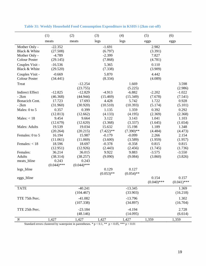
19
Table 31: Weekly Household Food Consumption Expenditure in KSHS i (2km cut-off)
(1)
meats
(2)
meats
(3)
legs
(4)
legs
(5)
eggs
(6)
eggs
Mother Only - -22.352 -1.691 2.982
Black & White (27.508) (6.797) (3.391)
Mother Only - -4.789 -2.399 7.827
Colour Poster (29.145) (7.868) (4.781)
Couples Visit - -16.536 5.365 0.110
Black & White (29.520) (7.338) (3.909)
Couples Visit - -0.669 5.870 4.442
Colour Poster (34.441) (8.334) (4.089)
Treat -12.254 1.669 3.598
(23.755) (5.225) (2.986)
Indirect Effect -12.825 -12.829 -4.913 -6.882 -2.202 -1.022
- 2km (46.368) (44.944) (15.469) (15.349) (7.678) (7.541)
Bonacich Cent. 17.723 17.693 4.428 5.742 1.722 0.928
- 2km (31.960) (30.920) (10.510) (10.393) (5.174) (5.101)
Males: 0 to 5 0.357 0.399 1.135 1.359 0.392 0.292
(12.813) (12.662) (4.133) (4.195) (2.369) (2.368)
Males: < 18 9.454 9.664 3.122 3.143 1.041 1.103
(12.679) (12.620) (3.368) (3.337) (1.645) (1.654)
Males: Adults 19.539 19.034 15.632 15.198 1.189 1.348
(20.264) (20.215) (7.422)** (7.390)** (4.484) (4.473)
Females: 0 to 5 16.194 15.987 -0.179 -0.099 2.266 2.154
(11.061) (11.069) (3.600) (3.589) (1.959) (1.957)
Females: < 18 18.596 18.697 -0.378 -0.358 0.815 0.815
(12.951) (12.926) (2.443) (2.456) (1.745) (1.736)
Females: 36.214 36.015 9.922 9.883 -3.575 -3.550
Adults (38.314) (38.257) (9.090) (9.084) (3.860) (3.826)
meats_bline 0.243 0.243
(0.044)*** (0.044)***
legs_bline 0.129 0.127
(0.053)** (0.054)**
eggs_bline 0.154 0.157
(0.040)*** (0.041)***
TATE -40.241 -13.345 1.369
(104.467) (33.903) (16.218)
TTE 75th Perc. -41.082
(107.338)
-13.796
(34.897)
1.302
(16.704)
TTE 25th Perc. -23.184
(48.146)
-4.194
(14.095)
2.728
(6.614)
N 1,427 1,427 1,427 1,427 1,359 1,359 Standard errors clustered by waterpoint in parentheses. * p < 0.1, ** p < 0.05, *** p < 0.01

20
Table 32: Weekly Household Food Consumption Expenditure in KSHS ii (2km cut-off)
Standard errors clustered by waterpoint in parentheses. * p < 0.1, ** p < 0.05, *** p < 0.01
(1)
fruit
(2)
fruit
(3)
veg
(4)
veg
(5)
starch
(6)
starch
Mother Only - -6.489 1.150 -72.672
Black & White (11.732) (11.775) (36.166)**
Mother Only - 17.905 -2.826 -46.495
Colour Poster (25.636) (17.433) (38.868)
Couples Visit - -5.878 11.565 -18.335
Black & White (11.025) (15.070) (38.895)
Couples Visit - 3.149 -38.964 55.940
Colour Poster (13.447) (11.425)*** (58.228)
Treat 1.172 -5.376 -24.841
(10.561) (9.481) (29.369)
Indirect Effect -75.729 -73.090 -11.590 -12.225 47.799 33.281
- 2km (44.653)* (41.953)* (25.697) (27.348) (80.824) (77.457)
Bonacich Cent. 51.491 49.639 11.225 11.465 -32.463 -22.663
- 2km (30.479)* (28.617)* (17.420) (18.585) (53.276) (51.148)
Males: 0 to 5 -9.417 -9.682 -0.013 -0.059 22.677 24.508
(8.453) (8.695) (6.880) (6.945) (22.698) (22.493)
Males: < 18 0.813 0.966 5.066 4.622 52.807 53.704
(4.624) (4.603) (6.675) (6.680) (20.070)*** (20.325)***
Males: Adults -8.649 -8.311 -2.964 -1.248 -2.966 -8.784
(9.876) (9.726) (13.709) (13.901) (41.866) (41.929)
Females: 0 to 5 -1.941 -2.365 -4.067 -4.183 24.849 25.262
(6.574) (6.756) (7.044) (7.105) (18.378) (18.273)
Females: < 18 -0.786 -0.688 -0.004 -0.055 38.026 38.336
(4.764) (4.748) (5.843) (5.833) (14.059)*** (14.101)***
Females: 12.896 12.735 -3.580 -3.317 105.664 104.706
Adults (10.653) (10.522) (15.670) (15.663) (48.021)** (48.046)**
fruit_bline 0.257 0.257
(0.068)*** (0.069)***
veg_bline 0.069 0.068
(0.060) (0.060)
starch_bline 0.171 0.173
(0.065)*** (0.065)***
TATE -158.272 -32.044 47.760
(86.870)* (60.918) (172.452)
TTE 75th Perc. -163.060
(89.603)*
-32.845
(62.688)
49.940
(177.455)
TTE 25th Perc. -61.096
(31.961)*
-15.791
(25.630)
3.512
(73.105)
N 1,427 1,427 1,427 1,427 1,427 1,427

21
Table 33: Weekly Household Food Consumption Expenditure in KSHS iii (2km cut-off)
(1)
dairy
(2)
dairy
(3)
other
(4)
other
(5)
agg
(6)
agg
Mother Only - -14.646 13.624 -104.394
Black & White (13.989) (57.220) (91.956)
Mother Only - -4.137 112.031 66.640
Colour Poster (15.734) (70.203) (121.613)
Couples Visit - -2.462 -49.207 -59.878
Black & White (15.303) (53.260) (93.981)
Couples Visit - -30.999 -71.770 -73.794
Colour Poster (14.943)** (56.511) (118.596)
Treat -12.418 0.400 -47.438
(11.433) (42.366) (77.782)
Indirect Effect -19.980 -20.344 68.000 98.519 -14.967 -3.226
- 2km (25.731) (26.395) (78.203) (81.730) (156.420) (153.514)
Bonacich Cent. 17.655 17.716 -55.272 -76.274 16.880 8.048
- 2km (17.658) (18.003) (52.404) (54.557) (105.330) (103.089)
Males: 0 to 5 -2.287 -2.301 -13.200 -16.839 -3.672 -4.987
(7.421) (7.411) (24.792) (25.087) (46.575) (46.892)
Males: < 18 -3.167 -3.341 -6.447 -6.743 51.884 52.281
(5.085) (5.108) (23.109) (23.249) (39.735) (40.004)
Males: Adults 11.655 12.714 94.821 101.823 97.923 101.556
(13.554) (13.520) (80.263) (82.599) (105.461) (106.896)
Females: 0 to 5 -4.389 -4.646 -30.197 -32.904 -0.245 -3.309
(6.826) (6.848) (26.153) (25.982) (42.031) (42.037)
Females: < 18 2.420 2.482 18.067 18.087 57.508 58.069
(5.301) (5.327) (20.596) (20.813) (31.051)* (31.172)*
Females: -2.651 -2.605 106.202 105.543 229.715 228.594
Adults (13.737) (13.702) (82.152) (82.310) (116.398)** (116.096)**
dairy_bline 0.167 0.164
(0.038)*** (0.038)***
other_bline 0.111 0.141
(0.206) (0.205)
agg_bline 0.411 0.412
(0.076)*** (0.076)***
TATE -56.797 215.317 -54.475
(58.134) (176.394) (335.193)
TTE 75th Perc. -58.130
(59.831)
221.771
(181.600)
-54.686
(344.987)
TTE 25th Perc. -29.749
(24.706)
84.331
(75.359)
-50.186
(144.471)
N 1,427 1,427 1,427 1,427 1,427 1,427 Standard errors clustered by waterpoint in parentheses. * p < 0.1, ** p < 0.05, *** p < 0.01

22
D4ii. Household Food Consumption (Quantities)
Table 34: Weekly household consumption of key foods in quantities i (1km cut-off)
(1)
meat_qtty
(2)
meat_qtty
(3)
gn_qtty
(4)
gn_qtty
(5)
omena_qtty
(6)
omena_qtty
Mother Only - 0.046 -0.031 0.019
Black & White (0.051) (0.035) (0.055)
Mother Only - 0.082 -0.027 0.049
Colour Poster (0.059) (0.040) (0.055)
Couples Visit - 0.047 -0.021 -0.007
Black & White (0.047) (0.035) (0.046)
Couples Visit - 0.111 -0.026 0.013
Colour Poster (0.061)* (0.038) (0.059)
Treat 0.068 -0.026 0.017
(0.036)* (0.029) (0.038)
Indirect Effect 0.058 0.057 0.055 0.054 -0.042 -0.039
- 1km (0.097) (0.096) (0.054) (0.053) (0.081) (0.080)
Bonacich Cent. -0.037 -0.039 -0.022 -0.021 0.033 0.031
- 1km (0.072) (0.071) (0.042) (0.041) (0.065) (0.064)
Males: 0 to 5 -0.023 -0.023 -0.006 -0.006 -0.017 -0.018
(0.024) (0.024) (0.019) (0.019) (0.023) (0.023)
Males: < 18 0.022 0.023 0.001 0.001 0.035 0.035
(0.020) (0.020) (0.012) (0.012) (0.021)* (0.021)*
Males: Adults 0.007 0.005 0.012 0.012 -0.127 -0.126
(0.047) (0.047) (0.027) (0.027) (0.044)*** (0.044)***
Females: 0 to 5 0.001 0.001 -0.015 -0.015 0.031 0.030
(0.023) (0.023) (0.017) (0.017) (0.024) (0.024)
Females: < 18 -0.019 -0.018 0.006 0.006 0.027 0.028
(0.018) (0.018) (0.012) (0.012) (0.024) (0.025)
Females: 0.012 0.011 -0.016 -0.016 -0.029 -0.029
Adults (0.055) (0.055) (0.024) (0.024) (0.055) (0.055)
meat_bline 0.257 0.256
(0.035)*** (0.035)***
gn_bline 0.054 0.054
(0.032)* (0.032)*
omena_bline 0.124 0.127
(0.034)*** (0.034)***
TATE 0.114 0.018 -0.014
(0.084) (0.046) (0.060)
TTE 75th Perc. 0.124
(0.099)
0.027
(0.053)
-0.021
(0.071)
TTE 25th Perc. 0.083
(0.043)*
-0.013
(0.029)
0.008
(0.034)
N 1,389 1,389 1,342 1,342 1,276 1,276 Standard errors clustered by waterpoint in parentheses. * p < 0.1, ** p < 0.05, *** p < 0.01
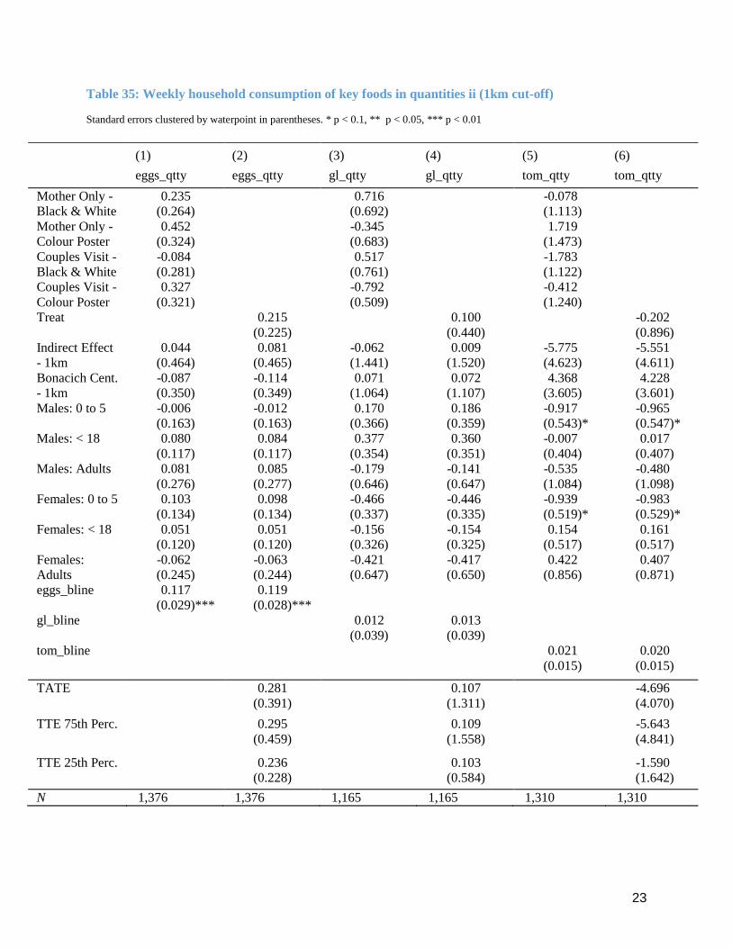
23
Table 35: Weekly household consumption of key foods in quantities ii (1km cut-off)
Standard errors clustered by waterpoint in parentheses. * p < 0.1, ** p < 0.05, *** p < 0.01
(1)
eggs_qtty
(2)
eggs_qtty
(3)
gl_qtty
(4)
gl_qtty
(5)
tom_qtty
(6)
tom_qtty
Mother Only - 0.235 0.716 -0.078
Black & White (0.264) (0.692) (1.113)
Mother Only - 0.452 -0.345 1.719
Colour Poster (0.324) (0.683) (1.473)
Couples Visit - -0.084 0.517 -1.783
Black & White (0.281) (0.761) (1.122)
Couples Visit - 0.327 -0.792 -0.412
Colour Poster (0.321) (0.509) (1.240)
Treat 0.215 0.100 -0.202
(0.225) (0.440) (0.896)
Indirect Effect 0.044 0.081 -0.062 0.009 -5.775 -5.551
- 1km (0.464) (0.465) (1.441) (1.520) (4.623) (4.611)
Bonacich Cent. -0.087 -0.114 0.071 0.072 4.368 4.228
- 1km (0.350) (0.349) (1.064) (1.107) (3.605) (3.601)
Males: 0 to 5 -0.006 -0.012 0.170 0.186 -0.917 -0.965
(0.163) (0.163) (0.366) (0.359) (0.543)* (0.547)*
Males: < 18 0.080 0.084 0.377 0.360 -0.007 0.017
(0.117) (0.117) (0.354) (0.351) (0.404) (0.407)
Males: Adults 0.081 0.085 -0.179 -0.141 -0.535 -0.480
(0.276) (0.277) (0.646) (0.647) (1.084) (1.098)
Females: 0 to 5 0.103 0.098 -0.466 -0.446 -0.939 -0.983
(0.134) (0.134) (0.337) (0.335) (0.519)* (0.529)*
Females: < 18 0.051 0.051 -0.156 -0.154 0.154 0.161
(0.120) (0.120) (0.326) (0.325) (0.517) (0.517)
Females: -0.062 -0.063 -0.421 -0.417 0.422 0.407
Adults (0.245) (0.244) (0.647) (0.650) (0.856) (0.871)
eggs_bline 0.117 0.119
(0.029)*** (0.028)***
gl_bline 0.012 0.013
(0.039) (0.039)
tom_bline 0.021 0.020
(0.015) (0.015)
TATE 0.281 0.107 -4.696
(0.391) (1.311) (4.070)
TTE 75th Perc. 0.295
(0.459)
0.109
(1.558)
-5.643
(4.841)
TTE 25th Perc. 0.236
(0.228)
0.103
(0.584)
-1.590
(1.642)
N 1,376 1,376 1,165 1,165 1,310 1,310

24
Table 36: Weekly household consumption of key foods in quantities iii (1km cut-off)
(1)
maizef_qtty
(2)
maizef_qtty
(3)
pmilk_qtty
(4)
pmilk_qtty
(5)
ban_qtty
(6)
ban_qtty
Mother Only - -0.828 -0.176 0.344
Black & White (0.449)* (0.268) (0.804)
Mother Only - -0.770 0.293 0.241
Colour Poster (0.468) (0.308) (0.754)
Couples Visit - -0.635 -0.177 -0.031
Black & White (0.478) (0.283) (0.840)
Couples Visit - -0.260 -0.376 -0.165
Colour Poster (0.583) (0.275) (0.923)
Treat -0.639 -0.113 0.108
(0.399) (0.216) (0.666)
Indirect Effect 0.958 0.925 0.564 0.554 0.116 0.165
- 1km (0.644) (0.645) (0.502) (0.505) (1.723) (1.738)
Bonacich Cent. -1.221 -1.215 -0.561 -0.552 -0.303 -0.318
- 1km (0.500)** (0.504)** (0.390) (0.394) (1.260) (1.259)
Males: 0 to 5 0.167 0.175 0.026 0.019 0.269 0.258
(0.229) (0.228) (0.129) (0.128) (0.526) (0.523)
Males: < 18 0.703 0.707 -0.067 -0.069 -0.102 -0.104
(0.187)*** (0.189)*** (0.087) (0.087) (0.243) (0.243)
Males: Adults 0.583 0.555 0.341 0.365 -0.012 0.002
(0.424) (0.423) (0.300) (0.304) (0.522) (0.528)
Females: 0 to 5 0.166 0.170 -0.065 -0.074 0.402 0.399
(0.236) (0.236) (0.117) (0.118) (0.755) (0.752)
Females: < 18 0.496 0.498 0.044 0.045 0.368 0.366
(0.164)*** (0.164)*** (0.092) (0.092) (0.451) (0.451)
Females: 0.950 0.946 0.161 0.161 0.441 0.441
Adults (0.499)* (0.497)* (0.241) (0.238) (0.742) (0.740)
TATE 0.110 0.335 0.242
(0.513) (0.409) (1.250)
TTE 75th Perc. 0.267
(0.595)
0.430
(0.485)
0.270
(1.518)
TTE 25th Perc. -0.408
(0.365)
0.026
(0.220)
0.150
(0.605)
N 1,386 1,386 1,200 1,200 1,346 1,346 Standard errors clustered by waterpoint in parentheses. * p < 0.1, ** p < 0.05, *** p < 0.01

25
Table 37: Weekly household consumption of key foods in quantities i (2km cut-off)
(1)
meat_qtty
(2)
meat_qtty
(3)
gn_qtty
(4)
gn_qtty
(5)
omena_qtty
(6)
omena_qtty
Mother Only - 0.044 -0.029 0.014
Black & White (0.050) (0.035) (0.051)
Mother Only - 0.081 -0.030 0.053
Colour Poster (0.059) (0.039) (0.053)
Couples Visit - 0.050 -0.016 -0.011
Black & White (0.048) (0.034) (0.046)
Couples Visit - 0.108 -0.030 0.005
Colour Poster (0.061)* (0.036) (0.060)
Treat 0.067 -0.026 0.014
(0.037)* (0.028) (0.035)
Indirect Effect 0.094 0.094 0.151 0.148 -0.150 -0.138
- 2km (0.112) (0.110) (0.064)** (0.065)** (0.102) (0.098)
Bonacich Cent. -0.050 -0.051 -0.092 -0.090 0.115 0.107
- 2km (0.074) (0.073) (0.043)** (0.043)** (0.070)* (0.068)
Males: 0 to 5 -0.024 -0.024 -0.007 -0.007 -0.015 -0.016
(0.024) (0.024) (0.019) (0.019) (0.023) (0.023)
Males: < 18 0.024 0.024 0.003 0.003 0.035 0.034
(0.020) (0.020) (0.012) (0.012) (0.021) (0.021)
Males: Adults 0.013 0.012 0.017 0.017 -0.125 -0.124
(0.047) (0.047) (0.027) (0.027) (0.044)*** (0.044)***
Females: 0 to 5 0.003 0.002 -0.014 -0.014 0.032 0.031
(0.023) (0.023) (0.017) (0.017) (0.024) (0.024)
Females: < 18 -0.019 -0.019 0.006 0.006 0.029 0.029
(0.018) (0.018) (0.012) (0.012) (0.025) (0.025)
Females: 0.015 0.015 -0.015 -0.015 -0.031 -0.031
Adults (0.055) (0.055) (0.024) (0.024) (0.056) (0.055)
meat_bline 0.253 0.252
(0.034)*** (0.034)***
gn_bline 0.056 0.056
(0.032)* (0.032)*
omena_bline 0.126 0.129
(0.033)*** (0.033)***
TATE 0.273 0.297 -0.286
(0.238) (0.141)** (0.213)
TTE 75th Perc. 0.279
(0.245)
0.307
(0.146)**
-0.295
(0.219)
TTE 25th Perc. 0.148
(0.097)
0.100
(0.059)*
-0.103
(0.086)
N 1,389 1,389 1,342 1,342 1,276 1,276 Standard errors clustered by waterpoint in parentheses. * p < 0.1, ** p < 0.05, *** p < 0.01
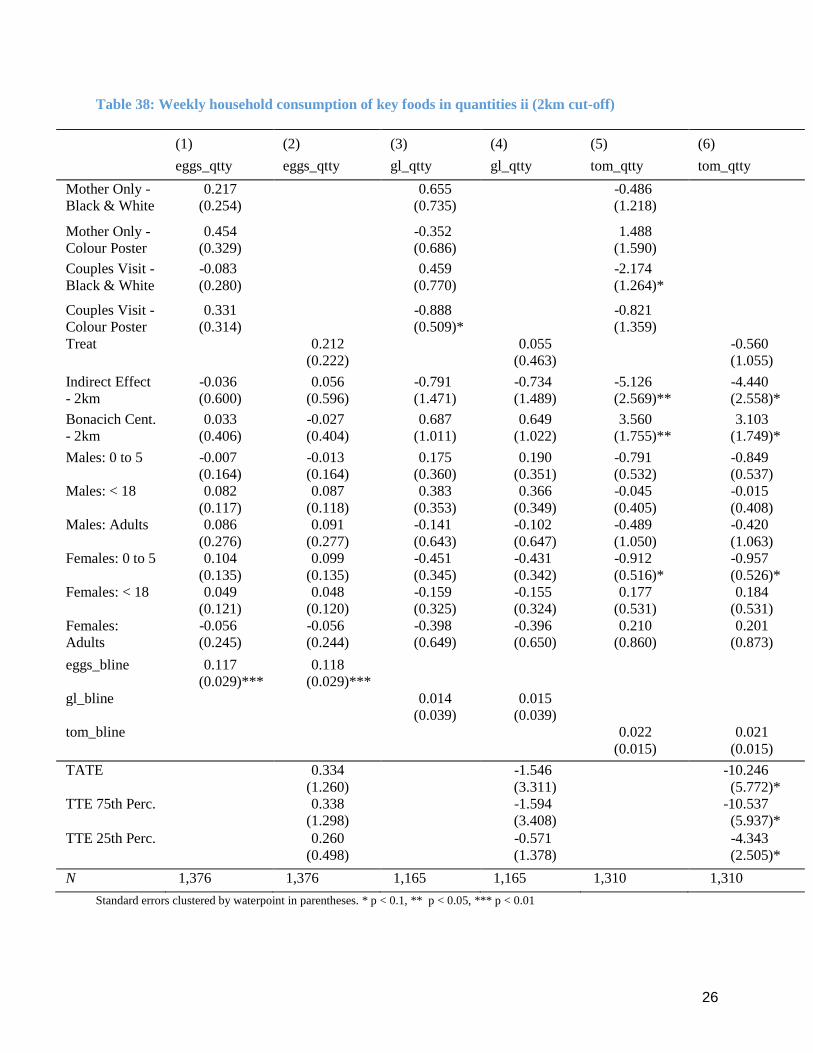
26
Table 38: Weekly household consumption of key foods in quantities ii (2km cut-off)
Standard errors clustered by waterpoint in parentheses. * p < 0.1, ** p < 0.05, *** p < 0.01
(1)
eggs_qtty
(2)
eggs_qtty
(3)
gl_qtty
(4)
gl_qtty
(5)
tom_qtty
(6)
tom_qtty
Mother Only - 0.217 0.655 -0.486
Black & White (0.254) (0.735) (1.218)
Mother Only - 0.454 -0.352 1.488
Colour Poster (0.329) (0.686) (1.590)
Couples Visit - -0.083 0.459 -2.174
Black & White (0.280) (0.770) (1.264)*
Couples Visit - 0.331 -0.888 -0.821
Colour Poster (0.314) (0.509)* (1.359)
Treat 0.212 0.055 -0.560
(0.222) (0.463) (1.055)
Indirect Effect -0.036 0.056 -0.791 -0.734 -5.126 -4.440
- 2km (0.600) (0.596) (1.471) (1.489) (2.569)** (2.558)*
Bonacich Cent. 0.033 -0.027 0.687 0.649 3.560 3.103
- 2km (0.406) (0.404) (1.011) (1.022) (1.755)** (1.749)*
Males: 0 to 5 -0.007 -0.013 0.175 0.190 -0.791 -0.849
(0.164) (0.164) (0.360) (0.351) (0.532) (0.537)
Males: < 18 0.082 0.087 0.383 0.366 -0.045 -0.015
(0.117) (0.118) (0.353) (0.349) (0.405) (0.408)
Males: Adults 0.086 0.091 -0.141 -0.102 -0.489 -0.420
(0.276) (0.277) (0.643) (0.647) (1.050) (1.063)
Females: 0 to 5 0.104 0.099 -0.451 -0.431 -0.912 -0.957
(0.135) (0.135) (0.345) (0.342) (0.516)* (0.526)*
Females: < 18 0.049 0.048 -0.159 -0.155 0.177 0.184
(0.121) (0.120) (0.325) (0.324) (0.531) (0.531)
Females: -0.056 -0.056 -0.398 -0.396 0.210 0.201
Adults (0.245) (0.244) (0.649) (0.650) (0.860) (0.873)
eggs_bline 0.117 0.118
(0.029)*** (0.029)***
gl_bline 0.014 0.015
(0.039) (0.039)
tom_bline 0.022 0.021
(0.015) (0.015)
TATE 0.334 -1.546 -10.246
(1.260) (3.311) (5.772)*
TTE 75th Perc. 0.338
(1.298)
-1.594
(3.408)
-10.537
(5.937)*
TTE 25th Perc. 0.260
(0.498)
-0.571
(1.378)
-4.343
(2.505)*
N 1,376 1,376 1,165 1,165 1,310 1,310

27
Table 39: Weekly household consumption of key foods in quantities iii (2km cut-off)
(1)
maizef_qtty
(2)
maizef_qtty
(3)
pmilk_qtty
(4)
pmilk_qtty
(5)
ban_qtty
(6)
ban_qtty
Mother Only - -0.831 -0.179 0.270
Black & White (0.439)* (0.260) (0.800)
Mother Only - -0.709 0.319 0.293
Colour Poster (0.468) (0.306) (0.717)
Couples Visit - -0.566 -0.140 -0.040
Black & White (0.462) (0.287) (0.835)
Couples Visit - -0.070 -0.326 -0.155
Colour Poster (0.576) (0.271) (0.822)
Treat -0.570 -0.088 0.101
(0.383) (0.213) (0.616)
Indirect Effect 0.280 0.197 0.279 0.337 -1.451 -1.369
- 2km (0.828) (0.825) (0.495) (0.511) (2.473) (2.390)
Bonacich Cent. -0.361 -0.304 -0.181 -0.222 1.108 1.053
- 2km (0.546) (0.547) (0.332) (0.343) (1.718) (1.665)
Males: 0 to 5 0.137 0.148 0.013 0.006 0.282 0.270
(0.230) (0.229) (0.128) (0.127) (0.522) (0.518)
Males: < 18 0.703 0.708 -0.057 -0.059 -0.094 -0.095
(0.188)*** (0.190)*** (0.088) (0.088) (0.250) (0.249)
Males: Adults 0.510 0.475 0.366 0.389 -0.003 0.012
(0.424) (0.424) (0.301) (0.305) (0.527) (0.531)
Females: 0 to 5 0.139 0.144 -0.063 -0.073 0.419 0.414
(0.238) (0.238) (0.117) (0.118) (0.754) (0.752)
Females: < 18 0.477 0.478 0.035 0.037 0.362 0.362
(0.162)*** (0.162)*** (0.091) (0.092) (0.452) (0.452)
Females: 0.992 0.987 0.198 0.197 0.468 0.469
Adults (0.500)** (0.498)** (0.241) (0.238) (0.734) (0.731)
TATE -0.411 0.185 -1.008
(0.711) (0.456) (2.114)
TTE 75th Perc. -0.378
(0.833)
0.242
(0.534)
-1.241
(2.507)
TTE 25th Perc. -0.521
(0.403)
-0.004
(0.243)
-0.241
(0.918)
N 1,386 1,386 1,200 1,200 1,346 1,346
Standard errors clustered by waterpoint in parentheses. * p < 0.1, ** p < 0.05, *** p < 0.01
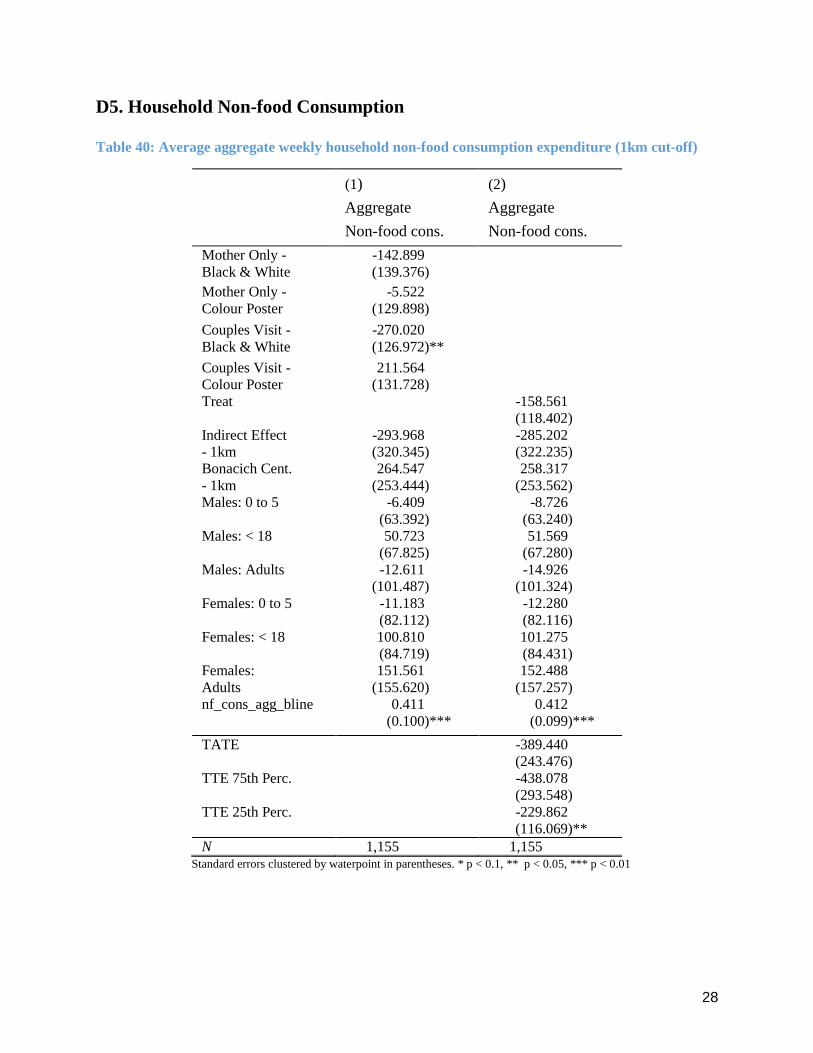
28
D5. Household Non-food Consumption
Table 40: Average aggregate weekly household non-food consumption expenditure (1km cut-off)
(1)
Aggregate
Non-food cons.
(2)
Aggregate
Non-food cons.
Mother Only - -142.899
Black & White (139.376)
Mother Only - -5.522
Colour Poster (129.898)
Couples Visit - -270.020
Black & White (126.972)**
Couples Visit - 211.564
Colour Poster (131.728)
Treat -158.561
(118.402)
Indirect Effect -293.968 -285.202
- 1km (320.345) (322.235)
Bonacich Cent. 264.547 258.317
- 1km (253.444) (253.562)
Males: 0 to 5 -6.409 -8.726
(63.392) (63.240)
Males: < 18 50.723 51.569
(67.825) (67.280)
Males: Adults -12.611 -14.926
(101.487) (101.324)
Females: 0 to 5 -11.183 -12.280
(82.112) (82.116)
Females: < 18 100.810 101.275
(84.719) (84.431)
Females: 151.561 152.488
Adults (155.620) (157.257)
nf_cons_agg_bline 0.411 0.412
(0.100)*** (0.099)***
TATE -389.440
(243.476)
TTE 75th Perc. -438.078
(293.548)
TTE 25th Perc. -229.862
(116.069)**
N 1,155 1,155 Standard errors clustered by waterpoint in parentheses. * p < 0.1, ** p < 0.05, *** p < 0.01

29
Table 41: Average aggregate weekly household non-food consumption expenditure (2km cut-off)
(1)
Aggregate
Non-food cons.
(2)
Aggregate
Non-food cons.
Mother Only - -195.469
Black & White (132.529)
Mother Only - 11.860
Colour Poster (128.320)
Couples Visit - -293.950
Black & White (118.952)**
Couples Visit - 190.475
Colour Poster (134.639)
Treat -198.007
(109.721)*
Indirect Effect 132.330 139.561
- 2km (252.548) (246.850)
Bonacich Cent. -39.015 -43.170
- 2km (173.542) (169.304)
Males: 0 to 5 -3.516 -5.387
(63.024) (62.928)
Males: < 18 56.044 57.166
(67.243) (66.755)
Males: Adults 18.631 16.704
(100.252) (99.575)
Females: 0 to 5 -5.513 -6.609
(81.105) (81.115)
Females: < 18 102.442 102.934
(84.084) (83.832)
Females: 141.387 142.022
Adults (153.820) (154.936)
nf_cons_agg_bline 0.401 0.401
(0.101)*** (0.100)***
TATE 106.442
(529.909)
TTE 75th Perc. 115.585
(545.751)
TTE 25th Perc. -79.111
(219.042)
N 1,155 1,155 Standard errors clustered by waterpoint in parentheses. * p < 0.1, ** p < 0.05, *** p < 0.01
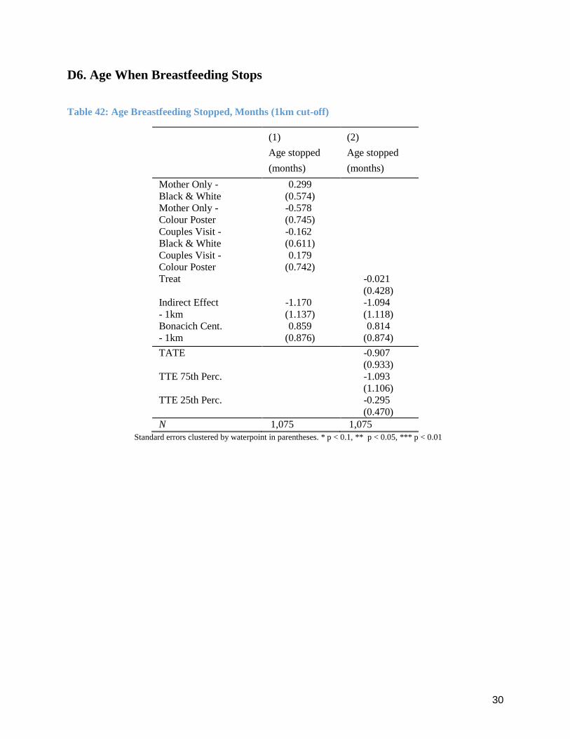
30
D6. Age When Breastfeeding Stops
Table 42: Age Breastfeeding Stopped, Months (1km cut-off)
(1)
Age stopped
(months)
(2)
Age stopped
(months)
Mother Only - 0.299
Black & White (0.574)
Mother Only - -0.578
Colour Poster (0.745)
Couples Visit - -0.162
Black & White (0.611)
Couples Visit - 0.179
Colour Poster (0.742)
Treat -0.021
(0.428)
Indirect Effect -1.170 -1.094
- 1km (1.137) (1.118)
Bonacich Cent. 0.859 0.814
- 1km (0.876) (0.874)
TATE -0.907
(0.933)
TTE 75th Perc. -1.093
(1.106)
TTE 25th Perc. -0.295
(0.470)
N 1,075 1,075
Standard errors clustered by waterpoint in parentheses. * p < 0.1, ** p < 0.05, *** p < 0.01

31
Table 43: Age Breastfeeding Stopped, Months (2km cut-off)
(1)
Age stopped
(months)
(2)
Age stopped
(months)
Mother Only - 0.388
Black & White (0.554)
Mother Only - -0.591
Colour Poster (0.729)
Couples Visit - -0.239
Black & White (0.584)
Couples Visit - 0.297
Colour Poster (0.758)
Treat 0.013
(0.418)
Indirect Effect -2.528 -2.436
- 2km (1.115)** (1.091)**
Bonacich Cent. 1.542 1.485
- 2km (0.744)** (0.729)**
TATE -5.302
(2.389)**
TTE 75th Perc. -5.461
(2.460)**
TTE 25th Perc. -2.062
(0.994)**
N 1,075 1,075 Standard errors clustered by waterpoint in parentheses. * p < 0.1, ** p < 0.05, *** p < 0.01
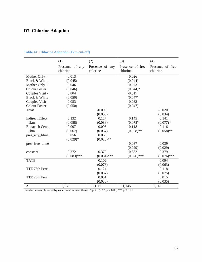
32
D7. Chlorine Adoption
Table 44: Chlorine Adoption (1km cut-off)
(1)
Presence of any
chlorine
(2)
Presence of any
chlorine
(3)
Presence of free
chlorine
(4)
Presence of free
chlorine
Mother Only - -0.013 -0.026
Black & White (0.045) (0.044)
Mother Only - -0.046 -0.073
Colour Poster (0.046) (0.044)*
Couples Visit - 0.004 -0.017
Black & White (0.050) (0.047)
Couples Visit - 0.053 0.033
Colour Poster (0.050) (0.047)
Treat -0.000 -0.020
(0.035) (0.034)
Indirect Effect 0.132 0.127 0.145 0.141
- 1km (0.088) (0.088) (0.078)* (0.077)*
Bonacich Cent. -0.097 -0.095 -0.118 -0.116
- 1km (0.067) (0.067) (0.058)** (0.058)**
pres_any_bline 0.056 0.059
(0.029)* (0.028)**
pres_free_bline 0.037 0.039
(0.029) (0.029)
constant 0.372 0.370 0.382 0.379
(0.083)*** (0.084)*** (0.076)*** (0.076)***
TATE 0.102 0.094
(0.073) (0.063)
TTE 75th Perc. 0.124 0.118
(0.087) (0.075)
TTE 25th Perc. 0.031 0.015
(0.038) (0.035)
N 1,155 1,155 1,145 1,145 Standard errors clustered by waterpoint in parentheses. * p < 0.1, ** p < 0.05, *** p < 0.01

33
Table 45: Chlorine Adoption (2km cut-off)
(1)
Presence of any
chlorine
(2)
Presence of any
chlorine
(3)
Presence of free
chlorine
(4)
Presence of free
chlorine
Mother Only - -0.011 -0.020
Black & White (0.044) (0.044)
Mother Only - -0.037 -0.061
Colour Poster (0.045) (0.043)
Couples Visit - 0.010 -0.008
Black & White (0.049) (0.047)
Couples Visit - 0.056 0.043
Colour Poster (0.050) (0.047)
Treat 0.004 -0.012
(0.034) (0.034)
Indirect Effect 0.037 0.022 0.040 0.024
- 2km (0.098) (0.099) (0.094) (0.095)
Bonacich Cent. -0.011 -0.000 -0.023 -0.011
- 2km (0.066) (0.067) (0.063) (0.063)
tcr_adoption_bline 0.055 0.058
(0.029)* (0.029)**
fcr_adoption_bline 0.038 0.040
(0.029) (0.029)
constant 0.248 0.236 0.259 0.246
(0.073)*** (0.074)*** (0.068)*** (0.069)***
TATE 0.051 0.041
(0.216) (0.209)
TTE 75th Perc. 0.053 0.042
(0.223) (0.215)
TTE 25th Perc. 0.022 0.009
(0.089) (0.087)
N 1,155 1,155 1,145 1,145 Standard errors clustered by waterpoint in parentheses. * p < 0.1, ** p < 0.05, *** p < 0.01

34
D8. Labour Supply
Table 46: Female respondent labour supply (1km cut-off)
(1)
Mother
working
(2)
Mother
working
(3)
Mother working
second job
(4)
Mother working
second job
Mother Only - 0.041 0.015
Black & White (0.047) (0.024)
Mother Only - -0.116 -0.042
Colour Poster (0.052)** (0.021)**
Couples Visit - 0.017 -0.032
Black & White (0.046) (0.020)
Couples Visit - -0.021 -0.028
Colour Poster (0.042) (0.021)
Treat -0.015 -0.020
(0.036) (0.017)
Indirect Effect 0.013 0.017 -0.055 -0.049
- 1km (0.084) (0.087) (0.048) (0.050)
Bonacich Cent. -0.009 -0.009 0.047 0.045
- 1km (0.063) (0.065) (0.036) (0.037)
mi_working_bline 0.111 0.111
(0.028)*** (0.028)***
mi_work_oth_bline 0.106 0.107
(0.045)** (0.044)**
constant 0.447 0.445 0.025 0.026
(0.085)*** (0.086)*** (0.042) (0.043)
TATE -0.001 -0.060
(0.072) (0.040)
TTE 75th Perc. 0.002 -0.068
(0.085) (0.048)
TTE 25th Perc. -0.010 -0.032
(0.038) (0.019)*
N 1,393 1,393 1,393 1,393 Standard errors clustered by waterpoint in parentheses. * p < 0.1, ** p < 0.05, *** p < 0.01

35
Table 47: Female respondent labour supply (2km cut-off)
(1)
Mother
working
(2)
Mother
working
(3)
Mother working
second job
(4)
Mother working
second job
Mother Only - 0.044 0.012
Black & White (0.046) (0.024)
Mother Only - -0.113 -0.045
Colour Poster (0.051)** (0.021)**
Couples Visit - 0.017 -0.035
Black & White (0.046) (0.020)*
Couples Visit - -0.020 -0.033
Colour Poster (0.041) (0.021)
Treat -0.012 -0.023
(0.035) (0.017)
Indirect Effect -0.072 -0.084 -0.016 -0.011
- 2km (0.096) (0.099) (0.043) (0.044)
Bonacich Cent. 0.049 0.058 0.011 0.009
- 2km (0.064) (0.066) (0.029) (0.029)
mi_working_bline 0.111 0.111
(0.028)*** (0.028)***
mi_work_oth_bline 0.104 0.104
(0.045)** (0.044)**
constant 0.387 0.377 0.068 0.070
(0.075)*** (0.077)*** (0.033)** (0.034)**
TATE -0.196 -0.048
(0.218) (0.097)
TTE 75th Perc. -0.201 -0.049
(0.224) (0.100)
TTE 25th Perc. -0.084 -0.033
(0.090) (0.041)
N 1,393 1,393 1,393 1,393 Standard errors clustered by waterpoint in parentheses. * p < 0.1, ** p < 0.05, *** p < 0.01

36
Table 48: Spousal labour supply (1km cut-off)
(1)
Spouse
working
(2)
Spouse
working
(3)
Spouse working
second job
(4)
Spouse working
second job
Mother Only - 0.029 0.028
Black & White (0.035) (0.030)
Mother Only - -0.072 -0.008
Colour Poster (0.043)* (0.026)
Couples Visit - -0.045 -0.008
Black & White (0.046) (0.025)
Couples Visit - -0.062 0.000
Colour Poster (0.042) (0.027)
Treat -0.033 0.004
(0.030) (0.020)
Indirect Effect 0.025 0.039 -0.003 0.003
- 1km (0.069) (0.068) (0.065) (0.065)
Bonacich Cent. -0.003 -0.008 0.000 -0.002
- 1km (0.054) (0.053) (0.049) (0.049)
sp_working_bline 0.053 0.055
(0.041) (0.041)
sp_work_oth_bline 0.010 0.011
(0.029) (0.029)
constant 0.649 0.651 0.091 0.092
(0.074)*** (0.074)*** (0.055)* (0.055)*
TATE -0.002 0.006
(0.058) (0.053)
TTE 75th Perc. 0.004 0.007
(0.068) (0.064)
TTE 25th Perc. -0.024 0.005
(0.032) (0.024)
N 1,125 1,125 1,125 1,125 Standard errors clustered by waterpoint in parentheses. * p < 0.1, ** p < 0.05, *** p < 0.01

37
Table 49: Spousal labour supply (2km cut-off)
(1)
Spouse
working
(2)
Spouse
working
(3)
Spouse working
second job
(4)
Spouse working
second job
Mother Only - 0.033 0.029
Black & White (0.035) (0.029)
Mother Only - -0.070 -0.006
Colour Poster (0.043) (0.027)
Couples Visit - -0.044 -0.009
Black & White (0.045) (0.025)
Couples Visit - -0.063 -0.000
Colour Poster (0.042) (0.027)
Treat -0.031 0.005
(0.029) (0.020)
Indirect Effect -0.011 -0.001 -0.067 -0.061
- 2km (0.079) (0.083) (0.058) (0.057)
Bonacich Cent. 0.014 0.008 0.047 0.043
- 2km (0.053) (0.055) (0.039) (0.039)
sp_working_bline 0.053 0.055
(0.041) (0.041)
sp_working_other_blin
e
0.010 0.011
(0.029) (0.029)
constant 0.630 0.633 0.041 0.044
(0.067)*** (0.067)*** (0.043) (0.043)
TATE -0.034 -0.129
(0.183) (0.122)
TTE 75th Perc. -0.034 -0.133
(0.189) (0.126)
TTE 25th Perc. -0.032 -0.047
(0.077) (0.049)
N 1,125 1,125 1,125 1,125 Standard errors clustered by waterpoint in parentheses. * p < 0.1, ** p < 0.05, *** p < 0.01
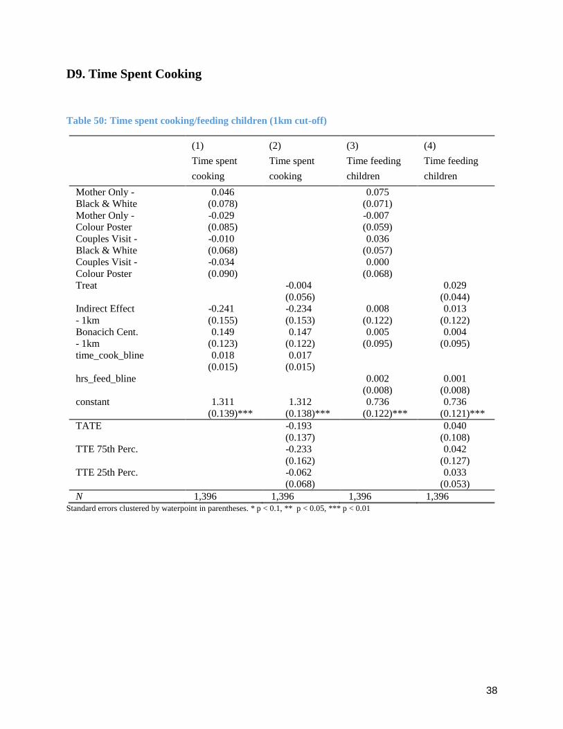
38
D9. Time Spent Cooking
Table 50: Time spent cooking/feeding children (1km cut-off)
(1)
Time spent
cooking
(2)
Time spent
cooking
(3)
Time feeding
children
(4)
Time feeding
children
Mother Only - 0.046 0.075
Black & White (0.078) (0.071)
Mother Only - -0.029 -0.007
Colour Poster (0.085) (0.059)
Couples Visit - -0.010 0.036
Black & White (0.068) (0.057)
Couples Visit - -0.034 0.000
Colour Poster (0.090) (0.068)
Treat -0.004 0.029
(0.056) (0.044)
Indirect Effect -0.241 -0.234 0.008 0.013
- 1km (0.155) (0.153) (0.122) (0.122)
Bonacich Cent. 0.149 0.147 0.005 0.004
- 1km (0.123) (0.122) (0.095) (0.095)
time_cook_bline 0.018 0.017
(0.015) (0.015)
hrs_feed_bline 0.002 0.001
(0.008) (0.008)
constant 1.311 1.312 0.736 0.736
(0.139)*** (0.138)*** (0.122)*** (0.121)***
TATE -0.193 0.040
(0.137) (0.108)
TTE 75th Perc. -0.233 0.042
(0.162) (0.127)
TTE 25th Perc. -0.062 0.033
(0.068) (0.053)
N 1,396 1,396 1,396 1,396 Standard errors clustered by waterpoint in parentheses. * p < 0.1, ** p < 0.05, *** p < 0.01

39
Table 51: Time spent cooking/feeding child (2km cut-off)
Standard errors clustered by waterpoint in parentheses. * p < 0.1, ** p < 0.05, *** p < 0.01
(1)
Time spent
cooking
(2)
Time spent
cooking
(3)
Time feeding
children
(4)
Time feeding
children
Mother Only - 0.021 0.067
Black & White (0.077) (0.070)
Mother Only - -0.038 -0.008
Colour Poster (0.086) (0.058)
Couples Visit - -0.027 0.033
Black & White (0.069) (0.057)
Couples Visit - -0.049 -0.013
Colour Poster (0.092) (0.068)
Treat -0.020 0.024
(0.056) (0.044)
Indirect Effect -0.268 -0.263 -0.047 -0.046
- 2km (0.162)* (0.161) (0.117) (0.116)
Bonacich Cent. 0.183 0.180 0.058 0.058
- 2km (0.110)* (0.110) (0.083) (0.081)
time_cook_bline 0.021 0.020
(0.015) (0.015)
hrs_feed_bline 0.004 0.003
(0.009) (0.009)
constant 1.267 1.271 0.630 0.631
(0.129)*** (0.129)*** (0.117)*** (0.115)***
TATE -0.594 -0.076
(0.354)* (0.256)
TTE 75th Perc. -0.612 -0.079
(0.365)* (0.263)
TTE 25th Perc. -0.244 -0.015
(0.147)* (0.107)
N 1,396 1,396 1,396 1,396
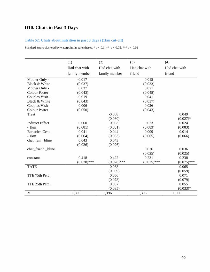
40
D10. Chats in Past 3 Days
Table 52: Chats about nutrition in past 3 days i (1km cut-off)
Standard errors clustered by waterpoint in parentheses. * p < 0.1, ** p < 0.05, *** p < 0.01
(1)
Had chat with
family member
(2)
Had chat with
family member
(3)
Had chat with
friend
(4)
Had chat with
friend
Mother Only - -0.017 0.015
Black & White (0.037) (0.033)
Mother Only - 0.037 0.071
Colour Poster (0.043) (0.048)
Couples Visit - -0.019 0.041
Black & White (0.043) (0.037)
Couples Visit - 0.006 0.026
Colour Poster (0.050) (0.043)
Treat -0.008 0.049
(0.030) (0.027)*
Indirect Effect 0.060 0.063 0.023 0.024
- 1km (0.081) (0.081) (0.083) (0.083)
Bonacich Cent. -0.041 -0.044 -0.009 -0.014
- 1km (0.064) (0.063) (0.065) (0.066)
chat_fam _bline 0.043 0.043
(0.026) (0.026)
chat_friend _bline 0.036 0.036
(0.025) (0.025)
constant 0.418 0.422 0.231 0.238
(0.078)*** (0.078)*** (0.075)*** (0.075)***
TATE 0.033 0.065
(0.059) (0.059)
TTE 75th Perc. 0.050 0.071
(0.078) (0.079)
TTE 25th Perc. 0.007 0.055
(0.035) (0.033)*
N 1,396 1,396 1,396 1,396
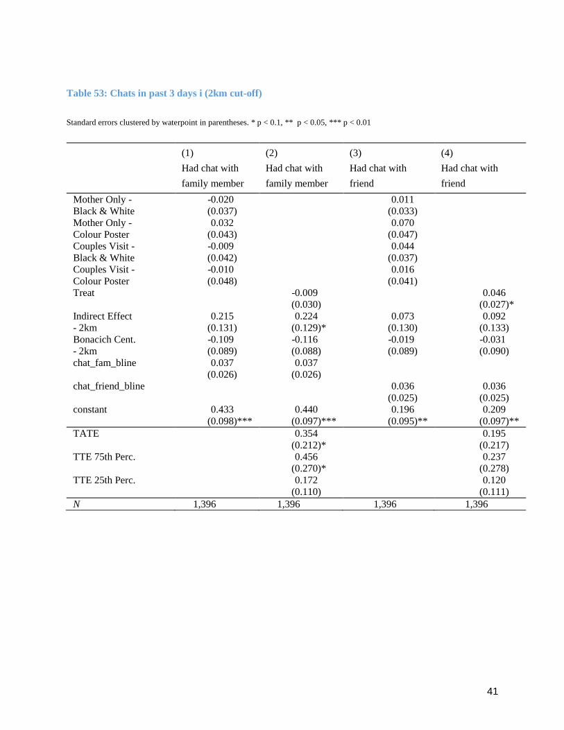
41
Table 53: Chats in past 3 days i (2km cut-off)
Standard errors clustered by waterpoint in parentheses. * p < 0.1, ** p < 0.05, *** p < 0.01
(1)
Had chat with
family member
(2)
Had chat with
family member
(3)
Had chat with
friend
(4)
Had chat with
friend
Mother Only - -0.020 0.011
Black & White (0.037) (0.033)
Mother Only - 0.032 0.070
Colour Poster (0.043) (0.047)
Couples Visit - -0.009 0.044
Black & White (0.042) (0.037)
Couples Visit - -0.010 0.016
Colour Poster (0.048) (0.041)
Treat -0.009 0.046
(0.030) (0.027)*
Indirect Effect 0.215 0.224 0.073 0.092
- 2km (0.131) (0.129)* (0.130) (0.133)
Bonacich Cent. -0.109 -0.116 -0.019 -0.031
- 2km (0.089) (0.088) (0.089) (0.090)
chat_fam_bline 0.037 0.037
(0.026) (0.026)
chat_friend_bline 0.036 0.036
(0.025) (0.025)
constant 0.433 0.440 0.196 0.209
(0.098)*** (0.097)*** (0.095)** (0.097)**
TATE 0.354 0.195
(0.212)* (0.217)
TTE 75th Perc. 0.456 0.237
(0.270)* (0.278)
TTE 25th Perc. 0.172 0.120
(0.110) (0.111)
N 1,396 1,396 1,396 1,396
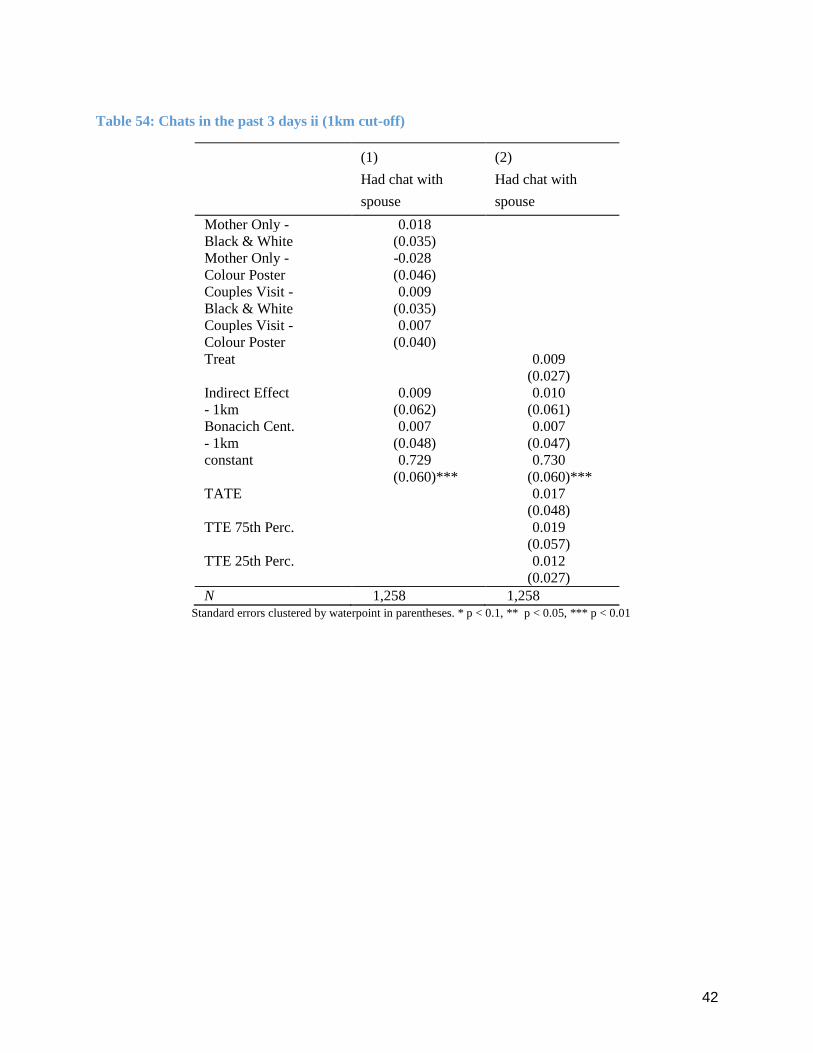
42
Table 54: Chats in the past 3 days ii (1km cut-off)
(1)
Had chat with
spouse
(2)
Had chat with
spouse
Mother Only - 0.018
Black & White (0.035)
Mother Only - -0.028
Colour Poster (0.046)
Couples Visit - 0.009
Black & White (0.035)
Couples Visit - 0.007
Colour Poster (0.040)
Treat 0.009
(0.027)
Indirect Effect 0.009 0.010
- 1km (0.062) (0.061)
Bonacich Cent. 0.007 0.007
- 1km (0.048) (0.047)
constant 0.729 0.730
(0.060)*** (0.060)***
TATE 0.017
(0.048)
TTE 75th Perc. 0.019
(0.057)
TTE 25th Perc. 0.012
(0.027)
N 1,258 1,258 Standard errors clustered by waterpoint in parentheses. * p < 0.1, ** p < 0.05, *** p < 0.01

43
Table 55: Chats in the past 3 days ii (2km cut-off)
(1)
Had chat with
spouse
(2)
Had chat with
spouse
Mother Only - 0.018
Black & White (0.033)
Mother Only - -0.032
Colour Poster (0.045)
Couples Visit - 0.011
Black & White (0.034)
Couples Visit - 0.003
Colour Poster (0.041)
Treat 0.008
(0.026)
Indirect Effect 0.107 0.104
- 2km (0.068) (0.067)
Bonacich Cent. -0.069 -0.068
- 2km (0.046) (0.046)
constant 0.810 0.808
(0.052)*** (0.052)***
TATE 0.236
(0.147)
TTE 75th Perc. 0.243
(0.151)
TTE 25th Perc. 0.097
(0.061)
N 1,258 1,258 Standard errors clustered by waterpoint in parentheses. * p < 0.1, ** p < 0.05, *** p < 0.01

44
D11. Incidence of Diarrhoea
Table 56: Incidence of Diarrhoea (1km cut-off)
Standard
errors clustered by
waterpoint in
parentheses. * p < 0.1, **
p < 0.05, *** p < 0.01
(1)
Index child
had diarrhoea in
past week
(2)
Index child
had diarrhoea in
past week
Mother Only - 0.023
Black & White (0.027)
Mother Only - -0.020
Colour Poster (0.027)
Couples Visit - -0.007
Black & White (0.030)
Couples Visit - 0.052
Colour Poster (0.039)
Treat 0.011
(0.022)
Indirect Effect -0.152 -0.150
- 1km (0.096) (0.097)
Bonacich Cent. 0.132 0.130
- 1km (0.073)* (0.074)*
ic_diarrhoea_bline 0.027 0.030
(0.022) (0.022)
constant -0.030 -0.028
(0.074) (0.075)
TATE -0.110
(0.084)
TTE 75th Perc. -0.136
(0.100)
TTE 25th Perc. -0.026
(0.034)
N 1,397 1,397
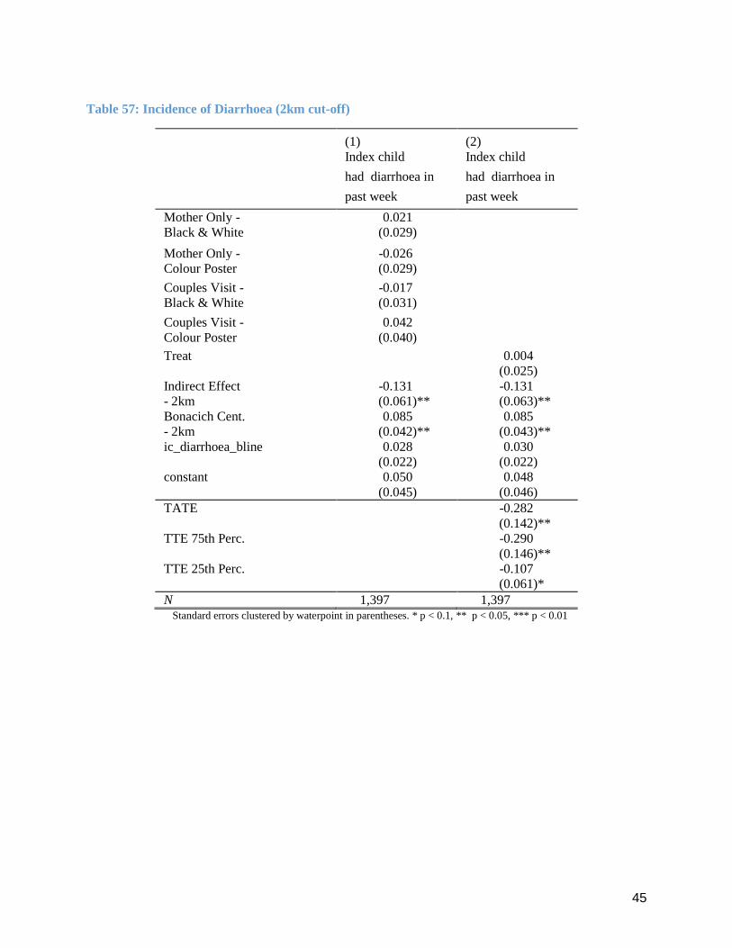
45
Table 57: Incidence of Diarrhoea (2km cut-off)
(1)
Index child
had diarrhoea in
past week
(2)
Index child
had diarrhoea in
past week
Mother Only - 0.021
Black & White (0.029)
Mother Only - -0.026
Colour Poster (0.029)
Couples Visit - -0.017
Black & White (0.031)
Couples Visit - 0.042
Colour Poster (0.040)
Treat 0.004
(0.025)
Indirect Effect -0.131 -0.131
- 2km (0.061)** (0.063)**
Bonacich Cent. 0.085 0.085
- 2km (0.042)** (0.043)**
ic_diarrhoea_bline 0.028 0.030
(0.022) (0.022)
constant 0.050 0.048
(0.045) (0.046)
TATE -0.282
(0.142)**
TTE 75th Perc. -0.290
(0.146)**
TTE 25th Perc. -0.107
(0.061)*
N 1,397 1,397 Standard errors clustered by waterpoint in parentheses. * p < 0.1, ** p < 0.05, *** p < 0.01

46
D12. Hygiene Practices
Table 58: Summary index for abidance by proper hygiene practices (1km cut-off)
(1)
Summary index of
hygiene practices
(2)
Summary index of
hygiene practices
Mother Only - -0.037
Black & White (0.051)
Mother Only - -0.013
Colour Poster (0.065)
Couples Visit - 0.024
Black & White (0.051)
Couples Visit - 0.018
Colour Poster (0.060)
Treat -0.006
(0.040)
Indirect Effect -0.035 -0.044
- 1km (0.091) (0.090)
Bonacich Cent. 0.019 0.023
- 1km (0.071) (0.070)
sum_index_hp_bline 0.027 0.026
(0.032) (0.032)
constant -0.011 -0.013
(0.088) (0.087)
TATE -0.041
(0.077)
TTE 75th Perc. -0.049
(0.090)
TTE 25th Perc. -0.017
(0.042)
N 1,396 1,396 Standard errors clustered by waterpoint in parentheses. * p < 0.1, ** p < 0.05, *** p < 0.01

47
Table 59: Summary index for abidance by proper hygiene practices (2km cut-off)
(1)
Summary index of
hygiene practices
(2)
Summary index of
hygiene practices
Mother Only - -0.052
Black & White (0.048)
Mother Only - -0.005
Colour Poster (0.065)
Couples Visit - 0.022
Black & White (0.050)
Couples Visit - 0.011
Colour Poster (0.059)
Treat -0.015
(0.039)
Indirect Effect 0.059 0.039
- 2km (0.096) (0.097)
Bonacich Cent. -0.026 -0.012
- 2km (0.065) (0.067)
sum_index_hp_bline 0.025 0.023
(0.033) (0.032)
constant 0.004 -0.009
(0.078) (0.079)
TATE 0.069
(0.210)
TTE 75th Perc. 0.072
(0.216)
TTE 25th Perc. 0.018
(0.086)
N 1,396 1,396 Standard errors clustered by waterpoint in parentheses. * p < 0.1, ** p < 0.05, *** p < 0.01
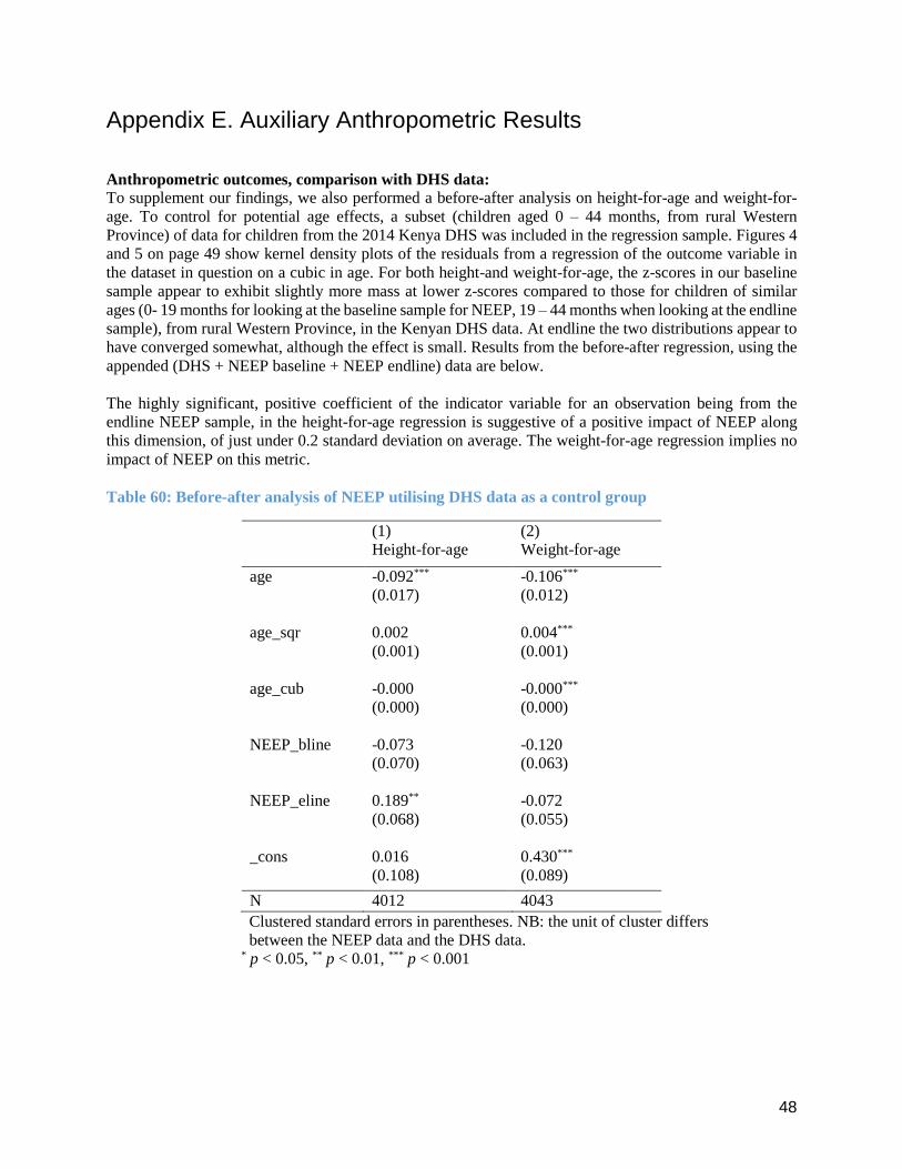
48
Appendix E. Auxiliary Anthropometric Results
Anthropometric outcomes, comparison with DHS data:
To supplement our findings, we also performed a before-after analysis on height-for-age and weight-for-
age. To control for potential age effects, a subset (children aged 0 – 44 months, from rural Western
Province) of data for children from the 2014 Kenya DHS was included in the regression sample. Figures 4
and 5 on page 49 show kernel density plots of the residuals from a regression of the outcome variable in
the dataset in question on a cubic in age. For both height-and weight-for-age, the z-scores in our baseline
sample appear to exhibit slightly more mass at lower z-scores compared to those for children of similar
ages (0- 19 months for looking at the baseline sample for NEEP, 19 – 44 months when looking at the endline
sample), from rural Western Province, in the Kenyan DHS data. At endline the two distributions appear to
have converged somewhat, although the effect is small. Results from the before-after regression, using the
appended (DHS + NEEP baseline + NEEP endline) data are below.
The highly significant, positive coefficient of the indicator variable for an observation being from the
endline NEEP sample, in the height-for-age regression is suggestive of a positive impact of NEEP along
this dimension, of just under 0.2 standard deviation on average. The weight-for-age regression implies no
impact of NEEP on this metric.
Table 60: Before-after analysis of NEEP utilising DHS data as a control group
(1) (2)
Height-for-age Weight-for-age
age -0.092*** -0.106***
(0.017) (0.012)
age_sqr 0.002 0.004***
(0.001) (0.001)
age_cub -0.000 -0.000***
(0.000) (0.000)
NEEP_bline -0.073 -0.120
(0.070) (0.063)
NEEP_eline 0.189** -0.072
(0.068) (0.055)
_cons 0.016 0.430***
(0.108) (0.089)
N 4012 4043
Clustered standard errors in parentheses. NB: the unit of cluster differs
between the NEEP data and the DHS data. * p < 0.05, ** p < 0.01, *** p < 0.001
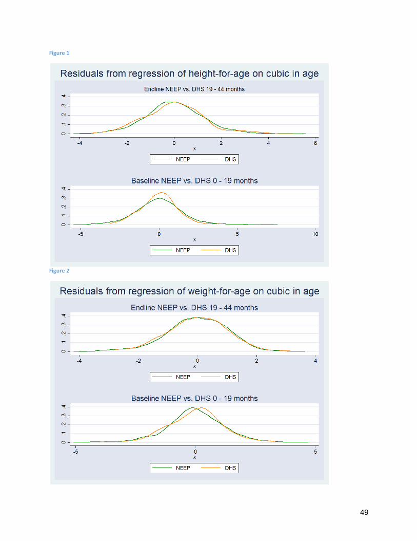
49
Figure 1
Figure 2
50
Original Regression Specification (Anthropometrics)
Anthropometric outcomes, original specifications:
As a check of the sensitivity of our results to the way that spillovers are measured, also included below are
the results from our original specification for the anthropometric regressions. Tables 65 - 69 present these
results; the variables diff_monly, diff_monlycol etc. simply count the number of waterpoints within a 1/2km
radius of the individual-of-observation’s waterpoint that belong to that treatment arm, and the variable
any_cluster counts the total number of waterpoints (to act as a rough control for any general geo-spatial
effects).
The results using the 1km radius are implicative of no treatment effects, and no significant spillover effects
as a result of having more treated waterpoints within a 1km radius of one’s own waterpoint. The
specification considering a 2km radius again implies no direct treatment effects, but several of the
coefficients capturing potential spillover effects are now positively signed and statistically significant.
When considering a 3km radius, the results are similar to in the 2km case; while at 5km significant
spillover effects disappear again.

51
Table 61: Anthropometric Indicators (original contamination controls, 1km cut-off)
(1)
Height-for-age
(2)
Height-for-age
(3)
Summary index of
other z-scores
(4)
Summary index of
other z-scores
monly 0.028 -0.023
(0.090) (0.044)
monlycol -0.088 0.021
(0.104) (0.052)
mandf 0.008 0.067
(0.109) (0.048)
mandfcol -0.004 -0.049
(0.101) (0.050)
treat -0.011 0.005
(0.074) (0.034)
diff_monly1 0.019
(0.066)
0.016
(0.065)
0.011
(0.032)
0.006
(0.034)
diff_monlycol1 -0.063
(0.086)
-0.062
(0.086)
0.013
(0.033)
0.015
(0.034)
diff_mandf1 0.040
(0.077)
0.033
(0.076)
0.045
(0.040)
0.039
(0.040)
diff_mandfcol1 -0.028
(0.074)
-0.026
(0.073)
0.033
(0.039)
0.027
(0.040)
any_cluster1 0.004 0.008 -0.015 -0.015
(0.041) (0.041) (0.020) (0.020)
zlen_bline 0.359*** 0.360***
(0.023) (0.023)
sum_index_oth
z_bline
0.502***
(0.024)
0.503***
(0.025)
age 0.209*** 0.209*** 0.012 0.012
(0.057) (0.057) (0.026) (0.027)
agesqr -0.004*** -0.004*** -0.000 -0.000
(0.001) (0.001) (0.000) (0.000)
fem 1.484 1.553 -0.032 -0.045
(1.507) (1.496) (0.632) (0.637)
age_fem -0.087 -0.092 0.015 0.016
(0.099) (0.098) (0.041) (0.042)
agesqr_fem 0.001 0.001 -0.001 -0.001
(0.002) (0.002) (0.001) (0.001)
_cons -4.145*** -4.154*** 0.022 0.010
(0.912) (0.911) (0.430) (0.437)
N 1359 1359 1388 1388

52
Table 62: Anthropometric Indicators (original contamination controls, 2km cut-off)
(1)
Height-for-age
(2)
Height-for-age
(3)
Summary index of
other z-scores
(4)
Summary index of
other z-scores
monly 0.024 -0.007
(0.086) (0.043)
monlycol -0.084 0.029
(0.099) (0.050)
mandf 0.027 0.074
(0.106) (0.046)
mandfcol 0.006 -0.046
(0.101) (0.050)
treat -0.005 0.013
(0.070) (0.033)
diff_ monly2 0.070**
(0.034)
0.064*
(0.034)
0.020
(0.017)
0.016
(0.017)
diff_ monlycol2 0.051
(0.038)
0.053
(0.037)
0.044**
(0.019)
0.043**
(0.020)
diff_ mandf2 0.030
(0.041)
0.022
(0.039)
0.043**
(0.022)
0.039*
(0.022)
diff_ mandfcol2 0.008
(0.034)
0.009
(0.034)
0.042**
(0.021)
0.038*
(0.021)
any_cluster2 -0.025 -0.023 -0.033*** -0.032***
(0.020) (0.020) (0.011) (0.010)
zlen_bline 0.357*** 0.359***
(0.023) (0.023)
sum_index_oth
z_bline
0.506***
(0.024)
0.507***
(0.024)
age 0.212*** 0.212*** 0.015 0.016
(0.056) (0.056) (0.026) (0.027)
agesqr -0.004*** -0.004*** -0.000 -0.000
(0.001) (0.001) (0.000) (0.000)
fem 1.387 1.444 -0.084 -0.093
(1.483) (1.475) (0.629) (0.635)
age_fem -0.081 -0.085 0.019 0.019
(0.097) (0.097) (0.041) (0.041)
agesqr_fem 0.001 0.001 -0.001 -0.001
(0.002) (0.002) (0.001) (0.001)
_cons -4.176*** -4.191*** 0.037 0.031
(0.903) (0.903) (0.427) (0.433)
N 1359 1359 1388 1388
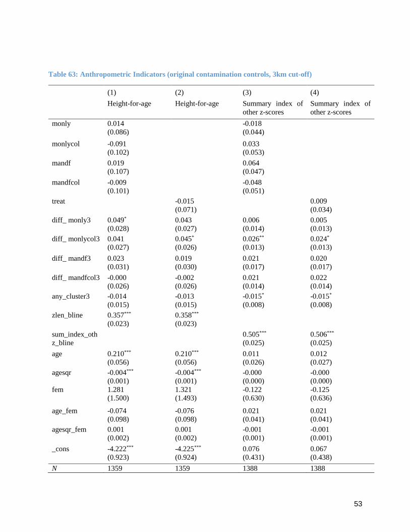
53
Table 63: Anthropometric Indicators (original contamination controls, 3km cut-off)
(1)
Height-for-age
(2)
Height-for-age
(3)
Summary index of
other z-scores
(4)
Summary index of
other z-scores
monly 0.014 -0.018
(0.086) (0.044)
monlycol -0.091 0.033
(0.102) (0.053)
mandf 0.019 0.064
(0.107) (0.047)
mandfcol -0.009 -0.048
(0.101) (0.051)
treat -0.015 0.009
(0.071) (0.034)
diff_ monly3 0.049*
(0.028)
0.043
(0.027)
0.006
(0.014)
0.005
(0.013)
diff_ monlycol3 0.041
(0.027)
0.045*
(0.026)
0.026**
(0.013)
0.024*
(0.013)
diff_ mandf3 0.023
(0.031)
0.019
(0.030)
0.021
(0.017)
0.020
(0.017)
diff_ mandfcol3 -0.000
(0.026)
-0.002
(0.026)
0.021
(0.014)
0.022
(0.014)
any_cluster3 -0.014 -0.013 -0.015* -0.015*
(0.015) (0.015) (0.008) (0.008)
zlen_bline 0.357*** 0.358***
(0.023) (0.023)
sum_index_oth
z_bline
0.505***
(0.025)
0.506***
(0.025)
age 0.210*** 0.210*** 0.011 0.012
(0.056) (0.056) (0.026) (0.027)
agesqr -0.004*** -0.004*** -0.000 -0.000
(0.001) (0.001) (0.000) (0.000)
fem 1.281 1.321 -0.122 -0.125
(1.500) (1.493) (0.630) (0.636)
age_fem -0.074 -0.076 0.021 0.021
(0.098) (0.098) (0.041) (0.041)
agesqr_fem 0.001 0.001 -0.001 -0.001
(0.002) (0.002) (0.001) (0.001)
_cons -4.222*** -4.225*** 0.076 0.067
(0.923) (0.924) (0.431) (0.438)
N 1359 1359 1388 1388

54
Table 64: Anthropometric Indicators (original contamination controls, 5km cut-off)
(1)
Height-for-age
(2)
Height-for-age
(3)
Summary index of
other z-scores
(4)
Summary index of
other z-scores
monly 0.012 -0.033
(0.084) (0.043)
monlycol -0.125 0.036
(0.100) (0.053)
mandf 0.005 0.053
(0.108) (0.045)
mandfcol -0.039 -0.048
(0.100) (0.051)
treat -0.033 0.003
(0.071) (0.033)
diff_ monly5 0.017
(0.023)
0.010
(0.023)
-0.022
(0.014)
-0.020
(0.014)
diff_ monlycol5 0.009
(0.020)
0.009
(0.020)
0.006
(0.011)
0.004
(0.012)
diff_ mandf5 0.010
(0.022)
0.005
(0.022)
0.001
(0.013)
0.002
(0.013)
diff_ mandfcol5 -0.033
(0.023)
-0.034
(0.022)
0.011
(0.012)
0.013
(0.012)
any_cluster5 0.003 0.006 0.000 -0.000
(0.012) (0.013) (0.007) (0.007)
zlen_bline 0.361*** 0.362***
(0.023) (0.023)
sum_index_oth
z_bline
0.504***
(0.024)
0.505***
(0.025)
age 0.217*** 0.217*** 0.013 0.013
(0.056) (0.056) (0.026) (0.026)
agesqr -0.004*** -0.004*** -0.000 -0.000
(0.001) (0.001) (0.000) (0.000)
fem 1.336 1.431 0.044 0.020
(1.490) (1.484) (0.622) (0.630)
age_fem -0.077 -0.084 0.010 0.011
(0.098) (0.097) (0.041) (0.041)
agesqr_fem 0.001 0.001 -0.000 -0.000
(0.002) (0.002) (0.001) (0.001)
_cons -4.426*** -4.427*** 0.039 0.037
(0.907) (0.909) (0.420) (0.429)
N 1359 1359 1388 1388

55
Appendix F: Other
Item Characteristic Curves
Figure 3
Figure 4