evaluation of the tiger superdarn over-the-horizon radar · pdf file ·...

The Centre for Australian Weather and Climate Research A partnership between CSIRO and the Bureau of Meteorology

Evaluation of the TIGER SuperDARN Over-The-Horizon radar systems for providing remotely sensed marine and oceanographic data over the Southern Ocean CAWCR Technical Report No. 045 Robert Greenwood, Eric Schulz, Murray Parkinson, Dave Neudegg November 2011

Evaluation of the TIGER SuperDARN Over-The-Horizon radar systems for providing

remotely sensed marine and oceanographic data over the Southern Ocean

Robert Greenwood1, 2, Eric Schulz1, Murray Parkinson2 and Dave Neudegg2

1 The Centre for Australian Weather and Climate Research

- a partnership between CSIRO and the Bureau of Meteorology 2 The Bureau of Meteorology, IPS Radio and Space Services

CAWCR Technical Report No. 045

November 2011

Series ISSN: 1836-019X

National Library of Australia Cataloguing-in-Publication entry

Author: Robert Greenwood, Eric Schulz, Murray Parkinson and Dave Neudegg

Title: Evaluation of the TIGER SuperDARN Over-The-Horizon radar systems for providing

remotely sensed marine and oceanographic data over the Southern Ocean.

ISBN: 978-0-643-10727-4 (Electronic resource) Series: CAWCR technical report; No. 45

Notes: Includes index and bibliography.

Subjects: Oceanography--Antarctic Ocean--Remote sensing.

Radar meteorology--Computer programs. Radar meteorology--Evaluation.

Dewey Number: 551.46

Enquiries should be addressed to: Robert Greenwood Centre for Australian Weather and Climate Research: A partnership between the Bureau of Meteorology and CSIRO GPO Box 1289 Melbourne VIC 3001 Australia [email protected] Phone: 61 3 9669 8455 Fax: 61 3 9669 4660

Copyright and Disclaimer

© 2011 CSIRO and the Bureau of Meteorology. To the extent permitted by law, all rights are reserved

and no part of this publication covered by copyright may be reproduced or copied in any form or by

any means except with the written permission of CSIRO and the Bureau of Meteorology.

CSIRO and the Bureau of Meteorology advise that the information contained in this publication

comprises general statements based on scientific research. The reader is advised and needs to be

aware that such information may be incomplete or unable to be used in any specific situation. No

reliance or actions must therefore be made on that information without seeking prior expert

professional, scientific and technical advice. To the extent permitted by law, CSIRO and the Bureau

of Meteorology (including each of its employees and consultants) excludes all liability to any person

for any consequences, including but not limited to all losses, damages, costs, expenses and any other

compensation, arising directly or indirectly from using this publication (in part or in whole) and any

information or material contained in it.

i

Contents

List of figures ................................................................................................................ii

List of tables.................................................................................................................iv

Executive summary ......................................................................................................1

Acknowledgments ........................................................................................................3

1. Introduction..........................................................................................................4

2. Background Information .....................................................................................5 2.1 TIGER and SuperDARN........................................................................................... 5 2.2 The Ionosphere and HF propagation........................................................................ 8 2.3 First-order radar Oceanography ............................................................................. 10 2.4 Second-order radar oceanography......................................................................... 12

3. Results................................................................................................................14 3.1 First-order analysis ................................................................................................. 14

3.1.1 Peak fitting procedures ....................................................................................... 14 3.1.2 Classification and categorisation of echoes ........................................................ 15 3.1.3 Estimates of dominant wind-wave directions ...................................................... 18 3.1.4 Sea scatter occurrence statistics ........................................................................ 23 3.1.5 Estimates of ocean surface currents................................................................... 25

3.2 Second-order analysis ............................................................................................ 27 3.2.1 Estimates of significant wave heights ................................................................. 28 3.2.2 Estimates of mean wave periods ........................................................................ 29

4. TIGER-3...............................................................................................................32 4.1 Design and capabilities of TIGER-3 ....................................................................... 32 4.2 Radar oceanography using TIGER-3 ..................................................................... 34

5. Summary and recomendations ........................................................................36

References...................................................................................................................38

Appendix A ..................................................................................................................42

Appendix B ..................................................................................................................45

Appendix C ..................................................................................................................48

ii Evaluation of the TIGER SuperDARN Over-The-Horizon radar systems for providing remotely sensed marine and oceanographic data over the Southern Ocean.

LIST OF FIGURES

Fig. 1: Fields of view of the SuperDARN radar systems located in (a) the Northern Hemisphere and (b) the Southern Hemisphere, with the TIGER systems highlighted in red. This figure is reproduced from the SuperDARN website, Johns Hopkins Applied Physics Laboratory.............................................................. 5

Fig. 2: TIGER Tasmania radar, located on Bruny Island, off the South-East coast of Tasmania. ................................................................................................................. 6

Fig. 3: Schematic diagram for a standard SuperDARN antenna array showing the dimensions of (a) a Sabre log-periodic antenna and (b) the complete array. This figure was reproduced from the Geophysical Institute tutorials website, University of Alaska Fairbanks.................................................................................. 7

Fig. 4: Representative profile of electron concentration in the day time at mid-latitudes. This figure is reproduced from the ionospheric physics website for the University of Leicester................................................................................................................ 9

Fig. 5: A schematic diagram illustrating the basic ionospheric propagation modes and regions from which HF backscatter can occur. This figure is reproduced from [Milan, et al., 1997a]................................................................................................ 10

Fig. 6: Geometry of rays reflected from a regular lattice.................................................... 11

Fig. 7: Illustration of second-order scattering mechanisms for (a) higher-order scattering of radio waves from harmonics of a non-sinusoidal ocean wave, (b) ‘corner-reflector’ scattering from two ocean waves travelling at right angles, and (c) Bragg-resonant scattering from a sea wave 3 produced as an interaction product of sea waves 1 and 2. This figure is reproduced from [Shearman, 1983]. 12

Fig. 8: Doppler spectrum for 00:32 UT on the 16th October 2005. The Doppler spectrum is shown in black. The red and blue curves show the fitted peaks for the Dominant and minor Bragg peaks respectively. ............................................... 14

Fig. 9: Summary plot of sea scatter for the 3rd March 2006. The top shows the SNR of the dominant Bragg peak in dB. The middle panel shows the net Doppler velocity of the spectrum in ms-1. The bottom panel shows the classification of the sea scatter echoes. ........................................................................................... 17

Fig. 10: Part a) shows an FFT-generated Doppler spectrum for 00:32 UT on the 16th October 2005. Data were for an azimuth of 194.6º, a range of 1035 km, and the frequency band of [10.6 MHz, 11.4 MHz]. The powers of the fitted approaching and receding Bragg peaks are given by BA and BR respectively. The thin vertical lines show the predicted Bragg frequencies for surface-wave propagation. Part b) shows a directional wave spectrum generated using Equation 1. The curve represents the wave energy density as a function of azimuth. ............................... 18

Fig. 11: Maps of radar-inferred dominant wind-wave directions starting at 00:00 UT on the 16th October, 2005. The maps show the dual wind direction solutions for: a) the TIGER Bruny Island radar, and b) the TIGER Unwin radar. The dominant wind-wave directions were generated using Equations 1 and 2 with a directional spread parameter of 2............................................................................................. 20

Fig. 12: Map of radar-inferred wind-wave directions starting at 00:00 UT on the 16th October, 2005. The ambiguous wind direction solutions for TIGER Unwin (light blue) and TIGER Bruny Island (orange) are shown, as well as the nominal unambiguous solutions in regions of overlapping data (black). .............................. 21

iii

Fig. 13: Map of dominant ocean wave directions starting at 00:00 UT on the 16th October, 2005. NWP dominant wind-wave directions provided by the Australian Bureau of Meteorology are shown in light blue and radar-inferred dominant wind-wave directions are over plotted in black. ...................................................... 22

Fig. 14: Average occurrence statistics from TIGER Bruny Island for data from 00:00 UT on the 16th October 2005 to 24:00 UT on the 18th October 2005 and from 12:00 UT on the 24th October 2005 to 12:00 UT on the 28th October 2005. .................... 25

Fig. 15: An FFT generated Doppler spectrum for 00:32 UT on the 16th October 2005. Data was for an azimuth of 194.6º, a range of 1755 km, and the frequency band of [10.6 MHz, 11.4 MHz]. The Doppler velocities of the fitted approaching and receding Bragg peaks are given by vA and vR respectively. ................................... 26

Fig. 16: An FFT generated Doppler spectrum for 00:30 UT on the 16th October 2005. Data was for an azimuth of 191.2º, a range of 990 km, and the frequency band of [10.6 MHz, 11.4 MHz]. The Highlighted regions show the regions over which second-order peaks are fitted. ................................................................................ 28

Fig. 17: Maps of sea scatter echoes detected by TIGER Bruny Island colour coded according to significant wave height in meters starting at 00:00 UT on the 16th October, 2005. Shown on the left are results from the WAM model. Shown on the right are results from TIGER Bruny Island........................................................ 29

Fig. 18: Illustration of a method to approximately estimate mean wave period. It is shown here that the dominant wave period is the reciprocal of the frequency displacement of the first and second-order Bragg peaks. This figure was supplied by Prof. Belinda Lipa. ............................................................................... 30

Fig. 19: Maps of sea scatter echoes detected by TIGER Bruny Island colour coded according to mean wave period in seconds starting at 00:00 UT on the 16th October, 2005. Shown on the left are results from the WAM model. Shown on the right are results from TIGER Bruny Island........................................................ 31

Fig. 20: Schematic diagram of the SuperDARN twin-terminated folded-dipole antenna design showing the (a) front view and (b) side view. Part (c) shows a photo of the Blackstone antenna array. These figures were reproduced from [Baker et al., 2008] and [Custovic et al., 2008]. ..................................................................... 32

Fig. 21: Photos of (a) the Underside and (b) the front of a transceiver for the TIGER-3 radar........................................................................................................................ 33

Fig. 22: Fields of view of the TIGER systems. The field of view emanating from T3 is the expected extended coverage of the TIGER-3 system. This figure was supplied by the La Trobe University Electronic Engineering department. ............................ 34

Fig. 23: Examples of wind wave maps with poor coverage and (a) poor agreement, (b) moderate agreement, and (c) good agreement...................................................... 42

Fig. 24: Examples of wind wave maps with moderate coverage and (a) poor agreement, (b) moderate agreement, and (c) good agreement. ............................................... 43

Fig. 25: Examples of wind wave maps with good coverage and (a) poor agreement, (b) moderate agreement, and (c) good agreement...................................................... 44

Fig. 26: Summary plots showing SNR, net Doppler shift, and scatter type categorisation for 16th – 18th October 2005. TIGER Bruny Island results are on the left and TIGER Unwin results are on the right. .................................................................... 45

Fig. 27: Summary plots showing SNR, net Doppler shift, and scatter type categorisation for 24th – 28th October 2005. TIGER Bruny Island results are on the left and TIGER Unwin results are on the right. .................................................................... 46

iv Evaluation of the TIGER SuperDARN Over-The-Horizon radar systems for providing remotely sensed marine and oceanographic data over the Southern Ocean.

Fig. 28: Summary plots showing SNR, net Doppler shift, and scatter type categorisation for 1st – 3rd March 2006. TIGER Bruny Island results are on the left and TIGER Unwin results are on the right. ................................................................................ 47

Fig. 29: Average occurrence statistics from TIGER Unwin for data from 00:00 UT on the 16th October 2005 to 24:00 UT on the 18th October 2005 and from 12:00 UT on the 24th October 2005 to 12:00 UT on the 28th October 2005. ............................... 48

Fig. 30: Average occurrence statistics from TIGER Bruny Island for data from 00:00 UT on the 1st March 2006 to 24:00 UT on the 3rd March 2006. .................................... 48

Fig. 31: Average occurrence statistics from TIGER Unwin for data from 00:00 UT on the 1st March 2006 to 24:00 UT on the 3rd March 2006. ............................................... 49

LIST OF TABLES

Table 1: SuperDARN Common Time program as per the SuperDARN principal-investigators agreement ......................................................................................... 6

Table 2: Summary of classification and categorisation of echoes ..................................... 15

Table 3: Selection criteria thresholds for each of the scatter type classifications .............. 16

Table 4: Quality classification for maps of dominant wind-wave direction for October 2005...................................................................................................................... 23

Table 5: Quality classification for maps of dominant wind-wave direction for March 2006...................................................................................................................... 24

Table 6: TIGER-3 transceiver analogue performance........................................................ 33

1

EXECUTIVE SUMMARY

The Tasman International Geospace Environment Radar systems (TIGER) located in Tasmania and New Zealand are High Frequency (HF) Over-The-Horizon Radar (OTHR) systems and represent Australia’s contribution to the Super Dual Auroral Radar Network (SuperDARN). SuperDARN is a network of more than 20 HF radars located at mid-high latitudes with fields of view covering the polar regions for the study of ionospheric physics. The TIGER systems have overlapping fields of view that cover much of the Southern Ocean in the Australian sector. The development and operation of TIGER has been led by La Trobe University. The BoM-IPS has and continues to support their development and operation. Previous studies have shown that HF sky-wave radars are capable of determining dominant wind-wave direction, a proxy for surface wind direction, and line-of-sight velocities (towards or away from the radar) of ocean surface currents using the first-order Bragg peaks of backscattered ocean echoes. They have also shown that significant wave heights and mean wave periods can be estimated using the second-order Bragg peaks of backscattered ocean echoes. Whilst this kind of data can be obtained using satellites, ground-based radars have the advantage of being able to provide continuous coverage in the same geographical region of interest. For this project, estimates of dominant wind-wave directions, ocean surface currents, significant wave heights, and mean wave periods were obtained with the TIGER Bruny Island and Unwin systems. It was found that:

• The current TIGER Bruny Island and Unwin radar systems are able to make reasonable estimates of dominant wind-wave directions.

• Estimates of ocean surface currents could not be estimated because the surface current Doppler shifts could not be separated from the bulk ionospheric motion.

• Estimates of significant wave height and mean wave period were inaccurate and would not meet the Bureau of Meteorology observational requirements.

The TIGER systems were designed for ionospheric research and the sea state mode of operation was experimental. The radars are not operational tools as the TIGER group at La Trobe University does not have sufficient resources to provide full-time maintenance and support staff, and therefore the radars cannot operate reliably on a 24/7 basis. Furthermore, the TIGER Unwin system did not correctly operate during the sea state mode when scheduled throughout 2010. Therefore, it was not possible to add to the 240 hours of sea state data collected during the principal author’s doctoral research prior to 2010. From the 240 hours of backscatter data obtained from the TIGER radars, good spatial coverage (>600,000 km2) was provided for approximately 32–67% of the time; reasonable coverage (300,000 km2–600,000 km2) for approximately 13–18% of the time; and poor coverage (<300,000 km2) for approximately 20–50% of the time. The operation of the new TIGER-3 system in the second half of 2011 and upgrades to the current TIGER and UNWIN radars will potentially address the problems currently limiting the quality of sea state measurements. For example:

2 Evaluation of the TIGER SuperDARN Over-The-Horizon radar systems for providing remotely sensed marine and oceanographic data over the Southern Ocean • March 2011, Version 1.0

• The new TIGER-3 radar will likely provide a 30–40 dB improvement in SNR. This will improve the accuracy of sea-state information and potentially lead to the provision of significant wave heights on a routine basis.

• The TIGER-3 radar field of view will be larger, covering an extended swath of the Southern Ocean and Tasman Sea.

• The TIGER-3 radar field of view will include Tasmania and New Zealand; echoes from which can be used to separate surface current Doppler shifts from ionospheric Doppler motions.

The authors recommend that a repeat follow-through study be undertaken by BOM-IPS in collaboration with La Trobe University using the new TIGER-3 radar when it has been commissioned.

3

ACKNOWLEDGMENTS

This study was a collaborative effort between CAWCR and IPS Radio and Space Services, the space weather branch of the Australian Bureau of Meteorology. The physics of skywave-radar oceanography covers multiple disciplines. IPS was able to provide guidance on the ionosphere and HF propagation. Likewise the CAWCR ocean analysis and prediction program was able to provide guidance on oceanography and sea state measurements. TIGER is supported by a consortium of institutions: La Trobe University, Monash University, University of Newcastle, Australian Antarctic Division, ISR Division DSTO and BOM-IPS Radio and Space Services. Funding has been received from Australian Research Council, Australian Antarctic Science, Victorian Partnership for Advanced Computing, British Antarctic Survey, USAF Office of Scientific Research, and RLM Systems Pty Ltd. Staff in the La Trobe University Electronic Engineering Department and in particular Prof. John Devlin, Dr. Jim Whittington, and Dr. Harvey Ye are thanked for providing assistance using the TIGER radars and information regarding the capabilities of TIGER-3. www.ips.gov.au


1. INTRODUCTION

This report seeks to determine if the TIGER SuperDARN systems are capable of providing sea state measurements of the Southern Ocean that could contribute to the Australian Bureau of Meteorology research and operational observational requirements. This report will explore the quantity and quality of data produced by the TIGER systems in their current state. It will also comment on likely improvements to the estimation of sea state parameters from data produced using the 3rd TIGER system and updated current TIGER systems. Very few sea state measurements are routinely made of the vast Southern Ocean. The main sources of sea state measurements of the Southern Ocean are from satellite altimetry and scatterometry. Satellite altimeters measure the distance from the satellite to the sea surface to high accuracy. From this, significant wave heights, wind speeds, and geostrophic surface currents can be inferred. Satellite scatterometers measure the Bragg backscatter from wind-generated capillary-gravity waves to infer surface wind speed and direction. The coverage and time resolution of measurements is determined by the orbit of the satellite. This is typically in the order of 10 days for 90% global coverage. Additionally, there are some in situ measurements. Vessels as part of the Voluntary Observing Ships (VOS) fleet take measurements of wind speed and wind direction. Estimates of significant wave height and mean wave period by manual inspection of the waves are also taken. Drifting buoys take measurements of surface wind speed and direction and ocean surface currents. Argo floats and are primarily used for depth profiling of temperature and salinity but can be used to infer ocean currents. Unfortunately, very few of the approximately 4,000 vessels in the VOS fleet, 1,000 drifting buoys, and 3,000 Argo floats are located in the Southern Ocean. The SOFS mooring is a tethered meteorological buoy located 350 nautical miles South West of Tasmania in the Southern Ocean, capable of measuring surface wind speed and direction, mean wave periods, and significant wave heights. Clearly any additional measurements of sea state properties would be beneficial. Measurements of surface currents, mean wave periods, and significant wave heights are particularly valuable given their scarcity. Sea state measurements from the TIGER over-the-horizon radars can be estimated over a greater than 500,000 km2 region of the Southern Ocean with a time resolution of 35 minutes. Estimates of dominant wind-wave directions from the North facing Jindalee system have been provided to the Bureau of Meteorology in the past when the DSTO operated the system [Anderson 2010]. That research radar has since been absorbed into the much larger JORN operational multi-radar system and is operated by the RAAF. While the JORN system is more powerful, it is also much more highly loaded with operational tasks and generates classified data, hence offering limited opportunity to directly meet ‘civilian’ needs. This was evidenced by the cessation of observation data-flow from JORN to the Bureau in 1999. It is unreasonable to expect that the much smaller TIGER systems will offer the same quality of data as the Jindalee system. Indeed, this report will show that in their current state the TIGER systems are unable to provide the highly sought after measurements of significant wave height, mean wave period, and surface currents. However, they were able to produce maps of dominant wind-wave directions with reasonable accuracy and with much greater temporal resolution than satellite scatterometers.

5

2. BACKGROUND INFORMATION

2.1 TIGER and SuperDARN

The data used for the completion of this project came from the Tasman International Geospace Environment Radar (TIGER) Bruny Island and Unwin systems. TIGER constitutes a major component of the Super Dual Auroral Radar Network (SuperDARN). SuperDARN is a network of HF radars located primarily at high latitudes for the study of ionospheric physics. The global network of poleward looking HF radars currently consists of 22 radars operated by 11 major partner countries [Chisham et al. 2007; Baker et al. 2008]. Figure 1a shows the fields of view for the 15 northern hemisphere radars, and Fig. 1b shows the fields of view for the 7 southern hemisphere radars with the TIGER systems highlighted red. The radar network covers vast and remote regions of ocean near the poles, which play a crucial role in global climate variability. Unlike polar orbiting satellites, HF radars permit continuous monitoring of these regions. The SuperDARN network is still expanding, with new radars joining the network almost yearly. Some of the most recent additions to SuperDARN are the Hokkaido radar, the Blackstone radar, and the Inuvik radar [Baker et al. 2008]. Furthermore, in November 2009 the Kansas radar became operational. SuperDARN is also being extended equatorward, with the combined footprints of the network covering ever increasing portions of the Earth’s oceans.

Fig. 1: Fields of view of the SuperDARN radar systems located in (a) the Northern Hemisphere and (b) the Southern Hemisphere, with the TIGER systems highlighted in red. This figure is reproduced from the SuperDARN website, Johns Hopkins Applied Physics Laboratory.

All SuperDARN radars must adhere to the rules governing operating times as specified in the Principal Investigators (PIs) agreement. There are three kinds of operating times for SuperDARN radars, Common Time, Special Time, and Discretionary Time. Common Time comprises at least 50% of the overall operating time available to the radar network. Features of the standard Common Time program are listed in Table 2.1. Special Time comprises a maximum of 20% of the available operating time, and involves the use of all SuperDARN radars. All

(a) (b)


radars will usually run the same operating mode to achieve a common goal. Discretionary Time comprises a maximum of 30% of the available operating time [Greenwald et al. 1995].

Table 1: SuperDARN Common Time program as per the SuperDARN principal-investigators agreement

Monthly schedule files are created to coordinate the operating times for all SuperDARN radars. The SuperDARN radar scheduling committee determines the optimum use of operating modes for the SuperDARN community, attempting where possible to accommodate requests for Discretionary Time. SuperDARN radars transmit HF radio waves with frequencies of 8–20 MHz, with corresponding wavelengths of 37.5–15.0 m [Greenwald et al. 1985]. In practice many frequencies in this bandwidth will be restricted due to military use, search and rescue operations, etc. HF radio waves interact with irregularities in the ionospheric plasma with a scale size of half the transmitted wavelength via Bragg backscatter. The same applies to backscatter from the ocean, namely the radars are sensitive to sea waves of length 18.75–7.5 m. The radars measure the in-phase and quadrature components of backscattered coherent signals, and importantly, the time rate of change of their phase to estimate Doppler shift. TIGER is a major project consisting of two radar systems. One of the radars is located on Bruny Island, off the South-East coast of Tasmania (43.38°S, 147.23°E, boresight = 180.0°N) [Dyson & Devlin 2000]. Figure 2 shows a photo of the TIGER Bruny Island radar. The second half of TIGER, TIGER Unwin, located near Invercargill, New Zealand (46.51°S, 168.38°E, boresight = 227.9°N) [Dyson et al. 2003] has been operational since November 2004.

Fig. 2: TIGER Tasmania radar, located on Bruny Island, off the South-East coast of Tasmania.

• Full 16-beam azimuth scan by each radar • Westerly radar of each pair scans clockwise • Easterly radar of each pair scans counterclockwise • Each scan commences on 2-minute boundary • Integration time on each beam: 3 or 6 s • Initial range sampled: 180 Km • Number of ranges sampled: 70 • Range separation: 45 Km • Transmitter pulse length: 300 μs • Pulse pattern is the standard 7-pulse set • Frequency is adjustable for best overlap in common viewing area

7

SuperDARN radars are pulsed monostatic radar systems, i.e. the main array is used to transmit and receive. These radars have an azimuthal resolution of approximately 4º for a transmission frequency of 12 MHz. This corresponds to a transverse spatial dimension of approximately 100 km at a range of 1500 km [Greenwald et al. 1995]. The radars are steered in azimuth by using preset time delays that produce 16 beams separated by 3.3º, thus achieving a nominal 52º scan. The radial spatial resolution is dependent on the pulse width; the standard pulse width is 300 μs which corresponds to 45 km. The Sabre log-periodic antennas used by the TIGER SuperDARN radars [Dyson & Devlin 2000] are identical to the antennas used by the Goose Bay radar [Greenwald et al. 1985], the first SuperDARN radar. Figure 3 shows a schematic diagram of the Kodiak SuperDARN antenna array. This is the same design used by the TIGER radars. Part (a) gives the dimensions for a Sabre log-periodic antenna and part (b) gives the dimensions for the complete array.

Fig. 3: Schematic diagram for a standard SuperDARN antenna array showing the dimensions of (a) a Sabre log-periodic antenna and (b) the complete array. This figure was reproduced from the Geophysical Institute tutorials website, University of Alaska Fairbanks.

The standard mode of operation for most SuperDARN systems is to transmit for 3 s with each new scan beginning on a 1 minute boundary. Auto Correlation Functions (ACFs) are generated from the coherently averaged backscatter returns utilising a pulse sequence that provides multiple unique lags. The resulting ACFs are then analysed by the FITACF algorithm [Baker et al. 1995]. The FITACF technique analyses backscattered echoes to determine key ionospheric Doppler parameters. These are the main, basic SuperDARN data products [Chisham et al. 2007]. However, this approach does not provide the required Doppler resolution to resolve the

(a)

(b)


Bragg peaks in the sea echo spectrum. Instead, the TMS operating system developed by Yukimatu et al. [2002a, 2002b] was utilised. The TMS approach extracts and stores the high time resolution in-phase and quadrature samples from the raw pulse set data. These samples are largely free of range ambiguities. Doppler spectra can be generated by taking the Fourier transform of the time series of in-phase and quadrature components. The Doppler resolution of the spectra increases for longer time series. In this case it was found that a time series of 128 s was adequate to fully resolve the Bragg peaks. Although the TMS operating system has a limit on the maximum integration time of 22 s, multiple integrations were concatenated to provide the larger integration times required. Dedicated radar control programs were compiled under the TMS operating system. In the sea-state mode of operation, the TIGER radar systems performs eight 16 s integrations on each beam before moving to the next, scanning from beam 15 to beam 0. A full scan takes approximately 35 minutes. The 128 s integration time is achieved by concatenating eight lots of 16 s integrations. Phase changes at the 16 s integration boundaries degrade the quality of the final Doppler spectra. Nevertheless, the available data is very useful and it should be possible to solve this problem by increasing the maximum integration time under future versions of the radar operating system.

2.2 The Ionosphere and HF propagation

The ionosphere is so named because it is a layer of the upper atmosphere which consists of ionized particles and free electrons. The ionosphere starts at an altitude of approximately 60 km. It is a layered structure with the peak electron density occurring at an altitude of approximately 300 km above which there is a steady decrease in electron density [Kelly 1989; Ratcliffe 1972]. The main source of the ionisation is solar UV and X-ray radiation that ionises neutral atmospheric particles. The production and loss processes of ionisation vary with altitude. The concentrations of species of atoms and molecules in the ionosphere are not homogeneous and the production and loss of ionisation varies with composition, concentration, and solar flux. The ionisation concentration will therefore vary with altitude, local time, and season. A representative profile of electron or total ion concentration and neutral temperature in the daytime at mid-latitudes is shown in Fig. 4.

9

Fig. 4: Representative profile of electron concentration in the day time at mid-latitudes. This figure is reproduced from the ionospheric physics website for the University of Leicester.

The ionosphere refracts radio waves in the HF band (3–30 MHz). The refraction is strong at HF because these frequencies are close to the natural plasma frequencies of the ionospheric plasma. The electron density of the ionosphere increases with height up to the maximum plasma density of the F2-layer, leading to an increase in the refractive index of the medium. This causes the HF radio waves to undergo continuous refraction as they propagate through the ionosphere, from which they can bend back to the Earth’s surface, which in the case of the TIGER radars is the Southern Ocean. A reasonable understanding of HF radio wave propagation through the ionosphere is necessary to determine where the backscatter echoes originate. Figure 5 shows possible propagation modes and the three main types of scatter observed; ionospheric, sea or ground, and meteor scatter. Ionospheric scatter occurs when some of the energy in the transmitted radio waves is backscattered from irregularities in the ionosphere. This is commonly referred to as half-hop scatter (1/2E and 1/2F in Fig. 5). Similarly, sea/ground scatter occurs when some of the energy in the transmitted radio waves is reflected by the ionosphere back to the Earth’s surface and then backscattered from ocean waves or the ground, returning to the transmitter via the ionosphere. This is commonly referred to as single or one-hop scatter [Milan et al. 1997b] (1E and 1F in Fig. 5).


Fig. 5: A schematic diagram illustrating the basic ionospheric propagation modes and regions from which HF backscatter can occur. This figure is reproduced from [Milan, et al., 1997a].

After reaching the Earth’s surface, most of the radio wave energy will be scattered forward, making possible further backscatter returns from the ionosphere and the sea/ground. These additional backscatter returns are referred to as one-and-a-half-hop scatter and two-hop scatter respectively (1 1/2F and 2F respectively in Fig. 5). Meteor scatter or meteor echoes occur when the radio waves backscatter from short duration ionised trails created by the ablation of meteors in the upper atmosphere. Echoes from meteor trails typically occur at group ranges of less than 400 km and have highly variable Doppler parameters [Hall et al. 1997]. If the ionosphere were a perfect mirror at a fixed known altitude then the determination of the ground range of the backscattering targets would be significantly simplified. This, however, is not the case; the vertical structure of the ionosphere causes radio waves that are transmitted at different frequencies and at different angles to be reflected at different heights. The propagation is also affected by the presence of horizontal gradients in electron density, and the structure of the ionosphere is constantly changing. This can result in complicated modes of propagation, and scatter from many different locations at a given time.

2.3 First-order radar Oceanography

Large powerful military OTHRs such as the Jindalee sky-wave radar [Anderson 1986] and the American OTHRs utilised by the Environmental Technology Laboratory (ETL) [Georges & Thorne 1990; Georges & Harlan 1999] of the National Oceanic and Atmospheric Administration (NOAA) have demonstrated the ability to measure sea state parameters via ionosphere propagation. Surface-wave radars can also be used to measure sea state properties [Barrick 1977; Kingsley 1986; Parkinson 1997]. Surface wave radars are usually smaller systems dedicated to coastal monitoring. They rely on the radio waves propagating across the surface of the ocean, and have a limited maximum range of approximately 100 to 400 km. The maximum range is much less than that of OTHR, but there are none of the problems associated with HF propagation through the ionosphere. For both surface-wave and sky-wave radars the mechanism for radio waves backscattering from ocean waves is analogous to the Bragg scatter of X-rays from crystals [Crombie 1955]. The

11

open ocean consists of many wavelengths of ocean waves travelling in all directions. However, for a single wavelength of ocean waves, the ocean waves moving towards and away from the radar can be considered to form a regular lattice. The geometry of waves scattering from a regular lattice is shown in Fig. 6.

Fig. 6: Geometry of rays reflected from a regular lattice.

Constructive interference will occur when the wavelengths of the transmitted radio waves, λ, and the ocean waves, Lb, satisfy the Bragg equation [Pedrotti 1993]. The general Bragg equation for rays reflected at an angle, ψ, is given in Equation 1 where n is a positive integer. This equation is applicable to Bragg backscatter from ocean waves via sky-wave propagation. Likewise, Bragg backscatter from ocean waves via surface-wave propagation is obtained when ψ = 90º. To first order this is given by Equation 2.

( )2 sinbL nψ λ= (1)

2 bLλ = (2)

For a given transmitted radio wavelength, backscatter will only be in-phase and hence constructively interfere for a single wavelength of ocean waves. The velocity of these ocean waves is governed by the gravity wave dispersion relationship, which means all ocean waves of a particular wavelength travel with the same velocity. To first order backscatter will only occur from waves moving in the line of sight direction towards and away from the radar. When the backscattered radio waves are received and Fourier-analysed, the resultant peaks in the Doppler spectra associated with backscatter from the approaching and receding ocean waves are referred to as ‘Bragg peaks’. Equation 3 shows how the measured Doppler shifts of the Bragg peaks, fb, are related to the transmission frequency of the radar, f, and the angle of incidence, θ. Where c is the speed of light and n is an integer.

( )

c

ngffb π

θsin±= (3)

Lb

λ

ψ

ψ Lb sin(ψ )


The relative Doppler shifts and SNRs of the first order Bragg peaks can be used to estimate the line-of-sight component of the surface currents and the prevailing wind-wave directions, respectively [Ahearn et al. 1974]. Furthermore, it has been well established that the line of sight velocity of ocean surface currents can be estimated from the Doppler offset of the Bragg peaks for surface-wave radars [Shearman 1986; Shearman 1990].

2.4 Second-order radar oceanography

In addition to the first-order Bragg resonance scattering mechanism there are higher order scatter mechanisms that result in coherent backscatter. The Doppler shifts imparted on the backscattered echoes from second-order effects occur as a continuum around the first-order peaks. The second-order features that form this continuum in sea scatter Doppler spectra are generally attributed to the combined effects of three scattering mechanisms: additional harmonics of Equation 3, electromagnetic coupling, and hydrodynamic coupling [Shearman 1983; Kingsley 1986]. These second-order scattering mechanisms are summarised in Fig. 7.

Fig. 7: Illustration of second-order scattering mechanisms for (a) higher-order scattering of radio waves from harmonics of a non-sinusoidal ocean wave, (b) ‘corner-reflector’ scattering from two ocean waves travelling at right angles, and (c) Bragg-resonant scattering from a sea wave 3 produced as an interaction product of sea waves 1 and 2. This figure is reproduced from [Shearman 1983].

(a)

(b)

(c)

13

Figure 7a gives an illustration of the process in which ocean waves with a wavelength equal to an integer multiple of the principal wavelength are subject to Bragg resonant backscatter. As per Equation 3, the backscattered echoes from harmonics of the principal ocean wavelength will have corresponding Doppler velocities of √2, √3, etc. of the first-order Bragg velocities. Figure 7b illustrates the process for electromagnetic coupling between two ocean waves. The transmitted radio waves are coherently scattered specularly from ocean waves that were not propagating directly towards or away from the radar of a size given by Equation 1. The specularly scattered radio waves are then coherently scattered back to the radar from ocean waves with suitable wavelengths. The relationship between the incident radar wave, k0, and the two sets of ocean waves with wave vectors, k, and, k', is given by Equation 4 [Stewart 1971; Lipa & Barrick 1986; Wyatt 2000]. In the case of electromagnetic coupling the two ocean wave vectors must be at a right angle and hence satisfy Equation 5. The Doppler shift, fd, due to the additive effect of the two wave vectors, k, and, k', is given by Equation 6, where, k, and, k′, are the magnitudes of the scattering wave vectors [Shearman 1983; Kingsley 1986]. Second-order effects due to electromagnetic coupling are well known to form peaks in Doppler spectra at 2¾ (~1.68) times the Bragg frequency [Barrick 1972; Kingsley 1986; Lipa & Barrick 1986]. 0' 2+ = −k k k (4)

' 0⋅ =k k (5)

'df gk gk= ± ± (6)

Figure 7c illustrates the process for hydrodynamic coupling between two sets of ocean waves to produce a third set of ocean waves of a suitable wavelength so as to satisfy the Bragg condition. As for the case for electromagnetic coupling, Equation 4 gives the relationship between the wave vectors of the two sets of ocean waves and the incident radar wave in the case of hydrodynamic coupling. Likewise, Equation 6 gives the observed Doppler shift. However, in the case of hydrodynamic coupling, Equation 5 need not be satisfied. Barrick [1971; 1972] also states that the hydrodynamic second-order effects dominate the electromagnetic contributions.


3. RESULTS

3.1 First-order analysis

3.1.1 Peak fitting procedures

Figure 8 shows a Doppler spectrum generated by taking the FFT of uniformly re-sampled in-phase and quadrature components recorded during 128 s at a sampling rate of 62.5 ms. The Doppler spectrum displays power as the ordinate and line-of-sight Doppler velocity as the abscissa. Peaks in the Doppler spectrum with positive line-of-sight Doppler velocities indicate echoes moving towards the radar and peaks with negative line-of-sight Doppler velocities indicate echoes moving away from the radar. The thin black lines at ±0.353 Hz represent the predicted Bragg frequencies for surface wave propagation. As expected for sea scatter, there are two peaks in the Doppler spectrum closely aligned to the predicted Bragg frequencies.

Fig. 8: Doppler spectrum for 00:32 UT on the 16th October 2005. The Doppler spectrum is shown in black. The red and blue curves show the fitted peaks for the Dominant and minor Bragg peaks respectively.

A sampling period of 62.5 ms corresponds to a sampling rate of 16 Hz and therefore a Nyquist frequency of ±8 Hz and a Doppler interval of approximately [−120 m s−1, +120 m s−1] at a transmission frequency of 10 MHz. In Fig. 8 the Doppler spectrum was displayed with a Doppler interval of [−50 m s−1, +50 m s−1]. An integration time of 128 s corresponds to a Doppler resolution of 1/128 Hz or approximately 0.09 m s−1 at a transmission frequency of 10 MHz. The results from over 45,000 FFT-generated Doppler spectra were analysed for every 24 hours of operation per radar at time steps of 128 s. Each 128 second interval contained 68 range bins separated by 45 km in group range. It was essential that the analysis of the Doppler spectra was

15

automated because almost 1 million Doppler spectra were generated from the 240 hours of available data. The process used to identify returned signals and assign key parameters was similar to that adopted by Greenwood [2010]. The amount of noise received for each time interval was considered to be the minimum of the median of the first and last 30% of data points of range bins 2 to 14. A Gaussian curve was fit over a ±3 m s−1 interval around the highest data point in the Doppler spectrum. If certain selection criteria were met then this peak was considered to be the dominant Bragg peak (red curve in Fig. 8). Gaussian curves were fit over ±3 m s−1 intervals one Bragg frequency either side of the Dominant Bragg peak. Both curves were subjected to certain selection criteria and either one or none was considered to be the minor Bragg peak (blue curve in Fig. 8). Doppler parameters are easily extractable from the Gaussian fits of the Dominant and minor Bragg peaks. The powers, spectral widths, and Doppler velocities from the Bragg peaks were recorded.

3.1.2 Classification and categorisation of echoes

Scatter type classification is an integrated part of the peak fitting procedures. In Greenwood [2010] the scatter was classified as either; sea scatter, ionospheric scatter, mixed scatter, other scatter, or no scatter. For this study we were not interested in the ionospheric component and were only interested in the sea scatter component. Furthermore, we wanted to record Doppler information from the maximum number of sea scatter echoes without degrading the quality of all sea scatter classifications. Therefore, we categorised the sea scatter echoes by how confident we were that it was sea scatter and how confident we were that the Bragg peaks were accurately estimated. Echoes were categorised as either sea scatter or no scatter with five classification of sea scatter, summarised in Table 2.

Table 2: Summary of classification and categorisation of echoes

• ‘S1’: Extremely confident scatter is sea scatter • ‘S2’: Confident scatter is sea scatter • ‘S3’: Reasonably confident scatter is sea scatter • ‘S4’: Scatter is most likely sea scatter • ‘S5’: Probably sea scatter • ‘NN’: Not sea scatter

17 different selection criteria were used in the classification of backscattered echoes. These selection criteria were based on parameters from the fitted Gaussian curves and the Doppler spectrum. Details of the section criteria are given below:

• PR1: The percentage of data points not in the middle 20% of the Doppler spectra that have a power greater than 1/3rd of the power of the dominant Bragg peak.

• PR2: The percentage of data points not in the middle 20% of the Doppler spectra that have a power greater than the power of the minor Bragg peak.

• PR3: Percentage of power in the Doppler spectra contained in the Bragg peaks • ERRT: The wind direction error. • PE_D: The percentage error in the fitted height of the dominant Bragg peak. • PE_M: The percentage error in the fitted height of the minor Bragg peak. • rD: The correlation of the fitted curve to the dominant Bragg peak. • rM: The correlation of the fitted curve to the minor Bragg peak.


• rA: The addition of the correlation for both Bragg peaks. • vD: The modulus of the Doppler velocity of the dominant Bragg peak. • SEP: The separation of the Bragg peaks • NDS: The net Doppler shift of the Bragg peaks. • pD: The height of the fitted curve to the dominant Bragg peak. • pM: The height of the fitted curve to the minor Bragg peak. • swD: The spectral width of the dominant Bragg peak. • swM: The spectral width of the minor Bragg peak. • RNG: The range bin. The range bin x 45 gives the group range in km.

Table 4 shows the range of values allowed for selection criteria for each of the sea scatter classifications. The selection criteria highlighted in red are considered the most important.

Table 3: Selection criteria thresholds for each of the scatter type classifications

Selection Criteria

S1 S2 S3 S4 S5

PR1 < 0.01 < 0.01 < 0.15 < 0.5 < 1 PR2 < 1 < 2 < 3 < 5 < 5 PR3 < 80 < 70 < 60 < 50 < 40

EERT ≤ 2.5 ≤ 3.5 ≤ 4.5 ≤ 6 ≤ 10 PE_D < 15 < 25 < 35 < 50 < 60 PE_M < 15 < 25 < 35 < 50 < 60

rD > 0.9 > 0.8 > 0.7 > 0.5 > 0.35 rM > 0.9 > 0.6 > 0.5 > 0.4 > 0.35 rA > 1.8 > 1.6 > 1.4 > 1.1 > 0.8 vD > 2 > 1.5 > 1 > 0 > 0

SEP [0.85, 1.15] [0.8, 1.2] [0.75, 1.25] [0.7, 1.3] [0.7, 1.3] NDS < 2 < 3 < 10 < 15 < 20 pD > 10 > 5 > 3 > 3 > 2 pM > 3 > 2 > 1 > 1 > 0.5 swD < 2 < 3 < 4 < 5 < 5 swM < 2 < 3 < 4 < 5 < 5 RNG > 15 > 12 > 10 > 10 > 10

Additionally, the fitted peak height cannot be greater than 1.5 x the height of the data points in the region of the fit for either the dominant or the minor Bragg peaks. Scatter was also be classified as S5 if it met either of the following criteria:

• (PR1 < 0.01) & (PR2 < 0.15) & (PR3 > 65) & (rA > 1.6) & (0.85 < SEP < 1.15) & (ERRT < 4.5)

• (pD > 40) & (PR1 < 0.15) & (PR3 > 70) & (RNG > 10) The “summary plot” is widely used by the SuperDARN community for the presentation of data obtained using SuperDARN radars [Dyson & Devlin 2000; Lester et al. 2004; Chisham et al. 2007]. The summary plot displays various colour coded parameters with group range as the ordinate and Universal Time (UT) as the abscissa. In the most common format of the summary plot the top panel displays the SNR of backscattered echoes, the middle panel the line of sight Doppler velocity, and the bottom panel the spectral width. Figure 9 shows a summary plot of echoes categorised as sea scatter for the 3rd March 2006. The top shows the SNR of the dominant Bragg peak in dB. The middle panel shows the net Doppler velocity of the spectrum

17

in m s−1. The bottom panel shows the classification of the sea scatter echoes. The horizontal striations are formed because information from all 16 beams is displayed.

Fig. 9: Summary plot of sea scatter for the 3rd March 2006. The top shows the SNR of the dominant Bragg peak in dB. The middle panel shows the net Doppler velocity of the spectrum in ms-1. The bottom panel shows the classification of the sea scatter echoes.

The top panel of Fig. 9 shows the SNR of the dominant Bragg peak, In this case there is a definite azimuthal dependency on the power of the backscattered echoes. Additionally, there are multiple propagation modes. From 0:00 UT to 7:00 UT there 3 propagation modes. Echoes that propagated through the E-region of the ionosphere are seen at the lowest group ranges (700–1,200 km). Echoes that propagated through the F-region of the ionosphere are seen at group ranges above echoes that propagated through the E-region (1,200–1,800 km). There is also a weak trace of two hop scatter at group ranges greater than 2,200 km. At approximately 7:00 UT (sunset local time) the E region trace disappears and the single and double hop traces merge. At night the E-region ionosphere and the bottom side of the F-region ionosphere are depleted and single hop F-region scatter occurs at greater group ranges. There is also a patch of night-time sporadic E from 14:00 UT to 19:30 UT that facilitated E-region propagation. Sunrise occurred at approximately 18:30 UT and the F-region trace moves to lower group ranges as the ionosphere strengthens. The middle panel shows the net Doppler shift of the sea scatter spectrum and is related to bulk motions of the ionosphere and ocean surface currents. Results pertaining to this panel will be discussed in section 3.1.5. The bottom panel in Fig. 9 shows the classification of the sea scatter echoes. Scatter classified as S1 is plotted in black, S2 is plotted in dark blue, S3 is plotted in light blue, S4 is plotted in green, and S5 is plotted in yellow. As expected the classifications show that the Bragg peaks are more accurately fitted to echoes that propagated through the E-region than from echoes that propagated through the F-region because the E-region is less turbulent than the F-region. Interestingly, there is an azimuthal dependency in the confidence of the accuracy of the fitted peaks. However, the azimuthal dependency was not correlated with the azimuthal dependency


of the power of the backscattered echoes. Furthermore, there is a distinct decrease in the confidence of the accuracy of the fitted peaks near sunset and sunrise because of the rapidly changing ionosphere. The details of the scatter, shown in Fig. 9 shows that the propagation conditions are complicated. The results of the classification of sea scatter echoes show that the confidence of the accuracy of the fitted Bragg peaks is structured, but that the structure is complicated.

3.1.3 Estimates of dominant wind-wave directions

Wind-driven waves propagate in all directions with the peak of the distribution in the direction of the prevailing wind, and minimal wave motion back into the prevailing wind. There is also a distribution of wave heights of all lengths generated up to some maximum related to the wind speed, fetch, and duration [Pierson and Moskowitz 1964]. For a particular wavelength, a reasonable approximation of the energy density of ocean waves in respect to direction is given by Equation 7 [Longuet-Higgins et al. 1963].

( )

+=

2cos99.001.0,D )(s θθ ff (7)

The radio waves are scattered from the ocean waves propagating in all directions. However, first-order radio waves will only be backscattered to the radar from ocean waves propagating towards and away from the radar systems. Furthermore, constructive interference occurs where transmitted radio waves are equal to twice the wavelength of the ocean waves. In deep water all ocean waves of the same wavelength will travel at the same speed. Therefore, Doppler spectra of backscattered sea echoes will show two distinct peaks related to the energy density of ocean waves moving towards and away from the radar.

Fig. 10: Part a) shows an FFT-generated Doppler spectrum for 00:32 UT on the 16th October 2005. Data were for an azimuth of 194.6º, a range of 1035 km, and the frequency band of [10.6 MHz, 11.4 MHz]. The powers of the fitted approaching and receding Bragg peaks are given by BA and BR respectively. The thin vertical lines show the predicted Bragg frequencies for surface-wave propagation. Part b) shows a directional wave spectrum generated using Equation 1. The curve represents the wave energy density as a function of azimuth.

Figure 10a shows a Doppler spectrum for 00:32 UT on the 16th October 2005. Data were collected from TIGER Bruny Island at an azimuth of 194.6 º east of south and at a range of

θ

D(θ)

Dominant wind-wave Direction

Towards radar

BR

BA

BR

BA

(a) (b)

19

1035 km. The radar transmitted in the frequency band [10.6 MHz, 11.4 MHz]. The Doppler spectrum was generated by taking an FFT of in-phase and quadrature samples at a sampling rate of 0.125 s for 128 s. The fitted powers of the approaching and receding Bragg peaks are denoted by BA and BR respectively. The thin black vertical lines show the predicted Bragg frequencies for surface-wave propagation. Figure 10b shows a model directional wave spectrum using Equation 7, with the spread parameter, s(f) equal to 2. The curve represents the wave energy density as a function of azimuth. The line BA to BR shows an example of how the powers of the approaching (BA) and receding (BR) Bragg peaks are related to the directional wave spectrum. The ratio of the Bragg peaks can be used to estimate the dominant wind-wave direction. The relationship between the ratio of the Bragg peaks and the dominant wind-wave direction relative to the radar line-of-sight, θ, is given in Equation 8.

( )( )

A

R

DB

B D

θθ π

=+

(8)

Except in the case where the dominant wind-wave direction is directly towards or away from the radar, solving Equation 8 will give two distinct solutions: θ1 and θ2, where θ2 = 360 – θ1. The solutions to Equation 8 give the dominant wind-wave direction relative to the radar line of sight. For the TIGER Bruny Island radar the boresight is directly south with a beam width of 3.24º. For these experiments a special phasing box also shifted the field of view 9.3º to the east. Equation 9 gives the dominant wind-wave direction, θ′, measured north (0°) through east (90°) as a function of dominant wind-wave direction relative to the radar line-of-sight, θ, the beam number, Bm, and the boresight measured north through east, BS. ( ) ( )1805.724.3' −+−+= BSBmθθ (9) Using the example Bragg peaks shown in Fig. 10a the two possible dominant wind-wave directions were 93º and 297º. The computational process of generating Doppler spectra and then fitting curves to features has been called HIGH Doppler Resolution spectral Analysis (HIGH-DRA). An example of the curves fitted to the two Bragg peaks in a Doppler spectrum can be seen in Fig. 10a (blue and red curves). For each 128-s interval HIGH-DRA analysis was performed for 68 range intervals. It is essential that estimates of the dominant wind-wave direction are based upon backscatter accurately classified as Bragg peaks. To this effect various logical criteria were developed to accurately classify the different scatter types and estimate their corresponding spectral parameters. The process of inferring dominant wind-wave directions given in the introduction was performed at every range bin on all beams where the HIGH-DRA technique fitted curves to both the dominant and minor Bragg peaks. An example of a radar-inferred dominant wind-wave direction map for the TIGER systems is shown in Fig. 11, corresponding to full scans starting at 00:00 UT on the 16th October 2005. Both solutions for the dominant wind-wave directions determined using Equation 8 were plotted for sea scatter returns. The results were mapped to ground range using the virtual height model proposed in Chisham et al. [2008]. This model makes a distinction between propagation through the E region and F region ionosphere; here the E-F region boundary was increased to 1,200 km group range because we are looking at sea scatter and not ionospheric scatter.


Fig. 11: Maps of radar-inferred dominant wind-wave directions starting at 00:00 UT on the 16th October, 2005. The maps show the dual wind direction solutions for: a) the TIGER Bruny Island radar, and b) the TIGER Unwin radar. The dominant wind-wave directions were generated using Equations 1 and 2 with a directional spread parameter of 2.

The observation cells of the TIGER systems do not occupy a uniform geodetic grid on the Earth’s surface. For ease of combining the Unwin and Bruny Island results, the powers of the approaching and receding Bragg peaks for both radar systems were mapped to a common, uniform geodetic grid having spatial steps of 1° in latitude and longitude. The average of the Bragg peak powers were used when the results for multiple observation cells from a single radar were mapped to the same uniform grid point. Estimates of the dominant wind-wave direction were then calculated for both radar systems at each uniform grid point. Figure 12 shows the dual solutions for TIGER Bruny Island (light blue) and TIGER Unwin (orange). The results were generated using a spread parameter of s(f) = 1.7, which was found to achieve optimum consistency in this case. The ambiguity in dominant wind-wave direction can be solved by combining the closest wind directions from both radar systems. The unambiguous solutions are shown in black. The midpoint between the Bruny Island and the Unwin solutions was chosen as the unambiguous dominant wind-wave direction solution.

(a) (b)

21

Fig. 12: Map of radar-inferred wind-wave directions starting at 00:00 UT on the 16th October, 2005. The ambiguous wind direction solutions for TIGER Unwin (light blue) and TIGER Bruny Island (orange) are shown, as well as the nominal unambiguous solutions in regions of overlapping data (black).

Unambiguous dominant wind-wave directions from adjacent grid points were used to solve the directional ambiguity for grid points when results were only available from one of the TIGER systems. That is, if there were unambiguous results in adjacent grid points then the ambiguity was solved for the minimum difference to the adjacent wind direction. In the case of unambiguous results in two adjacent grid points, the ambiguity was solved for the minimum difference to the average of the adjacent wind directions. Furthermore, the wind direction for a grid point was rejected if the minimum difference was greater than 45º. The newly solved dominant wind-wave directions were then used to solve the ambiguity for adjacent grid points in the same way. After several iterations a self-consistent map of dominant wind-wave direction was generated. It is extremely important that the initial unambiguous directions are as accurate as possible when solving the ambiguous dominant wind-wave directions using the results for adjacent grid points. Any gross errors in the initial results would otherwise be compounded in the final completed map of dominant wind-wave directions. Therefore, only overlapping results from grid points where the average SNR of the dominant Bragg peak was greater than 12 dB for both radar systems were used. Another potential disadvantage of this iterative approach is that the selection of self-consistent results will sometimes lead to the rejection of valid spatial gradients in the wind field. Figure 13 shows a map of dominant wind-wave directions for the same full scan starting at 00:00 UT on the 16th October 2005. Plotted in black are the radar-inferred dominant wind-wave directions, derived using the process outlined above. For comparison, plotted underneath in light blue are the model dominant wave directions provided by the Australian Bureau of Meteorology for grid points where there were radar-inferred results. These model-dominant


wave directions were generated using data from the WAve Model (WAM) [Bender and Leslie 1994; Greenslade 2000] as part of the Bureau’s then operational prediction systems.

Fig. 13: Map of dominant ocean wave directions starting at 00:00 UT on the 16th October, 2005. NWP dominant wind-wave directions provided by the Australian Bureau of Meteorology are shown in light blue and radar-inferred dominant wind-wave directions are over plotted in black.

The observations and model agree well on average while the observations exhibit a greater degree of spatial variability and structure. The field lacks any significant spatial structures that would have allowed for a more convincing demonstration of the agreement between observations and model. In this case the average difference between radar inferred and model dominant wind-wave directions was 13.44º with a standard deviation of 11.35º. The mean error in the radar-inferred dominant wind-wave directions due to the fitting of the Bragg peaks was 4.8º in this case. The error was calculated using the difference between the power of the fitted peak and the maximum power in the Doppler spectrum over the fitted interval. This only accounts for the error due to the fitting of the Bragg peaks and does not take into account errors in the coordinate registration mapping or errors related to the choice of directional wave spectrum. Furthermore, gross errors can occur when the wrong ambiguous wind direction is chosen. Reducing errors related to the fitted peaks, coordinate registration mapping, and the choice of directional wave spectrum is a key component to correctly choosing the correct ambiguous wind direction. It has been demonstrated here that the TIGER systems are capable of remotely monitoring wind directions with reasonable accuracy. The process used to determine wind-wave directions from the ratio of the sea scatter Bragg peaks estimated by the HIGH-DRA technique was illustrated. Furthermore, the resultant wind direction maps have the potential to further constrain the behaviour of the Australian Bureau of Meteorology operational model, potentially resulting in improved predictive skill scores. At the very least, they could contribute to the process of model validation.

23

3.1.4 Sea scatter occurrence statistics

The map of dominant wind-wave directions shown in Fig. 13 was one of 420 maps of dominant wind-wave directions generated for this study. Under the standard mode of operation the TIGER systems are not capable of determining the Doppler features of echoes required to generate maps of dominant wind-wave directions. By using the TMS operating radar control program in Discretionary Time (DT), the TIGER systems can operate in a mode where maps of dominant wind-wave directions can be generated. However, only 30% of the TIGER systems’ operating time can be used for DT campaigns. Access to DT is competitive as it is required for the completion of many different studies. Furthermore, out of almost 500 hours of scheduled TMS operation only 240 hours of data were recorded where both radars operated correctly. This was due to a number of reasons related to the maintenance of the TIGER systems and the installation of the TMS radar control program. Figure 13 shows that experimental results agreed well with the model results. However, the same mapping procedures did not always show the same coverage or agreement when applied to the entirety of the data. All 420 maps of dominant wind-wave directions were inspected manually and classified into 10 states of quality, including 3 classifications of agreement and 4 classifications of coverage. Maps of dominant wind-wave directions were classified as having Poor Coverage if there were less than 50 vectors (approximately 100,000 km2), Moderate Coverage if there were 50–100 vectors (approximately 100,000–200,000 km2), and Good Coverage if there were more than 100 vectors (approximately 200,000 km2). Furthermore they were classified as having No coverage if there were no overlapping grid points with SNRs greater than 12 for both radar systems. The maps of dominant wind-wave direction were also classified according to the agreement between the experimental and model results. They were classified as having Poor Agreement if less than 50% of the radar inferred dominant wind-wave directions were within 45º of the model results. Likewise, they were classified as having Moderate Agreement if between 50–80% of the radar inferred dominant wind-wave directions were within 45º of the model results and as having Good Agreement if more than 80% of the radar inferred dominant wind-wave directions were within 45º of the model results. Examples of the 9 classifications of coverage and agreement are shown in Appendix A. Table 4 shows the quality classification for maps of dominant wind-wave direction as a percentage for results conducted in October 2005. The results from October 2005 were from 2 campaigns. One undertaken from 0:00 UT on the 16th to 24:00 UT on the 18th and the other from 12:00 UT on the 24th to 12:00 UT on the 28th. Table 4 has also assigned a quality tag for each of the 9 classifications. P, M, and G denote Poor Coverage, Moderate Coverage, and Good Coverage respectively. Likewise a subscript P, M, and G, denote Poor Agreement, Moderate Agreement, and Good Agreement respectively. No Coverage classifications are not represented in Table 4.

Table 4: Quality classification for maps of dominant wind-wave direction for October 2005

Poor Agreement Moderate Agreement Good Agreement Poor Coverage PP 6.7% PM 1.2% PG 1.6% Moderate Coverage MP 8.3% MM 6.0% MG 3.2% Good Coverage GP 4.0% GM 15.9% GG 12.7%

Maps of dominant wind-wave directions that were classified as GG are clearly the desired result. However, those classified as GM and MG and to a lesser extent, those classified as MM and PG can be a useful result. Maps that have Poor Agreement are not considered to be useful. It can be seen that the example shown in Fig. 13 is representative of 12.7% of the maps of dominant wind-wave direction. Furthermore, potentially useful data was recorded approximately one third of the time (highlighted in red). Addition of the percentage in Table 4 will show that only


59.6% of wind-wave maps are represented, this is because 40.4% of the maps contained No Coverage. The maps that contained no data generally occurred between sunset and sunrise. Table 5 shows the quality classification for maps of dominant wind-wave direction as a percentage for results from the 1st to the 3rd March 2006.

Table 5: Quality classification for maps of dominant wind-wave direction for March 2006

Poor Agreement Moderate Agreement Good Agreement Poor Coverage 1.6% 0.8% 0% Moderate Coverage 9.6% 2.4% 1.6% Good Coverage 28.8% 24.8% 12.8%

As can be seen from Table 5 the occurrence of very good data (classified as GG) from the March 2006 campaigns were very similar to the October 2005 campaigns. However, wind-wave maps classified as GP, GM, and No Coverage were very different. Only 17.6% of maps were classified as No Coverage. The coverage is likely better due to the ionosphere containing a higher density of free electrons, which enables more single hop propagation. However, the additional backscatter returns provided more poor and moderate agreement. The poor and moderate agreement of the additional backscatter returns is likely due to errors in the mapping process. The coordinate registration mapping and choice of directional wave spectrum are governed by models. Care is taken to ensure that the models are good choices but they will be a source of error. There are also errors in the fitting of the Bragg peaks as well as contamination of the Doppler spectrum due to information recorded from side and back lobes of the transmitted radio waves. Furthermore, gross errors occur when the wrong ambiguous wind direction is chosen which can then perpetuate throughout the wind field. With more development, maps of dominant wind-wave directions should show better agreement with the model results. The results shown in Tables 4 and 5 do not show the local time dependence on occurrence of sea scatter echoes. The quality of the Doppler spectra from backscatter echoes is partly governed by the local ionospheric conditions. A high electron density is required to allow propagation to the ocean surface. Furthermore, higher quality Doppler spectra are observed if the ionosphere is relatively stable. Figure 14 shows the average occurrence of backscatter echoes, according to the classification of the echoes, from TIGER Bruny Island for data from October 2005. Specifically, 00:00 UT on the 16th October 2005 to 24:00 UT on the 18th October 2005 and from 12:00 UT on the 24th October 2005 to 12:00 UT on the 28th October 2005.

25

Fig. 14: Average occurrence statistics from TIGER Bruny Island for data from 00:00 UT on the 16th October 2005 to 24:00 UT on the 18th October 2005 and from 12:00 UT on the 24th October 2005 to 12:00 UT on the 28th October 2005.

Figure 14 shows that the best sea scatter returns occur from a few hours after sunrise until sunset. This is consistent with the strength of the ionosphere. The main source of ionisation is solar UV and X-ray radiation that ionises neutral atmospheric particles. Leading up to sunset this source of ionisation reduces before ceasing. The ionosphere continues to weaken through recombination of ionised particles and electrons and is at a minimum at sunrise. It can be seen that ocean echoes with particularly well defined Bragg peaks occur for approximately 9 hours a day and that occurrence and quality of sea echoes is diminished leading up to sunset, during the night and just after sunrise. A similar trend in the occurrence statistics is shown for the same time interval for results from the Unwin radar in Appendix C. The occurrence statistics from the TIGER Bruny Island and Unwin systems for data from 00:00 UT on the 1st March 2006 to 24:00 UT on the 3rd March 2006 are also shown in Appendix C. More scatter was observed in the March 2006 campaigns than the October 2005 campaigns. This is likely due to a stronger ionosphere just after summer than just before summer. Additionally, a summary of the ionospheric conditions in summary plot form for all 240 hours of recorded TMS data is given in Appendix B.

3.1.5 Estimates of ocean surface currents

Line-of-sight ocean surface current measurements can be estimated by the offset of the Bragg peaks for surface-wave radar systems. The process is similar for sky-wave radar systems but is complicated by bulk motions in the ionosphere. In the absence of Doppler contributions due to ionospheric motions, the line of sight ocean surface current can be calculated from the net Doppler shift of the spectrum. Equation 10 gives the net Doppler shift of the spectrum, vNDS, as a function of the velocity of the approaching, vA, and receding, vR, Bragg peaks.


2

dmNDS

vvv

+= (10)

Figure 15 shows a Doppler spectrum where there is evidence of a net Doppler shift; here the Bragg peaks are observed propagating at approximately 2.5 m s−1 away from the radar. Ocean surface currents are typically less than 1 m s−1. It is likely that bulk vertical ionospheric motions are the cause of this net Doppler shift. The middle panel in Fig. 9 shows the net Doppler shift imparted on the spectra. Echoes that propagated through the E-region had smaller net Doppler shifts than echoes that propagated through the F-region.

Fig. 15: An FFT generated Doppler spectrum for 00:32 UT on the 16th October 2005. Data was for an azimuth of 194.6º, a range of 1755 km, and the frequency band of [10.6 MHz, 11.4 MHz]. The Doppler velocities of the fitted approaching and receding Bragg peaks are given by vA and vR respectively.

For surface-wave radars the line-of-sight velocity component of surface currents is directly determined by the net Doppler shift of the Bragg peaks. However, for sky-wave radars the Bragg peaks can be Doppler shifted due to ionospheric motions; this will be the dominant effect for radar propagation via the sub-auroral ionosphere. The contributions to the net Doppler shift of the Bragg peaks due to surface currents and ionospheric motions can be separated if there are reliable ground scatter echoes from islands in the radar field of view. Surface currents will Doppler shift the Bragg peaks but the ground peak will be unaffected. In contrast, ionospheric motions will Doppler shift the Bragg peaks and the ground peak equally. SuperDARN radars that contain both ocean and land in their field of view, such as the Wallops Island and Hokkaido radars could be used to calculate line-of-sight surface currents.

fb fb

vNDS

vR vA

27

For grid points where line-of-sight surface currents were determined for both radars, two dimensional vector analysis of the ocean surface currents would be possible. Geodetic maps of surface currents could be produced and may provide useful information supplementing ocean buoy and satellite measurements.

3.2 Second-order analysis

The extraction of dominant wind-wave directions from echoes backscattered from the ocean surface that propagated through the ionosphere is a good result. However, surface wind directions which are reasonably analogous to dominant wind-wave directions are regularly measured via satellite. Very few measurements of ocean surface currents, mean wave periods and significant wave heights are available in the Southern Ocean and are therefore more valuable to the Bureau of Meteorology. As explained in section 3.1.5, ocean surface current measurements are not viable for the TIGER radars at present. The significant wave height and mean wave period are related to the energy in the second order spectrum of backscatter from ocean waves. It was not possible to identify the second-order side bands because they were not clearly resolved from the first-order Bragg peaks in any of the experiments conducted using the TIGER systems. The signals were averaged over a large cell footprint (2,000 km2) and long integration time (128 s) to resolve the first-order peaks. The ionosphere is in a constant state of flux, ionised particles and electrons are constantly being created and depleted and moving on many different scales. The net effect is that the first-order peaks were Doppler broadened to an extent that they subsumed the second-order peaks. As it wasn’t possible to fit peaks to the 2nd-order features the problem was approached in a different manner. Peaks were fit to the wings of the first order peaks in the hope that they may contain some information about the energy in the second order component of the backscattered echoes. This process is summarised in Fig. 16 which shows an FFT-generated Doppler spectrum for 00:30 UT on the 16th October 2005. Firstly, first-order peaks were fit to the Doppler spectrum. Then 4 regions located on the wings of the first-order Bragg peaks and related to the spectral widths of the first-order Bragg peaks were defined. These regions are highlighted in Fig. 16. The data points related to the first-order peaks between the highlighted second-order regions were set to 0 and then Gaussian curves were fitted to the data in each of the 4 regions. The powers (PSO) and Doppler velocities (vSO) of each of the 4 “second-order” peaks and the powers (PFO) and Doppler velocities (vFO) of the first-order peaks were recorded.


Fig. 16: An FFT generated Doppler spectrum for 00:30 UT on the 16th October 2005. Data was for an azimuth of 191.2º, a range of 990 km, and the frequency band of [10.6 MHz, 11.4 MHz]. The Highlighted regions show the regions over which second-order peaks are fitted.

3.2.1 Estimates of significant wave heights

One method of determining the significant wave height, used by Heron and Heron [1998] was to relate the significant wave height to the ratio of the second-order energy surrounding the highest first-order peak to the energy in that first-order peak. Equation 11 gives the significant wave height, SWH, as a function of the power of the first-order Bragg peaks, PFO, and the second-order Bragg peaks, PSO. Here a and b are tunable constants.

b

FO

SO

P

PaSWH

= (11)

Figure 17 shows maps of sea scatter echoes detected by TIGER Bruny Island colour coded according to significant wave height in meters starting at 00:00 UT on the 16th October, 2005. Shown on the left are significant wave height estimates from the Australian Bureau of Meteorology’s then operational WAve Model (WAM). Shown on the right are significant wave height estimated using Equation 11. Here, PSO was the sum of the powers of the second-order peaks surrounding the dominant first-order peak and PFO was the power of dominant first-order peak. Maps of significant wave height were produced with a varying from 2–8 with steps of 0.2

vFO vSO

PSO

PFO

2SD

29

and b varying from 0.3–0.5 with steps of 0.1. A minimum in the RMS of the differences between the model and experimental results was achieved for a = 4.8 and b = 0.3.

Fig. 17: Maps of sea scatter echoes detected by TIGER Bruny Island colour coded according to significant wave height in meters starting at 00:00 UT on the 16th October, 2005. Shown on the left are results from the WAM model. Shown on the right are results from TIGER Bruny Island.

The general values of significant wave height in Fig. 17 agree reasonably well between the model and experimental results, as should be expected when the experimental results were tuned to those of the model. The test of agreement in this case is if the contours of significant wave height agree between the model and experimental results. The values towards the west show the same general trend of larger significant wave heights at higher latitudes in the model and experimental results. However, the values near the centre and towards the east show no agreement. If there was good agreement in this case the next step would be to see if the agreement persisted for successive time intervals using the same values of the constants a and b. If the good agreement persisted the technique could then be considered to be capable of providing useful information.

3.2.2 Estimates of mean wave periods

The method used for this study to estimate mean wave periods was suggested by Prof. Belinda Lipa. She is one of the pioneering experts in the field of radar oceanography. Figure 18 summarizes an approximate method to obtain ocean mean wave periods from the Doppler spectrum. The frequencies of the first- and second-order Bragg peaks are identified and frequency displacement is calculated. The mean wave period is the reciprocal of the frequency displacement. A typical 10-second ocean wave will correspond to a frequency displacement of 0.1Hz.

3

5

3

5


Fig. 18: Illustration of a method to approximately estimate mean wave period. It is shown here that the dominant wave period is the reciprocal of the frequency displacement of the first and second-order Bragg peaks. This figure was supplied by Prof. Belinda Lipa.

In this study the mean wave period was estimated using Equation 12. The frequency displacement, ∆f, is equivalent to the modulus of the difference between the Doppler velocities of the first, vFO, and the second, vSO, order Bragg peaks multiplied by the speed of light, c, and divided by the transmission frequency, f, of the radio waves. a is tunable constant and the result has been normalised according to the half power half width of the dominant Bragg peak, SD, to account for ionospheric Doppler broadening.

SOFO

DD

vvf

Sac

f

SaMWP

−××=

Δ×= (12)

Figure 19 shows maps of sea scatter echoes detected by TIGER Bruny Island colour coded according to mean wave period in seconds starting at 00:00 UT on the 16th October, 2005. Shown on the left are mean wave period estimates from WAM. Shown on the right are mean wave periods estimated using Equation 12. Maps of mean wave period were produced with a varying from 1–2 with steps of 0.02. A minimum in the RMS of the differences between the model and experimental results was achieved for a = 1.56.

31

Fig. 19: Maps of sea scatter echoes detected by TIGER Bruny Island colour coded according to mean wave period in seconds starting at 00:00 UT on the 16th October, 2005. Shown on the left are results from the WAM model. Shown on the right are results from TIGER Bruny Island.

Figure 19 shows that there is no correlation between mean wave periods determined using Equation 12 and the WAM model data. If possible at all with the TIGER systems, the methods for determining significant wave height and mean wave period require considerable work. If they can be improved then they along with estimates of dominant wind-wave directions could be used to validate future evolutions of the wave model in a region where there are few other measurements available.

10

6

10

6


4. TIGER-3

TIGER-3 is an exciting addition to TIGER. It will be the first of a new generation of SuperDARN radars using completely digital transceivers to vastly improve the signal-to-noise ratios of backscatter echoes compared to standard analogue SuperDARN radars. TIGER-3 has been in development for many years and is now nearing completion [Whittington et al. 2004; Parkinson et al. 2006]. It will be located in Buckland Park, South Australia and its field of view will overlap the fields of view from both the Bruny Island and Unwin systems. It was scheduled to be completed at the end of March 2011. However, due to delays the installation is now expected to be completed mid to late 2011.

4.1 Design and capabilities of TIGER-3

Many of the latest SuperDARN radars, including the Wallops Island, Rankin Inlet, Inuvik and Blackstone radars [Baker et al. 2008] have been built using a twin-terminated folded-dipole antenna design. A schematic diagram of this antenna design is shown for front and side views in Figs 20a and 20b respectively [Baker et al. 2008]. A photo of the Blackstone radar is shown in Fig. 20c [Custovic et al. 2008]. Each antenna consists of two trapezoid loops of 12-gauge wire strung up between 55-foot traffic poles using 3 horizontal lengths of Kevlar cable (dashed lines). Behind the antennas is a corner reflector running the length of the entire array (horizontal dotted lines in part A and heavy dots in part B) which directs power forward.

Fig. 20: Schematic diagram of the SuperDARN twin-terminated folded-dipole antenna design showing the (a) front view and (b) side view. Part (c) shows a photo of the Blackstone antenna array. These figures were reproduced from [Baker et al., 2008] and [Custovic et al., 2008].

While the TIGER-3 radar antennas will be built based on the design of the Wallops Island and Blackstone radars, the design has been altered to improve performance and reduce the voltage standing wave ratio. The impendence of the antenna elements varies across the array,

(a) (b)

(c)

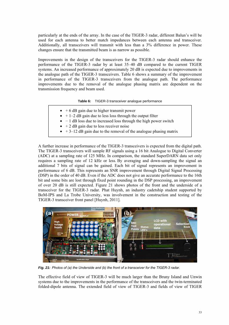
33

particularly at the ends of the array. In the case of the TIGER-3 radar, different Balun’s will be used for each antenna to better match impedances between each antenna and transceiver. Additionally, all transceivers will transmit with less than a 3% difference in power. These changes ensure that the transmitted beam is as narrow as possible. Improvements in the design of the transceivers for the TIGER-3 radar should enhance the performance of the TIGER-3 radar by at least 35–40 dB compared to the current TIGER systems. An increased performance of approximately 20 dB is expected due to improvements in the analogue path of the TIGER-3 transceivers. Table 6 shows a summary of the improvement in performance of the TIGER-3 transceivers from the analogue path. The performance improvements due to the removal of the analogue phasing matrix are dependent on the transmission frequency and beam used.

Table 6: TIGER-3 transceiver analogue performance

• + 6 dB gain due to higher transmit power • + 1–2 dB gain due to less loss through the output filter • − 1 dB loss due to increased loss through the high power switch • + 2 dB gain due to less receiver noise • + 3–12 dB gain due to the removal of the analogue phasing matrix

A further increase in performance of the TIGER-3 transceivers is expected from the digital path. The TIGER-3 transceivers will sample RF signals using a 16 bit Analogue to Digital Converter (ADC) at a sampling rate of 125 MHz. In comparison, the standard SuperDARN data set only requires a sampling rate of 12 kHz or less. By averaging and down-sampling the signal an additional 7 bits of signal can be gained. Each bit of signal represents an improvement in performance of 6 dB. This represents an SNR improvement through Digital Signal Processing (DSP) in the order of 40 dB. Even if the ADC does not give an accurate performance to the 16th bit and some bits are lost through fixed point rounding in the DSP processing, an improvement of over 20 dB is still expected. Figure 21 shows photos of the front and the underside of a transceiver for the TIGER-3 radar. Phat Huynh, an industry cadetship student supported by BoM-IPS and La Trobe University, was involvement in the construction and testing of the TIGER-3 transceiver front panel [Huynh, 2011].

Fig. 21: Photos of (a) the Underside and (b) the front of a transceiver for the TIGER-3 radar.

The effective field of view of TIGER-3 will be much larger than the Bruny Island and Unwin systems due to the improvements in the performance of the transceivers and the twin-terminated folded-dipole antenna. The extended field of view of TIGER-3 and fields of view of TIGER

(a) (b)


Bruny Island and Unwin are shown in Fig. 22. The TIGER-3 field of view will cover all of Tasmania, Victoria, New Zealand, the Tasman Sea and a large portion of the Southern Ocean.

Fig. 22: Fields of view of the TIGER systems. The field of view emanating from T3 is the expected extended coverage of the TIGER-3 system. This figure was supplied by the La Trobe University Electronic Engineering department.

4.2 Radar oceanography using TIGER-3

TIGER-3 will be operated using the latest version of the Radar Operating System (ROS). Under the old ROS, still in use on the TIGER Bruny Island and Unwin radars, the TMS radar control program was used to obtain high time resolution in-phase and quadrature samples over 128 s. This was achieved through the concatenation of multiple 16 second integration times. However, this resulted in discontinuities in the coherency of the signal at the integration boundaries which in turn reduced the quality of the resultant Doppler spectra. The latest version of the ROS can record the high time resolution in-phase and quadrature samples with integration times of 128 s. This will improve the quality of the Doppler spectra. Progress is also being made to install the current ROS on TIGER Bruny Island and Unwin. This process was started by Quang Anh Vu, an industry cadetship student supported by BoM-IPS and La Trobe University [Vu 2011]. A La Trobe University electronic engineering staff member will complete this work with the latest ROS planned to be tested at TIGER Bruny Island site in May 2011. The TMS radar control program was unreliable and did not behave predictably to changes in the command parameters resulting in radar operation failures, particularly at the Unwin radar. Operating the TIGER systems using the latest ROS should resolve the reliability issues. Improvements in the quality of the Doppler spectra due to the removal of discontinuities in the sampling interval combined with improved beam forming and 2–3 orders of magnitude better SNR for TIGER-3 should greatly improve the accuracy of sea state measurements. Estimates of the powers of the first-order Bragg peaks will likely be improved which in turn will increase the accuracy of estimates of dominant wind-wave directions. Furthermore, there will be a region of

35

overlap between 3 radars which will offer improved accuracy. TIGER-3 also offers the best chance of resolving second-order Bragg peaks. If 40–60 dB gain in SNR is realised it is likely that the second-order features will be resolved. If this is the case then estimates of significant wave height and mean wave period will be possible. The spatial coverage of the Southern Ocean and Tasman Sea will be increased at least threefold, with the area of overlapping radar footprints required to obtain directional information almost doubling. Victoria, Tasmania, and New Zealand are in the field of view of TIGER-3. The net Doppler shift of the ground echoes from these land masses can be used to calibrate the net Doppler shift of the Bragg peaks over coastal ocean regions to determine line-of-sight ocean surface currents. The requirements in the early 1990’s for oceanographic measurements from the Jindalee system for the Bureau of Meteorology for operational purposes are contained in the Bureau of Meteorology’s file on the Jindalee/JORN system. Maps of dominant wind-wave directions were required every 6 hours, preferably at 0:00, 6:00, 12:00, and 18:00 UT and provided to the Bureau of Meteorology within 1–2 hours. In the case of severe weather events oceanographic measurements were required every 3 hours and provided to the Bureau of Meteorology within 30–60 minutes. It is likely that similar conditions would be required from the TIGER systems if operational oceanographic measurements are provided to the Bureau of Meteorology. It is currently unclear how the TIGER systems will be operated to permit the generation of 128-second integrated Doppler spectra and comply with the requirements for common time (Table 1). There are several possible solutions. Firstly, the conditions of common time could be changed to allow for a 1 hour oceanographic full scan followed by 5 hours of ionospheric sounding. Secondly, the radar operating system could be modified to allow the TIGER-3 radar to transmit on all beams simultaneously as per [Parris, 2009]. Finally, the radar operating system could be modified to conduct sea state studies using the stereo channel on TIGER-3 and Unwin.


5. SUMMARY AND RECOMENDATIONS

This report has demonstrated that the TIGER SuperDARN systems are capable of providing some sea state measurements of the Southern Ocean that could be useful to the Australian Bureau of Meteorology. This report explored the quantity and quality of data produced by the TIGER systems in their current state. Estimates of dominant wind-wave directions, ocean surface currents, significant wave heights, and mean wave periods were obtained with the TIGER Bruny Island and Unwin systems. It was shown that the current TIGER Bruny Island and Unwin radar systems were able to make reasonable estimates of dominant wind-wave directions that agreed well with model results. Estimates of ocean surface currents could not be estimated because the surface current Doppler shifts could not be separated from the bulk ionospheric motion. SuperDARN radars that contain both ocean and land in their field of view, such as the Wallops Island, Hokkaido, and the soon to be completed TIGER-3 radars could be used to calculate line-of-sight surface currents. Estimates of significant wave height and mean wave period were inaccurate and would not meet the Bureau of Meteorology observational requirements. The TIGER systems were designed for ionospheric research and the sea state mode of operation was experimental. The radars are not operational tools as the TIGER group at La Trobe University does not have sufficient resources to provide full-time maintenance and support staff, and therefore the radars cannot operate reliably on a 24/7 basis. Furthermore, the TIGER Unwin system did not correctly operate during the sea state mode when scheduled throughout 2010. Therefore, it was not possible to add to the 240 hours of sea state data collected during the principal author’s doctoral research prior to 2010. Maps of dominant wind-wave directions were generated approximately every 35 minutes for the 240 hours of sea state data analysed. Of the 420 maps generated, approximately 20–50% had a spatial coverage less than 300,000 km2, approximately 13–18% had a spatial coverage between 300,000 km2, and 600,000 km2, and approximately 32–67% had a spatial coverage greater than 600,000 km2. In addition the maps of radar inferred wind-wave directions were compared to the WAM dominant wave directions. Of the 420 maps generated, approximately 19–40% had less than 50% of the experimental wind-wave vectors within 45º of the model results, approximately 23–28% had between 50-80% of the experimental wind-wave vectors within 45º of the model results, and approximately 14–18% had more than 80% of the experimental wind-wave vectors within 45º of the model results. Furthermore, 18–41% of the wind-wave maps generated contained no data. It was shown that the occurrence and quality of the estimates of wind direction were related to the strength and calmness of the ionosphere. The best results occurred 2–3 hours after sunrise until about an hour before sunset. The occurrence and quality of sea echoes was diminished leading up to sunset, during the night and just after sunrise. The operation of the new TIGER-3 system in the second half of 2011 and upgrades to the current TIGER and UNWIN radars will potentially address the problems currently limiting the quality of sea state measurements. The new TIGER-3 radar will likely provide a 30–40 dB improvement in SNR. This will improve the accuracy of sea-state information and potentially lead to the provision of significant wave heights on a routine basis. The increased SNR should also improve the occurrence and quality of the backscatter sea echoes. This should improve the coverage and accuracy of wind-wave direction estimates. The TIGER-3 radar field of view will be larger, covering an extended swath of the Southern Ocean and Tasman Sea. The field of view

37

will include Tasmania and New Zealand; echoes from which can be used to separate surface current Doppler shifts from ionospheric Doppler motions. The SOFS mooring will be located in the field of view of TIGER-3. Validation of radar inferred sea state parameters can be achieved using data from the SOFS mooring. The authors recommend that a repeat follow through study be undertaken by BOM-IPS in collaboration with La Trobe University using the new TIGER-3 radar when it has been commissioned.


REFERENCES

Ahearn, J.L., Curley, S.R., Headrick, J.M. and Trizna, D.B. “Test of remote skywave measurement of ocean surface conditions,” Proceedings of the IEEE, Vol. 62(6), pp. 681-687, 1974 Anderson, S.J. “Remote Sensing with the Jindalee Skywave radar,” IEEE Journal of Oceanic Engineering, Vol. 11(2), pp. 158-163, 1986 Anderson, S.J. “Remote sensing applications of HF skywave radar: The Australian experience,” Turkish Journal of Electrical Engineering and Computer Sciences, Vol. 18(3), pp. 339-372, 2010 Baker, K.B., Dudeney, J.R., Greenwald, R.A., Pinnock, M., Newell, P.T., Rodger, A.S., Marttin, N. and Meng, C.I. “HF radar signatures of the cusp and low-latitude boundary layer: Magnetospheric boundary layer, cusps, and associated ionospheric signatures,” Journal of Geophysical research, Vol. 100(A5), pp. 7671-7695, 1995 Baker, K.B., Ruohoniemi, J.M., Shepherd, S.G., McWilliams, K.A., Greenwald, R.A. and Bristow, W.A. “Those DARN Radars: New Directions for the Super Dual Auroral Radar Network,” URSI 2008 General Assembly, Chicago, 2008 Barrick, D.E. “Dependence of second-order Doppler sidebands in HF sea echo upon sea state,” G-AP International Symposium Digest, pp. 194-197, 1971 Barrick, D.E. “Remote sensing of sea-state by radar,” OCEANS 1984, Vol. 4, pp. 186-192, 1972 Barrick, D.E. “Extraction of wave parameters from measured HF radar sea-echo Doppler spectra,” Radio Science, Vol. 12(3), pp. 415-424, 1977 Bender, L.C. and Leslie, L.M. “Evaluation of a third generation ocean wave model for the Australian region,” BMRC Research Report No 43, Australian Bureau of Meteorology, 1994 Chisham, G., Lester, M., Milan, S., Freeman, M., Bristow, W., Grocott, A., McWilliams, K., Ruohoniemi, J., Yeoman, T., Dyson, P., Greenwald, R., Kikuchi, T., Pinnock, M., Rash, J., Sato, N., Sofko, G., Villain, J.P. and Walker, A. “A decade of the Super Dual Auroral Radar Network (SuperDARN): Scientific achievements, new techniques and future directions,” Surveys in Geophysics, Vol. 28(1), pp. 33-109, 2007 Chisham, G., Yeoman, T.K. and Sofko, G.J. “Mapping ionospheric backscatter measured by the SuperDARN HF radars – Part 1: A new empirical virtual height model,” Annales Geophysicae, Vol. 26, pp. 823-841, 2008 Crombie, D.D. “Doppler Spectrum of Sea Echo at 13.56 Mc/s,” Nature, Vol. 175, pp. 681-682, 1955 Custovic, E., Devlin, J. and Whittington, J. “Extensive modelling of twin-terminated folded dipole for use in TIGER 3,” Annual SuperDARN conference, Newcastle, 2008 Dyson, P.L. and Devlin, J.C. “The TIGER Radar - An Extension of SuperDARN to sub-auroral latitudes,” WARS’00 (Workshop on Applications of Radio Science) Proceedings, La Trobe University, Bundoora, 2000

39

Dyson, P.L., Devlin, J.C., Parkinson, M.L. and Whittington, J.S. “The Tasman International Geospace Environment Radar (TIGER) – Current Development and future plans,” IEEE Proceedings of the International Conference on Radar, Adelaide, pp. 282–287, 2003 Georges, T.M. and Thome, G.D. “An opportunity for long-distance oceanographic and meteorological monitoring using over-the-horizon defence radars,” Bulletin of the Meteorological Society, Vol. 71(12), pp. 1739-1745, 1990 Georges, T.M. and Harlan, J.A. “The Case for Building a Current-Mapping Over-the-horizon Radar,” IEEE Sixth Working Conference on Current Measurement, San Diego, 1999 Greenslade, D.J.M. “Upgrades to the Bureau of Meteorology’s ocean wave forecasting system,” BMRC Research Report No 79. Australian Bureau of Meteorology, 2000 Greenwald, R.A., Baker, K.B., Hutchins, R.A. and Hanuise, C. “An HF phased-array radar for studying small-scale structure in the high-latitude ionosphere,” Radio Science, Vol. 20, pp. 63-79, 1985 Greenwald, R.A., Baker, K.B., Dudeney, J.R., Pinnock, M., Jones, T.B., Thomas, E.C., Villain, J. P., Cerisier, J.C., Senior, C., Hanuise, C., Hunsucker, R.D., Sofko, G., Koehler, J., Nielsen, E., Pellinen, R., Walker, A.D.M., Sato, N. and Yamagishi, Y. “DARN/SuperDARN: A global view of high-latitude convection,” Space Science Reviews, Vol. 71, pp. 763-796, 1995 Greenwood, R.I. “Wind-Wave Mapping of the Southern Ocean using the TIGER SuperDARN Radars,” Ph.D. Thesis, La Trobe University, 2010 Hall, G.E., MacDougall, J.W., Moorcroft, D.R. and St.Maurice, J.P. “Super Dual Auroral Radar Network observations of meteor echoes,” Journal of Geophysical Research, Vol. 102(A7), pp. 14603-14614, 1997 Heron, S.F. and Heron, M.L. “A Comparison of Algorithms for Extracting Significant Wave Height from HF Radar Ocean Backscatter Spectra,” Journal of Atmospheric and Oceanic Technology, Vol. 15(5), pp. 1157–1163, 1998 Huynh, P., Devlin, J. and Greenwood, R. “Construction and Testing of TIGER-3 Transceiver Front Panel and Graphic User Interface,” IPS / La Trobe University Industry Cadetship Report, 2011 Kelly, M.C. “The Earth’s ionosphere: Plasma physics and electrodynamics,” Academic press, San Diego, 1989 Kingsley, S.P. “The coherence of HF Radar Sea echoes,” GEC Journal of Research, Vol. 4(3), pp. 203-210, 1986 Lester, M., Chapman, P.J., Cowley, S.W.H., Crooks, S.J., Davies, J.A., Hamadyk, P., McWilliams, K.A., Milan, S.E., Parsons, M.J., Payne, D.B., Thomas, E.C., Thornhill, J.D., Wade, N.M., Yeoman, T.K. and Barnes, R.J. “Stereo CUTLASS – A new capability for the SuperDARN HF radars,” Annales Geophysicae, Vol. 22, pp. 459−473, 2004 Lipa, B.J. and Barrick, D.E. “Extraction of sea state from HF radar sea echo: Mathematical theory and modelling,” Radio Science, Vol. 21, pp. 81-100, 1986


Longuet-Higgins, M.S., Cartwright, D.E. and Smith, N.D. “Observations of the directional spectrum of sea waves using the motions of a floating buoy: In Ocean wave spectra,” Prentice-Hall, pp. 111-136, 1963 Milan, S.E., Yeoman, T.K., Lester, M., Thomas, E.C. and Jones, T.B. “Initial backscatter occurrence statistics from the CUTLASS HF radars,” Annales Geophysicae, Vol. 15, pp. 703-718, 1997a Milan, S.E., Jones, T.B., Robinson, T.R., Thomas, E.C. and Yeoman, T.K. “Interferometric evidence for the observation of ground backscatter originating behind the CUTLASS coherent HF radars,” Annales Geophysicae, Vol. 15, pp. 29−39, 1997b Parkinson, M.L. “Observation of the Broadening and Coherence of MF/Lower HF Surface-Radar Ocean Echoes,” IEEE Journal of oceanic engineering, Vol. 22(2), pp.347-363, 1997 Parkinson, M.L., Whittington, J.S. and Devlin, J.C. “Why do we need “DigiDARN” – A global network of digital SuperDARN radars?,” WARS’06 (Workshop on Applications of Radio Science) Proceedings, Leura, New South Wales, 2006 Parris, R.T. and Bristow, W.A. “Imaging with the Kodiak Island SuperDARN HF Radar,” CEDAR Workshop, Santa Fe, New Mexico, 2009 Pedrotti, F.L. and Pedrotti, L.S. “Introduction to optics,” Prentice-Hall, Inc., New Jersey, 1993 Pierson, W.J. and Moskowitz, L. “A proposed spectral form for fully developed wind seas based on the similarity theory of S.A. Kitaigordskii,” Geophysical Research Letters, Vol. 69, pp. 5181-5190, 1964 Ratcliffe, J.A. “An introduction to the ionosphere and magnetosphere,” Cambridge University Press, London, 1972 Shearman, E. “Propagation and scattering in MF/HF ground-wave radar,” IEEE proceeding Communications, Radar and Signal Processing, Vol. 130(7), pp. 579-590, 1983 Shearman, E. “A review of methods of remote sensing of sea-surface conditions by HF radar and design considerations for narrow-beam systems,” IEEE Journal of Oceanic Engineering, Vol. 11(2), pp. 150-157, 1986 Shearman, E. “HF ground wave radar technique for large area mapping of surface current and directional wave spectrum,” IEE Colloquium on Monitoring the Sea, London, pp. 6(1)-6(3), 1990 Stewart, R.H. “Higher order scattering of radio waves from the sea,” IEEE/GAP International Symposium Digest, Los Angeles, pp. 190–193, 1971 Vu, Q., Devlin, J. and Greenwood, R. “New TIGER Radar Operation System,” IPS / La Trobe University Industry Cadetship Report, 2011 Whittington, J., Devlin, J. and Nguyen, M. “Digital stereo enhancement to the TIGER radar system,” WARS’04 (Workshop on Applications of Radio Science) Proceedings, Hobart, Tasmania, 2004

41

Wyatt, L.R. “Limits to the Inversion of HF Radar Backscatter for Ocean Wave Measurement,” Journal of Atmospheric and Oceanic Technology, Vol. 17(12), pp. 1651–1666, 2000 Yukimatu, A.S. and Tsutsumi, M. “A new SuperDARN meteor wind measurement raw time series analysis method and its applications to mesopause region dynamics,” Geophysical Research Letters, Vol. 29(20), pp. 42(1)-42(4), 2002a Yukimatu, A.S., Tsutsumi, M., Yamagishi, H. and Sato, N. “A new method for monitoring and removing SuperDARN radar DC offsets,” Advances in Polar Upper Atmosphere Research, Vol. 16, pp. 181-192, 2002b


APPENDIX A

Fig. 23: Examples of wind wave maps with poor coverage and (a) poor agreement, (b) moderate agreement, and (c) good agreement.

(a)

(b)

(c)

43

Fig. 24: Examples of wind wave maps with moderate coverage and (a) poor agreement, (b) moderate agreement, and (c) good agreement.

(a)

(b)

(c)


Fig. 25: Examples of wind wave maps with good coverage and (a) poor agreement, (b) moderate agreement, and (c) good agreement.

(a)

(b)

(c)

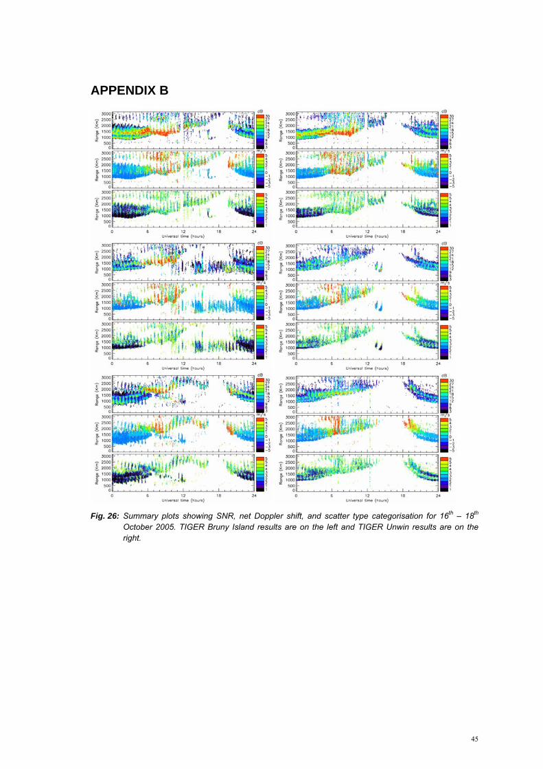
45

APPENDIX B

Fig. 26: Summary plots showing SNR, net Doppler shift, and scatter type categorisation for 16th – 18th October 2005. TIGER Bruny Island results are on the left and TIGER Unwin results are on the right.


Fig. 27: Summary plots showing SNR, net Doppler shift, and scatter type categorisation for 24th – 28th October 2005. TIGER Bruny Island results are on the left and TIGER Unwin results are on the right.

47

Fig. 28: Summary plots showing SNR, net Doppler shift, and scatter type categorisation for 1st – 3rd March 2006. TIGER Bruny Island results are on the left and TIGER Unwin results are on the right.


APPENDIX C

Fig. 29: Average occurrence statistics from TIGER Unwin for data from 00:00 UT on the 16th October 2005 to 24:00 UT on the 18th October 2005 and from 12:00 UT on the 24th October 2005 to 12:00 UT on the 28th October 2005.

Fig. 30: Average occurrence statistics from TIGER Bruny Island for data from 00:00 UT on the 1st March 2006 to 24:00 UT on the 3rd March 2006.

49

Fig. 31: Average occurrence statistics from TIGER Unwin for data from 00:00 UT on the 1st March 2006 to 24:00 UT on the 3rd March 2006.

evaluation of the tiger superdarn over-the-horizon radar · pdf file ·...

Documents