evaluation of the uncertainty of electrical impedance measurements… of the uncertainty of... ·...

Evaluation of the uncertainty of electrical impedancemeasurements: the GUM and its Supplement 2

Pedro M Ramos1, Fernando M Janeiro2 and Pedro S Girão1

1 Departamento de Engenharia Electrotécnica e de Computadores, Instituto SuperiorTécnico, Universidade de Lisboa and Instituto de Telecomunicações, Av. RoviscoPais, n. 1, 1049-001 Lisbon, Portugal2 Instituto de Telecomunicações and Universidade de Évora, Departamento de Física,Rua Romão Ramalho, n. 59, 7000-671 Évora, Portugal

E-mails: [email protected], [email protected],[email protected]

Abstract. Electrical impedance is not a scalar but a complex quantity. Thus, evaluation of theuncertainty of its value involves a model whose output is a complex. In this paper thecomparison of the evaluation of the uncertainty of the measurement of the electrical impedanceof a simple electric circuit using the GUM and using a Monte Carlo method according to theSupplement 2 of the GUM is presented.

1. Introduction

The publication, in 1993, of the Guide to the Expression of Uncertainty in Measurement (GUM) wasthe first significant result of the work of more than 15 years developed by individuals andorganizations to produce an internationally accepted procedure for expressing measurementuncertainty and for combining individual uncertainty components into a single total uncertainty. TheGuide, revised in 1995 and 2008 [1], materializes Recommendation INC-1 (1980) by the CPIMWorking Group on the Statement of Uncertainties by providing a conceptual framework allowing aconsistent treatment of uncertainty contributions. Complemented by the contribution of many [2-7],the impact of GUM in Metrology was increased when, in 2005, standard ISO/IEC17025 [8]established that accredited test laboratories were required to estimate the uncertainty and to report it.Notwithstanding, the original GUM soon evidenced some shortcomings, namely: (a) dealing with non-symmetrical measurement uncertainty distributions, with non-linearity of the measurement system,with input dependency and systematic bias; (b) it mainly concerns univariate measurement models,namely models having a single scalar output quantity.

To cope with these limitations, work has been developed by many authors (e.g. [9-18]) and twosupplements to the GUM – Supplement 1 and Supplement 2 – were issued. Based on the same basicideas of the GUM – measurement model and probability distribution of the input quantities –Supplement 1 [19], which deals also only with models having a single scalar output quantity,introduces numerical simulation using the Monte Carlo method (MCM) as alternative to analytical ornumerical integration for calculating the combination of the probability distributions of the inputquantities involved in the propagation of distributions required for the evaluation of measurement

IMEKO IOP PublishingJournal of Physics: Conference Series 588 (2015) 012045 doi:10.1088/1742-6596/588/1/012045

Content from this work may be used under the terms of the Creative Commons Attribution 3.0 licence. Any further distributionof this work must maintain attribution to the author(s) and the title of the work, journal citation and DOI.

Published under licence by IOP Publishing Ltd 1

uncertainty. Supplement 2 [20] extends the use of GUM and Supplement 1 to multivariatemeasurement models, namely models with more than one output quantity. It is true that the GUMincludes examples, from electrical metrology, with three output quantities [JCGM 100:2008 H.2], andthermal metrology, with two output quantities [JCGM 100:2008 H.3] [20], but Supplement 2describes a generalization of that Monte Carlo method to obtain a discrete representation of the jointprobability distribution for the output quantities of a multivariate model. The discrete representationis then used to provide estimates of the output quantities, and standard uncertainties and covariancesassociated with those estimates [20].

Supplements 1 and 2 to the GUM originate some inconsistency between the GUM and theSupplements. This fact, added to some non-solved limitations of the GUM itself, lead to the need of arevision of the GUM that, to the best of our knowledge, is underway [21].

The electrical impedance is a simple example of a complex quantity and the output of itsmeasurement model is a complex number. The uncertainty evaluation of electrical impedancemeasurements using the GUM and using the Supplement 2 to the GUM are compared.

2. Electrical impedance

Electrical impedance extends the concept of resistance to alternating current (AC) circuits, describingnot only the relative amplitudes of the voltage and current, but also their phase difference. However,electrical impedance measurement is important not only in the analysis of electric circuits but also forother purposes. In fact, because the electrical impedance allows the quantification of the behavior of aconducting medium to an electric current, the impedance measurement is used in the determination ofthe electromagnetic properties of materials and is the basis of various methods of electricaltransduction with applications in fields such as chemistry [22,23] and biomedicine [24-27].

Sometimes abusively used in other time varying regimes, electrical impedance, usually representedby Z, is an electric quantity defined in the context of sine wave alternating current. Thus if v(t) is theimpedance sinusoidal voltage with constant amplitude VM, constant frequency f, and constant phase φv

jj2π( ) cos 2π Re e e , vftM v Mv t V ft V (1)

where j is the imaginary unit and Re(x) is the real part of x, the impedance current is

jj2π( ) cos 2π Re e e . iftM i Mi t I ft I (2)

In complex amplitudes (phasors) both can be written asje v

MV V and je . iMI I (3)

The impedance is not a phasor but a complex number defined as the ratio /V I whose amplitude(module) is Z and whose phase is φ.

j j je e e cos j sin v iM M

M M

V VVZ Z Z ZI II

. (4)

The principles, methods, equipment and procedures for electrical impedance measurement arediverse [28] depending, namely, on the frequency and on the application. In the following sections,and because the purpose here is to compare the uncertainty evaluation using two different methods, theconsidered case is that of electrical impedance measurements, based on digital acquisition ofsinusoidal voltages and estimation of their amplitudes and phase differences as described in [29].


2

3. Results

3.1. Measurement Model

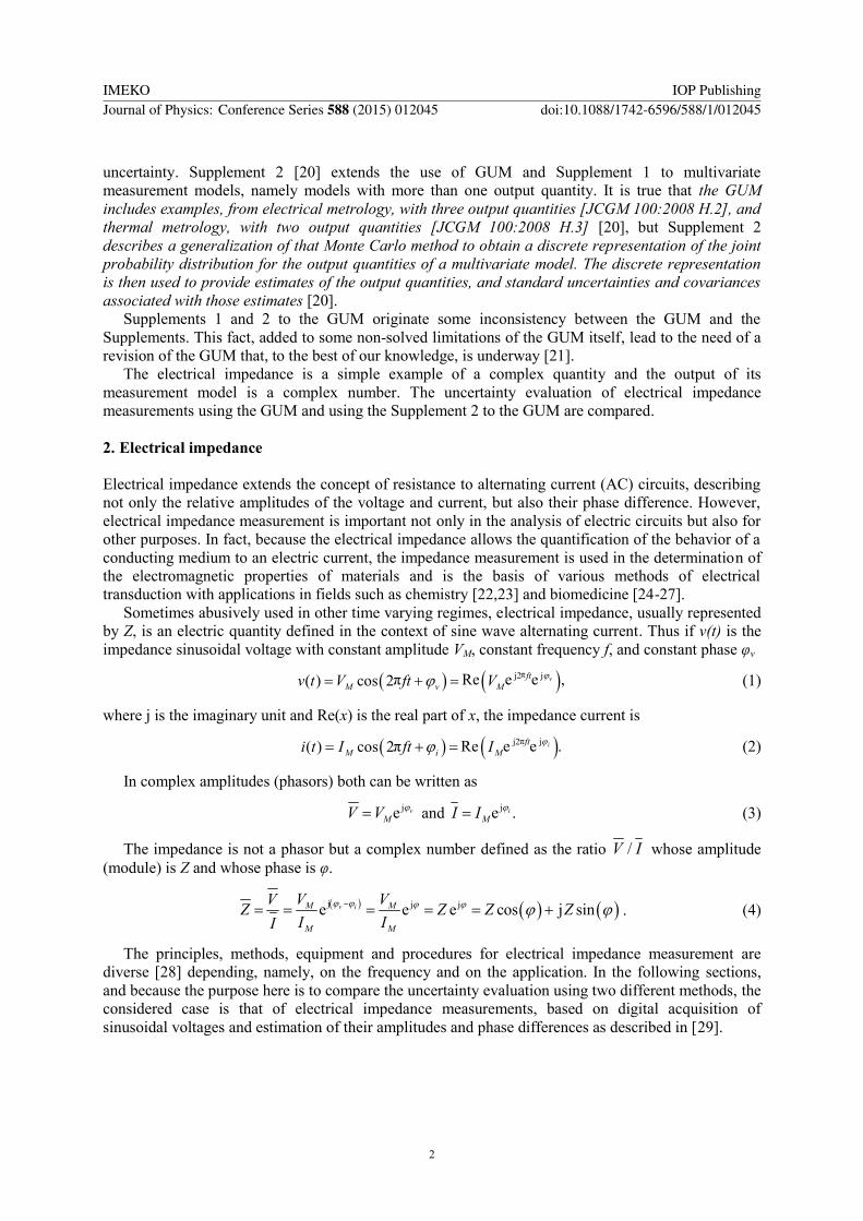
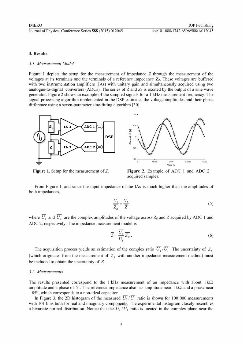
Figure 1 depicts the setup for the measurement of impedance Z through the measurement of thevoltages at its terminals and the terminals of a reference impedance ZR. These voltages are bufferedwith two instrumentation amplifiers (IAs) with unitary gain and simultaneously acquired using twoanalogue-to-digital converters (ADCs). The series of Z and ZR is excited by the output of a sine wavegenerator. Figure 2 shows an example of the sampled signals for a 1 kHz measurement frequency. Thesignal processing algorithm implemented in the DSP estimates the voltage amplitudes and their phasedifference using a seven-parameter sine-fitting algorithm [30].

Figure 1. Setup for the measurement of Z. Figure 2. Example of ADC 1 and ADC 2acquired samples.

From Figure 1, and since the input impedance of the IAs is much higher than the amplitudes ofboth impedances,

1 2R

U UZ Z

(5)

where 1U and 2U are the complex amplitudes of the voltage across ZR and Z acquired by ADC 1 andADC 2, respectively. The impedance measurement model is

2

1

RUZ ZU

. (6)

The acquisition process yields an estimation of the complex ratio 2 1/U U . The uncertainty of RZ(which originates from the measurement of RZ with another impedance measurement method) mustbe included to obtain the uncertainty of Z .

3.2. Measurements

The results presented correspond to the 1 kHz measurement of an impedance with about 1kamplitude and a phase of 5º . The reference impedance also has amplitude near 1k and a phase near85º , which corresponds to a non-ideal capacitor.

In Figure 3, the 2D histogram of the measured 2 1/U U ratio is shown for 100 000 measurementswith 101 bins both for real and imaginary components. The experimental histogram closely resemblesa bivariate normal distribution. Notice that the 2 1/U U ratio is located in the complex plane near the

-0.5

-0.25

0

0.25

0.5

0 0.0005 0.001 0.0015 0.002

Time [s]

Cha

nnel

1,2

[V]


3

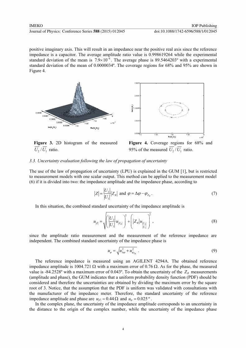
positive imaginary axis. This will result in an impedance near the positive real axis since the referenceimpedance is a capacitor. The average amplitude ratio value is 0.998619264 while the experimentalstandard deviation of the mean is 87.9 10 . The average phase is 89.5464203º with a experimentalstandard deviation of the mean of 0.0000034º. The coverage regions for 68% and 95% are shown inFigure 4.

Figure 3. 2D histogram of the measured

2 1/U U ratio.Figure 4. Coverage regions for 68% and95% of the measured 2 1/U U ratio.

3.3. Uncertainty evaluation following the law of propagation of uncertainty

The use of the law of propagation of uncertainty (LPU) is explained in the GUM [1], but is restrictedto measurement models with one scalar output. This method can be applied to the measurement model(6) if it is divided into two: the impedance amplitude and the impedance phase, according to

2

1

RU

Z ZU

and RZ

. (7)

In this situation, the combined standard uncertainty of the impedance amplitude is

2

1

22

2

1

R RZ Z UU

Uu u Z u

U, (8)

since the amplitude ratio measurement and the measurement of the reference impedance areindependent. The combined standard uncertainty of the impedance phase is

2 2

ZRu u u . (9)

The reference impedance is measured using an AGILENT 4294A. The obtained referenceimpedance amplitude is 1004.721 with a maximum error of 0.76 . As for the phase, the measuredvalue is -84.2528º with a maximum error of 0.043º. To obtain the uncertainty of the RZ measurements(amplitude and phase), the GUM indicates that a uniform probability density function (PDF) should beconsidered and therefore the uncertainties are obtained by dividing the maximum error by the squareroot of 3. Notice, that the assumption that the PDF is uniform was validated with consultations withthe manufacturer of the impedance meter. Therefore, the standard uncertainty of the referenceimpedance amplitude and phase are 0.44 Zu and 0.025 ºu .

In the complex plane, the uncertainty of the impedance amplitude corresponds to an uncertainty inthe distance to the origin of the complex number, while the uncertainty of the impedance phase


4

corresponds to an uncertainty of the complex number phase. The combination of these twouncertainties defines a region with the generic shape depicted in Fig. 8 of [31] and shown in Figure 5.Notice that the considerable distance to origin and the reduced phase uncertainty makes all the linesresemble straight lines when in fact, the real, limits of the coverage phase intervals are arcs.

Another way to interpret the results of the law of propagation of uncertainty is to combine the twooutcomes (the amplitude and phase PDFs) considering that they are independent. Since the GUMtransforms every uncertainty into a normal PDF distribution, it is possible to combine both outputPDFs (amplitude and phase) to obtain a bivariate PDF. The resulting equivalent 2D histogram isshown in Figure 6. Note that, the coverage regions of this histogram (which are ellipses) do notcorrespond to the intersection areas depicted in Figure 5.

(a)(b)

(c)

(d)

Figure 5. Coverage intervals obtained usingthe LPU. (a) and (b) are the coverage intervalsof the impedance phase for 95% and 68%. (c)and (d) are the coverage intervals of theimpedance amplitude for 95% and 68%.

Figure 6. Equivalent 2D histogram obtainedusing the law of propagation of uncertainty asdefined in the GUM [1].

3.4. Uncertainty evaluation using Monte Carlo method

The law of propagation of uncertainty approach, as shown in the previous section, has significantshortcomings in this (and similar) applications since it neglects any phase/amplitude dependence ofthe measured 2 1/U U ratio and takes a simplistic interpretation of the uncertainty of the referenceimpedance (transforming the uniform PDFs into normal ones). These shortcomings can be addressedby evaluating the uncertainty of the measurement model (6) using Monte Carlo simulations. InSupplement 1 [19], the use of Monte Carlo method (MCM) is described for single output measurementmodels where the law of propagation of uncertainty is not suited due to: (a) the type of PDFs of eachmeasurement model input are substantially different from normal PDFs; (b) the first order Taylorapproximation used in LPU is not suited for some measurement models; (c) measurement models thatcannot be described by a closed algebraic equation (to determine the partial derivates). Supplement 2[20], goes further by expanding the use of MCM for measurement models with any number of outputquantities. One significant evolution in this supplement is the definition of coverage regions and inparticular that of the smallest coverage region (and interval which is also suited for measurementmodels with a single output).

In the considered case of impedance measurements, the PDF of the reference impedance amplitudeis uniform as is the PDF of the reference impedance phase. In order to obtain the histogram of themeasured impedance, for each of 100 000 2 1/U U ratio measurements, 100 000 values of the referenceimpedance amplitude and phase are randomly generated in accordance to their uniform distributions.The values of the resulting estimated impedance are then used to generate the 2D histogram (Figure 7)and from the histogram, the coverage region with 95% is obtained (Figure 8).


5

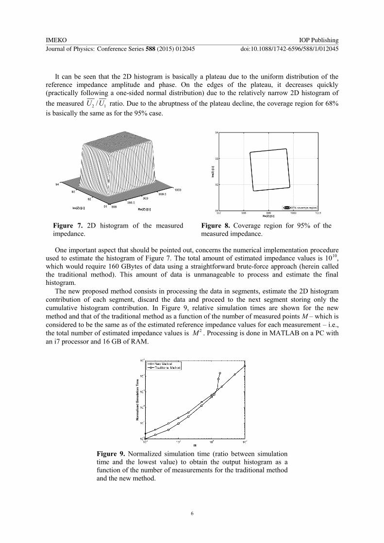
It can be seen that the 2D histogram is basically a plateau due to the uniform distribution of thereference impedance amplitude and phase. On the edges of the plateau, it decreases quickly(practically following a one-sided normal distribution) due to the relatively narrow 2D histogram ofthe measured 2 1/U U ratio. Due to the abruptness of the plateau decline, the coverage region for 68%is basically the same as for the 95% case.

Figure 7. 2D histogram of the measuredimpedance.

Figure 8. Coverage region for 95% of themeasured impedance.

One important aspect that should be pointed out, concerns the numerical implementation procedureused to estimate the histogram of Figure 7. The total amount of estimated impedance values is 1010,which would require 160 GBytes of data using a straightforward brute-force approach (herein calledthe traditional method). This amount of data is unmanageable to process and estimate the finalhistogram.

The new proposed method consists in processing the data in segments, estimate the 2D histogramcontribution of each segment, discard the data and proceed to the next segment storing only thecumulative histogram contribution. In Figure 9, relative simulation times are shown for the newmethod and that of the traditional method as a function of the number of measured points M – which isconsidered to be the same as of the estimated reference impedance values for each measurement – i.e.,the total number of estimated impedance values is 2M . Processing is done in MATLAB on a PC withan i7 processor and 16 GB of RAM.

Figure 9. Normalized simulation time (ratio between simulationtime and the lowest value) to obtain the output histogram as afunction of the number of measurements for the traditional methodand the new method.


6

Although the new method is slower for M < 104, due to the multiple histogram assessments, forM > 104, the simulation time of the traditional method increases substantially and for M > 18 000,Matlab can no longer conclude the process due to the use of virtual memory and the correspondingincrease in access time to the data. On the other hand, the new method has no such constrain and couldbe used even for M > 105. Note that the amount of required memory for the traditional method is16M 2 Bytes while for the new method it is only 16M Bytes. For M = 104, the traditional methodrequires 1.6 GBytes, while the new method requires only 160 kBytes.

The drawback of the new method is that the histogram range and its number of points must bedefined in the beginning of the process and cannot be changed during the process. This issue requiresthat the process is started with a low value of M to define the histogram range, which is refined beforethe final simulation is executed.

4. Conclusions

The example presented in this paper highlights some of the known limitations of the law ofpropagation of uncertainty. For this particular case where the estimated output is a complex number,its separation into two measurement models removes the dependency of the estimated complex ratioamplitude and phase. If the real and imaginary components were considered instead, the resultingellipsoid coverage regions would be different. The Monte Carlo method shows that the actualcoverage region is not an ellipsoid but instead a rotated rectangle mainly due to the uncertainty of thereference impedance and its considerable area when compared with the coverage region of themeasured complex voltage ratio.

5. References

[1] BIPM, IEC, IFCC, ILAC, ISO, IUPAC, IUPAP and OIML 2008 Guide to the Expression ofUncertainty in Measurement, JCGM 100:2008, GUM 1995 with minor corrections,http://www.bipm.org/utils/common/documents/jcgm/JCGM1002008E.pdf

[2] Phillips SD, Eberhardt KR, Parry B 1997 Guidelines for Expressing the Uncertainty ofMeasurement Results Containing Uncorrected Bias NIST Journal of Research Institute ofStandards and Technology

[3] Bell S 1999 A Beginner’s Guide to Uncertainty of Measurement (London: NPL)[4] Lira I 2002 Evaluating the Uncertainty of Measurement. Fundamentals and Practical Guidance

(Bristol, UK: Institute of Physics)[5] Kirkup L and Frenkel RB 2006 An Introduction to Uncertainty in Measurement. Using the

GUM (Guide to the Expression of Uncertainty in Measurement) (Cambridge University Press)[6] NASA HDBK-8739.19-3 – Measurement Uncertainty Analysis Principles and Methods, July,

2010[7] Willink R, Hall BD 2013 An extension to GUM methodology: degrees-of-freedom calculations

for correlated multidimensional estimates”, arXiv:1311.0343 [physics.data-an][8] ISO/IEC 17025:2005 General requirements for the competence of testing and calibration

laboratories[9] Yeung H and Papadopoulos CE 2000 Natural gas energy flow (quality) uncertainty estimation

using Monte Carlo simulation method International Conference on Flow Measurement,FLOMEKO

[10] Khu ST, and Werner MG 2003 Reduction of Monte-Carlo simulation runs for uncertaintyestimation in hydrological modelling Hydrology and Earth System Sciences Vol. 7 No. 5 680-690

[11] Andrae ASG, Mller P, Anderson J and Liu J 2004 Uncertainty estimation by Monte Carlosimulation applied to life cycle inventory of cordless phones and microscale metallizationprocesses IEEE Transactions on Electronics Packaging Manufacturing 27 No. 4 233-245


7

[12] Rossi GB, Crenna F, Harris PM, Cox MG 2006 Combining direct calculation and the MonteCarlo method for the probabilistic expression of measurement results Advanced Mathematicaland Computational Tools in Metrology VII, Series on Advances in Mathematics for AppliedSciences vol. 72 221-228, (World Scientific Publishing Co.)

[13] Cox MG and Bernd Siebert RL 2006 The use of a Monte Carlo method for evaluatinguncertainty and expanded uncertainty Metrologia 43 4 178-188

[14] Silva Ribeiro A 2006, Avaliação de Incertezas de Medição em Sistemas Complexos Lineares eNão-Lineares. PhD. thesis (in Portuguese)

[15] Alves e Sousa J, Silva Ribeiro A, Forbes AB, Harris PM, Carvalho F, Bacelar L 2007 TheRelevance of Using a Monte Carlo Method to Evaluate Uncertainty in Mass Calibration Proc.IMEKO TC3, TC16 & TC22 International Conference Merida México

[16] Jing H, Huang M-F, Zhong Y-R, Kuang B and Jiang X-Q 2007 Estimation of the measurementuncertainty based on quasi Monte-Carlo method in optical measurement Proceedings of theInternational Society for Optical Engineering

[17] Schueller GI 2007 On the treatment of uncertainties in structural mechanics and analysis,Journal Computers and Structures 85 5-6 235-243

[18] Koch KR 2008 Evaluation of uncertainties in measurements by Monte-Carlo simulations withan application for laser scanning Journal of Applied Geodesy 2 67-77

[19] BIPM, IEC, IFCC, ILAC, ISO, IUPAC, IUPAP and OIML 2008, Supplement 1 to the ‘Guide tothe Expression of Uncertainty in Measurement’—Propagation of distributions using a MonteCarlo method JCGM 101:2008,http://www.bipm.org/utils/common/documents/jcgm/JCGM.101.2008E.pdf

[20] BIPM, IEC, IFCC, ILAC, ISO, IUPAC, IUPAP and OIML 2011, Supplement 2 to the ‘Guide tothe Expression of Uncertainty in Measurement’—Extension to any number of output quantitiesJCGM 102:2011, http://www.bipm.org/utils/common/documents/jcgm/JCGM.102.2011.E.pdf

[21] Bich W et al. 2012 Revision of the 'Guide to the Expression of Uncertainty in MeasurementMetrologia 49 6 702-705

[22] McNeil CJ, Athey D, Ball M, Ho WO, Krause S, Armstrong RD, Wright JD and Rawson K1995 Electrochemical Sensors Based on Impedance Measurement of Enzymel CatalyzedPolymer Dissolution: Theory and Applications Anal. Chem., 67, 3928-3935

[23] Roy P, Tsai T-C, Liang C-T, Wua R-J and Chavali M 2011 Application of ImpedanceMeasurement Technology in Distinguishing Different Tea Samples with Ppy/SWCNTComposite Sensing Material Journal of the Chinese Chemical Society 58 714-722

[24] Guimerà A, Calderón E, Los P and Christie AM 2008 Method and device for bio-impedancemeasurement with hard-tissue applications Physiological Measurement 29 6 15-26

[25] Tang WH and Tong W 2009 Measuring impedance in congestive heart failure: Current optionsand clinical applications Am Heart J. 157 3 402–411

[26] Gupta AK 2011 Respiration Rate Measurement Based on Impedance Pneumography TexasInstruments Application Report SBAA181

[27] Marquez JC, Rempfler M, Seoane F and Lindecrantz K 2013 Textrode-enabled transthoracicelectrical bioimpedance measurements – towards wearable applications of impedancecardiography J Electr Bioimp. 4 45–50

[28] Callegaro L 2013 Electrical Impedance: Principles, Measurement and Applications (BocaRaton Fl. USA: CRC Press)

[29] Ramos PM, Silva MF, Serra AC 2004 Low Frequency Impedance Measurement Using Sine-Fitting Measurement 35 89-96

[30] Ramos PM, Serra AC 2008 A new sine-fitting algorithm for accurate amplitude and phasemeasurements in two channel acquisition systems Measurement 51 135-143

[31] Ramos PM, Janeiro FM, Tlemçani M, Serra AC 2009 Recent Developments on ImpedanceMeasurements with DSP-Based Ellipse-Fitting Algorithms IEEE Transactions onInstrumentation and Measurement 58 1680-1689


8

evaluation of the uncertainty of electrical impedance measurements… of the uncertainty of... ·...

Documents