evaluation of the wrf pbl parameterizations for marine

Evaluation of the WRF PBL Parameterizations for Marine Boundary LayerClouds: Cumulus and Stratocumulus

HSIN-YUAN HUANG

Joint Institute for Regional Earth System Science and Engineering, University of California, Los Angeles,

Los Angeles, California

ALEX HALL

Department of Atmospheric and Oceanic Sciences, University of California, Los Angeles, Los Angeles, California

JOAO TEIXEIRA

Jet Propulsion Laboratory, California Institute of Technology, Pasadena, California

(Manuscript received 2 October 2012, in final form 15 January 2013)

ABSTRACT

The performance of five boundary layer parameterizations in the Weather Research and Forecasting

Model is examined for marine boundary layer cloud regions running in single-column mode. Most parame-

terizations show a poor agreement of the vertical boundary layer structure when compared with large-eddy

simulation models. These comparisons against large-eddy simulation show that a parameterization based on

the eddy-diffusivity/mass-flux approach provides a better performance. The results also illustrate the key role

of boundary layer parameterizations in model performance.

1. Introduction

Stratocumulus and shallow cumulus clouds in sub-

tropical oceanic regions cover thousands of square ki-

lometers and play a key role in regulating global climate

(e.g., Tiedtke et al. 1988; Klein and Hartmann 1993).

Stratocumulus cools the climate by strongly reflecting

incoming shortwave radiation, playing an important role

in ocean–atmosphere interaction (e.g., Teixeira et al.

2008), while cumulus clouds play a key role in regulating

the planet’s evaporation and moisture transport to the

deep tropics. Numerical modeling is an essential tool to

study these clouds in regional and global systems, but

the current generation of climate and weather models

has difficulties in representing them in a realistic way.

Stratocumulus boundary layers in models are often

unrealistically shallow and have too little cloud (e.g.,

Duynkerke and Teixeira 2001; Zhang et al. 2005;

Stevens et al. 2007). Additionally, current models have

difficulties in simulating the critical transition from

stratocumulus to shallow cumulus clouds (Siebesma

et al. 2004; Teixeira et al. 2011).

While numerical models resolve the large-scale flow,

subgrid-scale parameterizations are needed to estimate

small-scale properties (e.g., boundary layer turbulence

and convection, clouds, radiation), which have signifi-

cant influence on the resolved scale due to the complex

nonlinear nature of the atmosphere. For the cloudy

planetary boundary layer (PBL), it is fundamental to

parameterize vertical turbulent fluxes and subgrid-scale

condensation in a realistic manner. The Weather Re-

search and Forecasting (WRF) Model version 3.1 pro-

vides multiple parameterization choices, which include

nine PBL schemes, 12 microphysics, and 6 moist con-

vection parameterizations (Skamarock et al. 2008). In

addition to a typical model structural drawback—an

artificial separation between turbulence and convection

parameterizations—this long menu suffers from a vari-

ety of issues including an uncertainty regarding the op-

timal combinations to select.

In this study, we aim to investigate the performance

of the various WRF PBL schemes in cloud simulations

of both marine stratocumulus and shallow cumulus.

Corresponding author address: Hsin-Yuan Huang, 7343 Math

Science Building, University of California, Los Angeles, Los

Angeles, CA 90095.

E-mail: [email protected]

JULY 2013 HUANG ET AL . 2265

DOI: 10.1175/MWR-D-12-00292.1

� 2013 American Meteorological SocietyUnauthenticated | Downloaded 12/15/21 07:12 PM UTC

Meanwhile, we also evaluate the ability of a new scheme

[total-energy–mass-flux (TEMF), which is described

below] based on the eddy-diffusivity–mass-flux (EDMF)

concepts. We design a set of several WRF single-column

model (SCM) simulations for threewell-known large-eddy

simulation (LES) case studies based on field campaigns.

Including the TEMF scheme, five PBL parameterizations

are examined against LES. Resolving the large eddies

that are responsible for the transport of mass, momen-

tum, and energy in the PBL, the LES result has been used

to serve as a proxy of reality to guide the development of

PBL parameterization. Section 2 briefly introduces the

EDMF and TEMF schemes. Section 3 describes the ex-

perimental design. Section 4 presents the simulation re-

sults followed by a discussion in section 5.

2. EDMF and TEMF parameterizations

The EDMF parameterization was first introduced by

Siebesma and Teixeira (2000) and subsequently tested

and implemented in the European Centre for Medium-

Range Weather Forecasts (ECMWF) model (e.g.,

Teixeira and Siebesma 2000; Koehler 2005). Recent

studies have shown its potential to represent the shallow

and dry convective PBL (Soares et al. 2004; Siebesma

et al. 2007; Neggers 2009; Witek et al. 2011; Suselj et al.

2012). Later, using total turbulent energy to calculate

eddy-diffusivity (Mauritsen et al. 2007), Angevine et al.

(2010) modified the EDMF parameterization to what is

referred to as the TEMF parameterization. The TEMF

scheme implemented inWRF version 3.1 is evaluated in

this study.

Rather than a specific parameterization, EDMF is

an approach based on an optimal combination of the

eddy-diffusivity (ED) parameterization, used to simu-

late turbulence within the PBL, and the mass-flux (MF)

parameterization, used for moist convection. Though

differences in the details are present in different EDMF

implementations on weather or climate models, the

fundamental idea is the same: local mixing is parame-

terized by the ED term, while the nonlocal transport

due to convective thermals is represented by the MF

term. The governing equation for the vertical fluxes in

EDMF is

w0c052K›c

›z1M(cup 2c) , (1)

where c can be any scalar quantity, such as liquid water

potential temperature (ul), total water specific humidity

(qt), or total energy (E). Here K and M are the ED and

MF terms, respectively; the subscript up in cup indicates

the value of c in the updraft. The temporal evolution of

the mean variable c is then given as the vertical gradient

of the flux: ›c/›t52›(w0c0)/›z.The main difference between TEMF and EDMF is

in the calculation of the ED coefficient: EDMF often

uses turbulent kinetic energy (TKE) while TEMF uses

total turbulent energy (TTE), a combination of TKE

and turbulent potential energy. Better handling of sta-

bly stratified conditions is themain reason for using TTE

rather than TKE (Mauritsen et al. 2007). For a full de-

scription of TEMF, the reader is referred to Angevine

(2005), Mauritsen et al. (2007), Siebesma et al. (2007),

and Angevine et al. (2010).

3. Experimental design

a. Study sites

We perform a suite of simulations using the SCM

version of WRF for three case studies associated with

field experiments, which are chosen because they have

been intensively studied using LES models. The three

field campaigns are the following: 1) the Second Dy-

namics and Chemistry of theMarine Stratocumulus field

study (DYCOMS-II), 2) the Barbados Oceanographic

and Meteorological Experiment (BOMEX), and 3)

the Rain in Cumulus over Ocean (RICO) experiment

(Fig. 1). DYCOMS- II took place in the subtropical

Pacific, while BOMEX and RICO were in the tropical

Atlantic. The marine clouds in BOMEX and RICO are

classified as shallow cumulus while the DYCOMS-II

case is classified as stratocumulus. DYCOMS-II was

conducted in the center of the northeast Pacific strato-

cumulus deck, about 500 km west-southwest of San

Diego, California, during July 2001 (Stevens et al. 2003,

2005). The first research flight mission ofDYCOMS-II is

selected for this study because it provides many appro-

priate atmospheric conditions for the LES experiment,

such as a relatively homogeneous atmospheric envi-

ronment and a uniform cloud distribution. BOMEX

(phase III) took place during June 1969 over a 500 km2

region near Barbados. The aim was to investigate the

large-scale heat and moisture budgets using radiosondes

(Delnore 1972; Holland and Rasmusson 1973). In this

study, the SCM setup and initialization for BOMEX

use the same settings as previous LES studies (e.g.,

Siebesma and Cuijpers 1995; Siebesma et al. 2003).

RICO was carried out near the Caribbean islands

during a two-month period between November 2004

and January 2005 (Caesar 2005; Rauber et al. 2007).

Here the SCM initialization for RICO follows the

designs of an LES intercomparison study presented in

the Ninth GCSS Boundary Layer Cloud Work-

shop (http://www.knmi.nl/samenw/rico/index.html).

2266 MONTHLY WEATHER REV IEW VOLUME 141

Unauthenticated | Downloaded 12/15/21 07:12 PM UTC

All LES ensemble results (for three study sites) shown

in the following analyses are taken from these in-

tercomparison studies.

b. Single-column model setup

This study uses WRF version 3.1 for all SCM experi-

ments. In addition to TEMF, four other PBL schemes

are used: the Yonsei University (YSU) scheme (Hong

et al. 2006), the Mellor–Yamada–Janjic (MYJ) scheme

(Mellor and Yamada 1982; Janjic 2002), the Mellor–

Yamada–Nakanishi–Niino (MYNN) scheme (Nakanishi

and Niino 2004, 2006), and the Medium-Range Forecast

(MRF) scheme (Hong and Pan 1996). Note that YSU

and MRF are classified as first-order schemes while the

others are TKE closure schemes, where a prognostic

TKE equation is used to determine the eddy diffusivity.

All PBL schemes used in this study are listed in Table 1.

In addition, a moist convection parameterization, the

Kain–Fritsch scheme (Kain and Fritsch 1993; Kain

2004), is selected for the non-TEMF SCM simulations of

the BOMEXandRICO cases. This allows us to compare

the results using the existing WRF PBL schemes with

TEMF for shallow cumulus cases. The TEMF code used

in WRF version 3.1 was a prereleased version, TEMF

was not released until version 3.3. However, the two

versions are similar.

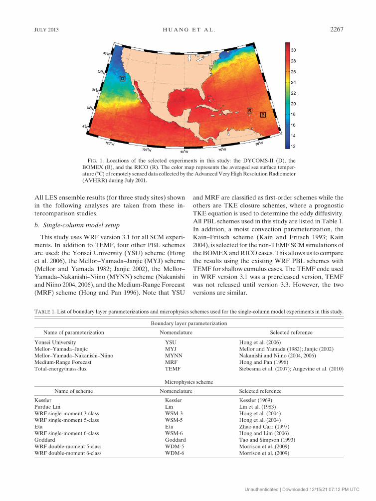
FIG. 1. Locations of the selected experiments in this study: the DYCOMS-II (D), the

BOMEX (B), and the RICO (R). The color map represents the averaged sea surface temper-

ature (8C) of remotely sensed data collected by theAdvancedVeryHighResolutionRadiometer

(AVHRR) during July 2001.

TABLE 1. List of boundary layer parameterizations and microphysics schemes used for the single-column model experiments in this study.

Boundary layer parameterization

Name of parameterization Nomenclature Selected reference

Yonsei University YSU Hong et al. (2006)

Mellor–Yamada–Janjic MYJ Mellor and Yamada (1982); Janjic (2002)

Mellor–Yamada–Nakanishi–Niino MYNN Nakanishi and Niino (2004, 2006)

Medium-Range Forecast MRF Hong and Pan (1996)

Total-energy/mass-flux TEMF Siebesma et al. (2007); Angevine et al. (2010)

Microphysics scheme

Name of scheme Nomenclature Selected reference

Kessler Kessler Kessler (1969)

Purdue Lin Lin Lin et al. (1983)

WRF single-moment 3-class WSM-3 Hong et al. (2004)

WRF single-moment 5-class WSM-5 Hong et al. (2004)

Eta Eta Zhao and Carr (1997)

WRF single-moment 6-class WSM-6 Hong and Lim (2006)

Goddard Goddard Tao and Simpson (1993)

WRF double-moment 5-class WDM-5 Morrison et al. (2009)

WRF double-moment 6-class WDM-6 Morrison et al. (2009)



InWRF, the cloudmicrophysics component estimates

the amount of various types of condensed water (i.e.,

cloud, rain, and ice). Thus, for a givenWRFPBL scheme,

the estimated cloud liquid water can vary with the choice

of microphysics scheme. For each PBL scheme used in

this study, we perform nine simulations with each of

the nine available microphysics schemes, also listed in

Table 1. However, because of the qualitative similarity of

the vertical profile shapes across microphysics schemes,

the average over the ensembles of simulations using the

various microphysics schemes is presented. The vertical

domain of the SCMexperiments includes 116 levels up to

an altitude of 12 000mand the simulation time step is 30 s.

Other model setups are consistent with previous LES

intercomparison studies.

4. Results

Vertical profiles of the temperature and water content

variables are illustrated in the following figures to

compare temporally averaged SCM estimates and the

LES results for the DYCOMS-II (Fig. 2), BOMEX

(Fig. 3), and RICO (Fig. 4) cases. In each subplot,

shaded areas and black dashed lines represent the range

of output of the LES ensembles and the ensemble mean

value, respectively. The LES ensembles are the results

selected from previous LES intercomparison studies,

where 6, 12, and 14 different LES models were used for

the DYCOMS-II, BOMEX, and RICO experiments,

respectively. Note that to show a more clear compari-

son, we plot the cloud liquid water qc profiles in loga-

rithm scale (Figs. 2c, 3c, and 4c). Quantitative statistics

are listed in Table 2. High correlation coefficients for

temperature and humidity profiles between SCM and

LES are expected, so we only show the root-mean-

square error (RMSE) for these two terms. On the other

hand, because we focus on the vertical structure of

cloud, instead of liquid water amount, we calculate the

correlation coefficient (r) between SCM and LES for

the liquid water term.

FIG. 2. Vertical profile of (a) liquidwater potential temperature, (b) total water vapormixing ratio, and (c) cloud liquidwater (on log scale)

for the DYCOMS-II experiments. See text for more details.

FIG. 3. Vertical profile of (a) potential temperature, (b) water vapormixing ratio, and (c) cloud liquid water (on log scale) for the BOMEX

experiments.



a. Stratocumulus case (DYCOMS-II)

While all liquid water potential temperature ul pro-

files are within the range of the LES ensemble, there are

slight differences in the inversion of the PBL (Fig. 2a). In

particular, near the entrainment zone the MRF param-

eterization creates a small temperature inversion that

could be an issue due to numerical instability. All SCM

experiments simulate comparable profiles of total water

mixing ratio qt, but a small overestimate within the PBL

is seen (Fig. 2b). No significant difference is seen in qcacross PBL schemes (Fig. 2c) mostly because this plot

uses a log scale and the cloud cover in this stratocumulus

case is close to 1. Estimates of qc in the MYNN and

TEMF experiments are quite close to LES, while larger

values are simulated by YSU and MRF and a smaller

value is performed by MYJ. The peak qc estimates vary

from 0.23 gkg21 in MYJ to 0.52 gkg21 using MRF, while

the LES ensemble mean is 0.31 gkg21.

b. Shallow cumulus case I: BOMEX

Figure 3 shows the vertical profiles from the BOMEX

case. For potential temperature u, TEMF and MYNN

provide the most realistic profiles, while MYJ is too cold

and shallow, and YSU leads to subcloud layers that are

too deep (Fig. 3a). For water vapor mixing ratio qy (Fig.

3a), the parameterizations show similar biases. The

significant differences between the parameterizations

are clear for cloud liquid water. The qc profiles from all

PBL parameterizations are significantly larger than LES

(Fig. 3c). Essentially, this shows the dangers of the un-

physical coupling between boundary layer, convection,

and cloud microphysics parameterizations in the WRF

Model. In addition, the SCM liquid water vertical

structures shown in Fig. 3c are profoundly different from

one another. The liquid water profiles that better re-

semble the LES results are seen in TEMF (and to

a certain extent MYNN) with realistic cloud-base and

cloud-top heights. YSU and MRF produce clouds that

are too shallow (500m deep instead of over 1 km) with

very large peak values, while MYJ produces a very

shallow cloud. This figure shows that TEMF (and to

a certain extent MYNN) produces the more realistic

vertical structures for this case and quantitative statistics

(e.g., r) listed in Table 2 also confirm this result.

c. Shallow cumulus case II: RICO

Profiles for RICO are plotted in Fig. 4. The results

overall are similar to BOMEX, which shows the ro-

bustness (or lack of it) of the various schemes. The

TEMF (and to a certain extent MYNN) parameteriza-

tion is again superior to the others, producing profiles of

potential temperature (Fig. 4a) and water vapor (Fig.

4b) that are relatively close to the LES ensembles. The

liquid water figure (Fig. 4c) shows again how poor the

FIG. 4. As in Fig. 3, but for the RICO experiments.

TABLE 2. Statistical comparison of temperature and water con-

tent variables between SCM results and LES ensemble mean.

RMSE and r indicate the root-mean-square error and correlation

coefficient, respectively.

Boundary layer

scheme YSU MYJ MYNN MRF TEMF

DYCOMS-II

ul RMSE (K) 0.95 0.89 0.61 0.92 0.71

qt RMSE (gkg21) 0.65 0.67 0.40 0.66 0.48

qc r 0.81 0.78 0.83 0.83 0.85

BOMEX

uy RMSE (K) 0.24 0.48 0.20 0.26 0.35

qy RMSE (gkg21) 0.40 0.61 0.24 0.52 0.34

qc r 0.51 0.01 0.82 0.54 0.82

RICO

uy RMSE (K) 0.73 0.92 0.65 0.69 0.55

qy RMSE (gkg21) 0.55 0.66 0.62 0.67 0.53

qc r 0.39 0.17 0.77 0.50 0.85



WRF SCM simulations for shallow convection situa-

tions are with SCM versions overestimating liquid

water by about one order of magnitude. TEMF shows

a vertical structure of liquid water that although over-

estimating the overall values (as for all other parame-

terizations) produces realistic cloud-base and cloud-top

heights. Again YSU and MRF produce clouds that are

quite shallow (around 500m deep vs 2 km for the LES)

and MYJ produces even shallower (and lower) clouds.

Table 2 also illustrates that the vertical cloud structures

from the MYNN and TEMF experiments are the ones

most close to LES.

5. Conclusions and discussion

An intercomparison of five PBL parameterizations

in the WRF Model for marine cloudy boundary layers

is presented in this study. Four existing WRF PBL

schemes and the recently developed TEMF scheme

(based on the EDMF approach) are evaluated for their

performance against LES results in terms of the vertical

profiles of meteorological states for one stratocumulus

case and two shallow cumulus cases.

For the stratocumulus case there are some differences

in the upper region of the PBL with some parameteri-

zations producing an artificial and noisy vertical struc-

ture in potential temperature. In liquid water, all models

produce a similar structure but with some differences in

terms of absolute values. For both shallow cumulus

cases, the results are fairly similar with TEMF, and to

a certain extent MYNN, producing superior depictions

of the thermodynamic vertical structure. All SCMs

clearly overestimate the values of liquid water when

compared to the LES results, mostly because of the

unphysical coupling between boundary layer and cloud

microphysics parameterizations in WRF. In spite of this

large positive bias, the TEMF version produces realistic

cloud base and cloud heights for both BOMEX and

RICO. Other parameterizations produce cloud struc-

tures that are too shallow not resembling shallow cu-

mulus boundary layers at all in this context.

In spite of its simplicity, this study leads to some key

general conclusions:

1) A parameterization based on the EDMF approach

(i.e., TEMF) that unifies different components (tur-

bulence and moist convection) produces a better re-

sult when compared with LES, with realistic vertical

structures for stratocumulus and cumulus regimes.

2) Existing PBL parameterizations inWRF are not able

to produce fully realistic results when simulating

stratocumulus and shallow cumulus regimes.

3) The often artificial modularity of parameterizations

as they are implemented inWRF produces unreliable

results that are virtually impossible to interpret

because of the plethora of available parameteriza-

tions and their coupling.

Acknowledgments. This work was supported by the

Department of Energy Grant DE-SC0001467. The

authors thank Dr. Wayne Angevine at the National Oce-

anic and Atmospheric Administration and Dr. Thorsten

Mauritsen at theMaxPlanck Institute forMeteorology for

their invaluable discussions on this work. We also thank

Dr. Joshua Hacker at the Naval Postgraduate School for

his help on WRF single-column model simulations. Help

and discussion from Dr. Kay Suselj at the Caltech Jet

Propulsion Laboratory are also greatly acknowledged.

REFERENCES

Angevine, W. M., 2005: An integrated turbulence scheme for

boundary layers with shallow cumulus applied to pollutant

transport. J. Appl. Meteor., 44, 1436–1452.——, H. Jiang, and T. Mauritsen, 2010: Performance of an eddy

diffusivity-mass flux scheme for shallow cumulus boundary

layers. Mon. Wea. Rev., 138, 2895–2912.

Caesar, K., 2005: Summary of the weather during the RICO pro-

ject. NCAR/EOL, 30 pp. [Available online http://www.eol.

ucar.edu/rico.]

Delnore, V. E., 1972: Diurnal variation of temperature and energy

budget for the oceanic mixed layer during BOMEX. J. Phys.

Oceanogr., 2, 239–247.

Duynkerke, P. G., and J. Teixeira, 2001: Comparison of the

ECMWF reanalysis with FIRE I observations: Diurnal vari-

ation of marine stratocumulus. J. Climate, 14, 1466–1478.Holland, J. Z., and E. M. Rasmusson, 1973: Measurement of at-

mospheric mass, energy, and momentum budgets over a 500-

kilometer square of tropical ocean.Mon.Wea. Rev., 101, 44–55.Hong, S.-Y., and H.-L. Pan, 1996: Nonlocal boundary layer vertical

diffusion in a medium-range forecast model. Mon. Wea. Rev.,

124, 2322–2339.

——, and J.-O. J. Lim, 2006: The WRF single-moment 6-class mi-

crophysics scheme (WSM6). J. KoreanMeteor. Soc., 42, 129–151.

——, J. Dudhia, and S.-H. Chen, 2004: A revised approach to ice

microphysical processes for the bulk parameterization of

clouds and precipitation. Mon. Wea. Rev., 132, 103–120.——, Y. Noh, and J. Dudhia, 2006: A new vertical diffusion

package with an explicit treatment of entrainment processes.

Mon. Wea. Rev., 134, 2318–2341.Janjic, Z. I., 2002: Nonsingular implementation of the Mellor–

Yamada level 2.5 scheme in the NCEP Meso model. NCEP

Office Note 437, 61 pp.

Kain, J. S., 2004: The Kain–Fritsch convective parameterization:

An update. J. Appl. Meteor., 43, 170–181.

——, and J. M. Fritsch, 1993: Convective parameterization for

mesoscale models: The Kain-Fritsch scheme. The Represen-

tation of Cumulus Convection in Numerical Models, Meteor.

Monogr., No. 46, Amer. Meteor. Soc., 165–170.

Kessler, E., 1969: On the Distribution and Continuity of Water

Substance inAtmosphericCirculation.Meteor.Monogr.,No. 32,

Amer. Meteor. Soc., 84 pp.

Klein, S. A., and D. L. Hartmann, 1993: The seasonal cycle of low

stratiform clouds. J. Climate, 6, 1587–1606.



Koehler, M., 2005: Improved prediction of boundary layer clouds.

ECMWF Newsletter, No. 104, ECMWF, Reading, United

Kingdom, 18–22.

Lin, Y.-L., R. D. Farley, and H. D. Orville, 1983: Bulk parame-

terization of the snow field in a cloud model. J. Climate Appl.

Meteor., 22, 1065–1092.

Mauritsen, T., G. Svensson, S. S. Zilitinkevich, I. Esau, L. Enger,

and B. Grisogono, 2007: A total turbulent energy closure

model for neutrally and stably stratified atmospheric boundary

layers. J. Atmos. Sci., 64, 4113–4126.

Mellor, G. L., and T. Yamada, 1982: Development of a turbulence

closure model for geophysical fluid problems. Rev. Geophys.

Space Phys., 20, 851–875.

Morrison, H., G. Thompson, and V. Tatarskii, 2009: Impact of

cloud microphysics on the development of trailing stratiform

precipitation in a simulated squall line: Comparison of one-

and two-moment schemes. Mon. Wea. Rev., 137, 991–1007.

Nakanishi, M., and H. Niino, 2004: An improved Mellor–Yamada

level-3 model with condensation physics: Its design and veri-

fication. Bound.-Layer Meteor., 112, 1–31.

——, and——, 2006: An improvedMellor–Yamada level-3 model:

Its numerical stability and application to a regional prediction

of advection fog. Bound.-Layer Meteor., 119, 397–407.Neggers, R. A. J., 2009: A dual mass flux framework for boundary-

layer convection. Part II: Clouds. J. Atmos. Sci., 66, 1489–1506.

Rauber, R. M., and Coauthors, 2007: Rain in Shallow Cumulus

over the Ocean: The RICO campaign. Bull. Amer. Meteor.

Soc., 88, 1912–1928.

Siebesma, A. P., and J. W. M. Cuijpers, 1995: Evaluation of para-

metric assumptions for shallow cumulus convection. J. Atmos.

Sci., 52, 650–666.

——, and J. Teixeira, 2000: An advection-diffusion scheme for the

convective boundary layer: Description and 1D results. Pre-

prints, 14th Symp. on Boundary Layers and Turbulence, As-

pen, CO, Amer. Meteor. Soc., 133–136.

——, and Coauthors, 2003: A large eddy simulation inter-

comparison study of shallow cumulus convection. J. Atmos.

Sci., 60, 1201–1219.

——, and Coauthors, 2004: Cloud representation in general-

circulation models over the northern Pacific Ocean: A

EUROCS intercomparison study. Quart. J. Roy. Meteor. Soc.,

130, 3245–3267.

——, P. M. M. Soares, and J. Teixeira, 2007: A combined eddy-

diffusivity mass-flux approach for the convective boundary

layer. J. Atmos. Sci., 64, 1230–1248.Skamarock, W. C., and Coauthors, 2008: A description of the

Advanced Research WRF Version 3. NCAR Tech. Note

NCAR/TN-4751STR, 125 pp.

Soares, P.M.M., P.M.A.Miranda,A. P. Siebesma, and J. Teixeira,

2004: An eddy-diffusivity/mass-flux parameterization for dry

and shallow cumulus convection. Quart. J. Roy. Meteor. Soc.,

130, 3365–3383.Stevens, B., and Coauthors, 2003: Dynamics and chemistry of

marine stratocumulus—DYCOMS-II. Bull. Amer. Meteor.

Soc., 84, 579–593.

——, and Coauthors, 2005: Evaluation of large-eddy simulations

via observations of nocturnal marine stratocumulus. Mon.

Wea. Rev., 133, 1443–1462.

——, A. Beijaars, S. Bordoni, C. Holloway, M. Kohler, S. Krueger,

V. Savic-Jovcic, and Y. Zhang, 2007: On the structure of

the lower troposphere in the summertime stratocumulus

regimes of the northeast Pacific. Mon. Wea. Rev., 135, 985–

1005.

Suselj, K., J. Teixeira, and G. Matheou, 2012: Eddy diffusivity/

mass flux and shallow cumulus boundary layer: An updraft

PDF multiple mass flux scheme. J. Atmos. Sci., 69, 1513–

1533.

Tao,W.-K., and J. Simpson, 1993: TheGoddard cumulus ensemble

model. Part I: Model description. Terr. Atmos. Oceanic Sci., 4,

35–72.

Teixeira, J., and A. P. Siebesma, 2000: A mass-flux/k-diffusion

approach to the parameterization of the convective boundary

layer: Global model results. Preprints, 14th Symp. on

Boundary Layers and Turbulence,Aspen, CO, Amer. Meteor.

Soc., 231–234.

——, and Coauthors, 2008: Parameterization of the atmospheric

boundary layer: A view from just above the inversion. Bull.

Amer. Meteor. Soc., 89, 453–458.——, and Coauthors, 2011: Tropical and subtropical cloud transi-

tions in weather and climate prediction models: The GCSS/

WGNE Pacific Cross-Section Intercomparison (GPCI). J. Cli-

mate, 24, 5223–5256.Tiedtke, M., W. A. Hackley, and J. Slingo, 1988: Tropical fore-

casting at ECMWF: The influence of physical parameteriza-

tion on the mean structure of forecasts and analyses. Quart.

J. Roy. Meteor. Soc., 114, 639–664.

Witek, M. L., J. Teixeira, and G. Matheou, 2011: An integrated

TKE based eddy-diffusivity/mass-flux boundary layer scheme

for the dry convective boundary layer. J. Atmos. Sci., 68, 1526–1540.

Zhang, M. H., and Coauthors, 2005: Comparing clouds and their

seasonal variations in 10 atmospheric general circulation

models with satellite measurements. J. Geophys. Res., 110,D15S02, doi:10.1029/2004JD005021.

Zhao, Q., and F. H. Carr, 1997: A prognostic cloud scheme for

operational NWP models. Mon. Wea. Rev., 125, 1931–1953.



evaluation of the wrf pbl parameterizations for marine

Documents