Evaporation of Multicomponent Droplets

Von der Fakultät für Luft- und Raumfahrttechnik und Geodäsie

der Universität Stuttgart zur Erlangung der Würde eines

Doktor-Ingenieurs (Dr.-Ing.) genehmigte Abhandlung

von

Dipl.-Ing. Jochen Wilms

aus Heidelberg

Hauptberichter: Prof. Dr.-Ing. habil. Bernhard Weigand

Mitberichter: Prof. Dr.-Ing. habil. Cam Tropea

Tag der mündlichen Prüfung: 26. Oktober 2005

Institut für Thermodynamik der Luft- und Raumfahrt

Universität Stuttgart

2005

Bibliografische Information Der Deutschen BibliothekDie Deutsche Bibliothek verzeichnet diese Publikation in der Deutschen Nationalbibliografie; detaillierte bibliografische Daten sind im Internetüber http://dnb.ddb.de abrufbar.

ISBN 3-89963-255-9

D93

© Verlag Dr. Hut, München 2005.Sternstr. 18, 80538 MünchenTel.: 089/66060798www.dr.hut-verlag.de

Die Informationen in diesem Buch wurden mit großer Sorgfalt erarbeitet. Dennoch können Fehler, insbesondere bei der Beschreibung des Gefahrenpotentials von Ver-suchen, nicht vollständig ausgeschlossen werden. Verlag, Autoren und ggf. Über-setzer übernehmen keine juristische Verantwortung oder irgendeine Haftung für eventuell verbliebene fehlerhafte Angaben und deren Folgen.

Alle Rechte, auch die des auszugsweisen Nachdrucks, der Vervielfältigung und Verbreitung in besonderen Verfahren wie fotomechanischer Nachdruck, Fotokopie, Mikrokopie, elektronische Datenaufzeichnung einschließlich Speicherung und Übertragung auf weitere Datenträger sowie Übersetzung in andere Sprachen, behält sich der Verlag vor.

1. Auflage 2005

Druck und Bindung: printy, München (www.printy.de)

Acknowledgements Above all, I want to thank my advisor, Prof. Dr.-Ing. habil. Bernhard Weigand, director of the Institute of Aerospace Thermodynamics (ITLR) and dean of the Faculty of Aerospace Engineering of the University of Stuttgart, for his great support. While being employed at ITLR, he gave me the opportunity to work on the research topic described in this dissertation with a large amount of own responsibility and scientific freedom. In addition, he encouraged me to present many of my results at several scientific conferences.

I also want to thank Prof. Dr.-Ing. habil. Cam Tropea, chair of Fluid Mechanics and Aerodynamics at the University of Darmstadt, for his prompt willingness to review this dissertation. Moreover, I want to express my gratitude to Prof. Dr. rer. nat. Ernst W. Messerschmid, Professor for Astronautics and Space Stations at the Institute of Space Systems at the University of Stuttgart and former director of the European Astronaut Centre, for being the chair of the examination committee of my dissertation and for his great support throughout my entire education at the University of Stuttgart.

Special thanks goes to Dr.-Ing. Stefan Arndt, representative for Robert Bosch GmbH, for the financial support of my research work.

I further want to thank all colleagues at ITLR for a fruitful cooperation within a friendly working environment. I owe special thanks to Prof. Dr.-Ing. Jens von Wolfersdorf, Dipl.-Phys. Detlef Pape, and Dr. Grazia Lamanna for helpful discussions and, most of all, to Dr.-Ing. Norbert Roth for sharing his broad expertise. In addition, I thank Jutta Schöllhammer and the staff from the mechanical and electrical workshops for their technical support. I also appreciate very much the opportunity of supervising several student research projects. Among those, the most valuable contributions to my research work were conducted by Dipl.-Ing. Marc O. Röhner and Dipl.-Ing. Eduard Rosenko.

With regard to the numerical simulations presented in this dissertation, I want to express my gratitude to Dipl.-Ing. Kai Gartung for allowing me to use his code for computations on droplet evaporation, to Prof. Dr. Gérard Gouesbet and Prof. Dr. Gérard Gréhan for providing their programs to compute the intensity of the scattered light of droplets, and to Prof. Dr. Hervé Jeanmart for performing simulations of the gas flow in the measurement chamber with FLUENT.

In addition, I gratefully acknowledge helpful discussions with many researchers I met on various occasions, especially with Dr. Patrick Le Clercq, Dr.-Ing. Nils Damaschke, Prof. Dr. Patrizio Massoli, and Dr.-Ing. Arne Graßmann.

I am also very grateful to Stan Foster and Dr.-Ing. Sean Jenkins for proofreading this dissertation.

Finally, I want to express my deepest personal thanks to my parents for always supporting me throughout my education.

Stuttgart 2005 Jochen Wilms

Abstract The objective of this study was to provide a better understanding of multicomponent droplet evaporation. The work was motivated by the need to understand the evaporation of fuel droplets in combustion chambers of aerospace and car engines. Within this dissertation, experimental and numerical investigations of the evaporation of droplets with one to three components are presented. From the experiments, data are presented considering mainly surface histories of droplets with various compositions evaporating at various ambient temperatures. Numerical results from different evaporation models are compared to the experimental data to validate the numerical models. The evaporation models and the experiments, especially the optical measurement techniques, are explained together with details on new developments.

For the experiments, setups for single, optically levitated and single, free-falling droplets were used. As droplet liquids, 1-hexadecene and n-alkanes from n-pentane to n-hexadecane were selected. The surrounding gas was either nitrogen or dry air. Experiments were conducted at standard atmospheric pressure and ambient temperatures from about 290 to 350 K. The initial droplet size was on the order of 50 µm. The droplet size was measured using Mie scattering imaging. Additionally, the change of droplet size was measured by detecting morphology-dependent resonances in the intensity of the scattered light. For this measurement technique, a method for the correction of the phase shift of the morphology-dependent resonances due to the changing composition in the case of multicomponent droplets is proposed using numerical simulations including Lorenz-Mie theory. As third optical measurement technique, rainbow refractometry was applied to measure the droplet temperature for pure-component droplets and the composition for binary mixture droplets with low evaporation rates. Moreover, rainbow refractometry was used to detect refractive index gradients for droplets where concentration gradients were predicted by a diffusion-limit model.

From droplet size measurements, histories of the non-dimensional droplet surface are presented. The setups allowed for measurement periods covering nearly the entire lifetime of the droplet. For pure-component droplets, evaporation rates were determined from size histories. Results for different substances at different ambient temperatures are shown. For mixture droplets, the compounds and the initial compositions were varied as well. The large amount of experimental data can be used for the validation of numerical models.

From the classical 2D -law, numerical models were developed for two- and three-component droplets assuming a constant droplet temperature for fast calculations of the droplet evaporation. For two-component droplets, an analytical solution was derived. In addition, a rapid-mixing and a diffusion-limit model with internal heat and mass transfer assuming spherical symmetry were used for numerical simulations.

The numerical models for two- and three-component droplets as well as the analytical solution showed good agreement with experimental data even for mixtures with a large difference in the volatilities of the substances when the appropriate reference state was selected. Rainbow refractometry was successfully applied to measure droplet temperatures and compositions. For mixture droplets, where concentration gradients were predicted by the diffusion-limit model, these gradients did not occur in the experiments. Instead, very good agreement was reached with the rapid-mixing model. This means that the mass transport inside the droplets was most likely enhanced by internal circulation caused by the generation process of the droplet.

Zusammenfassung Das Ziel dieser Arbeit bestand darin, die Verdunstung von mehrkomponentigen Tropfen zu untersuchen. Der Grund für diese Untersuchungen liegt im Bedarf nach einem besseren Verständnis und einer verbesserten Modellierung der Verdunstung von Kraftstofftropfen in den Brennräumen von Luft- und Raumfahrtantrieben sowie Kraftfahrzeugmotoren. In dieser Arbeit werden sowohl experimentelle als auch numerische Untersuchungen der Verdunstung von Tropfen bestehend aus einer bis zu drei Komponenten vorgestellt. Von den experimentellen Ergebnissen werden hauptsächlich Verläufe der Tropfenoberfläche als Funktion der Zeit präsentiert, wobei sowohl die Zusammensetzung der Tropfen als auch die Umgebungstemperatur, der die Tropfen während der Verdunstung ausgesetzt sind, variiert wurden. Numerische Ergebnisse von verschiedenen Verdunstungsmodellen werden mit den experimentellen Ergebnissen verglichen, um die Verdunstungsmodelle zu validieren. Bei den Verdunstungsmodellen kamen vereinfachte Modelle zur Anwendung, die in dieser Arbeit hergeleitet werden, und bei den Experimenten wurden für die optischen Messmethoden spezielle Auswerteroutinen für eine hohe Messgenauigkeit entwickelt.

Für die Experimente wurden Versuchsstände für optisch levitierte und frei fallende Einzeltropfen verwendet. Als Flüssigkeiten wurden 1-Hexadeken und die n-Alkane von n-Pentan bis n-Hexadekan ausgewählt. Das umgebende Gas war entweder Stickstoff oder trockene Luft. Die Experimente wurden bei Standard-Atmosphärendruck und bei Umgebungstemperaturen von 290 bis 350 K durchgeführt. Der Anfangstropfendurch-messer war in der Größenordnung von 50 µm. Die Tropfengröße wurde aus dem Streulicht des Tropfens bestimmt. Bei frei fallenden Tropfen wurde zusätzlich die Änderung der Tropfengröße mit einer Messmethode basierend auf gestaltabhängigen Resonanzen ermittelt. Um diese Methode bei mehrkomponentigen Tropfen einzusetzen, bei denen eine Phasenverschiebung der gestaltabhängigen Resonanzen auftrat, wurde ein Korrekturverfahren mit Hilfe von numerischen Simulationsrechnungen entwickelt. Als weitere optische Messmethode wurde Regenbogen-Refraktometrie zur Bestimmung der Tropfentemperatur bei einkomponentigen und zur Bestimmung der Zusammen-setzung bei zweikomponentigen Tropfen verwendet. Außerdem wurde diese Messtechnik zur Untersuchung von Konzentrationsgradienten im Tropfen benutzt.

Aus den Messungen der Tropfengröße wurde die dimensionslose Tropfenoberfläche als Funktion der Zeit ermittelt. Die Versuchsstände ermöglichten es, dass die Messzeit nahezu die gesamte Lebensdauer des Tropfens umfasste. Bei einkomponentigen Tropfen wurde für unterschiedliche Stoffe und bei unterschiedlichen Umgebungs-temperaturen die Verdunstungsrate bestimmt. Bei mehrkomponentigen Tropfen wurden zusätzlich die Mischungsverhältnisse variiert. Die umfangreichen experimentellen Ergebnisse können für die Validierung von numerischen Berechnungsmethoden verwendet werden.

Ausgehend vom klassischen 2D -Gesetz wurden numerische Modelle für zwei- und dreikomponentige Tropfen zur schnellen Berechnung der Tropfenverdunstung entwickelt, wobei eine konstante Tropfentemperatur angenommen wurde. Für zwei-komponentige Tropfen wurde eine analytische Lösung abgeleitet. Für numerische Berechnungen wurden außerdem ein Rapid-Mixing-Modell (unendlich schneller Wärme- und Stofftransport im Tropfeninneren) und ein Diffusion-Limit-Modell (Wärme- und Stofftransport allein durch Wärmeleitung und Diffusion) mit eindimen-sionaler Betrachtung des Wärme- und Stofftransportes verwendet.

Sowohl die numerischen Modelle für zwei- und dreikomponentige Tropfen als auch die analytische Lösung zeigten eine gute Übereinstimmung mit den experimentellen Ergeb-nissen, wenn ein geeigneter Referenzzustand gewählt wurde. Mit der Regenbogen-Refraktometrie war es möglich, sowohl die Tropfentemperatur als auch die Tropfenzusammensetzung zu messen. Bei mehrkomponentigen Tropfen, bei denen vom Diffusion-Limit-Modell Konzentrationsgradienten vorhergesagt wurden, traten diese nicht auf. Stattdessen wurde eine sehr gute Übereinstimmung mit dem Rapid-Mixing-Modell gefunden. Deswegen wird vermutet, dass der Stofftransport im Tropfeninneren durch Zirkulation der Flüssigkeit, die bei der Tropfenerzeugung entstand, erhöht wurde.

IX

Table of Contents

List of Symbols XIII

List of Acronyms XVII

1 Introduction 1

1.1 Motivation .......................................................................................................... 1

1.2 Literature Review ............................................................................................... 1

1.3 Objective............................................................................................................. 8

2 Droplet Liquids 9

2.1 General Properties of Droplet Liquids................................................................ 9

2.2 Refractive Index of Droplet Liquids................................................................. 10

2.3 Liquid Mixtures ................................................................................................ 12

2.3.1 Mixing Behavior ................................................................................. 12

2.3.2 Preparation of Liquid Mixtures........................................................... 12

3 Droplet Evaporation Models 13

3.1 Overview .......................................................................................................... 13

3.2 Classical D2-Law.............................................................................................. 15

3.2.1 Introduction and Assumptions............................................................ 15

3.2.2 Governing Equations .......................................................................... 16

3.2.3 Evaporation Rate and D2-Law............................................................ 17

3.2.4 Property Evaluation ............................................................................ 18

3.3 The D2-Model (D2M)....................................................................................... 19

3.4 Simplified D2-Model (SD2M).......................................................................... 21

3.4.1 Evaporation Rate by Simplification of D2M...................................... 21

3.4.2 Evaporation Rate from Basic Conservation Equations....................... 22

3.4.3 Influence of the Temperature on the Evaporation Rate...................... 23

X TABLE OF CONTENTS

3.4.4 Reference Temperature and Property Evaluation ...............................24

3.5 Simplified Rapid-Mixing Model (SRMM).......................................................25

3.6 SRMM for Two-Component Droplets..............................................................27

3.6.1 Set of Differential Equations...............................................................27

3.6.2 Property Evaluation.............................................................................28

3.6.3 Evaporation Rate .................................................................................29

3.7 SRMM for Three-Component Droplets............................................................29

3.8 Analytical Solution for Binary Mixture Droplets .............................................30

3.8.1 Solution for ξ(X1) ................................................................................31

3.8.2 Solution for t(X1) ................................................................................36

3.8.3 Application of ARMM........................................................................39

3.9 Models with Time and Space Discretization ....................................................39

4 Light Scattering from Droplets 41

4.1 Introduction.......................................................................................................41

4.2 Theories for Light Scattering ............................................................................44

4.3 Numerical Codes for LMT................................................................................46

4.4 Rainbow and Airy Theory.................................................................................47

4.5 Morphology-Dependent Resonances (MDRs)..................................................49

5 Experimental Methods 51

5.1 Setup for Single, Optically Levitated Droplets .................................................51

5.1.1 Optical Levitation................................................................................51

5.1.2 Experimental Setup .............................................................................54

5.2 Setup for Single, Free-Falling Droplets ............................................................56

5.3 Comparison of the Experimental Setups...........................................................58

5.4 Droplet-on-Demand Generators........................................................................61

5.5 Observation Chamber .......................................................................................63

5.5.1 Droplet Motion....................................................................................63

5.5.2 Gas Flow .............................................................................................69

5.5.3 Heating System ...................................................................................73

TABLE OF CONTENTS XI

5.6 Measurement Procedure ................................................................................... 75

5.6.1 Optical Levitation ............................................................................... 75

5.6.2 Free-Falling Droplets.......................................................................... 75

6 Optical Measurement Techniques 77

6.1 Droplet Sizing with Mie Scattering Imaging.................................................... 77

6.1.1 Introduction......................................................................................... 77

6.1.2 Optical Fourier Transform.................................................................. 78

6.1.3 Determination of the Droplet Size from a Single CCD Image........... 80

6.1.4 Initial Droplet Diameter D0 ................................................................ 81

6.2 Droplet Sizing with MDRs............................................................................... 82

6.2.1 Introduction......................................................................................... 82

6.2.2 Determination of D(t) ......................................................................... 83

6.2.3 Detection of MDRs............................................................................. 84

6.2.4 Correction Factor f∆D .......................................................................... 87

6.3 Rainbow Refractometry (RRF) ........................................................................ 89

6.3.1 Introduction......................................................................................... 89

6.3.2 Determination of the Refractive Index ............................................... 90

6.3.3 Improvement of Accuracy .................................................................. 92

6.3.4 Sensitivity ........................................................................................... 93

7 Measurement Uncertainties 95

7.1 Measured Quantities ......................................................................................... 95

7.1.1 Overview............................................................................................. 95

7.1.2 Ambient Temperature Τ∞ ................................................................... 95

7.1.3 Droplet Diameter D ............................................................................ 96

7.1.4 Change of Droplet Diameter ∆D ..................................................... 101

7.1.5 Refractive index n............................................................................. 103

7.2 Derived Quantities.......................................................................................... 104

7.2.1 Initial Droplet Diameter D0 .............................................................. 104

7.2.2 Non-dimensional Droplet Surface (D/D0)2....................................... 104

7.2.3 Evaporation Rate β ........................................................................... 104

XII TABLE OF CONTENTS

8 Results of Droplet Sizing 107

8.1 Overview.........................................................................................................107

8.2 General Remarks.............................................................................................107

8.3 Pure-Component Droplets...............................................................................108

8.3.1 N-Hexadecane ...................................................................................108

8.3.2 N-Nonane ..........................................................................................110

8.3.3 N-Pentane ..........................................................................................112

8.3.4 Evaporation Rates of Different n-Alkanes ........................................114

8.4 Binary Mixture Droplets .................................................................................116

8.4.1 N-Hexadecane with n-Tetradecane ...................................................116

8.4.2 N-Hexadecane with a Highly Volatile n-Alkane ..............................116

8.4.3 N-Hexadecane with n-Heptane .........................................................120

8.4.4 N-Hexadecane with n-Hexane ..........................................................123

8.4.5 Property Variation of DLM...............................................................124

8.5 Ternary Mixture Droplets ...............................................................................126

8.5.1 Variation of Substances.....................................................................127

8.5.2 Variation of Temperature ..................................................................129

9 Results of Rainbow Refractometry 133

9.1 Droplet Temperature .......................................................................................133

9.2 Droplet Composition.......................................................................................134

9.3 Refractive Index Gradients .............................................................................138

9.3.1 Effect of Refractive Index Gradients on the Rainbow Angle ...........138

9.3.2 Numerical Simulation of Refractive Index Gradients.......................139

9.3.3 Comparison of Experimental and Numerical Results .......................142

10 Conclusions 147

References 151

Appendix: Property Data 157

XIII

List of Symbols English Letter Symbols

A [m2] area

fA [m2] frontal area (area projected perpendicular to the free stream velocity)

YB [-] mass transfer number, Eq. (3.2)

TB [-] heat transfer number, Eq. (3.5) C [-] number of carbon atoms

pc [J/(kg⋅K)] specific heat at constant pressure D [m] droplet diameter, 2= sD r

0,lin.D [m] initial droplet diameter obtained by linear interpolation (see section 6.1.4)

ijA [m2/s] mass diffusion coefficient for a binary mixture, =ij jiA A

imA [m2/s] effective binary diffusion coefficient of component i in a mixture

F [N] force

dF [N] drag force

gF [N] gravitational force f [m] focal length

Df∆ [-] correction factor, introduced in Eq. (6.4)

OFTf [° or rad] transformation factor of optical Fourier transform fρ [-] factor, Eq. (3.69) g [m/s2] standard acceleration of gravity, 29 81 m/s.=g

Yg [kg/(m2⋅s)] mass transfer conductance h [W/( m2⋅K)] heat transfer coefficient I [W/m2] irradiance or light intensity vh [J/kg] latent heat of vaporization k [W/(m⋅K)] thermal conductivity Le [-] Lewis number, Le Sc /Pr=i i , e.g., Le /=i imα A M [kg/mol] molecular weight m [kg] mass ɺm [kg/s] mass flow rate ′′ɺm [kg/(m2⋅s)] mass transfer rate, mass flux

N ′′ɺ [mol/(m2⋅s)] absolute molar flux

pN [-] pixel number

FN∆ [-] fringe spacing on CCD array measured in number of pixels Nu [-] Nusselt number, e.g., /=dNu Dh k n [-, mol] real part of refractive index, number of moles

XIV LIST OF SYMBOLS

ɺn [mol/s] molar flow rate ′′ɺn [mol/(m2⋅s)] molar transfer rate, molar flux

532n [-] real part of refractive index at a wavelength of 532 nm p [Pa] pressure Pr [-] Prandtl number, Pr /= ν α molR [J/(mol⋅K)] molar gas constant, 8 314 J/(mol K).= ⋅molR

r [m] radial coordinate

sr [m] droplet radius Re [-] Reynolds number, e.g., Re /=d vD µρ S [-] standard deviation Sc [-] Schmidt number, e.g., /=i imSc ν A Sh [-] Sherwood number, e.g., , , /( )=d i Y i imSh g D ρA T [K or °C] temperature

bT [K or °C] boiling temperature

meT [K or °C] melting temperature t [s] time u [m/s] velocity component in the x -direction U [V] voltage v [m/s] velocity component in the y -direction v [m/s] velocity vector V [m3] volume w [m/s] velocity component in the z -direction X [-] mole fraction x [m] rectangular coordinate Y [-] mass fraction y [m] rectangular coordinate Z [-] volume fraction z [m] rectangular coordinate

Greek Letter Symbols

α [m2/s] thermal diffusivity, /( )pk cρ β [m2/s] evaporation rate, Eq. (3.10) γ [-] species property ratio, 2 1 2 1 2 1, ,: / ( / )( / )= = m m s sp pγ φ φ A A ε [-] species property ratio, 1 2: /= mol molV Vε ζ [-] normalized angular deviation from the geometrical rainbow

angle η [-] integration variable θ [° or rad] scattering angle, defined in section 4.1

ipθ [° or rad] angle of inflection point of the main peak of the 1st rainbow

raθ [° or rad] rainbow angle according to Airy theory, Eq. (4.4)

rgθ [° or rad] rainbow angle according to geometrical optics, Eq. (4.1)

LIST OF SYMBOLS XV

Fθ∆ [° or rad] angular fringe spacing λ [m] wavelength µ [kg/(m⋅s)] dynamic viscosity ν [m2/s] kinematic viscosity, /µ ρ ρ [kg/m3] density molmρ [mol/m3] molar density of the mixture, 1/( )= Σmol mol

m i iXVρ σ [N/m] surface tension

eτ [s] lifetime or evaporation time, 20 /e Dτ β= ( 2D -law)

rτ [s] relaxation time constant, 20 18: /( )r lD µτ ρ=

iφ [mol/(m⋅s)] species constant, ,: /( )= moli im i sp R Tφ A

ξ [-] non-dimensional droplet surface, 20: ( / )= D Dξ

rainbowΩ [-] rainbow integral

Subscripts

0 initial ∞ far away, ambient, free-stream g gas i species i j species j l liquid m mean, mixture max maximum min minimum r reference s s-surface (in a fluid, adjacent to an interface or wall) t terminal

Superscripts

mol molar ′′ per unit area

Overscores

mean ɺ per unit time ɶ approximate

Underscores

complex

XVII

List of Acronyms ARMM Analytical solution of the simplified Rapid-Mixing Model CCD Charge-Coupled Device CLM Conduction-Limit Model DODG Droplet-On-Demand Generator DLM Diffusion-Limit Model GO Geometrical Optics ITLR Institut für Thermodynamik der Luft- und Raumfahrt, Universität Stuttgart

(Institute of Aerospace Thermodynamics, University of Stuttgart) LMT Lorenz-Mie Theory MDRs Morphology-Dependent Resonances MSI Mie Scattering Imaging RMM Rapid-Mixing Model RRF Rainbow Refractometry SD2M Simplified 2D -Model SRMM Simplified Rapid-Mixing Model D2M 2D -Model UTM Uniform-Temperature Model VDI Verein Deutscher Ingenieure (Association of German Engineers)

1

1 Introduction

1.1 Motivation For modern combustion engines using liquid fuels, several processes play important roles in reaching high efficiency in the combustion cycle and low emissions in the exhaust gas. One of these processes is the evaporation of the fuel in the combustion chamber. For direct injection systems used in aircraft or car engines, the fuel enters the combustion chamber in the liquid state. During injection, the liquid disintegrates into single droplets by atomization. In addition, the droplets evaporate before combustion occurs.

Commercial fuels are complex mixtures of many compounds with different physical properties. For that reason, the evaporation of multicomponent droplets is a complex process. As the droplets travel through the combustion chamber, their size and composition changes. The size history influences the dynamic behavior of the droplets, whereas the variation of the composition determines the distribution of the gasified fuel compounds within the combustion chamber. The fundamental understanding of these processes is essential for the modeling of fuel sprays.

In fuel sprays, droplet evaporation is influenced by several effects such as convection of the surrounding gas flow or an interaction among droplets. However, for a basic understanding of multicomponent droplet evaporation, it is necessary to investigate droplet evaporation without these influences, i.e., to study the evaporation of a single droplet in a quiescent atmosphere.

Experiments of this type were conducted at the Institute of Aerospace Thermodynamics (ITLR), where several experimental and numerical studies have been performed in the field of droplet dynamics led by A. Frohn in the 1980s. The results are partially covered by the textbook of Frohn and Roth (2000) on droplet dynamics. For the investigation of droplets, optical measurement techniques were developed at ITLR for the measurement of size histories.

1.2 Literature Review In the literature, there are many experimental studies dealing with droplet evaporation. However, there are only few studies that come close to the basic and ideal case of a single, multicomponent droplet evaporating in a quiescent atmosphere. A large number of studies consider droplets in sprays. However, even in sparse sprays, the interaction of

2 1 INTRODUCTION

the droplets cannot be neglected. In other studies, a convective flow often enhances the heat and mass transfer around the droplet. Moreover, the shape of the droplet can be distorted by the flow. The heat transfer and the shape of the droplet can also be influenced by the measurement technique, e.g., when suspension or levitation techniques are used. In the published studies, frequently the droplet behavior is influenced by several parameters. However, the effects of the different parameters cannot be clearly separated. As a result, there are large uncertainties when trying to reduce the experimental data to the described ideal case.

With respect to the composition of the droplets, some of the studies consider real fuels. Generally, these fuels consist of a huge number of compounds. Often the composition is unknown. As a result, the effects of the single components on multicomponent droplet evaporation cannot be distinctly identified. For that reason, studies considering real fuels are not included in the literature review.

In the following, experimental studies on droplet evaporation are reviewed. The focus is on studies at standard atmospheric pressure and moderate ambient temperatures. Moreover, studies using n-alkanes or at least miscible compounds with an ideal mixing behavior are preferred. The main interest is in size histories and evaporation rates. Studies providing additional information on the droplet such as temperature and composition are reviewed at the end of this section. Additional references, especially with regard to the measurement techniques and the numerical models used in this study, can be found in the corresponding chapters.

In some respects, the review follows the historical development. In another sense, it begins with investigations on pure-component droplets and continues with multicomponent droplets. Some of the papers are grouped according to experimental techniques.

Fundamental studies on liquid droplet evaporation were performed by Frössling (1938). On the basis of a dimensionless analysis he derived the well-known relationship for the Sherwood number as a function of the Reynolds and Schmidt number. For the determination of the constant of the relationship, he investigated the evaporation of water, nitrobenzene, and aniline droplets suspended in air. Experiments were carried out at room temperature for Reynolds numbers ranging from 2 to 800 and droplet diameters from 0.1 to 0.9 mm.

Ranz and Marshall (1952a and 1952b) conducted experiments on the evaporation of pure-component droplets. They investigated droplets, mainly of water, at air temperatures up to 493 K for a Reynolds number range from 0 to 200. The droplet diameters ranged from 0.6 to 1.1 mm. The droplets were suspended from a feed capillary with a diameter of about 80 µm. In the capillary was a thermocouple used for measurements of the droplet temperature. The droplet was observed through a microscope and its image was recorded on a motion picture film at a rate of 24 Hz. The droplet diameters were measured frame by frame on a microfilm viewer. From their

1.2 LITERATURE REVIEW 3

experiments, they determined evaporation rates at different ambient conditions and used their results to modify the coefficient of Frössling's relationship. Their relationships for the Nusselt and Sherwood number are still used today in numerical models in order to account for convection.

Downing (1966) continued the work of Ranz and Marshall. He used the same experimental techniques and investigated droplets of pure liquids at temperatures from 300 to 613 K for Reynolds numbers from 24 to 325. Among the investigated liquids was an n-alkane, in this case n-hexane. The size of the droplets was on the order of a millimeter.

Beard and Pruppacher (1971) performed measurements of small water drops falling freely at terminal velocity in a wind tunnel. The air stream was directed upwards and controlled by a valve so that the droplet was kept stationary. The initial droplet size ranged from 70 to 375 µm. A minimum size of 27 µm was investigated. For the determination of the evaporation rate, they used drag relationships for droplets and their measurements of the terminal velocity. The results were presented as Sherwood numbers. For low Reynolds numbers, 2Re < , they found that the Sherwood number smoothly approached Sh 2= .

With the emergence of lasers, new measurement techniques evolved which allowed the determination of the droplet size with a higher accuracy than by photographic imaging. Ravindran et al. (1979) measured the size history of droplets suspended in an electric field. The initial droplet diameters were between 1.2 and 2.4 µm. The droplet liquids were pure organics with very low volatilities. The carrier gases were helium, nitrogen, or carbon dioxide. The experiments were performed at standard atmospheric pressure and at temperatures ranging from 280 to 307 K. The droplet size was measured using Mie theory. By traversing a photomultiplier, the intensity of the scattered light was scanned within an angular range of 40 150° ≤ ≤ °θ . The intensity distributions were compared to results from Mie theory. They claimed to reach an accuracy of 1% for the droplet radius. A traverse of the photomultiplier required 14 s, which was a short time period compared to the entire measurement period of up to 2500 s. During the measurement period, the droplets changed their size significantly. Plotting the square of the droplet radius versus time yielded straight lines showing that the evaporation process was diffusion-controlled. Davis and Ray (1980) found that the evaporation rates were in good agreement with the theory for isothermal diffusion-controlled evaporation.

Subsequent to their study on pure-component droplets, Ravindran and Davis (1982) investigated two-component droplets. In their publication, they presented a theoretical analysis of diffusion-controlled evaporation of two-component droplets based on an ideal solution behavior and diffusion of the individual species in the surrounding inert gas. Comparing their experimental results with results from theory for the surface area history, they claimed to reach reasonably good agreement. However, their experimental data was very sparse.

4 1 INTRODUCTION

In addition to electrostatic levitation, acoustic levitation is another levitation technique that was often used to study droplet evaporation. In this case, the droplet is levitated in an acoustic field with a standing wave. Due to the high-pressure gradients, there is a flow around the droplet which considerably influences the evaporation behavior. In addition, the droplet shape is distorted which leads to difficulties for the determination of the droplet size. For that reason, a great deal of effort was spent in order to study the effects of these influences on droplet evaporation.

Daidzic (1995) studied nonlinear droplet oscillations and evaporation in an ultrasonic levitator. Among other liquids, he investigated the evaporation of n-octane and n-decane. Yarin et al. (1999) presented surface area histories of pure-component droplets of different substances. They showed that the acoustic streaming in the gas provides a convective mechanism much stronger than the ordinary one and thus dominates the evaporation. Kastner (2001) investigated droplets of one and two components. Yarin et al. (2002) also presented results for binary mixture droplets. Recently, Brenn et al. (2003) showed experimental and numerical results from droplets containing three to five components. For organic compounds, they selected mainly alcohols. Due to the dipole moment of the hydroxil group, the mixing of the substances lead to a deviation from the ideal behavior. This was taken into account by calculating activities of the liquids. The experiments were conducted at room temperature, with initial droplet diameters larger than 1 mm. For the determination of the droplet size, a sharp image of the shadow of the ellipsoidal droplet was taken by a CCD camera and the droplet size was monitored until nearly complete evaporation.

Tuckermann et al. (2002) also used the acoustic levitation method. They used n-alkanes ranging from n-pentane to n-decane and investigated pure-component droplets. The droplet size was monitored with a CCD camera and ranged from 0.1 to 2.5 mm. In addition, the droplet temperature was measured by IR thermography. They presented results including surface histories and evaporation rates.

Another levitation technique is optical levitation. Here, a droplet is stabilized using radiation pressure forces. Since this technique is used in this study, it is described in more detail in section 5.1.1. In order to avoid heat input from the light used for levitation, the droplet liquid must not absorb the light. This requirement reduces the number of possible substances for investigations. In addition, the initial droplet size must be considerably smaller than a millimeter to permit levitation with reasonable laser power. This is in accordance with the desired droplet sizes. Looking at the Sauter mean diameters of typical gasoline and diesel sprays, they have their largest values for low pressure sprays for injection systems with intake tubes ranging from 50 to 120 µm. For direct injection systems using gasoline, the Sauter mean diameters are on the order of 15 to 25 µm. Diesel sprays have the smallest droplets with diameters smaller than 10 µm.

Using optical levitation, Roth et al. (1994) studied the evaporation of supercooled water droplets or ice crystals at ITLR. The droplet size was measured from the fringe spacing

1.2 LITERATURE REVIEW 5

of the scattered light at a scattering angle of 45°. In addition, oscillations of the droplet position caused by morphology-dependent resonances were recorded with a position-sensing detector at a scattering angle of 90°. From the frequency of the fluctuations, the change of the droplet radius with time was determined. Results of the droplet surface history were presented at ambient temperatures from about 240 to 270 K. The initial droplet diameter was on the order of 20 µm.

Other studies concerned binary mixtures of low volatile n-alkanes. Roth and Frohn (1997) showed droplet surface histories of two-component droplets of n-pentadecane and n-hexadecane with different initial compositions at room temperature. The initial droplet diameter was up to 50 µm. This time, the morphology-dependent resonances used for determining the change of the droplet size were detected in the region of the rainbow. Increasing the difference in volatilities of the binary mixture, Gartung et al. (2000) investigated droplets of n-tetradecane and n-hexadecane. Again, the initial composition was varied while the ambient temperature remained at room temperature. The initial droplet size was on the order of 20 µm.

Many experimental investigations dealt with monodisperse droplets produced by droplet stream generators. Monodisperse droplet streams offer the advantage of studying droplet evaporation in a quasi-stationary system without using high-speed measurement techniques. Another advantage is that the evaporation can be investigated very shortly after droplet generation within a time domain on the order of milliseconds. This allows for the study of droplets with very high evaporation rates. However, the tracking of the droplet history is limited to a certain stable regime. Beyond that regime, droplets start to oscillate and collisions can occur. With respect to the goal of investigating a single droplet in a quiescent atmosphere, droplet stream generators have two disadvantages. One is the enhancement of the evaporation due to the high speed of the droplets, the other one the interaction of the droplets due to the usually small spacing between the droplets. In order to minimize the latter disadvantage, one often tries to augment the spacing. One possible solution is to charge the droplets and extract some of the droplets in an electric field. Although droplet stream generators come close to the ideal case of monosized droplets, there is some uncertainty of the droplet size inherent to this technique. The size range of the droplets is usually in the desired submillimeter range.

Stengele et al. (1999) performed measurements of one- and two-component droplet evaporation with droplet stream generators. The droplets were free-falling in a high-pressure environment with pressures ranging from 20 to 40 bar and temperatures up to 650 K. The droplet size was measured by video technique and a stroboscope lamp. The initial diameters ranged from 0.6 to 0.8 mm. The smallest detectable droplet size was about 0.3 mm. The droplet distance was more than 100 times the initial droplet diameter in order to exclude interactions between the droplets. They presented size histories of droplets consisting of n-pentane, n-nonane, and binary mixtures of these two compounds. They found good agreement when comparing their experimental results

6 1 INTRODUCTION

with numerical calculations based on the conduction-limit model and on the diffusion-limit model.

Chen et al. (1997) investigated droplet evaporation in a heated air flow. They used a droplet-on-demand injection system which can be operated at frequencies up to 1 kHz. They investigated droplets of n-hexane, n-decane, and a binary mixture of equal amounts of hexane and decane. No information was given on the actual spacing between the droplets. The temperature of the flow was about 400 K. They compared their experimental results to numerical simulations with the diffusion-limit model and the infinite diffusion model (called the rapid-mixing model in this thesis). The binary mixture droplets have an initial diameter of about 70 µm. Comparing their experimental results with results from numerical simulations they claimed to reach better agreement with the infinite diffusion model than with the diffusion-limit model. However, a large scattering of their data was obvious and the difference between the results of the two numerical models was not significant.

Randolph et al. (1986) studied free-falling monodisperse droplets consisting of binary mixtures of n-alkanes. The mixtures contained n-hexadecane and n-tetradecane, n-dodecane, or n-decane. The droplet size was determined through photography and the composition through sampling and analysis with a gas chromatograph. The droplets had initial sizes of 130 to 300 µm and were injected at 67 per second to ensure vanishingly small droplet interaction effects. They studied both evaporation and combustion. For the case of evaporation, the droplets were exposed to temperatures of 675 and 1020 K. They discovered that the gasification mechanism of these droplets was intermediate to those in the batch distillation and diffusion-limited steady state.

Gartung et al. (2002) studied the evaporation of monodisperse droplets at 1 bar and 296 K. They investigated four different mixtures with either two or four components of n-alkanes between n-pentane and n-octane. The droplets were collected in a vial at different distances from the orifice of the generator. The droplet size was determined from the mass of the sampled liquid. In addition, the composition was determined by gas chromatography. When they compared their experimental results with numerical results of a diffusion-limit model, they obtained good agreement. However, they did not take into account the reduction of the evaporation rate due to the close spacing of the droplets, which was on the order of 3 to 4 droplet diameters, or the reduction of the droplet speed relative to the air due to the entrainment of the surrounding air caused by the droplet stream.

Due to their simplicity, suspension techniques are still used today. Often a thermocouple is used for the droplet suspension. There are special studies which address the heat transfer through the support fiber (Yang 2002, Nomura 2003). The initial droplet size is usually above one millimeter so that the droplet diameter is considerably larger than the diameter of the suspension fiber in order to minimize the influence of the fiber. Due to the relatively large droplet size, the lifetime of the droplets is large, which

1.2 LITERATURE REVIEW 7

allows one to obtain elaborate size histories, i.e., with a large amount of data points. Gökalp et al. (1994), Runge et al. (1998), and Daif et al. (1999) investigated droplets of pure n-heptane, n-decane, and binary mixtures of the two substances. While Gökalp et al. used different initial composition for the binary mixtures, the other studies considered only mixtures with equal amounts of the two compounds. All studies considered convective vaporization. Gökalp et al. and Daif et al. also investigated evaporation in a quiescent atmosphere. The droplet size was measured by recording the droplet image with a camera. All studies were conducted at ambient pressures. Runge et al. performed measurements at an ambient temperature of 273 K, Daif et al. at about 300 K and Gökalp et al. varied the temperature from about 300 to 450 K. Runge et al. used initial droplet diameters from about 0.5 to 0.6 mm, Daif et al. from about 0.6 to 0.8 mm and Gökalp et al. used an initial size of about 1.3 mm. Daif et al. and Runge et al. compared their experimental results with numerical results from a rapid-mixing model and found good agreement.

In addition to droplet size measurements, additional techniques are often used to gain further information on the droplet. The most interesting parameters are the droplet temperature and composition. When the droplet is suspended on a fiber, often a thermocouple is used to obtain the droplet temperature. Wong and Lin (1992) even measured temperature distributions in suspended droplets using fine thermocouples in droplets with a fixed size of 2 mm. In other experimental setups, additional measurement techniques are necessary. For the measurement of the surface temperature, infrared thermography has been applied (Daif et al. 1999). Another possibility is to use the sensitivity of the position of the rainbow to determine the droplet temperature (Roth et al. 1988). The intensity distribution of the scattered laser light in the region of the rainbow can also be used to measure the droplet temperature and size simultaneously (van Beeck and Riethmuller 1995). Castanet et al. (2003) measured temperature distributions within monodisperse droplets by two-colour laser-induced fluorescence. Laser-induced fluorescence allows one to also gain information on the evaporated liquid in the gas phase (Rossow et al. 2004).

For the measurement of the droplet composition, rainbow refractometry was used in this thesis for droplets with approximately uniform and constant temperatures. This can only be used for binary mixture droplets, since for droplets with more than two components, other techniques must be applied. As already mentioned, gas chromatography is one possible technique for the measurement of the droplet composition (Randolph et al. 1986, Gartung et al. 2002). This technique works well with monodisperse droplets where sufficient droplet liquid can be collected. For single, optically levitated droplets, Kiefer et al. (1997) used Raman scattering for the determination of the droplet composition.

It is clear that there are very few studies considering mixture droplets with more than two components. In addition, initial droplet diameters were rarely in the desired range of 20 to 100 µm. Usually, the droplets were larger than a millimeter where the shape of

8 1 INTRODUCTION

the droplet can be deformed and the internal processes due to circulation can also be different. Generally, the number of data points for size histories is small and measurement uncertainties are often large. No study was found where experimental data was provided to clearly decide whether multicomponent droplet evaporation is described best by the rapid-mixing model, the diffusion-limit model, or some intermediate model.

1.3 Objective As stated previously, there are several deficits concerning multicomponent droplet evaporation. This thesis strives to partially alleviate this situation. The primary focus of this thesis is the evaporation of single, multicomponent droplets in a quiescent atmosphere. Experiments were conducted at standard atmospheric pressure and the ambient temperature was varied from 290 to 350 K. Initially, pure-component droplets were investigated and results from the evaporation rate were compared to results from the classical 2d -law. Subsequently, mixture droplets with up to three components were studied. The substances used were n-alkanes as they comprise the major part of automotive and aviation fuels. The initial droplet diameter was on the order of 50 µm so that the droplet size corresponds roughly to the Sauter mean diameter of typical gasoline fuel sprays. Non-intrusive optical measurement techniques were used to obtain size histories with high accuracies. Existing experimental facilities at ITLR were modified and improved in order to achieve these objectives.

Parallel to the experiments, simple numerical and analytical models allowing fast calculation of the droplet evaporation were developed and results of these models were compared to experimental data. In addition, more complex models such as a diffusion-limit model considering internal heat and mass diffusion were used. Numerical simulations with this model and a rapid-mixing model were performed in order to find out under what conditions large differences in the droplet evaporation behavior were predicted. Experiments were conducted at these conditions to determine how experimental data related to results from these evaporation models.

9

2 Droplet Liquids

2.1 General Properties of Droplet Liquids Substances contained in automotive and aviation fuels were chosen as droplet liquids. These fuels are complex mixtures of many different hydrocarbon compounds. Commercial petrol is composed of 35 - 65% alkanes (paraffins), 0 - 35% alkenes (olefins), and 23 - 55% aromatics. Diesel fuel consists of about 45% alkanes, 25% naphthenes (cycloparaffins), and 30% aromatics (Wenck et al. 1993). Aviation fuels, such as JET A1 for civil use or JP-4 for military aircrafts, also have constituents from all of these groups of chemical compounds (Catoire et al., 1999). For all of these fuels the major constituents are alkanes, which are saturated hydrocarbons with the general structural formula 2 2+n nC H . N-alkanes, with a chainlike structure where the carbon atoms are arranged in a zigzag pattern, were used for this study.

N-alkanes offer several advantages for experimental investigations. First of all, they are non-toxic. In addition, they do not absorb the laser light used for optical levitation and optical measurement techniques. Non-absorption is important in order to not influence the thermodynamic behavior of the droplets. Another advantage to using n-alkanes is their diversity with respect to their volatility. By changing the number of carbon atoms, a broad range of volatilities, which can also be found among the components of automotive fuels, can be produced. Thus, different fuels can be modelled using different n-alkanes. If, for example, only one n-alkane is used to represent a fuel, petrol is represented best by n-octane, diesel by n-dodecane, and the aviation fuel JET A1 by n-nonane (Catoire et al., 1999).

For this study, n-alkanes ranging from n-pentane with 5 carbon atoms to n-hexadecane with 16 carbon atoms were used. These substances are liquid at room temperature. N-alkanes with less carbon atoms than n-pentane are gaseous, for example, n-butane with only 4 carbon atoms and a boiling temperature of 272.5 K at 1 bar. In contrast, n-alkanes with more carbon atoms than n-hexadecane are solid, which is the case for n-heptadecane with 17 carbon atoms and a melting point of 295 K. Detailed data on physical properties for the n-alkanes used in this study can be found in the appendix.

In addition to the above-mentioned n-alkanes, one compound from the group of alkenes was selected for experimental investigations. 1-hexadecene was chosen with a double bond placed at the beginning of the carbon chain. This substance was chosen particularly for measurements with rainbow refractometry in order to increase the measurement accuracy when multicomponent droplets were investigated. With regard to general physical properties such as density, volatility and characteristic temperatures,

10 2 DROPLET LIQUIDS

1-hexadecene is very close to n-hexadecane, but the refractive index is significantly larger. Hence, when 1-hexadecene is used instead of n-hexadecane for a two-component droplet, the evaporation behavior is nearly the same, but the difference in the refractive index of the two substances is larger.

2.2 Refractive Index of Droplet Liquids The refractive index is an important property for optical measurement techniques. It is especially important for rainbow refractometry, where the refractive index of the droplet is determined from the intensity distribution of the scattered light in the region of the rainbow, assuming a constant refractive index inside the droplet. Since the refractive index depends on the temperature and on the substance, information on these properties can be derived from the determination of the refractive index. For this reason, the refractive index of the droplet liquids is described in detail in this section.

In general, the refractive index n is a complex property

i= + ɶn n n (2.1)

where n is the real part and ɶin the imaginary part. The imaginary part describes the absorption of the light. For the substances of this study, 0=ɶn for the wavelengths of the lasers used for both optical levitation and the optical measurement techniques. This is desired in order to not influence the thermodynamic behavior of the droplet by absorption of energy from the laser light. In the following, the real part n is used and is simply called refractive index (since =n n with 0=ɶn ).

Values for the refractive index found in the literature are generally available at room temperature, i.e., at about 295 K, and at the wavelength of the sodium D line, which is 589 nm. However, in this study the temperature was varied and the laser wavelength was different from the sodium D line. For this reason, relationships for the refractive indices of n-alkanes for the conditions of this study are presented in the following. These relationships were derived from experimental and published data.

For selected n-alkanes, measurements of the refractive indices were performed with an Abbé-refractometer at a wavelength of 589 nm in order to determine the influence of the temperature. The measurements revealed a linear relationship between the refractive index and the temperature for the range from 290 K to 350 K for all substances. Therefore, the data were fitted to a straight line by a least squares method. In order to minimize discrepancies with available data from the literature, the ordinate intercept of the linear equation was changed so that there was an agreement with published values (Lide 1998) at a temperature of 293 15 K. .

For the experiments, especially for investigations with rainbow refractometry, a Nd:YAG laser was used with a wavelength of 532 nm. Since the refractive index depends also on the wavelength, another correction of the results was carried out using

2.2 REFRACTIVE INDEX OF DROPLET LIQUIDS 11

relationships and values from the literature (Camin 1945 and 1955; Forziati 1950), which describe the dependency of the refractive index on the wavelength at a temperature of 298 15 K. . This correction again changed the value of the ordinate intercept of the linear relationships.

290 300 310 320 330 340 3501.35

1.36

1.37

1.38

1.39

1.40

1.41

1.42

1.43

1.44

1.45

1615

1413

1211

109

8

7

6

n53

2 [-]

T [K]

5-16: No. of carbon atoms of n-alkane

5

1-hexadecene

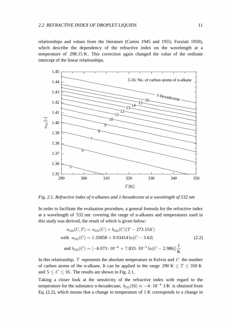
Fig. 2.1. Refractive index of n-alkanes and 1-hexadecene at a wavelength of 532 nm

In order to facilitate the evaluation procedure, a general formula for the refractive index at a wavelength of 532 nm covering the range of n-alkanes and temperatures used in this study was derived, the result of which is given below:

532 532 532

532

4 5532

273 15

with 1 35858 0 03414 3 63

1 and 6 073 10 7 833 10 2 986

K

( , ) ( ) ( )( . )

( ) . . ln( . )

( ) [ . . ln( . )]− −

= + −

= + −

= − ⋅ + ⋅ −

n C T a C b C T K

a C C

b C C

(2.2)

In this relationship, T represents the absolute temperature in Kelvin and C the number of carbon atoms of the n-alkane. It can be applied in the range 290 K 350 K≤ ≤T and 5 16≤ ≤C . The results are shown in Fig. 2.1.

Taking a closer look at the sensitivity of the refractive index with regard to the temperature for the substance n-hexadecane, 4

532 16 4 10 1/K( ) −≈ − ⋅b is obtained from Eq. (2.2), which means that a change in temperature of 1 K corresponds to a change in

12 2 DROPLET LIQUIDS

the refractive index of 44 10−⋅ . With regard to the substances used, the difference in the refractive index is smallest between n-hexadecane and n-pentadecane, where

33 10−∆ ≈ ⋅n in the given temperature range.

For 1-hexadecene, the following relationship was derived:

-4532

273 15 K1-Hexadecene, 1.45261 4.269 10

K.

( )T

n T−

= − ⋅ (2.3)

The results of this relationship are also depicted in Fig. 2.1.

2.3 Liquid Mixtures

2.3.1 Mixing Behavior The substances used within this study show an ideal mixing behavior. This is because the molecules are non-polar. Thus, properties of the liquid mixtures, such as the liquid density or the refractive index, can be obtained by averaging the properties of the liquid components with respect to their volume fractions. Furthermore, Raoult's law can be applied to the phase change occurring at the droplet surface. This law implies a linear relation between the vapor pressure and the liquid-phase composition measured in mole fractions.

2.3.2 Preparation of Liquid Mixtures For the liquid mixtures, substances with a purity grade of at least 99% were used. The liquid volumes were measured with pipettes. These pipettes had scale gradations of 0.1 ml. For that reason, an uncertainty of 0 05 ml.=Vδ was assumed. Usually, a mixture was prepared with a volume of least 30 ml. This means that for a binary mixture with a volume fraction of 0 5.=iZ for each component, volumes of

15 ml=V were measured. In this case, the uncertainty of the volume fraction was 0 33/ . %≈V Vδ . This inaccuracy increases for smaller volume fractions. However, the

uncertainty is of an acceptable magnitude and small compared to other uncertainties as shown in subsequent chapters.

When low volatile substances were part of the mixture, the mixture was immediately used to fill the reservoir of the droplet on demand generator in order to avoid a change of composition of the mixture due to a vaporization of the low volatile component.

13

3 Droplet Evaporation Models In this chapter, the droplet evaporation models used for this study are explained. The results of numerical simulations with these models were utilized for comparisons with experimental results.

3.1 Overview Table 3.1 gives an overview of the models used in this study. Within the table, the complexity of the models increases from the top to the bottom. Some of the main characteristics of the models are provided in order to highlight their differences.

The classical 2D -model for single component droplets, abbreviated as D2M, yields relatively good results for the selected liquids and the ambient conditions of the experiments. It is used as a starting point for the development of simplified models for both single component and multicomponent droplets. There are several reasons why these simplified models were developed. First of all, they allow a much quicker calculation of the droplet evaporation since there are fewer equations to be solved. This is an advantage not only for the calculation of a single droplet, but especially for the calculation of a spray consisting of many thousands of droplets and thus saving tremendous computation time. For the experiments it was also advantageous to develop simplified models: these simplified approximate solutions served as a useful tool for the planning of the measurements. Last but not least, by simplifying the equations, the dominant parameters for droplet evaporation can be identified and their influence can be highlighted. The main disadvantage is, of course, the increasing discrepancy between the results of these models and the real droplet behavior when simplifications are introduced. For this reason, the appropriate application range of these models was investigated.

In order to develop simplified models for multicomponent droplets, it was first necessary to simplify the classical 2D -model in order to provide explicit expressions for the droplet temperature and the evaporation rate, leading to the simplified 2D -model, abbreviated as SD2M. From this model, a model for binary and ternary mixture droplets was developed. Since the resulting model assumes a homogeneous mixture of the liquids inside the droplets at each point in time, which corresponds to a rapid-mixing of the substances, this model is called simplified rapid-mixing model (SRMM).

For the calculation of the droplet diameter and composition as a function of time, SRMM requires numerical methods since a set of coupled differential equations must be solved. In order to calculate the evaporation rate, the droplet diameter, or the droplet

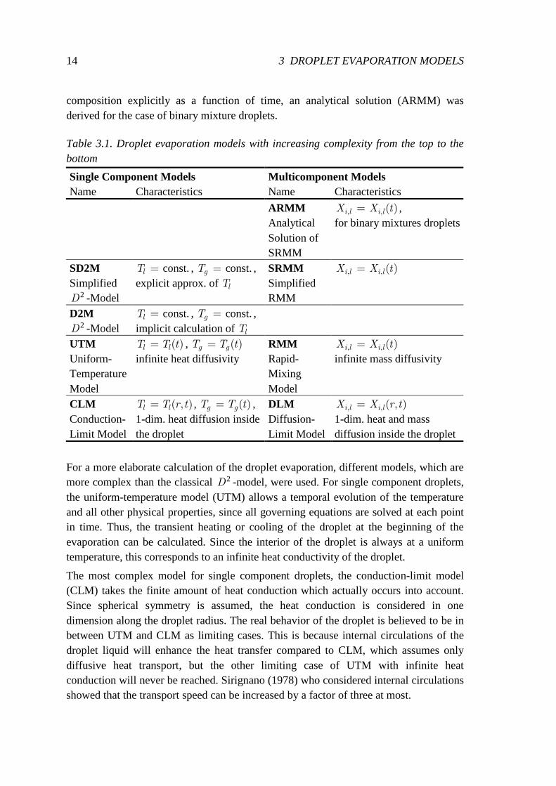
14 3 DROPLET EVAPORATION MODELS

composition explicitly as a function of time, an analytical solution (ARMM) was derived for the case of binary mixture droplets.

Table 3.1. Droplet evaporation models with increasing complexity from the top to the bottom

Single Component Models Multicomponent Models Name Characteristics Name Characteristics

ARMM Analytical Solution of SRMM

, , ( )=i l i lX X t , for binary mixtures droplets

SD2M Simplified

2D -Model

const.=lT , const.=gT , explicit approx. of lT

SRMM Simplified RMM

, , ( )=i l i lX X t

D2M 2D -Model

const.=lT , const.=gT , implicit calculation of lT

UTM Uniform- Temperature Model

( )=l lT T t , ( )=g gT T t infinite heat diffusivity

RMM Rapid- Mixing Model

, , ( )=i l i lX X t infinite mass diffusivity

CLM Conduction- Limit Model

( , )=l lT T r t , ( )=g gT T t , 1-dim. heat diffusion inside the droplet

DLM Diffusion- Limit Model

, , ( , )=i l i lX X r t 1-dim. heat and mass diffusion inside the droplet

For a more elaborate calculation of the droplet evaporation, different models, which are more complex than the classical 2D -model, were used. For single component droplets, the uniform-temperature model (UTM) allows a temporal evolution of the temperature and all other physical properties, since all governing equations are solved at each point in time. Thus, the transient heating or cooling of the droplet at the beginning of the evaporation can be calculated. Since the interior of the droplet is always at a uniform temperature, this corresponds to an infinite heat conductivity of the droplet.

The most complex model for single component droplets, the conduction-limit model (CLM) takes the finite amount of heat conduction which actually occurs into account. Since spherical symmetry is assumed, the heat conduction is considered in one dimension along the droplet radius. The real behavior of the droplet is believed to be in between UTM and CLM as limiting cases. This is because internal circulations of the droplet liquid will enhance the heat transfer compared to CLM, which assumes only diffusive heat transport, but the other limiting case of UTM with infinite heat conduction will never be reached. Sirignano (1978) who considered internal circulations showed that the transport speed can be increased by a factor of three at most.

3.2 CLASSICAL D2-LAW 15

For multicomponent droplets, the rapid-mixing model (RMM) is based on UTM and assumes in addition to an infinite heat conductivity a mixing of the droplet liquids at an infinite speed, so that at each point in time there is a homogeneous mixture and temperature inside the droplet. The diffusion-limit model (DLM) is based on CLM and assumes in addition to diffusive heat also diffusive mass transfer inside the droplet.

The most complex models, CLM for single component and DLM for multicomponent droplets, require considerably more computation time than UTM and RMM, respectively, due to the additional calculation of the internal processes.

3.2 Classical D2-Law

In this section, fundamental equations and assumptions of the classical 2D -law are reviewed, since some of the evaporation models used in this study are based on that law.

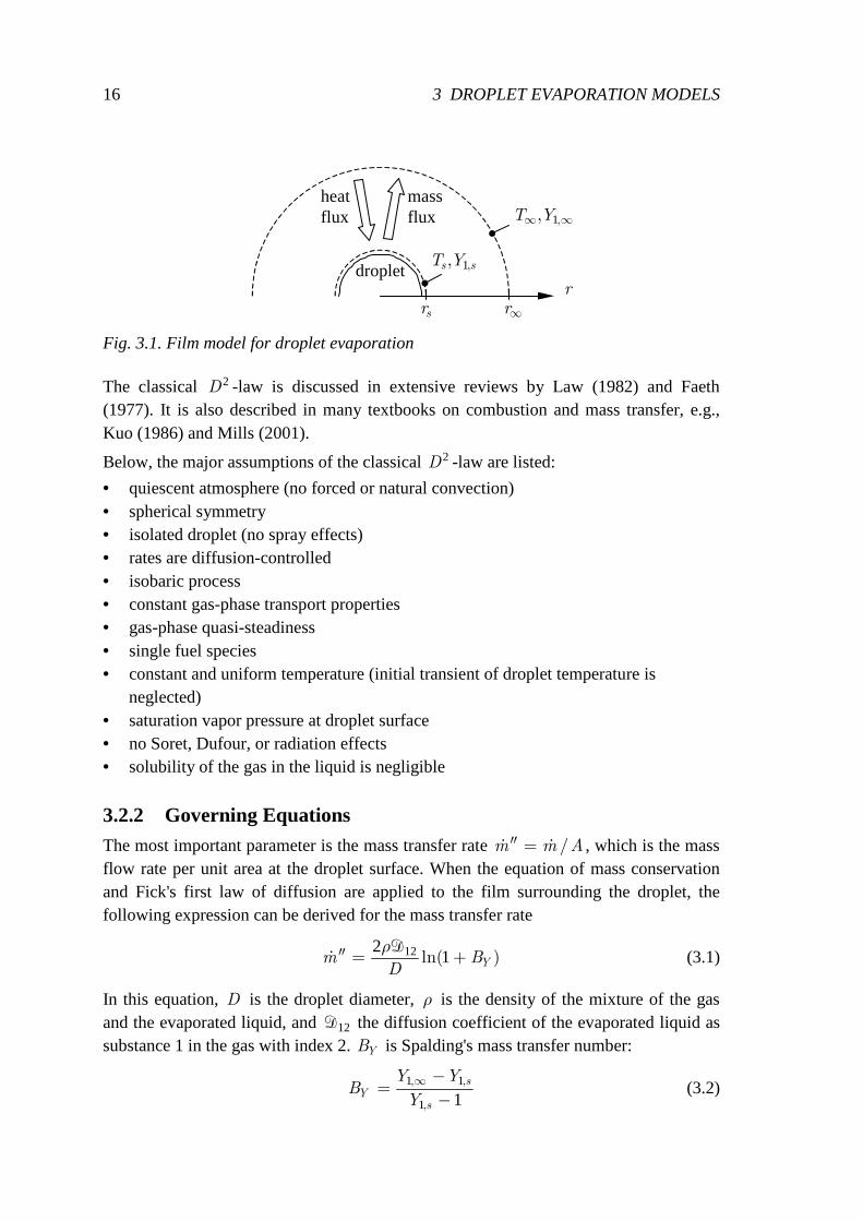
3.2.1 Introduction and Assumptions The classical 2D -law was formulated in the 1950s by Godsave (1953) and Spalding (1953). It was derived for an isolated, pure-component droplet burning in a quiescent, oxidizing environment. It has since then been termed the 2D -law, because it predicts that the square of the droplet diameter decreases linearly with time. The model can be used both for the combustion and for the evaporation of a droplet. But since there is no combustion in this study, the focus is only on evaporation. As a consequence, chemical reactions are not considered and the double-film model with flame front is reduced to a single-film model as depicted in Fig. 3.1.

The film model shown in Fig. 3.1 is also used in spray calculations with many droplets. Within the film, heat is transported solely by diffusion towards the droplet in exchange for mass diffusion from the evaporating droplet in the opposite direction. The film is surrounded by two boundaries. The outer boundary with the subscript ∞ represents the conditions far away from the droplet. In Fig. 3.1, the dominant parameters for heat and mass transfer, the Temperature T and the mass fraction of the fuel Y are indicated. The inner boundary with the subscript s is within the gas phase, but indefinitely close to the droplet surface. Between the droplet surface and the s -surface, the phase change from liquid-phase to gas-phase quantities occurs. From the droplet surface to the s -surface, the temperature remains constant, but the mass concentration changes abruptly and must be determined. This description goes back to Spalding (1953) and is explained in detail in Kays et al. (2004).

16 3 DROPLET EVAPORATION MODELS

droplet

massflux

heatflux 1,,∞ ∞T Y

1,,s sT Y

r

sr ∞r

Fig. 3.1. Film model for droplet evaporation

The classical 2D -law is discussed in extensive reviews by Law (1982) and Faeth (1977). It is also described in many textbooks on combustion and mass transfer, e.g., Kuo (1986) and Mills (2001).

Below, the major assumptions of the classical 2D -law are listed:

• quiescent atmosphere (no forced or natural convection) • spherical symmetry • isolated droplet (no spray effects) • rates are diffusion-controlled • isobaric process • constant gas-phase transport properties • gas-phase quasi-steadiness • single fuel species • constant and uniform temperature (initial transient of droplet temperature is

neglected) • saturation vapor pressure at droplet surface • no Soret, Dufour, or radiation effects • solubility of the gas in the liquid is negligible

3.2.2 Governing Equations The most important parameter is the mass transfer rate /′′ =ɺ ɺm m A , which is the mass flow rate per unit area at the droplet surface. When the equation of mass conservation and Fick's first law of diffusion are applied to the film surrounding the droplet, the following expression can be derived for the mass transfer rate

1221ln( )′′ = +ɺ Ym B

D

ρA (3.1)

In this equation, D is the droplet diameter, ρ is the density of the mixture of the gas and the evaporated liquid, and 12A the diffusion coefficient of the evaporated liquid as substance 1 in the gas with index 2. YB is Spalding's mass transfer number:

1 1

1 1, ,

,

∞ −=

−s

Ys

Y YB

Y (3.2)

3.2 CLASSICAL D2-LAW 17

In this equation, 1,sY denotes the mass fraction of the fuel on the s -surface and 1,∞Y the mass fraction far away from the droplet. Substituting Eq. (3.2) into Eq. (3.1), the mass transfer rate can be expressed in terms of the unknown vapor mass fraction 1,sY :

112

1

121

,

,

ln ∞ − ′′ = − ɺ

s

Ym

D Y

ρA (3.3)

When the energy equation is applied in order to account for the heat transfer, the following relationship is obtained:

1

21ln( )′′ = +ɺ T

p

km B

c D (3.4)

where k is the thermal conductivity and pc the specific heat at constant pressure. TB is Spalding's heat transfer number:

1( )∞ −=

p sT

v

c T TB

h (3.5)

where vh is the latent heat of vaporization at the temperature sT . Comparing Eqs. (3.1) and (3.4) for the mass transfer rate, one can see that the mass and heat diffusion in the gas phase are described by similar equations. Substituting Eq. (3.5) into Eq. (3.4), the mass transfer rate can be expressed in terms of the unknown temperature sT :

1

1

21

( )ln

∞ − ′′ = + ɺ

p s

p v

c T Tkm

c D h (3.6)

Together with the vapor pressure relation, Eq. (3.7):

1 1, , ( , )=s s sY Y T p (3.7)

Eqs. (3.1) and (3.4) form a set of equations for the three unknowns ′′ɺm , sT , and 1,sY . Equation (3.7) can be expressed, for example, using the Clausius-Clapeyron equation or can be evaluated from saturation vapor pressure tables.

3.2.3 Evaporation Rate and D2-Law

In the previous section, the mass transfer rate ′′ɺm was determined from the mass and heat diffusion in the gas phase for a fixed droplet size. Now the change in droplet size due to this mass transfer rate is considered. For this reason, the defining equation of the mass transfer rate is evaluated at the droplet surface, or, in other words, the equation of mass conservation is applied to the droplet surface:

( )32

16ls

m dm D

A dtD

πρ

π′′ = − = −

ɺɺ (3.8)

where lρ is the density of the droplet liquid. Substituting for ′′ɺm from Eq. (3.1) and rearranging yields:

18 3 DROPLET EVAPORATION MODELS

2

1281ln( )= − + Y

l

dDB

dt

ρ

ρ

A (3.9)

where the right hand side of this equation is a constant. Now the evaporation rate β is introduced, which is the surface regression rate and defined by:

2

:= −dD

dtβ (3.10)

Comparing Eqs. (3.9) and (3.10), it can be seen that the evaporation rate is constant and can be expressed as:

1281ln( )= + Y

l

Bρ

βρ

A (3.11)

In order to obtain the evolution of the droplet diameter, Eq. (3.10) is integrated with the boundary condition 00 s( )= =D t D as the initial droplet diameter, which results in

2 20( ) = −D t D tβ (3.12)

The result is the well-known 2D -law, stating that the square of the droplet diameter decreases linearly with time during droplet evaporation.

Since the mass transfer rate can be expressed either in terms of quantities from mass diffusion or heat diffusion, there is also an alternative expression for the evaporation rate β using heat transfer quantities:

1

81ln( )= + T

p l

kB

cβ

ρ (3.13)

In addition to the evaporation rate, another important parameter in droplet evaporation is the lifetime of the droplet, also called evaporation time eτ , which can be determined from Eq. (3.12) with 0( )= =eD t τ :

20 /e Dτ β= (3.14)

3.2.4 Property Evaluation In addition to the beforementioned assumptions, the classical 2D -law also includes the assumption that the Lewis number Leg within the gas phase is unity. Inspecting the definition of the Lewis number, i.e., 12Le /g α= A , it can be seen that 12=α A for

1Le = , where α is the thermal diffusivity with 1/( )= pk cα ρ . This implies that the rate of heat and mass transfer are of the same magnitude. Using this simplification and combining Eqs. (3.1) and (3.4) leads to =Y TB B . As a consequence, the number of properties which has to be evaluated in order to solve the problem is reduced.

The remaining properties are the gas density ρ and the specific heat 1pc at constant pressure of the evaporated liquid. Especially when the difference between the

3.3 THE D2-MODEL (D2M) 19

conditions on the droplet surface and those far away from the droplet are large, certain reference values must be taken for the temperature and composition in order to evaluate these properties. One possible scheme is to evaluate ρ at both the mean film temperature and composition and 1pc at just the mean film temperature. In the literature, several schemes have been proposed for the evaluation of variable properties, e.g., Hubbard et al. (1975), Kent (1973), and Law (1975). The scheme of Hubbard et al. (1975) seems to work best, since it is favored by many researchers who compared different schemes; recently e.g., Ochs (1999). Hubbard et al. (1975) compared results of different schemes in which all properties, including pc , were assumed constant at a reference state with numerical solutions in which all properties were calculated exactly. They found that a scheme which they called the 1/3 rule worked best. It was originally developed by Sparrow and Gregg (1958) for convective heat transfer and extended by Hubbard et al. (1975) to include simultaneous heat and mass transfer. The rule uses the following reference states for temperature and composition, designated with the subscript r :

1 1 1

1 3

1 3, , ,

( / )( )

( / )( )

∞

∞

= + −

= + −

r s s

r s s

T T T T

Y Y Y Y (3.15)

This means that the reference state is closer to the droplet surface than the mean film value. This scheme is used in this study whenever a property evaluation scheme is needed.

3.3 The D2-Model (D2M)

The 2D -model (D2M) is the application of the 2D -law to the conditions in this study, however not including the simplifying assumption of 1Le = . Basic assumptions of the

2D -law such as isolated droplets and a quiescent atmosphere match very well with the experimental conditions. Since, for the setups, an accumulation of the evaporated liquid around the droplets is avoided by a small gas flow, as described in chapter 5, it is assumed that 1 0,∞ =Y . Applying this condition to Eq. (3.3) and eliminating the mass transfer rate ′′ɺm with Eq. (3.6), the following set of equations is obtained for the two unknowns 1,sY and sT :

1

1 1 12

11

1 ,

( )ln ln ∞ − = + −

p s

s p v

c T Tk

Y c hρA (3.16)

1 1, , ( , )=s s sY Y T p (3.17)

Equation (3.17) is transformed to the problem of determining the vapor pressure of the fuel at the temperature sT . Once the vapor pressure, which is equal to the partial pressure 1,sp , is known, the molar fraction 1,sX can be determined using Dalton's law of partial pressure and assuming an ideal gas mixture:

20 3 DROPLET EVAPORATION MODELS

11

,, = ss

pX

p (3.18)

where p is the total pressure. Then, the mass fraction 1,sY can be obtained from the molecular weights of the gas and the liquid with the following equation:

1 11

1 1 1 21,

,, ,( )

=+ −

ss

s s

X MY

X M X M (3.19)

Table 3.2 gives an overview of the methods employed in calculating fuel and gas properties. For the reference state, Hubbard's 1/3 rule is used. The methods in Table 3.2 are used for this and all of the following models except for the models implemented in the numerical code by Gartung, which are presented in the last section of this chapter. In the following, some comments are given on the property evaluation methods.

Table 3.2. Property evaluation methods for D2M

Property Method

1,sp Antoine's vapor pressure relation with data from Lide (1998)

12A Fuller (from Reid et al. 1987) vh Watson (from VDI-Wärmeatlas 1988) ρ ideal gas law

lρ linear interpolation of data from VDI-Wärmeatlas (1988)

1pc linear interpolation of data from VDI-Wärmeatlas (1988) k linear interpolation of data from VDI-Wärmeatlas (1988)

532n Eqs. (2.2) and (2.3)

For the vapor pressure, Antoine's vapor pressure correlation is used in the following form (Reid et al. 1987)

1, exp = + −s

s

bp a

c T (3.20)

where 1,sp is obtained in Pa and sT is taken in Kelvin. The parameters a , b , and c depend on the substance. In Reid et al. (1987), values for these parameters are given covering a wide temperature range. However, since the vapor pressure has a significant influence on the evaporation rate and depends very much on the temperature, and, since for this study the temperature range is much smaller than the range of validity given in Reid et al. (1987), the values from Reid et al. (1987) were not used. Instead, these constants were determined by fitting Antoine's vapor pressure correlation to data from Lide (1998) with the least squares method in order to obtain more accurate results for the vapor pressure.

Since lρ , 1pc , and k depend only weakly on the temperature within the temperature range for this study, values for these properties are determined by interpolating data from tabulated values in the VDI-Wärmeatlas (1988) for different temperatures.

3.4 SIMPLIFIED D2-MODEL (SD2M) 21

Relations for the refractive index are used to produce data for the calculation of the scattered light by numerical codes presented later in chapter 4.

3.4 Simplified D2-Model (SD2M)

The simplified 2D -model (SD2M) is a simplified version of D2M and offers an explicit solution of the mole fraction 1,sY and the temperature sT in contrast to solving these quantities implicitly from Eqs. (3.16) and (3.17). Based on SD2M, SRMM for multicomponent droplets is derived in the subsequent section.

In the following, the evaporation rate of SD2M is derived in two different ways: the first by introducing simplifying assumptions to D2M in order to demonstrate how these two models are related to each other; the second approach begins with the basic equations of mass conservation for the gas film surrounding the droplet with all equations written in mole specific quantities. The second approach is followed because some of the derived equations are needed for the subsequent section.

3.4.1 Evaporation Rate by Simplification of D2M For SD2M, a simpler expression for the evaporation rate constant is derived from Eq. (3.11). For small mass transfer numbers 1≪YB , the term 1ln( )+ YB can be linearized resulting in YB only. Hence, Eq. (3.11) for the evaporation rate constant can be rewritten as

1 112

1

81, ,

,

∞ − = − s

l s

Y Y

Y

ρβ

ρ

A (3.21)

Since for this study, 1 0,∞ =Y is assumed, and since 1≪YB meaning that 1 1, ≪sY , Eq. (3.21) can be further reduced to

121

8,= s

l

Yρ

βρ

A (3.22)

When 1 1, ≪sY , also 1 1, ≪sX , and therefore Eq. (3.19) can also be simplified, yielding:

11 1

2, ,=s s

MY X

M (3.23)

Substituting Eqs. (3.23) and (3.18) into Eq. (3.22) yields

112 1

2

8 ,= s

l

pM

M p

ρβ

ρ

A (3.24)

22 3 DROPLET EVAPORATION MODELS

When 1 1, ≪sY and 1 0,∞ =Y , the mixture property ρ can be approximated by 2ρ . Using the ideal gas law in the form 2/= mol

rp R T Mρ with the molar gas constant molR , the number of properties can be further reduced, resulting in:

12 11

8,= smol

r l

Mp

R Tβ

ρ

A (3.25)

3.4.2 Evaporation Rate from Basic Conservation Equations In the following, molar quantities instead of mass specific quantities are used. This is more convenient for later use, since, according to Dalton's law of partial pressure and when using the ideal gas law, the molar fraction of a species i can be obtained directly from the partial pressure, i.e.,

= ii

pX

p (3.26)

where p is the total pressure. Instead of the mass transfer rate ′′ɺm , the molar transfer rate ′′ɺn is used. The analogous equation to Eq. (3.8) in terms of the molar transfer rate

′′ɺn is

1 12

, ,′′ = − = −ɺ ɺ

ɺs s

s

n nn

A Dπ (3.27)

where 1,ɺ sn is the molar flow rate of the evaporated liquid. Eq. (3.27) contains a minus sign, since 1 0, <ɺ sn . For the film surrounding the droplet for sr r r∞≤ ≤ , only the mass diffusion of the evaporated liquid as the 1st species must be considered, since the gas is stationary. The absolute molar flux N ′′ɺ at a certain position r of the radial coordinate can be determined by an analogous equation to Eq. (3.27) from

1 11 2

, ,s sn nN

A rπ′′ = − = −

ɺ ɺɺ (3.28)

In its general form, the absolute molar flux is composed of two parts:

1 1 1 1N X N J′′ ′′= +ɺ ɺ (3.29)

The first part, 1 1X N ′′ɺ , is the convective flux, which is called Stefan flow and occurs at high mass transfer rates. This part is neglected in the following analysis. The second part, 1J , is the diffusion molar flux and can be expressed using Fick's first law of diffusion

1 11 = − g m dXJ

M dr

ρ A (3.30)

where gρ is the density of the gas mixture, M the mean molecular weight of the gas mixture and 1mA the effective binary diffusion coefficient of the 1st component in the gas mixture. Moreover, 1mA can be approximated by 12A where the index 2 denotes the ambient gas.

3.4 SIMPLIFIED D2-MODEL (SD2M) 23

Substituting Eqs. (3.30) and (3.28) into Eq. (3.29) together with the assumption

1 1 0X N ′′=ɺ , and integrating with the boundary condition 1 1 0,( )∞ ∞= = =X r r X and solving for 1,ɺ sn results in:

1 11

4 ,, = −ɺ

m s g ss

X rn

M

π ρA (3.31)

Substituting Eq. (3.31) into Eq. (3.27), replacing 1,sX with Eq. (3.26), and introducing the ideal gas law leads to:

1 12 ,m smol

r

pn

DR T′′ =

Aɺ (3.32)

In a manner analogous to the solution procedure in section 3.2, the 2D -law for this model using molar quantities can be derived utilizing Eqs. (3.32) and (3.27). By doing so, the evaporation rate can be obtained. This results in the same expression as Eq. (3.25).

3.4.3 Influence of the Temperature on the Evaporation Rate For this study, the ambient gas was assigned various temperatures. This is why in this section the influence of the temperature on the evaporation rate is considered. For this task, the dependency of the evaporation rate on temperature dependent properties is investigated.

The equation for the evaporation rate, i.e., Eq. (3.24), is repeated here for convenience:

112 1

2

8,( ) ( ) ( )s

l

MT T p T

M pβ ρ

ρ= A (3.33)

The quantities which depend considerably on temperature, i.e., ρ , 12A , and 1,sp have been explicitly marked as temperature dependent in Eq. (3.33). In contrast, the temperature dependency of all other properties is small or non-existent and therefore neglected in the following. Equation (3.33) further demonstrates that the evaporation rate in turn is linearly proportional to all three of these temperature dependent quantities.

When the property evaluation methods from section 3.3 are used for the temperature dependency of these properties, it means that 1~ /Tρ since the density is calculated using the ideal gas law, 1 75

12.~TA from the property evaluation method by Fuller,

and 1,sp increases exponentially with rising temperature, as can be seen from Eq. (3.20). Thus, the vapor pressure has the largest influence on the evaporation rate when the temperature is varied. Combined all of the effects, the evaporation rate grows more than exponentially for a rising temperature.

24 3 DROPLET EVAPORATION MODELS

3.4.4 Reference Temperature and Property Evaluation When the evaporation rate is very low, e.g., for n-hexadecane evaporating at

300 K∞ =T , the droplet temperature is only slightly lower than the ambient temperature. Under these conditions, ∞=rT T can be used as a reference temperature with sufficient accuracy. But for higher evaporation rates, i.e., when the droplet temperature is significantly lower than the ambient temperature during steady evaporation, a suitable reference temperature must be used in order to avoid large errors in predicting the evaporation rate.

In the following, an explicit equation for the calculation of the droplet temperature sT is derived, which is particularly well adapted to the substances and the temperature range of interest. The temperature difference ∞ − sT T is included in Eq. (3.6), which describes the mass transfer rate due to diffusive heat transfer. In order to obtain an explicit solution for this temperature difference, the mass transfer rate is eliminated with Eq. (3.3) and, in addition, the Lewis number is set to unity resulting in

1 1

1

11

1,

,

( )∞ ∞− −= +

−

p s

s v

Y c T T

Y h (3.34)

Now, if 1 0,∞ =Y is assumed, and if 1 1, ≪sY , Eq. (3.34) can be approximated by

11,

( )∞ −=

p ss

v

c T TY

h (3.35)

Replacing 1,sY by Eq. (3.23), which is a simplified expression for 1 1, ≪sY , in combination with Eq. (3.18) and solving for the temperature difference yields the approximation:

11

2 1

,.

( )( )

∞∞ − ≈

svs approx

p

p TM hT T

M c p (3.36)

where all properties are evaluated at the temperature ∞T .

In Fig. 3.2, values of the temperature difference ∞∆ = − sT T T obtained from Eq. (3.36) are compared with numerical values from D2M. For the selected substances and temperatures, these values are around 3, except for two values on the left side of each curve, but in these cases 1 0 1, / .>sp p and therefore the assumption of 1 1, ≪sY does not hold any more.

Based on the results depicted in Fig. 3.2, the temperature difference from Eq. (3.36) is corrected with a factor of 1/3 for a rough estimate of the temperature. The resulting equation for the determination of sT is

11

2 1

13

,svs

p

pM hT T

M c p∞= −

(3.37)

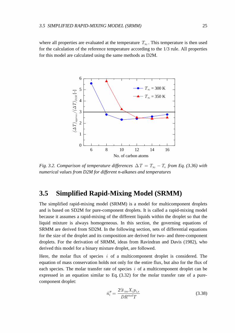
3.5 SIMPLIFIED RAPID-MIXING MODEL (SRMM) 25

where all properties are evaluated at the temperature ∞T . This temperature is then used for the calculation of the reference temperature according to the 1/3 rule. All properties for this model are calculated using the same methods as D2M.

6 8 10 12 14 160

1

2

3

4

5

6

(∆T) approx./(∆T) D2M [-

]

No. of carbon atoms

T∞ = 300 K

T∞ = 350 K

Fig. 3.2. Comparison of temperature differences ∞∆ = − sT T T from Eq. (3.36) with numerical values from D2M for different n-alkanes and temperatures

3.5 Simplified Rapid-Mixing Model (SRMM) The simplified rapid-mixing model (SRMM) is a model for multicomponent droplets and is based on SD2M for pure-component droplets. It is called a rapid-mixing model because it assumes a rapid-mixing of the different liquids within the droplet so that the liquid mixture is always homogeneous. In this section, the governing equations of SRMM are derived from SD2M. In the following section, sets of differential equations for the size of the droplet and its composition are derived for two- and three-component droplets. For the derivation of SRMM, ideas from Ravindran and Davis (1982), who derived this model for a binary mixture droplet, are followed.

Here, the molar flux of species i of a multicomponent droplet is considered. The equation of mass conservation holds not only for the entire flux, but also for the flux of each species. The molar transfer rate of species i of a multicomponent droplet can be expressed in an equation similar to Eq. (3.32) for the molar transfer rate of a pure-component droplet:

2 ,im i i s

i mol

X pn

DR T′′ =

Aɺ (3.38)

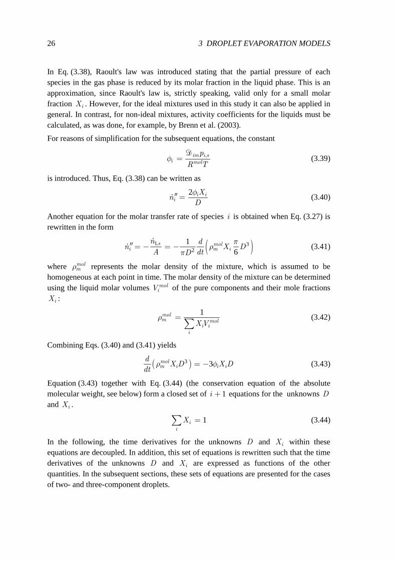
26 3 DROPLET EVAPORATION MODELS

In Eq. (3.38), Raoult's law was introduced stating that the partial pressure of each species in the gas phase is reduced by its molar fraction in the liquid phase. This is an approximation, since Raoult's law is, strictly speaking, valid only for a small molar fraction iX . However, for the ideal mixtures used in this study it can also be applied in general. In contrast, for non-ideal mixtures, activity coefficients for the liquids must be calculated, as was done, for example, by Brenn et al. (2003).

For reasons of simplification for the subsequent equations, the constant

,= im i si mol

p

R Tφ

A (3.39)

is introduced. Thus, Eq. (3.38) can be written as

2′′ =ɺ i i

iX

nD

φ (3.40)

Another equation for the molar transfer rate of species i is obtained when Eq. (3.27) is rewritten in the form

( )1 32

16

,′′ = − = −ɺ

ɺs mol

i m i

n dn X D

A dtD

πρ

π (3.41)

where molmρ represents the molar density of the mixture, which is assumed to be

homogeneous at each point in time. The molar density of the mixture can be determined using the liquid molar volumes moliV of the pure components and their mole fractions

iX :

1

=∑

molm mol

i ii

XVρ (3.42)

Combining Eqs. (3.40) and (3.41) yields

( )3 3= −molm i i i

dX D X D

dtρ φ (3.43)

Equation (3.43) together with Eq. (3.44) (the conservation equation of the absolute molecular weight, see below) form a closed set of 1+i equations for the unknowns D and iX .

1=∑ ii

X (3.44)

In the following, the time derivatives for the unknowns D and iX within these equations are decoupled. In addition, this set of equations is rewritten such that the time derivatives of the unknowns D and iX are expressed as functions of the other quantities. In the subsequent sections, these sets of equations are presented for the cases of two- and three-component droplets.

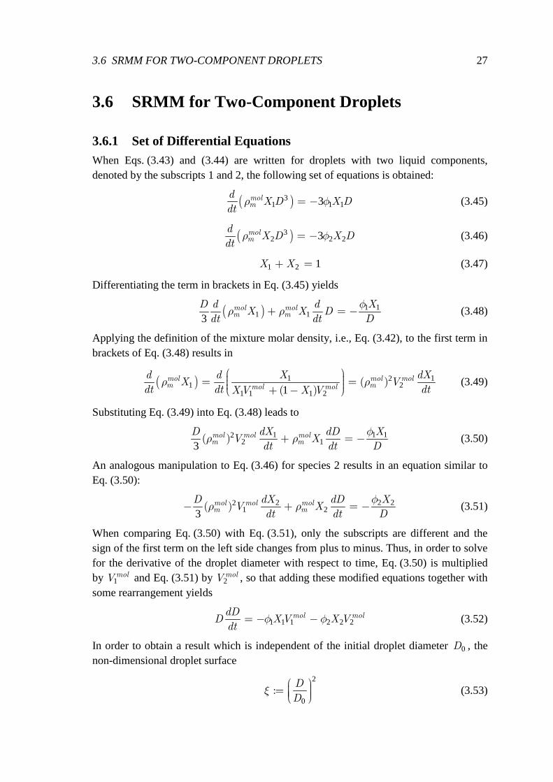
3.6 SRMM FOR TWO-COMPONENT DROPLETS 27

3.6 SRMM for Two-Component Droplets

3.6.1 Set of Differential Equations When Eqs. (3.43) and (3.44) are written for droplets with two liquid components, denoted by the subscripts 1 and 2, the following set of equations is obtained:

( )31 1 13= −mol

md

X D X Ddtρ φ (3.45)

( )32 2 23= −mol

md

X D X Ddtρ φ (3.46)

1 2 1+ =X X (3.47)

Differentiating the term in brackets in Eq. (3.45) yields

( ) 1 11 13

+ = −mol molm m

D d d XX X D

dt dt D

φρ ρ (3.48)

Applying the definition of the mixture molar density, i.e., Eq. (3.42), to the first term in brackets of Eq. (3.48) results in

( ) 1 121 2

1 1 1 21( )

( )

= = + − mol mol molm mmol mol

d d X dXX V

dt dt dtXV X Vρ ρ (3.49)

Substituting Eq. (3.49) into Eq. (3.48) leads to

1 1 122 13

( ) + = −mol mol molm m

D dX dD XV X

dt dt D

φρ ρ (3.50)

An analogous manipulation to Eq. (3.46) for species 2 results in an equation similar to Eq. (3.50):

2 2 221 23

( )− + = −mol mol molm m

D dX dD XV X

dt dt D

φρ ρ (3.51)

When comparing Eq. (3.50) with Eq. (3.51), only the subscripts are different and the sign of the first term on the left side changes from plus to minus. Thus, in order to solve for the derivative of the droplet diameter with respect to time, Eq. (3.50) is multiplied by 1

molV and Eq. (3.51) by 2molV , so that adding these modified equations together with

some rearrangement yields

1 1 1 2 2 2= − −mol moldDD XV X Vdt

φ φ (3.52)

In order to obtain a result which is independent of the initial droplet diameter 0D , the non-dimensional droplet surface

2

0:

= D

Dξ (3.53)

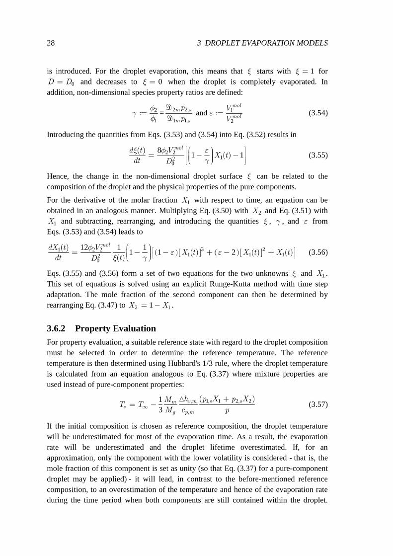
28 3 DROPLET EVAPORATION MODELS

is introduced. For the droplet evaporation, this means that ξ starts with 1=ξ for

0=D D and decreases to 0=ξ when the droplet is completely evaporated. In addition, non-dimensional species property ratios are defined:

2 22 1

1 1 1 2= and ,

,

: := =mol

m smol

m s

p V

p V

φγ ε

φ

A

A (3.54)

Introducing the quantities from Eqs. (3.53) and (3.54) into Eq. (3.52) results in

2 212

0

81 1

( )( )

= − −

mold t VX t

dt D

ξ φ ε

γ (3.55)

Hence, the change in the non-dimensional droplet surface ξ can be related to the composition of the droplet and the physical properties of the pure components.

For the derivative of the molar fraction 1X with respect to time, an equation can be obtained in an analogous manner. Multiplying Eq. (3.50) with 2X and Eq. (3.51) with

1X and subtracting, rearranging, and introducing the quantities ξ , γ , and ε from Eqs. (3.53) and (3.54) leads to

( )[ ] ( )[ ]3 21 2 21 1 12

0

12 1 11 1 2

( )( ) ( ) ( )

( )

= − − + − +

moldX t VX t X t X t

dt tD

φε ε

ξ γ (3.56)

Eqs. (3.55) and (3.56) form a set of two equations for the two unknowns ξ and 1X . This set of equations is solved using an explicit Runge-Kutta method with time step adaptation. The mole fraction of the second component can then be determined by rearranging Eq. (3.47) to 2 11= −X X .

3.6.2 Property Evaluation For property evaluation, a suitable reference state with regard to the droplet composition must be selected in order to determine the reference temperature. The reference temperature is then determined using Hubbard's 1/3 rule, where the droplet temperature is calculated from an equation analogous to Eq. (3.37) where mixture properties are used instead of pure-component properties:

1 1 2 213

, , ,

,

( )v m s sms

g p m

h p X p XMT T

M c p∞+

= −

(3.57)

If the initial composition is chosen as reference composition, the droplet temperature will be underestimated for most of the evaporation time. As a result, the evaporation rate will be underestimated and the droplet lifetime overestimated. If, for an approximation, only the component with the lower volatility is considered - that is, the mole fraction of this component is set as unity (so that Eq. (3.37) for a pure-component droplet may be applied) - it will lead, in contrast to the before-mentioned reference composition, to an overestimation of the temperature and hence of the evaporation rate during the time period when both components are still contained within the droplet.

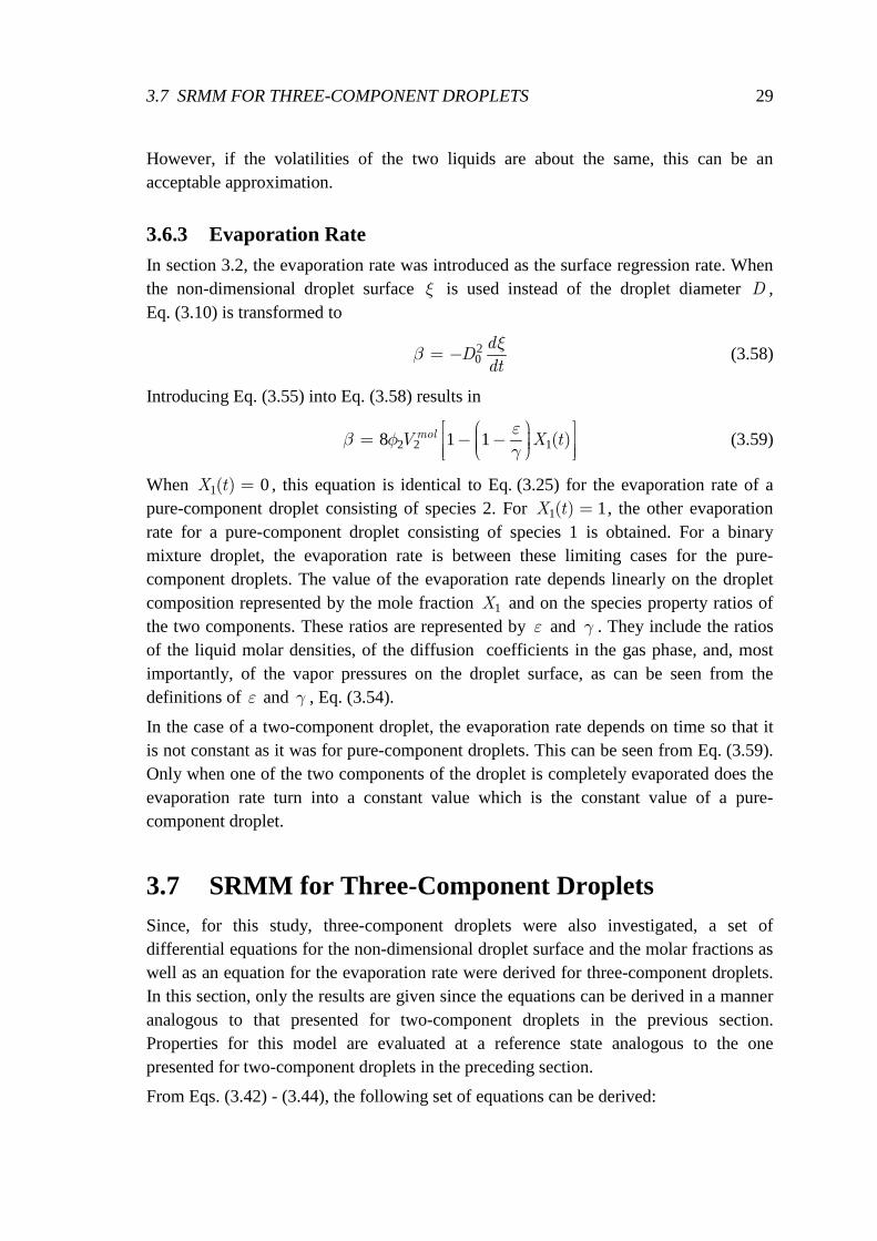
3.7 SRMM FOR THREE-COMPONENT DROPLETS 29

However, if the volatilities of the two liquids are about the same, this can be an acceptable approximation.

3.6.3 Evaporation Rate In section 3.2, the evaporation rate was introduced as the surface regression rate. When the non-dimensional droplet surface ξ is used instead of the droplet diameter D , Eq. (3.10) is transformed to

20= −d

Ddt

ξβ (3.58)

Introducing Eq. (3.55) into Eq. (3.58) results in

2 2 18 1 1 ( ) = − −

molV X tε

β φγ

(3.59)

When 1 0( ) =X t , this equation is identical to Eq. (3.25) for the evaporation rate of a pure-component droplet consisting of species 2. For 1 1( ) =X t , the other evaporation rate for a pure-component droplet consisting of species 1 is obtained. For a binary mixture droplet, the evaporation rate is between these limiting cases for the pure-component droplets. The value of the evaporation rate depends linearly on the droplet composition represented by the mole fraction 1X and on the species property ratios of the two components. These ratios are represented by ε and γ . They include the ratios of the liquid molar densities, of the diffusion coefficients in the gas phase, and, most importantly, of the vapor pressures on the droplet surface, as can be seen from the definitions of ε and γ , Eq. (3.54).

In the case of a two-component droplet, the evaporation rate depends on time so that it is not constant as it was for pure-component droplets. This can be seen from Eq. (3.59). Only when one of the two components of the droplet is completely evaporated does the evaporation rate turn into a constant value which is the constant value of a pure- component droplet.

3.7 SRMM for Three-Component Droplets Since, for this study, three-component droplets were also investigated, a set of differential equations for the non-dimensional droplet surface and the molar fractions as well as an equation for the evaporation rate were derived for three-component droplets. In this section, only the results are given since the equations can be derived in a manner analogous to that presented for two-component droplets in the previous section. Properties for this model are evaluated at a reference state analogous to the one presented for two-component droplets in the preceding section.

From Eqs. (3.42) - (3.44), the following set of equations can be derived:

30 3 DROPLET EVAPORATION MODELS

[ ]

[ ]

[ ]

1 1 3 1 2 3 2 3 1 3 120

2 1 3 1 2 3 2 3 2 3 2

1 3 1 2 3 2 3

1 3 1 2 3 2 3

8( ( ) ( ) ( ) ( )

( ) ( ) ( ) ( )

( ) ( )

( ) ( ) )

= − − + − + − −

+ − + − + − −

+ − + − +

⋅ − + − +

mol mol

mol mol

mol mol mol mol mol

dX X X V V

dt D

X X X V V

X X

V V X V V X V

ξφ φ φ φ φ φ

φ φ φ φ φ φ

φ φ φ φ φ

(3.60)

[ ]1

1 1 3 1 2 3 2 3 120

1 3 1 2 3 2 3

12( ) ( ) ( )

( ) ( )

= − + − + −

⋅ − + − + mol mol mol mol mol

dXX X X

dt D

V V X V V X V

φ φ φ φ φ φξ (3.61)

[ ]2

2 1 3 1 2 3 2 3 220

1 3 1 2 3 2 3

12( ) ( ) ( )

( ) ( )

= − + − + −

⋅ − + − + mol mol mol mol mol

dXX X X

dt D

V V X V V X V

φ φ φ φ φ φξ (3.62)

The molar fraction 3X of the third component can then be obtained by the summation rule for the molar fractions (Eq. (3.44)), resulting in 3 1 21= − −X X X .

The evaporation rate can be derived from Eqs. (3.58) and (3.60), resulting in:

[ ]

[ ]

[ ]

1 1 3 1 2 3 2 3 1 3 1

2 1 3 1 2 3 2 3 2 3 2

1 3 1 2 3 2 3

1 3 1 2 3 2 3

8( ( ) ( ) ( ) ( )

( ) ( ) ( ) ( )

( ) ( )

( ) ( ) )

= − + − + − −

+ − + − + − −

+ − + − +

⋅ − + − +

mol mol

mol mol

mol mol mol mol mol

X X X V V

X X X V V

X X

V V X V V X V

β φ φ φ φ φ φ

φ φ φ φ φ φ

φ φ φ φ φ (3.63)

With this equation, the evaporation rate can be determined for a given composition. For example, the initial evaporation rate can be obtained using the initial droplet composition. When one of the three components is completely evaporated so that its molar fraction equals zero, this equation reduces to the evaporation rate of a two-component droplet, i.e., Eq. (3.59). When finally only one component is left, Eq. (3.63) yields the same results as Eq. (3.25) for a pure-component droplet.

3.8 Analytical Solution for Binary Mixture Droplets From the Simplified Rapid-Mixing Model (SRMM), presented in the previous section, an analytical solution (ARMM) is derived for a two-component droplet. Since further simplifications are introduced, ARMM is an approximate solution of SRMM. However, ARMM allows an explicit calculation of the temporal evolution of the droplet diameter and the droplet composition. In addition, one can gain further insight into the driving parameters of multicomponent droplet evaporation.

From the equations of SRMM, it is not possible to obtain analytical solutions for the non-dimensional droplet surface ( )tξ or for the molar fraction 1( )X t as a function of

3.8 ANALYTICAL SOLUTION FOR BINARY MIXTURE DROPLETS 31

time t . Instead, analytical solutions were obtained for 1( )Xξ and 1( )t X . This means that 1( )X t can be determined from 1( )t X , whereas ( )tξ can be obtained by using the two equations for 1( )Xξ and 1( )t X together.

For the analytical solution, the molar fraction 1X is the molar fraction of the component with the higher volatility. Defining 1X in this way is necessary since, for the derivation of the analytical solution, simplifications are introduced which concern the ratios of the species properties. The introduction of these simplifications is necessary in order to be able to obtain an analytical solution, as will be seen in the following.

3.8.1 Solution for ξ(X1)

In the following, the derivation of the analytical solution is presented. The starting point is the set of equations of the simplified rapid-mixing model for two-component droplets, i.e., Eqs. (3.55) and (3.56), which are repeated here for convenience:

2 212

0

81 1

( )( )

= − −

mold t VX t

dt D

ξ φ ε

γ (3.55)

( )[ ] ( )[ ]3 21 2 21 1 12

0

12 1 11 1 2

( )( ) ( ) ( )

( )

= − − + − +

moldX t VX t X t X t

dt tD

φε ε

ξ γ (3.56)

Dividing Eq. (3.55) by Eq. (3.56) and integrating by the method of separation of variables results in an analytical solution for 1( )Xξ :

231

11 11 011

1 0 11 0

11 1

111

,

,,

( )− −

− − − = − − −

XXXX

X X X

γ

γ γ εξ

ε

(3.64)

In obtaining this solution, the boundary conditions 1 1 00 ,( )= =X t X and 0 1( )= =tξ have been used. For a better understanding of the significance of the different terms of Eq. (3.64), this equation is transformed by using the defining equations for the species property ratio ε , i.e., 1 2/= mol molV Vε , and for the molar density of the mixture molmρ , i.e., Eq. (3.42), as well as the summation rule for the molar fractions, i.e., Eq. (3.44), as follows:

21 3

1 12 0 011

1 0 2

, ,

,

( )− −

=

molmmolm

XXX

X X

γ

γ γ ρξ

ρ (3.65)

Equation (3.65) demonstrates that 1( )Xξ consists of three factors. The first two factors consider the change in the molar fractions of the two components. The influence of the factors is weighted by the exponent containing the species property ratio

2 1 2 1, ,( / )( / )= m m s sp pγ A A , which considers the ratios of the vapor pressures and

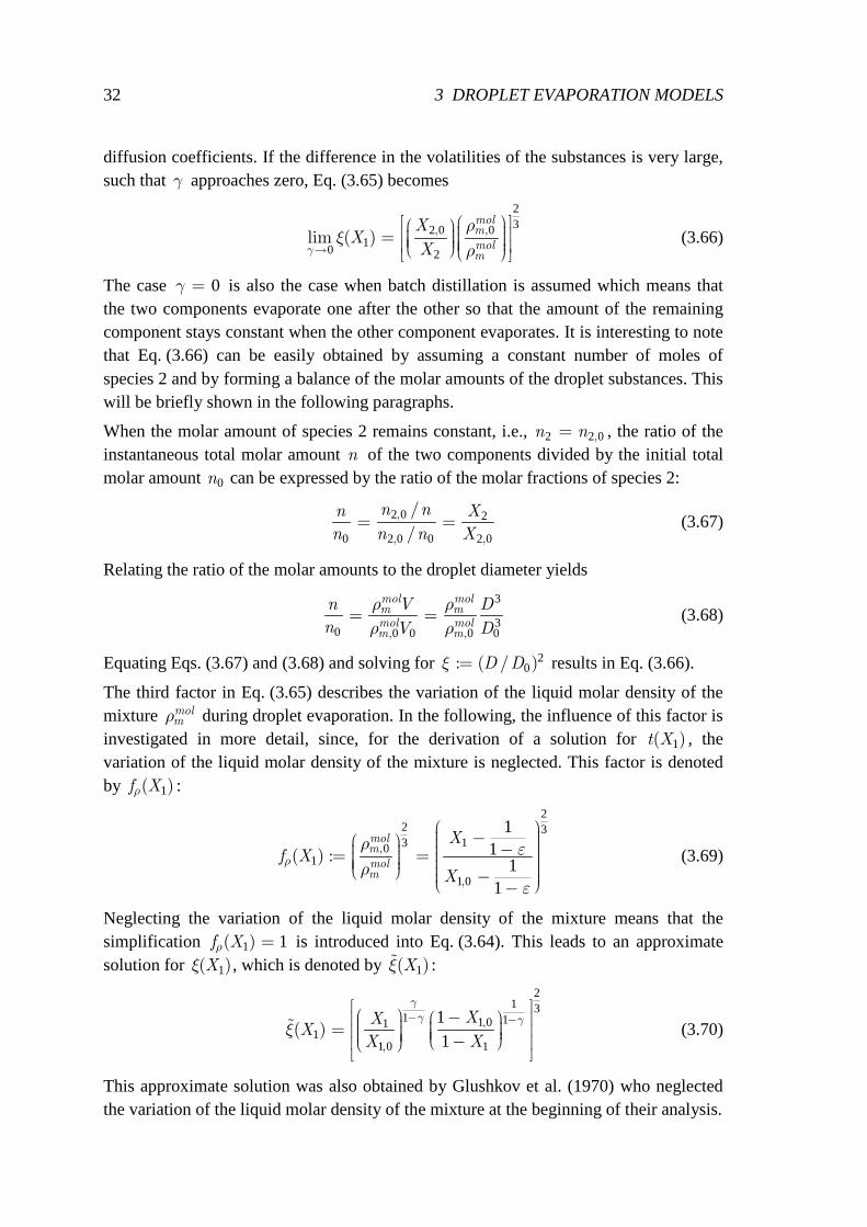
32 3 DROPLET EVAPORATION MODELS

diffusion coefficients. If the difference in the volatilities of the substances is very large, such that γ approaches zero, Eq. (3.65) becomes

232 0 0

10 2

, ,lim ( )

→

=

molmmolm

XX

Xγ

ρξ

ρ (3.66)

The case 0=γ is also the case when batch distillation is assumed which means that the two components evaporate one after the other so that the amount of the remaining component stays constant when the other component evaporates. It is interesting to note that Eq. (3.66) can be easily obtained by assuming a constant number of moles of species 2 and by forming a balance of the molar amounts of the droplet substances. This will be briefly shown in the following paragraphs.

When the molar amount of species 2 remains constant, i.e., 2 2 0,=n n , the ratio of the instantaneous total molar amount n of the two components divided by the initial total molar amount 0n can be expressed by the ratio of the molar fractions of species 2:

2 0 2

0 2 0 0 2 0

,

, ,

/

/= =n nn X

n n n X (3.67)

Relating the ratio of the molar amounts to the droplet diameter yields

3

30 0 0 0 0, ,

= =mol molm mmol molm m

n V D

n V D

ρ ρ

ρ ρ (3.68)

Equating Eqs. (3.67) and (3.68) and solving for 20: ( / )= D Dξ results in Eq. (3.66).

The third factor in Eq. (3.65) describes the variation of the liquid molar density of the mixture mol

mρ during droplet evaporation. In the following, the influence of this factor is investigated in more detail, since, for the derivation of a solution for 1( )t X , the variation of the liquid molar density of the mixture is neglected. This factor is denoted by 1( )f Xρ :

22 33 10

1

1 0

11

11

,

,

( ) :molmmolm

Xf X

Xρ

ρ ερ

ε

− − = = − −

(3.69)

Neglecting the variation of the liquid molar density of the mixture means that the simplification 1 1( )f Xρ = is introduced into Eq. (3.64). This leads to an approximate solution for 1( )Xξ , which is denoted by 1( )ɶ Xξ :

21 3

1 11 011

1 0 1

11

,

,

( )− −

− = −

ɶXX

XX X

γ

γ γξ (3.70)

This approximate solution was also obtained by Glushkov et al. (1970) who neglected the variation of the liquid molar density of the mixture at the beginning of their analysis.

3.8 ANALYTICAL SOLUTION FOR BINARY MIXTURE DROPLETS 33

In the following, the influence of 1( )f Xρ on 1( )Xξ is demonstrated and the effect of introducing the simplification 1 1( )f Xρ = is briefly discussed. Regarding molar densities in general, they have the same value for all different species when they are in the gaseous state and when the ideal gas law can be applied, resulting in

/=mol molg p R Tρ . However, in the liquid state, molar densities can differ significantly

among species. Although the mass specific densities of the liquids for this study vary only slightly, liquid molar densities differ significantly. This is because the molar density is related to the mass specific density by the molecular weight M :

/=mol Mρ ρ .

Since 1( )f X is a function of 1X , but also depends on 1 0,X and ε , as can be seen from Eq. (3.69), the influence of these three variables on 1( )f Xρ is investigated. In Fig. 3.3, the value of the factor 1( )f Xρ is depicted for different binary mixture droplets where the initial composition remains constant at 1 0 0 8, .=X and the species property ratio ε is varied. During droplet evaporation, this factor increases from 1 0 1,( )f Xρ = to the value of 0( )fρ . Hence, using the approximate solution 1( )ɶ Xξ instead of 1( )Xξ leads to increasing error and an underprediction of the actual droplet size. It can also be seen from Fig. 3.3 that the value of 0( )fρ increases for a decreasing value of ε , which means that 0( )fρ increases for an increasing difference in the liquid molar densities of the two components.

0.0 0.2 0.4 0.6 0.8 1.01.0

1.1

1.2

1.3

1.4

1.5

f ρ(X

1) [-

]

X1 [-]

C6/C16

C10/C16

C14/C16 ε = 0.89

ε = 0.67

ε = 0.45

Fig. 3.3. Factor 1( )f Xρ for binary mixture droplets of n-hexadecane (C16) with n-hexane (C6), n-decane (C10), and n-tetradecane (C14) with 1 0 0 8, .=X and

293 K=rT

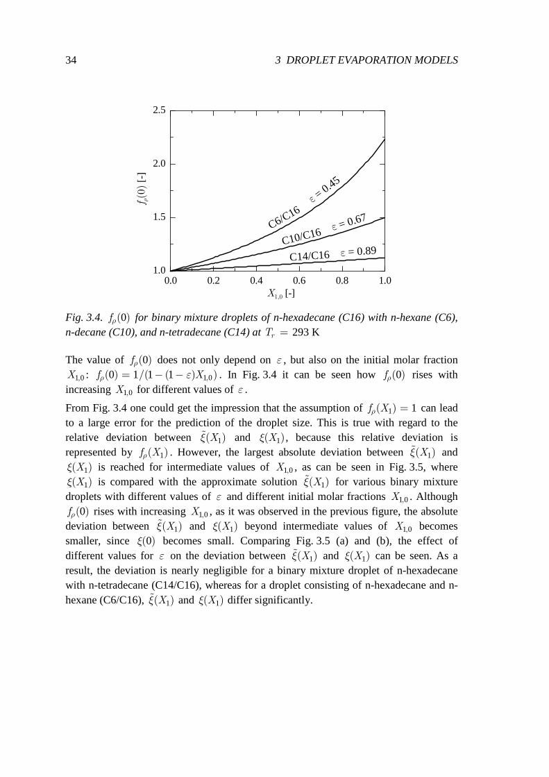
34 3 DROPLET EVAPORATION MODELS

0.0 0.2 0.4 0.6 0.8 1.01.0

1.5

2.0

2.5

f ρ(0

) [-

]

X1,0 [-]

C6/C16

C10/C16

C14/C16 ε = 0.89

ε = 0.67

ε = 0.45

Fig. 3.4. 0( )fρ for binary mixture droplets of n-hexadecane (C16) with n-hexane (C6), n-decane (C10), and n-tetradecane (C14) at 293 K=rT

The value of 0( )fρ does not only depend on ε , but also on the initial molar fraction

1 0,X : 1 00 1 1 1 ,( ) /( ( ) )f Xρ ε= − − . In Fig. 3.4 it can be seen how 0( )fρ rises with increasing 1 0,X for different values of ε .

From Fig. 3.4 one could get the impression that the assumption of 1 1( )f Xρ = can lead to a large error for the prediction of the droplet size. This is true with regard to the relative deviation between 1( )ɶ Xξ and 1( )Xξ , because this relative deviation is represented by 1( )f Xρ . However, the largest absolute deviation between 1( )ɶ Xξ and

1( )Xξ is reached for intermediate values of 1 0,X , as can be seen in Fig. 3.5, where

1( )Xξ is compared with the approximate solution 1( )ɶ Xξ for various binary mixture droplets with different values of ε and different initial molar fractions 1 0,X . Although

0( )fρ rises with increasing 1 0,X , as it was observed in the previous figure, the absolute deviation between 1( )ɶ Xξ and 1( )Xξ beyond intermediate values of 1 0,X becomes smaller, since 0( )ξ becomes small. Comparing Fig. 3.5 (a) and (b), the effect of different values for ε on the deviation between 1( )ɶ Xξ and 1( )Xξ can be seen. As a result, the deviation is nearly negligible for a binary mixture droplet of n-hexadecane with n-tetradecane (C14/C16), whereas for a droplet consisting of n-hexadecane and n-hexane (C6/C16), 1( )ɶ Xξ and 1( )Xξ differ significantly.

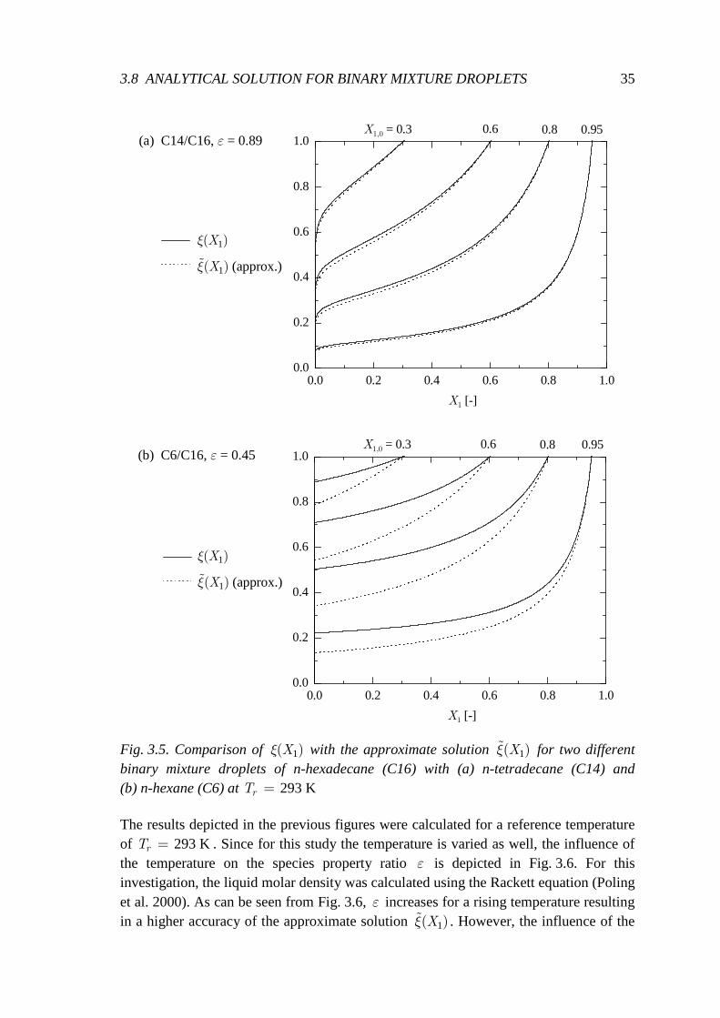
3.8 ANALYTICAL SOLUTION FOR BINARY MIXTURE DROPLETS 35

0.0 0.2 0.4 0.6 0.8 1.00.0

0.2

0.4

0.6

0.8

1.0

ξ(X1)

ξ(X1) (approx.)

X1 [-]

X1,0 = 0.3 0.6 0.8 0.95

0.0 0.2 0.4 0.6 0.8 1.00.0

0.2

0.4

0.6

0.8

1.0

ξ(X1)

ξ(X1) (approx.)

X1 [-]

X1,0 = 0.3 0.6 0.8 0.95

1

1 (approx.)

( )

( )ɶ

X

X

ξ

ξ

(a) C14/C16, ε = 0.89

(b) C6/C16, ε = 0.45

1

1 (approx.)

( )

( )ɶ

X

X

ξ

ξ

Fig. 3.5. Comparison of 1( )Xξ with the approximate solution 1( )ɶ Xξ for two different binary mixture droplets of n-hexadecane (C16) with (a) n-tetradecane (C14) and (b) n-hexane (C6) at 293 K=rT

The results depicted in the previous figures were calculated for a reference temperature of 293 K=rT . Since for this study the temperature is varied as well, the influence of the temperature on the species property ratio ε is depicted in Fig. 3.6. For this investigation, the liquid molar density was calculated using the Rackett equation (Poling et al. 2000). As can be seen from Fig. 3.6, ε increases for a rising temperature resulting in a higher accuracy of the approximate solution 1( )ɶ Xξ . However, the influence of the

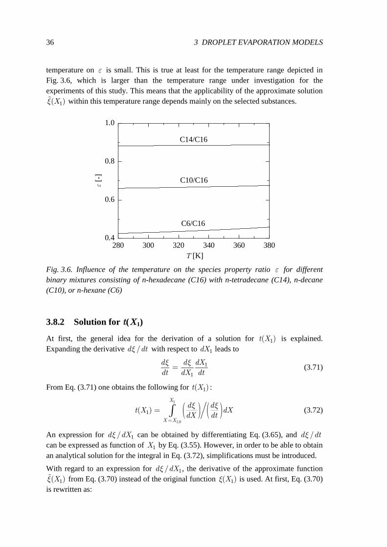
36 3 DROPLET EVAPORATION MODELS

temperature on ε is small. This is true at least for the temperature range depicted in Fig. 3.6, which is larger than the temperature range under investigation for the experiments of this study. This means that the applicability of the approximate solution

1( )ɶ Xξ within this temperature range depends mainly on the selected substances.

280 300 320 340 360 3800.4

0.6

0.8

1.0

ε [-

]

T [K]

C14/C16

C10/C16

C6/C16

Fig. 3.6. Influence of the temperature on the species property ratio ε for different binary mixtures consisting of n-hexadecane (C16) with n-tetradecane (C14), n-decane (C10), or n-hexane (C6)

3.8.2 Solution for t(X1)

At first, the general idea for the derivation of a solution for 1( )t X is explained. Expanding the derivative /d dtξ with respect to 1dX leads to

1

1=

d d dX

dt dX dt

ξ ξ (3.71)

From Eq. (3.71) one obtains the following for 1( )t X :

( ) ( )1

1 0

1

,

( )=

= ∫X

X X

d dt X dX

dX dt

ξ ξ (3.72)

An expression for 1/d dXξ can be obtained by differentiating Eq. (3.65), and /d dtξ can be expressed as function of 1X by Eq. (3.55). However, in order to be able to obtain an analytical solution for the integral in Eq. (3.72), simplifications must be introduced.

With regard to an expression for 1/d dXξ , the derivative of the approximate function

1( )ɶ Xξ from Eq. (3.70) instead of the original function 1( )Xξ is used. At first, Eq. (3.70) is rewritten as:

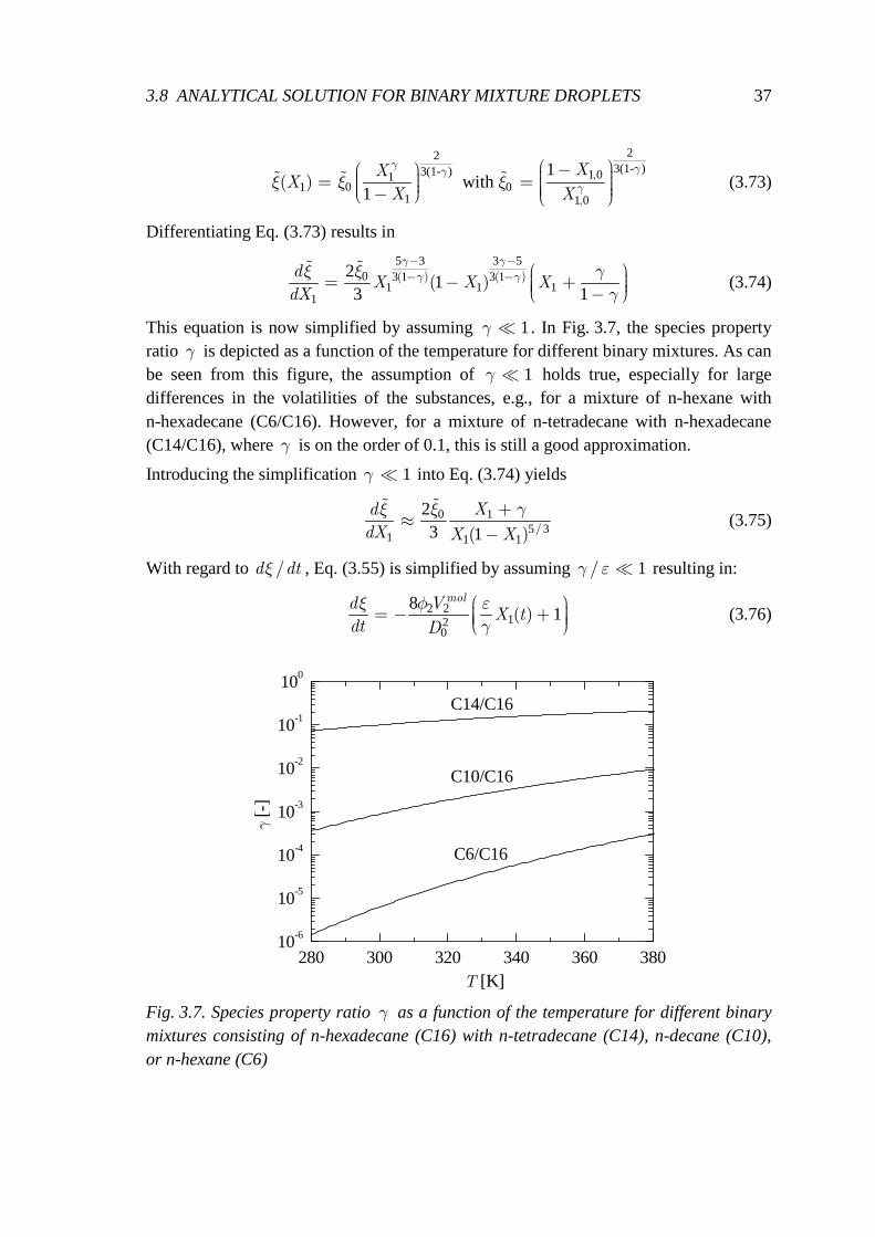
3.8 ANALYTICAL SOLUTION FOR BINARY MIXTURE DROPLETS 37

223(1- )3(1- ) 1 01

1 0 01 1 0

1 with

1,

,

( ) − = = −

ɶ ɶ ɶXX

XX X

γ γγ

γξ ξ ξ (3.73)

Differentiating Eq. (3.73) results in

5 3 3 5

0 3 1 3 11 1 1

1

21

3 1( ) ( )( )

− −− − = − + −

ɶ ɶdX X X

dX

γ γ

γ γξ ξ γ

γ (3.74)

This equation is now simplified by assuming 1≪γ . In Fig. 3.7, the species property ratio γ is depicted as a function of the temperature for different binary mixtures. As can be seen from this figure, the assumption of 1≪γ holds true, especially for large differences in the volatilities of the substances, e.g., for a mixture of n-hexane with n-hexadecane (C6/C16). However, for a mixture of n-tetradecane with n-hexadecane (C14/C16), where γ is on the order of 0.1, this is still a good approximation.

Introducing the simplification 1≪γ into Eq. (3.74) yields

0 15 3

1 1 1

23 1 /( )

+≈

−

ɶ ɶd X

dX X X

ξ ξ γ (3.75)

With regard to /d dtξ , Eq. (3.55) is simplified by assuming 1/ ≪γ ε resulting in:

2 212

0

81( )

= − +

mold VX t

dt D

ξ φ ε

γ (3.76)

280 300 320 340 360 38010-6

10-5

10-4

10-3

10-2

10-1

100

γ [-

]

T [K]

C14/C16

C10/C16

C6/C16

Fig. 3.7. Species property ratio γ as a function of the temperature for different binary mixtures consisting of n-hexadecane (C16) with n-tetradecane (C14), n-decane (C10), or n-hexane (C6)

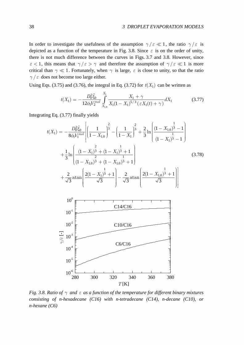
38 3 DROPLET EVAPORATION MODELS

In order to investigate the usefulness of the assumption 1/ ≪γ ε , the ratio /γ ε is depicted as a function of the temperature in Fig. 3.8. Since ε is on the order of unity, there is not much difference between the curves in Figs. 3.7 and 3.8. However, since

1<ε , this means that / >γ ε γ and therefore the assumption of 1/ ≪γ ε is more critical than 1≪γ . Fortunately, when γ is large, ε is close to unity, so that the ratio

/γ ε does not become too large either.

Using Eqs. (3.75) and (3.76), the integral in Eq. (3.72) for 1( )t X can be written as

( )

1

1 0

20 0 1

1 15 31 2 1 1 112 1

,

/( )

( ) ( )

+= −

− +∫ɶ

X

molX

D Xt X dX

V X X X t

ξ γ

φ ε γ (3.77)

Integrating Eq. (3.77) finally yields

12 22 33 3 1 00 0

1 11 0 11 1 3

1

2 13 3

1 12 13 3

1 0 1 0

13

1

1 11 1 21 1 38

1 1

1 1 1 13

1 1 1

2 2 1 13 3

,

,

, ,

( )( ) ln

( )

( ) ( )ln

( ) ( )

( )atan

− − = − − + − − − − − + − + + − + − +

− ++

ɶ

mol

XDt X

X XVX

X X

X X

X

ξ

φ

13

1 02 1 123 3

,( )atan

− + −

X

(3.78)

280 300 320 340 360 38010-6

10-5

10-4

10-3

10-2

10-1

100

γ/ε

[-]

T [K]

C14/C16

C10/C16

C6/C16

Fig. 3.8. Ratio of γ and ε as a function of the temperature for different binary mixtures consisting of n-hexadecane (C16) with n-tetradecane (C14), n-decane (C10), or n-hexane (C6)

3.9 MODELS WITH TIME AND SPACE DISCRETIZATION 39

3.8.3 Application of ARMM This section explains how the temporal evolution of the non-dimensional droplet surface for binary mixture droplets can be calculated using analytical solutions. For this purpose, the evaporation of the droplet is split into two phases. During the first phase, the two components evaporate simultaneously, whereas, during the second phase, only the remaining low volatile substance evaporates. For the first phase, ( )tξ is calculated using the analytical solutions for 1( )Xξ and 1( )t X , given by Eqs. (3.64) and (3.78). For the molar fraction 1X , values are selected from 1 1 0,( ) =X t X down to a certain limit

1 limit,X , e.g., 1 limit 0 01, .=X , which marks the end of the first phase. At this position, ( )tξ is continued using the analytical solution for a pure-component droplet. This

means that for the second phase, the following equation is applied:

[ ]2 21 limit 1 limit2

0

8, ,( ) ( ) ( )= − −

molVt X t t X

D

φξ ξ (3.79)

3.9 Models with Time and Space Discretization This section is devoted to the remaining four models, i.e., the Uniform-Temperature Model (UTM), the Conduction-Limit Model (CLM), the Rapid-Mixing Model (RMM), and the Diffusion-Limit Model (DLM). All four of these models include a discretization in time. This means that the governing equations for droplet evaporation are solved at each point in time. Thus, the transient heating or cooling of the droplet at the beginning of the evaporation can be simulated. For CLM and DLM, the droplet interior is discretized in one dimension in order to consider internal heat conduction and in case of DLM also internal mass diffusion.

These four models were implemented by Gartung into a numerical code. A short description of the code is given by Gartung et al. (2002). The modeling equations are based on the work of Kneer (1993). Compared to the work of Kneer, the numerical code of Gartung differs mainly with respect to the property evaluation methods and the algorithm for the solution of the numerical equations. The equations presented by Kneer go back to the work of Abramzon and Sirignano (1987), who presented an evaporation model for a pure-component droplet.

For multicomponent droplets, ideal mixtures are assumed both in the gas and the liquid phase. The vapor concentrations at the droplet surface are equated from Raoult's law. Inside the droplet, heat conduction and diffusive mass transfer are considered. Since spherical symmetry is assumed, this results in one-dimensional transport equations.

Separate consideration of all components contained in the mixture provides the governing equations for heat and mass transfer throughout the droplet surface. Each fuel compound is considered by a separate mass transfer equation. Together with the equations derived from film theory, this yields a set of parabolic differential equations.

40 3 DROPLET EVAPORATION MODELS

All equations are solved in a coupled fashion. This is achieved by a Crank-Nicholson discretization and an efficient tri-diagonal matrix algorithm.

The numerical code of Gartung can also consider a flow relative to the droplet. In this case, heat and mass transfer are enhanced due to convection. This is taken into account by correlations for the Nusselt and Sherwood number depending on the Reynolds number and the Prandtl or Schmidt number. Different correlations are implemented in the code, for example, the relations from Ranz and Marshall (1952a and 1952b):

1 2 1 3

1 2 1 3

2 0 6

2 0 6

/ /

/ /

Nu . Re Pr

Sh . Re Sc

= +

= + (3.80)

Models taking into account convective heat and mass transfer in this manner are commonly known as effective diffusion models. Numerical simulations demonstrated that convection in the gas phase could be neglected for the experiments of this study. This is because the phase where convection had a noticeable influence on droplet evaporation, i.e., the injection phase of the droplet in the measurement chamber, was very short and since in the measurement chambers, the Reynolds number was very small due to the small velocity of the air relative to the droplet. Therefore 2Nu = and

2Sh = were used for the numerical simulations.

The thermophysical properties are estimated according to the 1/3-rule. Some of the properties are calculated with the same evaluation methods used for the other models and listed in Table 3.2. Others are evaluated with more elaborate models in order to allow for a wider temperature range. Due to the higher complexity of the models, more property evaluation methods are necessary. In order to exclude discrepancies between the code by Gartung and the other models due to different property evaluation methods, results from RMM and D2M were compared and good agreement was found.

For the calculation of temporal and spatial distributions of the refractive index, the relations for the refractive index from Eqs. (2.2) and (2.3) were implemented into the numerical code.

When numerical simulations were carried out using CLM or DLM, the droplet was discretized in the radial direction by 50 data points. The temporal discretization was chosen depending on the use of the resulting data. For comparisons of size histories from numerical investigations and experiments, time intervals were chosen such that about 1000 data points were obtained. If the numerical results were used to perform numerical simulations of the scattered light of the droplet in order to detect morphology-dependent resonances within the resulting intensity distributions, much higher temporal resolutions were selected.

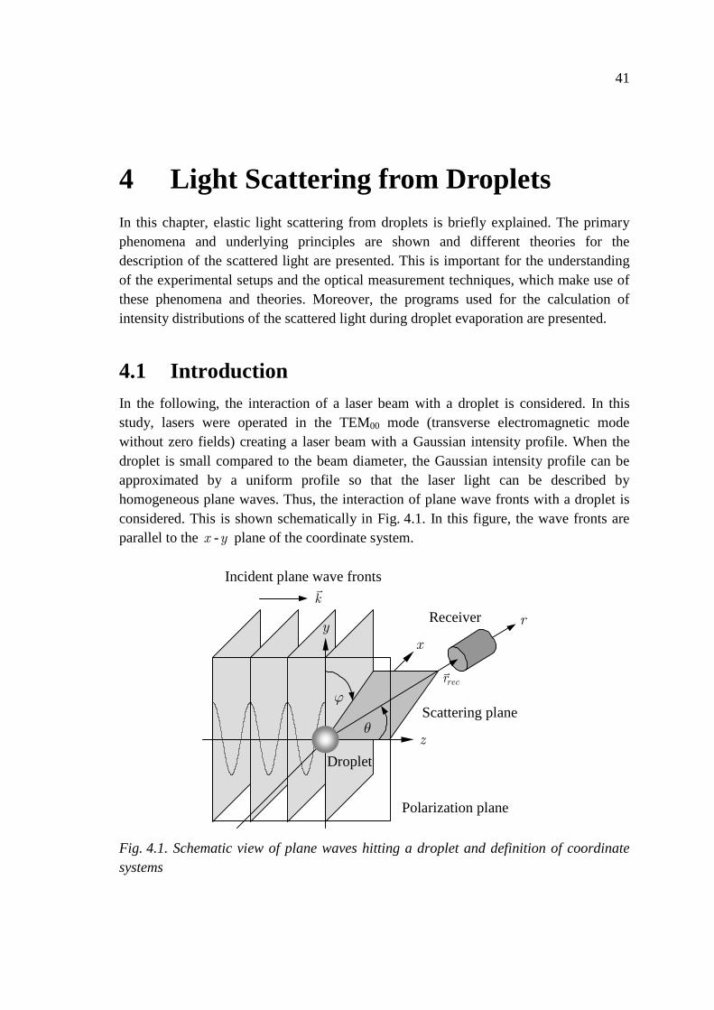
41

4 Light Scattering from Droplets In this chapter, elastic light scattering from droplets is briefly explained. The primary phenomena and underlying principles are shown and different theories for the description of the scattered light are presented. This is important for the understanding of the experimental setups and the optical measurement techniques, which make use of these phenomena and theories. Moreover, the programs used for the calculation of intensity distributions of the scattered light during droplet evaporation are presented.

4.1 Introduction In the following, the interaction of a laser beam with a droplet is considered. In this study, lasers were operated in the TEM00 mode (transverse electromagnetic mode without zero fields) creating a laser beam with a Gaussian intensity profile. When the droplet is small compared to the beam diameter, the Gaussian intensity profile can be approximated by a uniform profile so that the laser light can be described by homogeneous plane waves. Thus, the interaction of plane wave fronts with a droplet is considered. This is shown schematically in Fig. 4.1. In this figure, the wave fronts are parallel to the x -y plane of the coordinate system.

Incident plane wave fronts

θ

ϕ

Polarization plane

Droplet

x

z

y

Scattering plane

Receiver

recr

k

r

Fig. 4.1. Schematic view of plane waves hitting a droplet and definition of coordinate systems

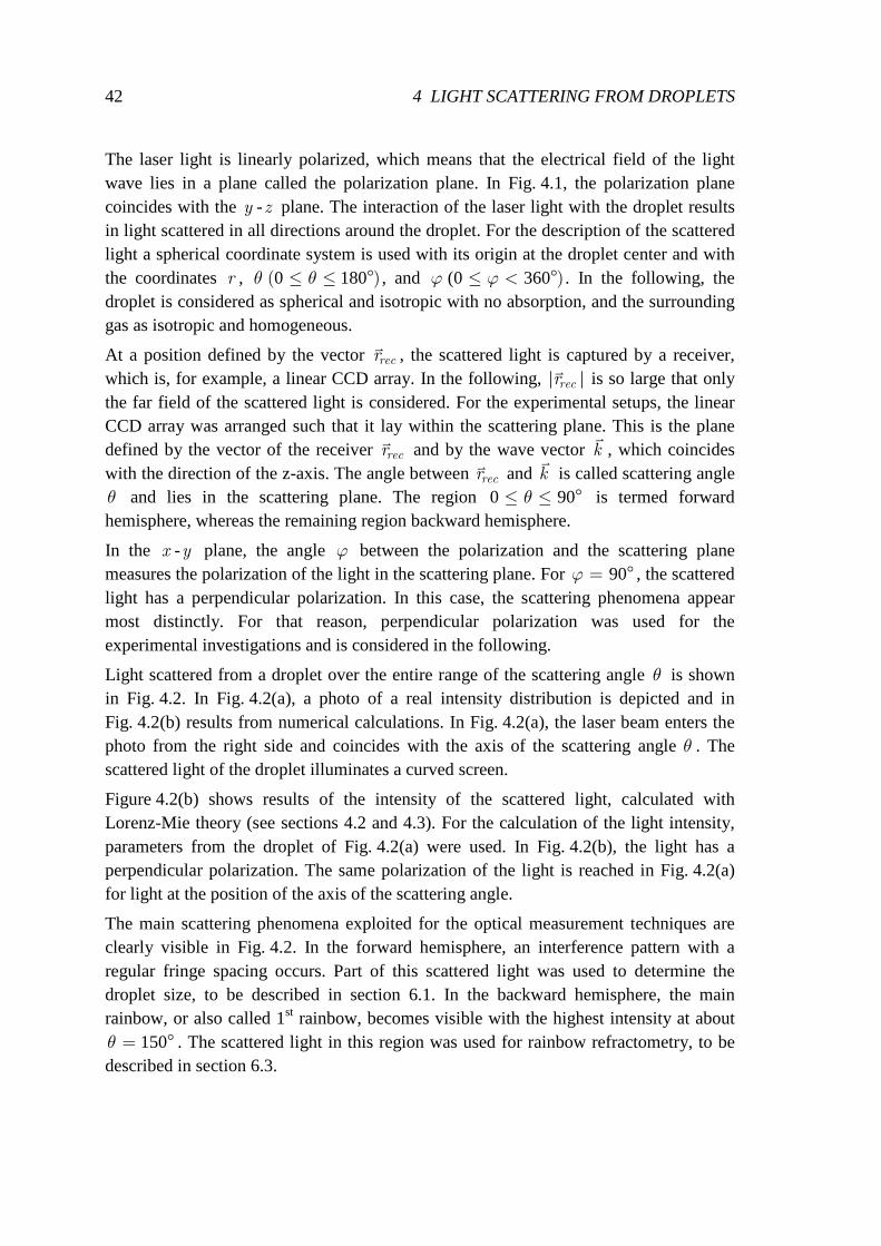
42 4 LIGHT SCATTERING FROM DROPLETS

The laser light is linearly polarized, which means that the electrical field of the light wave lies in a plane called the polarization plane. In Fig. 4.1, the polarization plane coincides with the y -z plane. The interaction of the laser light with the droplet results in light scattered in all directions around the droplet. For the description of the scattered light a spherical coordinate system is used with its origin at the droplet center and with the coordinates r , 0 180( )θ θ≤ ≤ ° , and (0 360)ϕ ϕ≤ < ° . In the following, the droplet is considered as spherical and isotropic with no absorption, and the surrounding gas as isotropic and homogeneous.

At a position defined by the vector recr , the scattered light is captured by a receiver,

which is, for example, a linear CCD array. In the following, recr is so large that only

the far field of the scattered light is considered. For the experimental setups, the linear CCD array was arranged such that it lay within the scattering plane. This is the plane defined by the vector of the receiver

recr and by the wave vector

k , which coincides

with the direction of the z-axis. The angle between recr and

k is called scattering angle

θ and lies in the scattering plane. The region 0 90θ≤ ≤ ° is termed forward hemisphere, whereas the remaining region backward hemisphere.

In the x -y plane, the angle ϕ between the polarization and the scattering plane measures the polarization of the light in the scattering plane. For 90= °ϕ , the scattered light has a perpendicular polarization. In this case, the scattering phenomena appear most distinctly. For that reason, perpendicular polarization was used for the experimental investigations and is considered in the following.

Light scattered from a droplet over the entire range of the scattering angle θ is shown in Fig. 4.2. In Fig. 4.2(a), a photo of a real intensity distribution is depicted and in Fig. 4.2(b) results from numerical calculations. In Fig. 4.2(a), the laser beam enters the photo from the right side and coincides with the axis of the scattering angle θ . The scattered light of the droplet illuminates a curved screen.

Figure 4.2(b) shows results of the intensity of the scattered light, calculated with Lorenz-Mie theory (see sections 4.2 and 4.3). For the calculation of the light intensity, parameters from the droplet of Fig. 4.2(a) were used. In Fig. 4.2(b), the light has a perpendicular polarization. The same polarization of the light is reached in Fig. 4.2(a) for light at the position of the axis of the scattering angle.

The main scattering phenomena exploited for the optical measurement techniques are clearly visible in Fig. 4.2. In the forward hemisphere, an interference pattern with a regular fringe spacing occurs. Part of this scattered light was used to determine the droplet size, to be described in section 6.1. In the backward hemisphere, the main rainbow, or also called 1st rainbow, becomes visible with the highest intensity at about

150= °θ . The scattered light in this region was used for rainbow refractometry, to be described in section 6.3.

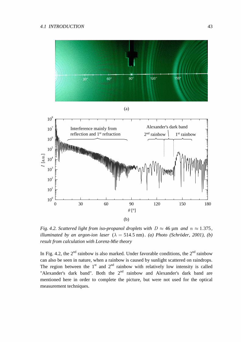
4.1 INTRODUCTION 43

(a)

(b)

2nd rainbow

Alexander's dark band

1st rainbowInterference mainly fromreflection and 1st refraction

0 30 60 90 120 150 180100

101

102

103

104

105

106

107

108

I [a

.u.]

θ [°]

Fig. 4.2. Scattered light from iso-propanol droplets with 46 µmD ≈ and 1 375.≈n , illuminated by an argon-ion laser ( 514 5 nm).λ = . (a) Photo (Schröder, 2001), (b) result from calculation with Lorenz-Mie theory

In Fig. 4.2, the 2nd rainbow is also marked. Under favorable conditions, the 2nd rainbow can also be seen in nature, when a rainbow is caused by sunlight scattered on raindrops. The region between the 1st and 2nd rainbow with relatively low intensity is called "Alexander's dark band". Both the 2nd rainbow and Alexander's dark band are mentioned here in order to complete the picture, but were not used for the optical measurement techniques.

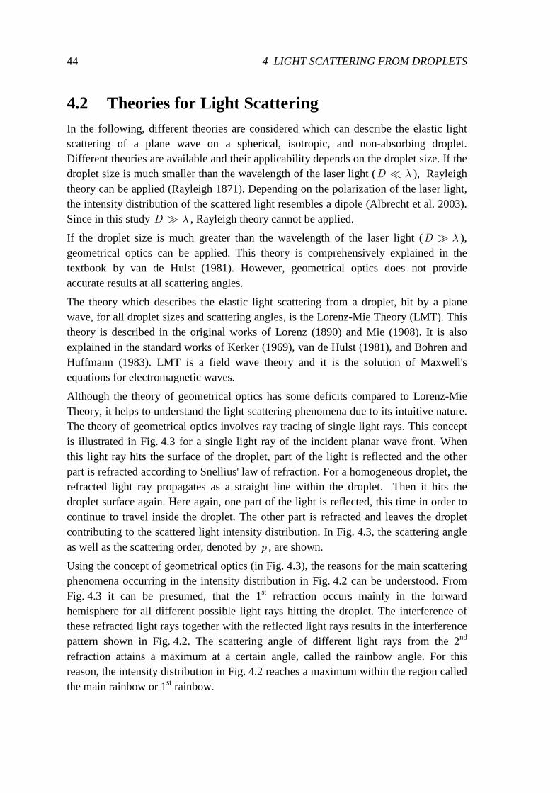
44 4 LIGHT SCATTERING FROM DROPLETS

4.2 Theories for Light Scattering In the following, different theories are considered which can describe the elastic light scattering of a plane wave on a spherical, isotropic, and non-absorbing droplet. Different theories are available and their applicability depends on the droplet size. If the droplet size is much smaller than the wavelength of the laser light (D λ≪ ), Rayleigh theory can be applied (Rayleigh 1871). Depending on the polarization of the laser light, the intensity distribution of the scattered light resembles a dipole (Albrecht et al. 2003). Since in this study D λ≫ , Rayleigh theory cannot be applied.

If the droplet size is much greater than the wavelength of the laser light (D λ≫ ), geometrical optics can be applied. This theory is comprehensively explained in the textbook by van de Hulst (1981). However, geometrical optics does not provide accurate results at all scattering angles.

The theory which describes the elastic light scattering from a droplet, hit by a plane wave, for all droplet sizes and scattering angles, is the Lorenz-Mie Theory (LMT). This theory is described in the original works of Lorenz (1890) and Mie (1908). It is also explained in the standard works of Kerker (1969), van de Hulst (1981), and Bohren and Huffmann (1983). LMT is a field wave theory and it is the solution of Maxwell's equations for electromagnetic waves.

Although the theory of geometrical optics has some deficits compared to Lorenz-Mie Theory, it helps to understand the light scattering phenomena due to its intuitive nature. The theory of geometrical optics involves ray tracing of single light rays. This concept is illustrated in Fig. 4.3 for a single light ray of the incident planar wave front. When this light ray hits the surface of the droplet, part of the light is reflected and the other part is refracted according to Snellius' law of refraction. For a homogeneous droplet, the refracted light ray propagates as a straight line within the droplet. Then it hits the droplet surface again. Here again, one part of the light is reflected, this time in order to continue to travel inside the droplet. The other part is refracted and leaves the droplet contributing to the scattered light intensity distribution. In Fig. 4.3, the scattering angle as well as the scattering order, denoted by p , are shown.

Using the concept of geometrical optics (in Fig. 4.3), the reasons for the main scattering phenomena occurring in the intensity distribution in Fig. 4.2 can be understood. From Fig. 4.3 it can be presumed, that the 1st refraction occurs mainly in the forward hemisphere for all different possible light rays hitting the droplet. The interference of these refracted light rays together with the reflected light rays results in the interference pattern shown in Fig. 4.2. The scattering angle of different light rays from the 2nd refraction attains a maximum at a certain angle, called the rainbow angle. For this reason, the intensity distribution in Fig. 4.2 reaches a maximum within the region called the main rainbow or 1st rainbow.

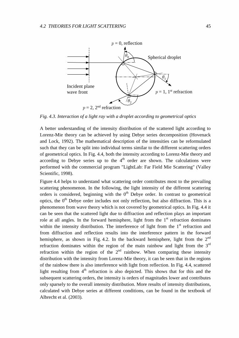
4.2 THEORIES FOR LIGHT SCATTERING 45

p = 0, reflection

p = 1, 1st refraction

p = 2, 2nd refraction

Incident planewave front

.

.

.

θ0

θ1

θ2

Spherical droplet

Fig. 4.3. Interaction of a light ray with a droplet according to geometrical optics

A better understanding of the intensity distribution of the scattered light according to Lorenz-Mie theory can be achieved by using Debye series decomposition (Hovenack and Lock, 1992). The mathematical description of the intensities can be reformulated such that they can be split into individual terms similar to the different scattering orders of geometrical optics. In Fig. 4.4, both the intensity according to Lorenz-Mie theory and according to Debye series up to the 4th order are shown. The calculations were performed with the commercial program "LightLab: Far Field Mie Scattering" (Valley Scientific, 1998).

Figure 4.4 helps to understand what scattering order contributes most to the prevailing scattering phenomenon. In the following, the light intensity of the different scattering orders is considered, beginning with the 0th Debye order. In contrast to geometrical optics, the 0th Debye order includes not only reflection, but also diffraction. This is a phenomenon from wave theory which is not covered by geometrical optics. In Fig. 4.4 it can be seen that the scattered light due to diffraction and reflection plays an important role at all angles. In the forward hemisphere, light from the 1st refraction dominates within the intensity distribution. The interference of light from the 1st refraction and from diffraction and reflection results into the interference pattern in the forward hemisphere, as shown in Fig. 4.2. In the backward hemisphere, light from the 2nd refraction dominates within the region of the main rainbow and light from the 3rd refraction within the region of the 2nd rainbow. When comparing these intensity distribution with the intensity from Lorenz-Mie theory, it can be seen that in the regions of the rainbow there is also interference with light from reflection. In Fig. 4.4, scattered light resulting from 4th refraction is also depicted. This shows that for this and the subsequent scattering orders, the intensity is orders of magnitudes lower and contributes only sparsely to the overall intensity distribution. More results of intensity distributions, calculated with Debye series at different conditions, can be found in the textbook of Albrecht et al. (2003).

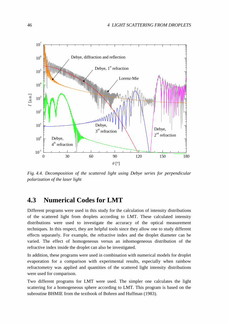
46 4 LIGHT SCATTERING FROM DROPLETS

0 30 60 90 120 150 18010-1

100

101

102

103

104

105

106

107

Lorenz-Mie

Debye,

4th refraction

Debye, diffraction and reflection

Debye, 1st refraction

Debye,

3rd refraction

I [a

.u.]

θ [°]

Debye,

2nd refraction

Fig. 4.4. Decomposition of the scattered light using Debye series for perpendicular polarization of the laser light

4.3 Numerical Codes for LMT Different programs were used in this study for the calculation of intensity distributions of the scattered light from droplets according to LMT. These calculated intensity distributions were used to investigate the accuracy of the optical measurement techniques. In this respect, they are helpful tools since they allow one to study different effects separately. For example, the refractive index and the droplet diameter can be varied. The effect of homogeneous versus an inhomogeneous distribution of the refractive index inside the droplet can also be investigated.

In addition, these programs were used in combination with numerical models for droplet evaporation for a comparison with experimental results, especially when rainbow refractometry was applied and quantities of the scattered light intensity distributions were used for comparison.

Two different programs for LMT were used. The simpler one calculates the light scattering for a homogeneous sphere according to LMT. This program is based on the subroutine BHMIE from the textbook of Bohren and Huffman (1983).

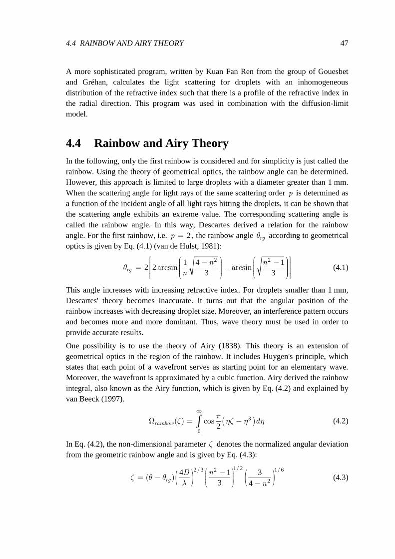
4.4 RAINBOW AND AIRY THEORY 47

A more sophisticated program, written by Kuan Fan Ren from the group of Gouesbet and Gréhan, calculates the light scattering for droplets with an inhomogeneous distribution of the refractive index such that there is a profile of the refractive index in the radial direction. This program was used in combination with the diffusion-limit model.

4.4 Rainbow and Airy Theory In the following, only the first rainbow is considered and for simplicity is just called the rainbow. Using the theory of geometrical optics, the rainbow angle can be determined. However, this approach is limited to large droplets with a diameter greater than 1 mm. When the scattering angle for light rays of the same scattering order p is determined as a function of the incident angle of all light rays hitting the droplets, it can be shown that the scattering angle exhibits an extreme value. The corresponding scattering angle is called the rainbow angle. In this way, Descartes derived a relation for the rainbow angle. For the first rainbow, i.e. 2=p , the rainbow angle rgθ according to geometrical optics is given by Eq. (4.1) (van de Hulst, 1981):

2 21 4 1

2 23 3

arcsin arcsin − − = −

rgn n

nθ (4.1)

This angle increases with increasing refractive index. For droplets smaller than 1 mm, Descartes' theory becomes inaccurate. It turns out that the angular position of the rainbow increases with decreasing droplet size. Moreover, an interference pattern occurs and becomes more and more dominant. Thus, wave theory must be used in order to provide accurate results.

One possibility is to use the theory of Airy (1838). This theory is an extension of geometrical optics in the region of the rainbow. It includes Huygen's principle, which states that each point of a wavefront serves as starting point for an elementary wave. Moreover, the wavefront is approximated by a cubic function. Airy derived the rainbow integral, also known as the Airy function, which is given by Eq. (4.2) and explained by van Beeck (1997).

( )3

02

( ) cosrainbow dπ

ζ ηζ η η

∞

Ω = −∫ (4.2)

In Eq. (4.2), the non-dimensional parameter ζ denotes the normalized angular deviation from the geometric rainbow angle and is given by Eq. (4.3):

( ) ( )1 22 3 1 62

2

4 1 33 4

// /

( ) − = − − rg

D n

nζ θ θ

λ (4.3)

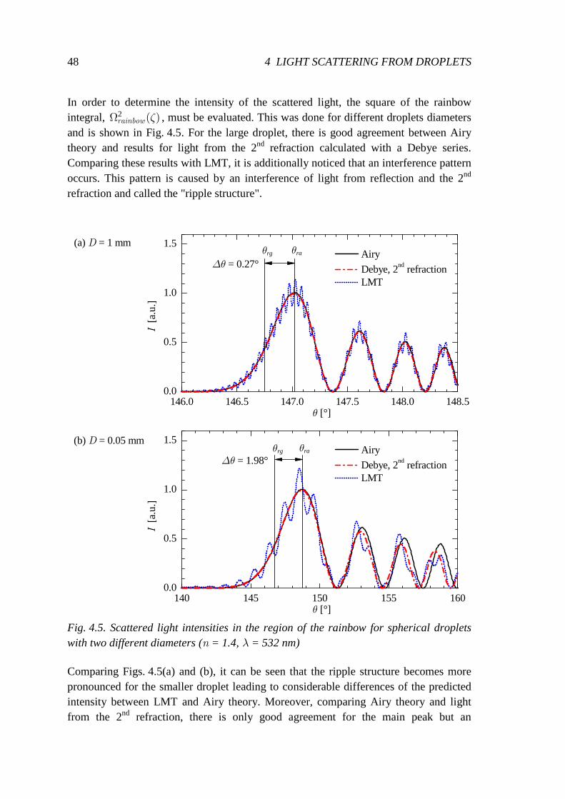
48 4 LIGHT SCATTERING FROM DROPLETS

In order to determine the intensity of the scattered light, the square of the rainbow integral, 2 ( )rainbow ζΩ , must be evaluated. This was done for different droplets diameters and is shown in Fig. 4.5. For the large droplet, there is good agreement between Airy theory and results for light from the 2nd refraction calculated with a Debye series. Comparing these results with LMT, it is additionally noticed that an interference pattern occurs. This pattern is caused by an interference of light from reflection and the 2nd refraction and called the "ripple structure".

146.0 146.5 147.0 147.5 148.0 148.50.0

0.5

1.0

1.5

140 145 150 155 1600.0

0.5

1.0

1.5(b) D = 0.05 mm

(a) D = 1 mm

I [a

.u.]

θ [°]

Airy

Debye, 2nd refraction LMT

∆θ = 0.27°θraθrg

θraθrg

∆θ = 1.98°

I [a

.u.]

θ [°]

Airy

Debye, 2nd refraction LMT

Fig. 4.5. Scattered light intensities in the region of the rainbow for spherical droplets with two different diameters (n = 1.4, λ = 532 nm)

Comparing Figs. 4.5(a) and (b), it can be seen that the ripple structure becomes more pronounced for the smaller droplet leading to considerable differences of the predicted intensity between LMT and Airy theory. Moreover, comparing Airy theory and light from the 2nd refraction, there is only good agreement for the main peak but an

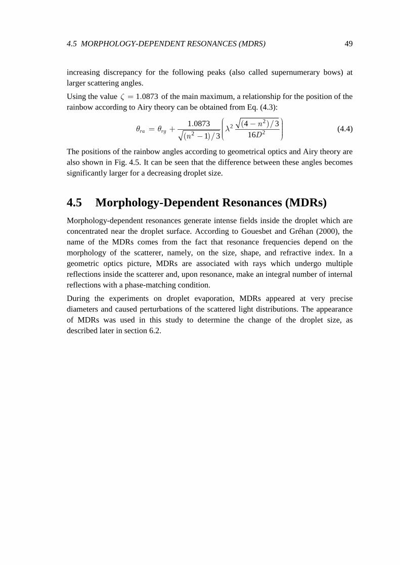
4.5 MORPHOLOGY-DEPENDENT RESONANCES (MDRS) 49

increasing discrepancy for the following peaks (also called supernumerary bows) at larger scattering angles.

Using the value 1 0873.=ζ of the main maximum, a relationship for the position of the rainbow according to Airy theory can be obtained from Eq. (4.3):

2

222

1 0873 4 3161 3

. ( )/

( )/

− = + − ra rg

n

Dnθ θ λ (4.4)

The positions of the rainbow angles according to geometrical optics and Airy theory are also shown in Fig. 4.5. It can be seen that the difference between these angles becomes significantly larger for a decreasing droplet size.

4.5 Morphology-Dependent Resonances (MDRs) Morphology-dependent resonances generate intense fields inside the droplet which are concentrated near the droplet surface. According to Gouesbet and Gréhan (2000), the name of the MDRs comes from the fact that resonance frequencies depend on the morphology of the scatterer, namely, on the size, shape, and refractive index. In a geometric optics picture, MDRs are associated with rays which undergo multiple reflections inside the scatterer and, upon resonance, make an integral number of internal reflections with a phase-matching condition.

During the experiments on droplet evaporation, MDRs appeared at very precise diameters and caused perturbations of the scattered light distributions. The appearance of MDRs was used in this study to determine the change of the droplet size, as described later in section 6.2.

51

5 Experimental Methods Two different experimental setups were used for the investigation of droplet evaporation. Single, optically levitated droplets were studied with one setup, and with the other setup, single, free-falling droplets were investigated. The setup for optically levitated droplets was especially suitable for the investigation of evaporation processes which lasted a long time and where the evaporation rate was low. This means that substances with a low volatility could be investigated very well. In the case of n-alkanes, substances ranging from n-nonane to n-hexadecane could be used for pure-component droplets evaporating at an ambient temperature of about 295 K. For example, a droplet of n-hexadecane with an initial diameter of 50 µm could be investigated during nearly its entire lifetime of about 20 min.

The setup for single, free-falling droplets was designed for the investigation of evaporation processes lasting a relatively short time and when the evaporation rate was high. As a consequence, this setup was suitable for highly volatile substances. In the case of n-alkanes, this means that at an ambient temperature of about 295 K, substances ranging from n-pentane to n-decane could be used for pure-component droplets. The maximum measurement period was generally 2 s.

In the case of multicomponent droplets with substances of both high and low volatility, a combination of the two experimental setups could be used to study the entire evaporation process.

In the first part of this chapter, a general overview of the experimental setups is given. In the following sections, details of the setups such as the droplet-on-demand generators and the observations chambers, where the motion of the droplet and the gas flow are analyzed, are described. The chapter concludes by describing the measurement procedure.

5.1 Setup for Single, Optically Levitated Droplets

5.1.1 Optical Levitation For the investigation of the evaporation of a single, motionless droplet, there are different possible ways to compensate for the gravitational force on the droplet and to stabilize it in a given position for observation. A general review of this subject can be found in Frohn and Roth (2000). A very simple solution is to suspend the droplet at the end of a thin fiber. However, with respect to the goal of investigating an isolated

52 5 EXPERIMENTAL METHODS

droplet, this technique has the disadvantages that the droplet shape is distorted by the fiber and that heat transfer occurs between the droplet and the fiber.

Therefore, levitation techniques, which allow contact-free positioning of the droplet, are more suitable. There are several different levitation techniques which use different forces. These forces include electrostatic or electrodynamic forces or forces resulting from light pressure or acoustical pressure. Electrostatic levitation requires electrical charging of the droplet in the case of n-alkane-droplets. Apart from the fact that this causes additional complexity, the physical behavior of the droplet might be changed as well. In the case of acoustic levitation, the droplet is levitated in an acoustic field with a standing wave. Due to the high-pressure gradients, the evaporation behavior of the droplet is generally considerably influenced.

Optical levitation is the most suitable levitation technique for the investigation of a single, motionless droplet, both for the expected initial droplet size of about 50 µm and the selected substances, n-alkanes. In the case of optical levitation, the droplet is levitated by the radiation forces of a continuous light source. In this study, a continuous Nd:YAG-laser with a wavelength of 532 nm was used. In order to avoid heat input from the laser light, the droplet liquid must not absorb the light. This requirement is fulfilled in the case of n-alkanes. Since n-alkanes are highly transparent liquids for the employed laser wavelength, most of the light passes through the droplet and only a small part of the light is reflected. Thus, the force of the laser light on the droplet results mainly from refraction of the light on the droplet surface.

In the experimental setup, the droplet was levitated by means of a single, vertical laser beam which hit the droplet from below in the opposite direction of the gravitational force. Due to the Gaussian intensity profile of the laser beam, the forces perpendicular to the laser beam acted to stabilize the droplet on the laser axis. This is described in detail in a review by Ashkin (1980). In the vertical direction, the laser beam was focused by means of a lens. In this way, there was a gradient of the forces in the direction of the laser beam, which helped to compensate for the gravitational force. In the experimental setup, a droplet was injected in the laser beam above its focus. Then the droplet fell along the laser beam until it reached an equilibrium position. At this position, the force of the light in the direction of the laser beam balanced the gravitational force.

When the beam waist at the focal point is considerably smaller than the droplet diameter, which was generally the case for the experiments and is shown in Fig. 5.1, there are two stable regimes for levitation as described by Ashkin and Dziedzic (1974). One is above the focus and the other one below. A regime along the axis of the laser beam is called stable, when the gradient of the force on the droplet resulting from the laser light and acting in the direction of the laser beam is such that there is a restoring force when the droplet is moved away from its equilibrium position.

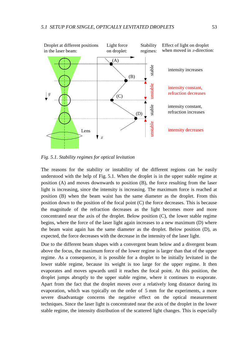
5.1 SETUP FOR SINGLE, OPTICALLY LEVITATED DROPLETS 53

g

Lensx

Droplet at different positionsin the laser beam:

Effect of light on droplet when moved in x-direction:

Light force on droplet:

Stability regimes:

intensity increases

intensity constant,refraction decreases

intensity constant,refraction increases

intensity decreases

unst

able

sta

ble

unst

able

stab

le

(A)

(B)

(C)

(D)

Fig. 5.1. Stability regimes for optical levitation

The reasons for the stability or instability of the different regions can be easily understood with the help of Fig. 5.1. When the droplet is in the upper stable regime at position (A) and moves downwards to position (B), the force resulting from the laser light is increasing, since the intensity is increasing. The maximum force is reached at position (B) when the beam waist has the same diameter as the droplet. From this position down to the position of the focal point (C) the force decreases. This is because the magnitude of the refraction decreases as the light becomes more and more concentrated near the axis of the droplet. Below position (C), the lower stable regime begins, where the force of the laser light again increases to a new maximum (D) where the beam waist again has the same diameter as the droplet. Below position (D), as expected, the force decreases with the decrease in the intensity of the laser light.

Due to the different beam shapes with a convergent beam below and a divergent beam above the focus, the maximum force of the lower regime is larger than that of the upper regime. As a consequence, it is possible for a droplet to be initially levitated in the lower stable regime, because its weight is too large for the upper regime. It then evaporates and moves upwards until it reaches the focal point. At this position, the droplet jumps abruptly to the upper stable regime, where it continues to evaporate. Apart from the fact that the droplet moves over a relatively long distance during its evaporation, which was typically on the order of 5 mm for the experiments, a more severe disadvantage concerns the negative effect on the optical measurement techniques. Since the laser light is concentrated near the axis of the droplet in the lower stable regime, the intensity distribution of the scattered light changes. This is especially

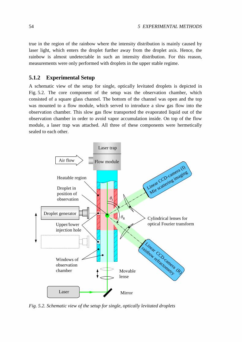
54 5 EXPERIMENTAL METHODS

true in the region of the rainbow where the intensity distribution is mainly caused by laser light, which enters the droplet further away from the droplet axis. Hence, the rainbow is almost undetectable in such an intensity distribution. For this reason, measurements were only performed with droplets in the upper stable regime.

5.1.2 Experimental Setup A schematic view of the setup for single, optically levitated droplets is depicted in Fig. 5.2. The core component of the setup was the observation chamber, which consisted of a square glass channel. The bottom of the channel was open and the top was mounted to a flow module, which served to introduce a slow gas flow into the observation chamber. This slow gas flow transported the evaporated liquid out of the observation chamber in order to avoid vapor accumulation inside. On top of the flow module, a laser trap was attached. All three of these components were hermetically sealed to each other.

Laser Mirror

Movable lense

Droplet generator

Air flow

Droplet in position of observation

Linear CCD-ca

mera (I)

Mie scat

tering im

aging

Cylindrical lenses for optical Fourier transform

Heatable region

Windows of observation chamber

Linear CCD-camera (R)

rainbow refractometry

Upper/lowerinjection hole

θR

Laser trap

θI

Flow module

Fig. 5.2. Schematic view of the setup for single, optically levitated droplets

5.1 SETUP FOR SINGLE, OPTICALLY LEVITATED DROPLETS 55

Although the gas flow was very slow, special care was taken in the design of the flow module in order to create a uniform and smooth flow inside the observation chamber as reported by Bernholz (1997). For this reason, the flow module was a complex component. The gas flow was delivered from the compressed air supply of the ITLR. It was controlled by a variable area flowmeter and was connected to the flow module by a tube. Inside the flow module, the air entered a circular channel and was thus distributed around the observation chamber. From this circular channel, the air passed through several uniformly spaced slots into a funnel-shaped inlet with a constant cross section so that the air flow remained smooth. The opening angle of the funnel was kept small so that the flow finally entered the main channel around the laser beam. The cross section of this channel changed gradually from a circular to a square cross section, so that there was a smooth transition to the square glass channel of the observation chamber.

The Nd:YAG laser beam was directed vertically upwards into the observation chamber using a mirror. The laser beam was adjusted in such a way that it coincided with the centerline of the observation chamber. It was focused by means of a movable lens. The focal point was located below the position at which the droplets were injected into the observation chamber.

The droplet was produced by a droplet-on-demand generator (described in detail in section 5.4) and injected into the observation chamber through a small hole in one of the glass windows. The position of the droplet generator in the horizontal direction could be varied relative to the laser beam and was adjusted in such a way that the droplet exactly reached the laser beam. Details of the movement of the droplet are described in section 5.5.1. When the droplet falls along the laser beam, the light forces of the laser beam begin to act in order to move the droplet into the equilibrium position.

There were two different positions for the injection of the droplet into the measurement chamber, i.e., the upper and the lower injection position. Initially the observation chamber had been designed such that the droplet was injected and levitated at a lower position and then moved into the measurement position by shifting the lens. It was designed this way because the droplet generator sometimes behaved in an unstable fashion, and the ejection range would change abruptly. As a consequence, the droplet hit the opposite wall of the observation chamber. This led to a contamination of the ambient conditions, since the liquid on the walls evaporated. If this occurred, the glass windows had to be cleaned. For this reason, the droplet was not injected directly into the measurement position, but at a lower position, where the contamination of the opposite glass wall did not influence the evaporation behavior of the droplet in the measurement position.

The drawback of this method was that, due to the movement of the droplet into the measurement position, a time period on the order of 2 s of the initial evaporation phase was lost for the measurements. The method for droplet injection was changed for this

56 5 EXPERIMENTAL METHODS

reason, and also since a great deal of experience was gained in operating the droplet generator more reliably.

When the new method was applied, the position of the droplet generator relative to the laser beam was calibrated using the lower injection position. After calibration was complete, the droplet generator was moved upwards and for the measurements the droplets were injected through the upper injection hole directly into the measurement position. Ultimately, both methods gave valid results, but the measurements could begin earlier using the newer method.

In the measurement position, a heating system was mounted around the observation chamber so that the air around the droplet could be heated. Varying the heat allowed measurements of droplet evaporation at different ambient temperatures. More information on the heating system can be found later in section 5.5.3.

The temperature of the ambient gas was measured by a K-type thermocouple with a molded construction and with an exposed transition junction. The diameter of the thermocouple was 0 5 mm. . The exposed transition junction of the thermocouple was positioned about 2 to 3 mm horizontally from the droplet when the droplet was in its measurement position. Measurement errors due to the influence of the scattered laser light were taken into account.

The interaction of the laser light with the droplet was not only used to levitate the droplet but also to perform measurements with optical measurement techniques. The laser light was scattered by the droplet and parts of this scattered laser light were recorded with two linear CCD cameras at different angles relative to the laser beam. The linear CCD camera in the forward hemisphere, placed at the scattering angle Iθ , was used to determine the droplet size from the fringe spacing (described later in section 6.1). The other camera in the backward hemisphere, positioned at the scattering angle Rθ , captured the scattered light in the region of the rainbow and was used for rainbow refractometry which is explained in detail in section 6.3.

A cylindrical lens was placed one focal length in front of each camera, which resulted in an optical Fourier transform so that the position of the scattered light on the camera was independent from the droplet position and depended only on the light scattering angle. More details regarding the optical Fourier transform can be found later in section 6.1.2.

5.2 Setup for Single, Free-Falling Droplets The setup for single, free-falling droplets was especially designed to capture the initial evaporation phase of the droplet. A schematic view of the setup is depicted in Fig. 5.3. For this setup, the laser light was not used to levitate the droplet, but to illuminate the droplet and perform optical measurements from the scattered light.

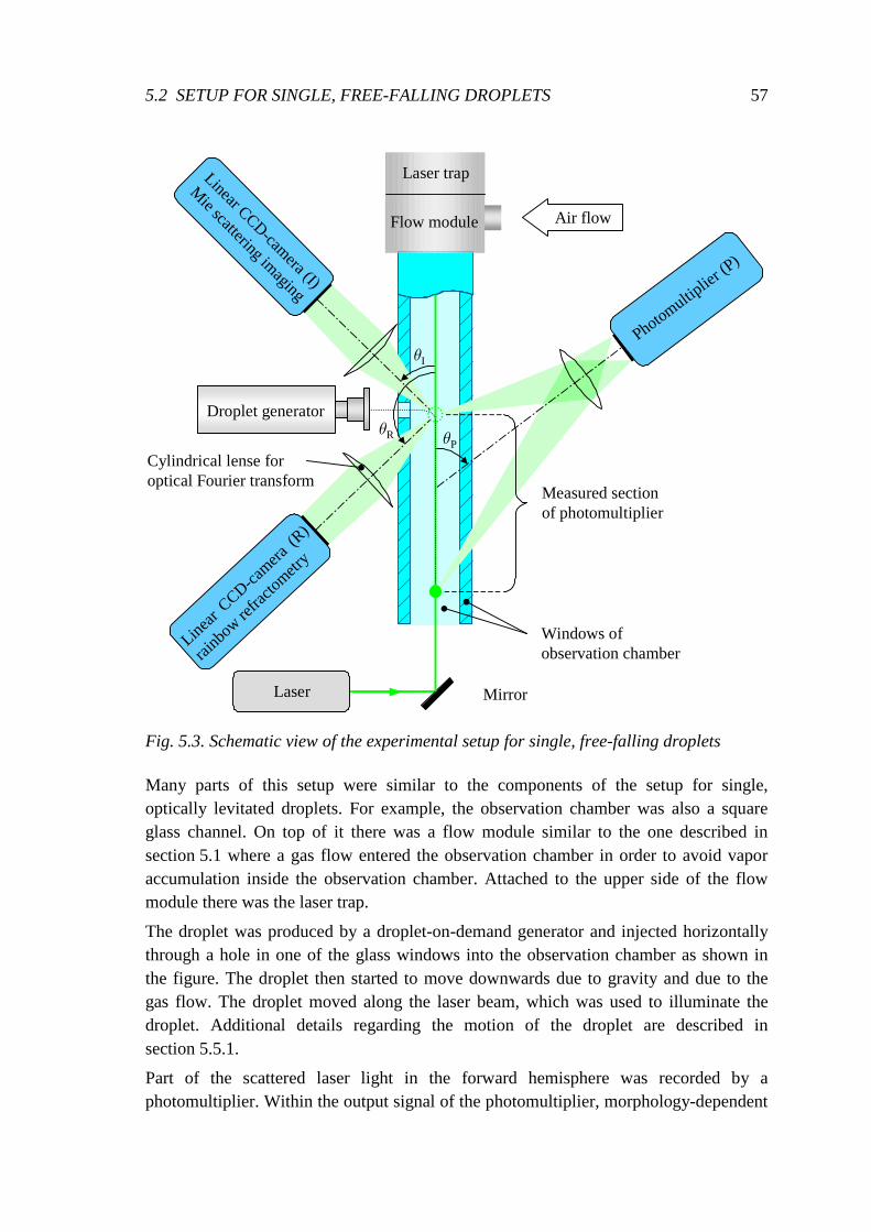
5.2 SETUP FOR SINGLE, FREE-FALLING DROPLETS 57

Mirror

Droplet generator

Air flow

Linear CCD-camera (I)

Mie scattering im

aging

Cylindrical lense for optical Fourier transform

Windows of observation chamber

Linear

CCD-camera

(R)

rainb

ow re

fracto

metry

θI

θR

Laser trap

Photom

ultipl

ier (P

)

θP

Flow module

Laser

Measured sectionof photomultiplier

Fig. 5.3. Schematic view of the experimental setup for single, free-falling droplets

Many parts of this setup were similar to the components of the setup for single, optically levitated droplets. For example, the observation chamber was also a square glass channel. On top of it there was a flow module similar to the one described in section 5.1 where a gas flow entered the observation chamber in order to avoid vapor accumulation inside the observation chamber. Attached to the upper side of the flow module there was the laser trap.

The droplet was produced by a droplet-on-demand generator and injected horizontally through a hole in one of the glass windows into the observation chamber as shown in the figure. The droplet then started to move downwards due to gravity and due to the gas flow. The droplet moved along the laser beam, which was used to illuminate the droplet. Additional details regarding the motion of the droplet are described in section 5.5.1.

Part of the scattered laser light in the forward hemisphere was recorded by a photomultiplier. Within the output signal of the photomultiplier, morphology-dependent

58 5 EXPERIMENTAL METHODS

resonances became visible. Using this information, the change in droplet diameter was determined as is discussed later in section 6.2.

As for the setup with optical levitation, one CCD camera was used to determine the droplet size by measuring the fringe spacing of the scattered laser light in the forward hemisphere. A second camera captured part of the scattered laser light in the backward hemisphere and was used for rainbow refractometry.

The optical measurement techniques covered different vertical distances during the free fall of the droplet. For the CCD cameras, this distance depended on the range of the optical Fourier transform. Due to the configuration of the optical components, the CCD camera for rainbow refractometry covered the shortest distance. Depending on the angle of observation, it was on the order of 20 mm. For the photomultiplier, the measurement section was limited by the length of the observation chamber and had a length of 100 mm.

The temperature was measured inside the observation chamber at two different positions. K-type thermocouples were also used for this setup. One thermocouple was mounted at the beginning and the other one at the end of the measurement section for the photomultiplier to verify the uniformity of the temperature in the measurement section. For the evaluation of the measurements, the mean value of the temperatures at the beginning and end of the measurement section was used as ambient temperature.

5.3 Comparison of the Experimental Setups In this section, the setups are compared with each other and typical operational characteristics are given. An overview of the main characteristics of the experimental setups is presented in Table 5.1.

Acquisition Rates and Devices for Optical Measurement Techniques Since the setup for the free-falling droplets was designed for evaporation processes with high evaporation rates, this setup could capture droplet characteristic data at the highest acquisition rates. By applying a measurement method using morphology-dependent resonances (see section 6.2), size changes with an increment on the order of 0 1 µm. were detectable. Depending on the evaporation rate of the droplet, it was possible to attain an acquisition rate of up to 2 kHz, as needed, for example, for the case of droplets consisting of pure n-pentane evaporating at an ambient temperature of about 295 K. The output signal of the photomultiplier was recorded by a data acquisition board. This board could store 64,000 data points with 8-bit resolution. Minimum time intervals of 25 ns were possible. Typical time intervals for the measurements were between 10 and 40 µs, resulting in measurement periods of 0.64 to 2.56 s.

Two different types of CCD cameras were used for the other optical techniques. For the setup with optical levitation, camera systems with linear CCD arrays were utilized that were developed and built onsite at ITLR. The CCD arrays had a 12-bit resolution. A

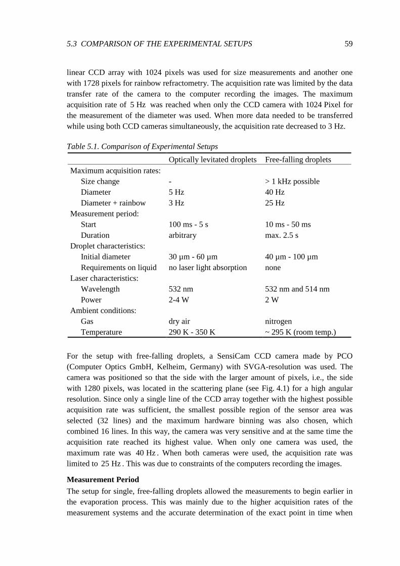
5.3 COMPARISON OF THE EXPERIMENTAL SETUPS 59

linear CCD array with 1024 pixels was used for size measurements and another one with 1728 pixels for rainbow refractometry. The acquisition rate was limited by the data transfer rate of the camera to the computer recording the images. The maximum acquisition rate of 5 Hz was reached when only the CCD camera with 1024 Pixel for the measurement of the diameter was used. When more data needed to be transferred while using both CCD cameras simultaneously, the acquisition rate decreased to 3 Hz.

Table 5.1. Comparison of Experimental Setups

Optically levitated droplets Free-falling droplets Maximum acquisition rates: Size change - > 1 kHz possible Diameter 5 Hz 40 Hz Diameter + rainbow 3 Hz 25 Hz Measurement period: Start 100 ms - 5 s 10 ms - 50 ms Duration arbitrary max. 2.5 s Droplet characteristics: Initial diameter 30 µm - 60 µm 40 µm - 100 µm Requirements on liquid no laser light absorption none Laser characteristics: Wavelength 532 nm 532 nm and 514 nm Power 2-4 W 2 W Ambient conditions: Gas dry air nitrogen Temperature 290 K - 350 K ~ 295 K (room temp.)

For the setup with free-falling droplets, a SensiCam CCD camera made by PCO (Computer Optics GmbH, Kelheim, Germany) with SVGA-resolution was used. The camera was positioned so that the side with the larger amount of pixels, i.e., the side with 1280 pixels, was located in the scattering plane (see Fig. 4.1) for a high angular resolution. Since only a single line of the CCD array together with the highest possible acquisition rate was sufficient, the smallest possible region of the sensor area was selected (32 lines) and the maximum hardware binning was also chosen, which combined 16 lines. In this way, the camera was very sensitive and at the same time the acquisition rate reached its highest value. When only one camera was used, the maximum rate was 40 Hz. When both cameras were used, the acquisition rate was limited to 25 Hz. This was due to constraints of the computers recording the images.

Measurement Period The setup for single, free-falling droplets allowed the measurements to begin earlier in the evaporation process. This was mainly due to the higher acquisition rates of the measurement systems and the accurate determination of the exact point in time when

60 5 EXPERIMENTAL METHODS

the droplet reached the laser beam using the output signal of the photomultiplier. For the setup with single, optically levitated droplets, the earliest start of the measurements was possible, when the droplet was injected directly into the measurement position.

With respect to the measurement period, the evaporation of the droplet could be investigated until evaporation was nearly complete using the setup for single, optically levitated droplets. When the droplet size decreased, the stabilizing forces on the droplet became weaker so that the droplet eventually fell off the laser beam due to small disturbances of the air inside the observation chamber. In the case of the setup for single, free-falling droplets, the measurement period was limited to the time period the droplet remained within the measurement sections of the photomultiplier and the CCD cameras, respectively. Usually, a maximum measurement time of 2 5 s. was reached. Within this time period, the droplet either evaporated or left the measurement region.

Droplet Characteristics For the setup with optical levitation, the maximum droplet size was about 60 µm for a laser power of 4 W . Although the laser could supply up to 5 5 W. , a maximum of 4 W was used to avoid too much additional heating of the observation chamber by the scattered laser light. A requirement of the droplet liquid was that it must not absorb the laser light in order to avoid additional heating of the droplet. This requirement was fulfilled in the case of n-alkanes.

The setup for free-falling droplets was not so restrictive with regard to the characteristics of the droplet liquids. With this setup, droplets up to 100 µm in diameter were investigated, but larger droplets could also have been studied. The disadvantage of the increasing size was a higher free fall velocity and a corresponding shorter measurement period. Since the intensity of the laser light was much smaller, an absorption of part of the laser light would have caused little influence on the evaporation behavior of the droplet.

Laser Characteristics For free-falling droplet setup, an argon-ion laser was initially used with a wavelength of 514 nm. But most of the results, presented in this thesis, were conducted with a Nd:YAG laser, which was also used for the optical levitation setup and had a wavelength of 532 nm. For the free-falling droplet setup, a power of 2 W was generally used. For the other setup the laser power was adjusted depending on the initial droplet size. The high laser power of up to 4 W was necessary for the trapping of the droplet. After that point, the laser power could be reduced in order to keep the droplet levitated.

Ambient Conditions The gas used for the setup with optical levitation was dry air from the pressurized air supply of the ITLR. For the free-falling droplet setup, nitrogen from a compressed tank was used. The gas temperature was about 295 K in case of the setup for free-falling

5.4 DROPLET-ON-DEMAND GENERATORS 61

droplets. For the optical levitation setup, the temperature could be varied by a heating system in a range from about 290 K to 350 K.

5.4 Droplet-on-Demand Generators Two different droplet-on-demand generators were used for this study. One type had an orifice plate (Fig. 5.4a), the other type a glass capillary (Fig. 5.4b). Inside these droplet generators, a liquid column was compressed and decompressed by a piezoelectric ceramic. This piezoelectric ceramic was driven by an electric pulse generator, where a single electric pulse was generated. The voltage amplitude of the pulse and the pulse width could be changed to adjust the droplet generator.

The liquid ligament emerging from the droplet generator generally disintegrated into more than one droplet. Photographs of the droplet formation process can be found in the textbook of Frohn and Roth (2000). For the experiments in this study, the droplet generator was adjusted so that a single droplet resulted from the ligament. However, if satellite droplets were unavoidable, an adjustment was made so that these satellite droplets did not enter the observation chamber.

Using the generator with the orifice plate, the droplet size could be varied by changing the diameter of the orifice. The commonly used setting was a diameter of 40 µm, but other diameters ranging from 20 µm to 100 µm were also used. The resulting droplet size for n-alkane droplets ranged from about the orifice diameter to 1.5 times this value depending on the adjustment of the electric pulse generator and the selected substances.

The other droplet-on-demand generator consisted of a glass capillary with a nozzle (Ulmke et al. 2001). The glass capillary was fitted into a piezoelectric tube and stuck to the tube using a two-component adhesive. The advantage of this droplet generator was that the tip of the glass capillary was very small in diameter so that the droplet generator could be shifted through the hole in the observation chamber very close to the laser beam without disturbing the ambient conditions around the droplet and the scattered laser light. This allowed an earlier beginning of the optical measurements, since the time needed by the droplet to travel from the droplet generator to the laser beam was shorter. It also facilitated the operation of the droplet generator, since the occurrence of satellite droplets was less probable for a shorter ejection range.

However, there were two major disadvantages of the droplet generator with the glass capillary which limited its usage. First, with the setup available at ITLR, the droplet diameter could only be varied within a very limited size range. Therefore this droplet generator was not used in combination with the optically levitated droplet setup since the resulting droplet size was too large. The other disadvantage was that the mixture ratio did not remain constant; i.e., when multicomponent droplets with highly volatile components were investigated. There were small fluctuations in the mixture ratio from one droplet to the other and a strong decrease of the fraction of the high volatility

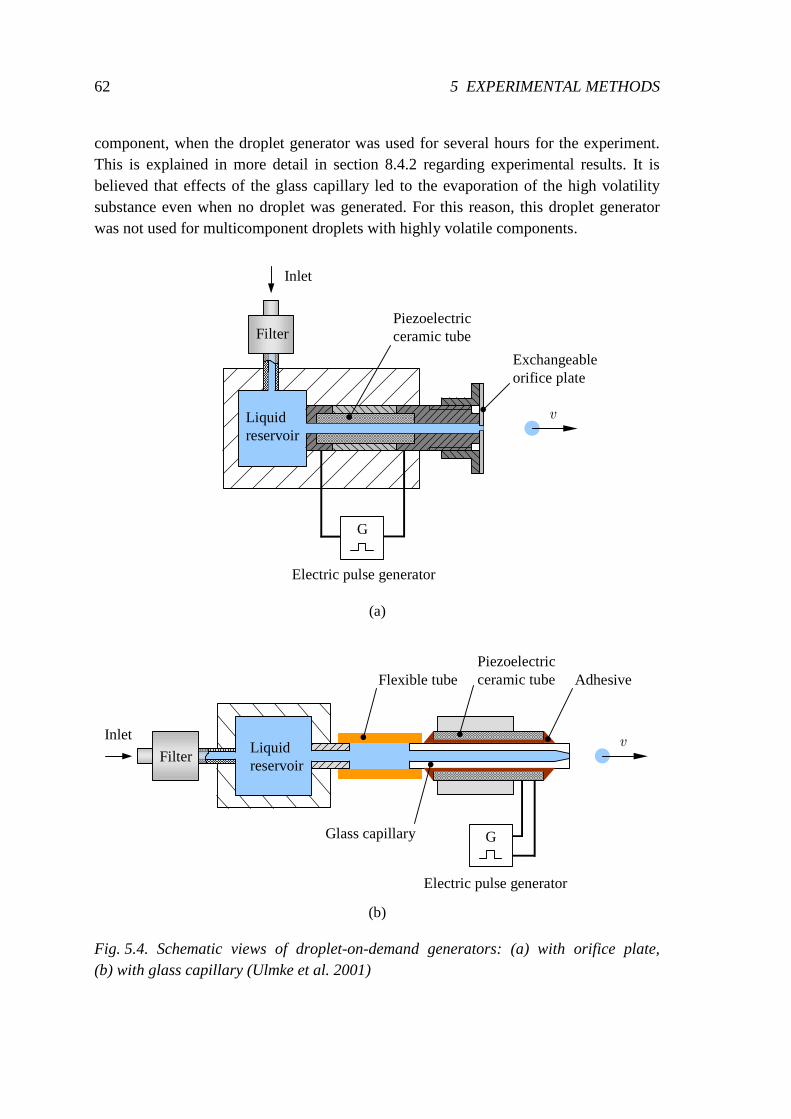
62 5 EXPERIMENTAL METHODS

component, when the droplet generator was used for several hours for the experiment. This is explained in more detail in section 8.4.2 regarding experimental results. It is believed that effects of the glass capillary led to the evaporation of the high volatility substance even when no droplet was generated. For this reason, this droplet generator was not used for multicomponent droplets with highly volatile components.

Electric pulse generator

Liquidreservoir

Filter

Inlet

Piezoelectric ceramic tube

Exchangeableorifice plate

v

G

vFilter

Inlet

Piezoelectric ceramic tube

G

Liquidreservoir

Flexible tube Adhesive

Electric pulse generator

Glass capillary

(a)

(b)

Fig. 5.4. Schematic views of droplet-on-demand generators: (a) with orifice plate, (b) with glass capillary (Ulmke et al. 2001)

5.5 OBSERVATION CHAMBER 63

The droplet generator with the orifice plate also had the problem that the initial mixture ratio did not correspond to the mixture ratio from the preparation of the mixture. However, the error was small and did not change in time as significantly as with the other generator. This change in the mixture ratio was unavoidable since some time was always needed before the droplet generator was adjusted and a stable droplet generation was reached to provide a constant ejection range.

5.5 Observation Chamber In the following paragraphs, different aspects of the observation chambers are considered in detail, such as the motion of the droplets, the gas flow, and the temperature field inside the chamber. In principle, the observation chambers of the two setups were quite similar. Apart from minor differences such as different dimensions, the main difference was that the observation chamber for the optically levitated droplet setup also had a heating system.

5.5.1 Droplet Motion In this paragraph, the movement of the droplets after their generation is described in detail. This helps in the understanding of important boundary conditions of the experimental setups, for example, the earliest possible beginning for the measurements or the falling distance of the droplets. General remarks on droplet kinetics and the underlying physical phenomena can be found in Lee (2003).

From the corresponding fundamental equations, equations for the motion of the droplets are derived in the following. In order to illustrate the order of magnitude of characteristic parameters of the droplet movement, results are derived for a sample droplet consisting of pure n-octane with an initial diameter of 0 50 µm=D . The droplet evaporates in air at an ambient temperature of 293 K=T with material properties of density at 31 19 kg/m.ρ = and a viscosity at 51 82 10 kg/(m s).µ −= ⋅ ⋅ .

For both setups, the droplets were ejected from the droplet generator in the horizontal direction. The arrangement of the droplet generator with respect to the laser beam is depicted in Fig. 5.5. After ejection in the horizontal direction, the droplet also started to fall downwards due to the gravitational force. The movement in the horizontal and the vertical directions can be considered separately, since the total movement of the droplet can be obtained by a linear superposition of these two.

In the following, first the horizontal and then the vertical movement of the droplet are considered. The origin of the coordinate system is in the middle of the exit hole of the droplet generator. The droplet generator has been placed such that the droplet exactly reaches the laser beam.

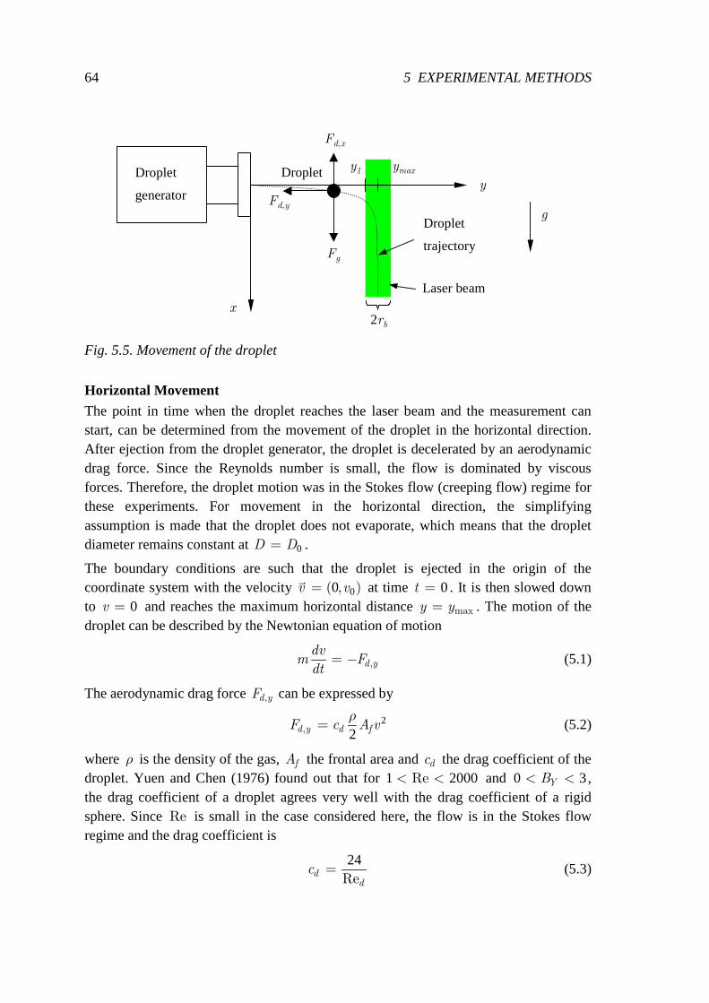
64 5 EXPERIMENTAL METHODS

y

x

Droplet

generator

Droplet

Laser beam

Droplet

trajectory

ymax

Fd,x

Fd,y

Fg

g

y1

2rb

Fig. 5.5. Movement of the droplet

Horizontal Movement The point in time when the droplet reaches the laser beam and the measurement can start, can be determined from the movement of the droplet in the horizontal direction. After ejection from the droplet generator, the droplet is decelerated by an aerodynamic drag force. Since the Reynolds number is small, the flow is dominated by viscous forces. Therefore, the droplet motion was in the Stokes flow (creeping flow) regime for these experiments. For movement in the horizontal direction, the simplifying assumption is made that the droplet does not evaporate, which means that the droplet diameter remains constant at 0=D D .

The boundary conditions are such that the droplet is ejected in the origin of the coordinate system with the velocity 00( , )=v v at time 0t = . It is then slowed down to 0v = and reaches the maximum horizontal distance max=y y . The motion of the droplet can be described by the Newtonian equation of motion

,= − d ydv

m Fdt

(5.1)

The aerodynamic drag force ,d yF can be expressed by

2

2, =d y d fF c A vρ

(5.2)

where ρ is the density of the gas, fA the frontal area and dc the drag coefficient of the droplet. Yuen and Chen (1976) found out that for 1 2000Re< < and 0 3< <YB , the drag coefficient of a droplet agrees very well with the drag coefficient of a rigid sphere. Since Re is small in the case considered here, the flow is in the Stokes flow regime and the drag coefficient is

24Re

=dd

c (5.3)

5.5 OBSERVATION CHAMBER 65

Using the definition of the Reynolds number 0Re /=d vD µρ and 20 4/=fA Dπ for

the frontal area, the aerodynamic drag force can be rewritten as

03, =d yF µvDπ (5.4)

When the droplet mass m is expressed by means of the droplet diameter D and the liquid density lρ , i.e., 3

0 6/= lm Dρ π , the differential equation

20

18= −

l

dv µv

dt Dρ (5.5)

is obtained. Introducing a relaxation time constant defined as

20

18:= l

rD

µ

ρτ (5.6)

and separating the variables, Eq. (5.5) can be integrated:

0 0

1= −∫ ∫

v t

rv

dvdt

v τ (5.7)

Thus, the droplet velocity v as a function of time t is obtained:

0( )−= rt

v t v e τ (5.8)

A second integration in time results in an equation for the distance travelled by the droplet

0 1( ) ( )−= − rt

ry t v e ττ (5.9)

The maximum distance maxy is obtained by taking the limit from 0=t to infinity:

20 0 018max lim ( )

→∞= = = l

rt

y y t v D vµ

ρτ (5.10)

For the operation of the droplet generator, the maximum distance maxy of the droplet was varied by changing the amplitude and/or the pulse width of the electric pulse generator. Thereby, the droplet diameter 0D remained approximately constant. According to Eq. (5.10), this means that the initial velocity 0v , which is proportional to the maximum distance maxy , was varied.

A typical distance of maxy is 10 mm. For the sample droplet, this means that the initial velocity is 0 1 9 m/s.=v since the relaxation time constant is 5 4 ms.=τ . The maximum Reynolds number for the maximum speed 0v is 6 6max,Re .=d . This means that Eq. (5.10) can only serve as an estimation, since according to Incropera and DeWitt (1996), Eq. (5.3) for the drag coefficient is valid for 0 5Re .<d . When a more sophisticated relation is used for the representation of the standard drag curve of a rigid sphere, for example,

66 5 EXPERIMENTAL METHODS

2 324

16

/Re

Re

= + dc (5.11)

as proposed by Putnam (1961), it turns out that the drag coefficient was underestimated by about 40% for 6 6max,Re .=d using Eq. (5.3). However, since the Reynolds number rapidly decreases during the droplet motion, the simpler relation in Eq. (5.3) still provides a good estimate of the overall movement.

Next, the point in time 1t , when the droplet reaches the laser beam and the measurement could start, is estimated. For the estimation of 1t , the radius br of the laser beam is needed, which defines the radius within which the light intensity is large enough for the optical measurements. Hence, after the droplet travels the distance

1 max= − by y r (5.12)

the optical measurement can be started. Substituting this condition into Eq. (5.9) and solving for 1t yields

1 maxln( / )= r bt y rτ (5.13)

Assuming 10 mmmaxy = and 0 5 mm.br = leads to 1 3 16 2 ms.≈ =rt τ for the sample droplet. Moving the droplet generator closer towards the laser beam, i.e., shortening the distance maxy , reduces 1t .

When maxy and br remain constant, the point in time 1t for the start of the measurement is proportional to rτ and thus proportional to the square of the initial droplet diameter

0D . According to the 2D -law, the evaporation rate also depends on the square of the diameter, so the same part of the evaporation process cannot be measured independently from the initial droplet size. For the sample droplet it follows that 1 16 2 ms.=t and

2 6 21 0 6 5 10 s/m/ . −= ⋅t D as the general lower time limit.

Vertical Movement Now the vertical movement for the free-falling droplet setup is considered. In the vertical direction, not only the aerodynamic drag force but also the gravitational force acts on the droplet. This means that in the x -direction the Newtonian equation of motion is

,= −g d xdu

m F Fdt

(5.14)

During free fall, the droplet reaches its terminal velocity tu , when there is zero acceleration, which corresponds to the condition 0/ =du dt . This results in

,=g d xF F . Substituting ,d xF with Eq. (5.4) written for the x -direction and gF with

3

6=g lF gDπρ (5.15)

and solving for tu leads to

5.5 OBSERVATION CHAMBER 67

2

18= l

tg

u Dµ

ρ (5.16)

As an estimate of the upper limit for the terminal velocity, the initial diameter 0D can be used, yielding

,max =t ru gτ (5.17)

For the sample droplet this results in 7 6 cm/s,max .=tu . Hence, 0,maxtu v≪ . Therefore the motion of the droplet is always within the Stokes flow regime. This condition holds true for all droplets investigated in this study.

Since the point in time 1t when the droplet reaches the laser beam is also a characteristic time for the droplet to reach its terminal velocity, the droplet reaches its terminal velocity at the same time as the start of the measurement. When the droplet evaporates, its diameter D decreases. Since the droplet adapts relatively quickly to its terminal velocity, the simplifying assumption can be introduced that the droplet always falls at its terminal velocity. From Eq. (5.16) it can be seen that the terminal velocity is proportional to the square of the droplet diameter. When the 2D -law is used for the description of droplet evaporation (see section 3.2.3), the square of the droplet diameter decreases linearly with time. As a consequence, the same is valid for the velocity component in the vertical direction ( )tu t∼ .

When there is a gas flow inside the observation chamber with a maximum velocity

,maxgu in the centerline of the chamber, which coincides with the laser beam, this movement of the gas can be superimposed on the motion of the droplet so that the droplet reaches the maximum velocity

max ,max ,max= +t gu u u (5.18)

with respect to the observation chamber. For the experiments, the gas velocity was usually very small and in the range of 0 1 1 cm/s. − .

For the determination of the total distance travelled by the droplet in the vertical direction, the equation of motion of the droplet in the x -direction is derived in the following. Using Eq. (5.14) and substituting for ,d xF with Eq. (5.4) written for the x -direction and for gF with Eq. (5.15), it follows that

2

18= −

l

du µg u

dt Dρ (5.19)

In this equation, the velocity u and also the droplet diameter D are functions of time since droplet evaporation is considered. For the description of droplet evaporation, the

2D -law is used. By introducing the droplet lifetime eτ with Eq. (3.14) and the relaxation time constant rτ with Eq. (5.6), Eq. (5.19) can be rewritten as

1( )

= −−r e

du ug

tdt τ τ (5.20)

68 5 EXPERIMENTAL METHODS

Integrating this equation with the given boundary conditions, a function for the velocity in the x -direction is obtained:

1 11

( ) ( ) = − − − −

err r

e ere

g tu tτττ τ

τ τττ

(5.21)

A second integration leads to the equation for the distance travelled in the x -direction:

2 11 121 1

( )( ) ( )

+ = − + − − − +

err r r

er ree e

g tx t tτττ τ τ

ττ τττ τ

(5.22)

The total distance travelled by the droplet in the x -direction is then

12

21

1

1( )

−+

= =−

er

tot e e rr

e

x x gττ

τ τ τ ττ

(5.23)

When ≪r eτ τ , this equation can be reduced to

12≈tot e rx gτ τ (5.24)

The ratio

18

=r l

e µ

τ ρ β

τ (5.25)

is independent of the droplet diameter and is dominated by the evaporation rate. For the sample droplet, 93 61 10 m/s.β −= ⋅ using the 2D -model as evaporation model. Therefore 0 69 s.=eτ and 38 10/ −≈ ⋅r eτ τ . Consequently, the simplified relationship for totx , i.e., Eq. (5.24), can be applied and the resulting distance is

1 8 cm.=totx . This value corresponds well with observed falling distances and means that in the setup for free-falling droplets the evaporation process could be measured until complete evaporation is reached.

For all droplets in this study, the ratio according to Eq. (5.25) was small enough so that the total distance travelled by the droplet could be estimated with Eq. (5.24).

When the time constants rτ and eτ in Eq. (5.24) are replaced by their definitions, i.e., Eqs. (5.6) and (3.14), it follows that

4036

≈ ltot

gx D

µ

ρ

β (5.26)

From this equation, it can be seen that the total distance travelled by the droplet in the vertical direction is proportional to 4

0D and therefore strongly affected by the initial droplet diameter.

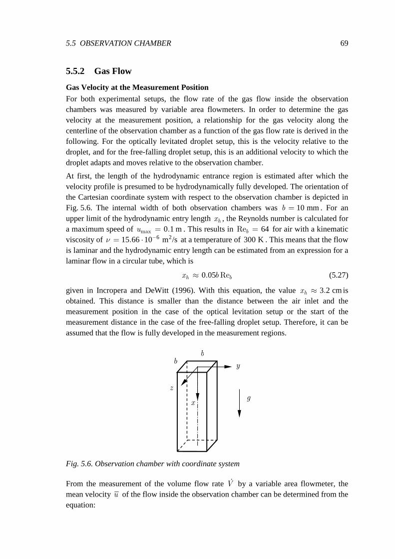
5.5 OBSERVATION CHAMBER 69

5.5.2 Gas Flow

Gas Velocity at the Measurement Position For both experimental setups, the flow rate of the gas flow inside the observation chambers was measured by variable area flowmeters. In order to determine the gas velocity at the measurement position, a relationship for the gas velocity along the centerline of the observation chamber as a function of the gas flow rate is derived in the following. For the optically levitated droplet setup, this is the velocity relative to the droplet, and for the free-falling droplet setup, this is an additional velocity to which the droplet adapts and moves relative to the observation chamber.

At first, the length of the hydrodynamic entrance region is estimated after which the velocity profile is presumed to be hydrodynamically fully developed. The orientation of the Cartesian coordinate system with respect to the observation chamber is depicted in Fig. 5.6. The internal width of both observation chambers was 10 mm=b . For an upper limit of the hydrodynamic entry length hx , the Reynolds number is calculated for a maximum speed of 0 1 mmax .=u . This results in 64Re =b for air with a kinematic viscosity of 6 215 66 10 m /s. −= ⋅ν at a temperature of 300 K. This means that the flow is laminar and the hydrodynamic entry length can be estimated from an expression for a laminar flow in a circular tube, which is

0 05. Re≈h bx b (5.27)

given in Incropera and DeWitt (1996). With this equation, the value 3 2 cm.≈hx is obtained. This distance is smaller than the distance between the air inlet and the measurement position in the case of the optical levitation setup or the start of the measurement distance in the case of the free-falling droplet setup. Therefore, it can be assumed that the flow is fully developed in the measurement regions.

y

z

x

bb

g

Fig. 5.6. Observation chamber with coordinate system

From the measurement of the volume flow rate ɺV by a variable area flowmeter, the mean velocity u of the flow inside the observation chamber can be determined from the equation:

70 5 EXPERIMENTAL METHODS

2=ɺV

ub

(5.28)

In order to calculate the velocity 0 0( , , )=cu u along the centerline, the ratio /cu u must be determined. At the centerline, the velocity profile reaches its maximum value in the y -z plane. For a fully developed flow, cu is a constant. When the velocity profile inside a circular tube is used as an estimate, where there is Hagen-Poiseuille flow, the ratio of cu with respect to the mean velocity u is 2/ =cu u . For a square channel, the value is slightly higher, as is shown in the following.

Spurk (1996) derived cu and u for a rectangular channel. The governing differential equation, which can be derived from the x -component of the Navier-Stokes equations, is given by

2 2

2 2

∂ ∂+ = −

∂ ∂u u K

y z µ (5.29)

In Eq. (5.29), the inhomogeneous term is /−K µ with the constant /= −∂ ∂ +K p x gρ . In comparison to Spurk (1996), where /= −∂ ∂K p x , the

influence of gravity is also considered. However, a variation of the constant K has no influence on the ratio /cu u , which is given by

[ ]31

5 51

1 116

2 2 1 2 12 2 096

2 11 64 23 2 1

( )

( ) cos ( ).

tanh ( )

( )

∞

=

∞

=

−+

− − = = − +

−

∑

∑

n

nc

n

n nu

u n

n

ππ

π

π

(5.30)

The velocity cu can then be determined by combining Eqs. (5.28) and (5.30):

22 096.=ɺ

cV

ub

(5.31)

Numerical Simulation of the Gas Flow During the design process of the heating system for the observation chamber for the optical levitation setup, the flow inside the observation chamber including parts of the flow module was studied by numerical simulations with the commercial software code FLUENT, version 6.0. The aim of these studies was to examine the effect of heating part of the glass wall on the temperature and velocity distributions of the air flow inside the observation chamber.

Numerical simulations were performed for air with a typical volume flow rate of 1 cm3/s. The air entered the flow module at a temperature of 300 K. Calculations were conducted for different temperatures of the glass walls in the heated region.

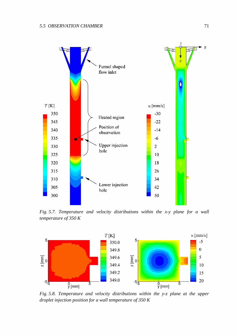
5.5 OBSERVATION CHAMBER 71

Fig. 5.7. Temperature and velocity distributions within the x-y plane for a wall temperature of 350 K

Fig. 5.8. Temperature and velocity distributions within the y-z plane at the upper droplet injection position for a wall temperature of 350 K

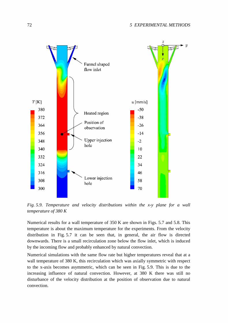
72 5 EXPERIMENTAL METHODS

Fig. 5.9. Temperature and velocity distributions within the x-y plane for a wall temperature of 380 K

Numerical results for a wall temperature of 350 K are shown in Figs. 5.7 and 5.8. This temperature is about the maximum temperature for the experiments. From the velocity distribution in Fig. 5.7 it can be seen that, in general, the air flow is directed downwards. There is a small recirculation zone below the flow inlet, which is induced by the incoming flow and probably enhanced by natural convection.

Numerical simulations with the same flow rate but higher temperatures reveal that at a wall temperature of 380 K, this recirculation which was axially symmetric with respect to the x-axis becomes asymmetric, which can be seen in Fig. 5.9. This is due to the increasing influence of natural convection. However, at 380 K there was still no disturbance of the velocity distribution at the position of observation due to natural convection.

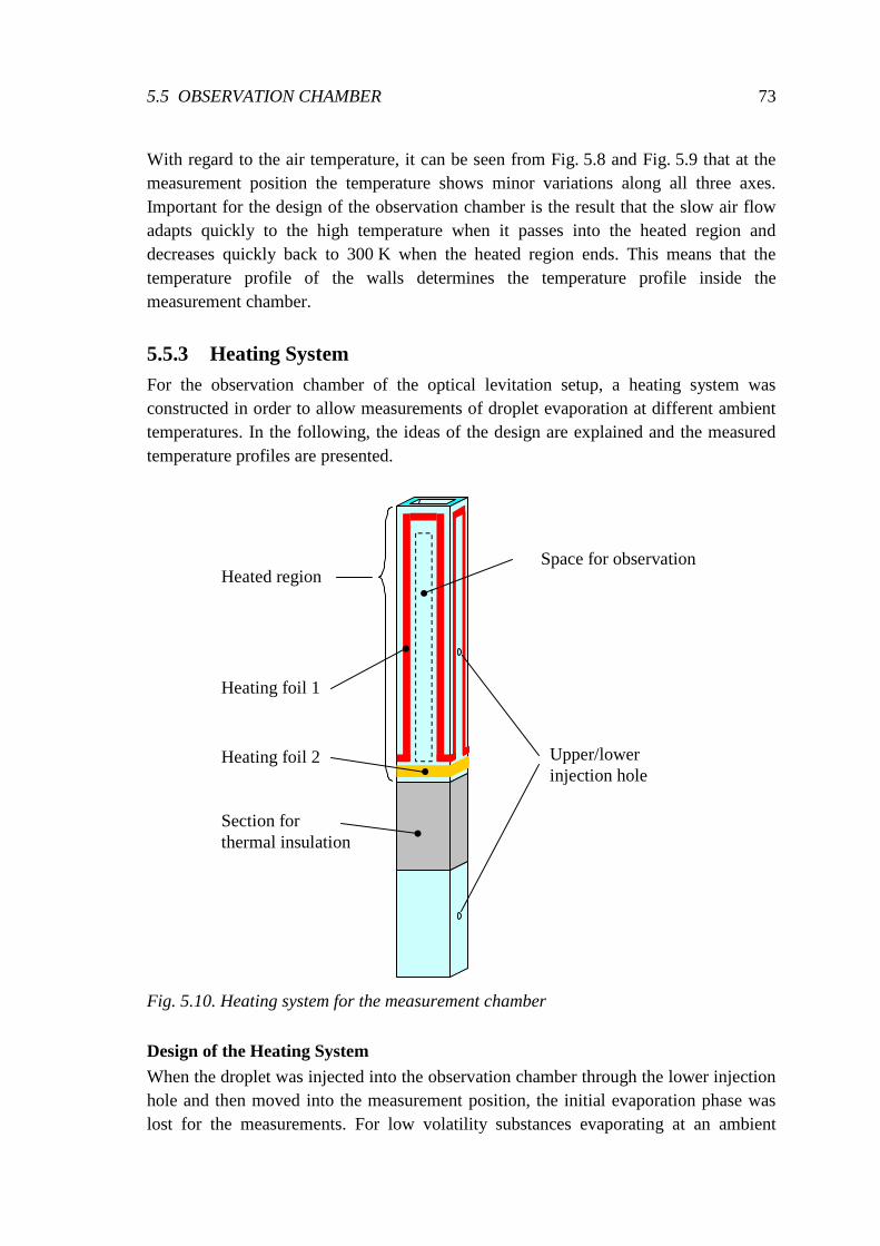
5.5 OBSERVATION CHAMBER 73

With regard to the air temperature, it can be seen from Fig. 5.8 and Fig. 5.9 that at the measurement position the temperature shows minor variations along all three axes. Important for the design of the observation chamber is the result that the slow air flow adapts quickly to the high temperature when it passes into the heated region and decreases quickly back to 300 K when the heated region ends. This means that the temperature profile of the walls determines the temperature profile inside the measurement chamber.

5.5.3 Heating System For the observation chamber of the optical levitation setup, a heating system was constructed in order to allow measurements of droplet evaporation at different ambient temperatures. In the following, the ideas of the design are explained and the measured temperature profiles are presented.

Heating foil 1

Heating foil 2

Space for observation

Upper/lowerinjection hole

Heated region

Section for thermal insulation

Fig. 5.10. Heating system for the measurement chamber

Design of the Heating System When the droplet was injected into the observation chamber through the lower injection hole and then moved into the measurement position, the initial evaporation phase was lost for the measurements. For low volatility substances evaporating at an ambient

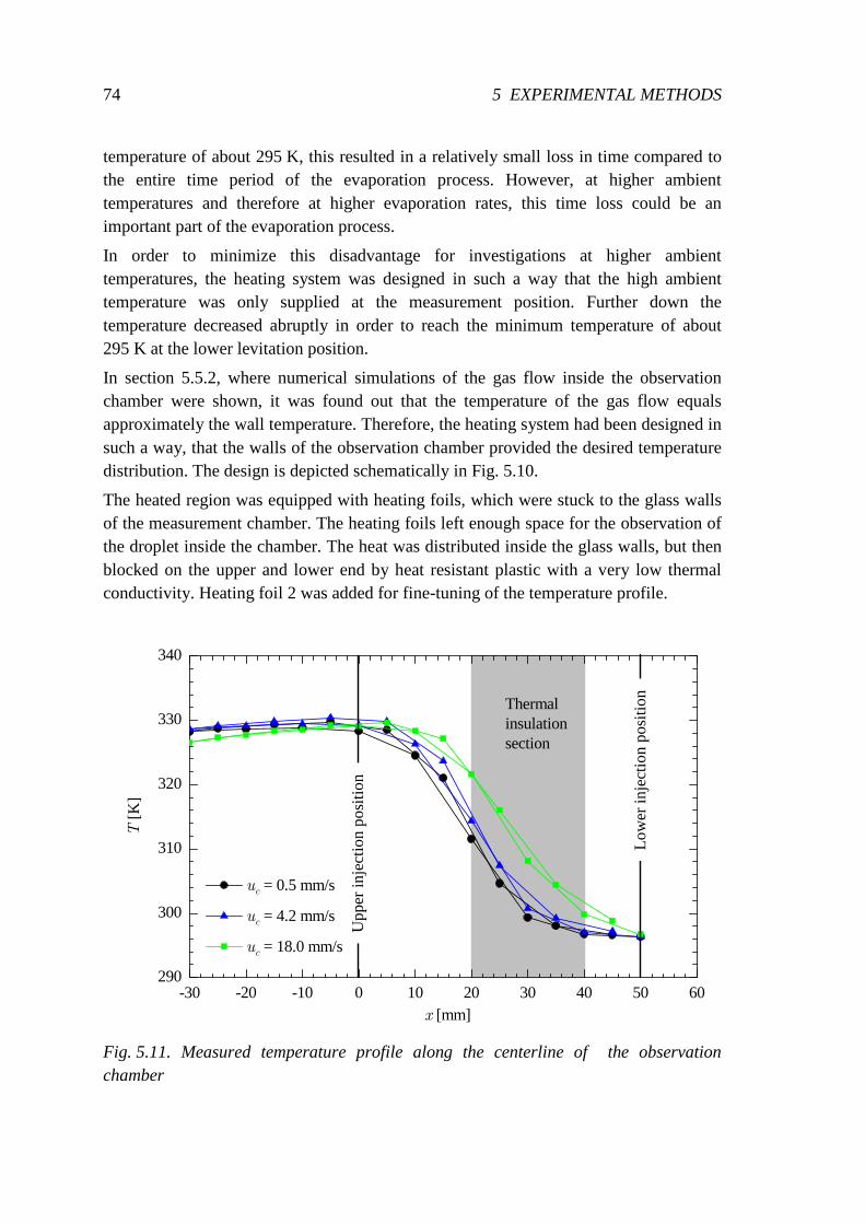
74 5 EXPERIMENTAL METHODS

temperature of about 295 K, this resulted in a relatively small loss in time compared to the entire time period of the evaporation process. However, at higher ambient temperatures and therefore at higher evaporation rates, this time loss could be an important part of the evaporation process.

In order to minimize this disadvantage for investigations at higher ambient temperatures, the heating system was designed in such a way that the high ambient temperature was only supplied at the measurement position. Further down the temperature decreased abruptly in order to reach the minimum temperature of about 295 K at the lower levitation position.

In section 5.5.2, where numerical simulations of the gas flow inside the observation chamber were shown, it was found out that the temperature of the gas flow equals approximately the wall temperature. Therefore, the heating system had been designed in such a way, that the walls of the observation chamber provided the desired temperature distribution. The design is depicted schematically in Fig. 5.10.

The heated region was equipped with heating foils, which were stuck to the glass walls of the measurement chamber. The heating foils left enough space for the observation of the droplet inside the chamber. The heat was distributed inside the glass walls, but then blocked on the upper and lower end by heat resistant plastic with a very low thermal conductivity. Heating foil 2 was added for fine-tuning of the temperature profile.

-30 -20 -10 0 10 20 30 40 50 60290

300

310

320

330

340

T [K

]

x [mm]

uc = 0.5 mm/s

uc = 4.2 mm/s

uc = 18.0 mm/s

Lo

wer

inje

ctio

n p

osi

tion

Up

per

inje

ctio

n p

osi

tion

Thermal insulation section

Fig. 5.11. Measured temperature profile along the centerline of the observation chamber

5.6 MEASUREMENT PROCEDURE 75

Temperature Profile The measured temperature profile in the vertical direction along the centerline of the observation chamber is depicted in Fig. 5.11. For the measurement of the temperature profile, a thermocouple was introduced through the open end into the observation chamber. After the thermocouple had been moved to a certain position, a time interval of at least 5 min was allowed before the temperature was measured. Data points were collected both on the way up and down so that hysteresis effects were accounted for. The small magnitude of the hysteresis revealed that the waiting time interval was long enough. The results show that the desired temperature profile was reached, which means that the temperature was low at the lower injection position and that the axial temperature gradient was nearly zero at the upper injection point. When the gas flow rate was augmented, the temperature profile was moved in the flow direction (positive x -direction).

5.6 Measurement Procedure

5.6.1 Optical Levitation All of the primary devices, i.e., the droplet generator, the linear positioner of the lens, the CCD cameras, the laser and the measurement unit for the thermocouple were connected to a single computer either by GPIB or a serial bus. This permitted control of the setup by a single program written in LabVIEW.

For the execution of the measurements, the ejection of a droplet from the droplet-on-demand generator was triggered manually via the keyboard of the computer. This marked the start of the measurement period. When the droplet was injected at the lower position, a second manual triggering started the movement of the droplet to the position of observation and the image acquisition with the CCD cameras. For the injection of the droplet at the upper position, a single manual trigger was used to start the measurements.

5.6.2 Free-Falling Droplets The setup for free-falling droplets was controlled using a trigger line. The triggering is shown schematically in Fig. 5.12. The droplet generation was triggered manually using a high voltage pulse of a pulse generator. The output trigger of this pulse generator was used to start the measurement with the photomultiplier. The output signal of the photomultiplier was not only recorded by the data acquisition board but also directed to another trigger unit, which sent a trigger signal at a certain threshold value. This threshold was designed to be reached when the droplet arrived at the laser beam. The trigger signal of this unit was used to start sending a preset number of trigger signals

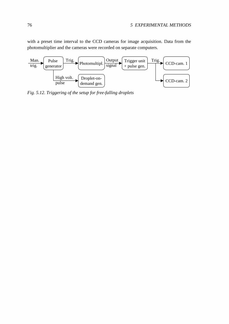
76 5 EXPERIMENTAL METHODS

with a preset time interval to the CCD cameras for image acquisition. Data from the photomultiplier and the cameras were recorded on separate computers.

Pulse generator

Man.trig.

Trig.

Droplet-on-demand gen.

Photomultipl.Trigger unit+ pulse gen.

Outputsignal

High volt. pulse

CCD-cam. 1Trig.

CCD-cam. 2

Fig. 5.12. Triggering of the setup for free-falling droplets

77

6 Optical Measurement Techniques For the measurements of droplet specific quantities, optical techniques were employed in order to minimize the influence of the measurement techniques on the evaporation process. In the present chapter, the principles of the measurement techniques are explained together with the evaluation of the measured data. In addition, the determination of the initial droplet diameter and the size history is described. For the evaluation of the measured data, LabVIEW programs were written.

6.1 Droplet Sizing with Mie Scattering Imaging

6.1.1 Introduction In chapter 4 it was shown that in the forward hemisphere, the interference of light from reflection and the 1st refraction generates a regular pattern of interference fringes. Glantschnig and Chen (1981) published the first theoretical study where a relationship between the droplet size and these interference fringes was presented. Their relationship is valid within an angular range between 30° and 70° and is based on geometrical optics considerations.

The first experimental study on the determination of the droplet size from fringe spacing was conducted by König et al. (1986). For the recording of the scattered light, they used a linear CCD array covering scattering angles from 31° to 35°. They presented size measurements of monodisperse droplets with diameters ranging from about 30 µm to 110 µm. For the determination of the diameter, they used a simplified relationship. Hesselbacher et al. (1991) described an improved method for the determination of the droplet size and used the relationship of Glantschnig and Chen (1981).

Ragucci et al. (1990) showed, for the first time, an out-of-focus image of a droplet taken with a CCD camera. The CCD camera was placed at a scattering angle of 90°. They compared the angular spacing of the fringes for droplet sizes from 20 µm to 100 µm with results from LMT. In their following studies, they called this measurement method Mie Scattering Imaging (MSI), as used within this study.

There are also other names for this measurement technique: Glover et al. (1995) called this method Interferometric Laser Imaging for Droplet Sizing (ILIDS). This name was also used by Maeda et al. (2000). In the textbook of Albrecht et al. (2003) this technique is denoted by Interferometric Particle Imaging (IPI).

In this study, the relationship of Glantschnig and Chen (1981) is used. With λ as the wavelength of the laser light, n the real part of the refractive index of the droplet liquid,

78 6 OPTICAL MEASUREMENT TECHNIQUES

Iθ the observation angle of the camera, and ∆ Fθ the angular distance of the interference fringes, the droplet diameter D can be obtained from the following equation:

2

22

21 2 2

sin( )cos( )

cos( )

I FI

I

Dn

n n

λ

θ θθ

θ

= ⋅∆

++ −

(6.1)

Eq. (6.1) is valid in the range 0 ,I I maxθ θ≤ ≤ with 2 1, arccos( / )I max nθ = (Semidetnov and Tropea, 2004). For this study, 84 4, .I maxθ = ° is obtained for

1 35.minn = . In addition to the range of validity, other considerations must be taken into account for the selection of θI. One issue is the general decrease of the intensity for larger scattering angles. Another issue is the contrast, i.e., the difference in intensity between the maxima and minima. Anders (1994) reported that for droplets with a refractive index of 1 3 1 4. .< <n and a Mie parameter of 300/ =Dπ λ ( 51 µm≈D for 532 nmλ = ), the contrast attains a maximum for a scattering angle around 70°. This is because the light intensity from reflection and the 1st refraction are of the same magnitude. Moreover, with regard to the accuracy of MSI, Massoli and Calabria (1999) showed that the dependence of the size measurement on the refractive index reduces to a minimum at a scattering angle of 60°.

In this study, the cameras were placed at an angle of 55= °Iθ . They covered an angular range of 11 9.∆ = °Iθ (optical levitation) and 4 9.∆ = °Iθ (falling droplets) with an angular resolution of 21 2 10 °/pixel. −⋅ (optical levitation) and

33 8 10 °/pixel. −⋅ (falling droplets). The angular fringe spacing Fθ∆ was obtained from the fringe spacing FN∆ on the CCD array measured in number of pixels:

F OFT Ff Nθ∆ = ∆ (6.2)

where OFTf is the transformation factor of the optical Fourier transform for the conversion of FN∆ into an angular distance.

6.1.2 Optical Fourier Transform An optical Fourier transform was necessary in order to avoid measurement uncertainties since the droplet moved along the laser beam during its evaporation as mentioned before. The schematic in Fig. 6.1 shows the optical Fourier Transforms where the lens is placed one focal length f in front of the CCD array. Light rays which leave droplets under the same scattering angle are detected at the same position on the linear CCD array although the droplets are located at different positions along the laser beam. Thus, the position of the light rays on the linear CCD array is independent from the position of the droplet on the laser beam and depends only on the scattering angle.

The calibration of the optical Fourier transform, i.e., the determination of the optimal distance between the CCD array and the lens, was conducted with an elaborate method using a separate setup with a turnable mirror which directed a light ray on the CCD

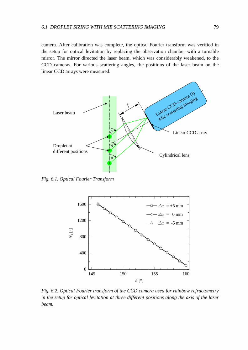
6.1 DROPLET SIZING WITH MIE SCATTERING IMAGING 79

camera. After calibration was complete, the optical Fourier transform was verified in the setup for optical levitation by replacing the observation chamber with a turnable mirror. The mirror directed the laser beam, which was considerably weakened, to the CCD cameras. For various scattering angles, the positions of the laser beam on the linear CCD arrays were measured.

Linear CCD-ca

mera (I)

Mie scat

tering im

aging

θ

f

θ

θ

Droplet at different positions

Laser beam

Cylindrical lens

Linear CCD array

Fig. 6.1. Optical Fourier Transform

145 150 155 1600

400

800

1200

1600

Np

[-]

θ [°]

∆x = +5 mm

∆x = 0 mm

∆x = -5 mm

Fig. 6.2. Optical Fourier transform of the CCD camera used for rainbow refractometry in the setup for optical levitation at three different positions along the axis of the laser beam.

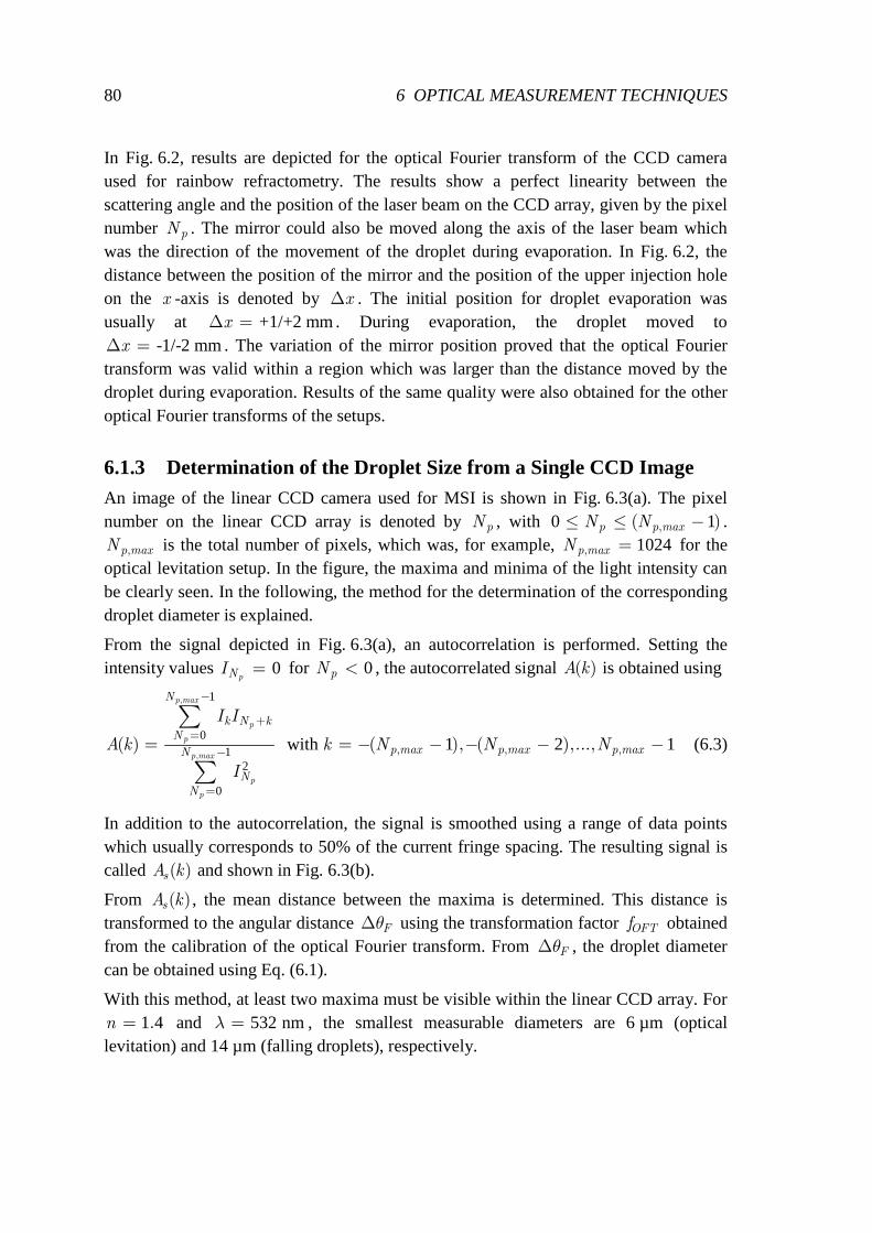
80 6 OPTICAL MEASUREMENT TECHNIQUES

In Fig. 6.2, results are depicted for the optical Fourier transform of the CCD camera used for rainbow refractometry. The results show a perfect linearity between the scattering angle and the position of the laser beam on the CCD array, given by the pixel number pN . The mirror could also be moved along the axis of the laser beam which was the direction of the movement of the droplet during evaporation. In Fig. 6.2, the distance between the position of the mirror and the position of the upper injection hole on the x -axis is denoted by x∆ . The initial position for droplet evaporation was usually at +1/+2 mmx∆ = . During evaporation, the droplet moved to

-1/-2 mmx∆ = . The variation of the mirror position proved that the optical Fourier transform was valid within a region which was larger than the distance moved by the droplet during evaporation. Results of the same quality were also obtained for the other optical Fourier transforms of the setups.

6.1.3 Determination of the Droplet Size from a Single CCD Image An image of the linear CCD camera used for MSI is shown in Fig. 6.3(a). The pixel number on the linear CCD array is denoted by pN , with 0 1,( )p p maxN N≤ ≤ − .

,p maxN is the total number of pixels, which was, for example, 1024,p maxN = for the optical levitation setup. In the figure, the maxima and minima of the light intensity can be clearly seen. In the following, the method for the determination of the corresponding droplet diameter is explained.

From the signal depicted in Fig. 6.3(a), an autocorrelation is performed. Setting the intensity values 0

pNI = for 0pN < , the autocorrelated signal ( )A k is obtained using

1

01

2

0

with 1 2 1

,

,, , ,( ) ( ), ( ),...,

p max

p

p

p max

p

p

N

k N kN

p max p max p maxN

NN

I I

A k k N N N

I

−

+=

−

=

= = − − − − −∑

∑ (6.3)

In addition to the autocorrelation, the signal is smoothed using a range of data points which usually corresponds to 50% of the current fringe spacing. The resulting signal is called ( )sA k and shown in Fig. 6.3(b).

From ( )sA k , the mean distance between the maxima is determined. This distance is transformed to the angular distance ∆ Fθ using the transformation factor OFTf obtained from the calibration of the optical Fourier transform. From ∆ Fθ , the droplet diameter can be obtained using Eq. (6.1).

With this method, at least two maxima must be visible within the linear CCD array. For 1 4.=n and 532 nmλ = , the smallest measurable diameters are 6 µm (optical

levitation) and 14 µm (falling droplets), respectively.

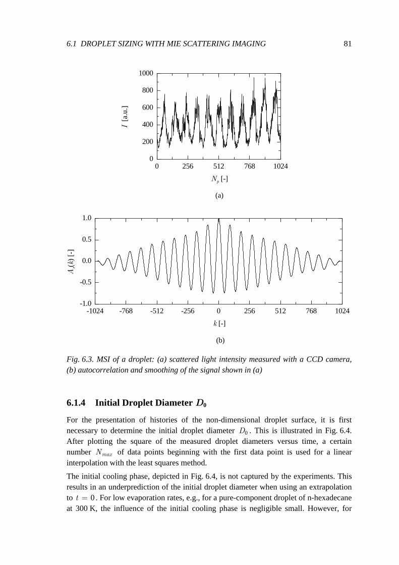
6.1 DROPLET SIZING WITH MIE SCATTERING IMAGING 81

0 256 512 768 10240

200

400

600

800

1000

-1024 -768 -512 -256 0 256 512 768 1024-1.0

-0.5

0.0

0.5

1.0

I [a

.u.]

Np [-]

(b)

As(k)

[-]

k [-]

(a)

Fig. 6.3. MSI of a droplet: (a) scattered light intensity measured with a CCD camera, (b) autocorrelation and smoothing of the signal shown in (a)

6.1.4 Initial Droplet Diameter D0

For the presentation of histories of the non-dimensional droplet surface, it is first necessary to determine the initial droplet diameter 0D . This is illustrated in Fig. 6.4. After plotting the square of the measured droplet diameters versus time, a certain number maxN of data points beginning with the first data point is used for a linear interpolation with the least squares method.

The initial cooling phase, depicted in Fig. 6.4, is not captured by the experiments. This results in an underprediction of the initial droplet diameter when using an extrapolation to 0t = . For low evaporation rates, e.g., for a pure-component droplet of n-hexadecane at 300 K, the influence of the initial cooling phase is negligible small. However, for

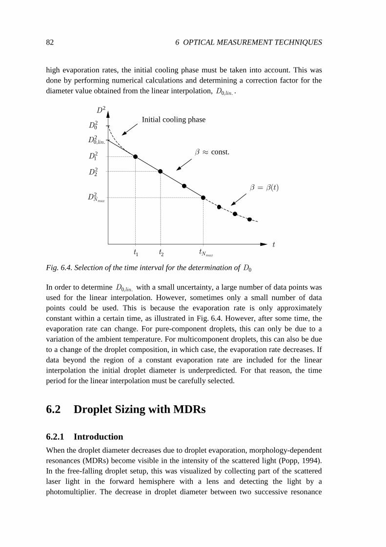
82 6 OPTICAL MEASUREMENT TECHNIQUES

high evaporation rates, the initial cooling phase must be taken into account. This was done by performing numerical calculations and determining a correction factor for the diameter value obtained from the linear interpolation, 0,lin.D .

t1t

20,lin.D

21D

2maxND

2D

maxNt

20D

Initial cooling phase

const.β ≈

( )tβ β=

t2

22D

Fig. 6.4. Selection of the time interval for the determination of 0D

In order to determine 0, .linD with a small uncertainty, a large number of data points was used for the linear interpolation. However, sometimes only a small number of data points could be used. This is because the evaporation rate is only approximately constant within a certain time, as illustrated in Fig. 6.4. However, after some time, the evaporation rate can change. For pure-component droplets, this can only be due to a variation of the ambient temperature. For multicomponent droplets, this can also be due to a change of the droplet composition, in which case, the evaporation rate decreases. If data beyond the region of a constant evaporation rate are included for the linear interpolation the initial droplet diameter is underpredicted. For that reason, the time period for the linear interpolation must be carefully selected.

6.2 Droplet Sizing with MDRs

6.2.1 Introduction When the droplet diameter decreases due to droplet evaporation, morphology-dependent resonances (MDRs) become visible in the intensity of the scattered light (Popp, 1994). In the free-falling droplet setup, this was visualized by collecting part of the scattered laser light in the forward hemisphere with a lens and detecting the light by a photomultiplier. The decrease in droplet diameter between two successive resonance

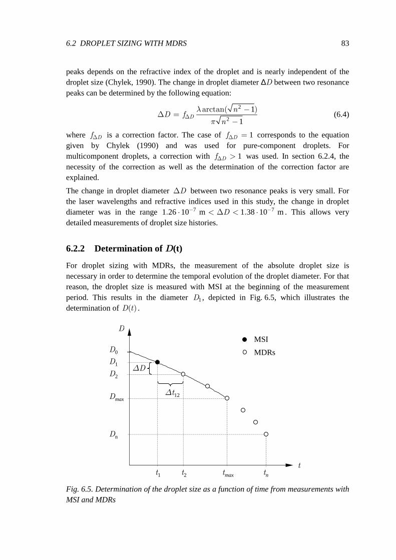
6.2 DROPLET SIZING WITH MDRS 83

peaks depends on the refractive index of the droplet and is nearly independent of the droplet size (Chylek, 1990). The change in droplet diameter ∆D between two resonance peaks can be determined by the following equation:

2

2

1

1

arctan( )D

nD f

n

λ

π∆

−∆ =

− (6.4)

where Df∆ is a correction factor. The case of 1Df∆ = corresponds to the equation given by Chylek (1990) and was used for pure-component droplets. For multicomponent droplets, a correction with 1Df∆ > was used. In section 6.2.4, the necessity of the correction as well as the determination of the correction factor are explained.

The change in droplet diameter D∆ between two resonance peaks is very small. For the laser wavelengths and refractive indices used in this study, the change in droplet diameter was in the range 7 71 26 10 m 1 38 10 m. .D− −⋅ < ∆ < ⋅ . This allows very detailed measurements of droplet size histories.

6.2.2 Determination of D(t)

For droplet sizing with MDRs, the measurement of the absolute droplet size is necessary in order to determine the temporal evolution of the droplet diameter. For that reason, the droplet size is measured with MSI at the beginning of the measurement period. This results in the diameter 1D , depicted in Fig. 6.5, which illustrates the determination of ( )D t .

D0

D1

D2

Dn

t1 t2 tnt

∆t12

∆D

MSI

MDRs

tmax

D

Dmax

Fig. 6.5. Determination of the droplet size as a function of time from measurements with MSI and MDRs

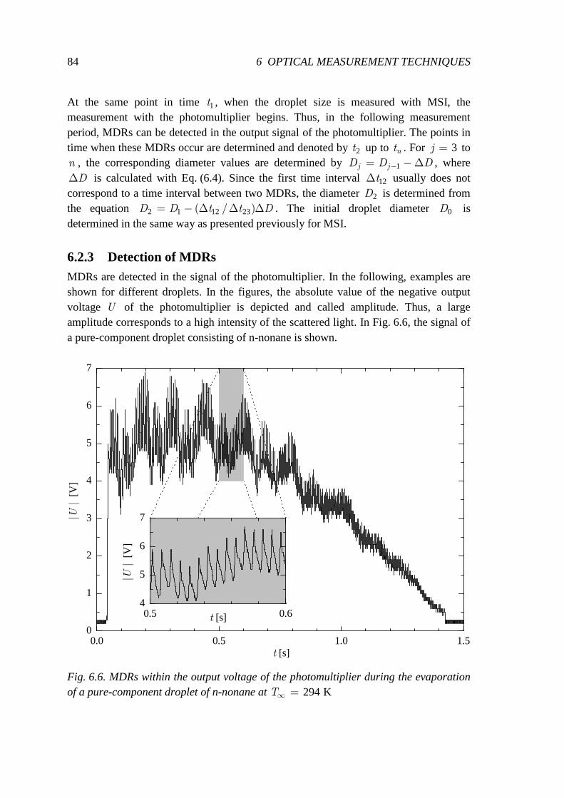
84 6 OPTICAL MEASUREMENT TECHNIQUES

At the same point in time 1t , when the droplet size is measured with MSI, the measurement with the photomultiplier begins. Thus, in the following measurement period, MDRs can be detected in the output signal of the photomultiplier. The points in time when these MDRs occur are determined and denoted by 2t up to nt . For 3=j to n , the corresponding diameter values are determined by 1−= − ∆j jD D D , where ∆D is calculated with Eq. (6.4). Since the first time interval 12∆t usually does not correspond to a time interval between two MDRs, the diameter 2D is determined from the equation 2 1 12 23( / )= − ∆ ∆ ∆D D t t D . The initial droplet diameter 0D is determined in the same way as presented previously for MSI.

6.2.3 Detection of MDRs MDRs are detected in the signal of the photomultiplier. In the following, examples are shown for different droplets. In the figures, the absolute value of the negative output voltage U of the photomultiplier is depicted and called amplitude. Thus, a large amplitude corresponds to a high intensity of the scattered light. In Fig. 6.6, the signal of a pure-component droplet consisting of n-nonane is shown.

0.0 0.5 1.0 1.50

1

2

3

4

5

6

7

0.5 0.64

5

6

7

|U |

[V

]

t [s]

|U |

[V

]

t [s]

Fig. 6.6. MDRs within the output voltage of the photomultiplier during the evaporation of a pure-component droplet of n-nonane at 294 K∞ =T

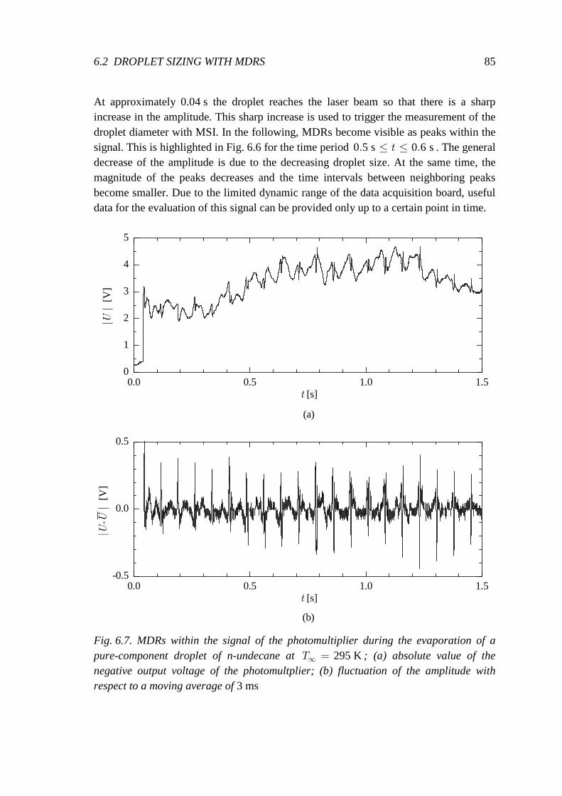
6.2 DROPLET SIZING WITH MDRS 85

At approximately 0.04 s the droplet reaches the laser beam so that there is a sharp increase in the amplitude. This sharp increase is used to trigger the measurement of the droplet diameter with MSI. In the following, MDRs become visible as peaks within the signal. This is highlighted in Fig. 6.6 for the time period 0 5 s 0 6 s. .≤ ≤t . The general decrease of the amplitude is due to the decreasing droplet size. At the same time, the magnitude of the peaks decreases and the time intervals between neighboring peaks become smaller. Due to the limited dynamic range of the data acquisition board, useful data for the evaluation of this signal can be provided only up to a certain point in time.

0.0 0.5 1.0 1.50

1

2

3

4

5

0.0 0.5 1.0 1.5-0.5

0.0

0.5

|U |

[V

]

t [s]

(b)

|U-U |

[V]

t [s]

(a)

Fig. 6.7. MDRs within the signal of the photomultiplier during the evaporation of a pure-component droplet of n-undecane at 295 K∞ =T ; (a) absolute value of the negative output voltage of the photomultplier; (b) fluctuation of the amplitude with respect to a moving average of 3 ms

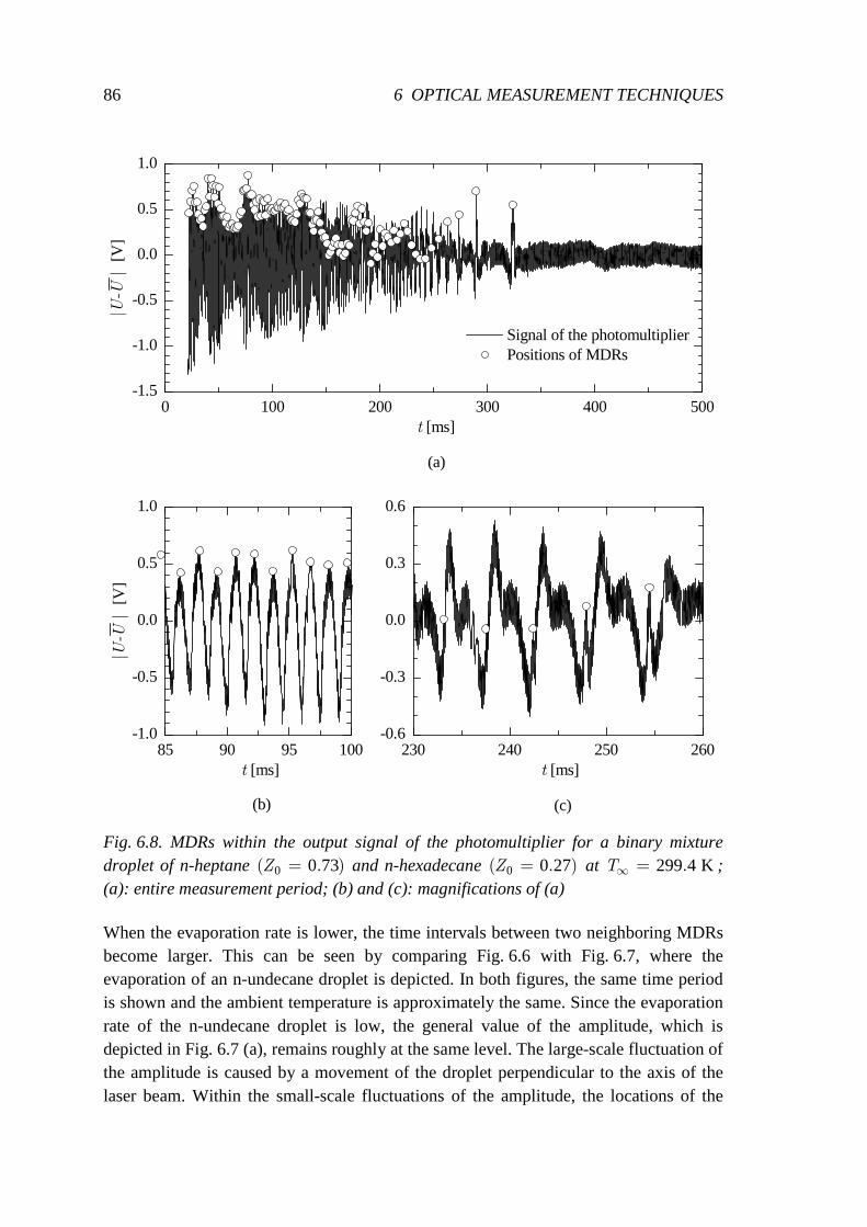
86 6 OPTICAL MEASUREMENT TECHNIQUES

0 100 200 300 400 500-1.5

-1.0

-0.5

0.0

0.5

1.0

85 90 95 100-1.0

-0.5

0.0

0.5

1.0

230 240 250 260-0.6

-0.3

0.0

0.3

0.6

t [ms]

Signal of the photomultiplier Positions of MDRs

|U-U |

[V]

|U-U |

[V]

(c)(b)

t [ms]

(a)

t [ms]

Fig. 6.8. MDRs within the output signal of the photomultiplier for a binary mixture droplet of n-heptane 0 0 73( . )=Z and n-hexadecane 0 0 27( . )=Z at 299 4 K.∞ =T ; (a): entire measurement period; (b) and (c): magnifications of (a)

When the evaporation rate is lower, the time intervals between two neighboring MDRs become larger. This can be seen by comparing Fig. 6.6 with Fig. 6.7, where the evaporation of an n-undecane droplet is depicted. In both figures, the same time period is shown and the ambient temperature is approximately the same. Since the evaporation rate of the n-undecane droplet is low, the general value of the amplitude, which is depicted in Fig. 6.7 (a), remains roughly at the same level. The large-scale fluctuation of the amplitude is caused by a movement of the droplet perpendicular to the axis of the laser beam. Within the small-scale fluctuations of the amplitude, the locations of the

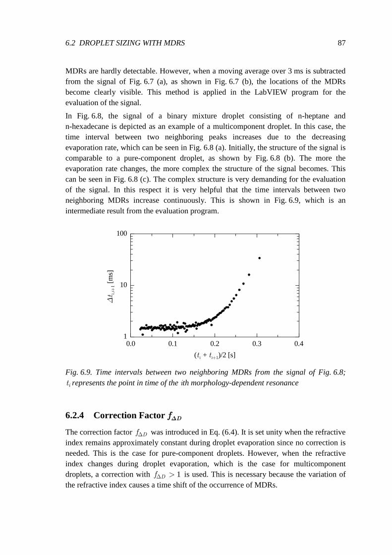
6.2 DROPLET SIZING WITH MDRS 87

MDRs are hardly detectable. However, when a moving average over 3 ms is subtracted from the signal of Fig. 6.7 (a), as shown in Fig. 6.7 (b), the locations of the MDRs become clearly visible. This method is applied in the LabVIEW program for the evaluation of the signal.

In Fig. 6.8, the signal of a binary mixture droplet consisting of n-heptane and n-hexadecane is depicted as an example of a multicomponent droplet. In this case, the time interval between two neighboring peaks increases due to the decreasing evaporation rate, which can be seen in Fig. 6.8 (a). Initially, the structure of the signal is comparable to a pure-component droplet, as shown by Fig. 6.8 (b). The more the evaporation rate changes, the more complex the structure of the signal becomes. This can be seen in Fig. 6.8 (c). The complex structure is very demanding for the evaluation of the signal. In this respect it is very helpful that the time intervals between two neighboring MDRs increase continuously. This is shown in Fig. 6.9, which is an intermediate result from the evaluation program.

0.0 0.1 0.2 0.3 0.41

10

100

∆t i

,i+1

[ms]

(ti + ti+1)/2 [s]

Fig. 6.9. Time intervals between two neighboring MDRs from the signal of Fig. 6.8;

it represents the point in time of the ith morphology-dependent resonance

6.2.4 Correction Factor f∆D

The correction factor Df∆ was introduced in Eq. (6.4). It is set unity when the refractive index remains approximately constant during droplet evaporation since no correction is needed. This is the case for pure-component droplets. However, when the refractive index changes during droplet evaporation, which is the case for multicomponent droplets, a correction with 1Df∆ > is used. This is necessary because the variation of the refractive index causes a time shift of the occurrence of MDRs.

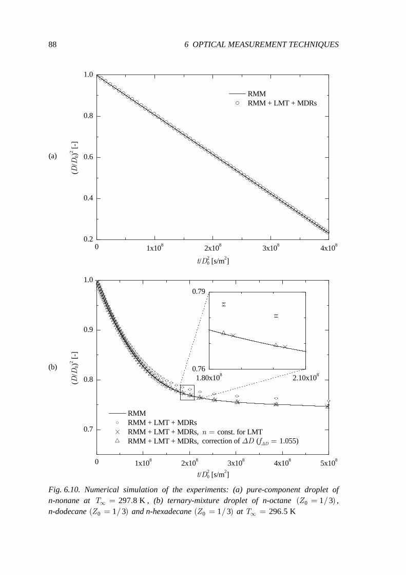
88 6 OPTICAL MEASUREMENT TECHNIQUES

0 1x108 2x108 3x108 4x108 5x108

0.7

0.8

0.9

1.0

1.80x108 2.10x1080.76

0.79

0 1x108 2x108 3x108 4x1080.2

0.4

0.6

0.8

1.0

n = const. for LMT

(D/D

0)2 [-

]

t/D20 [s/m2]

RMM RMM + LMT + MDRs RMM + LMT + MDRs, RMM + LMT + MDRs, correction of ∆D (f∆D = 1.055)

(b)

(D

/D0)

2 [-]

t/D20 [s/m2]

RMM RMM + LMT + MDRs

(a)

Fig. 6.10. Numerical simulation of the experiments: (a) pure-component droplet of n-nonane at 297 8 K.∞ =T , (b) ternary-mixture droplet of n-octane 0 1 3( / )=Z , n-dodecane 0 1 3( / )=Z and n-hexadecane 0 1 3( / )=Z at 296 5 K.∞ =T

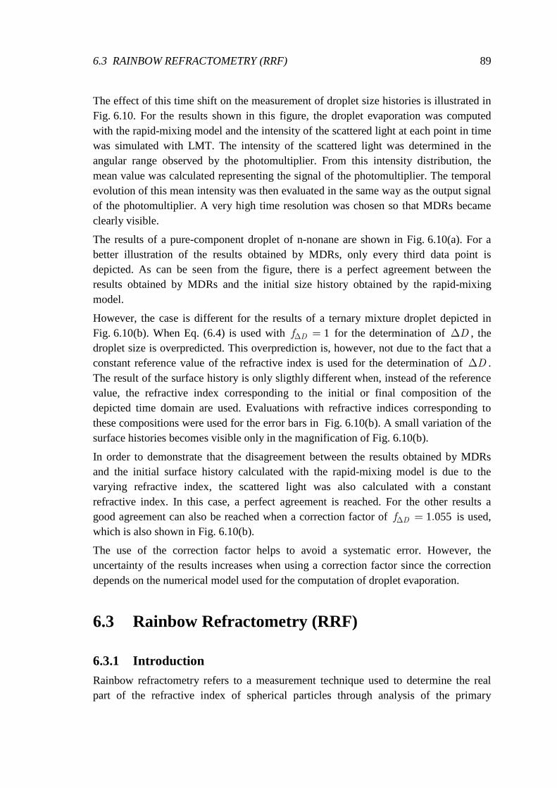
6.3 RAINBOW REFRACTOMETRY (RRF) 89

The effect of this time shift on the measurement of droplet size histories is illustrated in Fig. 6.10. For the results shown in this figure, the droplet evaporation was computed with the rapid-mixing model and the intensity of the scattered light at each point in time was simulated with LMT. The intensity of the scattered light was determined in the angular range observed by the photomultiplier. From this intensity distribution, the mean value was calculated representing the signal of the photomultiplier. The temporal evolution of this mean intensity was then evaluated in the same way as the output signal of the photomultiplier. A very high time resolution was chosen so that MDRs became clearly visible.

The results of a pure-component droplet of n-nonane are shown in Fig. 6.10(a). For a better illustration of the results obtained by MDRs, only every third data point is depicted. As can be seen from the figure, there is a perfect agreement between the results obtained by MDRs and the initial size history obtained by the rapid-mixing model.

However, the case is different for the results of a ternary mixture droplet depicted in Fig. 6.10(b). When Eq. (6.4) is used with 1Df∆ = for the determination of D∆ , the droplet size is overpredicted. This overprediction is, however, not due to the fact that a constant reference value of the refractive index is used for the determination of D∆ . The result of the surface history is only sligthly different when, instead of the reference value, the refractive index corresponding to the initial or final composition of the depicted time domain are used. Evaluations with refractive indices corresponding to these compositions were used for the error bars in Fig. 6.10(b). A small variation of the surface histories becomes visible only in the magnification of Fig. 6.10(b).

In order to demonstrate that the disagreement between the results obtained by MDRs and the initial surface history calculated with the rapid-mixing model is due to the varying refractive index, the scattered light was also calculated with a constant refractive index. In this case, a perfect agreement is reached. For the other results a good agreement can also be reached when a correction factor of 1 055.Df∆ = is used, which is also shown in Fig. 6.10(b).

The use of the correction factor helps to avoid a systematic error. However, the uncertainty of the results increases when using a correction factor since the correction depends on the numerical model used for the computation of droplet evaporation.

6.3 Rainbow Refractometry (RRF)

6.3.1 Introduction Rainbow refractometry refers to a measurement technique used to determine the real part of the refractive index of spherical particles through analysis of the primary

90 6 OPTICAL MEASUREMENT TECHNIQUES

rainbow scattering (Albrecht et al., 2003). From the determination of the refractive index, additional information about the droplet can be extracted.

In chapter 2, relationships describing the dependence of the refractive index on the temperature and the substance were presented. Using these relationships, the temperature of pure-component droplets can be determined from the refractive index. For binary mixture droplets, the droplet composition can be calculated with these relationships when a constant droplet temperature can be assumed. These two applications of RRF are based on the assumption of a homogeneous refractive index inside the droplets. This is important since RRF is very sensitive to gradients of the refractive index. Moreover, it is necessary that the droplets are spherical since RRF is also very sensitive to non-sphericity. Both requirements were fulfilled for the experiments when RRF was used for these applications. In addition, RRF was also applied to detect refractive index gradients, which is described in more detail in section 9.3.

6.3.2 Determination of the Refractive Index There are different possibilities for exploiting the intensity distribution in the region of the rainbow in order to determine the refractive index of the droplet. This is because several scattering phenomena occur in this region and can be linked to the refractive index and the diameter of the droplet.

Roth (1998) conducted a detailed study on the determination of the refractive index from the intensity distribution in the region of the rainbow using different methods. However, these methods could not be used for this study since their accuracy was not sufficiently high. This is partly because the methods used by Roth were founded on an empirical rather than theoretical basis.

For this study, Airy theory was used in order to determine the refractive index by comparing results from Airy theory with measured intensity distributions. Compared to LMT, it is only possible to use Airy theory as an approximation. However, this is compensated for by using an elaborate evaluation method. The advantage of using Airy theory instead of LMT is the reduced computational effort.

In section 4.4, it was seen that for large droplets, there is fairly good agreement of results from Airy theory with LMT, and therefore with real intensity distributions, within a large range of scattering angles. Since the ripple structure is small, results from Airy theory can be fitted to measured intensity distributions in the region of the rainbow in order to determine the refractive index. In order to perform the fitting, it is necessary to know the droplet diameter (see Eq. (4.3)), which needs to be obtained by a different measurement technique. However, it is also possible to use the rainbow for the determination of the droplet diameter. Van Beeck (1997) showed that the distance between the maxima of the main rainbow peak and first subsidiary bow is relatively independent from the refractive index and can be used to calculate the droplet diameter.

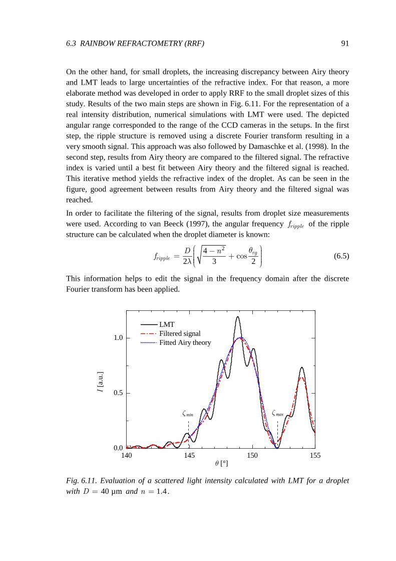
6.3 RAINBOW REFRACTOMETRY (RRF) 91

On the other hand, for small droplets, the increasing discrepancy between Airy theory and LMT leads to large uncertainties of the refractive index. For that reason, a more elaborate method was developed in order to apply RRF to the small droplet sizes of this study. Results of the two main steps are shown in Fig. 6.11. For the representation of a real intensity distribution, numerical simulations with LMT were used. The depicted angular range corresponded to the range of the CCD cameras in the setups. In the first step, the ripple structure is removed using a discrete Fourier transform resulting in a very smooth signal. This approach was also followed by Damaschke et al. (1998). In the second step, results from Airy theory are compared to the filtered signal. The refractive index is varied until a best fit between Airy theory and the filtered signal is reached. This iterative method yields the refractive index of the droplet. As can be seen in the figure, good agreement between results from Airy theory and the filtered signal was reached.

In order to facilitate the filtering of the signal, results from droplet size measurements were used. According to van Beeck (1997), the angular frequency ripplef of the ripple structure can be calculated when the droplet diameter is known:

24

2 3 2cos

− = + rg

rippleD n

fθ

λ (6.5)

This information helps to edit the signal in the frequency domain after the discrete Fourier transform has been applied.

140 145 150 1550.0

0.5

1.0

ζ max

I [a

.u.]

θ [°]

LMT Filtered signal Fitted Airy theory

ζ min

Fig. 6.11. Evaluation of a scattered light intensity calculated with LMT for a droplet with 40 µm=D and 1 4.=n .

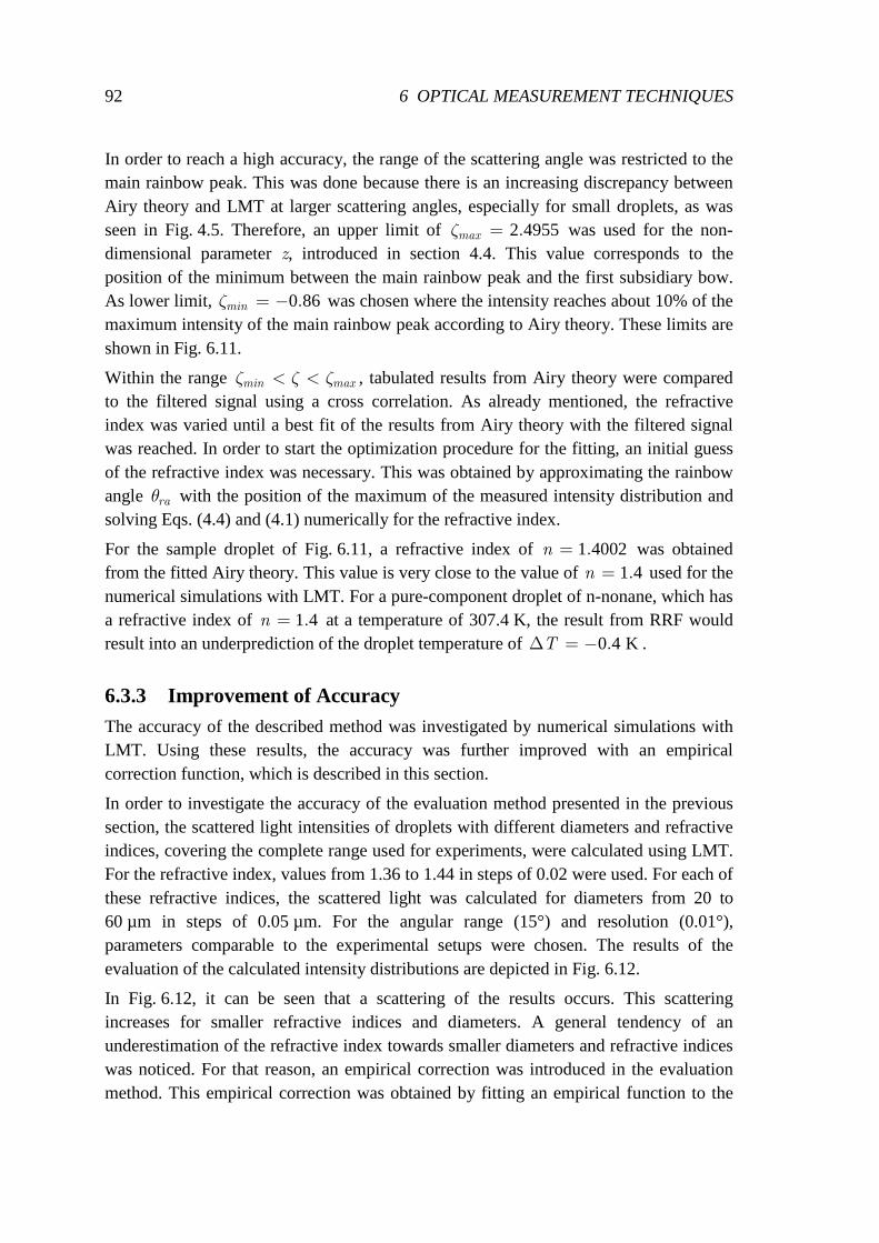
92 6 OPTICAL MEASUREMENT TECHNIQUES

In order to reach a high accuracy, the range of the scattering angle was restricted to the main rainbow peak. This was done because there is an increasing discrepancy between Airy theory and LMT at larger scattering angles, especially for small droplets, as was seen in Fig. 4.5. Therefore, an upper limit of 2 4955.maxζ = was used for the non-dimensional parameter z, introduced in section 4.4. This value corresponds to the position of the minimum between the main rainbow peak and the first subsidiary bow. As lower limit, 0 86.minζ = − was chosen where the intensity reaches about 10% of the maximum intensity of the main rainbow peak according to Airy theory. These limits are shown in Fig. 6.11.

Within the range min maxζ ζ ζ< < , tabulated results from Airy theory were compared to the filtered signal using a cross correlation. As already mentioned, the refractive index was varied until a best fit of the results from Airy theory with the filtered signal was reached. In order to start the optimization procedure for the fitting, an initial guess of the refractive index was necessary. This was obtained by approximating the rainbow angle raθ with the position of the maximum of the measured intensity distribution and solving Eqs. (4.4) and (4.1) numerically for the refractive index.

For the sample droplet of Fig. 6.11, a refractive index of 1 4002.=n was obtained from the fitted Airy theory. This value is very close to the value of 1 4.=n used for the numerical simulations with LMT. For a pure-component droplet of n-nonane, which has a refractive index of 1 4.=n at a temperature of 307.4 K, the result from RRF would result into an underprediction of the droplet temperature of 0 4 K.∆ = −T .

6.3.3 Improvement of Accuracy The accuracy of the described method was investigated by numerical simulations with LMT. Using these results, the accuracy was further improved with an empirical correction function, which is described in this section.

In order to investigate the accuracy of the evaluation method presented in the previous section, the scattered light intensities of droplets with different diameters and refractive indices, covering the complete range used for experiments, were calculated using LMT. For the refractive index, values from 1.36 to 1.44 in steps of 0.02 were used. For each of these refractive indices, the scattered light was calculated for diameters from 20 to 60 µm in steps of 0.05 µm. For the angular range (15°) and resolution (0.01°), parameters comparable to the experimental setups were chosen. The results of the evaluation of the calculated intensity distributions are depicted in Fig. 6.12.

In Fig. 6.12, it can be seen that a scattering of the results occurs. This scattering increases for smaller refractive indices and diameters. A general tendency of an underestimation of the refractive index towards smaller diameters and refractive indices was noticed. For that reason, an empirical correction was introduced in the evaluation method. This empirical correction was obtained by fitting an empirical function to the

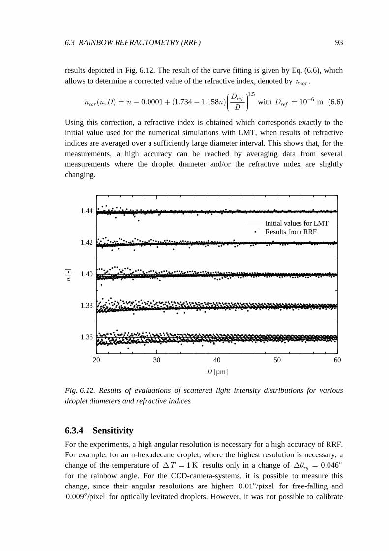
6.3 RAINBOW REFRACTOMETRY (RRF) 93

results depicted in Fig. 6.12. The result of the curve fitting is given by Eq. (6.6), which allows to determine a corrected value of the refractive index, denoted by corn .

1 5

0 0001 1 734 1 158.

( , ) . ( . . )ref

cor

Dn n D n n

D

= − + − with 610 mrefD −= (6.6)

Using this correction, a refractive index is obtained which corresponds exactly to the initial value used for the numerical simulations with LMT, when results of refractive indices are averaged over a sufficiently large diameter interval. This shows that, for the measurements, a high accuracy can be reached by averaging data from several measurements where the droplet diameter and/or the refractive index are slightly changing.

20 30 40 50 60

1.36

1.38

1.40

1.42

1.44

n [-

]

D [µm]

Initial values for LMT Results from RRF

Fig. 6.12. Results of evaluations of scattered light intensity distributions for various droplet diameters and refractive indices

6.3.4 Sensitivity For the experiments, a high angular resolution is necessary for a high accuracy of RRF. For example, for an n-hexadecane droplet, where the highest resolution is necessary, a change of the temperature of 1 K∆ =T results only in a change of 0 046.∆ = °rgθ for the rainbow angle. For the CCD-camera-systems, it is possible to measure this change, since their angular resolutions are higher: 0 01 /pixel. ° for free-falling and 0 009 /pixel. ° for optically levitated droplets. However, it was not possible to calibrate

94 6 OPTICAL MEASUREMENT TECHNIQUES

the absolute angles of the cameras with respect to the laser beam by mechanical means with such a high precision. For that reason, results from measurements of droplets with known temperature and composition were used for a calibration.

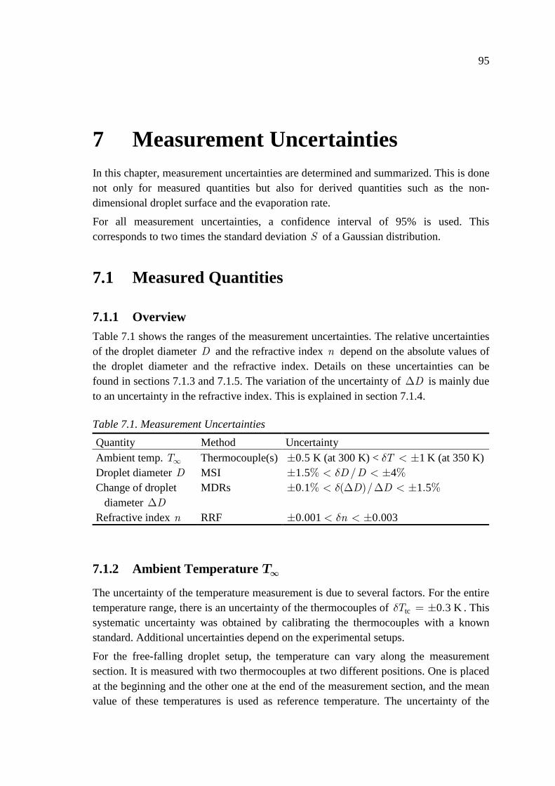
95

7 Measurement Uncertainties In this chapter, measurement uncertainties are determined and summarized. This is done not only for measured quantities but also for derived quantities such as the non-dimensional droplet surface and the evaporation rate.

For all measurement uncertainties, a confidence interval of 95% is used. This corresponds to two times the standard deviation S of a Gaussian distribution.

7.1 Measured Quantities

7.1.1 Overview Table 7.1 shows the ranges of the measurement uncertainties. The relative uncertainties of the droplet diameter D and the refractive index n depend on the absolute values of the droplet diameter and the refractive index. Details on these uncertainties can be found in sections 7.1.3 and 7.1.5. The variation of the uncertainty of D∆ is mainly due to an uncertainty in the refractive index. This is explained in section 7.1.4.

Table 7.1. Measurement Uncertainties

Quantity Method Uncertainty Ambient temp. ∞T Thermocouple(s) 0 5 K (at 300 K) < 1 K (at 350 K). Tδ± < ± Droplet diameter D MSI 1 5 4. % / %D Dδ± < < ± Change of droplet diameter D∆

MDRs 0 1 1 5. % ( )/ . %D Dδ± < ∆ ∆ < ±

Refractive index n RRF 0 001 0 003. .nδ± < < ±

7.1.2 Ambient Temperature Τ∞

The uncertainty of the temperature measurement is due to several factors. For the entire temperature range, there is an uncertainty of the thermocouples of tc 0 3 K.Tδ = ± . This systematic uncertainty was obtained by calibrating the thermocouples with a known standard. Additional uncertainties depend on the experimental setups.

For the free-falling droplet setup, the temperature can vary along the measurement section. It is measured with two thermocouples at two different positions. One is placed at the beginning and the other one at the end of the measurement section, and the mean value of these temperatures is used as reference temperature. The uncertainty of the

96 7 MEASUREMENT UNCERTAINTIES

temperature of the observation chamber is estimated to be chamber 0 4 K.Tδ = ± . Hence, the overall uncertainty of the temperature of this setup can be determined using the law of error propagation:

2 2falling droplets chamber 0 5 Ktc .T T Tδ δ δ= + = ± (7.1)

For the optically levitated droplet setup, the heating of the observation chamber as well as the thermocouple due to the scattered light cannot be neglected. The heating of the walls of the observation chamber leads to an inhomogeneous temperature distribution. This leads to an additional uncertainty since the thermocouple is placed at a certain distance from the droplet. The heating of the thermocouple leads to an overprediction of the temperature. This systematic error was corrected with calibration measurements, however, an additional random error remains. The overall uncertainty due to the heating is estimated to be heating 0 4 K.Tδ = ± . As a result, the temperature uncertainty for this setup is levitated droplets 0 5 K.Tδ = ± , which is the same value as for the other setup. However, it is only valid when the heating system is off, i.e., at a temperature of about 300 K.

At higher temperatures, an additional uncertainty must be taken into account. This uncertainty is due to an inhomogeneous heating of the observation chamber, but also due to heat conduction inside the thermocouple. This is because part of the thermocouple including the junction is exposed to the high temperature inside the observation chamber and the other part to a lower temperature outside. For these reasons, the uncertainty of the temperature increases with a rising ambient temperature and reaches a value of 1 KTδ = ± at 350 K.

7.1.3 Droplet Diameter D

The droplet diameter is measured with MSI. Its uncertainty depends mainly on the value of the droplet diameter itself. This is due to an increasing inaccuracy of Eq. (6.1) for smaller droplets. As a result, the uncertainty of D increases for smaller droplets. Considering the typical size range during droplet evaporation, 15 µm 60 µmD< < , the uncertainty increases from ±1.5% at 60 µmD = to ±4% at 15 µmD = .

In the following, the uncertainty of D is considered in detail. It consists of two parts, as shown in Eq. (7.2). The first term, subscribed with GO (geometrical optics), is determined using Eq. (6.1) and parameters from the camera system used for MSI. The second term estimates the error of Eq. (6.1) for real intensity distributions. It is determined using numerical simulations with LMT.

= +GO LMT

D D D

D D D

δ δ δ (7.2)

At the end of this section, other error sources such as an inhomogeneous distribution of the refractive index inside the droplet as well as Gaussian beam effects are discussed.

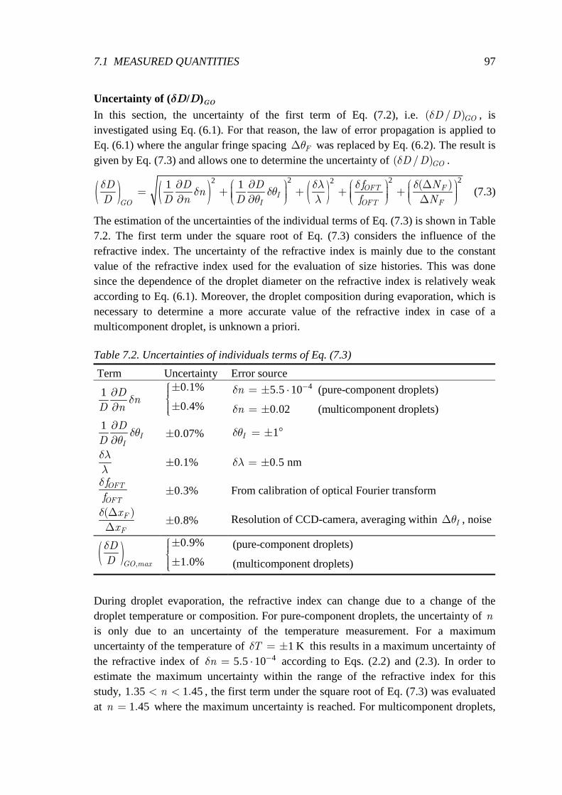
7.1 MEASURED QUANTITIES 97

Uncertainty of (δD/D)GO In this section, the uncertainty of the first term of Eq. (7.2), i.e. ( / )GOD Dδ , is investigated using Eq. (6.1). For that reason, the law of error propagation is applied to Eq. (6.1) where the angular fringe spacing ∆ Fθ was replaced by Eq. (6.2). The result is given by Eq. (7.3) and allows one to determine the uncertainty of ( / )GOD Dδ .

( ) ( ) ( )22 22 21 1 ( )OFT F

II OFT FGO

D D D f Nn

D D n D f N

δ δλ δ δδ δθ

θ λ

∂ ∂ ∆ = + + + + ∂ ∂ ∆ (7.3)

The estimation of the uncertainties of the individual terms of Eq. (7.3) is shown in Table 7.2. The first term under the square root of Eq. (7.3) considers the influence of the refractive index. The uncertainty of the refractive index is mainly due to the constant value of the refractive index used for the evaluation of size histories. This was done since the dependence of the droplet diameter on the refractive index is relatively weak according to Eq. (6.1). Moreover, the droplet composition during evaporation, which is necessary to determine a more accurate value of the refractive index in case of a multicomponent droplet, is unknown a priori.

Table 7.2. Uncertainties of individuals terms of Eq. (7.3)

Term Uncertainty Error source

1 Dn

D nδ

∂∂

0 1%

0 4%

.

.

±±

45 5 10 (pure-component droplets)

0 02 (multicomponent droplets)

.

.

n

n

δ

δ

−= ± ⋅

= ±

1I

I

D

Dδθ

θ

∂∂

0 07%.± 1Iδθ = ± °

δλ

λ 0 1%.± 0 5 nm.δλ = ±

OFT

OFT

f

f

δ 0 3%.± From calibration of optical Fourier transform

( )F

F

x

x

δ ∆∆

0 8%.± Resolution of CCD-camera, averaging within ∆ Iθ , noise

( ),GO max

D

D

δ

0 9%

1 0%

.

.

±±

(pure-component droplets)

(multicomponent droplets)

During droplet evaporation, the refractive index can change due to a change of the droplet temperature or composition. For pure-component droplets, the uncertainty of n is only due to an uncertainty of the temperature measurement. For a maximum uncertainty of the temperature of 1 KTδ = ± this results in a maximum uncertainty of the refractive index of 45 5 10. −= ⋅nδ according to Eqs. (2.2) and (2.3). In order to estimate the maximum uncertainty within the range of the refractive index for this study, 1 35 1 45. .n< < , the first term under the square root of Eq. (7.3) was evaluated at 1 45.n = where the maximum uncertainty is reached. For multicomponent droplets,

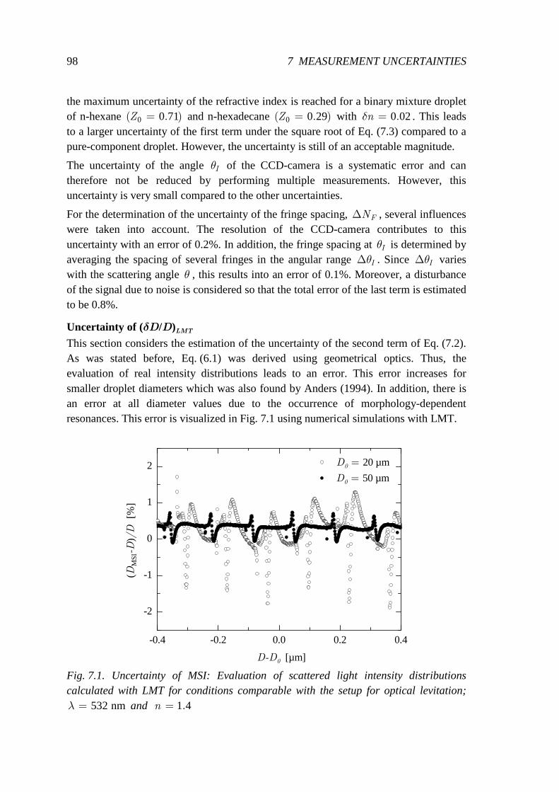
98 7 MEASUREMENT UNCERTAINTIES

the maximum uncertainty of the refractive index is reached for a binary mixture droplet of n-hexane 0 0 71( . )=Z and n-hexadecane 0 0 29( . )=Z with 0 02.nδ = . This leads to a larger uncertainty of the first term under the square root of Eq. (7.3) compared to a pure-component droplet. However, the uncertainty is still of an acceptable magnitude.

The uncertainty of the angle Iθ of the CCD-camera is a systematic error and can therefore not be reduced by performing multiple measurements. However, this uncertainty is very small compared to the other uncertainties.

For the determination of the uncertainty of the fringe spacing, FN∆ , several influences were taken into account. The resolution of the CCD-camera contributes to this uncertainty with an error of 0.2%. In addition, the fringe spacing at Iθ is determined by averaging the spacing of several fringes in the angular range ∆ Iθ . Since Iθ∆ varies with the scattering angle θ , this results into an error of 0.1%. Moreover, a disturbance of the signal due to noise is considered so that the total error of the last term is estimated to be 0.8%.

Uncertainty of (δD/D)LMT This section considers the estimation of the uncertainty of the second term of Eq. (7.2). As was stated before, Eq. (6.1) was derived using geometrical optics. Thus, the evaluation of real intensity distributions leads to an error. This error increases for smaller droplet diameters which was also found by Anders (1994). In addition, there is an error at all diameter values due to the occurrence of morphology-dependent resonances. This error is visualized in Fig. 7.1 using numerical simulations with LMT.

-0.4 -0.2 0.0 0.2 0.4

-2

-1

0

1

2 D0 = 50 µm

D0 = 20 µm

(DM

SI-D

)/D

[%]

D-D0 [µm] Fig. 7.1. Uncertainty of MSI: Evaluation of scattered light intensity distributions calculated with LMT for conditions comparable with the setup for optical levitation;

532 nmλ = and 1 4.=n

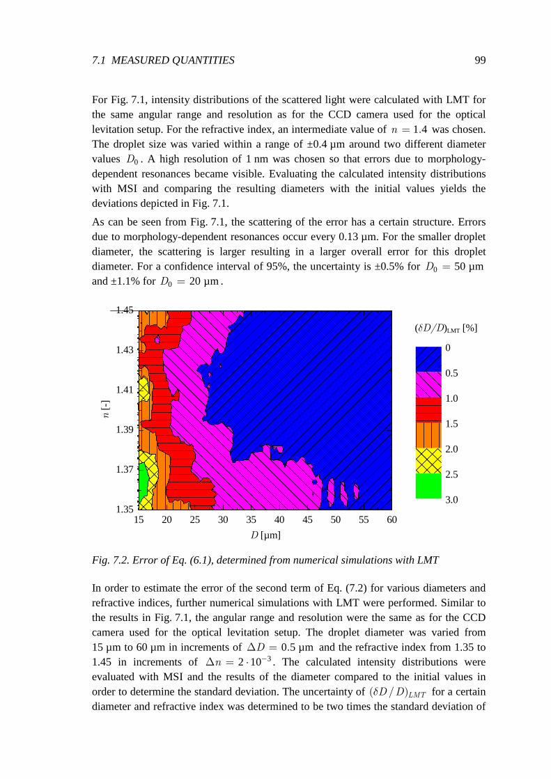
7.1 MEASURED QUANTITIES 99

For Fig. 7.1, intensity distributions of the scattered light were calculated with LMT for the same angular range and resolution as for the CCD camera used for the optical levitation setup. For the refractive index, an intermediate value of 1 4.=n was chosen. The droplet size was varied within a range of ±0.4 µm around two different diameter values 0D . A high resolution of 1 nm was chosen so that errors due to morphology-dependent resonances became visible. Evaluating the calculated intensity distributions with MSI and comparing the resulting diameters with the initial values yields the deviations depicted in Fig. 7.1.

As can be seen from Fig. 7.1, the scattering of the error has a certain structure. Errors due to morphology-dependent resonances occur every 0.13 µm. For the smaller droplet diameter, the scattering is larger resulting in a larger overall error for this droplet diameter. For a confidence interval of 95%, the uncertainty is ±0.5% for 0 50 µmD = and ±1.1% for 0 20 µmD = .

15 20 25 30 35 40 45 50 55 601.35

1.37

1.39

1.41

1.43

1.45

0

0.5

1.0

1.5

2.0

2.5

3.0

D [µm]

n [-

]

(δD/D)LMT [%]

Fig. 7.2. Error of Eq. (6.1), determined from numerical simulations with LMT

In order to estimate the error of the second term of Eq. (7.2) for various diameters and refractive indices, further numerical simulations with LMT were performed. Similar to the results in Fig. 7.1, the angular range and resolution were the same as for the CCD camera used for the optical levitation setup. The droplet diameter was varied from 15 µm to 60 µm in increments of 0 5 µm.∆ =D and the refractive index from 1.35 to 1.45 in increments of 32 10−∆ = ⋅n . The calculated intensity distributions were evaluated with MSI and the results of the diameter compared to the initial values in order to determine the standard deviation. The uncertainty of ( / )LMTD Dδ for a certain diameter and refractive index was determined to be two times the standard deviation of

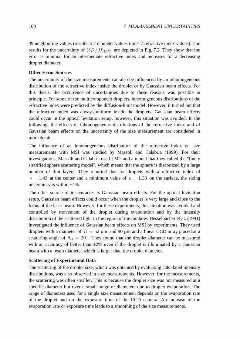
100 7 MEASUREMENT UNCERTAINTIES

49 neighboring values (results at 7 diameter values times 7 refractive index values). The results for the uncertainty of ( / )LMTD Dδ are depicted in Fig. 7.2. They show that the error is minimal for an intermediate refractive index and increases for a decreasing droplet diameter.

Other Error Sources The uncertainty of the size measurements can also be influenced by an inhomogeneous distribution of the refractive index inside the droplet or by Gaussian beam effects. For this thesis, the occurrence of uncertainties due to these reasons was possible in principle. For some of the multicomponent droplets, inhomogeneous distributions of the refractive index were predicted by the diffusion-limit model. However, it turned out that the refractive index was always uniform inside the droplets. Gaussian beam effects could occur in the optical levitation setup, however, this situation was avoided. In the following, the effects of inhomogeneous distributions of the refractive index and of Gaussian beam effects on the uncertainty of the size measurement are considered in more detail.

The influence of an inhomogeneous distribution of the refractive index on size measurements with MSI was studied by Massoli and Calabria (1999). For their investigations, Massoli and Calabria used LMT and a model that they called the "finely stratified sphere scattering model", which means that the sphere is discretized by a large number of thin layers. They reported that for droplets with a refractive index of

1 43.=n at the center and a minimum value of 1 33.=n on the surface, the sizing uncertainty is within ±4%.

The other source of inaccuracies is Gaussian beam effects. For the optical levitation setup, Gaussian beam effects could occur when the droplet is very large and close to the focus of the laser beam. However, for these experiments, this situation was avoided and controlled by movement of the droplet during evaporation and by the intensity distribution of the scattered light in the region of the rainbow. Hesselbacher et al. (1991) investigated the influence of Gaussian beam effects on MSI by experiments. They used droplets with a diameter of 52 µm=D and 90 µm and a linear CCD array placed at a scattering angle of 20= °Mθ . They found that the droplet diameter can be measured with an accuracy of better than ±2% even if the droplet is illuminated by a Gaussian beam with a beam diameter which is larger than the droplet diameter.

Scattering of Experimental Data The scattering of the droplet size, which was obtained by evaluating calculated intensity distributions, was also observed in size measurements. However, for the measurements, the scattering was often smaller. This is because the droplet size was not measured at a specific diameter but over a small range of diameters due to droplet evaporation. The range of diameters used for a single size measurement depends on the evaporation rate of the droplet and on the exposure time of the CCD camera. An increase of the evaporation rate or exposure time leads to a smoothing of the size measurements.

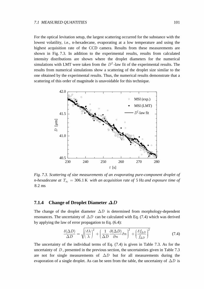
7.1 MEASURED QUANTITIES 101

For the optical levitation setup, the largest scattering occurred for the substance with the lowest volatility, i.e., n-hexadecane, evaporating at a low temperature and using the highest acquisition rate of the CCD camera. Results from these measurements are shown in Fig. 7.3. In addition to the experimental results, results from calculated intensity distributions are shown where the droplet diameters for the numerical simulations with LMT were taken from the 2D -law fit of the experimental results. The results from numerical simulations show a scattering of the droplet size similar to the one obtained by the experimental results. Thus, the numerical results demonstrate that a scattering of this order of magnitude is unavoidable for this technique.

230 240 250 260 270 28040.5

41.0

41.5

42.0

MSI (exp.)

MSI (LMT) D2-law fit

D

[µm

]

t [s] Fig. 7.3. Scattering of size measurements of an evaporating pure-component droplet of n-hexadecane at 306 1 K.∞ =T with an acquisition rate of 5 Hzand exposure time of 8 2 ms.

7.1.4 Change of Droplet Diameter ∆D

The change of the droplet diameter D∆ is determined from morphology-dependent resonances. The uncertainty of D∆ can be calculated with Eq. (7.4) which was derived by applying the law of error propagation to Eq. (6.4):

( )2 22 1( ) ( ) D

D

D D fn

D D n f

δ δλ δδ

λ∆

∆

∆ ∂ ∆ = + + ∆ ∆ ∂ (7.4)

The uncertainty of the individual terms of Eq. (7.4) is given in Table 7.3. As for the uncertainty of D , presented in the previous section, the uncertainties given in Table 7.3 are not for single measurements of D∆ but for all measurements during the evaporation of a single droplet. As can be seen from the table, the uncertainty of D∆ is

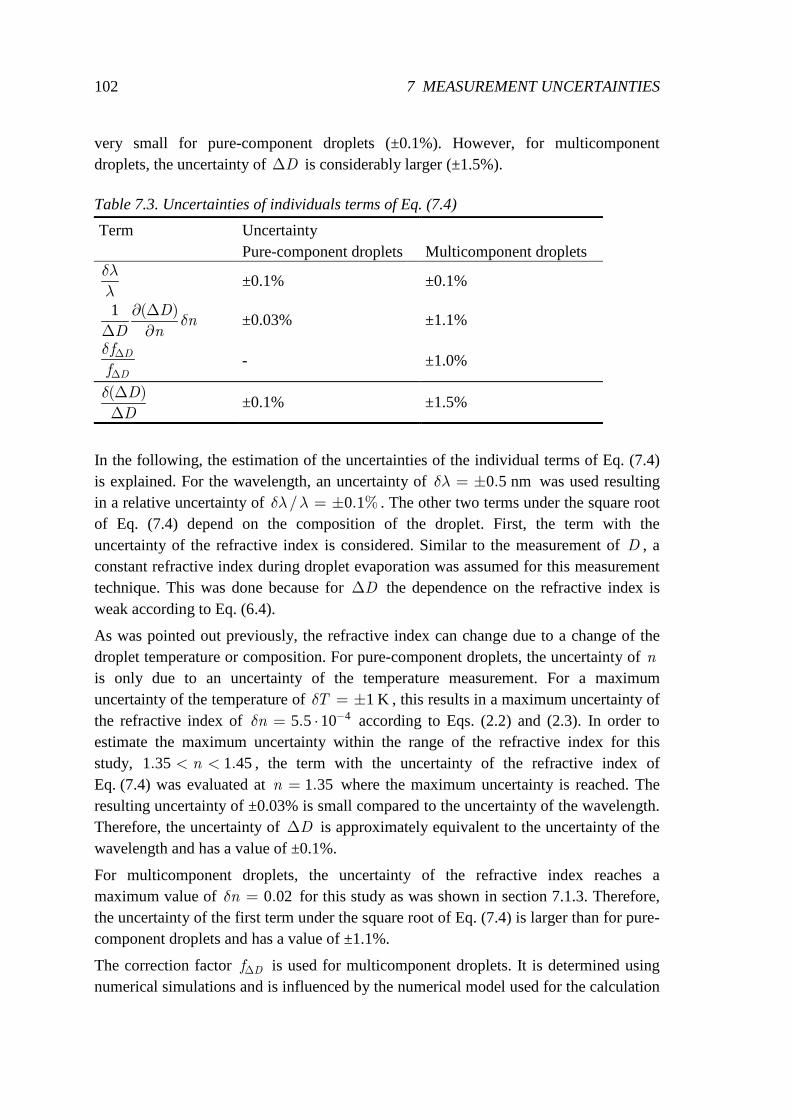
102 7 MEASUREMENT UNCERTAINTIES

very small for pure-component droplets (±0.1%). However, for multicomponent droplets, the uncertainty of D∆ is considerably larger (±1.5%).

Table 7.3. Uncertainties of individuals terms of Eq. (7.4)

Term Uncertainty Pure-component droplets

Multicomponent droplets

δλ

λ ±0.1% ±0.1%

1 ( )Dn

D nδ

∂ ∆∆ ∂

±0.03% ±1.1%

D

D

f

f

δ ∆

∆ - ±1.0%

( )D

D

δ ∆∆

±0.1% ±1.5%

In the following, the estimation of the uncertainties of the individual terms of Eq. (7.4) is explained. For the wavelength, an uncertainty of 0 5 nm.δλ = ± was used resulting in a relative uncertainty of 0 1/ . %δλ λ = ± . The other two terms under the square root of Eq. (7.4) depend on the composition of the droplet. First, the term with the uncertainty of the refractive index is considered. Similar to the measurement of D , a constant refractive index during droplet evaporation was assumed for this measurement technique. This was done because for D∆ the dependence on the refractive index is weak according to Eq. (6.4).

As was pointed out previously, the refractive index can change due to a change of the droplet temperature or composition. For pure-component droplets, the uncertainty of n is only due to an uncertainty of the temperature measurement. For a maximum uncertainty of the temperature of 1 KTδ = ± , this results in a maximum uncertainty of the refractive index of 45 5 10. −= ⋅nδ according to Eqs. (2.2) and (2.3). In order to estimate the maximum uncertainty within the range of the refractive index for this study, 1 35 1 45. .n< < , the term with the uncertainty of the refractive index of Eq. (7.4) was evaluated at 1 35.n = where the maximum uncertainty is reached. The resulting uncertainty of ±0.03% is small compared to the uncertainty of the wavelength. Therefore, the uncertainty of D∆ is approximately equivalent to the uncertainty of the wavelength and has a value of ±0.1%.

For multicomponent droplets, the uncertainty of the refractive index reaches a maximum value of 0 02.nδ = for this study as was shown in section 7.1.3. Therefore, the uncertainty of the first term under the square root of Eq. (7.4) is larger than for pure-component droplets and has a value of ±1.1%.

The correction factor Df∆ is used for multicomponent droplets. It is determined using numerical simulations and is influenced by the numerical model used for the calculation

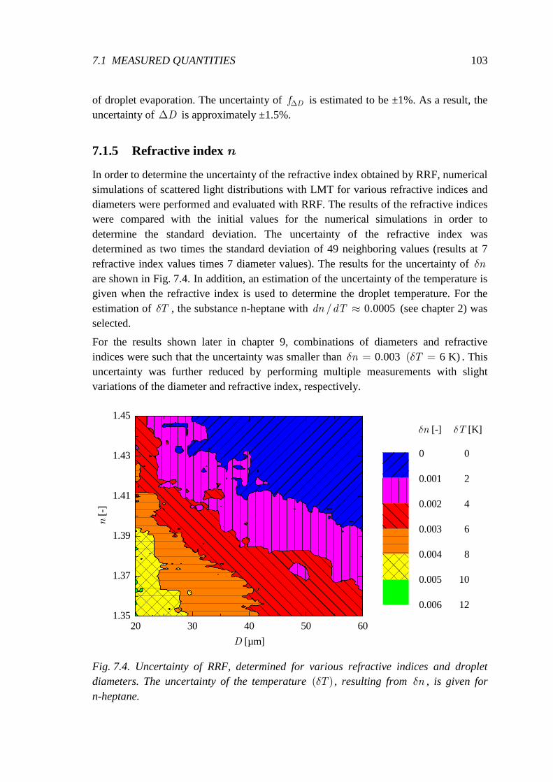
7.1 MEASURED QUANTITIES 103

of droplet evaporation. The uncertainty of Df∆ is estimated to be ±1%. As a result, the uncertainty of D∆ is approximately ±1.5%.

7.1.5 Refractive index n

In order to determine the uncertainty of the refractive index obtained by RRF, numerical simulations of scattered light distributions with LMT for various refractive indices and diameters were performed and evaluated with RRF. The results of the refractive indices were compared with the initial values for the numerical simulations in order to determine the standard deviation. The uncertainty of the refractive index was determined as two times the standard deviation of 49 neighboring values (results at 7 refractive index values times 7 diameter values). The results for the uncertainty of nδ are shown in Fig. 7.4. In addition, an estimation of the uncertainty of the temperature is given when the refractive index is used to determine the droplet temperature. For the estimation of Tδ , the substance n-heptane with 0 0005/ .≈dn dT (see chapter 2) was selected.

For the results shown later in chapter 9, combinations of diameters and refractive indices were such that the uncertainty was smaller than 0 003.=nδ 6 K)( =Tδ . This uncertainty was further reduced by performing multiple measurements with slight variations of the diameter and refractive index, respectively.

20 30 40 50 601.35

1.37

1.39

1.41

1.43

1.45

0

1.000E-3

0.002

0.003

0.004

0.005

0.006

D [µm]

n [-

]

0 0

0.001 2

0.002 4

0.003 6

0.004 8

0.005 10

0.006 12

δn [-] δT [K]

Fig. 7.4. Uncertainty of RRF, determined for various refractive indices and droplet diameters. The uncertainty of the temperature ( )Tδ , resulting from nδ , is given for n-heptane.

104 7 MEASUREMENT UNCERTAINTIES

7.2 Derived Quantities The purpose of this section is to give equations for the calculation of the uncertainties of the initial droplet diameter, the non-dimensional droplet surface, and the evaporation rate. Actual values of these uncertainties are presented with the results.

7.2.1 Initial Droplet Diameter D0

With respect to the uncertainty of 0,lin.D , it is assumed that the uncertainty of the time values can be neglected so that the uncertainty of 0D depends only on the uncertainty of the size measurements and is given by Eq. (7.5) (Barlow 1989):

2

2 20

1 with , .

maxN

lin imaxt max i

tD D t t

NS Nδ δ= = ∑ (7.5)

Generally, 0, .linDδ is small compared to Dδ since a large number maxN of data points is used for the linear interpolation.

7.2.2 Non-dimensional Droplet Surface (D/D0)2

According to the law of error propagation, the uncertainty of the non-dimensional droplet surface 2

0( / )D Dξ = is given by Eq. (7.6):

( )22

0

02

D D

D D

δξ δ δ

ξ

= + (7.6)

Since the uncertainty of 0D is usually very small, the uncertainty of ξ is dominated by the uncertainty of D .

7.2.3 Evaporation Rate β

For pure-component droplets where the evaporation rate is a constant after the initial cooling phase, this constant is determined from measurements of size histories. Therefore, the uncertainty of the evaporation rate is due to an uncertainty of the size measurement. This uncertainty is relatively small since a large number of size measurements is used for the determination of β . However, the evaporation rate also depends on the ambient temperature. Since the temperature has a large influence on the evaporation rate, as was shown in section 3.4.3, the uncertainty of β is dominated by the uncertainty of the ambient temperature. In order to evaluate the influence of the uncertainty of the ambient temperature, numerical simulations were used. In the following, the uncertainty of β due to an uncertainty of the size measurements is discussed.

7.2 DERIVED QUANTITIES 105

Using droplet size measurements with MSI, the uncertainty of a constant evaporation rate corresponds to the uncertainty of the slope of the linear interpolation shown previously in Fig. 6.4. This uncertainty is given by Eq. (7.7):

1

t max

DS N

δβ δ= (7.7)

Using measurements with MDRs, the uncertainty of the evaporation rate is determined in a different way. For that reason, the definition of the evaporation rate,

2 /dD dtβ = − , is rewritten as:

12 2dD D

D Ddt t

β∆

= − = −∆

(7.8)

where the droplet diameter 1D is determined by a measurement using MSI, D∆ is the decrease of the droplet diameter between two neighboring morphology-dependent resonances, and t∆ is the mean time interval between two neighboring morphology-dependent resonances. According to the law of error propagation, the uncertainty of the evaporation rate is given in this case by Eq. (7.9):

( ) ( )222D D t

D D t

δβ δ δ δ

β

∆ ∆ = + + ∆ ∆ (7.9)

The uncertainty of t∆ decreases the more peaks are used. Usually, a large number of peaks was used so that this uncertainty was small compared to the uncertainty of D which had the main influence on the uncertainty of β .

107

8 Results of Droplet Sizing

8.1 Overview In this chapter, size and non-dimensional surface histories are presented for droplets of different compositions and at different ambient temperatures. In the first part, results from pure-component droplets are shown. These results act as a validation of the experimental setups. For the free-falling droplet setup, results obtained by the two different measurement techniques were compared in order to prove the accuracy of the techniques. Finally, evaporation rates are presented of different substances and at different temperatures. These results are compared to results from numerical simulations. Since the 2D -law is valid for the conditions of the experiments, the comparison can be understood as a comparison of the accuracies of the experimental results and of the selected relationships for the species properties implemented in the numerical models.

Subsequently, results of binary and ternary mixture droplets are presented. A large variety of data is provided for the validation of numerical models. The comparison of the experimental results to results from numerical and analytical models demonstrate the accuracy and applicability of these models. Some studies of binary mixture droplets considered conditions where there was a large difference in the volatilities of the substances so that concentration gradients were predicted by the diffusion-limit model. Experimental results are compared to results of the rapid-mixing and the diffusion-limit model in order to investigate the influence of internal heat and mass transfer and to identify the dominating process for droplet evaporation.

8.2 General Remarks Results of the droplet size measurements are presented in two different types of graphs. One type depicts diameter histories so that the actual magnitude of the droplet size can be seen. The other type is of more general use. It shows the non-dimensional droplet surface 2

0( / )= D Dξ as a function of time divided by the square of the initial diameter 20/t D . From these graphs, the evaporation rate β , which is the magnitude of the

negative slope of the curves, can be obtained directly. Thus, if the curve is a straight line, the evaporation rate is a constant. However, when there is curvature, the evaporation rate changes. One reason for this behavior can be the initial cooling of the droplet. This transient phase is not captured by the experiments and can only be seen in the numerical results. The other reason for a change of the evaporation rate is a change

108 8 RESULTS OF DROPLET SIZING

of the droplet composition. This influence is of interest in this study and shown for various mixture droplets.

The use of this type of graph is also advantageous since, by normalizing both axes with the square of the initial droplet diameter, the results become independent from the initial droplet size. This is valid not only for the stationary evaporation phase, when the 2D -law can be applied, but also for the initial cooling phase. During this phase, the rate of change of the droplet temperature depends on the square of the droplet diameter. This can be shown using an energy balance of the droplet, which is, for example, presented by Mills (2001). The dependence of the temperature on the square of the droplet diameter is also valid for models with internal diffusion (CLM and DLM) as shown by Kneer (1993). As a consequence, the temporal evolution of the droplet temperature as well as the temperature profiles inside the droplet are the same when they are scaled with the initial droplet diameter. This is based on the assumption of constant properties during the initial cooling phase, which is generally an appropriate assumption, but especially for the small changes of temperature occurring in this study. Analogous to the droplet temperature, histories of the diameter and composition are also the same for different droplets when normalized with the square of the initial droplet diameter.

8.3 Pure-Component Droplets In this section, results from pure-component droplets are presented. These results are used to illustrate the range of application and certain characteristics of the experimental setups and of the measurement techniques. At the end of this section, results for evaporation rates are shown for various substances and temperatures.

8.3.1 N-Hexadecane Results for a pure-component droplet consisting of n-hexadecane are depicted in Fig. 8.1. The experiments were conducted with the optical levitation setup. The droplet had an initial diameter of 0 47 µm=D and was levitated for roughly 21 min. The droplet size was determined with MSI at an acquisition rate of 1 Hz. A running average of 10 data points was applied so that a very smooth non-dimensional surface history was obtained, which is depicted in Fig. 8.1(a).

As can be seen from the surface history, the evaporation rate changes slightly during droplet evaporation. The variation of the evaporation rate is shown in Fig. 8.1(c). For this figure, the momentary evaporation rate was determined from the surface history over time intervals of 100 s.

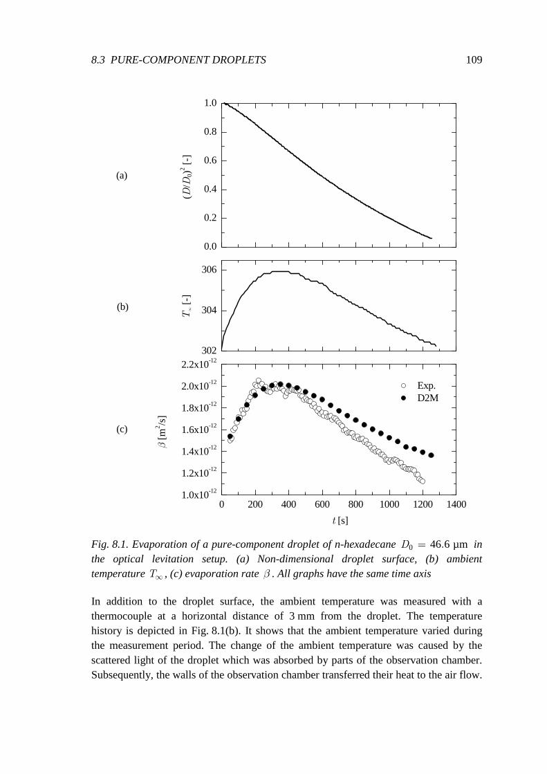
8.3 PURE-COMPONENT DROPLETS 109

0.0

0.2

0.4

0.6

0.8

1.0

302

304

306

0 200 400 600 800 1000 1200 14001.0x10-12

1.2x10-12

1.4x10-12

1.6x10-12

1.8x10-12

2.0x10-12

2.2x10-12

(D/D

0)2 [-

](a)

(b)

(c)

T∞ [-

]

Exp. D2M

β [m

2 /s]

t [s]

Fig. 8.1. Evaporation of a pure-component droplet of n-hexadecane 0 46 6 µm.=D in the optical levitation setup. (a) Non-dimensional droplet surface, (b) ambient temperature ∞T , (c) evaporation rate β . All graphs have the same time axis

In addition to the droplet surface, the ambient temperature was measured with a thermocouple at a horizontal distance of 3 mm from the droplet. The temperature history is depicted in Fig. 8.1(b). It shows that the ambient temperature varied during the measurement period. The change of the ambient temperature was caused by the scattered light of the droplet which was absorbed by parts of the observation chamber. Subsequently, the walls of the observation chamber transferred their heat to the air flow.

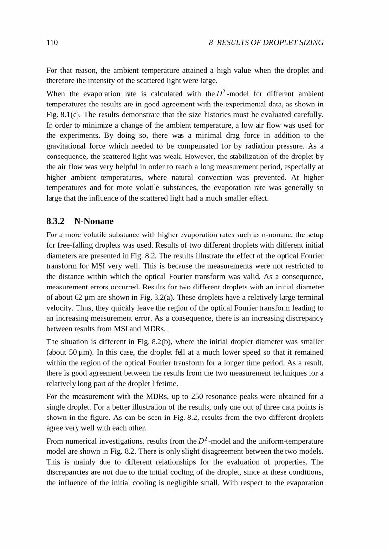
110 8 RESULTS OF DROPLET SIZING

For that reason, the ambient temperature attained a high value when the droplet and therefore the intensity of the scattered light were large.

When the evaporation rate is calculated with the2D -model for different ambient temperatures the results are in good agreement with the experimental data, as shown in Fig. 8.1(c). The results demonstrate that the size histories must be evaluated carefully. In order to minimize a change of the ambient temperature, a low air flow was used for the experiments. By doing so, there was a minimal drag force in addition to the gravitational force which needed to be compensated for by radiation pressure. As a consequence, the scattered light was weak. However, the stabilization of the droplet by the air flow was very helpful in order to reach a long measurement period, especially at higher ambient temperatures, where natural convection was prevented. At higher temperatures and for more volatile substances, the evaporation rate was generally so large that the influence of the scattered light had a much smaller effect.

8.3.2 N-Nonane For a more volatile substance with higher evaporation rates such as n-nonane, the setup for free-falling droplets was used. Results of two different droplets with different initial diameters are presented in Fig. 8.2. The results illustrate the effect of the optical Fourier transform for MSI very well. This is because the measurements were not restricted to the distance within which the optical Fourier transform was valid. As a consequence, measurement errors occurred. Results for two different droplets with an initial diameter of about 62 µm are shown in Fig. 8.2(a). These droplets have a relatively large terminal velocity. Thus, they quickly leave the region of the optical Fourier transform leading to an increasing measurement error. As a consequence, there is an increasing discrepancy between results from MSI and MDRs.

The situation is different in Fig. 8.2(b), where the initial droplet diameter was smaller (about 50 µm). In this case, the droplet fell at a much lower speed so that it remained within the region of the optical Fourier transform for a longer time period. As a result, there is good agreement between the results from the two measurement techniques for a relatively long part of the droplet lifetime.

For the measurement with the MDRs, up to 250 resonance peaks were obtained for a single droplet. For a better illustration of the results, only one out of three data points is shown in the figure. As can be seen in Fig. 8.2, results from the two different droplets agree very well with each other.

From numerical investigations, results from the2D -model and the uniform-temperature model are shown in Fig. 8.2. There is only slight disagreement between the two models. This is mainly due to different relationships for the evaluation of properties. The discrepancies are not due to the initial cooling of the droplet, since at these conditions, the influence of the initial cooling is negligible small. With respect to the evaporation

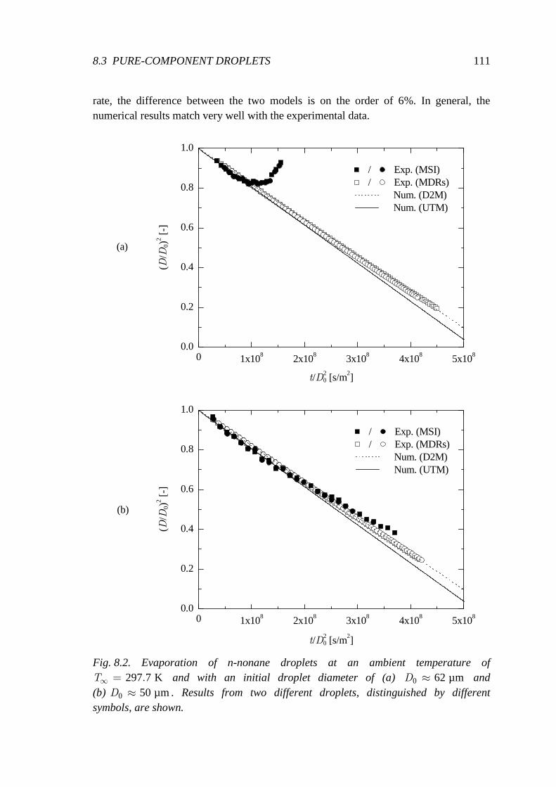
8.3 PURE-COMPONENT DROPLETS 111

rate, the difference between the two models is on the order of 6%. In general, the numerical results match very well with the experimental data.

0 1x108 2x108 3x108 4x108 5x1080.0

0.2

0.4

0.6

0.8

1.0

0 1x108 2x108 3x108 4x108 5x1080.0

0.2

0.4

0.6

0.8

1.0

(b)

(D/D

0)2 [-

]

t/D20 [s/m2]

/ Exp. (MSI)/ Exp. (MDRs)

Num. (D2M) Num. (UTM)

(a)

(D/D

0)2 [-

]

t/D20 [s/m2]

/ Exp. (MSI)/ Exp. (MDRs)

Num. (D2M) Num. (UTM)

Fig. 8.2. Evaporation of n-nonane droplets at an ambient temperature of

297 7 K.∞ =T and with an initial droplet diameter of (a) 0 62 µm≈D and (b) 0 50 µm≈D . Results from two different droplets, distinguished by different symbols, are shown.

112 8 RESULTS OF DROPLET SIZING

8.3.3 N-Pentane N-pentane droplets could only be investigated with the free-falling droplet setup due to their high evaporation rate at an ambient temperature of about 295 K. Because of the high evaporation rate, the size of the droplets decreased rapidly. Therefore, the droplets decelerated so fast that they evaporated completely within the range of the optical Fourier transform. As a consequence, it was possible to obtain size histories for a large change of the droplet diameter.

For n-pentane droplets, an orifice with a diameter of 88 µm was used instead of the standard orifice with a diameter of 40 µm. The resulting initial droplet diameter was about 100 µm. This orifice was selected in order to attain a sufficiently long lifetime of the droplet, of up to 0.25 s, as seen from Fig. 8.3(a).

Experimental results from two droplets with different initial diameters are depicted in Fig. 8.3. About 290 resonances were detected for the small droplet and 370 for the large droplet. In the figure, only one out of five data points of the measurements with MDRs are shown to allow for a better illustration. At a certain droplet size, no further resonances could be detected due to the limited dynamic range and the limited time-resolution of the data acquisition board used to record of the output signal of the photomultiplier.

In Fig. 8.3(b) it can be seen that the experimental results agree very well for the two different droplets. With respect to the different measurement techniques, Fig. 8.3 shows that results between MSI and MDRs agree very well also.

In addition to the experimental results, numerical results from the uniform-temperature model are depicted in Fig. 8.3. For the numerical calculations, the size of the initial droplet diameter was selected in such a way that the numerical result coincided with the experimental result for the first size measurement. The results from the uniform-temperature model show that there is a significant effect of the initial cooling of the droplet. This phase is neither captured by the experiments nor with the 2D -model. When the experimental data is evaluated in the usual way, such that the initial diameter is obtained by extrapolating data to 0t = , the initial droplet diameter is underestimated. However, this underestimation does not affect the result of the evaporation rate.

The uniform-temperature model can be used to correct the initial diameter obtained from the experimental results. When results from UTM, which do not include the initial cooling phase, are extrapolated back to 0t = in the same manner as the experiments, the results show that the droplet diameter is 8.4 % smaller than the initial droplet diameter used for the numerical simulation. This result was used to correct the initial droplet diameter obtained from the experimental data.

When comparing experimental results with numerical calculations, it can be seen from Fig. 8.3(b) that the evaporation rate, i.e., the slope of the curves, from the experiments is between those from D2M and UTM. Results from the conduction-limit model where

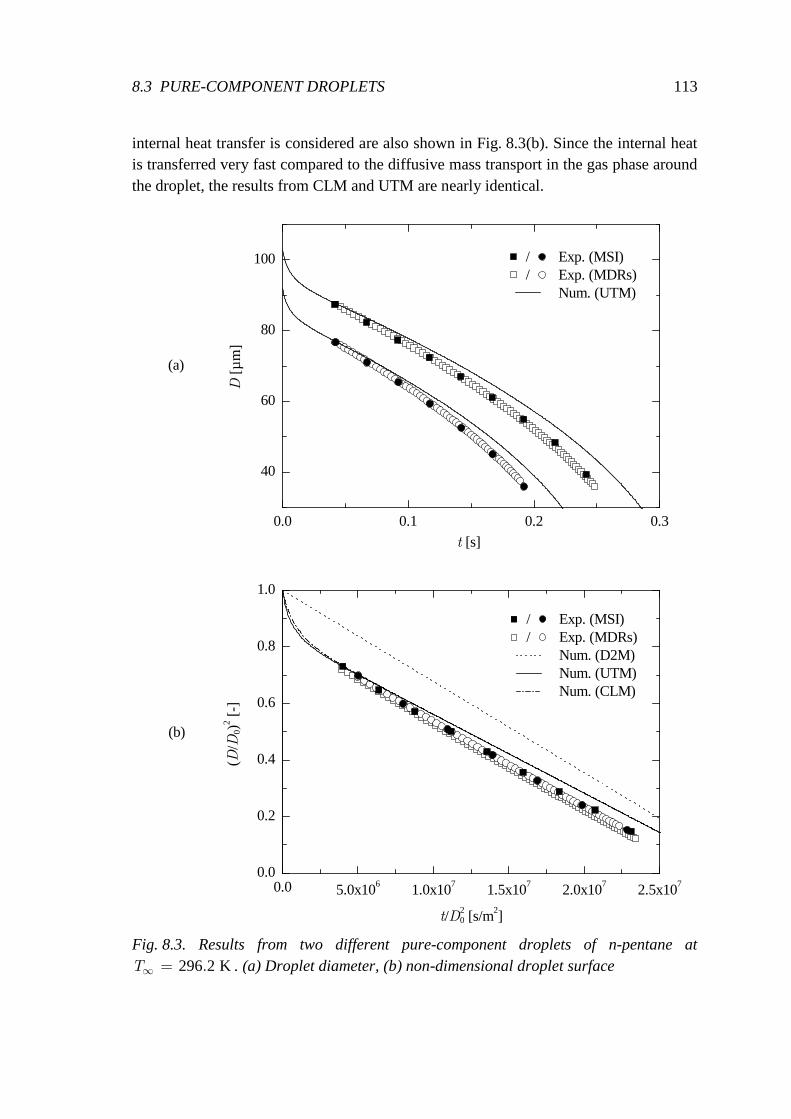
8.3 PURE-COMPONENT DROPLETS 113

internal heat transfer is considered are also shown in Fig. 8.3(b). Since the internal heat is transferred very fast compared to the diffusive mass transport in the gas phase around the droplet, the results from CLM and UTM are nearly identical.

0.0 0.1 0.2 0.3

40

60

80

100

0.0 5.0x106 1.0x107 1.5x107 2.0x107 2.5x1070.0

0.2

0.4

0.6

0.8

1.0

D [µ

m]

t [s]

/ Exp. (MSI)/ Exp. (MDRs)

Num. (UTM)

(b)

(D/D

0)2 [-

]

t/D20 [s/m2]

/ Exp. (MSI)/ Exp. (MDRs)

Num. (D2M) Num. (UTM) Num. (CLM)

(a)

Fig. 8.3. Results from two different pure-component droplets of n-pentane at

296 2 K.∞ =T . (a) Droplet diameter, (b) non-dimensional droplet surface

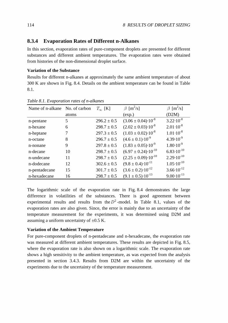
114 8 RESULTS OF DROPLET SIZING

8.3.4 Evaporation Rates of Different n-Alkanes In this section, evaporation rates of pure-component droplets are presented for different substances and different ambient temperatures. The evaporation rates were obtained from histories of the non-dimensional droplet surface.

Variation of the Substance Results for different n-alkanes at approximately the same ambient temperature of about 300 K are shown in Fig. 8.4. Details on the ambient temperature can be found in Table 8.1.

Table 8.1. Evaporation rates of n-alkanes

Name of n-alkane No. of carbon atoms

∞T [K] β [m2/s] (exp.)

β [m2/s] (D2M)

n-pentane 5 296.2 ± 0.5 (3.06 ± 0.04)·10-8 3.22·10-8 n-hexane 6 298.7 ± 0.5 (2.02 ± 0.03)·10-8 2.01·10-8 n-heptane 7 297.3 ± 0.5 (1.03 ± 0.02)·10-8 1.01·10-8 n-octane 8 296.7 ± 0.5 (4.6 ± 0.1)·10-9 4.39·10-9 n-nonane 9 297.8 ± 0.5 (1.83 ± 0.05)·10-9 1.80·10-9 n-decane 10 298.7 ± 0.5 (6.97 ± 0.24)·10-10 6.83·10-10 n-undecane 11 298.7 ± 0.5 (2.25 ± 0.09)·10-10 2.29·10-10 n-dodecane 12 302.6 ± 0.5 (9.8 ± 0.4)·10-11 1.05·10-10 n-pentadecane 15 301.7 ± 0.5 (3.6 ± 0.2)·10-12 3.66·10-12 n-hexadecane 16 298.7 ± 0.5 (9.1 ± 0.5)·10-13 9.00·10-13

The logarithmic scale of the evaporation rate in Fig. 8.4 demonstrates the large difference in volatilities of the substances. There is good agreement between experimental results and results from the2D -model. In Table 8.1, values of the evaporation rates are also given. Since, the error is mainly due to an uncertainty of the temperature measurement for the experiments, it was determined using D2M and assuming a uniform uncertainty of ±0.5 K.

Variation of the Ambient Temperature For pure-component droplets of n-pentadecane and n-hexadecane, the evaporation rate was measured at different ambient temperatures. These results are depicted in Fig. 8.5, where the evaporation rate is also shown on a logarithmic scale. The evaporation rate shows a high sensitivity to the ambient temperature, as was expected from the analysis presented in section 3.4.3. Results from D2M are within the uncertainty of the experiments due to the uncertainty of the temperature measurement.

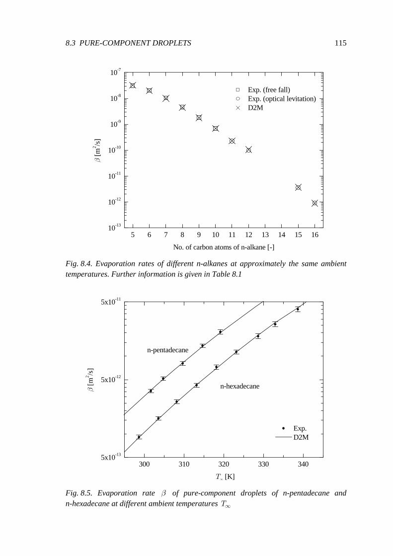
8.3 PURE-COMPONENT DROPLETS 115

5 6 7 8 9 10 11 12 13 14 15 1610-13

10-12

10-11

10-10

10-9

10-8

10-7

β [m

2 /s]

No. of carbon atoms of n-alkane [-]

Exp. (free fall) Exp. (optical levitation) D2M

Fig. 8.4. Evaporation rates of different n-alkanes at approximately the same ambient temperatures. Further information is given in Table 8.1

300 310 320 330 3405x10-13

5x10-12

5x10-11

n-pentadecane

β [m

2 /s]

T∞ [K]

Exp. D2M

n-hexadecane

Fig. 8.5. Evaporation rate β of pure-component droplets of n-pentadecane and n-hexadecane at different ambient temperatures ∞T

116 8 RESULTS OF DROPLET SIZING

8.4 Binary Mixture Droplets In the following, results of binary mixture droplets are presented where component one was always n-hexadecane. Initially, results are shown where the second component was n-tetradecane. Subsequently, the volatility of the other component was increased. The largest difference in volatilities was reached for the combination of n-hexadecane with n-hexane.

8.4.1 N-Hexadecane with n-Tetradecane In Fig. 8.6, results are shown for pure-component and binary mixture droplets of n-hexadecane and n-tetradecane with different initial compositions at approximately the same ambient temperature. For the mixture droplets, the initial evaporation rate was between the limiting evaporation rates of the pure-component droplets. This means that both substances evaporated simultaneously. After a certain time, a transition phase occurred where the evaporation rate changed significantly. At the end of the transition phase, n-tetradecane was depleted from the droplet and the evaporation rate of a pure n-hexadecane droplet was reached. From this point in time, the slopes of the surface histories for the mixture droplets were nearly identical to the slope of the n-hexadecane droplet. Small differences among the slopes in the experimental data are due to small variations of the ambient temperature.

In addition to the experimental results, results from the simplified rapid-mixing model and from the analytical solution of the simplified rapid-mixing model are shown in Fig. 8.6. Since the evaporation rate was very low, the ambient temperature was chosen as reference temperature. Results from both models matched very well with the experimental data. SRMM also showed good agreement with experimental results of binary mixture droplets of n-hexadecane with n-dodecane which is presented in section 9.2 where rainbow refractometry was applied in addition to size measurements.

8.4.2 N-Hexadecane with a Highly Volatile n-Alkane

Overview In order to have a large difference in the volatilities of the substances, binary mixture droplets of n-hexadecane with a highly volatile n-alkane were investigated. The experiments were conducted with the free-falling droplet setup. Mixtures were selected for which measurements with MSI still provided sufficient data for a representation of the surface histories. This was the case for mixtures of n-hexadecane with n-heptane or n-hexane.

For the highly volatile n-alkane (n-heptane or n-hexane), an initial volume fraction of at least 0 0 5.=Z was chosen for several reasons. First, it was important to have a nearly constant initial evaporation rate. This permitted the determination of the initial droplet diameter with a small uncertainty. It was also important to have sufficient data points

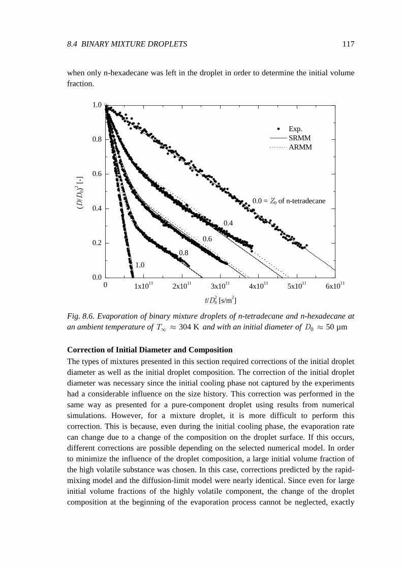
8.4 BINARY MIXTURE DROPLETS 117

when only n-hexadecane was left in the droplet in order to determine the initial volume fraction.

0 1x1011 2x1011 3x1011 4x1011 5x1011 6x10110.0

0.2

0.4

0.6

0.8

1.0

1.0

0.8

(D/D

0)2 [-

]

t/D20 [s/m2]

Exp. SRMM ARMM

0.0 = Z0 of n-tetradecane

0.4

0.6

Fig. 8.6. Evaporation of binary mixture droplets of n-tetradecane and n-hexadecane at an ambient temperature of 304 K∞ ≈T and with an initial diameter of 0 50 µm≈D

Correction of Initial Diameter and Composition The types of mixtures presented in this section required corrections of the initial droplet diameter as well as the initial droplet composition. The correction of the initial droplet diameter was necessary since the initial cooling phase not captured by the experiments had a considerable influence on the size history. This correction was performed in the same way as presented for a pure-component droplet using results from numerical simulations. However, for a mixture droplet, it is more difficult to perform this correction. This is because, even during the initial cooling phase, the evaporation rate can change due to a change of the composition on the droplet surface. If this occurs, different corrections are possible depending on the selected numerical model. In order to minimize the influence of the droplet composition, a large initial volume fraction of the high volatile substance was chosen. In this case, corrections predicted by the rapid-mixing model and the diffusion-limit model were nearly identical. Since even for large initial volume fractions of the highly volatile component, the change of the droplet composition at the beginning of the evaporation process cannot be neglected, exactly

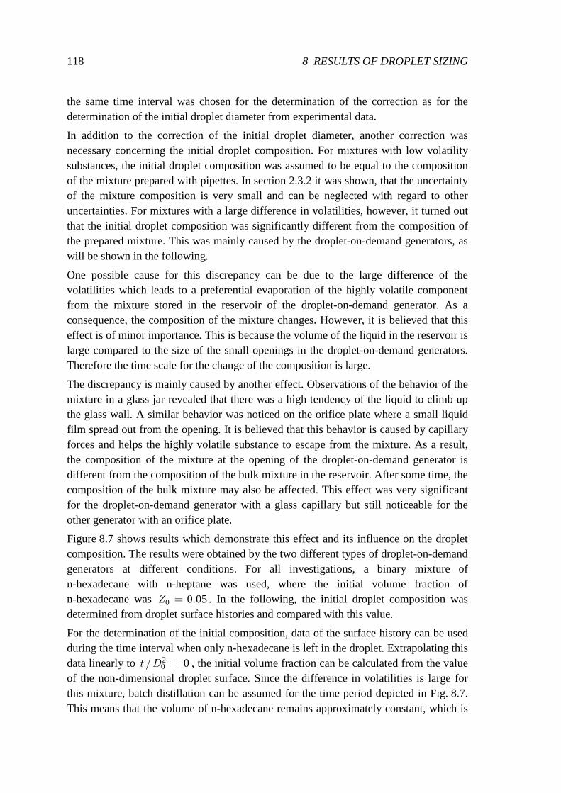
118 8 RESULTS OF DROPLET SIZING

the same time interval was chosen for the determination of the correction as for the determination of the initial droplet diameter from experimental data.

In addition to the correction of the initial droplet diameter, another correction was necessary concerning the initial droplet composition. For mixtures with low volatility substances, the initial droplet composition was assumed to be equal to the composition of the mixture prepared with pipettes. In section 2.3.2 it was shown, that the uncertainty of the mixture composition is very small and can be neglected with regard to other uncertainties. For mixtures with a large difference in volatilities, however, it turned out that the initial droplet composition was significantly different from the composition of the prepared mixture. This was mainly caused by the droplet-on-demand generators, as will be shown in the following.

One possible cause for this discrepancy can be due to the large difference of the volatilities which leads to a preferential evaporation of the highly volatile component from the mixture stored in the reservoir of the droplet-on-demand generator. As a consequence, the composition of the mixture changes. However, it is believed that this effect is of minor importance. This is because the volume of the liquid in the reservoir is large compared to the size of the small openings in the droplet-on-demand generators. Therefore the time scale for the change of the composition is large.

The discrepancy is mainly caused by another effect. Observations of the behavior of the mixture in a glass jar revealed that there was a high tendency of the liquid to climb up the glass wall. A similar behavior was noticed on the orifice plate where a small liquid film spread out from the opening. It is believed that this behavior is caused by capillary forces and helps the highly volatile substance to escape from the mixture. As a result, the composition of the mixture at the opening of the droplet-on-demand generator is different from the composition of the bulk mixture in the reservoir. After some time, the composition of the bulk mixture may also be affected. This effect was very significant for the droplet-on-demand generator with a glass capillary but still noticeable for the other generator with an orifice plate.

Figure 8.7 shows results which demonstrate this effect and its influence on the droplet composition. The results were obtained by the two different types of droplet-on-demand generators at different conditions. For all investigations, a binary mixture of n-hexadecane with n-heptane was used, where the initial volume fraction of n-hexadecane was 0 0 05.=Z . In the following, the initial droplet composition was determined from droplet surface histories and compared with this value.

For the determination of the initial composition, data of the surface history can be used during the time interval when only n-hexadecane is left in the droplet. Extrapolating this data linearly to 2

0 0/t D = , the initial volume fraction can be calculated from the value of the non-dimensional droplet surface. Since the difference in volatilities is large for this mixture, batch distillation can be assumed for the time period depicted in Fig. 8.7. This means that the volume of n-hexadecane remains approximately constant, which is

8.4 BINARY MIXTURE DROPLETS 119

confirmed by both the experimental and the numerical results. As a consequence, the initial composition can be directly calculated from the mean droplet surface in the time interval 8 2 2 8 2

010 s/m 1 5 10 s/m/ .t D< < ⋅ . For the numerical results using the rapid-mixing model, a mean surface of 2

0 0 136( / ) .=D D was obtained in this interval. This yields an initial volume fraction of 1 5

0 0 136 0 05.. .= =Z for n-hexadecane, which is in perfect agreement with the initial condition of the numerical simulation.

0.0 5.0x107 1.0x108 1.5x1080.0

0.2

0.4

0.6

0.8

1.0

1.2

(D/D

0)2 [-

]

t/D20 [s/m2]

/ (A) DODG-1; ∆t1 = 0.5h; ∆t2 = 0.5h; T∞ = 297.3 K

/ (B) DODG-1; ∆t1 = 5.0h; ∆t2 = 5.0h; T∞ = 297.9 K

/ (C) DODG-1; ∆t1 = 5.0h; ∆t2 = 0.0h; T∞ = 298.0 K

/ (D) DODG-2; ∆t1 = 7.0h; ∆t2 = 0.5h; T∞ = 298.5 K

RMM, T∞ = 298.5 K

Fig. 8.7. Results for binary mixture droplets of n-heptane 0 0 95( . )=Z and n-hexadecane 0 0 05( . )=Z at approximately the same ambient temperature ∞T ; 4 groups of measurements, (A)-(D), are presented; the different types of droplet-on-demand generators (DODG) are denoted by DODG-1 (glass capillary) and DODG-2 (orifice); the time elapsed since the preparation of the mixture is denoted by 1∆t ; the residence time of the liquid mixture in the DODG is described by 2∆t

The results in Fig. 8.7 show that, for the experiments, the initial volume fraction of n-hexadecane was larger than 0.05, especially when the droplet-on-demand generator with a glass capillary was used. The smallest initial volume fraction was reached shortly after the first filling (A) or a subsequent refill (C) of this generator. In addition, there was a large scattering of the initial droplet composition. For the two different droplets of group (A), initial volume fractions of 0.14 and 0.18 were obtained. The longer the

120 8 RESULTS OF DROPLET SIZING

mixture remained in the droplet generator, the larger this volume fraction became. After a residence time of 5 hours of the mixture in the droplet generator, the initial volume fraction reached a value of 0.28.

The generator with the orifice plate attained nearly the desired initial composition. For the experiments of group (D), an initial volume fraction of 0.061 was obtained for n-hexadecane. With this generator, the scattering of the initial volume fraction for different droplet was much smaller and the dependence of this volume fraction on the residence time of the mixture in the reservoir was not as distinct as for the other generator.

In order to reach initial droplet compositions close to the desired composition which was given by the composition of the mixture prepared with the pipettes, the droplet-on-demand generator with the orifice plate was used for experiments with multicomponent droplets. The initial composition of the droplets was determined from the size histories as explained above. This was done after the initial droplet diameter was corrected using results from numerical simulations.

8.4.3 N-Hexadecane with n-Heptane

73% n-Heptane In Fig. 8.8, results of binary mixture droplets of n-heptane with n-hexadecane are presented. The mixture was prepared with a volume fraction of 75% n-heptane. The initial composition of the droplets, which was determined using results from MSI, was slightly smaller ( 0 0 73.=Z ).

From the experiments, results of three different droplets are presented. Although there was a considerable difference of the initial droplet size, as can be seen from Fig. 8.8(a), good agreement for the non-dimensional droplet surface, depicted in Fig. 8.8(b), was reached. For the measurements with MSI, the largest droplet permitted the largest amount of data points to be obtained before n-heptane was depleted from the droplet. However, due to the increasing terminal velocity, only a few data points were obtained when only n-hexadecane was left. The contrary of these two aspects is true for the smallest droplet. This demonstrates the importance of the selection of the appropriate initial droplet size depending on the evaporation behavior of the droplet.

In addition to size measurements with MSI, results from MDRs are shown in Fig. 8.8. These results were corrected using the method presented in section 6.2. There is good agreement between the results from MDRs and MSI. However, since the measurements with MSI provide sufficient data and are more accurate in the case of multicomponent droplets, only measurements from MSI are presented in the following.

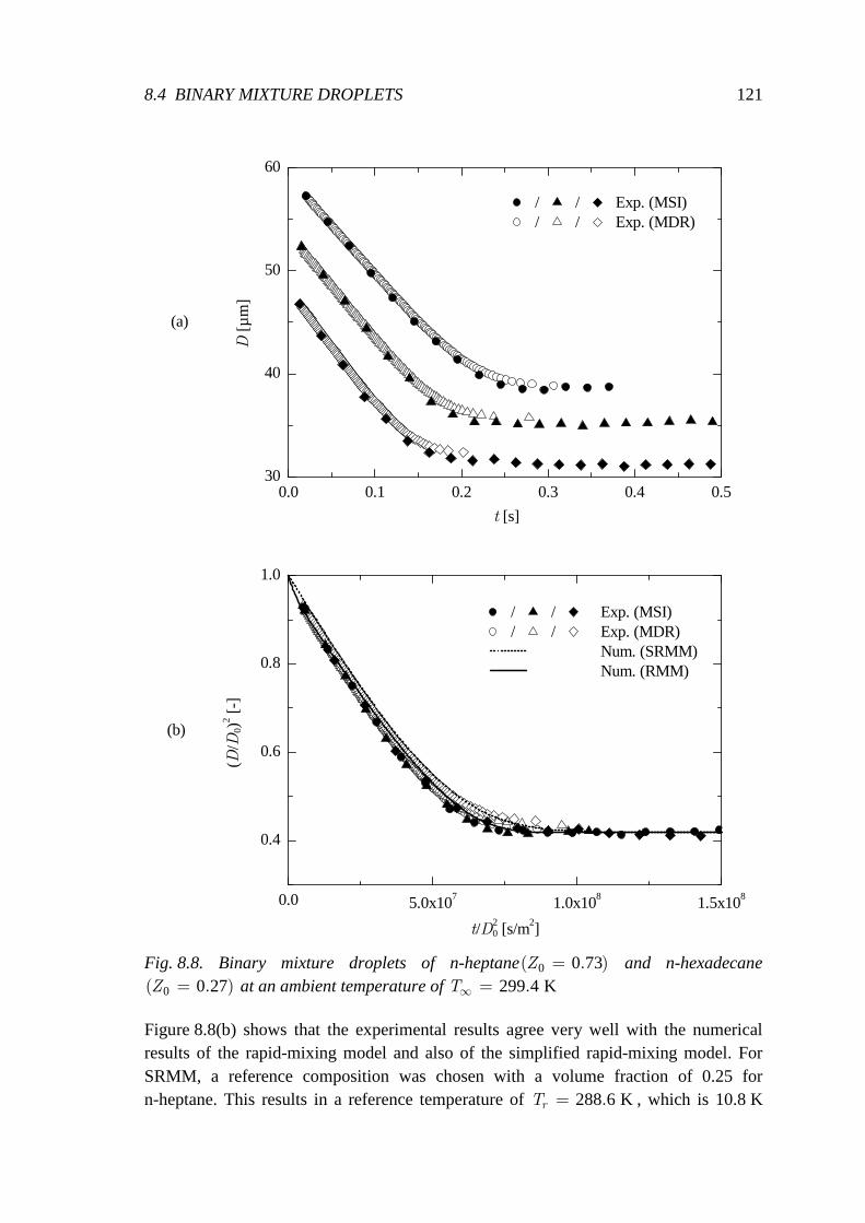
8.4 BINARY MIXTURE DROPLETS 121

0.0 0.1 0.2 0.3 0.4 0.530

40

50

60

0.0 5.0x107 1.0x108 1.5x108

0.4

0.6

0.8

1.0

(b)

D [µ

m]

t [s]

/ / Exp. (MSI)/ / Exp. (MDR)

(a)

(D/D

0)2 [-

]

t/D20 [s/m2]

/ / Exp. (MSI)/ / Exp. (MDR)

Num. (SRMM) Num. (RMM)

Fig. 8.8. Binary mixture droplets of n-heptane0 0 73( . )=Z and n-hexadecane

0 0 27( . )=Z at an ambient temperature of 299 4 K.∞ =T

Figure 8.8(b) shows that the experimental results agree very well with the numerical results of the rapid-mixing model and also of the simplified rapid-mixing model. For SRMM, a reference composition was chosen with a volume fraction of 0.25 for n-heptane. This results in a reference temperature of 288 6 K.=rT , which is 10.8 K

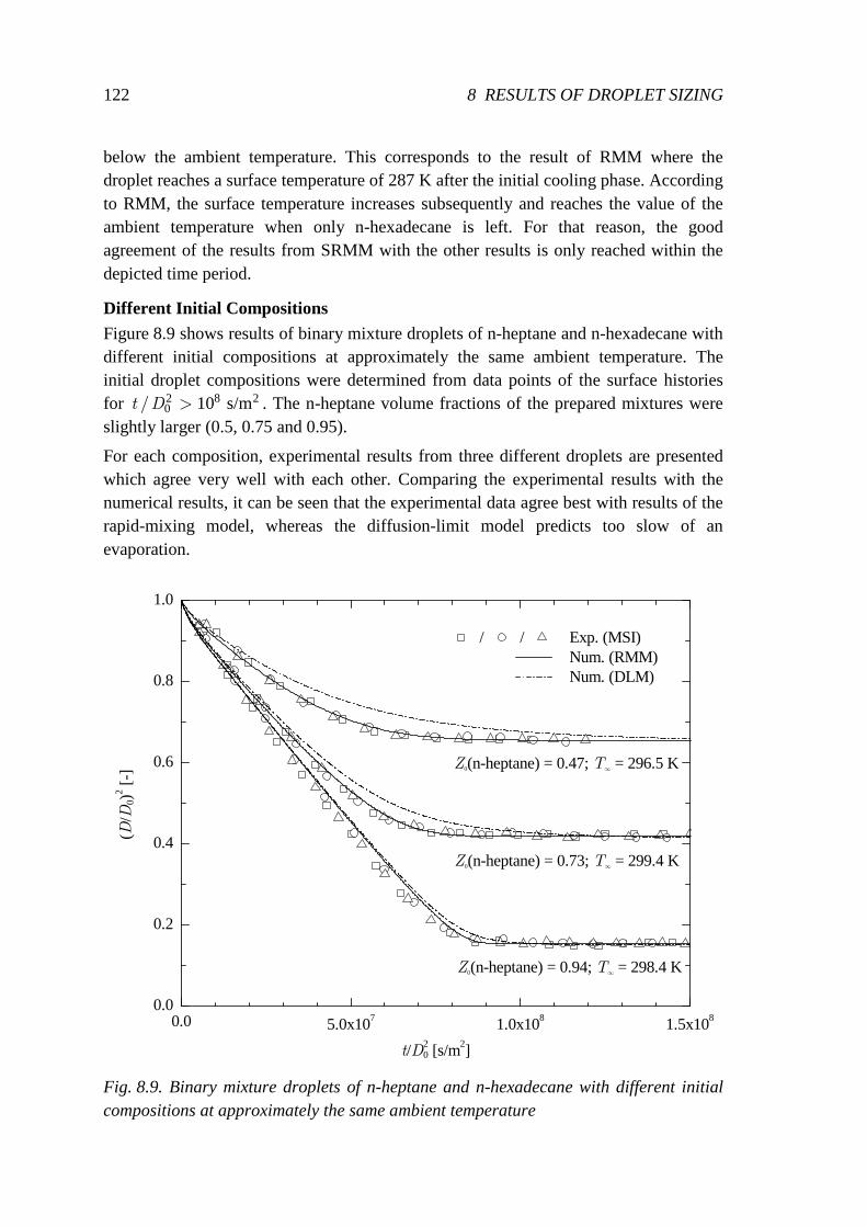
122 8 RESULTS OF DROPLET SIZING

below the ambient temperature. This corresponds to the result of RMM where the droplet reaches a surface temperature of 287 K after the initial cooling phase. According to RMM, the surface temperature increases subsequently and reaches the value of the ambient temperature when only n-hexadecane is left. For that reason, the good agreement of the results from SRMM with the other results is only reached within the depicted time period.

Different Initial Compositions Figure 8.9 shows results of binary mixture droplets of n-heptane and n-hexadecane with different initial compositions at approximately the same ambient temperature. The initial droplet compositions were determined from data points of the surface histories for 2 8 2

0 10 s/m/ >t D . The n-heptane volume fractions of the prepared mixtures were slightly larger (0.5, 0.75 and 0.95).

For each composition, experimental results from three different droplets are presented which agree very well with each other. Comparing the experimental results with the numerical results, it can be seen that the experimental data agree best with results of the rapid-mixing model, whereas the diffusion-limit model predicts too slow of an evaporation.

0.0 5.0x107 1.0x108 1.5x1080.0

0.2

0.4

0.6

0.8

1.0

Z0(n-heptane) = 0.94; T∞ = 298.4 K

Z0(n-heptane) = 0.73; T∞ = 299.4 K

Z0(n-heptane) = 0.47; T∞ = 296.5 K

(D/D

0)2 [-

]

t/D20 [s/m2]

/ / Exp. (MSI) Num. (RMM) Num. (DLM)

Fig. 8.9. Binary mixture droplets of n-heptane and n-hexadecane with different initial compositions at approximately the same ambient temperature

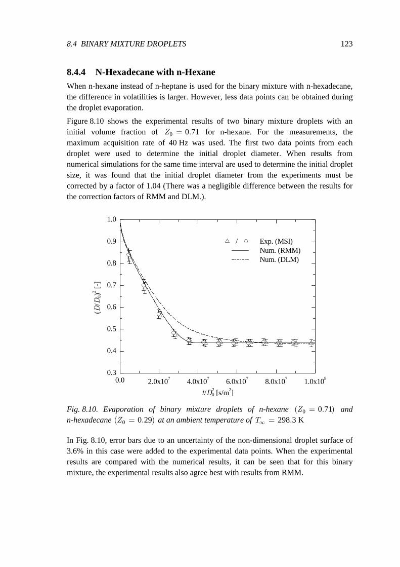
8.4 BINARY MIXTURE DROPLETS 123

8.4.4 N-Hexadecane with n-Hexane When n-hexane instead of n-heptane is used for the binary mixture with n-hexadecane, the difference in volatilities is larger. However, less data points can be obtained during the droplet evaporation.

Figure 8.10 shows the experimental results of two binary mixture droplets with an initial volume fraction of 0 0 71.=Z for n-hexane. For the measurements, the maximum acquisition rate of 40 Hz was used. The first two data points from each droplet were used to determine the initial droplet diameter. When results from numerical simulations for the same time interval are used to determine the initial droplet size, it was found that the initial droplet diameter from the experiments must be corrected by a factor of 1.04 (There was a negligible difference between the results for the correction factors of RMM and DLM.).

0.0 2.0x107 4.0x107 6.0x107 8.0x107 1.0x1080.3

0.4

0.5

0.6

0.7

0.8

0.9

1.0

(D/D

0)2 [-

]

t/D20 [s/m2]

/ Exp. (MSI) Num. (RMM) Num. (DLM)

Fig. 8.10. Evaporation of binary mixture droplets of n-hexane 0 0 71( . )=Z and n-hexadecane 0 0 29( . )=Z at an ambient temperature of 298 3 K.∞ =T

In Fig. 8.10, error bars due to an uncertainty of the non-dimensional droplet surface of 3.6% in this case were added to the experimental data points. When the experimental results are compared with the numerical results, it can be seen that for this binary mixture, the experimental results also agree best with results from RMM.

124 8 RESULTS OF DROPLET SIZING

8.4.5 Property Variation of DLM In the previous sections, it was seen that experimental results agreed very well with results from the rapid-mixing model whereas the diffusion-limit model predicted a too slow evaporation rate. However, the rapid-mixing model is physically not reasonable due to its assumption of infinite diffusion inside the droplet. For that reason, this section investigates whether a good agreement between experimental results and results from the diffusion-limit model can be reached by varying parameters for the numerical simulations with this model.

In the first part of this section, the ambient temperature was varied for the numerical simulations. This was done because, in addition to the uncertainties of the size measurements shown by error bars in the previous section, there is also an uncertainty of the temperature measurement. In the second part, the liquid mass diffusion is increased artificially. The liquid mass diffusion is the major process which causes the difference in the predictions of the rapid-mixing and diffusion-limit model for the investigated mixture droplets. It is possible that the liquid mass diffusion is underpredicted due to an inaccurate property evaluation method or due to neglecting convective mass transport inside the droplet.

For the investigations of this section, the case of a binary mixture droplet of n-hexadecane with n-heptane with an initial volume fraction of 0 0 47.Z = of n-heptane was selected. In this case, there was a significant difference between the predictions of the droplet surface histories of RMM and DLM. Figure 8.11(a) shows results where the ambient temperature was varied. It can be seen that a large increase of the ambient temperature was necessary to reach good agreement with the experimental results. This increase was much larger than the uncertainty of the ambient temperature of ±0.5 K. Therefore, the discrepancies between the experimental results and the results from the diffusion-limit model cannot be due to the uncertainty of the temperature measurement.

Next, liquid mass diffusion was considered. For the numerical simulations, the binary liquid diffusion coefficients at infinite dilution were calculated with the estimation method of Lusis and Ratcliff (1968). When Matthews and Akgerman (1987) compared this method with other methods for various binary n-alkane mixtures at various temperatures, they found that the method of Lusis and Ratcliff was one of the best methods. However, for the present mixture, with large differences in volatilities of the substances, there was a noticeable underprediction of the diffusion coefficients. Comparing the results from this method with experimental data at a temperature of 298 K (Vadovic and Colver, 1973), the diffusion coefficient of n-hexadecane in n-heptane was underpredicted by only 2%, however, the diffusion coefficient of n-heptane in n-hexadecane was underestimated by 33%.

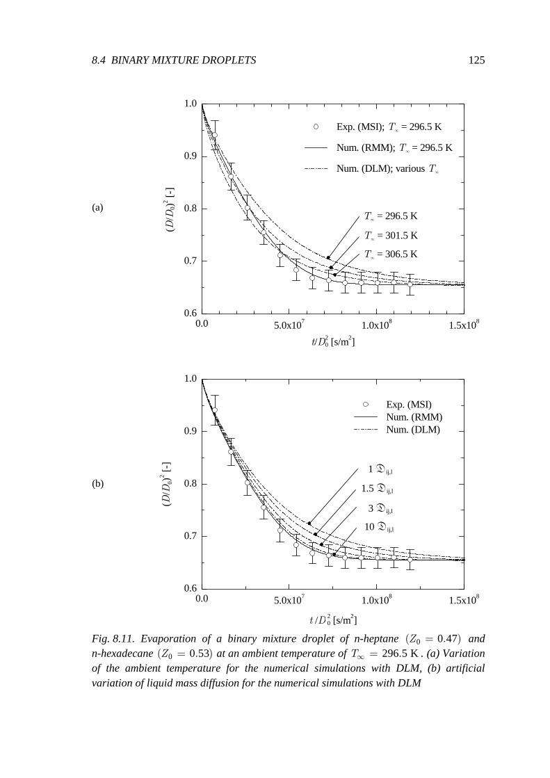
8.4 BINARY MIXTURE DROPLETS 125

0.0 5.0x107 1.0x108 1.5x1080.6

0.7

0.8

0.9

1.0

T∞ = 306.5 K

T∞ = 301.5 K

T∞ = 296.5 K

(D/D

0)2 [-

]

t/D20 [s/m2]

Exp. (MSI); T∞ = 296.5 K

Num. (RMM); T∞ = 296.5 K

Num. (DLM); various T∞

(a)

0.0 5.0x107 1.0x108 1.5x1080.6

0.7

0.8

0.9

1.0

1 aij,l

3 aij,l

10 aij,l

1.5 aij,l

(D/D

0)2 [-

]

t /D 2 0 [s/m2]

Exp. (MSI)Num. (RMM)Num. (DLM)

(b)

Fig. 8.11. Evaporation of a binary mixture droplet of n-heptane 0 0 47( . )=Z and n-hexadecane 0 0 53( . )=Z at an ambient temperature of 296 5 K.∞ =T . (a) Variation of the ambient temperature for the numerical simulations with DLM, (b) artificial variation of liquid mass diffusion for the numerical simulations with DLM

126 8 RESULTS OF DROPLET SIZING

For the calculation of the liquid mass diffusion at various compositions, the correlation proposed by Vignes (1966) was used. According to Poling (2000), this correlation gives excellent results for ideal mixtures such as mixtures of n-alkanes. Thus, no further increase of the error for the calculation of liquid mass diffusion was expected.

Although the liquid mass diffusion was underpredicted by the selected estimation method for the liquid diffusion coefficients, this error was not responsible for the discrepancy between the results from the experiments and the diffusion-limit model. This can be seen in Fig. 8.11(b) which shows results where the liquid mass diffusion for the computations with the diffusion-limit model was increased artificially. This was done by multiplying the diffusion coefficients obtained by the estimation method of Lusis and Ratcliff (1968) with a constant factor. Figure 8.11(b) shows that an increase of the liquid mass diffusion by a factor of at least three was necessary to reach good agreement with the experimental results.

According to Sirignano (1978), a factor of three is the maximum increase in heat and mass transfer due to circulation inside the droplet. In this respect, it is interesting to note that for the present mixture an increase of the diffusive heat transfer for the numerical results would not be noticeable due to the large liquid Lewis number. Sirignano (1978) investigated internal circulation due to a flow around the droplet. As was shown previously, a flow around the droplets only occurs during a short time period before the measurements start and with a relatively low Reynolds number. For these reasons, internal circulation cannot be generated or maintained by an external flow in the present case. However, internal circulation can still be the reason for an increase of the mass transfer inside the droplet. It is assumed that during droplet generation the liquid starts to circulate and continues to do so during droplet evaporation. It is also possible that effects which are not considered in the numerical models play an important role in this case. For example, an initially inhomogeneous distribution of the substances inside the droplets might lead to internal circulation driven by the Marangoni effect.

Although other liquid properties might be incorrectly predicted for the numerical simulations with DLM, it is believed that the underprediction of the mass transport in the droplet is the most probable cause for a deviation of the results from the diffusion-limit model compared to experimental data. For further investigations on this subject, the distribution of the liquid inside the droplet was investigated using rainbow refractometry. These results are presented in section 9.3.

8.5 Ternary Mixture Droplets This section presents results from ternary mixture droplets. It contains two parts: the first part considers ternary mixture droplets with different substances and the second part shows the influence of the ambient temperature.

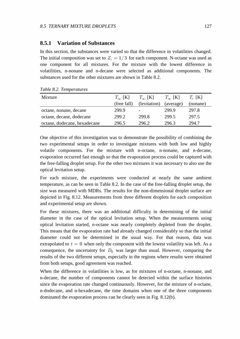
8.5 TERNARY MIXTURE DROPLETS 127

8.5.1 Variation of Substances In this section, the substances were varied so that the difference in volatilities changed. The initial composition was set to 1 3/=iZ for each component. N-octane was used as one component for all mixtures. For the mixture with the lowest difference in volatilities, n-nonane and n-decane were selected as additional components. The substances used for the other mixtures are shown in Table 8.2.

Table 8.2. Temperatures

Mixture ∞T [K] (free fall)

∞T [K] (levitation)

∞T [K] (average)

rT [K] (nonane)

octane, nonane, decane 299.9 - 299.9 297.8 octane, decane, dodecane 299.2 299.8 299.5 297.5 octane, dodecane, hexadecane 296.5 296.2 296.3 294.7

One objective of this investigation was to demonstrate the possibility of combining the two experimental setups in order to investigate mixtures with both low and highly volatile components. For the mixture with n-octane, n-nonane, and n-decane, evaporation occurred fast enough so that the evaporation process could be captured with the free-falling droplet setup. For the other two mixtures it was necessary to also use the optical levitation setup.

For each mixture, the experiments were conducted at nearly the same ambient temperature, as can be seen in Table 8.2. In the case of the free-falling droplet setup, the size was measured with MDRs. The results for the non-dimensional droplet surface are depicted in Fig. 8.12. Measurements from three different droplets for each composition and experimental setup are shown.

For these mixtures, there was an additional difficulty in determining of the initial diameter in the case of the optical levitation setup. When the measurements using optical levitation started, n-octane was nearly completely depleted from the droplet. This means that the evaporation rate had already changed considerably so that the initial diameter could not be determined in the usual way. For that reason, data was extrapolated to 0t = when only the component with the lowest volatility was left. As a consequence, the uncertainty for 0D was larger than usual. However, comparing the results of the two different setups, especially in the regions where results were obtained from both setups, good agreement was reached.

When the difference in volatilities is low, as for mixtures of n-octane, n-nonane, and n-decane, the number of components cannot be detected within the surface histories since the evaporation rate changed continuously. However, for the mixture of n-octane, n-dodecane, and n-hexadecane, the time domains when one of the three components dominated the evaporation process can be clearly seen in Fig. 8.12(b).

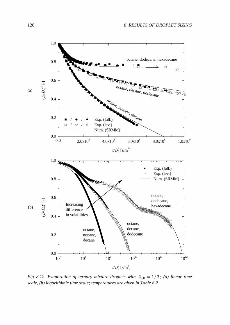
128 8 RESULTS OF DROPLET SIZING

0.0 2.0x108 4.0x108 6.0x108 8.0x108 1.0x1090.0

0.2

0.4

0.6

0.8

1.0

107 108 109 1010 1011 10120.0

0.2

0.4

0.6

0.8

1.0

octane, decane, dodecane

(b)

(D

/D0)

2 [-]

t/D20 [s/m2]

/ / Exp. (fall.)/ / Exp. (lev.)

Num. (SRMM)

octane, dodecane, hexadecane

octane, nonane, decane

(a)

Increasing differencein volatilities

octane, nonane, decane

octane, decane, dodecane

octane, dodecane, hexadecane

(D/D

0)2 [-

]

t/D20 [s/m2]

Exp. (fall.)Exp. (lev.)Num. (SRMM)

Fig. 8.12. Evaporation of ternary mixture droplets with 0 1 3, /iZ = ; (a) linear time scale, (b) logarithimic time scale; temperatures are given in Table 8.2

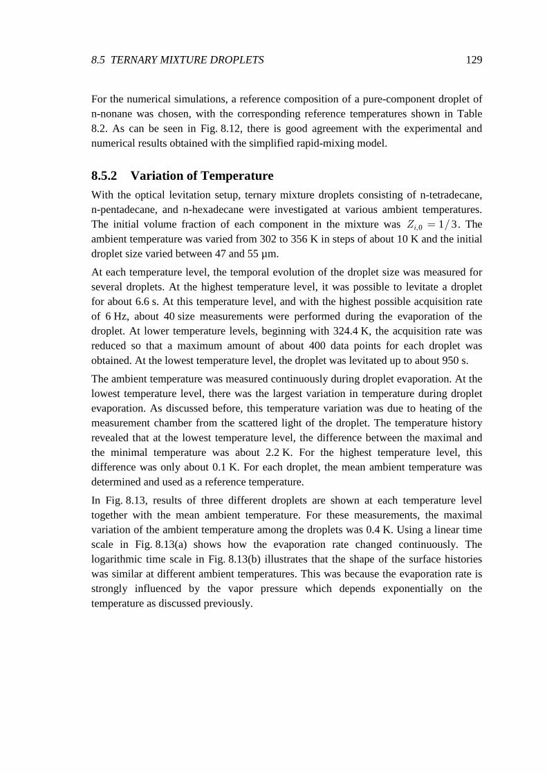
8.5 TERNARY MIXTURE DROPLETS 129

For the numerical simulations, a reference composition of a pure-component droplet of n-nonane was chosen, with the corresponding reference temperatures shown in Table 8.2. As can be seen in Fig. 8.12, there is good agreement with the experimental and numerical results obtained with the simplified rapid-mixing model.

8.5.2 Variation of Temperature With the optical levitation setup, ternary mixture droplets consisting of n-tetradecane, n-pentadecane, and n-hexadecane were investigated at various ambient temperatures. The initial volume fraction of each component in the mixture was 0 1 3, /=iZ . The ambient temperature was varied from 302 to 356 K in steps of about 10 K and the initial droplet size varied between 47 and 55 µm.

At each temperature level, the temporal evolution of the droplet size was measured for several droplets. At the highest temperature level, it was possible to levitate a droplet for about 6.6 s. At this temperature level, and with the highest possible acquisition rate of 6 Hz, about 40 size measurements were performed during the evaporation of the droplet. At lower temperature levels, beginning with 324.4 K, the acquisition rate was reduced so that a maximum amount of about 400 data points for each droplet was obtained. At the lowest temperature level, the droplet was levitated up to about 950 s.

The ambient temperature was measured continuously during droplet evaporation. At the lowest temperature level, there was the largest variation in temperature during droplet evaporation. As discussed before, this temperature variation was due to heating of the measurement chamber from the scattered light of the droplet. The temperature history revealed that at the lowest temperature level, the difference between the maximal and the minimal temperature was about 2.2 K. For the highest temperature level, this difference was only about 0.1 K. For each droplet, the mean ambient temperature was determined and used as a reference temperature.

In Fig. 8.13, results of three different droplets are shown at each temperature level together with the mean ambient temperature. For these measurements, the maximal variation of the ambient temperature among the droplets was 0.4 K. Using a linear time scale in Fig. 8.13(a) shows how the evaporation rate changed continuously. The logarithmic time scale in Fig. 8.13(b) illustrates that the shape of the surface histories was similar at different ambient temperatures. This was because the evaporation rate is strongly influenced by the vapor pressure which depends exponentially on the temperature as discussed previously.

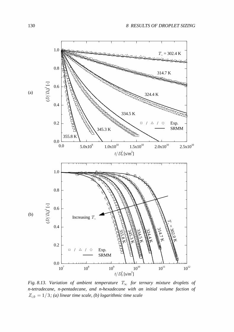
130 8 RESULTS OF DROPLET SIZING

107 108 109 1010 1011 10120.0

0.2

0.4

0.6

0.8

1.0

0.0 5.0x109 1.0x1010 1.5x1010 2.0x1010 2.5x10100.0

0.2

0.4

0.6

0.8

1.0

334.5 K

324.4 K

314.7 K

T∞ = 302.0 K

345.3 K

(D/D

0)2 [-

]

t/D20 [s/m2]

/ / Exp. SRMM

355.8 K

Increasing T∞

(D/D

0)2 [-

]

t/D20 [s/m2]

/ / Exp. SRMM

355.8 K

345.3 K

334.5 K

324.4 K

314.7 K

T∞ = 302.4 K

(a)

(b)

Fig. 8.13. Variation of ambient temperature ∞T for ternary mixture droplets of n-tetradecane, n-pentadecane, and n-hexadecane with an initial volume faction of

0 1 3, /=iZ ; (a) linear time scale, (b) logarithmic time scale

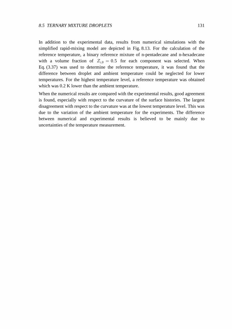
8.5 TERNARY MIXTURE DROPLETS 131

In addition to the experimental data, results from numerical simulations with the simplified rapid-mixing model are depicted in Fig. 8.13. For the calculation of the reference temperature, a binary reference mixture of n-pentadecane and n-hexadecane with a volume fraction of 0 0 5, .=iZ for each component was selected. When Eq. (3.37) was used to determine the reference temperature, it was found that the difference between droplet and ambient temperature could be neglected for lower temperatures. For the highest temperature level, a reference temperature was obtained which was 0.2 K lower than the ambient temperature.

When the numerical results are compared with the experimental results, good agreement is found, especially with respect to the curvature of the surface histories. The largest disagreement with respect to the curvature was at the lowest temperature level. This was due to the variation of the ambient temperature for the experiments. The difference between numerical and experimental results is believed to be mainly due to uncertainties of the temperature measurement.

133

9 Results of Rainbow Refractometry In addition to droplet size measurements, Rainbow Refractometry (RRF) was applied in order to gain further information on the droplet. In the first two sections of this chapter, a uniform refractive index within the droplet is assumed. From the measurement of the refractive index with RRF, the droplet temperature was determined for a pure-component droplet. This is presented in the first section.

In the second section, the droplet temperature was assumed to be constant for a binary mixture droplet with a low evaporation rate. In this case, the droplet composition can be determined from the refractive index measurements.

RRF is very sensitive to inhomogeneous distributions of the refractive index within droplets. Therefore, RRF was used for droplets where such inhomogeneous distributions of the refractive index were predicted by DLM. Results of these measurements are presented in the last section.

9.1 Droplet Temperature In this section, results of pure-component droplets of 1-hexadecene are presented. Assuming a uniform refractive index, the droplet temperature was determined from the measurements with RRF. Measurements were performed at five different temperature levels. At each temperature level, several droplets were investigated. The diameters of the droplets were within 35 and 40 µm. The measurements were conducted with the optical levitation setup.

Results from measurements of three different droplets at each temperature level are depicted in Fig. 9.1. Using RRF, several temperature measurements were performed for a single droplet. The measurement period was short enough in order to ensure a constant temperature within the observation chamber. For a single droplet, about 70 temperature measurements were performed at the lowest temperature level and about 20 measurements at the highest temperature level. From these measurements, the mean temperature was determined and is shown in the figure. The error bars are determined from the standard deviation S , where the magnitude of the error bars corresponds to ± 2S (95% confidence interval). The resulting error for the temperature is in the range 1 1 K 1.8 K. < <Tδ .

For a comparison of the results from rainbow refractometry, the droplet temperature was simultaneously determined by a different method. At first, the evaporation rate was obtained from measurements with MSI. Then, the droplet temperature was calculated with D2M.

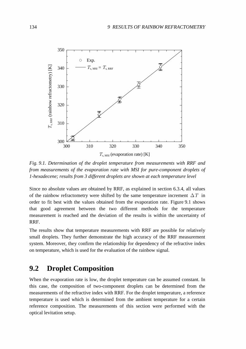
134 9 RESULTS OF RAINBOW REFRACTOMETRY

300 310 320 330 340 350300

310

320

330

340

350

Exp.

Ts, MSI = Ts, RRF

T

s, R

RF (

rain

bo

w r

efra

cto

met

ry)

[K]

Ts, MSI (evaporation rate) [K] Fig. 9.1. Determination of the droplet temperature from measurements with RRF and from measurements of the evaporation rate with MSI for pure-component droplets of 1-hexadecene; results from 3 different droplets are shown at each temperature level

Since no absolute values are obtained by RRF, as explained in section 6.3.4, all values of the rainbow refractometry were shifted by the same temperature increment ∆T in order to fit best with the values obtained from the evaporation rate. Figure 9.1 shows that good agreement between the two different methods for the temperature measurement is reached and the deviation of the results is within the uncertainty of RRF.

The results show that temperature measurements with RRF are possible for relatively small droplets. They further demonstrate the high accuracy of the RRF measurement system. Moreover, they confirm the relationship for dependency of the refractive index on temperature, which is used for the evaluation of the rainbow signal.

9.2 Droplet Composition When the evaporation rate is low, the droplet temperature can be assumed constant. In this case, the composition of two-component droplets can be determined from the measurements of the refractive index with RRF. For the droplet temperature, a reference temperature is used which is determined from the ambient temperature for a certain reference composition. The measurements of this section were performed with the optical levitation setup.

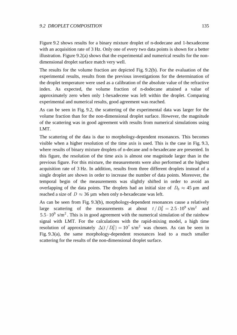
9.2 DROPLET COMPOSITION 135

Figure 9.2 shows results for a binary mixture droplet of n-dodecane and 1-hexadecene with an acquisition rate of 3 Hz. Only one of every two data points is shown for a better illustration. Figure 9.2(a) shows that the experimental and numerical results for the non-dimensional droplet surface match very well.

The results for the volume fraction are depicted Fig. 9.2(b). For the evaluation of the experimental results, results from the previous investigations for the determination of the droplet temperature were used as a calibration of the absolute value of the refractive index. As expected, the volume fraction of n-dodecane attained a value of approximately zero when only 1-hexadecene was left within the droplet. Comparing experimental and numerical results, good agreement was reached.

As can be seen in Fig. 9.2, the scattering of the experimental data was larger for the volume fraction than for the non-dimensional droplet surface. However, the magnitude of the scattering was in good agreement with results from numerical simulations using LMT.

The scattering of the data is due to morphology-dependent resonances. This becomes visible when a higher resolution of the time axis is used. This is the case in Fig. 9.3, where results of binary mixture droplets of n-decane and n-hexadecane are presented. In this figure, the resolution of the time axis is almost one magnitude larger than in the previous figure. For this mixture, the measurements were also performed at the highest acquisition rate of 3 Hz. In addition, results from three different droplets instead of a single droplet are shown in order to increase the number of data points. Moreover, the temporal begin of the measurements was slightly shifted in order to avoid an overlapping of the data points. The droplets had an initial size of 0 45 µm≈D and reached a size of 36 µm≈D when only n-hexadecane was left.

As can be seen from Fig. 9.3(b), morphology-dependent resonances cause a relatively large scattering of the measurements at about 2 9 2

0 2 5 10 s/m/ .t D = ⋅ and 9 25 5 10 s/m. ⋅ . This is in good agreement with the numerical simulation of the rainbow

signal with LMT. For the calculations with the rapid-mixing model, a high time resolution of approximately 2 7 2

0 10 s/m( / )t D∆ = was chosen. As can be seen in Fig. 9.3(a), the same morphology-dependent resonances lead to a much smaller scattering for the results of the non-dimensional droplet surface.

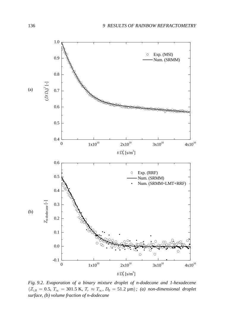
136 9 RESULTS OF RAINBOW REFRACTOMETRY

0 1x1010 2x1010 3x1010 4x10100.4

0.5

0.6

0.7

0.8

0.9

1.0

0 1x1010 2x1010 3x1010 4x1010-0.1

0.0

0.1

0.2

0.3

0.4

0.5

0.6

(b)

(D/D

0)2 [-

]

t/D20 [s/m2]

Exp. (MSI) Num. (SRMM)

(a)

Zn-

dode

cane

[-]

t/D20 [s/m2]

Exp. (RRF) Num. (SRMM) Num. (SRMM+LMT+RRF)

Fig. 9.2. Evaporation of a binary mixture droplet of n-dodecane and 1-hexadecene

0 00 5, 301 5 K, , 51 2 µm,( . . . )i rZ T T T D∞ ∞= = ≈ = ; (a) non-dimensional droplet surface, (b) volume fraction of n-dodecane

9.2 DROPLET COMPOSITION 137

0 1x109 2x109 3x109 4x109 5x109 6x1090.6

0.7

0.8

0.9

1.0

0 1x109 2x109 3x109 4x109 5x109 6x109-0.1

0.0

0.1

0.2

0.3

0.4

0.5

0.6

(b)

(D/D

0)2 [-

]

t/D20 [s/m2]

/ / Exp. (MSI) Num. (RMM) Num. (RMM+LMT+MSI)

(a)

Zn-

deca

ne [-

]

t/D20 [s/m2]

/ / Exp. (RRF) Num. (RMM) Num. (RMM+LMT+RRF)

Fig. 9.3. Evaporation of binary mixture droplets of n-decane and n-hexadecane

0 n-decane0 5, 300 8 K, 300 5 K for 0 25,( . . . . )i rZ T T Z∞= = = = ; (a) non-dimensional droplet surface, (b) volume fraction of n-decane

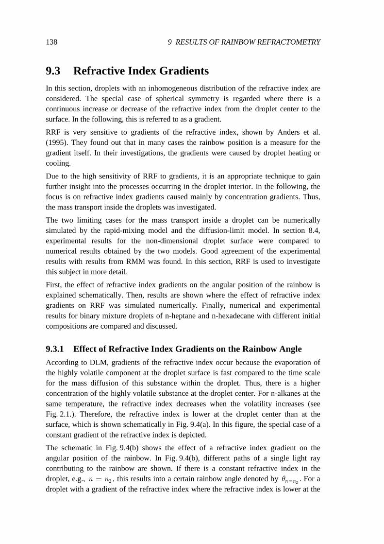
138 9 RESULTS OF RAINBOW REFRACTOMETRY

9.3 Refractive Index Gradients In this section, droplets with an inhomogeneous distribution of the refractive index are considered. The special case of spherical symmetry is regarded where there is a continuous increase or decrease of the refractive index from the droplet center to the surface. In the following, this is referred to as a gradient.

RRF is very sensitive to gradients of the refractive index, shown by Anders et al. (1995). They found out that in many cases the rainbow position is a measure for the gradient itself. In their investigations, the gradients were caused by droplet heating or cooling.

Due to the high sensitivity of RRF to gradients, it is an appropriate technique to gain further insight into the processes occurring in the droplet interior. In the following, the focus is on refractive index gradients caused mainly by concentration gradients. Thus, the mass transport inside the droplets was investigated.

The two limiting cases for the mass transport inside a droplet can be numerically simulated by the rapid-mixing model and the diffusion-limit model. In section 8.4, experimental results for the non-dimensional droplet surface were compared to numerical results obtained by the two models. Good agreement of the experimental results with results from RMM was found. In this section, RRF is used to investigate this subject in more detail.

First, the effect of refractive index gradients on the angular position of the rainbow is explained schematically. Then, results are shown where the effect of refractive index gradients on RRF was simulated numerically. Finally, numerical and experimental results for binary mixture droplets of n-heptane and n-hexadecane with different initial compositions are compared and discussed.

9.3.1 Effect of Refractive Index Gradients on the Rainbow Angle According to DLM, gradients of the refractive index occur because the evaporation of the highly volatile component at the droplet surface is fast compared to the time scale for the mass diffusion of this substance within the droplet. Thus, there is a higher concentration of the highly volatile substance at the droplet center. For n-alkanes at the same temperature, the refractive index decreases when the volatility increases (see Fig. 2.1.). Therefore, the refractive index is lower at the droplet center than at the surface, which is shown schematically in Fig. 9.4(a). In this figure, the special case of a constant gradient of the refractive index is depicted.

The schematic in Fig. 9.4(b) shows the effect of a refractive index gradient on the angular position of the rainbow. In Fig. 9.4(b), different paths of a single light ray contributing to the rainbow are shown. If there is a constant refractive index in the droplet, e.g., 2=n n , this results into a certain rainbow angle denoted by

2=n nθ . For a droplet with a gradient of the refractive index where the refractive index is lower at the

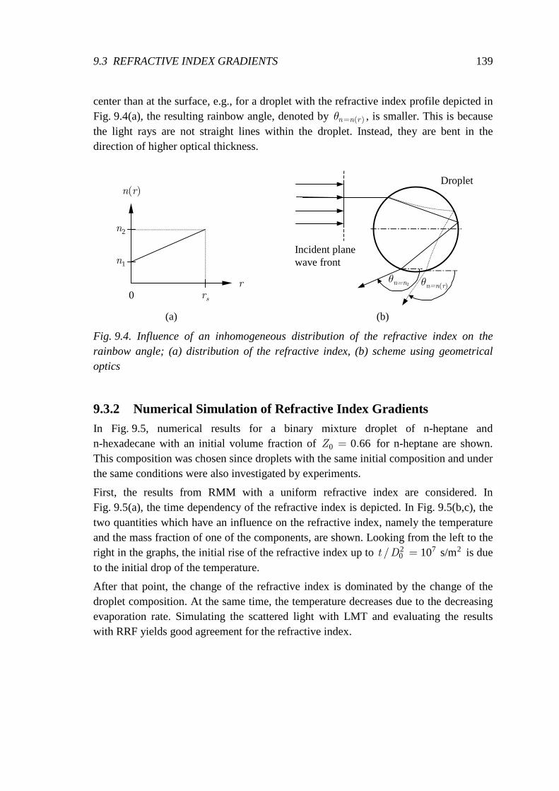
9.3 REFRACTIVE INDEX GRADIENTS 139

center than at the surface, e.g., for a droplet with the refractive index profile depicted in Fig. 9.4(a), the resulting rainbow angle, denoted by ( )=n n rθ , is smaller. This is because the light rays are not straight lines within the droplet. Instead, they are bent in the direction of higher optical thickness.

Incident planewave front

θn=n2

Droplet

θn=n(r)

(b)

n1

n(r)

r

n2

rs0

(a) Fig. 9.4. Influence of an inhomogeneous distribution of the refractive index on the rainbow angle; (a) distribution of the refractive index, (b) scheme using geometrical optics

9.3.2 Numerical Simulation of Refractive Index Gradients In Fig. 9.5, numerical results for a binary mixture droplet of n-heptane and n-hexadecane with an initial volume fraction of 0 0 66.=Z for n-heptane are shown. This composition was chosen since droplets with the same initial composition and under the same conditions were also investigated by experiments.

First, the results from RMM with a uniform refractive index are considered. In Fig. 9.5(a), the time dependency of the refractive index is depicted. In Fig. 9.5(b,c), the two quantities which have an influence on the refractive index, namely the temperature and the mass fraction of one of the components, are shown. Looking from the left to the right in the graphs, the initial rise of the refractive index up to 2 7 2

0 10 s/m/ =t D is due to the initial drop of the temperature.

After that point, the change of the refractive index is dominated by the change of the droplet composition. At the same time, the temperature decreases due to the decreasing evaporation rate. Simulating the scattered light with LMT and evaluating the results with RRF yields good agreement for the refractive index.

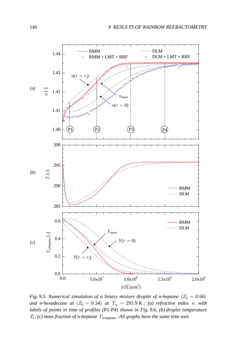
140 9 RESULTS OF RAINBOW REFRACTOMETRY

1.40

1.41

1.42

1.43

1.44

285

290

295

300

0.0 5.0x107 1.0x108 1.5x108 2.0x1080.0

0.2

0.4

0.6

nmean

n(r = 0)

DLM DLM + LMT + RRF

n [-

] RMM RMM + LMT + RRF

n(r = rs)

P1 P2 P3 P4

RMM DLM

Tl [

-]

Y(r = 0)

Y(r = rs)

Ymean

RMM DLM

Yn

-hep

tan

e [-]

t/D20 [s/m2]

(a)

(b)

(c)

Fig. 9.5. Numerical simulation of a binary mixture droplet of n-heptane 0 0 66( . )=Z and n-hexadecane at 0 0 34( . )=Z at 295 9 K.∞ =T ; (a) refractive index n with labels of points in time of profiles (P1-P4) shown in Fig. 9.6, (b) droplet temperature

lT , (c) mass fraction of n-heptane n-heptaneY . All graphs have the same time axis

9.3 REFRACTIVE INDEX GRADIENTS 141

Considering internal heat and mass diffusion with DLM yields significantly different results. Since the internal heat transfer occurs much faster than the mass diffusion, the temperature is nearly uniform within the droplet. For that reason, the temperature can be represented by a single curve, as is shown in Fig. 9.5(b). With respect to the composition of the droplets, the mass fraction is considerably different between the center and the surface of the droplet, as shown in Fig. 9.5(c). As a consequence, the refractive index is also different at the center and at the surface. Radial profiles of the refractive index at certain time points are shown in Fig. 9.6.

0.0 0.2 0.4 0.6 0.8 1.01.40

1.41

1.42

1.43

1.44

t/D20 = 0

t/D20 = 107 s/m2

t/D20 = 5x107 s/m2

t/D20 = 108 s/m2

t/D20 = 1.5x108 s/m2

n [-

]

r/rs [-]

P3

P2

P1

P4

Fig. 9.6. Refractive index profiles from numerical simulations with DLM for the droplet of Fig. 9.5

When the scattered light is determined using LMT and evaluated with RRF for the refractive index profiles, values for the refractive index are obtained which are smaller than any of the values of the profiles as can be seen in Fig. 9.5(a). This is due to the shape of the profiles. The refractive index profiles have their largest gradient close to the droplet surface. Most of the light which is responsible for the rainbow travels through this region.

Comparing the results of RMM and DLM for the refractive index from RRF, one can see that there is a large difference between the results. This difference is much larger than for the non-dimensional droplet surface as shown in the following. For that reason, concentration gradients can be detected more distinctly by measurements with RRF than by droplet size measurements.

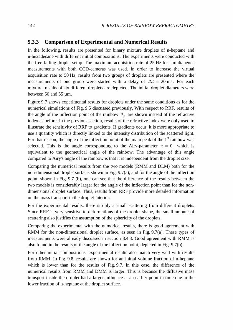
142 9 RESULTS OF RAINBOW REFRACTOMETRY

9.3.3 Comparison of Experimental and Numerical Results In the following, results are presented for binary mixture droplets of n-heptane and n-hexadecane with different initial compositions. The experiments were conducted with the free-falling droplet setup. The maximum acquisition rate of 25 Hz for simultaneous measurements with both CCD-cameras was used. In order to increase the virtual acquisition rate to 50 Hz, results from two groups of droplets are presented where the measurements of one group were started with a delay of 20 ms∆ =t . For each mixture, results of six different droplets are depicted. The initial droplet diameters were between 50 and 55 µm.

Figure 9.7 shows experimental results for droplets under the same conditions as for the numerical simulations of Fig. 9.5 discussed previously. With respect to RRF, results of the angle of the inflection point of the rainbow ipθ are shown instead of the refractive index as before. In the previous section, results of the refractive index were only used to illustrate the sensitivity of RRF to gradients. If gradients occur, it is more appropriate to use a quantity which is directly linked to the intensity distribution of the scattered light. For that reason, the angle of the inflection point of the main peak of the 1st rainbow was selected. This is the angle corresponding to the Airy-parameter 0=z , which is equivalent to the geometrical angle of the rainbow. The advantage of this angle compared to Airy's angle of the rainbow is that it is independent from the droplet size.

Comparing the numerical results from the two models (RMM and DLM) both for the non-dimensional droplet surface, shown in Fig. 9.7(a), and for the angle of the inflection point, shown in Fig. 9.7 (b), one can see that the difference of the results between the two models is considerably larger for the angle of the inflection point than for the non-dimensional droplet surface. Thus, results from RRF provide more detailed information on the mass transport in the droplet interior.

For the experimental results, there is only a small scattering from different droplets. Since RRF is very sensitive to deformations of the droplet shape, the small amount of scattering also justifies the assumption of the sphericity of the droplets.

Comparing the experimental with the numerical results, there is good agreement with RMM for the non-dimensional droplet surface, as seen in Fig. 9.7(a). These types of measurements were already discussed in section 8.4.3. Good agreement with RMM is also found in the results of the angle of the inflection point, depicted in Fig. 9.7(b).

For other initial compositions, experimental results also match very well with results from RMM. In Fig. 9.8, results are shown for an initial volume fraction of n-heptane which is lower than for the results of Fig. 9.7. In this case, the difference of the numerical results from RMM and DMM is larger. This is because the diffusive mass transport inside the droplet had a larger influence at an earlier point in time due to the lower fraction of n-heptane at the droplet surface.

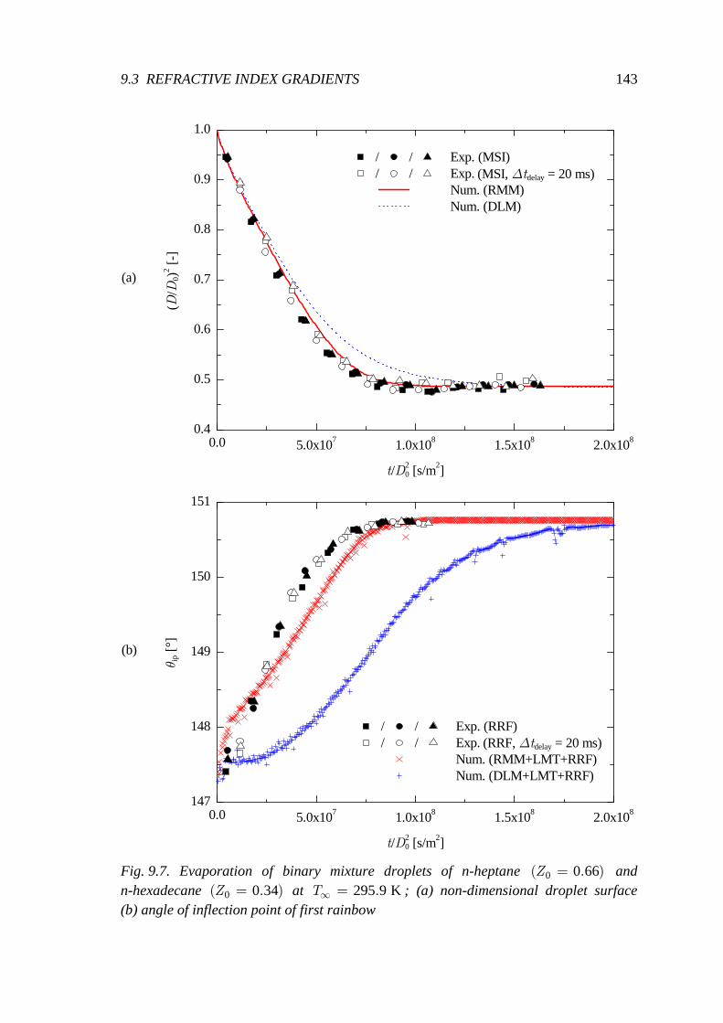
9.3 REFRACTIVE INDEX GRADIENTS 143

0.0 5.0x107 1.0x108 1.5x108 2.0x1080.4

0.5

0.6

0.7

0.8

0.9

1.0

0.0 5.0x107 1.0x108 1.5x108 2.0x108147

148

149

150

151

(MSI, ∆tdelay = 20 ms)

(D/D

0)2 [-

]

t/D20 [s/m2]

/ / Exp. (MSI)/ / Exp.

Num. (RMM) Num. (DLM)

(b)

(a)

θ ip [°

]

t/D20 [s/m2]

/ / Exp. (RRF)/ / Exp.

Num. (RMM+LMT+RRF) Num. (DLM+LMT+RRF)

(RRF, ∆tdelay = 20 ms)

Fig. 9.7. Evaporation of binary mixture droplets of n-heptane 0 0 66( . )=Z and n-hexadecane 0 0 34( . )=Z at 295 9 K.∞ =T ; (a) non-dimensional droplet surface (b) angle of inflection point of first rainbow

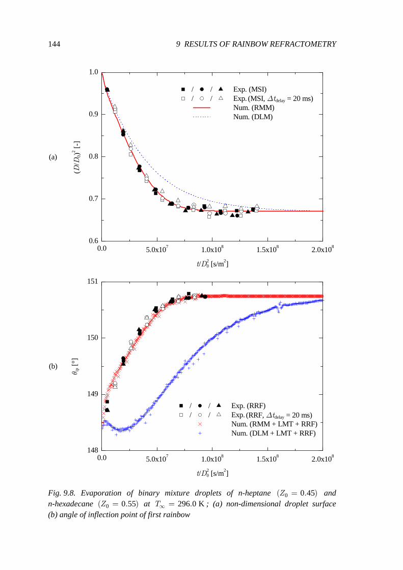
144 9 RESULTS OF RAINBOW REFRACTOMETRY

0.0 5.0x107 1.0x108 1.5x108 2.0x1080.6

0.7

0.8

0.9

1.0

0.0 5.0x107 1.0x108 1.5x108 2.0x108148

149

150

151

(MSI, ∆tdelay = 20 ms)

(D/D

0)2 [-

]

t/D20 [s/m2]

/ / Exp. (MSI)/ / Exp.

Num. (RMM) Num. (DLM)

(RRF, ∆tdelay = 20 ms)

θ ip [°

]

t/D20 [s/m2]

/ / Exp. (RRF)/ / Exp.

Num. (RMM + LMT + RRF) Num. (DLM + LMT + RRF)

(a)

(b)

Fig. 9.8. Evaporation of binary mixture droplets of n-heptane 0 0 45( . )=Z and n-hexadecane 0 0 55( . )=Z at 296 0 K.∞ =T ; (a) non-dimensional droplet surface (b) angle of inflection point of first rainbow

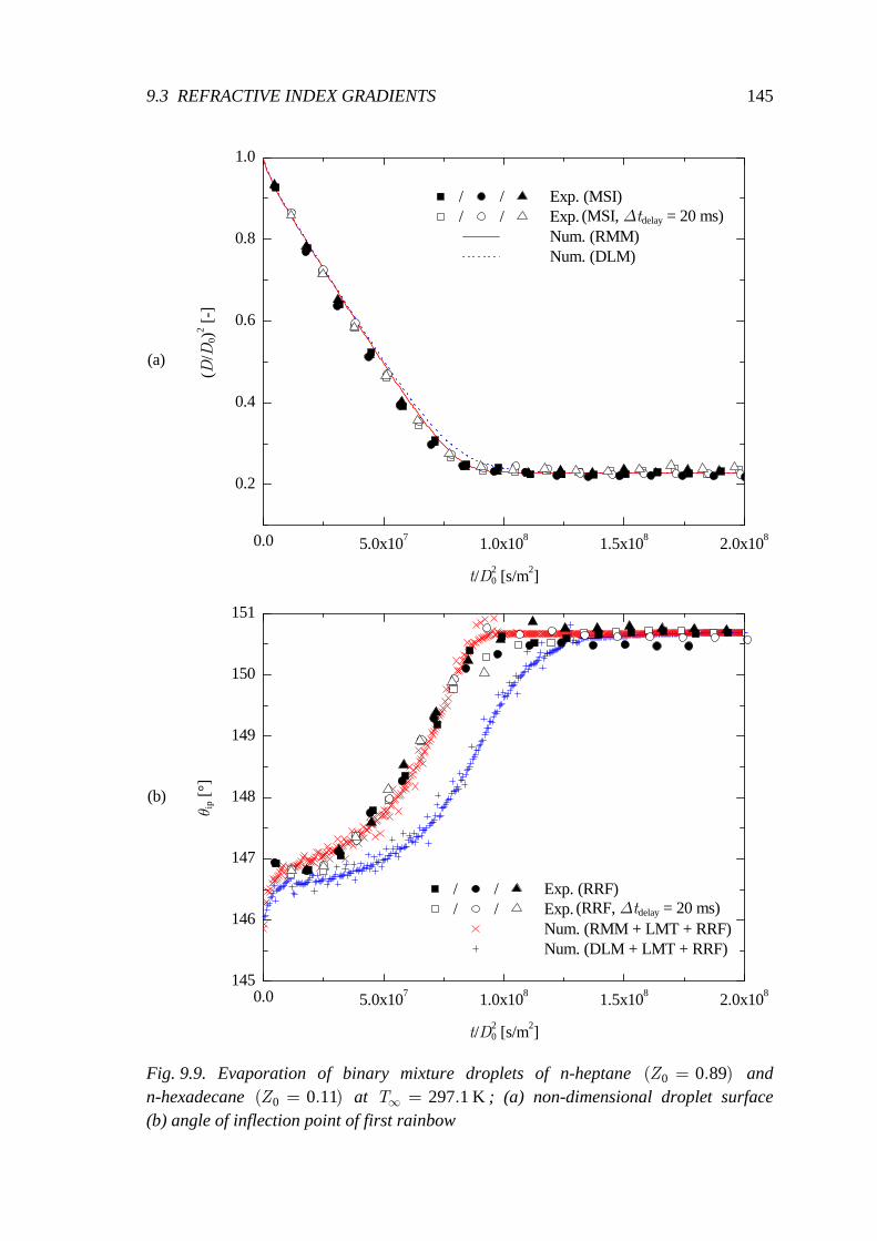
9.3 REFRACTIVE INDEX GRADIENTS 145

0.0 5.0x107 1.0x108 1.5x108 2.0x108

0.2

0.4

0.6

0.8

1.0

0.0 5.0x107 1.0x108 1.5x108 2.0x108145

146

147

148

149

150

151

(MSI, ∆tdelay = 20 ms)

(D/D

0)2 [-

]

t/D20 [s/m2]

/ / Exp. (MSI)/ / Exp.

Num. (RMM) Num. (DLM)

(RRF, ∆tdelay = 20 ms)

θ ip [°

]

t/D20 [s/m2]

/ / Exp. (RRF)/ / Exp.

Num. (RMM + LMT + RRF) Num. (DLM + LMT + RRF)

(b)

(a)

Fig. 9.9. Evaporation of binary mixture droplets of n-heptane 0 0 89( . )=Z and n-hexadecane 0 0 11( . )=Z at 297 1 K.∞ =T ; (a) non-dimensional droplet surface (b) angle of inflection point of first rainbow

146 9 RESULTS OF RAINBOW REFRACTOMETRY

In Fig. 9.9, results are depicted for droplets with a very high initial volume fraction of n-heptane. In this case, it is interesting to note that the longest measurement period was reached. This is because the droplets decelerated rapidly in the measurement chamber, since the droplet size decreased quickly to a small diameter of about 27 µm=D . The long measurement period made it possible to obtain several data points when only n-hexadecane is left in the droplet. The results show that the angle of the inflection point remains constant as it is expected from the optical Fourier transform.

147

10 Conclusions The aim of this thesis was to investigate the evaporation of droplets with up to three components in a quiescent atmosphere at standard atmospheric pressure and at different ambient temperatures. To accomplish this goal, experimental setups at the Institute of Aerospace Thermodynamics were modified and built for the investigation of droplet evaporation. Due to contact-free investigation of the droplet using optical levitation and free fall, the experimental techniques were superior to many other methods found in the literature. The use of non-intrusive optical measurement techniques allowed for measurements with very high accuracies compared to other techniques found in published studies.

For droplets with low evaporation rates, an optical levitation setup was used since it allowed for long measurement periods until nearly complete droplet evaporation. The droplet size was measured from the fringe spacing of the scattered laser light in the forward hemisphere by a technique called "Mie scattering imaging". For droplets with high evaporation rates, the free-falling droplet setup proved to be very suitable since it allowed for an early start of the measurements after droplet generation. In addition, data for size histories could be gained at a high acquisition rate with a technique using morphology-dependent resonances.

First, measurements of pure-component droplets were performed covering a broad range of volatilities by using substances from n-pentane to n-hexadecane at different temperatures. These measurements were used to validate the experimental setups. Results of surface histories showed that the evaporation rate was a constant as expected from the classical 2D -law. Moreover, the evaporation rate showed a strong dependence on the volatilities and on the temperature as expected from a theoretical analysis using property evaluation methods.

Next, multicomponent droplets with two and three components were investigated. In order to use the measurement technique with morphology-dependent resonances for these droplets, a correction method was proposed using numerical simulations for droplet evaporation and for the scattered light.

Results of surface histories from two-component droplets showed that both components evaporated simultaneously and that the initial evaporation rate was intermediate to those of the pure-component droplets. The evaporation behavior was close to batch-distillation, only when there was a large difference in the volatilities of the substances.

Next, results of three-component droplets were presented. For the investigation of droplets with both low and highly volatile components, both experimental setups were used in order to capture the entire evaporation process. Results of the surface histories

148 10 CONCLUSIONS

showed that the evaporation rate changes continuously and the number of components cannot be identified when the difference in volatilities of the substances is small. Different phases where one of the components dominates the evaporation process can be distinguished only when the difference in volatilities is sufficiently large. With respect to a variation of the ambient temperature, the surface histories were similar at different temperatures when the time axis was scaled logarithmically. This is because the evaporation rate is strongly influenced by the vapor pressure which depends exponentially on the temperature.

In addition to the experimental investigations, several numerical models for droplet evaporation were developed. From the classical 2D -law, numerical models for droplets with up to three components were presented assuming a constant and uniform temperature. Due to their simplicity, these models allowed for a fast calculation of the evaporation process with reasonable accuracy. For binary mixture droplets, an analytical solution was presented giving further insight into the driving parameters of droplet evaporation. Experimental results of the evaporation rate of pure-component droplets were in excellent agreement with results from these models. For two- and three-component droplets, results from these models showed good agreement with experimental results when the appropriate reference temperature and composition was selected.

In addition to these models, a rapid-mixing model with time-dependent droplet temperature and a diffusion-limit model with internal heat and mass diffusion were used for numerical simulations. These two models represent the limiting cases for mass transport inside the droplet. The diffusion-limit model represents the lower limit since it only considers diffusive transport, whereas the rapid-mixing model represents the upper limit by assuming diffusion at infinite speed. The true evaporation behavior is between these limiting cases since convection can enhance the mass transport in addition to diffusion. When binary mixture droplets were investigated where the difference in volatilities of the substances was large so that there was a significant difference of the surface histories predicted by the rapid-mixing and the diffusion-limit model, experimental data agreed very well with results from the rapid-mixing model. In order to reach good agreement between the experimental results and the diffusion-limit model, a large increase of the diffusive mass transport was necessary. Therefore it is believed that there is a strong convective mass transport in addition to the diffusive mass transport. The convective mass transport is most likely due to internal circulations caused by the generation process of the droplet.

Rainbow refractometry was applied in order to gain further information about the droplet in addition to the droplet size. An elaborate evaluation technique was developed in order to provide high accuracy for the small droplets of this study. First, rainbow refractometry was applied to pure-component droplets to measure the temperature. The results were in good agreement with results of the droplet temperature obtained from the measurement of the evaporation rate. For two-component droplets, where the

10 CONCLUSIONS 149

evaporation rate was so low that a constant droplet temperature could be assumed, rainbow refractometry was used to measure the droplet composition. The results showed good agreement with numerical models. Finally, rainbow refractometry was applied to binary mixture droplets with a large difference in volatilities in order to detect gradients of the refractive index which were predicted by the diffusion-limit model. However, experimental results showed that these gradients did not occur. Instead, the experimental results agreed very well with the rapid-mixing model meaning that there was rather a homogeneous distribution of the refractive index inside the droplet. These results further support the previously mentioned assumption of enhanced mixing inside the droplet due to internal circulation. Further investigation of this subject would be a very interesting research topic.

Overall, a large amount of experimental data was obtained for the evaporation of droplets with up to three components. Experimental results considered surface histories, droplet composition and temperature, and refractive index gradients inside droplets. These results can be used to validate numerical models. Results from the developed simplified numerical models were in good agreement with these data. The best agreement with experimental data was reached by using the uniform-temperature model for pure-component droplets and the rapid-mixing model for multicomponent droplets.

151

References Abramzon B and Sirignano WA (1987) Approximate theory of single droplet

vaporizing in a convective field: effects of variable properties, Stefan flow and transient liquid heating. Proc. 2nd ASME-JSME Thermal Engng. Joint Conf., Hawaii, 1: 11-18

Albrecht HE, Borys M, Damaschke N, and Tropea C (2003) Laser Doppler and phase Doppler measurement techniques. Springer, Berlin

Anders K (1994) Experimentelle und theoretische Untersuchung der Tropfenverdampfung für Knudsen-Zahlen im Übergangsbereich. Shaker Verlag, Aachen

Anders K, Roth N, and Frohn A (1995) Influence of Refractive Index Gradients within Droplets on Rainbow Position and Implications for Rainbow Refractometry. Part. Part. Syst. Charact. 13: 125-199

Airy GB (1838) On the intensity of light in the neighbourhood of a caustic. Transactions of the Cambridge Phylosophical Society, 6: 397-403

Ashkin A (1980) Applications of Laser Radiation Pressure. Science 210 (4474): 1081-1088

Ashkin A and Dziedzic JM (1974) Stability of optical levitation by radiation pressure. Applied Physics Letters, 24 (12): 586-588

Barlow RJ (1989) Statistics. John Wiley & Sons, Chichester

Beard KV and Pruppacher HR (1971) A Wind Tunnel Investigation of the Rate of Evaporation of Small Water Drops Falling at Terminal Velocity in Air. J. Atmos. Sci, 28: 1455-1465

Bernholz U (1997) Messung von Größe, Regenbogenposition und Verdunstungsrate an optisch levitierten Tropfen aus Kohlenwasserstoffen. Studienarbeit, ITLR, Stuttgart.

Bohren CF and Huffman D (1983) Absorption and Scattering of Light by Small Particles. John Wiley and Sons, New York

Brenn G, Deviprasath LJ, and Durst F (2003) Computations and experiments on the evaporation of multi-component droplets. Proc ICLASS 2003, Sorrento, Italy

Camin DL, Forziati AF, and Rossini FD (1954) Physical Properties of n-Hexadecane, n-Decylcyclopentane, n-Decylcyclohexane, 1-Hexadecene and n-Deylbenzene. Journal of phys. Chem., 58: 440-442

Camin DL and Rossini FD (1955) Physical Properties of 14 American Petroleum Institute Research Hydrocarbons, C9 to C15. Journal of phys. Chem., 59: 1173-1179

152 REFERENCES

Castanet G, Lavielle P, Lebouché M, and Lemoine F (2003) Measurement of the temperature distribution within monodisperse combusting droplets in linear streams using two-color laser-influenced fluorescence. Experimental in Fluids, 35: 563-571

Catoire F, Gauthier JED, Bardon MF, and Benaissa A (1999) Quasi-steady evaporation for real multi-component fuel droplets. Journal of the Institute of Energy, 72: 134-142

Chen G, Aggarwal SK, Jackson TA, and Switzer GL (1997) Experimental study of pure and multicomponent fuel droplet evaporation in a heated air flow, Atomization and Sprays, 7 (3): 317-337

Chylek P (1990) Resonance structure of Mie scattering: Distance between resonances. J. Opt. Soc. Am., 7 (9): 1609-1613

Daidzic N (1995) Nonlinear Droplet Oscillations and Evaporation in an Ultrasonic Levitator. Dissertation, Universität Erlangen-Nürnberg

Daif A, Bouaziz M, Chesneau X, and Ali Chérif A (1999) Comparison of multicomponent fuel droplet vaporization experiments in forced convection with the Sirignano model. Exp. Therm. Fluid Sci. 18 (4): 282-290

Damaschke N, Heukelbach K, Tropea C (1998) Messung von Partikeldurchmesser, Brechungsindex und Temperature mit dem Regenbogen. 6. Fachtagung Laser-methoden in der Strömungsmeßtechnik, Shaker-Verlag, Aachen: paper 23

Daubert TE and Danner RP (1993) Physical and Thermodynamic Properties of Pure Chemicals: Data Compilation. Hemisphere Publ. Co., New York

Davis E.J. and Ray A.K. (1980) Single Aerosol Particle Size and Mass Measurements Using an Electrodynamic Balance: J. Colloid and Interface Sci., 75 (2): 566-576

Downing CG (1966) The evaporation of drops of pure liquids at elevated temperatures: rates of evaporation and wet-bulb temperatures. AIChE J. 12 (4): 760-766

Faeth GM (1977) Current Status of Droplet and Liquid Combustion. Prog. Energy Combust. Sci., 3: 191-224

Forziati AF (1950) Refractive Index as a Function of Wavelength for Sixty API-NBS Hydrocarbons. J. of Research of the National Bureau of Standards, 44: 373-385

Frössling N. (1938) Über die Verdunstung fallender Tropfen. Gerlands Beitr. Geophys. 52: 170-216

Frohn A and Roth N (2000) Dynamics of Droplets. Springer-Verlag, Berlin

Gartung K, Arndt S, Roth N, and Weigand B (2000) Evaporation of Tetradecane-Hexadecane Mixture Droplets: An Experimental and Numerical Study. Proc. ILASS-Europe 2000, Darmstadt, Germany

Gartung K, Arndt S, and Seibel C (2002) Vaporization of Multicomponent Fuel Droplets: Numerical and Experimental Evaluation. Proc ILASS-Europe, Zaragoza

REFERENCES 153

Glantschnig WJ and Chen SH (1981) Light scattering from water droplets in the geometrical optics approximation, Appl. Opt. 20 (14): 2499-2509

Glover AR, Skippon SM, and Boyle, RD (1995) Interferometric laser imaging for droplet sizing: a method for droplet-size measurement in sparse spray systems. Appl. Opt., 34 (36): 8409-8421

Glushkov VE, Todes OM, and Fedoseev VA (1970) Evaporation Kinetics of Drops of Binary Mixtures of Organic Liquids. Colloid J. of the USSR, 32 (5): 566-570

Godsave, GAE (1953) Studies of the combustion of drops in a fuel spray: The burning of single drops of fuel. Fourth Symposium (International) on Combustion, Williams and Wilkins, Baltimore, 818-830

Gökalp I, Chauveau C, Berrekam H, and Ramos-Arroyo NA (1994) Vaporization of Miscible Binary Fuel Droplets under Laminar and Turbulent Convective Conditions. Atomization and Sprays, 4: 661-676

Gouesbet G and Gréhan G (2000) Generalized Lorenz-Mie Theories, from Past to Future. Atomization and Sprays, 10: 277-333

Hesselbacher KH, Anders K, and Frohn A (1991) Experimental investigation of Gaussian beam effects on the accuracy of a droplet sizing method. Appl. Opt., 30 (33): 4930-4935

Hovenac EA and Lock JA (1992) Assessing the contributions of surface waves and complex rays to far-field Mie scattering by use of Debye series. Opt. Soc. Am. A, 9 (5): 781-795

Hubbard GL, Denny VE, and Mills AF (1975) Droplet evaporation: Effects of transient and variable properties. Int. J. Heat and Mass Transfer, 18: 1003-1008

Incropera FP and DeWitt DP (1996) Fundamentals of Heat and Mass Transfer. John Wiley & Sons, New York

Kastner O. (2001) Theoretische und experimentelle Untersuchungen zum Stoffübergang von Einzeltropfen in einem akustischen Rohrlevitator. Dissertation, Universität Erlangen-Nürnberg

Kays WM, Crawford ME, and Weigand B (2005) Convective Heat and Mass Transfer. 4th ed., McGraw-Hill, New York

Kent JC (1973) Quasi-steady diffusion controlled droplet evaporation and condensation. Appl. Sci. Res. Ser. A, 28: 315-359

Kerker M (1969) The scattering of light and other electromagnetic radiation. Academic Press, London

Kiefer W, Popp J, Lankers M, Trunk M, Hartmann I, Urlaub E, and Musick J (1997) Raman-Mie scattering from single laser trapped microdroplets, J. of Molecular Structure, 408/409: 113-120

Kneer R (1993) Grundlegende Untersuchungen zur Sprühlstrahlausbreitung in hoch-belasteten Brennräumen: Tropfenverdunstung und Sprühstrahlcharakterisierung, Dissertation, Universität Karlsruhe

154 REFERENCES

König G, Anders K, and Frohn A (1986) A new light-scattering technique to measure the diameter of periodically generated moving droplets. J. Aerosol Sci., 17: 157-167

Kuo KK (1986) Principles of Combustion. Wiley, New York

Law CK (1975) Quasi-steady droplet vaporization theory with property variations. Physics of Fluids, 18: 1426-1432

Law CK (1982) Recent advances in droplet vaporization and combustion. Progr. Energy Combust. Sci. 8: 171-201

Lee ER (2003) Microdrop Generation. CRC Press, Boca Raton, Florida

Lide DR (1998) Handbook of Chemistry and Physics. 79th ed., CRC Press, Boca Raton, Florida

Lorenz L (1890) Lysbevaegeisen i og uden for en hal plane lysbôlger belyst kulge. Vidensk Selk Skr 6: 1-62

Lusis MA and Ratcliff GA (1968) Diffusion in Binary Liquid Mixtures at Infinite Dilution, Can. J. Chem. Eng., 46: 385-387

Maeda M, Kawaguchi T, Hishida K (2000) Novel interferometric measurement of size and velocity distributions of spherical particles in fluid flows. Meas Sci Technol 11: L13-L18

Massoli P, Calabria R (1999) Sizing of droplets in reactive fuel sprays by Mie scattering imaging. Proc ILASS-Europe '99, Toulouse, France

Matthews MA and Akgerman A (1987) Diffusion Coefficients for Binary Alkane Mixtures to 573 K and 3.5 MPa, AIChE Journal, 33(6): 881-885

Mie G (1908) Beiträge zur Optik trüber Medien, speziell kolloidaler Metallösungen. Annalen der Physik 25 (3): 377-447

Mills AF (2001) Mass Transfer, Prentice Hall, Upper Saddle River, New Jersey, USA

Ochs M (1999) Verdunstung monodisperser, frei beweglicher Brennstoff-Tropfen in einer turbulenten Heissluftströmung, Dissertation, ETH Zurich, Switzerland

Poling BE, Prausnitz JM, and O'Connell JP (2000) The Properties of Gases and Liquids. 5th ed., McGraw-Hill, New York

Popp J (1994) Elastische und inelastische Lichtstreuung an einzelnen spährischen Mikropartikeln. Dissertation, Universität Würzburg, Verlag Shaker, Aachen

Putnam A (1961) Integrable Form of Droplet Drag Coefficient. ARS Journal, 31: 1467-1468

Randolph AL, Makino A, and Law CK (1986) Liquid-Phase Diffusional Resistance in Multicomponent Droplet Gasification, 21st Symp. (Int.) on Combustion, the Comb. Inst., 601-608

Ranz WE and Marshall WR (1952a) Evaporation from Drops: Part I, Chemical Engineering Progress, 48 (3): 141-146

REFERENCES 155

Ranz WE and Marshall WR (1952b) Evaporation from Drops: Part II, Chemical Engineering Progress, 48 (3): 173-180

Ragucci R, Cavaliere A, and Massoli P (1990) Drop sizing by laser light scattering exploiting intensity angular oscillation in the Mie regime. Part Part Syst Charact 7: 221-225

Randolph AL, Makino A, and Law CK (1986) Liquid-Phase Diffusional Resistance in Multicomponent Droplet Gasification, 21st Symp. (Int.) on Combustion/ The Comb. Inst., 601-608

Ravindran P, Davis EJ, and Ray AK (1979) Diffusivities of Low-Volatility Species in Light Gases. AIChE Journal, 25 (6): 966-975

Ravindran P and Davis JE (1982) Multicomponent Evaporation of Single Aerosol Droplets. Journal of Colloid and Interface Science, 85 (1): 238-248

Rayleigh Lord (1871) On the light from the sky, its polarization and colour. Philos. Mag., 41: 107-120

Reid CR, Prausnitz JM, and Poling EP (1987) The Properties of Gases and Liquids. 4th edition, McGraw-Hill, New York

Rossow B, Krüger S, and Grünefeld G (2004) Evaporation of droplet streams and isolated free falling droplets investigated by means of ILIDS and planar LIF. Proc. Conf. Atomization and Spray Processes, Dortmund: paper 5.3

Roth N (1998) Bestimmung des Brechungsindex in Einzeltropfen aus dem Streulicht im Bereich des Regenbogens. Shaker Verlag, Aachen

Roth N, Anders K, and Frohn A (1988) Simultaneous measurement of temperature and size of droplets in the micrometer range. Proc. 7th Int. Congr. on Optical Methods in Flow and Parcticle Diagnostics ICALEO 88, L.I.A., Sunnyvale, USA, 67: 294-304

Roth N, Anders K, and Frohn A (1994) Determination of Size, Evaporation Rate and Freezing of Water Droplets Using Light Scattering and Radiation Pressure. Part. Part. Syst. Charact 11: 207-211

Roth N and Frohn A (1997) Measuring technique to investigate the evaporation process of droplets consisting of hydrocarbon mixtures. Proc. of the 13th Int. Conf. on Liquid Atomisation and Spray Systems, Florence, Italy

Runge T, Teske M, and Polymeropoulos CE (1998) Low-temperature vaporization of JP-4 and JP-8 fuel droplets, Atomization and Sprays, 8: 25-44

Schröder U (2001) Personal communications, ITLR Stuttgart

Semidetnov N and Tropea C (2004) Conversion relationships for multidimensional particle sizing techniques, Meas. Sci. Technol., 15: 112-118

Sirignano WA (1978) Theory of Multicomponent Vaporization, Arch. Thermodynam. Combustion, 9: 231-247

156 REFERENCES

Spalding DB (1953) The combustion of liquid fuels, Fourth Symposium (International) on Combustion, Williams and Wilkins, Baltimore, 847-864

Sparrow EM and Gregg JL (1958) The variable fluid-property problem in free convection. Tans. Am. Soc. Mech. Engrs 80: 879-886

Spurk JH (1996) Strömungslehre, Einführung in die Theorie der Strömungen. Springer-Verlag, Berlin

Stengele J, Prommersberger K, Willmann M, and Wittig S (1999) Experimental and Theoretical Study of One- and Two-Component Droplet Vaporization in a High Pressure Environment. Int. J. Heat Mass Transfer, 42: 2683-2694

Tuckermann R, Bauerecker S, and Neidhart B (2002) Evaporation rates of alkanes and alkanols from acoustically levitated droplets, Analytical and Bioanalytical Chemistry, 372 (1): 122-127

Ulmke H, Wriedt T, and Bauckhage K (2001) Piezoelectric Droplet Generator for the Calibration of Particle-Sizing Instruments. Chem. Eng. Technol. 24 (3): 265-268

Vadovic CJ and Colver CP (1973) Infinite Dilution Diffusion Coefficients in Liquids. AIChE Journal, 19 (3): 546-551

Valley Scientific (1998) Software package "LightLab: Far Field Mie Scattering", version 1.00

van Beeck JPAJ (1997) Rainbow Phenomena: development of a laser-based, non-intrusive technique for measuring droplet size, temperature and velocity. Dissertation, Technical University of Eindhoven, Netherlands

van de Hulst HC (1981) Light Scattering by Small Particles. Dover Publications, New York

VDI-Wärmeatlas (1988) 5th ed., VDI-Verlag, Düsseldorf 1988

Vignes A (1966) Diffusion in binary solutions, Ind. Eng. Chem. Fundam., 5: 189-199

Walker JD (1976) Multiple rainbows from single drops of water and other liquids. Am. J. of Physics, 44 (5): 421-433

Wenck H et al. (1993): Chemisch-physikalische Daten von Otto- und Dieselkraftstoffen (Collection of chemical and physical data of automotive fuels), DGMK (Deutsche Wissenschaftliche Gesellschaft für Erdöl, Erdgas und Kohle e.V.), Hamburg

Wong SC, Lin AR (1992) Internal temperature distributions of droplets vaporizing in high-temperature convective flows. J. Fluid Mech. 237: 671-687

Yarin AL, Brenn G, Kastner O, Rensink D, and Tropea C (1999) Evaporation of acoustically levitated droplets. J. Fluid Mech., 399: 151-204

Yarin AL, Brenn G, and Rensink D (2002) Evaporation of acoustically levitated droplets of binary liquid mixtures. Int. J. Heat Fluid Flow 23 (4): 471-486

Yuen MC and Chen LW (1976) On Drag of Evaporating Liquid Droplets. Combustion Science and Technology, 14: 147-154

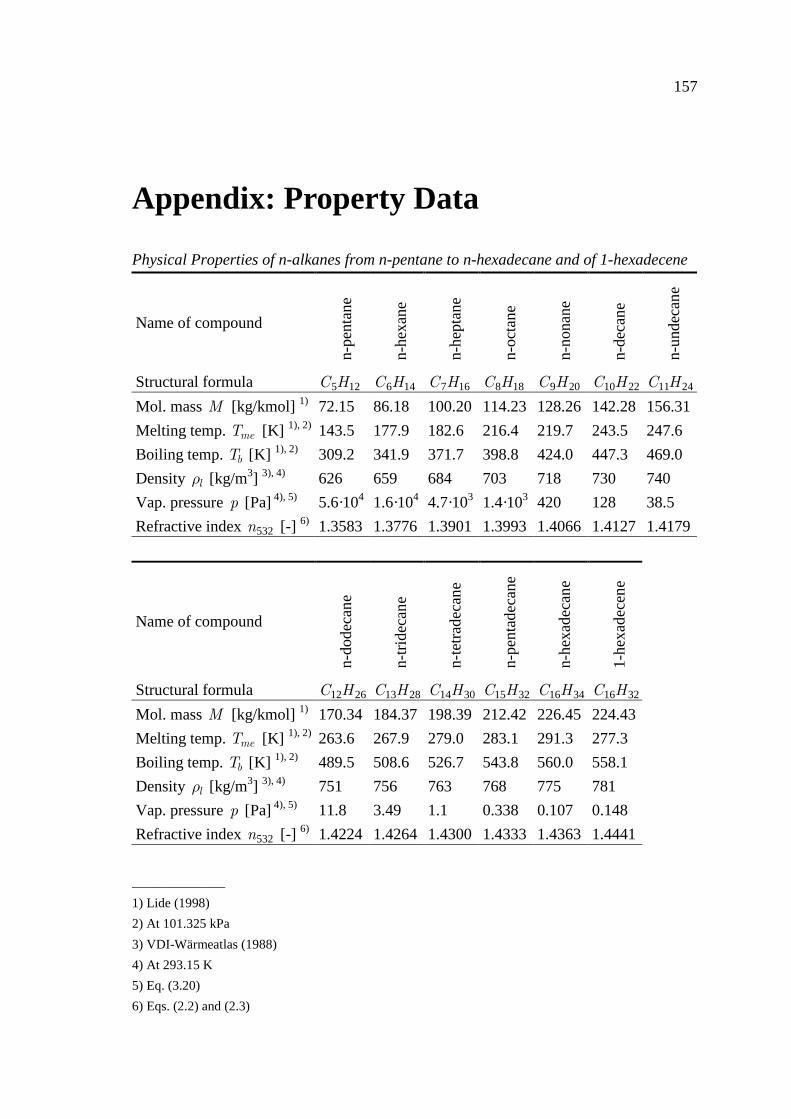
157

Appendix: Property Data

Physical Properties of n-alkanes from n-pentane to n-hexadecane and of 1-hexadecene

Name of compound

n-pe

ntan

e

n-he

xane

n-he

ptan

e

n-oc

tane

n-no

nane

n-de

can

e

n-un

deca

ne

Structural formula 5 12C H 6 14C H 7 16C H 8 18C H 9 20C H 10 22C H 11 24C H

Mol. mass M [kg/kmol] 1) 72.15 86.18 100.20 114.23 128.26 142.28 156.31

Melting temp. meT [K] 1), 2) 143.5 177.9 182.6 216.4 219.7 243.5 247.6

Boiling temp. bT [K] 1), 2) 309.2 341.9 371.7 398.8 424.0 447.3 469.0

Density lρ [kg/m3] 3), 4) 626 659 684 703 718 730 740

Vap. pressure p [Pa] 4), 5) 5.6·104 1.6·104 4.7·103 1.4·103 420 128 38.5

Refractive index 532n [-] 6) 1.3583 1.3776 1.3901 1.3993 1.4066 1.4127 1.4179

Name of compound

n-do

deca

ne

n-tr

idec

ane

n-te

trad

eca

ne

n-pe

ntad

eca

ne

n-he

xade

can

e

1-he

xade

cen

e

Structural formula 12 26C H 13 28C H 14 30C H 15 32C H 16 34C H 16 32C H

Mol. mass M [kg/kmol] 1) 170.34 184.37 198.39 212.42 226.45 224.43

Melting temp. meT [K] 1), 2) 263.6 267.9 279.0 283.1 291.3 277.3

Boiling temp. bT [K] 1), 2) 489.5 508.6 526.7 543.8 560.0 558.1

Density lρ [kg/m3] 3), 4) 751 756 763 768 775 781

Vap. pressure p [Pa] 4), 5) 11.8 3.49 1.1 0.338 0.107 0.148

Refractive index 532n [-] 6) 1.4224 1.4264 1.4300 1.4333 1.4363 1.4441

______________

1) Lide (1998)

2) At 101.325 kPa

3) VDI-Wärmeatlas (1988)

4) At 293.15 K

5) Eq. (3.20)

6) Eqs. (2.2) and (2.3)

Curriculum Vitae

Name Jochen Wilms

Email wilms@itlr.de

Date of birth 24 May, 1973

Place of birth Heidelberg

Nationality German

1983 - 1992 Helmholtz-Gymnasium Heidelberg, Abitur (High school diploma)

1992 Internship at Mercedes-Benz AG, Mannheim

1992 - 1993 Civil service at the biomolecular research laboratory of the

dermatological clinic of Universität Heidelberg

1993 - 1995 Ludwig-Maximilians-Universität München, prediploma in physics

1995 - 1996 Universität Stuttgart, prediploma in aerospace engineering

1996 - 1997 University of Toronto, scholarship of the

Ontario/Baden-Württemberg Student Exchange Program

1997 Practical training at Airbus Delivery Centre in Toulouse and

at Deutsche Aerospace AG, space infrastructure,

in Ottobrunn (Munich)

1997 - 1998 Universität Stuttgart, specialty in space systems

1998 - 1999 ENSAE in Toulouse, specialty in thermodynamics and aerospace

propulsion, Sokrates/Erasmus scholarship of the European Union

1999 Studienarbeit (Research project) at ONERA in Toulouse

(Experimental and Numerical Investigation of the Drag Coefficient

of Interacting Droplets), scholarship of the Hermann-Reissner-

Stiftung

2000 Diploma thesis at the Institute of Space Systems at Universität

Stuttgart (Conceptual Design of a Synergistic Propulsion System

for the International Space Station)

2000 Diploma in aerospace engineering

2000 - 2005 Research associate at the Institute of Aerospace Thermodynamics

at Universität Stuttgart