evolution of turbine blade deposits in an accelerated ...tom/papers/wammack_thesis.pdf · evolution...
TRANSCRIPT

EVOLUTION OF TURBINE BLADE DEPOSITS IN AN ACCELERATED
DEPOSITION FACILITY: ROUGHNESS
AND THERMAL ANALYSIS
by
James E. Wammack
A thesis submitted to the faculty of
Brigham Young University
In partial fulfillment of the requirements for the degree of
Master of Science
Department of Mechanical Engineering
Brigham Young University
December 2005


Copyright © 2005 James E. Wammack
All Rights Reserved


ABSTRACT
EVOLUTION OF TURBINE BLADE DEPOSITS IN AN ACCELERATED
DEPOSITION FACILITY: ROUGHNESS
AND THERMAL ANALYSIS
James E. Wammack
Department of Mechanical Engineering
Master of Science
During the operation of a gas turbine, ingested contaminants present in the air form
deposits on the surfaces of the turbine blades. These deposits grow over time, resulting in
an increasingly rough surface. This gradual increase in roughness results in several
negative consequences, among which is an increase in the rate of heat transfer to the
blade which shortens blade life. This thesis presents research in which deposits were
evolved on three different turbine blade coupons and their evolution was studied. A trend
in roughness change over time was discovered. Also, an attempt was made to find the
effect of the deposits on the heat transfer characteristics of a coupon surface. The deposits
were formed using the BYU Turbine Accelerated Deposition Facility (TADF), which was
used to simulate three months of deposition within a two hour test time. All three
coupons underwent four cycles in the TADF: eight total hours of combustor testing—or

one simulated year of deposition—with topological measurements being made on the
coupon surface after every two hours (three simulated months) of testing. The data
produced by the topological measurements were used with a CNC mill to machine
scaled-up plastic models of the rough surfaces: four surfaces per model representing
three, six, nine, and twelve simulated months of deposition. The models were placed in a
wind tunnel where, following a period of thermal soaking at room temperature, they were
suddenly exposed to a heated air stream. The thermal histories of the model were
recorded with an infrared camera and were used to derive the heat transfer coefficient of
each surface using the method developed by Shultz and Jones. The heat transfer
coefficients are reported in the form of Stanton numbers to allow for the difference in
thermal properties between the conditions and properties of the wind tunnel and its
components and those of a real gas turbine. The Stanton numbers for the various surfaces
were plotted versus the simulated gas turbine operational time. Additionally, several
roughness correlations were used to predict the Stanton number for each surface,
producing a probable Stanton number history for the coupon. The measured non-
dimensional heat transfer coefficients did not reach the magnitudes predicted by the
correlations. This is most likely due to unexpected flow conditions inside the wind
tunnel. Recommendations for future research are presented.


ACKNOWLEDGEMENTS
This thesis would not have been possible without the guidance, assistance, and support of
several people. I would like to thank my graduate advisor, Dr. Jeffrey Bons, for allowing
me the opportunity to work on such a fascinating and challenging project. I would also
like to thank the other members of my graduate committee, Drs. Tom Fletcher and Brent
Webb. Their varied fields of experience and insight allowed me to better understand and
appreciate the many facets of scientific research. I am also grateful for the generous grant
from the BYU Department of Mechanical Engineering that helped this project to reach
completion.
I would also like to express my gratitude for the efforts of Jared Jensen, whose research
made my own possible. Thanks also goes out to Ken Forster and Kevin Cole whose
expertise and willingness to help greatly benefited the project. The efforts and assistance
of Jared Crosby, Daniel Fletcher, and John Pettitt were instrumental in the successful
completion of this thesis.
Finally, I would like to thank my ever-patient wife La Tisha and our daughters MacKayla
and Annika for their love and support during a challenging time.


TABLE OF CONTENTS
TABLE OF CONTENTS................................................................................................. viii LIST OF FIGURES ............................................................................................................ x LIST OF TABLES........................................................................................................... xiv Nomenclature................................................................................................................... xvi Chapter 1: Introduction ....................................................................................................... 1
1.1 Background......................................................................................................... 1 1.2 TADF Validation ................................................................................................ 4
1.2.1 Topography of Accelerated Deposits.......................................................... 5 1.2.2 Internal Structure and Chemical Composition of Accelerated Deposits .... 7
1.3 Objective ........................................................................................................... 10 Chapter 2: Deposition Evolution—Experimental Facilities and Techniques ................... 11
2.1 Accelerated Deposition..................................................................................... 11 2.2 Turbine Accelerated Deposition Facility .......................................................... 14
2.2.1 TADF Operation ....................................................................................... 15 2.2.2 Instrumentation ......................................................................................... 19 2.2.3 TADF Modifications................................................................................. 21
2.3 Turbine Blade Coupons .................................................................................... 22 2.4 Deposition Evolution ........................................................................................ 23
2.4.1 Burn Procedures........................................................................................ 24 2.4.2 Coupon Surface Analysis.......................................................................... 24
Chapter 3: Deposition Evolution Results.......................................................................... 27 3.1 Roughness Measurement .................................................................................. 27
3.1.1 Form Removal .......................................................................................... 29 3.1.2 Data Drop-out Error.................................................................................. 30 3.1.3 Coupon Analysis....................................................................................... 31
3.2 Coupon 1: Unpolished Anti-Oxidation Coating ............................................... 32 3.3 Coupon 2: Polished Bare Metal Substrate ........................................................ 36
3.3.1 Coupon 2, Preburn—Overall Surface ....................................................... 38 3.3.2 Coupon 2, Burn 1—Overall Surface......................................................... 38 3.3.3 Coupon 2, Burn 2—Overall Surface......................................................... 39 3.3.4 Coupon 2, Burn 3—Overall Surface......................................................... 39 3.3.5 Coupon 2, Burn 4—Overall Surface......................................................... 40 3.3.6 Coupon 2 Overall Surface Roughness Trend............................................ 40 3.3.7 Commentary on Deposit Flaking .............................................................. 41 3.3.8 Coupon 2, Burn 1—Magnified Region..................................................... 44 3.3.10 Coupon 2, Burn 3—Magnified Region..................................................... 45 3.3.11 Coupon 2, Burn 4—Magnified Region..................................................... 46 3.3.12 Coupon 2 Magnified Region Roughness Trend........................................ 46
viii

3.4 Coupon 3: TBC Coated Substrate..................................................................... 47 3.4.1 Coupon 3, Burn 1...................................................................................... 52 3.4.2 Coupon 3, Burn 2...................................................................................... 53 3.4.3 Coupon 3, Burn 3...................................................................................... 54 3.4.4 Coupon 3, Burn 4...................................................................................... 54
3.5 Commentary on Roughness Similarities Between Coupons 1, 2, and 3........... 57 Chapter 4: Convective Heat Transfer Measurements—Experimental Facilities and Techniques ........................................................................................................................ 61
4.1 Roughened Turbine Blade Surfaces and Convective Heat Transfer ................ 61 4.2 Roughness Models ............................................................................................ 61 4.3 Wind Tunnel Heat Transfer Analysis ............................................................... 68 4.4 Wind Tunnel Description.................................................................................. 69 4.5 Thermal Measuring Devices ............................................................................. 74
4.5.1 FLIR Camera In Situ Calibration.............................................................. 75 4.5.2 FLIR Camera Ambient Temperature Correction...................................... 76 4.5.3 FLIR Camera Temperature Drift Correction ............................................ 78
4.6 Experimental Procedure.................................................................................... 79 4.7 Stanton Number Determination ........................................................................ 80
Chapter 5: Convective Heat Transfer Results................................................................... 85 5.1 Stanton Number Correlations ........................................................................... 85
5.1.1 Flat Plate Correlation ................................................................................ 85 5.1.2 Rough Surface Parameters........................................................................ 86 5.1.3 Friction Coefficient Correlations .............................................................. 89 5.1.4 Correlation Results.................................................................................... 89
5.2 Experimental Stanton Number Results............................................................. 92 5.2.1 Stanton Number Uncertainty .................................................................... 92 5.2.2 Flat Plate ................................................................................................... 93 5.2.3 Coupon 3, Burn 1...................................................................................... 93 5.2.4 Coupon 3, Burn 2...................................................................................... 93 5.2.5 Coupon 3, Burn 3...................................................................................... 94 5.2.6 Coupon 3, Burn 4...................................................................................... 95
5.3 Stanton Number Underprediction..................................................................... 95 Chapter 6: Conclusions and Recommendations ............................................................... 99
6.1 Review of Project Goals ................................................................................... 99 6.2 Deposit Evolution ............................................................................................. 99 6.3 Recommendations Regarding Deposition Evolution...................................... 100 6.4 Heat Transfer Rate Determination .................................................................. 100 6.5 Recommendations on Heat Transfer Rate Determination .............................. 101 6.6 Accomplishments............................................................................................ 101
Bibliography ................................................................................................................... 103 Appendix......................................................................................................................... 107 Appendix A: Derivation of the Schultz and Jones Equation .......................................... 109 Appendix B: MATLAB Programs.................................................................................. 113 Appendix C: Uncertainty Analysis ................................................................................. 123
ix
LIST OF FIGURES
Figure 1. Distribution of Ra values for multiple turbine blades from studies by Bons et al., 2001 and Tarada et al., 1993. .............................................................................. 3
Figure 2. Photographs of service turbine blade (left) and accelerated sample (right). Images are magnified 10 times. Photographs represent an area 3 mm x 3 mm............ 5
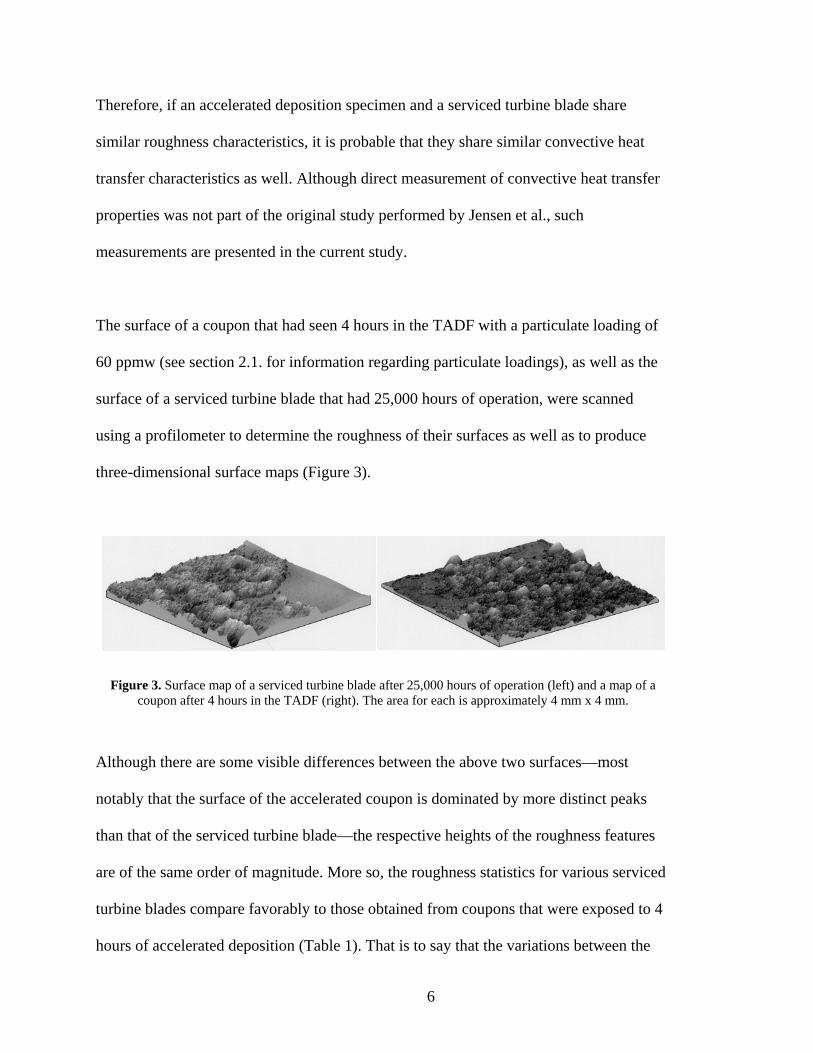
Figure 3. Surface map of a serviced turbine blade after 25,000 hours of operation (left) and a map of a coupon after 4 hours in the TADF (right). The area for each is approximately 4 mm x 4 mm. ................................................................................... 6
Figure 4. SEM cross-section from a 16000-hour service blade with a 50 μm metering bar (left) and an accelerated deposit specimen with a 100 μm metering bar (right). ........................................................................................................................... 8
Figure 5. Comparison of weight percentages of elements found in deposits on a land-based service turbine blade, an aircraft service blade (as reported by Borom et al, 1996), and a TADF-produced accelerated test sample. ................................................ 9
Figure 6. Photograph of accelerated deposits produced by a very high particulate loading......................................................................................................................... 12
Figure 7. Particle diameter distribution by mass percentage. ........................................... 14
Figure 8. TADF cross-sectional schematic....................................................................... 16
Figure 9. Cross-sectional schematic of particle-feed system............................................ 17
Figure 10. FLUENT produced vector diagram for the TADF sample holder. ................. 18
Figure 11. Brigham Young University TADF facility in building B-41. ......................... 19
Figure 12. Cross-sectional schematic of TADF sample holder. ....................................... 20
Figure 13. Cross-sectional drawing of coupons................................................................ 23
Figure 14. Illustration of coupon measured region and flow direction............................. 25
Figure 15. Surface roughness forward facing angle. ........................................................ 28
Figure 16. Topological map showing the preburn surface curvature Coupon 3 prior to (left) and following (right) a second order form removal........................................... 30
Figure 17. Illustration of data drop-out error. ................................................................... 31
Figure 18. Topological representations of deposits on Coupon 1 (Oxidation Resistant Coating)....................................................................................................................... 34
x
Figure 19. Three-dimensional representations of deposits on Coupon 1 (Oxidation Resistant Coating)....................................................................................................... 35
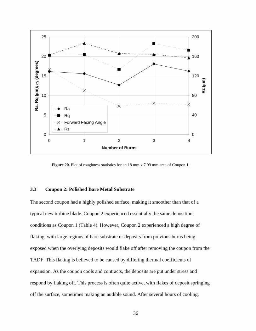
Figure 20. Plot of roughness statistics for an 18 mm x 7.99 mm area of Coupon 1......... 36
Figure 21. Illustration of location of surface measurement and magnified region........... 37
Figure 22. Topological representations of deposits on Coupon 2 (Bare Substrate). ........ 42
Figure 23. Three-dimensional representations of deposits on Coupon 2 (Bare Substrate). ................................................................................................................... 43
Figure 24. Plot of roughness statistics for the overall surface of Coupon 2. .................... 44
Figure 25. Topological representations of deposits on Coupon 2, zoomed region (Bare Substrate). ......................................................................................................... 48
Figure 26. Three-dimensional representations of deposits on Coupon 2, zoomed region (Bare Substrate). .............................................................................................. 49
Figure 27. Plot of roughness statistics for the zoomed 5 mm x 3 mm region of Coupon 2..................................................................................................................... 50
Figure 28. Illustration of location of surface measurement and magnified region. Image above is of Coupon 3 Burn 3. .......................................................................... 53
Figure 29. Topological representations of deposits on Coupon 3 (TBC). ........................ 55
Figure 30. Three-dimensional representations of deposits on Coupon 3 (TBC). ............. 56
Figure 31. Plot of roughness statistics for a 9.52 mm x 5.71 mm region of Coupon 3. ... 57
Figure 32. Comparison between deposit evolution on Coupons 1, 2, and 3..................... 59
Figure 33. Technique used to mirror data. 1. Original data is mirrored across the y-axis in order to form the top half of the model. 2. The top half is then mirrored across the x-axis in order to form the bottom half of the model................................. 63
Figure 34. A ball end mill is used to eliminate an abrupt smooth-to-rough transition at the model’s leading edge......................................................................................... 65
Figure 35. Cutting error worst case scenario. The red region represents material that has been incorrectly removed. Tool path may be into or parallel to the page. ........... 66
Figure 36. Cutting error for angles below 45°. The red region represents material that has been incorrectly removed. Tool path may be into or parallel to the page. ........... 67
Figure 37. Schematic of ridges formed by rounded tool-tip. Tool path is into the page. ............................................................................................................................ 68
Figure 38. Schematic of the wind tunnel used for heat transfer measurements for this study............................................................................................................................ 70
Figure 39. Schematic of wind tunnel test section. ............................................................ 71
Figure 40. Freestream velocities measured at various distances from the test section leading edge (boundary layer bleed)........................................................................... 73
xi

Figure 41. Boundary layer profiles taken at several distances from the leading edge of the wind tunnel test section. All measurements were taken at the wind tunnel centerline..................................................................................................................... 73
Figure 42. Boundary layer profiles measured across the width of the test section. Distances are measured from the tunnel centerline and are normalized by the tunnel width. ............................................................................................................... 74
Figure 43. Curve fit for FLIR camera in situ calibration.................................................. 76
Figure 44. Plot of temperature drift encountered prior to a wind tunnel test.................... 79
Figure 45. Typical temperature and velocity histories...................................................... 81
Figure 46. Illustration of heat transfer between a roughness model and the environment. ............................................................................................................... 83
Figure 47. Typical temperature and heat transfer histories. Note the initial instability in h and St. .................................................................................................................. 84
Figure 48. Stanton numbers derived from roughness correlations. .................................. 90
Figure 49. Comparison between trend in forward facing angle and predicted Stanton number percent augmentation..................................................................................... 91
Figure 50. Experimentally derived Stanton numbers compared to Stanton number correlations.................................................................................................................. 94
Figure 51. Experimentally derived Stanton number percent augmentation compared to Stanton number correlation results. ........................................................................ 95
xii

xiii

LIST OF TABLES
Table 1. Roughness comparisons between accelerated deposits and serviced hardware........................................................................................................................ 7
Table 2. Chemical composition of particulate used in the Turbine Accelerated Deposition Facility...................................................................................................... 13
Table 3. TADF experimental settings for Coupon 1 (Oxidation Resistant Coating)........ 33
Table 4. TADF experimental settings for Coupon 2 (Bare Substrate). ............................ 38
Table 5. TADF experimental settings for Coupon 3 (TBC). ............................................ 51
Table 6. Comparison between overall surface roughness statistics and the magnified region roughness statistics. ......................................................................................... 52
Table 7. Comparison between service blade roughness statistics and the TBC coupon (Coupon 3) statistics. .................................................................................................. 52
Table 8. Average thermal properties for Arkema Plexiglas G at 25°C. ........................... 62
Table 9. Rz/θ ratios for TBC coupon models. .................................................................. 63
Table 10. Measured momentum and displacement thickness versus the 1/7th power law prediction. Measurement was taken at the wind tunnel centerline at the location of the model. ................................................................................................. 72
Table 11. Average measured momentum and displacement thicknesses versus those predicted by the 1/7th power law. Measurements were taken across the width of the wind tunnel at the model location. ........................................................................ 74
Table 12. Roughness parameters for Coupon 3 (TBC) models. ....................................... 88
xiv

xv

Nomenclature
English Symbols
Aexit Area of TADF nozzle exit [m2]
B Bias error
cf Coefficient of friction
cP Specific heat [J/kg*K]
GT Gas Turbine
h Convective heat transfer coefficient [W/m2*K]
H Shape factor (δ*/θ)
HP High Pressure (in reference to a gas turbine)
k Average roughness height [mm or μm]
ks Equivalent sandgrain roughness [mm]
k+ Roughness Reynolds number
M Mach number
m& Mass flow rate [kg/s]
n Sample size
ppmw Parts per million by weight
Pr Prandtl number
Prt Turbulent Prandtl number
xP Precision uncertainty in the mean
xvi

ΔP Pressure difference (as measured by the Druck transducer) [Pa]
q Thermal energy [W]
R Gas constant [J/kg*K]
R Tool-tip radius [mm]
Ra Average roughness (a.k.a. Centerline average roughness) [μm]
Rex Reynolds number with respect to x
Rq Root-mean-square roughness [μm]
Rt Maximum peak-to-valley roughness [μm]
Rz Mean peak-to-valley roughness [μm]
St Stanton number
Stavg Average Stanton number
St0 Flat plate Stanton number
Sx Standard deviation
xS Standard deviation of the mean
Sw/S Ratio of wetted surface area versus planform area
Sy,x Standard error of estimate
t Time [s]; Student-t distribution
TADF Turbine Accelerated Deposition Facility
TBC Thermal Barrier Coat
TS Surface temperature [°C]
Tw Wind tunnel wall temperature [°C]
T∞ Freestream temperature [°C]
U∞ Freestream velocity [m/s]
xvii
w Uncertainty
x With respect to the x-axis
y With respect to the y-axis
Greek Symbols
α Thermal diffusivity (k/ρcP) [m2/s]
fα Average forward facing angle [degrees]
rmsα Root-mean-square of surface slope angle [degrees]
δ* Displacement thickness [mm]
κ Thermal conductivity [W/m*K];
Λs Roughness shape/density parameter
μ Viscosity [Pa*s]
ν Degrees of freedom [n-1]
θ Momentum thickness [mm]
ρ Density [kg/m3]
Subscripts
i Refers to the ith element
j Refers to the jth element
xviii

xix
Chapter 1: Introduction
1.1 Background
As a gas turbine operates, large quantities of air are ingested. This air is passed through
filters so as to remove various contaminants found in the atmosphere. These
contaminants may be composed of a variety of substances such as dust or airborne
pollutants that are produced by the combustion of fossil fuels. Although newly installed
filters may be able to capture most particulate before it is able to enter the engine,
degradation over time can allow particulate of ever-increasing size to pass through the
filter. Although after some service a filter may be capable of preventing the passage of
particles 20-80 μm in diameter, some particles less than 20 μm in diameter may still pass
through (Jensen, 2004). These particles pass through the combustor where they are heated
by the exhaust gases and can change phase. As they continue through the turbine section
of the engine, the particles tend to erode the turbine blades if the particles are below a
certain threshold temperature, or, if above the threshold temperature, to adhere to the
turbine blades, creating deposits on the blade surfaces. Once beyond the temperature
where the particulate changes phase, the rate of particulate agglomeration increases while
the rate of blade erosion decreases (Wenglarz & Wright, 2002). Studies involving aircraft
engines indicate that this threshold appears to occur between 980 and 1150°C (Wenglarz
& Wright, 2002; Smialek et al., 1992; Toriz et al., 1988). In one study involving volcanic
ash ingestion by an aircraft engine, deposits did not occur at temperatures lower than
1

1121°C (Kim et al., 1993). Once formed, deposits roughen the blade surfaces resulting in
an increase in the convective heat transfer rate between the exhaust gases and the turbine
blades. Over time, as the deposits grow, the heat transfer rate increases, thus decreasing
the life of the blades.
Unfortunately, because this deposition process requires thousands of hours to occur in a
gas turbine engine, and because it is not economically feasible to shut down a gas turbine
at frequent intervals for study, little is known about the heat transfer properties of real
turbine surfaces (Bons et al., 2001). Although many studies have been undertaken to
characterize the heat transfer properties of a roughened turbine blade, most suffer from at
least one of two shortcomings. First, in many studies, real roughness was simulated using
an artificially roughened surface [e.g., a study by Stripf and Wittig (2005) in which heat
transfer measurements were performed on blades roughened with evenly spaced
truncated cones]. While matching the roughness statistics of a real turbine blade, this
approach does not replicate the irregular structure of genuine turbine blade deposits
(Bons et al., 2001). Second, in the event that real roughened surfaces are used in a study,
the surfaces used represent the condition of the blade surface at a single moment in time
and do not provide a detailed account of the evolutionary history of the deposits. In one
extensive study in which real deposits were used as the basis for convective heat transfer
experiments, 100 samples were obtained from four turbine manufacturers that were
“representative of surface conditions generally found in the land-based gas turbine
inventory (Bons, 2002).”
2

Figure 1. Distribution of Ra values for multiple turbine blades from studies by Bons et al., 2001 and Tarada et al., 1993.
Although allowing a broad view of the different kinds of surfaces that may be found on
gas turbine blades after many hours of operation, these samples were taken from a variety
of gas turbines, each operating under different conditions and in different environments.
Figure 1 illustrates the amount of scatter encountered when the surface roughness from a
number of turbine blades procured from a variety of sources are plotted versus time of
service. Without being able to study a particular turbine over a period of time, it would be
impossible to make an in-depth study into the evolution of deposits under a given set of
conditions.
In any event, even if samples could be taken from a single gas turbine, the deposition
process occurs continuously from one maintenance period to the next—a duration of
several thousand hours. Thus, it would be both economically difficult and time
3

consuming to obtain samples with the frequency required to study the evolution of
deposits between maintenance cycles.
The difficulty of obtaining deposits for study under controlled conditions was overcome
with the creation of a facility that rapidly reproduces the sort of deposition found on
turbine blade surfaces (Jensen et al., 2005). The facility consists of a specialized
combustor capable of creating deposits on small turbine blade coupons at a vastly
accelerated rate and under controllable conditions. This combustor—named the Turbine
Accelerated Deposition Facility (TADF)—was designed, constructed, and operated by
Jensen with the author serving as an assistant.
1.2 TADF Validation
The deposits formed in the TADF were analyzed by Jensen et al. and presented at the
ASME TURBO EXPO 2004 as well as in the ASME Journal of Turbomachinery (Jensen
et al., 2005). Accelerated deposits were considered to be “valid” if they would produce
the same thermodynamic effects on a gas turbine blade as real deposits do. These effects
are twofold: first, as has already been mentioned, deposits increase the rate of convective
heat transfer. Second, by forming an extra layer of material on a gas turbine blade
surface, the deposits perform an insulating function. The validation process involved the
comparison between deposits formed on a serviced gas turbine blade over a long period
of time and deposits formed through accelerated deposition in the TADF. Three aspects
were investigated: topography, internal structure, and chemical composition.
4

1.2.1 Topography of Accelerated Deposits
The conventional deposits and the accelerated deposits were initially compared visually.
A side-by-side comparison showed a similar appearance with respect to color, roughness
structure, area coverage, and deposit thickness.
Figure 2. Photographs of service turbine blade (left) and accelerated sample (right). Images are magnified 10 times. Photographs represent an area 3 mm x 3 mm.
In addition to a visual comparison between surfaces (Figure 2), their respective roughness
statistics were also compared. Due to the irregular nature of roughness and the
unlikelihood of any two turbine blades having identical roughness patterns, blade
roughness is usually compared through roughness statistics (e.g. Ra, Rq, Rz) as well as
other parameters—such as the average forward-facing surface angle, fα , the rms slope
angle, rmsα , or the roughness shape/density parameter Λs (see Section 5.1.2)—that
describe the physical character of the surface. Additionally, surface roughness correlates
empirically with skin friction and convective heat transfer, thus giving an indication of
the convective heat transfer properties of a surface (Blair, 1994; Boynton et al., 1993).
5
Therefore, if an accelerated deposition specimen and a serviced turbine blade share
similar roughness characteristics, it is probable that they share similar convective heat
transfer characteristics as well. Although direct measurement of convective heat transfer
properties was not part of the original study performed by Jensen et al., such
measurements are presented in the current study.
The surface of a coupon that had seen 4 hours in the TADF with a particulate loading of
60 ppmw (see section 2.1. for information regarding particulate loadings), as well as the
surface of a serviced turbine blade that had 25,000 hours of operation, were scanned
using a profilometer to determine the roughness of their surfaces as well as to produce
three-dimensional surface maps (Figure 3).
Figure 3. Surface map of a serviced turbine blade after 25,000 hours of operation (left) and a map of a coupon after 4 hours in the TADF (right). The area for each is approximately 4 mm x 4 mm.
Although there are some visible differences between the above two surfaces—most
notably that the surface of the accelerated coupon is dominated by more distinct peaks
than that of the serviced turbine blade—the respective heights of the roughness features
are of the same order of magnitude. More so, the roughness statistics for various serviced
turbine blades compare favorably to those obtained from coupons that were exposed to 4
hours of accelerated deposition (Table 1). That is to say that the variations between the
6

accelerated deposits and the deposits found on serviced hardware were within the
variation expected to occur between any two real turbine blades exposed to differing
deposition conditions.
Table 1. Roughness comparisons between accelerated deposits and serviced hardware.
Surface Type Ra (μm) Rt (μm) α rms Sw/S Λ s60ppmw, at coupon edge
Figure 3 28 257 29 1.43 13280ppmw, 90deg
impingement 32 260 16.5 1.12 82280ppmw, 45deg
impingement 10 107 13.7 1.06 180
280ppmw, at coupon edge 38 249 18 1.11 87
25000hr blade Figure 3 32 240 27 1.36 22
22500hr blade 41 296 24 1.24 36
<1000hr blade 19 394 18 1.11 77
24000hr vane 17 220 15.8 1.09 134
Acc
eler
ated
Tes
t (4
hou
rs)
Serv
iced
Bla
des
1.2.2 Internal Structure and Chemical Composition of Accelerated Deposits
In addition to increasing the rate of convective heat transfer between the exhaust gases
and the surface of the deposits, deposits tend to form an insulating layer, their second
thermodynamic effect on a turbine blade. Given the difficulty in accurately measuring the
thermal conductivity of deposit layers, Jensen et al. studied extensively two factors which
strongly affect overall thermal conductivity: deposit structure and chemical composition.
Deposit structure was studied by sectioning segments of serviced turbine blades and
accelerated deposition coupons and viewing their cross-sections with a scanning electron
7
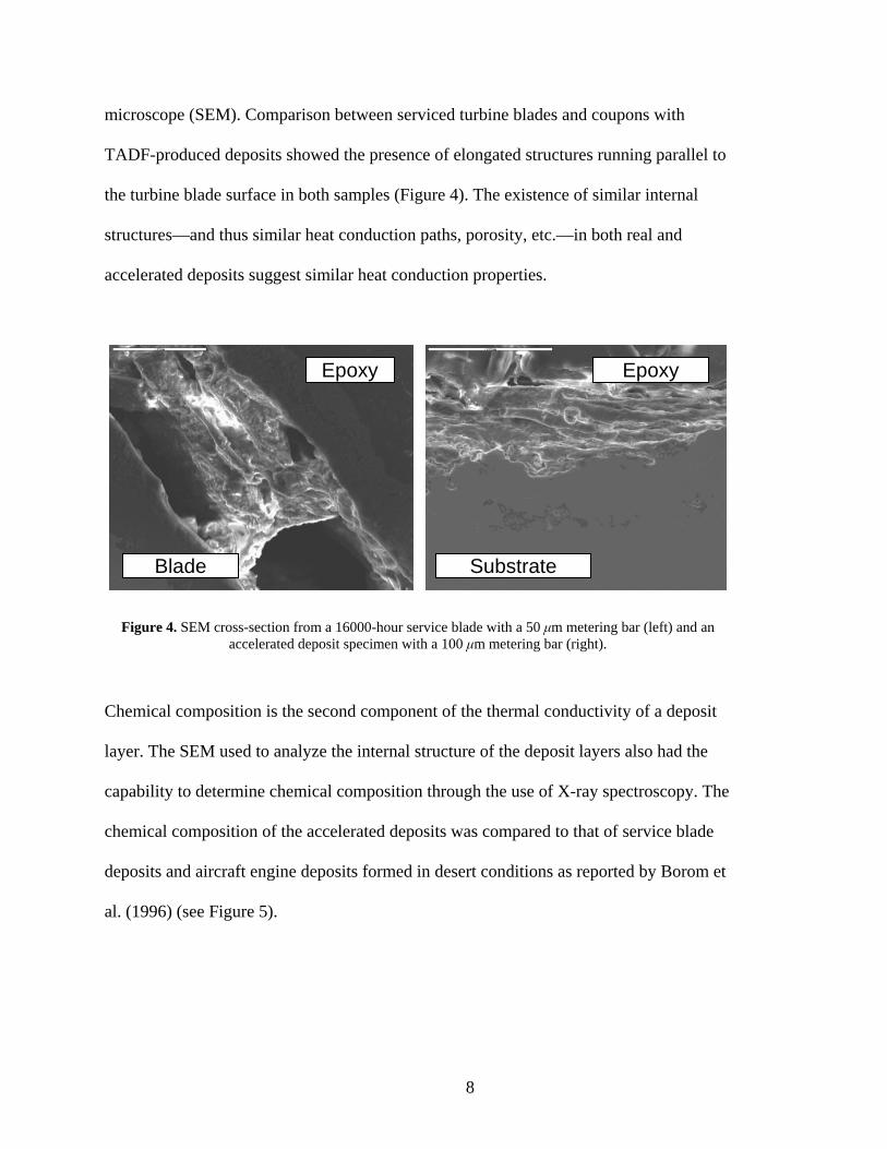
microscope (SEM). Comparison between serviced turbine blades and coupons with
TADF-produced deposits showed the presence of elongated structures running parallel to
the turbine blade surface in both samples (Figure 4). The existence of similar internal
structures—and thus similar heat conduction paths, porosity, etc.—in both real and
accelerated deposits suggest similar heat conduction properties.
Epoxy Epoxy
Blade Substrate
Figure 4. SEM cross-section from a 16000-hour service blade with a 50 μm metering bar (left) and an accelerated deposit specimen with a 100 μm metering bar (right).
Chemical composition is the second component of the thermal conductivity of a deposit
layer. The SEM used to analyze the internal structure of the deposit layers also had the
capability to determine chemical composition through the use of X-ray spectroscopy. The
chemical composition of the accelerated deposits was compared to that of service blade
deposits and aircraft engine deposits formed in desert conditions as reported by Borom et
al. (1996) (see Figure 5).
8

0%
5%
10%
15%
20%
25%
30%
35%
40%
45%
50%
CaO MgO Al2O3 SiO2 Fe2O3 TiO Cr2O3 ZnO Na2O NiO
Oxide
Service BladeBorom et al.Accelerated Test
Figure 5. Comparison of weight percentages of elements found in deposits on a land-based service turbine blade, an aircraft service blade (as reported by Borom et al, 1996), and a TADF-produced accelerated test
sample.
As shown in the figure, the chemical composition of the accelerated deposits most closely
matched the composition of the deposits studied by Borom et al. Some variation is
expected, however, due to the variety of chemical mixtures that can be found in different
environments. Most importantly, analysis of several locations throughout the accelerated
deposit layer showed that, like in-service turbine blades, the distribution of the
component chemicals throughout the accelerated deposits was relatively homogeneous
(Jensen, 2004). This indicates that a similar process occurs during both conventional
deposition as well as accelerated deposition.
9

1.3 Objective
With the development and validation of the TADF, the ability to simulate deposit
evolution within a reasonable time frame and under repeatable conditions was made
possible. The objectives of the current study are twofold. The first objective is the
production of deposits representative of those found on a gas turbine blade at several
discrete moments within an approximately 10,000 hour operational cycle and to study
any trends that may appear in the evolution of the surface roughness. The second
objective is the determination of the convective heat transfer characteristics of each
surface topology in order to determine how convective heat transfer rates change with
deposit evolution during the operation of a gas turbine. It is hoped that this study will be
the first in a line of studies meant to increase understanding of the changing conditions
within a gas turbine, thus allowing better informed decisions regarding maintenance
scheduling and the period between each shut-down.
10

Chapter 2: Deposition Evolution—Experimental Facilities and Techniques
2.1 Accelerated Deposition
The principle behind the production of accelerated deposits is that of matching the
product of the particle flow rate and the number of hours of operation. Thus, if the
particle flow rate through a gas turbine and the number of hours of operation was known,
then the particle flow rate through the TADF could be determined for a given
experimental time period. Conversely, a required experimental time period could be
determined from a given TADF particle flow rate.
GT Particle Flow (ppmw) x Operational Hours = TADF Particle Flow (ppmw) x Experiment Hours
Thus:
TADF Particle Flow (ppmw) = (GT Particle Flow (ppmw) x Operation Hours)/Experiment Hours
Or:
Experiment Hours = (GT Particle Flow (ppmw) x Operation Hours)/TADF Particle Flow (ppmw)
It must be noted that the limits of this technique have not yet been tested. Very high
particulate loadings tend to form unusual deposits that are dissimilar to real deposits.
Thus, a high particulate loading combined with a short test duration may produce
unrealistic deposits. Figure 6 illustrates the potential effect of overly high particulate
loadings. The deposits found immediately adjacent to the surface had a realistic
11
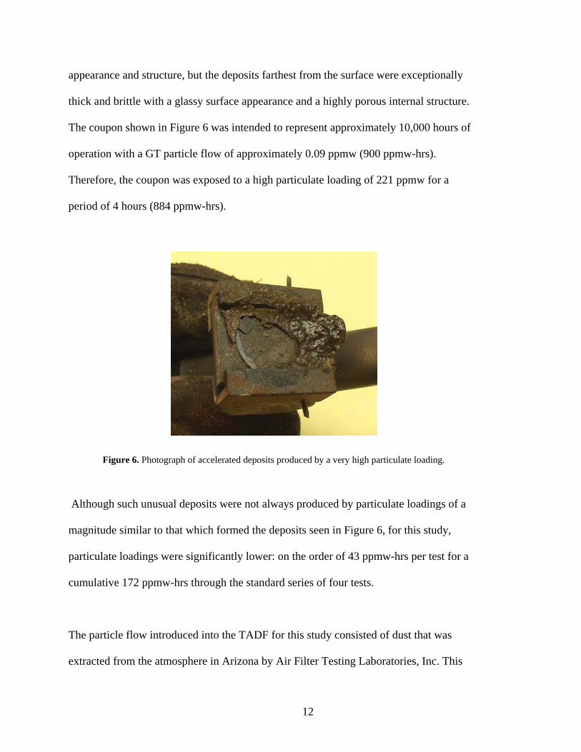
appearance and structure, but the deposits farthest from the surface were exceptionally
thick and brittle with a glassy surface appearance and a highly porous internal structure.
The coupon shown in Figure 6 was intended to represent approximately 10,000 hours of
operation with a GT particle flow of approximately 0.09 ppmw (900 ppmw-hrs).
Therefore, the coupon was exposed to a high particulate loading of 221 ppmw for a
period of 4 hours (884 ppmw-hrs).
Figure 6. Photograph of accelerated deposits produced by a very high particulate loading.
Although such unusual deposits were not always produced by particulate loadings of a
magnitude similar to that which formed the deposits seen in Figure 6, for this study,
particulate loadings were significantly lower: on the order of 43 ppmw-hrs per test for a
cumulative 172 ppmw-hrs through the standard series of four tests.
The particle flow introduced into the TADF for this study consisted of dust that was
extracted from the atmosphere in Arizona by Air Filter Testing Laboratories, Inc. This
12

dust meets the particulate size standards of ASHRAE (American Society of Heating,
Refrigeration, and Air Conditioning Engineers). Since the dust was taken directly from
the air, it has the same composition as particles that would have been drawn into a gas
turbine located in the same region. Therefore, this facility is able to produce deposits with
realistic chemical characteristics. Table 2 presents the chemical composition of the
particulate used in the Turbine Accelerated Deposition Facility for the current study. The
crustal composition of the earth as determined by Ford, 1954 is compared to the
composition of the Arizona dust as determined by Air Filter Testing Laboratories, Inc.
and as determined at BYU with X-ray spectroscopy. Figure 7 presents the size
distribution of the particulate used for the current study as a percentage of total mass.
Table 2. Chemical composition of particulate used in the Turbine Accelerated Deposition Facility.
Crustal Composition (Ford, 1954)
Manufacturer Assay of Seed
Particulate
BYU SEM Assay of Seed
Particulate
SiO2 59.8 68.5 60.2Al2O3 14.9 16 4.5CaO 4.8 2.9 13.7MgO 3.7 0.8 N/A
Other Alkalies 6.2 4.6 7.3Fe2O3 2.7 4.6 10.7FeO 3.4 negligible negligibleH2O 2 0 N/A
Ignition Losses N/A 2.7 N/A
13

0
5
10
15
20
25
30
35
40
45
0-5 5-10 10-20 20-40 40-80
Particle Diameter (μm)
Perc
ent o
f tot
al m
ass
(±3%
)
Figure 7. Particle diameter distribution by mass percentage.
2.2 Turbine Accelerated Deposition Facility
As mentioned above, the facility used to produce accelerated deposition is a highly
specialized natural gas-fueled combustor that reproduces the thermal and aerodynamic
conditions found at the first stage turbine blades in a gas turbine engine. This involves a
stream of combustion byproducts striking a turbine blade (or turbine blade coupon) at a
freestream temperature ranging from 1150°C-1200°C and a Mach number of
approximately 0.31. However, unlike the first stage of a gas turbine, the static pressure
within the TADF does not far exceed atmospheric pressure. As has been done by other
authors (Tabakoff et al., 1995; Wenglarz & Fox, 1990), no attempt was made to
reproduce the static pressures found in a real gas turbine with the TADF. These and other
authors (Borom et al., 1996; Kim et al., 1993) maintain that deposition rates are not a
function of static pressure. From the above studies and Jensen’s research, it can be
14

concluded that those parameters that are considered to be necessary for simulation of real
deposition are:
• Temperature—As mentioned in Chapter 1, deposition tends not to occur at
temperatures below which the particulate changes phase.
• Flow Velocity—In order to properly simulate the conditions inside a gas turbine,
particulate should strike the coupon surface with a momentum that is comparable
to that found in a real gas turbine.
• Particulate Concentration—As illustrated by Figure 6, overly high particulate
concentrations can result in unrealistic deposits.
2.2.1 TADF Operation
During operation, a horizontal stream of air is introduced into the base of the TADF. This
stream is diffused within a region filled with 1.3 cm-diameter marbles to ensure that the
flow is evenly distributed across the entire 30.5 cm-diameter base of the facility. The
diffused flow, now following a vertical path, is straightened by an aluminum honeycomb
and enters the combustion region. Within this region, four upward curving tubes
introduce partially pre-mixed natural gas, which is immediately ignited. A quartz
viewport allows visual monitoring of the flame. The viewport is kept clear of particulate
and soot by use of a purge that is fed by air bypassed from the main line. See Figure 8 for
details.
15

Marbles
Natural Gas Injection (2 of 4 shown)
Honeycomb Flow Straightener
Particulate Feed Tube
Main Air In
Particulate and Bypassed Air In
Natural Gas In
Flow Acceleration Cone
Equilibration Tube
Cone-mounted Thermocouple
Exit Flow Thermocouple
Probes
Coupon Holder
Quartz Viewport
Viewport Purge Air In
Figure 8. TADF cross-sectional schematic.
Particulate is introduced into the combustor through a line that is bypassed from the
primary air line. This secondary stream passes through a glass bulb into which particulate
is slowly injected with a motor-driven syringe (Figure 9). The particulate is entrained into
the flow and is sent into the combustor through a tube that enters the combustion region.
This tube initially curves downward, so as to keep it sufficiently clear of the flame, and
16

then upward. The particulate laden flow, now mixed with the hot exhaust gases, passes
through a cone directly above the combustion region which gradually accelerates the
flow. Immediately beyond the cone, the flow passes through a 1 m long equilibration tube
with a 1.58 cm inner diameter. The tube length was determined by the length of time it
would take to bring a 40 μm particle up to the freestream temperature and velocity of the
exit flow under test conditions (Jensen, 2004). At the exit, the flow velocity is
approximately 220 m/s (Mach 0.31). This value is typical of the inlet flow Mach number
experienced by first stage high pressure (HP) turbine blades and vanes during operation.
Mixing Bulb
Particulate Syringe
Bypassed Air In
Particulate and Bypassed Air Out to
TADF Motor-driven Syringe Plunger
Figure 9. Cross-sectional schematic of particle-feed system.
The tube terminates into a cup-shaped region within which a turbine blade coupon is
held. The coupon holder is located approximately 2 to 3 jet diameters above the exit of
17

the equilibration tube. At this point, the freestream temperature, which is between 1150ºC
and 1200ºC, matches that found in the first stage of G-class gas turbines.
The coupon holder is capable of being positioned at an angle of 30, 45, or 90°. For the
current study, an angle of 45° was decided upon due to the discovery by Jensen that the
statistical roughness factors Ra and Rt peaked in experiments where the coupon was held
at an angle 45° to the flow (Jensen, 2004). Additionally, of the three available angles, 45°
ensures that the greatest possible area would be exposed to parallel flow rather than
impinging flow. This was favorable since the convective heat transfer experiments were
performed with a heated stream of air flowing parallel to the surface. A FLUENT
simulation was used to determine how the exit gases flowed over the coupon and holder
(Figure 10). The simulation showed that the location of the stagnation point was below
the region where roughness measurements were taken.
Figure 10. FLUENT produced vector diagram for the TADF sample holder.
18
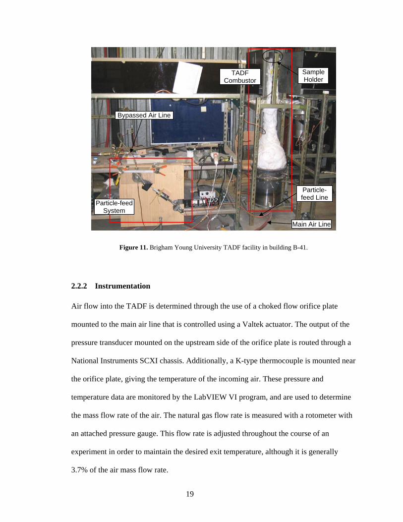
Bypassed Air Line
Particle-feed System
Sample Holder
Particle-feed Line
Main Air Line
TADF Combustor
Figure 11. Brigham Young University TADF facility in building B-41.
2.2.2 Instrumentation
Air flow into the TADF is determined through the use of a choked flow orifice plate
mounted to the main air line that is controlled using a Valtek actuator. The output of the
pressure transducer mounted on the upstream side of the orifice plate is routed through a
National Instruments SCXI chassis. Additionally, a K-type thermocouple is mounted near
the orifice plate, giving the temperature of the incoming air. These pressure and
temperature data are monitored by the LabVIEW VI program, and are used to determine
the mass flow rate of the air. The natural gas flow rate is measured with a rotometer with
an attached pressure gauge. This flow rate is adjusted throughout the course of an
experiment in order to maintain the desired exit temperature, although it is generally
3.7% of the air mass flow rate.
19

Figure 12. Cross-sectional schematic of TADF sample holder.
θ
Coupon Holder at 45°
Angle Thermocouple
probes
Exiting Flow
The exit temperature is measured by two 0.8mm diameter Super OMEGACLAD K-type
ermocouple probes capable of continuous use at 1150ºC protruding into the flow
t the
perature
n
(1)
th
(Figure 12). The probes are connected to a National Instruments NI SCXI-1112
thermocouple module mounted in an NI SCXI-1000 chassis. The temperature data a
exit is passed to the same LabVIEW VI program as the main air pressure and tem
data. Finally, the LabVIEW VI program calculates the total mass flow rate. The mass
flow rate, the data from thermocouple probes, and the cross-sectional area of the TADF
exit nozzle are used to calculate the flow Mach number using the Ideal Gas Law relatio
for the speed of sound (Equation 1). The specific heat ratio used was that for combustion
in air (γ=1.3) while the gas constant was approximated as being the same as the value for
air (i.e. R=287 J/kgK).
( )gasexitgas RTAmM
γρ&
=
20

2.2.3 TADF Modifications
he TADF as designed by Jensen was modified in several ways for this project. First it
e originally used within the combustor led to a problem
with incomplete combustion. To correct this, the air and natural gas lines were modified
to allow for partial premixing of the fuel. Because this modification increased the
velocity of the gas entering the TADF through the straight, horizontal fuel injection
nozzles, there was a tendency for the flame to impinge on the sides of the combustor. In
response, larger diameter nozzles which curved upward toward the cone of the TADF
were installed as shown in Figure 8.
Second, the flow Mach number at the exit of the TADF was originally determined prior
to an experiment, requiring that the air flow and exhaust temperature be maintained
within strict parameters during the course of the experiment so as to achieve that Mach
number. The air flow rate was monitored using a Fluke Multimeter which read the output
voltage from the pressure transducer mounted immediately upstream of the orifice plate
while the incoming air temperature was read by a pyrometer. Under this setup, only the
temperature of the flow exiting the TADF was recorded in real time. For the current
project, the pressure transducer output and main air thermocouple output were routed
through the National Instruments SCXI chassis and passed to a modified version of the
LabVIEW VI program used by Jensen in order to calculate the real time mass flow rate.
Further modifications of the VI allowed for a real time calculation and recording of the
exit flow Mach number.
T
was found that the diffusion flam
21

Third, bare wire S-type thermocouples which used ceramic sheathing for support were
replaced with the Super OMEGACLAD K-type thermocouple probes. It had been
iscovered that the brittle ceramic sheathes tended to develop deposits over the course of
nted
se of a
DF, the hand-cranked particle feed system originally mounted
as replaced by a motorized one. In addition, the larger syringe used by Jensen was
2.3 Turbine Blade Coupons
The TADF is designed to form deposits on turbine blade coupons rather than actual
turbine blades. These coupons—which are constructed of the same materials as those
e coated in the same manner—are used by turbine
his
of
d
an experiment, which often led to them breaking off under the aerodynamic load.
Although the thermocouple probes also developed deposits, their malleability preve
them from breaking while also allowing for the removal of deposits between tests without
suffering damage. The amount of deposits that formed on the probes over the cour
test was not sufficient to cause a noticeable change (i.e. a change larger than ±5°C) in the
measured temperature.
Finally, to allow for a more consistent rate of particulate feeding and to increase the level
of automation of the TA
w
replaced by a smaller diameter syringe to allow for the lower particulate loading used for
this project.
found in real turbine blades and ar
blade manufacturers for various testing purposes. The particular specimens used for t
project were flat, circular disks with a diameter of approximately 2.54 cm. Like real
turbine blades, the coupons consist primarily of a nickel-cobalt substrate. Three types
22

coupons—one with an unpolished oxidation resistant coating, one with a polished bare
metal surface, and one with an oxidation resistant coating and a polished overlying
thermal barrier coat (TBC)—were used in the current study (Figure 13). The TBC was air
plasma-sprayed, yttria stabilized zirconia (YSZ). These coupons were obtained from
several manufacturers of gas turbine components.
Until recently the TADF oncept of accelerated
deposition and to produce deposits for thermal conductivity experiments. These prior
and experiment time periods that recreated the amount
Figure 13. Cross-sectional drawing of coupons.
2.4 Deposition Evolution
had been used solely to demonstrate the c
experiments used particle loadings
of deposit that would be expected on a turbine blade that has undergone a full cycle
between maintenance periods. However, not only is the final state of a turbine blade of
interest, but also the intermediate states of the blade as it experiences deposition
conditions. Thus, each coupon used in this study underwent four cycles (hereafter
Coupon 1: Oxidation Resistant Coating
Coupon 2: Bare Substrate
Coupon 3: TBC and Oxidation Resistant
Coating
Oxidation resistant Bare substrate is flat and very smooth
TBC is somewhat smooth and wavy. A
thin oxidation resistant coating lies under the
TBC.
coating is very thin, flat, and rough
4.25 mm4.47 mm 4.62 mm 1.27 mm
23
referred to as “burns”) in the TADF, each simulating approximately three months of
operation, to produce a total of one year’s worth of deposition.
2.4.1 Burn Procedures
During a burn, each coupon experienced approximately 45 minutes of warm-up time,
during which the TADF was brought to an operational freestream temperature of between
eady state had been reached, particulate was introduced into
it
2.4.2 Coupon Surface Analysis
The surface of the coupon was analyzed with a Hommel Inc. T8000 profilometer
equipped with a TKU600 stylus. The Hommel profilometer runs the stylus across the
ata at a user-defined number of points during its
been
e in
1150ºC and 1160ºC. Once st
the facility. This particulate flow was maintained for a period of two hours after which
was closed off. The gas lines to the TADF were then shut off. The coupon was allowed to
cool for several hours, after which it was removed from its fixture. Upon removal, the
coupon was placed in another fixture and held firmly in place by four screws while
topological measurements were taken. Following this process, the coupon was
photographed and carefully stored until the following burn.
surface of a sample, taking height d
traverse. This direction of motion is defined as the x direction. Once a traverse has
made, the profilometer returns to its start position (i.e. x=0) and steps a certain distanc
the y direction, which is also user defined. The profilometer then repeats this process
until the predetermined number of steps has been made. The profilometer was set to
24

measure a region located roughly in the center of the circular coupon, 20 mm x 7.99 mm
in size. Approximately 2000 measurements were made in the x direction with each
traverse for a Δx of approximately 10 μm. Exactly 800 steps in the y direction were m
with a Δy of 10 μm.
ade
The m
surface topology of the coupon was measured five separate times: one measurement of
e clean surface prior to any deposition and one measurement after each of the four
Measured Region
y=7.99 mm
Flow Direction
x=20 mm
Figure 14. Illustration of coupon measured region and flow direction.
easurements were recorded as text files containing x, y, and z coordinates. The
th
burns in the TADF. Topological maps, three-dimensional surface representations, and
roughness statistics were produced with the Hommelwerke Hommel Map software.
25

26

Chapter 3: Deposition Evolution Results
3.1 Roughness Measurement
For this study, a statistical evaluation of the roughness of the deposits formed by the
TADF was an essential element in describing the evolutionary process as well as
predicting the convective heat transfer properties of each surface. Four statistics in
particular were utilized: Ra, Rq, Rz, and fα . The first three parameters are evaluated by
the Hommelwerke software. These values generally describe the unevenness of the
surface. The parameters Ra and Rq are defined as follows:
(2)
(3)
In a two-dimensional calculation, Ra is a measurement of the area bounded by the
roughness surface profile and the mean line of the roughness height. This area is then
divided by the evaluation length N. In a three-dimensional calculation, which is the type
of evaluation used in this project, the area is calculated along two dimensions and is
divided by both evaluation lengths N and M. Rq is similar to Ra but is an rms value.
∑ ∑−
=
−
=
=1
0
1
0,
1 N
x
M
yyxZ
NMRa
∑ ∑−
=
−
=
=1
0
1
0
2,
1 N
x
M
yyxZ
NMRq
27

As defined by the Hommelwerke software, the value of Rz is the mean of the vertical
istance between the five highest peaks and five deepest valleys within a neighborhood
of a given size. This statistic is often used to approximate the average roughness height k,
surface. The fourth
parameter mentioned,
d
which is the average distance between the peaks and valleys of a
fα , is the average forward facing angle (Figure 15). It was
determined for each surface with a MATLAB program written for that purpose. The
average forward facing angle gives a sense of the peakedness of the surface. This is
useful since equal Ra values can be obtained with very different surfaces. A surface
dominated by pointed cones may have the same Ra value as one that is covered with
hemispheres. Ra in conjunction with fα can describe a surface in great detail.
Additionally, Bons developed a correlation for determining the Stanton number of a
surface which involves the forward facing angle (Bons, 2005).
Flow Direction
αf
αf,1 αf,2αf,3
Figure 15. Surface roughness forward facing angle.
28

Surface roughness becomes important in cases where the surface is in contact with a
turbulent moving fluid. Rougher surfaces—especially those with higher average forward
facing angles—generally produce higher friction coefficients and rates of convective heat
transfer. It has been shown through experimentation that:
where k
(4)
(5)
has an average roughness height of ks which produces the equivalent effect. It has also
been shown that ks can be related to various roughness statistics:
(6)
3.1.1 Form Removal
While Coupons 1 and 2 were found to be flat, the TBC coating of Coupon 3 had a
noticeable degree of curvature. Such a curvature causes streamlines flowing over the
surface to curve, remaining tangent to the surface. Because the surface roughness that
affects the flow should be measured with respect to a meanline that runs parallel to the
flow, either the meanlin tened. Therefore, a
rm removal function available in the Hommelwerke software was used prior to
determining the surface roughness statistics. Whereas Coupons 1 and 2 were nearly flat,
s is a parameter known as the sandgrain roughness. The sandgrain roughness
correlates the average roughness height of a surface, k, with a sand-coated surface that
( )Re,sf kfc =
( )Re,skfSt =
( )
e must be curved or the surface must be flat
fo
fs kRafk α,,=
29

Coupon 3 had a curved surface similar to those seen on other TBC coated coupons us
in projects related to the current one.
ed
g
rvature prior to
ughness analysis (Figure 16).
3.1.2 Data Drop-out Error
A defect that was discovered in the Hommelwerke profilometer measurements for
4 is believed to have been caused by data drop-out error. This
ion in
, a
Figure 16. Topological map showing the preburn surface curvature Coupon 3 prior to (left) and followin(right) a second order form removal.
A second order form removal was therefore used to reduce the cu
ro
Coupon 3 Burns 1 through
error was caused by a short in the data transfer cables which resulted in an interrupt
the signal being sent from the profilometer stylus. Whenever this occurred, the data
would be smeared—data from a previous point would be used in place of the gap. Thus
discrete point would be seen as a short line (Figure 17). These lines originally occurred
parallel to the motion of the stylus. A 15° rotation to align the flow direction with the y-
axis has given the lines a 15° angle from the horizontal.
0 5 10 15 mm
mm
0
1
2
3
4
5
6
7
µm
0
5
10
15
20
25
30
35
40
45
50
x 0 5 10 15 mm
mm
0
1
2
3
4
5
6
µm
30
25
20
7
0
5
10
15y
30
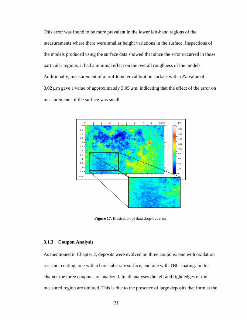
This error was found to be more prevalent in the lower left-hand regions of the
measurements where there were smaller height variations in the surface. Inspections of
e models produced using the surface data showed that since the error occurred in those
Additiona
3.02 μ r on
measurem
As mentioned in Chapter 2, deposits were evolved on three coupons: one with oxidation
resistant coating, one with a bare substrate surface, and one with TBC coating. In this
chapter the three coupons are analyzed. In all analyses the left and right edges of the
measured region are omitted. This is due to the presence of large deposits that form at the
th
particular regions, it had a minimal effect on the overall roughness of the models.
lly, measurement of a profilometer calibration surface with a Ra value of
m gave a value of approximately 3.05 μm, indicating that the effect of the erro
ents of the surface was small.
Figure 17. Illustration of data drop-out error.
3.1.3 Coupon Analysis
0 1 2 3 4 5 6 7 8 9 mm
mm
0
0.5
1
1.5
2
2.5
3
3.5
4
4.5
5
µm
140
120
100
80
60
40
205.5
0
160
180
31

interface between the coupon surface and the edges of the coupon holder. These
are ignored in this study since they are not representative of the deposits that form on the
free surface of a coupon.
deposits
3.2 Coupon 1: Unpolished Anti-Oxidation Coating
The surface of the first coupon was coated with an unpolished anti-oxidation layer,
making the surface rougher than that of a typical new turbine blade. The coupon
underwent four sequential burns, each lasting two hours, under similar temperatures and
particulate loadings (Table 3). Topological measurements were made following each
burn. The deposits showed little or no evidence of flaking after the coupon was removed
from the TADF. Although topological maps and three-dimensional representations of
Coupon 1 show deposition occurring during each burn (Figure 18 and Figure 19), the
surface does not become increasingly rougher with each experiment. In fact, the value of
Ra decreased from one test to the next in all but one case (see Figure 20). It is believed
that this behavior was caused primarily by the initially high level of roughness of the
coupon surface. Given the large number of peaks on the preburn surface, there were few
locations where new peak f regions where valleys
ould be filled in. Additionally, the average forward facing angle experiences only a
rns 2 and 3. Otherwise, the angle decreases steadily. This
would tend to reduce the convective heat transfer between the surface and the freestream
over time (see section 5.1.4).
s could be formed but a large number o
c
single slight rise between Bu
32

Table 3. TADF experimental settings for Coupon 1 (Oxidation Resistant Coating).
Time (hrs) ppmw Time (hrs) ppmw
2 1155
Simulated Parameters Test ParametersBurn Temperature (C) ppmw-hrs
1 1160 2619 0.02 52.37 2 26.192192 0.02 43.85 2 21.92
3 1155 2436 0.02 48.72 2 24.364 1160 2436 0.02 48.72 2 24.36
Considering that between the preburn surface and the Burn 4 surface, the value of Ra
increased by only 0.6%, the value of Rq increased by only 6.4%, and the value of fα
decreased by 53.5%, it is unknown at which point a trend of increasing roughness would
be seen. It is known that Jensen, who used several coupons from the same lot as
Coupon 1, was able to obtain a surface roughness that was significantly higher than that
of the preburn surface (Jensen, 2004). This is most likely due to the fact that Jensen us
a much higher particulate loading than was used in this study. It is possible that higher
particulate loadings per test, or more burns, would have eventually produced increasingly
rougher surfaces.
Although it did not follow the expected trend, Coupon 1 did serve to show that the TADF
could produce deposition evolution. It also indicated that the preburn roughness of the
surface may have a strong effect on the surface roughness after exposure to depositio
conditions. Later analysis would show that a period of a similar evolutionary behavior
occurred during the simulated operational cycles of Coupons 2 and 3 (
ed
n
Figure 32).
33

Figure 18. Topological representations of deposits on Coupon 1 (Oxidation Resistant Coating).
0 2 4 6 8 10 12 14 16 mm
mm
0
1
2
3
4
5
6
7
µm
0
20
40
60
80
100
120
140
160Figure 18a. Topological map of Coupon 1 prior to exposure to deposition conditions (Preburn).
Flow Direction
0 2 4 6 8 10 12 14 16 18 mm
mm
0
1
2
3
4
5
6
7
µm
0
20
40
60
80
100
120
140
160
180
0 2 4 6 8 10 12 14 16 18 mm
mm
0
1
2
3
4
5
6
µm
7
0
20
40
60
80
100
120
140
160
180
200Figure 18b. Topological map of Coupon 1 following Burn 1.
0 2 4 6 8 10 12 14 16 18 mm
mm
0
1
2
3
4
5
6
7
µm
0
20
40
60
80
100
120
140
160
180
200
220
Figure 18c. Topological map of Cofollowing Burn 2.
upon 1
Figure 18d. Topological map of Coupon 1 following Burn 3.
0 2 4 6 8 10 12 14 16 18 mm
mm
0
1
2
3
4
5
6
7
µm
0
20
40
60
80
100
120
140
160
180
200Figure 18e. Topological map of Coupon 1 following Burn 4.
34
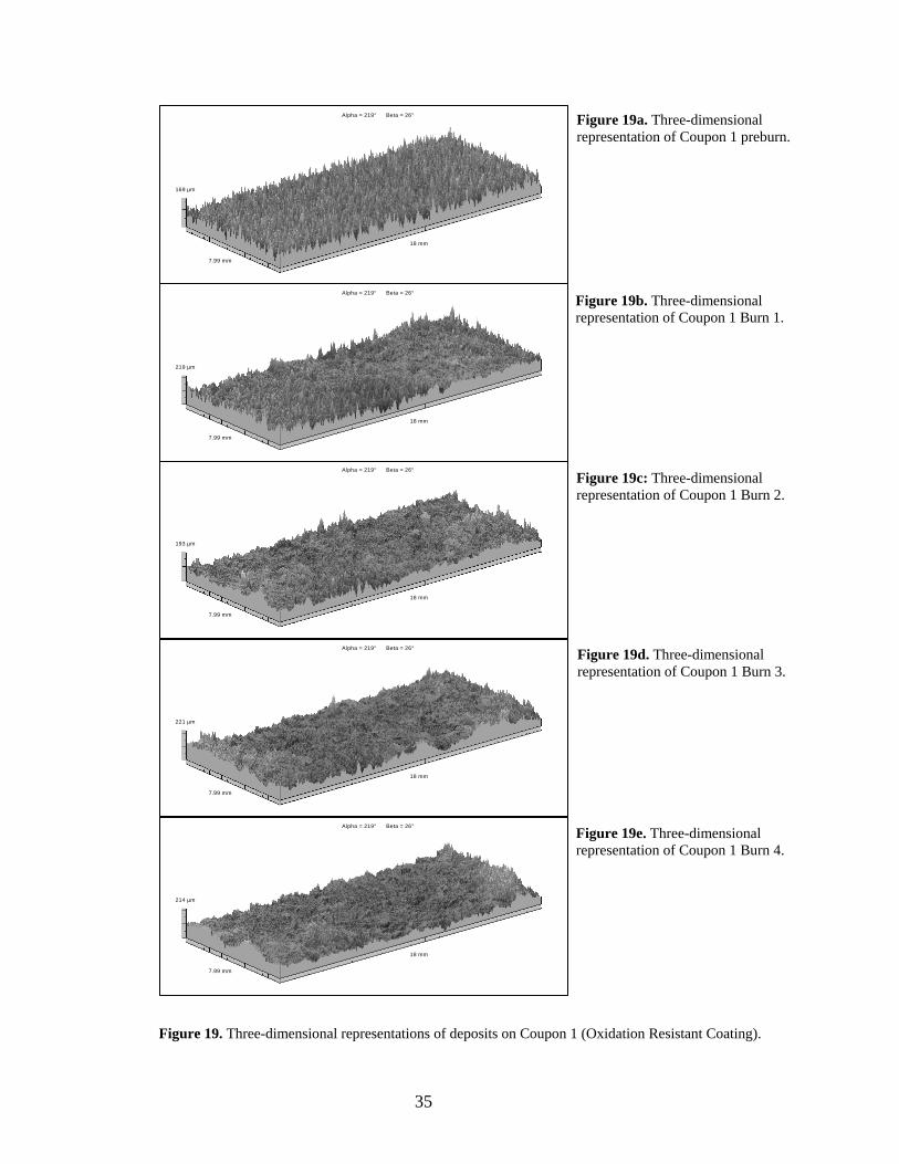
Figure 19. Three-dimensional representations of deposits on Coupon 1 (Oxidation Resistant Coating).
193 µm
7.99 mm
18 mm
Alpha = 219° Beta = 26°
Figure 19a. Three-dimensional representation of Coupon 1 preburn.
Figure 19c: Three-dimensional representation of Coupon 1 Burn 2.
169 µm
7.99 mm
18 mm
Alpha = 219° Beta = 26°
219 µm
7.99 mm
18 mm
Alpha = 219° Beta = 26°
Figure 19b. Three-dimensional representation of Coupon 1 Burn 1.
221 µm
7.99 mm
18 mm
Alpha = 219° Beta = 26° Figure 19d. Three-dimensional representation of Coupon 1 Burn 3.
214 µm
7.99 mm
18 mm
Alpha = 219° Beta = 26°
Figure 19e. Three-dimensional representation of Coupon 1 Burn 4.
35
36
0
5
10
15
20
25
0 1 2 3 4
Number of Burns
Ra,
Rq
( μm
); α
f (de
gree
s)
0
40
80
120
160
200
Rz
( μm
)
RaRqForward Facing AngleRz
Figure 20. Plot of roughness statistics for an 18 mm x 7.99 mm area of Coupon 1.
3.3 Coupon 2: Polished Bare Metal Substrate
The second coupon had a highly polished surface, making it smoother than that of a
typical new turbine blade. Coupon 2 experienced essentially the same deposition
conditions as Coupon 1 (Table 4). However, Coupon 2 experienced a high degree of
flaking, with large regions of bare substrate or deposits from previous burns being
exposed when the overlying deposits would flake off after removing the coupon from the
TADF. This flaking is believed to be caused by differing thermal coefficients of
expansion. As the coupon cools and contracts, the deposits are put under stress and
respond by flaking off. This process is often quite active, with flakes of deposit springing
off the surface, sometimes making an audible sound. After several hours of cooling,

flakes would often be found several inches away from the coupon. See section 3.3.7 for a
discussion of deposit flaking.
Due to the complication introduced by the flaking off of deposits, two approaches were
taken in analyzing the roughness characteristics of Coupon 2. In the first approach,
presented in sections 3.3.1 through 3.3.6, the surface roughness statistics were evaluated
based on the overall surface. In the second approach, presented in sections 3.3.8 through
3.3.11, a smaller portion of the overall measured surface was studied from burn to burn.
The portion selected consisted of a region where deposit flaking appeared to be minimal
(Figure 21). Representing three consecutive burns that produced long-lasting deposits, it
was believed that this magnified region would best represent the surface that Coupon 2
may have had if widespread flaking of deposits had not occurred.
Figure 21. Illustration of location of surface measurement and magnified region.
Original
MagRe
nified gion
Measurement
Flow Direction
37

3.3.1 Coupon 2, Preburn—Overall Surface
Figure 22a and Figure 23a show the topological features of Coupon 2 prior to TADF
sting. The image has been rotated so as to align the y-axis of the topological map and te
the flow direction. Additionally, the leftmost and rightmost sides have been cropped. This
is to exclude the ridges of deposits that form at the edges of the coupon holder from the
roughness analysis.
Table 4. TADF experimental settings for Coupon 2 (Bare Substrate).
1 1154 2192 0.02 43.85 2 21.922 1154 3410 0.02 68.21 2 34.13 1157 2631 0.02 52.62 2 26.314 1150 2558 0.02 51.16 2 25.5
Time (hrs) ppmw Time (hrs) ppmw
8
Test ParametersBurn Temperature (C) Simulated Parameters ppmw-hrs
3.3.2
t
the time of rem o the
the results given by the Homm
the coupon surfac e deposits in the
region at the top center of the measured area flaked off, leaving the surface seen in
igure 22b and Figure 23b. It is believed that the deposits remaining are representative of
the deposits that were removed.
Coupon 2, Burn 1—Overall Surface
Following Burn 1, the coupon was allowed to cool within the TADF for three hours. A
oval, the sample was found to be almost entirely coated in deposits. T
naked eye, the coating appeared to be nearly uniform. Since flaking deposits can affect
el profilometer, the coupon was left to cool further before
e was measured. During this time, a large portion of th
F
38

3.3.3 Coupon 2, Burn 2—Overall Surface
As with Burn 1, approximately three hours after the TADF was shut down, the sample
was removed. The sample was found to be almost entirely coated in deposits with a
visible discontinuity along the edges of the top center region where deposits had flaked
off following the first burn. As the coupon was allowed to further cool for several hours,
a large portion of the
deposits flaked off, leaving the surface seen in Figure 22c and
igure 23c. Flaking after Burn 2 appeared to occur primarily in the regions where
deposits had pre ious deposits
resulting from Burn 2 occurred in the region where deposits had flaked off following
Burn 1. This resulted in a topology that is a near mirror opposite of that obtained
following the Burn 1. Some flaking appeared to have occurred in those regions that
remained covered by deposits, although the f
the substrate. Much of this lighter flaking continued to occur for days after the burn and
the subsequent measurement with the Hommel profilometer.
ions
the deposits from Burn 1 flaked off, but not those from
urns 2 and 3, the highest region on the coupon—the top center region—shows only two
burns worth of deposition accumulation. Likewise, since the deposits from Burns 1 and 2
F
viously remained following Burn 1 whereas the most tenac
laking was not extensive enough to uncover
3.3.4 Coupon 2, Burn 3—Overall Surface
Unlike the previous burns, the majority of the deposits produced during Burn 3 remained
attached to the surface. It is notable that by this point the majority of deposits produced
during Burn 1 had almost completely flaked off, with the exception of two small reg
at the edges of the measured area (Figure 22c). Therefore, despite having experienced
three burns by this point, because
B
39

in the region surrounding the top center region simultaneously flaked off following burn
f this
Like the preceding burn, Burn 4 produced lasting deposits. Although some light flaking
occurred over much of the surface, only a thin layer of deposit was removed, leaving
behind the thick deposit layer underneath it (Figure 22e). The fact that the majority of the
deposits that were initially laid on the polished, unoxidized substrate surface had since
flaked off, whereas those deposits that formed on the later oxidized surface remained
firmly attached, suggests that permanent deposits form much more readily on the
oxidized substrate. This was despite the fact that the oxidized surface was only slightly
rougher than the unoxidized surface (see section 3.3.6).
3.3.6 Coupon 2 Overall Surface Roughness Trend
The evolution of the overall surface roughness behaved as expected, i.e. the roughness
increased continuously (Figure 24). From the preburn to Burn 3, the increase in Ra and
Rq is nearly linear, with a noticeably smaller rate of increase between Burns 3 to 4. The
average peak-to-valley roughness, Rz, increased by only 3% from Burns 1 to 2. This
suggests that the net deposit growth between these two burns was minimal. It is therefore
likely that deposit formation and subsequent flaking was the dominant mechanism in
two, those regions show only one burn worth of accumulation. Some light flaking
occurred in some of the thinner deposit layers following topological measurements o
surface.
3.3.5 Coupon 2, Burn 4—Overall Surface
40
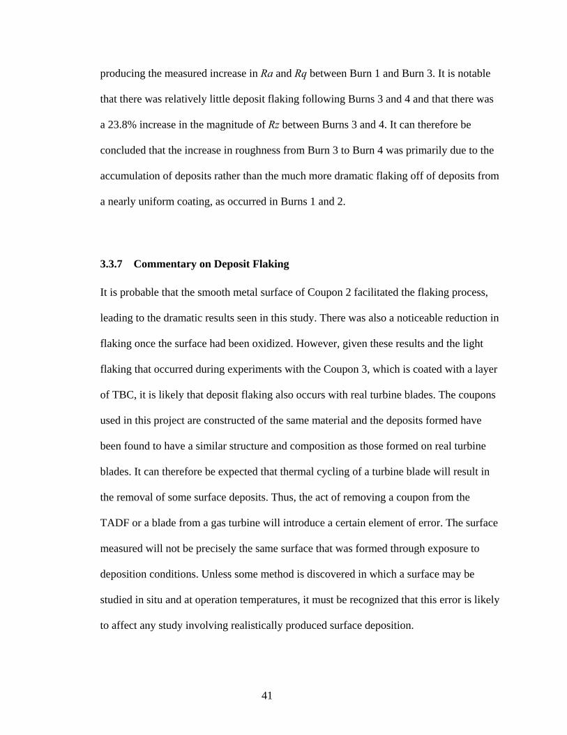
producing the measured increase in Ra and Rq between Burn 1 and Burn 3. It is notable
that there was relatively little deposit flaking following Burns 3 and 4 and that ther
a 23.8% increase in the magnitude of Rz between Burns 3 and 4. It can therefore be
conclude
e was
d that the increase in roughness from Burn 3 to Burn 4 was primarily due to the
ccumulation of deposits rather than the much more dramatic flaking off of deposits from
a nearly uniform coating, as occurred in Burns 1 and 2.
in
a layer
and the deposits formed have
een found to have a similar structure and composition as those formed on real turbine
blades. It can therefore be expected that thermal cycling of a turbine blade will result in
the removal of some surface deposits. Thus, the act of removing a coupon from the
TADF or a blade from a gas turbine will introduce a certain element of error. The surface
measured will not be precisely the same surface that was formed through exposure to
deposition conditions. Unless some method is discovered in which a surface may be
studied in situ and at operation temperatures, it must be recognized that this error is likely
to affect any study involving realistically produced surface deposition.
a
3.3.7 Commentary on Deposit Flaking
It is probable that the smooth metal surface of Coupon 2 facilitated the flaking process,
leading to the dramatic results seen in this study. There was also a noticeable reduction
flaking once the surface had been oxidized. However, given these results and the light
flaking that occurred during experiments with the Coupon 3, which is coated with
of TBC, it is likely that deposit flaking also occurs with real turbine blades. The coupons
used in this project are constructed of the same material
b
41
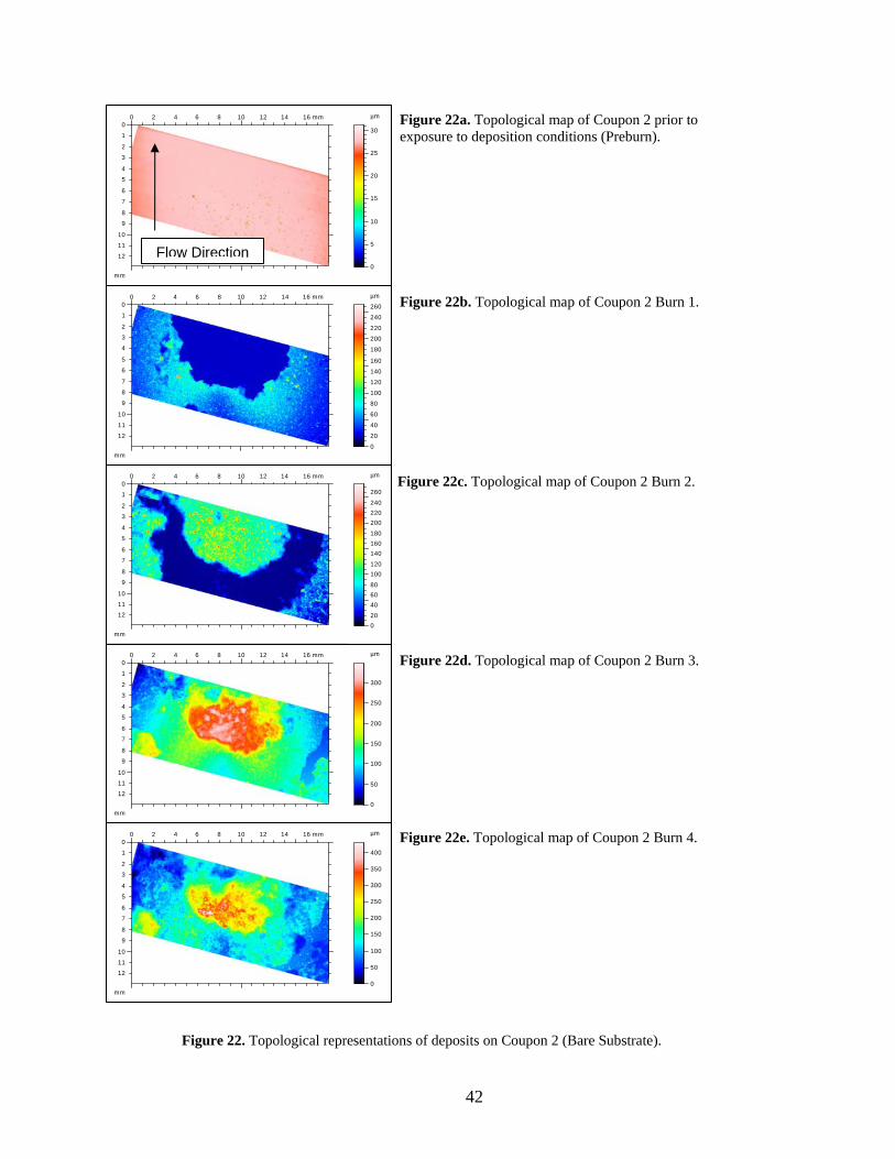
Figure 22. Topological representations of deposits on Coupon 2 (Bare Substrate).
0 2 4 6 8 10 12 14 16 mm
mm
0
1
2
3
4
5
6
7
8
9
10
11
12
µm
0
5
10
15
20
25
30Figure 22a. Topological map of Coupon 2 prior to exposure to deposition conditions (Preburn).
Flow Direction
0 2 4 6 8 10 12 14 16 mm
mm
0
1
2
3
4
5
6
7
8
9
10
11
µm
12
0
20
40
60
80
100
120
140
160
180
200
220
240
260 Figure 22b. Topological map of Coupon 2 Burn 1.
Figure 22c. Topological map of Coupon 2 Burn 2.
0 2 4 6 8 10 12 14 16 mm
mm
0
1
2
3
4
5
6
7
8
9
10
11
12
µm
0
50
100
150
200
250
300
Figure 22d. Topological map of Coupon 2 Burn 3.
0 2 4 6 8 10 12 14 16 mm
mm
0
1
2
3
4
5
6
7
8
9
10
11
12
µm
0
50
100
150
200
250
300
350
400
0 2 4 6 8 10 12 14 16 mm0
1
2
mm
3
4
5
6
7
8
9
10
11
12
µm
020
200
406080
100120
140160180
220240
260
Figure 22e. Topological map of Coupon 2 Burn 4.
42

31.2 µm
12.9 mm
18 mm
Alpha = 45° Beta = 30°
264 µm
12.9 mm
18 mm
Alpha = 45° Beta = 30° Figure 23b. Three-dimensional representation of Coupon 2 Burn 1.
Figure 23a. Three-dimensional representation of Coupon 2 prior to exposure to deposition conditions (preburn).
276 µm
12.9 mm
18 mm
Alpha = 45° Beta = 30° Figure 23c. Three-dimensional representation of Coupon 2 Burn 2.
349 µm
12.9 mm
18 mm
Alpha = 45° Beta = 30° Figure 23d. Three-dimensional representation of Coupon 2 Burn 3.
432 µm
12.9 mm
18 mm
Alpha = 45° Beta = 30° Figure 23e. Three-dimensional representation of Coupon 2 Burn 4.
Fig ). ure 23. Three-dimensional representations of deposits on Coupon 2 (Bare Substrate
43

44
0
10
20
30
40
50
60
70
80
0 1 2 3 4
Number of Burns
Ra,
Rq
( μm
)
0
60
120
180
240
300
360
420
480
Rz
( μm
)
RaRqRz
Figure 24. Plot of roughness statistics for the overall surface of Coupon 2.
3.3.8 Coupon 2, Burn 1—Magnified Region
Analysis of the magnified region of Coupon 2 shows that the surface changed little once
the deposits there had flaked off (Figure 25b; Figure 26b). The value of Ra increases
from 0.131 μm to 0.467 μm, which is significantly less rough than a polished TBC
surface (Coupon 3), which had a preburn Ra value of 2.14 μm. Although there are a few
small peaks, the majority of the surface is a nearly uniform, slightly rough surface. This
newly oxidized surface and its light deposits would form the basis for thick deposits in
later burns. The mean forward facing angle, fα , increased slightly from 0.3° to 1.14°
(Figure 27).

3.3.9 Coupon 2, Burn 2—Magnified Region
Burn 2 resulted in a deposit dominated by large peaks of roughness and is similar to that
shown in Figure 3 and Figure 26. These peaks led to a large spike in Rz for Burn 2, which
exceeded that of the following burn. The values of Ra and Rq also increased significantly,
reaching values of 13.3μm and 18.8μm respectively. The value of fα increased to 13.9°
(Figure 27).
3.3.10 Coupon 2, Burn 3—Magnified Region
With Burn 3, the valleys between the large peaks from Burn 2 appear to have been filled
in, reducing the value of Rz. While some of the peaks produced during Burn 2 may have
been broken off during Burn 3, the largest peak appeared to have survived while further
eposits built up around the base. The highest peak in Figure 25c, located approximately
at x=3.9 mm and y=0.2 mm can also be seen in Figure 25d, surrounded by further
s
e
d
deposits.
Burn 3 also marks a distinct change in the surface characteristics. Whereas Burn 2 wa
dominated by sharp peaks, Burn 3 now has a ‘wavy’ surface. Tall, distinct peaks hav
given way to large patches of deposits. The decrease in fα from the 13.9° of Burn 2 to
7.4° for Burn 3 confirms that the surface had indeed become less peaked. Interestingly,
despite the vast change in surface appearance, the Ra value increased only 28.6% from
Burn 2 to Burn 3; an increase that is much sm ler than is seen between any two other
burns. This ef
al
fect may be similar to that seen in Coupon 1, in which the valleys between
45

tall, sharp peaks were filled in with deposits, changing a peak-dominated surface into a
3.3.11 Coupon 2, Burn 4—Magnified Region
The change in surface appearance between Burn 3 and Burn 4 is also significant. Rather
g surface of Burn 3, the surface of Burn 4 is more jagged and has a
Ra value (115% percent higher) (Figure 27). The value of
‘wavier’ one.
than the rollin
fα significantly higher
increased from 7.4° for Burn 3 to 13.6° for Burn 4, confirming the visible increase in
3.3.12 Coupon 2 Magnified Region Roughness Trend
If the surface left behind after Burn 1—in which nearly all deposits had flaked off—were
to be taken as a starting point for deposition evolution, then an interesting trend is
revealed (Figure 27). Roughness—in the form of Ra and Rq—initially increases
substantially (Burn 1 to Burn 2). This is followed by a phase in which the rate of increase
peakedness. This value of the average forward facing angle is very close to that of
Burn 2, being only 2.2% lower. This much higher roughness may be due in part to some
post-burn deposit flaking, or possibly to some erosion that occurred during Burn 4, in the
upper left-hand portion of the region (Figure 26).
slows (Burn 2 to Burn 3). Finally, the rate of roughness increase picks up again (Burn 3
to Burn 4). Although it had been expected that the values of Ra and Rq would increase
with exposure to deposition conditions, this precise trend was unexpected.
46

Even more unexpected than the exact trend in the increase in roughness was the
fluctuation seen in the peakedness of the deposit structures, as shown by both a visual
xamination of the three-dimensional surface representations as well as by a comparison e
of the average forward facing angle, fα (Figure 27). After Burn 1 and the subsequent
flaking of the local deposits, the zoomed surface of Coupon 2 showed a relatively low
value of fα . This value increased by 1120% after Burn 2, resulting in the high pe
dominated surface seen in
ak-
duc d with
4
Figure 26c. With Burn 3, a ‘wavier’ surface was pro e
the attendant 46.8% drop in average forward facing angle. Finally, the surface of Burn
returned to a more peaked state, as was indicated by its 83.8% increase in fα over t
of Burn 3. Also of note is the fact that Rz follows the same trend as that of
hat
fα , with the
value of Rz following the first effective burn (Burn 2) exceeding that of the following
burn. This is then followed by a rapid upturn that coincides with the upturn in the average
rward facing angle. This trend in the increase in roughness as well as a similar fo
fluctuation in fα can also be seen in the evolution of deposits on the TBC coupon,
3.4 Coupon 3: TBC Coated Substrate
Coupon three was exposed to similar deposition conditions as the preceding two coupons
(Table 5). The surface topologies and three-dimensional representations presented are
derived from a 9.52 mm x 5.71 mm portion of the measured surface that was used as the
basis for the wind tunnel models intended for convective heat transfer experiments
(Figure 28).
Coupon 3 (see section 3.4.5).
47

Topological representations of deposits on Coupon 2, zoomed region (Bare Substrate). Figure 25.
0 0.5 1 1.5 2 2.5 3 3.5 4 4.5 5 mm
mm
00.20.40.60.8
11.21.41.61.8
22.22.42.62.8
µm
01234567891011121314
Figure 25a. Topological map of zoomed Coupon 2 preburn.
0 0.5 1 1.5 2 2.5 3 3.5 4 4.5 5 mm
Flow Direction
mm
00.20.40.60.8
11.21.41.61.8
22.22.42.62.8
µm
0
2
4
6
8
10
12
14
16
18
20
22
24 Figure 25b. Topological map of zoomed Coupon 2 Burn 1.
0 0.5 1 1.5 2 2.5 3 3.5 4 4.5 5 mm
mm
00.20.40.60.8
11.21.41.61.8
22.22.42.62.8
µm
0
20
40
60
80
100
120
140
160
180
200Figure 25c. Topological map of z ed Coupon 2 oomBurn 2.
0 0.5 1 1.5 2 2.5 3 3.5 4 4.5 5 mm
mm
00.20.40.60.8
11.21.41.61.8
22.22.42.62.8
µm
0
20
40
60
80
100
120
140
160
180
0 0.5 1 1.5 2 2.5 3 3.5 4 4.5 5 mm
mm
00.20.40.60.8
11.21.41.61.8
22.22.42.62.8
µm
0
50
100
150
200
250
300
Figure 25d. Topological map of zoomed Coupon 2 Burn 3.
Figure 25e. Topological map of zoomed Coupon 2 Burn 4.
48

14.6 µm
3 mm
5 mm
Alpha = 45° Beta = 30°
Figure 26a. Three-dimensional representation of zoomed Coupon 2 preburn.
24.6 µm
3 mm
5 mm
Alpha = 45° Beta = 30° Figure 26b. Three-dimensional representation of zoomed Coupon 2 Burn 1.
209 µm
3 mm
5 mm
Alpha = 45° Beta = 30° Figure 26c.: Three-dimensional representation of zoomed Coupon 2 Burn 2.
181 µm
3 mm
5 mm
Alpha = 45° Beta = 30° Figure 26d. Three-dimensional representation of zoomed Coupon 2 Burn 3.
310 µm
3 mm
5 mm
Alpha = 45° Beta = 30° Figure 26e. Three-dimensional representation of zoomed Coupon 2 Burn 4.
Figure 26. e). Three-dimensional representations of deposits on Coupon 2, zoomed region (Bare Substrat
49

50
0
10
20
30
40
50
0 1 2 3 4
Number of Burns
Ra,
Rq
( μm
); α
f (de
gree
s)
0
50
100
150
200
250
Rz
( μm
)
RaRqForward Facing AngleRz
Figure 27. Plot of roughness statistics for the zoomed 5 mm x 3 mm region of Coupon 2.
The near uniformity of the deposits on Coupon 3 allows the magnified region to be
representative of the whole with regards to Ra and Rq. However, due to the sensitivity of
Rz to relatively small areas of tall peaks or low valleys, the difference between the
average peak-to-valley values of the magnified region versus those of the overall surface
measurement is much more substantial (see Table 6).
This region was selected, in part, because of damage suffered by the TBC following
Burns 3 and 4. Thermal cycling caused portions of the TBC on the coupons left side to
crack and lift away from the rest of the surface, a process known as spallation. Further
damage occurred when the raised portions of the TBC were removed to avoid damage to
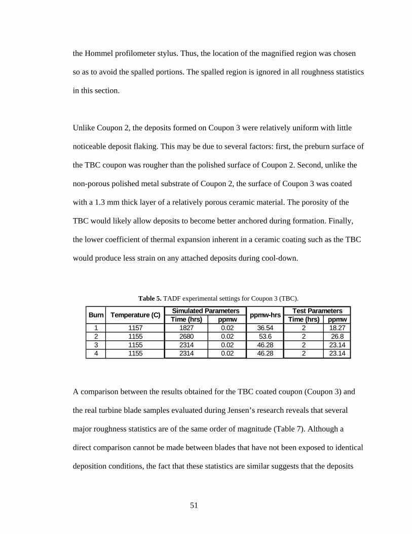
the Hommel profilometer stylus. Thus, the location of the magnified region was chosen
so as to avoid the spalled portions. The spalled region is ignored in all roughness statistics
in this section.
Unlike Coupon 2, the deposits formed on Coupon 3 were relatively uniform with little
noticeable deposit flaking. This may be due to several factors: first, the preburn surface of
the TBC coupon was rougher than the polished surface of Coupon 2. Second, unlike the
non-porous polished metal substrate of Coupon 2, the surface of Coupon 3 was coated
with a 1.3 mm thick layer of a relatively porous ceramic material. The porosity of the
TBC would likely allow deposits to become better anchored during formation. Finally,
the lower coefficient of thermal expansion inherent in a ceramic coating such as the TBC
would produce less strain on any attached deposits during cool-down.
3 1155 2314 0.02 46.28 2 23.14
Table 5. TADF experimental settings for Coupon 3 (TBC).
Time (hrs) ppmw Time (hrs) ppmw1 1157 1827 0.02 36.54 2 18.22 1155 2680 0.02 53.6 2 26.8
4 115
7
5 2314 0.02 46.28 2 23.14
Test ParametersBurn Temperature (C) Simulated Parameters ppmw-hrs
A comparison between the results obtained for the TBC coated coupon (Coupon 3) and
al
the real turbine blade samples evaluated during Jensen’s research reveals that several
major roughness statistics are of the same order of magnitude (Table 7). Although a
direct comparison cannot be made between blades that have not been exposed to identic
deposition conditions, the fact that these statistics are similar suggests that the deposits
51

that have formed on Coupon 3 are similar in character to deposits that formed on real
turbine blade surfaces.
Table 6. Comparison between overall surface roughness statistics and the magnified region roughness statistics.
Burn 1 2 3 4Overall Surface 16.3 18.1 22.9 30.9Zoomed Region 16.6 17.1 20.2 32.9
% Difference 1.84 -5.52 -11.79 6.47Burn 1 2 3 4
Zoomed Region 20.8 22 25.9 40.1Overall Surface 20.6 23.5 30.2 38.9
e 0.97 -6.38 -14.24 3.08% DifferencBurn 1 2 3 4
Zoomed Region 174 140 145 286% Differenc
Overall Surface 204 222 250 366
e -14.71 -36.94 -42.00 -21.86
Ra
Rq
Rz
Table 7. Comparison between service blade roughness statistics and the TBC coupon (Coupon 3) statistics.
Surface Type Ra (μm) Rt (μm) α rms Λ s
25000hr blade Figure 3 32 240 27 22
22500hr blade 41 296 24 36<1000hr blade 19 394 18 77
24000hr vane 17 220 15.8 134
Burn 1 16.6 194 17.2 49
Burn 2 17.1 172 15.8 72.5Burn 3 20.2 186 15.8 73
Burn 4 32.9 286 19 108
Serv
iced
B
lade
sTB
C C
oupo
n
3.4.1 Coupon 3, Burn 1
The surface produced by Burn 1 consists mostly of small, evenly distributed roughness
structures along with some sharp peaks and a few larger clumps of deposits (Figure 29b
and Figure 30b). Ra has increased from the 2.14 μm of the preburn surface to 16.6 μm.
52

Figure 28. Illustration of location of surface measurement and magnified region. Image above is of Coupon 3 Burn 3.
The fact that much of the roughness consists of sharp peaks rather than the thick crusts of
deposits found on later burns makes the surface of Coupon 3 Burn 1 somewhat similar to
oupon 2 Burn 2—the effectual first burn of Coupon 2. By comparison, the value of C fα
for Coupon 3, Burn 2 is 12.6°, which is 9.3% lower than that of Coupon 2, Burn 1.
3.4.2 Coupon 3, Burn 2
The large peak seen after Burn 1 located at x=8 mm and y=2 mm is missing from Burn 2
(Figure 30c). A region of deposits in the lower right-hand corner at approximately x=7
mm and y=5.5 mm has begun to grow. A very tall peak has also grown in the upper right-
ith regards to roughness, statistically there has been very little change: the
erage forward facing angle has dropped to 10.7°,
indicative of a slight decrease in the peakedness of the surface roughness.
hand corner. W
value of Ra increased by 3%. The av
Flow Direction
Magnified Region
Damaged Region
Original Measurement
53

3.4.3 Coupon 3, Burn 3
With Burn 3, the region of deposits in the lower right hand corner has persisted and has
become more prominent (Figure 30d). The peak in the upper right hand corner is now
gone. Except for these few changes, the appearance of the two surfaces is similar, as are
their respective roughness statistics. Ra has increased by 18.1% to a value of 20.2 μm.
The value of fα is nearly identical at 10.9°.
3.4.4 Coupon 3, Burn 4
With Burn 4, the deposits in the lower right hand corner have grown dramatically and
cover a sizeable portion of that corner (Figure 30e). A very large clumping of deposits
has formed in the upper left hand corner with no noticeable precursor in the previous
ely easy to trace over time, other structures appear quite suddenly.
u significantly: Ra has increased by 62.87% to a value of
burns. This suggests that, while some roughness structures have a long evolutionary
history that is relativ
The ro ghness has increased
32.9 μm. The average forward facing angle has increased to 12.95°, showing that the
surface is now more peak-dominated than following the previous burn. As was the case
for Coupon 2, Burn 4, this value of fα is similar to that of the first effective burn
(Burn 2 for Coupon 2, Burn 1 for Coupon 3). In the case of Coupon 3, the average
forward facing angle for Burn 4 is 2.61% higher than that of Burn 1.
54

Figure 29. Topological representations of deposits on Coupon 3 (TBC).
Figure 29a. Topological map of Coupon 3 preburn.
0 1 2 3 4 5 6 7 8 9 mm
mm
0
0.5
1
1.5
2
2.5
3
3.5
4
4.5
5
5.5
µm
0
20
40
60
80
100
120
140
160
180
Figure 29b. Topological map of Coupon 3 Burn 1.
0 1 2 3 4 5 6 7 8 9 mm
mm
0
0.5
1
1.5
2
2.5
3
3.5
4
4.5
5
5.5
µm
0
20
40
60
80
100
120
140
160
Figure 29c. Topological map of Coupon 3 Burn 2.
0 1 2 3 4 5 6 7 8 9 mm
mm
0
0.5
1
1.5
2
2.5
3
3.5
4
4.5
5
5.5
µm
0
20
40
60
80
100
120
140
160
180
0 1 2 3 4 5 6 7 8 9 mm
mm
0
0.5
1
1.5
2
2.5
3
3.5
4
4.5
5
µm
18
5.50
2
4
6
8
10
12
14
16
Flow Direction
Figure 29d. Topological map of Coupon 3 Burn 3.
0 1 2 3 4 5 6 7 8 9 mm
mm
0
0.5
1
1.5
2
2.5
3
3.5
4
4.5
5
5.5
µm
020406080100120140160180200220240260280 Figure 29e. Topological map of Coupon 3 Burn 4.
55
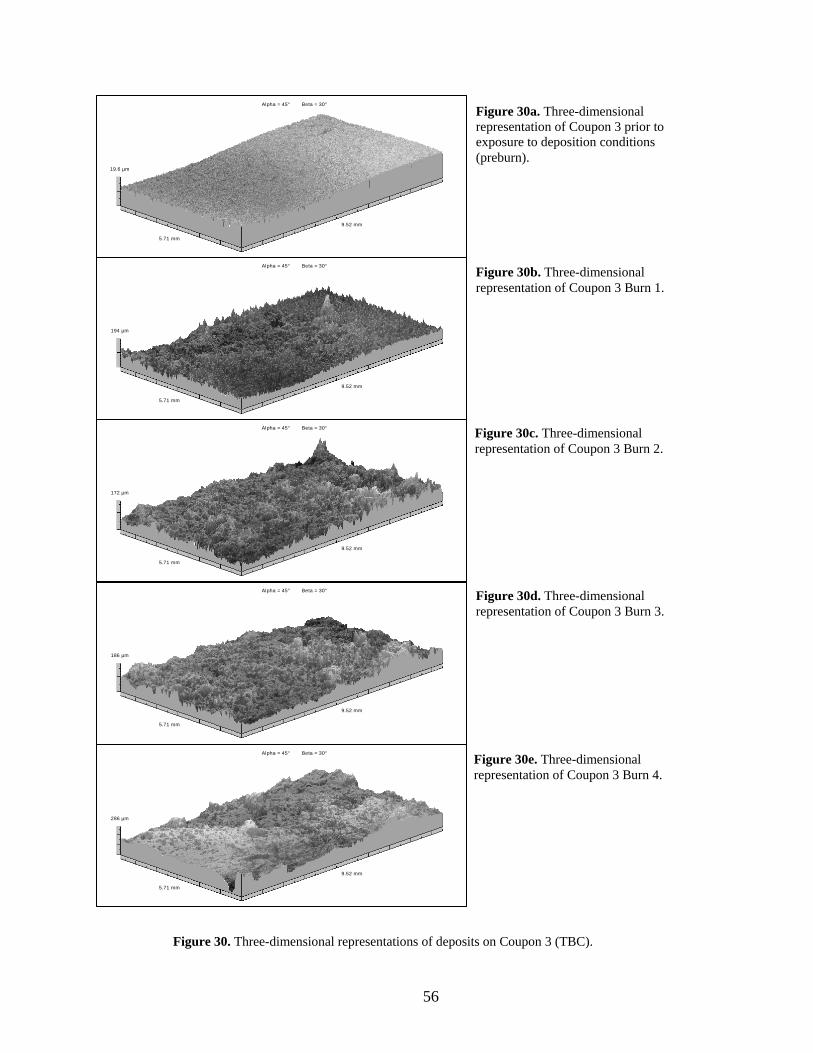
19.6 µm
5.71 mm
9.52 mm
Alpha = 45° Beta = 30°
Figure 30a. Three-dimensional representation of Coupon 3 prior to exposure to deposition conditions (preburn).
194 µm
5.71 mm
9.52 mm
Alpha = 45° Beta = 30°
Figure 30b. Three-dimensional representation of Coupon 3 Burn 1.
172 µm
5.71 mm
9.52 mm
Alpha = 45° Beta = 30° Figure 30c. Three-dimensional representation of Coupon 3 Burn 2.
186 µm
5.71 mm
9.52 mm
Alpha = 45° Beta = 30° Figure 30d. Three-dimensional representation of Coupon 3 Burn 3.
286 µm
5.71 mm
9.52 mm
Alpha = 45° Beta = 30°
Figure 30e. Three-dimensional representation of Coupon 3 Burn 4.
Fig ). ure 30. Three-dimensional representations of deposits on Coupon 3 (TBC
56

57
0
10
20
30
40
50
0 1 2 3 4
Number of Burns
Ra,
Rq
( μm
); α
f (de
gree
s)
0
60
120
180
240
300
Rz
( μm
)
RaRqForward Facing AngleRz
Figure 31. Plot of roughness statistics for a 9.52 mm x 5.71 mm region of Coupon 3.
3.5 Commentary on Roughness Similarities Between Coupons 1, 2, and 3
A review of the different types of surfaces experienced by Coupons 2 and 3 illustrates
that the deposits on a turbine blade surface may undergo extreme changes in character
and appearance over time, despite having been exposed to the same deposition conditions
(e.g., duration of exposure, particulate loading, and freestream temperature). At one point
the deposits may take the form of distinct peaks. At another point, the deposits may form
a thick, wavy crust. Some structures may slowly develop over time, whereas others
appear much more rapidly. The only apparent constant is that surface roughness, in the
form of Ra and Rq, continually increases with time, although not necessarily at a constant
rate.

The interruption in the rise of Ra, Rq, and fα , in which there is a “pause” in Ra and Rq
and a decrease in fα , is of particular interest. Whether or not this pattern continues could
be determined with further burns beyond what has been performed for this study.
Why this trend occurred is not entirely known. It is possible that, with the initial exposure
to deposition conditions, large peaks are formed across the relatively smooth surface,
resulting in a spike in Rz and average forward facing angle, fα . As time passes, the
continuing deposition fills in the valleys between the peaks, resulting in a decrease in
those two values. At this point, the surface roughness begins to plateau. This might
continue until a certain “critical mass” is reached, at which point a new series of peaks is
formed, resulting in an increase in Ra, Rz, and fα similar to that seen after the initial
xposure to deposition conditions.
Analysis of Coupon 1 shows that it follows a similar pattern as Coupons 2 and 3,
although with a different starting point. The preburn of Coupon 1 is 21% higher than
the Burn 2 Ra for the magnified region of Coupon 2 and only 5.8% lower than the Burn 1
Ra of Coupon 3. The average forward facing angle for the Coupon 1 preburn surface is
also quite high. Red boxes in Figure 32 illustrate where the evolution of deposits on the
surface of Coupon 1 falls with regards to deposit evolution on the other two coupons.
Whereas Coupons 2 and 3 developed peaked surfaces with higher values of
e
Ra
fα
following the first effective burn, Coupon 1 began with such a surface. Consequently, the
exposure of Coupon 1 to deposition conditions caused a decrease in the average forward
58

facing angle, just as it occurred with Coupons 2 and 3. Additionally, the values of Ra and
Rq saw a period of stagnation in all three cases. It is likely that further deposition would
have also caused Coupon 1 to experience an increase in the roughness statistics
mentioned.
0
40
50
Ra,
αf (
)
0
200
250
μm)
10
20
30
0 1 2 3 4
Number of Burns
Rq
( μm
); de
gree
s
50
100
150
Rz
(
RaRqForward Facing AngleRz
Figure 32. Comparison between deposit evolution on Coupons 1, 2, and 3.
0
30
m);
fre
es
0
180
240
Rz
( μm
)
10
20
0 1 2 3 4
Number of Burns
Ra,
Rq
( μ
60
120
40
50
)
300
α (d
eg
RaRqForward Facing AngleRz
1. First effective burn
3. α
2. αf, first peak
f, second peak
0
5
20
0 1 2 3 4
Number of Burns
a, R
q f (
d
0
120
160
0
m)
10
15
25
R( μ
m);
αeg
rees
)
40
80
20
Rz
( μ
RaRqForward Facing AngleRz
2.
1.
1.
2.3.
2.
3.
59

60
Chapter 4: Convective Heat Transfer Measurements—Experimental Facilities and Techniques
4.1 Roughened Turbine Blade Surfaces and Convective Heat Transfer
With the development of accelerated deposition evolution, the convective heat transfer
characteristics of the surfaces produced could be determined. The method chosen to
accomplish this is relatively common and involves the use of a heated wind tunnel and
scaled-up Plexiglas models of the rough coupon surfaces. In order to allow the use of a
fairly conventional wind tunnel with manageable freestream velocities and temperatures,
the heat transfer characteristics of the surfaces tested were expressed in the form of the
dimensionless Stanton number (St):
(7)
4.2 Roughness Models
Plexiglas models of the rough surfaces of the coupons were used for the wind-tunnel
based thermal studies for several reasons. First, the method used to find the Stanton
number requires that the thermal diffusivity of the rough surface be known. The non-
isotropic nature of the coupon surfaces with deposits makes determination of an average
density and specific heat difficult, while the complex structure of the deposits requires
extensive testing to determine their thermal conductivity. A scaled-up isotropic model of
pcuhSt∞
=ρ
61
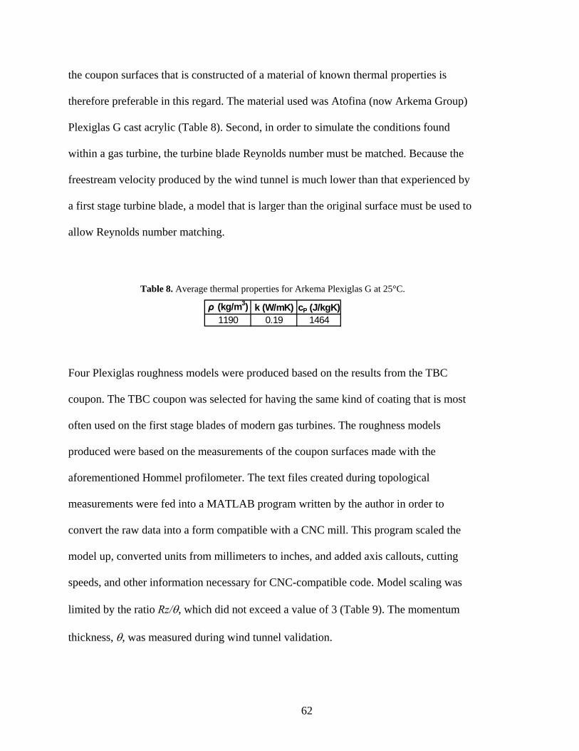
the coupon surfaces that is constructed of a material of known thermal properties is
erefore preferable in this regard. The material used was Atofina (now Arkema Group)
Plexiglas G cast acrylic (Table 8). Second, in order to simulate the conditions found
eestream velocity produced by the wind tunnel is much lower than that experienced by
allow Reynolds number matching.
th
within a gas turbine, the turbine blade Reynolds number must be matched. Because the
fr
a first stage turbine blade, a model that is larger than the original surface must be used to
Table 8. Average thermal properties for Arkema Plexiglas G at 25°C.
ρ (kg/m3) k (W/mK) cP (J/kgK)1190 0.19 1464
Four Plexiglas roughness models were produced based on the results from the TBC
coupon. The TBC coupon was selected for having the same kind of coating that is most
ften used on the first stage blades of modern gas turbines. The roughness models
produced were based on the measurem coupon surfaces made with the
forementioned Hommel profilometer. The text files created during topological
measurements were fed into a MATLAB program written by the author in order to
convert the raw data into a form compatible with a CNC mill. This program scaled the
model up, converted units from millimeters to inches, and added axis callouts, cutting
speeds, and other information necessary for CNC-compatible code. Model scaling was
limited by the ratio Rz/θ, which did not exceed a value of 3 (Table 9). The momentum
thickness, θ, was measured during wind tunnel validation.
o
ents of the
a
62

Table 9. Rz/θ ratios for TBC coupon models.
Burn 1 2 3 4Model Rz (mm) 3.48 2.8 2.9 5.72
Rz/θ 1.36 1.10 1.14 2.24
A review of the literature shows that, as a general guideline in turbine roughness
experimentation, the ratio of Rz/θ does not exceed a value of 3 (e.g. Bons, 2002). The
four surfaces in this study were enlarged by a factor of 20, which produced a maximum
θ ratio of 2.24 in the case of Burn 4. Because of this scaling factor, and due to the
limited size of the largest usable rectangular region of roughness with the appropriate
proportions (5.715 mm x 9.525 mm), the original data formed 25% of the total model
surface, with the remaining 75% being composed of mirror images of the original data.
hus the entire 22.86 cm x 38.1 cm space provided for the model in the wind tunnel was
across the y-axis in order to form the top half of the model. 2. The top half is then mirrored across the x-axis in order to form the bottom half of
the model.
Rz/
T
filled (Figure 33).
Figure 33. Technique used to mirror data. 1. Original data is mirrored
Original Data
1
2
63

Although by mirroring the ich the average forward
facing angle is now the leeward facing angle and vice versa, this only occurs on the
upstream half of the models. The average surface temperature of only the downstream
half, where the forward facing angles of the original surface are correctly oriented, is
measured by the FLIR camera. Each model measures 22.86 cm x 38.1 cm, with the
leading 11.43 cm of the model serving to accomplish the smooth-to-rough transition.
Antonia & Luxton (1971) and Taylor & Chakroun (1992) showed that the smooth-to-
f
. In order to ease the transition from flow over smooth panels to flow
panel, approximately 1 cm of the leading edge of each model was machined
ill down to the meanline of the model roughness (Figure 34).
Given that each raw data file was composed of nearly 550,000 discrete points, and that
this number of points would have to be quadrupled in order to fill the necessary area, the
program which produced the CNC code also deleted every other x-coordinate and every
other y-coordinate prior to mirroring the data. This increased the x and y distance
between each point from approximately 0.203 mm to 0.406 mm. Despite this fourfold
decrease in the number of points used to reproduce the coupon surfaces, the resulting
data a region has been produced in wh
rough transition occurs within approximately 3 to 4 boundary layer thicknesses. Within
the region of transition, skin friction values (c ) and Stanton numbers can be up to 20%
higher than the transitioned values. For the wind tunnel used in this project, pitot probe
measurements showed that the average boundary layer thickness in the vicinity of the
models was 2.3 cm, giving a smooth-to-rough transition length somewhere between
6.9 cm and 9.2 cm
over a rough
with a 5/8” ball end m
64

Figure 34. A ball end mill is used to eliminate an abrupt smooth-to-rough transition at the model’s leadinedge.
CNC code was 12.7 MB in size and required 10 hours to machine. The impact of this
decrease in resolution on the values of Ra and Rq was not measured.
With the CNC code, the roughness models were cut out of 2.54 cm thick Plexiglas acrylic
sheets using a Fryer CNC mill equipped with a modified countersink. The countersin
g
k
as chosen because it most closely approximated the tip of the profilometer stylus that
o a
ly
, in
hich the most amount of actual surface material is removed, is one in which the
countersink cuts along the side of a structure with a 45° slope. In this event there would
w
scanned the surface originally. Both are conical in shape with a 90° included angle. This
was to ensure that the model contours would be as close as possible to the original
surface measurements. However, the countersink is not precisely a 20x scaled-up model
of the Hommel stylus. The stylus had a tip radius of 5 μm, which would translate t
scaled-up tip radius of 0.1 mm, whereas the countersink had a tip radius of approximate
0.5 mm. This causes a slight error in the cutting of the model. The worst case scenario
w
Smooth Plate
Ball End Mill
Flow Direction
Rough Plate
65
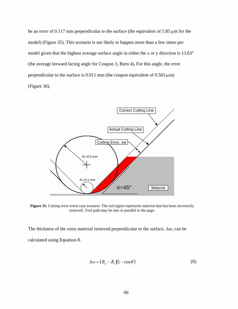
be an error of 0.117 mm perpendicular to the surface (the equivalent of 5.85 μm for t
Figure 35). This scenario is not likely to happen more than a few times per
model given that the highest average surface angle in either the x or y direction is 13.6
(the average leeward facing angle for Coupon 3, Burn 4). For this angle, the error
perpendicular to the surface is 0.011 mm (the coupon equivalent of 0.563 μm)
Figure 36).
he
model) (
3°
(
The thickness of the extra material removed perpendicular to the surface, Δw, can be
calculated using Equation 8.
(8)
Figure 35. Cutting error worst case scenario. The red region represents material that has been incorrectly removed. Tool path may be into or parallel to the page.
Correct Cutting Line
Actual Cutting Line
Cutting Error, Δw
R2=0.5 mm
R1=0.1 mm
θ=45° Material
( )( )θcos112= −Δ RRw −
66

Figure 36. Cutting error for angles below 45°. The red region represents material that has been incorrectly removed. Tool path may be into or parallel to the page.
Additionally, there is an advantage to using a tool with a slightly oversized tip radius.
Due to the fact that the tool-tip is rounded, small ridges are left between the rows that the
tool traces. The size of these ridges can be reduced either by reducing the distance
between the rows (Δy), by increasing the tool-tip radius, or both. Given the size of the file
and the time it takes to machine a model, the option of decreasing Δy was not considered.
Had a tool with a 20x scaled-up tip been used with the 0.406 mm spacing, it would have
produced ridges that w uivalent height of
8.09 μm on the coupon. The tool that was used, with the 0.5 mm tip-radius, produced
ridges that were approximately 0.043 mm in height—the scaled-down equivalent of
2.12 μm high ridges (Figure 37). Being on the order of the Ra value for the preburn
surface, this ridge height is more acceptable. The deviations from the original surfaces
introduced during the ma ake the models slightly
ere approximately 0.162 mm in height—an eq
nufacturing process will tend to m
Cutting Error, Δw
Actual Cutting Line
R2=0.5 mm
R1=0.1 mm
Material
Correct Cutting Line
θ
67

rougher. The equipment used during this project did not have the range necessary to
measure the magnitude of the effect on Ra and Rq.
Figure 37. Schematic of ridges formed by rounded tool-tip. Tool path is into the page.
4.3 Wind Tunnel Heat Transfer Analysis
Jones
solution of the heat diffusion equation as applied to a semi-infinite surface with one-
dimensional conduction. Small departures from a uniform heat transfer rate are assumed
and the surface temperature is assumed to be a piece-wise linear function. A derivation of
Equation 9 can be found in Appendix B.
(9)
Ridge Height Δy
In order to determine the convective heat transfer properties of the deposit roughened
surfaces, a technique which takes advantage of a relation developed by Schultz and
was utilized (Equation 9) (Schultz & Jones, 1973). The equation derives from the
−
−
−+−
−∑
=
=icondq ,"i
j jiji
jSjS
tttt
TT
1 1
1,,2πακ
68

This equation was developed to allow the determination of the heat flux into or out of
surface under transient conditions through average s
a
urface temperature measurements.
This is the sam In this technique,
following a period of therm
roughness model with kn erature history is
monitored w erature history is
all bead size
of the thermo
the radia 4°C
nd 51°C.
Due to the assumption that the surface temperature can be modeled as a piecewise linear
function, the equation initially produces an unstable prediction of the heat transfer
coefficient. Violation of the piecewise linear assumption is due to the temperature
fluctuations that occur immediately after heating of the freestream has begun. However,
after this period of instability, the heat transfer coefficient achieves a near constant value
with time.
.4 Wind Tunnel Description
A wind tunnel capable of producing a heated fr ble in building B-38 a
righam Young University (Figure 38). The wind tunnel produces a stream of air through
the use of a blower. The stream passes through a duct and through a section equipped
e technique and equation utilized by Bons (Bons, 2002).
al soaking, a heated freestream is suddenly blown over a
own thermal properties. The surface temp
ith a FLIR thermal camera, while the freestream temp
monitored by a 0.005” K-type thermocouple immersed in the flow. The sm
couple decreases its response time to much less than 1 second and decreases
tion error (Appendix C). Freestream temperatures typically fell between 4
a
4
t eestream is availa
B
69

with heating elements. The stream then passes through a conditioning plenum that
smoothly transitions the stream from a circular cross-section to a square one with side
lengths of 38.1 cm while also reducing the freestream turbulence through the use of
f
e to serve as a boundary layer trip.
Figure 38. Schematic of the wind tunnel used for heat transfer measurements for this study.
several layers of screen. The square section of tunnel runs for 134.8 cm until it connects
to a rectangular test section constructed for this study (Figure 39). The leading edge o
the floor of the test section is set 2.7 cm higher than the floor of the square section.
Through this gap the boundary layer that had developed up to this point is allowed to
bleed off for improved control over boundary layer growth. The first 7.62 cm of the test
section floor is constructed of a thin plate of aluminum which forms the leading edge. A
length of 2 mm diameter wire is stretched across this plate at a location 2.5 cm from the
leading edg
The test section consists of fixed vertical walls, a segmented floor section, and a
moveable ceiling. The floor is segmented to allow a roughness model to be placed at a
variety of distances from the boundary layer bleed. This allows for greater control over
Blower
Hea
To Secondary
ting Section
Test Section Conditioning Plenum
Pre-existing Plexiglas Section
Plexiglas Test Section
Butterfly Valve
Flow Direction
Tunnel Right Side
Tunnel Left Side
70

the ratio of the average roughness height Rz to the local momentum thickness θ of t
boundary layer. The roughness model is 38.1 cm wide and 22.9 cm long with its leadin
edge typically located 103.8 cm from the boundary layer bleed. The ceiling can be
adjusted to allow variation of the streamwise pressure gradient present within the test
section. Favorable and unfavorable pressure gradients of varying magnitudes may be
produced in addition to a pressure gradient of zero. This feature further enhances the
controllability of the momentum thickness of the flow over the roughness model.
he
g
For th ld be
early zero. To achieve this, the ceiling was angled upward approximately 0.3°. The
Figure 39. Schematic of wind tunnel test section.
is study, the wind tunnel ceiling was adjusted so that the pressure gradient wou
n
shape of the boundary layer at multiple points along the length of the test section
centerline was measured using a boundary layer pitot probe connected to the higher
pressure port of a 0.5” H2O Druck pressure transducer. The lower pressure port of the
Flow Direction
Boundary Layer Bleed
Boundary Layer Trip
Z-axis Traverse
Freestream Thermocouple
Roughness Panel
Downward Looking IR
Camera Pitot ProbeAdjustable
Support Panel
Ceiling
Adjustable Floor Panels
Pre-existing Plexiglas Section
71
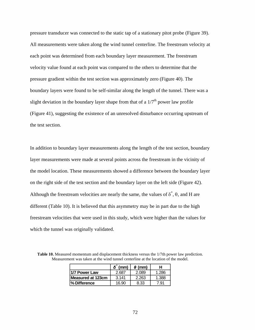
pressure transducer was connected to the static tap of a stationary pitot probe (Figure 39
All measurements were taken along the wind tunnel centerline. The freestream velocity a
each point was determined from each boundary layer measurement. The freestream
velocity value found at each point was compared to the others to determine that the
pressure gradient within the test section was approximately zero (Figure 40). The
boundary layers were found to be self-similar along the length of the tunnel. There wa
slight deviation in the boundary layer shape from that of a 1/7
).
t
s a
), suggesting the existence of an unresolved disturbance occurring upstream of
which the tunnel was or
(mm) θ (mm) H
th power law profile
(Figure 41
the test section.
In addition to boundary layer measurements along the length of the test section, boundary
layer measurements were made at several points across the freestream in the vicinity of
the model location. These measurements showed a difference between the boundary layer
on the right side of the test section and the boundary layer on the left side (Figure 42).
Although the freestream velocities are nearly the same, the values of δ*, θ, and H are
different (Table 10). It is believed that this asymmetry may be in part due to the high
freestream velocities that were used in this study, which were higher than the values for
iginally validated.
Table 10. Measured momentum and displacement thickness versus the 1/7th power law prediction. Measurement was taken at the wind tunnel centerline at the location of the model.
*
1/7 Power Law 2.687 2.089 1.286Measured at 123cm 3.141 2.263 1.388% Difference 16.90 8.33 7.91
δ
72
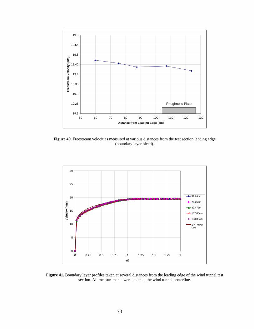
19.2
19.25
19.3
19.45
19.5
19.55
19.6
Free
ream
Voc
ity/s
)
19.35
19.4
50 60 70 80 90 100 110 120 130
Distance from Leading Edge (cm)
stel
(m
Roughness Plate
Figure 40. Freestream velocities measured at various distances from the test section leading edge (boundary layer bleed).
5
15ity
10
20
25
30
Velo
c (m
/s)
59.69cm
75.25cm
87.47cm
107.00cm
123.82cm
1/7 PowerLaw
00 0.25 0.5 0.75 1 1.25 1.5 1.75 2
z/δ
Figure 41. Boundary layer profiles taken at several distances from the leading edge of the wind tunnel test section. All measurements were taken at the wind tunnel centerline.
73

0
5
10
15
20
25
30
0 5 10 15 20 25 30 35 40 45 50
z (mm)
Velo
city
(m/s
)
+0.22
+0.13
+0.02
-0.07
-0.18
-0.24
1/7 PowerLaw
Fig ed from the tunnel cente by the tunnel width.
Table 11. Average measured momentum and displacement thicknesses versus those predicted by the 1/7th
power law. Measurements were taken across the width of the wind tunnel at the model location.
ure 42. Boundary layer profiles measured across the width of the test section. Distances are measurrline and are normalized
δ * θ H 1/7th Power Law 2.874 2.236 1.285Measured (average) 3.548 2.549 1.392% Difference 23.45 14.00 8.29
4.5 Thermal Measuring Devices
The FLIR infrared camera is vertically mounted on top of the wind tunnel test section and
is aimed directly at the roughness model. The surface temperature data recorded by the
camera over time is output to a laptop computer at a user-defined rate. The camera is
capable of showing the varying temperatures of a surface through a color coded image
and can determin is study, the
minimum zoom factor of 1.00 was selected, allowing the camera to view a section of the
e the average temperature of a user-selected region. For th
74

model 15.87 cm wide and 11.43 cm long with a resolution of 320x240 pixels. The surface
temperature data was recorded by the computer at a sample rate of one reading per
second. The freestream temperature was monitored by a K-type thermocouple with a
bead diameter of 0.127 mm inserted into the flow. This device is also sampled at a rate of
one reading per second. The thermocouple is located at the leading edge of the model and
is fixed approximately 50 mm (~2δ) above the test section floor. The distance of two
boundary layer thicknesses was chosen after it had been discovered that the core flow of
the wind tunnel was approximately 1 to 2 degrees cooler than those regions closer to the
tunnel floor. A measurement of the thermal boundary layer indicated that the freestream
t
onitored simultaneously with a static tap-equipped pitot probe to measure the
freestream velocity during testing.
4.5.1 FLIR Camera In Situ Calibration
alibration of the FLIR camera was performed which produced a correction
curve for temperature measurements made by the camera. A flat plate that was made of
am ness models and was shown through experiment to
9).
as
emperature was constant up to at least 2.5 boundary layers. This thermocouple is
m
An in situ c
the s e type of Plexiglas as the rough
have an emissivity of 0.9 was placed in the wind tunnel. One thermocouple was affixed
to the surface exposed to the flow and another 0.005” diameter bare wire thermocouple
was sandwiched between the underside of the plate and the support panel (see Figure 3
These two thermocouples indicated when the plate had become isothermal. The plate w
heated to five distinct temperatures within the range of temperatures that a model may
experience during a wind tunnel experiment. These five points were plotted against the
75

temperature indicated by the surface thermocouple and a curve fit was applied. The
temperatures recorded by the FLIR were found to deviate linearly from that of the a
surface (Figure 43).
ctual
Ts = 0.95176TIR + 1.97913
20
22
26
28
32
34
38
40
22 24 26
T s)
R2 = 0.9998924
30
36
28 30 32 34 36 38 40
TIR (C)
(C
R camera in situ calibration.
.
Figure 43. Curve fit for FLI
4.5.2 FLIR Camera Ambient Temperature Correction
The surface temperature measurements made by the thermal camera were found to be
very sensitive to the ambient temperature; i.e. the temperature of the Plexiglas walls
surrounding the model. Although the camera software can compensate for the ambient
and atmospheric temperatures, these values must be input into the computer manually
and cannot be changed while the camera is recording. This does not cause a problem
during steady state measurements such as those performed during the in situ calibration
76

However, since the ambient temperature is transient during the convective heat trans
experiments, a degree of error is introduced.
fer
he FLIR camera allows a recorded measurement to be played back with different
ambient and atmospheric temperature settings. The temperature history resulting from the
changes can be saved as a text file. In order to compensate for the error introduced by the
limitation of using a fixed ambient temperature, the recording was played back with two
different settings: the first set at the initial ambient temperature, immediately prior to the
moment at which the heated freestream passed over the surface, and the second at the
final ambient temperature achieved during the test. A linear interpolation between the
two surface temperature data sets was applied to determine the appropriate surface
temperature at any given moment of the temperature history based on the ambient
temperature at that moment.
nfortunately, the ambient temperature was initially assumed to be equal to the
onitored during
every test. However, the data obtained during those experiments in which the temperature
of the walls was measured was used to determine a relation between the freestream
temperature and the final wall temperature (i.e., the final ambient temperature). The wall
temperature history was reconstructed using the final ambient temperature of the walls
and the initial value and curvature of the surface temperature data. This was considered to
be an appropriate approach given that both the walls as well as the models are
constructed of the same material and are heated by the same stream. The error present in
T
U
freestream temperature. Thus, the temperature of the walls was not m
77

Tw has been approximated to be ±2°C due to the reconstructive method by which it was
determined. By replaying the thermal camera data with the ambient temperature set at the
o extremes of the ambient temperature data, it was determined that an additional bias
4.5.3 FLIR Camera Temperature Drift Correction
The measured temperature values tend to drift during camera operation. The magnitude
of the drift tended to be a function of how long the camera had been active prior to
testing. One hour of operation would produce an upward drift on the order of 0.5 degrees
per minute, whereas three hours of operation would produce a drift, either upward or
downward, of up to 0.1 degrees per minute (Figure 44). To correct this, the camera
performs an automatic adjustment of its internal shutter every few minutes. The
discontinuities introduced into the temperature history by this adjustment cause the
Schultz and Jones equation to predict momentary spikes in the heat transfer coefficient
and, due to the summation, an overall incorrect result. To avoid this, the auto-adjust was
turned off during wind tunnel tests. To compensate for the drift that would occur, a drift
test was performed prior to each test. While monitoring an isothermal plate, the camera
would be allowed to record temperature data for approximately 4 minutes: the length of a
wind tunnel test. The results would be plotted and the slope of the change in mean
temperature would be determined. This slope would be used in the post processing of the
data obtained during the subsequent wind tunnel test to correct for drift effects.
tw
error of ±0.24°C was appropriate for Ts (see Appendix C).
78

y = 0.0006x - 0.0129
0.1
0.2
0.25
0.3
e D
evia
on (C
)
-0.05
-0.10 40 80 120 160 200 240
0
0.05
0.15
Time (seconds)
Tem
pera
tur
ti
Figure 44. Plot of temperature drift encountered prior to a wind tunnel test.
4.6 Experimental Procedure
Before wind tunnel testing, a roughness model would be placed inside the wind t
test section (see
unnel
f the
d and ran
t a frequency of 45 Hz with the flow being ducted through the secondary test section
(see Figure 38). This frequency produces a freestream velocity of approximately 19.5 m/s
Figure 39). The test section was isolated by blocking off a portion o
tunnel a short distance upstream of the boundary layer bleed with a sheet of Plexiglas. A
second sheet was taped over the test section exit. The model was allowed time to reach a
near isothermal state—defined for this project as having a temperature difference of
0.6°C or less between the upper and lower surfaces of the model. The temperature
difference was determined with the thermocouple arrangement described in section 4.5.1.
The camera was activated at this point.
Once the model and the camera were ready, the wind tunnel blower was activate
a
79

at room temperature when ducted through the primary test section. Shortly after the
blower is turned on, the heating coils are activated. As the flow is heated, a thermocouple
mounted in the secondary test section monitors the temperature until steady state is
reached. At that point, the recording functions of the computer monitoring the primary
test section freestream thermocouple and the computer monitoring the IR camera are
activated simultaneously by hand. The Plexiglas sheets blocking off the primary test
section are then removed. The butterfly valve closing off the primary test section is
quickly opened and the valve leading to the secondary test section is immediately closed.
This produces a sudden gust of heated air through the primary test section and over the
odel. Each test would run for approximately 4 minutes before data collection would be
stopped and the heating coils deactivated.
ined, the data were conditioned in Microsoft
xcel. First, the surface temperature data produced with the two different ambient
m
4.7 Stanton Number Determination
One smooth Plexiglas panel, as well as the roughness models based on the four surface
measurements of the TBC coated Coupon 3, were tested in the manner described in
section 4.6. These tests resulted in surface temperature, freestream temperature, and
freestream velocity histories (Figure 45).
Once the temperature histories were obta
E
temperature settings would be corrected for drift, with the error as a function of time
being subtracted from the data. Second, the surface temperature data and the freestream
data would be plotted against each other (Figure 45). A slight disparity occurs in the two
80

time scales since the surface temperatures and the freestream temperatures are record
on two separate computers.
ed
0
10
20
30
50
mpe
rur
e (C
)
6
12
18
30
Velo
cit
(m/s
)
40
0 40 80 120 160 200 240
Time (seconds)
Teat
0
24
y
TinfTsVinf
erature and velocity histories.
Time was either added to or subtracted from the freestream history time scale in order to
was based on the moment in which both the freestream and the plate began to increase in
h an increase in velocity was measured. An
increase in velocity precedes the increase in freestream temperature due to the immediate
acceleration of a slug of non-heated air when the butterfly valve is opened. Once the
anton
number were exported as a tab-delimited text file:
• Column 1: Surface temperature data timescale
Figure 45. Typical temp
synchronize the moment in which heated air first flowed over the plate. Synchronization
temperature rather than the moment in whic
curves were properly aligned, seven columns of data necessary to determine the St
81

• Column 2: Surface temperature with the initial ambient temperature setting
• Column 3: Surface temperature with the final ambient temperature setting
• Column 4: Wall (ambient) temperature data
• Column 5: Freestream temperature timescale
• Column 6: Freestream temperature
• Column 7: Freestream velocity
This text file was exported into the MATLAB program “schultzjones.m” (see Appendix
C). Upon activation, this MATLAB program requests the name of the data file to be read
and the desired name for the results file. Next, the program asks for the ambient pressure
at the time of the test in order to calculate the appropriate air density in the tunnel.
Finally, the program asks for the initial and the final ambient temperature settings for the
linear interpolation be d into the program
re the thermal properties of Plexiglas G. However, the program can be altered so as to
asurements has been compensated for,
the r is applied to further correct the
tween surface temperature data sets. Hard code
a
make the properties user-defined.
Although the surface and freestream temperature data are both sampled at a rate of
approximately one measurement per second, the sample rate may fluctuate slightly. To
compensate, the program interpolates the freestream temperature data, aligning it with the
timescale of the surface temperature data. Following this, the program interpolates the
two surface temperature data sets as described in section 4.5.2. Once the effect of the
ambient temperature on the surface temperature me
co rection curve derived from the in situ calibration
82

surf e
pro m find
the a tive heat transfer coefficient, the
pro m account thermal radiation
exc unnel walls (Figure 46, Equations 10-12):
(10)
1)
2)
e
Stanton number data—leveled out (Figure 47). The average and the standard deviation
ac temperature values (section 4.5.1). With the data properly conditioned, the
gra performs the operations of the Schultz and Jones equation (Equation 9) to
he t flux into the surface. To solve for the convec
gra performs an energy balance which takes into
hange between the model and the wind t
Figure 46. Illustration of heat transfer between a roughness model and the environment.
qconv qrad
qcond
radconvcond qqq = −
(1
(1
The program results are saved as a text file and are exported back to Excel in order to
determine the moment at which the heat transfer coefficient data—and by association, th
( )( ) 44wsscond TTATThAq −−−= ∞ εσ
( )s
wscond
TTh
−=
∞
44 TTq −+" εσ
83
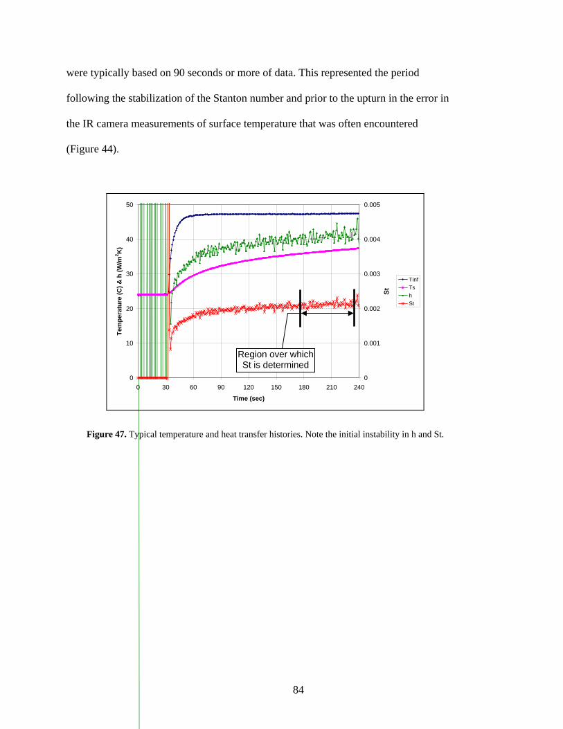
were typically based on 90 seconds or more of data. This represented the period
following the stabilization of the Stanton number and prior to the upturn in the error in
the IR camera measurements of surface temperature that was often encountered
(Figure 44).
0
10
20
30
40
50
0 30 60 90 120 150 180 210 240
Time (sec)
Tem
pera
ture
(C) &
h (W
/m2 K
)
0
0.001
0.002
0.003
0.004
0.005
St
TinfTshSt
Region over which St is determined
Figure 47. Typical temperature and heat transfer histories. Note the initial instability in h and St.
84

Chapter 5: Convective Heat Transfer Results
5.1 Stanton Number Correlations
There have been a number of correlations developed which relate the roughness statistics
of a surface with its heat transfer properties. In this chapter, several of these correlations
are applied to the experimental surface measurements of Coupon 3.
5.1.1 Flat Plate Correlation
The initial heat transfer measurements smooth, 2.54 cm thick
Plexiglas panel. The results obtained with this panel were compared to the results
obtained through Kays et al.’s Stanton number correlation for fully turbulent flow over a
smo ,
2005). Because the temperature of the wind tunnel surfaces is not constant with x, use of
this Stanton number relation will underestimate the value of St by approximately 3%.
(13)
This equation assumes that the momentum and thermal boundary layers are of similar
thickness with a turbulent Prandtl number of 0.85. It also assumed that the turbulent
boundary layer can be adequately described by a 1/7th power law.
( )
were made using a
oth flat surface with a temperature that is constant with x (Equation 13) (Kays et al
85.025.9Pr2.13Re169.0Re0287.0
1.0
2.0
+−= −
−
x
xSt
85

Given typical wind tunnel conditions during a test of a flat plate—a freestream
mperature of 50.5°C, a freestream velocity of 20.5 m/s, a model location of 1.21 m, and
an atmospheric pressure of 86.3 kPa—a Reynolds number of approximately 1.22x10⁶ is
h surface. The
quivalent sandgrain roughness, ks, which compares the behavior of any particular rough
surface—either roughened with symmetrically placed geometrical structures, packed
a surface roughened with tightly packed sand
rocessed with a MATL ht. For each of the
four rough surfaces, the program the surface used
ind tunnel models into 28 full squares having side lengths of 25.5 mm; approximately
k
e the average of these
te
achieved and Equation 13 yields a Stanton number of 0.00204.
5.1.2 Rough Surface Parameters
The majority of Stanton number correlations have been designed to compare the Stanton
number of an artificially roughened surface with that of a “real” roug
e
spheres, real roughness, etc.—with that of
grains, is widely used in such correlations.
Many Stanton number correlations require that certain parameters of the surface be
known. One of the most widely used is the average surface height, k. Although k is often
approximated to be Rz, the manner in which the Hommel software solves for Rz tends to
result in a high estimate (see section 3.1). Therefore, the raw data for each surface was
p AB program to yield an average surface heig
partitioned the scaled-up version of for
w
10 momentum thicknesses. Excess regions that were too small to be apportioned a full
square were omitted. In each square, the difference in height between the highest pea
and the lowest valley was found. The value of k was estimated to b
86

values. This is similar to the method used by Bons to determine k values for rou
surfaces measured from real turbine blades (Bons, 2005).
A two-dimensional version of k was also found for the four surf
gh
aces. This variant of the
verage roughness height was developed for use in cases in which three-dimensional
surface maps are unavailable and is based on simple streamwise traces of a surface. In
this method, for every 20 momentum thicknesses of distance along a trace, the seven
largest peak-to-valley distances are averaged (Bons, 2005). An average is then calculated
from the results of each streamwise trace.
A third parameter that is often used in roughness correlations is the shape/density
parameter, Λs (also Ls), developed by Sigal and Danberg (1990). This parameter is
defined by Bogard et al. as:
(14)
where S/S is the ratio of the surface area without roughness to the total frontal area of the
roughness elements, As is the forward projected surface area of the roughness elements,
and A is the wetted surface area of those elements (Bogard et al., 1996). Although
originally designed for use with artificially roughened surfaces using systematically
placed roughness elements, Bogard et al. and others have adapted it for use with real,
irregular surfaces.
a
f
f
6.1
⎠⎞
⎝⎛
⎠⎞
⎝⎛
ffs A
AS
S ⎟⎜⎟⎜=Λ s
87

Finally, with the above parameters the equivalent sand grain roughness may be
calculated. A version which varies from the original formulation in order to better apply
to real turbine roughness uses average roughness height, k and the shape/density
5)
parameter, Λs (Bons, 2005):
(1
Another relation for ks which uses the two-dimensional k value and the average forward
facing angle,
( ) 82.0log43.0log +Λ−=⎟⎞
⎜⎛
ssk
⎠⎝ k
fα has also been proposed (Bons, 2005):
(16)
equation initially proposed by Bons in that the calculation of
24k0736.00191.0 2
ffsk αα+=
Equation 16 differs from the
fα ignores all leeward facing a considers all leeward facing
angles to have a value of zero while av its the 4 and the 2 in the
denominator. These roughness parameters may be found in Table 12.
ngles. The original relation
eraging and om
Table 12. Roughness parameters for Coupon 3 (TBC) models.
Burn 1 2 3 4 Notesk (mm) 2.06 1.96 2.01 2.73 3-Dk (mm) 1.48 1.42 1.46 2.16 2-DΛ s 49 72.5 62.7 33.3 -
ks (mm) 1.78 1.01 1.26 3.91 From Equation 12ks (mm) 1.81 1.33 1.41 2.76 From Equation 13
88

5.1.3 Friction Coefficient Correlations
In order to use most Stanton number correlations, the friction coefficient, cf, of the
surface must be known. Thus, for a purely correlative determination of the
nondimensional heat transfer coefficient of a surface to be found, an appropriate relation
r the friction coefficient must also be applied. Bons found that the Schlichting friction
coefficient most closely ma ine blade surfaces when ks>
ons, 2002). Since ks>k/2 for all four Coupon 3 model surfaces, the Schlichting friction
(17)
.1.4 Correlation Results
Sab
(18)
(19)
The value of C in Equation 19 was set as 0.35 due to the discovery that the recommended
value of 1 causes the results to diverge from the real roughness data (Bons, 2002). The
rbulent Prandtl number, Prt, was set at 0.85, which is a typical value for air in an
external flow (Kays et al., 2005). The parameter k+ is often referred to as the roughness
fo
k/2 tched data taken from real turb
(B
coefficient was applied (Schlichting, 1979) (Equation 17).
[ ( )] 5.2/log58.187.2 −+= sf kxc
5
Two Stanton number correlations were used in this study: one developed by Dipprey and
ersky (1963) (Equation 18) and one by Kays et al. (2005) (Equation 19).
( )5.8Pr19.55.01 44.0 −+ +kc f
5.02.0
=c
St f
( )Ckc
c
ft /Pr5.0Pr
5.044.0++
St f
2.0=
tu
89

Reynolds number and is in terms of the wall velocity and equivalent sandgrain
ed a total of four series of
tanton number predictions for the different Coupon 3 surfaces (Figure 48). Note that
here Burn 0 refers to the sm to a model representative
reburn surface of Coupon 3.
roughness:
(20)
Each Stanton number correlation was calculated using the Schlichting friction coefficient
equation and either the equivalent sandgrain roughness derived from Equation 15 or the
sandgrain roughness derived from Equation 16. This produc
2Re f
ss
k
ckUuk
kνν
τ ∞+ =≡≡
S
of ooth flat plate value rather than
p
0
0.0005
0.001
0.0015
0.002
0.0025
0.003
0.0035
St
Bons k/ks, Schlichting cf, Dipprey & Sabersky StBons k/ks, Schlichting cf, Kays & Crawford StSigal & Danberg Ls, Schlichting cf, Dipprey & Sabersky StSigal & Danberg Ls, Schlichting cf, Kays & Crawford St
0 1 2 3 4Burn
Figure 48. Stanton numbers derived from roughness correlations.
90

The Stanton number predictions clearly show the influence of the drop in the av
forward faci
erage
ng angle between Burns 2 and 3. Despite the increase in the roughness
parameter Ra, the Stanton number falls. An interesting illustration of the dependence of
heat transfer rates on the p en the Stanton number
percentage augmentation with respect to the flat plate value is compared to the average
eakedness of the surface occurs wh
forward facing angle (Figure 49).
0
10
20
30
40
tatio
50
60
0 1 2 3 4Burn
% A
ugm
enn
0
3
6
9
12
15
18
αf (
degr
ees)
Bons k/ks, Schlichting cf, Dipprey & Sabersky StBons k/ks, Schlichting cf, Kays & Crawford StSigal & Danberg Ls, Schlichting cf, Dipprey & Sabersky StSigal & Danberg Ls, Schlichting cf, Kays & Crawford StForward Facing Angle
Figure 49. Comparison between trend in forward facing angle and predicted Stanton number percent augmentation.
The dependence of the Stanton number on the average forward facing angle and the
discovery made during this project that the average forward facing angle dropped and
climbed during the deposition process suggest that the heat transfer rate will behave in a
similar manner. R f heat transfer
during its operation, a turbine blade may see a periodic decline in convective heating.
ather than experiencing a continuously increasing rate o
91

5.2 Experimental Stanton Number Results
Several series of wind tunnel experiments were performed on the flat plate and the f
roughness surfaces during which different techniques and approaches were attempted.
Most of these techniques involved different methods of compensating for the changin
ambient temperature. The final series of experiments was the most sophisticated and
involved the ambient temperature i
our
g
nterpolation, in situ calibration, and drift correction
escribed in sections 4.5.1 through 4.5.3. The data obtained during this final series are
presented in Figure 50 and Figure 51.
5.2.1 Stanton Number Uncertainty
An uncertainty analysis performed on the final series results gives an average ±6%
combined bias and precision error in the measurement of the Stanton number for each
experiment. Error sources included noise in electronically gathered data, estimation errors
produced by the application of linear fits to temperature and velocity measurements
during calibration, and precision limitations of equipment. See Appendix C for details of
the uncertainty analysis. Uncertainty with regards to the Plexiglas thermal properties was
not included as part of the analysis sinc inty in the manufacturer’s
easurements is not known. However, to provide an estimate of the effect that
P
increase would cause the Stanton number to increase by 4.8%. A 10% decrease in either
d
e the uncerta
m
uncertainties in the material properties would have on the final calculation of Stanton
number, calculations of the Stanton number for the flat plate were performed with a 10%
change in the value of κ, c , and ρ respectively. In each case it was found that a 10%
property would lead to a 5% decrease in Stanton number.
92
5.2.2 Flat Plate
The average Stanton number measured for the flat plate yielded a value that was 21%
lower than that predicted through Kay’s relation (section 5.1.1). However, the two
measurements made during the final series of experiments showed excellent repeatabilit
This average, labeled as St
y.
her
5.2.3 Coupon 3, Burn 1
The average Stanton number measured for Burn 1 showed a 22.5% augmentation over
igure 51). This is well below the augmentation of
ints.
5.2.4 Coupon 3, Burn 2
The Stanton number of Burn 2 does not follow the expected trend; it appears to climb
0, became the baseline against which the results from the ot
plates were judged in the form of a percent augmentation (Figure 50).
the average flat plate Stanton number (F
40% that the correlations suggest. There is also a large variation between the two po
The source of this variation is unknown. An uncertainty analysis (Appendix C) shows
that the points are separated by a magnitude great enough to prevent the regions of
uncertainty from overlapping (see error bars in Figure 50).
slightly despite a reduced k and fα (Figure 50). However, the margin of error is wide
enough to put this into doubt. The average percent augmentation is still lower than
predicted, achieving a value of 24.2% versus an expected percent augmentation lying
between 28.1% and 40.4% (Figure 51). Like Burn 1, Burn 2 also suffers from a large
spread in the data. The percent augmentation for the highest Stanton number value
93

calculated for Burn 2 is the only point which falls among the values bracketed by the
correlations (Figure 51).
0.0025
0.003
0.0035
0.0005
0.001
.001
0.002
St
0 5
00 1 2 3 4
Burn
Experimental ValuesExperimental AverageBons k/ks, Schlichting cf, Dipprey & Sabersky StBons k/ks, Schlichting cf, Kays & Crawford StSigal & Danberg Ls, Schlichting cf, Dipprey & Sabersky StSigal & Danberg Ls, Schlichting cf, Kays & Crawford St
Figure 50. Experimentally derived Stanton numbers compared to Stanton number correlations.
.2.5 Coupon 3, Burn 3
The average Stanton number for Burn 3 has dropped to an augmentation of 17.6%
(Figure 51), contrary to the expectation of a slight rise. This trend defies the predictions,
given that the four primary roughness parameters discussed, Ra, Rq, Rz, k, and
5
fα , all
rose slightly between Burns 2 and 3. The data for Burn 3 have the lowest spread, with
less than a 0.2% discrepancy between the lowest and the highest St values obtained.
94

5.2.6 Coupon 3, Burn 4
Burn 4 was measured to have an average percent augmentation of 24.3%, which is the
ighest of the four surfaces. This is to be expected, considering that Burn 4 had the
highest values of k and
h
fα . However, this may not necessarily be correct given the wide
spread in the data for Burns 2 and 3, in addition to the uncertainty involved in each
measurement.
0
10
20
30
40
50
60
2 3 4Burn
% A
ugm
enta
tion
Experimental ValuesExperimental AverageBons k/ks, Schlichting cf, Dipprey & Sabersky StBons k/ks, Schlichting cf, Kays & Crawford StSigal & Danberg Ls, Schlichting cf, Dipprey & Sabersky StSigal & Danberg Ls, Schlichting cf, Kays & Crawford St
0 1
se in nearly all permutations of the wind
tunnel experiments. The failure of the measured values to match the magnitudes
Figure 51. Experimentally derived Stanton number percent augmentation compared to Stanton number correlation results.
5.3 Stanton Number Underprediction
Both the magnitude of the individual Stanton numbers and the percent augmentations fall
short of predictions. This proved to be the ca
95

predicted by the correlations and the cause for the spread in the data has not yet been
tions
at t
tunnel test section was closed at both ends for several hours to allow it to reach an
al state prior to each test. The order in which the models were tested was
distributed randomly in order to eliminate the possibility of confusing potential changing
conditions (e.g., drifting instruments, malfunctioning equipment, etc.) with real heat
transfer trends.
With regards to the method used in this study, the Schultz and Jones equation has been in
use for several decades and its derivation has been reviewed by the author. The specific
measurement technique has been successfully applied by other investigators.
Additionally, the correlations used with the modifications indicated have been shown to
bracket the heat transfer data from real turbine blade surfaces (Bons, 2002). Thus, all
indications are that the error lies with the data obtained.
is believed that the instruments behaved correctly due to the calibrations performed and
tained from a variety of measuring devices
t
the
discovered. Other than resulting in excessively low Stanton numbers, the data collected
for each individual measurement showed no unusual or unexpected behavior. Precau
were taken to ensure th he requirements of the Schultz and Jones equation were met:
e.g. thick Plexiglas panels were used to provide a semi-infinite surface and the wind
isotherm
It
the comparisons made between the results ob
(e.g., the IR camera was often compared against a Fluke thermocouple reader, the
freestream thermocouple was compared against a thermometer). It is also believed tha
the final approach taken to compensate for the transient ambient temperature was
96

most appropriate method available. It is probable that the error lies in the physical asp
of the experiment: the models, the wind tunnel, or both.
As mentioned above, the uncertainty in the physical properties of the Plexiglas is not
known. However, it is mentioned in section 5.2.1 that a 10% increase in any of the th
relevant material properties would cause a Stanton number increase of only 4.8%. E
all the magnitude of all three properties had been underestimated by 10%, a correc
the equation would only yield a Stanton number increase of 15.4%. This is far from the
26% increase needed to match the predicted flat plate Stanton number value.
ects
ree
ven if
tion in
he problem may lie with the wind tunnel, the test section, and the characterization of the
rline
s.
sed in the place of active
oundary layer suction may have contributed to or even caused some of the flow
ct
low
T
test section. First, this study was performed using a freestream velocity that was higher
than that for which the tunnel had originally been validated. This could have led to
irregularities in the flow such as the unresolved disturbance found in the cente
boundary layer measurements and the asymmetry in the flow about the axis of the tunnel
(section 4.4). It may be advisable to repeat the experiments at lower Reynolds number
Additionally, the passive boundary layer bleed that was u
b
deviations. There may be a benefit in applying active suction to better control the
beginning of the boundary layer in the test section.
Although it was initially deemed that the flow irregularities would have a minimal impa
on the heat transfer properties, the behavior of the flow could have changed once the f
97

was heated. It may be useful to perform extensive boundary layer measurements while
the wind tunnel is operating at higher temperatures. It has already been discovered that
mperatures in the core flow of the wind tunnel are 1°C to 2°C lower than temperatures
e
rfaces must
e determined through experimentally confirmed correlations such as those presented in
te
at the edge of the thermal boundary layer at higher speed settings. Measurements of th
thermal boundary layer along the centerline and across the width of the tunnel in the
vicinity of the model at elevated temperatures may also be helpful.
Until such time that the phenomenon or errors that have caused these underpredictions
can be discovered and compensated for, the Stanton numbers for these four su
b
this chapter.
98

6.1 Review of Project Goals
Chapter 6: Conclusions and Recommendations
ith the development of a facility that can produce realistic turbine blade deposits,
urface roughness changes over time with deposit evolution.
• Determine the convective heat transfer properties of the roughened surfaces that
result from accelerated deposit evolution.
6.2 Deposit Evolution
With regards to the first goal: accelerated deposition evolution was observed in all three
coupons. Although the three surfaces were different in their surface coatings and initial
roughness, deposits that changed with time were seen to form on their surfaces. Portions
of the two coupons with the most amount of deposit evolution—the bare substrate
coupon, Coupon 2, and the TBC coated coupon, Coupon 3—displayed an interesting
trend. The roughness in the form of Ra would increase rapidly with an accompanying
increase in average forward facing angle. The rate of roughness increase would then
subside slightly and the average forward facing angle would decrease. This would then be
followed by another increase in roughness and surface angle. These results show that
W
deposit evolution can now be simulated quickly and conveniently. For this project, three
coupons were exposed to deposition conditions with two primary objectives:
• Determine what trend, if any, can be discovered in the manner in which turbine
blade s
99

deposition evolution is not limited to a slow, linear process, but that it often occurs in
latively rapid jumps.
.3 Recommendations Regarding Deposition Evolution
oupons 2 and 3 will serve as a motivation for further
order
er or not
this e
the con indicator for
the c
deposit it could be predicted that the blade
ughness would soon plateau, the average forward facing angle would drop, and the
is would be accompanied by a slackening in the
re
6
It is hoped that the trends seen in C
study. It may be useful to expose multiple coupons to many more than four burns in
to determine whether or not the trend noted during this project is a common one and
whether or not it is continuous. It would also be of interest to determine wheth
ph nomenon occurs regularly in real gas turbines. If that proves to be the case then
dition of a turbine blade at one point in its cycle could be used as an
up oming conditions. For example, if a blade were found to have peak-dominated
s and a high average forward facing angle,
ro
value of Rz would go down. Th
convective heat transfer rate. A wavier surface with a lower value of fα and Rz could
mean that a spike in roughness and an increase in convective heat transfer is about to
occur. If substantial deposits already exist, the operator might want to choose that
moment to service the turbine.
6.4 Heat Transfer Rate Determination
While the deposition evolution followed an unexpected trend, its overall behavior (i.e. a
constant increase in surface roughness, Ra) had been expected. The Stanton numbers
100

obtained through wind tunnel testing, however, did not behave as expected or as
predicted through Stanton number correlations. Low Stanton number measurements and
ercent augmentations were the common result of several series of convective heat
transfer tests. The fact that a variety of different approaches to compensating for
changing ambient temperatures and calibrating measuring equipment resulted in the same
type of error suggests that the problem is physically rather than analytically based.
to
ed
more accurate measurement of important parameters
such as air flow rate and Mach number.
• Accelerated deposits were formed with surface features that compare favorably
with deposits found on real turbine blades (Table 7). This further corroborates the
p
6.5 Recommendations on Heat Transfer Rate Determination
The first task in determining the cause of the drop in Stanton number would be to further
validate the wind tunnel test section. This process should be performed at a temperature
equivalent to those reached during a convective heat transfer test. It may also be useful
investigate the effect of lower Reynolds numbers or active boundary layer suction on
Stanton number results.
6.6 Accomplishments
During the course of this study, there were several accomplishments of note:
• The Turbine Accelerated Deposition Facility was modified to allow improv
burning, ease of use, and
principle of accelerated deposition as a means to accurately simulate real
deposition.
101

• Deposits were evolved on three coupons simulating approximately one ye
worth of deposition.
• Distinct trends were discovered with respect to the evolution of certain rough
parameters over time. Studies have shown that these parameters have a str
influence on heat transfer properties.
• A simple and inexpensive method for constructing scaled-up models of roug
ar’s
ness
ong
hened
surfaces was developed and implemented, producing four models representing
• Roughness correlations for the prediction of the Stanton number were applied to
the four surfaces, producing a probable Stanton number history for the surface.
•
convective heat transfer experimentation using the scaled-up roughness panels.
• ents with the panels indicate that further characterization is
required in order to obtain appropriate values.
four distinct stages in the evolution of turbine blade deposits.
A wind tunnel test section was designed and constructed for the purpose of
Numerous experim
102

Antonia, R. A., and Luxton, R. E., 1971, “The Response of a Turbulent Boundary Layer
Blair, M e-Scale Turbine
Rotor Passage,” ASME J. Turbomach., 116, No. 1, pp. 1-13.
Bogard, D. G., Schm
”
&
Exhibition, Birmingham, UK, June 10-13, 1996).
Bons, J.P., Taylor, R., M
Bons, J rbine Roughness with Elevated
Freestream Turbulence,” Transactions of the ASME, vol. 124, OCT 2002, pgs
632-644.
Bons, J.P., 2005, “A Critical Assessment of Reynolds Analogy for Turbine Flows,”
Transactions of the ASME, vol. 127, MAY 2005, pgs 472-485.
Borom, Marcus P., Johnson, Curtis A., and Peluso, Louis A., 1996, “Role of
environmental deposits and operating surface temperature in spallation of air
plasma sprayed thermal barrier coatings,” Surface and Coatings Technology 86-
87, pp.116-126.
Boynton, J. L., Tabibzadeh, R., and Hudson, S. T., 1993, “Investigation of Rotor Blade
Roughness Effects on Turbine Performance,” ASME J. Turbomach., 115, pp.
614-620.
Bibliography
to a Step Change in Surface Roughness. Part 1: Smooth to Rough,” ASME J.
Fluid Mech. 48, pp. 721–726.
. F., 1994, “An Experimental Study of Heat Transfer in a Larg
idt, D. L., and Tabbita, M., “Characterization and Laboratory
Simulation of Turbine Airfoil Surface Roughness and Associated Heat Transfer,
96-GT-386, (1996), (presented at the Gas Turbine and Aeroengine Congress
cClain, S., and Rivir, R.B., “The Many Faces of Turbine Surface
Roughness,” ASME J. Turbomach., 123, No. 4, pp. 739-748.
.P., 2002, “St and Cf Augmentation for Real Tu
103

Dipprey, D. F., and Sabersky, R. H., 1963, “Heat and Momentum Transfer in Smooth and
Rough Tubes at Various Prandtl Numbers,” Int. J. Heat Mass Transfer, 6, pp.
329–353.
ord, W.E., (revision), Dana’s Textbook of Mineralogy (after E.S. Dana) 4th edn., 16th
printing, John Wiley & Son
cropera, F.P., and DeWitt, D.P., Fundamentals of Heat and Mass Transfer 5th edn.,
Jensen,
Turbine Engines,” M.S. Thesis, Brigham Young
Jensen, Based Turbine
Kays, W th
r. Gas Turbines &
Schlich
and
Sigal, A
Smiale A., and Garlick, R.G. in F.H. Froes et al. (eds.), The Chemistry
Stripf, M., Schulz, A., and Wittig, S., 2005, “Surface Roughness Effects on External Heat
Transfer of a HP Turbine Vane,” ASME J. Turbomach., 127, pp. 200-208.
F
s, NY 1954, p379.
In
John Wiley & Sons, NY 2002.
J. W., 2004, “The Development of an Accelerated Testing Facility for the Study
of Deposits In Land-Based Gas
University, Provo, Utah.
J. W., Squire, S. W., and Bons, J. P., 2005, “Simulated Land-
Deposits Generated in an Accelerated Deposition Facility,” ASME J.
Turbomach., 127, pp. 462-470.
. M., Crawford, M. E., and Weigand, B., Convective Heat and Mass Transfer, 4
Edition, 2005, McGraw-Hill, New York, NY.
Kim, J., Dunn, M.G., and Baran, A.J. et al, 1993, “Deposition of Volcanic Materials in
the Hot Sections of Two Gas Turbine Engines,” ASME J. Eng
Power, 115, pp. 641-651.
ting, H., Boundary Layer Theory, 7th Edition, 1979, McGraw-Hill, New York,
NY.
Schultz, D. L., and Jones, T. V., 1973, “Heat-transfer Measurements in Shortduration
Hypersonic Facilities,” Advisory Group for Aerospace Research
Development, No. 165, NATO.
., and Danberg, J. E., “New Correlation of Roughness Density Effects on the
Turbulent Boundary Layer,” AIAA Journal, vol. 28, pp. 554-556.
k, J.L., Archer, F.
of Saudi Arabian Sand: A Deposition Problem on Helicopter Turbine Airfoils,
Advances in Synthesis and Processes, SAMPE, 3, 1992, M92-M101.
104
Tabakoff, W., Metwally, M., and Hamed, A., 1995, “High-Temperature Coatings for
Protection Against Turbine Deterioration,” Transactions of the ASME, vol. 11
JAN 1995,
7,
pgs 146-151.
SME Paper No. 93-GT-74.
ace Roughness,” AIAA Paper No. 92-0249.
e Netherlands, June 6-9, 1988).
-
bines &
and Practices to Improve
Tarada, F., and Suzuki, M., 1993, “External Heat Transfer Enhancement to
Turbine Blading Due to Surface Roughness,” A
Taylor, R. P., and Chakroun, W. M., 1992, “Heat Transfer in the Turbulent Boundary
Layer with a Short Strip of Surf
Toriz, F.C., Thakker, A.B., and Gupta, S.K., J. ASME, “Thermal Barrier Coatings for Jet
Engines” 88-GT-279, (1988), (presented at the Gas Turbine and Aeroengine
Congress Amsterdam, Th
Wenglarz, R.A., and Fox, R.G. Jr., 1990, “Physical Aspects of Deposition From Coal
Water Fuels Under Gas Turbine Conditions,” ASME J. Engr. Gas Tur
Power, Jan 1990, pp. 9-14.
Wenglarz, R.A., and Wright, I.G., “Alternate Fuels for Land-Based Turbines,” published
in proceedings of the “Workshop on Materials
Resistance to Fuel Derived Environmental Damage in Land-and Sea-Based
Turbines,” October 22-24, 2002, Colorado School of Mines, Golden, Colorado.
105

106

Appendix
107

108

Appendix A: Derivation of the Schultz and Jones Equation
The heat diffusion equation:
(A.1)
Assume one-dimensional heat flux with no heat generation and constant properties:
(A.2)
(A.3)
Apply Laplace transform:
(A.4)
(A.5)
Auxiliary equation:
(A.6)
tTcq
zT
zyT
yxT
x ∂∂
=+⎟⎠⎞
⎜⎝⎛
∂∂
∂∂
+⎟⎟⎠
⎞⎜⎜⎝
⎛∂∂
∂∂
+⎟⎠⎞
⎜⎝⎛
∂∂
∂∂ ρκκκ &
tTc
xT
xT
x ∂∂
=∂∂
=⎟⎠⎞
⎜⎝⎛
∂∂
∂∂ ρκκ 2
2
tT
xT
∂∂
=∂∂
α1
2
2
[ ])0()(1)(2
2
TsTsx
sT−=
∂∂
α
02
2
2
2
=−∂∂
→=∂∂ Ts
xTTs
xT
αα
ααsmsmm ±=→=−+ 0)0(2
109

(A.7)
Transform
(A.8)
Substitute:
(A.9)
(A.10)
(A.11)
At the surface, x=0:
(A.12)
(
ααsxsx
ececT−
+= 21
boundary conditions,
0)(,0@"" =∞===∂∂
−→∂
xTxq
A.13)
Let sTssF =)( and s
sG 1)( = , invert the transform:
(A.14)
=∂
−xTκ
xTq && κ
00)( 1)(
2)(
1 =→+==∞=∞−∞
cececxTssαα
ακα
sqcqesc
xT s "")0( &&
=→−
=−=∂∂ −
κα 22
αα sxeqT
−=
"&κ s
sTqs
qT ss ακ
κα
=→= ""&
&
( ) ⎟⎠
⎞s
q"& ⎜⎝
⎛== Tss
Ts ss11
ακ
ακ
( ) ∫∫ −=
−=
ttd
tddT
dtd
dTq00
1" ττ
τπακτ
τπτακ
&
110

Integrate by parts, for τ=0, T(τ)=0:
(A.15)
Assuming small departures from a uniform rate of heat transfer:
(A.16)
Where
( ) ⎥
⎥⎦
⎤
⎢⎢⎣
⎡
−
−+= ∫
td
tTtT
ttTq
0 23
)()(21)(" τ
τ
τπακ
&
( )11
1)()()()( −
−− −
Δ−
+= iii
i tt
tTtTtTT ττ
ii tt ≤≤− τ1 and i=1, 2, 3,…,n. Evaluate integral:
(A.18)
Evaluate the first integral:
uate the se ntegral using integration by parts:
(A.20)
(A.17)
(A.19)
Eval cond i
( ) ( )∑∫∫= − −
−=
−
−=
n
i
t
tn
nt i
i
dt
TtTdt
TtTR1 2
30 23
1
)()(21)()(
21 τ
τ
τττ
τ
( )( )
[ ]( )∑ ∫ ∫ −−
−⎪⎭
⎪⎬⎫
⎪
⎪⎨⎧
−
−⎥⎦⎤
⎢⎣⎡
Δ−
−−
−=− −
n t
t
t
tn
iii
n
ini
i
i
i
dt
tt
tTtTt
dtTtT2
311
231
1 1
)()()()(21 τ
τ
τ
τ
τ
( )
= ⎩i 2
( )∫ ∫− − ⎢
⎢⎣
⎡−
−=−= −i
iin
t
t n ttdt
1 1
23
2
12ττ⎥⎥⎦
⎤
−− −
i
i
t
tinn
tttd
13
1τ
τ
( )( ) ( )
( ) ( )[ ]21
11
21
21
231 42
−− −−−+
−
Δ=
−
−inin
inn
i tttttttd
tt ττ∫
−
t
t
i
i
τ
111

Substitute back into the original equation:
(A.22)
At i=n
[ ]( )
(A.21)
in
in
tttTtT
−
− )()( is in d to be piecewise
(A.23)
For t0=0, T(t0)=0
(A.24)
te back into equation:
(A.25)
determinate. However, T(t) was assume linear:
Substitu
0)(
=n
n
ttT
when
(A.26)
(A.27)
t0=0:
[ ]⎪⎭
⎪⎬⎫
−−−+−= −=
−∑ 11
1 4()(221
inin
n
iin tttttTtTR
⎪⎩
⎪⎨⎧
−
Δ⎥⎦⎤
⎢⎣⎡
Δ−
−⎥⎥⎦
⎤
⎢⎢⎣
⎡
−−
−−
− 21
1
1
2)()(11)in
ii
inin ttt
ttTtT
tttt
∑ ∑∑ −
−+
−−
−= iinin
ttttttR 1 2
= = −
−
−= −+−−− n
i
n
i inin
i
in
n
i in tttTtTtTtTtTtT
1 1 1
1
11
)()()()()()(
∑−
=
−
−
−
−
−
⎪⎭
⎪⎬⎫
⎪⎩
⎪⎨⎧
Δ−
+−+−
−+
−−
−−
−=
1
1
1
1
1
1
1 )()()()(2)()()()(n
i
nn
inin
ii
in
in
in
in
ttTtT
tttttTtT
tttTtT
tttTtTR
∑= −
−
−+−−
=n
i inin
ii
tttttTtTR
1 1
1)()(2
⎥⎥⎦
⎤
⎢⎢⎣
⎡
−+−−
+= ∑= −
−n
i inin
ii
n
n
tttttTtT
ttTq
1 1
1)()()(2"πακ
& 2
∑= −
−
−+−=
i inin ttttq
1 1
1)"πα
&−n
ii tTtT ()(2κ
∑= −
−
−+−
−=
j jiji
jSjS
ttttq
1 1
1,,2"πακ
&i TT
112

schultz
his program uses conditioned temperature and velocity histories to determine the
% schultzjones.m % Written% Mo% Th% transfe
ear all; arning off;
ame of input file with its extension: ','s'); outfile = input('Enter name of output file with its extension: ','s'); % For user defined properties % k = input('Enter model thermal co% cp = input('Enter model sp
kg/m^3: '); ivity: ');
% Plexiglas G properties k = 0.18733; cp = 1464.4; rho = 1190; epsilon = 0.9; % Bons' mo% k = 0.226; % cp = 1913; % rho = 1207; press_eng = input('Enter pressureTamb1 = input('Enter initial ambTamb2 = input('Enter final ambient temperature: '); alpha = k/(rho*cp); % Read topological data into
Appendix B: MATLAB Programs
jones.m
T
Stanton number of a surface tested in a wind tunnel. The results are output to a text file.
by James Wammack 06/01/05 dified 08/11/05
is program uses the Shultz and Jones equation to determine the heat r coefficient given a set of temperature data
clw
% Obtain user inputs infile = input('Enter n
nductivity value in W/m*K: '); ecific heat in J/kg*K: ');
% rho = input('Enter model density in% epsilon = input('Enter model emiss
del properties
in psf:'); ient temperature: ');
MATLAB
113

M = dlmread(infile,'\t'); % Separate data into times, freestream temperature, su face temperature, % and velocity matrices % For data sets with twTs_data = M(1:size(M
nf_data = M(1:size(Ms1 = Ts_data(:,2);
Ts2 = Ts_data(:,3);
% Tinf_data = M(1:size(M,1),3:5);
= Ts_data(:,1);
time scale
inf_data(j,2))*... ((Tinf_data(j+1,1)-t(i))/(Tinf_data(j+1,1)-Tinf_data(j,1)));
) = Tinf_data(j+1,3)-(Tinf_data(j+1,3)-Tinf_data(j,3))*... nf_data(j+1,1)-t(i))/(Tinf_data(j+1,1)-Tinf_data(j,1)));
,1)==t(i)
(t,1)-1); e(t,1)-1);
==size(Tinf,2)+1 1))=Tinf(size(t,1)-1);
))=Vinf(size(t,1)-1);
at Tamb,i and Ts at Tamb,f )
(Ts2(i)-Ts1(i))*((Tinf(i)-Tamb1)/(Tamb2-Tamb1));
r
o different ambient temperatures ,1),1:4);
,1),5:7); TiT
Tw = Ts_data(:,4); % % For data sets with one ambient temperature % Ts_data = M(1:size(M,1),1:2);
% Ts = Ts_data(:,2);
t % Interpolate Tinf data based on Ts data's for i=1:size(t,1) for j=1:(size(Tinf_data,1)-1); if Tinf_data(j,1)<t(i) && Tinf_data(j+1,1)>t(i) Tinf(i) = Tinf_data(j+1,2)-(Tinf_data(j+1,2)-T
Vinf(i ((Ti
elseif Tinf_data(j Tinf(i) = Tinf_data(j,2); Vinf(i) = Tinf_data(j,3); end
end end if size(t,1)==size(Tinf,2)+2 Tinf(size(t,1)-1)=Tinf(size(t,1)-2); Vinf(size(t,1)-1)=Vinf(size(t,1)-2);
Tinf(size(t,1))=Tinf(size,1))=Vinf(siz Vinf(size(t)elseif size(t,1
t, Tinf(size( Vinf(size(t,1nd e
between TsIR% Interpolate
for i=1:size(t,1 TsIR(i) = Ts1(i)+nd e
% Apply In Situ calibration Ts = 0.95176*TsIR+1.97913; Ts(1)=Ts(2);
size = size(Tinf,2);T if Tsize<size(Ts,1)
114

for i=Tsize:size(Ts,1) Tinf(i) = Tinf(Tsize);
nd
tion
if j==1
t(t(i)-t(j))+sqrt(t(i)-t(j-1)));
end um(inner);
qc(i) = (2*k/sqrt(pi*alpha))*summation;
n
(press_eng/144)*6894.757;
1:size(t,1) if Vinf(i)~=0;
f(i)+273.15)); );
open(outfile,'at'); rintf(fid,'Time\tTinf\tTs\th\tSt\n');
2)
f(fid,'%.2f\t%.2f\t%.2f\t%.3f\t%.5f\n',t(a),Tinf(a),Ts(a),h(a),St(a)); nd
lot(t,Tinf,'-',t,Ts,'--',t,h,'-.'); );
Vinf(i) = Vinf(Tsize); end e % Perform Shultz & Jones equafor i=1:size(t,1) inner = 0; summation = 0; for j=1:i inner(j) = 0; else inner(j) = (Ts(j)-Ts(j-1))/(sqr end summation = s end % Perform radiation compensatiosigma = 5.67*10^-8; for i=1:size(t,1) qr(i) = epsilon*sigma*(Ts(i)^4-Tw(i)^4); h(i) = (qc(i)+qr(i))/(Tinf(i)-Ts(i)); end % Determine Stanton Number pressure = for i= rho(i) = pressure/(287*(Tin St(i) = h(i)/(rho(i)*Vinf(i)*1005.5 else St(i) = 0; end end % Print data to a text file fid=ffp % for a=1:size(t,for a=1:size(t,1) fprinte fclose(fid); % Plot data subplot(2,1,1) paxis([0 max(t) 0 80]
115

grid on; legend('T_i_n_f','T_S','h',4);
Transfer Coefficient History'); Time (sec)');
l('Temperature(C), Heat Transfer Coefficient (W/m^2 K)');
(sec)');
gles of a surface in both the cross-stream
It also computes their statistics and outputs the results to
e screen and to a text file.
/05 odified 06/18/05
s coordinates, determines the angle from the lates the statistics
h its extension:','s'); Enter name of output file with its extension:','s');
n counting time
to MATLAB
d:\t%.2f minutes\n',t1);
= 1; 0,1) = M0(i-1,2)
rows+1;
title('Temperature and Heat xlabel('ylabe subplot(2,1,2) plot(t,St); grid on; title('St history'); xlabel('Timeylabel('St');
angles.m
This program determines the roughness slope an
and the streamwise directions.
th
% W% M
ritten by James Wammack 04/01
% This program reads roughnes% horizontal from point to point and calcu clear all; warning off; % Obtain user inputs infile = input('Enter name of input file witoutfile = input(' % Btic;
egi
% Read topological data inM0 = csvread(infile); t1 = toc/60; fprintf('Data file rea % Determine number of rows and columns rfoowsr i=2:size(M
if M0(i,2) ~ rows = end end points = size(M0,1)/rows;
116

% Truncate data with respect to Y
(points-1)):points*i,:) = M0((points*(2*i-1)-(points-1))...
nd
data with respect to X ize(Mtruncy,1)/2)
Mtruncy((2*i-1),:);
Determine new number of rows and points ws2 = 1; r i=2:size(Mtruncxy,1)
(i,2) ~= Mtruncxy(i-1,2) rows2+1;
end
points2 = size(Mtruncxy,1)/rows2;
fprintf('Data truncated with respect to X and Y:\t%.2f minutes\n',t2);
% X column x = Mtruncxy(1:size(Mtruncxy,1),1);
uncxy(1:size(Mtruncxy,1),3);
gles in X direction
z(i-1); glex(i-1) = abs((atan(deltaxz(i-1)/deltax(i-1)))*180/pi);
ex); = median(anglex);
acing angles in Y direction
ints2) y(i) = My(points2+i)-My(i);
Mz(i); eltay(i)))*180/pi;
for i=1:(rows/2) Mtruncy((points*i- :points*(2*i-1),:); e % Truncatefor i=1:(s Mtruncxy(i,:) =end %rofo if Mtruncxy rows2 =
end
t2 = toc/60;
M % Y column My = Mtruncxy(1:size(Mtruncxy,1),2);
Z column %Mz = Mtr
Determine an%for i=2:(size(Mz,1)) deltax(i-1) = Mx(i)-Mx(i-1); if deltax(i-1)<0
deltax(i-1) = Mx(i+1)-Mx(i); end
ltaxz(i-1) = Mz(i)-M de an
end nglex_mean = mean(angla
anglex_med anglex_dev = std(anglex); nglex_skew = skewness(anglex); a
ine forward-facing and rearward-f% Determ
j = 0; k = 0;
:(size(Mz,1)-pofor i=1lta de
deltayz(i) = Mz(points2+i)- angley(i) = (atan(deltayz(i)/d
117

if angley(i)<=0
j) = abs(angley(i));
rangle(k) = abs(angley(i)); end
gle); rdangle_med = median(forwardangle);
rwardangle_dev = std(forwardangle);
arangle);
angle); le_skew = skewness(rearangle);
data found:\t%.2f minutes\n',t3);
Y plane screen printouts sis in the streamwise (Y) direction\n');
.2f degrees\n',forwardangle_mean); rintf('Median forward-facing angle:\t%.2f degrees\n',forwardangle_med);
rd deviation of forward-facing angles:\t%.2f degrees\n',forwardangle_dev); es:\t%.2f degrees\n\n',forwardangle_skew);
ge rearward-facing angle:\t%.2f degrees\n',rearangle_mean); .2f degrees\n',rearangle_med);
rintf('Standard deviation of rearward-facing angles:\t%.2f degrees\n',rearangle_dev); angles:\t%.2f degrees\n\n',rearangle_skew);
he cross-stream (X) direction\n'); %.2f degrees\n',anglex_mean);
Median roughness angle:\t%.2f degrees\n',anglex_med); les:\t%.2f degrees\n',anglex_dev);
;
Produce histogram of angles
angle)+(max(forwardangle)-min(forwardangle))/(bins)*i-.5*(max(forwardangle)...
rsrear(i) = [min(rearangle)+(max(rearangle)-min(rearangle))/(bins)*i-0.5*(max(rearangle)... -min(rearangle))/bins];
glex)-min(anglex))/(bins)*i-0.5*(max(anglex)...
j = j+1; forwardangle( elseif angley(i)>0 k = k+1; rea end forwardangle_mean = mean(forwardanforwafoforwardangle_skew = skewness(forwardangle); rearangle_mean = mean(rerearangle_med = median(rearangle); rearangle_dev = std(rearrearang t3 = toc/60; fprintf('Angle %fprintf('Analyfprintf('Average forward-facing angle:\t%fpfprintf('Standafprintf('Skewness of forward-facing angl fprintf('Averafprintf('Median rearward-facing angle:\t%fpfprintf('Skewness of rearward-facing % X plane screen printouts fprintf('Analysis in tfprintf('Average roughness angle:\tfprintf('fprintf('Standard deviation of angfprintf('Skewness of angles:\t%.2f degrees\n\n',anglex_skew) %bins = 50; for i=1:bins % Y plane centersforward(i) = [min(forward0 -min(forwardangle))/bins]; cente % X plane centersx(i) = [min(anglex)+(max(an -min(anglex))/bins];
118

end centersforward = centersforward';
(outfile,'at'); tf(fid,'Analysis of file %s\n',infile);
ion\n'); %.2f degrees\n',forwardangle_mean);
grees\n',forwardangle_med); rintf(fid,'Standard deviation of forward-facing angles:%.2f degrees\n',forwardangle_dev);
angles:%.2f degrees\n\n',forwardangle_skew);
ing angle:%.2f degrees\n',rearangle_mean); :%.2f degrees\n',rearangle_med);
rintf(fid,'Standard deviation of rearward-facing angles:%.2f degrees\n',rearangle_dev); wness of rearward-facing angles:%.2f degrees\n\n',rearangle_skew);
rintf(fid,'Analysis in the cross-stream (X) direction\n'); ss angle:%.2f degrees\n',anglex_mean);
ex_med);
Plot data
label('Frequency'); Facing Angle Data');
tle('Histogram of Rearward-Facing Angle Data');
data );
tersx);
e Data in the Cross-stream (X) Direction');
centersrear = centersrear'; centersx = centersx'; % Write data to file fid=fopenfprin % Y plane file printouts fprintf(fid,'Analysis in the streamwise (Y) directfprintf(fid,'Average forward-facing angle:fprintf(fid,'Median forward-facing angle:%.2f defpfprintf(fid,'Skewness of forward-facing fprintf(fid,'Average rearward-facfprintf(fid,'Median rearward-facing anglefpfprintf(fid,'Ske % X plane file printouts fpfprintf(fid,'Average roughnefprintf(fid,'Median roughness angle:%.2f degrees\n',anglfprintf(fid,'Standard deviation of angles:%.2f degrees\n',anglex_dev); fprintf(fid,'Skewness of angles:%.2f degrees\n',anglex_skew); fclose(fid); %% Y plane data subplot(3,1,1); hist(forwardangle,centersforward); xlabel('Forward-Facing Angles (deg)'); ytitle('Histogram of Forward- subplot(3,1,2) hist(rearangle,centersrear); xlabel('Rearward-Facing Angles (deg)'); ylabel('Frequency'); ti % X plane subplot(3,1,3hist(anglex,cenxlabel('Roughness Angle (deg)'); ylabel('Frequency'); title('Histogram of Roughness Angl
119

cnc_conversion.m
raw surface data into a CNC-compatible file for machining. The
to a text file.
d scaling:'); ','s');
read:\t%.2f minutes\n',t1);
ns
s+1;
nts*i-(points-1)):points*i,:) = M0((points*(2*i-1)-(points-1))...
Mtruncxy(i,:) = Mtruncy((2*i-1),:); d
t2 = toc/60; rintf('Data truncated with respect to X and Y:\t%.2f minutes\n',t2);
This program converts
results are output
% Written by James Wammack 03/01/05 % Revised 06/16/05 % This program reads roughness coordinates, converts from mm to in and % scales the coordinates by some value lear all; c
warning off; % Obtain user inputs infile = input('Enter name of input file with its extension:','s');
width = input('Input step size in y in microns:'); %scale = input('Input desireoutfile = input('Enter name of output file with its extension: % Begin counting time tic;
ological data into MATLAB % Read top0 = csvread(infile); M
t1 = toc/60; fprintf('Data file % Determine number of rows and columrows = 1; for i=2:size(M0,1)
if M0(i,2) ~= M0(i-1,2) rows = row end end
ows; points = size(M0,1)/r
Truncate data with respect to Y %for i=1:(rows/2) Mtruncy((poi :points*(2*i-1),:); end % Truncate data with respect to X or i=1:(size(Mtruncy,1)/2) f
en
fp
120

% Determine new number of rows and points rows2 = 1;
rows2 = rows2+1;
end oints2 = size(Mtruncxy,1)/rows2;
n 0.03937)*(Mtruncxy(1:size(Mtruncxy,1),2));
for machining purposes)
ints2*i);
Mz1a((points2+1)-j);
;
ts 1 and 2 into the lower half of data
nts2-1)):points2*(2*i-1)) = Mx1((points2*i+1)-points2:points2*i); -(points2-1)):points2*(2*i)) = Mx2((points2*i+1)-points2:points2*i);
((points2*(2*i-1)-(points2-1)):points2*(2*i-1)) = My1((points2*i+1)-points2:points2*i); nts2-1)):points2*(2*i)) = My2((points2*i+1)-points2:points2*i); oints2-1)):points2*(2*i-1)) = Mz1((points2*i+1)-points2:points2*i);
points2*(2*i)) = Mz2((points2*i+1)-points2:points2*i);
xa; ize(Mxa,2)+1:2*size(Mxa,2)) = Mxa;
= Mya+max(Mya);
b(((2*points2)*i+1)-(2*points2):(2*points2)*i) = ... ze(Mza,2)-i*(2*points2)+1):(size(Mza,2)-(i-1)*(2*points2)));
z(1:size(Mza,2)) = Mza;
for i=2:size(Mtruncxy,1) if Mtruncxy(i,2) ~= Mtruncxy(i-1,2)
end
p % Create first quadrant of data % X column
Mtruncxy,1),1)); Mx1 = (scale*0.03937)*(Mtruncxy(1:size( % Y columMy1 = (scale* % Z column (adjustedMz1o = (scale*0.03937)*(Mtruncxy(1:size(Mtruncxy,1),3)); Mz1 = Mz1o-max(Mz1o); % Create second quadrant of data
x2 = Mx1+max(Mx1); M
= My1; My2 for i=1:rows2
s2*i+1)-points2:po Mz1a = Mz1((point for j=1:points2
Mz1b(j) = end Mz2((points2*i+1)-points2:points2*i) = Mz1b
end % Combine quadranfor i=1:rows2
-1)-(poi Mxa((points2*(2*i((points2*(2*i) Mxa
ya M Mya((points2*(2*i)-(poi Mza((points2*(2*i-1)-(p
Mza((points2*(2*i)-(points2-1)):end
produce upper half % Mirror lower half to 1:size(Mxa,2)) = MMx(
x(sMMy(1:size(Mya,2)) = Mya;
ya,2)) My(size(Mya,2)+1:2*size(M
=1:rows2 for i Mz
Mza((siend M
121

Mz(size(Mza,2)+1:2*size(Mza,2)) = Mzb; t3 = toc/60; fprintf('Data has been scaled, mirrored, and converted to inches:\t%.2f minutes\n',t3);
ata to a CNC compatible file. Cutting speed is 12in/min 1:size(Mx,2)
if a==1 7\nS2000\nX0 Y0.2 Z0.1\nM3\nM100Y\nG01F12\n');
fprintf(fid,'X%.3f\tY%.3f\tZ%.4f\n',Mx(a),My(a),Mz(a)); )>=(max(Mx)-0.01) && a<size(Mx,2)
fprintf(fid,'G00\n'); d,'X%.3f\tY%.3f\tZ%.4f\n',Mx(a),My(a),(max(Mz)+0.05));
z)+0.05)); fprintf(fid,'G01F12\n');
;
nd
\nM5\nM2');
plete.\t%.2f minutes\n',t4);
% Print dfor a= fid=fopen(outfile,'at'); fprintf(fid,'G0T0Z0\nT1\nM elseif Mx(a fprintf(fid,'X%.3f\tY%.3f\tZ%.4f\n',Mx(a),My(a),Mz(a)); fprintf(fi fprintf(fid,'X%.3f\tY%.3f\tZ%.4f\n',0,My(a+1),(max(M else fprintf(fid,'X%.3f\tY%.3f\tZ%.4f\n',Mx(a),My(a),Mz(a)) end e fprintf(fid,'Z0.5\nG0T0Z0 fclose(fid); t4 = toc/60; fprintf('CNC code has been generated, program com
122

ainty Analysis
∞ S ing approximately 60 seconds of
(C.1)
was introduced when calibration curves were used to correct the measurements
was approximated to
be the standard error of estimate produced when a least-squares best fit is applied to a set
of data.
(C.2)
(C.3)
(C.4)
Appendix C: Uncert
Freestream and Surface Temperature Uncertainty
Precision error for both T and T were determined us
data taken at a moment in which the tunnel was isothermal.
nStP x
x =
Bias error
made by the FLIR camera and freestream thermocouple. This error
2
2
, −−−
= ∑ ∑ ∑n
yxaybyS iiii
xy
( )( )( )
∑∑ ∑
∑ ∑−
−= 22
ii
iiii
xxn
yxyxna
( )( )( )
∑∑
∑∑
∑ ∑−
−= 22
2
ii
iiiii
xxn
yxxyxb
123

The limited precision of the instruments used to calibrate these two devices (i.e. a Fluke
thermocouple reader for IR camera calibration and a mercury thermometer for the
freestream thermocouple) introduced further bias. This was approximated to be one half
e least count or ±0.05°
ated to be ±0.1°C. Finally, as
Density and Freestream Velocity Uncertainty
The density of the flow was determ e ideal gas relation. Pressure uncertainty
The uncertainty in velocity was caused by th ensity as well as the
uncertainty in the pressure ucer. The transducer e
was dominated by the standard error of estim te produced by the least-squares fit
roduced during the calibration of the transducer. The precision error of the velocity was
determined using 60 seconds of data taken at a near constant velocity.
th C. The error introduced into the surface temperature data due to
the drift in the IR camera’s measurements was approxim
mentioned in the text, the uncertainty in the ambient temperature introduced an error of
±0.24°C.
ined using th
was considered to be one half the least count of the pressure gage used to determine the
ambient pressure for all experiments, which was ±48 Pa. It was found that the uncertainty
in freestream temperature had the greatest contribution to the uncertainty in density.
21
w2
2
21
⎥⎥⎦
⎤
⎢⎢⎣
⎡⎟⎟⎠
⎞⎜⎜⎝
⎛−+⎟⎟
⎠
⎞⎜⎜⎝
⎛=
∞∞∞ RT
PwRT
w TPρ (C.5)
e uncertainty in d
rror differential measured by the transd
a
p
124
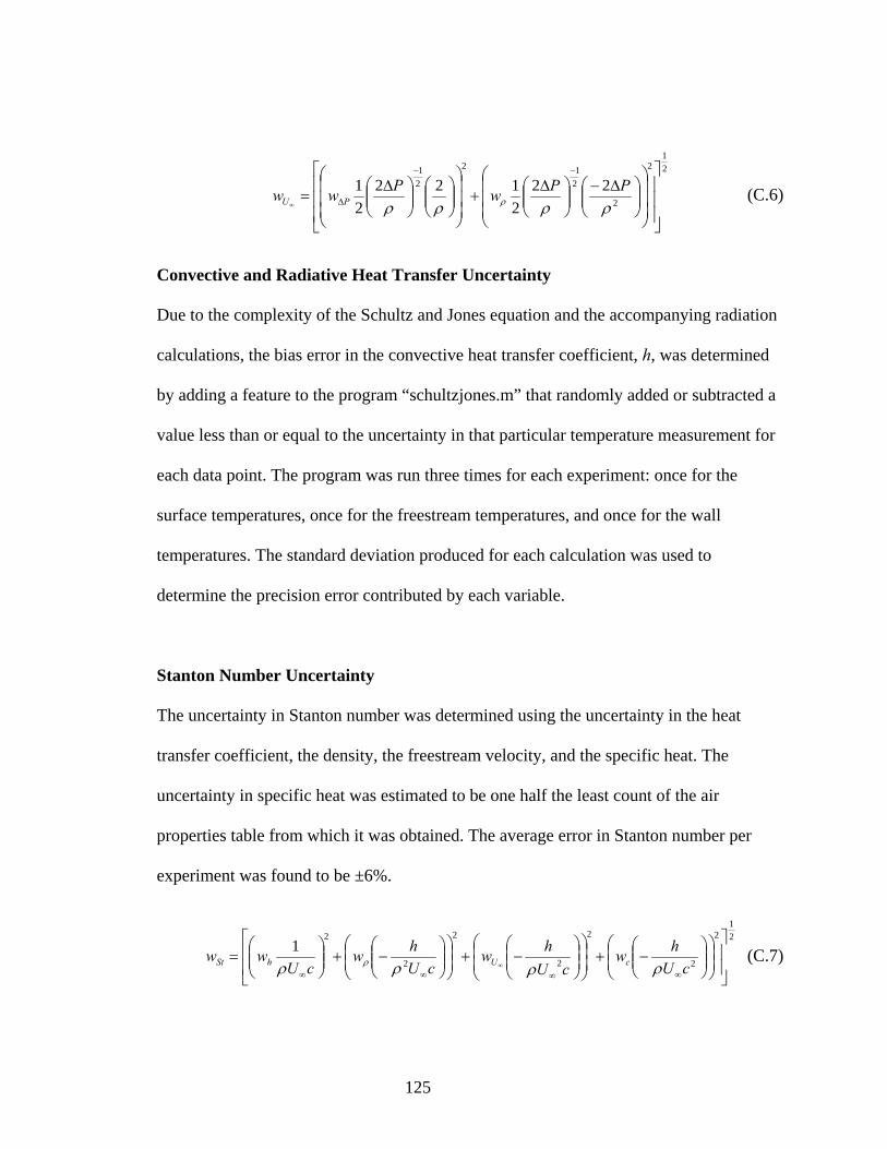
(C.6
Convective and Radiative Heat Transfer Uncertainty
Due to the complexity of the Schultz and Jones equation and the accompanying radiation
calculation
)
s, the bias error in the convective heat transfer coefficient, h, was determined
y adding a feature to the program “schultzjones.m” that randomly added or subtracted a
articular temperature measurement for
tanton Number Uncer
The uncertainty in Stanto t
ansfer coefficient, the density, the freestream velocity, and the specific heat. The
ncertainty in specific heat was estimated to be one half the least count of the air
er
21
2
2
2
2
2 222122
21
⎥⎥
⎦
⎤
⎢⎢
⎣
⎡
⎟⎟
⎠⎜⎜
⎝⎟⎟⎞
⎜⎜⎛ Δ−
⎟⎟⎞
⎜⎜⎛ Δ
+⎟⎟
⎠⎜⎜
⎝⎟⎟⎞
⎜⎜⎛
⎟⎟⎞
⎜⎜⎛ Δ
= Δ∞ ρρρρ ρPPwPww PU
11
⎥⎢ ⎟
⎞
⎜
⎛
⎠⎝⎠⎝⎟
⎞
⎜
⎛
⎠⎝⎠⎝
−−
b
value less than or equal to the uncertainty in that p
each data point. The program was run three times for each experiment: once for the
surface temperatures, once for the freestream temperatures, and once for the wall
temperatures. The standard deviation produced for each calculation was used to
determine the precision error contributed by each variable.
S tainty
n number was determined using the uncertainty in the hea
tr
u
properties table from which it was obtained. The average error in Stanton number p
experiment was found to be ±6%.
(C.7)
21
2222
⎦
⎤
⎣
⎡
⎠⎝ ⎠⎝⎠⎝ ⎠⎝⎠⎝ ⎠⎝⎠⎝ ∞∞∞∞222
1⎥⎥
⎢⎢
⎟⎟⎞
⎜⎜⎛
⎟⎟⎞
⎜⎜⎛
−+⎟⎟⎞
⎜⎜⎛
⎟⎟⎞
⎜⎜⎛
−+⎟⎟⎞
⎜⎜⎛
⎟⎟⎞
⎜⎜⎛
−+⎟⎟⎞
⎜⎜⎛
=∞ cU
hwcU
hwcU
hwcU
ww cUhSt ρρρρ ρ
125

Thermocouple Error
worst-case-scen
radiative heat transfer in eter
eestream thermocouple. The thermocouple bead was treated as a sphere in cross flow.
nt involving Coupon 3, Burn 2
(C.9)
urface
(C.10)
steady
the
(C.11)
A ario analysis was performed to determine how significant an error
troduced into the data collected by the 0.005” diam
fr
Temperatures and velocities were taken from an experime
where the average temperature measured by the thermocouple was 49.3°C.
(C.8)
The ratio μ/μs is close to one if the freestream and the film temperature near the s
of the bead are nearly equal.
8.123Re == ∞
μρ DU
D
174.7PrRe006.0Re4.0241
4.032
21
=⎟⎟⎞
⎜⎜⎛
⎟⎠⎞
⎜⎝⎛ ++= DDDNu
μμ
⎠⎝ s
KmWDkNu D
2/7.1634=h =
An energy balance was performed that assumed that the thermocouple bead was at
state. The emissivity of the chromel/alumel bead was assumed to be 0.87, which is
emissivity of oxidized chromel.
(C.12)
( ) ( )44wCTCT TTTTh −=− −−∞ εσ
CT o36.49=∞
126

The analysis indicated that the effects of radiation caused a temperature underprediction
of 0.06°C. This is 18% as large as the total error caused by other sources.
127