evolutionary training for dynamical recurrent neural

Mathware & Soft Computing 13 (2006) 89-110

Evolutionary Training for Dynamical Recurrent

Neural Networks: An Application in Finantial

Time Series Prediction

M. Delgado, M.C. Pegalajar, M.P. Cuellar

Dpto. Ciencias de la Computacion e Inteligencia Artificial.

ETS. Ingenierıa Informatica

University of Granada. 18071 Granada, Spain.

[email protected], [email protected], [email protected]

Abstract

Theoretical and experimental studies have shown that traditional training

algorithms for Dynamical Recurrent Neural Networks may suffer of local op-

tima solutions, due to the error propagation across the recurrence. In the last

years, many researchers have put forward different approaches to solve this

problem, most of them being based on heuristic procedures. In this paper,

the training capabilities of evolutionary techniques are studied, for Dynami-

cal Recurrent Neural Networks. The performance of the models considered is

compared in the experimental section, in real finantial time series prediction

problems.

Keywords: Recurrent Neural Networks, Evolutionary Algorithms, Time

Series Prediction

1 Introduction

Neural networks are bio-inspired mathematical models, which have successfullysolved many problems in the real world [17]. The neural network architecturesmost known are mainly feedforward models [17][22][24][27][31]. They have tradi-tionally been trained with algorithms based on gradient and error propagation.There is a huge variety of training algorithms for feedforward networks, being themost known the BackPropagation and its derivatives [17][27]. Dynamical Recur-rent Neural Networks (DRNN) [21][8][20] may be built from a feedforward model,by including recurrent connections in the network structure. The variety of train-ing algorithms for DRNN is not as high as for feedforward models, some examplesbeing the algorithms Real Time Recurrent Learning (RTRL) [8][9][26] and Back-propagation Through the Time (BPTT) [8][9][25]. These algorithms are also basedon error propagation across the recurrent connections. Theoretical and experimen-tal results have shown that traditional training methods for DRNN may suffer of

89

90 M. Delgado, M.C. Pegalajar & M.P. Cuellar

local optima solutions [32]. In the last years, many researchers have put forwarddifferent approaches to solve the shrinking gradient problems for DRNN training,most of them being based on heuristic procedures [1][2][3][5][14][19].

Evolutionary algorithms [10][13][18][29] are heuristic procedures that includea set of search, learning and optimization techniques, based on nature processes.In the last decade, evolutionary algorithms have been widely used to solve manyreal world problems, obtaining suitable results. Some evolutionary models havealso been proposed to improve the neural network training. In the case of DRNN,genetic algorithms have been applied for training and topology optimization, ob-taining promising results [2][3][19]. In this paper, we study the capabilities ofevolutionary algorithms to train DRNN. An Elman Recurrent Neural Network[8][15] is trained using different evolutionary techniques, in finantial time seriesforecasting problems [20][23][24][31]. The training models studied in this work aregenetic algorithms [22][19][3], using generational [2], stationary [29][30] and mixed[10] evolution schemes; the multimodal Clearing algorithm [4][6], and the CHC al-gorithm [13]. The original CHC scheme has been modified, to deal with real-codedvariables.

This paper is structured in the following way. Section 2 introduces the ElmanRecurrent Neural Network model. Section 3 explains the evolutionary algorithmsconsidered in this work. Section 4 exposes the evolutionary training procedure, forElman Recurrent Neural networks. Section 5 shows the experimental results anddiscusses the comparative study of evolutionary and traditional training algorithms.Finally, section 6 summarizes the conclusions obtained.

2 The Elman Recurrent Neural Network

Dynamical Recurrent Neural Networks may be used as input/output mapping mod-els. They can process patterns with undetermined size, temporal properties ordynamical behaviour. The DRNN models most known are the Fully ConnectedRecurrent Neural Network [8], the Jordan Network [8], and the Elman Network[8][15]. In this work, we study the Elman Network model. The Elman recurrentneural network (ERNN) is a widely studied model, for which it has been proved theequivalence with Markov models and Mealy-Moore machines [7][28]. The networkis provided with long and short term memory, codified in the network structureby mean of recurrent connections. The topology of an Elman network has thefollowing structure:

• The nodes in the input layer provide the input data corresponding to the currenttime, and distribute them across the other layers.

• The nodes in the hidden layer makes the non-linear transformations and opera-tions, needed to calculate the output of the network.

• The nodes in the output layer uses the results provided by the hidden neurons,and aggregates them to produce the network output.

Evolutionary Training for Dynamical Recurrent Neural Networks... 91

.

.

.

.

.

.

X 1 (t)

X n (t)

V S 1 (t)

S 2 (t)

S h (t)

O 1 (t)

U

.

.

.

O o (t)

W

Figure 1: Structure of the Elman Network

The recurrence is carried out in the hidden layer, so that the output value of ahidden neuron, at time t, is also input for all hidden neurons, at time t+1. Figure1 shows these ideas in the basic scheme of an Elman recurrent neural network.

The diagram in Figure 1 represents an Elman recurrent neural network with ninputs, h hidden neurons, and o outputs. Xi(t) is the input data to neuron i attime t (16i6n); Hj(t) is the output of hidden neuron j at time t (16j6h); andOk(t) is the k-th network output at time t (16k6o).

The values U, V, W are matrices that encode the network weights, so thatVji is the weight associated to connection from input neuron i to hidden neuronj; Ujr is the weight associated to the recurrent connection from hidden neuron rto hidden neuron j; and Wkj is the weight associated to connection from hiddenneuron j to output neuron k. Attending to this notation, the equations for thenetwork dynamics are:

nethj(t) =

h∑

r=1

UjrHr(t − 1) +

n∑

i=1

VjiXi(t) (1)

Hj(t) = f(nethj(t)) (2)

netok =

h∑

j=1

WkjHh(t − 1) (3)

Ok(t) = g(netok(t)) (4)

In equations (2) and (4), the functions f(x) and g(x) are the activation functionsfor hidden and output neurons, respectively. In this work, we use the sigmoid andthe identity functions for f(x) and g(x). Equations (5) and (6) introduce how theyare calculated:


POPULATION PARENTS

OFFSPRING

SELECTION

RECOMBINATION

MUTATION

REPLACEMENT

Figure 2: Main scheme of a Genetic Algorithm

f(x) =1

1 + e−x(5)

g(x) = x (6)

The traditional gradient-based algorithms to train Elman recurrent neural net-works are the Truncated BackPropagation Throught the Time (TBPTT) [8], andthe Real Time Recurrent Learning [8]. A complete guide about TBPTT and itsapplication to train Elman recurrent neural networks may be found in [8][9].

3 Evolutionary algorithms

This section introduces the evolutionary algorithms used in this work, for DRNNtraining. Firstly, genetic algorithms are introduced in subsection 3.1. After that,subsection 3.2 explains the multimodal Clearing procedure. Finally, the CHCscheme modified is exposed in subsection 3.3.

3.1 Genetic Algorithms

The evolution process in a genetic algorithm [16][13][18][29] is based on a nature-like selection procedure, the recombination and the mutation in a set of solutions(population). The genetic evolution schemes generational [2], stationary [29][30]and mixed [10] are generated from a basic genetic algorithm procedure [13] (seeFigure 2), by using different strategies for the selection, recombination, mutationand replacement of the solutions in the population. Below, algorithms 1, 2 and 3review the main procedures for the previous schemes.

Algorithms 1, 2 and 3 show the differences in the selection, recombination,mutation and replacement operator strategies, in order to build the generational,stationary and mixed procedures, respectively.

Firstly, a generational procedure uses the selection operator to build a set ofsolutions, P’, with size equals to the population’s size. It also allows P’ to includemultiple instances of a solution. After that, the recombination operator is appliedover the solutions in P’, to build —P(t)— new solutions, H. Then, the mutationprocedure alters these new individuals in H’. At the end of the evolutionary pro-cess, the replacement strategy sets the population in the following iteration of the


Algorithm 1 Genetic Procedure with Generational structure

1: t=0; Initialize starting population P(t)with S solutions2: while stopping condition is not satisfied do

3: set P’= ∅4: while |P’| < |P(t)| do

5: set s= select a solution from P(t)6: set P’= P’+s7: end while

8: set H= recombination of solutions in P’9: set H’= Mutation of solutions in H

10: evaluation of solution in H’11: set P(t+1)= H’12: Apply elite strategy in P(t) and P(t+1), if required13: set t= t+114: end while

15: Return best solution in P(t)

Algorithm 2 Genetic Procedure with Stationary structure

1: set t=0; Initialize starting population P(t)with S solutions2: while stopping condition is not satisfied do

3: set P’= ∅4: while |P’| < k do


8: set H= recombination of solutions in P’9: set H’= Mutation of solutions in H

10: evaluation of solutions in H’11: set P(t+1)= P(t)12: replacement of solutions in P(t+1) with solutions in H’13: Apply elite strategy in P(t) and P(t+1), if required14: set t= t+115: end while



Algorithm 3 Genetic Procedure with Mixed structure


3: set P’= ∅4: while (|P| < k do


8: set H= recombination of solutions in P’9: set H’= Mutation of solutions in H+P’

10: evaluation of solutions in H’11: set P(t+1)= P(t)12: replacement of solutions in P(t+1) with solutions in H’ and P’13: Apply elite strategy in P(t) and P(t+1), if required14: set t= t+115: end while


algorithm to the new solutions in H’. On the other hand, the stationary strategyuses the selection operator to choose a fixed number of k solutions in P(t). Usually,the value for k is k=2. After that, the recombination operator generates k new so-lutions, which are altered using the mutation procedure. The replacement schemein a stationary strategy also allows the designer of the algorithm to choose a re-placement strategy. For instance, some of the most common replacement schemesare to replace parents with offspring, to replace the worst solutions in P(t+1) withthe offspring, to replace the parents if the offspring is better, etc. Finally, themixed strategy uses the selection and recombination schemes of a stationary pro-cedure. However, the mutation operator is applied in both sets of parents, P’, andoffspring, H. The replacement scheme must also be chosen by the designer of thealgorithm. For instance, one of the most common replacement schemes in a mixedprocedure are to replace P(t+1) with the best —P(t+1)— solutions in H’.

This work considers all the previous evolution strategies. In the experimentalsection, all of them are compared to test the best strategy for the finantial timeseries problems approached.

3.2 Niching Clearing Procedure

Multimodal evolutionary algorithms [6] may be considered as a extension of agenetic evolution procedure. The population of a multimodal algorithm evolvescovering different areas in the solution space. Then, the solutions are set to one ofthe areas explored, like in a clustering procedure (niching). A niche comprises a setof solutions in the same neighbourhood. In this work, two solutions are neighbors ifthe Euclidean distance is under a threshold. The Clearing [4][6] algorithm evolvesa population of solutions. For each iteration, Clearing divides the solutions in clus-


ters (niches), and applies the selection, recombination, mutation and replacementprocedures as stated in algorithm 4.

Algorithm 4 Clearing Procedure


3: compute the number of niches at iteration t, N(t)4: niching of solutions in P(t)5: set B= ∅6: for all niche i=1..N(t) do

7: {sj: 1≤j≤k}= select the k best individuals of niche i8: set B= B+{sj}9: end for

10: set P’= selection of solutions from B11: set H= recombination of solutions in P’12: set H’= Mutation of solutions in H13: evaluation of solutions in H’14: set P(t+1)= P(t)15: replacement of solutions in P(t+1) with solutions in H’16: Apply elite strategy in P(t) and P(t+1), if required17: set t= t+118: end while


The Clearing main scheme in Algorithm 4 may be obtained from a genetic evo-lution procedure (Algorithms 1, 2 and 3). The relevant contribution in the Clearingscheme is in steps 3-9. Steps 3-4 compute the number of niches (or clusters) in thecurrent iteration. Then, each solution in P(t) is assigned to a niche in steps 5-9.Once the niching procedure has finished, then the selection, recombination, muta-tion and replacement procedures are carried out following a genetic generationalevolution strategy.

3.3 Algorithm CHC

The algorithm CHC [13] was firstly proposed as an alternative to solve problemswith binary-encoded solutions. It combines a balance in diversity and convergenceusing an elite selection, the HUX recombination operator [13], incest preventionin recombination, and population reinitialization. Below, these components arereviewed.

• The elite selection is carried out at the replacement step, so that the popu-lation at the next iteration is composed by the best individuals, consideringparents and offspring.

• The purpose of the HUX recombination operator is to produce new solutionsthat differ from the parents as much as possible, to explore new zones in


INIT

POPULATION

COMPUTE

RECOMBINATION

THRESHOLD

POPULATION PARENTS

OFFSPRING

RECOMBINATION

POPULATIO

N CHANGED?

YES

DECREMENT

RECOMBINATION

THRESHOLD

RECOMBINATION

THRESHOLD <=0?

YES

NO

SELECTION

REPLACEMENT

Figure 3: Main scheme for the CHC algorihm

Algorithm 5 CHC Procedure

1: set t=0; Initialize starting population P(t)with S solutions2: set D= Average Euclidean distance in P(t)3: set R= KA·D4: while stopping condition is not satisfied do

5: set P’=∅6: while |P| < |P(t)| do


10: set H= recombination of solutions in P’ by pairs. Two solutions a and b arenot combined iif || a-b|| <D

11: evaluation of solutions in H12: set P(t+1)= best solutions in H and P(t) : |P(t+1)|= S13: if P(t) = P(t+1) then

14: set D= D-R15: end if

16: if D≤0 then

17: re-start population P(t+1) with S-L random solutions and the L best so-lutions from P(t)

18: set D= Average Euclidean distance in P(t+1)19: set R= KA·D20: evaluation of new solutions in solutions P(t+1)21: end if

22: set t= t+123: end while



the search space. In this work, the HUX recombination operator is replacedwith the BLX-α operator [11], so that the algorithm may be applied to real-encoded solutions.

• The incest prevention is applied in the recombination step, to avoid prematureconvergence. It avoids two solutions to be combined if they are similar. Thesimilarity measure is provided by the Hamming distance for binary-encodedsolutions. In this work, the similarity measure used is the Euclidean distance,for real-encoded solutions.

• The reinitialization procedure re-starts the population if it has converged toan area in the solution space. It also uses an elite strategy that preserves thebest solutions found in the evolution process in the population.

Figure 3 shows the main scheme of the CHC algorithm. After that, Algorithm5 explains in depth the adaptation of scheme in figure 3 for real-encoded solutions.

4 Evolutionary Training of Recurrent Neural Net-

works

This section explains the use of evolutionary algorithms to train DRNN [2]. Firstly,subsection 4.1 exposes the representation of an Elman recurrent neural network.After that, subsection 4.2 introduces the fitness function to train an Elman networkin time series prediction problems.

4.1 The representation mechanism

In this work, an Elman recurrent neural network is codified into a real-valued vector.Each component in the vector is assigned to an only network connection. Then,the value of a component is the weight of the corresponding connection associated.Figure 4 shows an example of the encoding of an Elman network with one input, oneoutput, and two hidden neurons. Considering the notation introduced in section 2,the number of components of a vector s encoding an ERNN, Ns, may be calculatedusing the following equation:

Ns = h(n + h + o) (7)

For example, the number of components in the vector encoding the ERNN inFigure 4 is 8.

The Algorithm 6 explains the internal setting of a vector s = (s1, s2, ..., sNs),enconding an Elman network.


V 11 V 21 U 11 U 12 U 21 U 22 W 11 W 12

N s genes

O 1 (t) W

X 1 (t) V

U

Figure 4: Encoding of an Elman network into a vector

Algorithm 6 Encoding Procedure of an Elman Network into a vector

1: set m= 12: for j = 1 to h do

3: for i = 1 to n do

4: set network weight Vji = sm

5: set m= m+16: end for

7: end for

8: for j = 1 to h do

9: for r = 1 to h do

10: set network weight Ujr = sm


13: end for

14: for k = 1 to o do

15: for j = 1 to h do

16: set network weight Wkj = sm


19: end for


D.R.N.N.

Recurrent Connections

Y(t) Y(t+1)

Figure 5: Main scheme for the CHC algorihm

4.2 The evaluation procedure: DRNN for time series pre-

diction

This section introduces the use of DRNN for time series prediction, and the eval-uation procedure for Elman recurrent neural networks evolutionary training. Atime series [23] may be considered as a data sequence, indexed in time. The goalof time series prediction is to find the future values of the data sequence, usingthe knowledge provided by the previous known data. The main assumption thatallows us to model and to predict a time series is that the value of the time series,at time t, depends on the T previous values. Equation (8) illustrates this idea.

Y (t) = F (Y (t − 1), Y (t − 2), ..., Y (t − T )) + e(t) (8)

In equation (8), Y(t) is the value of the time series at time t; F is an unknownfunction, whose domain is the value of the time series for the previous T times,and its range is the current value of the time series. Finally, e(t) is the error whilecomputing the current value of the time series. To simplify the problem, we mayassume that e(t)=0.

Traditionally, the tools applied for time series prediction have been linear re-gressions and statistical models. However, when F is non-linear, other powerfultechniques must be applied. In the last decade, neural networks have been of-ten applied in time series prediction problems [23]. The problem of time seriesprediction may be approached using a dynamical recurrent neural network [1][20].Assuming that the network input, at time t, is the value of the time series at time t,the network provides an output depending on the current inputs and an unknownfunction. This function depends on the previous network inputs in time, and it islearnt by the network and recorded into the recurrent connections. The structureof a DRNN for time series prediction is shown in the diagram of Figure 5.

The time series is presented to the network, ordered in time. The networkoutput, at time t, must fit the value of the time series at time t+1. The trainingstage minimizes the mean square error between the network output at time t, andthe value of the time series at time t+1, for T training patterns (equation (9)).


F (s) =1

T

T∑

t=1

o∑

k=1

(Osk(t) − dk(t))2 (9)

In equation (9), o is the number of network outputs; Osk(t) is the outputcorresponding to the output neuron k of the ERNN associated to vector S, at timet; dk(t) is the desired output for neuron k at time t; and finally, T is the numberof training patterns.

On the other hand, in the prediction stage, the network output at time t + 1 isused as network input at time t + 2, to predict the time series value at time t + 3,following the scheme in figure 5. This process is cicled for times t+1, t+2, t+3, ...,until the prediction value for the time required is obtained.

5 Experiments

This section shows the performance of the training algorithms in section 3, to trainan Elman recurrent neural network in finantial time series prediction problems.Subsection 5.1 introduces the data sets. After that, subsection 5.2 exposes theparameters for the algorithms and the network. Finally, subsection 5.3 shows theexperimental results, and discusses the performance comparison of the algorithmsin the ERNN training.

5.1 The data sets and the case study: prediction of gross

indebtedness in the Spanish regions

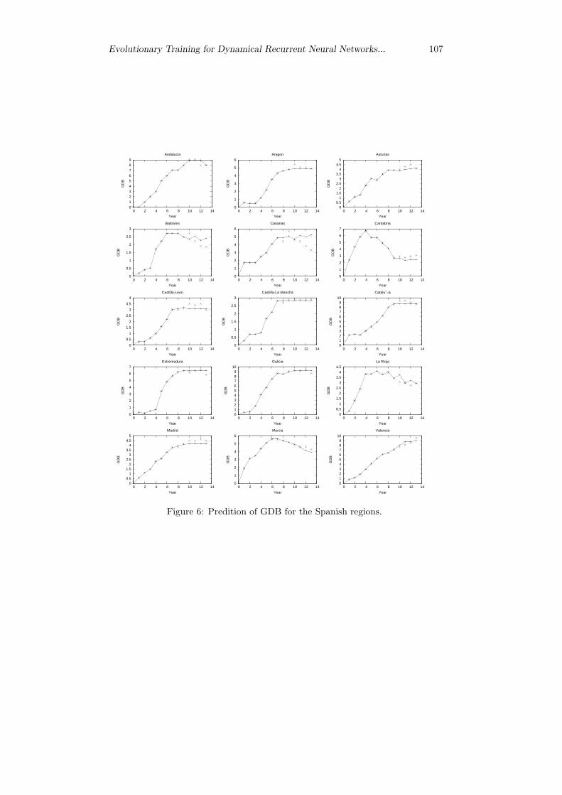
The GDP data for then autonomous regions in Spain, between years 1986 and 1996,are analyzed to predict the value from year 1997 to year 2000. Figure 6 shows thedata sets. Values from years 1986 to 1996 are used as training data set, and thenetworks trained are validated with the values from year 1997 to year 2000.

5.2 The parameters

This section exposes the parameters for the network and the algorithms. Table1 shows the settings for the Elman recurrent neural network. Table 2 explainsthe configuration for the evolutionary algorithms. Finally, table 3 introduces theparameters for the traditional training algorithms (TBPTT and RTRL). The con-figuration in table 1 is used for the neural network.

The algorithms evolve the population until 50000 solutions have been evaluated.The number of evaluations is also the comparison criterion in the experiments ofthe following subsection. Each algorithm is run for 30 times in all the problems.

The evolutionary algorithms are also compared with the traditional trainingalgorithms for DRNN. The comparison criterion is the computational time. Thealgorithms TBPTT and RTRL are run for 30 times, in a multi-start procedure.Each iteration of the multi-start procedure uses the highest computational time of


Table 1: Settings for the neural networkParameter V alue

Number of input neurons 1 (value of the time series at time t)Number of hidden neurons 7Number of output neurons 1 (value of the time series at time t+1)

Activation function Sigmoid for hidden nodes, linear for output units

the evolutionary algorithms as stopping criterion. Table 3 shows the parametersfor these algorithms.

5.3 Experimental results

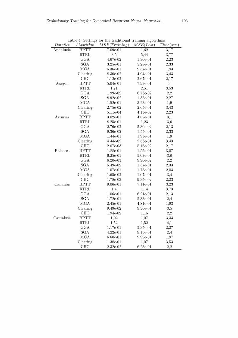
This subsection resumes the experimental results. Table 4 shows the average errorfor the solutions of the training algorithms, applied to all the data sets. Column 1means the data set. Column 2 introduces the algorithm. Columns 3 and 4 showthe mean square error of the best, in the training and test sets. Finally, column 5prints the average computing time.

A statistical test is applied to test the relevance of the results for the algorithms.The Kolmogorov-Smirnov test has been applied to check normality conditions inthe results obtained, for each algorithm. It concludes that most of results do notfollow a normal distribution. Thus, the Kruskal-Wallis non-parametric test hasbeen applied to the results of the algorithms, with 0.05 of confidence level. Table5 shows the statistical relevance of the algorithms, according to the results of theKruskal-Wallis test. Columns 1 and 3 mean the data sets. Columns 2 and 4 printthe pValue resulting from the statistical test, starting from the best algorithm tothe worst one for each data set. We mark (x) when the algorithm is statisticallyequivalent to the previous one, and (-) when it is worse.

Using the criterion in Algorithm 7 to compute the relevance of the evolutionarymodels, table 6 concludes that the best results have been found using the CHCevolutionary algorithm. On the other hand, the worst solutions have been providedby the traditional training algorithms, RTRL and BPTT. An indepth study oftables 3 and 5 may conclude that any of the evolutionary training models haveprovided better performance than the algorithms RTRL and BPTT. Thus, a partialconclusion of the experimental results is that evolutionary algorithms may improvethe traditional training of ERNN, in the problems attached to this work.

Considering the evolutionary procedures, there is a clear difference in the statis-tical results. While the best solutions have been found by the algorithm CHC in allthe data sets, the worst ones have been provided by the mixed genetic algorithm.

The algorithm CHC has addressed the search suitably, using the incest preven-tion, BLX-α recombination, the elite selection, and the reinitialization. However,the mixed genetic algorithm has made an excessive use of exploration in the searchspace, with the mutation operator, therefore reducing the convergence rate. Thisassumption is supported by the results in the stationary genetic procedure (thedifference in both algorithms is the mutation operator applied to the whole popu-


Table 2: Settings for the evolutionary algorithmsParameter GeneticAlgorithmsClearing CHCScheme Generational

/stationary/mixed

generational –

Selection opera-tor [11]

Binary tourna-ment selection



Recombinationoperator [12][11]

Blx-α (α= 0.5) Blx-α (α= 0.5) Blx-α (α= 0.5)

Mutation opera-tor [11]

Displacement Displacement –

Recombinationprobability

0.8 (genera-tional)

0.8 –

Mutation prob-ability

0.08 0.08 –

Replacement Parents are re-placed with off-spring (station-ary and mixed)

– –

Elite factor The two bestsolutions remainin the popula-tion

The two bestsolutions remainin the popula-tion

–

Size of popula-tion

50 50 50

Gene bounds [-5.0, 5.0] [-5.0, 5.0] [-5.0, 5.0]Ratio of a niche – 0.35*D (D=

Maximum Eu-clidean distanceof solutions inthe population)

–

Ratio to de-crease the Av-erage Euclideandistance

– – K= 0.1

Table 3: Settings for the traditional training algorithmsParameter TBPTT RTRL

Number of iterations 500 500Learning rate 0.001 0.001

Time to unfold the network 2 –Time for each multi-start iteration (sec.) 5 5


Table 4: Settings for the traditional training algorithmsDataSet Algorithm MSE(Training) MSE(Test) T ime(sec.)Andalucıa BPTT 7.09e-01 1,62 3,17

RTRL 3,5 5,44 3,77GGA 4.67e-02 1.36e-01 2,23SGA 3.25e-01 5.28e-01 2,33MGA 5.36e-01 9.57e-01 1,93

Clearing 8.30e-02 4.94e-01 3,43CHC 1.12e-02 2.67e-01 2,17

Aragon BPTT 5.04e-01 7.93e-01 3RTRL 1,71 2,51 3,53GGA 1.99e-02 6.73e-02 2,2SGA 8.92e-02 1.35e-01 2,27MGA 1.52e-01 3.23e-01 1,9


Asturias BPTT 3.02e-01 4.82e-01 3,1RTRL 8.25e-01 1,23 3,6GGA 2.76e-02 5.30e-02 2,13SGA 9.36e-02 1.55e-01 2,33MGA 1.44e-01 1.93e-01 1,9


Baleares BPTT 1.88e-01 1.55e-01 3,07RTRL 6.25e-01 5.03e-01 3,6GGA 6.20e-03 9.96e-02 2,2SGA 5.49e-02 1.37e-01 2,33MGA 1.07e-01 1.75e-01 2,03


Canarias BPTT 9.06e-01 7.11e-01 3,23RTRL 1,4 1,14 3,73GGA 1.06e-01 6.21e-01 2,13SGA 1.72e-01 5.33e-01 2,4MGA 2.45e-01 4.81e-01 1,93

Clearing 9.49e-02 9.36e-01 3,5CHC 1.94e-02 1,15 2,2

Cantabria BPTT 1,02 1,07 3,33RTRL 1,52 1,52 4,1GGA 1.17e-01 5.35e-01 2,27SGA 4.22e-01 9.15e-01 2,4MGA 6.60e-01 9.99e-01 1,97

Clearing 1.38e-01 1,07 3,53CHC 2.32e-02 6.23e-01 2,2


DataSet Algorithm MSE(Training) MSE(Test) T ime(sec.)Castilla-

Leon BPTT 3.10e-01 4.48e-01 3,1RTRL 8.07e-01 1,16 3,53GGA 6.14e-03 3.60e-02 2,27SGA 4.42e-02 9.07e-02 2,37MGA 8.34e-02 1.70e-01 2


Catalunia BPTT 2,81 5,96 3,23RTRL 3,95 7,53 3,83GGA 5.07e-02 1.00e-01 2,2SGA 2.40e-01 4.73e-01 2,37MGA 4.17e-01 1,01 1,97


Extremadura BPTT 8.65e-01 8.60e-01 2,93RTRL 3,31 3,73 3,53GGA 9.61e-03 4.77e-02 2,17SGA 2.49e-01 2.55e-01 2,3MGA 4.42e-01 4.11e-01 1,9


Galicia BPTT 6.73e-01 9.75e-01 3,13RTRL 4,67 5,67 3,7GGA 2.02e-02 1.01e-01 2,2SGA 3.48e-01 4.05e-01 2,3MGA 6.23e-01 7.13e-01 1,93


Madrid BPTT 2.00e-01 4.18e-01 3,4RTRL 8.11e-01 1,38 3,7GGA 1.50e-02 8.38e-02 2,17SGA 7.30e-02 1.52e-01 2,47MGA 1.02e-01 1.99e-01 2


Castilla-La Mancha BPTT 2.88e-01 3.46e-01 2,97

RTRL 6.30e-01 7.96e-01 3,63GGA 1.03e-02 1.09e-02 2,17SGA 6.73e-02 7.05e-02 2,27MGA 1.16e-01 1.42e-01 1,9


Murcia BPTT 2.16e-01 1.75e-01 3,23RTRL 8.60e-01 6.23e-01 3,87GGA 1.47e-02 1.55e-01 2,2SGA 7.15e-02 2.05e-01 2,33MGA 1.10e-01 2.03e-01 1,93



DataSet Algorithm MSE(Training) MSE(Test) T ime(sec.)Rioja BPTT 2.00e-01 1.83e-01 3,13

RTRL 7.94e-01 5.67e-01 3,67GGA 2.76e-02 3.14e-01 2,17SGA 6.54e-02 2.85e-01 2,27MGA 1.08e-01 3.13e-01 1,9


Valencia BPTT 5.07e-01 2,56 3,27RTRL 2,54 6,2 3,7GGA 2.25e-02 6.85e-01 2,2SGA 1.43e-01 9.68e-01 2,33MGA 2.92e-01 1,42 1,9


lation, in the mixed one). In all the problems, the ranking of the S. GA scheme hasprovided better results than the mixed one. It has improved the convergence rate,but it has not explored the search space enough. On the other hand, the genera-tional genetic scheme and the Clearing procedure have improved the explorationand exploitation of the stationary genetic algorithm, in the search space. Table 5shows that the genetic procedure may improve the Clearing scheme, in some cases.However, there may be situations in which both return similar solutions.

Figure 6 plots both training and test network outputs. Points plotted with Oare the real data, and points plotted with + are the network outputs.

6 Conclusions

This work has studied the training capabilities of evolutionary algorithms, based onpopulation evolution, for Dynamical Recurrent Neural Networks. The experimentalresults have shown that evolutionary training may improve the traditional trainingof Elman recurrent neural networks, in the time series prediction problems attachedin the experimental section.

On the other hand, the comparative statistical study of the algorithms pro-posed in this work, has concluded that algorithms with a better balance in diver-sity/convergence may provide better results: The algorithm CHC has found thebest solutions in the problems of GDB prediction for the Spanish regions. Theexperiments have concluded that Elman recurrent neural networks are suitablemodels for time prediction problems. The network is able to learn the dependen-cies in time of the training data sets, and may predict the future values suitablyin the test data. However, the use of evolutionary algorithms for DRNN trainingmay help to improve the network performance, in time series prediction problems.


Table 5: Results of the statistical testsProblem Algorithms Problem Algorithms

Andalucıa GGAMEM Cataluna CHCCHC 0.4688 x GGAMEM 1,95e-4 -

Clearing 0.0003666 - Clearing 0.0009775 -SGAMEM 0.0001948 - SGAMEM 0.0006373 -MGAMEM 0.00579 - MGAMEM 0.0006373 -

BPTT 0.00037 - BPTT 3,88e-8 -RTRL 2.87e-8 - RTRL 0.0001073 -

Aragon CHC Extremadura GGAMEMGGAMEM 8.7e-08 - CHC 0.2871 xClearing 0.008875 - Clearing 1,53e-4 -SGAMEM 0.0228 - SGAMEM 0.003585 -

MGAMEM 0.000858 - MGAMEM 1,69e-2 -BPTT 2.95e-5 - BPTT 3,34e-6 -RTRL 5.23e-8 - RTRL 2,87e-8 -

Asturias CHC Galicia CHCGGAMEM 0.01801 - GGAMEM 0.05099 x

Clearing 1,24e-3 - Clearing 0.0004337 -SGAMEM 0.1602 x SGAMEM 9,31e-7 -

MGAMEM 0.01355 - MGAMEM 5,10e-2 -BPTT 1,02e-6 - BPTT 0.003419 -RTRL 1,27e-7 - RTRL 2,87e-8 -

Baleares CHC La Rioja BPTTClearing 0.4077 x CHC 0.0005411 -

GGAMEM 0.3831 x Clearing 0.7901 xSGAMEM 0.001480 - SGAMEM 0.7562 xMGAMEM 0.02760 - MGAMEM 0.8016 x

BPTT 0.6048 x GGAMEM 0.1882 xRTRL 7,04e-7 - RTRL 1,44e-3 -

Canarias Clearing Madrid CHCSGAMEM 0.7788 x GGAMEM 0.4333 xMGAMEM 0.2939 x Clearing 0.01247 -GGAMEM 0.2428 x SGAMEM 0.7901 x

BPTT 0.03205 - MGAMEM 0.01801 -CHC 0.03089 - BPTT 3,39e-4 -RTRL 0.2089 x RTRL 6,37e-8 -

Cantabria GGAMEM Murcia CHCCHC 0.7562 x BPTT 0.001205 -

Clearing 0.2036 x GGAMEM 525 xSGAMEM 0.02463 - SGAMEM 0.4779 xMGAMEM 0.1242 x MGAMEM 0.1984 xBPTT 0.0005715 - Clearing 0.03847 -RTRL 2,87e-8 - RTRL 4,40e-7 -


0 1 2

3 4 5 6

7 8 9

0 2 4 6 8 10 12 14

GD

B

Year

Andalucia

0

1

2

3

4

5

6

0 2 4 6 8 10 12 14

GD

B

Year

Aragon

0 0.5

1 1.5

2 2.5

3 3.5

4 4.5

5

0 2 4 6 8 10 12 14

GD

B

Year

Asturias

0

0.5

1

1.5

2

2.5

3

0 2 4 6 8 10 12 14

GD

B

Year

Baleares

0

1

2

3

4

5

6

0 2 4 6 8 10 12 14

GD

B

Year

Canarias

0

1

2

3

4

5

6

7

0 2 4 6 8 10 12 14

GD

B

Year

Cantabria

0

0.5

1

1.5

2

2.5

3

3.5

4

0 2 4 6 8 10 12 14

GD

B

Year

Castilla-Leon

0

0.5

1

1.5

2

2.5

3

0 2 4 6 8 10 12 14

GD

B

Year

Castilla-La Mancha

0 1 2 3 4 5 6 7 8 9

10

0 2 4 6 8 10 12 14

GD

B

Year

Cataluˆ–a

0

1

2

3

4

5

6

7

0 2 4 6 8 10 12 14

GD

B

Year

Extremadura

0 1 2 3 4 5 6 7 8 9

10

0 2 4 6 8 10 12 14

GD

B

Year

Galicia

0 0.5

1

1.5 2

2.5 3

3.5 4

4.5

0 2 4 6 8 10 12 14

GD

B

Year

La Rioja

0 0.5

1 1.5

2 2.5

3 3.5

4 4.5

5

0 2 4 6 8 10 12 14

GD

B

Year

Madrid

0

1

2

3

4

5

6

0 2 4 6 8 10 12 14

GD

B

Year

Murcia

0 1 2 3 4 5 6 7 8 9

10

0 2 4 6 8 10 12 14

GD

B

Year

Valencia

Figure 6: Predition of GDB for the Spanish regions.


Problem Algorithms Problem Algorithms

Castilla-Leon GGAMEM Valencia CHCCHC 0.3077 x GGAMEM 0.002002 -

Clearing 0.006236 - Clearing 0.3671 xSGAMEM 0.0001538 - SGAMEM 0.02559 -MGAMEM 0.0002189 - MGAMEM 0.005445 -

BPTT 1,77e-5 - BPTT 2,47e-4 -RTRL 2,05e-7 - RTRL 2,87e-8 -

Castilla-La Mancha CHCGGAMEM 0.005445 -

Clearing 4,22e-2 -SGAMEM 2,58e-3 -MGAMEM 3,70e-3 -

BPTT 6,81e-6 -RTRL 5,32e-7 -

References

[1] A. Aussem. Dinamical Recurrent Neural Networks towards prediction andmodeling of dynamical systems. Neurocomputing, 28(1-3):207-232, 1999.

[2] A. Blanco, M. Delgado and M.C. Pegalajar. A Real-Coded genetic algorithmfor training recurrent neural networks. Neural Networks, 14:93-105, 2001.

[3] A. Blanco, M. Delgado and M.C. Pegalajar. A genetic algorithm to obtainthe optimal recurrent neural network. International Journal of ApproximateReasoning, 23:67-83, 2000.

[4] A. Petrowski. A Clearing Procedure as a Niching Method for genetic Al-gorithms. In IEEE International Conference of Evolutionary Computation,Nagoya, Japan. pp. 798-803, 1996.

[5] A. Tettamanzi, M. Tomassini, J. Janben. Soft Computing: Integrating Evolu-tionary, Neural, and Fuzzy Systems. ed. Springer, 2001.

[6] B. Sareni, L. Krahenbuhl. Fitness sharing and niching methods revised. IEEEtransactions on Evolutionary Computation, 2:97-106, 1998.

[7] C. Stefan, P. Kremer, P. Baldi. Hidden Markov models and neural networks.In Genetics, Genomics, Proteomics and Bioinformatics, 4, John Wiley andSons Ltd., 2005.

[8] D. P. Mandic, J. Chambers. Recurrent Neural Networks for Prediction. Wiley,John & Sons Inc., 2001.

[9] H. Jaeger. A tutorial on training recurrent neural networks, covering BPTT,RTRL, EKF, and the echo state network, GMD-report, 43p. 1999.


[10] D.E. Goldberg. Genetic Algorithms in Search, Optimization, and MachineLearning. Addison Wesley, 1989.

[11] F. Herrera, M. Lozano, J.L. Verdegay. Tackling Real-Coded Genetic Algo-rithms: operator and tools for behavioural analysis. Artificial Intelligence re-view, 12:265-319, 1998.

[12] F. Herrera, M. Lozano, A.M. SA¡nchez. A Taxonomy for the Crossover Opera-tor for Real-Coded Genetic Algorithms: An Experimental Study. InternationalJournal of Intelligent Systems, 18:309-338, 2003.

[13] G.J.E. Rawlins. Foundations of Genetic Algorithms. ED. Morgan Kauffman,1991.

[14] J. Schmidhuber. A fixed Size Storage O(n3) Time Complexity Learning Algo-rithm for Fully Recurrent Continually Running Networks. Neural Computa-tion, 4:243-248, 1992.

[15] J.L. Elman. Finding Structure in Time. Cognitive Science, 14:179-211, 1990.

[16] L.J. Eshelman, J.D. Scahffer. Real-coded genetic algorithms and interval-schemata. In Foundations of genetic algorithms 2. Morgan Kaufmann pub-lishers, 1993.

[17] L.P.J. Veelenturf. Analysis and Applications of Artificial Neural Networks, Ed.Prentice Hall, 1995.

[18] L. Schmitt. Fundamental Study: Theory of genetic algorithms. TheoreticalComputer Science, 259(1-2):1-61, 2000.

[19] M. Delgado, M.C. Pegalajar. A Multiobjective Genetic Algorithm for obtain-ing the optimal size of a Recurrent Neural network for Grammatical Inference.Pattern Recognition, Special Issue of Grammatical Interence. Vol 38(9):1444-1456, 2005.

[20] M. Husken, P. Stagge. Recurrent Neural Networks for Time Series classifica-tion. Neurocomputing, 50:223-235, 2003.

[21] M.P. Cuellar, M.A. Navarro, M.C. Pegalajar and R. Perez. A FIR NeuralNetwork to model the autonomous indebtedness. In SIGEF’03 Congress, Leon, vol 2, pp. 199-209, 2003.

[22] M.P. Cuellar, M. Delgado, M.C. Pegalajar and R. Perez. Prediccion del endeu-damiento economico espanol utilizando modelos bioinspirados. In SIGEF’03Congress, Leon, vol. 1. pp. 489-510, 2003.

[23] N. Davey, S.P. Hunt, R.J. Frank. Time Series Prediction and Neural Networks,In proc. 5th International Conference on Engineering Applications of NeuralNetworks, pp. 93-98, 1999.


[24] R. Zemomi, D. Racaceanu, N. Zerhonni. Recurrent Radial Basis fuction net-work for Time Series prediction. Engineering appl. Of Artificial Intelligence,16(5-6):453-463, 2003.

[25] R.J. Williams, D. Zipser. A learning algorithm for continually running fullyrecurrent neural networks. Neural Computation, 1:270-280, 1989.

[26] R.J. Williams, J. Peng. An efficient Gradient-Based Algorithm for On-LineTraining of Recurrent Network trajectories. Neural Computation, 2:491-501,1990.

[27] S. Haykin. Neural Networks (a Coprehensive foundation). Second Edition.Prentice Hall, 1999.

[28] S.C. Kremer. On the computational power of Elman-style recurrent networks.IEEE Trans. Neural Networks 6(4):1000-1004, 1995.

[29] T. Back. Evolutionary Algorithms in Theory and Practice. Oxford, 1996.

[30] T. Back, D. Fogel, Z. Michalewicz. Handbook of Evolutionary Computation.Institute of Physics Publishing and Oxford University Press, 1996.

[31] Wan. Finite Impulse Response Neural Networks with applications on time seresprediction. PhD Dissertation. Stanford University, 1993.

[32] Y. Bengio, P. Simard, P. Frasconi. Learning Long-Term Dependencies withGradient Descent is Difficult. IEEE Trans. on Neural Networks, 5(2):157-166,1994.

evolutionary training for dynamical recurrent neural

Documents