Incremental Training Of First Order

Recurrent Neural Networks To Predict A

Context-Sensitive Language

Stephan K. Chalup a,∗

aSchool of Electrical Engineering and Computer Science, The University of

Newcastle, Callaghan, 2308, Australia

Alan D. Blair b

bSchool of Computer Science and Engineering, The University of New South

Wales, Sydney, 2052, Australia

Abstract

In recent years it has been shown that first order recurrent neural networks trained

by gradient-descent can learn not only regular but also simple context-free and

context-sensitive languages. However, the success rate was generally low and se-

vere instability issues were encountered. The present study examines the hypothesis

that a combination of evolutionary hill climbing with incremental learning and a

well-balanced training set enables first order recurrent networks to reliably learn

context-free and mildly context-sensitive languages. In particular, we trained the

networks to predict symbols in string sequences of the context-sensitive language

Preprint submitted to Neural Networks 10 January 2003

{anbncn; n ≥ 1}. Comparative experiments with and without incremental learning

indicated that incremental learning can accelerate and facilitate training. Further-

more, incrementally trained networks generally resulted in monotonic trajectories

in hidden unit activation space, while the trajectories of non-incrementally trained

networks were oscillating. The non-incrementally trained networks were more likely

to generalise.

Key words: Mildly context-sensitive language, incremental learning, simple

recurrent neural network, evolutionary hill climbing, evolution strategy, hidden

unit dynamics

1 Introduction

Language processing has been the traditional domain of discrete automata

models. Noam Chomsky drew a distinction between semantics and syntax of

language and proposed a hierarchy of formal languages—the classical Chomsky

Hierarchy (Chomsky, 1959)—with the aim to investigate the syntax of natu-

ral language. The hierarchy is strict and has four complexity classes: regular,

context-free, context-sensitive and recursively enumerable languages (compare

Table 1). To each language class belongs a class of grammars and a class of au-

tomata. Regular grammars and finite state automata are at the most restricted

level while the other three classes are more general, with unrestricted gram-

∗ Corresponding author. Tel: +61-2-4921-6080; fax +61-2-4921-6929.E-mail address: chalup@cs.newcastle.edu.au (S. K. Chalup)

2

mars and Turing machines at the most general level (Hopcroft and Ullman,

1979). From the examples in the last column of Table 1 anbn is context-free

but not regular and anbncn is context-sensitive but not context-free 1 .

----------------------------------------------------------------

Table 1 comes in here

----------------------------------------------------------------

It has become widely accepted that natural language does not fit exactly into

the classical Chomsky hierarchy but has common features with context-free

and context-sensitive languages. Mildly context-sensitive languages (MCSL)

are slightly more powerful than context-free languages but preserve many of

their essential features (Joshi et al., 1991). We note that the class of MCSLs

can be characterised by the following properties 2 :

(1) It contains the three basic non-context-free constructions in natural lan-

1 Notation: anbn and anbncn are used as shortforms for {anbn; n ≥ 1} and{anbncn; n ≥ 1}, respectively. The exponent or index n of a particular string, forexample sn = anbncn, is in the following refereed to as the depth of the string sn.2 For more details on MCSLs and their characterisation see for example (Joshiet al., 1991; Martin-Vide et al., 1999; Ilie, 1999).

3

guage, that is multiple agreements {anbncn; n ≥ 1}, crossed agreements

{anbmcndm; m,n ≥ 1}, and duplication {wcw; w ∈ {a, b}∗}.

(2) MCSLs are semilinear.

(3) MCSLs are polynomial time parseable.

The language of multiple agreements MA = {anbncn; n ≥ 1} is therefore

mildly context-sensitive. The primary goal of this study is to show how first

order recurrent neural networks can learn to predict sequences of strings from

MA and to explore generalisation abilities of the trained neural networks.

Together with recent parallel or subsequent work (e.g. Boden and Wiles, 2000;

Gers and Schmidhuber, 2001; Rodriguez, 2001) on learning ofMA and similar

tasks our study might therefore contribute to a better understanding of the

capabilities of recurrent neural networks to process natural language. While

our first experimental results were announced in (Chalup and Blair, 1999) we

now provide a detailed exposition of our investigation.

Before talking about learning issues it is good to know what types of languages

artificial recurrent neural networks can theoretically process. Theoretical lan-

guage processing capabilities depend on the number of units, the network

topology, the type of weights and the type of activation function used by the

network (Moore, 1998). The present study focuses on simple recurrent net-

works as they were introduced by Elman (1990) and Robinson and Fallside

(1988). If these networks are used with simple threshold units instead of sig-

moidal units they can implement any deterministic finite state automaton (cf.

4

Minsky, 1967; Kremer, 1995). Assuming more general continuous activation

functions the existence of an artificial neural network which can simulate a

universal Turing machine has been proven (Pollack, 1987; Siegelmann, 1999).

But if we demand robustness to bounded noise, recurrent neural networks

cannot recognize anything beyond regular languages (Casey, 1996; Maass and

Orponen, 1997, 1998) and in the case of general Gaussian and other com-

mon noise distributions their capabilities are even more restricted (Maass and

Sontag, 1999a,b).

Different fixed network models have been constructed for predicting or recog-

nizing languages that are regular (Giles et al., 1992; Sontag, 1995; Carrasco

et al., 2000), context-free (Holldobler et al., 1997; Finn, 1998) or context-

sensitive (Steijvers and Grunwald, 1996). However, the question of how far

neural networks are able to learn language tasks of different complexity levels

is still being explored.

There are quite a number of studies which show how first and second order

recurrent networks can learn regular languages from examples and how finite

state automata can be extracted from the trained networks (see e.g. Cleere-

mans et al., 1989; Pollack, 1991; Giles et al., 1992; Zeng et al., 1994; Tino and

Sajda, 1995; Gori et al., 1998).

Several variants of the standard feed-forward backpropagation algorithm (Wer-

bos, 1974) for supervised training of recurrent neural networks have been de-

veloped (Rumelhart et al., 1986; Zipser, 1990; Doya, 1995; Pearlmutter, 1995;

5

Haykin, 1999). In contrast to feed-forward neural networks, generally the error

surface is not at all smooth in the recurrent case. This can disturb gradient-

based training algorithms and successful learning depends on finding a way

around bifurcation problems (see Pearlmutter, 1989; Doya, 1992). Bengio et al.

(1994) pointed out that learning long-term dependencies with gradient descent

methods is difficult.

Despite these difficulties, many recurrent neural networks have been trained

successfully by backpropagation methods. Wiles and Elman (1995) showed

how simple recurrent networks can be trained by backpropagation through

time (Rumelhart et al., 1986; Zipser, 1990) to predict symbols in finite string

sequences of the context-free language {anbn; n ≥ 1}. Following on from Wiles

and Elman’s study, several papers analysed hidden unit activity (Rodriguez

et al., 1999; Rodriguez, 2001) and stability issues (Tonkes and Wiles, 1999;

Boden et al., 1999). They observed instabilities during training, where small

changes in weights can result in significant changes to the dynamics of the

network, with the solution being repeatedly found, lost and found again.

It was suggested in Tonkes et al. (1998) that evolutionary hill-climbing might

overcome some of the instabilities observed using gradient descent on the anbn

task. Their results indicated that evolutionary hill climbing was able to learn

the anbn task more consistently and with better generalisation results than

backpropagation through time (BPTT). Comparative experiments between

evolutionary and gradient descent training of Boden et al. (2000) indicated

6

that evolutionary hill climbing is more reliable in finding solutions and also

produces a more diverse set of solutions than the gradient descent approach.

Chalup and Blair (1999) trained srns successfully on the anbncn language us-

ing a specially tuned version of evolutionary hill climbing. In this pilot study

it was shown for the first time that simple recurrent networks can learn to

predict strings from MA = {anbncn; n ≥ 1} up to a depth of n = 12. It was

later shown by Boden and Wiles (2000) that second order sequential cascaded

networks could successfully be trained by BPTT to predict the next symbol

in strings of MA, although training of first order recurrent networks remained

unsuccessful. A selection of studies about training on non-regular languages

such as anbn and anbncn was recently reviewed by Wiles et al. (2001). One com-

mon characteristic of all these studies was limited generalisation ability—the

networks generalised only a few steps ahead with respect to the depth of the

strings. Therefore they had only learned subsets of the infinite languages (cf.

Boden and Wiles, 2001). Tonkes and Wiles (1999) suggested that the limited

generalisation ability could model human performance when processing center

embedded sentences. In two recent studies Melnik et al. (2000) evolved RAAM

networks capable of expressing all strings of the anbn language, while Gers and

Schmidhuber (2001) trained Long Short-Term Memory Networks to predict

the anbncn language with substantial generalisation ability. Both these network

types are more complex than the first order networks of the present study and

also the task presentation was different.

7

In the present study we further refined the incremental learning combined with

evolutionary hill climbing approach of Chalup and Blair (1999). We show how

to obtain networks which are able to predict sequences of strings from MA =

{anbncn; n ≥ 1} and which are able to generalise to larger values of n as well

as to different orderings of the strings in the data sequence. The development

of each candidate network during the course of evolution is monitored and

some of the emerging solutions are tested on their generalisation ability.

The present study therefore examined the hypothesis that evolutionary hill

climbing when combined with incremental learning and a well-balanced train-

ing set can find recurrent networks that reliably learn context-free and mildly

context-sensitive languages.

The main achievements of this study are a refined incremental learning scheme

and network architecture as well as experimental results which provide answers

to the questions:

- Can first order recurrent neural networks learn to predict sequences of

strings from the language MA and can they generalise beyond the train-

ing data ?

- Is data incremental learning more efficient than non-incremental learning

and is there any qualitative difference in the training result ?

Additional achievements include comparative experiments on the anb2n lan-

guage prediction task and observations obtained from a qualitative analysis

8

of the dynamics of hidden unit activity in a movie-type animation of several

thousand networks which were generated for this experiment.

The article is structured as follows: Section 2 provides some background in-

formation on recurrent neural networks. The prediction task is explained in

Section 3. Incremental evolutionary hill climbing for recurrent networks and its

special adjustment called “data juggling” is the topic of Section 4. Section 5

covers simulations, experiments and their evaluation. The article concludes

with a discussion and summary in Section 6.

2 Recurrent Neural Networks

In recent years a large variety of different recurrent neural network architec-

tures for supervised learning have been investigated—see for example Hertz

et al. (1991), Haykin (1999) or Tsoi and Back (1997) and Tsoi (1998) for

overviews of the discrete and the continuous case. First order recurrent neural

networks operate similarly to feed-forward networks but have recurrent con-

nections. Second order networks additionally have multiplicative connections.

The present study employed a discrete time recurrent neural network with first

order architecture which is often referred to as a simple recurrent network

(srn). It was independently invented by Elman (1990) and Robinson and

Fallside (1988). A standard srn with three units in each layer is displayed in

Figure 1 with input units I1-I3, hidden units H1-H3, output units O1-O3 and

9

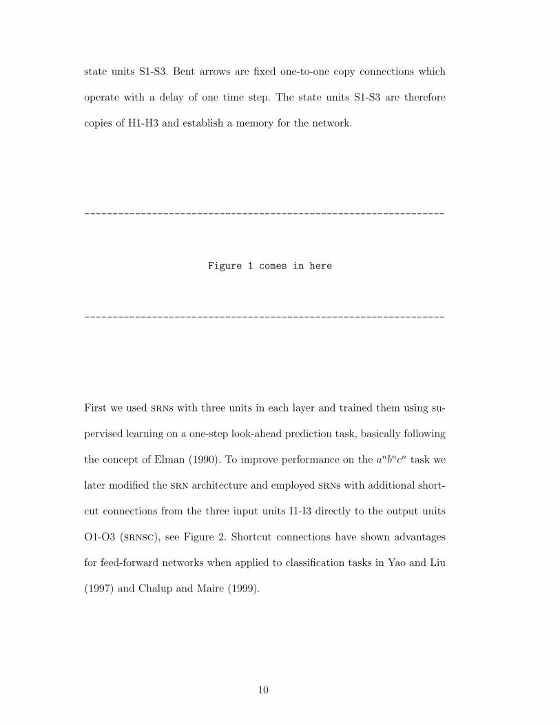
state units S1-S3. Bent arrows are fixed one-to-one copy connections which

operate with a delay of one time step. The state units S1-S3 are therefore

copies of H1-H3 and establish a memory for the network.

----------------------------------------------------------------

Figure 1 comes in here

----------------------------------------------------------------

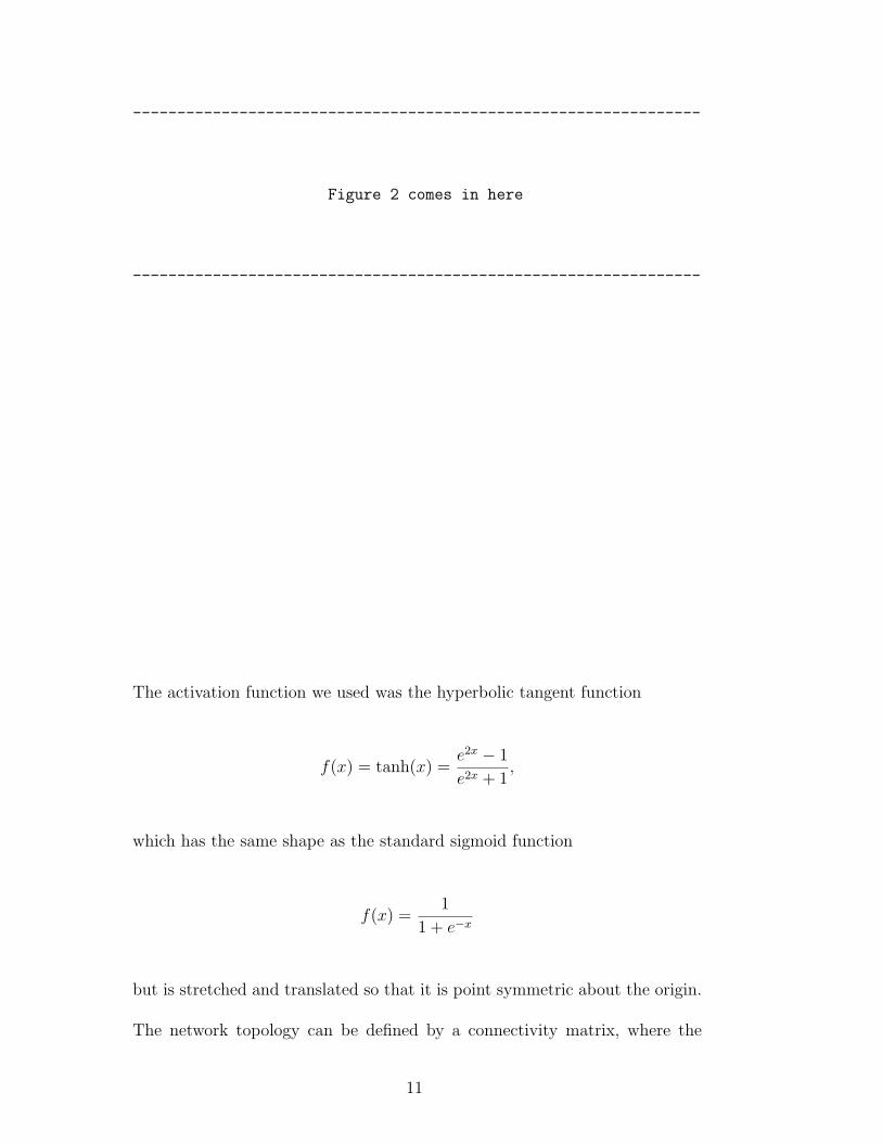
First we used srns with three units in each layer and trained them using su-

pervised learning on a one-step look-ahead prediction task, basically following

the concept of Elman (1990). To improve performance on the anbncn task we

later modified the srn architecture and employed srns with additional short-

cut connections from the three input units I1-I3 directly to the output units

O1-O3 (srnsc), see Figure 2. Shortcut connections have shown advantages

for feed-forward networks when applied to classification tasks in Yao and Liu

(1997) and Chalup and Maire (1999).

10

----------------------------------------------------------------

Figure 2 comes in here

----------------------------------------------------------------

The activation function we used was the hyperbolic tangent function

f(x) = tanh(x) =e2x − 1

e2x + 1,

which has the same shape as the standard sigmoid function

f(x) =1

1 + e−x

but is stretched and translated so that it is point symmetric about the origin.

The network topology can be defined by a connectivity matrix, where the

11

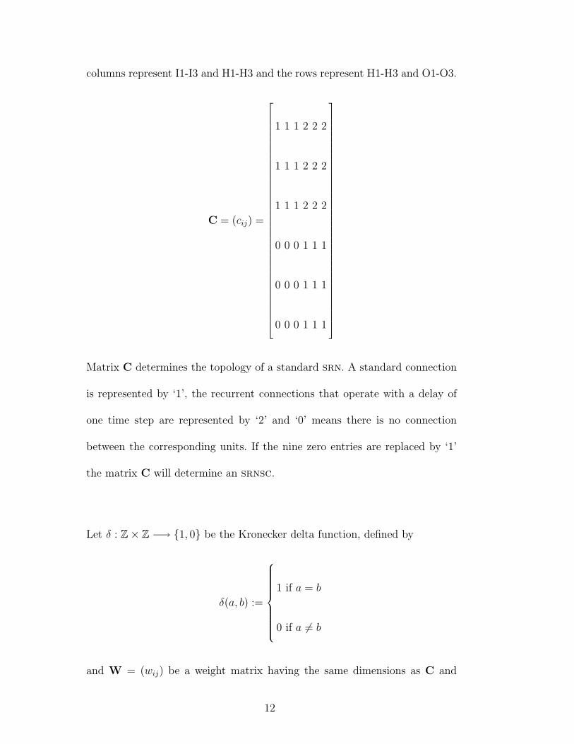
columns represent I1-I3 and H1-H3 and the rows represent H1-H3 and O1-O3.

C = (cij) =

1 1 1 2 2 2

1 1 1 2 2 2

1 1 1 2 2 2

0 0 0 1 1 1

0 0 0 1 1 1

0 0 0 1 1 1

Matrix C determines the topology of a standard srn. A standard connection

is represented by ‘1’, the recurrent connections that operate with a delay of

one time step are represented by ‘2’ and ‘0’ means there is no connection

between the corresponding units. If the nine zero entries are replaced by ‘1’

the matrix C will determine an srnsc.

Let δ : Z× Z −→ {1, 0} be the Kronecker delta function, defined by

δ(a, b) :=

1 if a = b

0 if a 6= b

and W = (wij) be a weight matrix having the same dimensions as C and

12

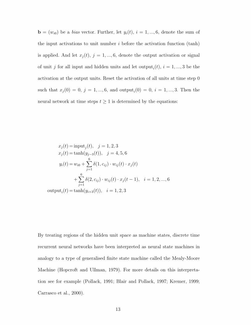
b = (wi0) be a bias vector. Further, let yi(t), i = 1, ..., 6, denote the sum of

the input activations to unit number i before the activation function (tanh)

is applied. And let xj(t), j = 1, ..., 6, denote the output activation or signal

of unit j for all input and hidden units and let outputi(t), i = 1, ..., 3 be the

activation at the output units. Reset the activation of all units at time step 0

such that xj(0) = 0, j = 1, ..., 6, and outputi(0) = 0, i = 1, ..., 3. Then the

neural network at time steps t ≥ 1 is determined by the equations:

xj(t) = inputj(t), j = 1, 2, 3

xj(t) = tanh(yj−3(t)), j = 4, 5, 6

yi(t) = wi0 +6∑

j=1

δ(1, cij) · wij(t) · xj(t)

+6∑

j=1

δ(2, cij) · wij(t) · xj(t− 1), i = 1, 2, ..., 6

outputi(t) = tanh(yi+3(t)), i = 1, 2, 3

By treating regions of the hidden unit space as machine states, discrete time

recurrent neural networks have been interpreted as neural state machines in

analogy to a type of generalised finite state machine called the Mealy-Moore

Machine (Hopcroft and Ullman, 1979). For more details on this interpreta-

tion see for example (Pollack, 1991; Blair and Pollack, 1997; Kremer, 1999;

Carrasco et al., 2000).

13

3 Prediction Task

One aspect of language processing is predicting a symbol sequence which is

formed according to syntactic rules determined by a grammar. A recurrent

neural network can transform an input sequence to an output sequence using

a stepwise prediction based on the input information. In the one-step look-

ahead prediction task (Elman, 1990, 1991) symbols of the input sequence are

presented to the network one by one and the network output is taken as a

prediction of the next symbol. For fully predictable sequences the input and

output sequences are supposed to be the same once the network has learned

the prediction task correctly. Hence a perfectly trained network could theoret-

ically predict the whole sequence if the output is fed back to the input units.

However, in some situations not all symbols of the sequence are uniquely de-

termined; for example in the case of the anbncn prediction task, with unknown

depth n at the beginning of a string, it is impossible to predict when the first

b will occur.

With the aim of investigating learnability of the one-step look-ahead predic-

tion task for non-regular languages we performed experiments using training

sequences formed by strings of one of the following types, where always n ≥ 1:

qn = anbn

rn = anb2n

sn = anbncn

14

Here anbn and anb2n are strings from context-free languages while anbncn is

a string from a (mildly) context-sensitive language. In all cases the neural

network is presented with a sequence of these strings for varying values of n.

Since our interest is focused on the language of multiple agreements MA =

{sn; n ≥ 1} we will from now on use strings sn = anbncn from this language as

examples in our explanations, which can be adjusted to the other languages

straightforwardly.

The training sequence is made of strings of different depths and the symbols

of each string are represented by vectors

a = (+1,−1,−1),

b = (−1,+1,−1),

c = (−1,−1,+1).

The symbols of the input sequence are fed one at a time into the three dimen-

sional input layer (I1-I3) of the neural network (Figure 1 or 2). Each output

unit (O1-O3) is assigned to one of the three symbols a, b, or c and, in our set-

ting of the task, the unit with the highest activation determines the predicted

symbol 3 .

Since the depth n is not known to the network at the start of a string it cannot

predict when the first b will occur and logically it cannot know how many a’s

3 Some authors have applied a more rigid interpretation, insisting that the outputfor the predicted symbol must be above a fixed threshold and that the outputs forall other symbols must be below that threshold (e. g. Rodriguez et al., 1999; Bodenand Wiles, 2000; Gers and Schmidhuber, 2001).

15

will follow the first a. The anbncn task is therefore not about predicting the

complete string but only a part of it. We chose to interpret the anbncn task

as an an ∗1 bn−1cn task 4 . Here, once the network has processed the first b,

it is required to predict n − 1 additional b’s, followed by n c’s, followed by

an indeterminate (but nonzero) number of a’s (which form the beginning of

the subsequent string). That is, the network has to learn that the first a is

followed by a’s and not by other symbols until the first b occurs. For example,

in the sequence of three strings

s3s2s4 = aaabbbccc|aabbcc|aaaabbbbcccc

all 27 symbols except the three bold b’s have to be correctly predicted.

4 Training Method

In the present study srns and srnscs were trained using a random search

algorithm which we call evolutionary hill climbing, following the terminology

of Pollack and Blair (1998). The algorithm was applied together with a special

way of presenting the data, called data juggling, which is a refined version of

the method employed already in (Chalup and Blair, 1999) and will be de-

4 A different interpretation, which could be called the a1 ∗n bn−1cn task, has beenemployed, for example, by Boden and Wiles (2000). This interpretation requiresthe network to do the same prediction as in the an ∗1 bn−1cn task with the onlydifference that it has free choice for all n symbols following the first a of each string.The network is only required to predict those symbols which are determined as alogical consequence of the properties of the anbncn language. With this easier taskonly 18 instead of 24 symbols in the example sequence are required to be correctlypredicted: s3s2s4 = aaabbbccc|aabbcc|aaaabbbbcccc.

16

scribed in more detail in Section 4.3. First we focus on the standard version

of evolutionary hill climbing, which is displayed in Table 2 in an abstract

form independent of data or network. It is essentially the (1+1)–ES algorithm

of Rechenberg (1965) and Schwefel (1965) and can be interpreted as a sim-

ple evolutionary algorithm which employs only mutation and selection for a

population containing just two networks (although it was later generalised to

larger populations and modified in several directions—see Rechenberg (1994);

Schwefel (1995); Rudolph (1997); Beyer (2001)).

----------------------------------------------------------------

Table 2 comes in here

----------------------------------------------------------------

Following the terminology of Pollack and Blair (1998) we call the current neu-

ral network with its corresponding weight matrix Wchamp =(wij) the champion.

In the experiments for the present project the initial weights for the champion

were all generated from an N(0, 0.05) normal distribution. Given the cham-

pion Wchamp, the hill climber endeavors to find a “fitter” weight matrix by

17

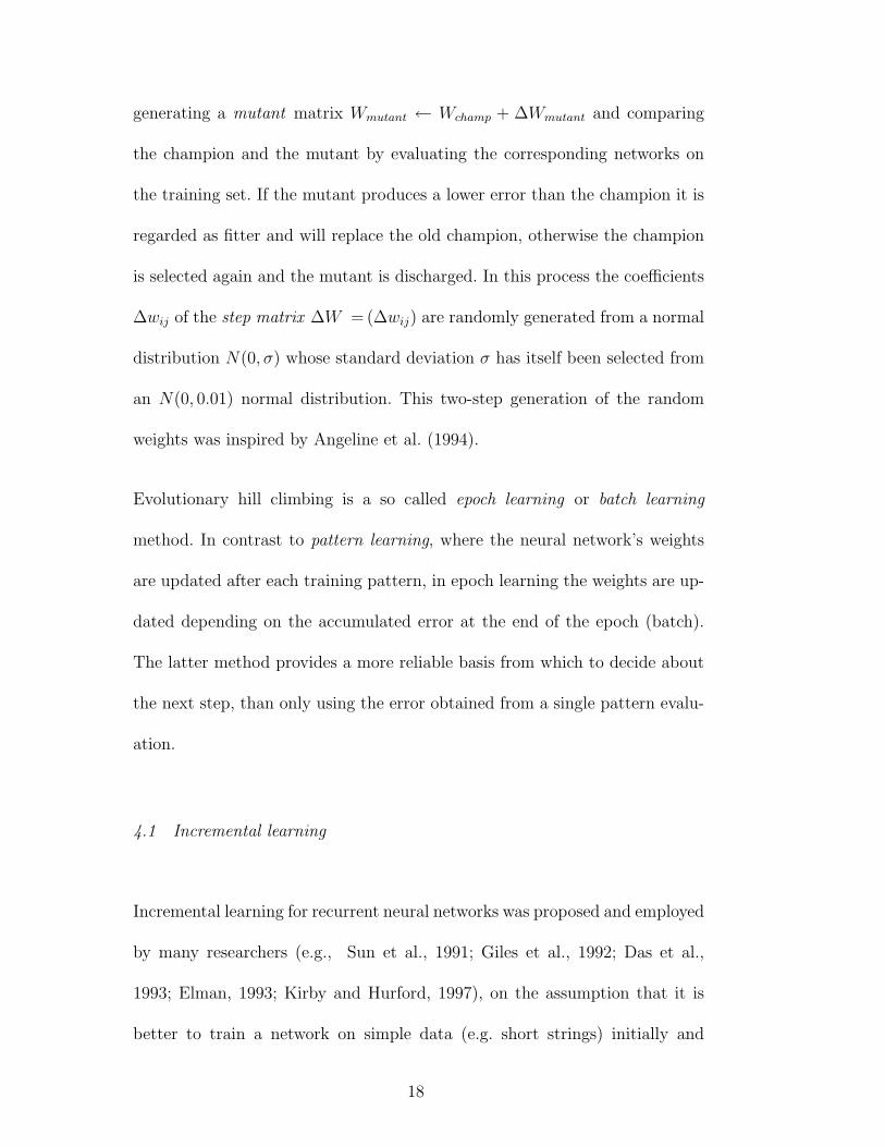
generating a mutant matrix Wmutant ← Wchamp + ∆Wmutant and comparing

the champion and the mutant by evaluating the corresponding networks on

the training set. If the mutant produces a lower error than the champion it is

regarded as fitter and will replace the old champion, otherwise the champion

is selected again and the mutant is discharged. In this process the coefficients

∆wij of the step matrix ∆W = (∆wij) are randomly generated from a normal

distribution N(0, σ) whose standard deviation σ has itself been selected from

an N(0, 0.01) normal distribution. This two-step generation of the random

weights was inspired by Angeline et al. (1994).

Evolutionary hill climbing is a so called epoch learning or batch learning

method. In contrast to pattern learning, where the neural network’s weights

are updated after each training pattern, in epoch learning the weights are up-

dated depending on the accumulated error at the end of the epoch (batch).

The latter method provides a more reliable basis from which to decide about

the next step, than only using the error obtained from a single pattern evalu-

ation.

4.1 Incremental learning

Incremental learning for recurrent neural networks was proposed and employed

by many researchers (e.g., Sun et al., 1991; Giles et al., 1992; Das et al.,

1993; Elman, 1993; Kirby and Hurford, 1997), on the assumption that it is

better to train a network on simple data (e.g. short strings) initially and

18

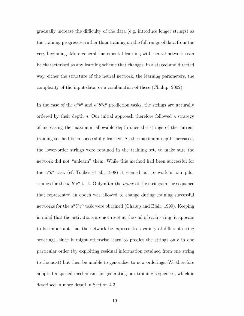
gradually increase the difficulty of the data (e.g. introduce longer strings) as

the training progresses, rather than training on the full range of data from the

very beginning. More general, incremental learning with neural networks can

be characterised as any learning scheme that changes, in a staged and directed

way, either the structure of the neural network, the learning parameters, the

complexity of the input data, or a combination of these (Chalup, 2002).

In the case of the anbn and anbncn prediction tasks, the strings are naturally

ordered by their depth n. Our initial approach therefore followed a strategy

of increasing the maximum allowable depth once the strings of the current

training set had been successfully learned. As the maximum depth increased,

the lower-order strings were retained in the training set, to make sure the

network did not “unlearn” them. While this method had been successful for

the anbn task (cf. Tonkes et al., 1998) it seemed not to work in our pilot

studies for the anbncn task. Only after the order of the strings in the sequence

that represented an epoch was allowed to change during training successful

networks for the anbncn task were obtained (Chalup and Blair, 1999). Keeping

in mind that the activations are not reset at the end of each string, it appears

to be important that the network be exposed to a variety of different string

orderings, since it might otherwise learn to predict the strings only in one

particular order (by exploiting residual information retained from one string

to the next) but then be unable to generalize to new orderings. We therefore

adopted a special mechanism for generating our training sequences, which is

described in more detail in Section 4.3.

19

A training sequence of depth k, with 3 ≤ k ≤ 20, is a concatenation of 30

strings of type sn, n ≤ k, such that the string of maximum depth sk appears

exactly once and the other 29 strings have randomly selected depths from

{1, ..., k − 1} with a distribution biased (linearly) towards the lower numbers

and with each of these depths guaranteed to occur at least once.

When we come to test the generalisation abilities of our networks (in Sec-

tion 5.3) we will therefore be looking for two different kinds of generalisation:

(1) Generalisation to sequences with different orderings of the strings sn.

(2) Generalisation to sequences which contain strings for larger values of n

than contained in the training set.

The following paragraphs introduce an incremental learning scheme for epoch

learning which instead of using a fixed data set modifies it during the evolu-

tionary training process. The pseudo code for this method is listed in Table 3.

4.2 Fitness Calculation and Selection Rule

Broadly speaking, there are two ways of measuring the success of a neural net-

work performing a symbol processing task—its accuracy (i.e. number of sym-

bols correctly predicted) and its error (a measure of the extent to which the

network outputs differ from their target values). Although the accuracy is what

ultimately ought to be maximized, many training algorithms instead make use

of the error measure because it has the advantage of being continuous and

20

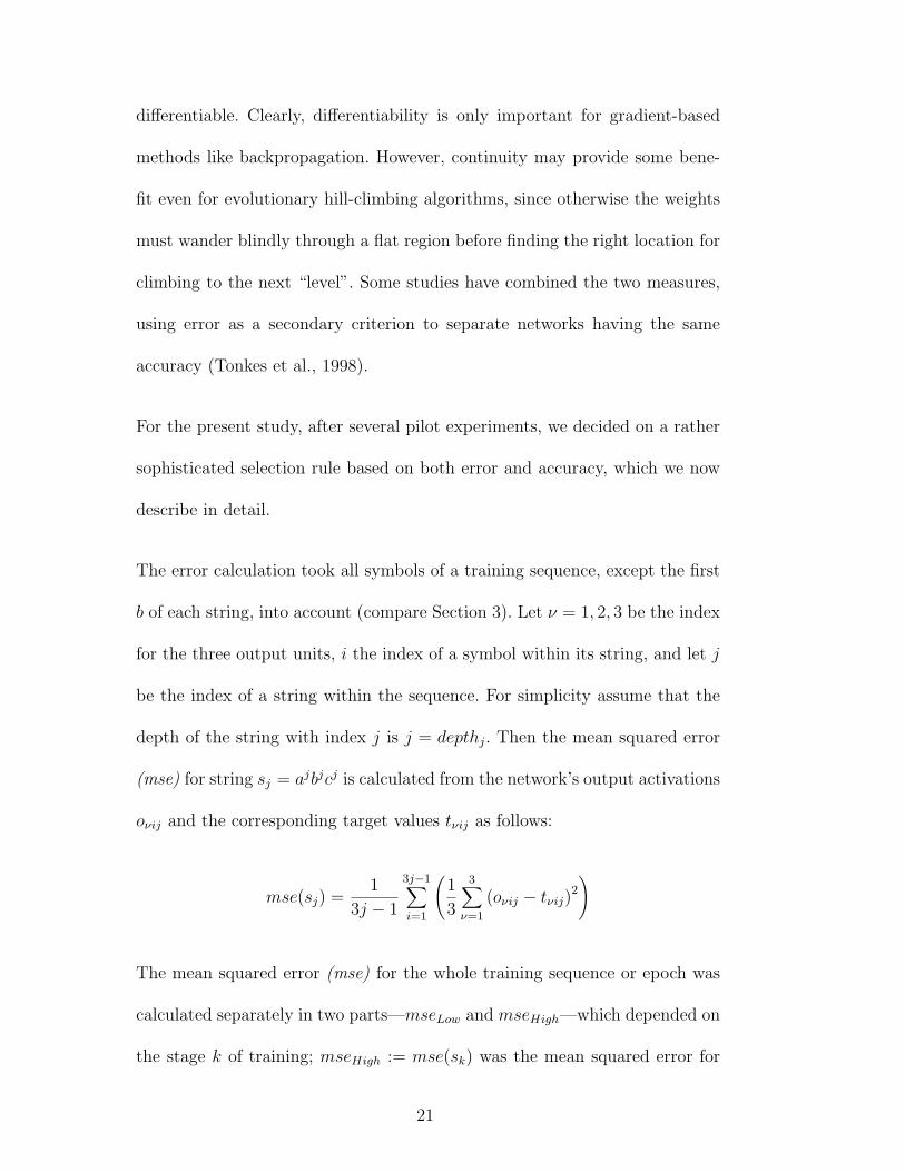
differentiable. Clearly, differentiability is only important for gradient-based

methods like backpropagation. However, continuity may provide some bene-

fit even for evolutionary hill-climbing algorithms, since otherwise the weights

must wander blindly through a flat region before finding the right location for

climbing to the next “level”. Some studies have combined the two measures,

using error as a secondary criterion to separate networks having the same

accuracy (Tonkes et al., 1998).

For the present study, after several pilot experiments, we decided on a rather

sophisticated selection rule based on both error and accuracy, which we now

describe in detail.

The error calculation took all symbols of a training sequence, except the first

b of each string, into account (compare Section 3). Let ν = 1, 2, 3 be the index

for the three output units, i the index of a symbol within its string, and let j

be the index of a string within the sequence. For simplicity assume that the

depth of the string with index j is j = depthj. Then the mean squared error

(mse) for string sj = ajbjcj is calculated from the network’s output activations

oνij and the corresponding target values tνij as follows:

mse(sj) =1

3j − 1

3j−1∑

i=1

(1

3

3∑

ν=1

(oνij − tνij)2

)

The mean squared error (mse) for the whole training sequence or epoch was

calculated separately in two parts—mseLow and mseHigh—which depended on

the stage k of training; mseHigh := mse(sk) was the mean squared error for

21

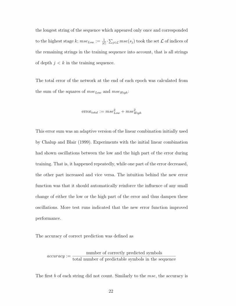
the longest string of the sequence which appeared only once and corresponded

to the highest stage k; mseLow := 1|L| ·

∑j∈L mse(sj) took the set L of indices of

the remaining strings in the training sequence into account, that is all strings

of depth j < k in the training sequence.

The total error of the network at the end of each epoch was calculated from

the sum of the squares of mseLow and mseHigh:

errortotal := mse2Low + mse2

High

This error sum was an adaptive version of the linear combination initially used

by Chalup and Blair (1999). Experiments with the initial linear combination

had shown oscillations between the low and the high part of the error during

training. That is, it happened repeatedly, while one part of the error decreased,

the other part increased and vice versa. The intuition behind the new error

function was that it should automatically reinforce the influence of any small

change of either the low or the high part of the error and thus dampen these

oscillations. More test runs indicated that the new error function improved

performance.

The accuracy of correct prediction was defined as

accuracy :=number of correctly predicted symbols

total number of predictable symbols in the sequence

The first b of each string did not count. Similarly to the mse, the accuracy is

22

separately calculated for the low and the high part of the training sequence.

Selection is based on fitness and follows the rule:

A new mutant is regarded as fitter than the champion if one of the following

two conditions is fulfilled :

(1) The mutant achieves 100% accuracy on the low part of the sequence and

its mean squared error on the high part of the sequence (mseHigh) is less

than that of the champion, or

(2) The champion achieves less that 100% accuracy on the low part of the

sequence, and the mutant’s total error is lower than that of the champion.

These conditions were chosen based on two observations from pilot experi-

ments. A selection rule based purely on accuracy seemed frequently to result

in training “without direction”, that is, it was not able to contribute to any

improvement with respect to error or accuracy. Similarly a selection rule based

on error minimisation alone showed only very slow improvements and seemed

to be too restrictive to go around minor local minima. Therefore we combined

both strategies. Condition (1) guided training by minimising the mseHigh while

it did not care about the mseLow as long as the accuracy on the low part was

100%. That is, there was some freedom for the error to increase on the low part

as long as the accuracy was not affected. Condition (2) took care of all cases

where the accuracy on the low part was not 100%. This could appear, for ex-

ample, after the juggling algorithm switched to a different permutation of the

training sequence (more details in Section 4.3). In this situation the network

23

would first have 100% accuracy on the low part and then after the switch the

accuracy could drop drastically. However, in these cases the network would

only require fine-tuning to regain the full accuracy. We had the impression

that, for training in this situation, accuracy alone was too unstable to be an

appropriate fitness measure. Therefore the above function for errortotal was

used. We note it could happen that, before the accuracy on the low part is

recovered, the mutant gets selected while it is less accurate but has a lower

errortotal than the champion.

----------------------------------------------------------------

Table 3 comes in here

----------------------------------------------------------------

4.3 Data Juggling

The idea of evolutionary hill climbing with data juggling is to use the function

“juggle” to permute the order of the symbol strings in the training sequence

24

and to continue training on the modified training set 5 . In contrast to Tonkes

et al. (1998) who employed training sequences with fixed (increasing) order of

strings (a1b1a2b2...anbn), data juggling approximates a random order presen-

tation of strings for epoch learning with weight update and reset at the end of

each epoch. The pseudo code of evolutionary hill climbing with data juggling

is listed in Table 3 which is an extension of Table 2 but does not repeat every

detail. The incremental learning scheme is controlled by the depth or stage

parameter k which starts from k = 3 and maximally reaches depthmax = 20.

Before the central FOR-loop is entered the current champion is evaluated on

a series of training sequences of increasing depth and with different orderings

of strings. Encapsulated in this evaluation are calls to the function “juggle”.

One outcome of the evaluation is the number depthchamp which is the largest

depth the champion was able to process with 100% accuracy. Then the FOR-

loop of evolutionary hill climbing is entered with the next training sequence

the champion was not able to process. After the FOR-loop the function “jug-

gle” can be called depending on some conditions—for example, as soon as

the champion has reached a new stage (i.e. depthchamp increased), or after a

fixed number (maxEpochs) of iterations (i.e. when the algorithm “got stuck”).

While epoch learning methods like evolutionary hill climbing typically use a

5 Some people have suggested to use an end-of-string marker so that the networkcan reset itself between strings and always start from the same state. This wouldalleviate the need for data juggling because the order of the strings would thenbe irrelevant. Gers and Schmidhuber (2001) employed an end-of-string marker butdid not reset activations at the end of the strings. Boden and Wiles (2000, 2001)did not use the end-of-string marker and updated the weights at the end of eachstring without resetting at all. All these studies including Rodriguez et al. (1999)and Rodriguez (2001) presented the strings in random order to the network.

25

fixed training set, data juggling can be regarded as a step towards pattern or

on-line learning. Three parameters control the juggling process. They follow

some heuristics which we decided in pilot experiments:

• Juggle factor : determines how many strings change positions in the sequence

during one permutation of strings. After a series of tests with different juggle

factors we decided to use juggle factor 4 as standard for our experiments.

This parameter is encapsulated in the juggle function in Table 3.

• Maximum of Juggles : determines on how many permutations of the 30-

string long training sequence the network is trained before a new stage is

approached. For each stage k the maximum of juggles was increased using

the formula min(1000, k3). This parameter is part of the juggling conditions

in Table 3.

• maxEpochs : determines the maximum number of epochs which should be

spent on one training sequence. This parameter was linearly increased for

each stage k following the function maxEpochs = 2500 · (k − 2).

The evolutionary training process which is implemented in the data juggling

algorithm starts from a randomly generated set of weights which was chosen

from an N(0, 0.05) normal distribution. The network then evolves, following

the combination of incremental learning with evolutionary hill climbing and

permutation of the training sequence. The epochs are counted from the be-

ginning and each time a network evolves which is able to process a newly

generated training sequence with 100% accuracy its weights and the asso-

26

ciated epoch are written into a special file which we call the epochfile. Each

training process results not only in a single network but in a series of networks

at different epochs with typically several of them for each stage.

5 Experimental Results and Evaluation

Training and evaluation of the networks in our experiments is focused on

stage 8. An evolutionary training process is deemed to be “successful” and

the latest trained network is called a solution (for stage 8) as soon as it is able

to process at least one sequence of strings correctly at stage 8. Networks which

begin their training at stage 3 are referred to as being trained with incremental

learning. Networks which begin training directly at stage 8 will be considered

to be trained without incremental learning because they do not experience

the incremental learning between stages 3 and 8 even if their training above

stage 8 up to the maximal stage 20 would be incremental. These experiments

at the same time address the question of whether incremental learning is more

efficient. The experimental investigation employed three types of evaluation

methods:

(1) Evaluation of the efficiency of training up to stage 8, see Section 5.1.

(2) Characterisation of the evolution of hidden unit dynamics, see Section 5.2.

(3) Refined evaluation of generalisation ability, see Section 5.3.

5.1 Efficiency of Training

27

Table 4 provides in seven columns an overview of the results of all our training

experiments. Each experiment or “run” is a training process using evolution-

ary hill climbing with data juggling which starts from a randomly initialised

network. The first row of the table specifies the task, the second row tells the

network architecture and the third row states whether incremental learning

was used or not. The fourth row of the table is the total number of runs and

the fifth and sixth rows indicate how many of these runs produced a solution

within one million and two million epochs, respectively. Rows 7 to 11 give

the minimum, maximum, median, mean and standard deviation of the epoch

numbers of the set of solutions for each class of experiments.

----------------------------------------------------------------

Table 4 comes in here

----------------------------------------------------------------

28

5.1.1 Incremental versus Non-Incremental Learning

To investigate the influence of the incremental training scheme, networks with

different random initial weights from an N(0, 0.5) Gaussian distribution were

generated; each of them was trained first with incremental learning, starting

from stage 3, and then again using the same initial weights without incremental

learning, directly for stage 8.

Thirty srnscs with two hidden units were trained with different random initial

weights on the anbn prediction task for a maximum of one million epochs.

The number of solutions found was the same with and without incremental

learning (24 out of 30). However, using a standard t-test we can infer from the

results displayed in Table 4 that training with incremental learning achieves a

solution significantly faster than training without incremental learning, with

a confidence level of 99% (p-value < 10−5).

Forty srnscs with three hidden units were trained with different random

initial weights on the anbncn prediction task for a maximum of two million

epochs, both with and without incremental learning. In column 4 and 5 of

Table 4 we can see that the number of successful networks is considerably

higher for incremental learning (23 out of 40) than for non-incremental learning

(10 out of 40). Training times were considerably longer than for the anbn task.

They seem to be slightly shorter for incremental learning compared to non-

incremental learning, although we can make this claim only with a statistical

significance of 90% (p-value = 0.0914).

29

For comparison we performed experiments using standard srns without short-

cut connections, of the kind used in previous work (Chalup and Blair, 1999)

where it was found that srns could learn the task and generalise to different

orderings of the strings in the data sequence. Some of them were also able

to generalise to sequences which contained strings of one or two stages larger

depth than the training sequence (cf. Section 5.3). Our experiments indicate

that the rate of training success is higher with srnscs than with srns (see

row 6 and columns 4–7 of Table 4).

5.1.2 Context-Free versus Context-Sensitive Language Learning

The question arises as to whether the improved performance for the anbn task

relative to the anbncn task can be explained by the smaller size of the network

and training data. To investigate this question, we trained 30 networks on

the context-free anb2n language using the same network which was used for

the anbncn experiments (i.e. the (3-3-3-3)–srnsc in Figure 2). The results in

column 3 and 4 of Table 4 show that even if network and data size are the

same, the context-free language anb2n can be learned faster and more reliably

than the context-sensitive language anbncn.

5.2 Dynamics of Hidden Unit Activation

Methods from dynamical systems theory can be used to evaluate the qual-

itative behaviour of recurrent neural networks after training (Hirsch, 1984,

30

1989, 1991; Kolen, 1994). For example, while processing an input sequence,

the activation of each network unit moves along a trajectory in the correspond-

ing activation space. Generally, a wide range of dynamical behaviour such as

periodic, quasi-periodic, steady-state and chaotic behaviour is possible (com-

pare e.g. Tino et al., 2001). The way the task is accomplished in the present

case can be understood in comparison with previously known solutions for the

anbn prediction task (Wiles and Elman, 1995) and the anbncn prediction task

(Chalup and Blair, 1999) which involved attracting fixed points (attractors)

and repelling fixed points (repellers). The network of Wiles and Elman (1995)

achieved the anbn task by effectively “counting up” the number of a’s as its

trajectory contracted towards an attractor, and then “counting down” the

same number of b’s as it diverged from a repeller. A trajectory is said to be

monotonic if its projections to the coordinate axes develop monotonically in

time, otherwise it is called oscillating (Rodriguez et al., 1999). A saddle point

is a fixed point which is attracting in one direction and repelling in another

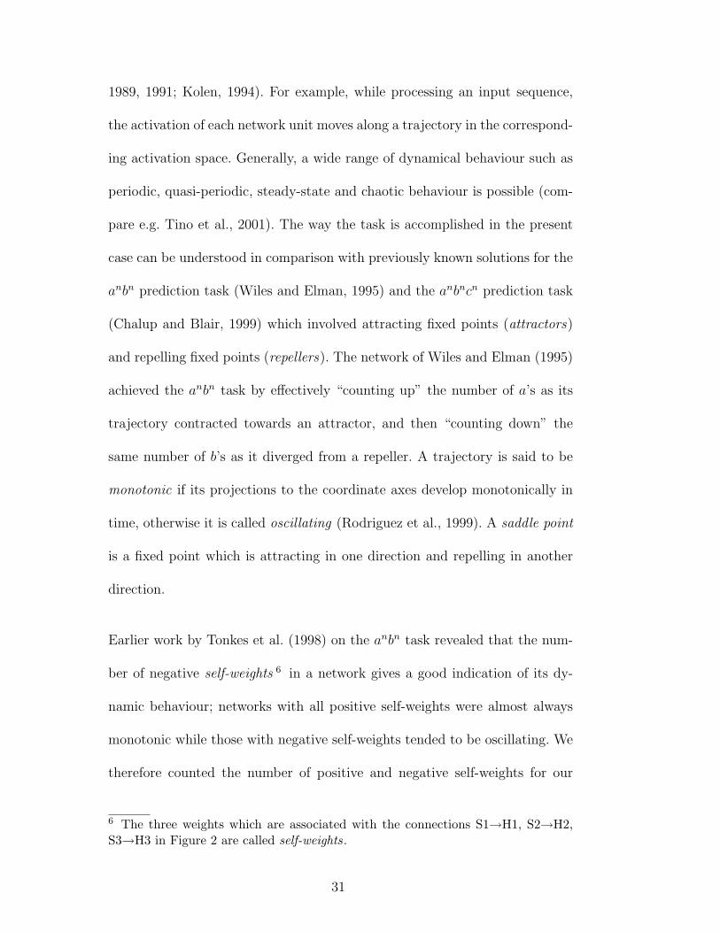
direction.

Earlier work by Tonkes et al. (1998) on the anbn task revealed that the num-

ber of negative self-weights 6 in a network gives a good indication of its dy-

namic behaviour; networks with all positive self-weights were almost always

monotonic while those with negative self-weights tended to be oscillating. We

therefore counted the number of positive and negative self-weights for our

6 The three weights which are associated with the connections S1→H1, S2→H2,S3→H3 in Figure 2 are called self-weights.

31

srnsc networks trained on the anbncn task. As can be seen from Table 5, 17

of the 23 successful networks found by incremental learning had no negative

self-weights, while 9 of the 10 networks found by non-incremental learning

had at least one negative self-weight, suggesting that incremental learning is

more likely to find monotonic solutions while non-incremental learning is more

likely to find oscillating solutions.

----------------------------------------------------------------

Table 5 comes in here

----------------------------------------------------------------

Only one network was found to have three negative self-weights (see Table 5).

Although this network is exceptional in the present context, it is a convenient

place to begin our discussion of dynamics because its behaviour is most similar

to that of networks reported in other articles (e.g. Chalup and Blair, 1999;

Rodriguez et al., 1999; Boden and Wiles, 2000). The state trajectory for a8b8c8

has 24 states (see Figure 3), each of them corresponding to an input symbol

(‘a1–a8’, ‘b1–b8’, ‘c1–c8’) and a predicted symbol (a = ‘•’, b = ‘×’, c = ‘◦’ and

32

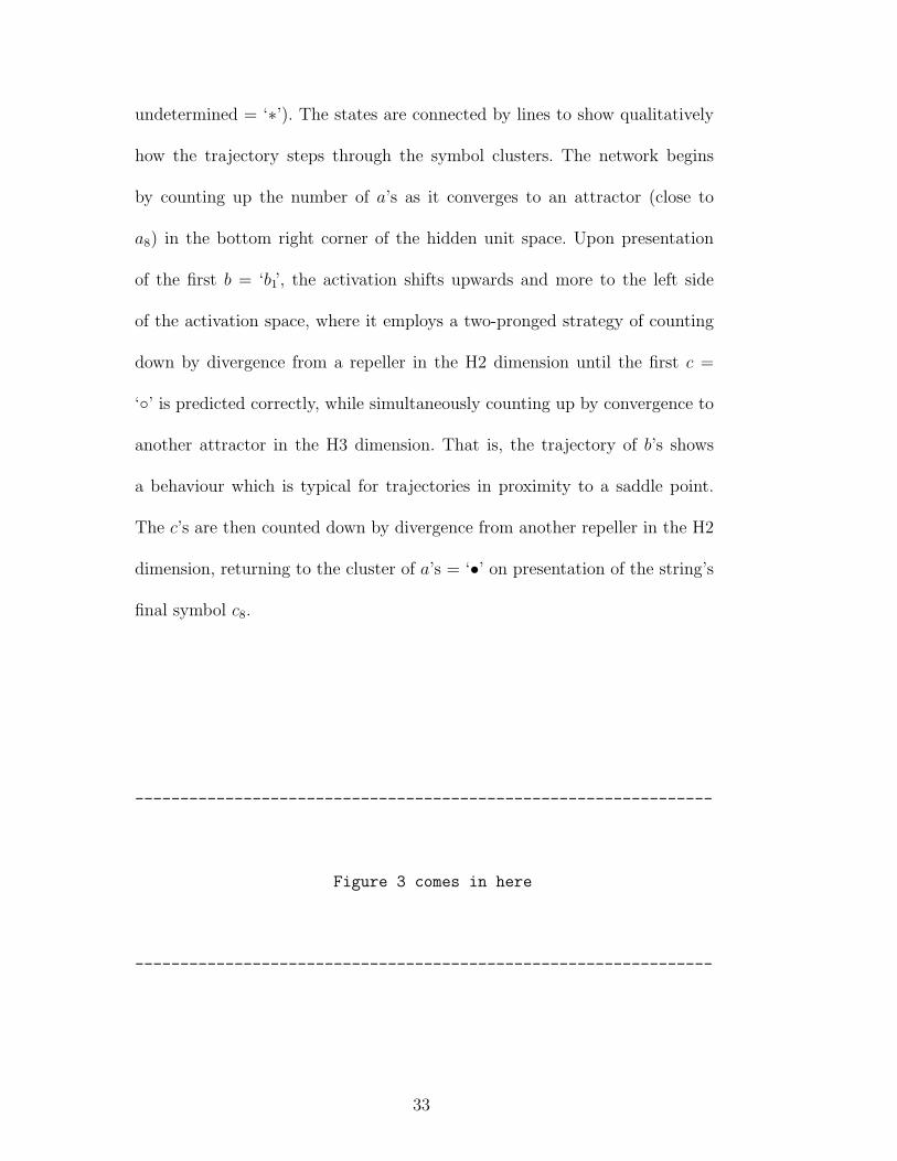
undetermined = ‘∗’). The states are connected by lines to show qualitatively

how the trajectory steps through the symbol clusters. The network begins

by counting up the number of a’s as it converges to an attractor (close to

a8) in the bottom right corner of the hidden unit space. Upon presentation

of the first b = ‘b1’, the activation shifts upwards and more to the left side

of the activation space, where it employs a two-pronged strategy of counting

down by divergence from a repeller in the H2 dimension until the first c =

‘◦’ is predicted correctly, while simultaneously counting up by convergence to

another attractor in the H3 dimension. That is, the trajectory of b’s shows

a behaviour which is typical for trajectories in proximity to a saddle point.

The c’s are then counted down by divergence from another repeller in the H2

dimension, returning to the cluster of a’s = ‘•’ on presentation of the string’s

final symbol c8.

----------------------------------------------------------------

Figure 3 comes in here

----------------------------------------------------------------

33

In order to globally analyse the hidden unit activation dynamics of the whole

evolutionary process we produced several movies which show how the dy-

namics evolve during training. We recorded the weights of every network that

reached a new stage or was able to process a new ordering of the data sequence

with 100% accuracy. All these weights together with the epoch at which they

emerged were stored in an epochfile. For the movies each weight-set stored

in the epochfile was evaluated on the string anbncn, where n was the highest

stage the network was trained on. The activation of the hidden units (H1-H3)

while processing anbncn was then plotted in a 3-dimensional graph. In this way

we obtained for each evolutionary process (corresponding to one initial condi-

tion) a sequence of graphs displaying the hidden unit activation dynamics of

all successful networks at all stages.

An examination of the movies generated by all the successful runs reveals that

the difference in signature of the self-weights between incremental and non-

incrementally trained networks reflects a qualitative difference in the pattern of

hidden unit activation dynamics, as illustrated in Figures 4 and 5. The network

in Figure 4 was trained incrementally while that in Figure 5 was trained

non-incrementally, starting from the same initial condition. The 3-dimensional

graphs and their 2-dimensional projections onto the three coordinate planes

show the activation of the srnscs’ hidden units H1–H3 while processing the

string a8b8c8.

34

----------------------------------------------------------------

Figure 4 comes in here

----------------------------------------------------------------

----------------------------------------------------------------

Figure 5 comes in here

----------------------------------------------------------------

The network in Figure 4 was trained incrementally. It has three positive and

no negative self-weights, and its trajectory moves through a sequence of three

repellers. It begins at ‘a1’ by counting up the number of a’s as it monotonically

diverges from a repeller at the beginning of the trajectory in 3D hidden unit

space (Figure 4(a)). Upon presentation of the first b = b1, the activation shifts

35

to the right side of the space, where it again moves monotonically away from a

repeller close to ‘b1’. The third repeller is close to ‘c1’ from where the trajectory

moves monotonically back to the left until it reaches, almost having completed

a circle, the area where it initially started with ‘a1’. Compared to previously

reported solution networks, this one is unusual in that it relies on nonlinear

dynamics to make the activations “turn a corner” as the b’s are processed.

The network in Figure 5 was trained non-incrementally starting from the same

initial weights as the network in Figure 4. It has two positive and one negative

self-weight, and employs a combination of oscillating and monotonic trajec-

tories. The displayed trajectory for the string a8b8c8 starts to count up the

a’s by oscillating towards an attractor in the bottom right corner of Figure 5

(b). It then counts down by divergence from an oscillating repeller in the H3

dimension, and at the same time counts up the b’s through a monotonic tra-

jectory in the H2 dimension (compare Figure 5(c)). The former ensures that

the first c = ‘◦’ is predicted correctly, while the latter prepares for the c’s

to be counted down by divergence from a new monotonic repeller in the H1

dimension (Figure 5(c)), ready to predict the first a = ‘•’ at the beginning of

the next string.

In contrast to the unstable picture of generalisation ability which we will dis-

cuss in Section 5.3, the characteristics of the hidden unit activity dynamics

during the course of evolution were generally stable. When evaluating the tra-

jectories and state clusters of 40 movies encompassing over 2000 networks,

36

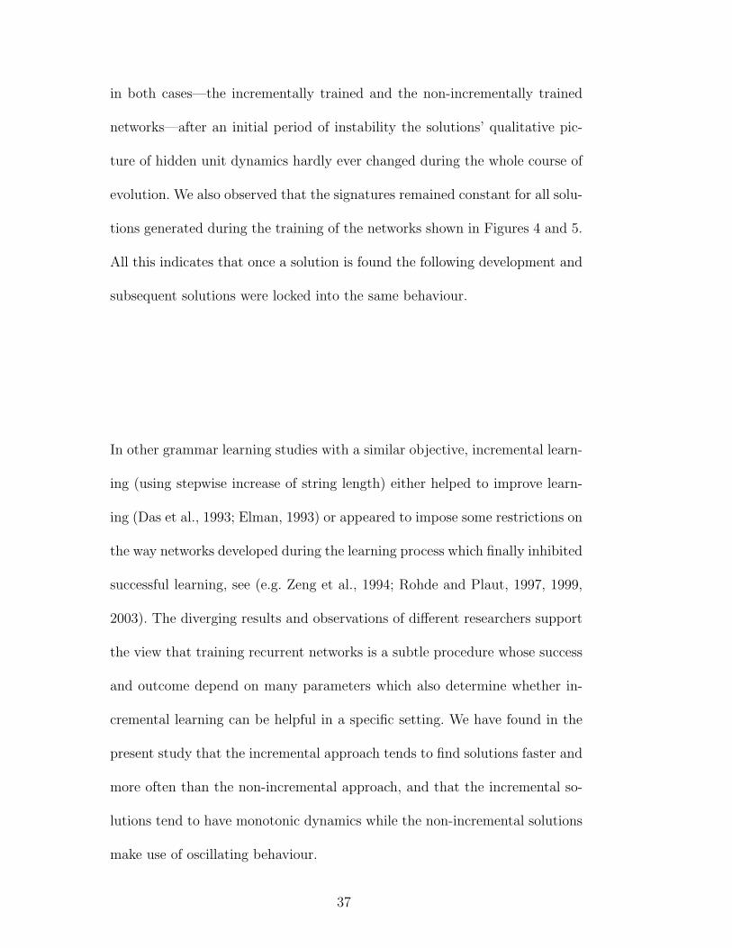
in both cases—the incrementally trained and the non-incrementally trained

networks—after an initial period of instability the solutions’ qualitative pic-

ture of hidden unit dynamics hardly ever changed during the whole course of

evolution. We also observed that the signatures remained constant for all solu-

tions generated during the training of the networks shown in Figures 4 and 5.

All this indicates that once a solution is found the following development and

subsequent solutions were locked into the same behaviour.

In other grammar learning studies with a similar objective, incremental learn-

ing (using stepwise increase of string length) either helped to improve learn-

ing (Das et al., 1993; Elman, 1993) or appeared to impose some restrictions on

the way networks developed during the learning process which finally inhibited

successful learning, see (e.g. Zeng et al., 1994; Rohde and Plaut, 1997, 1999,

2003). The diverging results and observations of different researchers support

the view that training recurrent networks is a subtle procedure whose success

and outcome depend on many parameters which also determine whether in-

cremental learning can be helpful in a specific setting. We have found in the

present study that the incremental approach tends to find solutions faster and

more often than the non-incremental approach, and that the incremental so-

lutions tend to have monotonic dynamics while the non-incremental solutions

make use of oscillating behaviour.

37

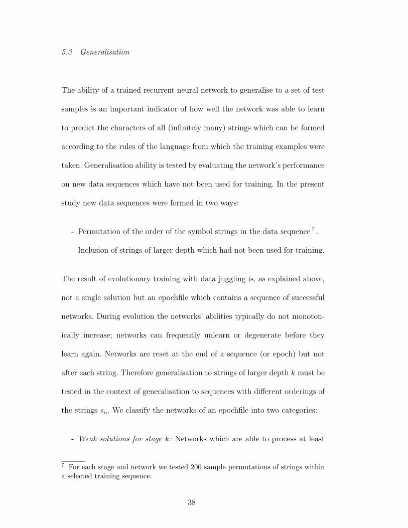
5.3 Generalisation

The ability of a trained recurrent neural network to generalise to a set of test

samples is an important indicator of how well the network was able to learn

to predict the characters of all (infinitely many) strings which can be formed

according to the rules of the language from which the training examples were

taken. Generalisation ability is tested by evaluating the network’s performance

on new data sequences which have not been used for training. In the present

study new data sequences were formed in two ways:

- Permutation of the order of the symbol strings in the data sequence 7 .

- Inclusion of strings of larger depth which had not been used for training.

The result of evolutionary training with data juggling is, as explained above,

not a single solution but an epochfile which contains a sequence of successful

networks. During evolution the networks’ abilities typically do not monoton-

ically increase; networks can frequently unlearn or degenerate before they

learn again. Networks are reset at the end of a sequence (or epoch) but not

after each string. Therefore generalisation to strings of larger depth k must be

tested in the context of generalisation to sequences with different orderings of

the strings sn. We classify the networks of an epochfile into two categories:

- Weak solutions for stage k: Networks which are able to process at least

7 For each stage and network we tested 200 sample permutations of strings withina selected training sequence.

38

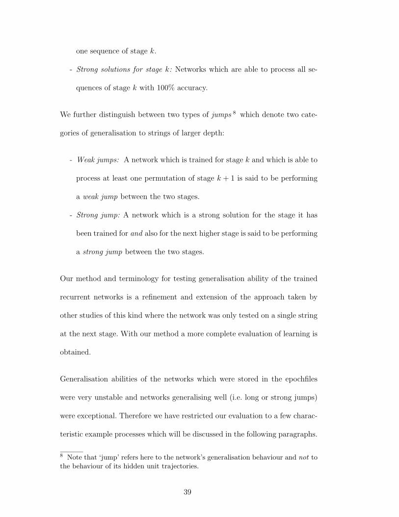
one sequence of stage k.

- Strong solutions for stage k: Networks which are able to process all se-

quences of stage k with 100% accuracy.

We further distinguish between two types of jumps 8 which denote two cate-

gories of generalisation to strings of larger depth:

- Weak jumps: A network which is trained for stage k and which is able to

process at least one permutation of stage k + 1 is said to be performing

a weak jump between the two stages.

- Strong jump: A network which is a strong solution for the stage it has

been trained for and also for the next higher stage is said to be performing

a strong jump between the two stages.

Our method and terminology for testing generalisation ability of the trained

recurrent networks is a refinement and extension of the approach taken by

other studies of this kind where the network was only tested on a single string

at the next stage. With our method a more complete evaluation of learning is

obtained.

Generalisation abilities of the networks which were stored in the epochfiles

were very unstable and networks generalising well (i.e. long or strong jumps)

were exceptional. Therefore we have restricted our evaluation to a few charac-

teristic example processes which will be discussed in the following paragraphs.

8 Note that ‘jump’ refers here to the network’s generalisation behaviour and not tothe behaviour of its hidden unit trajectories.

39

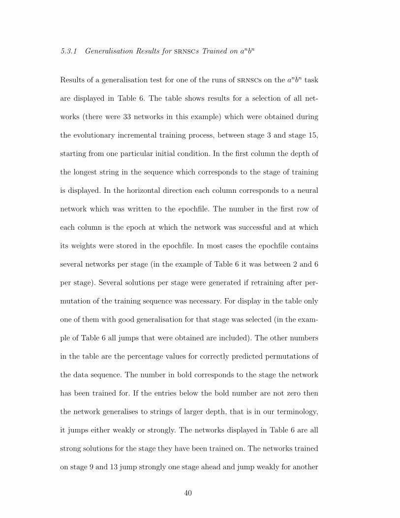
5.3.1 Generalisation Results for srnscs Trained on anbn

Results of a generalisation test for one of the runs of srnscs on the anbn task

are displayed in Table 6. The table shows results for a selection of all net-

works (there were 33 networks in this example) which were obtained during

the evolutionary incremental training process, between stage 3 and stage 15,

starting from one particular initial condition. In the first column the depth of

the longest string in the sequence which corresponds to the stage of training

is displayed. In the horizontal direction each column corresponds to a neural

network which was written to the epochfile. The number in the first row of

each column is the epoch at which the network was successful and at which

its weights were stored in the epochfile. In most cases the epochfile contains

several networks per stage (in the example of Table 6 it was between 2 and 6

per stage). Several solutions per stage were generated if retraining after per-

mutation of the training sequence was necessary. For display in the table only

one of them with good generalisation for that stage was selected (in the exam-

ple of Table 6 all jumps that were obtained are included). The other numbers

in the table are the percentage values for correctly predicted permutations of

the data sequence. The number in bold corresponds to the stage the network

has been trained for. If the entries below the bold number are not zero then

the network generalises to strings of larger depth, that is in our terminology,

it jumps either weakly or strongly. The networks displayed in Table 6 are all

strong solutions for the stage they have been trained on. The networks trained

on stage 9 and 13 jump strongly one stage ahead and jump weakly for another

40

stage. The evaluation of epochfiles from other runs of the same experiments

resulted also in networks which weakly jump up to five stages ahead but do

not jump strongly at all.

----------------------------------------------------------------

Table 6 comes in here

----------------------------------------------------------------

5.3.2 Generalisation Results for anbncn

Generalisation was evaluated for srns and srnscs trained on the anbncn task.

Compared with the generalisation results of the anbn task in the previous sec-

tion in the case of the anbncn task jumps were shorter and strong jumps were

not observed. Some of the srns and srnscs jumped weakly two or three stages

ahead where, within the small set of examples, srnscs performed better than

srns. Table 7 shows the generalisation results for example srnscs taken from

an epochfile which was the outcome of an incremental run. Jumping ability

and generalisation to different orderings changed during the course of evolu-

41

tion which reflects the typically unstable learning behaviour. The last three

columns in Table 7 seem to indicate a tradeoff between good generalisation

regarding the ordering (column 8) and good generalisation regarding depth

(column 7 and 9). The generalisation results obtained with non-incrementally

trained srnscs had similar characteristics. To get an indication whether incre-

mentally or non-incrementally trained solution networks were more likely to

generalise to higher stages we counted the number of networks that jumped

weakly from stage 8 to stage 9. First we counted all networks of success-

ful training runs for stage 8 and found that 14.1% of the 995 incremental

solutions and 24.7% of the 547 non-incrementally trained solutions jumped.

Taking into account that most runs produced several solution networks at each

stage 30% of the 23 successful incremental runs and 60% of the 10 successful

non-incremental runs generated jumping networks (cf. Table 4).

5.3.3 Discussion of Generalisation Results

When evaluating the generalisation ability of sequences of networks from sev-

eral epochfiles from all types of experiments of the present study we made the

following general observations:

- Generalisation of networks within an epochfile was very unstable. Once

a network had acquired a certain generalisation ability it often lost it

within a few more epochs.

- Jumping networks were the exception and the majority of networks in

42

the epochfiles could only generalise to different orderings of the strings

in the data sequence.

- Long strong jumps were almost never observed.

- Non-incrementally trained networks were more likely to jump than incre-

mentally trained networks.

Tonkes et al. (1998) speculated for the anbn task that oscillating solutions

generalise better than monotonic solutions. This hypothesis (in the case of

the anbncn task) is supported by the last item of the above list together with

our observation that most non-incrementally trained networks had oscillating

trajectories while incrementally trained networks tended to have monotonic

trajectories (Section 5.2).

We conclude that networks obtained via the approach of the present study

were, within the limited number of one or two million epochs, able to learn

to predict the symbols in finite sequences of strings from simple context-free

and context-sensitive languages. Several of the trained networks (srns and

srnscs) generalised to strings of slightly larger depth than used for training.

----------------------------------------------------------------

Table 7 comes in here

43

----------------------------------------------------------------

6 Discussion and Summary

Finally we can come back to answer the two questions stated in the introduc-

tion and summarise further insights we have gained. The experiments have

shown how evolutionary hill climbing can be used to train first order recur-

rent neural networks on the anbn and anbncn tasks. It was possible to evolve

solutions which generalise in depth and to different orderings of the strings in

the test sequences for both srns and srnscs. The additional shortcut connec-

tions of the latter architecture equipped the networks with more weights and

also allowed the input signals directly to influence the output signals. This

turned out to be an advantage in most experiments on the anbncn task. First

order networks are therefore sufficient for learning to predict subsets of this

type of context-sensitive language.

The question of whether incremental learning is more efficient than non-

incremental learning has been investigated on the anbn and the anbncn task.

In almost all experiments incremental learning produced more solutions than

non-incremental learning and incremental learning produced its solutions faster.

Comparative training experiments also revealed that learning the context-

sensitive language anbncn is harder than learning the context-free languages

44

anbn or anb2n.

All experiments showed that training was unstable. Symbol sequences which

had been learned by the network were often unlearned at a later stage of the

evolutionary training process and generalisation ability went up and down

during evolution. A classification of the solution networks according to the

signature of their self-weights together with a graphical analysis of hidden

unit dynamics revealed that incremental learning produced more monotonic

solutions while non-incremental learning resulted in solutions with trajectories

which tended to oscillate within the state clusters. The oscillating solutions

were more likely to generalise to strings of larger depth than the monotonic so-

lutions. In contrast to the abovementioned instability regarding generalisation

ability of the networks during training, the qualitative picture of hidden unit

dynamics and the signature of self-weights remained stable during the whole

process in almost all of the evaluated evolutionary runs. Once a network had

learned to process the first stage it was trained on, the essential characteristics

of hidden unit dynamics typically did not change during further training. This

finding seems to indicate that lack of robustness during learning is not related

to errors caused by the system’s bifurcations and there is no passing back and

forth between bifurcations during learning.

In the context of the ongoing debate about the capabilities of connectionist

networks for language processing tasks (Touretzky, 1991) the present study

shows that connectionist models start to be able to learn a kind of language

45

complexity which is, according to some current linguistic opinions, closer to

natural language than the traditional complexity classes of the Chomsky hi-

erarchy. According to Joshi et al. (1991) the family of MCSLs contains the

most significant languages that appear in the study of natural languages (cf.

Joshi and Schabes, 1997; Frank, 2000). Our result that first order recurrent

networks can to some degree learn MA might therefore shed additional light

on the question of which mechanisms and concepts constitute the human lan-

guage capacity.

Acknowledgements

The authors would like to thank all reviewers for their helpful suggestions.

The first author was supported by a PhD scholarship from the Faculty of

Information Technology at Queensland University of Technology, and through

a Research Grants Committee ECR grant from the University of Newcastle.

The second author was supported by the Australian Research Council under

grant S4005295, and by a supercomputer allocation from APAC.

References

Angeline, P. J., Saunders, G. M., Pollack, J. B., 1994. An evolutionary al-

gorithm that constructs recurrent neural networks. IEEE Transactions on

Neural Networks 5, 54–65.

46

Arbib, M. A. (Ed.), 1995. The Handbook of Brain Theory and Neural Net-

works. Cambridge, Mass : MIT Press.

Baeck, T., Fogel, D. B., Michalewicz, Z., Pidgeon, S., 1997. Handbook of Evo-

lutionary Computation. IOP Publishing Ltd. and Oxford University Press.

Bengio, Y., Simard, P., Frasconi, P., 1994. Learning long-term dependencies

with gradient descent is difficult. IEEE Transactions on Neural Networks

5 (2), 157–166.

Beyer, H.-G., 2001. The Theory of Evolution Strategies. Natural Computing

Series. Springer-Verlag.

Blair, A. D., Pollack, J. B., 1997. Analysis of dynamical recognizers. Neural

Computation 9 (55), 1127–1142.

Boden, M., Jacobson, H., Ziemke, T., 2000. Evolving context-free language

predictors. Morgan Kaufmann Publishers, San Francisco, CA, pp. 1033–

1040.

Boden, M., Wiles, J., 2000. Context-free and context-sensitive dynamics in

recurrent neural networks. Connection Science 12 (3,4), 197–210.

Boden, M., Wiles, J., 2001. On learning context-free and context-sensitive

languages. IEEE Transactions on Neural Networks 13 (2), 491–493.

Boden, M., Wiles, J., Tonkes, B., Blair, A., 1999. Learning to predict a context-

free language: Analysis of dynamics in recurrent hidden units. In: Proceed-

ings of the International Conference on Artificial Neural Networks (ICANN

99). IEE, Edinburgh, pp. 359–364.

Carrasco, R. C., Forcada, M. L., Valds-Muoz, M. N., Eco, R. P., 2000. Stable

47

encoding of finite-state machines in discrete-time recurrent neural nets with

sigmoid units. Neural Computation 12 (9), 2129–2174.

Casey, M., 1996. The dynamics of discrete-time computation, with application

to recurrent neural networks and finite state machine extraction. Neural

Computation 8 (6), 1135–1178.

Chalup, S., Blair, A. D., 1999. Hill climbing in recurrent neural networks for

learning the anbncn language. In: T. Gedeon et al. (Ed.), Proceedings, 6th

International Conference on Neural Information Processing (ICONIP’99).

Vol. 2. pp. 508–513.

Chalup, S., Maire, F., 1999. A study on hill climbing for neural network train-

ing. In: Proceedings of the 1999 Congress on Evolutionary Computation

(CEC’99). pp. 2014–2021.

Chalup, S. K., 2002. Incremental learning in biological and machine learning

systems. International Journal of Neural Systems 12 (6), 447–465.

Chomsky, N., 1959. On certain formal properties of grammars. Information

and Control 2, 137–167.

Cleeremans, A., Servan-Schreiber, D., McClelland, J. L., 1989. Finite state

automata and simple recurrent networks. Neural Computation 1 (3), 372–

381.

Das, S., Giles, C. L., Sun, G.-Z., 1993. Using prior knowledge in a NNPDA

to learn context-free languages. Advances in Neural Information Processing

Systems 5, 65–72.

Doya, K., 1992. Bifurcations in the learning of recurrent neural networks.

48

In: Proceedings of 1992 IEEE International Symposium on Circuits and

Systems. pp. 2777–2780.

Doya, K., 1995. Recurrent Networks: Supervised Learning. In: Arbib (1995),

pp. 796–800.

Elman, J. L., 1990. Finding structure in time. Cognitive Science 14, 179–211.

Elman, J. L., 1991. Distributes representations, simple recurrent networks,

and grammatical structure. Machine Learning 7, 195–225.

Elman, J. L., 1993. Learning and development in neural networks: The im-

portance of starting small. Cognition 48, 71–99.

Finn, G. D., 1998. A recurrent neural network for the language anbn: En-

coding and decoding binary strings in a neuron’s activation function. Tech.

rep., Machine Learning Research Centre, School of Computing Science, FIT,

Queensland University of Technology, unpublished.

Frank, R., 2000. From regular to context-free to mildly context-sensitive

tree rewriting systems: The path of child language acquisition. In: Abeille,

A., Rambow, O. (Eds.), Tree Adjoining Grammars: Formalisms, Linguistic

Analysis and Processing. CSLI, Stanford, CA, pp. 101–120.

Gers, F. A., Schmidhuber, J., 2001. LSTM recurrent networks learn simple

context-free and context-sensitive languages. IEEE Transactions On Neural

Networks 12 (6), 1333–1340.

Giles, C. L., Gori, M. (Eds.), 1998. Adaptive Processing of Sequences and

Data Structures. Lecture Notes in Artificial Intelligence. Springer-Verlag.

Giles, C. L., Miller, C. B., Chen, D., Chen, H. H., Sun, G. Z., Lee, Y. C., 1992.

49

Learning and extracting finite state automata with second-order recurrent

neural networks. Neural Computation 4 (3), 393–405.

Gori, M., Maggini, M., Martinelli, E., Soda, G., 1998. Inductive inference

from noisy examples using the hybrid finite state filter. IEEE Transactions

on Neural Networks 9 (3), 571–575.

Haykin, S., 1999. Neural Networks. A Comprehensive Foundation, 2nd Edi-

tion. Prentice Hall.

Heath, R., Hayes, B., Heathcote, A., Hooker, C., 1999. Dynamical Cognitive

Science: Proceedings of the Fourth Biennial Conference of the Australasian

Cognitive Science Society (OzCogSci97).

Hertz, J., Krogh, A., Palmer, R. G., 1991. Introduction to the Theory of Neural

Computation. Addison-Wesley Publishing Company.

Hirsch, M. W., 1984. The dynamical systems approach to differential equa-

tions. Bulletin (New Series) of the American Mathematical Society 11 (1),

1–63.

Hirsch, M. W., 1989. Convergent activation dynamics in continuous time net-

works. Neural Networks 2, 331–349.

Hirsch, M. W., 1991. Network dynamics: Principles and problems. In: Pase-

mann and Doebner (1991), pp. 3–29.

Holldobler, S., Kalinke, Y., Lehmann, H., 1997. Designing a counter: Another

case study of dynamics and activation landscapes in recurrent networks.

In: Proceedings of 21st German Conference on Artificial Intelligence. LNAI

1301. Springer-Verlag, pp. 313–324.

50

Hopcroft, J. E., Ullman, J. D., 1979. Introduction to Automata Theory, Lan-

guages and Computation. Addison-Wesley Publishing Company.

Ilie, L., 1999. An attempt to define a class of mildly context-sensitive lan-

guages. Publicationes Mathematicae Debrecen 54, 865–876.

Joshi, A. K., Schabes, Y., 1997. Tree-Adjoining Grammars. Vol. 3 of Rozenberg

and Salomaa (1997), pp. 69–123.

Joshi, A. K., Vijay-Shanker, K., Weir, D., 1991. The convergence of mildly

context-sensitive grammatical formalisms. In: Sells et al. (1991), pp. 31–81.

Kirby, S., Hurford, J. R., 1997. The evolution of incremental learning: lan-

guage, development and critical periods. Technical report, Language Evo-

lution and Computation Research Unit, University of Edinburgh.

Kolen, J. F., 1994. Recurrent networks: State machines or iterated function

systems? In: Mozer, M. C., Smolensky, P., Touretzky, D. S., Elman, J. L.

(Eds.), Proceedings of the 1993 Connectionist Models Summer School. Erl-

baum Associates, pp. 203–210.

Kolen, J. F., Kremer, S. C. (Eds.), 2001. A Field Guide to Dynamical Recur-

rent Networks. IEEE Press.

Kremer, S. C., 1995. On the computational power of Elman-style recurrent

networks. IEEE Transactions on Neural Networks 6 (4), 1000–1004.

Kremer, S. C., 1999. Identification of a specific limitation on local-feedback

recurrent networks acting as Mealy/Moore machines. IEEE Transactions on

Neural Networks 10 (2), 433–438.

Maass, W., Orponen, P., 1997. On the effect of analog noise in discrete-time

51

analog computation. In: Proceedings Neural Information Processing Sys-

tems 1996. The MIT Press, pp. 218–224.

Maass, W., Orponen, P., 1998. On the effect of analog noise in discrete-time

analog computations. Neural Computation 10, 1071–1095.

Maass, W., Sontag, E., 1999a. Analog neural nets with Gaussian or other

common noise distribution cannot recognize arbitrary regular languages.

Neural Computation 11, 771–782.

Maass, W., Sontag, E., 1999b. A precise characterization of the class of lan-

guages recognized by neural nets under gaussian and other common noise

distributions. In: Kearns, M. S., Solla, S. S., Cohn, D. A. (Eds.), Advances in

Neural Information Processing Systems 1999 (NIPS’99). Vol. 11. The MIT

Press.

Martin-Vide, C., Mateescu, A., Salomaa, A., 1999. Sewing contexts and mildly

context–sensitive languages. TUCS Technical Report 257, Turku Centre for

Computer Science.

Melnik, O., Levy, S., Pollack, J. B., 2000. RAAM for infinite context-

free languages. In: International Joint Conference on Neural Networks

(IJCNN’2000). Vol. 5. IEEE Press.

Minsky, M. L., 1967. Computation: Finite and Infinite Machines. Prentice

Hall, Englewood Cliffs, NJ.

Moore, C., 1998. Dynamical recognizers: Real-time language recognition by

analog computers. Theoretical Computer Science 201, 99–136.

Pasemann, F., Doebner, H.-D. (Eds.), 1991. Neurodynamics: Proceedings of

52

the 9th Summer Workshop on Mathematical Physics, 1990. Vol. 1 of Series

on Neural Networks. World Scientific.

Pearlmutter, B. A., 1989. Learning state-space trajectories in recurrent neural

networks. Neural Computation 1, 263–269.

Pearlmutter, B. A., 1995. Gradient calculations for dynamic recurrent neural

networks: A survey. IEEE Transactions on Neural Networks 5 (6), 1212–

1228.

Pollack, J., 1987. On connectionist models of natural language processing.

Ph.D. thesis, Computer Science Department, University of Illinois, Ur-

bana, IL.

Pollack, J., 1991. The induction of dynamical recognizers. Machine Learning

7, 227–252.

Pollack, J. B., Blair, A., 1998. Co-evolution in the successful learning of

backgammon strategy. Machine Learning 32, 225–240.

Rechenberg, I., 1965. Cybernetic solution path of an experimental problem.

Tech. rep., Royal Aircraft Establishment, Library Translation No. 1122.

Rechenberg, I., 1994. Evolutionsstrategie ’94. Frommann-Holzboog, Stuttgart.

Robinson, A. J., Fallside, F., 1988. Static and dynamic error propagation

networks with applications to speech coding. In: Anderson, D. Z. (Ed.),

Neural Information Processing Systems. American Institute of Physics, New

York.

Rodriguez, P., 2001. Simple recurrents networks learn context-free and

context-sensitive languages by counting. Neural Computation 13 (9), 2093–

53

2118.

Rodriguez, P., Wiles, J., Elman, J. L., 1999. A recurrent neural network that

learns to count. Connection Science 11 (1), 5–40.

Rohde, D. L. T., Plaut, D. C., August 1997. Simple recurrent networks and

natural language: How important is starting small ? Proceedings of the 19th

Annual Conference of the Cognitive Science Society .

Rohde, D. L. T., Plaut, D. C., 1999. Language acquisition in the absence of

explicit negative evidence: How important is starting small ? Cognition 72,

67–109.

Rohde, D. L. T., Plaut, D. C., 2003. Less is less in language acquisition. Hove,

UK: Psychology Press.

Rozenberg, G., Salomaa, A. (Eds.), 1997. Handbook of Formal Languages,

volume 3. Springer-Verlag.

Rudolph, G., 1997. Evolution strategies. In: Baeck et al. (1997), pp. B1.3:1–6.

Rumelhart, D. E., Hinton, G. E., Williams, R. J., 1986. Learning representa-

tions by back-propagating errors. Nature , 533–536.

Schwefel, H.-P., 1965. Kybernetische Evolution als Strategie der experi-

mentellen Forschung in der Stromungsmechanik. Master’s thesis, Technische

Universitat Berlin, Hermann Fottinger Institut fuer Hydrodynamik.

Schwefel, H.-P., 1995. Evolution and Optimum Seeking. John Wiley & Sons,

Chichester, UK.

Sells, P., Shieber, S. M., Wasow, T. (Eds.), 1991. Foundations Issues in Natural

Language Processing. MIT Press.

54

Siegelmann, H. T., 1999. Neural Networks and Analog Computation - Beyond

the Turing Limit. Progress in Theoretical Computer Science. Birkhauser

Boston.

Sontag, E., 1995. Automata and Neural Networks. In: Arbib (1995), pp. 119–

123.

Steijvers, M., Grunwald, P., 1996. A recurrent network that performs a

context-sensitive prediction task. In: Proceedings of the 18th Annual Con-

ference of the Cognitive Science Society. Morgan Kauffman, pp. 335–339.

Sun, G. Z., Chen, H. H., Giles, C. L., Lee, Y. C., Chen, D., 1991. Neural

networks with external memeory stack that learn context-free grammars

from examples. In: Proceedings of the Conference on Information Science

and Systems. Princeton University, pp. 649–653.

Tino, P., Horne, B. G., Giles, C. L., 2001. Attractive periodic sets in discrete–

time recurrent networks (with emphasis on fixed–point stability and bifur-

cations in two-neuron networks). Neural Computation 13, 1379–1414.

Tino, P., Sajda, J., 1995. Learning and extracting initial Mealy automata with

a modular neural network model. Neural Computation 7 (4).

Tonkes, B., Blair, A., Wiles, J., 1998. Inductive bias in context-free language

learning. In: Proceedings of the Ninth Australian Conference on Neural

Networks (ACNN’98), Brisbane. University of Queensland, pp. 52–56.

Tonkes, B., Wiles, J., 1999. Learning a context-free task with a recurrent

neural network: An analysis of stability. In: Heath et al. (1999).

Touretzky, D. (Ed.), 1991. Connectionist Approaches to Language Learning.

55

The Kluwer International Series in Engineering and Computer Science.

Kluwer Academic Publishers, a Special Issue of Machine Learning on Con-

nectionist Approaches to Language Learning.

Tsoi, A. C., 1998. Recurrent Neural Network Architectures: An Overview. In:

Giles and Gori (1998), pp. 1–26.

Tsoi, A. C., Back, A., 1997. Discrete time recurrent neural network architec-

tures: A unifying review. Neurocomputing 15, 183–233.

Werbos, P. J., 1974. Beyond regression: New tools for prediction and analysis

in the behavioural sciences. Ph.D. thesis, Harvard University, Cambridge,

MA.

Wiles, J., Blair, A. D., Boden, M., 2001. Representation Beyond Finite States:

Alternatives to Push-Down Automata. In: Kolen and Kremer (2001).

Wiles, J., Elman, J. L., 1995. Learning to count without a counter: A case

study of dynamics and activation landscapes in recurrent networks. In: Pro-

ceedings of the Seventeenth Annual Conference of the Cognitive Science

Society. MIT Press, pp. 482–487.

Yao, X., Liu, Y., May 1997. A new evolutionary system for evolving artificial

neural networks. IEEE Transactions on Neural Networks 8 (3), 694–713.

Zeng, Z., Goodman, R. M., Smyth, P., 1994. Discrete recurrent neural networks

for grammatical inference. IEEE Transactions on Neural Networks 5 (2),

320–330.

Zipser, D., 1990. Subgrouping reduces complexity and speeds up learning in

recurrent networks. Advances in Neural Information Processing Systems 2,

56

638–641, Morgan Kaufman Publishers.

57

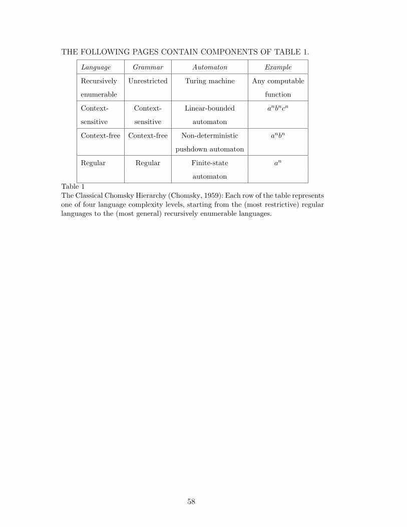
THE FOLLOWING PAGES CONTAIN COMPONENTS OF TABLE 1.

Language Grammar Automaton Example

Recursively Unrestricted Turing machine Any computable

enumerable function

Context- Context- Linear-bounded anbncn

sensitive sensitive automaton

Context-free Context-free Non-deterministic anbn

pushdown automaton

Regular Regular Finite-state an

automatonTable 1The Classical Chomsky Hierarchy (Chomsky, 1959): Each row of the table representsone of four language complexity levels, starting from the (most restrictive) regularlanguages to the (most general) recursively enumerable languages.

58

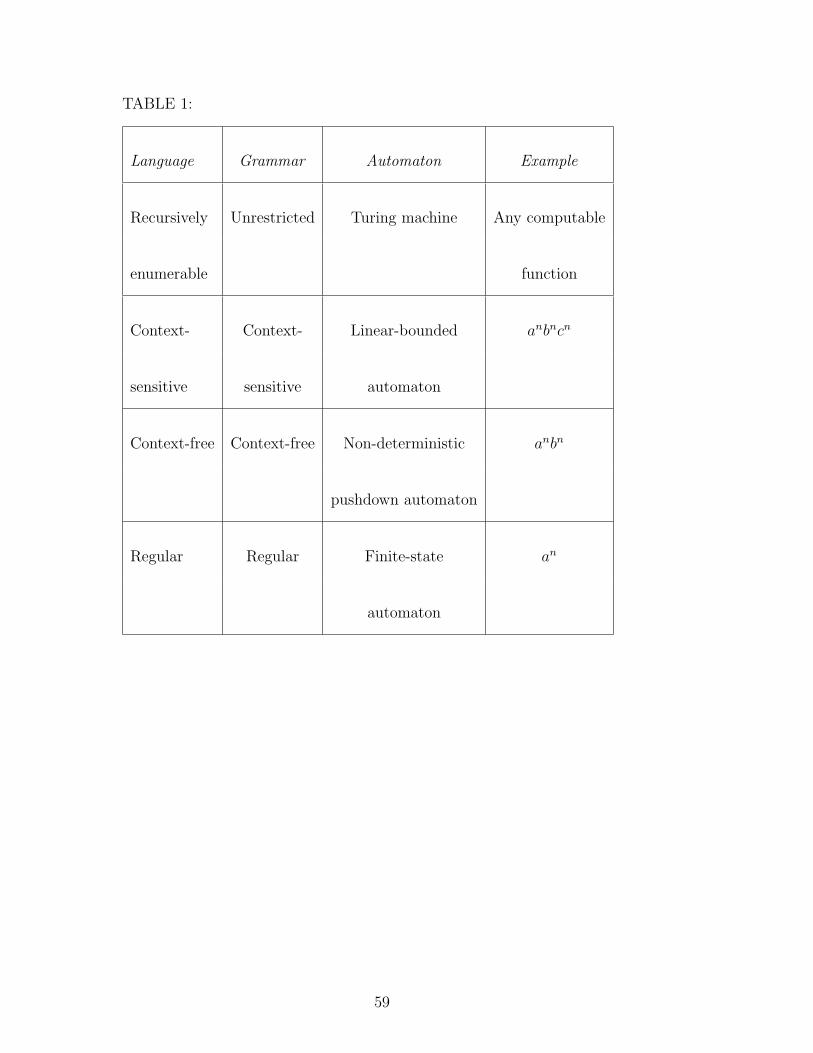
TABLE 1:

Language Grammar Automaton Example

Recursively Unrestricted Turing machine Any computable

enumerable function

Context- Context- Linear-bounded anbncn

sensitive sensitive automaton

Context-free Context-free Non-deterministic anbn

pushdown automaton

Regular Regular Finite-state an

automaton

59

LEGEND OF TABLE 1:

The Classical Chomsky Hierarchy (Chomsky, 1959): Each row of the table

represents one of four language complexity levels, starting from the (most

restrictive) regular languages to the (most general) recursively enumerable

languages.

60

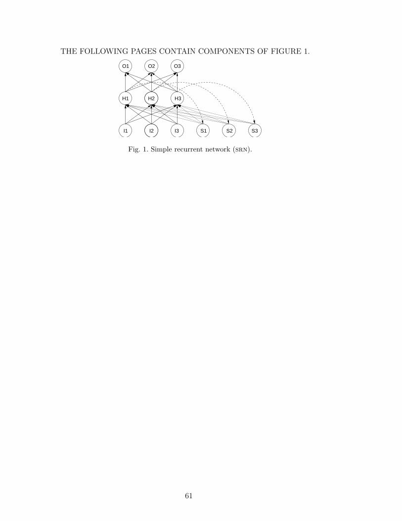
THE FOLLOWING PAGES CONTAIN COMPONENTS OF FIGURE 1.

O2

I2I1

H1 H2

O1

I3

H3

O3

S1 S2 S3

Fig. 1. Simple recurrent network (srn).

61

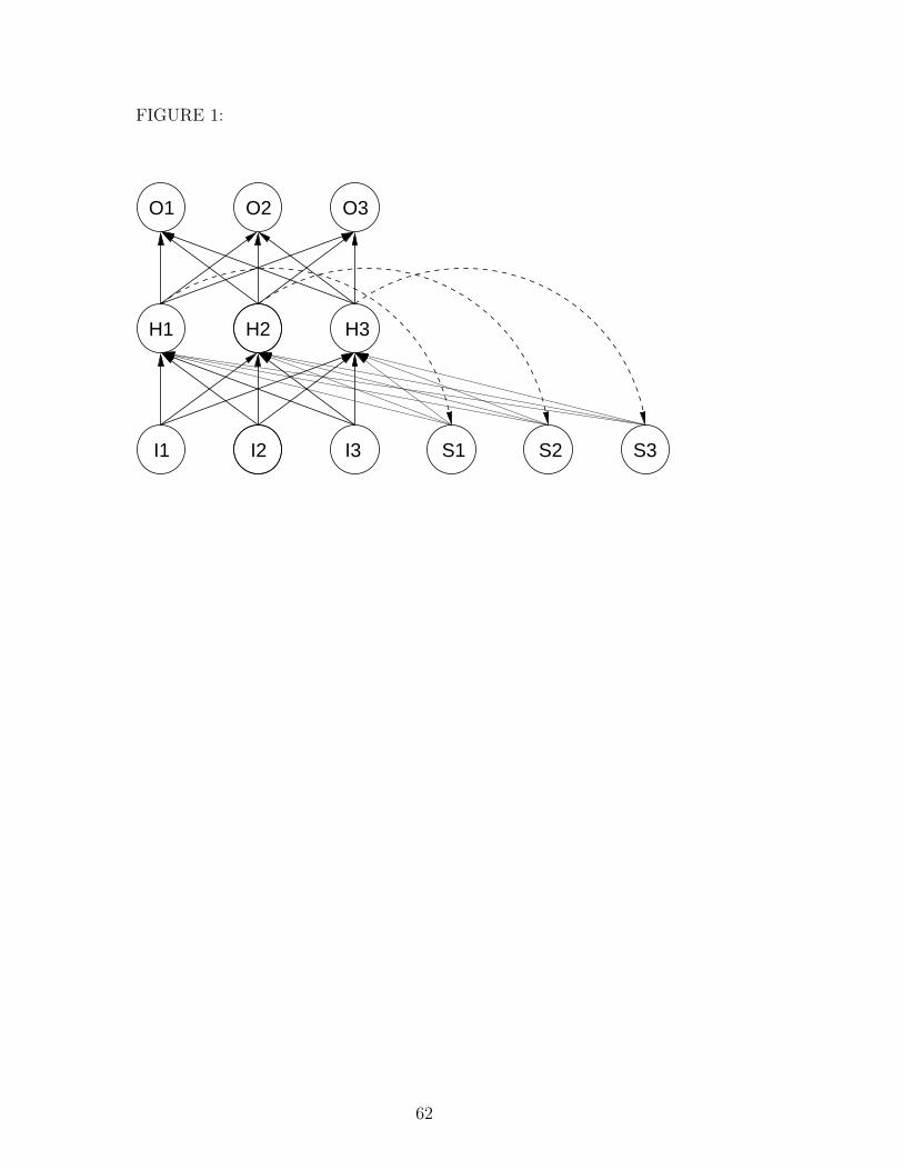
FIGURE 1:

O2

I2I1

H1 H2

O1

I3

H3

O3

S1 S2 S3

62

LEGEND FOR FIGURE 1:

Simple recurrent network (srn).

63

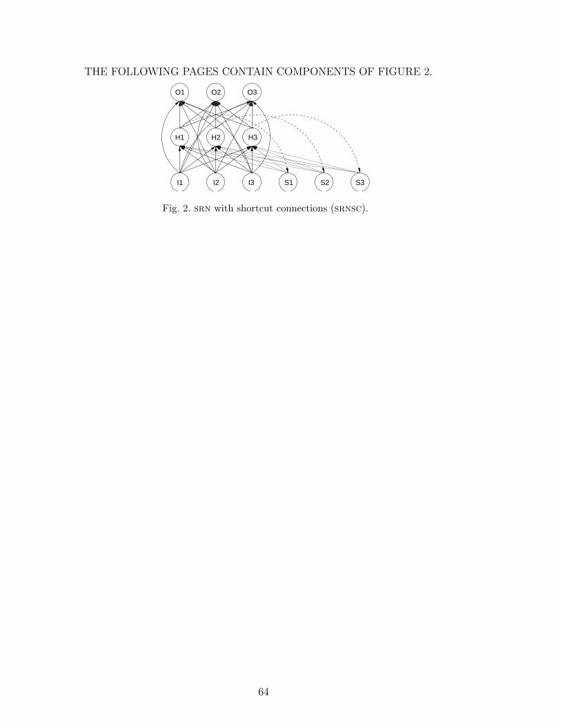
THE FOLLOWING PAGES CONTAIN COMPONENTS OF FIGURE 2.

O2

I2I1

H1 H2

O1

I3

H3

O3

S1 S2 S3

Fig. 2. srn with shortcut connections (srnsc).

64

FIGURE 2:

O2

I2I1

H1 H2

O1

I3

H3

O3

S1 S2 S3

65

LEGEND FOR FIGURE 2:

srn with shortcut connections (srnsc).

66

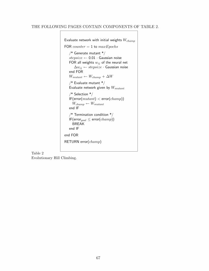
THE FOLLOWING PAGES CONTAIN COMPONENTS OF TABLE 2.

Evaluate network with initial weights Wchamp

FOR counter = 1 to maxEpochs

/* Generate mutant */stepsize ← 0.01 · Gaussian noiseFOR all weights wij of the neural net

∆wij ← stepsize · Gaussian noiseend FORWmutant ← Wchamp + ∆W

/* Evaluate mutant */Evaluate network given by Wmutant

/* Selection */IF(error(mutant) < error(champ))

Wchamp ← Wmutant

end IF

/* Termination condition */IF(errorgoal ≤ error(champ))

BREAKend IF

end FOR

RETURN error(champ)

Table 2Evolutionary Hill Climbing.

67

TABLE 2:

Evaluate network with initial weights Wchamp

FOR counter = 1 to maxEpochs

/* Generate mutant */

stepsize ← 0.01 · Gaussian noise

FOR all weights wij of the neural net

∆wij ← stepsize · Gaussian noise

end FOR

Wmutant ← Wchamp + ∆W

/* Evaluate mutant */

Evaluate network given by Wmutant

/* Selection */

IF(error(mutant) < error(champ))

Wchamp ← Wmutant

end IF

/* Termination condition */

IF(errorgoal ≤ error(champ))

BREAK

end IF

end FOR

RETURN error(champ)

LEGEND FOR TABLE 2:

Evolutionary Hill Climbing.

69

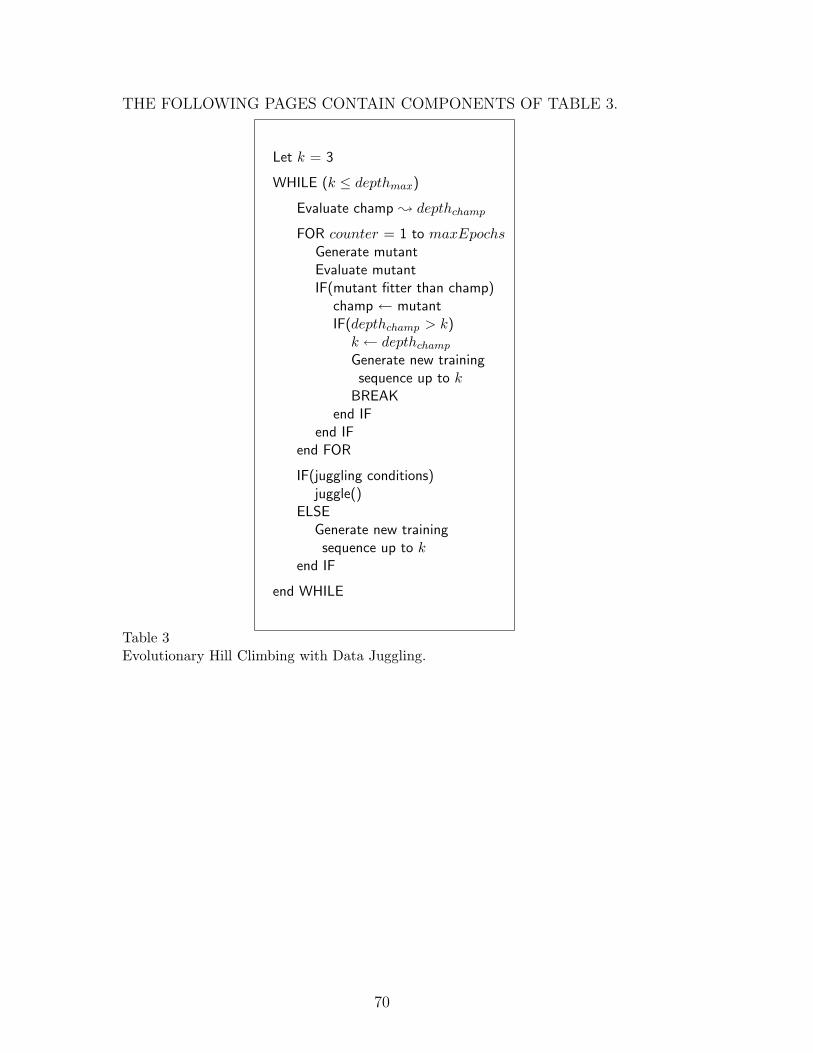
THE FOLLOWING PAGES CONTAIN COMPONENTS OF TABLE 3.

Let k = 3

WHILE (k ≤ depthmax)

Evaluate champ ; depthchamp

FOR counter = 1 to maxEpochsGenerate mutantEvaluate mutantIF(mutant fitter than champ)

champ ← mutantIF(depthchamp > k)

k ← depthchamp

Generate new trainingsequence up to k

BREAKend IF

end IFend FOR

IF(juggling conditions)juggle()

ELSEGenerate new trainingsequence up to k

end IF

end WHILE

Table 3Evolutionary Hill Climbing with Data Juggling.

70

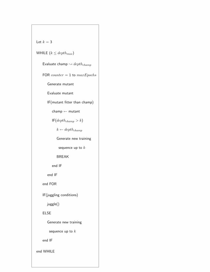
Let k = 3

WHILE (k ≤ depthmax)

Evaluate champ ; depthchamp

FOR counter = 1 to maxEpochs

Generate mutant

Evaluate mutant

IF(mutant fitter than champ)

champ ← mutant

IF(depthchamp > k)

k ← depthchamp

Generate new training

sequence up to k

BREAK

end IF

end IF

end FOR

IF(juggling conditions)

juggle()

ELSE

Generate new training

sequence up to k

end IF

end WHILE

LEGEND FOR TABLE 3:

Evolutionary Hill Climbing with Data Juggling.

72

THE FOLLOWING PAGES CONTAIN COMPONENTS OF TABLE 4.

73

Row

Exper

imen

t1

23

45

67

1Tas

ka

nbn

anb2

na

nbn

cn

2A

rchi

tect

ure

srnsc

srnsc

srnsc

srn

3In

crem

enta

lye

sno

yes

yes

noye

sno

4Tot

alru

ns30

3030

4040

3030

5Su

cces

s≤

1M24

(80%

)24

(80%

)20

(67%

)17

(43%

)5

(13%

)6

(20%

)4

(13%

)

6Su

cces

s≤

2M–

–20

(67%

)23

(58%

)10

(25%

)10

(33%

)6

(20%

)

7M

inim

um7,

380

30,8

2514

,746

183,

086

509,

997

58,7

4621

1,10

2

8M

axim

um39

6,11

944

2,40

782

5,07

91,

703,

701

1,71

0,47

31,

674,

318

1,99

5,11

9

9M

edia

n29

,888

204,

070

42,4

6277

,450

61,

005,

800

937,

290

490,

040

10M

ean

60,2

1322

6,66

010

6,36

078

6,73

01,

066,

600

863,

070

786,

190

11St

d95

,943

113,

210

179,

860

427,

770

415,

110

607,

700

707,

630

Tab

le4

Ove

rvie

wof

trai

ning

resu

ltsfo

ral

lse

ven

seri

esof

expe

rim

ents

:E

ach

seri

esof

expe

rim

ents

cons

iste

dof

30or

40ev

olut

iona

rypr

oces

ses

(‘ru

ns’)

,al

lst

arti

ngw

ith

adi

ffere

ntin

itia

lse

tof

neur

alne

twor

kw

eigh

ts.T

hefir

stth

ree

row

sst

ate

the

task

,ar

chit

ectu

rean

dw

heth

erin

crem

enta

lle

arni

ngw

asus

edor

not.

The

succ

ess

rate

sin

row

s5

and

6sh

owho

wm

any

netw

orks

ofea

chse

ries

wer

eab

leto

proc

ess

atr

aini

ngse

quen

cew

ith

100%

accu

racy

wit

hin

1m

illio

nor

2m

illio

nep

ochs

,re

spec

tive

ly.R

ows

7–11

indi

cate

the

num

ber

ofep

ochs

ofth

em

inim

um,m

axim

um,m

edia

n,m

ean

and

stan

dard

devi

atio

nfo

rea

chse

ries

ofex

peri

men

ts.

74

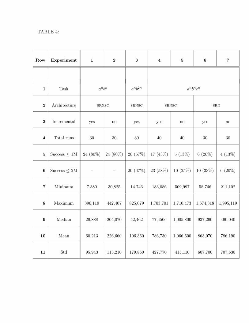
TABLE 4:

Row Experiment 1 2 3 4 5 6 7

1 Task anbn anb2n anbncn

2 Architecture srnsc srnsc srnsc srn

3 Incremental yes no yes yes no yes no

4 Total runs 30 30 30 40 40 30 30

5 Success ≤ 1M 24 (80%) 24 (80%) 20 (67%) 17 (43%) 5 (13%) 6 (20%) 4 (13%)

6 Success ≤ 2M – – 20 (67%) 23 (58%) 10 (25%) 10 (33%) 6 (20%)

7 Minimum 7,380 30,825 14,746 183,086 509,997 58,746 211,102

8 Maximum 396,119 442,407 825,079 1,703,701 1,710,473 1,674,318 1,995,119

9 Median 29,888 204,070 42,462 77,4506 1,005,800 937,290 490,040

10 Mean 60,213 226,660 106,360 786,730 1,066,600 863,070 786,190

11 Std 95,943 113,210 179,860 427,770 415,110 607,700 707,630

LEGEND OF TABLE 4:

Overview of training results for all seven series of experiments: Each series of

experiments consisted of 30 or 40 evolutionary processes (‘runs’), all starting

with a different initial set of neural network weights. The first three rows state

the task, architecture and whether incremental learning was used or not. The

success rates in rows 5 and 6 show how many networks of each series were

able to process a training sequence with 100% accuracy within 1 million or

2 million epochs, respectively. Rows 7–11 indicate the number of epochs of the

minimum, maximum, median, mean and standard deviation for each series of

experiments.

76

THE FOLLOWING PAGES CONTAIN COMPONENTS OF TABLE 5.

Signature (3, 0) (2, 1) (1, 2) (0, 3)

Incremental runs 17 4 1 1

Non-Incremental runs 1 8 1 0Table 5Successful anbncn networks classified according to the signature of their self-weights.The signature is defined to be (p, q) where p and q are the number of positive andnegative self-weights, respectively.

77

TABLE 5:

Signature (3, 0) (2, 1) (1, 2) (0, 3)

Incremental runs 17 4 1 1

Non-Incremental runs 1 8 1 0

78

LEGEND FOR TABLE 5:

Successful anbncn networks classified according to the signature of their self-

weights. The signature is defined to be (p, q) where p and q are the number of

positive and negative self-weights, respectively.

79

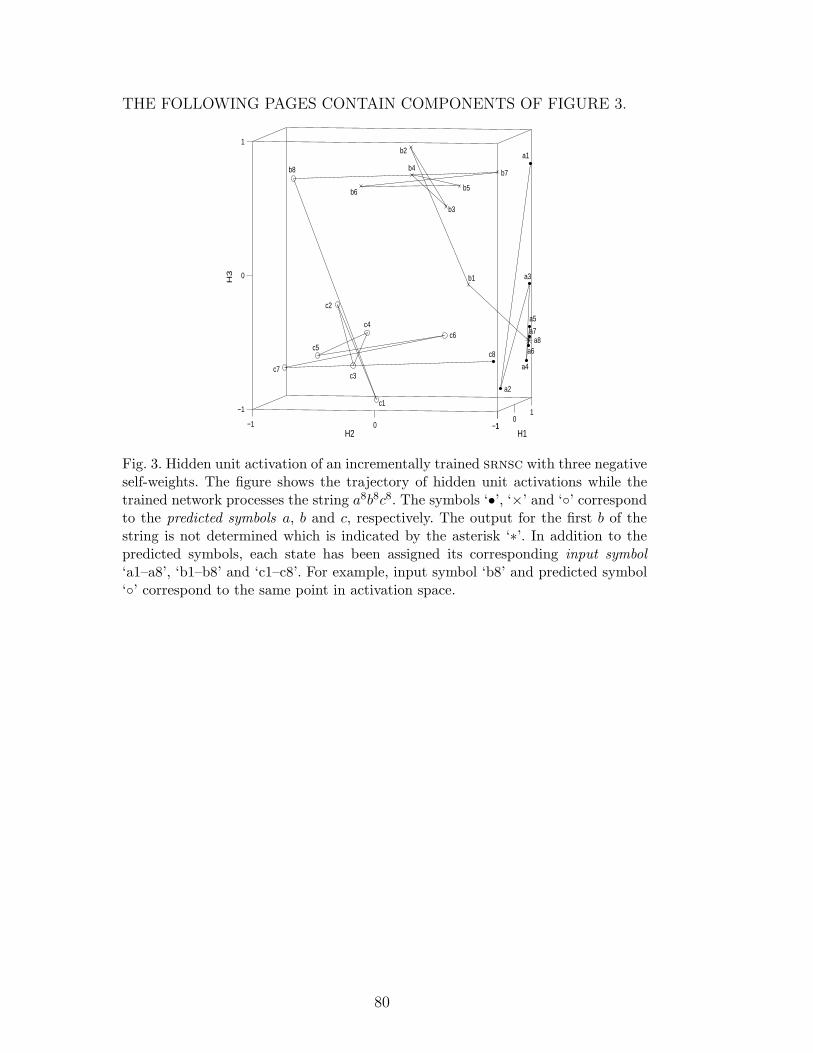
THE FOLLOWING PAGES CONTAIN COMPONENTS OF FIGURE 3.

−10

1

−1 0 1

−1

0

1

H1H2

H3

a1

a2

a3

a4

a5

a6

a7 a8

b1

b2

b3

b4

b5 b6

b7 b8

c1

c2

c3

c4

c5

c6

c7

c8

Fig. 3. Hidden unit activation of an incrementally trained srnsc with three negativeself-weights. The figure shows the trajectory of hidden unit activations while thetrained network processes the string a8b8c8. The symbols ‘•’, ‘×’ and ‘◦’ correspondto the predicted symbols a, b and c, respectively. The output for the first b of thestring is not determined which is indicated by the asterisk ‘∗’. In addition to thepredicted symbols, each state has been assigned its corresponding input symbol‘a1–a8’, ‘b1–b8’ and ‘c1–c8’. For example, input symbol ‘b8’ and predicted symbol‘◦’ correspond to the same point in activation space.

80

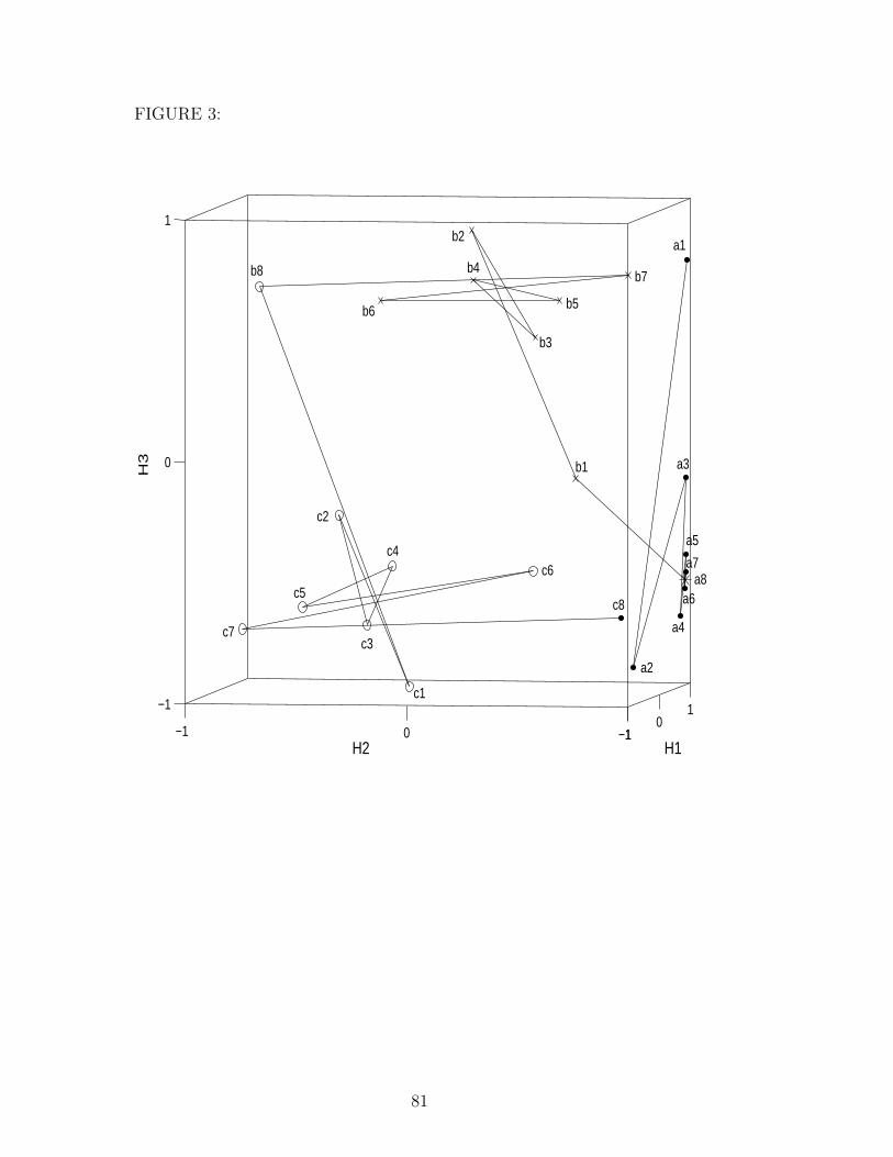
FIGURE 3:

−10

1

−1 0 1

−1

0

1

H1H2

H3

a1

a2

a3

a4

a5

a6

a7 a8

b1

b2

b3

b4

b5 b6

b7 b8

c1

c2

c3

c4

c5

c6

c7

c8

81

LEGEND FOR FIGURE 3:

Hidden unit activation of an incrementally trained srnsc with three negative

self-weights. The figure shows the trajectory of hidden unit activations while

the trained network processes the string a8b8c8. The symbols ‘•’, ‘×’ and ‘◦’

correspond to the predicted symbols a, b and c, respectively. The output for the

first b of the string is not determined which is indicated by the asterisk ‘∗’. In

addition to the predicted symbols, each state has been assigned its correspond-

ing input symbol ‘a1–a8’, ‘b1–b8’ and ‘c1–c8’. For example, input symbol ‘b8’

and predicted symbol ‘◦’ correspond to the same point in activation space.

82

THE FOLLOWING PAGES CONTAIN COMPONENTS OF FIGURE 4.

−1

0

1−1

0

1

−1

0

1

H3

H1

H2

a1

a5

a6

a7 a8

b3 b4 b5

b7

b8

c1

c2

c3

c4

c5 c6 c7

c8

a2 a3

a4

b6

b1 b2

(a) 3D view (b) right side view

(c) left side view (d) top view

Fig. 4. An srnsc has partially learned to predict the language anbncn. Incrementallearning has produced a monotonic solution. The trajectory was recorded while thenetwork was processing the string a8b8c8.

83

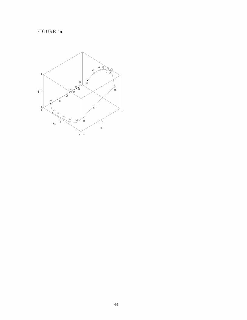
FIGURE 4a:

−1

0

1−1

0

1

−1

0

1

H3

H1

H2

a1

a5

a6

a7 a8

b3 b4 b5

b7

b8

c1

c2

c3

c4

c5 c6 c7

c8

a2 a3

a4

b6

b1 b2

84

FIGURE 4b:

85

FIGURE 4c:

86

FIGURE 4d:

87

LEGEND FOR FIGURE 4:

An srnsc has partially learned to predict the language anbncn. Incremental

learning has produced a monotonic solution. The trajectory was recorded while

the network was processing the string a8b8c8.

88

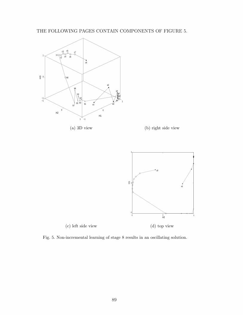
THE FOLLOWING PAGES CONTAIN COMPONENTS OF FIGURE 5.

−1

0

1−1

0

1

−1

0

1

H1H2

H3

a1

a2

a3

a4

a5

a6

a7 a8

b1

b2

b3

b4

b5

b6

b7

b8

c1

c3 c5

c6

c7

c8

c4 c2

(a) 3D view (b) right side view

0

1

0

H2

H21-1

-1

H1

c8

a1

(c) left side view (d) top view

Fig. 5. Non-incremental learning of stage 8 results in an oscillating solution.

89

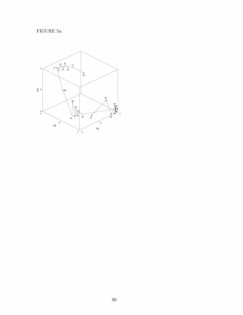
FIGURE 5a:

−1

0

1−1

0

1

−1

0

1

H1H2

H3

a1

a2

a3

a4

a5

a6

a7 a8

b1

b2

b3

b4

b5

b6

b7

b8

c1

c3 c5

c6

c7

c8

c4 c2

90

FIGURE 5b:

91

FIGURE 5c:

92

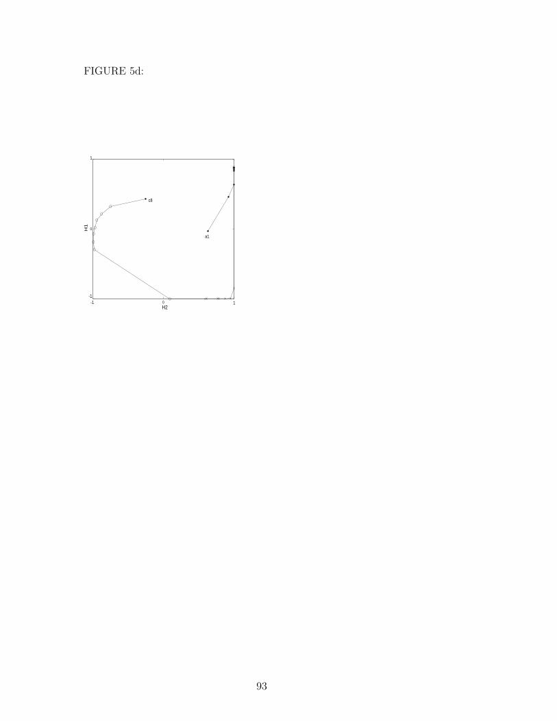
FIGURE 5d:

0

1

0

H2

H21-1

-1

H1

c8

a1

93

LEGEND FOR FIGURE 5:

Non-incremental learning of stage 8 results in an oscillating solution.

94

THE FOLLOWING PAGES CONTAIN COMPONENTS OF TABLE 6.

95

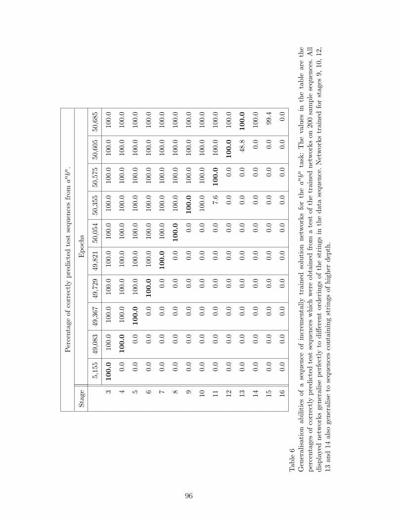
Per

cent

age

ofco

rrec

tly

pred

icte

dte

stse

quen

ces

from

anbn

.

Stag

eE

poch

s

5,15

549

,083

49,3

6749

,729

49,8

2150

,054

50,3

5550

,575

50,6

0550

,685

310

0.0

100.

010

0.0

100.

010

0.0

100.

010

0.0

100.

010

0.0

100.

0

40.

010

0.0

100.

010

0.0

100.

010

0.0

100.

010

0.0

100.

010

0.0

50.

00.

010

0.0

100.

010

0.0

100.

010

0.0

100.

010

0.0

100.

0

60.

00.

00.

010

0.0

100.

010

0.0

100.

010

0.0

100.

010

0.0

70.

00.

00.

00.

010

0.0

100.

010

0.0

100.

010

0.0

100.

0

80.

00.

00.

00.

00.

010

0.0

100.

010

0.0

100.

010

0.0

90.

00.

00.

00.

00.

00.

010

0.0

100.

010

0.0

100.

0

100.

00.

00.

00.

00.

00.

010

0.0

100.

010

0.0

100.

0

110.

00.

00.

00.

00.

00.

07.

610

0.0

100.

010

0.0

120.

00.

00.

00.

00.

00.

00.

00.

010

0.0

100.

0

130.

00.

00.

00.

00.

00.

00.

00.

048

.810

0.0

140.

00.

00.

00.

00.

00.

00.

00.

00.

010

0.0

150.

00.

00.

00.

00.

00.

00.

00.

00.

099

.4

160.

00.

00.

00.

00.

00.

00.

00.

00.

00.

0Tab

le6

Gen

eral

isat

ion

abili

ties

ofa

sequ

ence

ofin

crem

enta

llytr

aine

dso

luti

onne

twor

ksfo

rth

ea

nbn

task

:T

heva

lues

inth

eta

ble

are

the

perc

enta

ges

ofco

rrec

tly

pred

icte

dte

stse

quen

ces

whi

chw

ere

obta

ined

from

ate

stof

the

trai

ned

netw

orks

on20

0sa

mpl

ese

quen

ces.

All

disp

laye

dne

twor

ksge

nera

lise

perf

ectl

yto

diffe

rent

orde

ring

sof

the

stri

ngs

inth

eda

tase

quen

ce.N

etw

orks

trai

ned

for

stag

es9,

10,12

,13

and

14al

soge

nera

lise

tose

quen

ces

cont

aini

ngst

ring

sof

high

erde

pth.

96

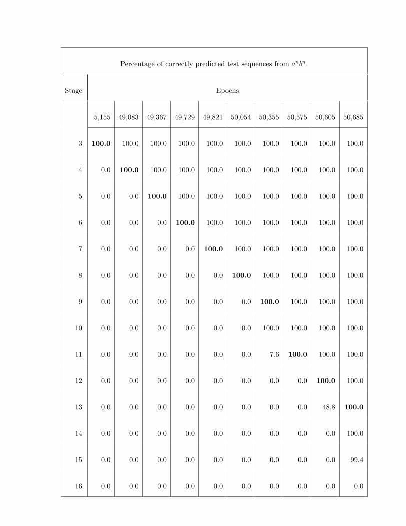
Percentage of correctly predicted test sequences from anbn.

Stage Epochs

5,155 49,083 49,367 49,729 49,821 50,054 50,355 50,575 50,605 50,685

3 100.0 100.0 100.0 100.0 100.0 100.0 100.0 100.0 100.0 100.0

4 0.0 100.0 100.0 100.0 100.0 100.0 100.0 100.0 100.0 100.0

5 0.0 0.0 100.0 100.0 100.0 100.0 100.0 100.0 100.0 100.0

6 0.0 0.0 0.0 100.0 100.0 100.0 100.0 100.0 100.0 100.0

7 0.0 0.0 0.0 0.0 100.0 100.0 100.0 100.0 100.0 100.0

8 0.0 0.0 0.0 0.0 0.0 100.0 100.0 100.0 100.0 100.0

9 0.0 0.0 0.0 0.0 0.0 0.0 100.0 100.0 100.0 100.0

10 0.0 0.0 0.0 0.0 0.0 0.0 100.0 100.0 100.0 100.0

11 0.0 0.0 0.0 0.0 0.0 0.0 7.6 100.0 100.0 100.0

12 0.0 0.0 0.0 0.0 0.0 0.0 0.0 0.0 100.0 100.0

13 0.0 0.0 0.0 0.0 0.0 0.0 0.0 0.0 48.8 100.0

14 0.0 0.0 0.0 0.0 0.0 0.0 0.0 0.0 0.0 100.0

15 0.0 0.0 0.0 0.0 0.0 0.0 0.0 0.0 0.0 99.4

16 0.0 0.0 0.0 0.0 0.0 0.0 0.0 0.0 0.0 0.0

LEGEND FOR TABLE 6:

Generalisation abilities of a sequence of incrementally trained solution net-

works for the anbn task: The values in the table are the percentages of cor-

rectly predicted test sequences which were obtained from a test of the trained

networks on 200 sample sequences. All displayed networks generalise perfectly

to different orderings of the strings in the data sequence. Networks trained for

stages 9, 10, 12, 13 and 14 also generalise to sequences containing strings of

higher depth.

98

THE FOLLOWING PAGES CONTAIN COMPONENTS OF TABLE 7.

99

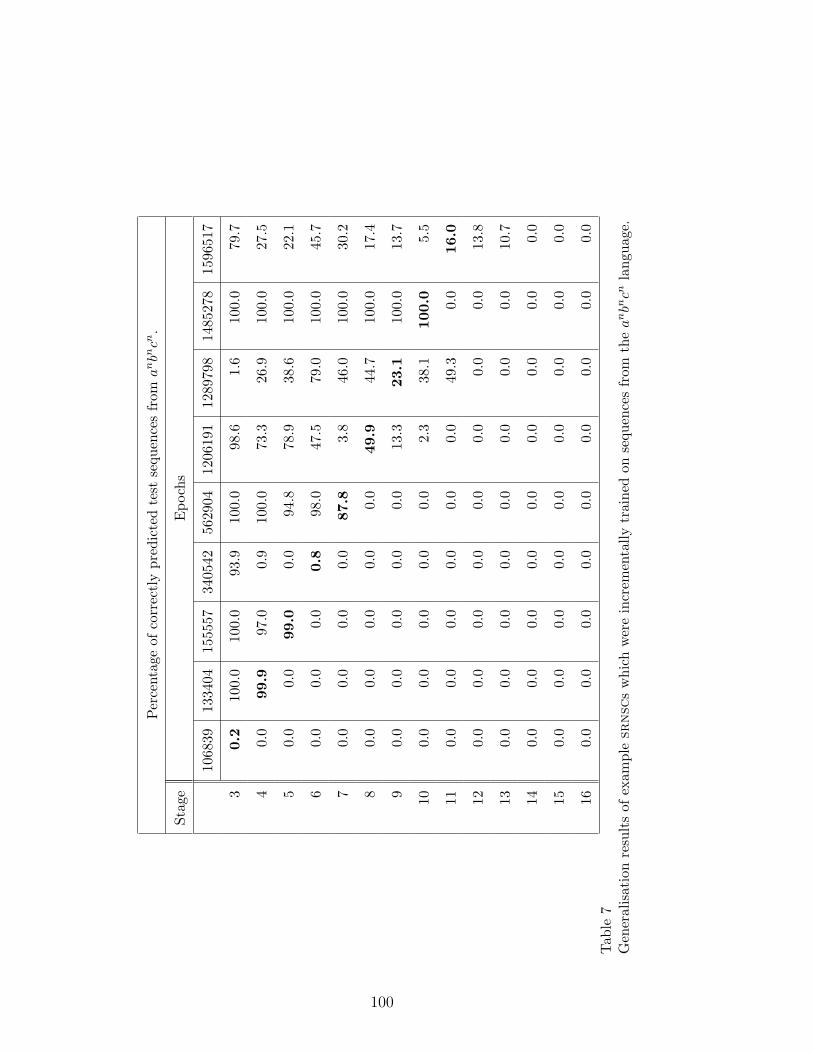
Per

cent

age

ofco

rrec

tly

pred

icte

dte

stse

quen

ces

from

anbn

cn.

Stag

eE

poch

s

1068

3913

3404

1555

5734

0542

5629

0412

0619

112

8979

814

8527

815

9651

7

30.

210

0.0

100.

093

.910

0.0

98.6

1.6

100.

079

.7

40.

099

.997

.00.

910

0.0

73.3

26.9

100.

027

.5

50.

00.

099

.00.

094

.878

.938

.610

0.0

22.1

60.

00.

00.

00.

898

.047

.579

.010

0.0

45.7

70.

00.

00.

00.

087

.83.

846

.010

0.0

30.2

80.

00.

00.

00.

00.

049

.944

.710

0.0

17.4

90.

00.

00.

00.

00.

013

.323

.110

0.0

13.7

100.

00.

00.

00.

00.

02.

338

.110

0.0

5.5

110.

00.

00.

00.

00.

00.

049

.30.

016

.0

120.

00.

00.

00.

00.

00.

00.

00.

013

.8

130.

00.

00.

00.

00.

00.

00.

00.

010

.7

140.

00.

00.

00.

00.

00.

00.

00.

00.

0

150.

00.

00.

00.

00.

00.

00.

00.

00.

0

160.

00.

00.

00.

00.

00.

00.

00.

00.

0Tab

le7

Gen

eral

isat

ion

resu

lts

ofex

ampl

esr

nsc

sw

hich

wer

ein

crem

enta

llytr

aine

don

sequ

ence

sfr

omth

ea

nbn

cnla

ngua

ge.

100

Percentage of correctly predicted test sequences from anbncn.

Stage Epochs

106839 133404 155557 340542 562904 1206191 1289798 1485278 1596517

3 0.2 100.0 100.0 93.9 100.0 98.6 1.6 100.0 79.7

4 0.0 99.9 97.0 0.9 100.0 73.3 26.9 100.0 27.5

5 0.0 0.0 99.0 0.0 94.8 78.9 38.6 100.0 22.1

6 0.0 0.0 0.0 0.8 98.0 47.5 79.0 100.0 45.7

7 0.0 0.0 0.0 0.0 87.8 3.8 46.0 100.0 30.2

8 0.0 0.0 0.0 0.0 0.0 49.9 44.7 100.0 17.4

9 0.0 0.0 0.0 0.0 0.0 13.3 23.1 100.0 13.7

10 0.0 0.0 0.0 0.0 0.0 2.3 38.1 100.0 5.5

11 0.0 0.0 0.0 0.0 0.0 0.0 49.3 0.0 16.0

12 0.0 0.0 0.0 0.0 0.0 0.0 0.0 0.0 13.8

13 0.0 0.0 0.0 0.0 0.0 0.0 0.0 0.0 10.7

14 0.0 0.0 0.0 0.0 0.0 0.0 0.0 0.0 0.0

15 0.0 0.0 0.0 0.0 0.0 0.0 0.0 0.0 0.0

16 0.0 0.0 0.0 0.0 0.0 0.0 0.0 0.0 0.0

LEGEND FOR TABLE 7:

Generalisation results of example srnscs which were incrementally trained on

sequences from the anbncn language.

102