example doppler measurements - contest university

[email protected]

Example Doppler Measurements Measurements by Steven Reyer WA9VNJ (SK)

[email protected]

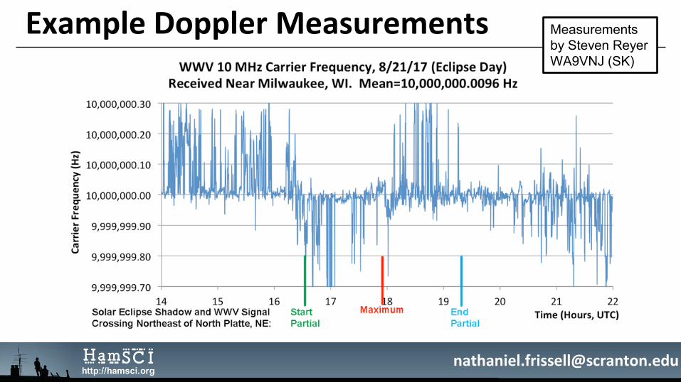
Example Doppler Measurements

WA9VNJ Frequency RecordWA9VNJ Frequency Record with Superimposed

Envelope Estimation

Envelope estimation with 7.5 minute timing markers superimposed over data record to allow manual digitization for computer analysis.

Analysis by Steve Cerwin WA5FRF

[email protected]

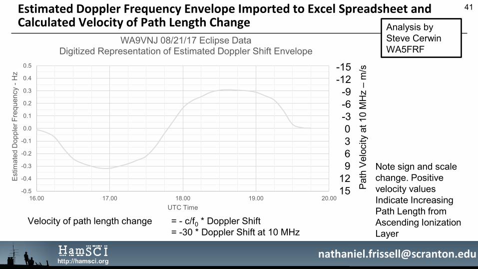
Estimated Doppler Frequency Envelope Imported to Excel Spreadsheet and Calculated Velocity of Path Length Change

41

-0.5

-0.4

-0.3

-0.2

-0.1

0.0

0.1

0.2

0.3

0.4

0.5

16.00 17.00 18.00 19.00 20.00

Estim

ated

Dop

pler

Fre

quen

cy -

Hz

UTC Time

WA9VNJ 08/21/17 Eclipse DataDigitized Representation of Estimated Doppler Shift Envelope

Velocity of path length change = - c/f0 * Doppler Shift = -30 * Doppler Shift at 10 MHz

-15-12-9-6-30369

1215 Pa

th V

eloc

ity a

t 10

MH

z –

m/s

Note sign and scale change. Positive velocity values Indicate Increasing Path Length from Ascending Ionization Layer


[email protected]

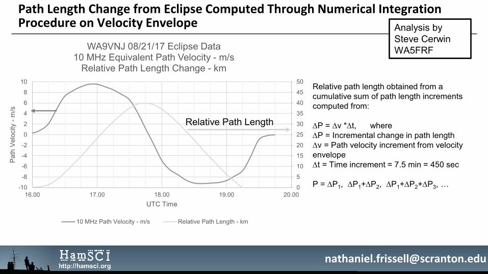
Path Length Change from Eclipse Computed Through Numerical Integration Procedure on Velocity Envelope

0

5

10

15

20

25

30

35

40

45

50

-10

-8

-6

-4

-2

0

2

4

6

8

10

16.00 17.00 18.00 19.00 20.00

Path

Vel

ocity

-m

/s

UTC Time

WA9VNJ 08/21/17 Eclipse Data10 MHz Equivalent Path Velocity - m/s

Relative Path Length Change - km

10 MHz Path Velocity - m/s Relative Path Length - km

Relative Path Length

Relative path length obtained from a cumulative sum of path length increments computed from:

'P = 'v *'t, where'P = Incremental change in path length'v = Path velocity increment from velocity envelope't = Time increment = 7.5 min = 450 sec

P = 'P1, 'P1+'P2, 'P1+'P2+'P3, …


[email protected]

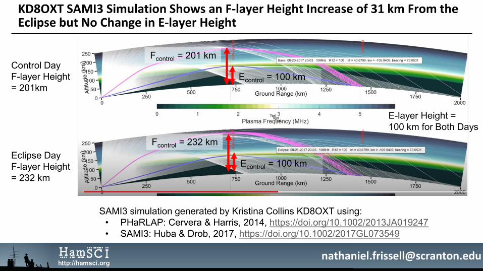
KD8OXT SAMI3 Simulation Shows an F-layer Height Increase of 31 km From the Eclipse but No Change in E-layer Height

SAMI3 simulation generated by Kristina Collins KD8OXT using:• PHaRLAP: Cervera & Harris, 2014, https://doi.org/10.1002/2013JA019247• SAMI3: Huba & Drob, 2017, https://doi.org/10.1002/2017GL073549

Control DayF-layer Height = 201km

Eclipse Day F-layer Height = 232 km

Fcontrol = 201 km

Econtrol = 100 km

Fcontrol = 232 km

Econtrol = 100 km

E-layer Height = 100 km for Both Days

https://doi.org/10.1002/2013JA019247

https://doi.org/10.1002/2017GL073549

[email protected]

Eclipse Study – Initial Observations• The eclipse-induced increase in layer height inferred from WA9VNJ Doppler data was 40 km. The SAMI3

simulations performed by KD8OXT showed the increase to be 32 km.Possible causes for the difference include:

• Error in the manually drawn Doppler envelope estimation.• Inaccuracies in the actual Doppler data reported by the FLDIGI frequency measuring program. • Error in the “flat earth” ray trace model used to calculate layer height from path length. This model does not take into account the curvature of the

earth and assumes straight line propagation paths with geometric reflection from a virtual reflection height instead of curved ray paths and a rounded refraction in the ionization layer.

• The F layer depictions in the SAMI3 simulations were not continuous in the video from which they were captured. It is possible the frame captures were not taken at the right time and did not reflect the actual minimum height on the control day or the maximum height during the eclipse day. Also the maximum height on the simulations was 250 km and it is possible higher layer predictions were there but not displayed.

• The solar-terrestrial forecasts used for the simulation may not have been the actual numbers present during the eclipse.

• The data presented here assumes the measured frequency shift data resulted only from Doppler shift caused by the ascending-then-descending refraction layer. It is possible that the extra frequency shift may have been caused by wave velocity modulation. The passage of the eclipse shadow over the propagation path causes both layer height changes and rapid changes in free electron density that can decelerate and accelerate wave velocity.

• The SAMI3 simulations showed an eclipse-induced increase in F-layer height but no change in the E-layer.This prediction ties in nicely with many spectral recordings that show a steady frequency track along with mode splitting into multiple higher order modes during daily dawn and dusk transitions. This suggests that the frequency swings and mode splitting occur in the F layer while the steady track comes from the E-layer.

44Analysis by Steve Cerwin WA5FRF

[email protected]

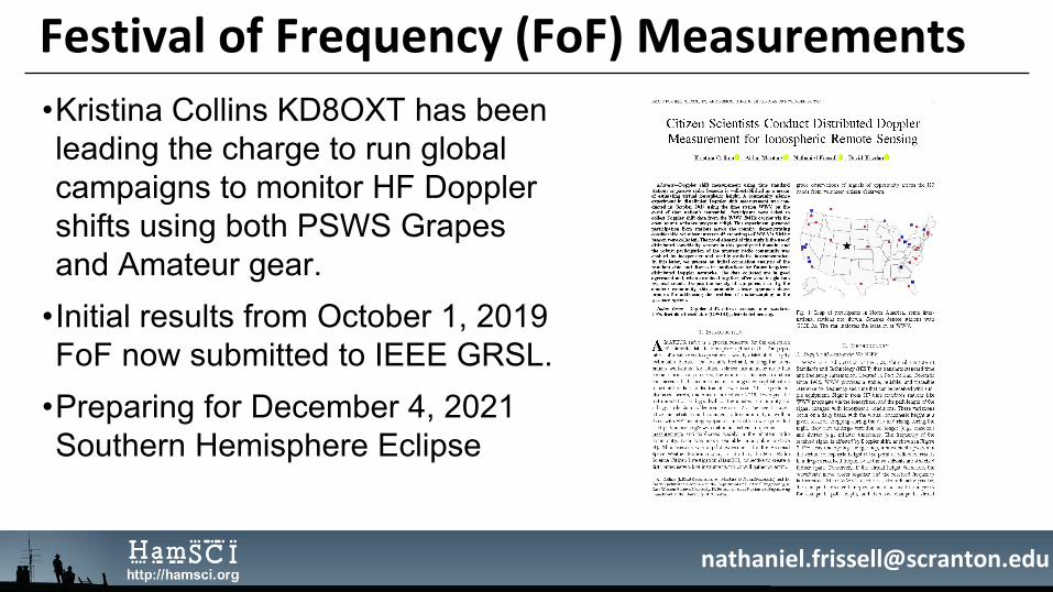
Festival of Frequency (FoF) Measurements•Kristina Collins KD8OXT has been leading the charge to run global campaigns to monitor HF Doppler shifts using both PSWS Grapes and Amateur gear.

•Initial results from October 1, 2019 FoF now submitted to IEEE GRSL.

•Preparing for December 4, 2021 Southern Hemisphere Eclipse

[email protected]

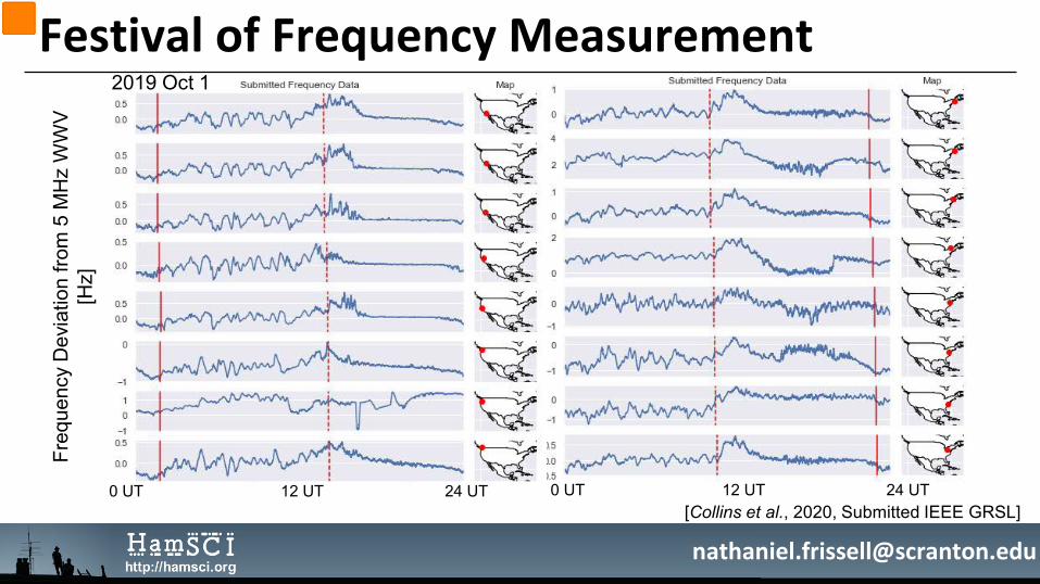
Festival of Frequency MeasurementFr

eque

ncy

Dev

iatio

n fro

m 5

MH

z W

WV

[Hz]

0 UT 12 UT 24 UT 0 UT 12 UT 24 UT

2019 Oct 1

[Collins et al., 2020, Submitted IEEE GRSL]

Presenter

Presentation Notes

Case Western PhD student Kristina Collins has led a number of national and international campaigns to collect data to help with Grape development. The observations shown here, recently submitted to IEEE Geophysical Remote Sensing Letters, show 5 MHz WWV observed frequency deviations over a 24 hour period during the October 1st, 2019 “Festival of Frequency” campaign. The nighttime observations all show wave-like variations with periodicities about 1 hour; the daytime observations are more quiescent.

[email protected]

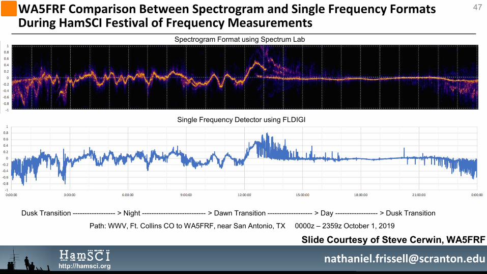
Spectrogram Format using Spectrum Lab

Single Frequency Detector using FLDIGI

WA5FRF Comparison Between Spectrogram and Single Frequency Formats During HamSCI Festival of Frequency Measurements

47

Dusk Transition ------------------ > Night --------------------------- > Dawn Transition ------------------- > Day ------------------ > Dusk Transition

Path: WWV, Ft. Collins CO to WA5FRF, near San Antonio, TX 0000z – 2359z October 1, 2019

Slide Courtesy of Steve Cerwin, WA5FRF

Presenter

Presentation Notes

Here are two 24-hour recordings of 5 MHz WWV taken during the HamSCI Festival of Frequency Measurements. The top trace is a spectrogram obtained using Spectrum Lab. The lower trace is a frequency record obtained with FLDIGI. The difference is Spectrum Lab presents an FFT spectrum analysis at each sample interval whereas FLDIGI outputs only the single frequency value of the strongest signal present in each time slot. When the actual frequency track is mostly single valued, such as during the middle parts of the day and night, the two show good agreement. But during the dawn and dusk transition periods the spectrogram is clearly the better choice. It faithfully represents each frequency component present in mode splitting whereas the single frequency measurement outputs a noisy band of frequency values that results as the different amplitudes capture the FM demodulator. While the single frequency format works well for frequency measurement, an in-depth analysis of propagation phenomena requires the spectrogram format.

[email protected]

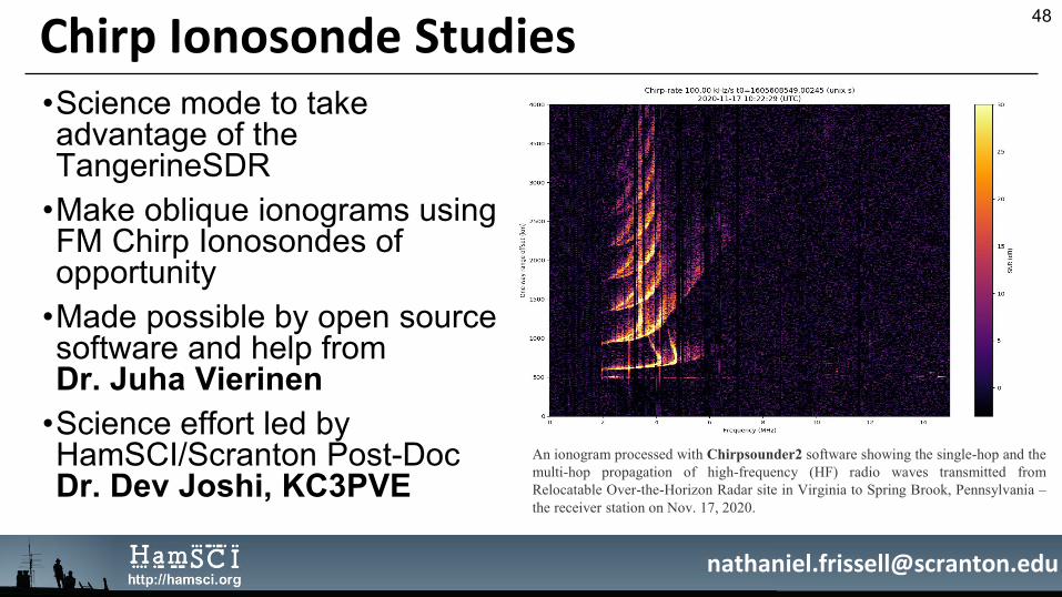
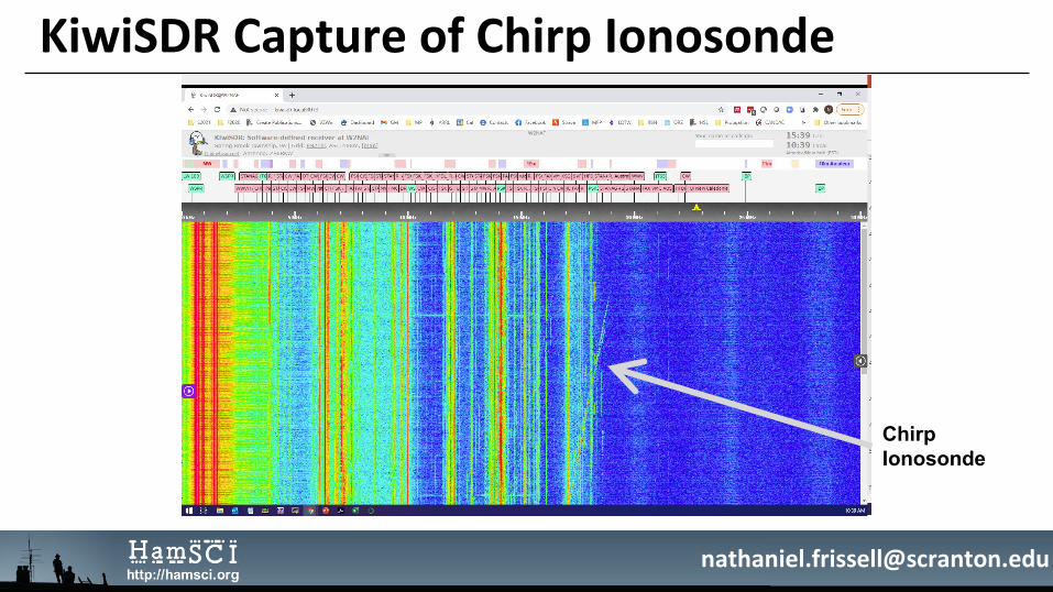
Chirp Ionosonde Studies•Science mode to take advantage of the TangerineSDR

•Make oblique ionograms using FM Chirp Ionosondes of opportunity

•Made possible by open sourcesoftware and help fromDr. Juha Vierinen

•Science effort led by HamSCI/Scranton Post-Doc Dr. Dev Joshi, KC3PVE

48

An ionogram processed with Chirpsounder2 software showing the single-hop and themulti-hop propagation of high-frequency (HF) radio waves transmitted fromRelocatable Over-the-Horizon Radar site in Virginia to Spring Brook, Pennsylvania –the receiver station on Nov. 17, 2020.

[email protected]

KiwiSDR Capture of Chirp Ionosonde

ChirpIonosonde

[email protected]

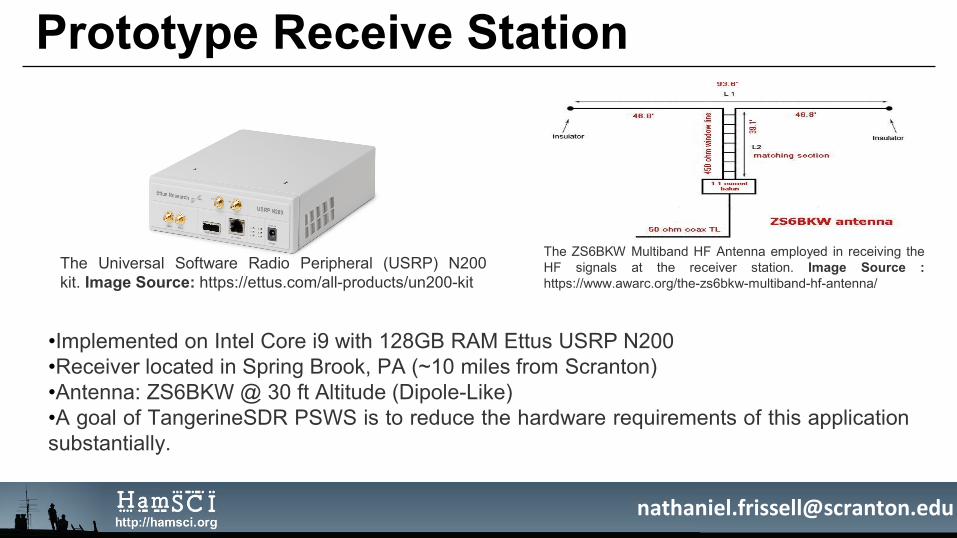
Prototype Receive Station

•Implemented on Intel Core i9 with 128GB RAM Ettus USRP N200•Receiver located in Spring Brook, PA (~10 miles from Scranton)•Antenna: ZS6BKW @ 30 ft Altitude (Dipole-Like)•A goal of TangerineSDR PSWS is to reduce the hardware requirements of this applicationsubstantially.

The ZS6BKW Multiband HF Antenna employed in receiving theHF signals at the receiver station. Image Source :https://www.awarc.org/the-zs6bkw-multiband-hf-antenna/

The Universal Software Radio Peripheral (USRP) N200kit. Image Source: https://ettus.com/all-products/un200-kit

[email protected]

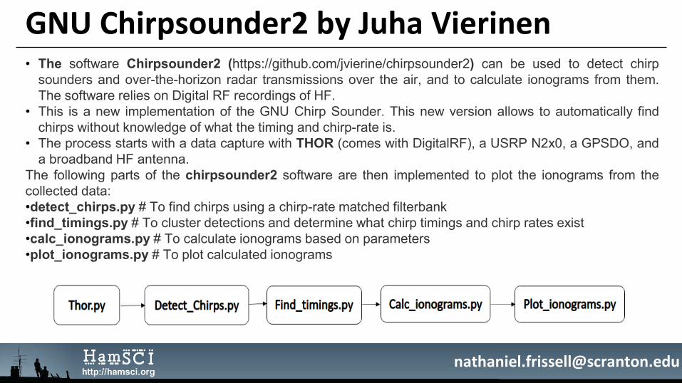
GNU Chirpsounder2 by Juha Vierinen• The software Chirpsounder2 (https://github.com/jvierine/chirpsounder2) can be used to detect chirp

sounders and over-the-horizon radar transmissions over the air, and to calculate ionograms from them.The software relies on Digital RF recordings of HF.

• This is a new implementation of the GNU Chirp Sounder. This new version allows to automatically findchirps without knowledge of what the timing and chirp-rate is.

• The process starts with a data capture with THOR (comes with DigitalRF), a USRP N2x0, a GPSDO, anda broadband HF antenna.

The following parts of the chirpsounder2 software are then implemented to plot the ionograms from thecollected data:•detect_chirps.py # To find chirps using a chirp-rate matched filterbank•find_timings.py # To cluster detections and determine what chirp timings and chirp rates exist•calc_ionograms.py # To calculate ionograms based on parameters•plot_ionograms.py # To plot calculated ionograms

[email protected]

Chirp Ionosonde Studies

[Joshi et al., 2020, https://github.com/jvierine/chirpsounder2]17 Nov 2020

Presenter

Presentation Notes

The capabilities of the TangerineSDR-based PSWS include emulating the Grape PSWS, observing WSPRNet and FT8 amateur radio transmissions, and providing precision raw spectrum observations. Additionally, through a collaboration with Juha Vierinen at the University of Tromsø, we are developing the capability to create oblique ionograms from chirp ionosondes of opportunity. This movie is an example of ionograms from the Virginia ROTHR radar received near Scranton, Pennsylvania. In this movie, you can observe rich ionospheric dynamics, including traveling ionospheric disturbances.

[email protected]

Monday Night TangerineSDR Telecons•Engineering-focused telecon to support

•TangerineSDR development•Magnetometer module development•TangerineSDR-based PSWS

•Monday nights at 9 PM Eastern•Hosted by TAPR andThe University of Scranton

•Zoom link, calendar, and archives at https://hamsci.org/get-involved

53

https://hamsci.org/get-involved

[email protected]

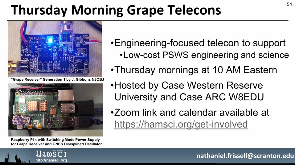
Thursday Morning Grape Telecons

•Engineering-focused telecon to support•Low-cost PSWS engineering and science

•Thursday mornings at 10 AM Eastern•Hosted by Case Western Reserve University and Case ARC W8EDU

•Zoom link and calendar available at https://hamsci.org/get-involved

54

“Grape Receiver” Generation 1 by J. Gibbons N8OBJ

Raspberry Pi 4 with Switching Mode Power Supply for Grape Receiver and GNSS Disciplined Oscillator


[email protected]

Thursday Bi-Weekly HamSCI Telecons

•Science-focused telecon to support HamSCI Science

•Every other Thursday 3 PM Eastern•Hosted by The University of Scranton•Contributed speakers are welcome!•Zoom link, calendar, and archives at https://hamsci.org/get-involved

55


[email protected]

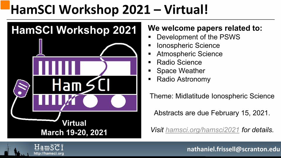
HamSCI Workshop 2021 – Virtual!HamSCI Workshop 2021

VirtualMarch 19-20, 2021

We welcome papers related to: Development of the PSWS Ionospheric Science Atmospheric Science Radio Science Space Weather Radio Astronomy

Theme: Midlatitude Ionospheric Science

Abstracts are due February 15, 2021.

Visit hamsci.org/hamsci2021 for details.

Presenter

Presentation Notes

The work shown in this presentation, as well as the work of many other amateur radio operators, citizen scientists, and space scientists, will be discussed in more detail at the 2021 Virtual HamSCI workshop. Please consider joining us!

https://hamsci.org/hamsci2021

[email protected]

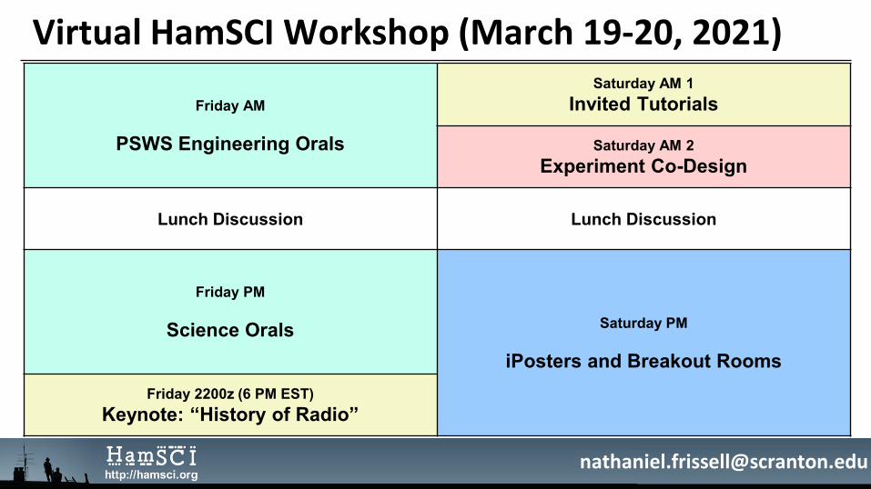
Friday AM

PSWS Engineering Orals

Saturday AM 1Invited Tutorials

Saturday AM 2Experiment Co-Design

Lunch Discussion Lunch Discussion

Friday PM

Science Orals Saturday PM

iPosters and Breakout RoomsFriday 2200z (6 PM EST)

Keynote: “History of Radio”

Virtual HamSCI Workshop (March 19-20, 2021)

[email protected]

Invited Scientist TutorialInvited Scientist Tutorial

Midlatitude Ionospheric PhysicsDr. J. Michael Ruohoniemi

The midlatitudes are where the bulk of humanity live and radio amateurs operate, however this region has traditionally been considered “quiet” compared to the auroral zone and equatorial region and therefore has received less scientific attention.

In this tutorial, Dr. Ruohoniemi will present a review of the physics of the midlatitude ionosphere, discuss recent advancements and open questions at the frontiers of research, and consider means by which the amateur radio community can contribute to advancing scientific understanding and technical capabilities.

Dr. J. Michael Ruohoniemi is a professor of electrical engineering at Virginia Tech and Principal Investigator of the Virginia Tech SuperDARN Laboratory.

Presenter

Presentation Notes

Abstract: The midlatitude portion of the ionosphere is located roughly between 30° and 60° magnetic latitude, where the vast majority of radio amateurs operate. The midlatitude ionosphere has historically been considered less ‘active’ than the high-latitude auroral regions or the low-latitude equatorial zone and has received less scientific attention. However, the bulk of humanity lives at these latitudes and major vulnerabilities to space weather disturbance are found there. Some will be well-known to radio amateurs operating HF communications links. Increased interest in the midlatitude ionosphere has spurred the deployment of new observational facilities such as the midlatitude component of SuperDARN and the Personal Space Weather Station. In this tutorial, Dr. Ruohoniemi will present a review of the physics of the midlatitude ionosphere, discuss recent advancements and open questions at the frontiers of research, and consider means by which the amateur radio community can contribute to advancing scientific understanding and technical capabilities. Bio: Dr. J. Michael Ruohoniemi is a professor of electrical engineering at Virginia Tech and Principal Investigator of the Virginia Tech Super Dual Auroral Radar Network (SuperDARN) Laboratory. Dr. Ruohoniemi earned his B.S. from the University of King's College and Dalhousie University, Nova Scotia in 1981 and his Ph.D. from the University of Western Ontario in 1986. After graduation he joined the team at the Johns Hopkins University Applied Physics Laboratory that developed HF radar into the SuperDARN concept to study the auroral (high-latitude) ionosphere. As a faculty member at Virginia Tech, he led a consortium of universities in building a chain of SuperDARN radars at midlatitudes across the U.S. His scientific publications now have over 9,700 citations. Today, 12 of the more than 30 radars in the SuperDARN network make continuous observations of the midlatitude ionosphere in both hemispheres, and these observations have been instrumental in advancing midlatitude ionospheric science in numerous studies.

[email protected]

Invited Amateur TutorialInvited Amateur Tutorial

Amateur Radio Observations andThe Science of Midlatitude Sporadic E

Joseph Dzekevich K1YOW

Amateurs may ask, “How are sporadic-E transatlantic VHF communications possible between North America and Europe?”

In his tutorial, Joe K1YOW will explain what Sporadic E is, how amateur operators use Sporadic E to enable long-distance VHF communications, current theories of Sporadic E formation, and how we might be able to better understand Es formation by examining amateur radio propagation logs.

Joe’s studies of Sporadic E using amateur radio have been published both in QST (2017) and CQ Magazine (2020).

Presenter

Presentation Notes

Abstract: Amateurs may ask, “Why do we see Sporadic E like propagation in November and December, when many of the variables like UV radiation and solar exposure are at a minimum, unlike the very active sporadic-E summer months?” How are sporadic-E transatlantic VHF communications possible between North America and Europe? In his tutorial, Joe K1YOW will explain what Sporadic E is, how amateur operators use Sporadic E to enable long-distance VHF communications, current theories of Sporadic E formation, and how we might be able to better understand Es formation by examining amateur radio propagation logs. Joe’s studies of Sporadic E using amateur radio have been published both in QST (2017) and CQ Magazine (2020). Bio: Joe Dzekevich, K1YOW, was first licensed in 1962 and currently holds an Amateur Extra Class license. He graduated from Northeastern University in 1977 with a B.S. in Industrial Technology and holds a M.B.A. from Clark University (1985). Joe is currently a retired Reliability Engineering Fellow who has worked for Bell Telephone Labs, Digital Equipment Corporation, Chipcom/3Com and Raytheon. Joe is also a senior member of the IEEE Reliability Society, where he held various offices in the local IEEE Boston Reliability Chapter and developed and taught many of the chapter’s courses. He is a member of NVARC (Nashoba Valley Amateur Radio Club), the ARRL, and HamSCI. He has always been interested in radio propagation, starting back in 1965 where he subscribed to the CRPL (Central Radio Prediction Lab) Ionospheric Predictions, where one used monthly CRPL prediction maps to chart predicted E-Layer and F-Layer radio paths.

https://hamsci.org/sites/default/files/publications/2017_QST_Dzekevich_UpperLevelLows.pdf

https://hamsci.org/sites/default/files/publications/202011_CQ_Dzekevich_K1YOW_SporadicE.pdf

[email protected]

Keynote AddressKeynote Address

History of RadioDr. Elizabeth Bruton

This talk will explore developments in the history, science, technology, and licensing of radio amateur communities from the early 1900s through to the present day, exploring how individuals and communities contributed to “citizen science” long before the term entered popular usage in the 1990s.

Dr. Brunton will also explore how these community-led developments can inspire the next generation’s interest in science, technology, engineering, and mathematics (STEM), citizen science, and amateur radio.

Dr. Bruton is Curator of Technology and Engineering at the Science Museum, London, specializing in the history of communications. Her PhD dissertation is entitled Beyond Marconi: the roles of the Admiralty, the Post Office, and the Institution of Electrical Engineers in the invention and development of wireless communication up to 1908.

Presenter

Presentation Notes

Abstract: This talk will explore developments in the history, science, technology, and licensing of radio amateur communities from the early 1900s through to the present day, exploring how individuals and communities contributed to “citizen science” long before the term entered popular usage in the 1990s. I will also explore how these community-led developments can inspire the next generation’s interest in science, technology, engineering, and mathematics (STEM), citizen science, and amateur radio. Bio: Dr Elizabeth Bruton is Curator of Technology and Engineering at the Science Museum, London, specializing in the history of communications. Prominent aspects of this role include curator of “Top Secret: From ciphers to cyber security” exhibition, which explored over a century’s worth of communications intelligence through hand-written documents, declassified files and previously unseen artefacts from the Science Museum Group's and GCHQ’s historic collections, and serving as co-Investigator on the “Electrifying Women: Understanding the Long History of Women in Engineering”, a nine-month Arts & Humanities Research Council (AHRC) project with Professor Graeme Gooday at the University of Leeds. Dr Bruton holds three degrees: a BAI in Computer Engineering from Trinity College, Dublin (2004); an MSc in history of science from the University of Oxford (2005) with a dissertation on “Marconi Wireless Telegraphy in the British Army during World War One”; and an AHRC-funded Collaborative Doctoral Award PhD with BT Archives and IET Archives at the University of Leeds on “Beyond Marconi: the roles of the Admiralty, the Post Office, and the Institution of Electrical Engineers in the invention and development of wireless communication up to 1908” (2013). Last and definitely not least, Dr Bruton has been non-licensed member of Oxford & District Amateur Radio Society since 2014 and their web manager since 2015.

https://www.sciencemuseum.org.uk/what-was-on/top-secret

[email protected]

AcknowledgmentsThe authors gratefully acknowledge the support of NSF Grants AGS-2002278, AGS-1932997, and AGS-1932972. We are especially grateful to the amateur radio community who voluntarily produced and provided the HF radio observations used in this presentation, especially the operators of the Reverse Beacon Network (RBN, reversebeacon.net), the Weak Signal Propagation Reporting Network (WSPRNet, wsprnet.org), PSKReporter(http://pskreporter.info), qrz.com, and hamcall.net. The Kp index was accessed through the OMNI database at the NASA Space Physics Data Facility (https://omniweb.gsfc.nasa.gov/). The SYM-H index was obtained from the Kyoto World Data Center for Geomagnetism (http://wdc.kugi.kyoto-u.ac.jp/). GOES data are provided by NOAA NCEI (https://satdat.ngdc.noaa.gov/). GPS-based total electron content observations and the Madrigal distributed data system are provided to the community as part of the Millstone Hill Geospace Facility by MIT Haystack Observatory under NSF grant AGS-1762141 to the Massachusetts Institute of Technology. We acknowledge the use of the Free Open Source Software projects used in this analysis: Ubuntu Linux, python, matplotlib, NumPy, SciPy, pandas, xarray, iPython, and others.

61

Presenter

Presentation Notes

Finally, I would like to acknowledge support from the National Science Foundation, the Amateur Radio Community, my science and engineering collaborators, and the many other people who have made this project possible.

http://reversebeacon.net/

http://wsprnet.org/

http://pskreporter.info/

https://qrz.com/

http://hamcall.net/

https://omniweb.gsfc.nasa.gov/

http://wdc.kugi.kyoto-u.ac.jp/

https://satdat.ngdc.noaa.gov/

[email protected]

Thank You!

Presenter

Presentation Notes

Thank you for watching my presentation, and I hope you have a good day!

[email protected]

Acronym Glossary 63

AE Auroral Electrojet IndexBKS Blackstone, VA SuperDARN RadarGNSS Global Navigation Satellite SystemHF High Frequency (3-30 MHz)LSTID Large Scale Traveling Ionospheric DisturbanceMSTID Medium Scale Traveling Ionospheric DisturbanceRBN Reverse Beacon NetworkSAMI3 SAMI3 is Another Model IonosphereSuperDARN Super Dual Auroral Radar NetworkSym-H Symmetric-H Index (For measuring geomagnetic storms)TEC Total Electron ContentTID Traveling Ionospheric DisturbanceWSPRNet Weak Signal Propagation Reporting Network

[email protected]

AbstractdŚĞ,ĂŵZĂĚŝŽ^ĐŝĞŶĐĞŝƚŝǌĞŶ/ŶǀĞƐƚŝŐĂƚŝŽŶ;,Ăŵ^/ͿŝƐĂƉůĂƚĨŽƌŵƚŽĨŽƐƚĞƌĐŽůůĂďŽƌĂƚŝŽŶƐďĞƚǁĞĞŶƚŚĞĂŵĂƚĞƵƌ;ŚĂŵͿƌĂĚŝŽĂŶĚƉƌŽĨĞƐƐŝŽŶĂůƐƉĂĐĞƐĐŝĞŶĐĞĂŶĚƐƉĂĐĞǁĞĂƚŚĞƌĐŽŵŵƵŶŝƚŝĞƐ/ƚƐŵŝƐƐŝŽŶŝƐƚŽ;ϭͿĂĚǀĂŶĐĞƐĐŝĞŶƚŝĨŝĐƌĞƐĞĂƌĐŚĂŶĚƵŶĚĞƌƐƚĂŶĚŝŶŐƚŚƌŽƵŐŚĂŵĂƚĞƵƌƌĂĚŝŽĂĐƚŝǀŝƚŝĞƐ;ϮͿĞŶĐŽƵƌĂŐĞƚŚĞĚĞǀĞůŽƉŵĞŶƚŽĨŶĞǁƚĞĐŚŶŽůŽŐŝĞƐƚŽƐƵƉƉŽƌƚƚŚŝƐƌĞƐĞĂƌĐŚĂŶĚ;ϯͿƉƌŽǀŝĚĞĞĚƵĐĂƚŝŽŶĂůŽƉƉŽƌƚƵŶŝƚŝĞƐĨŽƌƚŚĞĂŵĂƚĞƵƌƌĂĚŝŽĐŽŵŵƵŶŝƚǇĂŶĚƚŚĞŐĞŶĞƌĂůƉƵďůŝĐ^ŝŵŝůĂƌƚŽĂŵĂƚĞƵƌĂƐƚƌŽŶŽŵǇĂŵĂƚĞƵƌƌĂĚŝŽĂůůŽǁƐŝŶĚŝǀŝĚƵĂůƐŶĞǁƚŽƚŚĞĂǀŽĐĂƚŝŽŶĂƉĂƚŚĨŽƌůĞĂƌŶŝŶŐĂŶĚƚŚŽƐĞǁŝƚŚǇĞĂƌƐŽĨĞǆƉĞƌŝĞŶĐĞĂƉůĂĐĞƚŽĂƉƉůǇƚŚĞŝƌĂĚǀĂŶĐĞĚƐŬŝůůƐdŚŝƐŝƐĂĐĐŽŵƉůŝƐŚĞĚƚŚƌŽƵŐŚĐŽůůĂďŽƌĂƚŝǀĞƉƌŽũĞĐƚƐĐŽŽƌĚŝŶĂƚĞĚĞǆƉĞƌŝŵĞŶƚƐǁŽƌŬƐŚŽƉƐƚĞůĞĐŽŶƐĂŶĚĞ-ŵĂŝůŐƌŽƵƉƐ/ŶƚŚŝƐƉƌĞƐĞŶƚĂƚŝŽŶǁĞĚĞƐĐƌŝďĞĐƵƌƌĞŶƚ,Ăŵ^/ĂĐƚŝǀŝƚŝĞƐĂǀĂŝůĂďůĞĚĂƚĂƐĞƚƐƌĞĐĞŶƚƌĞƐƵůƚƐĂŶĚĨƵƚƵƌĞƉůĂŶƐdŚŝƐŝŶĐůƵĚĞƐƚŚĞ,Ăŵ^/WĞƌƐŽŶĂů^ƉĂĐĞtĞĂƚŚĞƌ^ƚĂƚŝŽŶ;W^t^ͿƉƌŽũĞĐƚĂŶĂůǇƐŝƐŽĨŶĞĂƌ-ŐůŽďĂůĐŽŵŵƵŶŝĐĂƚŝŽŶƐŵŽŶŝƚŽƌŝŶŐŶĞƚǁŽƌŬƐƐƵĐŚĂƐƚŚĞZĞǀĞƌƐĞĞĂĐŽŶEĞƚǁŽƌŬ;ZEͿĂŶĚtĞĂŬ^ŝŐŶĂůWƌŽƉĂŐĂƚŝŽŶZĞƉŽƌƚŝŶŐEĞƚǁŽƌŬ;t^WZEĞƚͿĂŶĚĂŶĂůǇƐŝƐŽĨŽďƐĞƌǀĞĚŽƉƉůĞƌƐŚŝĨƚƐĨŽƌŚŝŐŚĨƌĞƋƵĞŶĐǇƐŝŐŶĂůƐŽĨŽƉƉŽƌƚƵŶŝƚǇ

64

[email protected]

ReferencesCervera, M. A., and Harris, T. J. (2014), Modeling ionospheric disturbance features in quasi-vertically incident ionograms using 3-D magnetoionic ray tracing and atmospheric gravity waves, J. Geophys. Res. Space Physics, 119, 431– 440, doi:10.1002/2013JA019247.Collins, K., Montare, A., Frissell, N. A., & Kazdan, D. (2020). Citizen Scientists Conduct Distributed Doppler Measurement for Ionospheric Remote Sensing. IEEE Geosci. Remote Sens. Lett., (under review).)ULVVHOO1$%DNHU-ௗ%ௗ+5XRKRQLHPL-0*HUUDUG$-0LOOHU(60DULQL-3:HVW0/DQG%ULVWRZW. A. (2014), Climatology of medium-scale traveling ionospheric disturbances observed by the midlatitude Blackstone SuperDARN radar, J. Geophys. Res. Space Physics, 119, 7679– 7697, doi:10.1002/2014JA019870.Frissell, N. A., Vega, J. S., Markowitz, E., Gerrard, A. J., Engelke, W. D., Erickson, P. J., et al. (2019). High-frequency communications response to solar activity in September 2017 as observed by amateur radio networks. Space Weather, 17, 118– 132. https://doi.org/10.1029/2018SW002008.Huba, J. D., and Drob, D. (2017), SAMI3 prediction of the impact of the 21 August 2017 total solar eclipse on the ionosphere/plasmasphere system, Geophys. Res. Lett., 44, 5928– 5935, doi:10.1002/2017GL073549.Joshi, DR, Frissell NA, Liles, W, Vierinen, J, Miller, ES (2020). Developing an Ionospheric Sounding Mode Using Chirp Ionosondes of Opportunity for the HamSCI Personal Space Weather Station : Status and Early Results. AGU Fall Meeting. Virtual.Sanchez, D., Frissell, NA, Perry, GW, Coster, A, Erickson, PJ, Engelke, WD, Ruohoniemi, JM, and Baker, JBH (2020). A Climatology of Traveling Ionospheric Disturbances Observed by High Frequency Amateur Radio Networks. AGU Fall Meeting. Virtual.

https://doi.org/10.1029/2018SW002008

[email protected]

Backup Slides

[email protected]

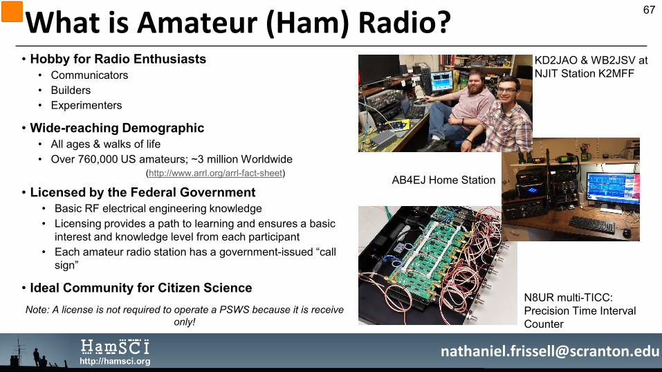
What is Amateur (Ham) Radio?• Hobby for Radio Enthusiasts

• Communicators• Builders• Experimenters

• Wide-reaching Demographic• All ages & walks of life• Over 760,000 US amateurs; ~3 million Worldwide

(http://www.arrl.org/arrl-fact-sheet)

• Licensed by the Federal Government• Basic RF electrical engineering knowledge• Licensing provides a path to learning and ensures a basic

interest and knowledge level from each participant• Each amateur radio station has a government-issued “call

sign”

• Ideal Community for Citizen ScienceNote: A license is not required to operate a PSWS because it is receive

only!

KD2JAO & WB2JSV atNJIT Station K2MFF

AB4EJ Home Station

N8UR multi-TICC:Precision Time Interval Counter

67

Presenter

Presentation Notes

The amateur radio community is an ideal community to work with for space weather citizen science. There are about 3 millions amateurs worldwide, and many already have technical training. Because high frequency radio operation is heavily affected by space weather, amateurs are often eager to participate in citizen science projects like this one.

http://www.arrl.org/arrl-fact-sheet

[email protected]

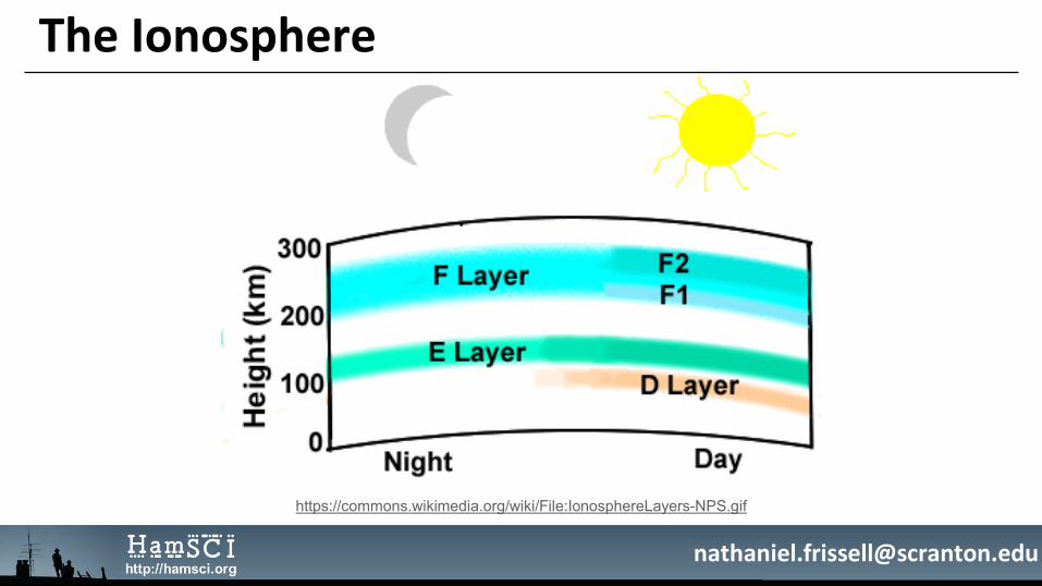
The Ionosphere

https://commons.wikimedia.org/wiki/File:IonosphereLayers-NPS.gif

https://commons.wikimedia.org/wiki/File:IonosphereLayers-NPS.gif

[email protected]

TIDs in Blackstone SuperDARN 69

[email protected]

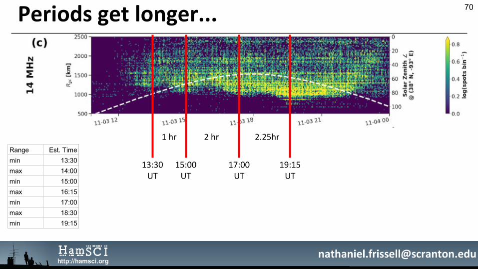
Periods get longer... 70

Range Est. Timemin 13:30max 14:00min 15:00max 16:15min 17:00max 18:30min 19:15

ϭŚƌ ϮŚƌ ϮϮϱŚƌ

ϭϯϯϬUT

ϭϱϬϬUT

ϭϳϬϬUT

ϭϵϭϱUT

[email protected]

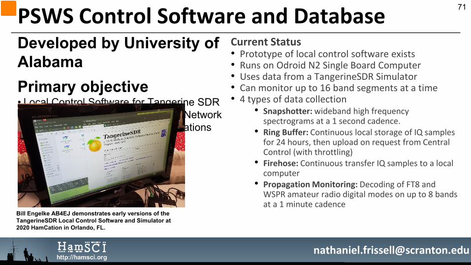
PSWS Control Software and DatabaseDeveloped by University of AlabamaPrimary objective• Local Control Software for Tangerine SDR• Central Control System for PSWS Network• Central Database to collect observations

Current Status• WƌŽƚŽƚǇƉĞŽĨůŽĐĂůĐŽŶƚƌŽůƐŽĨƚǁĂƌĞĞǆŝƐƚƐ• ZƵŶƐŽŶKĚƌŽŝĚEϮ^ŝŶŐůĞŽĂƌĚŽŵƉƵƚĞƌ• hƐĞƐĚĂƚĂĨƌŽŵĂdĂŶŐĞƌŝŶĞ^Z^ŝŵƵůĂƚŽƌ• ĂŶŵŽŶŝƚŽƌƵƉƚŽϭϲďĂŶĚƐĞŐŵĞŶƚƐĂƚĂƚŝŵĞ• ϰƚǇƉĞƐŽĨĚĂƚĂĐŽůůĞĐƚŝŽŶ

• Snapshotter: ǁŝĚĞďĂŶĚŚŝŐŚĨƌĞƋƵĞŶĐǇƐƉĞĐƚƌŽŐƌĂŵƐĂƚĂϭƐĞĐŽŶĚĐĂĚĞŶĐĞ

• Ring Buffer: ŽŶƚŝŶƵŽƵƐůŽĐĂůƐƚŽƌĂŐĞŽĨ/YƐĂŵƉůĞƐĨŽƌϮϰŚŽƵƌƐƚŚĞŶƵƉůŽĂĚŽŶƌĞƋƵĞƐƚĨƌŽŵĞŶƚƌĂůŽŶƚƌŽů;ǁŝƚŚƚŚƌŽƚƚůŝŶŐͿ

• Firehose: ŽŶƚŝŶƵŽƵƐƚƌĂŶƐĨĞƌ/YƐĂŵƉůĞƐƚŽĂůŽĐĂůĐŽŵƉƵƚĞƌ

• Propagation Monitoring: ĞĐŽĚŝŶŐŽĨ&dϴĂŶĚt^WZĂŵĂƚĞƵƌƌĂĚŝŽĚŝŐŝƚĂůŵŽĚĞƐŽŶƵƉƚŽϴďĂŶĚƐĂƚĂϭŵŝŶƵƚĞĐĂĚĞŶĐĞ

Bill Engelke AB4EJ demonstrates early versions of the TangerineSDR Local Control Software and Simulator at 2020 HamCation in Orlando, FL.

71

Presenter

Presentation Notes

I am now going to give a brief update on the status of each team and the specifications of their respective projects. The Personal Space Weather Station Control Software and Database is being developed by the University of Alabama. The Primary objective is to create local control software for Tangerine SDR, a central control system for PSWS Network, and a central database to collect observations. Currently, a prototype of the local control software exists and runs on a Odroid N2 Single Board Computer. This system uses data from a TangerineSDR Simulator, can monitor up to 16 band segments at a time, and 4 types of data collection implemented: Snapshotter: Provides wideband high frequency spectrograms at a 1 second cadence. Ring buffer: Continuous local storage of IQ samples for 24 hours, then upload on request from Central Control. Firehose: Continuous transfer IQ samples to a local computer Propagation Monitoring: Decoding of FT8 and WSPR amateur radio digital modes on up to 8 bands at a 1 minute cadence

[email protected]

Scientific SDR (TangerineSDR)Developed as “TangerineSDR” by TAPRData Engine Specifications• Altera/Intel 10M50DAF672C6G FPGA 50K LEs• 512MByte (256Mx16) DDR3L SDRAM• 4Mbit (512K x 8) QSPI serial flash memory• 512Kbit (64K x 8) serial EEPROM• ȝ6';&PHPRU\FDUGXSWR7%\WH

Data Engine Features• 11-15V wide input, low noise SMPS• 3-port GbESwitch (Dual GbEdata interfaces)• Cryptographic processor with key storage• Temperature sensors (FPGA, ambient)• Power-on reset monitor, fan header

RF Module• ϵϲϰϴϭϮϱĚƵĂůϭϰďŝƚϭϮϮϴϴDƐƉƐ• ϬĚϭϬĚϮϬĚϯϬĚƌĞŵŽƚĞůǇƐǁŝƚĐŚĂďůĞĂƚƚĞŶƵĂƚŽƌ

• >dϲϰϮϬϮϬϮϬĚ>E• &ŝǆĞĚϱϱD,ǌ>ŽǁWĂƐƐ&ŝůƚĞƌ• KƉƚŝŽŶĂůƵƐĞƌĚĞĨŝŶĞĚƉůƵŐŝŶĨŝůƚĞƌ• KŶ-ďŽĂƌĚϱϬɏ ĐĂůŝďƌĂƚŝŽŶŶŽŝƐĞƐŽƵƌĐĞ• KŶ-ďŽĂƌĚůŽǁŶŽŝƐĞƉŽǁĞƌƐƵƉƉůŝĞƐ• ƵĂů^DĂŶƚĞŶŶĂĐŽŶŶĞĐƚŽƌƐ

GNSS/Timing Module• WƌĞĐŝƐŝŽŶƚŝŵĞƐƚĂŵƉŝŶŐ;ϭϬƚŽϭϬϬŶƐĂĐĐƵƌĂĐǇͿ• &ƌĞƋƵĞŶĐǇƌĞĨĞƌĞŶĐĞ;WĂƌƚƐŝŶϭϬϭϯ ŽǀĞƌϮϰŚƌͿ

Current Status• WƌŽƚŽƚǇƉĞƐĞǆƉĞĐƚĞĚďǇ&ĂůůϮϬϮϬ• DŽƌĞŝŶĨŽƌŵĂƚŝŽŶĂƚƚĂŶŐĞƌŝŶĞƐĚƌĐŽŵ

72

Presenter

Presentation Notes

The scientific software defined radio is being developed as the TangerineSDR by TAPR. It consists of a data engine, a Radio Frequency (or RF) module, and a timing module. The Data Engine includes a 50,000 logic element FPGA, 512 MB of RAM, Gigabit ethernet, and can support up to 2 TB on a micro SD card. The data engine will be able to simultaneously support two separate RF modules. The RF receive module features dual synchronized 14 bit 122.88 Msps Analog to Digital Converters with dual SMA antenna connectors as input. It includes remotely switchable attenuation, a 20 dB low noise amplifier, a fixed 55 MHz low pass filter, an on-board 50Ω calibration noise source, and a place for an optional user-defined plug-in filter. The GNSS timing module will be dual frequency to provide precision timestamping with 10 to 100 ns accuracy and a frequency reference accurate to parts in 10^13 over 24 hours. Currently, prototypes are expected by Fall 2020. More information is available at tangerinesdr.com.

http://tangerinesdr.com/

[email protected]

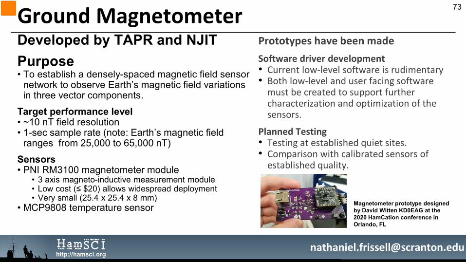
Ground MagnetometerDeveloped by TAPR and NJITPurpose• To establish a densely-spaced magnetic field sensor

network to observe Earth’s magnetic field variations in three vector components.

Target performance level• ~10 nT field resolution• 1-sec sample rate (note: Earth’s magnetic field

ranges from 25,000 to 65,000 nT)Sensors• PNI RM3100 magnetometer module

• 3 axis magneto-inductive measurement module• /RZFRVWDOORZVZLGHVSUHDGGHSOR\PHQW• Very small (25.4 x 25.4 x 8 mm)

• MCP9808 temperature sensor

Prototypes have been madeSoftware driver development• ƵƌƌĞŶƚůŽǁ-ůĞǀĞůƐŽĨƚǁĂƌĞŝƐƌƵĚŝŵĞŶƚĂƌǇ• ŽƚŚůŽǁ-ůĞǀĞůĂŶĚƵƐĞƌĨĂĐŝŶŐƐŽĨƚǁĂƌĞŵƵƐƚďĞĐƌĞĂƚĞĚƚŽƐƵƉƉŽƌƚĨƵƌƚŚĞƌĐŚĂƌĂĐƚĞƌŝǌĂƚŝŽŶĂŶĚŽƉƚŝŵŝǌĂƚŝŽŶŽĨƚŚĞƐĞŶƐŽƌƐ

Planned Testing• dĞƐƚŝŶŐĂƚĞƐƚĂďůŝƐŚĞĚƋƵŝĞƚƐŝƚĞƐ• ŽŵƉĂƌŝƐŽŶǁŝƚŚĐĂůŝďƌĂƚĞĚƐĞŶƐŽƌƐŽĨĞƐƚĂďůŝƐŚĞĚƋƵĂůŝƚǇ

Magnetometer prototype designed by David Witten KD0EAG at the 2020 HamCation conference in Orlando, FL

73

Presenter

Presentation Notes

The ground magnetometer module is being developed by TAPR and NJIT. Its purpose is to establish a densely-spaced magnetic field sensor network to observe Earth’s magnetic field variations in three vector components. The target performance level is about 10 nT field resolution with a 1 second cadence. The magneto-inductive PNI RM3100 magnetometer module will be used. The magnetometer module will also include a temperature sensor. Prototypes have been made, and software development is underway. Testing is planned at established quiet sites with co-located research-grade magnetometers, such as at the Jenny Jump Observatory in Hope, New Jersey.

[email protected]

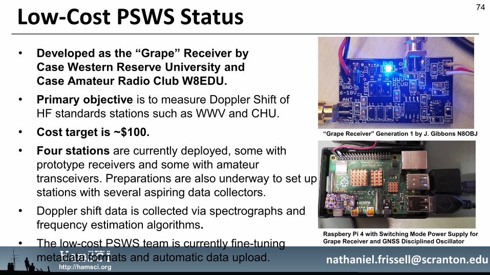
Low-Cost PSWS Status• Developed as the “Grape” Receiver by

Case Western Reserve University andCase Amateur Radio Club W8EDU.

• Primary objective is to measure Doppler Shift of HF standards stations such as WWV and CHU.

• Cost target is ~$100.• Four stations are currently deployed, some with

prototype receivers and some with amateur transceivers. Preparations are also underway to set up stations with several aspiring data collectors.

• Doppler shift data is collected via spectrographs and frequency estimation algorithms.

• The low-cost PSWS team is currently fine-tuning metadata formats and automatic data upload.

“Grape Receiver” Generation 1 by J. Gibbons N8OBJ

74

Raspbery Pi 4 with Switching Mode Power Supply for Grape Receiver and GNSS Disciplined Oscillator

[email protected]

[Tsugawa et al., 2007, doi:10.1029/2007GL031663]

௦ܫ =140.3

ଵଶଶଶ

ଵଶ െ ଶ

ଶ ଵܮ െ ଶܮ െ ଵଵߣ െ ଶଶߣ + + ௦

SlantTEC

FrequencyTerms

Recorded carrier

phases of the signal

(converted to distance

units)

Integer cycle ambiguities

Instrument (satellite and receiver) bias

terms

f1 = 1575.42 MHz (GPS L1)f2 = 1227.60 MHz (GPS L2)1 TECU = 1016 Electrons m-2

What is Total Electron Content (TEC)? 75

http://doi.org/10.1029/2007GL031663

example doppler measurements - contest university

Documents