examples of conformal maps and of critical pointstoledo/confmap.pdf · 2013. 9. 25. · examples of...
TRANSCRIPT

Examples of Conformal Maps and of Critical PointsWe know that an analytic function f(z) is conformal (preserves angles and
orientation) at all points where the derivative f’(z) is not zero. Here we look at
some examples of analytic functions that illustrate that they are conformal
maps. They also show what happens at places where f’(z) = 0.
To understand the pictures, we first draw the standard mesh of horizontal and
vertical lines in the complex plane, then we plot the resulting mesh under the
function f(z). The curves in this mesh meet at right angles, which is consistent
with conformal. To know that the map is conformal, we also need to know that
the curves in the mesh are moving at the same speed at any given point of
intersection.
In the pictures we will also see what happens at the Critical Points. These are,
by definition, the points where f’(z) = 0.
To begin, draw the standarad mesh in the z-plane:
ParametricPlotA9ReAHu + ä vL1E, ImAHu + ä vL1E=,
8u, -2, 2<, 8v, -2, 2<, MeshStyle ® 8Black, Red<, PlotRange ® 2E

-2 -1 0 1 2-2
-1
0
1
2
2 ConfMap1Post2.nb

As a first example, draw is image under the squaring function z -> z^2:
ParametricPlotA9ReAHu + ä vL2E, ImAHu + ä vL2E=,
8u, -2, 2<, 8v, -2, 2<, Mesh ® 30, MeshStyle ® 8Black, Red<E
-4 -2 0 2 4
-5
0
5
Observe that they indeed meet at right angles, except at the critical point z = 0. Here’s another view:
ConfMap1Post2.nb 3
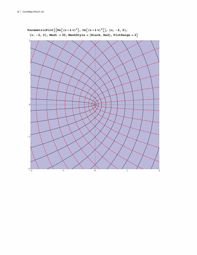
Observe that they indeed meet at right angles, except at the critical point z = 0. Here’s another view:
ParametricPlotA9ReAHu + ä vL2E, ImAHu + ä vL2E=, 8u, -2, 2<,
8v, -2, 2<, Mesh ® 30, MeshStyle ® 8Black, Red<, PlotRange ® 2E
-2 -1 0 1 2-2
-1
0
1
2
4 ConfMap1Post2.nb

Observe what happens at the critical point. The red curves bunch up on the positive real axis, the black ones on the negative real axis. This is because the real axis maps 2:1 on the positive real axis, while the imaginary axis maps 2:1 on the negative real axis. So the 90 degree angle at the origin beween the real and imaginary axes gets stretched to a 180 degree angle.
We know that z -> z^2 is 2:1, it cannot be inverted. But it is 1:1 when restricted to the open half-plane bound by any line through 0, in particular the imaginary axis. The folloiwing illustrates the image of the half-plane Re(z) > 0, which is the plane slit along the negative real axis:
ParametricPlotA9ReAHu + ä vL2E, ImAHu + ä vL2E=, 8u, .02, 2<,
8v, -2, 2<, Mesh ® 30, MeshStyle ® 8Black, Red<, PlotRange ® 2E
-2 -1 0 1 2-2
-1
0
1
2
ConfMap1Post2.nb 5
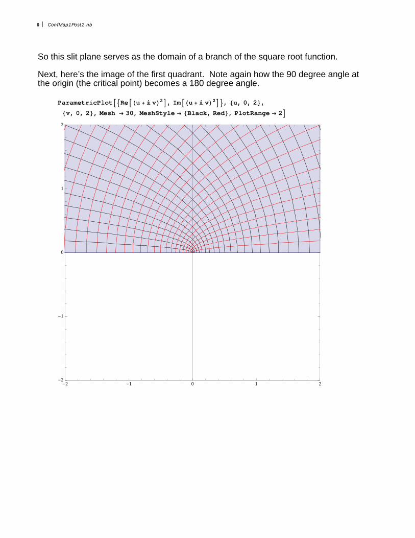
So this slit plane serves as the domain of a branch of the square root function.
Next, here’s the image of the first quadrant. Note again how the 90 degree angle at the origin (the critical point) becomes a 180 degree angle.
ParametricPlotA9ReAHu + ä vL2E, ImAHu + ä vL2E=, 8u, 0, 2<,
8v, 0, 2<, Mesh ® 30, MeshStyle ® 8Black, Red<, PlotRange ® 2E
-2 -1 0 1 2-2
-1
0
1
2
6 ConfMap1Post2.nb

Finally the image of the upper-half plane Im(z) > 0. This is the plane slit along the positive real axis. It would be the the domain of another branch of the square root, one not defined on positive real numbers.
ParametricPlotA9ReAHu + ä vL2E, ImAHu + ä vL2E=, 8u, -2, 2<,
8v, .02, 2<, Mesh ® 30, MeshStyle ® 8Black, Red<, PlotRange ® 2E
-2 -1 0 1 2-2
-1
0
1
2
ConfMap1Post2.nb 7

We can also draw picures in polar coordinates, the first indicating that z -> z^2 is 2:1, the second showing the image of -Pi / 2 < arg(z) < Pi / 2, the same as the half-plane Re(z) > 0.
ParametricPlotA9ReAHu Exp@I vDL2E, ImAHu Exp@I vDL2E=,
8u, 0, 2<, 8v, 0, 2 Pi<, Mesh ® 30, MeshStyle ® 8Black, Red<E
-4 -2 0 2 4
-4
-2
0
2
4
ParametricPlotA9ReAHu Exp@I vDL2E, ImAHu Exp@I vDL2E=, 8u, 0, 2<,
8v, -Pi � 2 + .02, Pi � 2 - .02<, Mesh ® 30, MeshStyle ® 8Black, Red<E
-4 -2 0 2 4-4
-2
0
2
4
8 ConfMap1Post2.nb

Now to z -> z^3, which should be more complicated than z -> z^2 since now not only f’(0) = 0 but in addition the second derivative f’’(0) = 0.
ParametricPlotA9Re@Hu + ä vL^3D, ImAHu + ä vL3E=,
8u, -2, 2<, 8v, -2, 2<, Mesh ® 20, MeshStyle ® 8Black, Red<E
-15 -10 -5 0 5 10 15
-15
-10
-5
0
5
10
15
ConfMap1Post2.nb 9

To understand this picture, look at the image of each quadrant. At the critical point at the origin the 90 degree angle gets multiplied by 3. The next four pictures give the image of each quadrant. You could piece them together to see how they fit into the original picture. Start at a point on the positive real axis in the first picture, travel counterclockwise in a circle around the origin until you reach the negative imaginary axis, then jump to the second picture, and so on, until you get back to the same point on the positive real axis on the fourth picture.
In[25]:= 9ParametricPlotA9ReAHu + ä vL3E, ImAHu + ä vL3E=, 8u, 0, 2<, 8v, 0, 2<, Mesh ® 20,
MeshStyle ® 8Black, Red<E, ParametricPlotA9ReAHu + ä vL3E, ImAHu + ä vL3E=,
8u, -2, 0<, 8v, 0, 2<, Mesh ® 20, MeshStyle ® 8Black, Red<E,
ParametricPlotA9ReAHu + ä vL3E, ImAHu + ä vL3E=, 8u, -2, 0<, 8v, -2, 0<, Mesh ® 20,
MeshStyle ® 8Black, Red<E, ParametricPlotA9ReAHu + ä vL3E, ImAHu + ä vL3E=,
8u, 0, 2<, 8v, -2, 0<, Mesh ® 20, MeshStyle ® 8Black, Red<E=
Out[25]= :
-15 -10 -5 0 5
-5
0
5
10
15
,
-5 0 5 10 15
-5
0
5
10
15
,
-5 0 5 10 15
-15
-10
-5
0
5
,
-15 -10 -5 0 5
-15
-10
-5
0
5
>
10 ConfMap1Post2.nb

Of course it may be more natural to use polar coordinates. First we look at how the whole plane triply covers its image:
ParametricPlot@8Re@Hu Exp@3 I vDLD, Im@Hu Exp@3 I vDLD<,8u, 0, 2<, 8v, 0, 2 Pi<, Mesh ® 30, MeshStyle ® 8Black, Red<D
-2 -1 0 1 2
-2
-1
0
1
2
Then the image of a 120 degree sector, which is a slit plane, one possible domain for a branch of the cube root function.
ParametricPlot@8Re@Hu Exp@3 I vDLD, Im@Hu Exp@3 I vDLD<,8u, 0, 2<, 8v, 0.02, 2 Pi � 3<, Mesh ® 30, MeshStyle ® 8Black, Red<D
-2 -1 0 1 2-2
-1
0
1
2
ConfMap1Post2.nb 11

Sin(z)
Now we look at sin(z). The first picture shows the image of the half-strip where -Pi/2 < Re(z) < Pi/2 and Im(z) > 0. The second as the image of the whole strip. Images of boundaries are included.
ParametricPlot@8Re@Sin@Hu + ä vLDD, Im@Sin@Hu + ä vLDD<,8u, -Pi � 2, Pi � 2<, 8v, 0, 2<, Mesh ® 30, MeshStyle ® 8Black, Red<D
-3 -2 -1 0 1 2 30.0
0.5
1.0
1.5
2.0
2.5
3.0
3.5
12 ConfMap1Post2.nb

ParametricPlot@8Re@Sin@Hu + ä vLDD, Im@Sin@Hu + ä vLDD<,8u, -Pi � 2, Pi � 2<, 8v, -2, 2<, Mesh ® 30, MeshStyle ® 8Black, Red<D
-3 -2 -1 0 1 2 3
-3
-2
-1
0
1
2
3
ConfMap1Post2.nb 13

Observe what we already know: images of horizontal lines are ellipses, collapsing to the interval [-1,1] on the real axis, and the images of the vertical lines are hyperbolas, collapsing to the inerbal [1,infinity) as they approach 1, and to (-infinity, -1] as they approach -1.
Observe that Pi/2, -Pi/2 are critical points with images 1, -1. Look at the picures near 1 and -1 and compare them with the pictures of z^2 at the origin. The similarity is not a coincidence. The derivatives sin’(Pi/2) = sin’(-Pi/2) = 0, but the second derivatives Sin’’(Pi/2), sin’’(- Pi/2) are not zero. This means that the quadratic approximation to sin(z) dictates the behavior near these critical points, in other words, they should look roughly like (constant) z^2.
Finally, if you take the interior of the above strip, it maps 1:1 ono its image, which is a doubly slit plane. So this is a possible domain for arcsin.
ParametricPlot@8Re@Sin@Hu + ä vLDD, Im@Sin@Hu + ä vLDD<,8u, H-Pi � 2 L + .02, HPi � 2 L - .02<, 8v, -2, 2<, Mesh ® 30, MeshStyle ® 8Black, Red<D
-3 -2 -1 0 1 2 3
-3
-2
-1
0
1
2
3
14 ConfMap1Post2.nb

1/z and (z+1)/(z-1)
These two transformations appear in the homework. Here are some pictures. First a picture of 1/z for z in the box | Re(z) | < 1/2, | Im(z) | < 1/2. . The gap you see in the middle is the image of the complement of this box, illuatrating that this function sends infinity to 0. If you were to keep expanding the values allowed in the image, you’d see that the picture never stops, illustrating that 0 goes to infinity.
In[26]:= ParametricPlot@8Re@1 � Hu + ä vLD, Im@1 � Hu + ä vLD<, 8u, -.5, .5<,8v, -.5, .5<, Mesh ® 50, MeshStyle ® 8Black, Red<, PlotRange ® 10D
Out[26]=
-10 -5 0 5 10-10
-5
0
5
10
Finally a picture of what the function ( z + 1 ) / ( z - 1 ) does to a box around the point z = 1 which goes to infinity. The gap you see about the point 1 is the image of the complement of this box, illustrating that infinity goes to 1.
ConfMap1Post2.nb 15

Finally a picture of what the function ( z + 1 ) / ( z - 1 ) does to a box around the point z = 1 which goes to infinity. The gap you see about the point 1 is the image of the complement of this box, illustrating that infinity goes to 1.
In[27]:= ParametricPlot@8Re@Hu + 1 + I vL � Hu - 1 + ä vLD, Im@Hu + 1 + I vL � Hu - 1 + ä vLD<,8u, -2, 4<, 8v, -4, 4<, Mesh ® 70, MeshStyle ® 8Black, Red<, PlotRange ® 5D
Out[27]=
-4 -2 0 2 4
-4
-2
0
2
4
16 ConfMap1Post2.nb