on the use of conformal maps to speed up numerical
TRANSCRIPT
On The Use Of ConformalMaps To Speed Up Numerical
Computations
Nicholas Hale
St Hugh’s College
University of Oxford
A thesis submitted for the degree of
Doctor of Philosophy
Trinity Term, 2009

Abstract
New numerical methods for quadrature, the solution of differential equations,
and function approximation are proposed, each based upon the use of confor-
mal maps to transplant existing polynomial-based methods. Well-established
methods such as Gauss quadrature and the Fourier spectral method are altered
using a change-of-variable approach to exploit extra analyticity in the underlying
functions and improve rates of geometric convergence. Importantly this requires
only minor alterations to existing codes, and the precise theorems governing the
performance of the polynomial-based methods are easily extended.
The types of maps chosen to define the new methods fall into two categories,
which form the two sections of this thesis. The first considers maps for ‘gen-
eral’ functions, and proposes a solution for the well-known end-point clustering
of grids in methods based upon algebraic polynomials which can ‘waste’ a fac-
tor of π/2 in each spatial direction. This results in quadrature methods that
are provably 50% faster that Gauss quadrature for functions analytic in an ε-
neighbourhood of [1, 1], and spectral methods which permit time steps up to
three times larger in explicit schemes.
The second part of the thesis considers a more specific type of problem, where
the underlying function has one or more pairs of singularities close to the com-
putational interval: usually characterised by fronts, shocks, layers, or spikes.
In these situations the region of analyticity that governs the convergence of
polynomial-based methods is small, and convergence slow. To define new meth-
ods, conformal maps are chosen to map to regions which wrap around these
singularities and take advantage of analyticity further into the complex plane
which would otherwise go unused. This (building on the ideas of Tee [Tee06])
leads to an adaptive spectral method, and a technique for automatically reducing
the length of interpolants which may be used in the chebfun system [TPPD08].
An outline of the numerous conformal maps used in this thesis is included in
Appendix A for quick reference.

Acknowledgements
I must first thank my supervisor Nick Trefethen for the tremendous amount of
encouragement, inspiration, and support he has given me throughout my DPhil.
This thesis would have taken far longer than three years were it not for Nick’s
guidance, and his eye for both the big picture and minute details (exemplified
in the phrase he borrows for his Spectral Methods in Matlab book — “Think
globally. Act locally”) is a tremendous tool for pursuing any research interest.
Special thanks too must go to the RPs, Ricardo Pachon and Rodrigo Platte. I’ve
lost track of how many times I’ve knocked on Rodrigo’s door over the last year
with ‘quick questions’, and how many hours we’ve spent discussing the answers
and developing ideas. The RPs are also responsible for developing the chebfun
system originally written by Zachary Battles into the powerful environment it is
today, and an indispensable tool for anyone working with polynomial (and now
mapped polynomial!) interpolants.
The ideas in this thesis are closely related to the work of Wynn Tee during his
DPhil at Oxford, and I’m grateful for all the advice he has since given me in
an area in which he arguably knows as much as anyone in the world. It was an
absolute pleasure to write a paper with Wynn combining our research ideas.
I thank my officemates Siobhan and Tyrone, and beg their forgiveness for the
uncountable number of times I’ve interrupted their concentration to ask trifling
questions along the lines of “Does anyone know how to do XXX in LaTeX?”. My
housemates Gareth and Charlotte deserve a deal of thanks too, both for putting
up with me and helping me to forget about maths every once in while.
Oxford is a fantastic place to meet and discuss ideas with world renowned aca-
demics who are always passing through for a week or two, and I’m grateful for
interesting conversations with Toby Driscoll, Michael Floater, and Andre Wei-
deman to name but a few. I was fortunate enough to meet and get to know
Gene Golub during his last summer at Oxford, and will never forget him.
Last, but by no means least, it remains to thank my close friends and family for
their continued love and support, particularly my mum Chris and brother Sam,
to both of whom this thesis is dedicated.
Contents
1 Introduction 11.1 Polynomial Interpolants for Analytic Functions . . . . . . . . . . . . . . . . . 21.2 The π/2 Concept . . . . . . . . . . . . . . . . . . . . . . . . . . . . . . . . . 41.3 Adaptive Concept . . . . . . . . . . . . . . . . . . . . . . . . . . . . . . . . . 61.4 The Chebfun System . . . . . . . . . . . . . . . . . . . . . . . . . . . . . . . . 7
I π/2 Methods 9
2 Transplanted Quadrature Methods 102.1 The Trapezium Rule and
Gauss–Legendre Quadrature . . . . . . . . . . . . . . . . . . . . . . . . . . . . 122.2 A ‘Transplanted’ Method . . . . . . . . . . . . . . . . . . . . . . . . . . . . . 132.3 Conformal Maps . . . . . . . . . . . . . . . . . . . . . . . . . . . . . . . . . . 142.4 Some Results . . . . . . . . . . . . . . . . . . . . . . . . . . . . . . . . . . . . 222.5 Integration of Constants . . . . . . . . . . . . . . . . . . . . . . . . . . . . . . 242.6 Convergence Results . . . . . . . . . . . . . . . . . . . . . . . . . . . . . . . . 252.7 Transplanted Clenshaw–Curtis . . . . . . . . . . . . . . . . . . . . . . . . . . 262.8 Related Work . . . . . . . . . . . . . . . . . . . . . . . . . . . . . . . . . . . . 292.9 Comments . . . . . . . . . . . . . . . . . . . . . . . . . . . . . . . . . . . . . . 32
3 Mapped Spectral Methods 353.1 Fourier and Chebyshev Spectral Methods . . . . . . . . . . . . . . . . . . . . 363.2 Mapped and Rational Methods . . . . . . . . . . . . . . . . . . . . . . . . . . 383.3 Maps and Parameter Choices . . . . . . . . . . . . . . . . . . . . . . . . . . . 423.4 Accuracy . . . . . . . . . . . . . . . . . . . . . . . . . . . . . . . . . . . . . . 433.5 Time-Stepping . . . . . . . . . . . . . . . . . . . . . . . . . . . . . . . . . . . 493.6 Comments . . . . . . . . . . . . . . . . . . . . . . . . . . . . . . . . . . . . . . 54
II Adaptive Methods 56
4 Multiple Slit Maps for an Adaptive Rational Spectral Method 574.1 Adaptive Rational Spectral Method . . . . . . . . . . . . . . . . . . . . . . . 584.2 Ellipse-to-Slit Maps . . . . . . . . . . . . . . . . . . . . . . . . . . . . . . . . 584.3 Periodic Strips-to-Periodic Slit Maps . . . . . . . . . . . . . . . . . . . . . . . 644.4 Adaptivity . . . . . . . . . . . . . . . . . . . . . . . . . . . . . . . . . . . . . . 714.5 Applications . . . . . . . . . . . . . . . . . . . . . . . . . . . . . . . . . . . . . 744.6 Other Adaptive Spectral Methods . . . . . . . . . . . . . . . . . . . . . . . . 824.7 Comments . . . . . . . . . . . . . . . . . . . . . . . . . . . . . . . . . . . . . . 84
i
Contents ii
5 The Resolution of Irregular Functions 865.1 Other Useful Maps . . . . . . . . . . . . . . . . . . . . . . . . . . . . . . . . . 865.2 Combining Maps: Multiple Pinches . . . . . . . . . . . . . . . . . . . . . . . . 925.3 Estimating Analyticity (or ‘Well-behavedness’) . . . . . . . . . . . . . . . . . 965.4 compress.m . . . . . . . . . . . . . . . . . . . . . . . . . . . . . . . . . . . . . 975.5 Comments . . . . . . . . . . . . . . . . . . . . . . . . . . . . . . . . . . . . . . 105
Conclusion 108
Appendices 110
A Master Figure of Conformal Maps 111A.1 Maps From an Ellipse . . . . . . . . . . . . . . . . . . . . . . . . . . . . . . . 111A.2 Maps From an Infinite Strip . . . . . . . . . . . . . . . . . . . . . . . . . . . . 112A.3 Periodic Maps From a Strip . . . . . . . . . . . . . . . . . . . . . . . . . . . . 112
B Conditioning of Slit-Mapped Differentiation Matrices 113
C Further Discussion on the Solution to the mKdV Equation 114
References 116
List of Figures
1.1 Geometric vs. algebraic convergence . . . . . . . . . . . . . . . . . . . . . . . 11.2 Regions of analyticity in trigonometric and polynomial interpolation . . . . . 21.3 Clustering of Legendre and Chebyshev points . . . . . . . . . . . . . . . . . . 41.4 Resolution of oscillatory functions with trigonometric and algebraic polynomials 51.5 Interpolation of f(x) = 1/(1.5− cos(πx)) . . . . . . . . . . . . . . . . . . . . 51.6 The transplantation idea for solving the π/2 problem . . . . . . . . . . . . . . 51.7 Differentiating a Runge-type function with the aid of a conformal map . . . . 7
2.1 Clustering of Gauss–Legendre and Clenshaw–Curtis nodes . . . . . . . . . . . 112.2 Integrating f(x) = 1/(1.5−cos(πx)) using trapezium rule and Gauss quadrature 112.3 Conformal map from the ρ-ellipse Eρ to an infinite strip . . . . . . . . . . . . 152.4 Four stages of the ellipse-to-strip map . . . . . . . . . . . . . . . . . . . . . . 162.5 Distribution of strip-transplanted Gauss and Clenshaw–Curtis nodes . . . . . 182.6 Images of smaller ellipses under the ellipse-to-strip map . . . . . . . . . . . . 182.7 Effect of the KTE map on the ellipse Eρ . . . . . . . . . . . . . . . . . . . . . 192.8 Comparison of strip- and KTE-mapped Gauss nodes . . . . . . . . . . . . . . 202.9 Sausage maps for d = 1, 3, 5, and 9 . . . . . . . . . . . . . . . . . . . . . . . . 212.10 Comparing nodes under all three maps . . . . . . . . . . . . . . . . . . . . . . 212.11 Solving 9 test integrals with transplanted Gauss formulae . . . . . . . . . . . 232.12 Distribution of Chebyshev nodes under strip and KTE maps . . . . . . . . . 282.13 Solving test integrands with transplanted Clenshaw–Curtis . . . . . . . . . . . 282.14 Ill-behaved example function and convergence of quadrature approximations . 292.15 Region in which the function in Figure 2.14 is ‘well-behaved’ . . . . . . . . . 292.16 Rational approximations of log(z + 1) /(z − 1) . . . . . . . . . . . . . . . . . 33
3.1 Convergence of mapped spectral methods on test functions with ρ = 1.4 . . . 443.2 Interesting behaviour of Example 4 . . . . . . . . . . . . . . . . . . . . . . . . 453.3 Convergence of mapped spectral methods on test functions with ρ−N = ε . . 463.4 Solving a BVP using spectral methods with maps . . . . . . . . . . . . . . . . 483.5 Eigenvalues of the Chebyshev differentiation matrix within stability regions
of the Euler and 4th-Order Runge–Kutta schemes . . . . . . . . . . . . . . . 513.6 Spectral radius of mapped differentiation matrices as ρ varies . . . . . . . . . 523.7 Eigenvalues of differentiation matrices as N with different map parameters . 533.8 ‘Optimal’ parameter choices which minimise the spectral radius . . . . . . . . 533.9 Eigenvalues of sausage map differentiation matrices with small N . . . . . . . 54
4.1 Differentiating a Runge-type function with the aid of a conformal map . . . . 574.2 Four stages of the ellipse-to-single-slit map . . . . . . . . . . . . . . . . . . . . 604.3 Stages the ellipse-to-multiple-slits map . . . . . . . . . . . . . . . . . . . . . . 614.4 An example of the multiple slit map . . . . . . . . . . . . . . . . . . . . . . . 644.5 Demonstrating the periodic slit maps . . . . . . . . . . . . . . . . . . . . . . . 654.6 Deriving the periodic strip-to-single-slit map . . . . . . . . . . . . . . . . . . 664.7 An alternative derivation . . . . . . . . . . . . . . . . . . . . . . . . . . . . . 68
iii
4.8 Stages of the periodic strip-to-multiple-slits map . . . . . . . . . . . . . . . . 704.9 An example of the periodic multiple slit map . . . . . . . . . . . . . . . . . . 724.10 Solution to a non-periodic ODE . . . . . . . . . . . . . . . . . . . . . . . . . . 764.11 Solution to Allen–Cahn equation (non-periodic) . . . . . . . . . . . . . . . . . 774.12 Solution to the mKdV equation (periodic) . . . . . . . . . . . . . . . . . . . . 794.13 Adaptive grid used to solve the mKdV equation . . . . . . . . . . . . . . . . . 794.14 Solution to Burgers’ equation (periodic) . . . . . . . . . . . . . . . . . . . . . 814.15 Adapting the number of collocation points . . . . . . . . . . . . . . . . . . . . 814.16 Repeat of Figure 4.10 with a domain decomposition method . . . . . . . . . . 83
5.1 Performance of various maps in ε→ 0 limit . . . . . . . . . . . . . . . . . . . 885.2 Four stages of the slit-to-slit-strip map . . . . . . . . . . . . . . . . . . . . . . 895.3 Polynomial pinch maps . . . . . . . . . . . . . . . . . . . . . . . . . . . . . . 905.4 Approximation to a slit map using a simpler composition . . . . . . . . . . . 915.5 Examples of multiple pinch maps . . . . . . . . . . . . . . . . . . . . . . . . . 945.6 Further examples of multiple pinch maps . . . . . . . . . . . . . . . . . . . . . 955.7 Estimating analyticity based upon decay of coefficients . . . . . . . . . . . . . 975.14 Box plot depicting the length of chebfun representations . . . . . . . . . . . . 1045.15 Repeat of Figure 4.10 with the multiple pinch map . . . . . . . . . . . . . . . 106
A.1 Conformal maps from an ellipse . . . . . . . . . . . . . . . . . . . . . . . . . . 111A.2 Conformal maps from an infinite strip . . . . . . . . . . . . . . . . . . . . . . 112A.3 Periodic conformal maps from a strip . . . . . . . . . . . . . . . . . . . . . . . 112
B.1 The conditioning of mapped differentiation matrices . . . . . . . . . . . . . . 113
C.1 Grids used in mKdV equation . . . . . . . . . . . . . . . . . . . . . . . . . . . 115
List of Tables
3.1 Number of time steps required to solve a time dependent 2D PDE example . 553.2 Number of time steps required to solve a time dependent 3D PDE example . 55
5.1 Error in ellipse-of-analyticity estimation . . . . . . . . . . . . . . . . . . . . . 965.2 Lengths of chebfuns and compressions for Runge-type functions . . . . . . . . 104
iv
Chapter 1
Introduction
Interpolation plays an important role in many modern numerical methods, even if the in-
terpolants often appear only implicitly. In some methods, such as Newton–Cotes or finite
difference formulae, interpolation is local and the approximation typically involves an error
that decreases algebraically. Alternatively one can construct methods based upon global
interpolants, where the function of interest is interpolated by a single smooth interpolant
across the entire domain. When applied to sufficiently smooth functions, such methods
can have far superior convergence properties. In particular, and a concept that forms the
basis of this thesis, when interpolating a function analytic in some neighbourhood of the
computational interval such methods often converge geometrically.
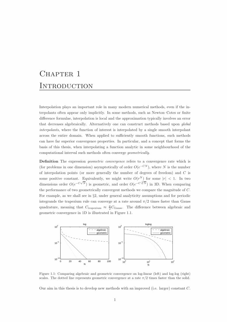
Definition The expression geometric convergence refers to a convergence rate which is
(for problems in one dimension) asymptotically of order O(e−CN ), where N is the number
of interpolation points (or more generally the number of degrees of freedom) and C is
some positive constant. Equivalently, we might write O(rN ) for some |r| < 1. In two
dimensions order O(e−C√
N ) is geometric, and order O(e−C 3√
N ) in 3D. When comparing
the performance of two geometrically convergent methods we compare the magnitude of C.
For example, as we shall see in §2, under general analyticity assumptions and for periodic
integrands the trapezium rule can converge at a rate around π/2 times faster than Gauss
quadrature, meaning that Ctrapezium ≈ π2 CGauss. The difference between algebraic and
geometric convergence in 1D is illustrated in Figure 1.1.
0 20 40 60 80 10010
−10
10−5
100
log
N
algebraicgeometric
100
101
102
10−10
10−5
100
N
loglog
algebraicgeometric
Figure 1.1: Comparing algebraic and geometric convergence on log-linear (left) and log-log (right)scales. The dotted line represents geometric convergence at a rate π/2 times faster than the solid.
Our aim in this thesis is to develop new methods with an improved (i.e. larger) constant C.
1
Chapter 1. Introduction 2
−1 1 −1 1
η
a
b
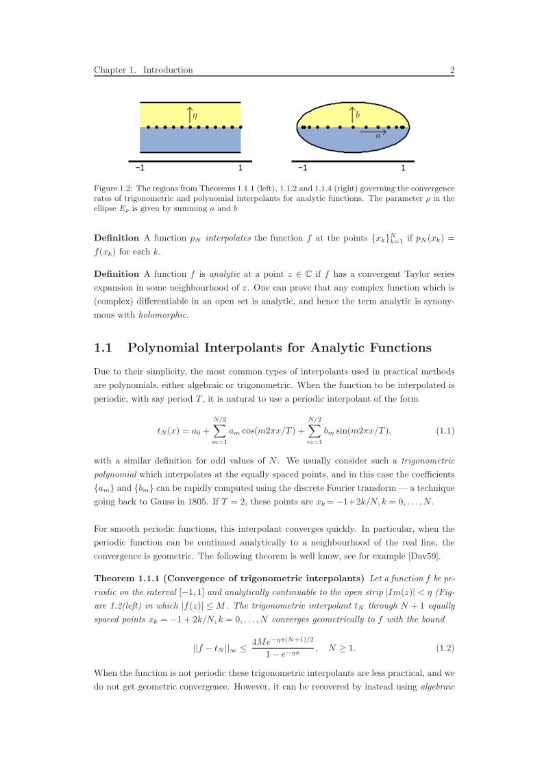
−→→→Figure 1.2: The regions from Theorems 1.1.1 (left), 1.1.2 and 1.1.4 (right) governing the convergencerates of trigonometric and polynomial interpolants for analytic functions. The parameter ρ in theellipse Eρ is given by summing a and b.
Definition A function pN interpolates the function f at the points xkNk=1 if pN (xk) =
f(xk) for each k.
Definition A function f is analytic at a point z ∈ C if f has a convergent Taylor series
expansion in some neighbourhood of z. One can prove that any complex function which is
(complex) differentiable in an open set is analytic, and hence the term analytic is synony-
mous with holomorphic.
1.1 Polynomial Interpolants for Analytic Functions
Due to their simplicity, the most common types of interpolants used in practical methods
are polynomials, either algebraic or trigonometric. When the function to be interpolated is
periodic, with say period T , it is natural to use a periodic interpolant of the form
tN (x) = a0 +
N/2∑
m=1
am cos(m2πx/T ) +
N/2∑
m=1
bm sin(m2πx/T ), (1.1)
with a similar definition for odd values of N . We usually consider such a trigonometric
polynomial which interpolates at the equally spaced points, and in this case the coefficients
am and bm can be rapidly computed using the discrete Fourier transform — a technique
going back to Gauss in 1805. If T = 2, these points are xk = −1+2k/N, k = 0, . . . , N .
For smooth periodic functions, this interpolant converges quickly. In particular, when the
periodic function can be continued analytically to a neighbourhood of the real line, the
convergence is geometric. The following theorem is well know, see for example [Dav59].
Theorem 1.1.1 (Convergence of trigonometric interpolants) Let a function f be pe-
riodic on the interval [−1, 1] and analytically continuable to the open strip |Im(z)| < η (Fig-
ure 1.2(left) in which |f(z)| ≤ M . The trigonometric interpolant tN through N + 1 equally
spaced points xk = −1 + 2k/N, k = 0, . . . , N converges geometrically to f with the bound
||f − tN ||∞ ≤4Me−ηπ(N+1)/2
1− e−ηπ, N ≥ 1. (1.2)
When the function is not periodic these trigonometric interpolants are less practical, and we
do not get geometric convergence. However, it can be recovered by instead using algebraic

Chapter 1. Introduction 3
polynomial interpolants. For brevity we shall often refer to such interpolants as simply
“polynomial” and state explicitly when we are talking about trigonometric polynomials.
Definition The degree N Chebyshev interpolant pN of a function f is the unique degree N
polynomial which interpolates f at the N+1 Chebyshev points xk = −cos(kπ/N), 0 ≤ k ≤ N.
Definition For any ρ > 1 the ρ-ellipse Eρ is the open region in the complex plane bounded
by the ellipse with foci ±1 and semiaxis lengths which sum to ρ (Figure 1.2(right). An
equivalent definition is the image of a ball of radius ρ about the origin under the Joukowsky
map z = (w + w−1)/2.
The following theorem was first given by Bernstein [Ber12, Section 61] in 1912, and describes
the rate of convergence for functions analytic in a neightbourhood of [−1, 1].
Theorem 1.1.2 (Convergence of Chebyshev interpolants) Let a function f be ana-
lytic in [−1, 1] and analytically continuable to the open ρ-ellipse Eρ in which |f | ≤ M for
some M. The Chebyshev interpolant pN of degree N satisfies
||f − pN ||∞ ≤4Mρ−N
ρ− 1, N ≥ 1. (1.3)
The Chebyshev coefficients ak of a function f Lipschitz continuous on [−1, 1] are those
such that
f(x) =
∞∑
k=0
akTk(x), (1.4)
where Tk(x) are the Chebyshev polynomials Tk(x) = cos(k arccos(x)). Such coefficients are
unique, and given by
ak(x) =2
π
∫ 1
−1
f(x)Tk(x)√1− x2
dx, (1.5)
with the exception that for k = 0 the factor 2/π changes to 1/π. Theorem 1.1.2 is an almost
direct consequence of the following, also due to Bernstein [Ber12, Section 61], regarding the
decay of these Chebyshev coefficients of an analytic function.
Theorem 1.1.3 (Decay of Chebyshev coefficients) Let a function f be analytic in
[−1, 1] and analytically continuable to the open ρ-ellipse Eρ in which |f | ≤ M for some
M. For all k ≥ 0 the Chebyshev coefficients ak of f satisfy
|ak| ≤ 2Mρ−k. (1.6)
The relation between Theorems 1.1.3 and Theorem 1.1.2 plays an important role in the
chebfun system [TPPD08], which we will introduce in §1.4.
If we choose to interpolate with Legendre rather than Chebyshev polynomials, i.e. through
the roots of the degree N + 1 Legendre polynomial, then the accuracy of the interpolation
is almost as good [Bai78].
Chapter 1. Introduction 4
Theorem 1.1.4 (Convergence of Legendre interpolants) Let the function f satisfy
the same conditions as in Theorem 1.1.2. The Legendre interpolant pN of degree N sat-
isfies
||f − pN ||∞ = O(√
Nρ−N), N →∞. (1.7)
1.2 The π/2 Concept
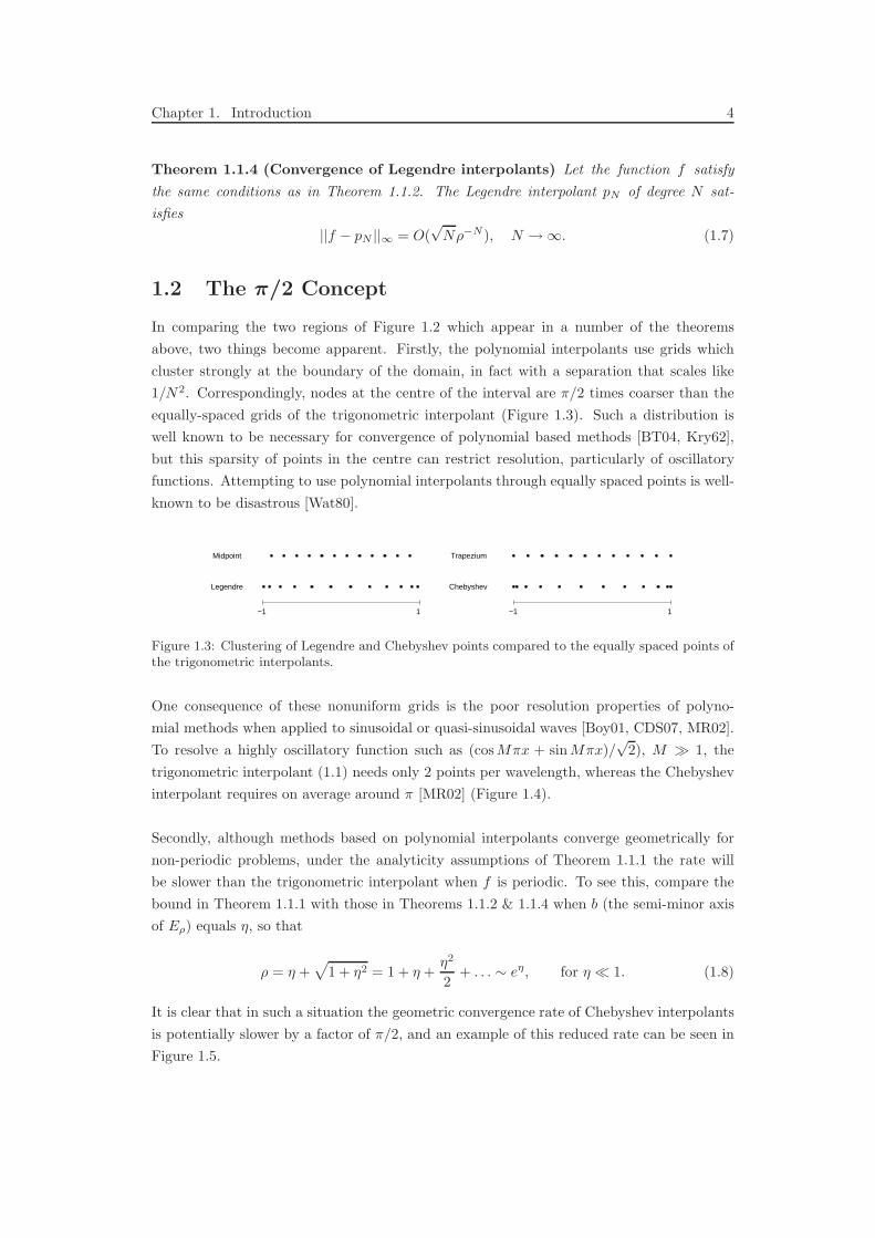
In comparing the two regions of Figure 1.2 which appear in a number of the theorems
above, two things become apparent. Firstly, the polynomial interpolants use grids which
cluster strongly at the boundary of the domain, in fact with a separation that scales like
1/N2. Correspondingly, nodes at the centre of the interval are π/2 times coarser than the
equally-spaced grids of the trigonometric interpolant (Figure 1.3). Such a distribution is
well known to be necessary for convergence of polynomial based methods [BT04, Kry62],
but this sparsity of points in the centre can restrict resolution, particularly of oscillatory
functions. Attempting to use polynomial interpolants through equally spaced points is well-
known to be disastrous [Wat80].
Midpoint
Legendre
−1 1
Trapezium
Chebyshev
−1 1
Figure 1.3: Clustering of Legendre and Chebyshev points compared to the equally spaced points ofthe trigonometric interpolants.
One consequence of these nonuniform grids is the poor resolution properties of polyno-
mial methods when applied to sinusoidal or quasi-sinusoidal waves [Boy01, CDS07, MR02].
To resolve a highly oscillatory function such as (cosMπx + sin Mπx)/√
2), M ≫ 1, the
trigonometric interpolant (1.1) needs only 2 points per wavelength, whereas the Chebyshev
interpolant requires on average around π [MR02] (Figure 1.4).
Secondly, although methods based on polynomial interpolants converge geometrically for
non-periodic problems, under the analyticity assumptions of Theorem 1.1.1 the rate will
be slower than the trigonometric interpolant when f is periodic. To see this, compare the
bound in Theorem 1.1.1 with those in Theorems 1.1.2 & 1.1.4 when b (the semi-minor axis
of Eρ) equals η, so that
ρ = η +√
1 + η2 = 1 + η +η2
2+ . . . ∼ eη, for η ≪ 1. (1.8)
It is clear that in such a situation the geometric convergence rate of Chebyshev interpolants
is potentially slower by a factor of π/2, and an example of this reduced rate can be seen in
Figure 1.5.
Chapter 1. Introduction 5
0 20 40 60 80 100 120 140 160 18010
−2
10−1
100
101
102
103
N
TrigonometricChebyshev
||(cos Mπx + sinMπx)/√
2− pN ||∞
M = 5 M = 20 M = 50
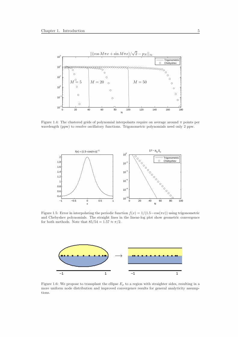
Figure 1.4: The clustered grids of polynomial interpolants require on average around π points perwavelength (ppw) to resolve oscillatory functions. Trigonometric polynomials need only 2 ppw.
−1 −0.5 0 0.5 1
0.4
0.6
0.8
1
1.2
1.4
1.6
1.8
2
f(x) = (1.5−cos(π x))−1
x0 20 40 60 80 100
10−10
10−8
10−6
10−4
10−2
100
N
|| f − pN
||∞
TrigonometricChebyshev
Figure 1.5: Error in interpolating the periodic function f(x) = 1/(1.5−cos(πx)) using trigonometricand Chebyshev polynomials. The straight lines in the linear-log plot show geometric convergencefor both methods. Note that 85/54 = 1.57 ≈ π/2.
−1 1 −1 1
→
Figure 1.6: We propose to transplant the ellipse Eρ to a region with straighter sides, resulting in amore uniform node distribution and improved convergence results for general analyticity assump-tions.
Chapter 1. Introduction 6
The solution we propose to these and related problems forms the basis of Part I of this
thesis. We show that by using appropriate conformal maps from the ellipse Eρ to more reg-
ular regions with straighter sides (Figure 1.6), and the same numerical methods in this new
mapped or transplanted basis, the π/2 factor in convergence rates and node distributions
can be recovered.
Rather than develop this idea from the point of view of approximation theory, we build it
through quadrature formulae in §2, where we show this suggested approach culminates in a
new method which can beat Gauss quadrature by 50%. In §3 we apply the same ideas to
spectral methods based upon polynomial interpolation, and demonstrate the new methods
have both better convergence properties and permit time steps up to three times larger in
explicit time stepping methods. Throughout these two chapters we review, where relevant,
related works in the literature which also attempt to ‘regain the π/2’, and observe how they
compare with our new approach.
1.3 Adaptive Concept
Usually the rapid geometric convergence of the polynomial based methods means that only
a few points, or degrees of freedom, are necessary to achieve a high degree of accuracy.
However, if f has singularities or is poorly behaved in the complex plane close to [−1, 1]
so that ρ ≈ 1, convergence can be too slow for such methods to be effective. Fortunately,
in these situations it is often the case that f may be continued analytically into a larger,
non-elliptical region. In this section we propose a number of methods to take advantage of
this additional analyticity which might otherwise be neglected, and use it to improve the
rates of convergence.
The approach we consider follows the ideas developed by Tee [Tee06, TT06], who to combat
this effect within the solution to differential equations constructs a conformal map g to a
region avoiding the singularities of f , so that the largest ρ-ellipse in which f g is analytic
is made larger than that of f alone. Applying the polynomial-based spectral method to
f g will then result in an improved convergence rate. Figure 1.7 shows the result of
applying one such map g when approximating the first derivative of the Runge-type function
f(x) = 1/(1 + 400x2) on [−1, 1].
Whilst in the first part of this thesis we concentrate only on mapping polynomial-based
methods, mapping ideas can also be used to improve trigonometric methods for periodic
problems. For example, when f has singularities close to the real line so that the parameter
η ≈ 0 in Theorem 1.1.1, convergence will be slow. By periodically mapping the rectangle
in the right-hand panel of Figure 1.2 to a region avoiding these singularities, we can again
improve this greatly.
Tee [Tee06] develops such methods for both non-periodic and periodic differential equations.
For the former he assumes the solution u to his equation is analytic in the complex plane
Chapter 1. Introduction 7
−1 0 1
−0.6
−0.4
−0.2
0
0.2
0.4
0.6
−1 0 1 0 16 32 48 64 10
−10
10−5
100
Eρ[f ], ρ = 1.051 Eρ[f g], ρ = 1.756 ‖f ′ − p′
N‖∞
Chebyshev
Mapped Method
no. of collocation points
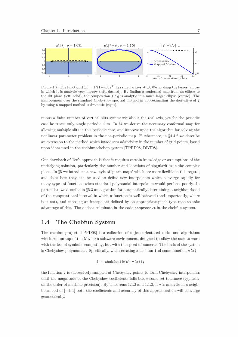
Figure 1.7: The function f(x) = 1/(1+400x2) has singularities at ±0.05i, making the largest ellipsein which it is analytic very narrow (left, dashed). By finding a conformal map from an ellipse tothe slit plane (left, solid), the composition f g is analytic in a much larger ellipse (centre). Theimprovement over the standard Chebyshev spectral method in approximating the derivative of fby using a mapped method is dramatic (right).
minus a finite number of vertical slits symmetric about the real axis, yet for the periodic
case he treats only single periodic slits. In §4 we derive the necessary conformal map for
allowing multiple slits in this periodic case, and improve upon the algorithm for solving the
nonlinear parameter problem in the non-periodic map. Furthermore, in §4.4.2 we describe
an extension to the method which introduces adaptivity in the number of grid points, based
upon ideas used in the chebfun/chebop system [TPPD08, DBT08].
One drawback of Tee’s approach is that it requires certain knowledge or assumptions of the
underlying solution, particularly the number and locations of singularities in the complex
plane. In §5 we introduce a new style of ‘pinch maps’ which are more flexible in this regard,
and show how they can be used to define new interpolants which converge rapidly for
many types of functions when standard polynomial interpolants would perform poorly. In
particular, we describe in §5.3 an algorithm for automatically determining a neighbourhood
of the computational interval in which a function is well-behaved (and importantly, where
it is not), and choosing an interpolant defined by an appropriate pinch-type map to take
advantage of this. These ideas culminate in the code compress.m in the chebfun system.
1.4 The Chebfun System
The chebfun project [TPPD08] is a collection of object-orientated codes and algorithms
which run on top of the Matlab software environment, designed to allow the user to work
with the feel of symbolic computing, but with the speed of numeric. The basis of the system
is Chebyshev polynomials. Specifically, when creating a chebfun f of some function v(x)
f = chebfun(@(x) v(x));
the function v is successively sampled at Chebyshev points to form Chebyshev interpolants
until the magnitude of the Chebyshev coefficients falls below some set tolerance (typically
on the order of machine precision). By Theorems 1.1.2 and 1.1.3, if v is analytic in a neigh-
bourhood of [−1, 1] both the coefficients and accuracy of this approximation will converge
geometrically.

Chapter 1. Introduction 8
Many of the standard Matlab routines for vectors have then been overloaded to apply to
functions. For example, the continuous analogue of the sum command is integration, and
I = sum(f) will approximate the definite integral of v on [−1, 1]. Similarly, df = diff(f)
and F = cumsum(f) will compute new chebfuns which accurate are approximations to the
derivative and indefinite integral of v respectively.
Chebops [DBT08] are built on the chebfun system, and offer a means of solving (chiefly
linear) differential equations using lazy evaluations1 of Chebyshev spectral discretisation
matrices, and a convergence ethos similar to that discussed above.
This strong grounding in Chebyshev polynomials make the chebfun and chebop systems
useful tools for this thesis, as we see particularly when using polynomial-based Clenshaw–
Curtis quadrature in §2.7 and Chebyshev spectral methods in §3 and §4. Furthermore, the
essence of this thesis is that often polynomial interpolants are not suitable, and the recent
development of mapped chebfuns allows us to suggest and implement improvements to the
chebfun system based upon the conformal mapping ideas we present herein.
The short Matlab code segments that appear throughout this thesis were written in Mat-
lab R2009a, and a snapshot of the latest chebfun version at the time of writing is available
at http://www2.maths.ox.ac.uk/chebfun/software/chebfun_v2_618.zip.
1a technique often used in computer science of delaying a computation until the result is required.
Part I
π/2 Methods
9
Chapter 2
Transplanted Quadrature Methods1
A quadrature rule is a numerical method of approximating the definite integral
I[a,b](f) =
∫ b
a
f(s)ds, (2.1)
where the function f is known and the values a < b fixed (and possibly infinite). If we
assume both a and b are finite, then without further loss of generality we may assume that
the interval of integration is [−1, 1], as the linear transformation 2y = (b − a)s − (a + b)
gives I[a,b](f) = 12 (b− a)I[−1,1](f y). For brevity we denote I[−1,1](f) by I, and our aim is
to compute
I =
∫ 1
−1
f(s)ds. (2.2)
Analytic (i.e. pen and paper) solutions to (2.2) are not possible in general, creating a require-
ment for efficient and accurate numerical methods of approximation. Standard quadrature
rules which attempt this take the form
IN =N∑
k=1
wkf(xk), (2.3)
that is, the integral I is approximated by evaluating the function f at the N nodes xk and
summing these contributions with certain weights wk. Clearly it is desirable that |I − IN |is small and converges to zero as N increases.
Amongst the most basic of such rules is the trapezium rule where, on a periodic interval,
the nodes are equally spaced (xk = −1+2k/N) and the weights constant (wk =2/N). Given
its simplicity, it may seem surprising that if f is periodic on [−1, 1] this rule can give a
highly accurate approximation to the integral. In particular, if the periodic function f can
be continued analytically to the complex plane around [−1, 1], then the approximation con-
verges geometrically as N is increased (see §2.1). This is not entirely unexpected, since
for a periodic integrand the trapezium rule is equivalent to integrating the geometrically
convergent trigonometric interpolant (1.1) discussed in the introduction.
1A large part of this chapter is joint work with the author’s supervisor L. N. Trefethen, and much of thetext adapted from the paper [HT08].
10
Chapter 2. Transplanted Quadrature Methods 11
Unfortunately, as with the trigonometric interpolant, it is well-known that the trapezium
rule loses its power when periodicity is lacking, and under the same analyticity conditions
will typically be only second order convergent (i.e. the error will decrease like 1/N2 as
N increases). Methods based upon polynomial interpolants, such as Gauss–Legendre or
Clenshaw–Curtis quadrature, can converge geometrically even when the integrand is not
periodic, and so become preferred to the trapezium rule in this situation. However, these
methods can suffer the drawbacks we saw earlier, namely the π/2 factors in node spacing
(Figure 2.1) and convergence rates (Figure 2.2).
Midpoint
Gauss
−1 1
Trapezium
Chebyshev
−1 1
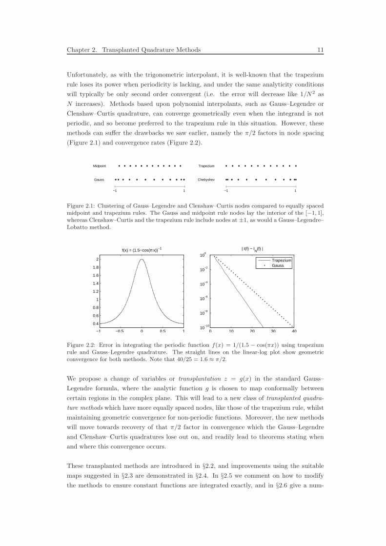
Figure 2.1: Clustering of Gauss–Legendre and Clenshaw–Curtis nodes compared to equally spacedmidpoint and trapezium rules. The Gauss and midpoint rule nodes lay the interior of the [−1, 1],whereas Clenshaw–Curtis and the trapezium rule include nodes at ±1, as would a Gauss–Legendre–Lobatto method.
−1 −0.5 0 0.5 1
0.4
0.6
0.8
1
1.2
1.4
1.6
1.8
2
f(x) = (1.5−cos(π x))−1
0 10 20 30 4010
−10
10−8
10−6
10−4
10−2
100
| I(f) − IN
(f) |
TrapeziumGauss
Figure 2.2: Error in integrating the periodic function f(x) = 1/(1.5 − cos(πx)) using trapeziumrule and Gauss–Legendre quadrature. The straight lines on the linear-log plot show geometricconvergence for both methods. Note that 40/25 = 1.6 ≈ π/2.
We propose a change of variables or transplantation z = g(x) in the standard Gauss–
Legendre formula, where the analytic function g is chosen to map conformally between
certain regions in the complex plane. This will lead to a new class of transplanted quadra-
ture methods which have more equally spaced nodes, like those of the trapezium rule, whilst
maintaining geometric convergence for non-periodic functions. Moreover, the new methods
will move towards recovery of that π/2 factor in convergence which the Gauss–Legendre
and Clenshaw–Curtis quadratures lose out on, and readily lead to theorems stating when
and where this convergence occurs.
These transplanted methods are introduced in §2.2, and improvements using the suitable
maps suggested in §2.3 are demonstrated in §2.4. In §2.5 we comment on how to modify
the methods to ensure constant functions are integrated exactly, and in §2.6 give a num-
Chapter 2. Transplanted Quadrature Methods 12
ber of results governing convergence of the new methods for functions analytic in epsilon-
neighbourhoods. The discussion in this chapter will be mostly limited to the case of Gauss–
Legendre quadrature, but in §2.7 we consider the effects of transplanting the Clenshaw–
Curtis method. In §2.8 we explore existing methods for ‘regaining π/2’ that appear in the
literature, and give a short summary in §2.9.
2.1 The Trapezium Rule and
Gauss–Legendre Quadrature
We first recall some of the theorems alluded to in the previous section, closely related to
those of §1.1. The first, regarding the convergence of the trapezium rule, was hinted at by
Poisson in the 1820s [Poi27] and first spelt out fully by Davis in the 1950s [Dav59].
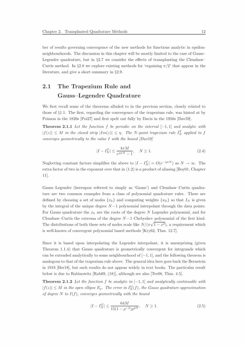
Theorem 2.1.1 Let the function f be periodic on the interval [−1, 1] and analytic with
|f(z)| ≤ M in the closed strip |Im(z)| ≤ η. The N -point trapezium rule ITN applied to f
converges geometrically to the value I with the bound [Dav59]
|I − ITN | ≤
4πM
eηπN − 1, N ≥ 1. (2.4)
Neglecting constant factors simplifies the above to |I − ITN | = O(e−ηπN ) as N → ∞. The
extra factor of two in the exponent over that in (1.2) is a product of aliasing [Boy01, Chapter
11].
Gauss–Legendre (hereupon referred to simply as ‘Gauss’) and Clenshaw–Curtis quadra-
ture are two common examples from a class of polynomial quadrature rules. These are
defined by choosing a set of nodes xk and computing weights wk so that IN is given
by the integral of the unique degree N−1 polynomial interpolant through the data points.
For Gauss quadrature the xk are the roots of the degree N Legendre polynomial, and for
Clenshaw–Curtis the extrema of the degree N−1 Chebyshev polynomial of the first kind.
The distributions of both these sets of nodes scale like N/(π√
1− x2), a requirement which
is well-known of convergent polynomial based methods [Kry62, Thm. 12.7].
Since it is based upon interpolating the Legendre interpolant, it is unsurprising (given
Theorem 1.1.4) that Gauss quadrature is geometrically convergent for integrands which
can be extended analytically to some neighbourhood of [−1, 1], and the following theorem is
analogous to that of the trapezium rule above. The general idea here goes back the Bernstein
in 1918 [Ber18], but such results do not appear widely in text books. The particular result
below is due to Rabinowitz [Rab69, (18)], although see also [Tre08, Thm. 4.5].
Theorem 2.1.2 Let the function f be analytic in [−1, 1] and analytically continuable with
|f(z)| ≤M in the open ellipse Eρ. The error in IGN (f), the Gauss quadrature approximation
of degree N to I(f), converges geometrically with the bound
|I − IGN | ≤
64M
15(1− ρ−2)ρ2N, N ≥ 1. (2.5)
Chapter 2. Transplanted Quadrature Methods 13
Again ignoring constant factors, we see that Theorem 2.1.2 ensures geometric convergence
at a rate O(ρ−2N ) as N → ∞, and as before aliasing is responsible for the extra factor of
two in the exponent. As with the interpolants, we see that if b, the semi-minor axis of Eρ,
equals η then
ρ = η +√
1 + η2 = 1 + η +η2
2+ . . . ∼ eη, for η ≪ 1, (2.6)
and the geometric convergence rate of Gauss is potentially slower by a factor of π/2. A the-
orem similar to 2.1.2 can also be given for Clenshaw–Curtis quadrature, with ρ2N replaced
by ρN−1, but we defer further discussion of this method until §2.7.
From the perspective of application, the assumption of analyticity in the region Eρ is unbal-
anced; it requires the function f to be ‘more analytic’ in the centre of the [−1, 1] where the
ellipse is fat, than towards the ends where it becomes narrow. Specifically, the Taylor series
of f about a point near ±1 is permitted to have far more rapidly increasing coefficients
than about a point z ≈ 0. This requirement is not a consequence of the generic quadrature
formula (2.3), rather it is a consequence of the underlying polynomial interpolant. Since the
use of polynomials is also the cause of the nonuniform node distribution, we might begin to
believe that polynomials are not always the best choice.
Our plan is to derive new quadrature formulae of the form (2.3) which use neither the
trigonometric interpolants of the trapezium rule, nor the polynomial interpolants of Gauss
quadrature, but which take certain benefits of each. From Gauss quadrature we would like
the geometric convergence for non-periodic functions, whilst we would like to emulate from
the trapezium rule both a more uniform distribution of nodes and more uniform convergence
region. Instead of haphazardly searching for such a basis, we suggest the solution is to take
the polynomial methods of Gauss quadrature and modify them to behave more like the
interpolants of the trapezium rule. Specifically, we introduce a change of variables chosen
so that the ellipse Eρ is mapped to a region around [−1, 1] with straighter sides, which will
not only take care of the more uniform convergence region directly, but also result in a more
equally spaced set of nodes.
2.2 A ‘Transplanted’ Method
Let the function f be analytic in Ωρ, a subset of the complex plane containing the interval
[−1, 1]. Consider another function g, analytic in some ellipse Eρ and satisfying
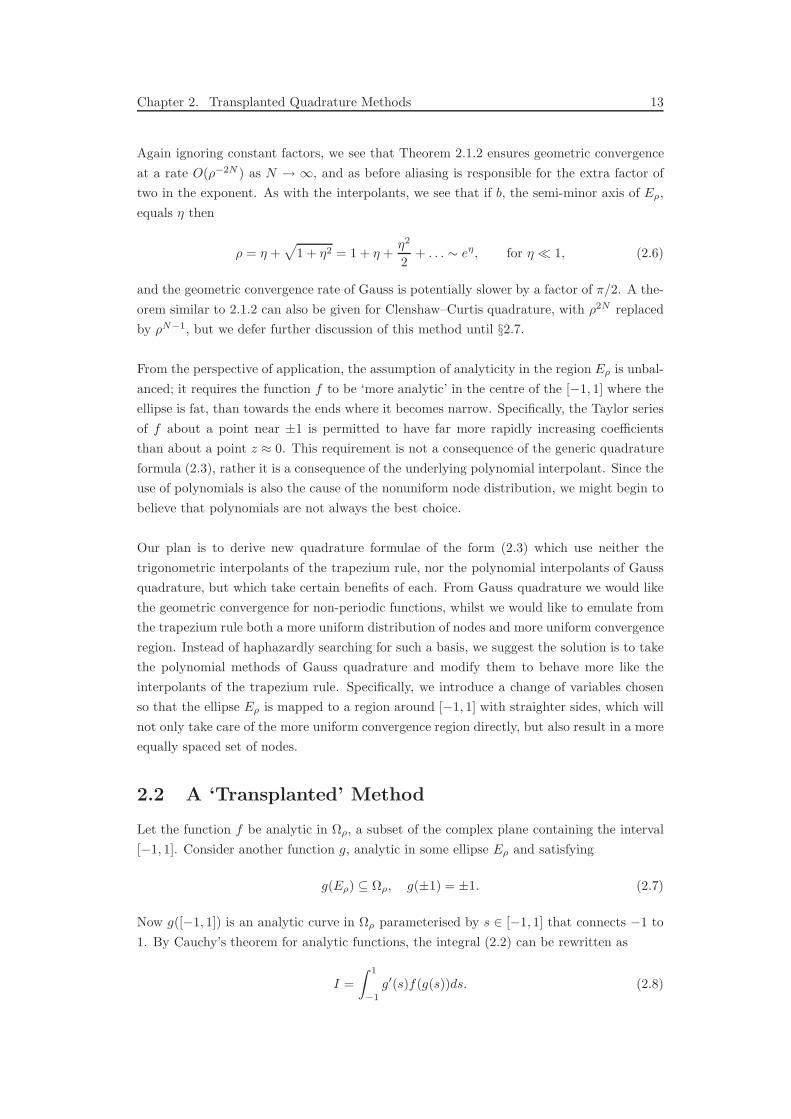
g(Eρ) ⊆ Ωρ, g(±1) = ±1. (2.7)
Now g([−1, 1]) is an analytic curve in Ωρ parameterised by s ∈ [−1, 1] that connects −1 to
1. By Cauchy’s theorem for analytic functions, the integral (2.2) can be rewritten as
I =
∫ 1
−1
g′(s)f(g(s))ds. (2.8)

Chapter 2. Transplanted Quadrature Methods 14
Applying a quadrature rule of the form (2.3) to this integral in the variable s, we obtain
IN (g′ · (f g)) =
N∑
k=1
wkg′(xk)f(g(xk)). (2.9)
Since the function, or map g is independent of the original integrand f , we can treat the
values wkg′(xk) and g(xk) as new weights and nodes of a transplanted quadrature method
IN = IN (f) =
N∑
k=1
wkf(xk), wk = wkg′(xk), xk = g(xk). (2.10)
Although not strictly necessary, it will usually be the case that g will map the interval [−1, 1]
to itself, i.e. g([−1, 1]) = [−1, 1]. Additionally, the map g need not be conformal, as we do
not require that the derivative remain nonzero. However, if both these points are true then
the transplanted Gauss method will have all of the nodes xk ∈ [−1, 1] as well as each of the
weights wk remaining positive. This second property is easily seen, as the Gauss weights
wk are positive and the derivative g′ cannot pass through zero on [−1, 1].
Furthermore, the word conformal immediately suggests a consideration of regions in the
complex plane — the key point in these transplanted methods. Indeed without such a
consideration, equation (2.10) is little more than a change of variables. By choosing the
‘right’ region as the image of the ellipse Eρ under g, not only do we find a ‘good’ change of
variables, but the following theorem demonstrates that geometric convergence of these new
transplanted methods as a corollary of Theorem 2.1.2.
Theorem 2.2.1 Let f be analytic in [−1, 1] and analytically continuable to an open region
Ωρ with |f(z)| ≤ M for some ρ > 1, and the transplanted quadrature method IN be defined
by a conformal map g satisfying (2.7). Then for all N ≥ 1,
|I − IN | ≤64Mγ
15(1− ρ−2)ρ2N, γ = sup
s∈Eρ
|g′(s)| ≤ ∞. (2.11)
If γ =∞ in this estimate, we can always shrink ρ a little bit to make it finite. Thus trans-
planted Gauss quadrature always converges geometrically if f is analytic in a neighbourhood
of [−1, 1].
2.3 Conformal Maps
Having defined the transplanted quadrature method using some conformal map g from Eρ
to some subset of Ωρ, we must now make a decision as to what this latter region, and hence
the map, should be. Since our aim is to alter the polynomial-based Gauss method so that
it resembles the trapezium rule whilst maintaining geometric convergence for non-periodic
functions, one choice of map would send the ellipse of the polynomial methods to something
like the rectangular strip of the trapezium rule. The non-periodic analogue of a rectangle
for a periodic function is an infinite strip.
Chapter 2. Transplanted Quadrature Methods 15
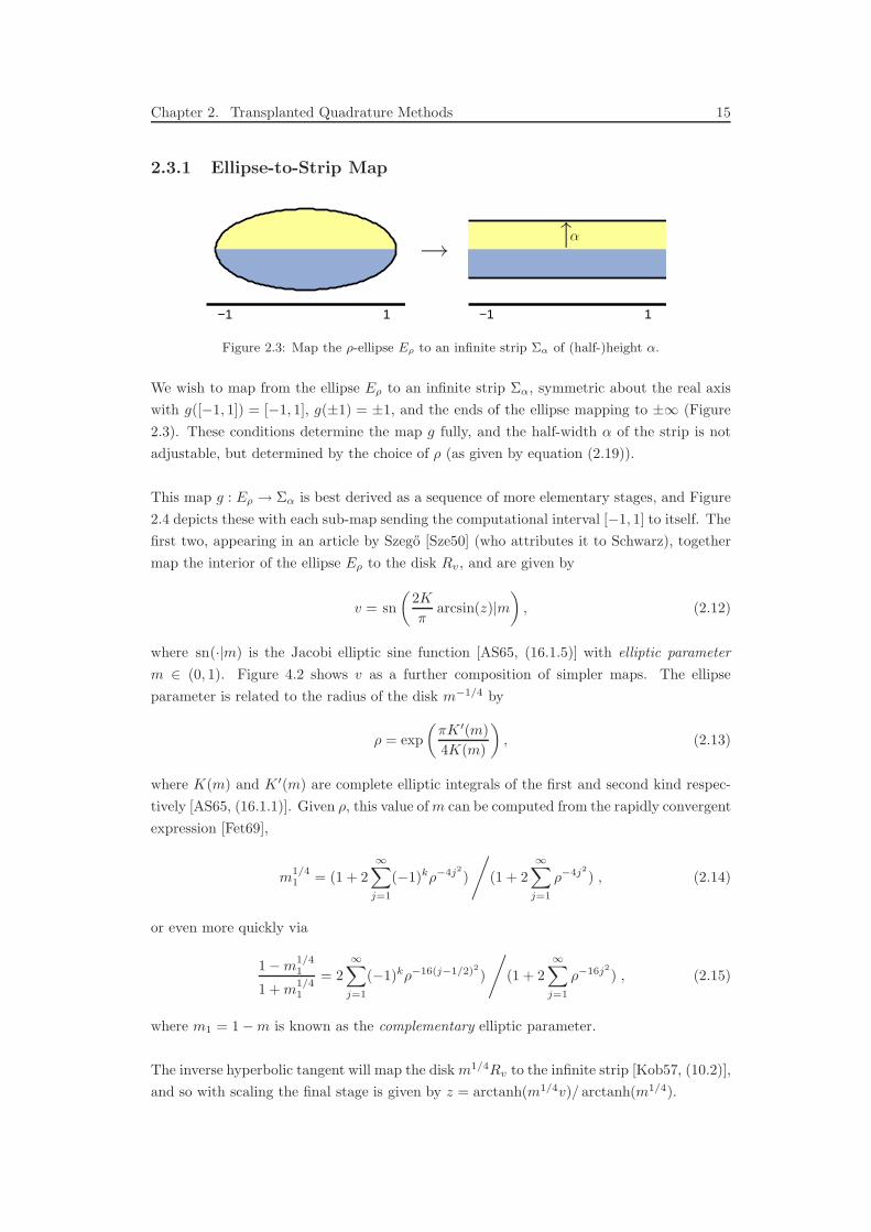
2.3.1 Ellipse-to-Strip Map
−1 1 −1 1
α→ →
Figure 2.3: Map the ρ-ellipse Eρ to an infinite strip Σα of (half-)height α.
We wish to map from the ellipse Eρ to an infinite strip Σα, symmetric about the real axis
with g([−1, 1]) = [−1, 1], g(±1) = ±1, and the ends of the ellipse mapping to ±∞ (Figure
2.3). These conditions determine the map g fully, and the half-width α of the strip is not
adjustable, but determined by the choice of ρ (as given by equation (2.19)).
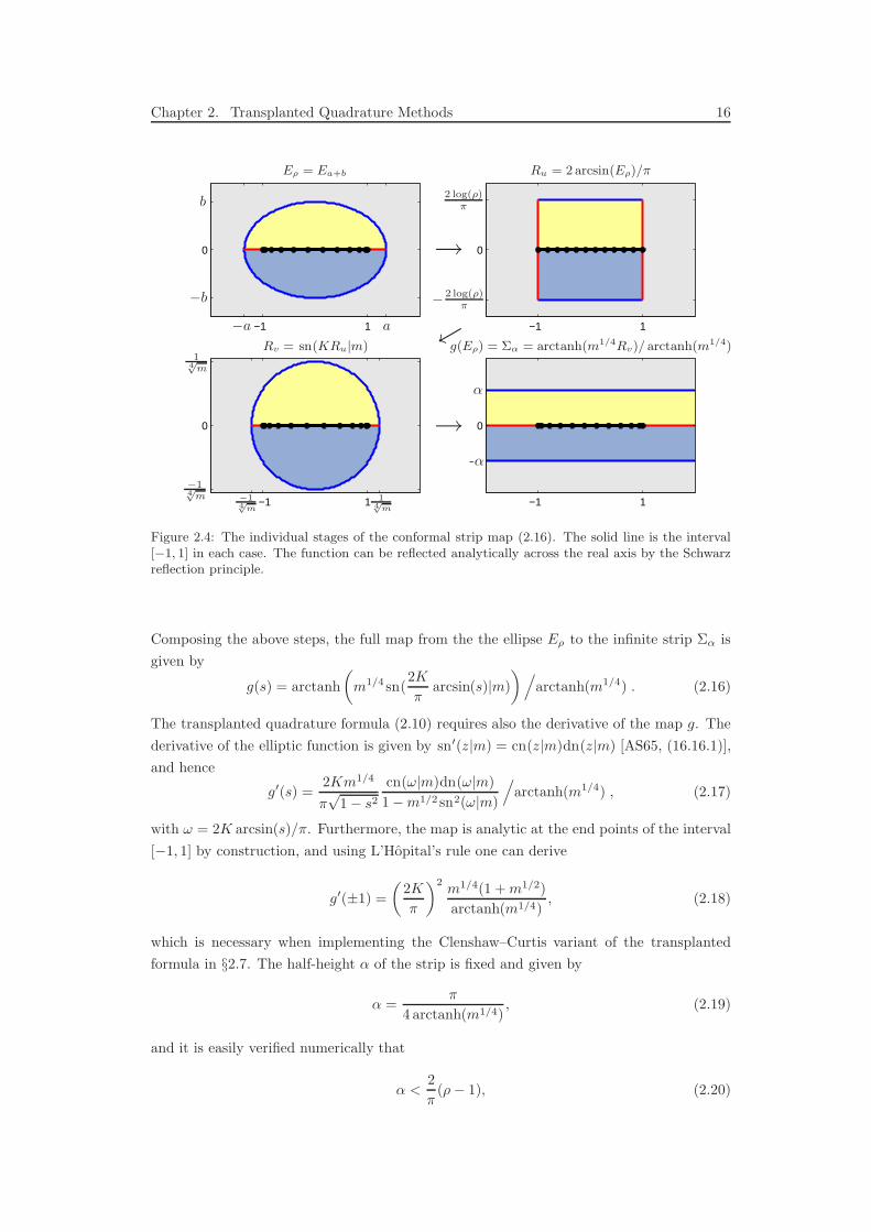
This map g : Eρ → Σα is best derived as a sequence of more elementary stages, and Figure
2.4 depicts these with each sub-map sending the computational interval [−1, 1] to itself. The
first two, appearing in an article by Szego [Sze50] (who attributes it to Schwarz), together
map the interior of the ellipse Eρ to the disk Rv, and are given by
v = sn
(
2K
πarcsin(z)|m
)
, (2.12)
where sn(·|m) is the Jacobi elliptic sine function [AS65, (16.1.5)] with elliptic parameter
m ∈ (0, 1). Figure 4.2 shows v as a further composition of simpler maps. The ellipse
parameter is related to the radius of the disk m−1/4 by
ρ = exp
(
πK ′(m)
4K(m)
)
, (2.13)
where K(m) and K ′(m) are complete elliptic integrals of the first and second kind respec-
tively [AS65, (16.1.1)]. Given ρ, this value of m can be computed from the rapidly convergent
expression [Fet69],
m1/41 = (1 + 2
∞∑
j=1
(−1)kρ−4j2
)
/
(1 + 2
∞∑
j=1
ρ−4j2
) , (2.14)
or even more quickly via
1−m1/41
1 + m1/41
= 2∞∑
j=1
(−1)kρ−16(j−1/2)2)
/
(1 + 2∞∑
j=1
ρ−16j2
) , (2.15)
where m1 = 1−m is known as the complementary elliptic parameter.
The inverse hyperbolic tangent will map the disk m1/4Rv to the infinite strip [Kob57, (10.2)],
and so with scaling the final stage is given by z = arctanh(m1/4v)/ arctanh(m1/4).
Chapter 2. Transplanted Quadrature Methods 16
−1 1
0
−1 1
0
−1 1
0
−1 1
0
−a a
−b
b
− 2 log(ρ)π
2 log(ρ)π
−14√m
14√m
−14√
m
14√
m
Eρ = Ea+b Ru = 2arcsin(Eρ)/π
Rv = sn(KRu|m) g(Eρ) = Σα = arctanh(m1/4Rv)/ arctanh(m1/4)
-α
α
→
←
→
Figure 2.4: The individual stages of the conformal strip map (2.16). The solid line is the interval[−1, 1] in each case. The function can be reflected analytically across the real axis by the Schwarzreflection principle.
Composing the above steps, the full map from the the ellipse Eρ to the infinite strip Σα is
given by
g(s) = arctanh
(
m1/4 sn(2K
πarcsin(s)|m)
)
/
arctanh(m1/4) . (2.16)
The transplanted quadrature formula (2.10) requires also the derivative of the map g. The
derivative of the elliptic function is given by sn′(z|m) = cn(z|m)dn(z|m) [AS65, (16.16.1)],
and hence
g′(s) =2Km1/4
π√
1− s2
cn(ω|m)dn(ω|m)
1−m1/2 sn2(ω|m)
/
arctanh(m1/4) , (2.17)
with ω = 2K arcsin(s)/π. Furthermore, the map is analytic at the end points of the interval
[−1, 1] by construction, and using L’Hopital’s rule one can derive
g′(±1) =
(
2K
π
)2m1/4(1 + m1/2)
arctanh(m1/4), (2.18)
which is necessary when implementing the Clenshaw–Curtis variant of the transplanted
formula in §2.7. The half-height α of the strip is fixed and given by
α =π
4 arctanh(m1/4), (2.19)
and it is easily verified numerically that
α <2
π(ρ− 1), (2.20)
Chapter 2. Transplanted Quadrature Methods 17
with α ∼ (2/π)(ρ − 1) as ρ → 1. This gives an indication of a π/2 speed up, since the
semi-axis height of Eρ in the same limit is ∼ (ρ − 1). In other words, the transplanted
formula needs a strip of analyticity only 2/π times as wide to achieve the same convergence
rate. This is confirmed by the following theorem.
Theorem 2.3.1 Let f be analytic in the strip about R of half-height (2/π)(ρ− 1) for some
ρ > 1. If f is integrated by the transplanted quadrature formula (2.10) associated with the
map (2.16) from Eρ to Σα, then for any ρ < ρ
|I − IN | = O(ρ−2N ), as N →∞. (2.21)
Proof The inequality (2.20) implies that f is analytic in the strip Σα of half-height α, and
therefore (f g) is analytic in Eρ. Since g takes the value infinity for this map, we do not
quite get O(ρ−2N ) convergence, and for this reason we have not assumed that f is bounded
in Σα. However, for any ρ < ρ Theorem 2.1.2 still applies to the integrand g′(s)f(g(s))
of (2.8), which will be analytic and bounded in this smaller ellipse. This implies Theorem
2.3.1. 2
The following Matlab code computes the strip map g and its derivative g′ for applying
transplanted Gauss quadrature. The functions ellipke and ellipj are standard Matlab
functions which compute the quarter period K and Jacobi elliptic functions sn, cn, dn for
real-valued arguments. The complex values required for Figure 2.6 can be computed using
ellipjc from Driscoll’s Schwarz-Cristoffel Toolbox [Dri05].
function [g,gprime] = stripmap(s,rho)
num = 0; den = 0;
for j = 1:round(.5+sqrt(10/log(rho))) % Given rho, find m
num = num + (-1)^j*rho^(-4*j^2);
den = den + rho^(-4*j^2);
end
m4 = 2*num/(1+2*den); m = m4^4; % m^1/4 and m
K = ellipke(m); % Jacobi elliptic parameter
u = 2*asin(s)/pi;
[v,cn,dn] = ellipj(K*u,m); % Jacobi elliptic function
duds = (2/pi)./sqrt(1-s.^2);
dvdu = K*cn.*dn;
dgdv = (m4./(1-m4.^2*v.^2))/atanh(m4);
g = atanh(m4*v)/atanh(m4); % g
gprime = dgdv.*dvdu.*duds; % g’
The map is also available within the chebfun system as a map structure resulting from
maps(’strip’,rho).
If using Clenshaw–Curtis quadrature rather than Gauss, the above must be modified slightly
to account for the nodes at ±1 (§2.7). Furthermore, if ρ is close to 1 (smaller than about
1.1), the code above suffers from numerical instability. This can be overcome by using a
domain decomposition technique, which is described in the appendix of [HT08]. Figure
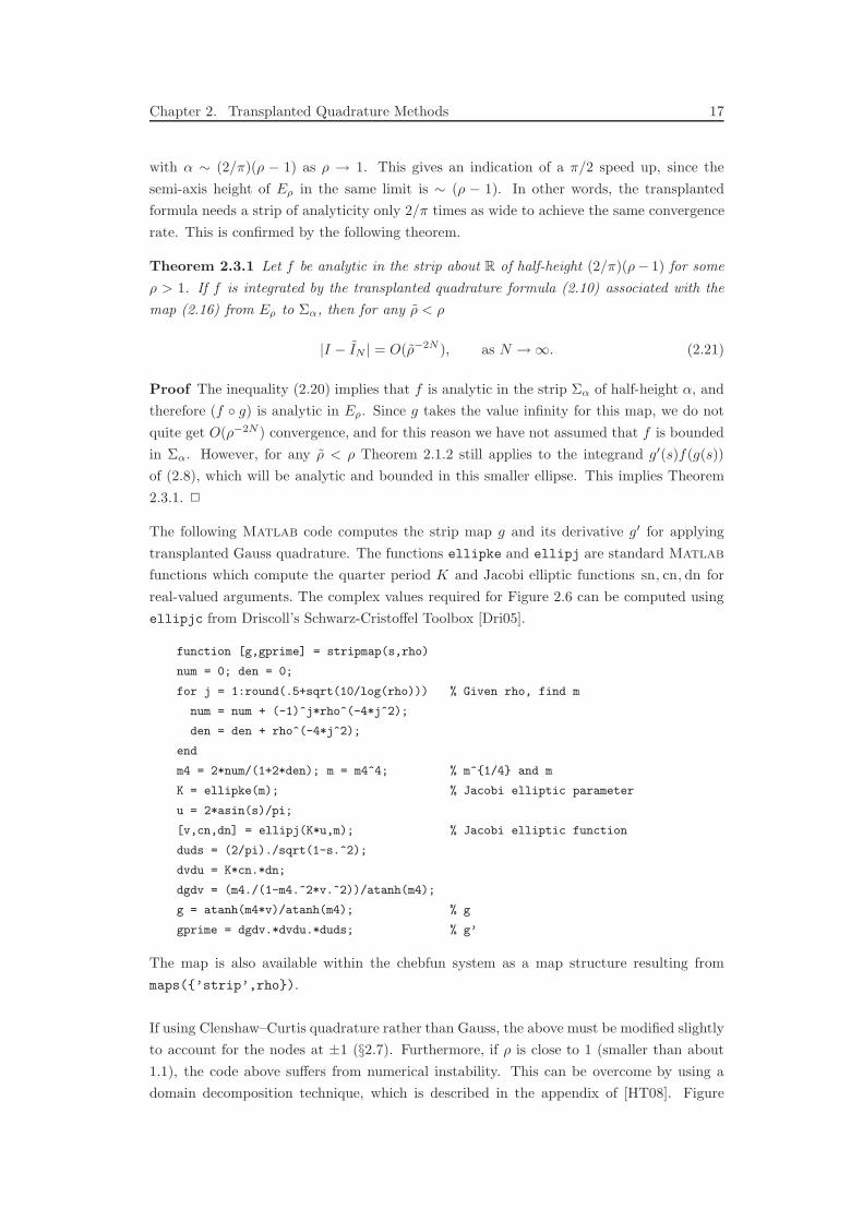
Chapter 2. Transplanted Quadrature Methods 18
2.5 shows the effect of the strip map on the clustered grids of Gauss and Clenshaw–Curtis
quadrature.
Midpoint
Gauss
Strip−Gauss
−1 1
Trapezium
Chebyshev
Strip−Chebyshev
−1 1
Figure 2.5: Improved distribution of the Gauss and Chebyshev nodes under the strip map (2.16)with ρ = 1.4 and N = 12. To the eye, the strip-Gauss points are equally spaced.
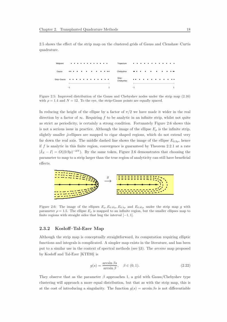
In reducing the height of the ellipse by a factor of π/2 we have made it wider in the real
direction by a factor of ∞. Requiring f to be analytic in an infinite strip, whilst not quite
as strict as periodicity, is certainly a strong condition. Fortunately Figure 2.6 shows this
is not a serious issue in practice. Although the image of the ellipse Eρ is the infinite strip,
slightly smaller ρ-ellipses are mapped to cigar shaped regions, which do not extend very
far down the real axis. The middle dashed line shows the image of the ellipse E0.9ρ, hence
if f is analytic in this finite region, convergence is guaranteed by Theorem 2.2.1 at a rate
|IN − I| = O((0.9ρ)−2N ). By the same token, Figure 2.6 demonstrates that choosing the
parameter to map to a strip larger than the true region of analyticity can still have beneficial
effects.
g→
Figure 2.6: The image of the ellipses Eρ, E0.95ρ, E0.9ρ and E0.85ρ under the strip map g withparameter ρ = 1.5. The ellipse Eρ is mapped to an infinite region, but the smaller ellipses map tofinite regions with straight sides that hug the interval [−1, 1].
2.3.2 Kosloff–Tal-Ezer Map
Although the strip map is conceptually straightforward, its computation requiring elliptic
functions and integrals is complicated. A simpler map exists in the literature, and has been
put to a similar use in the context of spectral methods (see §3). The arcsine map proposed
by Kosloff and Tal-Ezer [KTE93] is
g(s) =arcsinβs
arcsinβ, β ∈ (0, 1). (2.22)
They observe that as the parameter β approaches 1, a grid with Gauss/Chebyshev type
clustering will approach a more equal distribution, but that as with the strip map, this is
at the cost of introducing a singularity. The function g(s) = arcsinβs is not differentiable
Chapter 2. Transplanted Quadrature Methods 19
when s = ±1/β, and hence a choice of β restricts convergence to an ellipse Eρ with ρ =
1/β +√
1/β2 − 1. Alternatively, for a given value of ρ the parameter is given by
β =2
(ρ + 1/ρ). (2.23)
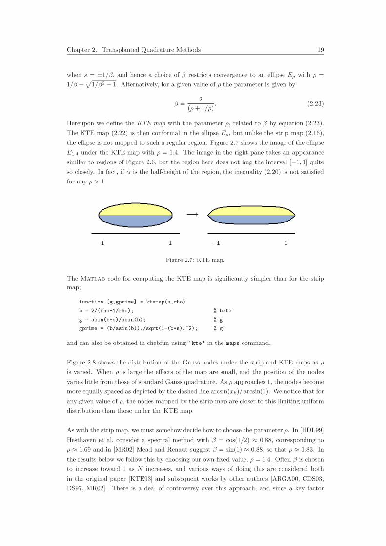
Hereupon we define the KTE map with the parameter ρ, related to β by equation (2.23).
The KTE map (2.22) is then conformal in the ellipse Eρ, but unlike the strip map (2.16),
the ellipse is not mapped to such a regular region. Figure 2.7 shows the image of the ellipse
E1.4 under the KTE map with ρ = 1.4. The image in the right pane takes an appearance
similar to regions of Figure 2.6, but the region here does not hug the interval [−1, 1] quite
so closely. In fact, if α is the half-height of the region, the inequality (2.20) is not satisfied
for any ρ > 1.
−1 1 −1 1
→
Figure 2.7: KTE map.
The Matlab code for computing the KTE map is significantly simpler than for the strip
map;
function [g,gprime] = ktemap(s,rho)
b = 2/(rho+1/rho); % beta
g = asin(b*s)/asin(b); % g
gprime = (b/asin(b))./sqrt(1-(b*s).^2); % g’
and can also be obtained in chebfun using ’kte’ in the maps command.
Figure 2.8 shows the distribution of the Gauss nodes under the strip and KTE maps as ρ
is varied. When ρ is large the effects of the map are small, and the position of the nodes
varies little from those of standard Gauss quadrature. As ρ approaches 1, the nodes become
more equally spaced as depicted by the dashed line arcsin(xk)/ arcsin(1). We notice that for
any given value of ρ, the nodes mapped by the strip map are closer to this limiting uniform
distribution than those under the KTE map.
As with the strip map, we must somehow decide how to choose the parameter ρ. In [HDL99]
Hesthaven et al. consider a spectral method with β = cos(1/2) ≈ 0.88, corresponding to
ρ ≈ 1.69 and in [MR02] Mead and Renaut suggest β = sin(1) ≈ 0.88, so that ρ ≈ 1.83. In
the results below we follow this by choosing our own fixed value, ρ = 1.4. Often β is chosen
to increase toward 1 as N increases, and various ways of doing this are considered both
in the original paper [KTE93] and subsequent works by other authors [ARGA00, CDS03,
DS97, MR02]. There is a deal of controversy over this approach, and since a key factor

Chapter 2. Transplanted Quadrature Methods 20
−1 −0.8 −0.6 −0.4 −0.2 0 0.2 0.4 0.6 0.8 11
1.2
1.4
1.6
1.8
2
2.2
2.4
2.6
2.8
ρ
x
Mapped Gauss nodes
stripkte
Figure 2.8: As ρ decreases towards 1 (y-axis), strip (blue) and KTE (red) maps send the clusteredGauss nodes to a more uniform spacing. The black dots are staggered for clarity.
is increasing the maximum time step allowable in explicit spectral methods, we shall defer
further discussion of this to §3.
2.3.3 Sausage Maps
A disadvantage shared by the two previous maps is the singularity they introduce, which
can artificially limit the rate of convergence in some cases. We might like a map which
maintains some of the benefits of the strip and KTE maps, (the stretching the region of
analyticity and equalising the distribution of nodes), but without introducing singularities.
We saw that as β (and by association ρ) approached 1 in the KTE map (2.22) the nodes
became more equally spaced, but that β can not be taken as 1 without losing geometric
convergence (due to singularities at ±1). Varying β with N as suggested above would be
one way to do this, but suppose instead we simply truncate the Taylor series expansion
arcsin s = s +1
6s3 +
3
40s5 +
5
112s7 +
35
1152s9 + . . . (2.24)
at some degree d and normalise so that g(±1) = ±1. For example, taking d = 1, 3, 5 or 9
gives respectively
g(s) = s, (2.25)
g(s) =1
7(6s + s3), (2.26)
g(s) =1
149(120s + 20s3 + 9s5), (2.27)
g(s) =1
53089(40320s + 6720s3 + 3024s5 + 1800s7 + 1125s9). (2.28)
The Matlab code to compute these maps is given below, and the line containing the
cumprod command computes the Taylor series coefficients of arcsin(x).
function [g,gprime] = sausagemap(s,d)
c = zeros(1,d+1);
Chapter 2. Transplanted Quadrature Methods 21
c(d:-2:1) = [1 cumprod(1:2:d-2)./cumprod(2:2:d-1)]./(1:2:d);
c = c/sum(c); % Normalise coefficients
cp = c(1:d).*(d:-1:1);
g = polyval(c,s); % g
gprime = polyval(cp,s); % g’
Again the map is available in chebfun, this time via maps(’sausage’,d).
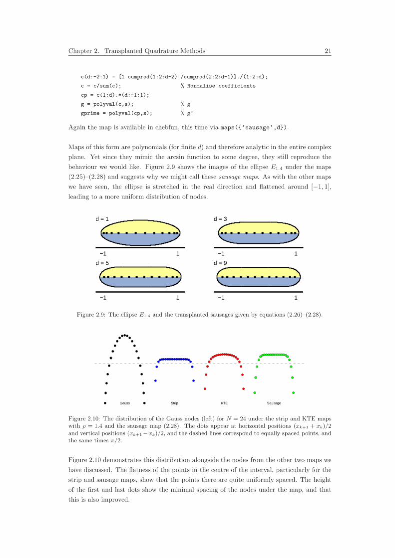
Maps of this form are polynomials (for finite d) and therefore analytic in the entire complex
plane. Yet since they mimic the arcsin function to some degree, they still reproduce the
behaviour we would like. Figure 2.9 shows the images of the ellipse E1.4 under the maps
(2.25)–(2.28) and suggests why we might call these sausage maps. As with the other maps
we have seen, the ellipse is stretched in the real direction and flattened around [−1, 1],
leading to a more uniform distribution of nodes.
−1 1
d = 1
−1 1
d = 3
−1 1
d = 5
−1 1
d = 9
Figure 2.9: The ellipse E1.4 and the transplanted sausages given by equations (2.26)–(2.28).
Gauss Strip KTE Sausage
Figure 2.10: The distribution of the Gauss nodes (left) for N = 24 under the strip and KTE mapswith ρ = 1.4 and the sausage map (2.28). The dots appear at horizontal positions (xk+1 + xk)/2and vertical positions (xk+1−xk)/2, and the dashed lines correspond to equally spaced points, andthe same times π/2.
Figure 2.10 demonstrates this distribution alongside the nodes from the other two maps we
have discussed. The flatness of the points in the centre of the interval, particularly for the
strip and sausage maps, show that the points there are quite uniformly spaced. The height
of the first and last dots show the minimal spacing of the nodes under the map, and that
this is also improved.
Chapter 2. Transplanted Quadrature Methods 22
2.4 Some Results
Having introduced the transplanted quadrature formula (2.10) and discussed some potential
conformal maps g in the previous section, we now observe how these combine to perform in
practice. The strip (2.16) and the KTE (2.22) maps contain a parameter ρ, and it is unlikely
to be beneficial to attempt to tune this parameter to the integrand at hand. However, as
we have seen, provided it is not taken too small a fairly generic choice can go a good way
to improve matters. With this in mind, we choose a fixed value of ρ = 1.4 for each of the
test integrands. Similarly, we make a fairly arbitrary choice in using the degree 9 sausage
map (2.28).
The following Matlab code is an example of how to implement the transplanted Gauss
quadrature method (2.10) using the strip map for an integrand f(x) = (1 + 20x2)−1. The
function legpts is a code within chebfun which computes the standard Gauss quadrature
weights and nodes, but this could be replaced with gauss from [Tre00].
f = @(x) 1./(1+20*x.^2); % Change this for other integrands
[s,w] = legpts(N); % Gauss nodes and weights
[g,gprime] = stripmap(s); % Change for a different map
In = (w.*gprime’)*f(g); % The integral
Although we haven’t done so here, it may be beneficial when N is very large to exploit
the symmetry of the nodes and the maps by computing only the nonnegative transplanted
nodes and weights, then reflecting across zero to obtain the rest. A fast Clenshaw–Curtis
implementation of the transplanted method using the FFT will be given in §2.7.
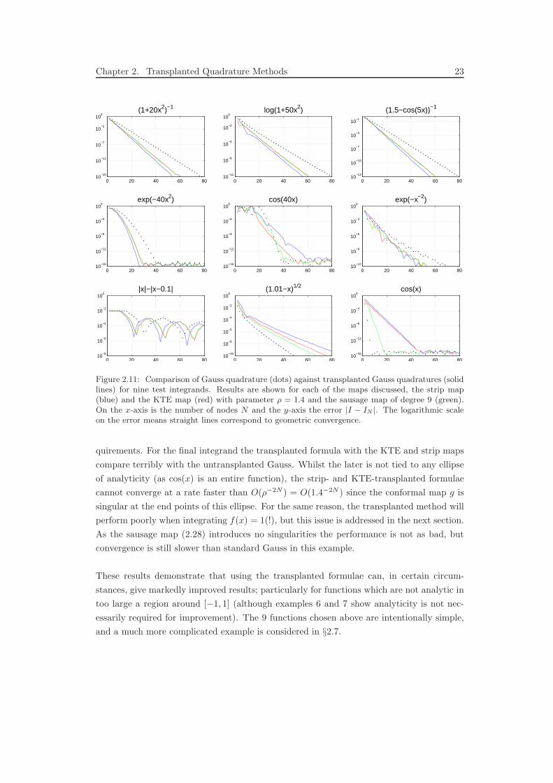
In Figure 2.11 we see that for many integrands the transplanted methods show a clear im-
provement over standard Gauss quadrature. This is most strongly demonstrated in the first
3 examples, where the integrands have poles or branch points in the complex plane close to
[−1, 1] (in particular near the origin). Since the strip map (2.16) maps the same ellipse to a
region ‘thinner’ in this direction, it converges slightly faster than the other two maps. The
fourth example shows a similar improvement, this time with super-geometric convergence.
Although f(z) is entire, it grows extremely rapidly as z moves away from the real axis; an
effect reduced by the transplantation. For the integrand cos(40x), the more equal distribu-
tion of nodes in the transplanted methods mean they are able to resolve the oscillations with
fewer points per wavelength and hence converge sooner. Once the error falls below around
10−5 for the strip or 10−8 for the KTE map, the untransplanted formula does better, since
the integrand is analytic and the convergence of the transplanted variant is restricted by
the choice of ρ = 1.4. The sixth integrand, exp(−x−2), is C∞ but not analytic and we see a
comparable performance of the methods. Similarly for |x| − |x− 0.1|, which is continuous,
but not differentiable.
The singularities of the penultimate example,√
1.01− x lie on the real axis, a short distance
from ±1. Since the maps stretch the region of analyticity required in the real direction, it is
unsurprising that the untransplanted rule is faster here because of its weaker analyticity re-
Chapter 2. Transplanted Quadrature Methods 23
0 20 40 60 8010
−15
10−11
10−7
10−3
100
(1+20x2)−1
0 20 40 60 8010
−11
10−8
10−5
10−2
100
log(1+50x2)
0 20 40 60 8010
−13
10−10
10−7
10−4
10−1
(1.5−cos(5x))−1
0 20 40 60 8010
−16
10−12
10−8
10−4
100
exp(−40x2)
0 20 40 60 8010
−16
10−12
10−8
10−4
100
cos(40x)
0 20 40 60 8010
−12
10−9
10−6
10−3
100
exp(−x−2)
0 20 40 60 8010
−8
10−6
10−4
10−2
100
|x|−|x−0.1|
0 20 40 60 8010
−10
10−8
10−6
10−4
10−2
100
(1.01−x)1/2
0 20 40 60 8010
−16
10−12
10−8
10−4
100
cos(x)
Figure 2.11: Comparison of Gauss quadrature (dots) against transplanted Gauss quadratures (solidlines) for nine test integrands. Results are shown for each of the maps discussed, the strip map(blue) and the KTE map (red) with parameter ρ = 1.4 and the sausage map of degree 9 (green).On the x-axis is the number of nodes N and the y-axis the error |I − IN |. The logarithmic scaleon the error means straight lines correspond to geometric convergence.
quirements. For the final integrand the transplanted formula with the KTE and strip maps
compare terribly with the untransplanted Gauss. Whilst the later is not tied to any ellipse
of analyticity (as cos(x) is an entire function), the strip- and KTE-transplanted formulae
cannot converge at a rate faster than O(ρ−2N ) = O(1.4−2N ) since the conformal map g is
singular at the end points of this ellipse. For the same reason, the transplanted method will
perform poorly when integrating f(x) = 1(!), but this issue is addressed in the next section.
As the sausage map (2.28) introduces no singularities the performance is not as bad, but
convergence is still slower than standard Gauss in this example.
These results demonstrate that using the transplanted formulae can, in certain circum-
stances, give markedly improved results; particularly for functions which are not analytic in
too large a region around [−1, 1] (although examples 6 and 7 show analyticity is not nec-
essarily required for improvement). The 9 functions chosen above are intentionally simple,
and a much more complicated example is considered in §2.7.
Chapter 2. Transplanted Quadrature Methods 24
2.5 Integration of Constants
Whilst the transplanted methods approximate constants with geometric accuracy, they no
longer integrate them exactly. Whilst it is rare that one wishes to integrate a constant
numerically, this property is certainly disturbing. Fortunately there is an easy fix. When
using either Gauss or Clenshaw–Curtis quadrature the weights are positive, and so they are
too for our transplanted methods. By adjusting the weights in our methods so that they
sum to 2 (an adjustment which will be exponentially small), it is clear that integration of
constants will not be a problem. To this end, we define a variant of our methods
IN (f) =2
IN (1)IN (f), (2.29)
which we could consider as simply modifying our weights so that
wk = 2wk
/
N∑
j=1
wj , k = 1, . . . , N. (2.30)
Now if we wish to integrate a constant C, then
IN (C) =
N∑
k=1
2wkC
/
N∑
j=1
wj = 2C = I(C) (2.31)
as required. Moreover, since the Gauss and Clenshaw–Curtis weights are symmetric about
the origin and our conformal maps g preserve this property, we can also integrate odd pow-
ers of x, and in particular linear functions, exactly.
The following result shows that this adjustment of the weights has no effect on the asymp-
totic rate of convergence of the transplanted methods;
|I(f)− IN (f)| = |I(f)− IN (f) + IN (f)− IN (f)|≤ |I(f)− IN (f)|+ |IN (f)− IN (f)|= |I(f)− IN (f)|+ |IN (f)− 2IN (f)/IN (1)|= |I(f)− IN (f)|+ |IN (f)/IN (1)||IN (1)− 2|= O(ρ−2N ) + O(ρ−2N ) = O(ρ−2N ).
Moreover, noting |IN (f)| ≤ M∑
g′(xk)wk = MIN (1), and that by Theorem 2.2.1 |I(f) −IN (f)| and M |IN (1)− 2| = M |IN (1)− I(1)| are bounded by 64Mγ
15(1−ρ−2)ρ2N , we have
|I(f)− IN (f)| ≤ 128Mγ
15(1− ρ−2)ρ2N. (2.32)
Thus the adjustment (2.29) to integrate constants will only hurt the convergence estimate
by at most a factor of 2.
Chapter 2. Transplanted Quadrature Methods 25
2.6 Convergence Results
One of the main advantages to the conformal mapping approach we have taken to the π/2
problem is that the existing theorems regarding geometric convergence transfer readily to the
transplanted case, cf. Theorem 2.2.1. The trick is deciding which analyticity assumptions
and conformal maps g to consider. The number of possibilities is unlimited, and rather
than explore the terrain thoroughly, we examine a few representative choices. Our class of
integrands will be as follows. For any ε > 0 define
A(ε) = set of functions analytic in the open ε-neighbourhood of [−1, 1]. (2.33)
Definition The ε-neighbourhood of the interval [−1, 1] is the set
z ∈ C : ∃ x ∈ [−1, 1] s.t. |z − x| < ε. (2.34)
Equivalently this can be thought of as
⋃
x∈[−1,1]
Bε(x). (2.35)
The largest ellipse Eρ that could fit into such a region will have a semi-axis of height ε, and
therefore have parameter ρ = ε +√
1 + ε2 = 1 + ε + O(ε2). Since ρ > 1, any f ∈ A(ε)
is bounded in the ellipse E1+ε and Gauss quadrature will converge at a rate of at least
O((1 + ε)−2N ) as N → ∞. On the other hand, since ρ ∼ (1 + ε) as ε → 0, it will do no
better than this in general as ε→ 0. By contrast, the following shows that the transplanted
method using the conformal maps of sections 2.3.1–2.3.3 converge at least 30%−40% faster.
Proposition 2.6.1 Let the transplanted Gauss quadrature formula (2.10) be applied to a
function f ∈ A(ε). The following statements pertain to the limit N →∞.
For the strip map (2.16) with ρ = 1.4 and any ε ≤ 0.24 :
|I − IN | = O((1 + 1.4ε)−2N).
For the KTE map (2.22) with ρ = 1.4 and any ε ≤ 0.3 :
|I − IN | = O((1 + 1.3ε)−2N).
For the sausage map (2.28) with d = 9 and any ε ≤ 0.8 :
|I − IN | = O((1 + 1.3ε)−2N).
Indeed, consider for example the first assertion, that the map (2.16) with ρ = 1.4 has a
convergence rate O((1 + 1.4ε)−2N). By Theorem 2.1.2, this conclusion will be valid if for
all ε < 0.24 the function g is analytic in the ellipse E1+1.4ε and maps this region into the
open ε-neighbourhood of [−1, 1]. We know that g is analytic in the ellipse E1.4, so the first
condition holds since 1+(1.4)(0.24) < 1.4. The second condition can be verified numerically
by plotting the image of the ellipse E1+1.4ε and the boundary of the ε-region for various ε,
and verifying that the first is inside the second. This is true of all the parameters above.
Chapter 2. Transplanted Quadrature Methods 26
The speedups of Proposition 2.6.1 are not particularly close to the limiting value of π/2 that
can be achieved as ε→ 0. We now give a further result that comes closer to this limit. This
time we modify the Gauss quadrature estimate by improving the exponent, rather than the
factor multiplying ε.
Proposition 2.6.2 Let the transplanted Gauss quadrature formula (2.10) be applied to a
function f ∈ A(ε) for any ε ≤ 0.05. For the strip map (2.16) with ρ = 1.1,
|IN − I| = O((1 + ε)−3N ), as N →∞. (2.36)
The justification is as before, combining Theorem 2.1.2 with a numerical verification for the
particular map g. Similarly, it can be shown that one gets |IN − I| = O((1 + ε)−2.7N ) for
ε < 0.1 with the strip map with ρ = 1.4, the KTE map with ρ = 1.2, or higher degree
analogue of the polynomial with d = 17, and |IN − I| = O((1 + ε)−2.5N) for ε < 0.3 with
the strip map with ρ = 1.5, the KTE map with ρ = 1.4, or the sausage with d = 9.
2.7 Transplanted Clenshaw–Curtis
Our discussion so far has been centred around Gauss quadrature. An alternative is Clenshaw–
Curtis, which is based upon integrating the polynomial which interpolates the integrand f(x)
at Chebyshev points. Whilst from this definition it is clear that the N -point Clenshaw–
Curtis quadrature rule will integrate polynomials of degree N−1 exactly, Gauss quadrature
is widely seen as optimal amongst polynomial based schemes as it exactly integrates all
polynomials up to degree 2N − 1 [Dav75, pg. 343]. This difference in optimality can also
be seen in the Clenshaw–Curtis version of the theorem regarding convergence for analytic
functions. The following given by Davis and Rabinowitz [DR84, (4.6.31)] is analogous to
Theorem 2.1.2 for Gauss quadrature.
Theorem 2.7.1 Let the function f be analytic in [−1, 1] and analytically continuable with
|f(z)| < M in the closed ellipse Eρ. The error in ICCN (f), the Clenshaw–Curtis quadrature
approximation of degree N to I(f), will decay geometrically with the bound
|I − ICCN | ≤ 64M
15(ρ2 − 1)(ρN−1 − ρ−(N−1)), N ≥ 3 odd. (2.37)
As before, if one is willing to ignore constants and consider only the asymptotic result,
this reduces to |I − ICCN | = O(ρ−N ). This result could leave one inclined to believe that
Clenshaw–Curtis was perhaps only half as accurate as Gauss quadrature, and therefore π
times slower than the trapezium rule. However, Trefethen and Weideman [Tre08, WT07]
have shown that for functions not analytic in a too sizeable region around [−1, 1] and rea-
sonable values of N , this is not the case, and Clenshaw–Curtis is in fact competitive. The
above theorem is indeed a sharp bound as N →∞, but for most practical values of N and
functions which are not entire, the error in Clenshaw–Curtis is O(ρ−2N ), the same as Gauss
quadrature. This is particularly useful, since the task of computing the weights and nodes
for Clenshaw–Curtis can be completed via an FFT in considerably less time, O(N log N),
Chapter 2. Transplanted Quadrature Methods 27
than solving the eigenvalue system to find those for Gaussian quadrature, O(N2)2.
The ellipse in the theorem above is precisely the same as appears in Theorem 2.1.2 and which
we have been discussing throughout this chapter, and so the new transplanted methods we
have described are directly applicable to the Clenshaw–Curtis quadrature with a few slight
modifications. Firstly, the code in §2.3.1 for computing the strip map does not compute the
values of g′(±1), but these values are given analytically in equation (2.18). We can then
plot in Figure 2.12 how the strip and KTE maps affect the Chebyshev modes as ρ is varied.
As we saw with the transplanted Gauss nodes under the same maps, as the parameter
decreases, the transplanted Chebyshev nodes become more equally spaced. In fact, since
the limit ρ→ 1 both maps reduce to g(s) = 2 arcsin s/π, the limiting positions of the N+1
nodes are
g(xk+1; m→ 1) = 2 arcsin(−cos
(
kπ
N
)
) /π = −1 +2k
N, (2.38)
for k = 0, ..., N . To see this, note sn(u|m) = tanh(u) + O(1−m) [AS65, (16.15.1)] and
that K(m)/ arctanhm1/4 → 1 as m→ 1, which is easily verified numerically. The points in
(2.38) are precisely the equally-spaced nodes of the (N +1)-point trapezium rule .
Secondly, we must implement the transplanted Clenshaw–Curtis method efficiently using
the FFT algorithm. For a stand-alone code we could use the code clenshaw curtis(f,N)
from [Tre08], which computes IN (f) given the values of f at the Chebyshev nodes xk. Recall
from equation (2.9) that our transplanted formula amounts to computing IN (g′ · (f g)),
so we simply pass g′kf(gk) instead of f(xk). This value appears in the line fx = ... in the
following code;
f = @(x) 1./(1+20*x.^2); % Change for other integrands
s = -cos((0:N)*pi/N)’; % Chebyshev nodes
[g,gprime] = sausagemap(s); % Change for a different map
fx = f(g).*gprime;
h = real(fft(fx([1:N+1 N:-1:2])/(2*N)));% Fast Fourier transform
a = [h(1); h(2:N)+h(2*N:-1:N+2); h(N+1)];
w = 0*a’; w(1:2:end) = 2./(1-(0:2:N).^2);
In = w*a; % The integral
In chebfun this could be implemented with the one-liner
In = sum(chebfun(f,’map’,’sausage’,9));
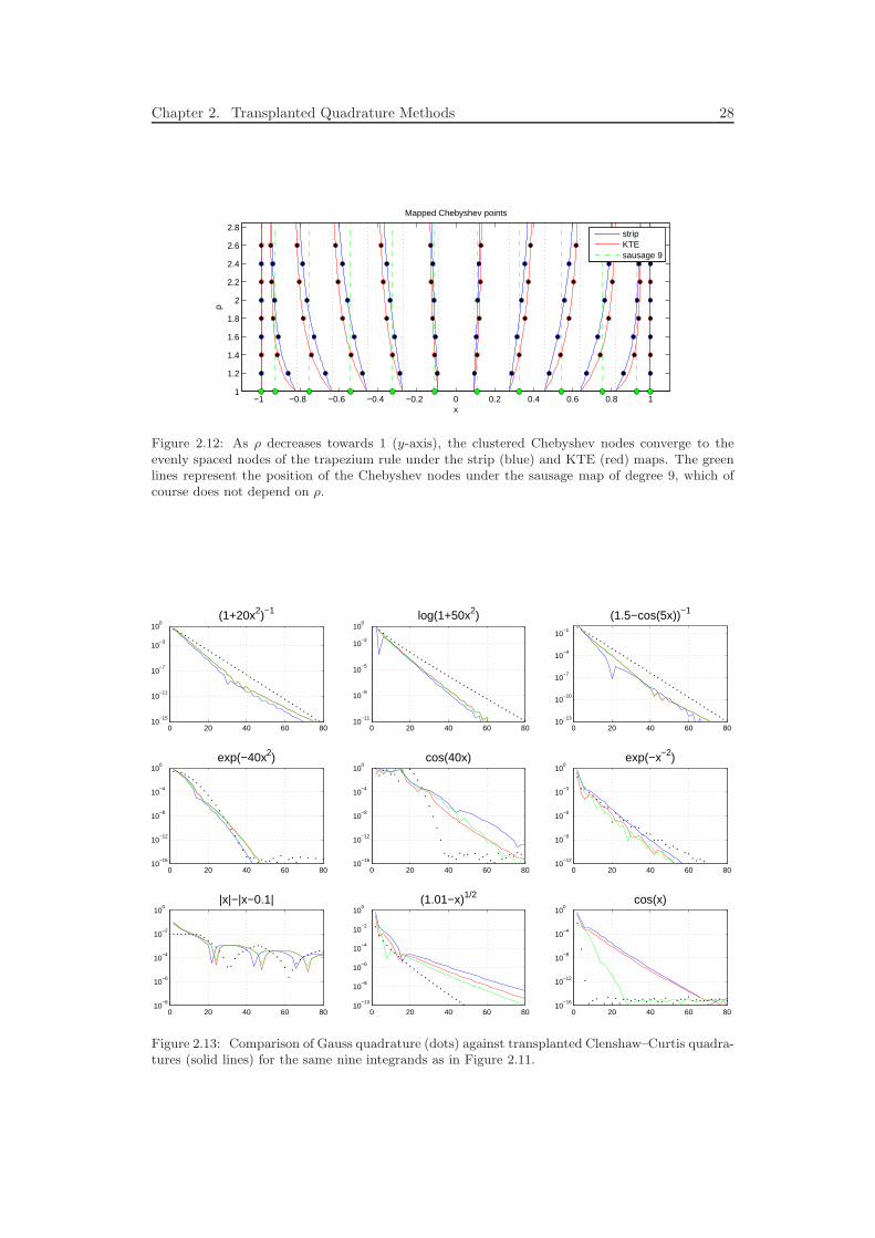
We repeat in Figure 2.13 the tests of §2.4, but this time using the Clenshaw–Curtis version
of the transplanted quadrature method. For a fixed value of ρ = 1.4 we see that transplanted
Clenshaw–Curtis does very well, with performance being similar, if only slightly worse, than
the transplanted Gauss methods. The only integrands for which we lose much in moving
from transplanted Gauss to transplanted Clenshaw–Curtis methods are those which have
large regions of analyticity or are entire, as explained in [Tre08, WT07].
2Glaser et al. [GLR07] recently devised a fast algorithm for computing the weights and nodes in O(N)operations, but the implied constant factors, and hence computation times, are still far larger than ofClenshaw–Curtis.
Chapter 2. Transplanted Quadrature Methods 28
−1 −0.8 −0.6 −0.4 −0.2 0 0.2 0.4 0.6 0.8 11
1.2
1.4
1.6
1.8
2
2.2
2.4
2.6
2.8ρ
x
Mapped Chebyshev points
stripKTEsausage 9
Figure 2.12: As ρ decreases towards 1 (y-axis), the clustered Chebyshev nodes converge to theevenly spaced nodes of the trapezium rule under the strip (blue) and KTE (red) maps. The greenlines represent the position of the Chebyshev nodes under the sausage map of degree 9, which ofcourse does not depend on ρ.
0 20 40 60 8010
−15
10−11
10−7
10−3
100
(1+20x2)−1
0 20 40 60 8010
−11
10−8
10−5
10−2
100
log(1+50x2)
0 20 40 60 8010
−13
10−10
10−7
10−4
10−1
(1.5−cos(5x))−1
0 20 40 60 8010
−16
10−12
10−8
10−4
100
exp(−40x2)
0 20 40 60 8010
−16
10−12
10−8
10−4
100
cos(40x)
0 20 40 60 8010
−12
10−9
10−6
10−3
100
exp(−x−2)
0 20 40 60 8010
−8
10−6
10−4
10−2
100
|x|−|x−0.1|
0 20 40 60 8010
−10
10−8
10−6
10−4
10−2
100
(1.01−x)1/2
0 20 40 60 8010
−16
10−12
10−8
10−4
100
cos(x)
Figure 2.13: Comparison of Gauss quadrature (dots) against transplanted Clenshaw–Curtis quadra-tures (solid lines) for the same nine integrands as in Figure 2.11.
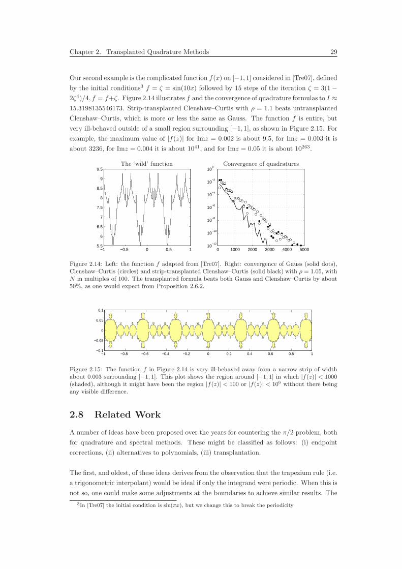
Chapter 2. Transplanted Quadrature Methods 29
Our second example is the complicated function f(x) on [−1, 1] considered in [Tre07], defined
by the initial conditions3 f = ζ = sin(10x) followed by 15 steps of the iteration ζ = 3(1 −2ζ4)/4, f = f+ζ. Figure 2.14 illustrates f and the convergence of quadrature formulas to I ≈15.3198135546173. Strip-transplanted Clenshaw–Curtis with ρ = 1.1 beats untransplanted
Clenshaw–Curtis, which is more or less the same as Gauss. The function f is entire, but
very ill-behaved outside of a small region surrounding [−1, 1], as shown in Figure 2.15. For
example, the maximum value of |f(z)| for Imz = 0.002 is about 9.5, for Imz = 0.003 it is
about 3236, for Imz = 0.004 it is about 1041, and for Imz = 0.05 it is about 10263.
−1 −0.5 0 0.5 15.5
6
6.5
7
7.5
8
8.5
9
9.5
0 1000 2000 3000 4000 500010
−12
10−10
10−8
10−6
10−4
10−2
100
The ‘wild’ function Convergence of quadratures
Figure 2.14: Left: the function f adapted from [Tre07]. Right: convergence of Gauss (solid dots),Clenshaw–Curtis (circles) and strip-transplanted Clenshaw–Curtis (solid black) with ρ = 1.05, withN in multiples of 100. The transplanted formula beats both Gauss and Clenshaw–Curtis by about50%, as one would expect from Proposition 2.6.2.
−1 −0.8 −0.6 −0.4 −0.2 0 0.2 0.4 0.6 0.8 1−0.1
−0.05
0
0.05
0.1
Figure 2.15: The function f in Figure 2.14 is very ill-behaved away from a narrow strip of widthabout 0.003 surrounding [−1, 1]. This plot shows the region around [−1, 1] in which |f(z)| < 1000(shaded), although it might have been the region |f(z)| < 100 or |f(z)| < 106 without there beingany visible difference.
2.8 Related Work
A number of ideas have been proposed over the years for countering the π/2 problem, both
for quadrature and spectral methods. These might be classified as follows: (i) endpoint
corrections, (ii) alternatives to polynomials, (iii) transplantation.
The first, and oldest, of these ideas derives from the observation that the trapezium rule (i.e.
a trigonometric interpolant) would be ideal if only the integrand were periodic. When this is
not so, one could make some adjustments at the boundaries to achieve similar results. The
3In [Tre07] the initial condition is sin(πx), but we change this to break the periodicity

Chapter 2. Transplanted Quadrature Methods 30
well-known Euler–Maclaurin formula gives an asymptotic (but not convergent) expression
for the error in the trapezium rule when applied to analytic functions;
ITN (f)− I(f) =
m−1∑
k=1
22kB2k
N2k(2k)!
(
f (2k−1)(1)− f (2k−1)(−1))
+22m+1B2m
N2m(2m)!f2m(ξ), (2.39)
for some ξ ∈ [−1, 1]. By adding known or approximated values of the derivatives on the
right-hand-side of the above, the trapezium rule can be ‘corrected’ to achieve higher order
convergence. If one replaces these terms by one-sided finite difference approximations of the
appropriate orders, the resulting quadrature rules are known as Gregory’s formulae [Hil56,
§5.9],[Jor65, §99]. These formulae are effective only up to medium orders of accuracy, at
which point exponentially large coefficients of alternating signs make such methods numer-
ically unstable.
An improvement on Gregory formulae capable of achieving convergence of arbitrarily high
degree has been proposed by Alpert [Alp99], building upon ideas of Rokhlin and Kapur
[MRW96, KR97]. Alpert’s formulae take the form
IA(a,j)N = h′
(
j∑
k=1
wk (f(−1 + xk) + f(1− xk)) +
N−2j∑
k=0
f(−1 + (a + k)h′)
)
, (2.40)
where h′ = 2/(N + 2(a− j)− 1). In essence, an equispaced grid of N − 2j points is used on
the interior of the interval with a small number, j, of extra Gauss-like nodes (with positive
weights) near the endpoints. High-precision computations are required in advance to obtain
the nodes and weights, but once they are known the method is highly effective and can even
cope with some forms of singular integrands.
By alternatives to polynomials we mean the explicit construction of orthogonal bases that
are non-polynomial, and have more uniform behaviour over the interval of interest. An
important set of functions with this property are the prolate spheroidal wave functions
(PSWFs), introduced by Slepian and Pollak in the 1960s [SP61]. These functions have ex-
cellent resolution properties, and more recent authors have shown their power for a variety
of computational applications [Boy04, BS05, CGH05, XRY01]. In this literature, rather
than derive theorems about convergence for functions analytic in specified domains, it is
customary to quantify the matter of resolution by considering applications to band-limited
functions. Boyd [Boy04] gives some discussion to the geometric convergence of the PSWFs,
and in particular their comparison to Legendre polynomials, but admits that the results
obtained are somewhat unsatisfying. There are certainly no results in the PSWF literature
analogous to those in §2.6.
Finally there is the transplantation idea. A notable contribution in this area is a forty-year-
old theoretical paper by Bakhvalov, “On the optimal speed of integrating analytic functions”
[Bak67]. Bakhvalov asks what might be the optimal family of quadrature formulae for the
set of functions analytic and bounded in a given complex region Ω containing [−1, 1]? His
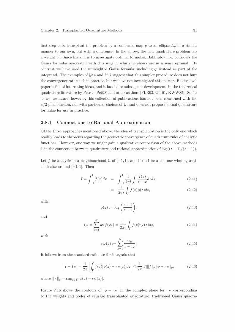
Chapter 2. Transplanted Quadrature Methods 31
first step is to transplant the problem by a conformal map g to an ellipse Eρ in a similar
manner to our own, but with a difference. In the ellipse, the new quadrature problem has
a weight g′. Since his aim is to investigate optimal formulas, Bakhvalov now considers the
Gauss formulas associated with this weight, which he shows are in a sense optimal. By
contrast we have used the unweighted Gauss formula, including g′ instead as part of the
integrand. The examples of §2.4 and §2.7 suggest that this simpler procedure does not hurt
the convergence rate much in practice, but we have not investigated this matter. Bakhvalov’s
paper is full of interesting ideas, and it has led to subsequent developments in the theoretical
quadrature literature by Petras [Pet98] and other authors [FLR93, Got01, KWW85]. So far
as we are aware, however, this collection of publications has not been concerned with the
π/2 phenomenon, nor with particular choices of Ω, and does not propose actual quadrature
formulae for use in practice.
2.8.1 Connections to Rational Approximation
Of the three approaches mentioned above, the idea of transplantation is the only one which
readily leads to theorems regarding the geometric convergence of quadrature rules of analytic
functions. However, one way we might gain a qualitative comparison of the above methods
is in the connection between quadrature and rational approximation of log ((z + 1)/(z − 1)).
Let f be analytic in a neighbourhood Ω of [−1, 1], and Γ ⊂ Ω be a contour winding anti-
clockwise around [−1, 1]. Then
I =
∫ 1
−1
f(x)dx =
∫ 1
−1
1
2πi
∫
Γ
f(z)
z − xdzdx, (2.41)
=1
2πi
∫
Γ
f(z)φ(z)dz, (2.42)
with
φ(z) := log
(
z + 1
z − 1
)
, (2.43)
and
IN =
N∑
k=1
wkf(xk) =1
2πi
∫
Γ
f(z)rN(z)dz, (2.44)
with
rN (z) :=
N∑
k=1
wk
z − xk. (2.45)
It follows from the standard estimate for integrals that
|I − IN | =1
2π
∣
∣
∣
∣
∫
Γ
f(z)[φ(z)− rN (z)]dz
∣
∣
∣
∣
≤ 1
2π|Γ|‖f‖
Γ‖φ− rN‖Γ , (2.46)
where ‖ · ‖Γ
= supz∈Γ |φ(z)− rN (z)|.
Figure 2.16 shows the contours of |φ − rN | in the complex plane for rN corresponding
to the weights and nodes of sausage transplanted quadrature, traditional Gauss quadra-
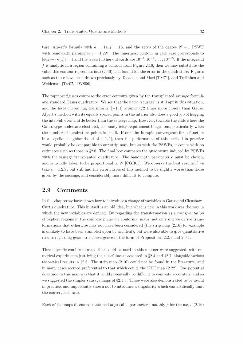
Chapter 2. Transplanted Quadrature Methods 32
ture, Alpert’s formula with a = 14, j = 16, and the zeros of the degree N + 1 PSWF
with bandwidth parameter c = 1.2N . The innermost contour in each case corresponds to
|φ(z)−rN (z)| = 1 and the levels further outwards are 10−1, 10−2, . . . , 10−13. If the integrand
f is analytic in a region containing a contour from Figure 2.16, then we may substitute the
value this contour represents into (2.46) as a bound for the error in the quadrature. Figures
such as these have been drawn previously by Takahasi and Mori [TM71], and Trefethen and
Weideman [Tre07, TWS06].
The topmost figures compare the error contours given by the transplanted sausage formula
and standard Gauss quadrature. We see that the name ‘sausage’ is still apt in this situation,
and the level curves hug the interval [−1, 1] around π/2 times more closely than Gauss.
Alpert’s method with its equally spaced points in the interior also does a good job of hugging
the interval, even a little better than the sausage map. However, towards the ends where the
Gauss-type nodes are clustered, the analyticity requirement bulges out, particularly when
the number of quadrature points is small. If our aim is rapid convergence for a function
in an epsilon neighbourhood of [−1, 1], then the performance of this method in practice
would probably be comparable to our strip map, but as with the PSWFs, it comes with no
estimates such as those in §2.6. The final box compares the quadrature induced by PSWFs
with the sausage transplanted quadrature. The bandwidth parameter c must be chosen,
and is usually taken to be proportional to N [CGH05]. We observe the best results if we
take c = 1.2N , but still find the error curves of this method to be slightly worse than those
given by the sausage, and considerably more difficult to compute.
2.9 Comments
In this chapter we have shown how to introduce a change of variables in Gauss and Clenshaw–
Curtis quadrature. This in itself is an old idea, but what is new in this work was the way in
which the new variables are defined. By regarding the transformation as a transplantation
of explicit regions in the complex plane via conformal maps, not only did we derive trans-
formations that otherwise may not have been considered (the strip map (2.16) for example
is unlikely to have been stumbled upon by accident), but were also able to give quantitative
results regarding geometric convergence in the form of Propositions 2.2.1 and 2.6.1.
Three specific conformal maps that could be used in this manner were suggested, with nu-
merical experiments justifying their usefulness presented in §2.4 and §2.7, alongside various
theoretical results in §2.6. The strip map (2.16) could not be found in the literature, and
in many cases seemed preferential to that which could, the KTE map (2.22). One potential
downside to this map was that it could potentially be difficult to compute accurately, and so
we suggested the simpler sausage maps of §2.3.3. These were also demonstrated to be useful
in practice, and importantly shown not to introduce a singularity which can artificially limit
the convergence rate.
Each of the maps discussed contained adjustable parameters, notably ρ for the maps (2.16)
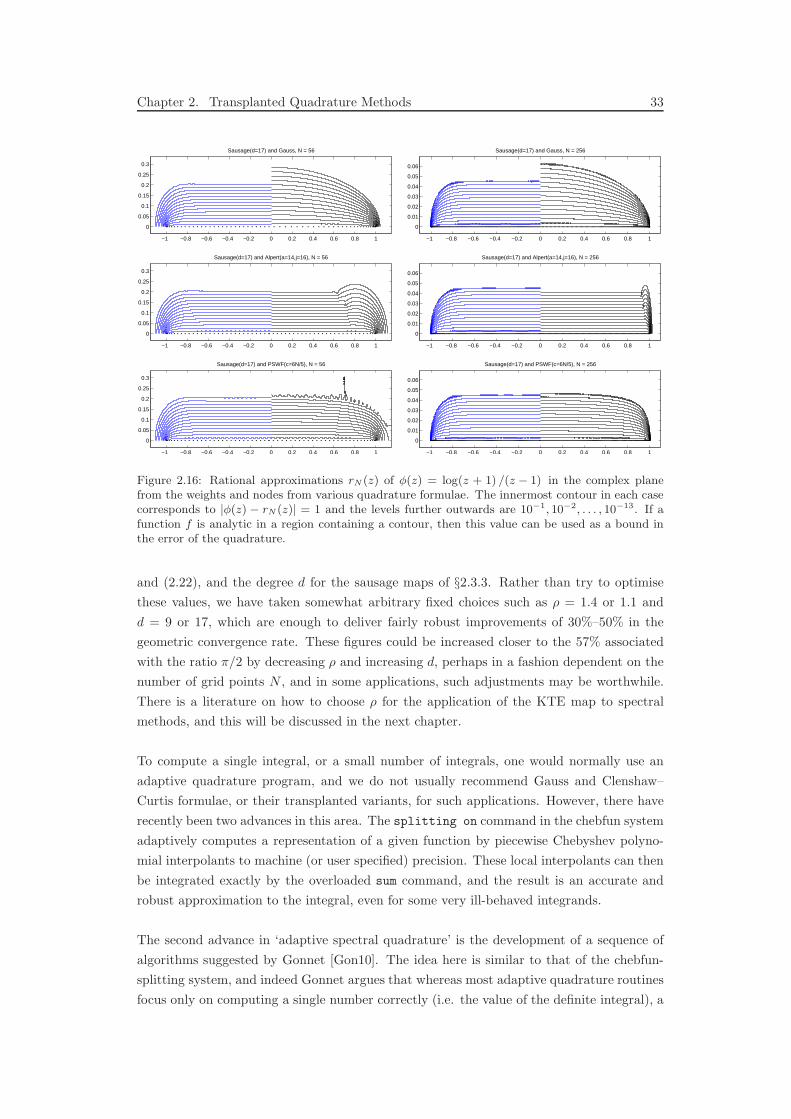
Chapter 2. Transplanted Quadrature Methods 33
Sausage(d=17) and Gauss, N = 56
−1 −0.8 −0.6 −0.4 −0.2 0 0.2 0.4 0.6 0.8 1
0
0.05
0.1
0.15
0.2
0.25
0.3
Sausage(d=17) and Alpert(a=14,j=16), N = 56
−1 −0.8 −0.6 −0.4 −0.2 0 0.2 0.4 0.6 0.8 1
0
0.05
0.1
0.15
0.2
0.25
0.3
Sausage(d=17) and PSWF(c=6N/5), N = 56
−1 −0.8 −0.6 −0.4 −0.2 0 0.2 0.4 0.6 0.8 1
0
0.05
0.1
0.15
0.2
0.25
0.3
Sausage(d=17) and Gauss, N = 256
−1 −0.8 −0.6 −0.4 −0.2 0 0.2 0.4 0.6 0.8 1
0
0.01
0.02
0.03
0.04
0.05
0.06
Sausage(d=17) and Alpert(a=14,j=16), N = 256
−1 −0.8 −0.6 −0.4 −0.2 0 0.2 0.4 0.6 0.8 1
0
0.01
0.02
0.03
0.04
0.05
0.06
Sausage(d=17) and PSWF(c=6N/5), N = 256
−1 −0.8 −0.6 −0.4 −0.2 0 0.2 0.4 0.6 0.8 1
0
0.01
0.02
0.03
0.04
0.05
0.06
Figure 2.16: Rational approximations rN (z) of φ(z) = log(z + 1) /(z − 1) in the complex planefrom the weights and nodes from various quadrature formulae. The innermost contour in each casecorresponds to |φ(z) − rN (z)| = 1 and the levels further outwards are 10−1, 10−2, . . . , 10−13. If afunction f is analytic in a region containing a contour, then this value can be used as a bound inthe error of the quadrature.
and (2.22), and the degree d for the sausage maps of §2.3.3. Rather than try to optimise
these values, we have taken somewhat arbitrary fixed choices such as ρ = 1.4 or 1.1 and
d = 9 or 17, which are enough to deliver fairly robust improvements of 30%–50% in the
geometric convergence rate. These figures could be increased closer to the 57% associated
with the ratio π/2 by decreasing ρ and increasing d, perhaps in a fashion dependent on the
number of grid points N , and in some applications, such adjustments may be worthwhile.
There is a literature on how to choose ρ for the application of the KTE map to spectral
methods, and this will be discussed in the next chapter.
To compute a single integral, or a small number of integrals, one would normally use an
adaptive quadrature program, and we do not usually recommend Gauss and Clenshaw–
Curtis formulae, or their transplanted variants, for such applications. However, there have
recently been two advances in this area. The splitting on command in the chebfun system
adaptively computes a representation of a given function by piecewise Chebyshev polyno-
mial interpolants to machine (or user specified) precision. These local interpolants can then
be integrated exactly by the overloaded sum command, and the result is an accurate and
robust approximation to the integral, even for some very ill-behaved integrands.
The second advance in ‘adaptive spectral quadrature’ is the development of a sequence of
algorithms suggested by Gonnet [Gon10]. The idea here is similar to that of the chebfun-
splitting system, and indeed Gonnet argues that whereas most adaptive quadrature routines
focus only on computing a single number correctly (i.e. the value of the definite integral), a
Chapter 2. Transplanted Quadrature Methods 34
reliable algorithm should instead concentrate on computing a sufficiently accurate represen-
tation of the integrand, which can then be integrated exactly. As with the chebfun system,
Gonnet’s representation of the integrand uses adaptively selected piecewise Chebyshev in-
terpolations, but can cope even with non-numerical values such as NaN and Inf.
The piecewise components in these approximations however are still Chebyshev polynomials
(simply scaled to a smaller interval, see (2.1), (2.2)), and are subject to the clustered grids
and irregular convergence regions discussed at the beginning of this chapter. An interesting
future development would be to see whether transplanted interpolants / quadratures on the
subintervals, such as those defined by the maps in §2.3, can lead to improvements in these
two highly competitive quadrature routines.
For now the potential practical relevance of the methods investigated in this chapter is to
situations where large numbers of integrals are embedded inside a bigger computation, and
we close with an artificial example of a multidimensional integral. Suppose we compute
∫ 1
−1
∫ 1
−1
∫ 1
−1
∫ 1
−1
cos(100(w + x + y + z))dwdxdydz =
(
sin(100)
50
)4
≈ 1.05× 10⁻⁸
numerically by a quadrature formula applied in four dimensions, exploiting none of the
symmetries or simple structure of this particular integrand. To get three digits of relative
accuracy, Gauss quadrature requires 634 = 15,752,961 points, whereas strip-transplanted
Gauss quadrature with ρ = 1.4 needs 524 = 7,311,616 points.

Chapter 3
Mapped Spectral Methods
Spectral methods are an incredibly useful tool for solving a variety of problems involving
derivatives of functions on simple domains. In this thesis we focus on spectral methods based
upon collocation, often referred to as “pseudospectral”. The idea of these is similar to that
of the quadrature methods in the previous chapter; we interpolate the function of interest
at a set of points using say a trigonometric or algebraic polynomial, and approximate the
derivative of the function by the (easily computed) derivative of the interpolant.
The geometric accuracy of the underlying global interpolants means that, under some rea-
sonable assumptions, these pseudospectral methods will also converge geometrically (see
§3.1). The Fourier spectral method is based upon the same trigonometric polynomial as the
trapezium rule, and so the points are equally spaced and convergence is geometric when
applied to a periodic function analytic on the domain of computation. The polynomial
based Chebyshev spectral method can give geometric convergence when the function is not
periodic, but this comes at the expense of the same clustered grid we saw with Clenshaw–
Curtis quadrature.
In the context of spectral methods, the clustering of points in polynomial methods has a fur-
ther negative effect, particularly when solving time dependent problems. The high density
of points near the boundaries can necessitate very small time steps in explicit time-stepping
methods, and make the differentiation matrices of implicit time-stepping methods very ill-
conditioned [CHQZ06, Tre00].
It has been suggested in the literature [BT92, For98, KTE93] that to overcome these difficul-
ties one should use methods with a non-polynomial basis. One such approach continues that
which we took in the previous chapter, where a map g is used to transplant the polynomi-
als to something which more closely resemble the trigonometric interpolants of the Fourier
method. In the context of spectral methods, this idea was first introduced by Kosloff and
Tal-Ezer [KTE93] with the arcsine transformation discussed in §2.3.2,
g(z) = arcsin(βz)/ arcsin(β). (3.1)
By considering this transformation as a conformal map, one can obtain similar convergence
to those results in §2.6 for this mapped Chebyshev method.
35
Chapter 3. Mapped Spectral Methods 36
Another approach is to leave behind polynomial interpolants altogether and use methods
based upon rational interpolants. This idea is realised in the work of Berrut and co-authors
in [BBN99], where they introduce a linear rational interpolant, and show that certain such
interpolants through conformally mapped Chebyshev points approximate analytic functions
with geometric accuracy. In the same paper they go on to differentiate the interpolant an-
alytically to form a linear rational collocation method. The conformal map they choose is
again the KTE transform (3.1), and they demonstrate that the rational collocation methods
have many of the same beneficial properties as the KTE mapped-polynomial method. Tee
[Tee06] shows that the derivatives of the rational interpolant are also geometrically con-
vergent, and combines the rational spectral method with his own conformal maps in an
adaptive rational spectral method [TT06]. We revisit this idea in §4.
In this chapter we observe the effect of replacing the KTE map (3.1) in the methods above
with those described in §2.3, and explore whether considering this transformation as a con-
formal map can lead to new insights or theorems. As such, the outline of this chapter is as
follows. In §3.1 we discuss the Fourier and Chebyshev spectral methods, and in particular
their geometric convergence for analytic functions. §3.2 describes the mapped-polynomial
method of [KTE93] and the rational method of [BBN99], which are then tested in §3.4 using
the same conformal maps and test functions as in the previous chapter.
In §3.5 we discuss the issue of time-stepping. Much of the work in the literature on mapped
Chebyshev methods revolves (effectively) around the choice of the parameter ρ in the KTE
map for time dependent problems. We discuss the effect of the parameter on others maps
from §2.3 and demonstrate that these may often be more useful in practice. We close the
chapter in §3.6 with a summary discussion.
3.1 Fourier and Chebyshev Spectral Methods
Suppose f is a differentiable function defined on some closed, bounded interval (as with the
quadratures previously, we take this to be [−1, 1] without loss of generality). In this interval
take a discrete grid xjNj=0 of distinct points and seek an approximation to the derivative f ′
at these points. Spectral methods achieve this by fitting an interpolating polynomial pN (x)
(trigonometric for Fourier and algebraic for Chebyshev) through the data points, which is
then differentiated analytically and evaluated on the grid to give p′N (xj) ≈ f ′(xj). These
values at the grid points can then be interpolated to approximate f ′ for any values in [−1, 1].
Higher-order derivatives are obtained in a similar way, by taking further derivatives of the
interpolant.
In practice, the choice of method and a degree N will give rise to a set of points xjNj=0
and a differentiation matrix DN . The approximation to the derivative at the grid points is
then given by
v = DNu, (3.2)
Chapter 3. Mapped Spectral Methods 37
where uj = f(xj) and vj ≈ f ′(xj). Detailed description of the background, implementa-
tion, and performance of various spectral methods can be found in a number of texts, e.g.
[Boy01, CHQZ06, For98, Tre00].
The Fourier method uses the same equally spaced nodes as the trapezium rule for a periodic
function, xj =−1+2j/N, j = 1, . . . , N . The following theorem governing the convergence of
the Fourier method for analytic functions follows from that first given by Tadmor [Tad86],
as does the analogous theorem for the Chebyshev method in Theorem 3.1.2. Subsequent im-
provements in the implied constant and algebraic factors have since been made, for example
in [RW05], but here we focus only on the asymptotic rate.
Theorem 3.1.1 Let f be a function periodic on [−1, 1] and analytic in the closed strip
|Imz| ≤ η. The error in the Fourier approximation to derivatives of f given by the trigono-
metric interpolant tN satisfies
max−1≤x≤1
|f (n)(x)− t(n)N (x)| = O(e−η(π/2)N)) as N →∞ (3.3)
for all integers n ≥ 0.
Note that the rate is a factor of two less here than in the error of the trapezium rule (The-
orem 2.1.1), as we do not benefit from aliasing [Boy01, Chapter 9],[Tre00].
The nodes of the (N+1)-point Chebyshev spectral method are the same as in Clenshaw–
Curtis quadrature, xj+1 = − cos(jπ/N), j = 0, . . . , N . The differentiation matrix can be
computed using the Matlab code D = cheb(N) from [Tre00]. Here however we use the
code bcmatrix from [TT06], for reasons that will become clear in the next section. Both of
methods compute the matrix DN+1, but the latter can also compute the 2nd-order matrix
D2N+1 efficiently.
x = -cos((0:N)’*pi/N); % Chebyshev nodes
w = [1/2 ones(1,N-1) 1/2].*(-1).^(0:N); % Barycentric weights
[D D2] = bcmatrix(w’,x); % Chebyshev differentiation matrix
v = D*f(x); % v = f’(x)
Using the chebop technology of the chebfun system, this same matrix D could be computed
by the following operations;
d = domain(-1,1); % Domain of computation
D = diff(d); % Chebyshev differentiation operator
D = D(N+1); % Discrete matrix of size N+1 x N+1
The theorem below also follows from a result due to Tadmor [Tad86], and is almost identical
to that for Clenshaw–Curtis quadrature (Theorem 2.7.1).
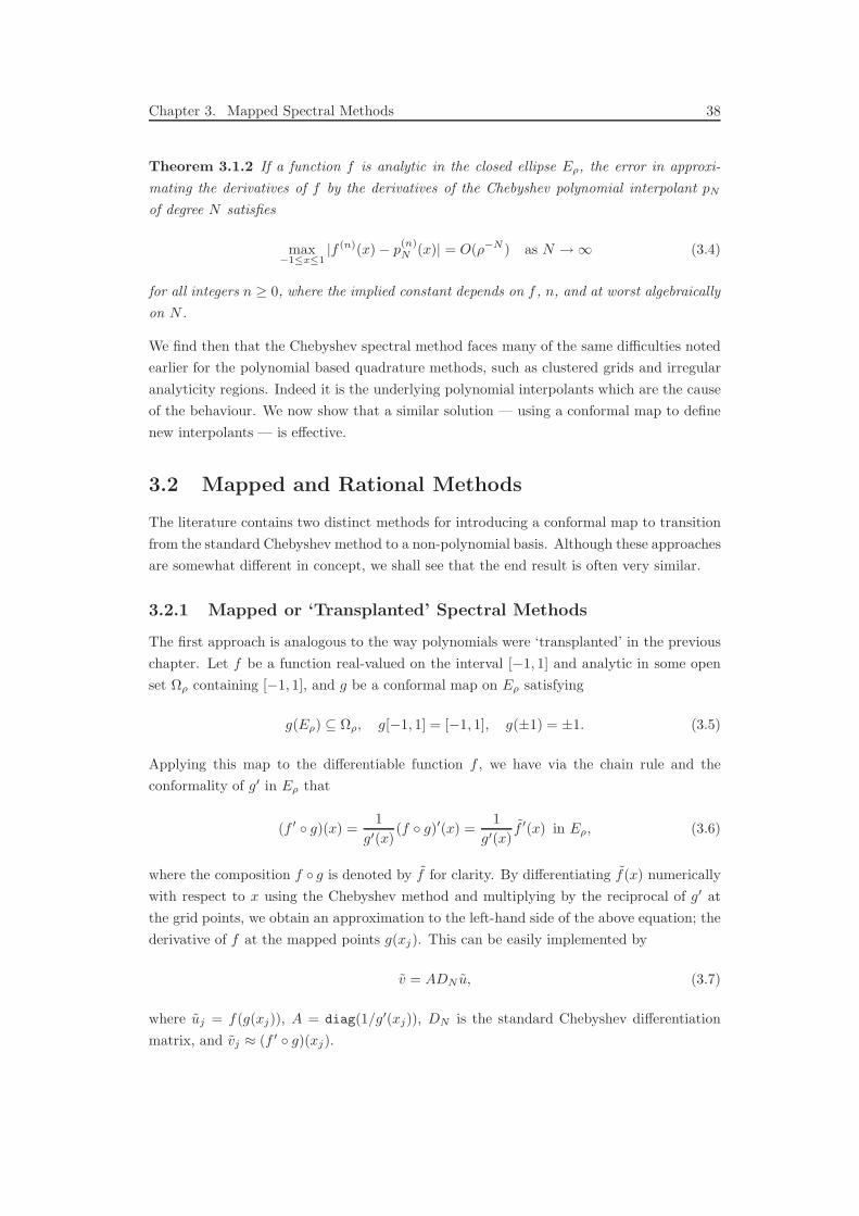
Chapter 3. Mapped Spectral Methods 38
Theorem 3.1.2 If a function f is analytic in the closed ellipse Eρ, the error in approxi-
mating the derivatives of f by the derivatives of the Chebyshev polynomial interpolant pN
of degree N satisfies
max−1≤x≤1
|f (n)(x)− p(n)N (x)| = O(ρ−N ) as N →∞ (3.4)
for all integers n ≥ 0, where the implied constant depends on f , n, and at worst algebraically
on N .
We find then that the Chebyshev spectral method faces many of the same difficulties noted
earlier for the polynomial based quadrature methods, such as clustered grids and irregular
analyticity regions. Indeed it is the underlying polynomial interpolants which are the cause
of the behaviour. We now show that a similar solution — using a conformal map to define
new interpolants — is effective.
3.2 Mapped and Rational Methods
The literature contains two distinct methods for introducing a conformal map to transition
from the standard Chebyshev method to a non-polynomial basis. Although these approaches
are somewhat different in concept, we shall see that the end result is often very similar.
3.2.1 Mapped or ‘Transplanted’ Spectral Methods
The first approach is analogous to the way polynomials were ‘transplanted’ in the previous
chapter. Let f be a function real-valued on the interval [−1, 1] and analytic in some open
set Ωρ containing [−1, 1], and g be a conformal map on Eρ satisfying
g(Eρ) ⊆ Ωρ, g[−1, 1] = [−1, 1], g(±1) = ±1. (3.5)
Applying this map to the differentiable function f , we have via the chain rule and the
conformality of g′ in Eρ that
(f ′ g)(x) =1
g′(x)(f g)′(x) =
1
g′(x)f ′(x) in Eρ, (3.6)
where the composition f g is denoted by f for clarity. By differentiating f(x) numerically
with respect to x using the Chebyshev method and multiplying by the reciprocal of g′ at
the grid points, we obtain an approximation to the left-hand side of the above equation; the
derivative of f at the mapped points g(xj). This can be easily implemented by
v = ADN u, (3.7)
where uj = f(g(xj)), A = diag(1/g′(xj)), DN is the standard Chebyshev differentiation
matrix, and vj ≈ (f ′ g)(xj).

Chapter 3. Mapped Spectral Methods 39
We have thus re-derived the mapped spectral method and from it two things are immediately
apparent. Firstly, by choosing an appropriate map g we can adjust the points at which
we evaluate f to ensure they are more evenly spaced. This was exactly the motivation of
Kosloff and Tal-Ezer in [KTE93] where they proposed the above method with the arcsine
transformation (3.1). A second observation is that defining g to be a map from Eρ (the ellipse
appearing in Theorem 3.1.2) to a subset of the region Ωρ, leads directly to the following
result [RWN98].
Theorem 3.2.1 Let f be analytic in a region Ωρ containing [−1, 1] and g be defined as in
(3.5) with g′ bounded away from 0 on [−1, 1]. If v is given by (3.7), then for all j = 0, . . . , N
|(f ′ g)(xj)− vj | = O(ρ−N ) as N →∞. (3.8)
Proof
|(f ′ g)(xj)− vj | =
∣
∣
∣
∣
1
g′(xj)f ′(xj)−
1
g′(xj)[DN u]j
∣
∣
∣
∣
= |1/g′(xj)|∣
∣
∣
∣
f ′(xj)−[
DN f(x)]
j
∣
∣
∣
∣
The second term on the right is none other than the error in the standard Chebyshev
approximation to f = (f g), and since this composition is analytic in the ellipse Eρ, this
term decreases at a rate O(ρ−N ) by Theorem 3.1.2. 2
The properties
min−1≤x≤1
g′(x) = g′(0), ∀ρ ≥ 1, (3.9)
min−1≤x≤1
g′(0) > 2/π, ∀ρ > 1, (3.10)
limρ→1
g′(0) = 2/π, (3.11)
can be shown simply for the KTE map, and are easily verified with the aid of Maple for the
strip map. Equations (3.9) and (3.10) can also be shown to hold for the sausage map (2.24)
with ρ replaced by d, and hence
1/g′(xj) ≤ π/2, (3.12)
for each of the maps presented in §2.3.
We implement the mapped spectral method using the Matlab code below. To use a
different map, one can change the line [g gp] = ... appropriately.
x = -cos((0:N)’*pi/N); % Chebyshev nodes
w = [1/2 ones(1,N-1) 1/2].*(-1).^(0:N); % Barycentric weights
D = bcmatrix(w,x); % Chebyshev differentiation matrix
[g gp] = ktemap(x,1.4); % KTE map
A = diag(1./gp);
v = A*(D*f(g)); % v = (f’ o g)(x)
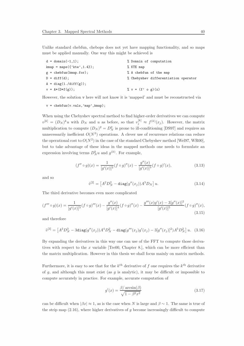
Chapter 3. Mapped Spectral Methods 40
Unlike standard chebfun, chebops does not yet have mapping functionality, and so maps
must be applied manually. One way this might be achieved is
d = domain(-1,1); % Domain of computation
kmap = maps(’kte’,1.4); % KTE map
g = chebfun(kmap.for); % A chebfun of the map
D = diff(d); % Chebyshev differentiation operator
A = diag(1./diff(g));
v = A*(D*f(g)); % v = (f’ o g)(x)
However, the solution v here will not know it is ‘mapped’ and must be reconstructed via
v = chebfun(v.vals,’map’,kmap);
When using the Chebyshev spectral method to find higher-order derivatives we can compute
v[k] = (DN )ku with DN and u as before, so that v[k]j ≈ f (k)(xj). However, the matrix
multiplication to compute (DN )2 = D2N is prone to ill-conditioning [DS97] and requires an
unnecessarily inefficient O(N3) operations. A clever use of recurrence relations can reduce
the operational cost to O(N2) in the case of the standard Chebyshev method [Wel97, WR00],
but to take advantage of these ideas in the mapped methods one needs to formulate an
expression involving terms DkNu and g(k). For example,
(f ′′ g)(x) =1
[g′(x)]2(f g)′′(x) − g′′(x)
[g′(x)]3(f g)′(x), (3.13)
and so
v[2] =[
A2D2N − diag(g′′(xj))A
3DN
]
u. (3.14)
The third derivative becomes even more complicated
(f ′′′ g)(x) =1
[g′(x)]3(f g)′′′(x)− g′′(x)
[g′(x)]4(f g)′′(x)− g′′′(x)g′(x) − 3[g′′(x)]2
[g′(x)]5(f g)′′(x),
(3.15)
and therefore
v[3] =[
A3D3N − 3diag(g′′(xj))A
4D2N − diag(g′′′(xj)g
′(xj)− 3[g′′(xj)]2)A5D2
N
]
u. (3.16)
By expanding the derivatives in this way one can use of the FFT to compute those deriva-
tives with respect to the x variable [Tre00, Chapter 8.], which can be more efficient than
the matrix multiplication. However in this thesis we shall focus mainly on matrix methods.
Furthermore, it is easy to see that for the kth derivative of f one requires the kth derivative
of g, and although this must exist (as g is analytic), it may be difficult or impossible to
compute accurately in practice. For example, accurate computation of
g′(x) =β/ arcsin(β)√
1− β2x2(3.17)
can be difficult when |βx| ≈ 1, as is the case when N is large and β ∼ 1. The same is true of
the strip map (2.16), where higher derivatives of g become increasingly difficult to compute

Chapter 3. Mapped Spectral Methods 41
both analytically and numerically.
The alternative is to set v[2] = (ADN )2u, although it should be stressed that the matrix
(ADN )2 is not the same as the matrix on the right-hand side of (3.14), and therefore neither
is the vector v[2]. Don and Solomonoff [DS97] found that in terms of numerical accuracy this
approach is essentially the same, but warn that as well as being computationally expensive,
this matrix multiplication is very ill-conditioned and recommend against it.
It seems then that calculating the differentiation matrices for the mapped Chebyshev method
is inherently problematic, particularly for large N or higher-order derivatives, and that one
of the main causes of this difficulty is in computing derivatives of the conformal map. We
now describe a different method which does not require these derivatives of g.
3.2.2 Rational spectral methods
An alternative approach to including the conformal map is suggested by Berrut and co-
authors in [BB01a, BBN99] using what they refer as a linear rational collocation method.
This, as the name might suggest, is a spectral method based upon rational interpolants. Of
particular relevance here is the barycentric interpolant of the form1
rN (x) =
N∑′′
k=0
(−1)k
x− ykf(yk)
N∑′′
k=0
(−1)k
x− yk
, (3.18)
where yk = g(xk), g is a conformal map and xkNk=0 are the Chebyshev points xk =
cos(kπ/N). The accuracy of the rational interpolant rN (x) and its derivatives is summarised
in the following theorem, given by Berrut et al. [BBN99] for the case n = 0, and generalised
by Tee [Tee06].
Theorem 3.2.2 Let rN (x) be the rational interpolant (3.18). If f is analytic and bounded
in Ωρ and g defined as in (3.5), then for all integers n ≥ 0
max−1≤x≤1
|r(n)N (x)− f (n)(x)| = O(ρ−N ), as N →∞. (3.19)
If g is chosen to be the identity map g(z) = z, then the rational interpolant rN (x) is precisely
the polynomial pN (x) interpolating the function f(x) at the Chebyshev points [Ber88], and
so Theorem 3.1.2 is a special case of Theorem 3.2.2.
A differentiation matrix DN can be constructed from derivatives of the interpolant using
either the differentiation formulae given by Schneider and Werner [SW86], Welfert [Wel97],
or a hybrid of these two suggested by Tee [Tee06]. The latter is implemented via bcmatrix
in the code below and computes the matrix of the rational spectral method defined us-
1The primes in the summations indicate that the first and last terms are halved.

Chapter 3. Mapped Spectral Methods 42
ing the strip map. Choosing the identity map g = x produces the standard Chebyshev
differentiation matrix as in the code segment of §3.1.
x = -cos((0:N)’*pi/N); % Chebyshev nodes
w = [1/2 ones(1,N-1) 1/2].*(-1).^(0:N); % Barycentric weights
g = stripmap(x, rho); % Strip map g
[D D2] = bcmatrix(w’,g); % Rational differentiation matrix
v = D*f(g); % v = (f’ o g)(x)
These rational differentiation matrices of up to fourth order can be computed via [D D2 D3
D4] = barychebdiff(w’,g) using barychebdiff.m from Tee’s thesis [Tee06, Appendix C].
One disadvantage of these rational methods is that they can no longer make use of the FFT
algorithm as the mapped-mathods we able to.
3.3 Maps and Parameter Choices
Since our aim of recovering the π/2 factor by mapping the ellipse Eρ to a region with
straighter sides has not changed from the quadrature chapter, the maps we consider are the
same; the infinite strip, the KTE arcsine transformation, and the sausage map. As before
the first two maps depend heavily on the parameter ρ, but the answer to the question of
how to choose this becomes ever more murky. In the previous chapter we took the approach
of fixing the parameter ρ = 1.4, and demonstrated that this typically gave good results, in
particular improving upon the standard Gauss and Clenshaw–Curtis quadratures when the
integrand was not analytic in too large a region about [−1, 1]. However, for entire functions,
or those analytic in a very large region, the singularities introduced by the strip and KTE
maps could significantly hinder convergence.
To avoid this last issue, it is common in practice with the modified spectral methods using
the KTE map to let the parameter β depend on N . In particular, a standard choice [KTE93]
is to take
β =2
ε1/N + ε−1/N= sech
( | ln ε|N
)
. (3.20)
This approach has been the subject of much controversy in the literature of mapped Cheby-
shev spectral methods, since theoretically such a choice destroys the exponential accuracy
of the method [ARGA00], but in practice this is not observed until the error falls below ε
[CDS03]. By taking ρ = ρN,Mε where
ρN,Mε = exp(log(Mε))/N), Mε = 2−52, (3.21)
it follows that ρ−NN,Mε
= Mε, and from Theorems 3.2.1 and 3.2.2 that the singularity intro-
duced by the map will only restrict convergence at around the level of machine precision.
Perhaps one reason for the lack of a consensus on the ‘best way’ to choose the parameter
is that there are at least three significantly different considerations in play: accuracy, reso-
lution, and time-stepping restrictions [MR02]. Furthermore, one might split accuracy into

Chapter 3. Mapped Spectral Methods 43
three further subcategories: singularities introduced by the map [ARGA00], conditioning
and rounding error in the differentiation matrix [DS97], and our own aim of regaining the
π/2 factor when f is not entire. This last issue is typically overlooked, as discussion in the
literature is typically focused on entire but oscillatory functions such as cos(Mπx), M ≫ 1.
Here of course the π/2 factor still arises, but in the resolution of the oscillations rather than
convergence.
With so many different factors to consider, it is of little surprise that the search to find a
single scheme for choosing the parameter β has been unsuccessful. For example, to improve
the resolution properties for a function like cos(Mπx), we would like to take β ∼ 1 so that
the oscillations could be resolved with only 2 points per wavelength (ppw), rather than π
ppw in the Chebyshev case (β = 0). However, since the function is analytic, convergence of
the Chebyshev method will be super-geometric once the oscillations are resolved, whereas
the mapped method with a β ∼ 1 will converge slowly because of singularities nearby to
[−1, 1] introduced by the map.
Choosing β as in (3.20) is also problematic. The singularities introduced may be below
machine precision, but as N → ∞ the error in the method as per Theorem 3.2.1 will be
O(ρ−NN,Mε
) = O(Mε), and thus convergence can no longer be considered geometric [RWN98].
Yet those who put this case forward usually agree that whilst “theoretical convergence is lost,
. . . the mapped method is still useful for practical purposes” [CDS03]. And still this is not
the full story! For practical choices for N as may be needed for two- or three-dimensional
modeling, say N . 30, the parameter choice (3.20) does little to improve standard the
Chebyshev method [MR02].
To make progress one must choose which of the above properties (accuracy, resolution, etc.)
they aim to improve, and/or make some assumptions regarding the types of functions to be
considered.
3.4 Accuracy
We begin by exploring the effects of the conformal maps we have been considering to approx-
imate the same 9 test functions as in §2.4 using the mapped and rational spectral methods.
In the strip and KTE maps we shall consider both a fixed value of ρ, again arbitrarily chosen
to be 1.4, and later a value of ρ which depends on N as in (3.21). For the sausage map we
again take d = 9.
Figure 3.1 shows these results using N +1 collocation points with N from 4 to 160. The
error is defined by interpolating the computed solution at 1000 random (but fixed) points
in [−1, 1] using the barycentric interpolation formula [BT04] and taking the L∞ norm of
the difference from the analytic solution. The pointwise error at each of the grid points
(unique to each map and each N) was also computed, and gave almost identical results
except where mentioned. The solid lines represent results from the rational implementation
Chapter 3. Mapped Spectral Methods 44
0 20 40 60 80 100 120 140 16010
−13
10−10
10−7
10−4
10−1
(1+20x2)−1
0 20 40 60 80 100 120 140 16010
−8
10−6
10−4
10−2
100
log(1+50x2)
0 20 40 60 80 100 120 140 16010
−10
10−8
10−6
10−4
10−2
100
(1.5−cos(5x))−1
0 20 40 60 80 100 120 140 16010
−15
10−11
10−7
10−3
101
exp(−40x2)
0 20 40 60 80 100 120 140 16010
−13
10−10
10−7
10−4
10−1
102
cos(40x)
0 20 40 60 80 100 120 140 16010
−10
10−8
10−6
10−4
10−2
100
exp(−x−2)
0 20 40 60 80 100 120 140 16010
−3
10−2
10−1
∫x(|y|−|y−0.1|)dy
0 20 40 60 80 100 120 140 160
10−4
10−3
10−2
10−1
100
(1.01−x)1/2
0 20 40 60 80 100 120 140 16010
−15
10−11
10−7
10−3
cos(x)
Figure 3.1: Comparison of Chebyshev (dots) against the transplanted Chebyshev method with thestrip (blue) and KTE (red) maps with ρ = 1.4, and the sausage map (green) with d = 9 for ninetest functions. The error is computed by interpolating the computed solution at 1000 randomlydistributed points in [−1, 1] and taking the L∞ norm of the difference from the true solution. Thedashed black line is 1.4−N for reference.
(§3.2.2) of the maps and the dashed lines from the mapped-polynomial method (§3.2.1), and
we rarely see much difference between the two. What we do observe is that the accuracy of
the mapped-polynomial method, particularly for the strip map, suffers for large N due to
inaccuracies in computing g′. The dashed black lines are ρ−N =1.4−N , and indicate when
convergence in the maps involving singularities is limited.
Results for the first three test functions are all but identical to the quadrature computa-
tions, although with the rate of convergence approximately halved in each case. The strip
map method converges faster than Chebyshev by a factor of around π/2, and the KTE and
sausage maps only slightly less than this. The fourth function also behaves similarly to
before, until at some point convergence is restricted by the rate 1.4−N . This kink does not
appear in the mapped-polynomial implementation if the error is only computed at the grid
points (Figure 3.2a), and highlights a difference in the mapped and rational interpolants.
Figure 3.2b shows the pointwise error at the grid points when differentiating exp(−10x2),
and here we see that the mapped-polynomial curve also kinks to the same gradient, but at
a considerably reduced magnitude.
Chapter 3. Mapped Spectral Methods 45
0 20 40 60 80 10010
−15
10−11
10−7
10−3
101
exp(−10x2)
0 20 40 60 80 10010
−15
10−11
10−7
10−3
101
exp(−40x2)
Figure 3.2: Left: pointwise error at grid points for example 4 above. Right: pointwise error fora function with a smaller exponent. The blue and red lines represent the mapped (dashed) andrational (solid) spectral methods using the strip map and KTE maps respectively.
The likely reason for this behaviour is that whilst, for say the KTE map, the magnitude of g
at its singularities is O(1) (for β ≈ 1), the value of f g at the same points is O(e−a) when f
is of the form exp(−ax2). In other words, the function f is very small at, and about, the sin-
gularity in the map. The mapped-polynomial can clearly take advantage of situations where
this occurs, since it is simply a polynomial approximation to the function f g. The case of
the rational interpolant is less clear, but from the proofs of Theorem 3.2.2 [BBN99, Tee06]
we find that we can, to some extent, regard the rational interpolant as a ratio of polynomial
approximations to (f g)/g′ and 1/g′. Whilst the first of these approximations will also
benefit for the small magnitude of f about the singularity, the denominator is independent
of f and will not. Thus although asymptotically the convergence rate will be the same (g is
conformal in Eρ, so 1/g′ will be analytic in this same ellipse), there may be large differences
in the implied constant factors between the mapped-polynomial and rational interpolants
for functions of this type.
For the oscillatory function cos(40x), the more equally spaced grid points mean that each
of the maps resolve the function much sooner than the Chebyshev method. As with the
quadrature examples, the rates of convergence of the strip and KTE maps however are both
limited by ρ, although the latter is unquestionably more accurate by as many as four digits.
The sixth function exp(−x−2) is C∞ but not analytic and we see that the mapped methods
improve upon the standard Chebyshev, whereas in the quadrature testing they were more
comparable. Clearly function 7 is not differentiable, so instead we use its indefinite integral
such that the true solution is |x| − |x − 0.1|. Of course this function is not analytic, so we
do not get geometric convergence, but the mapped methods again show an improvement,
with errors similar to when integrating this function in §2.4.
The final two functions also tell a story similar to the quadrature tests. The function√1.01− x has a branch point on the real axis close to x = 1, and since the maps we have
chosen stretch the regions of required analyticity in this direction, the modified methods
converge less quickly than the standard Chebyshev. The convergence of the methods involv-
ing singular maps when differentiating cos(x) are restricted by the map parameter. Similarly
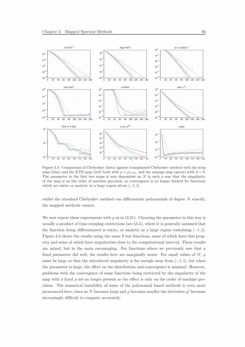
Chapter 3. Mapped Spectral Methods 46
0 20 40 60 80 100 120 140 16010
−13
10−10
10−7
10−4
10−1
(1+20x2)−1
0 20 40 60 80 100 120 140 16010
−8
10−6
10−4
10−2
100
log(1+50x2)
0 20 40 60 80 100 120 140 16010
−10
10−8
10−6
10−4
10−2
100
(1.5−cos(5x))−1
0 20 40 60 80 100 120 140 16010
−15
10−11
10−7
10−3
101
exp(−40x2)
0 20 40 60 80 100 120 140 16010
−13
10−10
10−7
10−4
10−1
102
cos(40x)
0 20 40 60 80 100 120 140 16010
−10
10−8
10−6
10−4
10−2
100
exp(−x−2)
0 20 40 60 80 100 120 140 16010
−3
10−2
10−1
∫x(|x|−|x−0.1|)dx
0 20 40 60 80 100 120 140 160
10−4
10−3
10−2
10−1
100
(1.01−x)1/2
0 20 40 60 80 100 120 140 16010
−15
10−11
10−7
10−3
cos(x)
Figure 3.3: Comparison of Chebyshev (dots) against transplanted Chebyshev method with the stripmap (blue) and the KTE map (red) both with ρ = ρN,Mε and the sausage map (green) with d = 9.The parameter in the first two maps is now dependent on N in such a way that the singularityof the map is on the order of machine precision, so convergence is no longer limited for functionswhich are entire or analytic in a large region about [−1, 1].
whilst the standard Chebyshev method can differentiate polynomials of degree N exactly,
the mapped methods cannot.
We now repeat these experiments with ρ as in (3.21). Choosing the parameter in this way is
usually a product of time-stepping restrictions (see §3.5), where it is generally assumed that
the function being differentiated is entire, or analytic in a large region containing [−1, 1].
Figure 3.3 shows the results using the same 9 test functions, some of which have this prop-
erty and some of which have singularities close to the computational interval. These results
are mixed, but in the main encouraging. For functions where we previously saw that a
fixed parameter did well, the results here are marginally worse. For small values of N , ρ
must be large so that the introduced singularity is far enough away from [−1, 1], but when
the parameter is large, the effect on the distribution and convergence is minimal. However,
problems with the convergence of some functions being restricted by the singularity of the
map with a fixed ρ are no longer present as the effect is only on the order of machine pre-
cision. The numerical instability of some of the polynomial based methods is even more
pronounced here, since as N becomes large and ρ becomes smaller the derivative g′ becomes
increasingly difficult to compute accurately.

Chapter 3. Mapped Spectral Methods 47
The most notable improvement in convergence is for the function cos(40x), where the KTE
map converges very rapidly all the way to 12 digits of accuracy, and at a much faster rate
than standard Chebyshev. The expense of this improvement is in not resolving the oscilla-
tions until a larger value of N (when compared to the same map with a fixed ρ), since ρ
is much larger than 1.4 when N is small, and thus the nodes further from equally spaced.
After the oscillations have been resolved, convergence of the strip map is initially rapid
and an improvement on the fixed value of ρ, but as N increases convergence seems to be
less than geometric. Convergence for the function√
1.01− x appears faster than for the
fixed parameter, but this is only the case since ρN,Mε < 1.4 for N < 107. For N ≥ 108,
the analyticity region of the maps with ρ dependent on N will be wider than those from
the fixed value 1.4, hence the rate will become slower. Finally, cos(x) can now be differ-
entiated accurately with few points, as the singularity introduced by the map can be ignored.
Comparing Figures 3.1 and 3.3 it seems that sometimes it is beneficial to choose a fixed
parameter, and at other times to let it depend on N as in (3.21). The latter is often the
case when the function is entire, or has singularities far away from [−1, 1], whereas choosing
a small fixed ρ is useful when the neighbourhood of analyticity is small. Since our motiva-
tion is to improve the speed of convergence for a more general class of functions, this would
suggest if using either the strip or KTE maps, we should take ρ as in (3.21). However,
if one knows further information about the singularity structure of the function near to
[−1, 1], such as with the first two examples, a more specialised map (such as discussed in
the 2nd Part of this thesis) might be advantageous. An important observation is that the
sausage map is comparable to each of the two maps involving singularities for almost all of
the functions.
Spectral methods are rarely used to compute directly the derivative of a known function,
their most practical use is in solving ordinary or partial differential equations. We give one
final example comparing the performance of the mapped and rational with the standard
Chebyshev method in case of a second-order linear differential equation. The equation
[Hem77, example 3.7.4],
εu′′ + xu′ = −επ2 cos(πx) − πx sin(πx), −1 < x < 1, ε > 0 (3.22)
with u(−1) = −2, u(1) = 0 has the solution
εu(x) = cos(πx) + erf(x/√
2ε)/erf(1/√
2ε) (3.23)
shown in the left pane of Figure 3.4 for ε = 0.01, and appears also in [BB01b]. The
following Matlab code demonstrates how to solve this using the sausage map (2.28) and
the rational spectral method. We see in the right pane of Figure 3.4 that each of the mapped
methods converges faster than the standard Chebyshev, with the strip and sausage maps
being slightly faster than the KTE. The error function is entire, but like exp(−40x2) above
grows so rapidly along the imaginary axis that it may be considered ‘numerically singular’,
thus limiting the rate of convergence.
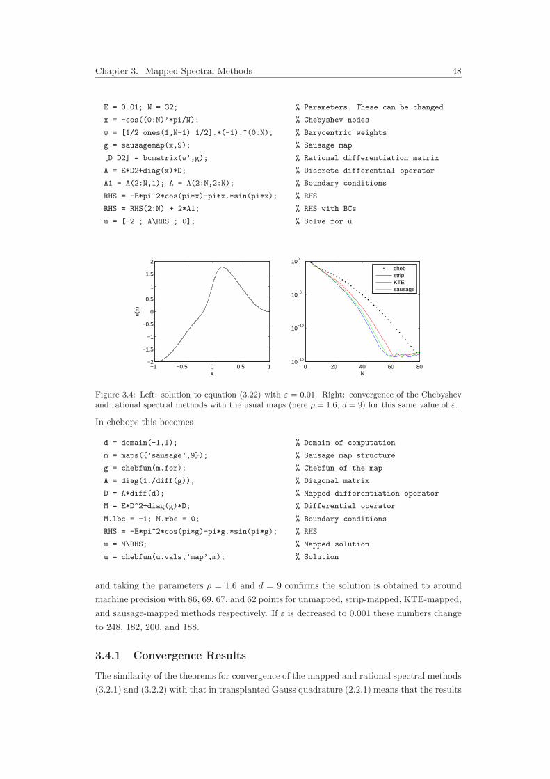
Chapter 3. Mapped Spectral Methods 48
E = 0.01; N = 32; % Parameters. These can be changed
x = -cos((0:N)’*pi/N); % Chebyshev nodes
w = [1/2 ones(1,N-1) 1/2].*(-1).^(0:N); % Barycentric weights
g = sausagemap(x,9); % Sausage map
[D D2] = bcmatrix(w’,g); % Rational differentiation matrix
A = E*D2+diag(x)*D; % Discrete differential operator
A1 = A(2:N,1); A = A(2:N,2:N); % Boundary conditions
RHS = -E*pi^2*cos(pi*x)-pi*x.*sin(pi*x); % RHS
RHS = RHS(2:N) + 2*A1; % RHS with BCs
u = [-2 ; A\RHS ; 0]; % Solve for u
0 20 40 60 8010
−15
10−10
10−5
100
N
chebstripKTEsausage
−1 −0.5 0 0.5 1−2
−1.5
−1
−0.5
0
0.5
1
1.5
2
x
u(x)
Figure 3.4: Left: solution to equation (3.22) with ε = 0.01. Right: convergence of the Chebyshevand rational spectral methods with the usual maps (here ρ = 1.6, d = 9) for this same value of ε.
In chebops this becomes
d = domain(-1,1); % Domain of computation
m = maps(’sausage’,9); % Sausage map structure
g = chebfun(m.for); % Chebfun of the map
A = diag(1./diff(g)); % Diagonal matrix
D = A*diff(d); % Mapped differentiation operator
M = E*D^2+diag(g)*D; % Differential operator
M.lbc = -1; M.rbc = 0; % Boundary conditions
RHS = -E*pi^2*cos(pi*g)-pi*g.*sin(pi*g); % RHS
u = M\RHS; % Mapped solution
u = chebfun(u.vals,’map’,m); % Solution
and taking the parameters ρ = 1.6 and d = 9 confirms the solution is obtained to around
machine precision with 86, 69, 67, and 62 points for unmapped, strip-mapped, KTE-mapped,
and sausage-mapped methods respectively. If ε is decreased to 0.001 these numbers change
to 248, 182, 200, and 188.
3.4.1 Convergence Results
The similarity of the theorems for convergence of the mapped and rational spectral methods
(3.2.1) and (3.2.2) with that in transplanted Gauss quadrature (2.2.1) means that the results
Chapter 3. Mapped Spectral Methods 49
of §2.6 giving quantitative convergence rates can be carried over almost directly to the
spectral methods case.
Proposition 3.4.1 Let v be the result of applying the mapped or rational spectral method
with a conformal map g to differentiate a function f ∈ A(ε) (where A(ε) is as in (2.33)).
The following statements pertain to the limit N →∞ for all j = 0, . . . , N .
For the strip map (2.16) with ρ = 1.4 and any ε ≤ 0.24 :
|(f ′ g)(xj)− vj | = O((1 + 1.4ε)−N).
For the KTE map (2.22) with ρ = 1.4 and any ε ≤ 0.3 :
|(f ′ g)(xj)− vj | = O((1 + 1.3ε)−N).
For the sausage map (2.28) with d = 9 and any ε ≤ 0.8 :
|(f ′ g)(xj)− vj | = O((1 + 1.3ε)−N).
For the strip map (2.16) with ρ = 1.1 and any ε ≤ 0.05 :
|(f ′ g)(xj)− vj | = O((1 + ε)−1.5N ).
The justification of this claim is analogous to that of Propositions 2.6.1 and 2.6.2. Similar
results to those at the end of §2.6 hold also, only with the exponent halved. Higher-order
derivatives will converge at the same asymptotic rates.
3.5 Time-Stepping
So far this chapter has paralleled the previous on quadrature methods; our aims in introduc-
ing the map g have been to define a method with a more uniform distribution of points and
a more general region for geometric convergence of analytic functions. We now consider a
separate issue that arises when using spectral methods, namely that of time-stepping. Con-
sider a differential equation with both time and space dependence, such as the 1D advection
equation
∂u
∂t=
∂u
∂x, x ∈ (−1, 1), t > 0, (3.24)
u(x, 0) = u0(x), (3.25)
u(1, t) = 0. (3.26)
A common way of discretising such a problem with spectral methods is the method of lines.
The spatial derivatives are approximated spectrally, by say the Chebyshev method, and the
temporal derivatives by a lower-order finite difference scheme. This leads to a system of
linear ODEs∂u
∂t(xj , t) =
[
DNu(x, t)]
j, (3.27)
where DN is the Chebyshev differentiation matrix DN with the final row and column re-
moved to impose the Dirichlet boundary condition u(1, t) = 0. The matrix DN can then be
thought of as a linear operator on yj(t) = u(xj , t)N−1j=0 , so that
Chapter 3. Mapped Spectral Methods 50
y′j(t) = Fj(y(t)) =
[
DNy(t)]
j. (3.28)
This system of ODEs can be advanced in time using one’s favourite time marching method.
When using explicit (i.e. iterative) schemes such as Forward Euler, Adams–Bashforth, or
Runge–Kutta, it is well-known that we encounter some form of stability condition on the
size of the time step, and here we find we must satisfy ∆t = O(N−2) [Boy01, Chapter
9],[CHQZ06, Appendix D],[Tre00, Chapter 10]. Such a condition can be very restrictive,
and is often (but not always) a product of the numerical discretisation, rather than the
physics of the underlying PDE.
An example with a second-order derivative in space, is the 1D heat equation
∂u
∂t=
∂2u
∂x2, x ∈ (−1, 1), t > 0, (3.29)
u(x, 0) = u0(x), (3.30)
u(±1, t) = 0, (3.31)
which can be discretised in a similar way to (3.28), by replacing DN with D2N (the Cheby-
shev second-order differentiation matrix with the first and last rows and columns removed).
In this case the stability condition is even worse, requiring ∆t = O(N−4) [WT88].
When Kosloff and Tal-Ezer [KTE93] introduce the map (3.1) they note that whilst there
is no direct relation between the minimal spacing of grid points and the time step size re-
striction as there is in explicit finite difference methods [ST89], numerical experience and
heuristic reasoning indicate the cause of the severe stability restriction is the tight clustering
of the Chebyshev nodes around the boundaries. To be precise, the clustering of points causes
a number of the complex eigenvalues of the differentiation matrices DN and D2N to grow like
O(N2) and O(N4) respectively [TT87, WT88, Van90]. The conditions ∆t = O(N−2) and
O(N−4) arise to enforce that the eigenvalues of the matrices ∆tDN and ∆tD2N lie within
the stability region of the time-stepping scheme, which must be of O(1). Kosloff and Tal-
Ezer demonstrate that by mapping the Chebyshev points to a another set of points with a
larger minimal spacing, the outlying eigenvalues of size O(N2) will be controlled and the
time-stepping restriction alleviated, potentially to ∆t = O(N−1) or ∆t = O(N−2) for the
second order problem.
To map to points with “a larger minimal spacing” is clearly connected to the aim of our con-
formal maps, which seek a “smaller maximal spacing”. In this effect, we saw that other types
of maps — the strip and sausage — were sometimes more useful than the KTE transform.
In this section, we explore the effect of these new maps on the time-stepping restriction
and other properties of the differentiation matrices when using the mapped-polynomial and
the rational spectral methods. Further, we investigate the effect of the parameter β (or
equivalently ρ) of the map (3.1) and discuss how this relates to the parameter choice for the
strip map (2.16).
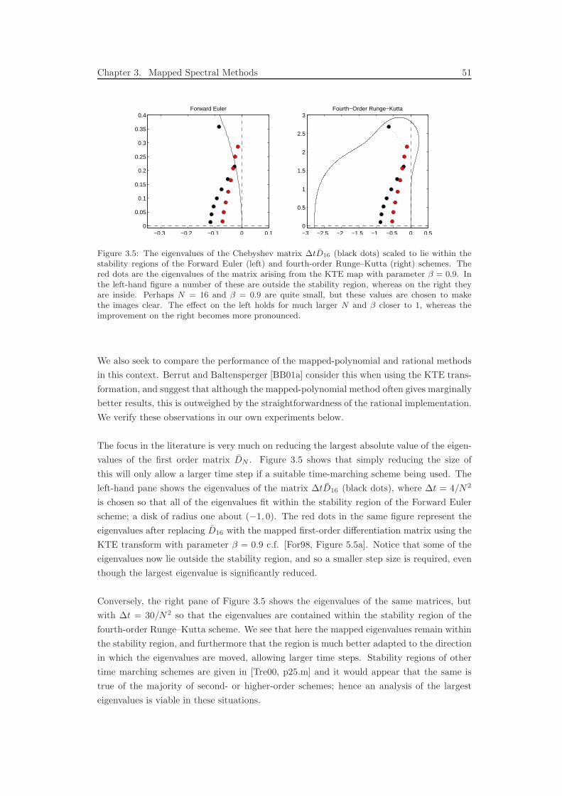
Chapter 3. Mapped Spectral Methods 51
−0.3 −0.2 −0.1 0 0.10
0.05
0.1
0.15
0.2
0.25
0.3
0.35
0.4Forward Euler
−3 −2.5 −2 −1.5 −1 −0.5 0 0.50
0.5
1
1.5
2
2.5
3Fourth−Order Runge−Kutta
Figure 3.5: The eigenvalues of the Chebyshev matrix ∆tD16 (black dots) scaled to lie within thestability regions of the Forward Euler (left) and fourth-order Runge–Kutta (right) schemes. Thered dots are the eigenvalues of the matrix arising from the KTE map with parameter β = 0.9. Inthe left-hand figure a number of these are outside the stability region, whereas on the right theyare inside. Perhaps N = 16 and β = 0.9 are quite small, but these values are chosen to makethe images clear. The effect on the left holds for much larger N and β closer to 1, whereas theimprovement on the right becomes more pronounced.
We also seek to compare the performance of the mapped-polynomial and rational methods
in this context. Berrut and Baltensperger [BB01a] consider this when using the KTE trans-
formation, and suggest that although the mapped-polynomial method often gives marginally
better results, this is outweighed by the straightforwardness of the rational implementation.
We verify these observations in our own experiments below.
The focus in the literature is very much on reducing the largest absolute value of the eigen-
values of the first order matrix DN . Figure 3.5 shows that simply reducing the size of
this will only allow a larger time step if a suitable time-marching scheme being used. The
left-hand pane shows the eigenvalues of the matrix ∆tD16 (black dots), where ∆t = 4/N2
is chosen so that all of the eigenvalues fit within the stability region of the Forward Euler
scheme; a disk of radius one about (−1, 0). The red dots in the same figure represent the
eigenvalues after replacing D16 with the mapped first-order differentiation matrix using the
KTE transform with parameter β = 0.9 c.f. [For98, Figure 5.5a]. Notice that some of the
eigenvalues now lie outside the stability region, and so a smaller step size is required, even
though the largest eigenvalue is significantly reduced.
Conversely, the right pane of Figure 3.5 shows the eigenvalues of the same matrices, but
with ∆t = 30/N2 so that the eigenvalues are contained within the stability region of the
fourth-order Runge–Kutta scheme. We see that here the mapped eigenvalues remain within
the stability region, and furthermore that the region is much better adapted to the direction
in which the eigenvalues are moved, allowing larger time steps. Stability regions of other
time marching schemes are given in [Tre00, p25.m] and it would appear that the same is
true of the majority of second- or higher-order schemes; hence an analysis of the largest
eigenvalues is viable in these situations.

Chapter 3. Mapped Spectral Methods 52
2 4 6 80
0.02
0.04
0.06
0.08
0.1
max|eig(DN
)/N2|, N = 16
2 4 6 80
0.01
0.02
0.03
0.04
0.05
max|eig(D2N
)/N4|, N = 16
1 1.5 2 2.5 30
0.02
0.04
0.06
0.08
0.1
max|eig(DN
)/N2|, N = 32
1 1.5 2 2.5 30
0.01
0.02
0.03
0.04
0.05
max|eig(D2N
)/N4|, N = 32
1 1.2 1.4 1.60
0.02
0.04
0.06
0.08
0.1
max|eig(DN
)/N2|, N = 64
1 1.2 1.4 1.60
0.01
0.02
0.03
0.04
0.05
max|eig(D2N
)/N4|, N = 64
1 1.1 1.2 1.30
0.02
0.04
0.06
0.08
0.1
max|eig(DN
)/N2|, N = 128
1 1.1 1.2 1.30
0.01
0.02
0.03
0.04
0.05
max|eig(D2N
)/N4|, N = 128
chebstripKTEsausage
Figure 3.6: The spectral radii (y-axis, scaled by N−2 and N−4) of the unmapped and mappeddifferentiation matrices DN (top row) and D2
N (bottom row) when varying parameter ρ (x-axis)for N = 16, 32, 64, 128. The solid circles and squares represent the values of ρ given by ρN,Mε andρN,
√Mε
respectively.
The behaviour of the second-order differentiation matrix D2N is considerably different. Here
all the eigenvalues lie on the negative axis and the matrix is far closer to normal. Stability
is then always conditional on the leftmost eigenvalue, which has the largest absolute size.
For more information about the eigenvalues of this matrix see [WT88].
Figure 3.6 shows for N = 16, 32, 64, 128 the size of the largest eigenvalues from DN and
D2N using each of the maps we consider as ρ is varied. We see that initially, as ρ decreases
towards 1, the spectral radii of both KTE and strip maps decrease monotonically. Notably,
for a given value of ρ the spectral radius of the strip mapped method is significantly smaller
than that of the KTE map, meaning that for the same rate of convergence the strip map
is able to take larger time steps. In the case of the second-order operator, we see that for
N = 128 these steps can be between 50% and 100% larger.
Recall that the choice of parameter ρ = ρN,ε as in (3.21) is such that ρ−NN,ε = ε, so singularities
introduced by the map are only of order ε. As already discussed, this choice is regularly
chosen in much of the literature when solving time dependent problems as the resulting map
will improve the time-stepping restrictions and the singularity introduced can be chosen to
be negligible with respect to the desired accuracy of the solution. Figure 3.7 shows the
largest eigenvalues of the mapped first- and second-order matrices with a number of choices
for ρ, two of which are ρ = ρN,Mε and ρ = ρN,√
Mεwhere Mε is machine precision. For
maps chosen in this manner, we see that the spectral radii grow at around (and slightly
greater than) O(N) and O(N2), compared to O(N2) and O(N4) in the standard Chebyshev
method. Moreover, we see again that the spectral radius of the method induced by the KTE
map is about 50% larger than that from the strip for the first-order matrices and around
a factor of 2 larger for the second-order. The finely dotted lines are the spectral radius
minimised over ρ for each N , which is around the same for both methods.
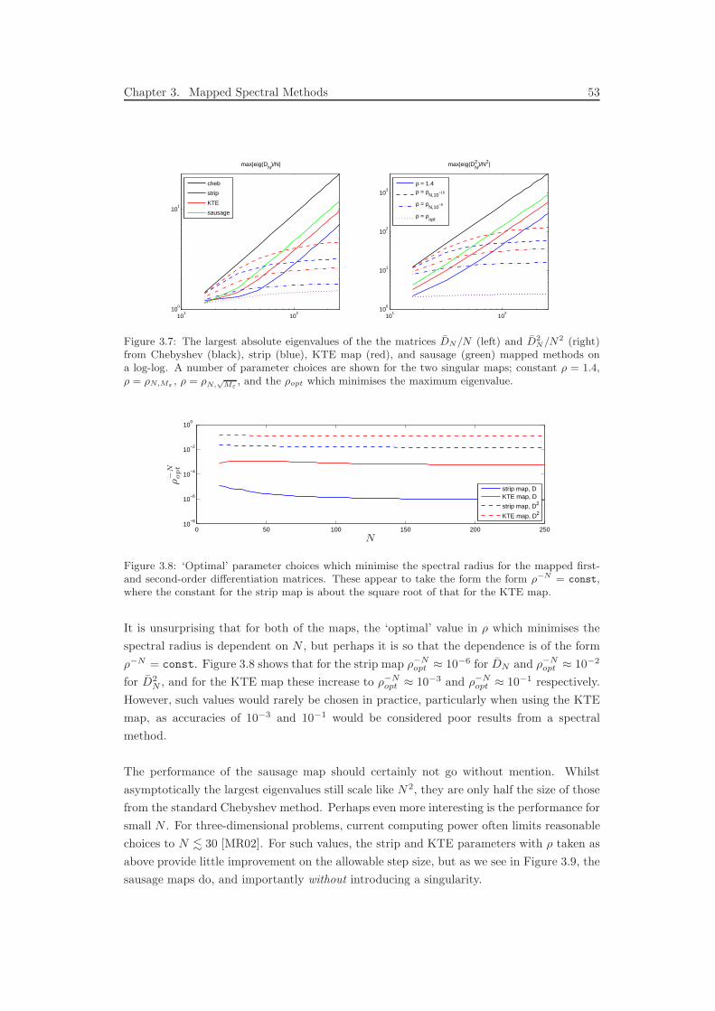
Chapter 3. Mapped Spectral Methods 53
101
102
100
101
max|eig(DN
)/N|
101
102
100
101
102
103
max|eig(D2N
)/N2|
cheb
strip
KTE
sausage
ρ = 1.4ρ = ρ
N,10−16
ρ = ρN,10
−8
ρ = ρopt
Figure 3.7: The largest absolute eigenvalues of the the matrices DN/N (left) and D2N/N2 (right)
from Chebyshev (black), strip (blue), KTE map (red), and sausage (green) mapped methods ona log-log. A number of parameter choices are shown for the two singular maps; constant ρ = 1.4,ρ = ρN,Mε , ρ = ρN,
√Mε
, and the ρopt which minimises the maximum eigenvalue.
0 50 100 150 200 25010
−8
10−6
10−4
10−2
100
strip map, DKTE map, D
strip map, D2
KTE map, D2
N
ρ−
Nopt
Figure 3.8: ‘Optimal’ parameter choices which minimise the spectral radius for the mapped first-and second-order differentiation matrices. These appear to take the form the form ρ−N = const,where the constant for the strip map is about the square root of that for the KTE map.
It is unsurprising that for both of the maps, the ‘optimal’ value in ρ which minimises the
spectral radius is dependent on N , but perhaps it is so that the dependence is of the form
ρ−N = const. Figure 3.8 shows that for the strip map ρ−Nopt ≈ 10−6 for DN and ρ−N
opt ≈ 10−2
for D2N , and for the KTE map these increase to ρ−N
opt ≈ 10−3 and ρ−Nopt ≈ 10−1 respectively.
However, such values would rarely be chosen in practice, particularly when using the KTE
map, as accuracies of 10−3 and 10−1 would be considered poor results from a spectral
method.
The performance of the sausage map should certainly not go without mention. Whilst
asymptotically the largest eigenvalues still scale like N2, they are only half the size of those
from the standard Chebyshev method. Perhaps even more interesting is the performance for
small N . For three-dimensional problems, current computing power often limits reasonable
choices to N . 30 [MR02]. For such values, the strip and KTE parameters with ρ taken as
above provide little improvement on the allowable step size, but as we see in Figure 3.9, the
sausage maps do, and importantly without introducing a singularity.
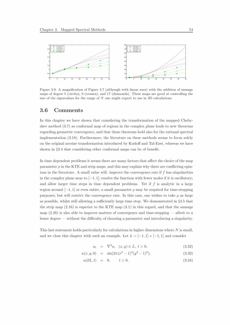
Chapter 3. Mapped Spectral Methods 54
0 5 10 15 20 25 30 35 400
0.5
1
1.5
2
2.5
3
3.5
4
sausage 5sausage 9sausage 17
0 5 10 15 20 25 30 35 400
10
20
30
40
50
60
70
80
sausage 5sausage 9sausage 17
Figure 3.9: A magnification of Figure 3.7 (although with linear axes) with the addition of sausagemaps of degree 5 (circles), 9 (crosses), and 17 (diamonds). These maps are good at controlling thesize of the eigenvalues for the range of N one might expect to use in 3D calculations.
3.6 Comments
In this chapter we have shown that considering the transformation of the mapped Cheby-
shev method (3.7) as conformal map of regions in the complex plane leads to new theorems
regarding geometric convergence, and that these theorems hold also for the rational spectral
implementation (3.18). Furthermore, the literature on these methods seems to focus solely
on the original arcsine transformation introduced by Kosloff and Tal-Ezer, whereas we have
shown in §3.4 that considering other conformal maps can be of benefit.
In time dependent problems it seems there are many factors that affect the choice of the map
parameter ρ in the KTE and strip maps, and this may explain why there are conflicting opin-
ions in the literature. A small value will: improve the convergence rate if f has singularities
in the complex plane near to [−1, 1]; resolve the function with fewer nodes if it is oscillatory;
and allow larger time steps in time dependent problems. Yet if f is analytic in a large
region around [−1, 1] or even entire, a small parameter ρ may be required for time-stepping
purposes, but will restrict the convergence rate. In this case, one wishes to take ρ as large
as possible, whilst still allowing a sufficiently large time step. We demonstrated in §3.5 that
the strip map (2.16) is superior to the KTE map (3.1) in this regard, and that the sausage
map (2.28) is also able to improve matters of convergence and time-stepping — albeit to a
lesser degree — without the difficulty of choosing a parameter and introducing a singularity.
This last statement holds particularly for calculations in higher dimensions where N is small,
and we close this chapter with such an example. Let L = [−1, 1]× [−1, 1] and consider
ut = ∇2u, (x, y) ∈ L, t > 0, (3.32)
u(x, y, 0) = sin(2π(x2 − 1)2(y2 − 1)2), (3.33)
u(∂L, t) = 0, t > 0. (3.34)
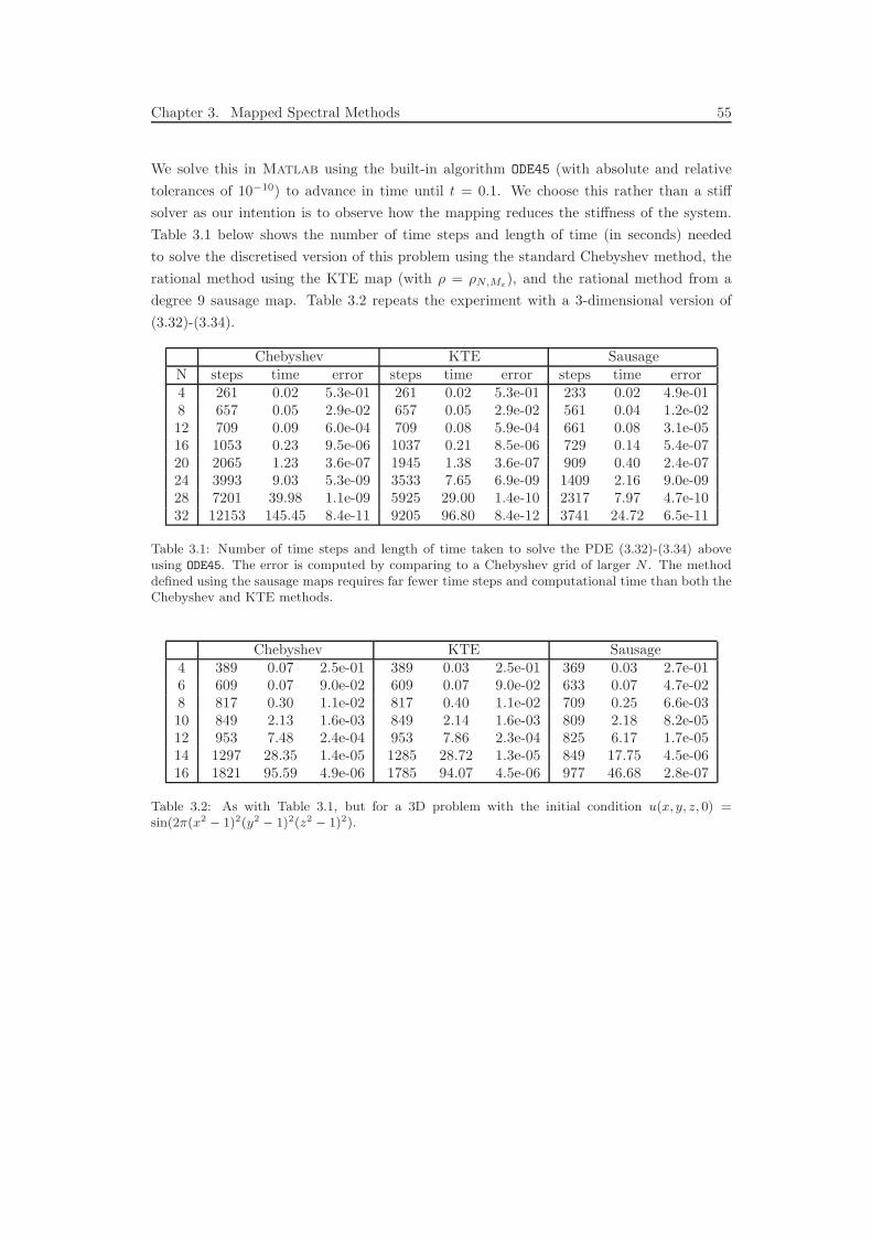
Chapter 3. Mapped Spectral Methods 55
We solve this in Matlab using the built-in algorithm ODE45 (with absolute and relative
tolerances of 10−10) to advance in time until t = 0.1. We choose this rather than a stiff
solver as our intention is to observe how the mapping reduces the stiffness of the system.
Table 3.1 below shows the number of time steps and length of time (in seconds) needed
to solve the discretised version of this problem using the standard Chebyshev method, the
rational method using the KTE map (with ρ = ρN,Mε), and the rational method from a
degree 9 sausage map. Table 3.2 repeats the experiment with a 3-dimensional version of
(3.32)-(3.34).
Chebyshev KTE SausageN steps time error steps time error steps time error4 261 0.02 5.3e-01 261 0.02 5.3e-01 233 0.02 4.9e-018 657 0.05 2.9e-02 657 0.05 2.9e-02 561 0.04 1.2e-0212 709 0.09 6.0e-04 709 0.08 5.9e-04 661 0.08 3.1e-0516 1053 0.23 9.5e-06 1037 0.21 8.5e-06 729 0.14 5.4e-0720 2065 1.23 3.6e-07 1945 1.38 3.6e-07 909 0.40 2.4e-0724 3993 9.03 5.3e-09 3533 7.65 6.9e-09 1409 2.16 9.0e-0928 7201 39.98 1.1e-09 5925 29.00 1.4e-10 2317 7.97 4.7e-1032 12153 145.45 8.4e-11 9205 96.80 8.4e-12 3741 24.72 6.5e-11
Table 3.1: Number of time steps and length of time taken to solve the PDE (3.32)-(3.34) aboveusing ODE45. The error is computed by comparing to a Chebyshev grid of larger N . The methoddefined using the sausage maps requires far fewer time steps and computational time than both theChebyshev and KTE methods.
Chebyshev KTE Sausage4 389 0.07 2.5e-01 389 0.03 2.5e-01 369 0.03 2.7e-016 609 0.07 9.0e-02 609 0.07 9.0e-02 633 0.07 4.7e-028 817 0.30 1.1e-02 817 0.40 1.1e-02 709 0.25 6.6e-0310 849 2.13 1.6e-03 849 2.14 1.6e-03 809 2.18 8.2e-0512 953 7.48 2.4e-04 953 7.86 2.3e-04 825 6.17 1.7e-0514 1297 28.35 1.4e-05 1285 28.72 1.3e-05 849 17.75 4.5e-0616 1821 95.59 4.9e-06 1785 94.07 4.5e-06 977 46.68 2.8e-07
Table 3.2: As with Table 3.1, but for a 3D problem with the initial condition u(x, y, z, 0) =sin(2π(x2 − 1)2(y2 − 1)2(z2 − 1)2).

Part II
Adaptive Methods
56
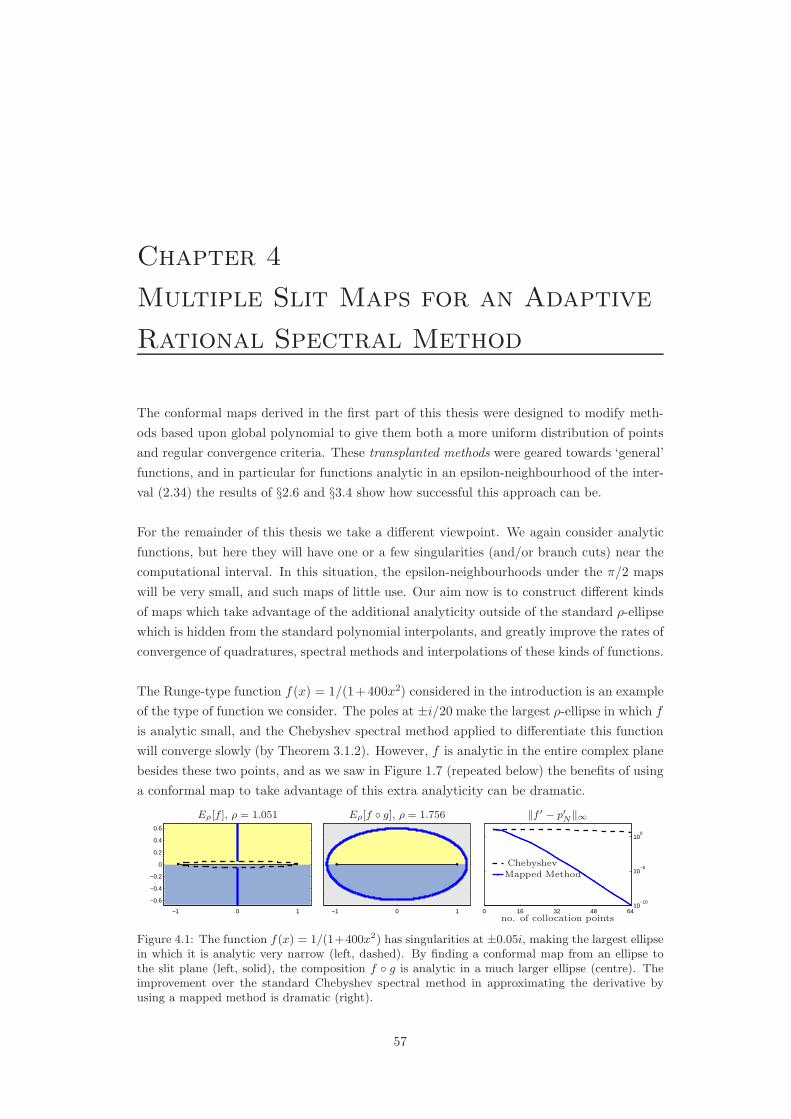
Chapter 4
Multiple Slit Maps for an Adaptive
Rational Spectral Method
The conformal maps derived in the first part of this thesis were designed to modify meth-
ods based upon global polynomial to give them both a more uniform distribution of points
and regular convergence criteria. These transplanted methods were geared towards ‘general’
functions, and in particular for functions analytic in an epsilon-neighbourhood of the inter-
val (2.34) the results of §2.6 and §3.4 show how successful this approach can be.
For the remainder of this thesis we take a different viewpoint. We again consider analytic
functions, but here they will have one or a few singularities (and/or branch cuts) near the
computational interval. In this situation, the epsilon-neighbourhoods under the π/2 maps
will be very small, and such maps of little use. Our aim now is to construct different kinds
of maps which take advantage of the additional analyticity outside of the standard ρ-ellipse
which is hidden from the standard polynomial interpolants, and greatly improve the rates of
convergence of quadratures, spectral methods and interpolations of these kinds of functions.
The Runge-type function f(x) = 1/(1+400x2) considered in the introduction is an example
of the type of function we consider. The poles at ±i/20 make the largest ρ-ellipse in which f
is analytic small, and the Chebyshev spectral method applied to differentiate this function
will converge slowly (by Theorem 3.1.2). However, f is analytic in the entire complex plane
besides these two points, and as we saw in Figure 1.7 (repeated below) the benefits of using
a conformal map to take advantage of this extra analyticity can be dramatic.
−1 0 1
−0.6
−0.4
−0.2
0
0.2
0.4
0.6
−1 0 1 0 16 32 48 64 10
−10
10−5
100
Eρ[f ], ρ = 1.051 Eρ[f g], ρ = 1.756 ‖f ′ − p′N‖∞
ChebyshevMapped Method
no. of collocation points
Figure 4.1: The function f(x) = 1/(1+400x2) has singularities at ±0.05i, making the largest ellipsein which it is analytic very narrow (left, dashed). By finding a conformal map from an ellipse tothe slit plane (left, solid), the composition f g is analytic in a much larger ellipse (centre). Theimprovement over the standard Chebyshev spectral method in approximating the derivative byusing a mapped method is dramatic (right).
57
Chapter 4. Multiple Slit Maps for an Adaptive Rational Spectral Method 58
4.1 Adaptive Rational Spectral Method
The ideas above form the basis of Tee’s Adaptive Rational Spectral Method [Tee06, TT06],
where by exploiting conformal maps to vertically slit regions in the complex plane one can
solve PDEs with interior layer-like behaviour using significantly fewer collocation points
than traditional spectral methods. Tee’s approach is very similar to that which we took in
§3, but rather than use maps to send the ρ-ellipse to regions with straighter sides, they are
adaptively chosen to ‘enlarge the region of analyticity’ by wrapping around singularities of
u, the underlying solution to the differential equation.
There are many ways such a map g could be constructed, and it is necessary to make further
assumptions about the properties of u. In [TT06] it is assumed that u is analytic in the
entire complex plane except along a pair of vertical slits extending from complex conjugate
points to infinity, an assumption which is encountered in a number of situations such as
when u has poles or branch points with a common real part. In practice, even when this
condition is not satisfied exactly, the nearest pair of singularities are still mapped away by
such a map, and the ellipse usually enlarged. In [Tee06] this assumption is extended to
allow periodic domains and multiple conjugate vertical slits in the non-periodic case.
The purpose of this chapter is to describe some new developments in this adaptive spectral
method. In §4.2 we consider the maps suitable for methods based upon algebraic polynomial
interpolation, from the ρ-ellipse to these vertical slits. Our contribution to this area is to
demonstrate how the maps may be expressed in such a way that half of the unknowns in the
parameter problem enter only linearly, allowing faster and more stable computation than
previously possible.
In §4.3 we turn our attention to periodic analogues of the multiple slit maps, which can be
applied to numerical methods based upon trigonometric polynomial interpolation. Using a
new approach loosely based on Schwarz–Christoffel ideas, we show that the periodic map
from a strip to a region with repeating multiple pairs of conjugate slits can also be expressed
in an explicit form. Such maps are original, and do not appear in [TT06] or [Tee06].
In §4.4.2 we describe how to introduce further adaptivity, this time in the number of colloca-
tion points. A number of demonstrations of these methods applied to challenging differential
equations are given in §4.5. In §4.6 we discuss some other adaptive spectral methods from
the literature, and give a short summary in §4.7.
4.2 Ellipse-to-Slit Maps
Here we briefly repeat the derivation of the ellipse to slit maps given in [Tee06]. As with
the maps of §2.3, the starting point is the ρ-ellipse Eρ. We consider first mapping this to a
region bounded by only a single pair of conjugate slits
Sδ+iε = C \ [δ − iε, δ − i∞] ∪ [δ + iε, δ + i∞] , |δ| ≤ 1, ε > 0, (4.1)
Chapter 4. Multiple Slit Maps for an Adaptive Rational Spectral Method 59
but then allow more generality with multiple slits Sδ+iε with tips at δk ± iεknk=1.
To achieve this, we make use of two important conformal mapping tools; the Schwarz–
Christoffel formula and the Schwarz reflection principle. If P is a polygon with vertices
w1, w2, . . . , wn and interior angles α1π, α2π, . . . , αnπ, the Schwarz–Christoffel formula for
the disk [DT02, (2.4)]
h(z) = A + C
∫ z n∏
k=1
(
1− ξ
zk
)αk−1
dξ, (4.2)
defines a conformal map h from the unit disk to the interior of P , where A and C are com-
plex constants and z1, z2, . . . , zn are prevertices such that h(zk) = wk for k = 1, 2, . . . , n.
There are two main difficulties associated with computing conformal maps from Schwarz–
Christoffel formulae; integrating the right-hand side of (4.2), and the so-called parameter
problem of determining prevertices so that h(zk) = wk is satisfied. Numerical quadrature is
usually required to evaluate the integral, and in general the parameter problem is nonlinear
with no analytic solution; thus solving the system of equations for the prevertices can be a
computationally expensive process. Finding an explicit expression by evaluating the integral
analytically can significantly reduce the time needed to compute the map.
The other important tool is the Schwarz reflection principle, which states that if an analytic
function extended to a straight or circular boundary arc maps this boundary to another
straight or circular arc, then this function can be continued analytically across the arc by
reflection.
4.2.1 Single Slit
The map to the single slit is composed of two separate stages. The first, which maps the
interior of the ellipse Eρ to the unit disk, we have seen already (up to a scaling) in (2.12),
h1(z) = 4√
m sn
(
2K
πarcsin(z)|m
)
. (4.3)
The second stage of the map sends the unit disk to the slit plane (4.1) with [−m1/4, m1/4]
mapping back to [−1, 1]. Since the boundary of the slit plane Sδ+iε describes a polygon
(with vertices at infinity) we may use the Schwarz–Christoffel formula (4.2). By symmetry
the vertices, prevertices, and interior angles in the map can be taken to be
w1 = δ + iε, z1 = exp(iθ), α1 = 2,
w2 =∞, z2 = −1, α2 = −1,
w3 = w1, z3 = z1, α3 = 2,
w4 =∞, z4 = 1, α4 = −1.
(4.4)
Substituting this information into (4.2), the map from the unit disk to the single conjugate
slit plane can be written in the form
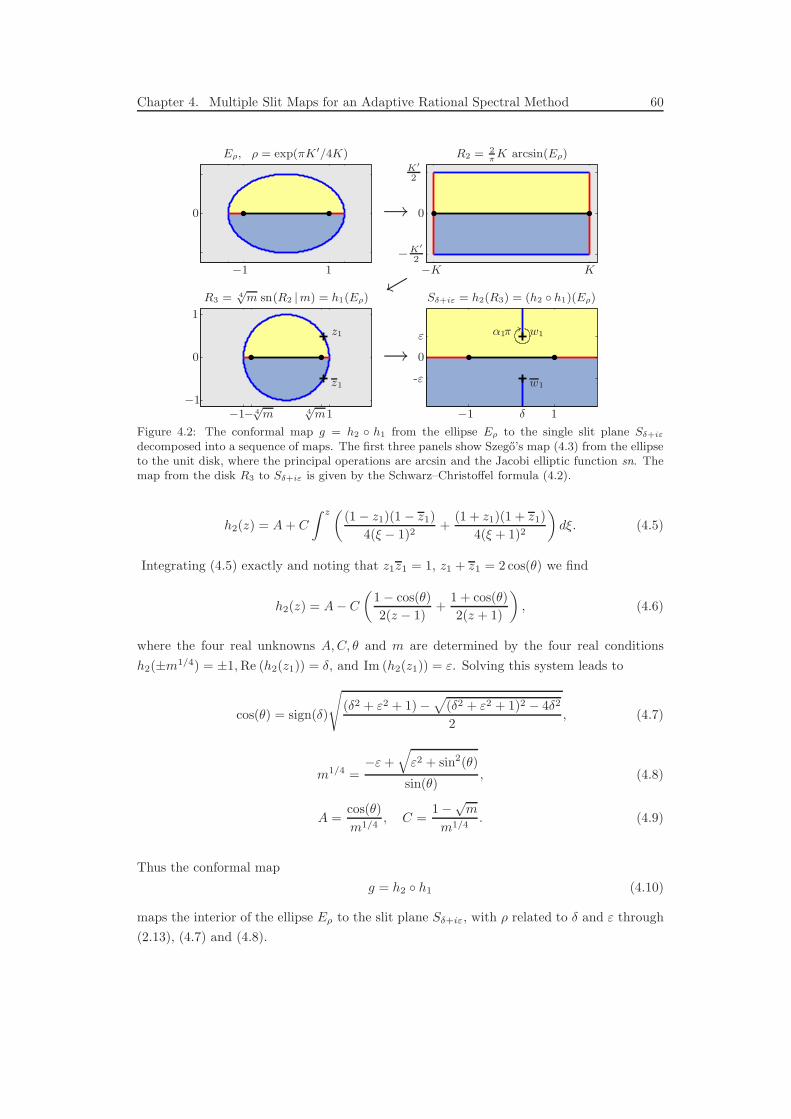
Chapter 4. Multiple Slit Maps for an Adaptive Rational Spectral Method 60
−1−1
−1
−1 1 1
1
1
00
00
−K K
−K′
2
K′
2
− 4√
m 4√
m
Eρ, ρ = exp(πK′/4K) R2 = 2πK arcsin(Eρ)
R3 = 4√
m sn(R2 |m) = h1(Eρ)
w1
δ
-ε
ε
w1
z1
z1
Sδ+iε = h2(R3) = (h2 h1)(Eρ)
α1π
→
←
→
Figure 4.2: The conformal map g = h2 h1 from the ellipse Eρ to the single slit plane Sδ+iε
decomposed into a sequence of maps. The first three panels show Szego’s map (4.3) from the ellipseto the unit disk, where the principal operations are arcsin and the Jacobi elliptic function sn. Themap from the disk R3 to Sδ+iε is given by the Schwarz–Christoffel formula (4.2).
h2(z) = A + C
∫ z ( (1− z1)(1 − z1)
4(ξ − 1)2+
(1 + z1)(1 + z1)
4(ξ + 1)2
)
dξ. (4.5)
Integrating (4.5) exactly and noting that z1z1 = 1, z1 + z1 = 2 cos(θ) we find
h2(z) = A− C
(
1− cos(θ)
2(z − 1)+
1 + cos(θ)
2(z + 1)
)
, (4.6)
where the four real unknowns A, C, θ and m are determined by the four real conditions
h2(±m1/4) = ±1, Re (h2(z1)) = δ, and Im (h2(z1)) = ε. Solving this system leads to
cos(θ) = sign(δ)
√
(δ2 + ε2 + 1)−√
(δ2 + ε2 + 1)2 − 4δ2
2, (4.7)
m1/4 =−ε +
√
ε2 + sin2(θ)
sin(θ), (4.8)
A =cos(θ)
m1/4, C =
1−√m
m1/4. (4.9)
Thus the conformal map
g = h2 h1 (4.10)
maps the interior of the ellipse Eρ to the slit plane Sδ+iε, with ρ related to δ and ε through
(2.13), (4.7) and (4.8).
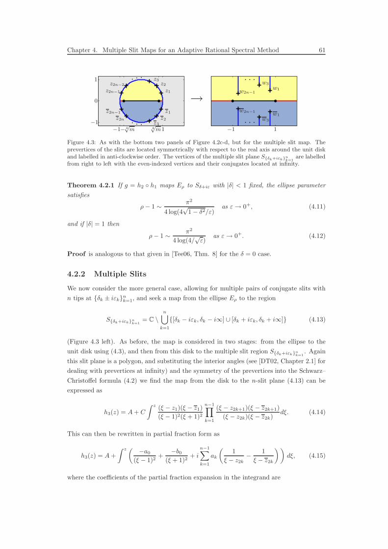
Chapter 4. Multiple Slit Maps for an Adaptive Rational Spectral Method 61
−1−1
1
1
0
− 4√
m 4√
m−1 1
z1
z2
z3z2n−2
z2n−1
z1
z2z3
z2n
z2n−1
w1
w3
w2n−1
w1w3
w2n−1
→
Figure 4.3: As with the bottom two panels of Figure 4.2c-d, but for the multiple slit map. Theprevertices of the slits are located symmetrically with respect to the real axis around the unit diskand labelled in anti-clockwise order. The vertices of the multiple slit plane Sδk+iεkn
k=1are labelled
from right to left with the even-indexed vertices and their conjugates located at infinity.
Theorem 4.2.1 If g = h2 h1 maps Eρ to Sδ+iε with |δ| < 1 fixed, the ellipse parameter
satisfies
ρ− 1 ∼ π2
4 log(4√
1− δ2/ε)as ε→ 0+, (4.11)
and if |δ| = 1 then
ρ− 1 ∼ π2
4 log(4/√
ε)as ε→ 0+. (4.12)
Proof is analogous to that given in [Tee06, Thm. 8] for the δ = 0 case.
4.2.2 Multiple Slits
We now consider the more general case, allowing for multiple pairs of conjugate slits with
n tips at δk ± iεknk=1, and seek a map from the ellipse Eρ to the region
Sδk+iεknk=1
= C \n⋃
k=1
[δk − iεk, δk − i∞] ∪ [δk + iεk, δk + i∞] (4.13)
(Figure 4.3 left). As before, the map is considered in two stages: from the ellipse to the
unit disk using (4.3), and then from this disk to the multiple slit region Sδk+iεknk=1
. Again
this slit plane is a polygon, and substituting the interior angles (see [DT02, Chapter 2.1] for
dealing with prevertices at infinity) and the symmetry of the prevertices into the Schwarz–
Christoffel formula (4.2) we find the map from the disk to the n-slit plane (4.13) can be
expressed as
h3(z) = A + C
∫ z (ξ − z1)(ξ − z1)
(ξ − 1)2(ξ + 1)2
n−1∏
k=1
(ξ − z2k+1)(ξ − z2k+1)
(ξ − z2k)(ξ − z2k)dξ. (4.14)
This can then be rewritten in partial fraction form as
h3(z) = A +
∫ z ( −a0
(ξ − 1)2+−b0
(ξ + 1)2+ i
n−1∑
k=1
ak
(
1
ξ − z2k− 1
ξ − z2k
))
dξ, (4.15)
where the coefficients of the partial fraction expansion in the integrand are

Chapter 4. Multiple Slit Maps for an Adaptive Rational Spectral Method 62
a0 = −C∏n−1
j=0
(
1− cos(θ2j+1))
2∏n−1
j=1
(
1− cos(θ2j)) , b0 = −
C∏n−1
j=0
(
1 + cos(θ2j+1))
2∏n−1
j=1
(
1 + cos(θ2j)) , (4.16)
ak =C∏n−1
j=0
(
cos(θ2k)− cos(θ2j+1))
2 sin3(θ2k)∏n−1
j=1j 6=k
(
cos(θ2k)− cos(θ2j)) , k = 1, 2, . . . , n− 1, (4.17)
with zk = exp(iθk). Thus integrating (4.15) exactly gives
h3(z) = A +
(
a0
z − 1+
b0
z + 1+ i
n−1∑
k=1
ak (log(z − z2k)− log(z − z2k))
)
, (4.18)
where the 2n + 2 real unknowns A, C, θ1, θ2, . . . , θ2n−1, and m can be determined from the
2n + 2 real conditions
h3(±m1/4) = ±1, (4.19)
Re(h3(z2k−1)) = δk, k = 1, 2, . . . , n,
Im(h3(z2k−1)) = εk, k = 1, 2, . . . , n.
In [Tee06] this parameter problem is solved by considering each of the prevertices zk2n−1k=1
(or more precisely their corresponding real-valued arguments θk) amongst the unknowns,
in addition to the constants A and m. This leads to a nonlinear problem in 2n+2 unknowns.
A more efficient approach arises in considering (4.18) with the 2n + 2 real parameters A,
b0, a0, . . ., an−1, θ2, θ4, . . ., θ2n−2, and m. In doing so, the system (4.19) separates into
a linear system in the n + 2 unknowns A, b0, akn−1k=0 and a smaller nonlinear system in
the n unknowns θ2kn−1k=1 and m1. To see this, suppose the latter n parameters have been
chosen and observe that as z passes anticlockwise through z2k on the upper half of the unit
circle, the kth term in the summation on the right-hand side of (4.18) causes a jump of
akπ in the real part of h3. The actual jump required is the horizontal distance to the next
slit tip, and choosing ak = (δk+1 − δk)/π will give exactly this spacing. A, a0, b0 are then
chosen so that h(±m1/4) = ±1 and Re(h3(z1)) = δ1, which leads to the 3× 3 linear system
M−1[A; a0; b0] = rhs in the short code segment on the following pages.
This leaves a nonlinear system in the n unknowns θ2kn−1k=1 and m to determine the vertical
distance of the n slit tips from the real line. The unknowns θ2k are subject to strict
inequality constraints 0 < θ2 < θ4 < · · · < θ2n−2 < π, but these can be eliminated by
transforming to an unconstrained set of variables
φk = arcsin
(
2
(
θ2k − θ2k−2
θ2k+2 − θ2k−2
)
− 1
)
, k = 1, 2, . . . , n− 1, (4.20)
with θ0 = 0, θ2n = π. These new variables take arbitrary real values, and the θ2k can be
1The separation of a nonlinear problem as described above forms the basis of the Variable Projectionmethod of Golub and Pereyra, and the corresponding FORTRAN routine VARPRO [GP73] developed some30 years ago. A recent review by the original authors can be found in [GP03], where the better conditioningand faster convergence of the reduced problems are demonstrated.
Chapter 4. Multiple Slit Maps for an Adaptive Rational Spectral Method 63
recovered by solving the system of linear equations
(
1− sin(φk)
2
)
θ2k−2 − θ2k +
(
1 + sin(φk)
2
)
θ2k+2 = 0, k = 1, 2, . . . , n− 1 (4.21)
in which the conditions (4.19) must be satisfied. A similar transformation can be used to
eliminate the constraint on m.
To solve the nonlinear system (4.19), we require the positions of the slit tips h3(z2k−1), but
locating these by computing the preimages z2k−1 from (4.16)-(4.17) at first seems cumber-
some. However, we simply note these points are the zeros of the integrand in (4.14) (which
can be evaluated in the form (4.15) using A, ak, b0 and θ2k) and furthermore that on
the unit circle between the poles z2k the integrand is monotonic, allowing the single root
between each two consecutive poles to be located by a simple algorithm combining Newton
iteration and bisection. The system (4.19) can then be solved using any nonlinear system
solver, such as the Matlab routine fsolve. We follow Tee in using the freely available
Newton–Armijo solver implemented in the routine nsold by Kelley [Kel03]. We have found
that the treatment of the parameters in this separable form allows faster and more robust
solution of the parameter problem than by considering θk2nk=1 as the unknowns directly.
Once the parameter problem is solved, h1 can be computed (with ρ related to m as in
(2.13)), and the map from the ellipse Eρ to the multiply slit domain Sδk+iεknk=1
is given by
g = h3 h1. The Matlab code below evaluates the map using these routines, although we
omit2 the code necessary to form and solve the system of nonlinear equations to determine
z2k=z2kn−1k=1 and m=m . As with the strip map in §2.3, we find in practice that the elliptic
parameter m can often be very close to 1, making it beneficial to use the ascending Landen
transform [AS65, (16.14)] with the complementary parameter m1 = 1 −m (which can be
better represented in IEEE arithmetic).
m14 = m^(.25); % 4th root of elliptic paramter
L = -2*log(m14)/pi;
[K Kp] = ellipkkp(L); % Elliptic integrals
h1 = m14*ellipjc(2*K*asin(z(:))/pi,L); % The map to the disk (2.12)
% Evaluate the summation on the rhs of (4.18)
ZZ = repmat([-m14;m14;h1],1,n-1); Z2K = repmat(z2k.’,length(h1)+2,1);
ZZ1 = ZZ - Z2K; idx1 = find(real(ZZ1)<0 & imag(ZZ1)>=0);
WW1 = log(ZZ1); WW1(idx1) = WW1(idx1) - 2i*pi;
ZZ2 = ZZ - conj(Z2K); idx2 = find(real(ZZ2)<0 & imag(ZZ2)<0);
WW2 = log(ZZ2); WW2(idx2) = WW2(idx2) + 2i*pi;
ak = diff(d)/pi; % ak given by jumps in delta
sumlogs = 1i*((WW1 - WW2)*ak); % The summation
2A full code for computing the map to a multiply slit region appears in [TT06], although without takingadvantage of the linear and nonlinear separation we have just described. Alternatively the map is availablein chebfun via the ’slit’ map. For a general outline of methods for solving parameter problems in Schwarz–Christoffel maps, see [DT02, Chapter 3.1].
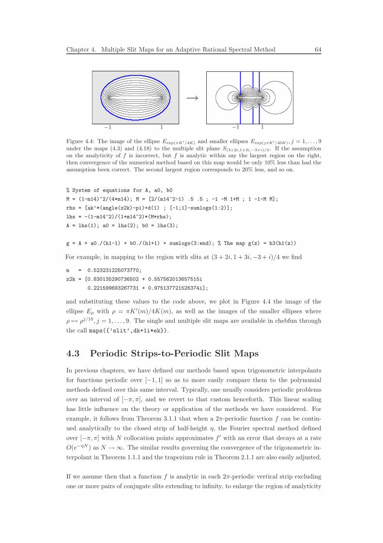
Chapter 4. Multiple Slit Maps for an Adaptive Rational Spectral Method 64
−1−1 11
→
Figure 4.4: The image of the ellipse Eexp(πK′/4K) and smaller ellipses Eexp(jπK′/40K), j = 1, . . . , 9under the maps (4.3) and (4.18) to the multiple slit plane S(3+2i,1+3i,−3+i)/4. If the assumptionon the analyticity of f is incorrect, but f is analytic within say the largest region on the right,then convergence of the numerical method based on this map would be only 10% less than had theassumption been correct. The second largest region corresponds to 20% less, and so on.
% System of equations for A, a0, b0
M = (1-m14)^2/(4*m14); M = [2/(m14^2-1) .5 .5 ; -1 -M 1+M ; 1 -1-M M];
rhs = [ak’*(angle(z2k)-pi)+d(1) ; [-1;1]-sumlogs(1:2)];
lhs = -(1-m14^2)/(1+m14^2)*(M*rhs);
A = lhs(1); a0 = lhs(2); b0 = lhs(3);
g = A + a0./(h1-1) + b0./(h1+1) + sumlogs(3:end); % The map g(z) = h3(h1(z))
For example, in mapping to the region with slits at (3 + 2i, 1 + 3i,−3 + i)/4 we find
m = 0.523231225073770;
z2k = [0.830135290736502 + 0.557562013657515i
0.221599693267731 + 0.975137721526374i];
and substituting these values to the code above, we plot in Figure 4.4 the image of the
ellipse Eρ with ρ = πK ′(m)/4K(m), as well as the images of the smaller ellipses where
ρ 7→ ρj/10, j = 1, . . . , 9. The single and multiple slit maps are available in chebfun through
the call maps(’slit’,dk+1i*ek).
4.3 Periodic Strips-to-Periodic Slit Maps
In previous chapters, we have defined our methods based upon trigonometric interpolants
for functions periodic over [−1, 1] so as to more easily compare them to the polynomial
methods defined over this same interval. Typically, one usually considers periodic problems
over an interval of [−π, π], and we revert to that custom henceforth. This linear scaling
has little influence on the theory or application of the methods we have considered. For
example, it follows from Theorem 3.1.1 that when a 2π-periodic function f can be contin-
ued analytically to the closed strip of half-height η, the Fourier spectral method defined
over [−π, π] with N collocation points approximates f ′ with an error that decays at a rate
O(e−ηN ) as N →∞. The similar results governing the convergence of the trigonometric in-
terpolant in Theorem 1.1.1 and the trapezium rule in Theorem 2.1.1 are also easily adjusted.
If we assume then that a function f is analytic in each 2π-periodic vertical strip excluding
one or more pairs of conjugate slits extending to infinity, to enlarge the region of analyticity

Chapter 4. Multiple Slit Maps for an Adaptive Rational Spectral Method 65
−π−π−π πππ 3π3π3π −3π−3π−3π δ δ1δ2δ3
εε1ε2
ε3
η
−η
Figure 4.5: The maps of §4.3. In §4.3.1 we derive a map from the infinite strip Ση (left) to thesingle periodic slit plane Sδ+iε (centre) which preserves intervals on the real line of width 2π. In§4.3.2 we give an alternative derivation, which is then generalised to produce a map from Ση to amultiple periodic slit plane Sδk+iεk (right).
we seek a 2π-periodic map g from the infinite strip Ση (Figure 4.5 left) of half-height η to
such a slit plane. We first follow Tee’s derivation [Tee06] of this map to the region
Sδ+iε = C \∞⋃
j=−∞[(δ + 2jπ)± iε, (δ + 2jπ)± i∞], ε > 0, (4.22)
with just one pair of slits within each period (Figure 4.5 centre), before generalising to allow
an arbitrary number of slits (Figure 4.5 right).
In a similar way to the transplanted/mapped/rational methods of Part I, rates of conver-
gence can then be improved by applying the numerical methods to the 2π-periodic function
f g, or by using g to define a linear trigonometric rational interpolant [Bal02] (see §4.5 for
examples).
4.3.1 Single Slit
The periodic map from the strip Ση to the single periodic slit plane Sδ+iε can be derived
directly using a sequence of elementary maps. By repeated application of the Schwarz
reflection principle, the problem reduces to mapping the interior of a rectangle R1 of width
π and height
η =πK ′
K(4.23)
to a semi-infinite strip R4 (Figure 4.6). The first map in the sequence rescales R1 to a width
K and height K ′, which the Jacobi elliptic function sn2(z|m) maps to the upper-half plane
R2 when K = K(m) and K ′ = K ′(m) are complete elliptic integrals of parameter m [Kob57,
(13.2)]. The upper-half plane is then mapped to itself by the Mobius transformation
z 7→ (1−m)z
1−mz, (4.24)
before a square root takes this to the upper-right quadrant R3. Observing that sin(z/2)
maps the semi-infinite strip R4 to R3 [Kob57, (10.5)], we use the inverse of this to map to
R4. Combining the above, reflecting across Re(z) = 0, and translating in the real direction
by a distance δ, the 2π-periodic map from Ση to Sδ+iε is
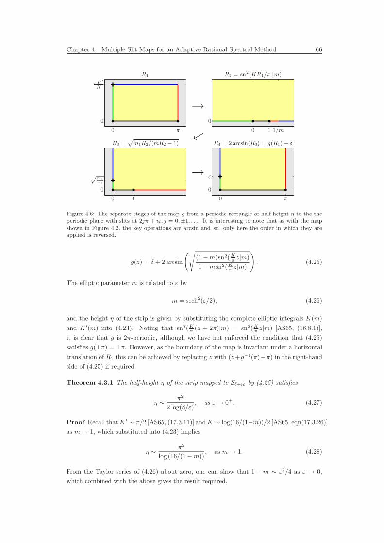
Chapter 4. Multiple Slit Maps for an Adaptive Rational Spectral Method 66
0
0
0
0
0
0
0
0
π
π
πK′
K
1
1 1/m
p
m1
m
ε
R1 R2 = sn2(KR1/π |m)
R3 =p
m1R2/(mR2 − 1) R4 = 2arcsin(R3) = g(R1) − δ
→
←
→
Figure 4.6: The separate stages of the map g from a periodic rectangle of half-height η to the theperiodic plane with slits at 2jπ + iε, j = 0,±1, . . .. It is interesting to note that as with the mapshown in Figure 4.2, the key operations are arcsin and sn, only here the order in which they areapplied is reversed.
g(z) = δ + 2 arcsin
(√
(1−m)sn2(Kπ z|m)
1−msn2(Kπ z|m)
)
. (4.25)
The elliptic parameter m is related to ε by
m = sech2(ε/2), (4.26)
and the height η of the strip is given by substituting the complete elliptic integrals K(m)
and K ′(m) into (4.23). Noting that sn2(Kπ (z + 2π)|m) = sn2(K
π z|m) [AS65, (16.8.1)],
it is clear that g is 2π-periodic, although we have not enforced the condition that (4.25)
satisfies g(±π) = ±π. However, as the boundary of the map is invariant under a horizontal
translation of R1 this can be achieved by replacing z with (z +g−1(π)−π) in the right-hand
side of (4.25) if required.
Theorem 4.3.1 The half-height η of the strip mapped to Sδ+iε by (4.25) satisfies
η ∼ π2
2 log(8/ε), as ε→ 0+. (4.27)
Proof Recall that K ′ ∼ π/2 [AS65, (17.3.11)] and K ∼ log(16/(1−m))/2 [AS65, eqn(17.3.26)]
as m→ 1, which substituted into (4.23) implies
η ∼ π2
log (16/(1−m)), as m→ 1. (4.28)
From the Taylor series of (4.26) about zero, one can show that 1 − m ∼ ε2/4 as ε → 0,
which combined with the above gives the result required.
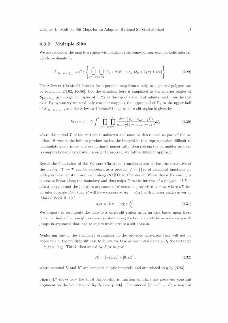
Chapter 4. Multiple Slit Maps for an Adaptive Rational Spectral Method 67
4.3.2 Multiple Slits
We next consider the map to a region with multiple slits removed from each periodic interval,
which we denote by
Sδk+iεknk=1
= C \
∞⋃
j=−∞
n⋃
k=1
[(δk + 2jπ)± iεk, (δk + 2jπ)± i∞]
. (4.29)
The Schwarz–Christoffel formula for a periodic map from a strip to a general polygon can
be found in [DT02, Flo86], but the situation here is simplified as the interior angles of
Sδk+iεk are integer multiples of π; 2π at the tip of a slit, 0 at infinity, and π on the real
axis. By symmetry we need only consider mapping the upper half of Ση to the upper half
of Sδk+iεknk=1
, and the Schwarz–Christoffel map to an n-slit region is given by
h(z) = A + C
∫ z ∞∏
j=−∞
n∏
k=1
sinh π2 (ξ − z2k − jT )
sinh π2 (ξ − z2k−1 − jT )
dξ, (4.30)
where the period T of the vertices is unknown and must be determined as part of the so-
lution. However, the infinite product makes the integral in this representation difficult to
manipulate analytically, and evaluating it numerically when solving the parameter problem
is computationally expensive. In order to proceed, we take a different approach.
Recall the foundation of the Schwarz–Christoffel transformation is that the derivative of
the map g : D → P can be expressed as a product g′ =∏
gk of canonical functions gk,
with piecewise constant argument along ∂D [DT02, Chapter 2]. When this is the case, g is
piecewise linear along the boundary and thus maps D to the interior of a polygon. If D is
also a polygon and the jumps in argument of g′ occur at prevertices z = zk where ∂D has
an interior angle βkπ, then P will have corners at wk = g(zk) with interior angles given by
[Mar77, Book II, §20]
αkπ = βkπ − [arg g′]z+
k
z−k
. (4.31)
We propose to recompute the map to a single-slit region using an idea based upon these
facts, i.e. find a function g′ piecewise constant along the boundary of the periodic strip with
jumps in argument that lead to angles which create a slit domain.
Neglecting one of the symmetry arguments in the previous derivation that will not be
applicable in the multiply slit case to follow, we take as our initial domain R1 the rectangle
[−π, π]× [0, η]. This is then scaled by K/π to give
R2 = [−K, K]× [0, iK ′], (4.32)
where as usual K and K ′ are complete elliptic integrals, and are related to η by (4.23).
Figure 4.7 shows how the third Jacobi elliptic function dn(z|m) has piecewise constant
argument on the boundary of R2 [Kob57, p.176]. The interval [K,−K] + iK ′ is mapped
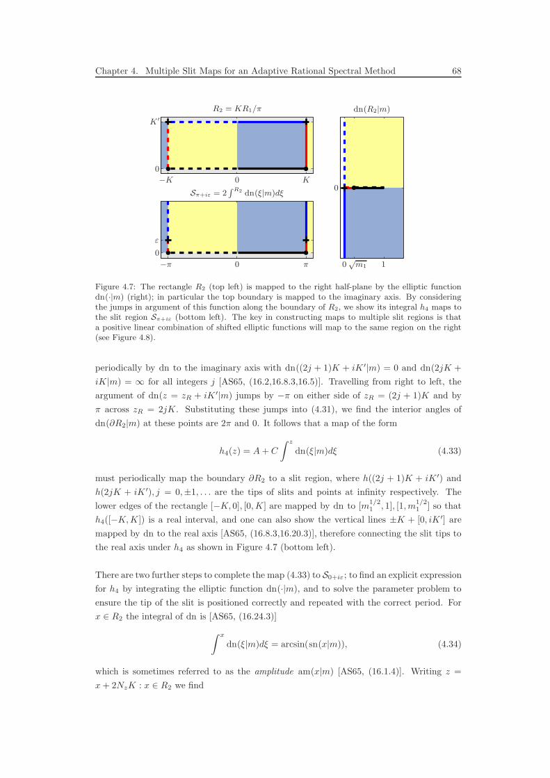
Chapter 4. Multiple Slit Maps for an Adaptive Rational Spectral Method 68
0
0
0
0
0
0
π−π
K−K
K′
1√
m1
ε
dn(R2|m)R2 = KR1/π
Sπ+iε = 2R R2 dn(ξ|m)dξ
Figure 4.7: The rectangle R2 (top left) is mapped to the right half-plane by the elliptic functiondn(·|m) (right); in particular the top boundary is mapped to the imaginary axis. By consideringthe jumps in argument of this function along the boundary of R2, we show its integral h4 maps tothe slit region Sπ+iε (bottom left). The key in constructing maps to multiple slit regions is thata positive linear combination of shifted elliptic functions will map to the same region on the right(see Figure 4.8).
periodically by dn to the imaginary axis with dn((2j + 1)K + iK ′|m) = 0 and dn(2jK +
iK|m) = ∞ for all integers j [AS65, (16.2,16.8.3,16.5)]. Travelling from right to left, the
argument of dn(z = zR + iK ′|m) jumps by −π on either side of zR = (2j + 1)K and by
π across zR = 2jK. Substituting these jumps into (4.31), we find the interior angles of
dn(∂R2|m) at these points are 2π and 0. It follows that a map of the form
h4(z) = A + C
∫ z
dn(ξ|m)dξ (4.33)
must periodically map the boundary ∂R2 to a slit region, where h((2j + 1)K + iK ′) and
h(2jK + iK ′), j = 0,±1, . . . are the tips of slits and points at infinity respectively. The
lower edges of the rectangle [−K, 0], [0, K] are mapped by dn to [m1/21 , 1], [1, m
1/21 ] so that
h4([−K, K]) is a real interval, and one can also show the vertical lines ±K + [0, iK ′] are
mapped by dn to the real axis [AS65, (16.8.3,16.20.3)], therefore connecting the slit tips to
the real axis under h4 as shown in Figure 4.7 (bottom left).
There are two further steps to complete the map (4.33) to S0+iε; to find an explicit expression
for h4 by integrating the elliptic function dn(·|m), and to solve the parameter problem to
ensure the tip of the slit is positioned correctly and repeated with the correct period. For
x ∈ R2 the integral of dn is [AS65, (16.24.3)]
∫ x
dn(ξ|m)dξ = arcsin(sn(x|m)), (4.34)
which is sometimes referred to as the amplitude am(x|m) [AS65, (16.1.4)]. Writing z =
x + 2NzK : x ∈ R2 we find
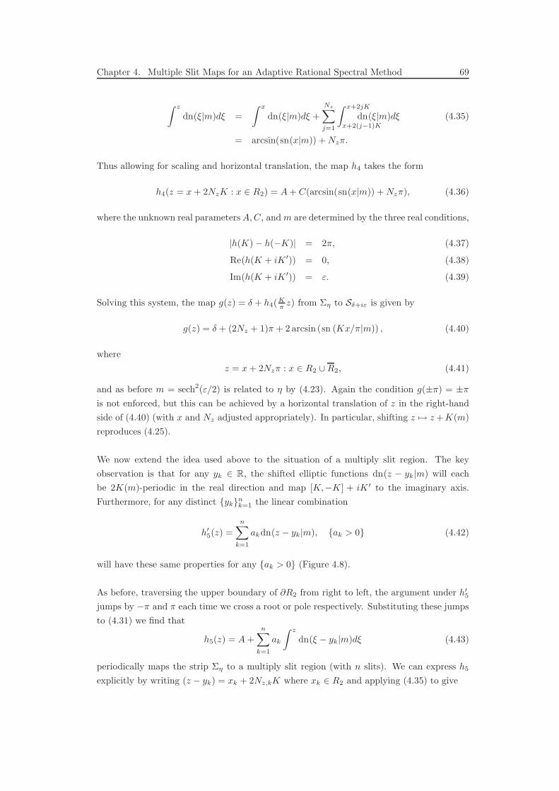
Chapter 4. Multiple Slit Maps for an Adaptive Rational Spectral Method 69
∫ z
dn(ξ|m)dξ =
∫ x
dn(ξ|m)dξ +
Nz∑
j=1
∫ x+2jK
x+2(j−1)K
dn(ξ|m)dξ (4.35)
= arcsin(sn(x|m)) + Nzπ.
Thus allowing for scaling and horizontal translation, the map h4 takes the form
h4(z = x + 2NzK : x ∈ R2) = A + C(arcsin(sn(x|m)) + Nzπ), (4.36)
where the unknown real parameters A, C, and m are determined by the three real conditions,
|h(K)− h(−K)| = 2π, (4.37)
Re(h(K + iK ′)) = 0, (4.38)
Im(h(K + iK ′)) = ε. (4.39)
Solving this system, the map g(z) = δ + h4(Kπ z) from Ση to Sδ+iε is given by
g(z) = δ + (2Nz + 1)π + 2 arcsin (sn (Kx/π|m)) , (4.40)
where
z = x + 2Nzπ : x ∈ R2 ∪R2, (4.41)
and as before m = sech2(ε/2) is related to η by (4.23). Again the condition g(±π) = ±π
is not enforced, but this can be achieved by a horizontal translation of z in the right-hand
side of (4.40) (with x and Nz adjusted appropriately). In particular, shifting z 7→ z +K(m)
reproduces (4.25).
We now extend the idea used above to the situation of a multiply slit region. The key
observation is that for any yk ∈ R, the shifted elliptic functions dn(z − yk|m) will each
be 2K(m)-periodic in the real direction and map [K,−K] + iK ′ to the imaginary axis.
Furthermore, for any distinct yknk=1 the linear combination
h′5(z) =
n∑
k=1
akdn(z − yk|m), ak > 0 (4.42)
will have these same properties for any ak > 0 (Figure 4.8).
As before, traversing the upper boundary of ∂R2 from right to left, the argument under h′5
jumps by −π and π each time we cross a root or pole respectively. Substituting these jumps
to (4.31) we find that
h5(z) = A +
n∑
k=1
ak
∫ z
dn(ξ − yk|m)dξ (4.43)
periodically maps the strip Ση to a multiply slit region (with n slits). We can express h5
explicitly by writing (z − yk) = xk + 2Nz,kK where xk ∈ R2 and applying (4.35) to give
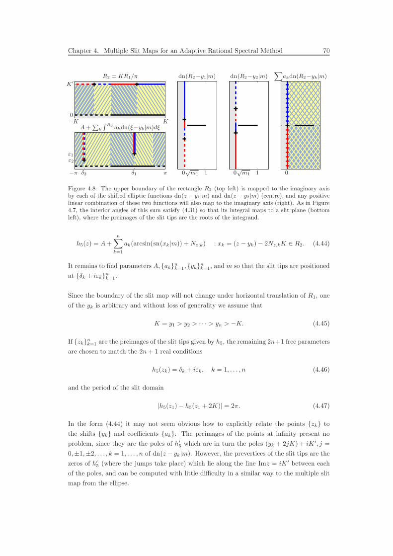
Chapter 4. Multiple Slit Maps for an Adaptive Rational Spectral Method 70
000
0
π−π
K−K
K′
11√
m1√
m1
ε1
ε2
δ1δ2
dn(R2−y1|m) dn(R2−y2|m)X
akdn(R2−yk|m)R2 = KR1/π
A +P
k
R R2 akdn(ξ−yk|m)dξ
Figure 4.8: The upper boundary of the rectangle R2 (top left) is mapped to the imaginary axisby each of the shifted elliptic functions dn(z − y1|m) and dn(z − y2|m) (centre), and any positivelinear combination of these two functions will also map to the imaginary axis (right). As in Figure4.7, the interior angles of this sum satisfy (4.31) so that its integral maps to a slit plane (bottomleft), where the preimages of the slit tips are the roots of the integrand.
h5(z) = A +n∑
k=1
ak(arcsin(sn(xk|m)) + Nz,k) : xk = (z − yk)− 2Nz,kK ∈ R2. (4.44)
It remains to find parameters A, aknk=1, yknk=1, and m so that the slit tips are positioned
at δk + iεknk=1.
Since the boundary of the slit map will not change under horizontal translation of R1, one
of the yk is arbitrary and without loss of generality we assume that
K = y1 > y2 > · · · > yn > −K. (4.45)
If zknk=1 are the preimages of the slit tips given by h5, the remaining 2n+1 free parameters
are chosen to match the 2n + 1 real conditions
h5(zk) = δk + iεk, k = 1, . . . , n (4.46)
and the period of the slit domain
|h5(z1)− h5(z1 + 2K)| = 2π. (4.47)
In the form (4.44) it may not seem obvious how to explicitly relate the points zk to
the shifts yk and coefficients ak. The preimages of the points at infinity present no
problem, since they are the poles of h′5 which are in turn the poles (yk + 2jK) + iK ′, j =
0,±1,±2, . . . , k = 1, . . . , n of dn(z − yk|m). However, the prevertices of the slit tips are the
zeros of h′5 (where the jumps take place) which lie along the line Imz = iK ′ between each
of the poles, and can be computed with little difficulty in a similar way to the multiple slit
map from the ellipse.

Chapter 4. Multiple Slit Maps for an Adaptive Rational Spectral Method 71
The parameter problem can again be reduced to two weakly coupled linear and nonlinear
problems, with n + 1 and n parameters respectively. Since Re(arcsin(sn(z|m))) jumps at
z = iK ′ by a distance −π, the Re(h(z)) jumps at z = yk + iK ′ by a distance −akπ, and
A = δ1 − π, (4.48)
ak = −(δk+1 − δk)/π, k = 1, . . . , n− 1,
an = −((δ1 − 2π)− δn)/π,
can be chosen instantly to match the position of the first slit, the distance between consec-
utive slits, and a period of 2π. Thus the nonlinear system needs only solve for the heights
of the slits through the n real parameters yknk=2 and m, which can be transformed to an
unconstrained problem in a similar manner as in the previous section.
Again omitting the code to form and solve this resulting nonlinear system to find the values
yk = ykNk=1and m = m, the following Matlab code computes the map g = h5(Kz/π)
from Ση to Sd(k)+iεkNk=1
.
L = -.5*log(m)/pi; [K Kp] = ellipkkp(L); % Elliptic integrals
ZZ = repmat(K*z(:).’/pi,length(yk),1); % R2 (repeated)
YK = repmat(yk,1,length(z)); % yk (repeated)
ZZ1 = ZZ - YK; % z - yk
Nz = floor(.5*(real(ZZ1)/K+1)); % ZZ1 = X + 2*Nz*K : Re(X)\in[-K,K)
sn = ellipjc(ZZ1 - 2*Nz*K,L); % Elliptic function sn(X|m)
gk = asin(sn) + Nz*pi; % gk
A = d(1) - pi; % Constant A
ak = -diff([d ; (d(1)-2*pi)])/pi; % ak given by jumps in real part
g = A + gk.’*ak; % g = A + sum_k ak*gk
For example, in the map to the region with slits at (3π + 2i, π + 3i,−3π + i)/4 + 2jπ, j =
0,±1, . . . we find
m = 0.999620736713857;
yk = [5.325344471289760
2.564368861260099
-2.384269371859549];
which can be used to produce Figure 4.9. In chebfun the map to single and multiple periodic
slit regions can be called with maps(’slitp’,dk+1i*ek).
4.4 Adaptivity
4.4.1 Map Adaptivity
The maps derived in the sections above assume the underlying function is analytic in the
whole complex plane except for some vertical slits extending to infinity. In some instances it
will be clear where these slits are positioned, such as when explicitly given a function with
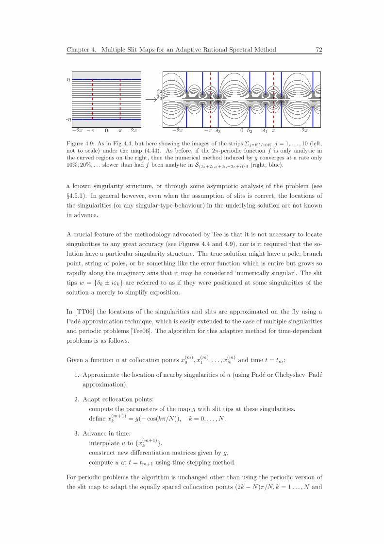
Chapter 4. Multiple Slit Maps for an Adaptive Rational Spectral Method 72
−2π−2π −π−π 00 ππ 2π2π δ1δ2δ3
ε1ε2
ε3
-η
η
→
Figure 4.9: As in Fig 4.4, but here showing the images of the strips ΣjπK′/10K , j = 1, . . . , 10 (left,not to scale) under the map (4.44). As before, if the 2π-periodic function f is only analytic inthe curved regions on the right, then the numerical method induced by g converges at a rate only10%, 20%, . . . slower than had f been analytic in S(3π+2i,π+3i,−3π+i)/4 (right, blue).
a known singularity structure, or through some asymptotic analysis of the problem (see
§4.5.1). In general however, even when the assumption of slits is correct, the locations of
the singularities (or any singular-type behaviour) in the underlying solution are not known
in advance.
A crucial feature of the methodology advocated by Tee is that it is not necessary to locate
singularities to any great accuracy (see Figures 4.4 and 4.9), nor is it required that the so-
lution have a particular singularity structure. The true solution might have a pole, branch
point, string of poles, or be something like the error function which is entire but grows so
rapidly along the imaginary axis that it may be considered ‘numerically singular’. The slit
tips w = δk ± iεk are referred to as if they were positioned at some singularities of the
solution u merely to simplify exposition.
In [TT06] the locations of the singularities and slits are approximated on the fly using a
Pade approximation technique, which is easily extended to the case of multiple singularities
and periodic problems [Tee06]. The algorithm for this adaptive method for time-dependant
problems is as follows.
Given a function u at collocation points x(m)0 , x
(m)1 , . . . , x
(m)N and time t = tm:
1. Approximate the location of nearby singularities of u (using Pade or Chebyshev–Pade
approximation).
2. Adapt collocation points:
compute the parameters of the map g with slit tips at these singularities,
define x(m+1)k = g(− cos(kπ/N)), k = 0, . . . , N .
3. Advance in time:
interpolate u to x(m+1)k ,
construct new differentiation matrices given by g,
compute u at t = tm+1 using time-stepping method.
For periodic problems the algorithm is unchanged other than using the periodic version of
the slit map to adapt the equally spaced collocation points (2k −N)π/N, k = 1 . . . , N and
Chapter 4. Multiple Slit Maps for an Adaptive Rational Spectral Method 73
Fourier–Pade rather than Chebyshev. The algorithm can also be modified to solve time-
independent problems.
In the examples to follow, we follow Tee by discretising in time by a highly accurate 7-stage,
13th-order fully implicit Runge–Kutta RADAU IIA method with step size control [HNW96].
Small relative and absolute error tolerances of 10−10 and 10−12 are chosen so that the results
are dominated by spatial rather than temporal errors. In practice one could use any time-
stepping routine which allows the option of pausing after each time step to adapt the grid
points. In particular, most of the built-in Matlab routines allow this by setting outputfcn
in odeset.
4.4.2 h-refinement / chebops
In finite element terminology, the adaptivity above would be referred to as r-refinement,
where the position of the grid/mesh is adjusted to reduce error. The other, more common,
types of adaptivity in finite element methods are h- and p-refinement, where the number of
elements or the polynomial degree on the elements are adjusted. In the context of spectral
methods, p-refinement is clearly tied to N (since the polynomial interpolation is global),
and we now suggest how this can be combined with the map adaptivity discussed earlier to
produce a fully adaptive method.
In the case of the non-periodic map from §4.2, defining slit tips δk + iεk will, by construc-
tion, fix a map from a certain ellipse with parameter ρ. If the assumption on the analyticity
of u is correct, then u g is now analytic in Eρ, and by Theorems 3.2.1 and 3.2.2 we can
expect convergence at a rate O(ρ−N ). To obtain an accuracy µ, it follows to that we need
a number of collocation points N ∼ | log(µ)|/ log(ρ). Similarly for the periodic methods, N
might be chosen proportional to | log(µ)|/(πν). Ideas related to these are discussed further
in §5.3.
Neither the uncustomised software we use to advance in time nor the built-in Matlab
time-steppers are capable of increasing the size of the system between time steps. One way
to resolve this is to call recursively a new instance of the time-stepping code whenever we
would like to increase or reduce N . The algorithm from the previous section then becomes
the following.
Given a function u at collocation points x(m)0 , x
(m)1 , . . . , x
(m)N and time t = tm:
1. Approximate the location of nearby singularities of u (using Pade or Chebyshev–Pade
approximation).
2. Adapt collocation points:
compute the parameters of the map g with slit tips at these singularites,
determine Nnew to satisfy error tolerances, ⋆
define x(m+1)k = g(− cos(kπ/Nnew)), k = 0, . . . , Nnew.
Chapter 4. Multiple Slit Maps for an Adaptive Rational Spectral Method 74
3. Advance in time:
interpolate u to x(m+1)k ,
construct new differentiation matrices given by g,
if N 6= Nnew
call the time-stepping routine with tnew0 = tm, unew(tnew
0 , x(m+1)k ) = u(tm, x
(m+1)k ),
return.
else
compute u at t = tm+1 using current time-stepping call.
Another option for introducing adaptivity is through the chebfun system (see §4.5.1 below
for an example). Recall that the chebop system [DBT08] uses the similar technology to
chebfun (it in fact makes use of the chebfun constructor) to solve linear systems involving
Chebyshev discretisation matrices of increasing size until the tailing coefficients of the solu-
tion are sufficiently small. However, chebops does not currently support maps and only has
limited functionality with time-stepping.
Instead we propose the following. Rather than use the parameter ρ returned by the con-
formal map to choose the number of points in the new discretisation at ⋆, compute a
mapped-chebfun approximation u to u using g and let Nnew = length(u). This will en-
sure that the number of collocation points used are at least enough to give an accurate
representation of the solution at the current time level. In principle we should perform
this chebfun-like test over the time step to ensure the new solution is represented accurately
enough, but in practice it is usually sufficient to take Nnew a little larger than the length of u.
This kind of approach can significantly improve the reliability of the adaptive spectral
method as if singularities or the map is incorrectly chosen, the number of collocation points
will be adjusted automatically to compensate.
4.5 Applications
We now demonstrate how the maps derived in this chapter can be applied to spectral
methods for solving differential equations, in particular those whose solutions u exhibit
localised regions of rapid variation indicative of nearby singularities in the complex plane.
As with the π/2 methods discussed in §3, we could use either the mapped spectral method
(§3.2.1) or the rational spectral method (§3.2.2). In most of the examples below, we choose
to use the latter due to its ease of implementation and not requiring derivatives of the map g.
However, when computing with the chebop system we use the mapped implementation with
the derivative of the map g computed as a chebfun (see §4.5.1). For periodic problems we
use the spectral collocation method based upon the linear rational trigonometric interpolant
[Bal02], for which a similar theorem to Theorem 3.2.2 holds [Tee06]. Conditioning of the
differentiation matrices resulting from these applications is discussed in Appendix B.
Chapter 4. Multiple Slit Maps for an Adaptive Rational Spectral Method 75
4.5.1 Time-independent Problem
As our first example, we consider the ODE
εd2u
dx2+ x(x2 − 1/2)
du
dx+ 3(x2 − 1/2)u = 0, −1 < x < 1, ε > 0, (4.49)
u(−1) = −2, u(1) = 4.
This two-point boundary value problem appears in [KNB86, Figure 10.1], only above it has
been differentiated so the solution u here is the derivative of the solution in [KNB86]. The
ODE has turning points at x = 0,±1/√
2, and u has interior layers at the latter two of these
points3.
Some elementary asymptotic matching determines that the solution of (4.49) has interior
layers at x = ±1/√
2, and in particular that about these points
u ∼ erf
(
x∓ 1/√
2√2ε
)
(4.50)
respectively. To limit the growth of this error function along the lines Rez = ±1/√
2, we
choose a map with four slit tips positioned at
w = 1/√
2± i√
2ε,−1/√
2± i√
2ε. (4.51)
Solving the parameter problem for the map g = h3h1 from §4.2 for ε = 10−5 with slits given
by (4.51), we find m = 0.999848332078409 and zk = i (the latter is evident by symmetry),
with which we can compute g and the differentiation matrices of the linear rational colloca-
tion method (concise Matlab codes for computing these matrices can be found in [TT06]).
Figure 4.10a shows this solution to (4.49) for ε = 10−5 with 123 grid points (the same
values as used in [KNB86]), and Figure 4.10b compares the convergence of this approach
against the standard Chebyshev method as the number of collocation points N +1 increases.
Since the problem is linear, it lends itself very well to the chebop system. We could imple-
ment a mapped chebop with the following Matlab code;
E = 1e-5; % This can be changed
[d x] = domain(-1,1); % The domain [-1,1]
map = maps(’slit’,[-1,1]/sqrt(2)+1i*sqrt(2*E)); % The approprite slit map
g = chebfun(@(x) map.for(x), d,’eps’,1e-10); % A chebfun of the map
D = diag(1./diff(g))*diff(d); D2 = D^2; % Mapped diff matrices
A = E*D2 + diag(g.*(g.^2-1/2))*D + 3*diag(g.^2-1/2); % Linear operator
A.lbc = -2; A.rbc = 4; % Boundary conditions.
u = A\0 % The solution u
3It is suggested in [KNB86] that the turning point at x = 0 might also cause ‘turning point behaviour’,and a grid highly clustered about this point is used. In our own computations and asymptotic analysis wefind this unnecessary, and so map only to slits with real parts at ±1/
√2 where the solution varies rapidly.

Chapter 4. Multiple Slit Maps for an Adaptive Rational Spectral Method 76
1 0 1−6
−4
−2
0
2
4
6
8
10
12
0 50 100 150 200 250
10−10
10−8
10−6
10−4
10−2
100
102
−√
2/2√
2/2
Figure 4.10: Left: an approximate solution to (4.49) with ε = 10−5 obtained using the rationalspectral method with 123 grid points (dots) defined by the map g. Right: the improvement inconvergence of the transformed grid (solid) over the Chebyshev grid (dashed) as the number ofcollocation points N + 1 is increased. The axes are log-linear scale, so straight lines representgeometric convergence.
which returns a chebfun of length 158 and is accurate to around 8 digits. As mentioned
before, chebops does not currently support maps, so the chebfun u will not know it is
mapped. To get the proper representation, we construct a new chebfun;
u = chebfun(u.vals,’map’,map)
4.5.2 Time-dependent Problem: Allen–Cahn
When introducing the adaptive rational spectral method, Tee demonstrates its performance
on the time-dependent Allen–Cahn equation with initial and boundary conditions taken
from [Tre00, p34.m]:
∂u
∂t= ε
∂2u
∂x2+ u(1− u2), −1 < x < 1, t > 0, (4.52)
u(x, 0) = 0.53x + 0.47 sin(−1.5πx), u(−1) = −1, u(1) = 1. (4.53)
The solution u has an unstable equilibrium at 0, and two stable equilibria at ±1 between
which it transitions rapidly in x with a layer-width which depends on ε. The initial condition
above gives rise to a solution with three such regions of rapid variation. Here we consider
the modified initial condition
u(x, 0) = 0.53x + 0.47 sin(−3.5πx), (4.54)
which will lead two a solution with seven such regions. Considering the parameter problem
in the form suggested in §4.2.2 allows us to compute the required map in this situation, even
when ε is as small as 10−4. The result of this computation is displayed in Figure 4.11.

Chapter 4. Multiple Slit Maps for an Adaptive Rational Spectral Method 77
−1 0 1−1
−0.5
0
0.5
1
t = 1
−1 0 1−0.2
−0.1
0
0.1
0.2
real part
imag
inar
y pa
rt
−1 0 1−1
−0.5
0
0.5
1
t = 3
−1 0 1−0.2
−0.1
0
0.1
0.2
real part
−1 0 1−1
−0.5
0
0.5
1
t = 7
−1 0 1−0.2
−0.1
0
0.1
0.2
real part
50 100 150 200
10−10
10−8
10−6
10−4
10−2
100
appr
oxim
atio
n er
ror
50 100 150 200
10−10
10−8
10−6
10−4
10−2
100
50 100 150 200
10−10
10−8
10−6
10−4
10−2
100
NNN
xxx
u(x
,t)
Figure 4.11: Solutions of the metastable Allen–Cahn problem (4.52) with ε = 10−4 using theadaptive rational spectral method. The first row shows the solution computed using 129 collocationpoints (dots), whilst the second row shows the poles computed by the Pade approximation and usedin the corresponding computation (crosses). The third row shows log-linear plots of approximationerror against the number of collocation points N + 1 for the rational adaptive (solid), Chebyshev(dashed) and Sausage-mapped (dotted) spectral methods. Compare with [Tee06, Figure 6.6].
Initially the solution is well behaved, and up until t = 1 the rational method induced by the
map is less accurate than the Chebyshev. This occurs because the Pade approximation for
the location of the singularities in the complex plane struggles when they are further from
the computational interval. As the solution develops to its metastable state and the singu-
larities move close to the real axis, the solution provided by the rational method becomes
far more accurate than the standard Chebyshev.
The dotted line in Figure 4.11 represents the solution computed with a sausage map of
degree 9 from §2.3.3 which, although it demonstrates a π/2 speed-up over the Chebyshev
method, is still far less accurate than the slit-mapped method for t > 1. To solve this
equation most accurately in practice, we might then choose to use a strip or sausage map
until t > 1 before turning on the adaptivity.

Chapter 4. Multiple Slit Maps for an Adaptive Rational Spectral Method 78
4.5.3 Periodic Time-dependent Problem: mKdV Equation
As a non-periodic example, we consider the modified Korteweg-de Vries (mKdV) equation
∂u
∂t+
∂3u
∂x3+ 6u2 ∂u
∂x= 0, t > 0. (4.55)
As with the standard KdV equation the mKdV admits soliton solutions, and in particular
a two soliton on the real interval is given explicitly by [DJ89]
u = 2(gxf − gfx)/(f2 + g2), (4.56)
where
f = 1− (k1 − k2)2ek1(x−x1)+k2(x−x2)−(k3
1+k32)t
4k1k2(k1 + k2)2, (4.57)
g =k2e
k1(x−x1)−k31t + k1e
k2(x−x2)−k32t
2k1k2. (4.58)
For sufficiently large k1 and k2 we can observe these solitons on a periodic domain. How-
ever, when these values are large the solitons are narrow and cannot be well represented by
the trigonometric polynomial implicit in the Fourier spectral method. We therefore use our
adaptive mapping strategy on (4.55) with an initial condition given by k1 = 20, k2 = 10,
x1 = −1, x2 = 0, and the initial location of the singularities in the complex plane deter-
mined by a Fourier–Pade approximation to this function. The results of this are shown in
Figures 4.12 and 4.13 when using N = 97 collocation points.
Figure 4.12 shows the solution as a three-dimensional plot in both time and space, and
is accurate to around 5 digits of accuracy (the tolerance used in the time-stepping). The
leftmost soliton in the initial condition has the higher peak and corresponding higher wave
speed, and quickly catches the shorter, slower moving one. After the collision both solitons
return to their original profiles, and we see the largest leaving the computational interval at
π and reappearing on the other side due to the periodic boundary conditions.
Figure 4.13 shows the grid used in the computation. Recall that the time-stepping is con-
trolled by an off-the-shelf code (in that case radau13), and that the spatial discretisation
at each step is determined by the conformal map from §4.3.2. As we might expect this
last grid clusters around the moving solitons where the solution changes rapidly, but impor-
tantly, and by construction, it does so in such a way to maximise the use of analyticity in the
solution. The time-stepping is reasonably uniform throughout, except at around t = 0.01
where the soliton passes through the boundary. The cause of this may be that the more
rapid movement of the grid points at this time make the equations stiffer, and we suggest a
possible remedy in Appendix C.
A trigonometric interpolant requires around N = 460 points to resolve the initial condition
to the same accuracy as above (based upon the decay of Fourier coefficients), and so the
Fourier spectral method will require at least this many points in solving (4.55).
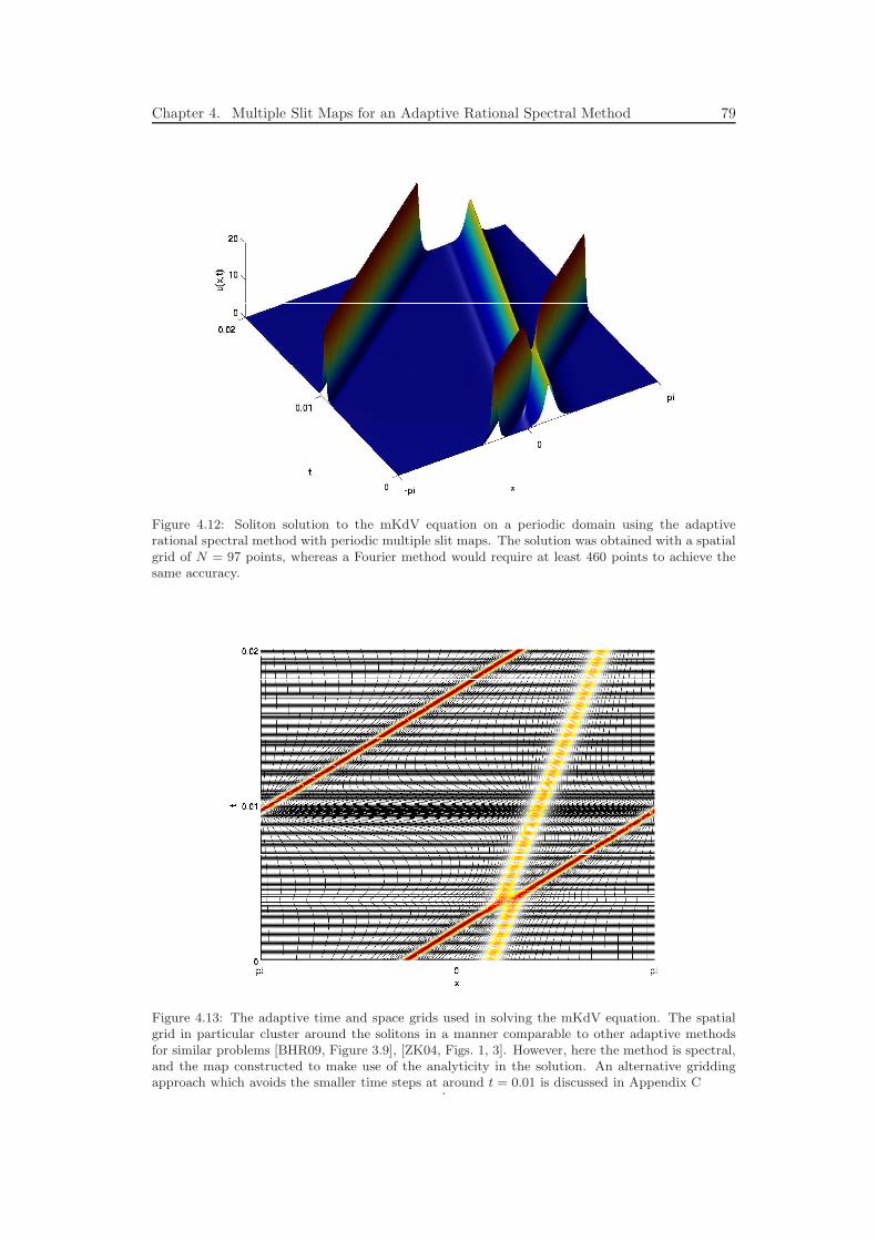
Chapter 4. Multiple Slit Maps for an Adaptive Rational Spectral Method 79
Figure 4.12: Soliton solution to the mKdV equation on a periodic domain using the adaptiverational spectral method with periodic multiple slit maps. The solution was obtained with a spatialgrid of N = 97 points, whereas a Fourier method would require at least 460 points to achieve thesame accuracy.
Figure 4.13: The adaptive time and space grids used in solving the mKdV equation. The spatialgrid in particular cluster around the solitons in a manner comparable to other adaptive methodsfor similar problems [BHR09, Figure 3.9], [ZK04, Figs. 1, 3]. However, here the method is spectral,and the map constructed to make use of the analyticity in the solution. An alternative griddingapproach which avoids the smaller time steps at around t = 0.01 is discussed in Appendix C
.
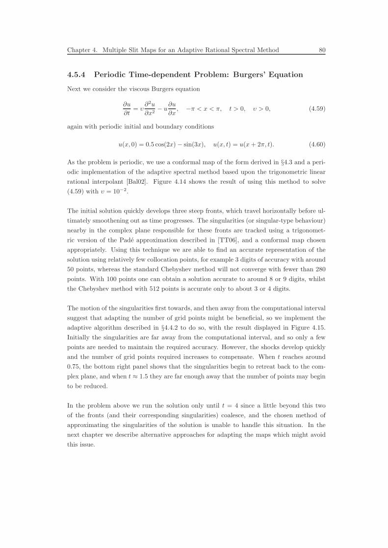
Chapter 4. Multiple Slit Maps for an Adaptive Rational Spectral Method 80
4.5.4 Periodic Time-dependent Problem: Burgers’ Equation
Next we consider the viscous Burgers equation
∂u
∂t= υ
∂2u
∂x2− u
∂u
∂x, −π < x < π, t > 0, υ > 0, (4.59)
again with periodic initial and boundary conditions
u(x, 0) = 0.5 cos(2x)− sin(3x), u(x, t) = u(x + 2π, t). (4.60)
As the problem is periodic, we use a conformal map of the form derived in §4.3 and a peri-
odic implementation of the adaptive spectral method based upon the trigonometric linear
rational interpolant [Bal02]. Figure 4.14 shows the result of using this method to solve
(4.59) with υ = 10−2.
The initial solution quickly develops three steep fronts, which travel horizontally before ul-
timately smoothening out as time progresses. The singularities (or singular-type behaviour)
nearby in the complex plane responsible for these fronts are tracked using a trigonomet-
ric version of the Pade approximation described in [TT06], and a conformal map chosen
appropriately. Using this technique we are able to find an accurate representation of the
solution using relatively few collocation points, for example 3 digits of accuracy with around
50 points, whereas the standard Chebyshev method will not converge with fewer than 280
points. With 100 points one can obtain a solution accurate to around 8 or 9 digits, whilst
the Chebyshev method with 512 points is accurate only to about 3 or 4 digits.
The motion of the singularities first towards, and then away from the computational interval
suggest that adapting the number of grid points might be beneficial, so we implement the
adaptive algorithm described in §4.4.2 to do so, with the result displayed in Figure 4.15.
Initially the singularities are far away from the computational interval, and so only a few
points are needed to maintain the required accuracy. However, the shocks develop quickly
and the number of grid points required increases to compensate. When t reaches around
0.75, the bottom right panel shows that the singularities begin to retreat back to the com-
plex plane, and when t ≈ 1.5 they are far enough away that the number of points may begin
to be reduced.
In the problem above we run the solution only until t = 4 since a little beyond this two
of the fronts (and their corresponding singularities) coalesce, and the chosen method of
approximating the singularities of the solution is unable to handle this situation. In the
next chapter we describe alternative approaches for adapting the maps which might avoid
this issue.
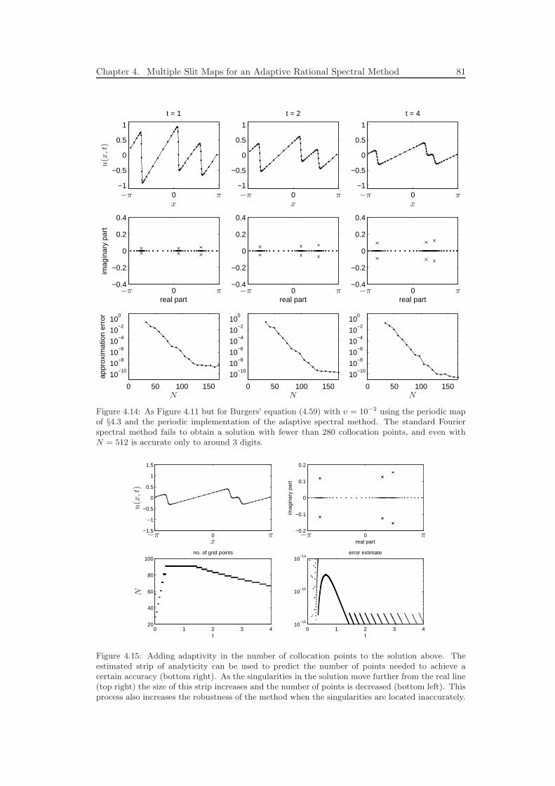
Chapter 4. Multiple Slit Maps for an Adaptive Rational Spectral Method 81
0 −1
−0.5
0
0.5
1
t = 1
0 −0.4
−0.2
0
0.2
0.4
real part
imag
inar
y pa
rt
0 −1
−0.5
0
0.5
1
t = 2
0 −0.4
−0.2
0
0.2
0.4
real part
0 −1
−0.5
0
0.5
1
t = 4
0 −0.4
−0.2
0
0.2
0.4
real part
0 50 100 150
10−10
10−8
10−6
10−4
10−2
100
appr
oxim
atio
n er
ror
0 50 100 150
10−10
10−8
10−6
10−4
10−2
100
0 50 100 150
10−10
10−8
10−6
10−4
10−2
100
NNN
−π
−π
−π
−π
−π
−π
π
π
π
π
π
πxxx
u(x
,t)
Figure 4.14: As Figure 4.11 but for Burgers’ equation (4.59) with υ = 10−2 using the periodic mapof §4.3 and the periodic implementation of the adaptive spectral method. The standard Fourierspectral method fails to obtain a solution with fewer than 280 collocation points, and even withN = 512 is accurate only to around 3 digits.
0 −1.5
−1
−0.5
0
0.5
1
1.5
0 −0.2
−0.1
0
0.1
0.2
real part
imag
inar
y pa
rt
0 1 2 3 420
40
60
80
100no. of grid points
t0 1 2 3 4
10−16
10−15
10−14
t
error estimate
N
−π−π ππx
u(x
,t)
Figure 4.15: Adding adaptivity in the number of collocation points to the solution above. Theestimated strip of analyticity can be used to predict the number of points needed to achieve acertain accuracy (bottom right). As the singularities in the solution move further from the real line(top right) the size of this strip increases and the number of points is decreased (bottom left). Thisprocess also increases the robustness of the method when the singularities are located inaccurately.
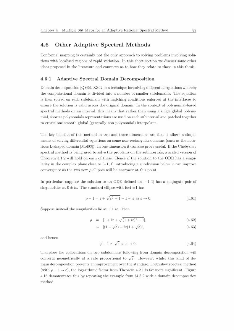
Chapter 4. Multiple Slit Maps for an Adaptive Rational Spectral Method 82
4.6 Other Adaptive Spectral Methods
Conformal mapping is certainly not the only approach to solving problems involving solu-
tions with localised regions of rapid variation. In this short section we discuss some other
ideas proposed in the literature and comment as to how they relate to those in this thesis.
4.6.1 Adaptive Spectral Domain Decomposition
Domain decomposition [QV99, XZ92] is a technique for solving differential equations whereby
the computational domain is divided into a number of smaller subdomains. The equation
is then solved on each subdomain with matching conditions enforced at the interfaces to
ensure the solution is valid across the original domain. In the context of polynomial-based
spectral methods on an interval, this means that rather than using a single global polyno-
mial, shorter polynomials representations are used on each subinterval and patched together
to create one smooth global (generally non-polynomial) interpolant.
The key benefits of this method in two and three dimensions are that it allows a simple
means of solving differential equations on some non-rectangular domains (such as the noto-
rious L-shaped domain [Mol03]). In one dimension it can also prove useful. If the Chebyshev
spectral method is being used to solve the problems on the subintervals, a scaled version of
Theorem 3.1.2 will hold on each of these. Hence if the solution to the ODE has a singu-
larity in the complex plane close to [−1, 1], introducing a subdivision below it can improve
convergence as the two new ρ-ellipses will be narrower at this point.
In particular, suppose the solution to an ODE defined on [−1, 1] has a conjugate pair of
singularities at 0± iε. The standard ellipse with foci ±1 has
ρ− 1 = ε +√
ε2 + 1− 1 ∼ ε as ε→ 0. (4.61)
Suppose instead the singularities lie at 1± iε. Then
ρ = |1 + iε +√
(1 + iε)2 − 1|, (4.62)
∼ |(1 +√
ε) + iε(1 +√
ε)|, (4.63)
and hence
ρ− 1 ∼√
ε as ε→ 0. (4.64)
Therefore the collocations on two subdomains following from domain decomposition will
converge geometrically at a rate proportional to√
ε. However, whilst this kind of do-
main decomposition presents an improvement over the standard Chebyshev spectral method
(with ρ− 1 ∼ ε), the logarithmic factor from Theorem 4.2.1 is far more significant. Figure
4.16 demonstrates this by repeating the example from §4.5.2 with a domain decomposition
method.
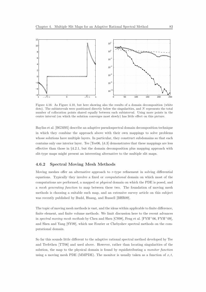
Chapter 4. Multiple Slit Maps for an Adaptive Rational Spectral Method 83
1 0 1−6
−4
−2
0
2
4
6
8
10
12
0 50 100 150 200 250
10−10
10−8
10−6
10−4
10−2
100
102
−√
2/2√
2/2
Figure 4.16: As Figure 4.10, but here showing also the results of a domain decomposition (whitedots). The subintervals were positioned directly below the singularities, and N represents the totalnumber of collocation points shared equally between each subinterval. Using more points in thecentre interval (on which the solution converges most slowly) has little effect on this picture.
Bayliss et al. [BGM95] describe an adaptive pseudospectral domain decomposition technique
in which they combine the approach above with their own mappings to solve problems
whose solutions have multiple layers. In particular, they construct subdomains so that each
contains only one interior layer. Tee [Tee06, §4.3] demonstrates that these mappings are less
effective than those in §4.2.1, but the domain decomposition plus mapping approach with
slit-type maps might present an interesting alternative to the multiple slit maps.
4.6.2 Spectral Moving Mesh Methods
Moving meshes offer an alternative approach to r-type refinement in solving differential
equations. Typically they involve a fixed or computational domain on which most of the
computations are performed, a mapped or physical domain on which the PDE is posed, and
a mesh generating function to map between these two. The foundation of moving mesh
methods is choosing a suitable such map, and an extensive survey article on this subject
was recently published by Budd, Huang, and Russell [BHR09].
The topic of moving mesh methods is vast, and the ideas within applicable to finite difference,
finite element, and finite volume methods. We limit discussion here to the recent advances
in spectral moving mesh methods by Chen and Shen [CS98], Feng et al. [FYH+06, FYH+09],
and Shen and Yang [SY09], which use Fourier or Chebyshev spectral methods on the com-
putational domain.
So far this sounds little different to the adaptive rational spectral method developed by Tee
and Trefethen [TT06] and used above. However, rather than locating singularities of the
solution, the map to the physical domain is found by equidistributing a monitor function
using a moving mesh PDE (MMPDE). The monitor is usually taken as a function of x, t,

Chapter 4. Multiple Slit Maps for an Adaptive Rational Spectral Method 84
and of the solution u(x, t) to the physical PDE, and is chosen to be large where grid points
need to be clustered. In the case of spectral moving mesh methods referenced above, it is
M(t, x, u) =√
1 + (βuxxξ)2, (4.65)
where ξ is the variable on the computational grid, x is the mapped variable, and β some
scaling constant. In this way the function clusters where the gradient of u is large. The
MMPDE is coupled to the physical PDE, and is also solved spectrally.
Whilst a large gradient might suggest difficulty in a trigonometric or polynomial expansion,
Theorems 3.1.1 and 3.1.2 dictate that the convergence of the expansion is determined by the
location of singularities. This means that whilst the coefficients in a Chebyshev expansion
of say the function tanh(50x) will decay at the same rate as those of its indefinite integral
on [−1, 1], this latter function is flat near the origin and the monitor M in (4.65) will not
cluster points where they are needed.
In the context of phase-field modelling (for which these spectral moving mesh methods were
developed) this is not usually a problem, as the underlying solutions do have steep tanh-like
profiles; yet it seems that truly general spectral moving mesh method should use a monitor
function incorporating the analyticity of the underlying solution.
The moving mesh methods do extend naturally to higher-dimensional problems, and have
been used in very impressive computations in 2D and 3D [DLW06, FYH+06, FYH+09,
SY09]. It seems there may be scope for combining the spectral moving mesh approach with
consideration of conformal maps and analyticity to produce methods which work in higher
dimensions, but also converge at rates like those in Theorems 4.2.1 and 4.3.1 in the ε → 0
sharp interface limit.
4.7 Comments
In this chapter we have presented two forms of conformal maps to multiply slit domains,
and shown their applicability in mapped and rational spectral methods for problems with
near-singular solutions. Importantly, the integrals in the Schwarz–Christoffel formulations
of the maps are computed analytically: a fully numerical approach, such as using the SC
Toolbox [Dri05] directly, would be far less efficient.
The first map derived by Tee [Tee06] is for non-periodic problems, and maps the ellipse
Eρ found in convergence results for Chebyshev and Legendre interpolation to the whole
complex plane minus a number of vertical slits symmetric about the real line extending to
infinity. Our contribution here was to reformulate the parameter problem in such a way
that it becomes linear in half of the unknowns, improving efficiency and robustness when
computing the map.

Chapter 4. Multiple Slit Maps for an Adaptive Rational Spectral Method 85
The ellipse-to-multiple-slit map is pleasing conceptually, since when the underlying function
is analytic in this slit plane, the rate of convergence is determined explicitly by Theorem
3.2.2. In practice it may be the case that simpler maps, say from an infinite strip or a rect-
angle rather than the ellipse, give results which are almost as good. Such ideas are explored
in the next chapter.
The second map we have derived is new and maps a periodic rectangle to periodic multiple
slits. As with the map from the ellipse, we demonstrated that this map can be computed
without evaluating the Schwarz–Christoffel integrals numerically (which in this case con-
tain an infinite product), and that the parameter problem can again be reduced into linear
and nonlinear parts. The maps were demonstrated to be effective for solving PDEs with
periodic solutions containing multiple layers, obtaining an accurate solution with far fewer
points than the standard Fourier method.
For periodic problems such as (4.55) and (4.59) one could apply periodic boundary con-
ditions to a mapped or rational Chebyshev method using the ellipse-to-multiple slit map.
However, the rate of convergence of such an approach would be at least π/2 times worse
than using a mapped Fourier method with the periodic map (for reasons related to the work
in Part I), although will be worse still as the assumption of analyticity in the complex plane
besides the slits above the computational interval will be false. A periodic grid also allows
the use of a ‘moving grid’ as described in Appendix C.
The second key development in these methods has been the ability to adapt in the number
of grid points. This can be done either as part of the mapping process (using the size of the
ellipse or periodic strip to estimate the number of collocation points needed for a required
accuracy), or through a process such as used in the chebop system, where the degree is
increased until the tailing coefficients of the computed solution are sufficiently small. In
practice a useful strategy is to use the number of points suggested by the map parameter
as an initial guess for this second procedure (e.g. chebfunpref(‘minsamples’, ...)).
Combining this kind of adaptivity and error estimation with both the slit maps of this
chapter and powerful high-order adaptive time-stepping schemes, we are left with a fully-
adaptive high-performance routine for solving near-singular ordinary and partial differential
equations in one space dimension, as demonstrated in the examples of §4.5.
Chapter 5
The Resolution of Irregular
Functions
The maps described in the previous chapter were shown to be very effective for provid-
ing new representations, be they rational or mapped-polynomial, of functions which obey
some quite specific analyticity requirements. In this chapter we demonstrate some simpler
maps, and propose a method in which the region of analyticity is estimated automatically
so that the only assumption is that the function is analytic in some neighbourhood of [−1, 1].
In §5.1 we introduce such maps, giving derivations and descriptions of the regions of the
complex plane they map, and provide examples of functions for which they might be appli-
cable. We then in §5.2 describe a method of combining these maps to produce multiple pinch
maps, which are similar to the multiple slit maps of the previous chapter, but simpler and
more robust in their computation. In §5.3 we suggest an automated method for estimating
the region of analyticity of a function using information from local Chebyshev interpolants,
and in §5.4 coupling this idea with the pinch maps of §5.2 to develop an algorithm which
attempts to reduce the length (in terms of the number of coefficients required to achieve a
certain approximation accuracy) of Chebyshev interpolants in the chebfun system.
5.1 Other Useful Maps
In Part I we first introduced the map from the ρ-ellipse governing convergence of Chebyshev
interpolants to the infinite strip about the real axis, before going on to demonstrate thaet
simpler maps which had similar properties were also effective in practice. Here we will see
how the same principle applies to the slit-type maps.
5.1.1 Strip-to-Slit
The first map we consider appears in the paper by Tee and Trefethen [TT06]. There they
map Σα (the infinite strip about the real axis of height α) to Sδ+iε (the complex plane minus
a pair of conjugate slits with tips at δ ± iε) using the map
g(s) = δ + ε sinh
(
π(s− 1)
2α+ arcsinh
(
1− δ
ε
))
, (5.1)
86
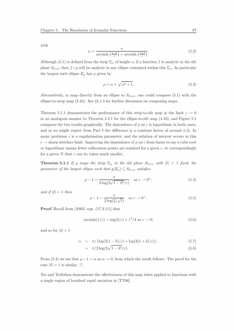
Chapter 5. The Resolution of Irregular Functions 87
with
α =π
arcsinh(
1−δε
)
+ arcsinh(
1+δε
) . (5.2)
Although (5.1) is defined from the strip Σα of height α, if a function f is analytic in the slit
plane Sδ+iε then f g will be analytic in any ellipse contained within this Σα. In particular
the largest such ellipse Eρ has ρ given by
ρ = α +√
α2 + 1. (5.3)
Alternatively, to map directly from an ellipse to Sδ+iε, one could compose (5.1) with the
ellipse-to-strip map (2.16). See §5.1.4 for further discussion on composing maps.
Theorem 5.1.1 demonstrates the performance of this strip-to-slit map in the limit ε → 0
in an analogous manner to Theorem 4.2.1 for the ellipse-to-slit map (4.10), and Figure 5.1
compares the two results graphically. The dependence of ρ on ε is logarithmic in both cases,
and as we might expect from Part I the difference is a constant factor of around π/2. In
many problems ε is a regularisation parameter, and the solution of interest occurs in this
ε→ sharp interface limit. Improving the dependence of ρ on ε from linear to say a cube root
or logarithmic means fewer collocation points are required for a given ε, or correspondingly
for a given N that ε can be taken much smaller.
Theorem 5.1.1 If g maps the strip Σα to the slit plane Sδ+iε with |δ| < 1 fixed, the
parameter of the largest ellipse such that g(Eρ) ⊆ Sδ+iε satisfies
ρ− 1 ∼ π
2 log(2√
1− δ2/ε)as ε→ 0+, (5.4)
and if |δ| = 1 then
ρ− 1 ∼ π
2 log(2/√
ε)as ε→ 0+. (5.5)
Proof Recall from [AS65, eqn. (17.3.11)] that
arcsinh(1/ε) ∼ log(2/ε) + ε2/4 as ε→ 0, (5.6)
and so for |δ| < 1
α ∼ π/ (log(2(1− δ)/ε) + log(2(1 + δ)/ε)) , (5.7)
= π/2 log(2√
1− δ2/ε). (5.8)
From (5.3) we see that ρ− 1 ∼ α as α→ 0, from which the result follows. The proof for the
case |δ| = 1 is similar. 2
Tee and Trefethen demonstrate the effectiveness of this map when applied to functions with
a single region of localised rapid variation in [TT06].
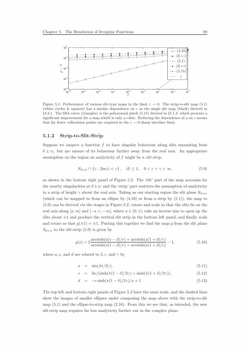
Chapter 5. The Resolution of Irregular Functions 88
10−10
10−9
10−8
10−7
10−6
10−5
10−4
10−3
10−2
10−4
10−3
10−2
10−1
100
ρ−
1
ε
(4.10)
|δ|=1
(5.1)
|δ|=1
(5.15)
ε
Figure 5.1: Performance of various slit-type maps in the limit ε → 0. The strip-to-slit map (5.1)(white circles & squares) has a similar dependence on ε as the single slit map (black) derived in§4.2.1. The fifth curve (triangles) is the polynomial pinch (5.15) derived in §5.1.3, which presents asignificant improvement for a map which is only a cubic. Reducing the dependence of ρ on ε meansthat far fewer collocation points are required in the ε → 0 sharp interface limit.
5.1.2 Strip-to-Slit-Strip
Suppose we suspect a function f to have singular behaviour along slits emanating from
δ ± iε, but are unsure of its behaviour further away from the real axis. An appropriate
assumption on the region on analyticity of f might be a slit-strip,
Sδ+iε ∩ z : |Imz| < γ , |δ| ≤ 1, 0 < ε < γ <∞, (5.9)
as shown in the bottom right panel of Figure 5.2. The ‘slit’ part of the map accounts for
the nearby singularities at δ± iε and the ‘strip’ part restricts the assumption of analyticity
to a strip of height γ about the real axis. Taking as our starting region the slit plane Sδ+iε
(which can be mapped to from an ellipse by (4.10) or from a strip by (5.1)), the map to
(5.9) can be derived via the stages in Figure 5.2: rotate and scale so that the slits lie on the
real axis along [a,∞] and [−a >,−∞], where a ∈ (0, 1); take an inverse sine to open up the
slits about ±1 and produce the vertical slit strip in the bottom left panel; and finally scale
and rotate so that g(±1) = ±1. Putting this together we find the map g from the slit plane
Sd+ie to the slit-strip (5.9) is given by
g(s) = 2arcsinh(a(s− d)/e) + arcsinh(a(1 + d)/e)
arcsinh(a(1− d)/e) + arcsinh(a(1 + d)/e)− 1, (5.10)
where a, e, and d are related to δ, ε, and γ by
a = sin(βπ/2γ), (5.11)
e = 2a/(sinh(π(1 − δ)/2γ) + sinh(π(1 + δ)/2γ)), (5.12)
d = −e sinh(π(1 − δ)/2γ)/a + 1. (5.13)
The top left and bottom right panels of Figure 5.2 have the same scale, and the dashed lines
show the images of smaller ellipses under composing the map above with the strip-to-slit
map (5.1) and the ellipse-to-strip map (2.16). From this we see that, as intended, the new
slit-strip map requires far less analyticity further out in the complex plane.
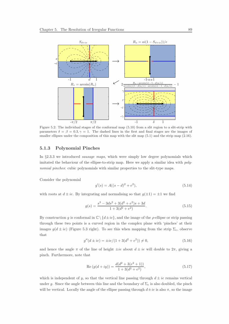
Chapter 5. The Resolution of Irregular Functions 89
-γ
γ
δ
ε
-ε
Sd+ie Ru = ai(1 − Sd+ie))/e
Rv = arcsin(Ru) 2 Rv−arcsin(i(−1−d)a/e)arcsin(i(1−d)a/e)−arcsin(i(−1−d)a/e)
− 1
-π/2 π/2
a-a
-ee
d
1
11
-1
-1-1
→
←
→
Figure 5.2: The individual stages of the conformal map (5.10) from a slit region to a slit-strip withparameters δ = β = 0.3, γ = 1. The dashed lines in the first and final stages are the images ofsmaller ellipses under the composition of this map with the slit map (5.1) and the strip map (2.16).
5.1.3 Polynomial Pinches
In §2.3.3 we introduced sausage maps, which were simply low degree polynomials which
imitated the behaviour of the ellipse-to-strip map. Here we apply a similar idea with poly-
nomial pinches: cubic polynomials with similar properties to the slit-type maps.
Consider the polynomial
g′(s) = A((s− d)2 + e2), (5.14)
with roots at d± ie. By integrating and normalising so that g(±1) = ±1 we find
g(s) =s3 − 3ds2 + 3(d2 + e2)s + 3d
1 + 3(d2 + e2). (5.15)
By construction g is conformal in C\d± ie, and the image of the ρ-ellipse or strip passing
through these two points is a curved region in the complex plane with ‘pinches’ at their
images g(d ± ie) (Figure 5.3 right). To see this when mapping from the strip Σe, observe
that
g′′(d± ie) = ±ie/(1 + 3(d2 + e2)) 6= 0, (5.16)
and hence the angle π of the line of height ±ie about d ± ie will double to 2π, giving a
pinch. Furthermore, note that
Re (g(d + iy)) =d(d2 + 3(e2 + 1))
1 + 3(d2 + e2), (5.17)
which is independent of y, so that the vertical line passing through d± ie remains vertical
under g. Since the angle between this line and the boundary of Σe is also doubled, the pinch
will be vertical. Locally the angle of the ellipse passing through d± ie is also π, so the image
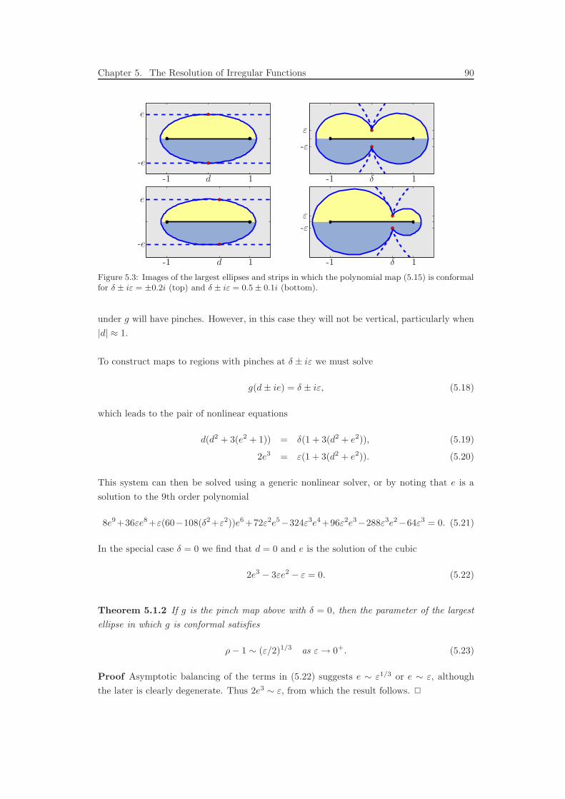
Chapter 5. The Resolution of Irregular Functions 90
δd
ε
-ε
e
-e
11 -1-1
δd
ε
-ε
e
-e
11 -1-1
Figure 5.3: Images of the largest ellipses and strips in which the polynomial map (5.15) is conformalfor δ ± iε = ±0.2i (top) and δ ± iε = 0.5 ± 0.1i (bottom).
under g will have pinches. However, in this case they will not be vertical, particularly when
|d| ≈ 1.
To construct maps to regions with pinches at δ ± iε we must solve
g(d± ie) = δ ± iε, (5.18)
which leads to the pair of nonlinear equations
d(d2 + 3(e2 + 1)) = δ(1 + 3(d2 + e2)), (5.19)
2e3 = ε(1 + 3(d2 + e2)). (5.20)
This system can then be solved using a generic nonlinear solver, or by noting that e is a
solution to the 9th order polynomial
8e9+36εe8+ε(60−108(δ2+ε2))e6 +72ε2e5−324ε3e4+96ε2e3−288ε3e2−64ε3 = 0. (5.21)
In the special case δ = 0 we find that d = 0 and e is the solution of the cubic
2e3 − 3εe2 − ε = 0. (5.22)
Theorem 5.1.2 If g is the pinch map above with δ = 0, then the parameter of the largest
ellipse in which g is conformal satisfies
ρ− 1 ∼ (ε/2)1/3 as ε→ 0+. (5.23)
Proof Asymptotic balancing of the terms in (5.22) suggests e ∼ ε1/3 or e ∼ ε, although
the later is clearly degenerate. Thus 2e3 ∼ ε, from which the result follows. 2
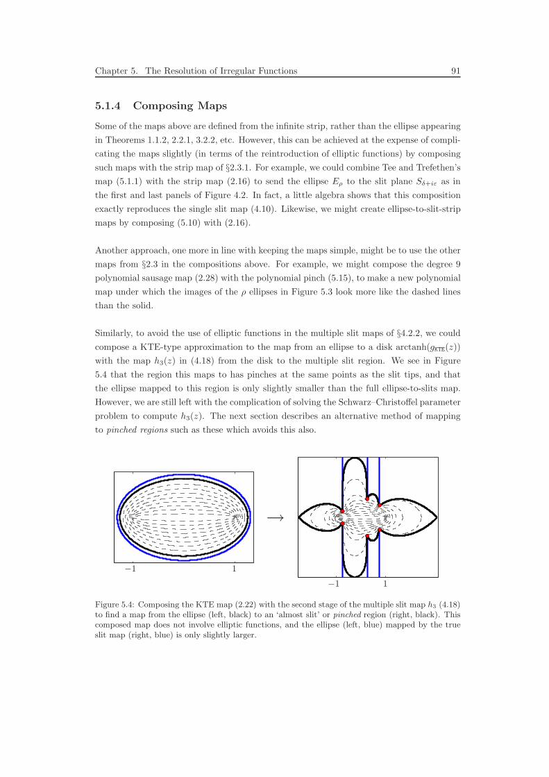
Chapter 5. The Resolution of Irregular Functions 91
5.1.4 Composing Maps
Some of the maps above are defined from the infinite strip, rather than the ellipse appearing
in Theorems 1.1.2, 2.2.1, 3.2.2, etc. However, this can be achieved at the expense of compli-
cating the maps slightly (in terms of the reintroduction of elliptic functions) by composing
such maps with the strip map of §2.3.1. For example, we could combine Tee and Trefethen’s
map (5.1.1) with the strip map (2.16) to send the ellipse Eρ to the slit plane Sδ+iε as in
the first and last panels of Figure 4.2. In fact, a little algebra shows that this composition
exactly reproduces the single slit map (4.10). Likewise, we might create ellipse-to-slit-strip
maps by composing (5.10) with (2.16).
Another approach, one more in line with keeping the maps simple, might be to use the other
maps from §2.3 in the compositions above. For example, we might compose the degree 9
polynomial sausage map (2.28) with the polynomial pinch (5.15), to make a new polynomial
map under which the images of the ρ ellipses in Figure 5.3 look more like the dashed lines
than the solid.
Similarly, to avoid the use of elliptic functions in the multiple slit maps of §4.2.2, we could
compose a KTE-type approximation to the map from an ellipse to a disk arctanh(gKTE(z))
with the map h3(z) in (4.18) from the disk to the multiple slit region. We see in Figure
5.4 that the region this maps to has pinches at the same points as the slit tips, and that
the ellipse mapped to this region is only slightly smaller than the full ellipse-to-slits map.
However, we are still left with the complication of solving the Schwarz–Christoffel parameter
problem to compute h3(z). The next section describes an alternative method of mapping
to pinched regions such as these which avoids this also.
−1
−1
1
1
→
Figure 5.4: Composing the KTE map (2.22) with the second stage of the multiple slit map h3 (4.18)to find a map from the ellipse (left, black) to an ‘almost slit’ or pinched region (right, black). Thiscomposed map does not involve elliptic functions, and the ellipse (left, blue) mapped by the trueslit map (right, blue) is only slightly larger.

Chapter 5. The Resolution of Irregular Functions 92
5.2 Combining Maps: Multiple Pinches
In the previous section we described a number of maps to slit or pinched regions which were
computationally simpler than those in §4, but which unfortunately do not extend directly
to the case of multiple pinches. Here we suggest one approach that can be used to combine
the single slit or pinch maps together to produce maps with such behaviour.
Suppose we have a collection of maps gk(s), k = 1, . . . , n, each with the effect of mapping
an infinite strip of height αk about the real axis to a region with conjugate slits or pinches
with tips at wk = δk ± iεk. We define the multiple pinch map
G(s) = H−1(s), (5.24)
where
H(w) =
n∑
k=1
akg−1k (w),
n∑
k=1
ak = 1, ak > 0. (5.25)
By the conformality of the gk and the inverse function theorem, the g−1k are conformal in
some neighbourhood of [−1, 1] (as the gk must be locally one-to-one in such a region and
are monotonic on the real interval). The positivity of the ak make this the case for H also,
and furthermore the constraint on the sum of the ak ensures that H : [−1, 1] 7→ [−1, 1].
Applying the inverse function to H , we find G : [−1, 1] 7→ [−1, 1] is conformal in at least
some neighbourhood of [−1, 1].
To construct the map from an ellipse Eρ to a multiply pinched region, we choose the ak so
that the preimages of the individual tips lie on the same ellipse. This leads to a constrained
system of n nonlinear equations in n unknowns,
|G−1(wk)±√
[G−1(wk)]2 − 1| = ρ, k = 1, . . . , n− 1, (5.26)
n∑
k=1
ak = 1, ak > 0, (5.27)
where ρ = |G−1(wn)±√
[G−1(wn)]2 − 1| and ± is chosen to make the value greater than 1
in each case. If instead we wish to map from an infinite strip Σα, we choose the ak so that
the preimages of the tips have the same imaginary part by replacing (5.26) with
ImG−1(wk) = α, k = 1, . . . , n− 1, (5.28)
where α = ImG−1(wn). Observe that for both cases, (5.27) is equivalent to
0 <1∑
k=1
ak <2∑
k=1
ak < · · · <n−1∑
k=1
ak < 1, an = 1−n−1∑
k=1
ak, (5.29)
and that these inequality constraints can be removed by change of variables similar to that
used in (4.20) and (4.21). As with the parameter problem of the Schwarz–Christoffel maps,
Chapter 5. The Resolution of Irregular Functions 93
these systems can be solved using a generic nonlinear system solver, such as Matlab’s
fsolve or Kelley’s nsold [Kel03]. In the case of the former, experience suggests that the
Levenberg–Marquardt algorithm is particularly well-suited to this problem.
One drawback to this approach is that the map G(s) is defined in terms of its inverse,
G−1(w) = H(w), and we must invert H numerically. Trefethen [Tre80] suggests using the
solution of the initial value problem
dw
ds= 1/H ′(w), w(−1) = −1, (5.30)
with a relaxed error tolerance as an initial guess for Newton iteration of the nonlinear
equation
H(w) − s = 0. (5.31)
However, we find in our situation (presumably due to the behaviour of [G−1]′) that solving
the ODE (5.30) to sufficient accuracy for the Newton iteration is computationally intensive
– in fact, such an ODE is precisely the kind that might require a conformal map so as to be
solved effectively! Instead we find that applying a trust-region based optimisation routine
to (5.31) directly is effective.
In either case, by choosing s to be a discrete set of Chebyshev points, the solutions w can be
used to form a polynomial interpolant of the forward map G using the barycentric formula.
Of course we could attempt to find a map to determine points which would give a more
efficient interpolant of G, but in practice this is rarely necessary.
Multiple pinch maps can be constructed in chebfun by maps(’mpinch’,dk+1i*ek).
5.2.1 Examples
We now demonstrate the performance of these maps on numerous examples. We choose as
gk the strip-to-slit maps (5.1), and compute maps from ellipses to various multiple pinch re-
gions with the pinch locations taken at random from a uniform distribution on [−1, 1]±i[0, ε]
(where ε differs in each example). In Figures 5.5 and 5.6 the solid black lines depict images
of Eρ under G where ρ is given by (5.26) and red circles show the locations of the pinch tips.
Dashed black lines represent images of smaller ellipses under G, and (where computable)
blue lines show the image of the same ellipse Eρ under the multiple-slit map from §4.2.2.
The titles of the figures show the number of pinch or slit tips, their approximate distance
from the real line, and the size of ellipses resulting from both the multiple pinch and multiple
slit maps. The second of these ellipses will always be the larger as the slit map assumes a
much larger region of analyticity in the complex plane. However, the pinch maps also offer
a significant improvement on the unmapped Chebyshev ellipse, and are much more reliably
computed — particularly when there are many tips, or they are close to the real axis.
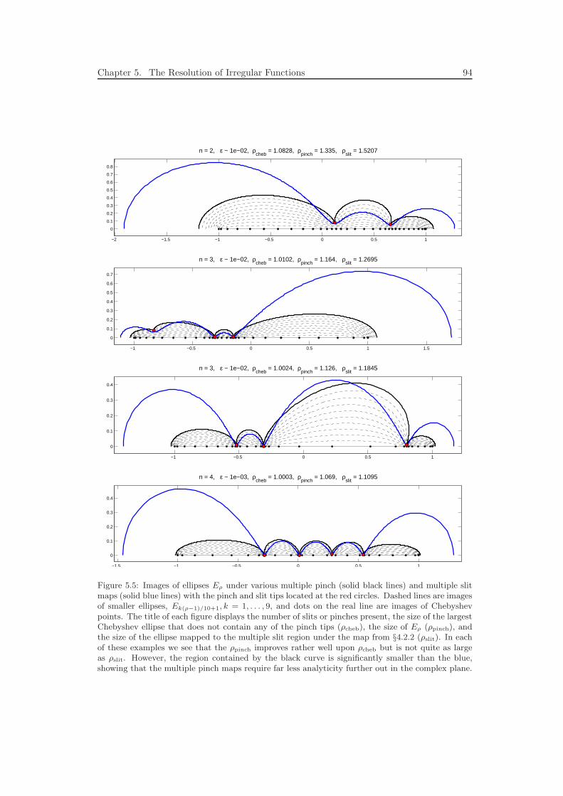
Chapter 5. The Resolution of Irregular Functions 94
−2 −1.5 −1 −0.5 0 0.5 1
0
0.1
0.2
0.3
0.4
0.5
0.6
0.7
0.8
n = 2, ε ~ 1e−02, ρcheb
= 1.0828, ρpinch
= 1.335, ρslit
= 1.5207
−1 −0.5 0 0.5 1 1.5
0
0.1
0.2
0.3
0.4
0.5
0.6
0.7
n = 3, ε ~ 1e−02, ρcheb
= 1.0102, ρpinch
= 1.164, ρslit
= 1.2695
−1 −0.5 0 0.5 1
0
0.1
0.2
0.3
0.4
n = 3, ε ~ 1e−02, ρcheb
= 1.0024, ρpinch
= 1.126, ρslit
= 1.1845
−1.5 −1 −0.5 0 0.5 1
0
0.1
0.2
0.3
0.4
n = 4, ε ~ 1e−03, ρcheb
= 1.0003, ρpinch
= 1.069, ρslit
= 1.1095
Figure 5.5: Images of ellipses Eρ under various multiple pinch (solid black lines) and multiple slitmaps (solid blue lines) with the pinch and slit tips located at the red circles. Dashed lines are imagesof smaller ellipses, Ek(ρ−1)/10+1, k = 1, . . . , 9, and dots on the real line are images of Chebyshevpoints. The title of each figure displays the number of slits or pinches present, the size of the largestChebyshev ellipse that does not contain any of the pinch tips (ρcheb), the size of Eρ (ρpinch), andthe size of the ellipse mapped to the multiple slit region under the map from §4.2.2 (ρslit). In eachof these examples we see that the ρpinch improves rather well upon ρcheb but is not quite as largeas ρslit. However, the region contained by the black curve is significantly smaller than the blue,showing that the multiple pinch maps require far less analyticity further out in the complex plane.

Chapter 5. The Resolution of Irregular Functions 95
−1 −0.8 −0.6 −0.4 −0.2 0 0.2 0.4 0.6 0.8 1
0
0.02
0.04
0.06
0.08
0.1
0.12
n = 4, ε ~ 1e−05, ρcheb
= 1, ρpinch
= 1.043
−1 −0.8 −0.6 −0.4 −0.2 0 0.2 0.4 0.6 0.8 1
0
0.05
0.1
0.15
n = 8, ε ~ 1e−03, ρcheb
= 1.0021, ρpinch
= 1.051, ρslit
= 1.1159
−1 −0.8 −0.6 −0.4 −0.2 0 0.2 0.4 0.6 0.8 1
0
0.02
0.04
0.06
0.08
0.1
n = 10, ε ~ 1e−03, ρcheb
= 1.0016, ρpinch
= 1.043, ρslit
= 1.1233
−1 −0.8 −0.6 −0.4 −0.2 0 0.2 0.4 0.6 0.8 1
0
0.01
0.02
0.03
0.04
n = 20, ε ~ 1e−02, ρcheb
= 1.0009, ρpinch
= 1.025
−1 −0.8 −0.6 −0.4 −0.2 0 0.2 0.4 0.6 0.8 1
0
0.005
0.01
0.015
0.02
0.025
0.03
0.035
0.04
n = 32, ε ~ 1e−02, ρcheb
= 1.0001, ρpinch
= 1.018
Figure 5.6: As in Figure 5.5, but for larger numbers of pinches/slits (4, 8, 10, 20, and 32 respec-tively). In these examples the multiple slit map of §4.2.2 either fails to compute, or as in the middletwo figures, returns a map with slits located incorrectly (as the red circles are contained within theblue line). These figures demonstrate that the multiple pinch maps can be reliably computed evenwhen the imaginary component of the slit tips is as small as 10−5, or when there are as many as32 pinches!
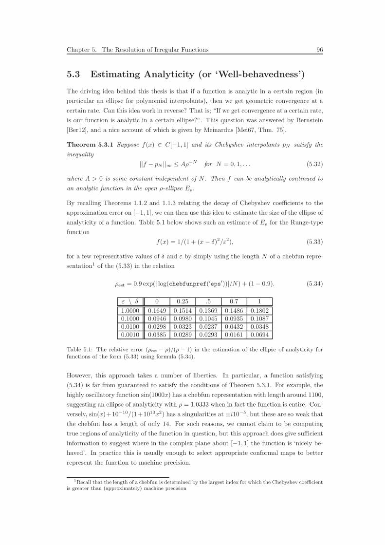
Chapter 5. The Resolution of Irregular Functions 96
5.3 Estimating Analyticity (or ‘Well-behavedness’)
The driving idea behind this thesis is that if a function is analytic in a certain region (in
particular an ellipse for polynomial interpolants), then we get geometric convergence at a
certain rate. Can this idea work in reverse? That is; “If we get convergence at a certain rate,
is our function is analytic in a certain ellipse?”. This question was answered by Bernstein
[Ber12], and a nice account of which is given by Meinardus [Mei67, Thm. 75].
Theorem 5.3.1 Suppose f(x) ∈ C[−1, 1] and its Chebyshev interpolants pN satisfy the
inequality
||f − pN ||∞ ≤ Aρ−N for N = 0, 1, . . . (5.32)
where A > 0 is some constant independent of N . Then f can be analytically continued to
an analytic function in the open ρ-ellipse Eρ.
By recalling Theorems 1.1.2 and 1.1.3 relating the decay of Chebyshev coefficients to the
approximation error on [−1, 1], we can then use this idea to estimate the size of the ellipse of
analyticity of a function. Table 5.1 below shows such an estimate of Eρ for the Runge-type
function
f(x) = 1/(1 + (x − δ)2/ε2), (5.33)
for a few representative values of δ and ε by simply using the length N of a chebfun repre-
sentation1 of the (5.33) in the relation
ρest = 0.9 exp(| log(chebfunpref(′eps′))|/N) + (1− 0.9). (5.34)
ε \ δ 0 0.25 .5 0.7 1
1.0000 0.1649 0.1514 0.1369 0.1486 0.18020.1000 0.0946 0.0980 0.1045 0.0935 0.10870.0100 0.0298 0.0323 0.0237 0.0432 0.03480.0010 0.0385 0.0289 0.0293 0.0161 0.0694
Table 5.1: The relative error (ρest − ρ)/(ρ − 1) in the estimation of the ellipse of analyticity forfunctions of the form (5.33) using formula (5.34).
However, this approach takes a number of liberties. In particular, a function satisfying
(5.34) is far from guaranteed to satisfy the conditions of Theorem 5.3.1. For example, the
highly oscillatory function sin(1000x) has a chebfun representation with length around 1100,
suggesting an ellipse of analyticity with ρ = 1.0333 when in fact the function is entire. Con-
versely, sin(x)+10−10/(1+1010x2) has a singularities at ±i10−5, but these are so weak that
the chebfun has a length of only 14. For such reasons, we cannot claim to be computing
true regions of analyticity of the function in question, but this approach does give sufficient
information to suggest where in the complex plane about [−1, 1] the function is ‘nicely be-
haved’. In practice this is usually enough to select appropriate conformal maps to better
represent the function to machine precision.
1Recall that the length of a chebfun is determined by the largest index for which the Chebyshev coefficientis greater than (approximately) machine precision
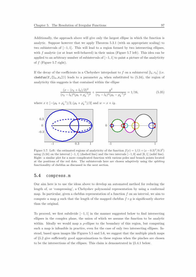
Chapter 5. The Resolution of Irregular Functions 97
Additionally, the approach above will give only the largest ellipse in which the function is
analytic. Suppose however that we apply Theorem 5.3.1 (with an appropriate scaling) to
two subintervals of [−1, 1]. This will lead to a region formed by two intersecting ellipses,
with f analytic (or at least well-behaved) in their union (Figure 5.7 left). This idea can be
applied to an arbitrary number of subintervals of [−1, 1] to paint a picture of the analyticity
of f (Figure 5.7 right).
If the decay of the coefficients in a Chebyshev interpolant to f on a subinterval [lk, rk] (i.e.
chebfun(f,[lk,rk])) leads to a parameter ρk when substituted to (5.34), the region of
analyticity this suggests is that contained within the ellipse
(x − (rk + lk)/2)2
(rk − lk)2(ρk + ρ−1k )2
+y2
(rk − lk)2(ρk − ρ−1k )2
= 1/16, (5.35)
where x ∈ [−(ρk + ρ−1k )/2, (ρk + ρ−1
k )/2] and w = x + iy.
0.3
0.3
-0.3
00
11 -1-1
Figure 5.7: Left: the estimated regions of analyticity of the function f(x) = 1/(1 + (x− 0.3)2/0.32)using (5.34) on the interval [−1, 1] (dashed line) and the two intervals [−1, 0] and [0, 1] (solid line).Right: a similar plot for a more complicated function with various poles and branch points locatedat the positions of the red dots. The subintervals here are chosen adaptively using the splitting
functionality of chebfun as discussed in the next section.
5.4 compress.m
Our aim here is to use the ideas above to develop an automated method for reducing the
length of, or ‘compressing’, a Chebyshev polynomial representation by using a conformal
map. In particular, given a chebfun representation of a function f on an interval, we aim to
compute a map g such that the length of the mapped chebfun f g is significantly shorter
than the original.
To proceed, we first subdivide [−1, 1] in the manner suggested below to find intersecting
ellipses in the complex plane, the union of which we assume the function to be analytic
within. Ideally we would map a ρ-ellipse to the boundary of this region, but computing
such a map is infeasible in practice, even for the case of only two intersecting ellipses. In-
stead, based upon images like Figures 5.5 and 5.6, we suggest that the multiple pinch maps
of §5.2 give sufficiently good approximations to these regions when the pinches are chosen
to be the intersections of the ellipses. This claim is demonstrated in §5.4.1 below.
Chapter 5. The Resolution of Irregular Functions 98
We propose the following algorithm for computing an appropriate map;
1. Subdivide [−1, 1] into appropriate subintervals:
Three methods suggest themselves here. The first is to simply divide [−1, 1] into a
fixed number of equally spaced subintervals, but this is problematic both when ρk is
too large on any subinterval as our method of approximating it becomes inaccurate.
Conversely, when we take too few intervals much of the available analyticity is not
located. A second approach is to recursively bisect [−1, 1] until the length of the
chebfun on each subinterval falls below some designated value (experience suggests
that 56 is a good choice). In this manner intervals and pinches are only introduced
where they are needed, and furthermore the bisection allows the following efficient
procedure for ‘downdating’ the Chebyshev coefficients from one interval to its two
children [Gon10]. Suppose
fN (x) =
N∑
k=0
ckTk(x), x ∈ [−1, 1] (5.36)
and we wish to restrict this to a Chebyshev approximation on [−1, 0] such that
N∑
k=0
c(l)k Tk(x) =
N∑
k=0
ckTk(x− 1
2), (5.37)
or on [0, 1] such thatN∑
k=0
c(r)k Tk(x) =
N∑
k=0
ckTk(x + 1
2). (5.38)
By multiplying both sides of these equations by Tj(x)/√
1− x2 and integrating over
[−1, 1], the orthogonality of the Chebyshev polynomials allows the new coefficients to
be computed by the matrix multiplications
c(l) = M−c, and c(r) = M+c, (5.39)
where c(l) = [c(l)0 , c
(l)1 , . . . , c
(l)N ]T, c(r) = [c
(r)0 , c
(r)1 , . . . , c
(r)N ]T, c = [c0, c2, . . . , cN ]T, and
M±′j,k =
2
π
∫ 1
−1
Tj(x)Tk(x±12 )dx√
1− x2, j, k = 0, . . . , N, (5.40)
(and the prime indicates that the terms with j = 0 are halved). These matrices are
independent of the function fN and can be precomputed or computed on thefly using
the recurrence relations
M±0,k = M±
1,k−1/2±M±0,k−1 −M±
1,k−2),
M±1,k = (2M±
0,k−1 + M±2,k−1)/2±M±
0,k−1 −M±1,k−2,
M±j,k = (M±
j−1,k−1 + M±j+1,k−1)/2±M±
j,k−1 −M±j,k−2, j = 2, . . . , k − 1,
M±k,k = 2−k,

Chapter 5. The Resolution of Irregular Functions 99
for k > 3 and
M−1:3,1:3 =
1 −0.5 −0.25
0.5 −1
0.25
, M+
1:3,1:3 =
1 0.5 −0.25
0.5 1
0.25
. (5.41)
The final alternative for choosing subintervals is the splitting functionality in chebfun
[PPT09, §3]. If no edges are detected (which will be the case if f is analytic in
some neighbourhood of [−1, 1]), the option splitting on within the construction
process will bisect intervals in a similar manner as suggested above when the required
length of the approximation on an interval is greater than some designated value
(again we choose 56). If this piecewise approximation is being computed from a
global one, the coefficients on the new subintervals will be computed by evaluating
the chebfun at Chebyshev points using the barycentric formula, and converting these
point evaluations to coefficients using a Fourier transform. An additional benefit of this
approach is that after the subdivision is completed, chebfun will attempt to ‘merge’
unnecessary subintervals.
2. Estimate the Chebyshev ellipses given by the decay of coefficients on each subinterval
using (5.34).
3. Calculate the intersection of these ellipses:
Having computed the estimated ellipses of analyticity on each subinterval, we deter-
mine the locations of pinches in the map by computing their intersections. To do this,
note that eliminating y2 in (5.35) using two consecutive ellipses leads to the quadratic
αk(βk − 16(x− γk)2) = αk+1(βk+1 − 16(x− γk+1)2), (5.42)
where
αk = (ρk − ρ−1k )2/(ρk + ρ−1
k )2, (5.43)
βk = (rk − lk)2(ρk + ρ−1k )2, (5.44)
γk = (rk + lk)/2. (5.45)
The solution xk to (5.42) is then the real coordinate of an intersection, and the imag-
inary component of wk = xk + iyk can be computed by substituting this to (5.35). In
practice, the fact that (5.34) is an estimate can lead to situations when consecutive
ellipses do not intersect. When this occurs we look either for intersections with the
next nearest neighbour, or simply use the top of the smaller of the two ellipses.

Chapter 5. The Resolution of Irregular Functions 100
4. Compute the map (5.24) from an ellipse or strip to a multiply pinched region, where
the pinches are chosen to be the intersections of the ellipses as computed above2. In
practice, it is often beneficial to include pinches where the left and rightmost ellipses
intersect the real line (although giving the pinch a small imaginary part). This is
particularly useful when singularities lie on the real interval close to [−1, 1], for example
with a function like
f(x) =√
1.000001− x (5.46)
(see Figure 5.12). We also modify the objective function slightly when solving (5.26)
so that pinch locations further from [−1, 1] are given less weight. This is useful in
situations such as when two pinch locations are given with a similar (or even the
same) real part, but the imaginary component of one is far greater than the other.
5.4.1 Examples
The algorithm above has been incorporated into the chebfun system in the code compress.m,
and here we give some examples of its use. For each of the functions f below we compare
length(chebfun(@(x) f(x))) and length(compress(chebfun(@(x) f(x)))). In Figures
5.8-5.13 we plot the ellipses computed by steps 1 and 2 above (left), and the image of their
union under the map G (right). The chosen location of the pinches are shown by green
circles, and when f has singularities with known locations, these are shown as red circles
In most other figures of this type throughout this thesis, we have shown on the left the
ρ-ellipse or strip, and on the right the image under the map g. In this final set of figures
however, we show the ellipse on the right-hand side as the image of interest is that of the
boundary of the union of the ellipses (5.35) under the inverse map G−1 (the coloured solid
lines). For the most part these lines lie outside the ellipse Eρ (solid black), showing that the
image of Eρ under G is usually contained within the region where the function is assumed to
be well-behaved. Discontinuities in the coloured curves on the right occur when consecutive
ellipses on the left do not intersect.
2In practice we reduce the imaginary part of the pinch to be 80% of the intersection, which explains whythe green circles do not lie on the coloured curves in Figures 5.8-5.13.
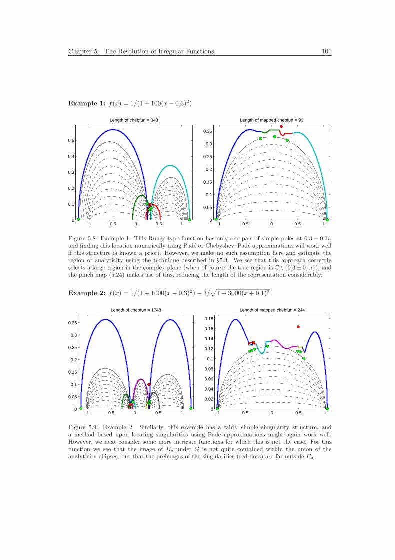
Chapter 5. The Resolution of Irregular Functions 101
Example 1: f(x) = 1/(1 + 100(x− 0.3)2)
−1 −0.5 0 0.5 10
0.1
0.2
0.3
0.4
0.5
Length of chebfun = 343
−1 −0.5 0 0.5 10
0.05
0.1
0.15
0.2
0.25
0.3
0.35
Length of mapped chebfun = 99
Figure 5.8: Example 1. This Runge-type function has only one pair of simple poles at 0.3 ± 0.1i,and finding this location numerically using Pade or Chebyshev–Pade approximations will work wellif this structure is known a priori. However, we make no such assumption here and estimate theregion of analyticity using the technique described in §5.3. We see that this approach correctlyselects a large region in the complex plane (when of course the true region is C \ 0.3 ± 0.1i), andthe pinch map (5.24) makes use of this, reducing the length of the representation considerably.
Example 2: f(x) = 1/(1 + 1000(x− 0.3)2)− 3/√
1 + 3000(x + 0.1)2
−1 −0.5 0 0.5 10
0.05
0.1
0.15
0.2
0.25
0.3
0.35
Length of chebfun = 1748
−1 −0.5 0 0.5 10
0.02
0.04
0.06
0.08
0.1
0.12
0.14
0.16
0.18
Length of mapped chebfun = 244
Figure 5.9: Example 2. Similarly, this example has a fairly simple singularity structure, anda method based upon locating singularities using Pade approximations might again work well.However, we next consider some more intricate functions for which this is not the case. For thisfunction we see that the image of Eρ under G is not quite contained within the union of theanalyticity ellipses, but that the preimages of the singularities (red dots) are far outside Eρ.
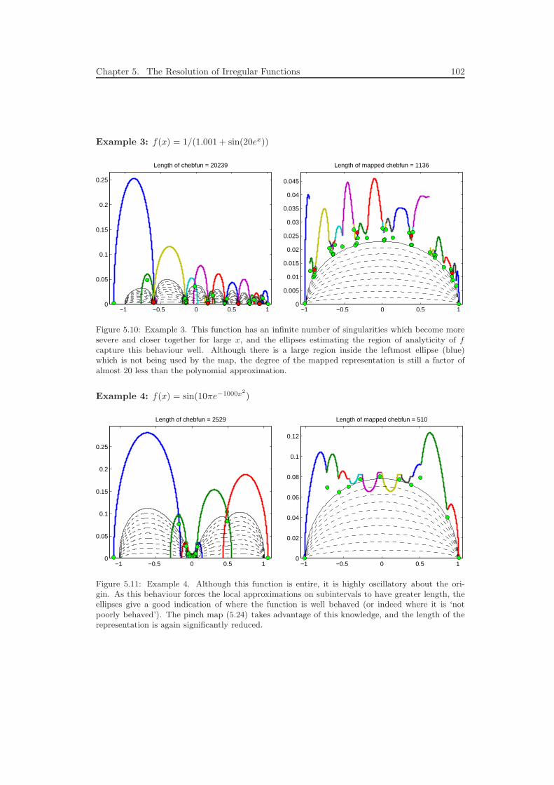
Chapter 5. The Resolution of Irregular Functions 102
Example 3: f(x) = 1/(1.001 + sin(20ex))
−1 −0.5 0 0.5 10
0.05
0.1
0.15
0.2
0.25
Length of chebfun = 20239
−1 −0.5 0 0.5 10
0.005
0.01
0.015
0.02
0.025
0.03
0.035
0.04
0.045
Length of mapped chebfun = 1136
Figure 5.10: Example 3. This function has an infinite number of singularities which become moresevere and closer together for large x, and the ellipses estimating the region of analyticity of fcapture this behaviour well. Although there is a large region inside the leftmost ellipse (blue)which is not being used by the map, the degree of the mapped representation is still a factor ofalmost 20 less than the polynomial approximation.
Example 4: f(x) = sin(10πe−1000x2
)
−1 −0.5 0 0.5 10
0.05
0.1
0.15
0.2
0.25
Length of chebfun = 2529
−1 −0.5 0 0.5 10
0.02
0.04
0.06
0.08
0.1
0.12
Length of mapped chebfun = 510
Figure 5.11: Example 4. Although this function is entire, it is highly oscillatory about the ori-gin. As this behaviour forces the local approximations on subintervals to have greater length, theellipses give a good indication of where the function is well behaved (or indeed where it is ‘notpoorly behaved’). The pinch map (5.24) takes advantage of this knowledge, and the length of therepresentation is again significantly reduced.
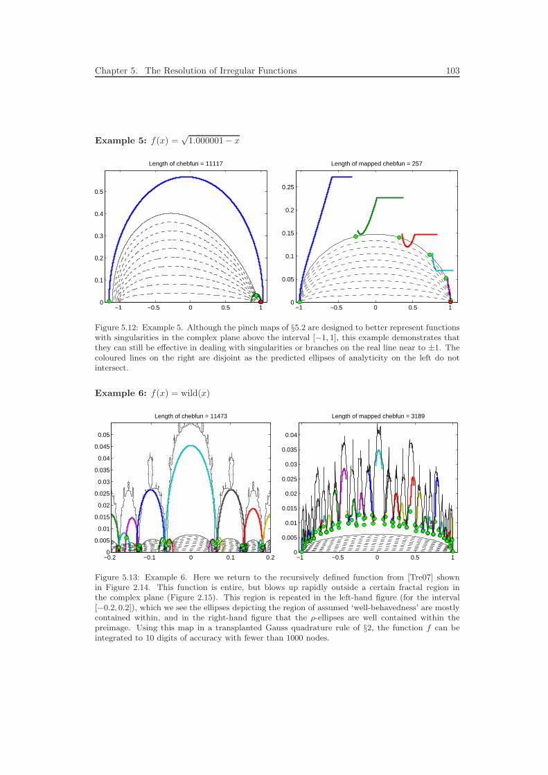
Chapter 5. The Resolution of Irregular Functions 103
Example 5: f(x) =√
1.000001− x
−1 −0.5 0 0.5 10
0.1
0.2
0.3
0.4
0.5
Length of chebfun = 11117
−1 −0.5 0 0.5 10
0.05
0.1
0.15
0.2
0.25
Length of mapped chebfun = 257
Figure 5.12: Example 5. Although the pinch maps of §5.2 are designed to better represent functionswith singularities in the complex plane above the interval [−1, 1], this example demonstrates thatthey can still be effective in dealing with singularities or branches on the real line near to ±1. Thecoloured lines on the right are disjoint as the predicted ellipses of analyticity on the left do notintersect.
Example 6: f(x) = wild(x)
Length of chebfun = 11473
−0.2 −0.1 0 0.1 0.20
0.005
0.01
0.015
0.02
0.025
0.03
0.035
0.04
0.045
0.05
−1 −0.5 0 0.5 10
0.005
0.01
0.015
0.02
0.025
0.03
0.035
0.04
Length of mapped chebfun = 3189
Figure 5.13: Example 6. Here we return to the recursively defined function from [Tre07] shownin Figure 2.14. This function is entire, but blows up rapidly outside a certain fractal region inthe complex plane (Figure 2.15). This region is repeated in the left-hand figure (for the interval[−0.2, 0.2]), which we see the ellipses depicting the region of assumed ‘well-behavedness’ are mostlycontained within, and in the right-hand figure that the ρ-ellipses are well contained within thepreimage. Using this map in a transplanted Gauss quadrature rule of §2, the function f can beintegrated to 10 digits of accuracy with fewer than 1000 nodes.
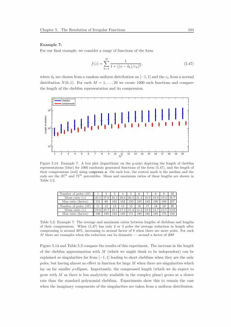
Chapter 5. The Resolution of Irregular Functions 104
Example 7:
For our final example, we consider a range of functions of the form
f(z) =
M∑
k=1
1
1 + ((x− δk)/εk)2, (5.47)
where δk are chosen from a random uniform distribution on [−1, 1] and the εk from a normal
distribution N(0, 1). For each M = 1, . . . , 20 we create 1000 such functions and compare
the length of the chebfun representation and its compression.
1 2 3 4 5 6 7 8 9 10 11 12 13 14 15 16 17 18 19 20
101
102
103
Leng
th o
f che
bfun
chebfuncompressed
M
Figure 5.14: Example 7. A box plot (logarithmic on the y-axis) depicting the length of chebfunrepresentations (blue) for 1000 randomly generated functions of the form (5.47), and the length oftheir compressions (red) using compress.m. On each box, the central mark is the median and theends are the 25th and 75th percentiles. Mean and maximum ratios of these lengths are shown inTable 5.2.
Number of poles (M) 1 2 3 4 5 6 7 8 9 10Mean ratio (%) 45.5 37.0 32.3 28.6 26.3 21.3 18.9 18.9 19.2 16.7
Max ratio (factor) 151 80 162 182 150 193 182 190 189 207
Number of poles (M) 11 12 13 14 15 16 17 18 19 20Mean ratio (%) 19.6 16.7 16.1 17.5 15.4 14.3 13.9 14.7 13.7 13.0
Max ratio (factor) 196 180 183 169 171 180 182 185 175 194
Table 5.2: Example 7: The average and maximum ratios between lengths of chebfuns and lengthsof their compressions. When (5.47) has only 2 or 3 poles the average reduction in length aftercompressing is around 30%, increasing to around factor of 8 when there are more poles. For eachM there are examples when the reduction can be dramatic — around a factor of 200!
Figure 5.14 and Table 5.2 compare the results of this experiment. The increase in the length
of the chebfun approximation with M (which we might think to be independent) can be
explained as singularities far from [−1, 1] leading to short chebfuns when they are the only
poles, but having almost no effect in function for large M when there are singularities which
lay on far smaller ρ-ellipses. Importantly, the compressed length (which we do expect to
grow with M as there is less analyticity available in the complex plane) grows at a slower
rate than the standard polynomial chebfuns. Experiments show this to remain the case
when the imaginary components of the singularities are taken from a uniform distribution.

Chapter 5. The Resolution of Irregular Functions 105
Although the Runge-type functions (5.47) may at first seem quite artificial, by what [Boy01,
§2.6] calls “Darboux’s Principle”, the results will be representative for any functions with
similar singularity structure. It seems that for functions with this behaviour, compress.m
can usually reduce the length of the representation by around a factor of 5−8, but sometimes
— particularly when singularities are very close to [−1, 1] — it can do far better.
5.5 Comments
This chapter introduced maps more elementary than those appearing in §4, but which also
had the effect of mapping to regions which avoided certain areas of the complex plane 5.1. A
method was described in §5.2 for combining these to create ‘multiple pinch’ maps, as well as
an automated process in §5.3 for estimating the region of analyticity (or ‘well-behavedness’)
in the underlying function to determine which such maps to use. These ideas culminated in
the Matlab code compress.m, which was demonstrated to be effective in automatically re-
ducing the number of degrees of freedom needed to represent various near-singular functions.
In some regard the maps of this chapter are less effective than the multiple slit maps of the
previous, as given the assumption of analyticity in a slit region the largest ellipse they map
from is smaller, and convergence rates not so fast. However, a key point in the development
of these maps was not to avoid making any such an assumption, but to map to regions were
analyticity could be infered from the underlying function. Furthermore, it was shown that
computation of these multiple pinches is often more reliable than multiple slits, particularly
when the number of slits (or pinches) is large.
To find the multiple pinch maps, one must first compute their inverse. This involves the
solution of a nonlinear system, but the objective function is inexpensive and the process
fairly speedy. In practice the system need not even be solved to a great deal of accuracy to
produce a useful map, which is not the case for the parameter problems in §4.2.2 and §4.3.2.
Inverting this function to find the forward map can be slightly more labourious, particularly
when pinches close to [−1, 1] make the derivative of G−1 large. This process might however
be sped up by taking advantage of the smoothness of the map, which is not used by the
trust-region based optimisation method.
The Pade approximation technique used to estimate the location of singularities and posi-
tion the maps in the previous chapter is sometimes precarious, requiring assumptions on the
number of singularities to look and a sensible choice for the degree of the numerator. There
is also the danger of so-called ‘spurious poles’ [Sta98]. We introduce an alternative a method,
whereby the region of the complex plane in which a function was suitably well-behaved is
estimated using information from local Chebyshev interpolants. The effectiveness of this
approach was then demonstrated on numerous test functions.
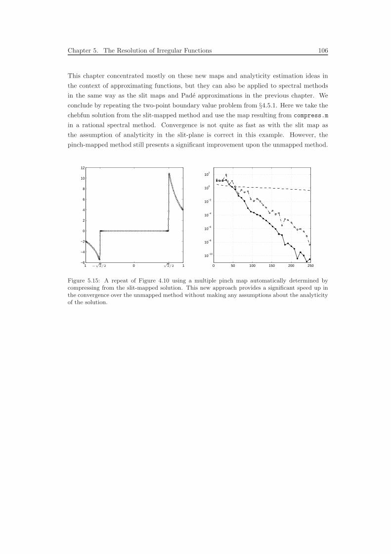
Chapter 5. The Resolution of Irregular Functions 106
This chapter concentrated mostly on these new maps and analyticity estimation ideas in
the context of approximating functions, but they can also be applied to spectral methods
in the same way as the slit maps and Pade approximations in the previous chapter. We
conclude by repeating the two-point boundary value problem from §4.5.1. Here we take the
chebfun solution from the slit-mapped method and use the map resulting from compress.m
in a rational spectral method. Convergence is not quite as fast as with the slit map as
the assumption of analyticity in the slit-plane is correct in this example. However, the
pinch-mapped method still presents a significant improvement upon the unmapped method.
1 0 1−6
−4
−2
0
2
4
6
8
10
12
0 50 100 150 200 250
10−10
10−8
10−6
10−4
10−2
100
102
−√
2/2√
2/2
Figure 5.15: A repeat of Figure 4.10 using a multiple pinch map automatically determined bycompressing from the slit-mapped solution. This new approach provides a significant speed up inthe convergence over the unmapped method without making any assumptions about the analyticityof the solution.

Conclusion
107
Conclusion
The motivation of this thesis has been the observation that whilst polynomial interpolants
and polynomial-based methods may perform well for functions which ‘look’ like polynomials
— which we now know to mean have a large ellipse or strip of analyticity in the complex
plane — they may not always be the best choice of basis.
Rather than build new global interpolants from scratch, we suggested that mapping or
transplanting the polynomials was a sensible approach. In particular, that by considering
regions of analyticity in the underlying functions and using conformal maps to send the
ellipse (or periodic strip) to regions which more closely resemble these, we find interpolants
which do ‘look’ much more like the function we are trying to represent. The conformal map-
ping approach also has other benefits, such as the direct extension of theorems regarding
convergence for analytic functions, and the simple alteration of algorithms to use the new
methods. It is the consideration of analyticity which makes the proposed methods different,
and more effective, than typical change of variable type ideas. A master figure with each of
the conformal maps used in this thesis can be found in Appendix A.
We saw too another way of introducing the maps in interpolants by using the barycentric
formula and linear rational interpolants, and that these had similar properties to the trans-
planted polynomials. Unlike the transplanted methods they do not need the inverse of the
map to evaluate the interpolant, and do not require derivatives of the maps in spectral
methods.
The conformal mapping ideas were applied in two distinct situations. The first in Part I
mapped the ρ-ellipses of Chebyshev and Legendre polynomials to regions with straighter
sides in an attempt to recover more equally spaced grids and the ‘π/2 factor’ that is often
wasted. We refered to these as ‘π/2 maps’ and discussed three examples with this prop-
erty, one of which appears in the literature — the arcsine map introduced by Kosloff and
Tal-Ezer — and two others that were new. The first of these new maps sends the ellipse to
an infinite strip, which is perhaps the most straightforward conceptually (from a conformal
transplantation point of view). It was used in a new type of transplanted quadrature which
was shown to be up to 50% faster than Gauss in §2 for functions analytic in an epsilon-
neighbourhood of [−1, 1].
108
Chapter 5. The Resolution of Irregular Functions 109
Yet as with the arcsine map, the strip requires a choice of parameter and introduces its own
singularity. To avoid this we introduced ‘sausage maps’, which are simply low-order polyno-
mials that prove to be similarly effective in practice. We saw that such maps are well suited
to the kinds of grids that might be used in two- or three-dimensional spectral calculations
for differential equations, and the improvement this has on time-stepping conditions was
demonstrated in §3. It would be of interest to test the performance of the sausage-mapped
method in a large scale computation, in say fluid flow or meteorology.
In Part II we considered a second situation which involved functions with localised regions
of rapid variation indicative of isolated singularities or branch cuts near the computational
interval. We referred to the maps in thesis part of the thesis as ‘adaptive maps’, which were
chosen to wrap around such singularities and make use of analyticity which would otherwise
be wasted. We began in §4 by building on the work of Tee and Trefethen with maps to
multiple slit domains (the entire complex plan minus a finite number of conjugate vertical
slits about the real line). In particular we developed an analytic expression for the integral
in the Schwarz–Christoffel formulation of such maps in periodic domains, allowing the adap-
tive rational spectral method to be extended to periodic problems with multiple regions of
rapid variation. For such problems these methods require far fewer collocation points than
standard Chebyshev or Fourier spectral methods, and result in more accurate solutions with
less computational time. These claims were demonstrated in some challenging test problems.
In the final chapter §5 we considered a new method of constructing maps based upon analyt-
icity estimates extracted from local interpolants. This approach required fewer assumptions
on the underlying functions than the multiple slit maps, and led to an automated process
of reducing the length of interpolants in the chebfun system. Such maps could also be in-
corporated into the adaptive rational spectral method.
The mapped, transplanted, and rational methods, particularly those introduced in Part II,
are still in their early stages of development, and there are a number of interesting directions
in which the research might be taken. For example: the method of estimating analyticity
could be extended to non-polynomial local interpolants; spectral moving mesh methods
could be altered to take analyticity into account in their monitor functions; and ultimately
the ideas could be extended to 2D, and ultimately 3D calculations where the reduced num-
ber of collocation points can make a huge difference to computation times. Ideas like those
underpinning the multiple pinch maps in the final chapter, of combining ‘single’ maps to
produce ‘multiple’ maps, could prove of use in this last situation. Questions regarding how
well mapped-type methods can approximate non-analytic functions or interpolate data on
equally-space nodes might also be addressed.
We close by repeating that whilst the idea of a mapping or a change of variables has been
used many times before, what is demonstrated in this thesis is that (particularly for analytic
functions) it is not enough for a grid to simply ‘look good’; it must correspond to a conformal
map from a large region of analyticity. If it does, you get a fast rate of geometric convergence.

Appendices
110
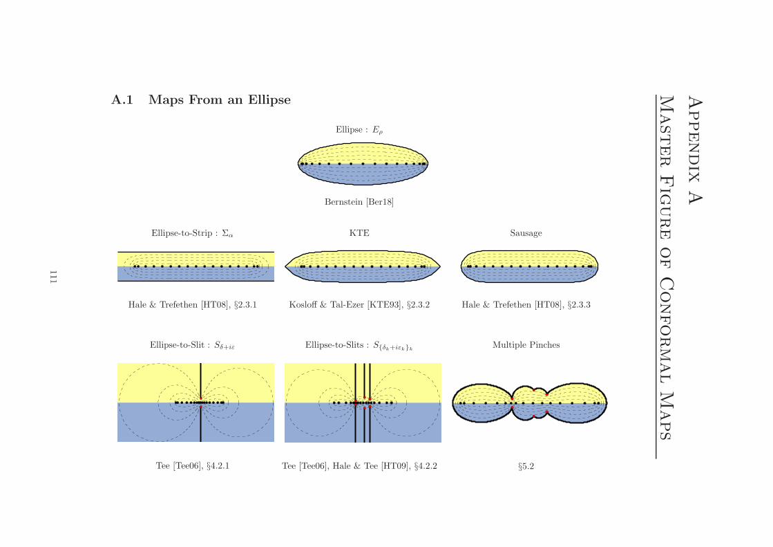
Appendix
A
Master
Fig
ure
of
Conformal
Maps
A.1 Maps From an Ellipse
Ellipse : Eρ
Bernstein [Ber18]
Ellipse-to-Strip : Σα
Hale & Trefethen [HT08], §2.3.1
KTE
Kosloff & Tal-Ezer [KTE93], §2.3.2
Sausage
Hale & Trefethen [HT08], §2.3.3
Ellipse-to-Slit : Sδ+iε
Tee [Tee06], §4.2.1
Ellipse-to-Slits : Sδk+iεkk
Tee [Tee06], Hale & Tee [HT09], §4.2.2
Multiple Pinches
§5.2
111
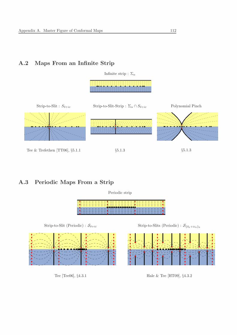
Appendix A. Master Figure of Conformal Maps 112
A.2 Maps From an Infinite Strip
Infinite strip : Σα
Strip-to-Slit : Sδ+iε
Tee & Trefethen [TT06], §5.1.1
Strip-to-Slit-Strip : Σα ∩ Sδ+iε
§5.1.3
Polynomial Pinch
§5.1.3
A.3 Periodic Maps From a Strip
Periodic strip
Strip-to-Slit (Periodic) : Sδ+iε
Tee [Tee06], §4.3.1
Strip-to-Slits (Periodic) : Sδk+iεkk
Hale & Tee [HT09], §4.3.2
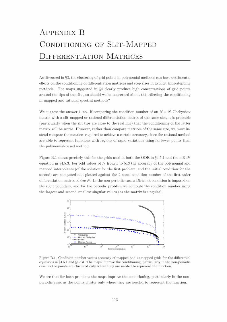
Appendix B
Conditioning of Slit-Mapped
Differentiation Matrices
As discussed in §3, the clustering of grid points in polynomial methods can have detrimental
effects on the conditioning of differentiation matrices and step sizes in explicit time-stepping
methods. The maps suggested in §4 clearly produce high concentrations of grid points
around the tips of the slits, so should we be concerned about this effecting the conditioning
in mapped and rational spectral methods?
We suggest the answer is no. If comparing the condition number of an N ×N Chebyshev
matrix with a slit-mapped or rational differentiation matrix of the same size, it is probable
(particularly when the slit tips are close to the real line) that the conditioning of the latter
matrix will be worse. However, rather than compare matrices of the same size, we must in-
stead compare the matrices required to achieve a certain accuracy, since the rational method
are able to represent functions with regions of rapid variations using far fewer points than
the polynomial-based method.
Figure B.1 shows precisely this for the grids used in both the ODE in §4.5.1 and the mKdV
equation in §4.5.3. For odd values of N from 1 to 513 the accuracy of the polynomial and
mapped interpolants (of the solution for the first problem, and the initial condition for the
second) are computed and plotted against the 2-norm condition number of the first-order
differentiation matrix of size N . In the non-periodic case a Dirichlet condition is imposed on
the right boundary, and for the periodic problem we compute the condition number using
the largest and second smallest singular values (as the matrix is singular).
10−10
10−8
10−6
10−4
10−2
100
102
100
101
102
103
104
105
106
Error in interpolation
2−no
rm c
ondi
tion
num
ber
ChebyshevMapped ChebyshevFourierMapped Fourier
Figure B.1: Condition number versus accuracy of mapped and unmapped grids for the differentialequations in §4.5.1 and §4.5.3. The maps improve the conditioning, particularly in the non-periodiccase, as the points are clustered only where they are needed to represent the function.
We see that for both problems the maps improve the conditioning, particularly in the non-
periodic case, as the points cluster only where they are needed to represent the function.
113
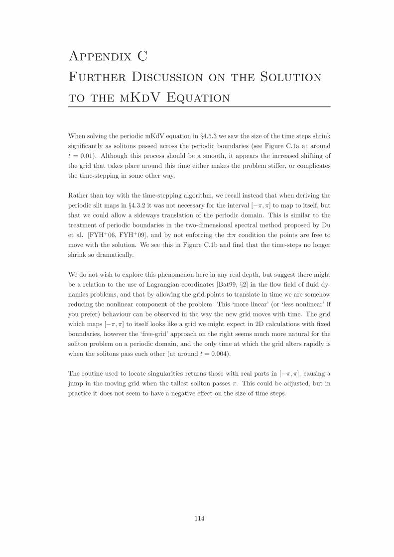
Appendix C
Further Discussion on the Solution
to the mKdV Equation
When solving the periodic mKdV equation in §4.5.3 we saw the size of the time steps shrink
significantly as solitons passed across the periodic boundaries (see Figure C.1a at around
t = 0.01). Although this process should be a smooth, it appears the increased shifting of
the grid that takes place around this time either makes the problem stiffer, or complicates
the time-stepping in some other way.
Rather than toy with the time-stepping algorithm, we recall instead that when deriving the
periodic slit maps in §4.3.2 it was not necessary for the interval [−π, π] to map to itself, but
that we could allow a sideways translation of the periodic domain. This is similar to the
treatment of periodic boundaries in the two-dimensional spectral method proposed by Du
et al. [FYH+06, FYH+09], and by not enforcing the ±π condition the points are free to
move with the solution. We see this in Figure C.1b and find that the time-steps no longer
shrink so dramatically.
We do not wish to explore this phenomenon here in any real depth, but suggest there might
be a relation to the use of Lagrangian coordinates [Bat99, §2] in the flow field of fluid dy-
namics problems, and that by allowing the grid points to translate in time we are somehow
reducing the nonlinear component of the problem. This ‘more linear’ (or ‘less nonlinear’ if
you prefer) behaviour can be observed in the way the new grid moves with time. The grid
which maps [−π, π] to itself looks like a grid we might expect in 2D calculations with fixed
boundaries, however the ‘free-grid’ approach on the right seems much more natural for the
soliton problem on a periodic domain, and the only time at which the grid alters rapidly is
when the solitons pass each other (at around t = 0.004).
The routine used to locate singularities returns those with real parts in [−π, π], causing a
jump in the moving grid when the tallest soliton passes π. This could be adjusted, but in
practice it does not seem to have a negative effect on the size of time steps.
114
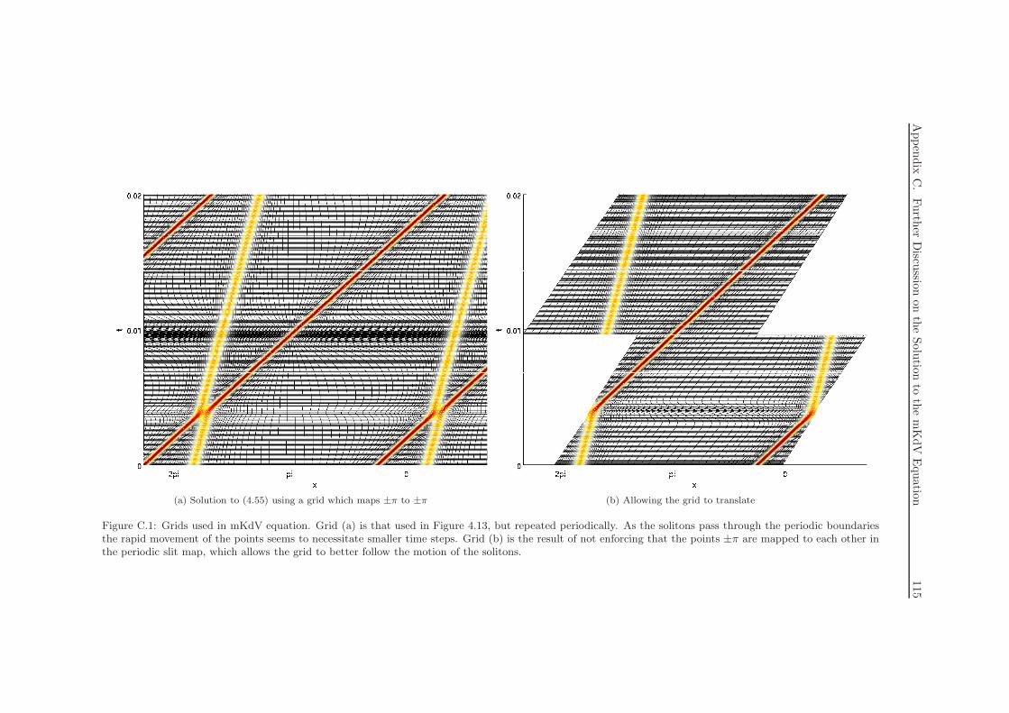
Appen
dix
C.
Furth
erD
iscussio
non
the
Solu
tion
toth
em
KdV
Equatio
n115
(a) Solution to (4.55) using a grid which maps ±π to ±π (b) Allowing the grid to translate
Figure C.1: Grids used in mKdV equation. Grid (a) is that used in Figure 4.13, but repeated periodically. As the solitons pass through the periodic boundariesthe rapid movement of the points seems to necessitate smaller time steps. Grid (b) is the result of not enforcing that the points ±π are mapped to each other inthe periodic slit map, which allows the grid to better follow the motion of the solitons.

References
[Alp99] B. K. Alpert.
Hybrid Gauss-trapezoidal quadrature rules.
SIAM J. Sci. Comput., 20(5):1551–1584, 1999. 30
[ARGA00] M. R. Abril-Raymundo and B. Garcıa-Archilla.
Approximation properties of a mapped Chebyshev method.
Appl. Numer. Math., 32(2):119–136, 2000. 19, 42, 43
[AS65] M. Abramowitz and I. A. Stegun.
Handbook of Mathematical Functions.
New York: Dover, 1965. 15, 16, 27, 63, 66, 68, 87
[Bai78] M. Bain.
On the uniform convergence of generalized Fourier series.
IMA J. Appl. Math., 21:379–386, 1978. 3
[Bak67] N. S. Bakhvalov.
Optimal speed of integration of analytic functions.
U.S.S.R. Comput. Math. Math. Phys., 7:63–75, 1967. 30
[Bal02] R. Baltensperger.
Some results on linear rational trigonometric interpolation.
Comput. Math. Appl., 43:737–746, 2002. 65, 74, 80
[Bat99] G. K. Batchelor.
An introduction to fluid dynamics.
Cambridge University Press, Cambridge, 1999. 114
[BB01a] R. Baltensperger and J.-P. Berrut.
The linear rational collocation method.
J. Comput. Appl. Math., 134(1-2):243–258, 2001. 41, 51
[BB01b] J.-P. Berrut and R. Baltensperger.
The linear rational pseudospectral method for boundary value problems.
BIT, 41(12):868–879, 2001. 47
[BBN99] R. Baltensperger, J.-P. Berrut, and B. Noel.
Exponential convergence of a linear rational interpolant between transformed Chebyshev points.
Math. Comput., 68(227):1109–1120, 1999. 36, 41, 45
[Ber12] S. N. Bernstein.
Sur lordre de la meilleure approximation des fonctions continues par des polynomes de degre
donne.
Mem. Acad. Roy. Belg., 1912. 3, 96
[Ber18] S. N. Bernstein.
Quelques remarques sur l’interpolation.
Journal Mathematische Annalen, 79:1–12, 1918. 12, 111
[Ber88] J.-P. Berrut.
Rational functions for guaranteed and experimentally well-conditioned global interpolation.
Comp. Math. Appl., 15(1):1–16, 1988. 41
116

References 117
[BGM95] A. Bayliss, M. Garbey, and B. J. Matkowsky.
Adaptive pseudo-spectral domain decomposition and the approximation of multiple layers.
J. Comput. Phys., 119(1):132–141, 1995. 83
[BHR09] C. J. Budd, W. Huang, and R. D. Russell.
Adaptivity with moving grids.
Acta Numerica, 18:111–241, 2009. 79, 83
[Boy01] J. P. Boyd.
Chebyshev and Fourier spectral methods.
Dover Publications Inc., Mineola, NY, 2nd edition, 2001. 4, 12, 37, 50, 105
[Boy04] J. P. Boyd.
Prolate spheroidal wavefunctions as an alternative to Chebyshev and Legendre polynomials for
spectral element and pseudospectral algorithms.
J. Comput. Phys., 199(2):688–716, 2004. 30
[BS05] G. Beylkin and K. Sandberg.
Wave propagation using bases for bandlimited functions.
Wave Motion, 41(3):263–291, 2005. 30
[BT92] A. Bayliss and E. Turkel.
Mappings and accuracy for Chebyshev pseudo-spectral approximations.
J. Comput. Phys., 101(2):349–359, 1992. 35
[BT04] J.-P. Berrut and L. N. Trefethen.
Barycentric Lagrange interpolation.
SIAM Review, 46(3):501–517, 2004. 4, 43
[CDS03] B. Costa, W.-S. Don, and A. Simas.
Spectral convergence of mapped Chebyshev methods.
Technical report, Brown University, 2003. 19, 42, 43
[CDS07] B. Costa, W.-S. Don, and A. Simas.
Spatial resolution properties of mapped spectral Chebyshev methods.
In Recent Progress in Scientific Computing; Proceedings of SCPDE05, pages 179–188.
Science Press (Beijing), 2007. 4
[CGH05] Q. Y. Chen, D. Gottlieb, and J. S. Hesthaven.
Spectral methods based on prolate spheroidal wave functions for hyperbolic PDEs.
SIAM J. Numer. Anal., 43(5):1912–1933, 2005. 30, 32
[CHQZ06] C. Canuto, M. Y. Hussaini, A. Quarteroni, and T. A. Zang.
Spectral methods: Fundamentals in single domains.
Springer-Verlag, Berlin, 2006. 35, 37, 50
[CS98] L. Q. Chen and J. Shen.
Applications of semi-implicit Fourier-spectral method to phase field equations.
Comput. Phys. Commun., 108(2-3):147–158, 1998. 83
[Dav59] P. J. Davis.
On the numerical integration of periodic analytic functions.
In On numerical approximation. Proceedings of a Symposium, Madison, April 21-23, 1958,
pages 45–59. The University of Wisconsin Press, Madison, 1959. 2, 12
[Dav75] P. J. Davis.
Interpolation and approximation.
Dover Publications Inc., New York, 1975. (Republication, with minor corrections, of the 1963
original with a new preface and bibliography). 26
[DBT08] T. A. Driscoll, F. Bornemann, and L. N. Trefethen.
The chebop system for automatic solution of differential equations.
BIT, 48(4):701–723, 2008. 7, 8, 74
References 118
[DJ89] P. G. Drazin and R. S. Johnson.
Solitons: an introduction.
Cambridge University Press, Cambridge, 1989. 78
[DLW06] Q. Du, C. Liu, and X. Wang.
Simulating the deformation of vesicle membranes under elastic bending energy in three dimen-
sions.
J. Comput. Phys., 212(2):757–777, 2006. 84
[DR84] P. J. Davis and P. Rabinowitz.
Methods of numerical integration.
Academic Press Inc., Orlando, FL, 2nd edition, 1984. 26
[Dri05] T. A. Driscoll.
Algorithm 843: Improvements to the Schwarz–Christoffel toolbox for MATLAB.
ACM Trans. Math. Softw., 31(2):239–251, 2005. 17, 84
[DS97] W.-S. Don and A. Solomonoff.
Accuracy enhancement for higher derivatives using Chebyshev collocation and a mapping tech-
nique.
SIAM J. Sci. Comput., 18(4):1040–1055, 1997. 19, 40, 41, 43
[DT02] T. A. Driscoll and L. N. Trefethen.
Schwarz–Christoffel Mapping.
Cambridge University Press, Cambridge, UK, 2002. 59, 61, 63, 67
[Fet69] H. E. Fettis.
Note on the computation of Jacobi’s nome and its inverse.
Computing, 4(3):202–206, 1969. 15
[Flo86] J. M. Floryan.
Conformal-mapping-based coordinate generation method for flows in periodic configurations.
J. Comput. Phys., 62(1):221–247, 1986. 67
[FLR93] P. Favati, G. Lotti, and F. Romani.
Bounds on the error of Fejer and Clenshaw-Curtis type quadrature for analytic functions.
Appl. Math. Lett., 6(6):3–8, 1993. 31
[For98] B. Fornberg.
A Practical Guide to Pseudospectral Methods.
Cambridge University Press, October 1998. 35, 37, 51
[FYH+06] W. M. Feng, P. Yu, S. Y. Hu, Z. K. Liu, Q. Du, and L. Q. Chen.
Spectral implementation of an adaptive moving mesh method for phase-field equations.
J. Comput. Phys., 220(1):498–510, 2006. 83, 84, 114
[FYH+09] W. M. Feng, P. Yu, S. Y. Hu, Z. K. Liu, Q. Du, and L. Q. Chen.
A Fourier spectral moving mesh method for the Cahn–Hilliard equation with elasticity.
Commun. Comput. Phys., 5(2–4):582–599, 2009. 83, 84, 114
[GLR07] A. Glaser, Xa Liu, and V. Rokhlin.
A fast algorithm for the calculation of the roots of special functions.
SIAM J. Sci. Comput., 29(4):1420–1438, 2007. 27
[Gon10] P. Gonnet.
Increasing the reliability of adaptive quadrature using explicit interpolants.
ACM T. Math. Software, 37(3), 2010. To appear. 33, 98
[Got01] M. Gotz.
Optimal quadrature for analytic functions.
J. Comput. Appl. Math., 137(1):123–133, 2001. 31
[GP73] G. H. Golub and V. Pereyra.
The differentiation of pseudo-inverses and nonlinear least squares problems whose variables sep-
arate.
SIAM J. Numer. Anal., 10(2):413–432, 1973. 62
References 119
[GP03] G. H. Golub and V. Pereyra.
Separable nonlinear least squares: the variable projection method and its applications.
Inst. Phys., Inverse Problems, 19:1–26, 2003. 62
[HDL99] J. S. Hesthaven, P. G. Dinesen, and J. P. Lynov.
Spectral collocation time-domain modeling of diffractive optical elements.
J. Comput. Phys., 155(2):287–306, 1999. 19
[Hem77] P. W. Hemker.
A numerical study of stiff two-point boundary problems.
Mathematisch Centrum, Amsterdam, 1977. 47
[Hil56] F. B. Hildebrand.
Introduction to numerical analysis.
McGraw-Hill Book Company, Inc., New York-Toronto-London, 1956. 30
[HNW96] E. Hairer, S. P. Norsett, and G. Wanner.
Solving Ordinary Differential Equations II. Stiff and Differential-Algebraic Problems.
Springer, Berlin, Germany, 1996. 73
[HT08] N. Hale and L. N. Trefethen.
New quadrature formulas from conformal maps.
SIAM J. Numer. Anal., 46(2):930–948, 2008. 10, 17, 111
[HT09] N. Hale and T. W. Tee.
Conformal maps to multiply slit domains and applications.
SIAM J. Sci. Comput., 31(4):3195–3215, 2009. 111, 112
[Jor65] C. Jordan.
Calculus of finite differences.
Chelsea Publishing Co., New York, 3rd edition, 1965. 30
[Kel03] C. T. Kelley.
Solving nonlinear equations with Newton’s method.
SIAM, Philadelphia, PA, 2003. 63, 93
[KNB86] H.-O Kreiss, N. K. Nichols, and D. L. Brown.
Numerical methods for stiff two-point boundary value problems.
SIAM J. Numer. Anal., 23(2):325–368, 1986. 75
[Kob57] H. Kober.
Dictionary of conformal representations.
Dover Publications Inc., New York, N. Y. 1957. 15, 65, 67
[KR97] S. Kapur and V. Rokhlin.
High-order corrected trapezoidal quadrature rules for singular functions.
SIAM J. Numer. Anal., 34(4):1331–1356, 1997. 30
[Kry62] V. I. Krylov.
Approximate calculation of integrals.
The Macmillan Co., New York, 1962. 4, 12
[KTE93] D. Kosloff and H. Tal-Ezer.
A modified Chebyshev pseudospectral method with an O(N−1) time step restriction.
J. Comput. Phys., 104(2):457–469, 1993. 18, 19, 35, 36, 39, 42, 50, 111
[KWW85] M. A. Kowalski, A. G. Werschulz, and H. Wozniakowski.
Is Gauss quadrature optimal for analytic functions?
Numer. Math., 47(1):89–98, 1985. 31
[Mar77] A. I. Markushevich.
Theory of functions of a complex variable. Vol. I, II, III.
Chelsea Publishing Co., New York, English edition, 1977. 67
[Mei67] G. Meinardus.
Approximation of functions: Theory and numerical methods.
Springer-Verlag New York, Inc., New York, 1967. 96
References 120
[Mol03] C. Moler.
Matlab central, “Cleve’s Corner”: The MathWorks Logo is an Eigenfunction of the Wave
Equation, 2003. http://tiny.cc/Lshaped. 82
[MR02] J. L. Mead and R. A. Renaut.
Accuracy, resolution, and stability properties of a modified Chebyshev method.
SIAM J. Sci. Comput., 24(1):143–160, 2002. 4, 19, 42, 43, 53
[MRW96] J. Ma, V. Rokhlin, and S. Wandzura.
Generalized Gaussian quadrature rules for systems of arbitrary functions.
SIAM J. Numer. Anal., 33(3):971–996, 1996. 30
[Pet98] K. Petras.
Guassian versus optimal integration of analytic functions.
Constr. Approx., 14(2):231–245, 1998. 31
[Poi27] S.-D. Poisson.
Sur le calcul numerique des integrales definies.
Memoires de L’Academie Royale des Sciences de L’Institut de France, 4:571–602, 1827. 12
[PPT09] R. Pachon, R. B. Platte, and L. N. Trefethen.
Piecewise-smooth chebfuns. IMA J. of Numer. Anal., 2009. 99
[QV99] A. Quarteroni and A. Valli.
Domain decomposition methods for partial differential equations.
Oxford University Press, New York, 1999. Oxford Science Publications. 82
[Rab69] P. Rabinowitz.
Rough and ready error estimates in Gaussian integration of analytic functions.
Commun. ACM, 12(5):268–270, 1969. 12
[RW05] S. C. Reddy and J. A. C. Weideman.
The accuracy of the Chebyshev differencing method for analytic functions.
SIAM J. Numer. Anal., 42(5):2176–2187, 2005. 37
[RWN98] S. C. Reddy, J. A. C. Weideman, and G. F. Norris.
On a modified Chebyshev pseudospectral method.
Technical report, Oregon State University, Corwallis, 1998. 39, 43
[SP61] D. Slepian and H. O. Pollak.
Prolate spheroidal wave functions, Fourier analysis and uncertainty. I.
Bell System Tech. J., 40:43–63, 1961. 30
[ST89] A. Solomonoff and E. Turkel.
Global properties of pseudospectral methods.
J. Comput. Phys., 81(2):239–276, 1989. 50
[Sta98] H. Stahl.
Spurious poles in Pade approximation.
In Proceedings of the VIIIth Symposium on Orthogonal Polynomials and Their Applications
(Seville, 1997), volume 99, pages 511–527, 1998. 105
[SW86] C. Schneider and W. Werner.
Some new aspects of rational interpolation.
Math. Comput., 47(175):285–299, 1986. 41
[SY09] J. Shen and X. Yang.
An efficient moving mesh spectral method for the phase-field model of two-phase flows.
J. Comput. Phys., 228(8):2978–2992, 2009. 83, 84
[Sze50] G. Szego.
Conformal mapping of the interior of an ellipse onto a circle.
Am. Math. Mon., 57(7):474–478, 1950. 15
[Tad86] E. Tadmor.
The exponential accuracy of Fourier and Chebyshev differencing methods.
SIAM J. Numer. Anal., 23(1):1–10, 1986. 37
References 121
[Tee06] T. W. Tee.
An Adaptive Rational Spectral Method for Differential Equations with Rapidly Varying Solu-
tions. D.Phil in Numerical Analysis, University of Oxford, 2006.
http://www.comlab.ox.ac.uk/oucl/research/na/thesis/thesistee.pdf. 2, 6, 36, 41, 42, 45,
58, 61, 62, 65, 72, 74, 77, 83, 84, 111, 112
[TM71] H. Takahasi and M. Mori.
Estimation of errors in the numerical quadrature of analytic functions.
Applicable Anal., 1(3):201–229, 1971. 32
[TPPD08] L. N. Trefethen, R. Pachon, R. B. Platte, and T. A. Driscoll.
chebfun version 2, 2008. http://www.comlab.ox.ac.uk/chebfun/. 2, 3, 7
[Tre80] L. N. Trefethen.
Numerical computation of the Schwarz-Christoffel transformation.
SIAM J. Sci. Statist. Comput., 1(1):82–102, 1980. 93
[Tre00] L. N. Trefethen.
Spectral methods in Matlab.
SIAM, Philadelphia, PA, USA, 2000. 22, 35, 37, 40, 50, 51, 76
[Tre07] L. N. Trefethen.
Computing numerically with functions instead of numbers.
In SNC ’07: Proceedings of the 2007 international workshop on Symbolic-numeric computation,
pages 28–28, New York, NY, USA, 2007. ACM. 29, 32, 103
[Tre08] L. N. Trefethen.
Is Gauss quadrature better than Clenshaw-Curtis?
SIAM Review, 50(1):67–87, 2008. 12, 26, 27
[TT87] L. N. Trefethen and M. R. Trummer.
An instability phenomenon in spectral methods.
SIAM J. Numer. Anal., 24(5):1008–1023, 1987. 50
[TT06] T. W. Tee and L. N. Trefethen.
A rational spectral collocation method with adaptively transformed Chebyshev grid points.
SIAM J. Sci. Comput., 28(5):1798–1811, 2006. 6, 36, 37, 58, 63, 72, 75, 80, 83, 86, 87, 112
[TWS06] L. N. Trefethen, J. A. C. Weideman, and T. Schmelzer.
Talbot quadratures and rational approximations.
BIT, 46(3):653–670, 2006. 32
[Van90] H. Vandeven.
On the eigenvalues of second-order spectral differentiation operators.
Comput. Methods Appl. M., 80(1-3):313–318, 1990. 50
[Wat80] G. A. Watson.
Approximation theory and numerical methods.
John Wiley & Sons Ltd., Chichester, 1980. 4
[Wel97] B. D. Welfert.
Generation of pseudospectral differentiation matrices I.
SIAM J. Numer. Anal., 34(4):1640–1657, 1997. 40, 41
[WR00] J. A. C. Weideman and S. C. Reddy.
A Matlab differentiation matrix suite.
ACM Trans. Math. Software, 26(4):465–519, 2000. 40
[WT88] J. A. C. Weideman and L. N. Trefethen.
The eigenvalues of second-order spectral differentiation matrices.
SIAM J. Numer. Anal., 25(6):1279–1298, 1988. 50, 52
[WT07] J. A. C. Weideman and L. N. Trefethen.
The kink phenomenon in Fejer and Clenshaw–Curtis quadrature.
Numer. Math., 107(4):707–727, 2007. 26, 27

References 122
[XRY01] H. Xiao, V. Rokhlin, and N. Yarvin.
Prolate spheroidal wavefunctions, quadrature and interpolation.
Inverse Problems, 17(4):805–838, 2001. 30
[XZ92] J. Xu and J. Zou.
Iterative methods by space decomposition and subspace correction.
SIAM Review, 34(4):581–613, 1992. 82
[ZK04] P. A. Zegeling and H. P. Kok.
Adaptive moving mesh computations for reaction-diffusion systems.
J. Comput. Appl. Math., 168(1-2):519–528, 2004. 79