Munich Personal RePEc Archive

Exchange Rate and External Trade

Flows: Empirical Evidence of J-Curve

Effect in Ghana

Kwame Akosah, Nana and Omane-Adjepong, Maurice

University of the Witwatersrand Bank of Ghana, University of the

Witwatersrand

March 2017

Online at https://mpra.ub.uni-muenchen.de/86640/

MPRA Paper No. 86640, posted 11 May 2018 13:25 UTC

1 | P a g e

Exchange Rate and External Trade Flows: Empirical Evidence

of J-Curve Effect in Ghana

NANA KWAME AKOSAH*a & b AND MAURICE OMANE-ADJEPONG a

a Wits Business School, University of the Witwatersrand, 2 St David's Place, Parktown, Wits 2050,

Johannesburg, South Africa

b Research Department, Bank of Ghana, Box 2674, Accra, Ghana

*Corresponding author’s emails: akosahk@gmail.com; 1770303@students.wits.ac.za;

nana.akosah@bog.gov.gh

Abstract Ghana’s external trade has remained in perpetual deficits over the three decades alongside depreciating domestic currency. This paper therefore examines the effect of real exchange rate (RER) movements on

Ghana’s external trade performance, using a battery of times series models. The study particularly

assesses the validity of Marshall-Lerner Condition, the J-Curve and Kulkarni Hypotheses in the case of

Ghana. The empirical analysis reveals inelastic responses of both export and import demand to changes

in RER. We found a steady long run link between RER movements and Ghana’s trade balance. However,

the impact of RER on Ghana’s trade balance was found to be asymmetric. Periods of minimal real

depreciation (a “tranquil” regime) lend support to Marshall-Lerner Condition (MLC), the J-Curve

theory and Kulkarni Hypothesis in the context of Ghana. In contrast, we found less visible evidence of J-

curve for periods of excessive real depreciation (an “intemperate” regime). It is therefore critical to

sustain macroeconomic stability in order to engender low and stable inflation and stable foreign

exchange rates. This however requires the adoption of appropriate and coordinated monetary and fiscal

policies.

JEL Classification: F13, F14, F31

Key Words: J-Curve Hypothesis; Kulkarni Hypothesis; Marshall-Lerner Condition; Trade Balance.

2 | P a g e

1 Introduction

The concern of exchange rate risk is omnipresent in international economics. This is well appreciated

and typified by the relentless discussions about the level and scope of its detrimental effects. Basically,

the inclination for exchange rates to move so quickly and by substantial amounts has been accused of

restraining the gains from international trade and hence, decreasing welfare (Straub and Tchakarov,

2004). A large body of theoretical and empirical literature since 1973 has explored the relationship

between exchange rate fluctuation and international trade flows. The universal conjecture is that currency

depreciation causes imports to be more expensive, while exports become cheaper due the change in

relative prices. The Marshall–Lerner condition (MLC, after Alfred Marshall and Abba P. Lerner)

provides the theoretical link between trade balance and real exchange rate movements. This refers to the

condition that an exchange rate depreciation (or devaluation) will only cause an improvement in trade

balance if the absolute sum of the long-term export and import demand elasticities is greater than one.

However, it has been found that trade in goods tends to be inelastic in the short term, as it takes time to

change consuming patterns and trade contracts (Bahmani-Oskooee and Ratha, 2004). Consequently, the

MLC is not met initially, and hence, currency devaluation is possible to worsen the trade balance in the

short run. But, as consumers adjust to the new prices in the long term, trade balance is expected to

improve. This dynamic link between trade balance and real exchange rate is famously christened as the

J-curve effect. Nevertheless, both theoretical models and empirical studies on J-curve effect have not

yielded a conclusive answer (Baum and Caglayan, 2006).

The debate has further been rekindled by the recent pace of globalisation which has affected the

sensitivity of the trade balance to real exchange rates (RER). On the one hand, the growth in intra-

industry trade (henceforth IIT) makes the trade balance more sensitive to real exchange rate movements.

On the other hand, a higher degree of vertical specialisation and more global supply chains act to reduce

the sensitivity of trade balance to real exchange rate movement. This is because vertical specialization

and global supply chain enhance the complementarity between imports and exports. But the relative

weight of these two effects varies across countries due to different degree of substitutability between the

types of goods imported and exported. For instance, countries with low level of IIT1 are expected to have

higher sensitivity of the trade balance to movements in real exchange rates than those with high IIT. On

the contrary, imports tend to plummet significantly in a high IIT country that depreciates its real exchange

rate, as these countries can more easily provide domestic substitutes for imports that have become more

expensive. Consequently, the literature posits that the sensitivity of the trade balance to the real exchange

rate should depend positively on IIT.

The exchange rate regime in Ghana shifted from fixed to a floating regime, following the financial

liberalization exercise after 1983 under the Economic Recovery (ERP) and Structural Adjustment

Programs (SAP) engineered by the International Monetary Fund (IMF) and World Bank (WB). Since

then, exchange rate fluctuations have become an important macroeconomic variable that influences the

1 Low IIT countries are typically those where raw materials or natural resources (like crude oil) constitute a major share of

imports. They could also be countries that have specialised in particular industries in order to benefit from a comparative

advantage in some sectors. Therefore, it is unlikely for the imports of low IIT countries to fall significantly following RER

depreciation, since the domestic industry cannot easily replace the imports that have become more expensive.

3 | P a g e

whole economy and thereby attracted keen attention of researchers. Over the past three decades, the

Ghanaian economy is epitomised by persistent trade imbalances alongside pervasive exchange rate

depreciation. At the same time, the domestic currency has remained among the weakest currencies in the

world. These developments have led to a renewed interest in better understanding the effect of exchange

rates on external trade in Ghana. In spite of the increasing number of studies on the topic, the actual effect

of exchange rates on Ghana’s external trade is still an open and controversial question.

The main purpose of this study is to empirically examine whether exchange rate really matters for

Ghana’s international trade. In other words, this paper investigates the degree of sensitivity of Ghana’s trade balance to movements in real exchange rate. Specifically, we attempt to address the following

fundamental policy questions: Is there significant link between real exchange rate and trade balance in

Ghana? Does real exchange rate depreciation have symmetric effect on Ghana’s trade balance? Is there

evidence of J-Curve in the case of Ghana? What are the relative elasticities of export and import in both

the short run and long run? Empirical responses to the above questions are deemed germane as the

literature on Ghana remains woefully inadequate.

This paper thus proffers substantial contribution to the literature regarding the relationship between

exchange rates and international trade in the context of frontier markets, such as Ghana. Specifically, it

offers information as to whether policy maker should be concerned about the persistent exchange rate

depreciation alongside continuous trade deficits. It also examines potential threshold and asymmetric

effects which are woefully neglected in the extant literature. In addition, the current study uses the most

recent real effective exchange rate for Ghana and its 18 major trading partners. Therefore, the study

proffers policy makers with up-to-date empirical results for consideration and application in decision-

making processes.

The rest of the paper is structured as follows: Section 2 briefly provides a brief literature on J-Curve

Hypothesis; Section 3 discusses the data and methodology; Section 4 presents the empirical results and

inferences while Section 5 concludes the study and give policy recommendations.

2 Review of Relevant Literature

2.1 Conceptual Literature

Theoretically, RER depreciation is expected to stimulate export demand and lower imports, thereby

improving the trade balance. In contrast, RER appreciation is expected to reduce exports demand and

increase the demand for imports, and hence, worsening the trade balance. However, the effects of RER

changes on the trade balance can be unpredictable at times and can contradict economic theory.

According to Magee (1973), the contradiction lies in the theory of the ‘J-curve effect’. This theory suggests that there is a lag period before imports and exports could respond to particular changes arising

from the foreign exchange rate market.

Another economic concept that explains the relationship between the exchange rate and the trade balance

is the Marshall–Lerner condition (MLC). The MLC posits that an increase in exchange rate can only lead

to a trade surplus if the sum of price elasticities of demand for exports by the rest of the world and demand

4 | P a g e

for imports by domestic residents exceed one. However, the MLC is not met initially as it takes time for

consumers and producers to adjust to new developments. Therefore, the trade balance is expected worsen

in the short run following currency depreciation but improve in the long run. Junz and Rhomberg (1973)

theoretically attributed the initial decline in trade balance following currency devaluation to five lags,

namely,

1. Lag in recognition of the new currency conditions by producers and consumers.

2. Lag in the decision by producers and consumers to change

3. Lag in delivery time

4. Lag in the replacement of inventory and material on the part of producers

5. Lag in production due to the production cycle

In sync, Krueger (1983) argued that the J-curve occurs because at the time an exchange rate change

occurs, goods already in transit and under contract have been purchased, causing a lag time in the effect

of exchange rate adjustment. Therefore, once transactions that had already been in progress prior to the

rate adjustment are concluded, subsequent commercial activity reflects the new competition

environment, allowing the trade balance to begin to improve. Specifically, he identified three conditions

that determine the extent to which there is a J-curve:

1. The extent to which trade takes place under pre-existing contrast (as contrasted with purchases

made in spot markets)

2. The degree to which there may be asymmetric use of domestic currency and foreign currency in

the making of contract

3. Length of the lag in the execution of contracts.

2.2 Empirical Literature

Although there is voluminous empirical literature on the effect of real exchange rate fluctuations on

trade balance (J-curve hypothesis), the evidence on Ghana remains shallow. Bahmani-Oskooee and

Ratha (2004a) provides a very comprehensive survey on the J-curve literature for the period 1973-2004

for thirty seven articles. Many other researchers have found support for the J-curve phenomenon, among

them are; Rose (1990); Bahmani-Oskooee and Alse (1994), Kulkarni (1996); Hacker and Hatemi-J

(2003), and Narayan and Narayan (2004). For instance, Rose (1990) examined the relationship between

currency depreciation and trade balance for 30 developing countries for the period 1970-1988. Rose

used statistical analysis to determine whether exchange rate has statistically significant effect of trade

balance at the 5% alpha level. He found that the null hypothesis cannot be rejected for 28 out of 30

countries. Particularly, Kulkarni (1996) expanded the J-Curve hypothesis by demonstrating the

likelihood of “dynamic and persistent BOT deficits” on the account of series of currency devaluations (or depreciations). This phenomenon is dubbed the Kulkarni Hypothesis, largely accounting for the real

world possibility that currencies may be devalued multiples times over a relatively short time period. In

contrast, the survey also showed that studies such as Bahmani-Oskooee and Ratha (2004); Bahmani-

Oskooee and Goswami (2004); and Rose and Yellen (1989) found no empirical evidence to supports the

J-curve phenomenon. For instance, Bahmani-Oskooee and Ratha (2004) did not detect a J-curve

phenomenon in the short-run but they did find a favorable long-run effect on the trade balance.

5 | P a g e

The J-curve phenomenon has also been tested on industry basis. More recent notable studies of the J-

Curve phenomenon include Kulkarni and Clarke (2009), Bahmani-Oskooee and Hajilee (2009); Hsing

(2008), Halicioglu (2008), Ardalani and Bahmani-Oskooee (2007); Bahmani-Oskooee et al (2006). For

instance, Ardalani et al (2007) found the long-run effect of RER depreciation on the trade balance

although with no evidence for a J-curve, while Bahmani-Oskooee et al (2009) and Halicioglu (2008)

found evidence for a J-curve. This attests to the fact that the empirical findings on J-curve hypothesis

remain fairly ambiguous.

Previous research has tested the phenomenon for many developed and developing countries. However,

African nations have not received much attention on this regard. Notable studies in Africa include

Ziramba and Chifamba (2014), Chiloane, Pretorius and Botha (2014), Bahmani-Oskooee and Gelan

(2012), Bahmani-Oskooee and Hosny (2012), Riti (2012), Adeniyi, Omisakin, and Oyinlola (2011),

Kulkarni et al (2009). For instance, Ziramba et al (2014) assessed the behaviour of South Africa’s trade balance following a depreciation of the real effective exchange rate using aggregate trade data for the

period 1975 to 2011. Their empirical results found no evidence in support of the J-curve phenomenon

for the sample. Also, Bahmani-Oskooee and Gelan (2012) tested the J-curve hypothesis for nine African

countries including Burundi, Egypt, Kenya, Mauritius, Morocco, Nigeria, Sierra Leone, South Africa,

and Tanzania using quarterly trade data and bounds testing approach to cointegration and error-correction

modelling. They were unable to find any support for the J-Curve.

Recent notable studies on Ghana include Anning, Riti and Yapatake (2015), Adeniyi, Omisakin, and

Oyinlola, (2011), Bhattarai and Armah (2005), Agbola (2004). However, the empirical result is mixed.

For instance, Anning et al (2015) and Bhattarai et al (2005) found evidence in support of J-curve theory,

while Adeniyi et al (2011) found no evidence of J-curve for Ghana. However, the common feature of

these studies is that they failed to account for potential non-linear relationship between RER and trade

balance in Ghana and this is the focus of the current study.

3. Data and Methodology

The trade balance model employed in this study adapted the form of Rose and Yellen (1989). However,

this paper focuses on possible non-linear link between real effective exchange rate and trade balance in

Ghana. As a result, we specify the long run (cointegrating) equations for trade balance using a threshold

ARDL model. In particular, assuming the indicator function 1(.) which takes the value of 1 if the

expression is true and 0 otherwise, and defining 1𝑗(𝑞𝑡,𝛾) =1(𝛾𝑗 ≤ 𝑞𝑡 < 𝛾𝑗+1), we can combine the j+1

individual regime specifications into a single log-log long run equation as; 𝑙𝑛𝑇𝐵𝑡 = 𝛿0 + 𝛿1𝑙𝑛𝐺𝐼𝑃𝑡∗ + 𝛿2𝑙𝑛𝑌𝐺𝑡 + ∑ 1𝑗(𝑞𝑡,𝛾) ∗𝑚𝑗=0 𝜌𝑗(𝑙𝑛𝑅𝐸𝐸𝑅𝐷𝐸𝑃𝑡) + 𝜀𝑡, (1) 𝑓𝑜𝑟 𝛾𝑗 ≤ 𝑞𝑡 < 𝛾𝑗+1

where 𝑞𝑡 is the observable threshold variable which is real effective exchange rate in this study; γ is the threshold value of real effective exchange rate; j = 0, 1, 2,…m regimes; 𝜌𝑗 is the threshold coefficient of

real effective exchange rate at regime j; 𝑙𝑛 is the natural logarithm transformation and 𝜀𝑡 is the random

6 | P a g e

error term. So we are in regime j if and only if the value of the threshold variable is at least as large as the

j-th threshold value, but not as large as the (j+1)-th threshold.

We apply nonlinear least square to estimate the parameters of the model using the following sum of

squares objective function;

𝑆(𝜌, 𝛿, 𝛾) = ∑ (𝑙𝑛𝑇𝐵𝑡 − 𝛿0 − 𝛿1𝑙𝑛𝐺𝐼𝑃𝑡∗ − 𝛿2𝑙𝑛𝑌𝐺𝑡 − ∑ 1𝑗(𝑞𝑡,𝛾) ∗𝑚𝑗=0 𝜌𝑗(𝑙𝑛𝑅𝐸𝐸𝑅𝐷𝐸𝑃𝑡))2𝑇

𝑡=1 , (2)

Therefore, we obtain the threshold regression estimates by minimizing 𝑆(𝜌, 𝛿, 𝛾) with respect to the

parameters.

According to the J-Curve phenomenon, it is expected that 𝜌𝑗 < 0 since an increase in real effective rate

initially reduces the demand for the home country’s exports and increases its demand for import. As a result, the balance of trade worsens initially but it will improve after a while as export and import volumes

adjust to price changes. While there are no apriori expectations about the signs of 𝛿1 and 𝛿2, however,

one asserts tentatively that 𝛿1 is negative and 𝛿2 is positive.

An augmented ARDL representation of equation (1) is formulated as follows: ∆𝑙𝑛𝑇𝐵𝑡 = 𝛿0 + ∑ 𝛿1𝑖𝑛𝑖=0 ∆𝑙𝑛𝑇𝐵𝑡−𝑖 + ∑ 𝛿2𝑖∆𝑙𝑛𝐺𝐼𝑃𝑡−𝑖∗𝑛

𝑖=0 + ∑ 𝛿3𝑖∆𝑌𝐺𝑡−𝑖𝑛𝑖=0 + ∑ 𝛿4𝑖∆(𝜓𝑅𝑒𝑔𝑖𝑚𝑒𝑙𝑛𝑅𝐸𝐸𝑅𝐷𝐸𝑃𝑡−𝑖𝑛

𝑖=0 )+ 𝜔1𝑙𝑛𝑇𝐵𝑡−1 + 𝜔2𝑙𝑛𝐺𝐼𝑃𝑡−1∗ + 𝜔3𝑌𝐺𝑡−1 + 𝜔4(𝜓𝑅𝑒𝑔𝑖𝑚𝑒𝑙𝑛𝑅𝐸𝐸𝑅𝐷𝐸𝑃𝑡−1)+ 𝑣𝑡 , (3)

where 𝜓𝑅𝑒𝑔𝑖𝑚𝑒 = ∑ 1𝑗(𝑞𝑡,𝛾) ∗𝑚𝑗=0 𝜌𝑗 and 𝑚 is the maximum number of regimes identified.

The bounds testing procedure is based on the F-, or Wald-statistics and is the stage of the ARDL

cointegration method. Accordingly, a joint significance test that implies no cointegration, (H0:𝜔1 = 𝜔2 = 𝜔3 = 𝜔4 = 0), should be performed for equation (3). The F-test used for this procedure has a non-standard

distribution. Pesaran et al (2001) computed two sets of critical values for a given significance level. One

set assumes that all variables are I(0) and the other set assumes they are all I(1). If the computed F-

statistic exceeds the upper critical bounds value, then the H0 is rejected, implying an existence of

cointegration. If the F-statistic falls into the bounds then the test becomes inconclusive. Lastly, if the F-

statistic is below the lower critical bounds value, it implies no cointegration.

Once a long run relationship has been established, equation (3) is estimated using an appropriate lag

selection criterion. At the second stage of the ARDL cointegration procedure, it is also important to

perform other diagnostic tests (including parameter stability test) for the selected ARDL representation

of the error correction model.

A general error correction model (ECM) of equation (3) is formulated as follows:

7 | P a g e

∆lnTBt = ϕ0 + ∑ ϕ1ini=0 ∆lnTBt−i + ∑ ϕ2i∆lnGIPt−i∗n

i=0 + ∑ ϕ3i∆YGt−ini=0

+ ∑ ϕ4i∆(𝜓𝑅𝑒𝑔𝑖𝑚𝑒lnREERDEPt−i)ni=0 + ΩECMt−1 + µt, (4)

where Ω is the speed of adjustment parameter and ECM is the residuals that are obtained from the

estimated cointegration model of equation (3).

To ascertain the robustness of the identified unique regime change from equation (1) and the respective

impact on trade balance based on equations (3) and (4), we proceed to determine the transition probability

of moving from one regime (state) to another as well as the duration of being in a particular regime. This

is carried out using first-order Markov Regime Switching Model (MRSM) with the assumption that the

regimes are unobserved2. The switching model assumes that there is a different regression model

associated with each regime. In particular, we specified two state MRSM in which trade balance is subject

to regime switching and the probability regressor is real effective exchange rate (LREER). That is,

LREER follows a regime-variant process. The first-order Markov assumption requires that the

probability of being in a regime depends on the information at the previous state, expressed as: 𝑝𝑖𝑗(𝑡) = 𝑝(𝑠𝑡 = 𝑗|𝑠𝑡−1 = 𝑖) (5)

with the transition matrix of: 𝑝(𝑡) = [𝑝𝑖,𝑖(𝑡) 𝑝𝑖,𝑗(𝑡)𝑝𝑗,𝑖(𝑡) 𝑝𝑗,𝑗(𝑡)] (6)

where 𝑖𝑗-th element represents the probability of transitioning from regime 𝑖 in period 𝑡 − 1 to regime 𝑗

in period 𝑡; 𝑠𝑡 is current state (or regime), while 𝑠𝑡−1 denotes previous state (or regime).

However, since macroeconomic data tends to be interrelated, we further evaluated the exchange rate-

trade nexus using impulse response functions (IRFs) based on both the unrestricted and Bayesian VARs

comprising four interested variables (namely, trade balance, real effective exchange rate, domestic real

GDP and global industrial production index). In this respect, we treated the global industrial production

index as an exogenous variable in the VAR framework.

This paper uses quarterly dataset over the period 2000Q1-2016Q1. The dataset was obtained from Bank

of Ghana, Ghana Statistical Service and the US Federal Reserve Database. Particularly, the main dataset

from Bank of Ghana include trade balance and real effective exchange rate index (REER). Trade balance

(TB) was measured as a log of real exports (EXP) divided by real imports (IMP). Real export (or import)

was computed by deflating nominal value of exports (or imports) by US consumer price index. On the

other hand, REER index comprised 18 major trading partners, constituting about 94% of Ghana’s total foreign trade between 2006 and 2012. Real gross domestic product (YG) was sourced from Ghana

Statistical Service. The dataset on global industrial production index (GIP), a proxy for global economic

activity, was obtained from US Federal Reserve Database (FRED Data).

2 Refer to Eviews 9 Manual for detailed exposition on Markow Regime Switching Model.

8 | P a g e

4. Empirical Analysis and Inference

In this paper, the empirical analysis of the exchange rate-trade nexus is in two folds. First, we determine

the existence of the J-Curve Hypothesis by exploring the co-movements of real effective exchange rate

and balance of trade using trend analysis and percentage changes. The second approach, however,

empirically estimate the both short run and long run impact of changes in real effective exchange rate on

balance of trade, values of real exports and imports employing several parametric and non-parametric

techniques.

4.1 Trend Analysis: Ghana’s Exchange Rate and Trade Balance

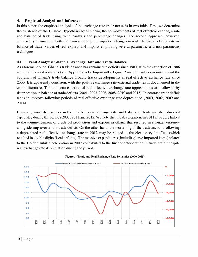
As aforementioned, Ghana’s trade balance has remained in deficits since 1983, with the exception of 1986

where it recorded a surplus (see, Appendix A1). Importantly, Figure 2 and 3 clearly demonstrate that the

evolution of Ghana’s trade balance broadly tracks developments in real effective exchange rate since

2000. It is apparently consistent with the positive exchange rate-external trade nexus documented in the

extant literature. This is because period of real effective exchange rate appreciations are followed by

deterioration in balance of trade deficits (2001, 2003-2006, 2008, 2010 and 2015). In contrast, trade deficit

tends to improve following periods of real effective exchange rate depreciation (2000, 2002, 2009 and

2014).

However, some divergences in the link between exchange rate and balance of trade are also observed

especially during the periods 2007, 2011 and 2012. We note that the development in 2011 is largely linked

to the commencement of crude oil production and exports in Ghana that resulted in stronger currency

alongside improvement in trade deficit. On the other hand, the worsening of the trade account following

a depreciated real effective exchange rate in 2012 may be related to the election-cycle effect (which

resulted in double digits fiscal deficits). The massive expenditures (including large imported items) related

to the Golden Jubilee celebration in 2007 contributed to the further deterioration in trade deficit despite

real exchange rate depreciation during the period.

Figure 2: Trade and Real Exchange Rate Dynamics (2000-2015)

9 | P a g e

Figure 3: Evolution of Changes in REER and BOT (%)

Note: In the case of change in REER, plus (+) = depreciation, while minus (-) = appreciation. For change in BOT, plus (+) =

improvement, while minus (-) = deterioration

The trend analysis seems to suggest a strong positive link between real effective exchange rate and trade

balance in Ghana, consistent with the J-Curve Hypothesis that real depreciation ultimately improves trade

deficit. In addition, the evidence also points to the existence of series of J-Curves in the short term

following successive depreciations and this indicates that the Kulkarni Hypothesis also applies to Ghana.

4.2 Estimation Results

In this section, we ascertain whether real exchange rate depreciation has symmetric effect on Ghana’s trade balance as well as determining the relative elasticities of export and import to changes in real

exchange rate in both the short run and long run. On the whole, the main estimation techniques employed

are linear and Threshold ARDL, threshold regression, impulse response functions (IRFs) from both

Unrestricted and Bayesian (using Minnesota Priors) VARs, and two-state Markov Regime Switching

Model with time-varying transition probabilities.

(A) Linear ARDL

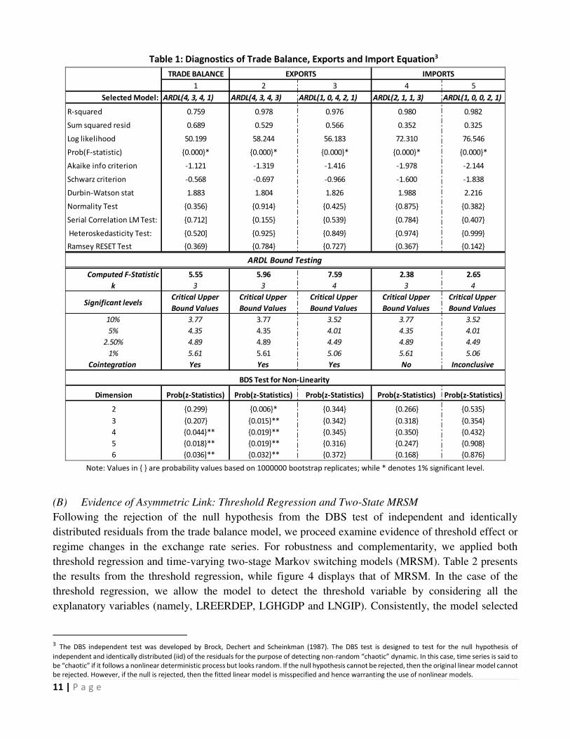
Table 1 present the optimal ARDL estimates for trade balance, exports and imports for Ghana based on

unconditional linear regression method and using Akaiki information criterion. The corresponding short

run and long run estimates are presented in Appendix A1 and A2. The upper portion of Table 1 shows

the model diagnostic tests which generally satisfy the OLS assumptions of normality and stability

alongside no evidence of serial correlation and heteroskedasticity in the respective residuals. In general,

the F-statistics of joint significance of the explanatory variable in all the equations are satisfactory with

R-square averaging 97%. However, the results from bound test in the middle of Table 1 clearly show

evidence of cointegration for trade balance and export equations, while that of the import equation was

inconclusive for the sample period.

10 | P a g e

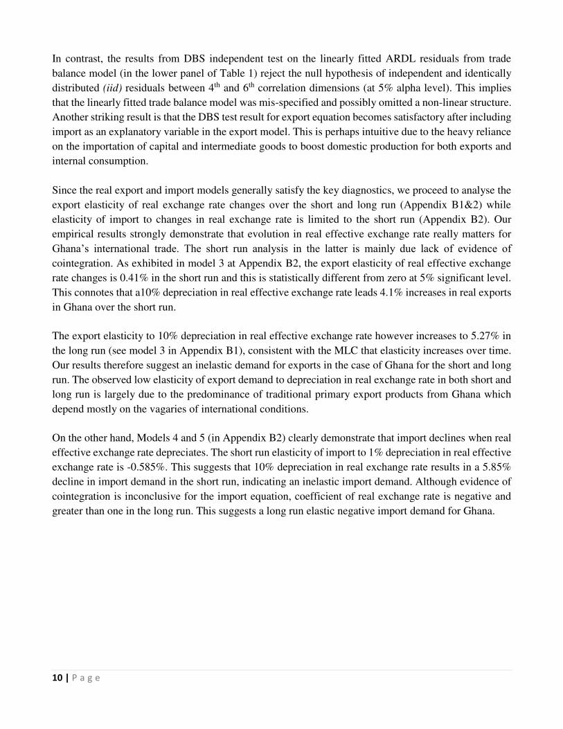
In contrast, the results from DBS independent test on the linearly fitted ARDL residuals from trade

balance model (in the lower panel of Table 1) reject the null hypothesis of independent and identically

distributed (iid) residuals between 4th and 6th correlation dimensions (at 5% alpha level). This implies

that the linearly fitted trade balance model was mis-specified and possibly omitted a non-linear structure.

Another striking result is that the DBS test result for export equation becomes satisfactory after including

import as an explanatory variable in the export model. This is perhaps intuitive due to the heavy reliance

on the importation of capital and intermediate goods to boost domestic production for both exports and

internal consumption.

Since the real export and import models generally satisfy the key diagnostics, we proceed to analyse the

export elasticity of real exchange rate changes over the short and long run (Appendix B1&2) while

elasticity of import to changes in real exchange rate is limited to the short run (Appendix B2). Our

empirical results strongly demonstrate that evolution in real effective exchange rate really matters for

Ghana’s international trade. The short run analysis in the latter is mainly due lack of evidence of cointegration. As exhibited in model 3 at Appendix B2, the export elasticity of real effective exchange

rate changes is 0.41% in the short run and this is statistically different from zero at 5% significant level.

This connotes that a10% depreciation in real effective exchange rate leads 4.1% increases in real exports

in Ghana over the short run.

The export elasticity to 10% depreciation in real effective exchange rate however increases to 5.27% in

the long run (see model 3 in Appendix B1), consistent with the MLC that elasticity increases over time.

Our results therefore suggest an inelastic demand for exports in the case of Ghana for the short and long

run. The observed low elasticity of export demand to depreciation in real exchange rate in both short and

long run is largely due to the predominance of traditional primary export products from Ghana which

depend mostly on the vagaries of international conditions.

On the other hand, Models 4 and 5 (in Appendix B2) clearly demonstrate that import declines when real

effective exchange rate depreciates. The short run elasticity of import to 1% depreciation in real effective

exchange rate is -0.585%. This suggests that 10% depreciation in real exchange rate results in a 5.85%

decline in import demand in the short run, indicating an inelastic import demand. Although evidence of

cointegration is inconclusive for the import equation, coefficient of real exchange rate is negative and

greater than one in the long run. This suggests a long run elastic negative import demand for Ghana.

11 | P a g e

Table 1: Diagnostics of Trade Balance, Exports and Import Equation3

TRADE BALANCE

1 2 3 4 5

Selected Model: ARDL(4, 3, 4, 1) ARDL(4, 3, 4, 3) ARDL(1, 0, 4, 2, 1) ARDL(2, 1, 1, 3) ARDL(1, 0, 0, 2, 1)

R-squared 0.759 0.978 0.976 0.980 0.982

Sum squared resid 0.689 0.529 0.566 0.352 0.325

Log likelihood 50.199 58.244 56.183 72.310 76.546

Prob(F-statistic) 0.000* 0.000* 0.000* 0.000* 0.000*

Akaike info criterion -1.121 -1.319 -1.416 -1.978 -2.144

Schwarz criterion -0.568 -0.697 -0.966 -1.600 -1.838

Durbin-Watson stat 1.883 1.804 1.826 1.988 2.216

Normality Test 0.356 0.914 0.425 0.875 0.382

Serial Correlation LM Test: 0.712] 0.155 0.539 0.784 0.407

Heteroskedasticity Test: 0.520] 0.925 0.849 0.974 0.999

Ramsey RESET Test 0.369 0.784 0.727 0.367 0.142

Computed F-Statistic 5.55 5.96 7.59 2.38 2.65

k 3 3 4 3 4

Significant levelsCritical Upper

Bound Values

Critical Upper

Bound Values

Critical Upper

Bound Values

Critical Upper

Bound Values

Critical Upper

Bound Values

10% 3.77 3.77 3.52 3.77 3.52

5% 4.35 4.35 4.01 4.35 4.01

2.50% 4.89 4.89 4.49 4.89 4.49

1% 5.61 5.61 5.06 5.61 5.06

Cointegration Yes Yes Yes No Inconclusive

Dimension Prob(z-Statistics) Prob(z-Statistics) Prob(z-Statistics) Prob(z-Statistics) Prob(z-Statistics)

2 0.299 0.006* 0.344 0.266 0.535

3 0.207 0.015** 0.342 0.318 0.354

4 0.044** 0.019** 0.345 0.350 0.432

5 0.018** 0.019** 0.316 0.247 0.908

6 0.036]** 0.032** 0.372 0.168 0.876

IMPORTS

ARDL Bound Testing

BDS Test for Non-Linearity

EXPORTS

Note: Values in are probability values based on 1000000 bootstrap replicates; while * denotes 1% significant level.

(B) Evidence of Asymmetric Link: Threshold Regression and Two-State MRSM

Following the rejection of the null hypothesis from the DBS test of independent and identically

distributed residuals from the trade balance model, we proceed examine evidence of threshold effect or

regime changes in the exchange rate series. For robustness and complementarity, we applied both

threshold regression and time-varying two-stage Markov switching models (MRSM). Table 2 presents

the results from the threshold regression, while figure 4 displays that of MRSM. In the case of the

threshold regression, we allow the model to detect the threshold variable by considering all the

explanatory variables (namely, LREERDEP, LGHGDP and LNGIP). Consistently, the model selected

3 The DBS independent test was developed by Brock, Dechert and Scheinkman (1987). The DBS test is designed to test for the null hypothesis of

independent and identically distributed (iid) of the residuals for the purpose of detecting non-random “chaotic” dynamic. In this case, time series is said to be “chaotic” if it follows a nonlinear deterministic process but looks random. If the null hypothesis cannot be rejected, then the original linear model cannot

be rejected. However, if the null is rejected, then the fitted linear model is misspecified and hence warranting the use of nonlinear models.

12 | P a g e

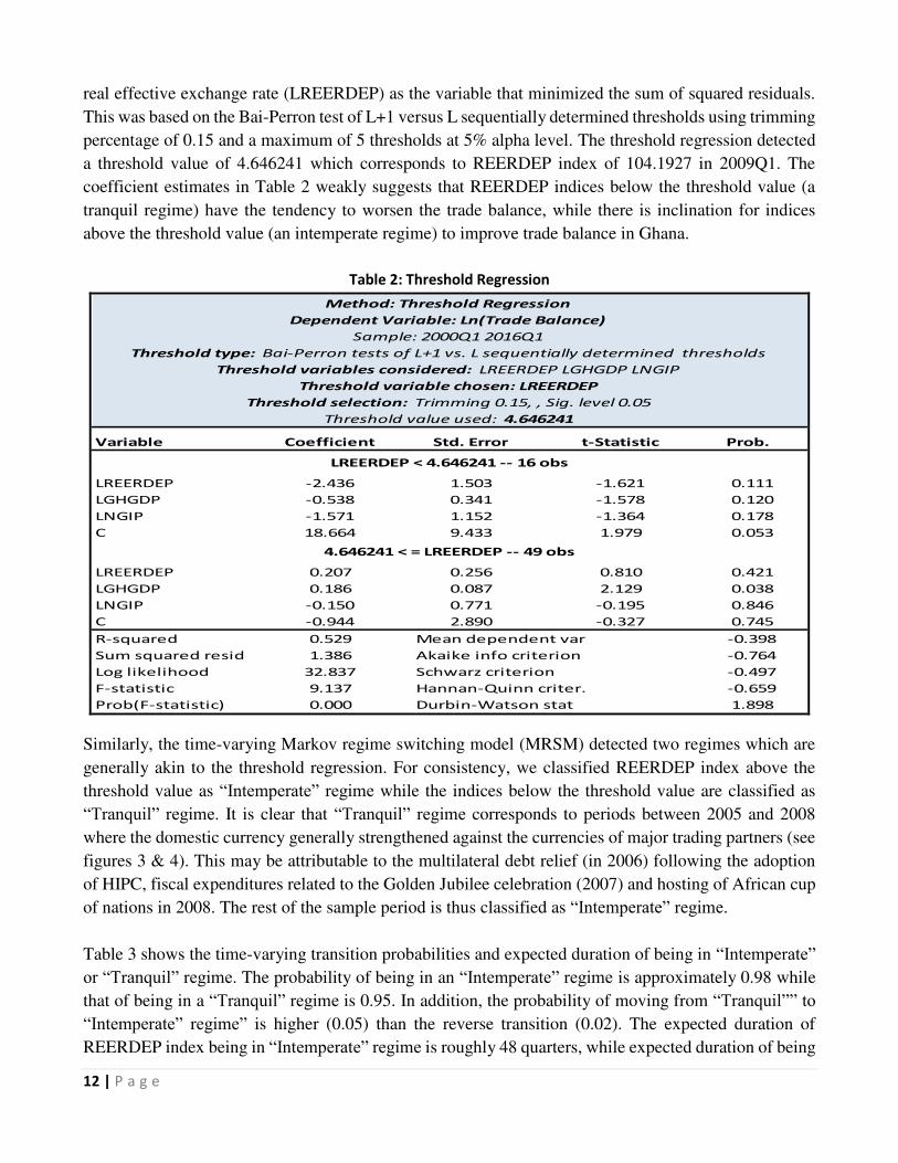
real effective exchange rate (LREERDEP) as the variable that minimized the sum of squared residuals.

This was based on the Bai-Perron test of L+1 versus L sequentially determined thresholds using trimming

percentage of 0.15 and a maximum of 5 thresholds at 5% alpha level. The threshold regression detected

a threshold value of 4.646241 which corresponds to REERDEP index of 104.1927 in 2009Q1. The

coefficient estimates in Table 2 weakly suggests that REERDEP indices below the threshold value (a

tranquil regime) have the tendency to worsen the trade balance, while there is inclination for indices

above the threshold value (an intemperate regime) to improve trade balance in Ghana.

Table 2: Threshold Regression

Variable Coefficient Std. Error t-Statistic Prob.

LREERDEP -2.436 1.503 -1.621 0.111

LGHGDP -0.538 0.341 -1.578 0.120

LNGIP -1.571 1.152 -1.364 0.178

C 18.664 9.433 1.979 0.053

LREERDEP 0.207 0.256 0.810 0.421

LGHGDP 0.186 0.087 2.129 0.038

LNGIP -0.150 0.771 -0.195 0.846

C -0.944 2.890 -0.327 0.745

R-squared 0.529 Mean dependent var -0.398

Sum squared resid 1.386 Akaike info criterion -0.764

Log likelihood 32.837 Schwarz criterion -0.497

F-statistic 9.137 Hannan-Quinn criter. -0.659

Prob(F-statistic) 0.000 Durbin-Watson stat 1.898

Threshold value used: 4.646241

Dependent Variable: Ln(Trade Balance)

LREERDEP < 4.646241 -- 16 obs

4.646241 < = LREERDEP -- 49 obs

Method: Threshold Regression

Sample: 2000Q1 2016Q1

Threshold type: Bai-Perron tests of L+1 vs. L sequentially determined thresholds

Threshold variables considered: LREERDEP LGHGDP LNGIP

Threshold variable chosen: LREERDEP

Threshold selection: Trimming 0.15, , Sig. level 0.05

Similarly, the time-varying Markov regime switching model (MRSM) detected two regimes which are

generally akin to the threshold regression. For consistency, we classified REERDEP index above the

threshold value as “Intemperate” regime while the indices below the threshold value are classified as

“Tranquil” regime. It is clear that “Tranquil” regime corresponds to periods between 2005 and 2008

where the domestic currency generally strengthened against the currencies of major trading partners (see

figures 3 & 4). This may be attributable to the multilateral debt relief (in 2006) following the adoption

of HIPC, fiscal expenditures related to the Golden Jubilee celebration (2007) and hosting of African cup

of nations in 2008. The rest of the sample period is thus classified as “Intemperate” regime.

Table 3 shows the time-varying transition probabilities and expected duration of being in “Intemperate” or “Tranquil” regime. The probability of being in an “Intemperate” regime is approximately 0.98 while

that of being in a “Tranquil” regime is 0.95. In addition, the probability of moving from “Tranquil”” to “Intemperate” regime” is higher (0.05) than the reverse transition (0.02). The expected duration of

REERDEP index being in “Intemperate” regime is roughly 48 quarters, while expected duration of being

13 | P a g e

in the “Tranquil” regime is 19 quarters. The analysis of the MRSM results therefore reveals a higher

propensity for the Ghana’s REER to depreciate than to appreciate against the currencies of major trading

partners.

Figure 4: Two-State Markov Regime Switching Result

0.0

0.2

0.4

0.6

0.8

1.0

2000 2001 2002 2003 2004 2005 2006 2007 2008 2009 2010 2011 2012 2013 2014 2015

P(S(t)= 1)

0.0

0.2

0.4

0.6

0.8

1.0

2000 2001 2002 2003 2004 2005 2006 2007 2008 2009 2010 2011 2012 2013 2014 2015

P(S(t)= 2)

One-step Ahead Predicted Regime Probabilities

Note: P(S(t) = 1) denotes “Intemperate” regime, while P(S(t) = 2) is the “Tranquil” regime.

Table 3: Time-varying transition probabilities and expected duration

Note: “Intemperate” regime is the period with REER values equal or greater than the threshold value,

while “Tranquil” regime corresponds to periods with REER values below the threshold level.

14 | P a g e

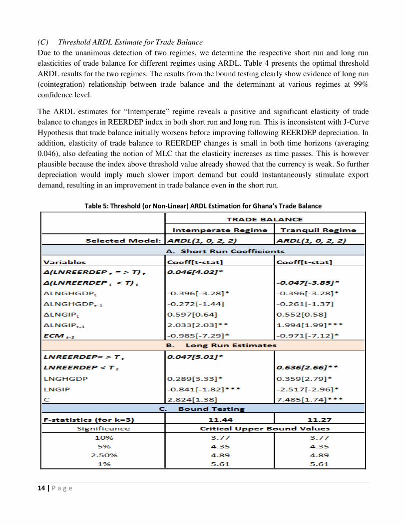
(C) Threshold ARDL Estimate for Trade Balance

Due to the unanimous detection of two regimes, we determine the respective short run and long run

elasticities of trade balance for different regimes using ARDL. Table 4 presents the optimal threshold

ARDL results for the two regimes. The results from the bound testing clearly show evidence of long run

(cointegration) relationship between trade balance and the determinant at various regimes at 99%

confidence level.

The ARDL estimates for “Intemperate” regime reveals a positive and significant elasticity of trade

balance to changes in REERDEP index in both short run and long run. This is inconsistent with J-Curve

Hypothesis that trade balance initially worsens before improving following REERDEP depreciation. In

addition, elasticity of trade balance to REERDEP changes is small in both time horizons (averaging

0.046), also defeating the notion of MLC that the elasticity increases as time passes. This is however

plausible because the index above threshold value already showed that the currency is weak. So further

depreciation would imply much slower import demand but could instantaneously stimulate export

demand, resulting in an improvement in trade balance even in the short run.

Table 5: Threshold (or Non-Linear) ARDL Estimation for Ghana’s Trade Balance

15 | P a g e

In contrast, the estimates for “Tranquil” regime clearly satisfies the J-Curve Hypothesis as the trade

deficit worsens in the short run (-0.047) but improves in the long run (0.636), following a depreciation

in real effective exchange rate. It is also apparent in “Tranquil” regime that the elasticity of trade balance to changes in real exchange rate increases in the long run. This reinforces the notion that elasticity of

trade increase as time passes to satisfy MLC.

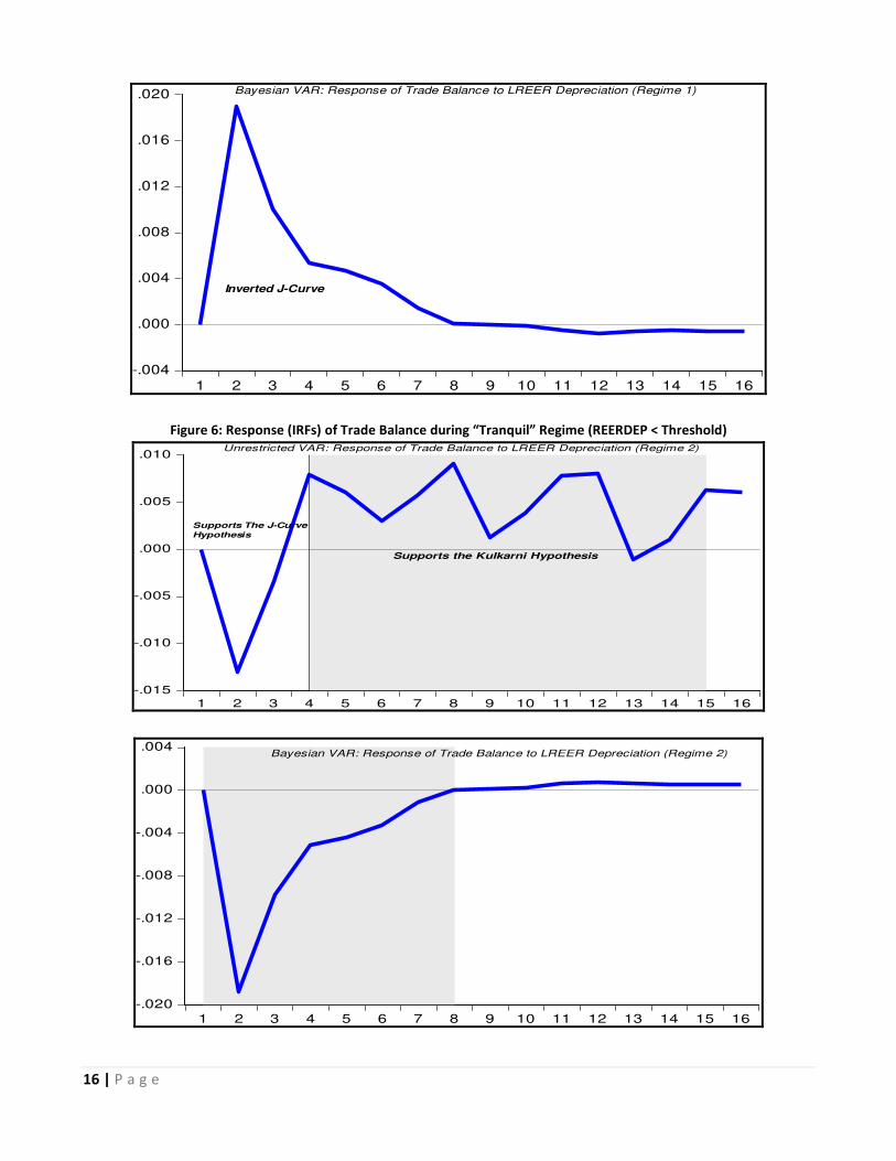
(D) Impulse Response Functions from Unrestricted and Bayesian VARs

Since macroeconomic time series data tend to be interrelated, we further ascertain the plausibility of the

regime estimates from threshold ARDL using impulse response functions (IRFs) from both unrestricted

and Bayesian VARs. In the formulation of the 4-variable VAR model, we treated only global industrial

production index (LNGIP) as exogenous variable, while LNTB, LREERDEP and LGHGDP were treated

as endogenous variables. In particular, we assumed the Minnesota priors for the Bayesian VAR. Based

on optimal lag length 4, figures 5 and 6 display the IRFs for “Intemperate” regime and “Tranquil” regime

respectively. The results from the IRFs are generally consistent with the estimates form the Threshold

ARDL model.

The results for the “Intemperate” regime clearly show evidence of weak J-curve or perhaps an inverted

J-curve as trade balance rather improves before deteriorating following real exchange rate depreciation.

However, some evidence of sequential J-curves after the second quarter, consistent with the Kulkarni

Hypothesis. In contrast, the IRFs for “Tranquil” regime clearly demonstrate that the link between trade

balance and real exchange rate depreciation satisfies both the J-curve and the Kulkarni Hypotheses in the

case of Ghana.

Figure 5: Response of Trade Balance within “Intemperate” regime (REERDEP ≥ Threshold)

-.010

-.005

.000

.005

.010

.015

1 2 3 4 5 6 7 8 9 10 11 12 13 14 15 16

Unrestricted VAR: Response of Trade Balance to REER Depreciation (Regime 1)

Support the Kulkarni Hypothesis

16 | P a g e

-.004

.000

.004

.008

.012

.016

.020

1 2 3 4 5 6 7 8 9 10 11 12 13 14 15 16

Bayesian VAR: Response of Trade Balance to LREER Depreciation (Regime 1)

Inverted J-Curve

Figure 6: Response (IRFs) of Trade Balance during “Tranquil” Regime (REERDEP < Threshold)

-.015

-.010

-.005

.000

.005

.010

1 2 3 4 5 6 7 8 9 10 11 12 13 14 15 16

Unrestricted VAR: Response of Trade Balance to LREER Depreciation (Regime 2)

Supports the Kulkarni Hypothesis

Supports The J-Curve

Hypothesis

-.020

-.016

-.012

-.008

-.004

.000

.004

1 2 3 4 5 6 7 8 9 10 11 12 13 14 15 16

Bayesian VAR: Response of Trade Balance to LREER Depreciation (Regime 2)

17 | P a g e

5. Conclusion and Policy Implications

This paper investigates the trade-exchange rate nexus in the case of Ghana using quarterly data over the

period 2000Q1-2016Q1, applying both parametric and non-parametric estimates techniques.

Specifically, we evaluated the validity of Marshall-Lerner Condition (MLC), the J-Curve and Kulkarni

Hypotheses in the case of Ghana using a battery of econometric methods.

The key findings of this study are summarised as follows:

Our empirical results strongly demonstrate that evolution in real effective exchange rate really matters

for Ghana’s international trade. We found cogent evidence in supports of the MLC, the J-Curve

Hypothesis and Kulkarni Hypothesis in the context of Ghana over the sample period. In particular, the

observed evidence of Kulkarni hypothesis (series or shifts in J-curves) suggests that the dynamic and

persistent trade deficits are largely the consequent of continuous depreciation of real exchange rate in

Ghana.

However, there is a strong evidence of asymmetric relationship between real exchange rate and trade

balance in Ghana. In particular, two main regimes were identified from both Threshold regression and

Markov Regime Switching Model. “Intemperate” regime represented period the REERDEP index

exceeded or was equal to a certain threshold value, while “Tranquil” regime comprises the period when

the REERDEP index lies below the threshold value. The threshold value was empirically identified as

the REERDEP index for 2009Q1. Although we found evidence of J-curve in both regimes, the evidence

was much clearer for “Tranquil” regime where the real exchange rate index lie below the threshold level.

Unlike “Intemperate” regime, trade balance tends to worsen in the short run but improve over the longer

horizon following real exchange rate depreciation during the “Tranquil” regime. This lends supports to

the J-curves hypothesis. There was also strong evidence of the Kulkarni Hypothesis for the “Tranquil” regime as series of J-curves were observed. This notwithstanding, the time-varying transition

probabilities and expected duration in a regime indicated a higher tendency for the real exchange rate to

be in the “Intemperate” regime. This connotes that the Ghana’s domestic currency has a greater tendency to depreciate (in real terms) against the currencies of the major trading partners over the sample period.

In addition, we found an inelastic positive demand for exports in response of changes in real exchange

rate in both short and long run in the case of Ghana. In terms of magnitude, a 10% depreciation in real

effective exchange rate leads to 4.1% increase in real exports in Ghana over the short run but increases

to 5.3% in the long run. The low elasticity of export demand to change in real exchange rate is largely

due to the preponderance of primary export products from Ghana which depends mostly on the whims

of international conditions. In contrast, we observed a negative Ghana’s demand for import in response to changes in real exchange rate, though it is inelastic in the short run but become elastic over the longer

horizon. In particular, we observed that 10% depreciation in real exchange rate causes Ghana’s import demand to decline by 5.8% in the short run and a drop of 11.95% in the long run. Our empirical results

are generally consistent with the MLC that elasticity increases as time passes.

Another important observation is a dual positive link between Ghana’s exports and imports in both the short and long run, although the effect from import appears to be larger over the sample period. This is

highly intuitive as domestic economic activities rely heavily on the importation of essential products

(such as intermediate and capital goods as well as crude oil).

18 | P a g e

The empirical results remit the following key policy recommendation. The analysis clearly suggests that

for Ghana to leverage on the continuous real depreciation (competitiveness), a deliberate policy toward

export diversification need to be pursued. Particularly, significant attention should be given to value

additions and non-traditional export sectors. This would warrant strong coordination between monetary

and fiscal policies to resolve the financial bottlenecks of players in the essential export sectors (including

high lending rate and lack of access to credit due to the perceived riskiness of agricultural ventures, etc).

In this regard, this study strongly supports the planned establishment of EXIM (Export-Import)

Guaranteed Bank with the aim of proffering financial support to key non-traditional exporters as well as

the importers of highly essential goods.

It is equally critical for monetary authority to sustain macroeconomic stability in order to create an

enabling environment for private sector to thrive. This requires the adoption of appropriate and

coordinated monetary and fiscal policies that would lead to low and stable inflation and stable foreign

exchange rates. The attainment of these goals is essential to minimize cost of borrowing of the players

in especially the non-traditional export sector and also strengthen foreign inflows (both portfolio and

FDI).

In addition, it is vital to intensify the on-going government’s debt restructuring strategy in favour of medium-to-long term debt. This would help lower interest rate in the money market and hence crowd-in

the private sector and to propel economic growth and development, and hence alleviate poverty.

Reference

Adeniyi, O., Omisakin, O and A., Oyinlola, (2011). “Exchange Rate and Trade Balance in West African

Monetary Zone: Is There a J-Curve?” The International Journal of Applied Economics and

Finance, 5, pp. 167-176.

Agbola, F. (2004). “Does devaluation improve trade balance of Ghana?” Paper to be presented at the International Conference on Ghana’s economy at the half Century, M- Plaza Hotel, Accra,

Ghana, July 18-20, 2004.

Akbostanci, E, (2004), “Dynamics of the Trade Balance: The Turkish J-Curve”, Emerging Market

Finance and Trade, 40, pp. 57-73.

Anning, L,. Riti, J. S., and K, T, P, Yapatake, 2015. “Exchange rate and trade balance in Ghana-testing

the validity of the Marshall Lerner condition” International Journal of Development and

Emerging Economies, 3(2), pp. 38-52.

Ardalani, Z., and M. Bahmani-Oskooee, (2007). "Is there a J-Curve at the Industry Level?" Economics

Bulletin, AccessEcon, 6(26), pages 1-12.

Bahmani-Oskooee, M., and A. Gelan, (2012). “Is there J-curve effect in Africa”, International Review of

Applied Economics, 26(1), pp. 73-81.

Bahmani-Oskooee, M., Economidou, C, and G. G. Goswami, (2006), “Bilateral J-Curve Between the

UK Vis-a-Vis Her Major Trading Partners”, Applied Economics, 38, pp. 879-888.

Bahmani-Oskooee, M., and G. G. Goswami, (2003), “A Disaggregated Approach to Test the J-Curve

Phenomenon: Japan versus Her major Trading Partners”, International Journal of Economics

and Finance, 27, pp. 102-113.

19 | P a g e

Bahmani-Oskooee, M., Goswami G. G. and B. K. Talukdar, (2005), “The Bilateral J-Curve: Australia

Versus Her 23 Trading Partners”, Australian Economic Papers, 44, pp. 110-120.

Bahmani-Oskooee, M., and A. S. Hosny, (2012). “Egypt-EU commodity trade and the J-curve”, International Journal of Monetary Economics and Finance, 5(2).

Bahmani-Oskooee, M. and Ratha, A (2004a), “The J-Curve: A Literature Review”, Applied Economics,

36, pp. 1377-1398.

Bahmani-Oskooee, M, and Ratha, A., (2004b), “The J-Curve Dynamics of US Bilateral Trade”, Journal

of Economics and Finance, 28, pp.32-38.

Bhattarai, K, R., and M. K. Armah, (2005). “The Effects of Exchange Rate on the Trade Balance in

Ghana: Evidence from Cointegration Analysis” Research Memorandum 52, (August 2005).

Chiloane, L., M. Pretorius and I. Botha, (2014). “The relationship between the exchange rate and the

trade balance in South Africa” Journal of Economic and Financial Sciences, 7(2), pp. 299-314.

Hsing, Y, (2008), ‘A Study of the J-Curve for Seven Selected Latin American Countries”. Global

Economic Journal, 8(4), pp. 1-11, forthcoming.

Hacker, R. S, and A. J., Hatemi, (2004), “The Effect of Exchange Rate Changes on Trade Balances in the Short and Long Run”, Economics of Transition, 12, pp. 777-799.

Halicioglu, F, (2008), “The J-Curve Dynamics of Turkey: An Application of ARDL Model”, Journal of

Applied Economics, 40(18), pp. 2423-2429.

Junz H. and R. Rhomberg (1973). “Price Competitiveness in Export Trade among Industrial Countries” American Economic Review, 63(2), pp. 412-418.

Kulkarni, K., (1996), “The J-Curve Hypothesis and Currency Devaluation: the case of Egypt and Ghana”, Journal of Applied Business Research, 12(2), pp. 1-8.

Kulkarni, K, and A., Clarke, (2009), “Testing the J-Curve Hypothesis: Case Studies From Around the

World”, International Economics Practicum, Final Paper. Pp. 1-30.

Magee, S. P. (1973). “Currency Contracts, Pass-through, and Devaluation”. Brookings Papers on

Economic Activity, 1, pp. 303-325.

Narayan, P. K, (2004), “New Zealand’s Trade Balance: Evidence from the J-Curve and Granger

Causality”, Applied Economics Letters, 11, pp. 351-354.

Narayan, P. K., and S., Narayan, (2004), “The J-Curve: Evidence from the Fiji”, International Journal

of Applied Economics, 18, pp. 369-380.

Osabuohien, E. S, (2015), “Trade-Exchange Rate Nexus in Sub-Saharan African Countries: Evidence

from Panel Cointegration Analysis”, Foreign Trade Review, 50(3), pp. 1-17.

Pesaran, M. H., Shin, Y., and R. J., Smith, (2001), “Bound Testing Approaches to the Analysis of Level Relationships”, Journal of Applied Econometrics, 16, pp. 289-326.

Riti, J. S. (2012). Estimation of Trade Elasticities in Nigeria: A Test of the Marshall Lerner Condition

(1981-2010). Jos Journal of Economics, Vol. 5 No. 1, 2012, 87-111.

Rose, A. K. and J. L. Yellen, (1989), “Is There a J-Curve?” Journal of Monetary Economics, 24, pp. 53-

68.

Ziramba, E., and R. T., Chifamba, (2014). “The J-curve dynamics of South African Trade: Evidence

from the ARDL Approach” European Scientific Journal, 10(19), pp. 346-358.

20 | P a g e

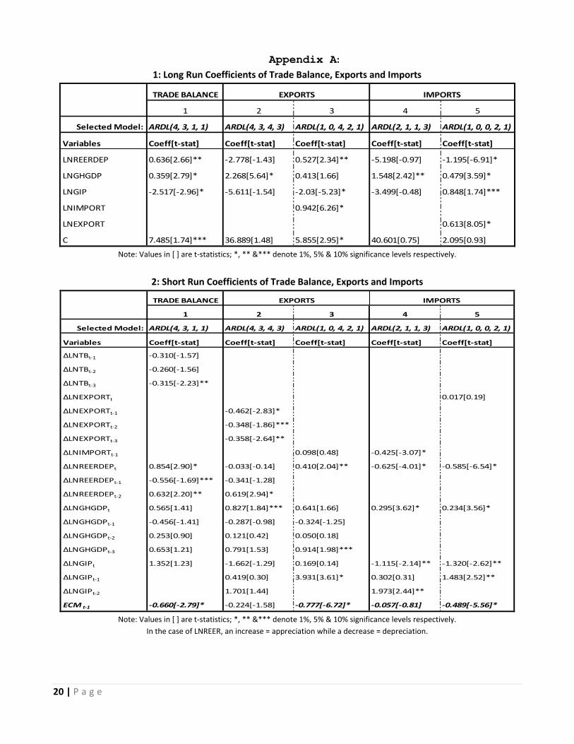
Appendix A:

1: Long Run Coefficients of Trade Balance, Exports and Imports

TRADE BALANCE

1 2 3 4 5

Selected Model: ARDL(4, 3, 1, 1) ARDL(4, 3, 4, 3) ARDL(1, 0, 4, 2, 1) ARDL(2, 1, 1, 3) ARDL(1, 0, 0, 2, 1)

Variables Coeff[t-stat] Coeff[t-stat] Coeff[t-stat] Coeff[t-stat] Coeff[t-stat]

LNREERDEP 0.636[2.66]** -2.778[-1.43] 0.527[2.34]** -5.198[-0.97] -1.195[-6.91]*

LNGHGDP 0.359[2.79]* 2.268[5.64]* 0.413[1.66] 1.548[2.42]** 0.479[3.59]*

LNGIP -2.517[-2.96]* -5.611[-1.54] -2.03[-5.23]* -3.499[-0.48] 0.848[1.74]***

LNIMPORT 0.942[6.26]*

LNEXPORT 0.613[8.05]*

C 7.485[1.74]*** 36.889[1.48] 5.855[2.95]* 40.601[0.75] 2.095[0.93]

IMPORTSEXPORTS

Note: Values in [ ] are t-statistics; *, ** &*** denote 1%, 5% & 10% significance levels respectively.

2: Short Run Coefficients of Trade Balance, Exports and Imports

TRADE BALANCE

1 2 3 4 5

Selected Model: ARDL(4, 3, 1, 1) ARDL(4, 3, 4, 3) ARDL(1, 0, 4, 2, 1) ARDL(2, 1, 1, 3) ARDL(1, 0, 0, 2, 1)

Variables Coeff[t-stat] Coeff[t-stat] Coeff[t-stat] Coeff[t-stat] Coeff[t-stat]

ΔLNTBt-1 -0.310[-1.57]

ΔLNTBt-2 -0.260[-1.56]

ΔLNTBt-3 -0.315[-2.23]**

ΔLNEXPORTt 0.017[0.19]

ΔLNEXPORTt-1 -0.462[-2.83]*

ΔLNEXPORTt-2 -0.348[-1.86]***

ΔLNEXPORTt-3 -0.358[-2.64]**

ΔLNIMPORTt-1 0.098[0.48] -0.425[-3.07]*

ΔLNREERDEPt 0.854[2.90]* -0.033[-0.14] 0.410[2.04]** -0.625[-4.01]* -0.585[-6.54]*

ΔLNREERDEPt-1 -0.556[-1.69]*** -0.341[-1.28]

ΔLNREERDEPt-2 0.632[2.20]** 0.619[2.94]*

ΔLNGHGDPt 0.565[1.41] 0.827[1.84]*** 0.641[1.66] 0.295[3.62]* 0.234[3.56]*

ΔLNGHGDPt-1 -0.456[-1.41] -0.287[-0.98] -0.324[-1.25]

ΔLNGHGDPt-2 0.253[0.90] 0.121[0.42] 0.050[0.18]

ΔLNGHGDPt-3 0.653[1.21] 0.791[1.53] 0.914[1.98]***

ΔLNGIPt 1.352[1.23] -1.662[-1.29] 0.169[0.14] -1.115[-2.14]** -1.320[-2.62]**

ΔLNGIPt-1 0.419[0.30] 3.931[3.61]* 0.302[0.31] 1.483[2.52]**

ΔLNGIPt-2 1.701[1.44] 1.973[2.44]**

ECM t-1 -0.660[-2.79]* -0.224[-1.58] -0.777[-6.72]* -0.057[-0.81] -0.489[-5.56]*

EXPORTS IMPORTS

Note: Values in [ ] are t-statistics; *, ** &*** denote 1%, 5% & 10% significance levels respectively.

In the case of LNREER, an increase = appreciation while a decrease = depreciation.