Exchange Rate Assessment for Oil

Exporters

Klaus Enders

WP/09/81

© 2009 International Monetary Fund WP/09/81 IMF Working Paper Middle East and Central Asia Department

Exchange Rate Assessment for Oil Exporters

Prepared by Klaus Enders1

April 2009

Abstract

This Working Paper should not be reported as representing the views of the IMF. The views expressed in this Working Paper are those of the author(s) and do not necessarily represent those of the IMF or IMF policy. Working Papers describe research in progress by the author(s) and are published to elicit comments and to further debate.

While the underlying methodologies continue to be widely debated and refined, there is little consensus on how to assess the equilibrium exchange rate of economies dominated by production of finite natural resources such as the oil economies of the Middle East. In part this is due to the importance of intertemporal aspects (as the real exchange rate may affect the optimal/equitable rate of transformation of finite resource wealth into financial assets), as well as risk considerations given the relatively high volatility of commodity prices. The paper illustrates some important peculiarities of the exchange rate assessment for such natural resource producers by working through a simple two-period model that captures certain key aspects of many resource economies. JEL Classification Numbers: D51, D90, E21, F32, O53 Keywords: Exchange rate, oil exports Author’s E-Mail Address: kenders@imf.org

1 I am grateful to Maher Hasan and Tahsin Saadi for their useful comments on an earlier draft, to Arthur Ribeiro da Silva for assistance with collecting data and preparing the charts, and Maria Orihuela-Quintanilla for her kind assistance in preparing the document.

2

Contents Page I. Overview ............................................................................................................................... 3 II. The Model ............................................................................................................................ 4 III. Market Clearing .................................................................................................................. 7 IV. Comparative Statics ............................................................................................................ 9 V. Private Consumption and Saving....................................................................................... 16 VI. External Equilibrium ........................................................................................................ 18 Appendix I .............................................................................................................................. 20 References............................................................................................................................... 21 Chart GCC Selected Indicators .........................................................................................................12

3

I. OVERVIEW

In recent years the Fund has stepped up its work on the assessment of equilibrium exchange rates of member countries. The approach typically involves identifying a stable relation between the real effective exchange rate (REER) and a set of fundamentals (such as demographic variables, fiscal policy stance, terms of trade, relative productivity etc), that is found to hold either across time or across countries (or both in panel based studies).2 Deviation from this “typical” relation signals a disequilibrium (misalignment) which if not addressed (or in the process of self-correcting) could lead to instability. While the underlying methodologies continue to be widely debated and refined, there is little consensus on how to assess the equilibrium exchange rate of economies dominated by production of finite natural resources such as the oil economies of the Middle East. In part this is due to the importance of intertemporal aspects (as the real exchange rate may affect the optimal/equitable rate of transformation of finite resource wealth into financial assets), as well as risk considerations given the relatively high volatility of commodity prices. This paper seeks to illustrate some important peculiarities of the exchange rate assessment for such natural resource producers by working through a simple two-period model that captures certain key aspects of many resource economies: • a production structure involving the natural resource sector (henceforth called “oil”)

and a nontradables sector, with little linkage between the two • a dominant role for government in the management of the oil sector, whereas

nontradables are produced by the private sector under competition. • Subsidization of domestic oil consumption, and no taxation of the private sector These stylized characteristics broadly fit many of the world’s oil producers, including the members of the GCC (Gulf Cooperation Council).3 They fit less well producers such as Russia where a sizable nonresource tradable sector exists and hence Dutch-disease type effects become important. The model is not intended to simulate oil sector economies, but to highlight in a simple setting key mechanisms and some potential pitfalls of generalizing from “normal” economies to oil exporters. In particular, working through the model highlights that:

2 See for example Zudik and Mongardini (2007), Hasan and Dridi (2008), Ricci, Milesi-Ferretti, and Lee (2008).

3 Bahrain, Kuwait, Oman, Qatar, Saudi Arabia, and the United Arab Emirates.

4

• Terms of trade shocks affect the real equilibrium real exchange rate (ERER) in the expected direction, working mainly through wealth effects. In particular an increase in oil wealth (through higher oil prices or finding of additional reserves allowing higher production) results in a new equilibrium with real appreciation, increased nontradable production, and higher real government spending. However, while an oil boom in the first period unambiguously improves the government budget balance in the same period, the impact on the current account is ambiguous as private saving may move opposite to public saving. • The ERER is influenced by fundamental factors other than oil wealth, and the importance of such factors may partly explain the relatively muted response of observed real effective exchange rates of GCC countries to the oil boom during 2004–08. In particular, the import of labor and other factors of production by itself tends to depreciate the ERER. There is furthermore some evidence that productivity may have improved in the nontradables sector relative to the tradable sector (essentially oil), perhaps reflecting stepped-up government spending on infrastructure, education etc, depreciating the ERER (the Balassa-Samuelson effect in reverse). • The model spells out how budget balance, real exchange rate and current account are jointly determined by “fundamentals” such as productivity, oil wealth, factor endowment etc. Therefore attempts to “explain” the current account by the real exchange rate, or treat the budget balance as a fundamental determinant of the equilibrium current account, are necessarily partial-equilibrium in nature and miss important aspects of the general equilibrium. We illustrate the point by examples where a current account improvement is associated with a real appreciation in one case, and a real depreciation in another.

II. THE MODEL

The economy lives for two periods and produces in periods i = 1, 2 Ni nontradables and Qi oil. Nontradables are produced by the private sector, with the help of energy (oil) QNi and domestic production factors (labor) Li.4 Technology is Cobb-Douglas: 1

i i i NiN A L Qβ β−= (1) where Ai > 0 is total factor productivity, and 0 ≤ β ≤ 1 the income share of energy. The government produces oil Qi of which it exports Qxi and sells QNi to the domestic private sector: Qi = Qxi + QNi (2) 4 Li will be referred to as “labor” but can be thought of a composite of domestic production factors such as labor, local know how, land, even institutions etc.—as long as the composition and relative returns to such factors do not change.

5

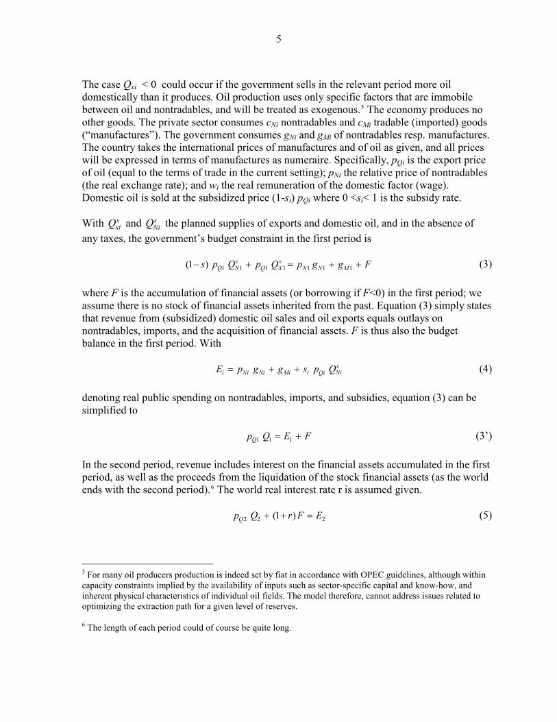
The case Qxi < 0 could occur if the government sells in the relevant period more oil domestically than it produces. Oil production uses only specific factors that are immobile between oil and nontradables, and will be treated as exogenous.5 The economy produces no other goods. The private sector consumes cNi nontradables and cMi tradable (imported) goods (“manufactures”). The government consumes gNi and gMi of nontradables resp. manufactures. The country takes the international prices of manufactures and of oil as given, and all prices will be expressed in terms of manufactures as numeraire. Specifically, pQi is the export price of oil (equal to the terms of trade in the current setting); pNi the relative price of nontradables (the real exchange rate); and wi the real remuneration of the domestic factor (wage). Domestic oil is sold at the subsidized price (1-si) pQi where 0 <si< 1 is the subsidy rate. With s

xiQ and sNiQ the planned supplies of exports and domestic oil, and in the absence of

any taxes, the government’s budget constraint in the first period is 1 1 1 1 1 1 1(1 ) s s

Q N Q X N N Ms p Q p Q p g g F− + = + + (3) where F is the accumulation of financial assets (or borrowing if F<0) in the first period; we assume there is no stock of financial assets inherited from the past. Equation (3) simply states that revenue from (subsidized) domestic oil sales and oil exports equals outlays on nontradables, imports, and the acquisition of financial assets. F is thus also the budget balance in the first period. With s

i Ni Ni Mi NiQiiE p g g s p Q= + + (4) denoting real public spending on nontradables, imports, and subsidies, equation (3) can be simplified to 1 1 1Qp Q E F= + (3’) In the second period, revenue includes interest on the financial assets accumulated in the first period, as well as the proceeds from the liquidation of the stock financial assets (as the world ends with the second period).6 The world real interest rate r is assumed given. 2 2 2(1 )Qp Q r F E+ + = (5)

5 For many oil producers production is indeed set by fiat in accordance with OPEC guidelines, although within capacity constraints implied by the availability of inputs such as sector-specific capital and know-how, and inherent physical characteristics of individual oil fields. The model therefore, cannot address issues related to optimizing the extraction path for a given level of reserves.

6 The length of each period could of course be quite long.

6

Elimination of F from the last two equations yields the government’s intertemporal budget constraint:

2 2 21 1 11 1

QQ

p Q EW p Q Er r

= + = ++ +

(6)

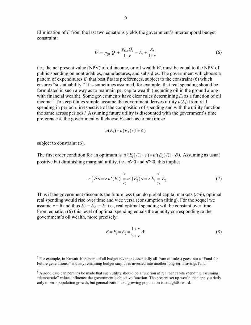
i.e., the net present value (NPV) of oil income, or oil wealth W, must be equal to the NPV of public spending on nontradables, manufactures, and subsidies. The government will choose a pattern of expenditures Ei that best fits its preferences, subject to the constraint (6) which ensures “sustainability.” It is sometimes assumed, for example, that real spending should be formulated in such a way as to maintain per capita wealth (including oil in the ground along with financial wealth). Some governments have clear rules determining Ei as a function of oil income.7 To keep things simple, assume the government derives utility u(Ei) from real spending in period i, irrespective of the composition of spending and with the utility function the same across periods.8 Assuming future utility is discounted with the government’s time preference δ, the government will choose Ei such as to maximize 1 2( ) ( ) /(1 )u E u E δ+ + subject to constraint (6). The first order condition for an optimum is 1 2'( ) /(1 ) '( ) /(1 ).u E r u E δ+ = + Assuming as usual positive but diminishing marginal utility, i.e., u'>0 and u''<0, this implies

(7) 1 2 1'( ) ' ( )< >

r u E u E Eδ≥≤> <

<=> = <=> = 2E

Thus if the government discounts the future less than do global capital markets (r>δ), optimal real spending would rise over time and vice versa (consumption tilting). For the sequel we assume r = δ and thus E1 = E2 = E, i.e., real optimal spending will be constant over time. From equation (6) this level of optimal spending equals the annuity corresponding to the government’s oil wealth, more precisely:

1 212

rE E E Wr

+= = =

+ (8)

7 For example, in Kuwait 10 percent of all budget revenue (essentially all from oil sales) goes into a “Fund for Future generations,” and any remaining budget surplus is invested into another long-term savings fund.

8 A good case can perhaps be made that such utility should be a function of real per capita spending, assuming “democratic” values influence the government’s objective function. The present set up would then apply strictly only to zero population growth, but generalization to a growing population is straightforward.

7

Substituting E for Ei in the period budget constraints ((3’) and (5)) and eliminating E yields

1 1 2 21 12

Q QQ

p Q p QF p Q E

r−

= =+

− (9)

which summarizes the fiscal rule for an oil exporter derived from the utility optimization process described above. It says the government should run a budget surplus in the first period (F > 0) if first period oil revenue pQ1 Q1 is greater than second period revenue, i.e., save some oil money for “future generations.” Note that in the extreme case that the country is running out of oil in the “future” (second period), it should roughly save half of “today’s” revenue; it should save nothing at all if future oil revenue is equal to or higher than today’s.9 If future revenue is higher, it is of course optimal to borrow today (F<0) to smoothen real spending. In any case government savings F equal the difference between current oil income and equilibrium (annuity) spending.

III. MARKET CLEARING

Assuming nontradables are produced under perfect competition, and that the private sector cannot reexport subsidized domestic oil, and cannot import (or buy from government) oil at world market prices10 the first order conditions for maximizing profits pNi - wi S

iN diL – (1-si)

pQi (where dNiQ ,d d

i NiL Q are the demand for labor and oil, and siN the supply of nontradables)

state as usual that factor rewards equal marginal products: (1 ) ( / )d d

i iNi Ni ip A Q L wββ− = (10) 1( / ) (1 )d d

i i iNi Ni Qip A Q L s pββ − = − (11) Different from the usual Salter-Swan type tradables/nontradables model, these equations are not enough to determine the real exchange rate, wages, and production even though the price of the tradable input (here oil, in the classical model internationally mobile capital) is given. This is because the local tradable sector, here oil, does not compete for factor inputs and hence does not provide equations corresponding to (10) and (11).

9In recent years, GCC countries have saved a large share of oil revenue, which if they were following fiscal rule (9) would indicate that they expect not to run out of oil soon, but at the same time are concerned that the expected value of future oil revenue may be lower than needed to sustain a desired level of real spending for the foreseeable future.

10 For many oil exporters there is anecdotal evidence that some oil purchased domestically at subsidized prices is smuggled abroad and sold at world market prices; many oil exporters also import some fuels (usually specialty refined products). However, especially for GCC countries such reexports and imports seem of minor importance and ruling them out should not unduly restrict the analysis.

8

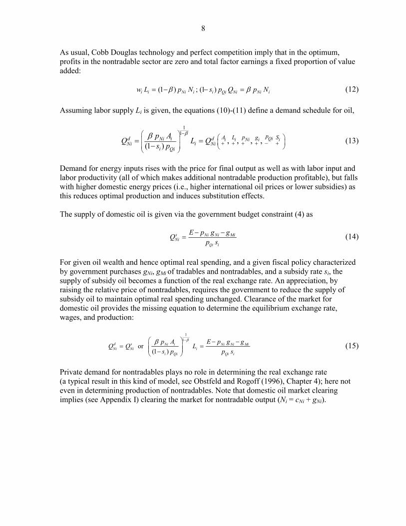
As usual, Cobb Douglas technology and perfect competition imply that in the optimum, profits in the nontradable sector are zero and total factor earnings a fixed proportion of value added: (1 ) ; (1 )i i i i iNi Ni NiQiw L p N s p Q p Nβ β= − − = (12) Assuming labor supply Li is given, the equations (10)-(11) define a demand schedule for oil,

11

(1 ), , , , Qii i Ni i id diNi

iNi Nii Qi

ppA L g Sp AQ L Qs p

ββ −

−+ + + + +⎛ ⎞ ⎛⎜ ⎟ ⎜⎜ ⎟ ⎝ ⎠⎝ ⎠

= =−

⎞⎟ (13)

Demand for energy inputs rises with the price for final output as well as with labor input and labor productivity (all of which makes additional nontradable production profitable), but falls with higher domestic energy prices (i.e., higher international oil prices or lower subsidies) as this reduces optimal production and induces substitution effects. The supply of domestic oil is given via the government budget constraint (4) as

Qi

s Ni Ni MiNi

i

E p g gQp s

− −= (14)

For given oil wealth and hence optimal real spending, and a given fiscal policy characterized by government purchases gNi, gMi of tradables and nontradables, and a subsidy rate si, the supply of subsidy oil becomes a function of the real exchange rate. An appreciation, by raising the relative price of nontradables, requires the government to reduce the supply of subsidy oil to maintain optimal real spending unchanged. Clearance of the market for domestic oil provides the missing equation to determine the equilibrium exchange rate, wages, and production:

1

1

or(1 )

d s Ni i Ni Ni MiNi Ni i

i Qi Qi i

p A E p gQ Q L

s p p s

ββ −⎛ ⎞ − −= =⎜ ⎟⎜ ⎟−⎝ ⎠

g (15)

Private demand for nontradables plays no role in determining the real exchange rate (a typical result in this kind of model, see Obstfeld and Rogoff (1996), Chapter 4); here not even in determining production of nontradables. Note that domestic oil market clearing implies (see Appendix I) clearing the market for nontradable output (Ni = cNi + gNi).

9

IV. COMPARATIVE STATICS

We now study the reaction of the economy to changes in the exogenous parameters. The easiest is the response of the equilibrium annuity E. From (8) and the definition of oil wealth (equation 6),

1 1 2 21 ˆˆ ˆ ˆ ˆ( ) (1 ) (2 1 Q

r r ˆ )QE w r w p Q w pr r

+⎛ ⎞= − + + + − +⎜ ⎟+ +⎝ ⎠Q (16)

where 1 1 ,Qp Qw

W= the share of first period oil income in total oil wealth, and a hat (^) indicates

the logarithmic derivative (percentage change) so that the relevant coefficients are elasticities. As expected, the sustainable level of government spending rises with higher oil wealth, whether due to higher prices (terms of trade gains) or higher production in any period. The impact of an increase in global interest rates is ambiguous: If a sufficiently large

share of oil wealth accrues in the first period, such that 1 ,2

rwr

+>

+ sustainable spending rises

because in that case the government ran a budget surplus in the first period and its investment income now rises. Since (1+r) / (2+r) > ½, if less than half of total oil wealth is generated in the first period, the government necessarily loses from a rise in interest rates. Next we study the impact of parameter changes on the equilibrium real exchange rate. Equation (15) cannot be solved explicitly, but rearranging it as i Qi

dNi Ni Mi NiE p g g s p Q= + + (17)

and taking total (logarithmic) differentials and using equation (13) yields

{1 ˆˆ ˆˆ ˆ ˆ ˆ ˆ ˆ ˆ( ) (1 ) (1 )1i Ni Ni i Mi i i i i Qi Ni i i QiE p g g L s p p A s pε η ε η

β }⎡ ⎤= + + + − − + + + + − − −⎢ ⎥−⎣ ⎦

(18)

where 1 is the share of spending on nontradables in total government spending, 1 the share of government spending on imports, and thus 1

/i Ni Nip g Eε≥ = >

0iη≥ >

0

iiε η− − the share

of subsidy spending. Collecting terms and setting 1 ( 0)1

notei ii i

βα αβ ε η−

= ≥− −

we obtain

ˆˆ ˆ ˆ ˆ(1 ) 1 (1 )

(1 ) (1 )

ˆ ˆ ˆ(1 ) (1 )1 1

iNi i i Ni i i Mi i i i i i i i i

i

ii i i i i i i Qi

sp g g s

s

A E p

α ε α η α ε η α ε ηβ

α βε η α α ε ηβ β

⎛ ⎞=− − − − − + − − −⎜ ⎟− −⎝ ⎠

− − − + + − −− −

L (19)

where Ê is given by (16).

10

The influence of the various exogenous variables on the equilibrium exchange rate is quite intuitive: • An increase in oil wealth (and hence the level of equilibrium public spending E) results in a real appreciation in both periods, with the effect particularly strong in the same period oil prices rise. Note that an increase in global interest rates will affect the exchange rate only through its impact on oil wealth, which as discussed will depend on the distribution of oil income across time. • Increases in labor supply or factor productivity depreciate the equilibrium exchange rate, as both tend to increase the supply, and hence lower the relative price, of nontradables. This is in line with the Balassa-Samuelson mechanism, whereby an increase in the relative productivity of tradables appreciates the equilibrium real exchange rate. Here the effect operates in a direction different from the typical emerging market story: with productivity in the tradables sector (here only oil) unchanged, an increase in productivity in the nontradables sector implies a decline in the relative productivity of the tradable sector, and will lead to a real depreciation. • Finally, raising any form of government spending (including raising the subsidy rate) depreciates the real exchange rate. This contrasts with at least some empirical findings that tend to find that expansionary fiscal policies appreciate the exchange rate, usually because higher government spending on nontradables drives up the relative price of nontradables.11 However, such findings may not represent changes in equilibrium, but rather pick up actual developments during moves to a new equilibrium. In particular, starting from an economy in internal and external equilibrium, an increase in government spending must ceteris paribus lead to a disequilibrium (showing up for example in rising inflation and unsustainable budget and current account balances), resulting in a real depreciation that restores the value of real government spending to its equilibrium level. Since equation (19) describes the comparative statics of equilibrium real exchange rates, the variables on the right side should be prime suspects in an econometric investigation seeking a long-term relation between the real exchange rate and “fundamentals.”12 It also provides a qualitative interpretation of recent developments in many oil-exporting countries, and in particular the GCC countries.

11 Ricci, Milesi-Ferretti, and Lee (2008).

12 Recent econometric studies do provide some evidence along these lines, e.g., for Kuwait a cointegrating relation between the real exchange rate, oil wealth, and government spending was found with the same signs (IMF 2008). Data problems have so far hampered attempts to test for the role of labor, productivity and subsidies.

11

The huge increase in oil prices implied a substantive terms of trade gain for the GCC countries during 2001–07.13 The level of production and reserves (future production) by contrast changed little: oil wealth rose essentially because of higher prices. There is little doubt that this has ceteris paribus pushed up the equilibrium real exchange rate for all GCC countries, along with the level of sustainable real government spending. In some cases (Kuwait, Qatar, and United Arab Emirates), this has quickly shown up in observed real exchange rates trending upwards, although the appreciation observed through 2007 seems modest compared to the terms of trade gains (Chart 1). In Bahrain, Oman, and Saudi Arabia by contrast the recorded real effective rate continued a trend decline that started around 2001, although an acceleration of inflation in late 2007/early 2008 may have started to change these trends. Of course, all these effects have recently gone into reverse with the precipitous decline in oil prices following the onset of the financial crisis. How to explain this rather slow reaction of the real exchange rate? One approach would attribute this to the different speed with which asset and goods prices adjust. With nominal exchange rates fixed in all GCC countries (peg to an undisclosed but certainly U.S. dollar- dominated basket for Kuwait, to the U.S. dollar for all other countries) the real exchange rate can only adjust through inflation (of domestic nontradables prices), which is a slow process compared to adjustment through the nominal exchange rate. This approach is consistent with the observed sharp pick-up in inflation for nontradables such as housing in virtually all GCC countries through at least mid-2008. While real exchange rates might have become undervalued during 2004–08 relative to prevailing equilibrium values (i.e., misaligned), equilibrium would have been gradually being restored through a real appreciation of the actual real exchange rate via inflation (Chart 2).

13 Yet much lower than the change in the headline dollar-prices for a barrel of oil of percent during 2001–07, as the dollar-price of imports also went up—in part reflecting the boom in non-oil commodities (food) as well as the depreciation of the dollar—to which all GCC except Kuwait peg—against the currencies of other countries from which the GCC import, such as Europe.

12

GCC: Selected Indicators

Sources: Information Notice System; and WEO.

Chart 1: Real Effective Exchange Rate(index, 2000=100)

70

90

110

130

150

170

190

1980 1984 1988 1992 1996 2000 2004 Oct.2008

70

90

110

130

150

170

190BahrainKuwaitOman QatarSaudi ArabiaUAE

Chart 2: Inflation (y/y)(annual change in percent)

-10

-5

0

5

10

15

20

1980 1984 1988 1992 1996 2000 2004 Oct.2008

-10

-5

0

5

10

15

20

Chart 3: Real Central Government Expenditure Growth

(in percent of non-oil GDP)

0

50

100

150

200

250

1990 1992 1994 1996 1998 2000 2002 2004 2006 20080

50

100

150

200

250

Chart 4. GCC: Workers Remittances(billions of U.S. dollars)

0

2

4

6

8

10

1990 1992 1994 1996 1998 2000 2002 2004 2006 20080

2

4

6

8

10

Chart 5. Saudi Arabia: Ratio of Real per capita Non-oil to Oil GDP(index, 1985=100)

90

110

130

150

170

190

210

230

1985 1988 1991 1994 1997 2000 2003 200690

110

130

150

170

190

210

230

Chart 6. GCC: Real Non-oil GDP Growth(in percent per annum)

-5

0

5

10

15

20

25

1990 1992 1994 1996 1998 2000 2002 2004 2006 2008-5

0

5

10

15

20

25

13

However, equation (19) points to additional possible reasons for the limited real appreciation observed through 2008. In all GCC countries real government spending shot up (broadly in line with surging non-oil GDP, even while fiscal balances improved due to higher oil income); much of it spent on increasing subsidies and transfers to counter the political pressures arising from inflation, along with ramped-up spending on infrastructure and capacity expansion in the oil sector. Equation (19) indicates that any increase in government spending on tradables, nontradables, or subsidies cet. par. depreciates the equilibrium real exchange rate, narrowing any “misalignment”. To the extent subsidies were increased it also depressed recorded inflation and hence the recorded real exchange rate (Chart 3). Another factor at play is the import of foreign factors of production, which per equation (19) would depreciate the real exchange rate (by expanding the supply on nontradables, reducing the increase in the relative price of nontradables needed to ensure equilibrium between supply and demand). For example, in recent years the inflows of foreign labor into GCC countries has been strong; probably even stronger if imported production factors such as know-how and capital are included (Chart 4). Finally, the reverse Balassa Samuelson effect may also have been at play, if relative productivity in the nontradables sector improved. This would be in particular the case if productivity in tradables (the oil sector) has been constant or even declining (for example if production has shifted from the “easiest” fields to those with higher cost of production), while productivity in the nontradables sector improved due to structural reforms hat ameliorated the business climate,14 enhanced the openness of the economy, or deepened the financial sector. While data on relative productivity are not available, the recent upswing in per capita non-oil GDP in Saudi Arabia relative to per capita oil GDP is consistent with such a (reverse) Balassa-Samuelson effect (Chart 5). From the comparative statics of the real exchange rate, it is straightforward to calculate the comparative statics of other variables of interest, notably the supply of subsidized oil QNi, nontradables production Ni, real wages wi, and oil exports QNi. To start, from equation (13) we have

ˆ ˆˆ ˆ(1 ) (1 ) (1 )Ni i Ni i i QiQ L p A sβ β− = − + + − − − p̂ Substituting ˆ Nip from equation (19) and collecting terms yields

14 The GCC have in recent years generally moved up the business climate/competitiveness rankings in global comparisons such as the World Bank’s Doing Business Report, or the World Economic Forum’s Global Competitiveness Report.

14

[ ]ˆ ˆˆ ˆ(1 ) (1 )

1 (1 ) (1 )(1 ) ˆˆ ˆ ˆ1 1 1 1

i i iNi i i i i i i i i i

i

i i i i i i iQi Ni Mi

Q L A ss

p g g E

α ε αα ε η ε ηβ β

α η ε α α η αβ β β β

= + + − − − −− − −

−− − − +

− − − −

s

ˆ)

(20)

From i

ˆ ˆQ (1i xi i Nix Q x= + − Q where xi = Qxi/Qi the share of oil production that is exported,

11ˆ ˆ i ˆxi i

i i

xQ Q Qx x Ni

−= − (21)

Substituting equation (20) into the production function (equation (1)) and collecting terms yields

[ ](1 ) ˆˆ ˆ ˆ(1 ) (1 ) (1

1 (1 ) (1 )(1 ) ˆˆ ˆ ˆ1 1 1 1

i i ii i i i i i i i i

i

i iQi i i Ni i i Mi i

iN L A ss

p g g E

α η α βα η η ε ηβ β

α η β β ββ ε α α η αβ β β β

−= − + + − − − −

− − −

−− − − +

− − − −

s (22)

Finally, from the labor-share equation (12) combined with equations (19) and (22) we get the change in the real wage,

ˆ ˆˆ ˆ ˆ(1 ) (1 )

ˆˆ ˆ(1 )1

i i i Ni i i Mi i i i i i

ii Qi i i i i i i i i

i

w g g L E

p s s As

β ε α α η α ε η ααα β ε η β ε α ε

− =− − − − − +

− − − − − +−

(23)

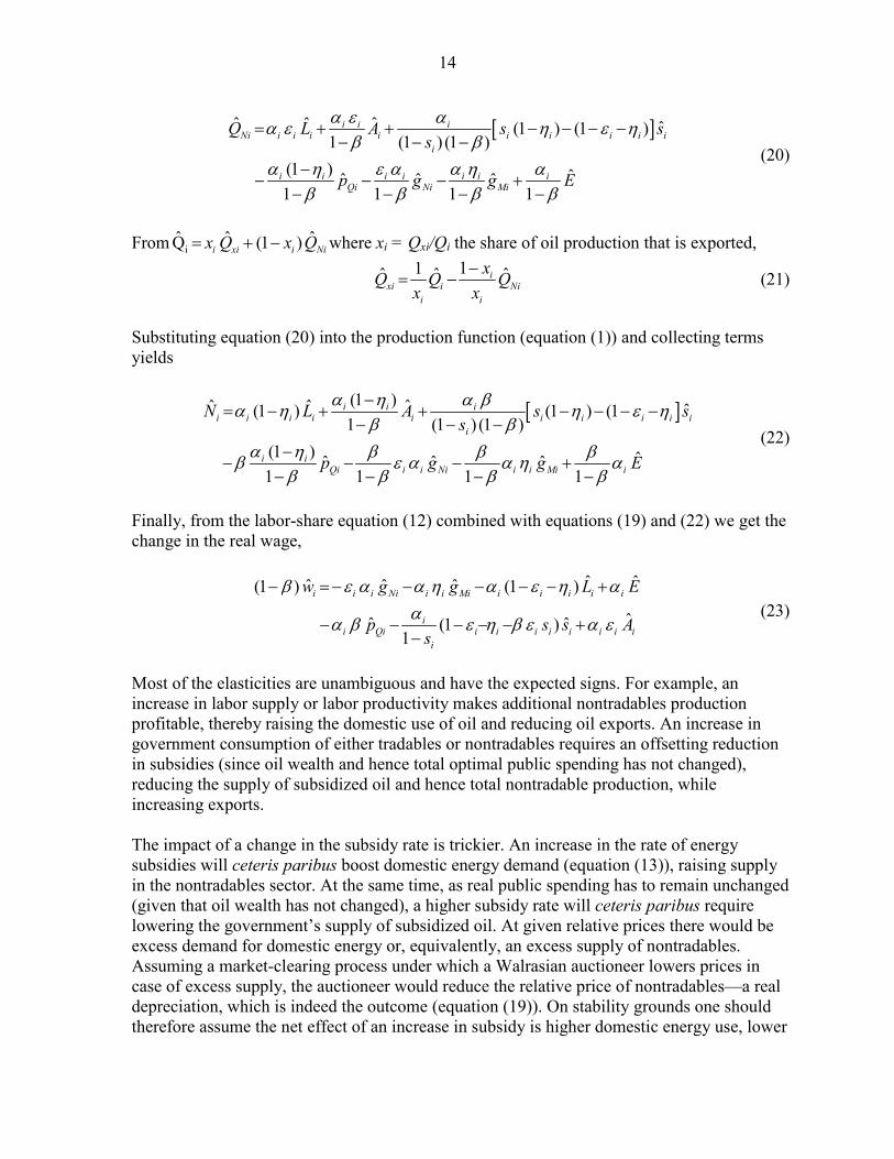
Most of the elasticities are unambiguous and have the expected signs. For example, an increase in labor supply or labor productivity makes additional nontradables production profitable, thereby raising the domestic use of oil and reducing oil exports. An increase in government consumption of either tradables or nontradables requires an offsetting reduction in subsidies (since oil wealth and hence total optimal public spending has not changed), reducing the supply of subsidized oil and hence total nontradable production, while increasing exports. The impact of a change in the subsidy rate is trickier. An increase in the rate of energy subsidies will ceteris paribus boost domestic energy demand (equation (13)), raising supply in the nontradables sector. At the same time, as real public spending has to remain unchanged (given that oil wealth has not changed), a higher subsidy rate will ceteris paribus require lowering the government’s supply of subsidized oil. At given relative prices there would be excess demand for domestic energy or, equivalently, an excess supply of nontradables. Assuming a market-clearing process under which a Walrasian auctioneer lowers prices in case of excess supply, the auctioneer would reduce the relative price of nontradables—a real depreciation, which is indeed the outcome (equation (19)). On stability grounds one should therefore assume the net effect of an increase in subsidy is higher domestic energy use, lower

15

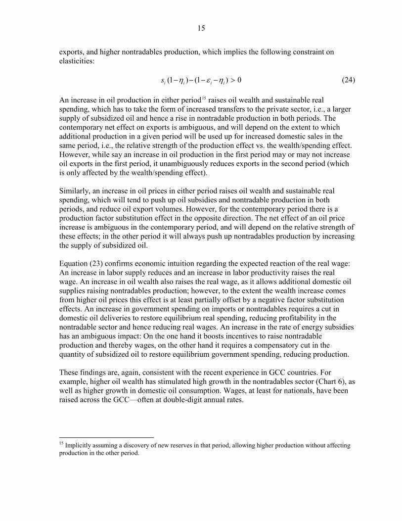
exports, and higher nontradables production, which implies the following constraint on elasticities: (1 ) (1 ) 0i i i is η ε η− − − − > (24) An increase in oil production in either period15 raises oil wealth and sustainable real spending, which has to take the form of increased transfers to the private sector, i.e., a larger supply of subsidized oil and hence a rise in nontradable production in both periods. The contemporary net effect on exports is ambiguous, and will depend on the extent to which additional production in a given period will be used up for increased domestic sales in the same period, i.e., the relative strength of the production effect vs. the wealth/spending effect. However, while say an increase in oil production in the first period may or may not increase oil exports in the first period, it unambiguously reduces exports in the second period (which is only affected by the wealth/spending effect). Similarly, an increase in oil prices in either period raises oil wealth and sustainable real spending, which will tend to push up oil subsidies and nontradable production in both periods, and reduce oil export volumes. However, for the contemporary period there is a production factor substitution effect in the opposite direction. The net effect of an oil price increase is ambiguous in the contemporary period, and will depend on the relative strength of these effects; in the other period it will always push up nontradables production by increasing the supply of subsidized oil. Equation (23) confirms economic intuition regarding the expected reaction of the real wage: An increase in labor supply reduces and an increase in labor productivity raises the real wage. An increase in oil wealth also raises the real wage, as it allows additional domestic oil supplies raising nontradables production; however, to the extent the wealth increase comes from higher oil prices this effect is at least partially offset by a negative factor substitution effects. An increase in government spending on imports or nontradables requires a cut in domestic oil deliveries to restore equilibrium real spending, reducing profitability in the nontradable sector and hence reducing real wages. An increase in the rate of energy subsidies has an ambiguous impact: On the one hand it boosts incentives to raise nontradable production and thereby wages, on the other hand it requires a compensatory cut in the quantity of subsidized oil to restore equilibrium government spending, reducing production. These findings are, again, consistent with the recent experience in GCC countries. For example, higher oil wealth has stimulated high growth in the nontradables sector (Chart 6), as well as higher growth in domestic oil consumption. Wages, at least for nationals, have been raised across the GCC—often at double-digit annual rates.

15 Implicitly assuming a discovery of new reserves in that period, allowing higher production without affecting production in the other period.

16

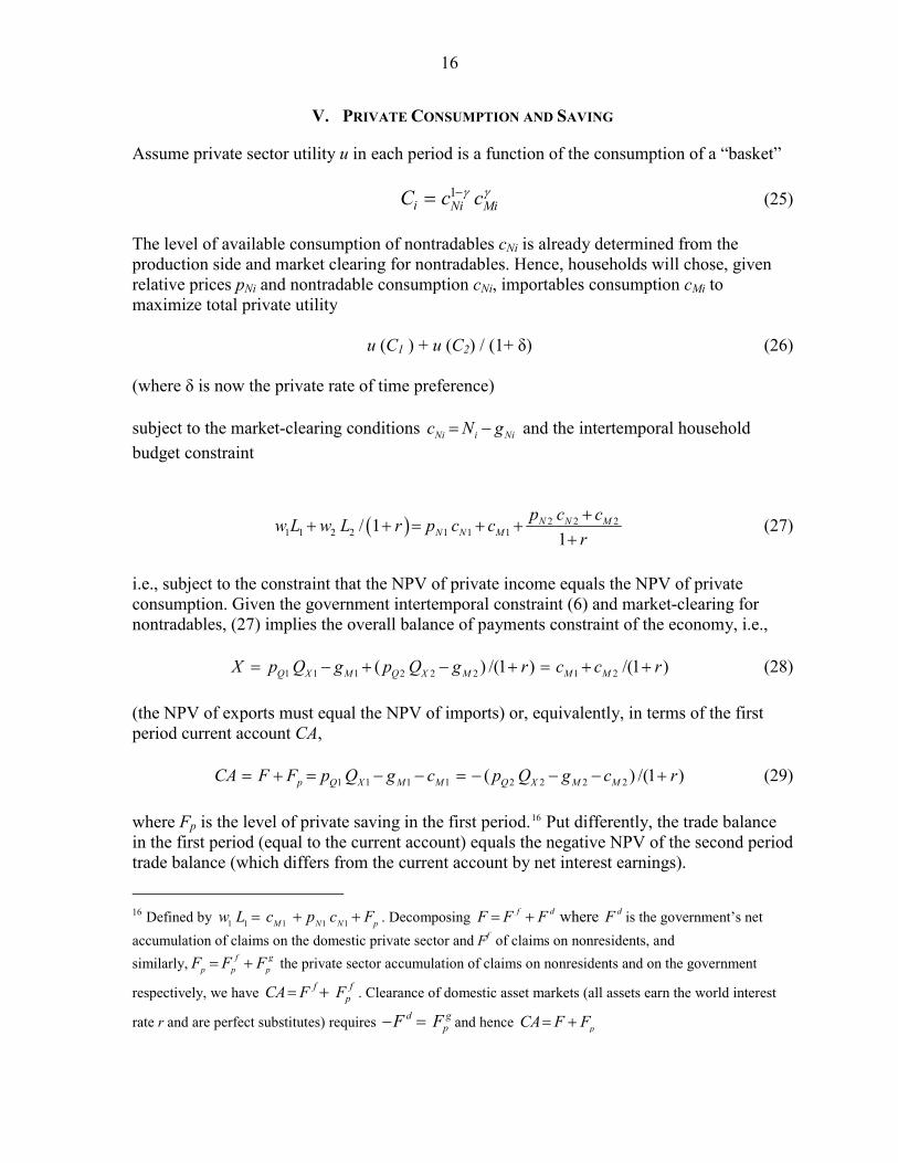
V. PRIVATE CONSUMPTION AND SAVING

Assume private sector utility u in each period is a function of the consumption of a “basket” 1

i Ni MiC c cγ γ−= (25) The level of available consumption of nontradables cNi is already determined from the production side and market clearing for nontradables. Hence, households will chose, given relative prices pNi and nontradable consumption cNi, importables consumption cMi to maximize total private utility u (C1 ) + u (C2) / (1+ δ) (26) (where δ is now the private rate of time preference) subject to the market-clearing conditions and the intertemporal household budget constraint

Ni i Nic N g= −

( ) 2 2 21 1 2 2 1 1 1/ 1

1N N M

N N Mp c cw L w L r p c c

r+

+ + = + ++

(27)

i.e., subject to the constraint that the NPV of private income equals the NPV of private consumption. Given the government intertemporal constraint (6) and market-clearing for nontradables, (27) implies the overall balance of payments constraint of the economy, i.e., (28) 1 1 1 2 2 2 1 2( ) /(1 ) /(1 )Q X M Q X M M MX p Q g p Q g r c c r= − + − + = + +

) /(1 )

(the NPV of exports must equal the NPV of imports) or, equivalently, in terms of the first period current account CA, (29) 1 1 1 1 2 2 2 2(p Q X M M Q X M MCA F F p Q g c p Q g c r= + = − − = − − − + where Fp is the level of private saving in the first period.16 Put differently, the trade balance in the first period (equal to the current account) equals the negative NPV of the second period trade balance (which differs from the current account by net interest earnings).

p

d16 Defined by . Decomposing 1 1 1 1 1M N Nw L c p c F= + + wheref dF F F F= + is the government’s net accumulation of claims on the domestic private sector and Ff of claims on nonresidents, and similarly, f g

p p pF F F= + the private sector accumulation of claims on nonresidents and on the government

respectively, we have f fpCA F F= + . Clearance of domestic asset markets (all assets earn the world interest

rate r and are perfect substitutes) requires d gpF F− = and hence pCA F F= +

17

To obtain explicit solutions, we specify17 (30) ( ) logiu C C= i

Using equations (25) and (28) transforms the problem into an unconstrained maximization, through choice of cM2, of

1 121 2log log / (1 )

1M

N Ncc X c c

r

γγ γ

2Mγ δ− −

⎡ ⎤⎛ ⎞ ⎡ ⎤− +⎢ ⎥⎜ ⎟ ⎣ ⎦+⎝ ⎠⎢ ⎥⎣ ⎦+ (31)

The first order condition immediately yields solutions

212M

rcδ

X+=

+ (32a)

112Mc Xδ

δ+

=+

(32b)

Thus optimal imports depend linearly on the NPV of net government (oil) exports. In particular,

2 11/1M M

rc cδ

+=

+ (33)

As long as the private sector discounts the future more (less) than capital markets, second period consumption of tradables will be lower (higher) than first period consumption. If r = δ, no consumption tilting occurs and imports are constant across periods and equal to the annuity corresponding to the NPV of exports:

1 212M M

rc cr

X+= =

+ (34)

17 A special case of the more general CES utility function 11

( ) 1 /(1 1/ )i iu C C σ σ−⎛ ⎞

= − −⎜ ⎟⎝ ⎠

for σ = 1. The

results for the general CES are qualitatively similar but the import demand functions are more complex and explicitly depend on the levels of nontradable consumption.

18

VI. EXTERNAL EQUILIBRIUM

Related to the question of the determinants of the equilibrium exchange rate is the issue of the equilibrium external current account of oil exporters. Fund staff estimates on current account “norms” for many countries, derived from panel estimates of the relation between current accounts and certain macroeconomic (and demographic) fundamentals (e.g. Ricci, Milesi-Ferretti, and Lee (2008)). However, such norms are more difficult to establish for oil exporters where the intertemporal aspects of the current account, as the channel to transfer oil wealth across time (through transformation in financial assets in our simple model, transformation in financial and real assets in more general settings), are central. In addition, in a more general model oil prices would follow stochastic processes and current account balances would also then reflect precautionary savings motives driven by uncertainty over future oil prices (and potentially also uncertainty over reserves and production profiles). (Bems and de Carvalho, 2008). Still, the present simple setting highlights some important features of equilibrium current accounts for oil exporters, i.e., “norms” against which actual developments may be assessed. The discussion will focus on the current account balance (CA) for the first period because the current account balance for the second period is simply–CA (no assets/liabilities are held at the end of the world after period 2). Equation (29) together with the behavioral equations for oil exports and private imports derived before describes a possible “norm” for the current account as it is consistent with public and private budget constraints (hence sustainable), and furthermore the outcome of reasonable optimizing rules (for the public sector resulting in the fiscal rule (9), for the private sector underlying the import demand function). Equation (29) highlights the important relation between budget and current account balance: barring offsetting private saving behavior, changes to the (equilibrium) budget balance translate one-to-one into changes in the (equilibrium) current account. Indeed, in many econometric investigations the budget balance is included as an explanatory variable for current account estimations. This model provides an example of why this may be misleading: the budget balance is not “exogenous” but itself jointly determined—along with the private savings balance and the real exchange rate—by the “fundamentals” i.e., the parameters determining oil wealth, domestic factor supply and productivity, and global parameters (interest rates, terms of trade). In particular, the current account for the first period is influenced by parameters pertaining to both the first and the second period: intertemporal effects matter for both the government’s period 1 oil exports and for private imports. An (trivial) benchmark is the situation where the two periods are “symmetric” in the sense that 1 2, 1 2 1,Q Q 2p p Q Q L L= = = , etc and the various elasticities also the same across periods. Then trade balances are the same in both periods, which from equation (29) implies they must equal zero. This highlights that the current account reflects intertemporal “trading opportunities” (consumption smoothing) arising from differences between the periods—if there are no such differences, the current account balance equals zero in each period.

19

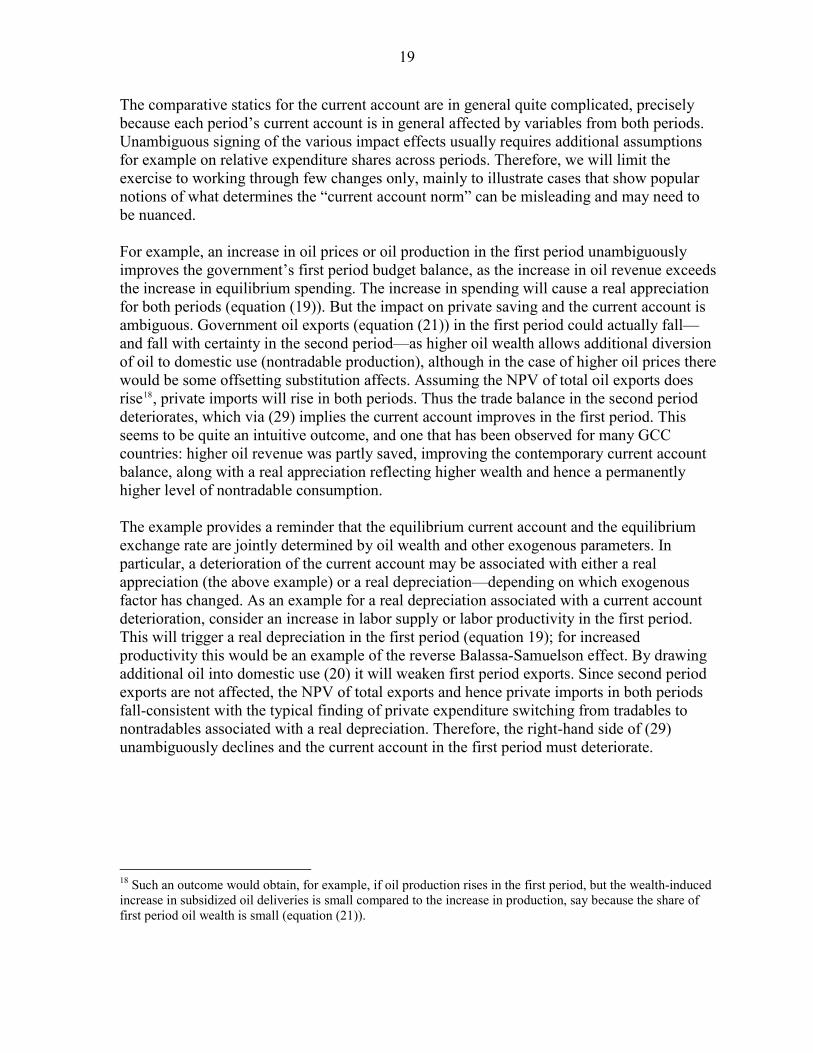
The comparative statics for the current account are in general quite complicated, precisely because each period’s current account is in general affected by variables from both periods. Unambiguous signing of the various impact effects usually requires additional assumptions for example on relative expenditure shares across periods. Therefore, we will limit the exercise to working through few changes only, mainly to illustrate cases that show popular notions of what determines the “current account norm” can be misleading and may need to be nuanced. For example, an increase in oil prices or oil production in the first period unambiguously improves the government’s first period budget balance, as the increase in oil revenue exceeds the increase in equilibrium spending. The increase in spending will cause a real appreciation for both periods (equation (19)). But the impact on private saving and the current account is ambiguous. Government oil exports (equation (21)) in the first period could actually fall—and fall with certainty in the second period—as higher oil wealth allows additional diversion of oil to domestic use (nontradable production), although in the case of higher oil prices there would be some offsetting substitution affects. Assuming the NPV of total oil exports does rise18, private imports will rise in both periods. Thus the trade balance in the second period deteriorates, which via (29) implies the current account improves in the first period. This seems to be quite an intuitive outcome, and one that has been observed for many GCC countries: higher oil revenue was partly saved, improving the contemporary current account balance, along with a real appreciation reflecting higher wealth and hence a permanently higher level of nontradable consumption. The example provides a reminder that the equilibrium current account and the equilibrium exchange rate are jointly determined by oil wealth and other exogenous parameters. In particular, a deterioration of the current account may be associated with either a real appreciation (the above example) or a real depreciation—depending on which exogenous factor has changed. As an example for a real depreciation associated with a current account deterioration, consider an increase in labor supply or labor productivity in the first period. This will trigger a real depreciation in the first period (equation 19); for increased productivity this would be an example of the reverse Balassa-Samuelson effect. By drawing additional oil into domestic use (20) it will weaken first period exports. Since second period exports are not affected, the NPV of total exports and hence private imports in both periods fall-consistent with the typical finding of private expenditure switching from tradables to nontradables associated with a real depreciation. Therefore, the right-hand side of (29) unambiguously declines and the current account in the first period must deteriorate.

18 Such an outcome would obtain, for example, if oil production rises in the first period, but the wealth-induced increase in subsidized oil deliveries is small compared to the increase in production, say because the share of first period oil wealth is small (equation (21)).

20

Appendix I We show that clearing the market for nontradable goods is equivalent to clearing the market for domestic oil input.

1 1 1 1 1 1S

N N N N Np c p g p N+ = (clearance of nontradables market)

1 1 1 1 1 0SN M p N Np N c F p gβ− − − + =

) 0

(using household constraint (37)) and wage equation (24)

1 1 1 1 1 1(1 ) 0dN N Q N M pp g s p Q c F− − − − = (zero profit conditions (24))

1 1 1 1 1 1 1 1 1(1 ) 0S dM Q N Q N M pE g s p Q s p Q c F− − − − − − = (government budget constrain (4))

1 1 1 1 1 1 1 1 1 1(1 ) ( ) 0S d SQ M Q N N Q N M pF p Q g s p Q Q p Q c F− + − + − − − − − = (fiscal rule (9))

1 1 1 1 1 1 1( ) ( ) (1 ) ( S dQ X M M p N Np Q g c F F s Q Q− − − + + − − = (collecting terms)

The first two brackets in the last equation each equal the current account (see (38)) and hence cancel out. Therefore, whenever the market for nontradables clears, the market for domestic oil will also clear, and vice versa.

21

References

Bems, Rudolf, and de Carvalho Filho, Irineu, 2008, “Current Account and Precautionary

Savings for Exporters of Exhaustible Resources” (Draft IMF Working Paper). Chudik, Alexander and Joannes Mongardini, 2007, “In Search of Equilibrium: Estimating

Real Exchange Rates in sub Saharan African Countries,” IMF Working Paper 07/90, (Washington: International Monetary Fund).

Di Bella, Gabriel, Mark Lewis, and Aurelie Martin, 2007, “Assessing Competitiveness and

Real Exchange Rate Misalignment in Low-Income Countries,” IMF Working Paper 07/201, (Washington: International Monetary Fund).

Hasan, Maher and Jemma Dridi, 2008, “The Impact of Oil-Related Income on the

Equilibrium Real Exchange Rate in Syria,” IMF Working Paper 08/196, (Washington: International Monetary Fund).

International Monetary Fund, 2008, Kuwait: 2008 Article IV Consultation—Staff Report,

Country Report 08/191, (Washington: International Monetary Fund). Lee, Jaewoo, Gian Maria Milesi-Ferretti, Jonathan David Ostry, Alessandro Prati, and Luca

Antonio Ricci, 2008, “Exchange Rate Assessments: CGER Methodologies,” IMF Occasional Paper No. 261, (Washington: International Monetary Fund).

Ricci, Luca Antonio, Gian Maria Milesi-Ferretti, and Jaewoo Lee, 2008, “Real Exchange

Rate and Fundamentals: A Cross-Country Perspective,” IMF Working Paper 08/13, (Washington: International Monetary Fund, Washington).

Obstfed, Maurice and Rogoff, Kenneth, 1996, Foundations of International Macroeconomics,

(Cambridge, Massachusetts: MIT Press).