exchange rate policy and ndogenous rice …€¦ · between exchange rate policy and price ... to...

HONG KONG INSTITUTE FOR MONETARY RESEARCH

®

EXCHANGE RATE POLICY AND ENDOGENOUS PRICE

FLEXIBILITY

Michael B. Devereux

HKIMR Working Paper No.20/2004

October 2004

Working Paper No.1/ 2000

Hong Kong Institute for Monetary Research(a company incorporated with limited liability)

All rights reserved.Reproduction for educational and non-commercial purposes is permitted provided that the source is acknowledged.

Exchange Rate Policy and Endogenous Price Flexibility

Michael B. Devereux *

The University of British Columbia

and

Hong Kong Institute for Monetary Research

October 2004

Abstract

Most theoretical analysis of flexible vs. fixed exchange rates take the degree of nominal rigidity to be

independent of the exchange rate regime choice itself. But informal policy discussion often suggests

that a credible exchange rate peg may increase internal price flexibility. This paper explores the relationship

between exchange rate policy and price flexibility, in a model where price flexibility is an endogenous

choice of profit-maximizing firms. A fixed exchange rate may increase the optimal degree of price flexibility

by increasing the volatility of demand facing firms. We find that a unilateral peg, such as a Currency

Board, adopted by a single country, will increase internal price flexibility, perhaps by a large amount. On

the other hand, when an exchange rate peg is supported by bilateral participation of all monetary

authorities (such as a monetary union), price flexibility is likely to be little affected, and may actually be

less than under freely floating exchange rates.

Keywords: Monetary Policy, Collateral Constraints, Exchange Rate

JEL Classification: F0, F4

The views expressed in this paper are those of the author and do not necessarily reflect those of the Hong Kong Institute forMonetary Research, its Council of Advisers or Board of Directors.

* email: [email protected] thank participants of the 2003 Bundesbank Spring Conference, Michael Dotsey, Fabio Ghironi, Luca Guerrieri, RobertoPerrotti, and especially three anonymous referees for very helpful comments on this paper. I thank SSHRC, Royal Bank ofCanada for financial and the Bank of Canada for financial assistance.


1

1. Introduction

The classic argument for flexible exchange rates is that they enhance the ability of the economy to

respond to shocks, in the presence of nominal rigidities (e.g. Friedman 1953). But a qualification to this

is that by eliminating the use of the exchange rate as a mechanism for adjustment, an exchange rate

peg may increase internal price flexibility within a country. This has been especially important in the

analysis of the conditions for single (small) countries to follow unilateral ‘hard peg’ policies, fixing the

exchange rate under a currency board or dollarization rule. Since these countries will generally not have

access to compensating policy responses from the monetary authorities of the currency to which they

are pegging, the need to increase internal price flexibility after a peg becomes more critical. Another

area where this discussion is important is that of the impact of a monetary union on flexibility. To the

extent that a single currency encourages price flexibility within the different regions of the monetary

union, this will reduce the loss from the absence of exchange rate adjustment. To this extent, the economic

case for a monetary union may be enhanced by the formation of the monetary union, as suggested by

Frankel and Rose (1998). 1

Is price flexibility likely to take place automatically in response to changes in monetary policy conditions,

through the decisions of individual price setters? We could think of price stickiness as being determined

by the trade-off between ‘costs of price flexibility’ (information or planning costs, for instance) and

benefits of ex-post price adjustment. These benefits would be higher, the more volatile is the environment

within which a price setter operates. If an exchange rate peg substantially increases the volatility of

demand for their product, the elimination of the exchange rate as a policy lever may cause price setters

to adjust more frequently.

This paper provides a theoretical investigation of the implications of exchange rate rules for the flexibility

of nominal prices, in an economy where price flexibility is itself endogenous. In a two-country model,

there are shocks to relative national demands, and country specific velocity shocks. Given this uncertainty,

profit maximizing firms may choose ex-ante to incur a cost so as to have the flexibility to adjust their

prices ex-post. Within this setting, we ask a) what features determine the equilibrium degree of price

flexibility, and b) in what way does an exchange rate peg affect the degree of price flexibility?

The incentive for ex-post price flexibility for any one firm is higher, the greater is the variance of nominal

demand it faces for its good. An increase in monetary variability will increase the variance of nominal

demand. But the variance of nominal demand will also depend on the degree of price flexibility itself.

This introduces a strategic interaction between the pricing decisions of firms. We find that, for standard

parameter values, the incentive for flexibility is increasing in the total number of firms who choose to

adjust their ex-post prices; there is a strategic complementarity in the choice of flexibility. If only a small

number of price setters adjust their price, then there may be little incentive for the marginal price setter

to pay the menu cost. But if all price setters choose to adjust, the volatility of prices will increase the

overall volatility of demand facing a price setter, increasing the incentive for a given firm to adjust.

1 In the discussion of EMU, the likelihood of wage and price flexibility being enhanced by the single currency was considered,e.g. OECD, (1999).

Working Paper No.20/2004

2

How does exchange rate policy affect the degree of price flexibility? The key feature of a fixed exchange

rate is that it requires that monetary policy to adjust to internal and external shocks in lieu of exchange

rate adjustment. Whether or not this enhances price flexibility depends on whether the policy increases

the volatility of firm’s demand. The answer to this depends on the type of shocks that occur, and the

way in which the fixed exchange rate system operates.

We first focus on a one-sided peg, which describes a situation where one country fixes its exchange

rate against a trading partner, and accepts sole responsibility for maintaining the peg. Our model predicts

unambiguously that such an arrangement will increase internal price flexibility in the pegging country,

while leaving foreign price flexibility unchanged. In a one-sided peg, the domestic monetary authority

must respond to all shocks, domestic and foreign, in order to protect the peg. This must lead to an

increase in the overall volatility of nominal demand facing firms. Therefore, more firms will choose to

incur the costs of price flexibility.

However, a cooperative peg, involving active participation of all monetary authorities, has an ambiguous

effect on price flexibility, depending on the source of shocks. If most shocks are ‘real’, coming from

fluctuations in relative demand for one country’s good relative to another, then a cooperative peg also

will increase price flexibility in all countries. But if most shocks are ‘monetary’ coming from exogenous

shocks to the velocity of money, then a cooperative peg will reduce price flexibility in all the pegging

countries.

How big is the impact of an exchange rate change on price flexibility? By strongly linking the decisions

of each agent with that of other agents, the presence of strategic complementarity allows for changes in

the external environment to have a potentially very large effect on the equilibrium degree of price flexibility.

We illustrate this point by exploring the effect of the exchange system on output and relative price

volatility.

Holding the degree of price flexibility constant, a unilateral peg will lead to a substantial increase in

output volatility, and a large fall in terms of trade volatility. But the peg itself increases the incentive for

firms to have flexible prices. If there is substantial strategic complementarity in the choice of price

flexibility, then there may be a very large increase in the share of price setters choosing the option of

expost flexibility. For a standard parameterization of the model, we find that this indirect effect of the

exchange rate peg on price flexibility can be of the same order of magnitude as the the direct effect of

the increased volatility in nominal aggregate demand coming from the peg itself. As a result, the volatility

of GDP remains essentially unchanged after a move from floating exchange rates to a unilateral peg.

The volatility of the terms of trade however, is substantially reduced, because the peg tends to cause

nominal prices to co-move positively across countries. The endogenous adjustment in price flexibility

therefore can explain why a comparison of fixed and floating exchange rates may show little differences

in the behavior of GDP, but substantial differences in relative price variability. This ‘puzzle’ has been

discussed by Baxter and Stockman (1990), Flood and Rose (1995) and others.

How does the presence of endogenous price flexibility affect optimal monetary policy rules? In general,

if monetary authorities wish to target the flexible price equilibrium allocation, they will set policy so that

firms never have to adjust prices. As a result, the possibility of endogenous price flexibility will not affect


3

the optimal monetary rule (see Dotsey King and Wolman (1999)). In our model, the flexible price allocation

is inefficient due to the absence of complete international financial markets. As a result, an optimal

monetary rule does not replicate the flexible price allocation. In principle, this could mean that the

presence of endogenous price flexibility significantly alters optimal monetary rules, relative to an economy

with exogenously sticky prices. But in our calibrated model, we find that optimal monetary rules are

almost the same as those in an economy with exogenously sticky prices. An optimal monetary policy in

the model allows for only a very very small degree of price flexibility.

The paper is related to a large recent literature evaluating the effects of monetary rules in sticky price

equilibrium models . But our departure is in allowing for the degree of price stickiness itself to be an

endogenous variable. In this respect, the paper is related to the literature on state-dependent pricing

and menu-costs of price change (see Ball and Romer 1991, Dotsey, King and Wolman, 1999). The

model is most closely related to Ball and Romer (1991). They show the possibility of multiple equilibrium,

in an environment where price setters can choose ex-post whether to adjust prices, given a common

menu cost of price change, within a one-country environment. Our analysis differs because we allow a

distribution of firm specific menu costs, and we assume that price setters choose in advance whether or

not to have the ex-post flexibility to adjust price. This is more in line with the view that a large change in

monetary policy regime (e.g. fixing the exchange rate) may lead to structural changes in the flexibility of

contracts within a monetary economy. Moreover, our focus is not primarily on multiple equilibrium, but

more on the role of strategic complementarity in the choice of flexibility. Finally of course, we use a two

country model.

The next section sets out the basic technology of endogenous price flexibility for a given firm. Section 3

incorporates this model into a two country general equilibrium environment. Section 4 examines the link

between price flexibility and the exchange rate regime. Section 5 investigates the predictions of the

model for output and relative price volatility, while section 6 discusses the optimal monetary policy

under endogenous price flexibility. Some conclusions follow.

2. The Firm and the Choice of Price Flexibility

We first describe the decision faced by a single firm with respect to the choice of price flexibility. In the

typical model of state dependent pricing 2, a firm chooses whether or not to adjust its price ex-post,

given information on its demand and cost, by trading off the benefits of price adjustment relative to the

direct (e.g. menu) costs of price change. By contrast, our assumption is that the firm must invest ex-

ante in flexibility. That is, a firm must choose ex-ante whether to have the flexibility to adjust its price ex-

post, after observing the realized state of the world. The firm incurs a fixed (labor) cost in order to have

this flexibility. Roughly speaking, this decision may correspond more accurately to the way in which

changes in monetary policy or other structural features of the economy would impact on the institutional

characteristics of nominal price or wage setting.

2 See, e.g. Dotsey King and Wolman (1999).


4

Let a firm have the production function

(2.1)

where is the firms output, is total employment, and is a firm-specific fixed cost of flexibility.

Assume that the firm knows . We let be an indicator variable, whereby if the

firm chooses to (not to) incur the cost of ex-post price flexibility. The firm’s production function indicates

that it has some firm specific factor of production, together with which it combines labor to produce

output for sale.

Assume that the firm faces market demand: 3

(2.2)

where is the firm’s price, is the (possibly stochastic) industry price, is the firm’s own elasticity

of demand, and is the (stochastic) total market demand shock. Assume the the firm faces a wage

(also stochastic) . From the production technology (2.1), the firms total operating cost is

(2.3)

Assume that the firm evaluates its expected profits using a stochastic discount factor . 4 Then discounted

expected profits may be written as

(2.4)

We further assume that the firm knows the distribution of the discount factor, the market demand and

the wage.

The firm chooses to maximize (2.4). If , then the firm can choose its price after observing ,

and , and it sets the following price:

(2.5)

where , and . When , the firm’s price is a constant

markup over the wage. But when , the optimal price will depend on a geometric average of the

wage and market demand.

3 We use this form of demand because it is obtained from the general equilibrium model analyzed below.

4 In the next section, we determine from the preferences of the firm’s household-shareholders.


5

When , the firm must choose the price ex-ante. In that case, its optimal price is given by:

(2.6)

When the wage and market demand are known ex-ante, (2.5) and (2.6) give the same answer. But in

general the two prices will differ, even in expectation, as the distribution of market demand and wages

will influence the mean pre-set price that the firm sets.

Now substituting (2.5) and (2.6) respectively into the expected profit function (2.4), we may evaluate the

firm’s expected profits (excluding fixed costs) under and . Let , then:

(2.7)

(2.8)

where . What determines whether the firm incurs the fixed cost of price flexibility? The

firm will choose whenever the gain in discounted expected profits exceeds the discounted

expected fixed costs. That is, whenever

Since is known to the firm ex-ante, . We can therefore rewrite this condition as

(2.9)

where represents the gain to price flexibility.

2.1 Approximation of 2.9

To provide analytical results in the next section, we can evaluate the gains to price flexibility by taking a

second order logarithmic approximation to around the mean value . In the Appendix, it is

shown that

(2.10)

where represents profits evaluated at the unconditionalmean ,

and represents the variance of the wage, market demand, and their covariance.

From (2.10), we see that, up to a second order, the incentive for a firm to incur the costs of price

flexibility depends on the variance of the wage, the variance of market demand, and their covariance.

Note that if , so that marginal cost is independent of output, then uncertainty in market demand


6

gives no incentive for flexible prices, and the gains from flexibility depend only on uncertainty in wages.

Intuitively, if , then optimal expected profits are linear in market demand, and further, if the wage

is known, then the firm’s price is the same whether it is set before or after is observed. In this case,

there is no gain to price flexibility. More generally however, optimal profits are convex in when prices

are flexible, but linear in under a fixed price. Hence, wage volatility raises expected profits when

prices are flexible relative to expected profits with preset prices. When , optimal profits are concave

in market demand , either when prices are flexible or fixed. But, intuitively the optimized profit function

is more concave in demand when prices are fixed than when they are flexible. Hence, uncertainty in

market demand increases the benefits to price flexibility, for .

Finally, we note that (2.10) does not depend on the properties of the stochastic discount factor . Up to

a second order approximation, the discount factor affects profits of fixed and flexible price firms in the

same way.

2.2 Determination of Price Flexibility in the Aggregate

The left hand side of (2.9) is common to all firms. Hence, firms will differ in their choice of price flexibility

solely due to differences in their specific fixed costs of flexibility. Without loss of generality, let each firm

draw from a distribution of fixed costs, , described by; . Hence firms are

ranked according their fixed cost of flexibility. In that case, we may describe the determine of price

flexibility in the aggregate as the measure of firms, who choose to incur the fixed cost of

price flexibility. Then is determined by the following condition:

(2.11)

(2.12)

This condition gives a link between the underlying uncertainty facing firms and the aggregate degree of

flexibility in the economy. So far however, we have left unexplained. In the next section we develop a

two country model that identi¯es the macroeconomic sources of the uncertainty facing firms.

3. A Two Country Model

Consider a two country world economy, where countries are called ‘home’ and ‘foreign’. Foreign variables

are denoted with an asterisk. In each country, there are consumers and firms, who have a single period

horizon. There is a continuum of households in each country along the unit interval, consuming both

home and foreign goods. Households receive income from wages and the ownership of firms. Firms

have the production technology as described by the previous section, and sort themselves into two

categories; those with fixed prices, and those with flexible prices.


7

3.1 Households

The home country household , has preferences given by:

(3.1)

where is a composite of the consumption of home and foreign goods, given by:

(3.2)

and is the price index, given by , where is the foreign currency price of

foreign goods. represents the relative preference for home goods. is the quantity of domestic

money held. We assume is a random variable which will capture shocks to the consumption velocity

of money. In addition, we let , the weight of the home good in composite consumption, also be a

random variable, with mean 0.5.

Assume foreign country preferences are identical to home, except that foreign household’s value foreign

money, and assume that (the foreign velocity shock) and are i.i.d. The random foreign composite

consumption weight is the same as that of home residents.

Consumption of home and foreign goods are differentiated, so that for household , the home good

consumption and price indices are

(3.3)

where . The indices for the foreign good are analogous.

Home household i faces the budget constraint:

(3.4)

where is initial money holdings, is the transfer from the monetary authority, and is total

profits of the final good firms.

Households choose money balances, labor supply, and consumption of each good to maximize utility,

subject to their budget constraint5 . We get the demand for each good, and , that of money

balances, and implicit labor supply as:

(3.5)

(3.6)

5 Households act after the realizations of the preference shocks are observed.


8

3.2 Firms

Firms in each country set prices, based on the technologies described in the previous section, and

demand coming from home and foreign consumers. In the home country for instance, a measure z of

firms set prices after the state of the world is realized, and set prices in advance.

The condition given by (2.11) (or 2.12) determines the size of the flexible price sector. Total profits of all

firms are written as:

(3.7)

3.3 Equilibrium

We focus on symmetric equilibria where all households and firms within a country are alike. Equilibrium

is defined in the usual way. Given money market clearing, , households ex post budget

constraints are given by:

(3.8)

The goods market for each category of firm implies that

(3.9)

(3.10)

Labor market clearing implies

(3.11)

where the last term on the right hand side denotes the fixed cost incurred by the measure of firms that

choose price flexibility.

Analogous conditions hold for the foreign economy.

We may define aggregate real GDP by aggregating over fixed and flexible price firms. Thus:


9

3.4 Equilibrium for given price flexibility

For given and , the equilibrium is very simple to characterize. Using the definition of aggregate GDP

and the household budget constraint, that . Hence we may write the money market

equilibrium condition as

(3.12)

Using this in combination with the goods market equilibrium (3.9) and (3.10), and aggregating, we get

solutions for both the exchange rate and GDP as:

(3.13)

A home country monetary expansion causes exchange rate depreciation, while a positive home country

velocity shock causes an appreciation. A shift in relative world demand towards home goods (rise in )

causes an appreciation. Home GDP is determined by the value of home real balances, in terms of home

goods, relative to the home velocity shock.

Since demand for the individual firm may be defined from (3.9) and (3.10), and wage determination is

given from (3.6), we may use (2.5) and (3.12) to define the flexible price firm’s price as:

(3.14)

The appropriate discount factor for firms is given by . 6 Then we can write as:

(3.15)

The domestic good price index is

(3.16)

Using this, (3.9), (3.10), and (3.11), we may write employment as

(3.17)

6 This is the households marginal utility of a dollar of home currency.


10

3.5 The determination of optimal price flexibility

To determine equilibrium price flexibility, we use condition (2.11) (or 2.12) from the previous section, in

combination with the values of , , and implied by the two-country general equilibrium model.

From the model equilibrium, market demand and the wage written as:

(3.18)

This, in combination with equations (3.14) - (3.17), and (2.11) determine the values of , , , , ,

, and for the home economy.

Notice that the simple structure of the model implies that the two economy’s dichotomize. The home

wage, demand, prices, employment, and equilibrium price flexibility are determined solely by the behavior

of home nominal aggregate demand . Conditional on the domestic money supply, the equilibrium is

independent of the distribution of foreign shocks and foreign monetary policy, as well as movements in

the share parameter . This result arises from the unit elasticity of substitution between home and

foreign goods. For given M, shocks to foreign demand are offset by movements in the exchange rate, so

as to leave overall demand for the home country’s good unchanged.

In general the model has no exact analytical solution. In the quantitative section below, we report results

from the numerical solution of the exact (stochastic) model, for a given calibration. Here however we

describe an approximate solution using the second-order approximation used in (2.10). In order to

determine the gains to price flexibility using (2.10) we must obtain the variance of and . We

may write these as:

(3.19)

(3.20)

For given , the model is log linear except for the price index equation (3.16) and the aggregate employment

term (3.17). In the Appendix, it is shown that and may be approximated around the mean values

and (where we use lower-case letters to denote deviations from means i.e.

) as:

(3.21)

(3.22)

Here represents the log deviation of the velocity shock from its mean value, is a constant term

given in the Appendix , and is an increas ing funct ion of , which sat is f ies

and . Note that, by the definition of , we have

.


11

Substituting (3.21) and (3.22) into (3.20) and (3.19), and then substituting into (2.10), we obtain the

conditions

(3.23)

(3.24)

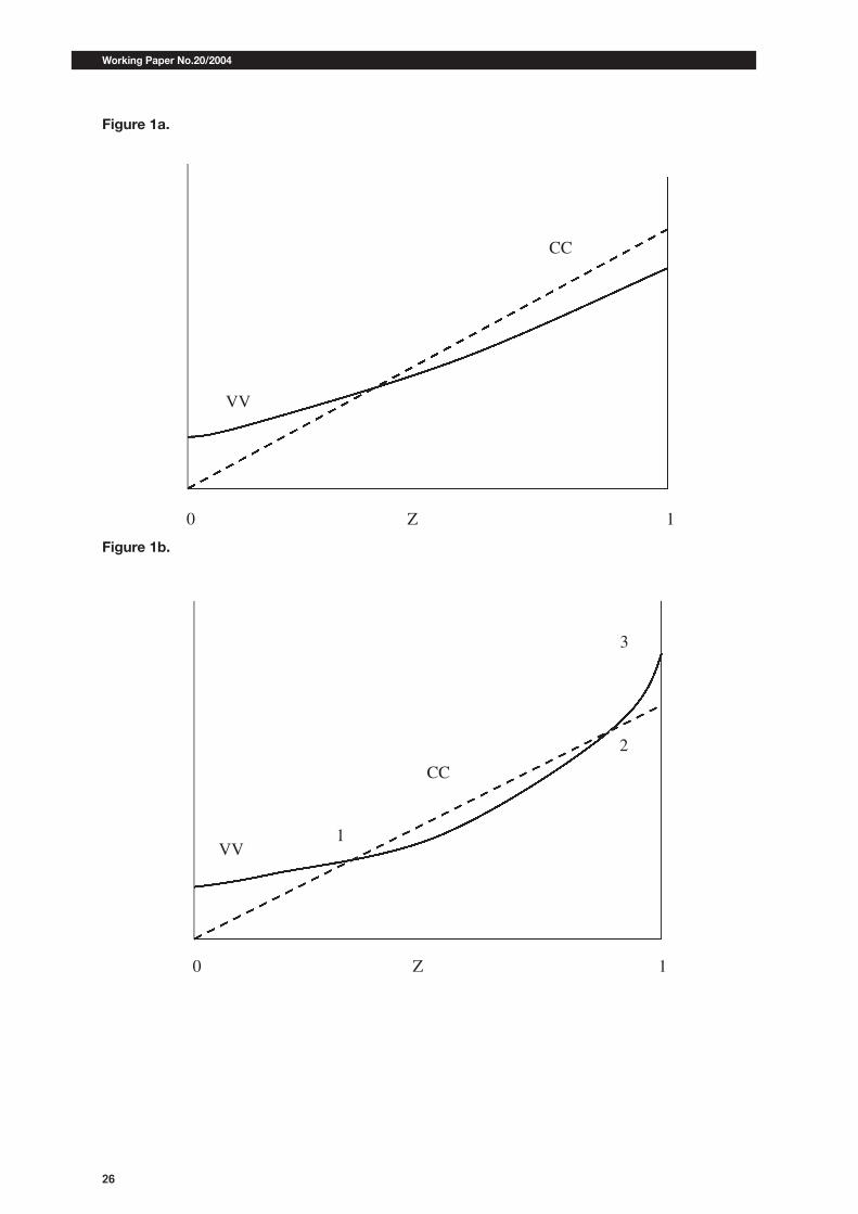
Figure 1a illustrates the determination of . The VV locus illustrates the left- hand side of condition

(3.23). This represents the benefit of price flexibility to the marginal price setter as measured along the

horizontal axis. This is higher, the higher is the variance of nominal aggregate demand (which

also equals ). The CC locus represents the fixed flexibility cost facing the marginal price setter. The

CC locus is upwards sloping, by assumption; marginal firms have higher costs of price flexibility. The VV

locus is also upward sloping, under the condition that . This is explained by the link between

the decisions made by all other firms and the incentive of any one firm to have flexible prices. To see this

relationship, focus on the flexible price firm’s optimal pricing policy, obtained from 3.14, which is written

as:

Say that there is a money shock which gives rise to a desire for the flexible price firm to adjust its price

upwards (both because the money shock increases demand directly, and increases the wage). The

extent to which the firm will adjust depends on the number of other firms z who also adjust. When other

firms adjust, this gives rise to two opposing forces. First, given that other firms raise their price, market

demand for any one firm rises, given that . This leads the firm to want to raise its price by

more, so long as , since its marginal cost is rising. But counter to this, the rise in the price

of other firms will reduce real balances , reducing the home demand for labor. This reduces the real

wage facing the firm, and reducing its desired price adjustment. If the first effect dominates, then the

price response of the firm to a money shock is increasing in . If the second effect dominates, the price

response is declining in . The first effect will dominate whenever . An equivalent

interpretation can be given for the case of shocks.

A given firm’s ex-ante incentive for price flexibility depends on how much it would wish to adjust its

price in response to a shock. If , then in response to a shock, the firm will have

a greater incentive to adjust its price, the greater is the measure of other firms adjusting. Hence the VV

curve is both upward sloping in . Intuitively, this is more likely, the flatter is labor supply (lower is ), the

higher is the market elasticity of demand , and the more upward sloping is marginal cost (lower is ). If

the VV curve is upward sloping, there is a strategic complementarity in the pricing decisions of firms; the

greater the measure of other firms adjusting to a money shock, the greater is the incentive of any one

firm to adjust its own price. Moreover, VV is also convex in if , so that the

marginal incentive to change prices as an additional firm changes its price is higher, the greater the

number of firms already changing prices. In the opposite case, when , the VV curve

is actually downward sloping, and there is a strategic substitutability between the pricing decisions of


12

firms. In the discussion below, we find that the conventional calibration suggests that

. In light of this, we focus henceforth on the case where the VV curve is upward

sloping.

It is clear that there is the possibility of multiple equilibrium. While Figure 1a describes the case of a

unique equilibrium, Figure 1b characterizes a situation where the VV curve intersects twice with the CC

curve. There are three equilibria, corresponding to low , , and an intermediate value of (unstable

based on the usual reasoning). In the low z equilibrium, a small fraction of firms choose price flexibility,

weakening the incentives for other firms to have flexible prices. But when , the volatility of demand

is so great that all firm’s will willingly pay the costs for flexibility, because all others do. Therefore,

multiple equilibria are generated by strategic complementarity in price setting. This strategic

complementarity, and the possibility of multiple equilibrium, is greater, the lower is , the lower is ,

and the higher is .

In general, for different assumptions regarding , there may be multiple crossing points. An equilibrium

with high price flexibility is not necessarily associated with full flexibility.

We may state a condition for a unique equilibrium as:

Condition 1

If is uniform, so that , for , then there is a unique equilibrium whenever

The left hand side of this expression gives the value of the VV curve at , while the right and side

gives the value the CC curve at . Since in this case CC curve is a straight line, and VV is convex,

so long as VV falls below the CC curve at , then a unique equilibrium is assured.

4. Price Flexibility and the Exchange Rate Regime

We now focus on the impact of monetary policy and the exchange rate regime on the equilibrium degree

of price flexibility. We assume henceforth that the equilibrium is unique. From (3.23), it is immediate to

see that an increase in the volatility of money or velocity will increase the degree of price flexibility. To

see how the exchange rate regime will affect price flexibility, we note that the exchange rate, in log

deviation form, may be written as

(4.1)

There are different ways to define an exchange rate policy. This requires us to specify both the form of

the monetary rules, as well as the degree to which each country participates in the monetary policy.

Since our objective in this section is just to describe the link between exchange rate policy and price

flexibility, we focus on a simple monetary rule where the authorities of one or both countries target the


13

exchange rate directly. This has the advantage that it allows for variation in the importance that exchange

rate stability plays in policy.7

With respect to the degree to which each country participates in the exchange rate policy, we describe

two alternatives. A unilateral or one-sided policy is a situation where one country alone follows a monetary

rule to target the exchange rate. Alternatively, a bilateral (or cooperative) exchange rate policy is one

where both monetary authorities target the exchange rate 8 In a unilateral policy, the home monetary

authority follows the rule , where is the degree of exchange rate intervention, and the

foreign country maintains a passive monetary rule, . Under a bilateral policy, both home and

foreign monetary authorities target the exchange rate, using the rules and . In both

cases, a value of corresponds to a freely floating exchange rate, and corresponds to a

fixed (or pegged) exchange rate.

Under these intervention rules (whether unilateral or bilateral), the exchange rate can be described as

Using this, and (3.23), we may establish:

Proposition 1

a) The degree of price flexibility is higher under a unilateral peg than under a freely floating exchange

rate. b) in the absence of velocity shocks, is uniformly increasing in the degree of exchange rate

intervention under a unilateral peg.

Proof: Under the assumptions made, is determined by

(4.2)

where

The first part of the proposition follows because the left hand side is higher when (fixed exchange

rate) than under (floating exchange rate). Then, as long as the equilibrium is unique, the right

hand side must be increasing in .

7 Below we compare this to a situation where monetary policy can directly target the stochastic disturbances. Note that themonetary rules here are not chosen optimally, in a welfare sense. We describe the welfare maximizing monetary rules insection 4 below.

8 These definitions were first made by Helpman (1980).


14

The second part of the proposition follows because, without velocity shocks (i.e. ), the left hand

side of the above condition is always increasing in .

To see the result more intuitively, note that equilibrium price flexibility will be higher, whenever the

variance of is higher. But in order to keep the exchange rate from changing in face of relative

demand shocks, the variance of must rise. Thus, in face of shocks, a one-sided peg tends to

increase . Without relative demand shocks, var is equal to var , both under a floating exchange

rate and under a unilateral peg. Although the peg offsets shocks, it must adjust the money supply to

prevent from affecting the exchange rate, so as to leave var unchanged. Hence, when relative

demand and velocity shocks are put together (and velocity shocks have equal variance), var

must be higher in a one sided peg than under a floating exchange rate.

This suggests that a policy of pegging the exchange rate should enhance the price flexibility of the

economy, if the exchange rate rule takes the form of a one-sided or unilateral peg, and velocity shocks

are equally volatile across countries. The one-sided intervention rule will always increase the volatility of

aggregate demand facing price setters. How does this compare to a bilateral pegged exchange rate? In

this case, we have:

Proposition 2

The degree of price flexibility may be higher or lower with a bilateral exchange rate peg than a freely

floating exchange rate, depending on the size of relative demand shocks and velocity shocks. In the

absence of relative demand shocks, is lower under a bilateral peg.

Proof: In this case, is determined by

(4.3)

When , the variance terms inside the expression (4.3) become . From this condition,

we see that, without relative demand shocks, the volatility of nominal aggregate demand is strictly lower

under a bilateral peg than under a freely floating exchange rate. Moreover, because each monetary

authority cooperates in offsetting demand shocks, the volatility of aggregate demand specifically due to

relative demand shocks is reduced, relative to that in a one-sided peg.

Intuitively, under a bilateral peg, in the case of velocity shocks alone, then var is lower, because

countries cooperate in eliminating these shocks, rather than putting the onus all on the pegging country.

As a result, the volatility of aggregate demand due to velocity shocks in both countries is reduced,

whereas with a one-sided peg, the pegging country has to absorb the full effect of the velocity shock in

the foreign country. Likewise, a bilateral peg also reduces the volatility of aggregate demand due to

relative demand shocks, as compared with a one-sided peg, again because both countries respond to

relative demand shocks.


15

Proposition 2 Corollary

There is always more price flexibility in a country that follows a one-sided peg than in a country that

engages in a bilateral fixed exchange rate. Proof: this is demonstrated in the previous discussion.

The variance of nominal aggregate demand is always higher under a one sided peg. Hence, price

flexibility must be greater in this case. Note also that in the cooperative peg, and are equal. The

cooperative peg affects price flexibility in both countries, whereas the one-sided peg affects price flexibility

in the pegging country alone.

From Propositions 1 and 2, we see that the question of whether a pegged exchange rate enhances

price flexibility depends on the nature of the shocks as well as the nature of the peg. When relative

demand shocks are the principal source of exchange rate fluctuations, then an exchange rate peg will

enhance price flexibility, and more so in a country that adopts a one-sided peg. In order to stabilize the

exchange rate following shock, countries must follow a pro-cyclical monetary policy, which increases

the variance of nominal aggregate demand, and hence encourages more price flexibility on the part of

firms. But when all exchange rate volatility is caused by velocity disturbances, an exchange rate peg will

either leave price flexibility unchanged (in a one sided peg), or actually reduce overall price flexibility (in

a bilateral peg).

How would these results be altered if we instead made the assumption that countries could fix the

exchange rate by directly reacting to the shocks themselves, rather than by indirectly doing so by way

of an exchange rate intervention rule? Essentially the same conclusions apply. In the case of a one-

sided peg, the monetary rule given by keeps the exchange rate fixed. This would

increase the var due to relative demand shocks, while leaving the variance due to velocity

shocks unchanged, and hence would increase the degree of price flexibility. In a bilateral peg, the

rules and ensure a fixed exchange rate. They eliminate the component of

var due to velocity shocks, but increase the component of this variance due to relative demand

shocks.

We have assumed that variance of velocity shocks is equal in the two countries. But imagine that

. We might think of this as a case where overall monetary/financial stability is higher in the

foreign country, and the home country chooses a pegged exchange rate in order to ‘import’ stability

from abroad. This has been a common rationale for fixed exchange rates in countries with a history of

monetary instability, especially in Latin America. Under this change, z is determined by the condition:

(4.4)

Now it is no longer necessarily true that the left hand side is increasing in . If is sufficiently greater

than , and relative demand shocks are unimportant, then even a one-sided peg can reduce overall

aggregate demand volatility, and reduce the equilibrium degree of price flexibility. If a country follows a

policy of pegging its exchange rate to import monetary stability from abroad, then the overall instability

of nominal aggregate demand may fall rather than increase.


16

5. Output and Relative Price Stability

The traditional view of floating exchange rates (e.g. Friedman (1953)) argues that the exchange rate acts

as a ‘shock absorber’. A freely floating exchange rate helps to stabilize output in response to relative

demand shocks, because it allows for a greater adjustment of relative prices. This suggests that the

volatility of output should be higher under an exchange rate peg than under a float, while the volatility of

the terms of trade should be lower. In our model, home country output is given by . Taking a

linear approximation, using the approximation for the home price index given by 3.21, we for we can

write:

(5.1)

From this expression, we may establish:

Proposition 3

If an exchange rate peg increases the volatility of output for a given degree of price flexibility, then it will

also increase the degree of price flexibility.

Proof: Expression (5.1) makes clear that output volatility will rise, for a given , whenever the volatility of

rises. But this is exactly the same condition for an increase in price flexibility under Propositions

1 and 2.

Thus, holding constant, a unilaterally pegged exchange rate will always increase output volatility,

when the volatility of velocity shocks is equal across countries. More generally, output volatility is higher

(for fixed ) under a fixed exchange rate when the variance of is dominated by relative demand

shocks.

But with endogenous movements in , there is a countervailing force. As rises, a higher fraction of

firms choose to adjust prices ex-post, and this tends to stabilize output. Hence, the indirect effects of

an exchange rate peg, through endogenous price flexibility, run counter to the direct effects, through

increasing the volatility of aggregate demand.

A similar conclusion may be obtained by looking at the terms of trade. We define the terms of trade as

. Denoting this in log changes as , we have

(5.2)

When and are close to zero (when most prices are sticky), a fixed exchange rate prevents any terms

of trade adjustment at all. But allowing price flexibility to respond to a peg creates terms of trade volatility

through nominal price adjustment.


17

Is it possible that, taking both the direct effect on volatility and the indirect effect through increased

price flexibility, that overall macroeconomic volatility is similar across exchange rate regimes? Although

it is to be expected that endogenous price flexibility would lessen the impact of an exchange rate peg

on output volatility, it would seem unlikely that this indirect response to the policy change would reverse

the effects of the change itself. But in the presence of strategic complementarities in price setting

behavior, even small policy changes might have substantial effects. Because both the benefits and

costs of flexibility are increasing in the number of firms that choose flexibility, the indirect effect of policy

changes, through movements in equilibrium price flexibility, may be of the same order as the direct

effects.

Figure 2 and Table 1 provide a quantitative illustration of this result. We calibrate the model so that the

standard deviation of relative demand shocks and velocity shocks is both set at 2 percent. The elasticity

of substitution between categories of goods is set at 11, corresponding to the standard ten percent

markup of price over marginal cost reported in Basu and Fernald (1997). The consumption constant

elasticity of labor supply is set to unity, following Christiano, Eichenbaum and Evans (1999). We

assume that the distribution is uniform. In the calibration, we choose the cost function so that if all

firms were choosing ex-post price flexibility, the total cost of this would be only 3 percent of GDP. This

corresponds to the quantification of costs of price change as measured by Zbaracki et. al. (2000), and

the calibration used in Dotsey et. al. (1999).

Table 1 illustrates the implications of alternative exchange rate regimes with and without endogenous

price flexibility.9 Under a floating exchange rate, output volatility is 1.7 percent, while terms of trade

volatility is 6 percent. The fraction of firms choosing ex-post price flexibility is only 10 percent. Now if we

impose a one-sided pegged exchange rate, but hold the degree of price flexibility unchanged, the

second column of the Table shows that output volatility more than doubles to 4.2 percent, while terms

of trade volatility falls to 0.2 percent. By contrast, allowing for endogenous price rigidity shows a dramatic

rise in the fraction of firms choosing ex-post price flexibility – rises from 10 percent to 68 percent. As

a result, output volatility is stabilized – the standard deviation of output falls to 1.8 percent – effectively

the same as under floating exchange rates. On the other hand, the volatility of the terms of trade is now

only 2.6 percent, rather than 6 percent under the floating exchange rate. Hence, comparing floating and

fixed exchange rates in the presence of endogenous price flexibility, we see that the fixed exchange

rate regime leads to a large drop in terms of trade volatility, but effectively no movement in output

volatility. The increased flexibility of nominal prices tends to offset the direct increase in macroeconomic

volatility introduced by a fixed exchange rate.

How can fixed exchange rates reduce terms of trade volatility, while leaving output volatility essentially

unchanged? Holding price flexibility constant, the peg leads output volatility to rise substantially, and

eliminates almost all terms of trade volatility. As price flexibility increases, output volatility declines, as

nominal prices adjust to offset relative demand shocks. The rise in price flexibility also raises terms of

trade volatility, but this effect is limited, because to the extent that nominal prices are flexible, the

9 As discussed in footnote ( ), Table 1 is constructed by exact numerical solution of the stochastic non-linear model. Details aregiven in the Appendix.


18

pegged exchange rate ensures that home and foreign prices respond identically to velocity shocks; the

peg means that foreign velocity shocks become common ‘world’ nominal demand shocks, so that

relative prices are not affected by these shocks. In the pegged exchange rate regime therefore, the

terms of trade can be affected only by relative demand shocks – it is unaffected by either home or

foreign velocity shocks. As a consequence, a unilateral exchange rate peg may significantly reduce

terms of trade volatility, but leave output volatility essentially unchanged.

These results may help to throw light on the well-known puzzle raised by Mussa (1986), Baxter and

Stockman (1990), and Flood and Rose(1995), concerning the relationship between exchange rate regimes

and macroeconomic volatility. Standard theory implies that, holding the distribution of underlying

fundamentals constant, a move from a fixed exchange rate to a floating exchange rate should have

substantial implications for the volatility of both exchange rates and real GDP, as well as other

macroeconomic aggregates. For instance, in a small economy facing a volatile external environment, a

floating exchange rate should stabilize the domestic economy, when compared with a fixed exchange

rate.

The evidence clearly shows that floating exchange rate regimes are associated with much higher real

exchange rate volatility. But, as argued by Baxter and Stockman (1990), there is little evidence that

other macroeconomic aggregates, such as the volatility of real GDP, changed substantially after

economies changed from fixed to floating exchange rate regimes. Flood and Rose (1995) further show

that there is little change in the underlying exchange rate fundamentals across fixed and floating exchange

rate regimes. So floating exchange rates appear to cause a large increase in nominal and real exchange

rate volatility, but have little affect on any other macroeconomic variables. 10 The quantitative results of

our model are consistent with the observation that holding economic the distribution of economic

fundamentals constant, following a move from fixed to floating exchange rates, a small economy may

experience very little change in the volatility of GDP, but a substantial rise in relative price variability.11

6. Optimal Monetary Policy

So far we have simply compared arbitrary monetary rules that target the exchange rate. In this section,

we discuss properties of the optimal monetary policy, taking into account the endogenous nature of

price rigidity.

The typical result in this literature is that the monetary authority chooses a rule so as to replicate the

flexible-price equilibrium. As shown by King and Wolman (1999) and Woodford (2003), this naturally

implies that an optimal monetary rule ensures price stability, since a rule which obviates the necessity

10 This conclusion has recently been challenged for developing economies by Broda (2003). He shows that in response to termsof trade shocks, floating exchange rates tend to substantially cushion the impact on GDP, relative to fixed exchange rates. Forother shocks, however, floating exchange rates tend to have little affect on the response.

11 Note that in our model the consumption based real exchange rate is always constant, as PPP holds. But in a more generalmodel with systematic home bias in preferences, the real exchange rate and the terms of trade would be positively correlated.Duarte (2003) and Dedola and Leduc (2001) propose a different explanation of the puzzle of small differences in macroeconomicvolatility across exchange rate regimes. In their models, the presence of ‘local currency pricing’ causes output and consumptionvolatility to be similar across fixed and flexible exchange rate systems.


19

for firms to change prices ensures that a sticky price equilibrium coincides with the flexible price

equilibrium.

In a two country setting, the environment becomes more complicated, because there are two new

sources of market failure. First, there is a problem of strategic interaction between monetary authorities

and the potential welfare losses from the absence of coordination (see for instance Benigno and Benigno

2003, Sutherland 2003). Secondly, markets for international risk-sharing may be incomplete, so that

even the flexible price equilibrium of the world economy is inefficient. Obstfeld and Rogoff (2002) and

Benigno (2002) show that in absence of full international risk sharing, an optimal monetary policy rule

may not target the flexible price equilibrium allocation, and moreover, there may be gains to international

policy coordination.

How does the possibility of endogenous price rigidity affect these conclusions? Dotsey King and Wolman

(1999) note that allowing for state dependent pricing does not alter the main implication for optimal

monetary policy in King and Wolman (1999). If the monetary authority wishes to replicate the flexible

price equilibrium then a monetary policy ensuring price stability will achieve this. Firms will not wish to

change their prices, even when they can do so in a state contingent manner.

When the monetary authority wishes to achieve an allocation other than the flexible price allocation

however, the state dependent pricing technology may alter the optimal monetary policy problem. In the

two country model of this paper, as described in section 2, a basic property is that the flexible price

allocation (equivalent to an equilibrium of the model where the cost of flexibility is zero for all firms) is

inefficient, due to the absence of international risk sharing – i.e. for the same reason as described in

Obstfeld and Rogoff (2002) and Benigno (2002). In this case, an optimal monetary rule in an environment

with sticky prices (equivalent to an equilibrium of the model where the cost of flexibility is in¯nite for all

firms) will not in general target the flexible price allocation.12

We first characterize the optimal monetary rule in the case where all prices are set in advance. We may

state the results in the following form:

Proposition 4

When , for all 0, 1:

a) the optimal monetary policy rule for the home and foreign country is written as:

(6.1)

where is a constant function of parameters.

b) there are no gains to international monetary policy coordination.

Proof: See Appendix.

12 This point is explored in Devereux (2003).


20

Hence, in response to a positive relative demand shock for the country’s output, the monetary authority

should respond in the proportion . The higher is the elasticity of labor supply, and the smaller is the

share of labor in production, the weaker should be the response of the monetary policy.

Note however that this policy will not sustain the flexible price equilibrium allocation, for reasons discussed

above. The flexible price equilibrium allocation is achieved using the rules and

.13 But the optimal monetary policy should be expansionary in face of positive relative demand

shocks for a country. Without monetary policy reaction, the domestic output response to relative demand

shocks is smaller than efficient, due to the absence of markets for international risk sharing (as in

Obstfeld and Rogoff (2002), and Benigno (2002)).14 The intuition for part b) of the proposition comes

from the way in which the model is dichotomized between home and foreign variables - there is no

strategic interaction between monetary authorities.

Without relative demand shocks, the optimal rule would sustain the flexible price allocation, so the

additional presence of endogenous costly price flexibility would have no implication for optimal monetary

policy. Under the optimal rule, firms would have no incentive to invest in flexibility.15 But when shocks

are present, the optimal monetary rules 6.1 would add monetary volatility to the firms environment, and

give them an incentive to invest in price flexibility.

How does endogenous price flexibility affect the optimal monetary rule? In general there will be no

simple closed form representation of optimal policy comparable to 6.1. We can however establish:

Proposition 5

a) The monetary rule takes form .

b) There are no gains to international policy coordination.

Proof: See Appendix.

The monetary authority should exactly accommodate domestic velocity shocks in the same way as

before, since with only velocity shocks, the optimal rule would sustain the flexible price allocation.

In order to determine the form of , we can numerically compute optimal monetary rules where the

monetary authorities take account of the impact of their policy rules on equilibrium price flexibility. We

13 It is easy to see from (3.14) and (3.17) that if is constant, then the ex-post optimal price is constant.

14 Some more intuition for this can be given. In the flexible price economy, a relative demand shock raises a country’s terms oftrade and income. This generates an wealth effect which reduces optimal labor supply. On the other hand, the terms of tradeincrease itself tends to increase optimal labor supply, as the return to working increases. In equilibrium these effects exactlyoffset each-other, and output is constant. But with full international risk sharing, the first effect – the wealth effect, is mitigated,because part of it goes to foreign households. As a result, the second effect dominates, and equilibrium domestic outputincreases (as is efficient).

15 It is easy to extend the model to allow for country specific productivity shocks, and to show that this conclusion is unaffectedby such an extension. That is, the optimal monetary rule with velocity and productivity shocks would still target the flexibleprice allocation, and so therefore endogenous price rigidity would not affect the optimal rule.


21

assume that takes the form , and solve for a by maximizing expected utility, for the home and

foreign countries. We use the same calibrated economy as that of Table 1.

Table 2 shows the results. The first column shows the optimal policy with exogenous (and zero) price

flexibility, and confirms Proposition 4 (where , where a is defined in the rule , so = 1

corresponds to Proposition 4) We find that the optimal monetary rule when the monetary authorities

take account of endogenous price flexibility calls for a slightly less pro-cyclical stance ( = 0.89). That is,

the authorities in each country place slightly less weight on the relative demand shock than they would

in the pure sticky price economy. Intuitively, they take into account that the pro-cyclical stance of

monetary policy leads more firms to incur the costs of price flexibility. This has welfare costs both

directly, in terms of the fixed labor cost incurred by flexible price firms, and indirectly, because the

closer that the firms get to the flexible price equilibrium, the further away will be the allocation from that

desired by the monetary authorities. On both counts, monetary policy becomes less activist.16

Table 2 illustrates also the degree of price flexibility that would occur if the monetary authorities were

‘passive’ in the sense that they maintained = 1. In the benchmark case, this would lead to = 1:3, only

slightly different from the optimal rule. But if relative demand shocks were much more volatile (columns

5 and 6 in Table 2, where the standard deviation of relative demand shocks is set at 8 percent), then a

passive policy would lead to jump to 19 percent. By contrast, in this case, the optimal policy would be

much less activist, setting equal to .58, and ensuring a lower of 6 percent. Interestingly, the more

volatile is the relative demand shock, the less activist is the optimal policy under endogenous price

flexibility (and more closely targeting the flexible price equilibrium).

Quantitatively, we find that under an optimal monetary policy rule, price flexibility is very very low – is

about 0.01 in each country. Thus, effectively, the optimal monetary policy in this economy ensures that

firms do not avail of the opportunity to use ex-post price flexibility. From a different perspective, the

results indicate that the presence of endogenous price flexibility has little impact on optimal monetary

policy rules.

What do these results imply for the monetary rules of section 3? First, we can note that in the sticky

price economy of proposition 4, a fixed exchange rate (whether one-sided or cooperative) is never

optimal. The exchange rate in the pure sticky price economy, under the optimal monetary policy rules,

will be

Hence, the exchange rate will still respond to relative demand shocks under the optimal rule. By extension,

a fixed exchange rate is then not an optimal monetary policy rule in the economy with endogenous price

flexibility, because as we found in that case, optimal monetary policy is even less responsive to relative

demand shocks. As an additional implication, a one-sided peg is not optimal for a second reason,

because it requires that the monetary authority responding to foreign as well as domestic velocity shocks.

16 We can also look at an environment where the optimal monetary rule is determined after firms have chosen the degree of priceflexibility. We find that the quantitative results differ only slightly.


22

Hence, optimal monetary policies are likely to take on quite different characteristics that the simply fixed

and floating exchange rate rules described in the previous section. Nevertheless, from a positive viewpoint,

our results do emphasize the sensitivity of the standard predictions about fixed and floating exchange

rates to the possibility of endogenous price flexibility.

7. Conclusions

Theoretical discussion of the merits of exchange rate flexibility almost always take the structural

characteristics of wage and price determination to be independent of the exchange rate regime choice.

But in policy circles, it is often emphasized that exchange rate commitments may help to affect private

sector expectations and alter the institutional structure of wage contracting and price setting. For instance,

many Latin American countries pursued exchange-rate-based stabilizations in the 1990s on the hope

that the fixed exchange rate would feed directly into private sector actions. Likewise, economies such

as Hong Kong that operate on Currency Board arrangements emphasize that a pre-requisite for success

is the flexibility of internal prices (Latter 2002). In a different context, there has been speculation that the

introduction of the euro might encourage price flexibility within Europe, and limit the cost of giving up on

the exchange rate as a response to national shocks within the euro area.

This paper has developed a theoretical underpinning to the link between exchange rate regime choice

and nominal price flexibility. We build up from the basic microeconomics of a firm’s decision to invest in

price flexibility, and then integrate this into a two country macroeconomic model where there are country

specific monetary and real shocks. We argue that there is a significant difference between unilateral

exchange rate pegs, where one country adopts a fixed exchange rate or a Currency Board, and a

bilateral fixed exchange rate (or a Monetary Union). In the first case, a peg will increase price flexibility –

perhaps by a large amount. In the second case, price flexibility is unlikely to be substantially affected –

it might even be reduced.


23

References

Bacchetta, Philippe, and Eric van Wincoop (2000), “Does exchange rate stability increase trade and

welfare?” American Economic Review, 90: 1093-109.

Ball, Laurence and David Romer (1991), “Sticky Prices as Coordination Failure,” American Economic

Review, 81: 539-52.

Baxter, Marianne, and Alan Stockman (1989), “Business Cycles and the Exchange Rate Regime: Some

International Evidence,” Journal of Monetary Economics, 23: 377-400.

Benigno, Gianluca (2001), “Price Stability with Imperfect Financial Integration,” CEPR Discussion Paper

No. 2854.

Benigno, Gianluca and Pierpaolo Benigno (2003), “Price stability in open economies,” Review of Economic

Studies, 70: 743-64.

Chari, V.V.; Patrick J. Kehoe; and, Ellen McGrattan (2002), “Can sticky-price models generate volatile

and persistent real exchange rates?” Review of Economic Studies, 69: 533-63.

Christiano, C., M. Eichenbaum and C. Evans (1998), “Modeling Money,” NBER Working Paper No.

6371, Cambridge MA: National Bureau of Economic Research.

Cooper, Russell and Andrew John (1988) “Coordinating Coordination Failures in Keynesian Models,”

Quarterly Journal of Economics, 103: 441-63.

Corsetti, Giancarlo, and Paolo Pesenti (2001), “Welfare and macroeconomic interdependence,” Quarterly

Journal of Economics, 116: 421-45.

Dedola, Luca and Sylvain Leduc (2000), “On Exchange Rate Regimes, Exchange Fluctuations, and

Fundamentals,” mimeo.

Devereux, Michael B. (2004), “Should the Exchange Rate be a Shock Absorber?” Journal of International

Economics, 62: 359-77.

Devereux, Michael B. and Charles Engel (2003), “Monetary Policy in the Open Economy Revisited: Price

Setting and Exchange Rate Flexibility,” Review of Economic Studies, 70: 765-83.

Dotsey, Michael Robert G. King, and Alexander Wolman (1999), “State Dependent Pricing and the

Equilibrium Dynamics of Money and Output,” Quarterly Journal of Economics, 656-89.

Duarte, Margarida (2003), “Why Don’t Macroeconomic Quantitities Respond to Exchange Rate Variability?”

Journal of Monetary Economics, 50: 889-913.


24

Frankel, Jeffrey and Andrew Rose (1998), “The Endogeneity of the Optimal Currency Area Criteria,”

Economic Journal, 108: 1009-45.

Flood, Robert and Andrew Rose (1995), “Fixing Exchange Rates: A Virtual Quest for Fundamentals,”

Journal of Monetary Economics, 36: 3-37.

Friedman, Milton (1953), “The case for flexible exchange rates,” in Essays in Positive Economics, Chicago:

University of Chicago Press: 157-203.

Helpman Elhanan (1981), “An Exploration in the Theory of Exchange Rate Regimes,” Journal of Political

Economy, 89: 865-90

King, R., and A. Wolman (1999), “What Should the Monetary Authority do when Prices are Sticky?” in

Taylor J. ed., Monetary Policy Rules, Chicago University Press: 349-98.

Kollmann, Robert (2000), “The exchange rate in a dynamic optimizing business cycle model: a quantitative

investigation,” Journal of International Economics, 55: 243-62.

Lane, Philip R. (2001), “The new open economy macroeconomics: a survey,” Journal of International

Economics, 54: 235-66.

Mussa, Michael (1986), “Nominal Exchange Rate Regimes and the Behavior of Real Exchange Rates:

Evidence and Implications,” Carnegie Rochester Conference Series on Public Policy, Vol. 25: 117-

213.

Obstfeld, Maurice and Kenneth Rogoff (1995), “Exchange rate dynamics redux,” Journal of Political

Economy,103: 624-60.

Obstfeld, Maurice and Kenneth Rogoff (1998), “Risk and exchange rates,” NBER Working Paper No.

6694, Cambridge MA: National Bureau of Economy Research.

Obstfeld, Maurice and Kenneth Rogoff (2000), “New directions for stochastic open economy models,”

Journal of International Economic, 50: 117-53.

Obstfeld, Maurice and Kenneth Rogoff (2002), “Global implications of self-oriented national monetary

rules,” Quarterly Journal of Economics, 117: 503-35.

Dotsey, M., R. King and A. Wolman (1999), “State-dependent Pricing and the General Equilibrium

Dynamics of Money and Output,” Quarterly Journal of Economics, 114: 655-90.

Zbaracki, M., M. Ritson, D. Levy, S. Dutta, and M. Bergen (2000), “The Managerial and Customer

Dimensions of the Cost of Price Adjustment: Direct Evidence from Industrial Markets,” mimeo.


25

Table 1. Real Effects of an Exchange Rate Peg

Variable St. dev. GDP St. dev. Terms of Trade Flexible Price Sector

Flexible 1.7 6.2 0.10

Fixed 4.2 0.2 0.10

Fixed 1.8 2.2 0.68

Table 2. Optimal Policy with Endogenous Flexibility

Regime Endogenous Endogenous, high volatility

Passive Optimal Passive Optimal

1 1.000 0.890 1.000 0.580

0 0.013 0.010 0.190 0.060


26

Figure 1a.

Figure 1b.

CC

VV

0 Z 1

VV

CC

0 Z 1

1

3

2


27

Appendix

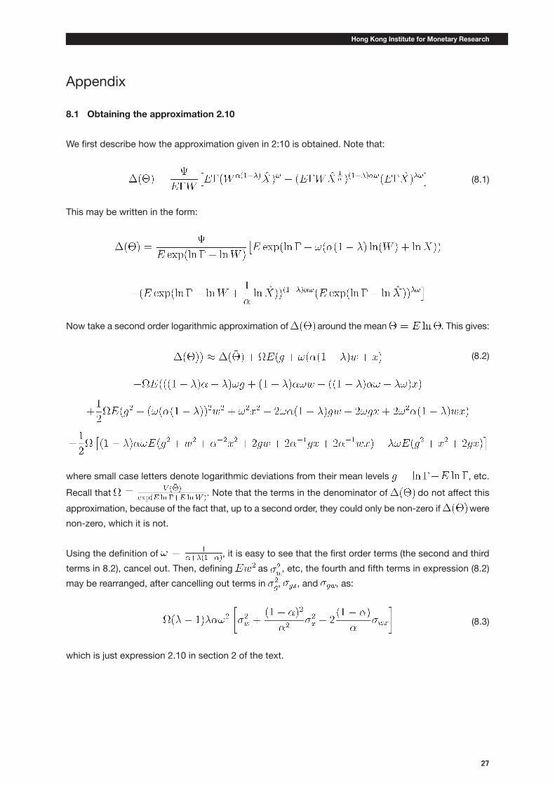
8.1 Obtaining the approximation 2.10

We first describe how the approximation given in 2:10 is obtained. Note that:

(8.1)

This may be written in the form:

Now take a second order logarithmic approximation of around the mean . This gives:

(8.2)

where small case letters denote logarithmic deviations from their mean levels , etc.

Recall that . Note that the terms in the denominator of do not affect this

approximation, because of the fact that, up to a second order, they could only be non-zero if were

non-zero, which it is not.

Using the definition of , it is easy to see that the first order terms (the second and third

terms in 8.2), cancel out. Then, defining as , etc, the fourth and fifth terms in expression (8.2)

may be rearranged, after cancelling out terms in , , and , as:

(8.3)

which is just expression 2.10 in section 2 of the text.


28

8.2 Approximating and H

We first approximate around the mean . Since is predetermined, we have:

(8.4)

where

is an increasing function of , and satisfies the properties , . This approximation

allows for the fact that the mean values and will not in general be the same.

From (3.14) in the paper, we may write

(8.5)

To derive (3.22) of the text, we take a linear approximation of (3.17) around the mean level of .

This gives

(8.6)

Here we define terms as:

The approximation 8.6 can be explained as follows. A rise in real aggregate demand raises

demand for labor by a factor of & , where reflects that fact that employment rises less than in

proportion to aggregate demand due to the fixed costs of price flexibility. The second term in (8.6)

re°ects the fact that changes in the flexible price index causes movements in aggregate demand between

the fixed price and flexible price sectors, which do not cancel out when . In the

exact numerical solution of the model we find the ter to be second order relative to the first terms in

(8.6). Given this, and in order to simplify the exposition of the model, we ignore these compositional

effects in the discussion in section. All of the propositions in section 3 would remain unchanged in the

absence of this simplification. Moreover, since the quantitative results of section 5 solves the exact

model, the compositional effects are automatically incorporated in Table 1.

Substituting from (8.6) (ignoring the terms as discussed) into (8.5) and then into (8.4) gives (3.21) of

the text.


29

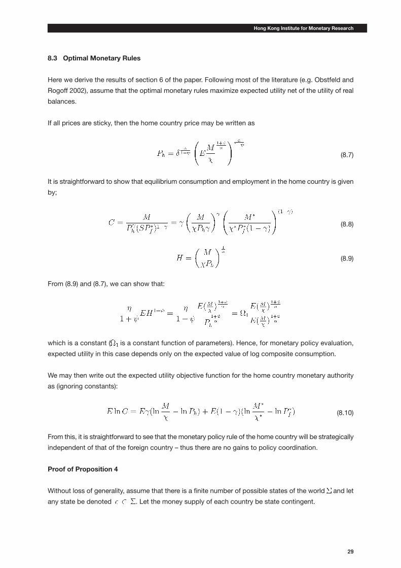
8.3 Optimal Monetary Rules

Here we derive the results of section 6 of the paper. Following most of the literature (e.g. Obstfeld and

Rogoff 2002), assume that the optimal monetary rules maximize expected utility net of the utility of real

balances.

If all prices are sticky, then the home country price may be written as

(8.7)

It is straightforward to show that equilibrium consumption and employment in the home country is given

by;

(8.8)

(8.9)

From (8.9) and (8.7), we can show that:

which is a constant ( is a constant function of parameters). Hence, for monetary policy evaluation,

expected utility in this case depends only on the expected value of log composite consumption.

We may then write out the expected utility objective function for the home country monetary authority

as (ignoring constants):

(8.10)

From this, it is straightforward to see that the monetary policy rule of the home country will be strategically

independent of that of the foreign country – thus there are no gains to policy coordination.

Proof of Proposition 4

Without loss of generality, assume that there is a finite number of possible states of the world and let

any state be denoted . Let the money supply of each country be state contingent.


30

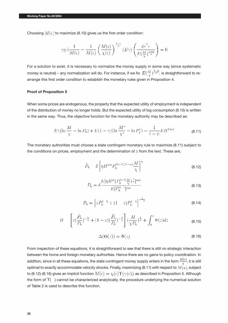
Choosing to maximize (8.10) gives us the first order condition:

For a solution to exist, it is necessary to normalize the money supply in some way (since systematic

money is neutral) – any normalization will do. For instance, if we fix , is straightforward to re-

arrange this first order condition to establish the monetary rules given in Proposition 4.

Proof of Proposition 5

When some prices are endogenous, the property that the expected utility of employment is independent

of the distribution of money no longer holds. But the expected utility of log consumption (8.10) is written

in the same way. Thus, the objective function for the monetary authority may be described as:

(8.11)

The monetary authorities must choose a state contingent monetary rule to maximize (8.11) subject to

the conditions on prices, employment and the determination of from the text. These are;

(8.12)

(8.13)

(8.14)

(8.15)

(8.16)

From inspection of these equations, it is straightforward to see that there is still no strategic interaction

between the home and foreign monetary authorities. Hence there are no gains to policy coordination. In

addition, since in all these equations, the state contingent money supply enters in the form , it is still

optimal to exactly accommodate velocity shocks. Finally, maximizing (8.11) with respect to , subject

to (8.12)-(8.16) gives an implicit function , as described in Proposition 5. Although

the form of ( ) cannot be characterized analytically, the procedure underlying the numerical solution

of Table 2 is used to describe this function.

exchange rate policy and ndogenous rice …€¦ · between exchange rate policy and price ... to...

Documents