Optimal Open Monetary Policy:

Exchange Rate Coordination

Raymond He

ECON40018/19 Economics Research Essay

This essay is submitted in partial fulfilment of the requirements of the

Bachelor of Commerce (Honours)

October 2019

Department of Economics

The University of Melbourne

Declaration

Plagiarism

Plagiarism is the presentation by a student of an assignment which has in fact been copied in

whole in part from another student’s work, or from any other source (e.g. published books

or periodicals), without due acknowledgements in the text.

Collusion

Collusion is the presentation by a student of an assignment as his or her own which is in

fact the result in or part of unauthorised collaboration with another person or persons.

Declaration

This essay is the sole work of the author whose name appears on the Title Page and contains

no material which the author has previously submitted for assessment at The University of

Melbourne or elsewhere. Also, to the best of the author’s knowledge and belief, the essay

contains no material previously published or written by another person except where due

reference is made in the text of the essay. I declare that I have read, and in undertaking this

research, have complied with the University’s Code of Conduct for Research. I also declare

that I understand what is meant by plagiarism and that this is unacceptable; except where

I have expressly indicated otherwise. This essay is my own work and does not contain any

plagiarised material in the form of unacknowledged quotations or mathematical workings or

in any other form.

I declare that this assignment is my own work and does not involve plagiarism or collusion.

This essay contains 9984 words and is 40 pages in length (double spaced), excluding font

matter.

Signed: Raymond He

Date: 20th October 2019

i

Acknowledgements

First and foremost, I am indebted to my supervisor Professor Chris Edmond for his invalu-

able guidance, kind encouragement, and unwavering support throughout the entire year.

Working with and learning from you has been a privilege - I could not have asked for a

better supervisor.

I have also benefited greatly from discussions with Dr James Brugler, for patiently intro-

ducing me to economic research, Dr Jiao Wang, for kindly giving her time and expertise on

Dynare and the NOEM literature throughout the year, and Associate Professor Mei Dong,

for her helpful comments and suggestions.

To my friends in the HEP ‘19 cohort but especially Tony Chen, Zoe Deed and Zan Fair-

weather - thank you for all the laughs in 137 Barry Street, proofreading early drafts and

making this challenging year one that I will nostalgically remember. Special thanks also goes

to Daniel Tiong and Katie Zhang - your insights and assistance from the very beginning has

been crucial along every step and more important than you realise.

I am also extremely grateful for the countless hours my girlfriend Tina Cheng spent metic-

ulously proofreading my drafts and waiting for me, and my family for their endless love and

support that got me through the year. I owe them my deepest thanks for their boundless

patience and understanding.

For financial support throughout this year, I would also like to acknowledge the generosity

of the Australian Prudential and Regulation Authority and the Reserve Bank of Australia

for awarding me the Brian Gray Scholarship.

ii

Abstract

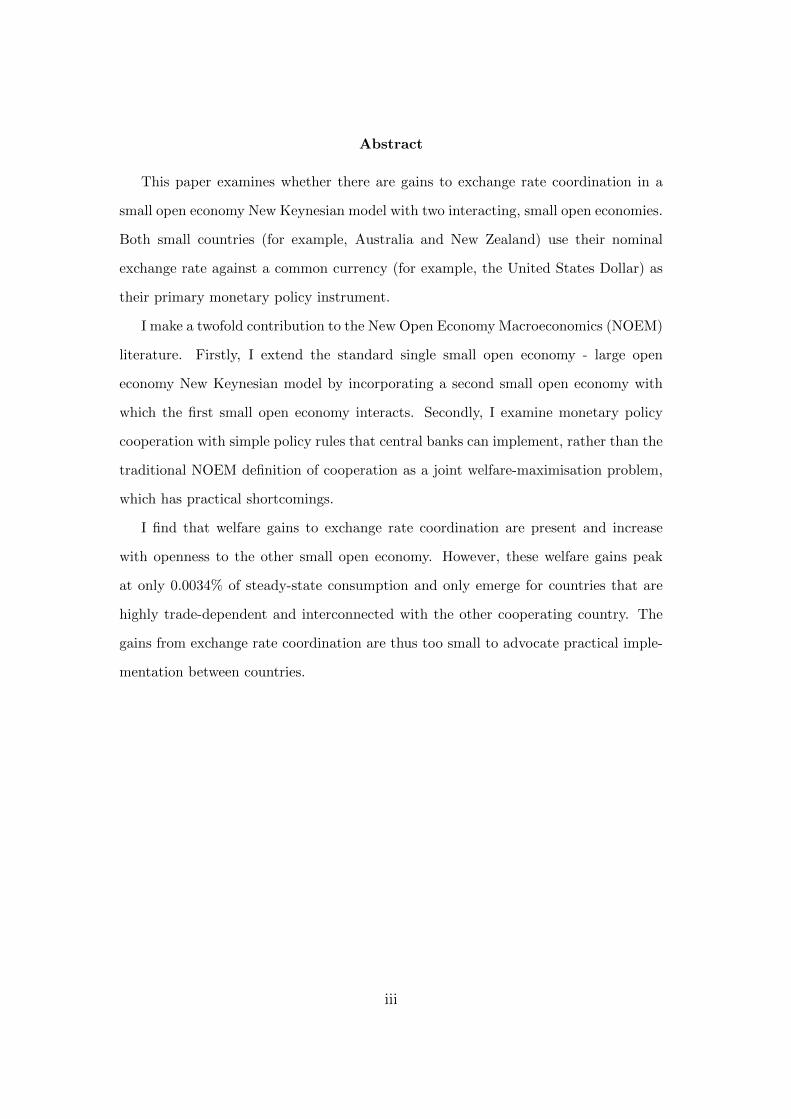
This paper examines whether there are gains to exchange rate coordination in a

small open economy New Keynesian model with two interacting, small open economies.

Both small countries (for example, Australia and New Zealand) use their nominal

exchange rate against a common currency (for example, the United States Dollar) as

their primary monetary policy instrument.

I make a twofold contribution to the New Open Economy Macroeconomics (NOEM)

literature. Firstly, I extend the standard single small open economy - large open

economy New Keynesian model by incorporating a second small open economy with

which the first small open economy interacts. Secondly, I examine monetary policy

cooperation with simple policy rules that central banks can implement, rather than the

traditional NOEM definition of cooperation as a joint welfare-maximisation problem,

which has practical shortcomings.

I find that welfare gains to exchange rate coordination are present and increase

with openness to the other small open economy. However, these welfare gains peak

at only 0.0034% of steady-state consumption and only emerge for countries that are

highly trade-dependent and interconnected with the other cooperating country. The

gains from exchange rate coordination are thus too small to advocate practical imple-

mentation between countries.

iii

Contents

1 Introduction 1

2 Literature Review 3

2.1 Gains to Cooperation . . . . . . . . . . . . . . . . . . . . . . . . . . . . . . . 4

2.2 Role of the Exchange Rate . . . . . . . . . . . . . . . . . . . . . . . . . . . . 5

3 Model 5

3.1 Households . . . . . . . . . . . . . . . . . . . . . . . . . . . . . . . . . . . . 6

3.2 International Identities . . . . . . . . . . . . . . . . . . . . . . . . . . . . . . 10

3.2.1 Bilateral Terms of Trade, Domestic Inflation & CPI Inflation . . . . . 10

3.2.2 International Risk Sharing . . . . . . . . . . . . . . . . . . . . . . . . 12

3.2.3 Uncovered Interest Parity . . . . . . . . . . . . . . . . . . . . . . . . 14

3.2.4 Exports . . . . . . . . . . . . . . . . . . . . . . . . . . . . . . . . . . 15

3.3 Firms . . . . . . . . . . . . . . . . . . . . . . . . . . . . . . . . . . . . . . . 15

3.3.1 Technology . . . . . . . . . . . . . . . . . . . . . . . . . . . . . . . . 15

3.3.2 Price Setting . . . . . . . . . . . . . . . . . . . . . . . . . . . . . . . 16

3.4 Equilibrium . . . . . . . . . . . . . . . . . . . . . . . . . . . . . . . . . . . . 17

3.4.1 Aggregate Demand and Output . . . . . . . . . . . . . . . . . . . . . 17

3.4.2 Marginal Cost and Inflation . . . . . . . . . . . . . . . . . . . . . . . 18

3.4.3 Equilibrium Dynamics . . . . . . . . . . . . . . . . . . . . . . . . . . 19

3.5 Rest of the World . . . . . . . . . . . . . . . . . . . . . . . . . . . . . . . . . 21

4 Monetary Policy 22

4.1 Non-cooperative Monetary Policy . . . . . . . . . . . . . . . . . . . . . . . . 23

4.2 Cooperative Monetary Policy . . . . . . . . . . . . . . . . . . . . . . . . . . 23

5 Calibration 24

iv

6 Results 25

6.1 Impulse Response Functions . . . . . . . . . . . . . . . . . . . . . . . . . . . 25

6.2 Moments . . . . . . . . . . . . . . . . . . . . . . . . . . . . . . . . . . . . . . 27

6.3 Welfare Losses . . . . . . . . . . . . . . . . . . . . . . . . . . . . . . . . . . . 27

6.4 Sensitivity . . . . . . . . . . . . . . . . . . . . . . . . . . . . . . . . . . . . . 29

6.4.1 Degree of Openness . . . . . . . . . . . . . . . . . . . . . . . . . . . . 29

6.4.2 Small Country Bias in Preferences . . . . . . . . . . . . . . . . . . . . 29

6.4.3 Domestic Inflation and Output Gap Feedback Coefficients . . . . . . 30

7 Limitations & Further Work 31

7.1 Ad hoc Welfare Loss Function . . . . . . . . . . . . . . . . . . . . . . . . . . 31

7.2 Producer Currency Pricing & Local Currency Pricing . . . . . . . . . . . . . 32

8 Conclusion 32

List of Figures

1 Country A Impulse Response Functions . . . . . . . . . . . . . . . . . . . . . 25

2 Country B Impulse Response Functions . . . . . . . . . . . . . . . . . . . . . 26

List of Tables

1 Cyclical Properties . . . . . . . . . . . . . . . . . . . . . . . . . . . . . . . . 27

2 Parameter Values . . . . . . . . . . . . . . . . . . . . . . . . . . . . . . . . . 37

3 Non-cooperative α - κ Sensitivity . . . . . . . . . . . . . . . . . . . . . . . . 39

4 Cooperative α - κ Sensitivity . . . . . . . . . . . . . . . . . . . . . . . . . . . 39

5 Non-cooperative φπ - φx Sensitivity . . . . . . . . . . . . . . . . . . . . . . . 40

6 Cooperative φπ - φx Sensitivity . . . . . . . . . . . . . . . . . . . . . . . . . 40

v

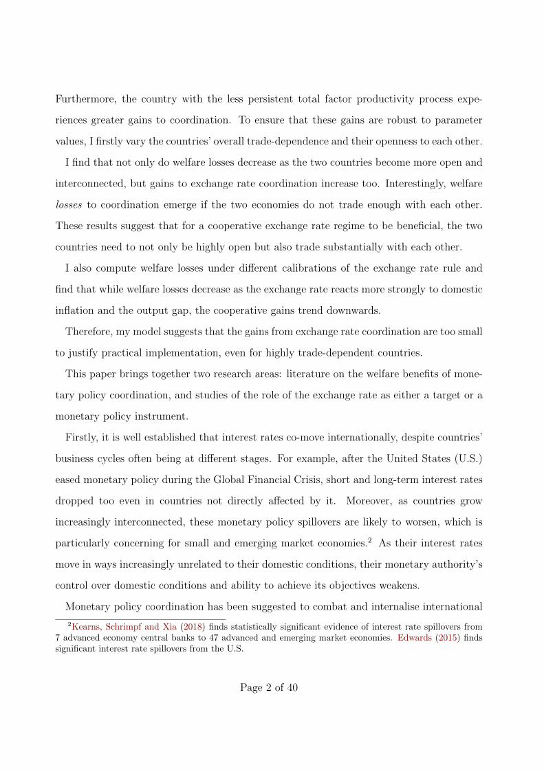
1 Introduction

Are there welfare gains from policy coordination between monetary authorities that use the

nominal exchange rate as their primary policy instrument? To answer my question, I create a

model that is different from those in the NOEM literature, which has only featured either one

focal small open economy among a continuum of infinitely small economies such as in Galı

and Monacelli (2005), or two large open economies such as in Benigno and Benigno (2003).

My model incorporates aspects from both modelling approaches by featuring two interacting

small open economies that take shocks from the rest of the world (modelled as an exogenous

third, large open economy) as given. The two small countries are perfectly symmetrical

in every way except for the persistence of their total factor productivity processes. This

difference allows their bilateral terms of trade to vary, and leads to different welfare outcomes

between the two countries.1

Both small economies use their nominal exchange rate with the large economy as their

monetary policy instrument in a managed float exchange rate regime. Under the non-

cooperative policy, the exchange rate only responds to domestic conditions. Under the

cooperative policy, both countries’ exchange rates react to each others’ economic conditions

in addition to their own.

Single small open economy models that feature an exogenous large economy cannot fa-

cilitate coordination as the large economy does not interact with the focal economy. Two

open economy models are unsuitable for examining exchange rate coordination because the

two coordinating economies require a third economy to provide a common currency for their

bilateral exchange rate.

I evaluate the two regimes’ performance with the quadratic welfare loss function from Galı

and Monacelli (2005) and find that there are indeed welfare gains to exchange rate coordi-

nation for both countries, although they are at most, 0.0034% of steady-state consumption.

1As explained in Section 3.2.2, countries’ terms of trade would be a constant if all countries were perfectlysymmetrical.

Page 1 of 40

Furthermore, the country with the less persistent total factor productivity process expe-

riences greater gains to coordination. To ensure that these gains are robust to parameter

values, I firstly vary the countries’ overall trade-dependence and their openness to each other.

I find that not only do welfare losses decrease as the two countries become more open and

interconnected, but gains to exchange rate coordination increase too. Interestingly, welfare

losses to coordination emerge if the two economies do not trade enough with each other.

These results suggest that for a cooperative exchange rate regime to be beneficial, the two

countries need to not only be highly open but also trade substantially with each other.

I also compute welfare losses under different calibrations of the exchange rate rule and

find that while welfare losses decrease as the exchange rate reacts more strongly to domestic

inflation and the output gap, the cooperative gains trend downwards.

Therefore, my model suggests that the gains from exchange rate coordination are too small

to justify practical implementation, even for highly trade-dependent countries.

This paper brings together two research areas: literature on the welfare benefits of mone-

tary policy coordination, and studies of the role of the exchange rate as either a target or a

monetary policy instrument.

Firstly, it is well established that interest rates co-move internationally, despite countries’

business cycles often being at different stages. For example, after the United States (U.S.)

eased monetary policy during the Global Financial Crisis, short and long-term interest rates

dropped too even in countries not directly affected by it. Moreover, as countries grow

increasingly interconnected, these monetary policy spillovers are likely to worsen, which is

particularly concerning for small and emerging market economies.2 As their interest rates

move in ways increasingly unrelated to their domestic conditions, their monetary authority’s

control over domestic conditions and ability to achieve its objectives weakens.

Monetary policy coordination has been suggested to combat and internalise international

2Kearns, Schrimpf and Xia (2018) finds statistically significant evidence of interest rate spillovers from7 advanced economy central banks to 47 advanced and emerging market economies. Edwards (2015) findssignificant interest rate spillovers from the U.S.

Page 2 of 40

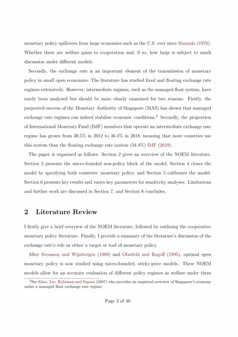
monetary policy spillovers from large economies such as the U.S. ever since Hamada (1976).

Whether there are welfare gains to cooperation and, if so, how large is subject to much

discussion under different models.

Secondly, the exchange rate is an important element of the transmission of monetary

policy in small open economies. The literature has studied fixed and floating exchange rate

regimes extensively. However, intermediate regimes, such as the managed float system, have

rarely been analysed but should be more closely examined for two reasons. Firstly, the

purported success of the Monetary Authority of Singapore (MAS) has shown that managed

exchange rate regimes can indeed stabilise economic conditions.3 Secondly, the proportion

of International Monetary Fund (IMF) members that operate an intermediate exchange rate

regime has grown from 39.5% in 2012 to 46.4% in 2018, meaning that more countries use

this system than the floating exchange rate system (34.4%) IMF (2019).

The paper is organised as follows. Section 2 gives an overview of the NOEM literature.

Section 3 presents the micro-founded non-policy block of the model, Section 4 closes the

model by specifying both countries’ monetary policy, and Section 5 calibrates the model.

Section 6 presents key results and varies key parameters for sensitivity analyses. Limitations

and further work are discussed in Section 7, and Section 8 concludes.

2 Literature Review

I firstly give a brief overview of the NOEM literature, followed by outlining the cooperative

monetary policy literature. Finally, I provide a summary of the literature’s discussion of the

exchange rate’s role as either a target or tool of monetary policy.

After Svensson and Wijnbergen (1989) and Obstfeld and Rogoff (1995), optimal open

monetary policy is now studied using micro-founded, sticky-price models. These NOEM

models allow for an accurate evaluation of different policy regimes as welfare under them

3See Khor, Lee, Robinson and Supaat (2007) who provides an empirical overview of Singapore’s economyunder a managed float exchange rate regime.

Page 3 of 40

could be correctly computed, whereas the traditional Mundell (1961) model used ad hoc

criteria, which may lead to spurious results.

A seminal contribution to the NOEM literature featuring Calvo (1983) pricing is Galı and

Monacelli (2005), which provides the tractable framework from which most of the NOEM

literature is built.4 Domestic inflation stabilisation is optimal in their model with assump-

tions on parameters such as unit elasticities and log utility. However, this result does not

survive if realistic departures from the model are considered, such as perfect international

risk sharing and unit elasticity of substitution between domestic and foreign goods.

2.1 Gains to Cooperation

The literature has also examined optimal monetary policy design in two-country models,

which create the possibility of strategic interactions and policy coordination.5 Following

Woodford (1999), policy cooperation in the NOEM literature consists of both countries

delegating monetary policy to a ‘supranational institution’ which maximises a weighted

average of the welfare of consumers in each country.

Although this approach results in the globally optimal welfare outcome, a critical drawback

is that finding an analytical expression for the policy that achieved the optimal outcome is

very rare, not to mention a policy that central banks can realistically implement. Even if

a functional form for the policy that delivered the globally optimal outcome can be found,

extreme parameter assumptions are usually required.6

While my ad hoc definition of cooperation does not yield the globally optimal welfare

outcome, it is actionable by central banks. Thus, I also explore whether gains to cooperation

are present under practical policies.

The NOEM literature examines whether gains from policy coordination are present under

4See Lane (2001) for a survey of earlier contributions to the NOEM literature, which often featured oneperiod in advance price setting.

5Fujiwara and Wang (2017) provides a detailed taxonomy of the cooperative NOEM literature.6For instance, Benigno and Benigno (2003) assumes equal international and intertemporal demand elas-

ticities to derive exact relationship between output, consumption and relative prices.

Page 4 of 40

a variety of settings. Fujiwara and Wang (2017) and Engel (2011) examine monetary policy

coordination under the more empirically appealing local-currency-pricing (LCP) setting in

contrast to the standard producer-currency pricing (PCP) assumption, such as in Benigno

and Benigno (2003).7 In addition to comparing non-cooperative and cooperative policy,

Pappa (2004) also examines monetary unions.

While these papers all find welfare gains to cooperation, they have always been modest

at best. Frictions other than nominal rigidities are needed to recommend cooperation as an

important policy framework. An exception is Liu and Pappa (2008), which finds significant

gains from cooperation with asymmetric trading structures.

2.2 Role of the Exchange Rate

The NOEM literature typically closes models with a simple Taylor nominal interest rate

rule. The literature thus traditionally regards the exchange rate as a target. For example,

De Paoli (2009) shows that under a general specification for preferences and in the presence

of inefficient steady-state output, optimal policy involves targeting the real exchange rate.

However, following Parrado (2004), there is a growing literature that is now investigating

the exchange rate as a monetary policy instrument with formalised policy reaction functions.

Chow, Lim and McNelis (2014) finds that exchange rate rules outperform the Taylor rule

when the economy’s source of volatility is export-price shocks. Mihov and Santacreu (2013)

shows that exchange rate rules surpass Taylor rules when deviations from uncovered interest

rate parity are introduced from a time-varying risk premium.

3 Model

This section outlines the non-policy block of my discrete-time, basic New Keynesian model.

The model is built from Galı and Monacelli (2005), which uses Calvo (1983) staggered price

7See Gopinath, Itskhoki and Rigobon (2010) for an empirical overview of the the LCP vs PCP debate.

Page 5 of 40

setting. I lay the microfoundations of my model and conclude by showing how my model

collapses into the canonical three equation representation analogous to a standard closed

economy New Keynesian model. It features a forward-looking IS curve and a Phillips curve

that depends on expectations of future inflation.

Two focal small open economies (for example Australia and New Zealand), denoted by A

and B, are modelled. Country A and B are assumed to be perfectly symmetrical in every

way except for their firms’ total factor productivity.8 Since each economy is of measure 0 in

the global economy, they both take the rest of the world as a singular, exogenously defined

large open economy. Each country is populated by a continuum of identical, infinitely

lived agents. There is no migration. Each agent produces a single differentiated good and

consumes goods which can be produced in both economies as well as the large country.

Analysis will be outlined from country A where, unless otherwise stated, analogous results

will also hold for country B.

For notational purposes, variables in levels are denoted with capital letters while variables

in lower-case are in logarithmic form. As two focal countries are being modelled, I depart

slightly from the notation in Galı and Monacelli (2005) by including a superscript to specify

the corresponding country. The large economy is denoted by *.

3.1 Households

A representative household from country A chooses consumption CAt and labour supply NA

t

(in hours) to maximise expected discounted lifetime utility:9

E0

∞∑t=0

βtU(CAt , N

At ) (1)

where 0 < β < 1 is the intertemporal discount factor. The period utility function is assumed

to be twice differentiable. I assume that Uc,t ≡ ∂Ut∂Ct

> 0, Ucc,t ≡ ∂2Ut∂C2

t≤ 0, Un,t ≡ ∂Ut

∂Nt≤ 0 and

8See Section 3.3.1 for further elaboration.9Following the literature, I assume that money’s only explicit rule is to serve as a unit of account.

Page 6 of 40

Unn,t ≡ ∂2Ut∂N2

t≤ 0. CA

t is a Dixit and Stiglitz (1977) aggregator of home and foreign bundles

of goods defined as:

CAt ≡

[(1− α)

1η (CA

A,t)η−1η + α

1η (CA

F,t)η−1η

] ηη−1

(2)

where α ∈ [0, 1] is inversely related to the degree of home bias in preferences, CAA,t is an index

of consumption of goods from economy A given by the Constant Elasticity of Substitution

(CES) function:

CAA,t ≡

(∫ 1

0

(CAA,t(j))

ε−1ε dj

) εε−1

where j ∈ [0, 1] denotes the good variety, and CAF,t is an index of consumption of foreign

goods. ε > 1 is the elasticity of substitution across goods produced within any given country

and η > 0 is the elasticity of substitution between CAA,t and CA

F,t. All goods are traded across

borders with no trade frictions. CAF,t is a CES index of goods foreign to country A given by:

CAF,t ≡

[(1− κ)

1η (CA

B,t)η−1η + κ

1η (CA

∗,t)η−1η

] ηη−1

(3)

where κ ∈ [0, 1] is inversely related to the degree of country B bias in preferences and CAB,t

and CA∗,t are indexes of consumption goods from country B and the rest of the world, given

by the respective CES functions:

CAB,t ≡

(∫ 1

0

CAB,t(j)

ε−1ε dj

) εε−1

; CA∗,t ≡

(∫ 1

0

CA∗,t(j)

ε−1ε dj

) εε−1

Note that elasticity of substitution between Country B and the large economy’s goods is

assumed to be the same as the elasticity of substitution between domestic and foreign goods.

Page 7 of 40

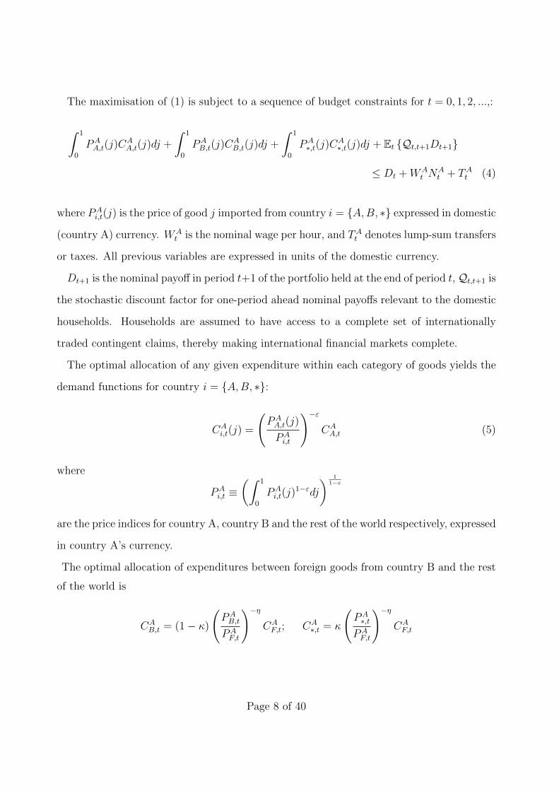
The maximisation of (1) is subject to a sequence of budget constraints for t = 0, 1, 2, ...,:

∫ 1

0

PAA,t(j)C

AA,t(j)dj +

∫ 1

0

PAB,t(j)C

AB,t(j)dj +

∫ 1

0

PA∗,t(j)C

A∗,t(j)dj + Et Qt,t+1Dt+1

≤ Dt +WAt N

At + TAt (4)

where PAi,t(j) is the price of good j imported from country i = A,B, ∗ expressed in domestic

(country A) currency. WAt is the nominal wage per hour, and TAt denotes lump-sum transfers

or taxes. All previous variables are expressed in units of the domestic currency.

Dt+1 is the nominal payoff in period t+1 of the portfolio held at the end of period t, Qt,t+1 is

the stochastic discount factor for one-period ahead nominal payoffs relevant to the domestic

households. Households are assumed to have access to a complete set of internationally

traded contingent claims, thereby making international financial markets complete.

The optimal allocation of any given expenditure within each category of goods yields the

demand functions for country i = A,B, ∗:

CAi,t(j) =

(PAA,t(j)

PAi,t

)−εCAA,t (5)

where

PAi,t ≡

(∫ 1

0

PAi,t(j)

1−εdj

) 11−ε

are the price indices for country A, country B and the rest of the world respectively, expressed

in country A’s currency.

The optimal allocation of expenditures between foreign goods from country B and the rest

of the world is

CAB,t = (1− κ)

(PAB,t

PAF,t

)−ηCAF,t; CA

∗,t = κ

(PA∗,t

PAF,t

)−ηCAF,t

Page 8 of 40

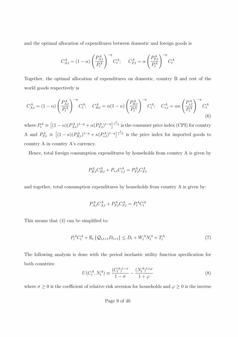
and the optimal allocation of expenditures between domestic and foreign goods is

CAA,t = (1− α)

(PAA,t

PAt

)−ηCAt ; CA

F,t = α

(PAF,t

PAt

)−ηCAt

Together, the optimal allocation of expenditures on domestic, country B and rest of the

world goods respectively is

CAA,t = (1− α)

(PAA,t

PAt

)−ηCAt ; CA

B,t = α(1− κ)

(PAB,t

PAt

)−ηCAt ; CA

∗,t = ακ

(PA∗,t

PAt

)−ηCAt

(6)

where PAt ≡

[(1− α)(PA

A,t)1−η + α(PA

F,t)1−η] 1

1−η is the consumer price index (CPI) for country

A and PAF,t ≡

[(1− κ)(PA

B,t)1−η + κ(PA

∗,t)1−η] 1

1−η is the price index for imported goods to

country A in country A’s currency.

Hence, total foreign consumption expenditures by households from country A is given by

PAB,tC

AB,t + P∗,tC

A∗,t = PA

F,tCAF,t

and together, total consumption expenditures by households from country A is given by:

PAA,tC

AA,t + PA

F,tCAF,t = PA

t CAt

This means that (4) can be simplified to:

PAt C

At + Et Qt,t+1Dt+1 ≤ Dt +WA

t NAt + TAt (7)

The following analysis is done with the period isoelastic utility function specification for

both countries:

U(CAt , N

At ) ≡ (CA

t )1−σ

1− σ− (NA

t )1+ϕ

1 + ϕ(8)

where σ ≥ 0 is the coefficient of relative risk aversion for households and ϕ ≥ 0 is the inverse

Page 9 of 40

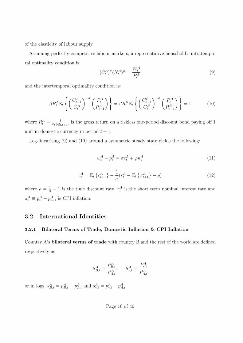
of the elasticity of labour supply.

Assuming perfectly competitive labour markets, a representative household’s intratempo-

ral optimality condition is:

(CAt )σ(NA

t )ϕ =WAt

PAt

(9)

and the intertemporal optimality condition is:

βRAt Et

(CAt+1

CAt

)−σ (PAt

PAt+1

)= βRB

t Et

(CBt+1

CBt

)−σ (PBt

PBt+1

)= 1 (10)

where RAt = 1

EtQt,t+1 is the gross return on a riskless one-period discount bond paying off 1

unit in domestic currency in period t+ 1.

Log-linearising (9) and (10) around a symmetric steady state yields the following:

wAt − pAt = σcAt + ϕnAt (11)

cAt = EtcAt+1

− 1

σ(rAt − Et

πAt+1

− ρ) (12)

where ρ = 1β− 1 is the time discount rate, rAt is the short term nominal interest rate and

πAt ≡ pAt − pAt−1 is CPI inflation.

3.2 International Identities

3.2.1 Bilateral Terms of Trade, Domestic Inflation & CPI Inflation

Country A’s bilateral terms of trade with country B and the rest of the world are defined

respectively as

SAB,t ≡PAB,t

PAA,t

; SA∗,t ≡PA∗,t

PAA,t

or in logs, sAB,t = pAB,t − pAA,t and sA∗,t = pA∗,t − pAA,t.

Page 10 of 40

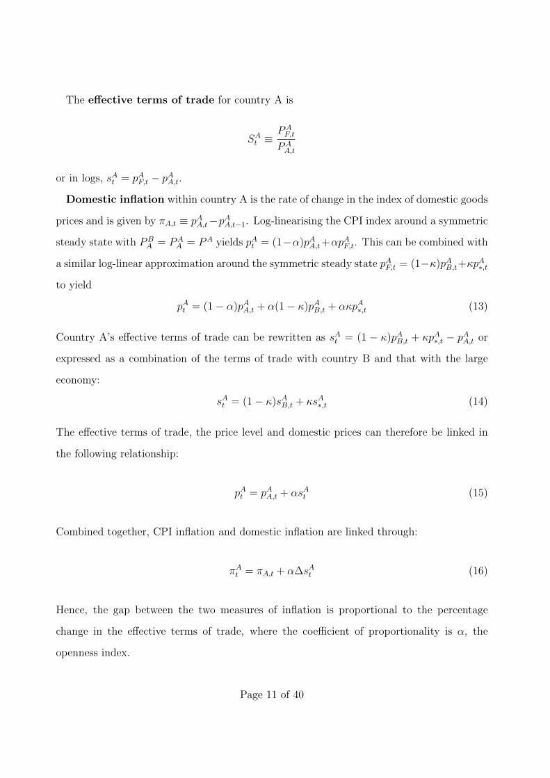
The effective terms of trade for country A is

SAt ≡PAF,t

PAA,t

or in logs, sAt = pAF,t − pAA,t.

Domestic inflation within country A is the rate of change in the index of domestic goods

prices and is given by πA,t ≡ pAA,t−pAA,t−1. Log-linearising the CPI index around a symmetric

steady state with PBA = PA

A = PA yields pAt = (1−α)pAA,t+αpAF,t. This can be combined with

a similar log-linear approximation around the symmetric steady state pAF,t = (1−κ)pAB,t+κpA∗,t

to yield

pAt = (1− α)pAA,t + α(1− κ)pAB,t + ακpA∗,t (13)

Country A’s effective terms of trade can be rewritten as sAt = (1 − κ)pAB,t + κpA∗,t − pAA,t or

expressed as a combination of the terms of trade with country B and that with the large

economy:

sAt = (1− κ)sAB,t + κsA∗,t (14)

The effective terms of trade, the price level and domestic prices can therefore be linked in

the following relationship:

pAt = pAA,t + αsAt (15)

Combined together, CPI inflation and domestic inflation are linked through:

πAt = πA,t + α∆sAt (16)

Hence, the gap between the two measures of inflation is proportional to the percentage

change in the effective terms of trade, where the coefficient of proportionality is α, the

openness index.

Page 11 of 40

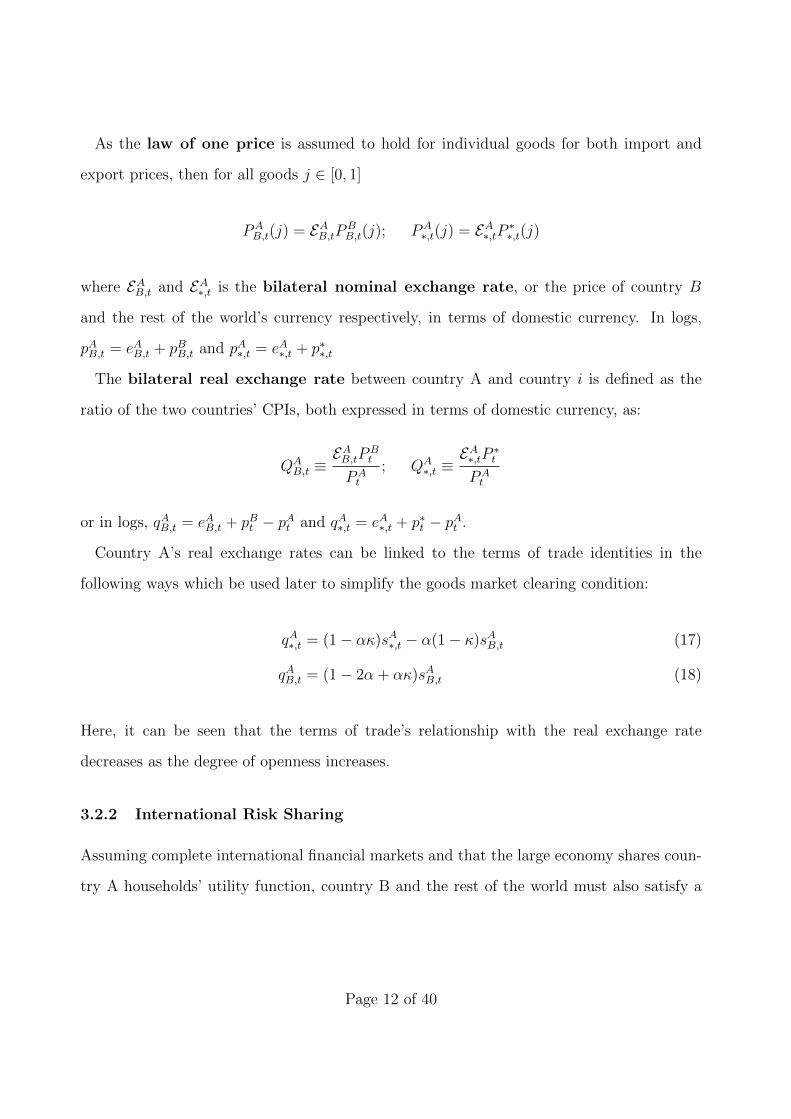
As the law of one price is assumed to hold for individual goods for both import and

export prices, then for all goods j ∈ [0, 1]

PAB,t(j) = EAB,tPB

B,t(j); PA∗,t(j) = EA∗,tP ∗∗,t(j)

where EAB,t and EA∗,t is the bilateral nominal exchange rate, or the price of country B

and the rest of the world’s currency respectively, in terms of domestic currency. In logs,

pAB,t = eAB,t + pBB,t and pA∗,t = eA∗,t + p∗∗,t

The bilateral real exchange rate between country A and country i is defined as the

ratio of the two countries’ CPIs, both expressed in terms of domestic currency, as:

QAB,t ≡

EAB,tPBt

PAt

; QA∗,t ≡

EA∗,tP ∗tPAt

or in logs, qAB,t = eAB,t + pBt − pAt and qA∗,t = eA∗,t + p∗t − pAt .

Country A’s real exchange rates can be linked to the terms of trade identities in the

following ways which be used later to simplify the goods market clearing condition:

qA∗,t = (1− ακ)sA∗,t − α(1− κ)sAB,t (17)

qAB,t = (1− 2α + ακ)sAB,t (18)

Here, it can be seen that the terms of trade’s relationship with the real exchange rate

decreases as the degree of openness increases.

3.2.2 International Risk Sharing

Assuming complete international financial markets and that the large economy shares coun-

try A households’ utility function, country B and the rest of the world must also satisfy a

Page 12 of 40

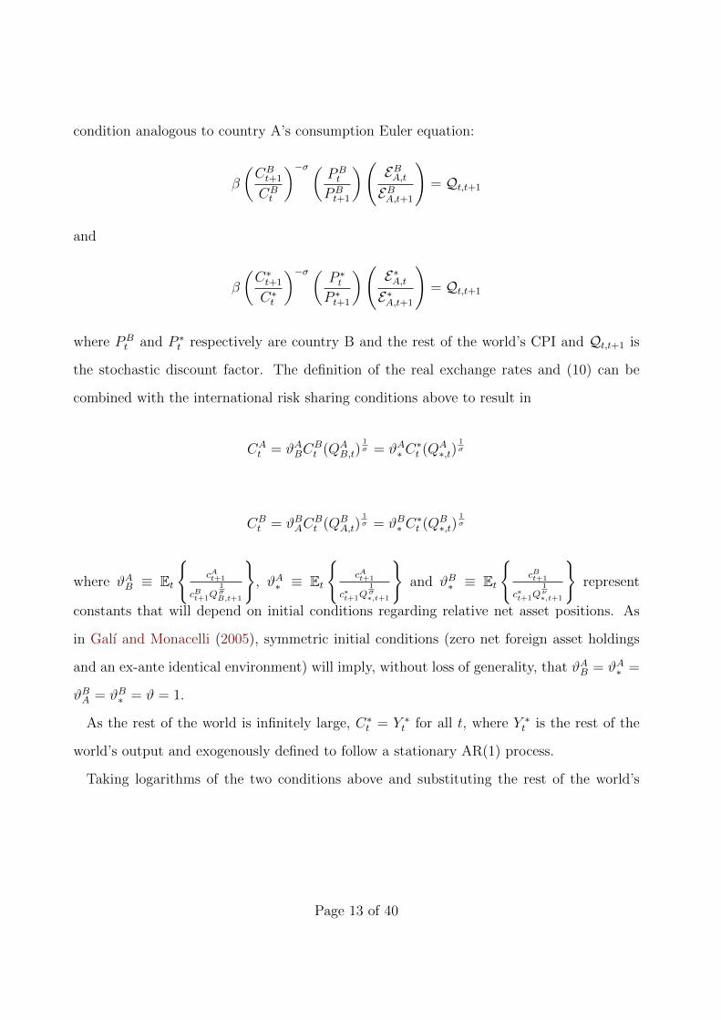
condition analogous to country A’s consumption Euler equation:

β

(CBt+1

CBt

)−σ (PBt

PBt+1

)( EBA,tEBA,t+1

)= Qt,t+1

and

β

(C∗t+1

C∗t

)−σ (P ∗tP ∗t+1

)( E∗A,tE∗A,t+1

)= Qt,t+1

where PBt and P ∗t respectively are country B and the rest of the world’s CPI and Qt,t+1 is

the stochastic discount factor. The definition of the real exchange rates and (10) can be

combined with the international risk sharing conditions above to result in

CAt = ϑABC

Bt (QA

B,t)1σ = ϑA∗ C

∗t (QA

∗,t)1σ

CBt = ϑBAC

Bt (QB

A,t)1σ = ϑB∗ C

∗t (QB

∗,t)1σ

where ϑAB ≡ Et

cAt+1

cBt+1Q1σB,t+1

, ϑA∗ ≡ Et

cAt+1

c∗t+1Q1σ∗,t+1

and ϑB∗ ≡ Et

cBt+1

c∗t+1Q1ν∗,t+1

represent

constants that will depend on initial conditions regarding relative net asset positions. As

in Galı and Monacelli (2005), symmetric initial conditions (zero net foreign asset holdings

and an ex-ante identical environment) will imply, without loss of generality, that ϑAB = ϑA∗ =

ϑBA = ϑB∗ = ϑ = 1.

As the rest of the world is infinitely large, C∗t = Y ∗t for all t, where Y ∗t is the rest of the

world’s output and exogenously defined to follow a stationary AR(1) process.

Taking logarithms of the two conditions above and substituting the rest of the world’s

Page 13 of 40

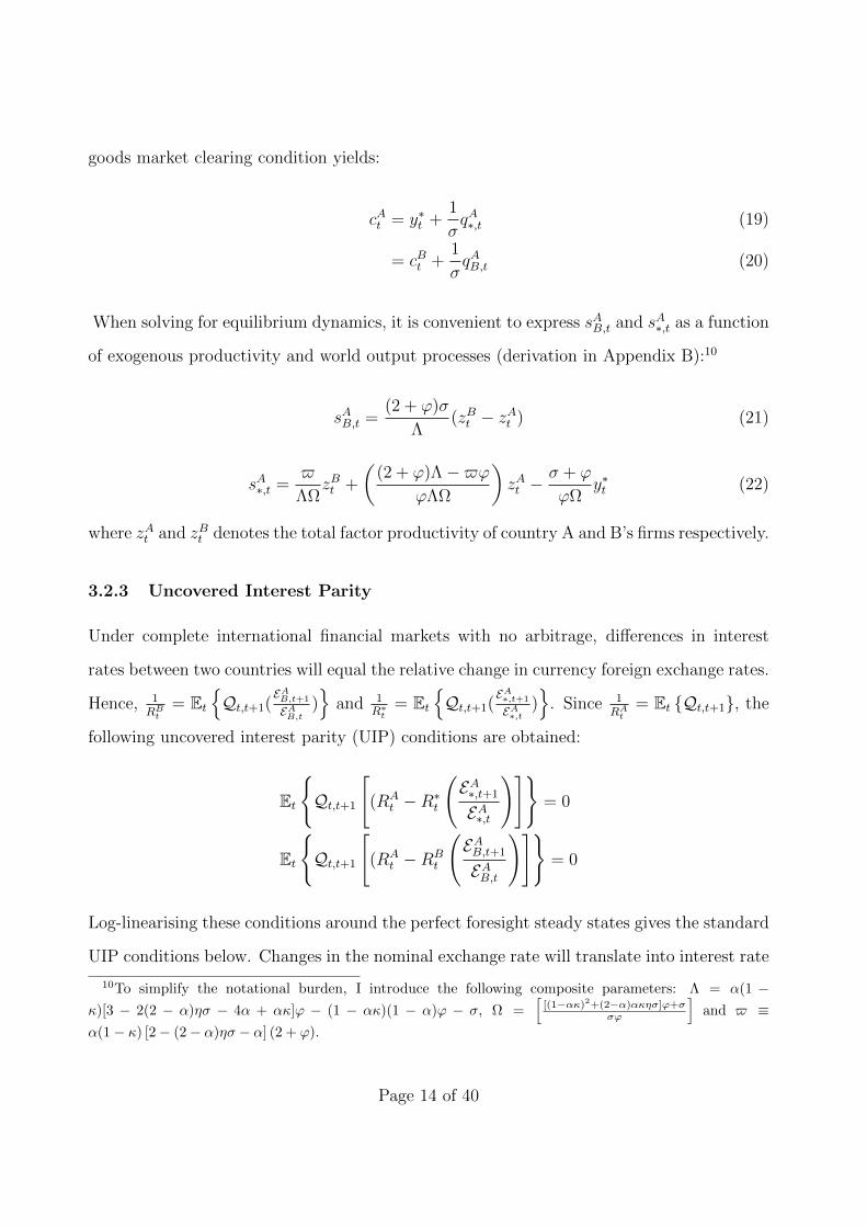
goods market clearing condition yields:

cAt = y∗t +1

σqA∗,t (19)

= cBt +1

σqAB,t (20)

When solving for equilibrium dynamics, it is convenient to express sAB,t and sA∗,t as a function

of exogenous productivity and world output processes (derivation in Appendix B):10

sAB,t =(2 + ϕ)σ

Λ(zBt − zAt ) (21)

sA∗,t =$

ΛΩzBt +

((2 + ϕ)Λ−$ϕ

ϕΛΩ

)zAt −

σ + ϕ

ϕΩy∗t (22)

where zAt and zBt denotes the total factor productivity of country A and B’s firms respectively.

3.2.3 Uncovered Interest Parity

Under complete international financial markets with no arbitrage, differences in interest

rates between two countries will equal the relative change in currency foreign exchange rates.

Hence, 1RBt

= EtQt,t+1(

EAB,t+1

EAB,t)

and 1R∗t

= EtQt,t+1(

EA∗,t+1

EA∗,t)

. Since 1RAt

= Et Qt,t+1, the

following uncovered interest parity (UIP) conditions are obtained:

Et

Qt,t+1

[(RA

t −R∗t

(EA∗,t+1

EA∗,t

)]= 0

Et

Qt,t+1

[(RA

t −RBt

(EAB,t+1

EAB,t

)]= 0

Log-linearising these conditions around the perfect foresight steady states gives the standard

UIP conditions below. Changes in the nominal exchange rate will translate into interest rate

10To simplify the notational burden, I introduce the following composite parameters: Λ = α(1 −κ)[3 − 2(2 − α)ησ − 4α + ακ]ϕ − (1 − ακ)(1 − α)ϕ − σ, Ω =

[[(1−ακ)2+(2−α)ακησ]ϕ+σ

σϕ

]and $ ≡

α(1− κ) [2− (2− α)ησ − α] (2 + ϕ).

Page 14 of 40

movements through these conditions.

rAt − rBt = Et

∆eAB,t+1

; rAt − r∗t = Et

∆eA∗,t+1

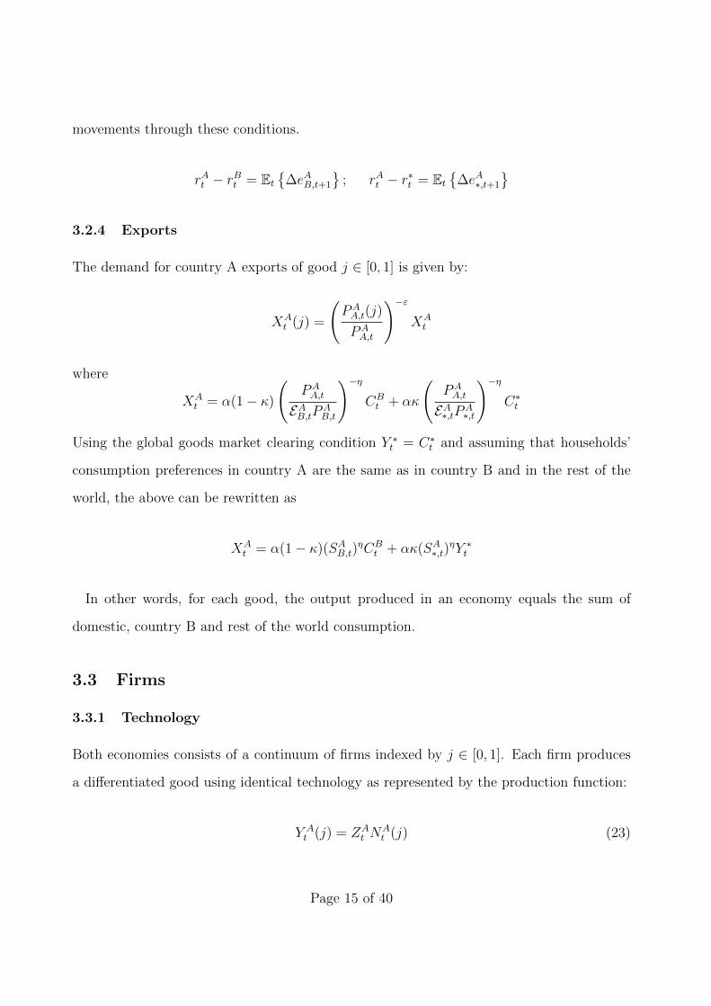
3.2.4 Exports

The demand for country A exports of good j ∈ [0, 1] is given by:

XAt (j) =

(PAA,t(j)

PAA,t

)−εXAt

where

XAt = α(1− κ)

(PAA,t

EAB,tPAB,t

)−ηCBt + ακ

(PAA,t

EA∗,tPA∗,t

)−ηC∗t

Using the global goods market clearing condition Y ∗t = C∗t and assuming that households’

consumption preferences in country A are the same as in country B and in the rest of the

world, the above can be rewritten as

XAt = α(1− κ)(SAB,t)

ηCBt + ακ(SA∗,t)

ηY ∗t

In other words, for each good, the output produced in an economy equals the sum of

domestic, country B and rest of the world consumption.

3.3 Firms

3.3.1 Technology

Both economies consists of a continuum of firms indexed by j ∈ [0, 1]. Each firm produces

a differentiated good using identical technology as represented by the production function:

Y At (j) = ZA

t NAt (j) (23)

Page 15 of 40

where At represents the level of technology, assumed to be common to all firms and evolving

according an exogenous AR(1) process: zAt ≡ log(ZAt ) = ρAz z

At−1 + εat with ρAz ∈ [0, 1].

Country A and B are assumed to be perfectly symmetrical in every way except for their

total factor productivity AR(1) processes. This deviation will be the cause behind the

different results between the two countries.11

3.3.2 Price Setting

Prices are set as in Calvo (1983), in which the fraction 1 − θ, θ ∈ [0, 1], of randomly

selected firms set new prices every period. An individual firm’s probability of re-optimising

in any given period being independent of the time elapsed since it last reset its price. When

reoptimising prices, firms are aware that they may be unable to reset prices for a certain

period of time. Domestic inflation therefore depends on future expectations, which generates

a forward-looking Phillips curve.

Let τ denote the rate at which the cost of employment is subsidised, which is financed by

a lump-sum tax used to offset firms’ monopolistic power as explained in Section 4.

As the marginal product of labour is mpnAt = zAt , then if such an employment subsidy is

in place, real marginal cost can be expressed as

mcrA,t = −v + wAt − pAA,t − zAt (24)

where v ≡ − ln(1− τ).

The optimal price setting strategy for the typical firm resetting its price in period t can

be approximated by the log-linear rule:

pA,t = µ+ (1− βθ)∞∑k=0

(βθ)kEtmcrA,t+k + pA,t

(25)

11As can be seen from (21), country A’s terms of trade with country B will always be 1 (in levels) undersymmetric productivity between countries. See Appendix A of Galı and Monacelli (2005) for a derivation.

Page 16 of 40

where pA,t denotes the log of newly set domestic prices, and µ ≡ log( εε−1), which corresponds

to the log of the gross mark-up in the steady state, or the flexible price economy.

Domestic inflation within country A is linked to firms’ marginal costs via:

πA,t = βE πA,t+1+ λmcrA,t (26)

where λ ≡ (1−βθ)(1−θ)θ

and mcrA,t ≡ mcrA,t −mcrA is the markup gap. Thus, the relationship

between domestic price inflation and the markup gap is not affected by the degree of openness

or the substitutability between domestic and foreign goods in the open economy.

3.4 Equilibrium

3.4.1 Aggregate Demand and Output

The goods market clearing condition is for all j ∈ [0, 1] and for all t:

Y At (j) = CA

A,t(j) +XAt (j)

=

(PAA,t(j)

PA,t

)ε [(1− α)

(PAA,t

PAt

)−ηCAt + α(1− κ)(SAB,t)ηCB

t + ακ(S∗A,t)ηY ∗t

]

Aggregate domestic output in country A is Y At ≡

(∫ 1

0Y At (j)dj

) εε−1

which when combined

with the condition above results in:

Y At = (1− α)

(PAA,t

PAt

)−ηCAt + α(1− κ)(SAB,t)η

[CAt (QA

B,t)− 1σ

]+ ακ(SA∗,t)ηY ∗t

Log-linearising country A’s goods market condition around a symmetric steady state and

substituting in (18) results in:

yAt = (1− ακ)cAt +α(1− κ)

σ((2− α)ησ − 1 + 2α− ακ)sAB,t + (2− α)καηsA∗,t + ακy∗t (27)

Page 17 of 40

Combining (16) and the consumption Euler equation gives

cAt = EtcAt+1

− 1

σ(rAt − Et πA,t+1 − ρ) +

α

σEt

∆sAt+1

(28)

Rearranging the goods market clearing condition for cAt , substituting it into (28) and then

collecting like-terms yields a version of the Dynamic IS (DIS) curve:12

yAt = EtyAt+1

+ΦAz

At −ΘAz

Bt −(σ + ϕ+ ακϕΩ

ϕΩ

)Et

∆y∗t+1

−1− ακ

σ(rAt −Et πA,t+1−ρ)

(29)

Thus, the DIS equation is similar to the one in a closed economy, except now, there is an

additional term linking domestic output to the large economy’s output and the country B’s

productivity. Note that if α and η are high enough, output becomes more sensitive to real

rate changes than in the closed economy case. This is because the direct negative effect of

an increase in the real rate on aggregate demand and output is amplified by the induced real

appreciation and the consequent switch of expenditure towards foreign goods. This will be

partly offset by any increase in CPI inflation relative to domestic inflation induced by the

expected real depreciation, dampening the change in consumption based on the real rate.

3.4.2 Marginal Cost and Inflation

The labour market clearing condition is

NAt ≡

∫ 1

0

NAt (j)dj =

(Y At

St

)∫ 1

0

(PA,t(j)

PA,t

)−εdj

Log-linearising (23) up to a first order gives

nAt = yAt − zAt (30)

12To lighten the notational burden, the following composite parameters are intro-

duced: ΦA =[α(1−κ)[2−(2−α)ησ−2α](2+ϕ)

Λ + ακ[1−ακ−(2−α)ησ][$ϕ−(2+ϕ)Λ]σϕΛΩ

](1 − ρAz ) and ΘA =[

α(1−κ)[2−(2−α)ησ−2α](2+ϕ)Λ + ακ$[1−ακ−(2−α)η]

σΛΩ

](1− ρBz ).

Page 18 of 40

The real marginal cost can be derived from substituting the household intra-optimality

condition, international risk sharing condition and (15) into (24):

mcrA,t = −v + wAt − pAA,t − zAt (31)

= −v + σy∗t + ϕyAt + sA∗,t − (1 + ϕ)zAt

= −v +

(σϕΩ− σ + ϕ

ϕΩ

)y∗t + ϕyAt +

$

ΛΩzBt +

((2 + ϕ)Λ−$ϕ

ϕΛΩ− 1− ϕ

)zAt

Domestic output affects marginal costs through its impact on employment as captured

by ϕ. World output affects marginal costs through its effect on consumption and hence,

the real wage as captured by σ. The effect of world output on marginal costs is positive if

σϕΩ + ϕ− σ > 0. This is because with sufficiently high σ, the size of the real appreciation

needed to absorb the change in relative supplies is small, with its negative effect on marginal

costs offset by the positive effect from a higher real wage.

3.4.3 Equilibrium Dynamics

Since mcr = −µ, the flexible price equivalent of the above is:

mcrA = −µ = −v +

(σϕΩ− σ + ϕ

ϕΩ

)y∗t + ϕyAt +

$

ΛΩzBt +

((2 + ϕ)Λ−$ϕ

ϕΛΩ− 1− ϕ

)zAt

The natural level of output (yAt ) can be solved:

yAt =v − µϕ

+

(σ − σϕΩ− ϕ

ϕ2Ω

)y∗t −

$

ΛΩϕzBt +

(1 + ϕ

ϕ+$ϕ− (2 + ϕ)Λ

ϕ2ΛΩ

)zAt

The effect of world output on natural output is ambiguous, depending on the effect of world

output on domestic marginal costs.

Letting xAt ≡ yAt − yAt be country A’s domestic output gap from the flexible price output,

mcrA,t = mcrA,t −mcrA = ϕxAt

Page 19 of 40

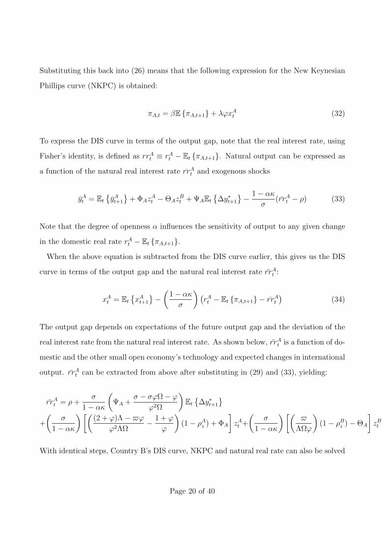
Substituting this back into (26) means that the following expression for the New Keynesian

Phillips curve (NKPC) is obtained:

πA,t = βE πA,t+1+ λϕxAt (32)

To express the DIS curve in terms of the output gap, note that the real interest rate, using

Fisher’s identity, is defined as rrAt ≡ rAt − Et πA,t+1. Natural output can be expressed as

a function of the natural real interest rate rrAt and exogenous shocks

yAt = EtyAt+1

+ ΦAz

At −ΘAz

Bt + ΨAEt

∆y∗t+1

− 1− ακ

σ(rrAt − ρ) (33)

Note that the degree of openness α influences the sensitivity of output to any given change

in the domestic real rate rAt − Et πA,t+1.

When the above equation is subtracted from the DIS curve earlier, this gives us the DIS

curve in terms of the output gap and the natural real interest rate rrAt :

xAt = EtxAt+1

−(

1− ακσ

)(rAt − Et πA,t+1 − rrAt

)(34)

The output gap depends on expectations of the future output gap and the deviation of the

real interest rate from the natural real interest rate. As shown below, rrAt is a function of do-

mestic and the other small open economy’s technology and expected changes in international

output. rrAt can be extracted from above after substituting in (29) and (33), yielding:

rrAt = ρ+σ

1− ακ

(ΨA +

σ − σϕΩ− ϕϕ2Ω

)Et

∆y∗t+1

+

(σ

1− ακ

)[((2 + ϕ)Λ−$ϕ

ϕ2ΛΩ− 1 + ϕ

ϕ

)(1− ρAz ) + ΦA

]zAt +

(σ

1− ακ

)[($

ΛΩϕ

)(1− ρBz )−ΘA

]zBt

With identical steps, Country B’s DIS curve, NKPC and natural real rate can also be solved

Page 20 of 40

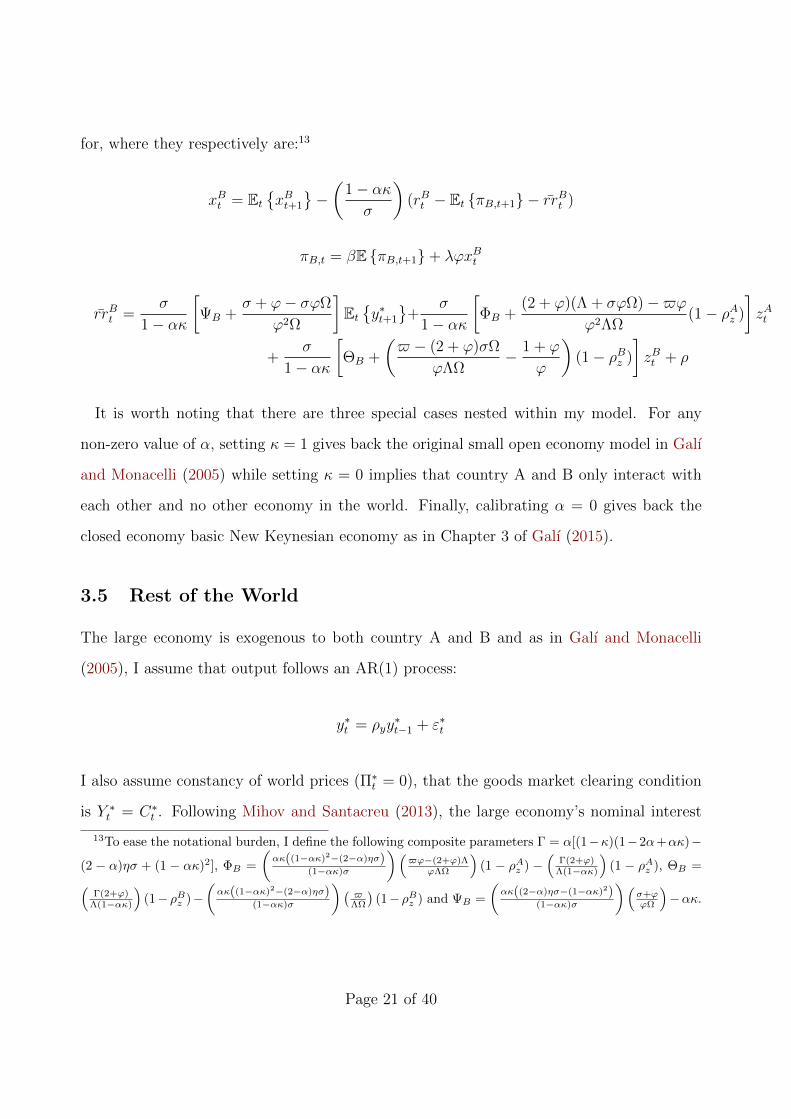
for, where they respectively are:13

xBt = EtxBt+1

−(

1− ακσ

)(rBt − Et πB,t+1 − rrBt )

πB,t = βE πB,t+1+ λϕxBt

rrBt =σ

1− ακ

[ΨB +

σ + ϕ− σϕΩ

ϕ2Ω

]Ety∗t+1

+

σ

1− ακ

[ΦB +

(2 + ϕ)(Λ + σϕΩ)−$ϕϕ2ΛΩ

(1− ρAz )

]zAt

+σ

1− ακ

[ΘB +

($ − (2 + ϕ)σΩ

ϕΛΩ− 1 + ϕ

ϕ

)(1− ρBz )

]zBt + ρ

It is worth noting that there are three special cases nested within my model. For any

non-zero value of α, setting κ = 1 gives back the original small open economy model in Galı

and Monacelli (2005) while setting κ = 0 implies that country A and B only interact with

each other and no other economy in the world. Finally, calibrating α = 0 gives back the

closed economy basic New Keynesian economy as in Chapter 3 of Galı (2015).

3.5 Rest of the World

The large economy is exogenous to both country A and B and as in Galı and Monacelli

(2005), I assume that output follows an AR(1) process:

y∗t = ρyy∗t−1 + ε∗t

I also assume constancy of world prices (Π∗t = 0), that the goods market clearing condition

is Y ∗t = C∗t . Following Mihov and Santacreu (2013), the large economy’s nominal interest

13To ease the notational burden, I define the following composite parameters Γ = α[(1−κ)(1−2α+ακ)−

(2 − α)ησ + (1 − ακ)2], ΦB =

(ακ((1−ακ)2−(2−α)ησ)

(1−ακ)σ

)($ϕ−(2+ϕ)Λ

ϕΛΩ

)(1 − ρAz ) −

(Γ(2+ϕ)

Λ(1−ακ)

)(1 − ρAz ), ΘB =(

Γ(2+ϕ)Λ(1−ακ)

)(1−ρBz )−

(ακ((1−ακ)2−(2−α)ησ)

(1−ακ)σ

)($ΛΩ

)(1−ρBz ) and ΨB =

(ακ((2−α)ησ−(1−ακ)2)

(1−ακ)σ

)(σ+ϕϕΩ

)−ακ.

Page 21 of 40

rate is determined by the rest of the world’s consumption Euler equation:

βR∗tEt

(C∗t+1

C∗t

)−σ= 1

Hence, the global economy is represented by country A and country B’s aggregate demand

and supply equations, the risk sharing conditions, the uncovered interest parity conditions,

and the law of motion for the exogenous productivity and the large economy’s output shocks.

4 Monetary Policy

As in Galı and Monacelli (2005), I assume that an optimal subsidy τ , set such that (1 −

τ)(1 − α) = 1 − 1ε, is in place to offset the firms’ monopolistic distortion and the terms of

trade distortion.14 This guarantees the optimality of the flexible price equilibrium allocation.

To close the model, I specify how monetary policy is conducted in Sections 4.1 and 4.2.

I consider policies under commitment, where monetary authorities cannot ignore past deci-

sions. Corsetti and Pesenti (2001) shows that under discretion, monetary authorities have

incentives to systematically affect the economy through unanticipated changes in monetary

policy because of terms of trade externalities. However, monetary authorities under com-

mitment cannot systematically affect the economy through monetary surprises.

I rank the two regimes with a quadratic welfare loss function that represents a second-order

Taylor series approximation to the level of expected utility of the representative household

in equilibrium with a given monetary policy.

I use the welfare loss function from Galı and Monacelli (2005):15

WA,t = −1− α2

∞∑t=0

βt[ ελπ2A,t + (1 + ϕ)xAt

](35)

14See Galı and Monacelli (2005) for a more careful derivation of the optimal subsidy in an open economy.Note that in a closed economy basic New Keynesian model, the optimal employment subsidy is τ = 1

ε .15See Section 7 for a discussion of the potential implications of using an ad hoc loss function.

Page 22 of 40

WB,t = −1− α2

∞∑t=0

βt[ ελπ2B,t + (1 + ϕ)xBt

](36)

4.1 Non-cooperative Monetary Policy

Both countries’ monetary policy is a managed float exchange rate regime with the large

economy, from which the nominal interest rate can be inferred from the UIP conditions.

The central bank has a target for the change in its nominal exchange rate with the large

economy, ∆eA∗,t+1, based on the state of the domestic economy. Both monetary authorities

are assumed to care about stabilising domestic inflation and output. As in Parrado (2004),

I specify the following monetary policy reaction function for countries A and B:

∆eA∗,t+1 = ∆eA∗ + φππA,t + φxxAt (37)

∆eB∗,t+1 = ∆eB∗ + φππB,t + φxxBt (38)

where ∆eA∗ and ∆eB∗ is the long-run equilibrium change in the nominal exchange rate with

the large economy and φπ and φx are reaction coefficients that are assumed to be positive.

4.2 Cooperative Monetary Policy

Monetary policy cooperation is modelled by both setting both countries’ nominal exchange

rate with the rest of the world to respond to both countries’ economic conditions:16

∆eA∗,t = ∆eA∗ + φππA,t + φx(xAt + xBt ) (39)

∆eB∗,t = ∆eB∗ + φππB,t + φx(xBt + xAt ) (40)

16Although gains to coordination are present if both exchange rules are modified to respond to bothcountries’ domestic inflation instead of the output gap, these gains are more muted. This preserves theoptimality of domestic inflation stabilisation from Galı and Monacelli (2005).

Page 23 of 40

5 Calibration

I now calibrate the model and compare the welfare performance of the two rules. I report and

analyse impulse responses, second moments, and welfare losses. I use numerical simulations

on Dynare to generate these results. Time is taken to be quarters and parameter values are

summarised in Table 2 in Appendix A.

As the welfare-loss function I use to evaluate various monetary policy regimes’ perfor-

mance is from Galı and Monacelli (2005), I follow their parameter calibration as closely as

possible. Hence, σ = η = 1, which is the special configuration used to derive a second-order

approximation of the utility of the small open economy’s representative consumer.

ϕ = 3, which consequently implies a value for the steady-state mark-up µ = 1.2. This

implies that ε = 6. θ is set to 0.75, a value consistent with an average period of one year

between price adjustments. In keeping with the literature, β = 0.99, which implies a riskless

annual return of about 4% in the steady state. I set the degree of openness, α, to 0.4 which

corresponds roughly to the import/GDP ratio in Canada, which the NOEM literature takes

as the standard small open economy. κ is set to 0.5, implying no bias between the other

small open economy and the large economy. To calibrate the exchange-rate rule, I follow

Galı and Monacelli (2005) and set φπ = φx = 1.5 for both countries.17

To calibrate the exogenous processes, Galı and Monacelli (2005) uses quarterly HP-filtered

data over the 1963:1 - 2002:4 period to estimate AR(1) processes to (log) labour productivity

in Canada and (log) U.S. GDP (the proxy for world output):

zAt = 0.66(0.06)

zAt−1 + εat , σzA = 0.0071

zBt = 0.65(0.06)

zBt−1 + εbt , σzB = 0.0071

y∗t = 0.86(0.04)

y∗t−1 + ε∗t , σy∗ = 0.0078

17See Appendix D for welfare loss results under different values of φπ and φx.

Page 24 of 40

The parameters for Country B’s total factor productivity process are chosen to be as close to

Country A’s as possible. They are only different in their persistence so that any differences

between Country A and B can be isolated to this cause.

6 Results

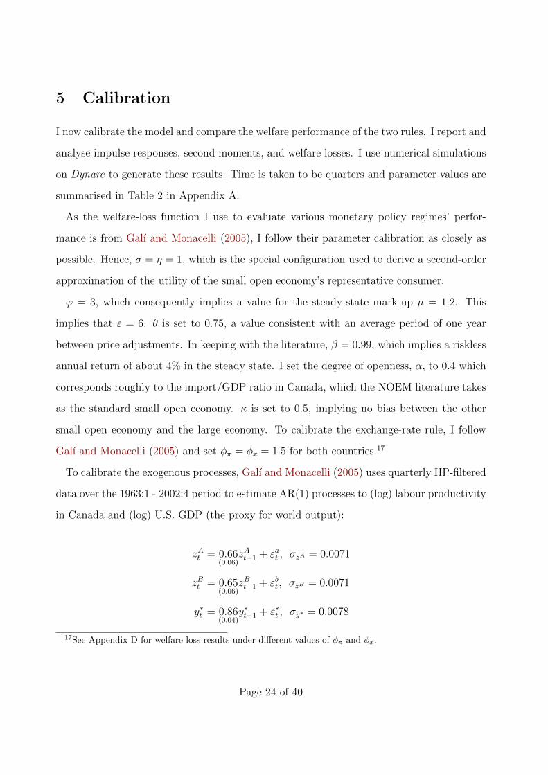
6.1 Impulse Response Functions

I compare the exchange rate regimes by computing impulse response functions to a 1 standard

deviation shock in the large economy’s output. Figures 1 and 2 show the results. In keeping

with the literature, the output gap, terms of trade, the nominal and real exchange rates are

expressed in terms of percentage deviations from steady state. Domestic and CPI inflation,

nominal and real interest rates are expressed as an annualised rate in percentage form.

Figure 1: Country A Impulse Response Functions

Page 25 of 40

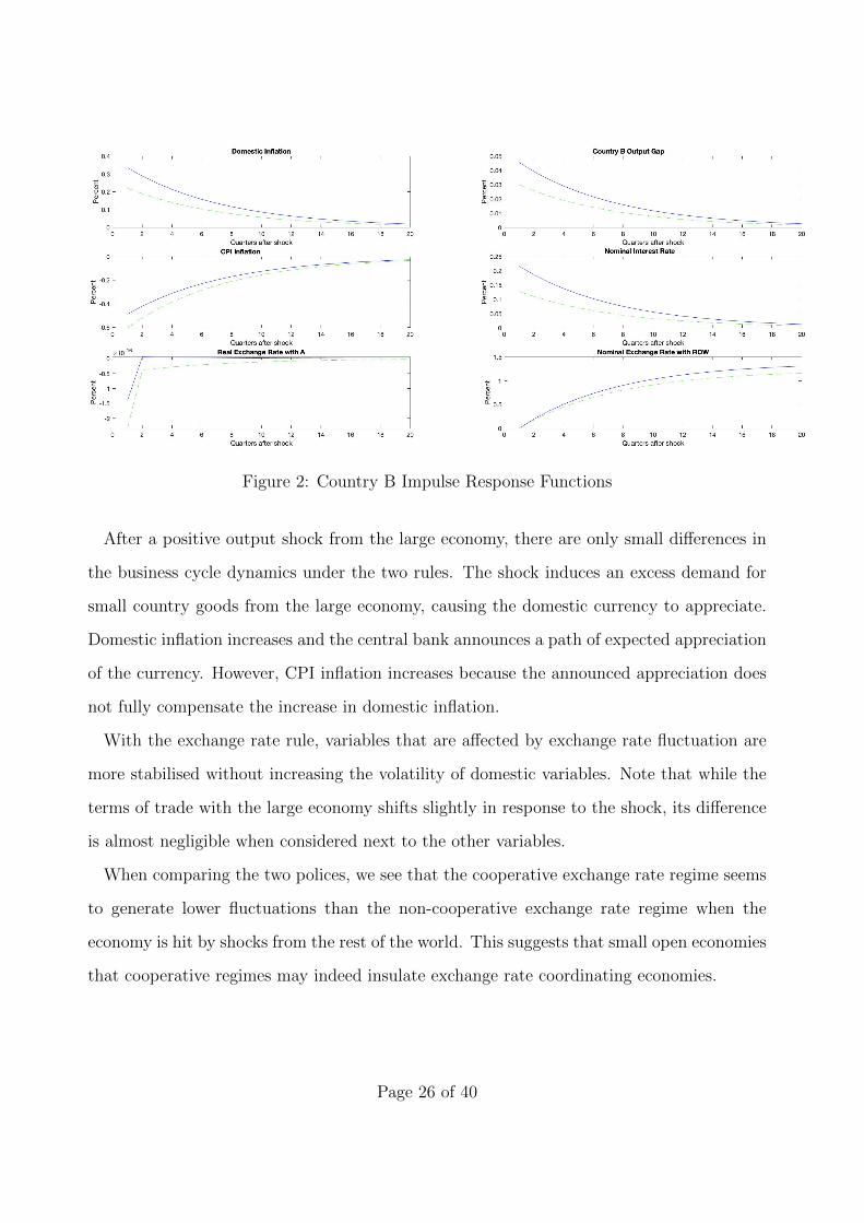
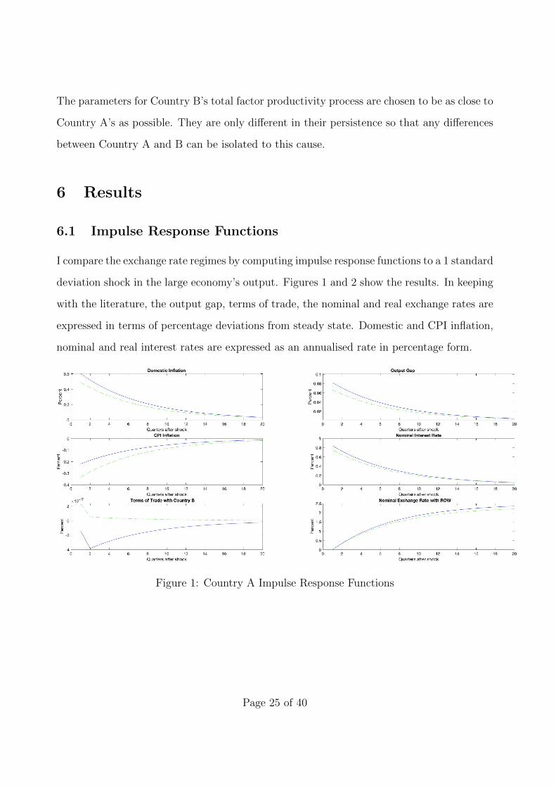
Figure 2: Country B Impulse Response Functions

After a positive output shock from the large economy, there are only small differences in

the business cycle dynamics under the two rules. The shock induces an excess demand for

small country goods from the large economy, causing the domestic currency to appreciate.

Domestic inflation increases and the central bank announces a path of expected appreciation

of the currency. However, CPI inflation increases because the announced appreciation does

not fully compensate the increase in domestic inflation.

With the exchange rate rule, variables that are affected by exchange rate fluctuation are

more stabilised without increasing the volatility of domestic variables. Note that while the

terms of trade with the large economy shifts slightly in response to the shock, its difference

is almost negligible when considered next to the other variables.

When comparing the two polices, we see that the cooperative exchange rate regime seems

to generate lower fluctuations than the non-cooperative exchange rate regime when the

economy is hit by shocks from the rest of the world. This suggests that small open economies

that cooperative regimes may indeed insulate exchange rate coordinating economies.

Page 26 of 40

6.2 Moments

Table 1 displays the business cycle properties of Country A and B’s key variables under the

two monetary policies. All results are reported as standard deviations in percentage terms.

Table 1: Cyclical Properties

Non-cooperative Cooperative

Country A Output 0.014 0.014

Country A Domestic Inflation 0.003 0.003

Country A CPI Inflation 0.008 0.009

Country A Consumption 0.009 0.010

Country A Effective Terms of Trade 0.017 0.017

Country B Output 0.007 0.008

Country B Domestic Inflation 0.002 0.001

Country B CPI Inflation 0.007 0.007

Country B Consumption 0.006 0.006

Country B Effective Terms of Trade 0.010 0.010

As will be shown in Section 6.3, there are minimal differences between the two regimes

with differences in many key variables that are too small even at 4 decimal places. As

both exchange rate rules respond to domestic inflation instead of CPI inflation, domestic

inflation is lower than its CPI equivalent in both countries, although the difference is very

minimal. Differences in cyclical properties between country A and B are driven by the

minute difference in productivity persistence.

6.3 Welfare Losses

Using Country A and Country B’s welfare loss functions, I now compare welfare under the

two regimes. All results are given in percentages of steady state consumption.

Under my baseline parameters in Table 2, welfare losses under non-cooperative monetary

policy are 0.0268 in country A and 0.0053 in country B. Under cooperative monetary policy,

welfare losses are lower at 0.0265 for country A and 0.0022 for country B, indicating positive

Page 27 of 40

but small gains to exchange rate coordination. This means that households in country A

and B are better off by 0.0003% and 0.0031% of steady state consumption respectively in

the cooperative regime.

These results imply that for larger welfare gains from cooperation to exist, additional

rigidities and/or different shocks are required. Since the already small gains to cooperation

reported in the NOEM literature are the result of the globally optimal policy, the lack of

more sizeable gains to exogenous definition of exchange rate coordination is not surprising.

It is significant however, that benefits to policy coordination are present even under ad hoc

policy functional forms that central banks can implement.

Note that while Country B’s welfare gains are small they are still larger than Country A’s.

Given how Country A and B only differ in their total factor productivity persistence with

Country A’s being higher, this implies that ceteris paribus, higher total factor productivity

persistence leads to lower welfare. This effect is closely related to how strongly the monetary

authority responds to domestic inflation.18 When the policy reaction function responds more

aggressively to domestic inflation, the real interest rate rises, which creates a counter-effect

on inflation, since a higher real interest rate causes the output gap to fall.

As total factor productivity persistence increases, monetary policy’s effect on domestic

inflation becomes more predictable, implying that the natural interest rate is closer to

steady-state and the output gap is less affected by technology shocks. However, Pancrazi

and Vukotisc (2011) shows that domestic inflation’s response to a technology shock is non-

monotonically related to total factor productivity persistence.

Hence, higher total factor productivity persistence means that domestic inflation is more

affected by a technology shock, which leads to greater inflation variance and thus welfare

losses. Although this is slightly offset by the lower output gap variance, my results suggests

that the former welfare decreasing effect is stronger.

18As seen in Section 6.4.3, increasing φπ and φx corresponds to lower welfare losses.

Page 28 of 40

6.4 Sensitivity

I now examine the pattern of coordination gains when key parameters are varied within a

realistic range. Key parameters of interest are varied while keeping all other benchmark

parameters constant as outlined in Table 2.

6.4.1 Degree of Openness

I assume that degree of openness is 0.4, which is high for most economies.19 It is therefore

interesting to examine how these two rules fare in an average economy. I repeat the analysis

in Section 6.3 but now with α ∈ [0.1, 0.9] in 0.1 increments. Results are given in Tables 4

and 5 in Appendix C.

Holding κ = 0.5 fixed, welfare losses unambiguously trend downwards as the degree of

openness increases in both monetary policy regimes. Given that the exchange rate is the

monetary policy, this is not surprising as the more trade dependent a country becomes,

the stronger the exchange-rate transmission channel on domestic economic conditions. The

gains from coordination peak at α = 0.1 with gains of 0.0003% and trend downwards with

α, with the lowest gains of 0.0001% for α = 0.9.

6.4.2 Small Country Bias in Preferences

I also assume no bias in preferences between the other small open economy and the large

economy (κ = 0.5), meaning that 50% of Country A’s foreign goods comes from Country

B.20 This too is likely to be an extreme parameter value for most countries, so I repeat my

analysis in Section 6.3 but now with κ ∈ [0.1, 0.9] in increments of 0.1. Results are given in

Tables 4 and 5 in Appendix C.

Intuitively, the gains from cooperation would be relatively smaller if the two coordinating

19Note that α = 0 corresponds to a closed economy.20Note that κ = 0 means that all foreign goods come from the other small open economy (no trade between

the small open economies and the large economy) and κ = 1 means that all foreign goods come from therest of the world. That is, there is no trade between the two small open economies.

Page 29 of 40

countries are relatively closed off from each other (smaller values of κ). As the two economies

become less interconnected, their economic conditions become less correlated and their policy

reaction functions (equations 39 and 40) respond less to domestic conditions. Holding α =

0.4 constant, the gains from coordination peak at κ = 0.1 at 0.0034%, and trends downwards

as κ increases, even becoming negative at κ = 0.9 with welfare losses of 0.0151%.

The presence of welfare losses from policy coordination is somewhat surprising. Although

Pappa (2004) also finds that lowering the degree of openness between the coordinating

economies lowers the gains from coordination, these gains have nonetheless always been

positive. I consider two plausible explanations for this.

Firstly, the welfare loss function I use to generate the results in Table 4s and 5 is from Galı

and Monacelli (2005), which was not derived with a second small open economy. Hence, the

effect of varying exposure to the other small open economy on domestic welfare is likely to

be biased. A micro-founded welfare loss function from my model is required to accurately

identify the effect of κ on welfare and assess whether there definitely is welfare loss given my

definition of coordination.

Secondly, as alluded to in Section 4.2, the results in the literature are computed as the

result of a globally optimal joint welfare maximisation problem, not from an ad hoc policy

reaction function. It may be that these welfare losses are the result of the specific way that

I have defined policy coordination and that under the globally optimal policy, these welfare

losses disappear even under extreme values of κ.

6.4.3 Domestic Inflation and Output Gap Feedback Coefficients

To ensure that the gains from monetary policy coordination are not driven by arbitrary

values of feedback coefficients, I also vary the reactivity of the nominal exchange rate to

domestic inflation and the output gap. Results are shown in Appendix D. I report values for

φπ, φx ∈ [1.1, 1.9]. To satisfy the Blanchard and Kahn (1980) conditions, φx and φπ must be

greater than 1 and although results for φx, φπ ≥ 1.9 are not displayed, the same relationship

Page 30 of 40

discussed below is maintained as the coefficients increase.21

For every combination of φπ, φx, I find that the cooperative exchange rate regime outper-

forms the non-cooperative regime. The more aggressively the nominal exchange rate reacts

to domestic inflation and the output gap, the lower the welfare losses. Interestingly, the

difference in welfare outcomes (coordination benefits) decreases as the coefficients increases.

7 Limitations & Further Work

7.1 Ad hoc Welfare Loss Function

The loss function that I use to evaluate the two regimes is not micro-founded but is from

Galı and Monacelli (2005). Although ad hoc objective functions are still widely used,22 they

are inherently flawed because objectives are endogenous. The underlying structure of the

economy is tightly linked to the objectives a policy maker concerned with maximising the

welfare of the representative agent should pursue. Using micro-founded loss functions to

derive and analyse optimal policy would ensure consistency with the model and overcomes

the misleading prescriptions that result from using exogenous loss functions.

While my model is a direct extension of Galı and Monacelli (2005) and simulations are

run under the same parameter values for consistency, the presence of a second small open

country may nonetheless lead to spurious welfare evaluations.

Alternatively, McCallum and Nelson (1999) suggests that a policy rule should perform

well across different models. This is a useful criterion when considering model uncertainty.

However, as explained in the introduction, a three-country model is necessary to facilitating

the possibility of exchange rate coordination. Since no other model in the NOEM literature

features more than two economies, it is not currently possible to evaluate the robustness of

my result across different models.

21Following Schmitt-Grohe and Uribe (2007), studies on optimal monetary policy have restricted feedbackcoefficients to φπ, φx ≤ 3.

22See for example Angeloni, Coenen and Smets (2003) and Adolfson, Laseen, Linde and Svensson (2011).

Page 31 of 40

7.2 Producer Currency Pricing & Local Currency Pricing

In my analysis, I assume that firms set prices in their own currency, or PCP. Under PCP,

changes in the nominal exchange rate automatically translate into a change in the price of

imported goods. The exchange rate immediately changes the relative price of imported to

local goods, and so plays an important role in achieving efficient outcomes.

However, as detailed in Corsetti, Dedola and Leduc (2010), the PCP assumption is ques-

tioned by a strand of the literature that favours LCP, where firms preset prices in domestic

currency for the domestic market, and in foreign currency for the market of destination.

In other words, exporting firms can price discriminate among markets and/or set prices in

the buyers’ currencies. A currency could be overvalued if the consumer price level is higher

at home than abroad when compared in a common currency, or undervalued if the relative

price level is lower at home. Hence, currency misalignment is possible under LCP.

An analysis under LCP would be interesting for two reasons. Firstly, it would provide

a more realistic flavour to the model as numerous empirical studies show that there are

significant deviations from the law of one price.23 Secondly, Engel (2011) shows that under

LCP, exchange rate misalignment is another key trade-off in addition to inflation and the

output gap, pointing to a greater role of the exchange rate. It is possible that the gains from

exchange rate coordination will be significantly different under LCP.

8 Conclusion

I study whether there are gains from exchange rate coordination in a novel two-country

extension of the small open economy New Keynesian model from Galı and Monacelli (2005).

I find welfare gains to exchange rate coordination, even with a simple exchange rate policy

reaction function. Although these gains are robust to parameter values, they peak at only

0.0034% of steady-state consumption. If the degree of openness decreases to values that are

23See for example, Alessandria (2004), Crucini and Shintani (2008) and Sarno, Taylor and Chowdhury(2004).

Page 32 of 40

reflective of most countries’ openness, then the exchange rate’s ability to minimise welfare

losses and facilitate gains from coordination diminish rapidly. Furthermore, if the degree of

bias in consumption between the other small country and the rest of the world becomes too

low, then the non-cooperative policy outperforms the cooperative policy.

Nonetheless, it is significant that gains emerge even from simple definitions of exchange

rate coordination that central banks can implement. Although this paper demonstrates that

countries would only find benefits from cooperation if they are highly open and trade heavily

with each other, perhaps incorporating additional rigidities such as currency misalignment

under LCP will yield more cooperative benefits.

I conclude by noting that my model abstracts away from geo-political game-theoretic

considerations. I assume monetary policy under commitment from all countries, which elim-

inates the possibility of countries strategically deviating from coordination in each period.

Such possibilities are beyond the scope of this paper.

References

Adolfson, Malin, Stefan Laseen, Jesper Linde, and Lars EO Svensson, “Opti-

mal Monetary Policy in an Operational Medium-Sized DSGE Model,” Journal of Money,

Credit and Banking, 2011, 43 (7), 1287–1331.

Alessandria, George, “International Deviations From the Law of One Price: The Role

of Search Frictions and Market Share,” International Economic Review, 2004, 45 (4),

1263–1291.

Angeloni, Ignazio, Gunter Coenen, and Frank Smets, “Persistence, the Transmission

Mechanism and Robust Monetary Policy,” Scottish Journal of Political Economy, 2003,

50 (5), 527–549.

Page 33 of 40

Benigno, Gianluca and Pierpaolo Benigno, “Price Stability in Open Economies,” The

Review of Economic Studies, 2003, 70 (4), 743–764.

Blanchard, Olivier Jean and Charles M Kahn, “The Solution of Linear Difference

Models Under Rational expectations,” Econometrica: Journal of the Econometric Society,

1980, pp. 1305–1311.

Calvo, Guillermo A, “Staggered Prices in a Utility-Maximizing Framework,” Journal of

Monetary Economics, 1983, 12 (3), 383–398.

Chow, Hwee Kwan, Guay C. Lim, and Paul D McNelis, “Monetary Regime Choice

in Singapore: Would a Taylor Rule Outperform Exchange-Rate Management?,” Journal

of Asian Economics, 2014, 30, 63–81.

Corsetti, Giancarlo and Paolo Pesenti, “Welfare and Macroeconomic Interdependence,”

The Quarterly Journal of Economics, 2001, 116 (2), 421–445.

, Luca Dedola, and Sylvain Leduc, “Optimal Monetary Policy in Open Economies,”

in “Handbook of Monetary Economics,” Vol. 3, Elsevier, 2010, pp. 861–933.

Crucini, Mario J and Mototsugu Shintani, “Persistence in Law of One Price Devia-

tions: Evidence from Micro-data,” Journal of Monetary Economics, 2008, 55 (3), 629–644.

Dixit, Avinash K and Joseph E Stiglitz, “Monopolistic Competition and Optimum

Product diversity,” The American Economic Review, 1977, 67 (3), 297–308.

Edwards, Sebastian, “Monetary policy independence under flexible exchange rates: an

illusion?,” The World Economy, 2015, 38 (5), 773–787.

Engel, Charles, “Currency Misalignments and Optimal Monetary Policy: A Reexamina-

tion,” American Economic Review, 2011, 101 (6), 2796–2822.

Page 34 of 40

Fujiwara, Ippei and Jiao Wang, “Optimal Monetary Policy in Open Economies Revis-

ited,” Journal of International Economics, 2017, 108, 300–314.

Galı, J., Monetary Policy, Inflation, and the Business Cycle: An Introduction to the New

Keynesian Framework and Its Applications, 2 ed., Princeton University Press, 2015.

Galı, Jordi and Tommaso Monacelli, “Monetary Policy and Exchange Rate Volatility

in a Small Open Economy,” The Review of Economic Studies, 2005, 72 (3), 707–734.

Gopinath, Gita, Oleg Itskhoki, and Roberto Rigobon, “Currency Choice and Ex-

change Rate Pass-through,” American Economic Review, 2010, 100 (1), 304–36.

Hamada, Koichi, “A Strategic Analysis of Monetary Interdependence,” Journal of Political

Economy, 1976, 84 (4, Part 1), 677–700.

IMF, International Monetary Fund, “Annual Report on Exchange Arrangements and

Exchange Restrictions, 2018,” Technical Report, International Monetary Fund 2019.

Kearns, J., Andreas Schrimpf, and Fan Dora Xia, “Explaining Monetary Spillovers:

the Matrix Reloaded,” Bank of International Settlements Working Paper, 2018.

Khor, Hoe Ee, Jason Lee, Edward Robinson, and Saktiandi Supaat, “Managed

Float Exchange Rate System: the Singapore Experience,” The Singapore Economic Re-

view, 2007, 52 (1), 7–25.

Lane, Philip R, “The New Open Economy Macroeconomics: A Survey,” Journal of Inter-

national Economics, 2001, 54 (2), 235–266.

Liu, Z and Evi Pappa, “Gains from International Monetary Policy Coordination: Does

it Pay to be Different?,” Journal of Economic Dynamics and Control, 2008, 32 (7), 2085–

2117.

Page 35 of 40

McCallum, Bennett and Edward Nelson, “An Optimizing IS-LM Specification for

Monetary Policy and Business Cycle Analysis,” Journal of Money, Credit and Banking,

1999, 31 (3), 296–316.

Mihov, Ilian and Ana Maria Santacreu, “The Exchange Rate as an Instrument of

Monetary Policy,” Macroeconomic Review, 2013, 12 (1), 74–82.

Mundell, Robert A, “A Theory of Optimum Currency Areas,” The American economic

review, 1961, 51 (4), 657–665.

Obstfeld, Maurice and Kenneth Rogoff, “Exchange Rate Dynamics Redux,” Journal

of Political Economy, 1995, 103 (3), 624–660.

Pancrazi, Roberto and Marija Vukotisc, “TFP Persistence and Monetary Policy,” in

“American Economics Association Annual Meeting, Chicago, Illinois” 2011.

Paoli, Bianca De, “Monetary Policy and Welfare in a Small Open Economy,” Journal of

International Economics, 2009, 77 (1), 11–22.

Pappa, Evi, “Do the ECB and the Fed Really Need to Cooperate? Optimal Monetary

Policy in a Two-country World,” Journal of Monetary Economics, 2004, 51 (4), 753–779.

Parrado, Eric, Singapore’s Unique Monetary Policy: How Does it Work?, International

Monetary Fund, 2004.

Sarno, Lucio, Mark P Taylor, and Ibrahim Chowdhury, “Nonlinear Dynamics in

Deviations From the Law of Pne Price: A broad-based Empirical Study,” Journal of

International Money and Finance, 2004, 23 (1), 1–25.

Schmitt-Grohe, Stephanie and Martin Uribe, “Optimal Simple and Implementable

Monetary and Fiscal Rules,” Journal of Monetary Economics, 2007, 54 (6), 1702–1725.

Page 36 of 40

Svensson, Lars EO and Sweder van Wijnbergen, “Excess Capacity, Monopolistic

Competition, and International Transmission of Monetary Disturbances,” The Economic

Journal, 1989, 99 (397), 785–805.

Woodford, Michael, “Optimal Monetary Policy Inertia,” The Manchester School, 1999,

67, 1–35.

Appendix

Appendix A: Parameter Values

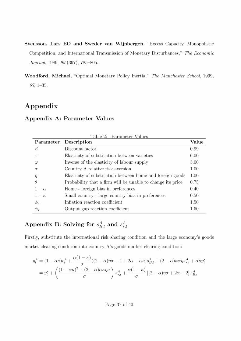
Table 2: Parameter ValuesParameter Description Value

β Discount factor 0.99

ε Elasticity of substitution between varieties 6.00

ϕ Inverse of the elasticity of labour supply 3.00

σ Country A relative risk aversion 1.00

η Elasticity of substitution between home and foreign goods 1.00

θ Probability that a firm will be unable to change its price 0.75

1− α Home - foreign bias in preferences 0.40

1− κ Small country - large country bias in preferences 0.50

φπ Inflation reaction coefficient 1.50

φx Output gap reaction coefficient 1.50

Appendix B: Solving for sAB,t and sA∗,t

Firstly, substitute the international risk sharing condition and the large economy’s goods

market clearing condition into country A’s goods market clearing condition:

yAt = (1− ακ)cAt +α(1− κ)

σ((2− α)ησ − 1 + 2α− ακ)sAB,t + (2− α)καηsA∗,t + ακy∗t

= y∗t +

((1− ακ)2 + (2− α)ακησ

σ

)sA∗,t +

α(1− κ)

σ[(2− α)ησ + 2α− 2] sAB,t

Page 37 of 40

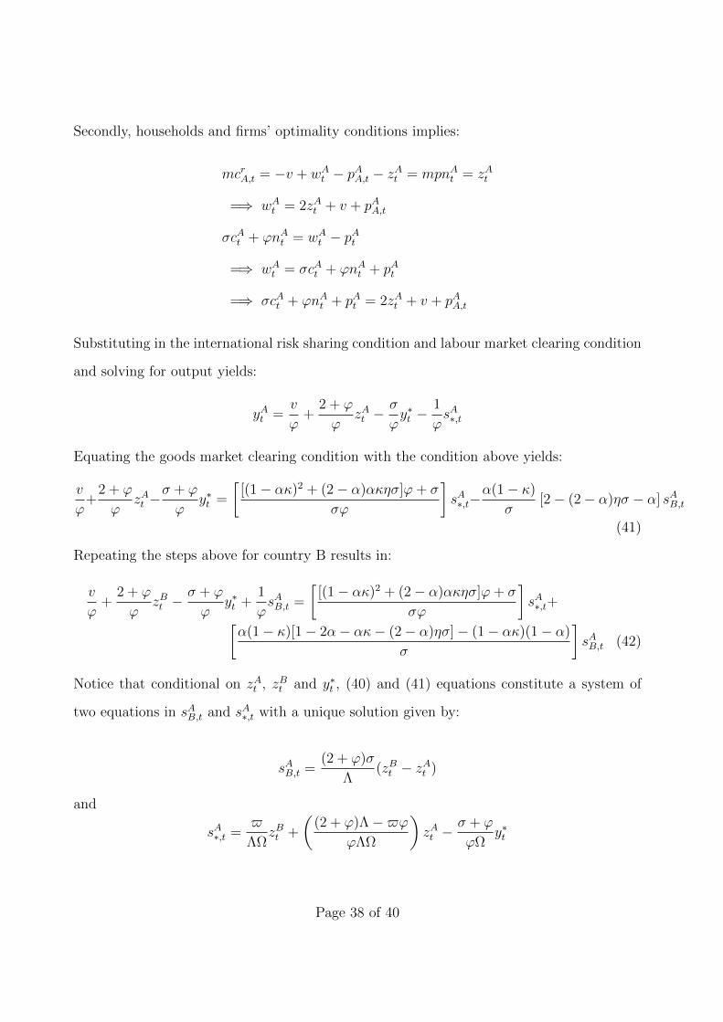
Secondly, households and firms’ optimality conditions implies:

mcrA,t = −v + wAt − pAA,t − zAt = mpnAt = zAt

=⇒ wAt = 2zAt + v + pAA,t

σcAt + ϕnAt = wAt − pAt

=⇒ wAt = σcAt + ϕnAt + pAt

=⇒ σcAt + ϕnAt + pAt = 2zAt + v + pAA,t

Substituting in the international risk sharing condition and labour market clearing condition

and solving for output yields:

yAt =v

ϕ+

2 + ϕ

ϕzAt −

σ

ϕy∗t −

1

ϕsA∗,t

Equating the goods market clearing condition with the condition above yields:

v

ϕ+

2 + ϕ

ϕzAt −

σ + ϕ

ϕy∗t =

[[(1− ακ)2 + (2− α)ακησ]ϕ+ σ

σϕ

]sA∗,t−

α(1− κ)

σ[2− (2− α)ησ − α] sAB,t

(41)

Repeating the steps above for country B results in:

v

ϕ+

2 + ϕ

ϕzBt −

σ + ϕ

ϕy∗t +

1

ϕsAB,t =

[[(1− ακ)2 + (2− α)ακησ]ϕ+ σ

σϕ

]sA∗,t+[

α(1− κ)[1− 2α− ακ− (2− α)ησ]− (1− ακ)(1− α)

σ

]sAB,t (42)

Notice that conditional on zAt , zBt and y∗t , (40) and (41) equations constitute a system of

two equations in sAB,t and sA∗,t with a unique solution given by:

sAB,t =(2 + ϕ)σ

Λ(zBt − zAt )

and

sA∗,t =$

ΛΩzBt +

((2 + ϕ)Λ−$ϕ

ϕΛΩ

)zAt −

σ + ϕ

ϕΩy∗t

Page 38 of 40

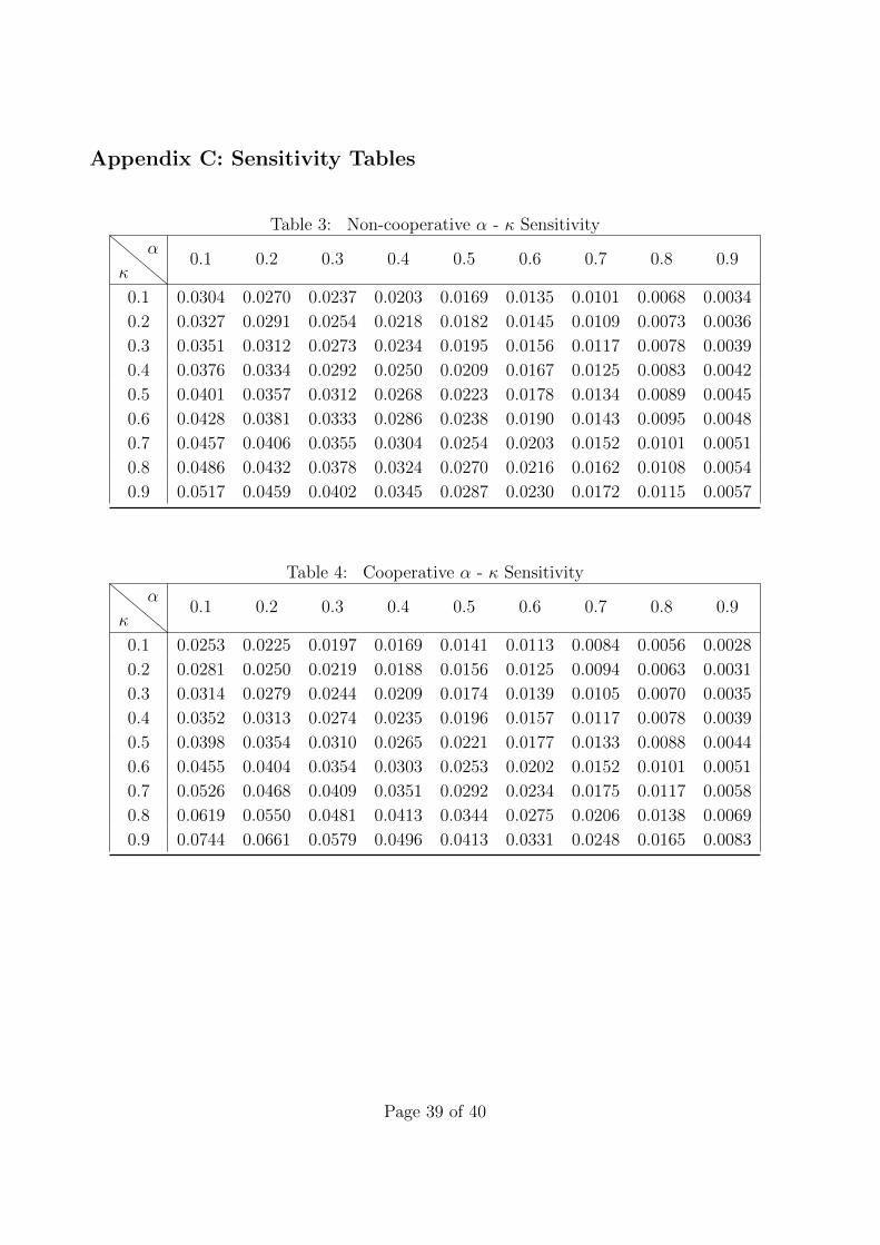
Appendix C: Sensitivity Tables

Table 3: Non-cooperative α - κ Sensitivity

κ

α0.1 0.2 0.3 0.4 0.5 0.6 0.7 0.8 0.9

0.1 0.0304 0.0270 0.0237 0.0203 0.0169 0.0135 0.0101 0.0068 0.0034

0.2 0.0327 0.0291 0.0254 0.0218 0.0182 0.0145 0.0109 0.0073 0.0036

0.3 0.0351 0.0312 0.0273 0.0234 0.0195 0.0156 0.0117 0.0078 0.0039

0.4 0.0376 0.0334 0.0292 0.0250 0.0209 0.0167 0.0125 0.0083 0.0042

0.5 0.0401 0.0357 0.0312 0.0268 0.0223 0.0178 0.0134 0.0089 0.0045

0.6 0.0428 0.0381 0.0333 0.0286 0.0238 0.0190 0.0143 0.0095 0.0048

0.7 0.0457 0.0406 0.0355 0.0304 0.0254 0.0203 0.0152 0.0101 0.0051

0.8 0.0486 0.0432 0.0378 0.0324 0.0270 0.0216 0.0162 0.0108 0.0054

0.9 0.0517 0.0459 0.0402 0.0345 0.0287 0.0230 0.0172 0.0115 0.0057

Table 4: Cooperative α - κ Sensitivity

κ

α0.1 0.2 0.3 0.4 0.5 0.6 0.7 0.8 0.9

0.1 0.0253 0.0225 0.0197 0.0169 0.0141 0.0113 0.0084 0.0056 0.0028

0.2 0.0281 0.0250 0.0219 0.0188 0.0156 0.0125 0.0094 0.0063 0.0031

0.3 0.0314 0.0279 0.0244 0.0209 0.0174 0.0139 0.0105 0.0070 0.0035

0.4 0.0352 0.0313 0.0274 0.0235 0.0196 0.0157 0.0117 0.0078 0.0039

0.5 0.0398 0.0354 0.0310 0.0265 0.0221 0.0177 0.0133 0.0088 0.0044

0.6 0.0455 0.0404 0.0354 0.0303 0.0253 0.0202 0.0152 0.0101 0.0051

0.7 0.0526 0.0468 0.0409 0.0351 0.0292 0.0234 0.0175 0.0117 0.0058

0.8 0.0619 0.0550 0.0481 0.0413 0.0344 0.0275 0.0206 0.0138 0.0069

0.9 0.0744 0.0661 0.0579 0.0496 0.0413 0.0331 0.0248 0.0165 0.0083

Page 39 of 40

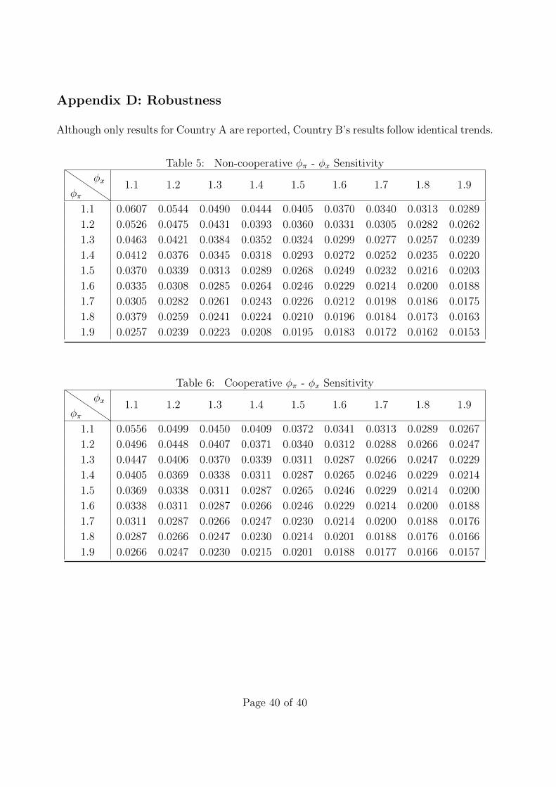
Appendix D: Robustness

Although only results for Country A are reported, Country B’s results follow identical trends.

Table 5: Non-cooperative φπ - φx Sensitivity

φπ

φx 1.1 1.2 1.3 1.4 1.5 1.6 1.7 1.8 1.9

1.1 0.0607 0.0544 0.0490 0.0444 0.0405 0.0370 0.0340 0.0313 0.0289

1.2 0.0526 0.0475 0.0431 0.0393 0.0360 0.0331 0.0305 0.0282 0.0262

1.3 0.0463 0.0421 0.0384 0.0352 0.0324 0.0299 0.0277 0.0257 0.0239

1.4 0.0412 0.0376 0.0345 0.0318 0.0293 0.0272 0.0252 0.0235 0.0220

1.5 0.0370 0.0339 0.0313 0.0289 0.0268 0.0249 0.0232 0.0216 0.0203

1.6 0.0335 0.0308 0.0285 0.0264 0.0246 0.0229 0.0214 0.0200 0.0188

1.7 0.0305 0.0282 0.0261 0.0243 0.0226 0.0212 0.0198 0.0186 0.0175

1.8 0.0379 0.0259 0.0241 0.0224 0.0210 0.0196 0.0184 0.0173 0.0163

1.9 0.0257 0.0239 0.0223 0.0208 0.0195 0.0183 0.0172 0.0162 0.0153

Table 6: Cooperative φπ - φx Sensitivity

φπ

φx 1.1 1.2 1.3 1.4 1.5 1.6 1.7 1.8 1.9

1.1 0.0556 0.0499 0.0450 0.0409 0.0372 0.0341 0.0313 0.0289 0.0267

1.2 0.0496 0.0448 0.0407 0.0371 0.0340 0.0312 0.0288 0.0266 0.0247

1.3 0.0447 0.0406 0.0370 0.0339 0.0311 0.0287 0.0266 0.0247 0.0229

1.4 0.0405 0.0369 0.0338 0.0311 0.0287 0.0265 0.0246 0.0229 0.0214

1.5 0.0369 0.0338 0.0311 0.0287 0.0265 0.0246 0.0229 0.0214 0.0200

1.6 0.0338 0.0311 0.0287 0.0266 0.0246 0.0229 0.0214 0.0200 0.0188

1.7 0.0311 0.0287 0.0266 0.0247 0.0230 0.0214 0.0200 0.0188 0.0176

1.8 0.0287 0.0266 0.0247 0.0230 0.0214 0.0201 0.0188 0.0176 0.0166

1.9 0.0266 0.0247 0.0230 0.0215 0.0201 0.0188 0.0177 0.0166 0.0157

Page 40 of 40