Exchange Rates, Optimal Debt Composition and Hedging in Small

Open Economies

Jose Berrospide*

University of Michigan

Job Market Paper

January 2007

Abstract This paper develops a model of the choice between local and foreign currency debt by firms facing exchange rate risk and hedging possibilities in small open economies. The model shows that the currency composition of debt and the optimal level of hedging are both endogenously determined as optimal firms’ responses to a tradeoff between the lower cost of borrowing in foreign debt and the higher risk involved due to exchange rate uncertainty. Both debt composition and hedging depend on common factors such as foreign exchange risk and financial default, interest rates, the size of net worth and costs of exchange rate risk management. Results of the model are broadly consistent with lending and hedging behavior of the corporate sector in small open economies recently hit by a currency crisis. In particular, the model is able to explain why, unlike predictions of previous work in the literature of currency crisis, the collapse of the fixed exchange rate regime in Brazil in early 1999 did not cause a major change in the currency composition of debt and the hedging behavior of the corporate sector. JEL Classification: F31, F34, F41, G18, G32 Keywords: Exchange rate regime, Debt composition and Hedging _________________ * Email: jberros@umich.edu. I would like to thank Linda Tesar, Uday Rajan, Jing Zhang, Kathryn Dominguez, Chris House and participants of the International Macro Lunch and the International Seminar at the University of Michigan for valuable advice. I am also grateful to the Center for International Business Education (CIBE) for financial support. All remaining errors are mine.

1. Introduction

Recent currency crises in East Asia and Latin America have been mainly characterized by the

presence of currency mismatches between assets and liabilities and inadequate hedging in the balance

sheets of the corporate sector.1 This mismatch between foreign currency liabilities and domestic currency

denominated assets in firm balance sheets has been argued to be the root cause of the large output

collapses following currency depreciations.2 Under a fixed exchange rate regime, firms understand fixed

exchange rates to be a guarantee and fail to insure their foreign exposure. 3 A direct implication of this

line of reasoning is that once the exchange rate is allowed to float, firms will recognize their exposure,

and foreign currency loans will be viewed as more costly so that firms reduce their foreign currency

borrowing. Firms that still opted to borrow internationally would have incentives to hedge their foreign

exposure. Unlike these predictions, firm level evidence from Brazil over the period of 1996-2001,

suggests that the collapse of the fixed exchange rate regime in Brazil, in early 1999, did not cause a major

change in the currency composition of debt and the hedging behavior of the corporate sector. This paper

attempts to offer an explanation to this apparently surprising result.

To study this phenomenon the paper develops a theoretical framework that examines the firm’s

choice of local and foreign currency debt in the presence of exchange rate risk and hedging possibilities.

The model shows that the currency composition of debt and the optimal level of hedging are joint

decisions and depend on common factors such as exchange rate risk and financial default, interest rates,

the size of net worth and costs of foreign currency risk management. The key element driving the model

results is the tradeoff that firms face between the lower cost of borrowing in foreign currency and the

higher risk involved due to exchange rate uncertainty. When affordable, hedging complements the

1 A currency mismatch occurs when a large fraction of firms’ debt is denominated in foreign currency while income and assets are denominated in domestic currency. 2 To see more on the balance sheet explanation of currency crises see for example Krugman (1999), Aghion, Bacchetta and Banerjee (2001) and Schneider and Tornell (2000). 3 This implication is also consistent with another strand in the literature that emphasizes a moral hazard problem introduced by implicit bailout guarantees provided by government, or free exchange rate risk management also provided by government when fixing the exchange rate. These guarantees bias the composition of debt toward foreign currency debt and eliminate incentives to hedge risk. See for example Burnside et al (2001) and Dooley (2000).

2

minimum net worth required by banks and expands the firms’ debt capacity. Furthermore, firms heavily

indebted in foreign currency are not necessarily exposed to exchange rate risk if they have enough net

worth or if they are able to hedge their currency risk through forward markets.

The model predictions are broadly consistent with lending and hedging behavior of the corporate

sector in small open economies that recently faced a currency crisis. The theory suggests that, when the

economy moves from fixed to floating exchange rates, some firms change financing policies and the

population of firms exposed to foreign exchange risk is altered. Firms with insufficient net worth and

those unable to afford buying a hedge lose access to capital markets. Firms with high enough net worth

and those able to hedge increase their foreign debt. Firms with intermediate net worth but unable to

hedge borrow less in foreign currency, turn to domestic banks and are monitored in order to maintain their

access to foreign capital markets. With a macroeconomic environment characterized by a moderate

probability of currency depreciation and inexpensive hedging, these changes in the population of firms

can offset each other so that the average currency composition of debt and hedging activities do not vary

significantly across regimes.

The paper builds on the model developed by Holmstrom and Tirole (1997) adapted to the context

of a small open economy. The paper with the analytical framework most closely related to this paper is

Martinez and Werner (2002). They also extend the Holmstrom and Tirole model to the small open

economy case and find that before the Mexican crisis in 1994, the decision of borrowing in pesos or

dollars depended on the exchange rate regime to the extent that an implicit guarantee was provided by the

government by fixing the exchange rate. However, these authors treat the exchange rate as a deterministic

variable so that no hedging strategies on the firm side are discussed. Arguably, their model captures only

part of the story; there is no discussion on how the interaction between domestic and dollar debt changes

and how the population of firms is altered when the economy moves to a floating regime and firms are

able to hedge. In their paper, as in most of the previous literature, it is implicit that large amounts of

foreign currency debt represent a high degree of exposure of firms to exchange rate risk.

3

As mentioned above, prior theoretical predictions suggest a negative impact of a large

devaluation on companies’ foreign currency borrowing and a reduction in currency mismatches.

However, empirical findings on the relationship between exchange rate regimes and currency mismatches

in the balance sheet of corporate sectors are mixed and still subject to debate. Some studies find that the

large devaluation that followed the collapse of the exchange rate regime reduced currency mismatches by

reducing the foreign currency borrowing and increasing the levels of hedging while others find that firms

were able to borrow even more after the currency crisis. 4 The model presented in this paper contributes to

explain these apparently contradicting results between theory and empirical evidence by providing an

analytical framework in which currency mismatches in the balance sheet of the corporate sector are

reduced after the currency crisis without having firms borrowing less in foreign debt. High enough net

worth as well as hedging operations allow corporations, on aggregate, to maintain their access to

international capital markets and have their currency composition of credit almost unchanged.

The reminder of the paper is organized as follows. Section II presents the main empirical facts

and the motivation for the analysis using firm-level data from Brazil. Section III describes the model of

optimal debt allocation and hedging at the firm level. Section IV offers the main results of the model

under flexible and fixed exchange rates. Section V concludes.

4 Empirical support of currency mismatches and exchange rate exposure during fixed exchange rate regimes is found by Burnside et al (2001) in the Asian crisis, Tesar and Dominguez (2001) in 8 non-industrialized and emerging markets and Bonomo et al (2003) using financial data from Brazilian. On a different study with Brazilian firms Rossi (2004) finds that the adoption of the floating regime reduced the foreign vulnerability of the corporate sector by having a negative impact on firms’ foreign borrowing and a positive impact on hedging. However, Martinez and Werner (2002) find that firms in Mexico were able to increase their dollar debt borrowing after the crisis in 1995 and Arteta (2002) in a cross-country study finds no evidence that a floating exchange rate regime reduces bank currency mismatches. Similarly, Allayannis et al (2002) find that non-financial firms in Asian countries were able to maintain substantial levels of foreign currency debt even after the currency crisis. It is important to say however, that except for only few studies such as Rossi (2004) and Allayannis et al (2002), most studies in the empirical literature only used data on the currency composition of debt at the firm and bank level since data on hedging are often not available or hard to collect.

4

2. Empirical evidence on foreign currency exposure and hedging: Brazil 1996-2001

In this section firm-level data on Brazilian firms are examined before and after the currency crisis

in 1999. Like other Latin American countries, Brazil suffered from unexpected reversals in capital flows

after subsequent crises in Mexico (1994), East Asia (1997) and Russia (1998). The macroeconomic

adjustment forced by substantial capital outflows at the end of 1998 brought large and persistent swings

in the exchange rate that finally led to the collapse of the crawling peg and a sharp devaluation of the real

in January 1999.

Firm-level data correspond to financial information for 350 companies publicly traded in the Sao

Paulo Stock Exchange Market over the period of 1996-2001.5 This information was taken directly from

companies’ annual financial reports. Data contain information on balance sheet variables such as the book

value of assets, the currency composition of debt and shareholder’s equity. Data on hedging transactions

was hand-collected and consists of the year-end notional value of currency derivatives (forwards, futures,

swaps and options) obtained from the explanatory notes to financial statements. Financial and state-

owned firms are excluded because of their different motivation for using currency derivatives.

Table I illustrates the currency composition of debt and hedging activities of firms across

exchange rate regimes. Over the sample, the share of dollar-denominated debt in total debt remains stable

around 46 percent. On average the dollar debt ratio slightly increased from 45 percent during the fixed

exchange rate period to 48 percent during the float period. Across different groups of firms the dollar debt

ratio seems to exhibit a similar pattern, except for small firms that on average slightly decrease their

dollar debt ratio. On the other hand, hedging operations, approximated by the fraction of the notional

value of currency derivatives to dollar debt, increased from 1 percent in 1996 to 18 percent in 2001.

Interestingly, data show that hedging operations increased during the floating exchange rate regime but

were already observed during the fixed exchange rate period, especially for medium and large

5 This period is chosen because it provides valuable information to a comparative analysis on firm’s behavior regarding financing and risk management policies before and after the currency crisis in 1999, and also because disclosure of information on derivatives was mandatory only after 1995.

5

corporations. Large companies increased their hedging ratio on average from 7 to 18 percent. This latter

observation indicates that even before the currency crisis, and most likely after crisis episodes in East

Asia and Russia, some firms indebted in foreign currency were taking care of the devaluation risk by

hedging their positions using currency derivatives. As will be seen later, this behavior is consistent with

the model predictions highlighting the hedging side of financing policies in small open economies subject

to currency risk. While highly suggestive, this table also seems to show some evidence of costly hedging

since the increase in the hedging ratio mostly occurred in large and medium size companies while small

firms appear to hedge a small fraction of their dollar debt even during the floating regime.

Table I - Brazil: Currency Composition of Debt and Hedging Operations: (in means) Average 1996 1997 1998 1999 2000 2001 Fixed Floating Dollar Debt/Total Debt 39.1 45.1 48.0 47.5 48.1 48.0 44.9 47.9 Small 25.8 35.6 27.4 27.1 29.1 28.0 29.4 28.1 Medium 40.0 43.1 51.1 49.1 49.7 48.6 45.7 49.1 Large 57.3 61.6 64.7 63.5 62.4 64.4 62.0 63.4

Dollar Derivatives/Dollar Debt 1/ 1.0 5.3 5.5 4.9 8.1 18.3 4.3 10.5 Small 0.0 0.0 1.9 1.7 1.9 4.1 0.7 2.6 Medium 0.0 6.4 6.0 5.1 6.2 15.5 4.7 9.0 Large 4.0 8.1 7.1 6.4 15.2 31.4 6.7 17.8 1/ Dollar derivatives correspond to the notional value in dollars of currency derivatives (forwards, futures, swaps and options). Source: Brazil Securities and Exchange Commission (CVM). Financial annual reports and explanatory notes to financial statements of companies publicly traded at the Sao Paulo Stock Exchange Market.

An interesting feature regarding the hedging behavior of the corporate sector in Brazil is that

most financial hedging transactions correspond to currency swap contracts. Unlike evidence for U.S. large

non-financial corporations, which report currency forwards and options as the most commonly used tool

to manage exchange rate exposure, firms in Brazil seem to prefer currency swaps, effectively converting

foreign debt into domestic debt by simultaneous transactions in the spot and the forward markets. Broad

preference for currency swaps is also consistent with costly hedging, since a swap reduces transaction

6

costs by allowing companies to arrange in only one contract what may take several transactions (e.g.

forward contracts) to replicate. 6

Table II shows the number of firms holding financial debt in domestic and foreign currency and

those using currency derivatives to hedge their foreign exposure. These data also provide evidence of

minor changes in lending and hedging behavior. The number of firms borrowing in both currencies and

the number of firms borrowing only in domestic currency both slightly increased during the floating

regime. The number of firms that hedge using currency derivatives increases after the collapse of the

exchange rate regime but, interestingly, about 80 percent of the firms with dollar debt in the sample still

remain unhedged during the floating regime.

Table II: Brazil: Exchange rate risk exposure overtime

Fixed ER Floating ER

1996 1997 1998 1999 2000 2001

Total Number of firms 275 296 348 350 328 306

1. Number of firms with no financial debt 12 9 19 18 19 20

2. Number of firms with only domestic debt 33 34 39 37 44 45

3. Number of firms with dollar and domestic debt 109 139 181 200 188 196

Firms hedged using dollar derivatives 2 10 26 27 38 58 Firms not hedged 107 129 155 173 150 138

4. Number of firms with only dollar debt 3 3 16 9 19 17

Firms hedged using dollar derivatives 0 0 0 0 1 0 Firms not hedged 3 3 16 9 18 17

5. Number of firms with unknown 118 111 93 86 58 28 debt position

Source: Brazil Securities Exchange Commission (CVM). Financial annual reports and explanatory notes to financial statements of companies publicly traded at the Sao Paulo Stock Exchange Market

6 Bonomo et al (2003) pointed out that Brazilian firms prefer currency swaps because they can obtain advantageous swap contracts from local banks. Banks, in turn, are able to offer these contracts because they are not exposed to exchange rate risk since they hold government bonds indexed to the dollar in their portfolios. According to these authors, in the end the hedge appears to be provided by government through bank intermediation.

7

Overall, the evidence presented in this section seems to support the view that there are no

significant changes in the lending and hedging patterns of the Brazilian corporate sector during the period

1996-2001, that is, before and after the currency crisis. It should be mentioned that having a genuine

measure of firm-level hedging is difficult, and the previous observations about hedging refer only to the

use of currency derivatives. Firms may use different hedging strategies other than derivatives, such as

holdings of dollar-denominated assets and revenues from exports, which are not emphasized in the

current analysis. The main point that can be emphasized however is that, contrary to prior suggestions,

after the large depreciation that followed the collapse of the fixed exchange rate firms in Brazil were still

able to borrow significantly in foreign currency, more companies hedged this debt by getting involved in

currency derivative markets and there was still a large fraction of firms holding dollar debt which was not

financially hedged through currency derivatives. As will be shown in the next section, predictions of the

model of optimal debt allocation and hedging are consistent with these empirical facts.

3. A Model of Optimal Currency Composition of Debt and Hedging

Consider a small open economy described by a two-date model (t = 0, 1). The economy is

populated by a continuum of risk-neutral firms, domestic banks and foreign banks. Firms are run by

wealth-constrained entrepreneurs who need to raise funds to cover their investment outlays. Firms’

investment projects can be financed by borrowing in either domestic currency from local banks or in

foreign currency from foreign banks. Given the uncertainty about the exchange rate, firms can choose to

hedge their foreign exchange risk by signing forward contracts offered by local banks. At t=0 firms sign

debt contracts and make investment, borrowing and hedging decisions. At t=1, exchange rate and

investment returns are realized and claims are settled. Agents are protected by limited liability so that no

party can end up with negative payoffs.

8

3.1 Investment Projects

Each firm has access to a project requiring an investment of fixed size I>0 at date 0, which yields

at date 1 a verifiable return in domestic currency R in case of success and nothing in case of failure. Firms

differ only in their initial capital A (which is publicly observable). The distribution of firms is described

by the cumulative distribution function F (A). It will be assumed that A<I, so that firms need external

funding to undertake their investments.

There are three types of investment projects as described in Figure 1: a good project with a high

probability of success PG, and a bad and a worse projects each with the same probability of success PB

(PG>PB). The bad project gives a low private benefit b and the worse project gives a high benefit B to the

entrepreneur, with B>b>0. Firms face a moral hazard problem in choosing a project. In the absence of

proper incentives or outside monitoring, entrepreneurs can divert resources by deliberately reducing the

probability of success of a project (from P

B

G to PBB) to enjoy the private benefit.

Figure 1: Three types of Investment Projects

Project Good Bad Worse Probability of success

PG PBB PBB

Private Benefit 0 b B

Local banks can monitor firms to reduce the moral hazard problem and eliminate the worse

project (B-project). Monitoring is costly so that local banks face a fixed cost C>0. Foreign banks are

uninformed investors (i.e. they are unable to monitor firms) and have access to alternative projects with a

gross rate of return r* in international markets. Furthermore, it is assumed that given the rate of return on

investor capital in domestic currency denoted by rf, only the good project has a positive expected net

present value (NPV), even if the private benefit of the firm is included:

PGR – rf I > 0 > PBR - r I + B (3.1) B

f

9

3.2 Financing Decisions and Exchange Rate Risk

In what follows, firms are represented by the index f; domestic banks are represented by the index

m and foreign banks are represented by the index u. At date 0 a representative firm invests all its funds A7

and sign debt contracts to borrow in domestic currency an amount Im from local banks and in foreign

currency an amount Iu from foreign investors so that: 8

I Is I A uLm =++ (3.2)

where sL >0 is the exchange rate at date 0, quoted as sL units of domestic currency per unit of foreign

currency.

Notice that investment return and exchange rate are both uncertain. Investment projects are

subject to two types of bad events: failure (economic default) or bankruptcy due to currency-led default

(financial default). Exchange rate fluctuations, therefore, can turn solvent firms into bankrupt firms even

when they undertake successful projects. It will also be assumed that in case of any type of default firms’

creditors are left with nothing.9

For simplicity, consider only two states of nature about the exchange rate: low (L) and high (H).

At date 0 the exchange rate is sL. If the economy operates under a fixed exchange rate regime then at date

1 s1 = sL. Under a floating exchange rate regime, at date 1 the exchange rate can either depreciate to sH>sL

with probability q, or remain unchanged with probability 1-q. To avoid losses due to exchange rate

fluctuations, companies may decide to hedge their foreign exchange risk by buying currency forward

contracts.

Let F be the one-period forward exchange rate charged to the firm and defined as units of

domestic currency per unit of foreign currency. Given the possibility of economic and financial default, it

7 It is also assumed that the internal rate of return of investment projets exceeds the market rate rf which means that funds invested in the firm are worth the external rate of return plus an incentive effect. 8 There is no other source of funding (e.g. equity finance) in the model. As is the case of emerging economies in Asia and Latin America, a large part of the funds for investments are provided in the form of bank loans. 9 In case of financial default the firm is declared bankrupt and its residual value goes to pay for bankruptcy costs.

10

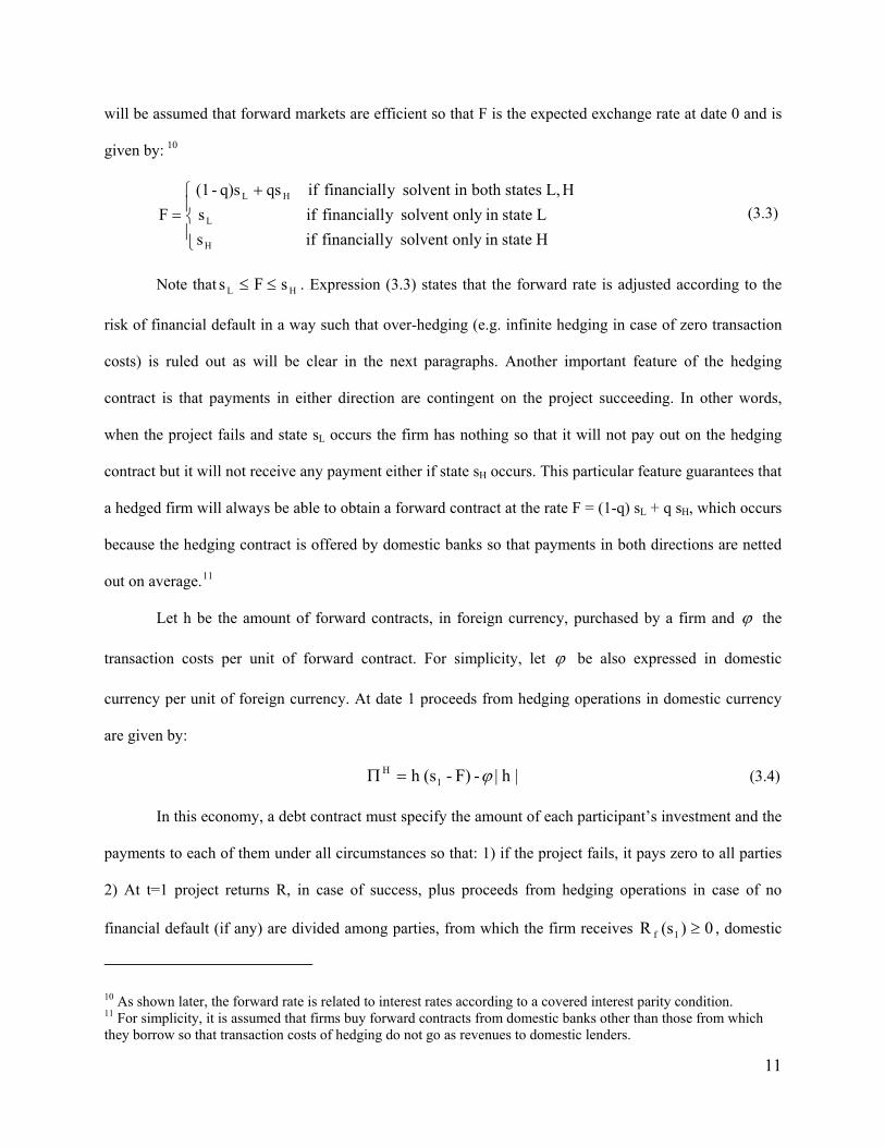
will be assumed that forward markets are efficient so that F is the expected exchange rate at date 0 and is

given by: 10

⎪⎩

⎪⎨

⎧ +=

H statein only solvent y financiall if s L statein only solvent y financiall if s

HL, statesboth in solvent y financiall ifqsq)s-(1F

H

L

HL

(3.3)

Note that HL sFs ≤≤ . Expression (3.3) states that the forward rate is adjusted according to the

risk of financial default in a way such that over-hedging (e.g. infinite hedging in case of zero transaction

costs) is ruled out as will be clear in the next paragraphs. Another important feature of the hedging

contract is that payments in either direction are contingent on the project succeeding. In other words,

when the project fails and state sL occurs the firm has nothing so that it will not pay out on the hedging

contract but it will not receive any payment either if state sH occurs. This particular feature guarantees that

a hedged firm will always be able to obtain a forward contract at the rate F = (1-q) sL + q sH, which occurs

because the hedging contract is offered by domestic banks so that payments in both directions are netted

out on average.11

Let h be the amount of forward contracts, in foreign currency, purchased by a firm and ϕ the

transaction costs per unit of forward contract. For simplicity, let ϕ be also expressed in domestic

currency per unit of foreign currency. At date 1 proceeds from hedging operations in domestic currency

are given by:

|h|-F)-(sh 1H ϕ=Π (3.4)

In this economy, a debt contract must specify the amount of each participant’s investment and the

payments to each of them under all circumstances so that: 1) if the project fails, it pays zero to all parties

2) At t=1 project returns R, in case of success, plus proceeds from hedging operations in case of no

financial default (if any) are divided among parties, from which the firm receives 0)(sR 1f ≥ , domestic

10 As shown later, the forward rate is related to interest rates according to a covered interest parity condition. 11 For simplicity, it is assumed that firms buy forward contracts from domestic banks other than those from which they borrow so that transaction costs of hedging do not go as revenues to domestic lenders.

11

banks receive 0R m ≥ , foreign banks receive 0Rs u1 ≥ and forward sellers receive 0|h| ≥ϕ . Note that

debt payments to lenders are independent of the exchange rate s1 provided the firm is solvent. However,

returns to the entrepreneur (the equity-holder) may depend on s1.

Financial default at date 1, is defined as a situation in which firms that undertake a successful

investment are unable to meet their financial obligations and become bankrupt. Financial default is then

given by the following condition:

0 |h|-F)-(sh )(sRs)(sR)(sR - R 11u11m1f <+−− φ , where s1 = sL , sH (3.5)

As mentioned above, the forward rate in expression (3.3) rules out over-hedging. For example,

consider the case of a firm wanting to buy a significantly high amount of forward contracts to increase its

expected payment when sH occurs but default when sL occurs. As a result, expression (3.5) becomes

positive in state H but negative in state L, that is, the firm is solvent only in state H. By setting F= sH

forward sellers eliminate incentives for firms to over-hedge because in such a case the firm will not be

paid in the depreciation state.

The preceding analysis implies that the firm hedges its foreign exchange exposure in order to

reduce the possibility of financial default. Furthermore, a firm that is hedged ex-ante cannot be insolvent

or solvent in only one state. Since financial default may occur in either state L or H, let 1L and 1H be

indicator variables such that:

⎩⎨⎧

=

⎩⎨⎧

=

L statein default if 0 L statein solvent if 1

1

H statein default if 0H statein solvent if 1

1

L

H

(3.6)

Accordingly, expected cash flows to the entrepreneur with zero proceeds from hedging when the

firm invests in the good project are:

⎩⎨⎧

=

⎩⎨⎧

=

L statein default if 0 L statein solvent if ]Rs - R - R [P

)(sR

H statein default if 0H statein solvent if ]Rs - R - R [P

)(sR

uLmGLf

uHmGHf

(3.7)

12

3.3 Firm’s Expected Profits

At date 0, a firm with initial capital A and investment I chooses the currency composition of its

debt (Im and Iu), creditors’ payments (Rm and Ru), its hedging amount (h) and its expected payments Rf

(sL) and Rf (sH) to maximize expected total profits:

)Is- I-A-I(r } |h|- ]Rs - R-[Rq1 ]Rs - R-[Rq)1-(1 {P ][ E uLmf

uHmHuLmLG TOT ++=Π φ (3.8)

subject to resource constraints, incentive and participation constraints and non-negativity constraints (e.g.

limited liability).

In setting up the problem in this way, it is assumed that the firm undertakes only good projects

with probability of success PG. This is going to be always the case because only good projects have a

NPV>0 which means that if bad projects are undertaken no borrowing is obtained from creditors.

Depending on the exchange rate realization, when the firm is financially solvent, project returns R

and proceeds from hedging operations are distributed among all the parties according to the following

resource constraints:

|h|-F)-h(s R RsR)(sR LuLmLf φ+=++ (3.9)

|h|-F)-h(s R RsR)(sR HuHmHf φ+=++ (3.10)

When the firm defaults in either state H or L it pays nothing to parties and the residual value of

the firm goes to pay for bankruptcy costs.

Let 1m be an indicator variable such that 1m =1 if the firm borrows from the local bank (with

monitoring) and 1m =0 if the firm borrow directly from foreign banks and not from local banks (without

monitoring). Given the two states of nature of the exchange rate, the firm invests in a good project

whenever it obtains an expected payment greater or equal than the expected payment of a bad project

including private benefits, in other words, when:

)B1-(1 b1)](sqR )(sq)R-[(1P )](sqR )(sq)R-[(1P mmHfLfBHfLfG +++≥+ (3.11)

13

This is the firm’s incentive constraint and can also be written as:

p

B)11(p

b1 )(sqR )(sq)R-(1 mmHfLf Δ−+

Δ≥+ (3.12)

where Δp = PG - PB >0. B

3.4 Domestic Bank Lending

A local bank monitors the firm and finances the project whenever it receives an expected

payment sufficient to cover the fixed monitoring cost C, then the bank’s incentive constraint is given by:

p

C1 q]R1 q)-(1[1 mmHL Δ≥+ (3.13)

On the other hand, the bank is willing to finance the project if it receives at least a net expected

payment (net of monitoring costs) equal to the opportunity cost of its funds. The participation constraint

for the bank is then given by:

mf

mmHLG IrC1q]R1 q)-(1[1P ≥−+ (3.14)

Let r denote the domestic lending rate that a local bank charges on Im funds lent to the firm,

defined as:

m

mHLG

Iq]R1 q)-(1[1P

r+

= (3.15)

The minimum domestic rate of return r acceptable for a bank that decides to finance an

investment project in domestic currency is determined by the condition,

prCP

rCpCP GfG

Δ=−

Δ (3.16)

This expression is obtained by combining (3.13) through (3.15), all holding with equality, and

assuming that the bank lends to the project so that 1m=1. This condition, in turn, implies that

B

Gf

PP

rr = (3.17)

14

This expression for the domestic lending rate states that the cost of domestic funds incorporates a

risk premium relative to the risk-free rate. At the minimum rate of return acceptable for a bank this risk

premium is equal to the ratio of success probabilities of the good and bad projects.

Local banks can borrow and lend internationally and are able to replicate a forward contract.

Perfect competition and non-arbitrage conditions ensure that banks are indifferent between lending in

domestic currency at rf, converting these funds into foreign currency at date 0 at the spot rate sL and

lending abroad in foreign currency where they earn r*, and converting these funds back to domestic

currency at the forward rate F. These transactions imply that:

L

*f

sFrr = (3.18)

This is a covered interest rate parity condition and can be also expressed in terms of the domestic

lending rate r and the international rate r* as:

LB

G*

sF

PPr

r = (3.19)

In this expression PG > PB and F > sL so that the bank lending rate r is always greater than the

international interest rate r* and, therefore, foreign debt is always preferred to domestic debt. As a result,

when they have to, firms want to borrow the least they can from a local bank and obtain the rest of their

funds from foreign lenders.

The firm will be able to borrow in foreign currency if foreign banks are promised an expected

payment greater than or equal to what they could obtain by investing their funds in international capital

markets at the rate r*. The foreign bank participation constraint in foreign currency is then:

u*

uHLG Irq]R1 q)-(1[1P ≥+ (3.20)

15

3.5 Firm’s Profit Maximization

The firm’s problem is to find variables h, Im, Iu, Rm, Ru, Rf (sL), Rf (sH) given exogenous

parameters such as the firm’s initial assets A, its fixed investment I, the foreign rate of return r*, the

probability of currency depreciation q and the cost of hedging ϕ , in order to:

Maximize)Is- I-A-I(r } |h|- ]Rs - R-[Rq1 ]Rs - R-[Rq)1-(1 {P ][ E uLm

fuHmHuLmLG TOT ++=Π φ

subject to

I IsIA uLm ≥++ (1) If firm is solvent: |h|-F)-(sh R RsR)(sR LuLmLf ϕ+=++ (2) |h|-F)(sh R RsR)(sR HuHmHf ϕ−+=++ (3)

pB)11(

pb1 )(sR q)(sR q)-(1 mmHfLf Δ

−+Δ

≥+ (4)

pC1 q]R1q)1-[(1 mmHL Δ

≥+ (5)

mf

mmHLG Ir C1-q]R1q)1-[(1P ≥+ (6)

u*

uHLG Ir R q]1q)1-[(1P ≥+ (7)

0)s(R Hf ≥ (8) 0)s(R Lf ≥ (9)

Conditions (1) through (3) are resource constraints. Conditions (4) and (5) are the incentive

constraints of the firm and the domestic bank. Conditions (6) and (7) are the participation constraints for

domestic and foreign banks. Conditions (8) and (9) are non-negativity constraints for the firm’s payments.

Only one of these two non-negativity constraints will be binding when the firm defaults in one state of the

exchange rate but is solvent in the other. Notice that there are 9 constraints to solve for 7 choice variables,

which means that in equilibrium at least 7 constraints must be binding.

3.6 Equilibrium

The determination of the equilibrium as well as closed-form solutions for the currency

composition of debt and optimal hedging are explained in detail in appendix 1 of the paper. As an

16

illustration, consider that both borrowing and hedging decisions are endogenously determined as optimal

firms’ responses to a tradeoff between the lower cost of borrowing in foreign debt and the higher risk

involved due to exchange rate uncertainty. As explained above, foreign currency debt is preferred to

domestic debt so that the firm always tries to borrow directly from foreign banks. The smaller the size of

its initial assets A, the more the firm demands from international banks. Since exchange rate uncertainty

makes foreign debt risky, foreign banks demand a minimum net worth and hedging operations through

currency forwards to ensure that the firm is solvent enough to repay its debt. If the firm’s initial net worth

is not sufficient to meet the foreign bank’s requirement then the firm must be monitored and borrow from

domestic banks first in order to be able to borrow from international markets. Local banks help firms

undertake investments projects because domestic lending reduces the net worth requirement. Depending

on the size of its net worth, the monitored firm may also need to hedge to demonstrate financial solvency.

Given that the internal rate of return is greater than the external rate on firm capital, entrepreneurs

prefer to invest all their funds in the project. Therefore, constraint (1) in the firm’s problem will be

binding in most cases. The only exception happens when a firm has to borrow only in domestic currency

from local banks. Recall that local banks have to cover the fixed monitoring costs so that they lend all

firms the same fixed amount in domestic currency. Therefore, when the firm has a net worth insufficient

to borrow only in foreign currency but high enough to borrow the fixed amount in domestic currency and

the sources of funds exceed the size of investment, then the firm has to invest its excess funds at the

market rate r f.

Another key feature of the model is that hedging decisions are perfectly observed by creditors. An

immediate implication is that firms have incentives to hedge their exchange rate risk to reduce the

probability of financial default. When affordable and useful, hedging increases profits by expanding the

possibility of borrowing in foreign currency at a lower interest rate. The equilibrium level of hedging

corresponds to any value within an optimal range defined by constraints (2), (3), (8) and (9) as shown in

the appendix. Depending on exogenous parameters, in particular q andϕ , the minimum level of hedging

in this range can be positive or negative (negative hedging implies that the firm sells forward contracts).

17

As shown in what follows, intermediate values of q and small enough ϕ make the minimum level of

hedging positive so that a profit maximizing firm will always choose this minimum level. However, there

will be situations when the firm optimally chooses not to hedge. To see this, let q be the probability of

depreciation that makes the minimum level of hedging equal to zero and ϕ be the transaction cost in

forward markets above which, for any given level of positive q, forward contracts are too costly to

provide insurance.12 When the probability of depreciation is too high, say qq > , describing for example a

situation of extreme exchange rate volatility, firms will find optimal to choose a zero level of hedging. On

the other hand, when too costly, say ϕϕ > , then even if available hedging is not affordable so that firms

will also choose not to hedge.

A representative firm solves its profit maximization problem under two situations: when it hedges

enough to avoid financial default and when it does not hedge at all.13 Given that hedging is a necessary

but not a sufficient condition for financial solvency, a firm with sufficiently high net worth can borrow

only small amounts of foreign currency debt and be financially solvent without hedging. Therefore, when

the firm does not hedge at all, there are two additional possibilities: the firm is solvent even without

hedging or the firm defaults if it is not hedged. Each of these situations exists for a monitored company

borrowing in both currencies and for a company borrowing only in foreign currency. These multiple cases

imply that creditors demand different net worth levels depending on the composition of credit and the

firm’s hedging strategy.

Appendix 2 of the paper illustrates the solution to all these net worth requirements. For the

purpose of analysis, a brief description of them is in order: upper bar net worth requirements refer to cases

of firms borrowing directly from foreign markets while lower bar net worth requirements refer to cases of 12 It can be shown that )

pCR/()

)s-(ss

pb(1q

LH

H

Δ−

Δ−= and )s-q)(s-(1 F-s LHH ==ϕ respectively.

13 Partly hedging is ruled out because in case of currency depreciation, this level of hedging is not sufficient to avoid default so that the firm is forced to default as if hedging was zero in the first place. With sufficiently small but positive costs of hedging the firm will prefer zero hedging to partly hedging.

18

firms being monitored and borrowing from domestic banks first. Accordingly, HA is the minimum net

worth for an optimally hedged firm that borrows in both domestic and foreign currency. Similarly, HA is

the minimum level of assets required for an optimally hedged firm wanting to borrow only in foreign

currency from international banks.

When the firm does not hedge and as a result it is not solvent in state H then the minimum net

worth requirements are NHA and NHA for firms being monitored by local banks and for firms borrowing

directly from foreign banks respectively. If the firm is unhedged but solvent in state H then it faces a

higher minimum net worth required by creditors: SNHA if monitored by local banks and SNHA if it wants

to borrow directly from foreign banks. 14 An unhedged but solvent firm faces the highest net worth

requirements. On the other hand, hedging, when affordable, allows the firm to face the lowest net worth

requirement. In equilibrium, depending on the size of the firm’s initial assets and its hedging strategy,

there are different financing possibilities. To decide the optimal currency composition of its debt (e.g.

how much to borrow from each source) and whether it should be hedged or not, the firm compares its

initial assets A with these cutoff levels.

4. Model results

Equilibrium with costless hedging ( 0=ϕ )

Costless hedging represents a long run equilibrium in which currency forward markets are

competitive and well-developed so that transaction costs are negligible. The next two results illustrate the

optimal financing policies when the economy operates under a fixed exchange rate regime and under

floating exchange rates as two separate steady state equilibria.

14 As explained in appendix 2, a second and more stringent criterion for unhedged and solvent firms is also considered. This is the case of firms that are solvent and expect to receive the maximum expected payment given by constraint (4) even in the depreciation state. The minimum net worth required to these firms is even higher: SA if

they are monitored and SA if they want to borrow only from international markets.

19

Lemma 1 In an economy with fixed exchange rates, that is when q=0, an optimal strategy for a firm is not

to hedge its dollar debt.

Proof: See Appendix

This basic result explains why a fixed exchange rate biases the currency composition of debt for

some firms towards foreign currency debt and eliminates incentives to operate in forward markets. By

fixing the exchange rate, the government provides a form of public hedging or free risk management to

the corporate sector by creating a perception of no foreign exchange risk.15 Consequently, some firms that

otherwise would not be able to borrow at all, or some others that should be monitored to have access to

international capital markets, are now able to obtain foreign currency debt without constraints. This

situation creates incentives for entrepreneurs to borrow extensively in foreign currency without hedging

and maintain currency mismatches in their balance sheets. As predicted by the balance sheet approach of

currency crises, in the event of unexpected and large currency depreciation the corporate sector in this

economy would face widespread bankruptcy.

Lemma 2 In an economy with floating exchange rates when qq <<0 in equilibrium the optimal

strategy for a firm with net worth A such that SNHH AAA << or SNHH AAA << is to hedge its dollar

debt through currency forwards enough to avoid bankruptcy.

Proof: See Appendix

According to this result, as long as the probability of currency depreciation makes forward

contracts a useful instrument to deal with exchange rate risk, hedging makes it easier for the firm to

obtain funding from foreign banks at a lower cost because it reduces the required net worth. Without

transaction costs in forward markets hedging is always preferred to not hedging and any firm that is not

solvent in state H has incentives to hedge enough to avoid financial default. This is the case when the firm

15 With costless hedging and q=0 the cutoff thresholds of the net worth ratios are at their lowest value and the firm is indifferent about how much it hedges since F= sL.

20

uses a mixture of domestic and foreign debt or when it borrows only in foreign currency. Note also that

hedging is beneficial only for firms that are not solvent in state H; firms with net worth above the

minimum requirement for solvency in state H do not need to hedge.

The previous two equilibrium results when hedging is costless determine a particular ordering of

net worth requirements and define an equilibrium segmentation of firms into different categories

depending on their demand for bank loans and their hedging strategy, as shown in Figure 2. Well-

capitalized firms with net worth A > HA finance their investment directly in foreign currency from

international banks. Poorly capitalized firms with A < HA cannot invest at all since they have no access

to any type of finance. In between, somewhat capitalized firms with HH AAA << can invest only to the

extent that they are monitored and demand domestic bank loans. Firms in the monitoring region

]A,A[ HH finance their investment with a mixture of domestic and foreign debt. As already mentioned,

whether firms hedge their foreign debt or not also depends on the size of their initial asset. Well-

capitalized firms need not hedge if A > SNHA but must hedge if A Є ]A,A[ SNHH . Similarly, somewhat

capitalized firms need not hedge if A Є ]A,A[ HSNH but must hedge if A Є ]A,A[ SNHH .

A typical firm within the monitoring region uses a mixture of domestic and foreign currency debt

to finance its investment. However, as mentioned above, there are firms with net worth A < HA but A +

Im > I that only demand bank loans in domestic currency and invest their excess funds outside the firm at

the market rate. The minimum net worth requirement for these firms is AB as is given by:B

16

p

CFs

rPIq),(rA L

*B*

B Δ−=

16 This happens when the monitoring cost C is sufficiently high so that local banks lend relatively high amounts in domestic currency. In general, this does not have to be always the case. When domestic debt is small enough so that AB >B HA then firms never borrow only in domestic currency because they have the possibility to borrow only in foreign currency at a lower cost.

21

Figure 2: Equilibrium segmentation of firms

No credit Only

foreign debt

Domestic and foreign debt

F(A)

Hedged Not hedged Hedged Not

Hedged

HA SNHA SNHA HA

Only domestic

debt

Not Hedged

0 AB

Monitoring region Net worth

The distribution of net worth requirements in the equilibrium segmentation implied by Lemma 2

and depicted in Figure 2 is:

SNHNHHBSNHNHH AAAAAAA <<<<<<

Interestingly now, within the monitoring region there are firms borrowing in domestic and foreign

currency, some of which must be hedged, and also firms borrowing only in domestic currency that need

not hedge. Notice also that NHA and NHA are irrelevant so they are not shown in the figure.

Lemma 1 and Lemma 2 are consistent with prior predictions in the literature, in particular with

the government guarantees approach that emphasizes the incentives for firms to borrow extensively in

foreign currency debt without hedging when the exchange rate is fixed. However, another interesting

implication derived from Lemma 2 is that not all firms must hedge during a floating regime because some

of them have enough net worth to be financially solvent even in the depreciation state.

22

Equilibrium with costly hedging 0>ϕ

In the previous analysis when 0=ϕ net worth requirements NHA and NHA are irrelevant

because

Proposition 1: With costly hedging and a positive probability of depreciation the optimal strategy for a

any firm is optimally hedged. The next result refers to the possibility that currency mismatches

also arise during floating regimes because hedging activities even if available can be unaffordable for all

firms when transaction costs in currency forward markets are sufficiently high.

firm in the monitoring region, regarding debt composition and hedging, depend on q and ϕ such that:

a. When qq ≥ the firm borrows the least it can in domestic currency from local ba ks and borron w

b.

the rest in foreign currency from foreign banks and does not hedge its foreign debt.

When qq <<0 and ))(1(0 LH ssq −−<< ϕ the firm finds it optimal to borrow the least it can

estic curr rom local banks and the in dom ency f rest in foreign currency from foreign banks and:

b1. If ϕ is small enough then the firm with SNHH AAA << will always hedge its foreign debt

b2. If ϕ is sufficiently high then only some firms with SNHNH AAA << hedge its foreign debt.

))(1( LH ssq −−≥ϕ the firm finds it optimal to borrow the least it can in domestic. When c

cy from local banks

trates all different hedging possibilities implied by Proposition 3. Notice that the

minimu

curren and the rest in foreign currency from foreign banks and does not

hedge its foreign debt.

Proof: See Appendix

Figure 3 illus

m net worth requirement to obtain credit in both domestic and foreign currency varies depending

on parameters q andϕ . In the first case, extremely high probability of depreciation makes optimal

hedging zero so that n firm participates in currency forward markets. A similar situation occurs in the

third case when some firms have incentives to hedge but forward contracts are too expensive or

inexistent. Although these two situations look similar in that firms do not hedge, they are different and

o

23

have different interpretations. Intuitively, higher values of both q andϕ increase the net worth

requirement making it more difficult to borrow in both domestic and foreign currency. In the first

situation (Case a), q is too high that the firm is forced to borrow only small amounts in foreign currency

so that it can be solvent in state H without hedging. In the third case (Case c), however, a firm that is not

solvent in state H is still able to borrow larger amounts of foreign debt even when it cannot afford to

hedge. This latter firm has a currency mismatch in its balance sheet and would default if state H happens.

Figure 3: Different Hedging Strategie for firms within the monitoring s

region

Case a: q very high

HA

No credit

Case b1: q moderate φ very small

Case b2: q very small φ moderate

Case c: φ very high

No credit

HA SNHA

Hedged

No credit Hedged Not hedged

Not hedged No credit

NHA SNHA

SNHA NHA

*A

No need to hedge

No need to hedge

No need to hedge

No need to hedge

Net worth

Net worth

Net worth

Net worth

24

The second case in proposition 1 corresponds to intermediate values of q andϕ which allow

firms to b hedge. When the cost of hedging is small enough any firm needing to hedge to e solvent will

always hedge (case b1) and the cutoff level NHA is irrelevant. However, as the cost of hedging increases

some firms have incentives to borrow in bo urrencies but find it optimal not to hedge their foreign

debt. Now

th c

NHA becomes the relevant cutoff level defining the lower limit in the equilibrium

segmentation. The proof of proposition 1 describes the cutoff level A* below which firms do not hedge

because hedging is too costly. These firms would default in the event of currency depreciation (case b2).

This particular situation describes the case of economies of scale in hedging operations. Firms with small

net worth tend to be highly leveraged and demand more foreign currency debt than larger firms and

cannot cover this exposure because the level of hedging required is not affordable. In contrast, firms with

higher net worth demand less foreign currency debt and require a lower level of hedging to manage their

foreign exchange risk even when forward contracts are somewhat expensive.

The preceding analysis shows that the segmentation of firms depends on exogenous parameters,

in parti

roposition 2: When the economy moves from fixed to floating exchange rates and in the floating regime

cular, those describing the macroeconomic environment such as interest rates, exchange rates,

probability of currency depreciation and costs of hedging. The next result illustrates how different

exchange rate regimes and different stages of development in forward markets affect the allocation of

domestic and foreign debt and hedging behavior.

P

qq <<0 and ))(1( LH ssq −−<ϕ , all else equal:

or their investmeni. Fewer firms obtain funding f t.

irectly form foreign banks.

ed exchange rate

ii. Fewer firms finance their investment borrowing d

iii. Some firms borrowing directly from foreign banks during the fix

increase their demand for domestic loans from local banks during the floating regime.

Proof: See Appendix

25

To illustrate these results, consider that in equilibrium, domestic currency borrowing Im is a fixed

amount and each firm in the economy demands the same minimum amount from local banks. The

aggregate demand for domestic bank loans Im is then:

[ ] q),(rI q)),(rAF(-q)),(rAF( q),(rD *m

*H

*H

*m =

where the individual demand Im is written as a decreasing function of both r* and q. On the other hand,

the aggregate demand for foreign currency loans is given by:

[ ] [ ] F(A) A - I F(A)A - q) ,(rI - I q),(rDq) ,(rAq) ,(rA mu *

H*

H

dd ∫∫∞

+

Since r* and q are exogenous parameters and assuming perfect competition in the domestic

banking

ime has an ambiguous

effect o

q) ,(rA ***

H

=

system, the supply of domestic funds is perfectly elastic at the domestic lending rate r and the

supply of foreign loans is perfectly elastic at the international interest rate r*, which means that Dm and Du

determine the aggregate amounts of domestic and foreign lending in equilibrium.

An increase in q brought by the collapse of the fixed exchange rate reg

n Dm because both cutoff levels q),r(A *H and q),r(A *

H increase and there are two opposing

effects. A first group of firms with insuff unable to hedge cannot borrow at all

and are dropped so that D

icient net worth and those

reign

debt an

collapse of the fixed exchange rate regime are illustrated in the next figure.

m decreases. Some other firms turn to domestic banks and increase Dm because

they have insufficient net worth or are unable to hedge and cannot borrow only in foreign currency.

The impact of q on Du is ambiguous as well. Firms that were previously borrowing in fo

d turned to domestic debt reduce their demand for foreign currency debt so that Du drops.

However, firms with intermediate net worth and those able to hedge remain in the monitoring region and

increase their demand for foreign debt because Im decreases for them and, as a result, Du increases. In

sum, a number of firms borrow less in both currencies and some others borrow more in foreign currency.

The extent to which these changes in the population of firms affect the aggregate currency composition of

debt depends on the distribution function F (A). Possible changes in the population of firms after the

26

Figure 4: Changes in the Equilibrium Segmentation: fr

exchange rates om fixed to floating

o the

right, m king it more difficult for firms to borrow in foreign currency. This figure illustrates changes in

hedging

Figure 4 shows that the switch in the exchange rate regime shifts the monitoring region t

a

behavior than can be significant if the increase in the probability of depreciation is relatively

small. However, depending on how large q and ϕ are, these changes could be small. For example, as q

increases and approximates to q the group of firms that hedge using currency forwards becomes smaller

and can be very small if ϕ is also sufficiently high as to prevent some firms from hedging.

4.1. The Brazilian Experience

As a final illustration, consider how the results of the model match up with the currency crisis in

the model results, the lack of major changes in the lending and hedging

behavior of the corporate sector in Brazil can be the result of a moderate increase in the probability of

Brazil in early 1999. In light of

No Credit

Fixed

Domestic and Foreign Debt

Not hedged Not hedged

Only Foreign Debt

Not hedged

Domestic and Foreign Debt Only Foreign Debt No Credit

Not hedged Hedged Hedged Floating

HA HA

HA HA

Net worth

Not hedged

SNHA BA

Not hedged

BA SNHA SNHA Net worth

27

currency

reality. Moreover, in contrast to what the model assumes, a currency crisis most likely affects

the firm

ing decisions in a model of optimal debt allocation at the firm level to

nderstand the sources of currency mismatch in the balance sheet of the corporate sector of countries that

ises. The model explains why some firms with access to foreign currency debt

hedge their exchange risk exposure and others do not, as an optimal response to appropriate incentives

depreciation and the existence of somewhat costless hedging. After the floating regime is

adopted, some firms borrow less in both domestic and foreign currency and some others borrow more in

foreign currency. Moreover, a group of firms borrowing in foreign currency do not hedge either because

they cannot afford to buy forward contracts or because their net worth is sufficiently high and they are

solvent even in the event of currency depreciation. These changes in the population of firms can offset

each other so that the currency composition of debt and hedging activities do not vary significantly across

regimes.

Needless to say, there are various other aspects of the macroeconomic environment as well as

firm-specific characteristics conditioning the currency composition of lending and the hedging behavior

of firms in

s’ net worth so that the distribution of firms may not be constant across regimes. Furthermore,

other parameters such as the probability of success and the investment payoff R are certainly different

across firms and are also affected by the collapse of the exchange rate regime. How companies deal with

higher foreign exchange risk definitely depend on changes in these variables, treated as invariant

parameters in the model. For example, depending on specific characteristics such as export status, type of

ownership or the existence of other sources of funding; firms can adopt hedging strategies other than the

use of currency forwards. Nevertheless, the model developed in the paper suggests changes in the

behavior of a representative firm and impacts on the population of firms that are broadly consistent with

the empirical facts observed in recent currency crises in small open economies, and in particular, in Brazil

during the period of 1996 to 2001.

5. Conclusions

This paper introduces hedg

u

recently faced a currency cr

28

given b

of

currenc

should give to the development of currency

derivati

y the macroeconomic environment. Under fixed exchange rates firms borrow extensively in

foreign currency and do not hedge because they have no incentives to do so given that government

provides a type of free risk management. Under a floating regime, when the probability of currency

depreciation is moderate and hedging is affordable firms use currency forwards to hedge their exchange

rare risk exposure and reduce the probability of financial default. Hedging complements net worth

required by creditors allowing hedged firms to expand their capacity to access foreign capital markets.

Despite the obvious limitations of a partial equilibrium analysis and some simplifying

assumptions, the model is able to provide an analytical framework to determine endogenously the

currency composition of credit and the optimal level of hedging at the firm level. Consistent with the

empirical evidence in Brazil during 1996 to 2001, the model predicts that with a moderate probability

y depreciation and somewhat costless hedging, the changes in the population of firms after the

economy adopts a floating regime can offset each other so that the currency composition of debt and

hedging activities do not vary significantly across regimes.

While the currency composition of debt remained stable in Brazil after the collapse of the

exchange rate regime, costless hedging operations seem to provide an effective vehicle to reduce foreign

exposure without affecting significantly the aggregate levels of borrowing. A direct policy implication of

the model is then the necessary emphasis that policymakers

ves markets to help the corporate sector in smoothing the transition to a free-floating exchange

rate regime.

29

REFERENCES

ghion, P., Bacchetta, P., Banerjee, A (2001) “A Corporate Balance-Sheet Approach to Currency

rises”, Gerzensee Study Center, Working Paper No. 01.05.

llayannis George and Eli Ofek (2001): “Exchange Rate Exposure, Hedging, and the Use of Foreign

Currency Derivatives”. Journal of International Money and Finance No 20.

Allayannis G., Brown, G. and Klapper L. (2003): “Capital Structure and Financial Risk: Evidence from

Arteta, C. (2002) “Exchange Rate Regime and Financial Dollarization: Does Flexibility Reduce Bank

Getulio Vargas. Graduate School of

Bank of Boston

Caballero, R. and Krishnamurthy, A. (2000) “Dollarization of Liabilities: Underinsurance and

Calvo, G. and Carmen Reinhart (2001) “Fear of Floating” NBER Working Paper No 7993.

e Rate Exposure”. American

Economic Review Papers and Proceedings.

ic Journal, Vol. 110, No 460.

sity Press.

Quarterly Journal of Economics. Vol 112, No 3, 663-691.

A

C

A

Foreign Debt Use in Eat Asia”. The Journal of Finance. Vol 58.

Currency Mismatches?” International Finance Discussion Papers No 738. Board of Governors of the

Federal Reserve System.

Bonomo, Marco, Martins B. and Pinto, R. (2003): “Debt Composition and Exchange Rate Balance

Sheet effects in Brazil: A Firm Level Analysis”. Fundacao

Economics. Rio de Janeiro, Brazil. Working Paper.

Beakley, Hoyt and K. Cowan (2002) “Corporate Dollar Debt and Depreciations: Much Ado About

Nothing”. Federal Reserve

Burnside, C., Eichenbaum, M. and Rebelo S. (2001) “Hedging and Financial Fragility in Fixed

Exchange Rate Regimes”. European Economic Review No 45. 1151-1193

Domestic Financial Underdevelopment”. NBER Working Paper No 7792

Dominguez, K., and L. Tesar (2001a) “A Re-Examination of Exchang

Dooley, M. (2000) “A Model of Crisis in Emerging Markets”. The Econom

Eichengreen, Barry (2002) “Financial Crises And What To Do About Them”. Oxford Univer

Eichengreen, B., Hausman, R.,(1999) “Exchange Rate and Financial Fragility” NBER Working Paper

No. 7418.

Holmstrom, B. and Tirole, J. (1997) “Financial Intermediation, Loanable Funds and the Real Sector”.

30

Inter-American Development Bank (2001) “Competitiveness: The Business of Growth”. Economic and

Social Progress in Latin America. 2001 Report. IADB, Washington D.C.

Crises, Essays in Honor of Robert P. Flood,

the Currency Composition of

eral Reserve Bank of Minneapolis. Discussion Paper 129.

Krugman, P. (1999) ”Balance Sheets, The Transfer Problem, and Financial Crises” in P. Isard, A. Razin,

and A. Rose (eds.), International Finance and Financial

Kluwer, Dordrecht.

Martinez L. and Werner, A. (2002) “The Exchange Rate Regime and

Corporate Debt: The Mexican experience”. Journal of Development Economics 69 (2002) 315– 334.

Repullo, R. and Suarez, J. (1999) “Entrepreneurial Moral Hazard and Bank Monitoring: A model of the

Credit Channel”. Fed

Rossi, Jose L. (2004) “Corporate Foreign Vulnerability, Financial Policies and the Exchange Rate

Regime: Evidence from Brazil”. Yale University. Manuscript.

Schneider, M. and Tornell, A. (2000) “Balance Sheet effects, Bailout Guarantees and Financial Crises”.

NBER Working Paper No 8060.

Tirole, Jean (2002) “Financial Crises, Liquidity, and the International Monetary System”. Princeton

University Press.

31

Appendix

1. Determination of Equilibrium

There are four possible cases in the profit maximization problem of a representative firm. The

maximized objective function is different depending on:

i. 1H=1 and 1L=1 if the firm is solvent in both states

ii. 1H=1 and 1L=0 if the firm is solvent only in state H

iii. 1H=0 and 1L=1 if the firm is solvent only in state L

iv. 1H=0 and 1L=0 if the firm is insolvent in both states

Case (iv) is the uninteresting case and is ruled out because no lender will lend the firm any

amount so that it cannot undertake the project. Moreover, given the features of the hedging contracts,

firms being solvent only in one state of the exchange rate are firms that chose h=0. Therefore, expected

profits for the remaining three cases are respectively:

] )Rs - R-(R q)-(1 [P ][ E iii.] )Rs - R-(R q [P ][ E ii.

] |h|- FR - R-[RP ][ E i.

uLmG TOT

uHmG TOT

umG TOT

=Π=Π=Π φ

Case (ii) is also ruled out because it is always dominated by case (i) when the firm is solvent even

if it chooses h=0. To see this, note that for any 0<q<1 then sH > F and profits are greater in case (i) than in

case (ii). Therefore, the relevant cases to evaluate are only (i) and (iii), which means that in equilibrium,

the firm is always solvent in state L (1L=1) and case (iii) of insolvency in state H happens only when the

firm is not hedged at all.

Given that the firm is the residual claimant in debt contracts, it is straight forward to see that

constraints (5) through (7) will be binding. This is the case because in order to maximize profits the firm

chooses the minimum payments that make its creditors willing to participate financing the project.

A representative firm solves its maximization problem at date 0 using the following algorithm:

i. Suppose that given the lower cost of foreign debt the firm decides to borrow directly from foreign banks

(1m =0). Furthermore, suppose the firm judges it is financially solvent without hedging (1H=1, 1L=1 and

h=0). Conditions (5) and (6) jointly determine Im=0 and Rm=0. Given A and I, the firm finds Iu using (1),

which holds with equality, and then Ru is determined by (7). With expected payments Rm and Ru already

32

pinned down, constraint (3) is used to verify if the firm is solvent in state H.17 If it is, then the firm can in

fact borrow directly from foreign markets without hedging.

ii. When the firm is not solvent in state H and decides not to hedge then foreign creditors adjust their

expected payment. Ru depends on q and is bigger to compensate for the possibility of default. Constraint

(8) is binding so that Rf (sH) = 0 (e.g. the residual value of the firm goes to pay for bankruptcy costs if

state H occurs). Constraint (2) gives the firm’s own payment Rf (sL). If constraint (4) is met then

borrowing in foreign currency without hedging is feasible. Otherwise, the firm could still borrow directly

from foreign markets but must use forward contracts to reduce the possibility of default in state H.

iii. If the firm hedges its foreign exchange risk via currency forwards then (2) and (3) combined with (8) and

(9) determine an optimal range for hedging ]h,h[ given by:

ϕϕ +

≤≤+

L

uLm

H

muH

s-FRs-R- R

h-F-s

R-RRs

Profit maximization implies that for any positive and small ϕ the firm chooses the minimum level to

avoid default so that optimal hedging is hh = with Rm=0. As a result, constraint (8) is binding and Rf (sH)

= 0. Note that when 0=ϕ there are multiple solutions for the optimal hedge because the firm is

indifferent choosing any value within the range ]h,h[ . If constraint (4) is met then borrowing in foreign

currency and hedging is feasible. The firm determines whether hedging is optimal or not by comparing

profits with the not hedging case. If constraint (4) is not met then the firm cannot borrow directly from

foreign markets and must turn to domestic banks first.

iv. Suppose the firm borrows from domestic banks (1m =1) and believes it is financially solvent without

hedging (1H=1, 1L=1 and h=0). As before, constraints (5) and (6) jointly determine Im and Rm. These two

variables are now:

) q1 q-p(1

CRH

m +Δ= and

pC

Fs

*rPI LB

m Δ=

17 Two cases of solvency in state H are considered. First, the firm is solvent if it receives the maximum expected payment in state H, that is Rf (sH)=b/Δp, even after paying its creditors (constraints (8) and (9) are both non binding). A less stringent second criterion for solvency is when the firm at least guarantees repayment in state H even though it is left with nothing so that Rf (sH)=0 (constraint (8) is binding but constraint (9) is non binding).

33

Notice that when the firm is solvent in state H, Rm does not depend on q. Given I and A, and

having determined Im then: if A + Im > I then resource constraint (1) is not binding, the firm borrows in

domestic currency only and invests excess funds I – A - Im at the market rate rf. If A + Im ≤ I then

constraint (1) is binding and the firms uses it to determine Iu so that the currency composition of debt is

pinned down. As in steps (ii) and (iii) of this algorithm, the firm can borrow now in both currencies

without hedging if it is solvent in state H or can face higher payments if it is not solvent in state H and

does not hedge. Whether the firm must hedge or not depends on exogenous parameters (in particular q

andϕ ). The firm solves for its optimal hedging decision by comparing profits in each case. If the firm

must hedge the optimal range for hedging is ]h,h[ with Rm>0. As before, the minimum level hh = is

chosen when 0>ϕ or any level within ]h,h[ when 0=ϕ . Finally, if constraint (4) is not met even with

a positive level of hedging then the firm is poorly capitalized (too small net worth) and will not be able to

borrow at all.

2. Determination of firm’s minimum net worth requirements in equilibrium

To find the minimum net worth requirements under different hedging strategies suppose that

instead of using its initial assets as an exogenous variable, the entrepreneur wants to determine the size of

A necessary to maximize expected profits and meet all the constraints. Net worth A can then be treated as

an additional endogenous variable that the entrepreneur finds in equilibrium and compare with her actual

initial assets, renamed as A0, to determine for example whether the firm is solvent without hedging, or

whether the firm needs to borrow form local banks and be hedged.

I. The firm borrows a mixture of domestic and foreign currency debt (1m=1) so that constraint (1) is

binding. There are three different cases:

a. The firm is solvent in both states only if hedged (1H=1 and 1L=1). There are 9 constraints to solve for 8

unknowns (h, Im, Iu, Rm, Ru, Rf (sL), Rf (sH), A) so that one constraint is non-binding. Constraints (2) and

(3) combined with (8) and (9) defines the range ]h,h[ for optimal hedging h and for any positive and

small transaction cost φ, the firm chooses hh = . This condition is equivalent to have constraint (8)

binding and (9) non-binding. Therefore, the firm hedges enough to avoid default and it gets zero cash

flow in the devaluation state. Having constraints (1) through (8) holding with equality, in equilibrium:

q)-p(1

b )(sR Lf Δ= , 0 )(sR Hf = ,

pCR m Δ

= , p

CFs

*rPI LB

m Δ=

34

)q)-(1)sp(s

bpCb-R(

F sR

LH

Lu −Δ

+Δ+

+=

ϕϕ

, ]pc)(b-R[

Fs

rP

I L*G

u Δ+

=

])s-q)(s1(

sp

bp

CR[ F

1hLH

H

−Δ−

Δ−

+=

ϕ

The minimum A required by foreign banks is:

ϕ

ϕϕ

+−−−

Δ−

Δ−

Δ−=

Fs]

ss)sq)(s-(1

q)-p(1b

pC -[R

rP

pC

Fs

rPI)q,,(rA L

LH

LH*GL

*B*

H

and total expected profits when HAA = are:

])s-q)(s1(

sp

bp

CR[ F

Pp

bP ][ ELH

HG G TOT −Δ

−Δ

−+

−Δ

=Πϕϕ

b. The firm is solvent in both states even if it is not hedged: (1H=1, 1L=1 and h=0). This situation requires

higher net worth A. The first criterion for solvency is that the firm is at least able to pay its debt even if it

has to give up its own expected payment during the depreciation state, that is Rf(sH)=0. A firm will be

able to invest if in return it expects to get higher payments during the non-depreciation state. Therefore

constraints (4) and (9) are not binding and there are 7 binding constraints to solve for 7 unknowns (Im, Iu,

Rm, Ru, Rf (sL), Rf (sH), A). The equilibrium solutions in this case are:

)s

ss)(p

C-R( )(sRH

LHLf

−Δ

= , 0 )(sR Hf = , h=0, p

CR m Δ= , )

pC-R(

s 1R

Hu Δ=

p

CFs

*rPI LB

m Δ= , ]

pC-R[

rP

s1 I *

G

Hu Δ=

The minimum A required by foreign banks is now:

]p

C -[Rss

rP

pC

Fs

rPI)(rA

H

L*GL

*B*

SNH Δ−

Δ−=

As can be seen, when h>0 then SNHH AA < which means that creditors would demand higher net

worth compared to the case when firms must hedge to be solvent. Also the firm gets a higher payment in

the good state, that is, Rf (sL) >b/[Δp(1-q)], as expected. Total expected profits when SNHAA = are:

)s

ss)(p

C-R(q)1(P ][ EH

LHG TOT

−Δ

−=Π

35

c. The firm is solvent in both states even if it is not hedged (1H=1, 1L=1 and h=0) but in this case the firm

still gets the maximum expected payment during the depreciation state, that is, Rf(sH)= b/Δp and the firm

gets higher payments during the non-depreciation state. Unlike the previous case, now the net worth

required is greater than SNHA . Constraints (4), (8) and (9) are not binding so that there are 6 binding

constraints to solve for 6 unknowns (Im, Iu, Rm, Ru, Rf (sL), A). The equilibrium solutions in this case are:

p

bs1)

sss)(

pC-R( )(sR

HH

LHLf Δ

+−

Δ= ,

pb )(sR Hf Δ

= , h=0, p

CR m Δ= ,

)p

Cp

b-R(s 1R

Hu Δ

−Δ

= , p

CFs

*rPI LB

m Δ= and ]

pC

pb-R[

rP

s1 I *

G

Hu Δ

−Δ

=

The minimum A required by creditors is now:

]p

Cp

b -[Rss

rP

pC

Fs

rPIq),(rA

H

L*GL

*B*

S Δ−

Δ−

Δ−=

As can be seen, SSNH AA < which means that this is an even higher net worth compared to the

case when the firm is solvent but gets zero expected payment. As expected Rf (sL) >b/[Δp(1-q)].

In all the previous cases, it is assumed that the monitoring technology is socially valuable.18 As a

result HH AA < , NHNH AA < and SS AA < . Total expected profits when SAA = are:

⎥⎦

⎤⎢⎣

⎡Δ

+−

Δ−=Π

pb

sF)

sss)(

pC-R(q)1(P ][ E

HH

LHG TOT

d. The firm is not solvent if it is not hedged (1H=0, 1L=1 and h=0). Since the firm is not solvent in state H

then (2) is ruled out and (8) is binding so that Rf (sH)=0. Moreover, (9) is non-binding so that Rf (sL) > 0.

Therefore, there are 7 constraints to solve for 7 unknowns (Im, Iu, Rm, Ru, Rf (sL), Rf (sH), A). The

equilibrium solution is:

q)-p(1

b )(sR Lf Δ= , 0 )(sR Hf = , h=0,

) q-p(1CR m Δ

= , p

CFs

*rPI LB

m Δ=

)q)-p(1

Cb-R(s 1R

Lu Δ

+= , ]

pc)(b-R[

rP

q)1( I *G

u Δ+

−=

18 Monitoring is valuable when ]b-[BP]P

Fs

[P C GBL

G <−

36

The minimum net worth requirement is:

]q)-p(1

bq)-p(1

C -[RrP

q)1(p

CFs

rPIq),(rA *

GL*B*

NH Δ−

Δ−−

Δ−=

and total expected profits when NHAA = are: p

bP ][ E G TOT Δ=Π

II. Firm borrows only in foreign currency from international banks (1m=0). There are also three different cases

as well:

a. The firm is solvent in both states if hedged (1H=1 and 1L=1). There are 7 constraints to solve for 6

unknowns (h, Iu, Ru, Rf (sL), Rf (sH), A) so that one constraint is non-binding. As before, constraints (2)

and (3) combined with (8’) and (9’) define the range ]h,h[ for optimal hedging h. For any positive and

small transaction cost φ, the firm chooses the minimum level to avoid default so that optimal hedging

is hh = . This result implies that (8) is binding and (9) is non-binding. The firm hedges enough to avoid

default and it gets zero cash flow in the devaluation state. In equilibrium:

q)-p(1

B )(sR Lf Δ= , 0 )(sR Hf = , 0R m = , 0Im = , ]

pB-R[

Fs

rP

I L*G

u Δ=

)q)-(1)sp(s

bpCb-R(

F sR

LH

Lu −Δ

+Δ+

+=

ϕϕ

, ])s-q)(s1(

sp

BR[ F

1hLH

H

−Δ−

+=

ϕ

The minimum A required by foreign banks is:

ϕ

ϕϕ

+−−−

Δ−−=

Fs]

ss)sq)(s-(1

q)-p(1B[R

rP

I)q,,(rA L

LH

LH*G*

H

and total expected profits when HAA = are:

])s-q)(s1(

sp

BR[ F

Pp

BP ][ ELH

HG G TOT −Δ

−+

−Δ

=Πϕϕ

b. The firm is solvent in both states even if it is not hedged: (1H=1, 1L=1 and h=0). Intuitively again, this

firm has high enough net worth (i.e. higher than the minimum A when it has to hedge to be solvent). As

37

in the case of 1m=1 now constraints (4) and (9) are not binding and there are 5 binding constraints to solve

for 5 unknowns (Iu, Ru, Rf (sL), Rf (sH), A). The equilibrium solutions are:

)s

ss(R )(sRH

LHLf

−= , 0 )(sR Hf = , h=0, 0R m = , R

s 1R

Hu = ,

0Im = , RrP

s1 I *

G

Hu =

The minimum A required by foreign banks is now:

Rss

rP

I)(rAH

L*G*

SNH −=

and total expected profits when SNHAA = are: p

BP ][ E G TOT Δ=Π

Note that when h>0 then SNHH AA < which means that banks demand higher net worth

compared to the case when firms must hedged to be solvent. Also, the firm gets a higher payment in the

good state, that is, Rf (sL) >B/[Δp(1-q)], as expected.

c. The firm is solvent in both states even if it is not hedged as before (1H=1, 1L=1 and h=0) but in this case

the firm still gets the maximum expected payment during the depreciation state, that is Rf(sH)= b/Δp and

the firm gets higher payments during the non-depreciation state. Unlike the previous case, now the net

worth required is higher than SNHA . Constraints (4) and (8) and (9) are not binding and there are 4 binding

constraints to solve for 4 unknowns (Iu, Ru, Rf (sL), A). The equilibrium solutions are:

p

Bs1)

sss(R )(sR

HH

LHLf Δ

+−

= ,p

B )(sR Hf Δ= , h=0, 0R m = , )

pB-R(

s 1R

Hu Δ=

0Im = , ]p

B-R[rP

s1 I *

G

Hu Δ=

The minimum A required by foreign banks is now:

]p

B -[Rss

rP

I)(rAH

L*G*

SΔ

−=

As can be seen, SSNH AA < and as expected Rf (sL) >B/[Δp(1-q)]. Total expected profits when

SAA = are:

⎥⎦

⎤⎢⎣

⎡Δ

+−

−=Πp

BsF)

sss(q)R1(P ][ E

HH

LHG TOT

38

d. The firm is not solvent if it is not hedged (1H=0, 1L=1 and h=0). Constraint (2) is ruled out and constraint

(8) is binding so that Rf (sH)=0. Constraint (9) is non-binding so that Rf (sL) > 0. Therefore, there are 5

constraints to solve for 5 unknowns (Iu, Ru, Rf (sL), Rf (sH), A). The equilibrium solution is:

q)-p(1

B )(sR Lf Δ= , 0 )(sR Hf = , h=0, 0R m = , )

q)-p(1B-R(

s 1R

Lu Δ=

0Im = , ]p

B-R[rP

q)1( I *G

u Δ−=

and the minimum net worth requirement is:

]q)-p(1

B[RrP

q)1(Iq),(rA *G*

NHΔ

−−−=

Total expected profits when NHAA = are: p

BP ][ E G TOT Δ=Π

III. The firm borrows only in domestic currency from local banks: then Ru = Iu =0. It can be shown that the

firm is indifferent between hedging and not hedging if φ=0. Hence, without loss of generality, it can be

concluded that in this case the firm is always solvent and does not hedge because it does not need to.

Constraints (8) and (9) are non-binding and constraint (7) is not relevant. Profit maximizing firms pay

domestic banks just the least banks demand to participate so that constraints (5) and (6) are binding and

the only possible non-binding constraint is (4). Therefore, by making constraint (1) bind to solve for the

minimum net worth A, there are 5 binding constraints to solve for 5 unknowns (Im, Rm, Rf (sL), Rf (sH), A).

The equilibrium solution is given by:

pC-R )(sR Lf Δ

= , p

C-R )(sR Hf Δ= , h=0,

pCR m Δ

= , 0R u = pC

Fs

*rPI LB

m Δ= , 0 Iu =

The minimum net worth requirement is:

p

CFs

rPIq),(rA L

*B*

B Δ−=

and total expected profits when BAA = are: )p

CFs

*rP

-(Ir)p

C-R(P ][ E LBfG TOT Δ

+Δ

=Π

39

3. Proof of Lemma 1:

Under fixed exchange rates: q=0. If 0=ϕ then the net worth requirements for being hedged and

being not hedged are equal, that is, SNHNHH AAA <= and SNHNHH AAA <= . Firms with net worth A

such that SNHAA ≥ or SNHAA ≥ need not hedge. Therefore, the relevant region of net worth

requirement for which a firm could hedge are SNHH AAA << if the firm borrow from local banks and

SNHH AAA << if the firm borrows directly in foreign currency. For any net worth A within these

regions profits are given by:

]|h|)Rs - R-R([P ][ E uLmG TOT ϕ−=Π

When 0≥ϕ , this expression is strictly lower if the firm is hedged given that qq ≤ ensures a

positive level of hedging when the firm decides to hedge. Therefore, not hedging is preferred to hedging

for firms in the above regions. ■

4. Proof of Lemma 2

When hedging is costless ( 0=ϕ ) a hedging firm faces a lower net worth requirement relative to

a firm that decides not to hedge, that is, NHH AA < and NHH AA < . Consider a firm with net

worth SNHNH AAA <≤ within the monitoring region having to choose between hedging or not. If the

firm decides not to hedge then ) q-p(1

CR m Δ= and

q)-(1P IurR

G

*

u = , both of which are lower than

pCR m Δ

= and P IurRG

*

u = respectively for any q>0 when the firm hedges. Therefore, profits are given

by:

)IrPF -

pC-R(P ][ E u

*

GG

HTOT Δ

=Π if hedged and

)IrPs -

pC-q)-R(1[P ][ E u

*

G

LG

NHTOT Δ

=Π if not hedged

Notice that a pair of similar expressions can be obtained for firms with SNHNH AAA <≤

borrowing directly from foreign banks (the only difference is that Rm=0 so that C/Δp does not appear in

40

the profit expressions). Costless hedging implies that ][Et HTOTΠ > ][Et NH

TOTΠ and hedging is

preferred over not hedging, when not hedging implies insolvency in state H. In cases in which

NH SNHA A≥ and SNHNH AA ≥ , net worth requirements NHA and NHA are irrelevant because any firm

with NHAA ≥ or NHAA ≥ is solvent enough and need not hedge. ■

5. Proof of Proposition 1:

This proposition refers to monitored firms with HA<A . There are three different cases so that each will

be separately proven.

Case (a) : When qq ≥ then, NHHSNH AAA <≤ , and 0h ≤ . If 0=ϕ the firm could choose a

negative level of hedging, that is, the firm could sell rather than buy currency forwards since hedging is a

fair game and does not affect profits. If 0>ϕ to maximize profits the firm must choose the minimum

level of hedging and this cannot be negative so that optimal hedging is zero. Therefore, for any non-

negative cost of hedging, zero hedging is optimal. An entrepreneur with net worth A such

SNH HA A A≤ ≤ cannot borrow at all because the firm’s expected payment qRf (sH) + (1-q) Rf (sL) < b/∆p.

Therefore, the minimum net worth cutoff is HA .

Case (c) When ))(1( LH ssq −−≥ϕ the firm also prefers zero hedging because a negative level

would reduce expected total profits so that zero hedging is also optimal.

Case (b) When qq <<0 and ))(1( LH ssq −−<ϕ then SNHH AA < and 0h > . Two possible

cases arise:

(b1) If q is sufficiently high such than SNHNH AA > then any ))(1(0 LH ssq −−<< ϕ guarantees that

the optimal level of hedging is positive and equal to h since ][Et HTOTΠ > ][Et NH

TOTΠ so that hedging

is preferred over not hedging for firms with net worth A such that SNHH AAA << .

(b2) If q is sufficiently small such that both cutoff levels NHA and HA are both smaller that SNHA then the

hedging decision depends on whether H NA A H< or H NA A> H . There exists a cost of hedging defined

by )/()/(//)1(

)//)(()(*

FspbspcpbRqpcpbRsFFRqq

HL

L

−Δ−Δ−Δ−−Δ−Δ−−−

=ϕ which makes firms indifferent between

41

hedging and not hedging, that is, NHH AA = and therefore ][Et HTOTΠ = ][Et NH

TOTΠ . For this

particular q it is the case that ))(1()(*LH ssqq −−<ϕ .

i. When ))(1()(*LH ssqq −−<< ϕϕ then NHH AA < and ][Et H

TOTΠ > ][Et NHTOTΠ and hedging

is preferred over not hedging when the firm has net worth A such that SNHH AAA <<

ii. When ))(1()(*LH ssqq −−<< ϕϕ then HNH AA < and ][Et H

TOTΠ < ][Et NHTOTΠ . Moreover

given parameters ϕ and q there exists a net worth A* with SNHH AA*A << that makes

][Et HTOTΠ = ][Et NH

TOTΠ such that:

- If *A.AANH << then ][Et HTOTΠ < ][Et NH

TOTΠ so that not hedging is preferred over

hedging.

- If SNHAAA* << then ][Et HTOTΠ > ][Et NH

TOTΠ so that hedging is preferred over not

hedging.

Since A* > HA , not any firm with HAA > will always prefer to hedge. However,

In sum, in case (b) for any transaction cost ϕ small enough (e.g. not prohibitive) any firm with HAA >

will always prefer to hedge. ■

6. Proof of Proposition 2:

The results follow directly from the minimum net worth requirements defining the monitoring region HA

and HA (or NHA and NHA if hedging costs are high but not prohibitive as to make some firms prefer to

be unhedged). First, higher q increases cutoff net worth defining the lower limit of the monitoring region

so that poorly capitalized firms lose their funding implying that aggregate investment drops. Second,

higher q also increases the upper limit of the monitoring region so that some firms borrowing only in

foreign currency from international banks during the fixed exchange rate regime lie within the monitoring

region after q increases. As a result, fewer firms are able to borrow directly from foreign banks and those

moving to the monitoring region demand more domestic debt from local banks. ■

42