excise taxes and the stability of price elasticity · contribution to the theory of the efficient...

Excise Taxes and the Stability of Price Elasticity

Ralph C. Gamble Fort Hays State University

Rory Terry

Fort Hays State University

Dosse Toulaboe Fort Hays State University

When demand is linear, and supply is perfectly elastic, tax revenue is maximized at a per-unit tax that causes demand elasticity to increase to twice its initial value, plus one. This is termed the 2+1 rule. This paper shows that the 2+1 rule also applies to classes of nonlinear demand functions, thus justifying the assumption of demand-function linearity for tax-revenue maximization in these cases. We also demonstrate that while optimal tax revenue and price elasticity of demand are inversely related, it is not necessarily best from a tax-revenue maximization perspective to tax the lower elasticity good. INTRODUCTION

For economics principles classes, excise taxes provide plentiful current-events linkages to topics such as elasticity of demand and supply, deadweight welfare loss, consumer and producer surplus, tax burden, tax efficiency, and trade. But the lessons illustrated are often more complex than they appear at first glance.

In this paper, “elasticity” (denoted by ε) will always mean “price elasticity”, will always be positive, and will range from 0 to ∞. We will use the following notation in referring to price elasticity of demand: ε = 0: “Perfectly inelastic” 0< ε <1: “Relatively inelastic” or just “inelastic” ε = 1: “Unit elastic” 1< ε <∞: “Relatively elastic” or just “elastic” ε = ∞: “Perfectly elastic” Furthermore, we refer to a good that has, for example, inelastic demand, as an inelastic good.

Demand elasticity

=

dpdq

qpε generally increases as price increases. The 2+1 rule for linear demand

curves and competitive markets (perfectly elastic supply) states: tax revenue is maximized when the incremental per unit tax causes unit price to reach a level such that demand elasticity equals exactly twice its no-tax value, plus one.2 For example, if the no-tax market equilibrium occurs at a point where demand elasticity is 1.5, then increasing per-unit taxes will increase both elasticity and tax revenue until elasticity

80 Journal of Applied Business and Economics vol. 12(5) 2011

equals 4 (that is, 2x1.5+1). Proofs of the 2+1 rule and the assertion that tax revenue increases as elasticity decreases (ceteris paribus for linear demand functions and perfect competition) are included in Appendix A. With regard to this latter statement, the ceteris paribus qualification is important. It is not necessarily true that the good with the lower price elasticity of demand will generate the greater tax revenue—as is shown in Appendix A and illustrated in an example below.

In this paper, we explore the relation between price elasticity of demand and revenue generated by a per-unit tax, within the context of the 2+1 rule. To state that a particular good should be a candidate for tax revenue maximization because of its demand elasticity is an oversimplification, and we make no such statement. Many factors in addition to revenue generation may motivate tax policy (consumption reduction and limitation of negative externalities, for example). Even when considering revenue generation potential, the criteria for selecting categories of goods for taxation are complex, can be politically motivated, and can include: the size of the taxable base, the dedicated use of the tax revenue, the availability of substitutes for the good, the price of the good in relation to individual income, the necessity of the good, the duration of any price change, and how broadly the good is defined (and this is far from an exhaustive list). From the perspective of avoiding negative externalities, for example, it would be preferred to tax liquor, gasoline and cigarettes if their demand were relatively elastic.

In his pioneering work on modern theory of optimal taxation, Ramsey (1927) posits that optimal excise tax rates vary inversely with elasticities of demand for taxed goods. In other words, uniform commodity taxes – taxing all goods and services at the same rate – are rarely optimal, and therefore, taxes should be low on goods with high price elasticity and high on goods with low price elasticity. In their contribution to the theory of the efficient design of multiproduct excise tax, Corlett and Hague (1953) show that optimal commodity tax rates depend crucially on the cross-price elasticity with leisure. Optimal tax requires imposing heavier excise taxes on goods that are more complementary to the untaxed leisure, and lowering taxes on goods that are more substitutable for leisure.

The potential for confusion in using elasticity to demonstrate tax revenue maximization has been noted in the literature. For example, Graves, et al. (1996) contend that the elasticity-tax policy discussion would be less confusing if slopes, rather than (or at least in addition to) elasticity were used, while Swinton and Thomas (2001) argue that using arc versus point elasticity would clarify the discussion. Actually, we find (see Appendix A) that optimal tax revenue is a function of three variables in the linear case: slope, intercept, and initial price. Price elasticity of demand does not fully capture the effect of all three variables and thus does not fully explain tax revenue potential.

The McConnell and Brue (2008) text presents a table showing the elasticity for 24 products and services, and includes several pages of elasticity applications. They write: “Because a higher tax on a product with elastic demand will bring in less tax revenue, legislatures tend to seek out products that have inelastic demand – such as liquor, gasoline and cigarettes – when levying taxes. In fact, the Federal government, in its effort to reduce the budget deficit, increased taxes on those very categories of goods in 1991.”

The authors state that goods such as tobacco have inelastic demand. True; but for individual states that border other states, the in-state demand elasticity of cigarettes is often quite high, making the taxation of cigarettes by these states quite susceptible to the law of unintended consequences (loss of revenue to border states).3

Parkin (2005) observes, “The most heavily taxed items are those that have either a low elasticity of demand or a low elasticity of supply. For these items, the equilibrium quantity doesn’t decrease much when a tax is imposed. So the government collects a large tax revenue….With an elastic supply and demand, a tax brings a large decrease in the equilibrium quantity, and a small tax revenue.” Parkin’s conclusion is correct if 1) initial expenditures on the goods are not considered, 2) elasticity is relatively non-constant, or 3) the decreased purchases of the elastic good do not cause substitution in favor of other, more highly taxed goods. But, if any of these conditions are violated, then tax revenue may be greater when goods with elastic demand are taxed. If a good has elastic demand and is widely purchased with high prices, then the imposition of an excise tax may cause a larger percentage decrease in quantity

Journal of Applied Business and Economics vol. 12(5) 2011 81

purchased than in price but still yield a sizeable tax revenue, especially if its elasticity does not increase as the tax increases.

Arnold (2004) provides an example to show that taxing low-elasticity goods produces greater revenue. He uses two goods with identical sales of 10,000 units—one good is perfectly inelastic; the other is less than perfectly inelastic. He demonstrates that with a $1 per-unit tax, levied on the seller, tax revenue for the perfectly inelastic good will be $10,000, while tax revenue for the other good will be less. As Arnold writes, “The lesson: Given the $1 tax per unit sold, tax revenues are maximized by placing the tax on the seller who faces the more inelastic (less elastic) demand curve.” In essence, Arnold’s argument implies that if BA εε < , then **

BA rr > , where ε represents equilibrium elasticity in the no-tax case and *r represents maximum tax revenue—in other words, if revenue generation is the objective, it is always better to tax the lower-elasticity good. It is not hard to disprove this implication of the Arnold example (See Appendix A).

Table 1 shows an example (based on Appendix A) of how taxing a good with greater elasticity of demand can produce greater tax revenue (even if both goods initially have the same level of quantity sold). Note that although the elasticity of good B is thirty-three percent greater than that of good A (both goods are inelastic), the optimal tax revenue from good B is twenty-five percent greater than that of A. Also note that the 2+1 rule holds for both goods. The example illustrates the inherent risk in making generalizations about tax revenue maximization based on price elasticity of demand. The example is made possible because, as stated above, more variables than just price elasticity of demand are involved in determining optimal tax policy and elasticity fails to capture the effect of all relevant variables (intercept, slope, and initial price).

TABLE 1 ILLUSTRATION THAT AS ELASTICITY INCREASES, OPTIMAL

TAX REVENUE CAN ALSO INCREASE Good A B Demand Curve ( ) qqf 846−= ( ) qqf 1060−= Supply Curve (no tax) ( ) 6=qf ( ) 10=qf Initial Quantity 50 =q 50 =q Initial Price 60 =p 100 =p Initial Revenue 30000 =⋅= pqr 50000 =⋅= pqr Initial Elasticity (absolute value) 15.0 ≈ε 2.0 ≈ε Tax-maximizing Quantity 5.2* =q 5.2* =q Tax-maximizing Price 26* =p 35* =p Optimal Tax 20* =t 25* =t Maximum Tax Revenue 50* =r 5.62* =r Tax-maximizing Price Elasticity 30.1* ≈ε 40.1* ≈ε

The conclusion is clear: it is not axiomatic that taxing goods that have lower elasticity of demand will

produce greater tax revenue. The revenue generated by a tax depends on the after-tax purchases of the good, rather than on the elasticity of the good.

This paper has two purposes: First, to test the utility of the 2+1 rule for non-linear demand functions. Second, to demonstrate that while the initial value of demand elasticity is important for reasons such as welfare shifts and employment, the stability of elasticity can be much more important than its initial value in establishing tax revenue maximization policy.


TEST PROCEDURE AND METRIC

We show in Appendix A and illustrate in Table 1 that the 2+1 rule produces optimal revenue generating tax policy in the case of linear demand curves. Our objective is to determine whether applying the 2+1 rule for purposes of establishing tax policy, even though the actual demand curve may be non-linear, results in low-bias in tax revenue relative to optimal tax revenue. We intend to make this determination by comparing the tax revenue inferred from the 2+1 rule with the revenue optimizing tax revenue in the case of several classes of non-linear demand curves. If the 2+1 rule produces low tax revenue bias in the case of non-linear demand curves, one could conclude, because the rule is based on linear demand curves, that using linear demand curves for establishing revenue maximizing tax policy is justified even if the actual demand curve is not known and is non-linear. In our tests, supply curves are assumed to be perfectly elastic in order to isolate the demand effects. Mathematica programs are used in the analysis. For our tests, we require both a procedure and a revenue-bias metric. Here, we describe both.

Because the slopes of non-linear demand functions are not constant, the formula MRp

p−

=ε is used

to calculate elasticity, where ε is elasticity (in absolute value), p is the market price of the good, MR is the marginal revenue, and • is the absolute value function. Supply is given by tpp += 0 , where 0p is the per-unit supply price and t is the per-unit excise tax.

Since the formulas discussed below are algebraically complex for specific classes of non-linear demand functions, when expressed in their most general form, and presenting them explicitly would provide little expositional value, we only enumerate the steps of our analytical process. These steps are used in our analysis of all demand functions and will not be repeated. Step 1: Use ( ) 00 pqP = to compute 0q .

Step 2: Compute the initial marginal revenue at 0q using ( ) ( )( )0

0qqdq

qPqdqMR=

⋅= .

Step 3: Compute initial price elasticity of demand at 0q using( )00

00 qMRp

p−

=ε .

Step 4: Compute the 2+1 price elasticity of demand using 12 02 += εε .

Step 5: Compute the price associated with 2ε by solving( )( )pQMRp

p−

=2ε . Numerical solutions are

used to compute ( )pQ because of the difficulty of inverting ( )qP . Call this solution 2p . Step 6: Compute the implicit tax based on the 2+1 rule by using 022 ppt −= . Step 7: Define the equilibrium quantity demanded as a function of the per-unit excise tax using

( )tpQ +0 . Step 8: Define the tax revenue function to be ( ) ( )tpQttR +⋅= 0 .

Step 9: Compute the optimal tax using ( ) .0' =tR Call this *t . Step 10: Compute the maximum tax revenue using ( ) ( )*

0*** tpQttRr +⋅== .

Step 11: Compute the 2+1 rule tax revenue using ( ) ( )20222 tpQttRr +⋅== . Step 12: Compute the 2+1 percentage bias relative to the optimal tax revenue introduced by using the


2+1 rule as ( ) 100*2

*

⋅−

=r

rrvbias , where v is a vector of parameters that depend on the

demand curve and initial price.

We could, in theory, calculate a mean percentage bias in tax revenue using the equation: ( )( )

∫∫=

dv

dvvbiasmeanbias . Theory is nice, but even in the case of the quadratic demand function, the

calculations involved are impossibly complex.4 Therefore, we will use numerical methods to obtain bias estimates at discrete points and then present the results in graphical form. Our methodology can produce biased results if we fail to select a point sample that represents the entire range of possible values (we have taken great care to ensure a robust result). We begin our analysis with the quadratic demand function. QUADRATIC DEMAND FUNCTION

Consider the general quadratic demand function given by ( ) cbqaqqP ++= 2 . Without loss of generality, we consider the class of quadratic demand functions with ( ) 100 =≡Π P and ( ) 0100 =P .

With these constraints, the demand function becomes ( ) ( ) 10100011012 ++−= qaaqqP , which meets

the positivity and slope conditions provided we impose the restriction [ ]001,.001.−∈a , (See Terry and Toulaboe (2009)).

To illustrate the steps in our test procedure, we show the results of each step for an arbitrarily selected demand function with 001.=a and 90 =p . With these parameters, the demand function becomes

( ) .102.001. 2 +−= qqqP A plot of this demand function is shown in Figure 1. As is clear, this is a concave demand function. All numbers below are rounded to two decimal places.

FIGURE 1 SAMPLE DEMAND CURVE ( ) .102.001. 2 +−= qqqP

20 40 60 80 100

2

4

6

8

10


Step 1: 13.50 =q Step 2: ( ) =0qMR 8.03 Step 3: 24.90 =ε ( 90 =p puts us on a highly elastic portion of the demand curve)

Step 4: 49.192 =ε Step 5: 51.9$2 =p Step 6: 51$.2 =t

Step 7: ( ) ( )ttpQ +−=+ 90632.2.5000 Step 8: ( ) ( )tptQtR += 0

Step 9: 50$.* =t Step 10: 2661.1$* =r Step 11: 2657.1$2 =r Step 12: =bias .03%

Notice that, in this example, we are on the relatively elastic portion of a convex demand curve and that the bias introduced from applying the 2+1 rule in this case is extremely small—.03 percent. To obtain a more complete picture of how the bias varies over a range of non-linear demand functions, ranging from concave to convex, we repeat the above steps over a grid (11 X 11 = 121 data points) that covers a range of a parameter values. We present the results of our test graphically in Figure 2.

FIGURE 2 BIAS (%) AS A FUNCTION OF CURVATURE (a) AND INITIAL

PRICE ( )0p


As can be seen, the bias is relatively small over the entire class of quadratic demand curves with the maximum bias of about 6 percent. The graph suggests that if the demand curve is concave, then bias is generally an increasing function of initial price, and this relation strengthens as concavity increases. The maximum bias clearly occurs in the case of concave demand functions with high initial prices. Interestingly, of the concave demand curves we considered, initial elasticities were no greater than 4 (the lower to middle of the range of possible initial elasticities). If the demand curve is convex, bias is generally a decreasing function of initial price and this relation becomes stronger as convexity increases. In all classes of quadratic demand function, price elasticity of demand is an increasing function of initial price. To measure the relation between bias, curvature, and initial price, we performed a linear regression analysis. We inserted an interaction term to help account for the observed reversal of the relation between initial price and bias as curvature moves from convex to concave. The results are presented in Table 2.

TABLE 2 REGRESSION ANALYSIS OF BIAS (in Percent) AS A FUNCTION OF CURVATURE (a), INITIAL PRICE ( 0p ), AND INTERACTION 0pa ⋅ Model: ( ) 00 159.3660996802.85.1256140618.% papaBias ⋅−++=

575808.2 =R Estimate Standard

Error t-Statistic p-value

Constant .140618 .128988 1.09016 .277882 Curvature ( )a 1256.85 203.948 6.16259 81004674.1 −× Initial Price ( )0p .0996802 .0230189 4.33036 .0000315931

0pa ⋅ -366.159 36.3981 -10.0604 171056379.1 −×

To understand the relations this regression provides, we make some substitutions. If we select a concave demand function (a = -.001), the equation becomes ( ) 0465389.11623.1% pBias +−= , giving us a positive relation between initial price and bias. In contrast, if we select a convex demand function (a = .001), the equation becomes ( ) 0266479.39747.1% pBias −= , giving us a negative relation between initial price and bias. This reversal of relation is consistent with our observations of Figure 2. Similarly, if we select a low initial price of 10 =p , the equation becomes ( ) aBias 69.890240498.% += , suggesting that at relatively low initial prices, bias increases as convexity increases. In contrast, if we select a relatively high initial price of 90 =p , the equation becomes ( ) aBias 58.203803774.1% −= , suggesting that at relatively high prices, bias increases as concavity increases. All coefficients are statistically significant at a greater than 5% confidence level. These observations are again consistent with a visual inspection of Figure 2.

We also explored the possible relation between bias, curvature (a), and initial elasticity ( )0ε . This relation (same data points as above) is shown graphically in Figure 3. The relation shown in Figure 3 supports the conclusion that the larger bias occurs in the relatively inelastic regions of the demand curves, but with initial elasticity less than approximately 6. The greatest bias occurs with initial elasticity around five with a second grouping of high bias around initial elasticity of two. The underlying explanation of these results is unclear. However, the relation between curvature (a) and bias is still clearly evident, with bias increasing as the demand curve becomes more concave.

As before, we performed a regression analysis of the data. The results are presented in Table 3. The curvature coefficient is still strongly significant, showing that bias increases as the demand curve becomes more concave.


There is no significant relation between bias and initial elasticity. The constant coefficient is strongly significant, suggesting a significant (but low) average bias after the effects of curvature and initial elasticity are removed.

Curvature in the form of concavity or convexity is one proxy of the non-linearity of a demand curve, but curvature can vary with price if we move beyond quadratic demand curves, with some regions being convex and others concave. To create a more robust measure of non-linearity, we computed the Degree of Non-Linearity (DNL) as defined in Terry and Toulaboe (2009). For the class of demand functions in this

example, we obtain: ( ) ( )( )∫ −−=100

0

21.10 dqqqPDNL .

TABLE 3

REGRESSION ANALYSIS OF BIAS (%) AS A FUNCTION OF CURVATURE (a) AND INITIAL ELASTICITY ( 0ε )

Model: ( ) 00273764.2.590587422.% ε+−= aBias 145238.2 =R

Estimate Standard Error t-Statistic p-value Constant .587422 .105796 5.55242 71076379.1 −× Curvature ( )a -590.2 131.822 -4.47726 .0000175608 Initial Elasticity ( )0ε .0273764 .0352635 .776338 .439103

DNL can be thought of as being analogous to the square root of the sum of squared error of a linear

regression equation. The smaller the number, the closer the demand curve is to linear. We computed DNL

FIGURE 3 BIAS (%) AS A FUNCTION OF CURVATURE (a) AND INITIAL

ELASTICITY ( )0ε


for each of our parameter data points. The relation between the DNL, the initial price ( )0p , and the tax-revenue bias is shown graphically in Figure 4.

As we would expect, the bias increases as the DNL increases (especially at higher values of 0p ). This result is not surprising since demand curves with lower DNL would be closer to linear, and we have proved that linear demand curves have zero tax-revenue bias with respect to the 2+1 rule.

To measure the relation between bias, DNL, and initial price, we performed a linear regression. The results are presented in Table 4.

TABLE 4 REGRESSION ANALYSIS OF BIAS (%)

AS A FUNCTION OF DNL AND INITIAL PRICE ( 0p ) Model: ( ) 00996802.0822739.678712.% pDNLBias ++−=

315195.2 =R Estimate Standard Error t-Statistic p-value Constant -.678712 .205892 -3.29644 .00129384 DNL .0822739 .0126058 6.52663 91076312.1 −× Initial Price ( )0p .0996802 .0291232 3.42271 .000852921

The regression analysis clearly shows that bias increases as DNL increases and also increases as

initial price increases. Both relations are statistically significant at a greater than 5% confidence level. In this instance, even the constant term is statistically significant, although we hesitate to attach any meaning to that fact.

FIGURE 4 BIAS (%) AS A FUNCTION OF INITIAL PRICE (p0) AND DEGREE OF

NON-LINEARITY (DNL)


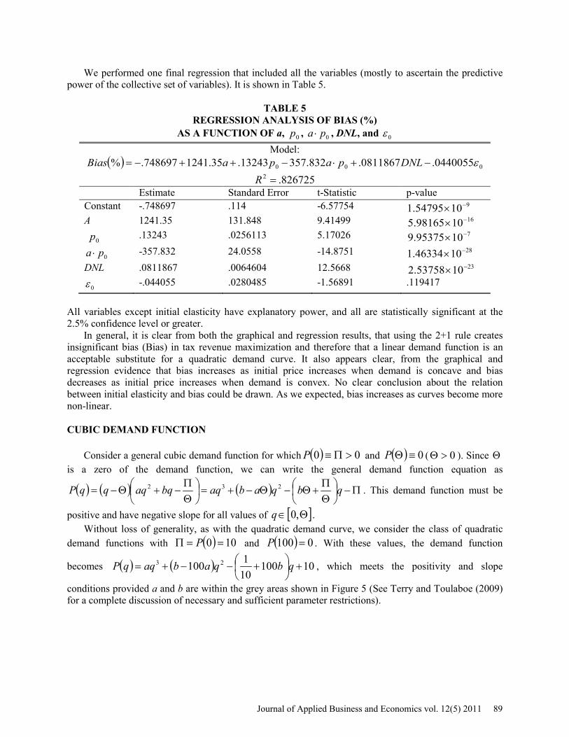
We performed one final regression that included all the variables (mostly to ascertain the predictive power of the collective set of variables). It is shown in Table 5.


AS A FUNCTION OF a, 0p , 0pa ⋅ , DNL, and 0ε Model:

( ) 000 0440055.0811867.832.35713243.35.1241748697.% ε−+⋅−++−= DNLpapaBias 826725.2 =R

Estimate Standard Error t-Statistic p-value Constant -.748697 .114 -6.57754 91054795.1 −× A 1241.35 131.848 9.41499 161098165.5 −× 0p .13243 .0256113 5.17026 71095375.9 −×

0pa ⋅ -357.832 24.0558 -14.8751 281046334.1 −× DNL .0811867 .0064604 12.5668 231053758.2 −×

0ε -.044055 .0280485 -1.56891 .119417 All variables except initial elasticity have explanatory power, and all are statistically significant at the 2.5% confidence level or greater.

In general, it is clear from both the graphical and regression results, that using the 2+1 rule creates insignificant bias (Bias) in tax revenue maximization and therefore that a linear demand function is an acceptable substitute for a quadratic demand curve. It also appears clear, from the graphical and regression evidence that bias increases as initial price increases when demand is concave and bias decreases as initial price increases when demand is convex. No clear conclusion about the relation between initial elasticity and bias could be drawn. As we expected, bias increases as curves become more non-linear. CUBIC DEMAND FUNCTION

Consider a general cubic demand function for which ( ) 00 >Π≡P and ( ) 0≡ΘP ( 0>Θ ). Since Θis a zero of the demand function, we can write the general demand function equation as

( ) ( ) ( ) Π−

ΘΠ

+Θ−Θ−+=

ΘΠ

−+Θ−= qbqabaqbqaqqqP 232 . This demand function must be

positive and have negative slope for all values of [ ]Θ∈ ,0q . Without loss of generality, as with the quadratic demand curve, we consider the class of quadratic

demand functions with ( ) 100 ==Π P and ( ) 0100 =P . With these values, the demand function

becomes ( ) ( ) 10100101100 23 +

+−−+= qbqabaqqP , which meets the positivity and slope

conditions provided a and b are within the grey areas shown in Figure 5 (See Terry and Toulaboe (2009) for a complete discussion of necessary and sufficient parameter restrictions).


As was the case with the quadratic demand function, we start our numerical analysis by selecting an

arbitrary representative of the class for illustration purposes. With 50000

1=a and

10001

−=b , we

obtain ( ) 1010003

50000

23

+−=qqqP .

A plot of this demand function is shown in Figure 6. This is a cubic demand curve with both concavity and convexity. Because this class of curves must be represented with two parameters, producing three-dimensional plots of bias as a function of curvature and initial price analogous to the quadratic case is not feasible. Therefore, we have chosen to represent curvature using the DNL term

( )( )

−−∫

100

0

21.10 dqqqP introduced earlier. DNL has the advantage of being adaptable to nearly any

non-linear demand curve. For the specific curve selected above, with 00.7$0 =p , the results of our twelve-step test procedure

are summarized below (all numbers rounded to two decimal places): Step 1: =0q 36.33 Step 2: ( ) =0qMR 1.96

FIGURE 5 ALLOWED PARAMETERS FOR CUBIC DEMAND FUNCTION


Step 3: 39.10 =ε Step 4: 78.32 =ε Step 5: 73.8$2 =p Step 6: 73.1$2 =t Step 7: ( )tpQ +0 (This function is long and is not presented here) Step 8: ( ) ( )tptQtR += 0

Step 9: 94.1$* =t Step 10: 20.39$* =r Step 11: 60.38$2 =r Step 12: =bias 1.55%

The DNL in this example is 6.90. To further evaluate this class of functions, we created 125 data points. We selected approximately 25 points evenly spaced across the shaded region of Figure 5. We did not deal with the event a = 0. For each of these 25 points, we selected five initial price points from

[ ]9,10 ∈p . Together, this produced a total of 125 data points from a 5 X 5 X 5 array. For each of these 125 data points, we collected four output values: DNL, initial price, initial elasticity, and tax-revenue bias.

Figure 7 shows graphically the relation between the tax-revenue bias, the DNL, and the initial price ( )0p . The maximum bias in the cubic case, for our 125 data points, is 11.24% and occurs at a DNL = 27.60 and 90 =p . The mean bias of our 125 data points is 1.57 and a 95% confidence interval of the mean is [ ]019.2,126.1 , suggesting that overall, the bias is low. Clearly, large bias occurs at high initial prices and high DNL.

FIGURE 6 SAMPLE DEMAND CURVE ( ) 10

10003

50000

23

+−=qqqP

20 40 60 80 100

2

4

6

8

10


We performed a regression of the data that produced Figure 7. The regression results are provided in Table 6. The regression shows strong significance in all variables and a fairly high 2R . The regressions show a strong positive relation between DNL and bias and between initial price and bias, as expected. We also explored the relation between bias, DNL, and initial elasticity ( )0ε . The relation is shown graphically in Figure 8.


AS A FUNCTION OF DNL AND INITIAL PRICE ( 0p ) Model: ( ) 0532707.139877.85952.2% pDNLBias ++−=

571169.2 =R Estimate Standard Bias t-Statistic p-value Constant -2.85952 .379039 -7.54413 121003736.9 −× DNL .139877 .0177232 7.89235 121044296.1 −× Initial Price ( )0p .532707 .0532161 10.0102 171038865.1 −×

One evident artifact of Figure 8 is the curvature in the initial elasticity variable. We have no

explanation for this curvature, but it is clear that any regression analysis should include a quadratic term in initial elasticity. Results of the regression analysis of the Figure 8 data are provided in Table 7.The 2R is high and all coefficients are highly significant. Bias increases as DNL increases and increases as initial elasticity increases. The negative coefficient on the 2

0ε term shows the concavity of the relation in initial elasticity, as is evident in Figure 8.

FIGURE 7 BIAS (%) AS A FUNCTION OF INITIAL PRICE ( )0p AND DNL


As a final test of the cubic demand function and how the bias is impacted by the various variables we collected, we performed one regression that combined all of the above variables. The results of this regression are shown in Table 8. The relations in the above regressions (Tables 6 and 7) are all evident in the combined regression of Table 8. We suspect that the insignificance of the “p0” variable is caused by correlation among the independent variables.

We conclude that the overall bias in tax revenue from applying the 2+1 rule when the demand curve is cubic is small. The tax-revenue bias as a percent, relative to optimal tax revenue, is increasing in initial price, initial elasticity, and in DNL (degree of nonlinearity). The relation between bias and initial elasticity has a significant concave component.

TABLE 7

REGRESSION ANALYSIS OF BIAS (%) AS A FUNCTION OF DNL, INITIAL ELASTICITY ( 0ε ), AND 2

0ε

Model: ( ) 200 295291.645973.2159051.44801.2% εε −++−= DNLBias

716207.2 =R Estimate Standard Bias t-Statistic p-value

Constant -2.44801 .273592 -8.94767 15101479.5 −× DNL .15905 .0146987 10.8208 191068242.1 −×

0ε 2.645973 .188008 14.0735 271005541.3 −× 20ε -.295291 .0238185 -12.3976 231075794.2 −×

FIGURE 8 BIAS (%) AS A FUNCTION OF DNL AND INITIAL ELASTICITY ( )0ε


TABLE 8

REGRESSION ANALYSIS OF BIAS (%) AS A FUNCTION OF DNL, 0p , 0ε , and 2

0ε Model:

( ) 2000 274591.41375.20778139.155519.57417.2% εε −+++−= pDNLBias

717379.2 =R Estimate Standard Bias t-Statistic p-value

Constant -2.57417 .327345 -7.86376 121081423.1 −× DNL .155519 .0155574 9.99648 171074752.1 −×

0p .0778139 .110324 .705321 .481977

0ε 2.41375 .379283 6.36397 91073953.3 −× 20ε -.274591 .0378297 -7.2586 111023354.4 −×

We turn next to an examination of the effect of the stability of elasticity on tax policy and tax revenue. Our discussion is intended to be demonstrative rather than probative. UNIT-ELASTIC DEMAND FUNCTION

One of our objectives is to demonstrate that the stability of elasticity is an important consideration in tax revenue maximization. To make this point, we consider several extreme classes of demand functions that have constant elasticity of demand. Figure 9 shows elasticity and tax revenue curves for the rectangular hyperbola demand function ( ) qqP /100= , with 20$0 =p .

For any market price, demand elasticity has a constant value of one. Initially, at 20$0 =p with no taxes, the seller captures revenue of $100. As the per-unit tax is raised, the market price is driven up from $20 but the quantity demanded declines in such a way that total revenue remains at a constant $100. The 2+1 rule is never realized, since elasticity is unitary throughout the demand function. The result is that as per-unit taxes increase, tax revenue captures an ever-expanding share of the $100 of revenue. In the theoretical limit, infinitely high taxes generate $100 of tax revenue, leaving no revenue for the seller. This result is, of course, a mathematical artifact: a model that is unsupportable in reality. INELASTIC DEMAND FUNCTION

As a second example, we consider the class of demand functions given by 1,/ >= xqaP x , which

have constant elasticity 11<=

xε (relatively inelastic at every point on the curve). Since total revenue

(TR) equals price multiplied by quantity sold, 1/ −= xqaTR . Demand is a hyperbolic function, whose semi-slope (dp/dq) increases in absolute value more rapidly than does that of the unit-elastic function. Figure 10 shows tax-revenue and elasticity curves for the hyperbolic

demand function given by ( ) 2

1000q

qP = .


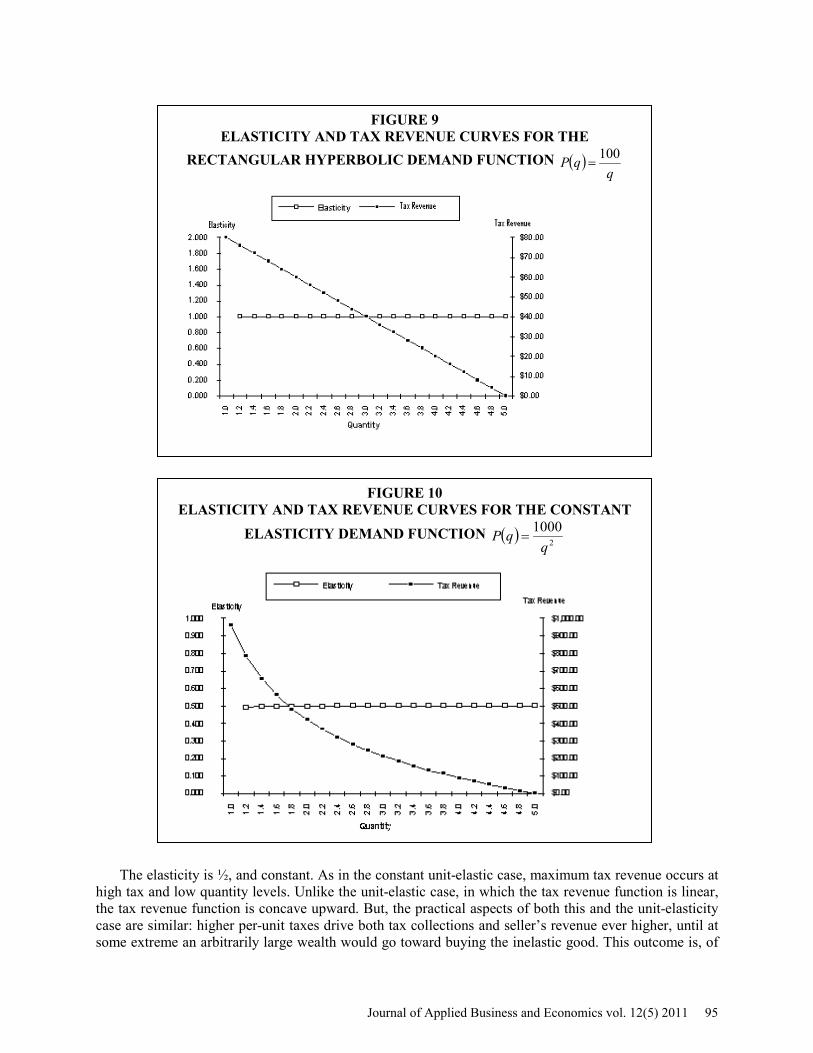
The elasticity is ½, and constant. As in the constant unit-elastic case, maximum tax revenue occurs at high tax and low quantity levels. Unlike the unit-elastic case, in which the tax revenue function is linear, the tax revenue function is concave upward. But, the practical aspects of both this and the unit-elasticity case are similar: higher per-unit taxes drive both tax collections and seller’s revenue ever higher, until at some extreme an arbitrarily large wealth would go toward buying the inelastic good. This outcome is, of

FIGURE 9 ELASTICITY AND TAX REVENUE CURVES FOR THE

RECTANGULAR HYPERBOLIC DEMAND FUNCTION ( )q

qP 100=

FIGURE 10 ELASTICITY AND TAX REVENUE CURVES FOR THE CONSTANT

ELASTICITY DEMAND FUNCTION ( ) 2

1000q

qP =


course, nonsensical; therefore, demand functions without an elastic range exist only as mathematical oddities. With respect to the 2+1 rule, the important point is that since the demand function does not allow elasticity to increase, no tax revenue maximization condition is reached, and thus the 2+1 rule is irrelevant. SUMMARY AND CONCLUSIONS

Tax policy is a complex issue and goods may be selected for taxation for a myriad of reasons besides their revenue generating potential. Even when considering revenue generation potential, the criteria for selecting categories of goods for taxation are complex, varied, and can be politically motivated. In this paper, we focus exclusively on optimal tax revenue generation as a criterion for selecting goods to be taxed. Throughout our discussion, we assume that supply is perfectly elastic so we can focus only on demand effects.

It appears to be nearly axiomatic in the literature that as initial price elasticity of demand decreases, optimal tax revenue potential increases, thus making goods with smaller initial price elasticity of demand preferred tax-revenue generation candidates. We show, however, that tax revenue generating potential is a function of three parameters of a linear demand curve—slope, intercept, and initial price. Since initial demand elasticity can represent only two of these parameters, it fails to completely categorize tax revenue potential. We provide an example in which taxing the good with greater elasticity produces greater tax revenue.

It is well known, and we prove, that if the demand curve for a good is linear, then the per-unit tax that generates optimal tax revenue occurs at a price at which the elasticity of demand equals twice the no-tax-equilibrium-price elasticity plus one (called the 2+1 rule). We test the tax-revenue bias from applying the 2+1 rule relative to optimal tax revenue for two classes of non-linear demand functions: quadratic and cubic. We conclude that overall, the percentage revenue bias is small.

In the quadratic case, we find that using the 2+1 rule creates insignificant bias in tax revenue maximization and therefore, we conclude that a linear demand function is an acceptable substitute for a quadratic demand curve. It also appears clear, from the graphical and regression evidence that bias increases as initial price increases when demand is concave and bias decreases as initial price increases when demand is convex. No clear conclusion about the relation between initial elasticity and bias could be drawn. As we expected, bias increases as curves become more non-linear.

In the cubic case, we also find that using the 2+1 rule creates insignificant bias in tax revenue maximization and therefore, we conclude that a linear demand function is an acceptable substitute for a cubic demand curve. The tax-revenue bias as a percent, relative to optimal tax revenue, is increasing in initial price, initial elasticity, and in DNL (degree of nonlinearity). The relation between bias and initial elasticity has a significant concave component. Since the quadratic and cubic demand curves can approximate a wide variety of demand situations, we suggest that when and if the demand curve is unknown, it is practical to assume that the demand function is linear, in the sense that little bias will be introduced into optimal tax policy decisions by such an assumption.

We examine two types of demand curves for which price elasticity of demand are constant—the hyperbolic demand function and the constant-elasticity demand function. For either of these demand curves, higher per-unit taxes drive both tax collections and seller’s revenue ever higher, until at some extreme an arbitrarily large wealth would go toward buying the inelastic good. This outcome is, of course, nonsensical; therefore, demand functions without an elastic range exist only as mathematical oddities. Nevertheless, these demand curves demonstrate that stable elasticity can be a dominant determinant of tax-revenue maximization. For these demand functions having constant inelasticity, the 2+1 rule predicts, correctly, that no tax revenue maximization exists—tax revenue increases without bound as unit-taxes are increased. As quantities sold decrease, so does the seller’s revenue, but since demand is inelastic, ever larger expenditures by purchasers flow to the taxing authority. Since demand elasticity never increases, there is no relation between elasticity and the optimal tax revenue.


It is sometimes asserted that governments are more likely to tax goods and services that are inelastic rather than elastic in demand. This assumption sounds correct, and may be true, ceteris paribus. But the diverse natures of goods, and the relative wealth and political importance of the good’s purchasers, suppliers, substitute and complement markets may have more influence on tax policy than the demand elasticity of the goods. If initial elasticity is indeed a criterion used by taxing authorities, it is not a particularly rational one. Excise taxes cause prices to rise, and demand elasticity to change.

In light of the 2+1 rule and the discussion above, taxing authorities would be wise to impose taxes on goods and services that command large expenditures and have stable elasticity, even if the current elasticity is high. Whether or not goods are inelastic may affect the deadweight welfare loss, and the quantity of resources consumed in their production. But the amount of tax revenue generated depends on the willingness of buyers to pay large sums for goods, and on the sensitivity of elasticity to price changes rather than the initial value of their elasticity. It is this nuance that recommends careful exposition. ENDNOTES Title: We wish to thank several anonymous referees whose helpful comments have greatly improved this paper.

2. See Gamble (1989). This rule applies for competitive supply, which is discussed in principles texts. In the case of monopoly or cartel supply, the rule is different. For the noncompetitive-supply case, see Lyon and Simon (1968).

3. See Coats (1995). Coats reports that “the average cross-border effect, i.e., state sales lost to other states, of a real (1967 = 100) 1¢ tax increase…in a state’s cigarette tax is a reduction of 2.1 percent of state sales.”

4. In fact, our computer could not get past step 5 due to memory and power constraints. REFERENCES Arnold, R. A. (2004). Microeconomics, South-Western Publishing Company, Sixth Edition: 151. Coats, R. M. (1995). A Note on Estimating Cross-Border Effects of State Cigarette Taxes. National Tax Journal, 48, (4), 573-584. Corlett W. J. and Hague, D. C. (1953). Complementarity and the Excess Burden of Taxation. Review of Economic Studies, 21, (1), 21-30. Gamble, R. (1989). Excise Tax Rates and the Elasticity of Demand. Journal of Economic Education, 20, 379-389. Graves, P. E., Sexton, R. L., and Lee, D. R. (1996). Slope Versus Elasticity and the Burden of Taxation. Journal of Economics Education, 27, 229-32. Lyon, H. C. and Simon, J. L. (1968). The Elasticity of Demand for Cigarettes in the United States. American Journal of Agricultural Economics, 50, 888-895. McConnell, C. R. and Brue, S. L. (2008). Economics: Principles, Problems and Applications, McGraw-Hill/Irwin, Seventeenth Edition: 347.


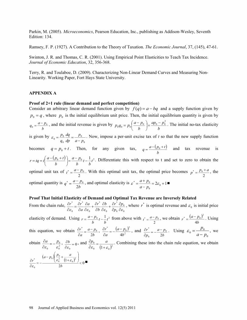
Parkin, M. (2005). Microeconomics, Pearson Education, Inc., publishing as Addison-Wesley, Seventh Edition: 134. Ramsey, F. P. (1927). A Contribution to the Theory of Taxation. The Economic Journal, 37, (145), 47-61. Swinton, J. R. and Thomas, C. R. (2001). Using Empirical Point Elasticities to Teach Tax Incidence. Journal of Economic Education, 32, 356-368. Terry, R. and Toulaboe, D. (2009). Characterizing Non-Linear Demand Curves and Measuring Non-Linearity. Working Paper, Fort Hays State University. APPENDIX A Proof of 2+1 rule (linear demand and perfect competition) Consider an arbitrary linear demand function given by bqaqf −=)( and a supply function given by

qp =0 , where 0p is the initial equilibrium unit price. Then, the initial equilibrium quantity is given by

bpaq 0

0−

= , and the initial revenue is given by b

papb

papqp2000

000−

=

−

= . The initial no-tax elasticity

is given by 0

0

0

00 pa

pdpdq

qp

−==ε . Now, impose a per-unit excise tax of t so that the new supply function

becomes tpq += 0 . Then, for any given tax, ( )b

tpaq +−= 0 and tax revenue is

( ) 200 1 tb

tb

pab

tpattqr −−

=

+−

== . Differentiate this with respect to t and set to zero to obtain the

optimal unit tax of 2

0* pat −= . With this optimal unit tax, the optimal price becomes

20* app +

= , the

optimal quantity is bpaq

20* −

= , and optimal elasticity is 12 00

0* +=−+

= εεpapa ■

Proof That Initial Elasticity of Demand and Optimal Tax Revenue are Inversely Related From the chain rule,

0

0

0

*

0

*

0

*

0

*

εεεε ∂∂

∂∂

+∂∂

∂∂

+∂∂

∂∂

=∂∂ p

prb

bra

arr , where *r is optimal revenue and 0ε is initial price

elasticity of demand. Using 20 1 tb

tb

par −−

= from above with 2

0* pat −= , we obtain ( )

bpar

4

20* −

= . Using

this equation, we obtain bpa

ar

20

* −=

∂∂ , ( )

2

20

*

4bpa

ar −

−=∂∂ , and

bpa

pr

20

0

* −−=

∂∂ . Using

0

00 pa

p−

=ε , we

obtain 20

0

0 εεpa

−=∂∂ , 0

0

=∂∂εb , and

( )200

0

1 εε +=

∂∂ ap . Combining these into the chain rule equation, we obtain

( )( )

02

1 20

20

00

0

*

<

++−

−=∂∂

b

appar εεε

■


Proof That it is Possible for BA 00 εε < and **BA rr < When BA qq 00 =

(Linear Demand Function with Perfect Competition) Just because optimal revenue and price elasticity of demand are inversely related for a given good, one should not conclude that it is always true that taxing a lower-elasticity good will produce a higher optimal tax revenue than taxing a higher-elasticity good, as this example illustrates. Consider two goods, A and B, with AAA bqap −= and BBB bqap η−= and let BA qq 00 = . Then, if the no-tax equilibrium price of

good B is Bp0 , the no-tax equilibrium price of good A is η

BBAA

paap 00

−−= . Using the results from the

proof of the 2+1 rule, the optimal tax for goods A and B will be ( )bpatt BBB

A ηη 20

** −

== . The optimal revenue

for good A will be ( )2

20*

4 ηbpar BB

A−

= , while for good B it will be η**AB rr = . The initial elasticities will be

BB

BB pa

p

0

00 −=ε and

BB

BABA pa

aa

000 −

−+=

ηεε . The question then becomes, is it possible that

BBB

BABA pa

aa0

000 εηεε <

−−

+= while η***ABA rrr =< ? To see that this is indeed possible, let 1>η be given so

that η***ABA rrr =< . Now, we need only make 0<− BA aa η , which will hold provided that

A

B

aa

<η .■


excise taxes and the stability of price elasticity · contribution to the theory of the efficient...

Documents