exercise 2 – basic digital elevation model (dem) … materials... · in this exercise we will...

SERVIR Workshop: Disaster Management and Response to Extreme Events Basic Digital Elevation Model (DEM) Processing: Characterizing Hydrological Networks and Surfaces

1

– EXERCISE 2 –

Basic Digital Elevation Model (DEM) Processing: Characterizing Hydrological Networks and Surfaces

In this exercise we will explore Digital Elevation Models (DEM) in order to characterize hydrological networks and surfaces through the use of various GIS tools. While we do this, we will continue our familiarization with data in raster format, learn about the processes and utility in converting between raster and vector and vice versa, and employ good data management practices. Explore basic tools

Data required: • DEM (Digital elevation model)

1) Create a new project in ArcMap. Save it as: C:\Taller_SERVIR\3_DEM\DEM_flujo.mxd

2) In Tools / Extensions, verify that the Spatial Analyst extension is turned on. If not, check

the box to the left.

3) Add the elevation layer, dem_gtopo from the directory: C:\Taller_SERVIR\3_DEM\ • Explore the properties of the DEM. Double click on the name of the layer in the Table of

Contents to open the properties. i. What is the range of values?

ii. What is the resolution?


2

Click to return to the Data View.

• Zoom.

i. What is in the window?

• We can change the color scheme (Color Ramp) in order to distinguish between different altitudes better. In the Table of Contents, double click on the name of the layer to open the properties, and select the Symbology tab.


3

Click to return to the Data View.

4) Now zoom out to see the entire layer,


4

Or the full extent of the data ( Full Extent)

5) Save the project (File / Save) or (Ctrl + S).

6) Open ArcToolbox if it is not already open. Open the Spatial Analyst Toolbox and then the Hydrology tools.

7) In the ArcToolbox Window double click on Flow Direction to determine the flow direction of all the cells in the DEM. Fill in the fields according to the following parameters: the input is the DEM, the output will remain in the same folder as the input DEM, and the we’ll name the output fdir1

• Click to run the Flow Direction tool. The output fdir1 should automatically

appear in the Table of Contents in the Data View. If not, add it.

8) Review the range of values (right click on the name fdir1 in the Table of Contents), and select Open Attribute Table.


5

• If the tool ran successfully, there should only be 8 values, because the “water” can only flow in 8 directions according to this methodology.

o Este 1

o Sureste 2 o Sur 4 o Suroeste 8 o Oeste 16 o Noroeste 32 o Norte 64 o Noreste 128

• It is very probable that fdir1 has more than only 8 values, due to sinks in the DEM. Spatial

Analyst cannot determine the flow direction if the DEM does not have a continuous surface on which the “water” can flow.

9) The tool Sink in the Hydrology toolset was designed specifically to identify sinks in the DEM that could interfere with the currents that flow towards the sea (or inland lakes):

N

S

E O


6

• Note the range of values that results in sink1—these reflect the individual sinks that must be

filled. You will probably need to turn off ( ) the other layers in order to see the sinks.

10) It will be necessary to “fill” these sinks in the DEM. Run Fill to fill the original DEM:

• Depending on the resolution of the grid, this step could take some time to process. It should eventually produce a new “filled” DEM (dem_fill).

11) For the second time, run Flow Direction, but this time use the filled DEM, dem_fill, and name the output fdir2.

• Note that the Flow Direction output has only eight values, representing the possible flow directions mentioned above:

sinks


7

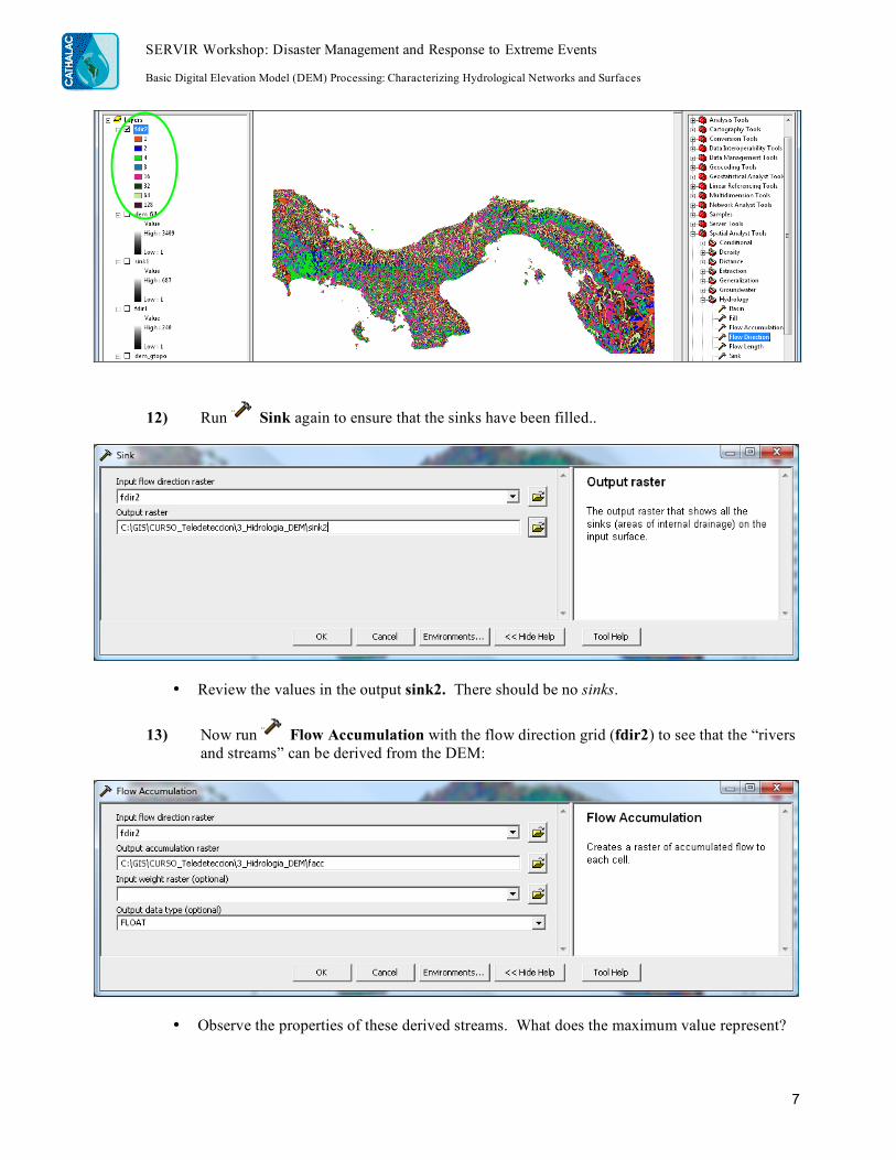
12) Run Sink again to ensure that the sinks have been filled..

• Review the values in the output sink2. There should be no sinks.

13) Now run Flow Accumulation with the flow direction grid (fdir2) to see that the “rivers and streams” can be derived from the DEM:

• Observe the properties of these derived streams. What does the maximum value represent?


8

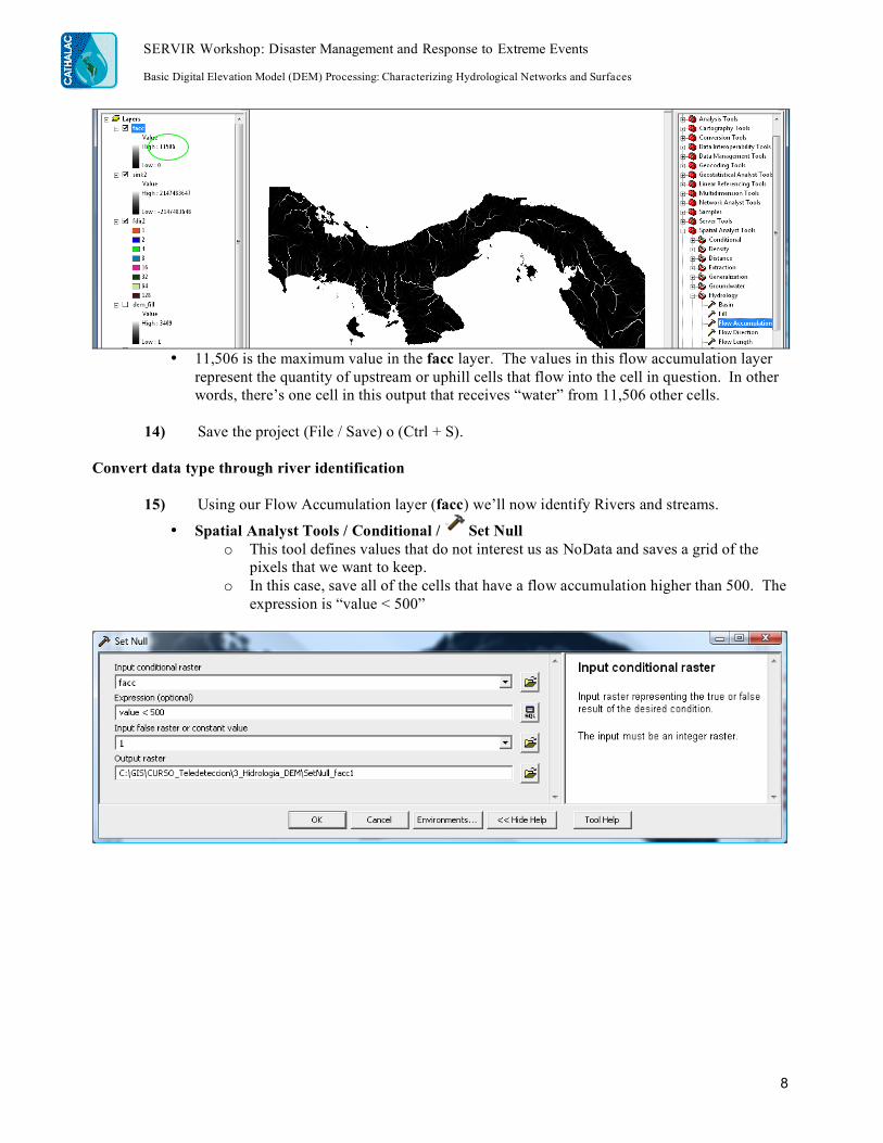
• 11,506 is the maximum value in the facc layer. The values in this flow accumulation layer

represent the quantity of upstream or uphill cells that flow into the cell in question. In other words, there’s one cell in this output that receives “water” from 11,506 other cells.

14) Save the project (File / Save) o (Ctrl + S).

Convert data type through river identification

15) Using our Flow Accumulation layer (facc) we’ll now identify Rivers and streams.

• Spatial Analyst Tools / Conditional / Set Null o This tool defines values that do not interest us as NoData and saves a grid of the

pixels that we want to keep. o In this case, save all of the cells that have a flow accumulation higher than 500. The

expression is “value < 500”


9

• Result of Set Null: flow accumulation cells higher than 500

16) Almost certainly, we’ll have to play with the limits of this expression. Repeat the Set Null process twice, just like before, but change the expression to “value < 100” and “value < 10”. What we’re looking for is a good representation of connected river networks that at the same time doesn’t over-identify cells where rivers don’t exist.

• The representative value of rivers and streams depends on the resolution and number of cells in the DEM.

o Flow accumulation cells higher than 100


10

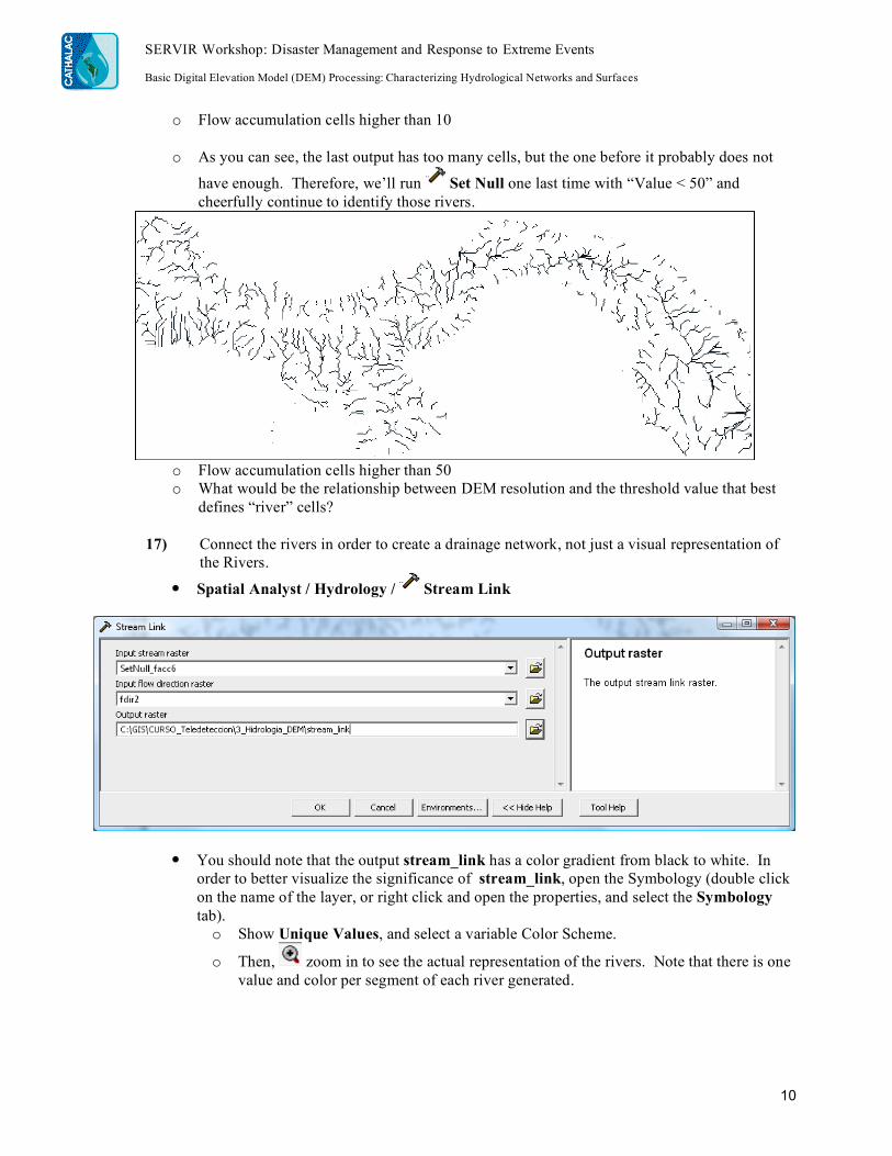
o Flow accumulation cells higher than 10

o As you can see, the last output has too many cells, but the one before it probably does not

have enough. Therefore, we’ll run Set Null one last time with “Value < 50” and cheerfully continue to identify those rivers.

o Flow accumulation cells higher than 50 o What would be the relationship between DEM resolution and the threshold value that best

defines “river” cells?

17) Connect the rivers in order to create a drainage network, not just a visual representation of the Rivers.

• Spatial Analyst / Hydrology / Stream Link

• You should note that the output stream_link has a color gradient from black to white. In order to better visualize the significance of stream_link, open the Symbology (double click on the name of the layer, or right click and open the properties, and select the Symbology tab). o Show Unique Values, and select a variable Color Scheme.

o Then, zoom in to see the actual representation of the rivers. Note that there is one value and color per segment of each river generated.


11

18) To give an order to each river segment, use Spatial Analyst / Hydrology / Stream Order

• For more information about Strahler y Shreve methods, see the documentation provided by

ESRI (support.esri.com) • Verify that the resulting orders agree with the locations and connections of each river

segment:


12

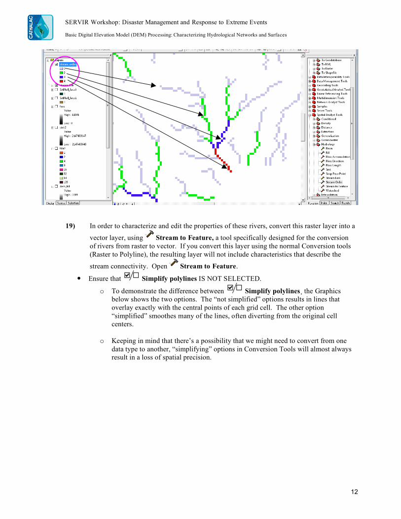
19) In order to characterize and edit the properties of these rivers, convert this raster layer into a

vector layer, using Stream to Feature, a tool specifically designed for the conversion of rivers from raster to vector. If you convert this layer using the normal Conversion tools (Raster to Polyline), the resulting layer will not include characteristics that describe the

stream connectivity. Open Stream to Feature.

• Ensure that Simplify polylines IS NOT SELECTED.

o To demonstrate the difference between Simplify polylines¸ the Graphics below shows the two options. The “not simplified” options results in lines that overlay exactly with the central points of each grid cell. The other option “simplified” smoothes many of the lines, often diverting from the original cell centers.

o Keeping in mind that there’s a possibility that we might need to convert from one

data type to another, “simplifying” options in Conversion Tools will almost always result in a loss of spatial precision.


13

20) Now we should be ready to delineate watersheds based on the flow direction. Run

Hydrology / Basin

21) Like before, change the Symbology to show Unique Values.


14

22) For later use, convert this Basin (watershed) GRID to

polygons: Conversion Tools / Raster to Polygon o Save the output as basin_poly.shp

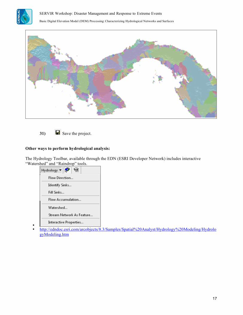
23) Examine the new watershed delineation layer basin_poly. How does it compare with your prior knowledge of watersheds in your area?

o Put the rivers on top of this layer to see how they run in relation to the watersheds. o We could also add an official watershed layer to see how it compares with the one we just

generated. o Can you distinguish familiar rivers and watersheds using the information you just generated?

24) Save the project (File / Save) o (Ctrl + S).

Surface analysis

25) Turn off—but do not delete—all of the layers except for the DEM.

26) Convert the DEM to Slope: Arc Toolbox / Spatial Analyst / Surface / Slope.

27) Revise the statistics in Properties / Symbology / Source.


15

o We’re looking for an average value near 3 and a maximum value near 30. If the resulting layer only has very high values (near 90), there is probably a problem with the spatial reference or projection.

o How would a higher resolution DEM affect the output?

28) Run Hillshade to create a layer we can use for lighting and shadow effects (under Surface tools).

o One can customize the tool by modifying the azimuth and altitude, but for our purposes, leave these fields blank.

o Regardless, click on each of the fields to see a short explanation of each term.

o Make the output more transparent by opening the layer properties and choosing the Display tab. Try 80% transparent.


16

29) Turn on another layer underneath, for example the watersheds or slope to see how they look with shaded relief.

30) Alternatively, one can change the transparency by using the Effects Menu. Right click on a blank space in the tool bar, and select “Effects:”


17

31) Save the project. Other ways to perform hydrological analysis: The Hydrology Toolbar, available through the EDN (ESRI Developer Network) includes interactive “Watershed” and “Raindrop” tools.

• • http://edndoc.esri.com/arcobjects/8.3/Samples/Spatial%20Analyst/Hydrology%20Modeling/Hydrolo

gyModeling.htm

exercise 2 – basic digital elevation model (dem) … materials... · in this exercise we will...

Documents