expectations, employment and prices

Expectations, Employment and Prices

This page intentionally left blank

ROGER E. A. FARMER

Expectations,Employmentand Prices

12010

3Oxford University Press, Inc., publishes works that furtherOxford University’s objective of excellencein research, scholarship, and education.

Oxford New YorkAuckland Cape Town Dar es Salaam Hong Kong KarachiKuala Lumpur Madrid Melbourne Mexico City NairobiNew Delhi Shanghai Taipei Toronto

With offices inArgentina Austria Brazil Chile Czech Republic France GreeceGuatemala Hungary Italy Japan Poland Portugal SingaporeSouth Korea Switzerland Thailand Turkey Ukraine Vietnam

Copyright © 2010 by Oxford University Press, Inc.

Published by Oxford University Press, Inc.198 Madison Avenue, New York, NY 10016

www.oup.com

Oxford is a registered trademark of Oxford University Press.

All rights reserved. No part of this publication may be reproduced,stored in a retrieval system, or transmitted, in any form or by any means,electronic, mechanical, photocopying, recording, or otherwise,without the prior permission of Oxford University Press.

Library of Congress Cataloging-in-Publication DataFarmer, Roger E. A.Expectations, employment and prices / Roger E. A. Farmer.

p. cm.Includes bibliographical references and index.ISBN 978-0-19-539790-11. Unemployment-Econometric models. 2. Unemployment-Effectof monetary policy on. 3. Capital market. 4. Equilibrium(Economics) 5. Rational expectations (Economic theory)I. Title.HD5707.5.F37 2010331.13′7—dc22 2009024295

9 8 7 6 5 4 3 2 1

Printed in the United States of Americaon acid-free paper

www.oup.com

To Roxanne, my inspiration.

PREFACE

IHAVE LONG BELIEVED that modern interpreters of Keynes missedthe main point of The General Theory; high unemployment is an

equilibrium phenomenon that can persist for a very long time if nothingis done by a government to correct the problem. This was the point ofmy 1984 paper, which argued that the natural rate hypothesis is false. Inthe intervening years, I have had time to refine this idea. This book is theculmination of my thought process.

I began thinking about a book on Keynesian economics, based on asearch theory of the labor market, in 2003. I have had many conversationswith friends and colleagues along the way and the question I hear againand again is, Why write a book? It has become the norm for seriouseconomists to convey their ideas in articles. There is a benefit to thisapproach since publishing an idea in a journal subjects it to a processof peer review. But there is also a downside to publishing in refereedjournals, particularly when the goal is as ambitious as the project thatI am engaged in. Even the very best journals (perhaps particularly thevery best journals) are biased toward publishing very good articles thatcontribute to what Thomas Kuhn, in his 1962 book The Structure ofScientific Revolutions, called “normal science.” A successful article ina top journal takes an established paradigm and solves a puzzle thatresearchers can identify as a valid question. I have a more ambitious goal:I want to overturn a way of thinking that has been established amongmacroeconomists for twenty years. The rejection of several different coreassumptions at the same time poses a problem if one wants to publish

journal articles since the pieces stand or fall together and there is nospace in a twenty-page article to explain why.

I have always found in writing research papers that no idea is evercomplete, and the same is true of a book, but more so. As this projectdeveloped, I added new pieces and changed old ones. The project gainednew urgency when the world economy began to disintegrate at an alarm-ing rate in the fall of 2008. I decided at that point that it was important topublish the ideas in whatever form they were currently in and to worryabout polishing them later. The theory I develop here has direct relevanceto the world economic crisis and it suggests a new and potentially impor-tant solution to the problem of maintaining global stability.

Expectations, Employment and Prices is aimed at economists inacademia and policy institutions, and the general reader will find itabstract. It is full of equations, theorems, definitions, and proofs thatmay be intimidating to the nonspecialist. For better or worse, that isthe way the language of academic articles has developed. The benefitof abstraction is that by phrasing arguments in this way, one is able tolay bare the logic that underlies one’s conclusions. But the ideas arenot so difficult as to be beyond the grasp of the average reader. For thatreason, I have written a second book on the same topic that translates myarguments into English. This second book, How the Economy Works:Confidence, Crashes and Self-Fulfilling Prophecies, will appear shortlyafter Expectations, and I hope it will influence the policy debate on thedevelopment of new institutions to prevent economic crises of the kindwe are witnessing as I write this Preface in December 2008.

Many people have helped me to develop my ideas. I am grateful to mybrother-in-law Ray Barrell and my late sister Mary K. Farmer for nurtur-ing my early love of and interest in economics. I have benefited tremen-dously from interactions with colleagues and students: Andy Atkeson,Arnold Harberger, Amy Brown, Ariel Burstein, Anton Cheremukhin, HalCole, Matthias Doepke, Corey Garriott, Gary Hansen, Christian Hellwig,Andrew Hollenhorst, Masanori Kashiwagi, Axel Leijhonhufrud, HannoLustig, Lee Ohanian, Paulina Restrepo, Karl Shell, Pierre-Olivier Weill,and Mark Wright have all, directly or indirectly, influenced the finalproduct. I have worked with many coauthors over the past twenty-five years. Jess Benhabib, Rosalind Bennett, Andreas Beyer, Jang TingGuo, Jerome Henry, Amartya Lahiri, Massimiliano Marcellino, KazuoNishimura, Daniel Waggoner, Ralph Winter, Michael Woodford, and TaoZha have all influenced my thinking in one way or another and indirectlycontributed to the ideas in this book. Thank you all. Alain Venditti and

VIII PREFACE

Carine Nourry of the University of Aix-Marseilles worked with me ona stochastic model that influenced Chapter 9. I am grateful for theirhospitality during a visit to Marseilles in the summer of 2008. RiccardoDiCecio from the St. Louis Fed, Marco Guerrazzi of the University ofPisa, and Colin Rogers of the University of Adelaide gave me commentsand corrections on an earlier draft, and Masanori Kashiwagi has readand criticized the entire manuscript. I thank all of them for helping me toweed out mistakes, although I am sure that some remain. I thank MartinWolf of the Finacial Times for providing me with an important platformover the past several months that enabled me to reach a larger audience toseriously consider my ideas. Thanks to Dave Cass and Karl Shell, whointroduced me to sunspots, an idea that they published in 1983 in theJournal of Political Economy, and to Costas Azariadis, who introducedme to the idea of a self-fulfilling prophecy both through personal dis-cussions and in his 1981 Journal of Economic Theory article. The early1980s was a wonderful time to be at the University of Pennsylvania. I amgrateful to the National Science Foundation, which has supported myresearch for many years with a series of grants that gave me the freedomto think independently and to develop new ideas. Most recently, I wasawarded grant #SBR 0720839, which helped to support the researchdeveloped in this book.

I thank Terry Vaughn and the entire team at Oxford University Pressfor their dedication and assistance throughout this project. My greatestdebt is to my wife, Roxanne, and my son, Leland, for their loving supportand encouragement for many years.

PREFACE IX

CONTENTS

PART I The Theory of Unemployment1 What This Book Is About 3

1.1 The Nature of the Enquiry 51.2 The Theory Summarized 71.3 The Theory of Aggregate Supply 81.4 The Theory of Aggregate Demand 101.5 A Road Map to the Book 11

2 The Basic Model 152.1 Components of the Theory 16

2.1.1 Relationship to Keynes 162.1.2 Households 172.1.3 Firms 182.1.4 Search and the Labor Market 20

2.2 Equilibrium and the Social Planner 222.2.1 The Planning Problem 222.2.2 Aggregate Demand and Supply 232.2.3 Effective Demand and the Multiplier 26

2.3 A Formal Definition of Equilibrium 292.4 Concluding Comments 30

3 An Extension to Multiple Goods 333.1 The Structure of the Model 34

3.1.1 Households 343.1.2 Firms 363.1.3 Search 37

3.2 Equilibrium and the Social Planner 383.2.1 The Social Planner 383.2.2 Aggregate Demand and Supply 403.2.3 Keynesian Equilibrium 43

3.3 Equilibrium and the Planning OptimumCompared 44

3.4 Concluding Comments 47

4 A Model with Investment and Saving 494.1 The Model Structure and the Planning Solution 50

4.1.1 Households 504.1.2 Firms 524.1.3 Search 534.1.4 The Social Planner 54

4.2 Investment and the Keynesian Equilibrium 554.2.1 How to Close the Model 554.2.2 The Definition of Equilibrium 56

4.3 Analyzing Equilibria 584.3.1 Aggregate Demand and Supply 584.3.2 Fiscal Policy in a Keynesian Model 60

4.4 Concluding Comments 624.5 Appendix 63

PART II Using the Theory to Understand Data5 A New Way to Understand Business Cycle Facts 69

5.1 What’s Wrong with the HP Filter? 705.2 Measuring Data in Wage Units 735.3 Interpreting Wage Units 755.4 The Components of GDP 765.5 Concluding Comments 80

6 The Great Depression: Tellingthe Keynesian Story in a New Way 816.1 Developing the Model 83

6.1.1 Preferences 836.1.2 Labor Supply and Consumption 846.1.3 Technology 85

6.2 Aggregate Supply 876.2.1 Aggregation Across Firms 876.2.2 Search and the Labor Market 89

XII CONTENTS

6.2.3 Selecting an Equilibrium withLong-Term Expectations 89

6.3 Equilibrium and the Planner’s Problem 906.3.1 The Social Planner 906.3.2 Demand-Constrained (Keynesian)

Equilibrium 926.3.3 An Existence Proof 936.3.4 Efficiency of Equilibrium 94

6.4 Using the Model to Understand Data 956.4.1 Keynes and the Great

Depression—Theory 956.4.2 Keynes and the Great

Depression—Data 966.5 The Recovery from the Depression 98

6.5.1 Adding Government 986.5.2 Consumption in a Model with

Government 996.6 Equilibrium with Government 100

6.6.1 Some Definitions 1006.6.2 Demand-Constrained Equilibrium with

Government 1016.6.3 An Important Result 103


7 The Wartime Recovery: A Dynamic Model WhereFiscal Policy Matters 1097.1 The Structure of the Model 110

7.1.1 Household Structure 1107.1.2 The Asset Markets 1127.1.3 Government Choices 1137.1.4 The Household Problem 113

7.2 The Aggregate Economy 1147.2.1 The Aggregate Consumption Function 1147.2.2 Aggregate Equations of Motion 116

7.3 Using the Model to Understand Data 1167.3.1 Steady-State Equilibria 1177.3.2 Two Equations to Study Steady-State

Equilibria 117

CONTENTS XIII

7.3.3 The Great Depression 1187.3.4 The Wartime Recovery 1197.3.5 A Quantitative Experiment 120


8 The U.S. Economy from 1951 to 2000:Employment and GDP 1278.1 Introduction 1278.2 The Impact of the Fed–Treasury Accord 1288.3 A Preview 1298.4 Unemployment and GDP 1328.5 Investment Is Not a Cause of Medium-Term

Movements 1338.6 Other Possible Causes of Medium-Term

Fluctuations 1358.7 Concluding Comments 138

PART III The Theory of Prices9 Money and Uncertainty 143

9.1 The Structure of the Model 1439.1.1 Money and Production 1439.1.2 Adding Uncertainty 1459.1.3 Households 1469.1.4 Government 1479.1.5 The Pricing Kernel and Asset Prices 148

9.2 The Complete Model 1499.3 Concluding Comments 150

10 Money and Inflation Since 1951 15110.1 A Complete Monetary Model 15210.2 Aggregate Supply and the Money Wage 15310.3 Theory and Data 15410.4 Modeling Monetary Policy 159

10.4.1 The Private Sector Equations Restated 15910.4.2 The Policy Rule 16010.4.3 A Linear Approximation 160

10.5 How Beliefs Influence the UnemploymentRate 16110.5.1 The Steady State 16210.5.2 Active and Passive Monetary Policy 162

XIV CONTENTS

10.6 Concluding Comments 164

11 How to Fix the Economy 16711.1 Monetary Policy Cannot Hit Two Targets 16811.2 Fiscal Policy Is Not the Most Effective

Solution 16911.3 What We Should Do Instead 17111.4 A New Role for the Fed 17211.5 Concluding Comments 174

Notes 177Bibliography 181Index 185

CONTENTS XV

PART I

THE THEORY OFUNEMPLOYMENT

THE FIRST FOUR CHAPTERS of this book develop a theory of themacroeconomy that brings the central ideas of Keynesian economics

up to date with modern macroeconomics. Chapter 1 presents an outlineof the book. Chapters 2, 3, and 4 develop a model of the economy thatexplains why unregulated capitalist economies may deliver inefficientoutcomes. Chapter 2 presents a basic model of the labor market, Chapter3 extends this model to multiple goods, and Chapter 4 adds saving andinvestment.

CHAPTER 1 What This Book Is About

Those who cannot remember the past are condemned to repeat it.

—George Santayana, The Life of Reason (1905)

THIS BOOK IS ABOUT the business cycle and how to control it. I willexplain why major recessions occur and how government policy

can and should be used to maintain high and stable employment. Thereasoning I will provide is inspired by Keynesian economics and is basedon ideas from The General Theory of Employment, Interest and Money(1936). Importantly however, I go beyond the ideas in Keynes’ book byproviding a microfoundation to the concept that the equilibrium levelof unemployment may be inefficient. I will argue that government canand should intervene in markets to maintain a high and stable level ofemployment. Some of the remedies I will propose are standard and partof the current arsenal of policies employed by the governments of allmarket economies. Some remedies are new and involve extensions of theinstitutions that were developed in the wake of the publication of TheGeneral Theory.

What is new in my assessment of standard remedies is a theoryof individual behavior that explains why fiscal and monetary policiesare appropriate and how they work. A byproduct of my extension ofKeynesian models is an explanation of how inflation and unemployment

can occur together and a theory of what it means to maintain full employ-ment. My extension of Keynesian theory gives rise to a policy suggestionthat involves an expansion of the role of the asset market managementthat has been conducted more or less actively since the inception ofthe Federal Reserve system in 1913. I will argue that the Fed shouldintervene to prevent both asset market bubbles and stock market crashes.Rather than simply raising or lowering the treasury bill rate throughpurchases and sales of T-bills, this would require active participation inthe stock market through the support of the price of an index fund. Iexplain this idea in Chapter 11.

Although economic fluctuations in the U.S. have been relatively mildin recent decades, during the Great Depression of the 1930s the unem-ployment rate exceeded 20% for a protracted period of time. The GreatDepression is not unique, and similar episodes have been a recurrentfeature of capitalist economies since the beginning of the industrialrevolution. Timothy Kehoe and Edward Prescott (2007) define a greatdepression to be a period of diminished economic output with at leastone year where output is 20% below the trend. According to this defi-nition, Argentina, Brazil, Chile, and Mexico have all experienced greatdepressions since 1980.

What causes big fluctuations in economic activity? For severaldecades following the publication of The General Theory, economiststhought they had an answer; the Great Depression was a failure of anunregulated capitalist economy to efficiently utilize available resources.But with the resurgence of classical ideas in the 1970s, the key premiseof The General Theory, that market economies are not inherently self-stabilizing, has been called into question. Although there has been arecent resurgence of Keynesian ideas under the rubric of “new-Keynesianeconomics,” the models studied by the new-Keynesians are hybrids thatincorporate a classical core. New-Keynesian models allow for temporarydeviations of unemployment from its “natural rate” as a consequenceof sticky prices, but they contain a stabilizing mechanism that causes areturn to the natural rate over time. Since the return to the steady state istypically rapid in these models, the welfare costs of business cycles arealso small and arise from second-order consequences of deviating fromthe social planning optimum.1

This book is different. All of the models I will describe reject thenatural rate hypothesis and treat the unemployment rate as a variable thatis determined in equilibrium by aggregate demand.

4 THE THEORY OF UNEMPLOYMENT

In his 1966 book, Axel Leijonhufvud made the distinction betweenKeynesian economics and the economics of Keynes. The neoclassicalsynthesis is the interpretation of The General Theory that was introducedby Samuelson (1955) in the third edition of his undergraduate textbook.According to this view, the economy is Keynesian in the short run, whenprices have not yet adjusted. It is classical in the long run, after priceadjustments have run their course. Leijonhufvud pointed out that theassumption that The General Theory is about sticky prices is centralto this orthodox interpretation of Keynesian economics, but it is not acentral argument of the text of The General Theory.

This book provides an alternative microfoundation to Keynesian eco-nomics that does not rely on sticky prices. In successive chapters, Iconstruct a series of models that build on a single idea. Each of themis constructed around a conventional general equilibrium model in whichreal resources must be used to move unemployed workers into jobs usinga “search technology.” Although this technology is convex, I assumethat the planning optimum cannot be decentralized as a competitiveequilibrium because moral hazard prevents the creation of markets forthe search inputs. As an alternative, I introduce an equilibrium conceptcalled demand-constrained equilibrium, in which the level of economicactivity is determined by self-fulfilling crises of confidence. I refer tothe resulting model as “old-Keynesian” to differentiate it from new-Keynesian economics that incorporates the natural rate hypothesis ofMilton Friedman (1968) and Edmund Phelps (1968). In contrast tonew-Keynesian models, those described in this book display multiplestationary perfect foresight equilibria, and there is a different stationaryunemployment rate for each possible level of beliefs.

1.1 The Nature of the Enquiry

The fact that great depressions occur relatively frequently in Westerneconomies suggests that unregulated capitalist economies sometimes govery wrong: This viewpoint is, however, controversial. Some observershave suggested that the Great Depression of the 1930s in the US was anaberration. Economists who take this view point to postwar U.S. experi-ence in which unemployment has been relatively low and business cyclesrelatively mild for long periods of time. But Kehoe and Prescott (2007)cite at least four episodes of great depressions in western economies in

WHAT THIS BOOK IS ABOUT 5

the past twenty-five years. These episodes require an explanation that isconsistent with our understanding of the functioning of the macroecon-omy in more normal times.

According to Keynes, the Great Depression was evidence of thesystemic failure of unregulated markets to deliver an efficient levelof employment. According to this view, government can and shouldintervene to maintain a high level of employment. An alternative viewthat has recently been regaining popularity is that great depressions arecaused by the interference of government regulatory bodies in the smoothfunctioning of markets. An early example of this view is the book byMilton Friedman and Anna Schwartz (1963), which argued that the GreatDepression in the U.S. was caused by incompetent monetary policy in the1920s. More recently, Cole and Ohanian (2004) have argued that HerbertHoover’s regulatory policies deepened the depression in the early 1930s.This is a remarkable turn of intellectual thought from the prevailing moodin the early postwar period, when President Richard Nixon was famouslyquoted as saying, “We are all Keynesians now.”2

A prevalent view of business cycles in the economics professionis that of real business cycles according to which most economicfluctuations are caused by unforeseen shocks to total factor productivity.According to this view, the market system is efficient and the allocationof resources in a laissez faire economy is, to a first approximation, areflection of the allocation that would be made by a benevolent socialplanner whose goal is to maximize social welfare. This view is moreextreme than that which Keynes ascribed to the “classical economists”of whom he considered Pigou a prime example. Pigou (1929), Lavington(1922), and Haberler (1937) all recognized a role for total factorproductivity, but they also recognized alternative sources of aggregatefluctuation including “errors of optimism and pessimism,” “harvestvariations,” and “autonomous monetary movements” (1929, Chapter22). In Industrial Fluctuations, Pigou concludes that although “ . . . thepopular opinion that industrial fluctuations as such must be social evils isinvalid,” nevertheless, “ . . . industrial fluctuations produced in the waysdescribed [above] are certainly social evils.”

The General Theory makes a break from 1920s business cycle theoryby separating the theory of distribution from the theory of aggregateeconomic activity. Although Keynes believed that the market systemwas probably an efficient way of deciding which kinds of goods wereproduced for a given volume of employment, he argued that unregulatedcapitalist systems did not produce an efficient allocation of labor. His


arguments had an important influence on political economy and resultedin the current state-capitalist system in which the monetary and fiscalauthorities in most Western democracies are charged with the objectiveof maintaining a high and stable level of employment. The fiscal andmonetary policy environment since 1940 has been very different fromthat of the 1920s and 1930s as a direct consequence of ideas that arosefrom the publication of The General Theory, and hence it is invalid to usethe postwar period as an example of the success of the market system.Rather, it represents prima facie evidence for the success of Keynesianeconomics.

A good example is provided by the U.S. economy. In 1929 federal andstate taxes together accounted for 11% of GDP, but by 1999 that figurehad risen to 36%. When the Fed was created in 1913, policymakers hadlittle conception of how to run a successful monetary policy, and for mostof the 1930s the short-term interest rate was too low to be used as aneffective instrument of control. Since 1945, however, the size of govern-ment has been large enough to create an automatic stabilizing mecha-nism that generates budget deficits in recessions and budget surpluses inexpansions. Further, the Fed actively pursues a countercyclical monetarypolicy by lowering the interest rate during recessions and raising itduring expansions. These are exactly the policies that Keynes arguedfor in the 1930s, and it is ironic that the success of these very policiesshould be seen by some as evidence against the theories that spawnedthem.

1.2 The Theory Summarized

Although the current volume is heavily influenced by The General The-ory, it is not a simple translation of that book into the language ofmodern economics. Seventy years of history since the publication of TheGeneral Theory have produced data that invalidate at least some of itskey themes. Most notable among these is the experience of stagflationin the 1970s that is inconsistent with the “reverse L” theory of aggregatesupply outlined in Chapter 21 of The General Theory, which explainedKeynes’s theory of prices.

There are two key ideas in The General Theory that set it apart frompre-Keynesian economics: The first is that there is something distinc-tive about the labor market that makes the marginal disutility of labordifferent in general from the real wage. The second is that aggregate


economic activity is determined by the “animal spirits” of investors.This book will preserve both of these ideas, modified in a way thatrespects recent developments in dynamic general equilibrium theory. Theintegration of dynamics into modern economic theory provides a set ofmathematical tools that enable me to bring dynamic ideas into Keynesianmacroeconomics in a way that was not possible in the 1930s.

The ideas that I have identified as central to Keynesian economics canbe separated into theories of aggregate supply and aggregate demand.Although the form with which I will state these ideas is different fromexisting interpretations of The General Theory, the intellectual prede-cessors are those formulated by Keynes in 1936, who expressed thefollowing sentiment in a 1937 article in response to his critics:

I am more attached to the comparatively simple fundamental ideasthat underlie my theory than to the particular forms in which Ihave embodied them, and have no desire that the latter should becrystallized at the present stage of the debate. If the simplest basicideas can become familiar and acceptable, time and experience andthe collaboration of a number of minds will discover the best wayof expressing them. (Keynes, 1937, pp. 211–212)

The following two sections outline briefly my main arguments andexplain how they are related to the “fundamental ideas” of The GeneralTheory.

1.3 The Theory of Aggregate Supply

Chapter 2 presents a reformulation of the theory of aggregate supply.Keynes’s theory has been widely criticized for its lack of microfoun-dations, and it is often asserted that if the marginal disutility of laboris not equal to the real wage, as Keynes assumed in Chapter 2 of TheGeneral Theory, then unemployed workers would be expected to offer towork for a lower wage. This argument is based on the implicit assump-tion that the labor market is an auction in which unemployed workerscan effectively signal their willingness to work for profit-maximizingfirms.

Following arguments by Patinkin (1956) and Clower (1965), the dise-quilibrium literature of the, ’70s, exemplified by Barro and Grossman(1971), Benassy (1975), and Malinvaud (1977), tried to address this


point by constructing an explicit theory of transactions at disequilib-rium prices. This literature was ultimately judged to be unsuccessfulby a generation of economists who followed the equilibrium approachof Lucas and Rapping (1969) and Lucas (1972). Although there werecontemporary writers (Axel Leijonhufvud [1966] is a leading example)who claimed that Keynesian economics was never about “sticky prices,”Leijonhufvud and his contemporaries never managed to formulate analternative theory that was capable of answering the new-Classical criti-cism that disequilibrium theory is empty. This argument rested on the factthat it contains what Lucas called “free parameters” and comes down tothe claim that, as a consequence, the theory is untestable.

In this book, I pick up on the recent literature developed by Shimer(2005) and Hall (2005) that follows earlier work in search theory.Pissarides (2000) provides an excellent summary. In this literature, itis assumed that the process by which an unemployed worker finds ajob requires the input of resources on the part of the firm and time onthe part of the worker. When a worker and a firm meet, they determinethe wage to be paid through a Nash bargain. Shimer pointed out thatthis assumption does not provide a good quantitative explanation ofemployment fluctuations, and Hall proposed to replace it with an alter-native wage determination mechanism. He assumed that the real wageis determined one period in advance. Shimer’s criticism has generateda considerable amount of recent work by researchers who are exploringalternative wage determination mechanisms in an attempt to reconcilethe volatility of vacancies and unemployment with a model in whicheconomic fluctuations are driven by productivity shocks.

Since the work of Diamond (1982, 1984), it has been known thatthere are often multiple equilibria in labor search models, and sincethe work of Howitt (1986) and Howitt and McAfee (1987), it has beenknown that there may be a continuum of equilibria. The response of mosteconomists has been to try to resolve this indeterminacy by adding a newfundamental equation. The use of the Nash bargaining equation, with afixed bargaining weight, is an example of one such addition.

In this book, I take an alternative approach. I develop a series ofmodels in which the labor market is cleared by search, but instead ofclosing it with an explicit bargaining assumption, I assume only that allfirms must offer the same wage. This leads to a new theory in whichthere are many wages, all of which are consistent with a zero profitequilibrium, and it provides a microfounded analog of Keynes’s idea thatthere are many levels of economic activity at which the macroeconomy


may be in equilibrium. To select an equilibrium and close the model, Iintroduce the idea that households form beliefs about the future valueof productive capital and I show that for any sequence of self-fulfillingbeliefs, less than a given bound, there exists a Keynesian equilibrium.This equilibrium will in general be inefficient in the sense that a benev-olent social planner would prefer a different employment level that maybe higher or lower. Hence, I am able to articulate the Keynesian storyof the Great Depression in a model with well-defined microfoundationsin which no individual agent has an incentive to deviate from his or herchosen action.

1.4 The Theory of Aggregate Demand

In addition to his theory of aggregate supply, Keynes contributed a theoryof effective demand based on the multiplier. Problems with this theorywere already apparent in the 1950s, when it was realized that estimates ofthe marginal propensity to consume were typically much lower in cross-section than time series data. This led to Friedman’s (1957) book, A The-ory of the Consumption Function, in which he proposed the concept ofpermanent income as a way of resolving the disparity between differentestimates. But this was not the only important debate that characterizedthe macroeconomics of the immediate postwar period.

The exercise of providing a dynamic foundation to Keynesian eco-nomics led to an attack on the intellectual foundations of the multiplierand a debate over the effectiveness of fiscal policy. Some economistshave argued, on purely theoretical grounds, that one dollar of expenditureby government might, under some circumstances, perfectly “crowd out”one dollar of private consumption expenditure and aggregate demandwould be unaltered. The debate was ultimately resolved by recognizingthat crowding out would occur only if government bonds were not per-ceived as net wealth by the community as a whole, although this debate,and other preoccupations of the postwar Keynesian economists, becameirrelevant when Keynesian economics was replaced by the real businesscycle paradigm.3

In this book, I will breathe new life into many of the old debates.I will construct a microfoundation to the theory of aggregate demandbased on the assumption that agents are forward looking with rationalexpectations of future prices. Although this is a departure from Keynes’stheory of expectations, it is a departure worth making since it allows


me to directly compare the implications of the theory with modernneoclassical alternatives.

Keynes believed that some forms of uncertainty cannot be quantifiedand that agents must act on the basis of partial information. Althoughthe agents in my model will be able to form probability distributionsover future events, not all of these events will be fundamental in thesense in which that word is now used in general equilibrium theory todescribe uncertainty due to changes in preferences, endowments, andtechnology. Although these sources of uncertainty may be present in themodels I describe in this book, in addition, agents will be required toform expectations of the future actions of others. It is here that I capturethe Keynesian idea of the importance of “animal spirits”.

If investors today believe that all future investors will be pessimistic,then this belief will be self-fulfilling. In contrast to the previous for-mulations of this idea that I described in my work with Jess Benhabib(1994) and Jang Ting Guo (1994, 1995) and summarized in my bookThe Macroeconomics of Self-Fulfilling Prophecies (1999), agents in themodels I will describe in the following chapters may form self-fulfillingbeliefs that lead to an increase in the unemployment rate in the steadystate.

1.5 A Road Map to the Book

This book is divided into three parts. Part I presents the basic theoryof the labor market and it consists of this introduction plus three morechapters. Chapter 2 presents the simplest version of my main idea—a microfounded model of a labor market, based on search theory, inwhich there exists a continuum of steady-state equilibria. This chapteris essential reading. Chapter 3 develops a model with multiple goods.It provides what I believe to be an interesting insight into the methodsused here and originally developed by Keynes. Unlike all of modernmacroeconomics, Keynesian economics has no need of the concept ofa production function. This notion, which is central to a theory based onclassical reasoning, is not missing because it was forgotten; it is missingbecause it is not needed. Keynesian economics determines employmentand the money value of GDP. Although it is possible to extend the theoryto explain the physical units of commodities that are produced in anyperiod, this extension is not needed to understand the concept of anequilibrium at less than full employment.


Chapter 4 was written early in the development of this book. It wasan attempt to use the search framework that I developed in chapters2 and 3 to provide a microfounded account of the Keynesian idea ofthe multiplier. Keynes thought that investors and savers have differentmotives, and he argued that investment is the driving force behind busi-ness fluctuations. This chapter reflects that idea. It is possible to makesense of the multiplier within the framework of this book, but as theproject developed I realized that a dynamic theory of aggregate demandcan provide a different interpretation of the Keynesian story of the GreatDepression in which consumption depends on wealth rather than income.The Keynesian multiplier is a fundamentally static concept and the ideaof separating investors and savers does not work well within an intertem-poral equilibrium model. I nevertheless decided to leave this chapter aspart of the final manuscript since it makes clear that fiscal interventionrelies on a distribution effect between different generations. This themewill be important later in the book when I discuss the effectiveness offiscal policy in two alternative models with long-lived agents.

The second part of the book breaks new ground. In Chapter 5, Iargue that most modern macroeconomists have defined away what isarguably the most interesting macroeconomic question: Why does unem-ployment move closely with the components of aggregate demand atmedium to low frequencies? I became interested in this question after mycollaboration with Andreas Beyer (2007) in which we studied the timeseries properties of the unemployment rate. It is a question that has beenignored for two reasons. First, real business cycle (RBC) economists donot try to explain the unemployment rate at all; instead, their modelscontain total hours worked as an index of labor market activity. AlthoughI see this as a deficiency of RBC theory, it is not a serious one since hoursworked move closely with unemployment. More important, much ofrecent data analysis by macroeconomists accepts an argument by RobertHodrick and Edward C. Prescott (1997), who claimed that the interestingfacts to explain are deviations of time series on employment, investmentconsumption, and GDP from a flexible trend. This use of their detrendingmethod leads economists who follow this approach to miss correlationsbetween employment and consumption at medium frequencies.4 Thesemovements are important to study since, if my theory is correct, theyhave large consequences for welfare. Chapter 5 explains an alternativedetrending procedure that reveals a new and arguably more interestingset of facts to be explained by the theory. This chapter is essential tounderstanding my claims for the empirical relevance of my ideas.


Chapters 6, 7, and 8 apply the detrending methods of Chapter 5 toview the data defined in this way through the lens of theory. Chapter 6builds a rudimentary infinite horizon model to explain the facts of theGreat Depression. Chapter 7 elaborates on it by adding a richer popu-lation structure to explain the wartime recovery, and Chapter 8 studiesdata from 1951 through 2000. Each of these chapters stands alone as adescription of a particular episode from economic history and togetherthey develop a narrative account that views the facts in a new way.Although the explanations I give of the depression and the recoverywill be familiar, my interpretation of the postwar data is new. I interpretthe slow-growth decade of the 1970s as a demand-induced slowdown asopposed to the usual supply-side explanation.

In Part III, I turn from the theory of unemployment to the theory ofprices. Chapter 9 adds money to a stochastic monetary version of therepresentative agent model from Chapter 6. Chapter 10 uses this modelto explain how inflation and unemployment can occur together and itargues that this fact should not lead us to give up on important ideas thatform the basis of The General Theory: notably, that unregulated capitalisteconomies can be inefficient in the steady state and that noneconomicfundamentals can influence economic activity. In Chapter 11, I argue forthe design of a new monetary policy for the 21st century. The Fed shouldconduct open market operations in a portfolio of assets by buying andselling shares in an index fund of stock market securities. Its goal wouldbe to peg the value of this fund to prevent excessive market movementseither up or down.


CHAPTER 2 The Basic Model

THIS CHAPTER DEVELOPS a one-sector model that explains the themeof the book: that inefficiently high levels of unemployment can exist

in steady-state equilibrium. The chapter builds on earlier work (2008b)published in a volume in honor of Axel Leijonhufvud. I develop a model,based on a labor market theory in which the search inputs of workersand firms are combined to produce matches. A match is an employedworker in place at a firm. Search requires two inputs: (1) the time spentsearching by workers and (2) the resources needed to post vacancies byfirms. Most existing search models do not assume that these inputs aretraded in competitive markets. Instead, they assume that vacancies andunemployed workers are matched randomly. If searching workers andvacancy posting firms take the real wage as given, the resulting generalequilibrium model has fewer equations than unknowns.

In search models, it is typical to assume that the match technologysatisfies standard neoclassical properties of monotonicity, differentiabil-ity, and constant returns to scale. These assumptions allow one to proveversions of the first and second welfare theorems in a general equilibriummodel with search: every competitive equilibrium is Pareto optimal, andevery Pareto optimal allocation can be decentralized as a competitiveequilibrium. But what might this decentralization look like?

The natural decentralization would posit the existence of a large num-ber of competitive employment agencies. Each agency would operatea match technology and would purchase search inputs from firms andworkers. The agency would purchase, from an unemployed worker, the

exclusive right to match that worker with a vacancy. From a firm with avacant job, the agency would purchase the right to match that vacancywith an unemployed worker. The agency would operate a matchingprocess and resell the joint product, a worker–firm match, back to theworker–firm pair.

Why is this decentralization implausible? First, it involves transac-tions that we do not observe in the real world. There are no privateinstitutions that pay money to unemployed workers for the right to findthem jobs. Nor do we find the widespread use of private employmentagencies that pay firms for the privilege of acting as their recruitingagents. A moment’s reflection suggests that these markets do not existbecause of the moral hazard associated with monitoring the motives ofthe participants. Efficient operation of these markets requires exclusivityof contracts. If such markets existed, it would be difficult or impossibleto prevent an unemployed worker from selling the exclusive right to bematched to multiple agencies and to turn down job offers when presentedon spurious but hard-to-monitor grounds. Since there may be legitimatereasons to refuse a job, the requirement that all potential matches mustbe accepted is not a feasible solution to this problem. Casual observationof state-run employment agencies suggests that this problem is presentin practice and is a significant impediment to the efficient operation of amatching market.

2.1 Components of the Theory

The model of this chapter is inspired by Keynes’s General Theory. In thatbook, Keynes claimed that the real wage is not equated to the marginaldisutility of labor and he introduced the principle of effective demand.These ideas are important and they have guided several generations ofpolicy. This chapter is an attempt to make sense of them in a micro-founded theory of labor market search.

2.1.1 RELATIONSHIP TO KEYNES

In The General Theory, effective demand is driven primarily by the“animal spirits” of investors. Animal spirits are a key component ofautonomous investment expenditure, which in turn, is the prime causeof fluctuations in effective demand. To capture this idea, one requiresa dynamic model since investment involves plans that span at least


two periods. However, autonomous expenditure is also determined bygovernment spending, and by recognizing this, I will be able to explainhow a search model of the labor market can be embedded into generalequilibrium in a relatively simple environment: a one-period model thatabstracts from capital in which output and employment are driven byfiscal policy.

The one-period model I will describe is simpler than the first dynamicmodel that I introduce in Chapter 4 since I abstract from capital andassume that all output is produced from labor. Sections 2.1.2 and 2.1.3are about the microeconomic behaviors of households and firms. Thequestions I study are not ones that occupied Keynes, who was concernedsolely with relationships between aggregates. But they are questions thatI will need to address in an enquiry that seeks to provide microfoun-dations to Keynes’s concepts of aggregate demand and supply. Initially,I will simplify the environment by studying a model in which there isa single period, a single commodity, and a large number of identicalhouseholds and firms. These are not simplifications found in The GeneralTheory and, as I will show in Chapter 3, they are unnecessary simplifica-tions if one is interested in a comparative static view of macroeconomicactivity.

Keynes took the existing stocks of capital and existing nominal wagesas historically determined and showed how effective demand woulddetermine economic activity. My goals are more comprehensive. I want,to demonstrate how the principle of effective demand can be consistentwith individual behavior at a point in time. Beyond that, I want to link theperiods in a dynamic general equilibrium model where the people in mymodel form rational expectations of future events. Although the single-agent, single-good fiction is unnecessary to explain effective demandin a comparative static model, it considerably simplifies the nature ofaggregate dynamics.

2.1.2 HOUSEHOLDS

The model consists of a unit mass of families, each of which has a unitmass of members. These assumptions allow me to abstract from the factthat unemployed workers are typically worse off than employed workers.In this model, the family self-insures its unfortunate members. The utilityof the family is represented by an increasing concave function j ,

J = j (C), (2.1)

THE BASIC MODEL 17

where J represents the utility of the family’s consumption, C . Since allfamilies are identical, I will refer to the consumption of an individualfamily and to aggregate consumption with the same symbol.

Each family has a measure 1 of workers, all of whom begin theperiod unemployed. Leisure has no utility and each household solves theproblem

max{C,H} j (C) (2.2)

such that

pC ≤ wL (1 − τ) + TR, (2.3)

H ≤ 1, (2.4)

L = q H, (2.5)

U = H − L . (2.6)

Equation (2.3) is a budget constraint. Each family’s consumption isconstrained by its after-tax employment income. w is the money wage,p is the money price, L is the measure of employed workers, τ is the taxrate, and TR is a lump-sum transfer, measured in dollars. H representsthe measure of household members that search for employment, andEquation (2.4) constrains this to be no greater than 1, the householdsize. The measure of household members that successfully find jobs isrepresented by q H , where q is taken as given by the household in asearch market equilibrium; Equation (2.5) is the relationship betweenemployment and search. Finally, Equation (2.6) defines the measure ofunemployed, U , to be those searching workers who do not find jobs. Thisproblem has the trivial solution

H = 1, (2.7)

pC = wL (1 − τ) + TR, (2.8)

L = q. (2.9)

Since there is no utility to leisure, all workers look for a job, and sincethere is no motive to save, all income is consumed.

2.1.3 FIRMS

Firms produce output using a constant returns-to-scale technology inwhich labor is the sole input. There is free entry and each firm solves


the problem

max{V,Y,L ,X}pY − wL (2.10)

such that

Y ≤ AX, (2.11)

X + V = L , (2.12)

L = qV . (2.13)

Equation (2.11) is the production function: Y is output, A > 0 is aproductivity parameter, and X is the measure of workers employed bythe firm in direct production. A firm that employs L workers may allocatethem to produce commodities (this is the measure X ) or to the recruitingdepartment (this is the measure V ). A firm that devotes V workersto recruiting will hire qV workers, where q is taken as given by thefirm.

I have assumed that labor, rather than output, is used to post vacancies,in contrast to most search models. This innovation is not important andis made for expositional simplicity and to allow me, later in the book,to write down models that can easily be compared with more familiarreal business cycle economies. The timing of the employment decisiondeserves some discussion since it allows the firm to use workers to recruitthemselves.

If a firm begins the period with no workers, and if workers arean essential input to recruiting, it might be argued that the firm cannever successfully hire a worker. Since I will be thinking of the timeperiod of the model as a quarter or a year, this assumption should beseen as a convenient way of representing the equilibrium of a dynamicprocess. The firm puts forward a plan that consists of a feasible 4-tuple{V, Y, L , X}. Given the exogenous hiring elasticity, q, a plan to use Vworkers in recruiting results in qV workers employed, of whom X areused to produce commodities.

Solving the firm’s problem leads to the correspondence

V =

⎧⎪⎪⎪⎪⎨⎪⎪⎪⎪⎩

∞ if(

p A(

1 − 1q

)− w

)> 0,

[0, ∞] if(

p A(

1 − 1q

)− w

)= 0,

0 if(

p A(

1 − 1q

)− w

)< 0.

(2.14)

THE BASIC MODEL 19

This expression is closely related to the condition that would arise in amodel where labor is hired in a spot market. In a model of that kind,there is no need for a recruiting department and one would require thereal wage, w/p, to equal the marginal product of labor,

A = w

p, (2.15)

in order for the firm to produce positive output. If productivity, A, weregreater than w/p, the firm would be willing to expand without limit. IfA were less than the real wage, the firm would shut down.

The correspondence represented in Equation (2.14) is similar to thelabor demand correspondence that holds when labor is hired in a spotmarket but productivity is weighted by the hiring effectiveness parameter,q, which represents the number of workers that can be hired by a singlerecruiter.5 As this parameter gets large, the relative size of the recruitingdepartment shrinks. In the limit, as q → ∞, the production functionof the search model converges to that of the spot market model. Thetechnology of the spot market model delivers a restriction on the realwage in equilibrium in the form of Equation (2.15). The search marketequivalent is the equation

A

(1 − 1

q

)= w

p. (2.16)

Equation (2.16) is consistent with a range of equilibrium real wagessince the hiring effectiveness parameter, q, is an endogenous variable.Existence of a solution with nonzero output requires q > 1. If q islarge, a small recruiting department can support a large workforce andproductivity, and the real wage, will be high in a zero profit equilibrium.If q is small, the reverse is true and in the limit, as q approaches 1,the entire workforce is engaged in recruiting and there is no one left toproduce commodities.

2.1.4 SEARCH AND THE LABOR MARKET

The structure of the labor market in this model is similar to other searchmodels. It differs in the assumption that firms must all offer the samewage and that this wage is determined in advance. There are manyalternative assumptions that one might make about the structure of alabor market in which there are search frictions. For example, firms and


workers might bargain over the wage after a match is formed, as in therandom search model of Mortensen and Pissarides (1994), or they mightinfluence the number of workers that take jobs, as in models of directedsearch. For a complete discussion of alternative models, see the surveyarticle by Richard Rogerson, Robert Shimer, and Randall Wright (2005).The assumption that I am making is closest to the competitive searchmodel of Espen Moen (1997) and Shimer (1996), which combines wageposting with directed search.

In a standard model of competitive search equilibrium, one conceivesof there being many submarkets for labor—each directed by a marketmaker. Submarkets are distinguished by the wage that a firm will pay toa worker if the pair is matched. Conceptually, these submarkets mightrepresent different geographical areas or different occupational cate-gories. In the limiting case that I consider here, firms and workers areidentical and can move costlessly between submarkets. Moen shows thatcompetition between market makers will lead to an equilibrium in whichmarket makers charge a zero entry fee, firms earn zero profits, and theworkers’ utility is maximized: This equilibrium implements a planningoptimum.

Although I use the competitive search framework, I explore the polaropposite assumption to that of frictionless search markets. I assume thatthere are no competitive market makers and the wage does not adjust toimplement the planning optimum. As a consequence of this assumption,there are many search equilibria, each of which can be Pareto ranked.I see this as a realistic way of capturing the idea that an economy maybecome stuck in a situation in which the social equilibrium is subopti-mal but in which no individual agent can profit from taking a differentaction.

To implement a search equilibrium, I assume the existence of anaggregate match technology. The match technology takes the form,

m = H1/2V 1/2, (2.17)

where m is the measure of workers that find jobs when H unemployedworkers search and a measure V of workers are assigned to post vacan-cies by firms. I have used bars over variables to distinguish aggre-gate from individual values. Since H = 1, this equation simplifies asfollows,

m = V 1/2. (2.18)

THE BASIC MODEL 21

A further simplification follows from the fact that, since all workersare initially unemployed, employment and matches are the same thingand hence,6

L = V 1/2. (2.19)

In all remaining models in this book, I suppress the notation for H sinceI maintain the assumptions that there is a unit measure of searchingworkers and that leisure does not yield disutility.

2.2 Equilibrium and the Social Planner

In Section 2.3, I define an equilibrium concept that captures the ideaof effective demand. Before taking this step, it is helpful to have abenchmark against which to measure the properties of equilibrium.

2.2.1 THE PLANNING PROBLEM

Consider a benevolent social planner who maximizes the welfare of therepresentative family. The planner solves the problem

max{C,V,L}J = j (C) (2.20)

C ≤ AX, (2.21)

L = X + V, (2.22)

L = V 1/2, (2.23)

L + U = 1. (2.24)

Since the objective function is increasing in C , the inequality (2.21)will hold with equality. Using this fact and combining equations (2.21)through (2.23) leads to the expression

C = AL (1 − L) , (2.25)

which is maximized at

V ∗ = 1

4, L∗ = 1

2, C∗ = A

4. (2.26)

Figure 2.1 illustrates the nature of this solution on a graph.7 Sincethere is a representative family in this economy, the only effective


C=AL(1 −L)

L

C

L * 1

4A

FIGURE 2.1 The Social Planning Optimum

decision of the social planner is how many workers to allocate torecruiting. Given the search technology, the optimum is achieved atV ∗ = 1/4. Any additional allocation of workers to recruiting would becounterproductive. Although the social planner could increase employ-ment, the additional employed workers would not produce additionaloutput—they would simply be recruiting additional recruiters and theresulting allocation would leave less, not more, output available forconsumption.

The social planning solution provides a clear candidate definition offull employment—it is the level of employment L∗ that maximizes percapita output. In The General Theory, Keynes argued that a laissez faireeconomic system would not necessarily achieve full employment, andhe claimed the possibility of equilibria at less than full employment as aconsequence of what he called a failure of effective demand. Section 2.3makes this notion precise in a microfounded model based on labor marketsearch.

2.2.2 AGGREGATE DEMAND AND SUPPLY

Before giving a formal definition of equilibrium, I will outline Keynes’sprinciple of effective demand in the context of a one-good generalequilibrium model where the spot market model of the labor market isreplaced by an appropriate definition of search market equilibrium.

THE BASIC MODEL 23

Keynes defined the aggregate supply price of a given volume ofemployment to be the

expectation of proceeds which will just make it worth the while ofthe entrepreneurs to give that employment. (Keynes, 1936, p. 24)

In Chapter 3, I provide a multisector version of the model. Thisdefinition easily generalizes to that case. In the one-sector representativeagent version, the following simplifications are possible. First, if oneassumes rational expectations and no uncertainty, then “expectations ofproceeds” may be replaced by “proceeds.” Second, proceeds are definedas factor cost plus profits and, in the representative agent environment,this is equivalent to the value of nominal GDP. Third, since I will beconcerned with a real model, nominal and real GDP can be set equal toeach other by choosing an appropriate numeraire.

It is tempting to notice that, in the one-good model, it is possibleto choose a price normalization rule by setting p = 1. I will resist thisnormalization since it does not generalize to the multiple-good worldand instead I will choose the normalization w = 1. This implies that pis the inverse of the real wage. This fact is important in interpreting theaggregate supply and demand diagram of The General Theory.

The Keynesian aggregate supply function may be represented on adiagram that measures the aggregate supply price in units of money onthe vertical axis, which Keynes called Z , and ordinary units of labor onthe horizontal axis, which Keynes called N . I have replaced the N ofThe General Theory with the symbol L to be consistent with the notationintroduced earlier in the chapter. Using this notational change, one canwrite Keynes’s Aggregate Supply Function as

Z = φ (L) . (2.27)

Bear in mind that in The General Theory, Z is the value of a set ofheterogenous commodities, and it is only in the one-commodity modelthat it can be reduced to the expression

Z ≡ pY, (2.28)

where Y is the number of physical units of the produced good. Moregenerally, Z would be defined by the expression

Z ≡n∑

i=1

pi Yi . (2.29)


To complete the description of his equilibrium concept, Keynesdefined D to be

the proceeds which entrepreneurs expect to receive from theemployment of L men, the relationship between D and L beingwritten D = f (L) which can be called the Aggregate DemandFunction. (Keynes, 1936, p. 25; “L” is substituted for “N” fromthe original)

Like Z , D is measured in monetary units. Keynes’s principle ofeffective demand amounts to the propositions that (1) employment isdetermined by the intersection of the aggregate demand and supplyschedules and (2) equilibrium may occur at a point less than L∗, thefull employment level that I have defined as the solution to the socialplanning problem.

To elucidate the properties of aggregate supply, Keynes asked usto consider what would happen if, for a given value of employment,aggregate demand D is greater than aggregate supply Z . In that case,..

there will be an incentive to entrepreneurs to increase employmentbeyond L and, if necessary, to raise costs by competing withone another for the factors of production, up to the value of Lfor which Z has become equal to D. (Keynes, 1936, p. 25; “N”replaced by “L” and italics added)

In the one-good representative agent model, the principle of effectivedemand implies that competition between profit-maximizing firms willcause the real wage to adjust to the point where profit is equal to zero.The following algebra establishes that for values of D in a given interval,there will exist a real wage that has this property.

Consider the implications of assuming that the economy is in a sym-metric equilibrium in which firms take the hiring effectiveness parameter,q, as given. Symmetry implies that the variables V and V and L and Lare equal, and the assumption that firms take q parametrically implies

L = qV . (2.30)

From the properties of the aggregate technology,

L = V 1/2. (2.31)

THE BASIC MODEL 25

It follows, in a symmetric equilibrium, that the following expressionscharacterize the relationships between q, V , and L:

q = 1

L, V = L2. (2.32)

Combining the first of these expressions with the first order profitmaximizing condition, Equation (2.16), it follows that there exists anequilibrium for any value of L ∈ [0, 1] with a real wage, given by theexpression

w

p= A (1 − L) , (2.33)

which, given the normalization w = 1, implies

p = 1

A (1 − L). (2.34)

Since the private technology is linear, firms make zero profit in equilib-rium. One can combine Equations (2.11), (2.12), and (2.32) to yield thefollowing expression for the physical quantity of output produced in thiseconomy:

Y = AL (1 − L) ≡ ψ (L) . (2.35)

Combining Equations (2.34) and (2.35) leads to the following expressionfor aggregate supply:

Z = pY = L . (2.36)

The aggregate supply function, φ (L), and the output function, Y =ψ (L) , are graphed on Figure 2.2 as the solid line and the dashed curve.8

Moving along the aggregate supply function from zero to L∗, output isincreasing. Moving beyond L∗, aggregate supply as defined by Keynescontinues to increase as the price level rises, but the physical quantity ofthe produced good falls. Although it is tempting to refer to ψ (L) as theaggregate supply function, this would be a mistake since, as Keynes madeclear in The General Theory, this measure cannot easily be generalizedbeyond the one-good case.

2.2.3 EFFECTIVE DEMAND AND THE MULTIPLIER

In modern Dynamic Stochastic General Equilibrium (DSGE) models,the government is assumed to choose expenditure and taxes subjectto a constraint. Models that incorporate a constraint of this kind weredubbed Ricardian by Robert Barro (1974). But in models with multiple


L

Z

L*

f (L) =L

(L)p (L)f (L)

Y ψ≡=

1

4A

45°

FIGURE 2.2 The Aggregate Supply Function

equilibria, there is no reason to impose a government budget constraint.When discussing models of monetary and fiscal policy, Eric Leeper(1991) has argued that one should allow government to choose both taxesand expenditure and that this choice selects an equilibrium. He calls apolicy in which the government chooses both taxes and expenditure an“active fiscal regime.” The modified search model of the labor market isone with multiple equilibria, and hence, one can close the model in theway advocated by Leeper.

To derive the aggregate demand function for the one-good represen-tative agent economy, one need only recognize that materials balancerequires

D = pC. (2.37)

This is the GDP accounting identity in a model with no governmentexpenditure and no investment. Aggregate demand is related to employ-ment by the expression

D = (1 − τ) wL + TR, (2.38)

where recall that τ is the tax rate and TR represents lump-sum transfersmeasured in dollars. Since we have chosen w as the numeraire, set equalto 1, it follows that aggregate demand is equal to

D = (1 − τ) L + TR, (2.39)

THE BASIC MODEL 27

D, Z

L*

TR

LK

AggregateDemand

D=(1−t) L+TR

L

AggregateSupplyZ=LY= y (L)

145°

1

4A

FIGURE 2.3 Aggregate Demand and Supply in the One-good Model

where all terms of this equation are now in wage units. Recall, fromEquation (2.36), that aggregate supply is given by the expression

Z = L . (2.40)

Substituting (2.40) into (2.39), it follows that

D = (1 − τ) Z + TR, (2.41)

and that in equilibrium when D = Z , the equilibrium value of income,Z K , is given by

Z K = TR

τ, (2.42)

where the superscript K is for Keynesian. The aggregate supply func-tion, Equation (2.36), and the aggregate demand function, Equation(2.39), are depicted in Figure 2.3 together with the physical quantity ofoutput, Y .

The equilibrium depicted in Figure 2.3 is one where there is positiveunemployment since L K , the Keynesian equilibrium, is less than L∗, thesocial planning optimum. If government were to increase transfers, TR,it would be possible to increase the Keynesian equilibrium to a pointto the right of L∗. A policy of this kind would result in a higher price


level (a lower real wage), less output than at L∗, and overemployment,since the Keynesian equilibrium would be associated with too manyworkers employed.

2.3 A Formal Definition of Equilibrium

This section provides a formal definition of equilibrium based on theideas outlined earlier. I appropriate a term, demand-constrained equi-librium, from literature developed in the 1970s by Jean Pascal Benassy(1975), Jacques Dreze (1975), and Edmond Malinvaud (1977). Althoughfixed-price models with rationing of the kind studied by these authors aresometimes called demand-constrained equilibria, that is not what I meanhere. Instead, I use this term to refer to a competitive search model thatis closed with a materials balance condition. The common heritage ofboth usages of demand-constrained equilibrium is the idea of effectivedemand from Keynes’s General Theory.

Definition 2.1: (Demand-Constrained Equilibrium): For any givenτ and T R, a symmetric demand-constrained equilibrium (DCE)is a real wage w/p, an allocation {Y, C, V, L , X}, and a pair ofnumbers q and q, with the following properties:

(1) Feasibility:

Y ≤ AX, (2.43)

C ≤ Y, (2.44)

L ≤ V 1/2, (2.45)

X + V = L , (2.46)

T R

w≤ τ

p

wAX. (2.47)

(2) Consistency with optimal choices by firms and households:

V =

⎧⎪⎪⎪⎪⎪⎨⎪⎪⎪⎪⎪⎩

∞ if(

A(

1 − 1q

)− w

p

)> 0,

[0, ∞] if(

A(

1 − 1q

)− w

p

)= 0,

0 if(

A(

1 − 1q

)− w

p

)< 0,

(2.48)

THE BASIC MODEL 29

p

wC = L (1 − τ) + TR

w. (2.49)

(3) Search market equilibrium:

q = L (2.50)

q = L

V. (2.51)

The modified search model of the labor market provides a microfoun-dation to the “Keynesian cross” that characterized textbook descriptionsof Keynesian economics in the 1960s. Income, equal to output, is demanddetermined and equal to a multiple of exogenous expenditure. Since Ihave abstracted from saving and investment, aggregate expenditure isdetermined as a multiple of transfer payments, where the multiplier isthe inverse of the tax rate.

2.4 Concluding Comments

The model I have described has many features in common with the “Key-nesian cross” that was taught to several generations of undergraduates.That model was criticized by Patinkin (1956), among others, since itlacked a coherent theory of the labor market. Patinkin combined Key-nesian economics with general equilibrium theory by including the realvalue of money balances in utility and production functions. Althoughthis route was intellectually coherent, it castrated the main messageof The General Theory: that the level of economic activity is demanddetermined in equilibrium.9

A major criticism of Keynesian theory is that, when augmented bya classical model of the labor market, unemployed workers are givenan incentive to offer to work for a lower wage. The combination of acomplete set of Walrasian markets and a demand-determined level ofeconomic activity is inconsistent: It results in a system with one moreequation than unknown. The search-based model of the labor marketdescribed in this chapter provides a microfoundation to Keynesian eco-nomics that is not Walrasian since by assumption, agents do not tradethe inputs to the search technology in competitive markets. The searchtechnology has two inputs: unemployed workers and vacancies and asingle price, the real wage. The resulting model lacks one equilibrium


condition, which makes it a perfect partner for the Keynesian theoryof demand determination. The resulting synthesis leads to a coherenttheory of output and relative prices that does not suffer from the classicalcriticism that unemployed workers have an incentive to offer to work fora lower wage.

THE BASIC MODEL 31

CHAPTER 3 An Extension to Multiple Goods

THE CONCEPTS OF AGGREGATE demand and supply are widely usedby contemporary economists.10 My purpose in this chapter is to

explain the meaning that Keynes gave to them. Aggregate demand andsupply are typically explained in the context of a one-commodity modelin which real GDP is unambiguously measured in units of commoditiesper unit of time. In The General Theory, there is no assumption that theworld can be described by a single-commodity model.

Chapter 4 of The General Theory is devoted to the choice of units.Here, Keynes is clear that he will use only two units of measurement,a monetary unit (I will call this a dollar) and a unit of ordinary labor.The theory of index numbers was not as well developed as it is today,and Keynes’s use of these units to describe relationships among thecomponents of aggregate economic activity was clever and new.

Keynes chose “an hour’s unit of ordinary labor” to represent the levelof economic activity because it is a relatively homogeneous unit. To getaround the fact that different workers have different skills, he proposedto measure labor of different efficiencies by relative wages. Thus,

. . . the quantity of employment can be sufficiently defined for ourpurpose by taking an hour’s employment of ordinary labour asour unit and weighting an hour’s employment of special labor inproportion to its remuneration; i.e. an hour of special labour remu-nerated at double ordinary rates will count as two units. (Keynes,1936, p. 41)

The other unit that Keynes uses in The General Theory is that of mon-etary value. His aggregate demand and supply curves are relationshipsbetween the value of aggregate GDP measured in dollars and the volumeof aggregate employment measured in units of ordinary labor. This is notthe same as the relationship between a price index and a quantity indexthat is used to explain aggregate demand and supply in most moderntextbooks.

3.1 The Structure of the Model

This section extends the model of Chapter 2 by adding multiple goods. Iwill begin by describing the problem of the households.

3.1.1 HOUSEHOLDS

Since I am going to concentrate on the theory of aggregate supply, I willcontinue to assume the existence of identical households, each of whichsolves the problem

max{C} J = j (C) , (3.1)

p · C ≤ (1 − τ)(Lw + r · K

) + TR, (3.2)

L = q, (3.3)

U = 1 − L . (3.4)

Each household has a measure 1 of members. C is a vector of n com-modities, p is a vector of n money prices, w is the money wage, r is avector of money rental rates, and K is a vector of m factor endowments.I use the symbol r j to refer to the j th rental rate. The factors may bethought of as different types of land. I will maintain the conventionthroughout the book that boldface letters are vectors and x · y is a vectorproduct.

The household sends a measure 1 of members to search for jobs. Ofthese workers, q find jobs and the household distributes the income of theemployed workers across all family members. The household chooses toallocate its income to each of the n commodities. TR is the lump-sumhousehold transfer (measured in dollars) and τ the income-tax rate. Theemployment rate q is taken parametrically by households. I will assume


that utility takes the form

j (C) =n∑

i=1

gi log (Ci ) , (3.5)

where the utility weights sum to 1,

n∑i=1

gi = 1. (3.6)

Later, I will also assume that each good is produced by a Cobb-Douglasproduction function and I will refer to the resulting model as a loga-rithmic Cobb-Douglas, or LCD, economy. Although the analysis couldbe generalized to allow utility to be homothetic and technologies to beConstant Elasticity of Substitution (CES), this extension would consid-erably complicate the algebra. My intent is to find a compromise modelthat allows for multiple commodities but is still tractable, and for thispurpose, the log utility model is familiar and suitable.

The solution to the utility maximization problem has the form

pi Ci = gi Z D, (3.7)

where gi is the budget share allocated to the i th good. For more generalhomothetic preferences, these shares would be functions of the pricevector p. Household income, Z , is defined as

Z ≡ Lw + r · K, (3.8)

and is measured in dollars. The term Z D in Equation (3.7) representsdisposable income and is defined by the equation

Z D = (1 − τ) Z + TR. (3.9)

Since all income is derived from the production of commodities, itfollows from the aggregate budget constraints of households, firms, andgovernment that Z is also equal to the value of the produced commoditiesin the economy,

Z ≡n∑

i=1

pi Yi . (3.10)

The equivalence of income and the value of output is a restatement ofthe familiar Keynesian accounting identity, immortalized in the textbookconcept of the “circular flow of income.”

AN EXTENSION TO MULTIPLE GOODS 35

3.1.2 FIRMS

There are n ≥ m commodities. Output of the i th commodity is denotedYi , and is produced by a constant returns-to-scale production function,

Yi = �i (Ki , Xi ) , (3.11)

where Ki is a vector of m capital goods used in the i th industry and Xi

is labor used in production in industry i. The j th element of Ki , denotedKi, j , is the measure of the j th capital good used as an input to the i thindustry and Ki is defined as

Ki ≡ (Ki,1, Ki,2 . . . , Ki,m

). (3.12)

The function �i is assumed to be Cobb-Douglas,

�i (Ki , Xi ) ≡ Ai Kai,1i,1 K

ai,2i,2 . . . K

ai,mi,m Xbi

i , (3.13)

where the constant returns-to-scale assumption implies that the weightsai, j and bi sum to 1,

m∑j=1

ai, j + bi = 1. (3.14)

Since the assumption of constant returns to scale implies that the numberof firms in each industry is indeterminate, I will refer interchangeably toYi as the output of a firm or of an industry.

Each firm recruits workers in a search market by allocating a measureVi of workers to recruiting. The total measure of workers, Li , employedin industry, i, is

Li = Xi + Vi . (3.15)

Each firm takes parametrically the measure of workers that can be hired,denoted q, and employment at firm i is related to Vi by the equation

Li = qVi . (3.16)

The firm solves the problem

max{Ki ,Vi ,Xi ,Li }pi Yi − wLi − r · Ki (3.17)

Yi ≤ Ai Kai,1i,1 K

ai,2i,2 . . . K

ai,mi,m Xbi

i , (3.18)

Li = Xi + Vi , (3.19)

Li = qVi . (3.20)


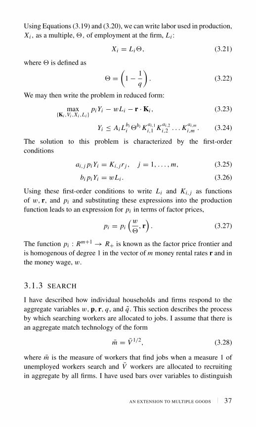
Using Equations (3.19) and (3.20), we can write labor used in production,Xi , as a multiple, �, of employment at the firm, Li :

Xi = Li�, (3.21)

where � is defined as

� =(

1 − 1

q

). (3.22)

We may then write the problem in reduced form:

max{Ki ,Vi ,Xi ,Li }pi Yi − wLi − r · Ki , (3.23)

Yi ≤ Ai Lbii �bi K

ai,1i,1 K

ai,2i,2 . . . K

ai,mi,m . (3.24)

The solution to this problem is characterized by the first-orderconditions

ai, j pi Yi = Ki, j r j , j = 1, . . . , m, (3.25)

bi pi Yi = wLi . (3.26)

Using these first-order conditions to write Li and Ki, j as functionsof w, r, and pi and substituting these expressions into the productionfunction leads to an expression for pi in terms of factor prices,

pi = pi

(w

�, r

). (3.27)

The function pi : Rm+1 → R+ is known as the factor price frontier andis homogenous of degree 1 in the vector of m money rental rates r and inthe money wage, w.

3.1.3 SEARCH

I have described how individual households and firms respond to theaggregate variables w, p, r, q, and q. This section describes the processby which searching workers are allocated to jobs. I assume that there isan aggregate match technology of the form

m = V 1/2, (3.28)

where m is the measure of workers that find jobs when a measure 1 ofunemployed workers search and V workers are allocated to recruitingin aggregate by all firms. I have used bars over variables to distinguish


aggregate from individual values. Further, since all workers are initiallyunemployed, employment and matches are equal,

L = V 1/2. (3.29)

Jobs are allocated to the i th firm in proportion to the fraction of aggregaterecruiters attached to firm i ; that is,

Li ≡ V 1/2 Vi

V, (3.30)

where Vi is the number of recruiters at firm i .

3.2 Equilibrium and the Social Planner

In this section, I extend the equilibrium concept from Chapter 2 to amultigood economy and I compare the properties of an equilibrium withthe solution to a social planning solution in a multigood environment.

3.2.1 THE SOCIAL PLANNER

In the multigood economy, the planner solves the problem

max{C,V,L} j (C) =n∑

i=1

gi log (Ci ) (3.31)

Ci ≤ Ai Kai,1i,1 K

ai,2i,2 . . . K

ai,mi,m (Li − Vi )

bi , i = 1, . . . n, (3.32)

n∑i=1

Ki, j ≤ K j , j = 1, . . . m (3.33)

Li =(

1

V

)1/2

Vi . (3.34)

Equation (3.34) can be rearranged to give the following expressionfor aggregate employment as a function of aggregate labor devoted torecruiting:

L ≡n∑

i=1

Li = V 1/2. (3.35)

Combining this expression with Equation (3.34) leads to the followingrelationship between labor used in recruiting at firm i , employment at


firm i , and aggregate employment:

Vi = Li L. (3.36)

Equation (3.36) implies that it takes more effort on the part of therecruiting department of firm i to hire a new worker when aggregateemployment is high; this is because of congestion effects in the matchingprocess.

Using Equation (3.36) to eliminate Vi from the production function,we can rewrite (3.32) in terms of Ki and Li :

Ci = Ai Kai,1i,1 K

ai,2i,2 . . . K

ai,mi,m Lbi

i

(1 − L

)bi. (3.37)

It follows that the externality � in Equation (3.24) is given by theexpression

� =(

1 − 1

q

)= 1 − L. (3.38)

Equation (3.37) makes clear that the match technology leads to a pro-duction externality across firms. When all other firms have high levels ofemployment, it becomes harder for the individual firm to recruit workersand this shows up as an external productivity effect, which is the term(1 − L

), in firm i ′s production function. The externality is internalized

by the social planner but may cause difficulties that private marketscannot effectively overcome. I will show that this externality is the sourceof Keynesian unemployment.

To find a solution to the social planning solution, we may substituteEquation (3.37) into the objective function (3.31) and exploit the loga-rithmic structure to write utility as a weighted sum of the logs of capitaland labor used in each industry, and of the externality terms that dependon the log of

(1 − L

). The first-order conditions for the problem can then

be written as

gi bi

Li=

∑ni=1 gi bi(1 − L

) , i = 1, . . . , n, (3.39)

gi ai, j

Ki, j= λ j , i = 1, . . . , n, j = 1, . . . , m, (3.40)

n∑i=1

Ki, j = K j , j = 1, . . . , m. (3.41)

The variable λ j is a Lagrange multiplier on the j th resource constraint.Using Equation (3.39) and the fact that L = ∑n

i=1 Li , it follows from


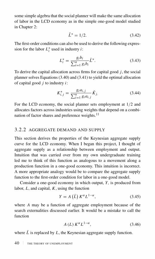
some simple algebra that the social planner will make the same allocationof labor in the LCD economy as in the simple one-good model studiedin Chapter 2:

L∗ = 1/2. (3.42)

The first-order conditions can also be used to derive the following expres-sion for the labor L∗

i used in industry i :

L∗i = gi bi∑n

i=1 gi biL∗. (3.43)

To derive the capital allocation across firms for capital good j , the socialplanner solves Equations (3.40) and (3.41) to yield the optimal allocationof capital good j to industry i :

K ∗i, j = gi ai, j∑n

i=1 gi ai, jK j. (3.44)

For the LCD economy, the social planner sets employment at 1/2 andallocates factors across industries using weights that depend on a combi-nation of factor shares and preference weights.11


This section derives the properties of the Keynesian aggregate supplycurve for the LCD economy. When I began this project, I thought ofaggregate supply as a relationship between employment and output.Intuition that was carried over from my own undergraduate trainingled me to think of this function as analogous to a movement along aproduction function in a one-good economy. This intuition is incorrect.A more appropriate analogy would be to compare the aggregate supplyfunction to the first-order condition for labor in a one-good model.

Consider a one-good economy in which output, Y, is produced fromlabor, L , and capital, K , using the function

Y = A(L)

K α L1−α, (3.45)

where A may be a function of aggregate employment because of thesearch externalities discussed earlier. It would be a mistake to call thefunction

A (L) K α L1−α, (3.46)

where L is replaced by L , the Keynesian aggregate supply function.


In the one-good economy, the equation that triggers competition forworkers is the first-order condition

(1 − α) Y

L= w

p. (3.47)

Aggregate supply, Z , is price times quantity. Using this definition, Equa-tion (3.47) can be rearranged to yield the expression

Z ≡ pY = wL

(1 − α), (3.48)

which is the Keynesian aggregate supply function. By fixing the moneywage, Keynes was not assuming disequilibrium in factor markets; he waschoosing a numeraire. Once this is recognized, the Keynesian aggregatesupply curve takes on a different interpretation from that which is givenin introductory textbooks. A movement along the aggregate supply curveis associated with an increase in the price level that reduces the realwage and brings it into equality with a falling marginal product oflabor.

In an economy with many goods, the aggregate supply price, Z , isdefined by the expression

Z ≡n∑

i=1

pi Yi . (3.49)

For the LCD economy, the aggregate supply function has a particularlysimple form since the logarithmic and Cobb-Douglas functional formsallow individual demands and supplies to be aggregated. The first-ordercondition for the use of labor at firm i has the form

Li = bi Yi pi

w. (3.50)

To aggregate labor across industries, we need to know how relative pricesadjust as the economy expands. To determine relative prices, we mustturn to preferences and here the assumption of logarithmic utility allowsa simplification since the representative agent consumes the output ofevery industry and allocates fixed budget shares to each commodity:

Yi pi = Ci pi = gi Z D, (3.51)

where Z D is disposable income. Combining Equation (3.50) with (3.51)yields the expression

Li = bi gi Z D

w. (3.52)


Summing Equation (3.52) over all i industries and choosing w = 1 asthe numeraire leads to the expression

Z D = 1

χL ≡ φ (L) , (3.53)

where

χ ≡n∑

i=1

gi bi . (3.54)

Since the government budget must also balance,

TR = τ Z , (3.55)

it follows that income and disposable income must be equal; that is,

Z D = Z (1 − τ) + TR = Z , (3.56)

and Equation (3.53) can be written as

Z = 1

χL ≡ φ (L) . (3.57)

Equation (3.57) is the Keynesian aggregate supply curve for the multi-good logarithmic Cobb-Douglas economy. To reiterate, the aggregatesupply curve in a one-good economy is not a production function. It isthe first-order condition for labor. In the LCD economy, it is an aggregateof the first-order conditions across industries with a coefficient that is aweighted sum of preference and technology parameters for the differentindustries.

Can this expression be generalized beyond the LCD case? The answeris yes, but the resulting expression for aggregate supply depends, ingeneral, on factor supplies; that is, Z will be a function not only of Lbut also of K1, . . . Km . The following paragraph demonstrates that, givenour special assumptions about preferences and technologies, these stocksserve only to influence rental rates.

The first-order condition for the j th factor used in firm i can bewritten as

Ki, j = ai, j Yi pi

r j. (3.58)

Combining the first-order conditions for factor j and summing over all iindustries leads to the expression

K j =n∑

i=1

Ki, j =∑n

i=1 ai, j Yi pi

r j. (3.59)


Exploiting the allocation of budget shares by consumers, Equation(3.51), one can derive the following expression:

r j = ψ j Z

K j, (3.60)

where

ψ j ≡n∑

i=1

ai, j gi . (3.61)

Equation (3.60) determines the nominal rental rate for factor j as afunction of the aggregate supply price, Z , and the factor supply, K j .

3.2.3 KEYNESIAN EQUILIBRIUM

What determines relative outputs in the Keynesian model and how areaggregate employment, L , and the aggregate supply price, Z , deter-mined? As in the one-good model, aggregate demand follows from theGDP accounting identity,

D =n∑

i=1

pi Ci . (3.62)

In an economy with government purchases and investment expenditure,this equation would have two extra terms as in the textbook Keynesianaccounting identity that generations of students have written as

Y = C + I + G. (3.63)

In our notation, C is replaced byn∑

i=1pi Ci , Y is replaced by D, and G

and I are absent from the model. The Keynesian consumption functionis simply the budget equation

n∑i=1

pi Ci = (1 − τ) Z + TR, (3.64)

and since D =n∑

i=1pi Ci and χ Z = L , from Equation (3.53), the aggre-

gate demand function for the LCD economy is given by the equation

D = (1 − τ)L

χ+ TR. (3.65)


The Aggregate SupplyFunction

Z L=

L

,Z D

TR

The Aggregate DemandFunction

LD = (1−t ) χ + TR

ZK

LK

1χ

1

cA

FIGURE 3.1 Aggregate Demand and Supply in the Multi-good Model

In a Keynesian equilibrium, when D = Z , the value of income, Z K , isgiven by the equality of aggregate demand and supply; that is,

Z K = TR

τ, (3.66)

and equilibrium employment is given by the expression

L K = χ Z K .

The Keynesian aggregate demand and supply functions for the LCDeconomy are graphed in Figure 3.1.

3.3 Equilibrium and the Planning Optimum

Compared

How well do markets work? Do we require government microman-agement of individual industries to correct inefficient allocations ofresources that are inherent in capitalist economies? Keynes responseto the first question was that the level of aggregate economic activitymay be too low as a consequence of the failure of effective demand.For this reason, he was a strong proponent of government interven-tion. But Keynes’s was not a communist and he recognized the merits


of the free market as an allocation mechanism to distribute resourcesacross industries. In this section, I will show that the model I havedeveloped provides a formalization of Keynes’s arguments. If effectivedemand is too low, the model displays an inefficient level of employment.In this sense there is an argument for a well-designed fiscal policy.But the allocation of factors across industries, for a given volume ofemployment, is the same allocation that would be achieved by a socialplanner. There is no reason for government to micromanage individualindustries.

To make the argument for fiscal intervention, one need only com-pare aggregate employment in the social planning solution with aggre-gate employment in a Keynesian equilibrium. The social planner wouldchoose

L∗ = 1

2. (3.67)

The Keynesian equilibrium at

L K = χTR

τ(3.68)

may result in any level of employment in the interval [0, 1]. For any valueof L K < L∗, we may say that the economy is experiencing Keynesianunemployment, and in this case there is a possible Pareto improvementthat would make everyone better off by increasing the number of peopleemployed.

The formalization of Keynesian economics based on search containsthe additional implication that there may be overemployment as well asunderemployment; that is, L K may be greater than L∗. Overemploymentis Pareto inefficient and welfare would be increased in an alternativeequilibrium in which fewer workers were employed in every industry.Although a value of L K greater than L∗ is associated with a higher valueof nominal GDP (Z K > Z∗), employment, in an equilibrium of thiskind, is too high and the economy is not maximizing output measured inphysical units. By lowering L back toward L∗, the economy can producemore goods in every industry. The increase in the physical quantity ofeach good is accompanied by an even greater drop in its price. Thisin turn causes the money value of output to fall even as the quantityproduced of every good rises.

In an overemployment equilibrium, the additional workers spendmore time recruiting their fellows than in productive activity. In thelimit, as employment tends to 1, nominal GDP tends to its upper bound,


1/χ . But although GDP measured in wage units always increases asemployment increases, for very high values of employment the physicalquantity of output produced in each industry is very low, and in the limitat L = 1, Yi is equal to zero in each industry and pi is infinite. Everyemployed worker is so busy recruiting additional workers that he or shehas no time to produce commodities.

What about the allocation of factors across industries? Here, thecapitalist system fares much better. Equations (3.43) and (3.44), whichdetermine factor allocations in the social planning solution, are repro-duced here:

L∗i = gi bi∑n

i=1 gi biL∗, (3.69)

K ∗i, j = gi ai, j∑n

i=1 gi ai, jK j. (3.70)

Given the resources K j for j = 1, ..., m, Equation (3.70) implies thatthese resources will be allocated across industries in proportion toweights that depend on the preference parameters gi and the productionelasticities ai, j . Equation (3.69) implies that the volume of resourcesemployed, L∗, will be allocated across industries in a similar manner.

Contrast these equations with their counterparts for the Keynesianequilibrium. The factor demand equations (3.58) and the resource con-straints (3.59) are reproduced here:

Ki, j = ai, j Yi pi

r j, (3.71)

K j =n∑

i=1

Ki, j =∑n

i=1 ai, j Yi pi

r j. (3.72)

Consumers with logarithmic preferences will set budget shares to utilityweights:

pi Yi = gi Z . (3.73)

Combining this expression with Equations (3.58) and (3.72) leads tothe following equation, which determines the allocation of factor j toindustry i in a Keynesian equilibrium:

Ki, j = gi ai, j∑ni=1 gi ai, j

K j . (3.74)


This expression is identical to the social planning solution, Equation(3.70). In other words, capital is allocated efficiently across industriesin a Keynesian equilibrium.

What about the allocation of labor across industries? The first-orderconditions for firms imply

bi pi Yi = wLi . (3.75)

Combining this expression with Equation (3.73) and using the fact thatχ Z K = L K gives

Li = gi bi∑ni=1 gi bi

L K , (3.76)

where I have used the fact that χ ≡ ∑ni=1 gi bi . Equation (3.76), which

determines the allocation of labor across industries, is identical tothe social planning solution with one exception; the efficient level ofaggregate employment, L∗, is replaced by the Keynesian equilibriumlevel, L K . It is in this sense that Keynes provided a general theoryof employment. The classical value L∗ is just one possible rest pointof the capitalist system, as envisaged by Keynes, and in general itis not one that he thought would be found by unassisted competitivemarkets.


It is difficult to read The General Theory without experiencing a dis-connect between what is in the book and what one has learned aboutKeynesian economics as a student. The most egregious misrepresen-tation is the notion of aggregate demand and supply that we teach toundergraduates and that bears little or no relationship to what Keynesmeant by these terms. The representative textbook author has adoptedthe Humpty Dumpty approach that, “ . . . when I use a word, it meansjust what I choose it to mean—neither more nor less.”12

The textbook aggregate demand curve slopes down; the Keynesianaggregate demand curve slopes up. The textbook aggregate demandcurve plots a price against a quantity; so does the Keynesian aggregatedemand curve, at least in name, but the “aggregate demand price” andthe “aggregate supply price” of The General Theory are very differentanimals from the price indices of modern theory. Beginning with Patinkin


(1956), textbook Keynesians have tried to fit the round peg of The Gen-eral Theory into the square hole of Walrasian general equilibrium theory.The fact that the fit is less than perfect has caused several generations ofstudents to abandon the ideas of The General Theory and to follow thetheoretically more coherent approach of real business cycle theory. Thetime has come to reconsider this decision.


CHAPTER 4A Model with Investmentand Saving

THE MODELS I INTRODUCED in chapters 2 and 3 are missing acentral component of The General Theory: the idea that investment

is the driving force of business cycles. Chapter 4 introduces this idea bydeveloping a model with saving and investment. In The General Theory,Keynes argued that the distinction between these concepts was centralto his theory of effective demand. I will explain this distinction with atwo-period model populated by three generations of households. Oneof these generations, the young in the first period, saves for the futureand invests in capital to produce commodities in the second period.In Walrasian general equilibrium models, saving and investment arebrought into equality by changes in intertemporal prices. In the Key-nesian model, they are equated by changes in employment. Explainingthe difference between these two mechanisms is the main purpose of thischapter.

Chapter 4 builds a model economy that has all the same features as theone-commodity environment that I introduced in Chapter 2. In addition,it has an extra period and a produced factor of production, capital. Thisricher structure allows me to discuss the idea that unemployment isproduced by a lack of investment spending. Whereas effective demandin Chapter 2 was a function of fiscal policy, in this chapter it will alsodepend on the beliefs of investors.

4.1 The Model Structure and the Planning

Solution

This section describes the physical environment and describes the socialplanning problem. There are two periods, labeled 1 and 2, and three gen-erations, labeled 0, 1, and 2. In period 1, there are two generations alive.Generation 0 is old and owns the capital stock. Generation 1 is young andowns an endowment of time. At the end of period 1, generation 0 dies.At the beginning of period 2, generation 2 is born and is endowed with aproduction technology. Throughout the chapter, a superscript will indexthe period in which a generation was born and a subscript will indexcalendar time; thus, xs

t is the date t value of the variable x associatedwith the generation born in period s.

4.1.1 HOUSEHOLDS

This section describes the economic choices made by households in eachgeneration. I begin by describing the choices made by the old and theyoung in the first period; I refer to them as generations 0 and 1. I thenmove on to the second period of the model and introduce the choicesof a third generation that I refer to as generation 2. The decisions ofgenerations 0 and 2 are limited, and most of the action in this modeltakes place with the choices made by generation 1. One could developthe model by adding more periods and more generations, although I havenot done that in this book.

The Initial Old

There are two coexistent generations in period 1. Generation 0 solves theproblem

max{C0

1

} j0(

C01

), (4.1)

subject to the constraint

p1C01 ≤ [

(1 − δ) p1 + r1]

K1. (4.2)

There is a unique commodity in each period that may be consumed oraccumulated to be used as capital in production in the subsequent period.This commodity has money price p1 in period 1. K1 is an initial stock ofcapital owned by generation 0, r1 is the money rental rate for capital inperiod 1, δ is the depreciation rate, and C0

1 is consumption of generation 0


in period 1. Since I assume that the utility function j0(C0

1

)is increasing

in C01 , the household’s decision problem has the trivial solution

p1C01 = [

(1 − δ) p1 + r1]

K1, (4.3)

which directs the household to consume all of its wealth.13

The Initial Young

As in previous chapters, I assume a unit measure of households withpreferences over current consumption of household members. The rep-resentative generation 1 household receives utility from consumption inperiods 1 and 2 and solves the problem

max{C1

1 ,C12 ,K2

} j1(

C11 , C1

2

)= g1 log

(C1

1

)+ g2 log

(C1

2

), (4.4)

where the preference weights g1 and g2 sum to 1:

g1 + g2 = 1. (4.5)

Each household member is endowed with a single unit of time in period1 and a unit measure of household members searches for a job. Of theseworkers, a fraction L1 find a job and the remaining U1 are unemployed;hence,

L1 + U1 = 1. (4.6)

In a search equilibrium, a fraction q workers find a job and L1 is givenby the expression

L1 = q, (4.7)

where q is taken parametrically by the household.Generation 1’s allocation problem is subject to the sequence of budget

constraints

p1C11 + p1K2 ≤ w1L1, (4.8)

p2C12 ≤ (r2 + p2 (1 − δ)) K2, (4.9)

where w1 is the money wage in period 1, K2 is capital carried into period2, r2 is the money rental rate in period 2, and p2 is the money price inperiod 2. Households may borrow and lend with each other at moneyinterest rate i , and hence the intertemporal budget constraint is

p1C11 + p2

1 + iC1

2 ≤ w1L1. (4.10)

A MODEL WITH INVESTMENT AND SAVING 51

The solution to this problem is characterized by the consumption alloca-tion decisions,

p1C11 = g1w1L1, (4.11)

p2C12

1 + i= g2w1L1, (4.12)

and the no-arbitrage condition,

1 + i =(

r2

p2+ 1 − δ

)p2

p1, (4.13)

that defines the money interest rate i at which households have no desireto borrow or lend with each other.

The Third Generation

In period 2, there is a third generation that solves the problem

max{K2,C2

2

} j2(

C22

), (4.14)

p2C22 ≤ p2Y2 − r2K2, (4.15)

where output Y2 is produced with the technology

Y2 ≤ K α2 . (4.16)

The solution to this problem is given by the expression

C22 = Y2 − r2

p2K2. (4.17)

In a model of multiple generations, each generation would face aproblem like that of generation 1. To keep this two-period example assimple as possible, I assume here that generation 2 owns the technologydescribed by Equation (4.16) and that members of this generation rentcapital from generation 1 and produce output Y2. There is no labor marketin period 2.

4.1.2 FIRMS

I have described the decisions made by households, and I have alsoexplained production in period 2. This section describes the choices madeby firms in period 1. Since the structure of this problem is a special caseof the problem described in Chapter 3, I will be relatively brief in mydescription.


There is a large number of competitive firms, each of which solvesthe problem

max{Y1,K1,V1,L1,X1}p1Y1 − w1L1 − r1K1, (4.18)

subject to the constraints

Y1 ≤ AK α1 X1−α

1 , (4.19)

L1 = X1 + V1, (4.20)

L1 = qV1. (4.21)

As in chapters 2 and 3, the firm must choose a feasible plan{Y1, K1, V1, L1, X1} to maximize profit, taking the wage w1, the rentalrate r1, the price p1, and the recruiting efficiency q as given. A firm thatallocates V1 workers to recruiting will hire qV1 = L1 workers, of whichX1 will be allocated to productive activity.

The solution to this problem is characterized by the first-order condi-tions

(1 − α)Y1

L1= w1

p1, (4.22)

αY1

K1= r1

p1, (4.23)

and the factor price frontier

p1 = 1

A

(w1

[1 − α] �

)1−α (r1

α

)α

, (4.24)

where the aggregate productivity variable

� =(

1 − 1

q

)(4.25)

is taken as given by the individual firm.

4.1.3 SEARCH

The search technology is identical to that described in Chapter 2. Thereis a match technology of the form

L1 = V 1/21 , (4.26)

where L is employment, equal to the measure of workers that find jobswhen a unit measure of unemployed workers search and V1 workers areallocated to recruiting by firms.


In a symmetric equilibrium, equations (4.20), (4.21), and (4.26) imply

� = (1 − L1

). (4.27)


How would a benevolent social planner arrange production and con-sumption in this economy? This section addresses that question by study-ing the solution to the following constrained optimization problem:

max{K2,L1,C0

1 ,C11 ,C1

2

}λ0 j0(

C01

)+ λ1 j1

(C1

1 , C12

)+ λ2 j2

(C2

2

), (4.28)

C01 + C1

1 + K2 ≤ AK α1 L1−α

1 (1 − L1)1−α + K1 (1 − δ) , (4.29)

C12 + C2

2 ≤ K α2 + (1 − δ) K2, (4.30)

where the numbers λi are welfare weights that sum to 1:

λ1 + λ2 + λ3 = 1. (4.31)

The social planner chooses K2, the amount of capital to carry intoperiod 2; L1, employment in period 1; and a way of allocating commodi-ties to individuals,

{C0

1 , C11 , C1

2 , C22

}. His or her problem is characterized

as the maximization of Equation (4.28) subject to the two feasibilityconstraints (4.29) and (4.30).

The solution to this problem requires that the two inequalities (4.29)and (4.30) should hold with equality and, in addition, the following sixfirst-order conditions should be satisfied:

−μ1 + μ2αK α−12 = 0, (4.32)

(1 − α) AK α1 L1−α

1 (1 − L1)1−α

(1

L1− 1

1 − L1

)= 0, (4.33)

λ0 j01

(C0

1

)= μ1, (4.34)

λ1 j11

(C1

1 , C12

)= μ1, (4.35)

λ1 j12

(C1

1 , C12

)= μ2, (4.36)

λ2 j21

(C2

2

)= μ2. (4.37)

The six equations (4.32) through (4.37) and the two constraints (4.29)and (4.30) determine the six variables K2, L1, C0

1 , C11 , C1

2 , and C22 and


the two Lagrange multipliers μ1 and μ2 associated with the inequalityconstraints (4.29) and (4.30).

The most important of these conditions is Equation (4.33), whichimplies that optimal employment in period 1, call this L∗

1, occurs when

L∗1 = 1

2. (4.38)

This problem differs from a conventional social planning problemsince there is an externality in the technology that is internalized bythe social planner. This is the occurrence of the term 1 − L1 in theproduction function in period 1. In all other ways, the problem is con-ventional. Given L1, the planner chooses how to allocate commodi-ties across individuals and across time. I show later that the existenceof this externality may make it difficult or impossible for a marketeconomy to make the right employment decision, and I formalize thisidea in the concept of a demand-constrained equilibrium. If this prob-lem can be corrected, the existence of commodity and asset marketsimplies that a decentralized economy can produce a Pareto efficientallocation.

4.2 Investment and the Keynesian Equilibrium

Economists are used to thinking of general equilibrium in Walrasianterms. Agents take prices and endowments as given and form demands.An equilibrium is a set of prices and an allocation of commodities suchthat all markets clear, and no individual has an incentive to alter his orher allocation through trade at equilibrium prices.

For the Keynesian model, we will require a different equilibriumconcept since, by construction, there are not enough markets to determineequilibrium allocations. This section extends the demand-constrainedequilibrium concept of Chapter 2 to the two-period model. I will usethis extended concept to introduce the idea that investment determineseconomic activity, and I will show that there is an interval such that,for any value of investment expenditure in that interval, there exists ademand-constrained equilibrium.

4.2.1 HOW TO CLOSE THE MODEL

Since the Keynesian model is missing an equation, there are manyequivalent candidates for an equation with which to close it. Following


The General Theory, this chapter closes the model with the assumptionthat investors form a set of beliefs about the future. Keynes called this“animal spirits”. But this assumption has many representations, all ofwhich are consistent with a self-fulfilling equilibrium. In this chapter, Ihave chosen to represent the assumption by assuming that the value ofcapital is determined by the beliefs of investors.

Specifically, let

I1 ≡ p1K2. (4.39)

I will refer to I1 as investment, although this is a misnomer since it isin fact the money value of the next period’s capital stock. I have chosenthis definition because it simplifies the equilibrium concept. By assumingthat entrepreneurs have fixed beliefs about the appropriate value of I1,

I am able to separate the equation that determines aggregate demandand employment from the equations that determine relative prices. Theresulting dichotomy allows me to provide an interpretation of textbookKeynesian models that has a firm microfoundation.

If I1 is large, I will say that investors are optimistic, and if I1 is small,they are pessimistic. I will show that there is value I1 such that for anyvalue of

I1 ∈ [0, I1

], (4.40)

there is an equilibrium, characterized by values for prices {p1, p2, w1, i},consumption allocations {C0

1 , C11 , C1

2 , C22}, employment L1, unemploy-

ment U1, productions Y1 and Y2, and capital K2 such that no individualhas an incentive to change his or her behavior given the prices and thequantities demanded and supplied for commodities in each period andfor borrowing, lending, and capital in the asset markets. In the labormarket, employment is determined by matching the equilibrium numbersof searchers on each side of the market.

4.2.2 THE DEFINITION OF EQUILIBRIUM

This section extends the definition of a demand-constrained equilibriumfrom Chapter 2 to the two-period model with capital. Since this conceptis based on ideas from The General Theory, I will also refer to it as aKeynesian equilibrium and I will refer to equilibrium values of variablesin the model with the superscript K , for Keynes. These values are tobe contrasted with the superscript ∗ that denotes the social planningoptimum when the planner uses the welfare weights λi .


Definition 4.2: (Demand-Constrained Equilibrium): Let K1 begiven as an initial condition and let I1 be given by the equation

I1 = (1 − b)

(1 − α), (4.41)

where

b = α + g1 (1 − α) . (4.42)

For any I1 ∈ [0, I1

], a symmetric demand-constrained equilibrium

is

(i) a six-tuple of prices {p1, p2, w1, r1, r2, i},(ii) a production plan {Y1, Y2, K2, V1, L1, X1},

(iii) a consumption allocation{C0

1 , C11 , C1

2 , C22

}, and

(iv) a pair of numbers q and q, with the following properties:

(1) Feasibility:

Y1 ≤ AK α1 X1−α

1 , (4.43)

Y2 ≤ K α2 , (4.44)

C01 + C1

1 + K2 − K1 (1 − δ) ≤ Y1, (4.45)

C12 + C2

2 ≤ Y2 + K2 (1 − δ) , (4.46)

L1 ≤ V 1/21 , (4.47)

X1 + V1 = L1, (4.48)

K2 = I1

p1. (4.49)

(2) Consistency with optimal choices by firms:

r1

p1= α

Y1

K1, (4.50)

w1

p1= (1 − α)

Y1

L1, (4.51)

r2

p2= α

Y2

K2, (4.52)

p1 = 1

A

(w1

[1 − α] �

)1−α (r1

α

)α

. (4.53)


(3) Consistency with optimal choices by households:

p1C01 = [

(1 − δ) p1 + r1]

K1, (4.54)

p1C11 = g1w1L1, (4.55)

p2C12

1 + i= g2w1L1, (4.56)

p2C22 = p2Y2 − r2K2. (4.57)


q = L1, (4.58)

q = L1

V1, (4.59)

L1 = V 1/21 , (4.60)

� =(

1 − 1

q

). (4.61)

In Section 4.3, I will show that a demand-constrained equilibriumexists, and in the Appendix to this chapter, I will show how to computethe prices and allocations associated with this equilibrium.

4.3 Analyzing Equilibria

This section develops aggregate demand and supply equations and showsthat the equality of aggregate demand and supply results in an equi-librium employment level L K

1 that is feasible and that satisfies theoptimality conditions of households. I call this a demand-constrainedequilibrium. An important feature of this Keynesian model is that thereis a different demand-constrained equilibrium for every value of I1 in theinterval

[0, I1

]: All of these equilibria have the property that no investor

has an incentive to deviate from his or her plan.


As in previous chapters, I choose the money wage w1 as the numeraireand I define aggregate supply to be the money value of GDP at which


employers are indifferent to hiring L1 workers. The function φ (L1) thathas this property is found from the first-order condition for labor (4.22)and is given by the expression

Z1 = 1

1 − αL1 ≡ φ (L1) . (4.62)

As in The General Theory, I refer to Z1 ≡ p1Y1 as the aggregate supplyprice of employment, L1.

Period 1 aggregate demand, D1, is equal to

D1 =[

p1

(C0

1 + C11

)]+

[I1 − (1 − δ) p1K1

], (4.63)

where the first term in square brackets is the money value of aggregateconsumption and the second is the money value of investment. UsingEquations (4.3) and (4.11) leads to the expression

D1 = [(1 − δ) p1 + r1

]K1 + g1w1L1 + I1 − (1 − δ) p1K1,

which, by using the first-order conditions (4.22) and (4.23), can besimplified as follows:

D1 = bZ1 + I1, (4.64)

where

b = α + g1 (1 − α) . (4.65)

This is the point where the definition of investment as I1, the moneyvalue of period 2 capital, rather than p1 I1, the money value of addi-tions to capital, leads to a considerable simplification of the equa-tions that determine equilibrium. If I had chosen p1 I1 as the objectof investors’ beliefs, the equation that determines equality of aggre-gate demand and aggregate supply would have contained the additionalterm − (1 − δ) K1 p1. There is no conceptual difficulty in following thisalternative definition, but it would break the separation of the equationsthat determine equilibrium prices from those that determine aggregatedemand and supply.

The Keynesian equilibrium occurs when DK1 = Z K

1 . Imposing thiscondition and solving Equations (4.62) and (4.64) leads to the followingexpression for the equilibrium value of the aggregate supply price:

Z K1 = 1

1 − bI1. (4.66)


1LK

Aggregate Demand

1− αbD1=

L

Aggregate Supply 1

1 − αZ1=

1

11−α

11−α

D1, Z1

L1

I1~

I1~ L1+

FIGURE 4.1 Aggregate Demand and supply in a Model with Investment

Equilibrium employment, L K1 , is equal to

L K1 = (1 − α) Z K

1 . (4.67)

The Keynesian equilibrium is illustrated in Figure 4.1. Since employmentmust lie in the interval [0, 1] and aggregate supply is defined by Equation(4.62), it follows that the maximum value of aggregate supply is equal to1/ (1 − α) . It follows from the linearity of the aggregate demand andsupply equations that there exists a Keynesian equilibrium for any valueof I1 ∈ [

0, I]

where

I = (1 − b)

(1 − α). (4.68)

The Appendix to this chapter establishes this claim formally by showinghow the other variables of the model are determined.

4.3.2 FISCAL POLICY IN A KEYNESIAN MODEL

A Keynesian equilibrium can result in any value of employment in theinterval [0, 1], but the social planner will choose L∗ = 1/2. It followsthat, unless investors happen fortuitously to choose the correct value ofI1, the Keynesian equilibrium may be one of over-or underemployment.This section describes the Keynesian remedy for this problem by puttingfiscal policy into the model.


Since there are three generations, a fiscal policy could conceptuallyconsist of a level of government expenditure and a set of taxes andtransfers indexed by the age of the household. I will exclude governmentexpenditure since that raises the issue of public goods, and instead, I willconsider policies that consist of an income tax rate τ , levied in period 1,and a transfer payment TR to generation 1. I will show that for any valueof I1, there exists a tax transfer policy {τ, TR} that implements the fullemployment level of employment, L∗

1.14

Conceptually, it is possible to tax wage income and capital incomeat different rates and the generational burden of these taxes will dif-fer. I am concerned with the question, Can fiscal policy maintain fullemployment? The answer to this question is yes, and further, there aremany policies that can implement full employment, each with a differentgenerational burden.

To implement a policy that maintains full employment, let τ1 bethe tax rate on income and let TR0

1 and TR11 be lump-sum transfers to

generations 0 and 1 in period 1. There are no taxes or transfers in period2 and the tax rate on rental income is the same as the tax rate on wageincome. These assumptions imply that aggregate demand is given by theexpression

D1 = (1 − τ1) αZ1 + TR01 + g1

[(1 − τ1) (1 − α) Z1 + TR1

1

]+ I1.

(4.69)

The first term on the right side is the consumption from after-tax rentalincome of the old generation in period 1 and TR0

1 is the transfer to theinitial old. The term in square brackets is after-tax income of the younggeneration. Their labor income (1 − α) Z1 is taxed at rate τ1 and theyreceive a transfer TR1

1. The parameter g1 is the marginal propensity toconsume for these individuals. It is clear from this expression that therewill be many choices of TR0

1, TR11, and τ1 that force the equilibrium

value, at which D1 equals Z1, to occur at the planning optimum Z∗1 ; but

most of these solutions will cause the government to accumulate debtthat will need to be repaid in the second period. Instead, let us confineourselves to tax transfer policies for which

TR01 + TR1

1 = τ1 Z1. (4.70)

These are balanced budget policies.Substituting Equation (4.70) into (4.69), replacing τ1 Z1 with TR0

1 +TR1

1, and solving for the Keynesian equilibrium for which Z1 = D1


leads to the expression

Z K1 = I1 + TR0

1 (1 − α) (1 − g1) − α (1 − g1) TR11

(1 − α) (1 − g1), (4.71)

which defines the Keynesian equilibrium generated by any balanced bud-get fiscal policy. Notice that if the tax rate on wage and rental income isthe same, as I have assumed, then a transfer to the old has a positive effecton equilibrium income and a transfer to the young has a negative effect.TR0

1 enters with a positive and TR11 with a negative sign. It follows that if

Z K1 < Z∗

1 (the case of underemployment in the Keynesian equilibrium),the optimal policy is to transfer income to the old, and if Z K

1 > Z∗1 (the

case of overemployment), it is to transfer income to the young. Thereason is that the young save a fraction g1 of their income while the oldconsume all of it, and so a transfer to the old increases aggregate demandwhile a transfer to the young reduces it.


The main early criticisms of Keynes’s work were theoretical, not empir-ical. It was pointed out that The General Theory does not have asatisfactory theory of the labor market. In chapters 2 and 3, I constructedone-period demand-driven models to address these criticisms. Both ofthese chapters were based on a search-theoretic model of the labor mar-ket. Their purpose was to provide a microfoundation to the Keynesiantheory of aggregate supply. Recall that the aggregate supply functionφ (L1) is a relationship between Z1, the supply price measured in dollars,and L1, employment. Z1 is “the expectations of proceeds [i.e. nominalgdp] that will just make it worth the while of the entrepreneurs to givethat employment.” (Keynes, 1936, p. 24)

Chapter 4 has developed the first, and simplest, of several models thatembody Keynes’s theory of effective demand. Aggregate demand D1 is“the proceeds that entrepreneurs expect to receive from the employmentof L1 men” (Keynes, 1936, p. 25) and it can be broken into two com-ponents, consumption and investment, each measured in dollars. I haveprovided a micro-founded model in which consumption expenditure isa linear function of income, and investment expenditure is determinedby beliefs of investors about future productivity, so called “animal spir-its.” A Keynesian equilibrium, formally defined in this chapter as a


demand-constrained equilibrium, is a value of employment at whichaggregate demand and aggregate supply are equal.

Keynes emphasized that saving and investment are equated not bythe interest rate, but by the level of economic activity. This chapter hasprovided an interpretation of that idea. We are used to teaching macroe-conomics in the language of Walrasian general equilibrium theory. InWalrasian theory, prices clear markets and the rate of interest equatessaving and investment. By adding a search externality and removingthe spot market for labor, I have provided a framework where thereare not enough Walrasian prices to equate demands and supplies for allof the quantities. This framework goes beyond The General Theory byproviding an explicit microfoundation to the Keynesian idea of aggregatesupply.

4.5 Appendix

I have shown how aggregate supply and employment are determinedin period 1 in a Keynesian equilibrium. It remains to be shownhow the prices pK

1 , pK2 , and (1 + i K ); the consumption allocations

C0K1 , C1K

1 , C1K2 , and C2K

2 ; the capital stock K K2 ; and the outputs Y K

1and Y K

2 are determined in equilibrium.I turn first to the determination of prices and of the physical value of

output, Y K1 in the Keynesian equilibrium. The equilibrium price in period

1, pK1 , can be found by solving the equation

pK1 = Z K

1

Y K1

, (4.72)

where

Y K1 = AK α

1

(L K

1

)1−α (1 − L K

1

)1−α

(4.73)

is the physical value of output. Using Equation (4.67), this gives thefollowing expression for the money price pK

1 ,

pK1 = 1

A (1 − α)

(L K

1

K α1

)α1(

1 − L K1

)1−α, (4.74)

as a function of the endowment of capital, K1, and the value of employ-ment at the Keynesian equilibrium, L K

1 . pK1 is an increasing mono-

tonic function of L K1 , reflecting the fact that the real wage falls as


investors become more optimistic and the economy moves up the aggre-gate supply curve. This is the same mechanism that was discussed inchapters 2 and 3.

I now turn to the variables K K2 and Y K

2 . Given I1 and pK1 , it follows

from the definition of I1 that

K K2 = I1

pK1

, (4.75)

and hence

Y2 =(

K K2

)α

. (4.76)

Next, consider the determination of real rental rates and consumptionallocation to each generation. Generation 0 consumes the amount C0K

1 ,which is found from the budget equation

C0K1 = (1 − δ) K1 + r K

1

pK1

K1. (4.77)

The real rental rate, r1/p1, is found from the first-order condition forrental capital in period 1:

r K1

pK1

= αY K

1

K1. (4.78)

Equations (4.77) and (4.78) imply that

C0K1 = (1 − δ) K1 + αY K

1 .

The second period real rental rate, r K2 /pK

2 , is found from the first-orderconditions

r K2

pK2

= αY K

2

K K2

, (4.79)

and generation 2’s consumption is

C2K2 = Y K

2 − r K2

pK2

K K2 = (1 − α) Y K

2 . (4.80)

Generation 1’s consumption in period 2 is found from market clearing,

C1K2 + C2K

2 = (1 − δ) K K2 + Y K

2 , (4.81)

as

C1K2 = (1 − δ) K K

2 + αY K2 . (4.82)


Finally, we can solve for pK2 /

(1 + i K

), the present value of pK

2 , fromEquation (4.12) as

pK2 C1K

2

1 + i K= g2w1L K

1 , (4.83)

which can be rearranged to give

pK2

1 + i K= g2 (1 − α) Z K

1

C1K2

. (4.84)

It is worth pointing out that pK2 and i K are not separately defined because

money enters the model only as a unit of account.


PART II

USING THE THEORY TOUNDERSTAND DATA

IN THE FIRST PART of this book, I presented three simple modelsof the aggregate economy designed to illustrate the mechanisms that

distinguish a Keynesian from a classical model of the business cycle. Allof them were based on the same idea: There may be multiple equilibria inthe labor market. In Part II I move beyond the basic framework to developa series of dynamic models that are rich enough to serve as vehicles tointerpret U.S. economic history since 1929.

Any interpretation of the data must first choose which aspects are tobe understood. Chapter 5 takes issue with an approach that has becomecommon since Hodrick and Prescott (1997) argued that business cyclefacts should be defined to be deviations of observed time series from aflexible trend. Instead, I present an alternative detrending method thatuncovers relationships between time series at medium-term frequenciesthat are missed by data detrended with the Hodrick-Prescott filter. Thesubsequent chapters interpret the facts defined this way through the lensof the labor market theory developed in Part I. Chapters 6 and 7 presentdynamic models to understand the Great Depression and the wartimerecovery. Chapter 8 studies the history of the real economy since theFed-Treasury Accord in 1951.

CHAPTER 5A New Way to UnderstandBusiness Cycle Facts

THIS CHAPTER DEVELOPS a way of presenting business cycle factsthat differs from most approaches taken in recent work in macroe-

conomics. Business cycles are recurrent events in which many differenttime series move together. To present their common features in a waythat is apparent to visual inspection, it helps to divide the time series intotwo components: the trend and the cycle. Almost all recent papers onbusiness cycles have achieved this division by separating aggregate timeseries into two parts using a method developed by Robert Hodrick andEdward C. Prescott, the Hodrick-Prescott (HP) filter.15

The HP filter is a mechanical way of splitting an economic time seriesinto two components. One is a slowly moving “trend”; the other recordsthe deviations from trend. This second component is called the cycle. TheHodrick-Prescott filter contains a “tuning parameter” that can be chosento make the trend as smooth as desired. At one extreme, it becomes astraight line. At the other extreme, it is the original series. In quarterlydata, economists typically set the tuning parameter to 1600, a value thatdefines a smooth trend that removes decade-long swings in economicactivity but attributes movements at frequencies of four to eight years tothe cycle.

In this chapter, I will present an alternative detrending method tothat of the HP filter. I will present a method suggested by Keynes’sdiscussion of measurement in Chapter 4 of The General Theory; themeasurement of aggregate variables using “wage units”. My purpose for

presenting this alternative way of representing data is to illustrate someconnections between medium-frequency movements in economic timeseries that are not apparent in data that have been HP filtered.

5.1 What’s Wrong with the HP Filter?

Before the advent of real business cycle theory, in the 1970s, macroe-conomists confronted models with data using econometric methods. Inthe 1960s and early 1970s, the state of the art in macroeconometrics con-sisted of the estimation of large simultaneous equation models identifiedby restrictions suggested by Keynesian theory. Usually these restrictionsconsisted of “exclusion restrictions,” the assumption that not all variablesappear in all equations. Keynesian models were estimated with systemsmethods such as maximum likelihood or three-stage least squares, andthe estimated models were used as guides by policymakers. A goodexample is the Wharton model developed by Lawrence Klein at theUniversity of Pennsylvania.

The Keynesian econometric methodology developed by Klein andassociates was criticized by Lucas in his 1976 “Critique of EconometricPolicy Evaluation” on the grounds that microfounded structural equa-tions should contain expectations of future variables. Since the parame-ters of these expectations should depend on the parameters of the rulesfollowed by the policy authorities, Lucas argued that the rational expec-tations assumption would invalidate the practice of using fixed parametermodels as policy guides.

The profession responded to the Lucas critique in two different ways.The first, introduced to economists in the (55) book Rational Expecta-tions and Econometric Practice, was to develop appropriate econometricmethods to estimate parameters in rational expectations environments.The second, explained most clearly in Kydland and Prescott’s (1996)article, “The Computational Experiment,” was to develop a new method-ology, calibration, that lowered the standards of what it means for amodel to be successful by requiring that a good model should explainonly a limited set of empirical moments.

In the introduction to their 1981 book, Lucas and Sargent arguedfor the development of econometric techniques that would recognizethe “cross-equation restrictions” imposed on a model by the rationalexpectations assumption. These restrictions arise from the fact that theparameters of econometric models are functions of some smaller set

70 USING THE THEORY TO UNDERSTAND DATA

of “deep parameters” that represent the true structure. However, whensimple RBC models were confronted with data, they often performedpoorly.

As a response to this road block in the development of a newparadigm, Kydland and Prescott argued that one could not expect thata science in its infancy would initially outperform established science.In their view, this did not mean that economists should abandon thenew approach. They argued instead, that a new paradigm brings itsown anomalies and puzzles and that, as real business cycle theoryis developed, it will eventually solve these puzzles and supplant itspredecessor.

In a related paper, Hodrick and Prescott introduced the Hodrick-Prescott filter that soon became the dominant method for confrontingbusiness cycle models with business cycle facts. I will make two separatebut related arguments in this chapter. First, I will argue that the correctapproach to confronting models with data is the one advocated by Lucasand Sargent and that the new paradigm is now ready to be confrontedwith a full set of empirical moments. Second, I will argue that theubiquitous use of the HP filter masks a serious shortcoming of the RBCmodel and that the use of filtered data to evaluate it overstates the model’sconformity with the facts.

The first issue of confronting models with data is beyond the scopeof the current work. The second, the issue of presenting limited sets ofstylized facts by detrending data, is the main focus of this chapter. I willdevelop an alternative methodology to the HP filter that corrects a seriousshortcoming of the HP approach.

There are advantages to the presentation of HP-filtered data and,properly used, the confrontation of theory with data can be simpli-fied with its careful use. But the HP filter has disadvantages that areoften overlooked. Most business cycle models have implications for thecomovements of variables at all frequencies. By filtering out the low-frequency movements, one ignores implications of these movements forthe relationships between economic variables that could potentially beused to discriminate between theories. Models in which the trend in datais assumed to be generated by a common productivity shock should befiltered by removing a common trend. Instead, the HP filter removesa different nonlinear trend from every series, thereby purging the dataof potentially useful information. These low-frequency movements arecritical in assessing explanations of unemployment that deny the naturalrate hypothesis.16

A NEW WAY TO UNDERSTAND BUSINESS CYCLE FACTS 71

2

3

4

5

6

7

8

9

10 –8

–6

–4

–2

0

2

4

6

8

50 55 60 65 70 75 80 85 90 95 00 05

Shaded areas areNBER recessions

Per

cent

Lab

or F

orce

(In

vert

ed S

cale

)P

ercent Deviation from

Trend

2

3

4

5

6

7

8

9

10 1.40

1.45

1.50

1.55

1.60

1.65

1.70

1.75

1.80

50 55 60 65 70 75 80 85 90 95 00 05


Per

cent

Lab

or F

orce

(In

vert

ed S

cale

)W

age Units (P

ure Num

ber)

Unemployment Rate Real GDP (HP Filtered)

Unemployment Rate Real GDP (Wage Units)

FIGURE 5.1 Unemployment and Real GDP (Filtered Two Different Ways)

The upper and lower panels of Figure 5.1 compare data from 1950through 2007 that has been detrended with the HP filter with data thathas been filtered with my proposed alternative (measuring GDP in wageunits). On both panels, the unemployment rate is measured on the leftaxis on an inverted scale, and real GDP is measured on the right axis.


Notice from the lower panel, where GDP is measured in wage units,that the unemployment rate has low-to medium-frequency movementsthat move closely with real GDP. Compare this with the upper panel,which plots unemployment against real GDP measured as percentagedeviations from the HP trend. GDP measured in wage units moves moreclosely with unemployment at medium to low frequencies, whereas thesemovements are filtered out of the GDP series when it is detrended withthe HP filter. It is for this reason that I am advocating the use of wageunits as a way of measuring real magnitudes.

An example of the kind of movement I have in mind is the slowincrease in unemployment that runs from 1969 through 1985, which ismirrored in the lower panel of the figure by a decrease in real GDP. Thismovement is absent from the GDP series in the upper panel of Figure 5.1,in which real GDP has been detrended with the HP filter.

One would like to be able to ask the question, Did the low-frequencyfall in GDP cause the increase in the unemployment rate, or did causationrun in the opposite direction? If one adopts a classical approach to thelabor market, then the low-frequency movements in unemployment mustbe explained by movements in the natural rate of unemployment. In aKeynesian model, in contrast, low-frequency movements in the unem-ployment rate are potentially explained by low-frequency movementsin aggregate demand. Since these low frequency movements are notpresent in the HP-filtered data, it is not possible to address the questionof the possible dependence of the “natural rate” on fiscal or monetarypolicy.

5.2 Measuring Data in Wage Units

What are wage units? The inflationary component of any two nominalseries can be removed by taking their ratio. A natural series to use forthis purpose is the nominal wage. This series grows for two reasons. Itgrows because of changes in the value of the monetary unit, but it alsogrows because the real wage increases as the economy becomes moreproductive.

In Section 5.4, I will illustrate the behavior of the components ofGDP using U.S. annual data from 1950 through 2007. Each seriesin that section will be described as a per capita nominal series,deflated by the money wage. In all cases, the nominal wage is con-structed by dividing compensation to employees from the national


0

10

20

30

40

50

60

1930 1940 1950 1960 1970 1980 1990 2000


Per

cent

Lab

or F

orce

(In

vert

ed S

cale

)

Annual Wage Per Worker

FIGURE 5.2 The Average Annual Real Wage from 1929 Through 2007

income and product accounts by full-and part-time-equivalent employ-ees. This wage series is graphed in Figure 5.2 for the period from1929 through 2007. These data are measured in units of thousandsof dollars per year. I have chosen to use full-and part-time-equivalentemployees as my measure of employment because it is available con-tinuously from 1929 through the present day. Because my goal isto end up with a stationary measure, I also need to remove thegrowth in GDP that occurs from increases in the number of workingpeople.

The number of employed people may fluctuate for two reasons. First,more or less people may choose to enter the labor force in responseto changes in incentives or changes in tastes. Second, the number ofpeople employed may fluctuate as members of the labor force enter andleave paid employment. These two reasons for fluctuating employmentcorrespond to different economic mechanisms.

Keynesian models account for changes in employment by assuminga fixed or exogenous labor force and modeling changes in employmentby assuming that the unemployment rate varies with aggregate demand.Real business cycle models abstract from unemployment and assumethat all variations in employment are caused by variations in labor forceparticipation. In practice, both margins are important.


The models in this book assume that the labor force is fixed. Just asRBC models ignore the unemployment margin, I ignore the participationmargin. For this reason I deflate series in this book by the number ofpeople in the labor force rather than by population. For the reasonsdiscussed later, this measure of GDP per capita moves closely withunemployment.

5.3 Interpreting Wage Units

To see what the use of wage units means in a concrete case, suppose thatthe data were generated by an economy in which a unique good was pro-duced by competitive firms from capital and labor with a Cobb-Douglasproduction function using a constant returns-to-scale technology. In thiscase, the first-order condition for labor would imply

bY p = wL , (5.1)

where b is the elasticity of labor, Y is the quantity of output produced inphysical units, p is the dollar price per unit, L is the number of workerhours used to produce Y , and w is the wage per worker hour. We havedata on compensation to employees, wL; the number of full-and part-time-equivalent employees, L; and nominal GDP, pY . In 1929, pY wasequal to 103.7 billion, compensation to employees was equal to 51.1billion, 37.7 million full-or-part-time-equivalent people were employed,and the labor force (call this N ) consisted of 47.6 million people. Theyearly wage is computed as

w = (wL)

L= 51, 100, 000, 000

37, 700, 000= 1, 355

dollars per year. GDP is computed as

Z = pY

N

1

w= 103, 700, 000, 000

47, 600, 000× 1

1, 355, (5.2)

which for 1929 gives a value of GDP per member of the labor force of1.6 in units of pure number. If we let

u = N − L

N

be the unemployment rate, then combining this definition with equations(5.1) and (5.2) implies that Z should be equal to the inverse of the


elasticity parameter b multiplied by one minus the unemployment rate;

Z = (pY )

N

L

(wL)= 1

b

L

N= 1

b(1 − u) .

These calculations show that, if the economy produced a single good,GDP in wage units would be equal to the inverse of the elasticity of laborin production (also equal to labor’s share of national income) multipliedby the employment rate. Since there are multiple goods produced in thereal economy, this statement oversimplifies the definition, but it is stilltrue that all measurements in wage units have units of pure numbers. Tothe extent that production technologies are close to Cobb-Douglas, GDPmeasured in this way is a weighted average of the employment rates ineach industry.

5.4 The Components of GDP

This section illustrates some comovements between the components ofGDP and the unemployment rate that would be filtered out by the HPfilter but that are clear in the data represented in wage units. Figure 5.3illustrates the comovements of private investment expenditure (top panel)and private consumption (bottom panel) with unemployment. Figure 5.4shows the comovements of government purchases and net exports withunemployment. In each of the panels of these figures, one of the com-ponents of GDP is measured on the right axis in wage units and theunemployment rate is measured on the left axis in percentage pointsusing an inverted scale.

The scale of the left axis, which measures the unemployment rate, isthe same in all four panels. The right scale is different for each graph.The investment scale varies from 0.18 to 0.34, consumption varies from0.92 to 1.24, and the government purchases scale is from 0.2 to 0.52. Netexports vary from plus 0.04 to minus 0.12. These four series together addup to GDP.

The top panel of Figure 5.3 illustrates that investment per memberof the labor force moves quite closely with unemployment at high fre-quency, but there are lower frequency movements that it does not pick up.For example, between 1969 and 1980, unemployment trends up (recallthat the axis is inverted) but investment fluctuates around a constant level.In contrast to the stationary fluctuations in investment over this period,consumption and government purchases trend down. These downward


2

3

4

5

6

7

8

9

10 .18

.20

.22

.24

.26

.28

.30

.32

.34

50 55 60 65 70 75 80 85 90 95 00 05


Per

cent

of t

he L

abor

For

ce (

Inve

rted

Sca

le)

Wage U

nits (Pure N

umber)

2

3

4

5

6

7

8

9

10 0.92

0.96

1.00

1.04

1.08

1.12

1.16

1.20

1.24

50 55 60 65 70 75 80 85 90 95 00 05


Per

cent

of t

he L

abor

For

ce (

Inve

rted

Sca

le)

Wage U

nits (Pure N

umber)

Unemployment Rate (Left Scale)

Investment (Right Scale)

Unemployment Rate (Left Scale)Consumption (Right Scale)

FIGURE 5.3 Unemployment, Investment, and Consumption

trends mirror the increase in the unemployment rate (see the bottompanel of Figure 5.3 and the top panel of Figure 5.4). This period is oftenreferred to as productivity slowdown since conventional measures ofGDP per person grow at a slower rate in the 1970s.

The model I will develop in this book suggests that the 1970sslowdown in GDP growth was associated with an increase in the


2

3

4

5

6

7

8

9

10 .20

.24

.28

.32

.36

.40

.44

.48

.52

50 55 60 65 70 75 80 85 90 95 00 05


Per

cent

of t

he L

abor

For

ce (

Inve

rted

Sca

le)

Wage U

nits (Pure N

umber)

2

3

4

5

6

7

8

9

10 –.12

–.10

–.08

–.06

–.04

–.02

.00

.02

.04

50 55 60 65 70 75 80 85 90 95 00 05


Per

cent

of t

he L

abor

For

ce (

Inve

rted

Sca

le)

Wage U

nits (Pure N

umber)

Unemployment Rate (Left Scale)Net exports (Right Scale)

Unemployment Rate (Left Scale)Government Purchases (Right Scale)

FIGURE 5.4 Unemployment, Government Purchases, and Net Exports

unemployment rate. This increase in unemployment was caused bythe reduction in government purchases accompanying the end of theVietnam War. Unemployment depends on aggregate demand and alarge component of aggregate demand, is government purchases. InChapter 7.1, I explain the mechanism that links aggregate demand to


–4

–2

0

2

4

6

8

10

0.88

0.92

0.96

1.00

1.04

1.08

1.12

1.16

1965 1970 1975 1980 1985 1990 1995


Per

cent

per

Yea

rW

age Units (P

ure Num

ber)

Real Interest Rate (Left Scale)Consumption (Right Scale)

FIGURE 5.5 Unemployment and Real GDP (Filtered Two Different Ways)

employment and I develop a model that can account for the 1970sslowdown.

The graph in the lower right panel of Figure 5.4 represents net exports.This is a relatively small component of U.S. aggregate demand. It dis-plays a clear downward trend since 1980. This downward trend in netexports is associated with growth in the consumption of U.S. householdsas domestic consumer spending sucked in imports from the rest of theworld.

The detrending method that I use in this book reveals a movementin unemployment and the components of GDP at medium frequenciesthat is not apparent if one detrends data with the Hodrick-Prescott filter.But this correlation is not present in all of the components of GDP.Consumption and government purchases display the same medium-frequency movement as unemployment during the 1970s. This mediumterm-movement is not present in the investment series.

From 1950 through 1980, unemployment has an upward trend andconsumption and government purchases trend down. The movements inunemployment and consumption are reversed after 1980, but govern-ment purchases continue to decline. What caused these medium-term-movements?


Figure 5.5 shows that a good candidate to explain the change in con-sumption behavior in 1980 is the dramatic reversal of monetary policythat occurred in 1980 when Paul Volcker took over as chairman of theFed. Figure 5.5 plots the ex post real interest rate (measured as the T-billrate minus the annualized rate of change of the consumer price indexon the left axis) against consumption in wage units on the right axis.This figure shows that the turnaround in consumption growth in 1980 isaccompanied by an increase in the real interest rate at the time of theVolcker policy initiative.


The data presented in this chapter is suggestive. It does not constituteformal statistical evidence for or against any given theoretical model.But the development of theory is guided by stylized facts, and for the pasttwenty years, business cycle stylized facts were defined by real businesscycle theorists. The RBC agenda is to construct models that can matchthe volatility and cross-correlations of time series data that has beenfiltered by removing all but a narrow band of frequencies. By using thislimited set of moments, a generation of theorists has been starved of aset of medium-frequency facts. By detrending data in the way describedin this chapter, a new set of stylized facts becomes apparent and theirexplanation provides a new set of puzzles. I attempt to make sense ofthese puzzles in the following chapters.


CHAPTER 6The Great Depression: Tellingthe Keynesian Story in a New Way

THIS CHAPTER IS ABOUT the Great Depression. In 1929, the stockmarket dropped by 11% in one day and, in the subsequent four years,

it continued to decline, bottoming out in 1934 at 12% of its 1929 value.Accompanying the stock market decline, unemployment increased from4% to 24% of the labor force and GDP fell 20% below trend. In thischapter, I use the ideas developed earlier in the book to tell the Keynesianstory of this period of world history in a new way.

According to the Keynesian explanation, the stock market crash of1929 was due to a loss of confidence in the economy that caused acalamitous drop in aggregate demand. This caused an increase in unem-ployment that was socially inefficient in the sense that unemployedpersons could and should have been profitably employed in productiveactivity. This story was taught to generations of undergraduates as theleading explanation of the Great Depression by Keynesian economistsof the postwar period. The competition to this explanation was not theRBC model of Kydland and Prescott (1982), but an alternative story ofmarket failure promoted by Milton Friedman (1948). Friedman disputedthe impetus to the depression, which for him was the failure of theFed to maintain sufficient liquidity, but he did not dispute the fact thatunemployment during the depression was socially inefficient.

Why do I need to revisit a story that has been accepted by severalgenerations of economists? The theoretical foundations of this storyhave been discredited because Keynes did not construct a credible

microfoundation to the theory of aggregate supply. In this chapter, I usethe search model developed earlier in this book to provide such a foun-dation. In so doing, I will have cause to revisit an important debate thatarose in the postwar literature: Does fiscal policy matter?

Before the rational expectations revolution of the 1970s, macroe-conomists attempted to extend Keynesian economics to dynamic envi-ronments by building microfoundations to each of the components of theKeynesian model. Lucas (1967) and Treadway (1971) estimated modelsof investment, Milton Friedman (1957) provided a permanent incometheory of the theory of consumption function, and Friedman (1956)breathed new life into the Quantity Theory of Money by making the casefor a stable demand-for-money function. A central goal of this researchwas to provide a quantitative explanation of the effects of governmentpolicy on employment and prices. This goal ran into theoretical difficul-ties when economists realized that dynamic optimizing models have norole for fiscal policy since a one-dollar increase in government expendi-ture is predicted to crowd out an equal amount of private consumptionexpenditure if consumption and investment functions are derived fromoptimizing behavior by a representative family.

In Section 6.6, I show that crowding out is a logical consequenceof the representative agent model, with time-separable preferences, inwhich government cannot influence the real rate of interest. This fact hasimportant practical consequences for the effectiveness of fiscal policy. Ifhouseholds plan for the future in the way that models of this kind assume,increased government purchases will be offset by reduced privateexpenditure.

In WWII, there was a massive increase in government purchases ofgoods and services, and this fiscal expansion was accompanied by a dropin unemployment from 17% in 1939 to 1% in 1944. This recovery isattributed by Keynesian economists to the direct effects of fiscal policy.Since the representative agent model developed in this chapter displayscrowding out, it is not a good model of the wartime recovery. Modelsof this kind have been dubbed “Ricardian” by Robert Barro (1974), whoattributes the idea to David Ricardo in the nineteenth century.

To understand the recovery of the economy during WWII, in Chap-ter 7 I will expand the model by providing an alternative framework inwhich fiscal policy does matter. This framework assumes that people donot care for their descendents in the way that Ricardian models assume.

There are still important quantitative questions that needs to beanswered: Is the world close to being Ricardian, or is the Ricardian


approximation a very bad one? If the world is close to Ricardian, thenfiscal policy will stimulate employment but at the cost of a very largeintergenerational transfer.

6.1 Developing the Model

This section develops the equations of an intertemporal model with arepresentative agent that has the same supply side that I introduced inPart I. The innovation over earlier models is to add an infinitely livedrepresentative consumer to determine the demand side.

6.1.1 PREFERENCES

I will study a multicommodity intertemporal representative family modelin which there is a single capital good in fixed supply. The simplificationof nonreproducible capital enables me to draw out a relationship betweenthe value of the stock market (represented by the value of capital) and thelevel of economic activity.

There is a unit measure of identical representative infinitely livedfamilies. There are n consumption goods and Kt = 1 units of capital.Preferences are described by the following logarithmic utility function:

Jt =∞∑

s=t

[βs−1

n∑i=1

gi log(Ci,s

)], (6.1)

wheren∑

i=1

gi = 1, (6.2)

and the gi are preference weights. Each family sends a measure 1 ofmembers to look for a job every period. All jobs last for one period andthere is 100% labor market turnover. These assumptions are very strongand are made to facilitate the exposition of the model.

The household faces the sequence of budget constraints

pk,t Kt+1 = (pk,t + rrt

)Kt + wt Lt −

n∑i=1

pi,t Ci,t , t = 1, . . .∞, (6.3)

Lt = qt , (6.4)

Ut = 1 − Lt , (6.5)

THE GREAT DEPRESSION 83

and the no-Ponzi scheme constraint

limT →∞ QT

t Kt+1 ≥ 0. (6.6)

The notation is defined as follows. Lt is the measure of workers that finda job and Ut is the measure that remain unemployed. wt is the moneywage, pi,t is the money price of good i , qt is the probability that asearching worker will find a job, Ci,t is consumption of good i , Kt isthe family’s ownership of capital, rrt is the rental price of capital, andpk,t is the money price of a unit of capital. All of these terms are definedfor each date t . All date t prices are in different date t units of accountthat I refer to as date t money. The variable QT

t represents the relativeprice of date T money in terms of date t money and is given by theexpression

QTt =

T −1∏k=t

1

(1 + ik), T > t, (6.7)

Qtt = 1. (6.8)

I assume riskless borrowing and lending at money rate of interest it .A no-arbitrage condition then implies that

1 + it = pk,t+1 + rrt+1

pk,t, (6.9)

where it is the money rate of interest between dates t and t + 1. Sinceall families are identical, there will be no borrowing or lending inequilibrium.

6.1.2 LABOR SUPPLY AND CONSUMPTION

Since the household derives no disutility from work, it will choose tosend all of its members into the labor force to look for a job. At the endof each period, all workers are fired and, in the next period, the entirelabor force is rehired. I make this assumption to facilitate exposition.

The first-order conditions for the problem are represented by an Eulerequation and a set of intertemporal first-order conditions that togetherimply

1

Ct= β

Ct+1(1 + it ) , (6.10)


where consumption expenditure, Ct , is defined as

Ct ≡n∑

i=1

pi,t Ci,t . (6.11)

Equation (6.10) describes how aggregate consumption expenditure,measured in dollars, evolves over time. This equation will be centrallater in this chapter when I discuss crowding out. For completeness, it ishelpful to write down the solution to the household’s problem by derivingan equation in which consumption expenditure is described as a functionof prices, its time endowment, and the hiring probability. These variablesare taken as given in equilibrium. This solution requires first that wedefine some alternative concepts of wealth.

Let

ht = wt Lt + ht+1

1 + it(6.12)

be the human wealth of the family.17 By iterating this equation forwardand using the no-Ponzi scheme constraint (6.6), human wealth can bewritten in terms of prices and hiring probabilities:

ht =∞∑

s=t

Qst ws Ls =

∞∑s=t

Qst ws qs . (6.13)

The household also has financial wealth in the form of claims to capital:(pk,t + rrt

)Kt .

The sum of financial and human wealth is total wealth, Wt .

Wt = (pk,t + rrt

)Kt + ht . (6.14)

The solution to the household problem is to spend a fixed fraction of totalwealth on consumption goods, and consumption expenditure is given by

Ct = (1 − β) Wt . (6.15)

I will need Equation (6.15) in Chapter 7 when I discuss a more com-plicated family structure. For the purpose of solving the representativeagent model in this chapter, it does not play a central role.

6.1.3 TECHNOLOGY

This section describes the production side of the economy. There is aunit measure of nonreproducible capital that must be allocated across


industries in every period. There is also a unit measure of workers, allof whom will be allocated, in equilibrium, to the activity of labor marketsearch. I assume that each industry is described by a Cobb-Douglas pro-duction function and that capital is rented in a competitive rental market.Labor is hired in a search market. I assume further that labor in eachfirm is divided between a recruiting department and a production depart-ment as in previous chapters. These assumptions lead to the observationthat average and marginal products are equal and are equated to factorprices.

Production is competitive and has the same structure as that describedin Chapter 3. Output of the i th commodity is denoted Yi,t , and is pro-duced by a Cobb-Douglas function,

Yi,t ≡ K aii,t Xbi

i,t , (6.16)

where

ai + bi = 1 (6.17)

and

n∑i=1

Ki,t = Kt . (6.18)

Ki,t is the rental demand for capital by firm i and Xi,t is the firm’s allo-cation of labor to production. Market clearing in each industry impliesthat

Ci,t = Yi,t . (6.19)

Firms maximize profits taking pi,t , wt , rrt , and qt as given. Each firmsolves the problem

max{Ki,t ,Vi,t ,Xi,t ,Li,t}pi,t K ai

i,t Xbii,t − wt Li,t − rrt Ki,t (6.20)

Li,t = Xi,t + Vi,t , (6.21)

Li,t = qt Vi,t , (6.22)

where Li,t is total labor hired by firm i and Vi,t is the labor that it allo-cates to recruiting. Substituting Equations (6.21) and (6.22) into (6.20)and defining

�t = (1 − 1/qt ) (6.23)


leads to the reduced form expression for profits:

pi,t�bit K ai

i,t Lbii,t − wt Li,t − rrt Ki,t , (6.24)

which is maximized when

ai pi,t Yi,t = rrt Ki,t (6.25)

and

bi pi,t Yi,t = wt Li,t . (6.26)

These expressions are identical to those that hold in an economywith a competitive labor market. This economy differs from the compet-itive model since the recruiting efficiency parameter �t is endogenouslydetermined by aggregate economic activity but is taken parametricallyby the firm; hence, there is an externality in the labor market that isnot priced. The following section combines equations (6.25) and (6.26)with consumer first-order conditions to obtain some simple aggregateequilibrium relationships.

6.2 Aggregate Supply

This section derives an aggregate supply equation, similar to that ofearlier chapters in the book.

6.2.1 AGGREGATION ACROSS FIRMS

Let the variable Zt denote nominal GDP. Recall that Ct is the nominalvalue of aggregate consumption, and since there is no investment orgovernment expenditure, these two variables will be identical as a con-sequence of accounting identities. My goal here is to find a relationshipbetween Zt and Lt that I refer to as aggregate supply.

From the solution to the household’s problem, it follows that theconsumer allocates a fraction gi of total consumption expenditure togood i ; that is,

pi,t Ci,t = gi Ct . (6.27)

Since all production of good i is consumed, this also implies that

pi,t Yi,t = gi Ct , (6.28)


and, definingn∑

i=1

pi,t Yi,t ≡ Zt , (6.29)

it follows that

pi,t Yi,t = gi Zt . (6.30)

Substituting Equation (6.30) into the first-order condition for the choiceof labor in industry i leads to the expression

bi gi Zt = wt Li,t , (6.31)

which can be summed over all industries to give the following expres-sion:

χ Zt = wt Lt , (6.32)

where

χ ≡n∑

i=1

gi bi . (6.33)

Since money in each period is simply an accounting device, there is adegree of freedom in choosing a price normalization in each period. I willchoose the date t numeraire to be labor by setting

wt = 1, t = 1, . . .∞. (6.34)

This normalization implies that pi,t is the inverse of the real productwage for each commodity, and it allows me to write Equation (6.32) as

Zt = 1

χLt , (6.35)

an equation that I referred to earlier (in Chapter 3) as the Keynesianaggregate supply curve.

A similar exercise using the first-order condition for rental capitalyields the expression

ψ Zt = rrt Kt , (6.36)

where

ψ ≡n∑

i=1

gi ai . (6.37)

In Section 6.3.2, I will use equations (6.35) and (6.36) to describe howthe properties of aggregates behave in a demand-constrained equilibrium.


6.2.2 SEARCH AND THE LABOR MARKET

As in Chapter 3, I assume there is an aggregate match technology thatresults in the following expression for aggregate employment:

Lt = V 1/2t , (6.38)

where Lt is the measure of workers that find jobs when a measure 1 ofworkers search and Vt workers are allocated to recruiting in aggregate byall firms. Each firm faces an individual hiring equation,

Li,t = qt Vi,t , (6.39)

which, when aggregated over all firms, yields the expression

Lt = qt Vt . (6.40)

These equations can be rearranged to find an expression relating themeasure of workers that can be hired by a single recruiter, qt , to aggregateemployment, Lt :

qt = 1

Lt. (6.41)

6.2.3 SELECTING AN EQUILIBRIUM WITHLONG-TERM EXPECTATIONS

As in earlier chapters of this book, the absence of markets for the searchtime of workers and recruiters leads to an equilibrium model with oneless equation than unknown. If firms and workers take all wages andprices as given, there is an equilibrium for every value of the sequence ofhiring effectiveness parameters {�s}∞s=t . There are many possible waysof resolving this indeterminacy, each of which corresponds to a differentpossible belief about the future. In The General Theory, Keynes arguedthat the level of economic activity is pinned down by the state of long-term expectations. In our model, this concept is represented by a self-fulfilling sequence of values for the capital good, that is, a sequence{

pk,t}.

In an economy with a stock market, pk,t represents the value of equity.In the model of this chapter, there is no underlying uncertainty in thephysical environment, but in reality technology, preferences, and endow-ments as well as political and social variables are themselves changing inunknown ways. In modern macroeconomics, agents are assumed to knowthe probability distributions of all uncertain future events. In contrast,


Keynes argued that the future is unknowable. As a consequence, thebelief of agents in the form of the animal spirits of investors becomesan independent driving force of the business cycle.

In work with Benhabib (1994) and Guo (1994, 1995). I have arguedthat animal spirits should be modeled by building general equilibriummodels in which there is an indeterminate continuum of equilibria,indexed by beliefs and Harrison and Weder (2006) have used this ideato explain the Great Depression. In this work, different equilibria repre-sented nonstationary paths, each of which converges to the same steadystate. The model in this chapter is different because I allow beliefs toinfluence the steady state itself through variations in the state of long-term expectations.

6.3 Equilibrium and the Planner’s Problem

This section defines an equilibrium concept and relates it to the socialplanning solution. As in earlier chapters in this book, one can showthat the Keynesian equilibrium mimics the decisions of a social plannerby allocating resources across industries in an efficient fashion; but theKeynesian equilibrium may fail to maintain full employment in a well-defined sense. The purpose of this section is to define what this means.


Consider the problem

max{Ci,s ,Xi,s ,Vi,s ,Li,s ,Ls ,Vs} Jt =∞∑

s=t

[βs−t

n∑i=1

gi log(Ci,s

)](6.42)

such that

Ci,s ≤ K aii,s Xbi

is i = 1, . . . n, (6.43)

Xi,s + Vi,s = Li,s, (6.44)

n∑i=1

Li,s = Ls, s = t, . . . ∞. (6.45)

n∑i=1

Ki,s = 1,

n∑i=1

Vi,s = Vs, s = t. . . . ∞, (6.46)


Ls = V 1/2s , s = t, . . . ∞, (6.47)

Li,s = Vi,s

VsLs s = t, . . . ∞. (6.48)

Equation (6.42) is the objective function of the social planner (iden-tical to that of the representative agent) and equations (6.43) through(6.48) define the constraint set. As in earlier chapters, this problem canbe simplified by using the match technology to eliminate Vi,s, Xis , andVs from the problem. Using Equations (6.43), (6.44), (6.47) and (6.48),one can write the production function for good i as

Ci,s ≤ K aii,s Lbi

i,s (1 − Ls)bi . (6.49)

Using this simplification, the social planning problem can be restatedas

max{Ci,s ,Li,s ,Ls} Jt =∞∑

s=t

[βs−t

n∑i=1

gi log(Ci,s

)](6.50)

subject to Equation (6.49) for each commodity at each date and the setof labor constraints represented by Equation (6.45).

Proposition 6.1 (SP): The solution to the social planning prob-lem has the following properties. Aggregate employment in eachperiod is given by the expression

Ls = 1

2, s = t . . . ∞, (6.51)

and labor and capital are allocated across industries according tothe equations

Li,s = gi bi

χLs, Ki,s = gi ai

ψ, s = t, . . . ∞, (6.52)

where∑n

i=1 gi bi = χ and∑n

i=1 gi ai = ψ .

The proof is in the Appendix to this chapter. As in the earlier modelsof this book, with a similar labor market structure, there is an optimalunemployment rate of 50%. I will return to this result later when I discusswhether fiscal policy can improve on the equilibrium.


6.3.2 DEMAND-CONSTRAINED (KEYNESIAN)EQUILIBRIUM

In this subsection, I define a demand-constrained equilibrium, which Irefer to interchangeably as a Keynesian equilibrium, for the dynamiceconomy with multiple commodities. I will proceed to show that aKeynesian equilibrium exists and that it is represented by a set of aggre-gate equations that determine employment and GDP and a separate setof equations that describe how labor and capital are allocated acrossindustries.

I begin by defining the set of feasible expectations.

Definition 6.1: A (bounded) state of (long-term) expectations is anon-negative sequence

{pk,s

}∞s=t with a bound B such that

pk,s < B

for all s.

I define the state of expectations to be a sequence of beliefs aboutthe value of capital in all future periods. In a more general model, therewould be a different sequence of beliefs for every type of reproduciblecapital, and discrepancies between expectations and the interest ratewould cause changes in investment expenditures. In this model, I amabstracting from investment spending by assuming that there is a uniquenonreproducible capital good. Even in this simple environment, changesin beliefs about the value of capital will have an effect on expendituresince long-term expectations influence wealth, which in turn influencesconsumption expenditure.

The following definition is of a demand-constrained equilibrium inthe infinite horizon economy. Following this definition, I show thataggregate variables in a demand-constrained equilibrium follow a rel-atively simple equation.

Definition 6.2: (Demand-Constrained Equilibrium): For any stateof expectations {pk,s}∞s=t , a demand-constrained equilibrium(DCE) is an n-tuple of price sequences {pi,s}∞s=t i = 1, . . . n; asequence of rental rates {rrs}∞s=t ; a set of quantity sequences{Yi,s, Xi,s, Vi,s, Li,s, Ci,s, Ki,s}∞s=t ; and a pair of sequences ofnumbers {qs, qs}∞s=t , such that the following equations hold for alls = t, . . . ∞:


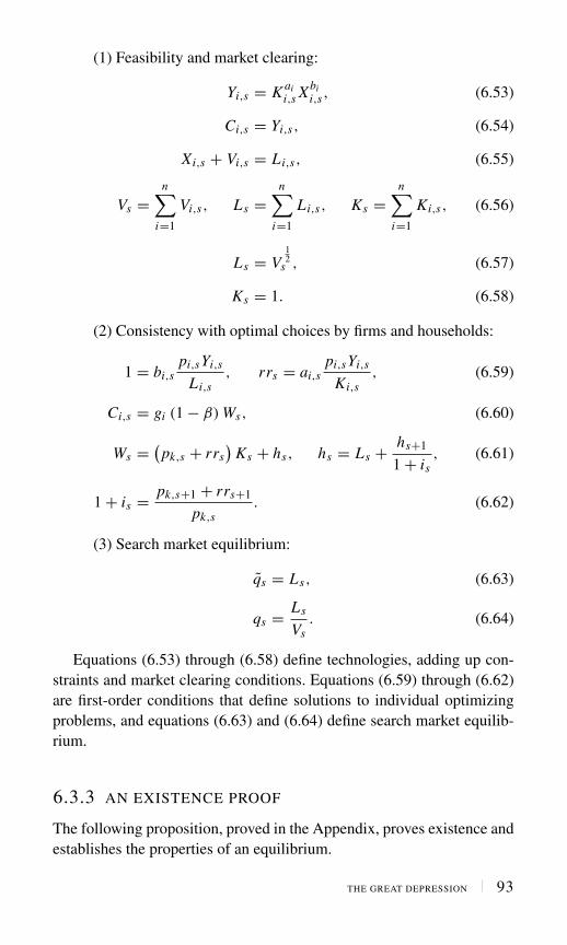
(1) Feasibility and market clearing:

Yi,s = K aii,s Xbi

i,s, (6.53)

Ci,s = Yi,s, (6.54)

Xi,s + Vi,s = Li,s, (6.55)

Vs =n∑

i=1

Vi,s, Ls =n∑

i=1

Li,s, Ks =n∑

i=1

Ki,s, (6.56)

Ls = V12

s , (6.57)

Ks = 1. (6.58)


1 = bi,spi,sYi,s

Li,s, rrs = ai,s

pi,sYi,s

Ki,s, (6.59)

Ci,s = gi (1 − β) Ws, (6.60)

Ws = (pk,s + rrs

)Ks + hs, hs = Ls + hs+1

1 + is, (6.61)

1 + is = pk,s+1 + rrs+1

pk,s. (6.62)


qs = Ls, (6.63)

qs = Ls

Vs. (6.64)

Equations (6.53) through (6.58) define technologies, adding up con-straints and market clearing conditions. Equations (6.59) through (6.62)are first-order conditions that define solutions to individual optimizingproblems, and equations (6.63) and (6.64) define search market equilib-rium.

6.3.3 AN EXISTENCE PROOF

The following proposition, proved in the Appendix, proves existence andestablishes the properties of an equilibrium.


Proposition 6.2 (DCE): There exists a unique demand-constrained equilibrium for every state of expectations withbound

B ≤ ψβ

χ (1 − β).

In a DCE, for s = t, . . . , aggregate expenditure, aggregateemployment, and the rental rate are described by equations (6.65)through (6.67):

Zs = 1

ψ

pk,s (1 − β)

β, (6.65)

Ls = χ Zs, (6.66)

rrs = pk,s (1 − β)

β. (6.67)

Equations (6.68) and (6.69), which hold for all i = 1, . . . n and alls = t, . . . ∞, determine the allocation of factors across industries:

Ki,s = ai gi

ψ, (6.68)

Li,s = bi gi Zs . (6.69)

The price in wage units of each commodity is given by the expres-sion

pi,s =(

ψ Zs

ai

)ai(

1

bi

)bi(

1

1 − χ Zs

)bi

, (6.70)

and the physical quantity of each good produced is given by theequation

Yi,s =(

ai

ψ

)ai

(bi Zs)bi gi (1 − χ Zs)

bi . (6.71)

6.3.4 EFFICIENCY OF EQUILIBRIUM

In a Keynesian equilibrium, the value of GDP is proportional to the valueof physical capital and is given by the expression

Zt = λpk,t , (6.72)

where λ = (1 − β)/(βψ). Employment, proportional to GDP, is equal to

Lt = χ Zt . (6.73)


It follows that there is a continuum of Keynesian equilibria indexed bypk,t . How do they compare with the social planning solution? Since thereis a unique solution to the planning problem, it follows that almost all ofthe Keynesian equilibria are inefficient. There is, however, a special valuep∗

k , given by the expression

p∗k = 1

2λχ. (6.74)

When the stock market price pk,t is equal to p∗k , the Keynesian equi-

librium implements the social planning optimum and employment, Lt ,

will equal its planning optimum of 1/2. If pk,t < p∗k,t , there will be

inefficiently high unemployment, and if pk,t > p∗k,t , unemployment will

be too low. In the case of overemployment, nominal GDP is high becauseprices are high and welfare and physical output could be increased by anincrease in the unemployment rate. In either case, if pk,t is too high ortoo low, the Keynesian equilibrium will be inefficient in the sense that adifferent belief by investors would result in an unambiguous increase insocial welfare.

In a calibrated model that allows for a more realistic rate of labormarket turnover, the socially efficient unemployment rate would be con-siderably less than 50%; perhaps 5% would be a good guess.18 If unem-ployment rose to 20% (or higher) as it did in the early 1930s, the addi-tional 15% represents workers that could have been gainfully employedin producing consumption and investment goods. Even if only half of thisadditional unemployment was due to an inefficiency of the kind modeledin this chapter, the implied welfare loss would be substantial.

6.4 Using the Model to Understand Data

We are now ready to confront the equations of the model with data fromthe Great Depression and from World War II.

6.4.1 KEYNES AND THE GREATDEPRESSION—THEORY

According to Keynes, the Great Depression was caused by a failure ofaggregate demand. The model developed in this chapter provides asimplified framework for understanding his explanation. In 1929, thestock market fell by 11% in one day. The drop in stock market value


L*L1929

1 − bZ =

1LχΖ=

Z =

*L1933

Z

pk,1929

pk,1933

by

1 − bby

FIGURE 6.1 The Keynesian Explanation for the Great Depression

was followed by a drop in expenditure on new capital goods from 16%of GDP in 1929 to 6% in 1932 and a corresponding dramatic increase inunemployment from 3.2% to 25% of the labor force. The economy didnot recover until 1942, when the United States entered World War II.

Figure 6.1 illustrates the Keynesian explanation for these events. In1929, investors lost confidence in the economy, causing a self-fulfillingdrop in stock market prices and a subsequent fall in investment pur-chases. This in turn triggered a drop in consumption expenditure througha wealth effect.

6.4.2 KEYNES AND THE GREATDEPRESSION—DATA

In the model of this chapter, pk is an exogenous driving variable and afall in pk causes an increase in unemployment. On the figure, pk fallsfrom pk,1929 to pk,1933, and as the economy moves down the aggregatesupply curve, employment falls from L∗

1929 to L∗1933. Is this explanation

consistent with the data?The upper panel of Figure 6.2 plots the value of the Standard and

Poor’s Stock Market (S&P) index in constant dollars against an invest-ment series and the unemployment rate plotted on an inverted scale. Thisfigure shows that although the model does not explain the investment


0

5

10

15

20

25

30

35 .00

.04

.08

.12

.16

.20

.24

.28

1930 1932 1934 1936 1938 1940 1942 1944

Unemployment Rate (Left scale)Real Stock Market Index (Right scale)Investment (Right scale)

Shaded area areNBER recessions

Wage units

Per

cent

of t

he la

bor f

orce

0

5

10

15

20

25

30

35

40 .0

.1

.2

.3

.4

.5

.6

.7

.8

1930 1932 1934 1936 1938 1940 1942 1944

Unemployment Rate (Left scale)Investment (Right scale)Government Purchases (Right scale)

Shaded area areNBER recessions

Wage units

Per

cent

of t

he la

bor f

orce

FIGURE 6.2 Some Data from the United States During the Great Depression

data, since capital is fixed, it does capture the increase in unemploymentthat accompanies the crash. Notice, however, that the recovery in theunemployment rate that occurred in the 1940s is not accompanied byan increase in the value of the S&P index, nor is it accompanied by anincrease in private investment expenditure.


The lower panel of Figure 6.2 plots investment, unemployment, andgovernment purchases. The investment and government purchases dataon this figure are measured in wage units and are comparable to eachother. Notice that although investment falls, government purchases shootup as the United States enters World War II in 1942. The Keynesianmodel explains the recovery with this fact since, in the textbook staticversion of the model, equilibrium GDP and employment are functionsof autonomous expenditure, which consists of the sum of investment andgovernment purchases. I now turn to the question, Can the dynamic Key-nesian model developed in this chapter explain the wartime recovery?

6.5 The Recovery from the Depression

During the 1930s, government spending was widely discussed as a pos-sible remedy to the Great Depression, but this remedy was not effectivelyput into practice until 1942, when the United States entered World War II.In the textbook Keynesian model, consumption is a function of incomethat is itself the sum of investment, consumption, and government spend-ing. In this simple model, an increase in government spending causes anincrease in equilibrium income that in effect pays for itself. This sectionexplores the possibility of telling a similar story in the context of theintertemporal representative agent model of this chapter.

6.5.1 ADDING GOVERNMENT

Consider the following variation on the model developed so far. Let therebe a government that purchases commodities Gi,t in each period. To keepthe model simple, I will assume that

Gi,t = gi Gt , (6.75)

where the weights gi for i = 1, . . . n are the same as the preferenceweights of the consumer. This assumption allows me to abstract fromdistribution effects associated with changes in the composition of aggre-gate demand between consumption and government purchases. To payfor its purchases, the government levies an income tax at rate τt on laborincome, or it may borrow money from households by issuing debt Bt .

The assumption that there is no capital tax is not inconsequential sinceone might wish to use capital taxes or subsidies to influence intertemporalprices. Since tax subsidy schemes of this kind are not the focus of the


expansionary fiscal policies that I am interested in, I will abstract fromcapital taxation in this section.

The government faces the following sequence of constraints:

Bs+1 = Bs (1 + is−1) + Gs − τs Ls, s = t, . . . (6.76)

with the no-Ponzi scheme condition

limT →∞ QT

t BT ≤ 0. (6.77)

Here, τt Lt is the tax revenue from the labor income tax and I have usedthe normalization ws = 1 to remove ws from the flow budget constraint.The sequence of constraints (6.76) together with Equation (6.77) isequivalent to the single infinite horizon constraint

∞∑s=t

Qst Gs + Bt (1 + it−1) ≤

∞∑s=t

Qst χτs Zs, (6.78)

where I have replaced Lt by χ Zt from the aggregate supply curve.

6.5.2 CONSUMPTION IN A MODEL WITHGOVERNMENT

How does the introduction of a government that spends, taxes, and issuesdebt influence the solution to the consumer’s problem? Recall that thehousehold solves the problem

max{Ci,s}Jt =

∞∑s=t

[βs−t

n∑i=1

gi log(Ci,s

)]. (6.79)

When we introduce taxes and government debt into the model, the budgetconstraint faced by the household becomes

∞∑s=t

Qst

(n∑

i=1

pi,sCi,s

)≤

∞∑s=t

Qst (1 − τs)Ls + At , (6.80)

where

At = pk,t + rrt + Bt (1 + it−1) (6.81)

represents its initial wealth. Aggregating first-order conditions for thisproblem leads to the consumption Euler equation

1

Ct= β

Ct+1(1 + it ) , (6.82)


and absence of riskless arbitrage implies

1 + it = pk,t+1 + rrt+1

pk,t. (6.83)

It follows from this analysis that the introduction of government pur-chases does not alter the household’s consumption Euler equation. Thisfact has an important implication for the usefulness of the representativeagent model in telling the story of the 1940s recovery.

6.6 Equilibrium with Government

In this section, I define a government expenditure plan and a fiscal policy,and use these definitions to describe the characteristics of an equilibriumin an economy with government. I define a class of fiscal policies thatrestricts spending by government to have the same distributional patternas spending by households. Although this restriction is not essential inthe sense that one could define an equilibrium without it, the assumptionsimplifies the characterization of an equilibrium. It would not be surpris-ing if expenditure by government on a particular sector of the economyhas distributional consequences by changing relative prices, but that isnot what one normally means by the effectiveness of fiscal policy.

6.6.1 SOME DEFINITIONS

A fiscal policy has two components. First, it is a decision by governmentto purchase a given quantity of goods and services in every period.Second, it is a decision on whether those purchases should be financedby raising taxes or by borrowing.

Definition 6.3 (Expenditure Policy): A (distributionally neutral)expenditure policy is a set of non-negative sequences

{Gi,s

}∞s=t

and an initial debt level Bt (1 + it−1) such that

Gi,s = gi Gs (6.84)

for all s. An expenditure policy together with a pair of sequences{τs, Bs}∞s=t is called a fiscal policy. If there exists a pair ofsequences {τs, Bs}∞s=t such that the budget equation

∞∑s=t

Qst Gs + Bt (1 + it−1) ≤

∞∑s=t

Qst χτs Zs (6.85)


is satisfied, the expenditure policy {Gi,s}∞s=t is said to be feasiblefor price sequence {Qs

t }∞s=t .

Given this definition, a particular class of stationary policies is ofparticular interest.

Definition 6.4 (Stationary Fiscal Policy): A feasible (distribu-tionally neutral) fiscal policy is stationary if the sequences{Gi,s, τs, Bs}∞s=t do not depend on s.

6.6.2 DEMAND-CONSTRAINED EQUILIBRIUMWITH GOVERNMENT

Given these definitions, I now provide a relatively straightforward exten-sion of Definition 6.2 to show how a Keynesian equilibrium is modifiedin the presence of government expenditure.

Definition 6.5 (Demand-Constrained Equilibrium with Govern-ment): For any state of expectations {pk,s}∞s=t and any dis-tributionally neutral expenditure policy {Gi,s}∞s=t , a demand-constrained equilibrium with government (DCEG) is an n-tupleof price sequences {pi,s}∞s=t i = 1, . . . n; a sequence of rentalrates {rrs}∞s=t and implied present value prices {Qs

t }∞s=t ; a set ofquantity sequences {Yi,s, Xi,s, Vi,s, Li,s, Ci,s, Ki,s}∞s=t ; a set of taxand debt sequences {τt , Bs}∞s=τ such that the policy is feasiblefor the present value prices {Qs

t }; and a pair of sequences ofnumbers {qs, qs}∞s=t , such that the following equations hold for alls = t, . . . ∞:

(1) Feasibility and market clearing:

Yi,s = K aii,s Xbi

i,s, (6.86)

Ci,s + Gi,s = Yi,s, (6.87)

Xi,s + Vi,s = Li,s, (6.88)

Vs =n∑

i=1

Vi,s, Ls =n∑

i=1

Li,s, Ks =n∑

i=1

Ki,s, (6.89)

Ls = V12

s , (6.90)

Ks = 1. (6.91)



1 = bi,spi,sYi,s

Li,s, rrs = ai,s

pi,sYi,s

Ki,s, (6.92)

Ci,s = gi (1 − β) Ws, (6.93)

hs = Ls(1 − τs) + hs+1

1 + is, (6.94)

As = (pk,s + rrs

)Ks + Bs (1 + is−1) , (6.95)

Ws = As + hs, (6.96)

1 + is = pk,s+1 + rrs+1

pk,s. (6.97)


qs = Ls, (6.98)

qs = Ls

Vs. (6.99)

This definition differs in three ways from Definition 6.2. First, Equa-tion (6.87) is modified to recognize the allocation of resources betweenhousehold and government sectors. Second, the definition of humanwealth in Equation (6.94) is modified to include only the after-tax valueof labor income. Third, financial wealth of the household sector, definedin Equation (6.95), includes government debt.

Definition 6.6 (Stationary DCEG): A DCEG is stationary if allvariables are independent of calendar time.

I now have enough machinery to define the main idea of this section.I will deal with the case in which households have stationary pessimisticexpectations in the sense that pk is constant and permanently less thanp∗

k . Stationarity is a strong assumption but a useful one since it is the casethat Keynes believed was characteristic of the Great Depression. In TheGeneral Theory, he argued that unemployment may be an equilibriumphenomenon in the sense of a stationary state. To capture this feature, Iassume that agents’ expectations are unchanging and that the economyis in a stationary Keynesian equilibrium with an unemployment rate thatis inefficiently high.


6.6.3 AN IMPORTANT RESULT

I would like to be able to model Keynes’s prescription of increased gov-ernment expenditure as a way out of the Great Depression. The followingproposition demonstrates that the representative agent environment isnot a good vehicle with which to make this case because one dollar ofgovernment expenditure is predicted to crowd out an equal amount ofprivate consumption expenditure.

Proposition 6.3 (Crowding Out): Let {pk,s} be a bounded station-ary state of expectations such that

pk,s = pk <ψβ

χ (1 − β), s = t . . . .∞.

Let {Gs} be a stationary sequence of expenditures such that

Gs = G ≤ 1

ψ

pk,s (1 − β)

β, s = t. . . . ∞.

There exists a unique stationary demand-constrained equilibriumwith government. This equilibrium has the following characteris-tics. Aggregate expenditure, aggregate employment, and the rentalrate are described by equations (6.100) through (6.102):

Zs = Z = 1

ψ

pk (1 − β)

β, (6.100)

Ls = L = χ Z , (6.101)

rrs = rr = pk (1 − β)

β. (6.102)

Equations (6.103) and (6.104), which hold for all i = 1, . . . nand all s = t, . . . ∞, determine the allocation of factors acrossindustries:

Ki,s = Ki = ai gi

ψ, (6.103)

Li,s = Li = bi gi Z . (6.104)

The price in wage units of each commodity is given by theexpression

pi,s = pi =(

ψ Z

ai

)ai(

1

bi

)bi(

1

1 − χ Z

)bi

, (6.105)


and the physical quantity of each good produced is given by theequation

Yi,s = Yi =(

ai

ψ

)ai

(bi Z)bi gi (1 − χ Z)bi . (6.106)

Consumption and government purchases of each commodity areallocated as follows:

Ci,s =(

Z − G

Z

)Yi,s, (6.107)

Gi,s =(

G

Z

)Yi,s . (6.108)

The proof of this proposition mirrors that of Proposition 6.2 and ithinges on the fact that the household Euler equation is unchanged by theintroduction of government. In aggregate, it can be written as

1

Cs= β

Cs+1

(pk,s+1 + rrs+1

pk,s

), (6.109)

or, using the first-order conditions from production,

1

Cs= β

Cs+1

(pk,s+1 + ψ Zs

pk,s

). (6.110)

In a stationary equilibrium, this implies

Zs = 1

ψpk

(1 − β

β

). (6.111)

Equation (6.111) implies that GDP in a stationary equilibrium is inde-pendent of government expenditure and is a function only of the state ofexpectations. Since

Z = C + G, (6.112)

it follows that a one-dollar increase in government expenditure mustcrowd out one dollar of private consumption expenditure. Since govern-ment spending and private spending are allocated in the same propor-tion across industries, the allocation of each commodity to householdsand government is in proportion to aggregate spending as in equations(6.107) and (6.108).



What have we learned from this exercise? When economists of thepostwar period began to provide microfoundations to Keynesian eco-nomics, they turned to the Ramsey model of a representative agent asthe simplest formal framework within which to model the evolution ofdynamic equilibrium models. The consumption function of undergradu-ate textbooks was a static function of income. It was soon realized that aforward-looking agent should be concerned not just with current incomebut also with wealth or in Friedman’s terms, “permanent income”. Thedifference between a consumption function that depends on income and aconsumption function that depends on wealth has important implicationsfor the effectiveness of fiscal policy.

Keynes argued that fiscal policy can be used to cure unemployment.The textbook Keynesian framework illustrated, in a relatively simpleway, why this ought to work. By replacing deficient investment demandby government demand, there would be a multiplied increase in aggre-gate demand working through a consumption function that depends onincome. But if consumption depends on wealth and not on income,then the channel by which extra government purchases should influenceaggregate demand is not so clear. If the world is close the Ricardian idealof Robert Barro, then government debt is not net wealth and a one-dollarincrease in government purchases will cause a one-dollar reduction inprivate consumption. If the world is not exactly Ricardian but close toit, then fiscal policy is a very inefficient way to restore full employmentsince it requires a massive wealth transfer from one generation to another.The borrowing that benefits the current generation must be repaid by ourgrandchildren.

The rational expectations revolution of the 1970s threw out the text-book Keynesian apparatus because it did not cope well with the simulta-neous appearance of high inflation and high unemployment in the 1970s.But the model could not have been rejected so quickly on empiricalgrounds if it was not already on weak theoretical foundations. In thisbook, I have attempted to shore up the theoretical foundations of aggre-gate supply by providing a sound microfoundation to the idea that thereis a continuum of stationary equilibrium unemployment rates indexed bybeliefs. This has led me down a road and toward a conclusion that wasdiscussed in the crowding-out debate of the 1970s.19 Chapter 7 movesforward by breaking away from the representative agent framework andproviding a model in which fiscal policy matters.


6.8 Appendix

Proof of Proposition 6.1: Let λi,s be the multiplier on the i thconstraint (6.49) at date s, and let μ, be the multiplier onEquation (6.45). The following three first-order conditions followfrom the choice of Ci,s, Li,s , and Ls :

βs−t gi

Ci,s= λi,s, (6.113)

λi,sbi Ci,s

Li,s= μs, (6.114)

n∑i=1

λi,sbi Ci,s

1 − Ls= μs . (6.115)

Combining Equation (6.113) with (6.114) and summing over igives

βs−tχ = μs Ls . (6.116)

Combining Equation (6.113) with (6.115) yields

βs−tχ = μs (1 − Ls) . (6.117)

Together, these equations imply

Ls = 1/2. (6.118)

To obtain the allocations of labor across industries, combineequations (6.113), (6.114), and (6.116). The allocation of capitalfollows from a similar analysis using the first-order condition forcapital.

Proof of Proposition 6.2: The proof of existence is constructive.Since labor supply is bounded above by 1, and since, in a DCE,Ls = χ Zs , from Equation (6.35), Zs is bounded above by χ−1. Byaggregating the consumer Euler equations, one obtains Equation(6.10), which can be combined with (6.9) and the market clearingconditions to give

1

Zs= β

Zs+1

(pk,s+1 + rrs+1

pk,s

). (6.119)


Using Equations (6.36) and (6.58) and rearranging terms,

1

Zs= β

Zs+1

(pk,s+1

pk,s

)+ βψ

pk,s, (6.120)

which can be iterated forward to obtain the expression

1

Zs= βψ

pk,s

(1 + β + β2 . . .

). (6.121)

Since β ∈ (0, 1) and

limT →∞

βT pk,s+T

pk,s

1

Zs+T= 0, (6.122)

the infinite sum on the RHS of Equation (6.121) converges to(1 − β)−1 and rearranging this expression then leads to Equation(6.65). Since Zs is bounded above by χ−1, it follows that a validequilibrium requires

pk,s ≤ ψβ

χ (1 − β). (6.123)

Equation (6.66) follows from (6.35), and Equation (6.67) followsfrom combining (6.65) with (6.119). Equations (6.68), (6.69), and(6.70) follow from rearranging the first-order conditions for thefirm and from the following argument. To obtain Equation (6.70),note that the production function for good i can be written, inreduced form, as

Yi,s = �bis K ai

i,s Lbii,s, (6.124)

where it follows from Equations (6.23), (6.35), and (6.41) that

�s = (1 − χ Zs) . (6.125)

Using the fact that the consumer spends a fraction gi on goodi leads to the equation

pi,s = gi Zs

Yi,s. (6.126)

Combing equations (6.124) and (6.126) and substituting for Ki,s

and Li,s from (6.68) and (6.69) leads to Equation (6.70). Equation(6.71) is derived similarly.


CHAPTER 7The Wartime Recovery: A DynamicModel Where Fiscal Policy Matters

THIS CHAPTER BUILDS a dynamic model in which fiscal policymatters. Fiscal policy works by replacing private demand with gov-

ernment demand. In a representative agent model, private consumptiondemand is infinitely interest elastic and the real interest rate is pinneddown in the steady state by the representative agent’s rate of time pref-erence. A one-dollar drop in lump-sum taxes, financed by a one-dollarincrease in government debt, has no effect on real economic activity.This property, dubbed Ricardian Equivalence by Robert Barro (1974),has become the benchmark for most recent macroeconomic models.

The overlapping generations model of Samuelson (1958) provides analternative framework with which to study the effects of fiscal policy.In this model, fiscal policy is effective because the government caninfluence aggregate demand through tax and transfer policies that shiftresources from one generation to another. Realistic versions of the over-lapping generations model are difficult to solve analytically since theyare described by very high order difference equations. This chapter usesa version of the overlapping generations model that was developed byOlivier Blanchard (1985), based on work by Menahem Yaari (1965).Blanchard showed how to combine the properties of an overlappinggenerations model with those of the infinite horizon model in a tractableway. Since the Blanchard model assumes that all agents have the sameprobability of death, independent of how old they are, I will refer to it asthe perpetual youth model.

In the perpetual youth model, government debt matters becauseincreased transfers to current generations provide them with realresources, which increases aggregate demand. This, in turn, increasesaggregate employment. Debt matters because existing generations do notdiscount the value of implied future tax liabilities. In Chapter 8, I arguethat the postwar behavior of consumption and GDP can be understoodin terms of consumption-driven movements in aggregate demand: Thesemovements in consumption are themselves explained by movements ingovernment debt. The current chapter provides an explanation for thewartime recovery based on this same idea.


I begin by describing the environment, starting with demographics.

7.1.1 HOUSEHOLD STRUCTURE

There are many generations alive at the same time. Generations areindexed by date of birth, and I refer to them interchangeably as house-holds or dynasties. Each household survives into the subsequent periodwith a fixed probability π . Every period, a measure (1 − π) of house-holds dies and a measure (1 − π) of new households is created. Thereare no bequests in this economy, no population growth, and no uncer-tainty, although these are features that can be added with a little extraalgebra.

Each generation has a different consumption pattern, which dependson its date of birth. Because each generation has logarithmic prefer-ences and the same human wealth, it is possible to derive a simple setof equations in aggregate variables that describes the properties of anequilibrium. These equations are similar to those of the representativeagent economy, but the representative agent’s Euler equation is replacedby an aggregate consumption equation in which income and wealth canaffect consumption in the steady state.

As in Chapter 6, there are n consumption goods and Kt = 1 units ofcapital. Preferences of a typical dynasty created at date h are describedby the logarithmic utility function

J ht =

∞∑s=t

[(πβ)s−t

n∑i=1

gi log(

Chi,s

)], t ≥ h, (7.1)


wheren∑

i=1

gi = 1. (7.2)

The gi are preference weights and β is the discount factor. In addition,households discount the future by the factor π to account for the possibil-ity that they may not survive into the subsequent period. The superscripton Ch

i,s denotes the birth date of the dynasty, and as in the previouschapter, s and t index calendar time and i indexes commodity.

Each dynasty sends a measure 1 of members to look for a job everyperiod. All jobs last for one period and there is 100% labor marketturnover. The dynasty faces the sequence of constraints

π Qt+1t Ah

t+1 = Aht + wt Lt + TRt − Tt −

n∑i=1

pi,t Chi,t ,

t = h, . . . ∞, (7.3)

Att = 0, (7.4)

Lt = qt , (7.5)

Ut = 1 − Lt , (7.6)

and the no-Ponzi scheme condition

limT →∞ πT QT

t Aht+1 ≥ 0. (7.7)

As in Chapter 6, a unit measure of family members search, Lt is themeasure that finds a job, and Ut is the measure that remains unemployed.wt is the money wage, pi,t is the money price of good i , qt is the prob-ability that a searching worker will find a job, and Ch

i,t is consumptionof good i by dynasty h. I have omitted the index h from Lt because theassumptions that families are large and the labor market turns over everyperiod imply that every family will have the same employment level.The terms TRt and Tt represent lump-sum transfers and taxes that areindependent of household.

Aht is the family’s assets. These are held as pure discount bonds that

sell for price Qt+1t . This represents the price at date t of a promise to pay

$1 at date t + 1. The household also holds an annuity contract, paid in theform of a further discount of π on the price of the discount bond. In theevent that the household dies, the bond reverts to the financial institutionthat issued it. Although all date t prices are in date t dollars, this is a realmodel and I choose the normalization wt = 1 for all t . This assumption

THE WARTIME RECOVERY 111

implies that all prices are denominated in wage units. Hence, pi,t is theinverse of the real product wage for product i .

7.1.2 THE ASSET MARKETS

Household assets, Aht , are the liabilities of a competitive financial sector.

This sector owns two kinds of assets: the capital stock, Kt , and outstand-ing claims to government debt, denoted Bt . In aggregate, I assume∑

h

Aht = At , (7.8)

where the sum is over all agents alive at date t. At is the total liabilities ofthe financial service sector. The capital stock, Kt , is valued at price pk,t .Government debt, Bt , pays a money rate of interest it that is negotiatedone period in advance. Hence,

At = Bt (1 + it−1) + (pk,t + rrt

), (7.9)

where rrt is the rental rate on a unit of capital. Kt is absent fromthis expression because capital is assumed to be in fixed supply at oneunit.

The relationship between the gross return earned by the financialservices sector on its assets and the gross return earned by each house-hold on its portfolio is determined by the assumption of a competitiveannuities market. The household return includes an annuity payment andhence its return exceeds the market gross return by the factor 1/π .

Each period t , the financial service firms pay the interest rate(1 + it−1) on their liabilities. Since only a fraction π of their liabil-ity holders survive, their effective payout is (1 + it−1) π . Competitionforces the sector to offer the interest rate (1 + it−1) /π to households,which implies that a household may buy a claim that delivers one dollarin period t for the price π Qt

t−1.

The assumptions of no arbitrage and of riskless borrowing and lend-ing at interest factor 1/Qt+1

t imply the following two conditions:

Qt+1t (1 + it ) = 1, (7.10)

Qt+1t

(pk,t+1 + rrt+1

pk,t

)= 1. (7.11)

The first of these equations is the condition that there are no risklessprofits by trading in government bonds, and the second is the no-arbitrage


condition for trade in capital. The steady-state version of Equation (7.11)implies

1

Q= (1 + i) = (1 + rr/pk) > 1. (7.12)

Since rr is non-negative, this expression places a lower bound of zero onthe rate of interest for steady-state equilibria in which capital is held.20

7.1.3 GOVERNMENT CHOICES

As in Chapter 6, the government purchases commodities Gi,t in eachperiod and it allocates its expenditure across commodities in the sameway as consumers:

Gi,t = gi Gt . (7.13)

The government faces the sequence of constraints

Bs+1 = Bs (1 + is−1) + Gs − Ts + TRs, s = t, . . . (7.14)

with the no-Ponzi scheme condition

limT →∞ QT

t BT ≤ 0. (7.15)

As in Chapter 6, I assume no tax on capital and I have used the normaliza-tion ws = 1. I have assumed that taxes are lump-sum, as opposed to theproportional labor income tax in Chapter 6. This assumption simplifiesthe algebra. The sequence of constraints (7.14), together with Equation(7.15), can be combined to impose the following single infinite horizonconstraint on government choices:

∞∑s=t

Qst (Gs + TRs) + Bt ≤

∞∑s=t

Qst Ts . (7.16)

7.1.4 THE HOUSEHOLD PROBLEM

Sections 7.1.4 and 7.2.1 draw on the ideas developed in Blanchard’s(1985) paper to develop an analog of the consumption Euler equationthat holds for aggregate consumption in the economy with births anddeaths. First, I restate the problem of each dynasty. This problem is tochoose a consumption sequence {Ch

i,s} to maximize the function

max{Ch

i,s

} J ht =

∞∑s=t

[(πβ)s−t

n∑i=1

gi log(

Chi,s

)], (7.17)


subject to the constraints (7.3) and (7.7). Define human wealth by theexpression

hht = Lt + TRt − Tt +

∞∑s=t+1

π s−t Qst (Ls + TRs − Ts) (7.18)

and notice that hht is the same for all families because all agents have

the same expected future. Future income is discounted by the survivalprobability π . Defining Ch

t as

Cht =

n∑i=1

Chi,t , (7.19)

one can derive the following expression for the value of dynastic con-sumption expenditure at date t :

Cht = (1 − βπ)

[Ah

t + hht

], (7.20)

which states that the dynasty devotes a constant fraction (1 − βπ) ofits wealth to consumption in each period where Ch

t , Aht , and hh

t are allmeasured in wage units.

7.2 The Aggregate Economy

This section moves from the description of the behavior of householdsand firms to a set of equations that describes how aggregate variablesbehave in equilibrium.

7.2.1 THE AGGREGATE CONSUMPTION FUNCTION

Define aggregate consumption, aggregate financial wealth, and aggregatehuman wealth as

Ct =∑h∈�t

Cht , At =

∑h∈�t

Aht , ht =

∑h∈�t

hht , (7.21)

where �t is the set of agents alive at date t . Household wealth Aht and

household consumption expenditure Cht will be different across dynasties

with different histories but, since the preferences lead to a consumptionfunction that is linear in wealth, the consumption functions of individualhouseholds can be aggregated. The assumption that makes this work isthat

hht = ht , (7.22)


where ht is independent of superscript h because a dynasty that hasexisted for a thousand years has the same survival probability as onenewly created.

If one thinks of dynasties as people, the literal interpretation wouldbe that a ninety-year-old man has the same life expectancy as a newbornbaby. A more reasonable interpretation is that of Philippe Weil (1989),who suggested that we think of these agents as dynasties in which,occasionally, children are unloved and left no bequest.

Equations (7.21) and (7.22), combined with the individual consump-tion function (7.20), lead to the expression

Ct = (1 − βπ) [At + ht ] . (7.23)

Combining this with the definition of human wealth, Equation (7.18),leads to the following representation of aggregate consumption:

Ct = Ct+1

β Rt+ α

(Zt + pk,t + Bt (1 + it−1) + TRt − Tt

), (7.24)

where the compound parameters, α and β, are defined as follows:

β = 1 − π (1 − βπ)

π, α = (1 − βπ) (1 − π)

1 − π (1 − βπ), (7.25)

and

Zt =n∑

i=1

pi,t Yi,t (7.26)

is the value of GDP measured in dollars and

Rt = 1

Qt+1t

= (1 + it ) (7.27)

is the rate of return between periods t and t + 1. The derivation ofequations (7.23) and (7.24) is contained in the Appendix to this chapter.

In the case where π = 1, it follows that α = 0, β = β, and the modelcollapses to a representative agent economy. For values of π less than 1,the model behaves very differently from the representative agent modeleven when π is close to 1. For the case in which 0 < π < 1, aggregateconsumption depends not only on expected future consumption but alsoon income and wealth with a coefficient α. Although one might expect α

to be small if β and π are close to 1, the model with positive α may stillbehave very differently from the representative agent model.


7.2.2 AGGREGATE EQUATIONS OF MOTION

This section brings together four equations that, when combined, deter-mine the properties of an equilibrium in this economy. My goal is toderive a graphical apparatus that can be used to analyze fiscal policy in asteady-state equilibrium. The equations are as follows:

Ct = Ct+1

β Rt+ α

(Zt + pk,t + Bt Rt−1 + TRt − Tt

), (7.28)

Rt−1 =(

pk,t + ψ Zt

pk,t−1

), (7.29)

Bt+1 = Bt Rt−1 + Gt + TRt − Tt , (7.30)

Zt = Ct + Gt . (7.31)

Equation (7.28) is an aggregate consumption function that describeshow current consumption expenditure depends on expected futureconsumption expenditure, income, and wealth. Since this is a perfectforesight model, at least for aggregate variables, expected future con-sumption is equal to realized future consumption. Wealth includes thevalue of the stock market, represented by pk,t , and the value of govern-ment debt, Bt . Equation (7.29) follows from the no arbitrage assumptionin the financial services industry, Equation (7.30) is the governmentbudget constraint, and Equation (7.31) is the GDP accounting identity.

The definition of equilibrium given in Chapter 6 can be modifiedin a natural way to give a definition of equilibrium for this economywith many agents. The main complication involves recognizing that theallocations of each dynasty will differ according to its date of birth. Oncethis modification is made, the equations that describe aggregate variables,for any given bounded price sequence, are those represented by equations(7.28) through (7.31). When π = 1, there is a single representative agentand, in this case, the model collapses to that of the representative agenteconomy studied in Chapter 6. One might be tempted to think thatfor π close to 1, the model behaves in essentially the same way. Thisassumption is not correct as the following analysis shows.

7.3 Using the Model to Understand Data

In this section, I develop a diagram to study steady-state equilibria anduse it to analyze a calibrated model of the US during the Great Depres-sion and the wartime recovery.


7.3.1 STEADY-STATE EQUILIBRIA

Imposing the assumption that all variables are time independent leads tothe following representation of a steady-state equilibrium:

C

(1 − 1

β R

)= α (pk + R B + Z + TR − T ) , (7.32)

Z = pk

ψ(R − 1) , (7.33)

T − G − TR = B (R − 1) , (7.34)

Z = C + G. (7.35)

A given state of long-term expectations is captured by the self-fulfillingbelief that the stock market price will equal pk . Taking pk as given andgiven a feasible fiscal policy {B, G}, this system describes four equationsin the four unknowns R, Z , C , and T − TR. The following analysisreduces this system to two equations in R and Z by eliminating T − TRand C using equations (7.34) and (7.35) and replacing their values asfunctions of Z and R in equations (7.32) and (7.33).

7.3.2 TWO EQUATIONS TO STUDY STEADY-STATEEQUILIBRIA

To facilitate the description and analysis of the steady state of the model,

consider the function g :(

1β, ∞

)→ R+, defined as follows:

g (R) = 1(1 − 1

Rβ

) . (7.36)

This function is decreasing on ( 1β, ∞) and has the property that g → 1

as R → ∞.Using the definition of g, one can rearrange equations (7.32) through

(7.35) to give the following two expressions:

Investment equals saving (IS) curve: Z = αg (R)

1 − αg (R)(pk + B) + G

(7.37)and

Interest rate (IR) curve: Z = pk (R − 1)

ψ. (7.38)


Equation (7.37) is a steady-state variant of the equation that, follow-ing Alvin Hansen and John Hicks, has been referred to in generationsof Keynesian textbooks as the IS curve. It differs in two ways fromthe usual representation of the IS curve. First, the equation recognizesthat the government budget constraint must be satisfied and it replacesgovernment expenditure with a function of debt and the interest rate.Second, textbook treatments of this equation assume that the savings rateis constant and the IS curve slopes down because investment expenditureis interest sensitive. In this model, there is no investment and instead, theIS curve slopes down because the Blanchard-Yaari model requires thatsaving is a function of the interest rate.

7.3.3 THE GREAT DEPRESSION

Equation (7.38) represents combinations of the interest rate and aggre-gate expenditure that are consistent with a zero profit equilibrium. OnFigure 7.1, I have labeled this curve “IR” for interest rate. This curvereplaces the vertical aggregate supply curve (GDP independent of R)of textbook classical models. Note also that I have plotted expenditure,Z , on the vertical axis in contrast to the usual textbook convention ofplotting R on this axis.

Z

R

Z*

IS(p*k)

IR(p*k)

IR(p1)

IS(p1)

R*,R1

Z1

FIGURE 7.1 The Keynesian Equilibrium in 1929 Contrasted with That in 1933


The figure illustrates the effect of a drop in the value of the stockmarket as predicted by the model. The point {Z∗, R∗} represents themodel’s description of the state of the economy in 1929 before the marketcrash. This point is chosen in a way such that pk implements the socialplanning optimum.21 The point {Z1, R1} is the position in 1933, after thecrash. The effect of a fall in pk is to shift the IS curve and the IR curvedown. Since the positions of both IR and IS curves depend on pk , Z ispredicted unambiguously to fall, but the effect on R is ambiguous anddepends on B. The picture draws the situation for B = 0 for which R ispredicted to remain unchanged.

7.3.4 THE WARTIME RECOVERY

Figure 7.2 illustrates the predicted effect of a fiscal expansion that raisesgovernment debt in the steady state from B1, its 1933 value, to B2,its 1942 value. In the data, the debt-to-GDP ratio went from 40% ofGDP in 1933 to 120% in 1945. Notice that the expansion in the size ofgovernment increases equilibrium GDP but also crowds out some privateexpenditure since the real interest rate increases and consumption falls.

These pictures and equations are suggestive, but they raise an impor-tant empirical question: How well can a calibrated model account forthe magnitudes of the changes observed in the data? A first guess at this

Z

R

AS(p1)

Z*

Z1

IS(p1,B2)

IS(p1,B1)

First best

Effect of fiscal, expansion

R*,R1

FIGURE 7.2 The Expansionary Effect of Fiscal Policy


question might give a pessimistic answer because of the crowding-outissue raised in Chapter 6. Although calibration of the survival probabilityis ultimately an empirical question, a model that required very low valuesof π would not be plausible since it would suggest that the horizon ofthe average family is short. But if π is close to 1, intuition suggeststhat crowding out will hold approximately and that wealth effects inconsumption in the steady state will be small.

This intuition is incorrect because the magnitude of aggregate wealtheffects in consumption depends on the ratio of two factors. In the numer-ator of this ratio is the compound parameter α, which is close to zero ifπ is close to 1. In the denominator is the term(

1 − 1

β R

), (7.39)

which is also small if the interest rate is close to β−1. In calibratedmodels, these two terms approximately balance each other and there aresizeable wealth effects in the steady state.

7.3.5 A QUANTITATIVE EXPERIMENT

Table 7.1 documents this assertion by studying the effects of a govern-ment fiscal expansion in a calibrated model. In it, I compare the valuesof GDP, government debt, government purchases, and the value of theStandard and Poor’s stock market index for the years 1929, 1933, and1942. In 1929, GDP measured in wage units was 1.6; it fell to 1.18 in1933 (its lowest value of the decade) and in 1942 had rebounded to its1929 value. The stock market fell 50% from 1929 to 1933 and had falleneven further by 1942, when it was just 29% of its 1929 value.

I argued in Chapter 6 that the Keynesian model can explain thefall between 1929 and 1933 but that the representative agent versionwould have difficulty explaining the wartime recovery. By adding theBlanchard-Yaari generational structure, the theoretical possibility arisesthat the recovery might also be explained since government debt, in thatstructure, is net wealth. But can the model explain the magnitude of thedepression and of the recovery?

To address this question, I simulated the steady state of the modelfor three different values of government purchases, government debt,and the stock market. The simulated data is reported in the left panelof Table 7.1. I chose plausible values of the three parameters β, π , andχ . β is the discount factor, and I chose an annual discount factor of 0.97.


TABLE 7.1 Fiscal Policy as a Response to a Fall in the Value ofthe Stock Market

1929 1933 1942 1929 1933 1942

Simulation Data

Govt. Wage units 0.26 0.47 0.73 0.26 0.47 0.73Debt (% of 1929) 100 181 281 100 181 281

Govt. Wage units 0.14 0.18 0.63 0.14 0.18 0.63Expend. (% of 1929) 100 129 450 100 129 450

S&P Index number 11.7 5.8 3.3 0.21 0.10 0.06Price (% of 1929) 100 50 29 100 50 29

GDP Wage units 0.67 0.40 0.67 1.60 1.18 1.64(% of 1929) 100 60 100 100 74 102

B = 0.97; π = 0.98; χ = 0.66.

The parameter π represents the survival probability of a dynasty, andhere I chose 0.98, which implies that the expected duration of adynasty is 50 years. The parameter χ is labor’s share of GDP, which Iset to 0.66.

The results are not highly sensitive to plausible variations in thesenumbers, although I plan, in future work, to estimate these parameterswith more formal methods. Here, I am merely interested in the answer toa back-of-the-envelope calculation to find out if the model has a hope ofexplaining the data quantitatively.

Next, I assumed that the economy was in a steady-state equilibriumin 1929, 1933, and 1949 and I fed numbers for government debt, gov-ernment expenditure, and the value of the stock market into the model.I used equations (7.37) and (7.38) to compute the implied value for Z .These numbers are reported in the fourth row of Table 7.1.

The numbers in the left column (which represent the simulation)should be compared with those in the right column (which represent thedata). The numbers for government debt and government expenditure arethe same in both panels since I fed these numbers directly into the model.The data for the value of the stock market is harder to calibrate since theS&P is an index number. I deflated this number by the money wage toput it into wage units, but the relative importance of stock market wealthand government debt is still not pinned down in the data since it dependson the value of the S&P in dollars at its inception.

I experimented with a number of different values for the initial ratioof debt to real assets. The table reports the solution when the stock


market price is equal to 80% of the efficient price in 1929 in a worldwith no government. This gives the best fit for an experiment in whichthe depression is explained by a drop in stock market wealth and therecovery is explained an the increase in government debt.

The fourth row of the table shows that the model can reproduce alarge drop in GDP, although it overstates the magnitude. Simulated GDPin 1933 is 60% of its 1929 value in the model but 74% in the data. Ifthe stock market price is calibrated to a higher value, the model canreproduce the percentage drop in GDP but it understates the magnitudeof the recovery.

Since my computations assume that 1929, 1933, and 1942 are allsteady states, it is perhaps not surprising that the numbers cannot comecloser than this to the data. Notice also that the model produces GDP of0.67 in 1929, whereas the true value is 1.6. Since the model excludesinvestment, this is not surprising.

The main feature that the reader should take away from this tableis the fact that a model with long-lived dynasties, each of which has anexpected duration of 50 years, is capable of generating substantial wealtheffects from government debt and government purchases.


I ended Chapter 6 on a pessimistic note. Although the search model ofunemployment can explain the magnitude of the Great Depression, themodel developed in that chapter could not account for the wartime recov-ery. Here, I have amended that model by adding a richer generationalstructure and I have shown that fiscal policy, of the same magnitudeas that observed in WWII, can influence the equilibrium of the econ-omy in a quantitatively significant way. This is perhaps surprising sinceagents in the model have realistically long horizons and one might thinkthat the model behaves much like the representative agent economy ofChapter 6. In practice, this is not the case for realistic values of the modelparameters.

One of the lessons that I learned from this exercise is that although themodel can explain how fiscal policy can increase employment, it doesnot follow that it is the most effective tool to restore full employment.Inspection of Figure 7.2 reveals that if the stock market price remainslow, fiscal policy alone cannot restore full optimality. By increasinggovernment debt, the government raises the real interest rate. This moves


the economy away from the initial social planning optimum by distortingintertemporal tradeoffs.

In a model with a nontrivial investment decision, government fiscalexpansion will crowd out private investment expenditure. Perhaps a pol-icy of directly targeting the price of capital would be a more effective wayof restoring optimality? In Chapter 11, I explore this idea further and Isuggest that control of an index fund of publicly traded stocks may be abetter alternative to monetary and fiscal policy as a way of maintainingfull employment.

7.5 Appendix

The budget constraints of the household consist of the sequence ofequations

π Qt+1t Ah

t+1 = Aht + Lt + TRt − Tt −

n∑i=1

pi,t Chi,t , t ≥ h, (7.40)

together with the no-Ponzi scheme condition

limT →∞ πT QT

t Aht+1 ≥ 0. (7.41)

The term π occurs on the left of Equation (7.40) because of theexistence of a perfect annuities market that permits a household to tradeclaims to future units of account that are delivered if and only if theagent is alive at that date. A promise to pay one unit of account at date sif and only if the agent is alive will trade for price Qs

t πs−t at date t < s.

Iterating Equation (7.40) forward and making use of (7.41) allows one towrite a single lifetime budget constraint,

∞∑s=t

Qst π

s−tn∑

i=1

pi,sChi,s ≤

∞∑s=t

Qst π

s−t (Ls + TRs − Ts) + Aht , (7.42)

or more compactly,

∞∑s=t

Qst π

s−tChs ≤ hh

t + Aht , (7.43)

where human wealth of household h, hht , is defined as

hht =

∞∑s=t

Qst π

s−t (Ls + TRs − Ts) , (7.44)


and

Chs =

∑i

pi,sChi,s (7.45)

is consumption expenditure at date s.The objective function of the family is

J ht =

∞∑s=t

[(πβ)s−t

n∑i=1

gi log(

Chi,s

)], t ≥ h. (7.46)

Maximizing Equation (7.46) subject to (7.42) leads to the first-ordercondition

gi (πβ)s−t

Chi,s

= λQst π

s−t pi,s, (7.47)

where λ is the Lagrange multiplier on (7.42). Since∑

i gi = 1, Equation(7.47) can be summed over all goods at each date to give the followingexpression relating consumption expenditure at date s to its present valueprice and the multiplier λ:

βs−t = λQst Ch

s . (7.48)

Substituting Equation (7.48) into (7.43) gives the following solutionfor λ−1:

λ−1 = (1 − βπ)[hh

t + Aht

]. (7.49)

It follows from Equation (7.48) that consumption expenditure at date t isequal to

Cht = (1 − βπ)

[hh

t + Aht

]. (7.50)

I now turn to the problem of deriving an aggregate expression for theconsumption equation. Recall that human wealth of agent h at dates tand t + 1 are related by the recursion

hht = Lt + TRt − Tt + π Qt+1

t hht+1. (7.51)

Let �t be the set of agents alive at date t and �t+1 be all agents alive atdate t + 1. Define aggregate human wealth as

ht =∑

h

hht , (7.52)


where the sum is over all agents alive at date t . This gives the expression∑h∈�t

hht =

∑h∈�t

[Lt + TRt − Tt ] + π Qt+1t

∑h∈�t

hht+1 (7.53)

where, ∑h∈�t

[Lt + TRt − Tt ] = [Lt + TRt − Tt ] . (7.54)

Since there is a unit measure of agents at each date, it also follows that,∑h∈�t

hht+1 =

∑h∈�t+1

hht+1 = ht+1. (7.55)

Combining Equations (7.52), (7.54), and (7.55) with (7.53) gives theequation

ht = Lt + TRt − Tt + π Qt+1t ht+1, (7.56)

which describes the evolution of aggregate human wealth.Notice that

∑h∈�t

π Aht+1 = At+1 since the assets of the fraction (1 −

π) of agents who die are returned to fraction π that survive.Using this fact, consider the budget constraint, Equation (7.40), which

may be aggregated over all agents alive at date t to give the expression

At+1 = 1

Qt+1t

[At + Lt + TRt − Tt − Ct ] , (7.57)

where

Ct =∑h∈�t

n∑i=1

pi,t Chi,t (7.58)

is aggregate consumption expenditure and At is aggregate net financialassets. Aggregating the policy function, Equation (7.50), across agentsgives

Ct = (1 − βπ) [ht + At ] . (7.59)

Rearranging Equation (7.59), substituting it into (7.56), and making useof (7.57) gives the following expression:

Ct

(1 − βπ)− At = Lt + TRt − Tt

+π Qt+1t

[Ct+1

1 − βπ− 1

Qt+1t

(At + Lt + TRt − Tt − Ct )

],

(7.60)


which can be rearranged to give

Ct

(1 − π (1 − βπ)

1 − βπ

)

= (Lt + TRt − Tt + At ) (1 − π) + π Qt+1t Ct+1

(1 − βπ). (7.61)

Define the following constants:

β = 1 − π (1 − βπ)

π, α = (1 − βπ) (1 − π)

1 − π (1 − βπ), (7.62)

and notice that

At = Bt (1 + it−1) + (pk,t + rrt

).

Using the fact that Lt + rrt = Zt from the national income accountingidentity, we have the following intermediate expression:

Lt + At = pk,t + Bt Rt−1 + Zt . (7.63)

Substituting this into Equation (7.61) and making use of (7.62) and ofthe interest factor

Rt ≡ 1

Qt+1t

(7.64)

yields the result

Ct = Ct+1

Rt β+ α

(Zt + pk,t + Bt Rt−1 + TRt − Tt

), (7.65)

which is the equation we seek.


CHAPTER 8The U.S. Economy from 1951 to 2000:Employment and GDP

8.1 Introduction

This chapter is about the economic history of the United States in theperiod from 1951 through 2000. I will ask the question, Can a demand-driven theory account for medium-term movements in unemploymentand real GDP per capita? The chapter begins in 1951, when the Accordbetween the Fed and the Treasury allowed the Fed to conduct activemonetary policy. Before that date, the Fed had agreed to a policy ofbuying Treasury bills at a fixed low-interest rate, a measure that wasintroduced to facilitate wartime financing. In the period after 1951, theFed began to control the short-term interest rate in an effort to managethe economy.

At the end of World War II, economists were concerned that theremight be a recurrence of the Great Depression but, with the end ofwartime price controls, inflation took over as a more immediate con-cern. A series of recessions in the 1950s was followed by an economicexpansion in the 1960s and, during the 1970s, growth slowed down andinflation began to increase. In 1952, the annual rate of wage inflationwas 3%, but by 1981 it had climbed to 11%. The increase in inflationwas accompanied by a simultaneous increase in the unemployment rate.The coincidence of low growth, high unemployment, and high inflationwas dubbed “stagflation” in the popular press.

In 1980, the Fed took aggressive action to end inflation by raisinginterest rates to unprecedented levels, and the subsequent two decadeswere a period of high growth, low unemployment, and low inflation. Thischapter documents these facts beginning in 1951 and ending in 2000, andit interprets them within the framework of a demand-determined modelof economic activity.

8.2 The Impact of the Fed–Treasury Accord

Figure 8.1 illustrates the behavior of a short-term interest rate, wageinflation, and the implied ex post real interest rate for the period from1929 through 2006. The interest rate is the three-month Treasury bill ratefor the period from 1934 to 2006. For the years from 1929 to 1934, it isa six-month commercial paper rate spliced and scaled to equal the T-billrate in 1934. The rate of wage inflation is constructed from the sameannual wage series that was used in chapters 6 and 7 to generate data in

0.80

0.85

0.90

0.95

1.00

1.05

1.10

1.15

1.20

1.25

30 40 50 60 70 80 90 00

Fed TreasuryAccord

Gross Treasury Bill RateWage Inflation

Gross Real Rate in Wage Units

FIGURE 8.1 Interest Rates and the Accord


wage units. The expost real rate is constructed as

Rt = (1 + it−1)wt−1

wt, (8.1)

where it−1 is the annualized T-bill rate between years t − 1 and t , and wt

is the money wage in year t constructed as compensation to employeesdivided by full-and part-time-equivalent employees.

Notice that before 1951, the T-bill rate is smooth and wage inflation isvolatile. The period after 1951 is one of less volatile fluctuations in wagesbut more volatile interest rate movements. Active monetary interventionin the form of countercyclical interest rate movements begins in 1951with the Accord. For this reason I have chosen to focus on this period inthe current chapter. A close inspection of Figure 8.1 reveals that for muchof the period from 1951 through 1980, the real interest factor is less thanone; this implies that the real interest rate, the real interest factor minusone, is negative. In contrast, the expansion of the 1980s and 1990s isaccompanied by positive real rates. The real rate appears to have a trendbreak in 1980. From 1951 through 1980, it fluctuates around a constantmean that is a little less than one. In 1983, it reaches a peak of a littleover 5% and slowly returns to its pre-1980 trend.

8.3 A Preview

Can movements in the components of GDP account for medium-termmovements in unemployment? Although “medium-term movements”could be defined more precisely through the use of a band-pass filterto extract a particular frequency, I will not do that here.22 Instead, Iadopt a narrative approach. I ask, How did consumption, wealth, gov-ernment purchases, and investment behave during historically definedepisodes?

The period begins in 1951 with the Fed–Treasury Accord. I will arguethat, during the ’50s and ’60s, aggregate demand was driven predomi-nantly by the requirements of financing the Korean and Vietnam wars.These episodes cause a V-shaped pattern in government purchases thatcauses aggregate demand to fall as the Korean War ends and to pick upagain as the Vietnam War escalates. Figure 8.2 illustrates the movementsin government purchases in the period from 1951 through 1980 alongsidethe movements in GDP. Both series are measured in wage units—GDPis measured on the left axis and government purchases on the right.

THE U.S. ECONOMY FROM 1951 TO 2000 129

1.550

1.575

1.600

1.625

1.650

1.675

1.700

1.725

1.750

.28

.30

.32

.34

.36

.38

.40

.42

.44

1955 1960 1965 1970 1975 1980

Gdp (Wage units)Government Purchases (Wage Units)

FIGURE 8.2 Government Purchases and GDP from 1951 Through 1980

Although the wartime financing of the 50s and 60s leads to importantmovements in GDP, it is a sideshow in the post-1951 data, which aredominated by major movements in two components of wealth. I contendthat these wealth movements caused consumption-driven movements inaggregate demand.

The first component of wealth is the stock market. I will argue thatthis variable is governed by what Keynes called the “state of long-termexpectations” and it is responsible for a good portion of postwar move-ments in aggregate consumption. The second component is governmentdebt, which is perceived to be net wealth by households that do not fullydiscount the value of future tax liabilities. This variable fell steadily from1951 through 1980 as the government retired the value of wartime debt.This decline was associated with a secular decline in consumption and aconsequent fall in aggregate demand.

According to my interpretation of the data, the growth slowdown ofthe 1970s was caused by the coincidence of a decline in the share ofgovernment in the economy and a fall in stock market wealth. Together,these drops in two components of wealth caused households to cut backon spending. The fall in demand was translated to an increase in the


0.0

0.5

1.0

1.5

2.0

2.5

3.0

3.5

4.0

4.5

0.4

0.5

0.6

0.7

0.8

0.9

1.0

1.1

1.2

1.3

55 60 65 70 75 80 85 90 95 00 05

S&P 500 (Index Weighted by Wage)Government Debt (Wage Units)

FIGURE 8.3 Wealth Movements from 1951 Through 2005

unemployment rate by the mechanisms discussed in the first part of thisbook.

The movements in debt and in the value of stock market wealth from1951 through 2005 are depicted in Figure 8.3. Government debt in wageunits is measured on the left axis and the S&P index divided by themoney wage is measured on the right axis.

This figure shows that from 1980 through 1996, government debtmeasured in wage units climbed. The post-1980 increase in debt wasassociated with a remarkable climb in stock market values. Part of thiswas associated with high-tech stocks, the so-called dot-com boom of the1990s. In the theory that I develop here, the increase in the stock marketthat occurred post-1980 is independent of policy since I model the stateof long-term expectations as independent of other economic variables. Itseems likely, however, that the stock market began to climb after 1980because of a change in the direction of monetary policy.

In standard Keynesian theory, investment expenditure is responsiblefor business cycle movements in aggregate demand that are in turnassociated with fluctuations in GDP. In contrast, I will argue that thedecline in GDP during the 1970s and the pickup of GDP in the 1980sare associated with consumption-driven movements in aggregate demand


that were themselves caused by movements in the components of wealth.Although investment is related to unemployment movements at businesscycle frequencies, it is not associated with the principal medium-termmovements defined as trends over historically defined episodes.

8.4 Unemployment and GDP

The behavior of GDP and unemployment is depicted in Figure 8.4. GDPis measured on the left axis in wage units and unemployment is plottedon the right axis and measured as percent of the labor force on an invertedscale. National Bureau of Economic Research recessions are shaded ingray.

I will divide the period from 1951 through 2007 into four subperiodsfor the analysis of the medium-frequency movements that concern me.During the 1950s there was a downward trend in GDP and a slow butsteady increase in the unemployment rate. Unemployment began thedecade at 4.5% and ended at over 7%. The 1960s saw a reversal of thismovement and there were seven years of uninterrupted expansion endingwith a recession in 1969. From 1970 through 1980, growth slowed down

1.48

1.52

1.56

1.60

1.64

1.68

1.72

1.76 3

4

5

6

7

8

9

10

55 60 65 70 75 80 85 90 95 00 05

GDP (Wage Units)Unemployment Rate

FIGURE 8.4 Unemployment and GDP


and unemployment moved from a low of 5% in the late 1960s to over9% in 1980. Finally, this medium-term trend was reversed in the 1980sand 1990s with a long expansion punctuated by a single brief recessionin 1990 that ended with a second recession in 2001.

In the Keynesian models developed in this book, unemployment iscaused by deficient aggregate demand, which is divided into three com-ponents: investment, consumption, and government purchases of goodsand services. Whereas a fall in investment spending is often blamed byKeynesians for the Great Depression, I will argue in this chapter thatconsumption and government purchases are more important causes ofpostwar movements in output and employment. Investment is highlycorrelated with business cycles at typical business cycle frequencies, butit is not correlated with the medium-term movements in employment thatare the focus of this enquiry.

8.5 Investment Is Not a Cause of Medium-Term

Movements

Proponents of the Keynesian explanation of the Great Depression oftenpoint to the drop in investment expenditure in 1929–1930 as a causalfactor for the subsequent fall in GDP and the increase in unemployment.A more plausible interpretation of these events is that investment fell asa consequence of the drop in asset values as the stock market lost 50% ofits value between 1929 and 1933.

In the theory I develop in this book, the capital stock is fixed and thereis no variable that matches investment in the data. I do not see this as aserious deficiency of the theory since, in my view, the fall in investmentexpenditure in the early 1930s was an effect and not a cause of a changein the state of expectations. It would not be difficult to construct a versionof the theory in which the fall in the value of capital in place would leadto an induced fall in purchases of investment goods.

Additional evidence for the view that investment is not a cause ofmedium-term fluctuations can be gained by inspecting the movements ofthe components of GDP in the data since 1951. Consider the upper panelof Figure 8.5, which plots investment, measured on the right scale, andGDP on the left scale. Both series are in wage units. Casual inspectionof this figure reveals that local peaks and troughs in the investment andGDP series often occur together, but the broad decade-long swings in


1.48

1.52

1.56

1.60

1.64

1.68

1.72

1.76

.20

.22

.24

.26

.28

.30

.32

.34

55 60 65 70 75 80 85 90 95 00 05

-.08

-.06

-.04

-.02

.00

.02

.04

.06

.08

.10

-.05

-.04

-.03

-.02

-.01

.00

.01

.02

.03

.04

55 60 65 70 75 80 85 90 95 00 05

GDP (Wage Units)

Private Investment (Wage Units)

GDP in Wage Units (HP Filtered)

Investment in Wage Units (HP Filtered)

FIGURE 8.5 GDP and Investment Measured in Two Different Ways

GDP are not associated with similar movements in investment. Thesemedium-term GDP swings are, however, associated with medium-termmovements in the unemployment rate that are often attributed to move-ments in its natural rate (see Figure 8.4). An example of the kind ofmedium-term movement I have in mind is the contraction of GDP that


begins in 1967 and ends in 1982; this is not associated with any similardiscernible trend in investment.

But although investment and GDP are not closely related at mediumfrequencies, they do move closely together at shorter horizons. The lowerpanel of Figure 8.5 shows the effect of passing the two series throughthe Hodrick-Prescott (HP) filter with a smoothing parameter of 100, avalue that is commonly used for annual data. The filtered series reveala much closer correlation of investment and GDP at typical businesscycle frequencies. It is these movements that modern business cycletheorists focus upon. The real business cycle explanation for cycles isthat they occur as a consequence of technology shocks that cause randomfluctuations in aggregate productivity.

In the RBC view, autocorrelated productivity shocks cause move-ments in investment as businesses expand to take account of futureopportunities. In this explanation, investment fluctuations and GDP fluc-tuations are both caused by the same driving force: productivity shocks.

It is likely that technology shocks are an important source of move-ments in aggregate economic activity at business cycle frequencies. Butmedium-term movements in GDP and employment are potentially muchmore important because they are associated with large movements inthe unemployment rate. Existing macroeconomic theory attributes thesemedium-term movements to changes in the natural rate of unemploy-ment. I argue instead that they are caused by changes in aggregatedemand.

As an example, consider the medium-frequency movement in GDPthat began with the 1967 peak and ended with the 1982 trough. This wasa movement of 2 wage units from 1.72 to 1.52. Although the lower panelof Figure 8.5 reveals that this movement was associated with a spike inHP-filtered investment in 1967 and a trough in 1982, the upper panelof the figure reveals that that investment was acyclic over the decade.Because a productivity shock should cause GDP and investment to movetogether, the medium-term downward trend in GDP from 1967 through1982 cannot have been caused by a productivity shock.

8.6 Other Possible Causes of Medium-Term

Fluctuations

In addition to investment spending, aggregate demand movements maybe due to changes in consumption that are themselves driven by


0.88

0.92

0.96

1.00

1.04

1.08

1.12

1.16

1.20

1.24

0.4

0.8

1.2

1.6

2.0

2.4

2.8

3.2

3.6

4.0

75 80 85 90 95 00 05

Government Debt (Wage Units) (Right Scale)Private Consumption (Wage Units) (Left Scale)S&P 500 (Index Weighted by Wage) (Right Scale)

FIGURE 8.6 Consumption and Wealth

movements in wealth and income. They may also be caused by move-ments in government purchases. This section studies each of these possi-bilities in the context of the history of changes in GDP since 1951.

Figure 8.6 depicts consumption, stock market wealth, and governmentdebt from 1971 through 2006. Government debt and the Standard andPoor’s index are measured on the right axis and the value of consumptionis measured on the left axis. Consistently measuring stock market wealthis potentially a problem because the device of measuring all variablesin wage units cannot be directly applied to the Standard and Poor’s(henceforth the S&P) since the S&P is an index number and is notmeasured in dollars.

To handle this issue, I divided the S&P by the money wage to givea series with units of inverse dollars. Movements in government debtare directly comparable with movements in stock market wealth, but thelevels of the two series depends on an arbitrary normalization.23

Let’s consider how the model developed in Chapter 7 attributesimportance to the components of aggregate demand as explanatoryfactors in causing movements in GDP. This model has a steady-state


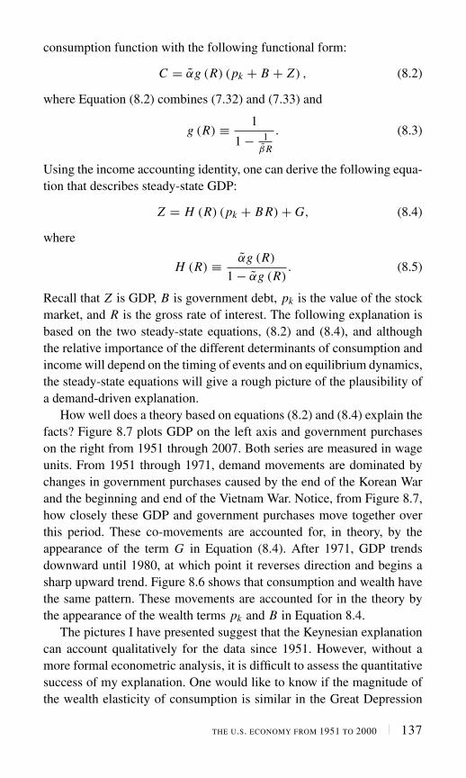
consumption function with the following functional form:

C = αg (R) (pk + B + Z) , (8.2)

where Equation (8.2) combines (7.32) and (7.33) and

g (R) ≡ 1

1 − 1β R

. (8.3)

Using the income accounting identity, one can derive the following equa-tion that describes steady-state GDP:

Z = H (R) (pk + B R) + G, (8.4)

where

H (R) ≡ αg (R)

1 − αg (R). (8.5)

Recall that Z is GDP, B is government debt, pk is the value of the stockmarket, and R is the gross rate of interest. The following explanation isbased on the two steady-state equations, (8.2) and (8.4), and althoughthe relative importance of the different determinants of consumption andincome will depend on the timing of events and on equilibrium dynamics,the steady-state equations will give a rough picture of the plausibility ofa demand-driven explanation.

How well does a theory based on equations (8.2) and (8.4) explain thefacts? Figure 8.7 plots GDP on the left axis and government purchaseson the right from 1951 through 2007. Both series are measured in wageunits. From 1951 through 1971, demand movements are dominated bychanges in government purchases caused by the end of the Korean Warand the beginning and end of the Vietnam War. Notice, from Figure 8.7,how closely these GDP and government purchases move together overthis period. These co-movements are accounted for, in theory, by theappearance of the term G in Equation (8.4). After 1971, GDP trendsdownward until 1980, at which point it reverses direction and begins asharp upward trend. Figure 8.6 shows that consumption and wealth havethe same pattern. These movements are accounted for in the theory bythe appearance of the wealth terms pk and B in Equation 8.4.

The pictures I have presented suggest that the Keynesian explanationcan account qualitatively for the data since 1951. However, without amore formal econometric analysis, it is difficult to assess the quantitativesuccess of my explanation. One would like to know if the magnitude ofthe wealth elasticity of consumption is similar in the Great Depression


1.48

1.52

1.56

1.60

1.64

1.68

1.72

1.76

.28

.30

.32

.34

.36

.38

.40

.42

55 60 65 70 75 80 85 90 95 00 05

GDP (Wage Units)

Government Purchases (Wage Units)

FIGURE 8.7 Government Purchases and GDP

and the postwar years. Is stock market wealth comparable in magnitudeto government debt? What is the importance of endogenous consumptiondynamics in helping to explain the facts? Can the addition of housingwealth add explanatory power, as the 2008 crisis in the market formortgage-backed securities suggests it might? These are all importantquestions that I will address in future empirical work.


Most recent studies of the postwar business cycle define the cycle as aseries of comovements between HP-filtered time series. The real businesscycle model, which explains the cycle as a set of optimal responses toan autocorrelated series of productivity shocks, is relatively successful atcapturing these comovements, and I have no doubt that this explanation isan important component of any successful theory of business cycles. Myobjection to the real business cycle approach is that the filtered data can-not explain movements at medium-term frequencies, which must insteadbe attributed to movements in “the natural rate of unemployment.” In thischapter, I have studied the plausibility of an alternative demand-driven


theory by examining the comovements of the components of aggregatedemand with movements in unemployment and GDP.

To summarize the argument: In my theory, aggregate demand hasthree main determinants: government purchases, government debt, andthe value of the stock market. In the period from 1951 to 1970, the majormovements in government purchases were driven by the requirements ofwartime financing. Those movements were responsible for a slowdownin the 1950s and a subsequent expansion in the 1960s. Superimposed onthe movements in government purchases, there was a decline in govern-ment debt from 1951 through 1979 that was subsequently reversed andfollowed by a period of increasing debt. As government debt increased,it fueled a consumption-led boom in economic activity as current gen-erations borrowed from future generations. A contributing factor to theboom of the 1980s and 1990s was a buildup of confidence, reflected ina huge stock market bubble. The bursting of this bubble led to the GreatRecession of 2008.


PART III

THE THEORY OF PRICES

THE MODELS I HAVE used so far have ignored money and uncertainty.In Part III, I introduce both of these elements. Chapter 9 brings

money into a stochastic version of the model from Chapter 6. Chapter 10continues the narrative account from Part II by describing the monetaryfeatures of the economy since 1951. These chapters provide a frameworkfor studying monetary policy in a dynamic stochastic environment, butthe analysis of the model is left for future work. Chapter 11 describesa new institution, as an alternative to fiscal policy, that provides analternative way of regulating excessive swings in the market economy.

CHAPTER 9 Money and Uncertainty

IN PART II, I EXPLAINED the economic history of the US since 1929using a model with no money that did not allow for uncertainty. In this

chapter, I bring in both money and uncertainty and I develop a modelthat can be used to understand how unemployment and inflation cancoexist.

To include money, I assume that it is a productive factor like laborand capital. To include uncertainty, I assume that there is a finite set ofstates in each period and agents are able to trade a complete set of Arrowsecurities.24


In Section 9.1, I introduce money by assuming that it acts as a productivefactor. This shortcut, first used by Patinkin (1956), has a distinguishedhistory in economics. It is meant to represent the benefit that accrues tothe firm from using cash in transactions.

9.1.1 MONEY AND PRODUCTION

I will assume the same production sector as in Chapter 6 with the excep-tion that each good is produced with money as well as with capital andlabor. As in that chapter, labor is hired in a competitive search marketand firms take the wage wt , the prices pi,t , for each good i, and the

hiring effectiveness of a recruiter qt as given. There are n commodities.Recall that in this structure each firm faces the production function

Yi,t = K aii,t Xbi

i,t mhii,t , (9.1)

and the labor market constraints

Li,t = Xi,t + Vi,t , (9.2)

Li,t = qt Vi,t , (9.3)

where

ai + bi + hi = 1. (9.4)

In Equation (9.1), I have modified the model of Chapter 6 by addingmoney,

mi,t = Mi,t

pi,t. (9.5)

mi,t represents the value of money balances measured in units of thefirm’s output price at date t . Money is held by the financial servicessector and “rented” to firms at rate it−1. Since the use of money at datet is negotiated at date t − 1, the relative price of date t money is thedate t − 1 interest rate, it−1. A slight modification to the argument fromChapter 6 gives the first-order conditions

bi pi,t Yi,t = wt Lt , (9.6)

ai pi,t Yi,t = rrt Ki,t , (9.7)

hi pi,t Yi,t = it−1 Mi,t , (9.8)

and aggregating across industries yields the aggregate supply curve,

χ Zt = wt Lt ; (9.9)

the definition of the rental rate,

ψ Zt = rrt ; (9.10)

and a new expression, which represents a demand function for money,

h Zt = it−1 Mt . (9.11)

The parameters χ and ψ are defined as in earlier chapters and h is definedin Equation (9.12):

h =∑

gi hi . (9.12)

144 THE THEORY OF PRICES

I will be studying policies in which the Fed controls the interest ratethrough open market operations. In this framework, the demand-for-money function, Equation (9.11), determines the money supply.

9.1.2 ADDING UNCERTAINTY

To introduce uncertainty I assume that in each period one of N uncertainstates may occur. The set of one-period states is S = {S1, . . . , SN }, anda realization of a state is called an event. A set of t events that occurssequentially is called a t-period history. The set of t-period histories, St ,

is defined recursively as follows:

S1 = S, (9.13)

St = St−1 × S, t = 2, . . . (9.14)

Because I want to highlight the effects of self-fulfilling beliefs, I assumethat all uncertainty is nonfundamental in the sense that it affects beliefsbut it does not affect preferences, technologies, or endowments. Theseare “sunspot shocks” in the sense of Cass and Shell (1983). This assump-tion can easily be modified to allow for fundamental shocks.

Agents are permitted to trade securities contingent on the states ofnature, and I assume agents trade a complete set of Arrow securities toinsure against uncertainty. Qs

t (Ssj ) denotes the price of a security that

pays one unit of money if and only if the history Ssj ∈ Ss occurs at date

s. Assets held by the representative household are given by the followingidentity:

At = (Bt + Mt ) (1 + it−1) + (pk,t + rrt

)Kt , (9.15)

where I assume

Kt = 1 (9.16)

as in previous chapters.Equation (9.15) decomposes household assets into three components:

government debt, money, and private capital. Each of these assets paysa return. One dollar of government debt or one dollar of money, issuedat date t − 1, pays 1 + it−1 units of money in date t in all states. In thecase of government debt, the interest is paid by government. In the caseof money, it is paid by firms who negotiate loans in period t − 1 for theuse of money in period t . Private capital pays the money rental rate rrt .

MONEY AND UNCERTAINTY 145

9.1.3 HOUSEHOLDS

The representative household maximizes expected utility and has log-arithmic preferences. Households trade financial assets in the form ofArrow securities At . Agents are assumed to maximize the function

Jt = Et

∞∑s=t

[βs−t

n∑i=1

gi log(Ci,s

)], (9.17)

subject to the sequence of constraints

ws Ls + TRs − Ts + As

=N∑

j=1

Qs+1s

(S j

)As+1

(S j

) +n∑

i=1

pi,sCi,s, s = t, . . . (9.18)

The expectations operator in Equation (9.17) is over realizations of allfuture state-contingent histories.

The labor market is identical to that described in earlier chapters. Eachhousehold sends a measure 1 of workers to look for jobs in each period.qs of these workers find jobs and earn money wage ws . pi,s is the priceand Ci,s is the quantity of goods i consumed at date s. TRs and Ts arelump-sum transfers and taxes. The no-Ponzi conditions must also hold ineach history:

limT →∞ QT

t

(ST

j

)AT +1

(ST

j

)≥ 0, for all ST

j ∈ ST . (9.19)

Together, Equations (9.18) and (9.19) imply the existence of a singlebudget constraint,

∞∑s=t

N st∑

j=1

Qst

(n∑

i=1

pi,s

(Ss

j

)Ci,s

(Ss

j

))≤ ht + At , (9.20)

where human wealth is defined recursively by the expression

ht = wt Lt + TRt − Tt +N∑

j=1

[Qt+1

t

(St+1

j

)ht+1

(St+1

j

)], (9.21)

plus the assumption that the net present value of after-tax labor incomeis finite, which places a limit on the set of feasible pricing kernels tothose for which the state-dependent prices do not grow “too fast”. Onemay derive the following closed form solution for the expenditure of the


household on good i :

pi,t Ci,t = (1 − β) gi [ht + At ] . (9.22)

Summing Equation (9.22) over all commodities yields

Ct = (1 − β) [ht + At ] , (9.23)

where

Ct =n∑

i=1

pi,t(S j

)Ci,t (9.24)

is the money value of consumption expenditure by the household.

9.1.4 GOVERNMENT

As in the previous chapters of this book, I model governmentmechanically. Here, that implies that government chooses sequences{TRt , Tt , Mt+1 + Bt+1} to satisfy the constraints

Bt+1 + Mt+1 = Bt (1 + it−1) + Mt + TRt − Tt . (9.25)

Equation (9.25) holds each period and constrains the joint behavior ofthe monetary and fiscal authorities. Bt+1 and Mt+1 represent one-periodbonds and money carried into period t + 1; it is the interest rate on aone-period bond issued at date t . The Fed chooses the mix of moneyand bonds in the hands of the public through open market operationswith the goal of attaining a nominal interest rate target. I set governmentpurchases to zero throughout.

I define the deficit for the consolidated government sector as

Dt = TRt − Tt − it−1 Mt . (9.26)

The deficit includes the revenues from money creation, sometimesreferred to as the inflation tax. I will assume that the deficit, defined inthis way, is an object of choice for the fiscal authority.

The budget equation can be simplified still further. Let BT representthe total outstanding nominal debt of the government sector:

BTt = Bt + Mt . (9.27)

Given this notation, one can express the government budget constraint as

BTt+1 = BT

t (1 + it−1) + Dt . (9.28)


Since I assume that government purchases are zero, it follows that

Zt = Ct , (9.29)

where Zt is the money value of GDP.

9.1.5 THE PRICING KERNEL AND ASSET PRICES

The first-order condition for the household can be used to derive anexpression for the Arrow security price Qt+1

t(S j

). From the state-by-

state first-order conditions, aggregated over commodities,

Qt+1t

(S j

)Ct+1

(S j

) = βCt p j , (9.30)

where p j is the probability that state S j occurs.The assumption that there is no riskless arbitrage implies the follow-

ing two relationships:

N∑j=1

Qt+1t

(S j

) = 1

1 + it, (9.31)

N∑j=1

Qt+1t

(S j

) [pk,t+1

(S j

) + rrt+1(S j

)pk,t

]= 1. (9.32)

Equation (9.31) is a no-arbitrage relationship between the safe returnon government debt and the prices of the N Arrow securities. Equation(9.32) is a no-arbitrage relationship between capital and Arrow securities.If either of these equations did not hold, an agent could buy or sell Arrowsecurities and make a profit with no associated risk.

If there were a single state, then these equations would imply

1 + it = pk,t+1 + rrt+1

pk,t, (9.33)

which states that the return on two riskless assets must be equal. Noticethat Equations (9.31) and (9.32) do not imply

1 + it = Et

[pk,t+1

(S j

) + rrt+1(S j

)pk,t

], (9.34)

since the Arrow security prices may be correlated with the stock price.


9.2 The Complete Model

I am now ready to describe a four-equation model that describes howGDP, the money supply, the value of employment, and the wage arerelated to the choice of the interest rate by the central bank. These fourequations are:

h Zt = it−1 Mt , (9.35)

E

[βZt

Zt+1

]= 1

1 + it, (9.36)

E

{βZt

Zt+1

[pk,t+1

(S j

) + ψ Zt+1(S j

)pk,t

]}= 1, (9.37)

χ Zt = wt Lt . (9.38)

Equation (9.35) is the demand-for-money equation. Equations (9.36)and (9.37) are asset pricing equations that combine (9.31), and (9.32)with the pricing kernel, Equation (9.30) and the accounting identity(9.29). Equation (9.38) is the aggregate supply equation. Solving Equa-tion (9.37) forward leads to the further simplification

Zt = (1 − β)

βψpk,t . (9.39)

Since there is a representative household, fiscal policy has no effect inthis model and the fiscal authority simply chooses the timing of lump-sum taxes.

This model looks deceptively simple, but it is capable of displayingvery rich nominal-real interactions. To close the model, we need toexplain how agents form beliefs about the money value of stock prices,that is, the sequence

{pk,t

}. In Chapter 10, I will explore the idea that

households form self-fulfilling beliefs about the real value of assets; thisassumption implies that the model is closed by an equation of the form

pk,t = wt xt , (9.40)

where {xt } is a sequence of beliefs. I will show that a model with thisstructure behaves a lot like the new-Keynesian model used by centralbanks throughout the world to guide monetary policy. It differs from thatmodel since I will allow self-fulfilling beliefs to determine unemploy-ment and GDP in the long run.



In the real models of Part II, movements in the real stock price causedmovements in the real value of consumption because the money wagewas chosen to equal 1. I assumed that the real stock price can be anybounded sequence. In the monetary model with uncertainty, I will assumeinstead that the sequence

{pk,t/wt

}is determined by self-fulfilling

beliefs.In Chapter 10, I will use this model to understand some of the mone-

tary features of data since 1951.


CHAPTER 10 Money and Inflation Since 1951

HOw CAN HIGH INFLATION and high unemployment coexist? In thefamiliar new-Keynesian account of monetary policy discussed, for

example by Richard Clarida, Jordi Galí, and Mark Gertler (2000) theFed pays attention to deviations of unemployment from its natural rate.In the old-Keynesian model, that I describe here, there is no naturalrate of unemployment and a drifting unemployment rate has big welfareconsequences.

When I began work on this chapter, in early drafts of the book, Ihad intended to develop the dynamic implications of the theory and tostudy dynamic equilibria similar to those analysized by new-Keynesianeconomists. But as the work developed, I realized that the dynamicbehavior of the old-Keynesian model is much richer than that of its new-Keynesian cousin. There is room for a new theory of expectations thatis consistent with rational choice but also displays the intertial behaviorthat we see in real-world data. I have chosen to report the steady-stateimplications of the model here and to save a more complete analysis ofthe dynamics for a future book.

The chapter begins, in Section 10.1, with a brief review of the model.Section 10.2 describes how changes in the money wage affect unemploy-ment. In Section 10.3, I review some features of the data and I showhow they are explained by the model. In Section 10.4, I lay out thelinearized old-Keynesian model, and in Section 10.5, I present a shortconclusion.

10.1 A Complete Monetary Model

The monetary model, introduced in chapter 9, is described by the follow-ing four equations:

Qt+1t = βZt

Zt+1, (10.1)

βEt

[Zt

Zt+1

]= 1

1 + it, (10.2)

Et

[βZt

Zt+1

(pk,t+1

(S j

) + ψ Zt+1(S j

)pk,t

)]= 1, (10.3)

χ Zt = wt Lt . (10.4)

To study its behavior, notice that Equation (10.3) can be solved itera-tively to give an expression for the value of nominal GDP as a functionof the value of the stock market:

Zt = pk,t(1 − β)

βψ. (10.5)

Using this expression, we may divide Equation (10.4) by pk,t to yield anequation linking employment to the value of the stock market measuredin wage units:

Lt = (1 − β) χ

βψ

pk,t

wt. (10.6)

One can also write GDP in wage units in this way:

Zt

wt= (1 − β)

ψβ

pk,t

wt. (10.7)

Finally, one can combine the solution for GDP from Equation (10.5)with the no-arbitrage condition, Equation (10.2), to yield an expressionlinking the growth rate of the asset price with the interest rate:

1

1 + it= βEt

[pk,t

pk,t+1

]. (10.8)

Since the central bank controls the money supply, it has the powerto set it through open market operations. For any given choice of theinterest rate, the implied value of the end-of-period money stock is givenby the money demand equation

h Zt = it−1 Mt . (10.9)


How does the model work? I have already demonstrated that, unlikethe neoclassical model, economic fundamentals are insufficient to deter-mine either employment or GDP measured in wage units. This isexpressed here by the fact that although equations (10.6) and (10.7) deter-mine both of these variables as functions of the real stock price pk,t/wt ,there is nothing in the economic structure of the model to pin this variabledown. In addition to this real indeterminacy, the model displays the samenominal indeterminacy that one finds in any monetary model. I discussthese issues further in Section 10.4. First, I will discuss the dependenceof aggregate supply on the money wage and the connection of the modelwith data.

10.2 Aggregate Supply and the Money Wage

How can unemployment and inflation coexist? This section gives ananswer to that question. The aggregate supply function, Equation (10.4),determines Zt as a function of wt and Lt . When wt = 1, all nominalmagnitudes are in wage units. For example, the statement that good icosts pi,t dollars means that one unit of labor can purchase pi,t units ofit. Scaling up the wage unit by choosing wt to be some value other than1 means that all money prices in the model must also be scaled up if thereal value of wealth is to remain unchanged.

In Chapter 6, I described a model that determines employment, moneyprices, and the quantities of each produced commodity as a functionof the state of long-term expectations. I modeled expectations as abounded sequence of self-fulfilling beliefs

{pk,t

}, where pk,t represents

the money value of the stock market at date t . If wt is different from 1,then these beliefs must also be scaled up or down by the money wage.If the money wage changes but beliefs about the money value of stocksdo not, this change in the nominal unit will alter the real variables of themodel.

Figure 10.1 illustrates how changes in the value of the nominal unitcan have an adverse effect on output and employment. The figure com-pares two steady states. In each of them, the money value of the stateof long-term expectations gives rise to a dollar price for stocks denotedpk . When household wealth is pk , households demand pk (1 − β) /βψ

dollars worth of goods and services. Since there is no government andno investment, aggregate consumption expenditure is equal to the moneyvalue of GDP.

MONEY AND INFLATION SINCE 1951 153

LL *1

1 − bZ pkβψ

=

w1LχZ =

L *2

Z w2Z = Lχ

FIGURE 10.1 Stagflation in the Keynesian Model

Consider the two steady states labeled{w1, L∗

1

}and

{w2, L∗

2

}on

Figure 10.1. In the first steady state, a unit of labor costs w1 dollars. Inthe second steady state, it costs w2 dollars where, by assumption, w2 isgreater than w1. Since the wage is higher in steady state 2, the same valueof aggregate demand will purchase fewer units of labor and there will belower employment in equilibrium. This analysis is suggestive of the phe-nomenon of stagflation, in which high unemployment and high inflationgo together. I use the word “suggestive” because Figure 10.1 comparestwo steady states, whereas stagflation is a dynamic phenomenon. Tocomplete the analysis, I will use the model developed in Section 10.1to study how a dynamic model of inflation and unemployment can beused to explain the data.

10.3 Theory and Data

Here, I will repeat the three main equations and discuss how to supple-ment them with a theory of beliefs. I then compare the ways that broadtrends in the data are explained by the model.


35

30

25

20

15

10

530 40 50 60 70 80 90 00

The S&P Deflated by the Real Wage (Logarithmic Scal

FIGURE 10.2 The Value of the Stock Market Since 1929

The three private sector equations are these:

Lt = (1 − β) χ

βψ

pk,t

wt, (10.10)

Zt

wt= (1 − β)

ψβ

pk,t

wt, (10.11)

1

1 + it= βEt

[pk,t

pk,t+1

]. (10.12)

I have argued that pk,t/wt is a driving force of aggregate demand.How does this variable behave? The value of the S&P, deflated by themoney wage, is depicted in Figure 10.2.

The data in this figure cover the period from 1929 through 2008. Thehypothesis that the S&P is nonstationary cannot be rejected at the 1%level, and to capture this property, I will assume that beliefs follow amartingale; that is, I will assume that

Et

[pk,t+1

wt+1

]= pk,t

wt. (10.13)


1,5001,000

500350250

150100

5035

20

10

5

12,0008,000

4,0002,8002,000

1,200800

400280

160

80

4030 40 50 60 70 80 90 00

S&P in Dollars (Logarithmic Units) (Left Scale)

Consumption in Dollars (Logarithmc Units) (Right Scale)

FIGURE 10.3 The Stock Market and Consumption

A second important equation in the model is (10.5), which I repeathere:

Zt = pk,t(1 − β)

βψ. (10.14)

This is the same equation that I derived in Chapter 6, in which I discussedthe Great Depression. In the model, Zt and Ct are equal since I abstractfrom investment and government purchases. In theory, it is Ct that isdetermined by pk,t , and for that reason, I have graphed the behaviorof Ct and pk,t in Figure 10.3. The log of the S&P is measured on theleft axis and the log of the dollar value of consumption on the right. IfEquation (10.14) holds, and if pk,t is a nonstationary variable driven bybeliefs, then the nominal value of consumption should be a nonstationaryvariable that is cointegrated with pk,t . Notice from the graph that thesetwo time series appear to grow together with a common stochastic trend,a hypothesis that is not rejected by formal tests.25

The model, of course, implies more than just cointegration betweenconsumption and the stock market—it implies that the variables areequal up to a scale factor. This strong implication is rejected as is clearfrom Figure 10.3. It would be surprising if it were not rejected since Ihave abstracted from many elements that are likely to be important inpractice. These abstractions include the representative agent assumption,the logarithmic preference assumption, the assumption that preferences


1.7

1.6

1.5

1.4

1.3

1.2

1.1 0.8

0.9

1.0

1.1

1.2

1.3

30 32 34 36 38 40 42 44 46 48 50

GDP (Wage Units)Private Consumption (Wage Units)

FIGURE 10.4 GDP and Consumption Before the Accord

are time separable, and the assumption that government purchases andinvestment are equal to zero. Any one of these factors might be respon-sible for providing richer dynamics to the model that would accountfor temporary deviations of consumption from the stock price. It wouldbe disturbing, however, if the cointegration property were to fail, sincethis should be independent of assumptions that generate richer short-rundynamics.

The absence of investment or government from the model impliesthat GDP equals consumption. This implication is clearly false, and amodel that assumed all important movements in aggregate demand weregenerated by movements in private consumption to understand the dataduring the wartime recovery would be badly off-base. The data for thisperiod are graphed in Figure 10.4.

On this figure, GDP is graphed on the left axis and private consump-tion on the right. Both series are measured in wage units. Notice fromthe figure that GDP and consumption move in opposite directions in the1940s. This should not be surprising since I argued in Chapter 7 thataggregate demand during WWII was driven by government purchases, avariable that is missing from the monetary model.

Figure 10.5 suggests that the approximation that demand is drivenby consumption fares much better in the period from 1951 to thepresent. The figure plots the same two variables that were graphed on


1.48

1.52

1.56

1.60

1.64

1.68

1.72

1.76

0.92

0.96

1.00

1.04

1.08

1.12

1.16

1.20

55 60 65 70 75 80 85 90 95 00 05

GDP (Wage Units)Private Consumption (Wage Units)

FIGURE 10.5 GDP and Consumption After the Accord

Figure 10.4 and illustrates that the important medium-term movementsin postwar GDP are reflected in the consumption series. Since con-sumption makes up approximately 70% of GDP, one might hope thata model in which aggregate demand is purely consumption driven will

1.48

1.52

1.56

1.60

1.64

1.68

1.72

1.76 3

4

5

6

7

8

9

1055 60 65 70 75 80 85 90 95 00 05

GDP (Wage Units)Unemployment Rate

FIGURE 10.6 GDP and Unemployment


capture the most important aspects of the data; this is borne out in thefigure.

A final feature that is central to the model is the equivalence of GDPmeasured in wage units and employment. In the model, equations (10.10)and (10.11) imply that employment is a multiple of GDP. Recall fromFigure 8.4, which is replicated as Figure 10.6, that unemployment andGDP are closely correlated. This figure plots unemployment on the rightscale measured from top to bottom and the real value of GDP per memberof the labor force on the left axis. The assumption that these variablesare equal does a very good job of explaining these data—the correlationcoefficient between GDP per member of the labor force measured inwage units and the unemployment rate is −0.88.

10.4 Modeling Monetary Policy

Central bankers and academics have been guided in their discussion ofmonetary policy for the past decade by the new-Keynesian model of amonetary economy. This is a three equation system of linear equationsin the interest rate, inflation, and GDP. My purpose in this section isto provide a similar model of an old-Keynesian economy and to drawattention to the differences between these two models. It is my hopethat this old-Keynesian monetary model may prove as useful as its new-Keynesian prodecessor in providing a simple tool to help guide policy,and I plan to study its implications further in future work.

10.4.1 THE PRIVATE SECTOR EQUATIONSRESTATED

Recall that the three private sector equations are given by

Lt = (1 − β) χ

βψ

pk,t

wt, (10.15)

Zt

wt= (1 − β)

ψβ

pk,t

wt, (10.16)

1

1 + it= βEt

[pk,t

pk,t+1

]. (10.17)


In addition, I have argued that the data are consistent with the assumptionthat the stock price is a martingale:

pk,t

wt= Et

[pk,t+1

wt+1

]. (10.18)

10.4.2 THE POLICY RULE

To model monetary policy, I assume that the interest rate is set inresponse to changes in inflation and real economic activity:

(1 + it ) = C1

[wt

wt−1

]η [pk,t

wt

]λ

. (10.19)

I refer to this expression interchangeably as a central bank reactionfunction or a Taylor rule, after the work of John Taylor (1993). Usually,a Taylor rule is represented in terms of the response of the interest rateto deviations of inflation and the output gap from some set of predefinedtargets. Since these targets are not separately identified without makingadditional assumptions, I have collapsed them into the constant C1.

In typical representations of the Taylor rule, the Fed responds to priceinflation and the output gap. In Equation (10.19), in contrast, it reacts towage inflation and the real stock price. These are appropriate variablesto use in the context of the model and they allow me draw conclusions ina relatively simple framework. I use wage inflation rather than a priceindex because this is the natural model-based concept of a nominalanchor. I use the real stock price instead of output since, in the model,these variables are equal up to a constant. The Taylor rule also typicallycontains a term in the lagged interest rate to represent slow adjustment ofthe policy toward the Fed’s target rate. Adding a term of this kind wouldenrich the dynamics of the model but would not affect the basic messageof the chapter. Therefore I have excluded it.

The parameter η in Equation (10.19) represents how strongly the Fedreacts to inflation. The parameter λ measures how strongly the Fed reactsto changes in the level of economic activity. In the following section, Ilay out a linearized version of this system.

10.4.3 A LINEAR APPROXIMATION

The model can be described by the following log linear representationof equations (10.15) through (10.19). A tilde over a variable denotesthe natural logarithm, and b1, b2, b3, and b4 are linearization constants.


Consider first equations (10.20) through (10.22), which are approxima-tions to (10.17) through (10.19):

it = b1 + Et[� pk,t+1

], (10.20)

pk,t − wt = Et[

pk,t+1 − wt+1], (10.21)

it = b2 + η (�wt ) + λ(

pk,t − wt). (10.22)

� is the first difference operator. These equations represent an indepen-dent subsystem that determines the time paths of it , pk,t , and wt . Givenvalues for the stock price and the money wage, the variables L t and Zt

are determined by equations (10.23) and (10.24):

L t = pk,t − wt + b3, (10.23)

Zt − wt = b4 + pk,t − wt . (10.24)

Solving equations (10.20) through (10.22) for steady-state wage infla-tion, steady-state stock market appreciation, the steady-state T -bill rate,and the steady-state real value of the stock market leads to only threeequations in four unknowns:

i = b1 + � pk,t , (10.25)

� pk,t = �wt , (10.26)

i = b2 + η�wt + λ(

pk,t − wt). (10.27)

This apparent indeterminacy of the model is a consequence of theunderlying real structure of the economy in which the level of realeconomic activity is determined by the state of long-term expectations.Beliefs are represented by a self-fulfilling expectation that the stockmarket will be worth some amount, x ; adding this belief equation closesthe system:

pk,t − wt = x . (10.28)

10.5 How Beliefs Influence the Unemployment

Rate

This section studies the interaction of real and monetary variables inthe steady state. My analysis differs from the standard new-Keynesianmonetary model in a respect: In the critical old-Keynesian model there


are multiple steady-state equilibria and beliefs influence the steady-stateunemployment rate.

10.5.1 THE STEADY STATE

The variable x represents the value of the stock market in wage units.Given x , equations (10.25) through (10.27) can be solved for the steady-state inflation rate, which is given by the following expression:

�w = b2 − b1

1 − η+ λ

1 − ηx . (10.29)

Equation (10.25) then determines the interest rate and (10.26) determinesthe rate of change of the stock price.

The steady-state equations are instructive, and contain an importantmessage. The correlations in the data between inflation and real eco-nomic activity should not be independent of the way that the centralbank conducts monetary policy. For example, suppose that the centralbank chooses a monetary policy for which 0 < η < 1. When x increases,unemployment will fall since x represents the real value of the stock mar-ket and increases in stock market wealth will increase aggregate demandand lower unemployment. Given this relationship between x and unem-ployment, Equation (10.29) implies that we should observe a Phillipscurve (a relationship between unemployment and wage inflation) with anegative slope. If investors become more optimistic (an increase in x),Equation (10.23) implies that employment will increase (unemploymentwill fall) and Equation (10.29) implies that this fall in unemployment willbe associated with an increase in inflation. If on the other hand, η > 1,the steady state Phillips curve will have the opposite slope.

10.5.2 ACTIVE AND PASSIVE MONETARY POLICY

In addition to the real steady-state indeterminacy discussed previously,this model also displays a dynamic indeterminacy for certain kinds of Fedpolicies. I will discuss this idea further in this section and I will presentan argument, due to Clarida and colleagues (2000), who claimed in thecontext of the new-Keynesian model of monetary policy that the Fedbrought inflation under control by enacting a more aggressive monetarypolicy after 1980 than before. Following Eric Leeper (1991), a policyin which 0 < η < 1 is called passive and one in which η > 1 is calledactive. A considerable amount of evidence in recent years has pointed


1.16

1.14

1.12

1.10

1.08

1.06

1.04

1.02

1.00

10

9

8

7

6

5

4

31960 1970 1980 1990 2000

Gross Treasury Bill Rate (Left Scale)Unemployment Rate (Right Scale)Wage Inflation - Left Scale

FIGURE 10.7 Unemployment, Inflation, and the Interest Rate

to the fact that U.S. monetary policy was passive before 1980 and activethereafter. This evidence is illustrated by figures 10.7 and 10.8.

Figure 10.7 displays the behavior of wage inflation, the interest rate,and inflation from 1951 through 2007. Notice that all three variablestrend upward from 1951 through 1979 and that, beginning in 1980, theytrend down. According to a leading explanation of these data, due toClarida and colleagues (2000) the turnaround in these trends occurredbecause the Fed switched policies in 1980 when Paul Volcker becamechairman.

Figure 10.8 is a scatter plot of the gross interest rate on Treasury billsagainst the gross rate of wage inflation for the period from 1951 through2007. On this figure, the data for the period from 1951 through 1979are plotted as open circles, and the data for 1980 throught 2007 appearas shaded squares. For each subperiod, I have drawn the least squaresline through the points. The best line through the first subperiod hasa slope of 0.78, while the best line through the second subperiod hasa slope of 1.35. These numbers have been interpreted in the literatureon new-Keynesian economics as estimates of η, the slope of the policyrule. Although least squares is likely to provide a biased estimate of η,alternative estimates of η using instrumental variables by Clarida andcolleagues (2000) and using Bayesian techniques in a complete model by


1.00

1.02

1.04

1.06

1.08

1.10

1.12

1.14

1.16

1.02 1.04 1.06 1.08 1.10Wage Inflation

Tre

asur

y B

ill R

ate

Slope = 1.35

(1980 – 2006)

Slope = 0.78

(1951 – 1979)

FIGURE 10.8 The Interest Rate and Wage Inflation

Lubik and Schorfheide (2004) have established similar results. Monetatypolicy was passive before 1980 and active thereafter.

In the new-Keynesian model studied by Clarida and colleagues(2000), a passive monetary policy leads to dynamic indeterminacy. Inthat model, there is a unique natural unemployment rate. The actualunemployment rate may deviate temporarily from its natural rate becauseprices are sticky. Clarida and colleagues show that an active monetarypolicy is sufficient under some additional assumptions to ensure that thepath back to full employment, following a shock, is unique. If monetarypolicy is passive, in contrast, there are many possible dynamic pathsleading back to full employment.

The model described in this book also displays dynamic indetermi-nacy for some kinds of monetary policy. This dynamic indeteminacy isin addition to the steady-state indeterminacy that follows from the labormarket search externality described in Part I.


This chapter integrated monetary theory into a representative agentmodel with Keynesian unemployment. The resulting model has a contin-uum of real equilibria, indexed by beliefs, but each of them is consistent


with any steady-state equilibrium rate of inflation. I refer to this model asold-Keynesian, to distinguish it from the new-Keynesian model, widelyused by central bankers and academics to study monetary policy. Whatdoes the job of the Fed look like in the old-Keynesian world?

From the viewpoint of a monetary authority, armed with the tool ofinterest rate control, the old-Keynesian model described in this chapter isvery similar to the new-Keynesian model that has been popular recentlyamong academics and central bankers. The difference is that in the new-Keynesian model permanent shocks to the unemployment rate are viewedas changes in the natural rate of unemployment that do not carry welfareimplications.

In the new-Keynesian world, there is nothing demand managementpolicy can or should do about increases in the natural rate. In the old-Keynesian world, there is nothing natural about any given unemploymentrate and if unemployment moves above or below the social optimum,demand management policy can and should try to move it back. The factthat movements in the unemployment rate are a bad thing that shouldbe prevented does not mean, however, that monetary policy, operatingthrough interest rate control, is the best tool for the job. Interest ratepolicy has been used to alleviate recessions. But it also affects inflation.The following chapter suggests an alternative tool of monetary policythat may be used to separate these two goals.


CHAPTER 11 How to Fix the Economy

IN THIS BOOK, I have contrasted two competing visions of the macroe-conomy. In the first, an unregulated capitalist economy converges

quickly to a social optimum. In the second, an unregulated capitalisteconomy can lead to very bad outcomes that persist for decades. Thisbook has argued that the second view is a more accurate description ofthe world. Although capitalism has much to recommend it, we do notlive in an unregulated economy and we have not done so since the turnof the nineteenth century. Modern political institutions are designed toimprove human welfare by moderating the swings of business cycles.Modern economic theory cannot explain why this is worth doing sinceboth classical and new-Keynesian explanations of the business cycleimply that the welfare costs of recessions are trivial.

This book has brought Keynesian theory into the twenty-first centuryby integrating it with general equilibrium theory in a new way andby providing microfoundations to the Keynesian theories of aggregatesupply and aggregate demand. My explanation is neither classical nornew-Keynesian. It is old-Keynesian. By grounding Keynes’s theory ofaggregate supply in the theory of labor market search, I am able toexplain why the money wage does not fall to restore employment to itssocially optimal level. By grounding aggregate demand in the theory ofdynamic choice under uncertainty, I am able to explain the economichistory of the twentieth century in a new way.

Keynesian economics provides two remedies to unemployment: mon-etary and fiscal policy. Since the money interest rate was already close

to zero in the 1930s, it was not possible to lower the interest rate fur-ther to increase aggregate demand. Hence, Keynes favored fiscal pol-icy, and his theory of the multiplier explained how this would work.The theory developed here explains why fiscal policy was effective. Inthis chapter, I will argue that although expansionary fiscal policy canrestore full employment, there is a more effective way to maintain fullemployment that does not burden future generations with governmentdebt.

Let me be clear about the premise that underlies the arguments I willmake. In a view shared by many academics at the very best universitiesand research institutes in the world, business fluctuations are efficientresponses of the market system to random shocks to fundamentals. In asecond view that I have put forward in this book, business fluctuations areinefficient reallocations of labor between market and nonmarket activi-ties that arise from the unpredictable movements of market psychology.If the first view is correct, there is no role for government policy and theproper response of government is to leave well alone. If the second viewis correct, government should act to maintain full employment and thecentral bank should promote a stable value for the currency. It will beclear by now that I favor the second view. However, I have misgivingsabout current approaches to the problem of maintaining full employmentthat I explain here.

11.1 Monetary Policy Cannot Hit Two Targets

In some currency areas (for example, Europe), the central bank is chargedsolely with maintaining a stable value for the currency. In others (forexample, the United States), the central bank is charged both with main-taining the value of the currency and with preventing recessions. Thesetwo goals may sometimes conflict.

Central banks throughout the world have, for the past fifteen years,been guided by new-Keynesian economics. This doctrine was developedfrom ideas of Paul Samuelson who, in the third edition of his textbook(1955), introduced the neoclassical synthesis. In Samuelson’s scheme,the economy converges, in the long run, to a full employment equilib-rium. It may deviate from full employment in the short run because pricesare slow to adjust. The new-Keynesians adopted this idea and developedit further. In new-Keynesian economics, there may be a short-run rolefor monetary policy to stimulate employment, but in the long run,


monetary policy cannot influence the natural rate of unemployment. Itis for this reason that the European Central Bank has been given themandate to control inflation but not to intervene to influence the levelof economic activity. It is widely believed that central banks cannotinfluence unemployment in the long run, and some have argued that theattempt to influence it in the short run will lead to a policy that unleashesinflationary pressures and is counterproductive.

The conflicting goals of monetary policy are apparent as I write. In2008, there was a large fall in U.S. household wealth triggered by adrop in the price of houses. This fall in wealth was transferred through-out the world through a newly developed market for mortgage-backedsecurities that allowed assets, backed by the U.S. housing market, to bepurchased by financial institutions throughout the globe. As the pricesof U.S. houses collapsed, these assets lost value and global demand forgoods and services fell. At the same time, world markets experiencedunprecedented increases in raw materials prices that were fueled by thegrowth of China and India. A scenario is being repeated that we last sawin the 1970s. A series of cost shocks that are putting upward pressureon domestic prices have coincided with a fall in asset prices that havereduced consumer demand.

The fallout from the housing crisis is global, but it has been addresseddifferently in Europe and the United States. In the U.S., the Fedresponded by lowering the interest rate in an attempt to stimulatedemand. The Bank of England and the European Central Bank took amore aggressive stance against inflation, and interest rates in Europe andthe United Kingdom came down more slowly. Central bankers there wereinitially more concerned with the long-term consequences of allowinginflation to build. The contradictory responses to similar events illustratesthe trade off between conflicting goals of monetary policy. A singleinstrument, the interest rate, cannot be used to hit two targets.

11.2 Fiscal Policy Is Not the Most Effective

Solution

During the Great Depression, Keynes argued that the government shouldpurchase goods and services and pay for its increased expenditure byborrowing from households. This policy was designed to increase aggre-gate demand. Expansionary fiscal policy was successful at increasing

HOW TO FIX THE ECONOMY 169

employment during World War II, but the huge increase in governmentpurchases that occurred to finance the war was accompanied by a bigpermanent increase in the scale of government.

Fiscal policy may be effective at increasing employment, but it is notthe best response to a recession for two reasons. In the textbook viewof Keynesian economics (Samuelson, 1955), a fiscal expansion involvessome combination of a cut in taxes, an increase in government purchases,and an increase in transfers to individuals. The most effective package isone in which a tax cut is accompanied by an increase in governmentpurchases. A policy of this kind will increase aggregate demand bymore than a transfer to individuals since, in textbook Keynesianism,households will save part of the transfer whereas government spendsit all. But there are also disadvantages to an increase in governmentpurchases, since most individuals would prefer to choose how to spendtheir income rather than have it spent for them. I do not deny that thereis a role for government to provide public goods—defense and the legalsystem are good examples—but the percentage of GDP that a societydevotes to government activities should not be changed in arbitrary waysto stimulate the economy during recessions.

This leaves transfers to the public, financed by borrowing, as a possi-ble remedy. In the housing crisis of 2008, the U.S. government enacteda tax rebate that returned checks of between $600 and $1,200 to mostfamilies. This policy may have helped to delay the onset of a recessionin the U.S., but it was at the cost of increasing the national debt. Sincegovernment debt is the liability of future generations, a transfer policyof this kind can only be effective by redistributing resources from onegeneration to another. This was the message of chapters 6 and 7, in whichI showed how the wartime recovery could be explained by a model thatrecognizes that debt is a transfer between generations. In the extremecase in which households fully discount future tax liabilities, a tax rebateof this kind can have no effect on aggregate employment.

Let me recap the two strikes against fiscal policy as a weapon to com-bat recessions. First, even if one accepts the mechanics that Samuelsonexplained in his interpretation of Keynes, and even if the governmentcan increase employment, the resulting equilibrium will be second bestsince the choices of consumers have been replaced by those of thestate. Second, for a given state of long-term expectations, governmentintervention through increased expenditure may get only partway backto full employment. The effectiveness of the intervention depends onthe ability to make transfers between different groups. As I write this


book, we are about to enter a recession at a time when the public purseis stretched to pay for a war in the Middle East. Additional government,debt will place a costly burden on future generations who are alreadyfacing significant costs as the baby boom generation ages and tax rev-enues from the working population begin to shrink. Perhaps we can dobetter than this?

11.3 What We Should Do Instead

I am going to present a different idea; I will argue that government shouldexpand the role of the Fed. Currently, the Central Bank meets eight timesa year and at each meeting the open market committee decides on a targetat which to set the interest rate on federal funds. To achieve any giventarget, the Federal Reserve Bank of New York is charged with the taskof buying or selling securities on the open market to raise or lower theinterest rate. Historically, open market operations have been conductedby buying or selling treasury bills. In January 2008, the Fed’s assets wereapproximately $850 billion, which was roughly 7% of GDP, and untilthe summer of 2008, almost all of these assets were held as high-gradegovernment securities. In the credit crisis of 2008, the Fed expandedcredit to a number of institutions by accepting lower grade securities ascollateral, and by September 2008, about a third of the Fed’s portfoliowas of this form. Why did it follow this policy?

From 2004 through July 2007, the Fed was more concerned aboutinflation than about a recession, and during this period the federal fundsrate increased from 1% in May 2004 to 5.25% in July 2007. In August2007, the Fed began a series of rate cuts, and by May 2008, the federalfunds rate was down to 2%. During this period, the Fed expanded creditthrough open market operations by approximately $30 billion and it cutthe federal funds rate by 325 basis points. By spring 2009, these policieshad resulted in a doubling of the stock of high-powered money from $850billion to $1.8 trillion.

In normal times, changes in the federal funds rate cause similarmovements in a whole spectrum of rates of return. If the Fed is willingto pay less on overnight loans, then lower grade securities also pay lessand the spread between assets of different grades remains approximatelyconstant. But in depressions, the spread on different assets widens.This happened in the Great Depression and it happened again in 2008.Although the Fed aggressively lowered the federal funds rate, the interest


rate on securities backed by subprime mortgages continued to fall in priceand institutions that held large portfolios of these assets were unable totrade them. As the Fed increased liquidity in the markets, the price ofsecurities backed by subprime mortgages did not respond. Instead, thespread between AAA bonds and mortgage-backed securities remainedhigh. The Fed was faced with the possibility of the collapse of one ormore major financial institutions and to prevent this from occurring, itbegan to accept lower grade securities as collateral for Federal Reserveloans.

The fraction of Federal Reserve assets backed by high-grade govern-ment securities has been 90% or greater since at least 1996, but by July2008, it had fallen to 50%. The decision to begin buying lower gradesecurities was a bold new move by the Bernanke Fed. Economists oftentalk as if there was a single interest rate. In practice, there is a wholespectrum of assets, each of which pays a different rate of return. Byagreeing to hold a portfolio of different securities, the Fed embarked ona path in which it can potentially control not just one rate of return, butseveral. This is a logical development of the role of the central bank andit is a path that leads to an expanded role for the Fed as a guarantor notjust of the value of the currency but also of the unemployment rate. I willexplain what I mean by this in the following section.

11.4 A New Role for the Fed

In the late 1990s, the public lost confidence in the value of stocks, buthousing wealth appreciated. The 2008 recession is different becausehouseholds lost confidence in stocks and houses simultaneously. Thedestruction of household wealth had a disastrous effect on aggregatedemand. What can we do about it? We need to support the value ofwealth through direct intervention in the asset markets.

One way of achieving this goal is for the Fed to vary not just the sizebut also the composition of its balance sheet. Under my proposal, theFed would define a basket of securities; ideally, this would include allpublicly traded stocks weighted by market capitalization. The exact com-position of the basket is not important. What matters is that it is knownand fixed. Just as the Fed controls the price of overnight borrowing bybuying and selling government debt in the open market, the Fed wouldstand ready to buy and sell shares in index funds.


The Fed open market committee meets eight times a year to decidethe interest rate on federal funds. In addition to setting the interest rate,the open market committee would announce a price at which it wouldstand willing to buy or sell shares of the index fund and a rate of growthat which this price would increase daily over the next month.

Initially, the Fed would encourage private companies such as Van-guard or Fidelity to create index funds and it would buy an initial blockof shares at market prices. To pay for these shares, it would issue its ownfixed interest liabilities that would be directly guaranteed by the Treasury.The open market committee would act to maintain the real value of thefund price within a set of bounds to prevent bubbles and stop marketcrashes. It would not have the mandate to intervene by buying and sellingindividual corporations—only the index fund.

How big would the purchase of shares need to be? In theory, the merestatement that the government stands ready to buy and sell at a fixed priceshould be enough to stabilize the markets. In practice, the balance sheetof the Fed was about $850 billion at the end of 2008 and an increaseof a further $850 billion seems about right. This increase would notaffect the money supply since it would be paid for by issuing debt. Tosupport the markets in time of panics, the Fed would have the abilityto buy additional shares on the open market. To dampen the marketduring bubbles, it would be able to sell back its own portfolio or, ifthat were to prove insufficient, it could design a financial instrument thatpays the same return as the index fund and sell this instrument on themarket.

Since the return to stocks has historically outpaced government debtby 5 percentage points, the Fed might make a sizeable profit for thegovernment. I think this is unlikely. A more plausible scenario is that,when the extreme swings of market volatility become part of the his-tory of capitalism, the returns to debt and equity will move closertogether and the equity premium will be eliminated or considerablyreduced.

Coming from a classical perspective, the proposal sounds irrespon-sible at best. Surely the market will go wherever it wants to go to findthe correct fundamental value of underlying assets. I do not believe thatthis is the correct theory of stock market value, and the extreme swingsin volatility that we observe in market valuation are not, in my view,reflections of changes in a unique underlying fundamental valuation.They are caused by self-fulfilling swings in confidence.


The plan I have advocated does not make sense in a classical environ-ment with a unique natural rate of unemployment and a self-stabilizingmarket system. But that is not the world in which we live. I believeinstead that there are many possible equilibrium unemployment ratesand the one we end up with is determined by demand. By placing afloor and a ceiling on the value of swings in stock market valuation,the Fed will nudge the market back toward a valuation that maintains amore stable growth rate for private wealth. By stabilizing wealth, the Fedwill maintain a predictable environment for private investors to createjobs and a stable environment for households to plan for the future. Mygoal is to preserve capitalism as an engine of growth without stiflingentrepreneurship.


When I began writing this book in 2005, the arguments were academic. Ihad long felt that the new-Keynesians misrepresented the main messageof The General Theory. It was my intention to recast this message in thelanguage of modern equilibrium economics. At the outset, I thought thatI was rescuing Keynesian economics. As the work progressed, I realizedthat Keynesian economics was not only misinterpreted but, in places, itwas simply wrong. One example is Keynes’s theory of prices that wasat best poorly developed. A second was his theory of the labor marketthat was nonexistent in the sense that we understand what is meant by agood theory in modern economics. When I began to construct a theorythat is consistent with the message of The General Theory, it becameapparent that the Keynesian remedy of fiscal deficits can be improvedupon.

In the fall of 2008, a work that began as purely academic quicklytook on an urgency and I discovered a new purpose that goes wellbeyond my original intention. In September 2008, financial institutionsthroughout the world began to fail, and by some accounts the capitalizedvalue of world stock markets fell by 50% in the space of six weeks.This crisis led economists, journalists, politicians, and commentators tosearch for new explanations. Some observers are returning to Keynesianeconomics: Others are searching for classical explanations. The newsmedia is full of talking heads with plausible explanations for the crisisand what to do about it, but none of the existing accounts providesa plausible explanation for why capitalist economies usually function


smoothly but at times can go spectacularly wrong. There are stories—but none that holds water as an account of the specific market failurethat justifies when and how there is a role for government interven-tion. In this book, I have given an account of the functioning of themarket system that explains what this market failure is and how tocorrect it.


NOTES

1. Galí, Gertler, and Salido (2007, p. 56) find that the average welfare costsof business fluctuations in a new-Keynesian model are approximately 0.01% ofsteady-state consumption, a number that is consistent with that cited by Lucas(1987, Chapter IV) in the context of the real business cycle model.

2. There appears to be a long history of misattributions of this quote. Inprivate correspondence, Riccardo DiCecio made the following observation: Mycolleague Ed Nelson pointed out to me that the phrase “We are all Keynesiansnow” attributed to Pres. Nixon is from Milton Friedman and is incomplete.Nixon said, “I’m now a Keynesian in economics,” according to journalistHoward K. Smith. Friedman, in an interview with Time, said, “In one sense, weare all Keynesians now; in another, no one is a Keynesian any longer.” However,Time magazine only quoted, “We are all Keynesians now.”

3. Keth Carlson and Roger Spencer (1975) have an early comprehensivediscussion of the crowding-out debate.

4. I am not the first to suggest that medium-term movements might beimportant features of the business cycle. In a recent article in the American Eco-nomic Review, Diego Comin and Mark Gertler (2006) have drawn attention topostwar medium-term fluctuations that they attribute to endogenous productivitymovements.

5. q is closely related to labor market tightness, which Mortensen andPissarides (1994) define to be the ratio of vacancies to unemployment.

6. In a dynamic model, employment will appear as a state variable in aprogramming problem since it takes time to recruit new workers. In this book, Iabstract from this aspect of labor market dynamics.

7. The main reason why unemployment is so high in the planning optimumis my assumption that labor is fired and rehired every period.

8. This is actually two figures superimposed since I am measuring bothmonetary and real units on the vertical axis. The function Z = φ(L) has unitsof dollars and the function Y = ψ(L) is in units of commodities.

9. It is for precisely this reason that Keynes called his book The GeneralTheory. He viewed the Walrasian equilibrium as one of many possible rest pointsof the system.

10. A version of this chapter appeared in the International Journal of Eco-nomic Theory (2008a) and is reprinted here with permission.

11. The fact that L∗ is equal to 1/2 follows from the assumption that theelasticity of the matching function is 0.5.

12. The quote is from Through the Looking Glass: And What Alice FoundThere", by Lewis Carroll, Chapter 6. I am indebted to Riccardo DiCecio forcorrecting a misattribution of this quote in an earlier draft of this manuscript.

13. I will abstract here from the bequest motive for saving. Adding bequestswill not change the main message of the book provided bequests are givenbecause the giver obtains direct utility from the size of the gift.

14. I have called this full employment in line with the language of The GeneralTheory although the model introduced here admits of overemployment as wellas underemployment.

15. Hodrick and Prescott. (1997).16. A second objection to the use of filtered data is one that is often raised

by those who favor a traditional econometric approach to the analysis of timeseries data. Since the filter is two sided, it is not consistent to assume thatfiltered data can be modeled “as if” it were chosen by a forward-looking rationalagent operating in a world with no trend in productivity. Despite this objection,a number of influential papers do use HP-filtered data in this way.

17. This is a nonstandard definition since wealth would normally be definedas the net present value of the labor endowment. Here it is the net present valueof labor income.

18. In her Ph.D. thesis, Amy Brown (2010, expected) shows that for the samematching function used here, the socially efficient unemployment rate can be aslow as 3% if all workers are not fired and rehired every period.

19. Carlson and Spencer (1975).20. The interest rate, in this model, must be non-negative and, since the growth

rate is zero, this condition rules out dynamic inefficiency of the kind that isknown to occur in overlapping generations models under some conditions. SeeKarl Shell (1971).

21. There is no presumption that the economy was at the social planningoptimum in 1929. I have nevertheless chosen this starting point for illustrativepurposes.

178 NOTES TO PAGES 22–119

22. Marianne Baxter and Robert G. King (1999) compare the band-pass filterto alternative detrending methods.

23. The government debt series has units of pure numbers and the deflatedS&P series has units of inverse dollars dated at the inception year of the index.The contribution of the S&P to aggregate wealth depends on this dollar valuethat is unknown, and hence the level of the series reported in Figure 8.6 is notdirectly comparable to the level of the debt series, although the movements inthe two series, can be directly compared.

24. This part of the model draws on a recent working paper with CarineNourry and Alain Venditti (2009) from the Groupement de Recherche enÉconomie Quantitative d’Aix-Marseille (GREQAM), in which we developeda stochastic model of long-lived agents. Farmer, Nourry, and Venditti (2009).

25. One cannot reject the hypothesis that each series is nonstationary. Further,one cannot reject the hypothesis that they are cointegrated at the 5% level usinga Johansen cointegration test and imposing the assumption of no deterministictrend.

NOTES TO PAGES 129–156 179

BIBLIOGRAPHY

Azariadis, C. (1981): “Self-Fulfilling Prophecies,” Journal of Economic Theory,25, 380–396.

Barro, R. J. (1974): “Are Government Bonds Net Wealth?” Journal of PoliticalEconomy, 82(6), 1095–1117.

Barro, R. J., and H. Grossman (1971): “A General Disequilibrium Model ofIncome and Employment,” American Economic Review, 61, 82–93.

Baxter, M., and R. G. King (1999): “Measuring Business Cycles: ApproximateBand-Pass Filters for Economic Time Series,” Review of Economics andStatistics, 81(November), 575–593.

Benassy, J. P. (1975): “Neo-Keynesian Disequilibrium Theory in a MonetaryEconomy,” Review of Economic Studies, 42, 503–523.

Benhabib, J., and R. E. A. Farmer (1994): “Indeterminacy and IncreasingRetums,” Journal of Economic Theory, 63(1), 19–41.

Beyer, A., and R. E. A. Farmer (2007), “Natural Rate Doubts,” Journal ofEconomic Dynamics and Control, 31, 797–825.

Blanchard, O. J. (1985): “Debts, Deficits, and Finite Horizons,” Journal ofPolitical Economy, 93(April), 223–247.

Brown, A. (2010, expected): “Three Essays in Macroeconomics” (Workingtitle), Ph.D. thesis, UCLA.

Carlson, K. M., and R. W. Spencer (1975): “Crowding Out and Its Critics,”Federal Reserve Bank of St. Louis, December, 2–16.

Cass, D., and Karl Shell (1983): “Do Sunspots Matter,” Journal of PoliticalEconomy, 91, 193–227.

Clarida, R., J. Galí, and M. Gertler (2000): “Monetary Policy Rules andMacroeconomic Stability: Evidence and Some Theory,” Quarterly Journalof Economics, 115(1), 147–180.

Clower, R. W. (1965): “The Keynesian Counterrevolution: A TheoreticalAppraisal,” in The Theory of Interest Rates, ed. by F. Hahn and F. Brechling.McMillan, London.

Cole, H. L., and L. E. Ohanian (2004): “New Deal Policies and the Persistenceof the Great Depression: A General Equilibrium Analysis,” Journal of Polit-ical Economy, 112(4), 779–816.

Comin, D., and M. Gertler (2006): “Medium Term Business Cycles,” AmericanEconomic Review, 96(3), 523–551.

Diamond, P. A. (1982): “Aggregate Demand Management in Search Equilib-rium,” Journal of Political Economy, 90, 881–894.

(1984): “Money in Search Equilibrium,” Econometrica, 52, 1–20.Dreze, J. H. (1975): “Existence of an Exchange Economy with Price Rigidities,”

International Economic Review, 16, 310–320.Evans, G. W., and S. Honkapohja (2001): Learning and Expectations in

Macroeconomics. Princeton University Press, Princeton.Farmer, R. E. A. (1984): “A New Theory of Aggregate Supply,” American

Economic Review, 74(5), 920–929.(1991): “Sticky Prices,” Economic Journal, 101(409), 1369–1379.(1999): The Macroeconomics of Self-Fulfilling Prophecies. MIT Press,

Cambridge, MA, second edn.(2002): “Fiscal Policy. Equity Premia and Heterogeneous Agents,”

UCLA mimeo, May.(2008a): “Aggregate Demand and Supply,” International Journal of

Economic Theory, 4(1), 77–94.(2008b): “Old Keynesian Economics,” in Macroeconomics in the Small

and the Large, Roger E. A. Farmer ed., Edward Elgar, London.Farmer, R. E. A., and J. T. Guo (1994): “Real Business Cycles and the Animal

Spirits Hypothesis,” Journal of Economic Theory, 63(1), 42–72.(1995): “The Econometrics of Indeterminacy,” The Carnegie Rochester

Conference Series on Public Policy, 43, 225–272.Farmer, R.E.A., C. Nourry and A. Venditti (2009): “Debt Deficits and Finite

Horizons, the Stochastic Case”, NBER WP15025.Friedman, M. (1948): “A Monetary and Fiscal Framework for Economic Stabil-

ity,” American Economic Review, 38(June), 245–264.(1956): “The Quantity Theory of Money—A Restatement,” in Studies in

the Quantity Theory of Money, ed. by M. Friedman. University of ChicagoPress, Chicago.

(1957): A Theory of the Consumption Function. Princeton UniversityPress, Princeton.

(1968): “The Role of Monetary Policy,” American Economic Review,58(March), 1–17.

Friedman, M., and A. J. Schwartz (1963): A Monetary History of the UnitedStates, 1867–1960. Princeton University Press, Princeton.

182 BIBLIOGRAPHY

Galí, J., M. Gertler, and D. L. Salido (2007): “Markups, Gaps and the WelfareCosts of Business Cycle Fluctuations,” Review of Economics and Statistics,89(1), 44–59.

Haberler, G. (1937): Prosperity and Depression. George Allen and Unwin Ltd,London.

Hall, R. E. (2005): “Employment Fluctuations with Equilibrium Wage Sticki-ness,” American Economic Review, 95(1), 50–65.

Harrison, S., and M. Weder. (2006): “Did Sunspot Forces Cause the GreatDepression?” Journal of Monetary Economics, 53, 1527–1539.

Hodrick, R. J., and E. C. Prescott. (1997): “Post-War U.S. Business cycles: ADescriptive Empirical Investigation,” Journal of Money Credit and Banking,29, 1–16.

Howitt, P. (1986): “The Keynesian Recovery,” Canadian Journal of Economics,19(4), 626–641.

Howitt, P., and R. P. McAfee (1987): “Costly Search and Recruiting,” Interna-tional Economic Review, 28(1), 89–107.

Kehoe, T. J., and E. C. Prescott (2007): Great Depressions of the TwentiethCentury. Federal Reserve Bank of Minneapolis, Minneapolis, MN.

Keynes, J. M. (1936): The General Theory of Employment, Interest and Money.MacMillan and Co, London.

(1937): “The General Theory of Employment,” Quarterly Journal ofEconomics, 51(2) 209–223.

Kuhn, T.S. (1962): The Structure of Scientific Revolutions. University ofChicago Press, Chicago II.

Kydland, F. E., and E. C. Prescott (1982): “Time to Build and AggregateFluctuations,” Econometrica, 50, 1345–1370.

(1996): “The Computational Experiment: An Econometric Tool,” Jour-nal of Economic Perspectives, 10(Winter), 69–85.

Lavington, F. (1922): The Trade Cycle. P.S. King and Son, London.Leeper, E. M. (1991): “Equilibria Under ‘Active’ and ‘Passive’ Monetary and

Fiscal Policies,” Journal of Monetary Economics, 27(1), 129–147.Leijonhufvud, A. (1966): On Keynesian Economics and the Economics of

Keynes. Oxford University Press, New York.Lubik, T. A., and F. Schorfheide (2004): “Testing for Indeterminacy: An Appli-

cation to U.S. Monetary Policy,” American Economic Review, 94(1), 190–219.

Lucas Jr., R. E. (1967): “Optimal Investment Policy and the Flexible Accelera-tor,” International Economic Review, 8, 78–85.

(1972): “Expectations and the Neutrality of Money,” Journal of Eco-nomic Theory, 4, 103–124.

(1976): “Econometric Pdicy Evaluation: A Critique”, CarnegieRochester Confersence Series on Public Policy, North Holland, 104–130.

(1987): Models of Business Cycles. Basil Blackwell, Oxford, UK.

BIBLIOGRAPHY 183

Lucas Jr., R. E., and L. A. Rapping (1969): “Real Wages Employment andInflation,” Journal of Political Economy, 77, 721–754.

Lucas Jr., R. E., and T. J. Sargent (1981): Rational Expectations and Economet-ric Practice. University of Minnesota Press, Minneapolis, MN.

Malinvaud, E. (1977): The Theory of Unemployment Reconsidered. Basil Black-well, Oxford, UK.

Moen, E. (1997): “Competitive Search Equilibrium,” Journal of Political Econ-omy, 105(2), 385–411.

Mortensen, D. T., and C. Pissarides (1994): “Job Creation and Job Destructionin the Theory of Unemployment,” Review of Economic Studies, 61, 397–415.

Patinkin, D. (1956): Money Interest and Prices (3rd ed. 1989). MIT Press,Cambridge, MA, second abridged ed.

Phelps, E.S. (1968): “Money Wage Dynamics and Labor Market Equilibrium,”Journal of Polittical Economy, 76, 678–711.

(1970): “The New Microeconomics in Inflation and Employment The-ory,” in Microeconomic Foundations of Employment and Inflation Theory,ed. by E. S. Phelps. Norton, New York.

Pigou, A. C. (1929): Industrial Fluctuations. McMillan, London.Pissarides, C. (2000): Equilibrium Unemployment Theory. MIT Press,

Cambridge, MA, 2nd ed.Rogerson, R., R. Shimer, and R. Wright (2005): “Search-Theoretic Models of

the Labor Market: A Survey,” Journal of Economic Literature, 43, 959–988.Samuelson, P. A. (1955): Economics: An Introductory Analysis. . McGraw Hill,

third ed., New York.(1958): “An Exact Consumption-Loan Model of Interest With or With-

out the Social Contrivance of Money,” Journal of Political Economy,66(December), 467–482.

Santayana, G. (1905): The Life of Reason. C Scribner’s Sons, New York.Shell, K. (1971): “Notes on the Economics of Infinity,” Journal of Political

Economy, 79, 1002–1011.Shimer, R. (1996): “Contracts in a Frictional Labor Market,” Unpublished

manuscript.(2005): “The Cyclical Behavior of Equilibrium Unemployment and

Vacancies,” American Economic Review, 95(1), 25–49.Taylor, J. B. (1993): “Discretion versus Policy Rules in Practice,” Carnegie

Rochester Conference Series on Public Policy, 39, 195–214.Treadway, A. B. (1971): “The Rational Multivariate Flexible Accelerator,”

Econometrica, 39(5), 845–855.Weil, P. (1989): “Overlapping Generations of Infinitely Lived Agents,” Journal

of Public Economics, 38, 183–198.Yaari, M. E. (1965): “Uncertain Lifetime, Life Insurance, and the Theory of the

Consumer,” Review of Economic Studies, 32, 137–150.

184 BIBLIOGRAPHY

INDEX

active fiscal regime, 27aggregate demand, 4, 8, 17, 24–25, 27,

33–34, 43–44, 47, 56, 58–63, 73–74,78–79, 81, 95, 98, 105, 109–110,129–131, 133, 135–136, 139, 149,154–155, 157–158, 162, 167–170,172

function, 25, 27–28, 43–44price, 47

aggregate supply, 7–8, 10, 17, 24–26, 28,33–34, 40–42, 44, 47, 58–60, 62–64,82, 87–88, 96, 99, 105, 118, 144,153, 167

function, 24, 26, 28, 40–41, 44, 62price, 24, 41, 43, 47, 59

animal spirits, 8, 11, 16, 56, 62, 90annuities market, 112, 123annuity contract, 111Arrow securities, 143, 145–146, 148asset market, 4, 56

bubbles, 4autonomous monetary movements, 6Azariadis, C., ix

band-pass filter, 129, 179Bank of England, 169Barro, R. J., 8, 26, 82, 105, 109Baxter, M., 179Bayesian, 163beliefs, 5, 49, 56, 59, 62, 89–90, 92, 95,

105, 145, 149, 154–156, 161–162,164 (see also self-fulfilling beliefs)

Benassy, J. P., 8, 29Benhabib, J., 11, 90Beyer, A., 12Blanchard, O. J., 109, 112, 118, 120Brown, A., 178business cycle, 3, 5–6, 49, 67, 71, 80,

90,131–133, 135, 138, 167, 177(see also real business cycle)

welfare costs of, 4, 177

calibration, 70, 120capitalism, 167, 173–174capitalist economy, 1, 4–5, 13, 44, 167,

174Carlson, K. M., 177–178Cass, D., 145circular flow of income, 35Clarida, R., 151, 162–164classical, 5, 11, 30–31, 67, 118, 167,

174economists, 6

Clower, R. W., 8Cobb-Douglas, 35–36, 41, 75–76,

86Cobb-Douglas, logarithmic (LCD),

35–36, 40–44cointegration, 156–157, 179Cole, H. L., 6collateral, 171, 172Comin, D., 177, 179compensation to employees, 73, 75,

129

competitive equilibrium, 5, 15, 46competitive market, 15, 30, 47competitive search, 21, 29confidence, 5, 81, 96, 139, 172–173constant elasticity of substitution (CES),

35continuum of equilibria, 11 (see also

multiple equilibria)credit crisis, 171crowding out, 10, 82 ,84, 103–105,

119–120, 123, 177

debt-to-GDP ratio, 119decentralization, 15–16deep parameters, 71demand-constrained equilibrium (DCE),

5, 55–56, 58, 63, 88, 106definition of, 29, 57, 92existence of, 94with government (DCEG), 101–103

demand-for-money function, 82, 144–145,149

Diamond, P. A., 9directed search, 21disequilibrium, 8–9, 41disposable income, 41–42dot-com boom, 131Dreze, J. H., 29

effective demand, 16–17, 22, 29, 45, 49,62

failure of, 23, 44principle of, 25

employment. See also full employmentefficient level of, 6

equilibrium, 4, 10–11, 15, 20, 22, 27, 30,38, 61, 84–87, 89, 91, 93, 98, 100,102, 107, 110, 114, 116, 119, 122,154, 168, 174

stationary, 104–105steady-state, 15, 113, 116, 117, 121,

165zero profit, 9, 20, 26, 118

equity premium, 173errors of optimism and pessimism,

6European Central Bank, 169Evans, G. W., 179exclusion restrictions, 70expansion, 7, 127, 129, 132–133

expenditure policy, 101definition of, 100

externality 39, 55, 63, 87, 164

factor price frontier, 37, 53Farmer, R. E. A., 11–12, 15, 90,

178–179Fed–Treasury Accord, 67, 127–129federal funds rate, 171Federal Reserve system (Fed), 4, 7, 13,

80–81, 127–128, 145, 147, 151, 160,162, 165, 169, 171–174

financial wealth, 85, 102, 114fiscal policy, 3, 7, 10, 12, 17, 27, 45, 49,

60–61, 73, 82–83, 91, 99–101, 105,109, 116, 117, 122–123, 141, 149,167–170

balanced budget, 61–62Friedman, M., 5–6, 10, 81–82, 105, 177full employment, 4, 11, 23, 25, 61, 90,

105, 122–123, 164, 168, 170, 178

Galí, J., 151, 162–164, 177general equilibrium, 17, 55

model, 5, 15, 17, 23theory, 8, 11, 30, 167

General Theory 3–8, 13, 16–17, 23–24,26, 29–30, 33–34, 47–49, 56, 59,62–63, 69, 89, 102, 174, 178

Gertler, M., 151, 162, 163, 164, 177, 179Great Depression, 4–6, 10, 12–13, 67, 81,

90, 95, 98, 102–103, 116, 122, 127,133, 137, 156, 169, 171

great depression, defined by Kehoe andPrescott, 5–6

Great Recession, 139Grossman, H., 8Guo, J. T., 11, 90

Haberler, G., 6Hall, R. E., 9Hansen, A., 118Harrison, S., 90harvest variations, 6Herbert Hoover’s regulatory policies, 6Hicks, J., 118high-powered money, 171Hodrick-Prescott (HP) filter, 67, 69–73,

76, 79, 135, 138, 178Hodrick, R. J., 12, 67, 69, 71, 178

186 INDEX

Honkapohja, S., 179housing

crisis, 169–170market, 169wealth, 138, 172

Howitt, P., 9human wealth, 85, 102, 110, 114–115,

123–125, 146

indeterminacy, 9, 89, 153, 161–162, 164inflation, 3, 13, 105, 127–129, 143, 151,

153–154, 159–160, 162–163, 165,169, 171

tax, 147interest rate, 7, 51, 63, 80, 82, 84, 92, 109,

112–113, 118–119, 122, 127–129,137, 145, 147, 149, 152, 159–160,162–163, 165, 167–169, 171–172,178

interest rate (IR) curve, 117–119investment equals saving (IS) curve,

117–119

Kehoe, T. J., 4, 5Keynes, J. M., 3, 6–12, 16–17, 23–26, 29,

33, 41, 44–45, 47, 49, 56, 62–63, 69,81, 89–90, 95, 102–103, 105, 130,167–170, 174, 178

economics of, 5Keynesian

cross, 30economics, 1, 3, 5, 7–11, 30, 45, 47, 82,

105, 170, 174equilibrium, 10, 28–29, 43–47, 55–56,

59–63, 90, 92, 94–95, 101–102theory, 4, 30–31, 62, 70, 131, 139, 167unemployment, 39, 45, 164

King, R. G., 179Klein, L., 70Korean War, 129, 137Kuhn, T., viiKydland, F. E., 70–71, 81

labor force participation, 74labor market searchlabor market, 1, 7–9, 11, 15–17, 20, 23,

27, 30, 51, 56, 62, 67, 73, 83, 87, 89,91, 95, 111, 144, 146, 174, 177

search, 16, 23, 86, 164, 167tightness, 177

Lavington, F., 6Leeper, E. M., 27, 162Leijonhufvud, A., 5, 9, 15low-frequency movements, 71, 73Lubik, T. A., 164, 178Lucas critique, 70Lucas Jr., R. E., 9, 70, 82, 177

Malinvaud, E., 8, 29marginal disutility of labor, 7–8, 16marginal product of labor, 41market maker, 21martingale, 155, 160match technology, 15, 21, 37, 39, 53, 89McAfee, R. P., 9medium-term

frequencies, 67, 70, 138movements, 79, 127, 129, 132–135,

158, 177microfoundation, 3, 5, 8, 10, 17, 30, 56,

62–63, 82, 105, 167Moen, E., 21monetary policy, 3, 6–7, 27, 73, 80, 123,

127, 141, 149, 159–160, 162–165,167–169

active, 162–164countercyclical, 7passive, 162–164

monetary unit, 25, 33money, 13, 141, 143–145, 147–149,

152–153price, 18, 50–51, 84, 111, 153supply, 145, 152, 173wage, 18, 37, 41, 51, 58, 73, 84, 111,

129, 131, 136, 146, 150–151, 153,155, 161, 167

moral hazard, 16Mortensen, D. T., 21, 177mortgage-backed securities, 138, 169, 172multiple equilibria, 5, 9, 26–27, 67, 162

(see also continuum of equilibria)multiplier, 10, 12, 30, 168

Nash bargain, 9natural rate hypothesis, 4–5, 71neoclassical synthesis, 5, 168new-Keynesian, 167

economics, 4–5, 163, 168model, 4, 149, 159, 161–162, 164–165,

177

INDEX 187

Nixon, R., 6, 177no arbitrage, 52, 84, 100, 112, 116, 148,

152no-Ponzi scheme, 84–85, 99, 111–112,

123, 146Nourry, C., 179

Ohanian, L. E., 6old-Keynesian, 5, 151, 159, 161, 165, 167open market operations, 13, 145, 147,

152, 171output gap, 160overemployment, 29, 45, 60, 62, 95, 178

(see also underemployment)overlapping generations model, 109, 178

Pareto efficient allocation, 55Pareto optimal, 15Patinkin, D., 8, 30, 143permanent income, 10, 82, 105perpetual youth model, 109–110Phelps, E. S., 5Phillips curve, 162Pigou, A. C., 6Pissarides, C., 9, 21, 177planning optimum, 21Prescott, E. C., 4–5, 12, 67, 69–71, 81,

178price, 13, 30, 34, 49, 53, 55–56, 58–59,

63, 82, 84–86, 88, 95, 117, 122, 143,146, 149–150, 157, 159, 162, 169,173–174

pricing kernel, 146, 148–149production function, 11, 19, 30, 35–36,

39–40, 75, 86productivity shocks, 9, 71, 135, 138

Quantity Theory of Money, 82

Ramsey model, 105random search, 21Rapping, L. A., 9rational expectations, 10, 17, 24, 70, 82,

105real business cycle (RBC), 12, 19, 71,

74–75, 80–81, 135, 138, 177 (seealso business cycle)

paradigm, 10theory, 48, 70–71

recession, 3, 7, 127, 132–133, 165,170–171

welfare costs of, 167recruiting, 19, 23, 36, 37, 38, 39, 45, 46,

53, 86, 87, 89Ricardian, 26, 82–83, 105Ricardian Equivalence, 109Rogerson, R., 21

Salido, D. L., 177Samuelson, P. A., 5, 168, 170Santayana, G., 3Sargent, T. J., 70Schorfheide, F., 164, 178Schwartz, A. J., 6search

model, 9, 15, 17, 19–20, 27, 30, 82,122

technology, 5, 23theory, 9, 11

self-fulfilling beliefs, 10–11, 117, 145,149–150, 153 (see also beliefs)

self-stabilizing market, 174Shell, K., 145, 178Shimer, R., 9,21social planner, 6, 10, 22–23, 39–40, 45,

53, 55, 60, 90–91social planning optimum, 4–5, 28, 38–39,

46–47, 56, 61, 95, 119, 123, 165,167, 178–179

social welfare, 6, 95Spencer, R. W., 177–178spot market, 20, 23, 63stagflation, 7, 127, 154Standard and Poor’s Stock Market index

(S&P index), 96–97, 120–121, 131,136, 155–156, 179

state of long-term expectations, 89–90,117, 130–131, 153, 161, 170

definition of, 92sticky prices, 4–5, 9stock market, 4, 81, 83, 89, 95–96,

116–118, 120–122, 130–131, 133,136, 137–138

bubble, 139crashes, 4, 81securities, 13

subprime mortgages, 172sunspot shocks, 145

188 INDEX

Taylor rule, 160Taylor, J. B., 160total factor productivity, 6total wealth, 85Treadway, A. B., 82treasury bill (T-bill), 4, 80, 127–129, 161,

163, 171

underemployment, 45, 60, 62, 178 (seealso overemployment)

unemployment, 3–5, 11–13, 28, 49, 56,71–79, 81–82, 91, 95–98, 102, 105,105, 122, 127–128, 131–135, 139,143, 149, 151, 153–154, 159, 162,165, 167, 169, 172, 177–178

equilibrium level of, 3inefficiently high level of, 15, 95natural rate of, 4, 73, 134–135, 138,

151, 164–165, 169, 174volatility of, 9

unit of account, 65unit of monetary value, 34unit of ordinary labor, 33–34

vacancies, 15–16, 19, 21, 30, 177volatility of, 9

value of equity, 89

Venditti, A., 179Vietnam War, 129, 137Volcker, P., 80, 163

wage, 7–9, 15–17, 20–21, 24–26, 29–31,33, 53, 63, 73–75, 89, 111, 127–129,143, 149, 154, 160–163

wage units, 28, 46, 69, 72–73, 75–76, 80,94, 98, 103, 111, 114, 120, 129,131–133, 136–137, 152–153, 157,159, 162

Walrasiangeneral equilibrium theory, 48–49, 63,

178market, 30

wartime recovery, 13, 67, 98, 109–110,116, 119–120, 122, 157, 170

wealth effect, 96, 120, 122Weder, M., 90Weil, P., 115welfare theorems, 15Wharton model, 70World War II (WWII), 95–96, 98, 122,

127, 157, 170Wright, R., 21

Yaari, M. E., 109, 118, 120

INDEX 189

expectations, employment and prices

Documents