Experiences with 100Gbps Network Applications∗

Mehmet Balman, Eric Pouyoul, Yushu Yao, E. Wes BethelBurlen Loring, Prabhat, John Shalf, Alex Sim, and Brian L. Tierney

Lawrence Berkeley National Laboratory

One Cyclotron Road

Berkeley, CA, 94720, USA

Abstract

100Gbps networking has finally arrived, and many research and educational in-

stitutions have begun to deploy 100Gbps routers and services. ESnet and Internet2

worked together to make 100Gbps networks available to researchers at the Super-

computing 2011 conference in Seattle Washington. In this paper, we describe two

of the first applications to take advantage of this network. We demonstrate a visu-

alization application that enables remotely located scientists to gain insights from

large datasets. We also demonstrate climate data movement and analysis over the

100Gbps network. We describe a number of application design issues and host

tuning strategies necessary for enabling applications to scale to 100Gbps rates.

∗DISCLAIMER:This document was prepared as an account of work sponsored by the United States Government. While this document is believed to contain correctinformation, neither the United States Government nor any agency thereof, nor the Regents of the University of California, nor any of their employees, makes any warranty,express or implied, or assumes any legal responsibility for the accuracy, completeness, or usefulness of any information, apparatus, product, or process disclosed, or representsthat its use would not infringe privately owned rights. Reference herein to any specific commercial product, process, or service by its trade name, trademark, manufacturer,or otherwise, does not necessarily constitute or imply its endorsement, recommendation, or favoring by the United States Government or any agency thereof, or the Regentsof the University of California. The views and opinions of authors expressed herein do not necessarily state or reflect those of the United States Government or any agencythereof or the Regents of the University of California.

1

1 Introduction

Modern scientific simulations and experiments produce an unprecedented amount ofdata. End-to-end infrastructure is required to store, transfer and analyze these datasetsto gain scientific insights. While there has been a lot of progress in computational hard-ware, distributed applications have been hampered by the lack of high-speed networks.Today, we have finally crossed the barrier of 100Gbps networking; these networks areincreasingly becoming available to researchers, opening up new avenues for tacklinglarge data challenges.

When we made a similar leap from 1Gbps to 10Gbps about 10 years ago, dis-tributed applications did not automatically run 10 times faster just because there wasmore bandwidth available. The same is true today with the leap for 10Gbps to 100Gbpsnetworks. One needs to pay close attention to application design and host tuning in or-der to be able to take advantage of the higher network capacity. Some of these issuesare similar to those of 10 years ago, such as I/O pipelining and TCP tuning, but someare different due to the fact that we have many more CPU cores involved.

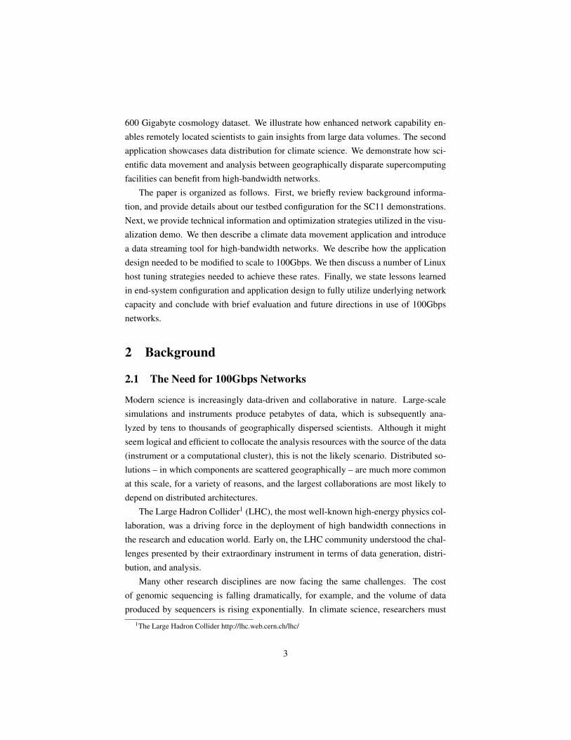
ESnet and Internet2, the two largest research and education network providers inthe USA, worked together to make 100Gbps networks available to researchers at theSupercomputing 2011 (SC11) conference in Seattle Washington, November 2011. Thisnetwork, shown in Figure 1, included a 100Gbps connection between National EnergyResearch Scientific Computing Center (NERSC) at Lawrence Berkeley National Lab-oratory (LBNL) in Oakland, CA, Argonne National Laboratory (ANL) near Chicago,IL, and Oak Ridge National Laboratory (ORNL) in Tennessee.

STAR

SC11

AOFANERSC

SALT

ORNL

SUNN

ANL

Router siteOptical regen site

Figure 1: 100Gbps Network for Supercomputing 2011

In this paper, we describe two of the first applications to take advantage of thisnetwork. The first application demonstrates real-time streaming and visualization of a

2

600 Gigabyte cosmology dataset. We illustrate how enhanced network capability en-ables remotely located scientists to gain insights from large data volumes. The secondapplication showcases data distribution for climate science. We demonstrate how sci-entific data movement and analysis between geographically disparate supercomputingfacilities can benefit from high-bandwidth networks.

The paper is organized as follows. First, we briefly review background informa-tion, and provide details about our testbed configuration for the SC11 demonstrations.Next, we provide technical information and optimization strategies utilized in the visu-alization demo. We then describe a climate data movement application and introducea data streaming tool for high-bandwidth networks. We describe how the applicationdesign needed to be modified to scale to 100Gbps. We then discuss a number of Linuxhost tuning strategies needed to achieve these rates. Finally, we state lessons learnedin end-system configuration and application design to fully utilize underlying networkcapacity and conclude with brief evaluation and future directions in use of 100Gbpsnetworks.

2 Background

2.1 The Need for 100Gbps Networks

Modern science is increasingly data-driven and collaborative in nature. Large-scalesimulations and instruments produce petabytes of data, which is subsequently ana-lyzed by tens to thousands of geographically dispersed scientists. Although it mightseem logical and efficient to collocate the analysis resources with the source of the data(instrument or a computational cluster), this is not the likely scenario. Distributed so-lutions – in which components are scattered geographically – are much more commonat this scale, for a variety of reasons, and the largest collaborations are most likely todepend on distributed architectures.

The Large Hadron Collider1 (LHC), the most well-known high-energy physics col-laboration, was a driving force in the deployment of high bandwidth connections inthe research and education world. Early on, the LHC community understood the chal-lenges presented by their extraordinary instrument in terms of data generation, distri-bution, and analysis.

Many other research disciplines are now facing the same challenges. The costof genomic sequencing is falling dramatically, for example, and the volume of dataproduced by sequencers is rising exponentially. In climate science, researchers must

1The Large Hadron Collider http://lhc.web.cern.ch/lhc/

3

analyze observational and simulation data sets located at facilities around the world.Climate data is expected to exceed 100 exabytes by 2020 [5]. The need for productiveaccess to such data led to the development of the Earth System Grid2 (ESG) [10], aglobal workflow infrastructure giving climate scientists access to data sets housed atmodeling centers on multiple continents, including North America, Europe, Asia, andAustralia.

Efficient tools are necessary to move vast amounts of scientific data over high-bandwidth networks, for such state-of-the-art collaborations. We evaluate climate datadistribution over high-latency high-bandwidth networks, and state the necessary stepsto scale-up climate data movement to 100Gbps networks. We have developed a newdata streaming tool that provides dynamic data channel management and on-the-flydata pipelines for fast and efficient data access. Data is treated as first-class citizen forthe entire spectrum of file sizes, without compromising on optimum usage of networkbandwidth. In our demonstration, we successfully staged real-world data from theIntergovernmental Panel on Climate Change (IPCC) Fourth Assessment Report (AR4)Phase 3, Coupled Model Intercomparison Project3 (CMIP-3) into computing nodesacross the country at ANL and ORNL from NERSC data storage over the 100Gbpsnetwork in real-time.

2.2 Visualization over 100Gbps

Modern simulations produce massive amounts of datasets that need further analysisand visualization. Often, these datasets cannot be moved from the machines that thesimulations are conducted on. One has to resort to in situ analysis (i.e. conduct anal-ysis while the simulation is running), or remote rendering (i.e. run a client on a localworkstation, and render the data at the supercomputing center). While these modes ofoperation are often desirable, a class of researchers would much rather prefer to streamthe datasets to their local workstations or facilities, and conduct a broad range of vi-sualization and analysis tasks locally. With the availability of the 100Gbps network,this mode of analysis is now feasible. To justify this claim, we demonstrate real-timestreaming of a large multi-Terabyte sized dataset in a few minutes from DOE’s pro-duction supercomputing facility NERSC, to four commodity workstations at SC11 inSeattle. For illustration purposes, we then demonstrate real-time parallel visualizationof the same dataset.

2Earth System Grid http://www.earthsystemgrid.org3CMIP3 Multi-Model Dataset Archive at PCMDI http://www-pcmdi.llnl.gov/ipcc/

4

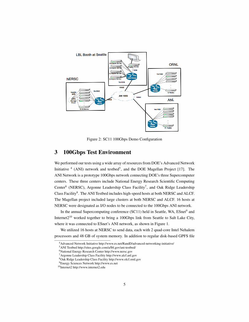
Figure 2: SC11 100Gbps Demo Configuration

3 100Gbps Test Environment

We performed our tests using a wide array of resources from DOE’s Advanced NetworkInitiative 4 (ANI) network and testbed5, and the DOE Magellan Project [17]. TheANI Network is a prototype 100Gbps network connecting DOE’s three Supercomputercenters. These three centers include National Energy Research Scientific ComputingCenter6 (NERSC), Argonne Leadership Class Facility7, and Oak Ridge LeadershipClass Facility8. The ANI Testbed includes high-speed hosts at both NERSC and ALCF.The Magellan project included large clusters at both NERSC and ALCF. 16 hosts atNERSC were designated as I/O nodes to be connected to the 100Gbps ANI network.

In the annual Supercomputing conference (SC11) held in Seattle, WA, ESnet9 andInternet210 worked together to bring a 100Gbps link from Seattle to Salt Lake City,where it was connected to ESnet’s ANI network, as shown in Figure 1.

We utilized 16 hosts at NERSC to send data, each with 2 quad-core Intel Nehalemprocessors and 48 GB of system memory. In addition to regular disk-based GPFS file

4Advanced Network Initiative http://www.es.net/RandD/advanced-networking-initiative/5ANI Testbed http://sites.google.com/a/lbl.gov/ani-testbed/6National Energy Research Center http://www.nersc.gov7Argonne Leadership Class Facility http://www.alcf.anl.gov8Oak Ridge Leadership Class Facility http://www.olcf.ornl.gov9Energy Sciences Network http://www.es.net

10Internet2 http://www.internet2.edu

5

system, these hosts are also connected via Infiniband to a Flash-based file system forsustained I/O performance during the demonstration. The complete system, includingthe hosts and the GPFS11 filesystem can sustain an aggregated 16 GBytes/second readperformance. Each host is equipped with a Chelsio 10Gbps NIC which is connected tothe NERSC Alcatel-Lucent router.

We utilized 12 hosts at OLCF to receive data, each with 24GB of RAM and aMyricom 10GE NIC. These were all connected to a 100Gbps Juniper router. We used14 hosts at ALCF to receive data, each with 48GB of RAM and a Mellanox 10GENIC. These hosts were connected to a 100Gbps Brocade router. Each host at ALCFand OLCF had 2 quad-core Intel Nehalem processors. We measured a round-trip time(RTT) of 50ms between NERSC and ALCF, and 64ms between NERSC and OLCF.We used four hosts in the SC11 LBL booth, each with two 8-core AMD processors and64 GB of memory. Each host is equipped with Myricom 10Gbps network adaptors,one dual port, and two single-port,connected to a 100Gbps Alcatel-Lucent router at thebooth. Figure 2 shows the hosts that were used for the two 100Gbps applications atSC11.

4 Visualizing the Universe at100Gbps

Computational cosmologists routinely conduct large scale simulations to test theoriesof formation (and evolution) of the universe. Ensembles of calculations with variousparametrizations of dark energy, for instance, are conducted on thousands of com-putational cores at supercomputing centers. The resulting datasets are visualized tounderstand large scale structure formation, and analyzed to check if the simulationsare able to reproduce known observational statistics. In this demonstration, we useda modern cosmological dataset produced by the NYX12 code. The computational do-main is 10243 in size; each location contains a single precision floating point valuecorresponding to the dark matter density at each grid point. Each timestep correspondsto 4GB of data. We utilize 150 timesteps for our demo purposes.

To demonstrate the difference between the 100Gbps network and the previous10Gbps network, we split the 100Gbps connection into two parts. 90Gbps of the band-width is used to transfer the full dataset. 10Gbps of the bandwidth is used to transfer1/8th of the same dataset at the same resolution. By comparing the real-time head-to-

11GPFS http://www.ibm.com/systems/software/gpfs12NYX: https://ccse.lbl.gov/Research/NYX/index.html

6

head streaming and rendering results of the two cases, the enhanced capabilities of the100Gbps network are clearly demonstrated.

Flash-based GPFS Cluster

Receive/Render

H1

Sender 01

Sender 02

Sender 16

Sender 03

… …

NERSC Router

100G Pipe

Receive/Render

H2

Receive/Render

H3

Receive/Render

H4

Low Bandwidth Receive/

Render/Vis

LBL Booth Router

High Bandwidth

Vis Srv

IB Cloud

Gigabit Ethernet

Infiniband Connection

10GigE Connection

1 GigE Connection

Low Bandwidth

Display

High Bandwidth Display

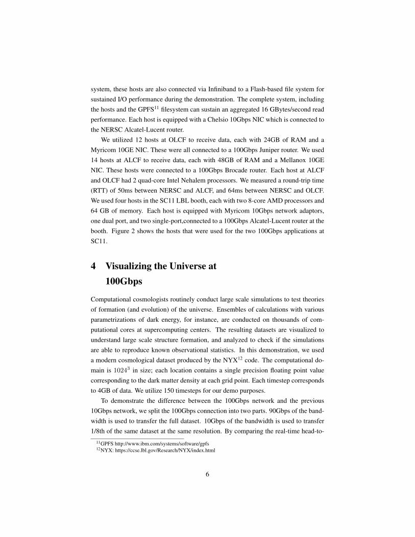
Figure 3: System diagram for the visualization demo at SC11.

4.1 Demo Configuration

Figure 3 illustrates the hardware configuration used for this demo. On the NERSCside, the 16 servers described above, named ”Sender 01-16”, are used to send data.The data resides on a the GPFS file system. In the LBL booth, four hosts, named”Receive/Render H1-H4”, are used to receive data for the high bandwidth part of thedemo. Each server has two 8-core AMD processors and 64 GB of system memory.Each host is equipped with 2 Myricom dual-port 10Gbps network adaptors which areconnected to the booth Alcatel-Lucent router via optical fibers. The ”Receive/Render”servers are connected to the ”High Bandwidth Vis Server” via 1Gbps ethernet connec-tions. The 1Gbps connection is used for synchronization and communication of therendering application, not for transfer of the raw data. A HDTV is connected to this

7

server to display rendered images. For the low bandwidth part of the demo, one server,named ”Low Bandwidth Receive/Render/Vis”, is used to receive and render data. AHDTV is also connected to this server to display rendered images. The low bandwidthhost is equipped with 1 dual-port 10Gbps network adaptor which is connected to thebooth router via 2 optical fibers. The one-way latency from NERSC to the LBL boothwas measured at 16.4 ms.

4.2 UDP shuffling

Prior work by Bethel, et al. [6, 7] has demonstrated that the TCP protocol is ill-suitedfor applications that need sustained high-throughput utilization over a high-latency net-work channel. For visualization purposes, occasional packet loss is acceptable, wetherefore follow the approach of VisaPult[6] and use the UDP protocol for transferringthe data for this demo.

We prepared UDP packets by adding position (x, y, z) information in conjunctionwith the density information. While this increases the size of the streamed dataset bya factor of 3 (summing up to a total of 16GB per timestep), this made the task of theplacing the received element into the right memory offset trivial. Also, we experi-mented with different data decomposition schemes (z-ordered space filling curves) asopposed to a z-slice based ordering, and this scheme allowed us to experiment withboth schemes without any change in the packet packing/unpacking logic.

Batch#,n X1Y1Z1D1 X2Y2Z2D2 … … XnYnZnDn

UDP Packet

In the final run n=560, packet size is 8968 bytes

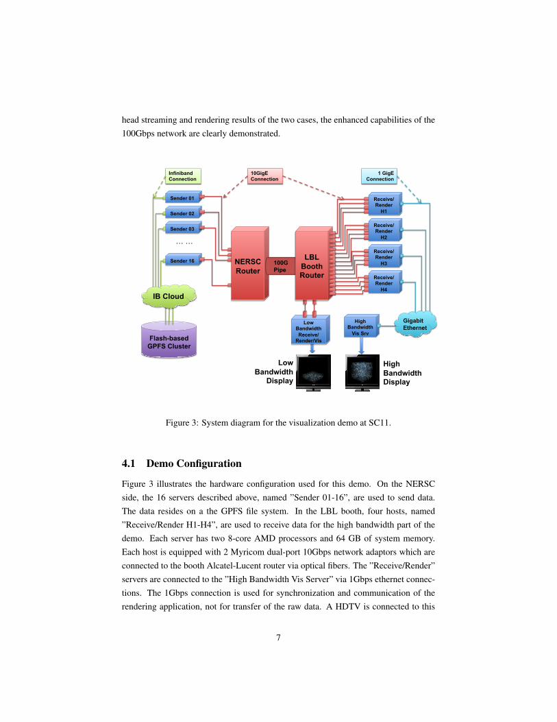
Figure 4: UDP Packet

As shown in Figure 4, a UDP packet contains a header followed by a series of quad-value segments. In the header, the batch number used for synchronization purposes,i.e., packets from different time steps have different batch numbers. An integer n isalso included in the header to specify the number of quad-value segments in this packet.Each quad-value segment consists 3 integers, which are the X, Y and Z position in the10243 matrix, and one float value which is the particle density at this position. Tomaximize the packet size within the MTU value of 9000, the number n is set to 560which gives the optimal packet size of 8968 bytes, which is the largest possible packet

8

size under 8972 bytes (MTU size minus IP and UDP headers) with the above describeddata structure.

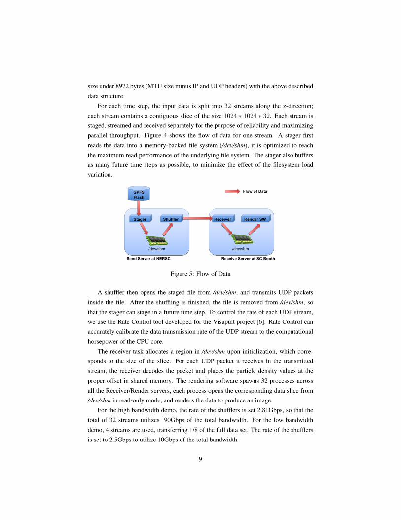
For each time step, the input data is split into 32 streams along the z-direction;each stream contains a contiguous slice of the size 1024 ∗ 1024 ∗ 32. Each stream isstaged, streamed and received separately for the purpose of reliability and maximizingparallel throughput. Figure 4 shows the flow of data for one stream. A stager firstreads the data into a memory-backed file system (/dev/shm), it is optimized to reachthe maximum read performance of the underlying file system. The stager also buffersas many future time steps as possible, to minimize the effect of the filesystem loadvariation.

Shuffler Receiver Stager Render SW

GPFS Flash

/dev/shm /dev/shm

Flow of Data

Send Server at NERSC Receive Server at SC Booth

Figure 5: Flow of Data

A shuffler then opens the staged file from /dev/shm, and transmits UDP packetsinside the file. After the shuffling is finished, the file is removed from /dev/shm, sothat the stager can stage in a future time step. To control the rate of each UDP stream,we use the Rate Control tool developed for the Visapult project [6]. Rate Control canaccurately calibrate the data transmission rate of the UDP stream to the computationalhorsepower of the CPU core.

The receiver task allocates a region in /dev/shm upon initialization, which corre-sponds to the size of the slice. For each UDP packet it receives in the transmittedstream, the receiver decodes the packet and places the particle density values at theproper offset in shared memory. The rendering software spawns 32 processes acrossall the Receiver/Render servers, each process opens the corresponding data slice from/dev/shm in read-only mode, and renders the data to produce an image.

For the high bandwidth demo, the rate of the shufflers is set 2.81Gbps, so that thetotal of 32 streams utilizes 90Gbps of the total bandwidth. For the low bandwidthdemo, 4 streams are used, transferring 1/8 of the full data set. The rate of the shufflersis set to 2.5Gbps to utilize 10Gbps of the total bandwidth.

9

4.3 Synchronization Strategy

The synchronization is performed at the NERSC end. All shufflers, including 32 forhigh bandwidth demo and 4 for low band demo, are listening to a UDP port for thesynchronization packet. Sent out from a controller running on a NERSC host, thesynchronization packets contains the location of the next file to shuffle out. Uponreceiving this synchronization packet, a shuffler will stop shuffling the current timestep (if it is unfinished), and start shuffling the next time step, until it has shuffled alldata in the time step, or receives the next synchronization packet. This mechanismensures all the shufflers, receivers, and renders are synchronized to the same time step.

We also made an important decision to decouple the streaming tasks from the ren-dering tasks on each host. The cores responsible for unpacking UDP packets, placethe data into a memory-mapped file location. This mmap’ed region is dereferenced inthe rendering processes. There is no communication or synchronization between therendering tasks and streaming tasks on each node.

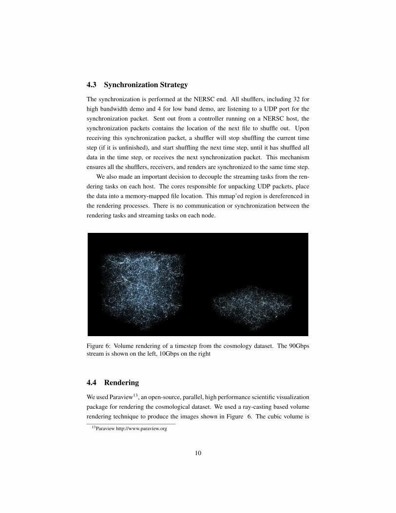
Figure 6: Volume rendering of a timestep from the cosmology dataset. The 90Gbpsstream is shown on the left, 10Gbps on the right

4.4 Rendering

We used Paraview13, an open-source, parallel, high performance scientific visualizationpackage for rendering the cosmological dataset. We used a ray-casting based volumerendering technique to produce the images shown in Figure 6. The cubic volume is

13Paraview http://www.paraview.org

10

decomposed in a z-slice order into 4 segments and streamed to individual renderingnodes. Paraview uses 8 cores on each rendering node to produce intermediate imagesand then composites the image using sort-last rendering over a local 10Gbps network.The final image is displayed on a front-end node connected to a display.

Since the streaming tasks are decoupled from the rendering tasks, Paraview is es-sentially asked to volume render images as fast as possible in an endless loop. It ispossible, and we do observe artifacts in the rendering as the real-time streams depositdata into different regions in memory. In practice, the artifacts are not distracting.We acknowledge that one might want to adopt a different mode of rendering (usingpipelining and multiple buffers) to stream data, corresponding to different timesteps,into distinct regions in memory.

4.5 Optimizations

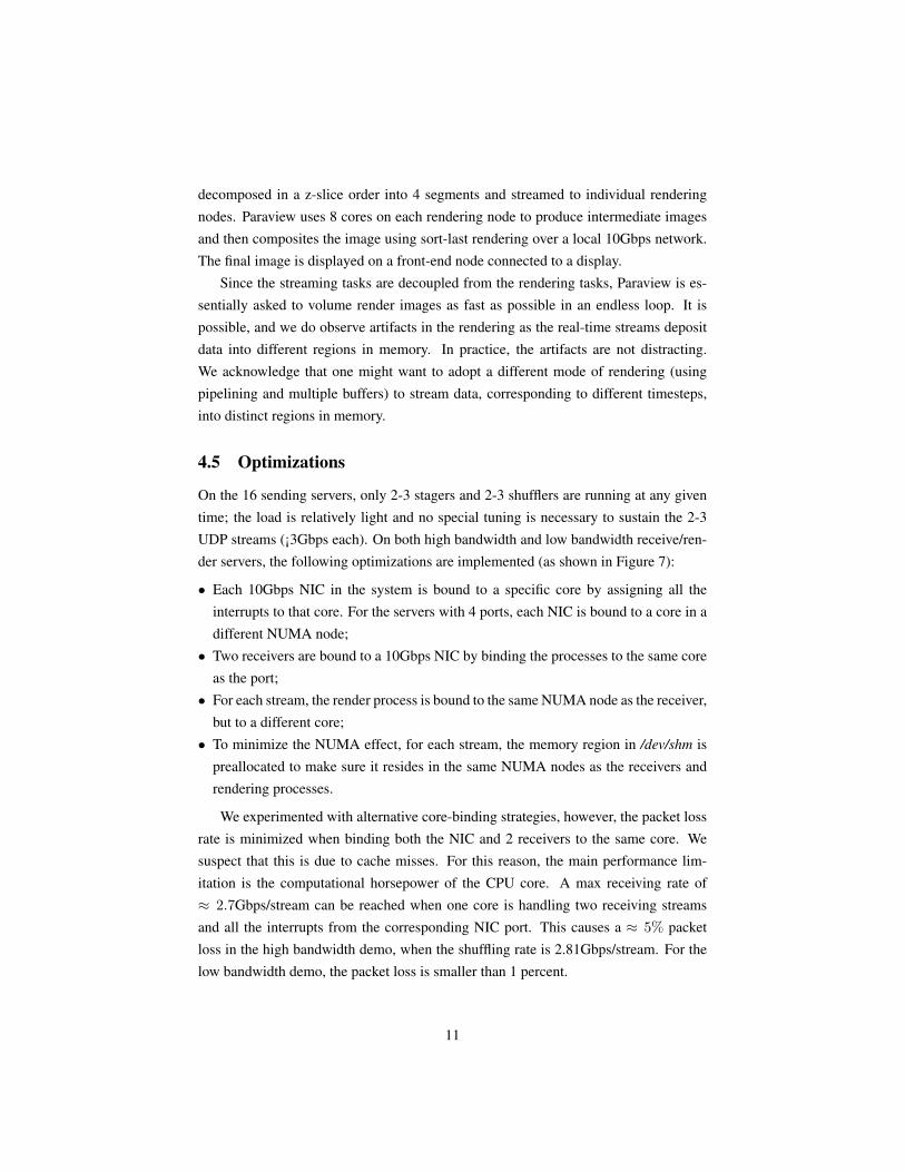
On the 16 sending servers, only 2-3 stagers and 2-3 shufflers are running at any giventime; the load is relatively light and no special tuning is necessary to sustain the 2-3UDP streams (¡3Gbps each). On both high bandwidth and low bandwidth receive/ren-der servers, the following optimizations are implemented (as shown in Figure 7):

• Each 10Gbps NIC in the system is bound to a specific core by assigning all theinterrupts to that core. For the servers with 4 ports, each NIC is bound to a core in adifferent NUMA node;

• Two receivers are bound to a 10Gbps NIC by binding the processes to the same coreas the port;

• For each stream, the render process is bound to the same NUMA node as the receiver,but to a different core;

• To minimize the NUMA effect, for each stream, the memory region in /dev/shm ispreallocated to make sure it resides in the same NUMA nodes as the receivers andrendering processes.

We experimented with alternative core-binding strategies, however, the packet lossrate is minimized when binding both the NIC and 2 receivers to the same core. Wesuspect that this is due to cache misses. For this reason, the main performance lim-itation is the computational horsepower of the CPU core. A max receiving rate of≈ 2.7Gbps/stream can be reached when one core is handling two receiving streamsand all the interrupts from the corresponding NIC port. This causes a ≈ 5% packetloss in the high bandwidth demo, when the shuffling rate is 2.81Gbps/stream. For thelow bandwidth demo, the packet loss is smaller than 1 percent.

11

Mem Mem

Mem Mem

Receiver 1

10G Port

Receiver 2

Render 1

NUMA Node

Core

Render 2

Figure 7: NUMA Binding

4.6 Network Performance Results

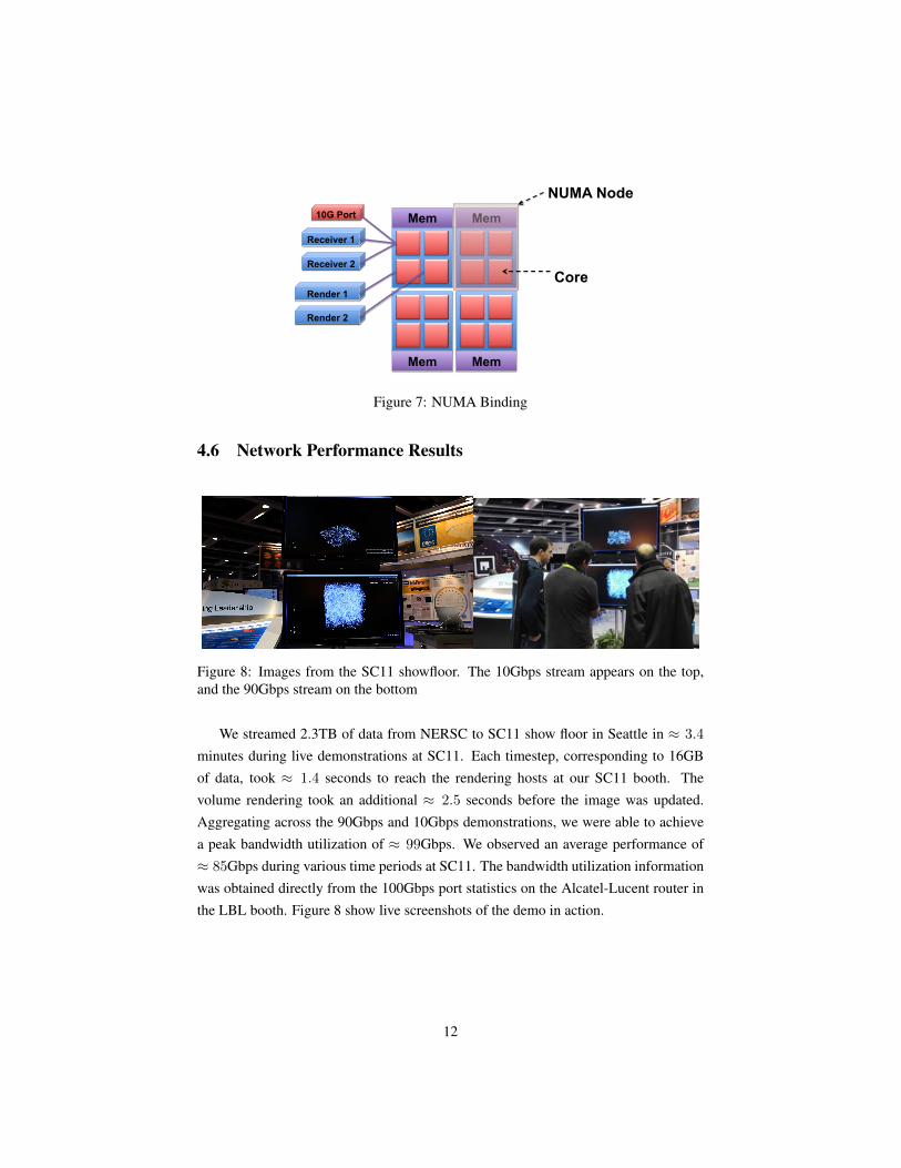
Figure 8: Images from the SC11 showfloor. The 10Gbps stream appears on the top,and the 90Gbps stream on the bottom

We streamed 2.3TB of data from NERSC to SC11 show floor in Seattle in ≈ 3.4

minutes during live demonstrations at SC11. Each timestep, corresponding to 16GBof data, took ≈ 1.4 seconds to reach the rendering hosts at our SC11 booth. Thevolume rendering took an additional ≈ 2.5 seconds before the image was updated.Aggregating across the 90Gbps and 10Gbps demonstrations, we were able to achievea peak bandwidth utilization of ≈ 99Gbps. We observed an average performance of≈ 85Gbps during various time periods at SC11. The bandwidth utilization informationwas obtained directly from the 100Gbps port statistics on the Alcatel-Lucent router inthe LBL booth. Figure 8 show live screenshots of the demo in action.

12

5 Climate Data over 100Gbps

High-bandwidth connections help increase throughput of scientific applications, open-ing up new opportunities for sharing data that were simply not possible with 10Gbpsnetworks. However, increasing the network bandwidth is not sufficient by itself. Next-generation high-bandwidth networks need to be evaluated carefully from the applica-tions’ perspectives. In this section, we explore how climate applications can adapt andbenefit from next generation high-bandwidth networks.

Data volume in climate applications is increasing exponentially. For example, therecent ”Replica Core Archive” data from the IPCC Fifth Assessment Report (AR5) isexpected to be around 2PB [10], whereas, the IPCC Forth Assessment Report (AR4)data archive is only 35TB. This trend can be seen across many areas in science [2, 9].An important challenge in managing ever increasing data sizes in climate science isthe large variance in file sizes [3, 21, 11]. Climate simulation data consists of a mix ofrelatively small and large files with irregular file size distribution in each dataset. Thisrequires advanced middleware tools to move data efficiently in long-distance high-bandwidth networks. We claim that with such tools, data can be treated as first-classcitizen for the entire spectrum of file sizes, without compromising on optimum usageof network-bandwidth.

To justify this claim, we present our experience from the SC11 ANI demonstra-tion, titled ‘Scaling the Earth System Grid to 100Gbps Networks’. We used a 100Gbpslink connecting National Energy Research Scientific Computing Center (NERSC), Ar-gonne National Laboratory (ANL) and Oak Ridge National Laboratory (ORNL). Forthis demonstration, we developed a new data streaming tool that provides dynamic datachannel management and on-the-fly data pipelines for fast and efficient data access.

The data from IPCC Fourth Assessment Report (AR4) phase 3, CMIP-3, with totalsize of 35TB, was used in our tests and demonstrations. In the demo, CMIP-3 data wasstaged successfully into the memory of computing nodes across the country at ANLand ORNL from NERSC data storage over the 100Gbps network on demand.

5.1 Motivation

Climate data is one of the fastest growing scientific data sets. Simulation results areaccessed by thousands of users around the world. Many institutions collaborate onthe generation and analysis of simulation data. The Earth System Grid Federation14

(ESGF) [10, 9] provides necessary middleware and software to support end-user data

14Earth System Grid Federation: http://esgf.org/

13

access and data replication between partner institutions. High performance data move-ment between ESG data nodes is an important challenge, especially between geograph-ically separated data centers.

In this study, we evaluate the movement of bulk data from ESG data nodes, and statethe necessary steps to scale-up climate data movement to 100Gbps high-bandwidth net-works. As a real-world example, we specifically focus on data access and data distribu-tion for the Coupled Model Intercomparison Project (CMIP) from IntergovernmentalPanel on Climate Change (IPCC).

IPCC climate data is stored in common NetCDF data files. Metadata from eachfile, including the model, type of experiment, and the institution that generated the datafile are retrieved and stored when data is published. Data publication is accomplishedthrough an Earth System Grid (ESG) gateway server. Gateways work in a federatedmanner such that the metadata database is synchronized between each gateway. TheESG system provides an easy-to-use interface to search and locate data files accord-ing to given search patterns. Data files are transferred from a remote repository usingadvanced data transfer tools (e.g., GridFTP [1, 8, 21]) that are optimized for fast datamovement. A common use-case is replication of data to achieve redundancy. In ad-dition to replication, data files are copied into temporary storage in HPC centers forpost-processing and further climate analysis.

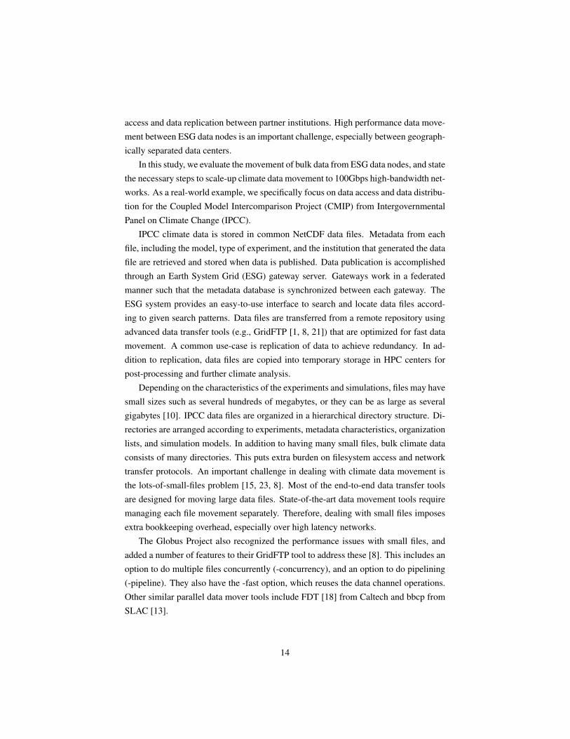
Depending on the characteristics of the experiments and simulations, files may havesmall sizes such as several hundreds of megabytes, or they can be as large as severalgigabytes [10]. IPCC data files are organized in a hierarchical directory structure. Di-rectories are arranged according to experiments, metadata characteristics, organizationlists, and simulation models. In addition to having many small files, bulk climate dataconsists of many directories. This puts extra burden on filesystem access and networktransfer protocols. An important challenge in dealing with climate data movement isthe lots-of-small-files problem [15, 23, 8]. Most of the end-to-end data transfer toolsare designed for moving large data files. State-of-the-art data movement tools requiremanaging each file movement separately. Therefore, dealing with small files imposesextra bookkeeping overhead, especially over high latency networks.

The Globus Project also recognized the performance issues with small files, andadded a number of features to their GridFTP tool to address these [8]. This includes anoption to do multiple files concurrently (-concurrency), and an option to do pipelining(-pipeline). They also have the -fast option, which reuses the data channel operations.Other similar parallel data mover tools include FDT [18] from Caltech and bbcp fromSLAC [13].

14

5.2 Climate Data Distribution over 100Gbps

Scientific applications for climate analysis are highly data-intensive [5, 2, 10, 9]. Acommon approach is to stage data sets into local storage, and then run climate applica-tions on the local data files. However, replication comes with its storage cost and re-quires a management system for coordination and synchronization. 100Gbps networksprovide the bandwidth needed to bring large amounts of data quickly on-demand. Cre-ating a local replica beforehand may no longer be necessary. By providing data stream-ing from remote storage to the compute center where the application runs, we can betterutilize available network capacity and bring data into the application in real-time. If wecan keep the network pipe full by feeding enough data into the network, we can hidethe effect of network latency and improve the overall application performance. Sincewe will have high-bandwidth access to the data, management and bookkeeping of datablocks would play an important role in order to use remote storage resources efficientlyover the network.

The standard file transfer protocol FTP establishes two network channels [19, 23].The control channel is used for authentication, authorization, and sending control mes-sages such as what file is to be transferred. The data channel is used for streaming thedata to the remote site. In the standard FTP implementation, a separate data channel isestablished for every file. First, the file request is sent over the control channel, and adata channel is established for streaming the file data. Once the transfer is completed,a control message is sent to notify that end of file is reached. Once acknowledgementfor transfer completion is received, another file transfer can be requested. This addsat least three additional round-trip-times over the control channel [8, 23]. The datachannel stays idle while waiting for the next transfer command to be issued. In addi-tion, establishing a new data channel for each file increases the latency between eachfile transfer. The latency between transfers adds up, as a results, overall transfer timeincreases and total throughput decreases. This problem becomes more drastic for longdistance connections where round-trip-time is high.

Keeping the data channel idle also adversely affects the overall performance forwindow-based protocols such as TCP. The TCP protocol automatically adjusts thewindow size; the slow-start algorithm increases the window size gradually. When theamount of data sent is small, transfers may not be long enough to allow TCP to fullyopen its window, so we can not move data at full speed.

On the other hand, data movement requests, both for bulk data replication and datastreaming for large-scale data analysis, deal with a set of many files. Instead of movingdata from a single file at a time, the data movement middleware could handle the entire

15

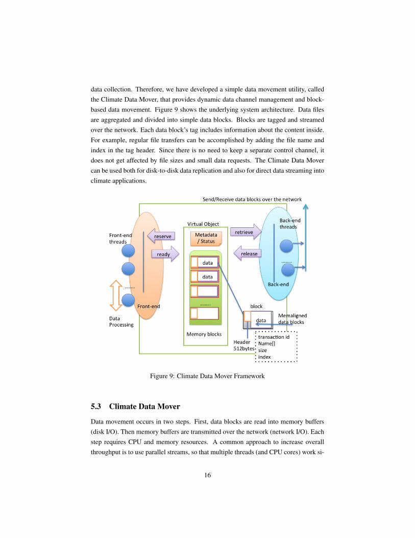
data collection. Therefore, we have developed a simple data movement utility, calledthe Climate Data Mover, that provides dynamic data channel management and block-based data movement. Figure 9 shows the underlying system architecture. Data filesare aggregated and divided into simple data blocks. Blocks are tagged and streamedover the network. Each data block’s tag includes information about the content inside.For example, regular file transfers can be accomplished by adding the file name andindex in the tag header. Since there is no need to keep a separate control channel, itdoes not get affected by file sizes and small data requests. The Climate Data Movercan be used both for disk-to-disk data replication and also for direct data streaming intoclimate applications.

Figure 9: Climate Data Mover Framework

5.3 Climate Data Mover

Data movement occurs in two steps. First, data blocks are read into memory buffers(disk I/O). Then memory buffers are transmitted over the network (network I/O). Eachstep requires CPU and memory resources. A common approach to increase overallthroughput is to use parallel streams, so that multiple threads (and CPU cores) work si-

16

multaneously to overcome the latency cost generated by disk and memory copy opera-tion in the end system. Another approach is to use concurrent transfers, where multipletransfer tasks cooperate together to generate high throughput data in order to fill thenetwork pipe [25, 4]. In standard file transfer mechanisms, we need more parallelismto overcome the cost of bookkeeping and control messages. An important drawbackin using application level tuning (parallel streams and concurrent transfers) is that theycause extra load on the system and resources are not used efficiently. Moreover, the useof many TCP streams may oversubscribe the network and cause performance degrada-tions.

In order to be able to optimally tune the data movement through the system, wedecoupled network and disk I/O operations. Transmitting data over the network islogically separated from the reading/writing of data blocks. Hence, we are able to havedifferent parallelism levels in each layer. Our data streaming utility, the Climate Data

Mover, uses a simple network library consisting of two layers: a front-end and a back-end. Each layer works independently so that we can measure performance and tuneeach layer separately. Those layers are tied to each other with a block-based virtualobject, implemented as a set of shared memory blocks. In the server, the front-end isresponsible for the preparation of data, and the back-end is responsible for the sendingof data over the network. On the client side, the back-end components receive datablocks and feed the virtual object, so the corresponding front-end can get and processdata blocks.

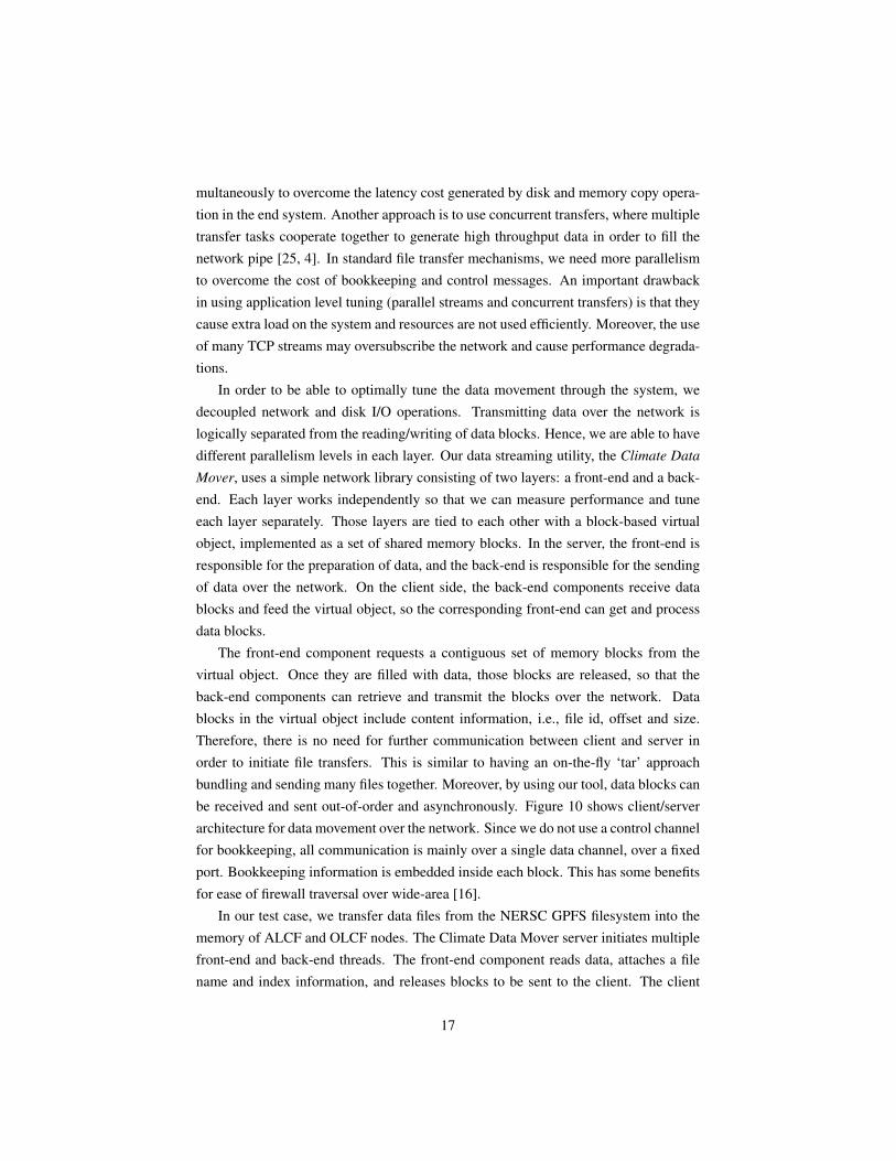
The front-end component requests a contiguous set of memory blocks from thevirtual object. Once they are filled with data, those blocks are released, so that theback-end components can retrieve and transmit the blocks over the network. Datablocks in the virtual object include content information, i.e., file id, offset and size.Therefore, there is no need for further communication between client and server inorder to initiate file transfers. This is similar to having an on-the-fly ‘tar’ approachbundling and sending many files together. Moreover, by using our tool, data blocks canbe received and sent out-of-order and asynchronously. Figure 10 shows client/serverarchitecture for data movement over the network. Since we do not use a control channelfor bookkeeping, all communication is mainly over a single data channel, over a fixedport. Bookkeeping information is embedded inside each block. This has some benefitsfor ease of firewall traversal over wide-area [16].

In our test case, we transfer data files from the NERSC GPFS filesystem into thememory of ALCF and OLCF nodes. The Climate Data Mover server initiates multiplefront-end and back-end threads. The front-end component reads data, attaches a filename and index information, and releases blocks to be sent to the client. The client

17

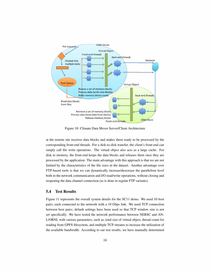
Figure 10: Climate Data Mover Server/Client Architecture

at the remote site receives data blocks and makes them ready to be processed by thecorresponding front-end threads. For a disk-to-disk transfer, the client’s front-end cansimply call file write operations. The virtual object also acts as a large cache. Fordisk to memory, the front-end keeps the data blocks and releases them once they areprocessed by the application. The main advantage with this approach is that we are notlimited by the characteristics of the file sizes in the dataset. Another advantage overFTP-based tools is that we can dynamically increase/descrease the parallelism levelboth in the network communication and I/O read/write operations, without closing andreopening the data channel connection (as is done in regular FTP variants).

5.4 Test Results

Figure 11 represents the overall system details for the SC11 demo. We used 10 hostpairs, each connected to the network with a 10 Gbps link. We used TCP connectionbetween host pairs; default settings have been used so that TCP window size is notset specifically. We have tested the network performance between NERSC and AN-L/ORNL with various parameters, such as, total size of virtual object, thread count forreading from GPFS filesystem, and multiple TCP streams to increase the utilization ofthe available bandwidth. According to our test results, we have manually determined

18

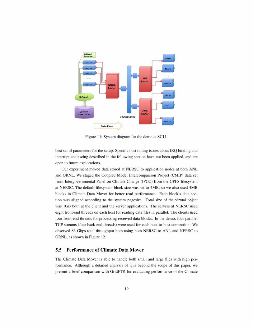
Figure 11: System diagram for the demo at SC11.

best set of parameters for the setup. Specific host tuning issues about IRQ binding andinterrupt coalescing described in the following section have not been applied, and areopen to future explorations.

Our experiment moved data stored at NERSC to application nodes at both ANLand ORNL. We staged the Coupled Model Intercomparison Project (CMIP) data setfrom Intergovernmental Panel on Climate Change (IPCC) from the GPFS filesystemat NERSC. The default filesystem block size was set to 4MB, so we also used 4MBblocks in Climate Data Mover for better read performance. Each block’s data sec-tion was aligned according to the system pagesize. Total size of the virtual objectwas 1GB both at the client and the server applications. The servers at NERSC usedeight front-end threads on each host for reading data files in parallel. The clients usedfour front-end threads for processing received data blocks. In the demo, four parallelTCP streams (four back-end threads) were used for each host-to-host connection. Weobserved 83 Gbps total throughput both using both NERSC to ANL and NERSC toORNL, as shown in Figure 12.

5.5 Performance of Climate Data Mover

The Climate Data Mover is able to handle both small and large files with high per-formance. Although a detailed analysis of it is beyond the scope of this paper, wepresent a brief comparison with GridFTP, for evaluating performance of the Climate

19

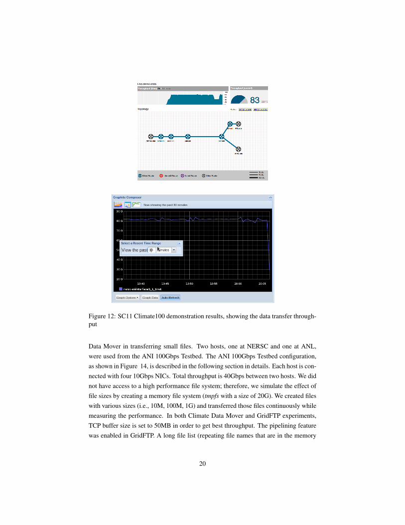
Figure 12: SC11 Climate100 demonstration results, showing the data transfer through-put

Data Mover in transferring small files. Two hosts, one at NERSC and one at ANL,were used from the ANI 100Gbps Testbed. The ANI 100Gbps Testbed configuration,as shown in Figure 14, is described in the following section in details. Each host is con-nected with four 10Gbps NICs. Total throughput is 40Gbps between two hosts. We didnot have access to a high performance file system; therefore, we simulate the effect offile sizes by creating a memory file system (tmpfs with a size of 20G). We created fileswith various sizes (i.e., 10M, 100M, 1G) and transferred those files continuously whilemeasuring the performance. In both Climate Data Mover and GridFTP experiments,TCP buffer size is set to 50MB in order to get best throughput. The pipelining featurewas enabled in GridFTP. A long file list (repeating file names that are in the memory

20

Figure 13: GridFTP vs. Climate Data Mover (CDM)

filesystem) is given as input. Figure 13 shows performance results with 10MB files.We initiated four server applications at ANL node (each running on a separate NIC),and four client applications at NERSC node. In the GridFTP tests, we tried both 16and 32 concurrent streams (-cc option). The Climate Data Mover was able to achieve37Gbps of throughput, while GridFTP was not able achieve more than 33Gbps.

6 Host Tuning Issues

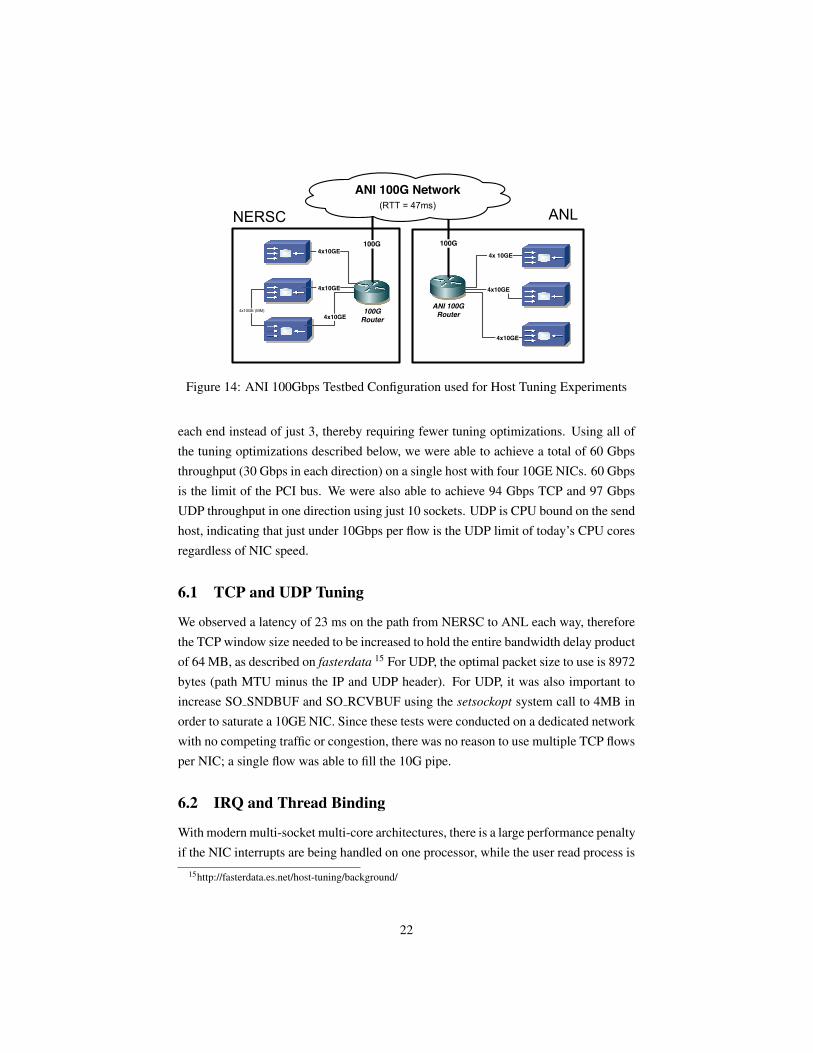
Optimal utilization of the network bandwidth on modern linux hosts requires a fairamount of tuning. There are several studies on network performance optimizationin 10Gbps networks [22, 24]. However, only a few recent studies have tested high-speed data transfers in a 100Gbps environment. One of these is the team at IndianaUniversity’s testing of the Lustre filesystem over the 100Gbps network at SC11 [14].Other recent studies include presentations by Rao [20] and by the team at Nasa Goddard[12]. They all have found that a great deal of tuning was required. In this section wespecifically discuss modifications that helped us increase the total NIC throughput.These additional host tuning tests were done after the SC11 conference on ESnet’sANI 100GbpsTestbed, shown in Figure 14.

We conducted these series of experiments on three hosts at NERSC connected witha 100Gbps link to three hosts at ANL. After adjusting the tuning knobs, we were ableto effectively fill the 100Gbps link with only 10 TCP sockets, one per 10Gbps NIC. Weused four 10GE NICS in two of the hosts, and two (out of 4) 10GE NICs in the thirdhost, as shown in Figure 14. The results of the two applications described in this paperused some, but not all of these techniques, as they both used more than 10 hosts on

21

ANI 100G Router

4x10GE

4x 10GE

NERSC ANL

Updated February 13, 2012

ANI Middleware Testbed

4x10GE

4x10GE

100G Router

4x10GE100G 100G

ANI 100G Network(RTT = 47ms)

4x10GE

4x10GE (MM)

Figure 14: ANI 100Gbps Testbed Configuration used for Host Tuning Experiments

each end instead of just 3, thereby requiring fewer tuning optimizations. Using all ofthe tuning optimizations described below, we were able to achieve a total of 60 Gbpsthroughput (30 Gbps in each direction) on a single host with four 10GE NICs. 60 Gbpsis the limit of the PCI bus. We were also able to achieve 94 Gbps TCP and 97 GbpsUDP throughput in one direction using just 10 sockets. UDP is CPU bound on the sendhost, indicating that just under 10Gbps per flow is the UDP limit of today’s CPU coresregardless of NIC speed.

6.1 TCP and UDP Tuning

We observed a latency of 23 ms on the path from NERSC to ANL each way, thereforethe TCP window size needed to be increased to hold the entire bandwidth delay productof 64 MB, as described on fasterdata 15 For UDP, the optimal packet size to use is 8972bytes (path MTU minus the IP and UDP header). For UDP, it was also important toincrease SO SNDBUF and SO RCVBUF using the setsockopt system call to 4MB inorder to saturate a 10GE NIC. Since these tests were conducted on a dedicated networkwith no competing traffic or congestion, there was no reason to use multiple TCP flowsper NIC; a single flow was able to fill the 10G pipe.

6.2 IRQ and Thread Binding

With modern multi-socket multi-core architectures, there is a large performance penaltyif the NIC interrupts are being handled on one processor, while the user read process is

15http://fasterdata.es.net/host-tuning/background/

22

on a different processor, as data will need to be copied between processors. We solvedthis problem using the following approach. First, we disabled irqbalance. irqbalance

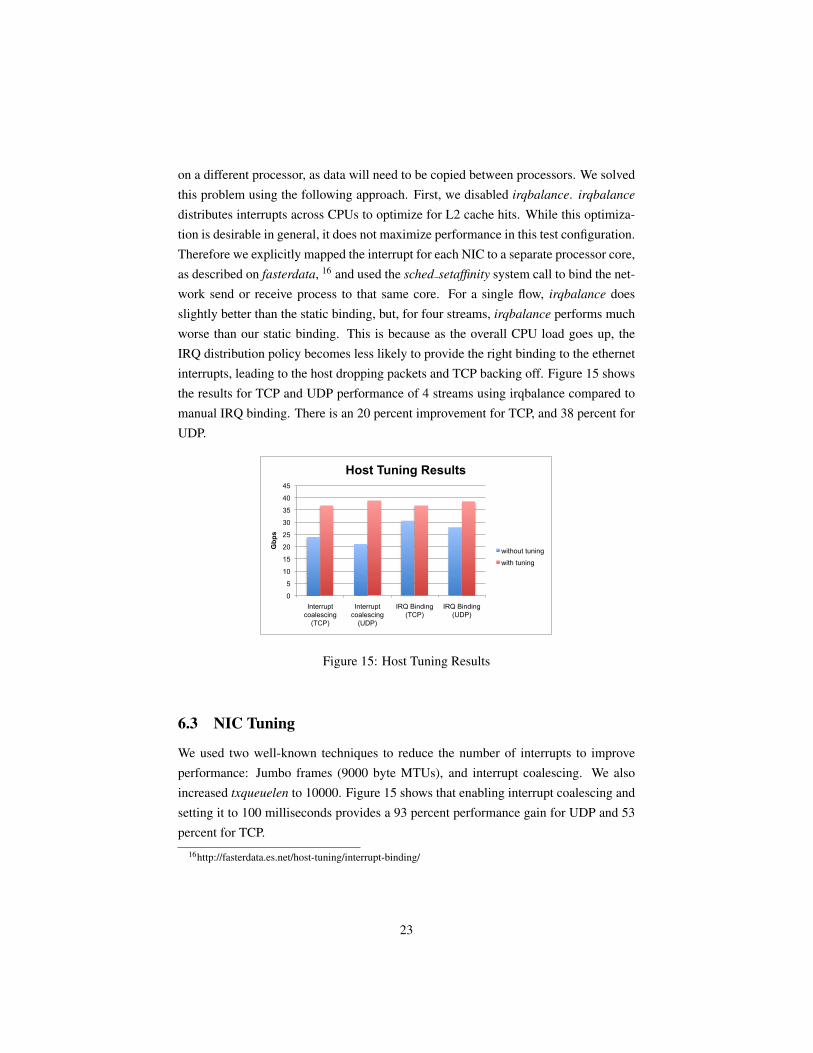
distributes interrupts across CPUs to optimize for L2 cache hits. While this optimiza-tion is desirable in general, it does not maximize performance in this test configuration.Therefore we explicitly mapped the interrupt for each NIC to a separate processor core,as described on fasterdata, 16 and used the sched setaffinity system call to bind the net-work send or receive process to that same core. For a single flow, irqbalance doesslightly better than the static binding, but, for four streams, irqbalance performs muchworse than our static binding. This is because as the overall CPU load goes up, theIRQ distribution policy becomes less likely to provide the right binding to the ethernetinterrupts, leading to the host dropping packets and TCP backing off. Figure 15 showsthe results for TCP and UDP performance of 4 streams using irqbalance compared tomanual IRQ binding. There is an 20 percent improvement for TCP, and 38 percent forUDP.

Tuning Setting without tuning with tuning % improvementInterrupt coalescing (TCP) 24 36.8 53.3333333

Interrupt coalescing (UDP) 21.1 38.8 83.8862559

IRQ Binding (TCP) 30.6 36.8 20.2614379

IRQ Binding (UDP) 27.9 38.5 37.9928315

0

5

10

15

20

25

30

35

40

45

Interrupt coalescing

(TCP)

Interrupt coalescing

(UDP)

IRQ Binding (TCP)

IRQ Binding (UDP)

Gbp

s

Host Tuning Results

without tuning

with tuning

Figure 15: Host Tuning Results

6.3 NIC Tuning

We used two well-known techniques to reduce the number of interrupts to improveperformance: Jumbo frames (9000 byte MTUs), and interrupt coalescing. We alsoincreased txqueuelen to 10000. Figure 15 shows that enabling interrupt coalescing andsetting it to 100 milliseconds provides a 93 percent performance gain for UDP and 53percent for TCP.

16http://fasterdata.es.net/host-tuning/interrupt-binding/

23

6.4 BIOS Tuning

It is important to verify that a number of BIOS settings are properly set to obtain max-imum performance. We modified the following settings in the course of our experi-ments:

• hyper-threading: We disabled hyper-threading. While it simulates more cores thanare physically present, this can reduce performance under variable load conditions

• memory speed: The default BIOS setting did not set the memory bus speed to themaximum.

• cpuspeed: The default BIOS setting did not set the CPU speed to the maximum.• energy saving: We disabled this to ensure the CPU was always running at the max-

imum speed.

6.5 Open Issues

This paper has shown that one needs to perform a lot of hand-tuning in order to saturatea 100Gbps networks. We need to optimize CPU utilization in order to achieve highernetworking performance. The Linux operating system provides a service, irqbalance,but as this paper has shown, its generic algorithm fails under certain workloads. Stat-ically binding IRQs and send/receive threads to a dedicated core is a simple solutionsthat works well in a well defined, predictable, environment, but quickly becomes diffi-cult to manage in a production context where many different applications may have tobe deployed.

PCI Gen3 motherboards are just becoming available, allowing up to 8Gbps perlane. These motherboards will allow a single NIC to theoretically go up to 64Gbps.In this environment more parallel flows will be needed, as current CPU speed limitsUDP flows to around 10Gbps, and TCP flows to around 18Gbps. This problem willbe further exacerbated when PCIe Gen4, slated for 2015, will further increase PCIbandwidth.

Last but not least, the various experiments reported in the paper were running ina closed network with no competing traffic. More thorough testing will be needed toidentify and address issues in a production network.

7 Conclusion

100Gbps networks have arrived, and with careful application design and host tuning, arelatively small number of hosts can fill a 100Gbps pipe. Many of the host tuning tech-

24

niques from 1Gbps to 10Gbps transition still apply. These include TCP/UDP buffertuning, using jumbo frames, and using interrupt coalescing. With the current gener-ation of multi-core systems, IRQ binding also is now essential for maximizing hostperformance.

While application of these tuning techniques will likely improve the overall through-put of the system, it is important to follow an experimental methodology in order tosystematically increase performance. In some cases a particular tuning strategy maynot achieve the expected results. We recommend starting with the simplest core I/Ooperation possible, and then adding layers of complexity on top of that. For example,one can first tune the system for a single network flow using a simple memory to mem-ory transfer tool such as Iperf17 or nuttcp18. Next optimize the multiple concurrentstreams, trying to model the application behavior as closely as possible. Once this isdone, the final step is to tune the application itself. The main goal of this methodologyis to verify performance for each component in the critical path. Applications mayneed to be redesigned to get the best out of high-bandwidth networks. In this paper, wedemonstrated two such applications to take advantage of this network, and described anumber of application design issues and host tuning strategies necessary for enablingthose applications to scale to 100Gbps.

Acknowledgments

We would like to thank Peter Nugent and Zarija Lukic for providing us with the cos-mology datasets used in the visualization demo. Our thanks go out to Patrick Dorn,Evangelos Chaniotakis, John Christman, Chin Guok, Chris Tracy and Lauren Rotmanfor assistance with 100Gbps installation and testing at SC11. Jason Lee, Shane Canon,Tina Declerck and Cary Whitney provided technical support with NERSC hardware.Ed Holohan, Adam Scovel, and Linda Winkler provided support at ALCF. Jason Hill,Doug Fuller, and Susan Hicks provided support at OLCF. Hank Childs, Mark Howisonand Aaron Thomas assisted with troubleshooting visualization software and hardware.John Dugan and Gopal Vaswani provided monitoring tools for 100Gbps demonstra-tions at SC11.

This work was supported by the Director, Office of Science, Office of Basic En-ergy Sciences, of the U.S. Department of Energy under Contract No. DE-AC02-

17iperf: http://iperf.sourceforge.net/18nuttcp: http://www.nuttcp.net

25

05CH11231. This research used resources of the ESnet Advanced Network Initiative(ANI) Testbed, which is supported by the Office of Science of the U.S. Departmentof Energy under the contract above, funded through the The American Recovery andReinvestment Act of 2009.

References

[1] W. Allcock, J. Bresnahan, R. Kettimuthu, M. Link, C. Dumitrescu, I. Raicu, andI. Foster. The globus striped gridftp framework and server. In Proceedings of the

2005 ACM/IEEE conference on Supercomputing, SC ’05, pages 54–, Washington,DC, USA, 2005. IEEE Computer Society.

[2] M. Balman and S. Byna. Open problems in network-aware data managementin exa-scale computing and terabit networking era. In Proceedings of the first

international workshop on Network-aware data management, NDM ’11, pages73–78, 2011.

[3] M. Balman and T. Kosar. Data scheduling for large scale distributed applications.In Proceedings of the 5th ICEIS Doctoral Consortium, in conjunction with the

International Conference on Enterprise Information Systems (ICEIS’07), 2007.

[4] M. Balman and T. Kosar. Dynamic adaptation of parallelism level in data transferscheduling. Complex, Intelligent and Software Intensive Systems, International

Conference, 0:872–877, 2009.

[5] BES Science Network Requirements, Report of the Basic Energy Sciences Net-work Requirements Workshop. Basic Energy Sciences Program Office, DOEOffice of Science and the Energy Sciences Network, 2007.

[6] E. W. Bethel. Visapult – A Prototype Remote and Distributed Application andFramework. In Proceedings of Siggraph 2000 – Applications and Sketches.ACM/Siggraph, July 2000.

[7] E. W. Bethel and J. Shalf. Consuming Network Bandwidth with Visapult. InC. Hansen and C. Johnson, editors, The Visualization Handbook, pages 569–589.Elsevier, 2005. LBNL-52171.

[8] J. Bresnahan, M. Link, R. Kettimuthu, D. Fraser, and I. Foster. Gridftp pipelining.In Proceedings of the 2007 TeraGrid Conference, June 2007.

26

[9] D. N. Williams et al. Data Management and Analysis for the Earth System Grid.Journal of Physics: Conference Series, SciDAC 08 conference proceedings, vol-ume 125 012072, 2008.

[10] D. N. Williams et al. Earth System Grid Federation: Infrastructure to Support Cli-mate Science Analysis as an International Collaboration. Data Intensive ScienceSeries: Chapman & Hall/CRC Computational Science, ISBN 9781439881392,2012.

[11] S. Doraimani and A. Iamnitchi. File grouping for scientific data management:lessons from experimenting with real traces. In Proceedings of the 17th interna-

tional symposium on High performance distributed computing, HPDC ’08, pages153–164, 2008.

[12] P. Gary, B. Find, and P. Lang. Introduction to GSFC High End Computing: 20,40 and 100 Gbps Network Testbeds. http://science.gsfc.nasa.gov/606.1/docs/HECN_10G_Testbeds_082210.pdf, 2010.

[13] A. Hanushevsky, A. Trunov, and L. Cottrell. Peer-to-peer computing for securehigh performance data copying. In Proceedings of computing in high energy and

nuclear physics, September 2001.

[14] IU showcases innovative approach to networking at SC11 SCinet ResearchSandbox. http://ovpitnews.iu.edu/news/page/normal/20445.html, 2011.

[15] R. Kettimuthu, S. Link, J. Bresnahan, M. Link, and I. Foster. Globus xio pipeopen driver: enabling gridftp to leverage standard unix tools. In Proceedings of

the 2011 TeraGrid Conference: Extreme Digital Discovery, TG ’11, pages 20:1–20:7. ACM, 2011.

[16] R. Kettimuthu, R. Schuler, D. Keator, M. Feller, D. Wei, M. Link, J. Bresnahan,L. Liming, J. Ames, A. Chervenak, I. Foster, and C. Kesselman. A Data Manage-ment Framework for Distributed Biomedical Research Environments. e-ScienceWorkshops, 2010 Sixth IEEE International Conference on, 2011.

[17] Magellan Report On Cloud Computing for Science. http://science.

energy.gov/˜/media/ascr/pdf/program-documents/docs/

Magellan_Final_Report.pdf, 2011.

27

[18] Z. Maxa, B. Ahmed, D. Kcira, I. Legrand, A. Mughal, M. Thomas, and R. Voicu.Powering physics data transfers with fdt. Journal of Physics: Conference Series,331(5):052014, 2011.

[19] J. Postel and J. Reynolds. File Transfer Protocol. RFC 959 (Standard), Oct. 1985.Updated by RFCs 2228, 2640, 2773, 3659, 5797.

[20] N. Rao and S. Poole. DOE UltraScience Net: High-Performance Experimen-tal Network Research Testbed. http://computing.ornl.gov/SC11/

documents/Rao_UltraSciNet_SC11.pdf, 2011.

[21] A. Sim, M. Balman, D. Williams, A. Shoshani, and V. Natarajan. Adaptive trans-fer adjustment in efficient bulk data transfer management for climate dataset. InParallel and Distributed Computing and Systems, 2010.

[22] T. Yoshino et al. Performance Optimization of TCP/IP over 10 gigabit Ethernetby Precise Instrumentation. Proceedings of the ACM/IEEE conference on Super-computing, 2008.

[23] D. Thain and C. Moretti. Efficient access to many samall files in a filesystem forgrid computing. In Proceedings of the 8th IEEE/ACM International Conference

on Grid Computing, GRID ’07, pages 243–250, Washington, DC, USA, 2007.IEEE Computer Society.

[24] W. Wu, P. Demar, and M. Crawford. Sorting reordered packets with interruptcoalescing. Comput. Netw., 53:2646–2662, October 2009.

[25] E. Yildirim, M. Balman, and T. Kosar. Dynamically tuning level of parallelism inwide area data transfers. In Proceedings of the 2008 international workshop on

Data-aware distributed computing, DADC ’08, pages 39–48. ACM, 2008.

28