experiment 1: uncertainty in measurementfaculty.ccbcmd.edu/~cyau/122 01 uncertainty in... ·...

Experiment 1:

UNCERTAINTY IN MEASUREMENT

13

Purpose: Determine uncertainty in measurements for various chemistry laboratory

apparatus and take the uncertainty under consideration in the construction and analysis of a

graph

Performance Goals: Determine the appropriate number of decimal places to use in recording measurements

Utilize calibration scales to determine the accuracy and precision of a laboratory

instrument or tool

Apply statistical functions in the analysis of experimental data

Construct a graph by hand and by the use of Excel based on data collected

Analyze a graph to determine the accuracy and precision of the data collected

Introduction:

Laboratory work involves making reliable measurements. Reliability of a measurement

depends primarily upon two factors: accuracy and precision. These two factors depend upon

the quality of the measuring device, the procedure, and the technique of the operator.

The accuracy of a measurement is how close the measurement is to the correct or commonly

accepted value. When we repeat the same measurement several times, the values obtained

are not usually exactly the same. The precision is how close those measurements are to each

other, that is, how reproducible the measurements are.

This is illustrated by the figure below showing the hits made by darts on a target. Good

accuracy would be having a dart hitting bull’s eye. Good precision would be hitting the

same spot consistently, but not necessarily hitting bull’s eye.

Poor accuracy Good accuracy Poor accuracy

Good precision Good precision Poor precision

In this experiment we will begin by examining the graduations marked on various laboratory

apparatus. The finer the graduation, the more precise is the measurement (the more reliable

digits that can be recorded). The general rule is to record to one-tenth of the smallest

increment in the scale of the measuring device by estimating the last digit. Thus, the

last digit of any measurement has a degree of uncertainty.

14 EXPERIMENT 1: UNCERTAINTY IN MEASUREMENT

For example, for Ruler I, shown below, the smallest increment is 0.1 cm and all readings

should be recorded to one-tenth of 0.1 cm, which is 0.01 cm (2 decimal places). For Ruler

II, however, the smallest increment is 1 cm, and all readings should be recorded to one-tenth

of 1 cm, which is 0.1 cm (1 decimal place). You should follow this rule throughout the

semester whenever you are making a measurement, unless the procedure specifically tells

you otherwise.

Ruler I

Ruler II

In the example below, the length of Object A, measured with Ruler I might be recorded as

8.14 cm, 8.15 cm or 8.16 cm. The last digit (the second decimal place) is estimated and is

said to have “a degree of uncertainty.” This is how all measurements should be recorded,

and it is understood that when a number is reported, that the last digit has this uncertainty in

measurement. The digits reported are known as significant figures. For a more extensive

coverage on significant figures, refer to Appendix 1 and your chemistry textbook.

Object A measured with Ruler I

In the next example, the length of Object A, measured with Ruler II might be recorded as

8.1 cm or 8.2 cm. We can estimate only to the first decimal place because that already has

uncertainty. We cannot estimate further into the second decimal place. Thus, it would be

incorrect to record 8.10 cm or 8.20 cm.

Object A measured with Ruler II

One of the errors most frequently made by beginning science students occurs when a

measurement falls “exactly” on the line, as shown in figure below for Object B. Students

often record the measurement as 5 cm, and if asked what the measurement is, they reply,

“Exactly 5 cm.” How “exact” is “5 cm”? It is not very exact at all! Remember that the last

digit is assumed to be estimated. By recording only one digit such as “5 cm” you are

implying that it could have been 4 cm, or it could have been 6 cm, but in actuality it could

not have been. Instead it should be recorded as 5.00 cm.

cm

cm

cm

cm

cm

EXPERIMENT 1: UNCERTAINTY IN MEASUREMENT 15

Object B measured with Ruler I

(This should not be recorded as 5 cm or 5.0 cm, but as 5.00 cm.)

The measurement “5 cm” would be more appropriate for Ruler III shown below, where

markings are only at 10-cm intervals (0, 10, 20, 30, 40…cm).

Object B measured with Ruler III (“5 cm” would imply a ruler of this sort was used.)

How do the graduations on a scale affect the precision of the measure-

ment?

With a little bit of thought one should be able to conclude that the finer the graduations are

on a scale, the more precise the measurements can be. Thus, Ruler I, graduated to 0.1 cm

can pinpoint for us that Object A is around 8.12 cm; whereas, Ruler II, graduated to only 1

cm can only tell us it is around 8.1 cm. Use of Ruler I would give us more precise

measurements.

When a measurement falls right “on the line” simply remember the rule of recording to one-

tenth of the smallest increment in the measuring device.

What is the precision of a measuring device that has

only one calibration mark?

One of the apparatus you will examine, in Part II of this

experiment, is the volumetric pipet (or transfer pipet). Unlike the

graduated cylinder it has only one calibrated mark. In this

experiment you will work with a 10-mL pipet and determine how

precisely one can measure 10 mL of water with this apparatus.

Graphical Analysis of Data: Analysis of data by constructing a graph is a way of finding the

relationship between two variables. It also allows us to quickly see whether any part of the data collected is in error, and if so, whether the

error is significant. Any piece of data that does not seem to fit in with the

rest of the data is called an outlier. In Part III of this experiment you will

heat up a sample of water and then record its temperature in C and F as

cm

0 10 20 30 40 50 cm

calibration

mark

volumetric pipet


it cools down. By constructing a graph of the temperature in F versus the temperature in C, you will obtain a mathematical relationship between the two temperature scale and at the same time be

able to detect any significant outliers.

Error Analysis: After an experiment the investigator is expected to reflect on what he or she did in the

experiment and determine possible errors that might have occurred. Throughout the

semester you will often be asked to provide possible sources of error. Some errors are

inherent to the apparatus used (Instrumental Error). Some are due to the poor technique of

the experimenter or failure of the experimenter to follow the procedure correctly (Operator

Error). Some are due to the method of measurement or due to the assumptions made in the

design of the experiment (Method Error) and cannot be avoided unless the design is

revised. It is important to learn to recognize such unavoidable errors as it will teach you to

design better experiments.

One of the post-lab questions in this experiment gives you examples of possible

experimental errors related to this experiment. In future lab reports you may find it helpful

to use these examples as a guideline for you to come up with sources of error on your own.

Equipment/Materials: 12"-Ruler (graduated in cm), 10-mL graduated cylinder, 50-mL graduated cylinder, 50-mL

buret, 50-mL beaker, 250-mL beaker, 10-mL pipet, pipet bulb or pipet pump, digital

thermometer, electronic balance, gas burner (Bunsen or Fisher), boiling chips

Procedure: Work with one partner in gathering data, but do calculations individually.

Remember that the raw data must be recorded directly in your lab notebook and not on

scratch paper or in the lab manual. Before arriving at the lab, prepare data tables in your

lab notebook similar to the ones shown below.

Part I: Uncertainty in Measurement Using Graduated Apparatus

Examine each of the following measuring devices and record in your lab notebook, the size

of its smallest increment, including the units. For example, in the figure for Ruler III on the

previous page, the smallest increment 10 cm. One-tenth of 10 cm is 1 cm and therefore

measurement should be recorded with no decimal places.

i) Ruler (graduated in cm)

ii) 10-mL Graduated Cylinder

iii) 50-mL Graduated Cylinder

iv) 50-mL Buret

v) 250-mL Beaker


Data Table for Part I: Uncertainty in Measurement Using Graduated Apparatus Name of Apparatus Size of Smallest Increment on

Apparatus Number of Decimal Places to be

Recorded

Ruler (in cm)

10-mL Graduated Cylinder


50-mL Buret

250-mL Beaker

Part II: Uncertainty in Measurement of a Volumetric Pipet

1. Record the mass of a clean and dry 50-mL beaker. Reminder: The balance should always be zeroed before weighing and you should always

record all the digits that show on the display of the balance. Make a habit to use the

same balance throughout this experiment to minimize instrumental error.

2. Place about 100 mL of deionized water at room temperature in a 250-mL beaker. Let it

sit on the lab bench for at least 5 minutes and then record the temperature of the water in

degree Celsius.

3. Obtain a 10-mL pipet. Record into your lab notebook, the tolerance marking on the

pipet. This is usually in very fine print on the glass, usually as some numerical value).

This tolerance represents the reliability of the pipet if it is used correctly by an

experienced operator. It is what you, as a chemistry student, should strive for in

developing your pipetting skills.

4. Remove the thermometer from the 250-mL beaker. Using the 10-mL pipet, deliver 10

mL of the deionized water into the pre-weighed 50-mL beaker. Before you proceed, read

the instructions described below.

Proper Use of the Pipet and Pipet Pump Never pipet by mouth in the chemistry laboratory!

The steps to transferring a desired volume of liquid by pipet varies somewhat depending on the type of pipet

pump available for use. Determine which type of pipet pump is available to you and follow the procedure for

your type of pipet pump.

Fast Release Pipet Pump Fast Release Pipet Pump Regular Pipet Pump

with Side Release Lever with Trigger Release Lever


Procedure for the Fast Release Pipet Pumps:

a) Examine the pipet pump. First ascertain that the bottom of the

pipet pump is dry. It is difficult to operate a pipet pump that is

wet. Also, it is likely that it will introduce contamination in

your samples. If it is wet, consult with your instructor, who will

either give you another one or help you dry it.

b) Examine the pipet. If it looks wet or dirty, consult with your

instructor as to the procedure for cleaning it.

c) Attach the pipet securely to the pipet pump.

d) Hold the pipet pump with one hand and the pipet with the

other, keeping it vertical. Immerse the tip of the pipet about 2

cm below the surface of the water in the 250-mL beaker.

e) Using the thumb wheel draw the water up into the pipet until

the bottom of the meniscus is exactly on the calibration mark.

Do not allow the water to reach the top of the pipet and get

into the pipet pump.

f) Lift the pipet tip above the surface of the liquid. If there are any drops hanging

outside the tip of the pipet, remove it by touching the tip to the inside of the 250-mL

beaker.

g) Hold the pipet over the pre-weighed 50-mL beaker and press the release lever on the

side (or the press the trigger). Allow the water to drain slowly into the beaker. If

there are any drops hanging on the outside of the pipet tip, touch the tip to the 50-mL

beaker. DO NOT BLOW OUT OR SHAKE OUT THE SMALL AMOUNT INSIDE

THE PIPET TIP. The calibration mark takes into account that there will be a small

amount remaining in the pipet tip.

Procedure for the Regular Pipet Pump:

a) Examine the pipet pump. First ascertain that the bottom of the pipet pump is dry. It

is difficult to operate a pipet pump that is wet. Also, it is likely that it will introduce

contamination in your samples. If it is wet, consult with your instructor; he/she will

either give you another one or help you dry it.

b) Examine the pipet. If it looks wet or dirty, consult with your instructor as to the

procedure for cleaning it.

c) Fit the top of the pipet to the bottom of the pipet pump just snug enough to effect a

seal. Do not attempt to push it too far up. You must be able to remove the pipet

easily at a later step. You should be holding the pipet pump with one hand and the

pipet with the other hand. You should not be dangling the pipet just by holding the

pump. The pipet is not meant to be fastened that tightly to this type of pump.

d) Immerse the tip of the pipet about 2 cm below the surface of the water in the 250-

mL beaker. Applying a gentle pressure downward, pressing the pump onto the

pipet. Use the thumb wheel to draw the water up into the pipet. You should see

the water slowly rise up into the pipet. If you don’t see the water rising, you do not


have a tight enough seal to the pump. Re-position the pipet and pump and try

again.

e) When the level of the water has risen about 2 or 3 cm above the calibration mark,

quickly remove the pump and place your index over the top of the pipet.

f) Rock your index finger back and forth to find a position where the level of the

water begins to slowly drop down towards the calibration mark. When the bottom

of the meniscus reaches the calibration mark, press your index finger tightly down

to prevent the water from draining any further. If the meniscus should drop below

the calibration mark, you must repeat Steps (e) and (f) until you have it just right.

g) While still holding your index finger tightly on the pipet, lift the pipet tip above the

surface of the liquid. If there are any drops hanging outside the tip of the pipet,

remove it by touching the tip to the inside of the 250-beaker.

h) Hold the pipet over the pre-weighed 50-mL beaker and lift up your index finger.

Allow the water to drain slowly into the beaker. If there are any drops hanging on

the outside of the pipet tip, touch the tip to the 50-mL beaker. DO NOT BLOW

OUT OR SHAKE OUT THE SMALL AMOUNT INSIDE THE PIPET TIP. The

calibration mark takes into account that there will be a small amount remaining in

the pipet tip.

Pipetting is a skill that takes time to learn. No one does it perfectly the first time.

5. Record the mass of the 50-mL beaker containing the water. Calculate the mass of the

water in the beaker. This is called weighing by difference.

6. Dry the 50-mL beaker thoroughly with paper towels (inside and outside).

7. Repeat the weighing and pipetting procedure (Steps 3–5) four more times. You need

to weigh the empty beaker only once and assume it is the same for all five trials.

8. Look up the density of water in the CRC Handbook of Chemistry & Physics at the

water temperature recorded.

The following is a section from the density table from a CRC handbook

available in the lab. It probably does not contain the section of the table that you

need but serves to show you how to read the table correctly.

The densities are given in 6 decimal places where the first 3 digits are the

same for specified groups of densities. In the table shown below, all of the densities

for 16 19 °C have in common, 0.998 as the first 3 digits and are not repeated in the

table. When you look up the density for your particular temperature, do not forget to

look up what the first 3 digits are for your temperature (may not be 0.998).

Absolute Density of Water

(density in grams per cubic centimeter) Degrees 0 1 2 3 4 5 6 7 8 9

16 0.998943 926 910 893 877 860 843 826 809 792

17 774 757 739 722 704 686 668 650 632 613

18 595 576 558 539 520 501 482 463 444 424

19 405 385 365 345 325 305 285 265 244 224

For example, the density at 18.4 °C is 0.998520 g/cm3. Remember that by definition

1 cm3 = 1 mL exactly, thus it can be recorded as 0.998520 g/mL.


Record the reference in the format commonly used for reference books in your lab

notebook. Below is an example of the format. Substitute in the appropriate edition

and page number: CRC Handbook of Chemistry and Physics, 47th

ed. Weast, R.C.,

Ed.; CRC Press: Cleveland, OH, 1966-1967; p. F4.

Data for Part II: Uncertainty in Measurement with 10-mL Pipet

Temperature of Water: _________

Tolerance of the Pipet (printed on the pipet stem): __________________

Trial # Mass Empty Beaker Mass Beaker + Water Mass Water

1

2

3

4

5

Density of Water (from Handbook) = ____________________

Reference: __________________________________________

Calculations: On the Calculation & Results Pages, calculate the following:

1) Volume of water delivered by the pipet for each trial (calculated from the measured

mass and the density of the water from the handbook)

2) Average volume of water delivered by the pipet

i

average i

VV = where V = V of each trial

# of trials

3) Deviation of the volume of each trial from the average volume.

i AverageDeviation = | V V | (Note the absolute value sign.)

4) Average deviation, which is the average of the deviations of the five trials. (This is

called the absolute deviation.)

average

Absolute Deviation = Average Deviation

Deviations of each trial from V =

# of trials

5) Percent average deviation (This is called the relative average deviation or RAD.)

average

RAD = Relative Average Deviation = Percent Average Deviation

Average Deviation = x 100

V

Sample Calculations: A scientist wished to check the calibration of a 10-mL pipet

which she intended to use for accurate delivery of 10-mL volumes in her research. She


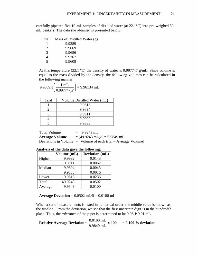
carefully pipetted five 10-mL samples of distilled water (at 22.1 C) into pre-weighed 50-

mL beakers. The data she obtained is presented below:

Trial Mass of Distilled Water (g)

1 9.9389

2 9.9669

3 9.9686

4 9.9767

5 9.9608

At this temperature (22.1 oC) the density of water is 0.997747 g/mL. Since volume is

equal to the mass divided by the density, the following volumes can be calculated in

the following manner:

1 mL9.9389 g = 9.96134 mL

0.997747 g

Trial Volume Distilled Water (mL)

1 9.9613

2 9.9894

3 9.9911

4 9.9992

5 9.9833

Total Volume = 49.9243 mL

Average Volume = (49.9243 mL)/5 = 9.9849 mL

Deviations in Volume = | Volume of each trial – Average Volume|

Analysis of the data gave the following:

Volume (mL) Deviation (mL)

Higher 9.9992 0.0143

9.9911 0.0062

Median 9.9894 0.0045

9.9833 0.0016

Lower 9.9613 0.0236

Total 49.9243 0.0502

Average 9.9849 0.0100

Average Deviation = 0.0502 mL/5 = 0.0100 mL

When a set of measurements is listed in numerical order, the middle value is known as

the median. From the deviation, we see that the first uncertain digit is in the hundredth

place. Thus, the tolerance of the pipet is determined to be 9.98 0.01 mL.

Relative Average Deviation = 0.100 % deviation

0.0100 mL= x 100

9.9849 mL


Part III: Graphical Analysis of Data In this part of the experiment you will collect a set of data to give you the relationship

between the Fahrenheit and Celsius temperature scales. Study Appendix 2 to review what

you should have already learned about the preparation and interpretation of graphs.

Procedure: Work with one partner to obtain the data, but construct a graph

individually.

1. Set up the apparatus as shown in the figure below. First set up the ring stand, iron ring,

wire gauze and Bunsen or Fisher burner. Adjust the height of the iron ring and wire

gauze so that there is about 6 centimeters between the top of the burner and the wire

gauze.

2. Place about 200 mL of hot tap water into a 400-mL beaker and add 2 or 3 boiling chips.

The boiling chips have rough surfaces that enable the water to form bubbles easily as it

boils. They are used as an aid to prevent the water from “bumping.”

3. Light the burner with the striker. Be sure to adjust the burner to give a blue flame (rather

than a yellow flame which produces less heat). This is done by opening up the chimney

to allow more air to go in. (See Figure below.)

Air Vents to control amount of oxygen

Needle Valve to control amount of methane gas

Hottest part of flame is the tip of the blue cone

wire gauze

about 6 cm

to gas valve

ring stand

beaker of water

iron ring

gas burner


4. Heat the water with the burner until the temperature has reached approximate 90 C. In

this experiment all temperatures must be recorded with a digital thermometer to 0.1 C.

5. Meanwhile record the temperature, in °C and °F, of room temperature water that your

instructor has set up in the front of the room. Always record all the digits that show on

the temperature probe. Remember all data must be recorded directly in your notebook

and not on scrap paper.

6. When your water has reached 90 C, one partner should call out the temperature readings

in °C and °F in quick succession while the other partner records them. Temperature

readings must be made with the probe held in the center of the water sample.

7. Turn off the burner and allow the water to cool. When the temperature has dropped

approximately 2 C, quickly record the temperature in both °C and in °F. Continue

doing this until the temperature has reached 70.0 °C.

Note: It is not essential to be recording exactly at 90.0 °C, 88.0 °C, 86.0 °C,

etc. For example, it is perfectly acceptable to record at 90.1 °C, 88.2 °C, and

86.3 °C (as long as they are approximately 2 degrees apart).

8. When you are finished, return all equipment to its proper place. Take extra precaution

that your boiling chips do not get into the sink or down the drain. The temperature

probes MUST BE TURNED OFF before being returned to the side shelf.

Before arriving at the lab, copy the data table below into your lab notebook.

DO NOT RECORD DATA ON THIS PAGE. Record directly in your lab notebook.

Data Table for Part III: Graphical Analysis of Data

Temperature of water at room temp = _________ °C

_________ °F

Temperature of Cooling Water

(starting from the boiling point)

Temp (°C) Temp (°F)

(Prepare a table to accommodate about 12 pairs of data.)

Plotting the Graph Manually:

Read the directions below carefully before you begin plotting!

You may discuss with each other what to do but each partner must do his/her own graph.

Your slope and intercept are not expected to be exactly the same as those of your partner.

1. Use the blank graph paper provided in Appendix 3. In the interest of time, you do not

have to plot all the points for this graph. Select 5 points from your data, spread out fairly


evenly between 90 °C and 70 °C. Indicate clearly in the data table in your lab notebook

with asterisks to show the points you have selected for your graph. Using the graph

paper provided, plot Temp (°F) vs. Temp (°C) for the temperature obtained as the water

cooled to 70.0 °C. By convention this means Temp (°F) goes on the y-axis (the vertical

axis) and the Temp (°C) goes on the x-axis (the horizontal axis). Each point should be

plotted with a sharp pencil, by drawing an X such that the intersection of the X indicates

the position of the point precisely. Include the temperatures of the water at room

temperature. You will be plotting 6 points in total: 5 selected points and the point at

room temperature.

2. Selection of a scale: Reread Appendix 2 on the proper selection of a scale. You need a

scale that is not awkward to read and points that are not bunched up in a small area of

the graph. (In particular, do not pick awkward scales such as using 6 squares for 5

degrees!) Since you will need to read the y-intercept on the graph, your x-scale should

extend from zero to beyond the highest temperature you recorded in C. For the y-scale,

start with 20 °F and go past your highest reading in F.

3. Your graph should indicate a linear relationship. Using a ruler and a sharp pencil, draw

one best straight line through your points. Do NOT draw several lines connecting dot-

to-dot! Your line may not necessarily pass through every single point. It should pass

through most of the points, and if there are points that do not fall on the line, there

should be as many points above as below the line.

4. Label the graph with a title at the top of the page. Next label each axis with a title,

including the units used. At the top right hand corner, write your full name. When you

are finished, show your graph to your partner and discuss with each other what

improvements might be made. Before you proceed, show your graph to your instructor.

Upon approval your graph will be initialed. Your graph is to be turned in at the next lab

period.

Obtaining Information from the Graph:

5. Interpolation: Using your graph, determine what the temperature in °C corresponds to

181.8 °F and record this on the Calculations & Results Page. Next, record the

temperature in °F corresponding to 65.3 °C. Interpolation refers to making a prediction

of values between two known values. If either of the two temperatures happens to be

one of your data points, select another temperature to illustrate “interpolation.”

6. Determine the slope of this line by choosing two points that lie on the line and are easily

read. Do not use your own data points. Record the coordinates used and the calculated

slope on the Calculations & Results Page. Note that since the temperature probe allows

you to read to one decimal place, the coordinates should also be read to no more than

one decimal place only. Be sure to include units for the coordinates and for the slope.

7. Read the y-intercept from the graph and record it on the Calculations & Results Page.

This is done by extrapolating the line to x = zero. Review Appendix 2 if you are not sure


what the y-intercept is. Before you record it, think about how many significant figures

are appropriate. (Hint: How precise are the y-values you measured? The y-intercept

cannot be more precise than your measurements.)

8. Deriving an Equation for the Graph: The equation of a straight line is commonly given

as y = m x + b where m is the slope and b is the y-intercept. Note that the slope is the

coefficient of x in this equation. Using the slope and y-intercept you determined in Step

7 above write the equation for your graph on the Calculations & Results Page.

Use the letter F to represent y and C for x. Do not confuse F with °F. F is a letter to

represent various values of the temperature in degree Fahrenheit, similar to how one

might use M for mass or V for volume. The symbol °F, however, is a unit for the

temperature measured on the Fahrenheit scale. (For example, we can write F = 32 °F

when water freezes.) The same goes for C and °C.

Plotting the Graph with the Use of Excel 2010: The objective is to create a

computer-generated graph to obtain the equation of the line of best fit, which will give us the

information we need. If lab tops are provided in the lab, work together with your partner on

this graph and print out two copies, one for each of you. You should plan on finishing this

graph in the lab before you leave.

If lab tops are not available in the lab, complete this exercise at home or at a computer lab

on campus. Note: All CCBC college computers are using Excel 2010. If you have to create

the graph at home on an older version of Excel these instructions will not be apply.

1. For this graph, do not include the temperature of the water at room temperature. You

will be plotting all the points gathered from the water as it cooled down (not just 5).

2. In the A1 cell (1st row, column A), type “T(deg C)” and in the B1 cell, type “T(deg F)”.

3. Enter your Celsius temperatures in column A, and the corresponding Fahrenheit

temperatures in column B. (Enter only the numbers. Do not include units.)

4. In the D1 cell, type “CHEM 122 – Sec (enter your sec #) – Expt #1 Temperature Scales

– (enter your full name and your partner’s full name).”

5. Highlight both the A and B columns, from Row 1 down to the last row that contains an

entry.

6. Click on the Insert tab, on Scatter, and then on Scatter with only markers.


7. You will be printing the graph embedded within the spreadsheet with both in Landscape

Mode. Place your cursor anywhere on the spreadsheet (not on the graph) and click on

Page Layout tab, Orientation and select Landscape. The dotted lines that appear

indicate the size of the page you will be printing. Click on the frame of the graph and

then resize the graph so that it is as large as possible without letting it spill beyond the

dotted lines. A common error is to set the graph instead of the spreadsheet on Landscape

Mode.

The graph you have created needs adjustments to the title, and to the scales because the

default is to include the (0, 0) causing the points to be all bunched up in a small area.

The following steps will allow you to format the graph to give titles to the graph and to

each axis. You will also format the scales on the two axes as necessary to give a more

acceptable graph.

At this point you will see that a new tab (Chart Tools) has appeared. This tab appears

only when a chart (i.e. graph) has been selected (highlighted). Directly below the Chart

Tools tab are three sub-tabs: Design, Layout, and Format. The instructions below will

focus on the most direct route to creating the graph we want and obtaining the equation

of the line of best fit.

Note the locations of the selections shown by the above arrows that you will be using

under the Chart Tools, Layout in the next few steps.

8. Highlight the title and replace it with a better title that must include your name and that

of your partner’s: “Temp in deg F vs. Temp in deg C - John Doe and Jane Smith”.

9. Click on Chart Tools (1), Layout (2), Axis Titles (3), then select Primary Horizontal

Axis Title, and Title Below Axis. Type in a title for the x-axis (Temp in deg C) and

press ENTER. (3) (1) (2)

(4) (5)


10. Click on Axis Titles (3), then select Primary Vertical Axis Title, and Rotated Title.

Type in a title for the y-axis (Temp in deg F) and press ENTER.

11. Click on Legend (4) and select None.

12. Click on Axes (5), select Primary Horizontal Axis and then on More Primary

Horizontal Axis Options. Since the lowest x-value is probably slightly above 70°C,

there is no reason why the minimum value has to be zero. This is where you are going to

fix the problem of having all the points bunched up in a small area. You do not want a

graph with large blank spaces because you would minimize the space for the section of

the graph that you are interested in. Select Fixed to allow you to change the default

settings.

Set the minimum x-value at a number lower than your lowest x-value. (If your lowest value

is something like 70.4 °C, set it at 70.) Similarly the maximums should be larger than the

highest x-value you have recorded. (If your highest value is 99.8 °C, set it at 100.)

14. Adjust the scale for the y-axis in a similar manner. Click on Axes, select Primary

Vertical Axis and then on More Primary Vertical Axis Options:

In order to include all your data points in your graph, remember your minimum y-value

cannot be larger than your smallest temperature in °F and your maximum cannot be

smaller than your largest temperature in °F.

Suggested settings (which may not work for you, depending on your data):

Minimum = 150; Maximum = 220; Major unit = 10; Minor unit = 1 and change

Minor tick mark type = Outside, then click on Close.

15. Click on Gridlines, select Primary Horizontal Gridlines and Major Gridlines.

16. Click on Gridlines, select Primary Vertical Gridlines and Major & Minor Gridlines.

13. Adjust your Major Unit and Minor Unit so

that the x-scale has reasonable looking numbers.

Try Major Unit = 5 and Minor Unit = 1.

Click on Fixed to allow you to enter these

numbers.

Major Unit controls which numbers are to

show on the scale. Major Unit of 5 means a

number will appear every 5 C. Minor Unit

controls how far apart the minor tick marks are

to be. Minor Unit of 1 means the minor tick

marks are 1 C apart. This will be apparent

only if the Minor tick mark type is not set at

“None.” Go down to Minor tick mark type

and change “None” to “Outside.” When you

are finished, click on Close.

Before proceeding, examine your graph. If there are any “outliers” first check to make sure it is not simply due to an error in entering the data. If it is due to some other error, consult with your

instructor, who will decide whether you should discard that particular point.


21. Highlight the area that contains your data table and the entire graph and click on Page

Layout, Print Area, and select Set Print Area. (If you have trouble highlighting the

entire area with the touch pad, try this: Click once in the A1 cell. Hold down Shift and

use the right ( ) and down arrows ( ) to highlight the area you want to print.)

22. Go over this CHECK LIST before printing your graph:

A) Spreadsheet: Columns must have proper headings and title must be at the top

indicating course, section, experiment # and experiment title, your name and your

partner’s name.

B) Graph must have title at the top and axes must be properly labeled.

C) Trendline must be clearly shown at the top.

D) Spreadsheet must be in Landscape Mode. DOUBLE CHECK!

E) Graph must be enlarged as much as possible but fit within the page.

17. Next add the line of best fit by

clicking Layout, Trendline, and

selecting Linear Trendline.

18. To obtain the equation for the

trendline, click again on Layout,

Trendline, and select More

Trendline Options at the very

bottom. The Format Trendline

window will then appear.

19. Place a check mark at

Display Equation on

chart, and click on Close.

20. If necessary, move the

equation to a position

where it can be read easily

(such as just below the

title). This is done by

clicking on the equation

once and then dragging it

to the desired position.

Close


F) DOUBLE CHECK THAT THE CURSOR IS ON THE SPREAD SHEET JUST

BEFORE YOU PRINT (to ensure graph is embedded in the spreadsheet.)

23. Click on File at the top left corner, select Print, and click on Print Preview to double

check that everything fits on the page. If no adjustments are necessary, click on Print.

Calculations Based On the Excel-Generated Equation: 24. Copy the equation of the trendline (showing as is, with all digits) onto the Calculations

& Results Page.

25. From the equation, copy the slope and the y-intercept onto your Calculations & Results

Page. Re-write the equation by replacing x and y in the equation with C (for temp in C)

and F (for temp in F).

Note: C in this equation is a letter representing the temperature in C, similar to using D

for density. A common student misconception is to think C is the unit. In the same way, F

is not a unit but the letter to represent the temperature in F.

26. Using this new equation (written in terms of C and F) calculate the temperature in C for

181.8 F. Round it to 1 decimal place. Show your calculations in your Calculations &

Results page.

27. Using the equation calculate the temperature in F for 65.3 C. Round it to 1 decimal

place. Show your calculations in your Calculations & Results Page.

28. Are there any outliers in your data? Write your answer on the Calculations & Results

page.

Pre-Lab Exercise: Before coming to the lab, be sure to study Appendix 2 on Preparation and Interpretation of

Graphs. Your instructor will indicate whether you are to submit answers to the following

questions at the beginning of the pre-lab discussion or you will take a pre-lab quiz with

questions similar to the following.

1. If the smallest increment on a ruler is 0.01cm, to how many decimal places should

measurements be recorded?

2. Name two major points to watch out for when selecting a scale for the graph other than

making sure none of the data points are excluded.

3. If the equation of a line is given as y = 7.8 x + 1.9, what is the slope and y-intercept of

this line?

4. If the y-intercept of a line is 2.31 and the slope is 0.825, what is the equation of this line?

5. The following are the coordinates of two points that lie on a line. (s stands for seconds.)

(15.8 s, 78.3 cm) and (29.1 s, 94.2 cm)

What is the slope of the line? Show your calculation setup. Include units in your setup

and in your answer.


Post-Lab Questions: Answers must be typed and in full sentences.

1. How does your experimental tolerance of the 10-mL pipet compare to the tolerance

stated on the pipet? If they are significantly different, give reasons why they are

different. If they are not significantly different, what conclusions can you draw?

2. When you use this 10-mL pipet to deliver a liquid into a container, would you say you

delivered 10 mL, 10.0 mL, 10.00 mL or 10.000 mL? Explain how you reached your

answer.

3. Based on your graphs, were the temperature data you collected accurate? Explain how

you reached your answer.

4. Based on your graph, were the temperature data you collected precise? Explain how you

reached your answer.

5. In Part III, would you have arrived at the same equation if you had used a different

liquid than water?

6. Give the location of each marker to the correct significant figure.

A B C D

E F (exactly on 45) G H

46 45 44 43 mL

7. You are told that a certain measurement has a deviation of 0.1 mL. Is this a large

deviation? What if you were told that a measurement has a 0.1% deviation? Is that a

large deviation? Explain your answers.

8. A student performing Part II neglected to dry the beaker thoroughly before the third trial.

How would that affect the volume of water he reports for the third trial? Explain. Would

this be Instrumental Error, Operator Error or Method Error?

0.3 0.4 0.5 0.6 in


Calculations & Results Name: __________________ Lab Sec: ____

Part I: Uncertainty in Measurement Using Graduated Apparatus

Part II: Uncertainty in Measurement Using the 10-mL Pipet

(Calculation instructions are on p.20-21.)

Temperature of Water = __________

Density of Water (from Handbook) = __________ (including units)

Trial # Mass of Water Volume of Water Deviation of Volume

from Average

1

2

3

4

5

Average N/A

Relative Average Deviation (Percent Average Deviation) = ___________________

Show setup:

Tolerance based on experiment =

Tolerance as listed on pipet =

Name of Apparatus Number of Decimal Places

to be Recorded

Ruler (in cm)



50-mL Buret

250-mL Beaker


Part III: Graphical Analysis of Data Name: __________________

Information from Hand-Drawn Graph:

181.8 F = ______________ C

65.3 C = ______________ F

Coordinates used to calculate the slope (including units). Do not use data points.

(______________, ______________) and (______________, ______________)

Calculation setup for the slope, including units:

Slope = (Include units & correct sig. fig!)

y-intercept = __________ (Include units & correct sig. fig.)

(Read from graph.) Hint: It cannot have more precision than that of your data.

Equation for the graph: ______________________________ (Include units.)

Re-write the equation substituting the letters F and C in place of y and x:

______________________________ (Include units.)


Information from the Excel Graph: Name: __________________

Equation for the trendline: ______________________________

Slope = _______________ (Include units, round to same sig. fig. as hand graph.)

y-intercept = _______________ (Include units, round to same decimal as hand graph.)

Using the equation written in terms of C and F, calculate the temperature in C for

181.8 F. SHOW YOUR WORK:

Using the equation calculate the temperature in F for 65.3 C. SHOW YOUR WORK.

SUMMARY: Include units in your answers.

Based on

Hand Graph

Based on

Excel Graph

Based on

Correct Equation*

Slope

y-Intercept

Equation

T in C for 181.8 F

T in F for 65.3 C

*Look up in a textbook the equation for relating the temperature in C with F.

Reference:

Are there any outliers in your data? Explain your answer in full sentences.

experiment 1: uncertainty in measurementfaculty.ccbcmd.edu/~cyau/122 01 uncertainty in... ·...

Documents