EXPERIMENT 14NUCLEAR MAGNETIC RESONANCE

1 Equipment list

• The Nuclear Magnetic Resonance spectrometer consists of three modules:

– Magnet - in which the sample vial can be inserted.– Case with power supply - this includes the receiver, pulse programmer, and os-

cillator/amplifier/mixer.– Oscilloscope to display the nuclear magnetic resonance signal.

• Sample vials containing copper sulphate solution, glycerine, mineral oil, and water.

References: A. Abragam, “Principles of Nuclear Magnetism”, Clarendon, Oxford (1961).C. P. Slichter, “Principles of Magnetic Resonance”

2 Aim

This experiment introduces you to Pulsed Nuclear Magnetic Resonance (PNMR), which isthe techniques used by all modern NMR spectrometers. You will investigate spin-lattice (T1)and spin-spin (T2) relaxation times, which are the two most important parameters in NMR,and consequently, Magnetic Resonance Imaging (MRI). You will see how these parametersare sensitive to the chemical environment of a liquid (or solid - but we will be investigatingliquids).

1

3 Introduction

Many nuclei behave like they are bar magnets. That is they have a magnetic moment,µ, and an angular momentum, I, where the axis is along the length of the magnet.Classically, a magnetic moment is defined as an electrical current, i, moving in a circle withan area A as shown in Fig. 1. The magnetic moment, µ, is mathematically defined as

Figure 1: The spinning charge distribution of a proton generates a magnetic moment in thesame way that as a circulating electrical current.

µ = iA (1)

where µ is a vector quantity that points along the normal to the plane of the circle. Nowconsider a nucleus with a spin angular momentum I and a magnetic moment µ. These arerelated by

µ = γI (2)

where γ is known as the gyromagnetic ratio and is simply a constant of proportionalitybetween the nuclear magnetic moment and the angular momentum. In this experiment wewill only be considering the nucleus of a hydrogen atoms (i.e. a single proton), which has agyromagnetic ratio of

γproton = 2.675× 108 rad sec−1Tesla−1 (3)

However, we are dealing with a quantum mechanical system. Consequently, the magnitudeof the angular momentum is given by

| I |= h̄ [I(I + 1)]1/2 (4)

where I is the nuclear spin quantum number and h̄ = h/2π, where h is Planck’s constant. Ifan axis of quantization z is defined by applying an external magnetic field with flux densityB0 (which we will refer to as magnetic field strength), the z component of I will be mI h̄,where mI is the magnetic quantum number, which takes the values of ±I,±(I − 1), . . . . . .giving (2I + 1) possible orientations of angular momentum.

For a proton, I = 12 and therefore mI can take values of ±1

2 , which correspond to spinup (+1

2)and spin down (−12). Figure 2 shows the two possible orientations of the angular

momentum of the proton.Note that the angle, β, with the z-axis is given by

cosβ =mI h̄

|I| =mI

[I(I + 1)]1/2(5)

2

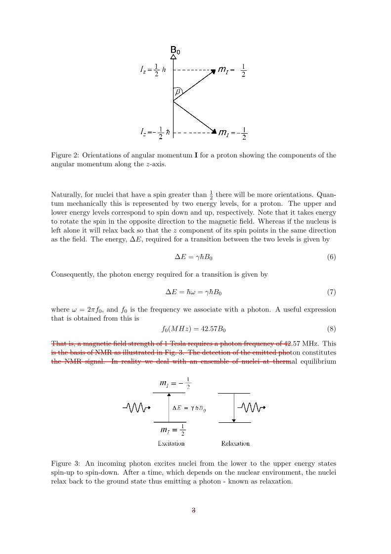
Figure 2: Orientations of angular momentum I for a proton showing the components of theangular momentum along the z-axis.

Naturally, for nuclei that have a spin greater than 12 there will be more orientations. Quan-

tum mechanically this is represented by two energy levels, for a proton. The upper andlower energy levels correspond to spin down and up, respectively. Note that it takes energyto rotate the spin in the opposite direction to the magnetic field. Whereas if the nucleus isleft alone it will relax back so that the z component of its spin points in the same directionas the field. The energy, ∆E, required for a transition between the two levels is given by

∆E = γh̄B0 (6)

Consequently, the photon energy required for a transition is given by

∆E = h̄ω = γh̄B0 (7)

where ω = 2πf0, and f0 is the frequency we associate with a photon. A useful expressionthat is obtained from this is

f0(MHz) = 42.57B0 (8)

That is, a magnetic field strength of 1 Tesla requires a photon frequency of 42.57 MHz. Thisis the basis of NMR as illustrated in Fig. 3. The detection of the emitted photon constitutesthe NMR signal. In reality we deal with an ensemble of nuclei at thermal equilibrium

Figure 3: An incoming photon excites nuclei from the lower to the upper energy statesspin-up to spin-down. After a time, which depends on the nuclear environment, the nucleirelax back to the ground state thus emitting a photon - known as relaxation.

3

distributed between the upper and lower states according the the Boltzmann equation givenby

N↓N↑

= exp(−∆E

kTs) (9)

where N↓ and N↑ are the number of spins with spins down and up (i.e. upper and lowerenergy levels), respectively, k is the Boltzmann constant, and Ts is the absolute tempera-ture of the spin system (which is equal to the lattice temperature when the sample is atequilibrium). In many NMR experiments the objective is to populated the upper energylevel with a greater number of spins than that in the lower level. Then wait for the spins torelax back into the equilibrium distribution of spins. The time required for 1/e of spins todo this is called the spin-lattice or longitudinal relaxation time, T1.

We can describe all of the NMR experiments that we will carry out in terms of the quan-tum mechanical description, but unfortunately this might become a little too mathematicaland abstract. It has been shown by Abragam that a classical description is valid for largeassemblies of independent nuclei, which is the case for our experiments. So we shall adoptthe classical picture since it makes the physics more transparent.

3.1 90◦ pulse

A nucleus placed in a magnetic field will precess around the direction of the field as shown inFig. 4. This bares some resemblance to a spinning top whose angular momentum precesses

Figure 4: The precession of a nuclear magnetic moment around the direction of the magneticfield, B0.

around the direction of the Earth’s gravitational field. However, in a sample consisting ofmany nuclei, the net magnetic moment, M, is the vector sum of all the nuclear magneticmoments, µ. Although the individual magnetic moments make the same angle with thez−axis, their x and y components are distributed uniformly in the xy plane thus producinga zero net magnetic moment in that plane. As a result, the net moment, M, is along thez−axis. NMR can only measure the xy component of M and therefore must be tilted intothe xy plane.

We can tilt M away from the z−axis by applying a magnetic field along the x−axis. As aresult, M will precess about it. But remember, as soon as it is tilted away from z it will nowalso try to precess about it. So clearly the motion is going to become complicated and wewill not reach our objective. We solve this problem by applying a magnetic field, B1, thatrotates in the xy−plane. The rate at which it rotates is equal to the precession frequency(also known as the Larmor frequency) of a magnetic moment. If we step into the rotatingframe by standing along the z−axis and spinning at the precession frequency, we will see

4

a stationary B1. Let’s now define x, y, and z axes in the rotating frame of reference andcall them x′, y′, and z′, respectively. Note that z and z′ are the same since that is the axisof rotation. As shown in Fig. 5, in the rotating frame B0 and B1 will add vectorially to

Figure 5: In the rotating frame, the magnetic moment M will precess about an effectivefield, Beff , which results from the vectorial addition of B1 and B0.

produce an effective field Beff , which will cause M to precesses in the direction shown bythe arrow in Fig. 5. By applying B1 for an appropriate time, we can cause M to rotateinto the xy plane as shown in Fig. 6(a), which is known as a 90◦ pulse simply because thenet magnetic moment has rotated from the z−axis to the x′y′−plane. Remember that we

(a) (b)

Figure 6: (a) A 90◦ pulse means that M now lies in the x′y′−plane (i.e. in the rotatingframe), (b) In the laboratory reference frame, the net magnetic moment, M, will rotate inthe xy−plane.

are still in the rotating frame. If we step back into the laboratory frame we will see that Mrotates in the xy−plane as shown in Fig. 6(b).

We are now in a position to detect the M by placing an induction coil whose axis liesin the xy−plane, as shown in Fig. 7. The induced oscillating voltage will have a frequencyequal to the precession frequency. This is our NMR signal. If that was all there isto it then we would get no extra information about the material other than its precessionfrequency. However, the interaction of individual magnetic moments with each other andtheir environment makes NMR such a useful technique, which we shall now discuss.

5

Figure 7: The rotating M in the xy−plane will induce an oscillating voltage between theends of a wire coil whose axis is in the xy−plane.

3.2 Free Induction Decay

The signal induced in a coil after a 90◦ pulse decays exponentially because the net magne-tization in the xy−plane decays exponentially as shown in Fig. 8. This is known as FreeInduction Decay (FID). The reason for this is that the individual spins experience differ-

Figure 8: The exponential decay of the net magnetization in the xy−plane.

ent magnetic fields from their local environment, which includes fluctuating magnetic fieldsdue to the other spins as well as inhomogeneities in the applied magnetic field. As a result,the precession frequency of each spin becomes slightly different to the others. In the rotatingframe this appears as a spread in the orientations of the spins as shown in Fig 9(a). We saythat spins are no longer in phase. Eventually, the spins are distributed uniformly over theentire x′y′− plane, as shown in Fig. 9(b) so that there is no net magnetization and thereforeno induced signal in the coil. The exponential decay in the net magnetization and thereforein the induced signal is given by

M(t) = M0e− t

T2 (10)

where M(t) is the net magnetization after a time t, M0 is the initial net magnetization, andT2 is known as the spin-spin or transverse relaxation time. It is this parameter thatis sensitive to the local environment of the nucleus.

In reality, the applied magnetic field can be nonuniform across the sample. As a result,the spreading out of the spins in the rotating frame (also known as dephasing) can bedominated by this field inhomogeneity and result in a faster Free Induction Decay (FID),given by the following

M(t) = M0e− t

T∗2 (11)

6

(a) (b)

Figure 9: (a) The individual spins precess at slightly different frequencies due to the differ-ent local magnetic environments, (b) Spins eventually become uniformly distributed in therotating frame so that there is no net magnetization.

where T ∗2 is known as the effective spin-spin or transverse relaxation time. We needto eliminate the contribution of the field inhomogeneity in order to obtain the actual T2 andtherefore know something about the material we are investigating. This is carried out bythe spin-echo pulse sequence described in the following section.

3.3 Spin-Echo Pulse Sequence

This is a sequence of two or more pulses in order to eliminate the effect of magnetic fieldinhomogeneity. All magnets can have some inhomogeneity, so the pulse echo method formsthe basis of most NMR experiments. The method is illustrated in Fig. 10. After a 90◦ pulse

(a) (b)

Figure 10: (a) The dephasing spins can be made to refocus by applying a 180◦ pulse alongthe x′ axis, (b) After the 180◦ pulse the spins flip by 180◦ so now they move towards eachother and refocus to produce a net magnetization and therefore produce a signal, known asan echo.

the spins start to dephase and therefore reduce the size of the NMR signal. Applying asecond pulse twice as long as the 90◦ pulse (along the x′ axis) causes the spins to be rotatedby 180◦ about the x′. The spins will then move towards each other and come to a focus asshown in Fig. 10(b) resulting in another signal called an echo. The height of the echo at thatpoint in time is the same as the amplitude of the FID had there been an absolutely uniformmagnetic field. A schematic diagram of this is shown in Fig. 11. A 90◦ pulse is applied to tip

7

Figure 11: The 90◦− τ − 180◦− τ− echo experiment. The detected FID decays quickly dueto magnetic field inhomogeneities, but the amplitude of the echo gives the amplitude of theactual FID at the position of the echo.

the net magnetic moment into the x′y′−plane. As the individual spins dephase and producean FID mostly due to magnetic field inhomogeneities, a 180◦ pulse is applied after a time τ toput the spins back in phase thus resulting in an echo at time τ after the second pulse. Thatis, the echo appears at a time of 2τ after the first pulse. The height of the echo is equal to theamplitude of the actual FID had there been a uniform magnetic field. Consequently, a plotof echo height versus varying values of 2τ gives the actual FID, and consequently allows thecalculation of the spin-spin relaxation time, T2, given by Eq. (10). In short-hand notation,this pulse sequence is written as 90◦ − τ − 180◦ − τ−echo or π/2x′ − τ − πx′ − τ−echoy′

pulse sequence. The subscript x′ implies that the pulse was applied along the x′−axis,whereas the detection of the echo was along the y′−axis. In practice, this means that whenthe instrument is detecting the echo it looks for a signal that is 90◦ out of phase with theapplied pulse signal.

Instead of varying 2τ in order to obtain a plot of the actual FID, there is a faster methodknown as a Carr-Purcell pulse sequence discussed in the next section.

3.4 Carr - Purcell pulse sequence

A way of shortening the time it takes to measure T2 from a spin-echo experiment was firstcarried out by Carr and Purcell in 1954. A 180◦ pulse is applied at a time τ after the echoof the 90−180−pulse sequence described in the previous section. This will result in anotherecho at time 4τ . One can continue to apply 180◦ pulses with a spacing of 2τ with echoesoccurring between each pulse, as shown in Fig. 12. The height of the echoes is governed by

Figure 12: The Carr-Purcell pulse sequence for obtaining T2. The dashed line shows theexponential decay of the amplitude of the echoes. The reflect the actual FID.

the exponential decay given in Eq. (11). Consequently, it will be possible to obtain T2.

8

3.5 Meiboon - Gill pulse sequence

In practice, the Carr-Purcell pulse sequence usually result in measured T2’s that are too shortbecause of cumulative errors of each pulse not being exactly 180◦ and of the inhomogeneityof the amplitude of the applied RF magnetic field B1. A common way to compensate forthese errors is the Meiboon-Gill pulse sequence. This is a modification of the Carr-Purcellsequence (CPMG) in which all the 180◦ pulses are phase shifted by 90◦ with respect to theinitial 90◦ pulse. That is, if the 90◦ pulse is applied along the x′ axis, then the 180◦ pulsesare applied along the y′ axis (remember these are the axes in the rotating frame).

3.6 Measurement of Spin-Lattice relaxation, T1

The determination of the characteristic time required for the magnetization to return alongthe z−axis, T1, is generally time consuming because it is usually not a “one shot” methodlike the CPMG sequence.

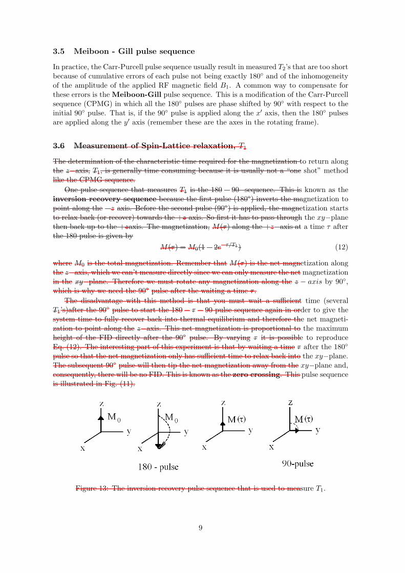
One pulse sequence that measures T1 is the 180 − 90−sequence. This is known as theinversion recovery sequence because the first pulse (180◦) inverts the magnetization topoint along the −z axis. Before the second pulse (90◦) is applied, the magnetization startsto relax back (or recover) towards the +z axis. So first it has to pass through the xy−planethen back up to the +zaxis. The magnetization, M(τ) along the +z−axis at a time τ afterthe 180 pulse is given by

M(τ) = M0(1− 2e−τ/T1) (12)

where M0 is the total magnetization. Remember that M(τ) is the net magnetization alongthe z−axis, which we can’t measure directly since we can only measure the net magnetizationin the xy−plane. Therefore we must rotate any magnetization along the z − axis by 90◦,which is why we need the 90◦ pulse after the waiting a time τ .

The disadvantage with this method is that you must wait a sufficient time (severalT1’s)after the 90◦ pulse to start the 180− τ − 90 pulse sequence again in order to give thesystem time to fully recover back into thermal equilibrium and therefore the net magneti-zation to point along the z−axis. This net magnetization is proportional to the maximumheight of the FID directly after the 90◦ pulse. By varying τ it is possible to reproduceEq. (12). The interesting part of this experiment is that by waiting a time τ after the 180◦

pulse so that the net magnetization only has sufficient time to relax back into the xy−plane.The subsequent 90◦ pulse will then tip the net magnetization away from the xy−plane and,consequently, there will be no FID. This is known as the zero crossing. This pulse sequenceis illustrated in Fig. (11).

Figure 13: The inversion-recovery pulse sequence that is used to measure T1.

9

3.7 Experimental Setup

Figure 14is a simplified schematic diagram of the NMR apparatus that you’ll be using.The diagram doesn’t show all the functions of each module, but it does represent the most

Figure 14: A schematic diagram of the NMR spectrometer.

important functions of each modular component of the spectrometer.The pulse programmer creates the pulse that controls the length of the radio-frequency

(RF) pulse from the RF Oscillator, as well as triggering the oscilloscope on the appropriatepulse. The RF pulse is amplified and sent to the transmitter coils, which are around thesample. The RF current in this coil produces a homogeneous 12 Gauss rotating magneticfield at the sample. This is the time-dependent B1 field that produces the 90◦ or 180◦ pulses.Remember that the direction of the static magnetic field from the permanent magnet isconsidered to be along the z−axis. Let’s assume that the transmitter coil’s axis is along they−axis, thus the coil that picks up the NMR signal is along the x−axis. Notice that thispick-up coil is the one tightly wound around the sample in the diagram.

Any rotating magnetization in the xy−plane induces a voltages in the pick-up coil, whichis then amplified by the receiver circuitry. This amplified radio frequency (15 MHz) signalcan be detected by two separate and different detectors. The box labelled “Detector” in thediagram simply outputs the positive amplitude of the RF-signal from the pick-up coil. Thisis the detector that you will use to record both the free induction decays and the pulse-echosignals.

The other detector is a mixer, which multiplies the signal from the pick-up coil withcontinuous RF-signal from the oscillator. The output frequency is proportional to the dif-ference between the two frequencies. This idea is the same as that of “beats” for soundwaves. Two similar (but not exactly the same) waves will produce a beating sound. In thesame way if the signal from the pick-up coil and the synthesis are not the same then theoutput frequency from the mixer is the difference between the two. If the two signals havethe same frequency then there will not be any oscillations from the output of the mixer.The mixture is essential for tuning the apparatus. The dual channel oscilloscope will showboth the detector and mixer outputs.

4 Procedure

Note that the bench notes explain the front panel of the spectrometer in moredetail. Make sure you refer to them since this will enable you to carry out theexperiment with less head-scratching.

10

4.1 Tuning

The following procedures will enable you to tune the applied frequency so that it equals theresonant frequency of the precessing nuclei.

• Turn on the spectrometer from the spectrometer from the switch at the back. It willdisplay a frequency of 15.40000 MHz.

• Insert the Mineral oil sample in the magnet and set up the following parameters.

– Width of pulse A: 20% of full range .

– Mode: Int

– Repetition time: 100 ms, 100% of full range.

– Number of B Pulses: 0

– Sync A

– A: On, B: Off

– Time constant: 0.01

– Gain: 30%

• We must now tune the spectrometer to the precession frequency of the nuclei. Look atthe trace of the mixer output on the oscilloscope. Adjust the frequency so that thereis zero beating (that is, no oscillations) from the mixer output.

• Now tune the receiver input for maximum signal.

• Look at the detected output and adjust the width of pulse A until the Free InductionDecay is a maximum. This is the so called 90◦ pulse. Note that the voltage measuredon the oscilloscope is directly proportional the the magnetization M(t) given in thetheory section of these notes.

• If you double the pulse width the Free Induction Decay should vanish, in which caseyou now have a 180◦ pulse.

4.2 Magnetic Field Uniformity

After you have found a free induction decay signal and set the spectrometer for a 90◦ pulse,it is time to find the most uniform part of the magnet. This is the so called “sweet spot”.The two controls on the sample carriage allow you to move the sample in the x − y plane.The magnetic field at the sample uniquely determines the frequency of the free-inductiondecay signal. The most uniform part produces the longest spin-spin relaxation time, T ∗2 .

• Try different positions by using the the x and y controls on the carriage until you findthe positions where T ∗2 is the longest, i.e. the longest FID. Try to make the detectedsignal so that it looks like a smooth exponential decay. If there are bumps in thedecay, then it means that you are in a highly non-uniform part of the field. Alwayschecke the mixer signal to see that you are on resonance.

• Record this value of T ∗2 , the resonant frequency, and the x and y positions where thesemeasurements were taken. The exponential decay of this FID is by Eq. (11), so youwill need this equation to determine T ∗2 .

11

• Note that you will have to change the frequency back to resonance (that is no oscilla-tions on the mixed signal) for each position since the resonant frequency changes withdifferent magnetic field strength.

Caution: The magnetic field in the gap changes with the changing room temperaturethroughout the day. So you must keep an eye on the mixer output in order to ensure thatthe spectrometer is on the resonant frequency.

The field difference (known as field gradient) over the sample can be estimated from T ∗2assuming that the field gradient is the major contributor to T ∗2 . For example, for mineraloil the real T2 is much longer than T ∗2 .

• Determine the change in the magnetic field, ∆B, across your sample by obtaining1/T ∗2 which is equal to change in resonant frequency, ∆f , across the sample. You canthen use this in the difference form of Eq. (8) such that

∆f(MHz) = 42.57∆B (13)

QUESTION: Explain why the most uniform part will produce the longest T ∗2 .

C1 .Tutor checkpoint. Obtain tutor’s signature before proceeding.

We will now determine the true spin-spin relation time T2, which is independent of themagnetic field gradient.

4.3 Spin-Spin relaxation time, T2, using only two pulses

• Use a two pulse spin-echo sequence, as outlined in the theory section to measure thespin-spin relaxation time, T2 for the mineral oil. Note that the ORIGIN program caneasily fit exponential decay equations to your data so that you can obtain T2.

4.4 T2 using CPMG

• Now measure the T2 for mineral oil using the Carr-Purcell-Meiboom-Gill pulse se-quence outline in the theory section.

• Make sure the M-G switch is on, which is located on the AMP/MIXER module.

• Compare the T2 obtained in this way with the T2 obtained from the previous section.

• Repeat the measurement for glycerine.

• There is a relationship between viscosity and T2. There are three oils (thin, medium,and thick) that you can use to qualitatively determine this relationship (if you havetime).

C2 .Tutor checkpoint. Obtain tutor’s signature before proceeding.

4.5 Spin-lattice relaxation time, T1

Before we make use of the pulse sequence given in the Theory section for measuring T1, wewill now examine a quick method for measuring it. Let’s start with an order of magnitudeestimate using the mineral oil sample.

• Adjust the spectrometer to resonance for a single pulse free induction decay signal.

12

• Change the Repetition time, reducing the FID until the maximum amplitude is re-duced by about 1/3 of its largest value.

The order of magnitude of T1 is the repetition time that was established in the second stepabove. Setting the repetition time equal to the spin-lattice relaxation time means that themagnetization does not return to its thermal equilibrium value before the next 90◦ pulse.Thus, the maximum amplitude of the free induction decay is reduced to about 1/e of itslargest value. Such a quick measurement is useful since it gives you a good idea of the timeconstant you are trying to measure and allows you to set up the experiment correctly thefirst time.

4.6 Spin-lattice relaxation time using inversion-recovery

• Now devise a method using the inversion-recovery two pulse sequence, given in thetheory, in order to obtain the spin-lattice relaxation time for mineral oil and glycerine.

• Note that you will now have to turn on pulse B.

• Also note that the trace of the oscilloscope can be made to start after pulse B byswitching the “Sync” switch to B on the pulse programmer.

• Compare the results for both the mineral oil and glycerine.

C3 .Tutor checkpoint. Obtain tutor’s signature before proceeding.

13