experimental aircraft parameter estimationadl.stanford.edu/groups/aa241x/wiki/e054d... ·...

Roberto A . Bunge

AA241X

May 14 2014 S tanford Univers i ty

Experimental Aircraft Parameter Estimation

AA241X, May 14 2014, Stanford University Roberto A. Bunge

Overview

Roberto A. Bunge AA241X, May 14 2014, Stanford University

1.  System & Parameter Identification

2.  Energy Performance Estimation ¡  Propulsion OFF ¡  Propulsion ON

3.  Stability & Control Derivative Estimation ¡  Based on Trim & CG shifting ¡  Linear regressions from dynamic data

4.  Measuring Moments of Inertia

System Identification


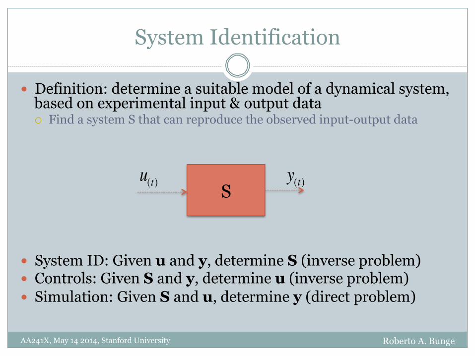
�  Definition: determine a suitable model of a dynamical system, based on experimental input & output data ¡  Find a system S that can reproduce the observed input-output data

�  System ID: Given u and y, determine S (inverse problem) �  Controls: Given S and y, determine u (inverse problem) �  Simulation: Given S and u, determine y (direct problem)

S u(t ) y(t )

System ID vs. Parameter ID


�  System ID: find the structure of S ¡  Very hard problem ¡  Potentially infinite number of models that can produce the same input-

output pairs, especially given noise in the data ¡  In practice, need to reduce the search to a given class of models

�  Parameter ID: given the structure of S, find the values of certain coefficients ¡  Much more tractable ¡  Incorporate prior knowledge about the structure of the system that we

know from first principles ¡  Many tools available

�  System ID is “just” data fitting ¡  Lots of overlap with Linear Algebra, Digital Signal Processing and

Machine Learning

Parameter ID


�  System model can have linear or nonlinear dynamics, and can be linear or nonlinear w.r.t. unknown parameters ¡  If linear in parameters, there are lots of tools to solve efficiently ¡  Thus, usually its a linear combination of regressors

�  is the vector of “free” coefficients in the model ¡  In a linear dynamic model, these could be elements of the A,B,C,D matrices

�  Need to compare the “quality” of different models with a Figure of Merit,

usually a sum of squared errors. For example:

�  is the measured output, and is the predicted output, if we apply the measured inputs to our model

E(θ ) = [ !yk −k∑ yk (u0…k,θ )]

2

θ

y

!x = θ xi fi (x,u)∑ +ε

y = θ yiigi (x,u)∑ +η

!y

Parameter ID (II)


�  Goal: find that minimizes error E:

�  This is just an optimization problem, have lots of tools to do this! Should be easy… ¡  If model is explicit, then we should be able to calculate:

�  In practice, its an art as well as a science: ¡  We have to provide the model structure! ¡  Need to define E ¡  The data has to be “good”:

÷  The experiments have to be good ÷  Noise should be low

¡  May have local minima…

�  Moreover, what we really want is to minimize E on new data ¡  What is the guarantee that minimizing E, will produce a good model?

θ ID = argminθ

E(θ )θ

∂E∂θ, ∂

2E∂2θ

,...

Parameter ID (III)


�  There are common issues in Parameter ID (beyond those of numerical optimization):

1.  Experimental data might have “little information” ¡  Number of data points too few ¡  Collinearity of data points and regressors (a.k.a linearly dependent equations) ¡  Input-output space is not covered enough

÷  Need to cover all the state & control space ÷  Need to excite all modes

¡  Unmeasured/Unmodeled disturbances

2.  Model complexity vs. noise fitting ¡  If model is very complex and we have few data points, it will have flexibility to contort and fit

the measured data very well ¡  But… this contortion can be too much, producing very bad predictions of new data. This is

known as “chasing the noise”

�  Ideally low order model that represents major effects, lots of measurements with low noise and excitation of all the modes

Parameter ID (IV)


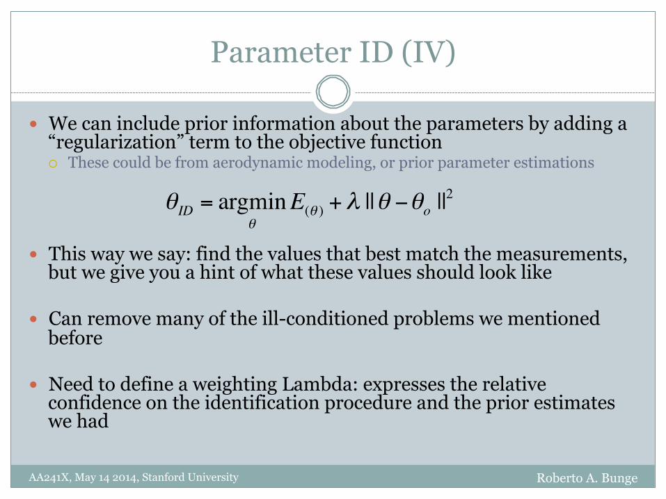
�  We can include prior information about the parameters by adding a “regularization” term to the objective function ¡  These could be from aerodynamic modeling, or prior parameter estimations

�  This way we say: find the values that best match the measurements, but we give you a hint of what these values should look like

�  Can remove many of the ill-conditioned problems we mentioned before

�  Need to define a weighting Lambda: expresses the relative confidence on the identification procedure and the prior estimates we had

θ ID = argminθ

E(θ ) +λ ||θ −θo ||2

Frequency Domain System ID


�  Parameter estimation can also be done in the Frequency Domain

�  Need to convert time-domain data into the frequency domain, using the Fourier Transform

�  Can be:

¡  More robust ¡  Faster, due to reduced data points in converting to

frequency ¡  More useful, since we can directly do control design with it

Performance Estimation


�  The (energy) performance of an electric aircraft is characterized by: 1.  Lifting aerodynamic efficiency 2.  Motor efficiency 3.  Propeller efficiency

�  In trim flight:

T = D+ Lsin(γ ) = DLL + sin(γ ) = [D

L+ sin(γ )]mg

CL =mg

1 2ρSV(δe )2

Propulsion OFF


�  When propulsion is off (glide):

�  By gliding at different velocities (i.e. different elevator positions) and measuring the trim velocity and glide path angle, we can obtain the L/D vs. CL curve

�  Need to do this in calm conditions, since wind is not measured

�  If lightly damped, the phugoid motion will be superimposed, and measurements will not be as good: ¡  Having a phugoid damper can improve the estimates, and increase productivity

of flight testing ¡  We need to average across several seconds

DL(CL ) = −sin(γ )

Propulsion ON


�  The electric power consumption is given by

�  Having obtained the L/D curve from the glide tests, we can now fly

with different throttle positions and speeds, and obtain the overall propulsive efficiency

�  Having an RPM sensor would allow for the characterization of the motor efficiency, and thus we could isolate the propeller efficiency:

Pelectric =VeA = [DLV + !h] mg

ηpropηmotor

ηpropηmotor = [DLV + !h] mg

VeA

ηprop = [DLV + !h] mg

VeAηm (Ω,v,R,Kv )

Propwash effects


�  In practice, the airflow over the wing is not the same when propeller is on and off

�  Thus, the L/D curve obtained during glides is not fully representative when the propeller is producing thrust

�  Some effects of propwash: 1.  Increased velocity within slipstream à Increase dynamic pressure,

thus drag on wing, fuselage and tail 2.  Swirl à Induced drag on wing and tail 3.  If propeller is angled, might also change angle of attack

SD & CD Estimation from Trim Flight & CG Shifting


�  We can also estimate Stability & Control Derivatives by flying at specific trim conditions

�  In UAVs its possible to shift the CG around to create useful trim conditions

�  Spanwise GC shift: lateral derivatives can be estimated by adding a small weight on the tip of the wing, and trimming it out with control surfaces

�  Moment balance at trim: Cl =

mghyqSb

=Clδaδa+Clβ

β +Clδrδr

Cn = 0 =Cnββ +Cnδr

δr +Cnδaδa

mg

h_y

Lateral CG Shifting


�  Test 1: deflect ailerons (and rudder if necessary)

�  Test 2: deflect rudder only, to induce sideslip

mgh1yqSb

=Clδaδa1 +Clδr

δr1

0 =Cnδrδr1 +Cn δa

δa1

mgh2yqSb

=Clββ2 +Clδr

δr2

0 =Cnββ2 +Cnδr

δr2

(1)

(2)

Lateral CG Shifting


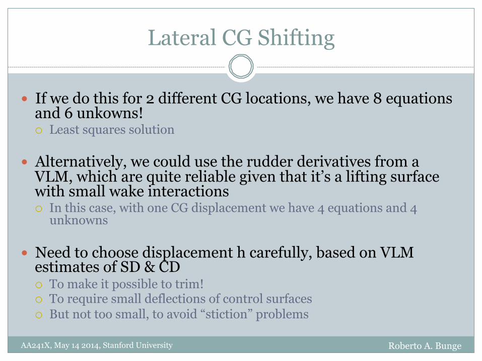
�  If we do this for 2 different CG locations, we have 8 equations and 6 unkowns! ¡  Least squares solution

�  Alternatively, we could use the rudder derivatives from a VLM, which are quite reliable given that it’s a lifting surface with small wake interactions ¡  In this case, with one CG displacement we have 4 equations and 4

unknowns

�  Need to choose displacement h carefully, based on VLM estimates of SD & CD ¡  To make it possible to trim! ¡  To require small deflections of control surfaces ¡  But not too small, to avoid “stiction” problems

Longitudinal CG Shifting


�  Test 0: Measure base trim condition

�  Test 1: Add or remove weight at the CG

�  Test 2: Move CG forward or back

�  Thus, 4 equations and 4 unkowns

h_x

mg

(m+Delta_m) g

CL =CL0=mgq0S

CL =(m+Δm)g

q1S=CL0

+CLαΔα1 +CLδe

δe1

Cm = 0 =CmαΔα1 +Cmδe

δe1

CL =mgq2S

=CL0+CLα

Δα2 +CLδeδe2

Cm =mghxq2Sc

=CmαΔα2 +Cmδe

δe2

Trim based Estimation


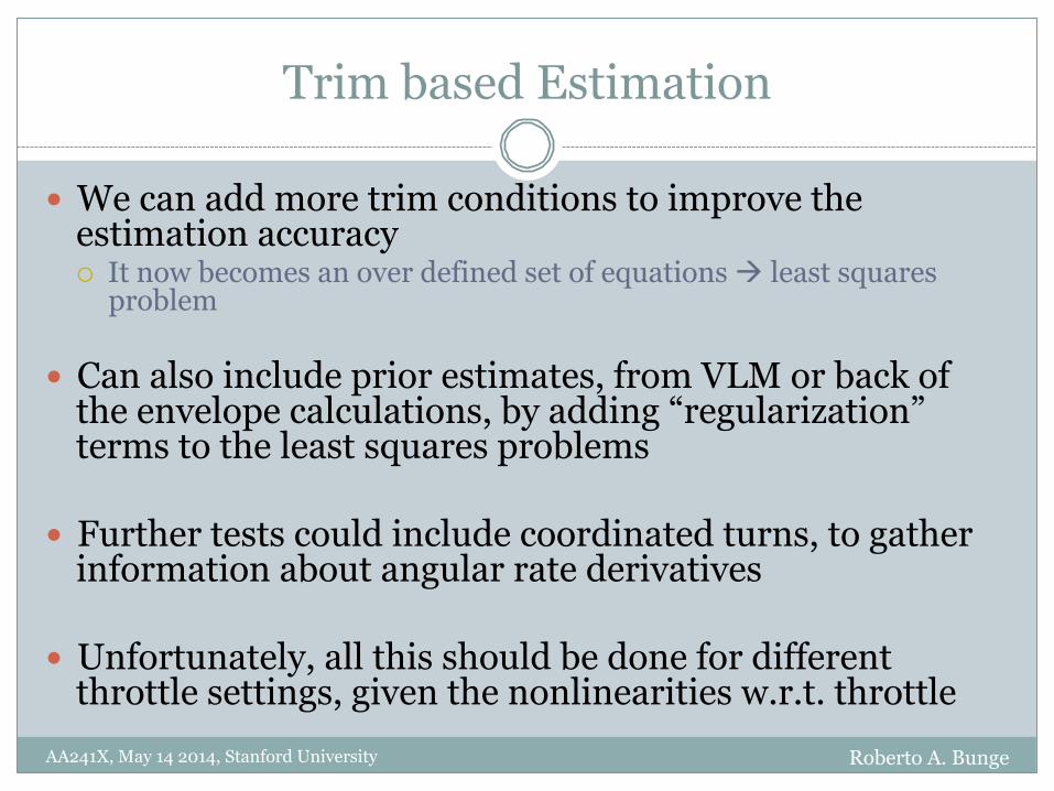
�  We can add more trim conditions to improve the estimation accuracy ¡  It now becomes an over defined set of equations à least squares

problem

�  Can also include prior estimates, from VLM or back of the envelope calculations, by adding “regularization” terms to the least squares problems

�  Further tests could include coordinated turns, to gather information about angular rate derivatives

�  Unfortunately, all this should be done for different throttle settings, given the nonlinearities w.r.t. throttle

Linear Regressions from Dynamic Data


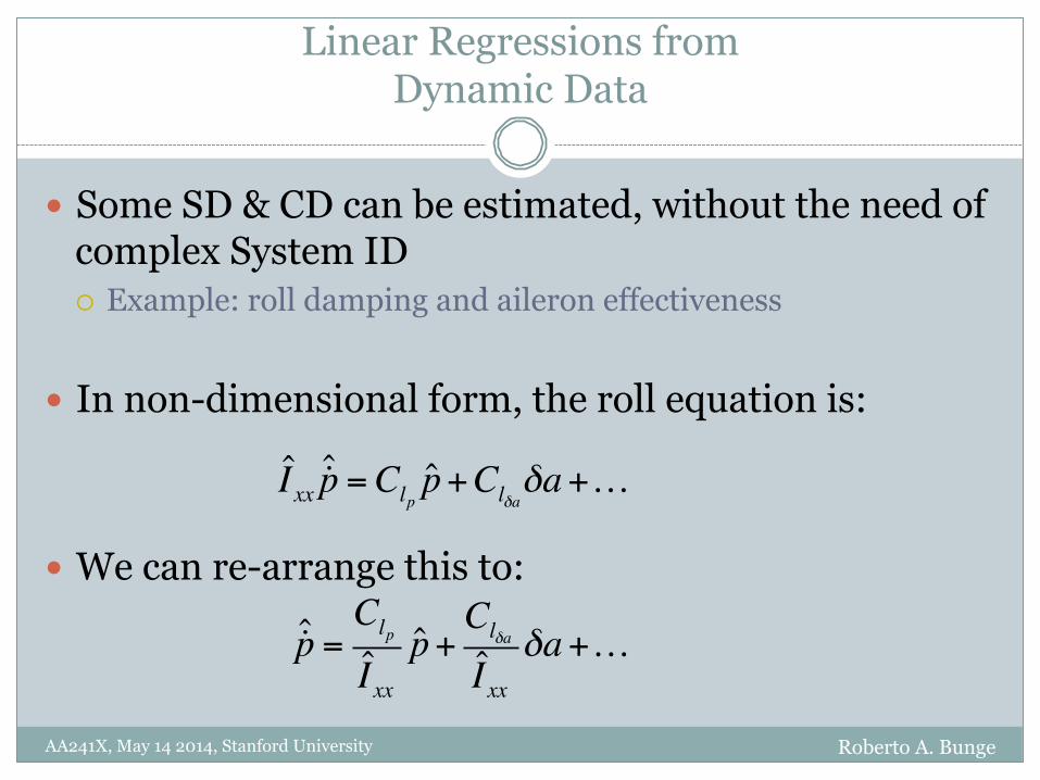
�  Some SD & CD can be estimated, without the need of complex System ID ¡  Example: roll damping and aileron effectiveness

�  In non-dimensional form, the roll equation is:

�  We can re-arrange this to:

I xx !p =Clpp+Clδa

δa+…

!p =Clp

Ixxp+

Clδa

I xxδa+…

Linear Regressions from Dynamic Data(II)


�  Using flight data for the Bixler 2* gathered at 50Hz, we can numerically differentiate the roll rate to obtain an estimate of roll acceleration

�  If we plot data points for which roll acceleration is almost zero we have:

* Thanks to Adrien Perkins and Drone Identity for gathering the flight data!

!p ≈ 0⇒ p =Clδa

Clp

δa

Clδa

Clp

≈ 0.43−0.6 −0.4 −0.2 0 0.2 0.4 0.6

−0.2

−0.15

−0.1

−0.05

0

0.05

0.1

0.15

Equilibrium roll rate vs. aileron deflecion

aileron deflection (fraction of full deflection)

Non−d

imen

sion

al ro

ll−ra

te


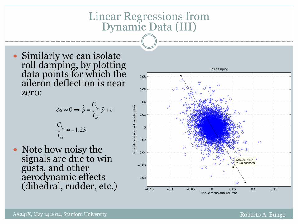
�  Similarly we can isolate roll damping, by plotting data points for which the aileron deflection is near zero:

�  Note how noisy the

signals are due to win gusts, and other aerodynamic effects (dihedral, rudder, etc.)

δa ≈ 0⇒ !p =Clp

Ixxp+ε

Clp

Ixx≈ −1.23

−0.15 −0.1 −0.05 0 0.05 0.1 0.15

−0.08

−0.06

−0.04

−0.02

0

0.02

0.04

0.06

0.08

X: 0.0516436Y: −0.0635985

Roll damping

Non−dimensional roll rate

Non−d

imen

sion

al ro

ll ac

cele

ratio

n

Linear Regressions from Dynamic Data (III)


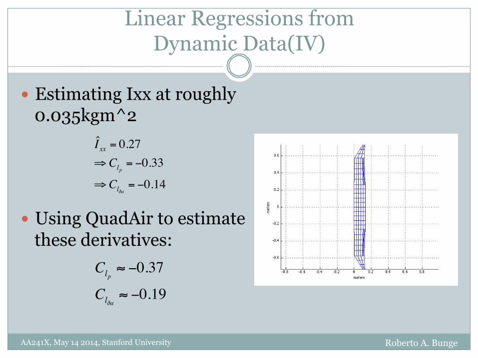
�  Estimating Ixx at roughly 0.035kgm^2

�  Using QuadAir to estimate

these derivatives:

I xx = 0.27⇒Clp

= −0.33

⇒Clδa= −0.14

Clp≈ −0.37

Clδa≈ −0.19

Linear Regressions from Dynamic Data(IV)

Linear Regressions from Dynamic Data(V)


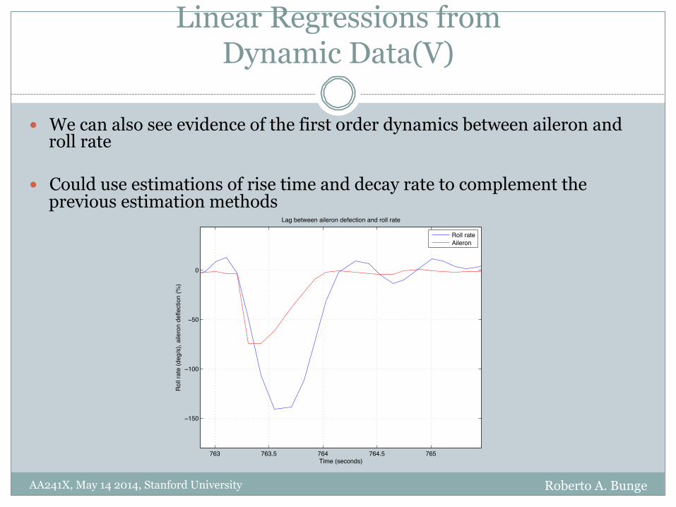
�  We can also see evidence of the first order dynamics between aileron and roll rate

�  Could use estimations of rise time and decay rate to complement the previous estimation methods

763 763.5 764 764.5 765

−150

−100

−50

0

Lag between aileron defection and roll rate

Time (seconds)

Rol

l rat

e (d

eg/s

), ai

lero

n de

flect

ion

(%)

Roll rateAileron

Measuring Moments of Inertia


�  The easiest way to measure the moment of inertia of a body is to use a trifilar pendulum

�  The period of oscillation T and moment of inertia I are related by:

÷  W: weight of body ÷  R: distance from strings to the center ÷  L: length of strings

I=Wr2T 2

4π 2L

Ib=(Wb +Wp )r

2Tb+p2

4π 2L− I p

Measuring Moments of Inertia


�  Procedure: 1.  Measure constants r & L 2.  Measure weight of platform W_p 3.  Measure the torsional oscillation period T_p of the platform only, and calculate

the moment of inertia of the platform I_p 4.  Measure weight of body W_b 5.  Place body on the platform with its CG in the center, and with the axis of

interest parallel to the strings 6.  Measure the torsional oscillation period T_b+p, and calculate the moment of

inertia of the body by substracting that of the platform �  To reduce measurement error we need to:

¡  Reduce timing error à measure multiple consecutive oscillations ¡  Increase radial distance r ¡  Reduce I_p (as small as can hold the body) ¡  Increase L (as big as possible) ¡  Make sure CG is centered ¡  Make sure the “strings” are rigid

experimental aircraft parameter estimationadl.stanford.edu/groups/aa241x/wiki/e054d... ·...

Documents