Louisiana State UniversityLSU Digital Commons

LSU Doctoral Dissertations Graduate School

2006

Experimental and computational analysis ofrandom cylinder packings with applicationsWenli ZhangLouisiana State University and Agricultural and Mechanical College wzhang2lsuedu

Follow this and additional works at httpsdigitalcommonslsuedugradschool_dissertations

Part of the Chemical Engineering Commons

This Dissertation is brought to you for free and open access by the Graduate School at LSU Digital Commons It has been accepted for inclusion inLSU Doctoral Dissertations by an authorized graduate school editor of LSU Digital Commons For more information please contactgradetdlsuedu

Recommended CitationZhang Wenli Experimental and computational analysis of random cylinder packings with applications (2006) LSU DoctoralDissertations 163httpsdigitalcommonslsuedugradschool_dissertations163

EXPERIMENTAL AND COMPUTATIONAL ANALYSIS OF RANDOM CYLINDER PACKINGS WITH APPLICATIONS

A dissertation

Submitted to the Graduate Faculty of the Louisiana State University and

Agricultural and Mechanical College in partial fulfillment of the

requirements for the degree of Doctor of Philosophy

in

The Cain Department of Chemical Engineering

by Wenli Zhang

BS Tsinghua University Beijing P R China 1993 ME Institute of Coal Chemistry Chinese Academy of Science 1996

December 2006

ACKNOWLEDGEMENTS

I would like to thank my major advisor Dr Karsten Thompson who provided me

with guidance suggestions and assistance This work would have been impossible

without his patience and support I would also like to thank my committee members (Dr

Gregory Griffin Dr Steven Watkins Dr Brian Mitchell Dr James Henry Dr Clinton

Willson Dr Danny Reible Dr Benjamin McCoy) for their time and many valuable

suggestions

This work was funded by NSF 0140175 amp 0140180 and collaborated with Dr

Mitchellrsquos lab at Tulane University I appreciate Dr Mitchell and his student for

performing the visualization experiments Special thanks should also go to Dr Allen

Reed who helped us with X-ray tomography experiments in Navy Research Lab Stennis

Space Center

I want to give thanks to my fellow graduate students Le Yan Matthew Balhoff

Pradeep Bhattad and Nathan Lane I appreciate the work of REU undergraduate student

Liese Beenken from University of Arizona in summer 2004 I am grateful to all the

people in our department who provided a lot of assistance

Last but not the least I would like to thank my family who helped and supported

me to finish this work

ii

TABLE OF CONTENTS

ACKNOWLEDGEMENTShelliphelliphelliphelliphelliphelliphelliphelliphelliphelliphelliphelliphelliphelliphelliphelliphelliphelliphelliphelliphelliphelliphellipii

LIST OF TABLEShelliphelliphelliphelliphelliphelliphelliphelliphelliphelliphelliphelliphelliphelliphelliphelliphelliphelliphelliphelliphelliphelliphelliphelliphelliphellipvi

LIST OF FIGUREShelliphelliphelliphelliphelliphelliphelliphelliphelliphelliphelliphelliphelliphelliphelliphelliphelliphelliphelliphelliphelliphelliphelliphelliphelliphellipvii

NOTATIONhelliphelliphelliphelliphelliphelliphelliphelliphelliphelliphelliphelliphelliphelliphelliphelliphelliphelliphelliphelliphelliphelliphelliphelliphelliphelliphelliphellipx

ABSTRACThelliphelliphelliphelliphelliphelliphelliphelliphelliphelliphelliphelliphelliphelliphelliphelliphelliphelliphelliphelliphelliphelliphelliphelliphelliphelliphelliphellipxii

CHAPTER 1 INTRODUCTIONhelliphelliphelliphelliphelliphelliphelliphelliphelliphelliphelliphelliphelliphelliphelliphelliphelliphelliphelliphelliphellip1

CHAPTER 2 BACKGROUND AND LITERATURE REVIEWhelliphelliphelliphelliphelliphelliphelliphellip5 21 Random Packinghelliphelliphelliphelliphelliphelliphelliphelliphelliphelliphelliphelliphelliphelliphelliphelliphelliphelliphelliphelliphelliphelliphellip5 211 Sphere Packinghelliphelliphelliphelliphelliphelliphelliphelliphelliphelliphelliphelliphelliphelliphelliphelliphelliphelliphelliphelliphelliphellip5 212 Cylinder Packinghelliphelliphelliphelliphelliphelliphelliphelliphelliphelliphelliphelliphelliphelliphelliphelliphelliphelliphelliphelliphellip6 22 Packing Structurehelliphelliphelliphelliphelliphelliphelliphelliphelliphelliphelliphelliphelliphelliphelliphelliphelliphelliphelliphelliphelliphelliphellip11 221 Radial Distribution Functionhelliphelliphelliphelliphelliphelliphelliphelliphelliphelliphelliphelliphelliphelliphelliphelliphellip11 2211 Generalization of Radial Distribution Functionhelliphelliphelliphelliphelliphelliphellip12 222 Orientational Ordering Theoryhelliphelliphelliphelliphelliphelliphelliphelliphelliphelliphelliphelliphelliphelliphelliphellip13 2221 Ordering in Liquid Crystalshelliphelliphelliphelliphelliphelliphelliphelliphelliphelliphelliphelliphelliphellip13 2222 Orientational Orderhelliphelliphelliphelliphelliphelliphelliphelliphelliphelliphelliphelliphelliphelliphelliphelliphellip15

2223 Legendre Polynomialshelliphelliphelliphelliphelliphelliphelliphelliphelliphelliphelliphelliphelliphelliphelliphellip16 2224 Spherical Harmonicshelliphelliphelliphelliphelliphelliphelliphelliphelliphelliphelliphelliphelliphelliphelliphelliphellip18 2225 Other Correlation Formulaehelliphelliphelliphelliphelliphelliphelliphelliphelliphelliphelliphelliphelliphellip20 2226 Local Global and Dynamic Orderinghelliphelliphelliphelliphelliphelliphelliphelliphelliphellip20 2227 Other Methodshelliphelliphelliphelliphelliphelliphelliphelliphelliphelliphelliphelliphelliphelliphelliphelliphelliphelliphellip22 23 Network Structure of Void Spacehelliphelliphelliphelliphelliphelliphelliphelliphelliphelliphelliphelliphelliphelliphelliphelliphelliphellip23 231 Pore-scale Networkhelliphelliphelliphelliphelliphelliphelliphelliphelliphelliphelliphelliphelliphelliphelliphelliphelliphelliphelliphelliphellip23 232 Network in Cylinder Packingshelliphelliphelliphelliphelliphelliphelliphelliphelliphelliphelliphelliphelliphelliphelliphelliphellip26 233 Generalized Gamma Distributionhelliphelliphelliphelliphelliphelliphelliphelliphelliphelliphelliphelliphelliphelliphelliphellip27 24 Modeling Flow in a Networkhelliphelliphelliphelliphelliphelliphelliphelliphelliphelliphelliphelliphelliphelliphelliphelliphelliphelliphelliphellip28 241 Microscopic Phenomenahelliphelliphelliphelliphelliphelliphelliphelliphelliphelliphelliphelliphelliphelliphelliphelliphelliphelliphellip29 242 Drainage and Imbibitionhelliphelliphelliphelliphelliphelliphelliphelliphelliphelliphelliphelliphelliphelliphelliphelliphelliphelliphellip34 243 Flow Simulationhelliphelliphelliphelliphelliphelliphelliphelliphelliphelliphelliphelliphelliphelliphelliphelliphelliphelliphelliphelliphelliphellip36 CHAPTER 3 RANDOM CYLINDER PACKINGShelliphelliphelliphelliphelliphelliphelliphelliphelliphelliphelliphelliphellip41 31 Simulated Random Cylinder Packingshelliphelliphelliphelliphelliphelliphelliphelliphelliphelliphelliphelliphelliphelliphelliphellip41 311 Packing Algorithmshelliphelliphelliphelliphelliphelliphelliphelliphelliphelliphelliphelliphelliphelliphelliphelliphelliphelliphelliphelliphellip41 312 Numerical Techniqueshelliphelliphelliphelliphelliphelliphelliphelliphelliphelliphelliphelliphelliphelliphelliphelliphelliphelliphelliphellip43 313 Isotropic Packing Resultshelliphelliphelliphelliphelliphelliphelliphelliphelliphelliphelliphelliphelliphelliphelliphelliphelliphelliphellip45 314 Discussionhelliphelliphelliphelliphelliphelliphelliphelliphelliphelliphelliphelliphelliphelliphelliphelliphelliphelliphelliphelliphelliphelliphelliphelliphellip47

iii

315 Anisotropic Packing Resultshelliphelliphelliphelliphelliphelliphelliphelliphelliphelliphelliphelliphelliphelliphelliphelliphelliphellip52 32 Experimental Packs of Equilateral Cylindershelliphelliphelliphelliphelliphelliphelliphelliphelliphelliphelliphelliphellip54 321 Experimental Methodshelliphelliphelliphelliphelliphelliphelliphelliphelliphelliphelliphelliphelliphelliphelliphelliphelliphelliphellip54 322 Cylinder Packs in a Cylindrical Containerhelliphelliphelliphelliphelliphelliphelliphelliphelliphelliphelliphellip60 323 Cylinder Packs in a Cubic Containerhelliphelliphelliphelliphelliphelliphelliphelliphelliphelliphelliphelliphelliphellip62 324 Preliminary Discussionhelliphelliphelliphelliphelliphelliphelliphelliphelliphelliphelliphelliphelliphelliphelliphelliphelliphelliphellip62 CHAPTER 4 STRUCTURAL ANALYSIS OF RANDOM CYLINDER PACKINGShelliphelliphelliphelliphelliphelliphelliphelliphelliphelliphelliphelliphelliphelliphelliphelliphelliphelliphelliphelliphelliphelliphelliphelliphelliphelliphelliphellip66 41 Structure of Simulated Packingshelliphelliphelliphelliphelliphelliphelliphelliphelliphelliphelliphelliphelliphelliphelliphelliphelliphellip68 411 Densityhelliphelliphelliphelliphelliphelliphelliphelliphelliphelliphelliphelliphelliphelliphelliphelliphelliphelliphelliphelliphelliphelliphelliphelliphelliphellip68 412 Positional Ordering and RDFhelliphelliphelliphelliphelliphelliphelliphelliphelliphelliphelliphelliphelliphelliphelliphelliphellip70 413 Orientational Orderinghelliphelliphelliphelliphelliphelliphelliphelliphelliphelliphelliphelliphelliphelliphelliphelliphelliphelliphellip71 414 Particle Contact Numberhelliphelliphelliphelliphelliphelliphelliphelliphelliphelliphelliphelliphelliphelliphelliphelliphelliphelliphellip76 42 Structures of Experimental Packs in a Rough-Walled Containerhelliphelliphelliphelliphellip77 421 Radial Density Profilehelliphelliphelliphelliphelliphelliphelliphelliphelliphelliphelliphelliphelliphelliphelliphelliphelliphelliphelliphellip77 422 Positional Orderinghelliphelliphelliphelliphelliphelliphelliphelliphelliphelliphelliphelliphelliphelliphelliphelliphelliphelliphelliphelliphellip79 423 Orientational Orderinghelliphelliphelliphelliphelliphelliphelliphelliphelliphelliphelliphelliphelliphelliphelliphelliphelliphelliphelliphellip80 424 Particle Contact Numberhelliphelliphelliphelliphelliphelliphelliphelliphelliphelliphelliphelliphelliphelliphelliphelliphelliphelliphellip81 43 Structures of Experimental Packs in a Cylindrical Containerhelliphelliphelliphelliphelliphelliphellip82 431 Radial Densityhelliphelliphelliphelliphelliphelliphelliphelliphelliphelliphelliphelliphelliphelliphelliphelliphelliphelliphelliphelliphelliphelliphellip83 432 RDF and Positional Orderinghelliphelliphelliphelliphelliphelliphelliphelliphelliphelliphelliphelliphelliphelliphelliphelliphellip87 433 Orientational Orderinghelliphelliphelliphelliphelliphelliphelliphelliphelliphelliphelliphelliphelliphelliphelliphelliphelliphelliphelliphellip89 434 Particle Contact Numberhelliphelliphelliphelliphelliphelliphelliphelliphelliphelliphelliphelliphelliphelliphelliphelliphelliphelliphellip97 44 A Standard Packing Tablehelliphelliphelliphelliphelliphelliphelliphelliphelliphelliphelliphelliphelliphelliphelliphelliphelliphelliphelliphelliphellip99 CHAPTER 5 NETWORK STRUCTURE IN RANDOM CYLINDER PACKINGS105 51 Network Structurehelliphelliphelliphelliphelliphelliphelliphelliphelliphelliphelliphelliphelliphelliphelliphelliphelliphelliphelliphelliphelliphelliphellip105 52 Numerical Techniquehelliphelliphelliphelliphelliphelliphelliphelliphelliphelliphelliphelliphelliphelliphelliphelliphelliphelliphelliphelliphelliphellip106 53 Computational Resultshelliphelliphelliphelliphelliphelliphelliphelliphelliphelliphelliphelliphelliphelliphelliphelliphelliphelliphelliphelliphellip116

531 Pore Size Distribution (PSD)helliphelliphelliphelliphelliphelliphelliphelliphelliphelliphelliphelliphelliphelliphelliphellip117 532 Throat Size Distribution (TSD) helliphelliphelliphelliphelliphelliphelliphelliphelliphelliphelliphelliphelliphelliphelliphellip118 533 Interconnectivityhelliphelliphelliphelliphelliphelliphelliphelliphelliphelliphelliphelliphelliphelliphelliphelliphelliphelliphelliphelliphelliphellip120

54 Conclusionhelliphelliphelliphelliphelliphelliphelliphelliphelliphelliphelliphelliphelliphelliphelliphelliphelliphelliphelliphelliphelliphelliphelliphelliphelliphellip121 CHAPTER 6 FLOW SIMULATIONShelliphelliphelliphelliphelliphelliphelliphelliphelliphelliphelliphelliphelliphelliphelliphelliphelliphellip129 61 Single-phase Flowhelliphelliphelliphelliphelliphelliphelliphelliphelliphelliphelliphelliphelliphelliphelliphelliphelliphelliphelliphelliphelliphelliphellip129 611 Model Formulationhelliphelliphelliphelliphelliphelliphelliphelliphelliphelliphelliphelliphelliphelliphelliphelliphelliphelliphelliphellip129 612 Numerical Procedurehelliphelliphelliphelliphelliphelliphelliphelliphelliphelliphelliphelliphelliphelliphelliphelliphelliphelliphellip130 613 Permeability Resultshelliphelliphelliphelliphelliphelliphelliphelliphelliphelliphelliphelliphelliphelliphelliphelliphelliphelliphelliphellip132 62 Two-phase Flowhelliphelliphelliphelliphelliphelliphelliphelliphelliphelliphelliphelliphelliphelliphelliphelliphelliphelliphelliphelliphelliphelliphellip135 621 Dynamic Imbibition Formulationhelliphelliphelliphelliphelliphelliphelliphelliphelliphelliphelliphelliphelliphelliphellip135 622 Proposed Numerical Procedurehelliphelliphelliphelliphelliphelliphelliphelliphelliphelliphelliphelliphelliphelliphelliphellip137 623 Additional Considerationshelliphelliphelliphelliphelliphelliphelliphelliphelliphelliphelliphelliphelliphelliphelliphelliphellip138

iv

CHAPTER 7 CONCLUSIONS AND FUTURE RESEARCH DIRECTIONShelliphelliphellip139 71 Conclusionshelliphelliphelliphelliphelliphelliphelliphelliphelliphelliphelliphelliphelliphelliphelliphelliphelliphelliphelliphelliphelliphelliphelliphelliphellip139 72 Future Research Directionshelliphelliphelliphelliphelliphelliphelliphelliphelliphelliphelliphelliphelliphelliphelliphelliphelliphelliphellip140 721 Packinghelliphelliphelliphelliphelliphelliphelliphelliphelliphelliphelliphelliphelliphelliphelliphelliphelliphelliphelliphelliphelliphelliphelliphelliphellip140 722 Structurehelliphelliphelliphelliphelliphelliphelliphelliphelliphelliphelliphelliphelliphelliphelliphelliphelliphelliphelliphelliphelliphelliphelliphelliphellip141 723 Networkhelliphelliphelliphelliphelliphelliphelliphelliphelliphelliphelliphelliphelliphelliphelliphelliphelliphelliphelliphelliphelliphelliphelliphellip141 724 Simulationhelliphelliphelliphelliphelliphelliphelliphelliphelliphelliphelliphelliphelliphelliphelliphelliphelliphelliphelliphelliphelliphelliphellip142 REFERENCEShelliphelliphelliphelliphelliphelliphelliphelliphelliphelliphelliphelliphelliphelliphelliphelliphelliphelliphelliphelliphelliphelliphelliphelliphelliphelliphellip143 VITAhelliphelliphelliphelliphelliphelliphelliphelliphelliphelliphelliphelliphelliphelliphelliphelliphelliphelliphelliphelliphelliphelliphelliphelliphelliphelliphelliphelliphelliphelliphellip149

v

LIST OF TABLES

Table 31 Properties of random dense cylinder packingshelliphelliphelliphelliphelliphelliphelliphelliphelliphelliphelliphellip46

Table 41 Local orders (when gap = Dparticle) of simulated packingshelliphelliphelliphelliphelliphelliphellip72

Table 42 Local orders (when gap=005Dparticle) of simulated packingshelliphelliphelliphelliphelliphellip73

Table 43 Global orders of simulated cylinder packingshelliphelliphelliphelliphelliphelliphelliphelliphelliphelliphelliphellip75

Table 44 Local ordering of three rough-walled packs (gap=Dparticle) helliphelliphelliphelliphelliphelliphellip80

Table 45 Local ordering of three rough-walled packs (gap=005Dparticle) helliphelliphelliphelliphellip80

Table 46 Global ordering of three rough-walled packshelliphelliphelliphelliphelliphelliphelliphelliphelliphelliphelliphellip81

Table 47 Packing densities in different regions of five experimental packshelliphelliphelliphellip85

Table 48 Packing densities in interior and near-wall regionshelliphelliphelliphelliphelliphelliphelliphelliphelliphellip85

Table 49 Local ordering of five experimental packs (gap=Dparticle) helliphelliphelliphelliphelliphelliphellip94

Table 410 Local ordering of five experimental packs (gap=005Dparticle) helliphelliphelliphelliphellip94

Table 411 Global ordering of five experimental packshelliphelliphelliphelliphelliphelliphelliphelliphelliphelliphelliphellip97

Table 412 Global ordering parameters of different cylinder packingshelliphelliphelliphelliphelliphellip102

Table 413 Local ordering parameters of different cylinder packingshelliphelliphelliphelliphelliphellip104

Table 51 All network parameters associated with a pore networkhelliphelliphelliphelliphelliphelliphellip106

Table 52 Some network parameters in four random close packingshelliphelliphelliphelliphelliphelliphellip128

Table 53 Fitted PSD parameters in Gamma distributionshelliphelliphelliphelliphelliphelliphelliphelliphelliphelliphellip128

Table 54 Fitted TSD parameters in Gamma distributionshelliphelliphelliphelliphelliphelliphelliphelliphelliphelliphellip128

Table 61 Permeability results of isotropic cylinder packingshelliphelliphelliphelliphelliphelliphelliphelliphellip132

Table 62 Permeability results for anisotropic cylinder packingshelliphelliphelliphelliphelliphelliphelliphellip134

vi

LIST OF FIGURES

Figure 21 A schematic of RDF in spherical particle systemhelliphelliphelliphelliphelliphelliphelliphelliphelliphellip12

Figure 22 2D illustration of a shell around the reference cylinderhelliphelliphelliphelliphelliphelliphelliphellip13

Figure 23 Illustration of structures of solid liquid crystal and liquid helliphelliphelliphelliphelliphellip14

Figure 24 Plots of some Legendre polynomials (x=cosθ) helliphelliphelliphelliphelliphelliphelliphelliphelliphelliphellip17

Figure 25 Projection and visualization of global ordering helliphelliphelliphelliphelliphelliphelliphelliphelliphelliphellip22

Figure 26 Wettability of different fluids (wetting nonwetting completely wetting)hellip30

Figure 27 Schematic of snap-off (From Lenormand et al 1983)helliphelliphelliphelliphelliphelliphelliphellip32

Figure 28 Wetting phase configuration in an idealized pore (from Thompson 2002)33

Figure 29 Hypothetical capillary pressure versus saturation in a porehelliphelliphelliphelliphelliphellip34

Figure 31 Flowchart of the parking algorithmhelliphelliphelliphelliphelliphelliphelliphelliphelliphelliphelliphelliphelliphelliphelliphellip42

Figure 32 Flowchart of collective rearrangement algorithmhelliphelliphelliphelliphelliphelliphelliphelliphelliphellip42

Figure 33 Illustrations of compact and slender cylinder packingshelliphelliphelliphelliphelliphelliphelliphellip46

Figure 34 Plots of Compact and slender cylinder packing limitshelliphelliphelliphelliphelliphelliphelliphellip49

Figure 35 Illustrations of different anisotropic packingshelliphelliphelliphelliphelliphelliphelliphelliphelliphelliphelliphellip53

Figure 36 The electric tubing cutter and sample cylindershelliphelliphelliphelliphelliphelliphelliphelliphelliphelliphellip55

Figure 37 X-ray microtomography CT facilityhelliphelliphelliphelliphelliphelliphelliphelliphelliphelliphelliphelliphelliphelliphellip56

Figure 38 Images from XMT imaginghelliphelliphelliphelliphelliphelliphelliphelliphelliphelliphelliphelliphelliphelliphelliphelliphelliphelliphellip57

Figure 39 Histogram of the size of connected componentshelliphelliphelliphelliphelliphelliphelliphelliphelliphelliphellip59

Figure 310 Computer reconstructed five packs in a cylindrical containerhelliphelliphelliphelliphellip61

Figure 311 Computer reconstructed packs in a rough-wall containerhelliphelliphelliphelliphelliphelliphellip62

Figure 312 Projection of particle centers in a cubic container helliphelliphelliphelliphelliphelliphelliphelliphellip63

vii

Figure 313 Projection of particle centers in a cylindrical container helliphelliphelliphelliphelliphelliphellip64

Figure 314 Projection of particle orientations in three rough-walled packs helliphelliphelliphellip65

Figure 41 A 2D schematic of domain discretization of a cube helliphelliphelliphelliphelliphelliphelliphelliphellip69

Figure 42 Density distributions versus wall-distance in simulated packingshelliphelliphelliphellip69

Figure 43 RDFs of simulated random packings (LD =151020) helliphelliphelliphelliphelliphelliphelliphellip71

Figure 44 Contact numbers versus minimal distance (LD=151020) helliphelliphelliphelliphelliphellip76

Figure 45 Density distributions in rough-walled packingshelliphelliphelliphelliphelliphelliphelliphelliphelliphelliphellip78

Figure 46 Particle RDFs of three rough-walled packings (R1R2R3) helliphelliphelliphelliphelliphellip79

Figure 47 Particle contact numbers of three rough-walled packs (R1R2R3) helliphelliphellip82

Figure 48 Radial density function versus wall-distance ξ (C1C2C3C4C5) helliphelliphellip84

Figure 49 Illustration of highly ordered structure in cylinder packingshelliphelliphelliphelliphelliphellip86

Figure 410 Wall RDFs versus ξ in five packs (C1C2C3C4C5) helliphelliphelliphelliphelliphelliphelliphellip87

Figure 411 Particle RDFs versus ξ in five packs (C1C2C3C4C5) helliphelliphelliphelliphelliphelliphellip88

Figure 412 Radial ordering versus wall distance in five packs (C1C2C3C4C5) hellip89

Figure 413 Cumulative radial ordering of five packs (C1C2C3C4C5) helliphelliphelliphelliphellip91

Figure 414 V-ordering versus α in three packs (C1 C3 C5) helliphelliphelliphelliphelliphelliphelliphelliphelliphellip92

Figure 415 Cumulative V-ordering of five packs (C1C2C3C4C5) helliphelliphelliphelliphelliphellip93

Figure 416 Local nematic and cubatic orientational ordering in five packshelliphelliphelliphellip95

Figure 417 Contact number versus minimal distance in five packshelliphelliphelliphelliphelliphelliphellip98

Figure 418 Imaginary different packing structureshelliphelliphelliphelliphelliphelliphelliphelliphelliphelliphelliphelliphellip100

Figure 51 Illustrations of pores in random cylinder packing helliphelliphelliphelliphelliphelliphelliphelliphellip107

Figure 52 Illustration of pore-throat and flow pathhelliphelliphelliphelliphelliphelliphelliphelliphelliphelliphelliphelliphellip109

Figure 53 Cross-sectional area of the triangular modelhelliphelliphelliphelliphelliphelliphelliphelliphelliphelliphelliphellip111

viii

Figure 54 Illustrations of random dense packings with varied cylinder aspect ratios114

Figure 55 A flowchart of computer algorithm of network extractionhelliphelliphelliphelliphelliphellip115

Figure 56 Illustration of the network connectivity in four random close packingshellip116

Figure 57 Histograms of maximal inscribed radii distributions in four packingshelliphellip123

Figure 58 Normalized maximal inscribed radii distributions in four packingshelliphelliphellip123

Figure 59 Histograms of pore volume distributions in four packingshelliphelliphelliphelliphelliphellip124

Figure 510 Histograms of throat size distributions in four packingshelliphelliphelliphelliphelliphelliphellip125

Figure 511 Gamma distributions of normalized throat size in four packingshelliphelliphellip125

Figure 512 Histograms of throat length distributions in four packingshelliphelliphelliphelliphelliphellip126

Figure 513 Histograms of coordination number distributions in four packingshelliphellip127

Figure 61 A flowchart of single-phase flow simulationhelliphelliphelliphelliphelliphelliphelliphelliphelliphelliphellip131

Figure 62 Predicted permeabilities of prototype fiber packingshelliphelliphelliphelliphelliphelliphelliphellip133

ix

NOTATION

φ = packing solid volume fraction (or packing density)

ε = porosity

L = particle or cylinder length

D = particle or cylinder diameter

c = number of random hard contacts per cylinder

ρ = mean number density of a packing

γ = the shape parameter in gamma distribution

β = the scale parameter in gamma distribution

micro = the location parameter in gamma distribution

mlY = spheric harmonics

mlP = associated Legendre polynomials

M = parallel parameter of particle pair correlation

S4α = V-ordering parameter

S2z S4z = nematic and orthogonal correlation parameters with gravitation

S2r S4r = nematic and orthogonal correlation parameters with radial direction

S2 S4 S6 = ordering parameters using Legendre polynomials

I2 I4 I6 = global ordering parameters using spherical harmonics

ξ =wall distance (dimensionless normalized in the unit of cylinder diameter)

Pc = capillary pressure

Pw = wetting phase pressure

Pnw = nonwetting phase pressure

x

σ = surface tension

Ncap = capillary number

Pi = pore pressure in a network modeling

qij = volumetric flow rate between pore i and j

G = hydraulic conductivity of a pore-throat

K = permeability tensor

Si = wetting phase saturation in pore i

Vi = volume of pore i

Reff = effective hydraulic radius of a pore-throat

ψ = distance function

Z = coordination number of a pore network

xi

ABSTRACT

Random cylinder packings are prevalent in chemical engineering applications and

they can serve as prototype models of fibrous materials andor other particulate materials

In this research comprehensive studies on cylinder packings were carried out by

computer simulations and by experiments

The computational studies made use of a collective rearrangement algorithm

(based on a Monte Carlo technique) to generate different packing structures 3D random

packing limits were explored and the packing structures were quantified by their

positional ordering orientational ordering and the particle-particle contacts

Furthermore the void space in the packings was expressed as a pore network which

retains topological and geometrical information The significance of this approach is that

any irregular continuous porous space can be approximated as a mathematically tractable

pore network thus allowing for efficient microscale flow simulation Single-phase flow

simulations were conducted and the results were validated by calculating permeabilities

In the experimental part of the research a series of densification experiments

were conducted on equilateral cylinders X-ray microtomography was used to image the

cylinder packs and the particle-scale packings were reconstructed from the digital data

This numerical approach makes it possible to study detailed packing structure packing

density the onset of ordering and wall effects Orthogonal ordering and layered

structures were found to exist at least two characteristic diameters from the wall in

cylinder packings

xii

Important applications for cylinder packings include multiphase flow in catalytic

beds heat transfer bulk storage and transportation and manufacturing of fibrous

composites

xiii

CHAPTER 1

INTRODUCTION

Random cylinder packings are of great interest because they are prototype models

of many real structures eg chain polymers liquid crystals fibrous materials and

catalytic beds These structures contribute to a wide variety of scientific research and

engineering applications including biomaterials colloids composites phase transitions

fabrics and chemical reactions In this work research on random cylinder packings has

been carried out The research includes 3D analysis of the structure in random dense

packings the structural evolution of real random cylinder packs during densification

analysis of pore structure in random cylinder packings and the simulation of fluid flow in

the void space

The first part of the work is the computer simulation of random packings of rigid

cylinders with a wide range of particle aspect ratios (1minus100) A sequential parking (SP)

algorithm was used to generate random loose packings and a collective rearrangement

(CR) algorithm was used to generate random close packings (RCP) The latter technique

is an ideal tool to reproduce disordered packing structures because of the ability to

control bulk material properties (eg porosity length or size distribution andor

heterogeneity) The random dense packing limits of mono-sized cylinders in periodic

domains have been explored and results show that the maximum density decreases with

the particle aspect ratio More interesting the existence of a weak maximum in random

packing density (φ =066 near a cylinder aspect ratio of 12) has been shown numerically

The phenomenon is explained by the orientational freedom gained with elongation

These simulated particulate systems might be used in different applications including

1

phase transitions liquid crystals metastable glass atomic structures amorphous metals

fibrous andor nano materials

In the experimental part of this study special equilateral cylinders (LD =1) were

produced and used for 3D imaging Two sets of experiments were carried out minusone in a

cylindrical container with smooth surfaces and one in a cubic container with rough

surfaces The purposes of the experiments were to address the packing structures with

and without wall effects during densification A state-of-the-art X-ray microtomography

system was used to obtain high-resolution images of various packings Then a

computational algorithm was used to identify individual cylinders in the packing (eg

their positions orientations and sizes) Based on the particle-scale structures the

experimental packing densities of equilateral cylinders were found to fall into a range of

0594minus0715 which corresponds to increasing positional and orientational ordering with

increasing packing density Statistical analysis showed that a layered structure and

orthogonal ordering are two attributes found in dense cylinder packings During the

densification process near-wall particles assume orthogonal orientations with respect to

the container wall and inner particle pairs assume orthogonal orientations with respect to

each other The contact number in the densest experimental packing was found to be

approximately 57 Detailed structural analyses (packing density radial distribution

function local and global orientational ordering contact number) were also performed on

computer-simulated random close packings Based on all the quantitative results we

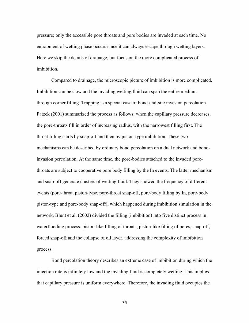
concluded that the RCPs generated by a Monte Carlo method (collective rearrangement)

do not duplicate the real dense random packings from the experiments in which a

reorganizing process was usually observed

2

The void structure in cylinder packings is important in that it governs fluid flow

through the packings In chapter 5 a numerical procedure to quantify the geometry and

topology of the void space in the packing is developed The method analyzes the void

structure in the framework of pore network models In this way the continuous void

space inside a cylinder packing can be effectively expressed as a mathematically

tractable microscale pore-throat network The resulting network represents a flow map

that can be used to quantify fluid transport Three basic elements in a network model are

pores throats and the map of their interconnectivity These elements correspond to larger

voids constrictions and the flow paths inside a packing In 3D random close packings

(RCPs) it was found that the normalized pore and throat sizes steadily increase as

cylindrical particles become slender and pore-throat aspect ratios maintain a value of

approximately 2 The interconnectivity in the network also increases with the particle

aspect ratio which suggests a transition from tunnel-like to cage-like porous geometry

inside the packings Additional statistical results from the networks included pore size

distributions (maximal inscribed diameter) throat size distributions (inscribed bottle-neck

diameter) and pore-coordination-number distributions

In chapter 6 of this work single-phase flow simulations are described and a set of

permeability tensors from random cylinder packings are presented In 3D random close

packings the results showed nearly isotropic permeability properties while in two

anisotropic packings (preferred horizontal or nearly nematic) anisotropic permeability

properties were found The derived permeabilities match extensive experimental data for

fibrous materials which suggests the correctness of network approach Hence a

predictive means of computing permeability of fibrous porous media is proposed For

3

multiphase flow simulations a model formulation for dynamic imbibition and a

preliminary numerical procedure were proposed which integrate detailed microscale pore

phenomena Simulations will be conducted in the future

4

CHAPTER 2

BACKGROUND AND LITERATURE REVIEW

21 Random Packing

The random packing structure of particles is of interest in a number of

applications Packings of simple shapes serve as prototype models for porous materials

packing structure dictates the bulk density of particulate materials and understanding

microscale structure provides insight into properties such as thermal fluid and electrical

conductance of various materials Simulated packings also provide fundamental insight

into molecular arrangements in crystalline and semi-crystalline materials

211 Sphere Packing

The most widely studied packings are those composed of uniform-sized spheres

Ordered structures include rhombohedral packings and cubic packings which bracket the

range of attainable solid volume fraction (SVF) at φmax = 07405 and φmin = 05326

respectively Disordered packings exhibit a much smaller range of SVF values A key

parameter of interest is the random-close-packed (RCP) porosity limit which has been

investigated using experiments (eg Scott and Kilgour 1969 Berryman 1983) theory

(eg Gotoh and Finny 1974) and numerical simulations (eg Jodrey and Tory 1981)

No generalized theory has provided an exact value but the well-accepted limit is

φmax = 064 (plus or minus some small amount that varies according to the source

consulted) Generally real packings fall into the fairly narrow density range φ = 060 ndash

064 as long as the spheres are nearly uniform in size Related studies have aimed to

quantify void structure (Mellor 1989 Nolan and Kavanagh 1994) changes in packing

5

structure during densification (Clarke and Jonsson 1993) radial distribution function

(Bennett 1972 Clark and Jonsson 1993 Finney 1970) contact coordination number

(Bennett 1972) and boundary effects (Reyes and Iglesia 1991) Finally it is worth

noting that Torquato et al (2000) have proposed the maximally random jammed (MRJ)

state as a more rigorous definition than the RCP limit to characterize the dense

disordered structures

212 Cylinder Packing

Packings of cylindrical particles are likewise of interest because of the application

to real systems such as fibrous materials and catalyst beds The most fundamental

distinction between sphere and cylinder packings is that the latter systems require one

additional orientational vector of each particle for the structure to be fully characterized

This extra orientational freedom leads to a number of interesting questions eg is there a

widely-accepted solid-volume fraction in random close packing of cylinders with a

specific particle aspect ratio What is the maximal random packing density (both

experimental and simulated) of equilateral cylinders compared to the packing of spheres

How does the structure evolve when a cylinder pack undergoes a densification process

Can computer simulations imitate the densification process and generate a maximal

random jammed (MRJ) structure These interesting questions have drawn a number of

scholars to examine cylinder packings either by experiments statistical analysis or

simulations

Fundamental experimental research on cylindrical packing was carried out since

1970s

6

Milewski (1973) did detailed experiments on cylindrical packings by using

wooden rods (uniform LD ratios from 4 to 72) and milled glass fibers (symmetric

distribution of LD) The author concluded that the cylinder aspect ratio (or average

aspect ratio) determines the solid fraction of random packing which decreases with

increasing aspect ratio The fraction from the fibers with size distribution is close to the

case of rods with of uniform distribution The work provided a series of experimental

benchmarks

Nardin (1985) generated loose and dense packings for a number of particle

shapes including fibers over large aspect ratios It was also found that the packing

volume fraction varies inversely with particle aspect ratio when the ratio is large (fibers)

Evans amp Gibson (1986) used liquid-crystal theory to formulate a model for the

maximum packing fraction They proposed an analogy between the thermodynamic

transition from a random to (partially) ordered state and the behavior of cylindrical

packings in which geometric considerations prohibit a random arrangement at

sufficiently high values of SVF From liquid-crystal theory the basic formula φmax = kDL

was presented where k is a constant Theoretical computations of the probability that the

rotational free volume around a fiber contains neighboring fibers gives k = 4 However a

fit to available experimental data gives k = 53 They suggested that those results were

limited to higher particle aspect ratios of above 10

Parkhouse amp Kelly (1995) used a combination of geometric probabilistic and

empirical arguments to obtain a general formula for the SVF of the form

φ = 2ln(LD)(LD) An extension to the formula was also proposed that accounted for the

7

possibility of filling in all available void space That gave higher values of SVF with an

additional term of 5π(LD)^2

Zou and Yu (1996) performed a series of experiments on a number of non-

spherical particles in an attempt to generate loose and tight packings They correlated

their data as a function of particle sphericity ψ (defined as the ratio of the surface area of

a sphere having the same volume as the particle to the surface area of the particle) For

cylinders in particular they obtained an empirical equation for the close-packed porosity

limit The limitation of their work is that no particle aspect ratio was correlated

Philipse (1996) described the arrangement of high-aspect ratio packings from the

perspective of the excluded volume available to a particle assuming a random orientation

in the packing He argued that analyzing the structure of high-aspect ratio particles is

simpler than compact particles because ldquofor sufficiently thin rods mechanical contacts

are effectively uncorrelated the random thin-rod array is essentially a collection of

independent pairs of rodsrdquo He suggested that φ(LD) = c for LD gt15 where c

represents the number of random hard contacts per cylinder (which is constant for long

particles) A value of c = 54 was proposed thus giving essentially the same expression

(a slight difference in the constant) as Evans amp Gibson (1986) He pointed out that this

isotropic random dense packing corresponds to metastable ldquorod-glassesrdquo He also pointed

out that uncorrelated pair contacts in this model is suffice to explain densities of a variety

of thin-rod systems as colloidal sediments rheology and percolation of random rods

Other investigators focused on packings of smaller aspect ratio (compact)

cylinders Nardin et al (1985) created loose and dense packings of polypropylene

8

cylinders For LD = 1 the minimum and maximum SVF values were reported to be

0538 and 0629 respectively

Dixon (1988) measured void fraction of fixed beds by using equilateral

cylindrical particles The columns were packed by fairly slow pouring of the packing by

hand without tamping or attempting to induce settling of the packing This process

suggests a random loose packing fraction of 064 in experiments

Foumeny amp Roshani (1991) extended Dixonrsquos results for equilateral cylinder

(LD=1) over a certain range of aspect ratios (LD=05-3) by introducing a concept of

diameter of sphere of equivalent volume To prepare a bed particles were simply poured

into a container and gently vibrated in order to get a more settled bed Since this process

included a settling process the resulting solid fractions are larger than the results from

Dixon Both of these authors alleged that the ratio of the equivalent cylinder diameter

compared to the tube is a key factor to determine the final porosity but they did not study

the effect of aspect ratio of cylinders

Zou amp Yu (1995 1996) proposed that the void fraction is strongly depended on

the aspect ratio (LpDp) of cylinders They did a series of experiments on packings that

include particles with aspect ratio of up to 25 Based on the experimental data they

introduced two formulas to compute RLP porosity and RCP porosity respectively

Loose packing ε0 = expψ558timesexp[589times(1-ψ)]timesln 040

Close packing ε0 = expψ674timesexp[800times(1-ψ)]timesln 036

where ψ=2621times(LpDp)23[1+2times(LpDp)]

Computer simulations on random cylinder packings are rare compared to

simulations on random sphere packings The earliest computer work on rod-like particles

9

is from Vold (1959) who built a numerical model to simulate the sedimentation of dilute

dispersions of randomly oriented rod-like particles with aspect ratio from 1 to 18 The

process is similar to the random loose packing algorithm Because of the assumption of

coherence between particles their derived solid fractions are very low The model can

apply to suspension of lithium stearate in benzene

Evans and Ferrar (1989) performed computer simulations to generate random

packings of thick fibers with aspect ratios between 1 and 30 However they used a

parking algorithm which is known to generate volume fractions that are significantly

lower than in real structures (Cooper 1987) Additionally they approximate each

cylinder as a series of overlapping spheres along a line (to simplify calculations) This

latter approximation affects the overlap calculations at the fiber ends and has a

particularly large influence on low-aspect-ratio particles

Coelho et al (1997) used a sequential deposition (SD) algorithm to construct

packings of cylinders with aspect ratios in the range of 01 and 10 However SD

algorithms do not allow for good control over solid volume fraction and tend to produce

stable but loose packings This problem is evidenced by tests of their algorithm to

generate sphere packings which produced ε = 0402 (significantly higher than the RCP

limit)

Nandakumar et al (1999) used computational solid-geometry and collision-

detection algorithms to create packed structures with arbitrary-shaped particles This

approach is again a SD-type algorithm and results show the same loose-packed

characteristics

10

Some researchers have examined other nonspherical particles (including

ellipsoids spheroids and spherocylinders) in which the geometry of particle-particle

contacts is simplified These particles also have axis-symmetric geometry For the

packings of very large aspect ratios all these nonspherical particles form quite similar

structures Sherwood (1997) studied the random packing of spheroids by computer

simulations Because a parking algorithm was used the packing densities are

significantly lower than the value for real systems Williams amp Philipse (2003) worked

on spherocylinders They simulated random packings of spherocylinders by a

mechanical-contraction method They found that the parameter governing the packing

limit is the particle aspect ratio As particle aspect ratio increases the maximal packing

density decreases A new yet puzzling phenomenon is that for compact spherocylinders

(eg low aspect ratios) there is a density hump (φ =0695) in the maximal packing limit

near aspect ratio of 04 Donev et al (2004) observed a similar phenomenon in both

computer-generated and real packings of ellipsoids and highest density (φ =0735) occurs

at aspect ratio of 13

22 Packing Structure

221 Radial Distribution Function

The radial distribution function (RDF or g(r)) is a way to quantify the average

structure of positional ordering in a molecular system For spherical particles it is used to

describe how the particles are radially packed around each other and have a structure of

layered extension Traditionally it is defined as

drr

rNrV

rNrN

rNrgshellideal

24)(

)()(

)()()(

πρρ sdot=

sdot== (2-1)

11

where ρ is the mean number density The shell volume (Vshell) is simply a spherical crust

that has radius r (also can be viewed as pair separation distance) and thickness dr A

typical RDF plot shows a number of important features Firstly at short separations

(small r) the RDF is zero This indicates the effective width of the atoms since they

cannot approach any more closely Secondly a number of obvious peaks appear which

indicates that the atoms pack around each other in shells of neighbors The occurrence of

peaks at long range indicates a high degree of positional ordering At very long range

every RDF tends to a value of 1 which happens because the RDF describes the average

density at this range A schematic of an RDF is showed in Figure 21 below

Figure 21 A schematic of RDF in spherical particle system

2211 Generalization of Radial Distribution Function

To extend the RDF to cylinder systems the pair distance is interpreted as a

minimal distance from a cylinder center to the reference cylinder surface Therefore an

effective distance between two cylinders is from 05 to some large number in finite

domain The mean number density (ρ) is the ratio of the total number of cylinders and the

computational domain volume The shell is a rotated crust around the reference cylinder

which includes a cylindrical part and two rotated caps (see Figure 22)

12

DrdrdrrdrDLdrDrrVshell sdot+++sdot+= 222 42

)2()( ππππ (2-2)

L

D

Figure 22 2D illustration of a shell around the reference cylinder

With periodic boundary conditions we can treat all the cylinders in the primary domain

as reference particles to obtain an improved average RDF

)(

)()(rVNfibers

rNrgshellsdotsdot

=ρ

(2-3)

Note that the distance of pair separation can also be interpreted as a minimal distance

between two cylinder surfaces and an effective distance will be starting from zero A

complicated excluded volume theory with statistical analysis will be involved Interested

reader may refer to the papers by (Onsager 1949 Blaak et al 1999 Williams 2003)

222 Orientational Ordering Theory

2221 Ordering in Liquid Crystal

Liquid crystals are a phase of matter whose order is intermediate between that of a

liquid and that of a solid The molecules in liquid crystals usually take a rod-like form In

a liquid phase molecules have no intrinsic orders and display isotropic properties In

highly ordered crystalline solid phase molecules have no translational freedom and

13

demonstrate anisotropic properties That is the molecules in solids exhibit both positional

and orientational ordering in liquids the molecules do not have any positional or

orientational ordering ndash the direction the molecules point and their positions are random

Figure 23 Illustration of structures of solid liquid crystal and liquid

There are many types of liquid crystal states depending upon the amount of

ordering in the material These states include (a) Nematic (molecules have no positional

order but tend to point in the same direction along the director) (b) Smectic (molecules

maintain the general orientational order of nematic but also tend to align themselves in

layers or planes) (c) Cholesteric (nematic mesogenic molecules containing a chiral

center which produces intermolecular forces that favor alignment between molecules at a

slight angle to one another) (d) Columnar (molecules in disk-like shape and stacked

columns)

Three following parameters completely describe a liquid crystal structure (a)

Positional order (b) Orientational order (c) Bond-orientational order Positional order

refers to the extent to which an average molecule or group of molecules shows

translational symmetry Orientational order represents a measure of the tendency of the

molecules to align along the director on a long-range basis Bond-orientational order

14

describes a line joining the centers of nearest-neighbor molecules without requiring a

regular spacing along that line (or the symmetry of molecule aggregationcluster) In non-

spherical particle systems evidence of bond-orientational ordering is rare

2222 Orientational Order

In a non-thermal non-polarized particulate system (eg random cylinder

packing) there are no forces between particles Structure analysis suggests that the

orientational ordering is more important We will focus on the orientational orders in the

structure

bull Nematic Ordering

The nematic ordering parameter provides the simplest way to measure the amount

of ordering in liquid crystals Traditionally this parameter has the following form

1cos321 2 minus= θS (2-4)

where θ is the angle between the director (preferred direction) and the long axis of each

molecule In an isotropic liquid the order parameter is equal to 0 For a perfect crystal

the order parameter is equal to 1 Typical values for the order parameter of a liquid

crystal range between 03 and 09 To find the preferred direction a second order tensor

is used which is defined

)21

23(1

1αββααβ δsum

=

minus=N

iii uu

NQ and zyx =βα (2-5)

where ui is the long axis of a molecule N is the number of molecules and δ is the

Kronecker delta function Qαβ is symmetric and traceless Diagonalization of Qαβ gives

three eigenvalues (λ1 λ2 λ3) which sum to zero The director is then given by the

eigenvector associated with the largest eigenvalue

15

The simple nematic ordering parameter is very sensitive in a highly ordered

system (eg close to crystalline) However for general disordered packings this

parameter is small

bull Cubatic Ordering

The cubatic phase is another long-range orientationally ordered phase without any

positional order of the particles In these systems the different molecular axes of the

particles align in three different orthogonal directions with equal probability of each This

elusive phase has been found in computer simulations of cut spheres (Veerman amp

Frenkel 1992) and short cylinders (Blaak et al 1999)

The formulae used to quantify the cubatic ordering include Legendre polynomials

and spherical harmonics which we will introduce in the next section

bull Other Ordering

In liquid crystals there are plenty of symmetric structures (bcc fcc sc hcp

icosahedral star tetrahedron etc) depending on the molecular shape forces and

polarized attributes In addition the global structures depend on the external magnetic

field Therefore it is possible to observe countless symmetric structures microscopically

in nature In our specific cylinder-packing problem we will focus on lower-order

symmetric parameters because the packing has not demonstrated many complex

structures from experimental observations

2223 Legendre Polynomials

The Legendre polynomials are a set of orthogonal solutions from the Legendre

differential equation They provide a means to measure structural information One of the

popular criteria is P2 to measure nematic ordering when the system displays uniaxial

16

ACKNOWLEDGEMENTS

I would like to thank my major advisor Dr Karsten Thompson who provided me

with guidance suggestions and assistance This work would have been impossible

without his patience and support I would also like to thank my committee members (Dr

Gregory Griffin Dr Steven Watkins Dr Brian Mitchell Dr James Henry Dr Clinton

Willson Dr Danny Reible Dr Benjamin McCoy) for their time and many valuable

suggestions

This work was funded by NSF 0140175 amp 0140180 and collaborated with Dr

Mitchellrsquos lab at Tulane University I appreciate Dr Mitchell and his student for

performing the visualization experiments Special thanks should also go to Dr Allen

Reed who helped us with X-ray tomography experiments in Navy Research Lab Stennis

Space Center

I want to give thanks to my fellow graduate students Le Yan Matthew Balhoff

Pradeep Bhattad and Nathan Lane I appreciate the work of REU undergraduate student

Liese Beenken from University of Arizona in summer 2004 I am grateful to all the

people in our department who provided a lot of assistance

Last but not the least I would like to thank my family who helped and supported

me to finish this work

ii

TABLE OF CONTENTS

ACKNOWLEDGEMENTShelliphelliphelliphelliphelliphelliphelliphelliphelliphelliphelliphelliphelliphelliphelliphelliphelliphelliphelliphelliphelliphelliphellipii

LIST OF TABLEShelliphelliphelliphelliphelliphelliphelliphelliphelliphelliphelliphelliphelliphelliphelliphelliphelliphelliphelliphelliphelliphelliphelliphelliphelliphellipvi

LIST OF FIGUREShelliphelliphelliphelliphelliphelliphelliphelliphelliphelliphelliphelliphelliphelliphelliphelliphelliphelliphelliphelliphelliphelliphelliphelliphelliphellipvii

NOTATIONhelliphelliphelliphelliphelliphelliphelliphelliphelliphelliphelliphelliphelliphelliphelliphelliphelliphelliphelliphelliphelliphelliphelliphelliphelliphelliphelliphellipx

ABSTRACThelliphelliphelliphelliphelliphelliphelliphelliphelliphelliphelliphelliphelliphelliphelliphelliphelliphelliphelliphelliphelliphelliphelliphelliphelliphelliphelliphellipxii

CHAPTER 1 INTRODUCTIONhelliphelliphelliphelliphelliphelliphelliphelliphelliphelliphelliphelliphelliphelliphelliphelliphelliphelliphelliphelliphellip1

CHAPTER 2 BACKGROUND AND LITERATURE REVIEWhelliphelliphelliphelliphelliphelliphelliphellip5 21 Random Packinghelliphelliphelliphelliphelliphelliphelliphelliphelliphelliphelliphelliphelliphelliphelliphelliphelliphelliphelliphelliphelliphelliphellip5 211 Sphere Packinghelliphelliphelliphelliphelliphelliphelliphelliphelliphelliphelliphelliphelliphelliphelliphelliphelliphelliphelliphelliphelliphellip5 212 Cylinder Packinghelliphelliphelliphelliphelliphelliphelliphelliphelliphelliphelliphelliphelliphelliphelliphelliphelliphelliphelliphelliphellip6 22 Packing Structurehelliphelliphelliphelliphelliphelliphelliphelliphelliphelliphelliphelliphelliphelliphelliphelliphelliphelliphelliphelliphelliphelliphellip11 221 Radial Distribution Functionhelliphelliphelliphelliphelliphelliphelliphelliphelliphelliphelliphelliphelliphelliphelliphelliphellip11 2211 Generalization of Radial Distribution Functionhelliphelliphelliphelliphelliphelliphellip12 222 Orientational Ordering Theoryhelliphelliphelliphelliphelliphelliphelliphelliphelliphelliphelliphelliphelliphelliphelliphellip13 2221 Ordering in Liquid Crystalshelliphelliphelliphelliphelliphelliphelliphelliphelliphelliphelliphelliphelliphellip13 2222 Orientational Orderhelliphelliphelliphelliphelliphelliphelliphelliphelliphelliphelliphelliphelliphelliphelliphelliphellip15

2223 Legendre Polynomialshelliphelliphelliphelliphelliphelliphelliphelliphelliphelliphelliphelliphelliphelliphelliphellip16 2224 Spherical Harmonicshelliphelliphelliphelliphelliphelliphelliphelliphelliphelliphelliphelliphelliphelliphelliphelliphellip18 2225 Other Correlation Formulaehelliphelliphelliphelliphelliphelliphelliphelliphelliphelliphelliphelliphelliphellip20 2226 Local Global and Dynamic Orderinghelliphelliphelliphelliphelliphelliphelliphelliphelliphellip20 2227 Other Methodshelliphelliphelliphelliphelliphelliphelliphelliphelliphelliphelliphelliphelliphelliphelliphelliphelliphelliphellip22 23 Network Structure of Void Spacehelliphelliphelliphelliphelliphelliphelliphelliphelliphelliphelliphelliphelliphelliphelliphelliphelliphellip23 231 Pore-scale Networkhelliphelliphelliphelliphelliphelliphelliphelliphelliphelliphelliphelliphelliphelliphelliphelliphelliphelliphelliphelliphellip23 232 Network in Cylinder Packingshelliphelliphelliphelliphelliphelliphelliphelliphelliphelliphelliphelliphelliphelliphelliphelliphellip26 233 Generalized Gamma Distributionhelliphelliphelliphelliphelliphelliphelliphelliphelliphelliphelliphelliphelliphelliphelliphellip27 24 Modeling Flow in a Networkhelliphelliphelliphelliphelliphelliphelliphelliphelliphelliphelliphelliphelliphelliphelliphelliphelliphelliphelliphellip28 241 Microscopic Phenomenahelliphelliphelliphelliphelliphelliphelliphelliphelliphelliphelliphelliphelliphelliphelliphelliphelliphelliphellip29 242 Drainage and Imbibitionhelliphelliphelliphelliphelliphelliphelliphelliphelliphelliphelliphelliphelliphelliphelliphelliphelliphelliphellip34 243 Flow Simulationhelliphelliphelliphelliphelliphelliphelliphelliphelliphelliphelliphelliphelliphelliphelliphelliphelliphelliphelliphelliphelliphellip36 CHAPTER 3 RANDOM CYLINDER PACKINGShelliphelliphelliphelliphelliphelliphelliphelliphelliphelliphelliphelliphellip41 31 Simulated Random Cylinder Packingshelliphelliphelliphelliphelliphelliphelliphelliphelliphelliphelliphelliphelliphelliphelliphellip41 311 Packing Algorithmshelliphelliphelliphelliphelliphelliphelliphelliphelliphelliphelliphelliphelliphelliphelliphelliphelliphelliphelliphelliphellip41 312 Numerical Techniqueshelliphelliphelliphelliphelliphelliphelliphelliphelliphelliphelliphelliphelliphelliphelliphelliphelliphelliphelliphellip43 313 Isotropic Packing Resultshelliphelliphelliphelliphelliphelliphelliphelliphelliphelliphelliphelliphelliphelliphelliphelliphelliphelliphellip45 314 Discussionhelliphelliphelliphelliphelliphelliphelliphelliphelliphelliphelliphelliphelliphelliphelliphelliphelliphelliphelliphelliphelliphelliphelliphelliphellip47

iii

315 Anisotropic Packing Resultshelliphelliphelliphelliphelliphelliphelliphelliphelliphelliphelliphelliphelliphelliphelliphelliphelliphellip52 32 Experimental Packs of Equilateral Cylindershelliphelliphelliphelliphelliphelliphelliphelliphelliphelliphelliphelliphellip54 321 Experimental Methodshelliphelliphelliphelliphelliphelliphelliphelliphelliphelliphelliphelliphelliphelliphelliphelliphelliphelliphellip54 322 Cylinder Packs in a Cylindrical Containerhelliphelliphelliphelliphelliphelliphelliphelliphelliphelliphelliphellip60 323 Cylinder Packs in a Cubic Containerhelliphelliphelliphelliphelliphelliphelliphelliphelliphelliphelliphelliphelliphellip62 324 Preliminary Discussionhelliphelliphelliphelliphelliphelliphelliphelliphelliphelliphelliphelliphelliphelliphelliphelliphelliphelliphellip62 CHAPTER 4 STRUCTURAL ANALYSIS OF RANDOM CYLINDER PACKINGShelliphelliphelliphelliphelliphelliphelliphelliphelliphelliphelliphelliphelliphelliphelliphelliphelliphelliphelliphelliphelliphelliphelliphelliphelliphelliphelliphellip66 41 Structure of Simulated Packingshelliphelliphelliphelliphelliphelliphelliphelliphelliphelliphelliphelliphelliphelliphelliphelliphelliphellip68 411 Densityhelliphelliphelliphelliphelliphelliphelliphelliphelliphelliphelliphelliphelliphelliphelliphelliphelliphelliphelliphelliphelliphelliphelliphelliphelliphellip68 412 Positional Ordering and RDFhelliphelliphelliphelliphelliphelliphelliphelliphelliphelliphelliphelliphelliphelliphelliphelliphellip70 413 Orientational Orderinghelliphelliphelliphelliphelliphelliphelliphelliphelliphelliphelliphelliphelliphelliphelliphelliphelliphelliphellip71 414 Particle Contact Numberhelliphelliphelliphelliphelliphelliphelliphelliphelliphelliphelliphelliphelliphelliphelliphelliphelliphelliphellip76 42 Structures of Experimental Packs in a Rough-Walled Containerhelliphelliphelliphelliphellip77 421 Radial Density Profilehelliphelliphelliphelliphelliphelliphelliphelliphelliphelliphelliphelliphelliphelliphelliphelliphelliphelliphelliphellip77 422 Positional Orderinghelliphelliphelliphelliphelliphelliphelliphelliphelliphelliphelliphelliphelliphelliphelliphelliphelliphelliphelliphelliphellip79 423 Orientational Orderinghelliphelliphelliphelliphelliphelliphelliphelliphelliphelliphelliphelliphelliphelliphelliphelliphelliphelliphelliphellip80 424 Particle Contact Numberhelliphelliphelliphelliphelliphelliphelliphelliphelliphelliphelliphelliphelliphelliphelliphelliphelliphelliphellip81 43 Structures of Experimental Packs in a Cylindrical Containerhelliphelliphelliphelliphelliphelliphellip82 431 Radial Densityhelliphelliphelliphelliphelliphelliphelliphelliphelliphelliphelliphelliphelliphelliphelliphelliphelliphelliphelliphelliphelliphelliphellip83 432 RDF and Positional Orderinghelliphelliphelliphelliphelliphelliphelliphelliphelliphelliphelliphelliphelliphelliphelliphelliphellip87 433 Orientational Orderinghelliphelliphelliphelliphelliphelliphelliphelliphelliphelliphelliphelliphelliphelliphelliphelliphelliphelliphelliphellip89 434 Particle Contact Numberhelliphelliphelliphelliphelliphelliphelliphelliphelliphelliphelliphelliphelliphelliphelliphelliphelliphelliphellip97 44 A Standard Packing Tablehelliphelliphelliphelliphelliphelliphelliphelliphelliphelliphelliphelliphelliphelliphelliphelliphelliphelliphelliphelliphellip99 CHAPTER 5 NETWORK STRUCTURE IN RANDOM CYLINDER PACKINGS105 51 Network Structurehelliphelliphelliphelliphelliphelliphelliphelliphelliphelliphelliphelliphelliphelliphelliphelliphelliphelliphelliphelliphelliphelliphellip105 52 Numerical Techniquehelliphelliphelliphelliphelliphelliphelliphelliphelliphelliphelliphelliphelliphelliphelliphelliphelliphelliphelliphelliphelliphellip106 53 Computational Resultshelliphelliphelliphelliphelliphelliphelliphelliphelliphelliphelliphelliphelliphelliphelliphelliphelliphelliphelliphelliphellip116

531 Pore Size Distribution (PSD)helliphelliphelliphelliphelliphelliphelliphelliphelliphelliphelliphelliphelliphelliphelliphellip117 532 Throat Size Distribution (TSD) helliphelliphelliphelliphelliphelliphelliphelliphelliphelliphelliphelliphelliphelliphelliphellip118 533 Interconnectivityhelliphelliphelliphelliphelliphelliphelliphelliphelliphelliphelliphelliphelliphelliphelliphelliphelliphelliphelliphelliphelliphellip120

54 Conclusionhelliphelliphelliphelliphelliphelliphelliphelliphelliphelliphelliphelliphelliphelliphelliphelliphelliphelliphelliphelliphelliphelliphelliphelliphelliphellip121 CHAPTER 6 FLOW SIMULATIONShelliphelliphelliphelliphelliphelliphelliphelliphelliphelliphelliphelliphelliphelliphelliphelliphelliphellip129 61 Single-phase Flowhelliphelliphelliphelliphelliphelliphelliphelliphelliphelliphelliphelliphelliphelliphelliphelliphelliphelliphelliphelliphelliphelliphellip129 611 Model Formulationhelliphelliphelliphelliphelliphelliphelliphelliphelliphelliphelliphelliphelliphelliphelliphelliphelliphelliphelliphellip129 612 Numerical Procedurehelliphelliphelliphelliphelliphelliphelliphelliphelliphelliphelliphelliphelliphelliphelliphelliphelliphelliphellip130 613 Permeability Resultshelliphelliphelliphelliphelliphelliphelliphelliphelliphelliphelliphelliphelliphelliphelliphelliphelliphelliphelliphellip132 62 Two-phase Flowhelliphelliphelliphelliphelliphelliphelliphelliphelliphelliphelliphelliphelliphelliphelliphelliphelliphelliphelliphelliphelliphelliphellip135 621 Dynamic Imbibition Formulationhelliphelliphelliphelliphelliphelliphelliphelliphelliphelliphelliphelliphelliphelliphellip135 622 Proposed Numerical Procedurehelliphelliphelliphelliphelliphelliphelliphelliphelliphelliphelliphelliphelliphelliphelliphellip137 623 Additional Considerationshelliphelliphelliphelliphelliphelliphelliphelliphelliphelliphelliphelliphelliphelliphelliphelliphellip138

iv

CHAPTER 7 CONCLUSIONS AND FUTURE RESEARCH DIRECTIONShelliphelliphellip139 71 Conclusionshelliphelliphelliphelliphelliphelliphelliphelliphelliphelliphelliphelliphelliphelliphelliphelliphelliphelliphelliphelliphelliphelliphelliphelliphellip139 72 Future Research Directionshelliphelliphelliphelliphelliphelliphelliphelliphelliphelliphelliphelliphelliphelliphelliphelliphelliphelliphellip140 721 Packinghelliphelliphelliphelliphelliphelliphelliphelliphelliphelliphelliphelliphelliphelliphelliphelliphelliphelliphelliphelliphelliphelliphelliphelliphellip140 722 Structurehelliphelliphelliphelliphelliphelliphelliphelliphelliphelliphelliphelliphelliphelliphelliphelliphelliphelliphelliphelliphelliphelliphelliphelliphellip141 723 Networkhelliphelliphelliphelliphelliphelliphelliphelliphelliphelliphelliphelliphelliphelliphelliphelliphelliphelliphelliphelliphelliphelliphelliphellip141 724 Simulationhelliphelliphelliphelliphelliphelliphelliphelliphelliphelliphelliphelliphelliphelliphelliphelliphelliphelliphelliphelliphelliphelliphellip142 REFERENCEShelliphelliphelliphelliphelliphelliphelliphelliphelliphelliphelliphelliphelliphelliphelliphelliphelliphelliphelliphelliphelliphelliphelliphelliphelliphelliphellip143 VITAhelliphelliphelliphelliphelliphelliphelliphelliphelliphelliphelliphelliphelliphelliphelliphelliphelliphelliphelliphelliphelliphelliphelliphelliphelliphelliphelliphelliphelliphelliphellip149

v

LIST OF TABLES

Table 31 Properties of random dense cylinder packingshelliphelliphelliphelliphelliphelliphelliphelliphelliphelliphelliphellip46

Table 41 Local orders (when gap = Dparticle) of simulated packingshelliphelliphelliphelliphelliphelliphellip72

Table 42 Local orders (when gap=005Dparticle) of simulated packingshelliphelliphelliphelliphelliphellip73

Table 43 Global orders of simulated cylinder packingshelliphelliphelliphelliphelliphelliphelliphelliphelliphelliphelliphellip75

Table 44 Local ordering of three rough-walled packs (gap=Dparticle) helliphelliphelliphelliphelliphelliphellip80

Table 45 Local ordering of three rough-walled packs (gap=005Dparticle) helliphelliphelliphelliphellip80

Table 46 Global ordering of three rough-walled packshelliphelliphelliphelliphelliphelliphelliphelliphelliphelliphelliphellip81

Table 47 Packing densities in different regions of five experimental packshelliphelliphelliphellip85

Table 48 Packing densities in interior and near-wall regionshelliphelliphelliphelliphelliphelliphelliphelliphelliphellip85

Table 49 Local ordering of five experimental packs (gap=Dparticle) helliphelliphelliphelliphelliphelliphellip94

Table 410 Local ordering of five experimental packs (gap=005Dparticle) helliphelliphelliphelliphellip94

Table 411 Global ordering of five experimental packshelliphelliphelliphelliphelliphelliphelliphelliphelliphelliphelliphellip97

Table 412 Global ordering parameters of different cylinder packingshelliphelliphelliphelliphelliphellip102

Table 413 Local ordering parameters of different cylinder packingshelliphelliphelliphelliphelliphellip104

Table 51 All network parameters associated with a pore networkhelliphelliphelliphelliphelliphelliphellip106

Table 52 Some network parameters in four random close packingshelliphelliphelliphelliphelliphelliphellip128

Table 53 Fitted PSD parameters in Gamma distributionshelliphelliphelliphelliphelliphelliphelliphelliphelliphelliphellip128

Table 54 Fitted TSD parameters in Gamma distributionshelliphelliphelliphelliphelliphelliphelliphelliphelliphelliphellip128

Table 61 Permeability results of isotropic cylinder packingshelliphelliphelliphelliphelliphelliphelliphelliphellip132

Table 62 Permeability results for anisotropic cylinder packingshelliphelliphelliphelliphelliphelliphelliphellip134

vi

LIST OF FIGURES

Figure 21 A schematic of RDF in spherical particle systemhelliphelliphelliphelliphelliphelliphelliphelliphelliphellip12

Figure 22 2D illustration of a shell around the reference cylinderhelliphelliphelliphelliphelliphelliphelliphellip13

Figure 23 Illustration of structures of solid liquid crystal and liquid helliphelliphelliphelliphelliphellip14

Figure 24 Plots of some Legendre polynomials (x=cosθ) helliphelliphelliphelliphelliphelliphelliphelliphelliphelliphellip17

Figure 25 Projection and visualization of global ordering helliphelliphelliphelliphelliphelliphelliphelliphelliphelliphellip22

Figure 26 Wettability of different fluids (wetting nonwetting completely wetting)hellip30

Figure 27 Schematic of snap-off (From Lenormand et al 1983)helliphelliphelliphelliphelliphelliphelliphellip32

Figure 28 Wetting phase configuration in an idealized pore (from Thompson 2002)33

Figure 29 Hypothetical capillary pressure versus saturation in a porehelliphelliphelliphelliphelliphellip34

Figure 31 Flowchart of the parking algorithmhelliphelliphelliphelliphelliphelliphelliphelliphelliphelliphelliphelliphelliphelliphelliphellip42

Figure 32 Flowchart of collective rearrangement algorithmhelliphelliphelliphelliphelliphelliphelliphelliphelliphellip42

Figure 33 Illustrations of compact and slender cylinder packingshelliphelliphelliphelliphelliphelliphelliphellip46

Figure 34 Plots of Compact and slender cylinder packing limitshelliphelliphelliphelliphelliphelliphelliphellip49

Figure 35 Illustrations of different anisotropic packingshelliphelliphelliphelliphelliphelliphelliphelliphelliphelliphelliphellip53

Figure 36 The electric tubing cutter and sample cylindershelliphelliphelliphelliphelliphelliphelliphelliphelliphelliphellip55

Figure 37 X-ray microtomography CT facilityhelliphelliphelliphelliphelliphelliphelliphelliphelliphelliphelliphelliphelliphelliphellip56

Figure 38 Images from XMT imaginghelliphelliphelliphelliphelliphelliphelliphelliphelliphelliphelliphelliphelliphelliphelliphelliphelliphelliphellip57

Figure 39 Histogram of the size of connected componentshelliphelliphelliphelliphelliphelliphelliphelliphelliphelliphellip59

Figure 310 Computer reconstructed five packs in a cylindrical containerhelliphelliphelliphelliphellip61

Figure 311 Computer reconstructed packs in a rough-wall containerhelliphelliphelliphelliphelliphelliphellip62

Figure 312 Projection of particle centers in a cubic container helliphelliphelliphelliphelliphelliphelliphelliphellip63

vii

Figure 313 Projection of particle centers in a cylindrical container helliphelliphelliphelliphelliphelliphellip64

Figure 314 Projection of particle orientations in three rough-walled packs helliphelliphelliphellip65

Figure 41 A 2D schematic of domain discretization of a cube helliphelliphelliphelliphelliphelliphelliphelliphellip69

Figure 42 Density distributions versus wall-distance in simulated packingshelliphelliphelliphellip69

Figure 43 RDFs of simulated random packings (LD =151020) helliphelliphelliphelliphelliphelliphelliphellip71

Figure 44 Contact numbers versus minimal distance (LD=151020) helliphelliphelliphelliphelliphellip76

Figure 45 Density distributions in rough-walled packingshelliphelliphelliphelliphelliphelliphelliphelliphelliphelliphellip78

Figure 46 Particle RDFs of three rough-walled packings (R1R2R3) helliphelliphelliphelliphelliphellip79

Figure 47 Particle contact numbers of three rough-walled packs (R1R2R3) helliphelliphellip82

Figure 48 Radial density function versus wall-distance ξ (C1C2C3C4C5) helliphelliphellip84

Figure 49 Illustration of highly ordered structure in cylinder packingshelliphelliphelliphelliphelliphellip86

Figure 410 Wall RDFs versus ξ in five packs (C1C2C3C4C5) helliphelliphelliphelliphelliphelliphelliphellip87

Figure 411 Particle RDFs versus ξ in five packs (C1C2C3C4C5) helliphelliphelliphelliphelliphelliphellip88

Figure 412 Radial ordering versus wall distance in five packs (C1C2C3C4C5) hellip89

Figure 413 Cumulative radial ordering of five packs (C1C2C3C4C5) helliphelliphelliphelliphellip91

Figure 414 V-ordering versus α in three packs (C1 C3 C5) helliphelliphelliphelliphelliphelliphelliphelliphelliphellip92

Figure 415 Cumulative V-ordering of five packs (C1C2C3C4C5) helliphelliphelliphelliphelliphellip93

Figure 416 Local nematic and cubatic orientational ordering in five packshelliphelliphelliphellip95

Figure 417 Contact number versus minimal distance in five packshelliphelliphelliphelliphelliphelliphellip98

Figure 418 Imaginary different packing structureshelliphelliphelliphelliphelliphelliphelliphelliphelliphelliphelliphelliphellip100

Figure 51 Illustrations of pores in random cylinder packing helliphelliphelliphelliphelliphelliphelliphelliphellip107

Figure 52 Illustration of pore-throat and flow pathhelliphelliphelliphelliphelliphelliphelliphelliphelliphelliphelliphelliphellip109

Figure 53 Cross-sectional area of the triangular modelhelliphelliphelliphelliphelliphelliphelliphelliphelliphelliphelliphellip111

viii

Figure 54 Illustrations of random dense packings with varied cylinder aspect ratios114

Figure 55 A flowchart of computer algorithm of network extractionhelliphelliphelliphelliphelliphellip115

Figure 56 Illustration of the network connectivity in four random close packingshellip116

Figure 57 Histograms of maximal inscribed radii distributions in four packingshelliphellip123

Figure 58 Normalized maximal inscribed radii distributions in four packingshelliphelliphellip123

Figure 59 Histograms of pore volume distributions in four packingshelliphelliphelliphelliphelliphellip124

Figure 510 Histograms of throat size distributions in four packingshelliphelliphelliphelliphelliphelliphellip125

Figure 511 Gamma distributions of normalized throat size in four packingshelliphelliphellip125

Figure 512 Histograms of throat length distributions in four packingshelliphelliphelliphelliphelliphellip126

Figure 513 Histograms of coordination number distributions in four packingshelliphellip127

Figure 61 A flowchart of single-phase flow simulationhelliphelliphelliphelliphelliphelliphelliphelliphelliphelliphellip131

Figure 62 Predicted permeabilities of prototype fiber packingshelliphelliphelliphelliphelliphelliphelliphellip133

ix

NOTATION

φ = packing solid volume fraction (or packing density)

ε = porosity

L = particle or cylinder length

D = particle or cylinder diameter

c = number of random hard contacts per cylinder

ρ = mean number density of a packing

γ = the shape parameter in gamma distribution

β = the scale parameter in gamma distribution

micro = the location parameter in gamma distribution

mlY = spheric harmonics

mlP = associated Legendre polynomials

M = parallel parameter of particle pair correlation

S4α = V-ordering parameter

S2z S4z = nematic and orthogonal correlation parameters with gravitation

S2r S4r = nematic and orthogonal correlation parameters with radial direction

S2 S4 S6 = ordering parameters using Legendre polynomials

I2 I4 I6 = global ordering parameters using spherical harmonics

ξ =wall distance (dimensionless normalized in the unit of cylinder diameter)

Pc = capillary pressure

Pw = wetting phase pressure

Pnw = nonwetting phase pressure

x

σ = surface tension

Ncap = capillary number

Pi = pore pressure in a network modeling

qij = volumetric flow rate between pore i and j

G = hydraulic conductivity of a pore-throat

K = permeability tensor

Si = wetting phase saturation in pore i

Vi = volume of pore i

Reff = effective hydraulic radius of a pore-throat

ψ = distance function

Z = coordination number of a pore network

xi

ABSTRACT

Random cylinder packings are prevalent in chemical engineering applications and

they can serve as prototype models of fibrous materials andor other particulate materials

In this research comprehensive studies on cylinder packings were carried out by

computer simulations and by experiments

The computational studies made use of a collective rearrangement algorithm

(based on a Monte Carlo technique) to generate different packing structures 3D random

packing limits were explored and the packing structures were quantified by their

positional ordering orientational ordering and the particle-particle contacts

Furthermore the void space in the packings was expressed as a pore network which

retains topological and geometrical information The significance of this approach is that

any irregular continuous porous space can be approximated as a mathematically tractable

pore network thus allowing for efficient microscale flow simulation Single-phase flow

simulations were conducted and the results were validated by calculating permeabilities

In the experimental part of the research a series of densification experiments

were conducted on equilateral cylinders X-ray microtomography was used to image the

cylinder packs and the particle-scale packings were reconstructed from the digital data

This numerical approach makes it possible to study detailed packing structure packing

density the onset of ordering and wall effects Orthogonal ordering and layered

structures were found to exist at least two characteristic diameters from the wall in

cylinder packings

xii

Important applications for cylinder packings include multiphase flow in catalytic

beds heat transfer bulk storage and transportation and manufacturing of fibrous

composites

xiii

CHAPTER 1

INTRODUCTION

Random cylinder packings are of great interest because they are prototype models

of many real structures eg chain polymers liquid crystals fibrous materials and

catalytic beds These structures contribute to a wide variety of scientific research and

engineering applications including biomaterials colloids composites phase transitions

fabrics and chemical reactions In this work research on random cylinder packings has

been carried out The research includes 3D analysis of the structure in random dense

packings the structural evolution of real random cylinder packs during densification

analysis of pore structure in random cylinder packings and the simulation of fluid flow in

the void space

The first part of the work is the computer simulation of random packings of rigid

cylinders with a wide range of particle aspect ratios (1minus100) A sequential parking (SP)

algorithm was used to generate random loose packings and a collective rearrangement

(CR) algorithm was used to generate random close packings (RCP) The latter technique

is an ideal tool to reproduce disordered packing structures because of the ability to

control bulk material properties (eg porosity length or size distribution andor

heterogeneity) The random dense packing limits of mono-sized cylinders in periodic

domains have been explored and results show that the maximum density decreases with

the particle aspect ratio More interesting the existence of a weak maximum in random

packing density (φ =066 near a cylinder aspect ratio of 12) has been shown numerically

The phenomenon is explained by the orientational freedom gained with elongation

These simulated particulate systems might be used in different applications including

1

phase transitions liquid crystals metastable glass atomic structures amorphous metals

fibrous andor nano materials

In the experimental part of this study special equilateral cylinders (LD =1) were

produced and used for 3D imaging Two sets of experiments were carried out minusone in a

cylindrical container with smooth surfaces and one in a cubic container with rough

surfaces The purposes of the experiments were to address the packing structures with

and without wall effects during densification A state-of-the-art X-ray microtomography

system was used to obtain high-resolution images of various packings Then a

computational algorithm was used to identify individual cylinders in the packing (eg

their positions orientations and sizes) Based on the particle-scale structures the

experimental packing densities of equilateral cylinders were found to fall into a range of

0594minus0715 which corresponds to increasing positional and orientational ordering with

increasing packing density Statistical analysis showed that a layered structure and

orthogonal ordering are two attributes found in dense cylinder packings During the

densification process near-wall particles assume orthogonal orientations with respect to

the container wall and inner particle pairs assume orthogonal orientations with respect to

each other The contact number in the densest experimental packing was found to be

approximately 57 Detailed structural analyses (packing density radial distribution

function local and global orientational ordering contact number) were also performed on

computer-simulated random close packings Based on all the quantitative results we

concluded that the RCPs generated by a Monte Carlo method (collective rearrangement)

do not duplicate the real dense random packings from the experiments in which a

reorganizing process was usually observed

2

The void structure in cylinder packings is important in that it governs fluid flow

through the packings In chapter 5 a numerical procedure to quantify the geometry and

topology of the void space in the packing is developed The method analyzes the void

structure in the framework of pore network models In this way the continuous void

space inside a cylinder packing can be effectively expressed as a mathematically

tractable microscale pore-throat network The resulting network represents a flow map

that can be used to quantify fluid transport Three basic elements in a network model are

pores throats and the map of their interconnectivity These elements correspond to larger

voids constrictions and the flow paths inside a packing In 3D random close packings

(RCPs) it was found that the normalized pore and throat sizes steadily increase as

cylindrical particles become slender and pore-throat aspect ratios maintain a value of

approximately 2 The interconnectivity in the network also increases with the particle

aspect ratio which suggests a transition from tunnel-like to cage-like porous geometry

inside the packings Additional statistical results from the networks included pore size

distributions (maximal inscribed diameter) throat size distributions (inscribed bottle-neck

diameter) and pore-coordination-number distributions

In chapter 6 of this work single-phase flow simulations are described and a set of

permeability tensors from random cylinder packings are presented In 3D random close

packings the results showed nearly isotropic permeability properties while in two

anisotropic packings (preferred horizontal or nearly nematic) anisotropic permeability

properties were found The derived permeabilities match extensive experimental data for

fibrous materials which suggests the correctness of network approach Hence a

predictive means of computing permeability of fibrous porous media is proposed For

3

multiphase flow simulations a model formulation for dynamic imbibition and a

preliminary numerical procedure were proposed which integrate detailed microscale pore

phenomena Simulations will be conducted in the future

4

CHAPTER 2

BACKGROUND AND LITERATURE REVIEW

21 Random Packing

The random packing structure of particles is of interest in a number of

applications Packings of simple shapes serve as prototype models for porous materials

packing structure dictates the bulk density of particulate materials and understanding

microscale structure provides insight into properties such as thermal fluid and electrical

conductance of various materials Simulated packings also provide fundamental insight

into molecular arrangements in crystalline and semi-crystalline materials

211 Sphere Packing

The most widely studied packings are those composed of uniform-sized spheres

Ordered structures include rhombohedral packings and cubic packings which bracket the

range of attainable solid volume fraction (SVF) at φmax = 07405 and φmin = 05326

respectively Disordered packings exhibit a much smaller range of SVF values A key

parameter of interest is the random-close-packed (RCP) porosity limit which has been

investigated using experiments (eg Scott and Kilgour 1969 Berryman 1983) theory

(eg Gotoh and Finny 1974) and numerical simulations (eg Jodrey and Tory 1981)

No generalized theory has provided an exact value but the well-accepted limit is

φmax = 064 (plus or minus some small amount that varies according to the source

consulted) Generally real packings fall into the fairly narrow density range φ = 060 ndash

064 as long as the spheres are nearly uniform in size Related studies have aimed to

quantify void structure (Mellor 1989 Nolan and Kavanagh 1994) changes in packing

5

structure during densification (Clarke and Jonsson 1993) radial distribution function

(Bennett 1972 Clark and Jonsson 1993 Finney 1970) contact coordination number

(Bennett 1972) and boundary effects (Reyes and Iglesia 1991) Finally it is worth

noting that Torquato et al (2000) have proposed the maximally random jammed (MRJ)

state as a more rigorous definition than the RCP limit to characterize the dense

disordered structures

212 Cylinder Packing

Packings of cylindrical particles are likewise of interest because of the application

to real systems such as fibrous materials and catalyst beds The most fundamental

distinction between sphere and cylinder packings is that the latter systems require one

additional orientational vector of each particle for the structure to be fully characterized

This extra orientational freedom leads to a number of interesting questions eg is there a

widely-accepted solid-volume fraction in random close packing of cylinders with a

specific particle aspect ratio What is the maximal random packing density (both

experimental and simulated) of equilateral cylinders compared to the packing of spheres

How does the structure evolve when a cylinder pack undergoes a densification process

Can computer simulations imitate the densification process and generate a maximal

random jammed (MRJ) structure These interesting questions have drawn a number of

scholars to examine cylinder packings either by experiments statistical analysis or

simulations

Fundamental experimental research on cylindrical packing was carried out since

1970s

6

Milewski (1973) did detailed experiments on cylindrical packings by using

wooden rods (uniform LD ratios from 4 to 72) and milled glass fibers (symmetric

distribution of LD) The author concluded that the cylinder aspect ratio (or average

aspect ratio) determines the solid fraction of random packing which decreases with

increasing aspect ratio The fraction from the fibers with size distribution is close to the

case of rods with of uniform distribution The work provided a series of experimental

benchmarks

Nardin (1985) generated loose and dense packings for a number of particle

shapes including fibers over large aspect ratios It was also found that the packing

volume fraction varies inversely with particle aspect ratio when the ratio is large (fibers)

Evans amp Gibson (1986) used liquid-crystal theory to formulate a model for the

maximum packing fraction They proposed an analogy between the thermodynamic

transition from a random to (partially) ordered state and the behavior of cylindrical

packings in which geometric considerations prohibit a random arrangement at

sufficiently high values of SVF From liquid-crystal theory the basic formula φmax = kDL

was presented where k is a constant Theoretical computations of the probability that the

rotational free volume around a fiber contains neighboring fibers gives k = 4 However a

fit to available experimental data gives k = 53 They suggested that those results were

limited to higher particle aspect ratios of above 10

Parkhouse amp Kelly (1995) used a combination of geometric probabilistic and

empirical arguments to obtain a general formula for the SVF of the form

φ = 2ln(LD)(LD) An extension to the formula was also proposed that accounted for the

7

possibility of filling in all available void space That gave higher values of SVF with an

additional term of 5π(LD)^2

Zou and Yu (1996) performed a series of experiments on a number of non-

spherical particles in an attempt to generate loose and tight packings They correlated

their data as a function of particle sphericity ψ (defined as the ratio of the surface area of

a sphere having the same volume as the particle to the surface area of the particle) For

cylinders in particular they obtained an empirical equation for the close-packed porosity

limit The limitation of their work is that no particle aspect ratio was correlated

Philipse (1996) described the arrangement of high-aspect ratio packings from the

perspective of the excluded volume available to a particle assuming a random orientation

in the packing He argued that analyzing the structure of high-aspect ratio particles is

simpler than compact particles because ldquofor sufficiently thin rods mechanical contacts

are effectively uncorrelated the random thin-rod array is essentially a collection of

independent pairs of rodsrdquo He suggested that φ(LD) = c for LD gt15 where c

represents the number of random hard contacts per cylinder (which is constant for long

particles) A value of c = 54 was proposed thus giving essentially the same expression

(a slight difference in the constant) as Evans amp Gibson (1986) He pointed out that this

isotropic random dense packing corresponds to metastable ldquorod-glassesrdquo He also pointed

out that uncorrelated pair contacts in this model is suffice to explain densities of a variety

of thin-rod systems as colloidal sediments rheology and percolation of random rods

Other investigators focused on packings of smaller aspect ratio (compact)

cylinders Nardin et al (1985) created loose and dense packings of polypropylene

8

cylinders For LD = 1 the minimum and maximum SVF values were reported to be

0538 and 0629 respectively

Dixon (1988) measured void fraction of fixed beds by using equilateral

cylindrical particles The columns were packed by fairly slow pouring of the packing by

hand without tamping or attempting to induce settling of the packing This process

suggests a random loose packing fraction of 064 in experiments

Foumeny amp Roshani (1991) extended Dixonrsquos results for equilateral cylinder

(LD=1) over a certain range of aspect ratios (LD=05-3) by introducing a concept of

diameter of sphere of equivalent volume To prepare a bed particles were simply poured

into a container and gently vibrated in order to get a more settled bed Since this process

included a settling process the resulting solid fractions are larger than the results from

Dixon Both of these authors alleged that the ratio of the equivalent cylinder diameter

compared to the tube is a key factor to determine the final porosity but they did not study

the effect of aspect ratio of cylinders

Zou amp Yu (1995 1996) proposed that the void fraction is strongly depended on

the aspect ratio (LpDp) of cylinders They did a series of experiments on packings that

include particles with aspect ratio of up to 25 Based on the experimental data they

introduced two formulas to compute RLP porosity and RCP porosity respectively

Loose packing ε0 = expψ558timesexp[589times(1-ψ)]timesln 040

Close packing ε0 = expψ674timesexp[800times(1-ψ)]timesln 036

where ψ=2621times(LpDp)23[1+2times(LpDp)]

Computer simulations on random cylinder packings are rare compared to

simulations on random sphere packings The earliest computer work on rod-like particles

9

is from Vold (1959) who built a numerical model to simulate the sedimentation of dilute

dispersions of randomly oriented rod-like particles with aspect ratio from 1 to 18 The

process is similar to the random loose packing algorithm Because of the assumption of

coherence between particles their derived solid fractions are very low The model can

apply to suspension of lithium stearate in benzene

Evans and Ferrar (1989) performed computer simulations to generate random

packings of thick fibers with aspect ratios between 1 and 30 However they used a

parking algorithm which is known to generate volume fractions that are significantly

lower than in real structures (Cooper 1987) Additionally they approximate each

cylinder as a series of overlapping spheres along a line (to simplify calculations) This

latter approximation affects the overlap calculations at the fiber ends and has a

particularly large influence on low-aspect-ratio particles

Coelho et al (1997) used a sequential deposition (SD) algorithm to construct

packings of cylinders with aspect ratios in the range of 01 and 10 However SD

algorithms do not allow for good control over solid volume fraction and tend to produce

stable but loose packings This problem is evidenced by tests of their algorithm to

generate sphere packings which produced ε = 0402 (significantly higher than the RCP

limit)

Nandakumar et al (1999) used computational solid-geometry and collision-

detection algorithms to create packed structures with arbitrary-shaped particles This

approach is again a SD-type algorithm and results show the same loose-packed

characteristics

10

Some researchers have examined other nonspherical particles (including

ellipsoids spheroids and spherocylinders) in which the geometry of particle-particle

contacts is simplified These particles also have axis-symmetric geometry For the

packings of very large aspect ratios all these nonspherical particles form quite similar

structures Sherwood (1997) studied the random packing of spheroids by computer

simulations Because a parking algorithm was used the packing densities are

significantly lower than the value for real systems Williams amp Philipse (2003) worked

on spherocylinders They simulated random packings of spherocylinders by a

mechanical-contraction method They found that the parameter governing the packing

limit is the particle aspect ratio As particle aspect ratio increases the maximal packing

density decreases A new yet puzzling phenomenon is that for compact spherocylinders

(eg low aspect ratios) there is a density hump (φ =0695) in the maximal packing limit

near aspect ratio of 04 Donev et al (2004) observed a similar phenomenon in both

computer-generated and real packings of ellipsoids and highest density (φ =0735) occurs

at aspect ratio of 13

22 Packing Structure

221 Radial Distribution Function

The radial distribution function (RDF or g(r)) is a way to quantify the average

structure of positional ordering in a molecular system For spherical particles it is used to

describe how the particles are radially packed around each other and have a structure of

layered extension Traditionally it is defined as

drr

rNrV

rNrN

rNrgshellideal

24)(

)()(

)()()(

πρρ sdot=

sdot== (2-1)

11

where ρ is the mean number density The shell volume (Vshell) is simply a spherical crust

that has radius r (also can be viewed as pair separation distance) and thickness dr A

typical RDF plot shows a number of important features Firstly at short separations

(small r) the RDF is zero This indicates the effective width of the atoms since they

cannot approach any more closely Secondly a number of obvious peaks appear which

indicates that the atoms pack around each other in shells of neighbors The occurrence of

peaks at long range indicates a high degree of positional ordering At very long range

every RDF tends to a value of 1 which happens because the RDF describes the average

density at this range A schematic of an RDF is showed in Figure 21 below

Figure 21 A schematic of RDF in spherical particle system

2211 Generalization of Radial Distribution Function

To extend the RDF to cylinder systems the pair distance is interpreted as a

minimal distance from a cylinder center to the reference cylinder surface Therefore an

effective distance between two cylinders is from 05 to some large number in finite

domain The mean number density (ρ) is the ratio of the total number of cylinders and the

computational domain volume The shell is a rotated crust around the reference cylinder

which includes a cylindrical part and two rotated caps (see Figure 22)

12

DrdrdrrdrDLdrDrrVshell sdot+++sdot+= 222 42

)2()( ππππ (2-2)

L

D

Figure 22 2D illustration of a shell around the reference cylinder

With periodic boundary conditions we can treat all the cylinders in the primary domain

as reference particles to obtain an improved average RDF

)(

)()(rVNfibers

rNrgshellsdotsdot

=ρ

(2-3)

Note that the distance of pair separation can also be interpreted as a minimal distance

between two cylinder surfaces and an effective distance will be starting from zero A

complicated excluded volume theory with statistical analysis will be involved Interested

reader may refer to the papers by (Onsager 1949 Blaak et al 1999 Williams 2003)

222 Orientational Ordering Theory

2221 Ordering in Liquid Crystal

Liquid crystals are a phase of matter whose order is intermediate between that of a

liquid and that of a solid The molecules in liquid crystals usually take a rod-like form In

a liquid phase molecules have no intrinsic orders and display isotropic properties In

highly ordered crystalline solid phase molecules have no translational freedom and

13

demonstrate anisotropic properties That is the molecules in solids exhibit both positional

and orientational ordering in liquids the molecules do not have any positional or

orientational ordering ndash the direction the molecules point and their positions are random

Figure 23 Illustration of structures of solid liquid crystal and liquid

There are many types of liquid crystal states depending upon the amount of

ordering in the material These states include (a) Nematic (molecules have no positional

order but tend to point in the same direction along the director) (b) Smectic (molecules

maintain the general orientational order of nematic but also tend to align themselves in

layers or planes) (c) Cholesteric (nematic mesogenic molecules containing a chiral

center which produces intermolecular forces that favor alignment between molecules at a

slight angle to one another) (d) Columnar (molecules in disk-like shape and stacked

columns)

Three following parameters completely describe a liquid crystal structure (a)

Positional order (b) Orientational order (c) Bond-orientational order Positional order

refers to the extent to which an average molecule or group of molecules shows

translational symmetry Orientational order represents a measure of the tendency of the

molecules to align along the director on a long-range basis Bond-orientational order

14

describes a line joining the centers of nearest-neighbor molecules without requiring a

regular spacing along that line (or the symmetry of molecule aggregationcluster) In non-

spherical particle systems evidence of bond-orientational ordering is rare

2222 Orientational Order

In a non-thermal non-polarized particulate system (eg random cylinder

packing) there are no forces between particles Structure analysis suggests that the

orientational ordering is more important We will focus on the orientational orders in the

structure

bull Nematic Ordering

The nematic ordering parameter provides the simplest way to measure the amount

of ordering in liquid crystals Traditionally this parameter has the following form

1cos321 2 minus= θS (2-4)

where θ is the angle between the director (preferred direction) and the long axis of each

molecule In an isotropic liquid the order parameter is equal to 0 For a perfect crystal

the order parameter is equal to 1 Typical values for the order parameter of a liquid

crystal range between 03 and 09 To find the preferred direction a second order tensor

is used which is defined

)21

23(1

1αββααβ δsum

=

minus=N

iii uu

NQ and zyx =βα (2-5)

where ui is the long axis of a molecule N is the number of molecules and δ is the

Kronecker delta function Qαβ is symmetric and traceless Diagonalization of Qαβ gives

three eigenvalues (λ1 λ2 λ3) which sum to zero The director is then given by the

eigenvector associated with the largest eigenvalue

15

The simple nematic ordering parameter is very sensitive in a highly ordered

system (eg close to crystalline) However for general disordered packings this

parameter is small

bull Cubatic Ordering

The cubatic phase is another long-range orientationally ordered phase without any

positional order of the particles In these systems the different molecular axes of the

particles align in three different orthogonal directions with equal probability of each This

elusive phase has been found in computer simulations of cut spheres (Veerman amp

Frenkel 1992) and short cylinders (Blaak et al 1999)

The formulae used to quantify the cubatic ordering include Legendre polynomials

and spherical harmonics which we will introduce in the next section

bull Other Ordering

In liquid crystals there are plenty of symmetric structures (bcc fcc sc hcp

icosahedral star tetrahedron etc) depending on the molecular shape forces and

polarized attributes In addition the global structures depend on the external magnetic

field Therefore it is possible to observe countless symmetric structures microscopically

in nature In our specific cylinder-packing problem we will focus on lower-order

symmetric parameters because the packing has not demonstrated many complex

structures from experimental observations

2223 Legendre Polynomials

The Legendre polynomials are a set of orthogonal solutions from the Legendre

differential equation They provide a means to measure structural information One of the

popular criteria is P2 to measure nematic ordering when the system displays uniaxial

16

TABLE OF CONTENTS

ACKNOWLEDGEMENTShelliphelliphelliphelliphelliphelliphelliphelliphelliphelliphelliphelliphelliphelliphelliphelliphelliphelliphelliphelliphelliphelliphellipii

LIST OF TABLEShelliphelliphelliphelliphelliphelliphelliphelliphelliphelliphelliphelliphelliphelliphelliphelliphelliphelliphelliphelliphelliphelliphelliphelliphelliphellipvi

LIST OF FIGUREShelliphelliphelliphelliphelliphelliphelliphelliphelliphelliphelliphelliphelliphelliphelliphelliphelliphelliphelliphelliphelliphelliphelliphelliphelliphellipvii

NOTATIONhelliphelliphelliphelliphelliphelliphelliphelliphelliphelliphelliphelliphelliphelliphelliphelliphelliphelliphelliphelliphelliphelliphelliphelliphelliphelliphelliphellipx

ABSTRACThelliphelliphelliphelliphelliphelliphelliphelliphelliphelliphelliphelliphelliphelliphelliphelliphelliphelliphelliphelliphelliphelliphelliphelliphelliphelliphelliphellipxii

CHAPTER 1 INTRODUCTIONhelliphelliphelliphelliphelliphelliphelliphelliphelliphelliphelliphelliphelliphelliphelliphelliphelliphelliphelliphelliphellip1

CHAPTER 2 BACKGROUND AND LITERATURE REVIEWhelliphelliphelliphelliphelliphelliphelliphellip5 21 Random Packinghelliphelliphelliphelliphelliphelliphelliphelliphelliphelliphelliphelliphelliphelliphelliphelliphelliphelliphelliphelliphelliphelliphellip5 211 Sphere Packinghelliphelliphelliphelliphelliphelliphelliphelliphelliphelliphelliphelliphelliphelliphelliphelliphelliphelliphelliphelliphelliphellip5 212 Cylinder Packinghelliphelliphelliphelliphelliphelliphelliphelliphelliphelliphelliphelliphelliphelliphelliphelliphelliphelliphelliphelliphellip6 22 Packing Structurehelliphelliphelliphelliphelliphelliphelliphelliphelliphelliphelliphelliphelliphelliphelliphelliphelliphelliphelliphelliphelliphelliphellip11 221 Radial Distribution Functionhelliphelliphelliphelliphelliphelliphelliphelliphelliphelliphelliphelliphelliphelliphelliphelliphellip11 2211 Generalization of Radial Distribution Functionhelliphelliphelliphelliphelliphelliphellip12 222 Orientational Ordering Theoryhelliphelliphelliphelliphelliphelliphelliphelliphelliphelliphelliphelliphelliphelliphelliphellip13 2221 Ordering in Liquid Crystalshelliphelliphelliphelliphelliphelliphelliphelliphelliphelliphelliphelliphelliphellip13 2222 Orientational Orderhelliphelliphelliphelliphelliphelliphelliphelliphelliphelliphelliphelliphelliphelliphelliphelliphellip15

2223 Legendre Polynomialshelliphelliphelliphelliphelliphelliphelliphelliphelliphelliphelliphelliphelliphelliphelliphellip16 2224 Spherical Harmonicshelliphelliphelliphelliphelliphelliphelliphelliphelliphelliphelliphelliphelliphelliphelliphelliphellip18 2225 Other Correlation Formulaehelliphelliphelliphelliphelliphelliphelliphelliphelliphelliphelliphelliphelliphellip20 2226 Local Global and Dynamic Orderinghelliphelliphelliphelliphelliphelliphelliphelliphelliphellip20 2227 Other Methodshelliphelliphelliphelliphelliphelliphelliphelliphelliphelliphelliphelliphelliphelliphelliphelliphelliphelliphellip22 23 Network Structure of Void Spacehelliphelliphelliphelliphelliphelliphelliphelliphelliphelliphelliphelliphelliphelliphelliphelliphelliphellip23 231 Pore-scale Networkhelliphelliphelliphelliphelliphelliphelliphelliphelliphelliphelliphelliphelliphelliphelliphelliphelliphelliphelliphelliphellip23 232 Network in Cylinder Packingshelliphelliphelliphelliphelliphelliphelliphelliphelliphelliphelliphelliphelliphelliphelliphelliphellip26 233 Generalized Gamma Distributionhelliphelliphelliphelliphelliphelliphelliphelliphelliphelliphelliphelliphelliphelliphelliphellip27 24 Modeling Flow in a Networkhelliphelliphelliphelliphelliphelliphelliphelliphelliphelliphelliphelliphelliphelliphelliphelliphelliphelliphelliphellip28 241 Microscopic Phenomenahelliphelliphelliphelliphelliphelliphelliphelliphelliphelliphelliphelliphelliphelliphelliphelliphelliphelliphellip29 242 Drainage and Imbibitionhelliphelliphelliphelliphelliphelliphelliphelliphelliphelliphelliphelliphelliphelliphelliphelliphelliphelliphellip34 243 Flow Simulationhelliphelliphelliphelliphelliphelliphelliphelliphelliphelliphelliphelliphelliphelliphelliphelliphelliphelliphelliphelliphelliphellip36 CHAPTER 3 RANDOM CYLINDER PACKINGShelliphelliphelliphelliphelliphelliphelliphelliphelliphelliphelliphelliphellip41 31 Simulated Random Cylinder Packingshelliphelliphelliphelliphelliphelliphelliphelliphelliphelliphelliphelliphelliphelliphelliphellip41 311 Packing Algorithmshelliphelliphelliphelliphelliphelliphelliphelliphelliphelliphelliphelliphelliphelliphelliphelliphelliphelliphelliphelliphellip41 312 Numerical Techniqueshelliphelliphelliphelliphelliphelliphelliphelliphelliphelliphelliphelliphelliphelliphelliphelliphelliphelliphelliphellip43 313 Isotropic Packing Resultshelliphelliphelliphelliphelliphelliphelliphelliphelliphelliphelliphelliphelliphelliphelliphelliphelliphelliphellip45 314 Discussionhelliphelliphelliphelliphelliphelliphelliphelliphelliphelliphelliphelliphelliphelliphelliphelliphelliphelliphelliphelliphelliphelliphelliphelliphellip47

iii

315 Anisotropic Packing Resultshelliphelliphelliphelliphelliphelliphelliphelliphelliphelliphelliphelliphelliphelliphelliphelliphelliphellip52 32 Experimental Packs of Equilateral Cylindershelliphelliphelliphelliphelliphelliphelliphelliphelliphelliphelliphelliphellip54 321 Experimental Methodshelliphelliphelliphelliphelliphelliphelliphelliphelliphelliphelliphelliphelliphelliphelliphelliphelliphelliphellip54 322 Cylinder Packs in a Cylindrical Containerhelliphelliphelliphelliphelliphelliphelliphelliphelliphelliphelliphellip60 323 Cylinder Packs in a Cubic Containerhelliphelliphelliphelliphelliphelliphelliphelliphelliphelliphelliphelliphelliphellip62 324 Preliminary Discussionhelliphelliphelliphelliphelliphelliphelliphelliphelliphelliphelliphelliphelliphelliphelliphelliphelliphelliphellip62 CHAPTER 4 STRUCTURAL ANALYSIS OF RANDOM CYLINDER PACKINGShelliphelliphelliphelliphelliphelliphelliphelliphelliphelliphelliphelliphelliphelliphelliphelliphelliphelliphelliphelliphelliphelliphelliphelliphelliphelliphelliphellip66 41 Structure of Simulated Packingshelliphelliphelliphelliphelliphelliphelliphelliphelliphelliphelliphelliphelliphelliphelliphelliphelliphellip68 411 Densityhelliphelliphelliphelliphelliphelliphelliphelliphelliphelliphelliphelliphelliphelliphelliphelliphelliphelliphelliphelliphelliphelliphelliphelliphelliphellip68 412 Positional Ordering and RDFhelliphelliphelliphelliphelliphelliphelliphelliphelliphelliphelliphelliphelliphelliphelliphelliphellip70 413 Orientational Orderinghelliphelliphelliphelliphelliphelliphelliphelliphelliphelliphelliphelliphelliphelliphelliphelliphelliphelliphellip71 414 Particle Contact Numberhelliphelliphelliphelliphelliphelliphelliphelliphelliphelliphelliphelliphelliphelliphelliphelliphelliphelliphellip76 42 Structures of Experimental Packs in a Rough-Walled Containerhelliphelliphelliphelliphellip77 421 Radial Density Profilehelliphelliphelliphelliphelliphelliphelliphelliphelliphelliphelliphelliphelliphelliphelliphelliphelliphelliphelliphellip77 422 Positional Orderinghelliphelliphelliphelliphelliphelliphelliphelliphelliphelliphelliphelliphelliphelliphelliphelliphelliphelliphelliphelliphellip79 423 Orientational Orderinghelliphelliphelliphelliphelliphelliphelliphelliphelliphelliphelliphelliphelliphelliphelliphelliphelliphelliphelliphellip80 424 Particle Contact Numberhelliphelliphelliphelliphelliphelliphelliphelliphelliphelliphelliphelliphelliphelliphelliphelliphelliphelliphellip81 43 Structures of Experimental Packs in a Cylindrical Containerhelliphelliphelliphelliphelliphelliphellip82 431 Radial Densityhelliphelliphelliphelliphelliphelliphelliphelliphelliphelliphelliphelliphelliphelliphelliphelliphelliphelliphelliphelliphelliphelliphellip83 432 RDF and Positional Orderinghelliphelliphelliphelliphelliphelliphelliphelliphelliphelliphelliphelliphelliphelliphelliphelliphellip87 433 Orientational Orderinghelliphelliphelliphelliphelliphelliphelliphelliphelliphelliphelliphelliphelliphelliphelliphelliphelliphelliphelliphellip89 434 Particle Contact Numberhelliphelliphelliphelliphelliphelliphelliphelliphelliphelliphelliphelliphelliphelliphelliphelliphelliphelliphellip97 44 A Standard Packing Tablehelliphelliphelliphelliphelliphelliphelliphelliphelliphelliphelliphelliphelliphelliphelliphelliphelliphelliphelliphelliphellip99 CHAPTER 5 NETWORK STRUCTURE IN RANDOM CYLINDER PACKINGS105 51 Network Structurehelliphelliphelliphelliphelliphelliphelliphelliphelliphelliphelliphelliphelliphelliphelliphelliphelliphelliphelliphelliphelliphelliphellip105 52 Numerical Techniquehelliphelliphelliphelliphelliphelliphelliphelliphelliphelliphelliphelliphelliphelliphelliphelliphelliphelliphelliphelliphelliphellip106 53 Computational Resultshelliphelliphelliphelliphelliphelliphelliphelliphelliphelliphelliphelliphelliphelliphelliphelliphelliphelliphelliphelliphellip116

531 Pore Size Distribution (PSD)helliphelliphelliphelliphelliphelliphelliphelliphelliphelliphelliphelliphelliphelliphelliphellip117 532 Throat Size Distribution (TSD) helliphelliphelliphelliphelliphelliphelliphelliphelliphelliphelliphelliphelliphelliphelliphellip118 533 Interconnectivityhelliphelliphelliphelliphelliphelliphelliphelliphelliphelliphelliphelliphelliphelliphelliphelliphelliphelliphelliphelliphelliphellip120

54 Conclusionhelliphelliphelliphelliphelliphelliphelliphelliphelliphelliphelliphelliphelliphelliphelliphelliphelliphelliphelliphelliphelliphelliphelliphelliphelliphellip121 CHAPTER 6 FLOW SIMULATIONShelliphelliphelliphelliphelliphelliphelliphelliphelliphelliphelliphelliphelliphelliphelliphelliphelliphellip129 61 Single-phase Flowhelliphelliphelliphelliphelliphelliphelliphelliphelliphelliphelliphelliphelliphelliphelliphelliphelliphelliphelliphelliphelliphelliphellip129 611 Model Formulationhelliphelliphelliphelliphelliphelliphelliphelliphelliphelliphelliphelliphelliphelliphelliphelliphelliphelliphelliphellip129 612 Numerical Procedurehelliphelliphelliphelliphelliphelliphelliphelliphelliphelliphelliphelliphelliphelliphelliphelliphelliphelliphellip130 613 Permeability Resultshelliphelliphelliphelliphelliphelliphelliphelliphelliphelliphelliphelliphelliphelliphelliphelliphelliphelliphelliphellip132 62 Two-phase Flowhelliphelliphelliphelliphelliphelliphelliphelliphelliphelliphelliphelliphelliphelliphelliphelliphelliphelliphelliphelliphelliphelliphellip135 621 Dynamic Imbibition Formulationhelliphelliphelliphelliphelliphelliphelliphelliphelliphelliphelliphelliphelliphelliphellip135 622 Proposed Numerical Procedurehelliphelliphelliphelliphelliphelliphelliphelliphelliphelliphelliphelliphelliphelliphelliphellip137 623 Additional Considerationshelliphelliphelliphelliphelliphelliphelliphelliphelliphelliphelliphelliphelliphelliphelliphelliphellip138

iv

CHAPTER 7 CONCLUSIONS AND FUTURE RESEARCH DIRECTIONShelliphelliphellip139 71 Conclusionshelliphelliphelliphelliphelliphelliphelliphelliphelliphelliphelliphelliphelliphelliphelliphelliphelliphelliphelliphelliphelliphelliphelliphelliphellip139 72 Future Research Directionshelliphelliphelliphelliphelliphelliphelliphelliphelliphelliphelliphelliphelliphelliphelliphelliphelliphelliphellip140 721 Packinghelliphelliphelliphelliphelliphelliphelliphelliphelliphelliphelliphelliphelliphelliphelliphelliphelliphelliphelliphelliphelliphelliphelliphelliphellip140 722 Structurehelliphelliphelliphelliphelliphelliphelliphelliphelliphelliphelliphelliphelliphelliphelliphelliphelliphelliphelliphelliphelliphelliphelliphelliphellip141 723 Networkhelliphelliphelliphelliphelliphelliphelliphelliphelliphelliphelliphelliphelliphelliphelliphelliphelliphelliphelliphelliphelliphelliphelliphellip141 724 Simulationhelliphelliphelliphelliphelliphelliphelliphelliphelliphelliphelliphelliphelliphelliphelliphelliphelliphelliphelliphelliphelliphelliphellip142 REFERENCEShelliphelliphelliphelliphelliphelliphelliphelliphelliphelliphelliphelliphelliphelliphelliphelliphelliphelliphelliphelliphelliphelliphelliphelliphelliphelliphellip143 VITAhelliphelliphelliphelliphelliphelliphelliphelliphelliphelliphelliphelliphelliphelliphelliphelliphelliphelliphelliphelliphelliphelliphelliphelliphelliphelliphelliphelliphelliphelliphellip149

v

LIST OF TABLES

Table 31 Properties of random dense cylinder packingshelliphelliphelliphelliphelliphelliphelliphelliphelliphelliphelliphellip46

Table 41 Local orders (when gap = Dparticle) of simulated packingshelliphelliphelliphelliphelliphelliphellip72

Table 42 Local orders (when gap=005Dparticle) of simulated packingshelliphelliphelliphelliphelliphellip73

Table 43 Global orders of simulated cylinder packingshelliphelliphelliphelliphelliphelliphelliphelliphelliphelliphelliphellip75

Table 44 Local ordering of three rough-walled packs (gap=Dparticle) helliphelliphelliphelliphelliphelliphellip80

Table 45 Local ordering of three rough-walled packs (gap=005Dparticle) helliphelliphelliphelliphellip80

Table 46 Global ordering of three rough-walled packshelliphelliphelliphelliphelliphelliphelliphelliphelliphelliphelliphellip81

Table 47 Packing densities in different regions of five experimental packshelliphelliphelliphellip85

Table 48 Packing densities in interior and near-wall regionshelliphelliphelliphelliphelliphelliphelliphelliphelliphellip85

Table 49 Local ordering of five experimental packs (gap=Dparticle) helliphelliphelliphelliphelliphelliphellip94

Table 410 Local ordering of five experimental packs (gap=005Dparticle) helliphelliphelliphelliphellip94

Table 411 Global ordering of five experimental packshelliphelliphelliphelliphelliphelliphelliphelliphelliphelliphelliphellip97

Table 412 Global ordering parameters of different cylinder packingshelliphelliphelliphelliphelliphellip102

Table 413 Local ordering parameters of different cylinder packingshelliphelliphelliphelliphelliphellip104

Table 51 All network parameters associated with a pore networkhelliphelliphelliphelliphelliphelliphellip106

Table 52 Some network parameters in four random close packingshelliphelliphelliphelliphelliphelliphellip128

Table 53 Fitted PSD parameters in Gamma distributionshelliphelliphelliphelliphelliphelliphelliphelliphelliphelliphellip128

Table 54 Fitted TSD parameters in Gamma distributionshelliphelliphelliphelliphelliphelliphelliphelliphelliphelliphellip128

Table 61 Permeability results of isotropic cylinder packingshelliphelliphelliphelliphelliphelliphelliphelliphellip132

Table 62 Permeability results for anisotropic cylinder packingshelliphelliphelliphelliphelliphelliphelliphellip134

vi

LIST OF FIGURES

Figure 21 A schematic of RDF in spherical particle systemhelliphelliphelliphelliphelliphelliphelliphelliphelliphellip12

Figure 22 2D illustration of a shell around the reference cylinderhelliphelliphelliphelliphelliphelliphelliphellip13

Figure 23 Illustration of structures of solid liquid crystal and liquid helliphelliphelliphelliphelliphellip14

Figure 24 Plots of some Legendre polynomials (x=cosθ) helliphelliphelliphelliphelliphelliphelliphelliphelliphelliphellip17

Figure 25 Projection and visualization of global ordering helliphelliphelliphelliphelliphelliphelliphelliphelliphelliphellip22

Figure 26 Wettability of different fluids (wetting nonwetting completely wetting)hellip30

Figure 27 Schematic of snap-off (From Lenormand et al 1983)helliphelliphelliphelliphelliphelliphelliphellip32

Figure 28 Wetting phase configuration in an idealized pore (from Thompson 2002)33

Figure 29 Hypothetical capillary pressure versus saturation in a porehelliphelliphelliphelliphelliphellip34

Figure 31 Flowchart of the parking algorithmhelliphelliphelliphelliphelliphelliphelliphelliphelliphelliphelliphelliphelliphelliphelliphellip42

Figure 32 Flowchart of collective rearrangement algorithmhelliphelliphelliphelliphelliphelliphelliphelliphelliphellip42

Figure 33 Illustrations of compact and slender cylinder packingshelliphelliphelliphelliphelliphelliphelliphellip46

Figure 34 Plots of Compact and slender cylinder packing limitshelliphelliphelliphelliphelliphelliphelliphellip49

Figure 35 Illustrations of different anisotropic packingshelliphelliphelliphelliphelliphelliphelliphelliphelliphelliphelliphellip53

Figure 36 The electric tubing cutter and sample cylindershelliphelliphelliphelliphelliphelliphelliphelliphelliphelliphellip55

Figure 37 X-ray microtomography CT facilityhelliphelliphelliphelliphelliphelliphelliphelliphelliphelliphelliphelliphelliphelliphellip56

Figure 38 Images from XMT imaginghelliphelliphelliphelliphelliphelliphelliphelliphelliphelliphelliphelliphelliphelliphelliphelliphelliphelliphellip57

Figure 39 Histogram of the size of connected componentshelliphelliphelliphelliphelliphelliphelliphelliphelliphelliphellip59

Figure 310 Computer reconstructed five packs in a cylindrical containerhelliphelliphelliphelliphellip61

Figure 311 Computer reconstructed packs in a rough-wall containerhelliphelliphelliphelliphelliphelliphellip62

Figure 312 Projection of particle centers in a cubic container helliphelliphelliphelliphelliphelliphelliphelliphellip63

vii

Figure 313 Projection of particle centers in a cylindrical container helliphelliphelliphelliphelliphelliphellip64

Figure 314 Projection of particle orientations in three rough-walled packs helliphelliphelliphellip65

Figure 41 A 2D schematic of domain discretization of a cube helliphelliphelliphelliphelliphelliphelliphelliphellip69

Figure 42 Density distributions versus wall-distance in simulated packingshelliphelliphelliphellip69

Figure 43 RDFs of simulated random packings (LD =151020) helliphelliphelliphelliphelliphelliphelliphellip71

Figure 44 Contact numbers versus minimal distance (LD=151020) helliphelliphelliphelliphelliphellip76

Figure 45 Density distributions in rough-walled packingshelliphelliphelliphelliphelliphelliphelliphelliphelliphelliphellip78

Figure 46 Particle RDFs of three rough-walled packings (R1R2R3) helliphelliphelliphelliphelliphellip79

Figure 47 Particle contact numbers of three rough-walled packs (R1R2R3) helliphelliphellip82

Figure 48 Radial density function versus wall-distance ξ (C1C2C3C4C5) helliphelliphellip84

Figure 49 Illustration of highly ordered structure in cylinder packingshelliphelliphelliphelliphelliphellip86

Figure 410 Wall RDFs versus ξ in five packs (C1C2C3C4C5) helliphelliphelliphelliphelliphelliphelliphellip87

Figure 411 Particle RDFs versus ξ in five packs (C1C2C3C4C5) helliphelliphelliphelliphelliphelliphellip88

Figure 412 Radial ordering versus wall distance in five packs (C1C2C3C4C5) hellip89

Figure 413 Cumulative radial ordering of five packs (C1C2C3C4C5) helliphelliphelliphelliphellip91

Figure 414 V-ordering versus α in three packs (C1 C3 C5) helliphelliphelliphelliphelliphelliphelliphelliphelliphellip92

Figure 415 Cumulative V-ordering of five packs (C1C2C3C4C5) helliphelliphelliphelliphelliphellip93

Figure 416 Local nematic and cubatic orientational ordering in five packshelliphelliphelliphellip95

Figure 417 Contact number versus minimal distance in five packshelliphelliphelliphelliphelliphelliphellip98

Figure 418 Imaginary different packing structureshelliphelliphelliphelliphelliphelliphelliphelliphelliphelliphelliphelliphellip100

Figure 51 Illustrations of pores in random cylinder packing helliphelliphelliphelliphelliphelliphelliphelliphellip107

Figure 52 Illustration of pore-throat and flow pathhelliphelliphelliphelliphelliphelliphelliphelliphelliphelliphelliphelliphellip109

Figure 53 Cross-sectional area of the triangular modelhelliphelliphelliphelliphelliphelliphelliphelliphelliphelliphelliphellip111

viii

Figure 54 Illustrations of random dense packings with varied cylinder aspect ratios114

Figure 55 A flowchart of computer algorithm of network extractionhelliphelliphelliphelliphelliphellip115

Figure 56 Illustration of the network connectivity in four random close packingshellip116

Figure 57 Histograms of maximal inscribed radii distributions in four packingshelliphellip123

Figure 58 Normalized maximal inscribed radii distributions in four packingshelliphelliphellip123

Figure 59 Histograms of pore volume distributions in four packingshelliphelliphelliphelliphelliphellip124

Figure 510 Histograms of throat size distributions in four packingshelliphelliphelliphelliphelliphelliphellip125

Figure 511 Gamma distributions of normalized throat size in four packingshelliphelliphellip125

Figure 512 Histograms of throat length distributions in four packingshelliphelliphelliphelliphelliphellip126

Figure 513 Histograms of coordination number distributions in four packingshelliphellip127

Figure 61 A flowchart of single-phase flow simulationhelliphelliphelliphelliphelliphelliphelliphelliphelliphelliphellip131

Figure 62 Predicted permeabilities of prototype fiber packingshelliphelliphelliphelliphelliphelliphelliphellip133

ix

NOTATION

φ = packing solid volume fraction (or packing density)

ε = porosity

L = particle or cylinder length

D = particle or cylinder diameter

c = number of random hard contacts per cylinder

ρ = mean number density of a packing

γ = the shape parameter in gamma distribution

β = the scale parameter in gamma distribution

micro = the location parameter in gamma distribution

mlY = spheric harmonics

mlP = associated Legendre polynomials

M = parallel parameter of particle pair correlation

S4α = V-ordering parameter

S2z S4z = nematic and orthogonal correlation parameters with gravitation

S2r S4r = nematic and orthogonal correlation parameters with radial direction

S2 S4 S6 = ordering parameters using Legendre polynomials

I2 I4 I6 = global ordering parameters using spherical harmonics

ξ =wall distance (dimensionless normalized in the unit of cylinder diameter)

Pc = capillary pressure

Pw = wetting phase pressure

Pnw = nonwetting phase pressure

x

σ = surface tension

Ncap = capillary number

Pi = pore pressure in a network modeling

qij = volumetric flow rate between pore i and j

G = hydraulic conductivity of a pore-throat

K = permeability tensor

Si = wetting phase saturation in pore i

Vi = volume of pore i

Reff = effective hydraulic radius of a pore-throat

ψ = distance function

Z = coordination number of a pore network

xi

ABSTRACT

Random cylinder packings are prevalent in chemical engineering applications and

they can serve as prototype models of fibrous materials andor other particulate materials

In this research comprehensive studies on cylinder packings were carried out by

computer simulations and by experiments

The computational studies made use of a collective rearrangement algorithm

(based on a Monte Carlo technique) to generate different packing structures 3D random

packing limits were explored and the packing structures were quantified by their

positional ordering orientational ordering and the particle-particle contacts

Furthermore the void space in the packings was expressed as a pore network which

retains topological and geometrical information The significance of this approach is that

any irregular continuous porous space can be approximated as a mathematically tractable

pore network thus allowing for efficient microscale flow simulation Single-phase flow

simulations were conducted and the results were validated by calculating permeabilities

In the experimental part of the research a series of densification experiments

were conducted on equilateral cylinders X-ray microtomography was used to image the

cylinder packs and the particle-scale packings were reconstructed from the digital data

This numerical approach makes it possible to study detailed packing structure packing

density the onset of ordering and wall effects Orthogonal ordering and layered

structures were found to exist at least two characteristic diameters from the wall in

cylinder packings

xii

Important applications for cylinder packings include multiphase flow in catalytic

beds heat transfer bulk storage and transportation and manufacturing of fibrous

composites

xiii

CHAPTER 1

INTRODUCTION

Random cylinder packings are of great interest because they are prototype models

of many real structures eg chain polymers liquid crystals fibrous materials and

catalytic beds These structures contribute to a wide variety of scientific research and

engineering applications including biomaterials colloids composites phase transitions

fabrics and chemical reactions In this work research on random cylinder packings has

been carried out The research includes 3D analysis of the structure in random dense

packings the structural evolution of real random cylinder packs during densification

analysis of pore structure in random cylinder packings and the simulation of fluid flow in

the void space

The first part of the work is the computer simulation of random packings of rigid

cylinders with a wide range of particle aspect ratios (1minus100) A sequential parking (SP)

algorithm was used to generate random loose packings and a collective rearrangement

(CR) algorithm was used to generate random close packings (RCP) The latter technique

is an ideal tool to reproduce disordered packing structures because of the ability to

control bulk material properties (eg porosity length or size distribution andor

heterogeneity) The random dense packing limits of mono-sized cylinders in periodic

domains have been explored and results show that the maximum density decreases with

the particle aspect ratio More interesting the existence of a weak maximum in random

packing density (φ =066 near a cylinder aspect ratio of 12) has been shown numerically

The phenomenon is explained by the orientational freedom gained with elongation

These simulated particulate systems might be used in different applications including

1

phase transitions liquid crystals metastable glass atomic structures amorphous metals

fibrous andor nano materials

In the experimental part of this study special equilateral cylinders (LD =1) were

produced and used for 3D imaging Two sets of experiments were carried out minusone in a

cylindrical container with smooth surfaces and one in a cubic container with rough

surfaces The purposes of the experiments were to address the packing structures with

and without wall effects during densification A state-of-the-art X-ray microtomography

system was used to obtain high-resolution images of various packings Then a

computational algorithm was used to identify individual cylinders in the packing (eg

their positions orientations and sizes) Based on the particle-scale structures the

experimental packing densities of equilateral cylinders were found to fall into a range of

0594minus0715 which corresponds to increasing positional and orientational ordering with

increasing packing density Statistical analysis showed that a layered structure and

orthogonal ordering are two attributes found in dense cylinder packings During the

densification process near-wall particles assume orthogonal orientations with respect to

the container wall and inner particle pairs assume orthogonal orientations with respect to

each other The contact number in the densest experimental packing was found to be

approximately 57 Detailed structural analyses (packing density radial distribution

function local and global orientational ordering contact number) were also performed on

computer-simulated random close packings Based on all the quantitative results we

concluded that the RCPs generated by a Monte Carlo method (collective rearrangement)

do not duplicate the real dense random packings from the experiments in which a

reorganizing process was usually observed

2

The void structure in cylinder packings is important in that it governs fluid flow

through the packings In chapter 5 a numerical procedure to quantify the geometry and

topology of the void space in the packing is developed The method analyzes the void

structure in the framework of pore network models In this way the continuous void

space inside a cylinder packing can be effectively expressed as a mathematically

tractable microscale pore-throat network The resulting network represents a flow map

that can be used to quantify fluid transport Three basic elements in a network model are

pores throats and the map of their interconnectivity These elements correspond to larger

voids constrictions and the flow paths inside a packing In 3D random close packings

(RCPs) it was found that the normalized pore and throat sizes steadily increase as

cylindrical particles become slender and pore-throat aspect ratios maintain a value of

approximately 2 The interconnectivity in the network also increases with the particle

aspect ratio which suggests a transition from tunnel-like to cage-like porous geometry

inside the packings Additional statistical results from the networks included pore size

distributions (maximal inscribed diameter) throat size distributions (inscribed bottle-neck

diameter) and pore-coordination-number distributions

In chapter 6 of this work single-phase flow simulations are described and a set of

permeability tensors from random cylinder packings are presented In 3D random close

packings the results showed nearly isotropic permeability properties while in two

anisotropic packings (preferred horizontal or nearly nematic) anisotropic permeability

properties were found The derived permeabilities match extensive experimental data for

fibrous materials which suggests the correctness of network approach Hence a

predictive means of computing permeability of fibrous porous media is proposed For

3

multiphase flow simulations a model formulation for dynamic imbibition and a

preliminary numerical procedure were proposed which integrate detailed microscale pore

phenomena Simulations will be conducted in the future

4

CHAPTER 2

BACKGROUND AND LITERATURE REVIEW

21 Random Packing

The random packing structure of particles is of interest in a number of

applications Packings of simple shapes serve as prototype models for porous materials

packing structure dictates the bulk density of particulate materials and understanding

microscale structure provides insight into properties such as thermal fluid and electrical

conductance of various materials Simulated packings also provide fundamental insight

into molecular arrangements in crystalline and semi-crystalline materials

211 Sphere Packing

The most widely studied packings are those composed of uniform-sized spheres

Ordered structures include rhombohedral packings and cubic packings which bracket the

range of attainable solid volume fraction (SVF) at φmax = 07405 and φmin = 05326

respectively Disordered packings exhibit a much smaller range of SVF values A key

parameter of interest is the random-close-packed (RCP) porosity limit which has been

investigated using experiments (eg Scott and Kilgour 1969 Berryman 1983) theory

(eg Gotoh and Finny 1974) and numerical simulations (eg Jodrey and Tory 1981)

No generalized theory has provided an exact value but the well-accepted limit is

φmax = 064 (plus or minus some small amount that varies according to the source

consulted) Generally real packings fall into the fairly narrow density range φ = 060 ndash

064 as long as the spheres are nearly uniform in size Related studies have aimed to

quantify void structure (Mellor 1989 Nolan and Kavanagh 1994) changes in packing

5

structure during densification (Clarke and Jonsson 1993) radial distribution function

(Bennett 1972 Clark and Jonsson 1993 Finney 1970) contact coordination number

(Bennett 1972) and boundary effects (Reyes and Iglesia 1991) Finally it is worth

noting that Torquato et al (2000) have proposed the maximally random jammed (MRJ)

state as a more rigorous definition than the RCP limit to characterize the dense

disordered structures

212 Cylinder Packing

Packings of cylindrical particles are likewise of interest because of the application

to real systems such as fibrous materials and catalyst beds The most fundamental

distinction between sphere and cylinder packings is that the latter systems require one

additional orientational vector of each particle for the structure to be fully characterized

This extra orientational freedom leads to a number of interesting questions eg is there a

widely-accepted solid-volume fraction in random close packing of cylinders with a

specific particle aspect ratio What is the maximal random packing density (both

experimental and simulated) of equilateral cylinders compared to the packing of spheres

How does the structure evolve when a cylinder pack undergoes a densification process

Can computer simulations imitate the densification process and generate a maximal

random jammed (MRJ) structure These interesting questions have drawn a number of

scholars to examine cylinder packings either by experiments statistical analysis or

simulations

Fundamental experimental research on cylindrical packing was carried out since

1970s

6

Milewski (1973) did detailed experiments on cylindrical packings by using

wooden rods (uniform LD ratios from 4 to 72) and milled glass fibers (symmetric

distribution of LD) The author concluded that the cylinder aspect ratio (or average

aspect ratio) determines the solid fraction of random packing which decreases with

increasing aspect ratio The fraction from the fibers with size distribution is close to the

case of rods with of uniform distribution The work provided a series of experimental

benchmarks

Nardin (1985) generated loose and dense packings for a number of particle

shapes including fibers over large aspect ratios It was also found that the packing

volume fraction varies inversely with particle aspect ratio when the ratio is large (fibers)

Evans amp Gibson (1986) used liquid-crystal theory to formulate a model for the

maximum packing fraction They proposed an analogy between the thermodynamic

transition from a random to (partially) ordered state and the behavior of cylindrical

packings in which geometric considerations prohibit a random arrangement at

sufficiently high values of SVF From liquid-crystal theory the basic formula φmax = kDL

was presented where k is a constant Theoretical computations of the probability that the

rotational free volume around a fiber contains neighboring fibers gives k = 4 However a

fit to available experimental data gives k = 53 They suggested that those results were

limited to higher particle aspect ratios of above 10

Parkhouse amp Kelly (1995) used a combination of geometric probabilistic and

empirical arguments to obtain a general formula for the SVF of the form

φ = 2ln(LD)(LD) An extension to the formula was also proposed that accounted for the

7

possibility of filling in all available void space That gave higher values of SVF with an

additional term of 5π(LD)^2

Zou and Yu (1996) performed a series of experiments on a number of non-

spherical particles in an attempt to generate loose and tight packings They correlated

their data as a function of particle sphericity ψ (defined as the ratio of the surface area of

a sphere having the same volume as the particle to the surface area of the particle) For

cylinders in particular they obtained an empirical equation for the close-packed porosity

limit The limitation of their work is that no particle aspect ratio was correlated

Philipse (1996) described the arrangement of high-aspect ratio packings from the

perspective of the excluded volume available to a particle assuming a random orientation

in the packing He argued that analyzing the structure of high-aspect ratio particles is

simpler than compact particles because ldquofor sufficiently thin rods mechanical contacts

are effectively uncorrelated the random thin-rod array is essentially a collection of

independent pairs of rodsrdquo He suggested that φ(LD) = c for LD gt15 where c

represents the number of random hard contacts per cylinder (which is constant for long

particles) A value of c = 54 was proposed thus giving essentially the same expression

(a slight difference in the constant) as Evans amp Gibson (1986) He pointed out that this

isotropic random dense packing corresponds to metastable ldquorod-glassesrdquo He also pointed

out that uncorrelated pair contacts in this model is suffice to explain densities of a variety

of thin-rod systems as colloidal sediments rheology and percolation of random rods

Other investigators focused on packings of smaller aspect ratio (compact)

cylinders Nardin et al (1985) created loose and dense packings of polypropylene

8

cylinders For LD = 1 the minimum and maximum SVF values were reported to be

0538 and 0629 respectively

Dixon (1988) measured void fraction of fixed beds by using equilateral

cylindrical particles The columns were packed by fairly slow pouring of the packing by

hand without tamping or attempting to induce settling of the packing This process

suggests a random loose packing fraction of 064 in experiments

Foumeny amp Roshani (1991) extended Dixonrsquos results for equilateral cylinder

(LD=1) over a certain range of aspect ratios (LD=05-3) by introducing a concept of

diameter of sphere of equivalent volume To prepare a bed particles were simply poured

into a container and gently vibrated in order to get a more settled bed Since this process

included a settling process the resulting solid fractions are larger than the results from

Dixon Both of these authors alleged that the ratio of the equivalent cylinder diameter

compared to the tube is a key factor to determine the final porosity but they did not study

the effect of aspect ratio of cylinders

Zou amp Yu (1995 1996) proposed that the void fraction is strongly depended on

the aspect ratio (LpDp) of cylinders They did a series of experiments on packings that

include particles with aspect ratio of up to 25 Based on the experimental data they

introduced two formulas to compute RLP porosity and RCP porosity respectively

Loose packing ε0 = expψ558timesexp[589times(1-ψ)]timesln 040

Close packing ε0 = expψ674timesexp[800times(1-ψ)]timesln 036

where ψ=2621times(LpDp)23[1+2times(LpDp)]

Computer simulations on random cylinder packings are rare compared to

simulations on random sphere packings The earliest computer work on rod-like particles

9

is from Vold (1959) who built a numerical model to simulate the sedimentation of dilute

dispersions of randomly oriented rod-like particles with aspect ratio from 1 to 18 The

process is similar to the random loose packing algorithm Because of the assumption of

coherence between particles their derived solid fractions are very low The model can

apply to suspension of lithium stearate in benzene

Evans and Ferrar (1989) performed computer simulations to generate random

packings of thick fibers with aspect ratios between 1 and 30 However they used a

parking algorithm which is known to generate volume fractions that are significantly

lower than in real structures (Cooper 1987) Additionally they approximate each

cylinder as a series of overlapping spheres along a line (to simplify calculations) This

latter approximation affects the overlap calculations at the fiber ends and has a

particularly large influence on low-aspect-ratio particles

Coelho et al (1997) used a sequential deposition (SD) algorithm to construct

packings of cylinders with aspect ratios in the range of 01 and 10 However SD

algorithms do not allow for good control over solid volume fraction and tend to produce

stable but loose packings This problem is evidenced by tests of their algorithm to

generate sphere packings which produced ε = 0402 (significantly higher than the RCP

limit)

Nandakumar et al (1999) used computational solid-geometry and collision-

detection algorithms to create packed structures with arbitrary-shaped particles This

approach is again a SD-type algorithm and results show the same loose-packed

characteristics

10

Some researchers have examined other nonspherical particles (including

ellipsoids spheroids and spherocylinders) in which the geometry of particle-particle

contacts is simplified These particles also have axis-symmetric geometry For the

packings of very large aspect ratios all these nonspherical particles form quite similar

structures Sherwood (1997) studied the random packing of spheroids by computer

simulations Because a parking algorithm was used the packing densities are

significantly lower than the value for real systems Williams amp Philipse (2003) worked

on spherocylinders They simulated random packings of spherocylinders by a

mechanical-contraction method They found that the parameter governing the packing

limit is the particle aspect ratio As particle aspect ratio increases the maximal packing

density decreases A new yet puzzling phenomenon is that for compact spherocylinders

(eg low aspect ratios) there is a density hump (φ =0695) in the maximal packing limit

near aspect ratio of 04 Donev et al (2004) observed a similar phenomenon in both

computer-generated and real packings of ellipsoids and highest density (φ =0735) occurs

at aspect ratio of 13

22 Packing Structure

221 Radial Distribution Function

The radial distribution function (RDF or g(r)) is a way to quantify the average

structure of positional ordering in a molecular system For spherical particles it is used to

describe how the particles are radially packed around each other and have a structure of

layered extension Traditionally it is defined as

drr

rNrV

rNrN

rNrgshellideal

24)(

)()(

)()()(

πρρ sdot=

sdot== (2-1)

11

where ρ is the mean number density The shell volume (Vshell) is simply a spherical crust

that has radius r (also can be viewed as pair separation distance) and thickness dr A

typical RDF plot shows a number of important features Firstly at short separations

(small r) the RDF is zero This indicates the effective width of the atoms since they

cannot approach any more closely Secondly a number of obvious peaks appear which

indicates that the atoms pack around each other in shells of neighbors The occurrence of

peaks at long range indicates a high degree of positional ordering At very long range

every RDF tends to a value of 1 which happens because the RDF describes the average

density at this range A schematic of an RDF is showed in Figure 21 below

Figure 21 A schematic of RDF in spherical particle system

2211 Generalization of Radial Distribution Function

To extend the RDF to cylinder systems the pair distance is interpreted as a

minimal distance from a cylinder center to the reference cylinder surface Therefore an

effective distance between two cylinders is from 05 to some large number in finite

domain The mean number density (ρ) is the ratio of the total number of cylinders and the

computational domain volume The shell is a rotated crust around the reference cylinder

which includes a cylindrical part and two rotated caps (see Figure 22)

12

DrdrdrrdrDLdrDrrVshell sdot+++sdot+= 222 42

)2()( ππππ (2-2)

L

D

Figure 22 2D illustration of a shell around the reference cylinder

With periodic boundary conditions we can treat all the cylinders in the primary domain

as reference particles to obtain an improved average RDF

)(

)()(rVNfibers

rNrgshellsdotsdot

=ρ

(2-3)

Note that the distance of pair separation can also be interpreted as a minimal distance

between two cylinder surfaces and an effective distance will be starting from zero A

complicated excluded volume theory with statistical analysis will be involved Interested

reader may refer to the papers by (Onsager 1949 Blaak et al 1999 Williams 2003)

222 Orientational Ordering Theory

2221 Ordering in Liquid Crystal

Liquid crystals are a phase of matter whose order is intermediate between that of a

liquid and that of a solid The molecules in liquid crystals usually take a rod-like form In

a liquid phase molecules have no intrinsic orders and display isotropic properties In

highly ordered crystalline solid phase molecules have no translational freedom and

13

demonstrate anisotropic properties That is the molecules in solids exhibit both positional

and orientational ordering in liquids the molecules do not have any positional or

orientational ordering ndash the direction the molecules point and their positions are random

Figure 23 Illustration of structures of solid liquid crystal and liquid

There are many types of liquid crystal states depending upon the amount of

ordering in the material These states include (a) Nematic (molecules have no positional

order but tend to point in the same direction along the director) (b) Smectic (molecules

maintain the general orientational order of nematic but also tend to align themselves in

layers or planes) (c) Cholesteric (nematic mesogenic molecules containing a chiral

center which produces intermolecular forces that favor alignment between molecules at a

slight angle to one another) (d) Columnar (molecules in disk-like shape and stacked

columns)

Three following parameters completely describe a liquid crystal structure (a)

Positional order (b) Orientational order (c) Bond-orientational order Positional order

refers to the extent to which an average molecule or group of molecules shows

translational symmetry Orientational order represents a measure of the tendency of the

molecules to align along the director on a long-range basis Bond-orientational order

14

describes a line joining the centers of nearest-neighbor molecules without requiring a

regular spacing along that line (or the symmetry of molecule aggregationcluster) In non-

spherical particle systems evidence of bond-orientational ordering is rare

2222 Orientational Order

In a non-thermal non-polarized particulate system (eg random cylinder

packing) there are no forces between particles Structure analysis suggests that the

orientational ordering is more important We will focus on the orientational orders in the

structure

bull Nematic Ordering

The nematic ordering parameter provides the simplest way to measure the amount

of ordering in liquid crystals Traditionally this parameter has the following form

1cos321 2 minus= θS (2-4)

where θ is the angle between the director (preferred direction) and the long axis of each

molecule In an isotropic liquid the order parameter is equal to 0 For a perfect crystal

the order parameter is equal to 1 Typical values for the order parameter of a liquid

crystal range between 03 and 09 To find the preferred direction a second order tensor

is used which is defined

)21

23(1

1αββααβ δsum

=

minus=N

iii uu

NQ and zyx =βα (2-5)

where ui is the long axis of a molecule N is the number of molecules and δ is the

Kronecker delta function Qαβ is symmetric and traceless Diagonalization of Qαβ gives

three eigenvalues (λ1 λ2 λ3) which sum to zero The director is then given by the

eigenvector associated with the largest eigenvalue

15

The simple nematic ordering parameter is very sensitive in a highly ordered

system (eg close to crystalline) However for general disordered packings this

parameter is small

bull Cubatic Ordering

The cubatic phase is another long-range orientationally ordered phase without any

positional order of the particles In these systems the different molecular axes of the

particles align in three different orthogonal directions with equal probability of each This

elusive phase has been found in computer simulations of cut spheres (Veerman amp

Frenkel 1992) and short cylinders (Blaak et al 1999)

The formulae used to quantify the cubatic ordering include Legendre polynomials

and spherical harmonics which we will introduce in the next section

bull Other Ordering

In liquid crystals there are plenty of symmetric structures (bcc fcc sc hcp

icosahedral star tetrahedron etc) depending on the molecular shape forces and

polarized attributes In addition the global structures depend on the external magnetic

field Therefore it is possible to observe countless symmetric structures microscopically

in nature In our specific cylinder-packing problem we will focus on lower-order

symmetric parameters because the packing has not demonstrated many complex

structures from experimental observations

2223 Legendre Polynomials

The Legendre polynomials are a set of orthogonal solutions from the Legendre

differential equation They provide a means to measure structural information One of the

popular criteria is P2 to measure nematic ordering when the system displays uniaxial

16

315 Anisotropic Packing Resultshelliphelliphelliphelliphelliphelliphelliphelliphelliphelliphelliphelliphelliphelliphelliphelliphelliphellip52 32 Experimental Packs of Equilateral Cylindershelliphelliphelliphelliphelliphelliphelliphelliphelliphelliphelliphelliphellip54 321 Experimental Methodshelliphelliphelliphelliphelliphelliphelliphelliphelliphelliphelliphelliphelliphelliphelliphelliphelliphelliphellip54 322 Cylinder Packs in a Cylindrical Containerhelliphelliphelliphelliphelliphelliphelliphelliphelliphelliphelliphellip60 323 Cylinder Packs in a Cubic Containerhelliphelliphelliphelliphelliphelliphelliphelliphelliphelliphelliphelliphelliphellip62 324 Preliminary Discussionhelliphelliphelliphelliphelliphelliphelliphelliphelliphelliphelliphelliphelliphelliphelliphelliphelliphelliphellip62 CHAPTER 4 STRUCTURAL ANALYSIS OF RANDOM CYLINDER PACKINGShelliphelliphelliphelliphelliphelliphelliphelliphelliphelliphelliphelliphelliphelliphelliphelliphelliphelliphelliphelliphelliphelliphelliphelliphelliphelliphelliphellip66 41 Structure of Simulated Packingshelliphelliphelliphelliphelliphelliphelliphelliphelliphelliphelliphelliphelliphelliphelliphelliphelliphellip68 411 Densityhelliphelliphelliphelliphelliphelliphelliphelliphelliphelliphelliphelliphelliphelliphelliphelliphelliphelliphelliphelliphelliphelliphelliphelliphelliphellip68 412 Positional Ordering and RDFhelliphelliphelliphelliphelliphelliphelliphelliphelliphelliphelliphelliphelliphelliphelliphelliphellip70 413 Orientational Orderinghelliphelliphelliphelliphelliphelliphelliphelliphelliphelliphelliphelliphelliphelliphelliphelliphelliphelliphellip71 414 Particle Contact Numberhelliphelliphelliphelliphelliphelliphelliphelliphelliphelliphelliphelliphelliphelliphelliphelliphelliphelliphellip76 42 Structures of Experimental Packs in a Rough-Walled Containerhelliphelliphelliphelliphellip77 421 Radial Density Profilehelliphelliphelliphelliphelliphelliphelliphelliphelliphelliphelliphelliphelliphelliphelliphelliphelliphelliphelliphellip77 422 Positional Orderinghelliphelliphelliphelliphelliphelliphelliphelliphelliphelliphelliphelliphelliphelliphelliphelliphelliphelliphelliphelliphellip79 423 Orientational Orderinghelliphelliphelliphelliphelliphelliphelliphelliphelliphelliphelliphelliphelliphelliphelliphelliphelliphelliphelliphellip80 424 Particle Contact Numberhelliphelliphelliphelliphelliphelliphelliphelliphelliphelliphelliphelliphelliphelliphelliphelliphelliphelliphellip81 43 Structures of Experimental Packs in a Cylindrical Containerhelliphelliphelliphelliphelliphelliphellip82 431 Radial Densityhelliphelliphelliphelliphelliphelliphelliphelliphelliphelliphelliphelliphelliphelliphelliphelliphelliphelliphelliphelliphelliphelliphellip83 432 RDF and Positional Orderinghelliphelliphelliphelliphelliphelliphelliphelliphelliphelliphelliphelliphelliphelliphelliphelliphellip87 433 Orientational Orderinghelliphelliphelliphelliphelliphelliphelliphelliphelliphelliphelliphelliphelliphelliphelliphelliphelliphelliphelliphellip89 434 Particle Contact Numberhelliphelliphelliphelliphelliphelliphelliphelliphelliphelliphelliphelliphelliphelliphelliphelliphelliphelliphellip97 44 A Standard Packing Tablehelliphelliphelliphelliphelliphelliphelliphelliphelliphelliphelliphelliphelliphelliphelliphelliphelliphelliphelliphelliphellip99 CHAPTER 5 NETWORK STRUCTURE IN RANDOM CYLINDER PACKINGS105 51 Network Structurehelliphelliphelliphelliphelliphelliphelliphelliphelliphelliphelliphelliphelliphelliphelliphelliphelliphelliphelliphelliphelliphelliphellip105 52 Numerical Techniquehelliphelliphelliphelliphelliphelliphelliphelliphelliphelliphelliphelliphelliphelliphelliphelliphelliphelliphelliphelliphelliphellip106 53 Computational Resultshelliphelliphelliphelliphelliphelliphelliphelliphelliphelliphelliphelliphelliphelliphelliphelliphelliphelliphelliphelliphellip116

531 Pore Size Distribution (PSD)helliphelliphelliphelliphelliphelliphelliphelliphelliphelliphelliphelliphelliphelliphelliphellip117 532 Throat Size Distribution (TSD) helliphelliphelliphelliphelliphelliphelliphelliphelliphelliphelliphelliphelliphelliphelliphellip118 533 Interconnectivityhelliphelliphelliphelliphelliphelliphelliphelliphelliphelliphelliphelliphelliphelliphelliphelliphelliphelliphelliphelliphelliphellip120

54 Conclusionhelliphelliphelliphelliphelliphelliphelliphelliphelliphelliphelliphelliphelliphelliphelliphelliphelliphelliphelliphelliphelliphelliphelliphelliphelliphellip121 CHAPTER 6 FLOW SIMULATIONShelliphelliphelliphelliphelliphelliphelliphelliphelliphelliphelliphelliphelliphelliphelliphelliphelliphellip129 61 Single-phase Flowhelliphelliphelliphelliphelliphelliphelliphelliphelliphelliphelliphelliphelliphelliphelliphelliphelliphelliphelliphelliphelliphelliphellip129 611 Model Formulationhelliphelliphelliphelliphelliphelliphelliphelliphelliphelliphelliphelliphelliphelliphelliphelliphelliphelliphelliphellip129 612 Numerical Procedurehelliphelliphelliphelliphelliphelliphelliphelliphelliphelliphelliphelliphelliphelliphelliphelliphelliphelliphellip130 613 Permeability Resultshelliphelliphelliphelliphelliphelliphelliphelliphelliphelliphelliphelliphelliphelliphelliphelliphelliphelliphelliphellip132 62 Two-phase Flowhelliphelliphelliphelliphelliphelliphelliphelliphelliphelliphelliphelliphelliphelliphelliphelliphelliphelliphelliphelliphelliphelliphellip135 621 Dynamic Imbibition Formulationhelliphelliphelliphelliphelliphelliphelliphelliphelliphelliphelliphelliphelliphelliphellip135 622 Proposed Numerical Procedurehelliphelliphelliphelliphelliphelliphelliphelliphelliphelliphelliphelliphelliphelliphelliphellip137 623 Additional Considerationshelliphelliphelliphelliphelliphelliphelliphelliphelliphelliphelliphelliphelliphelliphelliphelliphellip138

iv

CHAPTER 7 CONCLUSIONS AND FUTURE RESEARCH DIRECTIONShelliphelliphellip139 71 Conclusionshelliphelliphelliphelliphelliphelliphelliphelliphelliphelliphelliphelliphelliphelliphelliphelliphelliphelliphelliphelliphelliphelliphelliphelliphellip139 72 Future Research Directionshelliphelliphelliphelliphelliphelliphelliphelliphelliphelliphelliphelliphelliphelliphelliphelliphelliphelliphellip140 721 Packinghelliphelliphelliphelliphelliphelliphelliphelliphelliphelliphelliphelliphelliphelliphelliphelliphelliphelliphelliphelliphelliphelliphelliphelliphellip140 722 Structurehelliphelliphelliphelliphelliphelliphelliphelliphelliphelliphelliphelliphelliphelliphelliphelliphelliphelliphelliphelliphelliphelliphelliphelliphellip141 723 Networkhelliphelliphelliphelliphelliphelliphelliphelliphelliphelliphelliphelliphelliphelliphelliphelliphelliphelliphelliphelliphelliphelliphelliphellip141 724 Simulationhelliphelliphelliphelliphelliphelliphelliphelliphelliphelliphelliphelliphelliphelliphelliphelliphelliphelliphelliphelliphelliphelliphellip142 REFERENCEShelliphelliphelliphelliphelliphelliphelliphelliphelliphelliphelliphelliphelliphelliphelliphelliphelliphelliphelliphelliphelliphelliphelliphelliphelliphelliphellip143 VITAhelliphelliphelliphelliphelliphelliphelliphelliphelliphelliphelliphelliphelliphelliphelliphelliphelliphelliphelliphelliphelliphelliphelliphelliphelliphelliphelliphelliphelliphelliphellip149

v

LIST OF TABLES

Table 31 Properties of random dense cylinder packingshelliphelliphelliphelliphelliphelliphelliphelliphelliphelliphelliphellip46

Table 41 Local orders (when gap = Dparticle) of simulated packingshelliphelliphelliphelliphelliphelliphellip72

Table 42 Local orders (when gap=005Dparticle) of simulated packingshelliphelliphelliphelliphelliphellip73

Table 43 Global orders of simulated cylinder packingshelliphelliphelliphelliphelliphelliphelliphelliphelliphelliphelliphellip75

Table 44 Local ordering of three rough-walled packs (gap=Dparticle) helliphelliphelliphelliphelliphelliphellip80

Table 45 Local ordering of three rough-walled packs (gap=005Dparticle) helliphelliphelliphelliphellip80

Table 46 Global ordering of three rough-walled packshelliphelliphelliphelliphelliphelliphelliphelliphelliphelliphelliphellip81

Table 47 Packing densities in different regions of five experimental packshelliphelliphelliphellip85

Table 48 Packing densities in interior and near-wall regionshelliphelliphelliphelliphelliphelliphelliphelliphelliphellip85

Table 49 Local ordering of five experimental packs (gap=Dparticle) helliphelliphelliphelliphelliphelliphellip94

Table 410 Local ordering of five experimental packs (gap=005Dparticle) helliphelliphelliphelliphellip94

Table 411 Global ordering of five experimental packshelliphelliphelliphelliphelliphelliphelliphelliphelliphelliphelliphellip97

Table 412 Global ordering parameters of different cylinder packingshelliphelliphelliphelliphelliphellip102

Table 413 Local ordering parameters of different cylinder packingshelliphelliphelliphelliphelliphellip104

Table 51 All network parameters associated with a pore networkhelliphelliphelliphelliphelliphelliphellip106

Table 52 Some network parameters in four random close packingshelliphelliphelliphelliphelliphelliphellip128

Table 53 Fitted PSD parameters in Gamma distributionshelliphelliphelliphelliphelliphelliphelliphelliphelliphelliphellip128

Table 54 Fitted TSD parameters in Gamma distributionshelliphelliphelliphelliphelliphelliphelliphelliphelliphelliphellip128

Table 61 Permeability results of isotropic cylinder packingshelliphelliphelliphelliphelliphelliphelliphelliphellip132

Table 62 Permeability results for anisotropic cylinder packingshelliphelliphelliphelliphelliphelliphelliphellip134

vi

LIST OF FIGURES

Figure 21 A schematic of RDF in spherical particle systemhelliphelliphelliphelliphelliphelliphelliphelliphelliphellip12

Figure 22 2D illustration of a shell around the reference cylinderhelliphelliphelliphelliphelliphelliphelliphellip13

Figure 23 Illustration of structures of solid liquid crystal and liquid helliphelliphelliphelliphelliphellip14

Figure 24 Plots of some Legendre polynomials (x=cosθ) helliphelliphelliphelliphelliphelliphelliphelliphelliphelliphellip17

Figure 25 Projection and visualization of global ordering helliphelliphelliphelliphelliphelliphelliphelliphelliphelliphellip22

Figure 26 Wettability of different fluids (wetting nonwetting completely wetting)hellip30

Figure 27 Schematic of snap-off (From Lenormand et al 1983)helliphelliphelliphelliphelliphelliphelliphellip32

Figure 28 Wetting phase configuration in an idealized pore (from Thompson 2002)33

Figure 29 Hypothetical capillary pressure versus saturation in a porehelliphelliphelliphelliphelliphellip34

Figure 31 Flowchart of the parking algorithmhelliphelliphelliphelliphelliphelliphelliphelliphelliphelliphelliphelliphelliphelliphelliphellip42

Figure 32 Flowchart of collective rearrangement algorithmhelliphelliphelliphelliphelliphelliphelliphelliphelliphellip42

Figure 33 Illustrations of compact and slender cylinder packingshelliphelliphelliphelliphelliphelliphelliphellip46

Figure 34 Plots of Compact and slender cylinder packing limitshelliphelliphelliphelliphelliphelliphelliphellip49

Figure 35 Illustrations of different anisotropic packingshelliphelliphelliphelliphelliphelliphelliphelliphelliphelliphelliphellip53

Figure 36 The electric tubing cutter and sample cylindershelliphelliphelliphelliphelliphelliphelliphelliphelliphelliphellip55

Figure 37 X-ray microtomography CT facilityhelliphelliphelliphelliphelliphelliphelliphelliphelliphelliphelliphelliphelliphelliphellip56

Figure 38 Images from XMT imaginghelliphelliphelliphelliphelliphelliphelliphelliphelliphelliphelliphelliphelliphelliphelliphelliphelliphelliphellip57

Figure 39 Histogram of the size of connected componentshelliphelliphelliphelliphelliphelliphelliphelliphelliphelliphellip59

Figure 310 Computer reconstructed five packs in a cylindrical containerhelliphelliphelliphelliphellip61

Figure 311 Computer reconstructed packs in a rough-wall containerhelliphelliphelliphelliphelliphelliphellip62

Figure 312 Projection of particle centers in a cubic container helliphelliphelliphelliphelliphelliphelliphelliphellip63

vii

Figure 313 Projection of particle centers in a cylindrical container helliphelliphelliphelliphelliphelliphellip64

Figure 314 Projection of particle orientations in three rough-walled packs helliphelliphelliphellip65

Figure 41 A 2D schematic of domain discretization of a cube helliphelliphelliphelliphelliphelliphelliphelliphellip69

Figure 42 Density distributions versus wall-distance in simulated packingshelliphelliphelliphellip69

Figure 43 RDFs of simulated random packings (LD =151020) helliphelliphelliphelliphelliphelliphelliphellip71

Figure 44 Contact numbers versus minimal distance (LD=151020) helliphelliphelliphelliphelliphellip76

Figure 45 Density distributions in rough-walled packingshelliphelliphelliphelliphelliphelliphelliphelliphelliphelliphellip78

Figure 46 Particle RDFs of three rough-walled packings (R1R2R3) helliphelliphelliphelliphelliphellip79

Figure 47 Particle contact numbers of three rough-walled packs (R1R2R3) helliphelliphellip82

Figure 48 Radial density function versus wall-distance ξ (C1C2C3C4C5) helliphelliphellip84

Figure 49 Illustration of highly ordered structure in cylinder packingshelliphelliphelliphelliphelliphellip86

Figure 410 Wall RDFs versus ξ in five packs (C1C2C3C4C5) helliphelliphelliphelliphelliphelliphelliphellip87

Figure 411 Particle RDFs versus ξ in five packs (C1C2C3C4C5) helliphelliphelliphelliphelliphelliphellip88

Figure 412 Radial ordering versus wall distance in five packs (C1C2C3C4C5) hellip89

Figure 413 Cumulative radial ordering of five packs (C1C2C3C4C5) helliphelliphelliphelliphellip91

Figure 414 V-ordering versus α in three packs (C1 C3 C5) helliphelliphelliphelliphelliphelliphelliphelliphelliphellip92

Figure 415 Cumulative V-ordering of five packs (C1C2C3C4C5) helliphelliphelliphelliphelliphellip93

Figure 416 Local nematic and cubatic orientational ordering in five packshelliphelliphelliphellip95

Figure 417 Contact number versus minimal distance in five packshelliphelliphelliphelliphelliphelliphellip98

Figure 418 Imaginary different packing structureshelliphelliphelliphelliphelliphelliphelliphelliphelliphelliphelliphelliphellip100

Figure 51 Illustrations of pores in random cylinder packing helliphelliphelliphelliphelliphelliphelliphelliphellip107

Figure 52 Illustration of pore-throat and flow pathhelliphelliphelliphelliphelliphelliphelliphelliphelliphelliphelliphelliphellip109

Figure 53 Cross-sectional area of the triangular modelhelliphelliphelliphelliphelliphelliphelliphelliphelliphelliphelliphellip111

viii

Figure 54 Illustrations of random dense packings with varied cylinder aspect ratios114

Figure 55 A flowchart of computer algorithm of network extractionhelliphelliphelliphelliphelliphellip115

Figure 56 Illustration of the network connectivity in four random close packingshellip116

Figure 57 Histograms of maximal inscribed radii distributions in four packingshelliphellip123

Figure 58 Normalized maximal inscribed radii distributions in four packingshelliphelliphellip123

Figure 59 Histograms of pore volume distributions in four packingshelliphelliphelliphelliphelliphellip124

Figure 510 Histograms of throat size distributions in four packingshelliphelliphelliphelliphelliphelliphellip125

Figure 511 Gamma distributions of normalized throat size in four packingshelliphelliphellip125

Figure 512 Histograms of throat length distributions in four packingshelliphelliphelliphelliphelliphellip126

Figure 513 Histograms of coordination number distributions in four packingshelliphellip127

Figure 61 A flowchart of single-phase flow simulationhelliphelliphelliphelliphelliphelliphelliphelliphelliphelliphellip131

Figure 62 Predicted permeabilities of prototype fiber packingshelliphelliphelliphelliphelliphelliphelliphellip133

ix

NOTATION

φ = packing solid volume fraction (or packing density)

ε = porosity

L = particle or cylinder length

D = particle or cylinder diameter

c = number of random hard contacts per cylinder

ρ = mean number density of a packing

γ = the shape parameter in gamma distribution

β = the scale parameter in gamma distribution

micro = the location parameter in gamma distribution

mlY = spheric harmonics

mlP = associated Legendre polynomials

M = parallel parameter of particle pair correlation

S4α = V-ordering parameter

S2z S4z = nematic and orthogonal correlation parameters with gravitation

S2r S4r = nematic and orthogonal correlation parameters with radial direction

S2 S4 S6 = ordering parameters using Legendre polynomials

I2 I4 I6 = global ordering parameters using spherical harmonics

ξ =wall distance (dimensionless normalized in the unit of cylinder diameter)

Pc = capillary pressure

Pw = wetting phase pressure

Pnw = nonwetting phase pressure

x

σ = surface tension

Ncap = capillary number

Pi = pore pressure in a network modeling

qij = volumetric flow rate between pore i and j

G = hydraulic conductivity of a pore-throat

K = permeability tensor

Si = wetting phase saturation in pore i

Vi = volume of pore i

Reff = effective hydraulic radius of a pore-throat

ψ = distance function

Z = coordination number of a pore network

xi

ABSTRACT

Random cylinder packings are prevalent in chemical engineering applications and

they can serve as prototype models of fibrous materials andor other particulate materials

In this research comprehensive studies on cylinder packings were carried out by

computer simulations and by experiments

The computational studies made use of a collective rearrangement algorithm

(based on a Monte Carlo technique) to generate different packing structures 3D random

packing limits were explored and the packing structures were quantified by their

positional ordering orientational ordering and the particle-particle contacts

Furthermore the void space in the packings was expressed as a pore network which

retains topological and geometrical information The significance of this approach is that

any irregular continuous porous space can be approximated as a mathematically tractable

pore network thus allowing for efficient microscale flow simulation Single-phase flow

simulations were conducted and the results were validated by calculating permeabilities

In the experimental part of the research a series of densification experiments

were conducted on equilateral cylinders X-ray microtomography was used to image the

cylinder packs and the particle-scale packings were reconstructed from the digital data

This numerical approach makes it possible to study detailed packing structure packing

density the onset of ordering and wall effects Orthogonal ordering and layered

structures were found to exist at least two characteristic diameters from the wall in

cylinder packings

xii

Important applications for cylinder packings include multiphase flow in catalytic

beds heat transfer bulk storage and transportation and manufacturing of fibrous

composites

xiii

CHAPTER 1

INTRODUCTION

Random cylinder packings are of great interest because they are prototype models

of many real structures eg chain polymers liquid crystals fibrous materials and

catalytic beds These structures contribute to a wide variety of scientific research and

engineering applications including biomaterials colloids composites phase transitions

fabrics and chemical reactions In this work research on random cylinder packings has

been carried out The research includes 3D analysis of the structure in random dense

packings the structural evolution of real random cylinder packs during densification

analysis of pore structure in random cylinder packings and the simulation of fluid flow in

the void space

The first part of the work is the computer simulation of random packings of rigid

cylinders with a wide range of particle aspect ratios (1minus100) A sequential parking (SP)

algorithm was used to generate random loose packings and a collective rearrangement

(CR) algorithm was used to generate random close packings (RCP) The latter technique

is an ideal tool to reproduce disordered packing structures because of the ability to

control bulk material properties (eg porosity length or size distribution andor

heterogeneity) The random dense packing limits of mono-sized cylinders in periodic

domains have been explored and results show that the maximum density decreases with

the particle aspect ratio More interesting the existence of a weak maximum in random

packing density (φ =066 near a cylinder aspect ratio of 12) has been shown numerically

The phenomenon is explained by the orientational freedom gained with elongation

These simulated particulate systems might be used in different applications including

1

phase transitions liquid crystals metastable glass atomic structures amorphous metals

fibrous andor nano materials

In the experimental part of this study special equilateral cylinders (LD =1) were

produced and used for 3D imaging Two sets of experiments were carried out minusone in a

cylindrical container with smooth surfaces and one in a cubic container with rough

surfaces The purposes of the experiments were to address the packing structures with

and without wall effects during densification A state-of-the-art X-ray microtomography

system was used to obtain high-resolution images of various packings Then a

computational algorithm was used to identify individual cylinders in the packing (eg

their positions orientations and sizes) Based on the particle-scale structures the

experimental packing densities of equilateral cylinders were found to fall into a range of

0594minus0715 which corresponds to increasing positional and orientational ordering with

increasing packing density Statistical analysis showed that a layered structure and

orthogonal ordering are two attributes found in dense cylinder packings During the

densification process near-wall particles assume orthogonal orientations with respect to

the container wall and inner particle pairs assume orthogonal orientations with respect to

each other The contact number in the densest experimental packing was found to be

approximately 57 Detailed structural analyses (packing density radial distribution

function local and global orientational ordering contact number) were also performed on

computer-simulated random close packings Based on all the quantitative results we

concluded that the RCPs generated by a Monte Carlo method (collective rearrangement)

do not duplicate the real dense random packings from the experiments in which a

reorganizing process was usually observed

2

The void structure in cylinder packings is important in that it governs fluid flow

through the packings In chapter 5 a numerical procedure to quantify the geometry and

topology of the void space in the packing is developed The method analyzes the void

structure in the framework of pore network models In this way the continuous void

space inside a cylinder packing can be effectively expressed as a mathematically

tractable microscale pore-throat network The resulting network represents a flow map

that can be used to quantify fluid transport Three basic elements in a network model are

pores throats and the map of their interconnectivity These elements correspond to larger

voids constrictions and the flow paths inside a packing In 3D random close packings

(RCPs) it was found that the normalized pore and throat sizes steadily increase as

cylindrical particles become slender and pore-throat aspect ratios maintain a value of

approximately 2 The interconnectivity in the network also increases with the particle

aspect ratio which suggests a transition from tunnel-like to cage-like porous geometry

inside the packings Additional statistical results from the networks included pore size

distributions (maximal inscribed diameter) throat size distributions (inscribed bottle-neck

diameter) and pore-coordination-number distributions

In chapter 6 of this work single-phase flow simulations are described and a set of

permeability tensors from random cylinder packings are presented In 3D random close

packings the results showed nearly isotropic permeability properties while in two

anisotropic packings (preferred horizontal or nearly nematic) anisotropic permeability

properties were found The derived permeabilities match extensive experimental data for

fibrous materials which suggests the correctness of network approach Hence a

predictive means of computing permeability of fibrous porous media is proposed For

3

multiphase flow simulations a model formulation for dynamic imbibition and a

preliminary numerical procedure were proposed which integrate detailed microscale pore

phenomena Simulations will be conducted in the future

4

CHAPTER 2

BACKGROUND AND LITERATURE REVIEW

21 Random Packing

The random packing structure of particles is of interest in a number of

applications Packings of simple shapes serve as prototype models for porous materials

packing structure dictates the bulk density of particulate materials and understanding

microscale structure provides insight into properties such as thermal fluid and electrical

conductance of various materials Simulated packings also provide fundamental insight

into molecular arrangements in crystalline and semi-crystalline materials

211 Sphere Packing

The most widely studied packings are those composed of uniform-sized spheres

Ordered structures include rhombohedral packings and cubic packings which bracket the

range of attainable solid volume fraction (SVF) at φmax = 07405 and φmin = 05326

respectively Disordered packings exhibit a much smaller range of SVF values A key

parameter of interest is the random-close-packed (RCP) porosity limit which has been

investigated using experiments (eg Scott and Kilgour 1969 Berryman 1983) theory

(eg Gotoh and Finny 1974) and numerical simulations (eg Jodrey and Tory 1981)

No generalized theory has provided an exact value but the well-accepted limit is

φmax = 064 (plus or minus some small amount that varies according to the source

consulted) Generally real packings fall into the fairly narrow density range φ = 060 ndash

064 as long as the spheres are nearly uniform in size Related studies have aimed to

quantify void structure (Mellor 1989 Nolan and Kavanagh 1994) changes in packing

5

structure during densification (Clarke and Jonsson 1993) radial distribution function

(Bennett 1972 Clark and Jonsson 1993 Finney 1970) contact coordination number

(Bennett 1972) and boundary effects (Reyes and Iglesia 1991) Finally it is worth

noting that Torquato et al (2000) have proposed the maximally random jammed (MRJ)

state as a more rigorous definition than the RCP limit to characterize the dense

disordered structures

212 Cylinder Packing

Packings of cylindrical particles are likewise of interest because of the application

to real systems such as fibrous materials and catalyst beds The most fundamental

distinction between sphere and cylinder packings is that the latter systems require one

additional orientational vector of each particle for the structure to be fully characterized

This extra orientational freedom leads to a number of interesting questions eg is there a

widely-accepted solid-volume fraction in random close packing of cylinders with a

specific particle aspect ratio What is the maximal random packing density (both

experimental and simulated) of equilateral cylinders compared to the packing of spheres

How does the structure evolve when a cylinder pack undergoes a densification process

Can computer simulations imitate the densification process and generate a maximal

random jammed (MRJ) structure These interesting questions have drawn a number of

scholars to examine cylinder packings either by experiments statistical analysis or

simulations

Fundamental experimental research on cylindrical packing was carried out since

1970s

6

Milewski (1973) did detailed experiments on cylindrical packings by using

wooden rods (uniform LD ratios from 4 to 72) and milled glass fibers (symmetric

distribution of LD) The author concluded that the cylinder aspect ratio (or average

aspect ratio) determines the solid fraction of random packing which decreases with

increasing aspect ratio The fraction from the fibers with size distribution is close to the

case of rods with of uniform distribution The work provided a series of experimental

benchmarks

Nardin (1985) generated loose and dense packings for a number of particle

shapes including fibers over large aspect ratios It was also found that the packing

volume fraction varies inversely with particle aspect ratio when the ratio is large (fibers)

Evans amp Gibson (1986) used liquid-crystal theory to formulate a model for the

maximum packing fraction They proposed an analogy between the thermodynamic

transition from a random to (partially) ordered state and the behavior of cylindrical

packings in which geometric considerations prohibit a random arrangement at

sufficiently high values of SVF From liquid-crystal theory the basic formula φmax = kDL

was presented where k is a constant Theoretical computations of the probability that the

rotational free volume around a fiber contains neighboring fibers gives k = 4 However a

fit to available experimental data gives k = 53 They suggested that those results were

limited to higher particle aspect ratios of above 10

Parkhouse amp Kelly (1995) used a combination of geometric probabilistic and

empirical arguments to obtain a general formula for the SVF of the form

φ = 2ln(LD)(LD) An extension to the formula was also proposed that accounted for the

7

possibility of filling in all available void space That gave higher values of SVF with an

additional term of 5π(LD)^2

Zou and Yu (1996) performed a series of experiments on a number of non-

spherical particles in an attempt to generate loose and tight packings They correlated

their data as a function of particle sphericity ψ (defined as the ratio of the surface area of

a sphere having the same volume as the particle to the surface area of the particle) For

cylinders in particular they obtained an empirical equation for the close-packed porosity

limit The limitation of their work is that no particle aspect ratio was correlated

Philipse (1996) described the arrangement of high-aspect ratio packings from the

perspective of the excluded volume available to a particle assuming a random orientation

in the packing He argued that analyzing the structure of high-aspect ratio particles is

simpler than compact particles because ldquofor sufficiently thin rods mechanical contacts

are effectively uncorrelated the random thin-rod array is essentially a collection of

independent pairs of rodsrdquo He suggested that φ(LD) = c for LD gt15 where c

represents the number of random hard contacts per cylinder (which is constant for long

particles) A value of c = 54 was proposed thus giving essentially the same expression

(a slight difference in the constant) as Evans amp Gibson (1986) He pointed out that this

isotropic random dense packing corresponds to metastable ldquorod-glassesrdquo He also pointed

out that uncorrelated pair contacts in this model is suffice to explain densities of a variety

of thin-rod systems as colloidal sediments rheology and percolation of random rods

Other investigators focused on packings of smaller aspect ratio (compact)

cylinders Nardin et al (1985) created loose and dense packings of polypropylene

8

cylinders For LD = 1 the minimum and maximum SVF values were reported to be

0538 and 0629 respectively

Dixon (1988) measured void fraction of fixed beds by using equilateral

cylindrical particles The columns were packed by fairly slow pouring of the packing by

hand without tamping or attempting to induce settling of the packing This process

suggests a random loose packing fraction of 064 in experiments

Foumeny amp Roshani (1991) extended Dixonrsquos results for equilateral cylinder

(LD=1) over a certain range of aspect ratios (LD=05-3) by introducing a concept of

diameter of sphere of equivalent volume To prepare a bed particles were simply poured

into a container and gently vibrated in order to get a more settled bed Since this process

included a settling process the resulting solid fractions are larger than the results from

Dixon Both of these authors alleged that the ratio of the equivalent cylinder diameter

compared to the tube is a key factor to determine the final porosity but they did not study

the effect of aspect ratio of cylinders

Zou amp Yu (1995 1996) proposed that the void fraction is strongly depended on

the aspect ratio (LpDp) of cylinders They did a series of experiments on packings that

include particles with aspect ratio of up to 25 Based on the experimental data they

introduced two formulas to compute RLP porosity and RCP porosity respectively

Loose packing ε0 = expψ558timesexp[589times(1-ψ)]timesln 040

Close packing ε0 = expψ674timesexp[800times(1-ψ)]timesln 036

where ψ=2621times(LpDp)23[1+2times(LpDp)]

Computer simulations on random cylinder packings are rare compared to

simulations on random sphere packings The earliest computer work on rod-like particles

9

is from Vold (1959) who built a numerical model to simulate the sedimentation of dilute

dispersions of randomly oriented rod-like particles with aspect ratio from 1 to 18 The

process is similar to the random loose packing algorithm Because of the assumption of

coherence between particles their derived solid fractions are very low The model can

apply to suspension of lithium stearate in benzene

Evans and Ferrar (1989) performed computer simulations to generate random

packings of thick fibers with aspect ratios between 1 and 30 However they used a

parking algorithm which is known to generate volume fractions that are significantly

lower than in real structures (Cooper 1987) Additionally they approximate each

cylinder as a series of overlapping spheres along a line (to simplify calculations) This

latter approximation affects the overlap calculations at the fiber ends and has a

particularly large influence on low-aspect-ratio particles

Coelho et al (1997) used a sequential deposition (SD) algorithm to construct

packings of cylinders with aspect ratios in the range of 01 and 10 However SD

algorithms do not allow for good control over solid volume fraction and tend to produce

stable but loose packings This problem is evidenced by tests of their algorithm to

generate sphere packings which produced ε = 0402 (significantly higher than the RCP

limit)

Nandakumar et al (1999) used computational solid-geometry and collision-

detection algorithms to create packed structures with arbitrary-shaped particles This

approach is again a SD-type algorithm and results show the same loose-packed

characteristics

10

Some researchers have examined other nonspherical particles (including

ellipsoids spheroids and spherocylinders) in which the geometry of particle-particle

contacts is simplified These particles also have axis-symmetric geometry For the

packings of very large aspect ratios all these nonspherical particles form quite similar

structures Sherwood (1997) studied the random packing of spheroids by computer

simulations Because a parking algorithm was used the packing densities are

significantly lower than the value for real systems Williams amp Philipse (2003) worked

on spherocylinders They simulated random packings of spherocylinders by a

mechanical-contraction method They found that the parameter governing the packing

limit is the particle aspect ratio As particle aspect ratio increases the maximal packing

density decreases A new yet puzzling phenomenon is that for compact spherocylinders

(eg low aspect ratios) there is a density hump (φ =0695) in the maximal packing limit

near aspect ratio of 04 Donev et al (2004) observed a similar phenomenon in both

computer-generated and real packings of ellipsoids and highest density (φ =0735) occurs

at aspect ratio of 13

22 Packing Structure

221 Radial Distribution Function

The radial distribution function (RDF or g(r)) is a way to quantify the average

structure of positional ordering in a molecular system For spherical particles it is used to

describe how the particles are radially packed around each other and have a structure of

layered extension Traditionally it is defined as

drr

rNrV

rNrN

rNrgshellideal

24)(

)()(

)()()(

πρρ sdot=

sdot== (2-1)

11

where ρ is the mean number density The shell volume (Vshell) is simply a spherical crust

that has radius r (also can be viewed as pair separation distance) and thickness dr A

typical RDF plot shows a number of important features Firstly at short separations

(small r) the RDF is zero This indicates the effective width of the atoms since they

cannot approach any more closely Secondly a number of obvious peaks appear which

indicates that the atoms pack around each other in shells of neighbors The occurrence of

peaks at long range indicates a high degree of positional ordering At very long range

every RDF tends to a value of 1 which happens because the RDF describes the average

density at this range A schematic of an RDF is showed in Figure 21 below

Figure 21 A schematic of RDF in spherical particle system

2211 Generalization of Radial Distribution Function

To extend the RDF to cylinder systems the pair distance is interpreted as a

minimal distance from a cylinder center to the reference cylinder surface Therefore an

effective distance between two cylinders is from 05 to some large number in finite

domain The mean number density (ρ) is the ratio of the total number of cylinders and the

computational domain volume The shell is a rotated crust around the reference cylinder

which includes a cylindrical part and two rotated caps (see Figure 22)

12

DrdrdrrdrDLdrDrrVshell sdot+++sdot+= 222 42

)2()( ππππ (2-2)

L

D

Figure 22 2D illustration of a shell around the reference cylinder

With periodic boundary conditions we can treat all the cylinders in the primary domain

as reference particles to obtain an improved average RDF

)(

)()(rVNfibers

rNrgshellsdotsdot

=ρ

(2-3)

Note that the distance of pair separation can also be interpreted as a minimal distance

between two cylinder surfaces and an effective distance will be starting from zero A

complicated excluded volume theory with statistical analysis will be involved Interested

reader may refer to the papers by (Onsager 1949 Blaak et al 1999 Williams 2003)

222 Orientational Ordering Theory

2221 Ordering in Liquid Crystal

Liquid crystals are a phase of matter whose order is intermediate between that of a

liquid and that of a solid The molecules in liquid crystals usually take a rod-like form In

a liquid phase molecules have no intrinsic orders and display isotropic properties In

highly ordered crystalline solid phase molecules have no translational freedom and

13

demonstrate anisotropic properties That is the molecules in solids exhibit both positional

and orientational ordering in liquids the molecules do not have any positional or

orientational ordering ndash the direction the molecules point and their positions are random

Figure 23 Illustration of structures of solid liquid crystal and liquid

There are many types of liquid crystal states depending upon the amount of

ordering in the material These states include (a) Nematic (molecules have no positional

order but tend to point in the same direction along the director) (b) Smectic (molecules

maintain the general orientational order of nematic but also tend to align themselves in

layers or planes) (c) Cholesteric (nematic mesogenic molecules containing a chiral

center which produces intermolecular forces that favor alignment between molecules at a

slight angle to one another) (d) Columnar (molecules in disk-like shape and stacked

columns)

Three following parameters completely describe a liquid crystal structure (a)

Positional order (b) Orientational order (c) Bond-orientational order Positional order

refers to the extent to which an average molecule or group of molecules shows

translational symmetry Orientational order represents a measure of the tendency of the

molecules to align along the director on a long-range basis Bond-orientational order

14

describes a line joining the centers of nearest-neighbor molecules without requiring a

regular spacing along that line (or the symmetry of molecule aggregationcluster) In non-

spherical particle systems evidence of bond-orientational ordering is rare

2222 Orientational Order

In a non-thermal non-polarized particulate system (eg random cylinder

packing) there are no forces between particles Structure analysis suggests that the

orientational ordering is more important We will focus on the orientational orders in the

structure

bull Nematic Ordering

The nematic ordering parameter provides the simplest way to measure the amount

of ordering in liquid crystals Traditionally this parameter has the following form

1cos321 2 minus= θS (2-4)

where θ is the angle between the director (preferred direction) and the long axis of each

molecule In an isotropic liquid the order parameter is equal to 0 For a perfect crystal

the order parameter is equal to 1 Typical values for the order parameter of a liquid

crystal range between 03 and 09 To find the preferred direction a second order tensor

is used which is defined

)21

23(1

1αββααβ δsum

=

minus=N

iii uu

NQ and zyx =βα (2-5)

where ui is the long axis of a molecule N is the number of molecules and δ is the

Kronecker delta function Qαβ is symmetric and traceless Diagonalization of Qαβ gives

three eigenvalues (λ1 λ2 λ3) which sum to zero The director is then given by the

eigenvector associated with the largest eigenvalue

15

The simple nematic ordering parameter is very sensitive in a highly ordered

system (eg close to crystalline) However for general disordered packings this

parameter is small

bull Cubatic Ordering

The cubatic phase is another long-range orientationally ordered phase without any

positional order of the particles In these systems the different molecular axes of the

particles align in three different orthogonal directions with equal probability of each This

elusive phase has been found in computer simulations of cut spheres (Veerman amp

Frenkel 1992) and short cylinders (Blaak et al 1999)

The formulae used to quantify the cubatic ordering include Legendre polynomials

and spherical harmonics which we will introduce in the next section

bull Other Ordering

In liquid crystals there are plenty of symmetric structures (bcc fcc sc hcp

icosahedral star tetrahedron etc) depending on the molecular shape forces and

polarized attributes In addition the global structures depend on the external magnetic

field Therefore it is possible to observe countless symmetric structures microscopically

in nature In our specific cylinder-packing problem we will focus on lower-order

symmetric parameters because the packing has not demonstrated many complex

structures from experimental observations

2223 Legendre Polynomials

The Legendre polynomials are a set of orthogonal solutions from the Legendre

differential equation They provide a means to measure structural information One of the

popular criteria is P2 to measure nematic ordering when the system displays uniaxial

16

CHAPTER 7 CONCLUSIONS AND FUTURE RESEARCH DIRECTIONShelliphelliphellip139 71 Conclusionshelliphelliphelliphelliphelliphelliphelliphelliphelliphelliphelliphelliphelliphelliphelliphelliphelliphelliphelliphelliphelliphelliphelliphelliphellip139 72 Future Research Directionshelliphelliphelliphelliphelliphelliphelliphelliphelliphelliphelliphelliphelliphelliphelliphelliphelliphelliphellip140 721 Packinghelliphelliphelliphelliphelliphelliphelliphelliphelliphelliphelliphelliphelliphelliphelliphelliphelliphelliphelliphelliphelliphelliphelliphelliphellip140 722 Structurehelliphelliphelliphelliphelliphelliphelliphelliphelliphelliphelliphelliphelliphelliphelliphelliphelliphelliphelliphelliphelliphelliphelliphelliphellip141 723 Networkhelliphelliphelliphelliphelliphelliphelliphelliphelliphelliphelliphelliphelliphelliphelliphelliphelliphelliphelliphelliphelliphelliphelliphellip141 724 Simulationhelliphelliphelliphelliphelliphelliphelliphelliphelliphelliphelliphelliphelliphelliphelliphelliphelliphelliphelliphelliphelliphelliphellip142 REFERENCEShelliphelliphelliphelliphelliphelliphelliphelliphelliphelliphelliphelliphelliphelliphelliphelliphelliphelliphelliphelliphelliphelliphelliphelliphelliphelliphellip143 VITAhelliphelliphelliphelliphelliphelliphelliphelliphelliphelliphelliphelliphelliphelliphelliphelliphelliphelliphelliphelliphelliphelliphelliphelliphelliphelliphelliphelliphelliphelliphellip149

v

LIST OF TABLES

Table 31 Properties of random dense cylinder packingshelliphelliphelliphelliphelliphelliphelliphelliphelliphelliphelliphellip46

Table 41 Local orders (when gap = Dparticle) of simulated packingshelliphelliphelliphelliphelliphelliphellip72

Table 42 Local orders (when gap=005Dparticle) of simulated packingshelliphelliphelliphelliphelliphellip73

Table 43 Global orders of simulated cylinder packingshelliphelliphelliphelliphelliphelliphelliphelliphelliphelliphelliphellip75

Table 44 Local ordering of three rough-walled packs (gap=Dparticle) helliphelliphelliphelliphelliphelliphellip80

Table 45 Local ordering of three rough-walled packs (gap=005Dparticle) helliphelliphelliphelliphellip80

Table 46 Global ordering of three rough-walled packshelliphelliphelliphelliphelliphelliphelliphelliphelliphelliphelliphellip81

Table 47 Packing densities in different regions of five experimental packshelliphelliphelliphellip85

Table 48 Packing densities in interior and near-wall regionshelliphelliphelliphelliphelliphelliphelliphelliphelliphellip85

Table 49 Local ordering of five experimental packs (gap=Dparticle) helliphelliphelliphelliphelliphelliphellip94

Table 410 Local ordering of five experimental packs (gap=005Dparticle) helliphelliphelliphelliphellip94

Table 411 Global ordering of five experimental packshelliphelliphelliphelliphelliphelliphelliphelliphelliphelliphelliphellip97

Table 412 Global ordering parameters of different cylinder packingshelliphelliphelliphelliphelliphellip102

Table 413 Local ordering parameters of different cylinder packingshelliphelliphelliphelliphelliphellip104

Table 51 All network parameters associated with a pore networkhelliphelliphelliphelliphelliphelliphellip106

Table 52 Some network parameters in four random close packingshelliphelliphelliphelliphelliphelliphellip128

Table 53 Fitted PSD parameters in Gamma distributionshelliphelliphelliphelliphelliphelliphelliphelliphelliphelliphellip128

Table 54 Fitted TSD parameters in Gamma distributionshelliphelliphelliphelliphelliphelliphelliphelliphelliphelliphellip128

Table 61 Permeability results of isotropic cylinder packingshelliphelliphelliphelliphelliphelliphelliphelliphellip132

Table 62 Permeability results for anisotropic cylinder packingshelliphelliphelliphelliphelliphelliphelliphellip134

vi

LIST OF FIGURES

Figure 21 A schematic of RDF in spherical particle systemhelliphelliphelliphelliphelliphelliphelliphelliphelliphellip12

Figure 22 2D illustration of a shell around the reference cylinderhelliphelliphelliphelliphelliphelliphelliphellip13

Figure 23 Illustration of structures of solid liquid crystal and liquid helliphelliphelliphelliphelliphellip14

Figure 24 Plots of some Legendre polynomials (x=cosθ) helliphelliphelliphelliphelliphelliphelliphelliphelliphelliphellip17

Figure 25 Projection and visualization of global ordering helliphelliphelliphelliphelliphelliphelliphelliphelliphelliphellip22

Figure 26 Wettability of different fluids (wetting nonwetting completely wetting)hellip30

Figure 27 Schematic of snap-off (From Lenormand et al 1983)helliphelliphelliphelliphelliphelliphelliphellip32

Figure 28 Wetting phase configuration in an idealized pore (from Thompson 2002)33

Figure 29 Hypothetical capillary pressure versus saturation in a porehelliphelliphelliphelliphelliphellip34

Figure 31 Flowchart of the parking algorithmhelliphelliphelliphelliphelliphelliphelliphelliphelliphelliphelliphelliphelliphelliphelliphellip42

Figure 32 Flowchart of collective rearrangement algorithmhelliphelliphelliphelliphelliphelliphelliphelliphelliphellip42

Figure 33 Illustrations of compact and slender cylinder packingshelliphelliphelliphelliphelliphelliphelliphellip46

Figure 34 Plots of Compact and slender cylinder packing limitshelliphelliphelliphelliphelliphelliphelliphellip49

Figure 35 Illustrations of different anisotropic packingshelliphelliphelliphelliphelliphelliphelliphelliphelliphelliphelliphellip53

Figure 36 The electric tubing cutter and sample cylindershelliphelliphelliphelliphelliphelliphelliphelliphelliphelliphellip55

Figure 37 X-ray microtomography CT facilityhelliphelliphelliphelliphelliphelliphelliphelliphelliphelliphelliphelliphelliphelliphellip56

Figure 38 Images from XMT imaginghelliphelliphelliphelliphelliphelliphelliphelliphelliphelliphelliphelliphelliphelliphelliphelliphelliphelliphellip57

Figure 39 Histogram of the size of connected componentshelliphelliphelliphelliphelliphelliphelliphelliphelliphelliphellip59

Figure 310 Computer reconstructed five packs in a cylindrical containerhelliphelliphelliphelliphellip61

Figure 311 Computer reconstructed packs in a rough-wall containerhelliphelliphelliphelliphelliphelliphellip62

Figure 312 Projection of particle centers in a cubic container helliphelliphelliphelliphelliphelliphelliphelliphellip63

vii

Figure 313 Projection of particle centers in a cylindrical container helliphelliphelliphelliphelliphelliphellip64

Figure 314 Projection of particle orientations in three rough-walled packs helliphelliphelliphellip65

Figure 41 A 2D schematic of domain discretization of a cube helliphelliphelliphelliphelliphelliphelliphelliphellip69

Figure 42 Density distributions versus wall-distance in simulated packingshelliphelliphelliphellip69

Figure 43 RDFs of simulated random packings (LD =151020) helliphelliphelliphelliphelliphelliphelliphellip71

Figure 44 Contact numbers versus minimal distance (LD=151020) helliphelliphelliphelliphelliphellip76

Figure 45 Density distributions in rough-walled packingshelliphelliphelliphelliphelliphelliphelliphelliphelliphelliphellip78

Figure 46 Particle RDFs of three rough-walled packings (R1R2R3) helliphelliphelliphelliphelliphellip79

Figure 47 Particle contact numbers of three rough-walled packs (R1R2R3) helliphelliphellip82

Figure 48 Radial density function versus wall-distance ξ (C1C2C3C4C5) helliphelliphellip84

Figure 49 Illustration of highly ordered structure in cylinder packingshelliphelliphelliphelliphelliphellip86

Figure 410 Wall RDFs versus ξ in five packs (C1C2C3C4C5) helliphelliphelliphelliphelliphelliphelliphellip87

Figure 411 Particle RDFs versus ξ in five packs (C1C2C3C4C5) helliphelliphelliphelliphelliphelliphellip88

Figure 412 Radial ordering versus wall distance in five packs (C1C2C3C4C5) hellip89

Figure 413 Cumulative radial ordering of five packs (C1C2C3C4C5) helliphelliphelliphelliphellip91

Figure 414 V-ordering versus α in three packs (C1 C3 C5) helliphelliphelliphelliphelliphelliphelliphelliphelliphellip92

Figure 415 Cumulative V-ordering of five packs (C1C2C3C4C5) helliphelliphelliphelliphelliphellip93

Figure 416 Local nematic and cubatic orientational ordering in five packshelliphelliphelliphellip95

Figure 417 Contact number versus minimal distance in five packshelliphelliphelliphelliphelliphelliphellip98

Figure 418 Imaginary different packing structureshelliphelliphelliphelliphelliphelliphelliphelliphelliphelliphelliphelliphellip100

Figure 51 Illustrations of pores in random cylinder packing helliphelliphelliphelliphelliphelliphelliphelliphellip107

Figure 52 Illustration of pore-throat and flow pathhelliphelliphelliphelliphelliphelliphelliphelliphelliphelliphelliphelliphellip109

Figure 53 Cross-sectional area of the triangular modelhelliphelliphelliphelliphelliphelliphelliphelliphelliphelliphelliphellip111

viii

Figure 54 Illustrations of random dense packings with varied cylinder aspect ratios114

Figure 55 A flowchart of computer algorithm of network extractionhelliphelliphelliphelliphelliphellip115

Figure 56 Illustration of the network connectivity in four random close packingshellip116

Figure 57 Histograms of maximal inscribed radii distributions in four packingshelliphellip123

Figure 58 Normalized maximal inscribed radii distributions in four packingshelliphelliphellip123

Figure 59 Histograms of pore volume distributions in four packingshelliphelliphelliphelliphelliphellip124

Figure 510 Histograms of throat size distributions in four packingshelliphelliphelliphelliphelliphelliphellip125

Figure 511 Gamma distributions of normalized throat size in four packingshelliphelliphellip125

Figure 512 Histograms of throat length distributions in four packingshelliphelliphelliphelliphelliphellip126

Figure 513 Histograms of coordination number distributions in four packingshelliphellip127

Figure 61 A flowchart of single-phase flow simulationhelliphelliphelliphelliphelliphelliphelliphelliphelliphelliphellip131

Figure 62 Predicted permeabilities of prototype fiber packingshelliphelliphelliphelliphelliphelliphelliphellip133

ix

NOTATION

φ = packing solid volume fraction (or packing density)

ε = porosity

L = particle or cylinder length

D = particle or cylinder diameter

c = number of random hard contacts per cylinder

ρ = mean number density of a packing

γ = the shape parameter in gamma distribution

β = the scale parameter in gamma distribution

micro = the location parameter in gamma distribution

mlY = spheric harmonics

mlP = associated Legendre polynomials

M = parallel parameter of particle pair correlation

S4α = V-ordering parameter

S2z S4z = nematic and orthogonal correlation parameters with gravitation

S2r S4r = nematic and orthogonal correlation parameters with radial direction

S2 S4 S6 = ordering parameters using Legendre polynomials

I2 I4 I6 = global ordering parameters using spherical harmonics

ξ =wall distance (dimensionless normalized in the unit of cylinder diameter)

Pc = capillary pressure

Pw = wetting phase pressure

Pnw = nonwetting phase pressure

x

σ = surface tension

Ncap = capillary number

Pi = pore pressure in a network modeling

qij = volumetric flow rate between pore i and j

G = hydraulic conductivity of a pore-throat

K = permeability tensor

Si = wetting phase saturation in pore i

Vi = volume of pore i

Reff = effective hydraulic radius of a pore-throat

ψ = distance function

Z = coordination number of a pore network

xi

ABSTRACT

Random cylinder packings are prevalent in chemical engineering applications and

they can serve as prototype models of fibrous materials andor other particulate materials

In this research comprehensive studies on cylinder packings were carried out by

computer simulations and by experiments

The computational studies made use of a collective rearrangement algorithm

(based on a Monte Carlo technique) to generate different packing structures 3D random

packing limits were explored and the packing structures were quantified by their

positional ordering orientational ordering and the particle-particle contacts

Furthermore the void space in the packings was expressed as a pore network which

retains topological and geometrical information The significance of this approach is that

any irregular continuous porous space can be approximated as a mathematically tractable

pore network thus allowing for efficient microscale flow simulation Single-phase flow

simulations were conducted and the results were validated by calculating permeabilities

In the experimental part of the research a series of densification experiments

were conducted on equilateral cylinders X-ray microtomography was used to image the

cylinder packs and the particle-scale packings were reconstructed from the digital data

This numerical approach makes it possible to study detailed packing structure packing

density the onset of ordering and wall effects Orthogonal ordering and layered

structures were found to exist at least two characteristic diameters from the wall in

cylinder packings

xii

Important applications for cylinder packings include multiphase flow in catalytic

beds heat transfer bulk storage and transportation and manufacturing of fibrous

composites

xiii

CHAPTER 1

INTRODUCTION

Random cylinder packings are of great interest because they are prototype models

of many real structures eg chain polymers liquid crystals fibrous materials and

catalytic beds These structures contribute to a wide variety of scientific research and

engineering applications including biomaterials colloids composites phase transitions

fabrics and chemical reactions In this work research on random cylinder packings has

been carried out The research includes 3D analysis of the structure in random dense

packings the structural evolution of real random cylinder packs during densification

analysis of pore structure in random cylinder packings and the simulation of fluid flow in

the void space

The first part of the work is the computer simulation of random packings of rigid

cylinders with a wide range of particle aspect ratios (1minus100) A sequential parking (SP)

algorithm was used to generate random loose packings and a collective rearrangement

(CR) algorithm was used to generate random close packings (RCP) The latter technique

is an ideal tool to reproduce disordered packing structures because of the ability to

control bulk material properties (eg porosity length or size distribution andor

heterogeneity) The random dense packing limits of mono-sized cylinders in periodic

domains have been explored and results show that the maximum density decreases with

the particle aspect ratio More interesting the existence of a weak maximum in random

packing density (φ =066 near a cylinder aspect ratio of 12) has been shown numerically

The phenomenon is explained by the orientational freedom gained with elongation

These simulated particulate systems might be used in different applications including

1

phase transitions liquid crystals metastable glass atomic structures amorphous metals

fibrous andor nano materials

In the experimental part of this study special equilateral cylinders (LD =1) were

produced and used for 3D imaging Two sets of experiments were carried out minusone in a

cylindrical container with smooth surfaces and one in a cubic container with rough

surfaces The purposes of the experiments were to address the packing structures with

and without wall effects during densification A state-of-the-art X-ray microtomography

system was used to obtain high-resolution images of various packings Then a

computational algorithm was used to identify individual cylinders in the packing (eg

their positions orientations and sizes) Based on the particle-scale structures the

experimental packing densities of equilateral cylinders were found to fall into a range of

0594minus0715 which corresponds to increasing positional and orientational ordering with

increasing packing density Statistical analysis showed that a layered structure and

orthogonal ordering are two attributes found in dense cylinder packings During the

densification process near-wall particles assume orthogonal orientations with respect to

the container wall and inner particle pairs assume orthogonal orientations with respect to

each other The contact number in the densest experimental packing was found to be

approximately 57 Detailed structural analyses (packing density radial distribution

function local and global orientational ordering contact number) were also performed on

computer-simulated random close packings Based on all the quantitative results we

concluded that the RCPs generated by a Monte Carlo method (collective rearrangement)

do not duplicate the real dense random packings from the experiments in which a

reorganizing process was usually observed

2

The void structure in cylinder packings is important in that it governs fluid flow

through the packings In chapter 5 a numerical procedure to quantify the geometry and

topology of the void space in the packing is developed The method analyzes the void

structure in the framework of pore network models In this way the continuous void

space inside a cylinder packing can be effectively expressed as a mathematically

tractable microscale pore-throat network The resulting network represents a flow map

that can be used to quantify fluid transport Three basic elements in a network model are

pores throats and the map of their interconnectivity These elements correspond to larger

voids constrictions and the flow paths inside a packing In 3D random close packings

(RCPs) it was found that the normalized pore and throat sizes steadily increase as

cylindrical particles become slender and pore-throat aspect ratios maintain a value of

approximately 2 The interconnectivity in the network also increases with the particle

aspect ratio which suggests a transition from tunnel-like to cage-like porous geometry

inside the packings Additional statistical results from the networks included pore size

distributions (maximal inscribed diameter) throat size distributions (inscribed bottle-neck

diameter) and pore-coordination-number distributions

In chapter 6 of this work single-phase flow simulations are described and a set of

permeability tensors from random cylinder packings are presented In 3D random close

packings the results showed nearly isotropic permeability properties while in two

anisotropic packings (preferred horizontal or nearly nematic) anisotropic permeability

properties were found The derived permeabilities match extensive experimental data for

fibrous materials which suggests the correctness of network approach Hence a

predictive means of computing permeability of fibrous porous media is proposed For

3

multiphase flow simulations a model formulation for dynamic imbibition and a

preliminary numerical procedure were proposed which integrate detailed microscale pore

phenomena Simulations will be conducted in the future

4

CHAPTER 2

BACKGROUND AND LITERATURE REVIEW

21 Random Packing

The random packing structure of particles is of interest in a number of

applications Packings of simple shapes serve as prototype models for porous materials

packing structure dictates the bulk density of particulate materials and understanding

microscale structure provides insight into properties such as thermal fluid and electrical

conductance of various materials Simulated packings also provide fundamental insight

into molecular arrangements in crystalline and semi-crystalline materials

211 Sphere Packing

The most widely studied packings are those composed of uniform-sized spheres

Ordered structures include rhombohedral packings and cubic packings which bracket the

range of attainable solid volume fraction (SVF) at φmax = 07405 and φmin = 05326

respectively Disordered packings exhibit a much smaller range of SVF values A key

parameter of interest is the random-close-packed (RCP) porosity limit which has been

investigated using experiments (eg Scott and Kilgour 1969 Berryman 1983) theory

(eg Gotoh and Finny 1974) and numerical simulations (eg Jodrey and Tory 1981)

No generalized theory has provided an exact value but the well-accepted limit is

φmax = 064 (plus or minus some small amount that varies according to the source

consulted) Generally real packings fall into the fairly narrow density range φ = 060 ndash

064 as long as the spheres are nearly uniform in size Related studies have aimed to

quantify void structure (Mellor 1989 Nolan and Kavanagh 1994) changes in packing

5

structure during densification (Clarke and Jonsson 1993) radial distribution function

(Bennett 1972 Clark and Jonsson 1993 Finney 1970) contact coordination number

(Bennett 1972) and boundary effects (Reyes and Iglesia 1991) Finally it is worth

noting that Torquato et al (2000) have proposed the maximally random jammed (MRJ)

state as a more rigorous definition than the RCP limit to characterize the dense

disordered structures

212 Cylinder Packing

Packings of cylindrical particles are likewise of interest because of the application

to real systems such as fibrous materials and catalyst beds The most fundamental

distinction between sphere and cylinder packings is that the latter systems require one

additional orientational vector of each particle for the structure to be fully characterized

This extra orientational freedom leads to a number of interesting questions eg is there a

widely-accepted solid-volume fraction in random close packing of cylinders with a

specific particle aspect ratio What is the maximal random packing density (both

experimental and simulated) of equilateral cylinders compared to the packing of spheres

How does the structure evolve when a cylinder pack undergoes a densification process

Can computer simulations imitate the densification process and generate a maximal

random jammed (MRJ) structure These interesting questions have drawn a number of

scholars to examine cylinder packings either by experiments statistical analysis or

simulations

Fundamental experimental research on cylindrical packing was carried out since

1970s

6

Milewski (1973) did detailed experiments on cylindrical packings by using

wooden rods (uniform LD ratios from 4 to 72) and milled glass fibers (symmetric

distribution of LD) The author concluded that the cylinder aspect ratio (or average

aspect ratio) determines the solid fraction of random packing which decreases with

increasing aspect ratio The fraction from the fibers with size distribution is close to the

case of rods with of uniform distribution The work provided a series of experimental

benchmarks

Nardin (1985) generated loose and dense packings for a number of particle

shapes including fibers over large aspect ratios It was also found that the packing

volume fraction varies inversely with particle aspect ratio when the ratio is large (fibers)

Evans amp Gibson (1986) used liquid-crystal theory to formulate a model for the

maximum packing fraction They proposed an analogy between the thermodynamic

transition from a random to (partially) ordered state and the behavior of cylindrical

packings in which geometric considerations prohibit a random arrangement at

sufficiently high values of SVF From liquid-crystal theory the basic formula φmax = kDL

was presented where k is a constant Theoretical computations of the probability that the

rotational free volume around a fiber contains neighboring fibers gives k = 4 However a

fit to available experimental data gives k = 53 They suggested that those results were

limited to higher particle aspect ratios of above 10

Parkhouse amp Kelly (1995) used a combination of geometric probabilistic and

empirical arguments to obtain a general formula for the SVF of the form

φ = 2ln(LD)(LD) An extension to the formula was also proposed that accounted for the

7

possibility of filling in all available void space That gave higher values of SVF with an

additional term of 5π(LD)^2

Zou and Yu (1996) performed a series of experiments on a number of non-

spherical particles in an attempt to generate loose and tight packings They correlated

their data as a function of particle sphericity ψ (defined as the ratio of the surface area of

a sphere having the same volume as the particle to the surface area of the particle) For

cylinders in particular they obtained an empirical equation for the close-packed porosity

limit The limitation of their work is that no particle aspect ratio was correlated

Philipse (1996) described the arrangement of high-aspect ratio packings from the

perspective of the excluded volume available to a particle assuming a random orientation

in the packing He argued that analyzing the structure of high-aspect ratio particles is

simpler than compact particles because ldquofor sufficiently thin rods mechanical contacts

are effectively uncorrelated the random thin-rod array is essentially a collection of

independent pairs of rodsrdquo He suggested that φ(LD) = c for LD gt15 where c

represents the number of random hard contacts per cylinder (which is constant for long

particles) A value of c = 54 was proposed thus giving essentially the same expression

(a slight difference in the constant) as Evans amp Gibson (1986) He pointed out that this

isotropic random dense packing corresponds to metastable ldquorod-glassesrdquo He also pointed

out that uncorrelated pair contacts in this model is suffice to explain densities of a variety

of thin-rod systems as colloidal sediments rheology and percolation of random rods

Other investigators focused on packings of smaller aspect ratio (compact)

cylinders Nardin et al (1985) created loose and dense packings of polypropylene

8

cylinders For LD = 1 the minimum and maximum SVF values were reported to be

0538 and 0629 respectively

Dixon (1988) measured void fraction of fixed beds by using equilateral

cylindrical particles The columns were packed by fairly slow pouring of the packing by

hand without tamping or attempting to induce settling of the packing This process

suggests a random loose packing fraction of 064 in experiments

Foumeny amp Roshani (1991) extended Dixonrsquos results for equilateral cylinder

(LD=1) over a certain range of aspect ratios (LD=05-3) by introducing a concept of

diameter of sphere of equivalent volume To prepare a bed particles were simply poured

into a container and gently vibrated in order to get a more settled bed Since this process

included a settling process the resulting solid fractions are larger than the results from

Dixon Both of these authors alleged that the ratio of the equivalent cylinder diameter

compared to the tube is a key factor to determine the final porosity but they did not study

the effect of aspect ratio of cylinders

Zou amp Yu (1995 1996) proposed that the void fraction is strongly depended on

the aspect ratio (LpDp) of cylinders They did a series of experiments on packings that

include particles with aspect ratio of up to 25 Based on the experimental data they

introduced two formulas to compute RLP porosity and RCP porosity respectively

Loose packing ε0 = expψ558timesexp[589times(1-ψ)]timesln 040

Close packing ε0 = expψ674timesexp[800times(1-ψ)]timesln 036

where ψ=2621times(LpDp)23[1+2times(LpDp)]

Computer simulations on random cylinder packings are rare compared to

simulations on random sphere packings The earliest computer work on rod-like particles

9

is from Vold (1959) who built a numerical model to simulate the sedimentation of dilute

dispersions of randomly oriented rod-like particles with aspect ratio from 1 to 18 The

process is similar to the random loose packing algorithm Because of the assumption of

coherence between particles their derived solid fractions are very low The model can

apply to suspension of lithium stearate in benzene

Evans and Ferrar (1989) performed computer simulations to generate random

packings of thick fibers with aspect ratios between 1 and 30 However they used a

parking algorithm which is known to generate volume fractions that are significantly

lower than in real structures (Cooper 1987) Additionally they approximate each

cylinder as a series of overlapping spheres along a line (to simplify calculations) This

latter approximation affects the overlap calculations at the fiber ends and has a

particularly large influence on low-aspect-ratio particles

Coelho et al (1997) used a sequential deposition (SD) algorithm to construct

packings of cylinders with aspect ratios in the range of 01 and 10 However SD

algorithms do not allow for good control over solid volume fraction and tend to produce

stable but loose packings This problem is evidenced by tests of their algorithm to

generate sphere packings which produced ε = 0402 (significantly higher than the RCP

limit)

Nandakumar et al (1999) used computational solid-geometry and collision-

detection algorithms to create packed structures with arbitrary-shaped particles This

approach is again a SD-type algorithm and results show the same loose-packed

characteristics

10

Some researchers have examined other nonspherical particles (including

ellipsoids spheroids and spherocylinders) in which the geometry of particle-particle

contacts is simplified These particles also have axis-symmetric geometry For the

packings of very large aspect ratios all these nonspherical particles form quite similar

structures Sherwood (1997) studied the random packing of spheroids by computer

simulations Because a parking algorithm was used the packing densities are

significantly lower than the value for real systems Williams amp Philipse (2003) worked

on spherocylinders They simulated random packings of spherocylinders by a

mechanical-contraction method They found that the parameter governing the packing

limit is the particle aspect ratio As particle aspect ratio increases the maximal packing

density decreases A new yet puzzling phenomenon is that for compact spherocylinders

(eg low aspect ratios) there is a density hump (φ =0695) in the maximal packing limit

near aspect ratio of 04 Donev et al (2004) observed a similar phenomenon in both

computer-generated and real packings of ellipsoids and highest density (φ =0735) occurs

at aspect ratio of 13

22 Packing Structure

221 Radial Distribution Function

The radial distribution function (RDF or g(r)) is a way to quantify the average

structure of positional ordering in a molecular system For spherical particles it is used to

describe how the particles are radially packed around each other and have a structure of

layered extension Traditionally it is defined as

drr

rNrV

rNrN

rNrgshellideal

24)(

)()(

)()()(

πρρ sdot=

sdot== (2-1)

11

where ρ is the mean number density The shell volume (Vshell) is simply a spherical crust

that has radius r (also can be viewed as pair separation distance) and thickness dr A

typical RDF plot shows a number of important features Firstly at short separations

(small r) the RDF is zero This indicates the effective width of the atoms since they

cannot approach any more closely Secondly a number of obvious peaks appear which

indicates that the atoms pack around each other in shells of neighbors The occurrence of

peaks at long range indicates a high degree of positional ordering At very long range

every RDF tends to a value of 1 which happens because the RDF describes the average

density at this range A schematic of an RDF is showed in Figure 21 below

Figure 21 A schematic of RDF in spherical particle system

2211 Generalization of Radial Distribution Function

To extend the RDF to cylinder systems the pair distance is interpreted as a

minimal distance from a cylinder center to the reference cylinder surface Therefore an

effective distance between two cylinders is from 05 to some large number in finite

domain The mean number density (ρ) is the ratio of the total number of cylinders and the

computational domain volume The shell is a rotated crust around the reference cylinder

which includes a cylindrical part and two rotated caps (see Figure 22)

12

DrdrdrrdrDLdrDrrVshell sdot+++sdot+= 222 42

)2()( ππππ (2-2)

L

D

Figure 22 2D illustration of a shell around the reference cylinder

With periodic boundary conditions we can treat all the cylinders in the primary domain

as reference particles to obtain an improved average RDF

)(

)()(rVNfibers

rNrgshellsdotsdot

=ρ

(2-3)

Note that the distance of pair separation can also be interpreted as a minimal distance

between two cylinder surfaces and an effective distance will be starting from zero A

complicated excluded volume theory with statistical analysis will be involved Interested

reader may refer to the papers by (Onsager 1949 Blaak et al 1999 Williams 2003)

222 Orientational Ordering Theory

2221 Ordering in Liquid Crystal

Liquid crystals are a phase of matter whose order is intermediate between that of a

liquid and that of a solid The molecules in liquid crystals usually take a rod-like form In

a liquid phase molecules have no intrinsic orders and display isotropic properties In

highly ordered crystalline solid phase molecules have no translational freedom and

13

demonstrate anisotropic properties That is the molecules in solids exhibit both positional

and orientational ordering in liquids the molecules do not have any positional or

orientational ordering ndash the direction the molecules point and their positions are random

Figure 23 Illustration of structures of solid liquid crystal and liquid

There are many types of liquid crystal states depending upon the amount of

ordering in the material These states include (a) Nematic (molecules have no positional

order but tend to point in the same direction along the director) (b) Smectic (molecules

maintain the general orientational order of nematic but also tend to align themselves in

layers or planes) (c) Cholesteric (nematic mesogenic molecules containing a chiral

center which produces intermolecular forces that favor alignment between molecules at a

slight angle to one another) (d) Columnar (molecules in disk-like shape and stacked

columns)

Three following parameters completely describe a liquid crystal structure (a)

Positional order (b) Orientational order (c) Bond-orientational order Positional order

refers to the extent to which an average molecule or group of molecules shows

translational symmetry Orientational order represents a measure of the tendency of the

molecules to align along the director on a long-range basis Bond-orientational order

14

describes a line joining the centers of nearest-neighbor molecules without requiring a

regular spacing along that line (or the symmetry of molecule aggregationcluster) In non-

spherical particle systems evidence of bond-orientational ordering is rare

2222 Orientational Order

In a non-thermal non-polarized particulate system (eg random cylinder

packing) there are no forces between particles Structure analysis suggests that the

orientational ordering is more important We will focus on the orientational orders in the

structure

bull Nematic Ordering

The nematic ordering parameter provides the simplest way to measure the amount

of ordering in liquid crystals Traditionally this parameter has the following form

1cos321 2 minus= θS (2-4)

where θ is the angle between the director (preferred direction) and the long axis of each

molecule In an isotropic liquid the order parameter is equal to 0 For a perfect crystal

the order parameter is equal to 1 Typical values for the order parameter of a liquid

crystal range between 03 and 09 To find the preferred direction a second order tensor

is used which is defined

)21

23(1

1αββααβ δsum

=

minus=N

iii uu

NQ and zyx =βα (2-5)

where ui is the long axis of a molecule N is the number of molecules and δ is the

Kronecker delta function Qαβ is symmetric and traceless Diagonalization of Qαβ gives

three eigenvalues (λ1 λ2 λ3) which sum to zero The director is then given by the

eigenvector associated with the largest eigenvalue

15

The simple nematic ordering parameter is very sensitive in a highly ordered

system (eg close to crystalline) However for general disordered packings this

parameter is small

bull Cubatic Ordering

The cubatic phase is another long-range orientationally ordered phase without any

positional order of the particles In these systems the different molecular axes of the

particles align in three different orthogonal directions with equal probability of each This

elusive phase has been found in computer simulations of cut spheres (Veerman amp

Frenkel 1992) and short cylinders (Blaak et al 1999)

The formulae used to quantify the cubatic ordering include Legendre polynomials

and spherical harmonics which we will introduce in the next section

bull Other Ordering

In liquid crystals there are plenty of symmetric structures (bcc fcc sc hcp

icosahedral star tetrahedron etc) depending on the molecular shape forces and

polarized attributes In addition the global structures depend on the external magnetic

field Therefore it is possible to observe countless symmetric structures microscopically

in nature In our specific cylinder-packing problem we will focus on lower-order

symmetric parameters because the packing has not demonstrated many complex

structures from experimental observations

2223 Legendre Polynomials

The Legendre polynomials are a set of orthogonal solutions from the Legendre

differential equation They provide a means to measure structural information One of the

popular criteria is P2 to measure nematic ordering when the system displays uniaxial

16

LIST OF TABLES

Table 31 Properties of random dense cylinder packingshelliphelliphelliphelliphelliphelliphelliphelliphelliphelliphelliphellip46

Table 41 Local orders (when gap = Dparticle) of simulated packingshelliphelliphelliphelliphelliphelliphellip72

Table 42 Local orders (when gap=005Dparticle) of simulated packingshelliphelliphelliphelliphelliphellip73

Table 43 Global orders of simulated cylinder packingshelliphelliphelliphelliphelliphelliphelliphelliphelliphelliphelliphellip75

Table 44 Local ordering of three rough-walled packs (gap=Dparticle) helliphelliphelliphelliphelliphelliphellip80

Table 45 Local ordering of three rough-walled packs (gap=005Dparticle) helliphelliphelliphelliphellip80

Table 46 Global ordering of three rough-walled packshelliphelliphelliphelliphelliphelliphelliphelliphelliphelliphelliphellip81

Table 47 Packing densities in different regions of five experimental packshelliphelliphelliphellip85

Table 48 Packing densities in interior and near-wall regionshelliphelliphelliphelliphelliphelliphelliphelliphelliphellip85

Table 49 Local ordering of five experimental packs (gap=Dparticle) helliphelliphelliphelliphelliphelliphellip94

Table 410 Local ordering of five experimental packs (gap=005Dparticle) helliphelliphelliphelliphellip94

Table 411 Global ordering of five experimental packshelliphelliphelliphelliphelliphelliphelliphelliphelliphelliphelliphellip97

Table 412 Global ordering parameters of different cylinder packingshelliphelliphelliphelliphelliphellip102

Table 413 Local ordering parameters of different cylinder packingshelliphelliphelliphelliphelliphellip104

Table 51 All network parameters associated with a pore networkhelliphelliphelliphelliphelliphelliphellip106

Table 52 Some network parameters in four random close packingshelliphelliphelliphelliphelliphelliphellip128

Table 53 Fitted PSD parameters in Gamma distributionshelliphelliphelliphelliphelliphelliphelliphelliphelliphelliphellip128

Table 54 Fitted TSD parameters in Gamma distributionshelliphelliphelliphelliphelliphelliphelliphelliphelliphelliphellip128

Table 61 Permeability results of isotropic cylinder packingshelliphelliphelliphelliphelliphelliphelliphelliphellip132

Table 62 Permeability results for anisotropic cylinder packingshelliphelliphelliphelliphelliphelliphelliphellip134

vi

LIST OF FIGURES

Figure 21 A schematic of RDF in spherical particle systemhelliphelliphelliphelliphelliphelliphelliphelliphelliphellip12

Figure 22 2D illustration of a shell around the reference cylinderhelliphelliphelliphelliphelliphelliphelliphellip13

Figure 23 Illustration of structures of solid liquid crystal and liquid helliphelliphelliphelliphelliphellip14

Figure 24 Plots of some Legendre polynomials (x=cosθ) helliphelliphelliphelliphelliphelliphelliphelliphelliphelliphellip17

Figure 25 Projection and visualization of global ordering helliphelliphelliphelliphelliphelliphelliphelliphelliphelliphellip22

Figure 26 Wettability of different fluids (wetting nonwetting completely wetting)hellip30

Figure 27 Schematic of snap-off (From Lenormand et al 1983)helliphelliphelliphelliphelliphelliphelliphellip32

Figure 28 Wetting phase configuration in an idealized pore (from Thompson 2002)33

Figure 29 Hypothetical capillary pressure versus saturation in a porehelliphelliphelliphelliphelliphellip34

Figure 31 Flowchart of the parking algorithmhelliphelliphelliphelliphelliphelliphelliphelliphelliphelliphelliphelliphelliphelliphelliphellip42

Figure 32 Flowchart of collective rearrangement algorithmhelliphelliphelliphelliphelliphelliphelliphelliphelliphellip42

Figure 33 Illustrations of compact and slender cylinder packingshelliphelliphelliphelliphelliphelliphelliphellip46

Figure 34 Plots of Compact and slender cylinder packing limitshelliphelliphelliphelliphelliphelliphelliphellip49

Figure 35 Illustrations of different anisotropic packingshelliphelliphelliphelliphelliphelliphelliphelliphelliphelliphelliphellip53

Figure 36 The electric tubing cutter and sample cylindershelliphelliphelliphelliphelliphelliphelliphelliphelliphelliphellip55

Figure 37 X-ray microtomography CT facilityhelliphelliphelliphelliphelliphelliphelliphelliphelliphelliphelliphelliphelliphelliphellip56

Figure 38 Images from XMT imaginghelliphelliphelliphelliphelliphelliphelliphelliphelliphelliphelliphelliphelliphelliphelliphelliphelliphelliphellip57

Figure 39 Histogram of the size of connected componentshelliphelliphelliphelliphelliphelliphelliphelliphelliphelliphellip59

Figure 310 Computer reconstructed five packs in a cylindrical containerhelliphelliphelliphelliphellip61

Figure 311 Computer reconstructed packs in a rough-wall containerhelliphelliphelliphelliphelliphelliphellip62

Figure 312 Projection of particle centers in a cubic container helliphelliphelliphelliphelliphelliphelliphelliphellip63

vii

Figure 313 Projection of particle centers in a cylindrical container helliphelliphelliphelliphelliphelliphellip64

Figure 314 Projection of particle orientations in three rough-walled packs helliphelliphelliphellip65

Figure 41 A 2D schematic of domain discretization of a cube helliphelliphelliphelliphelliphelliphelliphelliphellip69

Figure 42 Density distributions versus wall-distance in simulated packingshelliphelliphelliphellip69

Figure 43 RDFs of simulated random packings (LD =151020) helliphelliphelliphelliphelliphelliphelliphellip71

Figure 44 Contact numbers versus minimal distance (LD=151020) helliphelliphelliphelliphelliphellip76

Figure 45 Density distributions in rough-walled packingshelliphelliphelliphelliphelliphelliphelliphelliphelliphelliphellip78

Figure 46 Particle RDFs of three rough-walled packings (R1R2R3) helliphelliphelliphelliphelliphellip79

Figure 47 Particle contact numbers of three rough-walled packs (R1R2R3) helliphelliphellip82

Figure 48 Radial density function versus wall-distance ξ (C1C2C3C4C5) helliphelliphellip84

Figure 49 Illustration of highly ordered structure in cylinder packingshelliphelliphelliphelliphelliphellip86

Figure 410 Wall RDFs versus ξ in five packs (C1C2C3C4C5) helliphelliphelliphelliphelliphelliphelliphellip87

Figure 411 Particle RDFs versus ξ in five packs (C1C2C3C4C5) helliphelliphelliphelliphelliphelliphellip88

Figure 412 Radial ordering versus wall distance in five packs (C1C2C3C4C5) hellip89

Figure 413 Cumulative radial ordering of five packs (C1C2C3C4C5) helliphelliphelliphelliphellip91

Figure 414 V-ordering versus α in three packs (C1 C3 C5) helliphelliphelliphelliphelliphelliphelliphelliphelliphellip92

Figure 415 Cumulative V-ordering of five packs (C1C2C3C4C5) helliphelliphelliphelliphelliphellip93

Figure 416 Local nematic and cubatic orientational ordering in five packshelliphelliphelliphellip95

Figure 417 Contact number versus minimal distance in five packshelliphelliphelliphelliphelliphelliphellip98

Figure 418 Imaginary different packing structureshelliphelliphelliphelliphelliphelliphelliphelliphelliphelliphelliphelliphellip100

Figure 51 Illustrations of pores in random cylinder packing helliphelliphelliphelliphelliphelliphelliphelliphellip107

Figure 52 Illustration of pore-throat and flow pathhelliphelliphelliphelliphelliphelliphelliphelliphelliphelliphelliphelliphellip109

Figure 53 Cross-sectional area of the triangular modelhelliphelliphelliphelliphelliphelliphelliphelliphelliphelliphelliphellip111

viii

Figure 54 Illustrations of random dense packings with varied cylinder aspect ratios114

Figure 55 A flowchart of computer algorithm of network extractionhelliphelliphelliphelliphelliphellip115

Figure 56 Illustration of the network connectivity in four random close packingshellip116

Figure 57 Histograms of maximal inscribed radii distributions in four packingshelliphellip123

Figure 58 Normalized maximal inscribed radii distributions in four packingshelliphelliphellip123

Figure 59 Histograms of pore volume distributions in four packingshelliphelliphelliphelliphelliphellip124

Figure 510 Histograms of throat size distributions in four packingshelliphelliphelliphelliphelliphelliphellip125

Figure 511 Gamma distributions of normalized throat size in four packingshelliphelliphellip125

Figure 512 Histograms of throat length distributions in four packingshelliphelliphelliphelliphelliphellip126

Figure 513 Histograms of coordination number distributions in four packingshelliphellip127

Figure 61 A flowchart of single-phase flow simulationhelliphelliphelliphelliphelliphelliphelliphelliphelliphelliphellip131

Figure 62 Predicted permeabilities of prototype fiber packingshelliphelliphelliphelliphelliphelliphelliphellip133

ix

NOTATION

φ = packing solid volume fraction (or packing density)

ε = porosity

L = particle or cylinder length

D = particle or cylinder diameter

c = number of random hard contacts per cylinder

ρ = mean number density of a packing

γ = the shape parameter in gamma distribution

β = the scale parameter in gamma distribution

micro = the location parameter in gamma distribution

mlY = spheric harmonics

mlP = associated Legendre polynomials

M = parallel parameter of particle pair correlation

S4α = V-ordering parameter

S2z S4z = nematic and orthogonal correlation parameters with gravitation

S2r S4r = nematic and orthogonal correlation parameters with radial direction

S2 S4 S6 = ordering parameters using Legendre polynomials

I2 I4 I6 = global ordering parameters using spherical harmonics

ξ =wall distance (dimensionless normalized in the unit of cylinder diameter)

Pc = capillary pressure

Pw = wetting phase pressure

Pnw = nonwetting phase pressure

x

σ = surface tension

Ncap = capillary number

Pi = pore pressure in a network modeling

qij = volumetric flow rate between pore i and j

G = hydraulic conductivity of a pore-throat

K = permeability tensor

Si = wetting phase saturation in pore i

Vi = volume of pore i

Reff = effective hydraulic radius of a pore-throat

ψ = distance function

Z = coordination number of a pore network

xi

ABSTRACT

Random cylinder packings are prevalent in chemical engineering applications and

they can serve as prototype models of fibrous materials andor other particulate materials

In this research comprehensive studies on cylinder packings were carried out by

computer simulations and by experiments

The computational studies made use of a collective rearrangement algorithm

(based on a Monte Carlo technique) to generate different packing structures 3D random

packing limits were explored and the packing structures were quantified by their

positional ordering orientational ordering and the particle-particle contacts

Furthermore the void space in the packings was expressed as a pore network which

retains topological and geometrical information The significance of this approach is that

any irregular continuous porous space can be approximated as a mathematically tractable

pore network thus allowing for efficient microscale flow simulation Single-phase flow

simulations were conducted and the results were validated by calculating permeabilities

In the experimental part of the research a series of densification experiments

were conducted on equilateral cylinders X-ray microtomography was used to image the

cylinder packs and the particle-scale packings were reconstructed from the digital data

This numerical approach makes it possible to study detailed packing structure packing

density the onset of ordering and wall effects Orthogonal ordering and layered

structures were found to exist at least two characteristic diameters from the wall in

cylinder packings

xii

Important applications for cylinder packings include multiphase flow in catalytic

beds heat transfer bulk storage and transportation and manufacturing of fibrous

composites

xiii

CHAPTER 1

INTRODUCTION

Random cylinder packings are of great interest because they are prototype models

of many real structures eg chain polymers liquid crystals fibrous materials and

catalytic beds These structures contribute to a wide variety of scientific research and

engineering applications including biomaterials colloids composites phase transitions

fabrics and chemical reactions In this work research on random cylinder packings has

been carried out The research includes 3D analysis of the structure in random dense

packings the structural evolution of real random cylinder packs during densification

analysis of pore structure in random cylinder packings and the simulation of fluid flow in

the void space

The first part of the work is the computer simulation of random packings of rigid

cylinders with a wide range of particle aspect ratios (1minus100) A sequential parking (SP)

algorithm was used to generate random loose packings and a collective rearrangement

(CR) algorithm was used to generate random close packings (RCP) The latter technique

is an ideal tool to reproduce disordered packing structures because of the ability to

control bulk material properties (eg porosity length or size distribution andor

heterogeneity) The random dense packing limits of mono-sized cylinders in periodic

domains have been explored and results show that the maximum density decreases with

the particle aspect ratio More interesting the existence of a weak maximum in random

packing density (φ =066 near a cylinder aspect ratio of 12) has been shown numerically

The phenomenon is explained by the orientational freedom gained with elongation

These simulated particulate systems might be used in different applications including

1

phase transitions liquid crystals metastable glass atomic structures amorphous metals

fibrous andor nano materials

In the experimental part of this study special equilateral cylinders (LD =1) were

produced and used for 3D imaging Two sets of experiments were carried out minusone in a

cylindrical container with smooth surfaces and one in a cubic container with rough

surfaces The purposes of the experiments were to address the packing structures with

and without wall effects during densification A state-of-the-art X-ray microtomography

system was used to obtain high-resolution images of various packings Then a

computational algorithm was used to identify individual cylinders in the packing (eg

their positions orientations and sizes) Based on the particle-scale structures the

experimental packing densities of equilateral cylinders were found to fall into a range of

0594minus0715 which corresponds to increasing positional and orientational ordering with

increasing packing density Statistical analysis showed that a layered structure and

orthogonal ordering are two attributes found in dense cylinder packings During the

densification process near-wall particles assume orthogonal orientations with respect to

the container wall and inner particle pairs assume orthogonal orientations with respect to

each other The contact number in the densest experimental packing was found to be

approximately 57 Detailed structural analyses (packing density radial distribution

function local and global orientational ordering contact number) were also performed on

computer-simulated random close packings Based on all the quantitative results we

concluded that the RCPs generated by a Monte Carlo method (collective rearrangement)

do not duplicate the real dense random packings from the experiments in which a

reorganizing process was usually observed

2

The void structure in cylinder packings is important in that it governs fluid flow

through the packings In chapter 5 a numerical procedure to quantify the geometry and

topology of the void space in the packing is developed The method analyzes the void

structure in the framework of pore network models In this way the continuous void

space inside a cylinder packing can be effectively expressed as a mathematically

tractable microscale pore-throat network The resulting network represents a flow map

that can be used to quantify fluid transport Three basic elements in a network model are

pores throats and the map of their interconnectivity These elements correspond to larger

voids constrictions and the flow paths inside a packing In 3D random close packings

(RCPs) it was found that the normalized pore and throat sizes steadily increase as

cylindrical particles become slender and pore-throat aspect ratios maintain a value of

approximately 2 The interconnectivity in the network also increases with the particle

aspect ratio which suggests a transition from tunnel-like to cage-like porous geometry

inside the packings Additional statistical results from the networks included pore size

distributions (maximal inscribed diameter) throat size distributions (inscribed bottle-neck

diameter) and pore-coordination-number distributions

In chapter 6 of this work single-phase flow simulations are described and a set of

permeability tensors from random cylinder packings are presented In 3D random close

packings the results showed nearly isotropic permeability properties while in two

anisotropic packings (preferred horizontal or nearly nematic) anisotropic permeability

properties were found The derived permeabilities match extensive experimental data for

fibrous materials which suggests the correctness of network approach Hence a

predictive means of computing permeability of fibrous porous media is proposed For

3

multiphase flow simulations a model formulation for dynamic imbibition and a

preliminary numerical procedure were proposed which integrate detailed microscale pore

phenomena Simulations will be conducted in the future

4

CHAPTER 2

BACKGROUND AND LITERATURE REVIEW

21 Random Packing

The random packing structure of particles is of interest in a number of

applications Packings of simple shapes serve as prototype models for porous materials

packing structure dictates the bulk density of particulate materials and understanding

microscale structure provides insight into properties such as thermal fluid and electrical

conductance of various materials Simulated packings also provide fundamental insight

into molecular arrangements in crystalline and semi-crystalline materials

211 Sphere Packing

The most widely studied packings are those composed of uniform-sized spheres

Ordered structures include rhombohedral packings and cubic packings which bracket the

range of attainable solid volume fraction (SVF) at φmax = 07405 and φmin = 05326

respectively Disordered packings exhibit a much smaller range of SVF values A key

parameter of interest is the random-close-packed (RCP) porosity limit which has been

investigated using experiments (eg Scott and Kilgour 1969 Berryman 1983) theory

(eg Gotoh and Finny 1974) and numerical simulations (eg Jodrey and Tory 1981)

No generalized theory has provided an exact value but the well-accepted limit is

φmax = 064 (plus or minus some small amount that varies according to the source

consulted) Generally real packings fall into the fairly narrow density range φ = 060 ndash

064 as long as the spheres are nearly uniform in size Related studies have aimed to

quantify void structure (Mellor 1989 Nolan and Kavanagh 1994) changes in packing

5

structure during densification (Clarke and Jonsson 1993) radial distribution function

(Bennett 1972 Clark and Jonsson 1993 Finney 1970) contact coordination number

(Bennett 1972) and boundary effects (Reyes and Iglesia 1991) Finally it is worth

noting that Torquato et al (2000) have proposed the maximally random jammed (MRJ)

state as a more rigorous definition than the RCP limit to characterize the dense

disordered structures

212 Cylinder Packing

Packings of cylindrical particles are likewise of interest because of the application

to real systems such as fibrous materials and catalyst beds The most fundamental

distinction between sphere and cylinder packings is that the latter systems require one

additional orientational vector of each particle for the structure to be fully characterized

This extra orientational freedom leads to a number of interesting questions eg is there a

widely-accepted solid-volume fraction in random close packing of cylinders with a

specific particle aspect ratio What is the maximal random packing density (both

experimental and simulated) of equilateral cylinders compared to the packing of spheres

How does the structure evolve when a cylinder pack undergoes a densification process

Can computer simulations imitate the densification process and generate a maximal

random jammed (MRJ) structure These interesting questions have drawn a number of

scholars to examine cylinder packings either by experiments statistical analysis or

simulations

Fundamental experimental research on cylindrical packing was carried out since

1970s

6

Milewski (1973) did detailed experiments on cylindrical packings by using

wooden rods (uniform LD ratios from 4 to 72) and milled glass fibers (symmetric

distribution of LD) The author concluded that the cylinder aspect ratio (or average

aspect ratio) determines the solid fraction of random packing which decreases with

increasing aspect ratio The fraction from the fibers with size distribution is close to the

case of rods with of uniform distribution The work provided a series of experimental

benchmarks

Nardin (1985) generated loose and dense packings for a number of particle

shapes including fibers over large aspect ratios It was also found that the packing

volume fraction varies inversely with particle aspect ratio when the ratio is large (fibers)

Evans amp Gibson (1986) used liquid-crystal theory to formulate a model for the

maximum packing fraction They proposed an analogy between the thermodynamic

transition from a random to (partially) ordered state and the behavior of cylindrical

packings in which geometric considerations prohibit a random arrangement at

sufficiently high values of SVF From liquid-crystal theory the basic formula φmax = kDL

was presented where k is a constant Theoretical computations of the probability that the

rotational free volume around a fiber contains neighboring fibers gives k = 4 However a

fit to available experimental data gives k = 53 They suggested that those results were

limited to higher particle aspect ratios of above 10

Parkhouse amp Kelly (1995) used a combination of geometric probabilistic and

empirical arguments to obtain a general formula for the SVF of the form

φ = 2ln(LD)(LD) An extension to the formula was also proposed that accounted for the

7

possibility of filling in all available void space That gave higher values of SVF with an

additional term of 5π(LD)^2

Zou and Yu (1996) performed a series of experiments on a number of non-

spherical particles in an attempt to generate loose and tight packings They correlated

their data as a function of particle sphericity ψ (defined as the ratio of the surface area of

a sphere having the same volume as the particle to the surface area of the particle) For

cylinders in particular they obtained an empirical equation for the close-packed porosity

limit The limitation of their work is that no particle aspect ratio was correlated

Philipse (1996) described the arrangement of high-aspect ratio packings from the

perspective of the excluded volume available to a particle assuming a random orientation

in the packing He argued that analyzing the structure of high-aspect ratio particles is

simpler than compact particles because ldquofor sufficiently thin rods mechanical contacts

are effectively uncorrelated the random thin-rod array is essentially a collection of

independent pairs of rodsrdquo He suggested that φ(LD) = c for LD gt15 where c

represents the number of random hard contacts per cylinder (which is constant for long

particles) A value of c = 54 was proposed thus giving essentially the same expression

(a slight difference in the constant) as Evans amp Gibson (1986) He pointed out that this

isotropic random dense packing corresponds to metastable ldquorod-glassesrdquo He also pointed

out that uncorrelated pair contacts in this model is suffice to explain densities of a variety

of thin-rod systems as colloidal sediments rheology and percolation of random rods

Other investigators focused on packings of smaller aspect ratio (compact)

cylinders Nardin et al (1985) created loose and dense packings of polypropylene

8

cylinders For LD = 1 the minimum and maximum SVF values were reported to be

0538 and 0629 respectively

Dixon (1988) measured void fraction of fixed beds by using equilateral

cylindrical particles The columns were packed by fairly slow pouring of the packing by

hand without tamping or attempting to induce settling of the packing This process

suggests a random loose packing fraction of 064 in experiments

Foumeny amp Roshani (1991) extended Dixonrsquos results for equilateral cylinder

(LD=1) over a certain range of aspect ratios (LD=05-3) by introducing a concept of

diameter of sphere of equivalent volume To prepare a bed particles were simply poured

into a container and gently vibrated in order to get a more settled bed Since this process

included a settling process the resulting solid fractions are larger than the results from

Dixon Both of these authors alleged that the ratio of the equivalent cylinder diameter

compared to the tube is a key factor to determine the final porosity but they did not study

the effect of aspect ratio of cylinders

Zou amp Yu (1995 1996) proposed that the void fraction is strongly depended on

the aspect ratio (LpDp) of cylinders They did a series of experiments on packings that

include particles with aspect ratio of up to 25 Based on the experimental data they

introduced two formulas to compute RLP porosity and RCP porosity respectively

Loose packing ε0 = expψ558timesexp[589times(1-ψ)]timesln 040

Close packing ε0 = expψ674timesexp[800times(1-ψ)]timesln 036

where ψ=2621times(LpDp)23[1+2times(LpDp)]

Computer simulations on random cylinder packings are rare compared to

simulations on random sphere packings The earliest computer work on rod-like particles

9

is from Vold (1959) who built a numerical model to simulate the sedimentation of dilute

dispersions of randomly oriented rod-like particles with aspect ratio from 1 to 18 The

process is similar to the random loose packing algorithm Because of the assumption of

coherence between particles their derived solid fractions are very low The model can

apply to suspension of lithium stearate in benzene

Evans and Ferrar (1989) performed computer simulations to generate random

packings of thick fibers with aspect ratios between 1 and 30 However they used a

parking algorithm which is known to generate volume fractions that are significantly

lower than in real structures (Cooper 1987) Additionally they approximate each

cylinder as a series of overlapping spheres along a line (to simplify calculations) This

latter approximation affects the overlap calculations at the fiber ends and has a

particularly large influence on low-aspect-ratio particles

Coelho et al (1997) used a sequential deposition (SD) algorithm to construct

packings of cylinders with aspect ratios in the range of 01 and 10 However SD

algorithms do not allow for good control over solid volume fraction and tend to produce

stable but loose packings This problem is evidenced by tests of their algorithm to

generate sphere packings which produced ε = 0402 (significantly higher than the RCP

limit)

Nandakumar et al (1999) used computational solid-geometry and collision-

detection algorithms to create packed structures with arbitrary-shaped particles This

approach is again a SD-type algorithm and results show the same loose-packed

characteristics

10

Some researchers have examined other nonspherical particles (including

ellipsoids spheroids and spherocylinders) in which the geometry of particle-particle

contacts is simplified These particles also have axis-symmetric geometry For the

packings of very large aspect ratios all these nonspherical particles form quite similar

structures Sherwood (1997) studied the random packing of spheroids by computer

simulations Because a parking algorithm was used the packing densities are

significantly lower than the value for real systems Williams amp Philipse (2003) worked

on spherocylinders They simulated random packings of spherocylinders by a

mechanical-contraction method They found that the parameter governing the packing

limit is the particle aspect ratio As particle aspect ratio increases the maximal packing

density decreases A new yet puzzling phenomenon is that for compact spherocylinders

(eg low aspect ratios) there is a density hump (φ =0695) in the maximal packing limit

near aspect ratio of 04 Donev et al (2004) observed a similar phenomenon in both

computer-generated and real packings of ellipsoids and highest density (φ =0735) occurs

at aspect ratio of 13

22 Packing Structure

221 Radial Distribution Function

The radial distribution function (RDF or g(r)) is a way to quantify the average

structure of positional ordering in a molecular system For spherical particles it is used to

describe how the particles are radially packed around each other and have a structure of

layered extension Traditionally it is defined as

drr

rNrV

rNrN

rNrgshellideal

24)(

)()(

)()()(

πρρ sdot=

sdot== (2-1)

11

where ρ is the mean number density The shell volume (Vshell) is simply a spherical crust

that has radius r (also can be viewed as pair separation distance) and thickness dr A

typical RDF plot shows a number of important features Firstly at short separations

(small r) the RDF is zero This indicates the effective width of the atoms since they

cannot approach any more closely Secondly a number of obvious peaks appear which

indicates that the atoms pack around each other in shells of neighbors The occurrence of

peaks at long range indicates a high degree of positional ordering At very long range

every RDF tends to a value of 1 which happens because the RDF describes the average

density at this range A schematic of an RDF is showed in Figure 21 below

Figure 21 A schematic of RDF in spherical particle system

2211 Generalization of Radial Distribution Function

To extend the RDF to cylinder systems the pair distance is interpreted as a

minimal distance from a cylinder center to the reference cylinder surface Therefore an

effective distance between two cylinders is from 05 to some large number in finite

domain The mean number density (ρ) is the ratio of the total number of cylinders and the

computational domain volume The shell is a rotated crust around the reference cylinder

which includes a cylindrical part and two rotated caps (see Figure 22)

12

DrdrdrrdrDLdrDrrVshell sdot+++sdot+= 222 42

)2()( ππππ (2-2)

L

D

Figure 22 2D illustration of a shell around the reference cylinder

With periodic boundary conditions we can treat all the cylinders in the primary domain

as reference particles to obtain an improved average RDF

)(

)()(rVNfibers

rNrgshellsdotsdot

=ρ

(2-3)

Note that the distance of pair separation can also be interpreted as a minimal distance

between two cylinder surfaces and an effective distance will be starting from zero A

complicated excluded volume theory with statistical analysis will be involved Interested

reader may refer to the papers by (Onsager 1949 Blaak et al 1999 Williams 2003)

222 Orientational Ordering Theory

2221 Ordering in Liquid Crystal

Liquid crystals are a phase of matter whose order is intermediate between that of a

liquid and that of a solid The molecules in liquid crystals usually take a rod-like form In

a liquid phase molecules have no intrinsic orders and display isotropic properties In

highly ordered crystalline solid phase molecules have no translational freedom and

13

demonstrate anisotropic properties That is the molecules in solids exhibit both positional

and orientational ordering in liquids the molecules do not have any positional or

orientational ordering ndash the direction the molecules point and their positions are random

Figure 23 Illustration of structures of solid liquid crystal and liquid

There are many types of liquid crystal states depending upon the amount of

ordering in the material These states include (a) Nematic (molecules have no positional

order but tend to point in the same direction along the director) (b) Smectic (molecules

maintain the general orientational order of nematic but also tend to align themselves in

layers or planes) (c) Cholesteric (nematic mesogenic molecules containing a chiral

center which produces intermolecular forces that favor alignment between molecules at a

slight angle to one another) (d) Columnar (molecules in disk-like shape and stacked

columns)

Three following parameters completely describe a liquid crystal structure (a)

Positional order (b) Orientational order (c) Bond-orientational order Positional order

refers to the extent to which an average molecule or group of molecules shows

translational symmetry Orientational order represents a measure of the tendency of the

molecules to align along the director on a long-range basis Bond-orientational order

14

describes a line joining the centers of nearest-neighbor molecules without requiring a

regular spacing along that line (or the symmetry of molecule aggregationcluster) In non-

spherical particle systems evidence of bond-orientational ordering is rare

2222 Orientational Order

In a non-thermal non-polarized particulate system (eg random cylinder

packing) there are no forces between particles Structure analysis suggests that the

orientational ordering is more important We will focus on the orientational orders in the

structure

bull Nematic Ordering

The nematic ordering parameter provides the simplest way to measure the amount

of ordering in liquid crystals Traditionally this parameter has the following form

1cos321 2 minus= θS (2-4)

where θ is the angle between the director (preferred direction) and the long axis of each

molecule In an isotropic liquid the order parameter is equal to 0 For a perfect crystal

the order parameter is equal to 1 Typical values for the order parameter of a liquid

crystal range between 03 and 09 To find the preferred direction a second order tensor

is used which is defined

)21

23(1

1αββααβ δsum

=

minus=N

iii uu

NQ and zyx =βα (2-5)

where ui is the long axis of a molecule N is the number of molecules and δ is the

Kronecker delta function Qαβ is symmetric and traceless Diagonalization of Qαβ gives

three eigenvalues (λ1 λ2 λ3) which sum to zero The director is then given by the

eigenvector associated with the largest eigenvalue

15

The simple nematic ordering parameter is very sensitive in a highly ordered

system (eg close to crystalline) However for general disordered packings this

parameter is small

bull Cubatic Ordering

The cubatic phase is another long-range orientationally ordered phase without any

positional order of the particles In these systems the different molecular axes of the

particles align in three different orthogonal directions with equal probability of each This

elusive phase has been found in computer simulations of cut spheres (Veerman amp

Frenkel 1992) and short cylinders (Blaak et al 1999)

The formulae used to quantify the cubatic ordering include Legendre polynomials

and spherical harmonics which we will introduce in the next section

bull Other Ordering

In liquid crystals there are plenty of symmetric structures (bcc fcc sc hcp

icosahedral star tetrahedron etc) depending on the molecular shape forces and

polarized attributes In addition the global structures depend on the external magnetic

field Therefore it is possible to observe countless symmetric structures microscopically

in nature In our specific cylinder-packing problem we will focus on lower-order

symmetric parameters because the packing has not demonstrated many complex

structures from experimental observations

2223 Legendre Polynomials

The Legendre polynomials are a set of orthogonal solutions from the Legendre

differential equation They provide a means to measure structural information One of the

popular criteria is P2 to measure nematic ordering when the system displays uniaxial

16

LIST OF FIGURES

Figure 21 A schematic of RDF in spherical particle systemhelliphelliphelliphelliphelliphelliphelliphelliphelliphellip12

Figure 22 2D illustration of a shell around the reference cylinderhelliphelliphelliphelliphelliphelliphelliphellip13

Figure 23 Illustration of structures of solid liquid crystal and liquid helliphelliphelliphelliphelliphellip14

Figure 24 Plots of some Legendre polynomials (x=cosθ) helliphelliphelliphelliphelliphelliphelliphelliphelliphelliphellip17

Figure 25 Projection and visualization of global ordering helliphelliphelliphelliphelliphelliphelliphelliphelliphelliphellip22

Figure 26 Wettability of different fluids (wetting nonwetting completely wetting)hellip30

Figure 27 Schematic of snap-off (From Lenormand et al 1983)helliphelliphelliphelliphelliphelliphelliphellip32

Figure 28 Wetting phase configuration in an idealized pore (from Thompson 2002)33

Figure 29 Hypothetical capillary pressure versus saturation in a porehelliphelliphelliphelliphelliphellip34

Figure 31 Flowchart of the parking algorithmhelliphelliphelliphelliphelliphelliphelliphelliphelliphelliphelliphelliphelliphelliphelliphellip42

Figure 32 Flowchart of collective rearrangement algorithmhelliphelliphelliphelliphelliphelliphelliphelliphelliphellip42

Figure 33 Illustrations of compact and slender cylinder packingshelliphelliphelliphelliphelliphelliphelliphellip46

Figure 34 Plots of Compact and slender cylinder packing limitshelliphelliphelliphelliphelliphelliphelliphellip49

Figure 35 Illustrations of different anisotropic packingshelliphelliphelliphelliphelliphelliphelliphelliphelliphelliphelliphellip53

Figure 36 The electric tubing cutter and sample cylindershelliphelliphelliphelliphelliphelliphelliphelliphelliphelliphellip55

Figure 37 X-ray microtomography CT facilityhelliphelliphelliphelliphelliphelliphelliphelliphelliphelliphelliphelliphelliphelliphellip56

Figure 38 Images from XMT imaginghelliphelliphelliphelliphelliphelliphelliphelliphelliphelliphelliphelliphelliphelliphelliphelliphelliphelliphellip57

Figure 39 Histogram of the size of connected componentshelliphelliphelliphelliphelliphelliphelliphelliphelliphelliphellip59

Figure 310 Computer reconstructed five packs in a cylindrical containerhelliphelliphelliphelliphellip61

Figure 311 Computer reconstructed packs in a rough-wall containerhelliphelliphelliphelliphelliphelliphellip62

Figure 312 Projection of particle centers in a cubic container helliphelliphelliphelliphelliphelliphelliphelliphellip63

vii

Figure 313 Projection of particle centers in a cylindrical container helliphelliphelliphelliphelliphelliphellip64

Figure 314 Projection of particle orientations in three rough-walled packs helliphelliphelliphellip65

Figure 41 A 2D schematic of domain discretization of a cube helliphelliphelliphelliphelliphelliphelliphelliphellip69

Figure 42 Density distributions versus wall-distance in simulated packingshelliphelliphelliphellip69

Figure 43 RDFs of simulated random packings (LD =151020) helliphelliphelliphelliphelliphelliphelliphellip71

Figure 44 Contact numbers versus minimal distance (LD=151020) helliphelliphelliphelliphelliphellip76

Figure 45 Density distributions in rough-walled packingshelliphelliphelliphelliphelliphelliphelliphelliphelliphelliphellip78

Figure 46 Particle RDFs of three rough-walled packings (R1R2R3) helliphelliphelliphelliphelliphellip79

Figure 47 Particle contact numbers of three rough-walled packs (R1R2R3) helliphelliphellip82

Figure 48 Radial density function versus wall-distance ξ (C1C2C3C4C5) helliphelliphellip84

Figure 49 Illustration of highly ordered structure in cylinder packingshelliphelliphelliphelliphelliphellip86

Figure 410 Wall RDFs versus ξ in five packs (C1C2C3C4C5) helliphelliphelliphelliphelliphelliphelliphellip87

Figure 411 Particle RDFs versus ξ in five packs (C1C2C3C4C5) helliphelliphelliphelliphelliphelliphellip88

Figure 412 Radial ordering versus wall distance in five packs (C1C2C3C4C5) hellip89

Figure 413 Cumulative radial ordering of five packs (C1C2C3C4C5) helliphelliphelliphelliphellip91

Figure 414 V-ordering versus α in three packs (C1 C3 C5) helliphelliphelliphelliphelliphelliphelliphelliphelliphellip92

Figure 415 Cumulative V-ordering of five packs (C1C2C3C4C5) helliphelliphelliphelliphelliphellip93

Figure 416 Local nematic and cubatic orientational ordering in five packshelliphelliphelliphellip95

Figure 417 Contact number versus minimal distance in five packshelliphelliphelliphelliphelliphelliphellip98

Figure 418 Imaginary different packing structureshelliphelliphelliphelliphelliphelliphelliphelliphelliphelliphelliphelliphellip100

Figure 51 Illustrations of pores in random cylinder packing helliphelliphelliphelliphelliphelliphelliphelliphellip107

Figure 52 Illustration of pore-throat and flow pathhelliphelliphelliphelliphelliphelliphelliphelliphelliphelliphelliphelliphellip109

Figure 53 Cross-sectional area of the triangular modelhelliphelliphelliphelliphelliphelliphelliphelliphelliphelliphelliphellip111

viii

Figure 54 Illustrations of random dense packings with varied cylinder aspect ratios114

Figure 55 A flowchart of computer algorithm of network extractionhelliphelliphelliphelliphelliphellip115

Figure 56 Illustration of the network connectivity in four random close packingshellip116

Figure 57 Histograms of maximal inscribed radii distributions in four packingshelliphellip123

Figure 58 Normalized maximal inscribed radii distributions in four packingshelliphelliphellip123

Figure 59 Histograms of pore volume distributions in four packingshelliphelliphelliphelliphelliphellip124

Figure 510 Histograms of throat size distributions in four packingshelliphelliphelliphelliphelliphelliphellip125

Figure 511 Gamma distributions of normalized throat size in four packingshelliphelliphellip125

Figure 512 Histograms of throat length distributions in four packingshelliphelliphelliphelliphelliphellip126

Figure 513 Histograms of coordination number distributions in four packingshelliphellip127

Figure 61 A flowchart of single-phase flow simulationhelliphelliphelliphelliphelliphelliphelliphelliphelliphelliphellip131

Figure 62 Predicted permeabilities of prototype fiber packingshelliphelliphelliphelliphelliphelliphelliphellip133

ix

NOTATION

φ = packing solid volume fraction (or packing density)

ε = porosity

L = particle or cylinder length

D = particle or cylinder diameter

c = number of random hard contacts per cylinder

ρ = mean number density of a packing

γ = the shape parameter in gamma distribution

β = the scale parameter in gamma distribution

micro = the location parameter in gamma distribution

mlY = spheric harmonics

mlP = associated Legendre polynomials

M = parallel parameter of particle pair correlation

S4α = V-ordering parameter

S2z S4z = nematic and orthogonal correlation parameters with gravitation

S2r S4r = nematic and orthogonal correlation parameters with radial direction

S2 S4 S6 = ordering parameters using Legendre polynomials

I2 I4 I6 = global ordering parameters using spherical harmonics

ξ =wall distance (dimensionless normalized in the unit of cylinder diameter)

Pc = capillary pressure

Pw = wetting phase pressure

Pnw = nonwetting phase pressure

x

σ = surface tension

Ncap = capillary number

Pi = pore pressure in a network modeling

qij = volumetric flow rate between pore i and j

G = hydraulic conductivity of a pore-throat

K = permeability tensor

Si = wetting phase saturation in pore i

Vi = volume of pore i

Reff = effective hydraulic radius of a pore-throat

ψ = distance function

Z = coordination number of a pore network

xi

ABSTRACT

Random cylinder packings are prevalent in chemical engineering applications and

they can serve as prototype models of fibrous materials andor other particulate materials

In this research comprehensive studies on cylinder packings were carried out by

computer simulations and by experiments

The computational studies made use of a collective rearrangement algorithm

(based on a Monte Carlo technique) to generate different packing structures 3D random

packing limits were explored and the packing structures were quantified by their

positional ordering orientational ordering and the particle-particle contacts

Furthermore the void space in the packings was expressed as a pore network which

retains topological and geometrical information The significance of this approach is that

any irregular continuous porous space can be approximated as a mathematically tractable

pore network thus allowing for efficient microscale flow simulation Single-phase flow

simulations were conducted and the results were validated by calculating permeabilities

In the experimental part of the research a series of densification experiments

were conducted on equilateral cylinders X-ray microtomography was used to image the

cylinder packs and the particle-scale packings were reconstructed from the digital data

This numerical approach makes it possible to study detailed packing structure packing

density the onset of ordering and wall effects Orthogonal ordering and layered

structures were found to exist at least two characteristic diameters from the wall in

cylinder packings

xii

Important applications for cylinder packings include multiphase flow in catalytic

beds heat transfer bulk storage and transportation and manufacturing of fibrous

composites

xiii

CHAPTER 1

INTRODUCTION

Random cylinder packings are of great interest because they are prototype models

of many real structures eg chain polymers liquid crystals fibrous materials and

catalytic beds These structures contribute to a wide variety of scientific research and

engineering applications including biomaterials colloids composites phase transitions

fabrics and chemical reactions In this work research on random cylinder packings has

been carried out The research includes 3D analysis of the structure in random dense

packings the structural evolution of real random cylinder packs during densification

analysis of pore structure in random cylinder packings and the simulation of fluid flow in

the void space

The first part of the work is the computer simulation of random packings of rigid

cylinders with a wide range of particle aspect ratios (1minus100) A sequential parking (SP)

algorithm was used to generate random loose packings and a collective rearrangement

(CR) algorithm was used to generate random close packings (RCP) The latter technique

is an ideal tool to reproduce disordered packing structures because of the ability to

control bulk material properties (eg porosity length or size distribution andor

heterogeneity) The random dense packing limits of mono-sized cylinders in periodic

domains have been explored and results show that the maximum density decreases with

the particle aspect ratio More interesting the existence of a weak maximum in random

packing density (φ =066 near a cylinder aspect ratio of 12) has been shown numerically

The phenomenon is explained by the orientational freedom gained with elongation

These simulated particulate systems might be used in different applications including

1

phase transitions liquid crystals metastable glass atomic structures amorphous metals

fibrous andor nano materials

In the experimental part of this study special equilateral cylinders (LD =1) were

produced and used for 3D imaging Two sets of experiments were carried out minusone in a

cylindrical container with smooth surfaces and one in a cubic container with rough

surfaces The purposes of the experiments were to address the packing structures with

and without wall effects during densification A state-of-the-art X-ray microtomography

system was used to obtain high-resolution images of various packings Then a

computational algorithm was used to identify individual cylinders in the packing (eg

their positions orientations and sizes) Based on the particle-scale structures the

experimental packing densities of equilateral cylinders were found to fall into a range of

0594minus0715 which corresponds to increasing positional and orientational ordering with

increasing packing density Statistical analysis showed that a layered structure and

orthogonal ordering are two attributes found in dense cylinder packings During the

densification process near-wall particles assume orthogonal orientations with respect to

the container wall and inner particle pairs assume orthogonal orientations with respect to

each other The contact number in the densest experimental packing was found to be

approximately 57 Detailed structural analyses (packing density radial distribution

function local and global orientational ordering contact number) were also performed on

computer-simulated random close packings Based on all the quantitative results we

concluded that the RCPs generated by a Monte Carlo method (collective rearrangement)

do not duplicate the real dense random packings from the experiments in which a

reorganizing process was usually observed

2

The void structure in cylinder packings is important in that it governs fluid flow

through the packings In chapter 5 a numerical procedure to quantify the geometry and

topology of the void space in the packing is developed The method analyzes the void

structure in the framework of pore network models In this way the continuous void

space inside a cylinder packing can be effectively expressed as a mathematically

tractable microscale pore-throat network The resulting network represents a flow map

that can be used to quantify fluid transport Three basic elements in a network model are

pores throats and the map of their interconnectivity These elements correspond to larger

voids constrictions and the flow paths inside a packing In 3D random close packings

(RCPs) it was found that the normalized pore and throat sizes steadily increase as

cylindrical particles become slender and pore-throat aspect ratios maintain a value of

approximately 2 The interconnectivity in the network also increases with the particle

aspect ratio which suggests a transition from tunnel-like to cage-like porous geometry

inside the packings Additional statistical results from the networks included pore size

distributions (maximal inscribed diameter) throat size distributions (inscribed bottle-neck

diameter) and pore-coordination-number distributions

In chapter 6 of this work single-phase flow simulations are described and a set of

permeability tensors from random cylinder packings are presented In 3D random close

packings the results showed nearly isotropic permeability properties while in two

anisotropic packings (preferred horizontal or nearly nematic) anisotropic permeability

properties were found The derived permeabilities match extensive experimental data for

fibrous materials which suggests the correctness of network approach Hence a

predictive means of computing permeability of fibrous porous media is proposed For

3

multiphase flow simulations a model formulation for dynamic imbibition and a

preliminary numerical procedure were proposed which integrate detailed microscale pore

phenomena Simulations will be conducted in the future

4

CHAPTER 2

BACKGROUND AND LITERATURE REVIEW

21 Random Packing

The random packing structure of particles is of interest in a number of

applications Packings of simple shapes serve as prototype models for porous materials

packing structure dictates the bulk density of particulate materials and understanding

microscale structure provides insight into properties such as thermal fluid and electrical

conductance of various materials Simulated packings also provide fundamental insight

into molecular arrangements in crystalline and semi-crystalline materials

211 Sphere Packing

The most widely studied packings are those composed of uniform-sized spheres

Ordered structures include rhombohedral packings and cubic packings which bracket the

range of attainable solid volume fraction (SVF) at φmax = 07405 and φmin = 05326

respectively Disordered packings exhibit a much smaller range of SVF values A key

parameter of interest is the random-close-packed (RCP) porosity limit which has been

investigated using experiments (eg Scott and Kilgour 1969 Berryman 1983) theory

(eg Gotoh and Finny 1974) and numerical simulations (eg Jodrey and Tory 1981)

No generalized theory has provided an exact value but the well-accepted limit is

φmax = 064 (plus or minus some small amount that varies according to the source

consulted) Generally real packings fall into the fairly narrow density range φ = 060 ndash

064 as long as the spheres are nearly uniform in size Related studies have aimed to

quantify void structure (Mellor 1989 Nolan and Kavanagh 1994) changes in packing

5

structure during densification (Clarke and Jonsson 1993) radial distribution function

(Bennett 1972 Clark and Jonsson 1993 Finney 1970) contact coordination number

(Bennett 1972) and boundary effects (Reyes and Iglesia 1991) Finally it is worth

noting that Torquato et al (2000) have proposed the maximally random jammed (MRJ)

state as a more rigorous definition than the RCP limit to characterize the dense

disordered structures

212 Cylinder Packing

Packings of cylindrical particles are likewise of interest because of the application

to real systems such as fibrous materials and catalyst beds The most fundamental

distinction between sphere and cylinder packings is that the latter systems require one

additional orientational vector of each particle for the structure to be fully characterized

This extra orientational freedom leads to a number of interesting questions eg is there a

widely-accepted solid-volume fraction in random close packing of cylinders with a

specific particle aspect ratio What is the maximal random packing density (both

experimental and simulated) of equilateral cylinders compared to the packing of spheres

How does the structure evolve when a cylinder pack undergoes a densification process

Can computer simulations imitate the densification process and generate a maximal

random jammed (MRJ) structure These interesting questions have drawn a number of

scholars to examine cylinder packings either by experiments statistical analysis or

simulations

Fundamental experimental research on cylindrical packing was carried out since

1970s

6

Milewski (1973) did detailed experiments on cylindrical packings by using

wooden rods (uniform LD ratios from 4 to 72) and milled glass fibers (symmetric

distribution of LD) The author concluded that the cylinder aspect ratio (or average

aspect ratio) determines the solid fraction of random packing which decreases with

increasing aspect ratio The fraction from the fibers with size distribution is close to the

case of rods with of uniform distribution The work provided a series of experimental

benchmarks

Nardin (1985) generated loose and dense packings for a number of particle

shapes including fibers over large aspect ratios It was also found that the packing

volume fraction varies inversely with particle aspect ratio when the ratio is large (fibers)

Evans amp Gibson (1986) used liquid-crystal theory to formulate a model for the

maximum packing fraction They proposed an analogy between the thermodynamic

transition from a random to (partially) ordered state and the behavior of cylindrical

packings in which geometric considerations prohibit a random arrangement at

sufficiently high values of SVF From liquid-crystal theory the basic formula φmax = kDL

was presented where k is a constant Theoretical computations of the probability that the

rotational free volume around a fiber contains neighboring fibers gives k = 4 However a

fit to available experimental data gives k = 53 They suggested that those results were

limited to higher particle aspect ratios of above 10

Parkhouse amp Kelly (1995) used a combination of geometric probabilistic and

empirical arguments to obtain a general formula for the SVF of the form

φ = 2ln(LD)(LD) An extension to the formula was also proposed that accounted for the

7

possibility of filling in all available void space That gave higher values of SVF with an

additional term of 5π(LD)^2

Zou and Yu (1996) performed a series of experiments on a number of non-

spherical particles in an attempt to generate loose and tight packings They correlated

their data as a function of particle sphericity ψ (defined as the ratio of the surface area of

a sphere having the same volume as the particle to the surface area of the particle) For

cylinders in particular they obtained an empirical equation for the close-packed porosity

limit The limitation of their work is that no particle aspect ratio was correlated

Philipse (1996) described the arrangement of high-aspect ratio packings from the

perspective of the excluded volume available to a particle assuming a random orientation

in the packing He argued that analyzing the structure of high-aspect ratio particles is

simpler than compact particles because ldquofor sufficiently thin rods mechanical contacts

are effectively uncorrelated the random thin-rod array is essentially a collection of

independent pairs of rodsrdquo He suggested that φ(LD) = c for LD gt15 where c

represents the number of random hard contacts per cylinder (which is constant for long

particles) A value of c = 54 was proposed thus giving essentially the same expression

(a slight difference in the constant) as Evans amp Gibson (1986) He pointed out that this

isotropic random dense packing corresponds to metastable ldquorod-glassesrdquo He also pointed

out that uncorrelated pair contacts in this model is suffice to explain densities of a variety

of thin-rod systems as colloidal sediments rheology and percolation of random rods

Other investigators focused on packings of smaller aspect ratio (compact)

cylinders Nardin et al (1985) created loose and dense packings of polypropylene

8

cylinders For LD = 1 the minimum and maximum SVF values were reported to be

0538 and 0629 respectively

Dixon (1988) measured void fraction of fixed beds by using equilateral

cylindrical particles The columns were packed by fairly slow pouring of the packing by

hand without tamping or attempting to induce settling of the packing This process

suggests a random loose packing fraction of 064 in experiments

Foumeny amp Roshani (1991) extended Dixonrsquos results for equilateral cylinder

(LD=1) over a certain range of aspect ratios (LD=05-3) by introducing a concept of

diameter of sphere of equivalent volume To prepare a bed particles were simply poured

into a container and gently vibrated in order to get a more settled bed Since this process

included a settling process the resulting solid fractions are larger than the results from

Dixon Both of these authors alleged that the ratio of the equivalent cylinder diameter

compared to the tube is a key factor to determine the final porosity but they did not study

the effect of aspect ratio of cylinders

Zou amp Yu (1995 1996) proposed that the void fraction is strongly depended on

the aspect ratio (LpDp) of cylinders They did a series of experiments on packings that

include particles with aspect ratio of up to 25 Based on the experimental data they

introduced two formulas to compute RLP porosity and RCP porosity respectively

Loose packing ε0 = expψ558timesexp[589times(1-ψ)]timesln 040

Close packing ε0 = expψ674timesexp[800times(1-ψ)]timesln 036

where ψ=2621times(LpDp)23[1+2times(LpDp)]

Computer simulations on random cylinder packings are rare compared to

simulations on random sphere packings The earliest computer work on rod-like particles

9

is from Vold (1959) who built a numerical model to simulate the sedimentation of dilute

dispersions of randomly oriented rod-like particles with aspect ratio from 1 to 18 The

process is similar to the random loose packing algorithm Because of the assumption of

coherence between particles their derived solid fractions are very low The model can

apply to suspension of lithium stearate in benzene

Evans and Ferrar (1989) performed computer simulations to generate random

packings of thick fibers with aspect ratios between 1 and 30 However they used a

parking algorithm which is known to generate volume fractions that are significantly

lower than in real structures (Cooper 1987) Additionally they approximate each

cylinder as a series of overlapping spheres along a line (to simplify calculations) This

latter approximation affects the overlap calculations at the fiber ends and has a

particularly large influence on low-aspect-ratio particles

Coelho et al (1997) used a sequential deposition (SD) algorithm to construct

packings of cylinders with aspect ratios in the range of 01 and 10 However SD

algorithms do not allow for good control over solid volume fraction and tend to produce

stable but loose packings This problem is evidenced by tests of their algorithm to

generate sphere packings which produced ε = 0402 (significantly higher than the RCP

limit)

Nandakumar et al (1999) used computational solid-geometry and collision-

detection algorithms to create packed structures with arbitrary-shaped particles This

approach is again a SD-type algorithm and results show the same loose-packed

characteristics

10

Some researchers have examined other nonspherical particles (including

ellipsoids spheroids and spherocylinders) in which the geometry of particle-particle

contacts is simplified These particles also have axis-symmetric geometry For the

packings of very large aspect ratios all these nonspherical particles form quite similar

structures Sherwood (1997) studied the random packing of spheroids by computer

simulations Because a parking algorithm was used the packing densities are

significantly lower than the value for real systems Williams amp Philipse (2003) worked

on spherocylinders They simulated random packings of spherocylinders by a

mechanical-contraction method They found that the parameter governing the packing

limit is the particle aspect ratio As particle aspect ratio increases the maximal packing

density decreases A new yet puzzling phenomenon is that for compact spherocylinders

(eg low aspect ratios) there is a density hump (φ =0695) in the maximal packing limit

near aspect ratio of 04 Donev et al (2004) observed a similar phenomenon in both

computer-generated and real packings of ellipsoids and highest density (φ =0735) occurs

at aspect ratio of 13

22 Packing Structure

221 Radial Distribution Function

The radial distribution function (RDF or g(r)) is a way to quantify the average

structure of positional ordering in a molecular system For spherical particles it is used to

describe how the particles are radially packed around each other and have a structure of

layered extension Traditionally it is defined as

drr

rNrV

rNrN

rNrgshellideal

24)(

)()(

)()()(

πρρ sdot=

sdot== (2-1)

11

where ρ is the mean number density The shell volume (Vshell) is simply a spherical crust

that has radius r (also can be viewed as pair separation distance) and thickness dr A

typical RDF plot shows a number of important features Firstly at short separations

(small r) the RDF is zero This indicates the effective width of the atoms since they

cannot approach any more closely Secondly a number of obvious peaks appear which

indicates that the atoms pack around each other in shells of neighbors The occurrence of

peaks at long range indicates a high degree of positional ordering At very long range

every RDF tends to a value of 1 which happens because the RDF describes the average

density at this range A schematic of an RDF is showed in Figure 21 below

Figure 21 A schematic of RDF in spherical particle system

2211 Generalization of Radial Distribution Function

To extend the RDF to cylinder systems the pair distance is interpreted as a

minimal distance from a cylinder center to the reference cylinder surface Therefore an

effective distance between two cylinders is from 05 to some large number in finite

domain The mean number density (ρ) is the ratio of the total number of cylinders and the

computational domain volume The shell is a rotated crust around the reference cylinder

which includes a cylindrical part and two rotated caps (see Figure 22)

12

DrdrdrrdrDLdrDrrVshell sdot+++sdot+= 222 42

)2()( ππππ (2-2)

L

D

Figure 22 2D illustration of a shell around the reference cylinder

With periodic boundary conditions we can treat all the cylinders in the primary domain

as reference particles to obtain an improved average RDF

)(

)()(rVNfibers

rNrgshellsdotsdot

=ρ

(2-3)

Note that the distance of pair separation can also be interpreted as a minimal distance

between two cylinder surfaces and an effective distance will be starting from zero A

complicated excluded volume theory with statistical analysis will be involved Interested

reader may refer to the papers by (Onsager 1949 Blaak et al 1999 Williams 2003)

222 Orientational Ordering Theory

2221 Ordering in Liquid Crystal

Liquid crystals are a phase of matter whose order is intermediate between that of a

liquid and that of a solid The molecules in liquid crystals usually take a rod-like form In

a liquid phase molecules have no intrinsic orders and display isotropic properties In

highly ordered crystalline solid phase molecules have no translational freedom and

13

demonstrate anisotropic properties That is the molecules in solids exhibit both positional

and orientational ordering in liquids the molecules do not have any positional or

orientational ordering ndash the direction the molecules point and their positions are random

Figure 23 Illustration of structures of solid liquid crystal and liquid

There are many types of liquid crystal states depending upon the amount of

ordering in the material These states include (a) Nematic (molecules have no positional

order but tend to point in the same direction along the director) (b) Smectic (molecules

maintain the general orientational order of nematic but also tend to align themselves in

layers or planes) (c) Cholesteric (nematic mesogenic molecules containing a chiral

center which produces intermolecular forces that favor alignment between molecules at a

slight angle to one another) (d) Columnar (molecules in disk-like shape and stacked

columns)

Three following parameters completely describe a liquid crystal structure (a)

Positional order (b) Orientational order (c) Bond-orientational order Positional order

refers to the extent to which an average molecule or group of molecules shows

translational symmetry Orientational order represents a measure of the tendency of the

molecules to align along the director on a long-range basis Bond-orientational order

14

describes a line joining the centers of nearest-neighbor molecules without requiring a

regular spacing along that line (or the symmetry of molecule aggregationcluster) In non-

spherical particle systems evidence of bond-orientational ordering is rare

2222 Orientational Order

In a non-thermal non-polarized particulate system (eg random cylinder

packing) there are no forces between particles Structure analysis suggests that the

orientational ordering is more important We will focus on the orientational orders in the

structure

bull Nematic Ordering

The nematic ordering parameter provides the simplest way to measure the amount

of ordering in liquid crystals Traditionally this parameter has the following form

1cos321 2 minus= θS (2-4)

where θ is the angle between the director (preferred direction) and the long axis of each

molecule In an isotropic liquid the order parameter is equal to 0 For a perfect crystal

the order parameter is equal to 1 Typical values for the order parameter of a liquid

crystal range between 03 and 09 To find the preferred direction a second order tensor

is used which is defined

)21

23(1

1αββααβ δsum

=

minus=N

iii uu

NQ and zyx =βα (2-5)

where ui is the long axis of a molecule N is the number of molecules and δ is the

Kronecker delta function Qαβ is symmetric and traceless Diagonalization of Qαβ gives

three eigenvalues (λ1 λ2 λ3) which sum to zero The director is then given by the

eigenvector associated with the largest eigenvalue

15

The simple nematic ordering parameter is very sensitive in a highly ordered

system (eg close to crystalline) However for general disordered packings this

parameter is small

bull Cubatic Ordering

The cubatic phase is another long-range orientationally ordered phase without any

positional order of the particles In these systems the different molecular axes of the

particles align in three different orthogonal directions with equal probability of each This

elusive phase has been found in computer simulations of cut spheres (Veerman amp

Frenkel 1992) and short cylinders (Blaak et al 1999)

The formulae used to quantify the cubatic ordering include Legendre polynomials

and spherical harmonics which we will introduce in the next section

bull Other Ordering

In liquid crystals there are plenty of symmetric structures (bcc fcc sc hcp

icosahedral star tetrahedron etc) depending on the molecular shape forces and

polarized attributes In addition the global structures depend on the external magnetic

field Therefore it is possible to observe countless symmetric structures microscopically

in nature In our specific cylinder-packing problem we will focus on lower-order

symmetric parameters because the packing has not demonstrated many complex

structures from experimental observations

2223 Legendre Polynomials

The Legendre polynomials are a set of orthogonal solutions from the Legendre

differential equation They provide a means to measure structural information One of the

popular criteria is P2 to measure nematic ordering when the system displays uniaxial

16

Figure 313 Projection of particle centers in a cylindrical container helliphelliphelliphelliphelliphelliphellip64

Figure 314 Projection of particle orientations in three rough-walled packs helliphelliphelliphellip65

Figure 41 A 2D schematic of domain discretization of a cube helliphelliphelliphelliphelliphelliphelliphelliphellip69

Figure 42 Density distributions versus wall-distance in simulated packingshelliphelliphelliphellip69

Figure 43 RDFs of simulated random packings (LD =151020) helliphelliphelliphelliphelliphelliphelliphellip71

Figure 44 Contact numbers versus minimal distance (LD=151020) helliphelliphelliphelliphelliphellip76

Figure 45 Density distributions in rough-walled packingshelliphelliphelliphelliphelliphelliphelliphelliphelliphelliphellip78

Figure 46 Particle RDFs of three rough-walled packings (R1R2R3) helliphelliphelliphelliphelliphellip79

Figure 47 Particle contact numbers of three rough-walled packs (R1R2R3) helliphelliphellip82

Figure 48 Radial density function versus wall-distance ξ (C1C2C3C4C5) helliphelliphellip84

Figure 49 Illustration of highly ordered structure in cylinder packingshelliphelliphelliphelliphelliphellip86

Figure 410 Wall RDFs versus ξ in five packs (C1C2C3C4C5) helliphelliphelliphelliphelliphelliphelliphellip87

Figure 411 Particle RDFs versus ξ in five packs (C1C2C3C4C5) helliphelliphelliphelliphelliphelliphellip88

Figure 412 Radial ordering versus wall distance in five packs (C1C2C3C4C5) hellip89

Figure 413 Cumulative radial ordering of five packs (C1C2C3C4C5) helliphelliphelliphelliphellip91

Figure 414 V-ordering versus α in three packs (C1 C3 C5) helliphelliphelliphelliphelliphelliphelliphelliphelliphellip92

Figure 415 Cumulative V-ordering of five packs (C1C2C3C4C5) helliphelliphelliphelliphelliphellip93

Figure 416 Local nematic and cubatic orientational ordering in five packshelliphelliphelliphellip95

Figure 417 Contact number versus minimal distance in five packshelliphelliphelliphelliphelliphelliphellip98

Figure 418 Imaginary different packing structureshelliphelliphelliphelliphelliphelliphelliphelliphelliphelliphelliphelliphellip100

Figure 51 Illustrations of pores in random cylinder packing helliphelliphelliphelliphelliphelliphelliphelliphellip107

Figure 52 Illustration of pore-throat and flow pathhelliphelliphelliphelliphelliphelliphelliphelliphelliphelliphelliphelliphellip109

Figure 53 Cross-sectional area of the triangular modelhelliphelliphelliphelliphelliphelliphelliphelliphelliphelliphelliphellip111

viii

Figure 54 Illustrations of random dense packings with varied cylinder aspect ratios114

Figure 55 A flowchart of computer algorithm of network extractionhelliphelliphelliphelliphelliphellip115

Figure 56 Illustration of the network connectivity in four random close packingshellip116

Figure 57 Histograms of maximal inscribed radii distributions in four packingshelliphellip123

Figure 58 Normalized maximal inscribed radii distributions in four packingshelliphelliphellip123

Figure 59 Histograms of pore volume distributions in four packingshelliphelliphelliphelliphelliphellip124

Figure 510 Histograms of throat size distributions in four packingshelliphelliphelliphelliphelliphelliphellip125

Figure 511 Gamma distributions of normalized throat size in four packingshelliphelliphellip125

Figure 512 Histograms of throat length distributions in four packingshelliphelliphelliphelliphelliphellip126

Figure 513 Histograms of coordination number distributions in four packingshelliphellip127

Figure 61 A flowchart of single-phase flow simulationhelliphelliphelliphelliphelliphelliphelliphelliphelliphelliphellip131

Figure 62 Predicted permeabilities of prototype fiber packingshelliphelliphelliphelliphelliphelliphelliphellip133

ix

NOTATION

φ = packing solid volume fraction (or packing density)

ε = porosity

L = particle or cylinder length

D = particle or cylinder diameter

c = number of random hard contacts per cylinder

ρ = mean number density of a packing

γ = the shape parameter in gamma distribution

β = the scale parameter in gamma distribution

micro = the location parameter in gamma distribution

mlY = spheric harmonics

mlP = associated Legendre polynomials

M = parallel parameter of particle pair correlation

S4α = V-ordering parameter

S2z S4z = nematic and orthogonal correlation parameters with gravitation

S2r S4r = nematic and orthogonal correlation parameters with radial direction

S2 S4 S6 = ordering parameters using Legendre polynomials

I2 I4 I6 = global ordering parameters using spherical harmonics

ξ =wall distance (dimensionless normalized in the unit of cylinder diameter)

Pc = capillary pressure

Pw = wetting phase pressure

Pnw = nonwetting phase pressure

x

σ = surface tension

Ncap = capillary number

Pi = pore pressure in a network modeling

qij = volumetric flow rate between pore i and j

G = hydraulic conductivity of a pore-throat

K = permeability tensor

Si = wetting phase saturation in pore i

Vi = volume of pore i

Reff = effective hydraulic radius of a pore-throat

ψ = distance function

Z = coordination number of a pore network

xi

ABSTRACT

Random cylinder packings are prevalent in chemical engineering applications and

they can serve as prototype models of fibrous materials andor other particulate materials

In this research comprehensive studies on cylinder packings were carried out by

computer simulations and by experiments

The computational studies made use of a collective rearrangement algorithm

(based on a Monte Carlo technique) to generate different packing structures 3D random

packing limits were explored and the packing structures were quantified by their

positional ordering orientational ordering and the particle-particle contacts

Furthermore the void space in the packings was expressed as a pore network which

retains topological and geometrical information The significance of this approach is that

any irregular continuous porous space can be approximated as a mathematically tractable

pore network thus allowing for efficient microscale flow simulation Single-phase flow

simulations were conducted and the results were validated by calculating permeabilities

In the experimental part of the research a series of densification experiments

were conducted on equilateral cylinders X-ray microtomography was used to image the

cylinder packs and the particle-scale packings were reconstructed from the digital data

This numerical approach makes it possible to study detailed packing structure packing

density the onset of ordering and wall effects Orthogonal ordering and layered

structures were found to exist at least two characteristic diameters from the wall in

cylinder packings

xii

Important applications for cylinder packings include multiphase flow in catalytic

beds heat transfer bulk storage and transportation and manufacturing of fibrous

composites

xiii

CHAPTER 1

INTRODUCTION

Random cylinder packings are of great interest because they are prototype models

of many real structures eg chain polymers liquid crystals fibrous materials and

catalytic beds These structures contribute to a wide variety of scientific research and

engineering applications including biomaterials colloids composites phase transitions

fabrics and chemical reactions In this work research on random cylinder packings has

been carried out The research includes 3D analysis of the structure in random dense

packings the structural evolution of real random cylinder packs during densification

analysis of pore structure in random cylinder packings and the simulation of fluid flow in

the void space

The first part of the work is the computer simulation of random packings of rigid

cylinders with a wide range of particle aspect ratios (1minus100) A sequential parking (SP)

algorithm was used to generate random loose packings and a collective rearrangement

(CR) algorithm was used to generate random close packings (RCP) The latter technique

is an ideal tool to reproduce disordered packing structures because of the ability to

control bulk material properties (eg porosity length or size distribution andor

heterogeneity) The random dense packing limits of mono-sized cylinders in periodic

domains have been explored and results show that the maximum density decreases with

the particle aspect ratio More interesting the existence of a weak maximum in random

packing density (φ =066 near a cylinder aspect ratio of 12) has been shown numerically

The phenomenon is explained by the orientational freedom gained with elongation

These simulated particulate systems might be used in different applications including

1

phase transitions liquid crystals metastable glass atomic structures amorphous metals

fibrous andor nano materials

In the experimental part of this study special equilateral cylinders (LD =1) were

produced and used for 3D imaging Two sets of experiments were carried out minusone in a

cylindrical container with smooth surfaces and one in a cubic container with rough

surfaces The purposes of the experiments were to address the packing structures with

and without wall effects during densification A state-of-the-art X-ray microtomography

system was used to obtain high-resolution images of various packings Then a

computational algorithm was used to identify individual cylinders in the packing (eg

their positions orientations and sizes) Based on the particle-scale structures the

experimental packing densities of equilateral cylinders were found to fall into a range of

0594minus0715 which corresponds to increasing positional and orientational ordering with

increasing packing density Statistical analysis showed that a layered structure and

orthogonal ordering are two attributes found in dense cylinder packings During the

densification process near-wall particles assume orthogonal orientations with respect to

the container wall and inner particle pairs assume orthogonal orientations with respect to

each other The contact number in the densest experimental packing was found to be

approximately 57 Detailed structural analyses (packing density radial distribution

function local and global orientational ordering contact number) were also performed on

computer-simulated random close packings Based on all the quantitative results we

concluded that the RCPs generated by a Monte Carlo method (collective rearrangement)

do not duplicate the real dense random packings from the experiments in which a

reorganizing process was usually observed

2

The void structure in cylinder packings is important in that it governs fluid flow

through the packings In chapter 5 a numerical procedure to quantify the geometry and

topology of the void space in the packing is developed The method analyzes the void

structure in the framework of pore network models In this way the continuous void

space inside a cylinder packing can be effectively expressed as a mathematically

tractable microscale pore-throat network The resulting network represents a flow map

that can be used to quantify fluid transport Three basic elements in a network model are

pores throats and the map of their interconnectivity These elements correspond to larger

voids constrictions and the flow paths inside a packing In 3D random close packings

(RCPs) it was found that the normalized pore and throat sizes steadily increase as

cylindrical particles become slender and pore-throat aspect ratios maintain a value of

approximately 2 The interconnectivity in the network also increases with the particle

aspect ratio which suggests a transition from tunnel-like to cage-like porous geometry

inside the packings Additional statistical results from the networks included pore size

distributions (maximal inscribed diameter) throat size distributions (inscribed bottle-neck

diameter) and pore-coordination-number distributions

In chapter 6 of this work single-phase flow simulations are described and a set of

permeability tensors from random cylinder packings are presented In 3D random close

packings the results showed nearly isotropic permeability properties while in two

anisotropic packings (preferred horizontal or nearly nematic) anisotropic permeability

properties were found The derived permeabilities match extensive experimental data for

fibrous materials which suggests the correctness of network approach Hence a

predictive means of computing permeability of fibrous porous media is proposed For

3

multiphase flow simulations a model formulation for dynamic imbibition and a

preliminary numerical procedure were proposed which integrate detailed microscale pore

phenomena Simulations will be conducted in the future

4

CHAPTER 2

BACKGROUND AND LITERATURE REVIEW

21 Random Packing

The random packing structure of particles is of interest in a number of

applications Packings of simple shapes serve as prototype models for porous materials

packing structure dictates the bulk density of particulate materials and understanding

microscale structure provides insight into properties such as thermal fluid and electrical

conductance of various materials Simulated packings also provide fundamental insight

into molecular arrangements in crystalline and semi-crystalline materials

211 Sphere Packing

The most widely studied packings are those composed of uniform-sized spheres

Ordered structures include rhombohedral packings and cubic packings which bracket the

range of attainable solid volume fraction (SVF) at φmax = 07405 and φmin = 05326

respectively Disordered packings exhibit a much smaller range of SVF values A key

parameter of interest is the random-close-packed (RCP) porosity limit which has been

investigated using experiments (eg Scott and Kilgour 1969 Berryman 1983) theory

(eg Gotoh and Finny 1974) and numerical simulations (eg Jodrey and Tory 1981)

No generalized theory has provided an exact value but the well-accepted limit is

φmax = 064 (plus or minus some small amount that varies according to the source

consulted) Generally real packings fall into the fairly narrow density range φ = 060 ndash

064 as long as the spheres are nearly uniform in size Related studies have aimed to

quantify void structure (Mellor 1989 Nolan and Kavanagh 1994) changes in packing

5

structure during densification (Clarke and Jonsson 1993) radial distribution function

(Bennett 1972 Clark and Jonsson 1993 Finney 1970) contact coordination number

(Bennett 1972) and boundary effects (Reyes and Iglesia 1991) Finally it is worth

noting that Torquato et al (2000) have proposed the maximally random jammed (MRJ)

state as a more rigorous definition than the RCP limit to characterize the dense

disordered structures

212 Cylinder Packing

Packings of cylindrical particles are likewise of interest because of the application

to real systems such as fibrous materials and catalyst beds The most fundamental

distinction between sphere and cylinder packings is that the latter systems require one

additional orientational vector of each particle for the structure to be fully characterized

This extra orientational freedom leads to a number of interesting questions eg is there a

widely-accepted solid-volume fraction in random close packing of cylinders with a

specific particle aspect ratio What is the maximal random packing density (both

experimental and simulated) of equilateral cylinders compared to the packing of spheres

How does the structure evolve when a cylinder pack undergoes a densification process

Can computer simulations imitate the densification process and generate a maximal

random jammed (MRJ) structure These interesting questions have drawn a number of

scholars to examine cylinder packings either by experiments statistical analysis or

simulations

Fundamental experimental research on cylindrical packing was carried out since

1970s

6

Milewski (1973) did detailed experiments on cylindrical packings by using

wooden rods (uniform LD ratios from 4 to 72) and milled glass fibers (symmetric

distribution of LD) The author concluded that the cylinder aspect ratio (or average

aspect ratio) determines the solid fraction of random packing which decreases with

increasing aspect ratio The fraction from the fibers with size distribution is close to the

case of rods with of uniform distribution The work provided a series of experimental

benchmarks

Nardin (1985) generated loose and dense packings for a number of particle

shapes including fibers over large aspect ratios It was also found that the packing

volume fraction varies inversely with particle aspect ratio when the ratio is large (fibers)

Evans amp Gibson (1986) used liquid-crystal theory to formulate a model for the

maximum packing fraction They proposed an analogy between the thermodynamic

transition from a random to (partially) ordered state and the behavior of cylindrical

packings in which geometric considerations prohibit a random arrangement at

sufficiently high values of SVF From liquid-crystal theory the basic formula φmax = kDL

was presented where k is a constant Theoretical computations of the probability that the

rotational free volume around a fiber contains neighboring fibers gives k = 4 However a

fit to available experimental data gives k = 53 They suggested that those results were

limited to higher particle aspect ratios of above 10

Parkhouse amp Kelly (1995) used a combination of geometric probabilistic and

empirical arguments to obtain a general formula for the SVF of the form

φ = 2ln(LD)(LD) An extension to the formula was also proposed that accounted for the

7

possibility of filling in all available void space That gave higher values of SVF with an

additional term of 5π(LD)^2

Zou and Yu (1996) performed a series of experiments on a number of non-

spherical particles in an attempt to generate loose and tight packings They correlated

their data as a function of particle sphericity ψ (defined as the ratio of the surface area of

a sphere having the same volume as the particle to the surface area of the particle) For

cylinders in particular they obtained an empirical equation for the close-packed porosity

limit The limitation of their work is that no particle aspect ratio was correlated

Philipse (1996) described the arrangement of high-aspect ratio packings from the

perspective of the excluded volume available to a particle assuming a random orientation

in the packing He argued that analyzing the structure of high-aspect ratio particles is

simpler than compact particles because ldquofor sufficiently thin rods mechanical contacts

are effectively uncorrelated the random thin-rod array is essentially a collection of

independent pairs of rodsrdquo He suggested that φ(LD) = c for LD gt15 where c

represents the number of random hard contacts per cylinder (which is constant for long

particles) A value of c = 54 was proposed thus giving essentially the same expression

(a slight difference in the constant) as Evans amp Gibson (1986) He pointed out that this

isotropic random dense packing corresponds to metastable ldquorod-glassesrdquo He also pointed

out that uncorrelated pair contacts in this model is suffice to explain densities of a variety

of thin-rod systems as colloidal sediments rheology and percolation of random rods

Other investigators focused on packings of smaller aspect ratio (compact)

cylinders Nardin et al (1985) created loose and dense packings of polypropylene

8

cylinders For LD = 1 the minimum and maximum SVF values were reported to be

0538 and 0629 respectively

Dixon (1988) measured void fraction of fixed beds by using equilateral

cylindrical particles The columns were packed by fairly slow pouring of the packing by

hand without tamping or attempting to induce settling of the packing This process

suggests a random loose packing fraction of 064 in experiments

Foumeny amp Roshani (1991) extended Dixonrsquos results for equilateral cylinder

(LD=1) over a certain range of aspect ratios (LD=05-3) by introducing a concept of

diameter of sphere of equivalent volume To prepare a bed particles were simply poured

into a container and gently vibrated in order to get a more settled bed Since this process

included a settling process the resulting solid fractions are larger than the results from

Dixon Both of these authors alleged that the ratio of the equivalent cylinder diameter

compared to the tube is a key factor to determine the final porosity but they did not study

the effect of aspect ratio of cylinders

Zou amp Yu (1995 1996) proposed that the void fraction is strongly depended on

the aspect ratio (LpDp) of cylinders They did a series of experiments on packings that

include particles with aspect ratio of up to 25 Based on the experimental data they

introduced two formulas to compute RLP porosity and RCP porosity respectively

Loose packing ε0 = expψ558timesexp[589times(1-ψ)]timesln 040

Close packing ε0 = expψ674timesexp[800times(1-ψ)]timesln 036

where ψ=2621times(LpDp)23[1+2times(LpDp)]

Computer simulations on random cylinder packings are rare compared to

simulations on random sphere packings The earliest computer work on rod-like particles

9

is from Vold (1959) who built a numerical model to simulate the sedimentation of dilute

dispersions of randomly oriented rod-like particles with aspect ratio from 1 to 18 The

process is similar to the random loose packing algorithm Because of the assumption of

coherence between particles their derived solid fractions are very low The model can

apply to suspension of lithium stearate in benzene

Evans and Ferrar (1989) performed computer simulations to generate random

packings of thick fibers with aspect ratios between 1 and 30 However they used a

parking algorithm which is known to generate volume fractions that are significantly

lower than in real structures (Cooper 1987) Additionally they approximate each

cylinder as a series of overlapping spheres along a line (to simplify calculations) This

latter approximation affects the overlap calculations at the fiber ends and has a

particularly large influence on low-aspect-ratio particles

Coelho et al (1997) used a sequential deposition (SD) algorithm to construct

packings of cylinders with aspect ratios in the range of 01 and 10 However SD

algorithms do not allow for good control over solid volume fraction and tend to produce

stable but loose packings This problem is evidenced by tests of their algorithm to

generate sphere packings which produced ε = 0402 (significantly higher than the RCP

limit)

Nandakumar et al (1999) used computational solid-geometry and collision-

detection algorithms to create packed structures with arbitrary-shaped particles This

approach is again a SD-type algorithm and results show the same loose-packed

characteristics

10

Some researchers have examined other nonspherical particles (including

ellipsoids spheroids and spherocylinders) in which the geometry of particle-particle

contacts is simplified These particles also have axis-symmetric geometry For the

packings of very large aspect ratios all these nonspherical particles form quite similar

structures Sherwood (1997) studied the random packing of spheroids by computer

simulations Because a parking algorithm was used the packing densities are

significantly lower than the value for real systems Williams amp Philipse (2003) worked

on spherocylinders They simulated random packings of spherocylinders by a

mechanical-contraction method They found that the parameter governing the packing

limit is the particle aspect ratio As particle aspect ratio increases the maximal packing

density decreases A new yet puzzling phenomenon is that for compact spherocylinders

(eg low aspect ratios) there is a density hump (φ =0695) in the maximal packing limit

near aspect ratio of 04 Donev et al (2004) observed a similar phenomenon in both

computer-generated and real packings of ellipsoids and highest density (φ =0735) occurs

at aspect ratio of 13

22 Packing Structure

221 Radial Distribution Function

The radial distribution function (RDF or g(r)) is a way to quantify the average

structure of positional ordering in a molecular system For spherical particles it is used to

describe how the particles are radially packed around each other and have a structure of

layered extension Traditionally it is defined as

drr

rNrV

rNrN

rNrgshellideal

24)(

)()(

)()()(

πρρ sdot=

sdot== (2-1)

11

where ρ is the mean number density The shell volume (Vshell) is simply a spherical crust

that has radius r (also can be viewed as pair separation distance) and thickness dr A

typical RDF plot shows a number of important features Firstly at short separations

(small r) the RDF is zero This indicates the effective width of the atoms since they

cannot approach any more closely Secondly a number of obvious peaks appear which

indicates that the atoms pack around each other in shells of neighbors The occurrence of

peaks at long range indicates a high degree of positional ordering At very long range

every RDF tends to a value of 1 which happens because the RDF describes the average

density at this range A schematic of an RDF is showed in Figure 21 below

Figure 21 A schematic of RDF in spherical particle system

2211 Generalization of Radial Distribution Function

To extend the RDF to cylinder systems the pair distance is interpreted as a

minimal distance from a cylinder center to the reference cylinder surface Therefore an

effective distance between two cylinders is from 05 to some large number in finite

domain The mean number density (ρ) is the ratio of the total number of cylinders and the

computational domain volume The shell is a rotated crust around the reference cylinder

which includes a cylindrical part and two rotated caps (see Figure 22)

12

DrdrdrrdrDLdrDrrVshell sdot+++sdot+= 222 42

)2()( ππππ (2-2)

L

D

Figure 22 2D illustration of a shell around the reference cylinder

With periodic boundary conditions we can treat all the cylinders in the primary domain

as reference particles to obtain an improved average RDF

)(

)()(rVNfibers

rNrgshellsdotsdot

=ρ

(2-3)

Note that the distance of pair separation can also be interpreted as a minimal distance

between two cylinder surfaces and an effective distance will be starting from zero A

complicated excluded volume theory with statistical analysis will be involved Interested

reader may refer to the papers by (Onsager 1949 Blaak et al 1999 Williams 2003)

222 Orientational Ordering Theory

2221 Ordering in Liquid Crystal

Liquid crystals are a phase of matter whose order is intermediate between that of a

liquid and that of a solid The molecules in liquid crystals usually take a rod-like form In

a liquid phase molecules have no intrinsic orders and display isotropic properties In

highly ordered crystalline solid phase molecules have no translational freedom and

13

demonstrate anisotropic properties That is the molecules in solids exhibit both positional

and orientational ordering in liquids the molecules do not have any positional or

orientational ordering ndash the direction the molecules point and their positions are random

Figure 23 Illustration of structures of solid liquid crystal and liquid

There are many types of liquid crystal states depending upon the amount of

ordering in the material These states include (a) Nematic (molecules have no positional

order but tend to point in the same direction along the director) (b) Smectic (molecules

maintain the general orientational order of nematic but also tend to align themselves in

layers or planes) (c) Cholesteric (nematic mesogenic molecules containing a chiral

center which produces intermolecular forces that favor alignment between molecules at a

slight angle to one another) (d) Columnar (molecules in disk-like shape and stacked

columns)

Three following parameters completely describe a liquid crystal structure (a)

Positional order (b) Orientational order (c) Bond-orientational order Positional order

refers to the extent to which an average molecule or group of molecules shows

translational symmetry Orientational order represents a measure of the tendency of the

molecules to align along the director on a long-range basis Bond-orientational order

14

describes a line joining the centers of nearest-neighbor molecules without requiring a

regular spacing along that line (or the symmetry of molecule aggregationcluster) In non-

spherical particle systems evidence of bond-orientational ordering is rare

2222 Orientational Order

In a non-thermal non-polarized particulate system (eg random cylinder

packing) there are no forces between particles Structure analysis suggests that the

orientational ordering is more important We will focus on the orientational orders in the

structure

bull Nematic Ordering

The nematic ordering parameter provides the simplest way to measure the amount

of ordering in liquid crystals Traditionally this parameter has the following form

1cos321 2 minus= θS (2-4)

where θ is the angle between the director (preferred direction) and the long axis of each

molecule In an isotropic liquid the order parameter is equal to 0 For a perfect crystal

the order parameter is equal to 1 Typical values for the order parameter of a liquid

crystal range between 03 and 09 To find the preferred direction a second order tensor

is used which is defined

)21

23(1

1αββααβ δsum

=

minus=N

iii uu

NQ and zyx =βα (2-5)

where ui is the long axis of a molecule N is the number of molecules and δ is the

Kronecker delta function Qαβ is symmetric and traceless Diagonalization of Qαβ gives

three eigenvalues (λ1 λ2 λ3) which sum to zero The director is then given by the

eigenvector associated with the largest eigenvalue

15

The simple nematic ordering parameter is very sensitive in a highly ordered

system (eg close to crystalline) However for general disordered packings this

parameter is small

bull Cubatic Ordering

The cubatic phase is another long-range orientationally ordered phase without any

positional order of the particles In these systems the different molecular axes of the

particles align in three different orthogonal directions with equal probability of each This

elusive phase has been found in computer simulations of cut spheres (Veerman amp

Frenkel 1992) and short cylinders (Blaak et al 1999)

The formulae used to quantify the cubatic ordering include Legendre polynomials

and spherical harmonics which we will introduce in the next section

bull Other Ordering

In liquid crystals there are plenty of symmetric structures (bcc fcc sc hcp

icosahedral star tetrahedron etc) depending on the molecular shape forces and

polarized attributes In addition the global structures depend on the external magnetic

field Therefore it is possible to observe countless symmetric structures microscopically

in nature In our specific cylinder-packing problem we will focus on lower-order

symmetric parameters because the packing has not demonstrated many complex

structures from experimental observations

2223 Legendre Polynomials

The Legendre polynomials are a set of orthogonal solutions from the Legendre

differential equation They provide a means to measure structural information One of the

popular criteria is P2 to measure nematic ordering when the system displays uniaxial

16

REFERENCES

Al-Raoush R Thompson KE Willson XS Comparison of Network Generation Techniques for Unconsolidated Porous Media (Draft) Bakke S Oren PE 3-D pore-scale modelling of sandstones and flow simulations in the pore networks SPE Journal 2(2) 1997 136-149 Benyahia F On the Local and Global Structural Properties of Packed Beds of Nonequilateral Cylindrical Partices Particulate Sci and Tech 1996 14 221-237 Berryman JG Random close packing of hard spheres and disks Physical Review E 27(2) 1053-1061 (1983) Blaak R Frenkel D Mulder BM Do Cylinders Exhibit a Cubatic Phase J Chem Phys 1999 110(23) 11652 Blunt MJ King MJ Scher H Simulation and Theory of Two-phase Flow in Porous Media Phys Rev A 1992 46(12) 7680-7699 Blunt MJ Jackson MD Piri M Valvatne PH Detailed Physics Predictive Capabilities and Macroscopic Consequences for Pore Network Models of Multiphase Flow Advance in Water Resources 2002 25 1069-1089 Blunt MJ Scher H Pore-level Modeling of Wetting Phys Rev E 1995 52(6) 6387-6403 Bryant SL Mellor DW Cade CA Physically Representative Network Models of Transport in Porous Media AIChE J 1993 39(3) 387-396 Bryant S Theoretical evaluation of the interfacial area between two fluids in soil Unpublished (1999) Bryant S Johnson A Wetting Phase Connectivity and Irreducible Saturation in Simple Granular Media J Colloid Interface Sci 2003 263 572-579 Bryant SL King PR Wellor DW Network Model Evaluation of Permeability and Spatial Correlation in a Real Random Sphere Packing Transport in porous media 1993 11 53-70 Chapra SC Canale RP Numerical Methods for Engineers with Programming and Software Applications (3rd Edition) McGraw-Hill College 1998 Cheung DLG Structures and properties of liquid crystals and related molecules from computer simulation PhD Thesis University of Durham
143
Chen K liu H Hu Z Local orientational order in binary Li-In alloys Journal of Physics Condensed Matter 7 517-530 (1995) Clarke AS Jonsson H ldquoStructural changes accompanying desification of random hard-sphere packings Physical Review E 47(6) 3975-3984 (1993) Coelho D Thovert JF Adler PM Geometrical and Transport Properties of Random Packing of Spheres and Aspherical Particles Phys Rev E 1997 55(2)1959-1978 Cooper DW Parking Problem (Sequential Packing) Simulation in Two or Three Dimensions J Colloid Interface Sci 1987 119(2) 442-440 Dixon AG Correlations for Wall and Particle Shape Effects on Fixed Bed Bulk Voidagerdquo Cana J Chem Eng 1988 66 705-708 Donev A Cisse I Sachs D Variano EA Stillinger FH Connelly R Torquato S Chaikin PM Improving the Density of Jammed Disordered Packings Using Ellipsoids Science 2004 303 990-993 Dullien FAL Porous Media Fluid Transport and Pore Structure New York Academic Press 1979 Evans KE Ferrar MD The Packing of Thick Fibers J Phys D Applied Physics 1989 22(2) 354-360 Evans KE Gibson AG Prediction of the Maximum Packing Fraction Achievable in Randomly Oriented Short-fiber Composites Composite Sci and Tech 1986 25 149-162 Foumeny EA Roshani S Mean Voidage of Packed Beds of Cylindrical Particles Chem Eng Sci 1991 46(9) 2363-2364 Ghassemzadeh J Hashemi M Sartor L Sahimi M Pore Network Simulation of Imbibition into Paper During Coating 1 Model Development AIChE J 2001 47(3) 519-535 Henley S Nonparametric Geostatistics London Applied Science Publications Ltd 1981 Hilpert M Glantz R Miller CT Calibration of Pore-Network Model by a Pore-Morphological Analysis Transport in porous media 2003 51 267-285 Ikegami T Model for Two Dimensional Compaction of Cylinders J Ceramic Soc Japan 1990 98(5) 517-520
144
Jackson GW James DF The Permeability of Fibrous Porous Media Cana J Chem Eng 1986 64 364-374 Jensen JL Lake LW Corbett PWM Statistics for Petroleum Engineers and Geoscientists New Jersey Prentice Hall Inc 1997 Kubie J Influence of Containing Walls on the Distribution of Voidage in Packed Beds of Uniform Spheres Chem Engineering Sci 1988 43(6) 1403-1405 Lindquist WB Network Flow Model Studies and 3D Pore Structure Contemporary Mathematics 2002 295 355-366 Liu G Thompson KE Influence of computational domain boundaries on internal structure in low-porosity sphere packing Powder Technology 113 185-196 (2000) Lowry MI Miller CT Pore-scale modeling of nonwetting-phase residual in porous media Water Resources Research 31(3) 455-473 (1995) Luchnikov VA Medvedev NN Oger L Troadec JP Voronoi-Delaunay Analysis of Voids in Systems of Nonspherical Particles Phys Rev E 1999 59(6) 7205-7212 Lumay G Vandewalle N Compaction of Anisotropic Granular Materials Experiments and Simulations Phys Rev E 2004 70 0513141-0513145 Mason G Morrow NR Effect of Contact Angle on Capillary Displacement Curvatures in Pore Throats Formed by Spheres J Colloid Interface Sci 1994 168 130-141 Michael AA Spaid FR Phelan Jr Lattice Boltzmann Methods for Modeling Microscale Flow in Fibrous Porous Media Phys Fluids 1997 9(9) 2468-2474 Milewski JV A Study of the Packing of Milled Fiberglass and Glass Beads Composites 1973 4(6) 258-265 Montillet A Coq LL Characteristics of Fixed Beds Packed with Anisotropic Particles-Use of Image Analysis Powder Tech 2001 121 138-148 Morgensen K Stenby E A Dynamic Pore-scale Model of Imbibition SPE 39658 1998 47-59 Nelson DR Toner J Bond-orientational Order Dislocation Loops and Melting of Solids and Semectic Liquids Crystals Phys Rev B 1981 24(1) 363-387 Nguyen VH Sheppard AP Knackstedt MA Pinczewski WV A Dynamic Network Model for Film Flow and Snap-off in Imbibition Displacements 8th International Symposium on Reservoir Wettability Rice University Houston Texas 2004
145
Ogston AG Personal Recollections Biophysical Chemistry 1995 57 3-5 Ogston AG The spaces in a uniform random suspension of fibers Transaction Faraday Society 1958 54 1754 Onsager L Ann (NY) Acad Sci 51 627 (1949) Oren PE Bakke S Arntzen OJ Extending Predictive Capabilities to Network Models SPE J 1998 3(4) 324-336 Parkhouse JG Kelly A The random packing of fibres in three dimensions Proc R Soc Lond A 1995 451 737-746 Patzek TW Verification of a Complete Pore network Simulator of Drainage and Imbibition SPE J 2001144-156 Philipse AP Caging Effects in Amorphous Hard-sphere Solids Colloid and Interface A Physicochem Eng Aspects 2003 213 167-173 Philipse AP The Random Contact Equation and its Implication for (Colloidal) Rods in Packings Suspensions and Anisotropic Powders Langmuir 1996 12 1127-1133 Philipse AP Wierenga AM On the Density and Structure Formation in Gels and Clusters of Colloidal Rods and Fibers Langmuir 1998 14 49-54 Philipse AP Kluijtmans SGJM Sphere caging by a random fibre network Physica A 1999 274 516-524 Philipse AP Verberkmoes A Statistical geometry of caging effects in random thin-rod structure Physica A 1997 235 186-193 Piri M Blunt MJ Three dimensional mixed-wet random pore-scale network modeling of two- and three-phase flow in porous media I Model description Phys Rev E 2005 71(2) 026301 Press WH Teukolsky SA Vetterling WT Flannery BP Numerical Recipes in Fortran 77 2nd edition Cambridge University Press 1992 Reeves PC Celia MA A functional relationship between capillary pressure saturation and interfacial area as revealed by a pore-scale network model Water resources Research 32(8) 2345-2358 (1996) Reyes SC Iglesia E Monte Carlo Simulations of Structural Properties of Packed Beds Chem Eng Sci 1991 46(4) 1089-1099
146
Roblee LHS Baird RM Tierney JW Radial Porosity Variations in Packed Beds AIChE J1958 4(4) 460-464 Schilling T Frenkel D Self-poisoning of Crysta Nuclei in Hard-Rod Liquids Phys Rev Lett 2004 92(8) 0855051-0855054 Sherwood JD Packing of spheroids in three-dimensional space by random sequential addition Physics A Math Gen 30 L839-L843 (1997) Soppe W Computer Simulation of Random Packing of Hard Spheres Powder Tech 1990 62 189-196 Steinhardt PJ Nelson DR Ronchetti M Icosahedral Bond Orientational Order in Supercooled Liquids Physical Review Letters 47(18) 1297-1300 (1981) Steinhardt PJ Nelson DR Ronchetti M Bond-orientational Order in Liquids and Glasses Phys Rev B 1983 28(2) 784-805 Thompson KE Project Description NSF Grant Number DMI-014075 amp DMI-014080 (Proposal) Thompson KE Pore-scale Modeling of Fluid Transport in Disordered Fibrous Materialsrdquo AIChE J 2002 48(7)1369-1389 Thompson KE Fogler HS Modeling flow in disordered packed beds from pore-scale fluid mechanics AIChE Journal 43(6) 1377-1389 (1997) Thompson KE Wilson CS Zhang W Quantitative computer reconstruction of particulate materials from microtomography images Powder Technology 163 p169-182 (2006) Torquato S Truskett TM Debenedetti PG Is Random Close Packing of Sphere Well Defined Phys Rev Lett 2000 84(10) 2064-2067 Torquato S Stillinger FH Controlling the Short Range Order and Packing Density of Many-particle Systems Phys Rev B 2002 106 8354-8359 Torquato S Stillinger FH Multiplication of Generation Selection and Classification procedures for jammed hard-particle packings J Phys Chem 2001 105 11849-11853 Vidales AM Riccardo JL Zgrablich G Pore-level modeling of wetting on correlated porous media Journal of Physics D Appl Phys 31 2861-2868 (1998) Villarruel FX Lauderdale BE Mueth DM Jaeger HM Compaction of Rods Relaxation and Ordering in Vibrated Anisotropic Granular Material Phys RevE 2000 61(6) 6914-6921
147
Veerman JAC Frenkel D Phase behavior of disklike hard-core mesogens Physical Review A 45(8) 5632-5648 (Apr 1992) Vold MJ Sediment Volume and Structure in Dispersions of Anisotropic Particles J Phys Chem 1959 63 1608-1612 Vroege GJ Lekkerkerker HNW Phase Transitions in Lyotropic Colloidal and Polymer Liquid Crystals Reports on Progress in Physics 1992 551241-1309 Weitz DA Packing in the Spheres Science 2004 303 968-969 Williams SR Philipse AP Random Packing of Spheres and Spherocylinders Simulated by Mechanical Contraction Phys Rev E 2003 67 051301 Zhang W Thompson KE Mitchell BS Simulation of random packing limits for rigid cylinders using collective rearrangement Phys Rev E (unpublished) Zhang W Thompson KE Reed AH Analysis of local and global structure during densification of non-spherical particulate materials Annual AIChE meeting Cincinnati OH (2005) Zhang W Thompson KE Mitchell BS Multiscale modeling of melt infiltration in random fibrous materials Annual AIChE meeting Cincinnati OH (2005) Zhang W Thompson KE Mitchell BS Microscale modeling of melt infiltration in random fibrous materials 5th Louisiana conference on advanced materials and emerging technologies (LaCOMET) New Orleans (2005) Zhang W Thompson KE Reed AH Beenken L Relationship between packing structure and porosity in fixed beds of equilateral cylinder packings Chem Engineering Sci (submitted 2006) Zou RP Yu AB The Packing of Spheres in a Cylindrical Container the Thickness Effect Chem Engineering Sci 1995 50(9) 1504-1507 Zou BP Yu AB Evaluation of Packing Characteristics of Mono-sized Non-spherical Particles Powder Tech 1996 88 71-79 Zou BP Yu AB Wall Effect on the Packing of Cylindrical Particles Chem Eng Sci 1996 51(7) 1177-1180
148
VITA
Wenli Zhang was born in1969 in Peoplersquos Republic of China He entered college
in 1988 and finished his undergraduate studies in the Department of Chemical
Engineering at Tsinghua University in 1993 In 1996 he obtained his master of
engineering degree in the Institute of Coal Chemistry Chinese Academy of Sciences In
2001 he came to Louisiana State University to pursue his doctoral degree in chemical
engineering In December 2006 he will receive the degree of Doctor of Philosophy from
the Department of Chemical Engineering at LSU
149
- Louisiana State University
- LSU Digital Commons