experimental and numerical investigations on stress...
TRANSCRIPT

Experimental and Numerical Investigations on Stress Laminated Timber Bridges
Master’s Thesis in the Master’s Programme Structural Engineering and Building Performance Design
EMIL ANDERSSON
JOHAN BERGENDAHL Department of Civil and Environmental Engineering Division of Structural Engineering Steel and Timber Structures CHALMERS UNIVERSITY OF TECHNOLOGY Göteborg, Sweden 2009 Master’s Thesis 2009:93


MASTER’S THESIS 2009:93
Experimental and Numerical Investigations of Stress Laminated Timber
Bridges Master’s Thesis in the Master’s Programme Structural Engineering and Building
Performance Design
EMIL ANDERSSON
JOHAN BERGENDAHL
Department of Civil and Environmental Engineering Division of Structural Engineering
Steel and Timber Structures CHALMERS UNIVERSITY OF TECHNOLOGY
Göteborg, Sweden 2009

Experimental and Numerical Investigations of Stress Laminated Timber Bridges Master’s Thesis in the Master’s Programme Structural Engineering and Building Performance Design EMIL ANDERSSON JOHAN BERGENDAHL
© EMIL ANDERSSON, JOHAN BERGENDAHL, 2009
Examensarbete 2009:93 Department of Civil and Environmental Engineering Division of Structural Engineering Steel and Timber Structures Chalmers University of Technology SE-412 96 Göteborg Sweden Telephone: + 46 (0)31-772 1000 Cover: Figure shows the principal behaviour of a Stress Laminated Timber Deck under point-load at edge. Chalmers Reproservice / Department of Civil and Environmental Engineering Göteborg, Sweden 2009

I
Experimental and Numerical Investigations of Stress Laminated Timber Bridges Master’s Thesis in the Master’s Programme Structural Engineering and Building Performance Design EMIL ANDERSSON JOHAN BERGENDAHL Department of Civil and Environmental Engineering Division of Structural Engineering Steel and Timber Structures Chalmers University of Technology
ABSTRACT
Today, a greater part of the timber bridges built in Sweden are utilized as bridges for pedestrians and bicycles. As a step towards a more sustainable society and building industry, the use of concrete and steel needs to be reduced. A low-footprint alternative is sustainable harvested wood. Research on the behaviour of stress laminated timber decks (SLTD) for road traffic has been very extensive in, for example USA and Australia, but limited in Sweden.
The aim of this project was to study some of the design guides that are proposed and used when designing timber bridges as a SLTD. Special attention has been put on studying the methods with, regards to deflection, for load application at the edge. It has also been to study the uplift behaviour in the supports of an orthotropic plate loaded at mid-span. Another part of the project has been to examine if elastic foundation theory can be used to approximate deflection in orthotropic plates like SLTD. Finally, it was also investigated if a failure mechanism could be predicted for edge loads in a SLTD.
The aims were fulfilled using data from two tests. Firstly, a full scale test performed at SP Trätek was used. Secondly, downscaled tests were carried out on plates of LVL in the laboratory of the Division of Structural Engineering at Chalmers University of Technology, Göteborg.
From the investigated hand calculation methods, it was found that Eurocode is the only method that gives results on the safe side for load applied at the edge. Relations between the uplift per applied load versus the length-width ratio was noticed.
The elastic foundation theory rendered higher maximal deflections than the measured values and thus leading to a result more on the safe side. However, for practical implementation of the theory, more test data needs to be analysed. A possible failure mechanism was also derived using elastic foundation theory.
Key words: stress laminated timber deck bridge, SLTD, orthotropic plate, beam on elastic foundation theory

II
Experimentell och Numerisk Utredning av Tvärspända Limträbroar Examensarbete inom Magisterprogrammet ’Structural Engineering and Building Performance Design’ EMIL ANDERSSON JOHAN BERGENDAHL Institutionen för bygg- och miljöteknik Avdelningen för Konstruktionsteknik Stål- och Träbyggnad Chalmers tekniska högskola
SAMMANFATTNING
Den största delen av träbroar som byggs i Sverige idag används som gång- och cykelbroar. Som ett steg mot ett mer hållbart samhälle och en mer hållbar byggnadsindustri finns det ett behov av att minska användningen av betong och stål. Ett alternativ till att bygga med stål och/eller betong är att bygga med trä, vilket är ett ur miljöhänsyn bra material. Forskning om broar som byggs som tvärspända träplattor och används för vägtrafik har varit mycket omfattande i länder som USA och Australien, men har varit begränsad i Sverige.
Syftet med detta projekt var att studera några av de mest använda metoderna vid dimensionering av träbroar. Särskild uppmärksamhet har riktats till vilka nedböjningar metoderna ger vid kantlast. Studier av upplyfts beteende vid stöd har även genomförts för ortotropa plattor. En annan del av projektet har varit att undersöka om teorin om balk på elastiskt underlag kan användas för att approximera nedböjningar i en träplatta. Slutligen så har en undersökning gjorts för att se om en brottsmod går att förutspå för träplattor som utsätts för kantlast.
Målen uppfylldes med hjälp av resultaten från två tester. Det ena från ett test utfört av SP Trätek och det andra från ett test som genomfördes av författarna på Chalmers Tekniska Högskola.
Undersökningen av handberäkningsmetoderna visade att Eurocode är den enda metoden som ger resultat på den säkra sidan för kantlast. Relationen mellan upplyft per pålagd last mot längd- bredd förhållandena kunde noteras.
Teorin om balk på elastiskt underlag gav högre maximala nedböjningar än de uppmätta värdena vilket ger ett resultat på den säkra sidan. För praktisk användning av teorin anser författarna att mer analys av testdata bör genomföras. En möjlig brottsmekanism kunde beräknas med hjälp av teorin om balk på elastiskt underlag.
Nyckelord: tvärspänd träplatta, ortotropisk platta, teorin om balk på elastiskt underlag

CHALMERS Civil and Environmental Engineering, Master’s Thesis 2009:93 III
Contents ABSTRACT I
SAMMANFATTNING II
CONTENTS III
PREFACE VII
NOTATIONS IX
1 INTRODUCTION 1
1.1 Background 1 1.1.1 Historical background 1 1.1.2 Manufacturing process 2 1.1.3 Mechanical behaviour 3
1.2 Aim of the thesis 5
1.3 Method and objectives 5
1.4 Limitations 5
1.5 Outline 6
2 SP TEST 7
2.1 Background 7
2.2 Test 7
2.3 Results from test 8
3 HAND CALCULATION METHODS 9
3.1 Ritters design guide 9
3.2 Eurocode 5 14
3.3 Crews design guide 16
3.4 West Virginia University method 17
3.5 Summary of hand calculation methods 18
4 BEAM ON ELASTIC FOUNDATION 19
4.1 Theory 19 4.1.1 Guiding differential equation 19 4.1.2 Finite element formulation 20 4.1.3 Evaluation of the elastic foundation stiffness matrix 21
4.2 Calculation methodology 23
4.3 Verification of model 24 4.3.1 Convergence 24 4.3.2 Beam behaviour 24

CHALMERS, Civil and Environmental Engineering, Master’s Thesis 2009:93 IV
5 DOWNSCALED TESTS 25
5.1 Background 25
5.2 Test procedure 25
5.3 Expected test results 28 5.3.1 Support behaviour 28 5.3.2 Effective width 28
5.4 Test results 29
6 EVALUATION 31
6.1 Hand calculation methods 31
6.2 Elastic foundation stiffness 32
6.3 Failure load 35
7 DISCUSSION 39
7.1 Downscaled tests 39
7.2 Hand calculation methods 39
7.3 FE model 40
7.4 Failure load 40
7.5 Suggestions for further research 40
8 REFERENCES 41
8.1 Literature 41
8.2 Verbal 41
APPENDIX A1 – USED DEFLECTIONS FROM SP TEST 42
APPENDIX A2 – PARAMETERS FROM THE SP TEST 43
APPENDIX B1 – RITTER 45
APPENDIX B2 – EUROCODE 5 48
APPENDIX B3 – CREWS 50
APPENDIX B4 – WEST VIRGINIA UNIVERSITY METHOD 52
APPENDIX C1 – CONVERGENCE FOR NUMBER OF ELEMENTS 54
APPENDIX C2 – BEHAVIOUR OF BEAM ON ELASTIC FOUNDATION 55
APPENDIX D1 – CONVERGENCE FOR CREEP 59

CHALMERS Civil and Environmental Engineering, Master’s Thesis 2009:93 V
APPENDIX D2 – COMPUTATIONS FOR MODULUS OF ELASTICITY 60
APPENDIX D3 – PROCEDURE FOR TESTING OF LVL 63
APPENDIX D4 – EXPECTED PLATE DEFLECTIONS 65
APPENDIX D5 – RESULTS FROM PLATE BEHAVIOUR TEST 69
APPENDIX E1 – RESULTS FROM PARAMETER STUDY 89

CHALMERS, Civil and Environmental Engineering, Master’s Thesis 2009:93 VI

CHALMERS Civil and Environmental Engineering, Master’s Thesis 2009:93 VII
Preface In this study, experimental and numerical investigations of stress laminated timber bridges were performed. This was done by analysing downscaled tests on LVL-plates, brand “Kerto-Q” and a full scale test performed by SP Trätek. The results were compared to different hand calculation methods and the theory of a beam on elastic foundation. The theory was also used to investigate if a failure mechanism could be predicted in a SLTD. The thesis was carried out from March 2009 to November the same year. The work is a part of the research project “Competitive timber bridges”, and it was carried out at the Division of Structural Engineering, Steel and Timber Structures, Chalmers University of Technology. The research project is financed as a part of VINNOVA’s trade research programme with the two timber bridge manufactures, Moelven Töreboda AB and Martinsons Träbroar AB as the main financiers. The tested LVL plates in this study came from Moelven Töreboda AB and their contribution was highly appreciated.
The project was carried out with PhD-student Kristoffer Karlsson as supervisor and adjunct Professor Roberto Crocetti as examiner. All downscaled tests were carried out in the laboratory of the Division of Structural Engineering at Chalmers University of Technology. Our supervisor Kristoffer Karlsson and our examiner Roberto Crocetti were of great help with planning our test and we would like to thank them for all their help during the whole process with this thesis.
An appreciated thanks to Lars “Lasse” Wahlström for all the help in the laboratory even though he was not part of our tests.
Thanks to Robert Bengtsson and Mikael Widén who could serve as opponent group with a short notice.
We would also like to thank PhD-student Fredrik Öisjöen for his comments, concerning language, when reading our report.
Finally we would like to thank the persons close to us for their support, and especially to have endured us during our work.
Göteborg, November 2009
Emil Andersson
Johan Bergendahl

CHALMERS, Civil and Environmental Engineering, Master’s Thesis 2009:93 VIII
”Knowledge and timber shouldn't be much used till they are seasoned”
Oliver Wendell Holmes (1809 – 1894)
"If the facts don't fit the theory, change the facts."
Albert Einstein (1879-1955)

CHALMERS Civil and Environmental Engineering, Master’s Thesis 2009:93 IX
Notations In the notation table, all variables occurring in the report are listed alphabetically.
Roman upper case letters
B Width of specimen Cb Reduction factor for butt joints Dw Effective width Ei Young’s modulus in i-direction Fv,Ed Design shear force G In plane shear modulus Ii Second moment of inertia in i-direction L Effective bridge span Mi Bending moment in i-direction N Prestressing force P Load R2 Coefficient of determination S Section modulus, Elastic foundation stiffness SS Sum of squares Vi Shear force in i-direction
Roman lower case letters
a Deck plate system factor b Width of bridge bef Effective width according to Eurocode blam Width of laminate bw Wheel-width c Distance between pre-stressing rods fmd Dimensioning bending resistance fmk Characteristic bending resistance fvd Dimensioning shear resistance fvk Characteristic shear resistance h Height of specimen k Fictive spring stiffness kls Load distribution factor ksys System strength factor n Number of loaded laminates, Number of butt-joints q Distributed load t Thickness of specimen w Effective width for “elastic foundation beam”
Greek letters
α Parameter for torsional stiffness, Unknown values in shape matrix β Parameter for choice of transversal shear, Load distribution angle δ Deflection η Scale factor θ Stiffness ratio, Rotation angle μ Friction coefficient σi Stress

CHALMERS, Civil and Environmental Engineering, Master’s Thesis 2009:93 X
σf Minimum level of prestress σf-initial Initial prestress σp-min Long term stress caused by prestressing force τ Shear χje Combined shear and moment utilization ratio
Signs and mathematical symbols
˚ Degree % Percent ∫ Integral [ ] Matrix/vector parentheses, Unit parenthesis cos, cosh Cosine, Hyperbolic cosine sin, sinh Sine, Hyperbolic sine di ith order derivate ∑ Summation w(x) Deflection as a function of x
Matrix notation letters
a Deflection vector c Arbitrary vector f Force vector B Shape gradient vector K Stiffness matrix N Shape function vector
Abbreviations
AASHTO American Association of State Highway and Transportation Officials CALFEM Computer Aided Learning of the Finite Element Method CEN Commitée Europeen de Normalisation FE Finite Element G Giga- k kilo- l Length LVL Laminated Veneer Lumber m Meter m milli- M Mega- MOE Modulus of Elasticity MTO Ontario Ministry of Transportation N Newton OHBDC Ontario Highway Bridge Design Code SLS Serviceability Limit State SLTD Stress-Laminated Timber Deck SP Sveriges Tekniska Forskningsinstitut (Swedish Institute for Technical
Research) ULS Ultimate Limit State

CHALMERS Civil and Environmental Engineering, Master’s Thesis 2009:93 XI


CHALMERS, Civil and Environmental Engineering, Master’s Thesis 2009:93 1
1 Introduction 1.1 Background The environmental consciousness among the population is constantly increasing, along with the need for a more sustainable building industry. For countries that can produce their own timber, bridges that utilise much of this material has definitely a smaller environmental footprint compared to concrete and steel. A commonly used timber bridge type is the Stress Laminated Timber Deck (SLTD). The SLTD is constructed of wooden laminates that are placed next to each other and stressed together by steel rods, leading to a plate-wise behaviour instead of a beam-like behaviour.
1.1.1 Historical background
The idea of reinforced timber deck bridges was first developed in Ontario, Canada during the 1970’s. Many of the existing nail-laminated timber bridges in the area were heavily loaded due to intensified traffic load, leading to partition of the nailed laminates. The loss of force between the laminates caused fractures and separation in the asphalt layer, making the bridge more vulnerable to external loading. To temporarily solve the problem, engineers at Ontario Ministry of Transportation (MTO) used a pre-stressing technique that already had been tested in other applications of civil engineering. Steel rods together with anchor plates were mounted on both sides of the bridge deck and compressed together with pre-stressing rods, Figure 1.1.
Figure 1.1 Parts for pre-stressing mounted on nail-laminated bridge, thus increasing the capacity of the structure.

CHALMERS, Civil and Environmental Engineering, Master’s Thesis 2009:93 2
Tests preformed after the mounting showed that the pre-stressing equipment not only recovered the original capacity of the bridge, but also increased it. To develop the method, MTO initiated cooperation with the Queen’s University in Ontario.
The studies conducted at the University included tests of small stress laminated decks in laboratory and the results from these studies showed that the pre-stressed plate had orthotropic behaviour, i.e. different stiffness properties in the directions perpendicular and parallel to the grain. The studies also showed that the stiffness perpendicular to the grain, called the transverse stiffness, could be expressed as a constant fraction of the stiffness parallel to the grain, called longitudinal stiffness. In 1979, the first design procedure for stress laminated timber (SLT) decks was proposed and implemented in the Ontario Highway Bridge Design Code (OHBDC), Ritter (1990).
1.1.2 Manufacturing process
The design of stress laminated timber bridges built today differs from the original design used in Canada. Bridges in Sweden are often made with glulam beams which are pressed together with high-strength steel, thereby creating a lamination effect between the glulam, see Figure 1.2.
Figure 1.2 Details on a stress laminated timber bridge.

CHALMERS, Civil and Environmental Engineering, Master’s Thesis 2009:93 3
Usually the bridges are assembled in a factory; this is common for smaller bridges. Due to restriction of transportation width, larger bridges have to be assembled on the site of construction. The on-site assembly can be done in two ways, either by assembling the structure directly on its final resting ground, or assemble it next to the constructions site, whereby the structure is lifted into its final position. The latter is a convenient method if there is a demand for little disturbance of the existing traffic.
No glue is used between the laminates and one of the reasons for this is due to the high cost. In addition some of the bridges are assembled on site, and the Swedish regulations prohibit load carrying structures to be glued outside of a factory environment, Crocetti (2009).
On modern stress laminated timber bridges, pre-stressing rods are integrated in the bridge body either in one or two layers. The pre-stressing force is transferred from the steel-rods to the timber with a nut and different plates. Upon assembly, the rods are stepwise stressed at different time intervals, thus allowing the creep effect in the wood to occur in a controlled way. After assembly on-site the bridge usually has a re-stressing plan that prescribes re-stressing of the rods in a 10-20 years cycle.
The pre-stressing force introduces a concentrated compressive stress perpendicular to the grain. This stress may cause a ductile failure which reduces the pre-stressing force, and as a consequence of this the overall performance of the deck is reduced. One way of treating this problem is to reinforce the deck at the anchor region by using full-threaded screws as reinforcement. With reinforcement of compression perpendicular to the grain the anchor capacity can be increased as much as 80%. Another advantage of reinforcement with screws is that the loss of pre-stressing force over time is reduced, Formolo and Granström (2007).
1.1.3 Mechanical behaviour
The most important attribute of the stress laminated timber deck is its pre-stressing system. It enables the laminates to act as a solid timber deck with orthotropic behaviour, allowing greater distribution of loads, and leading to smaller deflections, see Figure 1.3. The orthotropic behaviour is realised through the compression-friction connection between the laminates, created by the pre-stressed force in the steel rods.
By failure in SLS, the deck changes its properties but can still carry load. There are two major ways that the deck can fail in serviceability limit state, SLS. Firstly the shear force created by a vehicle may overcome the friction effect created by the pre-stressing system, leading to a slip between the laminates, see Figure 1.4 A. Secondly the vehicle may create a bending moment in the plate, thereby inducing a de-laminating effect, Figure 1.4 B. The forces created in these failure modes have to be overcome by the pre-stressing system.

CHALMERS, Civil and Environmental Engineering, Master’s Thesis 2009:93 4
Figure 1.3 Load behaviour in simply supported beams, with no prestress (left) and with prestressing (right.).
Figure 1.4 A) Top – Shear failure
B) Bottom – Moment failure

CHALMERS, Civil and Environmental Engineering, Master’s Thesis 2009:93 5
The governing equation for the failure modes is (with notations as in Figure 1.4):
max . , [Nmm-2] (1.1)
where: N Pre-stressing force in SLS
Vt Transversal shear force
t Thickness of the plate
μ Friction coefficient between the laminates
Mt Transversal bending moment
1.2 Aim of the thesis The aim of this thesis is to investigate different hand calculation methods that are used for design of SLTD and to compare which one has the best deflection approximation for edge-load. Moreover, a study of the uplift-behaviour at supports when a SLTD is loaded in mid-span is shown. Continuing, it was also decided to check the hypothesis that deflection in a SLTD can be approximated using the theory of beam on elastic foundation. And finally, the last aim is to investigate a possible failure mechanism for a SLTD.
1.3 Method and objectives Deflections from the different hand calculation methods were compared with results from a full scale test, hereby denoted as the SP test, and downscaled tests performed at Chalmers. The test data was also used to analyse the uplift behaviour for orthotropic plates.
The theory of beam on elastic foundation was investigated numerically together with the experiment test results to find out how good the deflection approximations were. These were all studied in MATLAB, especially using the toolbox CALFEM.
For the failure mechanism, values obtained from the elastic foundation theory were used together with the failure equation presented in Chapter 1, Section 1.1.3.
1.4 Limitations Due to the range of each hand calculation method, the authors had to limit the extent to what was found of interest for the thesis. The studied hand calculation methods were chosen with respect to the amount of available literature.
The FE model was only validated using edge-loads on simply supported one-span plates, mainly due to the amount of input data that was available for this load-case.

CHALMERS, Civil and Environmental Engineering, Master’s Thesis 2009:93 6
1.5 Outline To get a better overview of the thesis, a short description of the chapters is presented here. The outline follows the order of how the thesis work has been carried out.
1. Introduction: The feature of the thesis is present. Background information together with aims and facts about the implementations of the aims is presented.
2. SP Test: Information and relevant data from a full scale test performed by SP Trätek is presented.
3. Hand Calculation Methods: The different hand calculation methods that are studied in this thesis are presented.
4. Beam on Elastic Foundation: A presentation of the FE-implementation to the elastic foundation theory is presented and analysed. It also contains a calculation methodology together with a convergence study.
5. Downscaled Tests: Experiments performed on LVL plates was carried out at Chalmers. These plates represented a downscaled SLTD and test procedures together with results from the test are presented.
6. Evaluation: The different hand-calculation methods, the elastic foundation theory and the failure load that have been studied in this thesis are evaluated. The evaluation is based on data from the SP test and the downscaled tests.
7. Discussion: Discussion and conclusions are presented together with recommendations for further research.
8. References: A summary of the literature used in the thesis are listed in alphabetic order.
9. Appendices: The major results from the tests and calculations are presented.

CHALMERS, Civil and Environmental Engineering, Master’s Thesis 2009:93 7
2 SP Test 2.1 Background In August 2008, SP Trätek performed a full scale test of an SLTD bridge on behalf of Martinsons Träbroar AB. The test was performed to check the deck strength when loaded with a concentrated force placed on the longitudinal edge, see Picture 2.1, SP Trätek (2008). The intent of the test was also to test the strength when loaded in the centre of the deck, but since the deck failed at the edge-test, this was not possible.
Picture 2.1 Test of full scale bridge. Force plate mounted at edge in mid-span, top-centre of picture (Courtesy of Martinsons Träbroar).
2.2 Test The tested bridge had the dimensions 10600 x 5350 x 495 mm (l x w x h) and the deck was simply supported with a free span of 10 m. To measure the deflection of the deck, eleven measurement devices were placed on the deck, three at each support and five in the middle of the span. The deck was loaded cyclically with five loadings for each increase of applied load between 100 kN up to 500 kN. When the applied load got close to 600 kN a failure in the deck appeared, SP Trätek (2008). For the measured deflections with applied load around 100 kN, 20 data points were given in five different measure-points. The data from the measure-point that gave the largest deflections are presented as the darker points in Figure 2.1.

CHALMERS, Civil and Environmental Engineering, Master’s Thesis 2009:93 8
Figure 2.1 Measured deflections from different load series. The darker points are the measured deflections for different load series and the lighter point is the one used in the analysis.
The value that was chosen to be analysed is the value of the brighter point, which is a mean value from both the applied load and measured deflection. Data was also given for higher loads and the analysis procedure was done for applied loads around 200 and 300 kN. These results are presented in Appendix A1 together with the data from the other measure-points that were chosen to be analysed.
2.3 Results from test The analysis of the test data showed that the point load caused an upwards deflection on the unloaded side, leading to a twist-like behaviour. This positive deflection was also measurable at the supports, leading to a smaller load-carrying area, thus leading to higher concentrated stresses, SP Trätek (2008). However, this was neglected. Dimensions and parameters of the deck are presented in Appendix A2.
12
12,5
13
13,5
14
14,5
94 95 96 97 98 99 100 101
Deflection [mm]
Load [kN]
mean value

CHALMERS, Civil and Environmental Engineering, Master’s Thesis 2009:93 9
3 Hand Calculation Methods When designing a SLTD there are different hand calculation methods that can be used. Which method that is used partly depends on where in the world the bridge should be built, due to the fact that different countries have different regulations which the methods take into account. A common calculation method, which has been the most commonly used in Sweden, is Ritter’s design guide. This method was developed by Michael A. Ritter in 1990. In addition to Ritter’s design guide, EC5 also proposes a design method for SLTD. Another method that is commonly used, mostly in Australia, was developed by Keith Crews in 2002, while the West Virginia University method was developed in USA in 1993, Dahl (2002). All the methods that are studied in this thesis are simplified analyses where the deck is designed as a fictive beam, see Figure 3.1. The difference in the above mentioned methods is how to find the effective width, Dw, of the fictive beam. However, Eurocode uses the notation bef for the effective width. Hereby follows a summary of the different models, where special attention has been put on the differences in the effective width.
Figure 3.1 Effective width visualized.
3.1 Ritters design guide In the 1990 Michael A. Ritter presented his design guide for SLTD. When designing according to Ritters guide there are some general design criterion that you have to fulfil, Ritter (1990).
- The deck should be constructed from sawn lumber laminations and have the typical design of a SLTD
- The deck width is constant
- The deck thickness is constant and not less than 178 mm (8 inches)
- The deck is rectangular in plane, or skewed by less than 20°
- All supports should be continuous across the deck width

CHALMERS, Civil and Environmental Engineering, Master’s Thesis 2009:93 10
- The presence of butt joints should be limited to a maximum of one joint for any four adjacent laminations within a distance of 1220 mm (4 feet) in the longitudinal direction
Design loads are based on AASHTO1 loading requirements. For timber bridges it is allowed to increase the design stresses by 33% for overloads. In addition to this you calculate with load distribution factor kls that increase the bending stiffness with 30% or 50% depending on lumber grade. These values come from the lumbers possibility to redistribute from weak lamellas to stronger. The calculation model has been verified for quality graded timber from Douglas Fir-Larch, Hem-Fir, Red Pine and Eastern White Pine, Ritter (1990).
AASHTO does not specify any demand regarding live load deflection. Instead it is up to the engineer to put up reasonable demands for every single bridge, based on specific design circumstances. However, Ritter highly recommends that the designer follows the guide lines, regarding maximum deflection, given for other timber bridges, Ritter (1990).
Designing a SLTD according to Ritter is basically done in two parts. The first part is designing the deck for bending, shear and deflection as if it was a beam. The second part in the design procedure is designing the pre-stressing system. Both design procedures use graphs that are based on variable relationships developed by analytic modelling, verified by tests performed by M. Ritter, Ritter (1990).
The design procedure that follows is a shortening from Ritter´s design procedure:
1. Define the deck geometry and design loads. The geometry concerns bridge span, width and number of traffic lanes. The effective bridge span L is defined as the distance between centre to centre of two supports. Both the span length, L, and the width, b, is given in millimetre.
2. Choose of timber class. This gives the designer the maximum allowable value for the bending moment fmk and E-modulus is thereby known.
3. Preliminary design of butt joints. The presence of butt joints creates discontinuity in the deck. To compensate for this the reduction factor CB is used. CB is involved in different deck properties such as the effective deck section modulus, S, and the effective deck moment of inertia, I.
4. Compute values for the transverse bending modulus of elasticity, E90, and the in-plane shear modulus, G. In Ritter’s design guide the following two expressions are given to compute E90 and G:
0,013 [Nmm-2] (3.1)
0,03 [Nmm-2] (3.2)
1 American Association of State Highway and Transportation Officials

CHALMERS, Civil and Environmental Engineering, Master’s Thesis 2009:93 11
It should been taken into account that the expressions are only valid for the Douglas Fir-Larch, Hem Fir, Red Pine and Eastern White Pine.
5. The maximum moment M0 from live load caused by one wheel line of the design vehicle is found from beam analysis. If the deck is continuous over several supports the deck is calculated as continuous beams.
6. Determine wheel load distribution width, Dw, from diagram produced by Ritter, see Figure 3.2. SLTD are designed as beams and Dw is then the effective width of that fictive beam. Dw is dependent on the two parameters α and θ which are computed as:
[-] (3.3)
,
[-] (3.4)
where: α Parameter for the torsional stiffness of the deck
θ Ratio between the deck stiffness in longitudinal and transversal direction
CB Coefficient regarding butt joints
E0, E90 E-modulus in longitudinal and transversal direction respectively
G In-plane shear modulus of elasticity
b, L Dimensions of width and span of the deck
Figure 3.2 Graph used to determine Dw for a single lane bridge, Ritter (1990) and modified by Dahl (2002).

CHALMERS, Civil and Environmental Engineering, Master’s Thesis 2009:93 12
7. Estimate deck thickness and compute deck-section properties. Ritter gives some recommended values for the thickness, t, depending on span length and number of traffic lanes. The thickness is estimated so that the designer is able to compute the effective deck section modulus, S, and the effective deck moment of inertia, I:
[mm3] (3.5)
[mm4] (3.6)
where: t Deck thickness
8. Compute the design bending moment, Mγ, acting on the deck by adding the bending moment due to dead weight, Mg, to the bending moment due to live load, M0.
9. Compute maximum bending stresses in the deck by dividing the design moment by S, the effective deck sectional modulus, Ritter (1990).
[Nmm-2] (3.7)
where: kls Load distribution factor
10. Live load deflection is computed according to elastic analysis of a beam. Since the orthotropic behaviour of the deck results in a wider distribution width for deflection than for bending, the effective deck moment of inertia, I, could be increased by 33% for the design in Serviceability Limit State (SLS). AASHTO does not give any guidelines for maximum deflection but Ritter recommend that for a SLTD with asphalt layer should be limited to L/360.
11. To avoid sagging caused by dead load deflection the deck should be cambered at least 2 times, and preferably 3 times, the amount of dead load deflection.
12. The level of prestress for SLTD must be determined for two conditions, in service and at installation. The amount of prestress in service state represents the minimum compressive prestress level for adequate performance. At installation the level of prestress is the amount that needs to be introduced to the deck at time of prestressing, to be able meet the demand in service state.
The amount of prestress depends on the size of transverse bending moment and transverse shear from applied load. Values for both transverse bending moment, M90, and transverse shear, V90, are found in Figure 3.3. For M90 values α and θ are used and for the transverse shear, β is used.
[-] (3.8)
Both diagrams are developed for a wheel load of 71 kN. When other loads are used, the designer should multiply this load with the load ratio. Minimum

CHALMERS, Civil and Environmental Engineering, Master’s Thesis 2009:93 13
level of prestress, σf, is found as the maximum of Equation 3.9 and Equation 3.10, but not less than 0.276 Nmm-2, Ritter (1990):
[Nmm-2] (3.9)
[Nmm-2] (3.10)
where: σf Minimum prestressing-force
t Deck thickness
M90 Magnitude of transverse bending moment per unit
length
V90 Magnitude of transverse shear force per unit length
µ Friction coefficient (0,35 for surfaced, 0,45 for rough-sawn or surfaced on one side)
Because of the loss of prestressing-force over time, the initial prestressing,
σf-initial, should be 150% larger than the computed prestressing-force.
2,5 [Nmm-2] (3.11)
Figure 3.3 Graphs used to determine MT (M90) and VT (V90), Ritter
(1990) and modified by Dahl (2002).

CHALMERS, Civil and Environmental Engineering, Master’s Thesis 2009:93 14
3.2 Eurocode 5 The general recommendations in Eurocode2 when designing SLTD is to use one of the following three analysis methods:
- Orthotropic plate theory
- Grid-modelling of the deck
- A simplified method suggested in Eurocode
In the analysis, it was chosen to use the simplified method, since the analysis procedure have some similarities to Ritter´s design guide. The greatest similarity between the two methods is that both use a fictional width, given in Eurocode as bef (compare to Ritters width Dw). The use of the fictional width allows the load to distribute to the middle plane of the deck, thus making the stresses smaller and thereby allowing smaller dimensions on the bridge. To obtain bef, the following equations are used:
, /2 sin [m] (3.12)
, [m] (3.13)
The notations used are visualized in Figure 3.4. The load distribution angle, β, is a material constant whose values differ according to Table 3.1. The constant a is dependent on what deck plate system that is used, see Table 3.2, Eurocode (2004).
2 Eurocode 1995-2: 2004, hereby referred to as “Eurocode (2004)” or “Eurocode”
Figure 3.4 Load distribution under a contact surface with the width bw.

CHALMERS, Civil and Environmental Engineering, Master’s Thesis 2009:93 15
Table 3.1 Dispersion angle, β, for various materials.
Table 3.2 Width, a, for various deck plate systems.
The effective width, bef is then used as a width of an equivalent beam, allowing the design of the glulam used in the SLTD.
To verify the design, checks on bending moment and shear forces in the fictive beam needs to be preformed according to following:
, , , , [Nmm-2] (3.14)
, , , , [Nmm-2] (3.15)
where: fm,d,lam Bending strength of the lamination material
fv,d,lam Shear strength of the lamination material
ksys System strength factor as can be read from Figure 3.5
To calculate number of loaded laminations, the following equations are suggested, Eurocode (2004):
[-] (3.16)
where: blam Width of the lamination material
The deck strengths are then checked against the design moments and shear.
Materials used on bridge Dispersion angle β
Pavement 45˚
Laminated timber deck bridges
‐ In direction of the grain 45˚
‐ Perpendicular to the grain 15˚
Deck plate system a [m]
Nail laminated deck plate 0.1
Stress-laminated or glue laminated 0.2
Cross-laminated timber 0.5

CHALMERS, Civil and Environmental Engineering, Master’s Thesis 2009:93 16
To avoid laminar slip, Eurocode also recommends that the following requirement is fulfilled:
, , [Nmm-1] (3.17)
where: Fv,Ed Design shear force per unit length
μd Design friction coefficient
σp,min Long-term stress caused by the prestressing force
h Height of deck
Eurocode recommends that the long term residual stress σp,min should be greater than 0.35 Nmm-2, provided that the initial pre-stress is at least 1.0 Nmm-2, Eurocode (2004).
3.3 Crews design guide Designing a SLTD deck according to Crews model is to design the deck with equivalent beam analysis. The beam can be either simply supported or continuous over several spans, depending on support conditions. To be able to design the deck as a beam the designer needs to find the effective width of the fictive beam. This effective width, Dw, varies depending on whether the designer would like to compute deflections (SLS) or longitudinal flexural capacity (ULS) for the deck. The equivalent beam is the part of the orthotropic deck that is supposed to carry the load, Crews (2002).
In comparison with Ritter, Crews model is a bit more straightforward. This is since the only material parameter involved in the computation of the effective width is E0.
Figure 3.5 The system strength factor ksys and its dependence of loaded laminations, Eurocode 1995-1-1:2004, clause 6.6.

CHALMERS, Civil and Environmental Engineering, Master’s Thesis 2009:93 17
The transverse modulus of elasticity E90 and the in-plane shear modulus are already included in the model.
Distribution width, Dw, for a single lane bridge and a two lane bridge respectively is calculated as:
, 0,45 [m] (3.18)
, 0,45 [m] (3.19)
where: Longitudinal modulus of elasticity
Effective design span
Butt joint modification factor
,
1,0 For hardwood [-] (3.20)
,
,1,0 For Australian pine [-] (3.21)
where: n Number of butt joints transverse the deck in the range of
1200 mm in longitudinal direction.
These expressions are based on a prestress of 1.0 Nmm-2 which is the assumed serviceability prestress in Australia. The recommended initial pre-stressing forces in Australia are 1.2 to 1.5 Nmm-2 for hardwood and 1.0 to 1.3 Nmm-2 for softwood, Crews (2002).
From this part, the design of bending moment and shear force is done in the same manner as according to the method proposed by Ritter and is therefore not presented, Crews (2002).
3.4 West Virginia University method Like Ritter and Crews the University of West Virginia has developed a design procedure for stress-laminated timber decks. The design procedure in many ways corresponds to Ritter’s design guide which is described in Chapter 3.1. The most obvious differences are described below, Dahl (2002):
2 [mm] (3.22)
where: bw Total wheel width
t Thickness of the cross-section
CB Butt joint factor as described by Crews in Chapter 3.3

CHALMERS, Civil and Environmental Engineering, Master’s Thesis 2009:93 18
The method assumes a 45° distribution over the whole cross-section in transverse direction. For deflection caused by a concentrated force the designer can assume an increase in load distribution by 15%. So when designing against deflection it is possible to use 1,15*Dw as distribution width, Dahl (2002).
For a single line bridge the maximum moment and shear force, per unit length, in transverse direction is calculated as:
,
/ [Nmm/mm] (3.23)
10,4 [Nmm-1] (3.24)
where: M0 Moment in longitudinal direction caused by a single wheel set
L Span width
Pw Maximum load from one wheel
Like Crews the calculations from this point follows Ritter and are therefore not presented, Dahl (2002).
3.5 Summary of hand calculation methods As described in the introduction to Chapter 3 one of the biggest differences between the methods is how to achieve the effective width. This effective width affects the calculated deflections to a great extent. For the SP test described in Chapter 2, calculations for the deflections were computed for every method described in this thesis and these calculations are presented in Appendix B1-B4 respectively.

CHALMERS, Civil and Environmental Engineering, Master’s Thesis 2009:93 19
4 Beam on Elastic Foundation An approach when designing a SLTD could be to approximate the deflection of the cross-section in a section of the plate according to the theory of beam on elastic foundation, Marklund K.A. (1997). Having a simple method of approximating the deflection behaviour could make the design process faster and easier. This would also mean that it would be possible to determine internal forces without using a plate-theory. The cross-section would in this case be assumed as a beam which should have the length lbeam and an effective width, w, see Figure 4.1.
4.1 Theory
4.1.1 Guiding differential equation
The elastic foundation theory is often used in civil engineering applications such as plates and beams on soil where the structure of the soil can be modelled as a foundation of elastic springs. For the case of a beam on elastic foundation, the following differential equation for deflection, y, is used, Bing Y.Ting et al (1983):
Figure 4.1 Top) Section of SLT deck that acts as the imagined beam on elastic foundation
Bottom) Schematic figure of section A-A from top figure

CHALMERS, Civil and Environmental Engineering, Master’s Thesis 2009:93 20
(4.1)
where: k Modulus of sub grade reaction
EI The beams flexural rigidity
q The transversal load acting on the beam.
4.1.2 Finite element formulation
To be able to compare the theory of elastic foundation to the measured deflections from the SP-test, a FE-model was established. The derivation of the FE-expression was made without any consideration of axial forces and assuming that the beam rests on Winkler foundation, i.e. a foundation that has a linear relationship between the force on the foundation and the deflection. As a first step, Equation 4.1 was multiplied with a weight function, v(x), and integrated over the domain as suggested in Ottosen & Petersson (1993), leading to the following expression:
0 (4.2)
Integration by parts of the first expression in Equation 4.2 and using that dM/dx = V, we obtain:
(4.3)
By integrating the left hand side, the following expression is defined:
(4.4)
Where M and V are the natural boundary conditions. The expression obtained is the weak form of the equilibrium equation, and to obtain the strong form the following approximation for the deflection is introduced:
(4.5)
where:
(4.6)
From Equation 4.5 it can be shown that:
, where (4.7)
The next step is to adopt the Galerkin expression for the weight function:
(4.8)
This means:
; (4.9)

CHALMERS, Civil and Environmental Engineering, Master’s Thesis 2009:93 21
Observing that the weight function is arbitrary and thereby concluding that c also is arbitrary, Equation 4.4 is rewritten as:
0 (4.10)
The arbitrary property of c makes it possible to back this function out of the equation, and with the constant flexural rigidity we introduce:
(4.11)
leading to the final FE formulation defined as:
(4.12)
or:
(4.13)
where:
(4.14)
(4.15)
(4.16)
4.1.3 Evaluation of the elastic foundation stiffness matrix
In order to solve the FE equation, an approximation of the deflection is required. For infinitely small beam elements, inner deflection will be given by an arbitrary rigid-body motion superposed by an arbitrary constant curvature. This means that the approximation of the deflection must be able to represent both an arbitrary rigid-body motion as well as an arbitrary constant curvature, often referred to as the completeness requirements.
The approximation also has to fulfil the compatibility requirements, i.e. the approximation w must vary continuously and with continuous slopes over the element boundaries.
The following equation is used to approximate the deflection:
(4.17)
To determine the α-values, the selected beam element must possess four unknown, which are chosen as u1, u2, u3 and u4, where u1 and u3 are the deflection of the nodes in y-direction and u2 and u4 are the counter-clockwise slopes in the nodes, as in Figure 4.2.

CHALMERS, Civil and Environmental Engineering, Master’s Thesis 2009:93 22
Applying the C-matrix method suggested by Ottosen and Petersson (1993) the element shape functions will be expressed as:
(4.18)
where:
1 3 2 (4.19)
1 2 (4.20)
3 2 (4.21)
1 (4.22)
In the first step of developing the foundation stiffness matrix, Kspring, it is assumed that the stiffness properties of the fictive springs do not vary along the beams axis. Thereby it is possible to move the spring stiffness constant, k [Nmm-2], outside of the integral expression. From the element shape functions, the stiffness contribution to the beam from the elastic foundation can together with Equation 4.18 be expressed as:
(4.23)
After integrating the expression, the elastic foundation stiffness matrix is given by:
Figure 4.2 Simple beam element and the selected degrees of freedom.

CHALMERS, Civil and Environmental Engineering, Master’s Thesis 2009:93 23
156 225413
224133
5413156 22
133224
(4.24)
4.2 Calculation methodology The FE-calculations, which were performed in MATLAB, were created using the finite element toolbox CALFEM. To find a reliable model that was somewhat consistent with physical relationships, the following steps were performed, in chronological order:
1. The establishment of a MATLAB FE-model, where the deflections of a beam on elastic foundation could be calculated. The CALFEM routine beam2w.m was primarily used.
2. A convergence-study was performed on the model to be able to find a conforming number of elements for the model.
3. The behaviour of the model was then verified by a Swedish handbook for Civil Engineering, BYGG1 (1961).
4. The model was then analysed using only dead-weight where the main purpose was to get a better understanding of how the different parameters controlled the beams deflection behaviour. The self-weight used in the model were chosen from Structural Timber Design to Eurocode 5 (2007).
5. The next step was to introduce a load on the beam, to find out how the beam would react.
6. The MATLAB routine fminsearch.m was then used to vary the effective width w, and the elastic foundation stiffness, k.
7. The routine fminsearch.m was set to try to minimize the changes of the measured deflections and the calculated ones, using the coefficient of determination, R2. For the coefficient of determination, fi were the modelled values and yi were the observed values. The regression sum of squares was calculated as:
∑ (4.25) And the sum of squared errors was calculated as:
∑ (4.26)
The coefficient of determination was then calculated as:
(4.27)
For a good match between calculated deflections and measured ones, the value of R2 should be close to 1. The routine fminsearch.m was set to minimize the function 1- R2, thus leading to a minimum of deflection difference.
8. After establishing a good FE model with comforting values on the elastic foundation stiffness in SLS, the model was used to try to predict the failure mode. This was done by searching exponents x and y that satisfies:
1.0 (4.28)

CHALMERS, Civil and Environmental Engineering, Master’s Thesis 2009:93 24
where: τE Shear stress effect
τR Shear stress resistance
x Exponent, > 0, for the shear stress utilization
σE Bending stress effect caused by bending moment
σR Bending stress resistance
y Exponent, > 0, for the bending stress utilization
This was done by choosing exponents so that the failure in the model appeared in the same area as the failure from the SP test. The internal stresses were obtained from the CALLFEM routine beam2ws.m.
4.3 Verification of model
4.3.1 Convergence
The convergence was tested using the change of mean moment and the change of max shear force with increasing number of elements, see Appendix C1. The study was performed on a plate with the dimensions according to the bridge tested by SP and with an elastic foundation stiffness of 6995 kN/m2. The load was placed in the middle of the plate and had a magnitude of 100 kN. After the analysis according to Appendix C1, it was decided to use approximately 150 elements in the FE analysis.
4.3.2 Beam behaviour
To get familiar with the behaviour of a beam on elastic foundation, a series of calculations were executed with different load combinations and stiffness properties. The moment distribution from the analysis was then controlled against BYGG1 to get a confirmation that the model behaved as expected. Examples of the behaviour of the beam can be found in Appendix C2.

CHALMERS, Civil and Environmental Engineering, Master’s Thesis 2009:93 25
5 Downscaled Tests 5.1 Background The support behaviour results from the SP test were somewhat surprising. When the deck was loaded with a point load at the edge in the middle span, as in Figure 5.1, the positive deflection at the supports was larger than expected. This behaviour could result in sway of the structure, something that is not often taken into account when designing supports for SLTD bridges with small widths (Crocetti 2009).
Because of this, it was decided to carry out additional downscaled tests at Chalmers to verify and document the behaviour of an orthotropic plate, and especially examine:
The support behaviour when loaded with point load How well the test data could be approximated by the theory of beam on elastic
foundation
The outcome from this test was to better understand the behaviour of a plate and to be able to verify that the effective width actually is a good approximation when designing SLTD.
5.2 Test procedure The test was performed on plates of LVL, brand “Kerto-Q”, a material that also possesses orthotropic properties. However, the correlation between the stiffness properties is larger than for a SLTD. The test was performed on five different plates with different sizes, this especially to observe the differences in sway behaviour. Before the test started, estimation was done of how large the load-plate would need to be to avoid local compression of the wood. This was done by estimating the highest loads that were to affect the plates and thereafter calculating which area that would be necessary to not exceed the compression resistance in the specimen, which was obtained from Moelven (2009). The plate that was used and the load-anchoring screw can be seen in Picture 5.1.
Figure 5.1 Behaviour of the tested specimen, in exaggerated scale.

CHALMERS, Civil and Environmental Engineering, Master’s Thesis 2009:93 26
Picture 5.1 Load plate with dimensions 0.1 x 0.1 x 0.02 m3, and anchor screw.
The first test performed was a convergence study for creep to be able to see after how long time the deflections should be measured. This was done by loading one plate and get the initial deflection, then measurements were done every tenth second during the first minute, 20 seconds during the second minute, twice during the third minute and then once every minute for another 16 minutes. The convergence study showed that the deformation after five minutes was 0.26% larger than after 10 seconds, whereby it was decided to measure the deflections five minutes after load application. Measurements were also done when the plate was unloaded to see how large the remaining deformations were. Results from the convergence study are shown in Figure 5.2, for the measured deflections see Appendix D1. The measurements showed that there were remaining deformations in the plate, which was not expected. However, this remaining deformation is probably due to disturbance of the measurement equipment when unloading, which was a critical moment in this test.
Figure 5.2 Relative viscoelastic creeps.
0
0,1
0,2
0,3
0,4
0,5
0,6
0,7
0 500 1000 1500 2000
Relative deflection [mm]
Time [s]

CHALMERS, Civil and Environmental Engineering, Master’s Thesis 2009:93 27
Another constant of great importance for the test was to compute the modulus of elasticity, MOE, for the tested plates. This was done by adding two line loads, 100 mm from the middle of the plate, and measure the deflection caused by these loads. This was done both for the longitudinal and transversal direction. When the deflections were known, Ex and Ey could be calculated according to BYGG1 (1961) and verified by Timber Engineering STEP1 (1995), these results are presented in Table 5.1, where a comparison of the values suggested by Moelven (2009) is presented. For calculations of MOE, see Appendix D2.
Table 5.1 Values of modulus of elasticity
Ex [GPa] Ey [GPa]
BYGG1 11.887 2.051
STEP1 11.361 2.612
Moelven 10.500 ‐
The handbook from Moelven (2009) did not give any suggestions for the transversal modulus of elasticity, Ey. As can be seen, the calculated values were higher than then the manufactures values, while the correlations between the calculated values were acceptable. For any further calculations regarding LVL, the values calculated according to BYGG1 were used. Figure 5.3 shows the placement of the line loads and Picture 5.2 shows practical implementation.
Figure 5.3 Placement of line loads for computing MOE.

CHALMERS, Civil and Environmental Engineering, Master’s Thesis 2009:93 28
Picture 5.2 Line loads for computing MOE.
When the creep time and MOE was computed, the test could be performed. Each plate was tested in a similar way. The test procedure, load placement/ magnitudes and placement of deflection detectors can be found in Appendix D3.
5.3 Expected test results
5.3.1 Support behaviour
The results from the test were not expected to differ much from the SP test, concerning uplift at the support. However, it was hard to approximate to what extent the plate would get uplift.
5.3.2 Effective width
The hand calculation methods used to design SLTD-bridges is partly based on the relationship between the stiffness properties in longitudinal and transversal direction. This fact together with the large difference in dimensions between the plates that the methods are designed for and the test plates, the behaviour of the test specimen was hard to estimate. To verify if the hand calculation methods were good approximations compared to the test results, it was decided to use the calculated deflections divided by the measured ones as a verification factor and this is further presented in Chapter 6.1. Since the hand calculation methods are adapted to bridges of full size, the calculated distribution width had to be downscaled with a factor η. This factor was based on the relation between a bridge with a length of 15 m and the length of the test plates which were only 2 m. For the calculated deflections, see Appendix D4.

CHALMERS, Civil and Environmental Engineering, Master’s Thesis 2009:93 29
5.4 Test results The plates that were tested showed the same behaviour as the SLTD tested by SP, concerning the uplift at the supports. It could easily be seen with the naked eye that the plate lifted from the support at the corners, which is shown in Picture 5.3. Results from the plate with dimensions L x B = 2 x 1.8 m2, is shown in Figure 5.4 and Figure 5.5 for applied load at the edge and in the middle respectively. For the other results from the plate behaviour test, see Appendix D5.
Picture 5.3 Uplift at support when loaded at the edge of the plate.
Figure 5.4 Deflections in mid span for simply supported and fixed plate, with dimensions L x B = 2 x 1.8 m2. Applied load P=1.303 kN at the edge of the plate.
‐20
‐15
‐10
‐5
0
5
0 500 1000 1500 2000
Deflection [mm]
Width of plate [mm]
Simply
Fixed

CHALMERS, Civil and Environmental Engineering, Master’s Thesis 2009:93 30
Figure 5.5 Deflections in the mid span for simply supported and fixed plate, with dimensions L x B = 2 x 1.8 m2. Applied load P=1.303 kN in the middle of the plate.
Another thing of interest is the relation between uplift at the corner of the supports/applied load, δ/P, versus the length/width, L/B, relation, which is presented in Figure 5.6 for edge load and Figure 5.7 for load in the middle of the plate. As can be seen, the plates are more prone to get uplift for a length/width relation around one than for the other relations.
Figure 5.6 Uplift/load versus length/width for applied load at the edge of the plate.
Figure 5.7 Uplift/load versus length/width for applied load in the middle of the plate.
‐6
‐5
‐4
‐3
‐2
‐1
0
0 500 1000 1500 2000
Deflection [mm]
Width of plate [mm]
Simply
Fixed
0
1
2
3
4
0 1 2 3 4 5 6 7
δ/P
L/B
0
0,05
0,1
0,15
0,2
0 1 2 3 4 5 6 7
δ/P
L/B

CHALMERS, Civil and Environmental Engineering, Master’s Thesis 2009:93 31
6 Evaluation 6.1 Hand calculation methods To be able to evaluate the different hand calculation methods described in this thesis it was decided to compare them with the results from both the SP test and the downscaled tests. This was done by comparing calculated deflections with the measured deflections for the different cases. Figure 6.1 shows the results from the hand calculation methods, described in Chapter 3, compared to the SP test, as well as the effective width. It can be seen in Figure 6.1 that the effective width is not the only thing that affects the deflection. For example, in the case of designing with Crews design guide, the effective width has a very high value, while the ratio between the calculated deflections and the measured ones are relatively small. One important thing is if the designer could increase the second moment of inertia, I, when designing for deflections, which is suggested in Ritter’s design guide and in the method suggested from West Virginia University. Another thing of great importance is how close to the edge the models allow the designer to place the load. In the test performed by SP the load was placed 0.335 m from the edge, which is something that only Eurocode takes into account. Finally the deck tested at SP had a prestress of 0.4 Nmm-2 and for example Crews model do not allow prestress to be smaller than 0.5 Nmm-2. This could explain why this model gives a higher deflection compared to the other models.
Figure 6.1 Calculated Dw and relation between calculated deflection and measured deflection for the SP test, applied load 100 kN.
A similar comparison as the one done for the full scale test was done for the tested LVL plates. Figure 6.2 shows the same relations as Figure 6.1 but for the downscaled test. The studied plate in this case was the plate with L x B = 2 x 0.3 m2 and the applied load 0.46 kN placed at the edge of the plate. What can be seen when studying Figure 6.1 and Figure 6.2 is that the relations concerning calculated deflection/measured deflection is not the same. One of the reasons for this is that the relation between Ex and Ey is not the same for a SLTD and the tested plates. Another reason is that the hand calculation methods are not designed for downscaled tests, which was something that had to be taken into account when calculating the deflection for the downscaled tests. The author’s way of treating this by scaling the
0
0,5
1
1,5
2
2,5
Dw [m] Calculated deflection/measured delflection [‐]
Ritter
EC5
Crews
W.V.U

CHALMERS, Civil and Environmental Engineering, Master’s Thesis 2009:93 32
effective width was maybe not the best approach when treating downscaled bridges. Another matter of great importance is to what extent the different dimensions of the deck affect the effective width. A more proper way of scaling the plates would be to have different scale factors for different methods, dependent on which parameter affecting Dw the most.
Figure 6.2 Calculated Dw and relation between calculated deflection and measured deflection for a downscaled test, applied load 0.46 kN.
6.2 Elastic foundation stiffness The data points that were to be investigated were compared to the results obtained from the CALFEM routine mentioned in Chapter 4. The idea was to see if the beam on elastic foundation could get the same deflections as the deflection from the SP- and downscale-tests. This would be done by varying the stiffness properties of the beam. After being confident that the FE-model gave accurate results, the measured results from the LVL downscaled tests and from the SP-test were compared. The width of the beam was fixed according to:
[m] (6.1)
A visualization of how the deflection varied with different values of the foundation stiffness can be seen in Figure 6.3.
Figure 6.3 Visualisation of the search function in the MATLAB routine fminsearch.m. The applied load is 100 kN, at x=0.355 m and the width of the beam is 0.695m.The foundation stiffness is increased from 170 kN/m2to7171 kN/m2, leading to a maximal deflection of 0.0194 m.
0
0,5
1
1,5
2
Dw [m] Calculated deflection/measured deflection [‐]
Ritter
EC5
Crews
W.V.U

CHALMERS, Civil and Environmental Engineering, Master’s Thesis 2009:93 33
For the case in Figure 6.3, the start-value on the elastic foundation stiffness were 170 kN/m2, leading to a maximal deflection of 0.47 m, and the end-value were 7171 kN/m2 leading to a maximal deflection of 0.0194 m. The red deflection curve is the calculated optimal one with a coefficient of determination value of 84.6%.
As a step of confirming that the foundation stiffness of the different test specimens was correct, a simplified way of calculating the stiffness was applied. For a fictive simply supported beam with a width of Dw that is charged with a point-load, the deflection can be calculated as:
[m] (6.2)
where: P Load on beam
L Length of the span
E Beams longitudinal modulus of elasticity
Dw Width of fictive beam
h Height of beam
The general expression for the stiffness of one fictive spring is:
[Nmm-1] (6.3)
where: P Load on beam
δ Deflection under the point-load
When combining Equation 6.2 and Equation 6.3, the expression for the spring stiffness can be obtained as:
[Nmm-1] (6.4)
To be able to utilise the spring stiffness for an elastic foundation, Equation 6.4 must be divided over the width of the beam resting on these fictive springs. In this case, the notation w has been used as width of the beam, leading to the expression for the elastic foundation stiffness:
[Nmm-2] (6.5)
To compare the elastic foundation stiffness obtained from the FE analysis and the value obtained from Equation 6.5, the value Dw was calculated by integration of the deflection curves from the FE analysis and using the simplified method as indicated in Equation 6.6:
∑ [m] (6.6)

CHALMERS, Civil and Environmental Engineering, Master’s Thesis 2009:93 34
where: n Number of roots that satisfies w(x) = 0
w(x) Function that describes deflection
A Total area between the deflection curve and a zero-vector
δmax Maximal deflection
Example 6.1
Length of plate L = 10m
Width of plate B = 5m
Longitudinal modulus of elasticity E = 11 GPa
Height of plate h = 0.495 m
Effective width of plate Dw = 1 m
Width of fictive beam on elastic foundation w = 0.5 m
Spring stiffness:
. .
Elastic foundation stiffness:
..
.
The results from the FE analysis can be found in Table 6.1. The last column shows how well the elastic foundation from the hand calculation method agrees with the one from the FE-analysis.

CHALMERS, Civil and Environmental Engineering, Master’s Thesis 2009:93 35
Table 6.1 Results from FE-analysis
L [m] B [m] P [kN] w [m] SFE [Nmm‐2] R2 [%]
DW [m] S/SFE [‐]
10 5 98.63 0.695 7.35 83.7 0.848 0.966
10 5 198.34 0.695 7.31 84.3 0.915 1.048
10 5 298.39 0.695 7.19 86 1.023 1.191
2 1.8 1.3 0.133 0.39 86 0.237 0.96
2 0.9 1.3 0.133 0.35 90 0.252 1.16
2 0.6 0.87 0.133 0.36 75.4 0.217 0.97
2 0.3 0.46 0.133 0.28 58.3 0.122 0.69
1.4 1.8 1.3 0.133 0.11 91.7 0.257 1.14
6.3 Failure load After having established a comforting FE model of the elastic foundation theory, an attempt was made of trying to explain the failure mechanism in the SP test by analysing the shear and moment distribution over the beam on elastic foundation. The term “failure” in this chapter is as described in Chapter 1, Section 1.1.3, i.e. SLS failure, where the deck changes its properties but still have load carrying capacity.
An example of the shear and moment distribution from the SP test can be seen in Figure 6.4.

CHALMERS, Civil and Environmental Engineering, Master’s Thesis 2009:93 36
Figure 6.4 Deflection, shear and moment distribution for a beam on elastic foundation. S = 7.25 Nmm-2, w = 0.695 m, Load = 833 kN/m distributed on 0.6 m
In the SP test, slip failure was registered around 0.6 m from the loaded edge when the load got close to 600 kN. Since the force distributions in the longitudinal direction were hard to approximate, a parameter study was made to see if there were some correlation between the load distribution length, ldist, and the exponents of the failure equation. Similar to Equation 4.28, the failure could mathematically be described as:
1.0 (6.7)
where: .
V Shear force
ldist Distribution length for stresses in longitudinal direction
h Height of deck
M Moment
N Prestressing force

CHALMERS, Civil and Environmental Engineering, Master’s Thesis 2009:93 37
c Distance between prestressing rods
μ Coefficient of friction
When applying Equation 6.7 to the shear and moment-distribution from the elastic foundation FE-analysis, it was found that failure appeared in the same area as in the SP test for the exponent-relation:
0.5 [-] (6.8)
With this relation, the principal behaviour of the combined stress utilization can be seen in Figure 6.5. This exponent-relation suppresses the contribution from the shear stress utilization, while the bending stress utilization is magnified. Like in the failure from SP, the beam has sufficient resistance for the 500 kN load, but suffers failure, i.e. χje ≥ 1 for the applied load of 600 kN.
Figure 6.5 Combined stress utilization for a load distribution length of 8 m, x=2.00 and y=0.2.

CHALMERS, Civil and Environmental Engineering, Master’s Thesis 2009:93 38
A part of the parameter study can be found in Table 6.2 shows the value of x, y and χje for different ldist. For values of ldist below 5 m, the relation between σE and σR in Equation 6.8 reaches one and there exists no exponents that satisfy the equation. Further results for different relations between x and y are presented in Appendix E1.
Table 6.2 Values from parameter study.
ldist [m] x [‐] y [‐] Χje (500 kN) Χje (600 kN)
10 1.60 0.160 0.94 1.02
9 1.75 0.175 0.93 1.02
8 2.00 0.200 0.92 1.02
7 2.35 0.235 0.91 1.03
6 2.90 0.290 0.89 1.05
5 4.43 0.443 0.81 1.06
CHALMERS, Civil and Environmental Engineering, Master’s Thesis 2009:93 39
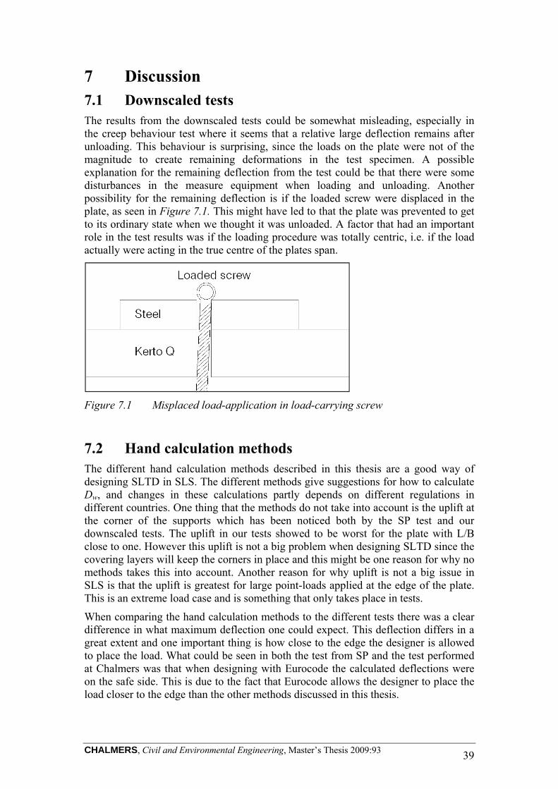
7 Discussion 7.1 Downscaled tests The results from the downscaled tests could be somewhat misleading, especially in the creep behaviour test where it seems that a relative large deflection remains after unloading. This behaviour is surprising, since the loads on the plate were not of the magnitude to create remaining deformations in the test specimen. A possible explanation for the remaining deflection from the test could be that there were some disturbances in the measure equipment when loading and unloading. Another possibility for the remaining deflection is if the loaded screw were displaced in the plate, as seen in Figure 7.1. This might have led to that the plate was prevented to get to its ordinary state when we thought it was unloaded. A factor that had an important role in the test results was if the loading procedure was totally centric, i.e. if the load actually were acting in the true centre of the plates span.
Figure 7.1 Misplaced load-application in load-carrying screw
7.2 Hand calculation methods The different hand calculation methods described in this thesis are a good way of designing SLTD in SLS. The different methods give suggestions for how to calculate Dw, and changes in these calculations partly depends on different regulations in different countries. One thing that the methods do not take into account is the uplift at the corner of the supports which has been noticed both by the SP test and our downscaled tests. The uplift in our tests showed to be worst for the plate with L/B close to one. However this uplift is not a big problem when designing SLTD since the covering layers will keep the corners in place and this might be one reason for why no methods takes this into account. Another reason for why uplift is not a big issue in SLS is that the uplift is greatest for large point-loads applied at the edge of the plate. This is an extreme load case and is something that only takes place in tests.
When comparing the hand calculation methods to the different tests there was a clear difference in what maximum deflection one could expect. This deflection differs in a great extent and one important thing is how close to the edge the designer is allowed to place the load. What could be seen in both the test from SP and the test performed at Chalmers was that when designing with Eurocode the calculated deflections were on the safe side. This is due to the fact that Eurocode allows the designer to place the load closer to the edge than the other methods discussed in this thesis.

CHALMERS, Civil and Environmental Engineering, Master’s Thesis 2009:93 40
The scale factor, η, affected the calculated deflections for the downscaled test. As mentioned in Chapter 6.1, a better way of treating this would be to have different scale factors for different methods. For example, in the method from West Virginia University the thickness of the plate affect the distribution width and thereby the deflection. With the used scale factor, that only takes the length of the plate into account, the distribution width is lower than it would have been if the scale factor also would have been dependent of the thickness of the plate.
7.3 FE model The CALFEM routines beam2w.m and beam2ws.m has proven to be a reasonable good method of predicting deflections, shear forces and moments in the SLS for SLTD bridges. However, the deflections are on the safe side, thus leading to higher deflections and internal forces. According to the results from the FE analysis, the best way of predicting the elastic foundation stiffness for a SLTD loaded with edge-load would be to estimate the effective width, Dw according to Eurocode and then calculate the elastic foundation stiffness according to Equation 6.4. The authors of this thesis thinks that this correlation is due to the fact that Eurocode takes into account the effect of high loads close to the edge in the span.
For the downscaled test plates the results contained some consistency for the larger plates, but gave unsatisfying results for the smallest plate.
Due to the limitation of this thesis, discussions of how well the approximation would be for a beam with point-load in the centre cannot be made. For a practical use of the elastic foundation theory, more full scale test data would be needed to analyse.
7.4 Failure load To establish a good model of the failure load, consideration of how the stress distributes in the transversal direction probably needs to be taken into account. The distributed lengths, ldist, from Chapter 6, Section 6.3 would probably be smaller if the stresses are allowed to distribute in both directions.
7.5 Suggestions for further research Modify the elastic foundation model against more full-scale tests
Examine the failure load in ABAQUS
Use different ldist for the shear and moment utilization

CHALMERS, Civil and Environmental Engineering, Master’s Thesis 2009:93 41
8 References 8.1 Literature Bing Y. Ting, Eldon M. (1984): Beams on elastic foundation finite element, Journal
of Structural Engineering, Vol. 110, No. 10, October, 1984, ASCE, ISSN.
Blass H.J et al. (1995): Timber Engineering – STEP 1. First Edition, Centrum Hout, The Netherlands.
BYGG1 – Allmänna Grunder, AB Byggmästarföreningens förlag, Stockholm 1961, (BYGG1 - General Basics).
Commitée Europeen de Normalisation, CEN (2004),: EN 1995-1:2004. Eurocode 5 – Design of Timber Structures Part 1 – General – Common rules and rules for buildings, 2004.
Commitée Europeen de Normalisation, CEN (2004),: EN 1995-2:2004. Eurocode 5 – Design of Timber Structures Part 2 – Bridges, 2004.
Crews, K. (2002): Behaviour and Critical Limit States of Transversely Laminated Timber Cellular Bridge Decks. Ph.D. Thesis. Faculty of Engineering, University of Technology, Sydney.
Crews, K. (2006): Recommended Procedures for Determination of Distribution Widths in the Design of Stress Laminated Timber Plated Decks, CIB W18/39-12-1.
Dahl, K. (2002): Tverspente Dekker i Tre. Master’s Thesis, (Stress Laminated Timber Decks), Institut for tekniske fag, Norges Landbrukshøgskole, (The Institute for technical research, Norwegian Agricultural School).
Formolo S, Granström R (2007): Compression Perpendicular to the Grain and Reinforcement of a Pre-Stressed Timber Deck. Master’s Thesis. Department of Civil and Environmental Engineering, Chalmers University of Technology, Göteborg.
Marklund K.A (1997): Nordic Timber Bridge Project – Deflection of Measuring of Stress-Laminated Deck Bridge, Institutet för Träteknisk Forskning (Institute for timber research).
Moelven (2009): Moelvens handbok om Kerto, tabell 2.6 och 2.7 (Moelven’s handbook about Kerto, table 2.6 and 2.7).
Ottosen N, Petersson H. (1992): Introduction to the finite element method. Prentice Hall, Great Britain, 1992.
Porteous J, Kermani A (2007): Strutural Timber Design to Eurocode 5. Blackwell Publishing, United Kingdom.
Ritter, M, A (1990): Timber Bridges – Design, Construction, Inspection and maintenance.
SP Trätek (2008): Report, Denotation P803586.
8.2 Verbal Crocetti, R (2009)

CHALMERS, Civil and Environmental Engineering, Master’s Thesis 2009:93 42
Appendix A1 – Used deflections from SP test
Figure A.1 Measured deflections from different load series around 200 kN.
Figure A.2 Measured deflections from different load series around 300 kN.
Table A.1 Measured deflections used for analysis of elastic foundation stiffness.
Measure point [m] ‐ Deflection [mm]
Load [kN] 0,143 0,523 1,477 2,518 4,689
98,6362 13,453 11,4645 6,602 3,102 ‐1,394
198,3392 27,232 23,068 12,96467 5,677333 ‐3,71067
298,3852 42,01133 35,25733 19,116 7,574 ‐7,27533
25,5
26
26,5
27
27,5
28
28,5
29
194 195 196 197 198 199 200 201
Deflection [m
m]
Load [kN]
39,5
40
40,5
41
41,5
42
42,5
43
43,5
44
44,5
294 295 296 297 298 299 300 301
Deflection [m
m]
Load [kN]

CHALMERS, Civil and Environmental Engineering, Master’s Thesis 2009:93 43
Appendix A2 – Parameters from the SP test
Dimensions and parameters of the bridge
Dimensions
lspan 10m Length of bridge
wbridge 5035mm Width of bridge
wglulam 95mm Width of glulam beam
hglulam 495mm Height of glulam beam
x 0 0.01m lspan
y 0 0.01m wbridge
Crossectional units
Ixbeam
wglulam hglulam3
129.602 10
4 m
4
Iybeam
hglulam wglulam3
123.537 10
5 m
4
Wxbeam
wglulam hglulam2
63.88 10
3 m
3
Wybeam
wglulam2
hglulam
67.446 10
4 m
3
Modification factors
Size effect
kh min600mm
hglulam
0.1
1.1
1.019
Load duration and service class
kmod 0.9
System effect
ksys 1.1
Deformation coefficent
kdef 2.0
Partial coefficent for material properties
Mglulam 1.3

CHALMERS, Civil and Environmental Engineering, Master’s Thesis 2009:93 44
Defining units in Mathcad
Nmm N mm
kNm kNm
Stregth and stiffness properties, combined glulam
spruce 380kg
m3
g 3.727kN
m3
Characteristic values
Bending strength
fmgk 28N
mm2
28MPa
Tension strength
ft0gk 16.5N
mm2
16.5MPa
ft90gk 0.4N
mm2
0.4MPa
Compression stregth
fc0gk 24N
mm2
24MPa
fc90gk 2.7N
mm2
2.7MPa
Shear stregth
fvgk 2.7N
mm2
2.7MPa
Modulus of elasticity
E0mean 12.0kN
mm2
12GPa
Shear modulus
Ggmean 0.72kN
mm2
0.72GPa
Dimensioning values
Bending strength
fmgdb
kh kmod ksys fmgk
Mglulam
21.737MPa
fvgdb
kmod ksys fvgk
Mglulam
2.056MPa

CHALMERS, Civil and Environmental Engineering, Master’s Thesis 2009:93 45
Appendix B1 – Ritter
Ritters Design guide
Reference:Z:\Skolan\Exjobb\Till Storegate\MathCad\Dimensioner och parametrar på bron.xmcd(R)
Loads acting on the deck
Ptest100
200
kN Loads for comparison with SP test
According to Ritter Design guide, the following points have been calculated.
1) Input data from Appendix A2
bdeck wbridge bdeck 5.035m Width of deck
lspan 10m Lenght of span
hglulam 0.495m Height of deck
E0mean 1.2 104
MPa
2) Timber class GL28c
fmgdb 21.737MPa
E0mean 12 GPa
3) CB - Coefficient for butt joints
CB 1.0 No butt joints
4) Stifness properties
E0 E0mean
E90 0.013 E0 156 MPa
G0 0.03 E0 360 MPa According to Ritter
5) Maximal pointload moment
M0
Ptest lspan
4
250
500
kNm

CHALMERS, Civil and Environmental Engineering, Master’s Thesis 2009:93 46
6) Effective width Dw
2 G0
E0 CB E900.526
Parameter for the Decks torsional stiffness
bdeck
2 lspan
E0 CB
E90
0.25
0.746 Relation between the deck stiffness in longitudinaland transversal direction
From diagram according to Ritter (1990),and modified by Dahl (2002).Dw 1800mm
7) Deck section modulus and effective deck moment inertia
I CB
Dw hglulam3
12 0.018m
4
S CB
Dw hglulam2
6 0.074 m
3
8) Design moment
qd spruce Dw hglulam
My M0 qd
lspan2
4
116.35
366.35
kNm
9) Bending strenght check
y fmgdb Cls
Cls 1.3
y
My
S
1.583
4.984
MPa
fmgdb Cls 28.258MPa
10) Deflection w from uniform load and point load
wtot wlim
Iw
Dw hglulam3
12

CHALMERS, Civil and Environmental Engineering, Master’s Thesis 2009:93 47
wbend_pointload
Ptest lspan3
48 E0mean 1.33 Iw Increase I for deflection
calculations
wbend_uniform
5 qd lspan4
384 E0mean 1.33 Iw
shear_amplification_point 1 1.2E0mean
G0
hglulam
lspan
2
1.098
shear_amplification_uniform 1 0.96E0mean
G0
hglulam
lspan
2
1.078
wtotfin wbend_pointload shear_amplification_point
wbend_uniform shear_amplification_uniform
9.484
17.362
mm
wlim
lspan
36027.778mm
wbend_pointload7.175
14.35
mm

CHALMERS, Civil and Environmental Engineering, Master’s Thesis 2009:93 48
Appendix B2 – Eurocode 5
Eurocode
Reference:Z:\Skolan\Exjobb\Till Storegate\MathCad\Dimensioner och parametrar på bron.xmcd(R)
Input data from Appendix A2
bdeck wbridge bdeck 5.035m Width of deck
lspan 10m Lenght of span
hglulam 0.495m Height of deck
E0mean 12 GPa
Loads acting on the deck
Ptest100
200
kN Loads to compare with SP test
Effective width
bw 0.6m Width of wheel
15deg Dispersion angle, according to Table 3.1
a 0.3m
bw_middle bw hglulam sin ( ) 0.728m
bef bw_middle a
bef 1.028m
Deck strenght
blam wglulam
nbef
blam10.822
ksys 1.1
fm_d_lam fmgdb
fv_d_lam fvgdb

CHALMERS, Civil and Environmental Engineering, Master’s Thesis 2009:93 49
fm_d_deck ksys fm_d_lam 23.911MPa
fv_d_deck ksys fv_d_lam 2.262MPa
Action effects
qd spruce bef hglulam 1.896kN
m
I bef
hglulam3
12
RA
Ptest
2qd
lspan
2
Mmax RA
lspan
2 qd
lspan2
4
250
500
kNm Design moment
wbend
Ptest lspan3
48 E0mean I
16.707
33.414
mm Deflection due to applied loads

CHALMERS, Civil and Environmental Engineering, Master’s Thesis 2009:93 50
Appendix B3 – Crews
Crews
Reference:Z:\Skolan\Exjobb\Till Storegate\MathCad\Dimensioner och parametrar p å bron.xmcd
Defining units in Mathcad
kNm kN m
Input data from Appendix A2
bdeck wbridge bdeck 5.035m Width of deck
lspan 10m Lenght of span
hglulam 0.495m Height of deck
E0mean 12 GPa
Loads acting on the deck
Ptest100
200
kN Loads to compare with SP test
Distribution width
Dw1
E0
10000
0.50lspan
25 0.45
CB for a single lane bridge
Dw2
E0
18000
0.40lspan
30 0.45
CB for a two lane bridge
Where:
E0 E0mean 12 GPa
CB_hardwood
n 1
n
0.751.0
where n is number of buttjoints
CB_australian.pine
n 1
n
0.851.0

CHALMERS, Civil and Environmental Engineering, Master’s Thesis 2009:93 51
Since we have glulam and therefore there is no effect of butt joints, CB=1.0
CB 1.0
Dw1
E0
10000MPa
0.50lspan
25 m 0.45
CB
Dw2
E0
18000MPa
0.40lspan
30 m 0.45
CB
Dw
Dw1
Dw2
m1.945
1.634
m
Dw Dw1 m Since we have a single line bridge
Dw 1.945m Calculated distrubution width accordito Crews
Second moment of inertia, I, and deflection, w.
ICB Dw hglulam
3
120.02 m
4
wPtest lspan
3
48 E0 I
w8.829
17.659
mm

CHALMERS, Civil and Environmental Engineering, Master’s Thesis 2009:93 52
Appendix B4 – West Virginia University method
West Virginia University method
Reference:Z:\Skolan\Exjobb\Till Storegate\MathCad\Dimensioner och parametrar på bron.xmcd
Reference:Z:\Skolan\Exjobb\Till Storegate\MathCad\Gammalt\Crews.xmcd
Defining units in Mathcad
kNm kN m
Nmm N mm
Nm N m
Loads acting on the deck
Ptest100
200
kN Loads to compare with SP test
Input data from Appendix A2
bdeck wbridge bdeck 5.035m Width of deck
lspan 10m Lenght of span
hglulam 0.495m Height of deck
E0mean 12 GPa
Distribution width
Dw bf 2 t CB
bf 600mm wheel width
CB 1 No effects of butt joints
Dw bf 2 hglulam CB
Dw 1.59m calculated distribution width according to W.V.U method
Second moment of inertia, I, and deflection, w.
IDw hglulam
3
120.016m
4

CHALMERS, Civil and Environmental Engineering, Master’s Thesis 2009:93 53
wPtest lspan
3
48 E0 1.15 I
w9.394
18.788
mm
Where I is increased with 15% because of deflection calculations

CHALMERS, Civil and Environmental Engineering, Master’s Thesis 2009:93 54
Appendix C1 – Convergence for number of elements
Figure C.1 Convergence, mean shear force versus number of elements.
Figure C.2 Convergence, mean moment versus number of elements.

CHALMERS, Civil and Environmental Engineering, Master’s Thesis 2009:93 55
Appendix C2 – Behaviour of beam on elastic foundation
Figure C.3 Influence-lines for moment in beam on elastic foundation, Figure from BYGG1 p.648
k48 Ex Ix
ldeck3
x
l0 2l0
4Ey Iy
k
lspan
l0 2
M P l0 2
CASE 1, 1000 N.
P 1000 h 0.495Ex 12 10
9
lspan 5 w 1 ldeck 10Ey 0.02 Ex
Iyw h
3
12
Ixh
3
12 k
48 Ex Ix
ldeck3

CHALMERS, Civil and Environmental Engineering, Master’s Thesis 2009:93 56
Figure C.4 Top right. Influence-lines for moment in beam on elastic foundation with values for the calculations to the left. Bottom. Y-axis: Moment distribution from CALFEM, X-axis: width of plate.
l0
4Ey Iy
k0.803
x 0.5
x
l0 20.44 lspan
l0 24.401
0.275
Mx P l0 2 312.46
x 1
x
l0 20.88 lspan
l0 24.401
0.32
Mx P l0 2 363.59
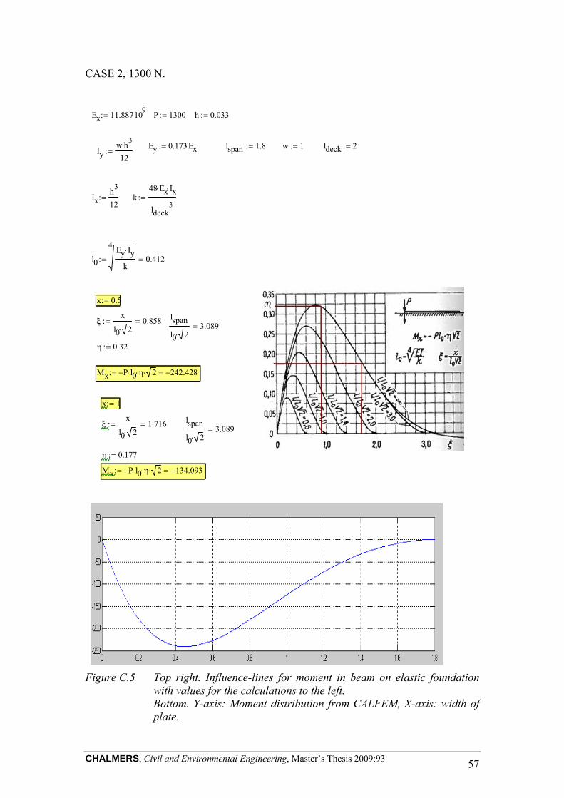
CHALMERS, Civil and Environmental Engineering, Master’s Thesis 2009:93 57
CASE 2, 1300 N.
Ex 11.887109
P 1300 h 0.033
Ey 0.173 Ex lspan 1.8 w 1 ldeck 2Iy
w h3
12
Ixh
3
12 k
48 Ex Ix
ldeck3
l0
4Ey Iy
k0.412
x 0.5
x
l0 20.858 lspan
l0 23.089
0.32
Mx P l0 2 242.428
x 1
x
l0 21.716 lspan
l0 23.089
0.177
Mx P l0 2 134.093
Figure C.5 Top right. Influence-lines for moment in beam on elastic foundation with values for the calculations to the left. Bottom. Y-axis: Moment distribution from CALFEM, X-axis: width of plate.

CHALMERS, Civil and Environmental Engineering, Master’s Thesis 2009:93 58
CASE 3, 480 N.
Ex 11.887109
P 480 h 0.033
Ey 0.173 Ex lspan 0.3 w 1 ldeck 2Iy
w h3
12
Ixh
3
12 k
48 Ex Ix
ldeck3
l0
4Ey Iy
k0.412
x 0.1
x
l0 20.172 lspan
l0 20.515
0.075
Mx P l0 2 20.979
x 0.2
x
l0 20.343 lspan
l0 20.515
0.035
Mx P l0 2 9.79
Figure C.6 Top right. Influence-lines for moment in beam on elastic foundation with values for the calculations to the left. Bottom. Y-axis: Moment distribution from CALFEM, X-axis: width of plate.

CHALMERS, Civil and Environmental Engineering, Master’s Thesis 2009:93 59
Appendix D1 – Convergence for creep
Table D.1 Convergence for creep with loading and unloading.
Loading Unloading
[min] Time [sec] def [mm]
Time [sec] def [mm]
10 14,486 1210 0,696 20 14,546 1220 0,676 30 14,59 1230 0,666 40 14,621 1240 0,652 50 14,647 1250 0,648 1 60 14,667 1260 0,642 80 14,7 1280 0,632 100 14,725 1300 0,623 2 120 14,747 1320 0,616 150 14,775 1350 0,608 3 180 14,797 1380 0,601 4 240 14,834 1440 0,589 5 300 14,864 1500 0,58 6 360 14,888 1560 0,572 7 420 14,91 1620 0,567 8 480 14,928 1680 0,561 9 540 14,945 1740 0,557 10 600 14,961 1800 0,553 11 660 14,976 1860 0,55 12 720 14,989 1920 0,546 13 780 15 1980 0,544 14 840 15,012 2040 0,542 15 900 15,022 2100 0,539 16 960 15,032 2160 0,537 17 1020 15,042 2220 0,535 18 1080 15,051 2280 0,533 19 1140 15,061 2340 0,531 20 1200 15,068 2400 0,53

CHALMERS, Civil and Environmental Engineering, Master’s Thesis 2009:93 60
P 19.99kg g 196.035N
d 200mm
h 0.033m
y1_midspan P
l a1 ll
2
6 E I 1
a12
l2
l
2
2
l2
y1_midspan_E P
l a1 ll
2
6 I 1
a12
l2
l
2
2
l2
5.973 106
m Pa
a2l d
21.1ma1
l d
20.9m
b1 l a1 b2 l a2
y2_midspan
P l b2 l
2 6 E I1
b22
l2
l
2
2
l2
y2_midspan_E
P l b2 l
2 6 I1
b22
l2
l
2
2
l2
5.973 106
m Pa
Appendix D2 – Computations for modulus of elasticity
Load
For Ex
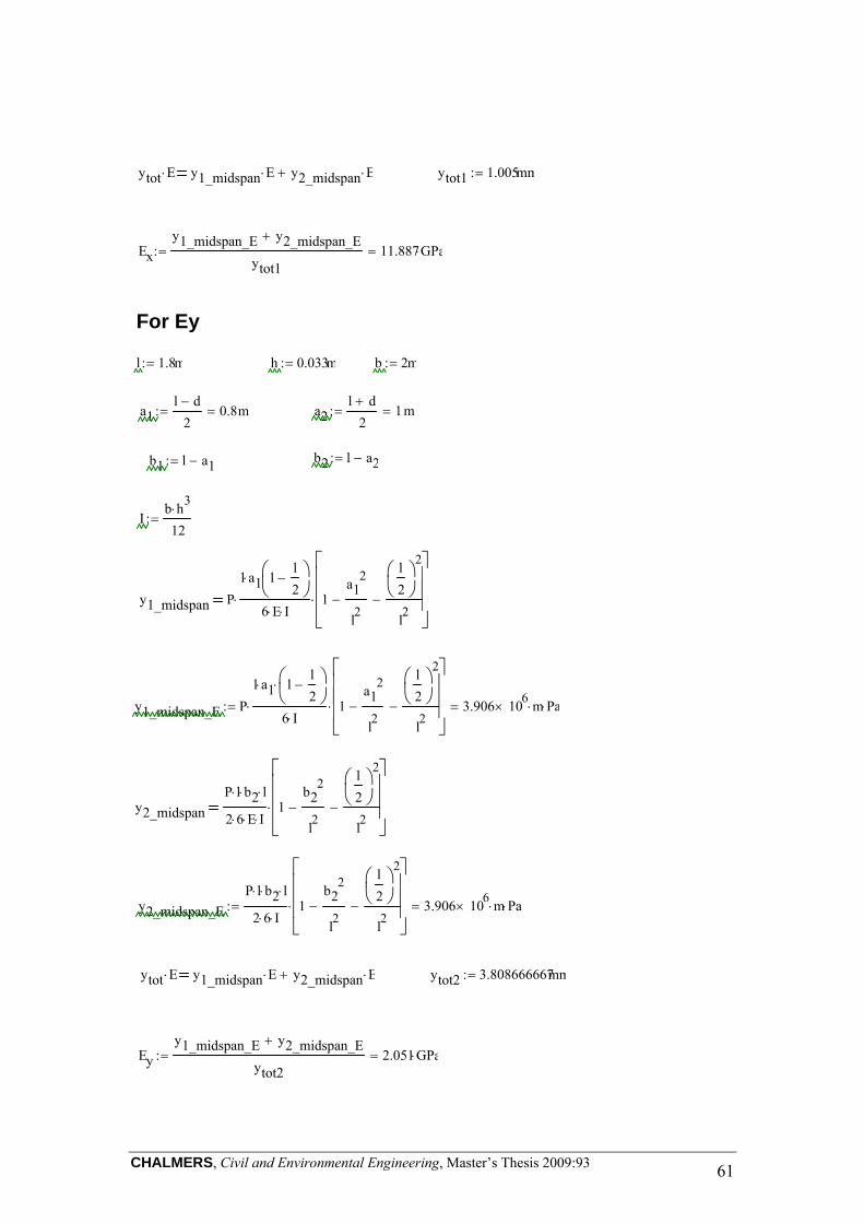
CHALMERS, Civil and Environmental Engineering, Master’s Thesis 2009:93 61
ytot E y1_midspan E y2_midspan E ytot1 1.005mm
Ex
y1_midspan_E y2_midspan_E
ytot111.887GPa
l 1.8m h 0.033m
a1l d
20.8m
b 2m
a2l d
21m
b2 l a2b1 l a1
Ib h
3
12
y1_midspan P
l a1 ll
2
6 E I 1
a12
l2
l
2
2
l2
y1_midspan_E P
l a1 ll
2
6 I 1
a12
l2
l
2
2
l2
3.906 106
m Pa
y2_midspan
P l b2 l
2 6 E I1
b22
l2
l
2
2
l2
y2_midspan_E
P l b2 l
2 6 I1
b22
l2
l
2
2
l2
3.906 106
m Pa
ytot E y1_midspan E y2_midspan E ytot2 3.808666667mm
Ey
y1_midspan_E y2_midspan_E
ytot22.051 GPa
For Ey

CHALMERS, Civil and Environmental Engineering, Master’s Thesis 2009:93 62
Caclulated E, according to STEP1
EI
i
Ei Ii =
E0 13.8GPa E90 0.43GPa
b 1
d0.033
11
Eparalell I E09 d
3
122 2 d( ) 1.5 d( )
24.5 d( )
2
E902 d
3
122 1 d( ) 3 d( )
2
=
Eparalell
E09 d
3
122 2 d( ) 1.5 d( )
24.5 d( )
2
E902 d
3
122 1 d( ) 3 d( )
2
11 d( )3
12
11.36 GPa
Eperpendicular I E02 d
3
122 1 d( ) 3 d( )
2
E909 d
3
122 2 d( ) 1.5 d( )
24.5 d( )
2
=
Eperpendicular
E02 d
3
122 1 d( ) 3 d( )
2
E909 d
3
122 2 d( ) 1.5 d( )
24.5 d( )
2
11 d( )3
12
2.61 GPa

CHALMERS, Civil and Environmental Engineering, Master’s Thesis 2009:93 63
Appendix D3 – Procedure for testing of LVL
Dimensions of tested plates L x B = 2 x (0.3, 0.6, 0.9, 1.8) and 1.4 x 1.8 m2.
Applied load, P= 0.46, 0.872, 1.302, 1.744 and 1.310 kN.
Procedure: 1. Place first plate on supports 2. Load with P at Lc1 as can be seen in Figure D1 3. Deformations are measured after five minutes 4. Unload, remaining deformations are noted five minutes after unloading 5. Remove transducers at position 9, 10, 11 and change the boundary conditions
so that the plate is no longer free for uplift, for boundary conditions see Picture D1 and D2
6. Change from LC1 to LC2 and redo the same procedure as for LC1 7. Redo step 1-7 for the next plate
Figure D.1 Load placement and measure points for the simply supported plates.

CHALMERS, Civil and Environmental Engineering, Master’s Thesis 2009:93 64
Picture D.1 Support conditions when simply supported.
Picture D.2 Support conditions when fixed.

CHALMERS, Civil and Environmental Engineering, Master’s Thesis 2009:93 65
Appendix D4 – Expected plate deflections
Expected plate deflection according to different hand-calculationmethods
Reference:Z:\Skolan\Exjobb\Till Storegate\MOE from experiment.xmcd
ORIGIN 1
Dimensions and indata for the test
E0 Ex 11.887GPaFrom Appendix D2, according to our test
E90 Ey 2.051 GPa
G0 600N
mm2
From manufactures, Table 2.7 Kerto Tekniskhandbok from Moelven
Dimensions of plates
lspan 2m Length of span
bdeck
1800
900
600
300
mm Width of plates
t 33mm Thickness of plates
Loads
P
2.5 45 44.4 43.9 42( )kg
2.5 44.4 43.9 42( )kg
2.5 42 44.4( )kg
2.5 44.4( )kg
g
1.744
1.302
0.872
0.46
kN
Parameters that will be used in calculations
CB 1.0 No effects from butt joints
lbridge 15m Length of bridge that our scale tests are based on.
lbridge
lspan7.5 Factor that the calculated effective width should be
scaled with

CHALMERS, Civil and Environmental Engineering, Master’s Thesis 2009:93 66
Expected deflections according to the different hand calculation methods
Ritter
britter bdeck
13.5
6.75
4.5
2.25
m Width of sclaed bridge
Effective width
2 G0
E0 CB E900.243
britter
2 lbridge
E0 CB
E90
0.25
0.698
0.349
0.233
0.116
a - Parameter for the Decks torsional stiffness
? - Relation between the deck stiffness in longitudinal and transversal direction
Dw_ritter 1800mm From diagram according to Ritter (1990),and modified by Dahl (2002).
Dw
Dw_ritter
0.24m Scaled width with respect to scale factor
Second moment of inertia, I, and deflection, w.
Iw
Dw t3
127.187 10
7 m
4
wRitter
P4
lspan3
48 E0 1.33 Iw6.746 mm For the load P=0.46 kN
Where I is increased due to deflection calculations.
Eurocode 5
Effective width
bw 0.6m Width of wheel
45deg Dispursion angle according to EN 1995-2:2004 (E),Table 5.2

CHALMERS, Civil and Environmental Engineering, Master’s Thesis 2009:93 67
a 0.5m For cross laminated timber according to EN1995-2:2004 (E), Table 5.3
bw_middle bw t sin ( ) 0.775m
Dw_EC5 bw_middle a
Dw_EC5 1.275m
Dw
Dw_EC5
0.17m Scaled width with respect to scale factor
Second moment of inertia, I, and deflection, w.
IDw t
3
125.091 10
7 m
4
wEC5
P4
lspan3
48 E0 I12.667mm For the load P=0.46 kN
Crews
Distribution width
Dw
E0
10000
0.50L
25 0.45
CB for a single lane bridge
Dw_crews
E0
10000MPa
0.50lbridge
25 m 0.45
CB 1 m
Dw_crews 2.14m
Dw
Dw_crews
0.285m Scaled width with respect to scale factor
Second moment of inertia, I, and deflection, w.
ICB Dw t
3
128.546 10
7 m
4

CHALMERS, Civil and Environmental Engineering, Master’s Thesis 2009:93 68
wCrews
P4
lspan3
48 E0 I7.546 mm For the load P=0.46 kN
West Virginia University
Distribution width
Dw bf 2 t CB
bf
bw
0.08 m Scaled wheel width with respect to scale factor
Dw_W.V.U bf 2 t CB
Dw_W.V.U 0.146m calculated distribution width according to W.V.U meth
Dw Dw_W.V.U 0.146m
Second moment of inertia, I, and deflection, w.
IDw t
3
124.372 10
7 m
4
wW.V.U
P4
lspan3
48 E0 1.15 I12.825mm For the load P=0.46 kN

CHALMERS, Civil and Environmental Engineering, Master’s Thesis 2009:93 69
‐6
‐4
‐2
0
2
0 500 1000 1500 2000
Deflection [m
m]
Width of plate [mm]
Centre load, simply supported B=1800
Mispan
Quarterspan
Supportspan
Appendix D5 – Results from plate behaviour test This section gives results from our tests performed on LVL plates with different dimensions and applied loads. All plates have the same thickness, 33mm.
Figure D.2 Deflections for simply supported plate with dimensions L x B = 2 x 1.8 m2. Applied load P=1.303 kN in the middle of the plate.
Figure D.3 Deflections for fixed plate with dimensions L x B = 2 x 1.8 m2. Applied load P=1.303 kN in the middle of the plate.
‐6
‐5
‐4
‐3
‐2
‐1
0
1
0 500 1000 1500 2000
Deflection [m
m]
Width of plate [mm]
Centre load, fixed. B=1800
Mispan
Quarterspan
Supportspan

CHALMERS, Civil and Environmental Engineering, Master’s Thesis 2009:93 70
Table D.2 Measured deflections for the plate with dimensions L x B = 2 x 1.8 m2. Applied load P=1.303 kN in the centre of the plate (measure point 3). Simply supported and fixed respectively.
LC1, simply mm Measure point Deflection
Midspan 0 1 -1,43
450 2 -3,37
900 3 -5,33
1350 4 -3,36
1800 5 -1,38
Quarter span 0 6 -1,1
900 7 -3,34
1800 8 -0,83
Support span 0 9 -0,04
900 10 -0,09
1800 11 0,21
LC1, fixed mm Measure point Deflection
Midspan 0 1 -1,4
450 2 -3,28
900 3 -5,14
1350 4 -3,24
1800 5 -1,37
Quarter span 0 6 -1,07
900 7 -3,24
1800 8 -0,89
Support span 0 9 -0,09
900 10 -0,1
1800 11 0,02

CHALMERS, Civil and Environmental Engineering, Master’s Thesis 2009:93 71
Figure D.5 Deflections for simply supported plate with dimensions L x B = 2 x 1.8 m2. Applied load P=1.303 kN at the edge of the plate.
Figure D.6 Deflections for fixed plate with dimensions L x B = 2 x 1.8 m2. Applied load P=1.303 kN at the edge of the plate.
‐20
‐15
‐10
‐5
0
5
0 500 1000 1500 2000
Deflection [m
m]
Width of plate [mm]
Edge load, simply supported B=1800
Mispan
Quarterspan
Supportspan
‐20
‐15
‐10
‐5
0
5
0 500 1000 1500 2000
Deflection [m
m]
Width of plate [mm]
Edge load, fixed. B=1800
Mispan
Quarterspan
Supportspan

CHALMERS, Civil and Environmental Engineering, Master’s Thesis 2009:93 72
Table D.3 Measured deflections for the plate with dimensions L x B = 2 x 1.8 m2. Applied load P=1.303 kN at the edge of the plate (measure point 1). Simply supported and fixed respectively.
LC2, simply mm Measure point Deflection
Midspan 0 1 -15,31
450 2 -6,14
900 3 -1,27
1350 4 0,82
1800 5 2,07
Quarter span 0 6 -9,98
900 7 -0,78
1800 8 2,66
Support span 0 9 -0,6
900 10 -0,02
1800 11 2,42
LC2, fixed mm Measure point Deflection
Midspan 0 1 -14,864
450 2 -5,99
900 3 -1,424
1350 4 0,28
1800 5 1,006
Quarter span 0 6 -9,11
900 7 -0,86
1800 8 0,74
Support span 0 9 -0,39
900 10 -0,06
1800 11 0,06

CHALMERS, Civil and Environmental Engineering, Master’s Thesis 2009:93 73
Figure D.8 Deflections for simply supported plate with dimensions L x B = 2 x 0.9 m2. Applied load P=1.303 kN in the middle of the plate.
Figure D.9 Deflections for fixed plate with dimensions L x B = 2 x 0.9 m2. Applied load P=1.303 kN in the middle of the plate.
Figure D.10 Deflections in the mid span for simply supported and fixed plate, with dimensions L x B = 2 x 0.9 m2. Applied load P=1.303 kN in the middle of the plate.
‐8
‐6
‐4
‐2
0
0 200 400 600 800 1000
Deflection [m
m]
Width of plate [mm]
Centre load, simply supported B=900
Mispan
Quarterspan
Supportspan
‐8
‐6
‐4
‐2
0
0 200 400 600 800 1000
Deflection [mm]
Width of plate [mm]
Centre load, fixed. B=900
Mispan
Quarterspan
Supportspan
‐8
‐6
‐4
‐2
0
0 200 400 600 800 1000
Deflection [mm]
Width of plate [mm]
Midspan, centre load
Simply
Fixed
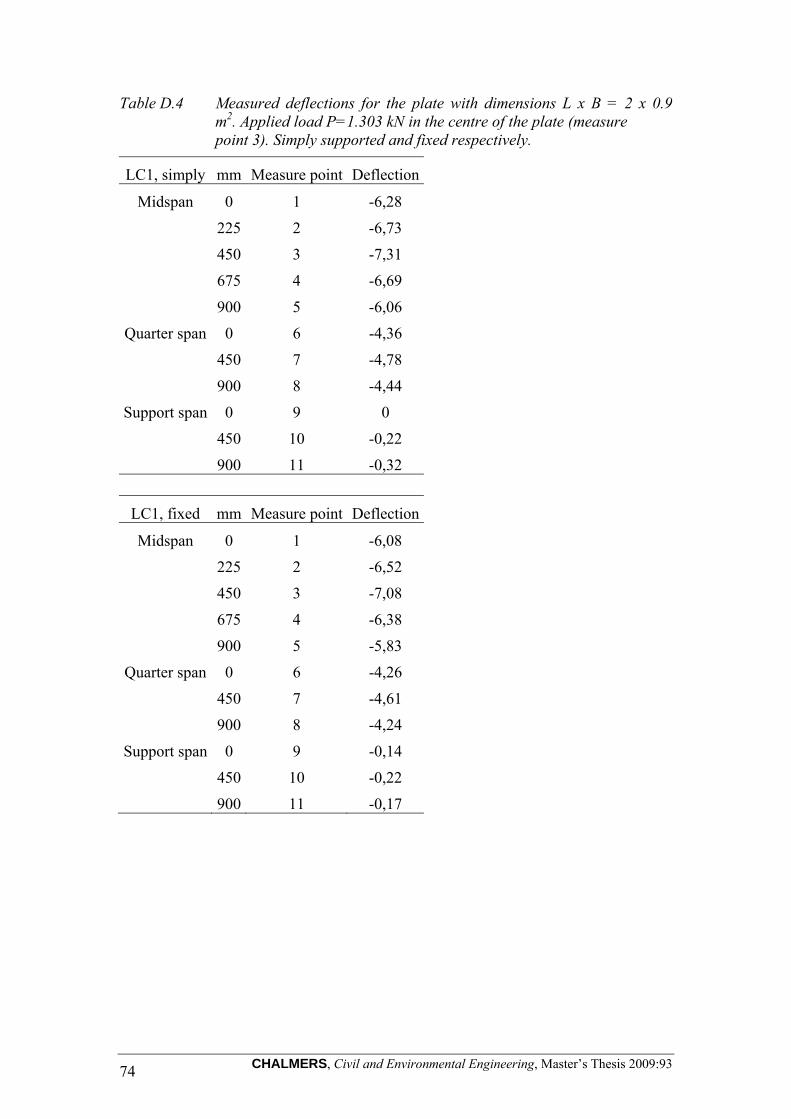
CHALMERS, Civil and Environmental Engineering, Master’s Thesis 2009:93 74
Table D.4 Measured deflections for the plate with dimensions L x B = 2 x 0.9 m2. Applied load P=1.303 kN in the centre of the plate (measure point 3). Simply supported and fixed respectively.
LC1, simply mm Measure point Deflection
Midspan 0 1 -6,28
225 2 -6,73
450 3 -7,31
675 4 -6,69
900 5 -6,06
Quarter span 0 6 -4,36
450 7 -4,78
900 8 -4,44
Support span 0 9 0
450 10 -0,22
900 11 -0,32
LC1, fixed mm Measure point Deflection
Midspan 0 1 -6,08
225 2 -6,52
450 3 -7,08
675 4 -6,38
900 5 -5,83
Quarter span 0 6 -4,26
450 7 -4,61
900 8 -4,24
Support span 0 9 -0,14
450 10 -0,22
900 11 -0,17

CHALMERS, Civil and Environmental Engineering, Master’s Thesis 2009:93 75
Figure D.11 Deflections for simply supported plate with dimensions L x B = 2 x 0.9 m2. Applied load P=1.303 kN at the edge of the plate.
Figure D.12 Deflections for fixed plate with dimensions L x B = 2 x 0.9 m2. Applied load P=1.303 kN at the edge of the plate.
Figure D.13 Deflections in mid span for simply supported and fixed plate, with dimensions L x B = 2 x 0.9 m2. Applied load P=1.303 kN at the edge of the plate.
‐20
‐15
‐10
‐5
0
5
0 200 400 600 800 1000
Deflection [mm]
Width of plate [mm]
Edge load, simply supported B=900
Mispan
Quarterspan
Supportspan
‐20
‐15
‐10
‐5
0
5
0 200 400 600 800 1000
Deflection [mm]
Width of plate [mm]
Edge load, fixed. B=900
Mispan
Quarterspan
Supportspan
‐20
‐15
‐10
‐5
0
5
0 200 400 600 800 1000
Deflection [mm]
Width of plate [mm]
Midspan, edge load
Simply
Fixed

CHALMERS, Civil and Environmental Engineering, Master’s Thesis 2009:93 76
Table D.5 Measured deflections for the plate with dimensions L x B = 2 x 0.9 m2. Applied load P=1.303 kN at the edge of the plate (measure point 1). Simply supported and fixed respectively.
LC2, simply mm Measure point Deflection
Midspan 0 1 -16,9
225 2 -10,92
450 3 -5,42
675 4 -1,12
900 5 2,8
Quarter span 0 6 -11,29
450 7 -4
900 8 2,71
Support span 0 9 -0,47
450 10 -0,08
900 11 2,92
LC2, fixed mm Measure point Deflection
Midspan 0 1 -15,837
225 2 -9,63
450 3 -5,945
675 4 -2,41
900 5 0,752
Quarter span 0 6 -10,4
450 7 -3,33
900 8 0,51
Support span 0 9 -0,39
450 10 -0,22
900 11 0,04

CHALMERS, Civil and Environmental Engineering, Master’s Thesis 2009:93 77
Figure D.14 Deflections for simply supported plate with dimensions L x B = 2 x 0.6 m2. Applied load P=0.872 kN in the middle of the plate.
Figure D.15 Deflections for fixed plate with dimensions L x B = 2 x 0.6 m2. Applied load P=0.872 kN in the middle of the plate.
Figure D.16 Deflections in the mid span for simply supported and fixed plate, with dimensions L x B = 2 x 0.6 m2. Applied load P=0.872 kN in the middle of the plate.
‐8
‐6
‐4
‐2
0
0 100 200 300 400 500 600
Deflection [mm]
Width of plate [mm]
Centre load, simply supported B=600
Mispan
Quarterspan
Supportspan
‐8
‐6
‐4
‐2
0
0 100 200 300 400 500 600
Deflection [mm]
Width of plate [mm]
Centre load, fixed. B=600
Mispan
Quarterspan
Supportspan
‐7
‐6,8
‐6,6
‐6,4
‐6,2
0 100 200 300 400 500 600
Deflection [mm]
Width of plate [mm]
Midspan, centre load
Simply
Fixed

CHALMERS, Civil and Environmental Engineering, Master’s Thesis 2009:93 78
Table D.6 Measured deflections for the plate with dimensions L x B = 2 x 0.6 m2. Applied load P=0.872 kN in the centre of the plate (measure point 3). Simply supported and fixed respectively.
LC1, simply mm Measure point Deflection
Midspan 0 1 -6,79
150 2 -6,83
300 3 -6,94
450 4 -6,52
600 5 -6,38
Quarter span 0 6 -4,8
300 7 -4,64
600 8 -4,6
Support span 0 9 -0,18
300 10 -0,27
600 11 -0,29
LC1, fixed mm Measure point Deflection
Midspan 0 1 -6,66
150 2 -6,69
300 3 -6,8
450 4 -6,37
600 5 -6,25
Quarter span 0 6 -4,66
300 7 -5,49
600 8 -4,43
Support span 0 9 -0,2
300 10 -0,28
600 11 -0,27

CHALMERS, Civil and Environmental Engineering, Master’s Thesis 2009:93 79
Figure D.17 Deflections for simply supported plate with dimensions L x B = 2 x 0.6 m2. Applied load P=0.872 kN at the edge of the plate.
Figure D.18 Deflections for fixed plate with dimensions L x B = 2 x 0.6 m2. Applied load P=0.872 kN at the edge of the plate.
Figure D.19 Deflections in mid span for simply supported and fixed plate, with dimensions L x B = 2 x 0.6 m2. Applied load P=0.872 kN at the edge of the plate.
‐15
‐10
‐5
0
5
0 100 200 300 400 500 600
Deflection [mm]
Width of plate [mm]
Edge load, simply supported B=600
Mispan
Quarterspan
Supportspan
‐15
‐10
‐5
0
5
0 100 200 300 400 500 600
Deflection [mm]
Width of plate [mm]
Edge load, fixed. B=600
Mispan
Quarterspan
Supportspan
‐15
‐10
‐5
0
0 100 200 300 400 500 600
Deflection [mm]
Width of plate [mm]
Midspan, edge load
Simply
Fixed

CHALMERS, Civil and Environmental Engineering, Master’s Thesis 2009:93 80
Table D.7 Measured deflections for the plate with dimensions L x B = 2 x 0.6 m2. Applied load P=0.872 kN at the edge of the plate (measure point 1). Simply supported and fixed respectively.
LC2, simply mm Measure point Deflection
Midspan 0 1 -12,52
150 2 -7,44
300 3 -6,73
450 4 -3,73
600 5 -1,38
Quarter span 0 6 -7,4
300 7 -4,6
600 8 -1
Support span 0 9 -0,34
300 10 -0,27
600 11 0,69
LC2, fixed mm Measure point Deflection
Midspan 0 1 -11,945
150 2 -9,17
300 3 -6,728
450 4 -4,06
600 5 -1,99
Quarter span 0 6 -7,92
300 7 -3,63
600 8 -1,55
Support span 0 9 -0,28
300 10 0
600 11 0,04

CHALMERS, Civil and Environmental Engineering, Master’s Thesis 2009:93 81
Figure D.20 Deflections for simply supported plate with dimensions L x B = 2 x 0.3 m2. Applied load P=0.460 kN in the middle of the plate.
Figure D.21 Deflections for fixed plate with dimensions L x B = 2 x 0.3 m2. Applied load P=0.460 kN in the middle of the plate.
Figure D.22 Deflections in the mid span for simply supported and fixed plate, with dimensions L x B = 2 x 0.3 m2. Applied load P=0.460 kN in the middle of the plate.
‐8
‐6
‐4
‐2
0
0 50 100 150 200 250 300
Deflection [mm]
Width of plate [mm]
Centre load, simply supported B=300
Mispan
Quarterspan
Supportspan
‐8
‐6
‐4
‐2
0
2
0 50 100 150 200 250 300
Delfection [mm]
Width of plate [mm]
Centre load, fixed. B=300
Mispan
Quarterspan
Supportspan
‐6,9
‐6,8
‐6,7
‐6,6
‐6,5
‐6,4
0 50 100 150 200 250 300
Deflection [mm]
Width of plate [mm]
Midspan, centre load
Simply
Fixed

CHALMERS, Civil and Environmental Engineering, Master’s Thesis 2009:93 82
Table D.8 Measured deflections for the plate with dimensions L x B = 2 x 0.3 m2. Applied load P=0.460 kN in the centre of the plate (measure point 3). Simply supported and fixed respectively.
LC1, simply mm Measure point Deflection
Midspan 0 1 -6,55
75 2 -6,57
150 3 -6,84
225 4 -6,66
300 5 -6,57
Quarter span 0 6 -4,52
150 7 -4,5
300 8 -4,48
Support span 0 9 -0,03
150 10 -0,08
300 11 -0,12
LC1, fixed mm Measure point Deflection
Midspan 0 1 -6,48
75 2 -6,48
150 3 -6,57
225 4 -6,52
300 5 -6,45
Quarter span 0 6 -4,54
150 7 -4,36
300 8 -4,31
Support span 0 9 -0,09
150 10 0,08
300 11 -0,13

CHALMERS, Civil and Environmental Engineering, Master’s Thesis 2009:93 83
Figure D.23 Deflections for simply supported plate with dimensions L x B = 2 x 0.3 m2. Applied load P=0.460 kN at the edge of the plate.
Figure D.24 Deflections for fixed plate with dimensions L x B = 2 x 0.3 m2. Applied load P=0.460 kN at the edge of the plate.
Figure D.25 Deflections in mid span for simply supported and fixed plate, with dimensions L x B = 2 x 0.3 m2. Applied load P=0.460 kN at the edge of the plate.
‐10
‐8
‐6
‐4
‐2
0
2
0 50 100 150 200 250 300
Deflection [mm]
Width of plate [mm]
Edge load, simply supported B=300
Mispan
Quarterspan
Supportspan
‐10
‐8
‐6
‐4
‐2
0
0 50 100 150 200 250 300
Deflection [mm]
Width of plate [mm]
Edge load, fixed. B=300
Mispan
Quarterspan
Supportspan
‐10
‐8
‐6
‐4
‐2
0
0 50 100 150 200 250 300
Deflection [mm]
Width of plate [mm]
Midspan, edge load
Simply
Fixed

CHALMERS, Civil and Environmental Engineering, Master’s Thesis 2009:93 84
Table D.9 Measured deflections for the plate with dimensions L x B = 2 x 0.3 m2. Applied load P=0.460 kN at the edge of the plate (measure point 1). Simply supported and fixed respectively.
LC2, simply mm Measure point Deflection
Midspan 0 1 -8,65
75 2 -7,76
150 3 -6,4
225 4 -5,74
300 5 -5,06
Quarter span 0 6 -5,41
150 7 -4,41
300 8 -3,45
Support span 0 9 -0,05
150 10 -0,22
300 11 0,14
LC2, fixed mm Measure point Deflection
Midspan 0 1 -8,028
75 2 -7,12
150 3 -6,335
225 4 -5,68
300 5 -5,027
Quarter span 0 6 -5,23
150 7 -4,34
300 8 -3,42
Support span 0 9 -0,07
150 10 -0,08
300 11 -0,08

CHALMERS, Civil and Environmental Engineering, Master’s Thesis 2009:93 85
Figure D.26 Deflections for simply supported plate with dimensions L x B = 1.4 x 1.8 m2. Applied load P=1.310 kN in the middle of the plate.
Figure D.27 Deflections for fixed plate with dimensions L x B = 1.4 x 1.8 m2. Applied load P=1.310 kN in the middle of the plate.
Figure D.28 Deflections in the mid span for simply supported and fixed plate, with dimensions L x B = 1.4 x 1.8 m2. Applied load P=1.310 kN in the middle of the plate.
‐3
‐2,5
‐2
‐1,5
‐1
‐0,5
0
0,5
0 500 1000 1500 2000
Deflection [mm]
Width of plate [mm]
Centre load, simply supported B=1800
Mispan
Quarterspan
Supportspan
‐3
‐2,5
‐2
‐1,5
‐1
‐0,5
0
0,5
0 500 1000 1500 2000
Deflection [mm]
Width of plate [mm]
Centre load, fixed. B=1800
Mispan
Quarterspan
‐3
‐2,5
‐2
‐1,5
‐1
‐0,5
0
0,5
0 500 1000 1500 2000
Deflection [mm]
Width of plate [mm]
Midspan, centre load
Simply
Fixed

CHALMERS, Civil and Environmental Engineering, Master’s Thesis 2009:93 86
Table D.10 Measured deflections for the plate with dimensions L x B = 1.4 x 1.8 m2. Applied load P=1.310 kN in the centre of the plate (measure point 3). Simply supported and fixed respectively.
LC1, simply mm Measure point Deflection
Midspan 0 1 -0,059
450 2 -1,14
900 3 -2,686
1350 4 -1,19
1800 5 0,035
Quarter span 0 6 -0,04
900 7 -1,73
1800 8 -0,08
Support span 0 9 0,01
900 10 -0,13
1800 11 0
LC1, fixed mm Measure point Deflection
Midspan 0 1 0,008
450 2 -1,06
900 3 -2,474
1350 4 -0,38
1800 5 0,022
Quarter span 0 6 -0,01
900 7 -1,56
1800 8 0,03
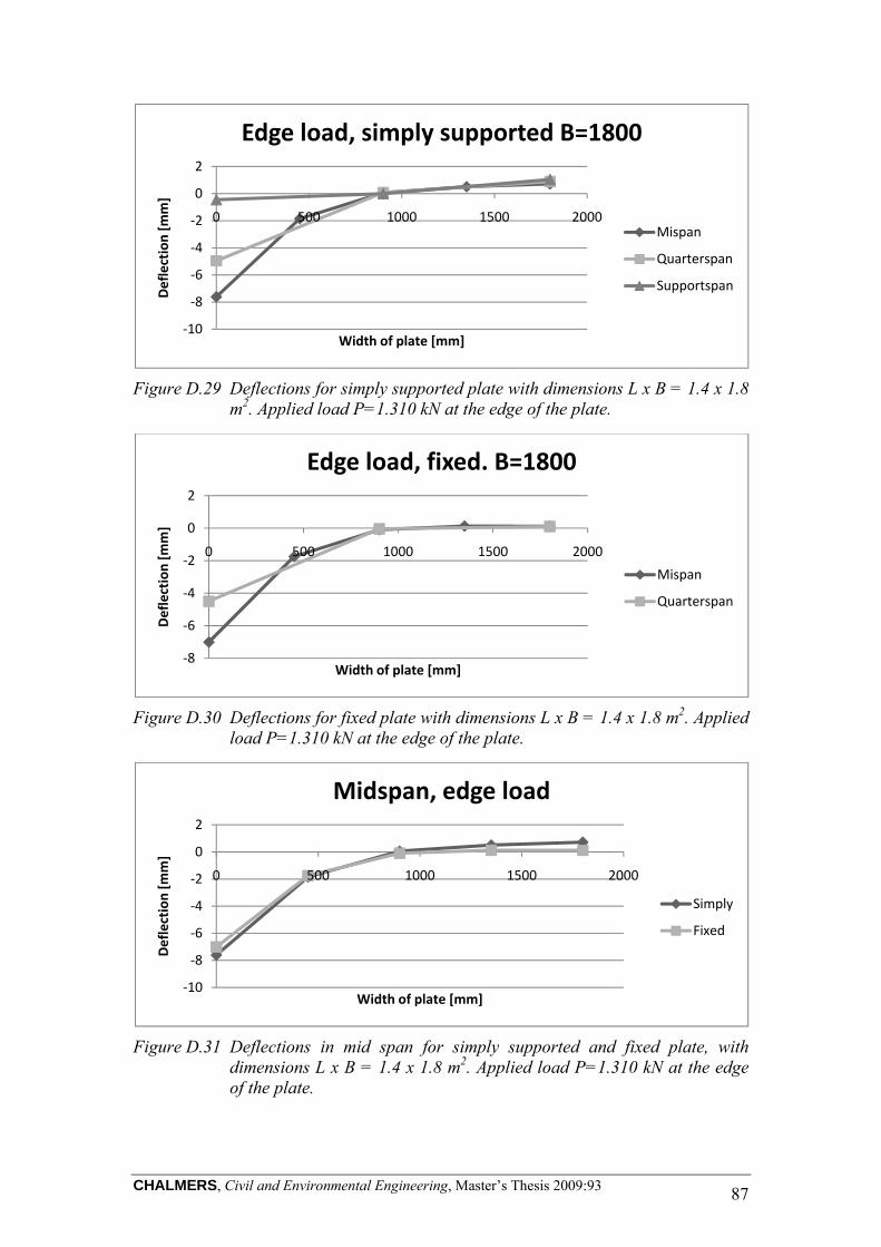
CHALMERS, Civil and Environmental Engineering, Master’s Thesis 2009:93 87
Figure D.29 Deflections for simply supported plate with dimensions L x B = 1.4 x 1.8 m2. Applied load P=1.310 kN at the edge of the plate.
Figure D.30 Deflections for fixed plate with dimensions L x B = 1.4 x 1.8 m2. Applied load P=1.310 kN at the edge of the plate.
Figure D.31 Deflections in mid span for simply supported and fixed plate, with dimensions L x B = 1.4 x 1.8 m2. Applied load P=1.310 kN at the edge of the plate.
‐10
‐8
‐6
‐4
‐2
0
2
0 500 1000 1500 2000
Deflection [mm]
Width of plate [mm]
Edge load, simply supported B=1800
Mispan
Quarterspan
Supportspan
‐8
‐6
‐4
‐2
0
2
0 500 1000 1500 2000
Deflection [mm]
Width of plate [mm]
Edge load, fixed. B=1800
Mispan
Quarterspan
‐10
‐8
‐6
‐4
‐2
0
2
0 500 1000 1500 2000
Deflection [mm]
Width of plate [mm]
Midspan, edge load
Simply
Fixed

CHALMERS, Civil and Environmental Engineering, Master’s Thesis 2009:93 88
Table D.11 Measured deflections for the plate with dimensions L x B = 1.4 x 1.8 m2. Applied load P=1.310 kN at the edge of the plate (measure point 1). Simply supported and fixed respectively.
LC2, simply mm Measure point Deflection
Midspan 0 1 -7,611
450 2 -1,85
900 3 0,064
1350 4 0,51
1800 5 0,719
Quarter span 0 6 -4,96
900 7 0,08
1800 8 0,89
Support span 0 9 -0,45
900 10 0
1800 11 1,04
LC2, fixed mm Measure point Deflection
Midspan 0 1 -7,012
450 2 -1,75
900 3 -0,096
1350 4 0,13
1800 5 0,119
Quarter span 0 6 -4,5
900 7 -0,04
1800 8 0,1

CHALMERS, Civil and Environmental Engineering, Master’s Thesis 2009:93 89
Appendix E1 – Results from parameter study In Table E.1-E.3 results from the parameter are presented where the relations between x and y varies for the different tables.
Table E.1 Values from parameter study
ldist [m] x [-] y [-] Χje (500 kN) Χje (600 kN)
10 1.99 0.1 0.96 1.02
9 2.24 0.112 0.94 1.02
8 2.56 0.128 0.93 1.02
7 2.94 0.147 0.93 1.03
6 3.74 0.187 0.91 1.05
5 5.8 0.29 0.84 1.06
Table E.2 Values from parameter study
ldist [m] x [-] y [-] Χje (500 kN) Χje (600 kN)
10 1.2 0.24 0.93 1.03
9 1.33 0.26 0.92 1.03
8 1.52 0.30 0.9 1.03
7 1.75 0.35 0.9 1.04
6 2.20 0.44 0.87 1.05
5 3.20 0.64 0.8 1.08
Table E.3 Values from parameter study
ldist [m] x [-] y [-] Χje (500 kN) Χje (600 kN)
10 0.7 0.35 0.92 1.02
9 0.89 0.445 0.91 1.02
8 1.00 0.5 0.9 1.03
7 1.16 0.58 0.89 1.04
6 1.43 0.715 0.86 1.05
5 2.05 1.025 0.79 1.06