Density-matrix simulation of small surface codes under current and projectedexperimental noise

T. E. O’Brien∗,1 B. Tarasinski∗,1, 2 and L. DiCarlo2, 3

1Instituut-Lorentz, Universiteit Leiden, P.O. Box 9506, 2300 RA Leiden, The Netherlands∗2QuTech, Delft University of Technology, P.O. Box 5046, 2600 GA Delft, The Netherlands

3Kavli Institute of Nanoscience, Delft University of Technology,P.O. Box 5046, 2600 GA Delft, The Netherlands

(Dated: January 9, 2018)

We present a density-matrix simulation of the quantum memory and computing performance ofthe distance-3 logical qubit Surface-17, following a recently proposed quantum circuit and using ex-perimental error parameters for transmon qubits in a planar circuit QED architecture. We use thissimulation to optimize components of the QEC scheme (e.g., trading off stabilizer measurement infi-delity for reduced cycle time) and to investigate the benefits of feedback harnessing the fundamentalasymmetry of relaxation-dominated error in the constituent transmons. A lower-order approximatecalculation extends these predictions to the distance-5 Surface-49. These results clearly indicateerror rates below the fault-tolerance threshold of surface code, and the potential for Surface-17to perform beyond the break-even point of quantum memory. However, Surface-49 is required tosurpass the break-even point of computation at state-of-the-art qubit relaxation times and readoutspeeds.

I. Introduction

Recent experimental demonstrations of small quantumsimulations1–3 and quantum error correction (QEC)4–7

position superconducting circuits for targeting quantumsupremacy8 and quantum fault tolerance9, two outstand-ing challenges for all quantum information processingplatforms. On the theoretical side, much modeling ofQEC codes has been made to determine fault-tolerancethreshold rates in various models10–12 with different er-ror decoders13–15. However, the need for computationalefficiency has constrained many previous studies to over-simplified noise models, such as depolarizing and bit-flip noise channels. This discrepancy between theoret-ical descriptions and experimental reality compromisesthe ability to predict the performance of near-term QECimplementations, and offers limited guidance to the ex-perimentalist through the maze of parameter choices andtrade-offs. In the planar circuit quantum electrodynam-ics (cQED)16 architecture, the major contributions to er-ror are transmon qubit relaxation, dephasing from fluxnoise and resonator photons leftover from measurement,and leakage from the computational space, none of whichare well-approximated by depolarizing or bit-flip chan-nels. Simulations with more complex error models arenow essential to accurately pinpoint the leading contribu-tions to the logical error rate in the small-distance surfacecodes10,13,17 currently pursued by several groups world-wide.

In this paper, we perform a density-matrix simulationof the distance-3 surface code named Surface-17, usingthe concrete quantum circuit recently proposed in18 andthe measured performance of current experimental multi-transmon cQED platforms19–22. For this purpose, wehave developed an open-source density-matrix simulationpackage named quantumsim23. We use quantumsim to

extract the logical error rate per QEC cycle, εL. Thismetric allows us to optimize and trade off between QECcycle parameters, assess the merits of feedback control,predict gains from future improvements in physical qubitperformance, and quantify decoder performance. Wecompare an algorithmic decoder using minimum-weightperfect matching (MWPM) with homemade weight cal-culation to a simple look-up table (LT) decoder, andweigh both against an upper bound (UB) for decoderperformance obtainable from the density-matrix simu-lation. Finally, we make a low-order approximation toextend our predictions to the distance-5 Surface-49. Thecombination of results for Surface-17 and -49 allows usto make statements about code scaling and to predictthe code size and physical qubit performance required toachieve break-even points for memory and computationalperformance.

II. Results

A. Error rates for Surface-17 under currentexperimental conditions

To quantify the performance of the logical qubit, wefirst define a test experiment to simulate. Inspired bythe recent experimental demonstration of distance-3 and-5 repetition codes4, we first focus on the performanceof the logical qubit as a quantum memory. Specifically,we quantify the ability to hold a logical |0〉 state, byinitializing this state, holding it for k ∈ {1, . . . , 20} cy-cles, performing error correction, and determining a finallogical state (see Fig. 6 for details). The logical fidelityFL[k] is then given by the probability to match the ini-tial state. We observe identical results when using |1〉 or|±〉 = 1√

2(|0〉 ± |1〉) in place of |0〉.

arX

iv:1

703.

0413

6v3

[qu

ant-

ph]

8 J

an 2

018

0.7

0.8

0.9

1

Decoder upper bound

MWPM decoderLook-up table decoder

Majority voting

Single qubit

0 5 10 15 20

0 4 8 12 16Wall-clock time [ ]s

=0.68%c

=1.07%c

=1.44%c

=1.33%c

z x z

z x z

x

x

Surface-17

QEC cycle number Fi

delit

ies

a

nd

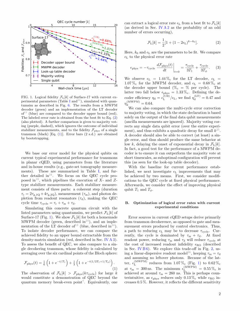
FIG. 1. Logical fidelity FL[k] of Surface-17 with current ex-perimental parameters (Table I and24), simulated with quan-tumsim as described in Fig. 6. The results from a MWPMdecoder (green) and an implementation of the LT decoderof13 (blue) are compared to the decoder upper bound (red).The labeled error rate is obtained from the best fit to Eq. (2)(also plotted). A further comparison is given to majority vot-ing (purple, dashed), which ignores the outcome of individualstabilizer measurements, and to the fidelity Fphys of a singletransmon (black) [Eq. (1)]. Error bars (2 s.d.) are obtainedby bootstrapping.

We base our error model for the physical qubits oncurrent typical experimental performance for transmonsin planar cQED, using parameters from the literatureand in-house results (e.g., gate-set tomography measure-ments). These are summarized in Table I, and fur-ther detailed in24. We focus on the QEC cycle pro-posed in18, which pipelines the execution of X- and Z-type stabilizer measurements. Each stabilizer measure-ment consists of three parts: a coherent step (durationτc = 2τg,1Q +4τg,2Q), measurement (τm), and photon de-pletion from readout resonators (τd), making the QECcycle time τcycle = τc + τm + τd.

Simulating this concrete quantum circuit with thelisted parameters using quantumsim, we predict FL[k] ofSurface-17 (Fig. 1). We show FL[k] for both a homemadeMWPM decoder (green, described in24), and an imple-mentation of the LT decoder of13 (blue, described in24).To isolate decoder performance, we can compare theachieved fidelity to an upper bound extractable from thedensity-matrix simulation (red, described in Sec. IV A 3).To assess the benefit of QEC, we also compare to a sin-gle decohering transmon, whose fidelity is calculated byaveraging over the six cardinal points of the Bloch sphere:

Fphys(t) = 16

(1 + e−t/T1

)+ 1

3

(1 + e−t(1/2T1+1/Tφ)

).

(1)The observation of FL[k] > Fphys(kτcycle) for large kwould constitute a demonstration of QEC beyond thequantum memory break-even point7. Equivalently, one

can extract a logical error rate εL from a best fit to FL[k](as derived in Sec. IV A 2 as the probability of an oddnumber of errors occurring),

FL[k] =1

2[1 + (1− 2εL)k−k0 ]. (2)

Here, k0 and εL are the parameters to be fit. We compareεL to the physical error rate

εphys = −τcycledFphys(t)

dt

∣∣∣∣t=0

=τcycle

3T1+τcycle

3Tφ. (3)

We observe εL = 1.44 %c for the LT decoder, εL =1.07 %c for the MWPM decoder, and εL = 0.68 %c atthe decoder upper bound (%c = % per cycle). Thelatter two fall below εphys = 1.33 %c. Defining the de-

coder efficiency ηd = ε(UB)L /εL, we find η

(LT)d = 0.47 and

η(MWPM)d = 0.64.We can also compare the multi-cycle error correction

to majority voting, in which the state declaration is basedsolely on the output of the final data qubit measurements(ancilla measurements are ignored). Majority voting cor-rects any single data qubit error (over the entire experi-ment), and thus exhibits a quadratic decay for small k25.A decoder should also be able to correct (at least) a sin-gle error, and thus should produce the same behavior atlow k, delaying the onset of exponential decay in FL[k].In fact, a good test for the performance of a MWPM de-coder is to ensure it can outperform the majority vote atshort timescales, as suboptimal configuration will preventthis (as seen for the look-up table decoder).

With the baseline for current performance estab-lished, we next investigate εL improvements that maybe achieved by two means. First, we consider modifi-cations to the QEC cycle at fixed physical performance.Afterwards, we consider the effect of improving physicalqubit T1 and Tφ.

B. Optimization of logical error rates with currentexperimental conditions

Error sources in current cQED setups derive primarilyfrom transmon decoherence, as opposed to gate and mea-surement errors produced by control electronics. Thus,a path to reducing εL may be to decrease τcycle. Cur-rently, the cycle is dominated by τm + τd. At fixedreadout power, reducing τm and τd will reduce τcycle atthe cost of increased readout infidelity εRO (describedin Sec. IV B 6). We explore this trade-off in Fig. 2, us-ing a linear-dispersive readout model26, keeping τm = τdand assuming no leftover photons. Because of the lat-

ter, ε(MWPM)L reduces from 1.07 %c (Fig. 1) to 0.62 %c

at τm = 300 ns. The minimum ε(MWPM)L = 0.55 %c is

achieved at around τm = 260 ns. This is perhaps coun-terintuitive, as εphys reduces only 0.13 %c while εRO in-creases 0.5 %. However, it reflects the different sensitivity

2

200 250 300 350

0.5

0.6

0.7

Logic

al err

or

rate

²MWPM

L

0

2

4

6

Physi

cal err

or

rate

[%]

Single qubit error Readout infidelityLogical error rate

200 250 300 350

2

3

²MWPM

L

[×10−3ns−1]

[ns]

Measurement time [ns]

Cycle time [ns]600 700 800 900

FIG. 2. Optimization of the logical error rate (per cycle)of Surface-17 as a function of measurement-and-depletiontime19. Changes in the underlying physical error rates areshown as well. Decreasing the measurement time causes anincrease in the readout infidelity (solid black curve with dots),whilst decreasing the single qubit decay from T1 and T2 (blackdashed curve) for all qubits. The logical rate with an MWPMdecoder (green curve) is minimized when these error rates areappropriately balanced. The logical error rate is calculatedfrom the best fit of Eq. (2). Error bars (2 s.d.) are obtainedby bootstrapping (N = 10, 000 runs). Inset: Logical errorrate per unit time, instead of per cycle.

of the code to different types of errors. Indeed, ε(MWPM)L

is smaller for τm = 200 ns than for τm = 300 ns, eventhough εRO increases to 5 %. It is interesting to notethat the optimal τm for quantum memory, which mini-mizes logical error per unit time, rather than per cycle,is τm = 280 ns (Fig. 2 inset). This shows that differentcycle parameters might be optimal for computation andmemory applications.

Next, we consider the possibility to reduce εL usingfeedback control. Since T1 only affects qubits in theexcited state, the error rate of ancillas in Surface-17 isroughly two times higher when in the excited state. Theunmodified syndrome extraction circuit flips the ancilla ifthe corresponding stabilizer value is -1, and since ancillasare not reset between cycles, they will spend significantamounts of time in the excited state. Thus, we considerusing feedback to hold each ancilla in the ground state asmuch as possible. We do not consider feedback on dataqubits, as the highly entangled logical states are equallysusceptible to T1.

The feedback scheme (Inset of Fig. 3) consists of re-placing the Ry(π/2) gate at the end of the coherent stepwith a Ry(−π/2) gate for some of the ancillas, depend-ing on a classical control bit p for each ancilla. This bitp represents an estimate of the stabilizer value, and theancilla is held in the ground state whenever this estimateis correct (i.e. in the absence of errors). Figure 3 showsthe effect of this feedback on the logical fidelity, both forthe MWPM decoder and the decoder upper bound. Weobserve εL improve only 0.05 %c in both cases. Future

0.8

0.85

0.9

0.95

10 5 10 15 20QEC cycle number

0 4 8 12 16

Log

ical fid

elit

y

±YAj

pjmj(t) mj(t+1)

Upper bound, with feedback

Upper bound, no feedback

MWPM, with feedback

MWPM, no feedback

Wall-clock time [ ]s

FIG. 3. Logical fidelity of Surface-17 with (solid) and without(dashed) an additional feedback scheme. The performance ofa MWPM decoder (green) is compared to the decoder upperbound (red). Curves are fits of Eq. (2) to the data, and errorbars (2 s.d.) are given by bootstrapping, with each pointaveraged over 10, 000 runs. Inset: Method for implementingthe feedback scheme. For each ancilla qubit Aj , we store aparity bit pj , which decides the sign of the Ry(π/2) rotationat the end of each coherent step. The time Aj spends in theground state is maximized when pj is updated each cycle t byXORing with the measurement result from cycle t − 1, afterthe rotation of cycle t has been performed.

experiments might opt not to pursue these small gains inview of the technical challenges added by feedback con-trol.

C. Projected improvement with advances inquantum hardware

We now estimate the performance increase that mayresult from improving the transmon relaxation and de-phasing times via materials and filtering improvements.To model this, we return to τcycle = 800 ns, and ad-just T1 values with both Tφ = 2T1 (common in exper-iment) and Tφ = ∞ (all white-noise dephasing elimi-nated). We retain the same rates for coherent errors,readout infidelity, and photon-induced dephasing as inFig. 1. Figure 4 shows the extracted εL and εphys overthe T1 range covered. For the MWPM decoder (up-per bound) and Tφ = 2T1, the memory figure of meritγm = εphys/εL increases from 1.3 (2) at T1 = 30 µs to2 (5) at 100 µs. Completely eliminating white-noise de-phasing will increase γm by 10% with MWPM and 30%at the upper bound.

A key question for any QEC code is how εL scales withcode distance d. Computing power limitations precludesimilar density-matrix simulations of the d = 5 surfacecode Surface-49. However, we can approximate the er-ror rate by summing up all lowest-order error chains (ascalculated for the MWPM decoder), and deciding indi-

3

20 40 60 80 100

10-1

100

T1 [ s]

T =2T1 T =∞

Upper bound

MWPM

Single qubitErr

or

rate

s

and

FIG. 4. T1 dependence of the Surface-17 logical error rate(MWPM and UB) and the physical error rate. We either fixTφ = 2T1 (solid) or Tφ =∞ (dashed). Logical error rates areextracted from a best fit of Eq. (2) to FL[k] over k = 1, . . . , 20QEC cycles, averaged over N = 50, 000 runs. Error bars (2s.d.) are calculated by bootstrapping.

20 40 60 80 10010-3

10-2

10-1

100

T1 [ s]

Surface-17, quantumsimSurface-17, analytic, 800 ns

Surface-17, analytic, 400 nsSurface-49, analytic, 800 ns

Surface-49, analytic, 400 ns Single qubit, 20 ns

Err

or

rate

s

and

FIG. 5. Analytic approximation of εL for Surface-17 (green)and Surface-49 (orange) using a MWPM decoder. Detailsof the calculation of points and error bars are given in24. Allplots assume Tφ = 2T1, and τcycle = 800 ns (crosses) or 400 ns(dots). Numerical results for Surface-17 with τcycle = 800 nsare also plotted for comparison (green, dashed). The physical-qubit computation metric is given as the error incurred by asingle qubit over the resting time of a single-qubit gate (black,dashed).

vidually whether or not these would be corrected by aMWPM decoder (see24 for details). Figure 5 shows thelowest-order approximation to the logical error rates ofSurface-17 and -49 over a range of T1 = Tφ/2. Com-paring the Surface-17 lowest-order approximation to thequantumsim result shows good agreement and validatesthe approximation. We observe a lower εL for Surface-49 than for -17, indicating quantum fault tolerance overthe T1 range covered. The fault-tolerance figure of merit

defined in9, Λt = ε(17)L /ε

(49)L , increases from 2 to 4 as T1

grows from 30 to 100 µs.

As a rough metric of computational performance, weoffer to compare εL (per cycle) to the error accrued by aphysical qubit idling over τg,1Q. We define a metric forcomputation performance, γc = (εphysτg,1Q)/(εLτcycle)and γc = 1 as a computational break-even point. Clearly,using the QEC cycle parameters of Table I and even withT1 improvements, neither Surface-17 nor -49 can break-even computationally. However, including the readoutacceleration recently demonstrated in22, which allowsτm = τd = 100 ns and τcycle = 400 ns, Surface-49 cancross γc = 1 by T1 = 40 µs. In view of first reports ofT1 up to 80 µs emerging for planar transmons27,28, thisimportant milestone may be within grasp.

III. Discussion

A. Computational figure of merit

We note that our metric of computational power isnot rigorous, due to the different gate sets available tophysical and logical qubits. Logical qubits can executemultiple logical X and Z gates within one QEC cycle,but require a few cycles for two-qubit and Hadamardgates (using the proposals of12,17), and state distillationover many cycles to perform non-Clifford gates. As such,this metric is merely a rough benchmark for computa-tional competitiveness of the QEC code. However, giventhe amount by which all distance-3 logical fidelities fallabove this metric, we find it unlikely that these codeswill outperform a physical qubit by any fair comparisonin the near future.

B. Decoder performance

A practical question facing quantum error correction ishow best to balance the trade-off between decoder com-plexity and performance. Past proposals for surface-codecomputation via lattice surgery17 require the decoder toprovide an up-to-date estimate of the Pauli error on phys-ical qubits during each logical T gate. Because track-ing Pauli errors through a non-Clifford gate is inefficient,however implemented, equivalent requirements will holdfor any QEC code29. A decoder is thus required to pro-cess ancilla measurements from one cycle within the next(on average). This presents a considerable challenge fortransmon-cQED implementations, as τcycle < 1µs. Thisshort time makes the use of computationally intensivedecoding schemes difficult, even if they provide lower εL.

The leading strategy for decoding the surface code isMWPM using the blossom algorithm of Edmonds10,14,30.Although this algorithm is challenging to implement, itscales linearly in code distance30. The algorithm requiresa set of weights (representing the probability that twogiven error signals are connected by a chain of errors) asinput. An important practical question (see24) is whetherthese weights can be calculated on the fly, or must be

4

precalculated and stored. On-the-fly weight calculationis more flexible. For example, it can take into account thedifference in error rates between an ancilla measured inthe ground and in the excited state. The main weaknessof MWPM is the inability to explicitly detect Y errors.In fact,24 shows that MWPM is nearly perfect in theabsence of Y errors. The decoder efficiency ηd may sig-nificantly increase by extending MWPM to account forcorrelations between detected X and Z errors originatingfrom Y errors31,32.

If computational limitations preclude a MWPM de-coder from keeping up with τcycle, the look-up table de-coder may provide a straightforward solution for Surface-17. However, at current physical performance, the ηd re-duction will make Surface-17 barely miss memory break-even (Fig. 1). Furthermore, memory requirements makelook-up table decoding already impractical for Surface-49. Evidently, real-time algorithmic decoding by MWPMor improved variants is an important research directionalready at low code distance.

C. Other observations

The simulation results allow some further observations.Although we have focused on superconducting qubits, wesurmise that the following statements are fairly general.

We observe that small quasi-static qubit errors are sup-pressed by the repeated measurement. In our simula-tions, the 1/f flux noise producing 0.01 radians of phaseerror per flux pulse on a qubit has a diamond norm ap-proximately equal to the T1 noise, but a trace distance100 times smaller. As the flux noise increases εL by only0.01 %c, it appears εL is dependent on the trace distancerather than the diamond norm of the underlying noisecomponents. Quasi-static qubit errors can then be easilysuppressed, but will also easily poison an experiment ifunchecked.

We further observe that above a certain value, ancillaand measurement errors have a diminished effect on εL.In our error model, the leading sources of error for a dis-tance d code are chains of (d − 1)/2 data qubit errorsplus either a single ancilla qubit error or readout error,which together present the same syndrome as a chain of(d+ 1)/2 data qubit errors. An optimal decoder decideswhich of these chains is more likely, at which point theless-likely chain will be wrongly corrected, completing alogical error. This implies that if readout infidelity (εRO)or the ancilla error rate (εanc) is below the data qubit

(εphys) error rate, εL ∝ (εanc + εRO)ε(d−1)/2phys . However, if

εRO (εanc) > εphys, εL becomes independent of εRO (εanc),to lowest order. This can be seen in Fig. 2, where the er-ror rate is almost constant as εRO exponentially increases.This approximation breaks down with large enough εanc

and εRO, but presents a counterintuitive point for experi-mental design; εL becomes less sensitive to measurementand ancilla errors as these error get worse.

A final, interesting point for future surface-code com-

putation is shown in Fig. 2: the optimal cycle parametersfor logical error rates per cycle and per unit time are notthe same. This implies that logical qubits functioning asa quantum memory should be treated differently to thosebeing used for computation. This idea can be extendedfurther: at any point in time, a large quantum computerperforming a computation will have a set Sm of memoryqubits which are storing part of a large entangled state,whilst a set Sc of computation qubits containing the restof the state undergo operations. To minimize the proba-bility of a logical error occurring on qubits within both Scand Sm, the cycle time of the qubits in Sc can be reducedto minimize the rest time of qubits in Sm. As a simpleexample, consider a single computational qubit qc and asingle memory qubit qm sharing entanglement. Operat-ing all qubits at τcycle = 720 ns to minimize εL wouldlead to a 1.09% error rate for the two qubits combined.However, shortening the τcycle of qc reduces the time overwhich qm decays. If qc operates at τcycle = 600 ns, theaverage error per computational cycle drops to 1.06%, asqm completes only 5 cycles for every 6 on qc. Althoughthis is only a meager improvement, one can imagine thatwhen many more qubits are resting than performing com-putation, the relative gain will be quite significant.

D. Effects not taken into account

Although we have attempted to be thorough in thedetailing of the circuit, we have neglected certain effects.We have used a simple model for C-Z gate errors as welack data from experimental tomography (e.g. one ob-tained from two-qubit gate-set tomography33). Most im-portantly, we have neglected leakage, where a transmonis excited out of the two lowest energy states, i.e., out ofthe computational subspace. Previous experiments havereduced the leakage probability per C-Z gate to∼ 0.3%34,and per single-qubit gate to ∼ 0.001%35. Schemes havealso been developed to reduce the accumulation of leak-age36. Extending quantumsim to include and investigateleakage is a next target. However, the representation ofthe additional quantum state can increase the simula-tion effort significantly [by a factor of (9/4)10 ≈ 3000].To still achieve this goal, some further approximations ormodifications to the simulation will be necessary. Futuresimulations will also investigate the effect of spread inqubit parameters, both in space (i.e., variation of physi-cal error rates between qubits) and time (e.g., T1 fluctu-ations), and cross-talk effects such as residual couplingsbetween nearest and next-nearest neighbor transmons,qubit cross-driving, and qubit dephasing by measurementpulses targeting other qubits.

5

IV. Methods

A. Simulated experimental procedure

1. Surface-17 basics

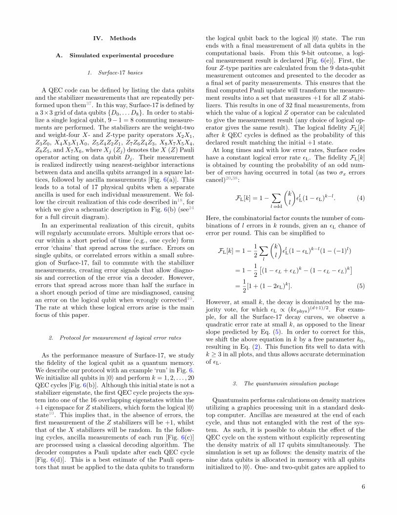
A QEC code can be defined by listing the data qubitsand the stabilizer measurements that are repeatedly per-formed upon them37. In this way, Surface-17 is defined bya 3×3 grid of data qubits {D0, . . . D8}. In order to stabi-lize a single logical qubit, 9− 1 = 8 commuting measure-ments are performed. The stabilizers are the weight-twoand weight-four X- and Z-type parity operators X2X1,Z3Z0, X4X3X1X0, Z5Z4Z2Z1, Z7Z6Z4Z3, X8X7X5X4,Z8Z5, and X7X6, where Xj (Zj) denotes the X (Z) Paulioperator acting on data qubit Dj . Their measurementis realized indirectly using nearest-neighbor interactionsbetween data and ancilla qubits arranged in a square lat-tices, followed by ancilla measurements [Fig. 6(a)]. Thisleads to a total of 17 physical qubits when a separateancilla is used for each individual measurement. We fol-low the circuit realization of this code described in18, forwhich we give a schematic description in Fig. 6(b) (see24

for a full circuit diagram).

In an experimental realization of this circuit, qubitswill regularly accumulate errors. Multiple errors that oc-cur within a short period of time (e.g., one cycle) formerror ‘chains’ that spread across the surface. Errors onsingle qubits, or correlated errors within a small subre-gion of Surface-17, fail to commute with the stabilizermeasurements, creating error signals that allow diagno-sis and correction of the error via a decoder. However,errors that spread across more than half the surface ina short enough period of time are misdiagnosed, causingan error on the logical qubit when wrongly corrected10.The rate at which these logical errors arise is the mainfocus of this paper.

2. Protocol for measurement of logical error rates

As the performance measure of Surface-17, we studythe fidelity of the logical qubit as a quantum memory.We describe our protocol with an example ‘run’ in Fig. 6.We initialize all qubits in |0〉 and perform k = 1, 2, . . . , 20QEC cycles [Fig. 6(b)]. Although this initial state is not astabilizer eigenstate, the first QEC cycle projects the sys-tem into one of the 16 overlapping eigenstates within the+1 eigenspace for Z stabilizers, which form the logical |0〉state10. This implies that, in the absence of errors, thefirst measurement of the Z stabilizers will be +1, whilstthat of the X stabilizers will be random. In the follow-ing cycles, ancilla measurements of each run [Fig. 6(c)]are processed using a classical decoding algorithm. Thedecoder computes a Pauli update after each QEC cycle[Fig. 6(d)]. This is a best estimate of the Pauli opera-tors that must be applied to the data qubits to transform

the logical qubit back to the logical |0〉 state. The runends with a final measurement of all data qubits in thecomputational basis. From this 9-bit outcome, a logi-cal measurement result is declared [Fig. 6(e)]. First, thefour Z-type parities are calculated from the 9 data-qubitmeasurement outcomes and presented to the decoder asa final set of parity measurements. This ensures that thefinal computed Pauli update will transform the measure-ment results into a set that measures +1 for all Z stabi-lizers. This results in one of 32 final measurements, fromwhich the value of a logical Z operator can be calculatedto give the measurement result (any choice of logical op-erator gives the same result). The logical fidelity FL[k]after k QEC cycles is defined as the probability of thisdeclared result matching the initial +1 state.

At long times and with low error rates, Surface codeshave a constant logical error rate εL. The fidelity FL[k]is obtained by counting the probability of an odd num-ber of errors having occurred in total (as two σx errorscancel)20,38:

FL[k] = 1−∑l odd

(k

l

)εlL(1− εL)k−l. (4)

Here, the combinatorial factor counts the number of com-binations of l errors in k rounds, given an εL chance oferror per round. This can be simplified to

FL[k] = 1− 1

2

∑l

(k

l

)εlL(1− εL)k−l(1− (−1)l)

= 1− 1

2

[(1− εL + εL)k − (1− εL − εL)k

]=

1

2[1 + (1− 2εL)k]. (5)

However, at small k, the decay is dominated by the ma-jority vote, for which εL ∝ (kεphys)

(d+1)/2. For exam-ple, for all the Surface-17 decay curves, we observe aquadratic error rate at small k, as opposed to the linearslope predicted by Eq. (5). In order to correct for this,we shift the above equation in k by a free parameter k0,resulting in Eq. (2). This function fits well to data withk ≥ 3 in all plots, and thus allows accurate determinationof εL.

3. The quantumsim simulation package

Quantumsim performs calculations on density matricesutilizing a graphics processing unit in a standard desk-top computer. Ancillas are measured at the end of eachcycle, and thus not entangled with the rest of the sys-tem. As such, it is possible to obtain the effect of theQEC cycle on the system without explicitly representingthe density matrix of all 17 qubits simultaneously. Thesimulation is set up as follows: the density matrix of thenine data qubits is allocated in memory with all qubitsinitialized to |0〉. One- and two-qubit gates are applied to

6

X2

X2

X2

X2

Z-type X-typeA1A3A4A6 A0A2A5A7

Z5 Z2

Z2Z5Z7 Z6

Z2Z6 Z5

Z5 Z2

Z5 Z2

D0D1D2D3D4D5D6D7D8

Cyc

le

- +

D0 D1 D2

D3 D4 D5

D6 D7 D8

A0

A2

A5A4

A7

A3A1

A6

repeat k times

k =

1

2

3

4

5

Quantum hardware

Syndrome measurements

calculate final z-parities from final readout

A'1A'3A'4A'6

Pauli update

Z errorsX errors

Measurement and decoding(after k cycles)

final readout

(a) (b)

(c) (d)

(e)

Example measurement Data qubit

Ancilla qubit for Z-type parity checkAncilla qubit for X-type parity check

apply decoding step to find final Pauli update X2X8

D0D1D2D3D4D5D6D7D8apply Pauli update to readout

D0D1D2D3D4D5D6D7D8 =declare logical measurement outcome

FIG. 6. Schematic overview of the simulated experiment. (a) 17 qubits are arranged in a surface code layout (legend top-right).The red data qubits are initialized in the ground state |0〉, and projected into an eigenstate of the measured X- (blue) and Z-(green) type stabilizer operators. (b) A section of the quantum circuit depicting the four-bit parity measurement implementedby the A3 ancilla qubit (+/− refer to Ry(±π/2) single-qubit rotations). The ancilla qubit (green line, middle) is entangledwith the four data qubits (red lines) to measure Z1Z2Z4Z5. Ancillas are not reset between cycles. Instead, the implementationrelies on the quantum non-demolition nature of measurements. The stabilizer is then the product of the ancilla measurementresults of successive cycles. This circuit is performed for all ancillas and repeated k times before a final measurement of all(data and ancilla) qubits. (c) All syndrome measurements of the k cycles are processed by the decoder. (d) After each cycle,the decoder updates its internal state to represent the most likely set of errors that occurred. (e) After the final measurement,the decoder uses the readout from the data qubits, along with previous syndrome measurements, to declare a final logical state.To this end, the decoder processes the Z-stabilizers obtained directly from the data qubits, finalizing its prediction of mostlikely errors. The logical parity is then determined as the product of all data qubit parities (

∏8j=0Dj) once the declared errors

are corrected. The logical fidelity FL is the probability that this declaration is the same as the initial state (|0〉).

the density matrix as completely positive, trace preserv-ing maps represented by Pauli transfer matrices. Whena gate involving an ancilla qubit must be performed, thedensity matrix of the system is dynamically enlarged toinclude that one ancilla.

Qubit measurements are simulated as projective and

following the Born rule, with projection probabilitiesgiven by the squared overlap of the input state with themeasurement basis states. In order to capture empiri-cal measurement errors, we implement a black-box mea-surement model (Sec. IV B 6) by sandwiching the mea-surement between idling processes. The measurement

7

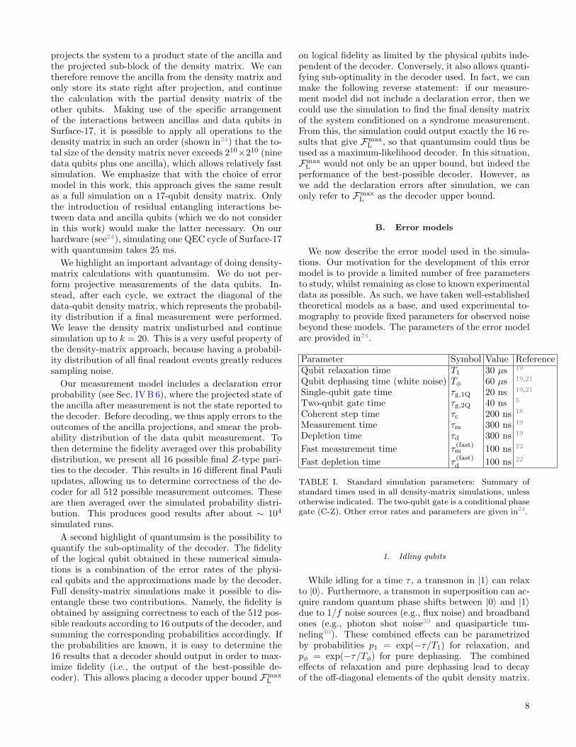
projects the system to a product state of the ancilla andthe projected sub-block of the density matrix. We cantherefore remove the ancilla from the density matrix andonly store its state right after projection, and continuethe calculation with the partial density matrix of theother qubits. Making use of the specific arrangementof the interactions between ancillas and data qubits inSurface-17, it is possible to apply all operations to thedensity matrix in such an order (shown in24) that the to-tal size of the density matrix never exceeds 210×210 (ninedata qubits plus one ancilla), which allows relatively fastsimulation. We emphasize that with the choice of errormodel in this work, this approach gives the same resultas a full simulation on a 17-qubit density matrix. Onlythe introduction of residual entangling interactions be-tween data and ancilla qubits (which we do not considerin this work) would make the latter necessary. On ourhardware (see24), simulating one QEC cycle of Surface-17with quantumsim takes 25 ms.

We highlight an important advantage of doing density-matrix calculations with quantumsim. We do not per-form projective measurements of the data qubits. In-stead, after each cycle, we extract the diagonal of thedata-qubit density matrix, which represents the probabil-ity distribution if a final measurement were performed.We leave the density matrix undisturbed and continuesimulation up to k = 20. This is a very useful property ofthe density-matrix approach, because having a probabil-ity distribution of all final readout events greatly reducessampling noise.

Our measurement model includes a declaration errorprobability (see Sec. IV B 6), where the projected state ofthe ancilla after measurement is not the state reported tothe decoder. Before decoding, we thus apply errors to theoutcomes of the ancilla projections, and smear the prob-ability distribution of the data qubit measurement. Tothen determine the fidelity averaged over this probabilitydistribution, we present all 16 possible final Z-type pari-ties to the decoder. This results in 16 different final Pauliupdates, allowing us to determine correctness of the de-coder for all 512 possible measurement outcomes. Theseare then averaged over the simulated probability distri-bution. This produces good results after about ∼ 104

simulated runs.

A second highlight of quantumsim is the possibility toquantify the sub-optimality of the decoder. The fidelityof the logical qubit obtained in these numerical simula-tions is a combination of the error rates of the physi-cal qubits and the approximations made by the decoder.Full density-matrix simulations make it possible to dis-entangle these two contributions. Namely, the fidelity isobtained by assigning correctness to each of the 512 pos-sible readouts according to 16 outputs of the decoder, andsumming the corresponding probabilities accordingly. Ifthe probabilities are known, it is easy to determine the16 results that a decoder should output in order to max-imize fidelity (i.e., the output of the best-possible de-coder). This allows placing a decoder upper bound Fmax

L

on logical fidelity as limited by the physical qubits inde-pendent of the decoder. Conversely, it also allows quanti-fying sub-optimality in the decoder used. In fact, we canmake the following reverse statement: if our measure-ment model did not include a declaration error, then wecould use the simulation to find the final density matrixof the system conditioned on a syndrome measurement.From this, the simulation could output exactly the 16 re-sults that give Fmax

L , so that quantumsim could thus beused as a maximum-likelihood decoder. In this situation,Fmax

L would not only be an upper bound, but indeed theperformance of the best-possible decoder. However, aswe add the declaration errors after simulation, we canonly refer to Fmax

L as the decoder upper bound.

B. Error models

We now describe the error model used in the simula-tions. Our motivation for the development of this errormodel is to provide a limited number of free parametersto study, whilst remaining as close to known experimentaldata as possible. As such, we have taken well-establishedtheoretical models as a base, and used experimental to-mography to provide fixed parameters for observed noisebeyond these models. The parameters of the error modelare provided in24.

Parameter Symbol Value ReferenceQubit relaxation time T1 30 µs 19

Qubit dephasing time (white noise) Tφ 60 µs 19,21

Single-qubit gate time τg,1Q 20 ns 19,21

Two-qubit gate time τg,2Q 40 ns 5

Coherent step time τc 200 ns 18

Measurement time τm 300 ns 19

Depletion time τd 300 ns 19

Fast measurement time τ(fast)m 100 ns 22

Fast depletion time τ(fast)d 100 ns 22

TABLE I. Standard simulation parameters: Summary ofstandard times used in all density-matrix simulations, unlessotherwise indicated. The two-qubit gate is a conditional phasegate (C-Z). Other error rates and parameters are given in24.

1. Idling qubits

While idling for a time τ , a transmon in |1〉 can relaxto |0〉. Furthermore, a transmon in superposition can ac-quire random quantum phase shifts between |0〉 and |1〉due to 1/f noise sources (e.g., flux noise) and broadbandones (e.g., photon shot noise39 and quasiparticle tun-neling40). These combined effects can be parametrizedby probabilities p1 = exp(−τ/T1) for relaxation, andpφ = exp(−τ/Tφ) for pure dephasing. The combinedeffects of relaxation and pure dephasing lead to decayof the off-diagonal elements of the qubit density matrix.

8

We model dephasing from broadband sources in this way,taking for Tφ the value extracted from the decay time T2

of standard echo experiments:

1

T2=

1

Tφ+

1

2T1. (6)

We model 1/f sources differently, as discussed below.

2. Dephasing from photon noise

The dominant broadband dephasing source is the shotnoise due to photons in the readout resonator. This de-phasing is present whenever the coupled qubit is broughtinto superposition before the readout resonator has re-turned to the vacuum state following the last measure-ment. This leads to an additional, time-dependent puredephasing (rates given in24).

3. One-qubit Y rotations

We model y-axis rotations as instantaneous rotationssandwiched by idling periods of duration τg,1Q/2. Theerrors in the instantaneous gates are modeled from pro-cess matrices measured by gate-set tomography33,41 in arecent experiment20. In this experiment, the GST anal-ysis of single-qubit gates also showed that the errors canmostly be attributed to Markovian noise. For simplicity,we thus model these errors as Markovian.

4. Dephasing of flux-pulsed qubits

During the coherent step, transmons are repeatedlymoved in frequency away from their sweetspot using fluxpulses, either to implement a C-Z gate or to avoid one.Away from the sweetspot, transmons become first-ordersensitive to flux noise, which causes an additional randomphase shift. As this noise typically has a 1/f power spec-trum, the largest contribution comes from low-frequencycomponents that are essentially static for a single run,but fluctuating between different runs. In our simula-tion, we approximate the effect of this noise through en-semble averaging, with quasi-static phase error added toa transmon whenever it is flux pulsed. Gaussian phaseerrors with the variance (calculated in24) are drawn in-dependently for each qubit and for each run.

5. C-Z gate error

The C-Z gate is achieved by flux pulsing a trans-mon into the |11〉 ↔ |02〉 avoided crossing with another,where the 2 denotes the second-excited state of the fluxedtransmon. Holding the transmons here for τg,2Q causesthe probability amplitudes of |01〉 and |11〉 to acquire

phases42. Careful tuning allows the phase φ01 acquiredby |01〉 (the single-qubit phase φ1Q) to be an even mul-tiple of 2π, and the phase φ11 acquired by |11〉 to be πextra. This extra phase acquired by |11〉 is the two-qubitphase φ2Q. Single- and two-qubit phases are affected byflux noise because the qubit is first-order sensitive dur-ing the gate. Previously, we discussed the single-qubitphase error. In24, we calculate the corresponding two-qubit phase error δφ2Q. Our full (but simplistic) modelof the C-Z gate consists of an instantaneous C-Z gatewith single-qubit phase error δφ1Q and two-qubit phaseerror δφ2Q = δφ1Q/2, sandwiched by idling intervals ofduration τg,2Q/2.

6. Measurement

We model qubit measurement with a black-box de-scription using parameters obtained from experiment.This description consists of the eight probabilities fortransitions from an input state |i〉 ∈ {|0〉 , |1〉} into pairs(m,|o〉) of measurement outcome m ∈ {+1,−1} and fi-nal state |o〉 ∈ {|0〉 , |1〉}. By final state we mean thequbit state following the photon-depletion period. Inputsuperposition states in the computational bases are firstprojected to |0〉 and |1〉 following the Born rule. Theprobability tree (the butterfly) is then used to obtain anoutput pair (m, |o〉). These experimental parameters canbe described by a six-parameter model (described in de-tail in24), consisting of periods of enhanced noise beforeand after a point at which the qubit is perfectly projected,

and two probabilities ε|i〉RO for wrongly declaring the re-

sult of this projective measurement. In24, a scheme formeasuring these butterfly parameters and mapping themto the six-parameter model is described. In experiment,

we find that the readout errors ε|i〉RO are almost indepen-

dent of the qubit state |i〉, and so we describe them witha single readout error parameter εRO in this work.

Acknowledgments

We thank C. C. Bultink, M. A. Rol, B. Criger, X. Fu,S. Poletto, R. Versluis, P. Baireuther, D. DiVincenzo,B. Terhal, and C.W.J. Beenakker for useful discussions.This research is supported by the Foundation for Fun-damental Research on Matter (FOM), the NetherlandsOrganization for Scientific Research (NWO/OCW), anERC Synergy Grant, and by the Office of the Director ofNational Intelligence (ODNI), Intelligence Advanced Re-search Projects Activity (IARPA), via the U.S. Army Re-search Office grant W911NF-16-1-0071. The views andconclusions contained herein are those of the authors andshould not be interpreted as necessarily representing theofficial policies or endorsements, either expressed or im-plied, of the ODNI, IARPA, or the U.S. Government.The U.S. Government is authorized to reproduce and

9

distribute reprints for Governmental purposes notwith- standing any copyright annotation thereon.

∗ These authors contributed equally to this work.1 O’Malley, P. J. J. et al. Scalable quantum simulation

of molecular energies. Phys. Rev. X 6, 031007 (2016).URL https://link.aps.org/doi/10.1103/PhysRevX.6.

031007.2 Barends, R. et al. Digital quantum simulation of fermionic

models with a superconducting circuit. Nat. Commun.6, 7654 (2015). URL http://www.nature.com/articles/

ncomms8654.3 Langford, N. K. et al. Experimentally simulating the dy-

namics of quantum light and matter at ultrastrong cou-pling. arXiv:1610.10065 (2016). URL arxiv.org/abs/

1610.10065.4 Kelly, J. et al. State preservation by repetitive error detec-

tion in a superconducting quantum circuit. Nature 519,66–69 (2015). URL https://www.nature.com/nature/

journal/v519/n7541/full/nature14270.html.5 Riste, D. et al. Detecting bit-flip errors in a logical

qubit using stabilizer measurements. Nat. Commun. 6,6983 (2015). URL https://www.nature.com/articles/

ncomms7983.6 Corcoles, A. D. et al. Demonstration of a quantum er-

ror detection code using a square lattice of four super-conducting qubits. Nat. Commun. 6, 6979 (2015). URLhttps://www.nature.com/articles/ncomms7979.

7 Ofek, N. et al. Extending the lifetime of a quantum bitwith error correction in superconducting circuits. Nature536, 441 (2016). URL http://www.nature.com/nature/

journal/v536/n7617/abs/nature18949.html.8 Boixo, S. et al. Characterizing Quantum Supremacy

in Near-Term Devices. arXiv:1608.00263 (2016). URLhttps://arxiv.org/abs/1608.00263.

9 Martinis, J. M. Qubit metrology for building a fault-tolerant quantum computer. npj Quantum Inf. 1,15005 (2015). URL https://www.nature.com/articles/

npjqi20155.10 Fowler, A. G., Mariantoni, M., Martinis, J. M. &

Cleland, A. N. Surface codes: Towards practicallarge-scale quantum computation. Phys. Rev. A 86,032324 (2012). URL https://link.aps.org/doi/10.

1103/PhysRevA.86.032324.11 Landahl, A. J., Anderson, J. T. & Rice, P. R.

Fault-tolerant quantum computing with color codes.arXiv:1108.5738 (2011). URL arxiv.org/abs/1108.5738.

12 Yoder, T. J. & Kim, I. H. The surface code with atwist. arXiv:1612.04795 (2016). URL arxiv.org/abs/

1612.04795.13 Tomita, Y. & Svore, K. M. Low-distance surface

codes under realistic quantum noise. Phys. Rev. A 90,062320 (2014). URL https://link.aps.org/doi/10.

1103/PhysRevA.90.062320.14 Fowler, A. G., Stephens, A. M. & Groszkowski, P. High-

threshold universal quantum computation on the surfacecode. Phys. Rev. A 80, 052312 (2009). URL http://link.

aps.org/doi/10.1103/PhysRevA.80.052312.15 Heim, B., Svore, K. M. & Hastings, M. B. Optimal circuit-

level decoding for surface codes. arXiv:1609.06373 (2016).URL arxiv.org/abs/1609.06373.

16 Blais, A., Huang, R.-S., Wallraff, A., Girvin, S. M.& Schoelkopf, R. J. Cavity quantum electrodynam-ics for superconducting electrical circuits: An archi-tecture for quantum computation. Phys. Rev. A 69,062320 (2004). URL https://link.aps.org/doi/10.

1103/PhysRevA.69.062320.17 Horsman, C., Fowler, A. G., Devitt, S. & Meter, R. V.

Surface code quantum computing by lattice surgery. NewJ. Phys. 14, 123011 (2012). URL http://stacks.iop.

org/1367-2630/14/i=12/a=123011.18 Versluis, R. et al. Scalable quantum circuit and control for

a superconducting surface code. arXiv:1612.08208 (2016).URL arxiv.org/abs/1612.08208.

19 Bultink, C. C. et al. Active resonator reset in the non-linear dispersive regime of circuit qed. Phys. Rev. Appl.6, 034008 (2016). URL https://link.aps.org/doi/10.

1103/PhysRevApplied.6.034008.20 Rol, M. A. et al. Restless tuneup of high-fidelity qubit

gates. Phys. Rev. Applied 7, 041001 (2017). URL https://

link.aps.org/doi/10.1103/PhysRevApplied.7.041001.21 Asaad, S. et al. Independent, extensible control of same-

frequency superconducting qubits by selective broadcast-ing. npj Quantum Inf. 2, 16029 (2016). URL https:

//www.nature.com/articles/npjqi201629.22 Walter, T. et al. Realizing Rapid, High-Fidelity, Single-

Shot Dispersive Readout of Superconducting Qubits.arXiv:1701.06933 (2017). URL arxiv.org/abs/1701.

06933.23 Please visit https://github.com/brianzi/quantumsim.24 See supplemental material.25 A distance-d code with majority voting alone should ex-

hibit a (d+ 1)/2-order decay.26 Frisk Kockum, A., Tornberg, L. & Johansson, G. Undo-

ing measurement-induced dephasing in circuit QED. Phys.Rev. A 85, 052318 (2012). URL https://link.aps.org/

doi/10.1103/PhysRevA.85.052318.27 Paik, H. et al. Experimental demonstration of a resonator-

induced phase gate in a multiqubit circuit-qed system.Phys. Rev. Lett. 117, 250502 (2016). URL https://link.

aps.org/doi/10.1103/PhysRevLett.117.250502.28 Gustavsson, S. et al. Suppressing relaxation in

superconducting qubits by quasiparticle pump-ing. Science 354, 1573–1577 (2016). URL http:

//science.sciencemag.org/content/354/6319/1573.http://science.sciencemag.org/content/354/6319/1573.full.pdf.

29 Terhal, B. M. Quantum error correction for quantummemories. Rev. Mod. Phys. 87, 307–346 (2015). URLhttp://link.aps.org/doi/10.1103/RevModPhys.87.307.

30 Fowler, A. G., Sank, D., Kelly, J., Barends, R. & Martinis,J. M. Scalable extraction of error models from the outputof error detection circuits. arXiv:1405.1454 (2014). URLhttps://arxiv.org/abs/1405.1454.

31 Delfosse, N. & Tillich, J. P. A decoding algorithm forcss codes using the x/z correlations. In 2014 IEEE In-ternational Symposium on Information Theory, 1071–1075(2014).

32 Fowler, A. G. Optimal complexity correction of correlatederrors in the surface code. arXiv:1310.0863 (2013). URL

10

https://arxiv.org/abs/1310.0863.33 Blume-Kohout, R. et al. Robust, self-consistent, closed-

form tomography of quantum logic gates on a trapped ionqubit. arXiv:1310.4492 (2013). URL https://arxiv.org/

abs/1310.4492.34 Barends, R. et al. Superconducting quantum circuits at the

surface code threshold for fault tolerance. Nature 508, 500(2014). URL http://www.nature.com/nature/journal/

v508/n7497/abs/nature13171.html.35 Chen, Z. et al. Multi-photon sideband transitions in

an ultrastrongly-coupled circuit quantum electrodynamicssystem. arXiv preprint arXiv:1602.01584 (2016). URLhttps://arxiv.org/abs/1602.01584.

36 Fowler, A. G. Coping with qubit leakage in topologicalcodes. Phys. Rev. A 88, 042308 (2013). URL https://

link.aps.org/doi/10.1103/PhysRevA.88.042308.37 Gottesman, D. Stabilizer Codes and Quantum Error Cor-

rection. Ph.D. thesis, Caltech (1997).38 We thank Barbara Terhal for providing this derivation.39 Sears, A. P. et al. Photon shot noise dephasing in the

strong-dispersive limit of circuit QED. Phys. Rev. B 86,180504 (2012). URL http://link.aps.org/doi/10.1103/

PhysRevB.86.180504.40 Riste, D. et al. Millisecond charge-parity fluctuations and

induced decoherence in a superconducting transmon qubit.Nat. Commun. 4, 1913 (2013). URL http://www.nature.

com/articles/ncomms2936.41 Blume-Kohout, R. et al. Demonstration of qubit opera-

tions below a rigorous fault tolerance threshold with gateset tomography. Nat. Commun. 8, 14485 (2017). URLhttps://www.nature.com/articles/ncomms14485.

42 DiCarlo, L. et al. Demonstration of two-qubit algo-rithms with a superconducting quantum processor. Nature460, 240 (2009). URL http://www.nature.com/nature/

journal/v460/n7252/abs/nature08121.html.43 The quantumsim package can be found at http://github.

com/brianzi/quantumsim.

A. Full circuit diagram for Surface-17implementation

The quantum circuit18 (Fig. 7) consists of Ry(π/2)(“+”) and Ry(−π/2) (“−”) rotations, C-Z gates, andancilla measurements. The coherent steps of the X andZ ancillas are pipelined (shifted in time with respect toeach other) to prevent transmon-transmon avoided cross-ings. As long as τm + τd ≥ τc, no time is lost due to thisseparation.

In a simulation of the given circuit, gates on differentqubits commute and may be applied to the density ma-trix in any order, regardless of the times at which they areperformed in an experiment. As described in Sec. IV A 3,by simulating gates in a specific order (Fig. 8), one canensure that only one ancilla is ancilla is entangled withthe data qubits at any point in the simulation. Thisallows a reduction in the maximum size of the densitymatrix from 217 × 217 to 210 × 210.

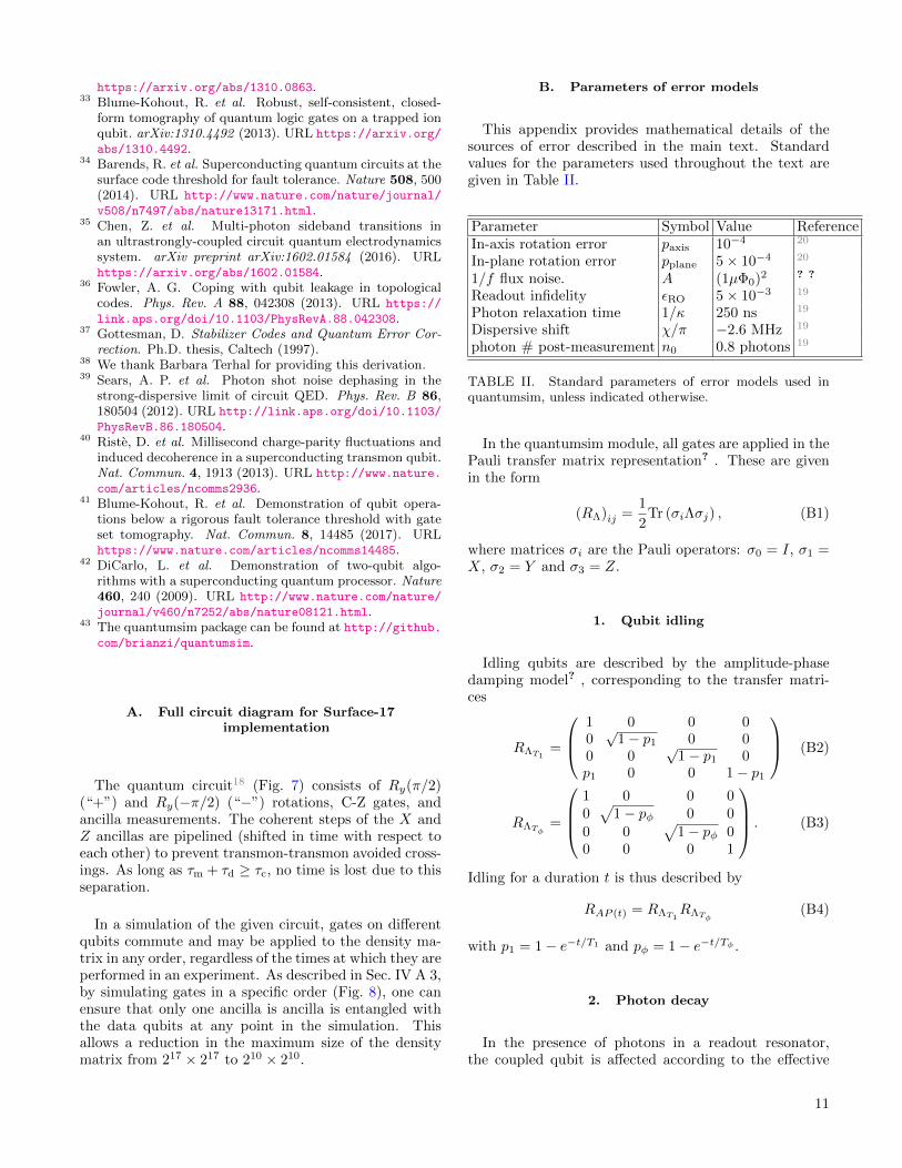
B. Parameters of error models

This appendix provides mathematical details of thesources of error described in the main text. Standardvalues for the parameters used throughout the text aregiven in Table II.

Parameter Symbol Value ReferenceIn-axis rotation error paxis 10−4 20

In-plane rotation error pplane 5× 10−4 20

1/f flux noise. A (1µΦ0)2 ? ?

Readout infidelity εRO 5× 10−3 19

Photon relaxation time 1/κ 250 ns 19

Dispersive shift χ/π −2.6 MHz 19

photon # post-measurement n0 0.8 photons 19

TABLE II. Standard parameters of error models used inquantumsim, unless indicated otherwise.

In the quantumsim module, all gates are applied in thePauli transfer matrix representation? . These are givenin the form

(RΛ)ij =1

2Tr (σiΛσj) , (B1)

where matrices σi are the Pauli operators: σ0 = I, σ1 =X, σ2 = Y and σ3 = Z.

1. Qubit idling

Idling qubits are described by the amplitude-phasedamping model? , corresponding to the transfer matri-ces

RΛT1=

1 0 0 00√

1− p1 0 00 0

√1− p1 0

p1 0 0 1− p1

(B2)

RΛTφ=

1 0 0 00√

1− pφ 0 00 0

√1− pφ 0

0 0 0 1

. (B3)

Idling for a duration t is thus described by

RAP (t) = RΛT1RΛTφ

(B4)

with p1 = 1− e−t/T1 and pφ = 1− e−t/Tφ .

2. Photon decay

In the presence of photons in a readout resonator,the coupled qubit is affected according to the effective

11

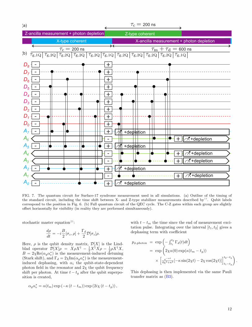
FIG. 7. The quantum circuit for Surface-17 syndrome measurement used in all simulations. (a) Outline of the timing ofthe standard circuit, including the time shift between X- and Z-type stabilizer measurements described by18. Qubit labelscorrespond to the position in Fig. 6. (b) Full quantum circuit of the QEC cycle. The C-Z gates within each group are slightlyoffset horizontally for visibility (in reality they are performed simultaneously).

stochastic master equation26:

dρ

dt= −iB

2[σz, ρ] +

Γd2D[σz]ρ.

Here, ρ is the qubit density matrix, D[X] is the Lind-blad operator D[X]ρ = XρX† − 1

2X†Xρ − 1

2ρX†X,

B = 2χRe(αgα∗e) is the measurement-induced detuning

(Stark shift), and Γd = 2χIm(αgα∗e) is the measurement-

induced dephasing, with αi the qubit-state-dependentphoton field in the resonator and 2χ the qubit frequencyshift per photon. At time t− tg after the qubit superpo-sition is created,

αgα∗e = α(tm) exp (−κ (t− tm)) exp (2iχ (t− tg)) ,

with t− tm the time since the end of measurement exci-tation pulse. Integrating over the interval [t1, t2] gives adephasing term with coefficient

pφ,photon = exp(−∫ t2t1

Γd(t)dt)

= exp

(2χα(0) exp(κ(tm − tg))

×[

e−κt

4χ2+κ2 [−κ sin(2χt)− 2χ cos(2χt)]]t2−tgt1−tg

).

This dephasing is then implemented via the same Paulitransfer matrix as (B3).

12

+depletion

+depletion

+depletion

+depletion

D0

D1

D2

D3

D4

D5

D6

D7

D8

A0

A1

A2

A3

A4

A5

A6

A7

+depletion

+depletion

+depletion

+depletion

--

-------

-

-

-

-

+

-

--

-

+++++++++

+

++

+

+

+

+

1 2 3 4 5 6 7 8

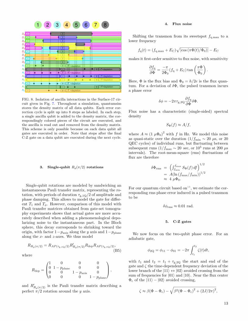
FIG. 8. Isolation of ancilla interactions in the Surface-17 cir-cuit given in Fig. 7. Throughout a simulation, quantumsimstores the density matrix of all data qubits. Each error cor-rection cycle is split up into 8 steps as labeled. In each step,a single ancilla qubit is added to the density matrix, the cor-respondingly colored pieces of the circuit are executed, andthe ancilla is read out and removed from the density matrix.This scheme is only possible because on each data qubit allgates are executed in order. Note that steps after the finalC-Z gate on a data qubit are executed during the next cycle.

3. Single-qubit Ry(π/2) rotations

Single-qubit rotations are modeled by sandwiching aninstantaneous Pauli transfer matrix, representing the ro-tation, with periods of duration τg,1Q/2 of amplitude andphase damping. This allows to model the gate for differ-ent T1 and Tφ. However, comparison of this model withPauli transfer matrices obtained from gate-set tomogra-phy experiments shows that actual gates are more accu-rately described when adding a phenomenological depo-larizing noise to the instantaneous part. In the Blochsphere, this decay corresponds to shrinking toward theorigin, with factor 1−paxis along the y axis and 1−pplane

along the x- and z-axes. We thus model

RRy(π/2) = RAP (τg,1Q/2)R′Ry(π/2)RdepRAP (τg,1Q/2),

(B5)where

Rdep =

1 0 0 00 1− pplane 0 00 0 1− paxis 00 0 0 1− pplane

,

and R′Ry(π/2) is the Pauli transfer matrix describing a

perfect π/2 rotation around the y axis.

4. Flux noise

Shifting the transmon from its sweetspot fq,max to alower frequency

fq(t) = (fq,max + EC)√|cos (πΦ(t)/Φ0)| − EC

makes it first-order sensitive to flux noise, with sensitivity

∂fq

∂Φ=−π2Φ0

(fq + EC) tan

(πΦ

Φ0

).

Here, Φ is the flux bias and Φ0 = h/2e is the flux quan-tum. For a deviation of δΦ, the pulsed transmon incursa phase error

δφ = −2πτg,2Q∂fq

∂ΦδΦ.

Flux noise has a characteristic (single-sided) spectraldensity

SΦ(f) ≈ A/f,

where A ≈ (1 µΦ0)2

with f in Hz. We model this noiseas quasi-static over the duration (1/fmin ∼ 20 µs, or 20QEC cycles) of individual runs, but fluctuating betweensubsequent runs (1/fmax ∼ 20 sec, or 105 runs at 200 µsintervals). The root-mean-square (rms) fluctuations offlux are therefore

δΦrms =(∫ fmax

fminSΦ(f) df

)1/2

= A(ln (fmax/fmin))1/2

≈ 4 µΦ0.

For our quantum circuit based on18, we estimate the cor-responding rms phase error induced in a pulsed transmonto be

δφrms ≈ 0.01 rad.

5. C-Z gates

We now focus on the two-qubit phase error. For anadiabatic gate,

φ2Q = φ11 − φ01 = −2π

∫ t2

t1

ζ(t)dt,

with t1 and t2 = t1 + τg,2Q the start and end of thegate and ζ the time-dependent frequency deviation of thelower branch of the |11〉 ↔ |02〉 avoided crossing from thesum of frequencies for |01〉 and |10〉. Near the flux centerΦc of the |11〉 − |02〉 avoided crossing,

ζ ≈ β(Φ− Φc)−√β2(Φ− Φc)

2+ (2J/2π)

2,

13

where 2J/2π ∼ 50 MHz is the minimum splitting be-tween |11〉 and |02〉, and

β =1

2

∂fq

∂Φ|Φ=Φc

.

Differentiating with respect to Φ at Φc gives

∂ζ

∂Φ|Φ=Φc

= β.

To estimate the δφ2Q error, we make the following sim-plification: we replace the exact trajectory created by theflux pulse by a shift to Φ = Φc + δΦ with duration τg,2Q.For a deviation of δΦ,

δφ2Q ≈ −2πτg,2Q∂ζ

∂Φ|Φ=ΦcδΦ.

Note that this two-qubit phase error is correlated withthe single-qubit phase error on the fluxed transmon. Theformer is smaller by a factor ≈ 2.

6. Measurement

The probabilities εm,oi are calibrated using the statis-tics of outcomes in back-to-back measurements (a fol-lowed by b) with the qubit initialized in |i〉.

P(ma = +1)i = ε+1,0i + ε+1,1

i ,

P(ma = +1)i = ε−1,0i + ε−1,1

i ,

P(mb = ma = +1)i =(ε+1,00 + ε+1,1

0

)ε+1,0i

+(ε+1,01 + ε+1,1

1

)ε+1,1i ,

P(mb = −ma = +1)i =(ε+1,00 + ε+1,1

0

)ε−1,0i

+(ε+1,01 + ε+1,1

1

)ε−1,1i ,

P(−mb = ma = +1)i =(ε−1,00 + ε−1,1

0

)ε+1,0i

+(ε−1,01 + ε−1,1

1

)ε+1,1i ,

P(−mb = −ma = +1)i =(ε−1,00 + ε−1,1

0

)ε−1,0i

+(ε−1,01 + ε−1,1

1

)ε−1,1i .

We obtain the six free parameters of the black-box de-scription from these 12 equations, using experimental val-ues on the left-hand side? . Table III shows the valuesused, achieved in a recent experiment19. For the simu-lation, we reproduce this behaviour of the measurementprocess by a model with several steps. The qubit un-dergoes dephasing, followed by periods of decay or ex-citation between which the measurement result is sam-pled. This measurement result is further subject to astate-dependent declaration error εRO before reportedto the decoder (see Fig.9). The six parameters of thismodel are in a one-to-one correspondence with the but-terfly parameters described above, and can be mapped bysolving the corresponding system of equations. The ex-

Probability Value Probability Value

ε+1,00 0.9985 ε+1,0

1 0.0050

ε+1,10 0.0000 ε+1,1

1 0.0015

ε−1,00 0.0015 ε−1,0

1 0.0149

ε−1,10 0.000 ε−1,1

1 0.9786

TABLE III. Measurement butterfly matching a recent char-acteristic experiment19 using a Josephson parametric ampli-fier? in phase-preserving mode as the front end of the readoutamplification chain.

dephase

decay/excitation

declarationerror

declaredmeasurementoutcome

decay/excitation

FIG. 9. The model for measurements consists of a dephasingof the qubit followed by a period of decay and excitation with

probability p(1)

↓/↑. At this point, the qubit state is sampled.

The sampling result is subject to a declaration error εRO, andthe qubit state is subject to further decay or excitation with

probabilities p(2)

↓/↑ before the end of the measurement block.

perimental results in Tab.III are very well explained byassuming unmodified amplitude-phase damping (withezero excitation probabilities) during the measurement pe-riod, and an outcome-independent declaration error ofεRO = ε1RO = ε0RO = 0.15%. We use this result to ex-trapolate measurement performance to different valuesof T1.

Reduction of measurement time is expected to reduceassignment fidelity. For the results presented in Fig. 2,we do not rely on experimental results, but assume asimplified model for measurement, following Ref. 26. Aconstant drive pulse of amplitude ε and tuned to the bareresonator frequency, ∆r = 0, excites the readout res-onator for time τm. The dynamics of the resonator isdependent on the transmon state (we approximate linearbehavior), and the transmitted signal is amplified and de-tected in a homodyne measurement as a noisy transient.This transient is processed by a linear classifier, whichdeclares the measurement outcome. For resonator deple-tion, we use a two-step clearing pulse with amplitude εc1and εc2, each active for τd/2 and chosen (by numericalminimization) so that, at the end of the depletion pulse,the transients for both transmon states return to zero.While the resonator dynamics is easily found if the trans-mon is in the ground state, amplitude damping of thetransmon in the excited state leads to non-deterministicbehavior. We thus numerically obtain an ensemble ofnoisy transients for each input qubit state, and optimizethe decision boundary of the linear classifier for this en-

14

Logic

al err

or

rate²M

WPM

L

FIG. 10. Logical error rate for Surface-17 as a function ofsingle-qubit over-rotation, using the MWPM decoder. Otherparameters are as given in the main text.

semble. Generating a second verification ensemble, the“butterfly” of the measurement setup is estimated.

The dynamics of the resonator is determined by theresonator linewidth κ as well as the dispersive shift χ. Wechose the parameters of the setup used in19, 1/κ = 250 nsand χ/π = −2.6 MHz. The signal-to-noise ratio of thedetected transient is reduced by the quantum efficiencyη = 12.5%. The driving strength ε is chosen to ap-proximate the “butterfly” used in most of the main text,and corresponds to a steady-state average photon popu-lation of about n = 15. We then keep ε constant whilechanging the measurement time, keeping τm = τd, to ob-tain the butterflies used in the density matrix simulation.We ignore effects leading to measurement-induced mix-ing and non-linearity of the readout resonator. Finally,since these simulations do not allow to make a realisticprediction about residual photon numbers achievable inexperiments, we ignore this effect when using these re-sults.

C. Effect of over-rotations and two-qubit phasenoise on logical error rate

In this section we provide additional numerical datashowing the effect of some common noise sources on thelogical error rate. In Fig. 10 we show the effect of acoherent over-rotation, whereby the R′Y (π/2) operatorin Eq. B5 is replaced by R′Y (π/2 + δφ). This can becaused by inaccurate calibration of the flux pulse usedto perform the gate. In Fig. 11 we show the effect of anincrease in the two-qubit flux noise δφrms as described inSec. B 4.

Log

ical err

or

rate²M

WPM

L

FIG. 11. Logical error rate for Surface-17 as a function oftwo-qubit phase error, using the MWPM decoder. Other pa-rameters are as given in the main text.

D. Calculation of decoder upper bound

We provide a detailed description how the decoder up-per bound is obtained from the simulation results. Asdescribed in the main text, after each cycle of simula-tion, the diagonal of the reduced density matrix of thedata qubits in the Z basis is stored. It contains the prob-ability distribution for the 29 = 512 different possiblemeasurement outcomes of the data qubits. In the quan-tum memory experiment described in the main text, eachof these outcomes are passed to the decoder, which thendeclares a logical measurement outcome.

It is evident that any decoder must declare oppositelogical outcomes if two of the 512 possible measurementsm and m’ are related by the application of a logical X op-erator. Thus, any decoder can give the correct result onlyfor half of the measurement outcomes. Subject to thisconstraint, we can find the set of 256 declarations whichmaximize the probability that the declaration is correct.It immediately follows that no decoder can achieve a dec-laration fidelity larger than this maximal probability. Wethus refer to it as the decoder upper bound.

In practice, the upper bound is found according to thefollowing approach. Since declarations are opposite iftwo outcomes differ by a logical X operator, they mustbe equal if they differ by the application of one or moreX stabilizers (applying two different logical X operatorsamounts to the application of a product of X stabilizers).We thus group the outcomes in 32 cosets which are re-lated by the application of X-stabilizers. (There are 4 X-stabilizers in Surface-17, so there are 512/24 = 32 cosets).For outcomes from the same coset, the declaration from adecoder must be the same. We obtain the probability of afinal measurement falling within each coset by summingthe probabilities from the density matrix diagonal. Wefurther group the 32 cosets to 16 pairs, which differ bythe application of a logical operator. The upper bound isthen obtained by selecting the more probable coset from

15

each pair and summing the corresponding probabilities.This upper bound can also be interpreted as the internaldecoherence of the logical qubit: it represents the maxi-mal overlap of the final state with the initial state, underany possible correction of errors.

We finally emphasize that the this upper bound canbe found only because we have access to the completeprobability distribution of outcomes (for a given resultof syndrome measurements), a major advantage of thedensity matrix simulation. However, we do not expectthat any decoder can actually achieve this upper bound:This is because we add syndrome measurement eventsindependently after the situation, which will decrease thelogical error rate further.

E. Hardware requirements of simulation

The simulations are performed using the quantum-sim package43, which were developed by the authors forthis work. The package is accelerated by performingthe density matrix manipulations on a GPU (graphicscard). The simulations for this work were performed ona NVidia Tesla K40 GPU, on which we observed runtimesof about 0.5 seconds for the simulation of a run of k=20cycles (25 ms per QEC cycle). We also had the opportu-nity to test the software on a more modern GPU (NVidiaTesla P100), observing about 15 ms per cycle, and on aconsumer-grade GPU (NVidia Quadro M2000), observ-ing about 40 ms per cycle. By comparison, the CPU ismostly idle during the simulation, except for handling ofinput and output. The memory requirements are modestfor both CPU and GPU RAM. They are dominated bythe storage of the density matrices and amount to a fewten megabytes.

F. Homemade MWPM decoder with asymmetricweight calculation

Every QEC code requires a decoder to track the mostlikely errors consistent with a given set of stabilizer mea-surements. The MWPM decoder has gained popularitysince it was shown to have threshold values above 1%14.The motivation behind MWPM is that single X or Z er-rors on data qubits in the bulk of a surface-code fabriccause changes of two stabilizers in the code. These sig-nals can then be considered vertices on a graph, with theerror the edge connecting them. Errors in measurement,or errors on a single ancilla qubit, behave as changes inthe stabilizer that are separated in time. Multiple errorsthat would join the same vertices create longer paths inthe graph, of which an experiment only records the end-points. Thus, the problem becomes that of finding themost likely set of generating errors given the error signalsthat mark their ends. This is made slightly simpler, as inthe surface code any chain of errors that forms a closedloop does not change the logical state. This implies that

all paths that connect two points are equivalent, and canbe considered together. The problem then is to join er-ror signals, either in pairs, or to a ‘boundary’ vertex.The latter corresponds to errors on data qubits at theboundary, which belong to only one X or Z stabilizer.This pairing P should be chosen as the most likely com-bination of single-qubit errors that could generate themeasured error signals. This has then been reduced tothe problem of minimum-weight perfect matching on agraph, which can be solved in polynomial time by theblossom algorithm10? .

The MWPM decoder we use differs from previousmethods by its weight calculation. As part of the de-coding process, it is required to calculate to some degreeof accuracy? the probability pe1,e2 of two measured errorsignals e1 and e2 being connected by a chain of individ-ual logical errors. This is then converted to a weightwe1,e2 = − log(pe1,e2), which form the input to the blos-som algorithm of Edmonds to find the most likely match-ing of error signals10? . An exact calculation of pe1,e2 re-quires a sum over all such chains between e1 and e2 thatdo not cross the boundary (these are equivalent modulostabilizer operators that do not change the logical state).In this appendix we detail a method of computing thissum, and approximations to make it viable within theruntime of the experiment.

Let us define the ancilla graph GA = (VA, EA) contain-ing a vertex v ∈ VA for every ancilla measurement, and anedge e ∈ EA connecting v, u ∈ VA if a single component(gate, single-qubit rest period, or faulty measurement)in the simulation can cause the u and v measurementsto return an error. We include a special ‘boundary’ ver-tex vB , to which we connect another vertex v if singlecomponents can cause errors on v alone. Then, to eachedge e we associate a probability pe, being the sum ofthe probabilities of each component causing this errorsignal. These error rates can be obtained directly fromquantumsim, by cutting the circuit at each C-Z gate andmeasuring the decay of single qubits between. Then, fora given experiment with given syndrome measurements,let us define the syndrome graph GS = (VS , ES) con-taining a vertex v ∈ VS for each syndrome measurementthat records an error, and an edge λu,v ∈ ES connectingu, v ∈ VS if u and v are either both X ancilla qubits orboth Z ancilla qubits. To each edge λu,v we associate aprobability pu,v given by the sum of the probabilities ofa chain of errors causing error signals solely on u and v.

If we assume that single-qubit errors are uncorrelated,we have to lowest order

pu,v ≈∑

paths (e1,e2,...,en) between u and v

n∏j=1

pej , (F1)

Let AA be the adjacency matrix on GA weighted by theprobabilities pe (i.e., (AA)u,v = pe with e connecting uand v), and AS the same for GS . Then, the above be-

16

comes

AS = AA +A2A +A3

A + · · · = 1

1−AA− 1, (F2)

noting that AS contains a subset of the indices that areused to construct AA.

The boundary must be treated specially in the abovecalculation. For the purposes of the surface code, theboundary can be described as a single vertex which hasno limit on the number of other vertices it may pairto10. For the purposes of weight calculation, any paththat passes through the boundary is already counted bypairing both end vertices to the boundary. This can betreated by making GA directed, and breaking the sym-metry ATA = AA. In particular, either (AA)vB ,u = 0 for

all u or (AA)u,vB = 0 for all u.The above calculation requires inversion of a Nmat ×

Nmat matrix, with Nmat the total number of ancilla mea-surements per experiment. Furthermore, as ancilla errorrates depend upon the previous ancilla state, elementsin AA are not completely known until the previous cy-cle. This implies that in an actual computation with run-time decoding, this inversion would need to be completedwithin a few microseconds (with a transmon-cQED archi-tecture), which is practically unfeasible. We suggest twoapproximations that can be made to shorten the decod-ing time. The first is to average all errors over the ancillapopulation, ignoring any asymmetry in the system. Theadjacency matrix is now the same for any experiment,and can be precalculated and stored as a look-up tablefor the run-time decoder. We call this the decoder withsymmetrized weights. The size of such a look-up tablescales poorly with the number of qubits and the num-ber of cycles. However, (AS)u,v is approximately invari-ant under simultaneous translation of u and v (excludingboundary effects). This implies that a precalculated AScan be vastly compressed, making this method feasible.

The second approximation to the full AS calculationis to perform it iteratively. We divide our graph GA (GS)by time steps; let GtA (GtS) be the subgraph of GA (GS)containing only ancillas measured before time step t, andlet ∂GtA (∂GtS) be the subgraph of GA (GS) containing onlyancillas measured during time step t. Then, if we assumewe have an approximation to the matrix AtS (being theadjacency matrix of GtS), we can approximate

At+1S ≈

(AtS Ct+1

S

(Ct+1S )

T(1− ∂At+1

A )−1

)(F3)

to lowest order in physical errors. Here, ∂At+1A is the

weighted adjacency matrix on ∂Gt+1A , and the coupling

matrix Ct+1S is approximated by

Ct+1S = AtSC

t+1A (1− ∂At+1

A )−1, (F4)

with Ct+1A the adjacency matrix containing only edges

between ∂Gt+1A and GtA. This procedure corresponds to

MWPM decoder

Log

ical fid

elit

y

Wall-clock time [ ]s

5 10 15 20

4 8 12 16

1

0.96

0.92

0.88

Decoder upper bound

Lookup table decoder

0

0

QEC cycle number

FIG. 12. Simulation of the experimental protocol usedthroughout the work, but using an error model that has Yerrors and readout infidelity removed. With these errors ab-sent, the MWPM decoder achieves the decoder upper boundwithin simulation error. The look-up table approach (blue)retains some inaccuracy beyond this.

a sum over all paths that are made by moving within∂Gt+1

A , shifting back in time to GtA, and then taking any

precalculated path in GtA. Ct+1A and (1− ∂At+1

A )−1

canbe precalculated, and so the runtime computation re-quirement is reduced to the product in Eq. (F4). This inturn can be sparsified, as Ct+1

A only contains connectionsto vertices in GtA close to the time boundary, and we candelete all terms in AtS that do not connect from thesevertices to errors.

We have used the second method for our MWPM de-coder, as we expect the error from neglecting higher-ordercombinations of errors to be small. In order to check thisassumption, in Fig. 12 we repeat our simulation protocolwith a modified physical error model that excludes allY and measurement errors. We see that in the absenceof these errors, the MWPM decoder performs within theerror margin of the decoder upper bound. Note that asmall deviation is expected from the discrepancy betweena MWPM decoder and a maximum-likelihood decoder15.With the parameters used in this work, we do not ob-serve any loss of fidelity when we stop accounting for thedifference in error rates between ancilla states. We ac-count this to the large error contribution from photonnoise and gate infidelity on the ancilla qubits, which donot have this asymmetry. We further note that we oper-ate in a regime of large ancilla error; as described in thetext this makes the system counter-intuitively less sen-sitive to ancilla noise. In systems where this is not thecase, it could be that accounting for ancilla asymmetryprovides a useful computational method to improve εL.

17

G. Implementation of a look-up table decoder

In13, the authors describe a decoding scheme specific toSurface-17, which is optimized to be implementable withlimited computational resources in a short cycle time.This decoding scheme works by using a short decisiontree to connect errors to each other in a style similar toblossom. Indeed, this scheme is equivalent to a blossomdecoder with all horizontal, vertical and diagonal weightsequal13. As such, we have implemented the new weightsin the blossom decoder rather than utilizing the exactmethod given.

H. Details of lowest-order approximation

We detail the approximation made to study Surface-49in Sec. II C. Note that this calculation is only for X er-rors, which are measured by the Z ancillas. This impliesthat our approximation should attempt to realize the re-sult of blossom, rather than the decoder upper bound.

We begin with the GA graph defined in App. F. Inthe absence of correlated errors that cause more thantwo error signals, any experiment can be approximatelydescribed by choosing a set S ⊂ EA of edges on the graphand assuming the errors that correspond to these edgeshave occurred. Each ancilla measurement corresponds toa vertex in GA, which records an error if an odd number ofedges in S point to the vertex. Each combination Ma ofancilla measurements can be generated by multiple errorsets S.

Formally, let us writeM for the set of all combinationsof ancilla measurements and S for the set of all combina-tions of errors (so S = 2EA). We then define a functionφ : S → M that takes a combination of errors to theresultant measurement outcomes. Let us fix a logical Zoperator ZL on the surface-code fabric. Then to eachS ∈ S we can assign a parity p(S) = ±1 depending onwhether the product of all errors in S commute with Zor not. A decoding then consists of a choice of paritypd(M) for each M ∈ M. Such a decoding correctly de-codes S ∈ S if pd(φ(S)) = p(S), and creates a logicalerror otherwise. The source of logical errors in a perfectdecoder is then precisely the fact that we can have twoerror combinations S1, S2 ∈ S such that φ(S1) = φ(S2)but p(S1) 6= p(S2).

The above suggests a method by which a perfect de-coder can be constructed. As defined, φ−1(M) ⊂ S is theset of error combinations S that return a measurementM∈M. For each error combination S, we can calculatethe probability of this occurring:

r(S) =∏e∈S

pe∏e/∈S

(1− pe). (H1)

The optimal choice of pd(Ma) is the one maximizing∑S∈φ−1(M),p(S)=pd(M)

r(S), (H2)

and the fidelity of such a decoder (over the entire exper-iment) can be calculated as

FL = 1−∑M∈M

min

∑S∈φ−1(M)

δp(S),+1 r(S) ,

∑S∈φ−1(M)

δp(S),−1 r(S)

. (H3)

At this point the only approximation that has been madeis to neglect the T1 asymmetry in the system, which wehave shown previously in this work to be negligible. Un-fortunately, the above function cannot be evaluated ex-actly; the number of error combinations S is approxi-mately 2200 for 4 cycles of Surface-49. Our goal insteadis to approximate this to the lowest order in the physicalqubit error rate.

Let us make the approximation that our error combina-tions S can be split into small, well-separated pieces of er-rors containing separate correctable and non-correctableparts, S = ∪iSi. To each Si we can assign a time stept(Si), being the earliest time of the first error measure-ment observed (in φ(Si)). The error rate per round, εL,can be determined by summing Eq. H3 over all piecesSi of all combinations S such that t(Si) = T (with arbi-trary T ), as the effect of repeated errors from Si, Sj ⊂ Sis taken into account during the derivation of the logicalfidelity equation (Eq. 2 in the main text).

εL =∑M∈M

min

∑S∈φ−1(M)

∑t(Si)=T

δp(Si),+1 r(S) ,

∑S∈φ−1(M)

∑t(Si)=T

δp(Si),−1 r(S)

. (H4)

Let us also extend the above division of S to a division ofM into separate pieces Ma, and rewrite our sum slightly,

εL =∑Ma

min

∑Si∈φ−1(Ma),t(Si)=T

δp(Si),+1r(Si) ,

∑Si∈φ−1(Ma),t(Si)=T

δp(Si),−1 r(Si)

, (H5)

Where here we have brought the sum over the globalcombinations of syndromes and measurements inside a

18

new function r

r(Si) =∏e∈Si

pe∑

M⊃Ma

∑(S⊃Si,S∈φ−1(M))∏

f∈S/Sipf∏g/∈Si

(1− pg)

=∏e∈Si

pe∑S⊃Si

∏f∈S/Si

pf∏g/∈Si

(1− pg) (H6)

If we took this approximation literally and considered thesum over every possible combination S containing Si, thefinal sum in Eq. H6 would reduce to

r(u)(Si) =∏e∈Si

pe. (H7)

However, this includes error combinations S that cannotbe easily separated into Si and ‘something else’, i.e. theycontain other errors e that cannot be separated fromSi. Eq. H7 is then equivalent to assuming that if Si

is an uncorrectable logical error, no nearby combinationof physical errors S′ can be combined such that Si ∪ S′is correctable unless S′ itself is an uncorrectable logicalerror. Such combinations would serve to reduce the cal-culated εL, and so r(u) gives an upper bound for εL in

Eq. H5. For a lower bound, we approximate that forany uncorrectable error combination Si, approximatelyone rounds-worth of single errors would undo the logicalerror, leading to the approximation

r(l)(Si) =∏e∈Si

pe∏

t({e})=T

(1− pe). (H8)

We now make one further approximation, and sumEq. H5 only over the shortest Si that can be expected tocontribute to the final error rate. That is, we sum overthose Si with |Si| ≤ (d + 1)/2, and that spread directlyacross the chain. The error incurred from this approx-imation is roughly proportional to the largest single er-ror, which is no more than 5% throughout our study.We use r(u) and r(l) to give the error bars shown inFig. 5. Points in the plot are taken as a log averageof the upper and lower bounds, and thus have no par-ticular relevance themselves. We see that the numeri-cal calculation falls within the corresponding error barsfor almost the entire dataset, giving verification for ourmethod, save a slight deviation at one point where it fallsbelow. Moreover, as the simulated Surface-17 error ratelies above the upper bound found for the Surface-49 errorrate (with the standard set of parameters from the maintext), our claim that Surface-17 will operate below thefault-tolerant threshold is quite strong.

19