experimental optimization of cooling tower fan control ... · pdf fileexperimental...

hA~IAT~fI j Form Approved

AD' A239 333 IINATO PAGE 0MB No. 070.4-0188U... 'itO o a e 1 nour Per rsocnse. including the time for reviewing instruchions. searchng existing oats sources.

I and ren'@.ewq the ColfeCtion of informiation Send comnments regarding tfhis burden estimate or any other aspect of thisgtnis burden, to Washington Headquarters Sermces. Dretorate for informa.tion Operations and Reports. 12 15 Jefferson

to the Office of Management and Budget. PaperwOrk Reduction Profect (0704-0183). Washington, DC 20503

1. A%2*.L ,. .. * REPORT DATE 3.* REPORT TYPE AND DATES COVERED

II THESIS /Ml QM4. TITLE AND SUBTITLE S. FUNDING NUMBERS

Experimental Optimization of Cooling Tower FanControl Based on Field Data

6. AUTHOR(S)

David L. Herman, Captain

7. PERFORMING ORGANIZATION NAME(S) AND ADDRESS(ES) 8. PERFORMING ORGANIZATIONREPORT NUMBER

AFIT Student Attending: Georgia Institute of AFIT/CI/CIA-91-OO2Technology

9. SPONSORING/ MONITORING AGENCY NAME(S) AND ADORE SS(U)f 10. SPONSORING/ MONITORING>' j:AGENCY REPORT NUMBER

AFIT/ClWright-Patterson AFB OH 45433-6.583AUO&9iA UG'

11. SUPPLEMENTARY NOTES

1 2a. DISTRIBUTION / AVAILABILITY STATEMENT 12b. DISTRIBUTION CODE

Approved for Public Release IAW 190-1Distributed UnlimitedERNEST A. HAYGOOD, 1st Lt, USAFExecutive Officer

13. ABSTRACT (Maximum 200 words)

91-07328

14. SUBJECT TERMS 15. NUMBER OF PAGES1 24____________________________________________

16. PRICE CODE

17. SECURITY CLASSIFICATION 18. SECURITY CLASSIFICATION 19. SECURITY CLASSIFICATION 20. LIMITATION OF ABSTRACT]OF REPORT OF THIS PAGE OF ABSTRACT

NSN 7540-01-280-5500 U , Standard Form 298 (Rev 2-89i'-t ic;~O b, 4rNY Sid I IQ*S

EXPERIMENTAL OPTIMIZATION OF COOLING TOWERFAN CONTROL BASED ON FIELD DATA

A THESISPresented to

The Academic Faculty

by

David Laurence Herman

In Partial Fulfillmentof the Requirements for the Degree

Master of Science in Mechanical Engineering

Georgia Institute of TechnologyApril 1991

EXPERIMENTAL OPTIMIZATION OF COOLING TOWERFAN CONTROL BASED ON FIELD DATA

APPROVED:

Samuel V. Shelton, Chairman

ppe//

Date Approved by Chairman , ' /

ACKNOWLEDGEMENTS

I would like to thank Dr. Sam Shelton for sharing his time and knowledge on

this study during the past 18 months. His guidance and enthusiasm made it possible

for me to complete this project.

I would also like to thank Dr. Bill Wepfer and Dr. Scott Patton for serving on

my advisory committee and reviewing my work. Additional thanks to the U.S. Air

Force for granting me the opportunity to attend graduate school and funding my

education.

Finally, I would like to thank my mother and father. Their love and support

are unconditional, and without it, nothing I do would be possible.

oii11

TABLE OF CONTENTS

LIST OF TABLES vi

LIST OF FIGURES vii

LIST OF ABBREVIATIONS ix

SUMMARY xii

CHAPTER I INTRODUCTION 1

1.1 Background 11.2 Objectives 51.3 Proposed Study 6

CHAPTER II FIELD EXPERIMENT 8

2.1 Chilled Water System 82.2 Operation 9

2.2.1 Chiller Control 92.2.2 Cooling Tower Fan Control 10

2.3 Data Acquisition System 152.4 Data Acquisition Methodology 17

CHAPTER III SIMULATION MODEL 21

3.1 Crossflow Cooling Tower Model 213.1.1 Calculation of Tower Coefficient 233.1.2 Tower Fan Model 24

3.2 Chiller Model 273.2.1 Manufacturer's Performance Specificatior. 283.2.2 Evaporator Model 293.2.3 Condenser Model 323.2.4 Compressor Model 35

3.3 Analytical Model Simulations 39

iv

3.3.1 Weather Data 393.3.1.1 Simulation 1 393.3.1.2 Simulation 2 40

3.3.2 Building Load Profile 41

CHAPTER IV RESULTS 45

4.1 Daily Data 454.2 Statistical Analysis 514.3 Hourly Data 614.4 Analytical Model 75

4.4.1 Simulation 1 754.4.2 Simulation 2 82

CHAPTER V CONCLUSIONS AND RECOMMENDATIONS 88

5.1 Conclusions 885.2 Recommendations 90

APPENDIX A FIELD DATA 92

APPENDIX B SIMULATION RESULTS 113

BIBLIOGRAPHY 122

V

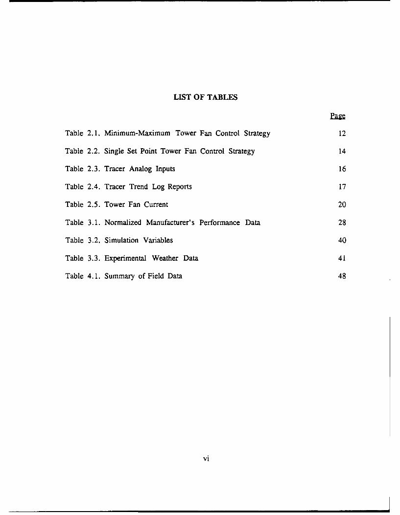
LIST OF TABLES

Table 2.1. Minimum-Maximum Tower Fan Control Strategy 12

Table 2.2. Single Set Point Tower Fan Control Strategy 14

Table 2.3. Tracer Analog Inputs 16

Table 2.4. Tracer Trend Log Reports 17

Table 2.5. Tower Fan Current 20

Table 3.1. Normalized Manufacturer's Performance Data 28

Table 3.2. Simulation Variables 40

Table 3.3. Experimental Weather Data 41

Table 4.1. Summary of Field Data 48

vi

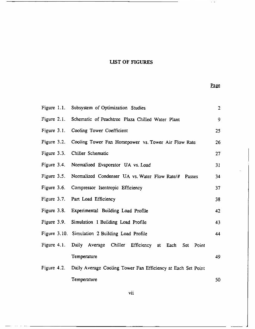
LIST OF FIGURES

Figure 1.1. Subsystem of Optimization Studies 2

Figure 2. 1. Schematic of Peachtree Plaza Chilled Water Plant 9

Figure 3.1. Cooling Tower Coefficient 25

Figure 3.2. Cooling Tower Fan Horsepower vs. Tower Air Flow Rate 26

Figure 3.3. Chiller Schematic 27

Figure 3.4. Normalized Evaporator UA vs. Load 31

Figure 3.5. Normalized Condenser UA vs. Water Flow Rate/# Passes 34

Figure 3.6. Compressor Isentropic Efficiency 37

Figure 3.7. Part Load Efficiency 38

Figure 3.8. Experimental Building Load Profile 42

Figure 3.9. Simulation 1 Building Load Profile 43

Figure 3.10. Simulation 2 Building Load Profile 44

Figure 4.1. Daily Average Chiller Efficiency at Each Set Point

Temperature 49

Figure 4.2. Daily Average Cooling Tower Fan Efficiency at Each Set Point

Temperature 50

vii

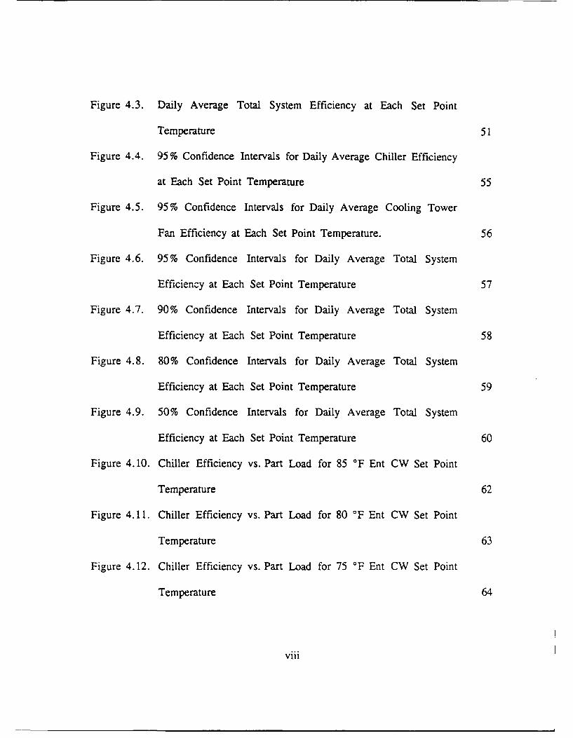
Figure 4.3. Daily Average Total System Efficiency at Each Set Point

Temperature 51

Figure 4.4. 95% Confidence Intervals for Daily Average Chiller Efficiency

at Each Set Point Temperature 55

Figure 4.5. 95% Confidence Intervals for Daily Average Cooling Tower

Fan Efficiency at Each Set Point Temperature. 56

Figure 4.6. 95% Confidence Intervals for Daily Average Total System

Efficiency at Each Set Point Temperature 57







Figure 4.10. Chiller Efficiency vs. Part Load for 85 'F Ent CW Set Point

Temperature 62

Figure 4.11. Chiller Efficiency vs. Part Load for 80 *F Ent CW Set Point

Temperature 63

Figure 4.12. Chiller Efficiency vs. Part Load for 75 'F Ent CW Set Point

Temperature 64

viii

Figure 4.13. Chiller Efficiency vs. Part Load for 70 OF Ent CW Set Point

Temperature 65

Figure 4.14. Chiller Efficiency vs. Part Load for Each Ent CW Set Point

Temperature 66

Figure 4.15. Tower Fan Efficiency vs. OSA Temp Bin for 85 °F Ent CW Set

Point Temperature 69

Figure 4.16. Tower Fan Efficiency vs. OSA Temp Bin for 80 °F Ent CW Set


Figure 4.17. Tower Fan Efficiency vs. OSA Temp Bin for 75 OF Ent CW Set


Figure 4.18. Tower Fan Efficiency vs. OSA Temp Bin for 70 OF Ent CW Set


Figure 4.19. Tower Fan Efficiency vs. OSA Temp Bin for Each Ent CW Set


Figure 4.20. Total System Efficiency vs. Part Load for Each Ent CW Set


Figure 4.21. Actual Part Load Efficiency 78

Figure 4.22. Chiller Efficiency Comparison to Daily Field Results 79

Figure 4.23. Tower Fan Efficiency Comparison To Daily Field Results 80

Figure 4.24. Total System Efficiency Comparison to Daily Field Results 81

Figure 4.25. Predicted Monthly Chiller Energy 84

ix

Figure 4.26. Predicted Monthly Fan Energy 85

Figure 4.27. Predicted Monthly Total System Energy 86

Figure 4.28. Predicted Yearly Eiergy 87

x

LIST OF ABBREVIATIONS

A - current

cP, - constant specific heat of liquid water

CHW - chilled water

CHWR - chilled water supply

CHWS - chilled water return

CW - condenser water

CWR - condenser water return

CWS - condenser water supply

ENT - entering

fda - cooling tower coefficient

GPMc - flow rate of the condenser water

GPME - flow rate of the evaporator water

k - cooling tower constant

KW c - chiller energy demand

KWF - cooling tower fan energy demand

KWT - total system energy demand

KWHc - chiller energy consumption

xi

KWHF - cooling tower fan energy consumption

KWHT - total system energy consumption

LMTD- - log mean temperature difference of the condenser

LMTDE - log mean temperature difference of the evaporator

LVG - leaving

rii- mass flow rate of dry air per unit area of tower face exposed to theair flow

ri CHW - mass flow rate of the chilled water through the evaporator

mcw - mass flow rate of the condenser water through the condenser

- mass flow rate of the liquid water per surface area exposed to waterflow

n - tower exponent

OSA - outside air

PF - power factor

PL - part load fraction

QC - condenser heat flow rate

QE - evaporator heat flow rate

UAc - overall conductance of the condenser

UAE - overall conductance of the evaporator

V - voltage

ATcrfw - temperature drop of the chilled water flowing through the evaporator

xii

-Tcw temperature rise of the condenser water flowing through thecondenser

11-t compressor isentropic efficiency at full load including electric motorefficiency

77wa - compressor part load efficiency

Additional subscripts used:

actual - relating to the experimental data

model - relating to the analytical model

Units:

BTUH - British thermal unit per hour

F - Fahrenheit

GPM - gallon per minute

KW - kilowatt

KWH - kilowatt-hour

RT - refrigeration ton (1 RT = 12,000 Btu/h)

xiii

SUMMARY-

Energy costs continue to play an important role in the decision-making process

for building design and operation. Since the chiller, cooling tower fans, and

associated pumps consume the largest fraction of energy in a heating, ventilating, and

air-conditioning (HVAC) system, the control of these components is of major

importance in determining building energy use. A significant control parameter for

the chilled water system is the minimum entering condenser water set point

temperature at which the cooling tower fans are cycled on and off. Several studies

have attempted to determine the optimum value for this minimum set point

temperature, but direct measurements are not available to validate these studies.

The purpose of this study was to experimentally determine the optimum

minimum entering condenser water set point temperature from field data based on

minimum energy consumption and to validate a chilled water system analytical model

previously developed in earlier work. The total chiller system electrical consumption

(chiller and cooling tower fan energy) was measured for four entering condenser

water set point temperatures (70, 75, 80, and 85 'dF). The field results were

compared to results obtained using an analytical model previously developed in a

thesis entitled "Optimized Design of a Commercial Building Chiller/Cooling Tower

System," written by Joyce. (

xlv

Based on total system energy for chiller part loads less than 50%, the field

results showed that the optimum for the system studied in this work corresponded

to an entering condenser water set point temperature of 85 'F. For part loads

greater than 50%, the optimum entering condenser water set point temperature was

found to be 80 'F. Although decreasing the entering condenser water set point

temperature further resulted in an increase in chiller efficiency, the chiller energy

savings were offset by the increase in tower fan energy consumption at lower set

points.

The trends predicted by the chilled water system analytical model are in close

agreement with the data obtained from the field results. Based on the total system

energy use for an entire year, the analytical model predicted an annual optimum

constant entering condenser water set point temperature of 85 °F, which is in

agreement with the field data. According to the results from the analytical model

simulation, the additional cost of lowering the entering condenser water set point

temperature from 85 °F to 70 'F would be approximately $25,000/year for the

1000 RT chiller studied in this work.

xv

CHAPTER I

INTROD. k;TION

1.1 Background

Energy costs continue to play an important role in the decision-making process

for building design and operation. Since the chiller, cooling tower fans, and

associated pumps consume the largest portion of energy in a heating, ventilating, and

air-conditioning (HVAC) system, the proper control of these components is

imperative in determining building energy costs. Numerous studies [Sud, 1984;

Hackner et al., 1984, 1985; Johnson, 1985; Lau et al., 1985; Braun, 19881 have been

performed to identify computer strategies to reduce the cost of operating the chilled

water plants of large commercial facilities.

To produce strategies to reduce energy costs, Lau et al. [1985] concentrated

on one subsystem of the entire chilled water system to simplify the problem. The

subsystem included the chiller, pumps, cooling tower, and condenser pumps (Figure

1. 1). Their objective was to find the proper control strategy that would result in

minimum power consumption for each combination of the wet-bulb temperature and

total chiller load. They developed computer models of the chilled water system to

study the energy conservation potential of various control strategies. They produced

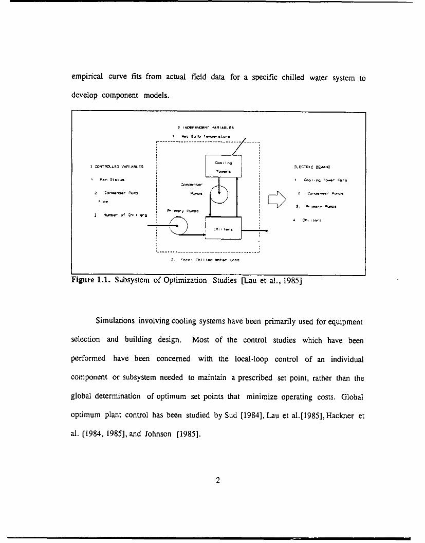
empirical curve fits from actual field data for a specific chilled water system to

develop component models.

Z INOEPeNDeNr VARIABLES

1 wet Bullb T.emi ature

3 CONTROLLED VARIABLES ELECTRIC ODB NOTowng

1 Fan Star-9 1 Cooing Towe rams

Concienser

2 Conoens e Pumo Pi v$ 2 Coinw@ n

Flow3 P I way Purms

j N ~/l''

9f C01lra i !4 r le 5

Chi I lies iI

2. Total Cr1lIGl ! Water Loac

Figure 1.1. Subsystem of Optimization Studies [Lau et al., 1985]

Simulations involving cooling systems have been primarily used for equipment

selection and building design. Most of the control studies which have been

performed have been concerned with the local-loop control of an individual

component or subsystem needed to maintain a prescribed set point, rather than the

global determination of optimum set points that minimize operating costs. Global

optimum plant control has been studied by Sud [1984], Lau et al.[1985],Hackner et

al. [1984, 19851, and Johnson [1985].

2

Braun [1988] provided the most complete consideration of the optimized

design and control of central chiller plants. His central objective was optimal

control. The system optimization involved minimizing the total instantaneous energy

consumption without considering annual energy costs or capital costs.

The power consumption of the chiller is sensitive to the condensing water

temperature, which is in turn affected by both the condensing water and tower air

flow rates. Increasing either of these flows reduces the chiller power requirement but

at the expense of an increase in the pump or fan power consumption. At any given

load, chilled water set point temperature, and wet bulb temperature, there exists an

optimum operating point.

Hackner et al. [1985b] stated that the correct control strategy to minimize

energy use of the chiller/cooling tower subsystem is to minimize the sum of the

chiller plus cooling tower fan power consumption. They also showed, through the

use of computer simulations using various combinations of chilled water load, OSA

wet bulb temperatures, cooling tower fan speeds, and number of operating chillers,

it is often more energy efficient to turn off some of the tower fans to optimize

cooling tower fan status. Once the optimum cooling tower fan status is determined

at a given load, it will remain the optimum tower fan status for any OSA wet bulb

temperature unless the chiller power draw limit is reached [Hackner et al., 1985b].

Cascia [1988] illustrated how actual chiller plant performance data collected

from an energy managcment system cat be used to adapt chiller plant control to

3

optimize energy savings. He presented a direct digital control (DDC) algorithm to

optimize the condenser water temperature by minimizing the sum of the chiller and

cooling tower fan energy consumption. His strategy cycled cooling tower fans based

on the change in the total energy consumption of the chiller plant.

The following generalizations can be made about all the previous studies:

e They were based on computer model simulations to determine the energy

savings of the hypothesized control strategy. Minimal field data was reported to

validate the computer simulations.

0 They all identified control strategies for complex systems based on

computer control algorithms. The strategies were specific to a particular system

based on variable speed fans, variable speed pumps, and multiple chillers. Control

parameters included condenser water flow rate, tower air flow rate, and multiple

chiller control.

* They used field data to develop empirical component models for use in the

computer simulation. The curve fits were applicable only to the specific equipment

and site. The models were not based on fundamental equations of heat transfer and

thermodynamics.

In this study, the focus was on a single control parameter, the minimum

entering condenser water set point temperature. The minimum entering condenser

water set point temperature is the temperature at which the cooling tower fans were

cycled on and off. Referring to Figure 1.1, two of the three controlled variables

4

were constant, the condenser pump flow and the number of chillers. The fan status

was changed to maintain the minimum condenser water set point temperature. The

independent variables and the means of evaluating the control strategy remained the

same.

This study differed from the previous studies in several ways. Field data was

collected to validate the proposed control strategy. The analytical model used was

based on fundamental equations for the chilled water system components, not on

empirical relationships specific to a particular equipment or site.

The analytical model used in this study was developed by Weber [1988] and

modified by Joyce [1990]. Weber investigated design optimization techniques for the

condenser water flow rate and tower air flow rate involving condenser side

components of a central chilled water system. Joyce investigated methodologies for

the optimized design of a central chilled water plant based on annual operating costs,

capital construction costs, and simple payback analysis.

1.2 Objectives

One of the major factors that effects the energy consumption of the chilled

water system is the control of the cooling tower fans. The control point at which the

cooling tower fans are cycled on and off has a major impact on this energy

consumption. It not only affects the cooling tower fan energy use, but also the chiller

energy use. The overall goal of this study is to experimentally determine the global

5

optimum minimum entering condenser water set point temperature at which the

cooling tower fans are cycled on and off.

The proposed study will meet the following three objectives:

* Experimentally determine this global optimum from experimental field

data. As discussed in the previous section, several people have used analytical

models to determine the optimum control point, but there has been no experimental

field validation of these models.

* Compare the field results to results generated using an analytical chilled

water system model developed by Weber [1988] and Joyce [1990]. Using actual field

component performance data in the analytical model, the results from the model can

be compared to the actual field results to determine the accuracy of the model.

Using manufacturer's component performance data in the analytical model, the

results can be compared to actual field results to determine the accuracy of the

manufacturer's performance data.

* Use the validated analytical model with manufacturer's component

performance data to determine the annual optimum constant set point temperature

for an entire year.

1.3 Progosed Study

The proposed study was designed to meet the three stated objectives. It will

examine the effect of four entering condenser water set point temperatures on a

6

large chilled water system. Field data will be collected using the chilled water system

at the Westin Peachtree Plaza Hotel in Atlanta, Georgia. The study will utilize the

existing chilled water system, controls, and energy management system. The field

data will include the OSA temperature and humidity, the CHWS, CHWR, CWS, and

CWR temperatures, the chilled water flow, the chiller amperage, and the cooling

tower fan run times.

The field data will be used to calculate chiller, cooling tower fan, and total

system efficiencies where the efficiency is defined as the ratio of the energy

consumption to the chilled water load. These efficiencies have units of kilowatts

per refrigeration ton (KW/RT). Based on total system efficiency, the optimum

entering condenser water set point temperature will be determined.

Two simulations of the analytical model will be run. The first will use actual

field weather data and actual field chilled water system component performance data.

The second will use standard weather data and manufacturer's component

performance data.

7

CHAPTER II

FIELD EXPERIMENT

This study was performed at the Westin Peachtree Plaza Hotel, a large

1200 room convention hotel in Atlanta, Georgia. The study utilized the existing

chilled water system, controls, and energy management system. Data was

collected for twenty days from November 6, 1990 to November 25, 1990. A

detailed analysis of the system and experimental procedures will now be given.

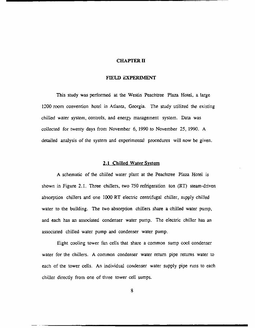
2.1 Chilled Water System

A schematic of the chilled water plant at the Peachtree Plaza Hotel is

shown in Figure 2.1. Three chillers, two 750 refrigeration ton (RT) steam-driven

absorption chillers and one 1000 RT electric centrifugal chiller, supply chilled

water to the building. The two absorption chillers share a chilled water pump,

and each has an associated condenser water pump. The electric chiller has an

associated chilled water pump and condenser water pump.

Eight cooling tower fan cells that share a common sump cool condenser

water for the chillers. A common condenser water return pipe returns water to

each of the tower cells. An individual condenser water supply pipe runs to each

chiller directly from one of three tower cell sumps.

8

8 Cool ig TowrS CCon*Cted Oy d co'm'o SiwV)

CWS CWS CWS

Conoe"Ser water

Chi I ler I Cr ie, 2 Ch Ij"l 3

I Chi I Iea water

C,-fWS Puo CHflhR

C to ul 11 i" g)?

Cfror au i li mgl)

Figure 2.1. Schematic of Peachtree Plaza Chilled Water Plant

A Trane Tracer Energy Management System monitors numerous chilled

water system temperatures, flows, and currents. The Tracer system has the

capability to control the chillers, pumps, and cooling tower fans. However, during

this study, it only controlled the cooling tower fans.

2.2 Operation

2.2.1 Chiller Control

The electric chiller serves as the primary chiller for the hotel and runs

twenty-four hours per day except for hours during which free cooling is possible.

9

The boiler room operator manually sets the chilled water supply temperature at

the chiller control panel. The chiller has an economizer or free cooling mode

that is manually activated.

When the electric chiller reaches its maximum capacity, one absorption

chiller can be brought "on-line" manually by a boiler room operator. The electric

chiller will generally reach its maximum capacity at OSA tenipeiatures greater

than 85 'F. The second absorption chiller is available, but is only required

during heavy load conditions, such as during the summer months.

During this study, the chilled water supply (CHWS) temperature was set to

a constant value of 44 F for OSA temperatures above 42 'F. Below OSA

temperatures of 42 'F, the chiller was manually turned off to start free cooling. If

the chiller was deactivated, it was not until the OSA temperature reached 47 'F

that the chiller would be brought back "on-line". It should be noted that during

the period of this study, the electric chiller was never fully loaded, and, therefore,

the absorption chillers did not rin.

2.2.2 Cooline Tower Fan Control

One of the objectives of this study was to experimentally determine the

optimum entering condenser water set point temperature. Thus, a major focus

was placed on the control of the cooling tower fans. A control strategy was

desired to produce data to predict this optimum set point temperature. The

10

entering condenser water set point temperature is the cycling temperature for the

cooling tower fans.

The Trane Tracer Energy Management System is used to control the eight

cooling tower fans in this system. The system was configured with three digital

output relays which allowed for only on-off fan control. The eight fans are

grouped in three sets, one set of two fans and two sets of three fans.

Prior to this study, the fans were controlled using a "minimum-maximum"

control strategy which is outlined in Table 2.1. A set of fans was turned on when

the condenser water temperature returning to the cooling towers rose above a

specified set point temperature. The same set of fans was turned off when the

temperature dropped below a lower set point temperature.

This strategy presented several problems for determining an optimum set

point temperature. The condenser water temperature was not constant, but

fluctuated by approximately ± 20'F as the fans cycled on and off. This

"minimum-maximum" control strategy was a "first on, last off' strategy, that is the

longest running set of fans was turned off last. The first set of fans brought "on-

line" would often run continuously, while the other sets of fans would be

continuously cycling.

For the purposes of this study, a single entering condenser water set point

temperature was used to simplify the optimization procedure. This single set

point temperature was chosen to be the cycling temperature for the cooling tower

11

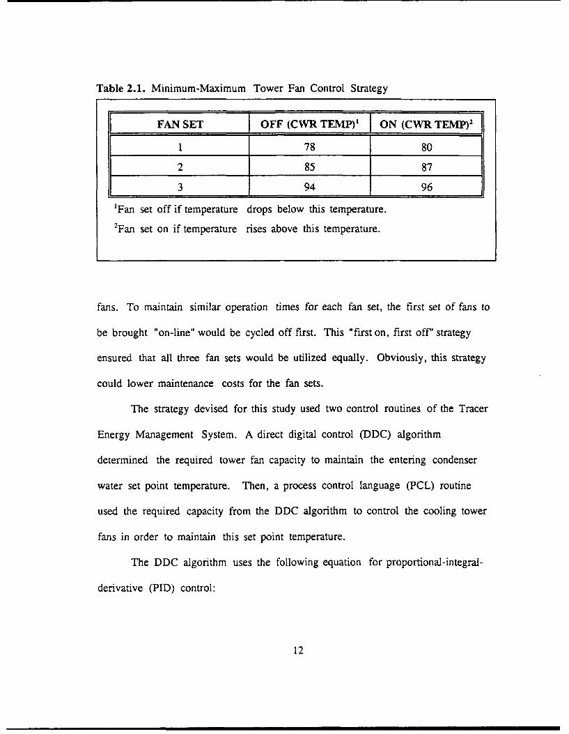
Table 2.1. Minimum-Maximum Tower Fan Control Strategy

FAN SET OFF (CWR TEMP)1 ON (CWR TEMP)2

1 78 80

2 85 87

3 94 96

'Fan set off if temperature drops below this temperature.2Fan set on if temperature rises above this temperature.

fans. To maintain similar operation times for each fan set, the first set of fans to

be brought "on-line" would be cycled off first. This "first on, first off' strategy

ensured that all three fan sets would be utilized equally. Obviously, this strategy

could lower maintenance costs for the fan sets.

The strategy devised for this study used two control routines of the Tracer

Energy Management System. A direct digital control (DDC) algorithm

determined the required tower fan capacity to maintain the entering condenser

water set point temperature. Then, a process control language (PCL) routine

used the required capacity from the DDC algorithm to control the cooling tower

fans in order to maintain this set point temperature.

The DDC algorithm uses the following equation for proportional-integral-

derivative (PID) control:

12

dG=K, *dE+C, *E +KD *d( ) (2.1)

where dG - change in output

K= proportional gain

dE = change in error

KI = integral gain

E = error

dT = time interval

KD = derivative gain

d(dE/dT) = rate of change in error

The DDC algorithm adjusts the output from its current value to a new value

based on the calculated change in output [Trane, 1987].

As mentioned above, the DDC algorithm calculated the percent capacity of

cooling tower fans required to maintain the condenser water set point

temperature. The proportional gain, integral gain, derivative gain, and sampling

time are determined by trial and error. These parameters were determined by

minimizing the overshoot of the set point temperature and cycling only one set of

fans. For example, an OSA temperature might require that one set of fans run

continuously, while a second set of fans would cycle. The set of fans chosen to be

running and the set being cycled were rotated depending on run-time.

13

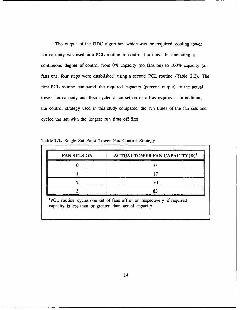
The output of the DDC algorithm which was the required cooling tower

fan capacity was used in a PCL routine to control the fans. In simulating a

continuous degree of control from 0% capacity (no fans on) to 100% capacity (all

fans on), four steps were established using a second PCL routine (Table 2.2). The

first PCL routine compared the required capacity (percent output) to the actual

tower fan capacity and then cycled a fan set on or off as required. In addition,

the control strategy used in this study compared the run times of the fan sets and

cycled the set with the longest run time off first.

Table 2.2. Single Set Point Tower Fan Control Strategy

FAN SETS ON ACTUALTOWER FAN CAPACITY(%)'

0 0

1 17

2 50

3 83

'PCL routine cycles one set of fans off or on respectively if requiredcapacity is less than or greater than actual capacity.

14

2.3 Data Acquisition System

The Trane Tracer Energy Management System served as the data

acquisition system. Table 2.3 gives a list of the analog input parameters. Using a

PCL routine, the parameters for Chiller #1 and the cooling tower fans were

monitored every minute. These data were then summed, and an average for each

hour was computed. The average hourly values were then stored in a "trend-log"

report for use in this study. These average hourly parameters are shown in

Table 2.4.

15

Table 2.3. Tracer Analog Inputs

ANALOG INPUT NAME

OUTSIDE AIR TEMP

OUTSIDE AIR HUMIDITY

CH-1 CHW LVG TEMP

CH-2 CHW LVG TEMP

CH-3 CHW LVG TEMP

COMMON CW LVG TEMP

CH-1 CW ENT TEMP

CH-2 CW ENT TEMP

COMMON CW LVG TEMP

CH-1 CHW FLOW

CH-2 CHW FLOW

CH-1 CURRENT (AMPS)

16

Table 2.4.. Tracer Trend Log Reports

TREND LOGS

AVG OSA TEMP

AVG OSA HUMIDITY

AVG CH-1 CHW LVG TEMP

AVG COMMON CHW RETURN TEMP

AVG CH-1 CW ENT TEMP

AVG COMMON CW LVG TEMP

AVG CH-1 CHW FLOW

AVG CH-1 CURRENT (AMPS)

FAN 3-6 RUN TIME

FAN 1-4-7 RUN TIME

FAN 2-5-8 RUN TIME

2.4 Data Acguisition Methodologv

This study examined four entering condenser water set point temperatures.

These set point temperatures were 70°F, 75°F, 80°F, 85°F. In collecting data, the

same set point temperature was maintained for a 24 hour period. At the end of

each 24 hour period, the Tracer automatically changed the set point temperature

at 12:01 am each day by using a PCL routine.

For each day, the average values were imported into a spreadsheet. From

these values, the chilled water load (RT), chiller energy demand (KWc), and

17

tower fan energy demand (KWF) were calculated. The chilled water load was

calculated using the following equation for the heat transfer rate through the

evaporator [Clifford, 1990]:

Qr=?hcttw*CP,. A TcHW (2.2)

where QE = chilled water load

ricuw = mass flow rate of the chilled water through the evaporator

AT = chilled water temperature rise through the evaporator

C= constant specific heat of water

The chilled water load had units of refrigeration tons (RT). The average value of

the chilled water load for each hour was assumed to be the refrigeration ton-

hours (RT-hours) produced by the chiller during that hour.

The energy used by the chiller (KWc) was calculated from the measured

average three phase current consumed by the chiller. This value was calculated

using the following expression [Baumeister, 1978]:

KWc V4 * V*A *PF (2.3)

where V = chiller voltage (470 V)

A = chiller current (amps)

PF = power factor

18

In this study, the power factor was assumed to be the commonly accepted value of

0.95. The hourly energy demand was considered to be the chiller energy use for

that hour (KWHc).

The energy consumed by the cooling tower fans was calculated using the

total time the cooling tower fans were in use. The hourly fan run-time for each

fan was multiplied by the electrical input in KW for each fan to calculate the

hourly energy use for each fan. The energy use for each fan was summed to

calculate the total fan energy use (KWHp). Each cooling tower fan is driven by

an 18 horsepower (HP) AC motor. This HP rating equates to an input of 22 KW

of electrical power, assuming a motor efficiency of 0.85. To validate this

assumption, the amperage of each tower fan motor was measured. The results of

these measurements and their corresponding calculated electrical input in KW are

shown in Table 2.5.

In this study, the parameters used to determine the optimum condenser

water set point temperature were the chiller efficiency, cooling tower fan

efficiency, and total system efficiency. Each efficiency was defined as the ratio of

the respective energy use to refrigeration ton-hours (RT-hours). This was

performed on both an hourly and daily basis. The efficiencies were in units of

KWH/RT-hour which is equivalent to KW/RT. The total system energy use

(KWHT) is the sum of the energy consumed by the chiller and the cooling tower

fans.

19

Table 2.5. Tower Fan Current

TOWER FAN # CURRENT (AMPS) KW DEMAND (KW)_

1 28 22.1

2 29 22.9

3 25 19.7

4 38 30.0

5 21 16.6

6 28 22.1

7 30 23.7

8 32 25.3

AVG 22.8

'Calculated using equation 2.3 (V =480 V).

20

CHAPTER III

SIMULATION MODEL

This study uses the analytical model for a chilled water system developed by

Weber [1988] and Joyce [1990]. A review this analytical model will now be given.

The complete system model consists of four component models. These component

models are a crossflow cooling tower model, an evaporator model, a condenser

model, and a compressor model. A brief outline of the development of each

component model is presented; however, the reader should consult Weber [1988]

and Joyce (19901 for the complete development. The modifications and additions to

these component models needed for this study will be given in detail.

3.1 Crossflow Cooling Tower Model

There are two generally accepted approaches to the modeling of cooling

towers. These two approaches, as outlined in the ASHRAE Equipment Handbook

[1988], are those based on the assumptions made by Merkel and those based on a

more detailed approach which makes few assumptions. The ASHRAE Equipment

Handbook [1988] uses the model developed by Merkel in its treatment of cooling

tower theory and presents a thorough explanation of the cooling tower

21

thermodynamic process. The cooling tower model developed by Weber[1988] and

Joyce [1990] uses a more detailed approach.

The principle elements and solution methodology of the cooling tower model

used in this study are as follows:

e A fundamental analysis of the mass and energy balances in the cooling

tower with mass diffusion and convective heat transfer as the driving forces is used.

This analysis results in three coupled partial differential equations.

* The three differential equations are solved by finite difference using the

Van Wijngaarden-Decker-Brent method [Press et al, 1986]. A finite difference grid

size of l0x10 is used in this study as recommended by Weber.

9 The correlation presented by Lowe and Christie [1961] is used to calculate

a volume transfer coefficient from a given cooling tower's tower coefficient (k) and

tower exponent (n). The tower coefficient and tower exponent are calculated from

manufacturer's performance data for a given cooling tower.

e The tower fan operation time required to maintain a minimum condenser

water supply temperature is then calculated.

22

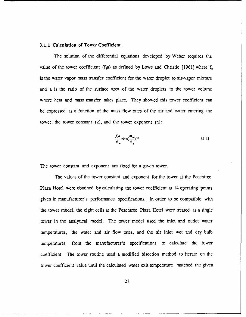
3.1.1 Calculation of Tower Coefficient

The solution of the differential equations developed by Weber requires the

value of the tower coefficient (fda) as defined by Lowe and Christie [1961] where fd

is the water vapor mass transfer coefficient for the water droplet to air-vapor mixture

and a is the ratio of the surface area of the water droplets to the tower volume

where heat and mass transfer takes place. They showed this tower coefficient can

be expressed as a function of the mass flow rates of the air and water entering the

tower, the tower constant (k), and the tower exponent (n):

fda **( m _Y (3.1)

The tower constant and exponent are fixed for a given tower.

The values of the tower constant and exponent for the tower at the Peachtree

Plaza Hotel were obtained by calculating the tower coefficient at 14 operating points

given in manufacturer's performance specifications. In order to be compatible with

the tower model, the eight cells at the Peachtree Plaza Hotel were treated as a single

tower in the analytical model. The tower model used the inlet and outlet water

temperatures, the water and air flow rates, and the air inlet wet and dry bulb

temperatures from the manufacturer's specifications to calculate the tower

coefficient. The tower routine used a modified bisection method to iterate on the

tower coefficient value until the calculated water exit temperature matched the given

23

water exit temperature within 0.0001 'F. The calculated tower coefficients at each

operating point were used to plot the ratio of fda/ri,, versus the ratio of r,/n .

Linear regression was used to calculate the slope of the line or the tower exponent

and the intercept of the line or the tower constant (Figure 3.1). For the tower at the

Peachtree Plaza Hotel, using the manufacturer's specifications resulted in a tower

exponent (n) of 1.12983 and a tower constant (k) of 2.167380.

3.1.2 TowerFan Model

The tower model calculates the fan shaft power (HP) from the air flow rate

through the tower. A correlation of the fan shaft power to the air flow rate through

the tower was obtained from a curve fit of manufacturer's performance specifications

for the tower at the Peachtree Plaza Hotel. Figure 3.2 is a graph of In(cooling tower

fan HP) versus In(cooling tower cfm) for the Plaza's cooling tower. A reduction of

the curve fit formula similar to the one done by Weber [1988] shows horsepower as

a function of air flow rate raised to the 3.8 power. The theoretical value, as stated

by Weber, is 3.0.

24

COOLING TOWER COEFFICIENT10.0 __ _ _ __ _ _ _

5o.o ",,j, I I

S1.0 _ _U- __ _ _ _ _ _ _

0. 1 __ _ _ _ __ _ _j ij0. 1.0 10.0

Figure 3.1. Cooling Tower Coefficient

25

COOLING TOWER FAN HP VS CFM

12 5.5-z

cL 5.2-

2 .0

z4.84.5

14.4

42P

4.0-

3.8~13.0 13.2 13.4 13.6 13.8 14.0 14.2 14.4 14.5 14.8 15.0

LN(COCLTNG TOWER CPM)

Figure 3.2. Cooling Tower Fan Horsepower vs. Tower Air Flow Rate

26

3.2 Chiller Model

T T

Evaoor etc.-

Figure 3.3. Chiller Schematic [Weber, 1988]

The chiller component model developed by Weber (Figure 3.3) is composed

of three sub-component models; one for the evaporator, condenser, and compressor.

One of the advantages of this approach is that modifications made to any of the sub-

27

components can be accurately modeled and show the effects on the chiller

performance.

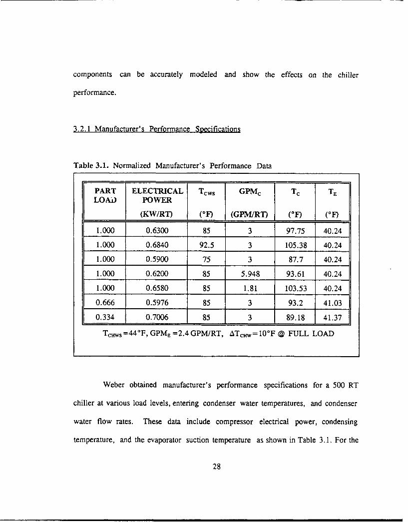
3.2.1 Manufacturer's Performance S1ecifications

Table 3.1. Normalized Manufacturer's Performance Data

PART ELECTRICAL Tcws GPMc Tc TE

LOAD POWER

(KW/RT) ('F) (GPM/RT) (-F) (OF)

1.000 0.6300 85 3 97.75 40.24

1.000 0.6840 92.5 3 105.38 40.24

1.000 0.5900 75 3 87.7 40.24

1.000 0.6200 85 5.948 93.61 40.24

1.000 0.6580 85 1.81 103.53 40.24

0.666 0.5976 85 3 93.2 41.03

0.334 0.7006 85 3 89.18 41.37

Tcnws =44°F, GPME =2.4 GPM/RT, ATcaw= 10F @ FULL LOAD

Weber obtained manufacturer's performance specifications for a 500 RT

chiller at various load levels, entering condenser water temperatures, and condenser

water flow rates. These data include compressor electrical power, condensing

temperature, and the evaporator suction temperature as shown in Table 3.1. For the

28

purposes of this study, the chiller load in RT, the electrical power in KW and the

condenser flow rate in GPM were normalized by the chiller size of 500 RT.

3.2.2 Evaporator Model

The evaporator model proposed by Weber considered the evaporator to be

a flooded shell and tube heat exchanger. The following two expressions for the

evaporator heat transfer rate were employed in his model:

QE =M cr. * Cp *ATcH. (3.2)

QE=UA *LMD E (3.3)

where QE = the chilled water load

ricaw = mass flow rate of the chilled water through the evaporator

ATcw = the chilled water temperature rise through the evaporator

UAE = evaporator overall heat conductance

LMTDE = evaporator log mean temperature difference

Equation 3.2 allowed the temperature decrease of the chilled water flowing

through the evaporator tubes to be calculated for a given cooling load and chilled

water flow rate. For the purposes of this study, the chilled water flow rate and the

chilled water supply temperature were held constant. Equation 3.3 can then be

29

viewed as the relationship between the variation in the chilled water temperature to

the product of the overall evaporator conductance and the evaporator log mean

temperature difference (LMTDF). When the flow rate was held constant, Weber

showed that the UAE was only a function of the refrigeration capacity. This

relationship was also assumed to be correct in this study.

Using the normalized manufacturer's performance data shown in Table 3.1

and equations 3.2 and 3.3, the normalized evaporator conductance was calculated.

A plot of UAE versus part load is shown in Figure 3.4. A curve fit was made to

determine an expression for UAE as a function of part load (PL). This expression

was found to be:

UAE =268.23206 +2568.6836 * PL -1281.09948 * PL 2 (3.4)

where PL is the part load fraction (PL = Model Chiller Load/Nominal Chiller Size)

and UAE has units of BTUH/(°F * RT).

30

EVAPORATOR UA VS LOAD(NORMALIZED BY NOMINRL TONNRGE)

1600

1500-

1400 -1300

1200

1000-900

800

700L00

500w 400

300

20010000.0 0.2 0.4 0.6 0.8 1.0

PRRT LORO

Figure 3.4. Normalized Evaporator UA vs. Load

31

3.2.3 Condenser Model

The condenser model used by Weber also considered the condenser to be a

flooded shell and tube heat exchanger. The critical difference from the evaporator

model was that a variation in the number of condenser passes was permitted to

maintain a minimum water velocity in the tubes of the condenser. The heat transfer

rate in the condenser is given by an energy balance on the chiller as follows:

Qc-Q +KWc (3.5)

where Qc = condenser heat transfer rate

KWc = power consumption of the compressor

The expressions used to approximate the condenser performance were very similar

to those for the evaporator model and are given by:

QC-r C. •n * Ar (3.6)

QC-UA C * LMTD c (3.7)

where rcw= condenser water flow rate

ATcw = the temperature rise of the condenser water

UAc = overall conductance of the condenser

32

LMTDc = condenser log mean temperature difference

Unlike in the evaporator, where the chilled water flow rate is held constant,

the condenser water flow rate is allowed to vary. As a result, in the model by Weber

it was found that the UAc is a function of both the heat transfer rate and the velocity

of the condenser water. The velocity of the condenser water is proportional to the

condenser water flow rate divided by the number of passes in the condenser.

Using the normalized manufacturer's performance data shown in Table 3. 1

and equations 3.5 - 3.7, the normalized condenser conductance was calculate at

various loading and condenser water velocity conditions. A plot of UAc versus

condenser water velocity at various part loads is shown in Figure 3.5. A curve fit was

used to determine an expression for UAc as a function of part load and condenser

water velocity. The expression was found to be:

UA =121 7 .0966 8 +261.29712 * PL -384.41132 * PL 2

GPMC ) GPMC )2 (3.8)+802.5367 * ( PSE )-123.8789 * (PASS)PASSES PASSES

where GPMc has units of GPM/RT and UAc has units of BTUH/(°F * RT).

33

CONDENSER UA VS GPMI#PASSES(NORMRLIZED BY NOMINRL TONNRGE)

2600

PULL LORD .... ..............2400

S0.666 LORD .....

2200 0334 LORD.

2000 .

f 1800-LUcl'1600

Z 1400CZ)

1200

1000

800 ...0.0 0.3 0.6 0.9 1.2 1.5 1.8 2.1 2.4 2.7 3.0

CONDENSER GPM/# PASSES

Figure 3.5. Normalized Condenser UA vs. Water Flow Rate/# Passes

34

3.2.4 Compressor Model

In the compressor model developed by Weber, the Carnot efficiency governing

the performance of the refrigeration devices was used with two efficiencies to

correlate the compressor performance based on manufacturer's performance data.

The values for these efficiencies were found using the manufacturer's data in Table

3.1. In the development of the compressor model, the compressor was assumed to

be adiabatic.

Weber used the Carnot cycle to develop the ideal, or Carnot based, kilowatts

per ton of cooling load. This assumed isentropic compression, constant temperature

heat rejection at To, and constant temperature heat addition at TE. Weber then

related the Carnot based KW/RT to the manufacturer's KW/RT using two

efficiencies, a compressor isentropic efficiency at design full load (n, .) and a

varying part load efficiency (1. d,,) based on the chiller load. The 77.,, is based

on input power to the electric motor, not the input power to the compressor shaft.

The part load efficiency accounts for the decrease in the efficiency of the compressor

at part load conditions. The equations for i, ,, and i, .. are found using

polynomial equation curve fits to the manufacturer's performance data in Table 3.1

(Figures 3.6 and 3.7). Since the manufacturer's design full loa.,. KW/RT for the

chiller at the Peachtree Plaza is 0.65 KW/RT, the equation found from Weber's

model data is multiplied by a ratio of the manufacturer's design KW/RT for the

35

model chiller to the manufacturer's KW/RT for the chiller at the Peachtree Plaza

(0.63/0.65). This resulting equation is plotted in Figure 3.6 and given below.

The model KW/RT is then determined by:

( KWKWRT (3.9)

where

KW T(-).. =[-c-.E-i] 3.517 (3.10)

RT T

(Tc and Tp are absolute temperatures and (KW/RT),x has units of KW/RT.)

=0.50013 +[1.5454 ((_) -0.3)] -[3.613 • ((.T).-0.3)1 ] (3.11)

([KW/RT]7I, x has units of KW/RT.)

1,..,,, ,f[4.5869* PL] -[8.16536*PL 1 +[6.65014*PL 1]-[2.07617*PL 4] (3.12)

(PL is the previously defined chiller part load fraction.)

36

COMPRESSOR ISENTROPIC EFFICIENCY~0.70

L 0 .6 5 -

LL

00

C 0

z~0.55

cnLU

a.' 0.50

0. 45'0.20 0.35 0.40 0.45 0.50

CRRNOT KW/RT

Figure 3.6. Compressor Isentropic Efficiency

37

PART LOAD EFFICIENCY VS LOAD

.00

0.89

S0.7z.;

-0.5

±0.5

0.2-

0.1

0.c0.0 0.1 0.2 0.3 0.4 0.5 0.6 0.7 0.8 0.0 1.0

PRRT LORO

Figure 3.7. Part Load Efficiency

38

3.3 Analytical Model Simulations

Two simulations were performed using the complete chilled water system

analytical model. The first simulation used actual field weather data and actual field

chiler component performance data obtained at the Peachtree Plaza Hotel. The

second simulation used standard weather data in conjunction with the manufacturer's

chiller component performance data. Both simulations utilized manufacturer's

cooling tower performance data. Table 3.2 lists the variables required for each

simulation. Both simulations used building load profiles developed from measured

field data.

Using experimental data in simulation 1 and comparing the results to actual

field data can be used to validate the analytical model developed by Weber. Once

this analytical model is validated, using manufacturer's performance data and

standard weather data in simulation 2 permits an estimate of the yearly performance

of the system. Comparing simulation 2 results to actual field data shows how

accurately the manufacturer's performance data predict actual field performance.

3.3.1 Weather Data

3.3.1.1 Simulation 1: Weather data for simulation 1 are tabulated from the

twenty days of experimental data collected at the Peachtree Plaza Hotel. The dry

bulb temperature bins and mean coincident wet bulb (MCWB) temperatures were

the same as those used in the standard weather data given in U.S. Air Force Manual

39

Table 3.2. Simulation Variables

Variable Simulation 1 Simulation 2'

Nominal Chiller 900 RT 1000 RTTonnage

Chiller Efficiency 0.85 KW/RT 0.65 KW/RT

Evaporator GPM 2444 GPM' 2400 GPM

CHWS Temperature 44 OF' 44 OF

Condenser Passes* 2 2

Condenser GPM 3441 GPM' 3093 GPM

CWS Pipe Diameter* 12" 12"

CWS Set Point 70/75/80/85/90 OF 70/75/80/85/90 OF

HTower Fan CFM 1,036,960CFM2 1,036,960CFM

'Based on actual system design.

'Based on actual field component performance data.2Based on m-anufacturer's component performance data.

88-29 [1978]. The summary of data are shown in Table 3.3.

3.3.1.2 Simulation 2: Weather data used for simulation 2 are obtained from

the U.S. Air Force Manual 88-29. The total number of hours in each dry bulb 5 OF

temperature range, or "bin,"was used as the Peachtree Plaza Hotel chilled water

system operates twenty-four hours per day. A computer algorithm calculated the

total number of hours for each bin and the cumulative number of hours for each

month of the year.

40

Table 3.3. Experimental Weather Data

OSA TDB Bin MCWB Temperature Hours'

72 60 1

67 60 80

62 57 100

57 52 140

52 47 77

47 42 52

42 38 4

Total Number of Hours: 454

1Total number of mechanical cooling hours observed in OSA TDB bin.(Free cooling hours are excluded.)

3.3.2 Building Load Profile

The actual building load profile was found by plotting the average hourly

chiller tonnage (RT) versus the average hourly OSA temperature from the

experimental data (Figure 3.8). The building load profiles for simulation 1 and

simulation 2 are shown in Figures 3.9 and 3.10 respectively. The profile for

simulation 1 is normalized by a nominal chiller tonnage of 900 RT; whereas the one

for simulation 2 by a nominal tonnage of 1000 RT. Both profiles assume free cooling

to be used below an OSA temperature of 42 OF.

41

AVG TONS VS AVG OSA TEMPERATUPEC8ASEO ON HOURLY EXPERIMENTAL DATAD

Avg Hourly Tons CPT) (Thousanisj1

0 8

0 6

-~. J .

0.2

a 10 20 30 40 50 50 70 80 90 100Avg Hour-ly GSA Temp~er-ature

Figure 3.8. Experimental Building Load Profile

42

BUILDING COOLING LOAD VS OSA TEMPEPATUPE

CNOPMALIZED BY 900 NOMINAL RTD

Part Load Factor

0.6

0.5

0.4

02

0 1III I I I I

0 10 20 30 40 50 60 70 80 90 100OSA Dry Bulb Tefrerature CP#

Figure 3.9. Simulation 1 Building Load Profile

43

BUILDING COOLING LOAD VS OSA TEMPERATURE

CNORMALIZED BY 1000 NOMINAL RTD

Part Load Factor

08a

0.8

04

02

0 I I 1

0 10 20 30 40 50 s0 70 80 90 100

OSA Dry Bulb Temperature CFD

Figure 3.10. Simulation 2 Building Load Profile

44

CHAPTER IV

RESULTS

4.1 Daift Data

As discussed in Chapter II, data was collected for the twenty days from

November 6, 1990 to November 24, 1990. For each day, one of the four entering

condenser water set point temperatures (70, 75, 80, 85 'F) was maintained. The

hourly field data for each day is tabulated in Appendix 1. Table 4.1 gives a daily

summary of the field data.

A major objective of this study was to determine the optimum condenser

water set point temperature. In this work, the total system efficiency was chosen as

the criterion for determining this optimum. The "total system" was defined as the

combination of the chiller and the cooling tower fans. The chilled water pumps and

condenser water pumps were not considered since their energy use was constant for

all cases. The total system efficiency is defined as the ratio of the total system

energy use to the total refrigeration ton-hours and has units of KW/RT.

Plotting the chiller efficiency, cooling tower fan efficiency, and total system

efficiency as a function of the four set point temperatures (Figures 4.1, 4.2, 4.3)

shows clearly the following trends. For the chiller energy consumption, the chiller

efficiency initially decreased as the set point temperature decreased from 85 'F to

45

75 *F. The chiller efficiency, however, then increased with further set point

temperature decreases. The tower fan energy consumption (the energy use per RT-

hour produced, KWF/RT) increased as the set point temperature decreased. The

total system efficiency showed the same trends as the chiller, first increasing as the

set point temperature was lowered from 85 *F to 80 *F, followed by an increase in

efficiency as the set point was further decreased. Although the chiller was more

efficient at a set point temperature of 75 "F, the total system efficiency was

maximized at an 80 *F set point temperature. This fact is explained by the large

increase in fan energy consumption from 80 'F to 75 *F outweighing the energy

savings in chiller energy for this temperature range.

These trends are consistent with known chiller operation [Trane, 19891.

Lowering the condenser water temperature lowers the head pressure on the

condenser and consequently increases the chiller efficiency. The energy used by the

chiller is used to compress the refrigerant gas from low pressure in the evaporator

to high pressure in the condenser. Decreasing the condenser water temperature will

lower the saturation temperature in the condenser, thereby decreasing the pressure

differential between the evaporator and the condenser. This pressure differential

decrease reduces the work required by the compressor and the energy consumption

of the compressor. The total result is to lower the chiller efficiency (KWc/RT).

As seen in the experimental data, there are limitations to lowering the

condenser water temperature. A minimum pressure differential is required between

46

the evaporator and the condenser to assure adequate refrigerant flow through the

orifice acting as the throttling device. If this minimum pressure differential is not

maintained, insufficient refrigerant is returned to the evaporator resulting in low

evaporation pressures. As the level of the liquid refrigerant drops, the evaporator

tubes are no longer fully covered, causing a decrease in the effective surface area

used to evaporate the refrigerant. This decrease will result in a reduction of the

chiller efficiency.

47

Table 4.1. Summary of Field Data

DATE SET AVG OSA TONHRS AVG TON CHILLER FAN TOTAL CHILLER FAN TOTALPOINT TERP (RT) KWH KWH KWH KW/RT KW/RT KW/RT

6 NOV 85 56.1 12261 511 12174 318 12492 0.9929 0.0259 1.018810 NOV 85 48.8 9124 380 10722 4 10726 1.1751 0.0004 1.175514 NOV 85 60.7 13921 580 13244 585 13829 0.9514 0.0420 0.993418 NOV 85 58.0 7464 574 6847 216 7063 0.9517 0.0292 0.980922 NOV 85 62.9 12251 510 12476 648 13124 1.0184 0.0529 1.0713AVG 57.3 11004 511 11093 354 11447 1.0179 0.0301 1.0480




48

<W/RT VS ENT CW SET POINT

CCHI LLERD

KW/ RT1 .1 0 I- -" ' , , , . ,.. ............ ... ................ . .......*- ----- --------------.--*- -----------

11 8 .... ................. ............. ......*...0 8. ..*. .... ........... ...... . ... " ------

1 .0 6 -. ..*. .................................... ...................

1 0 4 ... .*. ... .. .... ...... .... ........1 .... .. .. ........* --- .... .. ...... - - , -....... .

1 0 2 9 0 ----*- ------ ---* * *. .....*. .... .. .... ............... ... ...

0 75 ... 0. 8 5.. 1-* - ......" ' " , -

0 ~ ~ ~ ~ ~ N 98 ......... W....... .... S ET..... ......... ............P O I N T.............. .......... .. .....

Fiur 4.1. Daily...A.era....Chiller... Efficiency...at..Each..Set..Point..Temperature..

L ----- ................. 4..

KW/RT VS ENT CW SET POINT

CTOWEP FANSD

KW/ PT

0 . 1 7 ...................... 7.................................................8...............

0 .10 ~ ~ ~ E N CW--- SET..........................................I.........................T.......

0igur 4 ..................2............ Daily A..e..age Cooling Tower. ..a..Efficiency ...at ..Each..Set.. Point

T em p e...........ratu re,,....... .. ....... ....................................

0 , 4 - .......... .............................................. ......5 0 ..

<W/RT VS ENT C'V SET POINT

CTOTAL SYSTEMJ

KW/ PT

1 10 ......................................... ......... ..... ..........................................................................................................................

"1 0 6 ........... . . . . . . . . .. . . . . . . ......... ................................................................................ .........................................

01 . 6

1 0 ....... ......... ......... ......... ........ ......... ......... ......... ..................... ... ........-- ---I--*........

0 2 . ......................... ...... ........ ............................................ . . . ............... ... ... ... ............ . . . .. . .. .. . ... . . . . . . .

,--------',.........- .. .......................... .... .. . .0 9 8 ............. *.......... * **................. *......- -*... .... .... *.............. .... ... .... .... .... ....... . . . . . . . . . . . . . . . . . . . . . . . . . . . . . . . . . . . . . . . .

0 9 4 . .. . . . . . . . . . . . . . . . . . . . . . . . . . . . . . . . . . . . . . . . . ............................. ........... - *........................ ............................-- --- - - -- -

0 9 2 - . . . . . . . . . . . . . . . . . .. . . . . . . . . . . . . . . .............................................. ................................. .... ........... .................. - -

0.90 -1 1 1

70 75 80 85

ENT CW SET POINT

Figure 4.3. Daily Average Total System Efficiency at Each Set Point Temperature

4.2 Statistical Analysis

Statistical inference is the expression used to describe a process by which

information from sample data is used to draw conclusions about the population from

which the sample was selected. One of the techniques of statistical inference is

called "parameter estimation", which is estimating the parameter of interest to be

within a calculated range. In this study, the parameters of interest are the chiller

51

efficiency, the cooling tower fan efficiency, and the total system efficiency. To meet

the first objective of the study, the efficiencies at each of the four entering condenser

water set points should be statistically independent. One method of examining this

statistical independence is the use of "confidence intervals".

The confidence interval is the measure of the variation in the data. The

unknown parameter then lies in the observed interval with a given confidence. The

size of the observed confidence interval is an important measure of the quality of the

information obtained from the sample. The larger the confidence interval, the more

certain the interval actually contains the true value of the parameter. However, the

larger intervals provide less information about the true value of the parameter. The

most information is obtained when a relatively small interval has a high degree of

confidence.

The construction of the confidence interval assumes the population is normally

distributed. Tuve and Domholdt [1966] state four criteria for determining whether

the assumption of normal distribution is appropriate. The criteria are as follows:

0 The values comprise a population of some size or a fairly large and

representative sample from the total population.

* The deviations from the average in this representative sample are small,

random, and uncoupled and are due to a variety of causes.

* The range of values from highest to lowest looks reasonable.

52

- An examination of the highest and lowest values shows no significant bias

or skew.

The data collected in this study are assumed to meet these criteria.

To find the confidence interval for the mean of a normal distribution from a

random sample of size n where the population variance is unknown, the sample

mean, X, and the sample variance, S2, are employed in the following equation:

'- <L <Y1+ " (4.1)

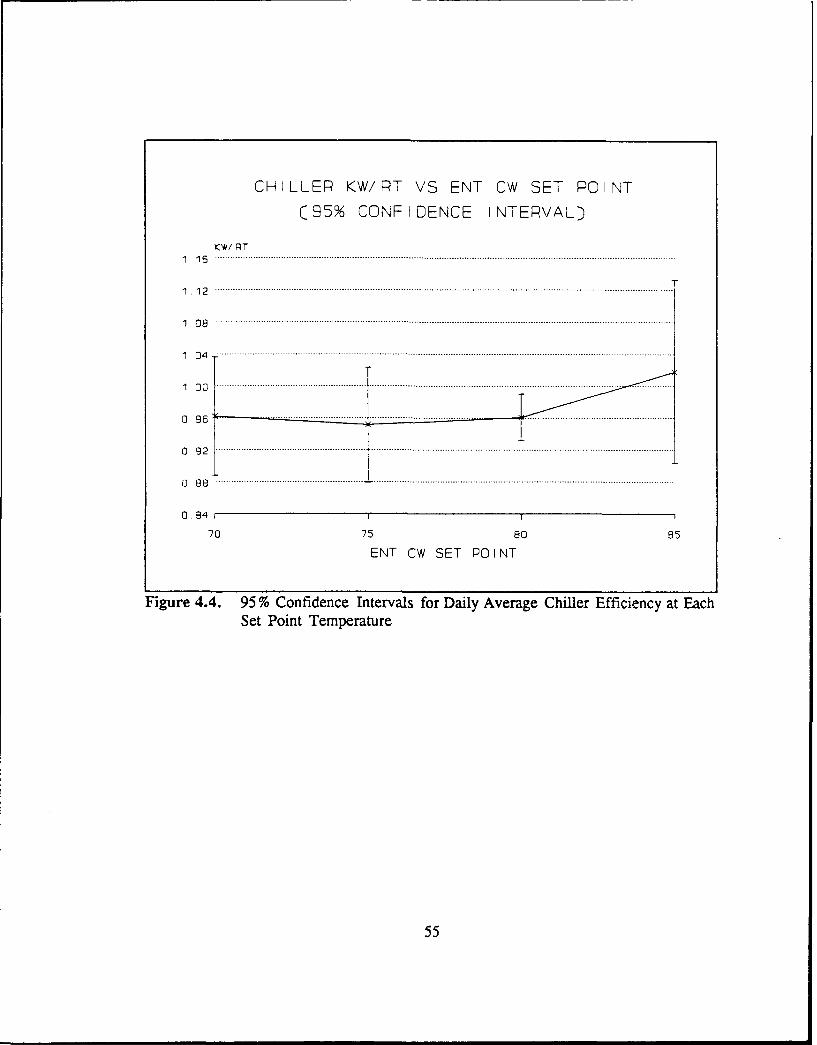
Fn Vn

where t.12,.-, is the t-distribution from Table IV in the Appendix of Hines and

Montgomery [1990].

Figures 4.4 - 4.6 show the chiller, cooling tower fan, and total syscem

efficiencies as functions of the four entering condenser water set point temperatures

with 95% confidence intervals. From the definition, the mean efficiency for the

entire population of possible efficiencies at each set point is between the upper and

lower limits of the interval with a confidence of 95%. This statement can also be

interpreted as, the mean lies within the interval 95% of the time. In this case, the

high confidence produces a large interval.

Figures 4.6 - 4.9 show the total system efficiency as a function of the four set

point temperatures with decreasing confidence levels. Since the size of the

confidence interval measures the precision of the estimation, the precision is

inversely related to the size of confidence interval. Simply stated, the large

53

confidence intervals are less precise than small confidence intervals. Therefore, it

is highly desirable to obtain a confidence interval that is small enough for decision-

making purposes that also has adequate confidence. In Figure 4.9, a set point

temperature of 80 *F has a lower total system efficiency than 70 'F with 50%

confidence.

The conclusions drawn from the experimental data are therefore believed to

be valid, despite the large confidence intervals at higher confidence levels. It is

difficult to obtain measurements with high confidence in the systems studied here,

since many variables affect the overall efficiency. More measurements must be

performed if one wishes to reduce the variation resulting in smaller confidence

intervals at higher confidence levels.

54

CHILLER KW/RT VS ENT CW SET POINT

C95% CONFIDENCE INTERVALD

rI,'/ PT1 1 6 ....... ........ *........**... ... ... .... ... ... ....... ... ... ... .......................................................................................................... ..

1 . 1 2 .. . ... . . . .. . . . .. .. . .. . ... . . ... . . . .. .. . .. . . . ......................................... ................................................ ... . . .

1 0 8 ................................................................................................................................................................................. .

"1 0 0 ... ....................................................... ............................................................... . .. . . . . ............. .. .. . . ....... ...... .

0 9 2 ... . . ...... ............... ................... .. . . . ................................................................................................................ .

0 8 8 .......................... ............................... .............................................................................................................. ........

1084

0, 8,4

70 75 80 85

ENT CW SET POINT

Figure 4.4. 95 % Confidence Intervals for Daily Average Chiller Efficiency at EachSet Point Temperature

55

TOWER FAN KW/PT VS ENT CW SET POINT


KW/ PT

0.15 0 .... -----------5............................................................. ... .... .................

0.-140 ..* .. . ... ................................................................ I.......................

001 5..................... .. ... ................................ ........ ........... ........ ...

01101.............................. ...

0 005 1

70 75 s0 e5

ENT OW SET POINT

Figure 4.5. 95 % Confidence Intervals for Daily Average Cooling Tower FanEfficiency at Each Set Point Temperature.

56

TOTAL SYSTEM KW/RT VS ENT CW SET


KW/ PT

19. ...............................---- ---................... *.......................

0.92 . .... ---- .................................... ................. I-------............ ...........

0 88............................................................................... ............

0.84 ________________________________________

70 75 80 85

ENT CW SET POINT

Figure 4.6. 95 % Confidence Intervals for Daily Average Total System Efficiencyat Each Set Point Temperature

57


C90% CONFIDENCE INTEPVALD

KW/ P~T

.......: T.... i ........... ....--- ......---.---

0 .88 .. ...... *....... .................... ................---............. -------............ .. ... ....

0 84 111

70 75 s0 85

ENT OW SET POINT

Figure 4.7. 90% Confidence Intervals for Daily Average Total System Efficiencyat Each Set Point Temperature

58


C80% CONEIDENCE INTEPVALD

<~W/ PT1 1 5 .................. . ..................... ...................... ....... . .........

0 92

o 88

70 75 s0 95

ENT OW SET POINT


59

TOTAL SYSTEM K'N/PT VS ENT CW SET

C50% CONFWDENCE INTEPVALD

rKW/ PT1 16 ...... .... .....

0 96

0 9 2 ---- - ----... ....

0 68 -- --

0,6 1

70 75 80 35

ENT CW SET POINT


60

4.3 Hourly Data

Due to the large variation in daily data, the hourly field data was examined.

The data was disaggregated by hourly average OSA dry bulb temperature and hourly

average chiller tonnage (RT). The OSA temperature was disaggregated using 5 *F

temperature bins as in the standard weather data. The average chiller tonnage was

disaggregated into 50 RT bins. The chiller efficiency, cooling tower fan efficiency,

and the total system efficiencies were calculated as described in Section 2.4, Data

Acquisition Methodology. Each efficiency was defined as the respective hourly energy

use divided by the hourly RT-hours of chilled water load and had the units of

KW/RT.

The chiller efficiency is known to be a function of the chiller chilled water

load and the entering condenser water set point temperature. It was found that by

plotting the KWc versus the chiller load for each temperature bin and at each

entering condenser water set point temperature, a smooth curve was generated

(Figures 4.10 - 4.13). Figure 4.14 summarizes these data by using a second order

curve fit for each set point temperature.

Figure 4.14 shows that the optimum entering condenser water set point

temperature based solely on chiller energy consumed is 70 'F. This differs from the

daily data results, which showed an optimum of 75 'F. This difference is due to the

chiller efficiency being a function of both chiller loading as well as the set point

temperature.

61

CHILLER KWIRT VS LOAD(85 ENT CW TEMP)

1 .5

0 42 A 47 C 5257 + 62 o 67

1 .3

11 o

3=3

0.9

0.8300 350 400 450 500 550 600 650 700 750RVG RT

Figure 4.10. Chiller Efficiency vs. Part Load for 85 *F Ent CW Set PointTemperature

62


o 42 o 52 57

.4 + 52 o 67

.2 - \

1.1-

0.8300 350 400 450 500 550 600 650 700 750

RVG RT


63


.5 A 47 a3 52 57

F + 62 0 57

:3 .0

0.9-

0.8"o

0.7 -300 350 400 450 500 550 600 650 700 750

RVG RT


64


15

0 42 A47 o 52

0 ~57 + 62 o 671 .3

1.2-

1.0

0.9

0 8

0.7300 350 400 450 500 550 600 650 700 750

RVG RT

Figure 4.13. Chiller Efficiency vs. Part Load for 70 'F Ent CW Set PointTemperature

65

CHILLER KWIRT VS LOAD.5

85 ENT- 80 ENT .. 75 ENT-1.4

70 ENT-

1. 3

3C 14.0

0.7300 350 400 450 500 550 600 650 700 750

AVG RT

Figure 4.14. Chiller Efficiency vF. Part Load for Each Ent GW Set PointTemperature

66

In the daily data, the chiller loading varied during each day. Ideally, this

variance and tne daily average for each day would be the same. However, the data

show this situation was not the case. For example, the average daily chiller tonnage

(RT) at 75 OF is 526 RT, whereas the average tonnage at 70 OF is 501 RT. The

hourly data removes the effect of variation in the efficiency due to changing load.

Although the variation in efficiency due to changing load is small compared to the

efficiency change due to changing set point temperature, the varying load causes

scatter in the daily data and accounts for the difference in the optimum between

daily and hourly data.

The data show there are two competing effects which to contribute to the

overall increase in the measure of chiller efficiency as part load is decreased. As

part load decreases, the compressor operates less efficiently causing an increase in

the required KW/RT to operate the compressor. In ontrast, the evaporator

temperature (TE) increases and the condenser temperature (Tc) decreases causing

the pressure difference between the evaporator and condenser to decrease as the

chiller loading decreases. This decrease in the pressure rise across the compressor

results in less KW/RT to operate the compressor as described previously in Section

4. A,Daily Data. The combined effect causes the chiller KW/RT to initially decrease

as the loading decreases and then to increase. The effect of the compressor

inefficiencies is much larger than, and quickly overcomes, the effect due to the

67

temperature difference. In Figure 4.14, the initial decrease in KW/RT is not

evident due to no data being available at full load condition.

The cooling tower fan operation time is a function of OSA temperature and

entering condenser water set point temperature. Although the cooling tower

performance is more directly a function of OSA wet bulb temperature, the accuracy

of the humidity sensor at the Peachtree Plaza was questionable and could not be

calibrated; therefore, the OSA dry bulb temperature is used to correlate the cooling

tower fan performance. It was found that by plotting the KWF/RT as a function of

OSA temperature bin for each refrigeration ton bin and at each set point

temperature, a straight line was generated (Figures 4.15 - 4.18). Figure 4.19 shows

a linear regression curve fit for each set point temperature. As expected considering

cooling tower performance, the tower fan efficiency (KWF/RT) increases as the

entering condenser water set point temperature is decreased.

The total system efficiency is known to be a function of the chiller chilled

water lead, the OSA temperature, and the entering condenser water set point

temperature. Plotting the KWT/RT as a function of the chiller load for each

temperature bin and at each entering condenser water set point temperature

generated a smooth curve using a second order curve fit for each set point

temperature (Figure 4.20).

68

TOWER FAN KWIRT VS OSA TEMP(85 ENT CW TEMP)

0.20

0.18 - o 300 TONS a 350 TONS 0 400 TONS

0.15 - 450 TONS + 500 TONS 0 550 TONS

C.14 - 600 TONS n 550 TONS 0 700 TONS

0.22 A 750 TONS

0. 0

z0.08

0.06

0.02[ - +::°

0.O0-42 47 52 57 62 67

OSR TEMP BIN

Figure 4.15. Tower Fan Efficiency vs. OSA Temp Bin for 85 °F Ent CW Set PointTemperature

69

TOWER FAN KW/RT VS OSA TEMP(80 ENT CW TEMP)

0.28 - 300 TONS a 350 TONS o 400 TONS

0.24 450 TONS + 500 TONS o 550 TONS

600 TONS v 650 TONS 0 700 TONS0.20

A 750 TONS

0.16

0.08 -

0.04 F0.001-°

42 47 52 57 62 67OSR TEMP BIN

Figure 4.16. Tower Fan Efficiency vs. OSA Temp Bin for 80 'F Ent CW Set PointTemperature

70


0.28 0 300 TONS A 350 TONS 0 400 TONS

0.24 - 450 TONS + 500 TONS o 550 TONS

600 TONS a 650 TONS 0 700 TONS0.20

a 750 TONS

0.16

N

S0.12-

0.04

0.0042 47 52 57 62 67

OSR TEMP BIN

Figure 4.17. Tower Fan Efficiency vs. OSA Temp Bin for 75 'F Ent CW Set PointTemperature

71


0.28 0 300 TONS a 350 TONS 0 4C0 TONS

0.24 - 450 TONS .500 TONS o 550 TONS

6C0 TONS u 650 TONS 0 700 TONS

0.20 -

0.120

.08"

0.04~

0.00'42 47 52 57 52 67

OSR TEMF BIN

Figure 4.18. Tower Fan Efficiency vs. OSA Temp Bin for 70 °F Ent CW Set PointTemperature

72

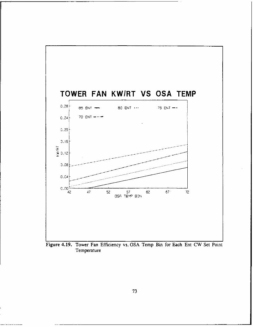
TOWER FAN KWIRT VS OSA TEMP0.28- 85 ENT -80 ENT 75 ENT --

0.24 - 70 ENT-"

0.20

S0.12 -------

---- ------

... .. .. ... ... .

0.0042 47 52 57 62 67- 72

Q9; TEMP BIN

Figure 4.19. Tower Fan Efficiency vs. OSA Temp Bin for Each Ent CW Set PointTemperature

73

TOTAL SYSTEM KWIRT VS LOAD.5

1. 5 ENT- 75 ENT--

7 80OENT.. 70 ENT-

1.3-

0.9 ......

0.7300 350 400 450 500 550 600 650 700 750

RVG RT

Figure 4.20. Total System Efficiency vs. Part Load for Each Ent CW Set PointTemperature

74

The resulting curves in Figure 4.20 show an optimum entering condenser

water set point temperature of 85 'F below 450 RT and an optimum of 80 *F above

450 RT. This result indicates the benefit of varying the set point temperature with

the chiller load, the OSA temperature, or possibly both. The ideal control strategy

would be to vary the set point temperature based on chiller load and OSA

temperature.

4.4 Analytical Model

4.4.1 Simulation I

As described in Chapter III, simulation 1 used measured weather data and

measured chiller component performance data obtained at the Peachtree Plaza Hotel

in the chilled water system analytical model used in this study. The operating

parameters are shown in Table 3.3. The compressor model was changed to more

accurately reflect field chiller performance data.

In the compressor model, the isentropic efficiency predicted by the analytical

model, i%,, , was adjusted by a ratio of the manufacturer's full load design

efficiency (0.65 KW/RT in this case) to the actual full load chiller efficiency at

standard conditions (85 'F entering CW temperature, 45 *F CHWS temperature) as

reflected in the field data. Since no full load efficiency data was collected, the full

load chiller efficiency was assumed to be 0.85 KW/RT which was the chiller

efficiency at the greatest load measured (750 RT) at a set point temperature of

75

85 'F. This assumption seems reasonable since the part load efficiency does not

change significantly above a part load of 80%. To summarize, the ratio used in this

study was 0.65/0.85.

The part load efficiency, %., was also adjusted to agree with the measured

decrease in compressor efficiency with decreasing loads. The actual part load

efficiency, .,., is given as:

(KW/R) , -, L"SA'-" (4.2)- (KWIRT)3", * %,,w ,,,, em mo,*,

The model isentropic efficiency, 7,,, ,d,, was then calculated as described above.

The actual isentropic efficiency, -6 ,, was calculated using field data at three part

load conditions (300, 600, and 700 or 750 RT) for each set point. Then, the data was

analyzed to produce an empirical expression for 7, by using a second order

polynomial curve fit to the data points (Figure 4.21).

The data clearly show that the manufacturer's part load efficiency is optimistic.

The fact that the part load efficiency can be well represented as a function of the

part load parameter only shows the validity of the chiller model.

The results of simulation 1 are shown graphically in Figures 4.22 - 4.24

(Numerical results are included in Appendix 2). The results for the chiller and total

system efficiencies produced by this simulation closely approximate the field data

results.

76

The simulation results for the tower fan efficiency differ from the measured

data in this work. This difference can be explained by the fact that the cooling tower

is performing less efficiently than the specification given by the manufacturer. The

original fill material in the cooling tower cells at the Peachtree Plaza was replaced.

The new fill material causes the water to fall in sheets rather than droplets, and

results in a less efficient cooling process.

77

PART LOAD COMPRESSOR EFFICIENCY(RCTURL)

I .0 - - - -- - - - - -

0.9 -

0.7"I5

o.- I. 80LLIj /.,

0.5 / 75//LL 75

LU 0.4 c: /70

0 / MODELS0.2 -

0.1 "

0. 00.0 0.1 0.2 0.J 0.4 0.5 0.6 0.7 0.8 0.9 1.0

PRRT LORD

Figure 4.21. Actual Part Load Efficiency

78

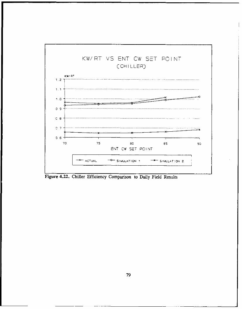
KW/RT VS ENT CW SET POINT

CCHf LLEPJ

Kw/ AT

1 .0 8 .. .. .......... ... .... . I. ... .... ...... .... ...... ..... ....... .. .... .......

o *6

70 75 80 85 90

ENT CW SET POINT

X~ ACTUAL 9 SIMULATION 1 46 SIMULATION 2

Figure 4.22. Chiller Efficiency Comparison to Daily Field Results

79

KW/PT V'S ENT CW SET POINT

CTOWER FANSD

KW/ PT

0 7 5----- .. ... ... ...... ... . 8 5.. ............

0 80

KW/RT VS ENT CW SET POINTCTOTAL SYSTEMJ

<W/ PT1 .2 -- -- .. .. .... ... ... ... ... .. .. ..... .. ... ... ..... .... .. .. ..... ......... .... .. ... ... .. ... .. .... .

7 0 ....... 8 0..... 8 5......... ... 9.*.... ...... 0... ----

ENT CW IE ON

~ACTUAL 9 SIMULATION I S5IMULATION 2

Figure 4.24. Total System Efficiency Comparison to Daily Field Results

81

4.4.2 Simulation 2

Simulation 2 used standard weather data and manufacturer's component data

as outlined in Chapter III. The analytical model was run as discussed in Chapter III.

The simulation calculated the monthly and yearly chiller, tower fan, and total system

energy use. The results of the simulation are shown graphically in Figures 4.25 - 4.28

(Numerical results are included in Appendix 2). The monthly energy use for

November was used to calculate chiller, tower fan, and total system efficiencies.

These efficiencies are also plotted on Figures 4.22- 4.24.

As illustrated in Figures 4.22,the manufacturer's data for chiller performance

is optimistic. The manufacturer's full load design efficiency is 0.65 KW/RT

compared to an actual full load efficiency of 0.85 KW/RT at standard rating

conditions. The part load compressor performance is also significantly less for

manufacturer and field data. Although the absolute chiller efficiency is

underpredicted by the analytical model when using manufacturer's data, the observed

trends for the simulation match the trends shown in the field data.

The monthly energy use profiles (Figures 4.26- 4.28) show that the sensitivity

due to the effect of changing the set point temperature is greater during the peak

cooling periods. Although the change in chiller energy due to decreasing set point

temperature is not significant, the energy penalty due to the increase in cooling tower

fan run-time is severe. Running away from the optimum set point during the

summer months results in a larger peak electrical demand than running at the

82

optimum. This peak could result in high electrical demand charges which are paid

throughout the year. The monthly energy use profile also further shows that the

condenser water set point temperature should be ideally varied based on chiller

loading and OSA temperature.

Looking at the yearly energy use in Figure 4.28, the chiller energy use

decreases for decreasing set point until 75 °F and then increases. The tower fan

energy use increases with decreasing set point. The total system energy use

decreases for decreasing set point until 85 °F and then increases. The decrease in

chiller energy use from 85 'F to 75 °F is overcome by the increase in tower fan

energy. The annual optimum constant entering condenser water set point

temperature based on total system energy use is 85 *F.

The yearly simulation results show that it is more advantageous to select a

higher entering condenser water set point temperature when considering the total

energy consumption of the system. This result is contrary to the customary practice

in the field. Operators tend to select lower set point temperatures to avoid perceived

problems in chiller operation. This practice is costly. In decreasing the set point

temperature from 85 °F to 70 °F, the total system energy use is predicted to increase

by 320,000 KWH/year. At an average cost of 8 C/KWH, the yearly increase in

energy cost would be $25,000.

83

MONTHLY CHILLEP ENEPGYCHILLEP ENEPGY CKWH) CThousandsD

400

300

200

100

JAN FEB MAP APP MAY JUN JUL AUG SEP OCT NOV DEC

MONT H

Figure 4.25. Predicted Monthly Chiller Energy

84

MONTHLY FAN ENERGYFAN ENEPGY CKWH) CThouSandSD

1401

120

100

80

40

20

0JAN FES MAP APP MAY JUN JUL AUG SEP OCT NOV DEC

MONTH

Figure 4.26. Predicted Monthly Fan Energy

85

MONTHLY TOTAL E--NERGOTOTAL ENEPGY CKWHD CThousandsD

500

400

300

200

100

JAN FEB MAP APP MAY JUN JUL AUG SEP OCT NOV DEC

MONTH

= 70 75 M 90 95 90

Figure 4.27. Predicted Monthly Total System Energy

86

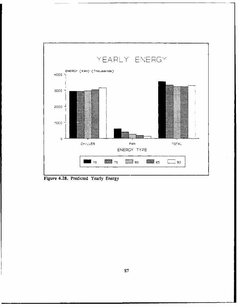
YEARLY ENERGY

ENEPOY CKWH) CThousarnds)

'4000

2000

2000

0

CHILLEP FAN TOTAL

ENERGY TYPE

-075 80 85 30

Figure 4.28. Predicted Yearly Energy

87

CHAPTER V

CONCLUSIONS AND RECOMMENDATIONS

5.1 Conclusions

The following conclusions are drawn from this study:

* Based on the field data taken during twenty winter days, the optimum

constant entering condenser water set point temperature is 80 'F for winter months.

(No field data was taken during summer months.) Although greater chiller energy

savings are possible by lowering the set point temperature further, these savings are

outweighed by the significant increase in cooling tower fan energy use.

* Analysis of the data on an hourly basis illustrates the effects of both chiller

loading and entering condenser water set point temperature on the energy use.

Based on the total system energy consumed for part loads less than 50%, the

optimum entering condenser water set point temperature was found to be 85 'F; for

part loads greater than 50%, the optimum was found to be 80 'F.

• The chilled water system analytical model developed by Weber predicts

trends and optimums in agreement with the field data. A comparison between actual

field results and the results produced by a simulation based on field weather data

and field chiller component performance data confirms the validity of the analytical

model proposed by Weber. In contrast, the energy use from the simulation based on

88

standard weather data and manufacturer's performance data were found to be

optimistic when compared to actual field results. However, the general trends are

the same. The use of this model, therefore, will accurately predict the optimum set

point temperature, but the data show that the absolute energy use will be under

predicted.

* Using a constant entering condenser water set point temperature over the

entire year, the analytical model predicts the optimum set point temperature to be

85 OF based on total system energy use. A comparison between total energy use for

lower set points and 85 OF shows that lowering the set point further would cost

approximately $25,000/year for a 1000 RT chiller. In practice, the current tendency

to set condenser water set point temperatures lower should be avoided. The data

show the energy use penalty for set point temperatures above the optimum is less

than for set points below the optimum. Simply stated, when in doubt, choose the

higher entering condenser water set point temperature. However, the chiller

manufacturer's recommendation regarding the maximum condenser water set point

temperature should not be exceeded. This temperature is typically 85 OF - 95 OF.

0 The optimum condenser water set point temperature is of greater

importance in the summer months when the energy penalty for increased tower fan

run-time at lower set point temperatures is significantly greater. This result further

emphasizes the need to avoid the current practice of setting the condenser water set

point temperature as low as possible.

89

5.2 Recommendations

The results of this study have provoked questions which need further study.

The recommendations of the author for further study are as follows.

* More field data should be gathered for a greater variety of chiller loads,

OSA temperatures, and buildings.

* Since the cooling tower fan energy use is more directly related to OSA wet

bulb temperature, wet bulb temperature should be measured. The data should be

analyzed relative to the wet bulb temperature rather than the dry bulb temperature.

e The analysis of the data should be based on actual entering condenser

water temperature, rather than minimum set point temperature. The chiller

performance is known to be directly related to the actual water temperature entering

the condenser, and this temperature may be higher than the minimum set point

temperature during peak cooling periods. This correlation would be necessary to

develop a more accurate chiller performance map based on field data.

* In practice, cooling tower fans are controlled by the entering condenser

water temperature. However, it would be instructive to explore possible advantages

in controlling the cooling tower fans using the water temperature leaving the

condenser. For certain chiller load and OSA temperature combinations, the energy

consumed by the total system may be less for cooling tower fan control using a

leaving condenser water set point temperature.

90

* The field and simulation results suggest that the optimum control strategy

would vary the condenser water set point temperature based on OSA temperature

and chiller loading. A greater range of field data would show this dependence and

provide further information necessary to develop a general strategy to optimize the

chilled water plant.

91

APPENDIX A

FIELD DATA

92

o o

ooo- o5o-

.. . .. . . ... = - - -

-- - -- - -- --3-

. .. .. .. .. .I~C

. ! o o .

.. . . .. . . . .. . . .

- - -

.. . . . . . . . . . . .

- - ---- --- ---

-. -1

IJ ----

-- --- ----- ----- ------------ ---- ---- --3

if

-- ---------

--------

- ----- - -

----- -- --- - - - - - - - - - - - - -

.. . .. . . .. . .. . .

-

j

xi~

94

----------- : ::

------------- N

'I---------------------------3

zJ zz -.i3! ax1-.4am2

;95

--!

-- - - -- - - - -- - - -

.---------- ~ - -

--- -- - ------ -- -

aIL U P4

2B ------------ s

IR4-

El a

96

........... ....

.....................

--- -- --

..... ............ ......

z.

---

Mi

al

I ~ 2:2S:2 332:: S:~:!all

-597

ii f R~I

4 4 4 4 4

..........

-- -- - -- -- - - ---

-- -- - -- -

...... . . . .. . . . .

t* -g -- 4.; .; - .. ;CC - -.

II

A Si A 2z2j ii-3 4-; -.. . . . . .. . . . . .

v i a iz NC-- ---- ---I ~

~9

==X: =Z 2

-- -- -- -

------- h

I 99

-w 7

---------- I 2 -Ul

~100

-- -- - -- -- -

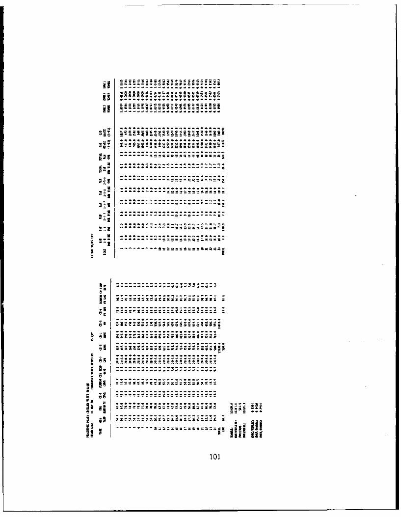
- -- -- 0 -P - . . -...

--------

...... .. . . .

------------ 5

~ --------------

-- - -- - -- - - ..... . ..

101

Li - -t~ a ;

a 71 -------

U. ----

.... .... .... ... ....

-------- -

----- ----- ----- -----

210

-! - -----

.- . .

........

-------------------

'! - !;

10

EIi -----------------

2.A

-- -- -- --

-- -- -- --.- - -

................

4 S--------------------------....

- g-a -

104

.. . . .. 4 4 4 . . .

~~~I~ aleooo -

4.4 44 .. . .

all

-- - - -- - - - -- - - -

~-------------

-- - - -- - - -

-- - - - -

-- -- -- -

-s -z- zssss

-- z

-- -- - - - - - - - -

I

105

ii 0

o~ o C- -. - - - -

----------------

- - -- - - - - - - - -

----------

Ikit

I106

-----------

--- -- --

271 -

- --------------- - --

-- -

it Zale------

- ---- -

107

~ - -----. . . . .

Ua --- ~ -----

-- - -- --

.A108

- ........... *

-----------------

--- -- --

-- - - - - -

----- ---- --- - - - -

------ ------

-7 --1 !--1!" !-

r" 0

;~ -p109

!5ii 2

- - -- --

-- - -- - -- - -

in------

-SE

110 z~~:

- - -- -- -- - .

- - ----

-- - -- - - -- - -- - -

......... ....----

-lls k-t

o! w 4.! -

-- -- -- -- -

11

APPENDIX B

SIMULATION RESULTS

113

TMIN COMPUTER MODEL RESULTS: SIMULATION I(BASED ON EXPERIMENTAL DATA)(3441 GPM, 1036960 CFM, 900 NON TONS, 2 PASS CONDENSER, 12" PIPE DIAMETER)

(DATA USED IN FIGURES 4.22 - 4.24)

PREDICTEDBIN HOURS TONS TONERS

72 1 703.30 703.3067 80 636.14 50891.2062 100 568.98 56898.0057 140 501.82 70254.8052 77 434.65 33468.0547 52 367.49 19109.4842 4 300.33 1201.32

TOTAL TONERS: 232526

SIMULATION RESULTS:

SET KWHC/ KWHFI KW,'T/POIN. KWC KWHY KBTA, TONI TON' TONER

---------------------------------------70 216432.3 13917.6 230349.9 0.9308 0.0599 0.990675 219136.9 9226.0 228362.9 0.9424 0.0397 0.982180 221349.0 6171.3 227520.3 0.9519 0.0265 0.978585 230351.1 4174.4 234525.5 0.9906 0.0180 1.00869( 238399.3 2710.5 241109.8 1.0253 0.0117 1.0369

114

TKIN COMPUTER MODEL RESULTS: SIMULATION 2(BASED ON STANDARD WEATHER DATA; MANUFACTURER'S CHILLER DATA;)(.65 KWITON; ACTUAL BUILDING LOAD PROFILE)(3093 GPM, 1036960 CFM, 1000 NON TONS, 2 PASS CONDENSER, 12" PIPE DIAMETER)


NUM COND WATER TEMP: 70CHILLER/

PUMP FAN CHILLER TOTAL FANMONTE ENERGY ENERGY ENERGY ENEG ENERGY

1 JAN 16138.41 7231.15 127441.90 150811.46 134673.052 FEB 17390.84 7967.60 140927.40 166285.84 148895.003 MAR 22686.81 13177.96 194040.20 229904.97 207218.164 APR 25263.23 29036.68 250631.20 304931.11 279667.885 KAY 26623.01 62944.45 307583.50 397150.96 370527.956 JUN 25764.20 102528.20 328855.70 457148.10 431383.907 JUL 26730.36 126483.80 350870.90 504085.06 477354.708 AUG 26587.22 120571.00 348967.00 496125.22 469538.009 SEP 25692.63 81922.63 307444.90 415060.16 389367.53

10 OCT 26229.39 35992.36 263858.50 326080.25 299850.8611 NOV 21935.36 13719.05 186866.70 222521.11 200585.7512 DEC 16675.16 6663.49 130005.70 153344.35 136669.19

TOTAL 277716.62 608238.38 2937493.60 3823449 3545732

115

TMIN COMPUTER MODEL RESULTS: SIMULATION 2(BASED ON STANDARD WEATHER DATA; MANUFACTURER'S CHILLER DATA;)(.65 KW/TON; ACTUAL BUILDING LOAD PROFILE)(3093 GPM, 1036960 CIM, 1000 NON TONS, 2 PASS CONDENSER, 12" PIPE DIAMETER)

(DATA USED I FIGURES 4.25 - 4.27)

MINIMUM COND WATER TEMP: 75CHILLER/

PUMP FAN CHILLER TOTAL FANMONTH ENERGY ENERGY ENERGY ENERGY ENERGY

I JAN 16138.41 4596.12 125247.40 145981.93 129843.522 FEB 17390.84 5151.60 138660.30 161202.74 143811.903 MAR 22686.81 8722.57 191369.60 222778.98 200092.174 APR 25263.23 19618.46 248713.70 293595.39 268332.165 MAY 26623.01 40321.51 307115.20 374059.72 347436.716 JUN 25764.20 66638.15 329239.50 421641.85 395877.657 JUL 26730.36 91452.79 351388.90 469572.05 442841.698 AUG 26587.22 82432.61 349636.30 458656.13 432068.919 SEP 25692.63 50801.53 307337.30 383831.46 358138.83

10 OCT 26229.39 23797.69 261962.00 311989.08 285759.6911 NOV 21935.36 9003.72 184256.10 215195.18 193259.8212 DEC 16675.16 4210.51 127697.40 148583.07 131907.91

TOTAL 277716.62 406747.27 2922623.70 3607088 3329371

116

ThIN COMPUTER MODEL RESULTS: SIMULATION 2(BASED ON STANDARD WEATHER DATA; KANUFACTURERIS CHILLER DATA;)(.65 KW/TON; ACTUAL BUILDING LOAD PROFILE)(3093 GPM, 1036960 CI'M, 1000 NOM TONS, 2 PASS CONDENSER, 12" PIPE DIAMETER)




1 JAN 16138.41 2893.37 125765.10 144796.88 128658.472 FEB 17390.84 3330.96 139342.80 160064.60 142673.763 MAR 22686.81 5826.03 192621.10 221133.94 198447.134 APR 25263.23 13755.92 251405.80 290424.95 265161.725 MAY 26623.01 28060.48 311798.30 366481.79 339858.786 JUN 2'n4.20 43717.54 335233.20 404714.94 378950.747 JUT 26730.36 56778.35 358056.90 441565.61 414835.258 1Ic 26587.22 52525.93 356286.00 435399.15 408811.939 F. 25692.63 34278.84 312316.00 372287.47 346594.84

10 OCT 26229.39 16502.93 264884.60 307616.92 281387.53Al NOV 21935.36 6001.36 185432.50 213369.22 191433.8612 DEC 16675.16 2662.61 128178.60 147516.37 130841.21

TOTAL 277716.62 266334.32 2961320.90 3505372 3227655

117

T IN COMPUTER MODEL RESULTS: SIMULATION 2(BASED ON STANDARD WEATHER DATA; MANUFACTURER'S CHILLER DATA;)(.65 KW/TON; ACTUAL BUILDING LOAD PROFILE)(3093 GPM, 1036960 CFM, 1000 NOM TONS, 2 PASS CONDENSER, 12" PIPE DIAETER)


MIIMUM COND WATER TEMP: 85CHILLER/


1 JAN 16138.41 1861.16 128190.30 146189.87 130051.462 FEB 17390.84 2158.51 142116.00 161665.35 144274.513 MAR 22686.81 3902.48 196699.10 223288.39 200601.584 APR 25263.23 9813.58 257578.70 292655.51 267392.285 MAY 26623.01 20398.31 320559.60 367580.92 340957.916 JUN 25764.20 31092.65 345460.00 402316.85 376552.657 JUL 26730.36 39348.87 369203.20 435282.43 408552.078 AUG 26587.22 36869.73 367391.10 430848.05 404260.839 SEP 25692.63 24597.47 321329.80 371619.90 345927.27

10 OCT 26229.39 11736.50 271456.80 309422.69 283193.3011 NOV 21935.36 4034.52 189334.80 215304.68 193369.3212 DEC 16675.16 1706.28 130615.00 148996.44 132321.28

TOTAL 277716.62 187520.06 3039934.40 3505171 3227454

118

THIN COMPUTER MODEL RESULTS: SIMULATION 2(BASED ON STANDARD WEATHER DATA; MANUFACTURER'S CHILLER DATA;)(.65 KWITON; ACTUAL BUILDING LOAD PROFILE)(3093 GPM, 1036960 CFM, 1000 NON TONS, 2 PASS CONDENSER, 12" PIPE DIAMETER)




1 JAN 16138.41 1153.75 132201.10 149493.26 133354.852 FEB 17390.84 1342.86 146635.50 165369.20 147978.363 MAR 22686.81 2544.76 203163.10 228394.67 205707.864 APR 25263.23 7037.00 266780.40 299080.63 273817.405 MAY 26623.01 15170.24 332995.40 374788.65 348165.646 JUN 25764.20 23111.73 359597.30 408473.23 382709.037 JUL 26730.36 28892.84 384514.60 440137.80 413407.448 AUG 26587.22 27266.38 382641.40 436495.00 409907.789 SEP 25692.63 18247.84 334008.20 377948.67 352256.04

10 OCT 26229.39 8377.66 281211.30 315318.85 289589.4611 NOV 21935.36 2653.82 195536.00 220125.18 198189.8212 DEC 16675.16 1050.83 134671.90 152397.89 135722.73

TOTAL 277716.62 136849.70 3153956.70 3568523 3290806

119

THIN COMPUTER MODEL RESULTS: SIMULATION 2(BASED ON STANDARD WEATHER DATA; MANUFACTURER'S CHILLER DATA;)(.65 KW/TON; ACTUAL BUILDING LOAD PROFILE)(3093 GPM, 1036960 CFM, 1000 NON TONS, 2 PASS CONDENSER, 12" PIPE DIAMETER)

(DATA USED IN FIGURE 4.28)

YEARLY YEARLY YEARLYSET CHILLER FAN TOTAL

POINT ENERGY ENERGY ENERGY

70 2937494 608238 354573275 2922624 406747 332937180 2961321 266334 322765585 3039934 187520 322745490 3153957 136850 3290806

120

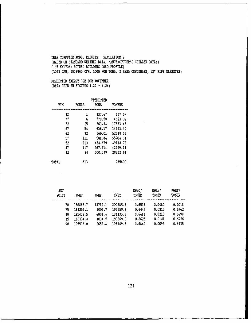
TMIN COMPUTER MODEL RESULTS: SIMULATION 2(BASED ON STANDARD WEATHER DATA; MANUFACTURER'S CHILLER DATA;)(.65 KWiTON; ACTUAL BUILDING LOAD PROFILE)(3093 GPM, 1036960 CFM, 1000 MOK TONS, 2 PASS CONDENSER, 12" PIPE DIEER)

PREDICTED ENERGY USE FOR NOVEMBER(DATA USED IN FIGURES 4.22 - 4.24)

PREDICTEDBIN HOURS TONS TONERS

82 1 837.67 837.6777 6 770.50 4623.0272 25 703.34 17583.4867 54 636.17 34353.4062 92 569.01 52348.3357 111 501.84 55704.6852 113 434.679 49118.7347 117 367.514 42999.1442 94 300.349 28232.81

TOTAL 613 285802

SET KWHC/ vu/ KWHT/?ODT KWHC KWHF KWHT TONER TONE TONMR

70 186866.7 13719.1 200585.8 0.6538 0.0480 0.701875 184256.1 9003.7 193259.8 0.6447 0.0315 0.676280 185432.5 6001.4 191433.9 0.6488 0.0210 0.669885 189334.8 4034.5 193369.3 0.6625 0.0141 0.676690 195536.0 2653.8 198189.8 0.6842 0.0093 0.6935

121

BIBLIOGRAPHY

American Society of Heating, Refrigerating, and Air-Conditioning Engineers(ASHRAE). 1989. ASHRAE Handbook of Fundamentals. Atlanta:ASHRAE.

American Society of Heating, Refrigerating, and Air-Conditioning Engineers. 1988.ASHRAE Equipment Handbook. Atlanta: ASHRAE.

Baumeister, Theodore, ed. 1978. Mark's Standard Handbook for MechanicalEngineers. New York: McGraw-Hill Book Company.

Braun, J.E. 1988. "Methodologies for the Design and Control of Central CoolingPlants." Ph.D. Thesis. University of Wisconsin-Madison.

Braun, J.E.,Klein, S.A.,Beckman, W.A.,and Mitchell, J.W. 1989a. "Methodologiesfor Optimal Control of Chilled Water Systems without Storage," ASHRAETransactions. Vol. 95, Part 1.

Braun, J.E., Klein, S.A.,Mitchell, J.W.,and Beckman, W.A. 1989b. "Applicationsof Optimal Control to Chilled Water Systems without Storage." ASHRAETransactions. Vol. 95, Part 1.

Braun, I.E., Mitchell, J.W., Klein, S.A., and Beckman, W.A. 1987. "Performanceand Control Characteristics of Large Central Cooling Systems." ASHRAETransactions. Vol. 93, Part 1.

Cascia, M.A. 1988. "Optimizing Chiller Plant Energy Savings Using Adaptive DDCAlgorithms." ASHRAE Transactions. Vol. 94, Part 2.

Clifford, G. 1990. Modem Heating. Ventilating, and Air-Conditioning. New Jersey:Prentice Hall.

Hackner, R.J.,Mitchell, J.W.,and Beckman, W.A. 1984. "HVAC System Dynamicsand Energy Use in Buildings- Part I." ASHRAE Transactions. Vol. 90,Part 2B.

122

1985a. "HVAC System Dynamics and Energy Use in Buildings- Part II."

ASHRAE Transactions. Vol. 91, Part lB.

1985b. "System Dynamics and Energy Use." ASHRAE Journal. June 1985.

Hines, W.W. and Montgomery, D.C. 1990. Probability and Statistics in Engineeringand Management Science. New York: John Wiley & Sons.

Johnson, G.A. 1985. "Optimization techniques for a Centrifugal Chiller Plant Usinga Programmable Controller." ASHRAE Transactions. Vol. 91, Part 2.

Joyce, C.T. 1990. "Optimized Design of a Commercial Building Chiller/CoolingTower System." Master's Thesis. Georgia Institute of Technology.

Lau, A.S.,Beckman, W.A.,and Mitchell, J.W. 1985. "Development of ComputerizedControl Strategies for a Large Chilled Water Plant." ASHRAE Transactions.Vol. 91, Part lB.

Lowe, H.J. and Christie, D.G. 1961. "Heat Transfer and Pressure Drop Data onCooling Tower Packings, and Mode Studies of the Resistance of Natural-Draught Towers to Airflow." ASME Heat Transfer Proceedings. Paper 113.

Press, W.H.,Brian, P.F.,Teukolsky, S.A.,and Vetterling, W.T. 1989. NumericalRecipeg: The Art of Scientific Computing. Cambridge: CambridgeUniversity Press.

Sud, I. 1984. "Control Strategies for Minimum Energy Usage." ASHRAETransactions. Vol. 90, Part 2.

Trane Co., Inc. 1987. "Tracer 100 Building Management System ProgrammingGuide." Pamphlet EMTB-PG-1A.

Trane Co., Inc. 1989. "Chiller Plant System Performance." Engineering Newsletter.Vol. 18, No. 2. Trane Co., Inc. Lacrosse, Wisconsin.

Tuve, G.L. and Domholdt, J.C. 1966. Engineering Experimentation. New York:McGraw-Hill Book Company.

United States. Department of the Air Force. 1978. AFM 88-29: EngineeringWeather Data. Washington: GPO.

123

Weber, E.D. 1988. "Modelling and Generalized Optimization of CommercialBuilding Chiller/Cooling Tower Systems." Master's Thesis. Georgia Instituteof Technology.

124

experimental optimization of cooling tower fan control ... · pdf fileexperimental...

Documents