Experimental Phonetics

2

LONGMAN LINGUISTICS LIBRARY

3

LONGMAN LINGUISTICS LIBRARY

General editorsR. H. ROBINS, University of London

GEOFFREY HORROCKS, University of Cambridge

DAVID DENISON, University of Manchester

For a complete list of books in the series, see pages vii & viii

4

5

Experimental PhoneticsKatrina Hayward

6

7

First published 2000 by Pearson Education Limited

Published 2013 by Routledge2 Park Square, Milton Park, Abingdon, Oxon OX14 4RN711 Third Avenue, New York, NY 10017, USA

Routledge is an imprint of the Taylor & Francis Group, aninforma business

Copyright © 2000, Taylor & Francis.

The right of Katrina Hayward to be identified as author of thiswork has been asserted by her in accordance with theCopyright, Designs and Patents Act 1988.

All rights reserved. No part of this book may be reprinted orreproduced or utilised in any form or by any electronic,mechanical, or other means, now known or hereafterinvented, including photocopying and recording, or in anyinformation storage or retrieval system, without permission inwriting from the publishers.

NoticesKnowledge and best practice in this field are constantlychanging. As new research and experience broaden ourunderstanding, changes in research methods, professionalpractices, or medical treatment may become necessary.

Practitioners and researchers must always rely on their ownexperience and knowledge in evaluating and using anyinformation, methods, compounds, or experiments describedherein. In using such information or methods they should be

8

mindful of their own safety and the safety of others, includingparties for whom they have a professional responsibility.

To the fullest extent of the law, neither the Publisher nor theauthors, contributors, or editors, assume any liability for anyinjury and/or damage to persons or property as a matter ofproducts liability, negligence or otherwise, or from any use oroperation of any methods, products, instructions, or ideascontained in the material herein.

ISBN 13: 978-0-582-29137-9 (pbk)

British Library Cataloguing-in-Publication Data

A catalogue record for this book is available from the BritishLibrary

Library of Congress Cataloging-in-Publication Data

A catalog record for this book is available from the Library ofCongress

Set by 35 in 10/12pt Times

9

10

to the memory of Eugénie Henderson

11

Longman LinguisticsLibraryGeneral Editors:

R. H. ROBINSUniversity of London

GEOFFREY HORROCKSUniversity of Cambridge

DAVID DENISONUniversity of Manchester

Introduction to Text LinguisticsROBERT DE BEAUGRANDE and WOLFGANGDRESSLER

Psycholinguistics Language, Mind and WorldDANNY D. STEINBERG

Principles of PragmaticsGEOFFREY N. LEECH

The English VerbSecond editionF. R. PALMER

Pidgin and Creole LanguagesSUZANNE ROMAINE

12

General LinguisticsAn Introductory SurveyFourth editionR. H. ROBINS

Generative and Non-linear PhonologyJACQUES DURAND

Modality and the English ModalsSecond editionF. R. PALMER

Dialects of EnglishStudies in Grammatical VariationPETER TRUDGILL and J. K. CHAMBERS (eds)

An Introduction to BilingualismCHARLOTTE HOFFMANN

Linguistic TheoryThe Discourse of Fundamental WorksROBERT DE BEAUGRANDE

A History of American EnglishJ. L. DILLARD

Aspect in the English VerbProcess and Result in LanguageYISHAI TOBIN

The Meaning of SyntaxA Study in the Adjectives of EnglishCONNOR FERRIS

13

Latin American SpanishJOHN LIPSKI

A Linguistic History of ItalianMARTIN MAIDEN

The History of LinguisticsAll edited by GIULIO LEPSCHY

Volume I:The Eastern Traditions of Linguistics

Volume II:Classical and Medieval Linguistics

Volume III:Renaissance and Early Modern Linguistics

Volume IV:Nineteenth Century LinguisticsANNA MORPURGO DAVIES

To come:Volume V:The Twentieth Century

Modern ArabicStructures, Functions and VarietiesCLIVE HOLES

Frontiers of PhonologyAtoms, Structures and DerivationsJACQUES DURAND and FRANCIS KATAMBA (eds)

14

An Introduction to the Celtic LanguagesPAUL RUSSELL

Causatives and CausationA Universal-typological perspectiveJAE JUNG SONG

A Short History of LinguisticsFourth editionR. H. ROBINS

Grammar and Grammarians in the Early Middle AgesVIVIEN LAW

GreekA History of the Language and its SpeakersGEOFFREY HORROCKS

The New Comparative SyntaxLILIANE HAEGEMAN (ed.)

The Structure and History of JapaneseLONE TAKEUCHI

The Acquisition of SyntaxStudies in Comparative Developmental LinguisticsMARC-ARIEL FRIEDEMANN and LUIGI RIZZI (eds)

Explaining Language Change:An Evolutionary ApproachWILLIAM CROFT

15

Experimental PhoneticsKATRINA HAYWARD

16

Author's acknowledgementsPublisher's acknowledgements

1 Introduction: impressionistic phonetics and experimentalphonetics1.1 What is experimental phonetics?1.2 Impressionistic phonetics

1.2.1 Assumptions1.2.2 Methodology

1.3 The scope of experimental phonetics1.4 The representation of speech sounds

1.4.1 Segments and phonemes1.4.2 Mental representations

1.5 Experimental phonetics and the structure of soundsystems1.6 The structure and scope of this book1.7 Further reading

Notes2 The nature of sound

2.1 Introduction2.2 Sound waves

2.2.1 Describing a simple sound wave2.2.2 From movements to pressures2.2.3 Sound waves in space2.2.4 Some definitions

2.3 Types of sound waves2.4 The structure of sound waves

2.4.1 Specifying sound waves2.4.2 The spectrum

17

2.4.3 Generating some vowel-like waveforms2.4.4 Spectra of aperiodic sounds

2.5 Scaling and the spectrum2.5.1 Amplitude, power and intensity2.5.2 The decibel scale2.5.3 The octave scale

2.6 Summary2.7 Further reading

Notes3 Analysing sound: the spectrograph

3.1 Introduction3.2 Spectrography

3.2.1 Basic principles3.2.2 An example spectrogram3.2.3 Narrow band spectrograms3.2.4 Pre-emphasis3.2.5 Two-dimensional spectra3.2.6 Supplementary displays: waveform, intensity and

fundamental frequency3.3 Recording

3.3.1 Recording as translation3.3.2 Fidelity3.3.3 Digital recording

3.3.3.1 Sampling rate3.3.3.2 Quantisation

3.4 Digital spectrography3.4.1 Recording for analysis3.4.2 Calculating the power spectrum3.4.3 Determining fundamental frequency (F0)

18

3.5 Summary3.6 Further reading

4 The acoustics of speech production4.1 Introduction4.2 Modelling a simple vowel

4.2.1 The voice source4.2.2 The vocal tract filter

4.2.2.1 The concept of filter4.2.2.2 Formant frequencies

4.2.3 Combining source and filter4.2.4 The radiation function4.2.5 Comparison with a spoken vowel

4.3 Varying the voice source4.4 Varying the vocal tract filter

4.4.1 Simple models for three vowels4.4.2 More realistic models of vowel articulation4.4.3 A general model of vowel production4.4.4 Phonological implications of modelling

4.5 Estimating filter characteristics: linear predictivecoding4.6 Extending the source-filter approach to other classes ofspeech sounds

4.6.1 Nasals, laterals and nasalised vowels4.6.2 Obstruent consonants

4.7 Summary4.8 Further reading

Notes5.Perception and hearing

5.1 Introduction

19

5.2 From acoustic signals to perceptual objects: the searchfor acoustic cues

5.2.1 An example: Voice Onset Time5.2.2 The problem of lack of invariance

5.2.3 Is speech special?5.2.3.1 Categorical perception5.2.3.2 Multiple cues and trading relations5.2.3.3 Duplex perception5.2.3.4 Bimodal perception5.2.3.5 Arguments against the specialness of speech

5.2.4 Theories of speech perception5.2.4.1 The Motor Theory5.2.4.2 Direct Realism5.2.4.3 The Fuzzy Logical Model5.2.4.4 Strong theories relating the acoustic signal to

phonological features5.2.4.5 Non-analytic approaches

5.3 Hearing5.3.1 Structure of the auditory system5.3.2 Spectra in the auditory nerve

5.3.2.1 Voiceless fricatives5.3.2.2 Vowels

5.3.3 The VOT boundary5.3.4 Adaptation

5.4 Psychophysics and the auditory spectrograph5.4.1 Scales of frequency based on auditory filters5.4.2 Auditory spectra

5.5 Conclusion5.6 Further reading

20

Note6.The acoustic description of vowels

6.1 Introduction6.2 Formant frequencies and the vowel quadrilateral

6.2.1 The rounding dimension6.2.2 Central vowels

6.3 Formant frequencies and vowel charts: the problem ofpsychological reality6.4 The spectral integration hypothesis

6.4.1 Integration of F2 with other formants6.4.2 A role for F0?

6.5 A system of binary features for vowels?6.6 The traditional vowel quadrilateral revisited6.7 Other dimensions of vowel classification

6.7.1 Nasalised vowels6.7.2 Advanced Tongue Root (ATR) vowels6.7.3 Rhoticity and pharyngealisation

6.8 Diphthongs6.9 Alternative approaches to vowel quality6.10 The problem of normalisation6.11 Predicting the structure of vowel systems6.12 Summary6.13 Further reading

7 The acoustic description of consonants7.1 Introduction7.2 General concepts

7.2.1 Intervals and transitions7.2.2 Acoustic dimensions in the description and

classification of consonants

21

7.2.3 Acoustic boundaries and consonants7.3 Stop consonants

7.3.1 General characteristics of stop consonants7.3.2 Voicing and aspiration7.3.3 Place of articulation

7.3.3.1 Stop bursts7.3.3.2 Formant transitions7.3.3.3 Spectral templates as invariant cues

7.4 Fricatives7.5 Affricates7.6 The fricative-affricate contrast7.7 Phonological contrasts involving voicing in obstruents7.8 Sonorant consonants

7.8.1 Nasals7.8.2 Semivowels7.8.3 Lateral approximants (L-sounds)7.8.4 Rhodes (R-sounds)7.8.5 An overview of manner contrasts involving

sonorants7.9 Acoustic phonetics and the structure of consonantsystems7.10 Further reading

Notes8 Speech production

8.1 Introduction8.2 The airstream

8.2.1 Principles of air flow8.2.2 Respiratory function in speech8.2.3 Measuring and quantifying pressure and flow

22

8.2.3.1 Pressure8.2.3.2 Flow

8.3 The larynx and the vocal folds8.3.1 A simple description of the larynx8.3.2 Vocal fold vibration8.3.3 Aerodynamics of vocal fold vibration8.3.4 Experimental investigation of the larynx8.3.5 The laryngeal setting

8.3.5.1 Direct observation8.3.5.2 Imaging8.3.5.3 Electromyography

8.3.6 More indirect methods for monitoring vocal foldactivity

8.3.6.1 Inverse filtering8.3.6.2 Photoelectric glottography8.3.6.3 Electroglottography (electrolaryngography)8.3.6.4 Acoustic measures of phonation types

8.3.7 Models of vocal fold vibration and features of thelarynx

8.3.8 Control of fundamental frequency8.3.9 Control of voicing in obstruents

8.3.9.1 Problems of maintaining voicing: aerodynamicaspects

8.3.9.2 Strategies for maintaining and inhibitingvoicing8.4 Articulation

8.4.1 Imaging techniques8.4.2 Point-tracking techniques8.4.3 Palatography

23

8.4.4 Identifying articulatory dimensions: the case ofvowels8.5 Wider issues: relating phonological representations tospeech production8.6 Further reading

Appendix: An overview of impressionistic-phoneticclassification

A.l Preliminaries: air flow in the vocal tractA.2 Consonants

A.2.1 Sonorants and obstruentsA.2.2 The place dimensionA.2.3 The manner dimensionA.2.4 Simultaneous and sequential articulationsA.2.5 Non-pulmonic consonantsA.2.6 RefinementsA.2.7 Impossible and unattested sound types

A.3 VowelsA.3.1 Dimensions of vowel classificationA.3.2 RefinementsA.3.3 Diphthongs

A.4 Suprasegmentals (prosodic features)A.5 Using the IPAA.6 Further reading

BibliographyIndex

24

Contents

25

26

Author's acknowledgementsA number of people have made contributions, directly orindirectly, to this work. I should particularly like to thankSarah Hawkins, Mark Huckvale, Peter Roach, Iggy Roca,Burton Rosner and Justin Watkins for reading and providingsuggestions on various chapters. Any mistakes or infelicitieswhich remain are my own responsibility.

I am greatly indebted to Bernard Howard for technicalsupport with regard to recording and production ofspectrograms. Geoff Williams and Alan Hirson kindlyprovided assistance with LPC analysis. I should also like tothank the School of Oriental and African Studies forpurchasing the Mathematica software for me, without whichmany of the illustrations could not have been prepared.

Bruce Ingham deserves particular thanks for generouslylending his good spectrographic voice to the project. MartinBarry kindly recorded the EPG examples for Figure 8.15. Iam also indebted to Muhammed El-Ashiry for allowing me touse to his recordings of Qur'anic recitation and to KeithHoward for advice on Korean musical terms in connectionwith Figure 8.9.

Special thanks are due to Nigel Phillips for unselfishly doingmore than his share of our joint teaching and administrativeduties, thus helping to bring the work to completion. It isimpossible to mention everyone who has providedencouragement and moral support, but I should particularly

27

like to thank Diana Flint, Jiyoung Shin and Lone Takeuchi fortheir understanding friendship and encouragement. Thanksare also due to my parents and friends outside the academicworld, who uncomplainingly put up with less contact thanthey might reasonably have expected while the work was inprogress.

To conclude, I should particularly like to thank ProfessorBobby Robins, who persuaded me to undertake the work inthe first place and whose confidence in me has been a sourceof strength in troubled times. The final thanks are for myhusband, Dick, who remained encouraging while having tolive with the work on a day-to-day basis, and who told mehonestly how boring the first version was.

28

29

Publisher'sacknowledgementsWe are grateful to the following to reproduce copyrightmaterial:

Blackwell Publishers for our Figure 5.10 which appeared inB. Delgutte's chapter in The Handbook of Phonetic Sciencesedited by W. J. Hardcastle and J. Laver (1997); OxfordUniversity Press for our Figure 8.2 from Peter Ladefoged'sThree Areas of Experimental Phonetics (1987); TheUniversity of Chicago Press for our Figure 5.7 from PeterLadefoged's Elements of Acoustic Phonetics, second edition(1996); Lawrence Erlbaum Associates Inc. for our Figure 7.8from K. N. Stevens and S. E. Blumstein's contribution inPerspectives on the Study of Speech (1981) edited by P.Eimas and J. Miller.

Whilst every effort has been made to trace the owners ofcopyright material, in a few cases this has proved impossibleand we take this opportunity to offer our apologies to anycopyright holders whose rights we may have unwittinglyinfringed.

30

31

Chapter 1Introduction: impressionisticphonetics and experimentalphonetics1.1 What is experimental phonetics?

Phonetics is the study of speech. Traditionally, phoneticianshave relied on their ears and eyes, and their awareness of theirown vocal organs, to study pronunciation. Increasingly,however, they have been using instruments of various types tosupplement the information they derive from their ownsensations. Experimental phonetics, as the term is commonlyused, includes any investigation of speech by means ofinstruments. It is understood here that the instruments areused to visualise some aspect of the speech event, andpossibly also to provide a basis for measurements. Forexample, making a tape recording for the purpose of repeatedlistening does not fall within the scope of experimentalphonetics, but if the tape recording is fed into a computer andused to produce an acoustic analysis, the activity would bedescribed as an experimental investigation.

There are four main reasons for studying experimentalphonetics. The first of these is that speech is interesting initself. The ability to produce and understand speech is afundamental part of our identity, as individuals, as members

32

of larger communities, and as human beings. However, manyaspects of speaking and hearing are inaccessible without theaid of instruments.

The second reason for studying experimental phonetics is thatit expands the range of contexts in which we can studyspeech. To give but two examples, speech is a highly skilledmotor activity, which can be studied as part of the generalstudy of movement. Speech is also a type of sound which canbe compared with other types of sound from the perspectiveof general acoustics. Each of these contexts has its owntheoretical perspective, to which the study of speech cancontribute.

A third reason is provided by the numerous practicalapplications of experimental phonetics. Obvious examples aremedical applications such as helping patients with disorderedspeech, applications in the fields of telecommunications andman-machine communication, and the development ofaudio-visual aids for improving pronunciation in languageteaching.

The fourth reason, and the one which underlies this book, isthe relevance of speech for the study of language in general.Theoretical linguistics operates with an inner world oflanguage, in which discrete, inherently timeless elements suchas words, sounds and even individual components of soundsare arranged in meaningful patterns in accordance withlogical principles. This contrastsmarkedly with the outer world of speech, where individualsounds are anchored in space and time and merge into oneanother, where boundaries become obscured, and whereanswers to questions tend to come from statistical, rather than

33

logical, inference. As speakers and hearers, we constantlymove between these two worlds, and the processes by whichwe do so are still not well-understood. However, the twoworlds must necessarily influence each other, and it isdoubtful that a full explanation of the abstract properties oflanguage will ever be possible without an understanding ofthe more concrete properties of speech.

This book aims to provide an introduction to the methods ofexperimental phonetics, the nature of the data whichexperimental phoneticians must deal with, and the nature ofthe questions to which the data may provide answers. At thesame time, it aims to avoid too many technical details, whichmay obscure the main points for readers new to the subject.Its orientation is primarily linguistic, but, because oflimitations of space and time, it cannot cover all aspects ofexperimental phonetics which are relevant to linguists.

Since experimental phonetics is defined primarily by itsmethodology rather than by its subject matter, it is somewhatmisleading to suggest that a clear-cut distinction can be drawnbetween experimental phonetics with non-experimentalphonetics. Nevertheless, we shall assume such a divisionhere. We shall use the term impressionistic phonetics to referto the more traditional type of phonetic investigation whichrelies on the unaided skill of the phonetician in recognisingand reproducing speech sounds. The purpose of the presentchapter is twofold. Firstly, it aims to point out ways in whichthe availability of instruments has influenced the nature ofresearch into speech. Secondly, it aims to provide anoverview of the basic methodology and assumptions ofimpressionistic phonetics, since it will be necessary to buildon these in the chapters which follow.

34

1.2 Impressionistic phonetics

The term impressionistic is taken from Abercrombie (1954,1967), where it is applied to a style of phonetic transcription.In Abercrombie's usage, it is not meant to suggest any neglectof detail, but, rather, the absence of preconceived notionsabout the structure of the language being transcribed. Forexample, a linguistic field worker beginning work on apreviously unstudied language would make a very detailedimpressionistic transcription. In the present context,impressionistic is opposed to instrumental, and is meant toconvey the idea of the phonetician relying entirely on his ownimpressions of sound, unaided by technology.

Impressionistic phonetics involves, first and foremost,acquiring and cultivating a skill in recognising, discriminatingbetween, and performing, a wide range of speech sounds. Forsome practitioners, this skill is an end in itself. For others, it isan essential part of a larger, more theoretical enterprise ofdelimiting and classifying the set of possible speech soundswhich may occur in humanlanguage. To quote Catford (1988: 2), 'What the competentphonetician must acquire is a deep, internally experienced,awareness of what is going on within the vocal tract - anability to analyse, and hence describe and ultimately control,the postures and movements of organs that produce thesounds of speech ... the acquisition of these practical skills isby far the best way of acquiring a deep understanding ofphonetic theory.'

Impressionistic phonetics has a long history, extending backto before the fifth century BC, at least in Ancient India (Allen

35

1953: 5). At the risk of being overly simplistic, we might saythat the basic framework and methodology of the subject as itis taught and practised today were already in place by theearly years of this century. In contrast, experimental phoneticsis a young field. Convenient benchmark dates are thepublication of Principes de phonétique expérimentale byRousselot (often considered to be the father of the subject) in1897-98 and, most importantly for the character of the subjecttoday, the invention of the sound spectrograph in the 1940s.Experimental phonetics has built on the foundations ofimpressionistic phonetics, and has taken over much as regardsorientation and basic assumptions. At the same time, the basicclassificatory framework of impressionistic phonetics hasitself been an object of study for experimental phoneticians.Some knowledge of impressionistic phonetics is thereforeessential for the study of experimental phonetics, whereas theopposite is not true. It is possible to become a highly skilledimpressionistic phonetician without ever setting foot in aphonetics laboratory.

In this section, I shall give a brief account of some of thebasic assumptions which provide the foundation forimpressionistic phonetics, and also of its methodology. Anoverview of the classificatory framework is given in theAppendix.

1.2.1 Assumptions

Impressionistic phonetics focusses on the positions andmovements of the speech organs involved in the productionof individual speech sounds. It is based on a number of

36

assumptions about the nature of speech. Important amongthese are:

1. Speech can be represented as a series of segments.2. Each segment has a target, and can be specified

uniquely with reference to its target. Each targetcorresponds to a unique auditory percept in the mindof a trained observer.

3. Any segmental target can be specified using a limitednumber of dimensions. These dimensions do not needto be defined for each language individually. Instead,there is a universal set of dimensions which arerelevant to all human languages.

For example, the English word fan might be represented as[fæn].1 This implies that it is made up of a sequence of threesegments, as, indeed, is suggested by the spelling. Let us nowfocus our attention on the first segment, represented by theletter f. It is produced by forcing air through a narrow openingbetween the lower lip and the upper teeth. The target may bedescribedas: 'loose contact between lower lip and upper teeth, vocalfolds open and not vibrating', and is conventionally specifiedas a voiceless labiodental fricative. Each term of thisthree-term label refers to one articulatory dimension.Voiceless refers to the fact that the vocal folds are notvibrating (the voicing dimension), labiodental to contactbetween the upper teeth and the lower lip (the place ofarticulation dimension), and fricative to the fact that theconstriction between the lips and the teeth is sufficientlynarrow for the rasping sound to be produced when air flowsbetween them, but does not cut off the airstream entirely (themanner of articulation dimension). These three dimensions

37

are crucial for the description of consonants in all knownlanguages.

1.2.2 Methodology

Acquiring skill in impressionistic phonetics is, in many ways,like studying the pronunciation of a new language. Forexample, a native speaker of English who sets out to learnFrench must master the vowel sound which occurs in wordssuch as lune 'moon' or tu 'you (familiar)', and which ispronounced rather like the vowel of English see but withclosely rounded lips. There are three aspects to this mastery:(1) learning to pronounce the vowel oneself (2) learning torecognise the vowel when it is pronounced by native speakersof French and to distinguish it from the other French vowelsand (3) learning to associate this particulararticulatory-auditory package with the letter u, which is neverpronounced in this way in English.

In more abstract terms, learning a new speech sound involveslearning to get the speech organs to adopt a new position or tomove in a new way, and to associate this new activity with anew and distinct auditory percept. In the process, studentsmay be led to a new awareness of their own vocal organs,especially if they have not studied a foreign language before.(How many monolingual English speakers stop to think aboutthe position of their tongue and lips when pronouncing thevowel of see?) The association with the letter u is alsoimportant because it helps to give students access to therepresentation of French words in writing.

Training in impressionistic phonetics aims to increasestudents' repertoire of speech sounds beyond what might be

38

found in any particular language. In the ideal case, it wouldresult in mastery of all possible speech sounds of all possiblehuman languages. Students must concentrate on theproprioceptive (tactile and kinaesthetic) sensations associatedwith producing speech, in order to achieve an increasedawareness of, and control over, the movements of their ownvocal organs. Training should also result in an increasedability to distinguish between similar sounds and an increasedawareness of the relationship between what the speech organsare doing and the auditory percept which results. Thus, thetrained impressionistic phonetician, hearing an unfamiliarlanguage for the first time, should be able to make aneducated guess as regards what the speaker is doing with hisor her vocal organs. This task is made easier if it is possible tolook at the speaker. The guess can be refined byrepeated listening and by trying to imitate the pronunciationto the satisfaction of a native-speaker informant.

The final elements in impressionistic phonetic training arelearning to specify speech sounds in terms of universalarticulatory dimensions and to use phonetic notation, mostcommonly the International Phonetic Alphabet (IPA). Onceour trained impressionistic phonetician has worked out whatthe informant is doing with his or her vocal organs, he or shewill want to communicate his or her observations to others.Most commonly, this will involve producing a transcriptionof the speech, that is, writing the speech down as a string ofindividual speech sounds (segments), each represented by itsown alphabetic letter, as in the example of [fæn] above.

Both proprioceptive percepts of position and movement andauditory percepts of sound are entirely personal matters, andit is necessary to have a simple and convenient means of

39

talking about them. In the example of the sound [f], discussedabove, the relevant universal dimensions were voicing, placeof articulation and manner of articulation, and thespecification was voiceless labiodental fricative. Ifunderstood literally, the specification refers to the articulatorytarget for [f], that is, the position of the speech organs whichresults from the movement of the lower lip upwards to touchthe upper teeth and the opening of the vocal folds (though theterm fricative also refers to the rasping sound or audiblefriction which characterises this sound). However, in practice,the specification is also identified with the sound of [f].

It is obviously desireable that phonetic notation should not betied to any particular language and should not vary betweenor within languages. For example, in writing Englishphonetically, the letter f would have to be used rather than phfor the initial sound of phonetics. Learning to write in IPAnotation is, in some respects, easier than learning to write aforeign language. The relation between sounds and symbols isone-to-one; there are no inconsistencies such as the Englishuse of both f and ph to spell the single sound [f], (Whenletters are used with their universal values, it is customary toenclose them in square brackets, as will be explained below.)However, IPA notation is also more difficult because thereare so many more symbols to remember and because it isnecessary to concentrate on the individual sounds one by onerather than going for whole words.

The characteristic of impressionistic phonetics which we wishto call attention to here, and which distinguishes it fromexperimental phonetics, is the direct association betweenarticulations and auditory percepts. In reality, of course, thereis no direct contact between the speaker's vocal organs and

40

the hearer's ears (except in the case of a speaker listening tohim- or herself). The two are linked by a sound wave, whichtravels from the one to the other. However, without the aid ofinstruments, we have no access to the sound wave itself. Nordo we have a ready-made vocabulary for describing speechsounds in a precise way. If we want to refer to a particularsound there are three options. The first is to produce animitation of the sound (which is not possible in writing). Thesecond is to describe how the sound is produced: 'In Englishspelling, the letter combination ph is used to represent avoiceless labiodental fricative in words of Greek origin.' Thethird is to refer to the alphabetic or phonetic symbol which wewould use to represent it: 'Young children acquiring Englishoften substitute w for r.'

1.3 The scope of experimentalphonetics

From what has been said already, it should be clear that thescope of impressionistic phonetics is limited by thecapabilities of the human senses. Another potentialshortcoming is the impossibility of verifyingimpressionistic-phonetic descriptions without access to thespeakers whose pronunciation is being described. Forexample, if we read that the t-sound of language X, spoken bya small number of speakers in the depths of the Amazonjungle, is slightly retroflexed, we can only take thephonetician's word for it. Thus, one function of instrumentalmethods in phonetics has been to extend, back up, andprovide a check on impressionistic methods. Ladefoged andMaddieson's monumental Sounds of the World's Languages

41

(1996) is an outstanding example of this kind of use ofexperimental data.

FIGURE 1.1 The 'speech chain': stages in the transmission ofa spoken message from the brain of the speaker to the brain ofthe listener. After Denes and Pinson (1993: 5).

In other ways, experimental methods have widened the scopeof phonetic studies and have led to a change in perception ofwhat phonetics is about. Here, it is useful to start from theidea of the speech chain, as formulated by Denes and Pinson(1993). Their diagram is reproduced in Figure 1.1. Thespeaker first conceives what he or she wants to say, and putsthe message into linguistic form. The linguistic form is thentranslated into a set of motor commands, which ensure thatthe requisite muscles are activated at the necessary time. Theresult of all this motor activity is a sound wave, which travelsto the ear of the listener. The sound wave, in its turn, bringsabout activity inside the ear. This results in nerve impulses

42

which travel, via a complicated set of neural pathways, to thebrain of the listener. Finally, the brain is able to interpret thenerve impulses as a message in linguistic form. Thus, speechcommunication is conceived of as a series of levels, with theoutput of one level serving as input to the next level. Denesand Pinson's diagram also takes into account the ability ofspeakers to monitor their own performance by including afeedback link which takes the sound from the speaker's mouthback to his or her own ears.

The sound wave - or, as it is often referred to, the acousticsignal - is at the very centre of the speech chain. Only at thisstage does speech exist outside of the human body. Whenspeech is in this form, we can achieve our mostcomprehensive knowledge of it. Furthermore, the acousticsignal defines the common ground between the study ofspeech production and the study of speech perception. Forresearchers into speech production, the acoustic signal is theendpoint, the output which they must try to explain withreference to the speech organs. For researchers into speechperception, the acoustic signal is the beginning, the inputfrom which they must derive auditory percepts.

The acoustic signal is thus pivotal within experimentalphonetics. For this reason, introductory university courses inexperimental phonetics always include some study ofacoustics, though they may differ greatly with regard to whatelse is covered and with what emphasis. As we move alongthe speech chain, away from the acoustic signal and in thedirection of either the speaker's or the hearer's brain, itbecomes increasingly difficult to say what falls within thescope of experimental phonetics and what belongs properly tosome other field. For example, in the study of speech

43

perception, it is difficult to draw a sharp line betweenphonetics and psychology (Chapter 5). It is only at theendpoints of the speech chain that we arrive within thedomain of language proper and theoretical linguistics. Thelinks between linguistic sound as it exists in the mind and thereality of sound as it exists outside the body, must thereforeoperate across the diverse layers of the speech chain. Thenature of these links is not yet fully understood, and comingto such an understanding is an important research goal in bothfields.

In any case, experimental phonetics includes at least someaspects of both the study of speech production and the studyof speech perception, and I shall close this section by pointingout important differences between the two. Diagrams of thespeech chain, such as Figure 1.1, might suggest that the twoactivities are the mirror image of each other and involveessentially the same stages in reverse order. This ismisleading.

The problem of speech production is essentially one ofcoordination. It has often been pointed out that the organs ofspeech are quite diverse and that none of them has speakingas its primary biological function. For example, theprimary function of the lungs is breathing and the structuresof the mouth are primarily for eating. Furthermore, they varygreatly with regard to the nature of the tasks required of them,the speed at which they can move, and the time needed formessages to reach them from the brain via the appropriatenerves. Even pronouncing a simple monosyllabic word suchas fan on its own requires a good deal of planning: amongother things, the lungs must produce a sustained airstream ofsuitable strength; the lower lip must be brought into contact

44

with the upper teeth for the [f ], and this movement must becoordinated with the opening of the vocal folds; the tongue tipmust move up to touch the ridge behind the teeth for the [n]just as the soft palate is lowering to open up the nasal cavity.Estimates of the number of muscles involved in speechproduction vary. Lenneberg (1967) puts the figure at over100, and estimates that speaking may involve as many as10-15 thousand neuromuscular events per minute.

Although the complexity of speech production poses achallenge for research, there is a compensating advantage inthat the organs involved are relatively accessible. Indeed, it ispossible to monitor the activity of just about any part of thespeech-producing apparatus. Such monitoring might causeextreme discomfort to, or pose a health risk for, the subject,but it is not directly life-threatening. Phoneticians have oftenacted as their own subjects in production studies and haveendured a variety of tortures such as tubes down the nose,wires stuck into the muscles of the tongue or larynx, needlesthrough the rings of the trachea (windpipe), and even in oneinstance having dentalimpression material inserted into thelower pharynx for the purpose of making a cast (Ladefoged etal. 1971)! While it is still not possible to make a trulycomprehensive study of any particular speech act because itwould not be practical to monitor all aspects of all the organsinvolved in speech production simultaneously, repeatedexperimentation is possible, and has provided a good idea ofthe complexities involved.

The case of speech perception is quite different. In this caseeverything depends on a single organ, the ear. No muscularactivity is involved, and nerves take over from structureswhich respond to sound mechanically at an early stage of the

45

process. Furthermore, the hearing mechanism is highlyinaccessible, so that it is not possible to monitor what goes onas a living human being perceives speech. The great bulk ofour knowledge of the processes of speech perception musttherefore come from the more indirect methods ofexperimental psychology and from studies of experimentalanimals. For this reason, the perception of speech posesdifferent kinds of difficulties than the production of speech.

At the linguistic level, there would appear to be no differencebetween the sounds we produce and the sounds we hear, andthe two are also the same at the acoustic level. In between,however, the paths along the speech chain which mediatebetween them are very different.

The questions we have just raised are complicated, and muchmore research will be necessary before definitive answers canemerge. The point to be madehere is that the questions could not even be asked if we hadonly the techniques of impressionistic phonetics at ourdisposal.

1.4 The representation of speechsounds

Sound of any kind is invisible and intangible and exists onlyas a pattern of changes through time. To study the sound ofspeech systematically, we must represent it in some moreconcrete and more permanent way which is accessible to theeye. Similarly, we can only study the movements of thespeech organs, which give rise to the sound, by means of amore concrete visual representation of changing position

46

through time (for example, a graph showing up-and-downmovements of the jaw or the tip of the tongue). The visualrepresentation of sound is the main topic of Chapters 2 and 3,and the representation of movement will be taken up inChapter 8.

At the other end of the speech chain, it is clear that we mustcarry around some sort of representations of the sound ofspeech in our minds. Were this not the case, we should not beable to recognise points of similarity between new utterancesand utterances which we have heard before. As will becomeclear in Chapter 5, the nature of these representations is aproblem which occupies psychologists as well as linguists,and is highly controversial.

Theoretical linguists working within the general approachknown as Generative Grammar hold that the grammar ofevery language, which the native speaker carries around in hisor her head, includes a lexicon. Among other things, thelexicon relates abstract and invariant representations ofpronunciation to meanings (whatever those are). The questionof what such abstract representations might be like is of someimportance for experimental phoneticians with a linguisticorientation, though it is usually considered to be outside thescope of phonetics proper. Within linguistics, teasing out thenature of mental representations falls within the province ofphonology, which deals with the role of sound in language.Phonology has its home base, as it were, at the brain end ofthe speech chain, while phonetics is based at the acoustic end.The two must meet up somewhere in both production andperception pathways, and understanding the nature of thatmeeting is a research goal for practitioners in both fields.Such questions will occupy us particularly in Chapters 5 and

47

8 below. Later in this chapter (Section 1.4.2), I shall attemptto give a very brief and general summary of current viewsheld by phonologists on the nature of mental representations.

In any case, it should be clear that the problem ofrepresentation is to be found at all levels of the study ofspeech. Indeed, many researchers would conceive of thespeech chain as a series of translations from one type ofrepresentation into another. However, all areas of researchinto speech find a common point of reference in therepresentation of speech as a string of segments, representedby alphabetic letters, following the conventions ofimpressionistic phonetics. In fact, impressionistic phoneticsrecognises two major types ofalphabetic representations, namely, impressionistic, alsocalled general phonetic, and phonemic, also called systematic.We shall now give a brief account of these.

1.4.1 Segments and phonemes

The assumption that speech can be represented as a string ofindividual sounds or segments is fundamental toimpressionistic phonetics. The justification for thisassumption comes not from speech itself, but from thepatternings which are observed in language. For example,poetic devices such as alliteration and rhyme, which dependon matching single segments or groups of segments, wouldprovide one type of justification. Linguists have laidparticular emphasis on the possibilities for substitution(sometimes referred to as commutation). For example, it ispossible to move from the word fan to another word via three,and only three, types of substitution: (a) at the beginning,

48

giving pan, tan, dan, etc.; (b) in the middle, giving fin, fun,fen, etc.; and (c) at the end, giving fat, fad, fang, etc. Thereare no smaller units on which substitution can operate. Forexample, the f portion cannot, as it were, be split in half. Thisjustifies the statement that fan contains three segments.

One of the rules of impressionistic-phonetic representation is,as we have seen, that the same symbol should always be usedto represent the same sound. Although this sounds simpleenough, much hangs on what we mean by 'the same'. To someextent, this varies from language to language. For example, toa native speaker of English, the k-sound at the beginning ofkin is the same as the k-sound of skin. However, for a nativespeaker of Hindi, the two would not be the same because thek-sound of kin is followed by a short h-like element, knownas 'aspiration', while the k-sound of skin is not. This isbecause, in Hindi, the difference between aspirated k andunaspirated k is crucial for distinguishing between words(khānā 'food' vs. kān 'ear') while it is not in English. On theother hand, English speakers think of the d-sound of den andthe th-sound of then ([ð]) as quite distinct while many nativespeakers of Spanish are unaware of a distinction betweend-like sounds and ð-like sounds in their own language. In thiscase, the same type of explanation applies.

The trained impressionistic phonetician would side with theHindi speakers in the first case and with the English speakersin the second case, while recognising that languages may treattwo phonetically different sounds as varieties of 'the same'sound. In other words, languages not only vary as regardswhich sounds they use, they vary as regards the way thosesounds are organised into a system. The term phoneme isused to refer to a grouping of sounds which are treated as the

49

variants of one another within the system of a particularlanguage. If two sounds contrast, that is, if substituting onefor the other will result in another (real or potential) word,they must belong to different phonemes. For example,aspirated k and unaspirated k belong to the same phoneme inEnglish, but they are different phonemes in Hindi. Thequestion of how a linguist might decide that two soundswhich he or she hears as differentreally are 'the same' in the system of the language he or she isstudying is one which we cannot take up here.

From what has just been said, it should be clear that there aretwo distinct approaches to the problem of representing speechas a sequence of segments. One is to use a distinct symbol foreach distinct sound, as defined by the system of the languageconcerned. This is known as a phonemic transcription orphonemic representation. Conventionally, phonemictranscriptions are set off by slashes (//). For example, theEnglish words pan and nap would be represented as /pæn/ and/næp/ in phonemic transcription.

The second approach involves the use of a distinct symbol foreach distinguishable sound, where 'distinguishable' is meantin a more universal way, without reference to the system ofany particular language. This is known as impressionistictranscription or impressionistic representation.Conventionally, impressionistic transcriptions are set off bysquare brackets ([ ]). In this case, there is also a decision to betaken as to how much phonetic detail to represent.Transcriptions may be narrow (detailed) or broad, these twoqualities being matters of degree. For example, relativelynarrow transcriptions of the English words pan and nap in aSouthern British pronunciation might be [phæn] and [næ?p¬]

50

(where the superscript h indicates aspiration, the superscript?indicates that the [p] is accompanied by a 'glottal stop' and then indicates that the [p] is not released). Broad transcriptionswould be [pæn] and [næp]. In this book, I shall use mostlyphonemic representations (//), but in some cases generalphonetic representations ([]) will be more appropriate.

1.4.2 Mental representations

As I have already said, the task of teasing out the nature ofmental representations of the sounds of language belongs tothe domain of phonology, a branch of theoretical linguistics.Hypotheses about mental representations are usuallyexpressed in the form of diagrams (visual representations ofsupposed mental representations), and this makes phonologya very visual subject. Although a number of distinct schoolsof thought exist, they share a good deal of common ground.At the risk of oversimplification, I shall attempt to give anoverview of some of this common ground which we shallneed to refer back to at various points in the remainder of thebook.

1 Structure is separated from phonetic-phonological content.For example, the English monosyllabic words fan, cat and topwould all be considered to have the same structure, but todiffer in content. The term melody is often used to refer towhat we term content.

Structure is basically hierarchical, though individualphonologists would disagree as to the number of levels,precisely which constituents are involved at each level, andthe 'rules of the game' for forming the structures. Figure 1.2shows one possible view of the structure of the English word

51

fan. In this formulation, the highest level in the structure isthe syllable (σ). At the lowestend of structure is a series of timing units or skeletal slots,which serve to provide the link between structure and content.Usually, but not always, the slots are equivalent to thesegments of impressionistic phonetics (a long vowel is onesegment but occupies two skeletal slots). These slots are notrelated to physical time in an explicit way, though they doprovide information about relative timing. For example,although two Xs will have a longer duration than one X, it isnot expected that the duration of XX will be exactly twice theduration of X. X-slots also serve to indicate how theindividual segments (melodic items) are ordered with respectto each other.

FIGURE 1.2 One possible representation of the structure ofthe English word fan.

52

The hierarchical structure does not in fact end with thesyllable. Syllables are organised into higher-level rhythmicunits, consisting of alternating strong and weak elements. Forexample, the word language is a single foot, consisting of astrong first syllable and a weak second syllable. Thecompound language teacher is made up of two such feet. Inthis more complex structure, the first element (language) isstronger than the second (teacher). This approach can betaken further, building up higher-level units such asintonational phrases or even whole utterances. It is clear thatsome aspects of production and perception, such as intonationtunes, must be directly related to these higher-level units.

2 As regards content, segments are decomposable into morebasic units, commonly referred to as distinctive features,which are said to be the atoms or primes of phonologicalrepresentation. These features can be translated into theclassificatory dimensions of impressionistic phonetics in astraightforward way, though the correspondence is notnecessarily one-to-one. The features are not simply listed, aswould be the case in an impressionistic description (or inearlier theoretical approaches to phonology), but exist withina hierarchical structure.

Some controversy exists as to how the features should bedefined and whether or not they should be expressed as binaryoppositions. The philosophical issues involved cannot bediscussed here. It should be remembered, however, that,whatever names are given to the features, and however theyare represented visually, they are essentially abstract mentalcodings which we identify only by virtue of their translationequivalents at lower levels of the speech chain. For example,a nasal consonant might be specified by a positive-valued

53

feature [+ nasal] or by a more abstract nasal elementrepresented by capital N, and either of these might be definedwith reference to speech production, the acoustic signal, orspeech perception. We might choose the first option, anddefine the nasality feature with reference to a low position ofthe soft palate (which allows air to flow into the nasal cavity),but still it is not the same thing as a low position of the softpalate. Nor is it the same thing as a motor command to lowerthe soft palate.

Something of the nature of views on what lies below theX-slot can be seen in Figure 1.3, though, because the natureof segmental structure is continually subject to debate andrevision, neither of the two diagrams can be taken asdefinitive. The figure contrasts two representations of anaspirated [ph], in impressionistic terms a voiceless aspiratedbilabial (plosive) stop. Both are similar in that they have atree structure, consisting of nodes at various levels, with thetop node known as the root node. Diagram (a), taken fromKenstowicz (1994: 152), is formulated in the FeatureGeometry framework. In this framework, features are definedas dimensions. The root node specifies that the segment is anon-sonorant consonant (terms not included in theconventional descriptive label, but which could be inferredfrom it). Otherwise, [- continuant] translates into stop, thepresence of the node labial under the oral node translates intobilabial, [- voiced] translates into voiceless, and [+ spreadglottis] translates into aspirated.

Diagram (b), based on Harris (1994), is within the frameworkknown as Government Phonology. In this approach, theprimes are called elements rather than features, and areconceived of as whole entities in their own right which are

54

defined formally in terms of abstract acoustic properties. Inthis case, the upper-case H under the laryngeal node translatesinto voiceless aspirated, the U under the place node translatesinto bilabial, and the? attached directly to the root nodetranslates into stop. The lower-case h additionally specifiesthat the stop is released. The elements are more abstract thanthe features of (a), and their interpretation in terms ofimpressionistic-phonetic dimensions depends on what otherelements they are combined with. For example, when small happears without the?, it translates into theimpressionistic-phonetic dimension fricative.

3 It is necessary to distinguish between two levels ofrepresentation, underlying representation and surfacerepresentation. In this context, slashes (//) are often used forunderlying representations and square brackets ([]) for surfacerepresentations. This should be distinguished from the use of// for phonemic representations and [] for impressionisticrepresentations described in Section 1.4.1. In this section, andhere only, we shall follow the phonological convention ofusing // and [] for underlying and surface representationsrespectively.

55

FIGURE 1.3 Two views of the phonological structure of avoiceless aspirated bilabial plosive ([ph]).

Differences between underlying and surface representationsarise when complex words or phrases are built up fromsimpler elements. To take a simple and often-discussedexample, in English, there is a negative prefix which has theform in- when it is attached to a word beginning with avowel, as in ineligible. However, its pronunciation varieswhen it is attached to a word beginning with a consonant:compare, for example, impossible, intolerant and incomplete.(In the last of these, the orthographic n is pronounced like the

56

ng sound of sing, transcribed [η].) On the one hand, weshould like to think that there is only one prefix, but, on theother hand, we must account for the diversity in the way it ispronounced. Theoretical phonology offers a solution byallowing the prefixto exist on two levels. At the underlying level, it has only oneform, while, on the surface level, it takes on a variety offorms. A crucial point here is that the surface form of theprefix is entirely predictable. For example, in the case ofwords beginning with stop consonants, the final nasal soundmust agree with the initial consonant in place of articulation.Thus, only the bilabial nasal [m] (im-) may appear before thebilabial stop [p].

It is examples like this one which provide motivation forgiving the status of independent primes to classificatorydimensions of sounds. For example, we might wish to claimthat the prefix has the form in- at the deep level but ischanged to im- at the surface level whenever a /p/ follows.However, this is not very insightful, because the change isonly a minimal one. Like [n], [m] is a nasal consonant, and allthat has changed is its place of articulation. It is simpler to saythat what has changed is the specification for place (bilabialfor coronal) rather than that the entire segment [m] has beensubstituted for /n/. In other terminology, the /n/ of the prefixhas undergone a phonological process of assimilation to thefollowing /p/.

An alternative would be to claim that the consonant of theprefix has no inherent place of articulation at the underlyinglevel. It is only an abstract nasal consonant, which might berepresented orthographically as N. In this case, it would onlyacquire its specification when it comes to be adjacent to /p/.

57

Another way of putting the matter would be that the labialspecification for place of articulation spreads from the /p/ tothe adjacent nasal. Whichever of the alternatives we choose(changing specification or acquiring specification), suchprocesses are easy to represent visually using diagrams suchas those of Figure 1.3. Individual specifications may bedelinked or spread at the level of any node.

An example which uses the same type of formalism as Figure1.3 (a) is shown in Figure 1.4. This illustrates how anunderlying sequence /np/ would be converted into a surfacesequence [mp] in the Feature Geometry framework (based onKenstowicz 1994: 150-151). The node for the coronal placeof articulation is delinked in the feature tree for /n/. The nodefor the labial place of articulation from the adjacent /p/ is thenassociated with the 'mother' Oral node. The process would bedescribed as 'changing specification' because the nasalconsonant is specified as coronal /n/ underlyingly and is thenchanged to labial [m].

As many readers will be aware, the nature of underlyingrepresentations and the way in which they are converted tosurface representations has been the subject of much debate.For example, some theoreticians would argue that surfacerepresentations are generated by applying sets of rules tounderlying representations, while others would prefer to thinkin terms of constraints which rule out infelicitouspossibilities. These issues cannot be taken up here.

To conclude this section, it is useful to ask what lightexperimental-phonetic data might be able to shed on thenature of mental representations. Firstly, since features canonly be defined with reference to their translation equivalents

58

at lower levels of the speech chain, experimental-phoneticdata can be of

FIGURE 1.4 An example of how 'feature trees' may be usedto represent assimilation (in the Feature Geometryframework). In this example, an underlying sequence /np/ isconverted into a surface sequence of [mp], A possibleexample from English would be the derivation of surfaceimpossible from underlying /in/ + possible. In this example, itis assumed that the /p/ is aspirated as in English.

use in suggesting and refining definitions. For example, theuse of the feature [spread glottis] to define aspiration wassuggested by experimental-phonetic research, as will beexplained in Section 8.3.7. It is with reference to definitionsof features that phonologists are most frequently moved toconsult their phonetician colleagues. However, it is unlikelythat experimental-phonetic data can provide crucial evidencefor deciding between different theories about the nature of thefeatures (binary or non-binary) or about how underlyingrepresentations are related to surface representations.

Secondly, experimental phonetics has provided more insightinto the nature of structural units above the X-slot (prosodic

59

structure), such as syllables (Figure 1.2), feet, and phrases.This has two aspects: (1) identifying special characteristicswhich mark out the beginnings and endings of such units and(2) investigating how the internal organisation of such unitsaffects both articulatory organisation and the acoustic signal.

Thirdly, the techniques of experimental phonetics can be usedto investigate the operation of phonological processes such asassimilation. Some examples of this type of data will bediscussed in Section 8.5.

Fourthly, as already mentioned, experimental-phonetic data iscrucial for understanding the link between phonetics andphonology within the paths of the speech chain. If it were tobe shown that some hypothesized mental representationscould not be translated into production or arrived at viaperception in a straightforward way, this would provide astrong argument for rejecting the hypothesis in question. Asyet, no such case has come to light. However, variousproposals have been put forward which would, as it were,move phonetics higher up the speech chain into territory moreusually considered to belong to the domain of phonology.Some examples will be considered briefly in Section 5.2.4.5and Section 8.5.

1.5 Experimental phonetics and thestructure of sound systems

We mentioned above that the sounds of any particularlanguage form a system. If we compare systems acrosslanguages, a number of statistical tendencies emerge. To givea well-known example, languages appear to prefer rounded

60

back vowels to unrounded back vowels, and no vowelsystems have come to light which have only unrounded backvowels without also having rounded ones. Acoustic studies ofvowel quality suggest an explanation: lip rounding makesback vowels more different from front vowels in acousticterms and, consequently, they should be easier to distinguishfrom one another (Chapter 6).

Theories of mental representations have incorporated variousdevices for giving expression to such general preferences inthe structure of systems. Such concerns are a major theme ofArchangeli and Pulleyblank (1994). Experimental-phoneticdata cannot provide decisive evidence for choosing betweentheoretical approaches, but it can suggest explanations as towhy such preferences should occur. More generally, weimagine that language shouldhave evolved to make maximally efficient use of humancapabilities for producing and perceiving speech. What isefficient can be established only by means ofexperimental-phonetic methods. Considerations of efficiencyarise particularly in the study of speech aerodynamics, whichwill be taken up in Chapter 8.

1.6 The structure and scope of thisbook

From what has been said already, it should be clear thatexperimental phonetics is an extremely diverse field, in whichthe study of the acoustics of speech plays a pivotal role. Anyintroduction to experimental phonetics must therefore beginwith the acoustic signal, how it can be represented visually,

61

and how it can be described in both qualitative andquantitative terms. These topics will be the main focus ofChapters 2 and 3. Chapter 4 deals with the acoustics of speechproduction, while Chapter 5 provides an introduction toperception and hearing. Chapters 6 and 7 deal with theacoustic characteristics of vowels and consonantsrespectively. Chapter 8 is concerned with various aspects ofspeech production.

Probably the most important topic which has not beenincluded is intonation, which is a major research interest formany experimental phoneticians, following on from work byJanet Pierrehumbert. This is partly for reasons of space andpartly because the study of intonation arguably belongs muchmore to the domain of phonology than to the domain ofphonetics proper. An excellent introduction to the study ofintonation with substantial coverage of the work ofexperimental phoneticians in this field is Ladd (1996).

Another regrettable omission is an account ofexperimental-phonetic studies relating to prosodic structure(Section 1.4.2) and rhythm. Interest in these areas has beenincreasing in recent years, and they are likely to become moreimportant. A good starting point for further reading are thevolumes Papers in Laboratory Phonology (Kingston andBeckman 1990; Docherty and Ladd 1992; Keating 1994;Connell and Arvaniti 1995).

Finally, it should be mentioned that the book assumes afamiliarity with the basic descriptive framework ofimpressionistic phonetics and the alphabet of the InternationalPhonetic Association (IPA). A brief overview of

62

impressionistic phonetic classification is given in theAppendix.

1.7 Further reading

A large number of books provide elementary introductions tothe impressionisticphonetic classification of speech sounds.Most of these also include an introduction to the phoneme andphonemic transcription. Such works include booksspecifically about phonetics, such as Abercrombie (1967),Ashby (1995), Ladefoged (1993) or O'Connor (1973);introductory textbooks on phonology, such as Gussenhovenand Jacobs (1998), Katamba (1989) or Spencer (1996);introductory textbooks on general linguistics, such as Robins(1989) or O'Grady et al. (1997); and books aimed atimproving the student's pronunciation of English or otherlanguages, such as Roach (1991). A good introduction tophonetics and phonology for the absolute beginner isDavenport and Hannahs (1998). Clark and Yallop (1995) alsocovers both fields, and is more comprehensive.

Special mention should be given to Catford (1988), which isbased on a carefully thought out and rigorous programme ofphonetic experiments which are profitable for beginner andmore advanced student alike. The most complete and in-depthtreatment of impressionistic phonetics is Laver (1994), whichalso assumes no background knowledge on the part of thereader.

As regards theoretical phonology (within the tradition ofGenerative Grammar), a large number of books are availableas well. To those already mentioned, I shall add Kenstowicz

63

(1994), Roca (1994) and Roca and Johnson (1999). Thesecond of these includes an introduction to the GovernmentPhonology approach (illustrated in Figure 1.3), as does Harris(1994). A comprehensive reference work on phonology is theHandbook of Phonological Theory, edited by Goldsmith(1994). Finally, special mention should be made of Kelly andLocal (1989), which discusses in some detail how one goesfrom a detailed narrow phonetic transcription to a moreabstract phonological analysis.

Note

1 Unless otherwise stated, references to 'English' will bebased on Standard Southern British pronunciation and willnot necessarily apply to all varieties of English.

64

65

Chapter 2The nature of sound2.1 Introduction

The ability to represent sound visually and to describe itobjectively, in a way that does not depend on human sensoryperception, is central to modern experimental phonetics(Section 1.3). Accordingly, in this chapter, I shall concentrateon the nature of sound.

Sound is very elusive. It ultimately depends on very small andvery quick movements of air particles, and movements existonly in time. The particles themselves are much too small tobe seen with the naked eye and the movements are too quickto be perceived as separate events. In order even to begintalking about sound, it is necessary to be able to picture it on amuch larger scale. It is important to add here that the samesound can be visualised and conceptualised in a number ofdifferent ways, just as the same object can be photographedfrom a number of different angles. Different representationsof the same sound can be quite different in appearance andcan also provide quite different types of information, just asdifferent photographs of the same object do not look the sameand may reveal quite different aspects of the object. To theexperienced acoustic phonetician, this multiplicity of ways ofviewing the same acoustic event is an advantage to beexploited, but to the beginner it can make the subiect seemconfusing.

66

Sound has a dual nature. It is at once a unified entity and acollection of individual components working together. Wemight suggest an analogy with an orchestra (or any musicalensemble), which is a unity with a single voice but is, at thesame time, a collection of individual instruments, allcontributing their own voices to the whole in variousproportions. In this chapter, I shall present two ways ofvisualising a single sound, corresponding to these twoaspects. The waveform corresponds to the first view of sound,and presents it as a single entity, evolving through time. Thespectrum corresponds to the second view, and is essentiallyan overview of individual components, which also sets out therelative importance of each contribution to the whole.

2.2 Sound waves

To describe sound is to describe sound waves. Sound wavesinvolve transmission of a pattern of motion through amedium. Within the medium, eachparticle transmits its motion to its neighbour - there can be nosound in a vacuum. In most everyday situations, the mediumis air. Air particles, too small to be seen, are set in motion bythe sound-producing body. Each particle sets its neighbour inmotion, with the result that, invisibly and with surprisingspeed, the pattern of motion travels through space and reachesthe ears of any potential hearers.

Sound waves are difficult to visualise because the particles ofair are moving back and forth in the same direction as thewave travels. The result is that, at any given point along thewave's path, air particles are continually coming closertogether and then moving further apart. A good analogy is the

67

movement of a disturbance down the length of a spring,which is easy to demonstrate using the toy springs known as'Slinkys'. If you lay the spring out flat, take hold of one end,and move your hand back and forth repeatedly, a series ofcompressions, in which individual rings of the spring comecloser together, appears to move down the length of thespring. The rings of the spring are moving back and forth,along the same line as the wave itself is moving. Although noindividual ring of the spring moves very far, the compressionstravel the whole length of the spring. Furthermore, the motionof each individual ring duplicates the original motion of yourhand.

2.2.1 Describing a simple sound wave

Everyday experience tells us that many sounds originate fromthe vibration of objects. For example, when the string of aninstrument such as a guitar or a harp is plucked, it can usuallybe seen to vibrate as the sound is produced.

The acoustician's usual example is the sounding of a tuningfork. A tuning fork is a small two-pronged fork which istuned to a particular pitch, and which is used by musicians asan aid to tuning their instruments. When the fork is struck, orwhen its prongs are pinched, the prongs move in and out, asillustrated in Figure 2.1 (a). Let us now focus our attention onthe right-hand prong. In the drawing, the outward movementis to the right. Each outward movement pushes theimmediately adjacent air particles to the right. Each inwardmovement creates an unfilled space which will immediatelybe filled by a corresponding leftward movement of particles.

68

In fact, the motions of the individual air particles willreproduce the motion of the prong of the fork.

To describe the motion of a prong of a tuning fork, we need toconsider how its position changes with time. We start whenthe right-hand prong is moving through the upright position,which is also its position at rest (Position 1 of Figure 2.1 (a)).At this stage, it is moving with maximum speed. As itcontinues to move rightwards, it will gradually slow downuntil it reaches its maximum displacement (Position 2). Atthis point, it reverses direction and begins moving to the left,picking up speed and reaching maximum speed as it movesback through the upright position (Position 3). It continuesmoving leftwards, gradually slowing down, until it reaches itsmaximum leftward displacement (Position 4). It then reversesdirection again, picking up speed as itmoves toward the upright position (Position 5). We are nowback to where we started at Position 1. The prong of the forkhas gone through one complete cycle.

69

FIGURE 2.1 Describing the motion of a prong of a tuningfork.

Figure 2.1 (b) shows a graph illustrating this motion. Themiddle or baseline position, when the prong of the fork isupright, is represented by a straight horizontal line. Outwardmovements of the prong correspond to upward movements onthe graph, while inward movements of the prong correspondto downward movements on the graph. The graph starts whenthe prong of the fork is upright (Position 1). The curveascends to its maximum height as the prong of the fork movesoutward to its maximum displacement (Position 2). It thenreverses direction and moves down, crossing the baseline(Position 3), until it reaches its minimum, corresponding tothe prong's maximum inwarddisplacement (Position 4). Finally, it returns to the baseline(Position 5) and the cycle can begin all over again.

The curve which describes the motion of the tuning forkprong is called a sine curve, or sinusoid (meaning sine-like),

70

and the prong of the tuning fork itself is said to move insimple harmonic motion. We would produce a graph of thesame shape if we were to set out to describe the motion of anumber of other simple oscillating objects such as theup-and-down movements of a weight on the end of a springor the back-and-forth movements of a swing or pendulum.The sound produced by a tuning fork is known as a pure tone.

2.2.2 From movements to pressures

What is more important for our purposes is that the sine curveshown in Figure 2.1 (b) also describes the motion of the airparticles immediately to the right of the right-hand prong.Moreover, these particles are setting their neighbours inmotion, which are in turn setting their neighbours in motion,and so on. Thus, the graph describes the pattern of motionwhich is being transmitted from one layer of air particles toanother. It gives us a visual representation of the pattern, andwe can think of it as a picture of the sound wave which isbeing transmitted from the tuning fork. In this instance, werefer to the wave itself as a sine wave and to the picture whichdescribes it as a sinusoidal waveform or a sine waveform. Inpractice, the distinction between wave and waveform may beblurred, and the two-dimensional representations of waves(i.e. waveforms) may be referred to simply as 'waves'.

Less obviously, the graph of Figure 2.1 (b) also describesvariations in air pressure. As air particles move closertogether and further apart, air pressure increases anddecreases. Figure 2.2 shows how the spacing between airparticles in a line will change over time during thetransmission of a sine wave along the line. The double rows,

71

numbered 1 to 12, show a series of particles in two parallelrows, at twelve points in time. Each individual particle movesa small distance, to the left or to the right, in simple harmonicmotion, and performs just over half a complete cycle in thetime between row 1 and row 12. The series of short curvedlines labelled c, in the middle of the figure, pick out themotion of one pair of particles.

Each row contains alternating compressions (where theparticles are more crowded together and the pressure ishigher) and rarefactions (where the particles are further apartand the pressure is lower), as illustrated in Figures 2.2 and2.3. As we move in time from row 1 to row 12, thecompressions appear to be travelling to the right. The distancefrom one compression to the next, however, remains constant.This is illustrated by the two lines at the bottom, labelled dand e, each of which runs between points of maximalcompression. We shall return to this point below.

Now let us concentrate on the area enclosed by the twovertical lines a and b, which corresponds to a fixed position inspace. The number of particles between the lines increasesfrom time 1 to time 4 and then decreases. This

72

FIGURE 2.2 The changing position of air particles during thetransmission of a simple sound wave. The twelve rowsrepresent a double row of air particles at twelve successivepoints in time. Each particle moves back and forth in simpleharmonic motion. The short curved lines (c) pick out themotion of one pair of particles. Each row contains alternatingcompressions (where the particles are crowded together andthe pressure is higher) and rarefactions (where the particles

73

are further apart and pressure is lower). The compressionsappear to move gradually to the right, but remain equallyspaced. Lines d andBe run between points of maximalcompression in row 12.

The area between the two vertical lines, a and b, correspondsto a fixed position in space. As we move from time 1 to time12, particles become more crowded together, and then moredispersed, at this position. In other words, increasing pressurealternates with decreasing pressure.

FIGURE 2.3 Spatial variation in air pressure during thetransmission of a simple sound wave. The drawing at the top,which is identical to row 8 of Figure 2.2, represents a doublerow of air particles. The waveform below depicts thecorresponding variation in air pressure. Like the graph ofFigure 2.1 (b), it is a sine wave. The wavelength is thedistance required to execute one cycle.

makes the point that, if we were to take up a fixed position inspace and observe changes in air pressure as the wave travelsby, we should find that the pressure goes up and down. A

74

graph showing how air pressure increases and decreases withtime will have exactly the same sinusoidal form as the graphwhich describes the motion of the individual particles or themotion of the prong of the tuning fork. The same holds truefor more complicated patterns of motion.

Equipment for recording and displaying sound waves is basedon responding to changes in air pressure and, for this reason,graphs representing sound waves are sometimes referred to aspressure waveforms. It is probably easier to think about soundwaves as patterns of movement. It is easier still to thinkpictorially, in terms of a two-dimensional visual waveformlike that of Figure 2.1 (b). Indeed, there is much to be said forthis third view, since it is the pattern which is of primaryimportance rather than the particles or the pressure variationswhich may be involved in executing it.

As we shall see in Chapter 3, recording, displaying andanalysing sound waves depends crucially on our ability totranslate patterns of variation in pressure into patterns ofvarying electrical voltage, and by the time a 'sound wave'comes to be displayed on a computer screen, it is severaltranslations away from the original variations in air pressure.Furthermore, the same principles which we use to analysesound waves can also be applied to other things which varythrough time such as rate of air flow. These must also betranslated into patterns of varying electrical voltage beforethey can be displayed and analysed. Thus, it has becomecommon to think and speak abstractly, not of displaying andanalysing sound waves, but of displaying and analysingsignals. The sound waves which we record are often referredto as 'acoustic signals'.

75

2.2.3 Sound waves in space

Whether we conceive of a waveform as depicting variation inpressure or movements of particles or variations in electricalvoltage, we are thinking about a pattern of variation in onedimension through time. I have been at pains to make clearthat it is the pattern itself which is of primary importance. It isalso possible, however, to think about waveforms as patternsof variation in space. This is clear from diagrams such asFigure 2.2, which show a pattern of alternating compressionand rarefaction moving through space. If we imagine taking asnapshot of the wave at any instant in time, we should seesomething like one of the rows of Figure 2.2. We could drawa graph in which distance, rather than time, was on thehorizontal axis and air pressure was on the vertical axis, as inFigure 2.3. This graph has the same form as the graph ofFigure 2.1 (b), which shows variation through time.

2.2.4 Some definitions

An important feature of sine waves is that they repeatthemselves over and over again, so that they can be describedas a series of cycles. Figure 2.4 shows ten cycles of a sinewave. The duration of a single cycle is called the period. It isoften represented by the capital letter T, and may be measuredin seconds or in milliseconds (thousandths of a second). Thefrequency is the number of cycles per second, and isrepresented by capital F or lower-case f. There is an importantrelationship between F and T, namely

f x T = 1, which implies that

76

f = 1/T and T = 1/f.

For example, in Figure 2.4, T is .01 seconds and F is 100cycles per second (.01 x 100 = 1). In general, the shorter theperiod, the higher the frequency.

FIGURE 2.4 Ten cycles of a sine wave with frequency 100Hz. The period (duration of a single cycle) is 0.01 sec. In thisexample, we have measured from the peak of the first cycle tothe peak of the second cycle.

Frequency plays an important role in specifying the internalstructure of speech sounds (Section 2.4.2). It is measured incycles per second, abbreviatedcps. However, it is very common to use the term Hertz,abbreviated Hz, and we shall do so in this book. This usagehonours the memory of the German physicist Heinrich Hertz(d. 1894).

The period is important because it provides a means ofdetermining frequency. For example, in the case of Figure2.4, we can divide 1/.01 to obtain a frequency of 100 cyclesper second. This is much easier than extending the graph to afull second of time and then counting up the number of cycleswhich occur within that second. In any case, it would be

77

highly unusual for a speech sound to be prolonged to aduration of a full second. As regards the period, the formulagiven above (f = 1/T) requires that the period should bemeasured in seconds. It is common, however, to reportdurations in milliseconds (abbreviated msec or ms).

As already mentioned, sounds with sinusoidal waveforms arecalled pure tones. The pitch of a pure tone is related to itsfrequency; if the frequency increases, the pitch rises (Section5.4). In principle, it is important to distinguish betweenfrequency, which is a measurable characteristic of sounds asthey exist in the physical world, and pitch, which is apsychological attribute of sounds and exists only in the mind.We cannot measure pitch directly; we can only measurefrequency. Accordingly, frequency is often used to specifypitch, as, for example, when an orchestra tunes to modern'concert pitch' defined by the frequency of the note A (440cycles per second).

Measuring frequency in speech or music is rather likemeasuring the speed at which a car is travelling. For example,it is possible to travel at 60 miles per hour for less than aminute, and then accelerate to 70 miles per hour. Strictlyspeaking, the figure of 60 mph displayed on the dashboard isdetermined by monitoring the revolutions of the wheels; ittells us that if the wheels were to continue to turn at the samerate for an hour, we should expect to cover a distance of 60miles. However, we usually think of a figure like '60 mph' asa means of quantifying how fast we are going at someparticular moment in time. In the same way, the frequency ofa sound at any particular moment in time tells us how manycycles of vibration the air particles might execute in a secondif they kept going at the same rate. In practice, we usually

78

think of it as a means of quantifying pitch, which might go upor down a few milliseconds later.

Another important aspect of sine waves is wavelength. If wethink about a sine wave as a pattern in space rather than apattern in time, we again observe a pattern which repeatsitself, this time over equal distances (Figure 2.3). The distancerequired to execute one cycle is the wavelength. Wavelengthis commonly represented by the Greek letter β, (lambda).

It is well known that sound travels at a constant velocity.Precisely what this velocity is depends on the mediumthrough which it travels and other factors such as temperature.Here, we shall assume a value of 340 metres per second forsound travelling through air. The velocity of sound iscommonly represented by the letter c. There is also animportant relationship between frequency and wavelength,namely

c = f x β, which implies thatf = c/β andβ = c/f.

For example, in the case of the 100 FIz wave of Figure 2.4,the wavelength would be 3.4 metres (340/100 = 3.4). Moregenerally, the shorter the wavelength, the higher thefrequency. This particular relationship will become importantwhen we discuss a simple model of vowel production inSection 4.2.2.2.

79

2.3 Types of sound waves

Sound waves may be classified into three basic types:

1 Periodic. A periodic wave is one which is cyclic in nature,and is characterised by a repeating pattern. A sine wave is thesimplest example of a periodic wave and, accordingly, is saidto be simple. All other types of periodic waves are complex.Among speech sounds, periodic waveforms are characteristicof voiced sonorants, that is, vowels and sonorant consonants([m], [1], etc.). Each period of the acoustic signal correspondsto a single cycle of vocal fold vibration (Section 8.3.2). Thefrequency of repetition is the fundamental frequency,symbolised by F0 or lower-case f0. We have already said thatthe pitch of a pure tone is related to its frequency; moregenerally, the pitch of a sound with a periodic waveform isrelated to its fundamental frequency.1

Figure 2.5 (a) is an example of a periodic waveform fromspeech.2 It shows the waveform for a single pronunciation ofthe vowel [i] (English /i/ of beat) by a male speaker. In thisexample, the period is 8.3 msec (.0083 sec) and thefundamental frequency is 120.5 Hz (120.5 x .0083 = 1).

The opposite of periodic is aperiodic. Aperiodic waveformsare waveforms which have no repeating pattern. There aretwo types of aperiodicity, giving two further types of sound.

2 Aperiodic continuous. We shall use the term noisy to referto this type. Variation in air pressure is essentially random,and there is no repeating pattern, although the sound may becontinued for a considerable length of time. Among speech

80

sounds, voiceless fricatives are noisy sounds par excellence.The aspiration which is typically heard following the releaseof plosives in English is another good example. An exampleof a waveform for a voiceless fricative [s] (English /s/)pronounced by a male speaker is shown in Figure 2.5 (b).

Types (1) and (2) may combine to give a compound type,characterised by periodicity with superimposed noise.Prototypical examples of this type of sound are the voicedfricatives, in which noise is superimposed on the regularwaveform associated with vocal fold vibration. A goodexample is shown in Figure 2.5 (c), which is a waveform forthe voiced fricative [z] (English /z/) pronounced by a malespeaker. This has a discernible pattern of up-and-downmovement rather similar to that of (a) but with superimposednoise which resembles the waveform of (b).

81

FIGURE 2.5 Four examples of speech waveforms.

3 Transient. Transient sounds are defined by their very briefduration. Although their waveforms may show up-and-downmovements which resemble those of periodic waveforms, themovements die away too quickly for any pattern to develop.Transient sounds in speech are exemplified by releases ofstop consonants. (The term stop here includes voiced andvoiceless plosives, ejectives and implosives, but excludesnasals.) Figure 2.5 (d) shows an example of a waveform forthe release of a stop - in this case, an unaspirated [t] (Thai /t/)pronounced by a male speaker of Standard Thai.

In the case of fully voiced stops, a periodic waveform will beobserved during the closure interval, when the vocal folds arevibrating, but this will be followedby a transient, corresponding to the release of the oral closure(Section 7.3.2). Accordingly, the waveforms associated withvoiced stops combine periodic and aperiodic elements, butthese occur in sequence (periodicity followed by aperiodictransient) rather than simultaneously as in the case of voicedfricatives.

82

More generally, voiceless obstruents have aperiodicwaveforms and voiced obstruents have waveforms whichcombine periodicity and aperiodicity in some way. However,aperiodicity is not in itself sufficient to distinguish obstruentsfrom sonorants in all cases. Voiceless sonorants (for example,voiceless vowels) have aperiodic, fricative-like waveforms.Sonorants produced with breathy voicing have waveforms inwhich aperiodicity is superimposed on periodicity (Section8.3.6.4).

2.4 The structure of sound waves

It is remarkable that, although the four waveforms shown inFigure 2.5 are quite diverse in appearance, they are all builtup out of the same basic elements. The basic elements - wemight say the 'atoms' or 'primes' - of acoustic analysis are sinewaves. In other words, it is possible to generate anywaveform, be it periodic, noisy, transient, or somecombination of these, by combining sine waves. The sinewaves themselves cannot be broken down into anythingsimpler. In this section, we shall focus on complex periodicwaves.

A second point is that the relationship between a particularcomplex wave and the set of sine waves which will generateit is one-to-one. Any given set of sine waves will combine toform one, and only one, complex wave, and any givencomplex wave can be generated by one, and only one, set ofsine waves. That having been said, the order in which the sinewaves are combined is not crucial. They can be mixedtogether, as it were, all at once or added in one by one in anyorder - the final result is the same.

83

The above statement belongs to the general domain ofmathematics rather than acoustics. In the case of a periodicwave (in mathematical terms, a periodic function), it can beshown that all of the component waves will have frequencieswhich are multiples of the fundamental frequency. Forexample, a periodic wave with period 10 msec (0.01 sec) andfundamental frequency 100 Hz will be entirely made up ofsine waves having frequencies which are multiples of 100.The work of the French mathematician and EgyptologistJoseph Fourier (d. 1830) was of fundamental importance inestablishing this property of periodic functions, and for thisreason the analysis of a wave into its sine wave components isknown as Fourier analysis.

The sine wave components of a complex periodic wave areknown as harmonics. The harmonic which is the lowest infrequency is known as the fundamental. The harmonics arenamed according to their relationship to the fundamental. Forexample, if the fundamental frequency is 100 Hz, acomponent with frequency 300 Hz would be called the thirdharmonic and a component with frequency 1000 Hz would becalled the tenth harmonic; the fundamental itself is the firstharmonic.

84

85

FIGURE 2.6 A simple example of how a complex periodicwave can be generated by combining two sine waves.

A simple example showing how two sine waves can becombined to generate a third, more complex, wave is shownin Figure 2.6. Wave (a) has a frequency of 100 Hz and wave(b) has a frequency of 500 Hz. In (c), both waves are shownon the same graph, together with a third wave (in bold) whichis theirsum, or combination. It is clear that the sum wave of (c)combines characteristics of both of its components; it lookslike the 100 Hz wave with additional up-and-downmovements, corresponding to the 500 Hz wave, superimposedon it. In this case, the 100 Hz component is the fundamentalwhile the 500 Hz component is the fifth harmonic. Note thatthe name 'fifth harmonic' does not imply that there are fourother harmonics in the complex wave; it merely indicates thatthe frequency of the relevant harmonic is five times that ofthe fundamental.

2.4.1 Specifying sound waves

Since all sound waves are unique combinations of sine waves,it follows that we can specify any wave uniquely byspecifying its sine wave components. Fortunately, for ourpurposes, any sine wave can be specified adequately thoughnot uniquely - using only two classificatory dimensions:frequency and amplitude. Only the first (frequency) has beendiscussed thus far.

The term amplitude in this context refers to the maximumheight above the baseline achieved by the sine wave,irrespective of frequency. This is distinguished from the

86

peak-to-peak amplitude, which is the difference between thehighest and lowest points, as illustrated in Figure 2.7 (a).Frequency and amplitude are independent. This is illustratedin Figure 2.7, which shows all four possible ways ofcombining two different frequencies and amplitudes.

• Same frequency, different amplitudes: (a) and (b)(100 Hz) vs. (c) and (d) (200 Hz).

• Same amplitude, different frequencies: (a) and (c) vs.(b) and (d). The amplitude of waves (b) and (d) ishalf the amplitude of waves (a) and (c).

In Figure 2.6, the amplitude of wave (a) is three times theamplitude of wave (b), while the frequency of wave (b) is fivetimes that of wave (a).

Whereas frequency is related to our sensation of pitch,amplitude is related to our sensation of loudness. Other thingsbeing equal, the larger the amplitude, the louder the sound.We can also regard amplitude as a measure of the strength ofa wave. Strictly speaking, amplitude should be measured inthe units which physicists use to measure air pressure.However, linguistic phoneticians almost never need to workwith such units. This is because what really matters for ourpurposes is relative amplitude. For example, in Figure 2.6, itis crucial that the amplitudes of waves (a) and (b) stand in theproportion 3:1, but we are not really bothered about what theamplitudes are. This is because the perceived quality of asound depends on what sine waves are present in whatproportions, but not on their absolute (actual) amplitudes. It isfortunate for us that this is so. If the perceived quality of asound depended on absolute amplitude, then our ability torecognise sounds would depend crucially on their having the

87

'correct' degree of loudness or softness. Among other things,it would not be possible for us to recognise sounds whichherald the approach of danger (e.g. the noise of anapproaching car) unless they maintained a fixed loudness.

FIGURE 2.7 Four sine waves which illustrate theindependence of frequency and amplitude. The amplitude of asine wave is its maximum height above the baseline. Thiscorresponds to the maximum displacement from the restposition of the prong of the tuning fork in Figure 2.1 (position2). The difference between the highest and lowest levels of asine wave is the peak-to-peak amplitude, as illustrated in (a).The pairs (a)-(b) and (c)-(d) have the same frequency butdiffer in amplitude; the amplitude of (a) and (c) is twice thatof (b) and (d). In contrast, the pairs (a)-(c) and (b)-(d) havethe same amplitude but differ in frequency.

From what has just been said, it follows that a complex soundcan be specified by giving the frequencies and relativeamplitudes of its sine wave components. Such specificationshave often been compared to culinary recipes which list

88

ingredients and proportions. For example, a standard recipefor salad dressing calls for oil and vinegar in the proportions3:1. Whether the cook chooses to use 3 tablespoons of oil to 1of vinegar or 3 cups of oil to 1 of vinegar, he or she is stillmaking the 'same' recipe. Similarly, whenever we combine a100 Hz wave and a 500 Hz wave in the proportions 3:1, wegenerate the 'same' waveform.

FIGURE 2.8 Two sine waves which have the same frequencyand the same amplitude, but which differ in phase. Wave (b)is a quarter-cycle ahead of wave (a).

89

To conclude this section, we should note that, in order tospecify a sine wave fully, it would also be necessary toinclude information about phase. Figure 2.8 illustrates what ismeant by 'phase'. The two sine waves shown have the sameamplitude and frequency, but wave (b) is a quarter-cycleahead of wave (a). It is said that the two waves differ in phaseor, more colloquially, that they are 'out of phase'. It should beobvious that, when sine waves are combined together as inFigure 2.6, the relative phases of the individual waves that is,how the waves are aligned with one another - will affect theshape of the combination. However, this is not considered tohave a significant effecton the perceived sound. For this reason, information aboutphase is generally ignored when specifying sounds forphonetic (as well as many other) purposes.

2.4.2 The spectrum

We have seen that sine waves can be specified sufficientlyusing only two classificatory dimensions, frequency andrelative amplitude. Accordingly, it is possible to represent thestructure of a complex sound using a two-dimensionaldiagram. Such a diagram is called a spectrum (plural spectra).Spectra are important for two reasons. Firstly, they are ahighly convenient way of visualising the internal structures ofcomplex sounds, which makes it easy to compare one soundwith another. Secondly, it is clear that a sort of spectralanalysis of incoming sound is performed by the auditorysystem (Section 5.3). Thus, a spectrum (as compared with awaveform) brings us closer to the way in which the auditorysystem 'sees' an incoming sound.

90

Figure 2.9 shows the spectrum of the complex wave of Figure2.6. It is a two-dimensional graph with the horizontal axisrepresenting frequency and the vertical axis representingrelative amplitude. We have seen that the wave contains twosine wave components with frequencies 100 Hz and 500 Hzand relative amplitudes 3 and 1. Accordingly, the firstcomponent corresponds to a point with horizontal coordinate100 and vertical coordinate 3, while the second componentcorresponds to a point with horizontal coordinate 500 andvertical coordinate 1. It is customary to draw vertical linesconnecting each point to the horizontal axis, which makes iteasier to identify the frequencies of the components.

As regards the vertical dimension, the fact that we areworking with proportions rather than absolute values makesthe labelling of the vertical axis somewhat arbitrary. For thisreason, the vertical axis is usually left unlabelled on examplespectra in introductory textbooks.

FIGURE 2.9 Spectrum of the complex wave shown in Figure2.6 (c). Each line corresponds to one of the two sine wavecomponents. The height of the line for the 100 Hz componentis three times the height of the line for the 500 Hz component,reflecting the relative amplitudes of the two waves.

91

Spectra are often referred to as frequency-domainrepresentations. By contrast, waveforms are time-domainrepresentations.

2.4.3 Generating some vowel-like waveforms

Figure 2.10 shows three near-periodic waveforms fromspeech. These represent the vowels (a) [u] (English /u/ inwho'd),3 (b) [i] (English /i/ in beat) and (c) [a] (English /a/ inbark) pronounced by male speakers. In this section, we shallgenerate waveforms which resemble them by combiningsmall numbers of sine waves.

92

FIGURE 2.10 Waveforms for the vowels [u], [i], and [a],pronounced by male native speakers of English.

Of the three vowels, [u] is the simplest to analyse by eye.Each fundamental period contains two major peaks and twomajor valleys. This suggests that a sine wave which has afrequency twice that of the fundamental - in other words, thesecond harmonic - is prominent. In fact, we can produce asimilarshape by combining only two sine waves. This is illustrated inFigure 2.11, which shows the two relevant wavesindividually, together with their combination. Thefundamental component has frequency 135 Hz and the secondharmonic has frequency 270 Hz. The amplitude ratio is 1:2, inother words, the second harmonic has twice the amplitude ofthe fundamental.

93

FIGURE 2.11 Combining two sine waves to generate an[u]-like wave.

The second vowel, [i], resembles [u] in that it has two majorpeaks and valleys in each fundamental period. However,superimposed on this basic pattern is a high-frequency patternof up-and-down movement. This suggests that ahigher-frequency sine wave is superimposed on a more[u]-like pattern. An similar waveform, produced bycombining only three sine waves, is shown in Figure 2.12.Part (a), which resembles our /u/-like waveform, represents a

94

combination of a fundamental of 120 Hz and thecorresponding second harmonic of 240 Hz. In (b), theeighteenth harmonic, with frequency 2160 Hz,is superimposed to give the high-frequency up-and-downmovements. The amplitude ratio of the three components is3:4:2.

FIGURE 2.12 Combining three sine waves to generate an[i]-like wave.

The third vowel, [a], is difficult to analyse by eye, andappears to contain a larger number of components. Thesecond harmonic does not appear to be very prominent (eachperiod does not contain two major peaks and valleys), nor dowe see superimposed high-frequency squiggles like those of[i]. To produce a similar waveform, it is necessary to give aprominent role to frequencies in between. An example isgiven in Figure 2.13, which shows (as (d)) the effect ofcombining four sine waves: (a) a fundamental of 125 Hz, (b)the seventh harmonic, 875 Hz, (c) the eighth harmonic, 1000Hz, and also the tenth harmonic, 1250 Hz (not shown). Theamplitude ratio of the four components is 5:9:9:9.

95

Spectra for our three vowel imitations are shown in Figure2.14. For [u], our two components are at the lower end of thefrequency scale. The spectrum of [i] is similar but there isalso a somewhat prominent high-frequency component. For[a], the most prominent components lie in the middle,between the low-frequency and high-frequency componentsof [i]. We shall relate these characteristics to vowelproduction in Chapter 4. They will also be important in ourdiscussion of the acoustic characteristics of vowels in Chapter6.

2.4.4 Spectra of aperiodic sounds

Periodic waveforms are characterised by the regularrelationship between their sine wave components. Bycontrast, in the case of aperiodic waveforms - which bydefinition never repeat themselves - there can be no suchregular relationship. Such sounds have an infinite number ofsine wave components infinitely close together. Accordingly,it is not possible to draw individual vertical lines for all of thecomponents, and it no longer makes sense to think in terms ofdiscrete individual components. Spectra of aperiodic soundsare continuouscurves, and are called continuous spectra in contrast to theline spectra of periodic sounds. An example of a continuousspectrum is given in Figure 2.15, which shows a spectrum fora voiceless fricative consonant (English /s/ in sigh).

96

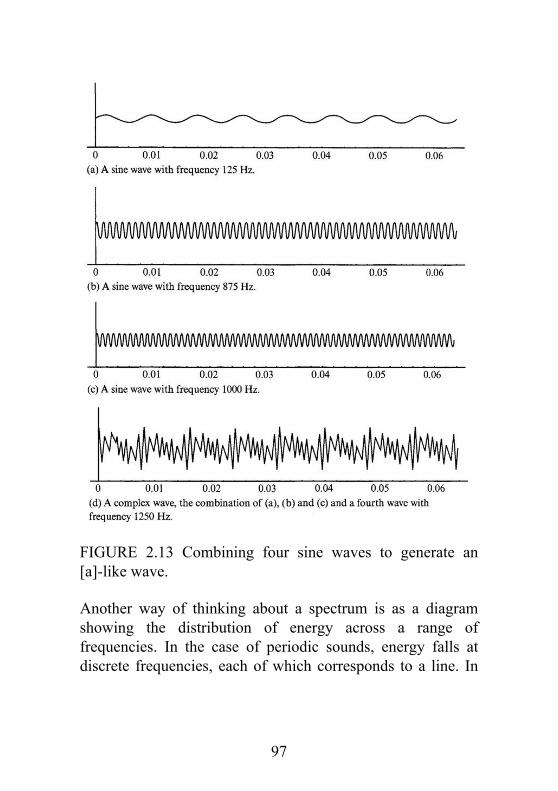
FIGURE 2.13 Combining four sine waves to generate an[a]-like wave.

Another way of thinking about a spectrum is as a diagramshowing the distribution of energy across a range offrequencies. In the case of periodic sounds, energy falls atdiscrete frequencies, each of which corresponds to a line. In

97

the case of aperiodic sounds, energy is distributed over acontinuous band of frequencies.

There are two types of aperiodic sounds, noisy and transient(Section 2.3), but, for reasons which cannot be gone into here,these do not correspond totwo distinct types of spectra. In the case of noisy (continuous)sounds, the overall shape of the spectrum may emerge onlywhen the waveform is averaged over a period of time. Thispoint becomes important in the acoustic analysis of fricativeconsonants (Section 7.4).

98

FIGURE 2.14 Spectra of the three vowel-like wavesillustrated in Figures 2.11, 2.12 and 2.13.

FIGURE 2.15 Spectrum of the initial /s/ of English sigh,pronounced by a male speaker. As for aperiodic soundsgenerally, the spectrum is a continuous curve rather than aseries of vertical lines, representing a fundamental and higherharmonics.

99

2.5 Scaling and the spectrum

The main point which emerges from Section 2.4 is that soundwaves of all types can be generated by combining sine waves.In order to specify a sound wave, it is sufficient to give thefrequencies and relative amplitudes of its sine wavecomponents. This information is presented visually in thespectrum.

In the example spectra I have shown so far, the relationshipbetween the component waves, the complex waveform andthe spectrum has been straightforward in visual terms. Forexample, in our imitation [u] of Figures 2.11 and 2.14 (a), it isclear that the amplitude of the second harmonic (Figure 2.11(b)) is twice that of the fundamental (Figure 2.11 (a)).Correspondingly, the height of the line corresponding to thesecond harmonic is twice the height of the line correspondingto the fundamental in Figure 2.14 (a). Visually, it all makesgood sense. This kind of arrangement, in which relativedistance (in this case, along the vertical axis) corresponds tothe relative magnitude of the thing being measured (in thiscase, amplitude) is called linear scaling.

Linear scaling is the obvious choice for introductorydiscussions of spectra, but it is rarely, if at all, found in thespectra of speech sounds which appear in publications onphonetics. Linear scaling works much less well when therange of amplitude values which we need to display is large.Consider, for example, the waveform of Figure 2.16 (a). Thiswaveform will be of particular interest to us in Section 4.2.1because it is a good approximation to the pattern of air flow

100

through the vocal folds during vocal fold vibration. In thisexample, thefundamental frequency is 100 Hz. The spectrum of thewaveform up to 1000 Hz is shown in (b). The amplitude ratioof the fundamental (100 Hz) to the tenth harmonic (1000 Hz)is roughly 100:1. If we were to continue the spectrum up to4000 Hz (which we shall want to do in Chapter 4), we shouldfind that the amplitude ratio of the fundamental to the 40thharmonic (4000 Hz) was roughly 1600:1. This is not a largeratio from the point of view of the human ear, but it is toolarge to take in by eye or to represent on a textbook-size pieceof paper.

101

FIGURE 2.16 An example of a waveform and a spectrum forwhich it is necessary to display a large range of amplitudevalues.

These difficulties appear worse still when we point out thatthere is, in fact, a patterning in the relative heights of the linesin Figure 2.16 (b). For every doubling along the frequencyaxis, the amplitude decreases by a factor of 4. Thus, theamplitude of the second harmonic (200 Hz) is one fourth thatof the fundamental and the amplitude of the fourth harmonic(400 Hz) is one fourth that of the second harmonic (200 Hz)and one sixteenth that of the fundamental (100 Hz). It isimpossible to take in this patterning by eye.

The solution to such problems is to change the scaling of thevertical axis from linear scaling to logarithmic scaling. Theessence of logarithmic scaling is that equal proportionscorrespond to equal distances along the scale. This is ratherlike our use of percentages rather than absolute numbers intalking about matters such as inflation, wages and prices. Forexample, suppose we read that the price of houses in Londonwent up by 5% last year. This means that a house whichwould have sold for £20,000 at the beginning of the yearhas increased in value to £21,000, whereas a house whichwould have sold for £200,000 has increased in value to£210,000. The first has gone up by £1,000 and the second hasgone up by £10,000 - a large difference in absolute terms butwhen the values are converted to a percentage scale, each hasgone up by exactly the same amount. (This analogy cannot bepushed too far, because a percentage scale does not have allof the properties of a logarithmic scale.)

102

The logarithmic scale used for comparing amplitudes isknown as the decibel scale. The -bel element of the namehonours A. G. Bell (d. 1922), while the deci- element refers toa factor of 10, which enters into the calculation. Actually, thedecibel scale is defined not with reference to amplitude butwith reference to another quantity, intensity. It is thereforenecessary to digress slightly and to consider intensity and itsrelation to amplitude.

2.5.1 Amplitude, power and intensity

Amplitude, as defined earlier, is a measure of how far a sinewave departs from its baseline value. However, we can alsothink of amplitude in relation to the amount of energyexpended. This notion is relevant whether we conceive of sinewaves as movements of air particles, as variations in airpressure, or as variations in electrical voltage. Expendingmore energy requires greater power, and it is the power ofsounds which is, in fact, our chief concern.

'Power' is an abstract concept, which we apply in manyeveryday situations. For example, the powers of diversehousehold appliances such as light bulbs, hair dryers andvacuum cleaners are all measured using the same unit, thewatt. The power of a sound wave may also be measured inwatts. In general, however, we are not interested in the totalpower generated by the source which is what we quantify inthe case of light bulbs - but the power at the particularposition in space where the sound impinges on our ears or ourmicrophones. Thus, acousticians usually refer to intensity,which may be loosely defined as power per unit area.

103

Intensity may be measured in watts per square centimetre (orother equivalent units) when a precise value is required.

In the case of sine waves, there is a simple relationshipbetween the waveform's maximum height above the baseline(amplitude) and intensity: the intensity is proportional to thesquare of the amplitude. In other words, other things beingequal, if the height of a sine waveform is doubled, the motionor pressure variation which it represents must require fourtimes as much power.

Unfortunately, however, this simple rule cannot be applied tocomplex waves. Instead, it is necessary to consider theaverage deviation from the baseline exhibited by thewaveform. This average deviation of a complex waveformfrom its baseline is known as root mean square or RMSamplitude.4 Just as the square of the amplitude of a sine waveis proportional to its intensity, so the square of the RMSamplitude of a complex wave is proportional to its intensity.Fortunately, phoneticians are never called upon either tocalculate RMS amplitudes, or to calculate their squares, andwe shall not illustrate such calculations here. The importantpoint is that it is possible to extend the notion ofamplitude from sine waves to complex waves, and that, ingeneral, the intensity of a wave is proportional to the squareof its amplitude. This has an important implication: relativeintensity can be obtained by squaring relative amplitude. Forexample, if the amplitude ratio of two waves is 2:1, theintensity ratio will be 4:1. If the amplitude ratio is 5:3, theintensity ratio will be 25:9. If the amplitude ratio is 9:7, theintensity ratio will be 81:49. Thus, we (or, rather, ourcomputers) can compare the overall intensity of one complexsound with another as well as making comparisons involving

104

two sine waves. For example, we might wish to compare theintensities of two different vowels or of stressed andunstressed versions of the 'same' vowel.

2.5.2 The decibel scale

The decibel scale (abbreviated dB) is defined with referenceto intensity, and is so constructed that each tenfold increase ofintensity corresponds to adding on 10 decibels. Conversely,each decrease of intensity by a factor of 10 corresponds tosubtracting 10 decibels. The reader with memories oflogarithms from school mathematics will see that the decibelscale is based on logarithms. The intensity in dB of Sound Brelative to Sound A is obtained by finding the logarithm to thebase 10 of the intensity ratio (IB/IA) and multiplying by 10.For example, if B has twice the intensity of A, the intensityratio is 2. The logarithm of 2 is 0.3, and multiplying this by10 gives a value of 3 dB. If the intensity of B is half that of A,the intensity ratio is 1/2. The logarithm of 1/2 is -0.3, andmultiplying this by 10 gives a value of-3 dB.

Since the intensity ratio can be obtained by squaring theamplitude ratio, the decibel scale can also be used forcomparisons if relative amplitudes are known. The differencein decibels can also be determined by taking the logarithm ofthe amplitude ratio and multiplying by 20. For example, if the

105

amplitude ratio is 2:1, the difference in decibels (6 dB) maybe obtained either (1) by calculating the intensity ratio (4:1)and converting that value to decibels (6 dB) or (2) bymultiplying 0.3 (the logarithm of 2) by 20. Some examplesare as follows: The effect of using the decibel scale in theexample of Figure 2.16 is shown in Figure 2.17 (a). We havesaid that for each doubling of frequency, the amplitudedecreases by a factor of 4. The table above shows that this isequivalent to a decrease of 12 decibels. Between 100 and 800Hz, the frequency doubles three times (100 x 2 = 200; 200 x 2= 400; 400 x 2 = 800). Accordingly, the amplitude willdecrease by 36 decibels (36 = 12 x 3). Between 800 and 1000Hz, there willbe a further decrease of just under 4 decibels. Consequently,an overall range of 50 decibels, as in Figure 2.17 (a), is morethan sufficient to show the range of amplitude values of thefirst ten harmonics.

106

FIGURE 2.17 The effects of applying logarithmic scaling tothe spectrum of the wave illustrated in Figure 2.16.

Figure 2.17 (a) also illustrates an important consequence ofusing logarithmic scaling in general and the decibel scale inparticular: it is no longer possible to get away with leavingthe vertical axis unlabelled. In the spectra of Figure 2.14, therelative heights of the lines corresponded to the relativeamplitude of the components. The actual numbers were notimportant because relative amplitude could, in principle, bedetermined by comparing the heights of the lines. When thedecibel scale is used, it is the differences in numbers ofdecibelsrather than proportions which indicate relative amplitude. Forexample, if the vertical axis in Figure 2.17 (a) were leftuncalibrated, we would not be able to work out that thedifference in amplitude between the fundamental and thesecond harmonic was 12 decibels, in other words that theamplitude of the first was four times that of the second.

107

At the same time, there is a sense in which the numbers usedto label the vertical axis in Figure 2.17 are arbitrary. Thefigure was designed so that the fundamental componentwould have an amplitude of 0 and the amplitudes of all of theharmonics would be negative. However, we might also havechosen to give the fundamental some other amplitude value.For example, if the fundamental had been assigned anamplitude of 100, the amplitude of the second harmonicwould have been 88. It is the differences which matter ratherthan the absolute values of the numbers. This point willbecome relevant when we consider the practicalities ofanalysing sound waves (or, more generally, signals)inChapter 3.

A common way of expressing the feature of the decibel scalejust mentioned is to say that the choice of reference level isarbitrary. Sometimes, however, decibels are used as thoughthey were absolute numbers, as for example when the noiselevel produced by a pneumatic drill or an antisocialneighbour's loudspeakers is quantified in terms of numbers ofdecibels. In such cases, the value in decibels is to beunderstood as relative to the intensity of the faintest soundaudible (in the absence of other sounds) to an average humanwith normal hearing. If a sound level is specified relative tothis reference level, it is referred to as a sound pressure level,abbreviated SPL. Normal conversational speech typically hasa pressure level of 60-70 dB (more fully, dB SPL). Soundswhich are loud enough to cause pain have a level of about 130dB SPL.

108

2.5.3 The octave scale

The use of logarithmic scaling for the vertical (amplitude)axis of spectra - in other words, the use of the decibel scale -is very much the norm among acoustic phoneticians. Thespectra which are produced by computer workstations andwhich appear in published articles are typically done in thisway. By contrast, it is unusual to see logarithmic scalingapplied to the horizontal (frequency) axis. This is probablybecause the range of frequencies phoneticians need to dealwith is not unmanageably large.

When logarithmic scaling of the frequency axis is wanted, thescale used is the octave scale. The octave scale is so definedthat an increase of one octave corresponds to a doubling offrequency, while a decrease of one octave corresponds to ahalving of frequency. For example, 200 Hz is one octaveabove 100 Hz, and 400 Hz (= 200 Hz x 2) is two octavesabove 100 Hz. Similarly, 50 Hz is one octave below 100 Hz(50 = 100 x 1/2). The name octave comes from Westernmusic, where, if a player or singer performs a major scale, the'same' note will re-occur every eight notes. (For example, C DE F G A B C D E F G , etc.) In terms of frequency, thepassage from one note to its counterpart anoctave above corresponds to a doubling, while the passagefrom one note to its counterpart an octave below involves ahalving. Thus, if we start from A = 440 Hz (the A abovemiddle C on a piano keyboard), the next occurrence of thenote A going up the scale has a frequency of 880 Hz. If we godown the scale from A 440, the next A has a frequency of 220Hz. Like the decibel scale, the octave scale is inherentlyrelative and presupposes a point of reference. For example,

109

we can specify a particular note as 'one octave above A 440'or 'one octave below A 440' but not as simply 'one octave'.

Figure 2.17 (b) shows the advantage of applying the octavescale to horizontal axis of 2.17 (a). The lines corresponding tothe individual harmonics now decrease in height in a straightline. This brings out the systematic nature of the relationshipbetween frequency and amplitude in the spectrum: for eachoctave increase in frequency (doubling), the amplitudedecreases by 12 decibels (by a factor of 4). The relationshipcan be summed up by saying that the slope of the spectrum is-12 dB per octave.

A final point about logarithmic scaling is that it brings uscloser to perception. Although decibels and octaves are not, infact, measures of loudness and pitch (Section 5.4), they bringus closer to loudness and pitch than does straightforwardlinear scaling. For example, the perceived difference in pitchbetween 220 Hz and 440 Hz is nearly the same as theperceived difference between 440 Hz and 880 Hz; as we havejust seen, both correspond to musical intervals of an octave.By contrast, the perceived difference in pitch between 440 Hzand 660 Hz (660 = 440 + 220) is much less, and correspondsto the musical interval of a fifth. When we reflect on this fact,it seems rather anomalous that spectra are usually drawn withlogarithmic scaling (decibels) used for the vertical axis butwith linear scaling (Hz) used for the horizontal axis.Nevertheless, this is the most common format.

110

2.6 Summary

We have now gone through all of the essential points aboutthe structure of sound and its visual representation. We haveseen that sound is a type of wave motion, usually through themedium of air, in which patterns of movement are transmittedfrom one layer of air particles to another. These patterns ofmovement result in small variations of air pressure, whichfollow the same pattern as the movements which give rise tothem. Visually, we can represent a sound wave by means of atwo-dimensional graph showing variation through time. Suchrepresentations are known as waveforms.

In principle, every sound wave is a combination of sine wavesand every sound wave can be specified by listing its sinewave components. This is conventionally done visually, usinga two-dimensional diagram known as a spectrum. Thedimensions of a spectrum are frequency (on the horizontalaxis) and amplitude (on the vertical axis). A spectrum is afrequency-domain representation, in contrast to a waveformwhich is a time-domain representation.

We have classified waveforms into three basic types:periodic, noisy (aperiodic continuous) and transient. Amongspeech sounds, vowels and sonorant consonants areprototypical examples of periodic waveforms, voicelessfricatives are prototypical examples of noisy waveforms, andthe releases of stop consonants are prototypical examples oftransient waveforms. There are also composite types, forexample, voiced fricatives which have noise superimposed onperiodicity. Periodic sounds are composed of a fundamentalcomponent and higher frequency components known as

111

harmonics. The frequencies of the harmonics are all multiplesof the fundamental. By contrast, aperiodic sounds (both noisyand transient) have no 'fundamental' frequency, and their sinewave components are infinitessimally close together.

The chapter concluded with further consideration of scalingand its effect on the visual appearance of the spectrum. Wedistinguished between logarithmic and linear scaling, andnoted that it was particularly advantageous to use logarithmicscaling for the vertical axis of spectra because of the largerange of values which need to be represented. The scale usedfor logarithmic scaling of amplitude is known as the decibelscale. Logarithmic scaling of the horizontal axis is lesscommon, but the octave scale is sometimes used for thispurpose. As regards the decibel scale, it is also commonlyused outside the context of the spectrum to compare theoverall amplitude of one sound with another.

2.7 Further reading

There is currently a wide choice of books which provide anintroduction to acoustics for phoneticians. The most detailed,but still elementary, treatment is Ladefoged (1996). I shallalso mention Borden et al. (1994), Clark and Yallop (1995),Denes and Pinson (1993), Fry (1979), Johnson (1997),Lieberman and Blumstein (1988), Pickett (1980) and Rosenand Howell (1991). A personal favourite is Handel (1989).

Notes

1 It needs to be added here that the perceived pitch of a soundwith a complex periodic waveform will be influenced by

112

factors other than fundamental frequency, althoughfundamental frequency is of primary importance. For a puretone, frequency and fundamental frequency are the same.

2 Strictly speaking, a waveform is periodic only if therepetitions of the pattern are absolutely identical and if itcontinues for an infinite amount of time. However, it is usefulto treat waveforms like that of Figure 2.5 (a) as if they wereperiodic.

3 This was a careful production of the word by a speaker withphonetic training, so that the vowel was further back andcloser to IPA [u] than most Southern British Englishpronunciations.

4 To give a formal definition, the RMS amplitude is thesquare root of the average (mean) of the square of the distanceof the curve from the baseline.

113

114

Chapter 3Analysing sound: thespectrograph3.1 Introduction

In Chapter 2, we adopted an abstract way of thinking aboutand describing sound. Sound waves are, in essence, complexpatterns of variation through time, which we can represent astwo-dimensional pictures, or waveforms, on pieces of paperor computer screens. In principle, any such wave is acombination of sine waves, and any two-dimensionalwaveform can be re-created by combining sine waveforms.Because of this, it is also possible to describe a wave byspecifying its sine wave components. This is the basic ideabehind the spectrum. A spectrum is a two-dimensionaldiagram which shows which sine wave components arepresent and their relative strengths.

Unfortunately, the knowledge that every sound, in principle,has a spectrum does not in itself enable us to determine whatthat spectrum is. In a few cases - for example, the imitation[u] of Figure 2.11 - it is possible to arrive at a reasonablygood approximation by visual analysis and a small amount oftrial and error. However, such methods are not really practicalfor research into speech because, even when they work well,they are too slow. The difficulty is made worse by the factthat the spectrum of speech is constantly changing. Even at

115

slow tempos, segments of very different types, such as stops,fricatives and vowels, alternate with one another in quicksuccession. In any case, as students of speech, we want to domore than analyse individual segments; we want to see howthe spectrum changes as the speaker moves from one segmentto another.

A practical solution to the problem is provided by thetechnique of sound spectrography. Spectrography is the mostimportant technique available to the experimentalphonetician, and the visual images which it produces - knownas spectrograms - are the visual images most often associatedwith experimental phonetic research. The purpose of thischapter is to introduce spectrography and related techniquesfor analysing sound.

3.2 Spectrography

3.2.1 Basic principles

The technique of spectrography is based on a differentapproach to the analysis of sound from that of Chapter 2. It isvery difficult to determine the spectra ofspeech sounds exactly, but it is much easier to test for thepresence of sine wave components within particularfrequency bands. Devices which do this are known as filters,more specifically bandpass filters. For example, a bandpassfilter with pass band 300-600 Hz could be used to determinewhether or not a particular vowel sound contained any sinewave components between 300 and 600 Hz. Another way ofexpressing this is to say that a filter may be used to detect thepresence of acoustic energy within its pass band. More

116

specifically, when the signal to be analysed is input to thefilter, the filter will produce an output signal, the amplitude ofwhich is proportional to the amplitude of the combined sinewave components within its pass band. (In fact, filter is amore general concept, as we shall see in Section 4.2.2.) It isthe amplitude of this output signal which is of interest.

To give a simple example, let us imagine using bandpassfilters to analyse our three imitation vowel waves of Figures2.11-2.13. Obviously, one filter on its own will not be veryinformative, but if we use a series of filters which cover asufficiently wide range between them, we can obtain anoverall picture of the structure of the three vowel sounds. Theresult is illustrated in Figure 3.1. We imagine using eightfilters, each with a pass band 300 Hz wide, which betweenthem cover the frequency range 0-2400 Hz. Filter 1 has passband 0-300 Hz, Filter 2 has pass band 301-600 Hz, and so on.In the case of the imitation [u], both of the harmonics (135 Hzand 270 Hz) have frequencies less than 300 Hz, and both willfall within the pass band of the first filter. In the case of theimitation [i], there are two harmonics below 300 Hz, and alsoone highfrequency harmonic which will fall within the passband of the eighth filter (2101-2400 Hz). In the case of theimitation [a], each harmonic falls within the pass band of adifferent filter, giving a wide and broad pattern of filterresponse in the mid frequencies. The three spectra of Figure3.1 appear rather crude in comparison with the line spectra ofFigure 2.14; for example, in the case of [i] and [u] it isimpossible to separate the fundamental (lowest) componentfrom the second harmonic, since both fall within the passband of the first filter (0-300 Hz). On the other hand, thespectra still bring out the essential characteristics of the threevowels.

117

The graphs shown in Figure 3.1 are still only two-dimensionaland do not show change through time. An illustration of howfilters can be used to produce a three-dimensional image isprovided in Figure 3.2. This shows the Direct Translator, adevice developed with the aim of making speech visible to thedeaf (Potter et al. 1947).

The Direct Translator used twelve analysing filters, each witha bandwidth of 300 Hz, giving a total frequency range of3600 Hz. Each filter was linked to a small lamp, which in turnproduced a trace of light on a moving belt of phosphorescentmaterial. The greater the intensity of the output of a filter, thestronger the light produced by the corresponding lamp, andthe brighter the trace on the phosphorescent belt. Thus, thepossibility of varying degree of brightness provides for a thirddimension in the representation. The lowest band offrequencies is at the bottom and the highest band offrequencies at thetop, so that frequency is now represented on the vertical axis.The example illustrates an analysis of the words one, two,three.

118

FIGURE 3.1 Using eight hypothetical filters to analyse the[u]-like, [i]-like, and [a]-like waves of Figures 2.11, 2.12, and2.13. Each filter has a bandwidth of 300 Hz, so that the eightfilters span a total range of 0-2400 Hz. Each filter detects thepresence of acoustic energy within its frequency band. Noticethat, for [i], there is both a low-frequency bar and ahigh-frequency bar (above 2000 Hz). These correspondroughly to the two lowest of the wide, dark bands runningfrom left to right on the spectrogram of Figure 3.4. In thesediagrams, the relative amplitude of the output of the filters isshown on the vertical axis, and the decibel scale is used. Theoutput of the first (0-300 Hz) filter is set at 10 dB in eachcase.

The capabilities of the Direct Translator are inherently limitedby the number of filters. In order to span a frequency range ofover 3000 Hz with only twelve filters, it is necessary that eachfilter should have a wide pass band, and this results in the loss

119

of detail. On the other hand, reducing the bandwidth of someor all of the filters would also reduce the frequency rangewhich could be displayed. The problem was solved by usingonly one filter and varying the centre frequency (and,accordingly, the pass band) to which it is 'tuned'. This is theprinciple behind the Sound Spectrograph, developed in theearly 1940sat Bell Telephone Laboratories. The Direct Translator grewout of the same research and was an attempt to producespectrograms in 'real time'.

FIGURE 3.2 The Direct Translator. This machine made useof twelve analysing filters, each linked to a small lamp. Thegreater the intensity of the output of each filter, the strongerthe light produced by the corresponding lamp, and thebrighter the track on the phosphorescent belt. This pictureillustrates an analysis of the English words one, two, three.From Potter et al. (1947).

A schematic diagram illustrating how the original SoundSpectrograph worked is shown in Figure 3.3, reproduced from

120

Potter et al. (1947). A short utterance to be analysed isrecorded onto a tape loop either from a microphone or from atape recorder. Once the recording has been made, the loop isplayed back over and over again. The speech is input to thefilter, the tuning of which is shifted for each repetition. Thecentre frequency of the filter is gradually moved up thefrequency scale, until the maximum frequency is reached. Inthis way, it is possible to create what is, in effect, a large bankof filters using only one filter.

The filter output is connected to a stylus, which just touches apiece of electrically sensitive paper, wrapped around a drum.The drum revolves together with the tape loop. The strongerthe output of the filter, the darker the mark which is burnedonto the paper. As the centre frequency of the filter is shiftedupwards, the stylus is shifted along the drum from the bottomto the top of the paper. In this way, the output traces from theseries of repetitions are recorded one above the other, in thesame way that the outputs of the twelve filters are displayedtogether in the Direct Translator. In the case of the SoundSpectrograph, the display is a permanent record on paperrather than a temporary display on a belt of phosphorescentmaterial. Intensity is represented on a scale of relativedarkness rather than a scale of relative brightness.

121

FIGURE 3.3 A schematic diagram of the original SoundSpectrograph. In contrast to the Direct Translator, the SoundSpectrograph makes use of only one bandpass filter withvariable frequency band. The utterance to be analysed isrecorded onto the tape loop and is played back many times insuccession. With each repetition, the centre frequency of thefilter is increased until the maximum frequency is reached. Asthe centre frequency of the filter moves up the frequencyscale, the stylus moves up the paper. The greater the intensityof the output of the filter, the darker the mark produced by thestylus on the paper. From Potter et al. (1947).

The Sound Spectrograph was a major breakthrough in thestudy of acoustic phonetics. Firstly, it greatly speeded up theprocess of speech analysis, making it possible to study theacoustics of speech on a large scale. Secondly, it wasstraightforward to use, so that anyone who possessed such aninstrument was able to break down speech into componentfrequencies, whether or not they had an extensive backgroundin acoustics. Thirdly, it provided a means of representing thechange of sound through time which can make visual sense to

122

acoustician and non-acoustician alike. Advances intechnology have meant that it is possible to use computers todetermine the output of the filters by calculation, so that it isno longer necessary to construct actual filters. This has madethe technique more flexible, giving the user more choice as tothe frequency range and the temporal length of eachspectrogram, and also as to the bandwidths of the filters.However, both the basic principles and the nature of thevisual display have remained essentially unchanged.

The term Sonagraph is sometimes used rather thanspectrograph; Sonagraph is the name of the series ofinstruments manufactured by Kay Elemetrics Corporation,which have been extremely popular. Computer-based systemsare known by a variety of names such as speech workstations,speech analysis software packages, and digital spectrographs.I shall use the term computer-based spectrograph here.

3.2.2 An example spectrogram

Figure 3.4 shows a spectrogram of the vowel of the Englishword be, pronounced by a male speaker on a rising pitch, inthe sentence Did you say 'be'? This spectrogram wasproduced on a computer-based spectrograph, using a broadfilter bandwidth (Section 3.4.2). The frequency range of thisspectrogram is 0-5000 Hz or 5 kHz (kiloHertz), and thevertical axis is labelled accordingly. The total duration shownis 319 msec (.319 sec). This speaker also produced theexample of [i] for which the waveform appears in Figure 2.10and is imitated in Figure 2.12.

The release of the /b/ corresponds to the somewhat weakvertical spike on the left of the spectrogram just before the

123

onset of the vowel. It can be seen that there is a brief gapbetween the release spike and the onset of striations for thevowel. This reflects the fact that the voicing has faded outduring the /b/ closure, and a short amount of time (about 7msec) is necessary for it to get going again. (The nature ofvoicing in obstruent consonants such as /b/ is a point whichwe shall return to in Chapters 7 and 8.)

In looking at the vowel itself, a first obvious point is that theshading becomes lighter overall as we move from left to right,indicating that the sound is becoming softer (less intense). Asecond point is that dark, somewhat broad bars extend fromleft to right across the vowel's duration. These bars pick outregions in which harmonics are particularly prominent. Thelowest is low in frequency (below 500 Hz), while the secondrises to just over 2000 Hz. These two bars correspond roughlyto the two bars on the bar chart for [i] in Figure 3.1, and alsoto the regions of prominent harmonics in the line spectra ofFigure 2.14.

As we shall see in Chapter 4, the bars correspond to theso-called formants of the vowel. The frequencies of theformants are determined by the shape and size of the mouthand pharynx (and in some cases also the nasal) cavities. Thefact that higher-frequency bars rise at the onset of the vowelreflects the change in the configuration of the oral cavity asthe lips move from the closed position (which is necessary for/b/) to a more open and spread position (Section 7.3.3.2).

More unexpected - at least on the basis of what we have saidso far - is the presence of vertical lines, called striationsthroughout the course of the vowel. To understand why theseare present we need to think about how vowel sounds are

124

produced. Vowel sounds are normally produced with vocalfold vibration, and it is the regular opening and closing of thevocal folds which ultimately accounts for the periodiccharacter of vowel waveforms. When the vocal folds vibrate,they open and then snap shut in quick succession. Eachsnapping shut is like giving a quick tap to the cavities above,making them 'ring' briefly rather as a bottle or glass ringswhen tapped. As listeners, we are unaware of the individualtaps because they are too quick to be perceived as separateevents, and our ears smear them together. However, they doshow up as separate events on the spectrogram provided thatthe frequency of the vibration is not

FIGURE 3.4 Spectrogram of the English word be,pronounced on a rising pitch.

125

too high. In practice, this means that the striations are usuallyvisible for male speakers but not always for female or childspeakers.

As we move from left to right in the spectrogram, thestriations become closer together. This reflects the fact thatthe vocal folds are speeding up, so that there is less timebetween taps. In other words, the period of the vocal foldvibration is gradually decreasing, with the result that thefundamental frequency is increasing (Section 2.2.4). Thegradual increase in fundamental frequency is perceived as arise in pitch. Figure 3.4 may be contrasted with thespectrograms of Figure 3.6, which show the word doorpronounced on a falling pitch, in the sentence I said 'door'. Inthis case, the striations gradually become further apart as thepitch falls. There is also noticeable irregularity, reflecting thisspeaker's tendency to use creaky voice at low pitches (Section8.3.2). We should also notice in passing that the formantpattern (as shown in the dark bars) is different for this vowel

than for the vowel of be.

It may seem paradoxical to describe the voiced sounds ofspeech as successions of separate and discrete taps. We havealready said in Chapter 2 that they were combinations ofsmooth and continuous sine waves. Nevertheless, bothconceptions are correct, and it can be shown that they aremathematically equivalent. Phoneticians may choose to adoptone view or the other, depending on which is the more usefulfor the purpose at hand. Spectrograms like that of Figure 3.4are more in accord with the 'series of taps' view.

126

3.2.3 Narrow band spectrograms

We have already said that the technique of spectrography isbased on the use of bandpass filters to detect the presence ofacoustic energy within their individual frequency bands. Inthe example of Figure 3.4 (and also the hypothetical exampleof Figure 3.1), the filter bandwidths were too wide to separateout or resolve individual sine wave components (harmonics).Another way of expressing this is to say that the frequencyresolution of the filters is poor. On the other hand, as regardsthe temporal aspects of the signal, the filters have done quitewell in separating out the individual taps of the vocal folds(reflected in the presence of striations). Another way ofexpressing this is to say that the temporal resolution of thefilters is good.

The combination of poor frequency resolution and goodtemporal resolution evident in Figure 3.4 is not accidental. Itis part of the nature of filter based analysis that it isimpossible to achieve both good frequency resolution andgood temporal resolution simultaneously. The broader thepass band of a filter - that is, the less precise it is as afrequency detector - the better its temporal resolution.Conversely, filters with narrow pass bands will have goodfrequency resolution because (at least in the case of voicedsounds) only one harmonic will fall within each pass band,but they will have poor temporal resolution. Accordingly, it iscommon to distinguish between broad band and narrow bandtypes of analysis. The original spectrographs provided foronly two possibilities: a broad band analysis based on a filterbandwidth of 300 Hz

127

and a narrow band analysis based on a filter bandwidth of 45Hz. Current computer-based spectrography, which does notrequire the manufacture of actual filters, also offersintermediate possibilities.

The spectrogram of Figure 3.4 is of the broad band type.Figure 3.5 shows a narrow band spectrogram of the sameword. In this case, the individual harmonics which make upthe vowel appear as relatively narrow lines running from leftto right. These lines rise in parallel as the fundamentalfrequency (and with it, the perceived pitch) of the voice rises.Because of the poor temporal resolution, the vertical spikewhich corresponds to the release of the /b/ is not sharplydefined, and there are no vertical striations. Thus, narrowband analysis is more in accord with the alternativeconception of (voiced) speech as combined sine waves.

Although narrow band analysis provides more detail asregards frequency, broad band analysis is the more generallyuseful. In the first place, spectrograms are frequently used tomeasure durations of sounds. It is now usual forcomputer-based spectrographs to include provision for two ormore cursors, which can be placed at the boundaries of thesound to be measured; the temporal distance between themcan then be determined automatically. For such purposes, thegreater temporal precision of broad band spectrograms andtheir sharper definition of onsets and offsets (beginnings andends) of sounds is a real advantage. For example, if wewished to measure the temporal distance between the releaseof the /b/ and the onset of voicing (the Voice Onset Time, seeChapters 5 and 7), this could only be done from the broadband spectrogram of Figure 3.4.

128

A second advantage of broad band spectrograms is that it isusually easier to discern overall patterns. The detail of thenarrow band spectrogram may obscure the gross alternationsof darker and lighter areas along the vertical axis. This isparticularly true if the pattern is changing. The onset of thevowel in Figures 3.4 and 3.5 provides a good example; inFigure 3.4, it is easy to see that the dark bars above 2000 Hzare rising, whereas this point is rather lost in the detail of theharmonics in Figure 3.5.

3.2.4 Pre-emphasis

It is characteristic of speech generally that the lowerfrequencies are stronger than the higher frequencies. Thepractical consequence of this is that higherfrequencycomponents may be weak or even invisible on a spectrogram.If the phonetician is particularly interested in the highercomponents, this is a major disadvantage. A solution is toboost the amplitude of the high-frequency components. Thisis known as pre-emphasis. Pre-emphasis is not part of theanalysis procedure itself, but is applied beforehand.

Figure 3.6 shows two broad band spectrograms of the Englishword door , pronounced on a falling pitch, in thesentence I said 'door'. Pre-emphasis was not applied in (a), butit was applied in (b). If we compare the two, we can see thatthe lower frequencies are weaker and the higher frequenciesare stronger in (b) as compared with (a).

129

FIGURE 3.5 Narrow band spectrogram of the English wordbe, illustrated in Figure 3.4.

130

FIGURE 3.6 Two broad band spectrograms of the Englishword door, pronounced on a falling pitch. The first wasrecorded without pre-emphasis, while the second wasrecorded with pre-emphasis. As a result, the balance betweenlow and high frequencies is different in the two versions.Note that the striations are further apart than in Figure 3.4,and the size of the gaps between them increases as thefundamental frequency falls.

3.2.5 Two-dimensional spectra

The great advantage of spectrography is its ability to providea threedimensional display on a two-dimensional surface.However, it has to be admitted that the detail of the thirddimension (amplitude) is difficult to judge by eye, even when,as in many systems, the scale of dark-to-light shading isreplaced by a scale of colours. Furthermore, a scale based onshading or colour does not lend itself to precise measurement.

131

For many purposes, we wish to make more precisemeasurements of relative amplitude for a stretch of speechwhich is relatively steady-state. For example, we might wishto examine in detail the structure of the vowel of be at itsmidpoint. In such cases, it is useful to be able to produce atwo-dimensional spectrum from which more precisemeasurements can be made. A common procedure is to use abroad band spectrogram to locate the time of interest and thento request the two-dimensional display. On computer-basedspectrographs, this is typically done by positioning a cursorand then selecting the appropriate instruction from a menu.The cursor, in this case, does not really specify an instant intime but rather the location of the window which will be usedto calculate the spectrum (Section 3.4.2).

FIGURE 3.7 Broad band (a) and narrow band (b) spectra forthe vowel [i] of be, the spectrogram for which is shown inFigure 3.4. The cursors pick out the lowest two peaks in the

132

spectrum, corresponding to the lowest two formants of thevowel.

Figure 3.7 shows two spectra, one broad band (a) and onenarrow band (b), for our example [i]. In requesting both thesespectra, the cursor was placed at apoint 79 msec after the onset of the striations for the vowel inthe broad band spectrogram of Figure 3.4. (The number0.839s in the upper left-hand corner is the starting time of thewindow, measured from the beginning of the segment ofspeech stored in the computer's memory.) As we wouldexpect, the broad band spectrum (for which the filter effectivebandwidth was 160 Hz) does not separate the individualharmonics, while the narrow band (for which the filtereffective bandwidth was 40 Hz) does.

Each spectrum spans a frequency range of 5000 Hz, which, aswe shall see, is determined by the user's choice of samplingrate at the time the speech is input to the computer (Section3.4.1). The vertical axis is scaled using the decibel scale(Section 2.5.2), and displays a range of 40 decibels. In manysystems, as in this one, the range of amplitudes to bedisplayed is specified by the user. Since the decibel scale isbased on relative intensity (power), such spectra are oftenreferred to as power spectra. The term FFT spectra, whichrefers to the method used to calculate the outputs of the filters(Section 3.4.2), is also used.

Each spectrum shows two cursors, which have beenpositioned to coincide with the first and second peaks. It willbe seen that, in both cases, the peaks match up in frequencywith the broad bars on the broad band spectrogram of Figure3.4 and the darker harmonics on the narrow band spectrogram

133

of Figure 3.5. At the top, an amplitude value, in decibels, isgiven for each cursor. On this particular system, amplitudesare measured relative to a 'ceiling' value, and so the valueswhich appear are always negative. They have little meaningin themselves, but they are very useful in makingcomparisons. For example, on the basis of the narrow bandspectrum, we could say that the strongest harmonic in thefirst, low-frequency peak (250 Hz) is 15 dB more intense thanthe strongest harmonic in the second peak (2061 Hz); thisvalue is arrived at by subtracting -27 from -12.

Another type of spectrum, which is not based on the use offilters, and which is known as an LPC spectrum, will beillustrated in Section 4.5.

3.2.6 Supplementary displays: waveform,intensity and fundamental frequency

Spectrographs typically provide for other types of displays aswell. Figure 3.8 shows three common possibilities. In (a), wesee the waveform of the sound. This shows less detail than the'close-up' view of the waveform of Figure 2.10 (b). In (b), wesee an overall intensity contour (Section 2.5.1), which showshow the overall intensity rises and falls; on computer-basedsystems, this is determined from the RMS amplitude of thewave (Section 2.5.1). We have already observed (Section3.2.2) that the intensity of the vowel appears to decrease overthe course of its duration. This is confirmed by both thewaveform and the intensity displays; the waveform clearlydecreases in amplitude in parallel with the decline inintensity. Figure 3.8 (c) shows the fundamental

134

frequency, abstracted from other characteristics of the speech.Fundamental frequency tracking is extremely useful forstudying tone and intonation, where the rise and fall of thefundamental frequency of the voice (heard as rising andfalling pitch) is the main object of interest.

FIGURE 3.8 Waveform (a), relative intensity (b), andfundamental frequency (c) displays for the vowel [i] of be, thespectrogram for which is shown in Figure 3.4.

This concludes our introductory overview of the technique ofspectrography. In order to use the technique effectively, it is

135

necessary to have some understanding of how a spectrographworks. Accordingly, in what follows, we shall look at some ofthe technicalities of computer-based spectrography. Beforewe begin, however, it is necessary to give some considerationto the nature of sound recording. In fact, equipment forspeech analysis never works with the sound directly. Rather,it deals with electrical signals which are analogous to thesound being analysed. A microphone, and usually also arecording (on tape or compact disk or some other medium),provide the necessary intermediate links.

3.3 Recording

From what has been said about the nature of sound, it shouldbe clear that sound is very elusive. The movements of airparticles and the resulting variations in air pressure are verysmall, take place very quickly and cannot, in themselves, bepreserved. To record sound, we must record enoughinformation about the small variations in air pressure toenable them to be re-created.

3.3.1 Recording as translation

The first sound recordings, made by Thomas Edison in 1877,achieved this by what now seems a very simple and primitivesystem. Edison's recording system was based on a horn, witha diaphragm at the narrow end. A steel needle was attached tothe diaphragm. When someone spoke or sang into the horn,the diaphragm, and with it the steel needle, were set intovibration. While this was going on, a cylinder covered withtin foil was rotated under the needle, in such a way that theneedle made indentations in the tin foil, going from one end

136

of the cylinder to the other in a spiral pattern. Theindentations in the tin foil provided a record of the smallvariations in air pressure (resulting from the motions of the airparticles) in the original sound.

To play back the recording, the process was reversed. Thecylinder was turned, causing the needle to vibrate followingthe pattern recorded in the tin foil. The needle in turn causedthe diaphragm to vibrate, which in turn caused the adjacentair particles to vibrate, so that the sound which emerged fromthe horn was recognisably a reproduction of the original.

The whole process of recording might be described astranslating the small variations in air pressure produced by thesmall movements of air particles into variations in somethingelse. In Edison's case, the 'something else' was the groovedrawn by the needle along the surface of the tin foil. Thediaphragm and the needle provided the link between the two.In more technical terminology, translation from one mediumto another is known as transduction (from Latin transduco'lead across'). Transducers need to be distinguished fromamplifiers, which produce a larger-scale copy of an inputsignal without changing the medium.

Like the early phonograph, modern recording systems arebased on translating and re-creating the original acousticsignal, though it is not possible to follow the process by eye.We can distinguish three general stages:

1. Variations in air pressure in the input acoustic signalare translated (transduced) into variations in voltagein an output electrical signal. Whatever the eventual

137

storage medium, this is always the first step. The roleof the microphone is to perform this conversion.

2. Variations in voltage in the electrical signal (outputfrom the microphone) are translated into a formsuitable for transfer to the storage medium. This mayinvolve several intermediate stages, includingamplifying the microphone output. In the case of atape recorder, the final output of this process is avarying magnetic field in the record head.

3. The third and final step is the transfer to the storagemedium itself. In the case of tape recording (cassetteor open reel), small particles of metal on the surfaceof the tape, which are invisible to the naked eye, aremagnetised as the tape is wound past the record head.(Before reaching the record head, the tape is woundpast an erase head which wipes out any previousrecording.) In this way, variations in the magneticfield in the record head are translated into variationsin magnetisation on the surface of the tape. Since thevariations in the strength of the magnetic field are,ultimately, translations of the variations in airpressure in the original acoustic signal, the surface ofthe magnetic tape provides a permanent record of theoriginal, just like the surface of the tin foil in Edison'sprimitive system.

To play back a copy of the original sound, the multi-stageprocess of translation is reversed. The final stage is alwaysvibration of a diaphragm, inside a speaker or headphone,which brings about vibration of the surrounding air particles -in other words, a sound wave.

138

3.3.2 Fidelity

A good system for recording and reproducing sound ischaracterised by high fidelity. The greater the fidelity, themore closely the reproduction corresponds to the original.Since the recording process involves re-creating the inputsound several times, fidelity will be achieved only if thetransmission is accurate at every stage. For example, in thecase of the early phonograph, it does not matter how well themotion of the diaphragm reproduces the motion of the airparticles if the steel needle does not do its job well. Anexpensive high-quality tape recorder cannot achieve fidelity ifit is used with a low-quality microphone. The chain is only asstrong as its weakest link.

To evaluate the fidelity of a system as a whole, or of anindividual component such as a microphone, two factorsstand out as crucial:

1. Frequency response. If a particular instrument - forexample, a tape recorder - reproduces soundfaithfully, the spectrum of the reproduction must beidentical to the spectrum of the original. In otherwords, it will show the same sine wave componentsin the same proportions. The same general criterioncan be applied to an instrument such as amicrophone, which translates the original pressurevariations into variations in some other medium. Thespectrum of the translation must be identical to thespectrum of the original.

Let us now imagine testing out a tape recorder with acomplex sound in which all of the sine wave

139

components are equal in amplitude. In this case, all ofthe sine wave components in the reproduction shouldalso be equal in amplitude. This possibility isillustrated in Figure 3.9 (a) and (b). If, on the otherhand, the spectrum of the reproduction is not 'flat' -that is, if some frequencies are larger in amplitudethan others, as in Figure 3.9 (c) - then

140

FIGURE 3.9 An imaginary experiment to determine thefrequency response of two recording systems.

• the reproduction is not faithful. In practice, this kindof check can be performed by testing the sine wavecomponents one at a time rather than all at once aswe have envisaged it.

An experiment like the one just described is said todetermine the frequency response of the instrumentbeing tested. The ideal is an absolutely flat response

141

across the frequency range perceived by the humanear (roughly 20-22,000 Hz).

• 2 Dynamic range. A faithful system must not onlygive all frequencies equal treatment - it must be ableto do so for both loud and soft sounds. For example,in recording a performance by a large symphonyorchestra, the system must be able to reproduce boththe quiet passages performed by the solo flute and theloud passages, when all the instruments are playingtogether at high volume. When recording speech, thesystem must reproduce both inherently quiet soundssuch as [f] and inherently sonorous sounds such as[a].

A common measure of dynamic range is the so-calledsignal to noise ratio, abbreviated S/N ratio. This isdefined as the ratio of the intensity of the signal to theintensity of any background noise inherent in thesystem. It is measured in decibels. Since the dynamicrange of speech is about 55 dB, recording systemsused in speech analysis should have a S/N ratio of 60to 70 dB.

3.3.3 Digital recording

Most, if not all, readers will be aware that a distinction existsbetween digital and analogue recording. In an analoguesystem, what is stored or displayed varies continuously in amanner analogous to the original. For example, all of thedrawings of waveforms in this book are analogues of (actualor imagined) waves. In Edison's early phonograph, thecontinuously changing position of the line traced by the

142

needle on the tin foil is an analogue to the continuouslychanging air pressure at the diaphragm. In the case ofrecording on magnetic tape, the magnetic properties of theparticles on the tape change continuously. They are analogousto the variations in voltage in the electrical signal which wasoutput from the microphone and, ultimately, to the variationsin air pressure in the original sound wave.

In a digital recording, no continuously varying counterpart ofthe original signal is created. Instead, information aboutvariation in voltage is stored as a series of numbers. Thesenumbers indicate the amplitude (height) of the waveform atequally spaced intervals of time. (Notice that, in this usage,amplitude may refer to the height of the waveform at anychosen point in time rather than to the maximum height as inSection 2.3.1.) This method, known as sampling, is illustratedin Figure 3.10. Part (a) shows one cycle of a continuous sinewave. This drawing on paper is an analogue of a single cycleof a pure tone with frequency 100 Hz. For the purposes of thisillustration, we haveimagined that the vertical axis is calibrated in 'voltage units'and that the baseline value is 127 voltage units.

143

FIGURE 3.10 Sampling a wave.

In (b), the same wave is represented as a series of 21 points(including the beginning and end points), separated byintervals of 0.0005 seconds. The values (heights in voltageunits) for the individual points are given underneath. Thesenumbers alone are sufficient to enable us to draw anapproximation to the waveform - we need only plot them on agraph like that of Figure 3.10 (b) and then connect the dots.Accordingly, in a digital record of the waveform,only the numbers need to be stored. Any storage mediumwhich can cope with large numbers of numbers can be used,

144

the most generally familiar being computers and compactdisks.

Sampling the sound wave is the essential step in analogue todigital conversion, usually abbreviated as A-to-D conversion.A-to-D conversion does not work directly from the soundwave, but from an amplified version of the electrical signaloutput from the microphone. Thus, the amplitude values areusually measured in volts.

As in the case of analogue recording, the fidelity of a digitalsystem will depend on its frequency response and dynamicrange. However, these characteristics are usually quantified indifferent ways, reflecting the special characteristics of digitalrecording. Two aspects need to be examined here: samplingrate and quantisation.

3.3.3.1 Sampling rate

Sampling rate refers to the number of times the amplitude ofthe wave is recorded per second. The higher the samplingrate, the shorter the time interval between individual samples,the closer together the dots in the visual representation, andthe greater the resemblance between the sampled version andthe original. In the example of Figure 3.10, the sampling rateis 2000 samples per second or 2000 Hz. (The unit Hertz isoften applied to sampling rates as well as to frequencies ofvibration.)

The choice of sampling rate is important because it sets anupper limit on the frequency range of the recording. Thisupper limit is half the sampling rate, a value frequently

145

referred to as the Nyquist frequency. For example, a samplingrate of 2000 Hz (samples per second) can only be used torecord signals for which all the sine wave components are lessthan 1000 Hz, which is the Nyquist frequency in this case. Asampling rate of 10,000 Hz, providing for a frequency rangeof 0-5000 Hz, is frequently used in phonetic research.Recordings of music for storage on compact disk commonlyuse a sampling rate of 44,100 Hz, in order to allow forfrequencies of up to 22,050 Hz in the reproduced sound.

3.3.3.2 Quantisation

Quantisation refers to the accuracy with which the amplitudevalues are recorded. This determines the dynamic range of adigital recording.

Storing the actual numbers in a digital recording is like fillingin a form, in which a fixed number of slots is allocated toeach value. For example, when reporting the reading of adomestic electricity meter in the UK, the customer must writethe numbers shown on the meter in a set of boxes on a formprovided for the purpose by the supplier. Four boxes areprovided, while the meter itself shows five numbers. Therightmost number on the meter musttherefore be ignored, with the result that the reported readingis less accurate than it could be. The smallest reading whichcan be reported is 1 'unit of electricity', while the largestreading which can be reported is 9999 - nearly 10,000 timesas great. If, however, five boxes were to be made available onthe form, it would be possible to report fractions of a unit ofelectricity. The smallest reading which could be reportedwould be 0.1 unit and the largest reading which could be

146

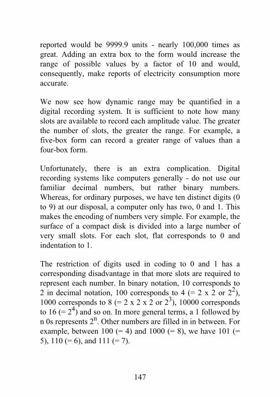
reported would be 9999.9 units - nearly 100,000 times asgreat. Adding an extra box to the form would increase therange of possible values by a factor of 10 and would,consequently, make reports of electricity consumption moreaccurate.

We now see how dynamic range may be quantified in adigital recording system. It is sufficient to note how manyslots are available to record each amplitude value. The greaterthe number of slots, the greater the range. For example, afive-box form can record a greater range of values than afour-box form.

Unfortunately, there is an extra complication. Digitalrecording systems like computers generally - do not use ourfamiliar decimal numbers, but rather binary numbers.Whereas, for ordinary purposes, we have ten distinct digits (0to 9) at our disposal, a computer only has two, 0 and 1. Thismakes the encoding of numbers very simple. For example, thesurface of a compact disk is divided into a large number ofvery small slots. For each slot, flat corresponds to 0 andindentation to 1.

The restriction of digits used in coding to 0 and 1 has acorresponding disadvantage in that more slots are required torepresent each number. In binary notation, 10 corresponds to2 in decimal notation, 100 corresponds to 4 (= 2 x 2 or 22),1000 corresponds to 8 (= 2 x 2 x 2 or 23), 10000 correspondsto 16 (= 24) and so on. In more general terms, a 1 followed byn 0s represents 2n. Other numbers are filled in in between. Forexample, between 100 (= 4) and 1000 (= 8), we have 101 (=5), 110 (= 6), and 111 (= 7).

147

In accordance with computer usage, the lengths of numbersare measured in binary digits or bits rather than in decimaldigits. A system with two bits per number at its disposal canrecord four values: 0, 1, 10 (= 2), and 11 (= 3). A system withthree bits can record seven values, from 0 up to (but notincluding) 8. More generally, a system with n bits can recordvalues from 0 up to (but not including) 2n.

The effect of quantisation level on the shape of the storedwaveform is shown in Figure 3.11. In (a), we see one cycle ofa complex waveform which is the sum of a 100 Hz sine waveand a 500 Hz sine wave (compare Figure 2.6). In (b), thesame waveform is represented using only four amplitudelevels, 0, 1, 2 and 3 (requiring 2 bits), resulting inconsiderable distortion. If the wave were played back, itwould sound as if noise had been added.

In Figure 3.11 (c), the number of levels is doubled to eight(requiring 3 bits). In (d), the number of levels is againdoubled to sixteen (requiring 4 bits). Each doubling producesa waveform more like the original shown in (a). In the case ofFigure 3.10, 256 levels (0-255) were allowed for. This wouldrequire 8 bits (256 = 28). Sixteen-bit quantisation is usual inhigh-fidelity music recording.

148

149

FIGURE 3.11 The effect of quantisation level on the overallshape of a waveform.

To sum up, in a digital recording system, the dynamic rangeis determined by the level of quantisation, measured in bits.There is a simple relationship between the number of bits andthe range in decibels:

range (in dB) = number of bits x 6.

150

This follows from the fact that each additional bitapproximately doubles the range of amplitude values, andeach doubling results in the addition of 6 decibels on thedecibel scale (Section 2.5.2).

This concludes our discussion of fidelity in analogue anddigital recording systems. For prospective users ofcomputer-based spectrographs, the most important point toremember is the relationship between sampling rate andfrequency range in a digital recording: the upper limit of thefrequency range will be half the sampling rate.

3.4 Digital spectrography

Both the Direct Translator of Figure 3.2 and the SoundSpectrograph of Figure 3.3 are analogue devices. The outputspectrogram is essentially a series of continuous horizontaltraces, one on top of the other, with each trace correspondingto a single filter. Each line varies in intensity - manifested asdarkness of marking or brightness on a moving belt ofphosphor - according to the strength of its filter's output. Incomputer-based digital spectrography, a bank of filters is alsoused, but the output of the various filters is determined not bymeasurement but by calculation, in most cases by a techniqueknown as the Fast Fourier Transform or FFT. The result isvisually indistinguishable from a spectrogram produced by ananalogue spectrograph.

When using such equipment, it is useful to have a basicknowledge of how the calculations are done. In what follows,we shall give a brief account of the steps involved. From thepoint of view of the user, the two most important

151

specifications for digital spectrograms are the sampling rateand the number of sample points in the FFT.

3.4.1 Recording for analysis

As in the case of the Sound Spectrograph, the first stepinvolves recording. The signal to be analysed (from amicrophone, tape, or some other medium) is input andundergoes A-to-D conversion. There will normally be achoice of sampling rates. This is important, because, as wehave seen, it is the sampling rate which determines the rangeof frequencies represented in the recording and, ultimately, inthe calculated spectrogram. For most purposes, a samplingrate of 10,000 Hz (giving a frequency range of 5000 Hz) willbe sufficient. However, if the intention is to study fricativeconsonants, a higher sampling rate should be used becausethese sounds typically show concentrations of energy above5000 Hz. The user may also need to request pre-emphasis(Section 3.2.4) at this stage. Some systems may offer a choiceof quantisation levels.

3.4.2 Calculating the power spectrum

After recording, the digital spectrograph has at its disposal awaveform, coded as a series of points as in Figure 3.10 (b). Inorder to perform its calculations, it must look at the waveformone chunk at a time. For each chunk, referred to as a window,the frequency range is divided into bands, corresponding toindividual bandpass filters. The output of each filter iscalculated, and the values are converted to decibels. Theresult is a power spectrum like those displayed graphically inFigure 3.7.

152

The power spectra for the individual windows must then be,as it were, turned on their side so that frequency is on thevertical axis. The amplitude values must be translated into theappropriate shadings or colours. When the resulting verticalspectra are lined up side by side, the result is a spectrogram.From the point of view of the user, the power spectrum is anextra display which supplements the main spectrogram, but infact calculation of power spectra is logically prior toassembling the spectrogram.

The bandwidth of the filters depends on the duration (in time)of the window selected. The longer the window, the narrowerthe filter bandwidth. This makes intuitive sense, for we caneasily imagine that the longer the chunk of waveform theanalyser has to work with, the more accuracy it will be able toachieve in its frequency analysis. At the same time, since theanalyser can produce only one spectrum per window, longerwindows will give less detail about timing (poorer temporalresolution). As with the earlier spectrograph, greater accuracyin the frequency domain (better frequency resolution) mustnecessarily go with less accuracy in the time domain (poorertemporal resolution).

Figure 3.12 illustrates the steps involved, using a simpleexample. Part (a) shows a complex wave to be analysed. Itwas constructed by adding together two sine wavecomponents with frequencies 300 and 1500 Hz. Theamplitude of the 300 Hz component is 6 dB above (twice) theamplitude of the 1500 Hz component (Section 2.5.2). Wehave sampled the wave at a frequency of 5000 Hz, and thesample points are superimposed on the waveform. With ourchoice of sampling frequency, we have determined the range

153

of the analysis, which will cover frequencies between 0 and2500 Hz (= 5000/2).

We now select a chunk which is 64 points long. The durationof this chunk (window) is 64/5000 seconds or .0128 seconds.A 32-point window (with length .0064 seconds) is alsoshown. The duration in time of a given number of samplepoints will depend on the sampling rate. For example, if thesampling rate had been 10,000 Hz, the duration of a 64-pointwindow would be only .0064 (= 64/ 10000) seconds.

In (b), our selection of 64 points is reshaped, in a processknown as windowing. The purpose of the windowing is toattenuate the amplitude at the right and left edges. Thiseliminates the sudden and unnatural transitions to and fromsilence which would unavoidably occur if the selection inquestion were simply chopped out. In our example, a type ofshaping known as a Hanning window has been applied. If noshaping at all is used, it is said that the window is

154

155

156

157

FIGURE 3.12 Calculating an FFT spectrum.

rectangular. In general, spectrographs will apply a defaulttype of shaping, chosen by the programmers who put togetherthe necessary software. The user may be able to specify analternative, but most will probably be content to opt for thedefault.

After windowing, the spectrum is calculated (c). Thetechnique commonly used is known as the Fast FourierTransform (FFT). The FFT is a quick method of calculatingthe so-called Discrete Fourier Transform (DFT) and may beused only when the number of sample points is a power oftwo. This is why possible window lengths are often restrictedto numbers which are powers of two (16, 32, 64, 128, etc.).DFT/FFT analysis is an adaptation of the technique of Fourier

158

Analysis (Section 2.4), but it works from a set of individualpoints rather than from a continuous wave.

As already mentioned, the frequency range is, in effect,divided up into a number of bands, and an amplitude level iscalculated for each band. This is like putting a small chunk ofsignal through a bank of filters. The number of bands in thefrequency range covered by the analysis (from 0 to half thesampling rate) will be half the number of points in thewindow. In the present example, the frequency range is0-2500 Hz, and it is divided into 32 bands.

If FFT analysis is applied to the windowed points of (b), it issaid that a 64-point FFT is calculated. The result is presentedas a graph in (c). The decibel scale has been used for thevertical axis, and a range of just over 30 dB has been allowedfor. Each point corresponds to one frequency band. Thecalculated amplitude for each band (on the vertical axis) isplotted versus the centre frequency (on the horizontal axis). Infact, only six points are shown; the points for the remaining26 lie below the zero line.

The bands showing the highest amplitudes are the fifth band(312-390 Hz, centre frequency 351 Hz) and the twentiethband (1481-1560 Hz, centre frequency 1521 Hz). Thedifference in amplitude between the two is 6.1 dB. On thebasis of Figure 3.12 (c), we would estimate that our chunk ofinput signal contains two components with frequencies ofabout 351 and 1501 Hz and that the first of these is 6.1 dBmore intense than the second. In this particular case, we are inthe fortunate (though unusual) position of knowing what theanswer should be, and we can see that our estimate is quiteclose to the truth (components at 300 and 1500 Hz, amplitude

159

difference 6 dB), though the estimated frequency of the firstcomponent is too high.

It is also necessary to comment on the vertical axis which, inaccordance with common practice, shows relative amplitudeand is on the decibel scale. In such diagrams, the choice ofbaseline is somewhat arbitrary, and individual systems differfrom one another. What is important is the range of valuesdisplayed and the difference in height between the variouscomponents (Section 2.5.2). For the purposes of our example,we have chosen to display a range of just over 30 dB.

Finally, part (d) of Figure 3.12 shows the effect of decreasingthe window length to 32 points. The spikes are thicker and thefrequency analysis is correspondingly less accurate. Inpractice, it is common to smooth out the spectrumin a DFT or FFT analysis. Thus, the broad band spectrum ofFigure 3.7 appears considerably smoother than our calculatedspectrum in (d).

As already mentioned, from the point of view of the user, thetwo most important specifications for digital spectrograms arethe sampling rate and the number of points in the FFT. Thesampling rate determines the frequency range of the resultingspectrogram. The number ofpoints in the FFT determines thebandwidth of the analysing filters. The greater the number ofpoints, the narrower the bandwidth, though the preciserelationship will depend on the sampling rate. Somecomputer-based spectrographs make the choice easier byasking the user to choose a filter effective bandwidth ratherthan to specify a window length.

160

3.4.3 Determining fundamental frequency (F0)

As we have already pointed out (Section 3.2.6),computer-based spectrographs typically include provision fordetermining and displaying the fundamental frequencycontour of the speech signal being analysed. Unfortunately,determining the fundamental frequency of running speech israther difficult. The nature of the difficulty can be appreciatedif we return to the vowel waveforms of Figure 2.10. In theory,the most straightforward way of extracting the fundamentalshould be based on determining the period (Section 2.2.4). Itis fairly easy to divide all three of the waveforms into periodsby eye. At the same time, it is not so easy to come up with acookbook-like set of instructions which a computer couldfollow and which would work in all cases. In this particulargroup of three waveforms, particular difficulties are posed by[a], because the shape changes from cycle to cycle.

A number of methods exist for determining fundamentalfrequency. Some are based on looking for peaks in thewaveform ('peak-picking'). In such cases, the input signal willusually be simplified by eliminating higher-frequencyharmonics, so that the analyser can work with somethingmore like a sine wave. Sine waves are much easier, becauseeach period has only one peak and one valley, and the periodcan be defined as the distance between peaks (see Figure 2.4).

Another possibility is to shift the wave forward in timegradually and look for the point at which shifted andunshifted versions match up (or nearly match up); forexample, if the waveform for [i] of Figure 2.5 (a) is shifted tothe left, it will match up with itself when it has been shifted

161

by 8.3 msec; it follows that 8.3 msec must be the period of thewave. This method is known as autocorrelation.

Still another possibility is to start from narrow band spectra.The vertical spikes of a narrow band spectrum are evenlyspaced, reflecting the even spacing between harmonics inperiodic sounds (Section 2.4.2). This can be seen clearly inthe narrow band spectrum of Figure 3.7. A narrow bandspectrum is itself like a periodic signal, since it has spikes(corresponding to individualharmonics) at regular intervals. The interval between spikes(which would be the period of the spectrum) is the frequencyof the original wave and the frequency of the spectrum(defined as 1 divided by the period, Section 2.2.4) will be theperiod of the original wave; the term quefrency is used forthis quantity. Taking the spectrum of the narrow bandspectrum will accordingly get us back to the period of theoriginal and enable us to determine the fundamentalfrequency. The spectrum of the narrow band spectrum isknown as the cepstrum. (The words quefrency and cepstrumare derived by rearranging the letters of frequency andspectrum.) The fundamental frequency contour of Figure 3.8(c) was determined by the cepstrum method.

Finally, the most accurate method of determiningfundamental frequency is to use a system based onmonitoring vocal fold vibration, if this is possible. This isbecause each cycle of vocal fold vibration corresponds to aperiod in the acoustic signal. Such methods will be discussedbriefly in Section 8.3.6.

162

3.5 Summary

We have now come to the end of our overview ofspectrographic analysis. The most important points toremember are as follows:

1. The dimensions of a spectrogram are time (on thehorizontal axis), frequency (on the vertical axis) andintensity (reflected in the darkness or brightness ofthe marking).

2. Spectrographic analysis is based on the use of filtersas detectors. The signal to be analysed is put througha bank of filters and the strength of the output of eachfilter is recorded.

3. Spectrographs provide for both broad band andnarrow band analysis, so named because thebandwidth of the analysing filters is broad or narrowrespectively. Broad band analysis is more precise asregards time but less precise as regards frequency,while for narrow band analysis the opposite is thecase. In general, a broad band analysis provides agood general picture, while a narrow band analysisshows more details of harmonic structure.

4. Users of computer-based digital spectrographs willgenerally have a choice of sampling rate and filterbandwidth. The former relates to the recording of thesignal prior to analysis, and determines the frequencyrange, which will be equal to half the sampling rate.The filter bandwidth is often specified by giving thenumber of sample points to be used in the FFTanalysis, but is sometimes specified more directly.

163

5. In addition to producing spectrograms, spectrographsnormally produce power spectra or FFT spectra. Likethe spectra of Chapter 2, these have the dimensionsfrequency (on the horizontal axis) and relativeamplitude (on the vertical axis). Power spectra are auseful supplement to spectrograms, as they give abetter view of relative amplitude for a short windowof time within the signal being analysed.

3.6 Further reading

Sound spectrography is discussed in a number of works,though only the more recent publications include coverage ofdigital methods. Here, we shall cite Borden et al. (1994),Clark and Yallop (1990), Denes and Pinson (1993), Fry(1979), Lieberman and Blumstein (1988), Pickett (1980) andRosen and Howell (1991). Potter et al. (1947), though notwidely available, is still to be recommended, and remains oneof the most fully and clearly illustrated books onspectrography.

Particular mention should be made of Ladefoged (1996) andJohnson (1997), which provide illustrations of thecalculations involved in digital methods, and which do notpresuppose any advanced mathematics. Of these two works,Ladefoged's is the more detailed and has somewhat fullercoverage. Baken (1987, Chapter 5) provides a good review oftechniques for determining fundamental frequency.

164

165

Chapter 4The acoustics of speechproduction4.1 Introduction

In Chapters 2 and 3, our main concern was with thedescription of speech as sound. For phoneticians andlinguists, however, this is not an end in itself. As explained inChapter 1, we need to relate the sound of speech to speechproduction on the one hand and to speech perception on theother. In this chapter, we shall focus on the relationshipbetween acoustics and production. The crucial link isprovided by the source-filter theory, also often referred to asthe acoustic theory of speech production.

More specifically, the source-filter theory is concerned withthe final stage of speech production, when sound is actuallygenerated. It addresses the question of why particulararticulations should give rise to particular sounds, but is notconcerned with how the speaker produces the articulations inthe first place. For example, the source-filter theory canexplain why a vowel produced with a high front tongueposition and spread lips ([i]) will have a spectrum like that ofFigure 3.7, but it has nothing to say about how the speakergets his or her tongue to the high front position.

166

The basic idea behind the source-filter theory is quite simple.Sound production often involves more than one stage, and soit is necessary to distinguish between the original source ofsound and later modifications (filtering) of that source. Forexample, in the case of a violin, the original source of soundis a vibrating string, but the vibration of the string istransmitted to a sort of box and it is the vibration of thissecond object which is responsible for the sound which istransmitted to our ears. At the risk of oversimplification, wemay say that the string and the box make separate andindependent contributions to the output sound. For example,the pitch and loudness of a note (among other things) dependon what the player does to the string, but the overall 'violin'quality comes from the box.

It is not difficult to see how this general approach might beapplied to the description of vowel sounds. In this case, thesource is the vibrating vocal folds (more accurately, the airflowing through them). They produce a sound-to-be which isthen modified in the oral and pharyngeal (and possibly alsothe nasal) cavities. The pitch, the loudness and the phonationtype are determined at the level of the source, whereas thevowel quality is determined by the filter (that is, by theshaping of the cavities above the vocal folds).

None of what we have said thus far goes beyond the insightsof impressionistic phonetics, which recognises theindependence of the vocal folds and the cavities above themand incorporates this into its descriptive framework. Thesource-filter theory represents an advance insofar as itprovides a means of relating both vocal fold activity and thepositions of the vocal organs to the output sound in aprincipled way. In impressionistic phonetic description, the

167

sound which corresponds to a particular vocal setting issomething to be heard and retained in memory. In thesource-filter approach, the sound - which is now conceived ofnot as an auditory percept but as a visual spectrum - ispredicted from the setting by universally valid procedureswhich apply not only to speech but to the production of soundin general. In the next section, I shall illustrate the basicprinciples by working through a simple example.

4.2 Modelling a simple vowel

Perhaps ironically, the sounds which are easiest to describe interms of the source-filter theory are those which have posedthe greatest problems for impressionistic phoneticians, that is,vowels. Of all the vowels, the easiest to describe is amid-central vowel, often referred to as schwa and transcribedas [a] or, in the context of British English, [3] (used for thevowel in words such as sir or fur). For this reason, it is thestandard textbook example. We shall imagine that we aredescribing the speech of a male speaker with a low-pitchedvoice.

A first point to be made is that speech ultimately originates inair flow. The small variations in air pressure which constitutethe output sound begin as variations in rate of flow. When thesound-to-be leaves the mouth at the lips, the main bulk of theair flow is absorbed into the vastness of the outsideatmosphere, while the small variations set up a pressure wavewhich is transmitted through the air in the same way that anyother sound wave would be. This means that, strictlyspeaking, from the glottis to the lips, a speech sound consistsof variations in flow rather than variations in pressure. It is

168

possible to feel the air flow of speech, but it is necessary toplace the hand immediately in front of the mouth in order todo so.

Rate of air flow - in more technical terms, volume velocity -can be translated into a pattern of varying electrical voltage(Section 8.2.3.2), displayed as a waveform and analysed as asum of sine wave components. When working in thesource-filter framework, it is customary to think simply interms of modifications of an abstract pattern (Section 2.2.2).Before radiation into the outside atmosphere, this is a patternof variation in flow; by the final stage, it has been translatedinto a pattern of variation in pressure.

4.2.1 The voice source

For any voiced sound, the source is the voice source,produced by the vibrating vocal folds. When the vocal foldsvibrate, they peel open and snap shut (Section 8.3.2).Remembering that, at this stage, our concern is flow ratherthanpressure, we can represent the voice source as a graphshowing volume velocity (measured in units such asmillilitres per second) vs. time. The waveform already shownin Figure 2.16 (a) is commonly used as an approximation tothe typical pattern of flow during normal (modal) voice. Themore gradually sloping left side and steeper right side of theindividual pulses of air reflect the fact that vocal fold openingis gradual but closure is more sudden. The spectrum of thiswaveform was shown in Figure 2.17 (a) (repeated at the topof Figure 4.3).

169

4.2.2 The vocal tract filter

4.2.2.1 The concept of filter

At this stage, we must digress slightly, and clarify what ismeant by the concept of filter. In everyday language, a filteris a device used to 'filter out' something undesirable from amixture. For example, the function of a coffee filter is toseparate out the coffee grounds from a mixture of groundsand coffee-flavoured liquid. Bearing in mind that every soundwave is a mixture of sine waves, we might imagine that'filtering' a sound wave would involve eliminating undesirablesine wave components. Sometimes this is indeed the case. Forexample, an unpleasent hiss on a tape recording may often bemade less obtrusive or even eliminated altogether by filteringout the high-frequency components. This would be called lowpass filtering, since all frequencies above a specified cut-offfrequency would be eliminated but the frequencies belowwould be allowed to pass through the filter.

Filters may also be used as detectors. We have already seen(Section 3.2.1) that the technique of spectrography is basedon the use of bandpass filters. Because a bandpass filter willonly allow frequencies within its band to pass through, itfollows that, if anything at all does pass through, there musthave been some component(s) within the pass band in theoriginal input sound.

The term filter may also be used in a more general way, andapplied to devices which simply alter the balance between thevarious component frequencies of a sound, with noimplication that undesirables are being eliminated. For

170

example, it is common for radios, cassette players, and CDplayers to have a knob which can be used to alter the balancebetween bass and treble; those which come equipped with'graphic equalisers' are more sophisticated, allowing the userto make more elaborate adjustments as regards the relativestrengths of frequencies within various bands. All suchadjustments are examples of 'filtering' in this more generalsense.

The behaviour of a filter is conveniently described in terms ofa frequency response curve. We have already seen anexample of one such curve in Figure 3.9 (d). In that example,it was used for the purpose of characterising a poor recordingsystem, which altered the balance between the low and highfrequencies in the original sound. In the terminology usedhere, this is also a sort of filtering, since the low frequencieshave been given more prominence and the high frequenciesless prominence than in the original. What the frequencyresponse curve tells us is how many decibels will be added toor taken away fromeach possible input frequency during the filtering process.This is sometimes called the gain of the filter.

In Section 3.3.2 and Figure 3.9, we imagined determiningsucn a curve experimentally, by recording a mixture of sinewaves of equal amplitude and then seeing if any of thesewaves showed up as strengthened or weakened in thereproduction. The input was the original wave and the outputwas the reproduced version (the output of the recordingprocess). When we model the vocal tract filter, our aim is notto determine the curve experimentally, but to predict it from asimplified representation of the vocal tract itself. If the model

171

is successful, the predicted vowel spectrum will match thespectra of naturally produced vowels.

4.2.2.2 Formant frequencies

For schwa, the vocal tract is essentially unconstricted, asillustrated in Figure 4.1. For the purposes of our model, weshall ignore the bend at the junction of the pharynx and mouthcavities and variations in shape, and think of it as a straightuniform tube, with no taperings or bulges. The tube is open atone end, for it is closed at the glottis (that is, the vocal folds)and open at the lips. Fortunately, tubes open at one end havebeen well studied (for example, open organ pipes fit into thiscategory), and much is known about their frequency responsepatterns. More accurately, we should say 'the responsepatterns of the column of air inside such a tube' since it is thevibration of the air inside which will produce the outputsound.

172

FIGURE 4.1 Schematic view of the vocal tract tube duringthe production of a midcentral vowel ([a]). For the productionof this vowel, the shape of the vocal tract is very similar tothat of a uniform tube, with no taperings or bulges.

FIGURE 4.2 Frequency response curve for a tube open at oneend. The resonant (formant) frequencies are odd multiples ofc/41, where 1 is the length of the tube. In the case of a tubewhich is about the length of a male vocal tract (17 cm), thesewill be 500 Hz, 1500 Hz, 2500 Hz, etc.

The frequency response curve of a tube open at one end lookslike the curve of Figure 4.2. It has peaks which arewell-defined, regularly spaced and separated by valleys. Themost important part of the specification of the curve is thefrequencies of the peaks. These are the frequencies which aremost favoured, and they are known as the resonantfrequencies. In the context of speech research, the termformant frequencies is commonly used to refer to the resonantfrequencies of the vocal tract. The lowest peak is known asthe first formant, the second as the second formant, and so on.The frequencies of the formants are commonly represented bycapital F followed by an appropriate number, so that, for

173

example, the first formant frequency is F, and the secondformant frequency is F2.

The resonant frequencies (formant frequencies) of a tube openat one end are easy to calculate. The wavelength (Section2.2.4) of the lowest resonant frequency is 4l where 1 is thelength of the tube. Applying the general formula of Section2.2.4, we arrive at the more specific formula f = c/4l (where cis the velocity of sound in air). The higher resonantfrequencies are odd multiples of this number, that is, 3c/4l,5c/4l, 7c/4l, etc. The basic idea behind these calculations isthat - for reasons which we shall not go into here - a tubeopen at one end is ideally suited to accommodate aquarter-wavelength (and, by extension, ¾ wavelength, 11/4wavelengths, etc.) of a sine wave.

A commonly used estimate of the length of the average malevocal tract is 17 cm. Using c = 340 metres/second (34,000cm/sec), we only need divide 34,000 by 68 cm (68 = 17 x 4)to obtain a value of 500 Hz for the lowest resonance; in otherwords, F1 = 500 Hz. The higher resonances will be oddmultiples of this number, that is, 1500 Hz, 2500 Hz, 3500 Hz,etc. Thus, the frequency response curve of Figure 4.2, whichhas peaks at these frequencies, is in fact our predicted curvefor schwa.

Another term sometimes used to refer to the frequencyresponse curve of the vocal tract is the transfer function.Within this terminological framework, the formantfrequencies are called poles of the transfer function or simplypoles.

174

These terms are taken from the vocabulary of electricalengineering, and reflect the crucial role played by engineersin developing models of the vocal tract.

4.2.3 Combining source and filter

We must now combine the spectrum of the source with thefrequency response curve of the filter. This is verystraightforward. The spectrum shows the harmonics which arepresent in the source and their relative amplitudes in decibels;the frequency response curve tells us how many decibels willbe added to or taken away from each harmonic by the filter.The process is illustrated in Figure 4.3 (a)-(c). It will be seenthat the output spectrum has the general downward slope ofthe source but with the peaks (formants) of the filtersuperimposed. These coincide with the fifth harmonic (500Hz), the fifteenth harmonic (1500 Hz), the twenty-fifthharmonic (2500 Hz) and the thirty-fifth harmonic (3500 Hz).In principle, we could extend the model to higher frequenciesas well.

4.2.4 The radiation function

Strictly speaking, we have not quite finished. The spectrumderived by combining source and filter is the spectrum offlow at the lips; this must still be transformed into a pressurewave, via radiation into the outside atmosphere. Radiationwill not affect the overall pattern of peaks and valleys, but itwill boost the amplitude of the high-frequency components.More precisely, according to the model for each doublingalong the frequency (horizontal) axis, there will be anincrease of 6 dB along the vertical axis, in other words there

175

will be an increase of 6 dB per octave. The effects of radiationcan be represented by means of a frequency response curve -the radiation function which gradually slopes upwards. Theeffects of adding in radiation are shown in Figure 4.3 (d) and(e).

In practice, radiation is of little interest, since its effects areassumed to be constant and are totally outside the speaker'scontrol. The overall effect of the high-frequency boost of 6dB per octave is to cancel out -6 dB of the slope of theoriginal source spectrum (which was -12 dB per octave).Accordingly, some accounts of the source-filter theorysimplify matters by eliminating the radiation stage altogetherand using a source spectrum with a slope of -6 dB (= -12 dB -(-6 dB)).

4.2.5 Comparison with a spoken vowel

The ultimate test of our model lies in comparing the outputspectrum which we have predicted with the spectrum of anactual spoken vowel. Figure 4.4 shows an FFT spectrum forthe vowel of heard, pronounced by a male speaker on afundamental frequency of 187 Hz. When comparing this withthe output spectrum of Figure 4.3, it should be borne in mindthat the range of amplitudes shown in Figure 4.4 is only 50dB, whereas in Figure 4.3 it is 100 dB.

176

177

FIGURE 4.3 Predicting the spectrum of a mid-central vowel.The source spectrum (a) is modified by the vocal tract filter(b) to give the spectrum of air flow at the lips (c). Thisspectrum is, in turn, modified as part of the process ofradiation (d) to give the spectrum of the resulting sound wave(e).

FIGURE 4.4 Narrow band power spectrum of the vowel /3/ ofEnglish heard pronounced by a male speaker. This should becompared with the predicted output spectrum of Figure 4.3(e).

It will be seen that the strongest harmonics are the thirdharmonic (561 Hz), the eighth harmonic (1496 Hz), thethirteenth harmonic (2431 Hz), and the nineteenth harmonic(3553 Hz). These are very close to the first four predicted

178

peaks of the vocal tract filter function (500 Hz, 1500 Hz,2500 Hz, 3500 Hz).

The resemblance between the predicted spectrum and theactual spectrum appears remarkably good. This is despite thefact that our representations were really rather crude.Furthermore, we have not done a single measurement of thespeaker's mouth or pharynx and have not examined thevibration of his vocal folds.

4.3 Varying the voice source

As mentioned above, the source-filter theory agrees withtraditional impressionistic phonetic description in itsassumption that source and filter are independent - in otherwords, that the vocal folds and the shaping of the vocal tractare controlled separately. Training in impressionisticphonetics helps us to recognise in a vowel, perceived via theear, characteristics due to the vocal folds (pitch and phonationtype) and characteristics due to the shaping of the vocal tract(vowel quality). Similarly, the source-filter approach to vowelproduction helps us to recognise in the spectrum of a vowel,perceived via the eye, characteristics due to the source andcharacteristics due to the filter.

Our theoretical spectrum of the voice source, as shown inFigures 2.17 and 4.3 (a), is based on a very simplifiedtwo-parameter model of the source spectrum. What thismeans is that the source spectrum is uniquely specified bytwo numbers (parameters): the fundamental frequency (in Hz)and the overall slope (expressed in dB per octave).Accordingly, if we are to reflect modifications to what the

179

vocal folds are doing, we must make appropriatemodifications to one or both of these numbers.

The fundamental frequency of the source spectrum, andaccordingly the fundamental frequency of the output sound, isthe same as the frequency ofvocal fold vibration. When we look at the spectrum of avowel (or any other voiced sound), the most obviousmanifestation of fundamental frequency lies in the spacingbetween the individual harmonics. The higher thefundamental frequency, the greater the spacing. This followsfrom the fact that all of the harmonics are multiples of thefundamental (Section 2.4).

In constructing the source spectrum of Figures 2.17 and 4.3,we used a fundamental frequency of 100 Hz, which wouldcorrespond to a low-pitched male voice relatively low in itsrange. If we double the fundamental frequency, the spacingbetween the individual harmonics will also double, with theresult that the frequency range 0-4000 Hz will contain only 20harmonics rather than 40. The effect of losing so manyharmonics is that the shape of the vocal tract frequencyresponse curve shows up much less clearly in the outputspectrum. This is illustrated in Figure 4.5, which shows theeffect of doubling the fundamental frequency on both thesource spectrum and the spectrum of the output vowel. Thepeaks in the output vowel spectrum are much less clearlydelineated than in the output spectrum of Figure 4.3 (e), andaccordingly it is not so obvious exactly where the peaks(formants) were in the original frequencyresponse curve forthe filter. The situation will become worse if we raise thefundamental frequency still further, particularly if noharmonics happen to coincide with the formant frequencies.

180

As regards the slope of the spectrum, this can be related tophonation type. It is common to operate with a three-waydivision of phonation types into normal or modal, breathy,and creaky or pressed (Section 8.3.2), depending on thespacing between the vocal folds and the amount of air passingthrough them. What is not so obvious from this description isthat, in breathy voice, the flow waveform (Figure 2.16) willbe more symmetrical, while in pressed (creaky) voice, it willbe more asymmetrical with more gradual opening and sharperclosing. In terms of the spectrum, this involves a difference inslope. For breathy voice, the fundamental component is moredominant and the slope is steeper, whereas for creaky voice,the fundamental component is less dominant and the slope isless steep. Figure 4.6 shows theoretical source waveforms andspectra and output vowel spectra for more breathy and morecreaky versions of the schwa of Figure 4.3. It is clear theoverall slope is the steepest in the breathy version and leaststeep in the creaky version; the version of Figure 4.3 lies inbetween.

The relative steepness of the source spectrum may also berelated to loudness or 'vocal effort'. The source spectrum forvoicing with less vocal effort is similar to the spectrum ofFigure 4.6 (a) (breathy) while the spectrum for voicing withmore vocal effort is like the spectrum of Figure 4.6 (b)(creaky). This is because louder speech typically has sharperclosure of the vocal folds and consequently a less steepspectrum.

The vowel spectra of Figures 4.3, 4.5 and 4.6 were allconstructed using exactly the same vocal tract filter, so anydifferences between them are due to differences in the sourcebrought about by differences in our representation of vocal

181

fold activity. The spacing between the harmonics is entirelydeterminedby the fundamental frequency. The slope - that is, the balancebetween high and low frequencies - is determined by thephonation type and/or vocal effort. Here, however, we mustadd that the overall slope of the output spectrum will also beaffected by the vocal tract filter, as will be explained below.

182

FIGURE 4.5 Predicted spectra of the voice source (a) and theradiated vowel (b) for a mid-central vowel [Əa] as in Figure4.3, but with the fundamental frequency increased to 200 Hz.The overall slope of the spectrum in (a) is the same as in thesource spectrum of Figure 4.3 (a), but the harmonics are twiceas far apart. In the spectrum in (b), the peaks are lesswell-defined than in the corresponding spectrum of Figure 4.3(e).

4.4 Varying the vocal tract filter

The vowel schwa is the example of choice in introductions tothe source-filter theory because, for this vowel, the vocal tractmost closely approximates a

183

FIGURE 4.6 Theoretical source waveforms, spectra for thevoice source, and spectra for the radiated vowel for relativelybreathy and relatively creaky (or 'pressed') phonation. Thewaveforms should be compared with Figure 2.16 (a). It willbe seen that the waveform for relatively breathy voice is moresymmetrical while the waveform for relatively creaky voice issomewhat more skewed. The spectra of (b) and (c) should becompared with the spectra of Figure 4.3 (a) and (e). Thefundamental frequency (and thus the spacing betweenharmonics) is the same as in the example of Figure 4.3, butthe overall slope of the spectrum is altered. For relativelybreathy voice, the slope is more steep, whilst for relativelycreaky voice it is more shallow.

184

FIGURE 4.7 A two-tube model for [a].

simple uniform tube and the formant frequencies are easy tocalculate. To extend this type of approach to other shapes -that is, to other vowels - it is necessary to use a slightly morecomplex representation of the vocal tract.

For example, in Figure 4.7 (a), two tubes are joined togetherto approximate the shape of the vocal tract during theproduction of a low central vowel ([a]). Although thistwo-tube representation is very simple and crude, it presentssome complications which do not arise in the case of thesingle tube. This is because the two tubes are not independentof one another, and the coupling between them causes theresonant frequencies (formant frequencies) to shift away fromthe values for the corresponding single, uncoupled tubes.Accordingly, the effects of coupling must be taken intoaccount when determiningthe formant frequencies. The calculations are too complicatedto be done by hand.

185

In fact, the crucial step in going from a representation likethat of Figure 4.7 (a) to the corresponding frequency-responsecurve (transfer function) is to determine the formantfrequencies of the system. This may be done by calculation,or by estimating from graphs known as nomograms (Section4.4.3). As we shall see (Chapter 6), the fact that vowel spectracan be predicted from their formant frequencies has lentsupport to the view that vowel quality should be specified interms of formant frequencies.

Strictly speaking, it is not entirely true that the formantfrequencies alone determine the shape of thefrequency-response curve (transfer function). We need toknow not only where the peaks are but also how wide andhow high they are - in technical terms, their bandwidths andtheir relative levels. However, these can be estimatedprovided that the formant frequencies are known and certainstandard assumptions hold. In this regard, the theoretical workof Gunnar Fant (1956, 1960) has been of crucial importance.In the examples of Figures 4.7, 4.8 and 4.9, bandwidths wereestimated from frequencies using an equation suggested byFant (1985). If the bandwidths are known, the levels aredetermined automatically.

Once the transfer function has been determined, it onlyremains to combine it with the source spectrum and radiationfunction. This proceeds as in the case of our schwa example,illustrated in Figure 4.3.

4.4.1 Simple models for three vowels

Figures 4.7, 4.8 and 4.9 illustrate simple models for threevowels: a low central unrounded vowel ([a]), a high front

186

unrounded vowel ([i]) and a high back rounded vowel ([u]).In each case, we give (a) a configuration of tubesapproximating the vocal tract shape, (b) the calculated vocaltract transfer function and (c) the calculated output spectrum.For the output spectrum (c) in all three cases, we have usedthe same representation of the voice source as in Figure 4.3(F0 = 100 Hz, slope of -12 dB per octave as expected formodal phonation).1

For [a], the mouth passage is wide but the pharynx issomewhat constricted. In Figure 4.7, the articulation isrepresented by a pair of interconnected tubes, the narrowertube representing the pharynx and the wider tube the oralcavity. For [i], the mouth passage is narrow, due to the raisedposition of the tongue body, while the pharynx is wide. InFigure 4.8, we have used three tubes, a wide one for thepharynx, a narrow one for the constriction along the hardpalate, and one of intermediate diameter for the oral cavity infront of the constriction. For [u], the vocal tract tube isdivided into two at the velum and there is an additionalconstriction at the lips (lip rounding). In Figure 4.9, we haveused four tubes, two wide and two narrow - the wide onescorrespond to the pharyngeal and oral cavities and the narrowones to the constrictions at the velum and at the lips. It shouldbe noted that adding on a constriction at the lips has the effectof lengthening the vocal tract as a whole.

187

FIGURE 4.8 A three-tube model for [i].

The three calculated vowel spectra are visually distinct fromeach other and also from the calculated spectrum for schwa.Notice that not only the position of the peaks, but also theoverall slope, differs from vowel to vowel. This reflects theinfluence of the vocal tract filter on the overall slope of thespectrum. If two formants are close in frequency (as F1 andF2 for [a] and [u] or F2 and F3 for [i]), they reinforce eachother, resulting in a particularly prominent region in theoutput spectrum. If, on the other hand, F1 and F2 are both low

188

in frequency, as for [u], F3 and F4 will have no reinforcement,and will remain rather weak.

For [a], F1 (the leftmost peak) is higher in frequency than F1for [i] or [u]. F2 is not far from F1 and, taken together, the twoform a double peak centred at about 1000 Hz. For [i], F1 islow and is separated from F2 by a pronouncedvalley. In more general terms, it appears that [u] hasprominent low frequencies and weak high frequencies, [i] hasprominent high frequencies balancing a strong F1, and [a] hasmarked prominence in the middle region. These samecharacteristics emerged from our analysis of the same threevowels in Chapters 2 (Figure 2.14) and 3 (Figure 3.1), whichwas based on picking out prominent harmonics in the outputsound. We now see that these are the harmonics which areclosest to the formant frequencies. What the models havedone for us is to enable us to go beyond simply observingdifferences between the vowels; we are now able to predictsuch differences, and to relate them to the shape of the oraland pharyngeal cavities.

189

FIGURE 4.9 A four-tube model for [u].

4.4.2 More realistic models of vowel articulation

The use of one, two, three or four tubes to approximate theshape of the vocal tract is really rather crude. What isimpressive - even surprising - about the models we have beendescribing is just how close it is possible to get to the spectraof naturally produced speech using such simplerepresentations. Nevertheless, one purpose of such models is

190

to provide a link between realistic models of tongue and jawactivity and the sound which eventually emerges from thelips, and it is clear that our crude assemblies of tubes will notdo for such purposes.

Greater accuracy can be achieved, however, by using a largernumber of tubes. For example, Fant (1960), modelling thevowels of a single native speaker of Russian, used arepresentation of his subject's vocal tract involving aboutforty tubes (the precise number varied from vowel to vowel).Each tube in the assembly was only five millimetres long.With such a large number of tubes, it is possible to vary thecross-sectional area of the model in small steps, replicatingthe changing cross-sectional area of the vocal tract. It shouldalso be mentioned here that in studies which, like Fant's, seekto model the vowel production of a specific speaker, muchwill depend on how accurately the cross-sectional area of thevocal tract can be estimated along the whole of its length,from the glottis to the lips.

Obviously, calculating the formant frequencies isconsiderably more complicated if one has forty tubes ratherthan just three or four, though, with the availability ofincreasingly powerful computers, this is no longer anobstacle. An alternative is to construct an analogous electricalcircuit and to use this 'electrical vocal tract' to determineformant frequencies experimentally. The electrical analoguesdeveloped at MIT (Stevens et al. 1953) and at the RoyalInstitute of Technology in Stockholm (Fant 1960) played animportant role in advancing our understanding of therelationship between articulation and acoustics.

191

To conclude this section, we should point out that otherfactors, apart from accuracy in the representation of the shapeof the vocal tract, need to be taken into consideration in orderto achieve more accurate models. For example, the elasticproperties of the walls (soft and compliant or stiff) will alsoplay a role in determining the character of the outputspectrum. It has also come to be realised that the assumptionsof the source-filter theory may be too strong, and that thesource and filter are not entirely independent. Asunderstanding of these matters progresses, it is becomingpossible to achieve ever more realistic models which relatethe vocal tract configuration to the output sound.

4.4.3 A general model of vowel production

In the preceding section, we were concerned with getting asclose as possible to the shape of a specific person's vocal tractduring the pronunciation of a specific vowel. However,linguists are usually more interested in thinking about vowelsin a more general way. If we try to think about vowels in themost general way possible, even the crude representations ofFigures 4.7, 4.8 and 4.9 are too specific.

A very general way of thinking about vowels is to start fromschwa, for which, as we have seen, the vocal tract most nearlyapproximates a uniform tube (Figure 4.1). For other vowels,this basic tube is constricted somewhere along its length. InFigure 4.7 ([a]), the constriction is at the larynx end; in Figure4.8 ([i]), it is towards the lip end; in Figure 4.9 ([u]), it is inthe middle. The three vowels thus differ in constrictionlocation. There is a further discrepancy as regards the lengthof the tube corresponding to the constriction, which is longest

192

for [a] and shortest for [u]. Finally, the cross-sectional area ofthe constriction is greater for [al than for lil or ful.

If we standardise the constriction length and cross-sectionalarea, we shall have a very general model, which allows us toexamine the relationship between constriction location andformant frequencies. In addition, we can model the effects ofrounding the lips by adding on a small fourth tube at the frontend, as in Figure 4.9. This would be called a two-parametermodel because two parameters (constriction location andpresence/absence of lip rounding) are allowed to vary whileeverything else (cross-sectional areas, total overall length) isheld constant. We can also imagine a slightly moresophisticated two-parameter model in which lip rounding wasnot simply present or absent but varied in degree. This wouldcorrespond to varying the cross-sectional area of the fourthtube.

Figure 4.10 (a) illustrates a very simple model. It is based onthree tubes, with the possibility of adding a fourth to representlip rounding. The middle tube, which represents theconstriction, has a length of 2 cm and a crosssectional area of.3 cm2. The total length of the three main tubes is fixed at 17cm. For any given constriction location, it is possible tocalculate formant frequencies, both with and without adding aseparate tube representing the lips.

The results of these calculations are presented in the graph ofFigure 4.10 (b), which is known as a nomogram. Constrictionlocation is specified by giving the length of the back cavity.(For example, if the back cavity is 10 cm long, the 2 cmconstriction begins 10 cm from the larynx end.) The solidlines show how the frequencies of the first four formants - F1,

193

F2, F3 and F4 - change as the constriction location varies fromback (on the left) to front (on the right). The dashed linesshow the results of similar calculations, carried out when thefourth tube (representing lip rounding) is added. AH fourdashed lines lie below their corresponding solid lines. Thisreflects the fact that, if the fourth (lip) tube is added to thethree basic tubes for any particular constriction location, theformant frequencies will be lowered. At the same time, theextent of the lowering will differ from one location toanother. For example, when the back cavity length is 2 cm,the dashed line for F2 is only slightly lower than thecorresponding solid line. By contrast, when the back cavitylength is 11 cm, the gap between the two lines for F2 is muchgreater.

It remains to say something about the phonetic quality of thevowels which would correspond to the various constrictionlocations in this model. Here, we

194

FIGURE 4.10 In this general model of vowel articulation (a),the supralaryngeal vocal tract is represented as a series ofthree tubes with an optional fourth tube representing the lips.The total length is fixed at 17 cm and the constriction lengthis fixed at 2 cm. However, the lengths of the front and backtubes may be varied. The location of the constriction can bespecified by giving the length of one of these cavities, in thiscase, the length of the back cavity. The nomogram based onthe model (b) shows how formant frequencies vary withconstriction location and also the effects of adding liprounding. Nomograms can be used to estimate formantfrequencies. For example, if the back cavity length is 2 cmand there is no lip rounding, F1 will be about 500 Hz and F2will be about 1000 Hz. These numbers are arrived at byestimating the height of the solid lines corresponding to F1and F2 at the points corresponding to 2 on the horizontal axis.

195

must take the cross-sectional area of the constriction intoaccount. In fact, the value which I have chosen is rather small,and corresponds to the situation where the relevant part of thetongue is close to the outer wall of the vocal tract. In terms ofimpressionistic phonetic classification, this includes all highvowels (which would be placed at the top of the vowelquadrilateral) and all fully back vowels. For the high vowels,the front of the tongue is close to the roof of the mouth; forfully back vowels, the back of the tongue is close to the backwall of the pharynx.

To represent mid and low front and central vowels, it wouldbe necessary to allow for the possibility of widening thecross-sectional area of the middle tube. Of course, it would bepossible to redo all of the calculations using a larger value forthe cross-sectional area, and to produce a new graph todisplay the results. In this case, we should have extended ourtwo-parameter model to a three-parameter model by allowinga third parameter (cross-sectional area) to vary in addition tothe other two (constriction location and presence or absenceof lip rounding). The models described by Stevens and House(1955) and Fant (1960) are three-parameter models.

4.4.4 Phonological implications of modelling

Although it might seem that nomograms are of little generalinterest, it is possible that they may help us to understand whylanguages prefer particular vowel articulations. This point hasbeen discussed at some length in two classic papers byStevens (1972, 1989), which present an approach to studyingarticulatory-acoustic relations known as the QuantaI Theory.The Quantal Theory begins from the observation that, if we

196

vary a single articulatory parameter along a continuum, theacoustic consequences will be more dramatic at some pointsalong the continuum than at others. For example, suppose thatwe use the nomogram to study the effects of changing theback cavity length (and with it the constriction location) on F2in the absence of lip rounding. To do this, we must focus ourattention on the solid line labelled F2. For lengths between 2and 4 cm, and lengths of 10-12 cm, F2 is relatively stable. Incontrast, for lengths between 5 and 9 cm, F2 rises rapidly. Wemight say that changing the constriction location involves arapid transition between two regions of relative stability. Thisis the meaning conveyed by the adjective quantal. Stevensfurther argues that languages should prefer articulations inregions of stability. This is because they do not demand toomuch precision on the part of the speaker as regards thepositioning of the articulators.

For example, in the case of vowels pronounced without liprounding, we have just seen that when the back cavity lengthis just over 10 cm, F2 is relatively stable as it reaches itsmaximum; furthermore, F3 reaches its minimum, and F1 isrelatively stable. If the constriction location is moved toslightly forward of or slightly behind this point, the formantfrequencies will not change very much. In other words, theoutput sound will not be very different. Speakers cantherefore afford to be a bit sloppy with their tongues if theywish to produce a vowel with a low F1 and a high F2 which isclose to the F3. The vowel which has these characteristics is[i] (Figures 3.1, 3.7, 4.8). Accordingly, [i] should be a 'good'speech sound.

Taking this kind of reasoning further, we can see that whenthe constriction is in the lower pharynx (with back cavity

197

length around 2-4 cm) - corresponding to a low back [a]-likevowel - the acoustic output will also be relatively stable.Finally, when lip rounding is added (corresponding to thedashed curves in Figure 4.10), there is a region of stabilitywhen the back cavity length is 7-8 cm, since F2 has a verybroad minimum, F1 is relatively stable, and F3 is high andwell-separated from both (and is bound to be quite weak).This corresponds to an [u]-like vowel. Our examination of thenomogram thus suggests that [i]-like vowels, [a]-like vowelsand [u]-like vowels should be particularly common speechsounds in the languages of the world, and the experience ofphoneticians and phonologists confirms that this is, in fact,the case. Following Stevens, these three vowels aresometimes referred to as quantal vowels.

The Quantal Theory remains controversial amongphoneticians. A variety of views are presented in a specialissue of Journal of Phonetics (volume 17 number 1/2, 1989)which was devoted to discussion of the theory. This issue alsocontains Stevens' definitive presentation cited above.

4.5 Estimating filter characteristics:linear predictive coding

As we have seen, the spectrum of any vowel sound isdetermined partly by the source and partly by the filter. Inmany situations - particularly if we wish to relate acousticdata to the categories of impressionistic phonetics - we needto focus on characteristics of the filter only. In particular, wehave seen that it is the filter (the shaping of the vocal tract)rather than the source which is responsible for distinguishing

198

between various vowel qualities. If we wish to describe vowelquality in acoustic terms, it is useful to be able to get at thefilter on its own, without taking the source into account.

The technique known as linear predictive coding (LPC) isfrequently used to estimate the filter from the output speech.As its name implies, LPC is, in origin, a technique forencoding the speech signal. It was developed as a means ofdigital recording which would require storing fewer numbersthan conventional sampling. It is based on determiningequations which will predict the amplitude (height) of thewaveform at any particular moment in time on the basis ofwhat has just gone before. Ladefoged (1996) provides athorough introduction to the calculations involved which doesnot assume any background in advanced mathematics.

On the face of it, encoding the signal in this way might seemto have little to do with determining formant frequencies.However, the equations which emerge from LPC analysis areremarkably similar to the equations which would be used todefine the vocal tract filter. LPC can therefore be used toestimate the formant frequencies and, more generally, toderive a smooth spectrum in which the formant peaks (that is,peaks of the vocal tract filter function) stand out clearly.Figure 4.11 shows an LPC spectrum for the vowel of heard([3]), which may be compared with the FFT spectrum of thesame vowel which was shown in Figure 4.4.2

199

FIGURE 4.11 LPC spectrum for the vowel of English heard.The FFT spectrum for this vowel was shown in Figure 4.4.The frequencies of the peaks are: 550 Hz, 1540 Hz, 2380 Hz,3500 Hz and 4240 Hz.

LPC analysis produces precise values for the formantfrequencies and eliminates the necessity of estimating themby moving a cursor on a spectrogram or FFT spectrum. Thisis particularly useful in cases where the formant peaks are notvery clearly defined, as in Figure 4.4 or the hypotheticalexample of Figure 4.5. Not surprisingly, the technique hasproved very popular in studies of vowel quality, which aretypically based on determining formant frequencies (Chapter6). Unfortunately, however, LPC analysis is not withoutlimitations. Chief among these is the assumption that the filterdoes not contain any negative peaks or zero, as will beexplained in Section 4.6.

200

4.6 Extending the source-filterapproach to other classes of speechsounds

4.6.1 Nasals, laterals and nasalised vowels

Of all classes of speech sounds, oral vowels - and alsosemivowels such as [j] or [w] and some types of R-sound -are the most straightforward from the point of view of thesource-filter theory. Second in terms of level of complicationare the other sonorant consonants, namely nasals and laterals,and also nasalised vowels. All of these share the characteristicthat the vocal tract branches in some way. In the case ofnasals and nasalised vowels, the split is at the soft palate,where the tract divides into a nasal branch and an oral branch.In the case of laterals, the split is further forward, at the placeof articulation, and there is a small cavity behind the tongueconstriction.

201

FIGURE 4.12 Schematic view of the vocal tract tube duringthe production of a bilabial nasal ([m]). The tube branchesinto a main passage (through the nose) and a side branch (inthe mouth).

To illustrate the effects of branching, we may consider Figure4.12, which shows the vocal tract in position for a bilabialnasal consonant [m]. The main passage for the airstream isnow through the nose, and the mouth cavity is a cul-de-sacwhich, as it were, turns off from the main route. Under thesecircumstances, the mouth cavity plays a dual role. On the onehand, it is part of a complex system of tubes, and willcontribute its own formants to the ensemble. On the otherhand, it is competing in a selfish way with the pharynx andnose for the energy which is being put into the system as thevocal folds vibrate. At some frequencies, most or all of theavailable energy will be diverted from the main route and will

202

remain trapped, with the result that there will be gaps in theoutput spectrum. This blocking - or at least marked reduction- of energy transmission at particular frequencies is expressedin the frequencyresponse curve for the vocal tract filter by theintroduction of negative peaks, known as antiformants orzeros. The curve for the filter thus exhibits both extraformants (or poles) and also antiformants (or zeros). Eachextra formant has a corresponding antiformant, so that the twooccur in pairs.

Figure 4.13 shows an FFT spectrum for the [m] of Englishsimmer, together with an LPC spectrum. LPC is not usuallyused for the analysis of sounds with zeros in their spectrabecause it is not able to detect zeros. However, something ofthe nature of the effects of the branching vocal tract can beseen in a comparison of the two. Most obviously, the FFTspectrum dips sharply at around 760 Hz, reflecting thepresence of a zero. The low-frequency peak is also broaderthan in the LPC version.

203

FIGURE 4.13 FFT (a) and LPC (b) spectra for the [m] ofEnglish simmer. The FFT spectrum shows a broaderlow-frequency peak and a zero at about 760 Hz. The LPCanalysis does not take the possibility of zeros into account.

The case of nasalised vowels is slightly more complicatedbecause of the possibility of different degrees of nasalisation:the soft palate may be in a fully lowered position, resulting inheavy nasalisation, or it may be only slightly lowered,resulting in only slight nasalisation. The lower the soft palate,the wider the passage into the the nasal cavity, and the morestrongly the oral and nasal cavities are coupled together. Forreasons which cannot be gone into here, stronger couplingresults in greater separation between the extra formants andtheir corresponding antiformants, making both more

204

prominent in the output spectrum. At the other extreme, if thesoft palate is only slightly lowered and the passage into thenasal cavity is narrow, the formants and antiformants will beclose together and will nearly cancel each other out, so theeffects on the output spectrum will be relatively minor.Accordingly, when acoustic phoneticians have sought toproduce nasalised vowels in artificial (synthetic) speech, theyhave been able to vary degree of nasalisation by varying theseparation between the formants (poles) and antiformants(zeros). A spectrogram of a nasalised vowel, together with itsFFT spectrum, is shown in Figure 6.9.

To sum up, nasals, laterals and nasalised vowels use the samesource as oral vowels, but the filter is more complicated. Thefrequency-response curve can no longer be specified using theformant frequencies alone; it is also necessary to take intoaccount the position of various zeros.

4.6.2 Obstruent consonants

While sonorant consonants and nasalised vowels require morecare in the specification of the filter, they pose no extracomplications with regard to the source. Obstruentconsonants, on the other hand, are distinguished by their useof a source other than the vibrating vocal folds. For fricatives,the source will be continuous and noisy, while for stops it willbe of the transient type (Section 2.3). It is also necessary togive some thought to the location of the source, which will beat or near the place of articulation rather than at the larynx.

Within the class ot obstruents, fricatives have been consideredthe most challenging. The rasping sound associated with theseconsonants is due to the turbulent air flow which results from

205

forcing the airstream through a narrow constriction. Since theflow becomes turbulent as the airstream emerges from theconstriction, it seems clear that the actual source of the soundmust be located in front of the constriction itself. In fact, thereare two possibilities. Firstly, if a jet of air emerges from theconstriction and is directed at an obstacle (in practice, theupper or lower teeth), sound will be generated at the obstacle.This is the case for the so-called sibilant fricatives, including[s] (as in English sip) and [ʃ] (as in English ship). Secondly, atleast for fricatives with places of articulation along the roof ofthe mouth such as palatal [ç] (as in English ẖuge) and velar[x] (as in Scottish English loch no obstacle interrupts theflow, and the sound will be generated along a relatively rigidsurface (in this case, the hard palate) running parallel to thedirection of flow. Accordingly, Shadle (1990), whose workhas been of crucial importance in this area, distinguishesbetween an obstacle source and a wall source. Other thingsbeing equal, obstacle-source fricatives have higher intensitythan their non-obstacle counterparts. It has been suggested byLadefoged and Maddieson (1996) that the traditional class ofsibilant fricatives should be equated with the class of obstaclefricatives.

As regards the filter, it is clear that the cavity in front of theconstriction is of primary importance for all obstruentconsonants. (Labials, which have a constriction at the lips, arean exception to this generalisation; in effect, no filtering takesplace in this case.) The importance of the front cavity may beillustrated by means of a comparison between the fricatives[s] and [ʃ]. Although neither of these sounds has a musicalpitch, it is nevertheless the case that [s] sounds higher in somesense. The high-frequency character of [s] as compared with[ʃ] can be related to the fact that the cavity in front of the

206

constriction for [s] is smaller than the cavity for [ʃ]. (Otherthings being equal, smaller tubes have higher resonantfrequencies.) It is also possible, however, that cavities behindthe obstruent constriction may introduce zeros (antiformants)into the frequency-response curve. In this matter, their rolemay be compared to the role of the mouth cavity in theproduction of nasal consonants (Section 4.6.1). We shall notdiscuss these complications here.

4.7 Summary

The main concern of this chapter has been the source-filtertheory of speech production. The source-filter theory is amodel of the final stage of speech production, when theairstream from the lungs is converted into sound. It has twomajor underlying assumptions. The first of these is that it ispossible to make a division between the original source of asound and subsequent modifications (filtering) of that source.The second is that the source and the filter are independent sothat possible interactions between them do not need to betaken into account.

Applying the source-filter theory in any particular caseinvolves predicting the spectrum of the output sound. Thereare two main steps: firstly, determining the spectrum of thesource and, secondly, determining the frequency-responsecurve (or, in alternative terminology, the transfer function) ofthe vocal tract filter. Source and filter are combined followingstandard universally valid procedures. Finally, the effects ofradiation - the process whereby a pattern of air flow at the lipsis transformed into a pattern of variation in air pressure - must

207

be taken into account. These are assumed to be the same forall speech sounds and are outside the speaker's control.

In the case of voiced sounds, the source spectrum is relativelystraightforward, since we know that it must be periodic andwill, therefore, have harmonics at regularly spaced intervals.The spacing between harmonics depends on the fundamentalfrequency. It is also expected that the spectrum will slopedownwards to the right and that the slope will depend on thephonation type and/or vocal effort. The breathier thephonation, the steeper the slope and the more the spectrum isdominated by the fundamental; the more creaky (or pressed)the phonation, the shallower the slope, and the moreprominent the high-frequency components. The slope of thespectrum can also be related to vocal effort, higher effortbeing associated with a more shallow slope.

As regards the vocal tract filter, the frequency-response curvewill consist of a series of peaks and valleys. The moststraightforward sounds are voiced vowels. Here, the mostimportant step is to determine the frequencies of the peaks, orformants. Provided that standard assumptions holdconcerning the relationship between the frequencies of theformants, their relative heights and their relative widths, theshape of the curve is determined by the formant frequenciesalone.

Calculations to determine the formant frequencies are basedon simplified representations of the supralaryngeal vocal tractas a series of tubes. The simplest case is that of a mid-centralvowel (schwa), for which the vocal tract is very like a singletube, closed at one end (the glottis). For other vowels, it is

208

necessary to use two or more tubes, and this makes thecalculations more complicated because the effects of thecoupling between the tubes must be taken into account.Surprisingly good approximations to actual vowel spectra canbe obtained using only a small number of tubes, though moreelaborate representations involving larger numbers of tubeswill obviously lead to greater accuracy. It is also possible toconstruct a very general model of vowel articulation, whichcan be used to study how changes in constriction location andconstriction cross-sectional area, and also the presence orabsence of lip rounding, affect the formant frequencies of theoutput vowel sound.

Applying the source-filter theory to other classes of speechsounds presents additional complications. For nasals, lateralsand nasalised vowels, it is necessary to take into account thepresence of zeros - frequencies where acoustic energy is, as itwere, held back inside the vocal tract. For these sounds, thesource is air flow through the vibrating vocal folds, as forvowels. By contrast, obstruent consonants are distinguishedby their use of another type of source located at or near thepoint of constriction, with the result that determining theprecise nature of the source can be problematic.

4.8 Further reading

Most works on acoustic aspects of speech include an accountof the acoustics of speech production. Of the works cited inSection 3.6, Borden et al. (1994), Clark and Yallop (1990),Denes and Pinson (1993), Fry (1979), Johnson (1997),Ladefoged (1996), Lieberman and Blumstein (1988), Pickett(1980) and Rosen and Howell (1991) are also relevant here.

209

Kent and Read (1992) also provides a good introduction. Atpresent, the most thorough account of the acoustics of speechproduction is Stevens (1998), which is extremely well-writtenand which promises to become a classic work in the field.

Notes

1 Formant frequencies and bandwidths were calculated usingan adapted version of a calculator programme published byFant (1985), and the curves for the transfer function werecalculated according to the procedure described in Fant(1960). The dimensions chosen for the tubes are similar tothose of Stevens (1989).

2 The LPC spectra of Figures 4.11 and 4.13 were computedusing a programme written by Geoff Williams. The analysisuses a 25 msec window and 14 LPC coefficients.

210

211

Chapter 5Perception and hearing5.1 Introduction

The first difficulty confronting any would-be researcher intospeech perception is deciding just what speech perception is.Does it mean recognising that sound which has impinged onour ears is human speech? Does it mean being able tointerpret human speech as a sequence of individual soundsegments, whether or not we can assign a meaning to them?Or does it mean being able to recognise the words which thespeaker has uttered, whether or not we were able to catch allof the individual sounds? Does a phonetician, using the IPAto transcribe words in a language which he doesn't know,provide an example of speech perception? What aboutsomeone with a slight hearing loss, who relies on lip readingto supplement the information which he receives from hisears?

The term speech perception has most commonly been used inconnection with the recognition and identification ofindividual phonetic segments. It thus presupposes an ability toidentify incoming sound as speech in a particular language.More specifically, the study of speech perception hasfocussed on the ability of the monolingual native listener withnormal hearing to identify and distinguish between theindividual sounds (phonemes) of his native language. Therecognition of words is usually treated as a separate area of

212

research (lexical access or spoken word recognition).However, the term speech perception is sometimes applied tothe study of word recognition, in which case the recognitionof individual segments is called phonetic perception (thoughphonemic perception would be more appropriate). There hasalso been considerable interest in relating the two types ofperception. Here, we shall concentrate exclusively on speechperception as the recognition of phonetic segments.

Two major issues dominate research into speech perception.The first of these is: what exactly does the perceiver perceive?Here, it is useful to invoke a distinction, made by manypsychologists, between proximal stimulus and distal object.The proximal stimulus is always a kind of energy - such aslight rays reflected from objects, sound waves, or pressure onthe skin - which is picked up by a human sensory receptor.The distal object is the object in the surrounding environmentof which the perceiver gains awareness via his or her senses.For example, when I see the plant on my desk, the proximalstimulus is the light rays being reflected from the plant whichimpinge on my eyes, and the distal object is the plant itself. Inthe case of speech perception, the proximalstimulus is a sound wave which impinges on the ears, but theidentity of the distal object is far from clear.

There are three general possibilities to consider. Firstly, thedistal objects of speech perception might be the articulatorymovements which are directly responsible for the sound.Secondly, the objects might be abstract auditory images orprototypes. Thirdly, the objects might be still more abstractlinguistic representations, similar to those visualised in Figure1.3. To give a concrete example, when the native Englishlistener perceives the nonsense syllable pa, he or she might be

213

perceiving a human vocal tract performing a coordinated setof movements involving (among other things) a change in theposture of the lips from fully closed to fully open. A secondpossibility is that he or she perceives a sound pa or a sound pfollowed by a sound a. A third possibility is that he or sheperceives two constellations of abstract phonological features(one for p and one for a). Since the p of pa will typically beaspirated in English, the list of features associated with pmight match up with one of the representations of Figure 1.3.

The second major issue concerns the specialness of speech. Isthe perception of speech fundamentally different from theperception of other sounds? Are there special mechanisms -catered for by specialised neural circuitry - which arededicated to speech perception and nothing else? This issuehas come to be seen as part of a larger debate about thepossible 'modular' organisation of human mental capacity(Fodor 1983).

According to the modularity hypothesis, the human mind isorganised around a central processor, responsible for generalcapabilities such as thought, reasoning and belief. This centralprocessor obtains information about the outside environmentvia a number of input systems. Between them, the inputsystems cover the domains of the traditional five senses(seeing, hearing, touch, smell, taste) plus language. However,the domains of individual input systems are more specialised.For example, in the case of vision, there might be separateinput systems for colour perception and for the analysis ofshape. Each input system is associated with a specialised task,has its own specialised neural architecture, operatesautomatically without having to be consciously turned on, andis not subject to central control. For example, if I look out of

214

the window during the daytime, I can't help but see the treesin the garden.

Theoretical linguists working within the Chomskyan traditionhave been enthusiastic in their support for the modularityhypothesis. An important part of this view is the idea thathuman beings have an innate predisposition (via a languagemodule) to learn a language. The complexities of syntax, it isargued, are so great that children could not possibly acquiregrammars if they were not pre-programmed to do so. Withinthis general context, any evidence that phonetic categories(such as /p/ vs. /t/ vs. /k/) should be inherently difficult tolearn, or evidence that there is a distinction between auditoryperception (of sounds in general) and phonetic perception, isparticularly welcome. For example, in his popular book TheLanguage Instinct (1994), Steven Pinker writes: 'phoneticperception is like a sixth sense. When we listen to speech theactual sounds go in one ear and out the other; what weperceive is language' (p. 159). However,as we shall see (Section 5.2.3.5), the evidence as regardsspeech is less than clear and the issues involved are difficultones.

There have been two main lines of enquiry into speechperception. The first involves attempting to relatecharacteristics of the acoustic signal directly to perceptualobjects. The second involves attempting to understand howthe ear deals with incoming sound and how information aboutsound is transmitted to the brain. This second line of enquiry,in turn, is divided into two main approaches. Firstly, neuralresponses to speech sounds can be monitored directly inexperimental animals. Secondly, human listeners can beasked to make judgements about very simple, basic sounds,

215

revealing much about the basic dimensions of humanperceptions.

We shall now consider each of these lines of enquiry in turn.

5.2 From acoustic signals to perceptualobjects: the search for acoustic cues

From what has just been said, it might appear that the task ofrelating acoustic signals to perceptual objects is an impossibleone, since we do not know what the objects are in the firstplace. In practice, however, it has been possible to tackle theproblem experimentally by investigating listener responses tocarefully controlled acoustic stimuli. In the most commontype of experiment, listeners are asked to classify individualstimuli into a limited number of categories, each of which hasa distinct written representation. For example, English nativelisteners might be asked to classify nonsense-syllable stimulias ta or da by ticking boxes on an answer sheet. It is assumedthat the distinct written representations correspond to distinctperceptual objects.

It is to be expected that the acoustic-phonetic classification ofsounds will match up with the articulatory-phoneticclassification of sounds, familiar from impressionisticphonetics. Thus, experiments are usually designed with aparticular impressionistic-phonetic dimension in mind such asthe voicing dimension or place of articulation. It is furtherassumed that listeners classify sounds into categories byattending to particular acoustic dimensions which,accordingly, serve as cues for the impressionistic-phoneticdimension being investigated.

216

In the next section, we shall work through a specific examplerelating to the voicing contrast in stop consonants. In order toavoid confusion, we shall use [+ voiced] and [- voiced] torefer to phonemic categories, for example to English /p t k/and /b d g/. The terms voiced and voiceless will be used intheir more strictly phonetic sense; voiced sounds are thoseproduced with vocal fold vibration whereas voiceless soundsare not.

5.2.1 An example: Voice Onset Time

The search for acoustic cues usually has its beginnings ininspection of spectrograms. This will typically suggest ahypothesis as to what acoustic dimension(s)may serve as cues for the listener. The hypothesis must thenbe tested by means of controlled perceptual experiments. Iflisteners respond as predicted, the hypothesis is confirmed.

Consider, for example, the spectrograms of Figure 5.1, whichillustrate the English words tore and doorpronounced by a male native speaker of Southern BritishEnglish. As these two words are a minimal pair, anydifferences which we observe between them will beassociated with differences in their initial consonants. Oneobvious difference concerns the timing of the onset of thevowel. The striations, associated with voicing, beginimmediately after the release of the consonant in door (thereis no evidence of voicing during the /d/ closure itself). In tore,however, there is a considerable gap between the consonantalrelease and the onset of the voiced vowel. The gap is notblank, but is filled with noise. It corresponds to the aspiration,

217

or h-like sound, which is characteristic of English /p/, /t/ and/k/ when they occur initially in stressed syllables.

We have now found two acoustic landmarks, which are easyto identify in both spectrograms, namely the release of thestop consonant and the beginning of the striations which markthe onset of voicing. We shall refer to these as R and Orespectively. In door, the gap between R and O is short, whilein tore, the gap between R and O is long. To be more precise,we can measure the duration of the gap in both words: in doorit is 17 msec, while in tore it is 91 msec. This measurement isknown as the Voice Onset Time, or VOT.

It is also possible for voicing to occur during the closure.Although voiced initial stops may occur in English, we shallillustrate this possibility from Spanish, where they are verymuch more the norm. Figure 5.2 shows spectrograms of theminimal pair tos 'cough' and dos 'two' in Spanish,pronounced by a male native speaker from Ecuador. In tos,the striations which indicate voicing onset begin almostimmediately after the release, as was the case in English door.In dos, they are already in evidence before the release, duringthe closure for the /d/. In an impressionistic description, weshould say that /t/ is unaspirated and /d/ is fully voiced.

The measurement of VOT for tos is straightforward; the gapis, in fact, 13 msec in duration. Dos is different in that O(onset of voicing) precedes R (the consonantal release),resulting in a low-frequency voice bar which is clearly visibleon the spectrogram. In order to give expression to this, we saythat VOT for dos is negative. In fact, the voice bar is 74 mseclong, so that dos has a VOT of -74 msec.

218

Although we have chosen to illustrate VOT using coronalstops (/t/ and /d/), it can be applied to stop consonants at anyplace of articulation. This single acoustic dimension may beused to quantify differences between true voiced stops (as inSpanish dos), voiceless unaspirated stops (as in Spanish tos),or voiceless aspirated stops (as in English tore). (When the /d/of English door is produced without voicing, as in ourexample, it is usually described as a 'devoiced' voiced stop.)In a real-life experimental situation, the definition of VOTand the observations regarding differences between Englishand Spanish would, of course, be based on more than just fourtokens.

219

FIGURE 5.1 Broad band spectrograms for the English wordstore and door pronounced by a male speaker. Theinitial consonants are voiceless in both words, but in torethere is a much longer gap between the release of the stopclosure and the onset of voicing for the following vowel.

220

FIGURE 5.2 Broad band spectrograms for the Spanish wordstos 'cough' and dos 'two'. In tos, there is ashort gap between the release of the stop closure and the onset

221

of the voicing for the following vowel. In dos, alow-frequency voice bar is seen before the release of the stopclosure. The voice bar is 74 msec long.

VOT is very much associated with the names of Leigh Liskerand Arthur Abramson, and arose out of their efforts 'todetermine experimentally the acoustic cues by which listenersdistinguish between English /b d g/ and /p t k/' (Lisker andAbramson 1964). Since English /p t k/ and /b d g/ aresometimes distinguished by aspiration (as in our example oftore vs. door) and sometimes by voicing (as in vs.where the preceding vowel is stressed), the idea of combiningthe two articulatory categories into a single acousticdimension was a particularly attractive one. However, Liskerand Abramson were also concerned to show that the samesingle dimension would be useful for distinguishing betweencategories of stops in other languages.

In any case, having defined VOT, we may formulate ahypothesis as follows: both English and Spanish listenersutilise VOT as a cue for distinguishing between classes ofstop consonants, at least in initial position. Negative VOTsand small positive VOTs will give a [+ voiced] (/b d g/)percept while sufficiently high positive VOTs will give a [-voiced] (/p t k/) percept. We might also suspect that, in orderto identify a stop consonant as /p/, /t/ or /k/, English listenerswill need to hear longer VOT than will Spanish listeners. If,on the other hand, our basic hypothesis is incorrect, we shouldexpect to observe random responses, with no particularpreference for /p t k/ or /b d g/ whatever the VOT.

To test the hypothesis properly, it is necessary to conduct anexperiment in which subjects are presented with a continuum

222

of possible VOTs, for example a continuum from fully voiced[da] to fully aspirated [tha], produced by varying VOT insmall steps but keeping everything else the same. Thesyllables - or stimuli - can be arranged on a tape, leavingsuitable gaps for subjects to respond between successivestimuli. Subjects can then be asked to classify each syllablethey hear as da or ta, for example by writing down thesyllables, ticking boxes on an answer sheet, or pushingbuttons labelled da and ta. Good experimental practice wouldrequire random ordering, and also more than one repetition ofeach stimulus.

In order to create such a continuum of stimuli, it is necessaryto use artificially produced synthetic speech. Only in this waycan we be assured that the individual stimuli will differ onlyin VOT and nothing else. No one, not even the mostaccomplished practical phonetician, could be relied on tochange VOT systematically in 10 msec steps keepingeverything else absolutely constant. With synthetic speech, itis possible to exert precise control over where voicing begins.

Such an experiment was, in tact, carried out by Lisker andAbramson tor both American English speakers (Abramsonand Lisker 1970) and Latin American Spanish speakers(Abramson and Lisker 1973). The results for the Englishspeakers are presented graphically in Figure 5.3. Thehorizontal axis represents the VOT continuum, from -150msec on the left to +150 msec on the right. Each stimuluscorresponds to a point along this continuum. In most cases,the interval between successive VOT steps was 10 msec, butextra intermediate steps were added between -10 msec and+50 msec, giving a total of 37 stimuli in all.

223

The vertical axis represents listener responses, reported aspercentages. Each graph has two crossing curves, one for pa(or ta or ka) responses and one for ba (or da or ga) responses.When, as in this case, pa and ba are the only

224

FIGURE 5.3 Classification of synthetic CV syllables withvarying VOT by native English listeners. If VOT is negative,the initial consonant is unanimously classified as [+ voiced](/b/, /d/ or /g/). If VOT is positive and is sufficiently large, theinitial consonant is unanimously classified as [- voiced] (/p/,/t/ or /k/). Between these two extremes, there is a transitionalregion, in which the [+ voiced] and [- voiced] curves cross.The vertical lines on each graph provide data relating to aseparate and complementary experiment in which VOTvalues were measured for native English speakers producinginitial [+ voiced] and [- voiced] consonants. Each lineindicates the percentage of examples which showed particularVOTs (following rounding off of the actual measured values).Notice that English speakers generally produce /p/, /t/ and /k/with VOTs to the right of the crossover point, while /b/, /d/and /q/ show VOTs to the left of the crossover point. FromLisker and Abramson (1970).

possible responses, the two values will add up to 100% at anypoint along the horizontal VOT continuum. Thus, where paresponses are near 100%, ba responses are near 0 and viceversa. As predicted, the results show that syllables with alarge positive VOT are unanimously perceived as pa andsyllables with large negative values of VOT are unanimouslyperceived as ba. There is also a middle ground, where both paand ba responses are obtained. If the basic hypothesis hadbeen incorrect, and listeners were not attending to VOT, weshould have observed no particular preference for pa or ba ateither end of the continuum.

In an experiment of this nature, particular interest attaches tothe crossover point, where the two curves cross at height50%. This is be taken as the boundary between the [+ voice]

225

and [- voice] sections of the continuum of possible VOTs. Inthe case of ba and pa, the crossover point obtained for Englishin Abramson and Lisker's experiment was approximately 25msec; for Spanish speakers (data not shown), it wassomewhat lower, approximately 14 msec.

In order to facilitate comparison between production andperception, the graphs also display the results of anotherexperiment in which native speakers were recorded producinginitial voiced and voiceless stops. This is the meaning of thevertical lines at the baseline. Each line indicates thepercentage of examples which showed particular VOTs(following rounding off of the actual measured values). Forexample, in the top graph, the solid vertical lines indicate thatEnglish speakers produced /p/ with VOTs ranging from +20msec (represented by the leftmost line) to +90 msec(represented by the rightmost line). The most commonlyrecorded value was VOT = +50 msec (for which the line isthe tallest), accounting for just over 20% of the cases. For /b/,there was a strong preponderance of values close to 0 (asshown by the positioning of the dotted lines).

The experimental results provide evidence in favour of thehypothesis that VOT serves as a cue for the distinctionbetween [± voiced] pairs. Both Spanish and English listenersdivided the VOT continuum into two parts, a [+ voiced] partand a [- voiced] part. It is also interesting that the results areat least to some extent language-specific. English speakers,who produce their /p/s with longer VOT than Spanishspeakers, also need longer VOTs if they are to identify aninitial stop consonant as /p/. The language-specific characterof the results also received support from a similar experimentwith Thai subjects, also described in Lisker and Abramson

226

(1970). They were asked to classify the same stimuli intothree categories, corresponding to the three types of stopconsonants ([+ voiced],[- voiced] unaspirated, and [- voice] aspirated) in their nativelanguage. For example, for labials, the category labels weresymbols for /ba/, /pa/ and /pha/ in the Thai script.

To sum up, we have defined a simple methodology which canbe used to gain insight into what native listeners utilise whenthey recognise and distinguish between the sounds of theirown language. Firstly, the researcher looks for a singleacoustic dimension which serves to distinguish between thesounds of interest when they are produced by native speakers.Secondly, a continuum of stimuli, varying along this singleacoustic dimension, is synthesized. Thirdly, subjects areasked to listen to the stimuli as if they were listening tospeech and classify them into the appropriate categories (forexample, as pa or ba).

We should conclude this section on a historical note.Experiments of the type I have just been describing, in whichlisteners' responses are elicited to variation in a single cue, arebased on the application to speech of methodology originallydeveloped for research in psychophysics (Section 5.4). Thistype of research into speech perception was pioneered in the1950s at Haskins Laboratories in New York. Many of theexperiments conducted at Haskins including those of Liskerand Abramson - have laid the foundation for our currentunderstanding of the nature of speech perception, and Haskins(now in New Haven, Connecticut) remains a leading centrefor speech research.

227

5.2.2 The problem of lack of invariance

Unfortunately, the interpretation of acoustic cues is not sostraightforward as Section 5.2.1 might suggest. The majorproblem is variability or, as it is more commonly put, lack ofinvariance. It would be nice to think that, for everyclassificatory dimension of impressionistic phonetics, wecould find one or more acoustic dimensions which serve asconsistent cues. For example, at least for English nativelisteners, we might like to suppose that if a stop consonanthad a VOT greater than 25 msec, listeners would report a [-voiced] percept while if the VOT was less than 25 msec theywould report a [+ voiced] percept. (Recall that, in theexperiment described above, 25 msec was said to be theboundary between /p/ and /b/.)

In the case of VOT and the [± voiced] distinction, a firstdifficulty is that the boundary between [+ voiced] and [-voiced] categories varies with place of articulation. Otherthings being equal, VOT will be greatest for velar stops andsmallest for labial stops, with coronals occupying anintermediate position. Lisker and Abramson (1973) give thefollowing average crossover values for English subjects:

Labial 25 msecCoronal 35 msecVelar 42 msec

This means that, for English listeners, a VOT of 35 msec islikely to be interpreted as [- voiced] (pa) if the stop inquestion is labial but as [+ voiced] (ga) if it is velar; it couldbe ambiguous (ta/da) if the stop is coronal.

228

The situation becomes more complicated when we come toconsider a wider variety of contexts. A good example is theinteraction between VOT and stress. The classic VOTexperiments involved stops in initial position in isolatedmonosyllabic words. In such cases, the stop consonant is notonly word-initial but initial in a stressed syllable. However, atleast for the [- voiced] series (p, t, k), VOT is shorter in theabsence of stress. For example, Lisker and Abramson (1967)report an average VOT for /p/ of 59 msec in stressed syllablesbut of only 38 msec in unstressed syllables (based on data forthree speakers pronouncing isolated words). This latter valueis within the [+ voiced] range for velar stops (i.e. for /g/ asopposed to /k/). VOT is also influenced by the identity of thefollowing vowel (it is longer before high vowels than beforelow vowels).

Finally, there are some cases in which VOT cannot bedefined. Obvious examples are syllable-final unreleased stops(where there is neither a release nor a following voicedvowel) and pre-pausal stops of any sort (where there may be arelease but no vowel follows). The case of intervocalic [+voiced] stops (b, d, g) is also problematic because voicingtends to carry over from a preceding vowel, resulting in fullvoicing during the closure interval or, worse still, partialvoicing at the beginning of the closure interval.

The problem of lack of invariance has arisen time and againin the search for acoustic cues corresponding toimpressionistic-phonetic dimensions. Some of this variabilityis due to the immediate phonetic context, as in the examplesrelating to VOT which we have just been discussing.Variability can also arise from a change in the overall context,relating to such factors as speaking rate or whether the

229

speaker is male or female (Section 6.9). The problem of howlisteners relate highly variable acoustic signals to moreabstract and invariant units of linguistic representationappears to be much more difficult than could ever have beenimagined 50 years ago, when research into acoustic cues wasonly just beginning.

5.2.3 Is speech special?

As already mentioned (Section 5.1), a major issue in the studyof speech perception has been whether or not, and to whatextent, speech perception might constitute a special module -possibly a sub-module of a language module within mentalorganisation. In other words, does the perception of speechrequire special types of processing which are not involved inthe case of non-speech sounds? The debate has centredaround certain specific phenomena which have come to lightin the course of research into acoustic cues. Some researchershave claimed that these phenomena are unique to speechperception, and this has inspired others to look for evidence toshow that they are not unique to speech perception. Whateverthe final resolution of the debate, thephenomena are not without interest in themselves and providefurther examples of the lack of invariance in speech.

5.2.3.1 Categorical perception

Probably the most-discussed evidence in the debate about thespecialness of speech is that concerning categoricalperception. In categorical perception, the listener 'hears' acontinuum of sounds not as a continuum but as a smallnumber of discrete categories. In the ideal case, this is

230

manifested in two ways. Firstly, when asked to identifystimuli varying along the continuum, listeners switchsuddenly, rather than gradually, between categories.Secondly, and more importantly, listeners are better atdiscriminating between stimuli which belong to differentcategories than they are between stimuli which belong to thesame category.

Abramson and Lisker's experiments concerning VOT providean example of categorical perception. In the graph of Figure5.3, it can be seen that most of the stimuli are categorisedunanimously as pa or ba; the transition region is really verysmall. By contrast, if perception were 'continuous', we shouldexpect a much more gradual transition from definite bas todefinite pas.

In other, complementary studies, Lisker and Abramson testedlisteners' ability to discriminate between the stimuli. Forexample, could listeners hear that two CV (consonant-vowel)syllables were different when they were only one step apartalong the continuum (that is, when they differed in VOT byonly 10 msec)? What about syllables which were two or threesteps apart?

A general expectation in such experiments is that listenersshould do better overall when the degree of separation isgreater. In other words, it should be easier to tell that two CVsyllables are different when the VOTs differ by 40 msec thanwhen the VOTs differ by only 20 msec. If listeners are usingcategorical perception, however, then they should also domuch better when the two CV syllables are on opposite sidesof a boundary. In the case of English listeners classifyinglabial stops before low vowels (pa vs. ba), we have seen that

231

the boundary between categories is about VOT = +25 msec.Accordingly, listeners should find it easier to distinguishbetween syllables with VOT = +20 and VOT = +40 thanbetween syllables with VOT = +50 and VOT = +70 becauseboth members of the second pair are firmly in the pa category.Figure 5.4, taken from Abramson and Lisker (1970),illustrates a discrimination function for a group of fiveEnglish listeners. The percent correct discrimination for eachpair of CV syllables is plotted as a function of their averageVOT (on the horizontal axis). For example, for a pair ofsyllables with VOT = +10 and VOT = +30, the average VOTwould be +20.

On this figure, the vertical line corresponds to the 50%crossover point determined in the identification experiment(Figure 5.3). The three plots correspond to two-step,three-step and four-step discrimination. 'Step' here refers tothe number of steps along the continuum, so that for exampletwo-step discrimination involves discriminating between twoCV syllables which differ in VOT by 20 msec. As expected,the subjects performed best in four-stepdiscrimination. (This is shown by the fact that the four-stepcurve is broader than the other two.) However, even thefour-step discrimination is not good when the VOTs of thestimuli are either negative or high and positive. This confirmsthat discrimination is easiest when the two stimuli belong todifferent categories, even when the VOT values differ by 4steps (40 msec).

232

FIGURE 5.4 Discrimination function for CV stimuli along apa-ba continuum for native English listeners. The percentcorrect discrimination for each pair of CV syllables is plottedas a function of the average of the two VOTs. The three plotscorrespond to two-step, three-step and four-stepdiscrimination. 'Step' here refers to the number of 10 msecsteps along the continuum, so that for example two-stepdiscrimination involves discriminating between two CVsyllables which differ in VOT by 20 msec. The vertical linecorresponds to the 50% crossover point determined in theidentification experiment (Figure 5.3). All three graphs peakat the 50% crossover point, confirming that discrimination iseasiest when the two stimuli being compared belong todifferent categories (in this case, /pa/ or /ba/). FromAbramson and Lisker (1970).

The main point about categorical perception is that listenersperceive the test stimuli not as sounds pure and simple, butrather as members of categories. If they were listening to thestimuli (in this case CV syllables) as sounds, then the ability

233

to discriminate should not depend on the position of thecategory boundary.

5.2.3.2 Multiple cues and trading relations

Experiments in speech perception have commonly focussedon a single acoustic cue and a single impressionistic-phoneticdimension. Nevertheless, it would be highly exceptional for asingle cue to be solely responsible for signalling a simplephonetic contrast. In other words, speech is highly redundant.This is, of course, beneficial from the listener's point of view,since the use of multiple cues will serve to heighten thecontrast between distinct segments.

The distinction between [+ voiced] and [- voiced] stopconsonants in English is a good example. The contrastbetween [- voiced] /p/ (or /t/ or /k/) and [+ voiced] /b/ (or /d/or /g/) is associated with a number of other cues in addition toVOT. These include the fundamental frequency (F0) of theonset of the following vowel (higher for /p/, lower for /b/), thefrequency of the first formant at the onset of the followingvowel (higher for /p/ lower for /b/), and, in the case ofintervocalic stops, the closure duration (longer for /p/, shorterfor /b/). Indeed, Lisker (1986) lists sixteen such cues. Not allpotential cues will be relevant in any single example of /p/ or/b/, but there will usually be more than one to go on.

If listeners are asked to classify stimuli which vary withregard to two or more cues, then there is typically a tradingrelation between the cues. 'Trading relation' is used here in thesense in which 'trade-off' is used in everyday situations. Forexample, in deciding whether to travel by train or by bus,

234

there is a trade-off between cost and journey time. The bus ischeaper but the train is quicker. If the difference in pricebecomes very large, nearly everyone will opt for the bus; ifdifference in price is reduced to a few pennies, nearlyeveryone will opt for the train. However, there is a largemiddle ground where a change in one factor can becompensated for by a change in the other. If the bus becomesjust a bit cheaper, the train can retain its share of the marketby becoming a bit quicker.

A well-known example of a trading relation in speechinvolves the VOT and the first formant (F1) of the followingvowel. We start with the observation that naturally producedCV sequences show that VOT tends to vary with the onsetfrequency of F1. For low vowels (which have high F1, seeSection 6.2), F1s which rise from a low onset frequency areassociated with [+ voiced] consonants, while F1S which aremore nearly flat are associated with [- voiced] consonants. Anexample is shown in Figure 5.5, which presents contrastingspectrograms for the English words tart and dart.

Let us now return to VOT. Figure 5.3 suggests that, at leastfor English native listeners, VOTs above about +60 msec willgive a 'voiceless' percept (/p/, /t/ or /k/) while VOTs belowabout +10 msec will give a 'voiced' percept (/b/, /d/ or /g/).Within the middle ground of+10-+60 msec, the preciselocation of the VOT boundary varies with the place ofarticulation of the consonant. An obvious next step is toinvestigate the effect of varying F1 onset frequency within themiddle ground.

In a well-known series of experiments, Summerfield andHaggard (1977) showed that F1 onset frequency could be

235

traded for VOT. Their stimuli were synthetic CV syllables inwhich the C was a velar consonant (/k/ or /g/). Theexperimental designs were rather complicated because theexperimenters were keen to show that it was the onsetfrequency of F1 which was the decisive cue, rather than rising(as opposed to flat) F1 or other factors related to the secondformant (F2). Figure 5.6 shows one set of results. In thisexperiment, there were three possible F1 onsets (208 Hz, 311Hz and 412 Hz), each corresponding to one graph in thefigure. For each onset value, F1 could be flat (solid lines) or

236

FIGURE 5.5 Spectrograms of the English words tart (/tat/)and dart (/dat/), pronounced by a male speaker. In tart, the barcorresponding to F1 begins high and remains flat. In dart, thebar corresponding to F, can be seen to rise following the onsetof voicing, though it quickly flattens out. Accordingly, the F1onset frequency is higher in tart.

rising (dashed lines); furthermore, a smaller rise wascontrasted with a larger rise (represented by two types ofdashing). VOT was varied between +15 msec and +50 msec,corresponding to the middle ground of Lisker and Abramson'scontinuum. In all three graphs, all three curves slopedownwards, indicating a shift toward /k/ as VOT increases.At the same time, the effect of varying F1onset frequency can be seen in a comparison of the threegraphs. In the rightmost graph, the greater part of the curveslies below the 50% line, indicating that /k/ responsespredominate. In the leftmost graph, nearly all of the curves lieabove the 50% line, indicating that /g/ responses predominate.

237

The situation in the middle graph is between these twoextremes.

FIGURE 5.6 Evidence for a trading relation between VOTand F1 onset frequency. In this experiment, three F1 onsetswere combined with a continuum of VOT values to give aseries of CV syllables. C was a velar stop (/k/-like or /g/-like)in all cases. There was also a contrast between flat F1 (solidlines) and rising F1 (dashed lines). Listeners were asked toclassify the initial consonant as /k/ or /g/, and each graphshows percent /g/ responses. In all three graphs, all threecurves slope downwards, indicating a shift toward /k/ as VOTincreases. The effect of varying F, onset frequency can beseen in a comparison of the three graphs. In the rightmostgraph, the greater part of all three curves lies below the 50%line, indicating that /k/ responses predominate, althoughlisteners identify stimuli with low VOTs as /g/ more than 50%of the time. In the leftmost graph, nearly all of the curves lieabove the 50% line, indicating that /g/ responses predominate,although listeners identify stimuli with high VOTs as /k/ morethan 50% of the time. Taken together, the graphs suggest thata low F1 onset (suggesting [+ voiced] /g/) can be

238

compensated for by a high VOT (suggesting [- voiced] /k/).Adapted from Summerfield and Haggard (1977).

The overall results of Summerfield and Haggard's study canbe summed up as follows: the lower the F1 onset frequency,the more likely a [+ voiced] percept. However, a low F1 onset(which will incline the listener towards a [+ voiced] percept)can be offset by increasing the VOT (which will incline thelistener towards a [- voiced] percept). In other words, there isa 'trade off' between VOT and F1 onset frequency. The mainpoint here is that listeners automatically arrive at the samephonetic percept (/k/) for stimuli which are actually quitedifferent. Higher onset F1 + lower VOT is equivalent to loweronset F1 + higher VOT. Trading relations are also examplesof lack of invariance in that the same acoustic cue (forexample VOT = +35 msec) is interpreted differently (in thiscase, as /g/ or /k/) in different contexts (when combined withdifferent F1 frequencies).

5.2.3.3 Duplex perception

One striking characteristic of speech is that it contains anumber of sounds which do not sound like speech at all ifthey are taken out of context. This is easy to illustrate in acrude way on a computer-based spectrograph which makes itpossible to cut out bits of sound and listen to them inisolation. For example, the thr- (/θ/) cluster of English wordssuch as threw or three (commonly pronounced withdevoicing of the /r/) may sound like a descending whistlewhen it is cut out and played on its own.1 However, when it isjoined to the rest of its source word, its whistle-like characterdisappears, and it sounds like a sequence of /θ/ and /r/.

239

More sophisticated experiments have shown that it is possibleto elicit a 'normal CV sequence' percept and a 'whistle'percept simultaneously, a phenomenon known as duplexperception. In one well-known experiment described inWhalen and Liberman (1987), the focus of attention was thethird formant (F3) transition in CV syllables. The thirdformant transition is the rapid change of F3 at the onset of avowel as the articulators move from the consonant position tothe vowel position; furthermore, the direction of the F3transition can be crucial in distinguishing da from ga (Section7.3.3.2). When an F3 transition is synthesised and played inisolation, it sounds like a sort of whistle: da transitions fall inpitch whilst ga transitions rise in pitch. In the crucialexperiments, synthetic CV syllables were constructed withouta third formant transition and were presented to one ear; ontheir own, these syllables sounded like CV syllables with anindeterminate initial consonant. A possible formant transitionwas then simultaneously presented to the other ear: In thesecircumstances, listeners reported hearing da or ga asappropriate to the transition. Provided that the transition wassufficiently intense, they also heard the highfrequencywhistle. The fact that they could identify the syllable as da orga showed that they must be combining the whistle and thebasic CV syllable into a perceptual whole but, on the otherhand, the fact that they continued to hear the whistle showedthat they must also be perceiving it as a separate event. Sincethe transition-whistle is perceived in two distinct wayssimultaneously, the percept is said to be duplex.

It has been claimed that duplex perception points to adivergence between the perception of sound in general andphonetic perception. A single whistle or chirp ceases to beperceived as a whistle or chirp when it is integrated into a

240

suitable phonetic whole. More generally, duplex perceptionprovides another example of lack of invariance, since thesame sound can be heard as (a component of) speech or assomething which is not speech at all.

5.2.3.4 Bimodal perception

Although we think of speech as primarily something to beheard, there are many situations - such as trying to carry on aconversation through the window of a train carriage - inwhich lip reading can provide a valuable supplementto sound. Furthermore, a mismatch between lip movementsand sound, such as occurs when films are dubbed into asecond language, is usually noticeable, and can be veryannoying if the mismatch is too great. Other things beingequal, we expect that what we see will be consistent withwhat we hear. In more technical language, speech perceptionis often bimodal and involves combining (integrating) visualand auditory information.

The best-known work on the role of visual information inspeech perception is that of McGurk and MacDonald(McGurk and MacDonald 1976; also MacDonald andMcGurk 1978). For their 1976 study, a woman was filmed asshe pronounced the simple CVCV nonsense words ba-ba,ga-ga, pa-pa and ka-ka. When subjects watched the film, orlistened to the sound track alone, they identified all fourwords correctly. A new film was prepared by dubbing theoriginal in such a way that visual labials (ba-ba and pa-pa)were combined with audio velars (ga-ga and ka-ka) and viceversa. When they watched this material, subjects'identifications were very different. When audio labials were

241

combined with visual velars (ba-ba with ga-ga and pa-pa withka-ka), they reported hearing da-da or ta-ta. In the reversecase (audio velars with visual labials), they tended to hearwords which included both types of consonant, such as bagbaor paka. In general terms, what the subjects 'heard' was verymuch affected by what they saw.

The phenomenon of visual information influencing whatlisteners 'hear' is known as the McGurk effect. The McGurkeffect is yet another example of lack of invariance, insofar asthe same sound is interpreted differently in different visualcontexts. Cross-linguistic aspects of the McGurk effect arediscussed by Massaro et al. (1993) and Sekiyama andTohkura (1993).

5.2.3.5 Arguments against the specialness of speech

Although the perceptual effects described above arewell-established, their significance for speech perceptionremains controversial. The main point at issue has beenwhether or not they are unique to speech. If they are indeedunique to speech, then they would constitute evidence for aspecial speech modality involving special neural circuitry. If,however, the same phenomena can also be observed outsideof speech, then they must belong to auditory perceptiongenerally and cannot be taken as evidence for a speech mode.

In any case, there is now a large body of work which hassought to demonstrate that categorical perception, tradingrelations, bimodal perception and duplex perception are not,after all, confined to the perception of speech by humanbeings. There have been three lines of attack. Firstly, it has

242

been shown that the same phenomena can be observed in theperception of other, nonspeech, objects by human beings. Thenon-speech objects most commonly investigated have beensimple stimuli, in which tones and buzzes are put together inspeech-like patterns, and music. An example of a particularlyingenious experiment is Fowler and Rosenbaum's study ofduplex perception using stimuliderived from a recording of a slamming metal door (Fowlerand Rosenbaum 1990, 1991).

The second line of attack has involved investigating animalperception. Since speech is confined to human beings, anyevidence that animals can learn to categorise speech sounds inthe same way that humans do must argue against the proposalthat speech is special and in favour of the view that generalauditory mechanisms are involved. As an example, we maymention Kuhl and Miller's demonstration that chinchillasperform in a way remarkably similar to humans when they aremade to categorise stimuli varying in VOT (Kuhl and Miller1978; Kuhl 1981). To quote Ehret (1992: 108), 'Fundamentaldifferences between human and mammalian speech andcomplex sound perception may first occur at the recognitionor language level, that is, in the interpretation of the semanticcontent of speech sounds. Animals can perceive and analysespeech, but they do not know what we mean.'

The third line of attack has involved arguing that, at least inthe case of categorical perception, the phenomena are aby-product of particular experimental designs, and may notexist in real-life perception (Massaro 1994). Taken together,then, all of this work has cast serious doubt upon, if noteliminated altogether, the positive evidence in favour of aspecial speech module. At the same time, it does not prove

243

that a special speech mode does not or could not exist, and sothe possibility remains open.

If a special speech module did exist, this would imply that theevolution of the human capacity for speech included thedevelopment of special perceptual capabilities. The oppositeposition must also be considered. This would be that, as thehuman capacity for speech evolved, it took advantage of anumber of special capabilities and sensitivities which existedalready.

To give a concrete example: data from both studies ofproduction and studies of perception show that the VOTboundaries between unaspirated (= English [+ voiced]) andaspirated (= English [- voiced]) categories are remarkablysimilar across languages. Despite variation betweenlanguages, they typically fall within a range of +20-+40 msec(as for example in Figure 5.3). There is also some evidencefrom perceptual studies to indicate that discrimination iseasier across this 20-40 msec boundary (Section 5.2.3.1). Itseems likely that this preference for a boundary in the 20-40msec range is neither accidental nor a special characteristic ofspeech. It may reflect a natural auditory sensitivity (Section5.3.3). If so, then speech has, as it were, 'latched on' to thissensitivity and put it to work for the purposes ofdistinguishing phonetic categories.

For a strong statement of this view, we may quote Stevens(1981: 74): 'the auditory system discriminates physicaldifferences in speechlike sounds organised along variouscontinua. Our point of view is that the auditory system ispredisposed to provide some kind of distinctive pattern ofresponse when the sounds have these attributes. This

244

predisposition in fact may impose constraints on the kinds ofacoustic distinctions that are used in language to formphonetic contrasts.' Whether or not such a position is totallyincompatible with the modularity hypothesis remains to beseen.

5.2.4 Theories of speech perception

The considerable difficulties involved in the study of speechperception have not discouraged researchers from theorisingabout it, and a great variety of views have been put forward.In this section, we shall give a brief overview of fivecontrasting theories, which represent very different views asto both what is perceived and how it is perceived. This is farfrom a complete treatment, but it will give some idea of howvarious theoretical approaches have dealt with the problem oflack of invariance, and how they differ from one another.

5.2.4.1 The Motor Theory

The Motor Theory, which is particularly associated withAlvin Liberman, is one of the best-known theories of speechperception. It is also the theory most closely associated withthe modularity hypothesis. The theory has its roots in primaryresearch into acoustic cues at Haskins Laboratories. It wasfirst proposed as a solution to the problem of lack ofinvariance, especially with regard to cues for place ofarticulation (Section 7.3.3). Given the disappointing lack ofinvariance in the acoustic domain, an obvious solution is tolook for invariance in the articulatory domain. For example,an English /t/ is always associated with contact between thetip and/or blade of the tongue and the roof of the mouth

245

somewhere between the teeth and the back of the alveolarridge, however that is manifested acoustically.

In practice, articulatory movements - and the motorcommands which initiate them - are not so invariant as mightbe supposed. For example, what actual movements areinvolved in producing an English /t/ will depend crucially onwhat other sounds precede or follow. Accordingly, in thedefinitive account of the current theory published byLiberman and Mattingly (1985), it is supposed that thelistener perceives not the actual articulatory movements butabstract intended gestures which exist in the mind of thespeaker. More specifically (ibid., p. 30), 'the neuralrepresentation of the utterance that determines the speaker'sproduction is the distal object that the listener perceives;accordingly; speaking and listening are both regulated by thesame structural constraints and the same grammar'.Presumably, in recovering the neural representation, thelistener also recovers the intended utterance.

One criticism of the Motor Theory has been that it does notprovide an account of just how acoustic signals are translatedinto intended gestures. Proponents of the theory appeal to themodularity hypothesis, and argue that this must be handled bythe relevant module. In other words, specialised neuralstructures must exist which are able to translate acousticinformation into intended gestures directly. These structuresare innate, so that the relationships between acoustics andintended gestures do not need to be learned. Accordingly, themechanisms can be fully understood only when these neuralstructures are identified and investigated. Liberman andMattingly (1985: 8) suggest a parallel with auditorylocalisation (the ability to locate sounds in space), for

246

which such specialised mechanisms exist. However, animportant difference is that, whereas neural mechanisms forlocalisation are similar across species, neural mechanisms forprocessing speech could exist only in humans. Thus, theycould not be investigated by studying the neurophysiology ofhearing in other species, a limitation which makes the MotorTheory untestable at present.

Liberman's papers are collected and published together inLiberman (1996), and this volume provides an excellentintroduction to Motor Theory. The volume Modularity andthe Motor Theory of Speech Perception (Mattingly andStuddert-Kennedy 1991), which includes papers by bothproponents and critics of the theory, is also of great interest.

5.2.4.2 Direct Realism

The Direct Realist theory, which is particularly associatedwith Carol Fowler, is sometimes considered to be a variant ofthe Motor Theory. This is because, like the Motor Theory, itholds that the distal objects of perception are articulatorgestures. However, the philosophical view of perceptionwhich underlies it is quite different.

The Direct Realist position takes as its starting point thegeneral theory of direct perception put forward by thepsychologist James Gibson. The essence of the Gibsonianapproach is that perception is best studied from outside theperceiver. As observers, we should study the nature of thestimulus which impinges on an organism's senses and the wayin which the organism reacts to the stimulus. It is argued thatthe organism recovers information about the distal objects in

247

the environment directly, making use of information from theproximal stimulus to this end; it perceives an object, not animage of an object. For example, suppose that, when I amcrossing a road, light rays impinge on my eyes which arereflected from a bicycle headed towards me at full tilt. Whatis important is not that the size of the reflected image isgetting larger as the bicycle approaches, but that I can use thatinformation to see that a bicycle is about to hit me and takeappropriate action. I perceive the bicycle itself, not an imageof the bicycle.

In the case of speech perception, the distal objects in theenvironment are the moving vocal tracts which producespeech. Accordingly, the listener is said to use information inthe acoustic signal to recover the actual vocal tract gestures.Furthermore, recovery of the gestures is an end in itself, notmerely the first stage in recovering some more abstractrepresentation. If different individual pronunciations (tokens)are regarded as instances of the same thing, this is because oftheir inherent similarity in the real world, not because they arerelated to a common abstract mental representation. Forexample, pronunciations of the English word cup have incommon that the back of the tongue is raised to touch thevelum at the beginning, that the lips are brought together atthe end, and that between these two movements there is someopening and closing of the jaw; this commonality is inherentin the gestures themselves anddoes not need to be explained in terms of a more abstractrepresentation such as /kAp/. In this sense, my recognition ofthis particular set of gestures as the lexical item cup is nodifferent from my recognition that an object which I see onthe table is a cup. Accordingly, the perception of speechmakes use of the same kind of mechanisms as other types of

248

perception. Fowler also allows for the possibility of mirages.For example, human beings may perceive the 'utterances' ofparrots or speech synthesizers as speech because theystructure the acoustic signal in ways that mimic structuring byhuman vocal tracts.

Lack of invariance is not a problem for the Direct Realistapproach because it arises naturally from the gestural pattern.For example, the fact that VOT is longer in /gi/ than in /pa/ inEnglish is simply a 'lawful' result arising from particularcombinations of movements involving the mouth and larynx.Listeners unconsciously know that this is so and take it intoaccount when they perceive speech. Indeed, experimentalevidence cited in support of the Direct Realist approachindicates that this is, in fact, what listeners do.

In practice, the Direct Realist theory has been closely linkedwith the approach to defining articulatory gestures known astask dynamics. A very brief account of task dynamics will begiven in Section 8.5.

The first number of Volume 14 of the Journal of Phonetics(1986) is entirely devoted to papers on Direct Perception andTask Dynamics, and includes a paper by Fowler herself,papers by critics of the theory, and Fowler's replies to thecritics.

5.2.4.3 The Fuzzy Logical Model

The Fuzzy Logical Model of Perception, proposed byDominic Massaro, is very different from the two approachesjust outlined. According to this model, the listener is equipped

249

with a set of prototypes, stored in memory, corresponding tothe various V, CV and VC syllables of his or her language.Each prototype is defined in terms of a number ofcharacteristics. For example, the prototype for English /ba/would include initial closure of the lips.

In order to decide whether or not a particular CV syllable is oris not /ba/, the perceiver may combine information from avariety of sources. For example, judgements about labialitycould take visual as well as auditory information into account.Each potential source of information might or might notprovide a clear answer, and this is where the fuzzy logiccomes in. Answers can be not only 'yes' or 'no' but also'possibly'. For example, definite closure of the lips wouldindicate 'definitely labial' and a wide mouth opening wouldindicate 'definitely not labial', but if the perceiver cannot quitesee whether the lips completely close or not, this wouldindicate 'possibly labial'. What we have just called the'possibly' category would be expressed mathematically interms of a 'fuzzy' truth value somewhere between 0 (false)and 1 (true). By combining the definite and fuzzy truth valuesfrom as many sources of information as are available, theperceiver arrives at a judgement as to whether or not theconsonant is in fact labial.

Lack of invariance is not a problem for the Fuzzy LogicalModel because it allows for a large number of prototypes; forexample, the prototype for /ba/ would incorporate a differentideal VOT value than the prototype for /gi/. The particularstrength of this theory is its ability to account for integrationof information from different sources.

250

Massaro's contribution to the Handbook of Psycholinguistics(Gernsbacher 1994) contains a succinct account of the FuzzyLogical Model, in the context of a more general account ofpsychological aspects of speech perception. Massaro (1987) isa full-length work which presents the model in more detail.

5.2.4.4 Strong theories relating the acoustic signal tophonological features

Very different still are the views put forward by KennethStevens and his colleagues, according to which the listeneridentifies individual segments by extracting abstractphonological features (Section 1.4.2) from an auditoryrepresentation.

According to Stevens, it is possible to find straightforward,robust and invariant correlates for all phonological features inboth the acoustic signal and the auditory spectrum, providedthat one looks for them in the right place. For example, thefeature [+ spread glottis] which characterises aspirated stopconsonants (Figure 1.3) would be signalled by a VOT greaterthan about +25 msec. The feature [- sonorant] would besignalled by a reduction in the amplitude of the spectrum atlow frequencies. Since acoustic and auditory correlates of thefeatures can be defined in a straightforward way, the problemof lack of invariance simply does not exist (though it is notclear how the theory would account for bimodal perception).Such proposals have been particularly controversial asregards features for place of articulation, a matter to which weshall return in Section 7.3.3.

251

In fact, Stevens' approach is much more than a theory of howspeech sounds are perceived. Rather, it is part of a moreambitious account of articulatoryacoustic-auditory relationswhich attempts to elucidate the structure of linguistic soundsystems as well as the activities of individual speaker-hearers.Stevens argues that some segment types are particularlycommon among the world's languages precisely because thesesegments are well-suited to human capacities for perceptionand production. For example, it is natural that languagesshould define a category of stop consonants with reference toa VOT category boundary of around +25 msec because thereis a natural auditory sensitivity in this region. This is verymuch in line with his views on the evolution of speech,already quoted in Section 5.2.3.5. As regards speechproduction, an example regarding the production of vowelswas discussed in Section 4.4.4.

Stevens' position has been characterised as 'double strong' byNeary (1995) because it posits two types of simple, robustand transparent relationships: (1) between phonologicalfeatures and auditory properties and (2) between phonologicalfeatures and articulatory gestures. This contrasts with 'stronggestural' approaches such as the Motor Theory and DirectRealism, which argue for relationships of type (2) but seerelationships of type (1) as more complex and indirect.

We have not yet mentioned the possibility of a 'strongauditory' theory which would posit relationships of type (1)but see relationships of type (2) (between features andgestures) as more complex and indirect. Strong arguments forsuch a position have been put forward by Randy Diehltogether with colleagues. As regards perception, their generalclaims are very similar to those of Stevens. Diehl and Stevens

252

and their co-researchers have also shared an interest inauditory enhancement, that is, in the possibility that variousacoustic properties may, as it were, work together to increasethe auditory salience of phonological contrasts. We shallconsider some specific proposals concerning auditoryenhancement in Sections 7.7 and 7.9.

As regards the modularity hypothesis, it has received littleexplicit attention in discussions of perception from a'double-strong' or 'strong auditory' perspective. Althoughspecialised neural circuitry is not required to solve theproblem of lack of invariance (as in the case of the MotorTheory), the possibility remains open that some specialisedmechanisms might exist to link the information extractedfrom the incoming acoustic signal with abstract phonologicalfeatures.

A good introduction to the views of Stevens and hiscolleagues is Stevens and Blumstein (1981). The secondnumber of Volume 1 of the journal Ecological Psychology(1989) is devoted to papers discussing the position of Diehland his colleagues from a variety of perspectives. It beginswith a paper by Diehl and Kluender, setting out their views onthe objects of speech perception.

5.2.4.5 Non-analytic approaches

When we listen to speech, we can recognise both what is saidand (at least in many cases) who is saying it. For example, if Ipick up the telephone and hear the voice of a good friendsaying the single word hello, I can identify both the word andthe talker. Is there any connection between these two types of

253

recognition? Most theoretical accounts of speech perception(including all four considered thus far) have taken for grantedthat there is not. Indeed, concepts such as invariant cue carrywith them the implication of invariance across talkers (andother aspects of the environment) as well as invariance acrossphoneticphonological contexts. If, for example, a reduction inthe spectral amplitude at low frequencies enables a listener toidentify a segment as [- sonorant], this applies not only to all[- sonorant] segments produced by a single talker but also toall such segments produced by all talkers, whether they speakslowly or quickly, in a noisy or a quiet environment.

From this basic assumption, it follows that any variabilitywhich does exist must make speech perception more difficultfor the listener rather than facilitating it. Furthermore, sinceinformation about specific instances of a particular word is, asit were, discarded by the listener in the process of speechperception, such information can play no role in therepresentation of words in memory. This fits in well with, andindeed has been influenced by, theories put forward bylinguists about the abstract and invariant character ofrepresentations within the mental lexicon (Section 1.4). Toquote Halle (1985: 101), writing about the representation ofwords in memory: 'voice quality, speed of utterance, andother properties directly linked to the unique circumstancessurrounding every utterance are discarded in the course oflearning a new word'.

In recent years, this major assumption has come to bequestioned by researchers working within a non-analytic orexemplar-based approach to speech perception and wordrecognition. Like the Direct Realist approach, the nonanalyticapproach starts from a very general psychological theory

254

(Jacoby and Brooks 1984), and regards speech perception andcategorisation as basically similar to other types of perceptionand categorisation. The basic premise is opposite to Halle's:information about particular instances (episodic information)is not discarded, but is retained in memory and continues tobe utilised by the listener in perception. Mentalrepresentations need not be highly abstract, and they do notnecessarily lack redundancy.

The non-analytic approach par excellence is found inexemplar models of perception. In exemplar models,categorisation of an incoming stimulus (such as a word) isaccomplished not by comparison with an abstract,prototypical representation (as in the linguist's mentallexicon) but instead by comparison with all rememberedinstances of each category. For example, if each time I hearthe word hello I store a detailed trace in memory, I canrecognise a new instance of the word hello because it willhave much in common with all the stored instances of hello.Similarly, I can compare an incoming hello with all storedinstances of a particular talker's voice. Thus, my simultaneousrecognition of the word hello and of the voice whichproduced it are both based on comparison with memorytraces. More specifically, exemplars stored in memory will beactivated to a greater or lesser extent according to their degreeof similarity to an incoming stimulus, and activation levelswill determine the eventual categorisation. The lexicon itselfis basically episodic (based on memories of specificinstances) rather than abstract and general.

Two obvious problems would seem to exist for exemplarmodels of speech perception. The first is lack of sufficientmemory capacity (even though humans can remember a

255

surprising amount, it is doubtful that we can retain a uniquetrace in memory of every utterance we have ever heard). Forthis reason, there must be some allowance for more generalmemories, especially of very frequent words, even in modelswhich take the idea of exemplar-based recognition to itslogical extreme (Goldinger 1997). The second problem isaccounting for human abilities to produce speech as well asunderstand it. This might be overcome by assuming that atalker's memory of his or her own utterances includesinformation about the articulatory gestures involved inproducing them, as suggested by Johnson (1997). Anotherpossibility, suggested by Coleman (1998), is that talkers areable to compute articulatory plans as needed to produceutterances that will sound like their auditory memories.

If we propose that the lexicon is based on unanalysed auditorymemories, we are, in effect, suggesting that unanalysedauditory representations exist at the very highest levels of thespeech chain (Section 1.3). In this respect, exemplar modelsmight be compared to the theory of Articulatory Phonology(Section 8.5), according to which high-level mentalrepresentations are in terms of articulatory gestures. In bothcases, representations usually said to belong to the domain ofphonetics (articulatory or auditory) are projected upwards tothe brain end of the speech chain (Section 1.3), into territorytraditionally said to be the domain of phonology. However, ineither case, it is unclear that more abstract phonologicalrepresentations can be, or should be, eliminated altogetherfrom models of linguistic knowledge. An interestingcontribution to the debate is Beckman and Pierrehumbert(1999), who argue that phonological categories must emergein acquisition, as children remember and come to categorisenewly encountered linguistic forms.

256

A good introduction to non-analytic approaches is the volumeTalker Variability in Speech Processing, edited by Johnsonand Mullennix (1997).

This brings to an end our brief overview of five contrastingapproaches to perception. Of the proposals considered,Stevens' and Fowler's are the most comprehensive, since theyincorporate views about phonological representation and alsoprovide a basis for accounting for speech production in astraightforward way (see further Section 8.5). However, muchtesting remains to be done before a definitive accountemerges. We shall now turn our attention to the secondgeneral approach to perception, namely, that which startsfrom the processing of sound in the ear.

5.3 Hearing

It seems obvious that a full understanding of speechperception will be possible only when we are able to followthe progress of an incoming sound up the neural pathwayswhich link the ear with the areas concerned with speech in thebrain. At present, for obvious reasons, recordings of neuralresponses to sound must be done using experimental animals,rather than human beings, as subjects. Since the organisationof the auditory system, particularly at the periphery, is verysimilar across mammalian species, it seems likely that resultsof studies on animals can be applied to humans as well.

Neurophysiological studies of animals, however revealing,tell us nothing about matters such as the limits of humanperception, human abilities to discriminate between soundswhich are only slightly different, or human judgements

257

concerning the perceptual distance between sounds.Accordingly, such studies are complemented by othermethods which probe into the workings of the humanauditory system by determining how human listeners respondto very simple acoustic stimuli. These belong to the field ofpsychophysics, more specifically psychoacoustics. The resultsof both neurophysiological and psychophysical investigationsapply to sound in general rather than to speech in particular.

It is generally agreed that a spectral analysis of all incomingsound is performed in the ear and that the information aboutsound which is transmitted to the brain starts out as a kind ofspectrogram. Accordingly, a major research goal has been todescribe the workings of the 'auditory spectrograph' and todevelop computer programs which will transform narrowband FFT spectra or spectrograms (Sections 3.2 and 3.4) intovisualisations of 'auditory spectra'.

It would be nice to think that auditory processing of speechcould be divided into a purely mechanical stage, over whichthe brain exerts no control, followed by later stages which aresubject to management from the centre. This would mirror thedivision of speech production into articulation and actualsound production (Section 4.1). If such a division does exist,it is likely to correspond to the division between theperipheral and central parts of the auditory system (Section5.3.1). However, it is also possible that the brain exerts somecontrol over the earliest stages, as suggested by Greenberg(1996). If it could indeed be shown that a special kind ofintervention occurs when humans listen to speech, this mightprovide some support for the existence of a speech module.

258

5.3.1 Structure of the auditory system

An overview of the structure of the auditory system is shownin Figure 5.7 (a). From the inner ear (cochlea), nerve impulsesare transmitted by the auditory nerve to the cochlear nucleus,which is part of the brain stem. A complicated system ofneural pathways links the cochlear nucleus with the auditorycortex and, ultimately, with those areas of the brain involvedin speech recognition. Special neural pathways, representedby dashed lines, are devoted to the localisation of sound inspace. It is common to make a major division between theauditory periphery and the remaining central parts of thesystem, and this is also shown on the diagram.

Figure 5.7 (b) shows a simplified representation of theauditory periphery, which consists of the ear itself and theauditory nerve. Incoming sound is channelled into the earcanal (outer ear). The ear-drum - which might be compared tothe diaphragm of the early phonograph (Section 3.3.1) - is setinto vibration and transmits its vibration to a bone chain in themiddle ear. The bone chain in turn transmits the vibration to asmall membrane at the end of the inner ear, and this, in turn,causes the fluid inside the inner ear to vibrate.

The inner ear is essentially a thin tube, about 32 mm long,which is rolled up into a coil. This makes it resemble a snailshell, and because of this resemblance it is called the cochlea(which means 'snail' in Latin). Inside, the tube is filled withfluid. It is divided in half lengthwise by a partition which runsnearly the whole of its length (a small gap at the end allowsfluid to pass between upper and lower parts). The partitionhas a complicated structure which we shall not discuss here,

259

beyond noting that the membrane which forms its base -called, appropriately, the basilar membrane - is set intovibration when the surrounding fluid vibrates. The fibres ofthe auditory nerve are attached to the partition.

FIGURE 5.7 The structure of the auditory system and of theauditory periphery.

260

Although the auditory periphery is many stages removed fromthe areas of the brain concerned with speech, it is still ofcrucial importance in the perception of speech as well as ofother sounds. It is here that mechanical vibrations areconverted into nerve impulses, and a basic spectral analysis isperformed. Also, because the auditory periphery is peripheral,it is more accessible, and more is known about it than abouthigher parts of the system. In what follows, we shall considera few aspects of the representation of sound at the level of theauditory nerve which are of particular interest for students ofspeech.

5.3.2 Spectra in the auditory nerve

The auditory nerve is made up of a large number of individualnerve fibres. These individual fibres are attached to thecochlear partition all along its length. When the basilarmembrane vibrates, its motion will bring about stimulationof at least some of the nerve fibres, causing them to fire. Theresulting impulses will then provide stimulation for othernerve fibres further up the chain of neural pathways. Whichfibres are stimulated, and how strongly, depends on the natureof the vibration, which ultimately depends on the nature ofthe stimulus presented to the ear.

The firing of a nerve fibre is essentially a chemical reactionaccompanied by electrical discharge. It is important tounderstand that it is a simple, all-ornothing event. A singlenerve fibre cannot fire with different strengths. Furthermore,individual fibres fire from time to time in the absence ofstimulation, so that each has a characteristic spontaneous rate(SR). When a fibre responds to stimulation, an increase in the

261

rate of firing is observed above the spontaneous rate. Firingrates are usually measured in spikes per second.

How is it possible for the auditory nerve fibres (ANFs) totransmit information about spectral structure? When we say'information about spectral structure', we mean informationabout which sine wave components are present, and in whatstrengths, in a complex sound. Accordingly, the ANFs mustbe able to convey information about frequency and intensityfor a number of component frequencies all at the same time.Although the encoding of frequency and intensity in theauditory nerve is not yet fully understood, three basicmechanisms have been identified by which this could beaccomplished.

Firstly, individual fibres are tuned to particular frequencies.Each has a preferred frequency, known as its characteristicfrequency (CF), to which it is most sensitive. This tuning isparticularly manifest when the stimulus is of low intensity(soft). In such a case, for example, an ANF with CF = 2000Hz will respond only to tones with frequencies at or close to2000 Hz. At higher levels of processing, impulses from anANF with CF = 2000 Hz would signal the presence of a sinewave component of around 2000 Hz in the original stimulus.The characteristic frequency of any particular ANF isdetermined by the place at which it is attached to the cochlearpartition in the inner ear, and an association between locationand frequency is also found at higher levels along the neuralpathways. For this reason, it is often said that the organisationof the auditory system is tonotopic (from Greek tonos 'tone,note' and topos 'place').

262

Secondly, as the intensity of stimulation increases, the firingrate of individual ANFs increases. Thus, a higher firing ratewould signal a higher-intensity stimulus. However, there aresome complicating factors. The association between stimulusintensity and firing rate breaks down at high intensitiesbecause the ANFs reach their maximum firing rates(saturation) at intensities lower than the upper end of theaudible range. Also, at higher intensities, more ANFs,representing a broader band of CFs, will be stimulated to fire,so the association between particular fibres and particularfrequencies is weakened.

Thirdly, ANFs show a tendency to fire 'in step' with thewaveform of the stimulus. This tendency is known asphase-locking. A hypothetical example of perfectphase-locking is shown in Figure 5.8. In this case, the nervefibre fires only when the sine wave stimulus is at the lowestpoint of its cycle. Whatis important here is that the firing always takes place at thesame point in the cycle; there need not be one firing per cycle.Accordingly, information about frequency could be derivedby monitoring the intervals between firings (spikes), whichwill be multiples (at least approximately) of the fundamentalperiod of the stimulus. The tendency to phase-lockingbecomes more marked when the intensity of the stimulus ishigh.

263

FIGURE 5.8 A hypothetical example of perfect phaselocking. The stimulus is a sine wave with frequency 100 Hzand a period of 0.01 seconds. The nerve fibre fires only at thelowest point of the cycle, though it skips over some cycles.Accordingly, the intervals between firings are multiples of0.01 seconds.

To illustrate how these mechanisms may encode spectralstructure, we shall look briefly at some data concerningvoiceless fricatives and vowels.

5.3.2.1 Voiceless fricatives

Voiceless fricatives provide an example of a class of speechsounds where CF and firing rate may work together to conveyinformation about spectral structure. Figure 5.9 shows someresults from a set of experiments carried out by Delgutte andKiang (1984b) which involved monitoring the response ofANFs of cats to synthetic fricative stimuli. In the graphs of(b), discharge rates are plotted versus characteristic

264

frequency. Each circle represents the discharge rate for asingle ANF at the onset of the stimulus, and the continuouslines represent average discharge rates computed for a seriesof frequency bands. There is a marked similarity between thegraphs of (b) and the spectra of the original stimuli, shown in(a).

265

FIGURE 5.9 Some results from a set of experiments whichinvolved monitoring the response of ANFs of cats to syntheticfricative stimuli.

266

5.3.2.2 Vowels

Vowels are the most intense of speech sounds. Accordingly, itmight be expected that phase-locking should be important forconveying information about the spectral structure of vowels.Experimental studies have confirmed this expectation.

FIGURE 5.10 Neurogram showing the activity of cat ANFs inresponse to a synthetic [æ], presented at a medium intensitylevel (60 dB SPL, roughly that of conversational speech). Theneurogram shows response patterns for fourteen ANFs, with

267

chracteristic frequencies (CFs) spanning the frequency rangefrom 0 to 3000 Hz. Each horizontal line corresponds to asingle ANF. The vertical arrangement of the CFs gives theneurogram some resemblance to a conventional spectrogram.Two periods from the vowel's waveform are shown below theneurogram. See text for further explanation. From Delgutte(1997).

Figure 5.10 shows a neurogram for auditory nerve activity inresponse to a synthetic [æ], presented at a medium intensitylevel (60 dB SPL, roughly that ofconversational speech). The vowel stimulus had afundamental frequency of 100 Hz, with F1 = 750 Hz, F2 =1450 Hz, and F3 = 2450 Hz. The neurogram shows responsepatterns for fourteen ANFs, with CFs spanning the frequencyrange from 0 to 3000 Hz. Each trace corresponds to a singleANF.

The neurogram is constructed by analysing the firings foreach ANF in 20-msec 'chunks', corresponding to two periodsof the original vowel. The height of the trace at each pointcorresponds to the number of times the ANF fired at thecorresponding point in the ensemble of 20-msec chunks. Forexample, the peaks at 5 msec and 15 msec in the lowest traceindicate that the ANF showed a strong tendency to fire at timeintervals 5 msec and 15 msec after the start of each chunk.This is evidence of phase-locking to F0, since the intervalbetween the peaks (10 msec) is equal to the fundamentalperiod (10 msec = 1/100 sec). Fibres with CFs near to the firstformant frequency (F1) phase-lock to F1 and fibres with CFsnear to the second formant frequency (F1) phase-lock to F2.The higher-frequency fibres show patterns which can berelated to the periods of F0, F1 and F2. Data such as this

268

provide evidence that the auditory system is able to extractinformation about the formant frequencies of vowels,particularly F1 and F2. This, in turn, has provided support forformant-based theories of vowel quality (Section 6.3).

5.3.3 The VOT boundary

One of the most discussed proposals regarding naturalsensitivities in the auditory system is that concerning thepossible VOT boundary in the region of +20 - +40 msec. Inmore general terms, this involves, firstly, a sensitivity towhether or not two particular events (stop release and onset ofvoicing) occur simultaneously and, secondly, a sensitivity tothe relative length of time separating them. For example,distinguishing between CV syllables with VOT = +20 msecand VOT = +30 msec involves a duration ratio of 1.5 (= 30/20). Distinguishing between CV syllables with VOT = +60msec and VOT = +70 msec involves a smaller duration ratioof 1.17 and should therefore be more difficult. One mightexpect that such sensitivities would be very general and thatthey would be found outside the human species.

The animal most frequently used in studies relating to VOThas been the chinchilla (a small rodent), which shows aremarkable similarity to native English listeners in itscategorisation of VOT continua (Kuhl and Miller 1978).Interestingly, a study of the responses of chinchilla ANFswith low characteristic frequencies revealed temporalresponse patterns which were clearly distinct for stimulicategorised by humans as ta and da and differing in VOT by10 msec. In contrast, there was less difference between thepatterns for pairs of das and still less between the patterns for

269

pairs of tas. (Sinex et al. 1991). This provides some supportfor the existence of a natural boundary. It further raises thepossibility that neural correlates may be found for otherphonetic categories which appear to be perceivedcategorically.

270

FIGURE 5.11 (opposite) Experimental data illustrating thephenomenon of adaptation. The illustration shows responsepatterns of a single cat ANF to five synthetic stimuli. TheANF in question has a CF of 1800 Hz and a high spontaneousrate. Broad band spectrograms of the stimuli are shown in (a).All incorporate a /da/like element (appropriate transitionsfollowed by steady-state vowel formants, beginning at about300 msec on the time axis). However, they differ as regardswhat precedes. Accordingly, they are perceived by humans asdifferent CV or VCV sequences.

In (b), which shows the response patterns, discharge (firing)rate is plotted vs. time. Shading is used to pick out the timeinterval corresponding to the formant transition and the onset

271

of the vowel (from 300 msec to 350 msec on the time axis).Although this part of the stimulus is the same in all five of the(V)CV sequences, the neural response patterns are noticeablydifferent. In particular, strong peaks occur at the vowel onsetfor /da/ and /na/ because there has been little or no stimulationat 1800 Hz prior to the vowel onset. From Delgutte (1997).

5.3.4 Adaptation

Another aspect of ANF behaviour which is of particularinterest to phoneticians is adaptation. Everyone is familiarwith the fact that the same sound becomes less obtrusive asone gets used to it. For example, on returning to a busy cityfrom a visit to the countryside, the noise level from trafficseems very loud, but one soon adapts to it and 'tunes it out'.Similar phenomena can be observed on a much smaller scalefor individual ANFs. When an ANF is first stimulated at itsCF, its firing rate is high, but this soon levels off to a moremoderate rate.

The effects of adaptation on neural response to particularspeech sounds depend on what sounds have preceded. This iswell-illustrated in Figure 5.11, which shows a plot of firingrate vs. time for a single ANF with CF = 1800 Hz, respondingto five different synthetic syllables. The shaded areacorresponds to the onset of the vowel and the formanttransitions (Section 7.2.1). Strong peaks, called adaptationpeaks, occur at vowel onset for da and na, because there hasbeen at best weak stimulation at 1800 Hz prior to the vowelonset. The situation is different for ʃa and ada, since both the[ʃ] and the [a] preceding the closure interval of ada haveconsiderable energy close to 1800 Hz, resulting in adaptation.

272

Thus, the contrast in ANF response is greater than issuggested by the visual appearance of the spectrograms. Moregenerally, the effect of adaptation will be to give greaterprominence to onsets (i.e., the beginnings of certain sounds)under certain conditions. This could conceivably haveimplications as regards preferred linguistic structures.

The main concern of this brief account of the auditory nervehas been to demonstrate that various mechanisms exist forencoding the structure of incoming sound at this very lowlevel of auditory processing. However, recordings of neuralactivity are not, in themselves, sufficient to enable us tovisualise how the auditory system 'sees' incoming sound. Tothis end, neurophysiological studies must be complementedby other research based on the techniques of psychophysics.

5.4 Psychophysics and the auditoryspectrograph

Psychophysics investigates the relationship between physicaland perceptual quantities by eliciting judgements about verysimple stimuli. A good example of a psychophysicalinvestigation is the set of experiments, carried out in the1930s (Stevens and Volkmann 1940), in order to investigatethe relationship between frequency and the psychologicalquantity of pitch. These experiments made it possible todevelop a scale of pitch, known as the mel scale. Subjectswere presented with a reference tone of known frequency andloudness. They were then asked to adjust the frequency of asecond tone of equal loudness so that its pitch was twice orhalf that of the reference tone. In this way, for any reference

273

frequency, the frequency corresponding to a doubling (orhalving) of pitch could be determined. In a complementary setof experiments, subjects used a similar technique to divideranges of frequency (for example 3000 Hz to 12,000 Hz) intofour equal intervals.

Taken together, the experimental results made it possible todevelop a psychologically realistic scale of pitch. The pitch ofa 1000 Hz pure tone was set at 1000 mels. The frequencywhich was judged to correspond to a doubling of pitch was,accordingly, given a value of 2000 mels, and so on.

A formula which converts frequency, f (in Hz), to mels isgiven by Fant (1973: 48):

The relationship is shown graphically in Figure 5.12 (middlecurve). It is obvious that frequency in Hz increases faster thanpitch in mels. This is especially true for frequencies above1000 Hz, above which the curve flattens out noticeably. Inaddition to the mel scale, two other scales (the Bark and theERB-rate scales) are illustrated in Figure 5.12. These will bediscussed in Section 5.4.1.

More sophisticated psychophysical techniques have beenemployed to investigate the nature of the auditoryspectrograph. The essential characteristic of any spectrographis that it uses a bank of filters to analyse complex inputsounds. Accordingly, much psychophysical research hasfocussed on the 'filters' of the inner ear. For linguisticphoneticians, the best-known and most influential aspect ofthis work has concerned the frequency dimension of spectra

274

and spectrograms. It is on this aspect that we shall concentratehere.

5.4.1 Scales of frequency based on auditory filters

An important defining characteristic of a spectrographicanalysing filter is its bandwidth. The phonetician'sspectrograph usually offers a choice of narrow band or broadband filters (Section 3.2.3), and we have seen that this choiceis crucial in determining the appearance of the outputspectrum. In contrast, the auditory system offers no choice,but operates, as it were, with a fixed set of filters. The filtersincrease in bandwidth with increasing frequency, so that thereis a gradual transition from relatively narrow band analysis atlow frequencies to extremely broad band analysis at highfrequencies. In this way, the listener gets the best of bothworlds. At low frequencies, the filters will be able to 'see'individual harmonics, and so the harmonics will be perceivedindividually (resolved). In contrast, at high frequencies,harmonics will be smeared together. The filters are referred toas auditory filters or simply the auditory filter. The number offilters is large, and their ranges overlap.

275

FIGURE 5.12 The relationship between frequencies (in Hz),the mel scale, the ERB-rate scale and the Bark scale. The melscale is derived from subjects' judgements about the relativepitch of pure tones and is so devised that a pure tone withfrequency 1000 Hz has a pitch of 1000 mels. By contrast, theBark and ERB-rate scales are derived from data on auditoryfilter bandwidth and, as it were, recast the frequencydimension in terms of numbers of filter bandwidths. It may beseen that the ERB-rate scale rises more rapidly at lowfrequencies than do the others. A comparison of the curvesfor the ERB-rate and Bark scales also shows that ERB-ratevalues are higher overall. In the right-hand part of the graph(above about 3000 Hz), the curves for the ERB-rate scale andthe Bark scale are nearly parallel, and the ERB-rate value isabout 1.5 times the Bark-scale value.

Finally, it is necessary to point out that the visual impressionas regards the mel scale is influenced by the scaling used todraw the curve (see the right-hand vertical axis). Analternative scaling would make the mel and Bark scales look

276

more similar. An example may be found in Ladefoged (1996:81).

The relationship between auditory filter bandwidth andfrequency must be determined experimentally, but it has alsobeen possible to work out equations which estimate filterbandwidths for particular frequencies. A further possibility isto recast the frequency dimension so that it becomes a scalebased on filter bandwidth. To give a simple example, supposethat on a conventional spectrograph, we use a filter bandwidthof 40 Hz. In this case, 40 Hz is equivalent to one filterbandwidth, 400 Hz is equivalent to 10 filter bandwidths and1000 Hz is equivalent to 25 filter bandwidths. For anyparticular frequency (in Hz) we can determine thecorresponding number of filter bandwidths if we divide by 40.

Devising a scale based on filter bandwidth becomes morecomplicated it the filters overlap with one another and morecomplicated still if the bandwidth increases as frequencyincreases. As we have just said, this is the case for the filtersof the inner ear. Two well-known scales, based on twosomewhat different views of the nature of auditory filters,have been proposed. The earlier, which has come to be widelyused by phoneticians, is known as the Bark scale (after theGerman engineer H. G. Barkhausen, who devised a scale ofloudness). The Bark scale has its roots in the fundamentalresearch into the auditory filter carried out by Zwicker and hiscolleagues. In their approach, the bandwidth of the auditoryfilter is referred to as the critical band and the Bark-scalevalue is the critical band rate, symbolised by the letter z.Conversion from frequency, f (in Hz), to Bark can beaccomplished by means of a simple formula, which is validfor frequencies above 200 Hz (Traunmüller 1990):

277

A graph relating the Bark scale to frequency in Hz is shownin Figure 5.12 (solid curve).

The second of the two scales is known as the ERB-rate scale(ERB stands for equivalent rectangular bandwidth). It isbased on more recent research into the auditory filter, and islikely to become more widely used, displacing the Bark scale,in the future. The ERB-rate scale differs from the Bark scalein that the filter bandwidth is considerably smaller at lowfrequencies and rises rapidly in the lower part of thefrequency scale. A simple equation relating ERB-rate,symbolised by E, to frequency (in Hz) is given by Moore(1997):

A graph relating the ERB-rate scale to frequency in Hz is alsoshown in Figure 5.12 (upper curve).

For frequencies above 1000 Hz, the shape of the curve for theERB-rate scale is similar to that for the mel and Bark scales,but its slope is steeper at low frequencies. At higherfrequencies (above about 2500 Hz), the ERB-rate, Bark andmel scales increase at about the same rate. More generally,the correspondence between the mel, Bark, and ERB scalessuggests that the basis of our sensation of pitch lies in the wayincoming sound is dealt with in the auditory periphery (ratherthan at some higher level of processing).

It would be misleading to suggest that the only differencebetween the ERB-rate scale and the Bark scale is the

278

bandwidth of the auditory filters at low frequencies. The twoscales are based on rather different views concerning thefrequency-response curves which are associated with thefilters. The differences cannot be discussed here, and theinterested reader is referred to the references in Section 5.6.

5.4.2 Auditory spectra

Research into auditory filters is part of a larger programme ofresearch into the representation of sound in the auditoryperiphery. One goal of such research is to produce models ofauditory processing. Models make it possible to see sounds asthey are 'seen' by the auditory system. In practice, a fullmodel of the auditory periphery involves several stages ofcalculation, taking into account the effects of the outer ear,the middle ear, the inner ear, and the way in which the motionof the basilar membrane in the inner ear (Section 5.3.1) istranslated into neural impulses. However, the most importantstage is the spectral analysis by auditory filters which takesplace in the inner ear. By focussing on this stage, it is possibleto gain some idea of how an 'auditory spectrum' differs fromthe spectrum produced by a conventional spectrograph. Moreaccurately, this type of spectrum is known as an excitationpattern since it reflects the motion along the length of thebasilar membrane in the inner ear.

Figure 5.13 shows the [i]-like spectrum of Figure 4.8 and acalculated excitation pattern. The excitation pattern is arrivedat by plotting the output level of individual auditory filters (onthe vertical axis) vs. their centre frequencies (on thehorizontal axis). The horizontal axis of the excitation patternis on the ERB-rate scale. One effect of the change from Hz to

279

E-units is to increase the spacing between the lowerharmonics, giving particular prominence to the lowest three.(Compare the position of the lowest harmonic, H1 on bothdiagrams.) At the same time, the peaks corresponding to theupper formants F2, F3 and F4 are much closer together. Thiskind of diagram has been of particular interest to linguisticphoneticians engaged in the description and classification ofvowels.

Because of the increasing bandwidth of the auditory filter, thefrequency resolution becomes poorer as frequency increasesfrom left to right. Individual harmonics become less and lessdistinct. For example, the thirteenth harmonic (H13) onlycorresponds to a ripple on the excitation pattern.

As we have just said, excitation patterns represent only onestage of processing in the auditory periphery. As researchprogresses, models are being developed which are able toarrive at visual representations of speech sounds which bear acloser resemblance to neural patterns and, at the same time,can provide the basis for a three-dimensional representationwhich resembles a conventional spectrogram. A goodexample of such a model is Auditory Image Model (AIM) ofPatterson and his colleagues (Patterson et al. 1992).

5.5 Conclusion

This chapter has covered a number of seemingly disparatetopics, all relating to the perception of speech. However, allare important for piecing together an account of speechperception. As we have seen, a major handicap in the study of

280

perception is the lack of access to intermediate stages. Earlystudies had no

FIGURE 5.13 Spectrum and calculated excitation pattern fora high front vowel ([i]). The spectrum is identical to that ofFigure 4.8 (c). The excitation pattern was calculated using themethod described by Moore and Glasberg (1983). Thehorizontal axis of the excitation is on the ERB-rate (E) scale.F1, F2, F3 and F4 are the four formants of the vowel. H, andH2 are the first two harmonics with frequencies 100 Hz and200 Hz respectively. H13 is the thirteenth harmonic (1300 Hz,17.65 E), which is only barely visible as a distinct ripple onthe overall pattern. Note that, on the excitation pattern, the

281

first three harmonics stand out as separate peaks, wellseparated from one another. By contrast, the high-frequencyharmonics are, as it were, fused together to give a smoothcontour. The peaks corresponding to F2, F3 and F4 are closertogether than they are in the spectrum. This is because thefrequency resolution of the auditory filter becomes poorerwith increasing frequency.

choice but to try to link the lowest stage (the acoustic signal)directly with the final stage (the identification of a linguisticobject), and it is hardly surprising that such a disparate rangeof theories has emerged from that enterprise. As bothknowledge and experimental techniques have progressed, it isbecoming possible to model various stages in the processingof speech in the ear and neural pathways, and to piecetogether an account of perception which takes the workings ofthe auditory system into account. A particularly excitingaspect of this enterprise is the possibility of determining howauditory capabilities and constraints have influenced theselection of sounds used in human language. For theoreticallinguists, another area of particular interest is the question ofmodularity, and one task which remains to be undertaken isthat of elucidating the role of both speech perception andspeech production within a modular view of language.

5.6 Further reading

Good overviews of research on speech perception areprovided by Borden et al. (1994), Goldinger et al. (1996),Handel (1989) and the relevant chapters by Kluender,Massaro and Remez in the Handbook of Psycholinguistics(Gernsbacher 1994). Klatt (1989), though not so

282

comprehensive, is also to be recommended. Sawusch (1996)concentrates on the methodology of speech perceptionstudies.

Denes and Pinson (1993) and Borden et al. (1994) are goodstarting points for reading about the auditory system andauditory processing. Also to be recommended are Handel(1989), Johnson (1997) and Rosen and Howell (1991).Delgutte (1997) and Moore (1997), already referred to, aresomewhat more specialised. Greenberg (1996) is general butless elementary. Moore (1989) is particularly to berecommended as a full-length work.

The ability to produce synthetic speech, which has not beentouched on here, is of crucial importance in experimentalwork on speech perception. An elementary introduction isprovided by Denes and Pinson (1993). Kent and Read (1992)also include a discussion of synthesis. Javkin (1996) is a morethorough introduction.

Note

1 It needs to be added here that the 'whistling' character of /θr/is not so striking if the /r/ is not fully devoiced.

283

284

Chapter 6The acoustic description ofvowels6.1 Introduction

In this chapter, we shall be concerned with the acousticdescription of vowels. With regard to the source-filter theory,these sounds are the most straightforward, since it is notnecessary to take into account any source other than air flowthrough the vibrating vocal folds. Their spectra show peaksand valleys, defined by the increasing and decreasingamplitude of their harmonics, as one moves up or down thefrequency scale. We have seen that particular importanceattaches to the frequencies of the peaks. These correspond tothe formants, that is, the resonant frequencies of the vocaltract (Section 4.2.2.2). We have seen that, given a set offormant frequencies for a (non-nasal) vowel, it is possible topredict the output spectrum for that vowel (provided that thespectrum of the source is known, Section 4.4).

In Chapter 4, formants were treated as part of the realm ofspeech production, and we concentrated on their role ingenerating vowel spectra. However, we may also think offormants in purely acoustic terms, that is, as peaks in thespectrum which will be heard by the listener. On this view,the primary role of formants is to characterise the input to

285

speech perception rather than to determine the output ofspeech production.

In acoustic studies of vowel quality, the focus of attention istypically on the steady state of the vowel. In natural speech,vowels are rarely pronounced in isolation. In pronouncing aCV, VC or CVC sequence, the organs of speech must movefrom the consonantal position to the vocalic position and/orfrom the vocalic position to the consonantal position. Thesetransitional movements are reflected in so-called transitions inthe vowel's formant pattern. A good example is thespectrogram of the word door, shown in Figure 3.6. The darkband running from left to right which corresponds to thesecond formant (F2) begins at the spike which corresponds tothe release of the [d], at a frequency just under 2000 Hz (2kHz). It shows continuous downward movement until, by thetime the midpoint of the vowel is reached, it has almostcompletely merged with the lowest dark band whichcorresponds to the first formant (F1). Similarly, the thirdformant (F3) moves upward from just above 2000 Hz toaround 2750 Hz. These downward and upward movementsare the transitions (see also Section 7.2.1). The steady state isto the right, where F2 is low and stable and F3 is high andstable. It is often assumed that the steady state is what thespeaker aims for and what the listener attends to in identifyingvowels, whilethe transitions are more important for the identification ofconsonants (though this is an oversimplification).

286

6.2 Formant frequencies and the vowelquadrilateral

For linguistic phoneticians, the most striking characteristic ofvowel formants is the remarkable correspondence betweenplots of the frequencies of the first and second formants (F1and F2) and the traditional vowel quadrilateral. If we recallour crude models of vowel production (Section 4.4), weremember that a prototypical [i] has low F1 frequency andhigh F2 frequency, a prototypical [u] has low F1 frequencyand low F2 frequency, and a prototypical central [a] has highF1 frequency and mid F2 frequency. If we set up our plot sothat F1 frequency is on the vertical axis, increasing from topto bottom, and F2 frequency is on the horizontal axis,increasing from right to left, we obtain: An example showingfrequencies of F1 and F2 for the five vowels of KiMvitaSwahili, pronounced by a single male speaker, is shown inFigure 6.1. In (a), each point corresponds to a single voweltoken, while in (b), F1 and F2 values for each vowel qualityhave been averaged together, so that each point represents anaverage value. Figure 6.2 shows average frequencies of F1and F2 for ten vowels of American English as pronounced by33 male speakers. This data is taken from a well-known studyof vowels by Peterson and Barney (1951). Such F1-F2 plotscan be an extremely useful tool for the descriptive linguist,since they provide an objective means of diagramming vowelqualities which does not depend on the individual researcher'sjudgement concerning his or her own or the informant'stongue position.

287

Although it is possible to regard F1-F2 plots as simply auseful tool for descriptive purposes, they may also have adeeper significance. Since formant frequencies are derivedfrom acoustic signals, and since acoustic signals are the inputto all human speech perception, it has seemed natural tosuppose that formant charts must, in some way, reveal auniversal perceptual vowel space. On this view, drawing aformant chart for a particular speaker or a particular languageis like producing a map of that speaker's (or language's)vowels in the universal vowel space. If such a vowel spacedoes exist, it might also provide a means of accounting for theperception of vowels. For example, if I hear a word of theform sVt in isolation and have to decide between sit, set andsat,I might, as it were, locate the vowel on my mental vowelmap. I could then decide to assign the vowel to the /I/category (sit), the ε category (set) or the æ category (sat) onthe basis of its location on the map. (Such proposals remainhighly controversial however.)

288

FIGURE 6.1 Formant frequencies for the five distinctivevowels of KiMvita Swahili, pronounced by a male speakerfrom Mombasa. All of the vowels were pronounced instressed penultimate syllables of disyllabic words. In (a), eachpoint represents a single token. In (b), the four F1 and F2

289

values have been averaged for each vowel, giving a singlepoint for each vowel.

If we accept the idea that a universal perceptual vowel spaceexists, then there are two types of questions that need to beasked. The first concerns how to define the space in acousticterms. The second concerns the relationship between thefamiliar articulatory dimensions of vowel classification andthe proposed perceptual dimensions. Both of these willconcern us in this chapter.

FIGURE 6.2 Average formant frequencies for the distinctmonophthongal vowels of American English. Each pointrepresents an average of 33 tokens (produced by 33 malespeakers). All of the vowels were pronounced in words of theform /hVd/ (heed, hid, head, etc.). The data are taken fromPeterson and Barney (1952).

290

6.2.1 The rounding dimension

The correspondence between F1-F2 plots and the vowelquadrilateral is closest for front unrounded vowels, lowunrounded vowels and back rounded vowels. Nevertheless,vowels with a front tongue position may be produced with liprounding, while vowels with a back tongue position may beproduced without lip rounding. There can be no doubt that liprounding is an independent articulatory dimension, but it ismuch less clear that it has a corresponding independentacoustic dimension.

We must first consider the effect of lip rounding (or the lackof it) on a vowel's formant frequencies. As can be seen fromthe nomogram of Figure 4.10, rounding generally results inlower formant frequencies, most commonly F2 frequencies.This means that, in general, back unrounded vowels will havehigher F2 than their rounded counterparts and front roundedvowels will have lower F2 than their unrounded counterparts.On an F1-F2 plot, such vowels will be located in the middlepart of the chart. This is illustrated in Figure 6.3, which plotsF1 and F2 values in Hz for the vowels of (a) French (whichdistinguishes rounded and unrounded front vowels) and (b)Thai (which distinguishes rounded and unrounded backvowels).

In placing front rounded and back unrounded vowels on atwo-dimensional vowel chart, we have kept to our originaltwo acoustic dimensions (F1 frequency and F2 frequency) andsimply filled in areas which were previously blank. Is thereany other characteristic of rounded vowels, any independentthird acoustic dimension, which sets them apart from their

291

unrounded counterparts? To put the question in a moreabstract way: can we define rounded vowels in terms ofintrinsic characteristics of their spectra rather than in terms oftheir formant frequencies relative to those of unroundedvowels? This problem remainsunresolved. Stevens (1985a) suggests that rounded vowelsmight be characterised by a greater degree of prominence of asingle spectral peak (which will be relatively low infrequency for back vowels but relatively high in frequency forfront vowels), but this proposal needs to be formulated inmore precise terms and tested.

292

FIGURE 6.3 F1-F2 plots for (a) a vowel system with frontrounded vowels (French) and (b) a vowel system with backunrounded vowels (Thai).

It appears that, while F1 frequency corresponds fairly closelyto the articulator dimension of vowel height, F2 frequencydepends both on backness androunding. The three primary dimensions of articulatory vowelclassification are, as it were, collapsed into two acousticdimensions.

293

FIGURE 6.4 F1-F2 plot for the seven distinctive vowels ofAmharic, pronounced by a male speaker from Gondar. All ofthe vowels were pronounced in monosyllabic words. Eachpoint represents an average of four tokens.

6.2.2 Central vowels

Another type of vowel occupying the central area of the chartis the class of so-called 'central vowels', that is, vowels forwhich the tongue position is, in traditional terms, neither frontnor back. The full set of Cardinal Vowels includes highcentral unrounded and rounded but no mid-central [ə].Figure 6.4 shows an F1-F2 plot of the vowels of Amharic,which has both high central (impressionistically somewhatlower than the top line of the chart) and mid-central /ə/ asdistinct phonemes.

Many linguists do not distinguish between central and backunrounded vowels, but use the symbol for vowels of bothcategories. For example, the high back unrounded vowel of

294

Thai, which we have represented with ui is often transcribedas A comparison of the Amharic and Thai charts suggeststhat the two can easily be distinguished acoustically, since theAmharic central vowels are closer to the front vowels(because of their higher F2 frequency) than their Thaicounterparts.

6.3 Formant frequencies and vowelcharts: the problem of psychologicalreality

The correspondence between F1-F2 plots and the traditionalvowel quadrilateral does not, in itself, prove that frequenciesof the formants - and especially the first two formants - play aprimary role in the perception of vowels. Two other types ofevidence may be given greater weight. The first of these is thepractical experience of producing synthetic speech. Whensynthetic vowels have the formant frequencies of theircorresponding target vowels (with appropriate bandwidthsand relative amplitudes), listeners will generally hear them asexpected. Two formants are sufficient to enable subjects torecognise vowels, though two-formant synthetic vowels donot sound like natural vowels. At least, two formants appearto be sufficient for vowels which can be specified in terms ofheight, backness and rounding, but which lack secondaryfeatures such as nasalisation or rhoticity.

The second type of evidence comes from studies of how theauditory system responds to vowel-like stimuli. If we lookagain at the excitation pattern of Figure 5.13, we see that, atthe upper end of the frequency scale, individual harmonics are

295

fused together (integrated) to give a smooth pattern of peaksand valleys. At the lower end, individual harmonics areresolved and appear as separate peaks. The frequencies ofspectral peaks are encoded in the auditory nerve by means offiring patterns of individual nerve fibres (Sections 5.3.2,5.4.2). Thus, it seems clear that the brain has access toinformation about the location of spectral peaks. It should bepossible to make use of such information when deciding whatphonological category any particular vowel belongs to,however this is done. Some special mechanisms might haveto be invoked for identifying F1 since the constituentharmonics will normally not be fused together into a smoothpeak.

In any case, if we take the two-dimensional F1-F2 plot as ourstarting point in our quest for a universal perceptual vowelspace, we should first try to ensure that the spacing of thevowels on such plots is 'psychologically real'. An obviousfirst step toward greater psychological reality is to redraw thehorizontal and vertical axes so that they correspond to pitchrather than to frequency. Many early studies of vowel qualityused logarithmic scaling, which, as we have seen, is likeusing a musical scale of tones and semitones (Section 2.5.3).However, in recent years, use of the mel Scale, the Bark scaleand the ERB-rate scale (Section 5.4.1), which correspondmore closely to perceived pitch, has become more common.

Figure 6.5 shows two F1-F2 plots for the Cardinal Vowels,based on the Hz scale (a) and the Bark scale (b). It will beseen that the change in scale from Hz to Bark has little effecton the spacing between vowels in the height (F1) dimensionbut does affect the spacing between vowels in the backness(F2) dimension. The effect is greatest for the front vowels

296

(with high F2), which are, as it were, shifted towards thecentre of the chart when the Bark scale is used.

6.4 The spectral integration hypothesis

We must now address two other potential difficulties inherentin the F1-F2 plot. The first of these is that it assumes that F1and F2 will always be perceived as distinct peaks. Thesecond, and related, difficulty is that it ignores F3 and thehigher formants.

297

FIGURE 6.5 F1-F2 plots for a set of synthetic CardinalVowels, based on natural productions by a male speaker. Thedata are taken from Bladon (1983). In (a), formant frequencyvalues are plotted in Hz, while in (b), the Bark scale is used.In these plots, the horizontal (F2 frequency) axis extends overa wider range than in the plots of Figures 6.1-6.4. This makesit easier to compare them with Figure 6.7. Note that the samerange of frequencies is used for both the horizontal andvertical axes in (a) and (b); the differences in the positioningof individual vowels and in the spacing between them are dueto the use of the Bark, rather than the Hz, scale.

When two formants are close together in frequency, they maycombine to give a single perceived peak. This possibility wasfirst discussed by Delattre and his colleagues (Delattre et al.1952), reporting the results of their efforts to synthesiserecognisable one- and two-formant versions of all eightprimary and eight of the ten secondary Cardinal Vowels. Twoaspects of their results stood out as particularly important.

298

Firstly, for vowels in which F1 and F2 are typically closetogether (that is, back rounded vowels and low vowels), itwas possible to produce recognisable synthetic versionswhich had only one formant. Otherwise, two formants wererequired. This suggested that, when F1 and F2 are closetogether, listeners averaged them together, so that they heardonly a single formant peak. Consequently, only one peak wasnecessary in a synthetic version. Secondly, efforts tosynthesise vowels which typically have high F2 (particularly[i] and [e], but also [ε]) were most successful when F2 washigher than would be expected from natural speech. Since, forthese vowels, F2 is typically close to F3, it was suggested thatthe perceived F2 was, in fact, a sort of fusion of F2 and F3. Inother words, F2 and F3 might be integrated into a singleperceived peak.

If such integration (fusion) does occur, then it cannot takeplace at the first level of auditory processing where individualformant peaks may be, as it were, moved closer together butare usually not completely fused (Figure 5.13). Accordingly,a number of researchers have argued that a large scaleintegration, resulting in fusion of the individual formants,takes place as part of central auditory processing. If this viewis correct, it raises two important questions. Firstly, how closein frequency must two formants be for integration to occur?Secondly, when integration does take place, combining twoformants into a single perceived peak, what is the frequencyof this new peak?

Some classic experiments which suggested answers to thesequestions were carried out by the Russian phoneticianLudmilla Chistovich and her colleagues in Leningrad in the1970s (reviewed in Chistovich 1985). The crucial

299

experiments involved matching vowels with differentnumbers of formants. For example, subjects might bepresented with a single reference vowel, with two formants F1and F2, and a one-formant vowel, for which the singleformant was referred to as F*. The frequency of F* wasvariable and could be adjusted by the subjects. Accordingly,they would be asked to manipulate the frequency of F* andfind the frequency at which the one-formant vowel wasclosest to the two-formant reference. If they consistentlyagreed on a one-formant vowel with F* between F1 and F2,the experimenters concluded that integration had occurredand that the frequency of the perceived peak was the same asF*. If subjects preferred one-formant vowels for which F*was close to either F1 or F2 of the reference vowel, theexperimenters concluded that integration had not occurred.

The general results concerning integration of formants whichemerged from the Leningrad experiments are illustrated inFigure 6.6. As regards our first question, they providedevidence for a critical distance between formants ofapproximately 3 to 3.5 on the Bark scale. If two formantfrequencies are

300

301

FIGURE 6.6 The spectral integration hypothesis. (Note thatthe dashed line corresponds to a frequency half-way between1 and F2.)

separated by less than 3-3.5 Bark, integration (fusion into asingle peak) will occur. If they are separated by more than thecritical distance, integration will not occur. This claim isknown as the spectral integration hypothesis.

The results obtained by Chistovich and her colleagues alsosuggested an answer to our second question, concerning thefrequency of the new combined peak. This was that thefrequency of the new peak should depend on the relativeamplitudes of the original peaks. If the two integratedformants were of equal amplitude, the perceived peak shouldbe halfway in between. Otherwise, the perceived peak shouldbe closer in frequency to the stronger of the two originalpeaks. This is known as the centre of gravity (COG) effect.

The spectral integration hypothesis has been of great interestto linguistic phoneticians. Firstly, it has interestingimplications for vowel classification (Section 6.5). Secondly,this type of integration, if it does occur, is likely to be specificto speech and must take place after general processing in theauditory periphery, which applies to all types of sound(Sections 5.3, 5.4). Even if the proposed 3-3.5 Bark criticaldistance is rejected, it is still possible that some sort ofspecial, speech-specific integration does occur. Thus, Rosnerand Pickering (1994), who strongly reject Chistovich'shypothesis, argue in favour of another type of speech-specificintegration. This serves to fuse together lowfrequencyharmonics into a single peak corresponding to F1.

302

In any case, it is important to distinguish between theperceived formant frequencies and the 'real' formantfrequencies. The terms effective and nominal are often usedfor this purpose. For example, effective F1 is the frequency ofF1 as perceived by the listener, whereas nominal F1 is thefrequency of F1 which could be measured from displays suchas spectrograms, power spectra and LPC analysis.

6.4.1 Integration of F2 with other formants

Let us now think about the possibilities for spectralintegration. F2 is the most important formant from this pointof view. This is because the range of values taken by F2 is solarge - larger than that of any of the other formants. Forexample, in the set of Cardinal Vowels plotted in Figure 6.5,F2 ranges from 700 Hz for [u] to 2300 Hz for [i]. F2 thusserves as a sort of energy resource which can be used toprovide an extra boost to either the low-frequency or thehigh-frequency part of the spectrum. If it is sufficiently low infrequency, it reinforces F1; if it is sufficiently high infrequency, it reinforces F3. In between these two possibilitiesis a middle ground, in which F2, as it were, retains its identityas a separate peak.

The integration of F2 with F3 (and possibly also F4) has beenthe subject of particular interest. The effective F2 - which willbe higher than the nominal ('real') F2 in cases where it isintegrated with F3 - is often referred to as F2' (F2 prime).Figure 6.7 shows a plot of F1 vs. F2' for the set of CardinalVowels shown in Figure 6.5. The values of F2' weredetermined by means of a perceptual experiment which weshall not describe here (see Bladon 1983).

303

FIGURE 6.7 F1-F2' plots for the set of Cardinal Vowelsshown in Figure 6.5. As in Figure 6.5 (b), frequencies in Hzhave been converted to Bark-scale values. Notice thatsubstitution of F2' for F2 changes the spacing between vowelsin the horizontal dimension, particularly the front vowels. TheF2' values were determined experimentally. In the experiment,subjects were asked to match synthetic two-formant vowelswith synthetic four-formant vowels. The F2 value of thepreferred two-formant vowel was taken to be F2' (Bladon1983).

At the lower end of the spectrum, the possible integration ofF1 and F2 has been the subject of fewer studies. However, theresults of work by Beddor and Hawkins (1990), Assman(1991) and others suggest that the spectral integrationhypothesis needs some modification when the formantsconcerned are in the lower part of the spectrum. As we haveseen, it is in this part of the spectrum that individualharmonics are most clearly separated and where special

304

mechanisms for identifying formant peaks might have toapply.

6.4.2 A role for F0?

Although F0 (the fundamental frequency) is not a formant, itis typically a prominent element in vowel spectra, and oftenconstitutes a peak in its own right (as in the crude [a]-likespectrum of Figure 3.1). Some researchers have suggestedthat this F0 peak might interact with the F1 peak in vowelperception. There are two hypotheses to be considered.Firstly, F0 might be susceptible to integration with F1 inaccordance with the spectral integration hypothesis. Secondly,F0, as well as F1, might play a role in determining vowelheight.

The idea that F0 plays a role in the perception of vowel heightis attractive because F0 varies to some extent with vowelquality. This phenomenon isknown as the intrinsic pitch of vowels. When high vowels arecompared with low vowels pronounced in the sameintonational (or tonal) context, the high vowels tend to havehigher F0. In other words, as we move down the vowelquadrilateral from high to low, F0 and F1 change in oppositedirections F0 becomes lower while F1 becomes higher.Accordingly, other things being equal, the difference betweenF0 and F1 will be smallest for high vowels and greatest forlow vowels. Thus, F1-F0 might be a better measure of vowelheight than F1.

The matter is far from clear-cut and raises some rathercomplicated issues. F0 goes up and down as required by theintonational (or tonal) pattern, so that phonologically high and

305

low pitches can, in principle, be applied to any vowel. Thismeans that the relationship between F0 and F1 can varyconsiderably, especially for speakers who employ a widerange of pitches (F0 values). Another obvious problem isexplaining the perception of whispered vowels, which are notvoiced and which therefore have no F0.

Unfortunately, experimental evidence relating to theinteraction of F1 and F0 is correspondingly unclear. Thehypothesis that listeners determine vowel height bycomparing the frequencies of F0 and F1 was supported bysome well-known experiments by Traunmiiller (1981). Forhis study, the subjects were speakers of a variety of AustrianGerman, chosen for its five phonemically distinct vowelheights. For a contrasting result, we may cite the study ofHoemeke and Diehl (1994) with American English listeners.Although they found some evidence to support the hypothesisof F0-F1 integration, F1 was more strongly correlated withperceived height than (F1-F0).

6.5 A system of binary features forvowels?

From the linguist's point of view, one interesting implicationof the spectral integration hypothesis is that it provides for aclassification of vowels in terms of binary categories orfeatures (Section 1.4.2). Each of the possibilities forintegration already mentioned (F1 with F2, F2 with F3, andalso F1 with F0) divides vowels into two classes, dependingon whether integration does or does not occur.

306

Such a classification has been carried out for AmericanEnglish vowels by Syrdal (1985) and Syrdal and Gopal(1986), using data from Peterson and Barney's (1952) study ofAmerican English vowels (from which the average formantvalues of Figure 6.2 were taken) together with a similar database made available by the Speech Research Group of TexasInstruments (Dallas, Texas). They also took into accountpossibilities for integration of F4 with F3 and possibly also F2.Their results are shown in the table below. In the right-handcolumn of the table, we have given the correspondingarticulatory classification.

Although the spectral integration hypothesis primarilyconcerns vowel perception, it may also provide explanationsfor some historical shifts in vowel quality. The reasoningbehind such proposals is rather complicated, and the reader isreferred to the detailed discussion in Beddor (1991). Anenthusiasticdiscussion of the implications of the spectralintegration hypothesis for the structure of vowel systems maybe found in Bladon (1986).

307

6.6 The traditional vowel quadrilateralrevisited

The plot of Figure 6.7 was constructed with the aim ofproducing a visual analogue of an auditory two-dimensionalvowel space. For some phoneticians, however, anothercriterion has had major importance. This is that vowel chartsconstructed from formant frequencies should, as far aspossible, resemble the traditional quadrilateral used inimpressionistic description. Since the use of F1-F2 plots fordescriptive purposes is increasing, it is clearly desirable thatthey should correspond as closely as possible to thearticulatory-based quadrilateral which they are coming toreplace. At the same time, it must be remembered that thegoal of reproducing a phonetician's impressionisticdescription of vowels is somewhat different from the goal ofpsychological reality. We cannot simply assume that thevowel quadrilateral which appears on the IPA chartcorresponds to a universal perceptual vowel space.

In general, the correspondence between F1-F2 plots and thevowel quadrilateral is better in the height (vertical) dimensionthan in the backness (horizontal) dimension. As regards thebackness dimension, an obvious shortcoming is that our F1-F2plots are too symmetrical. In the traditional quadrilateral, theright-hand side, corresponding to the back of the vowel space,is vertical, while the left-hand side slopes downward to theright.

One solution to the problem is to plot the difference betweenthe first and second formants (F2-F1) rather than simply F2 onthe horizontal axis. This system has been particularly

308

advocated by Ladefoged (Ladefoged 1975; Ladefoged andMaddieson 1990), who also uses a pitch-based scale (the melscale or the Bark scale, Section 5.4.1) for both axes. Anexample of this type ofchart, for the KiMvita vowels of Figure 6.1, is shown inFigure 6.8. Two steps are involved: (1) conversion offrequencies in Hz to the Bark scale and (2) calculation ofF2-F1 from the Bark-scale values for each vowel.

FIGURE 6.8 Average formant frequencies for the fivedistinctive vowels of KiMvita Swahili, pronounced by a malespeaker from Mombasa (see Figure 6.1). Here, the differencebetween the frequencies of the first and second formants,rather than the second formant frequency, has been plotted onthe horizontal axis.

In my view, the method of plotting (F2-F1) vs. F1 is not verysatisfactory because of its effect on the placing of centralvowels. This is apparent in the plot of KiMvita vowels inFigure 6.8, which may be compared with Figure 6.1. The

309

vowel /a/, which is, in traditional terms, low and central,appears to the right of the back vowels. For speakers whoseback vowels are slightly centralised, with F2 somewhat higherthan expected, a low central /a/ will appear to be further backthan vowels which are transcribed or /u/; the effect can bemore extreme for languages which have a back /a/. In anycase, as we have seen, the correspondence between F1-F2plots and the vowel quadrilateral is straightforward only iffront rounded and back unrounded vowels are left out ofaccount.

A very different approach to the problem is proposed byCatford (1981), who suggests developing a new kind of F1-F2plot which he calls Cardinal Vowel Formant Charts. Thismethod involves devising a special frequency scale whichensures that the Cardinal Vowels are placed where theyshould be. It achieves the desired result but, in view of thecomplicated and somewhat ad hoc nature of the calculations,it is unlikely that it will come into general use.

6.7 Other dimensions of vowelclassification

Height, backness and rounding were the three majorarticulatory dimensions used in the classification of vowels. Ifwe think in purely acoustic terms, wehave seen that the third dimension, that of rounding, does notappear to have a straightforward acoustic correlate. Atpresent, it appears that rounded vowels are most easilydistinguished from their unrounded counterparts by theirdistinctive formant frequencies rather than by other

310

characteristics which might be defined independently of theformant frequencies.

Apart from rounding, there are other dimensions which mayplay a role in the classification of vowels. These are of twomajor types:

1. Lowering the soft palate. If the soft palate is lowered,allowing air to escape through the nasal cavity, anasalised vowel will result.

2. Modification of the shape of the vocal tract tubeaway from its default shape. The traditional system ofclassifying vowels is based on the position of thehighest point of the tongue hump. Implicit in this isan assumption that there is a usual or default overallshape for each possible tongue position. However,departures from this shape may occur. The pharynxmay be expanded (by advancing the tongue root and/or lowering the larynx), to give Advanced TongueRoot (ATR) vowels. Conversely, the pharynx may becontracted (by retracting the tongue root and/orraising the larynx) to give Retracted Tongue Root(RTR) or pharyngealised vowels. A third possibilityis that the vowel may be given an R-like quality(rhoticity), either by raising the tip of the tongue orby bunching up the body of the tongue andsimultaneously constricting the pharynx.

As in the case of rounded vowels, we can ask two types ofquestions about these additional dimensions of vowelclassification. On the one hand, we may ask what effectparticular differences in articulation will have on a vowel'sformant frequencies. On the other hand, we may look for

311

differences which do not involve formant frequencies. Here,we shall concentrate on nasalised vowels and ATR vowels,and then give brief consideration to pharyngealisation andrhoticity.

6.7.1 Nasalised vowels

It has seemed obvious that nasal quality must involve someacoustic characteristic other than positioning of formantfrequencies, if only because it is easily identified by peoplewithout phonetic training. At the same time, there is goodreason to think that nasalisation cannot be totally independentof other aspects of vowel quality. Firstly, in languages whichcontrast nasalised and non-nasalised vowels, it is notuncommon for some oral vowels to lack nasalisedcounterparts, whereas no known language has more nasalisedvowels than it has oral vowels. An extreme example isStandard French, which distinguishes at most four nasalisedvowels (/ã/, and, for some speakers, also besideits ten oral vowels (Figure 6.3a). This suggests thatdistinctions involving height, backness and/or rounding maybe more difficult to perceive for nasalised vowels. Secondly,in some cases nasalised vowels have undergonehistorical shifts in quality. Typically, such shifts involvevowel height, with high vowels becoming lower and lowvowels becoming higher (Beddor 1982). These tendenciescannot readily be explained in articulatory terms, since theposition of the soft palate is, in principle, independent of theposition and shaping of the tongue. It thus seems likely thatnasalisation may affect the perception of vowel quality - inparticular, vowel 'height' - and any account of the perceptionof nasalisation must provide some explanation for this.

312

We have seen (Section 4.6.1) that lowering the soft palateduring the production of a vowel results in both newresonances (formants or poles) and new anti-resonances(antiformants or zeros) at certain frequencies, and that thisaffects the overall shape of the spectrum. The most prominentmodifications are at low frequencies, in the region of F1. Formost vowels, the low-frequency peak associated with F1becomes broader and generally less well-defined.

This effect of nasalisation is illustrated in Figure 6.9, whichshows a spectrogram of the Yorùbá minimal pair ìrí 'dew' andìrìn 'walk' pronounced by a male speaker. In thislanguage, intervocalic sonorant consonants, including thetapped /r/ ([r]), are nasalised when they are followed by anasalised vowel, and so the /r/ of the second word is also anasalised sound. Below the spectrogram are narrow-band FFTspectra of the vowels in the second syllables. The oral vowelis on the left, while the nasalised vowel is on the right. In theoral vowel, the peak associated with F1 is quite narrow andwell-defined, while in the nasalised vowel, the slope downfrom the corresponding peak is more gradual, and there is anadditional resonance (FN) above F1. This difference betweenthe two vowels is also visible in the spectrogram. In the fullyoral word on the left, the upper edge of the horizontal barassociated with F1 is clearly defined. In the word on the right,the effects of nasalisation begin to appear towards the end ofthe first vowel, when an additional dark area appears abovethe F1 bar. This continues throughout the /r/ and also thesecond vowel. Finally, we should note that there is a sharp dipin the spectrum of the nasalised vowel just above FN, which islikely to reflect to the presence of the antiformant (zero).

313

The broadening and flattening of the low-frequencyprominence associated with F1 is an expected result of addinga paired resonance and anti-resonance (pole-zero pair) to thevocal tract filter function (Section 4.6.1). The effect may besimulated by simply adding energy to a synthetic vowel in theregion of the first formant (Delattre 1954). There is someevidence that a broader and flatter F1 prominence can beutilised by listeners as a cue for nasality (Hawkins andStevens 1984). Alternatively, listeners might be sensitive tothe presence of the extra peak associated with the nasalformant FN (Rosner and Pickering 1994). However, thepossibility that listeners may utilise other cues, relating tohigherfrequency parts of the spectrum, also needs to beinvestigated.

There has also been some interest in the implications of thespectral integration hypothesis for the perception of nasalisedvowels. We cannot take up this matter here, and the reader isreferred to articles by Beddor and her colleagues (Beddor1982, 1991; Beddor et al. 1986; Beddor and Hawkins 1990).

314

FIGURE 6.9 Broad band spectrograms of the Yoruba words

ìrì 'dew' and ìrìn 'walk' pronounced by a male speaker.Below each spectrogram is an FFT spectrum taken from themiddle of the vowel of the second syllable. In the oral vowel(on the left), the narrow peak of the first formant dominatesthe lower part of the spectrum. In the nasalised vowel (on theright), an additional nasal formant FN, appears to the right ofF„ making the downward overall slope of the spectrum moregradual. A sudden drop in amplitude, which would seem toreflect the presence of a nasal zero ZN, is also visible. Theeffects of nasalisation, which begin before the end of the firstvowel, can also be seen in the spectrogram.

315

6.7.2 Advanced Tongue Root (ATR) vowels

ATR vowels are characterised by a relatively largepharyngeal cavity. In general, expanding the pharyngealcavity will cause lowering of F1, and so we expect that [+ATR] vowels will be located higher on a conventional F1-F2plot than their non-ATR counterparts. This is indeed the case.Figure 6.10, taken from Ladefoged and Maddieson (1990,1996), shows plots for the vowels of six 'ATR languages', fivefrom West Africa (Nigeria and Ghana) and one from theSudan (Dho Luo). The [+ ATR] vowels are picked out by thesubscript diacritic. In accordance with Ladefoged's practice(Section 6.6), (F2-F1) rather

316

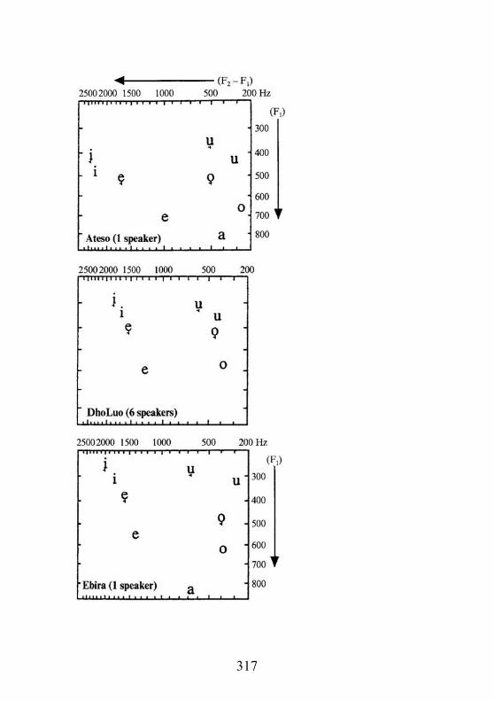
317

FIGURE 6.10 Average formant frequencies for the vowels ofsix African languages which distinguish [+ ATR] and [-ATR] vowels. These plots were constructed in the same wayas the plot of Swahili vowels in Figure 6.8. The [+ ATR]vowels are picked out by the subscript diacritic FromLadefoged and Maddieson (1996).

than F2 is plotted on the horizontal axis. Although the axesare labelled in Hz, they are scaled according to the Bark scale.

318

Without exception, each [+ ATR] vowel is higher (i.e. haslower F1 frequency) than its [- ATR] counterpart on theseplots. Another feature which requires mention is thesomewhat centralised position of the [+ ATR] back roundedvowels, most frequently /u/ but also /o/. Ladefoged andMaddieson suggest that centralisation of these vowels relativeto their [- ATR] counterparts might be diagnostic of ATRcontrasts. This would contrast with the situation in languagessuch as English or German, which distinguish vowels whichare conventionally transcribed with the symbols /u/ (as infood) and (as in good). (The /u/- contrast is often said tobe similar to the [± ATR] -/u/ contrast.) It should be bornein mind, however, that any apparent centralisation of [+ ATR]

and will be exaggerated by the practice of plotting(F2-F1) rather than F2 on the horizontal axis. (If F1 is loweredwhile F2 remains stable, the distance between F1 and F2 willincrease.) Also, it is possible that a vowel which isconventionally transcribed as /u/ may be equally centralisedin a 'non-ATR' language. Southern British English (where thevowel /u/ found in words such as food is coming to bepronounced as a central vowel, especially among youngerspeakers) would be a case in point. Thus, it is doubtful that acentral position of vowels transcribed as /u/ and/or /o/ relativeto vowels transcribed as and/or can really be taken asdiagnostic of a system with a [± ATR] contrast.

The question remains as to whether there is any featureintrinsic to the spectra of [+ ATR] vowels which serves todistinguish them from their f- ATR] counterparts. Such afeature may be related to perceived voice quality. A numberof linguists who have worked on ATR languages' havereported that the two types of vowels typically exhibit

319

distinctive voice qualities, the [+ ATR] type sounding more'hollow' or 'breathy' than its [- ATR] counterpart.

The ATR contrast in Kwawu (an Akan language) has beenstudied from this point of view by Hess (1992), who reportsthat, at least for the speaker she studied, the most consistentdifference between [+ ATR] and [- ATR] vowels lies in thebandwidth of the first formant, which is wider for the [- ATR]type. On the other hand, in a fuller study involving sixspeakers of another West African 'ATR language', Degema,Fulop (1996) found that the relative strength of F1 and F2served, at least in most cases, to distinguish between the twotypes, with F1 and F2 being closer in amplitude in the [- ATR]vowels.

Both types of differences are illustrated in Figure 6.11, whichshows two FFT spectra of the low-toned verbal prefix bèpronounced by a female speaker of another Akan language,Asante Twi. (This particle is pronounced with either a [+ATR] vowel or a [- ATR] vowel, in agreement with the vowelof the root it is attached to.) In the [+ ATR] version,transcribed /e/, the F1 peak is noticeably narrower than in the[- ATR] version, transcribed /ε/. At the same time, F1 and F2are closer in amplitude in the [- ATR] version.

Hess' and Fulop's proposals need to be tested on morespeakers of more languages before any firm conclusions canbe reached. A final point is that thewider bandwidth of the first formant appears to function as acue for nasalisation (Section 6.7.1). Since, at least in WestAfrica, many languages with ATR contrasts also make use ofdistinctive nasalisation, we must ask how the two dimensionsinteract. (In my experience, voice quality contrasts between

320

[+ ATR] and [- ATR] vowels are considerably more difficultto hear when the vowels in question are nasalised.) This is aquestion for future research. A thorough investigation of theproblem might shed more light on the nature of acoustic cuesfor nasality as well as on the natures of cues for the [± ATR]contrast.

FIGURE 6.11 FFT spectra of the vowels /e/ ([+ ATR]) and /ε/([- ATR]) pronounced by a female speaker of Asante Twi.

321

The spectrum of Itl illustrates two reported characteristics of[- ATR] vowels: (1) a broader and less well-defmed F1 peakand (2) a smaller difference in amplitude between F1 and F2.

6.7.3 Rhoticity and pharyngealisation

Rhoticised vowels are defined by their perceived R-likecharacter. They are found in only a few languages, but, sinceone of those languages is American English, they have beenthe subject of a number of investigations.

American English has one phonemic rhoticised vowel, whichis found in words such as bird, fur and heard, and iscommonly symbolised . The most obvious acousticcharacteristic of this vowel is its markedly low F3, a featurewhich it shares with consonantal /r/ in both American andSouthern British pronunciations (Section 7.8.4 and Figure7.18). Presumably it is the low position of F3 which gives thisvowel its distinctive character. If the spectral integrationhypothesis (Section 6.4) is correct, then is highly unusualin showing a strong peak, resulting from integration of F2 andF3, in the middle of the range of possible F2 values. In theclassification scheme of Section 6.5, stands out as uniquebecause of the lack of integration of F4 and F3.

Interestingly, lowered F3 has also been reported ascharacteristic of pharyngealised vowels (Catford 1983;Ladefoged and Maddieson 1996). The effects ofpharyngealisation on the spectra of vowels, and the nature ofsimilarities and differences between pharyngealisation andrhoticity are also interesting topics for future research.

322

6.8 Diphthongs

Diphthongs are vowels which change in quality. Inimpressionistic transcriptions, it is standard practice torepresent diphthongs as a sequence of two vowels, onecorresponding to the starting position and one to the endingposition. For example, the diphthong of English buy iscommonly transcribed /aI/. On spectrograms, we typically seea smooth and gradual transition from one quality to another.An example is the spectrogram of buy shown in Figure 6.12.

Te extent to which languages vary in their realisation ot thesame diphthongs remains a matter for further study. In theexample of Figure 6.12, there are two identifiable steadystates, corresponding to the /a/ and I/I/portions of thediphthong and a relatively quick transition between them. It isalso possible for diphthongs to occur in which the transition isrelatively longer, taking up a greater portion of the whole.Correspondingly, the steady states are relatively shorter insuch cases (Lindau et al. 1990). A historical overview ofproposals for describing and classifying the diphthongs ofAmerican English, which could be extended to diphthongs inother languages, is provided by Gottfried et al. (1993).

6.9 Alternative approaches to vowelquality

From the beginning in this chapter, we have assumed thatformant frequencies are the primary determinants of vowelquality. We have suggested that the three major articulatorydimensions of vowel classification (height, backness and

323

rounding) might correspond to two dimensions of acousticclassification, namely effective F1 and effective F2. For thesecondary articulatory dimensions (nasalisation, ATR,rhoticity, pharyngealisation), additional dimensions appear tobe necessary. It is possible that these secondarycharacteristics are associated with other types of cues. Forexample, nasalisation might be associated with abroadening and flattening of the spectral peak correspondingto F1. Another possibility is that three spectral peaks need tobe taken into account rather than two. For example, retroflexand pharyngealised vowels might be accounted for by a thirdacoustic dimension corresponding to effective F3.

FIGURE 6.12 Spectrogram of English buy (/baI/),pronounced by a male speaker. In this example, it is possibleto pick out sections corresponding to the /a/ and /I/ portions,and a transition which links the two. Some movement of theupper formants is visible following the release of /b/; this

324

represents the transition from consonant to vowel (Section7.2.1).

This is not the only possible approach to the study of vowelquality, and in this section we shall take note of a fewalternatives. One possibility is that the overall spectral shapeis of primary importance. This is adopted as a workinghypothesis by Bladon and Lindblom (1981) in a well-knownarticle which attempts to quantify perceptual distancebetween vowels by evaluating the degree of overlap of theirauditory spectra. The idea that the overall shape of thespectrum as a whole is primary has also proved attractive tosome phonologists. A good example of this is the discussionof phonological 'elements' in Harris (1994). Harris' theorypostulates three primary elements I, A and U, all of which aredefined in terms of spectral shape templates. This is dippingfor I (prominence at both high and low frequencies), slopingdownwards to the right for U (prominence at low frequencies)and peaking in the centre for A.

All of the approaches discussed so far are similar in that theyfocus on the static, steady-state part of the spoken vowel.Another, still more radically different possibility is to focuson the dynamic characteristics of vowels, in particular theformant trajectories in CVC syllables. Unfortunately, only afew perceptual studies have involved manipulating the timecourse of formanttrajectories in synthesized words. A more common type ofexperiment involves the perception of 'silent centre' syllables,in which subjects are asked to identify syllables from whichthe central portions, containing the steady state of the vowel,have been removed. The fact that subjects do rather well insuch tasks indicates that listeners can make use of dynamic as

325

well as of static information about spectral structure - indeed,given that the spectrum of speech is constantly changing, itwould be surprising if listeners did not make use of suchinformation. Strange (1989a, 1989b) provides a goodoverview of studies based on this approach, which she termsdynamic specification.

6.10 The problem of normalisation

Nearly all of the vowel charts, and most of the examples,presented in this chapter have been based on male speakers.The problem of how to describe vowels becomes moredifficult when women's and children's voices are taken intoaccount. In general, women have higher formant frequenciesthan men and children have higher formant fequencies thanwomen. This is because women and children have smallervocal tracts. However, the magnitude of the difference alsovaries from vowel to vowel. For example, in a study based ondata from American English and Swedish speakers, Fant(1973: 87) reports an average female F1/ male F1 ratio of 30%for American English /æ/ but a corresponding ratio of only2% for American English Such differences are due to thefact that the relative length of the pharyngeal cavity(considered as a portion of the whole) is smaller in womenand children than in men (Fant 1973: Chapter 4).

The ability to abstract phonetic sameness from the diversitywhich exists across speakers is known as normalisation. Thetopic of normalisation is a complex one and may beapproached in a variety of ways. A distinction is sometimesdrawn between theories of intrinsic and extrinsic specificationof vowel quality. Intrinsic specification means that all

326

information necessary to identify a vowel is contained withinthe vowel itself. For example, Syrdal's (1985) and Syrdal andGopal's (1986) studies of American English vowels (Section6.5) had intrinsic specification as one of their main concerns.They argued that, when differences between pairs of formants(F1 and F2, F2 and F3, etc.) or between F1 and F0 were used toclassify vowels, differences between talkers were greatlyreduced. Accordingly, listeners might base their identificationof particular vowels on distances between effective formantfrequencies rather than on the effective frequenciesthemselves. Such a procedure, if it works, would eliminate theneed for normalisation, since differences between talkerswould be minimal.

By contrast, theories of extrinsic specification take it as giventhat the listener must adjust his or her vowel recognitionprocedures to the characteristics of the talker's voice. On thisview, the boundaries of the talker's vowel space must bedetermined as needed from the immediately precedingcontext. For example, hearing someone say hi (/haI/) wouldgive some clues as to what formant frequencies should beexpected for low central-to-back and high frontvowels. A good overview of intrinsic and extrinsicapproaches to the normalisation problem may be found inNearey (1989).

To conclude this section, we should note that normalisation isnot a serious problem for some theories of speech perception.In the Direct Realist approach, which argues that the listenerrecovers the talker's articulatory gestures directly, there is noneed to suppose that the listener must tune in to the talker'sF1-F2 space. In the case of exemplar-based models, it issupposed that vowels (and speech sounds generally) will be

327

recognised on the basis of their similarity to other vowelsstored in the listener's memory. The exemplars stored inmemory incorporate information about talker characteristicsas well as about phonetic identity. The fact that a new vowelis similar to other vowels produced by the same speaker aswell as to the 'same' vowel produced by different speakers,aids the listener in identification (Johnson 1997).

6.11 Predicting the structure of vowelsystems

It is common practice among linguists to think of vowels notjust as isolated segments but as members of a system ofcontrasts. For example, we might speak of 'the vowel systemof Southern British English' or 'the vowel system of ParisianFrench'. Certain systems are extremely common and othersrare or non-existent. For example, systems with fivecontrasting vowels of the type /i e a o u/ are found in manylanguages but no one has yet reported a language which has afive-vowel system consisting of /y φ λ It seems thatlanguages show a striking preference for vowels around theperiphery of the acoustic vowel quadrilateral, and it has longbeen supposed that this preference must reflect a tendency tomaximise perceptual contrast. According to the voweldispersion hypothesis, languages tend to disperse their vowelsin the perceptual vowel space in such a way as to make themmaximally contrastive; for example, the optimal three-vowelsystem would be /i a u/.

How can we test the hypothesis that vowel systems tend to bebuilt around maximal perceptual contrast? One way is to

328

develop a model to generate vowel systems based onmaximum dispersion of vowels within a perceptual vowelspace. For any given number of vowels, the model shouldpredict what the most common vowel system(s) should be;for example, the optimal three-vowel system would be /i a u/.If the predictions are correct, we have evidence to support thehypothesis. There are three prerequisites to carrying out suchan activity. Firstly, the space of possible vowels must bedetermined and each phonetic vowel quality must be defined.Secondly, it is necessary to be able to measure perceptualdistance. Thirdly, enough data must be available about vowelsystems from a wide variety of languages to enabletendencies to be picked out with confidence.

The most thorough investigations of this type have beencarried out by Liljencrants and Lindblom (1972) andLindblom (1986). In both cases, an articulatory model wasused to generate the total space of possible vowelarticulations. The main difference between the earlier andlater papers lies in the way in which perceptual distances werecalculated. In the earlier paper, distances were based ondifferences between formant frequencies. In the later paper, amore sophisticated method was used, based on comparisonsof entire spectra (see Section 6.8). A set of nineteenquasi-Cardinal Vowels, with formant frequencies appropriatefor a male speaker, was taken as the starting point. Two typesof transformed spectra were calculated, giving two separatebut similar sets of results. 'Systems' of 3, 4, 5, 6, and so on,vowels were selected in such a way as to maximise thedistance between all possible pairs in the system. Figure 6.13shows the optimal eight-vowel system predicted by one of thetwo sets of calculations.

329

FIGURE 6.13 Optimal eight-vowel system, as predicted byLindblom's vowel dispersion model. After Lindblom (1986).

In its preference for peripheral vowels, the model agrees wellwith data from actual languages, but there are somediscrepancies. The most serious of these is its preference forhigh 'interior' vowels, so that, for example, the seven-vowelsystem shows two vowels between [i] and [u] but nomid-central [ə], (Contrast the not uncommon Amharic systemof Figure 6.4.) The seven-vowel triangular system /i e ε a ou/ of languages such as Italian or Yoruba is not predicted.Nor, as Disner (1984) points out in her discussion of voweldispersion, do the calculations reflect a hierarchy observed innatural languages, whereby, of the three 'corner' vowels, /i/,/a/ and /u/, the last is most likely to be missing from aphonological inventory (/i/, /a/ > /u/). Still, despite suchproblems, Disner concludes that the agreement ofphonological systems with the model is extremely good and 'avowel dispersion theory correctly captures a principle

330

governing the distribution of vowels in natural language'(Disner 1984: 154).

One unavoidable practical problem which arises in evaluatingany predictions concerning vowel dispersion is the difficultyof relating the vowel qualities reported for actual languages tothe qualities used for the purposes of the model. This issue isimportant because it is only possible to test a model bycomparing its predicted systems with systems which areactually attested in languages. Two large-scale surveys ofvowel systems, by Crothers (1978) and Maddieson (1984)(only the first of which was available to Lindblom), are nowavailable, both based largely on published phonologicaldescriptions. Such descriptions report vowel qualities in termsof phonetic symbols rather than formant frequencies orspectra, and there is often variation in the qualities associatedwith particular symbols. This is well-illustrated by the vowelscommonly transcribed with the symbol u, which may havelow F2, close to F1 (as in Thai) or higher F2, more separatedfrom F1 (as in American - and also in Southern British -English or Amharic). Furthermore, as Maddieson (1997: 638)points out, the F1-F2 space may be smaller for languages withsmall numbers of distinctive vowels than for languages withlarge numbers of distinctive vowels. For example, the /u/ of alarge vowel system may be higher and more back and havemore extreme formant frequencies than the /u/ of athree-vowel system.

6.12 Summary

In acoustic studies of vowel quality, primary importance isattached to the frequencies of the vowel formants during the

331

steady state of the vowel. This reflects not only theimportance of formants in the source-filter theory of speechproduction, but also the probability that formants play a majorrole in vowel perception. A further reason for the emphasis onformants is the resemblance between acoustic vowel charts,based on plotting F1 frequency vs. F2 frequency, and theimpressionistic vowel quadrilateral. This resemblance hasmade it possible to use F1-F2 plots for descriptive linguisticpurposes. It has also raised questions about the relationshipbetween the dimensions of impressionistic vowel description,measurable acoustic characteristics of vowels, anddimensions of vowel perception.

The impressionistic description of vowels is based on thethree major dimensions of height, backness and rounding. Onan F1-F2 plot, the placing of a vowel in the F1 dimensionappears to depend primarily on its height, whilst its placing inthe F2 dimension depends both on backness and rounding. Asregards the other minor dimensions of vowel classification(nasalisation, ATR, pharyngealisation, rhoticity), these mayhave additional acoustic correlates which can be definedindependently of a vowel's placing on an F1-F2 plot. Forexample, nasalised vowels appear to be characterised by abroad relatively flat low-frequency peak (F1). More researchis needed in this area. In the past, phoneticians engaged indescriptive linguistic work tended to concentrate exclusivelyon measuring formant frequencies. However, now that digitalspeech analysis has made other types of measurements (forexample, formant bandwidths) easier, considerable progresscan be expected in the near future.

As regards vowel perception, the idea that vowel formantsmight define a two-dimensional perceptual vowel space has

332

proved to be an attractive one. In defining such a space, it isnecessary to use the effective formant frequencies,perceived by the listener, rather than the nominal formantfrequencies, which are what the techniques of speech analysisare designed to measure.

The hypothesized perceptual vowel space may also shed lighton more purely linguistic problems. One idea which has beenattractive is the vowel dispersion hypothesis, according towhich languages tend to disperse their vowels in theperceptual vowel space in such a way as to make themmaximally contrastive. We have also seen that the spectralintegration hypothesis might provide a basis for a system ofbinary features for vowels. However, more work needs to bedone with acoustic data recorded from actual languages (asopposed to models).

We have also seen that formant-based approaches to definingvowel quality are not entirely unproblematic. A majordifficulty is explaining normalisation, that is, how listenerstune in to the vowel spaces of particular speakers. The roleplayed by more dynamic aspects of vowels, in particular thetransitions to and from flanking consonants, also needs to beclarified.

Another area of interest for linguists is the possibility ofpredicting the structure of vowel systems. It has long beenobserved that languages show a preference for vowels whichare located around the periphery of the vowel quadrilateral.This has suggested the hypothesis that vowel systems must, asit were, be designed to maximise perceptual contrast. Variousstudies have attempted to determine the maximally dispersedvowel qualities for vowel systems of particular sizes (for

333

example, the optimal seven-vowel system). In general, theresults have been consistent with expectations, but someproblems remain. These reflect both the theoreticaldifficulties inherent in calculating perceptual distance and thepractical difficulties involved in relating theoretical systemsobtained by calculation to descriptions of vowel systemswhich report vowel qualities in terms ofimpressionistic-phonetic symbols.

6.13 Further reading

Borden et al. (1994), Clark and Yallop (1990), Denes andPinson (1993), Fry (1979), Johnson (1997), Kent and Read(1992), Lieberman and Blumstein (1988) and Pickett (1980)all provide introductions to vowel formants, vowel charts andvowel perception. Kent et al. (1996), devoted entirely toAmerican English, is also to be recommended. Ladefoged andMaddieson's work (1990, 1996) is the most comprehensivefrom a cross-linguistic point of view and includes discussionof vowels from a wide spectrum of languages. Rosner andPickering (1994) is a full-length and detailed work coveringboth production and perception, and includes a very fullbibliography. Stevens (1998) includes an excellent account ofproduction and perception, with a focus on acoustic aspects.

Measuring vowel formants can be more difficult than mostelementary introductions suggest. Ladefoged (1967) andLadefoged and Bladon (1982) are excellent discussions of thepractical difficulties involved in measuring vowel formants.Ladefoged (1967) also includes an account of the history ofvowel classification.

334

335

Chapter 7The acoustic description ofconsonants7.1 Introduction

From the point of view of acoustics and perception,consonants present more difficulties than vowels. It is noaccident that the debate about the specialness of speech(Section 5.2.3) has centred around evidence concerning theperception of consonants. There are two main reasons for this.

Firstly, vowels contain more information about themselveswithin themselves. In Chapter 6, we saw that any vowel canbe located in a two-dimensional vowel space on the basis ofinformation derived from its formant pattern. The formantpattern is an inherent part of the vowel itself, and it exists allat once during the time when the vocal organs are in the targetposition for the vowel. By contrast, it is common for essentialinformation about a consonant to appear in the acoustic signalbefore and/or after the vocal organs have assumed the targetposition for the consonant. For example, in the English wordsspy, sty and sky, the target positions for the stop consonants(/p/, /t/ and /k/) - in which there is a complete closure in themouth and the vocal folds are not vibrating - will correspondonly to silence in the acoustic signal. In order to distinguishbetween the three stop consonants (and the three words), it isnecessary to attend to the transitions to the following vowel

336

(/aI/). Because information relevant to individual consonantsoverlaps with preceding and following speech sounds, it is notpossible to divide the acoustic signal up into neat segments,each complete in itself.

Secondly, the basic dimensions of the two-dimensional vowelchart are of the same type (they are based on frequency), andconsequently are measured in the same units such as Hz orBark. A two- or three-dimensional plot based on formantfrequencies would be a straightforward and obvious visualdisplay, even if it did not correspond so closely to theimpressionistic vowel quadrilateral. By contrast, any acousticclassification of consonants must bring together a number ofacoustic dimensions of different types, including not onlyfrequency but also intensity and timing. Different acousticdimensions are relevant in different cases. There is no simpleand obvious way of converting acoustic measurements intogeneral charts for consonants and there is no commonlyaccepted consonantal counterpart to the F1-F2 plot used forvowels.

Because of the great variety of consonants found in theworld's languages and the great variety of acousticdimensions which play a role in describing and classifyingthem, it is not possible to give a complete account of theacousticsof consonants in a short chapter. Since English is thebest-studied language as regards the acoustics and perceptionof consonants, the discussion here will be largely (though notexclusively) concerned with English sounds. We shall alsoconcentrate on single consonants between vowels.

337

7.2 General concepts

7.2.1 Intervals and transitions

The production of any consonant involves contact or at leastclose approximation between two articulators at some 'place'between the larynx and the lips. This constriction ismaintained for a certain length of time, and will haveparticular acoustic consequences. For example, Figure 7.1shows the /ʃ/ of English a shark. The strong band of noisyenergy, which fills the upper part of the spectrogram (aboveabout 1500 Hz), represents the audible friction which isgenerated during the period of constriction. We shall refer tothe time corresponding to the constriction as the constrictioninterval.

FIGURE 7.1 Spectrogram of English /ʃ/ in the sentence Wesaw a shark, pronounced by a male speaker.

338

A consonantal constriction does not just happen; thearticulators must move into their target position and thenmove away to the target position for the following sound.When a vowel precedes or follows, these movements will bereflected in movements of the vowel's formants from or totheir steady-state values. These movements are known as theformant transitions. In the case of the vowel /a/ of shark inFigure 7.1, the movements of F2 and F3 (the F2transition and the F3 transition) can be seen clearly at theonset of the vowel. Similar, though not identical, transitions,moving in the opposite direction, can be seen at the end of thepreceding vowel /ə/. Of course, if there is no preceding orfollowing vowel - for example if the consonant occurs after orbefore a pause - there will be no corresponding transitions.

Finally, we must consider the activity of the vocal folds andits acoustic consequences. If the consonant is voiceless theconstriction interval will be accompanied by a voicelessinterval, when the vocal folds are not vibrating and nolow-frequency striations will be visible on the spectrogram(see Section 5.2.1). In our example /ʃ/, the constrictioninterval and the voiceless interval nearly coincide (thoughthere is a slight gap between the end of the friction and theonset of voicing for the /a/). In the case of aspiratedconsonants, the voiceless interval extends beyond theconstriction interval, resulting in a long Voice Onset Time(Section 5.2.1).

339

7.2.2 Acoustic dimensions in the description andclassification of consonants

We have already noted that, in contrast to vowels, theacoustic description of consonants depends not only on whathappens during the constriction interval itself but also onwhat immediately precedes or follows. To begin, I shall listthree general types of acoustic information which arerelevant, both within and outside the constriction intervalitself.

1. Presence or absence of aperiodic energy. Forexample, aperiodic energy which may be continuousnoise or transient (Section 2.3) - during theconstriction interval distinguishes obstruentconsonants (stops, fricatives and affricates) fromvoiced sonorants. Presence of continuous noisefollowing the interval, overlapping with the formanttransitions, is characteristic of aspirated (as opposedto unaspirated) consonants.1

2. Timing. For example, voiced obstruents tend to haveshorter constriction intervals than voicelessobstruents. Outside the constriction interval, acontrast between quick and gradual formanttransitions is important in distinguishing betweensemivowels on the one hand and voiced stops andnasals on the other (for example, [w] vs. [b] and [m]).

3. Spectral structure. For example, the nasal [n] and thelateral [1], which have some general characteristics incommon, show differences in their spectra during theconstriction interval. Outside the interval, for allconsonants the starting points and trajectories of the

340

formant transitions (both preceding and following)play a major role as cues for place of articulation.

All three of the main acoustic dimensions just mentioned(presence vs. absence of aperiodic energy, timing, spectralstructure) are necessary to define the impressionistic-phoneticcategories of place of articulation, manner of articulation andvoicing in acoustic terms.

7.2.3 Acoustic boundaries and consonants

Another way of approaching the description of consonants, atleast when they occur before vowels, is to compare thespectrum of the interval sound with the spectrum of the onsetof the following vowel. For example, to compare /ʃ/ with /a/in Figure 7.1, we should note that the lower edge of the bandof noise in /ʃ/ (just below 2000 Hz) is at roughly the sameheight at the onset of F3 for /a/. The darkest part of the band(just below 3000 Hz) is between F3 and F4.

The general hypothesis behind this approach is that theacoustic boundary between consonant and vowel is ofparticular importance for the listener. It is at acousticboundaries that abrupt changes occur in the spectrum towhich the auditory system may be particularly sensitive(Section 5.3.4). To quote Stevens (1985b: 253), 'Either theacoustic correlates of phonetic features consist ofspecification of how the spectrum is changing in this region,or the region provides a landmark that indicates where nearbyspectral or temporal information is to be sampled.'

341

I shall now give an overview of the acoustic characteristics ofvarious types of consonants, organised according to mannerof articulation.

7.3 Stop consonants2

7.3.1 General characteristics of stop consonants

During the production of stop consonants, there is a completeclosure somewhere in the vocal tract, cutting off the airstreamfrom the lungs. The soft palate is raised, so that air cannotescape through the nasal cavity. If the vocal folds are notvibrating, no sound will be produced at all, resulting in aperiod of silence. On the other hand, during the closureperiod, air pressure is building up behind the closure. If avowel immediately follows, release of the closure will beaccompanied by a brief burst of noise, appropriately known asthe burst. Stop consonants may also show release bursts whenthey occur before a pause or before another consonant, thoughthis will vary depending on the language, the speaker and thespeaking style.

The constriction interval for a stop consonant, accordingly,consists of silence or near-silence. It is often referred to as thesilent interval or the stop gap. The interval ends with therelease of pressure at the burst. This is generally easy tolocate on a spectrogram, because it corresponds to a briefvertical spike, though it is weaker for labials than for otherplaces of articulation. In contrast, the beginning of theinterval is often difficult to locate precisely. This is notsurprising when we remember that, unlike the burst, theblocking of the airstream is not a sudden event but occurs

342

more gradually as the articulators come together. Also,although the articulators are together and the soft palate israised, the seal may not be absolutely complete. Accordingly,some acoustic energy may be visible (as faint shading) duringthe interval itself. These general characteristics are apparentin the stop consonants illustrated in Figures 7.2-7.4.

FIGURE 7.2 Spectrogram of the Javanese word papat 'four',pronounced by a male speaker from East Java.

7.3.2 Voicing and aspiration

Any account of voicing in stop consonants runs the risk ofconfusing the reader because the terms voiced and voicelessare used in two distinct ways. On the one hand, they may beused as phonetic terms to designate presence or absence ofvocal fold vibration during the consonantal interval. On theother hand, they may be used to refer to opposed members ofa phonological contrast which might or might not be

343

pronounced as their labels suggest. For example, English /b dg/ are usually described as 'voiced stops' in opposition to'voiceless' /p t k/ even though they may be produced withoutany vocal fold vibration during the closure. As in Section 5.2,I shall use voiced and voiceless as phonetic terms. When theterms are used in a more abstract, phonological way (as whenreferring to the contrast between English /p t k/ and /b d g/), Ishall use [- voiced] and [+ voiced].

To illustrate voiceless unaspirated and fully voiced stops, Ishall draw examples from languages other than English.Figure 7.2 shows a spectrogram of the Javanese word papat'four', pronounced by a male speaker from East Java. Thespeaker paused both before and after the word, which waspart of a counting sequence, and so there is no indication ofwhere the constriction interval begins for the first /p/ or ofwhen the constriction interval ends for the final /t/, which isunreleased. The bursts of the two /p/s, which are voicelessand unaspirated, are clearly visible, though the first issomewhat stronger than the second. The gap corresponding tothe second /p/ is also clear, though it is somewhat difficult tosay exactly where it begins. Similarly, it is difficult topinpointthe beginning of the constriction interval for the final /t/. Inthis particular instance, the end of the bars corresponding tothe higher formants was taken to be the end of the vowel.

344

FIGURE 7.3 Spectrogram of Italian /d/ in the sentence Dicodata cosi, pronounced by a male speaker from Sardinia.

For fully voiced stop consonants, a low-frequency voice bar(Section 5.2.1) can be seen throughout the constrictioninterval. An example is shown in Figure 7.3, which shows the/d/ of Italian data 'date' extracted from the phrase dico data 'Isay data', pronounced by a male speaker from Sardinia. Thevoice bar is darker at the beginning than at the end of theconstriction interval. This reflects a general tendency forvoicing to weaken and become more breathy in character overthe course of the interval. Indeed, it is not uncommon for thevoice bar to fade out altogether before the interval comes toan end. (The reasons for this will be discussed in Section8.3.9.) Thus, even fully voiced stops may appear to be slightlyaspirated. In my experience, such fading out is often lessmarked and is less commonly observed in absolute initialposition. (In this regard, the /d/ of Figure 7.3 may becompared with the initial /d/ of Figure 5.2.) As already

345

mentioned (Section 5.2.1), the English [+ voiced] stops /b/,/d/ and /g/ are frequently produced without voicing inabsolute initial position.

It remains to give an example of an intervocalic voicelessaspirated stop. Figure 7.4 shows an example of Englishaspirated /k/ in a car. Here, the burst stands out as a darkspike at the beginning of the aspiration noise. In this case, thetransitions can be seen as darker bands in the aspiration noise;by the time the striations appear, they have nearly reachedtheir steady-state values. The spectrogram of English tore inFigure 5.1 provides an example of an aspirated stop inabsolute initial position.

FIGURE 7.4 Spectrogram showing the English aspirated /k/in the sentence We bought a car.

To sum up, prototypical stop consonants are definedacoustically by a constriction interval of silence which

346

typically ends with the burst. The voiceless unaspirated andaspirated types differ in that, in the unaspirated case, thevoiceless interval comes to an end at about the same time asthe constriction interval, with the voicing for a followingvowel beginning immediately after the release. If there isaspiration, the voiceless interval extends beyond theconstriction interval, overlapping with the formant transitionsfor the following vowel. In the case of fully voiced stops, theconstriction interval is not totally silent, since the vocal foldscontinue to vibrate. Low-frequency striations, known as thevoice bar, will be visible.

7.3.3 Place of articulation

It should be clear that no information about place ofarticulation can be contained within the stop gap. Even if avoice bar is present, its acoustic character will not differ fromone place of articulation to another. The two most obviouspotential acoustic cues for place of articulation in stops are (1)the spectrum of the burst and (2) the transitions to thefollowing vowel. Perceptual experiments have shown thatboth of these may indeed function as cues. However, bothhave been problematic as regards lack of invariance (Section5.2.2).

7.3.3.1 Stop bursts

Typical examples of bursts for labial, alveolar and velarplaces of articulation are illustrated in Figure 7.5. This showsspectrograms for the three English

347

FIGURE 7.5 Spectrograms of the English words bib, did andgig, pronounced by a male speaker. The bursts for /b/ and /d/are said to be 'diffuse', with energy spread out over a widerange of frequencies. By contrast, the bursts for /g/ are more'compact', with energy concentrated in the middle of thefrequency range. This is especially true for the /g/ in finalposition. The F2 and F3 transitions have been highlighted.Notice that both transitions are rising for /b/ but are morenearly level for /d/. The F2 and F3 transitions for /g/ converge,forming a wedge-like shape.

348

349

FIGURE 7.6 (opposite) Design (a) and results (b) of a classicexperiment on the perception of place of articulation in stopconsonants (Liberman et al. 1952). Twelve bursts, ranging infrequency from 360 Hz to 4320 Hz (A), were paired withtwoformant versions of seven vowels (B), to give 84 CVsyllables (as in C). Listeners were asked to identify the initialconsonant of each syllable as /p/, /t/ or /k/. The graph of (b)shows the dominant responses for each CV combination.Syllables with high-frequency bursts are uniformly identifiedas beginning with /t/. The lower part of the graph is, as itwere, shared by /p/ and /k/. Notice that /k/ responses (slantedlines) dominate where the burst frequency is close to the F2 ofthe following vowel.

words bib, did and gig. The final consonant is released in allcases. Thus, there are two bursts for each consonant: one inword-initial position and one in final position before pause.There are several points to notice:

1. The bursts for /b/ are weaker than those for /d/ or /g/;the spike corresponding to the final /b/ is particularlyfaint.

2. The burst for final /b/ also shows somewhat moreenergy in the lower part of the frequency axis, andbecomes particularly faint at the top of the display.

3. The bursts for /d/ have more energy at highfrequencies than /b/ or /g/; both initially and finally,the spike is quite dark around 4000 Hz, and for theinitial /d/ the darkness extends up to the top of thedisplay (5000 Hz).

4. The bursts for /g/, especially pre-pausal /g/, show aconcentration of energy in the middle of thefrequency axis. For this reason, velars are sometimes

350

characterised as compact (following Jakobson et al.1952). By contrast, labials, dentals and alveolars aresaid to be diffuse because the energy in the burst isnot so concentrated in a particular frequency region.

5. There is a difference between the initial /g/ and thepre-pausal /g/. For the initial /g/, the darkest area ofthe burst is around 2500 Hz, and there is alsonoticeable energy at higher frequencies. This makesthe spectrum less compact since the energy spreadsout, as it were, beyond the middle frequencies. Forpre-pausal /g/, the darkest part of the burst is lower infrequency (around 2000 Hz) and there is little energyabove 3000 Hz. In fact, the burst of the pre-pausal /g/is more typical for the velar place of articulation. Thecharacter of the initial /g/, which has a more forwardplace of articulation, is due to the influence of thefollowing front vowel.

Although the spectrum of a stop burst may be quite diffuse, itis possible to imitate stop bursts in synthetic speech using anarrower burst of noise. The earlist perceptual studies of stopbursts used this method. In a classic study carried out atHaskins Laboratories, Liberman et al. (1952) synthesised aseries of CV syllables with simple noise bursts andtwo-formant vowels. The basic experimental design isillustrated in Figure 7.6 (a). There were twelve bursts, rangingin frequency from 360 Hz to 4320 Hz. Although the stylisedspectrograms of the stimuli might appear quite crude incomparison with real spectrograms, listeners were able tohear the stimuli as the intended CV syllable and toclassify the initial stop consonants as /p/, /t/ or /k/. The resultsare shown in Figure 7.6 (b). As might be expected,high-frequency bursts (above about 2800 Hz) were heard as

351

/t/. However, the lower part of the diagram is, at it were,shared by /p/ and /k/. One general rule which emerges is thatif the burst is near to the F2 frequency of the vowel, listenerswill tend to hear /k/. Nevertheless, the distribution oflower-frequency bursts between /p/ and /k/ is somewhatcomplicated. The results were regarded as encouragingbecause they showed that listeners could identify place ofarticulation on the basis of burst frequency alone. However,they were also seen as somewhat discouraging because therelationship between burst frequency and recognisedphoneme was less straightforward than expected.

7.3.3.2 Formant transitions

Formant transitions provide the second obvious potential cuefor place of articulation in stop consonants. It is easy toconfirm that stop consonants can be identified from theirtransitions alone. If you extract and play the sequence oftransition + vowel in a CV sequence beginning with a [+voiced] stop (such as in the words bay, day or gay), youshould have no difficulty in recognising the initial consonant,although the burst is missing. If the experiment is extended towords beginning with fricatives (such as say), you should findthat, if you hear only the transitions and the vowel, the wordin question sounds like it begins with a voiced stop as well.The transition + vowel part of say will sound like day.

Experiments with English native listeners have tended toconcentrate on the [+ voiced] stops (/b/, /b/ and /g/) sinceaspiration typically overlaps with the transitions in voiceless/p/, /t/ and /k/ (Figure 7.4). Transitions are generally describedwith reference to CV sequences. For example, if we say that

352

labials are associated with rising F2 transitions, we mean that,in a syllable such as bee (/bi/), F2 rises from consonant tovowel. It is understood that VC transitions (as in (b)ib) will bethe mirror image of the corresponding CV transitions thoughthe rate of formant movement may be different.

At least for places of articulation located in the mouth (asopposed to the pharynx), F1 will rise in CV transitions. This isin line with theoretical considerations which suggest thatduring a stop closure in the oral cavity, F1 should be 0.However, F2 and F3 may vary considerably with place ofarticulation. This is obvious in Figure 7.5. F2 and F3 risesteeply for the initial /b/ fo bib, but rise only very slightly forthe initial /d/ of did. For the initial /g/ of gig, F2 is falling, butF3 is rising, so that the two come together in a wedge-likeshape. The situation begins to appear more complicated whenother vowels are taken into account. This is evident if wecompare Figure 7.5 with Figure 7.7, which shows bursts andformant transitions extracted from the beginnings of thewords barb, dart, and guard (/bab/, /dat/, /gad/). This time, theF2 transition for /b/ is more level (though the F3 transition isstill rising). For /d/, the F2 transition falls steeply until itreaches the appropriate level for the steady stateof the vowel /a/. The F3 transition is less clear, but it is morelevel. For /g/, the transitions resemble those of gig in Figure7.5 in that F2 and F3 appear to start from the same point, theone falling and the other rising. However, the starting point islower than for the transitions of gig. It is also useful tocompare the /g/ of guard with the /k/ of car in Figure 7.4. Inthese two words, the burst and the transitions are very similar,though the transitions for the /k/ show up less well in theaspiration noise. The transitions for the /k/ of car appearslower, but this is because of the expanded time scale.

353

FIGURE 7.7 Spectrogram showing bursts and formanttransitions extracted from the English words barb, dart andguard, pronounced by a male speaker. As in Figure 7.5, the F2and F3 transitions have been highlighted. Notice that, incontrast to the examples of Figure 7.5, the F2 transition for /b/is nearly level while the F2 transition for /d/ is falling. Thetransitions for /g/ are similar to those of Figure 7.5 in that theF2 and F3 transitions converge, forming a wedge-like shape.

In general, for labial stops (/p/ and /b/), F2 and F3 transitionsare level or rising. In the case of F2, the rise is steepest whenthe following vowel is a front vowel with high F2 (as in bib)and most nearly level when the following vowel is a backvowel with low F2 (as in barb). For velar stops (/k/ and /g/),the F2 transition commonly begins just above the vowel'ssecond formant and falls; the F3 transition begins at about thesame point and rises, giving a distinct wedge-like shape asillustrated both in gig (Figure 7.5) and in guard (Figure 7.7).For alveolar stops (/t/ and /d/), the F2 transition will generallybe level or rising for front vowels (as in did, Figure 7.5) but

354

falling for back vowels (as in dart, Figure 7.7). The F3transition will typically be level or falling. These generalpatterns were noted for spectrograms of natural speech byPotter et al. (1947). Early studies on the synthesis andperception of formant transitions focussed on the role of F2.

The behaviour of F, transitions for /d/ is elucidated by theconcept of locus. The locus is 'a place on the frequency scaleat which a transition begins or to which it may be assumed to"point"' (Delattre et al. 1955: 769 n. 3). The qualificationabout 'pointing' is necessary because, in the case of stopconsonants, the very beginnings of the transitions -corresponding to the beginning of the tongue's movementtoward the position for the following vowel - are not visibleon spectrograms.

The locus is essentially determined by the location of theclosure (place of articulation). For example, in pronouncingthe words dart and did, the tongue starts from roughly thesame position but moves in different directions. Since the F2(and other) transitions reflect tongue and jaw movement, wemight expect that they would start from the same position onthe frequency axis but move in different directions. In thecase of alveolar stops (/t/ and /d/), the F2 locus is generallyaround 1800 Hz, at least for male speakers, and does not varyfrom vowel to vowel. Accordingly, if the vowel F2 is above1800 Hz (as in did), the transition will be rising, but if thevowel F2 is below 1800 Hz (as in dart or door), the transitionwill be falling.

The concept of locus may also be applied to bilabials, whichappear to have a locus in the region of 700-800 Hz. This fitsin well with the observation that the F2 transition rises steeply

355

before front vowels but only a little or not at all before backvowels. The situation is less straightforward for the velars (/g/and /k/). As we have just noted, the F2 transitions for velarsare generally falling (but not steeply falling), no matter whatthe identity of the following vowel. This reflects the tendencyfor the precise location of tongue contact for velars to varyaccording to the tongue position for the following sound.

In fact, the F2 transitions for /g/ and /d/ may be quite similarbefore low vowels. This is certainly the case in our examplesdart and guard (Figure 7.7), though the F3 transitions are quitedifferent. Accordingly, we might expect that the F3 transitionwould play a crucial role in distinguishing between the twoplaces of articulation. This was confirmed in another series ofexperiments reported in Harris et al. (1958).

Perhaps the best known of the perceptual experiments carriedout at Haskins is one described by Liberman et al. (1957),which demonstrated that listeners could distinguish between/b/, /d/, and /g/ on the basis of the F2 transition alone. It wasalso shown that, if the F2 transition was varied whileeverything else was held constant, listeners would perceivethe place of articulation contrast categorically (Section5.2.3.1). This is probably the most frequently cited exampleof categorical perception.

7.3.3.3 Spectral templates as invariant cues

When individual cues to place of articulation such assimplified bursts or F2 transitions are studied one at a time,the patterns which emerge are quite complicated. This ismainly because the same bit of acoustic information will be

356

interpreted differently for different vowels. This acousticvariability in theface of evident articulatory sameness was a major inspirationfor the development of the Motor Theory (Section 5.2.4.1).As an example, we may quote Liberman et al. (1967: 438),discussing the concept of locus for alveolars:

Though the locus can be defined in acoustic terms - that is, asa particular frequency - the concept is more articulatory thanacoustic ... What is common to /d/ before all the vowels isthat the articulatory tract is closed at very much the samepoint... it seems clear that though the locus is more nearlyinvariant with the phoneme than is the transition itself, theinvariance is a derived one, related more to articulation thanto sound.

Other researchers have been less pessimistic about theprospect of finding invariant cues for articulatory place, andhave taken the view that such cues do indeed exist. However,it is necessary to approach the problem in a somewhatdifferent way. Consider, for example, the velar stops (/k/ and/g/). It is usually easy to recognise these visually on aspectrogram. The F2 and F3 transitions typically start fromabout the same point and diverge, and this starting frequencyis generally close to the burst frequency. Thus, the burst, theF2 transition and the F3 transition all converge, as it were,into a small section of the frequency axis, resulting in thecompact type of spectrum (Figures 7.5, 7.7). However, it isdifficult to arrive at a notion of compactness if we study theeffects of varying burst frequency, the F2 transition and the F3transition one at a time and look for invariance in each one.

357

One way of giving formal explicitness to a notion such ascompact spectrum is to develop a model shape, or template,with which actual spectra can be compared. This approach isparticularly associated with the names of Kenneth Stevensand Sheila Blumstein. Their methodology has involvedanalysing LPC spectra (Section 4.5) with high-frequencypre-emphasis (Section 3.2.4), taken for a short (about 25msec) time window beginning at the release burst. ForEnglish /b/, /d/ and /g/, the window generally includes thestart of the formant transitions, whereas for /p/, /t/ and /k/, itdoes not.

Stevens and Blumstein's approach is illustrated in Figure 7.8.The spectra of alveolars should fit into a diffuse-risingtemplate, while those of labials should fit into adiffuse-falling or diffuse-flat template. The spectra for velarsshould fit into a compact template. For the diffuse types(labial and alveolar), the templates are defined by a pair ofdashed lines, which should, as it were, contain the outline ofthe spectrum. In the case of velars, a prominentmid-frequency peak must dominate the spectrum. It should bestressed here that the templates are intended to be valid acrossall vowel contexts. The approach is said to be based onintegration of cues because information from the burst andinformation from the beginning of the transitions bothcontribute to the spectrum which is compared with thetemplate.

The original templates of Stevens and Blumstein might betermed static in that only one template, unchanging over time,is said to be necessary to define each articulatory place. Otherresearchers have argued that templates should be defined in a

358

more dynamic way. Thus, Kewley-Port (1983) argues that, ifa

359

FIGURE 7.8 (opposite) Templates developed by Stevens andBlumstein to classify spectra as diffuse-rising (alveolars),diffuse-falling (labials) or compact (velars). The two panels tothe right of each template show one spectrum which fits thetemplate (above) and one spectrum which does not (below).For the diffuse-rising template, an arrow pointing to the rightfrom 2200 Hz (just above 2 kHz) indicates that, whencomparing a spectrum with the template, a spectral peakabove 2200 Hz must be made to coincide with the upperreference line. The remaining lower-frequency peaks mustthen fall between the reference lines. For the diffuse-fallingtemplate, there must be one peak between the reference linesin region (a) (1200-2400 Hz) and one peak in region (b)(2400-3600 Hz). For the compact template, a prominentmid-frequency peak must fit entirely within one of thecontours of the template. From Stevens and Blumstein (1981).

spectrum is to be classified as compact, it must not only havea mid-frequency peak at the moment of the burst, but also thatthe peak must extend over a time interval of about 20 msec.This would be true of both the /g/ of Figure 7.5 and the /g/ of

360

Figure 7.7, where the central dark band of energy in the burstpersists into the start of the F2 and F3 transitions.

Although spectral templates have seemed to work well for thethree-way contrast between labials, alveolars and velars inEnglish, there have been some problems in extending theapproach to more complicated systems of contrasts. In across-linguistic study, Lahiri et al. (1984) found that the burstspectra of dentals could appear very similar to those oflabials, and it did not seem possible to distinguish betweenthem by means of spectral templates. Such results suggest thata more sophisticated notion of invariance is needed. Theirproposal is that invariance is both dynamic and relative.Dynamic here refers to change through time. What matters isthe way in which the spectrum changes across the acousticboundary from the release burst to following vowel (as in theproposed definition of compact just mentioned). Relativerefers to a comparison between the lower and upper parts ofthe spectrum. In the typical case, there is an increase inenergy overall from burst to vowel onset. For dentals andalveolars, most of this increase involves the lower part of thespectrum whereas, for labials, the amount of change is moreevenly split between the two. For example, in thespectrograms of barb and dart shown in Figure 7.7, the burstfor /b/ is very weak, so that there is a large increase inintensity (darkness) at vowel onset for all frequencies. Bycontrast, the burst for /d/ shows a good deal of energy at highfrequencies, so that there is little if any increase in intensity(darkness) at vowel onset in the upper part of the frequencyrange, though there is a noticeable increase in the lower part.

To sum up, the problem of identifying cues which may beutilised by listeners to identify the place of articulation for

361

stop consonants is a difficult one. Three main cues have beenextensively studied: the frequency of the burst, the F2transition and the F3 transition. When these are investigatedindependently, the relationship between the acoustic signaland the corresponding speech sound (phoneme) appears to behighly variable. Alternative approaches have focussedon the overall spectrum in the neighbourhood of the burst andon changes across the acoustic boundary between a consonantand its adjacent vowel. These have been more successful inidentifying characteristics which might serve as invariantcues.

A good overview of work on place of articulation up to theearly 1980s is Syrdal (1983).

7.4 Fricatives

The rasping sound associated with fricative consonants is dueto turbulent air flow, which occurs when the airstreamemerges from the narrow constriction formed by thearticulators. Accordingly, fricative consonants are definedacoustically by constriction intervals which are filled withnoise rather than with silence. A good example is provided bythe spectrogram of English /ʃ/ shown in Figure 7.1.

In the IPA chart, fricatives are classified using the twodimensions of place of articulation and voicing. It might beexpected that each place should be associated with its owncharacteristic pattern of spectral peaks and valleys, rather aseach vowel has its own characteristic formant pattern. Theone exception is the glottal fricative [h]. This is because [h]does not involve any special positioning of the vocal organs

362

above the larynx. The peaks and valleys in the spectrum ofany particular [h] will generally match those of following orpreceding vowels. In the case of intervocalic [h] betweenvowels which differ in quality, a gradual change in formantstructure, linking the preceding and following vowels, isgenerally observed during the consonantal interval.

In addition to spectral shape, fricatives differ from oneanother in relative intensity and in the nature of their formanttransitions. Relative intensity is particularly important fordistinguishing between sibilant and non-sibilant fricatives; inEnglish, for example, sibilant /s/ and /ʃ/ are clearly moreintense than non-sibilant /f/ and /θ/. As regards formanttransitions, these are similar in character to transitions for stopconsonants, and reflect the movement of the tongue and jawfrom the position for the fricative to the position for thefollowing vowel.

We have seen that the waveforms of voiceless fricatives areaperiodic, without any repeating pattern (Section 2.3).Accordingly, FFT spectra (Section 3.4.2) and LPC spectra offricatives are less stable than vowel spectra, and may varyconsiderably over even a small portion of the fricative. This isnot to say that an overall pattern is lacking - for example, inthe /ʃ/ of Figure 7.1, the overall visual impression is that thecharacter of the spectrum remains more or less constant overthe consonantal interval. In order to get the overall pattern toemerge, it is important to take as much of the consonantalinterval into account as possible. This means that narrow bandspectra are to be preferred to broad band spectra because theyuse a longer window (Section 3.4.2). A still better method isto average several spectra, taken over the course of the

363

fricative, though not all speech analysis software provides forthis possibility. Another point is that the spectra of fricatives -particularly [s] - may show prominent peaks above 5000 Hz.Accordingly, if fricatives are to be the object of study, it isimportant to use a higher sampling rate than 10,000 Hz(Section 3.4.1).

FIGURE 7.9 Averaged broad band spectra for the Englishvoiceless fricatives /f/, /θ/, /s/ and /ʃ/, extracted from thewords fight, thigh, sigh and shy, pronounced by a malespeaker.

Figure 7.9 shows a comparison of averaged broad bandspectra for the four non-glottal voiceless fricatives of English(/s/, /ʃ/, /f/, /θ/) produced by a single male speaker. In thiscase, the sampling rate was 22,000 Hz; frequencies up to10,000 Hz are displayed. (The glottal fricative /h/ is excludedbecause it does not have its own characteristic spectrum.)Notice that (1) /s/ and /ʃ/ are more intense than /f/ and /θ/; (2)

364

the main spectral peak for /s/ is higher in frequency than thatfor /ʃ/; and (3) /f/ and /θ/ are more diffuse in character, whilst/ʃ/ is more compact, with a prominent mid-frequency peak.Another difference which may be significant involves theslope of the overall spectrum; in this example, the curve for/ʃ/ rises steeply to its peak, while the curve for /s/ rises moregradually. A good discussion of the possible role of spectralslope in classifying sibilant fricatives may be found in Everset al. (1998).

It should also be mentioned here that the spectra of Englishfricatives vary considerably from speaker to speaker, so that,while the observations just made are generally valid, it wouldbe inappropriate to add more detail. At least for English, ithas seemed appropriate to describe fricative spectra in termsof the general categories we might apply to the spectra of stopbursts (diffuse vs. compact, high-frequency prominent vs.low-frequency prominent) rather than in terms of specificformant frequencies, as would be the case for vowel spectra.

As regards perception, fricatives have been much lesswell-studied than stops. A classic study on English /s/, /ʃ/, /f/and /θ/ was carried out by Harris (1958). She used naturallyproduced fricative + vowel syllables and also unnaturalsyllables, which she created by combining the fricative noisefrom one syllable with the transitions and vowel fromanother. The complete set of stimuli included all possiblenoise-transition combinations for five vowels. Her resultssuggested that there was a difference between sibilant andnon-sibilant fricatives (/s/, /ʃ/ vs. /f/, /θ/). Sibilant fricativescould be identified correctly even when they were paired withthe 'wrong' formant transitions. For the non-sibilants,however, the formant transitions played a more crucial role,

365

so that, for example, when the noise interval for /f/ wascombined with the transitions for /θ/, the listeners identifiedthe fricative as /θ/ rather than as /f/. Further experiments haveindicated that the sibilant-non-sibilant dichotomy may not beso clear-cut and that formant transitions do, in fact, play somerole in the identification of sibilant fricatives. In languageswith richer inventories of sibilants, formant transitions maybe more important still. This result emerged from someperceptual experiments carried out by Bladon et al. (1987)involving speakers of Shona, a language with three distinctivesibilants (/s/, /ʃ/ and a labialised or labiodentalised /sw/).Formant transitions were found to be an important cue to thedistinction between /ʃ/ and /sw/, for which the frequency ofthe main spectral peak is lower than for /s/.

Thus far, we have said nothing about voiced fricatives. Aswould be expected, these have a low-frequency voice baracross the bottom of the spectrogram. Above the voice bar,the overall pattern will be similar to that for the correspondingvoiceless fricatives, but the intensity of the friction will beweaker. The duration of the friction will generally be shorter.A pattern of striations, corresponding to the individual vocalfold pulses, will be discernible, at least for low-pitchedvoices. An example is provided in Figure 7.10, which showsspectrograms for the English words sip and zip. In the case ofweak nonsibilants (such as English /v/ or /ð/), it may bedifficult to see anything corresponding to frication above thevoice bar on a spectrogram.

It is also possible that changes in the spectrum across acousticboundaries play a role in the perception of fricatives. Thispossibility is discussed both for the English /s/-/θ/ contrastand for the English /s/-/ʃ/ contrast by Stevens (1985b). He

366

carried out some perceptual experiments that involvedidentification of synthetic fricative + vowel syllables (such as/sa/) by American English listeners. The results suggested thatthe frequency region around a vowel's F5 may be crucial fordistinguishing between /s/ and /θ/. If the friction noise for thefricative was stronger (that is, more intense) than the vowel inthe F5 region, listeners heard /s/. If the friction noise wasweaker than the vowel in this region, listeners heard /θ/. Ofcourse, we expect that the friction for /s/ will be more intensethan that for /θ/ in any case. What is crucial here is that thefifth formant of the following vowel appeared to provide astandard of comparison against which the level of noise in thefricative could be assessed. As regards the /s/-/ʃ/ contrast, thecrucial region of the spectrum was the areaaround the vowel's F3. A /s/ could be, as it were, turned into a/ʃ/ by adding a band of lower-frequency noise energy at thelevel of the vowel's F3. For /ʃ/ identification, it was alsocrucial that the intensity of the noise should match or exceedthat of the vowel F3 peak.

367

FIGURE 7.10 Contrasting spectrograms of English /s/ and /z/,extracted from the sentences Did you say 'sip'? and Did yousay 'ẕip'? pronounced by a male speaker. Notice that the /z/ isshorter in duration, its friction is weaker, and a low-frequencyvoice bar is present.

7.5 Affricates

In purely phonetic terms, an affricate is a sequence of stopfollowed by fricative at the same place of articulation. Aswould be expected, the constriction interval for a voicelessaffricate consists of two parts: silence followed by friction.The release burst of the stop provides a boundary between thetwo. This is illustrated in Figure 7.11, which contrasts theinitial consonants of the English words ship and chip. Otherthings being equal, the duration of the stop portion of anaffricate is less than that of the corresponding stop and theduration of the fricative portion is less than that of thecorresponding fricative. In Figure 7.11, the total duration ofthe (236 msec) is only slightly longer than that of the /ʃ/(212 msec).

I shall not give examples of voiced affricates, which are likecombinations of voiced stops and voiced fricatives.

368

FIGURE 7.11 Contrasting spectrums of English /ʃ/ andextracted from the sentences Did you say 'ship'? and Did yousay 'chip'? pronounced by a male speaker. The affricateincludes a stop (/t/) portion and a fricative (/ʃ/) portion, but isonly slightly longer than the fricative.

7.6 The fricative—affricate contrast

All obstruent consonants, voiced and voiceless, share thecharacteristic of noise during, or at the very end of, theconstriction interval. In the case of stop consonants, this isentirely concentrated in the transient burst at the end. If wecompare affricates with stops (in the same voicing categoryand at the same place of articulation), it appears that the noiseportion is lengthened and the period of silence is shortened.Finally, in the case of fricatives, the noise portion fills theconstriction interval and there is no period of silence.

A number of studies have been concerned with perception ofthe fricativeaffricate distinction in English. Two minimalphonemic contrasts are involved (/ʃ/ vs. as in share vs.chair, and /ʒ/ vs. /dʒ/ as in leisure vs. ledger). However, thesecond of these is rather limited since /ʒ/ never occursword-initially or before a stressed vowel. Attention has thusbeen focussed on the /ʃ/- contrast. Also, the /ʃ vs.

369

contrast seems more problematic because in absolute initialposition the silent ([t]) part of will blend in to a precedingsilence. By contrast, the [d] part of /dʒ/ may stand out from apreceding silence because of its voice bar.

Not surprisingly, both the duration of the silent interval andthe duration of the noise interval have been shown to functionas cues in the affricate-fricative distinction. Lengthening thesilent interval (when a vowel precedes) will elicit moreaffricate responses from listeners whereas lengtheningthe noise interval will elicit more fricative (/ʃ/) responses; agood review of the evidence,including a discussion of the effect of speaking rate, may befound in Miller (1981). A third possible cue is the so-calledrise time. This is defined as the time from the onset of thefriction to its maximum amplitude. In fricative consonants,the amplitude of the friction typically builds up gradually,whereas in affricates the friction increases more rapidly fromthe beginning. This is illustrated in Figure 7.12, whichpresents a comparison of waveforms for the initial consonantsof share and chair, pronounced in isolation by a male speaker.In some well-known experiments, Cutting and Rosner (1974)found evidence of categorical perception for the /ʃ/ vs.contrast based on listeners' categorisation of stimuli in acontinuum with varying rise times. Moreover, similar resultswere obtained when listeners were asked to categorise stimuliin a rise time continuum based on string instruments as bowed(long rise time) or plucked (short rise time). They suggestedthat an ability to categorise sounds on the basis of rise time isa general property of the auditory system. More recently, thisclaim has come to be seen as controversial (Rosen andHowell 1987; Kluender and Walsh 1992).

370

FIGURE 7.12 Comparison of waveforms for the initial

consonants of English share (/ʃ/) and chair pronouncedin utterance-initial position by a male speaker. The rise timeis the time from the onset of friction to its maximumamplitude. In this example, as is typically the case, the rise

time is considerably shorter for than for /ʃ/.

7.7 Phonological contrasts involvingvoicing in obstruents

The phonological contrast between [+ voiced] and [- voiced]obstruents is one of the most discussed in the literature onacoustic phonetics. Although stops,fricatives and affricates are involved, the discussion hasalmost exclusively centred on stops. There are two mainreasons for this. Firstly, the contrast in English is particularlycomplicated. As regards English stops, [- voiced] /p t k/ and

371

[+ voiced] /b d g/ may vary considerably from one position inthe word or phrase to another and, consequently, the acousticcues to the distinction must also vary from one context toanother. We have already seen (Section 5.2.3.2) that a numberof cues have been identified and that they enter into tradingrelations with one another. More generally, five acousticdimensions appear to be important in distinguishing betweenphonologically 'voiced' and 'voiceless' obstruents in English:

1. Vocal fold vibration (voicing):

[+ voiced]: varies according to context from fullvoicing during closure to unvoiced

[- voiced]: at most, partially voiced (and that onlywhen the voicing is carried over from a precedingvowel)

2. Aspiration (stops only):

[+ voiced]: if unvoiced, always unaspirated

[- voiced]: varies according to context fromunaspirated (short positive VOT) to aspirated (longpositive VOT); onset of voicing is always later thanfor a [+ voiced] stop in the same context3

3. Duration of a preceding vowel and of the constrictioninterval itself:

[+ voiced]: longer vowel, shorter constriction interval

[- voiced]: shorter vowel, longer constriction interval

372

4. Intensity of burst (stops, if released) or friction noise(fricatives and affricates)

[+ voiced]: less intense

[- voiced]: more intense

5. F0 and F1 frequencies at the onset of immediatelyfollowing vowels

[+ voiced]: lower

[- voiced]: higher

Secondly, it is not clear just how many types of [± voiced]contrast occur cross-linguistically. If we extend the discussionto other languages with twoway contrasts, then it appears thata good deal of variation is to be found, particularly withregard to dimensions (1) and (2). For example, in French, the[+ voiced] obstruents are fully voiced and the [- voiced]obstruents are unvoiced and (in the case of stops) unaspirated.As regards dimension (3), the general pattern is nearlyuniversal, though the magnitude of the effect varies fromlanguage to language. It seems possible that still lesscross-linguistic variation would be observed with regard todimensions (4) and (5), though less data is available. Thus,there is evidence for both cross-linguistic diversity andcrosslinguistic similarity. A good discussion of the issuesinvolved may be found in Keating (1984a).

If we do recognise a cross-linguistic unity, then it must beadmitted that the label [± voiced] is rather unfortunate, since

373

it is precisely in the matter of presence or absence of vocalfold vibration that languages exhibit the mostobvious variability. Possible alternatives might be fortisllenis(as in Kohler 1979) or high-pitchedllow-pitched (as in theproposed system of phonological elements illustrated inFigure 1.3). However, the terms voiced and voiceless are verywell-established, and it is likely that phoneticians andphonologists will prefer to continue making a rather clumsydistinction between phonetic voicing and phonologicalvoicing rather than adopt a new set of terms.

Questions of terminology aside, the most strikingcharacteristic of the [± voiced] contrast is the consistencywith which the five dimensions just listed pattern togetheracross languages. For example, voicing during the closureinterval goes with shorter duration (of the interval), weakernoise (of burst or of friction) and lower F0. At least part of theexplanation is to be found in the aerodynamics of voicing(Section 8.3.9.1). However, it also appears that the patterningserves to enhance the contrast between the two types, a matterwhich will be taken up in Section 7.9.

7.8 Sonorant consonants

In contrast to obstruents, sonorants are only rarely involved inphonemic voicedvoiceless contrasts, and so it is not surprisingthat acoustic and perceptual studies of sonorants haveconcentrated on voiced sonorants. Voiceless sonorants, likevoiceless fricatives, are characterised acoustically by thepresence of friction during the consonantal interval. InEnglish, this chiefly affects the consonants /1/ and /r/, which

374

are typically devoiced following voiceless stops and fricatives(as in please or pray).

7.8.1 Nasals

With regard to production, nasals share some characteristicswith vowels on the one hand and with stop consonants on theother. As with vowels, their only source is air flow throughthe vibrating vocal folds. Thus, they have a recognisablepattern of formants, at frequencies which differ according tothe place of articulation. The strongest formant in a nasalconsonant is a low-frequency nasal formant (see also Section6.7.1 and Figure 6.9). This is the resonance of the long doublecavity formed by the pharynx and the nasal cavity. Above thestrong low-frequency formant, the intensity of the formants isweak, reflecting the presence of zeros in the transfer (filter)function (Section 4.6.1) and also the absorption of acousticenergy by the slack walls of the nasal cavity. The soundwhich is emitted during a nasal consonant is, in essence, ahum. It is often referred to as the nasal murmur.

From an articulatory point of view, nasals are very similar tovoiced stop consonants. The only difference is the loweredposition of the soft palate. Accordingly, a nasal consonantwill show stop-like formant transitions on either side of theconstriction interval. The beginning of the constrictioninterval is typically marked by an abrupt reduction inamplitude and a sudden shiftin the formant pattern. At the end of the constriction interval,the shift back to a vowel-like spectrum is generally equallyabrupt. All of these characteristics are evident in the spectrum

375

of intervocalic English /m/ (in the phrase say may) shown inFigure 7.13.

FIGURE 7.13 Spectrogram of English intervocalic /m/,extracted from the sentence Did you say 'may'? pronouncedby a male speaker. The F2 transitions have been highlighted.Notice the reduction in amplitude and the shift in the formantpattern which occur during the constriction interval.

As regards the perception of nasal consonants, a first andobvious hypothesis is that the murmur is a cue for manner ofarticulation whereas the transitions constitute the main cue forplace of articulation. This hypothesis found some support inearly experiments at Haskins, which showed that it waspossible to synthesise recognisable nasal + vowel syllables(e.g. ma and na) by combining a standard nasal murmur withtransitions appropriate to the corresponding voiced stops (baand da). Other experiments used a splicing technique to mixand match murmurs and transitions, much as in Harris's

376

experiments with fricatives described above (Malécot 1956;Recasens 1983). These indicated that, although the murmurdid influence listeners' identifications to some extent, thetransitions provided the dominant cue for articulatory place.

There is also reason to think, however, that the division oflabour between murmur and transitions cannot be so neat asthis. If the murmur is cut out of a nasal + vowel sequence, theresult does not sound like a plain voiced stop. For example, ifyou record a word such as mad or me, cut out the nasalmurmur, and play back the result, it will probably not soundlike bad or bee; this isbecause a bit of nasalisation carries over into the vowel onset.More recently, Kurowski and Blumstein (1984) have arguedthat murmur and transitions (which, as just mentioned,include some nasalisation) are combined (integrated) ratherthan perceived separately in the perception of place ofarticulation.

7.8.2 Semivowels

The so-called semivowels or glides are the most vowel-like ofall consonants. For example, the /j/ of English yes is very likea short version of the vowel [i], as in English see. Similarly,the /w/ of English we is very like a short version of the vowel[u]. It should be noted, however, that English /w/ is ratherdifferent from the English vowel which is commonlytranscribed /u/. At least in current Southern Britishpronunciation, /u/ is a more central vowel with a relativelyhigh F2 in most contexts. More generally, both /w/ and /j/may show a greater degree of constriction than theircorresponding vowels. The relationship between semivowels

377

and vowels in a number of languages is discussed byMaddieson and Emmorey (1985).

In phonological representations, it is generally considered thatsemivowelvowel pairs such as /i/-/j/ have identical featurespecifications but differ as regards their position in syllablestructure (Section 1.4.2 and Figure 1.2). Vowels function assyllable nuclei whereas semivowels function as syllableonsets or syllable codas.

Spectrograms of semivowels may or may not show anidentifiable consonantal interval. A more consistent definingcharacteristic is the slow transitions which link the semivowelwith preceding and/or following vowels. This is very evidentin the contrast between the English /m/ (of say may) shown inFigure 7.13 and the /w/ (of say way) shown in Figure 7.14. Inthis particular example, the /w/ does have a constrictioninterval which resembles that of a voiced stop (as in Figure7.3). As regards the formant transitions, these appear to risefrom a low-frequency starting point, as is typical of labialconsonants. However, the transitions are rather slow anddrawn out. In contrast, the transitions for the /m/ are veryabrupt, making the change from consonant to vowel muchquicker. A corresponding spectrogram of the semivowel /j/(of say yea) is shown in Figure 7.15. It appears that the slowand gradual character of the transitions for semivowels canserve as a cue for listeners, distinguishing semivowels fromvoiced stops.

7.8.3 Lateral approximants (L-sounds)

In impressionistic-phonetic classification, lateralapproximants are defined by the fact that the airstream is

378

diverted from the centre of the vocal tract and is made to flowalong one or both sides of the tongue. The approximationbetween the side(s) of the tongue and the roof of the mouth isnot so close as to cause the turbulent air flow which ischaracteristic of fricatives. From the point of view of thesource-filter theory, L-sounds are most similar to nasals,because

FIGURE 7.14 Spectrogram of English intervocalic /w/,extracted from the sentence Did you say 'way'? pronouncedby a male speaker. The F2 transitions have been highlighted.Notice the gradual character of the transitions as comparedwith the transitions for the /m/ of may in Figure 7.13.

379

FIGURE 7.15 Spectrogram of English intervocalic /j/,extracted from the sentence Did you say 'vea'? pronounced bya male speaker. The /j/ shows an [i]-like formant structure,with high F2 and gradual F2 transitions. In this case, it is notpossible to say exactly where the consonant begins and whereit ends.

380

FIGURE 7.16 Spectrogram of English intervocalic clear /l/,extracted from the sentence Did you say 'aloud'? pronouncedby a male speaker. As in the case of the /m/ of Figure 7.13,there is a reduction in amplitude and a shift in the formantpattern during the constriction interval.

the source is the same (air flow through the vibrating vocalfolds) and the transfer (filter) function contains zeros. Since,for L-sounds, the soft palate is raised, there is no super-largecavity which will give rise to a strong lowfrequency formantin the acoustic output. (This statement leaves the possibilityof nasalised laterals out of account.)

Figure 7.16 shows a spectrogram of the intervocalic /l/ inEnglish aloud. As with the /m/ of Figure 7.13, there is anabrupt reduction in amplitude and a shift in the formantpattern at the beginning of the constriction interval followedby an equally abrupt shift to a vowel-like pattern at the end ofthe constriction interval.

381

The formant patterns of the various allophones of a single /l/phoneme may exhibit considerable variation. The English /l/phoneme is well known for its clear and dark (velarised)allophones, at least in some dialects. The addition ofvelarisation gives the dark /l/ a more [u]-like character, andthis is reflected in a lower F2. However, English speakersmay vary considerably with regard to degree of velarisation,and this is reflected in considerable variation in F2 frequency.An extreme example of a dark /l/ is shown in Figure 7.17. Itwill be seen that, in this particular example, the transitionfrom the vowel to the /l/ is more gradual and semivowel-likethan that of the same speaker's clear /l/ shown in Figure 7.16.

Studies of the perception of laterals have focussed on thedistinction between /l/ and /r/ rather than on, for example, thedistinction between /l/ and/n/, though /l/ and /n/ appear more similar on spectrograms.This is probably because the distinction between /l/ and /r/presents particular difficulties to some learners of English.The English /r/ sound is characterised by a markedly low F3(Section 7.8.4 and Figure 7.18), and it is not surprising thatthe frequency of F3 should prove to be a very important cuefor native English listeners (O'Connor et al. 1957; Miyawakiet al. 1975). In addition, as we have just noted, the transitionsfor /l/ in prevocalic position tend to be rapid and stop-likewhereas the transitions for /r/ are more gradual andvowel-like. Accordingly, the tempo of the F1 transition canalso influence perception of the English /l/-/r/ contrast (Polkaand Strange 1985).

382

FIGURE 7.17 Spectrogram of English final dark /l/, extractedfrom the sentence Did you say 'peal'? pronounced by a malespeaker. The F2 transition (highlighted) is gradual, and maybe compared with the transition following the semivowel /w/(Figure 7.14).

7.8.4 Rhotics (R-sounds)

Rhotic is a general term for R-like sounds. That there shouldbe a perceived unity to Rs is quite remarkable. Rs may beproduced using a variety of articulations, and it is to beexpected that the various types of R should exhibit a similarlybroad variety of acoustic manifestations. Thus, in a detailedcrosslinguistic study, Lindau (1985) concludes that there is nosingle acoustic property which all Rs have in common,though many are characterised by a low third formant.

383

The most common type of English /r/ is an approximantarticulation and involves little tongue contact in mostphonetic-phonological contexts. From anacoustic point of view, it lacks the sudden weakening of theupper formants and shifts in the formant pattern which are socharacteristic of the nasals and of (at least some types of) /l/.Its more gradual transitions make it more similar to thesemivowels /w/ and /j/. The most salient characteristic of theEnglish /r/, the one which distinguishes it from all otherconsonants in the language, is its unusually low F3, acharacteristic which it shares with the American Englishrhoticised vowels (Section 6.7.3). This is quite easy to pickout in spectrograms. An example is shown in Figure 7.18. Anexample of a very different kind of R-sound (a tap) can beseen in Figure 6.9 (Yorùbá ìrìn).

FIGURE 7.18 Spectrogram of English intervocalic /r/,extracted from the sentence Did you say 'around'? pronouncedby a male speaker. Notice the dramatic lowering of F3

384

(highlighted), which is very characteristic of this consonant.Here, F4 shows considerable lowering as well.

7.8.5 An overview of manner contrasts involvingsonorants

We have seen that manner contrasts in obstruents (stops,fricatives and affricates) depend primarily on the distributionof aperiodic energy within the constriction interval. In stops,it is concentrated in the burst at the end, in affricates, it ismore prominent continuous noise in the latter part of theinterval, and in fricatives, it is long continuous noise whichdominates the interval. In contrast, manner contrasts insonorants (nasals, laterals, semivowels and rhotics) depend ontiming and spectral structure.

At least in English (excluding varieties which use a tapped ortrilled /r/ sound), the sonorant consonant which is mostobviously distinct is /r/. As we have seen, it is distinguishedfrom all the other sonorants by its low F3. Thelow F3 occurs during the constriction interval; it also bringsabout characteristic transitions, as F3 plunges to its unusuallylow value on either side of the interval. In spectrographicterms, English /r/ is often very similar to /w/, with which itshares gradual rather than abrupt formant transitions and aconcentration of energy in the low-frequency part of thespectrum.

If we move on to consider the semivowels /w/ and /j/, we findthat the transitions appear to be of great importance. This isparticularly true of /w/, for which, as the example of Figure7.14 illustrates, the constriction interval can appear

385

remarkably similar to the constriction interval of a voicedstop.

It remains to consider the nasals and the lateral approximant(/l/). The constriction intervals of nasals and laterals (at least,clear /l/s in syllable-initial position) can appear very similaron spectrograms. We have seen that both typically show asudden reduction in amplitude and shift in formant structurein comparison with a preceding or following vowel. Nasals,however, are distinguished by the strong low-frequencyformant which is absent from /l/.

7.9 Acoustic phonetics and thestructure of consonant systems

Impressionistic-phonetic study teaches us that it is possible toproduce a great variety of consonants. However, someconsonants appear much more frequently in the consonantalinventories of languages than others. For example, mostlanguages contrast stops at labial, coronal and velar places ofarticulation (e.g. /p/ vs. /t/ vs. /k/); most have a bilabial nasal(/m/) and an alveolar sibilant fricative (/s/). The survey inMaddieson (1984), based on a data base of 317 languages,provides a good source of information about relativefrequencies of individual segment types and also about thestructure of inventories as a whole.

Preferences for particular consonants might be compared tothe preference for /i/, /a/ and /u/ in vowel systems (Section6.10). In the case of vowel systems, it is clear that /i/, /a/ and/u/ are maximally spread out on a two-dimensional vowelchart. It seems obvious that they should be maximally distinct

386

from one another. In the case of consonant systems, notionssuch as maximally distinct or more distinct are much moredifficult to formulate because the acoustic dimensionsinvolved in the description of consonants are so varied.

The most comprehensive account of why consonant systemsshould be structured as they are is provided by the theories ofauditory enhancement developed by Kenneth Stevens,together with his colleagues (Stevens et al. 1986; Stevens andKeyser 1989) and by Randy Diehl together with hiscolleagues (Diehl and Kluender 1989). The account whichfollows is based on Stevens and Keyser (1989).

Stevens and Keyser's theory presupposes (1) a description ofspeech sounds in terms of binary features (Section 1.4.2) and(2) the existence of invariant correlates for these features inthe acoustic signal (Section 5.2.4.4). Both of thesepropositions are somewhat controversial. However, if weaccept them, we must pose questions about preferencesomewhat differently. We should not ask, 'Whydo languages in general prefer particular consonants?' butrather, 'Why do languages in general prefer particularcombinations of features?'

According to the theory of enhancement, the acousticmanifestations of some features are more perceptually salientthan others. This leads to a distinction between more salient'primary' features and less salient 'secondary' features.Languages will tend to make full use of the possibilities forcontrast provided by the salient primary features. Especiallyin languages with small numbers of consonants, thesecondary features will be used in such a way as to enhancethe primary features.

387

For consonants, there are three primary features: continuant,sonorant and coronal.

The definition of sonorant is based on the low part of thespectrum, that is, the region of the first two harmonics (in thespeaker's voiced sounds). This region is only the very bottomof a conventional spectrogram, but it is much more prominentin an auditory excitation pattern (Section 5.4.2). Consonantsounds which are [+ sonorant] show continuity with adjacentvowels at low frequencies. In contrast, sounds which are [-sonorant] show a reduction of amplitude at low frequencies.Nasals, laterals and semivowels are [+ sonorant]; stops,fricatives and affricates are [- sonorant]. In terms ofimpressionisticphonetic classification, [- sonorant] isequivalent to obstruent.

The definition of continuant is based on the spectrum abovethe sonorant region, that is, above the first two harmonics.Sounds which are [- continuant] are characterised by aninterval of weak amplitude relative to adjacent vowels. Theboundaries of this interval are well defined, so that, if a vowelprecedes, the decrease in amplitude is sudden. If a vowelfollows, there is an abrupt increase in amplitude. As we haveseen, the auditory system shows an enhanced response whenstimulation follows silence in a particular frequency region(adaptation, Section 5.3.4), so [- continuant] sounds shouldhave this property. By this definition, stops, nasals andlaterals are [- continuant]; fricatives and semivowels are [+continuant].

The definition of coronal is based on a comparison of higherand lower parts of the spectrum. Sounds which are [+coronal] show greater spectrum amplitude at high frequencies

388

than at low frequencies and/or an increase in amplitude athigh frequencies relative to adjacent sounds. In articulatoryterms, the high-frequency prominence can be related to thesize of the cavity between the constriction and the lips(Section 4.6.2). If the cavity is sufficiently small, it will havea high resonant frequency, above that of an adjacent vowel'sF3. The more forward the constriction, the smaller the cavity.Accordingly, whether or not a sound will be classified ascoronal by these criteria depends on its place of articulation.Dentals, alveolars and palatals are coronal while velars, andsounds articulated further back in the mouth, are not. Also,labials and labiodentals are not coronal (since the consonantalconstriction is at the lips, there can be no cavity between theconstriction and the lips).

The unaspirated [p]s of Figure 7.2 are [- sonorant] becausethey do not show continuity at low frequencies (amplitudedecreases markedly during thestop gap). They are [- continuant] because there is a period ofminimal amplitude (the stop gap) followed by an abruptincrease in amplitude (the burst and the onset of the followingvowel). They are [- coronal] because of the diffusefallingcharacter of the burst and vowel onset (Section 7.3.3.3). Incontrast, the [j/ (y) of Figure 7.15 is [+ sonorant] becausethere is no reduction in amplitude at the very bottom of thespectrogram. It is [+ continuant] because the decrease andincrease in amplitude at higher frequencies is gradual ratherthan abrupt. It is [+ coronal] because of its relativelyprominent high frequencies.

As an example of a secondary feature, we shall consider thefeature [± voiced]. Firstly, voicing (characterised by thefeature [+ voiced]) is necessarily present in sounds which are

389

[+ sonorant]. This is because sounds which are producedwithout vocal fold vibration lack the low-frequency energywhich is the essential characteristic of [+ sonorant] sounds.On the other hand, voicing will weaken the [- sonorant]character of obstruent consonants. It should be easy to seewhy this is the case. Sounds which are [- sonorant] havereduced energy in the lowest regions of the spectrum.Accordingly, the strongest manifestation of [- sonorant]would be the absence of any low-frequency energywhatsoever, as is the case in voiceless stops, fricatives andaffricates. If a voice bar is present, this will involve somelow-frequency energy, which is more in tune with [+sonorant] than [- sonorant]. Thus, the unaspirated [p] ofFigure 7.2 and the aspirated [kh] of Figure 7.4 are definitely [-sonorant] in character, whereas the [d] of Figure 7.3 is lessclearly so. Such considerations suggest that, for example, [t]and [n] are more distinct from a perceptual point of view thanare [d] and [n], which seems to make intuitive sense. Moregenerally, we expect that voiceless obstruents should be morecommon in languages than voiced obstruents, because theywill contrast more strongly with sonorant consonants. If alanguage has only a small number of obstruent consonants,these will tend to be voiceless.

Auditory enhancement may also be invoked to explain whycertain phonetic characteristics tend to co-occur in therealisation of particular features. Not surprisingly, the [±voiced] contrast has received particular attention. Kingstonand Diehl (1994, 1995) provide a more detailed discussion ofauditory enhancement as it relates to the [± voiced] contrast inobstruents (Section 7.7). In their account, three generalproperties play a role in the [± voiced] contrast generally(across languages):

390

1. A low-frequency property, characterising [+ voiced]obstruents. Continuous voicing across the acousticboundary between a consonant and the followingvowel, lowered F0, and lowered F, all contribute tothis general effect, and, accordingly, are mutuallyenhancing. (This suggestion was first made byStevens and Blumstein 1981.)

2. C/V duration ratio (smaller for [+ voiced], larger for[- voiced]). When voicing is present during a closure,listeners will perceive the closure as shorter and thepreceding vowel as longer.

3. Aspiration, which may characterise [- voiced]segments. Although Kingston and Diehl do notdiscuss aspiration in detail, we might suppose that thepresence of aspiration enhances [- voiced], since adelay in the onset of voicing (in a following vowel) ismaximally different from continuous voicing across aconsonant-vowel boundary.

From this brief description, it should be clear that the theoryof enhancement makes predictions about the relativefrequencies of classes of sounds, or of one sound relative toanother. For example, it predicts that voiceless obstruentsshould be more frequent than voiced obstruents. However, incontrast to the vowel dispersion model, it does not makespecific predictions about what consonants should make up aninventory of a particular size.

In any case, the predictions which emerge from suchapproaches to consonant systems can be compared with thedata on phonological inventories published by Maddieson(1984). All of the languages in his data base contrast sonorantand obstruent consonants, and all have at least one stop

391

consonant. All contrast continuant sounds (fricatives and/orsemivowels) with non continuants. All have at least onecoronal consonant (dental or alveolar) and only one(Hawaiian) lacks a coronal stop. Voiceless obstruents (stops,fricatives and affricates) are considerably more common thantheir voiced counterparts.

7.10 Further reading

Most of the works mentioned in Section 6.12 are includedhere as well. Borden et al. (1994), Clark and Yallop (1990),Denes and Pinson (1993), Fry (1979), Johnson (1997), Kentand Read (1992), Kent, Dembowski and Lass (1996),Lieberman and Blumstein (1988) and Pickett (1980) allprovide good introductions to the acoustics of consonants.Ladefoged and Maddieson (1996) is the most comprehensivefrom a cross-linguistic point of view and includes discussionof a wide variety of consonant types which could not beincluded here. Stevens (1998) includes an excellent accountof production and perception, with a focus on acousticaspects.

Notes

1 This leaves out of account voiceless sonorants andsonorants produced with breathy voicing (see also Sections2.3 and 8.3.6.4).

2 The term stop is used here as equivalent to IPA plosive (anoral stop produced with a pulmonic airstream mechanism).This usage has been common in writings on acousticphonetics and speech perception.

392

3 This leaves out of account the fully voiced and flappedpronunciation of /t/ which is so characteristic of NorthAmerican English (in words such as writer or butter) and thereplacement of /t/ by glottal stop in similar contexts in anumber of other dialects.

393

394

Chapter 8Speech production8.1 Introduction

Speech production is the process by which a linguisticrepresentation in the brain of a speaker is translated intoaudible sound. This is accomplished by means of movement,including movement which is necessary to generate theairstream. The individual movements involved must beexecuted very quickly, and require precise coordination. Wehave already quoted Lenneberg's (1967) estimate thatspeaking may involve as many as 10-15 thousandneuromuscular events per minute (Section 1.3), and someresearchers have estimated that there are over 70 differentmuscular 'degrees of freedom' (independently variableparameters) in the production of speech (Kent et al. 1996: 8).Accordingly, the major theoretical problem which arises inthe study of speech production is understanding just howthese very complex patterns of movement are organised andcontrolled.

From the perspective of theoretical linguistics, speechproduction is interesting from three distinct, though related,points of view.

1. A theory of phonological representation should, inprinciple, be able to account for all speech sounds ofall human languages. Unfortunately, it is extremely

395

difficult to determine just how many distinct soundsthere are, and how many classificatory dimensionsare necessary to describe them. This has traditionallybeen a concern of impressionistic phonetics and, aswe have seen in Chapter 1, a framework fordescribing sounds existed before instrumentalmethods came to be widely used. Instrumentalmethods have served to extend this work, and provideclarification and documentation to supplement moretraditional methods of articulatory classification. Agood discussion of the issues involved may be foundin Ladefoged (1997).

2. Within the phonologies of various languages, certaindistinct sounds may pattern together. For example, anumber of languages have vowel harmony systems inwhich vowels transcribed /i/, /e/, /o/ and /u/ patterntogether as opposed to vowels transcribed /I/, /ε/,and . In such cases, the problem is to discoverwhat common property defines the groupings. Mostcommonly, phoneticians have looked first toarticulation (rather than acoustics) when trying todiscover what such common properties might be.Instrumental techniques have been very important,particularly in caseswhere the articulatory common ground is elusive. Inthe example just given, the articulatory propertyAdvanced Tongue Root appears to unite the vowelsin the first set (/i/, etc.). This was not proposed untilthe 1960s (Ladefoged 1964; Stewart 1967) and X-raystudies have played an important role in establishingits existence.

396

Both (1) and (2) are concerned with the general problem oflinking phonemes or phonological features with phoneticsegments. In both cases, the primary objective is to linkabstract representations with articulatory descriptions directly,bypassing the problem of how the necessary movements arecontrolled. Research of this kind thus parallels research intospeech perception in which acoustic cues are related directlyto phonemes or features, bypassing questions of auditoryprocessing (Section 5.2).

• 3 Phonological theories within the generativetradition assume a distinction between underlying andsurface representations (Section 1.4.2). It is thesurface representations which are assumed to be theinput to speech production. Thus, a number of issuesarise concerning just how surface representations are,as it were, translated into independent dimensions ofarticulatory movement. Most importantly, can wepredict articulatory movements from surfacerepresentations? If not, how much additionalinformation is necessary? Is such information part ofan individual native speaker's knowledge of his or herlanguage and, if so, how does this knowledge fit inwith other aspects of linguistic knowledge? Suchtheoretical questions are inextricably linked with themore theoretical problem of how speech productionis controlled.

Because the organs involved in speech production are sodiverse, the specific questions involved in untangling thecomplications of how they work are also quite diverse. So arethe instrumental techniques available for studying them.Some techniques are quite general in their application, others

397

quite specific. Some require medical supervision, others donot. Some are uncomfortable or even dangerous for thesubject whereas others are quite harmless. It should also bementioned here that instrumental investigations of just aboutall aspects of speech production have been complemented bymathematical studies, based on models, and that these haveplayed an important role in expanding our knowledge. Inwhat follows, I shall give most attention to instrumentaltechniques which are widely available and do not requiremedical supervision. Excellent more detailed descriptions ofmost of the instrumental techniques are provided by Baken(1987), which assumes no background in electronics on thepart of the reader.

Speech production is often divided into three majorcomponents - the airstream, the larynx and the vocal folds,and articulation proper - though in practice it is often difficultto separate them. I shall follow this basic scheme here.

8.2 The airstream

Speech is produced when movements of the articulatorsinteract with the airstream which human beings produce whenthey breathe out. As we have seen (Section 4.2), air flow isthe source for all of the sounds of speech. The basic threetypes of sound waves (periodic, noisy and transient, Section2.3) correspond to distinct types of flow. Accordingly, thestudy of the airstream in speech, known as speechaerodynamics, is essential to understanding how sound isgenerated in the vocal tract. A particular challenge forresearchers has been understanding the nature of turbulent airflow, and how sound is generated in a turbulent airstream.

398

This is crucial in the study of fricative consonants (Hixon1966; Stevens 1971; Shadle 1990). Aerodynamics also playsan important role in the study of vocal fold vibration, as willbe explained in Section 8.3.3.

An understanding of aerodynamics is also important if one isto evaluate the efficiency of an individual's voice or of aparticular type of articulation. Since the air stored in the lungsis ultimately the 'power supply' for speech, it follows thatspeakers or articulations which get more sound for lessexpenditure of breath are making more efficient use of theirresources. Thus, breathy voice, in which air escapes throughthe vocal folds as they vibrate (Section 8.3.2), is less efficientthan modal voice, where such leakage does not occur. It canalso be argued that voiceless velar stops ([k]s) are moreefficient than voiceless labial stops ([p]s). This is because ittakes less air flowing up from the lungs to build up higherpressures in the smaller cavity behind the closure, which isrelatively far back in the mouth (Section 8.2.1).

Much of the work done in speech aerodynamics is not veryaccessible to the general linguist, firstly because it is tooheavily mathematical; secondly, since much of the modellingis done in terms of electric circuits, it presupposes somebackground in this area. At the same time, speechaerodynamics may be looked at in a more general way, withreference to a few basic principles which are not difficult tounderstand. For a general overview of aerodynamic aspects ofspeech, it is easiest to start from a simplified representation ofthe vocal tract, as shown in Figure 8.1. There are two majorcavities: the oro-pharyngeal cavity (above the larynx) and thesubglottal cavity (below the larynx), to which the nasal cavitymay be added as a third. The subglottal cavity is by far the

399

largest of these, and includes both the lungs and the trachea(windpipe). Although it is, in fact, quite complicated instructure, it is can be treated as a single cavity for thepurposes of a general discussion. The oro-pharyngeal cavitycomprises the mouth and the pharynx.

During speech, air flows from the lungs to the outsideatmosphere, passing through the larynx and theoro-pharyngeal cavity as it does so. Along this path, the lungsare upstream, whereas the oro-pharyngeal cavity isdownstream. The vocal folds, within the larynx, function as avalve, which may inhibit or cut off the flow of air between thetwo major cavities. There are two routes out of theoro-pharyngeal cavity, one via the lips and one via the nasalcavity. As regards the nasal cavity, it is the soft palate whichfunctions as a valve and cancut off the flow of air. The opening between the soft palateand the pharyngeal wall is often referred to as thevelopharyngeal port. As regards the pathway via the lips,there is no single valve comparable to the soft palate, but theflow of air can be cut off or restricted at a number of locationsand in a number of ways between the larynx and the lips. Aconstriction in the pharynx will also affect the possibilities forair flow through the nose.

400

FIGURE 8.1 A simplified representation of the vocal tract,showing the three major cavities and the connections betweenthem. Air flows from the lungs to the outside atmosphere, viathe mouth and/or nose. Along this path, the lungs are'upstream' while the oro-pharyngeal and nasal cavities are'downstream'.

8.2.1 Principles of air flow

The basic principles which account for air flow in the vocaltract are principles which govern the behaviour of liquids andgases generally. These spell out relationships between threetypes of quantities: pressure, flow rate and volume. Pressure

401

is also affected by changes in temperature, but, since thetemperature inside the body remains stable, it is not necessaryto take this possibility into account. Pressure is usuallyrepresented by upper-case P, volume by upper-case V andflow rate by upper-case U. Subscripts are usually added tomake these symbols more precise. Thus, Psg is often used forthe subglottal pressure (inthe cavities below the larynx), Po for the intraoral pressure(inside the oropharyngeal cavity), and Patm for the pressure ofthe outside atmosphere.

The following three principles are of primary importance:

1. For a fixed quantity of air (that is, a fixed number ofair particles) enclosed in a container, pressureincreases as volume decreases and vice versa. Inother words, if the container becomes smaller, thepressure inside rises. If the container becomes bigger,the pressure inside falls. In fact, pressure and volumeare inversely proportional, and their product (P × V)remains constant (provided that the temperature alsoremains constant). This is known as Boyle's Law.

2. Air will always flow from a region of higher pressureto a region of lower pressure, taking whateverpathway is available. Flow will stop if and when thepressures in the two regions become equal.

3. When air flows through an orifice from a region ofhigher pressure to a region of lower pressure, the rateof flow will depend on both (a) the size of thepressure difference and (b) the size of the orifice.Other things being equal, the larger the pressuredifference and/or the larger the orifice, the greater the

402

rate of flow. (A tyre will deflate quickly if it isslashed but slowly if it has a small puncture.)

8.2.2 Respiratory function in speech

Principles (1) and (2) operate together in breathing in andbreathing out. The lungs, which make up the greater part ofthe subglottal cavity, are often compared to a bellows. In thecase of a bellows, the handles are pulled apart, causing thevolume of the central air chamber to increase. Increasingvolume brings about decreasing pressure (principle 1), and airrushes in until the inside of the cavity has a pressure equal tothat of the air outside (principle 2). When the handles of thebellows are pushed together, the volume decreases and airflows out through the opening at the point, in the directionchosen by the user. The user can control the speed at whichair flows in or out by moving the handles more quickly ormore slowly.

Following up the analogy, air is made to flow into and out ofthe lungs by increasing and decreasing the volume of thechest cavity (thorax) which contains them. The lungsthemselves contain no muscles, and it is movements of thewalls of the chest cavity which make them expand andcontract. As regards the chest cavity, it may be described as abeehive-shaped container, which has the rib cage as its sides.Its floor is a dome-shaped sheet of muscle, the diaphragm,which is also the roof of the abdominal cavity. The chestcavity can be expanded for inspiration (breathing in) bymoving the rib cage upward and/or outward, by flattening thediaphragm, or both. All of these activities involve muscular

403

effort, and all are opposed by restoring forces, which will tendto return the lungs to their original configuration.

The situation with regard to expiration (breathing out) is morecomplicated. Once the thorax has been expanded from itsresting position, it can be returnedto its resting position simply by 'letting go'. However, to letgo is to relinquish all control, rather like putting the bellowsdown on their side, and letting gravity close them on its own.This is suitable for simple breathing in most situations, but itis not suitable for speech, which requires a controlled, steadyairstream.

Research on breathing in speech has indicated, firstly, thatexpiration for speech is a highly controlled activity and,secondly, that the goal of this activity appears to bemaintaining a stable baseline subglottal pressure (Psg). Thebest-known and most influential work in this area was carriedout in the 1950s by Peter Ladefoged, together with othercolleagues (summarised in Ladefoged 1962, 1967). Theirfigure, reproduced here as Figure 8.2, appears in manytextbooks on phonetics. It shows gradually and steadilydecreasing lung volume and stable (though not absolutelyconstant) subglottal pressure. The figure also showsrecordings of muscle activity. These indicate that the musclesof inspiration remain active during the first part of theexpiration, thereby braking the contraction of the thorax. Inthe second part of the expiration, other muscles act to pull inon the walls of the thorax, ensuring that lung volumecontinues to decrease at the same rate. More recent work onrespiration in speech has confirmed this basic result, despitesome modification of views on the roles played by variousmuscles.

404

It also appears that the respiratory muscles do not simplywork to ensure that lung volume decreases at a (nearly)constant rate but also speed up or slow down at various pointsin response to conditions downstream. Consider, for example,the effects of making a closure for a voiceless aspirated stopin the oral cavity. The soft palate is in a raised position (sothat the velopharyngeal port is closed) and the glottis is open.When this happens, the outward flow of air from the vocaltract as a whole is cut off. If the respiratory muscles were tocontinue to contract the chest cavity at the same rate, Psgwould continue to rise, possibly to a very high level.Accordingly, if a steady Psg is to be maintained, therespiratory muscles must slow down or even stop themovement of the walls of the chest cavity until the stopclosure is released. Evidence from studies of chest wallmovement in speech indicates that this is indeed whathappens. In this way, Psg (and also Po, the pressure in theoro-pharyngeal cavity) is prevented from rising above thebaseline level.

The fact that subglottal pressure (Psg) remains approximatelyconstant has important implications for the interpretation ofaerodynamic data. The easiest type of data to collect concernsflow rate at the lips and/or nostrils. In general, flow rate willalternately increase and decrease over the course of anutterance. From principle (3) above, we know that an increasein flow must reflect (a) an increase in the cross-sectional areaof the passage through the supraglottal cavities and/or (b) anincrease in Psg (more accurately, an increase in the differencebetween Psg and Patm, the pressure of the outside atmosphere,which is assumed to remain constant). If we assume that therespiratory muscles are in control of Psg and are working to

405

keep it at a constant level, then this effectively elminates thesecond possibility. Thus, a sudden increase in flow can

FIGURE 8.2 A record of respiratory activity during speech.The upper part of the figure shows a record of the changingvolume of air in the lungs during respiration and speech(counting from 1 to 32 at a conversational loudness). Belowthis is a record of the subglottal pressure which, despite some

406

variation, remains at roughly the same level over the courseof the utterance. The dashed line, which is superimposed onthe pressure record, shows the 'relaxation pressure' for thecorresponding volume of air in the lungs; this is the pressurewhich would be observed if the lungs were allowed to returnto their rest position in an uncontrolled way. It is equal to 0when the amount of air in the lungs is the same as that at theend of a normal breath. The bottom five lines of the diagramrelate to muscular activity. In the first part of the expirationfor speech, muscles which expand the thorax (the diaphragmand the external intercostals) remain active, slowing down therate at which lung volume decreases. In the second part of theexpiration, other muscles which serve to contract the thoraxare activated. This ensures that lung volume continues todecrease at the same rate, maintaining a steady subglottalpressure. The change-over point corresponds to the point atwhich the subglottal pressure is equal to the relaxationpressure. More recent research has suggested an overlap inthe activity of the two groups of muscles rather than a suddenchange-over. From Ladefoged (1967).

usually be assumed to reflect a widening of the air passage atthe level of the larynx or above rather than a change in theactivity of the respiratory muscles.

For the reasons just given, recordings of air flow are oftenused as a means of gaining information about the positionsand movements of various articulators. They are particularlyuseful in investigations of nasality and the movement of thesoft palate. If air is flowing out of the nostrils at all, the softpalate cannot be fully raised; otherwise the air could not havegot into the nasal cavity in the first place. Although therelationship between the size of the opening and rate of flow

407

is not entirely straightforward, the rate of nasal air flow canprovide information about degree of nasalisation (goodexamples are Cohn 1990 and Huffman 1990). Less obviously,recordings of air flow can be useful in studying howmovements of the vocal folds are coordinated withmovements of the upper articulators (Section 8.2.3.2).

It remains to comment on two situations in which controlledincreases or decreases in Psg occur. Firstly, it is wellestablished that higher Psg is necessary for greater loudness.However, an increase in Psg can be accomplished either bymaking the thorax contract at a faster rate (controlled by therespiratory muscles) or by narrowing the opening between thevocal folds (controlled by the laryngeal muscles). It seemsthat either mechanism may be used. An interesting study inthis regard is Gauffin and Sundberg (1989), whose resultssuggested that trained singers tended to control loudness, as itwere, entirely from the lungs without changing the vocal foldconfiguration whereas subjects without vocal training tendedto use a tighter vocal fold configuration when an increase inloudness was required.

Secondly, it is well established that, within an utterance,stressed syllables show raised Psg as compared withunstressed syllables. As in the case of overall loudness, anincrease in Psg can be accomplished by respiratory activity,by laryngeal activity, or by some combination of the two, andit is possible that different speakers rely on differentmechanisms. Another possibility is that the respiratorymuscles are involved in cases of strong stress, whereasweaker stresses are regulated from the larynx (Ohala et al.1979). A full overview of the issues involved and of

408

published data which are relevant to the problem is providedby Dixit and Shipp (1985).

More controversial is the suggestion that talkers mightregulate fundamental frequency (F0) by increasing ordecreasing Psg (Lieberman 1967). There is no doubt that,other things being equal, an increase in Psg results in anincrease in F0. However, it now seems that the laryngealsetting, rather thanPsg, is likely to be of primary importance in this regard. Therehave also been suggestions that different types of respiratoryactivity might be associated with different syllable structures(Stetson 1951) or with aspirated and unaspirated consonants(Chomsky and Halle 1968), but these have not been borne outby experimental data.

8.2.3 Measuring and quantifying pressure andflow

8.2.3.1 Pressure

Formal definitions of pressure refer to force per unit area.Accordingly, pressure may be measured in units such asdynes (force) per square centimetre or Pascals (= Newtons(force) per square metre). However, it is unusual to find suchunits in the literature dealing with pressures in speech.Phoneticians are normally not concerned with pressure in anabsolute sense but with relative pressure. The term relativehere has two senses. It can mean 'relative to other speechsounds', as in a comparison of intraoral pressures (Po) forvoiced and voiceless stops. It can also mean 'relative to thepressure of the outside atmosphere'. In the first case, arbitrary

409

units of measurement may be used. In the second case,measurements are usually reported in centimetres of water,abbreviated cm H20 or cm Aq. This scale of measurement iscomparable to the scale of millimetres of mercury, used inreporting air pressures in weather forecasts. However, as justmentioned, such measurements report pressure relative to thepressure of the outside atmosphere, which is a convenientbaseline for comparison.

A variety of specialised pressure transducers, which translatevariations in pressure into variations in electrical voltage, arenow available. The output of these devices is an electricalsignal, the strength of which varies with pressure. Thetransducers can be connected to various recording devices inorder to obtain a permanent record.

Whatever type of pressure transducer is used, the researchermust face the problem of how to connect the transducer to thecavity in which the pressure is to be measured. Measuring thepressure in the subglottal cavity involves particulardifficulties which we shall not consider here (a gooddiscussion is provided by Baken 1987). For measurementsrelating to the oro-pharyngeal cavity, connection is made bymeans of a narrow tube, a few millimetres in diameter. Theend of the tube should be perpendicular to the direction of airflow and must be located behind the constrictions for all ofthe consonants which are included in the study. Ifmeasurements relate to labial and coronal consonants, thetube may be inserted through the mouth and curled round theback teeth. In such a case, the tube emerges from the cornersof the lips but, because its diameter is small, it interferes onlyminimally with normal articulation. Another possibility is tointroduce the tube into the pharynx via the nasal cavity. This

410

will interfere less with articulation, but it may be unpleasentfor the subject and also has the disadvantage of requiring alonger tube.

8.2.3.2 Flow

Measurement of flow, like measurement of pressure, involvestranslating (itransducing) flow rate into an electrical signal.The process may be divided into two parts: firstly, collectionof the air of which the flow is to be measured and, secondly,the transduction itself.

The most common means of collecting air for flowmeasurement is having the subject wear a mask, of the typeusually used for anaesthesia. It is important that no air shouldbe able to escape from around the sides of the mask, and useof a head harness is recommended to achieve a tight seal. Formost research (as opposed to clinical) applications, it isdesirable to separate oral and nasal flow. For this purpose, thebasic mask may be partitioned into oral and nasalcompartments. Additional care is necessary in order to ensurethat no leakage occurs from one into the other. The secondstep in air flow measurement is the transduction of flow intoan electrical signal. The most popular type of instrument forachieving this is the pneumotachograph (Greekpneumo'breath' + tacho- 'speed' + graph 'write').

For many applications, it is sufficient to observe whereincreases and decreases in rate of flow occur over the courseof an utterance. If precise values are required, then it isnecessary to calibrate the output of the transducer, and specialequipment exists for doing this. Flow is measured as volume

411

per unit time, usually millilitres per second (ml/sec) or litresper second (1/sec).

A modification of the pneumotachograph is the systemdeveloped by Rothenberg (Rothenberg 1973, 1977). This usesa special mask, which does not channel air through a singleoutlet, but is ventilated with fine wire mesh through a seriesof small holes around its circumference. The system willrecord even very small fluctuations of flow. Althoughdeveloped with the application of inverse filtering in mind(Section 8.3.6.1), it is also used in more purely aerodynamicstudies.

It remains to comment on the difference between filtered andunnltered flow signals. The stream of air flowing out of themouth (or nose) has small variations in flow ratesuperimposed on it. It is the small variations which will, as itwere, be converted into small variations in air pressure andradiated as a sound wave (Section 4.2.4). The gross up anddown movements of an air flow signal are often referred to asthe DC component and the small variations which aresuperimposed are often referred to as the AC component. (DCand AC stand for direct current and alternating currentrespectively.) In aerodynamic studies, it is the gross up anddown movements which are usually of interest. Accordingly,it is often convenient to filter out the small variations. Thismeans filtering out the higher-frequency components. (Grossmovements are slow; small superimposed variations are fast.)The result is a smoother curve, in which the overall pattern iseasier to discern.

Figure 8.3 shows filtered and unfiltered oral air flow tracesfor the English sentence We saw a shark, pronounced by a

412

male speaker. These were recorded simultaneously using aRothenberg mask. The spectrogram is derived from

FIGURE 8.3 Unfiltered (b) and filtered (c) oral air flow tracesfor the English sentence We saw a shark, pronounced by amale speaker. These were recorded simultaneously using aRothenberg mask. The spectrogram (a) is derived from theunfiltered signal. Notice that the unfiltered signal shows smallvariations in flow associated with the closing and opening ofthe vocal folds, while the filtered signal does not. The arrowson the filtered trace (c) point to increases in flow at the end ofthe fricative /s/, and at the beginning and ending of thefricative ʃ. At these points, the glottis is being closed (oropened) while the constriction at the alveolar ridge is beingreleased (or formed). For a brief interval of time, the vocaltract is relatively unconstricted, resulting in a brief increase inthe flow rate.

the unfiltered signal, which looks like an ordinary pressurewaveform superimposed on an overall pattern of air flow. Theportion relating to /ʃ/ may be compared with the spectrogramof Figure 7.1, which relates to an audio recording of the same

413

utterance by the same speaker. In the filtered trace, the detailhas been eliminated so that only the gross pattern is visible.This particular example is also interesting as an example ofhow an air flow recording can be used to obtain data on howmovements of the oral articulators are coordinated withlaryngeal activity.

The feature of interest in Figure 8.3 is the peaks in the flowtrace which occur at the end of the /s/ and on either side of the/ʃ/, indicating a brief increase in flow rate. To understand whythese should occur, it is necessary to think about theproduction of voiceless fricatives. At the level of the larynx,the glottis must be opened to allow a free passage of air.Further downstream, a fricative-like constriction must beformed in the oro-pharyngeal cavity. If the glottis is widenedbefore the constriction is achieved or the constriction isreleased before the glottis returns to a closed position, thenthere will be a brief interval in which the passage through theoro-pharyngeal cavity is relatively unconstricted, resulting inan increase in flow. On the spectrogram of Figure 7.1, thiscorresponds to the short gap which occurs at the end of theconstriction interval before the onset of voicing for the /α/.

The example of Figure 8.3 is also interesting because of whatit reveals about the timing of vocal fold vibration. Theoscillations which reflect the onset of voicing following /s/begin just after the peak in the flow trace, when the glottis isstill quite open. It can also be seen that the voicing for thevowel /ə/, which precedes the /ʃ/ continues until the flow tracereaches its peak.

414

8.3 The larynx and the vocal folds

Of all the organs involved in the production of speech, thevocal folds have the most diverse range of functions. For(voiced) vowels and sonorant consonants, modification of theairstream by means of vocal fold vibration is the only sourceof acoustic energy (Section 4.2.1). For these sounds, it ispossible to vary the rate of vibration (fundamental frequencyor F0). This gives rise to perceived variation in pitch, whichgives human language its melodic character. Perhaps lesscommonly, vowels and sonorant consonants may participatein contrasts based on phonation type, for example betweenbreathy and nonbreathy. For obstruent consonants, on theother hand, the vocal folds are responsible for distinctionsbetween voiced, voiceless and aspirated varieties, and someless common types as well.

The vocal folds may serve as primary articulators in their ownright, forming constrictions for [h] (and its voiced counterpart

and glottal stop ([?]). Finally, the entire larynx may bemoved up or down to compress or rarefy air which is trappedin the cavities above. These manoeuvres are essential for theproduction of ejectives and implosives.

Experimental investigation of the larynx has revealed thatlaryngeal activity can be accounted for in terms of four basicgesture types (Sawashima and Hirose 1983; Hirose 1997).Two of these stand out as particularly important for speech,and might be termed primary: (1) opening-closing gestures,which regulate the degree of opening between the vocal foldsand (2) stiffeningslackening gestures, which regulate thelength, thickness and stiffness of the folds. Gestures of type

415

(1) account for glottal stops and fricatives and also forphonation types. Gestures of type (2) account for F0 variation.The two additional gesture types are: (3) raising-loweringgestures, which move the entire larynx up or down and (4)supplementary constricting gestures, which constrict theupper part of the larynx, above the vocal folds. These mayalso play a role in the glottal stop and, more generally, insounds pronounced with glottal constriction.

Understanding just how the vocal folds work posesparticularly difficult challenges. Firstly, the larynx and thevocal folds are not very accessible. Secondly, their structureis complicated. Thirdly, vocal fold vibration depends not onlyon the configuration of the folds themselves but also onaerodynamic factors. Fourthly, when the vocal folds vibrate,they move very quickly. Near the lower end of a low-pitchedmale voice, the folds might execute about 100 cycles ofvibration per second (100 Hz), which is much too fast to befollowed by eye. Fifthly, laryngeal activity must becoordinated with movements of the tongue and otherstructures above. The consequences of positioning the folds inany particular way will depend to some extent on eventsdownstream in the vocal tract.

8.3.1 A simple description of the larynx

The larynx is a box of cartilage which continues the tube ofthe trachea and projects into the bottom part of the pharynx.The basic framework consists of four cartilages, the cricoid,the thyroid and the two arytenoids. Schematic drawings ofthese are shown in Figure 8.4. Notice in particular thecricothyroid joint, where the cricoid and the thyroid are

416

hinged to each other. The two cartilages can rotate around thisjoint. If the front of the cricoid moves up, so that the gapbetween the two cartilages is narrowed, the top edge of theback must move downward and outward, taking thearytenoids with it. In this way, the distance from thearytenoids to the front of the thyroid will be increased. Thismanoeuvre will have the effect of stretching the vocal folds,which run between the front of the thyroid and the arytenoids.

Figure 8.5 shows a schematic view of the vocal folds fromabove. As already mentioned, the folds run between the frontof the thyroid cartilage at the front and the arytenoidcartilages at the rear. Each fold is attached to the vocalprocess of one of the arytenoids. The vocal processes projectforward from the arytenoids. When they are brought together,they point towards the front of the thyroid cartilage. Theextent to which the folds are together or apart at the reardepends on the positioning of the arytenoids in general and ofthe vocalprocesses in particular. By contrast, at the thyroid (front) end,the folds come together and cannot be moved apart.

417

FIGURE 8.4 Schematic diagrams showing the thyroid,cricoid and arytenoid cartilages as viewed from the front (a),read (b) and side (c). Adapted from Laver (1980). The sideview (c) shows the position of the vocal folds and theventricular folds, which run from the thyroid cartilage at thefront to the arytenoid cartilages at the rear. When the twocartilages are brought closer together at the front, the distancefrom the front of the thyroid to the arytenoids increases. As aresult, the vocal folds are stretched.

418

We should also note that there is a second set of folds abovethe vocal folds (Figure 8.4). These are called the ventricularfolds or false vocal folds. These also attach to the thyroid andthe arytenoid cartilages, but they are somewhat further apartthan the true vocal folds. In comparison with the true vocalfolds, they contain much less muscle. The space between thetrue vocal folds and the ventricular folds is known as thelaryngeal ventricle or the ventricle of Morgagni.

The true vocal folds are complex layered structures. The mostdetailed classification scheme is that of Hirano (Hirano 1977;Hirano 1981), who identifies five layers of soft tissue.However, these may be grouped into two, namely,an outer cover and an inner body. The body and cover havevery different mechanical properties. The cover, whichcontains no muscle, is relatively pliant and mobile whereasthe body is relatively stiff and immobile.

419

FIGURE 8.5 Schematic view of the vocal folds from above.The glottis is the space between the folds. It is bounded by thevocal ligaments (the inner edges of the vocal folds) at thefront and by the arytenoid cartilages at the rear. Notice alsothe position of the vocal processes, which project forwardfrom the arytenoids.

In any case, the two vocal folds project inward from the sides.They may be pulled apart at the rear, allowing air to passfreely from the lungs to the pharynx. Or, they may be pulledtogether, protecting the entrance to the lungs. When vocalfold vibration (voicing) occurs, the folds move towards andaway from each other. The frequency of vibration may be aslow as 20 cycles per second (in low-pitched creaky, at theother extreme, frequencies upwards of 1500 cycles per secondare used in high soprano singing.

420

8.3.2 Vocal fold vibration

Figure 8.6 illustrates a cycle of vocal fold vibration seen infrontal cross-section and from above. Notice that: (1) Thefolds move vertically as well as horizontally. (2) There is adifference in timing between the upper and lower edges - inboth closure (Frame 3) and opening (Frame 6), the loweredges of the folds are ahead of the upper. (3) The foldschange in shape, owing to displacement of tissue. In Frames5-8, when the folds are moving apart, the tissue which coversthe inner margins is pushed upward and outward; in frames1-4, the bump onthe upper surface of the folds moves away from the midline.When the process is viewed from above, a wave (called themucosal wave because the displacement involves the outerlayer, or mucosa, of the folds) appears to travel across thesurface of the folds, towards the sides of the tube.

421

FIGURE 8.6 Schematic view of a single cycle of vocal foldvibration viewed in frontal cross-section (left) and from above(right). Adapted from Sundberg (1987).

This cycle of vibration is a prototypical example of modalvoice. It is the sort of vibration which occurs when thespeaker is in the low or middle part of his or her pitch range,with the folds relatively relaxed. It is also possible forvibration to occur under a variety of other conditions,

422

resulting in different phonation types. For example, the foldsmay be brought more closely together than for modal voice.This typically results in a rather tense quality, which weshall refer to here as pressed voice, though the term creakyvoice is more frequently used. It is also possible for the foldsto vibrate when they are somewhat apart, so that completeclosure does not occur and more air escapes during each cycleof vibration. This results in breathy voice, as can often beheard in intervocalic /h/ in English, for example in the wordbehind.

Discussions of phonation types are confusing for two reasons.Firstly, different terms are used by different authors. We havealready referred to the use of the terms pressed and creaky torefer to a type of vocal fold vibration in which the folds areheld more tightly together than in modal voice;laryngealisation and globalised phonation have also been usedfor this phenomenon. In my view, pressed is a betterdesignation since creaky voice and laryngealisation may alsoimply the presence of irregularity like that found inlow-pitched creak (see below and Figure 8.9) while pressedsuggests only a greater degree of vocal fold adduction (cf.Gauffin and Sundberg 1989; Stevens 1988). It thus allows fora further distinction between presence or absence ofirregularity. Ladefoged has distinguished between more thanone degree of constriction. In Ladefoged (1971), threedegrees are allowed for, but in later publications this numberis reduced to two (cf. Ladefoged 1973, 1993; Ladefoged andMaddieson 1996). Stiff voice refers to the less constrictedtype (closer to modal voice) while creaky voice andlaryngealisation are alternative terms for the more constrictedtype (closer to glottal stop).

423

For vibration with a greater degree of opening between thefolds there is less confusion. Ladefoged's classification hasparalleled his classification of types involving moreconstriction, with three degrees distinguished in Ladefoged(1971) but only two degrees distinguished in later works.Slack voice is used for the less open type (closer to modalvoice) while breathy voice and murmur are alternative termsfor the type which shows a greater degree of opening. In thisway, phonation types may be placed on a continuumextending from fully closed vocal folds (as in glottal stop)through modal voice to fully open vocal folds.

A second reason for confusion is that the number ofdimensions used in classifying phonation types may vary. Inthis book, all references to phonation types are based on aone-dimensional classification of the type just described (seealso Section 4.3). This seems to work well for linguisticdescription; no language has yet been reported whichcontrasts, for example, two types of relatively pressed(creaky) phonation, produced by different mechanisms. Aone-dimensional classification is also presupposed by thesystem of laryngeal features now commonly used byphonologists, which uses the features [spread glottis] and[constricted glottis] (see Section 1.4.2 and Section 8.3.7).However, much more research is needed on linguisticdistinctions which involve phonation type, and it is possiblethat a one-dimensional classification will prove to beinadequate.

More elaborate classifications allow for vibration in differentparts of the vocal folds, for different settings of theventricular folds, and for production of two or morephonation types simultaneously. The most elaborate system of

424

this type is Catford's classification (Catford 1964, 1977).Laver's classification(Laver 1980, 1994) is also well-known among phoneticians.There is not space to discuss either of these here, though it isinteresting to note that Laver's classification incorporates acontinuum from tense (highly constricted) to moderatelybreathy which parallels Ladefoged's one-dimensionalclassification but which is said to be based on the overalltension of the laryngeal musculature rather than on phonationtype proper (see Laver 1994: 418-420). Both Catford andLaver go beyond the needs of phonological description, andaim to provide a framework for describing types of voiceproduction which might characterise individuals or socialgroups but which do not seem to be used contrastively inphonological systems.

At extremely low and extremely high pitches, modal vibrationis no longer possible, and different mechanisms must bebrought into play. These are known as vocal registers. Adefinitive description of register distinctions relevant tospeech production has been given by Hollien (1974). (Finerdistinctions between registers are often made in studies ofsinging.) For very low pitches, the rate of vibration issufficiently slow for the individual taps of the vocal folds(when they snap shut) to be audible. There may beconsiderable irregularity in the duration of individualvibratory cycles (periods), giving the resulting sound a harsh,irregular character. This register is known as creak, vocal fryor pulse. In contrast, for extremely high pitches, falsetto orloft phonation would be used. Falsetto phonation is generallysofter and breathier than modal phonation, and its pressurewaveform more closely approximates a sine curve. A number

425

of authors (for example, Laver 1994) treat creak and falsettoas phonation types rather than as registers.

8.3.3 Aerodynamics of vocal fold vibration

Aerodynamic factors play an important role in vocal foldvibration. When the folds are held loosely together, theairstream coming up from the lungs is obstructed, and airpressure builds up below them. When the pressure frombelow is sufficiently large, they yield to it and come apart(Figure 8.6, Frames 6-8). Once the folds have opened,however, other forces act to pull them together again. Theseare of two types: (1) elastic recoil force, which acts to restorethe folds to their original position, and (2) the so-calledBernoulli force exerted by the airstream.

The Bernoulli force takes its name from theeighteenth-century Swiss mathematician Daniel Bernoulli,who developed a general theory of the motion of gases andliquids. When a flowing gas or liquid is made to travel faster,there is a drop in the pressure which it exerts perpendicular tothe direction of flow. One case in which such an increase willoccur is when the liquid or gas is made to flow through anarrow passage. The outward pressure on the sides of thepassage drops, with the result that an inward force is exertedon the sides. A common situation in which the Bernoulli forceis observed is when a wind blows down a corridor fromwhich doors open off to the sides; the drop in pressure exertsan inward force, causing the doors to slam shut. In Figure 8.6,it is the Bernoulli force which causes the lower edges of thevocal folds to come together in Frame 3.

426

This account of vocal fold vibration, known as themyoelastic-aerodynamic theory, has been generally acceptedsince the 1950s, though subsequent research has led to abetter understanding of both elastic and aerodynamic aspects.The important point is that voicing is the result of a complexinteraction between the airstream and the vocal folds. Theinward and outward movements of the folds are notcontrolled individually but depend on both aerodynamicfactors and the laryngeal setting (controlled by the laryngealmuscles). In this regard, vocal fold vibration is like trilling thetongue tip, the uvula or the lips.

8.3.4 Experimental investigation of the larynx

Studies of the larynx may be divided into three main types.The first type is concerned with the overall laryngeal setting.Into this category come investigations of the length andthickness of the vocal folds, the width of the glottis and theactivity of the laryngeal muscles. These generally requireexpensive equipment and the cooperation of skilled medicalpractitioners, and accordingly cannot be carried out on a largescale.

The second type involves more indirect methods ofmonitoring vocal fold vibration. Under this heading, we mayinclude techniques for tracking the movements of the vocalfolds and the patterns of air flow during vocal fold vibration.There has also been considerable interest in developingmeasures of phonation type which can be derived directlyfrom acoustic waveforms and spectra. Techniques in thiscategory are widely available and do not require medicalsupervision. The subject does not experience serious

427

discomfort or danger. Accordingly, this kind of investigationis both much easier to carry out and much easier to findsubjects for, and large-scale studies are possible.

The third type of study involves developing models of vocalfold activity. Models help to elucidate the relationshipsbetween aerodynamic conditions, the vocal fold setting, vocalfold movement and the output sound. Models of the vocalfolds have been of greater interest to linguists than, forexample, models of the tongue because they have played arole in developing a system of distinctive features (Section1.4.2) to account for vocal fold activity.

8.3.5 The laryngeal setting

Three general types of techniques have been used ininvestigations of the laryngeal setting. These are directobservation, imaging and electromyography.

8.3.5.1 Direct observation

Much of our understanding of the mechanics of vocal foldvibration has come from direct observation. Directobservation refers to situations where theinvestigator is able to look directly at the larynx. Thisinvolves using excised larynges - that is, larynges extractedfrom cadavers.

8.3.5.2 Imaging

Imaging techniques are techniques which register informationabout positions or movements of structures without actually

428

contacting the structures (Stone 1997). Into this categorycome radiographic (X-ray) investigations and techniquesbased on viewing the larynx from above. We shall not discussradiograhic techniques here, since X-ray investigations havebeen carried out only infrequently, at least in work of interestto linguistic phoneticians.

Viewing the larynx from above began in 1854 with theinvention of the laryngeal mirror by the singing teacherManuel Garcia. The idea is a simple one. A small circularmirror is inserted into the subject's mouth so that the mirroritself is at the back, over the pharynx. The larynx is directlybelow the mirror, and will be reflected in it, and (assumingsufficient illumination) the reflection can also be seen by theinvestigator looking into the mirror. The laryngeal mirror hasnow been superseded by modern endoscopes orlaryngoscopes. These are like rigid telescopes, with aneyepiece for the investigator at the exterior end, which areinserted into the oral cavity. However, the basic idea -obtaining a view of the larynx from the top of the pharynx - isthe same. The main shortcoming of the technique for thelinguistic phonetician is that, because the mouth must be fullyopen and the tongue protruded, it is not possible to observethe larynx during the production of consonants or in runningspeech generally.

It is possible to view the larynx from above and leave thesubject's mouth free if the larynx is viewed via the nasalcavity. This may be accomplished by means of a techniqueknown as fibre-optic laryngoscopy, which makes use of theflexible endoscope or fibrescope. The fibrescope is a flexibletube which is inserted through the nasal cavity down into thepharynx. The tube contains two bundles of thin glass fibres,

429

one to transmit light down to illuminate the folds and theother to transmit the image of the folds up to the eyepiece.The fibrescope has been much used in linguistic phoneticresearch, particularly to study laryngeal adjustments duringconsonant articulations. It has also proved useful as a meansof obtaining information about the laryngeal setting above thelevel of the vocal folds, and also about the size of thepharyngeal opening and the position of the soft palate.

Whichever method is used to view the larynx, the image maybe photographed, recorded on cine film, displayed on a videomonitor or, as has recently become possible, digitised anddisplayed on a computer screen. Good discussions ofmethodology may be found in Baken (1987) and Hirose(1995), the second of which includes a description of ahigh-speed digital imaging system.

8.3.5.3 Electromyography

The third general method of investigating the laryngealsetting mentioned above involves recording the activity of thelaryngeal muscles. This is accomplished viaelectromyography (EMG), which is a technique for detectingthe electrical activity associated with muscle contraction.

It is well known that muscles initiate movement bycontracting, bringing the structures to which they are attachedcloser together. It is also possible for contraction to occurwithout shortening (for example, if another, opposing, musclecontracts simultaneously). In the first case (contraction withshortening), the tension of the muscle remains the same, andthe contraction is said to be isotonic. In the second case,

430

although the length of the muscle remains unchanged, itstension increases. The contraction is said to be isometric.

Muscle contraction is always associated with electricalactivity, and electrical activity occurs only if contraction istaking place. From this, it follows that if we can detectelectrical activity in a particular muscle fibre, we know that itis contracting (though it is not possible to distinguishisometric from isotonic contraction). Electrical activity maybe detected by means of electrodes, which must be in closeproximity to the muscle fibres whose activity is to berecorded. Especially in the case of the laryngeal muscles,correct insertion of the electrodes requires a very high degreeof experience and skill.

The laryngeal muscles, which we shall not discuss in detailhere, control the setting of the vocal folds by positioning thevarious cartilages. The muscles are usually divided into twogroups: the intrinsic muscles, which link the thyroid, cricoidand arytenoid cartilages to each other, and the extrinsicmuscles, which attach to the thyroid cartilage and hyoid boneand link the entire laryngeal assembly to other structuresabove and below, including the mandible (jaw) and sternum(breastbone). The extrinsic muscles are sometimes referred toas the strap muscles (some authors restrict this term to themuscles which link the larynx and the hyoid with structuresbelow). The intrinsic muscles are largely responsible forcontrolling the primary dimensions of stiffness and glottalwidth and also for constriction above the level of the vocalfolds. The extrinsic muscles move the entire larynx up anddown.

431

By far the greatest interest has attached to the intrinsicmuscles, which, between them, are responsible for the twoprimary gesture types (openingclosing andstiffening-slackening). In discussions of stiffening andslackening of the vocal folds, referred to below, particularattention has focussed on the cricothyroid muscle and thevocalis muscle. When the cricothyroid muscle (CT) contractsand shortens, it brings about rotation about the cricothyroidjoint (Figure 8.4). This has the effect of stretching the vocalfolds, making them longer, thinner and stiffer. The vocalismuscle (VOC), which makes up the bulk of the inner body ofthe folds, is opposed to the cricothyroid. If it contracts andshortens, it brings the arytenoids closer to the front of thethyroid, thereby making the vocal folds shorter and thicker.Since the vocalis is internal to the folds, its contraction willtypically affect the body (i.e. itself) and thecover in different ways. (See Section 8.3.1.) In the case of anisotonic contraction (involving shortening but no change intension), its own stiffness will remain unchanged but thecover will become thicker and slacker.

FIGURE 8.7 Schematic drawing of an idealised flowglottogram, obtained by inverse filtering. Umax is the peakflow rate.

432

8.3.6 More indirect methods for monitoring vocalfold activity

Under this heading belong inverse filtering,electroglottography (EGG), photoelectric glottography (PGG)and acoustic measures of phonation types.

8.3.6.1 Inverse filtering

The technique of inverse filtering is an application of thesource-filter theory of speech production (Chapter 4). Wehave seen that the source waveform for voiced sounds is, infact, a pattern of air flow through the glottis. By the time theairstream emerges from the lips, giving rise to a sound wave,the pattern has become more complicated due to effects of thevocal tract filter. The aim of inverse filtering is to start fromthe final output sound, or from a recording of air flow at thelips, and to undo the effects of the vocal tract filter, reversingthe process diagrammed in Figure 4.3. The filter whichreverses the effects of the vocal tract filter is called theinverse filter.

The output of the process is a waveform which estimates therate of air flow through the glottis over time, rather like thatshown in Figure 2.16. This is often referred to as the flowglottogram, abbreviated FLOGG. A schematic drawing of anidealised FLOGG for modal voice is shown in Figure 8.7.Each 'mountain' corresponds to a single opening and closingof the vocal folds. The left-hand side corresponds to vocalfold opening, when flow rate increases as glottal areaincreases. The right-hand side corresponds to vocal foldclosing. Taken together, the opening and closing portions

433

constitute the open phase, that is, the portion of the cyclewhen the glottis is open. The flat portion of theFLOGG corresponds to that part of the vibratory cycle whenthe vocal folds are closed and no air can flow through theglottis. This is the closed phase.

Unfortunately, inverse filtering is more complicated than itsounds. In the example of Figure 4.3, we had the advantage ofbeing able to choose the filter shape. In inverse filtering, theresearcher has to deal with a real speech waveform 'warts andall', and does not know in advance what the filter is like. Agood account of the difficulties involved may be found in NiChasaide and Gobi (1997).

Despite its attendant difficulties and limitations, inversefiltering has one major advantage which makes it the methodof choice for many researchers. This is its close relationshipto the source-filter theory. As we have just said, the FLOGGcorresponds to the waveform of the glottal source.Accordingly, inverse filtering makes it possible to study therelationship between glottal activity and its acousticconsequences in a straightforward and mathematicallyrigorous way, which is not possible using other methods suchas photoelectric glottography or electroglottography (Sections8.3.6.2, 8.3.6.3).

8.3.6.2 Photoelectric glottography

Photoelectric glottography (PGG) is based on monitoring theamount of light which passes through the glottis. There mustbe a source of light below the glottis and a sensor above, orvice versa. During investigations of running speech, the

434

component which lies above the glottis (whether light sourceor sensor) must be inserted via the nasal cavity, as with theflexible fibrescope. The component which lies below theglottis is able to sense or transmit light through the skin, andmust be in contact with the skin at the appropriate place onthe subject's neck. A good overview of the various techniquesmay be found in Gerratt et al. (1991).

If the glottis is fully closed, light will not pass through it. If,on the other hand, the glottis is fully open, a maximal amountof light will pass through. Intermediate degrees of openingshould result in transmission of intermediate amounts of light.During normal vocal fold vibration, there will be oneupand-down movement of the PGG trace per cycle, reflectingopening (with increasing light) and closing (with decreasinglight) movements of the vocal folds. PGG has been used insome important studies of vocal fold activity during obstruentconsonants (a thorough overview is provided by Dixit 1989),but is now less popular than electroglottography.

8.3.6.3 Electroglottography (electrolaryngography)

The technique known as electroglottography (EGG) oralternatively as electrolaryngography or laryngography isused to monitor changing patterns of vocal fold contactduring speech. It is becoming increasingly popular as atechnique for investigating vocal fold activity. This is becauseit involves little or nodiscomfort and is not intimidating for the subject (or, in aclinical context, the patient). It is easy to use, and can betaken into the field.

435

In electroglottography, electrodes are placed on the neck, ateither side of the subject's thyroid cartilage. A weak current isthen passed between them. If the vocal folds are fully together(as in Frame 5 of Figure 8.6), the current can pass in a directpath across them. By contrast, if the folds are fully apart (as inFrames 1, 2, and 8 of Figure 8.6), the direct passage of thecurrent will, as it were, be blocked by the intervening air.Between these two extremes, intermediate levels of currentflow are possible.

If the vocal folds are vibrating, current flow will alternatelyincrease and decrease as the extent of contact between thefolds increases and decreases. To put the matter another way,resistance across the larynx alternately decreases andincreases, and it is actually resistance which is measured bythe apparatus. In any case, the output waveform shows aseries of upward and downward movements, with each cyclecorresponding to a cycle of vocal fold vibration. Thiswaveform is often referred to as Lx (for larynx excitation),following Fourcin (1974). It should also be mentioned thatsome systems display the waveform the other way round,with minimum contact (i.e. maximum resistance) at the toprather than at the bottom.

The question of overriding importance for EGG has been howto interpret the output waveform. Investigations of varioustypes have confirmed that EGG provides a good indication ofthe amount of contact between the vocal folds. On the otherhand, if the vocal folds are not in contact, EGG provides noinformation about the size of the glottal opening. Goodoverviews of the technique of EGG and the problemsinvolved in interpreting EGG waveforms are provided byBaken (1992), Colton and Conture (1990) and Titze (1990).

436

It is possible to link various sections of the typical EGG cyclewith various parts of the vocal fold cycle. A schematicillustration is given in Figure 8.8. The prototypical Lx (EGG)cycle indicates increasing followed by decreasing contactarea. The slope of the upward portion (corresponding to vocalfold closure) is rather steep. This may be followed by a sort ofplateau (corresponding to a period of maximum contact). Theslope of the downward portion (corresponding to vocal foldopening) is more gradual. Finally, a low plateau (trough)corresponds to the open part of the cycle, before the vocalfolds snap shut.

Figure 8.9 shows examples of EGG (Lx) waveforms forprototypical (a) breathy and (c) pressed phonation. Bothcontrast with (b), which is closer to canonical modal voice.All three examples are sustained pronunciations of a lowcentral vowel ([a]). Examples (a) and (b) were produced by aKorean female singer who specialises in the style known asP'ansori. In the lower part of her range, the qualities known asT'ongsong and Agusong are distinguished by phonation type.T'ongsong is very breathy, while Agusong is more modal.The waveform for the breathy type is shown in (a) and thewaveform for the modal type is shown in (b). It will be seenthat the breathy type (a) has small mountains separated bywide valleys, indicating a short closed phase and along open phase. This is as expected, given the definition ofbreathy voice (Section 8.3.2), though it should also be notedthat example (a) is a rather extreme case.

437

FIGURE 8.8 The Lx (EGG) waveform and vocal foldmovement. In this example, the beginning of the open phaseis identified as the point at which the waveform descends to30% of its peak-to-peak value. Adapted from Baken (1987).

By contrast, example (c) illustrates a waveform for highlypressed (creaky) phonation. This was produced by anEgyptian professional reciter of the Qur'ān, who uses this typeof phonation in the upper part of his range. The waveformshown in (d) is the exact opposite of that in (a), in that itshows broad plateaux separated by narrow valleys. Thisindicates a long closed phase and short open phase.

There is also a difference in the pressure waveforms for thesevowels. In (a), there is one prominent peak at the beginning ofeach period, followed by rather small secondary peaks. In (b),

438

the secondary peaks are more prominent, and in (c) they aremore prominent still. These differences in the strength of thesecondary peaks reflect the strength of the higher-frequencycomponents in the spectrum, as will be seen in Section8.3.6.4. We should also notice that there is a one-to-onecorrespondence between periods in the Lx waveforms andperiods in the audio waveforms. Each period of the audiowaveform corresponds to a brief 'ripping' of the cavitiesabove the larynx brought about by the snapping shut of thevocal folds (Section 3.3.2).

FIGURE 8.9 Example of Lx (EGG) waveforms illustratingfour phonation types. Examples (a), (b) and (c) are sustainedproductions of a low central vowel ([a]). The breathy (a) andmodal (b) examples were produced by a Korean femalesinger. The example of pressed (creaky) phonation wasproduced by a male professional reciter of the Qur'an fromEgypt. Example (d) shows an intervocalic geminate

439

glottalised /d'd'/ from the Gamo word /ʃ/od'd'e/ 'frog',pronounced by a male speaker from South West Ethiopia.

Figure 8.9 (d) shows a typical example of a fourth phonationtype, lowpitched creak. The Lx waveform relates to thepronunciation of glottalised geminate alveolar stop (/d'd'/) inGamo, a language of South West Ethiopia. This consonant ispronounced with an accompanying glottal stop and is slightlyimplosive. At the beginning of the oral closure, there is asteep (though small) upward movement of the Lx waveformto a peak. The corresponding valley does not appear until theend of the oral closure. Before the oral closure, the cyclesbecome longer and increasingly asymmetrical whereas, on theright side of the closure, the waveform shows highly irregularalternation between longer and shorter cycles. It is theright-hand portion which is like prototypical creak.

Figure 8.9 (d) illustrates another feature of some EGGwaveforms, that is, up and down movement of the trace as awhole. This would be described as the DC component of thewaveform, whereas the smaller variations correspond to theAC component (Section 8.2.3.2). The interpretation of suchgross movements is controversial, but it is possible that theymay reflect vertical movements of the larynx. A moreaccurate means of determining larynx height is provided bythe recently developed multichannel electroglottograph,which makes use of two pairs of electrodes (Rothenberg1992).

Finally, it should be mentioned that both EGG and inversefiltering are very reliable methods for determining F0. If wecompare the Lx waveforms of Figure 8.9 (a)-(c) with theexamples of periodic waveforms in Figure 2.10, we can see

440

that it would be much easier to determine precisely theduration of each individual period. Accordingly, no matterwhat method of F0 extraction is used (Section 3.4.3), it willprobably work better if applied to an EGG signal or to theoutput of an inverse filter than if applied to the speech signalitself. Introductions to EGG (electrolaryngography), whichare usually aimed at clinical applications, typicallyconcentrate on the use of EGG for F0 extraction (Abbertonand Fourcin 1984; Fourcin et al. 1995).

8.3.6.4 Acoustic measures of phonation types

In our account of the source-filter theory (Section 4.3), wesaid that breathier phonation is associated with a steeper slopeof the source function, and, accordingly with weakerhigh-frequency harmonics. By contrast, more pressed(creaky) phonation is generally associated with a shallowerslope of the source function and stronger high-frequencyharmonics. These general characteristics remain evident inoutput spectra, in spite of the pattern of peaks and valleyssuperimposed by the vocal tract filter (Figure 4.6).

The extent to which the overall spectrum slopes downwardsfrom low to high frequencies is known as the spectral tilt.Spectral tilt is a single dimension, and it marries well with aone-dimensional classification of phonation types frombreathy (relatively open glottis) to creaky (relatively closedglottis) to glottal stop (fully closed glottis) (Ladefoged 1973;Ladefoged and Maddieson 1996). As we progress frombreathy to pressed (creaky), we expect a change fromrelatively large (steep) spectral tilt to relatively small(shallow) spectral tilt.

441

Figure 8.10 shows narrow band spectra for the examples ofFigure 8.9 (a)(c). Notice that the high frequencies (above3000 Hz) are relatively highest in amplitude for the exampleof very pressed (creaky) phonation (c) and lowest inamplitude for the example of breathy phonation (a). Asalready mentioned, the weakness or strength of the higherharmonics is evident in the relative prominence of secondarypeaks in the acoustic waveforms of Figure 8.9 (a)-(c).

Such examples might suggest that measuring the relativeprominence of the high-frequency end of the spectrum wouldbe a good means of quantifying phonation type. In practice,however, it has proved difficult to come up with a generallyaccepted formula for doing this. A more popular approach hasbeen to compare the prominence of individual harmonics atthe lower end of the spectrum. One possible measure is thedifference in amplitude between the second harmonic (H2)and the first, or fundamental, harmonic (H1 or F0). In (a), H1dominates H2, whereas in (b) the two are nearly equal and in(c) H2 dominates H1. Another possibility would be tocompare the amplitude of the fundamental with the amplitudeof the strongest harmonic in the first formant peak. Measuresof this type must be used with caution because the amplitudesof individual harmonics will be influenced by the peaks andvalleys of the vocal tract filter (Section 4.3). On the otherhand, there is some evidence from perceptual experimentsthat vowels with a prominent fundamental (H1) will soundmore breathy (Bickley 1982). More research needs to be donein this area.

Two other types of measurements have been suggested asmeans of quantifying degrees of breathiness or creakiness.One noticeable characteristic of breathy voice is the presence

442

of [h]-like friction which is, as it were, superimposed, on thebasic sound quality. Accordingly, one way of quantifyingbreathiness would be to quantify the amount of frictionpresent (Ladefoged et al. 1988). As regards creaky voice (atleast low-pitched creaky voice), it may be characterised byconsiderable irregularity in the duration of individual periods.The example of Figure 8.9 (d), in which short periodsalternate with long ones, is an extreme case. Variation of thistype is known as jitter. Jitter also characterises some voicedisorders, and there are standard methods for quantifying it(Baken 1987). Measurements relating to jitter in distinctivelycreaky vowels in Jalapa Mazatec (spoken in Mexico) arepresented in Ladefoged et al. (1988).

8.3.7 Models of vocal fold vibration and featuresof the larynx

Vocal fold vibration is particularly challenging because of thecomplicated interaction between aerodynamic factors and theproperties of the folds themselves. It is only via models that afull understanding will be possible. In practice, individualapproaches to modelling have focussed on either aerodynamicaspects or biomechanical aspects.

Probably the best-known and most influential model of vocalfold vibration is the two mass model, developed by Ishizakaand Matsudaira (1968). In this model, each vocal fold isrepresented by two masses and three springs, as in

443

444

FIGURE 8.10 (opposite) Narrow band FFT spectra (effectivebandwidth 40 Hz) for the low central vowels illustrated inFigure 8.9 (a)-(c). The amplitude of the highfrequencyharmonics is lowest for breathy phonation (a) and highest forpressed phonation (c). The difference in amplitude betweenthe first and second harmonics also changes with changingphonation type. In general, breathy phonation is associatedwith a strong first harmonic (fundamental) while in pressed(creaky) phonation the first harmonic is weak as comparedwith the second harmonic. In this case, the difference isexaggerated because the fundamental frequency of (c) isconsiderably higher than that of (a) and the second harmonicis closer to the first formant peak.

445

FIGURE 8.11 The two mass model of the vocal folds. In thismodel, each vocal fold is represented by two masses, m1 andm2, and three springs, s1 s2 and s3. Two of the springsconnect the masses to the pharyngeal walls, and the thirdspring connects them to each other. The masses move inwardsand outwards, as do the vocal folds when they vibrate.

Figure 8.11. The masses move inwards and outwards, as dothe vocal folds when they vibrate. The use of two massesrather than one (as in earlier models) makes it possible torepresent the difference in motion between the upper andlower parts of the folds, illustrated in Figure 8.6. Thisdifference between upper and lower parts is seen to play acrucial role in maintaining oscillation once it has started.More generally, the analysis of the aerodynamic contributionto vocal fold vibration is highly sophisticated. A goodappreciation of how the model works may be gained byworking through the step-by-step account in Broad (1979).

446

The application of the model to breathy and pressed (creaky)types of phonation is discussed by Stevens (1988).

The two-mass model is familiar to linguists via the classicpaper of Halle and Stevens (1971), though the revised versionof Stevens (1977) is a betterconsidered presentation. Halleand Stevens present results of calculationswhich determine whether or not vocal fold vibration willoccur under conditions defined by three parameters: thepressure drop across the glottis (ΔP), the average glottal width(w) and the stiffness of the spring s3 which connect the twomasses (k). The connecting springs are taken to correspond tothe glottal walls (i.e. the inner edges of the vocal folds).

In order to derive their system of features, Halle and Stevensdivided up both stiffness and glottal width parameters (k andw) into three levels, namely stiff-neutral-slack andspread-neutral-constricted. This gives nine possiblecombinations of stiffness and width levels (stiff, spread; stiff,neutral; stiff, constricted, etc.). These nine combinations canbe identified with impressionistic phonetic categories thoughthe same cautions apply here as in the case of the voweldispersion model (Section 6.10). Halle and Stevens expressthe nine categories in terms of four binary features ([± stiffvocal folds], [± slack vocal folds], [± spread glottis], [±constricted glottis]). The feature [+ spread glottis] is used tospecify aspiration in the feature tree of Figure 1.3 (a).

More recently, attention has focussed on the mechanicalproperties of vocal fold tissue, as researchers have takenadvantage of advances in the physics and mathematics ofelasticity. This general approach to modelling is bearing fruitin a better understanding of how the laryngeal muscles

447

regulate frequency and amplitude of vibration (Titze 1994).Another recent development has been the application of chaostheory to account for irregularities between cycles (Baken1995).

Thus far, advances in vocal fold modelling have had noinfluence on phonological feature systems. This is probablybecause, unlike the two-mass model, more recent modelshave not lent themselves to reduction to a small number ofsimple dimensions. In the longer term, if vocal fold stiffnessis to be a basic dimension in systems of phonologicalfeatures, it will be necessary to take into account progress inour understanding of the nature of stiffness in vocal foldtissue.

8.3.8 Control of fundamental frequency

The frequency at which the vocal folds vibrate should dependprimarily on their stiffness. We expect high F0 from stiff, thinfolds and low F0 from slack, thick folds. The folds becomeboth stiffer and thinner when they are stretched, and soincreasing the amount of 'pull' on the folds should result in anincrease in F0. This expectation was confirmed by earlystudies based on X-ray imaging and the laryngeal mirror.These showed that, as fundamental frequency rose, the foldsbecame both longer and thinner.

Elongation of the vocal folds is brought about by contractionof the cricothyroid (CT) muscle (Section 8.3.5.3). EMGstudies have confirmed that, as expected, increases in F0 areaccompanied by increases in the level of CT activity.Unfortunately, the situation is more complicated because ofthe possibility of contracting the vocalis muscle, which forms

448

the body of the folds. It is clear that the possibilities forinteraction between the CT and the vocalis (VOC)are numerous and allow for fine control over the stiffness ofboth the body and the cover of the vocal folds. This, in turn,must account for the fine control which speakers (and singers)are able to exert over vocal pitch.

Two other factors also appear to play a role in determiningthe frequency of vibration. These are subglottal pressure andlarynx height. Other things being equal, an increase insubglottal pressure will increase F0, This relationship isquantified and discussed in some detail in Titze (1989, 1994).As regards larynx height, it has long been observed (and it iseasy to verify oneself) that the larynx tends to be placedhigher in the neck as F0 increases. The nature of therelationship between larynx height and F0 is still not wellunderstood. One proposal is that, as the larynx is raised, morevertical pull is exerted on the membrane which lines thelaryngeal airway and this increases the overall tension on thevocal folds (Stevens 1977; Ohala 1978; Hombert et al. 1979).It also seems likely that, as the larynx moves up and down,the relationship between the cricoid and thyroid cartilageswill change, thereby changing the amount of pull on the vocalfolds in the longitudinal (front-back) direction (Honda 1995).

8.3.9 Control of voicing in obstruents

The phonological contrast between [+ voiced] and [- voiced]obstruents has been a major preoccupation of linguisticphoneticians. Two related questions concerning theseconsonants have occupied researchers. The first questionconcerns how the contrast is implemented. The second

449

question concerns the commonly observed differences in F0at the onset of vowels following the [- voiced] and [+ voiced]types. One possibility is that the differences in F0 are simplyautomatic consequences of measures taken to inhibit orpromote voicing and are not implemented independently.Another possibility is that the mechanisms which raise orlower F0 are not necessary for implementing the [± voiced]contrast. On this view, differences in F0 are, as it were, addedon primarily for the purposes of auditory enhancement(Section 7.9).

8.3.9.1 Problems of maintaining voicing: aerodynamicaspects

From an aerodynamic point of view, producing obstruentconsonants, especially stops, with vocal fold vibration issomewhat problematic. During each cycle of vocal foldvibration, air pressure from below forces the vocal folds apart(Section 8.3.3). This can happen only if there is a sufficientpressure drop across the glottis (that is, if the pressure belowthe vocal folds, Psg, is sufficiently greater than the pressureabove, Po). If there is a complete closure in theoro-pharyngeal cavity and the velopharyngeal port is closed,then any air particles which flow into the cavity will remaintrapped there. This means that Po will rise. Since, as we haveseen, Psg tends to remain approximately constant (Section8.2.2), the difference between Psg and Po will lessen. In otherwords, the pressure drop across the glottis will decrease, andmay become too small for voicing to continue. This is whyvoicing often becomes weaker or fades outaltogether during stop consonants which are [+ voiced],particularly if they are phonologically long. An example is

450

provided in Figure 8.12, which shows a spectrogram and Lxwaveform for the Arabic word 'to count' pronouncedby a male speaker of Egyptian Arabic.

In contrast, for vowels and sonorant consonants, air particlesalways have an escape route from the oral cavity (through thenasal cavity for nasals; around one or both sides of the tonguefor laterals). Excessive air pressure does not build up in theoro-pharyngeal cavity. Accordingly, it should be possible tocontinue vocal fold vibration for as long as the speakerchooses to prolong the sound. Voicing that can be prolongedis sometimes referred to as spontaneous voicing, a termintroduced by Chomsky and Halle (1968).

Modelling studies have been very important in determiningjust how long voicing can be maintained under variousconditions. A much-cited study is that of Westbury (1983),who calculates that voicing can be maintained during a stopclosure for about 60 msec if no active measures are taken bythe speaker (Section 8.3.9.2).

8.3.9.2 Strategies for maintaining and inhibiting voicing

Since it is the building up of pressure in the oro-pharyngealcavity which will tend to curtail voicing in [+ voiced]obstruents, any mechanisms which prevent pressure in theoral cavity from rising too rapidly will also tend to favourvoicing. Three mechanisms which may serve this functionare:

1. Lowering the larynx and/or advancing the tongueroot, which will expand the pharynx (Section 8.2.1).

451

2. Incomplete closure of the velopharyngeal port. Thiswill allow a bit of air to leak out, preventing thebuild-up of pressure. At the same time, the openingcannot be so great as for a proper nasal consonant.

3. Slackening the vocal folds, thereby reducing the sizeof the pressure drop needed to maintain vibration.This mechanism was suggested by Halle and Stevens(1971). The effect would be slower, breathier vocalfold vibration. However, the situation is complicatedby the fact that the character of vocal fold vibrationwill change as the pressure drop across the glottisdecreases, even without any active adjustment on thepart of the speaker (Bickley and Stevens 1986).

All three of the mechanisms just mentioned are said to beactive because they involve movements which are under thespeaker's control. To these may be added the possibility ofpassive expansion of the oro-pharyngeal cavity. If the walls ofthe oro-pharyngeal cavity are slack and compliant, then anincrease in the air pressure inside will exert a slight outwardpush, causing the cavity to expand and the pressure inside tolower. The extent to which this is possible depends on placeof articulation. Passive expansion is greatest for bilabials,which have the largest oro-pharyngeal cavity and,accordingly, the

452

FIGURE 8.12 Spectrogram, audio waveform and Lxwaveform for geminate /dd/ in Arabic 'to count',pronounced by a male speaker from Egypt. The voicingdecreases in amplitude and becomes increasingly breathyduring the closure interval.

largest surface area of compliant walls. It is smallest forvelars, for the opposite reason.

By contrast, [- voiced] obstruents present the opposite kind ofdifficulty. If the vocal folds are vibrating, and there is nochange in the laryngeal setting, they will continue to vibrateas long as aerodynamic conditions permit. It thus seemspossible that, in producing [- voiced] obstruents, speakerstake active steps to turn off voicing. There are two mainpossibilities: (1) opening the glottis, thereby allowing moreair to flow into the oral cavity so that Po rises more quicklyand (2) stiffening the vocal folds, thereby increasing the sizeof the pressure drop needed to maintain vibration. To thesemay be added the possibility of stiffening the walls of theoro-pharyngeal cavity in order to prevent passive expansion.

453

From this brief summary, it should be clear that a widevariety of experimental techniques have been involved ininvestigating the possibilities. Whether or not thevelopharyngeal port is open during [+ voiced] stops can bedetermined by recording air flow through the nose (as inNihalani 1975) or by means of a fibrescope (Section 8.3.5.2)inserted into the nasal cavity. Spectrograms may also provideevidence for incomplete velopharyngeal closure ifleft-to-right bars resembling nasal formants are present. Anexample is shown in Figure 8.13, which shows a spectrogramand Lx waveform for a geminate /dd/, in the word keddi''coward', in Madurese (spoken in Madura and East Java,Indonesia); notice that, in this case, the voicing does not cometo an end in the middle of the consonant (though it doesdecrease in amplitude) and that the 'formants' of theconsonant continue throughout its duration.

Evidence for active expansion of the oro-pharyngeal cavityduring [+ voiced] stops has come from radiographic studies(Perkell 1969; Kent and Moll 1969; Westbury 1983) as wellas from more specialised investigations of larynx height(Riordan 1980). There has been particular interest in theposition of the larynx. This is because a lower larynx positionis commonly associated with lower F0 (Section 8.3.8).Accordingly, it is possible that lower F0 at vowel onsetfollowing a [+ voiced] stop is an automatic consequence ofthe lower larynx position, adopted as a voicing-maintainingstrategy, though this remains controversial (Hombert et al.1979; Kingston and Diehl 1994).

As regards [- voiced] obstruents, evidence that the vocal foldsmay open during the closure interval has come fromfibre-optic studies. An example is shown in Figure 8.14,

454

which is taken from a study of Hindi stop consonants byKagaya and Hirose (1975). The graph shows changing glottalwidth over time for the three consonants /p/ (plain voiceless),/ph/ (voiceless aspirated) and (voiced with abreathy-voiced release). (The Hindi system also includesplain voiced stops, but these have the glottis closed forvoicing throughout.) The three graphs are aligned withrespect to the release of the bilabial closure. Notice that in thecase of /p/ the vocal folds open but are closed again by thetime of the release. By contrast, the curve for is similar induration and in degree of opening but the timing is verydifferent; in the opening begins only at the release.Experiments such as these have also shown that voiceless

FIGURE 8.13 Spectrogram, audio waveform and Lxwaveform for geminate /dd/ in Madurese keddi' 'coward',pronounced by a male speaker. In this case, voicing continuesthroughout the closure interval, which has a duration of 279msec. The bars running from left to right across theconsonantal interval of the spectrogram (picked out byarrows) may be identified as nasal formants and would seemto reflect some velopharyngeal opening.

455

FIGURE 8.14 A record of changing glottal width during theproduction of Hindi bilabial stop consonants. The threeconsonants in question are /p/ (plain voiceless), /ph/ (voiceless

aspirated) and (voiced with a breathy-voiced release).The numbers along the horizontal axis are frame numbers onthe cine film. The frames for each consonant have beennumbered so that the frame corresponding to the release ofthe articulatory closure is frame 0. The interval betweenframes is 20 msec. Notice that in the case of /p/, the vocalfolds open but have closed again by the time of the release.The curve for is similar as regards duration and indegree of opening, but the timing is very different: theopening begins only at the release. As regards /ph/, the glottalopening is much wider at its maximum point. The timing issuch that the point of maximum opening coincides, or nearlycoincides, with the release. This is typically the case for

456

voiceless aspirated stops. Adapted from Kagaya and Hirose(1975).

aspirated stops are associated with an open glottis; the curvefor /ph/ is taller than the other two and the timing is such thatthe point of maximum opening nearly coincides with therelease.

Perhaps the most controversial aspect of the [± voiced]contrast has been the suggestion that the vocal folds might bestiffened actively as a means of inhibiting voicing during [-voiced] obstruents. In such a case we should expectinvolvement of the cricothyroid (CT) muscle, which, as wehave seen, is the stiffener par excellence and is also primarilyresponsible for raising F0. Cricothyroid activity can bestudied only by means of electromyography, and the results ofthe relevant studies have not been entirely consistent. A goodoverview of studies in this area is provided by Löfqvist et al.(1989).

8.4 Articulation

The study of articulation includes the positions andmovements of the speech organs above the larynx. As theterms positions and movements imply, there are both staticand dynamic aspects to be taken into account.

The positions of interest are the target positions which are thebasis of impressionistic-phonetic classification (Section 1.2).For example, the target position for the English vowel /i/requires that the front of the tongue should be making aconstriction of appropriate closeness along the hard palate and

457

that the lips should be at least moderately spread. However,target positions do not just happen; the vocal organs must bemoved to them from what precedes and moved away fromthem to what follows. For example, in a word such as Englishseem (/sim/), the talker must move his or her vocal organsfrom the /s/ position to the /i/ position and from the /i/position to the /ml position. This involves coordinating thetongue, the lips and the soft palate (and also the vocal foldsand the respiratory muscles). Another approach to describingthe activity would be to regard the movements as primary andthe supposed target positions as consequences of the way inwhich the movements are coordinated.

The study of articulation is, in many ways, morestraightforward than the study of laryngeal activity. This isbecause the organs involved are bigger, the movements areslower, and the aerodynamic aspects are less complex.Following Stone (1996, 1997) it is useful to make a majordivision between imaging techniques, point-trackingtechniques, palatography and electromyography (in Stone'sarticles, the last two are grouped together as techniques for'measurement of complex behaviors'). To these may be addedmodelling and the statistical technique of factor analysis.Electromyography was described briefly above (Section8.3.5.3), and, accordingly, we shall concentrate on the others.

8.4.1 Imaging techniques

As already mentioned (Section 8.3.5.2), imaging techniquesare techniques which register information about positions ormovements of structures without actually contacting thestructures. Another general characteristic of imaging

458

techniques is that they do not commit the researcher to aparticular type of measurement. For example, we might take afilm of the lips viewed from the front with a view tomeasuring the distance between the upper and lower lips atthe midpoint. However, after the film had been taken, wecould decide to measure the width of the mouth opening fromcorner to corner as well. By contrast, if we use a pointtracking technique (Section 8.4.2) to record the movement ofa single point on the lower lip, there is no possibility ofdeciding to look at something else after the recording hasbeen made. In practice, this type of flexibility can be a mixedblessing, since it may be difficult to decide what to measure;it is possible to end up with so much data that no clear-cut,general result emerges from it.

Historically, the most important imaging technique used inthe study of articulation has been radiography, and we shallfocus our attention upon it here. Other techniques which haveplayed a more limited role are photography (for recordinglabial activity), ultrasound and, more recently, magneticresonance imaging (MRI).

X-rays are, in essence, similar to light rays, and, like lightrays, can be used to expose photographic film. However, theycan 'see through' some materials which would beimpenetrable to light. The extent to which X-rays are able topass through any given material will depend on that material'sdensity, so that, for example, the cheeks and other soft tissueswill be transparent whereas the teeth and bones will not.

X-ray equipment is both expensive and potentially dangerous,and can only be used under specialist medical supervision. Itis also well known that overexposure to radiation can have

459

adverse effects on health and should be avoided. For thesereasons X-ray imaging is now available for phonetic researchonly in highly exceptional circumstances. However, suchsevere restrictions on the use of X-rays are relatively recent.Much published (and unpublished) material, gathered inearlier, less scrupulous times, is still available to - and stillused by - phoneticians. For example, in an important paper onthe articulatory and acoustic characteristics of palatal andvelar consonants, Keating and Lahiri (1993) base theirarticulatory analysis primarily on published x-ray profiles.

It is necessary to distinguish between radiography proper andthe more indirect method of fluorography. In radiography, theX-rays themselves expose the photographic film directly afterpassing through the subject's body. In fluorography, on theother hand, the image is produced by arranging for the X-raysto strike a fluorescopic screen rather than photographic film.In this way, the image produced by the x-radiation is, as itwere, translated into a fluorescent image. This image is ratherweak, but an image intensifier may be used to enhance itsquality. This intensified image may be observed in real timeby the experimenter, and may be recorded on cine film orvideotape for future playback. One of the main advantages offluorography is that it requires lower doses of radiation. Amore detailed account of the various radiographic techniquesmay be found in Ball (1984).

Once radiographic images have been collected - either asstills or as frames of a cinefilm - it is usual to project themand trace the outlines of the structures onto tracing paper. It isthe resulting line drawings which are usually published. If thepurpose of the investigation is purely qualitative description,the report on the research will simply describe what is

460

observed. If, on the other hand, measurements are to be taken,they will usually be taken from the tracings.

8.4.2 Point-tracking techniques

In contrast to imaging techniques, point-tracking techniquesare very focussed. Particular points on the surface of one ormore articulators are chosen for tracking at the start of theinvestigation. The motion of these points, in one,two or, in some cases, three dimensions, is then recorded, andis taken to be representative of the motion of the articulatorsas a whole so that, for example, the motion of a point at thecentre of the lower lip would be taken as representative of themotion of the lower lip. The output is not a picture, but atrajectory.

Over the past 15-20 years, instruments for tracking motionduring speech have become more sophisticated and morewidely available. On the one hand, this reflects an increasedinterest in dynamic aspects of speech production. On the otherhand, the availability of the equipment has served to stimulateinterest in dynamic aspects of speech production. The types ofpoint-tracking systems most commonly used inlinguistic-phonetic studies are listed below.

1. Optical systems. In optical systems, smalllight-emitting diodes (LEDs) are attached to thechosen point or points on the subject's face. Specialsensors, themselves fixed in position, are used totrack the positions of the LEDs, which emit infra-redsignals. However, such systems cannot be used totrack points inside the vocal tract, since, if the LEDs

461

were placed inside the mouth, the reception of theirsignals by the sensors would be blocked.

2. Electromagnetic systems. Electromagnetic systemstrack motion by determining the distance betweengenerator coils, which produce alternating magneticfields, and sensor coils. The magnetic fields serve toinduce a voltage in the sensor coils, which variesinversely with the distance from the sensor to thereceiver. If a single sensor coil is made to respond totwo or more generators, operating at differentfrequencies, the sensor can be located in spacerelative to two or more reference points and itsposition can be determined precisely. It is alsopossible to use several sensors at the same time, andthus monitor the motion of several pointssimultaneously.

Electromagnetic systems have an importantadvantage over optical systems in that the sensors canbe used inside the mouth. They can thus, in principle,be used to record the motion of points on the tongue,velum, or pharynx wall, provided that the subject isable to tolerate the coils in those places.

3. X-ray microbeam. As its name implies, the X-raymicrobeam system uses a very thin (0.44 mm) X-raybeam. The beam tracks the motion of small metalpellets, which are attached at the points of interest,and which may be located inside the subject's mouth.For example, a series of pellets might be fixed to themidline of the tongue. The location of each pellet,specified by x and y (horizontal and vertical)

462

coordinates, is recorded (sampled) in turn by acomputer, with up to 1000 pellet positions recordedper second. In this way, it is possible to obtain a veryaccurate record of the movements of the pellets andaccordingly of the movements of the points at whichthey are attached. The X-ray dosage required is verysmall, so a considerable amount of data can begathered from a single subject without riskingoverexposure to radiation.

The X-ray microbeam system would probably be theinstrument of choice for tracking articulatormovement were it not for the fact that it is extremelyexpensive to build and to maintain. At present, such asystem exists only at the University of Wisconsin,and users must travel there to avail themselves of it.

More detailed accounts of various systems are provided byStone (1996,1997) and Baken (1987).

8.4.3 Palatography

Palatography is a group of techniques used to record contactbetween the tongue and the roof of the mouth. In the contextof experimental phonetics, palatography has a relatively longhistory, going back to the 1870s, and it has remained popularamong phoneticians.

A major distinction may be drawn between direct and indirectpalatography. In direct palatography, a marking substance issprayed or painted onto the roof of the mouth; a mixture ofpowdered charcoal and powdered chocolate has beenfrequently used for this purpose. The speaker pronounces the

463

sound of interest - for example, an alveolar [t] - in anappropriate context. The substance on the roof of the mouthwill be wiped off in places where there is contact between thetongue and the roof of the mouth (in this particular example,along the alveolar ridge) but will be left undisturbed where nocontact has occurred. The subject must then keep his mouthopen while a record is made of the wipe off, this is usuallydone by taking a photograph. Since the marking substancewill adhere to the tongue, a linguogram, recording whichparts of the tongue were involved in the articulation, may alsobe made. In an alternative version of the technique, themarking substance is painted onto the tongue and istransferred to the upper surface of the mouth. This method ispreferred by Ladefoged (1997a), who recommends a mixtureof olive oil and powdered charcoal as the marking substance.Provided that a suitable marking substance and suitablephotographic equipment are to hand, palatograms can bemade in the field with a minimum of preparation.

The methodology of indirect palatography is essentially thesame as that of direct palatography, but the subject wears acustom-made artificial palate, which can be removedimmediately after the articulation has been completed, leavingthe mouth free. The indirect method has severaldisadvantages. Firstly, the presence of the artificial palatemay interfere with natural articulation. Secondly, since theartificial palate does not cover the teeth and usually onlyextends as far back as the soft palate, the range ofarticulations which can be examined is smaller. Thirdly, thetechnique requires that a palate be made for each subject. Thislast disadvantage effectively rules out its use in the field.

464

Both direct and indirect techniques share the disadvantagesthat articulations can only be recorded one at a time and that itis not possible to study the timing of the contact pattern. Thenumber of contexts which may be observed is also verylimited, since care must be taken to avoid words containingtwo articulations which use the same part of the palate. Forexample, Englishwords such as sat or stop would be unsuitable for apalatographic study of either /s/ or /t/ because /s/ and /t/ areboth alveolar articulations and it would be unclear whetherany wipe-off in the alveolar region was due to one, the other,or both. These limitations are overcome byelectropalatography (EPG). EPG is now widely available andis becoming increasingly popular as a technique forinvestigating the positions and movements of the tongue.

Electropalatography is a type of indirect palatography in thatthe subject wears an artificial palate. In this case, however, anumber of electrodes are embedded in the palate. These serveas sensors for tongue contact. The system is controlled by acomputer, which samples and records the pattern of tonguecontact 100 or more times per second. The patterns can thenbe printed out and/or subjected to various kinds ofquantitative analysis. A further advantage is that EPG is easyto use in combination with other methods of investigationsuch as air flow recording (pneumotachography, Section8.2.3.2), or electroglottography (Section 8.3.6.3).

Although EPG provides direct information about the palate,most investigators have been keen to interpret thatinformation in relation to the tongue. Two assumptions areinvolved. Firstly, it is assumed that each part of the tonguewill contact that part of the palate which lies immediately

465

above it. (This does not apply for retroflex consonants, whichare produced by curling the tongue back.) Secondly, it isassumed that the greater the contact area, the higher thetongue position; this makes sense, since if the tongue is notcontacting the palate in a particular region it must berelatively lower than in a situation where contact is observed.

As an example, we may consider an EPG printout for English/tʃ/, in the phrase the chap, recorded by a male speaker, shownin Figure 8.15. The first contact is at the very front of thepalate, in frame 452. This is assumed to involve the tip or thefront of the blade. Between frame 452 and frame 459, contactin the front-to-middle part of the palate increases, suggestingraising of the front part of the tongue body. At the same time,the contact in the first row decreases after frame 455, fromwhich we can infer that the tongue tip is being lowered.Overall, we can say that the tongue configuration becomesmore convex (with higher body and lower tip) over the courseof the articulation. Notice that it is the tongue body contact, inthe middle and back parts of the palate, which is the last to bereleased. In frame 462, we see evidence of a narrow centralchannel, as would be expected for a grooved fricativearticulation.

8.4.4 Identifying articulatory dimensions: the caseof vowels

As already mentioned (Section 8.1), one of the main problemsin the study of articulation is determining how manyindependent articulatory dimensions are necessary to accountfor the speech sounds which occur in the languages of theworld. A good example is the case of vowel sounds, which

466

have been particularly problematic from this point of view. Aclassic discussion of vowel features is Lindau (1978).

FIGURE 8.15 EPG printout for English in the phrase thechap, recorded by a male speaker. The printout shows a seriesof frames, representing a sequence of tongue contact patterns.The interval between frames is 100 msec. Each dot or zerocorresponds to a single electrode on the artificial palate; thezeros are used to represent electrodes for which tongue

467

contact is registered. It should also be noted that theelectrodes at the front of the palate (in the first four rows) arecloser together than the electrodes at the back of the palate.The fourth row (counting from the top) corresponds (roughly)to the back of the alveolar ridge.

Few topics have occasioned so much discussion and disputeamong phoneticians as the description of vowels. Theimpressionistic vowel quadrilateral has the height andbackness of the highest point of the tongue hump as its basicdimensions. This system of vowel classification dates back tothe nineteenth century, prior to the discovery of X-rays. Onceradiographic imaging became available, it was possible to testclaims about the height and backnessof the highest point of the tongue hump in an objective way.Unfortunately, the X-ray evidence brought to light severalpotential problems with, and objections to, the classificationscheme.

Probably the most-discussed problem is the existence ofmismatches between vowel height (as implied by the symbolused in an impressionistic transcription) and the relativeheight of the highest point of the tongue hump (as determinedfrom an X-ray tracing). For example, the tongue hump mightbe higher for a 'low' vowel, transcribed /a/ or /a/, than for a'mid' vowel, transcribed /o/ or (Wood 1975). Whether ornot such examples of height inversion are very numerous orvery serious has been a matter of controversy (Lindau 1978;Catford 1981). Nor is it clear that they reveal weaknesses inthe basic classification scheme itself (as opposed toweaknesses in the way it is implemented).

468

At the same time, we cannot simply assume that the vowelquadrilateral represents the best way of describing vowelarticulation within the context of speech production as awhole. Here I shall mention three alternative approaches. Thefirst is to start from simple models of the vocal tract (Sections4.4.1, 4.4.3). This naturally leads to the suggestion thatconstriction location and constriction degree should be centralto the articulatory description of vowels. This proposal wasmade by Wood (1979) on the basis of both X-ray and EMGdata. In his framework, the vocal tract tube is divided intofour zones: the hard palate, the soft palate, the upper pharynxand the lower pharynx. Each of these is associated with aparticular type of muscle activity. For example, in the case ofthe palatal vowels ([i], [e], [ε]), muscles at the base of thetongue, known as the genioglossi, push the tongue upwardand forward. In Wood's view, constriction location andconstriction degree should also form the basis for thephonological specification of vowels. His ideas have provedattractive to some phonologists.

The second alternative approach is to generate vocal tractshapes from a small number of basic parameters or basicshapes. X-ray profiles are essential to this enterprise, sincethey generally provide the output shapes which the modelmust generate. A well-known example is the model proposedby Lindblom and Sundberg (1971). They were able togenerate two-dimensional tongue profiles for the distinctivevowels of Swedish by combining four basic shapes. Thesecorresponded to the vowels [a], [i], [u] and a neutral position.Lindblom and Sundberg's approach is similar in spirit totheories of phonological distinctive features which describevowels as combinations of a small number of particles orelements (e.g. Schane 1984).

469

The third approach is similar but works the opposite wayround, starting from the output tongue shapes and arriving atthe basic shapes by means of statistical techniques. This hasbeen particularly developed by Ladefoged and his colleaguesat UCLA. The most thorough study of this type is Jackson(1988), which also contains a good summary of models ofvowel articulation. Thus far, this type of approach appears tohave had little impact on theories of phonological features.

As regards classificatory dimensions which might form thebasis for systems of features, still another possibility is toregard acoustic dimensions as basic (Chapter 6). This doesnot eliminate the need for an economical description of vowelarticulation, since the talker must, in this case, be able toconvert his or her acoustic-based representations intoarticulations.

8.5 Wider issues: relating phonologicalrepresentations to speech production

As we have seen (Section 5.2.3), one of the maincontroversies in the study of speech perception is whether ornot 'speech is special' - that is, does the processing of anincoming speech signal involve a different mode ofperception from the processing of other types of sounds? Acomparable question might be asked with regard to speechproduction - that is, are mechanisms unique to speechinvolved in the planning and execution of spoken utterances?Perhaps surprisingly, the question is not often posed, at leastin these terms. It has seemed more useful to ask other, yetclosely related, questions. To what extent is the planning of

470

articulatory movement part of a talker's linguistic knowledge?Is it linked to the generation of surface forms in thephonological component of the native speaker's internalgrammar? Or is it a separate process which takes place onlyafter the phonological component has done its work?

A concrete example of data which might have some bearingon this general problem is shown in Figure 8.16. This isconcerned with the phenomenon of assimilation in English. Itis well known that word-final alveolar consonants mayassimilate in place of articulation to the initial consonants offollowing words, particularly in rapid or casual styles; forexample bad boy may be pronounced as ba[b] boy or ten girlsas te|η] girls. In a more phonological treatment, it would besaid that the features relating to place of articulation spreadfrom one consonant to the other, as in Figure 1.4.

The examples of Figure 8.16, taken from Nolan (1992), areprintouts from an electropalatographic study. Examples (a),(b) and (c), relate to pronunciations of the phrase boatcovered (where the final /t/ of boat could undergoassimilation to the following /k/), whereas example (d)illustrates a pronunciation of oak cupboard (where the firstword has underlying final /k/) for comparison. In (a),described by Nolan as full alveolar, the tongue contact patternprovides clear evidence of an alveolar /t/ closure. In (b),described as residual alveolar, there is some evidence ofcontact between the tongue tip and the alveolar ridge, but nofull closure occurs. In (c), described as zero alveolar, the EPGprintout provides no evidence for alveolar contact at all;indeed, (c) and (d) are remarkably similar. As Nolan pointsout, it is still possible that some slight movement of the

471

tongue towards the alveolar ridge has taken place withoutresulting in increased tongue contact.

The significance of the data of Figure 8.16 is in theirdemonstration that assimilation may be gradient - that is, it ispossible that a final /t/ is not fully

472

FIGURE 8.16 EPG printouts for various pronunciations of /t/+ /k/ sequences across word boundaries (a)-(c) and for a /k/ +/k/ sequence (d) for comparison. From Nolan (1992).

articulated but also that it is not fully replaced by somethingelse. Of course, it would be incorrect to imply thatphoneticians were unaware of such possibilities before suchinstrumental investigations of articulation and spectrographicanalysis became possible (cf. Laver 1970). However,instrumental articulatory data has revealed more cases ofgradience than might otherwise have been detected, and haschallenged researchers to account for them in a precise andprincipled way.

In at least some cases, gradience is an obvious consequence otthe dynamic character of speech. For example, in the Englishword team (/tim/), the first consonant should be pronouncedwith the soft palate in the raised position whereas the finalnasal consonant should be pronounced with the soft palate ina low position. It is clear that the soft palate must be loweredduring the /i/ portion of the word if it is to be fully low for the/m/. Thus, not only will the vowel be partially nasalised butthe degree of nasality will increase over the course of itsduration. This example would be described as coarticulation,

473

because characteristics of the /m/ (a lowered soft palate)overlap with the preceding vowel.

It is often convenient to present information aboutoverlapping articulations, whether obtained from aninstrumental record or from introspection, in a parametricphonetic representation. A parametric phonetic representationis a multi-tiered graph in which the movements of variousarticulators (for example, up and down movements of thetongue tip and the soft palate) are plotted one above the otherand the temporal coordination between them can beexamined. The plot of Figure 8.17 (b) below, showingmovements of various articulators, is a sort of parametricrepresentation.

In its dynamic and gradient character, actual articulationcontrasts markedly with the surface phonologicalrepresentations. Surface phonological representations areassumed to be categorical. For example, in the examplesinvolving English final /t/ of Figure 8.16, the final consonantwould have to be specified either as alveolar or as somethingelse; it could not be partially alveolar. Furthermore, surfacephonological representations are conceived of as sequences ofdiscrete specifications (Section 1.4.2).

The problems posed by the disparity between gradient anddynamic speech and the categorical and discrete character ofsurface phonological representations are complex and havebeen the subject of much discussion. For many researchers, ithas been convenient to think in terms of going from aphonological feature tree (as in Figure 1.3 (a) or (b)) to aparametric phonetic representation. A good introduction tovarious viewpoints is a special number of Journal of

474

Phonetics (volume 18, no. 3) dedicated to the question of'phonetic representation'.

One possible position is that taken by Chomsky and Halle(1968) in their influential Sound Pattern of English. In theirproposals, each distinctive feature of phonologicalrepresentation was intended to correspond to an'independently controllable aspect of the speech event' (p.298). The first stage in goingfrom an underlying representation to a phoneticrepresentation involves deriving fully specified matrices offeatures, in which each feature has the value '+' or '-' for eachsegment. Next, the '+' and '-' values are converted, byphonological rules, to gradient values which are the basis forinstructions to articulators. Chomsky and Halle's approach isdistinctive on two grounds. Firstly, it assumes a particularlyclose link between features and the control of speechproduction (each feature corresponds to a single articulatorydimension); evidence concerning the number ofindependently controllable aspects of speech would,accordingly, have to be taken into account when determiningthe total number of features. Secondly, it assumes that thediscrete character of phonological representation projects, asit were, down into the phonetics of production. A sequence ofgradient feature values comes first; the details of timing andmovement are added only at the final stage.

A position opposite to that of Chomsky and Halle wouldinvolve, as it were, projecting the dynamic character ofspeech up into the level of underlying representation. This isthe essence of the theory of Articulatory Phonology, which ismost closely associated with the names of CatherineBrowman and Louis Goldstein (cf. Browman and Goldstein

475

1986). In their view, the basic units of phonologicalrepresentation are not discrete features or elements butdynamic gestures. In this way, the production of anyparticular utterance can be described as a one-stage processrather than as a two-stage process requiring a translation fromabstract, timeless phonological units to physically real eventswithin the vocal tract. A special number of the periodicalPhonetica (volume 49, no. 3-4) is devoted to papers onArticulatory Phonology by proponents and sceptics and thisprovides a good introduction to the details of Browman andGoldstein's proposals.

Articulatory Phonology is closely linked to the TaskDynamics model, which provides the framework for defininggestures and relating them to the movement of specificarticulators. Task Dynamics is a general model of the controlof skilled movement which was originally developed toaccount for non-speech tasks such as reaching. The essence ofthe model is its concern with overall regularity rather thanwith the details of specific patterns of muscle activity. Forexample, raising the tongue tip to form a constriction with thealveolar ridge is an example of a gesture. The generaltrajectory of the tongue tip is quite similar no matter where itstarts from, but the details of which muscles are involved andto what degree may differ considerably from one instance toanother.

The gestures involved in any particular word or utterance,together with their relative timings, are specified in a gesturalscore. An example, taken from Browman and Goldstein(1989), is shown in Figure 8.17. This shows a gestural scorefor the word palm, transcribed [pham]. Each level of the scorecorresponds to a single tract variable. On each level, boxes

476

are used to mark out the time intervals when particulargestures are active. The height of each box reflects the degreeof aperture. In the lower part (b), the movements of the tractvariables

477

FIGURE 8.17 Gestural score for Ihe English word palm,adapted from Browman and Goldstein (1989: 212). Thediagram in (a) is the score itself, which specifies in an abstractway how the various gestures involved in an utterance arecoordinated. On the vertical axis, the tiers represent the sets ofarticulators involved, while the horizontal axis representstime. The boxes correspond to the individual gestures, and theextent of each box in the horizontal dimension corresponds tothe interval of time during which the particular gesture isactive. Gestures involving the velum or the glottis arespecified in terms of their constriction degree only. Forexample, a wide opening of the velum (achieved by loweringthe soft palate) is specified at the end of the score, where thenasal [m] occurs. Gestures involving articulators in the mouthare specified in terms of both their location and their degree.For example, the two closures of the lips (for [p] and [m])must be specified both as labial (location) and as completeclosure (degree). From the specifications for each gesture, itis possible to calculate the corresponding trajectory for therelevant vocal tract variable using a task-dynamic model. Forexample, the tract variable corresponding to the labial closuregesture would be the vertical distance between the upper andlower lips (lip aperture). In (b), estimated trajectories havebeen drawn in, and a time scale has been added. Thus, (b)represents a possible realisation of the abstract scorepresented in (a). Notice that the peak of the glottal openinggesture nearly coincides with the release of the labial closurefor the aspirated [ph], as in the experimental data of Figure8.14.

are also computed and are superimposed on the boxes. Thus,the gestural score provides a basis for computing thetrajectories of the individual articulators. Although no

478

example is provided here, it should be clear that data on themovements of individual articulators, such as can be providedby point-tracking systems, have been crucial to developingand testing this theory.

A further look at Figure 8.17 makes it clear howcoarticulation is dealt with in the Articulatory Phonologyframework. In the gestural score, the lowering of the softpalate starts before the labial closing gesture for /m/, and somust overlap with the pharyngeal narrowing associated with/a/. The resulting nasality is not treated as an inherent featureof /m/ which spreads to /a/. Rather, the overall pattern resultsfrom the relative timing of the various gestures. Thisapproach also provides a good framework for accounting forvarious kinds of assimilations, a matter which cannot be goneinto here.

A third possibility as regards the question of relatingphonological representations to speech production is toassume that a native speaker's internal grammar contains aseparate 'phonetic component' which serves to translatesurface phonological representations into parametric phoneticrepresentations. This approach has been pursued by PatriciaKeating in a number of papers (Keating 1985, 1988, 1990a,1990b). In her view, the surface phonological representations(termed categorical phonetic in Keating 1990a) provide asequence of targets, which are then connected up by processesof interpolation. It should be noted, however, that targets maybe rather loosely specified, allowing for a certain amount ofvariation.

The conversion from categorical phonetic feature tree to anarticulatory target may vary from language to language. For

479

example, English vowels would not have a target of 'fullyraised soft palate'. Instead, the target would be a range ofpossible positions of the soft palate, allowing a relatively low(but still not fully open) position in cases where a vowel isbetween two nasal consonants, as in the word man. The rangeof possibilities - termed a window in Keating (1990b) - mightbe different in a language which had a phonemic contrastbetween nasalised and non-nasalised vowels. Other aspects ofthe conversion are language-specific - or evenspeaker-specific - as well. For example, in some languagescategorical phonetic specifications [+ voiced] and [- voiced]would affect the duration of the preceding vowel (see Section7.7), whereas in others they would not.

One implication of Keating's approach, which allows a singlefeature to correspond to more than one articulatory parameterand vice versa, is that the nature of articulatory parametersand their control need not impose any constraints onphonological representations. For example, either the featuretree of Figure 1.3 (a) or the tree of Figure 1.3 (b) could, inprinciple, be translated into a parametric phoneticrepresentation. The question of whether there is a one-to-onerelationship between features and major articulators orwhether the features are more abstract simply does not arise.At the same time, it seems clear that more abstraction in thesurface phonological (categorical phonetic) representationmust entail more complex procedures in the phoneticcomponent which performs the conversion. The implicationsof this still need to be explored.

In this section, we have been able to give only a brief view ofsome of the issues involved in relating surface phonologicalrepresentations to the complications of speech production. It

480

should be clear, however, that the debate is a lively one, andwill continue to be so for some time to come.

8.6 Further reading

Borden et al. (1994) and Lieberman and Blumstein (1988) aregood starting points for further reading about speechproduction. For more advanced reading, the collections ofarticles by Lass (1996) and Hardcastle and Laver (1997)provide comprehensive coverage and are good sources ofbibliography. Lass's collection includes articles on models ofspeech production by Kent, Adams and Turner, on the larynxby Orlikoff and Kahane, on breathing by Warren, and oninstrumentation by Stone. Hardcastle and Laver's volume hasparticularly good articles on articulatory processes,coarticulation and theories and models of speech productionby Perkell, Farnetani and Lofqvist respectively. The articleson aerodynamics by Shadle, on the voice source by NiChasaide and Gobi, and on instrumentation by Stone (similarto her contribution to Lass's volume) are also to berecommended.

Outside of these volumes, Hawkins (1992) provides anexcellent readable introduction to the task dynamics model.Byrd (1994) is a good introduction to the practicalities ofinterpreting electropalatographic data. Ohala (1983) considersthe influence of vocal tract constraints on sound patterns.Hardcastle and Marchal (1990) also contains a number ofgood papers on speech production, of which we shall mentionparticularly Ohala's excellent account of respiratory functionand Lindblom's thought-provoking discussion of speechproduction. Schneiderman (1984) is a well-illustrated

481

introduction to the anatomy and physiology of speechproduction.

As regards the larynx, Sundberg (1987) is a very good,readable and nontechnical introduction, which will be ofparticular interest to readers with an interest in singing. Hayward (1992), which is generally available, provides anintroduction to the larynx and phonation types on video.

For technical aspects, Baken (1987) provides excellent overallcoverage of techniques which are currently relevant to clinicalwork. Code and Ball (1984) contains a number of usefularticles, of which we shall mention particularly Abberton andFourcin on electrolaryngography, Anthony and Hewlett onaerometry and Ball on radiographic techniques.

482

483

AppendixAn overview ofimpressionistic-phoneticclassificationOne of the main assumptions of impressionistic-phoneticclassification is that every segment can be specified uniquelywith reference to a target. Impressionistic-phoneticclassification is thus based on specifying target positions ofthe speech organs. With the exception of the lateral sounds,these positions are (at least roughly) symmetrical around themidline of the body. They are commonly represented in twodimensions on a mid-sagittal section of the head and neck. Asomewhat schematic mid-sagittal section of the entire vocaltract is shown in Figure A.1.

A first observation is that the vocal tract is made up of fourmajor cavities: (1) the lungs and trachea, below the larynx;(2) the pharynx, immediately above the larynx; (3) the nasalcavity; and (4) the oral (mouth) cavity.

A.1 Preliminaries: air flow in the vocaltract

Although the most obvious activity involved in speechproduction involves movement in the mouth, the process of

484

speaking actually begins in the lungs. In normalcircumstances we speak while breathing out, although it ispossible to speak while breathing in. In any case, speechcannot take place without an airstream.

The lungs provide a reservoir of air. The rate at which that airis allowed to flow out to the outside atmosphere is controlledby muscles located in the chest cavity. Whether or not speechsounds are produced, and what kind of sounds are produced,depends on what happens to the air during its passage to theoutside atmosphere.

As Figure A.1 illustrates, all air leaving (or entering) thelungs must travel via the trachea, a tube made up of rings ofcartilage which is also appropriately called the windpipe. Itmust then pass through the larynx, a box of cartilages whichis both the end of the trachea and the beginning of thepharyngeal cavity. The most important component of thelarynx is the vocal folds. These are a pair of flange-likestructures of soft tissue, which project inward from the sidesof the larynx and run horizontally from back to front acrossthe top of the trachea. They are fixed in position at the front,but may be moved apart or together at the back. They mayalso be stretched and lengthened or compressed andshortened. The space between the folds is known as theglottis. If the folds are held tightly together (a position knownas a glottal stop), no air

485

486

FIGURE A.1 A schematic mid-sagittal section of the vocaltract.

can pass through the larynx in either direction. Conversely,the folds must be held apart if air is to flow freely from thelungs into the oral cavity.

Between the open and closed positions of the glottis, there isan important intermediate possibility. The folds may be heldloosely together so that they are set into vibration by theairstream from the lungs. Vibration of the vocal foldsinvolves their moving apart and together so that the air passesthrough in a series of small puffs rather than as a continuousstream. Vocal fold vibration is a very efficient means ofproducing sound and consequently plays an important role inspeech production. In phonetic terminology, vocal foldvibration is called phonation or voice, and a major distinctionis made between voiced sounds, which are produced withvocal fold vibration, and voiceless sounds, which areproduced without it. Voicing gives language its musicalcharacter and is essential for the art of singing. The rate atwhich the vocal folds vibrate determines the pitch of thesound, faster vibrations being associated with higher pitchand slower vibrations with lower pitch. In addition, theoverall character of the voicing, known as the phonation type,can be varied. If the vocal folds do not come togethercompletely when they vibrate, more air is able to pass throughthe glottis, resulting in breathy voice. Conversely, the vocalfolds may be held together rather tightly (but not so tightly asto make vibration impossible), resulting in creaky voice orpressed phonation.

487

Once the airstream has got past the larynx, it has two possibleexit routes via the mouth and via the nose. From the point ofview of phoneticians, the mouth is the main route. There isonly one route into the nose, via the back of the mouth. Theentrance to the nasal cavity may be closed off by raising thesoft palate or velum, which, as Figure A.1 illustrates, is partof the roof of the mouth, at the very back end of the oralcavity and the top of the pharynx. The adjective velic is usedto refer to the passage between the soft palate and the backwall of the pharynx; thus, velic closure refers to the closureformed by raising the soft palate. Although the soft palatemay, in principle, assume any position from fully raised tofully lowered, phonetic classification distinguishes only twopossibilities: up and down. If the soft palate is up and thenasal cavity is shut off, the speech sound in question is said tobe oral. If the soft palate is down, the sound will be eithernasal or nasalised (see below).

The lungs can hold a large quantity of air, and are able tomaintain a steady, controlled airstream which will supportseveral seconds of speech. All speech sounds produced withlung air are called pulmonic (from Latin pulmo, 'lung'),though this is usually left unspecified as it is by far the mostcommon situation. For quick and unsustained movement ofsmall quantities of air, there are alternative possibilities. Forexample, if the lips are smacked to produce a kissing sound, asmall amount of air is sucked into the mouth. It is this suddenmovement of air which is responsible for the sound; the lungsare not involved at all. Such alternative airstreams are callednon-pulmonic. They are not suitable for sustained speech oreven for single vowel sounds, but they can be used to producesome types of consonant sounds.

488

We now move on to consider the possibilities for modulatingthe airstream by means of movement of structures in themouth and pharynx. This is knownas articulation. Articulation determines how the airstream willbe modified once it has passed through the larynx and thus itdetermines each sound's specific character. It is generallyassumed that sounds can be divided into two general types,vowels and consonants. These are described using differentsets of dimensions.

A.2 Consonants

When pronouncing a consonant sound, it is usually possibleto feel, and sometimes also to see, that two (or, in some cases,more) parts of the mouth are touching or in any case are veryclose to one another. These are the articulators for theconsonant. The target position which they assume is calledthe articulation. For example, for the /p/ of English pan thearticulators are the two lips and they come together to form anarticulation involving complete closure. No air can escapethrough the mouth until the lips are opened again, in otherwords until the closure is released. The vocal folds are notvibrating.

These observations give us the basis for a three-dimensionalclassification of p. The first dimension is voicing, whichdistinguishes between voiced sounds (produced with vocalfold vibration) and voiceless sounds (produced without vocalfold vibration). English /p/ is voiceless because the vocalfolds are not vibrating. The second dimension is place ofarticulation, i.e. where in the mouth and by means of whicharticulators is it produced. In this case, the articulators are the

489

two lips and the articulation is said to be bilabial. The thirddimension is manner of articulation, i.e. what kind ofconstriction is involved. In this case, the lips form a completeclosure, blocking the airstream's escape through the mouth,and the manner is said to be a stop or, more specifically, aplosive (see below). The three dimensions may be puttogether to give a three-term label for the sound, in this casevoiceless bilabial stop or voiceless bilabial plosive.

This three-dimensional voice-place-manner classificationprovides the framework of the IPA Consonant Chart (FigureA.2). The columns correspond to place, and the rowscorrespond to manner. Voiceless sounds are on the left oftheir boxes, while voiced sounds are on the right. Thus thebox containing p is at the intersection of the bilabial columnand the plosive row. Within the box, the symbol p is to theleft of symbol b, which represents its voiced counterpart.

A.2.1 Sonorants and obstruents

One obvious feature of the chart is that some boxes have twosymbols and others contain only one. If there is only onesymbol, the sound is voiced, and the symbol stands at theright of its box. This reflects tendencies observed acrosslanguages. Some types of sounds typically come invoiced-voiceless pairs in languages, while others do not. Thefirst type are known as obstruents while the second type areknown as sonorants. For example, in the bilabial plosive box,English contrasts voiceless /p/ and voiced /b/ (pan vs. ban)but in the bilabial nasal box, English has voiced /m/ only.Although it is perfectly

490

FIGURE A.2 The International Phonetic Alphabet. From theHandbook of the International Phonetic Association (1999).

491

FIGURE A.3 Mid-sagittal section of the supralaryngeal vocaltract showing active articulators and places of articulation.From Nolan (1995).

possible to pronounce a voiceless [m] (by closing the lips andblowing out through the nose) and such sounds do occur insome languages, voiced [m] is very much the norm. When itis necessary to write a voiceless [m], a modification (diacritic)is added to the m symbol, in this case a subscript circle (m).

A.2.2 The place dimension

The dimension with the greatest number of categories is placeof articulation. 'Place' is usually said to refer to location (asabove), but it also, at least implicitly, refers to the articulatorsinvolved in making the constriction. For such purposes,general designations such as 'the tongue' or 'the roof of the

492

mouth' are inadequate, and so it is necessary to use a moredetailed terminology to refer to parts of the tongue and partsof the roof of the mouth. Most of the terms used areillustrated in the mid-sagittal section of the head and neckshown in Figure A.3. It will be seen that all but two of thecolumn labels on the IPA chart are represented, theexceptions being labiodental and retroflex.

In discussing the place dimension, it is useful to make adistinction between active and passive articulators. The activearticulator moves while the passive articulator remains fixedin position. The tongue and the lower lip (supported by thelower jaw) are mobile and can function as active articulators.By contrast, the roof of the mouth and the back wall of thepharynx are immobile and can only play a passive role inarticulation. (For these purposes, it is convenient to ignorevertical movement of the soft palate, contraction of thepharyngealpassage and protrusion of the upper lip which plays a role inlip rounding.) The difference between active and passivearticulators is reflected in Figure A.3. It will be seen that thepassive locations have been labelled with adjectives, whilethe mobile active articulators have been labelled with nouns.

There is not space to go through all of the place categoriesone by one, but I shall distinguish two general types:

1. The active articulator moves towards that part of theroof of the mouth or the pharyngeal wall which isopposite to it. This is by far the most commonsituation, and might be considered to be the default.In such cases, the place of articulation is designatedusing the appropriate adjective from Figure A.3 (in

493

the case of bilabial, the prefix bi- species that the twolips are involved). For example, if the tip or blade ofthe tongue moves up to make contact with thealveolar ridge (just behind the teeth), the articulationis said to be alveolar. If the front of the tongue movesup to make contact with the hard palate, thearticulation is said to be palatal. If the root of thetongue is pulled back towards the back wall of thepharynx, the articulation is pharyngeal. For the lowerlip, the only possibility is to move up, making contactwith the upper lip.

2. The active articulator moves to a point of contactwhich is outside of its default territory. There are twomain examples. The first is the case of retroflexsounds, which are formed by bringing the tip (or eventhe underside) of the tongue back to make contactwith the back of the alveolar ridge or the hard palate(the term refers to the tongue's curled back, concaveposture). Retroflex consonants are particularlyassociated with languages of the Indian subcontinent.

The second example is the case of labiodentalarticulations, in which the lower lip moves up andback to make contact with the upper teeth. English /f/and /v/ are both examples of labiodental sounds.

It remains to mention the terms apical, laminal and coronal.The first two refer to the tip (apex) and blade (lamina) of thetongue respectively, and are usually used to make the placelabel more specific - for example, an apical alveolar plosive(stop) would be a plosive made by raising the tip of thetongue to the alveolar ridge. The term coronal is often used as

494

a general place term on its own, and refers to any articulationfor which the active articulator is the tip or blade of thetongue. The category of coronals includes dental, alveolar,postalveolar and retroflex places.

A.2.3 The manner dimension

The IPA Consonant Chart has eight rows, corresponding toeight manners of articulation. Although manner is usuallytreated as a single dimension, it involves a complexintersection of potentially distinct dimensions, as listedbelow.

1. Degree of stricture in the oral or pharyngeal cavity.There are three distinct degrees of stricture: (a)complete closure, which completely blocks air flow;(b) very narrow stricture, which results in turbulentair flow, which in turn produces sound with a raspingquality known as audible friction; (c) more openstricture which does not bring about turbulent airflow, but is still close enough for the introspectingspeaker to feel that there is a constriction in the vocaltract. Category (a) includes plosives and nasals,category (b) includes fricatives and lateral fricatives,and category (c) includes approximants and lateralapproximants.

2. Nasality. The opening vs. closure of the velic passagedistinguishes the nasal manner from the plosivemanner within category (a). In the case of plosives,both nasal and oral passages are blocked, and thisresults in a build-up of pressure inside the oral cavitywhen air flows into the pharynx and mouth from the

495

lungs. A small explosion, or burst, occurs when theclosure is released. Since, in the case of nasals, thenasal passage is open, the build-up of pressure doesnot occur, and there is no burst. In English, /p/ and /b/are bilabial plosives, while /m/ is a bilabial nasal.

The term stop is also frequently used to refer toplosive sounds. Strictly speaking, stop is a moregeneral category, and includes various non-pulmonicsounds as well as plosives.

3. Central vs. lateral passage of air. This binarydimension subdivides the fricative and approximantcategories. The distinguishing characteristic of lateral(L-) sounds is that the airstream is diverted from themidline of the vocal tract. Instead, it flows along oneor both sides of the tongue. In lateral fricatives, as infricatives generally, the passage is sufficiently narrowto cause audible friction; in lateral approximants, it isnot. Non-lateral fricatives and approximants have themore usual central passage of air. English /s/ is africative, while English /j/ (orthographic y) is anapproximant. English /l/ is a lateral approximant.Lateral fricatives do not occur in English; for Englishspeakers (at least in the British Isles), the mostfamiliar example of a lateral fricative is the soundwhich is written ll in Welsh ([ ]), as in the place nameLlangollan.

The other manner categories, trills and taps/flaps, standoutside the categories identified above. Trills are producedwhen one articulator is made to vibrate against another by theairstream. The possibilities are effectively limited to the lips,

496

the tip of the tongue and the uvula; of these, the tongue-tiptrill is most common cross-linguistically. Taps and flaps aredefined by their short duration; one articulator (usually thetongue tip) simply taps against another rather than forming asustained closure. From a strictly logical point of view, tapsand flaps ought to be described as very short plosives, butthey are most typically perceived as a kind of R-sound(rhotic). This is reflected in the use of svmbols based on theletter R to represent them.

For many phoneticians and linguists, the terms tap and flapare synonymous. When the two are distinguished, flap is usedto single out cases in which thetongue tip strikes the roof of the mouth in passing, usually aspart of a back-to-front movement (Ladefoged and Maddieson1996: 231). This gives flaps an affinity with retroflex stops.

Both tapped and trilled R-sounds are commonly associatedwith Scottish English. However, the best-known example of atap in English is the American English pronunciation oforthographic t(t) and d(d) following a stressed vowel, as inwriter, rider, latter, ladder.

A.2.4 Simultaneous and sequential articulations

Some sounds do not have a single place of articulation, butare produced with two simultaneous articulations. A goodexample is [w], which is not found in the main body of thechart. The body of the tongue must be brought towards thesoft palate - as for a very 'lazy' [k] - and at the same time thelips must be rounded. Thus, [w] involves two simultaneousapproximants, one labial and one velar. Accordingly, it iscalled a labial-velar approximant. In cases where the IPA

497

provides no special symbol (as it does for [w]), doublearticulations are represented by writing two symbols tiedtogether by a ligature. For example, doubly articulatedvoiceless labial-velar stops, which are found in a number ofWest African languages, are represented as [ ].

Sometimes, a sequence of two consonant sounds appears tofunction as a single sound in the system of a particularlanguage. There are two types of cases:

1. Affricates. These involve sequences of stop +fricative at the same place of articulation. A goodexample is the English sound represented by theletters ch which occurs in words such as church. Thisis a post-alveolar affricate. Affricates are representedby compound symbols joined by a tie bar - in thiscase as [ ].

2. Prenasalised stops. These involve sequences of nasal+ stop at the same place of articulation. For example,in Swahili, the sequence [mb] functions as a singlesound, as in mbuzi 'goat'. Prenasalised stops are alsorepresented by compound symbols joined by a tie bar- in this case as [ ].

Both affricates and prenasalised stops are sequences ofhomorganic sounds, that is, of sounds having the same placeof articulation. However, not all homorganic sequencesfunction as single sounds. For example, the [mb] of Englishnumber and the [ts] of English cats are not usually consideredto be single sounds. The criteria which are used to decidewhether a homorganic sequence functions as a single soundcannot be discussed here.

498

A.2.5 Non-pulmonic consonants

We have already said that some consonant sounds areproduced without using the airstream from the lungs and that,for this reason, they are said to be non-pulmonic. There arethree types, known as ejectives, implosives and clicks.In earlier versions of the IPA chart, ejectives and implosiveswere given their own rows at the bottom of the mainconsonant chart, but the current version lists them in aseparate table, together with the clicks. All three types ofsounds are somewhat 'exotic' from an English point of view,but all function as normal speech sounds in at least someother languages. Ejectives and implosives are widely attestedin regions as diverse as the Caucasus and the Americas, whileclicks are almost entirely confined to southern Africa.

Ejectives and implosives are similar to more commonpulmonic consonants but differ in that the airstream isproduced by moving the larynx up or down rather than bylung action. This technique for producing an airstream isreferred to as the glottalic air stream mechanism.

Ejective stops differ from plosives in the way in which airpressure is built up in the mouth. We have seen that, inplosive consonants, this is caused by air flowing out from thelungs. In ejectives, the vocal folds close tightly, forming aglottal stop, and the entire larynx is raised. This makes theoro-pharyngeal cavity smaller and, consequently, causes thepressure inside to rise. Before the larynx descends again, theclosure in the mouth is released. It is possible to generate veryhigh pressures inside the mouth cavity in this way, and theexplosion may sound quite strong. (One way of

499

demonstrating this is to breathe out all the air in the lungs andtry to make a strong k-sound.) The same mechanism can beused to produce fricatives and affricates.

Implosives are produced in the opposite way, by moving thelarynx down rather than up. This has the effect of loweringthe air pressure inside the mouth so that, when the stopclosure in the mouth is released, air is sucked into the mouth.

Because a glottal stop is essential for the production ofejectives, it is not possible for the vocal folds to vibratesimultaneously. For this reason, all ejectives are voiceless.However, the requirements for producing implosives are lessstrict, and both voiced and voiceless varieties have beenreported. Prototypical, 'textbook' implosives are producedwith voicing. Particularly good examples are to be found inthe Sindhi language (spoken in Pakistan).

Ejectives and implosives may be thought of as stronglyemphasised variants of more common speech sounds, butclicks are sui generis. Examples of clicks are the sound madeby sliding the blade of the tongue backwards along the upperteeth (as in pronouncing the interjection which is sometimeswritten tut-tut) and the sound used to encourage horses, whichinvolves sliding one side of the tongue inward along the edgeof the upper surface of the mouth.

The technique for producing clicks is known as the velaric airstream mechanism. The tongue is used to seal off a smallpocket of air just below the roof of the mouth and is thenlowered to create a suction. The production of a click requiresa [k]-like (velar) closure, which serves to seal off this smallpocket of air at the back end. This back closure remains in

500

place while the more obvious movements involved inlowering the tongue are performed, and is only releasedafterwards. It is these more obvious movements whichdetermine the click's place of articulation. For example,because the tut-tut click involves sliding theblade of the tongue back along the upper teeth, it is said tohave a dental place of articulation.

A.2.6 Refinements

The main IPA chart provides symbols for general categoriesto which more detail may be added. For example, in animpressionistic transcription, we would wish to note thatEnglish /p/ is aspirated in certain circumstances. The presenceof aspiration may be expressed by adding a superscript h tothe appropriate symbol, for example, [ph], English /l/, when itoccurs word-finally or before another consonant (i.e. in asyllable rhyme) has a 'dark' quality which results from raisingthe back of the tongue towards the soft palate. Raising theback of the tongue in this way is like superimposing anapproximant articulation on a more neutral [l] sound and isknown as velarisation. It can be represented by adding asuperscript γ (the symbol for a voiced velar fricative), forexample [lγ], or by drawing a tilda through the main symbol,for example [ł]. Such modifications to the basic symbols areknown as diacritics. An extensive list of diacritics, whichcannot be discussed in detail here, is given at the bottom ofthe chart.

501

A.2.7 Impossible and unattested sound types

It remains to comment on another very obvious feature of thechart. Some of the boxes contain no symbols and some ofthese empty boxes are shaded. The shaded boxes correspondto place-manner combinations which are thought to beimpossible. For example, it is not possible to make a glottalnasal, because a nasal, by definition, requires that air shouldpass out through the nose while a glottal stop cuts off theairstream at the larynx, making it impossible for air to passout through the nose. The unshaded empty boxes correspondto place-manner combinations which are not judged to beimpossible but which have not been observed as sounds inlanguage. For example, although it may be possible to trill thelower lip against the upper teeth, a labiodental trill has yet toturn up in a language.

We shall now move on to consider the classification ofvowels.

A.3 Vowels

We have already said that vowels are classified usingdimensions different from those used to classify consonants.This is because of the difficulties involved in identifying avowel's place of articulation. For example, in the Englishword sad, it is easy to feel that the [s] and the [d] involvecontact between the tongue and the alveolar ridge, but thevowel in between is not so readily placeable.

502

For consonants, the tongue, as it were, puts into portsomewhere on the coastline of the mouth space, defined bythe roof of the mouth and the backwall of the pharynx, while for vowels it ventures out into theopen sea. The phonetician aims to construct atwo-dimensional map of possible tongue locations, using asystem which has been compared to geographical mappingusing lines of latitude and longitude. Of course, since thetongue is a large structure which takes up a good deal ofspace inside the mouth, it does not really make sense to speakof a precise location of the tongue in the mouth. Rather, onemust determine the location of a reference point on thesurface of the tongue. This reference point is conventionallytaken to be the highest point of the tongue.

A.3.1 Dimensions of vowel classification

The mapping of tongue positions depends on the idea of avowel space, which is a two-dimensional area on amid-sagittal section of the mouth. The vowel space includesall possible positions assumed by the highest point of thetongue in forming vowel sounds. It is commonly representedas a quadrilateral, as can be seen in Figure A.2. The verticaldimension of the quadrilateral is height and the horizontaldimension is backness. The height dimension ranges fromclose at the top to open at the bottom or, in a popularalternative terminology, from high to low. The horizontaldimension ranges from front at the left to back at the right. Itwill also be noticed that the quadrilateral is wider at the topthan at the bottom, and that the left-hand side is longer thanthe right-hand side.

503

The four corners of the quadrilateral are denned by tourextreme vowel articulations, [i], [u], [ ] and [a]. The firstthree of these are defined by an approximation of theappropriate part of the tongue to the hard palate ([i]), the softpalate ([u]) and the lower pharynx ([ ]); the approximationmust be close, but not so close as to result in audible friction.In the case of [u], the lips are also rounded. The fourth vowel,[a], is not so easily specified, but involves a maximally lowand front position of the tongue hump.

Since these four articulations represent the extremepossibilities, it follows that all other articulations (asrepresented by the highest point of the tongue) must belocated somewhere in between. To aid in the placement oftongue positions, the quadrilateral is divided by grid lines.These provide for two intermediate levels along the heightdimension and one intermediate level along the backnessdimension. Some phoneticians would take the view that thebasis for the division is auditory, while others would maintainthat it is articulatory. The intermediate heights are close-mid(or upper-mid) and open-mid (or lower-mid), and theintermediate level between front and back is central. Symbolsare provided for vowel qualities which correspond tointersections of the grid lines. A few commonly used symbolswhich correspond to qualities between the lines are alsoincluded. For example, the symbol schwa (Ə) which is, inpractice, the most frequently used symbol for vowels withmid-central qualities, is placed in the very centre of the chart.It is unfortunate that the chart provides no symbol for a lowcentral vowel, since such vowels are found in a wide varietyof languages. In practice, the symbol a is often used torepresent vowels of this type.

504

Thus far, we have said nothing about the position of the lips.The basic IPA classification allows for two possibilities:rounded and unrounded. Rounding functions as a thirddimension, which is independent of height and backness. Inother words, all possible tongue positions may be pronouncedwith either rounded or unrounded lips. This dimension isrepresented in the same way that the voicing dimension isrepresented for consonants. With a few exceptions involvingcommonly used symbols, vowel symbols are provided inpairs. The left member represents an unrounded vowel, whilethe right member represents a rounded vowel. For example,the symbol [y] represents a vowel with the tongue position of[i] pronounced with rounded lips (as in French tu 'you').

The IPA vowel symbols may be understood in either a broador a narrow way. For example, the symbol may be used torefer to an -region of the chart (which would border on ana-region and an A-region). It may also be used in a morespecific way, to refer to the one unique point at the corner ofthe chart, which is maximally open and maximally back. Onthe first interpretation, [ ] is quite a suitable transcription forthe vowel of English palm. On the second interpretation, itwould be necessary to add one or more diacritic marks toindicate that the vowel is somewhat more forward than thereference vowel (for example, [ ]). If the vowel symbols areunderstood in the second, more specific, way, they provide aset of cardinal reference points to which other vowels can becompared.

The idea of using specific vowel qualities as reference pointsis particularly associated with the great twentieth-centuryBritish phonetician Daniel Jones, who was also responsiblefor designing the vowel quadrilateral. Jones designated eight

505

vowels around the periphery of the chart ([i], [e], [ε], [a], [ ], [], [o], [u]) as Primary Cardinal vowels, and the ten remaining

peripheral vowels ([y], [ ], [œ], [Œ], [ ], [ ], [ ], [ ], [ ], [ ])as Secondary Cardinal vowels. These vowels were defined inuniversal phonetic terms rather than with reference to thevowels of any specific language, and Jones's ownpronunciation (taught directly to his students, and laterrecorded on a grammophone record) has continued to providea definitive point of reference.

A.3.2 Refinements

Unmodified IPA symbols represent oral vowels (producedwith the soft palate in the raised position). Vowels may alsobe produced with a lowered soft palate, in other words,nasalised. A tilde placed over a vowel symbol marksnasalisation; for example, [ẽ] represents a nasalised [e].

Implicit in the IPA system is the idea that, for each position ofthe highest point of the tongue, there is a unique normal ordefault overall tongue shape. There are three possibledepartures from this shape: (1) Advanced Tongue Root(ATR), in which the root of the tongue is more forward; (2)Retracted Tongue Root (RTR), in which the root of thetongue is further back; and (3) rhoticity, or R-colouring (likethat evident in the American English vowel of bird) whichmay be achieved by curling up the tip of the tongue(retroflexion) and/or by additional constriction in the lowerpharynx.

Of these, ATR has been of particular interest because itprovides the basis for systems of vowel harmony. In vowel

506

harmony systems, vowels within a word or some part of aword must agree with regard to some given classificatorydimension. For example, in Turkish, vowels in suffixes mustagree in frontness or backness with the final vowel of the rootword they are attached to. The suffix meaning 'to' thus hasboth a front form /e/ and a back form /a/ as in deniz-e 'to thesea' and yol-a 'to the road'.

In a typical ATR harmony system, vowels are divided intotwo sets, which are usually represented as (1) /i/, /e/, /o/, /u/and (2) /I/, /ε/, / /, / / (these symbols do not have their IPAvalues). Low [a]-like vowels are typically neutral as regardsthe distinction. Within a word, all of the vowels must be takenfrom either one set or the other. For example, in Asante Twi(spoken in Ghana) the verbal prefix which marks agreementwith a 3rd person singular subject has the form /o/ or / /,depending on whether the root it attaches to contains a vowelfrom set 1 or set 2. Thus, / / 'he digs up' contrasts with / /'he throws'. There is now a specific diacritic for ATR vowels,a subscript.

A.3.3 Diphthongs

Many languages have diphthongs, or vowels which changefrom one quality to another over the course of their duration.In IPA notation, a diphthong is represented as a sequence oftwo vowels, the first representing the starting point and thesecond representing the ending point. For example, the vowelof English boy is a diphthong which starts from an [ ]-likeposition and ends somewhere in the neighbourhood of [I].

507

This concludes our review of the IPA framework forclassifying segments. We shall conclude our review of IPAclassification with a brief look at the so-calledsuprasegmentals.

A.4 Suprasegmentals (prosodicfeatures)

Suprasegmentals and prosodic features are general terms usedto refer to patterned variation in pitch, force (stress) andduration - in other words, to the properties which spokenlanguage shares with music. Pitch variation gives spokenlanguage its melody, while stress provides a sense of beat.Contrasts between long and short duration (quantity) may alsocontribute to the perceived rhythmic character of a language.It is not surprising, therefore, that supra-segmentals have beenconsidered as different in kind from the segmental propertieswhich serve to define vowel and consonant articulations.

Of the three suprasegmentals, stress has proved to be both themost straightforward to analyse impressionistically and themost difficult to define in purely phonetic terms. Stress picksout certain syllables as more prominent than others.Phoneticians have differed as to how many levels of stressthey allow for. The IPA chart of Figure A.2 provides athree-level system: primary stress,secondary stress and unstressed (unmarked). Despite generalagreement as to the rhythmic and hierarchical nature of stress,its phonetic nature has remained elusive. Other things beingequal, stressed syllables may have longer duration, higherpitch, greater acoustic intensity and more carefully articulated

508

vowel and consonant sounds than unstressed syllables.However, none of these properties will consistently andunambiguously distinguish stressed from unstressed syllables.

By contrast, both pitch and duration are extremely simple todefine in physical terms; duration needs no special definition,while the auditory sensation of pitch can be correlated withthe fundamental frequency of the voice in a straightforwardway. However, pitch and duration function in numerous andinterrelated ways within linguistic systems, making it difficultto formulate a universally valid framework for recording themin a systematic way in transcription. Apart from their possiblecontributions to stress, we may distinguish three general typesof functions:

1. As contributors to contrasts which primarily involvesegmental properties. For example, in English,vowels are higher in pitch (at least at the beginning)following voiceless consonants than following voicedconsonants (compare peat and beat). Vowels arelonger before voiced consonants than beforevoiceless consonants (compare bead and beat).

2. As contrasting properties in their own right, servingto distinguish between individual segments orsyllables. In many languages (so-called tonelanguages), each morpheme has its own characteristicpitch, and changing the pitch can result in a change inmeaning; for example, in Thai, the syllable /maa/may mean 'dog', 'come' or 'horse', depending onwhether it is pronounced with rising, mid level, orhigh level pitch. Similarly, many languages contrastlong and short vowels and/or consonants.

509

3. As properties which vary over, and help to delimit,whole phrases. As regards pitch, this function isknown as intonation. English has a particularlycomplex system of intonation tunes. For example, asimple sentence such as John smokes can be utteredwith a large number of melodies depending onwhether the emphasis is on John or the smoking, andalso on the attitude of the speaker. Characteristicpatterns of speeding up and slowing down (resultingin shorter and longer durations of individualsegments) also play a role in linguistic phrasing.

Not all of these functions are equally well catered for by theIPA, which is oriented toward the recording of segmentalrather than phrasal variation in pitch and duration. Thisorientation reflects the lack (as yet) of a generally agreeduniversal system of categories for classifying intonational andtemporal aspects of phrasing. As can be seen from the bottomright of the chart, there is an elaborate system of accents and'tone letters' for recording the pitch of individual sounds.There is also provision for four degrees of duration:extra-short, short (unmarked), half-long and long.

A.5 Using the IPA

The IPA is intended to be a flexible system of notation, whichcan be used for a wide variety of purposes. By making fulluse of the available diacritics, it is possible to represent agood deal of detail about pronunciation in an unbiased way(so far as that is humanly possible). This is usually done as afirst step in analysing the phonological system of a language,particularly if the language has not been described before.

510

A more common use of the IPA has been to provide symbolsfor phonemic (systematic) representation, allowing the user todefine conventions which will apply in the interpretation ofvarious symbols and to take account of variation betweenindividuals or between dialects. This kind of usage is found inthe 'Illustrations of the IPA', which are published regularly inthe Journal of the International Phonetic Association. Forexample, in the Illustration of Hebrew (Laufer 1990), the'conventions' note that while the R-sound, represented as /r/,is usually an alveolar trill ([r]) in the Oriental dialect, it isusually a uvular approximant ([ ]) in the Non-Oriental dialect.The same symbol, /r/, is used in the example texts for bothdialects.

The fact that individual symbols can be re-defined in this waysometimes gives the impression that some practitioners ofIPA transcription are not really committed to IPA usage.However, flexibility has been the Alphabet's strength. It hasallowed the Association to be a 'broad church' as regards whatwe might call the 'philosophy of transcription'. It has alsomade the IPA very useful for practical applications, such asrepresenting pronunciation in dictionaries or languageteaching, where typographical simplicity may be a factor inchoosing a system of notation.

A.6 Further reading

General references on impressionistic-phonetic classificationare given in Section 1.7 of Chapter 1. The most authoritativeintroduction to the IPA symbols and their use is the IPAHandbook (International Phonetic Association 1999). Nolan(1995), which is published as Volume 25 of the Journal of the

511

International Phonetic Association, is a preliminary version.The reader may also be interested in the more personal viewsof the nature of phonetic transcription published byAbercrombie (1985) and Ladefoged (1990).

512

513

BibliographyAbberton, E. and A. Fourcin (1984). Electrolaryngography. InCode and Ball (1984), 62-78.

Abberton, E., D. Howard and A. Fourcin (1989).Laryngographic assessment of normal voice: a tutorial.Clinical linguistics and phonetics 3, 281-296.

Abercrombie, D. (1954). The recording of dialect material.Orbis 3, 231-235.

Abercrombie, D. (1957). Direct palatography. Zeitschrift fürPhonetik 10, 21-25.

Abercrombie, D. (1967). Elements of General Phonetics.Edinburgh: Edinburgh University Press.

Abercrombie, D. (1985). Daniel Jones's teaching. In Fromkin(1985), 15-24.

Abercrombie, D., D. B. Fry, P. A. D. MacCarthy, N. C. Scottand J. M. Trim, eds. (1964). In Honour of Daniel Jones.London: Longman.

Abramson, A. (1962). The Vowels and Tones of StandardThai: Acoustical Measurements and Experiments.Bloomington: Indiana University Research Center inAnthropology, Folklore, and Linguistics, Publication 20.

514

Abramson, A. S. and L. Lisker (1970). Discriminability alongthe voicing continuum: cross-language tests. In Hála et al.(1970), 569-573.

Abramson, A. S. and L. Lisker (1973). Voice-timingperception in Spanish word-initial stops. Journal of Phonetics1, 1-8.

Abry, C., L.-J. Boë and J.-L. Schwartz (1989). Plateaus,catastrophes, and the structuring of vowel systems. Journal ofPhonetics 17, 47-54.

Allen, W. S. (1953). Phonetics in Ancient India. London:Oxford University Press.

Anthony, J. and N. Hewlett (1984). Aerometry. In Code andBall (1984), 79-106.

Archangeli, D. and D. Pulleyblank (1994). GroundedPhonology. Cambridge, MA: MIT Press.

Ashby, P. (1995). Speech Sounds. London: Routledge.

Asher, R. E. and E. J. A. Henderson, eds. (1981). Towards aHistory of Phonetics. Edinburgh: Edinburgh University Press.

Assmann, P. F. (1991). The perception of back vowels: centreof gravity hypothesis. Quarterly Journal of ExperimentalPsychology 43A, 423 -448.

Baken, R. J. (1987). Clinical Measurement of Speech andVoice. London: Taylor and Francis Ltd.

515

Baken, R. J. (1992). Electroglottography. Journal of Voice 6,98-110.

Baken, R. J. (1995). Between organization and chaos: adifferent view of the voice. In Bell-Berti and Raphael (1995),233-245.

Ball, M. (1984). X-ray techniques. In Code and Ball (1984),107-128.

Beckman, M. E. and J. Pierrehumbert (1999). Interpreting'phonetic interpretation' over the lexicon. To appear in Papersin Laboratory Phonology VI.

Beddor, P. S. (1982). Phonological and Phonetic Effects ofNasalization on Vowel Height. Ph.D. Dissertation, Universityof Minnesota.

Beddor, P. S. (1991). Predicting the structure of phonologicalsystems. Phonetica 48, 83-107.

Beddor, P. S. and S. Hawkins (1990). The influence ofspectral prominence on perceived vowel quality. Journal ofthe Acoustical Society of America 87, 2684-2704.

Beddor, P. S., R. A. Krakow and L. M. Goldstein (1986).Perceptual constraints and phonological change: a study ofnasal vowel height. Phonology Yearbook 3, 197— 217.

Bell-Berti, F. and L. J. Raphael, eds. (1995). ProducingSpeech: Contemporary Issues. For Katherine Safford Harris.New York: American Institute of Physics.

516

Bickley, C. (1982). Acoustic analysis and perception ofbreathy vowels. Working Papers, MIT SpeechCommunication Group 1, 71-81.

Bickley, C. A. and K. N. Stevens (1986). Effects of avocal-tract constriction on the glottal source: experimentaland modelling studies. Journal of Phonetics 14, 373-382.

Bladon, A. (1983). Two-formant models of vowel perception:shortcomings and enhancements. Speech Communication 2,305-313.

Bladon, A. (1986). Phonetics for hearers. In McGregor(1986), 1-24.

Bladon, A., C. Clark and K. Mickey (1987). Production andperception of fricatives: Shona data. Journal of theInternational Phonetic Association 17, 39-65.

Bladon, R. A. W. and G. Fant (1978). A two-formant modeland the cardinal vowels. Royal Institute of Technology,Speech Transmission Laboratory, Stockholm, QuarterlyProgress and Status Report 1, 1-8.

Bladon, R. A. W. and B. Lindblom (1981). Modelling thejudgment of vowel quality differences. Journal of theAcoustical Society of America 69, 1414-1422.

Bless, D. M. and J. H. Abbs, eds. (1983). Vocal FoldPhysiology: Contemporary Research and Clinical Issues. SanDiego: College-Hill Press.

517

Borden, G. J., K. S. Harris and L. J. Raphael (1994). SpeechScience Primer (3rd edn). Baltimore: Williams and Wilkins.

Broad, D. J. (1979). The new theories of vocal fold vibration.In Lass (1979), 203-256.

Browman, C. P. and L. Goldstein (1986). Towards anarticulatory phonology. Phonology Yearbook 3, 219-252.

Browman, C. P. and L. Goldstein (1989). Articulatorygestures as phonological units. Phonology 6, 201-251.

Byrd, D. (1994). Palatogram reading as a phonetic skill: ashort tutorial. Journal of the International PhoneticAssociation 24, 21-34.

Catford, J. C. (1964). Phonation types: the classification ofsome laryngeal components of speech production. InAbercrombie et al. (1964), 26-37.

Catford, J. C. (1977). Fundamental Problems in Phonetics.Edinburgh: Edinburgh University Press.

Catford, J. C. (1981). Observations on the recent history ofvowel classification. In Asher and Henderson (1981), 19-32.

Catford, J. C. (1983). Pharyngeal and laryngeal sounds inCaucasian languages. In Bless and Abbs (1983), 344-350.

Catford, J. C. (1988) A Practical Introduction to Phonetics.Oxford: Clarendon Press.

518

Chistovich, L. A. (1985). Central auditory processing ofperipheral vowel spectra. Journal of the Acoustical Society ofAmerica 77, 789-805.

Chomsky, N. and M. Halle (1968). The Sound Pattern ofEnglish. New York, Evanston and London: Harper & Row.

Clark, J. and C. Yallop (1995). An Introduction to Phoneticsand Phonology (2nd edn). Cambridge, MA, and Oxford:Blackwell.

Code, C. and M. Ball, eds. (1984). Experimental ClinicalPhonetics. London and Canberra: Croom Helm.

Cohn, A. C. (1990). Phonetic and Phonological Rules ofNasalization. UCLA Working Papers in Phonetics 76.

Coleman, J. (1998). Cognitive reality and the phonologicallexicon: a review. Journal of Neurolinguistics 11, 295-320.

Colton, R. H. and E. G. Conture (1990). Problems and pitfallsof electroglottography. Journal of Voice 4, 10-24.

Connell, B. and A. Arvaniti (1995). Phonology and PhoneticEvidence. Papers in Laboratory Phonology IV. Cambridge:Cambridge University Press.

Cooper, F. S., P. C. Delattre, A. M. Liberman, J. M. Borst andL. J. Gerstman (1952). Some experiments on the perceptionof synthetic speech sounds. Journal of the Acoustical Societyof America 24, 597-606.

519

Crothers, J. (1978). Typology and universals of vowelsystems. In Greenberg, Ferguson and Moravcsik (1978),93-152.

Cutting, J. E. and B. S. Rosner (1974). Categories andboundaries in speech and music. Perception andPsychophysics 16, 564-570.

Davenport, M. and S. J. Hannahs (1998). IntroducingPhonetics and Phonology. London: Arnold.

David, E. E. Jr. and P. B. Denes, eds. (1972). HumanCommunication: A Unified View. New York: McGraw-Hill.

Delattre, P. (1954). Les attributs de la nasalité vocalique etconsonantique. Studia Linguistica 8, 103 109.

Delattre, P. (1981). Studies in Comparative Phonetics.English, German, Spanish and French. Edited and Introducedby Bertil Malmberg. Heidelberg: Julius Gross Verlag.

Delattre, P., A. M. Liberman, F. S. Cooper and L. J. Gerstman(1952). An experimental study of the acoustic determinants ofvowel color: observations on one- and two-formant vowelssynthesized from spectrographic patterns. Word 8, 195-210.

Delattre, P. C., A. M. Liberman, and F. S. Cooper (1955).Acoustic loci and transitional cues for consonants. Journal ofthe Acoustical Society of America 27, 769-773.

Delgutte, B. (1997). Auditory neural processing of speech. InHardcastle and Laver (1997), 507-538.

520

Delgutte, B. and N. Y. S. Kiang (1984a). Speech coding inthe auditory nerve: I. Vowellike sounds. Journal of theAcoustical Society of America 75, 866-878.

Delgutte, B. and N. Y. S. Kiang (1984b). Speech coding inthe auditory nerve: III. Voiceless fricative consonants. Journalof the Acoustical Society of America 75, 887896.

Denes, P. B. and E. N. Pinson (1993). The Speech Chain: ThePhysics and Biology of Spoken Language (2nd edn). NewYork: W. H. Freeman and Company.

Diehl, R. and K. Kluender (1989). On the objects of speechperception. Ecological Psychology 1, 123-144.

Disner, S. F. (1984). Insights on vowel spacing. In Maddieson(1984), 123-155.

Dixit, R. P. (1989). Glottal gestures in Hindi plosives. Journalof Phonetics 17, 213-237.

Dixit, R. P. and P. F. MacNeilage (1980). Cricothyroidactivity and control of voicing in Hindi stops and affricates.Phonetica 37, 397-406.

Dixit, R. P. and T. Shipp (1985). Study of subglottal airpressure during Hindi stop consonants. Phonetica 42, 53-77.

Docherty, G. J. and D. R. Ladd, eds. (1992). Papers inLaboratory Phonology II. Gesture, Segment, Prosody.Cambridge: Cambridge University Press.

521

Ehret, G. (1992). Preadaptations in the auditory system ofmammals for phonetic recognition. In Schouten (1992),99-112.

Eimas, P. and J. Miller, eds. (1981). Perspectives on the Studyof Speech. Hillsdale, NJ: Lawrence Erlbaum.

Evers, V., H. Reetz and A. Lahiri (1998). Crosslinguisticacoustic categorization of sibilants independent ofphonological status. Journal of Phonetics 26, 345-370.

Ewan, W. G. and R. Krones (1974). Measuring larynxmovement using the thyroumbrometer. Journal of Phonetics2, 327-335.

Fant, G. (1956). On the predictability of formant levels andspectrum envelopes from formant frequencies. In Halle et al.(1956), 109-119.

Fant, G. (1960). Acoustic Theory of Speech Production. TheHague: Mouton.

Fant, G. (1973). Speech Sounds and Features. Cambridge,MA, and London: MIT Press.

Fant, G. (1985). The vocal tract in your pocket calculator. InFromkin (1985), 55-77.

Farnetani, E. (1997). Coarticulation and connected speechprocesses. In Hardcastle and Laver (1997), 371-404.

Fischer-Jcrgensen, E. J., J. Rischel and N. Thorsen, eds.(1979). Proceedings of the Ninth International Congress of

522

Phonetic Sciences, Volume I. Copenhagen: University ofCopenhagen Institute of Phonetics.

Fodor, J. A. (1983). The Modularity of Mind. Cambridge,MA: MIT Press.

Fourcin, A. J. (1974). Laryngographic examination of vocalfold vibration. In Wyke (1974), 315-333.

Fourcin, A. J., E. Abberton, D. Miller and D. Howells (1995).Laryngograph: speech pattern element tools for therapy,training, and assessment. European Journal of Disorders ofCommunication 30, 101-115.

Fowler, C. A. and L. D. Rosenbaum (1990). Duplexperception: a comparison of monosyllables and slammingdoors. Journal of Experimental Psychology: HumanPerception and Performance 16, 742-754.

Fowler, C. A. and L. D. Rosenbaum (1991). The perceptionof phonetic gestures. In Mattingly and Studdert-Kennedy(1991), 33-67.

Fromkin, V. A., ed. (1978). Tone. A Linguistic Survey. NewYork: Academic Press.

Fromkin, V. A., ed. (1985). Phonetic Lingidstics: Essays inHonour of Peter Ladefoged. Orlando, FL: Academic Press.

Fry, D. B. (1979). The Physics of Speech. Cambridge:Cambridge University Press.

523

Fujimura, O., ed. (1988). Vocal Physiology: VoiceProduction, Mechanisms and Functions. New York: RavenPress.

Fulop, S. A. (1996). An acoustic study of the tongue rootcontrast in Degema vowels. UCLA Working Papers inPhonetics 93, 13-46.

Gauffin, J. and J. Sundberg (1989). Spectral correlates ofglottal voice source waveform characteristics. Journal ofSpeech and Hearing Research 32, 556-565.

Gernsbacher, M. A., ed. (1994). Handbook ofPsycholinguistics. San Diego: Academic Press.

Gerratt, B. R., D. G. Hanson, G. S. Berke and K. Precoda(1991). Photoglottography: a clinical synopsis. Journal ofVoice 5, 98-105.

Goldinger, S. D. (1997). Words and voices: perception andproduction in an episodic lexicon. In Johnson and Mullennix(1997), 33-66.

Goldinger, S. G., D. B. Pisoni and P. A. Luce (1996). Speechperception and spoken word recognition: research and theory.In Lass (1996), 277-327.

Goldsmith, J. (1994). The Handbook of Phonological Theory.Cambridge, MA, and Oxford: Blackwell.

Gottfried, M., J. D. Miller and D. J. Meyer (1993). Threeapproaches to the classification of American Englishdiphthongs. Journal of Phonetics 21, 205-229.

524

Greenberg, J. H., C. A. Ferguson and E. A. Moravcsik, eds.(1978). Universals of Human Language 2: Phonology.Stanford: Stanford University Press.

Greenberg, S. (1996). Auditory processing of speech. In Lass(1996), 362-407.

Gussenhoven, C. and H. Jacobs (1998). UnderstandingPhonology. London: Arnold.

Hála, B., M. Romportl and P. Janota (1970). Proceedings ofthe Sixth International Congress of Phonetic Sciences,September 1967. Prague: Academia.

Halle, M. (1985). Speculations about the representation ofwords in memory. In Fromkin (1985), 101-114.

Halle, M., H. Lunt and H. MacLean, eds. (1956). For RomanJakobson. The Hague: Mouton.

Halle, M. and K. Stevens (1971). A note on laryngealfeatures. Quarterly Progress Report MIT Research Laboratoryof Electronics 101, 198-213.

Handel, S. (1989). Listening. Cambridge, MA: MIT Press.

Hardcastle, W., W. Jones, C. Knight, A. Trudgeon and G.Calder (1989). New developments in electropalatography: astate-of-the-art report. Clinical Linguistics and Phonetics 3,1—38.

Hardcastle, W. J. and J. Laver, eds. (1997). The Handbook ofPhonetic Sciences. Cambridge, MA, and Oxford: Blackwell.

525

Hardcastle, W. J. and A. Marchal, eds. (1990). SpeechProduction and Speech Modelling. Dordrecht: KluwerAcademic Publishers.

Harris, J. (1994). English Sound Structure. Oxford andCambridge, MA: Blackwell.

Harris, K. S. (1958). Cues for the discrimination of AmericanEnglish fricatives in spoken syllables. Language and Speech1, 1-7.

Harris, K. S., H. S. Hoffman, A. M. Liberman, P. C. Delattreand F. S. Cooper (1958). Effect of third-formant transitionson the perception of the voiced stop consonants. Journal ofthe Acoustical Society of America 30, 122-126.

Hawkins, S. (1992). An introduction to task dynamics. InDocherty and Ladd (1992), 9-25.

Hawkins, S. and K. N. Stevens (1985). Acoustic andperceptual correlates of the nonnasal-nasal distinction forvowels. Journal of the Acoustical Society of America 77,1560-1575.

Hayward, K. (1992). Phonation Types Seen by FibreopticLaryngoscopy: Hausa, Korean, and Gujarati. Video, SO AS,University of London.

Hess, S. (1992). Assimilatory effects in a vowel harmonysystem: an acoustic analysis of advanced tongue root in Akan.Journal of Phonetics 20, 475-492.

526

Hirano, M. (1977). Structure and vibratory behavior of thevocal folds. In Sawashima and Cooper (1977), 13-27.

Hirano, M. (1981). Clinical Examination of Voice. Wien andNew York: Springer-Verlag.

Hirose, H. (1995). Imaging of the larynx - past and present. InBell-Berti and Raphael (1995), 247-257.

Hirose, H. (1997). Investigating the physiology of laryngealstructures. In Hardcastle and Laver (1997), 116-136.

Hirose, H., C. Y. Lee and T. Ushijima (1974). Laryngealcontrol in Korean stop production. Journal of Phonetics 2,161-180.

Hixon, T. (1966). Turbulent noise sources for speech. FoliaPhoniatrica 18, 168-182.

Hoemeke, K. A. and R. L. Diehl (1994). Perception of vowelheight: the role of F1-F0 distance. Journal of the AcousticalSociety of America 96, 661-674.

Hollien, H. (1974). On vocal registers. Journal of Phonetics 2,125-143.

Hombert, J.-M., J. J. Ohala and W. G. Ewan (1979). Phoneticexplanations for the development of tones. Language 55,37-58.

Honda, K. (1995). Laryngeal and extra-laryngeal mechanismsof F0 control. In Bell-Berti and Raphael (1995), 215-232.

527

Hong, K., S. Niimi and H. Hirose (1991). Laryngealadjustments for Korean stops, affricates, and fricatives - anelectromyographic study. Annual Bulletin, Research Instituteof Logopedics and Phoniatrics 25, 17-31.

Huffman, M. K. (1990). Implementation of Nasal: Timingand Articulatory Landmarks. UCLA Working Papers inPhonetics 75.

International Phonetic Association (1999). Handbook of theInternational Phonetic Association. A Guide to the Use of theInternational Phonetic Alphabet. Cambridge: CambridgeUniversity Press.

Ishizaka, K. and M. Matsudaira (1968). What makes the vocalcords vibrate? In Kohasi (1968), B9-B12.

Jackson, M. T. T. (1988). Phonetic Theory andCross-Linguistic Variation in Vowel Articulation. UCLAWorking Papers in Phonetics 71.

Jacoby, L. L. and L. R. Brooks (1984). Nonanalyticcognition: memory, perception and concept learning. ThePsychology of Learning and Motivation 18, 1-47.

Jakobson, R., C. G. M. Fant and M. Halle (1952).Preliminaries to Speech Analysis. Acoustics Laboratory,Massachusetts Institute of Technology.

Javkin, H. R. (1996). Speech analysis and synthesis. In Lass(1996), 245-273.

528

Johnson, K. (1997). Acoustic and Auditory Phonetics.Cambridge, MA, and Oxford: Blackwell.

Johnson, K. (1997). Speech perception without speakernormalization: an exemplar model. In Johnson and Mullennix(1997), 145-165.

Johnson, K. and J. W. Mullennix, eds. (1997). TalkerVariability in Speech Processing. San Diego: AcademicPress.

Kagaya, R. and H. Hirose (1975). Fiberoptic,electromyographic, and acoustic analyses of Hindi stopconsonants. Annual Bulletin, Research Institute ofLogopedics and Phoniatrics 9, 27-46.

Katamba, F. (1989). An Introduction to Phonology. Londonand New York: Longman.

Keating, P. A. (1984a). Phonetic and phonologicalrepresentation of stop consonant voicing. Language 60,286-319.

Keating, P. A. (1984b). Physiological effects on stopconsonant voicing. UCLA Working Papers in Phonetics 59,29-34.

Keating, P. A. (1985). Universal phonetics and theorganization of grammars. In Fromkin (1985), 115-132.

Keating, P. A. (1988). The phonology-phonetics interface. InNewmeyer (1988), 281-302.

529

Keating, P. A. (1990a). Phonetic representations in agenerative grammar. Journal of Phonetics 18, 321-334.

Keating, P. A. (1990b). The window model of coarticulation:articulatory evidence. In Kingston and Beckman (1990),451-470.

Keating, P. A., ed. (1994). Phonological Structure andPhonetic Form. Papers in Laboratory Phonology III.Cambridge: Cambridge University Press.

Keating, P. and A. Lahiri (1993). Fronted velars, palatalizedvelars, and palatals. Phonetica 50, 73-101.

Kelly, J. and J. Local (1989). Doing Phonology. Manchesterand New York: Manchester University Press.

Kenstowicz, M. (1994). Phonology in Generative Grammar.Cambridge, MA, and Oxford: Blackwell.

Kent, R. D., S. G. Adams and G. S. Turner (1996). Models ofspeech production. In Lass (1996), 3-45.

Kent, R. D., J. Dembowski and N. J. Lass (1996). Theacoustic characteristics of American English. In Lass (1996),185-225.

Kent, R. D. and K. L. Moll (1969). Vocal-tract characteristicsof the stop cognates. Journal of the Acoustical Society ofAmerica 46, 1549-1555.

Kent, R. D. and C. Read (1992). The Acoustic Analysis ofSpeech. San Diego: Whurr Publishers.

530

Kewley-Port, D. (1982). Measurement of formant transitionsin naturally produced stop consonant-vowel syllables. Journalof the Acoustical Society of America 72, 379-389.

Kewley-Port, D. (1983). Time-varying features as corelates ofplace of articulation in stop consonants. Journal of theAcoustical Society of America 73, 322-335.

Kingston, J. and M. E. Beckman (1990). Papers in LaboratoryPhonology I. Between the Grammar and Physics of Speech.Cambridge: Cambridge University Press.

Kingston, J. and R. L. Diehl (1994). Phonetic knowledge.Language 70, 419-454.

Kingston, J. and R. L. Diehl (1995). Intermediate propertiesin the perception of distinctive feature values. In Connell andArvaniti (1995), 7-27.

Kiritani, S., H. Hirose and H. Fujisaki, eds. (1997). SpeechProduction and Language. In Honor of Osamu Fujimura.Berlin and New York: Mouton de Gruyter.

Klatt, D. H. (1989). Review of selected models of speechperception. In Marslen-Wilson (1989), 169-226.

Kluender, K. R. (1994). Speech perception as a tractableproblem in cognitive science. In Gernsbacher (1994),173-217.

Kluender, K. R. and M. A. Walsh (1992). Amplitude rise timeand the perception of the voiceless affricate/fricativedistinction. Perception and Psychophysics 51, 328-333.

531

Kohasi, Y., ed. (1968). Proceedings of the Sixth InternationalCongress on Acoustics, Vol. 2. New York: AmericanElsevier.

Kohler, K. J. (1984). Phonetic explanation in phonology: thefeature fortis/lenis. Phonetica 41, 150-174.

Kuhl, P. K. (1981). Discrimination of speech by nonhumananimals: basic auditory sensitivities conducive to theperception of speech-sound categories. Journal of theAcoustical Society of America 70, 340-349.

Kuhl, P. K. and J. D. Miller (1978). Speech perception by thechinchilla: identification functions for synthetic VOT stimuli.Journal of the Acoustical Society of America 63, 905-917.

Kurowski, K. and S. E. Blumstein (1984), Perceptualintegration of the murmur and formant transitions for place ofarticulation in nasal consonants. Journal of the AcousticalSociety of America 76, 383-390.

Ladd, D. R. (1996). Intonational Phonology. Cambridge:Cambridge University Press.

Ladefoged, P. (1962). Sub-glottal activity during speech. InSovijarvi and Aalto (1962), 73-91.

Ladefoged, P. (1964). A Phonetic Study of West AfricanLanguages. Cambridge: Cambridge University Press.

Ladefoged, P. (1967). Three Areas of ExperimentalPhonetics. London: Oxford University Press.

532

Ladefoged, P. (1971). Preliminaries to Linguistic Phonetics.Chicago and London: University of Chicago Press.

Ladefoged, P. (1973). The features of the larynx. Journal ofPhonetics 1, 73-83.

Ladefoged, P. (1975). A Course in Phonetics (1st edn). NewYork: Harcourt Brace Jovanovich.

Ladefoged, P. (1983). The linguistic use of differentphonation types. In Bless and Abbs (1983), 351-360.

Ladefoged, P. (1990). Some reflections on the IPA. Journal ofPhonetics 18, 335-346.

Ladefoged, P. (1993). A Course in Phonetics (3rd edn). FortWorth: Harcourt Brace College Publishers.

Ladefoged, P. (1996). Elements of Acoustic Phonetics (2ndedn). Chicago and London: University of Chicago Press.

Ladefoged, P. (1997a). Instrumental techniques for linguisticphonetic fieldwork. In Hardcastle and Laver (1997), 137-166.

Ladefoged, P. (1997b). Linguistic phonetic descriptions. InHardcastle and Laver (1997), 589-618.

Ladefoged, P., J. F. K. Anthony and C. Riley (1971). Directmeasurement of the vocal tract. UCLA Working Papers inPhonetics 19, 4-13.

533

Ladefoged, P. and A. Bladon (1982). Attempts by humanspeakers to reproduce Fant's nomograms. SpeechCommunication 1, 185-198.

Ladefoged, P. and I. Maddieson (1990). Vowels of theworld's languages. Journal of Phonetics 18, 93-122.

Ladefoged, P. and I. Maddieson (1996). The Sounds of theWorld's Languages. Cambridge, MA, and Oxford: Blackwell.

Ladefoged, P., I. Maddieson and M. Jackson (1988).Investigating phonation types in different languages. InFujimura (1988), 297-318.

Lahiri, A., L. Gewirth and S. E. Blumstein (1984). Areconsideration of acoustic invariance for place of articulationin diffuse stop consonants: evidence from a cross-languagestudy. Journal of the Acoustical Society of America 76,391-404.

Lass, N. J., ed. (1979). Speech and Language. Advances inBasic Research and Practice 2. New York: Academic Press.

Lass, N. J., ed. (1983). Speech and Language. Advances inBasic Research and Practice 9. New York: Academic Press.

Lass, N. J., ed. (1996). Principles of Experimental Phonetics.St Louis: Mosby-Year Book.

Laufer, A. (1990). Hebrew. Journal of the InternationalPhonetic Association 20, 40-43.

534

Laver, J. (1970). The production of speech. In Lyons (1970),53-75.

Laver, J. (1980). The Phonetic Description of Voice Quality.Cambridge: Cambridge University Press.

Laver, J. (1994). Principles of Phonetics. Cambridge:Cambridge University Press.

Lehiste, L., ed. (1967). Readings in Acoustic Phonetics.Cambridge, MA, and London: MIT Press.

Lenneberg, E. H. (1967). Biological Foundations ofLanguage. New York: John Wiley & Sons, Inc.

Liberman, A. M. (1996). Speech: A Special Code.Cambridge, MA, and London: MIT Press.

Liberman, A. M., F. S. Cooper, D. P. Shankweiler and M.Studdert-Kennedy (1967). Perception of the speech code.Psychological Review 74, 431-461.

Liberman, A. M., P. Delattre and F. S. Cooper (1952). Therole of selected stimulus variables in the perception ofunvoiced stop consonants. American Journal of Psychology65, 497-516.

Liberman, A. M., K. S. Harris, H. S. Hoffman and B. C.Griffity (1957). The discrimination of speech sounds withinand across phoneme boundaries. Journal of ExperimentalPsychology 54, 358-368.

535

Liberman, A. M. and I. G. Mattingly (1985). The motortheory of speech perception revised. Cognition 21, 1-36.

Lieberman, P. (1967). Intonation, Perception, and Language(Research Monograph No. 38). Cambridge, MA: MIT Press.

Lieberman, P. and S. Blumstein (1988). Speech Physiology,Speech Perception and Acoustic Phonetics. Cambridge:Cambridge University Press.

Liljencrants, J. and B. Lindblom (1972). Numericalsimulation of vowel quality systems: the role of perceptualcontrast. Language 48, 839-862.

Lindau, M. (1978). Vowel features. Language 54, 541-564.

Lindau, M. (1985). The story of /r/. In Fromkin (1985),157-168.

Lindau, M., K. Norlin and J.-O. Svantesson (1990). Somecross-linguistic differences in diphthongs. Journal of theInternational Phonetic Association 20, 10-14.

Lindblom, B. (1986). Phonetic universals in vowel systems.In Ohala and Jaeger (1986), 13-44.

Lindblom, B. (1990). Explaining phonetic variation: a sketchof the H&H theory. In Hardcastle and Marchal (1990),403-439.

Lindblom, B. E. F. and J. Sundberg (1971). Acousticalconsequences of lip, tongue, jaw, and larynx movement.Journal of the Acoustical Society of America 50, 1166-1179.

536

Lisker, L. (1986). 'Voicing' in English: a catalogue of acousticfeatures signaling /b/ versus /p/ in trochees. Language andSpeech 29, 3-11.

Lisker, L. and A. S. Abramson (1964). A cross-languagestudy of voicing in initial stops: acoustical measurements.Word 20, 384-422.

Lisker, L. and A. S. Abramson (1967). Some effects ofcontext on Voice Onset Time in English stops. Language andSpeech 10, 1—28.

Lisker, L. and A. S. Abramson (1970). The voicingdimension: some experiments in comparative phonetics. InHala et al. (1970), 563-567.

Löfqvist, A. (1997). Theories and models of speechproduction. In Hardcastle and Laver (1997), 405-426.

Lofqvist, A., T. Baer, N. S. McGarr and R. S. Story (1989).The cricothyroid muscle in voicing control. Journal of theAcoustical Society of America 85, 1314-1321.

Lyons, J., ed. (1970). New Horizons in Linguistics.Harmondsworth: Penguin Books.

MacDonald, J. and H. McGurk (1978). Visual influences onspeech perception processes. Perception and Psychophysics24, 253-257.

MacNeilage, P., ed. (1983). The Production of Speech. NewYork: Springer-Verlag.

537

Maddieson, I. (1984). Patterns of Sounds. Cambridge:Cambridge University Press.

Maddieson, I. (1997). Phonetic universals. In Hardcastle andLaver (1997), 619-639.

Maddieson, I. and K. Emmorey (1985). Relationship betweensemivowels and vowels: cross-linguistic investigations ofacoustic differences and coarticulation. Phonetica 42,163-174.

Malecot, A. C. (1956). Acoustic cues for nasal consonants.An experimental study involving a tape-splicing technique.Language 32, 274-284.

Marslen-Wilson, W., ed. (1989). Lexical Representation andProcess. Cambridge, MA: MIT Press.

Massaro, D. W. (1987). Speech Perception by Ear and Eye: AParadigm for Psychological Inquiry. Hillsdale, NJ: LawrenceErlbaum.

Massaro, D. W. (1994). Psychological aspects of speechperception. Implications for research and theory. InGernsbacher (1994), 219-263.

Massaro, D. W., M. M. Cohen, A. Gesi, R. Heredia and M.Tsuzaki (1993). Bimodal speech perception: an examinationacross languages. Journal of Phonetics 21, 445-478.

Mattingly, I. G. and M. Studdert-Kennedy, eds. (1991).Modularity and the Motor Theory of Speech Perception.Hillsdale, NJ: Lawrence Erlbaum.

538

McGregor, G., ed. (1986). Language for Hearers. Oxford:Pergamon Press.

McGurk, H. and J. MacDonald (1976). Hearing lips andseeing voices. Nature 264, 746-748.

Miller, J. (1981). Effects of speaking rate on segmentaldistinctions. In Eimas and Miller (1981), 39-74.

Miyawaki, K., W. Strange, R. Verbrugge, A. M. Liberman, J.J. Jenkins and O. Fujimura (1975). An effect of linguisticexperience: the discrimination of [r] and [1] by nativespeakers of Japanese and English. Perception andPsychophysics 18, 331-340.

Moore, B. C. J. (1989). An Introduction to the Psychology ofHearing (3rd edn). London: Academic Press.

Moore, B. C. J. (1997). Aspects of auditory processing relatedto speech perception. In Hardcastle and Laver (1997), 539-565.

Moore, B. C. J. and B. R. Glasberg (1983). Suggestedformulae for calculating auditoryfilter bandwidths andexcitation patterns. Journal of the Acoustical Society ofAmerica 74, 750-753.

Myers, T., J. Laver and J. Anderson, eds. (1981). TheCognitive Representation of Speech. Amsterdam:North-Holland Publishing Company.

539

Nearey, T. M. (1989). Static, dynamic, and relationalproperties in vowel perception. Journal of the AcousticalSociety of America 85, 2088-2113.

Nearey, T. M. (1995). A double-weak view of tradingrelations: comments on Kingston and Diehl. In Connell andArvaniti (1995), 28-40.

Newmeyer, F. J., ed. (1988). Linguistics: The CambridgeSurvey. Volume I. Linguistic-Theory: Foundations.Cambridge: Cambridge University Press.

Ni Chasaide, A. and C. Gobi (1993). Contextual variation ofthe vowel voice source as a function of adjacent consonants.Language and Speech 36, 303-320.

Ni Chasaide, A. and C. Gobi (1997). Voice Source Variation.In Hardcastle and Laver (1997), 427 461.

Nihalani, P. (1975). Velopharyngeal opening in the formationof voiced stops in Sindhi. Phonetica 32, 89-102.

Nolan, F. (1992). The descriptive role of segments: evidencefrom assimilation. In Docherty and Ladd (1992), 261-280.

Nolan, F. (1995). Preview of the IP A Handbook. Journal ofthe International Phonetic Association 25.

O'Connor, J. D. (1973). Phonetics. Harmondsworth: Penguin.

O'Connor, J. D., L. J. Gerstman, A. M. Liberman, P. C.Delattre and F. S. Cooper (1957). Acoustic cues for theperception of initial /w, j, r, 1/ in English. Word 13, 25-43.

540

O'Grady, W., M. Dobrolovsky and F. Katamba, eds. (1997).Contemporary Linguistics: An Introduction (3rd edn).London: Longman.

Ohala, J. J. (1978). The production of tone. In Fromkin(1978), 5-39.

Ohala, J. J. (1983). The origin of sound patterns in vocal tractconstraints. In MacNeilage (1983), 189-216.

Ohala, J. J. (1990). Respiratory activity in speech. InHardcastle and Marchal (1990), 23-53.

Ohala, J. J. (1997). The relation between phonetics andphonology. In Hardcastle and Laver (1997), 674-694.

Ohala, J. J. and J. J. Jaeger, eds. (1986). ExperimentalPhonology. Orlando, FL: Academic Press.

Ohala, J. J., C. J. Riordan and H. Kawasaki (1979).Investigation of pulmonic activity in speech. InFischer-Jorgensen et al. (1979), 205.

Orlikoff, R. F. and J. C. Kahane (1996). Structure andfunction of the larynx. In Lass (1996), 112-181.

Patterson, R. D., J. Holdsworth and M. Allerhand (1992).Auditory models as preprocessors for speech recognition. InSchouten (1992), 67-83.

Perkell, J. S. (1969). Physiology of Speech Production:Results and Implications of a Quantitative CienradiographicStudy. Cambridge, MA: MIT Press.

541

Perkell, J. S. (1997). Articulatory processes. In Hardcastleand Laver (1997), 333-370.

Perkell, J. S. and D. H. Klatt, eds. (1986). Invariance andVariability in Speech Processes. Hillsdale, NJ: LawrenceErlbaum.

Peterson, G. E. and H. L. Barney (1952). Control methodsused in a study of the vowels. Journal of the AcousticalSociety of America 24, 175-184.

Pickett, J. M. (1980). The Sounds of Speech Communication.Baltimore: University Park Press.

Pinker, S. (1994). The Language Instinct. London: PenguinBooks.

Polka, L. and W. Strange (1985). Perceptual equivalence ofacoustic cues that differentiate /r/ and /1/. Journal of theAcoustical Society of America 78, 1187-1197.

Potter, R. K., G. A. Kopp and H. C. Green (1947). VisibleSpeech. New York: D. Van Nostrand.

Recasens, D. (1983). Place cues for nasal consonants withspecial reference to Catalan. Journal of the Acoustical Societyof America 73, 1346- 1353.

Remez, R. E. (1994). A guide to research on the perception ofspeech. In Gernsbacher (1994), 145-172.

Riordan, C. J. (1980). Larynx height during English stopconsonants. Journal of Phonetics 8, 353-360.

542

Roach, P. (1991). English Phonetics and Phonology: APractical Course (2nd edn). Cambridge: CambridgeUniversity Press.

Robins, R. H. (1989). General Linguistics: An IntroductorySurvey (4th edn). London: Longman.

Roca, I. (1994). Generative Phonology. London and NewYork: Routledge.

Roca, I. and W. Johnson (1999). A Course in Phonology.Oxford: Blackwell.

Rosen, S. and P. Howell (1987). Is there a natural sensitivityat 20ms in relative tone-onset-time continua? A reanalysis ofHirsch's (1959) data. In Schouten (1987), 199-209.

Rosen, S. and P. Howell (1991). Signals and Systems forSpeech and Hearing. London: Academic Press.

Rosner, B. and J. Pickering (1994). Vowel Perception andProduction. Oxford: Oxford University Press.

Rothenberg, M. (1968). The Breath-Stream Dynamics ofSimple-Released-Plosive Production. Basel and New York: S.Karger.

Rothenberg, M. (1973). A new inverse-filtering technique forderiving the glottal airflow waveform during voicing. Journalof the Acoustical Society of America 53, 1632-1645.

Rothenberg, M. (1977). Measurement of airflow in speech.Journal of Speech and Hearing Research 20, 155-176.

543

Rothenberg, M. (1992). A multichannel electroglottograph.Journal of Voice 6, 36 -43.

Russell, G. O. (1970/1928). The Vowel: Its PhysiologicalMechanism as Shown by X Ray. College Park, MD:McGrath.

Sawashima, M. (1977). Fiberoptic observation of the larynxand other speech organs. In Sawashima and Cooer (1977), 3146.

Sawashima, M. and F. S. Cooper, eds. (1977). DynamicAspects of Speech Production. Tokyo: University of TokyoPress.

Sawashima, M. and H. Hirose (1983). Laryngeal gestures inspeech production. In MacNeilage (1983), 11-38.

Sawusch, J. R. (1996). Instrumentation and methodology forthe study of speech perception. In Lass (1996), 525-550.

Schane, S. (1984). The fundamentals of particle phonology.Phonology Yearbook 1, 129-155.

Schneiderman, C. R. (1984). Basic Anatomy and Physiologyin Speech and Hearing. San Diego: College-Hill Press.

Schouten, M. E. H., ed. (1987). The Psychophysics of SpeechPerception. Dordrecht: Martinus Nijhoff.

Schouten, M. E. H., ed. (1992). The Auditory Processing ofSpeech. From Sounds to Words. Berlin and New York:Mouton de Gruyter.

544

Sekiyama, K. and Y. Tohkura (1993). Inter-languagedifferences in the influence of visual cues in speechperception. Journal of Phonetics 21, 427-444.

Shadle, C. H. (1990). Articulatory-acoustic relations infricative consonants. In Hardcastle and Marchal (1990),187-209.

Shadle, C. H. (1997). The aerodynamics of speech. InHardcastle and Laver (1997), 33 -64.

Silverman, D. (1997). Laryngeal complexity in Otomangueanvowels. Phonology 14, 235-261.

Sinex, D. G., L. P. McDonald and J. B. Mott (1991). Neuralcorrelates of nonmonotonic temporal acuity for voice onsettime. Journal of the Acoustical Society of America 90,2441-2449.

Sovijärvi, A. and P. Aalto, eds. (1962). Proceedings of theFourth International Congress of Phonetic Sciences. TheHague: Mouton & Co.

Spencer, A. (1996). Phonology. Theory and Description.Cambridge, MA, and Oxford: Blackwell.

Stetson, R. H. (1951). Motor Phonetics: A Study of SpeechMovements in Action (2nd edn). Amsterdam: North HollandPublishing Co.

Stevens, K. N. (1971). Airflow and turbulence noise forfricative and stop consonants: static considerations. Journal ofthe Acoustical Society of America 50, 1180-1192.

545

Stevens, K. N. (1972), The quantal nature of speech: evidencefrom articulatoryacoustic data. In David and Denes (1972),51-66.

Stevens, K. N. (1977). Physics of laryngeal behavior andlarynx modes. Phonetica 34, 264-279.

Stevens, K. N. (1981). Constraints imposed by the auditorysystem on the properties used to classify speech sounds: datafrom phonology, acoustics and psychoacoustics. In Myers,Laver and Anderson (1981), 61-74.

Stevens, K. N. (1983). Design features of speech soundsystems. In MacNeilage (1983), 247-261.

Stevens, K. N. (1985a). Spectral prominences and phoneticdistinctions in language. Speech Communication 4, 137-144.

Stevens, K. N. (1985b). Evidence for the role of acousticboundaries in the perception of speech sounds. In Fromkin(1985), 243-255.

Stevens, K. N. (1988). Modes of vocal fold vibration based ona two-section model. In Fujimura (1988), 357-371.

Stevens, K. N. (1989). On the quantal nature of speech.Journal of Phonetics 17, 3-45.

Stevens, K. N. (1997). Articulatory-acoustic-auditoryrelationships. In Hardcastle and Laver (1997), 462-506.

Stevens, K. N. (1998). Acoustic Phonetics. Cambridge, MAand London: MIT Press.

546

Stevens, K. N. and S. E. Blumstein (1981). The search forinvariant acoustic correlates of phonetic features. In Eimasand Miller (1981), 1-38.

Stevens, K. N. and A. S. House (1955). Development of aquantitative description of vowel articulation. Journal of theAcoustical Society of America 27, 484-493.

Stevens, K. N., S. Kawasaki, and C. G. M. Fant (1953). Anelectrical analogue of the vocal tract. Journal of theAcoustical Society of America 25, 734-742.

Stevens, K. N. and S. J. Keyser (1989). Primary features andtheir enhancement in consonants. Language 65, 81-106.

Stevens, K. N., S. J. Keyser and H. Kawasaki (1986).Towards a phonetic and phonological theory of redundantfeatures. In Perkell and Klatt (1986), 426-449.

Stevens, S. S. and J. Volkman (1940). The relation of pitch tofrequency: a revised scale. The American Journal ofPsychology 53, 329-353.

Stewart, J. M. (1967). Tongue root position in Akan vowelharmony. Phonetica 16, 185-204.

Stone, M. (1996). Instrumentation for the study of speechphysiology. In Lass (1996), 495-524.

Stone, M. (1997). Laboratory techniques for investigatingspeech articulation. In Hardcastle and Laver (1997), 9-32.

547

Strange, W. (1989a). Dynamic specification of coarticulatedvowels spoken in sentence context. Journal of the AcousticalSociety of America 85, 2135-2153.

Strange, W. (1989b). Evolving theories of vowel perception.Journal of the Acoustical Society of America 85, 2081-2087.

Summerfield, Q. and M. Haggard (1977). On the dissociationof spectral and temporal cues to the voicing distinction ininitial stop consonants. Journal of the Acoustical Society ofAmerica 62, 436-448.

Sundberg, J. (1987). The Science of the Singing Voice.DeKalb, IL: Northern Illinois University Press.

Syrdal, A. K. (1983). Perception of consonant place ofarticulation. In Lass (1983), 313-349.

Syrdal, A. K. (1985). Aspects of a model of the auditoryrepresentation of American English vowels. SpeechCommunication 4, 121-135.

Syrdal, A. K. and H. S. Gopal (1986). A perceptual model ofvowel recognition based on the auditory representation ofAmerican English vowels. Journal of the Acoustical Societyof America 79, 1086-1100.

Titze, I. R. (1989). On the relation between subglottalpressure and fundamental frequency in phonation. Journal ofthe Acoustical Society of America 85, 901-906.

Titze, I. R. (1990). Interpretation of the electroglottographicsignal. Journal of Voice 4, 19.

548

Titze, I. R. (1994). Principles of Voice Production.Englewood Cliffs, NJ: Prentice Hall.

Titze, I. R., E. S. Luschei and M. Hirano (1989). Role of thethyroarytenoid muscle in regulation of fundamentalfrequency. Journal of Voice 3, 213-224.

raunmüller, H. (1981). Perceptual dimension of openness invowels. Journal of the Acoustical Society of America 69,1465-1475.

Traunmiüler, H. (1990). Analytical expressions for thetonotopic sensory scale. Journal of the Acoustical Society ofAmerica 88, 97-100.

Wakita, H. J. (1996). Instrumentation for the study of speechacoustics. In Lass (1996), 469-494.

Warren, D. W. (1996). Regulation of speech aerodynamics. InLass (1996), 46-92.

Westbury, J. R. (1983). Enlargement of the supraglottal cavityand its relation to stop consonant voicing. Journal of theAcoustical Society of America 73, 1321-1336.

Whalen, D. H. and A. M. Liberman (1987). Speechperception takes precedence over nonspeech perception.Science 237, 169-171.

Wood, S. (1975). The weakness of the tongue-arching modelof vowel articulation. Phonetics Laboratory, Department ofLinguistics, Lund University Working Papers 11, 55-107.

549

Wood, S. (1979). A radiographic analysis of constrictionlocation for vowels. Journal of Phonetics 7, 25- 43. Reprintedin Wood (1982).

Wood, S. (1982). X-Ray and Model Studies of VowelArticulation. Phonetics Laboratory, Department ofLinguistics, Lund University Working Papers 23.

Wyke, B., ed. (1974). Ventilatory and Phonatory ControlSystems. New York: Oxford University Press.

Zwicker, E. and E. Terhardt (1980). Analytical expressionsfor the critical-band rate and critical bandwidth as a functionof frequency. Journal of the Acoustical Society of America68, 1523-1525.

550

551

IndexAbberton, E., 234

Abercrombie, D., 2

Abramson, A. S., 111, 112-13, 117, 150

AC component, 217

acoustic boundaries, 177, 192-3

acoustic characteristics of, 163-6

acoustic cues, experimental determination of, 107

acoustic description of, 193-4

acoustic signal, 7, 25

acoustic theory of speech production see source-filter theory

active articulator, 265

adaptation, 138-9

Advanced Tongue Root (ATR) vowels, 161, 208-9, 272-3

aerodynamics, 210

affricate consonants, 268

552

air flow, 260-3

general principles, 211-12

measurement of, 217-19

see also air flow, air pressure, vocal fold vibration

air pressure, and sound waves, 23-5

and flow, 211-12

measurement of, 216

see also subglottal pressure

Akan languages, 164

Asante Twi, 165-6, 273

Kwawu, 165

alveolar place, 266

Amharic, 151

amplifier, 63

amplitude, 32-3, 43-4, 66

analogue recording, 63-6

analogue to digital (A-to-D) conversion, 68

553

and source in source-filter theory, 80

and vocal fold vibration, 225-6, 236-8

and voicing in obstruent consonants, 239-40

antiformants see zeros

aperiodic waves, 28-9

spectra of, 38-41

apical articulations, 266

Arabic, 240, 241

Archangeli, D., 17

articulation, 263

investigation of, 245-54

Articulatory Phonology, 130, 255-7

arytenoid cartilages, 220, 221

aspiration, 207

on spectrograms, 178-80

see also Voice Onset Time

assimilation, 252-4

554

Assman, P. F., 157

Ateso, 164

audible friction, 5, 267

auditory enhancement, 204-7

auditory filter, 141

auditory nerve, 132-4

adaptation, 139

Voice Onset Time, 137

voiceless fricatives, 134-6

vowels, 136-7

auditory periphery, 131-2

auditory system, 131-2

autocorrelation, 76

backness (of vowels), 271

and F2 frequency 150-1, 159-60

Baken, R. J., 209, 216, 227, 231, 232, 238, 248

Ball, M., 246

555

bandpass filters, 50

bandwidth

of vowel formants, 91

see also broad band spectrograms, narrow band spectrograms

Bark scale, 141-2, 152, 154-6, 159-60

Barkhausen, H., 142

Barney, H. L., 147, 149, 158

basilar membrane, 131

Beckman, M., 130

Beddor, P. S., 157, 159, 162

Bernoulli force, 225

Bickley, C. A., 235, 240

bilabial place, 266

bimodal perception, 121-2

bit (binary digit), 69

Bladon, A., 153, 156, 157, 159, 168, 192

Blumstein, S. E., 128, 187-8, 189, 199, 206

556

Boyle's law, 212

breathy voice see phonation type

broad band spectrograms, 56

Broad, D. J., 237

Browman, C. P., 255-7

burst, 267

as a cue for place of articulation, 180-4

Cardinal Vowel Formant Chart, 160

Cardinal Vowels, 272

F1-F2 plots for, 153, 157

synthesis of, 154

categorical nature of surface phonological representations,254

categorical perception, 116-17

categorical phonetic representation, 257

Catford, J. C., 3, 160, 167, 224-5, 251

central vowels, 151, 271

centre of gravity effect, 156

557

cepstrum, 77

characteristic frequency, 133

chest cavity, 212-13

Chistovich, L. A., 154

Chomsky, N., 216, 240, 254-5

click consonants, 269-70

closed phase, 230

cochlea, 131

cochlear nucleus, 131

Cohn, A. C., 215

Coleman, J., 129

Colton, R. H., 231

compact spectrum, 183

complex periodic wave, 28, 30, 31, 34, 35

compression, 23, 24

consonants, 263-70

see also obstruent consonants, sonorant consonants

558

constriction interval, 175, 176

continuous spectrum, 39

contrast with fricatives, 194-5

Conture, E. G., 231

coronal, 266

acoustic definition of, 205

creak, 222, 225, 234

creaky voice see phonation type

cricoid cartilage, 220, 221

cricothyroid joint, 220, 221

cricothyroid muscle, 228-9, 238-9, 244

critical band, 142

critical distance between vowel formants, 154-6

Crothers, J., 172

Cutting J. E., 195

cycles of a periodic wave, 22, 26

cycles per second, 26-7

559

DC component, 217

decibel scale, 44-6

Degema, 165

Delattre, P., 150, 154, 162, 186

Delgutte, B., 134, 135, 136, 138-9

Denes, P. B., 6

DhoLuo, 164

diacritics, 270

diaphragm, 212

Diehl, R., 128, 158, 204, 206, 242

diffuse spectrum, 183

digital recording, 66-71

diphthongs, 167, 273

direct observation, 226-7

direct palatography, 248

direct perception, 125

Direct Realism, 125-6, 170

560

Direct Translator, 50-2

Discrete Fourier Transform (DFT), 75

discrimination function, 116-17

Disner, S. F., 171

distal object, 105-6, 125

distinctive features see features

Dixit, R. P., 215, 230

duplex perception, 121

duration, 273-4

dynamic invariance, 189

dynamic range, 66

dynamic specification of vowels, 168-9

Ebira, 164

Edison, T., 63

effective formant frequencies, 156

efficiency, 210

Ehret, G., 123

561

ejective consonants, 269

electroglottography (EGG), 230-4

electrolaryngography see electroglottography

electromagnetic systems for pointtracking, 247

electromyography (EMG), 228-9, 245

electropalatography (EPG), 249, 250

elements, 13, 168

Emmorey, K., 199

endoscope, 227

English

air flow, 218

assimilation in, 16, 252-3

EPG printouts for, 249, 250

gestural score, 256

illustrations relating to, 29, 36, 41, 55, 59, 86, 99, 101, 109,112, 117, 119, 149, 168, 169, 175, 180, 181, 182, 185, 191,193, 194, 195, 198, 200, 201, 202, 203

respiratory activity, 214

562

syllable structure, 12

ERB-rate scale, 142

Evers, V., 191

excitation pattern, 143-4

exemplar models of perception see non-analytic approaches

expiration, see respiration

extrinsic muscles (of the larynx), 228

extrinsic specification of vowels, 169

F0, see fundamental frequency

F1, onset frequency 118-20

and vowel height, 150

see also formant frequencies

F1-F2 plots, 147-53

F2

integration with other formants, 156-7

relationship to backness and rounding, 150-1

false vocal folds see ventricular folds

563

falsetto, 225

Fant, G., 91, 94, 97, 104 n. 1, 140, 169

Fast Fourier Transform (FFT), 71, 75-6

Feature Geometry, 13, 14, 15, 16

features, 12-13, 16-17

acoustic and auditory correlates of, 127

for vowels, 158-9

of the larynx, 235-8

see also elements

fibre-optic laryngoscopy, 227, 242-4

fidelity, 64-6

filters, in spectrographic analysis, 49-50

and air flow measurement, 217-19

broad band vs. narrow band, 56-7

general definition, 81-2

see also vocal tract filter

flap, 267-8

564

flow glottogram (FLOGG), 229-30

fluorography, 246

Fodor, J., 106

formant frequencies, 54, 83

calculated for [i], [u], and [a], 91-3

calculated in general model of vowel production, 95-7, 146-7

related to vowel quadrilateral, 147-9

see also F1, F2, F1-F2 plots

formant transitions, 146, 175-6, 184-6

Fourcin, A. J., 231, 234

Fourier analysis, 30

Fowler, C., 122, 125-6

French, 150, 161

frequency, 26

frequency-domain representation, 36

frequency response, 64-6, 81

for a uniform tube, 83

565

related to formant frequencies, 91

fricative consonants, 5, 267

acoustic description of, 190-3

air flow in, 210, 217-19

and source-filter theory, 102

and the auditory nerve, 134-5

Fulop, S. A., 165

fundamental frequency, 30

and source spectrum, 86-7

and subglottal pressure, 215-16

control of, 238-9

methods for determining, 76-7, 234

role in perception of vowel height, 157-8

Fuzzy Logical Model, 126-7

gain, 82

Gamo, 233, 234

Garcia, M., 227

566

Gauffin, J., 215, 224

Generative Grammar, 9

German, 158

Gerratt, B. R., 230

gestural score, 255-7

Gibson, J., 125

Glasbera, B. R., 144

glottalic air stream mechanisms, 269

glottalised phonation see phonation type

glottis, 222, 260, 261

Gobi, C., 230

Goldinger, S., 129

Goldstein, L., 255-7

Gopal, H. S., 158, 169

Gottfried, M., 167

Government Phonology, 13, 14

gradience, 252-4

567

Greenberg, S., 131

Haggard, M., 120-1

Halle, M., 129, 216, 237-8, 240, 254-5

Handel, S., 132

harmonics, 30

Harris, J., 13, 14, 168

Harris, K. S., 186

Haskins Laboratories, 114, 124, 183

Hawkins, S., 157, 162

hearing, structure of the auditory system, 131-2

and psychophysics, 140-3

spectra in the auditory nerve, 132-9

Hebrew, 275

height (of vowels), 271

and F0 frequency, 157-8

and F1 frequency, 150

Hertz scale, 27

568

Hess, S., 165

Hindi, 10, 242, 244

Hirano, M., 221

Hirose, H., 220, 227, 242-4

Hixon, T., 210

Hoemeke, K. A., 158

Hollien, H., 225

Hombert, J.-M., 239, 242

Honda, K., 239

Howell, P., 195

Huffman, M. K., 215

Igbo, 164

Ijo, 164

imaging techniques, 245-6

for the vocal folds, 227

implosive consonants, 269

impossible sound types, 270

569

impressionistic phonetics, 2-3, 60, 208

assumptions of, 3-4

classification of speech sounds, 260-74

methodology of, 4-6

see also International Phonetic Alphabet

impressionistic transcription, 11

in fricative consonants, 102

indirect palatography, 248

inspiration, see respiration

integration,

in bimodal perception, 122

in duplex perception, 121

in the Fuzzy Logical Model, 127

of vowel formants see spectral integration hypothesis

intensity, 43-4

displayed by spectrograph, 61-2

on spectrograms, 52

570

International Phonetic Alphabet, 264, 275

intonation, 274

intrinsic muscles (of the larynx), 228-9

intrinsic pitch of vowels, 158

intrinsic specification of vowels, 169

in variance, 114-15, 186-9

inverse filtering, 229-30

Ishizaka, K., 235

Italian, 179

Jackson, M. T. T., 251

Jakobson, R., 183

Javanese, 178

Johnson, K., 129, 170

Kagaya, R., 242-4

Kay Elemetrics Corporation, 53

Keating, P. A., 196, 246, 257-8

Kenstowicz, M., 13, 14, 15

571

Kent, R. D., 208, 242

Kewley-Port, D., 187

Keyser, S. J., 204

Kiang, N. Y. S., 134-5

Kingston, J., 206, 242

Kluender, K. R., 195, 204

Kohler, K. J., 197

Kuhl, P., 123, 137

Kurowski, K., 199

labial-velar articulations, 268

labiodental articulations, 266

lack of invariance see invariance

Ladd, D. R., 18

Ladefoged, P., 6, 8, 98, 102, 132, 141 159, 163-4, 167, 168,208, 213-15, 224, 234, 235, 248, 251

Lahiri, A., 189, 246

laminal articulations, 266

large scale integration, 154

572

laryngealisation see phonation type

laryngography see electroglottography

larynx, 260, 261

description of, 220-2

direct observation of, 226-7

features of, 235-8

gestures involving, 220

height, 239, 240

imaging of, 227

muscles of, 228-9

see also vocal folds

lateral consonants, 267

acoustic description of, 199-202

and source-filter theory, 99

Laufer, A., 275

Laver, J., 221, 224-5, 254

Lenneberg, E. H., 8, 208

573

lexical access, 105

Liberman, A. M., 121, 124-5, 182-3, 187

Lieberman, P., 215

Liljencrants, J., 170

Lindau, M., 167, 202, 249, 251

Lindblom, B., 168, 170, 171, 251

line spectrum, 39

linear predictive coding (LPC), 97-8

linear scaling see scaling

lip rounding see rounding

Lisker, L., 111-13, 117

locus frequency, 186

Löfqvist, A., 244

loft phonation, 225

logarithmic scaling see scaling

loudness, 32

loudness, control of, 215

574

lungs, 260, 261, 262

see also respiration

MacDonald, J., 122

Maddieson, I., 6, 102, 159, 163-4, 167, 172, 199, 204, 207,234, 268

Madurese, 242, 243

magnetic resonance imaging, 246

Malécot, A. C., 198

manner of articulation, 263, 266-8

in sonorant consonants, 203-4

Massaro, D., 122, 123, 126-7

Matsudaira, M., 235

Mattingly, I., 124

McGurk, H., 122

mel scale, 140

mental representations (in phonology), 11-17

microphone, 63

Miller, J., 123, 137, 195

575

mirages, 126

Miyawaki, K., 202

modal voice see phonation type

modularity hypothesis, 106, 122-3

Moll, K. L., 242

Moore, B. C. J., 142, 144

Motor Theory, 124-5

mucosal wave, 223

myoelastic-aerodynamic theory, 226

narrow band spectrograms, 56-7

nasal cavity, 210-11

nasal consonants, 267

acoustic description of, 197-9

and source-filter theory, 99-101

nasal formants, 101, 162

nasal murmur, 197

nasalisation

576

and Advanced Tongue Root, 166

and air flow, 215

and source-filter theory, 101

of vowels, 161-3, 272

Neary, T. M., 127, 170

neurogram, 136

Ní Chasaide, A., 230

Nihalani, P., 242

noisy sounds, 28

Nolan, F., 252-3, 265

nominal formant frequencies, 156

nomograms, 91, 95

non-analytic approaches to perception, 128-9, 170

non-pulmonic consonants, 268-70

normal voice see phonation type

normalisation, 169-70

Nyquist frequency, 68

577

obstacle source (fricative consonants), 102

obstruent consonants, 263-5

and source-filter theory, 102

voicing in, 195-7, 230, 239-44

waveforms, 30

see also affricates, fricatives, stops

O'Connor, J. D., 202

octave scale, 46-7

Ohala, J. J., 215, 239

open phase, 229

optical systems for point-tracking, 247

oral cavity, 261

see also oro-pharyngeal cavity

oropharyngeal cavity, 210-11, 216, 240-2

palatography, 248-9, 250

P'ansori singing, 231, 233, 236

parametric phonetic representation, 254

578

passive articulator, 265

passive expansion, 240-2

Patterson, R., 143

peak picking, 76

perception see speech perception

perceptual distance between vowels, 168

perceptual vowel space, 147-9

period, 26

periodic waves, 28, 30

Perkell, J. S., 242

Peterson, G. E., 147, 149, 158

pharyngeal place, 265, 266

pharyngealisation, 167

pharynx, 261

see also oropharyngeal cavity

phase, 34-5

phase-locking, 133-4, 136-7

579

phonation type, 262

acoustic measures of, 234-5

and source spectrum, 87

classification of, 223-5

Lx(EGG) waveforms for, 231-4

phoneme, 10-11

phonemic transcription, 11

phonetic perception, 105

phonograph, 63

phonology, 9

and models of the vocal tract, 97

and speech production, 208-9

see also Articulatory Phonology

photoelectric glottography (PGG), 230

Pickering, J., 156, 162

Pierrehumbert, J., 18, 130

Pinker, S. 106-7

580

Pinson, E. N., 6

pitch, 27, 274

place of articulation, 263, 265-6

cues for, 180-90

plosive, 207 n. 2, 267

see also stop

pneumotachograph, 217

point-tracking, 46-8

pole, 83

Polka, L., 202

Potter, R. K., 52, 53, 185

pre-emphasis, 57, 59

prenasalised stops, 268

pressed phonation see phonation type

pressure see air pressure

pressure waveform, 25

prosodic features, 273-4

581

proximal stimulus, 105

psychoacoustics see psychophysics

psychological reality, and F1-F2 plots, 151-2

psychophysics, 130, 140-3

Pulleyblank, D., 17

pulmonic speech sounds, 262

pulse register, 225

pure tone, 23

Quantal Theory, 97-8

quantisation, 68-71

quefrency, 77

Qur'anic recitation, 232, 233, 236

radiation function, 84

radiography, 242, 246, 250-1

rarefaction, 23, 24

Recasens, D., 198

recording of sound, 63-71

582

relative in variance, 189

resonant frequency, 83

respiration, 212-26

Retracted Tongue Root vowels, 272

retroflex articulations, 266

rhotic consonants, 267

acoustic description of, 202-3

perception of, 202

rhoticity, 272

acoustic characteristics of, 166-7

Riordan, C. J., 242

rise time, 195

root mean square (RMS) amplitude, 43-4

Rosen, S., 195

Rosenbaum, L., 122

Rosner, B., 156, 162, 195

Rothenberg, M., 217

583

rounding (of vowels), 272

and formant frequencies, 149-51

in simple models, 91

Rousselot, P. J., 3

sampling, 67-8

sampling rate, 68

Sawashima, M., 220

scaling

linear scaling, 41

logarithmic scaling, 42-3

and F1-F2 plots, 152

see also decibel scale, octave scale

Schane, S., 251

schwa, 271

segment, 10

Sekiyama, K., 122

semivowels, acoustic description of, 199, 200

584

Shadle, C. H., 210

Shipp, T., 215

sibilant fricatives, 102, 190

signal to noise ratio, 66

simple harmonic motion, 23

Sindhi, 269

sine waveform, 23

Sinex, D., 137

soft palate, 210, 215, 262

Sonograph, 53

sonorant consonants, 263-5

acoustic description of, 197-204

waveforms, 30

sonorant feature, acoustic definition of, 205

Sound Pressure Level (SPL), 46

Sound Spectrograph, 52-3

sound systems, structure of, 17-18

585

sound waves, 7

basic description, 20-8

structure of, 30-5

types of, 28-30

source-filter theory

basic principles, 79-80

example involving a simple vowel, 80-6

inverse filtering and, 230

see also vocal tract filter, voice source

Spanish, 108, 110, 111, 113

spectral integration hypothesis, 152-9

spectral templates, 186-9

spectral tilt, 234-5

spectrography

basic principles 49-53

digital methods, 71-6

discussion of example, 54-6

586

narrow band vs. broad band, 56-7

pre-emphasis, 57

spectrum, 35-6

methods for calculating, 72-6

of periodic sounds, 35-6

of aperiodic sounds, 38-9

produced by spectrographs, 60-1

speech chain, 6-7

speech perception, 8

definition, 105-7

experimental design in studying, 107-14

lack of invariance in, 114-15

of affricate consonants, 194-5

of fricative consonants, 192

of lateral consonants, 201-2

of nasal consonants, 198

of place of articulation in stops, 182-3, 186-90

587

specialness of, 115-23

theories of, 124-30

speech production, 7-8

aerodynamic aspects of, 210-19

and theoretical linguistics, 208-9

articulation in, 245-52

related to phonological representations, 252-8

the larynx in, 219-44

spoken word recognition, 105

spontaneous rate, 133

spontaneous voicing, 240

Stetson, R. H., 216

Stevens, K. N., 94, 97-8, 104 n. 1, 123, 127-8, 150, 162, 177,187-8, 189, 192, 204, 206, 210, 237-8, 239, 240

Stevens, S. S., 140

Stewart, J. M., 209

Stone, M., 227, 245, 248

stop consonants, 267

588

formant transitions and, 184-6

general characteristics of, 177

invariant cues for, 186-90

place of articulation of, 180-4

voicing and aspiration in, 178-80

Strange, W., 202

strap muscles, 228

stress, 273-4

role of lungs in, 215

striations, 54-6

'strong auditory' theories of perception, 128

Studdert-Kennedy, M., 125

subglottal cavity, 210-11

subglottal pressure, 213-15

Summerfield, Q., 118-20

Sundberg, J., 215, 223, 224, 251

suprasegmentals, 273-4

589

surface representation, 13-15

Swahili, 147-8, 160, 268

Syrdal, A. K., 158, 169, 190

tap, 267-8

task dynamics, 126, 253

Thai, 29, 114, 150, 274

thorax see chest cavity

time-domain representation, 36

Titze, I. R., 231, 238, 239

Tohkura, Y., 122

tone languages, 274

tonotopic, 133

trachea, 260, 261

trading relations, 117-20

transducer, 63

for measuring air flow, 217

for measuring air pressure, 216

590

transfer function, 83

transient, 29

Traunmüller, H., 142, 158

trill, 267

tuning fork, 21-3

Turkish, 273

two-mass model (of the vocal folds), 235-8

two-parameter model

of the voice source, 86

of the vocal tract in vowel production, 95

underlying representation, 13-15

uniform tubes, 82

use in simple models of vowels, 82-3, 91-3

velaric air stream mechanism, 269-70

velarisation, 270

velic closure, 262

velocity of sound in air, 27

591

velopharyngeal port, 211

velum see soft palate

ventricular folds, 221

vocal effort, and source spectrum, 87

vocal folds, 210, 215, 261-2

functions of, 219

gestures, 220

structure of, 220-2

see also phonation type, voice source, voicing

vocal fry, 225

vocal processes, 220, 221

vocal register, 225

vocal tract filter, 88-93

for nasals, laterals, and nasalised vowels, 100-2

for obstruent consonants, 102-3

see also source-filter theory

vocalis muscle, 228-9, 238-9

592

Voice Onset Time (VOT)

auditory nerve, 137

categorical perception of, 116-17

illlustrated, 107-14

lack of invariance and, 114-15

natural auditory sensitivity to, 123

trading relations in, 117-20

voice source, 86-9

see also source-filter theory

voicing (vocal fold vibration), 262

aerodynamics of, 225-6

description of, 222-3

in obstruent consonants, 239-44

models of, 235-8

see also phonation type, vocal folds

voicing contrast, 263

acoustic description of, 195-7, 206-7

593

control of, 239-45

features for, 13-14

see also Voice Onset Time

Volkmann, J., 140

volume velocity, 80

vowel dispersion model, 170-2

vowel harmony, 273

vowel quadrilateral, 264, 271-2

and formant frequencies, 147, 151-2, 159-60

vowel systems, structure of, 170-2

vowels, 270-3

Advanced Tongue Root, 163-6

and auditory nerve, 136-7

and spectral integration, 152-8

approaches to the acoustic description of vowel quality, 167-9

articulatory dimensions for, 249-52

binary features for, 158-9

594

diphthongs, 176

formant frequencies and description of, 147-52, 159-60

general model, 94-7

modelling a simple vowel (schwa), 80-6

more realistic models, 94

nasalised, 101, 161-3

normalisation of, 169-70

rhoticity and pharyngealisation of, 166-7

similar waveforms and their spectra, 36-8, 39, 40, 51

simple models of [i], [u], and [a], 91-3

see also vowel quadrilateral

wall source (fricative consonants), 102

Walsh, M. A., 195

waveform, 23

displayed by spectrograph, 61-2

for vowels, 36-8

types of, 28-9

595

see also aperiodic wave, periodic wave, sine wave, soundwaves

wavelength, 25, 27

Westbury, J. R., 240, 242

Whalen, D., 121

Williams, G., 104 n. 2

window, 72

Wood, S., 251

X-ray see radiography

X-ray microbeam, 247-8

X-slot, 12

Yorùbá, 162-3

zeros, 100-3, 162, 163

Zwicker, E., 142

596