experimental study and simulation of cyclic softening of tempered
TRANSCRIPT
HAL Id: pastel-00710628https://pastel.archives-ouvertes.fr/pastel-00710628
Submitted on 21 Jun 2012
HAL is a multi-disciplinary open accessarchive for the deposit and dissemination of sci-entific research documents, whether they are pub-lished or not. The documents may come fromteaching and research institutions in France orabroad, or from public or private research centers.
L’archive ouverte pluridisciplinaire HAL, estdestinée au dépôt et à la diffusion de documentsscientifiques de niveau recherche, publiés ou non,émanant des établissements d’enseignement et derecherche français ou étrangers, des laboratoirespublics ou privés.
Experimental study and simulation of cyclic softening oftempered martensite ferritic steels
Pierre-François Giroux
To cite this version:Pierre-François Giroux. Experimental study and simulation of cyclic softening of tempered martensiteferritic steels. Materials. École Nationale Supérieure des Mines de Paris, 2011. English. <NNT :2011ENMP0087>. <pastel-00710628>
T
H
È
S
E
INSTITUT DES SCIENCES ET TECHNOLOGIES
École doctorale nO432 : Sciences des Métiers de l'Ingénieur
Doctorat ParisTech
T H È S E
pour obtenir le grade de docteur délivré par
l'École Nationale Supérieure des Mines de Paris
Spécialité Sciences et Génie des Matériaux
présentée et soutenue publiquement par
Pierre-François GIROUX
le 22 décembre 2011
Étude expérimentale et modélisation de l'adoucissement cycliquedes aciers ferritiques-martensitiques revenus
Experimental study and simulation of cyclic softening of temperedmartensite ferritic steels
Directrice de thèse : Anne-Françoise GOURGUES-LORENZON
Co-encadrement de la thèse : Maxime SAUZAY
France DALLE
Thilo MORGENEYER
JuryM. Alain MOLINARI, Professeur, Université Paul Verlaine Metz, France Président
M. Gunther EGGELER, Professeur, Ruhr-University Bochum, Allemagne Rapporteur
M. Antonín DLOUHÝ, Professeur, Institute of Physics of Materials Brno, République Tchèque Rapporteur
M. Félix LATOURTE, Ingénieur de Recherche, EdF R&D Les Renardières, France Examinateur
M. Emmanuel CINI, Ingénieur de Recherche, Vallourec Research Aulnoye, France Examinateur
Mme Anne-Françoise GOURGUES-LORENZON, Professeur, MINES ParisTech, France Examinateur
M. Maxime SAUZAY, Chercheur-Ingénieur, CEA Saclay, France Examinateur
Mme France DALLE, Chercheur-Ingénieur, CEA Saclay, France Invité
M. Thilo MORGENEYER, Chargé de Recherche, MINES ParisTech, France Invité
MINES ParisTech
Centre des Matériaux - UMR CNRS 7633
B.P. 87 - 91003 Évry Cedex, France

2

3
Resume
Inscrit au sein d’un grand projet aboutissant a la mise en œuvre des reacteurs nucleaires de genera-tion IV, ce travail de these porte sur l’etude des aciers martensitiques revenus a 9 % de chrome.Actuellement utilises pour des applications a haute temperature, notamment dans les centrales ther-miques, ils presentent en fatigue et en fatigue-fluage un phenomene d’adoucissement mecanique etdes evolutions microstructurales particulierement prononcees, en particulier disparition de nombreuxjoints de sous-grains et baisse de la densite de dislocations. Les objectifs principaux de cette thesesont (i) d’etablir experimentalement une correlation entre l’adoucissement mecanique des aciers a 9 %de chrome constate en fatigue a 550 C et l’evolution de leur microstructure au cours de ce type desollicitation et (ii) de modeliser les mecanismes physiques de deformation afin de predire les evolutionsde la microstructure et du comportement mecanique de ces aciers sous chargement cyclique.
Une etude des proprietes mecaniques en traction monotone et sous sollicitations cycliques a 550 Ca ete conduite sur un acier de Grade 92 (9Cr-0,5Mo-1,8W-V-Nb) en faisant varier vitesse et ampli-tude de deformation. L’expertise des eprouvettes de traction suggere que le faible adoucissement dumateriau est principalement lie a l’effet de la striction et a une augmentation de la taille moyenne dessous-grains de plus de 15 % par rapport a l’etat initial. L’etude de l’evolution de la contrainte macro-scopique durant les essais cycliques montre que l’adoucissement du materiau est du a la diminution del’ecrouissage cinematique. Les observations effectuees au MET montrent une augmentation de la taillemoyenne des sous-grains comprise entre 60 et 100 % et une diminution de la densite de dislocationsde plus de 50 % dans le materiau apres les essais de fatigue, par rapport a l’etat initial.
Un modele auto-coherent a champ moyen fonde sur l’elastoviscoplasticite cristalline et les den-sites de dislocations continues, predisant le comportement mecanique macroscopique du materiau etl’evolution microstructurale au cours de la deformation est propose. En se fondant sur les mecanismeschoisis a partir des observations microstructurales, le modele necessite l’ajustement de seulement deuxparametres du glissement viscoplastique (energie et volume d’activation effectifs) induits par les ob-stacles varies (petits precipites, solution solide. . . ). Les valeurs de l’ensemble des autres parametressont fixees grace a des mesures experimentales ou des calculs issus de la litterature. Le modele preditconvenablement l’adoucissement macroscopique ainsi que l’evolution microstructurale au cours de ladeformation. L’etude parametrique montre que les predictions sont stables des lors que les parametresdu modele varient dans des intervalles physiquement acceptables d’apres les donnees de la litterature.La prise en compte d’une distribution initiale de taille de sous-grains et d’une distribution initiale dedensites de dislocations permet d’ameliorer les predictions du comportement mecanique macroscopiqueet de l’evolution de la microstructure. Enfin, des essais de torsion cyclique sont simules et le modeleest applique a un acier EUROFER 97 afin de predire les evolutions microstructurales au cours d’unessai cyclique a temperature ambiante.
Mots-cles: Adoucissement cyclique a haute temperature ; Aciers martensitiques revenus ; Evolutionmicrostructurale ; Modelisation polycristalline ; Densites de dislocations continues.

4
5
Abstract
The present work focuses on the high temperature mechanical behaviour of 9%Cr tempered martensitesteels, considered as potential candidates for structural components in the next Generation IV nuclearpower plants. Already used for energy production in fossil power plants, they are sensitive to softeningduring high-temperature cycling and creep-fatigue. This phenomenon is coupled to a pronouncedmicrostructural degradation: mainly vanishing of subgrain boundaries and decrease in dislocationdensity. This study aims at (i) linking the macroscopic cyclic softening of 9%Cr steels and theirmicrostructural evolution during cycling and (ii) proposing a physically-based modelling of deformationmechanisms in order to predict the macroscopic mechanical behaviour of these steels during cycling.
Mechanical study includes uniaxial tensile and cyclic test at 550 C performed on a Grade 92 steel(9Cr-0,5Mo-1,8W-V-Nb). The effect of both strain amplitude and rate on mechanical behaviour isstudied. Examination of tensile specimens suggests that the physical mechanism responsible for slightmeasured softening is mainly the necking phenomenon and the evolution of mean subgrain size, whichincreases by more than 15 % compared to the as-received state. The evolution of the macroscopicstress during cycling shows that cyclic softening is due to the decrease in kinematic stress. TEMobservations highlights that the mean subgrain size increases by 60 to 100 % while the dislocationdensity decreases by more than 50 % during cycling, compared to the as-received state.
A self-consistent homogenization model based on crystalline elastoviscoplasticity and dislocationdensities, predicting the mechanical behaviour of the material and its microstructural evolution dur-ing deformation is proposed. This model takes some of the main physical deformation mechanismsinto account and only the two parameters of crystalline viscoplasticity should be ajusted (the ef-fective activation energy and volume) linked to the various small obstacles present in the material(microprecipitates, solid solution. . . ). The value of the other parameters are either experimentallymeasured or deduced from computation results available in literature. The model correctly predictsthe macroscopic softening behaviour and as well as the microstructural evolution during cycling. Theparametrical study shows that the predictions are rather stable with respect to the variation of thephysically-based parameter values. Predictions are improved by taking the initial subgrain size distri-bution and the initial dislocation density distribution into account. Finally, torsion tests are simulatedand the presented model is used to predict the microstructural evolution of EUROFER 97 steel duringcycling at room temperature.
Keywords: High-temperature cyclic softening; Tempered martensite steels; Polycrystalline model;Microstructural evolution.

6

7
Remerciements
Je pense que je n’etonnerai personne en ecrivant qu’il serait trop simpliste de resumer le doctorat auseul aspect scientifique. Durant ces trois annees, j’ai eu la chance de rencontrer nombre de personnesqui ont participe, chacun a leur maniere, a l’aboutissement de ce projet. Donc, avant de commencer avous raconter mon histoire sur les aciers a 9 % de chrome, je tiens a remercier toutes ces personnalitescroisees au cours de cette aventure.
J’adresse tout d’abord mes remerciements a mes encadrants pour la confiance et l’autonomie qu’ilsm’ont accordees. Je souhaite donc remercier Maxime Sauzay qui, en plus de sa disponibilite et de sonenthousiasme, a su m’initier au monde de la modelisation polycristalline. Un grand merci a Anne-Francoise Gourgues-Lorenzon qui a su diriger cette these tout en m’accordant la liberte de mener mestravaux selon mes initiatives. Je souhaite aussi remercier France Dalle de m’avoir permis de debutercette aventure, ainsi que pour son soutien durant ces trois ans. Enfin merci a Thilo Morgeneyer pourson apport scientifique lors de nos reunions de travail.
J’aimerais egalement remercier l’ensemble des membres du jury pour l’interet qu’ils ont porte ames travaux : merci aux Professeurs Gunther Eggeler et Antonın Dlouhy d’avoir accepte de relire lepresent manuscrit ; au Professeur Alain Molinari de m’avoir fait l’honneur de presider ce jury, ainsiqu’a Felix Latourte d’avoir accepte d’y participer. Enfin, merci a Emmanuel Cini pour les echangesscientifiques enrichissants, a la fois en tant que partenaire industriel de ce projet et membre du jury.
Je tiens a remercier Luc Paradis, chef du Service de Recherche Metallurgiques Appliquees duCEA, Laurence Portier, chef du Laboratoire d’etude du Comportement Mecanique des Materiaux etEsteban Busso, directeur du Centre des Materiaux MINES ParisTech, de m’avoir accueilli au sein deleur laboratoire afin que puisse se derouler au mieux l’ensemble de ces travaux.
Je souhaite remercier les collegues du SRMA qui m’ont aide a mettre en place les essais mecaniqueset a utiliser les moyens de caracterisation indispensables a l’analyse experimentale menee au coursde cette these. Je remercie donc Christel Caes qui, outre sa disponibilite et sa gentillesse, a misen place les essais de fatigue et de fatigue-fluage presentes dans ce manuscrit. De meme, merci aIvan Tournie d’avoir lance les essais de fluage. Je souhaite egalement remercier Joel Malaplate etThierry Van Den Berghe de m’avoir forme a l’utilisation du MET et aide a effectuer de nombreuxcliches. Merci a Benoit Arnal d’avoir pris les cliches durant cette derniere annee. Enfin, merci aBenjamin Fournier pour les multiples echanges autour des aciers a 9 % de chrome.
Si ce travail de these a pu etre mene a bien a l’issue de ces trois annees, c’est aussi grace a tousceux qui, quotidiennement, apportent leur bonne humeur, leur ecoute et leur amitie. Je tiens donc aremercier chaleureusement Camille et Antonin pour tous les moments que nous avons partages autourde la machine a cafe ou d’un tableau blanc (un merci special a Antonin pour les longues discutions lieesau fonctionnement de SiDoLo). Merci a Lionel, Christian et Aurelien d’avoir contribue a l’ambianceagreable de nos pauses-dejeuner. Merci egalement a Denis et Fret, coureurs de haut niveau, qui m’ontaccompagne (ou plutot traine) lors de nos seances de course a pied, particulierement salutaires. Je

8
souhaite remercier Nathalie pour ses qualites professionnelles, mais aussi et surtout pour les momentspasses en compagnie de Khadija, Louis, Yang et Jerome. Je remercie aussi Laurent, Thomas, Aurelie,Florine, Gregory et Lingtao qui m’ont accompagne au cours de ces trois annees et avec qui j’ai partagede tres bon moments au Centre des Materiaux. Enfin, merci a tous les doctorants et stagiaires croisesdurant cette periode tres enrichissante : Charlotte, Lea, Louise, Emma, Gwenael, Daniel, Cyril,Marian, Rodrigo, Ronald, Claire. . . Un merci special a Clara pour l’ecoute et la disponibilite dont ellea fait preuve durant ces trois ans.
Pour finir, j’adresse mes plus sinceres remerciements a mes proches qui m’ont soutenu tout au longde cette aventure. Merci a Julien, Emilie, Benoit, Guillaume, Alexandre et tous les autres amis de lyceede m’avoir offert quelques soirees de detente en votre compagnie ; merci aux thesards de l’universitede Strasbourg pour les virees lors de mes week-end dans l’Est de la France ; merci aux handballeursde l’Entente avec qui j’ai passe un grand nombre de samedis soirs. Je souhaite sincerement remerciermes parents pour leur soutien indefectible tout au long de mes etudes. Enfin, merci a Chloe pour sapresence, son soutien et ses encouragements qui ont ete une grande source de reconfort.

9
Contents
Abstract (in French) 3
Abstract 5
Acknowledgments (in French) 7
About the manuscript (in French) 13
About the manuscript 15
Table of symbols and notations 17
1 General introduction and presentation of the material under study (in French) 19
1.1 General context of the study and problematic . . . . . . . . . . . . . . . . . . . . . . . 20
1.2 Tempered martensite ferritic steels - Presentation of the material under study . . . . . 21
1.2.1 Chemical composition and heat treatments . . . . . . . . . . . . . . . . . . . . 21
1.2.1.1 Chemical composition of the material under study . . . . . . . . . . . 21
1.2.1.2 Heat treatments applied to the material under study . . . . . . . . . . 21
1.2.2 Microstructure of tempered martensite steels . . . . . . . . . . . . . . . . . . . 22
1.2.2.1 The various scales of the microstructure . . . . . . . . . . . . . . . . . 22
1.2.2.2 From austenitic microstructure to martensite microstructure . . . . . 23
1.2.2.3 From martensite microstructure to tempered martensite microstructure 25
1.2.2.4 Dislocation density . . . . . . . . . . . . . . . . . . . . . . . . . . . . 26
1.2.2.5 Dislocations nature . . . . . . . . . . . . . . . . . . . . . . . . . . . . 27
1.2.2.6 Inclusions and cavities . . . . . . . . . . . . . . . . . . . . . . . . . . . 28
1.2.2.7 Composition of the precipitates . . . . . . . . . . . . . . . . . . . . . 29
1.2.2.8 Precipitates size . . . . . . . . . . . . . . . . . . . . . . . . . . . . . . 30
1.2.2.9 Localisation of the precipitates . . . . . . . . . . . . . . . . . . . . . . 30
10 Contents
2 Mechanical and microstructural stability of P92 steel under uniaxial tension athigh temperature 33
Abstract (in French) . . . . . . . . . . . . . . . . . . . . . . . . . . . . . . . . . . . . . . . . 35
2.1 Introduction . . . . . . . . . . . . . . . . . . . . . . . . . . . . . . . . . . . . . . . . . . 37
2.2 Material and experimental procedure . . . . . . . . . . . . . . . . . . . . . . . . . . . . 37
2.2.1 Material . . . . . . . . . . . . . . . . . . . . . . . . . . . . . . . . . . . . . . . . 37
2.2.2 Tensile tests . . . . . . . . . . . . . . . . . . . . . . . . . . . . . . . . . . . . . . 37
2.2.3 Metallographic investigation of the tensile specimens after the tests . . . . . . . 38
2.2.3.1 Damage evolution . . . . . . . . . . . . . . . . . . . . . . . . . . . . . 38
2.2.3.2 Macroscopic necking . . . . . . . . . . . . . . . . . . . . . . . . . . . . 38
2.2.3.3 Microstructural evolution . . . . . . . . . . . . . . . . . . . . . . . . . 38
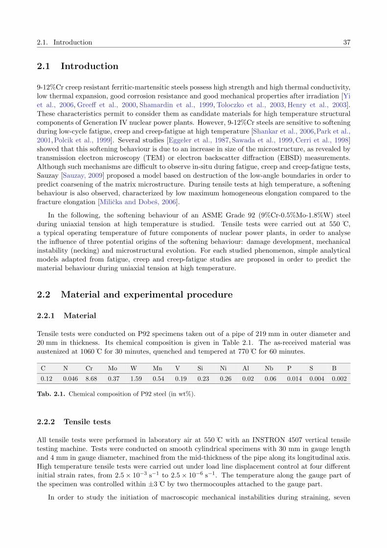
2.3 Results of tensile tests carried out up to fracture . . . . . . . . . . . . . . . . . . . . . 39
2.4 Damage assessment . . . . . . . . . . . . . . . . . . . . . . . . . . . . . . . . . . . . . . 40
2.5 Necking: experimental results and modelling . . . . . . . . . . . . . . . . . . . . . . . 42
2.5.1 Interrupted tensile tests and onset of macroscopic necking . . . . . . . . . . . . 42
2.5.2 Prediction of mechanical instability and of fracture elongation . . . . . . . . . . 45
2.6 Microstructural evolution of the matrix during tensile deformation . . . . . . . . . . . 51
2.6.1 Experimental results: EBSD and TEM investigations . . . . . . . . . . . . . . 51
2.6.2 Modelling of microstructural evolution during straining . . . . . . . . . . . . . 51
2.7 Conclusions . . . . . . . . . . . . . . . . . . . . . . . . . . . . . . . . . . . . . . . . . . 57
3 Mechanical behaviour and microstructural evolution during cyclic and creep load-ing 59
Abstract (in French) . . . . . . . . . . . . . . . . . . . . . . . . . . . . . . . . . . . . . . . . 61
3.1 Macroscopic cyclic loading, creep and creep-fatigue behaviour . . . . . . . . . . . . . . 63
3.1.1 Cyclic loading tests . . . . . . . . . . . . . . . . . . . . . . . . . . . . . . . . . . 63
3.1.1.1 Experimental conditions and specimen geometry . . . . . . . . . . . . 63
3.1.1.2 Influence of strain amplitude at high strain rate on cyclic flow be-haviour and fatigue lifetime . . . . . . . . . . . . . . . . . . . . . . . . 64
3.1.1.3 Influence of strain rate on cyclic flow behaviour and fatigue lifetime . 65
3.1.2 Creep tests . . . . . . . . . . . . . . . . . . . . . . . . . . . . . . . . . . . . . . 68
3.1.2.1 Experimental conditions and specimen geometry . . . . . . . . . . . . 68
3.1.2.2 Creep curves and lifetime . . . . . . . . . . . . . . . . . . . . . . . . . 68
3.1.3 Cyclic test including tensile holding periods . . . . . . . . . . . . . . . . . . . . 71

Contents 11
3.1.3.1 Experimental conditions and specimen geometry . . . . . . . . . . . . 72
3.1.3.2 Creep-fatigue mechanical behaviour . . . . . . . . . . . . . . . . . . . 72
3.2 Macroscopic analysis of softening during cyclic loading . . . . . . . . . . . . . . . . . . 74
3.3 Observations of microstructural evolutions during cyclic loading tests . . . . . . . . . . 76
3.3.1 Evolution of the subgrain size distribution . . . . . . . . . . . . . . . . . . . . . 77
3.3.1.1 Methodology . . . . . . . . . . . . . . . . . . . . . . . . . . . . . . . . 77
3.3.1.2 Evolution of subgrain size distribution during fatigue test . . . . . . . 77
3.3.1.3 Effect of the strain on subgrain size evolution . . . . . . . . . . . . . . 79
3.3.2 Evolution of the dislocation density during high temperature cyclic loading . . 84
3.3.3 Discussion about deformation and annihilation mechanisms . . . . . . . . . . . 85
3.4 Concluding remarks . . . . . . . . . . . . . . . . . . . . . . . . . . . . . . . . . . . . . 87
4 Modelling of the cyclic behaviour and microstructure evolution during cycling 89
Abstract (in French) . . . . . . . . . . . . . . . . . . . . . . . . . . . . . . . . . . . . . . . . 91
4.1 Introduction to polycrystalline modelling . . . . . . . . . . . . . . . . . . . . . . . . . 93
4.2 Crystalline constitutive equations . . . . . . . . . . . . . . . . . . . . . . . . . . . . . . 94
4.2.1 Description and hypotheses of the modelling . . . . . . . . . . . . . . . . . . . 94
4.2.1.1 Dislocations types considered in the model . . . . . . . . . . . . . . . 95
4.2.1.2 Low-angle boundaries structures . . . . . . . . . . . . . . . . . . . . . 95
4.2.1.3 Crystallographic features at the block scale . . . . . . . . . . . . . . . 97
4.2.2 Isotropic stress . . . . . . . . . . . . . . . . . . . . . . . . . . . . . . . . . . . . 98
4.2.3 Evolution of the kinematic stress . . . . . . . . . . . . . . . . . . . . . . . . . . 99
4.2.4 Crystal viscoplasticity flow rule . . . . . . . . . . . . . . . . . . . . . . . . . . . 102
4.3 Modelling the microstructural evolutions . . . . . . . . . . . . . . . . . . . . . . . . . . 103
4.3.1 Modelling the evolution of dislocation density . . . . . . . . . . . . . . . . . . . 103
4.3.1.1 Production of dislocations . . . . . . . . . . . . . . . . . . . . . . . . . 104
4.3.1.2 Inter-annihilation of free dislocations . . . . . . . . . . . . . . . . . . 105
4.3.1.3 Annihilation of free dislocations with low-angle boundary dislocations 106
4.3.2 Modelling of low-angle boundaries misorientation evolution . . . . . . . . . . . 106
4.3.3 Modelling the subgrain size evolution . . . . . . . . . . . . . . . . . . . . . . . 108
4.4 Self-consistent homogenization scheme . . . . . . . . . . . . . . . . . . . . . . . . . . . 108
4.4.1 Thermoelastic modelling proposed by Kroner . . . . . . . . . . . . . . . . . . . 108
4.4.2 Molinari’s model for viscoplastic material . . . . . . . . . . . . . . . . . . . . . 109
12 Contents
4.5 Choice of the values of the model parameters . . . . . . . . . . . . . . . . . . . . . . . 110
4.5.1 Measured, calculated and fixed parameters . . . . . . . . . . . . . . . . . . . . 110
4.5.2 Identification process . . . . . . . . . . . . . . . . . . . . . . . . . . . . . . . . . 112
4.6 Simulation of cyclic loading . . . . . . . . . . . . . . . . . . . . . . . . . . . . . . . . . 115
4.6.1 Validation of the model on the first macroscopic loop for both strain rates . . . 115
4.6.2 Prediction of cyclic softening for both strain rates . . . . . . . . . . . . . . . . 115
4.6.2.1 Predicted macroscopic behaviour . . . . . . . . . . . . . . . . . . . . . 115
4.6.2.2 Predicted microstructural evolution . . . . . . . . . . . . . . . . . . . 116
4.6.3 Predictions of the macroscopic cyclic softening for different strain amplitudes . 120
4.6.4 Sensitivity of model predictions to the values of model parameters . . . . . . . 122
4.6.4.1 Influence of the critical annihilation distance for edge dislocations onmodel predictions . . . . . . . . . . . . . . . . . . . . . . . . . . . . . 123
4.6.4.2 Influence of the critical annihilation distance for screw dislocations onmodel predictions . . . . . . . . . . . . . . . . . . . . . . . . . . . . . 125
4.6.4.3 Influence of the initial mean low-angle boundary misorientation onmodel predictions . . . . . . . . . . . . . . . . . . . . . . . . . . . . . 127
4.6.4.4 Influence of the value of the critical misorientation on model predictions129
4.6.4.5 Influence of the respective fractions of mobile edge / screw dislocationdensities on model predictions . . . . . . . . . . . . . . . . . . . . . . 131
4.6.4.6 Concluding remarks from the parametric study . . . . . . . . . . . . . 133
4.7 Concluding remarks . . . . . . . . . . . . . . . . . . . . . . . . . . . . . . . . . . . . . 133
5 Influence of the initial heterogeneity of microstructure, multiaxiality, temperatureand material on the model predictions (in French) 135
5.1 Use of the measured initial distributions of subgrain sizes and dislocation densities . . 136
5.1.1 Initial subgrain size distribution . . . . . . . . . . . . . . . . . . . . . . . . . . 136
5.1.2 Initial mobile dislocation density distribution . . . . . . . . . . . . . . . . . . . 142
5.2 Simulations of cyclic torsion . . . . . . . . . . . . . . . . . . . . . . . . . . . . . . . . . 148
5.3 Modelling of the cyclic behaviour of the EUROFER 97 steel at room temperature . . 149
5.4 Conclusions . . . . . . . . . . . . . . . . . . . . . . . . . . . . . . . . . . . . . . . . . . 151
6 General conclusions and recommendations for further work 153
6.1 Conclusions . . . . . . . . . . . . . . . . . . . . . . . . . . . . . . . . . . . . . . . . . . 154
6.2 Some recommendations for future work . . . . . . . . . . . . . . . . . . . . . . . . . . 156
References 159
13
A propos du manuscrit
Le present manuscrit est structure en six chapitres. Le premier chapitre est une introduction generaleau travail de these. Apres une introduction des objectifs de ce travail, le materiau etudie, l’acierGrade 92, est presente et une courte synthese bibliographique concernant la microstructure des aciersmartensitiques revenus est decrite.
Le chapitre 2 est consacre a l’etude du comportement mecanique de l’acier Grade 92 en tractionmonotone a 550 C. Trois phenomenes sont etudies afin de comprendre les mecanismes a l’originede l’adoucissement macroscopique mesure : l’instabilite mecanique (striction), l’endommagement etl’evolution de la taille des sous-grains. Deux modeles analytiques predisant l’apparition de l’instabilitemecanique et la croissance des sous-grains sont proposes.
Le chapitre 3 est dedie a l’etude du comportement mecanique de l’acier Grade 92 lors de sollicita-tions de type chargement cyclique continu et fluage a 550 C. L’etude se concente sur les mecanismesde deformation lors des essais sous chargement cyclique continu, avec notamment la decomposition dela contrainte macroscopique selon la methode de Cottrell. Des observations MET visant a caracteriserl’evolution de la microstructure sont finalement presentees et discutees.
Le chapitre 4 est dedie a la modelisation polycristalline du comportement mecanique de l’acierGrade 92 lors de sollicitations cycliques continues a 550 C. Le modele est construit autour de deuxaxes majeurs : le changement d’echelle (du bloc de martensite revenu au polycristal) et la modelisationde l’evolution de la microstructure (taille de sous-grain et densite de dislocations). Les resultats despredictions du comportement mecanique macroscopique et de l’evolution microstructurale sont ensuitepresentes. Enfin, l’influence de la valeur des parametres physiques du modele sur les predictions estetudiee et discutee.
Le chapitre 5 presente deux ameliorations apportees au modele decrit dans le chapitre 4 : la priseen compte de distributions initiales de taille de sous-grains et de densite de dislocations moyennepar bloc. Dans un second temps, le modele est applique a des chargements cycliques de torsion etles predictions obtenues sont etudiees qualitativement. Ce chapitre se clot sur une presentation dessimulations de sollicitation cyclique a temperature ambiante sur l’acier EUROFER 97 en collaborationavec M. F. Giordana (Universidad Nacional de Rosario, Argentina).
Enfin, les conclusions et perspectives de ce travail sont presentees dans le chapitre 6.
Ce manuscrit ne comporte pas de chapitre consacre a une revue bibliographique extensive desaciers martensitiques revenus et de leur comportement mecanique en general. Cependant, chaquecomposante de cette etude insere des elements bibliographiques presentant les travaux et resultatsdisponibles dans la litterature.

14 Contents

15
About the manuscript
This present manuscript is divided into six chapters. The first one focuses on the general context of thisstudy. After an introduction to the objectives of this work, a description of the material under study,a Grade 92 steel, and a short literature survey of the tempered martensite ferritic steel microstructureare presented.
Chapter 2 focuses on the mechanical behaviour of the Grade 92 steel during monotonic tensile testsat 550 C at various strain rates. Three phenomena are studied in order to understand the physicalmechanisms inducing the observed softening stage: mechanical instability (necking), damage andsubgrain size evolution. Two analytical models predicting respectively the beginning of the mechanicalinstability and the subgrain growth are proposed.
Chapter 3 focuses on the experimental mechanical behaviour of the Grade 92 steel during con-tinuous cyclic loading and creep at 550 C. Then, the study focuses on the physical mechanisms ofdeformation during continuous cycling deformation based on the partition of macroscopic stress pro-posed by Cottrell. Finally, TEM observations of the microstructure are presented in order to charac-terize quantitatively the microstructure evolution and the possibly involved physical mechanisms arediscussed.
Chapter 4 focuses on the modelling of the mechanical behaviour of Grade 92 steel during contin-uous cycling at 550 C. The description of the hypotheses of the modelling is divided into two parts:polycrystalline homogeneisation (from the tempered martensite block to the macroscopic scale) andmicrostructural evolution modelling (subgrain size and dislocation density). Then, the predictions ofthe modelling of the macroscopic mechanical behaviour and microstructural evolution are presented.Finally, the influence of the values of the used parameters on the predictions is studied and discussed.
Chapter 5 focuses on two important improvements of the model presented in chapter 4 : an initialmean subgrain size distribution per block and an initial dislocation density distribution are taken intoaccount instead of using averaged values. Then, predictions of the model under cyclic torsion are stud-ied. Finally, some results about the predictions of the microstructural evolution of EUROFER 97 steelduring cycling at room temperature are presented, in collaboration with M. F. Giordana (UniversidadNacional de Rosario, Argentina).
Finally, general conclusions and recommendations for further work are presented in chapter 6.
In this manuscript, no chapter presents a general literature survey of the tempered martensitesteels and their mechanical behaviour under various loading conditions. However, each part of thisstudy is presented with literature elements available published work and results.

16 Contents

17
Table of symbols and notations
Symbols
d Total derivative
∂ Partial derivative
δ Infinitesimal change in the value of a variable
∆ Macroscopic change in the value of a variable
u Scalar quantity
u Mean value
u First-order tensor
u Second-order tensor
u Fourth-order tensor
Notations
b Burgers vector magnitude
d Subgrain diameter
e Thin foil thickness
l Mean path of a dislocation
li Length of a segment
m Hart’s viscoplastic parameter
ni Number of intersections between a segment and a dislocation
s Standard deviation of a distribution
tf Failure time of creep test
x Mean block kinematic shear stress
xmax Mean block maximum kinematic shear stress

18 Contents
Ad Area swept by a dislocation
A Cross-section of a specimen
A0 Initial cross-section of a specimen
Ep Macroscopic plastic strain tensor
R Isotropic part of the macroscopic stress
X Kinematic part of the macroscopic stress
γ Hart’s strain hardening parameter
γp Plastic slip
ε, ε1 Axial engineering strain
ε2, ε3 Radial engineering strain
εe Elastic engineering strain tensor
εp Plastic engineering strain tensor
εvp Principal component of visco-plastic strain tensor
εvp Principal component of visco-plastic strain rate tensor
εs Minimum (or secondary) creep rate
εp Mean block plastic strain tensor
µ Elastic shear modulus
ν Elastic Poisson ratio
ρ Total dislocation density
σ Principal component of stress tensor
σ Mean block stress tensor
τ Mean block shear stress
Σv Viscous part of the macroscopic stress
Σ Macroscopic stress tensor
19
Chapitre 1
Introduction generale et presentationdu materiau de l’etude
This first chapter focuses on the general context of this study. After an introduction to the objec-tives of this PhD work, a description of the material under study – Grade 92 steel (9%Cr-0.5%Mo-1.8%W-NbV) – and a short literature survey on tempered martensite-ferritic steel microstructures arepresented, together with the properties of the material.
Ce premier chapitre presente le contexte general de l’etude de la deformation. Une introduction ala problematique de la these et une rapide presentation du materiau etudie, l’acier Grade 92 (9%Cr-0.5%Mo-1.8%W-NbV), sont proposees. Enfin, une description bibliographique succincte axee sur lamicrostructure de ces materiaux est presentee, et mise en regard des proprietes du materiau.
Contents
1.1 General context of the study and problematic . . . . . . . . . . . . . . . . . 20
1.2 Tempered martensite ferritic steels - Presentation of the material understudy . . . . . . . . . . . . . . . . . . . . . . . . . . . . . . . . . . . . . . . . . . 21
1.2.1 Chemical composition and heat treatments . . . . . . . . . . . . . . . . . . . . 21
1.2.2 Microstructure of tempered martensite steels . . . . . . . . . . . . . . . . . . . 22

20 Chapitre 1. General introduction and presentation of the material under study (in French)
1.1 Contexte general de l’etude et problematique
Afin d’apporter une reponse a la demande croissante en energie, les principaux acteurs de l’industrienucleaire tel que le Commissariat a l’Energie Atomique ont oriente des projets de recherche versla realisation d’un nouveau type de reacteur de fission a neutrons rapides, dit de Generation IV.Cette technologie, plus sure en termes d’exploitation et moins risquee vis-a-vis des problemes lies ala proliferation, a egalement pour objectif d’allonger la duree de vie de ces nouveaux reacteurs a laconception et d’ameliorer leur rendement energetique. Une des voies explorees pour parvenir a larealisation de ce dernier objectif passe par l’augmentation de la temperature de fonctionnement (entre450 et 600 C contre 300 a 400 C pour les reacteurs actuels) et par consequent, necessite le choix d’unfluide caloporteur autre que l’eau, tel que le sodium.
Cette accroissement de la temperature de fonctionnement et de la duree de vie des reacteurs induitinevitablement des repercussions sur le choix des materiaux de structure. C’est dans ce contexte queles aciers martensitiques revenus a 9 % de chrome ont ete retenus comme candidats potentiels pourla conception de certains elements de circuiterie tels que les generateurs de vapeur. En effet, cesaciers presentent une meilleure conductivite thermique et un coefficient de dilatation thermique plusfaible que les aciers austenitiques de type AISI 316L, ce qui peut permettre de reduire les sollicitationsmecaniques liees a la fatigue thermique. Outre ces proprietes, son cout de production moindre peutetre un avantage.
Les structures a haute temperature subiront des sollicitations de type fluage mais peuvent etreaussi soumises a des chargements cycliques, lies aux phases d’arret et redemarrage des reacteurs. Envue de leur dimensionnement au sein du reacteur, l’etude des aciers martensitiques revenus a 9 % dechrome se doit de considerer leurs proprietes mecaniques lors de chargement cyclique, en fluage etfatigue-fluage. Ces sollicitations en conditions de service peuvent etre assimiliees a du fluage long-terme (avec un temps de maintien de l’ordre du mois), interrompu par des chargements cycliques afaible amplitude de deformation. Bien entendu, une telle succession de sollicitations est impossible areproduire en laboratoire pour des raisons de temps d’occupation des machines d’essais, a fortiori, surune periode de 60 ans.
Le dimensionnement des structures se fonde donc sur une extrapolation des resultats des essais real-ises en laboratoire. Or, celle-ci reste risquee si elle tient uniquement compte des resultats mecaniquesmacroscopiques obtenus lors de ces essais, relativement eloignes des sollicitations en conditions deservice. Il s’avere donc primordial, afin d’ameliorer la fiabilite de ces extrapolations, de comprendreet de modeliser les mecanismes physiques de la deformation qui induisent les resultats macroscopiquesobserves en laboratoire. C’est dans cette optique que s’incrit le present travail de these.
Les differentes nuances d’aciers martensitiques revenus ont ete optimisees dans l’optique d’ameliorerleurs proprietes en fluage. Sous chargement cyclique, ils sont sensibles au phenomene d’adoucissement,qui se caracterise par une perte de la resistance mecanique. L’etude de ce phenomene est motiveepar l’objectif lie a l’augmentation des durees de vie des composants. En effet, les aciers martensi-tiques revenus possedent une duree de vie plus courte en fatigue sous air que sous vide [Kim andWeertman, 1988] et en environnement sodium [Kannan et al., 2009]. Dans ces deux derniers typesd’environnement, la phase d’adoucissement cyclique se trouve donc prolongee. De plus, celle-ci estd’autant plus prononcee que la temperature est elevee [Armas et al., 2004]. Enfin, des resultats recentsont montre que la tenue mecanique en fluage chutait lorsque le materiau etait soumis a un precyclageen fatigue [Fournier et al., 2011a], soulignant ainsi l’effet nefaste de l’adoucissement cyclique pour lesapplications industrielles visees. L’etude de l’influence des facteurs experimentaux sur ce phenomenese revele donc necessaire. Peu abordes dans la litterature, nous avons choisi de nous concentrer surles effets de la vitesse de deformation lors des essais cycliques en traction/compression a haute tem-

1.2. Tempered martensite ferritic steels - Presentation of the material under study 21
perature.
Notre premier objectif est donc d’etudier les proprietes mecaniques de ces aciers a haute tempera-ture. Dans ce cadre, des essais de traction, de fatigue, de fluage et de fatigue-fluage ont ete menes surun acier de Grade 92 afin de mettre en evidence le comportement mecanique macroscopique de cetacier sous diverses sollicitations. Dans un second temps, des observations de la microstructure ont eteeffectuees sur le materiau apres chargement monotone ou cyclique continu dans le but de quantifierles modifications de la microstructure et de proposer des mecanismes de deformation en accord avecles observations.
Le second objectif consiste en l’integration de ces mecanismes physiques au sein d’un modelepredictif du comportement mecanique et de l’evolution de la microstructure sous chargement monotoneet/ou cyclique. Les predictions de ce modele sont ensuite comparees aux donnees experimentalesprecedemment obtenues puis discutees.
Avant d’entamer cette etude, nous allons poursuivre cette introduction en presentant succincte-ment la famille des aciers martensitiques revenus a 9 % de chrome. Nous accorderons une importanceparticuliere a la description de leur microstructure, point de depart de la comprehension des mecan-ismes de deformation.
1.2 Les aciers martensitiques revenus - Presentation du materiau del’etude
1.2.1 Composition chimique et traitements thermiques
1.2.1.1 Composition chimique du materiau de l’etude
La famille des aciers a 9%Cr possede un historique relativement riche en termes d’evolution de com-position. Cette richesse se traduit par des optimisations successives en divers elements d’alliage, dansle but de repondre a des criteres de performances mecaniques toujours plus eleves essentiellementdans le domaine du fluage. Dans le present travail de recherche, nous nous sommes particulierementinteresses a un tube en acier de Grade 92 fourni par Vallourec & Mannesmann Tubes France, dont lacomposition chimique est reportee dans le Tableau 1.1.
C N Cr Mo W Mn V Si Ni Al Nb P S B
0.12 0.046 8.68 0.37 1.59 0.54 0.19 0.23 0.26 0.02 0.06 0.014 0.004 0.002
Tab. 1.1. Composition chimique en pourcentage massique de l’acier de Grade 92 etudie.
Nous allons maintenant presenter les traitements thermiques appliques a l’acier. Ces derniersinfluencent grandement sa microstructure et donc son comportement mecanique sous sollicitation.
1.2.1.2 Traitements thermiques appliques au materiau de l’etude
Generalement, les traitements thermiques appliques aux aciers 9%Cr se resument en une austenitisa-tion, une trempe et un revenu, les parametres de traitement pouvant differer d’un produit a l’autreen termes de duree ou de temperature. Dans le cas du tube en acier de Grade 92 etudie, l’etaped’austenitisation a ete effectuee a 1060 C pendant 30 minutes, suivie par une trempe a l’air et enfinpar un revenu a 770 C pendant 60 minutes.
22 Chapitre 1. General introduction and presentation of the material under study (in French)
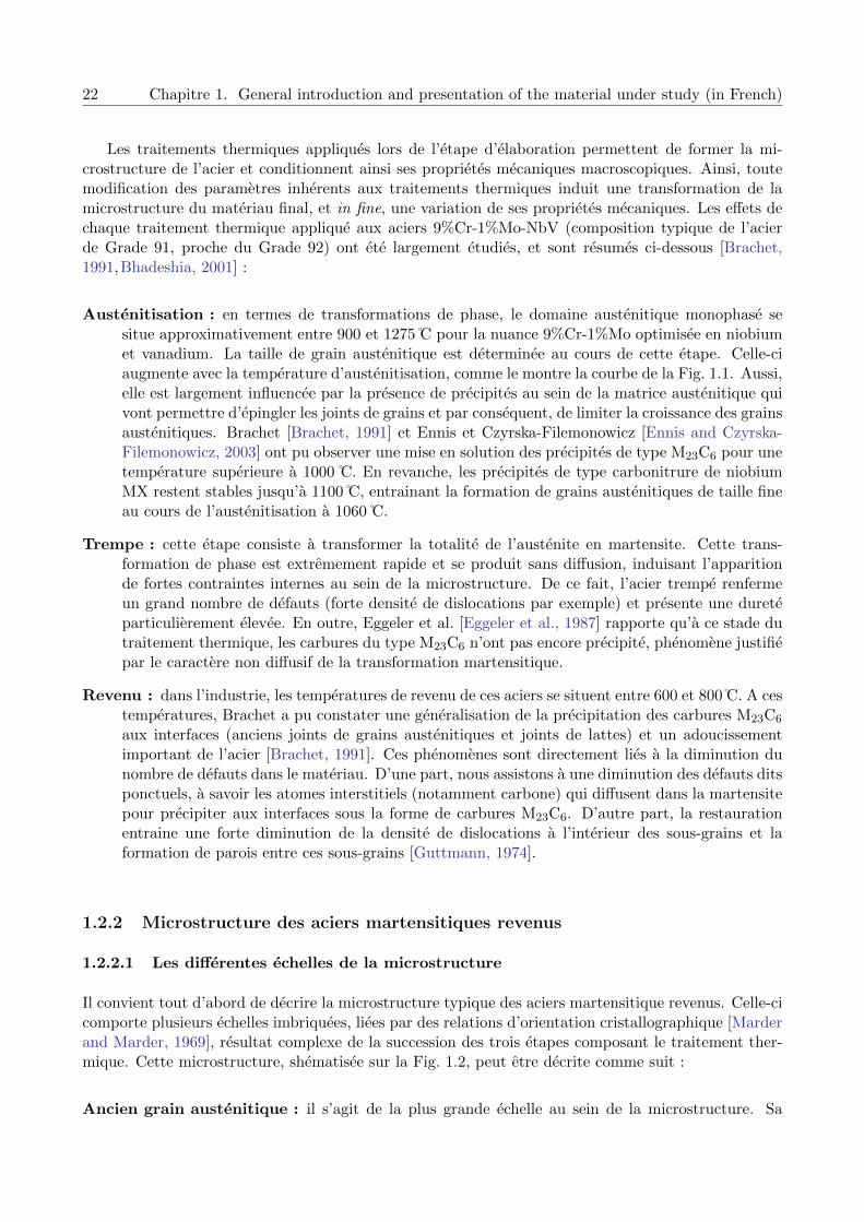
Les traitements thermiques appliques lors de l’etape d’elaboration permettent de former la mi-crostructure de l’acier et conditionnent ainsi ses proprietes mecaniques macroscopiques. Ainsi, toutemodification des parametres inherents aux traitements thermiques induit une transformation de lamicrostructure du materiau final, et in fine, une variation de ses proprietes mecaniques. Les effets dechaque traitement thermique applique aux aciers 9%Cr-1%Mo-NbV (composition typique de l’acierde Grade 91, proche du Grade 92) ont ete largement etudies, et sont resumes ci-dessous [Brachet,1991,Bhadeshia, 2001] :
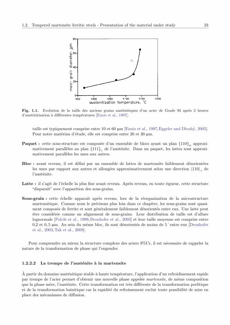
Austenitisation : en termes de transformations de phase, le domaine austenitique monophase sesitue approximativement entre 900 et 1275 C pour la nuance 9%Cr-1%Mo optimisee en niobiumet vanadium. La taille de grain austenitique est determinee au cours de cette etape. Celle-ciaugmente avec la temperature d’austenitisation, comme le montre la courbe de la Fig. 1.1. Aussi,elle est largement influencee par la presence de precipites au sein de la matrice austenitique quivont permettre d’epingler les joints de grains et par consequent, de limiter la croissance des grainsaustenitiques. Brachet [Brachet, 1991] et Ennis et Czyrska-Filemonowicz [Ennis and Czyrska-Filemonowicz, 2003] ont pu observer une mise en solution des precipites de type M23C6 pour unetemperature superieure a 1000 C. En revanche, les precipites de type carbonitrure de niobiumMX restent stables jusqu’a 1100 C, entrainant la formation de grains austenitiques de taille fineau cours de l’austenitisation a 1060 C.
Trempe : cette etape consiste a transformer la totalite de l’austenite en martensite. Cette trans-formation de phase est extremement rapide et se produit sans diffusion, induisant l’apparitionde fortes contraintes internes au sein de la microstructure. De ce fait, l’acier trempe renfermeun grand nombre de defauts (forte densite de dislocations par exemple) et presente une dureteparticulierement elevee. En outre, Eggeler et al. [Eggeler et al., 1987] rapporte qu’a ce stade dutraitement thermique, les carbures du type M23C6 n’ont pas encore precipite, phenomene justifiepar le caractere non diffusif de la transformation martensitique.
Revenu : dans l’industrie, les temperatures de revenu de ces aciers se situent entre 600 et 800 C. A cestemperatures, Brachet a pu constater une generalisation de la precipitation des carbures M23C6
aux interfaces (anciens joints de grains austenitiques et joints de lattes) et un adoucissementimportant de l’acier [Brachet, 1991]. Ces phenomenes sont directement lies a la diminution dunombre de defauts dans le materiau. D’une part, nous assistons a une diminution des defauts ditsponctuels, a savoir les atomes interstitiels (notamment carbone) qui diffusent dans la martensitepour precipiter aux interfaces sous la forme de carbures M23C6. D’autre part, la restaurationentraine une forte diminution de la densite de dislocations a l’interieur des sous-grains et laformation de parois entre ces sous-grains [Guttmann, 1974].
1.2.2 Microstructure des aciers martensitiques revenus
1.2.2.1 Les differentes echelles de la microstructure
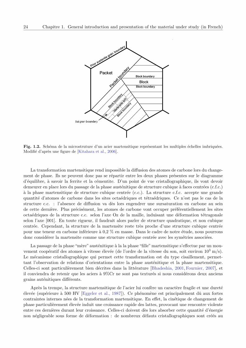
Il convient tout d’abord de decrire la microstructure typique des aciers martensitique revenus. Celle-cicomporte plusieurs echelles imbriquees, liees par des relations d’orientation cristallographique [Marderand Marder, 1969], resultat complexe de la succession des trois etapes composant le traitement ther-mique. Cette microstructure, shematisee sur la Fig. 1.2, peut etre decrite comme suit :
Ancien grain austenitique : il s’agit de la plus grande echelle au sein de la microstructure. Sa
1.2. Tempered martensite ferritic steels - Presentation of the material under study 23
Fig. 1.1. Evolution de la taille des anciens grains austenitiques d’un acier de Grade 92 apres 2 heuresd’austenitisation a differentes temperatures [Ennis et al., 1997].
taille est typiquement comprise entre 10 et 60 µm [Ennis et al., 1997,Eggeler and Dlouhy, 2005].Pour notre materiau d’etude, elle est comprise entre 20 et 30 µm.
Paquet : cette sous-structure est composee d’un ensemble de blocs ayant un plan 110α approxi-mativement paralleles au plan 111γ de l’austenite. Dans un paquet, les lattes sont approxi-mativement paralleles les unes aux autres.
Bloc : avant revenu, il est defini par un ensemble de lattes de martensite faiblement desorienteesles unes par rapport aux autres et allongees approximativement selon une direction 〈110〉γ del’austenite.
Latte : il s’agit de l’echelle la plus fine avant revenu. Apres revenu, en toute rigueur, cette structure“disparaıt” avec l’apparition des sous-grains.
Sous-grain : cette echelle apparaıt apres revenu, lors de la reorganisation de la microstructuremartensitique. Comme nous le precisons plus loin dans ce chapitre, les sous-grains sont quasi-ment composes de ferrite et sont generalement faiblement desorientes entre eux. Une latte peutetre consideree comme un alignement de sous-grains. Leur distribution de taille est d’allurelognormale [Polcik et al., 1999,Dronhofer et al., 2003] et leur taille moyenne est comprise entre0,2 et 0, 5 µm. Au sein du meme bloc, ils sont desorientes de moins de 5˚entre eux [Dronhoferet al., 2003,Tak et al., 2009].
Pour comprendre au mieux la structure complexe des aciers 9%Cr, il est necessaire de rappeler lanature de la transformation de phase qui l’engendre.
1.2.2.2 La trempe de l’austenite a la martensite
A partir du domaine austenitique stable a haute temperature, l’application d’un refroidissement rapidepar trempe de l’acier permet d’obtenir une nouvelle phase appelee martensite, de meme compositionque la phase mere, l’austenite. Cette transformation est tres differente de la transformation perlitiqueet de la transformation bainitique car la rapidite du refroissement exclut toute possibilite de mise enplace des mecanismes de diffusion.
24 Chapitre 1. General introduction and presentation of the material under study (in French)
Fig. 1.2. Schema de la microstruture d’un acier martensitique representant les multiples echelles imbriquees.Modifie d’apres une figure de [Kitahara et al., 2006].
La transformation martensitique rend impossible la diffusion des atomes de carbone lors du change-ment de phase. Ils ne peuvent donc pas se repartir entre les deux phases presentes sur le diagrammed’equilibre, a savoir la ferrite et la cementite. D’un point de vue cristallographique, ils vont devoirdemeurer en place lors du passage de la phase austenitique de structure cubique a faces centrees (c.f.c.)a la phase martensitique de structure cubique centree (c.c.). La structure c.f.c. accepte une grandequantite d’atomes de carbone dans les sites octaedriques et tetraedriques. Ce n’est pas le cas de lastructure c.c. : l’absence de diffusion va des lors engendrer une sursaturation en carbone au seinde cette derniere. Plus precisement, les atomes de carbone vont occuper preferentiellement les sitesoctaedriques de la structure c.c. selon l’axe Oz de la maille, induisant une deformation tetragonaleselon l’axe [001]. En toute rigueur, il faudrait alors parler de structure quadratique, et non cubiquecentree. Cependant, la structure de la martensite reste tres proche d’une structure cubique centreepour une teneur en carbone inferieure a 0,2 % en masse. Dans le cadre de notre etude, nous pourronsdonc considerer la martensite comme une structure cubique centree avec les symetries associees.
La passage de la phase “mere” austenitique a la la phase “fille” martensitique s’effectue par un mou-vement cooperatif des atomes a vitesse elevee (de l’ordre de la vitesse du son, soit environ 103 m/s).Le mecanisme cristallographique qui permet cette transformation est du type cisaillement, permet-tant l’observation de relations d’orientations entre la phase austenitique et la phase martensitique.Celles-ci sont particulierement bien decrites dans la litterature [Bhadeshia, 2001, Fournier, 2007], etil conviendra de retenir que les aciers a 9%Cr ne sont pas textures si nous considerons deux anciensgrains autenitiques differents.
Apres la trempe, la structure martensitique de l’acier lui confere un caractere fragile et une dureteelevee (superieure a 500 HV [Eggeler et al., 1987]). Ce phenomene est principalement du aux fortescontraintes internes nees de la transformation martensitique. En effet, la cinetique de changement dephase particulierement elevee induit une croissance rapide des lattes, provocant une rencontre violenteentre ces dernieres durant leur croissance. Celles-ci doivent des lors absorber cette quantite d’energienon negligeable sous forme de deformation : de nombreux defauts cristallographiques sont crees au
1.2. Tempered martensite ferritic steels - Presentation of the material under study 25
sein meme de la latte, en particulier des dislocations.
1.2.2.3 De la martensite a la martensite revenue
Le traitement de revenu permet alors d’agir sur la microstructure de l’acier de maniere a diminuer lescontraintes internes. En effet, le maintien en temperature du materiau (entre 600 et 800 C) pendantun temps donne permet la mise en place de mecanismes microstructuraux thermiquement actives,tels que la diffusion et la restauration [Guttmann, 1974, Ennis et al., 1997]. Nous assistons donc aun rearrangement de la microstructure qui, selon les lois de la thermodynamique, tend a minimiserl’energie du systeme.
L’activation des mecanismes de diffusion est a l’origine de l’apparition de plusieurs types de pre-cipites, notamment M23C6, et ceci rapidement apres le debut de l’etape de revenu [Eggeler et al.,1987]. En termes de localisation, la germination des carbures se produit principalement aux inter-faces, c’est-a-dire aux differents types de joints qui composent la microstructure (joints d’anciensgrains austenitiques, de paquets, de blocs et de lattes). Ce phenomene s’explique aisement en con-siderant les lois thermodynamiques de germination et de segregation de phase [Beranger et al., 1994].Nous verrons plus precisement dans la partie 1.2.2.7 les differentes caracteristiques de ces precipites,telles que leur composition, leur structure et leur taille.
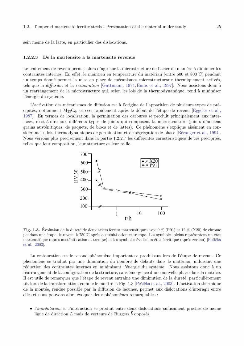
Fig. 1.3. Evolution de la durete de deux aciers ferrito-martensitiques avec 9 % (P91) et 12 % (X20) de chromependant une etape de revenu a 750 C apres austenitisation et trempe. Les symboles pleins representent un etatmartensitique (apres austenitisation et trempe) et les symboles evides un etat ferritique (apres revenu) [Pesickaet al., 2003].
La restauration est le second phenomene important se produisant lors de l’etape de revenu. Cephenomene se traduit par une diminution du nombre de defauts dans le materiau, induisant unereduction des contraintes internes en minimisant l’energie du systeme. Nous assistons donc a unrearrangement de la configuration de la structure, sans emergence d’une nouvelle phase dans la matrice.Il est utile de remarquer que l’etape de revenu entraine une diminution de la durete, particulierementtot lors de la transformation, comme le montre la Fig. 1.3 [Pesicka et al., 2003]. L’activation thermiquede la montee, rendue possible par la diffusion de lacunes, permet aux dislocations d’interagir entreelles et nous pouvons alors evoquer deux phenomenes remarquables :
l’annihilation, si l’interaction se produit entre deux dislocations suffisament proches de memeligne de direction L mais de vecteurs de Burgers ~b opposes.

26 Chapitre 1. General introduction and presentation of the material under study (in French)
le rearrangement, qui se traduit par une mise en ordre des dislocations. Ce phenomene reduitl’energie du systeme en organisant les dislocations de maniere a minimiser le champ de con-trainte engendre par chacune d’entre elles. Ce mecanisme conduit a la formation de sous-jointsfaiblement desorientes constitues de reseaux reguliers de dislocations (voir Fig. 1.4).
Fig. 1.4. Image MET montrant le mecanisme de “knitting-out” d’un sous-joint de faible desorientation (acierGrade 91 soumis a un essai de fatigue-fluage a 600 C [Sauzay et al., 2008].
Ce deuxieme point permet d’expliquer l’existence des sous-grains, echelle la plus fine de la mi-crostructure du materiau considere. En effet, le rearrangement des dislocations au sein de la latte lesamene a s’espacer regulierement les unes des autres pour former des parois de dislocations. Celles-cise caracterisent par une desorientation de part et d’autre du reseau, partageant ainsi les lattes ensous-grains. Ce phenomene est nomme polygonisation [Francois et al., 1995a].
En termes de microstructure, la division en sous-grains des lattes de martensite lors de l’etape derevenu ne nous permet plus de parler de structure martensitique. En effet, comme le souligne Hald,ces sous-grains sont composes de ferrite [Hald, 2008] et sont aussi appeles “micrograins” [Dronhoferet al., 2003, Pesicka et al., 2004, Tak et al., 2009]. Comme la microstructure est proche de celle de lamartensite en lattes, nous lui prefererons donc l’appellation de martensite revenue.
Cette courte description de la structure martensitique revenue des aciers 9%Cr nous amene donca entrevoir la complexite des mecanismes induit lors de la deformation a haute temperature. En sebasant sur le mouvement des dislocations comme moteur de la deformation viscoplastique, il apparaıtclairement que l’etude des mecanismes de deformation doit se baser sur les diverses interactions de cesdernieres avec les elements de la microstructure.
1.2.2.4 Densite de dislocations
Les dislocations apparaissent comme le point central de l’etude des mecanismes de deformation. Danscette optique, leur quantification et leur localisation au sein de la structure sont essentielles. Pourcommencer, nous avons donc reuni dans le Tableau 1.2 plusieurs valeurs de densite de dislocationsrelevees dans la litterature pour cette famille d’aciers, a l’etat de reception.
Si la temperature d’austenitisation n’a aucun impact significatif sur la densite de dislocations, latemperature de revenu va influencer notablement le processus de restauration. En effet, en passantd’une temperature de 715 a 835 C, la densite de dislocations chute d’un facteur proche de 5. La maıtrisedes conditions de revenu est donc particulierement importante pour le controle de l’adoucissement dumateriau.

1.2. Tempered martensite ferritic steels - Presentation of the material under study 27
Traitements thermiques Densite de dislocations (1014 m−2) References
1070C (2h) - 715C (2h) 9, 0± 1, 0
1070C (2h) - 775C (2h) 7, 0± 0, 9 [Ennis et al., 1997]
1070C (2h) - 835C (2h) 2, 3± 0, 6
970C (2h) - 775C (2h) 8, 7± 1, 2 [Ennis et al., 2000]
1070C (2h) - 775C (2h) 7, 9± 0, 8 [Ennis and Czyrska-Filemonowicz, 2003]
Tab. 1.2. Densites de dislocations mesurees au MET par la technique d’intersection des segments, dans l’acierde Grade 92.
1.2.2.5 Nature des dislocations
La nature des dislocations est un parametre important dans l’etude des mecanismes de deformation.Il existe en effet schematiquement deux grands types de dislocations : les dislocations coin et les dislo-cations vis. Par definition, une dislocation coin se caracterise par un vecteur de Burgers ~b orthogonal
a sa ligne−→L alors que la dislocation vis se caracterise par un vecteur de Burgers parallele a sa ligne.
Au sein de la microstructure, il est frequent de rencontrer des dislocations dites mixtes, c’est-a-diredont le vecteur de Burgers forme un angle compris entre 0 et 90˚avec la ligne de la dislocation.
Outre leur nature, les dislocations presentes au sein d’un acier martensitique revenu se divisent endeux grandes familles [Pesicka et al., 2004] :
Les dislocations mobiles (“free dislocations” [Eggeler, 1989]) qui, par definition, se deplacent lorsde la deformation viscoplastique. C’est lors de ce mouvement qu’elles vont interagir avec deselements presents dans la microstructure (autres dislocations composant la foret, atomes ou amasd’atomes en solution solide, precipites, sous-joints de grains. . . ).
Les dislocations composant les sous-joints dont nous avons evoque l’existence dans la par-tie 1.2.2.3. Rearrangees, elles forment les sous-joints de faible desorientation [Read and Shockley,1950]. Ces sous-joints sont compose en generale de deux familles de dislocations [Guttmann,1974] de caractere vis [Guetaz et al., 2003]. Nous verrons qu’elles jouent un role importantdans la croissance de la taille des sous-grains, observee lors de sollicitations en fatigue, fluage etfatigue-fluage.
En termes de population, il est donc possible de repartir la densite de dislocations totale entrela densite de dislocations mobiles et la densite de dislocations composant les sous-joints de grains.Globalement, la microstructure martensitique revenue de l’acier de Grade 92 se caracterise par uneforte densite de dislocations, de l’ordre de 1014 m−2 apres le revenu : [Pesicka et al., 2004] pour leX20, [Sauzay et al., 2005] pour le Grade 91, [Giordana et al., 2011] pour l’EUROFER 97.
Si nous nous interessons maintenant a la nature des dislocations, chacune de ces deux populationspeut alors etre definie comme un ensemble de dislocations de type coin, de type vis et de type mixte.L’observation des dislocations au sein des aciers nous rapporte l’existence de boucles, phenomene dua l’ancrage sur deux obstacles (atomes ou clusters d’atomes en solution solide, precipites, joints degrains. . . ) de la dislocation qui continue a glisser entre ces deux derniers sous l’effet de la contrainteappliquee (Fig. 1.5). Nous pouvons des lors comprendre aisement que le caractere de la dislocationvarie le long de sa ligne de direction, demontrant ainsi qu’il n’existe pas de dislocations purement coinou purement vis.
Lors de leur mouvement, les dislocations mobiles vont interagir avec differents elements presentsdans la matrice, notamment avec les precipites et les atomes en solution solide. Comme la foret
28 Chapitre 1. General introduction and presentation of the material under study (in French)
Fig. 1.5. Schema representant l’evolution du caractere d’une dislocation lorsqu’elle interagit avec des precipitessous l’effet d’un cisaillement τ [Francois et al., 1995a].
de dislocations, les precipites, et plus rarement les inclusions et les cavites presentes dans les aciers9%Cr, se comportent comme des obstacles au mouvement des dislocations. Ils ont donc une influenceremarquable sur le comportement mecanique de l’acier et nous presentons maintenant brievement cestrois types d’obstacles en s’attachant essentiellement au cas de l’acier de Grade 92 a l’etat revenu.
1.2.2.6 Inclusions et cavites
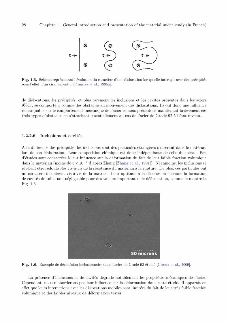
A la difference des precipites, les inclusions sont des particules etrangeres s’inserant dans le materiaulors de son elaboration. Leur composition chimique est donc independante de celle du metal. Peud’etudes sont consacrees a leur influence sur la deformation du fait de leur faible fraction volumiquedans le materiau (moins de 5× 10⁻⁴ d’apres Zhang [Zhang et al., 1991]). Neanmoins, les inclusions serevelent etre redoutables vis-a-vis de la resistance du materiau a la rupture. De plus, ces particules ontun caractere incoherent vis-a-vis de la matrice. Leur aptitude a la decohesion entraıne la formationde cavites de taille non negligeable pour des valeurs importantes de deformation, comme le montre laFig. 1.6.
Fig. 1.6. Exemple de decohesion inclusionnaire dans l’acier de Grade 92 etudie [Giroux et al., 2009].
La presence d’inclusions et de cavites degrade notablement les proprietes mecaniques de l’acier.Cependant, nous n’aborderons pas leur influence sur la deformation dans cette etude. Il apparaıt eneffet que leurs interactions avec les dislocations mobiles sont limitees du fait de leur tres faible fractionvolumique et des faibles niveaux de deformation testes.

1.2. Tempered martensite ferritic steels - Presentation of the material under study 29
1.2.2.7 Nature des precipites
La nature des precipites est particulierement influencee par deux parametres : la teneur en elementsd’addition presents dans l’alliage et les traitements thermiques appliques [Brachet, 1991, Gotz andBlum, 2003]. Dans le cas des aciers de Grades 91 et 92 a l’etat revenu, il existe principalement troistypes de precipites. Ces derniers sont listes dans le Tableau 1.3.
Aciers Precipites Formules Remarques
M23C6 (Cr,Fe,Mo)23C6 Precipitent pendant l’etape de revenu
P91 MX primaires (Nb,V)(N,C) Non dissous pendant l’etape d’austenitisation
MX (V,Nb)(N,C) Precipitent pendant l’etape de revenu
M23C6 (Cr,Fe,Mo,W)23C6 Precipitent pendant l’etape de revenu
P92 MX primaires (Nb,V)(N,C) Non dissous pendant l’etape d’austenitisation
MX (V,Nb)(N,C) Precipitent pendant l’etape de revenu
Tab. 1.3. Principaux precipites dans les aciers de Grade 91 et 92 [Hald, 2008].
Ces trois types de precipites sont les plus courants au sein de la matrice, puisqu’ils represententau moins 96 % de la population totale : en volume, les precipites du type M23C6 sont de loin les pluscommuns (85 a 90 %), suivis par les V(N,C) (10 a 13%) et enfin par les Nb(C,N) (1 a 2%) [Giesekeet al., 1993]. Ennis [Ennis et al., 1997] insiste sur le fait que les precipites de type MX apparaissentdans un ordre defini. Les precipites Nb(C,N) de forme spheroıdale ne sont pas dissous pendant l’etaped’autenitisation et certains d’entre eux peuvent servir de sites de germination a des precipites V(N,C)en forme de lamelles lors du revenu. Dans ce cas, nous pouvons observer des precipites de formes etde compositions complexes, couramment nommes “V-wings” [Ennis et al., 1997], comme le montre laFig. 1.7.
Fig. 1.7. Observation en microscopie electronique en transmission d’un acier de Grade 92 (normalise a 970 Cet revenu a 775 C) montrant des precipites spheriques M(C,N) riches en Nb et des precipites complexes deM(C,N) [Ennis et al., 1997].
Le reste des precipites, presents en faible quantite dans la matrice, sont de composition chimique etstœchiometrie variees : M2X, M3C, M7C3. . . Leur presence depend essentiellement des caracteristiquesdes traitements thermiques appliques et de la composition chimique des aciers etudies. Enfin, d’autresphases telles que les phases de Laves et les phases-Z peuvent apparaitre dans ces aciers [Panait, 2010].

30 Chapitre 1. General introduction and presentation of the material under study (in French)
1.2.2.8 Taille des precipites
Tout comme leur composition chimique, la taille des precipites est directement influencee par lestraitements thermiques appliques. Plusieurs valeurs pour diverses nuances d’aciers 9%Cr ont eterelevees dans la litterature et il est interessant de retenir les points suivants :
Les precipites de type MX ont un diametre moyen compris entre 5 et 60 nm suivant le traitementthermique. Pour le Grade 92 avec un traitement thermique proche de celui de la presente etude,le diametre moyen des MX se situe entre 15 et 20 nm [Ennis et al., 1997,Hattestrand and Andren,2001,Park et al., 2001,Gustafson and Hattestrand, 2002,Ennis and Czyrska-Filemonowicz, 2003].Ces precipites resistent a la coalescence puisque leur diametre moyen augmente de quelquesnanometres lorsque la temperature de revenu augmente de 715 a 835C. Ils sont incoherents avecla matrice des que leur taille depasse 10 nm, ce qui est le cas du materiau de l’etude.
Les precipites de type M23C6 ont un diametre moyen compris entre 50 et 350 nm suivant letraitement thermique [Eggeler et al., 1987, Eggeler, 1989, Park et al., 2001, Gotz and Blum,2003]. Pour le Grade 92 avec un traitement thermique proche de celui de la presente etude,le diametre moyen des M23C6 se situe entre 70 et 100 nm [Ennis et al., 1997, Hattestrand andAndren, 2001, Gustafson and Hattestrand, 2002, Ennis and Czyrska-Filemonowicz, 2003]. Cetype de precipite resiste moins bien a la coalescence que les MX puisque leur diametre moyenaugmente de 72 a 89 nm lorsque la temperature de revenu augmente de 715 a 775C.
Les distributions de taille de precipites sont d’allure log-normale [Eggeler, 1989, Cerri et al.,1998,Gotz and Blum, 2003]
Les precipites M23C6 ayant germe sur ou a proximite des joints d’anciens grains austenitiques ontun diametre moyen deux fois plus important que ceux ayant germe sur les sous-joints [Eggeler,1989].
Ce dernier point nous mene directement a l’etude de la localisation des precipites dans la matrice.
1.2.2.9 Localisation des precipites
La localisation des precipites est intimement liee a l’etape du traitement thermique durant laque-lle ils sont formes. Ainsi, les observations microstructurales publiees dans la litterature conduisentgeneralement aux deux conclusions suivantes :
Les precipites de type M23C6 se situent sur les anciens joints de grains autenitiques pour lesplus volumineux, et les joints de paquets, blocs, lattes et sous-joints pour les autres [Eggeler,1989,Eggeler and Dlouhy, 2005].
Les precipites de type MX, de taille plus faible que les precipites M23C6, sont disperses au seinmeme des sous-grains et sur l’ensemble des anciens joints de grains autenitiques, de paquets, deblocs, de lattes et de sous-grains [Abe et al., 2007].
La localisation des precipites de types M23C6 et MX est clairement schematisee sur la Fig. 1.8.
Cette courte description de la microstructure des aciers martensitiques revenus nous a permisd’entrevoir tres succinctement les principaux elements sur lesquels repose une grande majorite des

1.2. Tempered martensite ferritic steels - Presentation of the material under study 31
Fig. 1.8. Schema de la distribution spatiale des precipites M23C6 et MX au sein de la microstructure pour cequi est des joints de paquets, de blocs et de lattes [Abe et al., 2007].
modifications observees apres exposition du materiau a haute temperature, avec ou sans sollicitationmecanique. Dans le chapitre suivant, nous allons etudier le comportement mecanique de l’acier deGrade 92 au cours d’essais de traction uniaxiale puis observer les evolutions de la microstructureinduites par ce type de sollicitation monotone a haute temperature.

32 Chapitre 1. General introduction and presentation of the material under study (in French)

33
Chapter 2
Mechanical and microstructuralstability of P92 steel under uniaxialtension at high temperature
This second chapter focuses on the mechanical behaviour of Grade 92 steel during monotonic tensiletests at 550 C. Three phenomena are studied in order to understand the physical mechanisms inducingthe weak softening stage observed: mechanical instability (necking), damage and subgrain size evolu-tion. Two analytical models predicting respectively the beginning of the mechanical instability andthe subgrain growth are proposed. This chapter was published in Materials Science and EngineeringA - Structural Materials Properties Microstructure and Processing [Giroux et al., 2010].
Ce second chapitre est consacre a l’etude du comportement mecanique de l’acier Grade 92 entraction monotone a 550 C. Trois phenomenes sont etudies afin de comprendre et quantifier les me-canismes a l’origine du leger adoucissement macroscopique mesure : l’instabilite mecanique liee a lastriction, l’endommagement ductile et l’evolution de la taille des sous-grains. Deux modeles analy-tiques predisant respectivement l’apparition de l’instabilite mecanique et la croissance des sous-grainssont proposes. Ce chapitre a fait l’objet d’une publication dans le journal Materials Science andEngineering A - Structural Materials Properties Microstructure and Processing [Giroux et al., 2010].
Contents
Abstract (in French) . . . . . . . . . . . . . . . . . . . . . . . . . . . . . . . . . . . . 35
2.1 Introduction . . . . . . . . . . . . . . . . . . . . . . . . . . . . . . . . . . . . . 37
2.2 Material and experimental procedure . . . . . . . . . . . . . . . . . . . . . . 37
2.2.1 Material . . . . . . . . . . . . . . . . . . . . . . . . . . . . . . . . . . . . . . . . 37
2.2.2 Tensile tests . . . . . . . . . . . . . . . . . . . . . . . . . . . . . . . . . . . . . . 37
2.2.3 Metallographic investigation of the tensile specimens after the tests . . . . . . . 38
2.3 Results of tensile tests carried out up to fracture . . . . . . . . . . . . . . . 39
2.4 Damage assessment . . . . . . . . . . . . . . . . . . . . . . . . . . . . . . . . . 40
2.5 Necking: experimental results and modelling . . . . . . . . . . . . . . . . . . 42
2.5.1 Interrupted tensile tests and onset of macroscopic necking . . . . . . . . . . . . 42
2.5.2 Prediction of mechanical instability and of fracture elongation . . . . . . . . . . 45
2.6 Microstructural evolution of the matrix during tensile deformation . . . . 51
2.6.1 Experimental results: EBSD and TEM investigations . . . . . . . . . . . . . . 51
2.6.2 Modelling of microstructural evolution during straining . . . . . . . . . . . . . 51

34Chapter 2. Mechanical and microstructural stability of P92 steel under uniaxial tension at high
temperature
2.7 Conclusions . . . . . . . . . . . . . . . . . . . . . . . . . . . . . . . . . . . . . . 57

35
Resume
Ce chapitre presente les resultats de l’etude des proprietes mecaniques en traction monotone a 550 Csous air sur l’acier Grade 92. Ces tests ont ete effectues sur des eprouvettes cylindriques de 30 mm delongueur utile et 4 mm de diametre, prelevees a mi-epaisseur dans le sens longitudinal d’un tube de219 mm de diametre exterieur et de 20 mm d’epaisseur. Les vitesses etudiees varient de 2,5× 10⁻³ s−1
a 2,5× 10⁻⁶ s−1 et sont controlees par le deplacement de la traverse. La temperature est mesuree avecune precision de ±3 C grace a deux thermocouples attaches a la partie utile de l’eprouvette .
Les courbes conventionnelles contrainte-deformation en traction monotone de l’acier Grade 92 a550 C se decomposent en trois partie. La premiere etape correspond a un faible ecrouissage. Elle estsuivie d’une longue et stable decroissance de la contrainte, d’autant plus importante que la vitesse dedeformation diminue. Enfin la derniere etape correspond a un changement de la pente d’adoucissement,conduisant a la rupture de l’eprouvette.
Trois phenomenes ont ete etudies dans le but de comprendre l’adoucissement mecanique de ce typed’acier : l’endommagement, la striction (instabilite mecanique) et l’evolution de la microstructure.
Des observations MEB ont ete effectuees sur le materiau de reception et sur une eprouvette loin dela zone de rupture, apres un essai de traction a 550 C avec une vitesse de deformation de 2,5× 10⁻⁴ s−1.Dans les deux echantillons, la taille maximale des cavites observees n’excede pas 5 µm. Ce resultatsuggere que l’endommagement a une influence negligeable sur l’adoucissement du materiau.
Afin d’etudier l’influence de la striction sur le comportement mecanique, 7 essais de traction con-duits a 550 C avec une vitesse de deformation de 2,5× 10⁻⁴ s−1 ont ete interrompus pour differentesvaleurs de deformation axiale. Une etude profilometrique de ces eprouvettes non rompues a demon-tree que la striction macroscopique apparaıt a la fin de la longue et stable etape de decroissance dela contrainte. L’utilisation du critere etabli par Hart [Hart, 1967] permet de predir l’apparition del’instabilite mecanique pour des valeurs de deformation correspondant a la fin de la premiere etaped’ecrouissage. Ainsi, si la striction macroscopique est detectee apres l’etape d’adoucissement lineairede la contrainte, des instabilites mecaniques apparaissent probablement plus tot au cours de la defor-mation homogene.
Les observations effectuees a l’EBSD n’ont pas permis de mesurer de modifications significativesde la microstructure au cours de la deformation uniaxiale. En revanche, les mesures effectuees surles observations MET ont mis en evidence une augmentation de la taille moyenne des sous-grains depres de 21 % entre le materiau a l’etat de reception et l’echantillon preleve sur l’eprouvette loin de lazone de rupture, apres un essai de traction a 550 C et une vitesse de deformation de 2,5× 10⁻⁴ s−1.Cette croissance de la taille des sous-grains contribue a l’adoucissement mesure du materiau. Unmodele analytique, fonde sur la disparition des sous-joints au cours de la deformation [Sauzay, 2009]est propose dans ce chapitre. La prediction de la croissance des sous-grains est cependant surestimeeet necessite une meilleure prise en compte de la nature des sous-joints et de l’activation des systemesde glissement au sein des blocs de martensite revenue. Ces ameliorations sont discutees au chapitre 4.

36Chapter 2. Mechanical and microstructural stability of P92 steel under uniaxial tension at high
temperature
2.1. Introduction 37
2.1 Introduction
9-12%Cr creep resistant ferritic-martensitic steels possess high strength and high thermal conductivity,low thermal expansion, good corrosion resistance and good mechanical properties after irradiation [Yiet al., 2006, Greeff et al., 2000, Shamardin et al., 1999, Toloczko et al., 2003, Henry et al., 2003].These characteristics permit to consider them as candidate materials for high temperature structuralcomponents of Generation IV nuclear power plants. However, 9-12%Cr steels are sensitive to softeningduring low-cycle fatigue, creep and creep-fatigue at high temperature [Shankar et al., 2006,Park et al.,2001, Polcik et al., 1999]. Several studies [Eggeler et al., 1987, Sawada et al., 1999, Cerri et al., 1998]showed that this softening behaviour is due to an increase in size of the microstructure, as revealed bytransmission electron microscopy (TEM) or electron backscatter diffraction (EBSD) measurements.Although such mechanisms are difficult to observe in-situ during fatigue, creep and creep-fatigue tests,Sauzay [Sauzay, 2009] proposed a model based on destruction of the low-angle boundaries in order topredict coarsening of the matrix microstructure. During tensile tests at high temperature, a softeningbehaviour is also observed, characterized by low maximum homogeneous elongation compared to thefracture elongation [Milicka and Dobes, 2006].
In the following, the softening behaviour of an ASME Grade 92 (9%Cr-0.5%Mo-1.8%W) steelduring uniaxial tension at high temperature is studied. Tensile tests were carried out at 550 C,a typical operating temperature of future components of nuclear power plants, in order to analysethe influence of three potential origins of the softening behaviour: damage development, mechanicalinstability (necking) and microstructural evolution. For each studied phenomenon, simple analyticalmodels adapted from fatigue, creep and creep-fatigue studies are proposed in order to predict thematerial behaviour during uniaxial tension at high temperature.
2.2 Material and experimental procedure
2.2.1 Material
Tensile tests were conducted on P92 specimens taken out of a pipe of 219 mm in outer diameter and20 mm in thickness. Its chemical composition is given in Table 2.1. The as-received material wasaustenized at 1060 C for 30 minutes, quenched and tempered at 770 C for 60 minutes.
C N Cr Mo W Mn V Si Ni Al Nb P S B
0.12 0.046 8.68 0.37 1.59 0.54 0.19 0.23 0.26 0.02 0.06 0.014 0.004 0.002
Tab. 2.1. Chemical composition of P92 steel (in wt%).
2.2.2 Tensile tests
All tensile tests were performed in laboratory air at 550 C with an INSTRON 4507 vertical tensiletesting machine. Tests were conducted on smooth cylindrical specimens with 30 mm in gauge lengthand 4 mm in gauge diameter, machined from the mid-thickness of the pipe along its longitudinal axis.High temperature tensile tests were carried out under load line displacement control at four differentinitial strain rates, from 2.5× 10⁻³ s−1 to 2.5× 10⁻⁶ s−1. The temperature along the gauge part ofthe specimen was controlled within ±3 C by two thermocouples attached to the gauge part.
In order to study the initiation of macroscopic mechanical instabilities during straining, seven

38Chapter 2. Mechanical and microstructural stability of P92 steel under uniaxial tension at high
temperature
tensile tests, carried out at 2.5× 10⁻⁴ s−1, were interrupted before fracture after various amounts ofstrain.
2.2.3 Metallographic investigation of the tensile specimens after the tests
2.2.3.1 Damage evolution
A JEOL 5400 scanning electron microscope (SEM) was used to investigate cavitation, both for theas-received material and for the specimen fractured at 2.5× 10⁻⁴ s−1. Observations were carried outon the homogeneously deformed part of the specimen, far from the necking area. The observed samplewas cut at mid-thickness of the tensile specimen, parallel to the loading axis. It was then mechanicallypolished down to 3 µm diamond paste followed by colloidal silica polishing during 4 hours. Typicalmagnification used is about 300, allowing cavities larger than about 0.5 µm to be detected. Thefracture surface of the specimen fractured at 2.5× 10⁻⁴ s−1 was also observed by SEM in order tostudy the fracture mode and inclusions from which voids nucleated.
2.2.3.2 Macroscopic necking
A LASERMIKE 183B-100 laser profilometer bench (optical resolution of 0.3 µm) was used to studythe development of macroscopic necking along the gauge part of each specimen after tensile testsinterrupted before fracture.
2.2.3.3 Microstructural evolution
The microstructure of the tempered martensite matrix of 9%Cr steels is composed of several elementsat various scales: former austenite grains, packets, blocks, laths, and subgrains [Marder and Marder,1969]. We focused on the observation of subgrain evolution during deformation, because of the expectedinfluence of this phenomenon on material softening during fatigue, creep and creep-fatigue tests.
Prior austenite grains were distinguished on the as-received material with an OLYMPUS IX70optical microscope after a Villela etching – 5 cm3 of hydrochloric acid, 100 cm3 of ethanol and 1 g ofpicric acid (see Fig. 2.1).
Fig. 2.1. Optical micrograph of P92 steel in the as-received condition. Villela etching.

2.3. Results of tensile tests carried out up to fracture 39
EBSD measurements were carried out in order to study the microstructural evolution of the ho-mogeneously deformed part of the samples for two values of the strain rate, namely, 2.5× 10⁻⁴ s−1
and 2.5× 10⁻⁶ s−1. To prepare specimens for EBSD measurements, the cross-section cut along thespecimen axis were mechanically polished in three short steps with 9 µm, 6 µm and 1 µm diamondpastes. The fourth step consisted in colloidal silica polishing for 10 minutes.
EBSD measurements were performed on a Zeiss DSM 982 Gemini field emission gun (FEG) scan-ning electron microscope (SEM) with an accelerating voltage of 20 kV, an aperture of 120 µm, aworking distance of 19 mm and a tilt angle of 70 . For all investigations, a magnification of 500 anda scan step size of 0.15 µm (square grids) were chosen. This value yields a good compromise betweenobservation of fine tempered martensite substructure (which requires high spatial resolution) versusinvestigation over large areas to get statistically representative data. To cleanup EBSD data by agrain dilation procedure, only misorientation angles higher than 2˚and crystals larger than 5 pixelswere considered.
Subgrains were observed with a PHILIPS EM430 Transmission Electron Microscope operated at300 kV. Thin foils were taken from the as-received material and from the homogeneously deformedpart of the specimen fractured at 2.5× 10⁻⁴ s−1, perpendicular to the tensile axis. Their preparationconsisted in cutting and mechanically polishing a small slice of both as-received material and fracturedspecimen far from the necking region, down to a thickness of 200 µm. Three-millimeter-diameter discswere punched and electrolytically thinned with a solution composed of 90% ethanol and 10% perchloricacid.
To determine the average subgrain size, two typical TEM pictures with a magnification of 10,300were selected from different observed regions on thin foils from both as-received and homogeneouslydeformed material. On each picture, the number of subgrains was manually counted in three chosensquare areas of interest of about 15 µm2 each. Subgrain boundaries were identified by a change inbright field contrast.
The average dislocation density, ρ, was determined within martensite subgrains from two TEMpictures with a mean linear intercept method using five randomly oriented segments per picture [Klaaret al., 1992]. The values of ρ were determined using Eq. 2.1.
ρ =2∑5
i=1 ni
e∑5
i=1 li(2.1)
With e the thickness of the thin foil (which was assumed to be 150 nm), ni the number of inter-sections between sampling segment i and a dislocation and li the length of segment i.
2.3 Results of tensile tests carried out up to fracture
The as-received P92 steel presents an average former austenite grains size of about 20− 30 µm(Fig. 2.1). A quasi-constant macrohardness of 224 ± 4 HV30 was found along the pipe thicknessin sections both parallel and perpendicular to the pipe axis, suggesting that the plastic flow behaviourof the studied steel in as-received condition should be homogeneous. Engineering stress-strain curvesof the steel at 550 C for various initial strain rates from 2.5× 10⁻³ s−1 to 2.5× 10⁻⁶ s−1 are presentedin Fig. 2.2 and 2.3. A short work hardening step (from O to A in Fig 2.3) is observed, followed bya long and stable softening stage (from A to B in Fig 2.3). The softening stage is characterised by adecrease in flow stress, more significant for lower strain rates. At point B, a higher softening induces
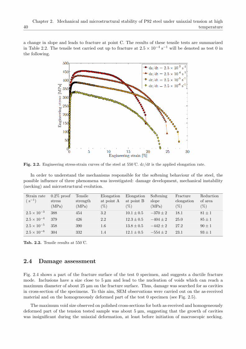
40Chapter 2. Mechanical and microstructural stability of P92 steel under uniaxial tension at high
temperature
a change in slope and leads to fracture at point C. The results of these tensile tests are summarizedin Table 2.2. The tensile test carried out up to fracture at 2.5× 10⁻⁴ s−1 will be denoted as test 0 inthe following.
Fig. 2.2. Engineering stress-strain curves of the steel at 550 C. dε/dt is the applied elongation rate.
In order to understand the mechanisms responsible for the softening behaviour of the steel, thepossible influence of three phenomena was investigated: damage development, mechanical instability(necking) and microstructural evolution.
Strain rate 0.2% proof Tensile Elongation Elongation Softening Fracture Reduction( s−1) stress strength at point A at point B slope elongation of area
(MPa) (MPa) (%) (%) (MPa) (%) (%)
2.5× 10⁻³ 388 454 3.2 10.1± 0.5 −370± 2 18.1 81± 1
2.5× 10⁻⁴ 379 426 2.2 12.3± 0.5 −404± 2 25.0 85± 1
2.5× 10⁻⁵ 358 390 1.6 13.8± 0.5 −442± 2 27.2 90± 1
2.5× 10⁻⁶ 304 332 1.4 12.1± 0.5 −554± 2 23.1 93± 1
Tab. 2.2. Tensile results at 550 C.
2.4 Damage assessment
Fig. 2.4 shows a part of the fracture surface of the test 0 specimen, and suggests a ductile fracturemode. Inclusions have a size close to 5 µm and lead to the nucleation of voids which can reach amaximum diameter of about 25 µm on the fracture surface. Thus, damage was searched for as cavitiesin cross-section of the specimens. To this aim, SEM observations were carried out on the as-receivedmaterial and on the homogeneously deformed part of the test 0 specimen (see Fig. 2.5).
The maximum void size observed on polished cross-sections for both as-received and homogeneouslydeformed part of the tension tested sample was about 5 µm, suggesting that the growth of cavitieswas insignificant during the uniaxial deformation, at least before initiation of macroscopic necking.

2.4. Damage assessment 41
Fig. 2.3. Engineering stress-strain curve at 550 C and 2.5× 10⁻⁴ s−1 (test 0) with the 4 noticeable pointsdescribed in part 2.3 (O, A, B and C).
Fig. 2.4. Secondary electron SEM image of fractured test 0 specimen.

42Chapter 2. Mechanical and microstructural stability of P92 steel under uniaxial tension at high
temperature
(a) (b)
Fig. 2.5. Backscattered electron SEM pictures taken from logitudinal cross-section of (a) the as-received steeland (b) the homogeneously deformed part of the test 0 specimen.
Even in the necked area, damage was only observed very close to the fracture surface. Senior etal. [Senior et al., 1986] observed ductile cavity nucleation at M23C6 carbides with a mean diameter of34 nm in a commercial 9%Cr-1%Mo steel after room temperature tensile tests at 1.5× 10⁻² s−1. Theobservations showed that void nucleation begins at M23C6 carbides for a plastic strain value of 0.25.For the test 0 specimen, the plastic strain reaches a maximum value lower than 0.1 (according to thecorresponding average diameter) in the homogeneously deformed region. Consistently with Senior etal. [Senior et al., 1986], damage development is negligible in the homogeneously deformed part of thetest 0 specimen and cannot be the cause of the observed softening behaviour.
2.5 Necking: experimental results and modelling
2.5.1 Interrupted tensile tests and onset of macroscopic necking
To study the beginning of macroscopic necking, seven different tests were interrupted at various valuesof elongation. The corresponding engineering stress-strain curves are presented in Fig. 2.6.
Although the seven curves are not superimposed with the curve corresponding to the referencetest 0, experimental reproducibility remains acceptable. Only tests 6 and 7 significantly differ fromtest 0. If both tests had been carried out until fracture, test 6 would have shown a lower fractureelongation than test 0, and test 7 a higher one.
Following Fig. 2.7, macroscopic necking is observed for specimens 5, 6 and 7 whilst specimens 1, 2,3 and 4 seem to be homogeneously deformed. To confirm this result, laser profilometry measurementsalong the gauge length of the seven specimens (Fig. 2.8) showed that necking appears clearly forspecimens 5, 6, 7, and much less clearly for specimen 4. Interrupted tests were, accordingly, classifiedusing the various stages identified in Fig. 2.3: tests on specimens 1, 2, 3 (and probably 4) wereinterrupted between O and B while tests on specimens 5, 6 and 7 were interrupted between B and C.

2.5. Necking: experimental results and modelling 43
Fig. 2.6. Engineering stress-strain curves: test 0 (curve 0) and seven tensile tests (1-7) interrupted after variousamounts of strain.
Fig. 2.7. The seven specimens after interrupted tensile tests.

44Chapter 2. Mechanical and microstructural stability of P92 steel under uniaxial tension at high
temperature
Fig. 2.8. Average diameters along the gauge length for the seven interrupted specimens, determined by laserprofilometry. The accuracy of measurements is about 0.5 µm.
The hypothesis of volume conservation during plastic deformation (which is consistent with theabsence of significant damage development mentioned above) is another way to confirm the onset ofmacroscopic necking. Under uniaxial tension, assuming an isotropic yield behaviour (to support this,at least, circular sections were observed to remain circular), neglecting elastic strains and consideringthe small perturbations hypothesis, the trace of the strain tensor is equal to zero if deformation ishomogeneous and this hypothesis leads to a linear relationship between axial (ε1) and radial (ε2, ε3)strains, as shown in Eq. 2.2:
Tr εp = 0Tr εeTr εp
=⇒ Tr
ε1 · ·
· ε2 ·
· · ε3
= 0ε2=ε3=⇒ ε2 = −1
2ε1 (2.2)
Eq. 2.2 is plotted as a dotted straight line in Fig. 2.9. The experimental value of the radialstrain ε2 is calculated using three measurements of the diameter carried out on the homogeneouslydeformed section far from the necking region of the seven specimens. Points close to the dotted lines(tests 1, 2, 3, 4) correspond to specimens homogeneously deformed along their gauge length. Forpoints far from the dotted line (tests 5, 6, 7), strain can not be homogeneous, which means that thesetests were interrupted after the onset of macroscopic necking. This result confirms that macroscopicnecking begins for a longitudinal elongation between those reached for specimens 4 and 5, respectively,consistently with point B of Fig. 2.3. In the following, it will be assumed that macroscopic neckingstarts at point B.
Elongation at point B was derived from each tensile curve at various strain rates by using thetangent to the softening part of the curve. A difference of 3± 1 MPa was arbitrarily chosen betweenthe curve and the tangent to determine the elongation at point B. This method is illustrated in Fig. 2.10for test 0 tensile curve and the results are presented in Table 2.2. The accuracy of this measurementleads to a sensitivity of ±0.5% in elongation at point B. Owing that deformation is homogeneous up topoint B, it is possible to build and analyse true stress-strain curves from point O to point B, presented
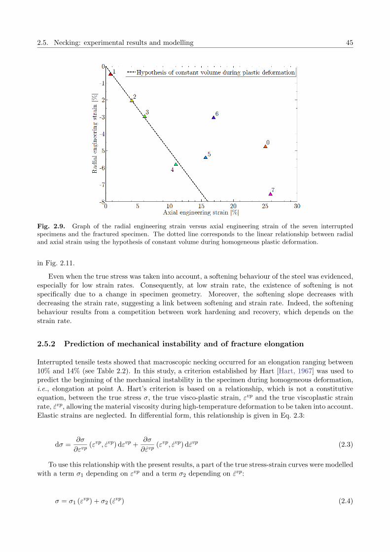
2.5. Necking: experimental results and modelling 45
Fig. 2.9. Graph of the radial engineering strain versus axial engineering strain of the seven interruptedspecimens and the fractured specimen. The dotted line corresponds to the linear relationship between radialand axial strain using the hypothesis of constant volume during homogeneous plastic deformation.
in Fig. 2.11.
Even when the true stress was taken into account, a softening behaviour of the steel was evidenced,especially for low strain rates. Consequently, at low strain rate, the existence of softening is notspecifically due to a change in specimen geometry. Moreover, the softening slope decreases withdecreasing the strain rate, suggesting a link between softening and strain rate. Indeed, the softeningbehaviour results from a competition between work hardening and recovery, which depends on thestrain rate.
2.5.2 Prediction of mechanical instability and of fracture elongation
Interrupted tensile tests showed that macroscopic necking occurred for an elongation ranging between10% and 14% (see Table 2.2). In this study, a criterion established by Hart [Hart, 1967] was used topredict the beginning of the mechanical instability in the specimen during homogeneous deformation,i.e., elongation at point A. Hart’s criterion is based on a relationship, which is not a constitutiveequation, between the true stress σ, the true visco-plastic strain, εvp and the true viscoplastic strainrate, εvp, allowing the material viscosity during high-temperature deformation to be taken into account.Elastic strains are neglected. In differential form, this relationship is given in Eq. 2.3:
dσ =∂σ
∂εvp(εvp, εvp) dεvp +
∂σ
∂εvp(εvp, εvp) dεvp (2.3)
To use this relationship with the present results, a part of the true stress-strain curves were modelledwith a term σ1 depending on εvp and a term σ2 depending on εvp:
σ = σ1 (εvp) + σ2 (εvp) (2.4)

46Chapter 2. Mechanical and microstructural stability of P92 steel under uniaxial tension at high
temperature
Fig. 2.10. Scheme of the test 0 engineering stain-stress curve illustrating the determination of the deformationat point B with the method of the tangent. A difference of 3 ± 1 MPa is chosen between the curve and thetangent to determine the elongation at point B.
Fig. 2.11. Effect of the strain rate on the true stress-true strain curves derived from Fig. 2.2 (from point O topoint B).

2.5. Necking: experimental results and modelling 47
Term σ1 (εvp) was based on the empirical equation of Voce [Kishore and Sinha, 1996]:
σ1 = σ0 +Q [1− exp (−βεvp)] (2.5)
Term σ2 (εvp) was built with a classical expression corresponding to thermally activated viscoplasticflow [Francois et al., 1995a]:
σ2 =1
αln
(εvp
εvp0
)(2.6)
By combining Eqs. 2.4, 2.5 and 2.6, it was possible to model the true stress-strain curves withEq. 2.7:
σ = σ0 +Q [1− exp (−βεvp)] +1
αln
(εvp
εvp0
)(2.7)
In order to improve the fit quality, the β coefficient was made dependent on εvp by Eq. 2.8:
β = β1 ln (εvp) + β2 (2.8)
The six parameters values adjusted for predicting reasonably the true stress-strain curves for thedifferent strain rates are reported in Table 2.3. The corresponding ajusted curves are presented inFig 2.12.
Parameters σ0 (MPa) Q (MPa) β1 β2 α (MPa−1) εvp0 (s−1)
Values 100 98 -42.92 -203.31 5.18× 10⁻² 1× 10⁻⁹
Tab. 2.3. Parameters values used for the fit of the true stress-strain curves (Eqs. 2.7 and 2.8).
The evolution of the mechanical instability during deformation was studied following the workof Hart. In the undeformed state, Hart considers that the specimen has a uniform cross-section A0
except for a small part which has a cross-section of A0 − δA0 where δA0 is small and corresponds toan imperfection of the specimen geometry. During deformation, the principal cross-section changesfrom A0 to A and A0 − δA0 becomes A − δA. In this model, both sections (the necked area and thenon-necked area) of the material are sustaining the same load, but may deform independently fromeach other, i.e. no constraint effect of the smallest section area by the largest one is taken into account.Hart computed the expression of δA from A, A0 and δA0:
δA = δA0
(A0
A
) γ+m−1m
(2.9)
In Eq. 2.9, a term γ (Eq. 2.10) corresponding to strain hardening and a term m (Eq. 2.11) corre-sponding to visco-plasticity are defined:
γ =1
σ
∂σ
∂εvp(2.10)

48Chapter 2. Mechanical and microstructural stability of P92 steel under uniaxial tension at high
temperature
Fig. 2.12. Experimental (full symbols) and adjusted curves (open symbols) using Eq. 2.7, Eq. 2.8 and param-eters values presented in Table 2.3.
m =εvp
σ
∂σ
∂εvp(2.11)
According to Eq. 2.9, the deformation is stable if γ+m is higher than 1, then the offset δA decreases(in absolute value) and the section A+δA becomes A, i.e. the initial geometrical defect is erased : bothwork hardening and viscosity tend to stabilize deformation along the gauge region. On the contrary, ifγ +m is lower than 1, then the offset δA increases (in absolute value), leading to further developmentof the mechanical instability and, eventually, to the onset of macroscopic necking. Hart proposes thefollowing criterion to predict the initiation of the mechanical instability:
γ +m = 1 (2.12)
Parameter δA0 is determined by laser profilometry carried out on the specimens before the tensiletests. Considering d+ (d−) the maximun (minimum) value of the diameter measured for each specimenalong the gauge part, δA0 is defined as:
δA0 =π
4
[(d+)2 − (d−)2] (2.13)
As elongation at the onset of macroscopic necking is much higher than 10−3, elastic strains areneglected. In the homogeneously deformed part, the ratio A0
A and engineering strain ε are linked inthe following way:
A0
A= 1 + ε (2.14)
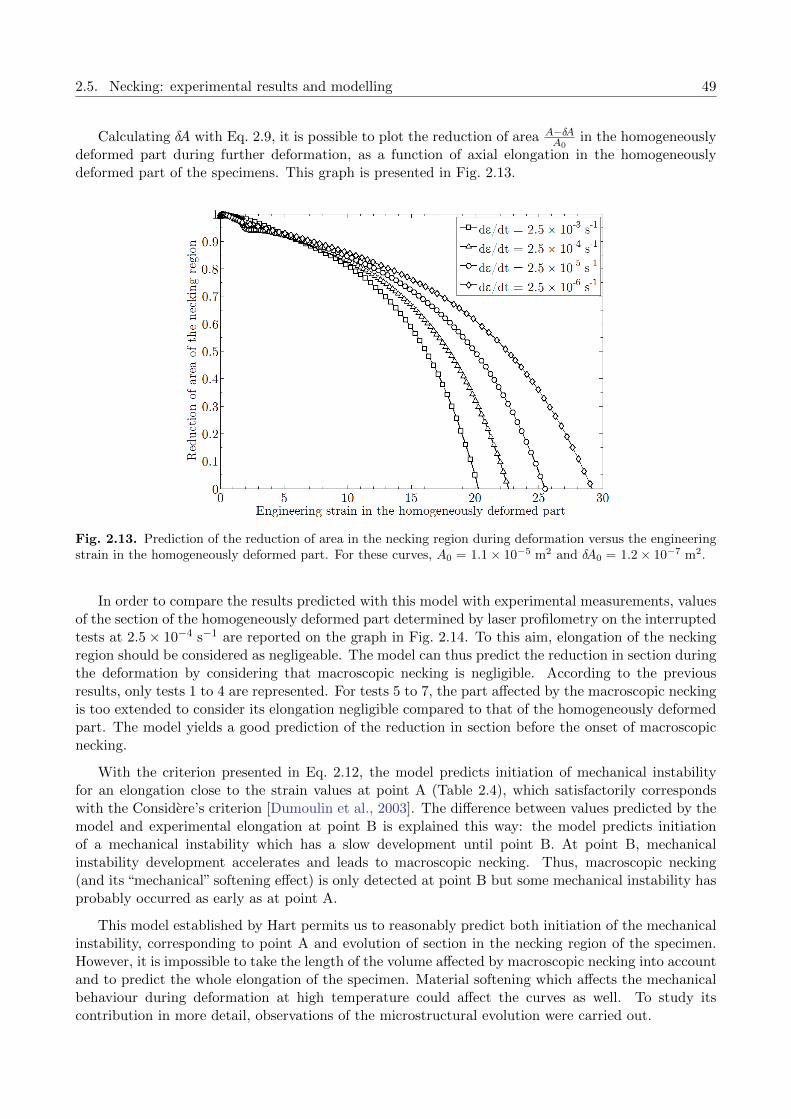
2.5. Necking: experimental results and modelling 49
Calculating δA with Eq. 2.9, it is possible to plot the reduction of area A−δAA0
in the homogeneouslydeformed part during further deformation, as a function of axial elongation in the homogeneouslydeformed part of the specimens. This graph is presented in Fig. 2.13.
Fig. 2.13. Prediction of the reduction of area in the necking region during deformation versus the engineeringstrain in the homogeneously deformed part. For these curves, A0 = 1.1× 10⁻⁵ m2 and δA0 = 1.2× 10⁻⁷ m2.
In order to compare the results predicted with this model with experimental measurements, valuesof the section of the homogeneously deformed part determined by laser profilometry on the interruptedtests at 2.5× 10⁻⁴ s−1 are reported on the graph in Fig. 2.14. To this aim, elongation of the neckingregion should be considered as negligeable. The model can thus predict the reduction in section duringthe deformation by considering that macroscopic necking is negligible. According to the previousresults, only tests 1 to 4 are represented. For tests 5 to 7, the part affected by the macroscopic neckingis too extended to consider its elongation negligible compared to that of the homogeneously deformedpart. The model yields a good prediction of the reduction in section before the onset of macroscopicnecking.
With the criterion presented in Eq. 2.12, the model predicts initiation of mechanical instabilityfor an elongation close to the strain values at point A (Table 2.4), which satisfactorily correspondswith the Considere’s criterion [Dumoulin et al., 2003]. The difference between values predicted by themodel and experimental elongation at point B is explained this way: the model predicts initiationof a mechanical instability which has a slow development until point B. At point B, mechanicalinstability development accelerates and leads to macroscopic necking. Thus, macroscopic necking(and its “mechanical” softening effect) is only detected at point B but some mechanical instability hasprobably occurred as early as at point A.
This model established by Hart permits us to reasonably predict both initiation of the mechanicalinstability, corresponding to point A and evolution of section in the necking region of the specimen.However, it is impossible to take the length of the volume affected by macroscopic necking into accountand to predict the whole elongation of the specimen. Material softening which affects the mechanicalbehaviour during deformation at high temperature could affect the curves as well. To study itscontribution in more detail, observations of the microstructural evolution were carried out.

50Chapter 2. Mechanical and microstructural stability of P92 steel under uniaxial tension at high
temperature
Fig. 2.14. Prediction of the reduction of the necking region during deformation at 2.5× 10⁻⁴ s−1 compared withexperimental results determined with tests 1 to 4. For this curve, A0 = 1.1× 10⁻⁵ m2 and δA0 = 1.2× 10⁻⁷ m2.
Strain rate ( s−1) Experimental value of elongationat point A (%)
Prediction of elongation at point A(%) using the present model
2.5× 10⁻³ 3.2 3.6
2.5× 10⁻⁴ 2.2 2.2
2.5× 10⁻⁵ 1.6 1.6
2.5× 10⁻⁶ 1.4 1.3
Tab. 2.4. Experimental measurements and predicted values of elongation at point A.
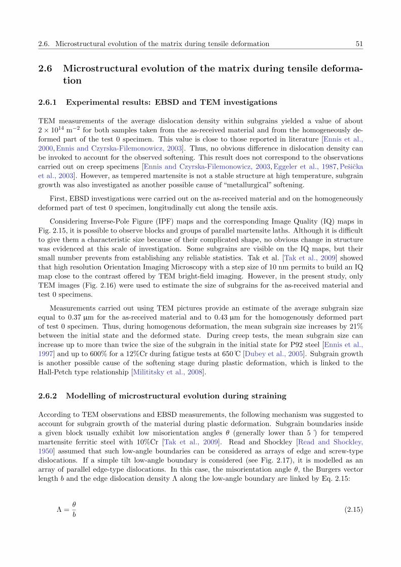
2.6. Microstructural evolution of the matrix during tensile deformation 51
2.6 Microstructural evolution of the matrix during tensile deforma-tion
2.6.1 Experimental results: EBSD and TEM investigations
TEM measurements of the average dislocation density within subgrains yielded a value of about2× 1014 m−2 for both samples taken from the as-received material and from the homogeneously de-formed part of the test 0 specimen. This value is close to those reported in literature [Ennis et al.,2000, Ennis and Czyrska-Filemonowicz, 2003]. Thus, no obvious difference in dislocation density canbe invoked to account for the observed softening. This result does not correspond to the observationscarried out on creep specimens [Ennis and Czyrska-Filemonowicz, 2003, Eggeler et al., 1987, Pesickaet al., 2003]. However, as tempered martensite is not a stable structure at high temperature, subgraingrowth was also investigated as another possible cause of “metallurgical” softening.
First, EBSD investigations were carried out on the as-received material and on the homogeneouslydeformed part of test 0 specimen, longitudinally cut along the tensile axis.
Considering Inverse-Pole Figure (IPF) maps and the corresponding Image Quality (IQ) maps inFig. 2.15, it is possible to observe blocks and groups of parallel martensite laths. Although it is difficultto give them a characteristic size because of their complicated shape, no obvious change in structurewas evidenced at this scale of investigation. Some subgrains are visible on the IQ maps, but theirsmall number prevents from establishing any reliable statistics. Tak et al. [Tak et al., 2009] showedthat high resolution Orientation Imaging Microscopy with a step size of 10 nm permits to build an IQmap close to the contrast offered by TEM bright-field imaging. However, in the present study, onlyTEM images (Fig. 2.16) were used to estimate the size of subgrains for the as-received material andtest 0 specimens.
Measurements carried out using TEM pictures provide an estimate of the average subgrain sizeequal to 0.37 µm for the as-received material and to 0.43 µm for the homogenously deformed partof test 0 specimen. Thus, during homogenous deformation, the mean subgrain size increases by 21%between the initial state and the deformed state. During creep tests, the mean subgrain size canincrease up to more than twice the size of the subgrain in the initial state for P92 steel [Ennis et al.,1997] and up to 600% for a 12%Cr during fatigue tests at 650 C [Dubey et al., 2005]. Subgrain growthis another possible cause of the softening stage during plastic deformation, which is linked to theHall-Petch type relationship [Milititsky et al., 2008].
2.6.2 Modelling of microstructural evolution during straining
According to TEM observations and EBSD measurements, the following mechanism was suggested toaccount for subgrain growth of the material during plastic deformation. Subgrain boundaries insidea given block usually exhibit low misorientation angles θ (generally lower than 5 ) for temperedmartensite ferritic steel with 10%Cr [Tak et al., 2009]. Read and Shockley [Read and Shockley,1950] assumed that such low-angle boundaries can be considered as arrays of edge and screw-typedislocations. If a simple tilt low-angle boundary is considered (see Fig. 2.17), it is modelled as anarray of parallel edge-type dislocations. In this case, the misorientation angle θ, the Burgers vectorlength b and the edge dislocation density Λ along the low-angle boundary are linked by Eq. 2.15:
Λ =θ
b(2.15)

52Chapter 2. Mechanical and microstructural stability of P92 steel under uniaxial tension at high
temperature
Fig. 2.15. Inverse pole figure maps of (a) as-received material and (b) homogeneously deformed part of test 0specimen. The unit triangle is a colour key according to the crystallographic poles aligned with the samplesurface normal direction. (c) and (d) Image Quality maps of the same region as (a) and (b), respectively. Thetensile axis is horizontal and the scale bar stands for 30 µm in all maps.

2.6. Microstructural evolution of the matrix during tensile deformation 53
(a) (b)
Fig. 2.16. TEM pictures taken from (a) a sample from the as-received steel and (b) a sample taken far fromthe necking region, i.e. in the homogeneously deformed part of test 0 specimen. The direction of the tube axisis perpendicular to the plane of the picture.
Fig. 2.17. Scheme of the interactions between mobile edge dislocations (moving along the dashed line) andparallel low-angle boundary edge dislocations (aligned along the continuous line) (symmetric tilt low-angleboundary).

54Chapter 2. Mechanical and microstructural stability of P92 steel under uniaxial tension at high
temperature
Sauzay [Sauzay, 2009] proposed a model to predict the decrease in misorientation of the low-angleboundaries during high temperature deformation of tempered martensite ferritic steel. Mobile disloca-tions interact with low-angle boundaries during glide. Indeed, if appropriate slip systems are activated,mobile dislocations may move toward a low-angle boundary which contains parallel dislocations of op-posite sign. Annihilation takes place between two edge (or screw) dislocations of opposite signs andparallel line vectors, if their distance is smaller than a critical value. These critical distances are de-noted as ye for edge dislocations and as ys for screw dislocations. Considering Eq. 2.15, annihilation ofdislocation of opposite signs induces a decrease in boundary dislocation density, Λ, and consequentlyin the misorientation angle θ of the boundary under interest. During deformation, accumulated strainmay increase high enough to allow complete annihilation of many low-angle boundaries and thus anincrease in subgrain size. The purpose of this section is to apply this model to the tensile deformationof the P92 specimens at 823 K. If the Burgers vectors of the mobile dislocations are parallel to those ofboundary dislocations, misorientation angles θe (resp. θs) for low-angle boundaries consisting of edge(rep. screw) dislocations is given by Sauzay’s model [Sauzay, 2009] as a function of the plastic strainεP , the Burgers vector length b, the Taylor factor M , the critical annihilation distance ye (resp. ys)and the initial misorientation θ0 of low-angle boundaries:
θe = θ0 exp
(yeb
M
5εP)
(2.16)
θs = θ0 exp
(ysb
M
5εP)
(2.17)
For ye, ys and M parameters, the following values were used: ye ≈ 1.6 nm, ys ≈ 50 nm (due to lackof information, dislocation annihilation distances in copper at room temperature were used [Essmannand Differt, 1996]) and M ≈ 2.9 (Taylor factor value for a textureless body centred cubic struc-ture [Taylor, 1938]). Although martensitic steels are characterised by a microtexture, prior austenitegrains are considered as textureless to simplify the model. Otherwise, finite element modelling is nec-essary to take the influence of texture on local stress and strain fields into account, which is outsidethe scope of this study.
Interactions between low-angle boundary dislocations and mobile parallel ones are limited by thenumber of slip systems activated in each subgrain. The crystal structure of the P92 tempered marten-site matrix was supposed to be body-centred cubic. Two families of slip systems were considered:110 and 112 planes and 〈111〉 slip directions. Altogether, this means 24 slip systems. Indeed, themodel considers activation of mobile dislocations in neighbouring subgrains A and B during deforma-tion. As dislocations with Burgers vector ~b move in the direction opposite to that of parallel ones witha Burgers vector −~b, interactions between low-angle boundary dislocations and mobile parallel oneswith a Burgers vector ~b or −~b is possible during deformation, independently of the dislocation movingdirection. Consequently, in this model one considers that two opposite slip systems are equivalent,leading to divide by 2 the total number of possible activated slip systems.
In a major part of subgrains, several slip systems are likely to be activated, due to the highmacroscopic plastic strain. This is why the Taylor model is used in the present work: the plastic strainis supposed to be the same in each subgrain as well as in each block, packet and prior austenite grain.Taylor suggests that only five slip systems are generally activated in each subgrain to accommodatethe macroscopic plastic strain. The number of ways to choose 5 slip systems among 24 is noted C5
24,

2.6. Microstructural evolution of the matrix during tensile deformation 55
corresponding to the following definition:
Cpn =
n !
p ! (n− p) !(2.18)
To allow annihilation between a mobile dislocation and a low-angle boundary dislocation, theirBurgers vectors have to be opposite. This means that to avoid annihilation, it is necessary to choose5 slip systems with none having dislocations parallel to the boundary ones. The number of waysto choose 5 different slip systems with no dislocation parallel to the considered low-angle boundaryones is noted C5
24−q where q is the number of slip systems with dislocation parallel to the ones of the
subgrain boundary. Consequently, the probability of non-annihilation isC5
24−q
C524
, and the probability
P (q) of annihilation is:
P (q) = 1−C5
24−q
C524
(2.19)
For low-angle boundary dislocations of edge (resp. screw) type, q is equal to 1 (resp. 6). Theprobability Pe (resp. Ps) of annihilation for edge (resp. screw) type is equal to 0.21 (resp. 0.81).
To determine the misorientation angle of subgrain boundaries, it is assumed that:
subgrain boundaries are either pure tilt or either pure twist i.e. that they are described usingeither one set of edge dislocations, or one set of screw dislocations.
the fraction of pure tilt and pure twist boundaries are, respectively, the same as the edge (screw)mobile dislocation density.
Using Eqs. 2.16 and 2.17 and considering the proportion Ne (resp. Ns) of low-angle boundarydislocations of edge (resp. screw) type, it is possible to determine the cumulated frequency afterdeformation of:
The low-angle boundaries (pure tilt and pure twist) which did not interact with mobile disloca-tions. Their final misorientation is equal to their initial one, and their cumulated frequency isequal to Ne (1− Pe) +Ns (1− Ps).
The pure tilt low-angle boundaries which interacted with mobile dislocations. Their final mis-orientation is equal to θe, and their cumulated frequency is equal to NePe.
The pure twist low-angle boundaries which interacted with mobile dislocations. Their finalmisorientation is equal to θs, and their cumulated frequency is equal to NsPs.
As accurate values of the model parameters could not be estimated, the proportions Ne and Ns wereconsidered as equal (Ne = Ns = 0.5). Using the cumulated frequency of low boundary misorientationangles in a tempered martensite ferritic steel (X 20 CrMoV 12 1) measured by Tak et al. [Tak et al.,2009], the cumulated frequency of misorientation angles versus the misorientation angle was plottedin Fig. 2.18. The value of plastic strain εP = 9.6%, considered in the graph, corresponds to the strainin the homogeneous part of test 0 specimen, far from the necking region.
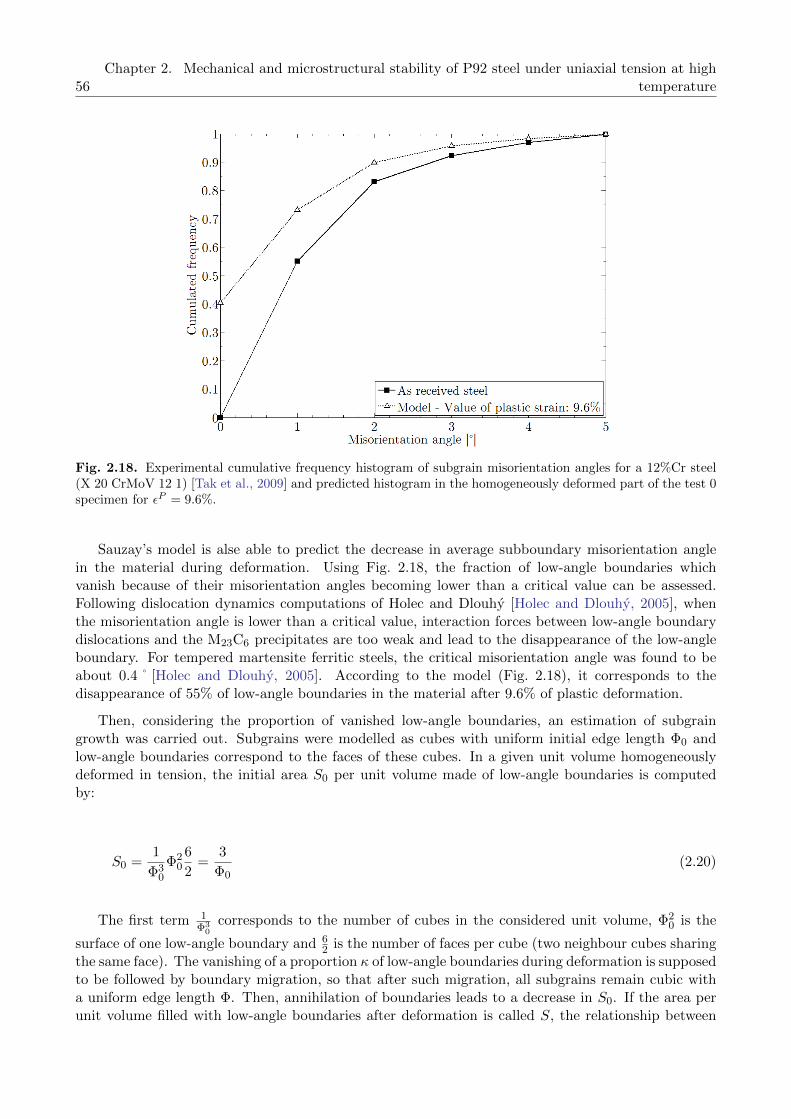
56Chapter 2. Mechanical and microstructural stability of P92 steel under uniaxial tension at high
temperature
Fig. 2.18. Experimental cumulative frequency histogram of subgrain misorientation angles for a 12%Cr steel(X 20 CrMoV 12 1) [Tak et al., 2009] and predicted histogram in the homogeneously deformed part of the test 0specimen for εP = 9.6%.
Sauzay’s model is alse able to predict the decrease in average subboundary misorientation anglein the material during deformation. Using Fig. 2.18, the fraction of low-angle boundaries whichvanish because of their misorientation angles becoming lower than a critical value can be assessed.Following dislocation dynamics computations of Holec and Dlouhy [Holec and Dlouhy, 2005], whenthe misorientation angle is lower than a critical value, interaction forces between low-angle boundarydislocations and the M23C6 precipitates are too weak and lead to the disappearance of the low-angleboundary. For tempered martensite ferritic steels, the critical misorientation angle was found to beabout 0.4˚[Holec and Dlouhy, 2005]. According to the model (Fig. 2.18), it corresponds to thedisappearance of 55% of low-angle boundaries in the material after 9.6% of plastic deformation.
Then, considering the proportion of vanished low-angle boundaries, an estimation of subgraingrowth was carried out. Subgrains were modelled as cubes with uniform initial edge length Φ0 andlow-angle boundaries correspond to the faces of these cubes. In a given unit volume homogeneouslydeformed in tension, the initial area S0 per unit volume made of low-angle boundaries is computedby:
S0 =1
Φ30
Φ20
6
2=
3
Φ0(2.20)
The first term 1Φ3
0corresponds to the number of cubes in the considered unit volume, Φ2
0 is the
surface of one low-angle boundary and 62 is the number of faces per cube (two neighbour cubes sharing
the same face). The vanishing of a proportion κ of low-angle boundaries during deformation is supposedto be followed by boundary migration, so that after such migration, all subgrains remain cubic witha uniform edge length Φ. Then, annihilation of boundaries leads to a decrease in S0. If the area perunit volume filled with low-angle boundaries after deformation is called S, the relationship between

2.7. Conclusions 57
S0 and S is:
S = (1− κ)S0 (2.21)
In the same way as in Eq. 2.20, S is defined as a function of the edge length Φ of the cube afterdeformation:
S =3
Φ(2.22)
Knowing that the proportion κ of vanished low-angle boundaries is equal to 55% (Fig. 2.18), thisleads to the following relationship:
Φ ≈ 2.2Φ0 (2.23)
The model predicts a growth of the microstructure equal to a factor of about 2.2. This result ishigher than the growth factor equal to about 1.2 deduced from the TEM pictures in part 2.6.1. Thedifference between experimental and predicted results can be due to the following reasons:
Experimental results, manually determined with about 100-120 subgrains from TEM pictures,were used to estimate an average subgrain size. This method induces a problem of statistical sig-nificance of the data set, and the growth factor should be probably different if it was determinedfrom a whole subgrain size distribution.
In the model, subgrain boundaries are either of pure tilt or of pure twist-type. This hypothesisis very strong, because most subgrain boundaries are composed with a mix of edge and screwdislocations [Guttmann, 1974]. In this case, interactions between mobile dislocations and low-angle boundaries (arrays of somewhat entangled dislocations) are more complex and induce adecrease in the probability of annihilation of all dislocations of the low-angle boundary and thusin the predicted growth factor. Consequently, pure low-angle twist boundaries will be consideredas arrays of two families of screw dislocations [Guttmann, 1974].
The activation of exactly five slip systems in each grain during the deformation, due to the Tay-lor’s model, is probably overestimated for the tempered martensite ferritic steels. The activationof less slip systems may be enough to permit the deformation. Consequently, it would lead to adecrease of the probability of annihilation of the low-angle boundary dislocations.
Polycrystalline modelling is needed for predicting more accuratly the progressive activation of slipsystems in the various blocks.
2.7 Conclusions
Tensile tests at various strain rates were carried out at 550 C on a P92 steel. True stress-strain curvesconfirm the existence of a weak softening stage during deformation at low strain rate, a typical char-acteristic of 9%Cr steels deformed at high temperature. Considering the relatively low temperature
58Chapter 2. Mechanical and microstructural stability of P92 steel under uniaxial tension at high
temperature
of 550 C and the high strain rates of tensile tests (compared to creep), the diffusion processes areneglected. The softening mechanisms are based on the annihilation of subgrain boundaries and mo-bile dislocations. Nucleation, growth and coarsening of precipitates can be neglected because of thepreliminar tempering and short test duration (≤ 15 hours) at 550 C. Experimental results and modelpredictions lead to the following conclusions:
1. For strain rates up to 2.5× 10⁻⁴ s−1, both engineering and true stress-strain curves show a firstsoftening stage well before the onset of macroscopic visible necking. This stage is characterisedby constantly decreasing load and true stress, which depends on the applied elongation rate: thelower the elongation rate, the more pronounced the softening stage.
2. The Hart’s criterion predicts the onset of mechanical instability for a low elongation close to theelongation at maximum load. In fact, diffuse necking occurs after a few percents of elongation.Macroscopic necking, in turn, induces a second softening stage with a stronger decreasing slope,leading to fracture.
3. This first softening stage is not due to cavity nucleation and growth in the specimen, whichoccurs only in the necking volume and shortly before fracture. TEM observations show that thesubgrain size increases by about 21%, contributing to the material softening behaviour. Thisgrowth is overestimated by the low-angle boundary vanishing model in its present form. Improvedmodelling taking into account more accuratly low-angle boundary structure and activation ofslip systems within tempered martensite blocks is needed. This will be carried out in chapter 4.
In the following chapter, we focus on the mechanical behaviour and microstructural evolutionduring cycling at 550 C. A more detailled study of the subgrain size distribution and dislocationdensity evolution, using fatigue test interrupted after a given number of cycles, is proposed. Thischapter is dedicated to experimental results which permit us to propose a model coupling mechanicalbehaviour and microstructural evolution in chapter 4.

59
Chapter 3
Mechanical behaviour andmicrostructural evolution during cyclicand creep loading
This third chapter focuses on the mechanical behaviour of Grade 92 steel during continuous cyclicloading and creep at 550 C. Two creep tests performed at 600 C and cyclic test including tensile holdingperiods at 550 C are also presented. Then, the study focuses on the physical mechanisms of deformationduring continuous cycling test. The macroscopic stress partition based on Cottrell’s method is applied.Finally, TEM observations of the microstructure are presented in order to characterize microstructureevolution and possibly involved physical mechanisms are discussed.
Ce troisieme chapitre est dedie a l’etude du comportement mecanique de l’acier Grade 92 lors desollicitations de type chargement cyclique continu et fluage a 550 C. Deux essais de fluage a 600 C etun essai de chargement cyclique avec temps de maintien en traction a 550 C sont aussi presentes. Parla suite, l’etude se focalise sur les mecanismes de deformation lors des essais sous chargement cycliquecontinu. La decomposition de la contrainte macroscopique selon la methode de Cottrell est appliquee.Enfin, des observations MET visant a caracteriser l’evolution de la microstructure sont presentees etles mecanismes potentiellement impliques sont discutes.
Contents
Abstract (in French) . . . . . . . . . . . . . . . . . . . . . . . . . . . . . . . . . . . . 61
3.1 Macroscopic cyclic loading, creep and creep-fatigue behaviour . . . . . . . 63
3.1.1 Cyclic loading tests . . . . . . . . . . . . . . . . . . . . . . . . . . . . . . . . . . 63
3.1.2 Creep tests . . . . . . . . . . . . . . . . . . . . . . . . . . . . . . . . . . . . . . 68
3.1.3 Cyclic test including tensile holding periods . . . . . . . . . . . . . . . . . . . . 71
3.2 Macroscopic analysis of softening during cyclic loading . . . . . . . . . . . . 74
3.3 Observations of microstructural evolutions during cyclic loading tests . . 76
3.3.1 Evolution of the subgrain size distribution . . . . . . . . . . . . . . . . . . . . . 77
3.3.2 Evolution of the dislocation density during high temperature cyclic loading . . 84
3.3.3 Discussion about deformation and annihilation mechanisms . . . . . . . . . . . 85
3.4 Concluding remarks . . . . . . . . . . . . . . . . . . . . . . . . . . . . . . . . . 87

60 Chapter 3. Mechanical behaviour and microstructural evolution during cyclic and creep loading
61
Resume
Ce chapitre presente les resultats de l’etude des proprietes mecaniques en chargement cyclique continuet en fluage a 550 C sous air sur l’acier Grade 92. Toutes les eprouvettes ont ete prelevees a mi-epaisseur dans le sens longitudinal du tube. Les essais de fatigue ont ete effectues sur des eprouvettescylindriques de 16 mm de longueur utile et 8 mm de diametre. Les essais de fluage ont ete conduitssur des eprouvettes cylindriques de 30 mm de longueur utile et 8 mm de diametre.
Dix essais ont ete effectues pour des amplitudes de deformation totale variant de ±0,2 a ±0,5 %,avec une vitesse de deformation de 2× 10⁻³ s−1. Afin d’etudier l’influence de la vitesse de deformationsur le comportement mecanique et l’evolution de la microstructure, un essai a ete effectue avec uneamplitude de deformation de ±0,35 % et une vitesse de deformation de 1× 10⁻⁵ s−1. Enfin, pourmesurer l’evolution de la microstructure au cours du cyclage, trois essais de fatigue interrompus a 60,300 et 1 000 cycles ont ete menes avec une amplitude de deformation de ±0,35 % et une vitesse dedeformation de 1× 10⁻⁵ s−1.
Les resultats de ces essais n’ont montre aucune difference significative entre les aciers Grade 91et 92 en termes de duree de vie en fatigue. De meme, les parametres de Monkman-Grant, utilisant lesresultats des essais de fluage de l’acier Grade 92, sont tres proches de ceux etablis dans la litteraturepour l’acier Grade 91.
Les resultats des essais de fatigue ont montre que l’acier Grade 92 est sensible a l’adoucissement cy-clique. Bien que plus prononce pour les amplitudes de deformation elevees, ce phenomene est aussi ob-serve pour les tres faibles valeurs d’amplitude de deformation plastique (environ 10−4). L’adoucissementest aussi influence par la vitesse de deformation : plus celle-ci est faible, plus l’amplitude de deforma-tion viscoplastique par cycle est elevee, plus la chute de la contrainte est rapide. Cependant, l’impactde la vitesse de deformation sur la duree de vie en fatigue est faible.
Dans le but d’etudier le phenomene d’adoucissement cyclique, une decomposition de la contraintemacroscopique mesuree selon la methode de Cottrell [Cottrell, 1953] est proposee. Comme pourl’acier Grade 91, les resultats montrent que l’adoucissement cyclique de l’acier Grade 92 a 550 Cest principalement du a la diminution de la composante cinematique au cours du cyclage. Cetteobservation indique une decroissance des interactions a longue portee entre les dislocations mobiles etla foret de dislocations ou les sous-joints de faible desorientation.
Pour confirmer ces hypotheses, des observations MET ont ete effectuees afin de mesurer l’evolutionde la distribution de la taille des sous-grains et de la densite moyenne de dislocations au cours ducyclage. Les distributions de tailles des sous-grains, correctement decrites par des fonctions de densitede probabilite lognormale, montrent une croissance globale de la taille moyenne et une augmentationde la dispersion des mesures durant la deformation cyclique. La densite de dislocations dans les sous-grains diminue au cours de l’essai. Ces evolutions microstructurales sont d’autant plus prononcees quela vitesse de deformation est faible. A ce stade, les observations MET sont compatibles avec l’hypothesede mecanismes de deformation liant la decroissance de la densite de dislocations et l’augmentation dela taille des sous-grains. Cette hypothese est developpee dans le chapitre 4.

62 Chapter 3. Mechanical behaviour and microstructural evolution during cyclic and creep loading

3.1. Macroscopic cyclic loading, creep and creep-fatigue behaviour 63
3.1 Macroscopic cyclic loading, creep and creep-fatigue behaviour
This present section aims to describe the results of cyclic loading tests, creep tests and cyclic loadingtests with holding periods, carried out on Grade 92 steel at 550 C. Creep tests performed at 600 Care also presented.
3.1.1 Cyclic loading tests
Several grades of 9% and 12% chromium tempered martensitic steels (EUROFER 97 [Armas et al.,2002,Lindau et al., 2002, Marmy and Kruml, 2008], Grade 91 [Kim and Weertman, 1988,Choudharyet al., 1991,Kunz and Lukas, 2001,Nagesha et al., 2002,Fournier et al., 2010], Grade 92 [Kannan et al.,2010, Fournier et al., 2011a], X20 and X22 [Earthman et al., 1989, Eggeler, 1989, Petersmeier et al.,1998, Kostka et al., 2007, Aghajani et al., 2009]) are known to be sensitive to softening during cyclicloading at high temperature. This softening stage is characterized by a continous decrease in flow stressamplitude, leading to an increase in viscoplastic strain amplitude per cycle if loading is deformationcontrolled. Tomkins showed that the crack propagation rate during fatigue test is proportional tothe visco-plastic strain range [Tomkins, 1968]. The mechanical softening, which induces a decreasein resistance to crack propagation, is mainly due to microstructural instability, characterized by anincrease in subgrain size and a decrease in dislocation density. This point is exposed in section 3.3. Theinfluence of the strain localisation and fatigue damage during cycling on the mechanical behaviour isnot studied in this PhD work. Formation of intense slip bands has been already observed during fatiguetests on Grade 91 steel at room temperature, but not yet for higher temperatures [Fournier et al.,2006b]. Although these sources of microstructural heterogeneities may occur at high temperature, thepresent study only focuses on the subgrain size and dislocation density evolution during cycling.
3.1.1.1 Experimental conditions and specimen geometry
Cyclic loading tests, conducted at CEA/SRMA laboratory, were performed in laboratory air at 550 Cusing a MAYES ESM100 servo-mechanical machine with resistance furnace heating. They were car-ried out on smooth cylindrical specimens with 16 mm in gauge length, 8 mm in gauge diameter anda shoulder radius of 16 mm (see Fig. 3.1), machined from mid-thickness of the pipe along its longi-tudinal axis. The temperature along the gauge part of the specimen was controlled within ± 2 C bythermocouple attached to the gauge part.
Cyclic loading tests were performed under total strain control, measured by a capacitive exten-someter (10 mm in gauge length) directly attached on the gauge part of the specimen. The accuracyof elongation measurements is better than 0.5 µm, allowing cyclic loading tests with a total strainrange as low as 0.1 % to be conducted. Ten cyclic loading tests were carried out at 2× 10⁻³ s−1 forvarious values of the total strain amplitude from ± 0.50 % to ± 0.20 %. In order to estimate theexperimental scatter, two cyclic tests were performed at 2× 10⁻³ s−1 and 550 C for every value ofstrain amplitude. Additionally, a test was performed at 1× 10⁻⁵ s−1 for a total strain amplitude of± 0.35 % to investigate the effect of strain rate on both macroscopic flow behaviour and microstruc-tural evolution of the material. Considering the very low values of deformation which are expectedto be involved for structural components in nuclear reactors, the softening mecanisms observed in9%Cr tempered martensite steels should necessarily be studied and understood in order to predict themechanical behaviour during service conditions.

64 Chapter 3. Mechanical behaviour and microstructural evolution during cyclic and creep loading
Fig. 3.1. Geometry of the smooth specimens used for cyclic loading tests (dimensions in mm).
3.1.1.2 Influence of strain amplitude at high strain rate on cyclic flow behaviour andfatigue lifetime
Mechanical results of cyclic loading tests on Grade 92 steel at 550 C are reported in Table 3.1. Therelationship between plastic strain range and fatigue lifetime∗ for Grade 91 and Grade 92 steels ispresented in Fig. 3.2. For both steels, tests were performed at 2× 10⁻³ s−1 in conditions described inpart 3.1.1.1. The test carried out on Grade 92 steel at 1× 10⁻⁵ s−1 is also presented in Table 3.2.
Strain rate ( s−1) ∆E (%) ∆Ep (%) N50 (cycles) Nf (cycles)
2× 10⁻³ 1.00 0.610 1,872 2,291
2× 10⁻³ 1.00 0.618 2,225 2,392
2× 10⁻³ 0.70 0.335 4,450 4,552
2× 10⁻³ 0.70 0.334 5,193 6,689
2× 10⁻³ 0.60 0.245 7,613 8,545
2× 10⁻³ 0.60 0.242 8,482 9,786
2× 10⁻³ 0.50 0.155 12,957 13,450
2× 10⁻³ 0.50 0.158 15,374 15,961
2× 10⁻³ 0.40 0.083 144,766 157,017
2× 10⁻³ 0.40 0.089 169,793 170,829
Tab. 3.1. Cyclic loading tests results on Grade 92 steel at 550 C. ∆E is the macroscopic strain range (R= −1)and ∆Ep is its plastic part at N50. N50 and Nf are respectively the number of fatigue cycles leading to a 50 %decrease in maximum stress and leading to fracture.
For the cyclic tests performed at 2× 10⁻³ s−1, no significant difference between Grade 91 andGrade 92 steels is observed in terms of lifetime. Indeed, the Manson-Coffin parameters of each adjustedcurves for both steels do not differ significantly with respect to experimental scatter.
The influence of strain amplitude on the evolution of stress amplitude is presented in Fig. 3.3(a). Asignificant cyclic softening effect is observed and it is more pronounced for the higher values of strainamplitude. However, the comparison between tests is more relevant in terms of cumulated viscoplasticstrain, as shown in Fig. 3.3(b). From this graph, the cyclic softening observed for each test is faster
∗The fatigue lifetime N50 is defined as the number of cycles corresponding to a decrease of 50 % of the maximumstress measured during the test. This had been shown to be close to the final failure number of cycles (see Table 3.1).

3.1. Macroscopic cyclic loading, creep and creep-fatigue behaviour 65
Fig. 3.2. Manson-Coffin curves for Grade 91 [Fournier et al., 2008] and Grade 92 steels at 550 C.
for the higher values of strain amplitude in terms of cumulative viscoplastic strain. Moreover, fatiguelifetime is also impacted by strain amplitude: the lower the strain amplitude, the higher the cumulatedvisco-plastic strain before fracture, in agreement with the Manson-Coffin law. These results mean thatGrade 92 steel is more sensitive to softening for the higher values of strain amplitude.
Fig 3.3 shows that while the softening phenomenon is more pronounced for higher values of strainamplitude, it is still significant for the lower values of strain amplitude. Thus, for a total strainamplitude of 0.2 %, Grade 92 steel is characterized by a decrease in stress amplitude of about 50 MPawhereas the viscoplastic strain amplitude is very low at half-life and only about 4× 10⁻⁴ at the firstcycle (see Table 3.1).
To complete this study, results published in literature show that tempered martensite ferritic steelare sensitive to cyclic softening even at room temperature [Kunz and Lukas, 2001,Armas et al., 2004,Giordana et al., 2011]. This softening behaviour is more pronounced at higher temperature [Armaset al., 2004].
From our knowledge, the influence of strain rate on the cyclic softening has not been as studied asthe influence of amplitude, temperature and environment [Earthman et al., 1989, Petersmeier et al.,1998, Kunz and Lukas, 2001, Nagesha et al., 2002, Armas et al., 2004, Shankar et al., 2006, Kannanet al., 2009,Kannan et al., 2010,Fournier et al., 2011a] but not on the effect of the strain rate. This iswhy we will focus from now on the effect of strain rate on the cyclic behaviour of the studied Grade 92steel.
3.1.1.3 Influence of strain rate on cyclic flow behaviour and fatigue lifetime
For Grade 92 steel, the influence of strain rate on fatigue lifetime is studied based on the Manson-Coffin curves presented in Fig. 3.2 . Although only one cyclic test was carried out at 1× 10⁻⁵ s−1, itseems that the strain rate has no significant influence on fatigue lifetime. However, some other testson Grade 92 steel at low strain rate and for lower strain amplitude are necessary to definitely conclude

66 Chapter 3. Mechanical behaviour and microstructural evolution during cyclic and creep loading
(a) (b)
Fig. 3.3. Variation (a) of the peak tensile stress during cyclic loading tests for various applied amplitudes ofthe total strain at 550 C and (b) of the difference between the peak tensile stress at the Nth cycle and that atthe first cycle during cyclic loading tests at 2× 10⁻³ s−1.
about the effect of strain rate on the fatigue lifetime.
Strain rate ( s−1) ∆E (%) ∆Ep (%) N50 Nf Nint
2× 10⁻³ 0.70 0.335 4,450 4,552 -
2× 10⁻³ 0.70 0.334 5,193 6,689 -
1× 10⁻⁵ 0.70 0.376 3,793 3,960 -
Interrupted tests
1× 10⁻⁵ 0.70 - - - 60
1× 10⁻⁵ 0.70 - - - 300
1× 10⁻⁵ 0.70 - - - 1,000
Tab. 3.2. Results of the cyclic loading tests on Grade 92 steel at 550 C for two different values of the appliedtotal strain rate. ∆E is the macroscopic strain range and ∆Ep is its plastic part at N50. N50 and Nf are thenumber of fatigue cycles leading to a 50 % decrease in maximum stress and leading to fracture, respectively.Nint is the number of fatigue cycles corresponding to a voluntary interruption of the cyclic loading test.
Table 3.2 presents the cyclic loading tests results on Grade 92 steel at 550 C and ± 0.35 % of strainamplitude for two different values of total strain rate. Hysteresis loops recorded at 1st, 10th, 100th and1,000th cycles of pure fatigue test for both strain rates are presented in Fig. 3.4. Fig 3.5(a) shows theeffect of strain rate on cyclic loading softening curves plotted in terms of number of cycles. For bothstrain rates, cyclic softening is significant. The difference between the stress levels for a given numberof cycles is constant and thus considered to be mainly due to viscosity effects at high temperature.Fig 3.5(b) presents the softening curve as a function of the cumulated visco-pastic strain. In thisgraph, the stress drop is slightly more pronounced for the curve corresponding to the lower strainrate. As the total strain amplitude is constant during the tests, the lower the peak tensile stress, thehigher the visco-plastic strain amplitude per cycle. Although the impact on fatigue lifetime is slight(see Tab 3.2), this result means that Grade 92 steel is more sensitive to softening for lower strain rate.
Three tests performed at 1× 10⁻⁵ s−1 were interrupted after the 60th, 300th and 1,000th cyclesrespectively. These values were choosen in order to obtain three specimens at three different steps ofthe softening curve and thus to get insight into the metallurgical evolution of the specimen during
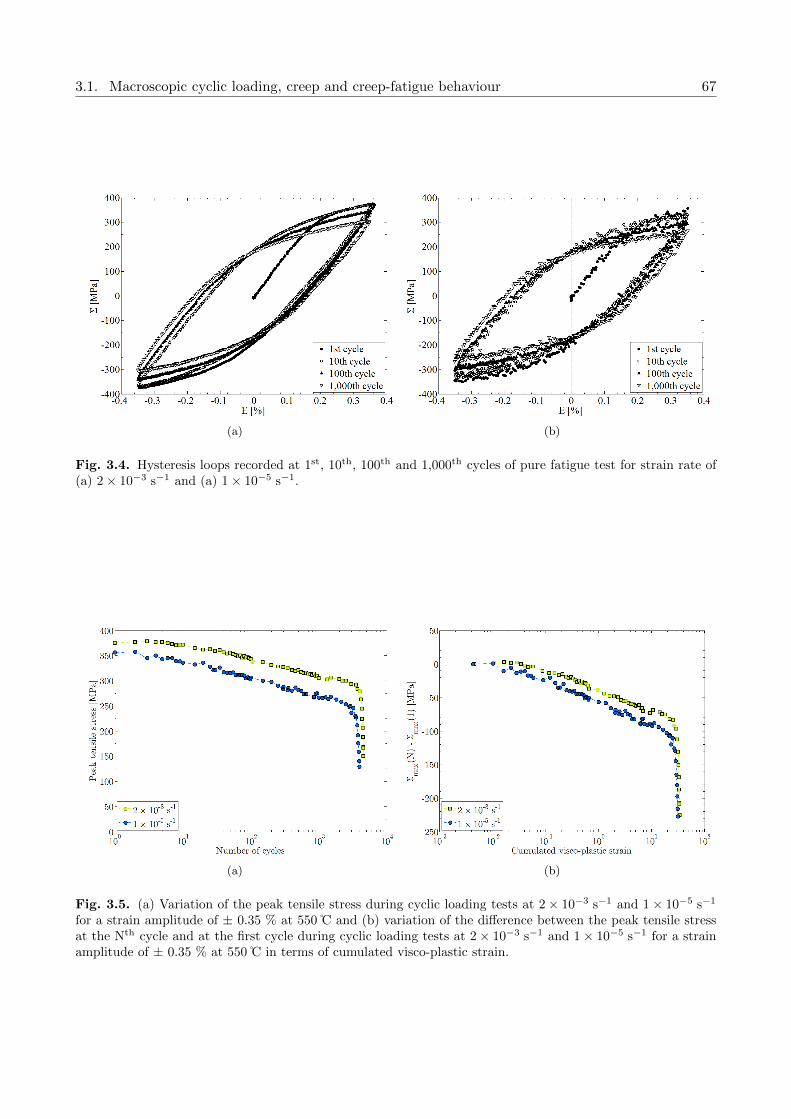
3.1. Macroscopic cyclic loading, creep and creep-fatigue behaviour 67
(a) (b)
Fig. 3.4. Hysteresis loops recorded at 1st, 10th, 100th and 1,000th cycles of pure fatigue test for strain rate of(a) 2× 10⁻³ s−1 and (a) 1× 10⁻⁵ s−1.
(a) (b)
Fig. 3.5. (a) Variation of the peak tensile stress during cyclic loading tests at 2× 10⁻³ s−1 and 1× 10⁻⁵ s−1
for a strain amplitude of ± 0.35 % at 550 C and (b) variation of the difference between the peak tensile stressat the Nth cycle and at the first cycle during cyclic loading tests at 2× 10⁻³ s−1 and 1× 10⁻⁵ s−1 for a strainamplitude of ± 0.35 % at 550 C in terms of cumulated visco-plastic strain.
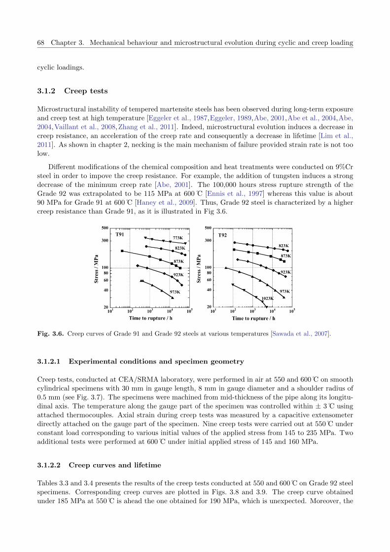
68 Chapter 3. Mechanical behaviour and microstructural evolution during cyclic and creep loading
cyclic loadings.
3.1.2 Creep tests
Microstructural instability of tempered martensite steels has been observed during long-term exposureand creep test at high temperature [Eggeler et al., 1987,Eggeler, 1989,Abe, 2001,Abe et al., 2004,Abe,2004,Vaillant et al., 2008,Zhang et al., 2011]. Indeed, microstructural evolution induces a decrease increep resistance, an acceleration of the creep rate and consequently a decrease in lifetime [Lim et al.,2011]. As shown in chapter 2, necking is the main mechanism of failure provided strain rate is not toolow.
Different modifications of the chemical composition and heat treatments were conducted on 9%Crsteel in order to impove the creep resistance. For example, the addition of tungsten induces a strongdecrease of the minimum creep rate [Abe, 2001]. The 100,000 hours stress rupture strength of theGrade 92 was extrapolated to be 115 MPa at 600 C [Ennis et al., 1997] whereas this value is about90 MPa for Grade 91 at 600 C [Haney et al., 2009]. Thus, Grade 92 steel is characterized by a highercreep resistance than Grade 91, as it is illustrated in Fig 3.6.
Fig. 3.6. Creep curves of Grade 91 and Grade 92 steels at various temperatures [Sawada et al., 2007].
3.1.2.1 Experimental conditions and specimen geometry
Creep tests, conducted at CEA/SRMA laboratory, were performed in air at 550 and 600 C on smoothcylindrical specimens with 30 mm in gauge length, 8 mm in gauge diameter and a shoulder radius of0.5 mm (see Fig. 3.7). The specimens were machined from mid-thickness of the pipe along its longitu-dinal axis. The temperature along the gauge part of the specimen was controlled within ± 3 C usingattached thermocouples. Axial strain during creep tests was measured by a capacitive extensometerdirectly attached on the gauge part of the specimen. Nine creep tests were carried out at 550 C underconstant load corresponding to various initial values of the applied stress from 145 to 235 MPa. Twoadditional tests were performed at 600 C under initial applied stress of 145 and 160 MPa.
3.1.2.2 Creep curves and lifetime
Tables 3.3 and 3.4 presents the results of the creep tests conducted at 550 and 600 C on Grade 92 steelspecimens. Corresponding creep curves are plotted in Figs. 3.8 and 3.9. The creep curve obtainedunder 185 MPa at 550 C is ahead the one obtained for 190 MPa, which is unexpected. Moreover, the
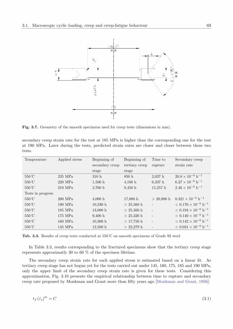
3.1. Macroscopic cyclic loading, creep and creep-fatigue behaviour 69
Fig. 3.7. Geometry of the smooth specimens used for creep tests (dimensions in mm).
secondary creep strain rate for the test at 185 MPa is higher than the corresponding one for the testat 190 MPa. Later during the tests, predicted strain rates are closer and closer between these twotests.
Temperature Applied stress Beginning of Beginning of Time to Secondary creep
secondary creep tertiary creep rupture strain rate
stage stage
550 C 235 MPa 310 h 850 h 2,037 h 20.8× 10⁻⁶ h−1
550 C 220 MPa 1,500 h 4,100 h 6,337 h 6.27× 10⁻⁶ h−1
550 C 210 MPa 2,760 h 8,450 h 15,257 h 2.46× 10⁻⁶ h−1
Tests in progress
550 C 200 MPa 4,000 h 17,800 h > 20,980 h 0.321× 10⁻⁶ h−1
550 C 190 MPa 10,330 h > 25,560 h - < 0.176× 10⁻⁶ h−1
550 C 185 MPa 13,000 h > 25,560 h - < 0.194× 10⁻⁶ h−1
550 C 175 MPa 9,400 h > 25,320 h - < 0.140× 10⁻⁶ h−1
550 C 160 MPa 10,300 h > 17,750 h - < 0.142× 10⁻⁶ h−1
550 C 145 MPa 12,500 h > 22,279 h - < 0.031× 10⁻⁶ h−1
Tab. 3.3. Results of creep tests conducted at 550 C on smooth specimens of Grade 92 steel.
In Table 3.3, results corresponding to the fractured specimens show that the tertiary creep stagerepresents approximatly 30 to 60 % of the specimen lifetime.
The secondary creep strain rate for each applied stress is estimated based on a linear fit. Astertiary creep stage has not begun yet for the tests carried out under 145, 160, 175, 185 and 190 MPa,only the upper limit of the secondary creep strain rate is given for these tests. Considering thisapproximation, Fig. 3.10 presents the empirical relationship between time to rupture and secondarycreep rate proposed by Monkman and Grant more than fifty years ago [Monkman and Grant, 1956]:
tf (εs)m = C (3.1)

70 Chapter 3. Mechanical behaviour and microstructural evolution during cyclic and creep loading
(a) (b)
Fig. 3.8. Creep curves of Grade 92 steel at 550 C for different stresses: (a) fractured specimens and (b) testsin progress.
Temperature Applied stress Beginning of Beginning of Time to rupture Secondary creep
secondary creep tertiary creep strain rate
stage stage
600 C 165 MPa 600 h 1,450 h 2,612 h 13.8× 10⁻⁶ h−1
600 C 145 MPa 1,300 h 6,810 h 13,995 h 1.58× 10⁻⁶ h−1
Tab. 3.4. Results of creep tests conducted at 600 C on smooth specimens of Grade 92 steel.
Fig. 3.9. Creep curves of Grade 92 steel at 600 C under 165 and 145 MPa.

3.1. Macroscopic cyclic loading, creep and creep-fatigue behaviour 71
Eq. 3.1 can be written in logarithmic form:
log (εs) = m′ log (tf ) + C ′ (3.2)
In both equations, m, m′, C, and C ′ are constants. For the moment, the limited number ofplots for Grade 92 steel creep tests at 550 and 600 C in this study does not permit us to evaluatecorrectly the Monkman-Grant equation. In order to adjust the parameters, creep data from the presentwork are compared with the results of creep test performed on Grade 92 steel at 600 and 650 C byPanait [Panait, 2010] and Ennis [Ennis et al., 1997,Ennis and Czyrska-Filemonowicz, 2003].
Fig. 3.10 shows that Monkman-Grant equation can be fitted on creep data with m′ = −1.2 andC ′ = −2.1. These values are close to those established for Grade 91 steel [Haney et al., 2009]. Inthese conditions, it is possible to predict the time to rupture of specimens which are already in thetertiary creep stage. Thus, the time to rupture of the creep specimen at 200 MPa is predicted to be62,100 hours. For tests carried out under lower stress values, the predictions based on the Monkman-Grant relationship must be handled carefully. Indeed, several studies [Povolo, 1985,Dlouhy et al., 2009]lead to the conclusion that the exponent m different from 1 compensates for stress dependencies ofthe rupture strain and the creep curve shape factor. In the low stress domain where the creep rupturestrain significantly decreases, the extrapolation of the short term data may lead to large overestimationof the creep life.
Fig. 3.10. Monkman-Grant equation plots for Grade 92 steel. Continuous straight line corresponds to Eq. 3.2with m′ = −1.2 and C ′ = −2.1. Dotted straight lines correspond to the 95 % confidence interval.
3.1.3 Cyclic test including tensile holding periods
In the present work, one cyclic loading test with tensile holding periods was conducted in order tostudy the interaction between cyclic and creep flow behaviour. This test results are compared with theresults obtained during similar cyclic loading test but without holding time in terms of macroscopicmechanical behaviour.

72 Chapter 3. Mechanical behaviour and microstructural evolution during cyclic and creep loading
3.1.3.1 Experimental conditions and specimen geometry
A cyclic test including tensile holding periods was conducted at CEA/SRMA laboratory using specimengeometry FFL4, shown in Fig. 3.1. It was carried out in the same conditions as the cyclic testspresented in subsection 3.1.1.1. The test was performed under total strain control. During tensileholding periods, the stress was held constant up to 0.5 % of creep strain or until 12 hours of creep timeis reached. Tensile and compressive stress peaks where recorded for all cycles. Stress-strain hysteresisloops were recorded for selected cycles (about 830 points per loop).
This cyclic test including tensile holding periods was carried out at 2× 10⁻³ s−1 for a total cyclicstrain amplitude of ± 0.35 % and a tensile creep strain of 0.5 %. These experimental conditions werechosen in order to compare this test to a pure fatigue test performed in the same cyclic conditions.
3.1.3.2 Creep-fatigue mechanical behaviour
Cyclic deformation is known to induce a decrease in creep resistance of tempered martensite steels.Indeed, a significative increase in secondary creep strain rate has been observed for a specimen aftercycling, compared to the as-received state [Dubey et al., 2005, Fournier et al., 2011a]. These resultsseem to be linked to the microstructural evolution observed during cyclic tests, as will be discussed insection 3.3.
The results of the present creep-fatigue test are presented in Table 3.5. In terms of number ofcycles, creep holding periods induce a reduction of lifetime by more than 80 % compared to a purefatigue test performed in the same cyclic conditions.
Strain rate (s-1) ∆Efat (%) ∆Epcreep (%) ∆Ep (%) N50(0.5%) Nf (0.5%) N50(0.5%)/N50(0%)
2× 10⁻³ ± 0.35 0.5 0.82 787 832 0.18
Tab. 3.5. Cyclic loading test including tensile holding periods results on Grade 92 steel at 550 C for a cyclicstrain amplitude of ± 0.35 % and a tensile creep strain up to 0.5 %. N50(0.5%)/N50(0%) correspond to theratio of number of cycles N50 with and without holding periods at the maximum load.
The hysteresis loops presented in Fig. 3.11(a) show significative softening of the specimen during thetest. They are characterized by an asymmetry between the peak stress in tension and in compression.This phenomenon is induced by the tensile holding periods: indeed, the total fatigue strain is equalto 0.3 % in tension whereas it is equal to 0.8 % in compression. During the test, for the 800th cycle,damage influence is visible on the compressive part of the cycle as a decrease in the initial linear slopeduring unloading. The creep time recorded for each cycle is reported in Fig. 3.11(b). Its evolution isthought to be governed by two phenomena, which have opposite effects: the decrease in stress appliedduring the holding periods and the coarsening of the microstructure. The creep time evolution duringthe test follows three stages as found for Grade 91 steel [Fournier et al., 2011a]:
1. For the first twenty cycles, the fast decrease in dislocation density and subgrain growth due tocyclic loading (see section 3.3) leads to a significative softening and to a fast decrease in the peaktensile stress: the creep time increases from 380 s to about 2,000 s.
2. From the 20th up to the 500th cycle, the mean creep time value slightly decreases: subgraingrowth and decrease in dislocations induce a decrease in creep resistance.
3. After the 500th cycle, the softening behaviour leads to a gradual decrease in the peak tensilestress and to an increase in the mean creep time. At the end of the test, damage is a majorfactor which leads to fast increase in creep holding time.
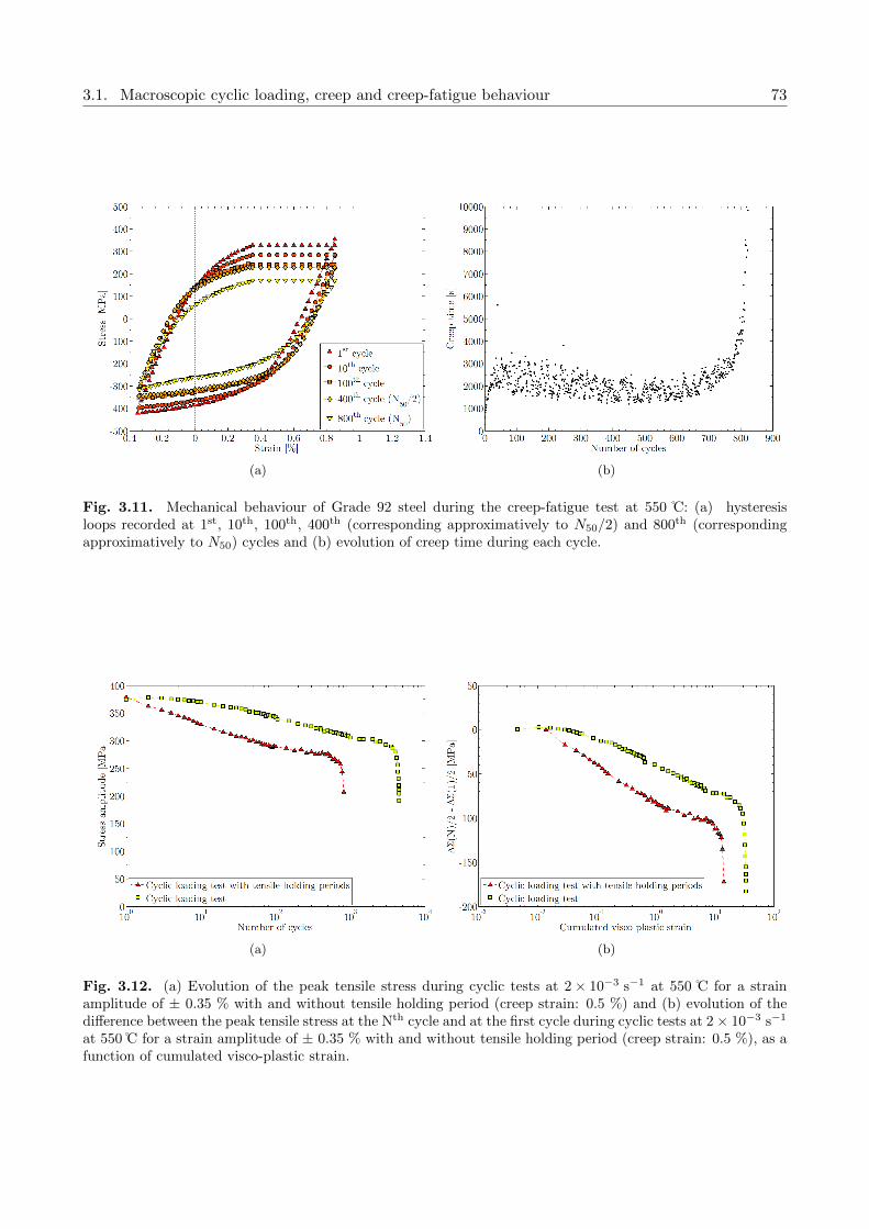
3.1. Macroscopic cyclic loading, creep and creep-fatigue behaviour 73
(a) (b)
Fig. 3.11. Mechanical behaviour of Grade 92 steel during the creep-fatigue test at 550 C: (a) hysteresisloops recorded at 1st, 10th, 100th, 400th (corresponding approximatively to N50/2) and 800th (correspondingapproximatively to N50) cycles and (b) evolution of creep time during each cycle.
(a) (b)
Fig. 3.12. (a) Evolution of the peak tensile stress during cyclic tests at 2× 10⁻³ s−1 at 550 C for a strainamplitude of ± 0.35 % with and without tensile holding period (creep strain: 0.5 %) and (b) evolution of thedifference between the peak tensile stress at the Nth cycle and at the first cycle during cyclic tests at 2× 10⁻³ s−1
at 550 C for a strain amplitude of ± 0.35 % with and without tensile holding period (creep strain: 0.5 %), as afunction of cumulated visco-plastic strain.

74 Chapter 3. Mechanical behaviour and microstructural evolution during cyclic and creep loading
Fig 3.12 presents the softening curves with and without tensile holding period. In terms of cumu-lated visco-plastic strain, the softening behaviour is more significant for creep-fatigue than for purecyclic loading. Moreover, creep-fatigue induces a decrease in specimen lifetime. The fractured spec-imen has a lower cumulated visco-plastic strain than the specimen after pure cyclic loading. Theseresults suggest that cyclic loading test with tensile holding period leads to a larger microstructuralevolution than pure cyclic loading.
3.2 Macroscopic analysis of softening during cyclic loading
To improve the understanding of softening during cyclic loading tests, the evolution of the isotropic R,the kinematic X and the viscous Σv parts of the macroscopic stress was studied in detail. This partitionis used to investigate the mechanisms responsible for the mechanical behaviour of crystalline materialsunder cyclic loading [Cottrell, 1953, Lemaitre and Chaboche, 1990, Fardoun et al., 1997, Feaugas andGaudin, 2001,Polak et al., 2001a,Polak et al., 2001b,Sauzay et al., 2005,Fournier et al., 2006b,Fournieret al., 2006a,Blum and Eisenlohr, 2009].
The sum of the isotropic and viscous parts, called effective stress, corresponds to short-rangeinteractions and is assimilated to the stress required to move a dislocation locally [Haddou et al.,2004]. Thus, this quantity depends mainly on solid solution, small precipitates and other short-rangeobstacles to mobile dislocations. The kinematic stress corresponds to long-range interactions, whichare divided into two contributions to the internal stress [Feaugas and Haddou, 2003]:
Intergranular stress induced by subgrain boundary effects (production of glissile dislocations inthe neighbouring subgrain) and plastic strain incompatibilities between neighbouring subgrainsdue to crystallographic misorientations.
Intragranular stress which corresponds to the heterogeneous distribution of dislocations in sub-grains.
A procedure based on both Cottrell’s method and statistical process control principles was de-veloped by Fournier et al. for highly viscous materials [Fournier et al., 2006b]. This is used toautomatically extract and study the evolution of the three components during one of the two cyclicloading tests at 550 C with a strain amplitude of ± 0.35 % and a strain rate of 2× 10⁻³ s−1 (Fig. 3.13).
Both in compression and in tension presented in Fig. 3.14, R and Σv are constant during the test:they do not decrease, except at the very end of the test, due to macroscopic cracks in the specimen.However, the evolution of X shows a gradual decrease: during the first cycles, X is about 70 MPahigher that R, whereas their respective values are equal at the end of the test. Thus, similarly to thecase of Grade 91 steel [Fournier et al., 2006b], cyclic softening of Grade 92 steel during cyclic loadingat 550 C is mainly due to a decrease in kinematic hardening [Yaguchi and Takahashi, 2000] i.e. to adecrease in long-range interactions, probably induced by the decrease in dislocation density and thecoarsening of laths and/or the vanishing of low-angle subgrain boundaries [Eggeler et al., 1987, Abe,2004,Sauzay, 2009].
Concerning the cyclic test performed at 550 C with a strain amplitude of ± 0.35 % and a strain rateof 1× 10⁻⁵ s−1, the significant noise which affects experimental data did not permit us to apply thesame procedure to extract each stress contributions (see Fig. 3.4(b)). However, the curves presentedin Fig. 3.5 show similar trends for both tests: a decrease in the value of X is also expected for testat lowest strain rate. In order to confirm these results, microstructural observations are presented insection 3.3.

3.2. Macroscopic analysis of softening during cyclic loading 75
Fig. 3.13. Scheme of the stress partition applied to a schematic hysteresis loop.
(a) (b)
Fig. 3.14. Evolution of the kinematic (X), isotropic (R) and viscous (Σv) contributions to the total stress fora cyclic test at 550 C with a strain amplitude of ± 0.35 % and a strain rate of 2× 10⁻³ s−1 (a) in compressionand (b) in tension.

76 Chapter 3. Mechanical behaviour and microstructural evolution during cyclic and creep loading
3.3 Observations of microstructural evolutions during cyclic loadingtests
The microstructure of 9% chromium tempered martensitic steels is presented in section 1.2. Variousscales (former austenite grains, packets, blocks, laths and subgrains) are involved. The creep resistanceof these materials is improved by the large number of obstacles which add pinning points and inhibitthe dislocation motion (several kinds of boundaries, high dislocation density, small precipitates, solidsolution strengthening by Mo and W solute atoms).
Due to the applied heat treatment, this microstructure is stable during thermal exposure up toabout 550 C. For higher temperature, microstructural evolution is observed. At 600 C, thermalexposure leads to a slight increase in subgrain size [Ghassemi-Armaki et al., 2009,Stratil et al., 2011],a decrease in misorientation of low-angle boundaries [Dronhofer et al., 2003, Sanchez-Hanton andThomson, 2007] and a decrease in dislocation density [Pesicka et al., 2004, Panait et al., 2010a].Growth of the M23C6 precipitates is observed up to 26,000 h [Hattestrand and Andren, 2001] whereasthe increase in size of MX precipitate is negligible [Gustafson and Hattestrand, 2002,Paul et al., 2008],even after creep test longer than 100,000 h [Panait et al., 2010b]. However, for higher temperature,precipitates coarsen faster and larger: at 750 C, MX precipitates size increase and the growth of M23C6
precipitates is larger [Sawada et al., 2001].
During high-temperature mechanical loading, microstructural evolution is faster and more pro-nounced than during stress-free thermal exposure [Orlova et al., 1998]. To summarize, several mi-crostructural evolution mechanisms proposed in literature and observed at 550-600 C are listed be-low [Nagesha et al., 2002,Shankar et al., 2006]:
1. Evolution from the initial thin lath and subgrain microstructure to larger equi-axed subgrains.
2. Decrease in dislocation density, initially high due to martensitic transformation (even after sub-sequent temper heat treatment).
3. Coarsening of precipitates if time exposure and temperature are high enough.
Some other mechanisms are observed at higher temperature or for tempered martensite-ferriticsteels with a different chemical composition. Thus, during creep exposure over 600 C, Laves phaseprecipitates nucleate [Hattestrand et al., 1998]. Observations in tungsten-alloyed 9%Cr show that thepresence of tungsten provide nucleation of a larger number of Laves phase particles [Hattestrand andAndren, 2001, Korcakova et al., 2001] and reduces their coarsening during long-term creep exposure,with respect to steels containing only Mo, such as in Grade 91 steel, which probably leads to theimprovement of creep resistance [Hald, 2008]. For 12%Cr steels, the modified Z-phase nucleatesduring long-term creep exposure apparently at the expense of MX precipitates [Sawada et al., 2006],leading to a creep strength degradation at long-term [Sawada et al., 2007]. Although the modifiedZ-phase is observed in 9%Cr steels after long-term creep tests at 600 C [Sawada et al., 2006], it doesnot obviously induce a loss of creep resistance [Panait et al., 2010a].
Although Kim and Weertman observed coarsening of carbides during low-cycle fatigue includinghold time at 593 C in a modified 9Cr-1Mo-VNb steel [Kim and Weertman, 1988], this phenomenon doesnot seem to be significant during cycling at 550 C [Fournier et al., 2009b]. Moreover, the addition ofboron in Grade 92 steel contributes to reducing the coarsening rate of M23C6 precipitates [Hattestrandand Andren, 1999,Abe et al., 2004,Abe, 2011] and stabilizing subgrain boundaries [Eggeler and Dlouhy,2005]. Moreover, recent observations show that carbide coarsening is not significant (in Grade 91steel) after short-time creep-fatigue tests at 550 C [Fournier et al., 2011a]. Concerning the lost of solid

3.3. Observations of microstructural evolutions during cyclic loading tests 77
solution strengthening, Hald showed that a decrease in concentration of molybdenum and tungstensolute atoms due to Laves phase precipitation has a negligible influence on creep resistance in 9-12%Crsteels [Hald, 2008]. Consequently, the following study only focuses on the evolution of subgrain sizeand dislocation density, which appear to be the main microstructural changes in Grade 92 steel duringcyclic tests at 550 C.
3.3.1 Evolution of the subgrain size distribution
3.3.1.1 Methodology
Subgrain and dislocation observations presented in this study were carried out using a PHILIPS EM430Transmission Electron Microscope operated at 300 kV. One thin foil was taken out of each of fivespecimens after cyclic tests at ± 0.35 % and 550 C:
As-received material
Specimen of interrupted test after 60 cycles at 1× 10⁻⁵ s−1
Specimen of interrupted test after 300 cycles at 1× 10⁻⁵ s−1
Specimen of interrupted test after 1,000 cycles at 1× 10⁻⁵ s−1
Fractured specimen at 1× 10⁻⁵ s−1 (3,960 cycles)
Fractured specimen at 2× 10⁻³ s−1 (4,552 cycles)
For each specimen, thin foils were cut perpendicularly to the loading axes in the gauge length, farfrom any fracture surface. Their preparation is described in section 2.2.3.3.
To measure the subgrain size distributions, three TEM bright field pictures with a magnification of5,550 were selected from different observed regions on various thin foils. Observations were performedon an area of interest of about 800 µm2 for each sample. Subgrains were manually traced on atransparent medium. Then image processing using the Visilog software was applied. The measuredsubgrain areas were then convected to equivalent discs which permit us to calculate the equivalentdiameter. Fig. 3.15 presents the different steps of image processing that were necessary to determinethe distribution of subgrain size.
3.3.1.2 Evolution of subgrain size distribution during fatigue test
Fig. 3.16 presents three TEM pictures of Grade 92 steel. In each picture, subgrain boundaries areidentified by a change in bright field contrast, due to small misorientations. The picture of as-receivedsteel reveals a fine lath structure, composed by small subgrains (Fig. 3.16(a)). This microstructureis clearly modified after cyclic loading at 550 C: the fine subgrain structure changes into a largermicrostructure, made of larger equi-axed subgrains. The influence of strain rate on the microstructuralevolution is observed by comparing Fig. 3.16(b) with Fig. 3.16(c). TEM pictures show that themicrostructural evolution is more pronounced in the fractured specimen after the cyclic test performedat the lowest strain rate. In Fig. 3.16(c), the subgrain size is larger and mobile dislocation densityappears to be lower than in Fig. 3.16(b). No obvious difference is observed concerning the precipitatesize.

78 Chapter 3. Mechanical behaviour and microstructural evolution during cyclic and creep loading
(a) (b) (c)
Fig. 3.15. The three steps required to measure the distribution of subgrain size. Grade 92 as-received steel:(a) bright field TEM picture (magnification of 5,550), (b) extraction of the boundaries and (c) individualsubgrains identified by the image processing software.
(a) (b) (c)
Fig. 3.16. TEM observations of the microstructure (magnification of 5,550) (a) in the as-received material,(b) in the specimen fractured after 4,552 cycles at 2× 10⁻³ s−1 and 550 C and (c) in the specimen fracturedafter 3,960 cycles at 1× 10⁻⁵ s−1 and 550 C (far away from the fractured surface).
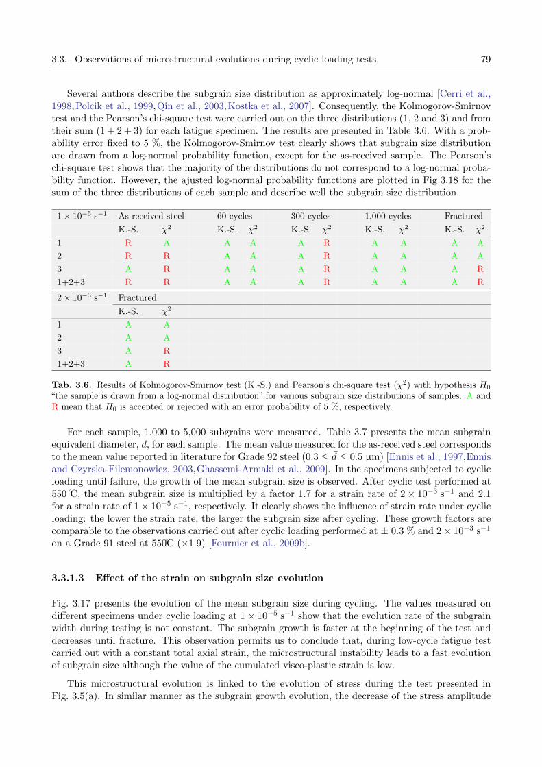
3.3. Observations of microstructural evolutions during cyclic loading tests 79
Several authors describe the subgrain size distribution as approximately log-normal [Cerri et al.,1998,Polcik et al., 1999,Qin et al., 2003,Kostka et al., 2007]. Consequently, the Kolmogorov-Smirnovtest and the Pearson’s chi-square test were carried out on the three distributions (1, 2 and 3) and fromtheir sum (1 + 2 + 3) for each fatigue specimen. The results are presented in Table 3.6. With a prob-ability error fixed to 5 %, the Kolmogorov-Smirnov test clearly shows that subgrain size distributionare drawn from a log-normal probability function, except for the as-received sample. The Pearson’schi-square test shows that the majority of the distributions do not correspond to a log-normal proba-bility function. However, the ajusted log-normal probability functions are plotted in Fig 3.18 for thesum of the three distributions of each sample and describe well the subgrain size distribution.
1× 10⁻⁵ s−1 As-received steel 60 cycles 300 cycles 1,000 cycles Fractured
K.-S. χ2 K.-S. χ2 K.-S. χ2 K.-S. χ2 K.-S. χ2
1 R A A A A R A A A A
2 R R A A A R A A A A
3 A R A A A R A A A R
1+2+3 R R A A A R A A A R
2× 10⁻³ s−1 Fractured
K.-S. χ2
1 A A
2 A A
3 A R
1+2+3 A R
Tab. 3.6. Results of Kolmogorov-Smirnov test (K.-S.) and Pearson’s chi-square test (χ2) with hypothesis H0
“the sample is drawn from a log-normal distribution” for various subgrain size distributions of samples. A andR mean that H0 is accepted or rejected with an error probability of 5 %, respectively.
For each sample, 1,000 to 5,000 subgrains were measured. Table 3.7 presents the mean subgrainequivalent diameter, d, for each sample. The mean value measured for the as-received steel correspondsto the mean value reported in literature for Grade 92 steel (0.3 ≤ d ≤ 0.5 µm) [Ennis et al., 1997,Ennisand Czyrska-Filemonowicz, 2003,Ghassemi-Armaki et al., 2009]. In the specimens subjected to cyclicloading until failure, the growth of the mean subgrain size is observed. After cyclic test performed at550 C, the mean subgrain size is multiplied by a factor 1.7 for a strain rate of 2× 10⁻³ s−1 and 2.1for a strain rate of 1× 10⁻⁵ s−1, respectively. It clearly shows the influence of strain rate under cyclicloading: the lower the strain rate, the larger the subgrain size after cycling. These growth factors arecomparable to the observations carried out after cyclic loading performed at ± 0.3 % and 2× 10⁻³ s−1
on a Grade 91 steel at 550C (×1.9) [Fournier et al., 2009b].
3.3.1.3 Effect of the strain on subgrain size evolution
Fig. 3.17 presents the evolution of the mean subgrain size during cycling. The values measured ondifferent specimens under cyclic loading at 1× 10⁻⁵ s−1 show that the evolution rate of the subgrainwidth during testing is not constant. The subgrain growth is faster at the beginning of the test anddecreases until fracture. This observation permits us to conclude that, during low-cycle fatigue testcarried out with a constant total axial strain, the microstructural instability leads to a fast evolutionof subgrain size although the value of the cumulated visco-plastic strain is low.
This microstructural evolution is linked to the evolution of stress during the test presented inFig. 3.5(a). In similar manner as the subgrain growth evolution, the decrease of the stress amplitude

80 Chapter 3. Mechanical behaviour and microstructural evolution during cyclic and creep loading
Strain rate Sample n d ( µm) s ( µm) Median ( µm) d/d0
- As-received 4,956 0.37± 0.1 0.17 0.347 1.0
1× 10⁻⁵ s−1 Interrupted - 60 cycles 3,242 0.45± 0.03 0.23 0.406 1.22
1× 10⁻⁵ s−1 Interrupted - 300 cycles 2,073 0.52± 0.02 0.26 0.469 1.41
1× 10⁻⁵ s−1 Interrupted - 1,000 cycles 1,438 0.61± 0.05 0.33 0.542 1.65
1× 10⁻⁵ s−1 Fractured - 3,960 cycles 1,004 0.76± 0.08 0.39 0.680 2.05
2× 10⁻³ s−1 Fractured - 4,552 cycles 1,605 0.62± 0.12 0.31 0.557 1.67
Tab. 3.7. Results of the TEM observations performed on specimen samples after cyclic loading at 550 C.The number of counted subgrains is n (summarized over the three investigated region from each sample) ands is the standard deviation. d is the mean equivalent diameter of the n subgrains for each sample. The errorcorresponds to the interval in which the mean equivalent diameter values of each of the three distributions areincluded. d/d0 is the ratio between the mean subgrain equivalent diameter of the considered sample and themean subgrain equivalent diameter of the as-received steel.
is more pronounced at the beginning of the test than just before fracture.
The subgrain growth means a reduction of the number of subgrain boundaries. The fast decrease inthe number of these obstacles, which already happen for low values of cumulated visco-plastic strain,should contribute to a drop of long-range obstacles to dislocation motion and to the observed evolutionof the kinematic stress observed in Fig. 3.14 [Morrison and Moosbrugger, 1997, Moosbrugger et al.,2000,Haddou et al., 2001,Feaugas and Haddou, 2003]. The microstructural evolution, significant evenfor a low value of cumulated visco-plastic strain, is a real challenge for industrial applications. It meansthat during service condition in nuclear reactor, i.e. for low values of cumulated visco-plastic strain,this microstructural degradation could possibly happen and will lead to a decrease in the mechanicalstrength of the material.
Fig. 3.17. Evolution of the mean subgrain equivalent diameter during cyclic loading tests performed at 550 C.
The evolution of the mean subgrain size gives us a global information about the microstructuraldegradation. In this study, we choose to focus on the evolution the subgrain size distribution duringcyclic loading. The subgrain size distributions of the samples corresponding to the as-received material,
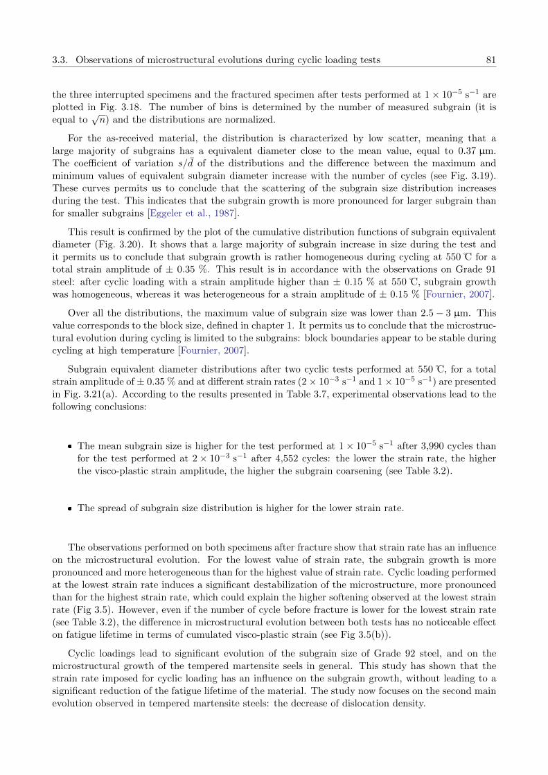
3.3. Observations of microstructural evolutions during cyclic loading tests 81
the three interrupted specimens and the fractured specimen after tests performed at 1× 10⁻⁵ s−1 areplotted in Fig. 3.18. The number of bins is determined by the number of measured subgrain (it isequal to
√n) and the distributions are normalized.
For the as-received material, the distribution is characterized by low scatter, meaning that alarge majority of subgrains has a equivalent diameter close to the mean value, equal to 0.37 µm.The coefficient of variation s/d of the distributions and the difference between the maximum andminimum values of equivalent subgrain diameter increase with the number of cycles (see Fig. 3.19).These curves permits us to conclude that the scattering of the subgrain size distribution increasesduring the test. This indicates that the subgrain growth is more pronounced for larger subgrain thanfor smaller subgrains [Eggeler et al., 1987].
This result is confirmed by the plot of the cumulative distribution functions of subgrain equivalentdiameter (Fig. 3.20). It shows that a large majority of subgrain increase in size during the test andit permits us to conclude that subgrain growth is rather homogeneous during cycling at 550 C for atotal strain amplitude of ± 0.35 %. This result is in accordance with the observations on Grade 91steel: after cyclic loading with a strain amplitude higher than ± 0.15 % at 550 C, subgrain growthwas homogeneous, whereas it was heterogeneous for a strain amplitude of ± 0.15 % [Fournier, 2007].
Over all the distributions, the maximum value of subgrain size was lower than 2.5− 3 µm. Thisvalue corresponds to the block size, defined in chapter 1. It permits us to conclude that the microstruc-tural evolution during cycling is limited to the subgrains: block boundaries appear to be stable duringcycling at high temperature [Fournier, 2007].
Subgrain equivalent diameter distributions after two cyclic tests performed at 550 C, for a totalstrain amplitude of ± 0.35 % and at different strain rates (2× 10⁻³ s−1 and 1× 10⁻⁵ s−1) are presentedin Fig. 3.21(a). According to the results presented in Table 3.7, experimental observations lead to thefollowing conclusions:
The mean subgrain size is higher for the test performed at 1× 10⁻⁵ s−1 after 3,990 cycles thanfor the test performed at 2× 10⁻³ s−1 after 4,552 cycles: the lower the strain rate, the higherthe visco-plastic strain amplitude, the higher the subgrain coarsening (see Table 3.2).
The spread of subgrain size distribution is higher for the lower strain rate.
The observations performed on both specimens after fracture show that strain rate has an influenceon the microstructural evolution. For the lowest value of strain rate, the subgrain growth is morepronounced and more heterogeneous than for the highest value of strain rate. Cyclic loading performedat the lowest strain rate induces a significant destabilization of the microstructure, more pronouncedthan for the highest strain rate, which could explain the higher softening observed at the lowest strainrate (Fig 3.5). However, even if the number of cycle before fracture is lower for the lowest strain rate(see Table 3.2), the difference in microstructural evolution between both tests has no noticeable effecton fatigue lifetime in terms of cumulated visco-plastic strain (see Fig 3.5(b)).
Cyclic loadings lead to significant evolution of the subgrain size of Grade 92 steel, and on themicrostructural growth of the tempered martensite seels in general. This study has shown that thestrain rate imposed for cyclic loading has an influence on the subgrain growth, without leading to asignificant reduction of the fatigue lifetime of the material. The study now focuses on the second mainevolution observed in tempered martensite steels: the decrease of dislocation density.

82 Chapter 3. Mechanical behaviour and microstructural evolution during cyclic and creep loading
(a) (b)
(c) (d)
(e)
Fig. 3.18. Subgrain size distribution in Grade 92 steel for (a) the as-received sample and after cyclic loadingtests at 550 C with a strain amplitude of ± 0.35 % and a strain rate of 1× 10⁻⁵ s−1 for (b) the 60 cyclesinterrupted specimen, (c) the 300 cycles interrupted specimen, (d) the 1,000 cycles interrupted specimen and(e) the 3,960 cycles fractured specimen.
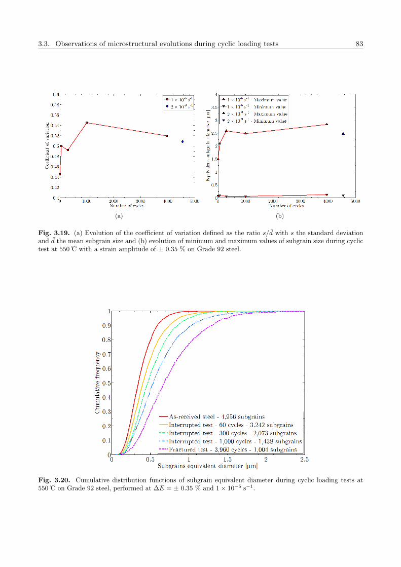
3.3. Observations of microstructural evolutions during cyclic loading tests 83
(a) (b)
Fig. 3.19. (a) Evolution of the coefficient of variation defined as the ratio s/d with s the standard deviationand d the mean subgrain size and (b) evolution of minimum and maximum values of subgrain size during cyclictest at 550 C with a strain amplitude of ± 0.35 % on Grade 92 steel.
Fig. 3.20. Cumulative distribution functions of subgrain equivalent diameter during cyclic loading tests at550 C on Grade 92 steel, performed at ∆E = ± 0.35 % and 1× 10⁻⁵ s−1.
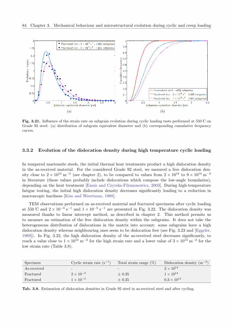
84 Chapter 3. Mechanical behaviour and microstructural evolution during cyclic and creep loading
(a) (b)
Fig. 3.21. Influence of the strain rate on subgrain evolution during cyclic loading tests performed at 550 C onGrade 92 steel: (a) distribution of subgrain equivalent diameter and (b) corresponding cumulative frequencycurves.
3.3.2 Evolution of the dislocation density during high temperature cyclic loading
In tempered martensite steels, the initial thermal heat treatments product a high dislocation densityin the as-received material. For the considered Grade 92 steel, we mesured a free dislocation den-sity close to 2× 10¹⁴ m−2 (see chapter 2), to be compared to values from 2 × 10¹⁴ to 9× 10¹⁴ m−2
in literature (these values probably include dislocations which compose the low-angle boundaries),depending on the heat treatment [Ennis and Czyrska-Filemonowicz, 2003]. During high-temperaturefatigue testing, the initial high dislocation density decreases significantly leading to a reduction inmacroscopic hardness [Kim and Weertman, 1988].
TEM observations performed on as-received material and fractured specimens after cyclic loadingat 550 C and 2× 10⁻³ s−1 and 1× 10⁻⁵ s−1 are presented in Fig. 3.22. The dislocation density wasmeasured thanks to linear intercept method, as described in chapter 2. This method permits usto measure an estimation of the free dislocation density within the subgrains. It does not take theheterogeneous distribution of dislocations in the matrix into account: some subgrains have a highdislocation density whereas neighbouring ones seem to be dislocation free (see Fig. 3.23 and [Eggeler,1989]). In Fig. 3.22, the high dislocation density of the as-received steel decreases significantly, toreach a value close to 1× 10¹⁴ m−2 for the high strain rate and a lower value of 3× 10¹³ m−2 for thelow strain rate (Table 3.8).
Specimen Cyclic strain rate (s−1) Total strain range (%) Dislocation density (m−2)
As-received - - 2× 10¹⁴
Fractured 2× 10⁻³ ± 0.35 1× 10¹⁴
Fractured 1× 10⁻⁵ ± 0.35 0.3× 10¹⁴
Tab. 3.8. Estimation of dislocation densities in Grade 92 steel in as-received steel and after cycling.

3.3. Observations of microstructural evolutions during cyclic loading tests 85
(a) (b) (c)
Fig. 3.22. TEM observations of dislocations within subgrain (a) in the as-received material, (b) in specimenfractured after 4,552 cycles at 2× 10⁻³ s−1 and strain amplitude of ± 0.35 % at 550 C and (c) in specimenfractured after 3,960 cycles at 1× 10⁻⁵ s−1 and strain amplitude of ± 0.35 % at 550 C (far away from thefracture surface).
3.3.3 Discussion about deformation and annihilation mechanisms
In the as-received steel, dislocations in the subgrains appear as straight lines, pinned at subgrainboundaries (see Fig. 3.23(a)). On the contrary, Fig. 3.23(b) shows that they are bowed out after cycling(this phenomenon is less pronounced after cycling at high strain rate). This evolution is probably dueto the modification of the mobile dislocation character: initially, the main part of dislocations isprobably composed by screw dislocations [Wakasa and Wayman, 1981, Guetaz et al., 2003] whichare pinned at subgrain boundaries or carbide precipitates localised at boundaries [Mughrabi et al.,1979, Sauzay and Kubin, 2011]. During cycling, these straight screw dislocations bow out and glidein the subgrain. This expansion may lead to the production of mixed dislocations, composed by bothscrew and edge dislocations.
Fig. 3.24(b) shows the interactions between such dislocations and carbide precipitates. In thispicture, the mobile dislocations are pinned between two precipitates. This induces a reduction of theirmotion and bowing under stress. However, the mechanisms of interaction are not clearly defined. Theabsence of residual dislocation loops around the precipitates permits us to conclude that Orowan’smechanism does not take place. Other mechanisms of deformation could be considered and studiedto explain the crossing of precipitates by dislocations: cross-slip, climb. . .
The subgrain boundaries were described in chapter 1: their misorientation angle is lower than5 [Sonderegger et al., 2007,Sonderegger et al., 2008,Tak et al., 2009,Panait et al., 2010a]. Fig. 3.24(a)shows a low-angle boundary observed in Grade 92 steel. It is characterized by a kind of “honeycomb”structure: it is composed by at least two families of dislocations mixed together. Low-angle boundariescan be modelled as arrays of dislocations [Read and Shockley, 1950]. Similar observations carried outfor other 9-12%Cr steels have shown the same kind of low-angle boundary structure [Eggeler et al.,1987,Eggeler, 1989,Eggeler et al., 1989,Sauzay, 2009].
The microstructural growth studied in section 3.3.1 is due to the coarsening of the subgrains. Thisphenomenon can take place if the low-angle subgrain boundaries move or vanish during cycling. Afterthe test, aligned carbides precipitates are observed within the larger subgrains (Fig. 3.25). Carbides

86 Chapter 3. Mechanical behaviour and microstructural evolution during cyclic and creep loading
(a) (b)
Fig. 3.23. TEM observations of the dislocations (a) in the as-received material and (b) in fractured specimenafter cyclic test at 1× 10⁻⁵ s−1 and strain amplitude of ± 0.35 % at 550 C. Mobile dislocations are pointed outby the white arrows.
(a) (b)
Fig. 3.24. TEM observations of (a) a low-angle subgrain boundary and (b) the interaction between mobiledislocations and precipitates in the specimen fractured after 3,960 cycles at 1× 10⁻⁵ s−1 under a total strainamplitude of ± 0.35 % at 550 C. White arrows point out some dislocations which are pinned on a boundary.

3.4. Concluding remarks 87
precipitates nucleate during tempering heat treatment at the boundaries [Eggeler et al., 1987,Eggelerand Dlouhy, 2005,Abe et al., 2007] and only MX precipitates are observed in the subgrains [Hattestrandand Andren, 2001, Abe et al., 2007]. This indicates that the former low-angle boundaries wherethe carbides precipitates were initially located vanished during cycling (the large number of carbideprecipitate prevents the low-angle boundaries from moving). One possible mechanism is proposed:subgrain boundary vanishing during cycling is due to the interaction between the mobile dislocationswith the arrays of dislocations which composed the low-angle boundaries [Sauzay, 2009]. Indeed,annihilation can take place between two edge or two screw dislocations with a Burger vector of oppositesigns. This phenomenon can occur if their distance is smaller than a critical spontaneous annihilationdistance, which is respectively about 2 nm and 50 nm for edge and screw dislocations for copper atroom temperature [Essmann and Mughrabi, 1979,Essmann and Differt, 1996] (dislocation climb maybe taken into account as well). These mechanisms lead to a decrease in low-angle boundary dislocationdensity. For a high number of cycles, the vanishing of the low-angle boundary occurs. These hypotheseswhich permit us to link partially subgrain growth to decrease in free dislocation density are exposedin chapter 4.
Fig. 3.25. TEM observation carried out after cyclic tests at 550 C on Grade 92 steel, performed at a strainamplitude of ± 0.35 % and a strain rate of 1× 10⁻⁵ s−1. The white arrows point out aligned carbides precipitateslocated on former vanished low-angle boundaries.
3.4 Concluding remarks
Cyclic tests, creep tests and cyclic tests including tensile holding periods were carried out at 550 C ona Grade 92 steel. Experimental results lead to the following conclusions:
According to Manson-Coffin curves, no significant difference between Grade 91 and Grade 92steels is observed in terms of cyclic lifetime at 550 C. Similarly, the parameters of Monkman-Grant equation fitted on Grade 92 steel creep data are close to those etablished for Grade 91

88 Chapter 3. Mechanical behaviour and microstructural evolution during cyclic and creep loading
steel. This suggests that the mecanisms controling cyclic deformation and fatigue lifetime arethe same for both steels.
Grade 92 steel is sensitive to cyclic softening and although it is more pronounced for high valuesof strain amplitude, this phenomenon is even significant for very low values of visco-plastic strainamplitude (about 10−4).
Cyclic softening is more pronounced for lower strain rate: the lower the strain rate, the lower thestress amplitude, the higher the visco-plastic strain amplitude per cycle and finally the faster thestress drop. Additionnal effect of time and temperature may play a role. However, the impactof the strain rate on fatigue lifetime is slight.
Softening behaviour is more pronounced during creep-fatigue than during pure fatigue: it leadsto a decrease in fatigue lifetime by about 80 % in terms of number of cycles.
Similarly to Grade 91 steels, the cyclic softening of the investigated Grade 92 steel at 550 Cis mainly due to a decrease in kinematic stress. This indicates a decrease in rather long-rangeinteractions between the mobile dislocations and the dislocation forest or the low-angle subgrainboundaries.
TEM observations showed that the mean subgrain size increases during cycling. The subgrainsize distributions are satisfactory described by log-normal probability density functions. Theirevolutions during cycling show that subgrain growth is more pronounced for larger subgrainsthan for smaller ones, inducing an increase in distribution spread. These phenomena are morepronounced for the lower strain rate.
A decrease in dislocation density within subgrain is also estimated during cycling from 2× 10¹⁴ m−2
down to 0.3× 10¹⁴ m−2. It is more pronounced for low cyclic strain rate.
The proposed mechanism of interaction between mobile dislocations and low-angle boundariescould account for the TEM observations and partially link decrease in free dislocation densityand subgrain growth.
In service conditions, cyclic strain rate and cyclic strain amplitude are expected to be significantlylower than those investigated here. Following the mechanism of deformation described in this chapter,we will now focus on the modelling of the physical mechanisms of deformation, in order to predict bothmacroscopic mechanical behaviour and microstructural evolution of Grade 92 steel during cycling.

89
Chapter 4
Modelling of the cyclic behaviour andmicrostructure evolution during cycling
This fourth chapter focuses on the modelling of the mechanical behaviour of Grade 92 steel during con-tinuous cycling at 550 C. The description of the hypotheses of the modelling is divided into two parts:polycrystalline homogeneization (from the block scale to the macroscopic one) and microstructuralevolution modelling (subgrain size and dislocation density). Then, the simulations of macroscopicmechanical behaviour and microstructural evolution are presented. Finally, the influence of the valuesof the parameters on the predictions is studied and discussed.
Ce quatrieme chapitre est dedie a la modelisation du comportement mecanique de l’acier Grade 92lors de sollicitations cycliques continues a 550 C. La description du modele est construite autourde deux axes majeurs : l’homogeneisation polycristalline (du bloc au polycristal) et la modelisationde l’evolution de la microstructure (taille de sous-grain et densite de dislocations). Les resultats dessimulations du comportement mecanique macroscopique et de l’evolution microstructurale sont ensuitepresentees. Enfin, l’influence des valeurs des parametres sur les predictions est etudiee et discutee.
Contents
Abstract (in French) . . . . . . . . . . . . . . . . . . . . . . . . . . . . . . . . . . . . 91
4.1 Introduction to polycrystalline modelling . . . . . . . . . . . . . . . . . . . . 93
4.2 Crystalline constitutive equations . . . . . . . . . . . . . . . . . . . . . . . . . 94
4.2.1 Description and hypotheses of the modelling . . . . . . . . . . . . . . . . . . . 94
4.2.2 Isotropic stress . . . . . . . . . . . . . . . . . . . . . . . . . . . . . . . . . . . . 98
4.2.3 Evolution of the kinematic stress . . . . . . . . . . . . . . . . . . . . . . . . . . 99
4.2.4 Crystal viscoplasticity flow rule . . . . . . . . . . . . . . . . . . . . . . . . . . . 102
4.3 Modelling the microstructural evolutions . . . . . . . . . . . . . . . . . . . . 103
4.3.1 Modelling the evolution of dislocation density . . . . . . . . . . . . . . . . . . . 103
4.3.2 Modelling of low-angle boundaries misorientation evolution . . . . . . . . . . . 106
4.3.3 Modelling the subgrain size evolution . . . . . . . . . . . . . . . . . . . . . . . 108
4.4 Self-consistent homogenization scheme . . . . . . . . . . . . . . . . . . . . . 108
4.4.1 Thermoelastic modelling proposed by Kroner . . . . . . . . . . . . . . . . . . . 108
4.4.2 Molinari’s model for viscoplastic material . . . . . . . . . . . . . . . . . . . . . 109
4.5 Choice of the values of the model parameters . . . . . . . . . . . . . . . . . 110
4.5.1 Measured, calculated and fixed parameters . . . . . . . . . . . . . . . . . . . . 110
4.5.2 Identification process . . . . . . . . . . . . . . . . . . . . . . . . . . . . . . . . . 112

90 Chapter 4. Modelling of the cyclic behaviour and microstructure evolution during cycling
4.6 Simulation of cyclic loading . . . . . . . . . . . . . . . . . . . . . . . . . . . . 115
4.6.1 Validation of the model on the first macroscopic loop for both strain rates . . . 115
4.6.2 Prediction of cyclic softening for both strain rates . . . . . . . . . . . . . . . . 115
4.6.3 Predictions of the macroscopic cyclic softening for different strain amplitudes . 120
4.6.4 Sensitivity of model predictions to the values of model parameters . . . . . . . 122
4.7 Concluding remarks . . . . . . . . . . . . . . . . . . . . . . . . . . . . . . . . . 133

91
Resume
Ce chapitre est consacre a la modelisation du comportement mecanique et de l’evolution microstruc-turale de l’acier Grade 92 au cours de sollicitations cycliques a 550 C. Dans le cadre de cette etude,un modele d’homogeneisation polycristalline auto-coherent est propose afin de decrire l’adoucissementcyclique des aciers martensitiques revenus a haute temperature. Ce modele est capable de predire lecomportement mecanique macroscopique et l’evolution de la microstructure (chute de la densite dedislocations, augmentation de la taille des sous-grains) observee et mesuree au cours du cyclage.
Les equations implementees dans ce modele sont fondees sur la description de phenomenes physiqueslies a des hypotheses de mecanismes microstructuraux se deroulant lors de la deformation cyclique(interaction entre les dislocations mobiles et les dislocations composant les sous-joints, destructionprogressive des sous-joints. . . ). Cette approche permet d’attribuer un sens physique a l’ensembledes parametres du modele et de limiter a seulement deux le nombre de variables d’ajustement. Cesderniers (energie d’activation et volume d’activation) correspondent a l’effet de viscosite et sont ajustesa l’aide des courbes monotones a differentes vitesses de deformation. Ainsi, aucune donnee concernantl’adoucissement cyclique du materiau n’est utilisee pour ajuster ces parametres. Ce modele permetdonc de predire l’adoucissement mecanique de l’acier Grade 92 lors d’essais cycliques pour differentesamplitudes de deformation et vitesses de deformation.
L’energie d’activation et le volume d’activation, seuls parametres ajustes sur les courbes monotonesexperimentales, ont des valeurs de l’ordre de 1,2 eV et 216 b3 respectivement. Selon des donneesissues de la litterature [Marmy et al., 1993, Caillard and Martin, 2003], elles correspondent a desmecanismes d’interaction entre les dislocations mobiles et les nuages d’atomes en solution solide, lespetits precipites. . .
Le modele permet de predire assez convenablement le comportement mecanique de l’acier Grade 92durant la premiere boucle de fatigue, pour deux vitesses de deformation differentes (2× 10⁻³ s−1 et1× 10−5 s−1). Au cours du cyclage, la cinetique d’adoucissement est bien predite pour l’essai ayantune amplitude de deformation de ±0,35 %. A faible vitesse de deformation, la contrainte maximaleen traction predite est legerement sous-estimee, alors que, pour une vitesse de deformation elevee, lespredictions sont tres proches des valeurs experimentales. En termes d’evolution microstructurale, lemodele predit correctement la valeur finale de la densite de dislocations, bien qu’il surestime l’evolutionde la taille moyenne de sous-grains au cours de l’essai. L’adoucissement mecanique du materiau estcorrectement predit pour des amplitudes de deformation comprises entre ±0,25 et ±0,35 % a vitessede deformation elevee. En revanche, il est surestime pour des amplitudes superieures a ±0,35 %.
Du fait du sens physique attribue aux parametres du modele, certaines valeurs ne sont pas connuesavec exactitude pour l’acier Grade 92 et sont extrapolees a partir de mesures experimentales effectueessur d’autres materiaux et/ou sous differents types de conditions (essais mecaniques, temperature. . . ).Une etude parametrique du modele a donc ete menee afin d’etudier la stabilite du modele vis-a-vis deces parametres. Ainsi, cette etude de l’influence de la variation des valeurs des parametres microstruc-turaux dans un intervalle physiquement acceptable a montre que les predictions du comportementmecanique et de l’evolution de la densite de dislocations sont particulierement stables. Seule la pre-diction de l’evolution de la taille moyenne de sous-grains est sensible a ces variations de parametres.

92 Chapter 4. Modelling of the cyclic behaviour and microstructure evolution during cycling

4.1. Introduction to polycrystalline modelling 93
4.1 Introduction to polycrystalline modelling
A large number of experimental studies of the mechanical behaviour of ferritic-martensite steels (andalloys in general) during cycling is available in literature. At the same time, a significant numberof phenomenological models using nonlinear kinematic hardening rule has been proposed in order toreproduce this cyclic behaviour (see [Lemaitre and Chaboche, 1990, Koo and Lee, 2007, Chaboche,2008] for example). For a modified 9Cr-1Mo steel during cycling at high temperature, Yagushi andTakahashi have developped a model based on the Chaboche model [Chaboche, 1989] to describecyclic softening behavior by fitting a large number of parameters on the experimental evolution ofmacroscopic backstress and effective stress [Yaguchi and Takahashi, 2000]. Although their model isable to reproduce experimental macroscopic behaviour during cycling (for example: cyclic hardening,cyclic softening. . . ), it does not focus on the physical phenomena which occur during deformation. Inthis case, modelling is limited to the loading conditions of the data base used for the identification ofthe parameters, and predictions and extrapolations of the cyclic behaviour are not much reliable. Noguideline for improving material resistance is given either.
Significant efforts were made in order to model the physical mechanisms of deformation and the mi-crostructural changes during cycling or creep deformation. For instance, Blum and coworkers proposeda mechanism of coarsening of subgrains based on the movement of the low-angle boundaries. Usinga phenomenological model, they succeed to reproduce the subgrain size evolution during creep [Pol-cik et al., 1999]. However, no movement of the sugrain boundaries was observed by in-situ TEMobservations during tensile tests at 550 C in EUROFER [Guetaz et al., 2003]. Dislocation dynamicssimulations performed by Holec and Dlouhy showed that symmetric tilt boundaries decorated withprecipitates become unstable and move under an applied shear stress only if their misorientation reacha critical value, of the order of a few tenth of degres [Holec and Dlouhy, 2005]. For higher misorienta-tion angle, the pinning effect by precipitates is strong enough to avoid any low-angle boundary climband/or glide. To describe the dislocation density evolution during cycling or creep, several authorsproposed a physical-based modelling which take several observed phenomena into account (production,annihilation, interactions with boundaries. . . ) [Estrin et al., 1998,Blum and Eisenlohr, 2009].
Although they are not so numerous, a few self-consistent homogeneization models are proposedin the literature to simulate the cyclic behavior of polycrystalline metals [Cailletaud, 1992, Pilvin,1994, Toth et al., 2000, Fournier et al., 2011b]. However, even if they are able to reproduce themacroscopic mechanical behaviour during cycling, they can not predict accurately the microstructureevolution and mechanical behaviour without fitting parameters using the cyclic softening curves. Theaim of this study is to predict the cyclic behaviour of tempered ferritic-martensite steels by fittinga very limited number of physically-based viscoplasticity parameters. Only experimental monotonictensile curves are used in the identification process but no cyclic data. As the physical mechanisms ofdeformation are modelled at the dislocation scale, this model may display more relevant predictionsand extrapolations for both microstructure evolution and mechanical behaviour during long-termsollicitations (low strain, long hold time. . . ).
In the following part, the physical bases of the model are presented and hypotheses stemmingeither from experimental observations or from previous numerical simulations are presented.

94 Chapter 4. Modelling of the cyclic behaviour and microstructure evolution during cycling
4.2 Crystalline constitutive equations
4.2.1 Description and hypotheses of the modelling
The as-received material presented in chapter 1 displays several microstructural scales: prior austeniticgrains, packets, blocks, laths and subgrains. Martensite packets and blocks are characterized byspecific misorientations between neighbours, induced by the martensitic transformation [Kurdjumovand Sachs, 1930, Nishiyama, 1934, Wakasa and Wayman, 1981, Gourgues et al., 2000]. Here, we willconsider that there are two kinds of boundaries:
1. The prior austenitic grain boundaries, the packet boundaries and the block boundaries whichhave misorientation angle higher than 5 [Barcelo et al., 2009,Barcelo et al., 2010].
2. Some of laths and subgrain boundaries which have misorientation angle lower than 5 . They areconsidered to be low-angle boundaries [Tak et al., 2009]. These ones are located within blocksonly.
Both kinds of boundaries are significantly different in terms of stability during mechanical testsat high temperature. EBSD measurements showed that prior austenitic grain boundaries, packetboundaries and block boundaries remain unchanged during mechanical tests [Kimura et al., 2006,Fournier et al., 2009a]. This result is confirmed by TEM observations and subgrain size measurementspresented in section 3.3.1: the maximum subgrain size measured in the sample after cycling is lowerthan 2.5− 3 µm, which corresponds to the mean block size [Fournier, 2007]. Moreover, Dronhofer et al.showed that the evolution of the distribution of misorientation angle during creep was mainly limitedto the low values of misorientation angle (lower than 5 ) [Dronhofer et al., 2003]. These observationslead us to conclude that the coarsening is confined to subgrains and that blocks are stable duringhigh-temperature mechanical loading. Thus, the microstructural growth is linked to the vanishing ofthe low-angle subgrain boundaries within the blocks.
The coarsening mechanism proposed by Abe is based on the recombination of two low-angle bound-aries [Abe, 2004]. The progressive coalescence of subgrains low-angle boundaries is supposed to belocalised near triple points of boundaries, called “Y-junctions”. This mechanism was proposed morethan fifty years ago for polygonized silicon iron crystals and for zinc single crystal [Dunn and Daniels,1951,Gilman, 1955]. In these materials, the boundaries, free from precipitates, are highly mobile. Intempered martensite steels, a small number of “Y-junctions” is observed after tempering (see Fig. 3.16and [Guttmann, 1974] for example). Carbide precipitates stabilize the subgrain boundaries and dras-tically reduce their mobility. Abe suggests that dissolution and re-precipitation of carbide precipitatestake place repeatedly during moving of boundaries and lead to progressive recombination of low-angleboundaries. However, no significant modification of precipitates during cycling at high temperaturehas been reported in literature, and as mentionned above, in situ TEM observations do not mentionany low-angle boundary displacement.
Considering these observations, the mechanism described by Abe is not suitable for cyclic defor-mation of tempered ferritic-martensite steels. Some other mechanisms were proposed and based onannihilation of dislocations dipoles in subgrain and of dipolar configurations at dislocation boundaries,followed by a mechanism of annihilation and/or recombination of subgrain boundaries [Blum, 2001].A mechanism based on the interaction between low-angle boundaries and mobile dislocations has beenalso proposed [Sauzay et al., 2005] based on the knitting-in (free dislocations are absorbed into thelow-angle boundaries) and knitting-out (free dislocations are released from the low-angle boundaries)mechanisms, initially highlighted by Eggeler in tempered ferritic-martensite steels [Eggeler, 1989]

4.2. Crystalline constitutive equations 95
and Caillard and Martin in aluminium [Caillard and Martin, 1982b]. The corresponding analyticalmodel is described in section 2.6.2 and in [Sauzay et al., 2005], [Sauzay et al., 2008] for cyclic loadingand [Sauzay, 2009] for creep loading. In the following, the microstructural hypothesis adapted topolycrystalline homogenization modelling are presented.
4.2.1.1 Dislocations types considered in the model
For the sake of simplicity, only two types of dislocations are considered in the following:
Pure edge dislocations characterized by a Burgers vector perpendicular to the line direction.
Pure screw dislocations characterized by a Burgers vector parallel to their line direction.
Following this hypothesis, the well-known dislocations loops generated from Frank-Read sources in aslip plane under shear stress [Frank, 1980] are only described by a succession of edge and screw parts(see Fig. 4.1).
(a) (b)
Fig. 4.1. Scheme of (a) a typical Frank-Read source and (b) a modelled Frank-Read source with pure edgeand screw parts.
This hypothesis leads to a significant simplification by considering mixed dislocations as pure edgeor pure screw dislocations. However, it allows taking dislocation properties which depend on their type(movement, interactions. . . see section 4.2.1.3) into account. As we focus on the interaction betweenmobile dislocations and low-angle boundaries, this approach is more realistic than only considering aglobal dislocation density without distinction between edge and screw part.
In this model, we divide dislocations into two kind of populations: mobile dislocations, which arelocated within the subgrains and glide during viscoplastic deformation and dislocations composinglow-angle boundaries.
4.2.1.2 Low-angle boundaries structures
In the following, low-angle boundaries are considered as interfaces defined by a misorientation angleθ between two subgrains [Sutton and Balluffi, 1995]. They are considered as a periodic network ofboundary dislocations [Priester, 2001]. This hypothesis is based on the description proposed by Read

96 Chapter 4. Modelling of the cyclic behaviour and microstructure evolution during cycling
and Shockley which consider low-angle boundaries as planar arrangements of dislocations [Read andShockley, 1950]. This scheme leads to model two kinds of boundaries:
Pure tilt boundaries made by a alignment of edge dislocations of the same Burgers vector (seeFig 4.2).
Pure twist bondaries made by a arrangement of two families∗ of screw dislocations. This hy-pothesis is based on the microstructural observations of subgrain boundaries (see Fig. 3.24(a)and [Guttmann, 1974]).
More generally, all low-angle boundaries can be built using one family of edge dislocations and twofamilies of screw ones.
The proposed mechanism partially links the decrease in the mobile dislocation density to thevanishing of some low-angle boundaries. We consider that mobile dislocations can annihilate with thedislocations composing the low-angle boundaries. During cycling, some slip systems are activated andthe mobile dislocations contained in these planes move towards the low-angle boundaries. Annihilationof mobile dislocations with dislocations at the low-angle boundaries leads to a decrease in the lineicdislocation density at the low-angle boundaries. It induces a decrease in the misorientation angle θ ofthe boundary under interest [Read and Shockley, 1950]:
θ = bΛ (4.1)
In Eq. 4.1, Λ is the edge dislocation density in the low-angle boundary and b is the Burgersvector magnitude. Annihilation takes place between two edge (or two screw) dislocations of oppositeBurgers vector and parallel line vectors if their distance is smaller than a critical value, denoted asye for edge dislocations and as ys for screw dislocations [Essmann and Mughrabi, 1979, Differt andEssmann, 1993, Essmann and Differt, 1996, Sauzay et al., 2005]. The annihilation mechanism duringcycling is illustrated for a pure tilt boundary in Fig. 4.2. Interactions between two edge (or two screw)dislocations of same Burgers vector and parallel line vectors are not taken into account because of thelocal stress field effect close to the finite subgrain boundary [Li, 1960].
The activated slip systems are considered to be the same in both subgrains (this hypothesis isdiscussed in section 4.2.1.3). In Fig. 4.2, during the first half-cycle, mobile dislocations glide towardsthe boundary dislocation in subgrain A and annihilation can occur if their distance is smaller than ye.In subgrain B, mobile dislocations of the same sign glide towards the boundary [Sauzay et al., 2005].The deformation fields induced by the dislocations of the same sign lead to the creation of a dislocationpile-up on this side of the low-angle boundary [Priester, 2001]. During the second half-cycle, theopposite mechanism happens at this interface. Successive annihilations lead to a decrease in dislocationdensity within the low-angle boundary and thus in its corresponding misorientation angle. Afternumerous annihilation events, the low-angle boundary dislocation density may be low enough toinduce its complete annihilation. This hypothesis is discussed later.
Interaction between mobile screw dislocations and twist boundaries is similar to interaction de-scribed for mobile edge dislocations and tilt boundaries. However, as a simple alignment of screwdislocations is unstable, we assume that twist low-angle boundaries are composed by two families ofscrew dislocations, as described in [Sutton and Balluffi, 1995]. Thus, the annihilation mechanism be-tween twist boundaries and mobile screw dislocations takes place only when the two families of screwdislocations of opposite signs are activated in the neighboring subgrains.
∗A family of dislocation is a set of dislocations with the same Burgers vector.

4.2. Crystalline constitutive equations 97
Fig. 4.2. Schematic drawing of the interactions between mobile edge dislocations (moving along the dottedline) and parallel edge dislocations composing a symmetric tilt low-angle boundary (aligned along the continuousline) during cycling.
In order to model these microstructural interactions, we focus on the crystallographic features usedin the model.
4.2.1.3 Crystallographic features at the block scale
The tempered martensite structure is almost body-centered cubic because of M23C6 precipitate forma-tion during tempering. For the tempered ferritic-martensite steels, we observed that the smallest imbri-cated microstructural scale which is stable during cycling is the block of laths (see subsection 3.3.1.3).Blocks of laths are considered as a phase with a almost homogeneous crystallographic orientation.The model predicts the mechanical behaviour of a block of laths in the matrix composed by a largenumber of other blocks. Although specific misorientations between blocks of laths were described inthe literature [Kurdjumov and Sachs, 1930,Wassermann, 1933,Nishiyama, 1934,Wakasa and Wayman,1981, Gourgues et al., 2000], the crystallographic structure of the as-received material modelled as alarge aggregate of blocks is considered here as textureless for the sake of simplicity even concerningtheir local texture. We thus assume that the crystal orientation of each block of laths is randomlydistributed ans does not depend on the neighbour block orientations. Neglecting such local textureshould not affect macroscopic predictions strongly.
The body-centered cubic structure requires taking the two families of slip systems 110 and 112planes which are the easiest to activate and 〈111〉 slip directions into account (123 slip planes are notconsidered) [Franciosi, 1983,Hoc and Forest, 2001,Caillard and Martin, 2003]. In a given slip system,the structure of dislocation loops, generated from Frank-Read sources, permit us to considered thatthe number of dislocations of opposite Burgers vector are the same (see Fig. 4.1(b)). Moreover, low-angle boundary dislocations can interact with mobile dislocations of both subgrain A and subgrain B(Fig. 4.2). The misorientation between these neighbouring subgrains is low enough to considered thattheir activated slip systems during viscoplastic deformation are the same in all subgrain located inthe same block. Consequently, the annihilation mechanism takes place during plastic deformation,independently of the dislocation glide direction, on either the subgrain A side or B one.
This hypothesis allows us to assume that two opposite slip systems are equivalent, leading todivide by 2 the total number of slip systems considered in the model. It means that 24 slip systems
98 Chapter 4. Modelling of the cyclic behaviour and microstructure evolution during cycling
are considered. For a given slip system, the following hypothesis on dislocation structure are:
One mobile edge dislocation can be activated by only one slip system. No other one has similarparallel dislocations. Therefore, edge dislocations are divided into 24 families.
Six different slip systems have similar parallel mobile screw dislocations. So screw dislocationsare divided into 4 families, coresponding to the four 〈111〉 Burgers vectors.
These slip properties valid for mobile dislocations are also true for dislocations within low-angleboundaries:
Pure tilt boundaries are made of parallel edge dislocations, so they are divided into 24 families.
Pure twist boundaries are made of two families of screw dislocations, so they are divided into6 families, i.e. the number of distinct groups of two families of screw dislocations taken out of 4.
In the model, we assume that dislocations can only glide on their slip system. Although we areconcerned by high temperature viscoplasticity, dislocation climb is not taken into account duringcycling at least at this stage. Indeed, in a first approximation, we assume that this phenomenonoccurs less significantly during cycling at 10−5 s−1 than during creep or relaxation test with strainrate which can reach 10−9 − 10−10 s−1. Dislocation climb may be taken into account later, increasingsoftening rate [Sauzay et al., 2008].
These microstructural hypothesis are necessary to propose a set of equations to model the physicalmechanisms happening during cycling.
4.2.2 Isotropic stress
Considering one block and one slip system i, the resolved shear stress τ i is expressed in Eq. 4.2,resulting from the projection of the local stress tensor σ on the ith slip system.
τ i = σ :(mi ⊗ ni
)(4.2)
In Eq. 4.2, mi is the slip vector and ni is the normal to the slip plane.
The critical resolved shear stress τc required to activate viscoplastic slip is supposed to be the samefor all slip systems i. According to the forest model analysis [Kocks and Mecking, 2003], it is expressedas:
τc = τ0 + αµb√ρe + ρs (4.3)
The value of critical resolved shear stress τc depends on the interactions due to forest dislocations.It is linked to the total free dislocation density (total free edge dislocation density ρe and total freescrew dislocation density ρs) in the considered block. It is here considered as athermal. This termweakly depends on the temperature, because of the dependance to the shear modulus µ which isinfluenced by the temperature.
4.2. Crystalline constitutive equations 99
In Eq. 4.3, τ0 is linked to the energy necessary for the dislocations to move to the next Peierls’valley [Sommer et al., 1998]. This thermally activated process mainly depends on temperature and onviscoplastic strain rate. Sommer and coworkers showed that temperature is high enough to neglect thisterm for temperatures higher than 150 C in alpha-iron polycrystals, regardless the viscoplastic strainrate [Sommer et al., 1998]. Consequently, the temperature applied during cycling (550 C) permits usto take τ0 equal to zero.
While the effect of Peierls’ stress is neglected in the model, solid solution strengthening, which alsocorresponds to thermally activable obstacles, is taken into account in the model. This effect is linkedto the viscoplastic deformation mechanisms and is discussed later in section 4.2.4.
In the well-known Taylor’s relationship presented in Eq. 4.3, the average strength of dislocationinteractions is defined by the coefficient α, with a value in the range 0.35 ± 0.15 in f.c.c. crys-tals [Devincre et al., 2005]. This approach was improved by considering the contribution of individualslip systems [Franciosi et al., 1980]. This approach leads to define a cross-hardening matrix composedby the interaction coefficients aij which correspond to the average strength of the interactions betweenpairs of slip systems i and j.
Experimental measurements of these coefficients are hardly available and, in b.c.c. crystals, onlyestimations based on latent hardening tests are available in literature [Takeuchi and Mano, 1972,Fran-ciosi, 1983]. On the other hand, dislocation dynamics simulations were performed to calculate thefive interaction coefficients in f.c.c. crystals. But, from our knowledge, only a part of the much morenumerous coefficients were calculated in α-iron [Madec and Kubin, 2004,Queyreau et al., 2009]. Con-sequently, this partial information on the cross-hardening matrix for the b.c.c. structure leads us toapproximate the values of the coefficients aij . For the
110〈111〉 slip systems in alpha-iron with a
threshold friction stress of 30 MPa and a forest density of 2× 10¹³ m−2, the interaction coefficients aij
of the four types of reactions between slip systems classically defined in b.c.c. crystals (collinear,symmetrical junction, asymmetrical junction and edge junction) were calculated by dislocation dy-namics simulations [Queyreau et al., 2009]. Consequently, the average value of the Taylor coefficientα obtained is close to 0.3 [Queyreau et al., 2009,Naamane, 2008].
4.2.3 Evolution of the kinematic stress
The study of the mechanical behaviour during cycling at high temperature of Grade 92 steel, andmore generally of 9%Cr steels, shows that cyclic softening is mainly due to a decrease in the kinematicstress (see section 3.2 and [Fournier et al., 2006b] for Grade 91 steel). Consequently, the model shouldtake this evolution of the kinematic stress into account, here at the crystal scale.
A large number of equations modelling the evolution of kinematic stress are available in litera-ture [Armstrong and Frederick, 1966,Lemaitre and Chaboche, 1990,Steckmeyer et al., 2011]. However,most of them are characterized by phenomenological formula and requires the adjustement of physicalbaseless parameters. In order to drastically reduce the number of adjustable parameters, the evolutionlaw of the kinematic stress was based in the present model on the slip mechanisms. Consequently, thehighest number of parameters correspond to values measured from microstructural observations or atleast have a physical meaning.
In the as-received material, we observed that mobile dislocations seem to be straight lines, pinnedat subgrain boundaries (see Fig. 3.23(a), [Wakasa and Wayman, 1981] and [Guetaz et al., 2003]).During viscoplastic glide, the resolved shear stress applied on a given slip system i induces a bowingout of these dislocations [Essmann and Differt, 1996] even in the EUROFER 97 steel at 550 C [Guetazet al., 2003]. Consequently, they move over a mean distance l. During the bowing-out, the Orowan

100 Chapter 4. Modelling of the cyclic behaviour and microstructure evolution during cycling
formula permits us to express the viscoplastic slip as a function of l and of the mobile dislocationdensity ρie + ρis on the slip system i:
γp,i =(ρie + ρis
)lb (4.4)
Considering the low values of viscoplastic slip amplitude during cycling, we assume that mobile dis-locations only bow-out and stay pinned at subgrain boundaries (by carbide precipitates or dislocationsbelonging to the low-angle boundaries). They could not go through the low-angle boundaries [Guetazet al., 2003]. The average distance h covered by a given dislocation can be expressed as a function ofthe area swept by this dislocation A and the subgrain diameter d:
h =A
d(4.5)
Fig. 4.3. Scheme of a mobile dislocations pinned at subgrain boundaries and bowing-out under shear stressτ . For sake of understanding, the mobile dislocation drawn on the figure is not only composed by pure edge orpure screw parts.
Based on Fig. 4.3, a simple geometrical consideration leads us to link the area swept by thedislocation A, the radius of curvature r, the slip lenght l and the angle φ by:
A = φr2 − d
2(r − l)
with φ = arctan
(d
2 (r − l)
) (4.6)
Eqs. 4.4, 4.5 and 4.6 lead to:
γp,i =ρb
d
[r2 arctan
(d
2 (r − l)
)− d
2(r − l)
](4.7)

4.2. Crystalline constitutive equations 101
Each element of the curved free dislocation is under equilibrium between the force resulting from theshear stress F i = τ ib and the tension line T which is different for edge and screw dislocations [Brown,2006]. Dupuy and Fivel have shown that the critical shear stress required to bow-out a dislocationsegment of a Frank-Read source weakly vary between a pure edge segment and a pure screw one, inthe case of an isotropic linear elastic f.c.c. crystal with a Poisson ratio close to 0.35 [Dupuy and Fivel,2002]. For the sake of simplicity, this result permits us to use an average value of the tension line foredge and screw dislocations (T = µb2/2). For r ∈ [ d2 ; +∞ [ , the radius of curvature r is calculed by:
r =T
F i=
µb
2τ i(4.8)
The maximum value of τ i allowed by the geometric configuration of Fig. 4.3 is reached for r = d/2.The local backstress xi in a slip system i is defined as the stress induced by tension line. Its maximumvalue is thus given by:
ximax =µb
d(4.9)
With the geometry of Fig. 4.3, the radius of curvature r can be expressed as a function of the sliplength l:
r =l
2+d2
8l(4.10)
Eq. 4.10 gives two solutions for the slip length l:
l =2r +
√4r2 − d2
2(4.11)
l =2r −
√4r2 − d2
2(4.12)
As the slip length l has to be lower than the radius of curvature R, the only acceptable value isthat of Eq. 4.12. The slip length l is thus expressed as :
l =µb
2xi− 1
2
√(µb
xi
)2
− d2 (4.13)
Eqs. 4.7, 4.8, 4.9 and 4.13 lead to the expression of the amount of slip γp,i, for xi ∈ ]−ximax ; 0 [ ∪] 0 ; ximax [ .
γp,i =
(ρie + ρis
)bd
4
(ximax)2(xi)2 arctan
((ximax
)2(xi)2 − 1
)− 12
−
√(ximax)2
(xi)2 − 1
(4.14)
102 Chapter 4. Modelling of the cyclic behaviour and microstructure evolution during cycling
We assume that dislocations densities ρie and ρis and subgrain diameter d do not change during aninfinitesimal change in time dt. The derivation of the function presented in Eq. 4.14 with respect totime leads to the evolutionnary equation of the kinematic stress induced by the tension line:
xi =2d∣∣∣(xi)3∣∣∣ γp,i
(ρie + ρis) b3µ2
((ximax)2(xi)2 − 1
)− 12
− arctan
((ximax
)2(xi)2 − 1
)− 12
−1
(4.15)
Eq. 4.15 is defined for xi ∈ ]− ximax ; 0 [ ∪ ] 0 ; ximax [ . It admits finite limits as xi approaches 0and ±ximax:
limxi→ximax
xi = limxi→−ximax
xi = 0
limxi→0
xi =6µ
(ρie + ρis) d2γp,i
(4.16)
The maximum kinematic stress on a slip system is inversely proportional to the subgrain size (seeEq. 4.9). By this way, this law allows us to link subgrain growth and cyclic softening induced by thedecrease in kinematic stress. Let us now focus on the expression of viscoplastic slip rate γp,i whichwill be the driving force of the microstructural evolutions.
4.2.4 Crystal viscoplasticity flow rule
In the model, the total free dislocation density is divided into pure edge and pure screw dislocationdensities. Viscoplastic slip rates are expressed therefore separately for edge and screw dislocations.For a given block, viscoplastic slip on slip system i requires the existence of a positive viscous stressAi, defined as [Cottrell, 1953]:
Ai =∣∣τ i − xi∣∣− τc (4.17)
If the viscous stress Ai is negative or equal to zero, viscoplastic flow does not occur, and thecumulated viscoplastic slip rate is expressed as:
γp,ie,cum = γp,is,cum = 0 (4.18)
On the contrary, if the viscous stress Ai is positive, viscoplastic glide γp,icum = γp,ie,cum+γp,is,cum occurs:
γp,ie,cum = ν0 b2 ρie exp
(− Q
kT
)sinh
(V Ai
kT
)
γp,is,cum = ν0 b2 ρis exp
(− Q
kT
)sinh
(V Ai
kT
) (4.19)
4.3. Modelling the microstructural evolutions 103
Similar equations can be found in the literature [Van Swygenhoven et al., 1999, Conrad andNarayan, 2000, Wei et al., 2004, Fournier et al., 2011b]. In Eq. 4.19, V and Q are respectively theactivation volume and the activation energy of viscoplastic slip. Their values are linked to the interac-tion mechanism between dislocations and local obstacles to their motion. In a first approximation, themecanisms of glide over these obstacles are considered to be independant from the dislocation nature:V and Q values are assumed to be the same for edge and screw dislocations.
For the sake of simplicity, the obstacles to dislocation motion are considered to be homoge-neously distributed in the matrix, i.e. we assume that the spacing between the obstacles is thesame for all obstacles in the slip plane. This hypothesis leads to the simplified equations presentedin Eq. 4.19 [Francois et al., 1995b,Caillard and Martin, 2003]. Finally, T is the temperature, k is theBoltzmann constant and ν0 is the Debye frequency. Pre-exponential factor ν0 b
2 corresponds to thethermal vibration and the density of obstacles for dislocations movement [Caillard and Martin, 2003].
The local viscoplastic strain rate tensor εp in the considered block is expressed as:
εp =
24∑i=1
(γp,ie,cum + γp,is,cum
)mi ⊗ ni sign
(τ i − xi
)(4.20)
In Eq. 4.20, sign(τ i − xi
)is equal to 1 if
(τ i − xi
)is positive and -1 if
(τ i − xi
)is negative. In
order to predict the macroscopic mechanical behaviour evolution, the model takes microstructuralevolutions into account as well.
4.3 Modelling the microstructural evolutions
In chapter 3, we observed that microstructural evolution during cycling at 550 C mainly consists in adecrease in dislocation density and an increase in subgrain diameter. Although the modelled physicalmechanisms are based on strong assumptions, some of the main mecanisms features may have beencaptured. In this part, we focus on the evolutionnary equations which govern the microstructureevolution: the density of free dislocation, the low-angle boundary misorientation angle and the subgrainsize. The modelling aims finally at predicting the evolution of dislocation density and subgrain size.
4.3.1 Modelling the evolution of dislocation density
For a given slip system i, the difference in the behaviour of edge and screw dislocations leads us toexpress the variation of density of free edge and screw dislocations separatly (respectively ρie and ρis).Both evolution rates can be divided into three additive terms which correspond to three differentmechanisms:
ρie = ρie,1 + ρie,2 + ρie,3 (4.21)
ρis = ρis,1 + ρis,2 + ρis,3 (4.22)
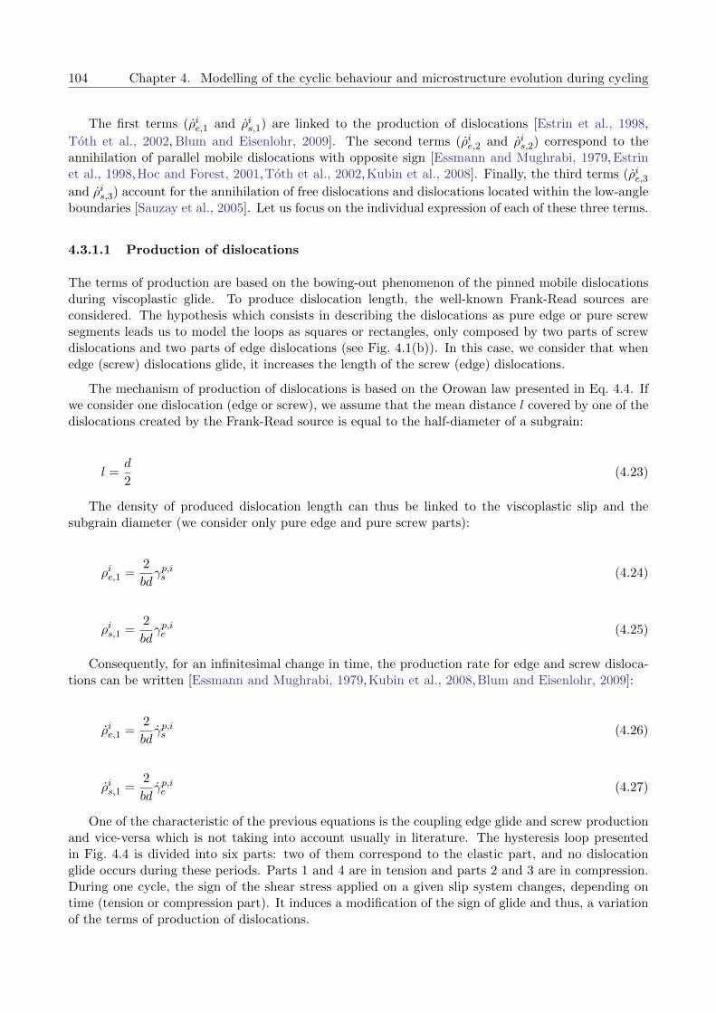
104 Chapter 4. Modelling of the cyclic behaviour and microstructure evolution during cycling
The first terms (ρie,1 and ρis,1) are linked to the production of dislocations [Estrin et al., 1998,
Toth et al., 2002, Blum and Eisenlohr, 2009]. The second terms (ρie,2 and ρis,2) correspond to theannihilation of parallel mobile dislocations with opposite sign [Essmann and Mughrabi, 1979, Estrinet al., 1998,Hoc and Forest, 2001,Toth et al., 2002,Kubin et al., 2008]. Finally, the third terms (ρie,3and ρis,3) account for the annihilation of free dislocations and dislocations located within the low-angleboundaries [Sauzay et al., 2005]. Let us focus on the individual expression of each of these three terms.
4.3.1.1 Production of dislocations
The terms of production are based on the bowing-out phenomenon of the pinned mobile dislocationsduring viscoplastic glide. To produce dislocation length, the well-known Frank-Read sources areconsidered. The hypothesis which consists in describing the dislocations as pure edge or pure screwsegments leads us to model the loops as squares or rectangles, only composed by two parts of screwdislocations and two parts of edge dislocations (see Fig. 4.1(b)). In this case, we consider that whenedge (screw) dislocations glide, it increases the length of the screw (edge) dislocations.
The mechanism of production of dislocations is based on the Orowan law presented in Eq. 4.4. Ifwe consider one dislocation (edge or screw), we assume that the mean distance l covered by one of thedislocations created by the Frank-Read source is equal to the half-diameter of a subgrain:
l =d
2(4.23)
The density of produced dislocation length can thus be linked to the viscoplastic slip and thesubgrain diameter (we consider only pure edge and pure screw parts):
ρie,1 =2
bdγp,is (4.24)
ρis,1 =2
bdγp,ie (4.25)
Consequently, for an infinitesimal change in time, the production rate for edge and screw disloca-tions can be written [Essmann and Mughrabi, 1979,Kubin et al., 2008,Blum and Eisenlohr, 2009]:
ρie,1 =2
bdγp,is (4.26)
ρis,1 =2
bdγp,ie (4.27)
One of the characteristic of the previous equations is the coupling edge glide and screw productionand vice-versa which is not taking into account usually in literature. The hysteresis loop presentedin Fig. 4.4 is divided into six parts: two of them correspond to the elastic part, and no dislocationglide occurs during these periods. Parts 1 and 4 are in tension and parts 2 and 3 are in compression.During one cycle, the sign of the shear stress applied on a given slip system changes, depending ontime (tension or compression part). It induces a modification of the sign of glide and thus, a variationof the terms of production of dislocations.
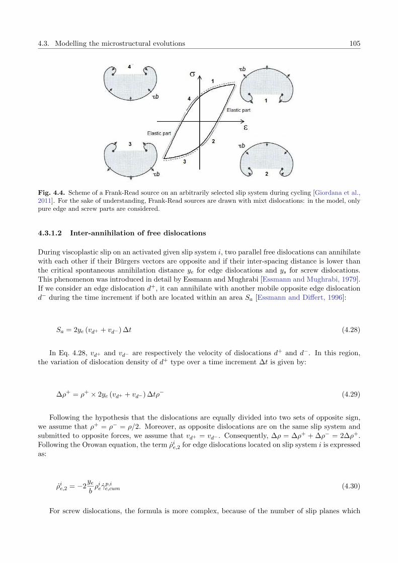
4.3. Modelling the microstructural evolutions 105
Fig. 4.4. Scheme of a Frank-Read source on an arbitrarily selected slip system during cycling [Giordana et al.,2011]. For the sake of understanding, Frank-Read sources are drawn with mixt dislocations: in the model, onlypure edge and screw parts are considered.
4.3.1.2 Inter-annihilation of free dislocations
During viscoplastic slip on an activated given slip system i, two parallel free dislocations can annihilatewith each other if their Burgers vectors are opposite and if their inter-spacing distance is lower thanthe critical spontaneous annihilation distance ye for edge dislocations and ys for screw dislocations.This phenomenon was introduced in detail by Essmann and Mughrabi [Essmann and Mughrabi, 1979].If we consider an edge dislocation d+, it can annihilate with another mobile opposite edge dislocationd− during the time increment if both are located within an area Sa [Essmann and Differt, 1996]:
Sa = 2ye (vd+ + vd−) ∆t (4.28)
In Eq. 4.28, vd+ and vd− are respectively the velocity of dislocations d+ and d−. In this region,the variation of dislocation density of d+ type over a time increment ∆t is given by:
∆ρ+ = ρ+ × 2ye (vd+ + vd−) ∆tρ− (4.29)
Following the hypothesis that the dislocations are equally divided into two sets of opposite sign,we assume that ρ+ = ρ− = ρ/2. Moreover, as opposite dislocations are on the same slip system andsubmitted to opposite forces, we assume that vd+ = vd− . Consequently, ∆ρ = ∆ρ+ + ∆ρ− = 2∆ρ+.Following the Orowan equation, the term ρie,2 for edge dislocations located on slip system i is expressedas:
ρie,2 = −2yebρieγ
p,ie,cum (4.30)
For screw dislocations, the formula is more complex, because of the number of slip planes which
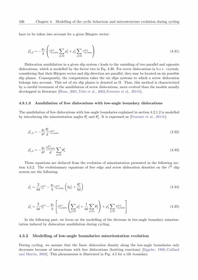
106 Chapter 4. Modelling of the cyclic behaviour and microstructure evolution during cycling
have to be taken into account for a given Burgers vector:
ρis,2 = −ysb
γp,is,cum∑j∈Ω
ρjs + ρis∑j∈Ω
γp,js,cum
(4.31)
Dislocation annihilation in a given slip system i leads to the vanishing of two parallel and oppositedislocations, which is modelled by the factor two in Eq. 4.30. For screw dislocations in b.c.c. crystals,considering that their Burgers vector and slip direction are parallel, they may be located on six possibleslip planes. Consequently, the computation takes the six slips systems to which a screw dislocationbelongs into account. This set of six slip planes is denoted as Ω. Thus, this method is characterizedby a careful treatment of the annihilation of screw dislocations, more evolved than the models usuallydevelopped in literature [Blum, 2001,Toth et al., 2002,Fournier et al., 2011b].
4.3.1.3 Annihilation of free dislocations with low-angle boundary dislocations
The annihilation of free dislocations with low-angle boundaries explained in section 4.2.1.2 is modelledby introducing the misorientation angles θie and θis. It is expressed as [Fournier et al., 2011b]:
ρie,3 = −yeb2θiedγp,ie,cum (4.32)
ρis,3 = −ysb2γp,is,cumd
∑j∈Ω
θjs (4.33)
These equations are deduced from the evolution of misorientation presented in the following sec-tion 4.3.2. The evolutionnary equations of free edge and screw dislocation densities on the ith slipsystem are the following:
ρie =2
bdγp,is −
yebγp,ie,cum
(2ρie +
θiebd
)(4.34)
ρis =2
bdγp,ie −
ysb
γp,is,cum∑j∈Ω
ρjs +1
bd
∑j∈Ω
θjs
+ ρis∑j∈Ω
γp,js,cum
(4.35)
In the following part, we focus on the modelling of the decrease in low-angle boundary misorien-tation induced by dislocation annihilation during cycling.
4.3.2 Modelling of low-angle boundaries misorientation evolution
During cycling, we assume that the lineic dislocation density along the low-angle boundaries onlydecreases because of interactions with free dislocations (knitting reactions) [Eggeler, 1989, Caillardand Martin, 2003]. This phenomenon is illustrated in Fig. 4.5 for a tilt boundary.
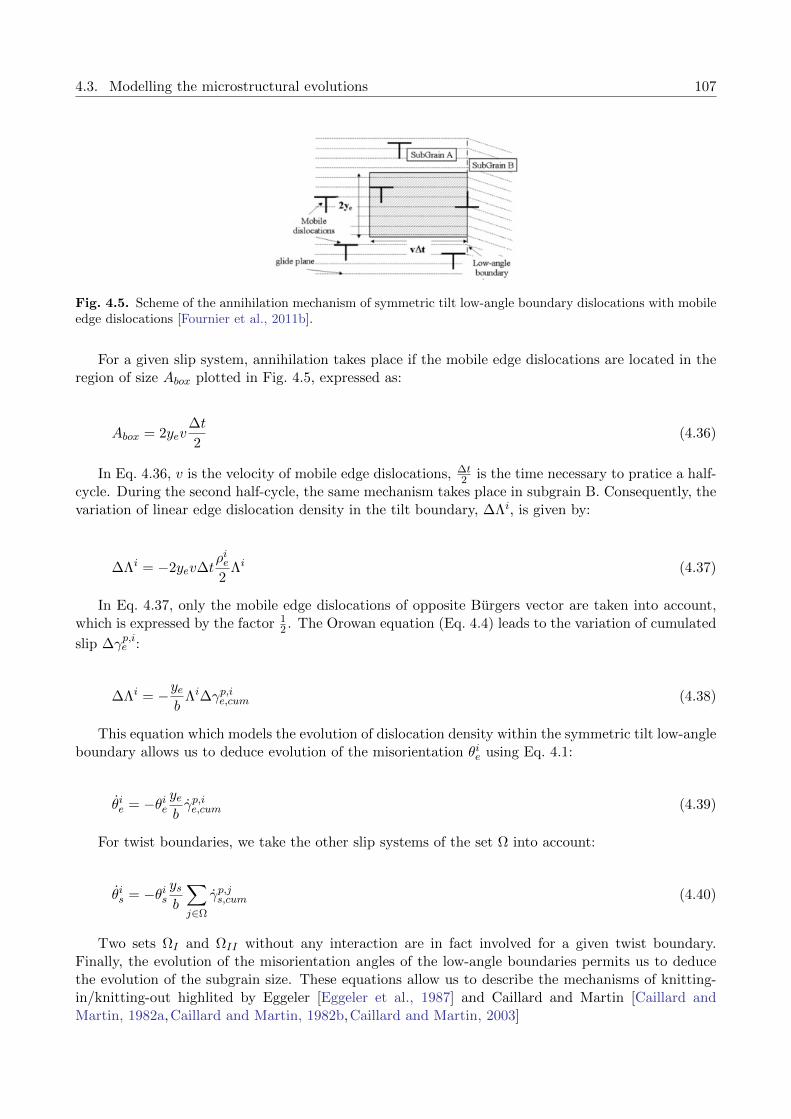
4.3. Modelling the microstructural evolutions 107
Fig. 4.5. Scheme of the annihilation mechanism of symmetric tilt low-angle boundary dislocations with mobileedge dislocations [Fournier et al., 2011b].
For a given slip system, annihilation takes place if the mobile edge dislocations are located in theregion of size Abox plotted in Fig. 4.5, expressed as:
Abox = 2yev∆t
2(4.36)
In Eq. 4.36, v is the velocity of mobile edge dislocations, ∆t2 is the time necessary to pratice a half-
cycle. During the second half-cycle, the same mechanism takes place in subgrain B. Consequently, thevariation of linear edge dislocation density in the tilt boundary, ∆Λi, is given by:
∆Λi = −2yev∆tρie2
Λi (4.37)
In Eq. 4.37, only the mobile edge dislocations of opposite Burgers vector are taken into account,which is expressed by the factor 1
2 . The Orowan equation (Eq. 4.4) leads to the variation of cumulated
slip ∆γp,ie :
∆Λi = −yeb
Λi∆γp,ie,cum (4.38)
This equation which models the evolution of dislocation density within the symmetric tilt low-angleboundary allows us to deduce evolution of the misorientation θie using Eq. 4.1:
θie = −θieyebγp,ie,cum (4.39)
For twist boundaries, we take the other slip systems of the set Ω into account:
θis = −θisysb
∑j∈Ω
γp,js,cum (4.40)
Two sets ΩI and ΩII without any interaction are in fact involved for a given twist boundary.Finally, the evolution of the misorientation angles of the low-angle boundaries permits us to deducethe evolution of the subgrain size. These equations allow us to describe the mechanisms of knitting-in/knitting-out highlited by Eggeler [Eggeler et al., 1987] and Caillard and Martin [Caillard andMartin, 1982a,Caillard and Martin, 1982b,Caillard and Martin, 2003]
108 Chapter 4. Modelling of the cyclic behaviour and microstructure evolution during cycling
4.3.3 Modelling the subgrain size evolution
The computation of subgrain size is presented in section 2.6.2 and leads to:
d =d0
1− κ(4.41)
In Eq. 4.41, the sugrain size d is expressed as a function of the initial subgrain size d0 and thefraction of vanished low-angle boundaries, κ.
For a given activated slip system, we assume that the interactions between mobile edge dislocationsand corresponding symmetric tilt boundary dislocations lead to the vanishing of the correspondingfamily of tilt low-angle boundary if the misorientation is lower that a critical angle θe,crit. This criterionwas proposed by Holec and Dlouhy [Holec and Dlouhy, 2005] and is based on the fact that the distancebetween edge dislocations along low-angle boundary is too high to garantee the stability of the arrayof dislocations when the lineic dislocation density of a tilt boundary reachs a critical value under agiven applied shear stress. In this case, the dislocations of the tilt boundary become mobile and thelow-angle boundary vanishes.
Let us assume that one-half of the low-angle boundaries is symmetric tilt boundaries and one-half is twist boundaries. In a block, 24 families of low-angle tilt boundaries may be considered (seesection 4.2.1.3). Consequently, the vanishing of a family of tilt low-angle boundaries leads to anincrease in the value of the fraction κ by 1
48 if twist low-angle boundaries are taken into account.
For twist boundaries, two families of dislocations are considered. In this case, we consider that afamily of twist low-angle boundary vanishes if the two families of screw dislocations which composethem both reach a critical value of misorientation θs,crit.
As the screw dislocations are divided into 4 families, the different possibilities of arrangementspermits us to assume the existence of 6 families of low-angle twist boundaries. The vanishing of afamily of low-angle twist boundaries leads to increase the value of the fraction κ by 1
12 if symmetriclow-angle tilt boundaries are taken into account.
The different equations presented in this part model the evolution of the microstructure duringcycling. In the following part, we focus on the localisation rule, which links the macroscopic stresstensor to the mean block stress tensor.
4.4 Self-consistent homogenization scheme
4.4.1 Thermoelastic modelling proposed by Kroner
The interaction law proposed by Kroner [Kroner, 1961] is based on thermoelasticity. Using the self-consistent scheme, the interaction law is derived from the solution of Eshelby’s inclusion problem [Es-helby, 1957]. Kroner considers each crystal (here, block) as an inclusion, and the deformed matrixas an equivalent homogeneous medium. Thus, for a block with a plastic strain εp embedded in thepolycrystal deformed with a plastic strain Ep, Kroner solves the localization problem considering aninclusion with a “free” deformation εp in the infinite matrix with a uniform “free” deformation. Severalassumptions are made to solve and simplify the Eshelby’s problem:
Elasticity is considered as isotropic and homogeneous
4.4. Self-consistent homogenization scheme 109
Plastic deformation is isovolumic
Inclusions (blocks) are considered as spherical
Considering these assumptions, the solution of the Eshelby problem leads to the Kroner interactionlaw:
σ = Σ + 2µ (1− β)(Ep − εp
)with β =
2 (4− 5ν)
15 (1− ν)
(4.42)
The Kroner model is based on the elastic interaction between the crystals (here, blocks) and thematrix. Consequently, the Kroner model gives us a good approximation of elastic behaviour andplastic behaviour only at low plastic strain. Indeed, at high plastic strains, the Kroner model givestoo hard predictions close to those obtained using the Taylor assumption [Taylor, 1938,Berveiller andZaoui, 1978]. Thus, the Kroner model is expected to give good predictions for low-cycle fatigue testsbecause of the low values of strain amplitude. But, in the framework of viscoplasticity, the modelproposed by Molinari is more suitable [Molinari et al., 1987].
4.4.2 Molinari’s model for viscoplastic material
Molinari’s model aims at predicting the mechanical behaviour of heterogeneous viscoplastic materialstill using a self-consistent scheme [Molinari et al., 1987, Molinari and Toth, 1994, Molinari, 1999].Considering large deformations, Molinari solves the nonlinear Eshelby problem and obtains an ap-proximate solution calculating the ellipsoide behaviour with uniform nonlinear properties embeddedin an infinite homogeneous matrix. In order to simplify the problem, the matrix behaviour is ap-proximated by using a first order expansion of the strain rate based on a tangent approximation andelasticity is neglected. The proposed homogeneization scheme is derived from the use of the Greenfunctions. Introducing a uniform reference medium, the properties of the heterogeneous material aresupposed to be carried by the homogeneous equivalent medium.
The interaction law is expressed as follows:
s = S +
[Atg −
(P tg)−1
]:(εvp − Evp
)(4.43)
In Eq. 4.43, S and s are respectively the macroscopic and local deviatoric stress tensors, Atg is a
fourth-order macroscopic tangent stiffness modulus tensor and P tg is a fourth-order tensor depending
on Atg and on the shape of the inclusion (block).
Fig.4.6 shows that the tensile stress-plastic strain curve predicted by the Kroner model used inthe present study is in accordance with the results available in literature [Hutchinson, 1964] and theMolinari’s model seems to tend to the Reuss bound [Reuss, 1929], as expected for f.c.c. polycrystalin literature [Liu and Castaneda, 2004]. To predict the mechanical behaviour of Grade 92 steel

110 Chapter 4. Modelling of the cyclic behaviour and microstructure evolution during cycling
Fig. 4.6. Tensile stress-plastic strain curves of a b.c.c. polycrystal predicted by the models proposed by Kroner(red dashed line) and Molinari (blue dotted line) respectively. The results of Taylor’s model (black continuousline) and Kroner’s model (empty diamond symbols) available in literature are also plotted [Hutchinson, 1964].ε is the strain at the initial elastic limit.
during cycling at high temperature, the interaction law of Kroner was chosen in the present study.Indeed, considering the low values of viscoplastic strain amplitudes during the differents tests (lowerthan a few 10−3), the Kroner’s model should be able to give reliable predictions of the mechanicalbehaviour [Berveiller and Zaoui, 1978, Sauzay, 2000, Rachdi and Sauzay, 2011] and the Molinari’sviscoplasticity model will be used as well for comparison. In the following part, we focus on theparameters used in the model, and their physical values, measured or taken from literature.
4.5 Choice of the values of the model parameters
4.5.1 Measured, calculated and fixed parameters
In the presented model, all parameters have a physical meaning. Table 4.1 shows the values ofparameters corresponding to constants and intrinsic material parameters.
Parameter Value Unit Reference
ν 0.3 [Francois et al., 1995b]
µ 68 GPa
ν0 1013 s−1 [Caillard and Martin, 2003]
b 2.54× 10⁻¹⁰ m [Francois et al., 1995b]
k 1.38× 10⁻²³ J.K−1
Tab. 4.1. Universal constants and intrinsic material parameters of the model.
The shear stress modulus µ was measured on the Grade 92 steel during cyclic test with a capacitiveextensometer. The Poisson ratio ν and the magnitude of the Burgers vector b were measured on b.c.c.
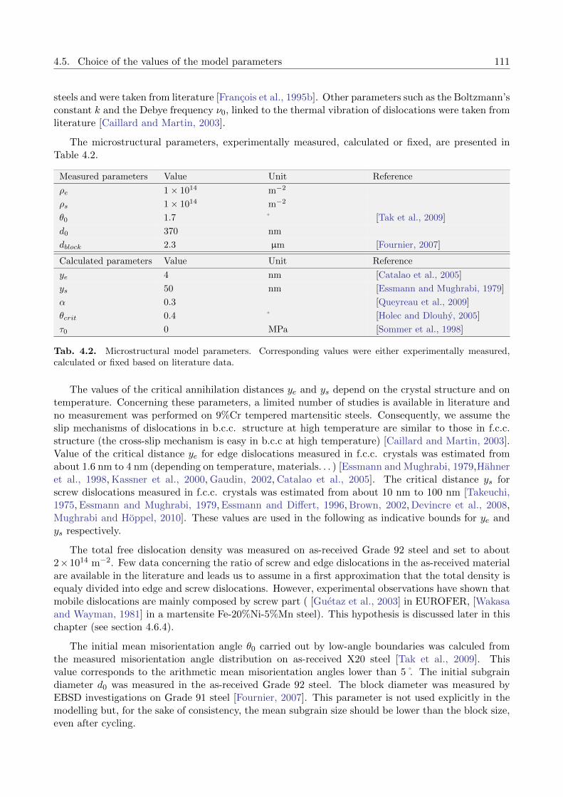
4.5. Choice of the values of the model parameters 111
steels and were taken from literature [Francois et al., 1995b]. Other parameters such as the Boltzmann’sconstant k and the Debye frequency ν0, linked to the thermal vibration of dislocations were taken fromliterature [Caillard and Martin, 2003].
The microstructural parameters, experimentally measured, calculated or fixed, are presented inTable 4.2.
Measured parameters Value Unit Reference
ρe 1× 10¹⁴ m−2
ρs 1× 10¹⁴ m−2
θ0 1.7 ˚ [Tak et al., 2009]
d0 370 nm
dblock 2.3 µm [Fournier, 2007]
Calculated parameters Value Unit Reference
ye 4 nm [Catalao et al., 2005]
ys 50 nm [Essmann and Mughrabi, 1979]
α 0.3 [Queyreau et al., 2009]
θcrit 0.4 ˚ [Holec and Dlouhy, 2005]
τ0 0 MPa [Sommer et al., 1998]
Tab. 4.2. Microstructural model parameters. Corresponding values were either experimentally measured,calculated or fixed based on literature data.
The values of the critical annihilation distances ye and ys depend on the crystal structure and ontemperature. Concerning these parameters, a limited number of studies is available in literature andno measurement was performed on 9%Cr tempered martensitic steels. Consequently, we assume theslip mechanisms of dislocations in b.c.c. structure at high temperature are similar to those in f.c.c.structure (the cross-slip mechanism is easy in b.c.c at high temperature) [Caillard and Martin, 2003].Value of the critical distance ye for edge dislocations measured in f.c.c. crystals was estimated fromabout 1.6 nm to 4 nm (depending on temperature, materials. . . ) [Essmann and Mughrabi, 1979,Hahneret al., 1998, Kassner et al., 2000, Gaudin, 2002, Catalao et al., 2005]. The critical distance ys forscrew dislocations measured in f.c.c. crystals was estimated from about 10 nm to 100 nm [Takeuchi,1975, Essmann and Mughrabi, 1979, Essmann and Differt, 1996, Brown, 2002, Devincre et al., 2008,Mughrabi and Hoppel, 2010]. These values are used in the following as indicative bounds for ye andys respectively.
The total free dislocation density was measured on as-received Grade 92 steel and set to about2×1014 m−2. Few data concerning the ratio of screw and edge dislocations in the as-received materialare available in the literature and leads us to assume in a first approximation that the total density isequaly divided into edge and screw dislocations. However, experimental observations have shown thatmobile dislocations are mainly composed by screw part ( [Guetaz et al., 2003] in EUROFER, [Wakasaand Wayman, 1981] in a martensite Fe-20%Ni-5%Mn steel). This hypothesis is discussed later in thischapter (see section 4.6.4).
The initial mean misorientation angle θ0 carried out by low-angle boundaries was calculed fromthe measured misorientation angle distribution on as-received X20 steel [Tak et al., 2009]. Thisvalue corresponds to the arithmetic mean misorientation angles lower than 5 . The initial subgraindiameter d0 was measured in the as-received Grade 92 steel. The block diameter was measured byEBSD investigations on Grade 91 steel [Fournier, 2007]. This parameter is not used explicitly in themodelling but, for the sake of consistency, the mean subgrain size should be lower than the block size,even after cycling.

112 Chapter 4. Modelling of the cyclic behaviour and microstructure evolution during cycling
The critical value of misorientation θcrit was calculed by Holec and Dlouhy and set to 0.4˚inthe conditions of temperature, stress and precipitation close to those of the Grade 92 steel duringcycling [Holec and Dlouhy, 2005].
Most parameters values were either experimentaly measured or calculated. However, some pa-rameter values are not exactly known and little information is available in literature concerning theirvalues for Grade 92 steel or more generally for the 9%Cr steel family. Consequently, a parametricstudy is presented in section 4.6.4 in order to study the impact of each value on the model predictions.
This model uses a low number of ajustable parameters : only the values of the activation volume, V ,and the activation energy, Q, are fitted using the first experimental quarters of cycles (monotonicloading). As these physical parameters correspond to the mechanisms of dislocation glide, their orderof magnitude is known and consequently, they are not totally let free during the identification processpresented in the following section.
4.5.2 Identification process
In order to predict the cyclic behaviour of the material at high temperature, the identification processaims to fit the two ajustable parameters of the model : the activation volume V and the activationenergy Q. This low number of ajustable parameters permits us to reduce the identification process toa very limited number of experimental data, excluding all data in relationship to the cyclic softeningbehaviour. They are ajusted on:
a monotonic tensile test up to 0.35 % with a strain rate of 2× 10⁻³ s−1
a monotonic tensile test up to 0.35 % with a strain rate of 1× 10⁻⁵ s−1
Only two monotonic tests at different strain rates are used to adjust the two remaining parameters.Thus, all cyclic tests available at different strain amplitudes and strain rates (see Tables 3.1 and 3.2)are kept for the validation process. Moreover, the limited number of adjustable parameters andexperimental data used to fit them induces a reduction of the parameter identification time. Finally,it should be noticed that tests using various strain rates are indeed required for adjusting these valuesof the viscoplasticity parameters.
Numerical simulations, performed with the SiDoLo software [Pilvin, 2003], were carried out on apolycrystalline aggregate (each crystal representing, here, a block of laths) with 100 random crystal-lographic orientations. The influence of the number of blocks and the set of random orientations onthe predicted macroscopic behaviour is presented in Fig. 4.7.
The results presented in Fig. 4.7(a) show that the model gives a similar response for aggregatescomposed of more than 100 blocks. Consequently, in order to reduce the computation time†, simu-lations are carried out using an aggregate of 100 blocks. Fig. 4.7(b) shows that the set of randomcrystallographic orientations of the 100 blocks has no significant impact on the predicted macroscopicresponse and it permits us to neglect its influence on the model predictions. This confirms that thenumber of blocks is high enough to get a representative elementary volume.
The results of the adjustement process are presented in Fig. 4.8. The values of the fitted parameters,the activation volume V and the activation energy Q are reported in Table 4.3.
†The computation time is 10 times higher to predict the mechanical behaviour of an aggregate of 500 blocks than ofan aggregate of 100 blocks.

4.5. Choice of the values of the model parameters 113
(a) (b)
Fig. 4.7. Influence of (a) the number of blocks and (b) different sets of crystallographic orientations of 100 blockson the simulated monotonic tensile curves up to 0.5% at 2× 10⁻³ s−1. For Fig (b), each randomly selected setof 100 crystallographic orientations is different from the others.
Fig. 4.8. Comparison between the experimental and simulated monotonic curves up to 0.35 %, at two differentstrain rates.
Parameter Value Unit
Q 1.2 eV
V 216 b3
Tab. 4.3. Values of the parameters fitted on monotonic tensile curves up to 0.35 %, with a strain rate of2× 10−3 s−1 and 1× 10⁻⁵ s−1.

114 Chapter 4. Modelling of the cyclic behaviour and microstructure evolution during cycling
The study of the hysteresis loops of the Grade 91 steel at 550 C permits Fournier et al. to measurean activation volume close to 60 b3 [Fournier et al., 2006a]. In a 12%Cr ferritic-martensitic steelcontaining different alloying elements (C, N, Ni, Mo, V, Nb, Si, Mn and B), Marmy et al. measured avalue equal to 45 b3 during tensile test at 600 C [Marmy et al., 1993]. The b.c.c. materials are knownto have low activation volumes (from about 15 to 300 b3 depending on the temperature) compared tof.c.c. materials which have values 10 to 100 times larger at low temperature [Voyiadjis and Abed, 2005].The fitted value of the activation volume in the current model is slightly larger than measured valuesin other steels, but we have to consider this comparison cautiously: the value of the activation volumewidely depends on the microstructure of the considered material, and particularly on precipitates andchemical elements which compose the solid solution. Consequently, we can carefully conclude that thefitted value of the activation volume is in accordance with the order of magnitude measured in b.c.c.materials and remains significanly lower than the f.c.c. materials one.
The fitted value of activation volume is low compared to the subgrain size. This indicates thatthe mechanisms which govern the viscoplastic glide take place at a smaller scale than the subgrainstructure in this steel. The fitted value is too high to correspond to interactions with individual soluteatom in the matrix (atomic volum is close to 1 b3) [Conrad and Narayan, 2000, Wei et al., 2004]and seems rather low for corresponding to interactions with small precipitates like MX-types (severalthousands of b3) [Caillard and Martin, 2003]. Several studies on Ni(Al) and Al(Mg) alloys proposedthat solid solution hardening is not simply the result of a direct dislocation / solute atoms interaction,but the result of close solute-solute atoms repulsion [Rodary et al., 2004,Proville et al., 2006,Provilleand Patinet, 2010]. This repulsion force is considered to be an obstacle to dislocation glide [Rodaryet al., 2004]. Thus, the interaction between dislocations and solid solution is not only describe withisolated solute atoms but also with clusters of solute atoms. We can assume that similar mechanismsmay occur in ferritic-martensite steels strengthened by Mo and/or W solute atoms. In this case, thefitted value of the activation volume may correspond to the volume of (Mo,W) clusters.
As for the activation volume, experimental values of the activation energy published in literaturewidely vary and depend on the considered deformation mechanism, the experimental technique used,temperature and material under consideration [Spigarelli et al., 1997,Fournier et al., 2006a]. The fittedvalue of the activation energy is significantly lower than the bulk diffusion one which is measured to2.5 eV [Francois et al., 1995b]. In 12%Cr-Mo-VNb ferritic-martensitic steel, Marmy and coworkers havemeasured a value of the activation energy of about 1.2 eV during tensile test at 600 C [Marmy et al.,1993]. The fitted value of activation energy in the current model is equal to this experimental value.According to Marmy et al., this energy barrier corresponds to mechanims of deformation which needlow activation energy and we can assume that it corresponds to the energy required for dislocationsglide through solid solution and small carbo-nitride obstacles [Marmy et al., 1993], assumed to becomposed of small clusters of solute atoms. Following the experimental study of Abe using variousamounts of W and C elements, both W solid solution and MX precipitates lead to decrease in creepstrain rates [Abe, 2001]. This means that both are obstacles to dislocation glide. The activation volumeand energy adjusted previously may be effective values corresponding to several kinds of obstacles.
Values of the parameters used during the identification process remain the same for all the presentedsimulation results in the following sections, unless it is explicitely expressed in the parametric study.Because of the few experimental data that are necessary to fit the two adjustable parameters, alarge number of independant tests are available to validate the model. In the following section, theexperimental hysteresis loops at the first cycle of fatigue test and the corresponding predicted onesare compared for both strain rates.

4.6. Simulation of cyclic loading 115
4.6 Simulation of cyclic loading
4.6.1 Validation of the model on the first macroscopic loop for both strain rates
The first step of the validation concerns the prediction of the first loop. As the identification processrequires two monotonic tests at different strain rates, their corresponding first cycles are compared tothe model predictions. Results are presented in Fig. 4.9.
(a) (b)
Fig. 4.9. Comparison between experimental and predicted macroscopic cycles for a strain amplitude of ± 0.35%(a) with a strain rate of 2× 10⁻³ s−1 and (b) with a strain rate of 1× 10⁻⁵ s−1.
The model predicts the mechanical behaviour of the Grade 92 steel during the first hysteresis loopquite accurately for both strain rates. A slight difference between the model and the experimentaldata is observed for the minimum stress in compression: for both tests, the predicted minimum stressis slightly overestimated, whereas the predicted maximum stresses are very close to the experimentaldata. This phenomenon is probably due to, on the one hand, experimental scatter or, on the otherhand, to a too fast softening rate.
Although maximum and minimum stresses are rather accurately predicted, the shape of the pre-dicted hysteresis loop is characterized by a change in curvature both in compression and tension, butnot during the first quarter of cycle. This unexpected behaviour is due to the expression of the kine-matic stress evolution. However, the reasons which induce this problem are not clearly establishedand complementary studies are necessary to understand this phenomenon exactly. This unaccuracytakes place only during a short part of each cycle and it probably has no significant influence on theprediction of the softening behaviour of the material.
4.6.2 Prediction of cyclic softening for both strain rates
4.6.2.1 Predicted macroscopic behaviour
The main objective of the model is to predict the softening behaviour, which characterizes the temperedmartensite steels during cycling. In order to clarify the presentation of the results, only the experi-mental and predicted data corresponding to the maximum tensile stress are compared. It is very closeto the amplitude. Fig. 4.10 shows the cyclic softening predicted by the modelling at ± 0.35% and two

116 Chapter 4. Modelling of the cyclic behaviour and microstructure evolution during cycling
different strain rates. The computation time is approximatly equal to 25 - 30 hours to obtain theseresults.
According to Fig. 4.10, the model predicts a cyclic softening for both strain rates: it reproducesthe stress drop of 70 MPa measured experimentally during the test. Moreover, the cyclic evolutionis correctly predicted by the model. The difference between the predicted and experimental curvesis lower than 10 MPa for the higher strain rate and 20 MPa for the lower one (in both case, thesedifferences are lower than 5 % of the corresponding initial stress). Thus, the model is able to predictreasonably the overall softening observed during cycling at intermediate strain amplitude.
However, although the softening rate is well predicted (predicted slopes are almost parallel to theexperimental ones), the predicted and experimental curves are not superimposed for the lower strainrate. This leads to an underestimation of the maximum tensile stress during all the test whereas forhigh strain rate, this phenomenon is limited to the beginning of the tests, up to 500 cycles, and themodel accurately predicts the mechanical behaviour after 900 cycles. This difference may be explainedby the experimental scatter (which can reach ± 15 MPa) of the data measured during cycling at lowstrain rate (see Fig. 4.8 for example). Scatter is lower at higher strain rate (see Fig. 4.9).
4.6.2.2 Predicted microstructural evolution
The mean subgrain size evolution is presented in Fig. 4.11. Although the model reproduces theexperimentally observed tendency of the subgrain size evolution (fast growth followed by a reductionof evolution rate), this figure shows that the subgrain growth rate is overestimated. Indeed, themodelling predicts a too fast evolution of the subgrain growth up to 400 cycles, which might induceat least partially the high softening rate observed on the predicted macroscopic behaviour. Moreover,predicted final subgrain sizes for both strain rate are overestimated (see Table 4.4): for high strainrate, the growth factor is equal to about 2.2 (experimental data gives about 1.7) and for low strainrate, it is equal to about 3.1 (experimental data gives about 2.0). These results can be explainedby the strong assumptions made to describe the low-angle boundary structure (pure symmetric tiltboundary with only one family of edge dislocations, pure twist boundaries. . . ): these simplificationsprobably lead to an overestimation of the number of vanished low-angle boundaries.
Strain rate Final experimental mean subgrainsize
Final predicted mean subgrain size
2× 10⁻³ s−1 0.62 ± 0.12 µm 0.84 µm
1× 10⁻⁵ s−1 0.78 ± 0.08 µm 1.16 µm
Tab. 4.4. Values of the measured and predicted mean subgrain size in a sample of fractured specimen afterfatigue test of a strain amplitude of ± 0.35 %, for different strain rates.
The effect of strain rate on the subgrain growth is clearly observable. For the lower strain rate,the predicted subgrain growth rate is significantly higher than for the higher strain rate, even after1,000 cycles. This difference might be explained by the plastic strain amplitude applied on the materialduring fatigue cycles. Indeed, Fig. 4.8 shows that for imposed total strain amplitude, the modelpredicts a higher plastic strain amplitude for the low strain rate than for the high strain rate, asexperimentally observed (see Table 3.1 and 3.2). Thus, the amount of cumulated viscoplastic strainis higher in the material deformed at low strain rate. In addition, Fig. 4.12 shows the predictedevolution of the mean number of activated slip system per block during a monotonic tensile test upto 0.5 % and for the two different strain rates. We observe that a decrease in strain rate leads to asignificant increase in the mean number of activated slip system per block. Thus, the annihilationterms and annihilation probabilities between the free dislocations and the low-angle boundaries are
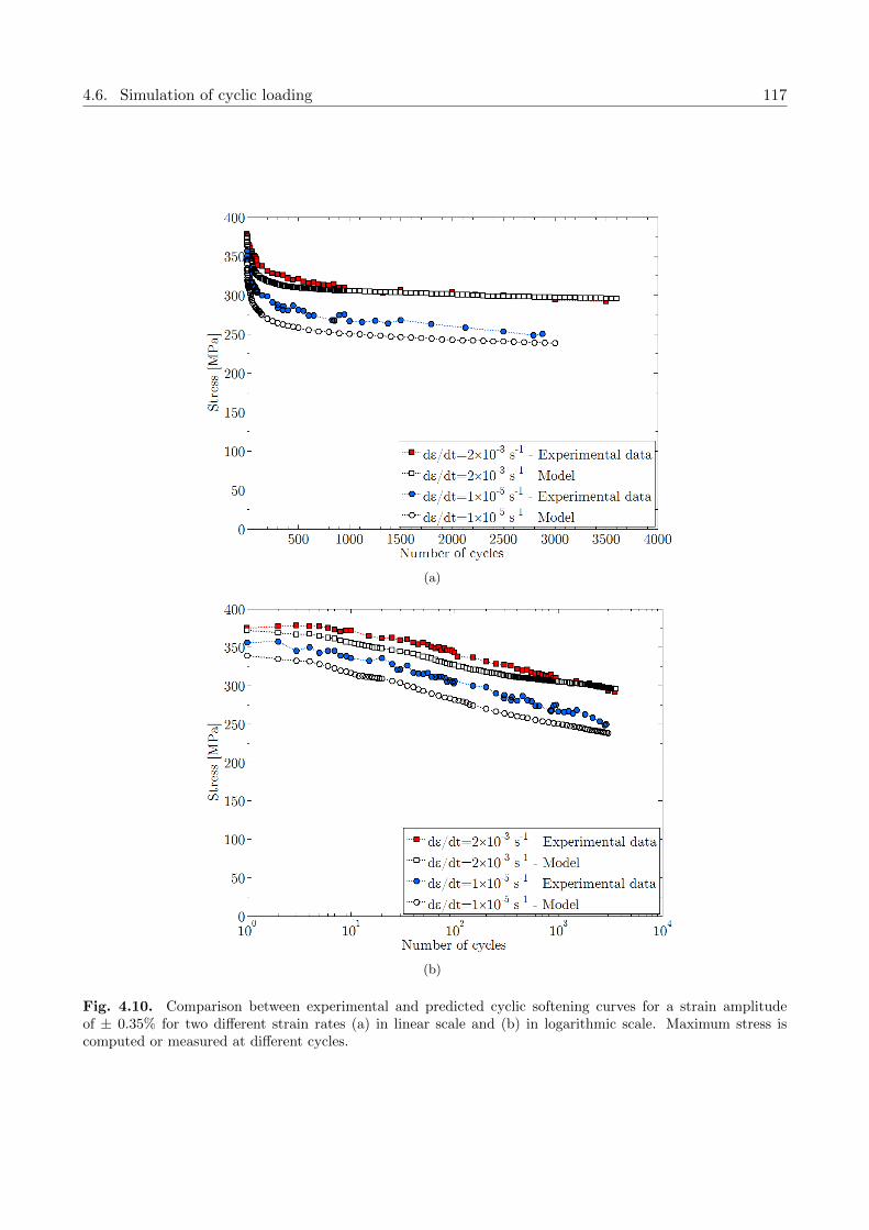
4.6. Simulation of cyclic loading 117
(a)
(b)
Fig. 4.10. Comparison between experimental and predicted cyclic softening curves for a strain amplitudeof ± 0.35% for two different strain rates (a) in linear scale and (b) in logarithmic scale. Maximum stress iscomputed or measured at different cycles.

118 Chapter 4. Modelling of the cyclic behaviour and microstructure evolution during cycling
Fig. 4.11. Comparison between experimental and predicted mean subgrain size evolutions during fatigue testswith a strain amplitude of ± 0.35% for two different strain rates.
higher in material during cycling at the lower strain rate than during cycling at the higher strain rate.Consequently, the decrease in strain rate leads to an enhancement of the annihilation phenomenabetween mobile dislocations and low-angle boundaries in the aggregate and finally, to a faster growthof subgrains.
Fig. 4.13 presents the predictions of the mobile edge and screw dislocation density evolutions.The local variations of the curves are due to the term of production of dislocations introduced in thedislocation density evolutionnary equations (see Eqs. 4.34 and 4.35). Fig. 4.13(a) shows that the modelpredicts a fast evolution of the mobile dislocation density: the main variations occur before 1,000 cyclesand they remain approximatly stable. As expected, mobile screw dislocations annihilate faster thanmobile edge dislocations, due to their geometrical properties (higher probability of annihilation [Sauzayet al., 2005]) and higher critical annihilation distance with respect to the edge ones.
The model predicts a very fast evolution of the mobile dislocation densities: the main variationsoccur during the 100 first cycles. The strain rate has an influence on the predicted dislocationsdensities. Although this effect is slight on the mobile screw dislocation density evolution, it is clearlyvisible on the mobile edge dislocation density evolution. Up to 20 cycles, no significant differencebetween both curves is observed, but after the 20th cycle, the mobile edge dislocation density decreasesfaster in the case of the lower strain rate than in the case of the higher strain rate. As for subgraingrowth, that is the consequence of the plastic strain amplitude per cycle, higher for the lower strainrate, which leads to a higher number of actived slip systems in blocks too and finally, promotes theannihilation phenomena.
No experimental value of dislocation density evolution is available for this material. Only the totaldislocation density were measured at the end of the test and can be compared to the predicted values.Experimental and predicted values are presented in Table 4.5. Although the predicted value for thelow strain rate is overestimated, the model correctly predicts the final value measured in the foilsextracted from the specimens fractured at high strain rate.
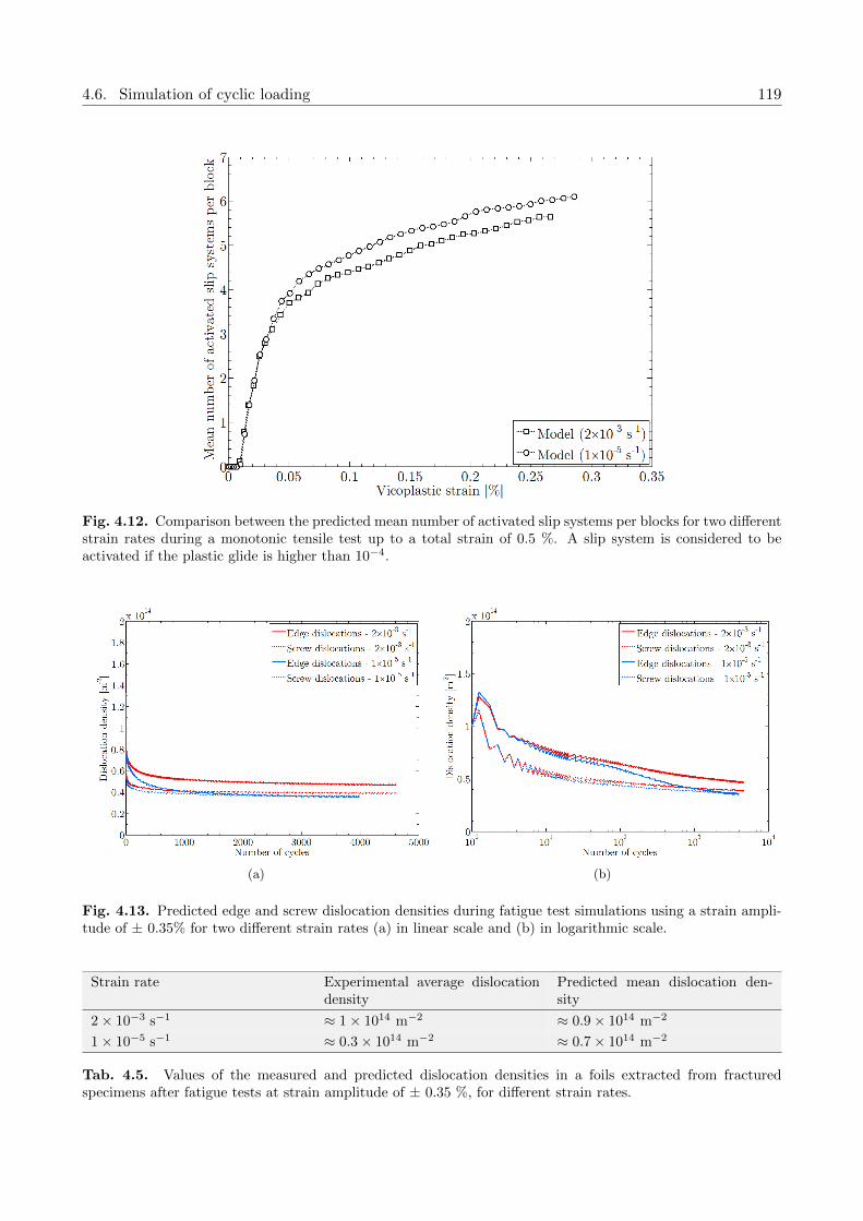
4.6. Simulation of cyclic loading 119
Fig. 4.12. Comparison between the predicted mean number of activated slip systems per blocks for two differentstrain rates during a monotonic tensile test up to a total strain of 0.5 %. A slip system is considered to beactivated if the plastic glide is higher than 10−4.
(a) (b)
Fig. 4.13. Predicted edge and screw dislocation densities during fatigue test simulations using a strain ampli-tude of ± 0.35% for two different strain rates (a) in linear scale and (b) in logarithmic scale.
Strain rate Experimental average dislocationdensity
Predicted mean dislocation den-sity
2× 10⁻³ s−1 ≈ 1× 10¹⁴ m−2 ≈ 0.9× 10¹⁴ m−2
1× 10⁻⁵ s−1 ≈ 0.3× 10¹⁴ m−2 ≈ 0.7× 10¹⁴ m−2
Tab. 4.5. Values of the measured and predicted dislocation densities in a foils extracted from fracturedspecimens after fatigue tests at strain amplitude of ± 0.35 %, for different strain rates.
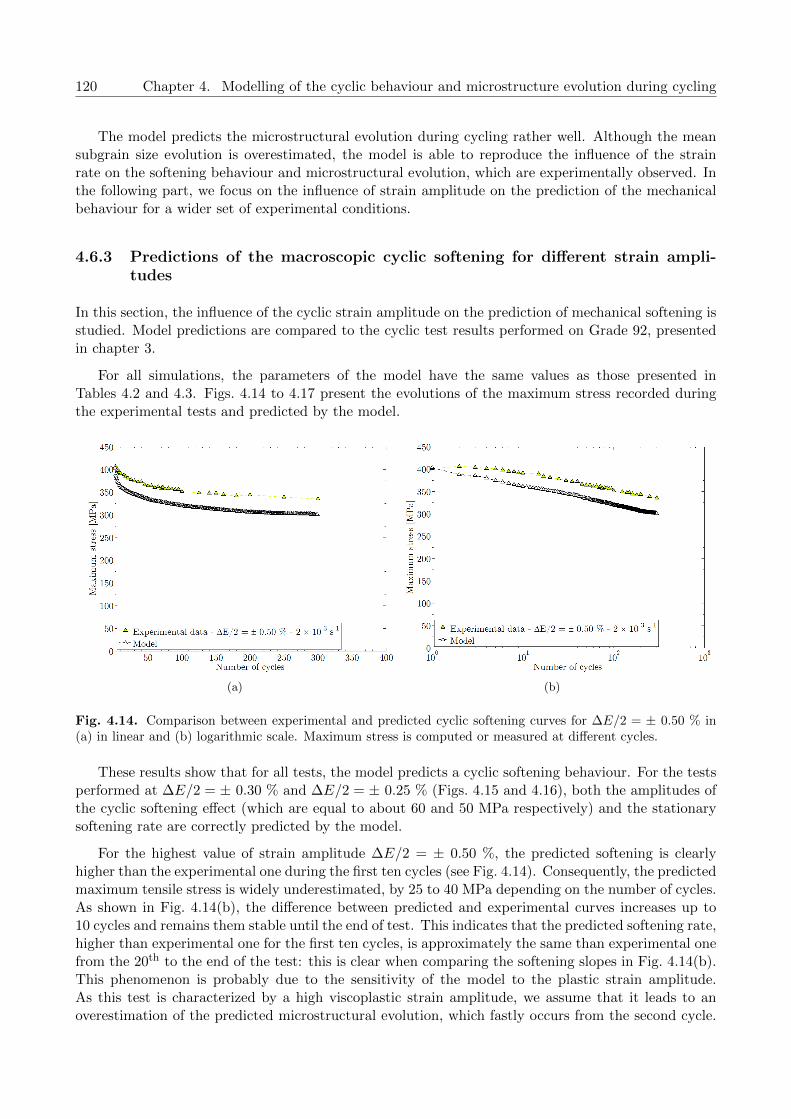
120 Chapter 4. Modelling of the cyclic behaviour and microstructure evolution during cycling
The model predicts the microstructural evolution during cycling rather well. Although the meansubgrain size evolution is overestimated, the model is able to reproduce the influence of the strainrate on the softening behaviour and microstructural evolution, which are experimentally observed. Inthe following part, we focus on the influence of strain amplitude on the prediction of the mechanicalbehaviour for a wider set of experimental conditions.
4.6.3 Predictions of the macroscopic cyclic softening for different strain ampli-tudes
In this section, the influence of the cyclic strain amplitude on the prediction of mechanical softening isstudied. Model predictions are compared to the cyclic test results performed on Grade 92, presentedin chapter 3.
For all simulations, the parameters of the model have the same values as those presented inTables 4.2 and 4.3. Figs. 4.14 to 4.17 present the evolutions of the maximum stress recorded duringthe experimental tests and predicted by the model.
(a) (b)
Fig. 4.14. Comparison between experimental and predicted cyclic softening curves for ∆E/2 = ± 0.50 % in(a) in linear and (b) logarithmic scale. Maximum stress is computed or measured at different cycles.
These results show that for all tests, the model predicts a cyclic softening behaviour. For the testsperformed at ∆E/2 = ± 0.30 % and ∆E/2 = ± 0.25 % (Figs. 4.15 and 4.16), both the amplitudes ofthe cyclic softening effect (which are equal to about 60 and 50 MPa respectively) and the stationarysoftening rate are correctly predicted by the model.
For the highest value of strain amplitude ∆E/2 = ± 0.50 %, the predicted softening is clearlyhigher than the experimental one during the first ten cycles (see Fig. 4.14). Consequently, the predictedmaximum tensile stress is widely underestimated, by 25 to 40 MPa depending on the number of cycles.As shown in Fig. 4.14(b), the difference between predicted and experimental curves increases up to10 cycles and remains them stable until the end of test. This indicates that the predicted softening rate,higher than experimental one for the first ten cycles, is approximately the same than experimental onefrom the 20th to the end of the test: this is clear when comparing the softening slopes in Fig. 4.14(b).This phenomenon is probably due to the sensitivity of the model to the plastic strain amplitude.As this test is characterized by a high viscoplastic strain amplitude, we assume that it leads to anoverestimation of the predicted microstructural evolution, which fastly occurs from the second cycle.

4.6. Simulation of cyclic loading 121
(a) (b)
Fig. 4.15. Comparison between experimental and predicted cyclic softening curves for ∆E/2 = ± 0.30 % in(a) in linear and (b) logarithmic scale. Maximum stress is computed or measured at different cycles.
(a) (b)
Fig. 4.16. Comparison between experimental and predicted cyclic softening curves for ∆E/2 = ± 0.25 % in(a) in linear and (b) logarithmic scale. Maximum stress is computed or measured at different cycles.

122 Chapter 4. Modelling of the cyclic behaviour and microstructure evolution during cycling
(a) (b)
Fig. 4.17. Comparison between experimental and predicted cyclic softening curves for ∆E/2 = ± 0.20 % in(a) in linear and (b) logarithmic scale. Maximum stress is computed or measured at different cycles.
This hypothesis is discussed in chapter 5.
The opposite case can be described with the test performed using ∆E/2 = ± 0.20 % presentedin Fig. 4.17. In this case, the viscoplastic strain amplitude is very low at the first cycle. Instead ofcyclic softening, the model predicts a slight hardening up to about 40 cycles. After this stage, a slightdecrease in the maximum stress is predicted, but neither its amplitude nor its kinetics are in a correctagreement with the experimental data. Thus, the predicted softening amplitude is underestimated byabout 20 - 25 MPa.
Because of its sensitivity to the viscoplastic strain amplitude during cycling, the model is not ableto predict the mechanical behaviour of the material for low strain amplitudes (∆E/2 ≤ ± 0.20 %)and for high strain amplitudes (∆E/2 ≥ ± 0.50 %) very accurately.
4.6.4 Sensitivity of model predictions to the values of model parameters
All the parameters used in the model have a physical meaning. However, most of them were not exper-imentally determined in the conditions under interest and only very limited amount of information isavailable in literature concerning annihilation distances, initial and critical misorientations angle andthe ratio between the free edge or screw dislocations densities and the total free dislocation densities.Consequently, in a first approximation, their assigned parameter values corresponded to measurementsor computation carried out for a different material, in different conditions of environment, temperatureor mechanical loadings. The involved parameters are presented in the following list:
The critical annihilation distance of edge dislocations ye
The critical annihilation distance of screw dislocations ys
The initial mean low-angle boundary misorientation θ0
The critical value of low-angle boundary misorientation θcrit
The ratio between the mobile edge and screw dislocations densities and the total mobile dislo-cation density

4.6. Simulation of cyclic loading 123
To analyse the sensitivity of the model to each parameter, all the values of the other parametersare kept the same as those used for the identification process (Tables 4.2 and 4.3). A upper and alower bound values are defined for the studied parameters, based on information available in literature.Using both values, two predictions of the mechanical behaviour and microstructure evolution duringcyclic test at a strain amplitude of ± 0.35 % and a strain rate of 1× 10⁻⁵ s−1 are then calculed usingthe model. Then, they are compared to the reference curves obtained in the previous section and theinfluence of parameter values on the prediction is discussed.
4.6.4.1 Influence of the critical annihilation distance for edge dislocations on modelpredictions
As it has been described in section 4.5, little information about the value of the critical annihilationdistance at high temperature for edge dislocations ye is available in the literature and no measurementwas performed in 9%Cr steels at 550 C. Considering the different values published in the literature,the upper and lower bounds are fixed to 2 nm and 4 nm respectively. The impact of this parameterchange on the macroscopic mechanical behaviour is presented in Fig. 4.18.
(a) (b)
Fig. 4.18. Influence of the value of ye on the predicted macroscopic mechanical behaviour.
Up to 10 cycles, the value of ye has no influence on the predicted mechanical behaviour. Then, upto about 200 cycles, the softening rate slightly increases with the value of ye: as expected, the higherthe annihilation distance, the higher the softening rate. Finally, at the end of the test, the parameterchange induces a difference of about 10 MPa for the maximum tensile stress (which is less than 5 %of the current value).
The influence of the value of ye on the predicted mean subgrain size evolution is presented inFig. 4.19. As expected, the subgrain growth rate is higher when ye increases. Consequently, thepredicted final subgrain size varies by about 17 % between both calculations. The impact of ye on thepredicted average dislocation density evolution is presented in Fig 4.20. As expected, no impact onthe screw dislocation density evolution is observed. But an effect is visible for edge dislocation densityevolution rate: as expected, the higher the value of ye, the faster the free edge dislocation densitydecreases. However, ye does not impact the prediction of the final dislocation density.
The sensitivity of the model to the value of ye is limited to the predicted subgrain size evolution.Its impact on the macroscopic mechanical behaviour is slight. This indicates that, except for subgrain

124 Chapter 4. Modelling of the cyclic behaviour and microstructure evolution during cycling
Fig. 4.19. Influence of the value ye on the predicted mean subgrain size evolution.
(a) (b)
Fig. 4.20. Influence of the value ye on the predicted mean dislocation density evolution.

4.6. Simulation of cyclic loading 125
size, the predictions are relatively stable with respect to the variation of this parameter.
4.6.4.2 Influence of the critical annihilation distance for screw dislocations on modelpredictions
As for parameter ye, little information about the critical annihilation distance for screw dislocations ysis available in the literature at high temperature and no measurement was performed in 9%Cr steels.By considering the values presented in section 4.5, the upper and lower bound values are fixed to25 nm and 100 nm respectively, which include almost all values available in literature. The influenceof this parameter on the macroscopic mechanical behaviour is presented in Fig. 4.21.
(a) (b)
Fig. 4.21. Influence of the value of ys on the predicted macroscopic mechanical behaviour. 50 nm is the valueused in the previous section.
The influence of ys on the predicted mechanical behaviour is noticeable up to about 300 cycles.During this short first stage, the parameter change induces a variation of about ± 10 MPa of themaximum tensile stress (which is lower than 4 % of the current value). After this transient stage, thepredicted mechanical behaviour is no longer influenced by the value of ys.
Fig. 4.22. Influence of the value of ys on the predicted mean subgrain size evolution.

126 Chapter 4. Modelling of the cyclic behaviour and microstructure evolution during cycling
(a) (b)
(c) (d)
Fig. 4.23. Influence of the value of ys on the predicted mean dislocation density evolution for free edgedislocations ((a) and (b)) and free screw dislocations ((c) and (d)).
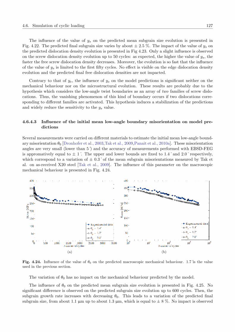
4.6. Simulation of cyclic loading 127
The influence of the value of ys on the predicted mean subgrain size evolution is presented inFig. 4.22. The predicted final subgrain size varies by about ± 2.5 %. The impact of the value of ys onthe predicted dislocation density evolution is presented in Fig 4.23. Only a slight influence is observedon the screw dislocation density evolution up to 50 cycles: as expected, the higher the value of ys, thefaster the free screw dislocation density decreases. Moreover, the evolution is so fast that the influenceof the value of ys is limited to the first fifty cycles. No effect is visible on the edge dislocation densityevolution and the predicted final free dislocation densities are not impacted.
Contrary to that of ye, the influence of ys on the model predictions is significant neither on themechanical behaviour nor on the microstructural evolution. These results are probably due to thehypothesis which considers the low-angle twist boundaries as an array of two families of screw dislo-cations. Thus, the vanishing phenomenon of this kind of boundary occurs if two dislocations corre-sponding to different families are activated. This hypothesis induces a stabilization of the predictionsand widely reduce the sensitivity to the ys value.
4.6.4.3 Influence of the initial mean low-angle boundary misorientation on model pre-dictions
Several measurements were carried on different materials to estimate the initial mean low-angle bound-ary misorientation θ0 [Dronhofer et al., 2003,Tak et al., 2009,Panait et al., 2010a]. These misorientationangles are very small (lower than 5 ) and the accuracy of measurements performed with EBSD-FEGis appromatively equal to ± 1 . The upper and lower bounds are fixed to 1.4˚and 2.0˚respectively,which correspond to a variation of ± 0.3˚of the mean subgrain misorientations measured by Tak etal. on as-received X20 steel [Tak et al., 2009]. The influence of this parameter on the macroscopicmechanical behaviour is presented in Fig. 4.24.
(a) (b)
Fig. 4.24. Influence of the value of θ0 on the predicted macroscopic mechanical behaviour. 1.7 is the valueused in the previous section.
The variation of θ0 has no impact on the mechanical behaviour predicted by the model.
The influence of θ0 on the predicted mean subgrain size evolution is presented in Fig. 4.25. Nosignificant difference is observed on the predicted subgrain size evolution up to 600 cycles. Then, thesubgrain growth rate increases with decreasing θ0. This leads to a variation of the predicted finalsubgrain size, from about 1.1 µm up to about 1.3 µm, which is equal to ± 8 %. No impact is observed

128 Chapter 4. Modelling of the cyclic behaviour and microstructure evolution during cycling
Fig. 4.25. Influence of the value of θ0 on the predicted mean subgrain size evolution.
(a) (b)
(c) (d)
Fig. 4.26. Influence of the value of θ0 on the predicted mean dislocation density evolution for free edgedislocations ((a) and (b)) and free screw dislocations ((c) and (d)).
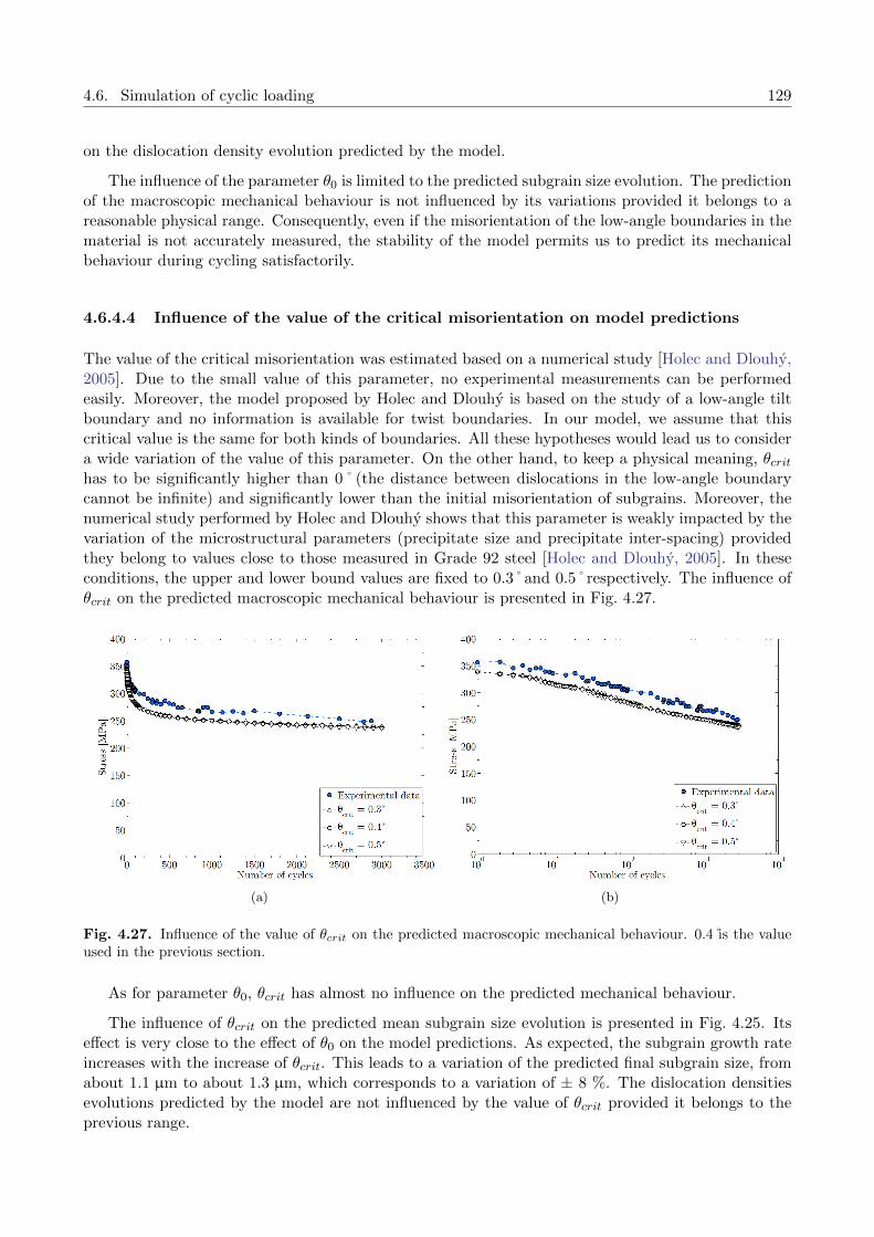
4.6. Simulation of cyclic loading 129
on the dislocation density evolution predicted by the model.
The influence of the parameter θ0 is limited to the predicted subgrain size evolution. The predictionof the macroscopic mechanical behaviour is not influenced by its variations provided it belongs to areasonable physical range. Consequently, even if the misorientation of the low-angle boundaries in thematerial is not accurately measured, the stability of the model permits us to predict its mechanicalbehaviour during cycling satisfactorily.
4.6.4.4 Influence of the value of the critical misorientation on model predictions
The value of the critical misorientation was estimated based on a numerical study [Holec and Dlouhy,2005]. Due to the small value of this parameter, no experimental measurements can be performedeasily. Moreover, the model proposed by Holec and Dlouhy is based on the study of a low-angle tiltboundary and no information is available for twist boundaries. In our model, we assume that thiscritical value is the same for both kinds of boundaries. All these hypotheses would lead us to considera wide variation of the value of this parameter. On the other hand, to keep a physical meaning, θcrithas to be significantly higher than 0˚(the distance between dislocations in the low-angle boundarycannot be infinite) and significantly lower than the initial misorientation of subgrains. Moreover, thenumerical study performed by Holec and Dlouhy shows that this parameter is weakly impacted by thevariation of the microstructural parameters (precipitate size and precipitate inter-spacing) providedthey belong to values close to those measured in Grade 92 steel [Holec and Dlouhy, 2005]. In theseconditions, the upper and lower bound values are fixed to 0.3˚and 0.5˚respectively. The influence ofθcrit on the predicted macroscopic mechanical behaviour is presented in Fig. 4.27.
(a) (b)
Fig. 4.27. Influence of the value of θcrit on the predicted macroscopic mechanical behaviour. 0.4 is the valueused in the previous section.
As for parameter θ0, θcrit has almost no influence on the predicted mechanical behaviour.
The influence of θcrit on the predicted mean subgrain size evolution is presented in Fig. 4.25. Itseffect is very close to the effect of θ0 on the model predictions. As expected, the subgrain growth rateincreases with the increase of θcrit. This leads to a variation of the predicted final subgrain size, fromabout 1.1 µm to about 1.3 µm, which corresponds to a variation of ± 8 %. The dislocation densitiesevolutions predicted by the model are not influenced by the value of θcrit provided it belongs to theprevious range.

130 Chapter 4. Modelling of the cyclic behaviour and microstructure evolution during cycling
Fig. 4.28. Influence of the value of θcrit on the predicted mean subgrain size evolution.
(a) (b)
(c) (d)
Fig. 4.29. Influence of the value of θcrit on the predicted mean dislocation density evolution for free edgedislocations ((a) and (b)) and free screw dislocations ((c) and (d)).
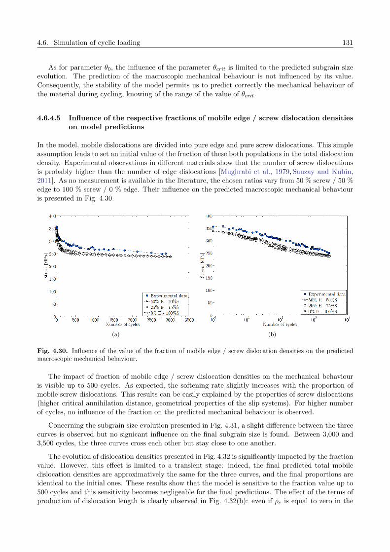
4.6. Simulation of cyclic loading 131
As for parameter θ0, the influence of the parameter θcrit is limited to the predicted subgrain sizeevolution. The prediction of the macroscopic mechanical behaviour is not influenced by its value.Consequently, the stability of the model permits us to predict correctly the mechanical behaviour ofthe material during cycling, knowing of the range of the value of θcrit.
4.6.4.5 Influence of the respective fractions of mobile edge / screw dislocation densitieson model predictions
In the model, mobile dislocations are divided into pure edge and pure screw dislocations. This simpleassumption leads to set an initial value of the fraction of these both populations in the total dislocationdensity. Experimental observations in different materials show that the number of screw dislocationsis probably higher than the number of edge dislocations [Mughrabi et al., 1979, Sauzay and Kubin,2011]. As no measurement is available in the literature, the chosen ratios vary from 50 % screw / 50 %edge to 100 % screw / 0 % edge. Their influence on the predicted macroscopic mechanical behaviouris presented in Fig. 4.30.
(a) (b)
Fig. 4.30. Influence of the value of the fraction of mobile edge / screw dislocation densities on the predictedmacroscopic mechanical behaviour.
The impact of fraction of mobile edge / screw dislocation densities on the mechanical behaviouris visible up to 500 cycles. As expected, the softening rate slightly increases with the proportion ofmobile screw dislocations. This results can be easily explained by the properties of screw dislocations(higher critical annihilation distance, geometrical properties of the slip systems). For higher numberof cycles, no influence of the fraction on the predicted mechanical behaviour is observed.
Concerning the subgrain size evolution presented in Fig. 4.31, a slight difference between the threecurves is observed but no signicant influence on the final subgrain size is found. Between 3,000 and3,500 cycles, the three curves cross each other but stay close to one another.
The evolution of dislocation densities presented in Fig. 4.32 is significantly impacted by the fractionvalue. However, this effect is limited to a transient stage: indeed, the final predicted total mobiledislocation densities are approximatively the same for the three curves, and the final proportions areidentical to the initial ones. These results show that the model is sensitive to the fraction value up to500 cycles and this sensitivity becomes negligeable for the final predictions. The effect of the terms ofproduction of dislocation length is clearly observed in Fig. 4.32(b): even if ρe is equal to zero in the

132 Chapter 4. Modelling of the cyclic behaviour and microstructure evolution during cycling
Fig. 4.31. Influence of the value of the fraction of mobile edge / screw dislocations densities on the predictedmean subgrain size evolution.
(a) (b)
(c) (d)
Fig. 4.32. Influence of the value of the fraction of mobile edge / screw dislocations densities on the predictedmean dislocation density evolution for free edge dislocations ((a) and (b)) and free screw dislocations ((c)and (d)).

4.7. Concluding remarks 133
initial state, a significant increase in free edge dislocation density occurs during the first cycle and thevalue then decreases until the end of the test.
4.6.4.6 Concluding remarks from the parametric study
The accurate values of the five parameters considered in this section are not exactly known but theirrange can be defined. The study of the influence of the variation of their values on model predictionsleads to the following conclusions:
Except for the critical annihilation distance of edge dislocations, the studied parameters haveno influence on the predicted long-term macroscopic behaviour.
Most of these parameters lead to significant differences of the predicted final subgrain size (about20 %).
The predicted final dislocation density is not significantly influenced by the variation of theconsidered parameters.
The proposed model is relatively stable with respect to the variation of the physically-based param-eters, which values are not accurately known. Only the prediction of the main subgrain size evolutionis sensitive to the variation of these parameters. It could probably be improved by a better descriptionof the low-angle boundary structure taking into account three kinds of dislocations in each low-angleboundaries (one edge and two screw dislocations) [Sutton and Balluffi, 1995].
4.7 Concluding remarks
In order to described the cyclic softening effect measured at high temperature on tempered ferritic-martensite steels and particularly on a Grade 92 steel, a self-consistent homogeneisation model isproposed. This modelling is able to predict the softening behaviour and the microstructure evolution(decrease of dislocation density and coarsening of subgrains) measured during cycling. Constitutiveequations of the model are based on physical phenomena occuring during deformation. Thus, all theparameters used in this model have a physical meaning, and only two of them corresponding to theviscosity effect are adjusted in order to predict well monotonic curves. No experimental data concern-ing the softening behaviour is used to adjust the model parameters. Predictions of the mechanicalbehaviour are performed for all amplitudes used in the cyclic tests presented in chapter 3. The mainresults lead to the following conclusions:
The activation volume and the activation energy, fitted on experimental monotonic curves cor-respond to the mechanisms of interaction of dislocations with clusters of solute atoms, smallprecipitates. . .
The model predicts quite accurately the mechanical behaviour of the Grade 92 steel during thefirst hysteresis loop at different strain rates (2×10⁻³ and 1× 10⁻⁵ s−1). Although the predictedsubgrain size evolution is overestimated, the predictions of the final dislocation density arecorrect.
During cycling at ∆E/2 = 0.35 %, the softening rate is well predicted. However, at low strainrate, the maximum tensile stress is slightly underestimated whereas predictions agree rather wellwith experimental data for high strain rate.
134 Chapter 4. Modelling of the cyclic behaviour and microstructure evolution during cycling
The cyclic softening effect is correctly predicted for tests performed at high strain rate with totalstrain amplitude from 0.25 to 0.35 %.
The proposed model is relatively stable with respect to the variation of the physically-basedparameters which values are not accurately known. Only the prediction of the mean subgrainsize evolution is sensitive to the variation of these parameters.
As it was discussed in the previous section, some hypothesis of the model can be improved to lead tobetter predictions of the cyclic behaviour (better description of the subgrain boundary structure. . . ).In the following chapter, some elements contributing to improve the predictions of the modelling arepresented, mainly taking into account initial distributions of mean block subgrain size and dislocationdensity. Other loading conditions and material are considered as well.

135
Chapitre 5
Effet de l’heterogeneite initiale de lamicrostructure, de la multiaxialite, dela temperature et du materiau sur lespredictions du modele
This fifth chapter focuses on two important improvements of the model presented in chapter 4: aninitial mean subgrain size distribution per block and an initial mean block dislocation density distri-bution are taken into account. The influence of these refinement on the predictions of the macroscopicmechanical behaviour and of the microstructural evolution is presented and discussed. Then, pre-dictions of the softening under cyclic torsion are studied and discussed with respect to experimentaldata concerning the Grade 91 steel. Finally, the predictions of the microstructural evolution of theEUROFER 97 steel during cycling at room temperature are presented. These results were recentlypresented at the EUROMAT conference [Giordana et al., 2011].
Ce cinqueme chapitre presente deux ameliorations apportees au modele decrit dans le chapitre 4 :la prise en compte d’une distribution de taille moyenne initiale de sous-grains par bloc et d’unedistribution de densite de dislocations initiale. L’impact de ces deux modifications sur les predictionsdu comportement mecanique macroscopique et sur l’evolution microstructurale est presente et discute.Dans un second temps, le modele est applique a des chargements cycliques de torsion et les predictionsobtenues sont etudiees qualitativement au regard de resultats d’essai sur l’acier Grade 91. Enfin, cechapitre se clot sur une presentation des predictions du modele lors d’une sollicitation cyclique atemperature ambiante sur l’acier EUROFER 97, dont les resultats ont ete recemment presentes a laconference EUROMAT [Giordana et al., 2011].
Contents
5.1 Use of the measured initial distributions of subgrain sizes and dislocationdensities . . . . . . . . . . . . . . . . . . . . . . . . . . . . . . . . . . . . . . . 136
5.1.1 Initial subgrain size distribution . . . . . . . . . . . . . . . . . . . . . . . . . . 136
5.1.2 Initial mobile dislocation density distribution . . . . . . . . . . . . . . . . . . . 142
5.2 Simulations of cyclic torsion . . . . . . . . . . . . . . . . . . . . . . . . . . . . 148
5.3 Modelling of the cyclic behaviour of the EUROFER 97 steel at roomtemperature . . . . . . . . . . . . . . . . . . . . . . . . . . . . . . . . . . . . . . 149
5.4 Conclusions . . . . . . . . . . . . . . . . . . . . . . . . . . . . . . . . . . . . . . 151
136Chapitre 5. Influence of the initial heterogeneity of microstructure, multiaxiality, temperature and
material on the model predictions (in French)
5.1 Prise en compte de la distribution initiale des tailles de sous-grains et des densites de dislocations bloc par bloc
Dans le chapitre 4, nous avons vu que le modele, tel que nous l’avons implemente, est capable de predireassez precisement l’adoucissement cyclique du materiau. De plus, l’etude parametrique presentee dansla sous-partie 4.6.4 nous a montre que le comportement mecanique macroscopique predit est assez peuinfluence par les variations des valeurs des parametres testees (distances critiques d’annihilation desdislocations coin et vis, desorientations initiale et critique portees par les sous-grains, proportion desdensites de dislocations coin et vis par rapport a la densite totale de dislocations), lorsque ces dernieresappartiennent a un intervalle de valeurs physiquement acceptables d’apres les mesures experimentalesou estimees comme realistes par le calcul. En revanche, si la valeur de la densite finale de dislocationsest correctement predite par le modele, la prediction de l’evolution de la taille moyenne des sous-grainsau cours du cyclage met en evidence une surestimation de la taille moyenne par rapport aux valeursmesurees experimentalement. Comme nous l’avons vu dans la conclusion de l’etude parametrique(voir sous-partie 4.6.4.6), cette prediction peut probablement etre amelioree en utilisant un jeu deparametres adequats, tout en restant dans un intervalle de valeurs physiquement acceptables.
Cette approche permet d’obtenir une prediction assez raisonable de l’evolution de la microstructure.Cependant, pour des raisons de simplicite, nous avons fait le choix dans le chapitre 4 de considereruniquement l’evolution de la taille moyenne des sous-grains dans la matrice. Ainsi, nous avons priscomme hypothese de depart que le materiau a l’etat de reception presentait une taille de sous-grainshomogene. Or cette hypothese est restrictive puisqu’elle est tres simplificatrice vis-a-vis du caractereheterogene de la microstructure initiale. Comme nous l’avons vu dans le chapitre 3, le materiau dereception se caracterise par une distribution de la taille des sous-grains d’allure log-normale. Lesobjectifs de cette amelioration du modele sont donc de :
1. Permettre une approche plus physique et complete de la microstructure du materiau.
2. Integrer aux predictions du modele une information supplementaire : une distribution statistiquea partir de laquelle on peut calculer une dispersion autour de la valeur moyenne.
3. Permettre une comparaison plus pertinente avec les distributions mesurees apres essai cyclique(par exemple pour les densites de dislocations [Pesicka et al., 2003,Pesicka et al., 2004], les anglesde desorientation entre sous-grains [Tak et al., 2009] ou encore les tailles de sous-grains [Eggeleret al., 1987,Dronhofer et al., 2003]).
En effet, nous avons vu dans le chapitre 3 que la dispersion de la taille des sous-grains autour deleur moyenne augmente au cours du cyclage (voir Fig. 3.18). Dans la sous-partie suivante, nous allonsdonc etudier l’influence de la prise en compte de la distribution de la taille initiale de sous-grainssur les predictions du modele. Pour mesurer au mieux les changements apportes par cette nouvellehypothese, nous utiliserons les valeurs “de reference” des parametres presentees dans les Tableaux 4.1,4.2 et 4.3.
5.1.1 Distribution initiale de la taille de sous-grain bloc par bloc
Concernant les tailles de sous-grains, le modele presente dans le chapitre 4 ne nous permet pas deconsiderer dans chaque bloc la taille de chaque sous-grain individuellement. En effet, pour raisons dessimplicite liees a la vitesse de calcul, la taille des sous-grains est consideree comme homogene au seind’un meme bloc. Ainsi, en ce qui concerne les predictions, nous prefererons utiliser ici le terme de

5.1. Use of the measured initial distributions of subgrain sizes and dislocation densities 137
“taille moyenne de sous-grains par bloc”, plus juste dans ce cas que le terme “taille de sous-grains” quirenvoie aux mesures experimentales presentees dans le chapitre 3.
Dans ce modele, la taille moyenne de sous-grains est definie pour chaque bloc, et celle-ci variesuivant l’Eq. 4.41 en fonction de la taille initiale, de l’angle de desorientation initiale θ0 et de laproportion κ de sous-joints ayant disparu au cours de l’essai∗. Ainsi, le modele est capable de predireune dispersion de la taille moyenne de sous-grains par bloc apres cyclage. Cependant, l’hypotheseconsistant a definir une taille de sous-grains initiale homogene au sein de la matrice (i.e. la memedans tous les blocs) conduit a des resultats tres differents de ceux mesures experimentalement, commele montre la Fig. 5.1.
Fig. 5.1. Comparaison de la distribution de la taille de sous-grains mesuree experimentalement et de ladistribution de la taille de sous-grains par bloc predite par le modele presente dans le chapitre 4, apres 3 960cycles a 1× 10⁻⁵ s−1 et amplitude de deformation ∆E/2 = ±0.35% a 550 C.
Comme nous l’avions remarque lors de l’analyse des resultats de la modelisation (voir partie 4.6.2.2),la taille moyenne de sous-grains par bloc finale predite (1.16 µm) est superieure a la taille moyennede sous-grain finale mesuree dans le materiau (0.78 µm). De plus, il est interessant de remarquerque le modele predit une croissance assez homogene : l’ensemble des tailles moyennes de sous-grainpar bloc predites sont tres proches de la valeur moyenne calculee sur l’ensemble du polycristal de100 blocs. La dispersion de la distribution predite est donc beaucoup plus faible que celle mesureeexperimentalement.
Dans l’optique d’ameliorer la prediction de la taille moyenne des sous-grains dans le materiau etleur dispersion, nous avons choisi de prendre en compte une taille moyenne initiale de sous-grains parbloc differente d’un bloc a l’autre. Ainsi, a l’aide du logiciel Matlab, nous avons tire aleatoirement100 valeurs parmi la population composee de 4 956 valeurs de taille de sous-grains mesuree experimen-talement a l’etat initial. Le resultat de ce tirage est presente sur la Fig. 5.2.
Les fonctions cumulees des deux distributions presentees sur la Fig. 5.2 sont tres proches l’une del’autre, ce qui indique que le tirage des 100 valeurs de taille de sous-grain represente d’une manieresatisfaisante la distribution des tailles de sous-grains mesuree dans le materiau de reception.
∗voir page 108
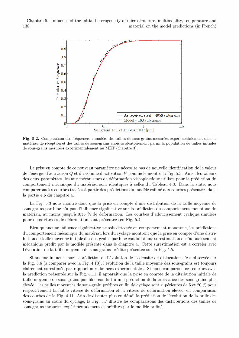
138Chapitre 5. Influence of the initial heterogeneity of microstructure, multiaxiality, temperature and
material on the model predictions (in French)
Fig. 5.2. Comparaison des frequences cumulees des tailles de sous-grains mesurees experimentalement dans lemateriau de reception et des tailles de sous-grains choisies aleatoirement parmi la population de tailles initialesde sous-grains mesurees experimentalement au MET (chapitre 3).
La prise en compte de ce nouveau parametre ne necessite pas de nouvelle identification de la valeurde l’energie d’activation Q et du volume d’activation V comme le montre la Fig. 5.3. Ainsi, les valeursdes deux parametres lies aux mecanismes de deformation viscoplastique utilises pour la prediction ducomportement mecanique du materiau sont identiques a celles du Tableau 4.3. Dans la suite, nouscomparerons les courbes tracees a partir des predictions du modele raffine aux courbes presentees dansla partie 4.6 du chapitre 4.
La Fig. 5.3 nous montre donc que la prise en compte d’une distribution de la taille moyenne desous-grains par bloc n’a pas d’influence significative sur la prediction du comportement monotone dumateriau, au moins jusqu’a 0,35 % de deformation. Les courbes d’adoucissement cyclique simuleespour deux vitesses de deformation sont presentees en Fig. 5.4.
Bien qu’aucune influence significative ne soit detectee en comportement monotone, les predictionsdu comportement mecanique du materiau lors du cyclage montrent que la prise en compte d’une distri-bution de taille moyenne initiale de sous-grains par bloc conduit a une surestimation de l’adoucissementmecanique predit par le modele presente dans le chapitre 4. Cette surestimation est a correler avecl’evolution de la taille moyenne de sous-grains predite presentee sur la Fig. 5.5.
Si aucune influence sur la prediction de l’evolution de la densite de dislocation n’est observee surla Fig. 5.6 (a comparer avec la Fig. 4.13), l’evolution de la taille moyenne des sous-grains est toujoursclairement surestimee par rapport aux donnees experimentales. Si nous comparons ces courbes avecla prediction presentee sur la Fig. 4.11, il apparaıt que la prise en compte de la ditribution initiale detaille moyenne de sous-grains par bloc conduit a une prediction de la croissance des sous-grains pluselevee : les tailles moyennes de sous-grain predites en fin de cyclage sont superieures de 5 et 20 % pourrespectivement la faible vitesse de deformation et la vitesse de deformation elevee, en comparaisondes courbes de la Fig. 4.11. Afin de discuter plus en detail la prediction de l’evolution de la taille dessous-grains au cours du cyclage, la Fig. 5.7 illustre les comparaisons des distributions des tailles desous-grains mesurees experimentalement et predites par le modele raffine.

5.1. Use of the measured initial distributions of subgrain sizes and dislocation densities 139
Fig. 5.3. Comparaison entre les courbes monotones experimentales et simulees avec le modele tenant comptede la distribution initiale de taille de sous-grains, jusqu’a 0,35 % a deux vitesses de deformation differentes (Q= 1.2 eV et V = 216 b3).
(a) (b)
Fig. 5.4. Comparaison entre les courbes d’adoucissement cyclique experimentales et predites avec le modeletenant compte de la distribution initiale de taille de sous-grains pour une amplitude de deformation de ± 0, 35%et deux vitesses de deformation (a) en echelle lineaire et (b) en echelle logarithmique. La contrainte maximaleest calculee ou mesuree en fonction du nombre de cycles.

140Chapitre 5. Influence of the initial heterogeneity of microstructure, multiaxiality, temperature and
material on the model predictions (in French)
Fig. 5.5. Comparaison entre la taille moyenne de sous-grains predite par le modele tenant compte de la distri-bution initiale de taille de sous-grains et experimentale au cours du cyclage pour une amplitude de deformationde ± 0.35% et deux vitesses de deformation.
(a) (b)
Fig. 5.6. Predictions des evolutions des densites de dislocations mobiles coin et vis au cours du chargementcyclique pour une amplitude de deformation de ± 0.35% et deux vitesses de deformation (a) en echelle lineaireet (b) en echelle logarithmique. Modele tenant compte de la distribution initiale de taille de sous-grains.

5.1. Use of the measured initial distributions of subgrain sizes and dislocation densities 141
(a) (b)
(c) (d)
(e)
Fig. 5.7. Comparaison de la distribution de la taille de sous-grain mesuree experimentalement et predite par lemodele tenant compte de la distribution initiale de taille de sous-grains (a) initialement et apres (b) 60 cycles,(c) 300 cycles, (d) 1 000 cycles et (e) 3 960 cycles. Cas de l’essai a 1× 10⁻⁵ s−1 avec une amplitude de deformation∆E/2 = ±0.35%.

142Chapitre 5. Influence of the initial heterogeneity of microstructure, multiaxiality, temperature and
material on the model predictions (in French)
La Fig. 5.7 montre que la taille moyenne predite des sous-grains est surestimee par rapport auxmesures experimentales. Cependant, la prise en compte de la dispersion de la taille moyenne initialede sous-grains par bloc permet une meilleure prediction de la dispersion des valeurs autour de lamoyenne, plus conforme aux mesures experimentales que la dispersion issue de la prediction presenteesur la Fig. 5.1. Ceci tend a montrer que la dispersion de taille de sous-grains en fin d’essai est engrande partie conditionnee par la distribution de taille de sous-grains a l’etat initial.
La prise en compte de la distribution initiale de la taille moyenne de sous-grains bloc par blocn’apporte donc pas de reelle amelioration au modele presentee dans le chapitre 4. En effet, cettehypothese induit une surestimation de l’adoucissement mecanique et de la croissance de la taillemoyenne des sous-grains. En revanche, elle permet de predire une dispersion des valeurs de taille desous-grains, plus proche de celle observee experimentalement. Dans la partie suivante, nous allonscoupler cette hypothese avec la prise en compte d’une distribution initiale de densites de dislocationsmobiles bloc par bloc.
5.1.2 Distribution initiale des densites de dislocations mobiles bloc par bloc
Tout comme la taille initiale de sous-grains par bloc, le modele raffine peut tenir compte d’une distri-bution initiale de densite de dislocations mobiles par systeme de glissement de chaque bloc considere.Dans le modele initial presente dans le chapitre 4, de la meme maniere que la taille initiale de sous-grains par bloc, la densite initiale de dislocations est supposee homogene pour des raisons de simplicite.Or, bien qu’il soit long et fastidieux de mesurer une distribution experimentale des densites de dislo-cations par systeme de glissement, il apparaıt toutefois possible d’estimer la distribution de la densitede dislocations par bloc au sein du materiau.
Le nombre de mesures de densites de dislocations effectuees sur le Grade 92 etudie ne nous permetpas d’etablir une distribution statistique satisfaisante. En revanche, des mesures, en beaucoup plusgrand nombre, ont ete effectuees par Giordana sur un acier EUROFER 97 a l’etat de reception [Gior-dana et al., 2011]. Vingt-cinq mesures de densites de dislocations ont ete effectuees dans 25 blocsdifferents de facon a etablir une representation statistique consideree comme plus significative de ladistribution des densites. En prenant toutes les precautions necessaires a l’utilisation de ces valeurs,nous avons fait l’hypothese que la dispersion des densites etait similaires dans l’acier EUROFER 97et l’acier de Grade 92. La densite de dislocations moyenne mesuree dans l’EUROFER 97 a l’etatde reception (environ 2, 3× 10¹⁴ m−2) etant tres proche de celle mesuree dans le Grade 92 (envi-ron 2× 10¹⁴ m−2), nous avons donc construit un ensemble de 100 valeurs de densites de dislocationsmoyenne par bloc en effectuant un tirage aleatoire parmi les 25 mesures disponibles sur l’acier EURO-FER 97. Cet ensemble a ensuite ete pris en compte dans le modele. Ainsi, a l’etat initial, a chaquebloc du polycristal de la section precedente est associe une valeur de densite de dislocations et unevaleur de taille de sous-grains, toutes deux issues de nombreuses mesures experimentales.
La prise en compte additionnelle de la distribution initiale de densites initiale de dislocations parbloc n’a pas necessite un nouvel ajustement des valeurs de l’energie d’activation Q et du volumed’activation V , qui restent identiques a celles du Tableau 4.3. Les courbes monotones experimentaleset simulees jusqu’a 0.35 % pour deux vitesses de deformation differentes sont presentees sur la Fig. 5.8.
Si les courbes simulees du comportement monotone jusqu’a 0.35 % de deformation ne presententpas de difference notable par rapport aux courbes presentees sur les Figs. 4.8 et 5.3, une ameliorationde la prediction de l’adoucissement mecanique est observee, comme le montre la Fig. 5.9.
Comme le montre la Fig. 5.9, les predictions de l’adoucissement cyclique sont proches du comporte-ment experimental mesure. Bien que la cinetique d’adoucissement predite soit un peu plus rapide que
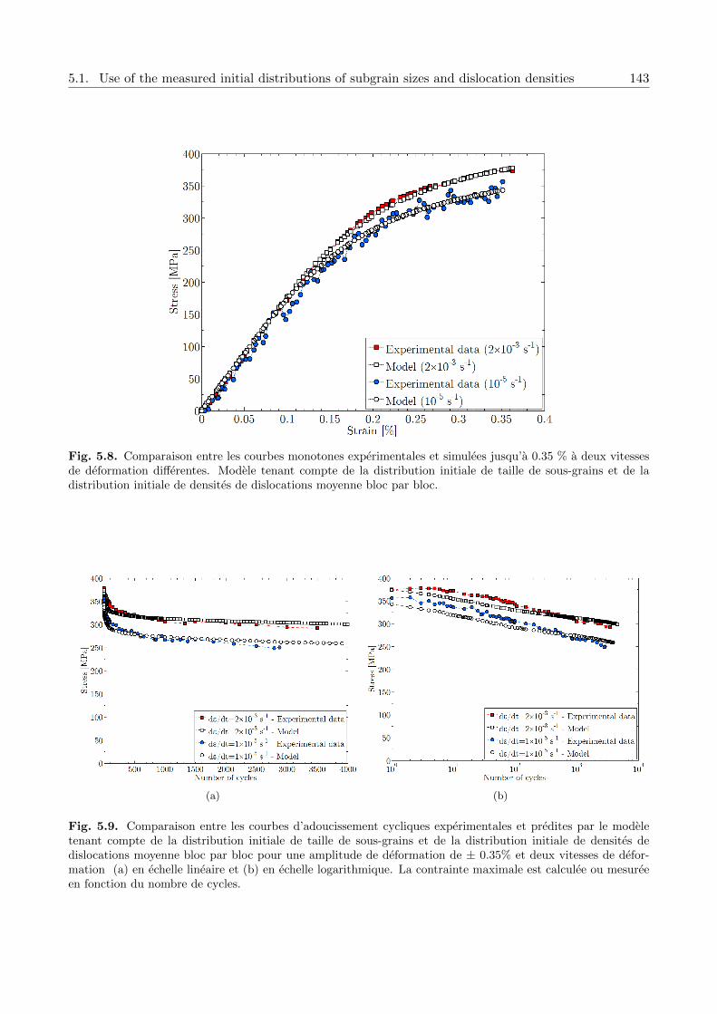
5.1. Use of the measured initial distributions of subgrain sizes and dislocation densities 143
Fig. 5.8. Comparaison entre les courbes monotones experimentales et simulees jusqu’a 0.35 % a deux vitessesde deformation differentes. Modele tenant compte de la distribution initiale de taille de sous-grains et de ladistribution initiale de densites de dislocations moyenne bloc par bloc.
(a) (b)
Fig. 5.9. Comparaison entre les courbes d’adoucissement cycliques experimentales et predites par le modeletenant compte de la distribution initiale de taille de sous-grains et de la distribution initiale de densites dedislocations moyenne bloc par bloc pour une amplitude de deformation de ± 0.35% et deux vitesses de defor-mation (a) en echelle lineaire et (b) en echelle logarithmique. La contrainte maximale est calculee ou mesureeen fonction du nombre de cycles.
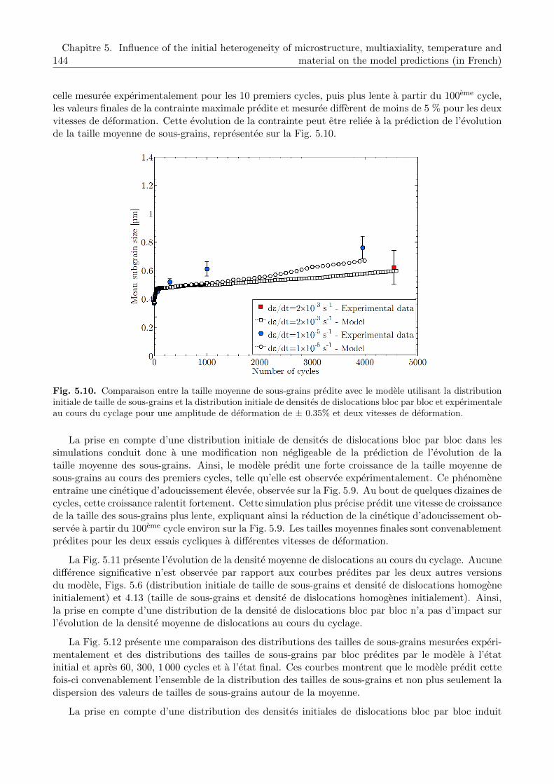
144Chapitre 5. Influence of the initial heterogeneity of microstructure, multiaxiality, temperature and
material on the model predictions (in French)
celle mesuree experimentalement pour les 10 premiers cycles, puis plus lente a partir du 100eme cycle,les valeurs finales de la contrainte maximale predite et mesuree different de moins de 5 % pour les deuxvitesses de deformation. Cette evolution de la contrainte peut etre reliee a la prediction de l’evolutionde la taille moyenne de sous-grains, representee sur la Fig. 5.10.
Fig. 5.10. Comparaison entre la taille moyenne de sous-grains predite avec le modele utilisant la distributioninitiale de taille de sous-grains et la distribution initiale de densites de dislocations bloc par bloc et experimentaleau cours du cyclage pour une amplitude de deformation de ± 0.35% et deux vitesses de deformation.
La prise en compte d’une distribution initiale de densites de dislocations bloc par bloc dans lessimulations conduit donc a une modification non negligeable de la prediction de l’evolution de lataille moyenne des sous-grains. Ainsi, le modele predit une forte croissance de la taille moyenne desous-grains au cours des premiers cycles, telle qu’elle est observee experimentalement. Ce phenomeneentraıne une cinetique d’adoucissement elevee, observee sur la Fig. 5.9. Au bout de quelques dizaines decycles, cette croissance ralentit fortement. Cette simulation plus precise predit une vitesse de croissancede la taille des sous-grains plus lente, expliquant ainsi la reduction de la cinetique d’adoucissement ob-servee a partir du 100eme cycle environ sur la Fig. 5.9. Les tailles moyennes finales sont convenablementpredites pour les deux essais cycliques a differentes vitesses de deformation.
La Fig. 5.11 presente l’evolution de la densite moyenne de dislocations au cours du cyclage. Aucunedifference significative n’est observee par rapport aux courbes predites par les deux autres versionsdu modele, Figs. 5.6 (distribution initiale de taille de sous-grains et densite de dislocations homogeneinitialement) et 4.13 (taille de sous-grains et densite de dislocations homogenes initialement). Ainsi,la prise en compte d’une distribution de la densite de dislocations bloc par bloc n’a pas d’impact surl’evolution de la densite moyenne de dislocations au cours du cyclage.
La Fig. 5.12 presente une comparaison des distributions des tailles de sous-grains mesurees experi-mentalement et des distributions des tailles de sous-grains par bloc predites par le modele a l’etatinitial et apres 60, 300, 1 000 cycles et a l’etat final. Ces courbes montrent que le modele predit cettefois-ci convenablement l’ensemble de la distribution des tailles de sous-grains et non plus seulement ladispersion des valeurs de tailles de sous-grains autour de la moyenne.
La prise en compte d’une distribution des densites initiales de dislocations bloc par bloc induit

5.1. Use of the measured initial distributions of subgrain sizes and dislocation densities 145
(a) (b)
Fig. 5.11. Predictions des evolutions des densites de dislocations mobiles coin et vis au cours du cyclage pourune amplitude de deformation de ± 0.35% et deux vitesses de deformation (a) en echelle lineaire et (b) enechelle logarithmique. Modele utilisant la distribution initiale de taille de sous-grains et la distribution initialede densites de dislocations bloc par bloc .
donc une amelioration de la prediction de l’evolution de la microstructure, tout en menant a uneprediction de l’adoucissement macroscopique en accord avec les mesures experimentales. Cependant,comment la prise en compte de l’heterogeneite des densites de dislocations initiales influence-t-elle lespredictions des evolutions microstructurales ? La Fig. 5.13 nous apporte un element de reponse.
Sur la Fig. 5.13, nous avons reporte pour chaque bloc considere dans le modele sa densite dedislocations (en ordonnee) et sa taille moyenne de sous-grains (en abscisse). Initialement, les blocsont une densite de dislocations elevee et une taille moyenne de sous-grain faible : ils sont representespar les symboles circulaires rouges. A l’etat final, apres 3 960 cycles simules, les blocs correspondentau nuage de symboles carres bleus. Cette figure nous permet de constater trois phenomenes :
1. Le modele predit bien une baisse globale de la densite de dislocations bloc par bloc. Il faut noterqu’un petit nombre de blocs ont une densite de dislocations et une taille moyenne de sous-grainsqui evoluent peu au cours du cyclage.
2. A l’inverse, certains blocs connaissent une forte transformation de leur microstructure : leurdensite de dislocations diminue (moins de 5×10¹³ m−2) et leur taille moyenne de sous-grain croıtfortement (superieure a 1 µm en fin d’essai). Ce phenomene est en accord avec les observationsexperimentales (voir Fig. 3.16(c)).
3. Enfin, le dernier cas regroupe un grand nombre de blocs qui ont vu leur densite de dislocationsdiminuer alors que leur taille moyenne de sous-grains n’a pas autant evoluee. Ce phenomene estaussi observe experimentalement (voir Fig. 3.16(c)).
En l’etat actuel des investigations, il est hasardeux de proposer directement une interpretationdes mecanismes qui pourrait expliquer ces resultats. Il est en effet preferable d’etudier au prealablel’evolution individuelle de chaque bloc au cours de l’essai. Cependant, quelques hypotheses pourraientservir de pistes de travail afin d’interpreter ces resultats :
Le premier groupe est compose de blocs qui se deforment probablement peu au cours du cyclage,

146Chapitre 5. Influence of the initial heterogeneity of microstructure, multiaxiality, temperature and
material on the model predictions (in French)
(a) (b)
(c) (d)
(e)
Fig. 5.12. Comparaison de la distribution de la taille de sous-grains par bloc mesuree experimentalement et dela distribution de la taille de sous-grains par bloc predite par le modele tenant compte de la distribution initialede taille de sous-grains et la distribution initiale de densites de dislocations bloc par bloc (a) initialement etapres (b) 60 cycles, (c) 300 cycles, (d) 1 000 cycles et (e) 3 960 cycles. Cas de l’essai a 1× 10⁻⁵ s−1 avec uneamplitude de deformation ∆E/2 = ±0.35%.

5.1. Use of the measured initial distributions of subgrain sizes and dislocation densities 147
Fig. 5.13. Correlation entre la taille de sous-grains moyenne par bloc et la densite de dislocations par bloc al’etat initial et apres cyclage a 1× 10⁻⁵ s−1 pour une amplitude de deformation ∆E/2 = ±0.35% avec le modeleutilisant la distribution initiale de taille de sous-grains et la distribution initiale de densites de dislocations blocpar bloc.
du fait de leur orientation cristalline (faible facteur de Schmid). Ainsi, le nombre d’annihilationsentre dislocations de signes opposes (mobile/mobile et mobile/dislocations de sous-joint) estfaible. Peu de transformations microstructurales sont observees. C’est le fait d’un pilotage deces evolutions par les glissements viscoplastiques en accord avec les observations.
Le second groupe pourrait a l’inverse correspondre a des sous-grains tres deformes plastiquementdurant le cyclage. Leur nombre de systeme de glissement actives est donc sans doute eleve.Initialement, ils ont probablement une forte densite de dislocations mobiles, ce qui entraıneun grand nombre de phenomenes d’annihilation et donc des transformations microstructuralesmajeures.
Enfin, le dernier groupe se compose probablement de blocs qui sont moins deformes que les prece-dents ou qui ont une faible densite initiale de dislocations mobiles. La majorite des annihilationsdoit se produire entre dislocations mobiles, les annihilations dislocations mobiles / dislocationsdes sous-joints etant trop peu nombreuses pour permettre la destruction complete des sous-jointsde faible desorientation. Ainsi, ces blocs sont “nettoyes” de leurs dislocations mobiles mais nesubissent pas pour autant une modification de leur taille moyenne de sous-grains.
Il convient toutefois de rester prudent vis-a-vis de ces interpretations. En effet, elles necessitentune etude complementaire des resultats, en suivant l’evolution individuelle de chaque bloc.
Les resultats de la figure 5.13 sont particulerement interessants du point de vue des perspectivesde travail. Outre l’interpretation des mecanismes mis en œuvre, il serait en effet possible de mesurerles tailles de sous-grains dans lequels la densite de dislocation est aussi mesuree. Des graphiquesd’origine experimentale similaires a ceux predits pourraient etre traces et compares (Fig. 5.13). Bienque cette etude puisse etre fastidieuse vu le grand nombre de mesures a effectuer pour obtenir unedistribution statistiquement representative (et les difficultes experimentales liees a la precision des
148Chapitre 5. Influence of the initial heterogeneity of microstructure, multiaxiality, temperature and
material on the model predictions (in French)
mesures elles-memes et a la complexite de la structure des aciers martensitiques revenus – comme lesoulignent [Pesicka et al., 2004]), elle pourrait apporter des elements de comparaison interessants afinde discuter les predictions du modele.
Cette partie nous a montre que la prise en compte simultanee des distributions initiales de taillemoyenne de sous-grains par blocs et de densite de dislocations dans les blocs permettait d’ameliorer lespredictions du modele tant a l’echelle macroscopique que microscopique. Bien qu’un certain nombrede parametres dont les variations pourraient avoir un impact sur les predictions du modele restent aetudier (l’influence du tirage aleatoire, du nombre de bloc considere. . . sur les predictions du comporte-ment mecanique et de l’evolution microstructurale), ces ameliorations donnent quelques perspectivesde travail, tant sur le plan de la modelisation que sur le plan experimental.
Dans la partie suivante, nous etudions les predictions du modele pour d’autres sollicitations cy-cliques de type torsion. Dans ce cadre, nous utiliserons le modele tel qu’il est implemente dans lechapitre 4.
5.2 Simulation de la torsion cyclique
Le modele presente dans le chapitre 4 a ete identifie sur des essais cycliques de traction / compression.Ce mode de sollicitation uniaxiale est frequemment utilise pour caracteriser les proprietes mecaniquesdes materiaux, ce qui permet de disposer d’une base de donnees experimentales consequente pouretablir des comparaisons avec les predictions du modele. Cependant, dans l’optique d’une applica-tion a l’echelle industrielle, les sollicitations mecaniques appliquees au materiau ne se limitent pasa des chargements uniaxiaux et il convient donc d’etudier les proprietes pour des sollicitations pluscomplexes, telles que des chargements multiaxiaux par exemple.
Dans ce cadre, nous avons choisi d’etudier les predictions du modele pour un chargement cycliquede type torsion. Dans la base de donnees experimentales, nous ne disposons pas de resultats ducomportement mecanique de l’acier Grade 92 sous ce type de sollicitation. Cependant, de nombreuxessais ont ete effectues sur un acier de Grade 91 [Sauzay et al., 2006]. Ces deux nuances d’aciersetant assez proches en termes de comportement a haute temperature (ils presentent tous les deux unadoucissement cyclique a 550 C), la comparaison des courbes d’adoucissement cyclique experimentalesen traction / compression et en torsion de l’acier de Grade 91 peuvent nous renseigner sur la tendancequi pourrait etre observee sur l’acier de Grade 92 dans les memes conditions d’essais. Ainsi, nous nousbornerons a une etude qualitative des predictions du modele. La courbe de torsion cyclique de l’acierGrade 91 a 550 C pour une amplitude de deformation ∆γ/2 = ±0.52% et une vitesse de deformationde 2× 10⁻³ s−1 est presentee sur la Fig. 5.14(a). Afin de comparer l’adoucissement cyclique en trac-tion / compression a l’adoucissement cyclique en torsion, un essai de traction / compression soumis aune deformation viscoplastique equivalente est aussi presente.
En tenant compte des orientations cristallographiques des blocs, la formulation des equations dumodele permet de simuler des chargements multiaxiaux. La courbe de prediction du comportementmecanique pour un essai de torsion cyclique appliquee a l’acier de Grade 92 est presentee sur laFig. 5.14(b). La courbe de prediction du comportement en traction / compression pour une deforma-tion viscoplastique equivalente est aussi presentee en Fig. 5.14(b).
En torsion, le modele est capable de predire un adoucissement cyclique, observe experimentale-ment sur l’acier de Grade 91. Des etudes complementaires sont a mener pour caracteriser de manierequantitative les predictions du modele pour ce type de sollicitation. En l’absence de donnees ex-perimentales sur l’acier Grade 92, une identification des parametres de la viscoplasticite cristallinepour l’acier Grade 91 est a envisager. Ce travail a deja ete mis en place dans le cadre de l’etude du

5.3. Modelling of the cyclic behaviour of the EUROFER 97 steel at room temperature 149
(a) (b)
Fig. 5.14. (a) Courbes experimentales en torsion et traction / compression d’un acier Grade 91 a 550 C avecune vitesse de deformation de 2× 10⁻³ s−1 et deux amplitudes de deformation equivalentes identiques pour lesdeux essais et (b) courbes predictives du comportement d’un acier Grade 92 dans les memes conditions.
comportement cyclique de l’acier EUROFER 97 a temperature ambiante, dans le cadre d’une collabo-ration avec M. F. Giordana, etudiante en doctorat a l’Universite de Rosario (Argentine). Son sujet dethese porte sur l’etude experimentale de l’adoucissement cyclique de l’acier EUROFER 97 a differentestemperatures et sur la simulation grace a une modelisation similaire a la notre.
5.3 Application du modele a l’acier EUROFER 97
Dans cette partie, nous aborderons succinctement les resultats des predictions du modele issus dutravail de M. F. Giordana sur les proprietes mecaniques de l’acier EUROFER 97 sous sollicitationcyclique uniaxiale a temperature ambiante [Giordana et al., 2011].
(a) (b) (c)
Fig. 5.15. Comparaison entre les donnees experimentales et les predictions de la premiere boucle d’un essaicyclique sur l’acier EUROFER 97 a temperature ambiante pour une variation de deformation plastique de(a) 0,2 %, (b) 0,3 % et (c) 0,6 %.
La Fig. 5.15 presente une comparaison entre les boucles experimentales d’un acier EUROFER 97 atemperature ambiante sous sollicitations cycliques pour plusieurs amplitudes de deformation plastiqueet les predictions correspondantes. Bien que de legeres imperfections soient visibles sur le cycle predit

150Chapitre 5. Influence of the initial heterogeneity of microstructure, multiaxiality, temperature and
material on the model predictions (in French)
(tout comme sur les courbes presentees au chapitre 4 dans le cas du Grade 92 sous chargementcyclique a haute temperature), le modele predit assez correctement le comportement mecanique del’acier EUROFER 97 a temperature ambiante durant le premier cycle de fatigue. Seule la courbeexperimentale de la Fig. 5.15(a) a ete utilisee pour l’identification, en imposant de plus un effet devitesse negligeable.
Fig. 5.16. Stabilite des predictions du modele vis-a-vis de la valeur de la proportion de densite de dislocationsvis mobiles dans le materiau (essai de deformation cyclique sur acier EUROFER 97 a temperature ambiantepour une variation de deformation plastique de 0,2 %).
La Fig. 5.16 demontre que les predictions sont stables vis-a-vis de la proportion de dislocations vismobiles parmi la population totale de dislocations mobiles. En effet, dans ce cas, l’evolution de la taillemoyenne de sous-grain varie tres peu (moins de 3 %) par rapport a la valeur de ce parametre. Cetteetude de la stabilite des predictions du modele menee par M. F. Giordana (et dont nous presentonsici le resultat pour un parametre seulement) aboutit aux memes conclusions que celles observees ahaute temperature, abordees dans la partie 4.6.4 : les predictions varient tres faiblement lorsque lesparametres evoluent dans un intervalle de valeurs physiquement acceptables.
La Fig. 5.17 represente les evolutions experimentales et predites de la taille moyenne de sous-grainset de la densite de dislocations moyenne au cours d’un essai cyclique avec une variation de deformationplastique de 0,2 % sur un acier EUROFER 97 a temperature ambiante. Dans le cas de l’evolution dela taille moyenne des sous-grains, bien que le modele predise une valeur finale legerement sous-estimee,l’evolution predite au cours du cyclage est assez proche des observations experimentales. La densite dedislocations finale predite est clairement surestimee. Cependant, le modele reproduit correctement lachute tres rapide de la densite de dislocations constatee des les premiers cycles. Pour le moment, desetudes complementaires sont en cours afin de proposer une prediction convenable du comportementmecanique macroscopique de l’acier EUROFER 97 sous sollicitation cyclique a temperature ambiante.
Ces resultats montrent que le modele peut etre applique a la fois a des aciers de la famille des9 %Cr autres que l’acier Grade 92 et a des temperatures differentes de 550 C.
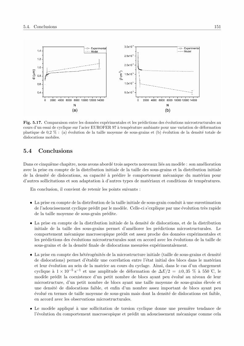
5.4. Conclusions 151
Fig. 5.17. Comparaison entre les donnees experimentales et les predictions des evolutions microstructurales aucours d’un essai de cyclique sur l’acier EUROFER 97 a temperature ambiante pour une variation de deformationplastique de 0,2 % : (a) evolution de la taille moyenne de sous-grains et (b) evolution de la densite totale dedislocations mobiles.
5.4 Conclusions
Dans ce cinquieme chapitre, nous avons aborde trois aspects nouveaux lies au modele : son ameliorationavec la prise en compte de la distribution initiale de la taille des sous-grains et la distribution initialede la densite de dislocations, sa capacite a predire le comportement mecanique du materiau pourd’autres sollicitations et son adaptation a d’autres types de materiaux et conditions de temperatures.
En conclusion, il convient de retenir les points suivants :
La prise en compte de la distribution de la taille initiale de sous-grain conduit a une surestimationde l’adoucissement cyclique predit par le modele. Celle-ci s’explique par une evolution tres rapidede la taille moyenne de sous-grain predite.
La prise en compte de la distribution initiale de la densite de dislocations, et de la distributioninitiale de la taille des sous-grains permet d’ameliorer les predictions microstructurales. Lecomportement mecanique macroscopique predit est assez proche des donnees experimentales etles predictions des evolutions microstructurales sont en accord avec les evolutions de la taille desous-grains et de la densite finale de dislocations mesurees experimentalement.
La prise en compte des heterogenites de la microstructure initiale (taille de sous-grains et densitede dislocations) permet d’etablir une correlation entre l’etat initial des blocs dans le materiauet leur evolution au sein de la matrice au cours du cyclage. Ainsi, dans le cas d’un chargementcyclique a 1× 10⁻⁵ s−1 et une amplitude de deformation de ∆E/2 = ±0, 35 % a 550 C, lemodele predit la coexistence d’un petit nombre de blocs ayant peu evolue au niveau de leurmicrostructure, d’un petit nombre de blocs ayant une taille moyenne de sous-grains elevee etune densite de dislocations faible, et enfin d’un nombre assez important de blocs ayant peuevolue en termes de taille moyenne de sous-grain mais dont la densite de dislocations est faible,en accord avec les observations microstructurales.
Le modele applique a une sollicitation de torsion cyclique donne une premiere tendance del’evolution du comportement macroscopique et predit un adoucissement mecanique comme cela

152Chapitre 5. Influence of the initial heterogeneity of microstructure, multiaxiality, temperature and
material on the model predictions (in French)
est observe pour l’acier Grade 91.
L’application du modele a des chargements de traction / compression sur l’acier EUROFER 97a temperature ambiante, un autre acier de la famille des 9 %Cr, permet de predire correctementl’evolution de la taille de sous-grains au cours du cyclage, mais seulement qualitativement cellede la densite de dislocations.

153
Chapter 6
General conclusions andrecommendations for further work

154 Chapter 6. General conclusions and recommendations for further work
6.1 Conclusions
The present work was concerned with the high temperature mechanical behaviour of tempered ferritic-martensite steel Grade 92 (9%Cr-0.5%Mo-1.8%W-NbV), considered as potential candidate for struc-tural components in Generation IV nuclear power plants. Already used for energy production in fossilpower plants, tempered martensitic are subjected to strong softening during high-temperature cycling.
This study focused on the following two main points:
The experimental study of macroscopic mechanical behaviour and microstructural evolutionduring monotonic tensile tests and cyclic loading at 550 C.
The modelling of some of the most relevant deformation and recovery mechanisms in order topredict both macroscopic mechanical behaviour and microstructural evolution during monotonicand cyclic loading.
The first objective of this work was addressed using an approach based on the coupling of me-chanical test results and microstructural observations (mainly TEM observations). In the secondchapter, the mechanical behaviour and microstructural evolution during monotonic tensile tests at550 C and various strain rates were studied. Two simple analytical models were proposed in orderto predict respectively the beginning of the mechanical instability (necking) and the subgrain growth.The following conclusions can be drawn:
1. For strain rates lower than 2.5× 10⁻⁴ s−1, engineering stress-strain curves show a first soften-ing stage well before the onset of macroscopic visible necking. This stage is characterised byconstantly decreasing load.
2. True stress-strain curves show this softening stage which depends on the strain rate: the lowerthe strain rate, the more pronounced the softening stage.
3. Modelling of mechanical instability using the Hart criterion predicts its onset for a low elongationclose to the elongation at maximum load. In fact, diffuse necking occurs after a few percentsof elongation. Macroscopic necking, in turn, induces a second softening stage with a strongerdecreasing slope, leading to fracture.
4. The first softening stage is not due to ductile cavity nucleation and growth in the specimens.
5. Subgrain size increases by about 21%, contributing to the material softening behaviour. Thisgrowth is overestimated by the simple model founded on a basic mechanism of low-angle bound-aries vanishing by interactions with mobile dislocations.
In the third chapter, the mechanical behaviour of the Grade 92 steel during continuous cyclicloading and creep at 550 C is studied experimentally. It was shown that:
1. No significant difference appears between the Grade 91 and Grade 92 steels in terms of cyclic life-time, according to Manson-Coffin curves. The Monkman-Grant equation fitted on the Grade 92steel creep data is close to that etablished for the Grade 91 steel. This indicates that the mech-anisms controling cyclic deformation and creep lifetime are the same for both steels.

6.1. Conclusions 155
2. Grade 92 steel is subjected to cyclic softening. This phenomenon is more pronounced for highvalues of strain amplitude in agreement with literature results. However, it is still significant forvery low values of viscoplastic strain amplitude.
3. Cyclic softening is more pronounced for lower strain rate. However, the impact of strain rate onfatigue lifetime is slight.
4. Cyclic softening is mainly due to a decrease in kinematic stress, as it was measured in Grade 91steels. This indicates a decrease in rather long-range interactions between the mobile dislocationsand the dislocation forest or the low-angle subgrain boundaries.
5. The subgrain size distributions (at initial state and during cycling) are satisfactorily describedby log-normal probability density functions.
6. During cycling, mean subgrain size increases and a decrease in dislocation density within sub-grains is observed. Corresponding evolutions are faster and more pronounced for low cyclic strainrate.
The second objective consisted in proposing a model able to predict both macroscopic mechanicalbehaviour and microstructural evolution during cycling. This self-consistent homogeneisation modelaimed at taking into account the deformation and recovering mechanisms observed in agreement withour TEM observations and already described in literature. It is based on experimentally measured,calculated or fixed parameters which have a physical meaning. Only two of them (activation volumeand activation energy) corresponding to the viscosity effect are adjusted using experimental monotonictensile curves at two strain rates only. The identification process is reduced to a very limited numberof experimental data, excluding all data in relationship to the softening behaviour. The activationvolume and activation energy may correspond to the mechanisms of interaction of dislocations withclusters of solute atoms or small carbo-nitride precipitates. Due to the various obstacles existing intempered martensite ferritic steels (solid solution, MX particles. . . ), only such inverse adjustement ispossible. Simulation results lead to the following conclusions:
1. The mechanical behaviour of the Grade 92 steel during the first hysteresis loop at different strainrates (2× 10⁻³ and 1× 10⁻⁵ s−1) is rather accuratly predicted.
2. Cyclic softening effect is correctly predicted for tests performed at high strain rate with totalstrain amplitude from 0.25 to 0.35 %.
3. At low strain rate, the maximum tensile stress is slightly underestimated whereas predictionsare rather accurate for high strain rate.
4. Although the predicted subgrain size evolution is overestimated, the predictions of the finaldislocation density are in agreement with measured one.
5. The proposed model is relatively stable with respect to the variation of the physically-basedparameters which values are only known to belong to specific range. Only the prediction of themain subgrain size evolution is sensitive to the variation of these parameters.
Two main improvements of the modelling are presented in chapter 5: initial mean subgrain sizedistribution per block and initial dislocation density distribution are taken into account based onmeasured distributions. Following conclusions can be drawn:

156 Chapter 6. General conclusions and recommendations for further work
1. When only the initial mean subgrain size distribution per block is taken into account, the sub-grain size growth and the cyclic softening are both overestimated.
2. To improve the accuracy of the prediction, it is necessary to take into account the initial meansubgrain size distribution per block and the initial dislocation density distribution. By this way,the cyclic softening is rather well predicted and predictions of the microstructural evolution givea fair estimation of subgrain size evolution and final dislocation density whatever the appliedstrain rate.
3. At the block scale, the modelling is able to predict the microstructural heterogeneities concern-ing the subgrain size and dislocation density in the material, in agreement with distributionsmeasured during interrupted tests and after failure whatever the conditions.
Although this model was identified using uniaxial tensile curves on a Grade 92 steel, a torsion testwas simulated and showed that modelling is able to predict a cyclic softening during torsion test, as it isexperimentally observed in the Grade 91 steel. The same modelling was applied to the prediction of themicrostructural evolution during cycling at room temperature in EUROFER 97 steel. Results showedthat subgrain growth is rather well predicted but dislocation density decrease is underestimated.
The experimental study permits us to observe and quantify the two main evolutions in the temperedmartensite steels during tensile tests and cycle fatigue tests at 550 C: subgrain growth and decreasein dislocation density. A deformation and recovery mechanism based on the knitting-in / kitting-out [Eggeler et al., 1987, Eggeler, 1989] and low-angle boundary vanishing [Holec and Dlouhy, 2005,Sauzay et al., 2005] was proposed to link the microstructural evolution to the cyclic softening measuredat high temperature. These experimental hypothesis permitted us to propose a model which enablesto give rather fair predictions of the microstructural evolution and cyclic softening behaviour at hightemperature.
Although the proposed model is able to predict macroscopic mechanical softening and microstruc-tural evolution during cycling (tension / compression, torsion), some improvements are necessary topredict the mechanical behaviour during loading conditions like creep, creep-fatigue and relaxationloading. Several ideas are proposed and discussed in the following part.
6.2 Some recommendations for future work
Constant applied stress
At this stage, the proposed modelling is not able to reproduce correctly the influence of constantapplied stress on material. Even if the viscoplastic model of Molinari is used, the model predictsan increase in dislocation density during creep, which is not observed experimentally. Consequently,this phenomenon lead to the impossibility to reproduce the macroscopic mechanical behaviour duringcreep or cyclic loading with constant applied stress (creep-fatigue, torsion).
A possible way to partially solve this problem is to take dislocation climb mechanism into account.This mechanism, observed during long-term exposure at high temperature, should induce a decreasein dislocation density experimentally observed in tempered martensite steels during creep tests. Thisimprovement is already implemented in a model, and it would permit us to describe the diffusionmechanisms, important during creep and relaxation tests.

6.2. Some recommendations for future work 157
Precipitate state
In this study, we assumed that no evolution of the precipitate state takes place during low-cyclefatigue test at 550 C. Indeed, TEM observations performed on thin foils taken from both as-receivedmaterial and specimens after cycling at high strain rate did not show a significant difference in termsof precipitate size. However, during cycling at low strain rate, high-temperature time exposure isapproximatly equal to two months for test performed at 1× 10⁻⁵ s−1 with a strain amplitude of±0.35 % and TEM observations on thin foils taken from corresponding specimens showed large alignedprecipitates on existing and former boundaries. It should be important to investigate the nature andchemical composition of these precipitates and a complementary study of their size evolution shouldbe necessary in order to describe the influence of this phenomenon on the mechanical behaviour.
In the present model, the influence of the precipitate state is indirectly taken into account by thecriterion allowing the destruction of low-angle boundaries proposed by Holec and Dlouhy [Holec andDlouhy, 2005]. However, it should be important to take the influence of other particles whithin thesubgrain (like MX precipitates for example) into account because of their beneficial influence on themechanical properties in V-Nb optimised steels. Indeed, a correlation between secondary creep rateand low-angle boundary interparticle distance was highlighted [Kucharova et al., 1997]. Modellingthe influence of these particules is necessary to predict correctly the macrocopic mechanical behaviourduring creep. More generally, the simulation of long-term sollicitations at high temperature leads toextend the microstructural evolution to particule size evolution.
Prediction of the mechanical properties over a larger temperature range
The prediction of the microstructural evolution in EUROFER 97 steel showed that the model is ableto predict qualitatively the mechanical behaviour at room temperature. However, it would interestingto study the predictions of the mechanical behaviour for different temperatures and compare themto experimental data. This study would permit us to charactize the influence of temperature on thepredictions of the model and to know if it is able to reproduce the temperature effect on the mechanicalbehaviour which is experimentally observed.

158 Chapter 6. General conclusions and recommendations for further work

References 159
References
[Abe, 2001] Abe, F. (2001). Creep rates and strengthening mechanisms in tungsten-trengthened 9Crsteels. Materials Science and Engineering A - Structural Materials Properties Microstructure andProcessing, 319:770–773.
[Abe, 2004] Abe, F. (2004). Coarsening behavior of lath and its effect on creep rates in temperedmartensitic 9Cr-W steels. Materials Science and Engineering A - Structural Materials PropertiesMicrostructure and Processing, 387:565–569.
[Abe, 2011] Abe, F. (2011). Creep life estimation of Gr.91 based on creep strain analysis. Materialsat High Temperatures, 28(2):75–84.
[Abe et al., 2004] Abe, F., Horiuchi, T., Taneike, M., and Sawada, K. (2004). Stabilization of marten-sitic microstructure in advanced 9Cr steel during creep at high temperature. Materials Science andEngineering A - Structural Materials Properties Microstructure and Processingl, 378(1-2):299–303.
[Abe et al., 2007] Abe, F., Taneike, M., and Sawada, K. (2007). Alloy design of creep resistant 9Crsteel using a dispersion of nano-sized carbonitrides. International Journal of Pressure Vessels andPiping, 84(1-2):3–12.
[Aghajani et al., 2009] Aghajani, A., Somsen, C., and Eggeler, G. (2009). On the effect of long-termcreep on the microstructure of a 12% chromium tempered martensite ferritic steel. Acta Materialia,57(17):5093–5106.
[Armas et al., 2004] Armas, A. F., Petersen, C., Schmitt, R., Avalos, M., and Alvarez, I. (2004).Cyclic instability of martensite laths in reduced activation ferritic/martensitic steels. Journal ofNuclear Materials, 329:252–256.
[Armas et al., 2002] Armas, A. F., Petersen, C., Schmitt, R., Avalos, M., and Alvarez-Armas, I.(2002). Mechanical and microstructural behaviour of isothermally and thermally fatigued fer-ritic/martensitic steels. Journal of Nuclear Materials, 307:509–513.
[Armstrong and Frederick, 1966] Armstrong, P. J. and Frederick, C. O. (1966). A mathematical rep-resentation of the multiaxial bauschinger effect. Technical Report RD/B/N731, C.E.G.B., BerkeleyNuclear Laboratories, Berkeley, U.K.
[Barcelo et al., 2010] Barcelo, F., Bechade, J. L., and Fournier, B. (2010). Orientation relationshipin various 9%Cr ferritic/martensitic steels - EBSD comparison between Nishiyama-Wassermann,Kurdjumov-Sachs and Greninger-Troiano. Phase Transitions, 83(8):601–614.
[Barcelo et al., 2009] Barcelo, F., De Carlan, Y., Bechade, J. L., and Fournier, B. (2009). Orientationrelationship in Eurofer martensitic steels. Phase Transitions, 82(11):808–820.

160 References
[Berveiller and Zaoui, 1978] Berveiller, M. and Zaoui, A. (1978). Extension of the self-consistentscheme to plastically-flowing polycrystals. Journal of the Mechanics and Physics of Solids,26(5):325–344.
[Bhadeshia, 2001] Bhadeshia, H. K. D. H. (2001). Bainite in steels - 2nd Edition. Institute of Materials.
[Blum, 2001] Blum, W. (2001). Creep of crystalline materials: experimental basis, mechanisms andmodels. Materials Science and Engineering A - Structural Materials Properties Microstructure andProcessing, 319:8–15.
[Blum and Eisenlohr, 2009] Blum, W. and Eisenlohr, P. (2009). Dislocation mechanics of creep. Ma-terials Science And Engineering A - Structural Materials Properties Microstructure and Processing,510-11:7–13.
[Brachet, 1991] Brachet, J.-C. (1991). Alliages martensitiques 9Cr-1Mo : effets de l’addition del’azote, du niobium et du vanadium sur la microstructure, les transformations de phase et les pro-prietes mecaniques. PhD thesis, Universite de Paris-Sud, Orsay.
[Beranger et al., 1994] Beranger, G., Henry, G., and Sanz, G. (1994). Le livre de l’acier. Lavoisier,Paris.
[Brown, 2002] Brown, L. M. (2002). A dipole model for the cross-slip of screw dislocations in fccmetals. Philosophical Magazine A, 82:1691–1711.
[Brown, 2006] Brown, L. M. (2006). Dislocation bowing and passing in persistent slip bands. Philo-sophical Magazine, 86(25–26):4055–4068.
[Caillard and Martin, 1982a] Caillard, D. and Martin, J. L. (1982a). Microstructure of alumninumduring creep at intermediate temperature. I. Dislocation networks after creep. Acta Metallurgica,30(2):437–445.
[Caillard and Martin, 1982b] Caillard, D. and Martin, J. L. (1982b). Microstructure of alumninumduring creep at intermediate temperature. II. In situ study of subboundary properties. Acta Met-allurgica, 30(4):791–798.
[Caillard and Martin, 2003] Caillard, D. and Martin, J. L. (2003). Thermally activated mechanismsin crystal plasticity, volume 8. Pergamon Materials Series.
[Cailletaud, 1992] Cailletaud, G. (1992). A micromechanical approach to inelastic behavior of metals.International Journal of Plasticity, 8(1):55–73.
[Catalao et al., 2005] Catalao, S., Feaugas, X., Pilvin, P., and Cabrillat, M. T. (2005). Dipole heightsin cyclically deformed polycrystalline AISI 316L stainless steel. Materials Science and EngineeringA - Structural Materials Properties Microstructure and Processing, 400:349–352.
[Cerri et al., 1998] Cerri, E., Evangelista, E., Spigarelli, S., and Bianchi, P. (1998). Evolution of mi-crostructure in a modified 9Cr-1Mo steel during short term creep. Materials Science and EngineeringA - Structural Materials Properties Microstructure and Processing, 245(2):285–292.
[Chaboche, 1989] Chaboche, J. L. (1989). Constitutive equations for cyclic plasticity and cyclic vis-coplasticity. International Journal of Plasticity, 5:247–302.
[Chaboche, 2008] Chaboche, J. L. (2008). A review of some plasticity and viscoplasticity constitutivetheories. International Journal of Plasticity, 24:1642–1693.

References 161
[Choudhary et al., 1991] Choudhary, B. K., Rao, K. B. S., and Mannan, S. L. (1991). High temper-ature low cycle fatigue properties of a thick-section 9wt.%Cr-1wt.%Mo ferritic steel forging. Ma-terials Science and Engineering A - Structural Materials Properties Microstructure and Processing,148(2):267–278.
[Conrad and Narayan, 2000] Conrad, H. and Narayan, J. (2000). On the grain size softening innanocrystalline materials. Scripta Materialia, 42(11):1025–1030.
[Cottrell, 1953] Cottrell, A. H. (1953). Dislocations and plastic flow in crystals. Oxford UniversityPress.
[Devincre et al., 2005] Devincre, B., Hoc, T., and Kubin, L. P. (2005). Collinear interactions of dis-locations and slip systems. Materials Science and Engineering A - Structural Materials PropertiesMicrostructure and Processing, 400-401:182–185.
[Devincre et al., 2008] Devincre, B., Hoc, T., and Kubin, L. P. (2008). Dislocation mean free pathsand strain hardening of crystals. Science, 320:1745–1748.
[Differt and Essmann, 1993] Differt, K. and Essmann, U. (1993). Dynamic model of the wall structurein persistent slip bands of fatigued metals. I. Dynamical model of edge dislocation walls. MaterialsScience and Engineering A - Structural Materials Properties Microstructure and Processing, 164(1-2):295–299.
[Dlouhy et al., 2009] Dlouhy, A., Kucharova, K., and Orlova, A. (2009). Long-term creep and creeprupture characteristics of TiAl-base intermetallics. Materials Science and Engineering A - StructuralMaterials Properties Microstructure and Processing, 510-511:350–355.
[Dronhofer et al., 2003] Dronhofer, A., Pesicka, J., Dlouhy, A., and Eggeler, G. (2003). On the natureof internal interfaces in tempered martensite ferritic steels. Zeitschrift fur Metallkunde, 94(5):511–520.
[Dubey et al., 2005] Dubey, J. S., Chilukuru, H., Chakravartty, J. K., Schwienheer, M., Scholz, A.,and Blum, W. (2005). Effects of cyclic deformation on subgrain evolution and creep in 9-12 %Cr-steels. Materials Science and Engineering A - Structural Materials Properties Microstructureand Processing, 406(1-2):152–159.
[Dumoulin et al., 2003] Dumoulin, S., Tabourot, L., Chappuis, C., Vacher, P., and Arrieux, R. (2003).Determination of the equivalent stress-equivalent strain relationship of a copper sample under tensileloading. Journal of Materials Processing Technology, 133(1-2):79–83.
[Dunn and Daniels, 1951] Dunn, C. G. and Daniels, F. W. (1951). Formation and behavior of sub-boundaries in silicon iron crystals. Transactions of the American Institute of Mining and Metallur-gical Engineers, 191(2):147–154.
[Dupuy and Fivel, 2002] Dupuy, L. and Fivel, M. C. (2002). A study of dislocation junctions in FCCmetals by an orientation dependent line tension model. Acta Materialia, 50(19):4873–4885.
[Earthman et al., 1989] Earthman, J. C., Eggeler, G., and Ilschner, B. (1989). Deformation anddamage processes in a 12%Cr-Mo-V steel under high temperature low cycle fatigue conditions in airand vacuum. Materials Science and Engineering A - Structural Materials Properties Microstructureand Processing, 110:103–114.
[Eggeler, 1989] Eggeler, G. (1989). The effect of long-term creep on particle coarsening in temperedmartensite ferritic steels. Acta Metallurgica, 37(12):3225–3234.

162 References
[Eggeler and Dlouhy, 2005] Eggeler, G. and Dlouhy, A. (2005). Boron segregation and creep in ultra-fine grained tempered martensite ferritic steels. Zeitschrift fur Metallkunde, 96(7):743–748.
[Eggeler et al., 1989] Eggeler, G., Earthman, J. C., Nilsvang, N., and Ilschner, B. (1989). Microstruc-tural study of creep rupture in a 12% chromium ferritic steel. Acta Metallurgica, 37(1):49–60.
[Eggeler et al., 1987] Eggeler, G., Nilsvang, N., and Ilschner, B. (1987). Microstructural changes in a12-percent chromium steel during creep. Steel Research, 58(2):97–103.
[Ennis and Czyrska-Filemonowicz, 2003] Ennis, P. J. and Czyrska-Filemonowicz, A. (2003). Recentadvances in creep-resistant steels for power plant applications. Sadhana - Academy Proceedings inEngineering Sciences, 28(Part 3-4):709–730.
[Ennis et al., 2000] Ennis, P. J., Zielinska-Lipiec, A., and Czyrska-Filemonowicz, A. (2000). Influenceof heat treatments on microstructural parameters and mechanical properties of P92 steel. MaterialsScience and Technology, 16(10):1226–1232.
[Ennis et al., 1997] Ennis, P. J., Zielinska-Lipiec, A., Wachter, O., and Czyrska-Filemonowicz, A.(1997). Microstructural stability and creep rupture strength of the martensitic steel P92 for advancedpower plant. Acta Materialia, 45(12):4901–4907.
[Eshelby, 1957] Eshelby, J. D. (1957). The determination of the elastic field of an ellipsoidal inclusion,and related problems. Proceedings of the Royal Society, 241:376–396.
[Essmann and Differt, 1996] Essmann, U. and Differt, K. (1996). Dynamic model of the wall structurein persistent slip bands of fatigued metals. II. The wall spacing and the temperature dependence ofthe yield stress in saturation. Materials Science and Engineering A - Structural Materials PropertiesMicrostructure and Processing, 208(1):56–68.
[Essmann and Mughrabi, 1979] Essmann, U. and Mughrabi, H. (1979). Annihilation of dislocationsduring tensile and cyclic deformation and limits of dislocation densities. Philosophical Magazine A- Physics of Condensed Matter Structure Defects and Mechanical Properties, 40(6):731–756.
[Estrin et al., 1998] Estrin, Y., Toth, L. S., Molinari, A., and Brechet, Y. (1998). A dislocation-basedmodel for all hardening stages in large strain deformation. Acta Materialia, 46(15):5509–5522.
[Fardoun et al., 1997] Fardoun, F., Polak, J., and Degallaix, S. (1997). Internal and effective stressanalysis in stainless steels using the statistical approach method. Materials Science and EngineeringA - Structural Materials Properties Microstructure and Processing, 234:456–458.
[Feaugas and Gaudin, 2001] Feaugas, X. and Gaudin, C. (2001). Different levels of plastic strainincompatibility during cyclic loading: in terms of dislocation density and distribution. Materi-als Science and Engineering A - Structural Materials Properties Microstructure and Processing,309:382–385.
[Feaugas and Haddou, 2003] Feaugas, X. and Haddou, H. (2003). Grain-size effects on tensile behaviorof nickel and AISI 316L stainless steel. Metallurgical and Materials Transactions A - PhysicalMetallurgy and Materials Science, 34A(10):2329–2340.
[Fournier, 2007] Fournier, B. (2007). Fatigue-fluage des aciers martensitiques a 9-12%Cr : comporte-ment et endommagement. PhD thesis, Ecole Nationale Superieure des Mines de Paris.
[Fournier et al., 2011a] Fournier, B., Dalle, F., Sauzay, M., Longour, J., Salvi, M., Caes, C., Tournie,I., Giroux, P. F., and Kim, S. H. (2011a). Comparison of various 9-12%Cr steels under fatigueand creep-fatigue loadings at high temperature. Materials Science and Engineering A - StructuralMaterials Properties Microstructure and Processing, 528(22-23):6934–6945.

References 163
[Fournier et al., 2010] Fournier, B., Salvi, M., Dalle, F., De Carlan, Y., Caes, C., Sauzay, M., andPineau, A. (2010). Lifetime prediction of 9-12%Cr martensitic steels subjected to creep-fatigue athigh temperature. International Journal of Fatigue, 32(6):971–978.
[Fournier et al., 2006a] Fournier, B., Sauzay, M., Caes, C., Mottot, M., Noblecourt, A., and Pineau,A. (2006a). Analysis of the hysteresis loops of a martensitic steel - Part II: Study of the influenceof creep and stress relaxation holding times on cyclic behaviour. Materials Science and EngineeringA - Structural Materials Properties Microstructure and Processing, 437(2):197–211.
[Fournier et al., 2006b] Fournier, B., Sauzay, M., Caes, C., Noblecourt, M., and Mottot, M. (2006b).Analysis of the hysteresis loops of a martensitic steel - Part I: Study of the influence of strain am-plitude and temperature under pure fatigue loadings using an enhanced stress partitioning method.Materials Science and Engineering A - Structural Materials Properties Microstructure and Process-ing, 437(2):183–196.
[Fournier et al., 2009a] Fournier, B., Sauzay, M., Caes, C., Noblecourt, M., Mottot, M., Allais, L.,Tournie, I., and Pineau, A. (2009a). Creep-fatigue interactions in a 9 pct Cr-1 pct Mo marten-sitic steel: Part I. Mechanical test results. Metallurgical and Materials Transactions A - PhysicalMetallurgy and Materials Science, 40A(2):321–329.
[Fournier et al., 2008] Fournier, B., Sauzay, M., Caes, C., Noblecourt, M., Mottot, M., Bougault, A.,Rabeau, V., and Pineau, A. (2008). Creep-fatigue-oxidation interactions in a 9Cr-1Mo martensiticsteel. Part I: effect of tensile holding period on fatigue lifetime. International Journal of Fatigue,30(4):649–662.
[Fournier et al., 2011b] Fournier, B., Sauzay, M., and Pineau, A. (2011b). Micromechanical modelof the high temperature cyclic behavior of 9-12%Cr martensitic steels. International Journal ofPlasticity, 27(11):1803–1816.
[Fournier et al., 2009b] Fournier, B., Sauzay, M., Renault, A., F., B., and Pineau, A. (2009b). Mi-crostructural evolutions and cyclic softening of 9%Cr martensitic steels. Journal of Nuclear Mate-rials, 386:71–74.
[Franciosi, 1983] Franciosi, P. (1983). Glide mechanisms in bcc crystals: an investigation of the caseof α-iron through multislip and latent hardening tests. Acta Metallurgica, 31:1331–1341.
[Franciosi et al., 1980] Franciosi, P., Berveiller, M., and Zaoui, A. (1980). Latent hardening in copperand aluminium single crystals. Acta Metallurgica, 28:273–283.
[Frank, 1980] Frank, F. C. (1980). The Frank-Read source. Proceedings of the Royal Society of LondonSeries A - Mathematical Physical and Engineering Sciences, 371(1744):136–138.
[Francois et al., 1995a] Francois, D., Pineau, A., and Zaoui, A. (1995a). Comportement mecaniquedes materiaux - elasticite et plasticite. Hermes, Paris.
[Francois et al., 1995b] Francois, D., Pineau, A., and Zaoui, A. (1995b). Comportement mecaniquedes materiaux - viscoplasticite, endommagement, mecanique de la rupture, mecanique du contact.Hermes, Paris.
[Gaudin, 2002] Gaudin, C. (2002). Etude des mecanismes associes au rochet cyclique d’un acieraustenitique AISI 316L. PhD thesis, Universite de Technologie de Compiegne.
[Ghassemi-Armaki et al., 2009] Ghassemi-Armaki, H., Chen, R. P., Maruyama, K., Yoshizawa, M.,and Igarashi, M. (2009). Static recovery of tempered lath martensite microstructures during long-term aging in 9-12% Cr heat resistant steels. Materials Letters, 63(28):2423–2425.
164 References
[Gieseke et al., 1993] Gieseke, B. G., Brinkman, C. R., and Maziasz, P. J. (1993). The influence ofthermal aging on the microstructure and fatigue properties of modified 9Cr-1Mo steel. In FirstInternational Conference on Microstructure and Mechanical Properties of Aging Materials, pages197–205. Minerals, Metals & Materials Society.
[Gilman, 1955] Gilman, J. J. (1955). Structure and polygonization of bent zinc monocrystals. ActaMetallurgica, 3(3):277–288.
[Giordana et al., 2011] Giordana, M. F., Giroux, P. F., Alvarez-Armas, I., Sauzay, M., and Armas, A.(2011). Microstructural evolution during cyclic loading of ferritic/martensitic steels at room tem-perature. In European Congress and Exhibition on Advanced Materials and Processes, EUROMAT2011, 12-15 september 2011, Montpellier, France.
[Giroux et al., 2009] Giroux, P. F., Dalle, F., Sauzay, M., Bougault, A., Fournier, B., Malaplate, J.,Perez, G., Rabeau, V., Tancray, A., Tournie, I., Van Den Berghe, T., and Gourgues-Lorenzon, A. F.(2009). Etude des proprietes de restauration dynamique en traction de l’acier P92. Technical report,DEN/DANS/DMN/SRMA/LC2M-09-2997.
[Giroux et al., 2010] Giroux, P. F., Dalle, F., Sauzay, M., Malaplate, J., Fournier, B., and Gourgues-Lorenzon, A. F. (2010). Mechanical and microstructural stability of P92 steel under uniaxial tensionat high temperature. Materials Science and Engineering A - Structural Materials Properties Mi-crostructure and Processing, 527(16-17):3984–3993.
[Gotz and Blum, 2003] Gotz, G. and Blum, W. (2003). Influence of thermal history on precipitation ofhardening phases in tempered martensite 10%Cr-steel X12CrMoWVNbN 10-1-1. Materials Scienceand Engineering A - Structural Materials Properties Microstructure and Processing, 348(1-2):201–207.
[Gourgues et al., 2000] Gourgues, A. F., Flower, H. M., and Lindley, T. C. (2000). Electron backscat-tering diffraction study of acicular ferrite, bainite, and martensite steel microstructures. MaterialsScience and Technology, 16(1):26–40.
[Greeff et al., 2000] Greeff, A. P., Louw, C. W., and Swart, H. C. (2000). The oxidation of industrialFeCrMo steel. Corrosion Science, 42(10):1725–1740.
[Gustafson and Hattestrand, 2002] Gustafson, A. and Hattestrand, M. (2002). Coarsening of precipi-tates in an advanced creep resistant 9% chromium steel - quantitative microscopy and simulations.Materials Science and Engineering A - Structural Materials Properties Microstructure and Process-ing, 333(1-2):279–286.
[Guetaz et al., 2003] Guetaz, L., Millier, J.-P., and Urvoy, S. (2003). Mecanisme de deformation del’acier martensitique Eurofer. Technical report, CEA/DTEN/SMP/LSMM 2002-128.
[Guttmann, 1974] Guttmann, D. (1974). Etude du revenu de la martensite dans les aciers faiblementallies a 2 % de manganese. Influence de l’antimoine. PhD thesis, Universite de Nancy.
[Haddou et al., 2001] Haddou, H., Gaudin, C., and Feaugas, X. (2001). Stacking fault energy (s.f.e.)and grain size effects (d) on the tensile behaviour of f.c.c. polycrystalline alloys at 300 K: Back stressand effective stress evolutions. Journal de Physique IV, 11(PR4):283–291.
[Haddou et al., 2004] Haddou, H., Risbet, M., Marichal, G., and Feaugas, X. (2004). The effectsof grain size on the cyclic deformation behaviour of polycrystalline nickel. Materials Science andEngineering A - Structural Materials Properties Microstructure and Processing, 379(1-2):102–111.

References 165
[Hahner et al., 1998] Hahner, P., Tippelt, B., and Holste, C. (1998). On the dislocation dynamics ofpersistent slip bands in cyclically deformed fcc metals. Acta Materialia, 46(14):5073–5084.
[Hald, 2008] Hald, J. (2008). Microstructure and long-term creep properties of 9-12%Cr steels. Inter-national Journal of Pressure Vessels and Piping, 85(1-2):30–37.
[Haney et al., 2009] Haney, E. M., Dalle, F., Sauzay, M., Vincent, L., Tournie, I., Allais, L., andFournier, B. (2009). Macroscopic results of long-term creep on a modified 9Cr-1Mo steel (T91).Materials Science and Engineering A - Structural Materials Properties Microstructure and Process-ing, 510-11:99–103.
[Hart, 1967] Hart, E. W. (1967). Theory of the tensile test. Acta Metallurgica, 15:351–355.
[Hattestrand and Andren, 1999] Hattestrand, M. and Andren, H. O. (1999). Boron distribution in9-12% chromium steels. Materials Science and Engineering A - Structural Materials PropertiesMicrostructure and Processing, 270(1):33–37.
[Hattestrand and Andren, 2001] Hattestrand, M. and Andren, H. O. (2001). Evaluation of particlesize distributions of precipitates in a 9% chromium steel using energy filtered transmission electronmicroscopy. Micron, 32(8):789–797.
[Hattestrand et al., 1998] Hattestrand, M., Schwind, M., and Andren, H. O. (1998). Microanalysisof two creep resistant 9-12% chromium steels. Materials Science and Engineering A - StructuralMaterials Properties Microstructure and Processing, 250(1):27–36.
[Henry et al., 2003] Henry, J., Averty, X., Dai, Y., Lamagnere, P., Pizzanelli, J. P., Espinas, J. J.,and Wident, P. (2003). Tensile properties of 9Cr-1Mo martensitic steel irradiated with high energyprotons and neutrons. Journal of Nuclear Materials, 318:215–227.
[Hoc and Forest, 2001] Hoc, T. and Forest, S. (2001). Polycrystal modelling of IF-Ti steel undercomplex loading path. International Journal of Plasticity, 17(1):65–85.
[Holec and Dlouhy, 2005] Holec, D. and Dlouhy, A. (2005). Interactions between particles and low-angle dislocation boundaries during high-temperature deformation. Zeitschrift fur Metallkunde,96(6):558–565.
[Hutchinson, 1964] Hutchinson, J. W. (1964). Plastic deformation of b.c.c polycrystals. Journal ofthe Mechanics and Physics of Solids, 12(1):25–33.
[Kannan et al., 2009] Kannan, R., Sandhya, R., Ganesan, V., Valsan, M., and Rao, K. B. S. (2009). Ef-fect of sodium environment on the low cycle fatigue properties of modified 9Cr-1Mo ferritic marten-sitic steel. Journal of Nuclear Materials, 384(3):286–291.
[Kannan et al., 2010] Kannan, R., Srinivasan, V. S., Valsan, M., and Rao, K. B. S. (2010). Hightemperature low cycle fatigue behaviour of P92 tungsten added 9Cr steel. Transactions of theIndian Institute of Metals, 63(2-3):571–574.
[Kassner et al., 2000] Kassner, M. E., Perez-Prado, M. T., Vecchio, K. S., and Wall, M. A. (2000).Determination of internal stresses in cyclically deformed copper single crystals using convergent-beam electron diffraction and dislocation dipole separation measurements. Acta Materialia, 48:4247–4254.
[Kim and Weertman, 1988] Kim, S. and Weertman, J. R. (1988). Investigation of microstructuralchanges in a ferritic steel caused by high temperature fatigue. Metallurgical Transactions A -Physical Metallurgy and Materials Science, 19(4):999–1007.
166 References
[Kimura et al., 2006] Kimura, M., Yamaguchi, K., Hayakawa, M., Kobayashi, K., and Kanazawa,K. (2006). Microstructures of creep-fatigued 9-12% Cr ferritic heat-resisting steels. InternationalJournal of Fatigue, 28(3):300–308.
[Kishore and Sinha, 1996] Kishore, R. and Sinha, T. K. (1996). Analysis of the stress-strain curvesof a modified 9Cr-1Mo steel by the Voce equation. Metallurgical and Materials Transactions A -Physical Metallurgy and Materials Science, 27(10):3340–3343.
[Kitahara et al., 2006] Kitahara, H., Ueji, R., Tsuji, N., and Minamino, Y. (2006). Crystallographicfeatures of lath martensite in low-carbon steel. Acta Materialia, 54(5):1279–1288.
[Klaar et al., 1992] Klaar, H., Schwaab, P., and Osterle, W. (1992). Round robin investigation intothe quantitative measurement of dislocation density in the electron microscope. Praktische Metal-lographie, 29:1–24.
[Kocks and Mecking, 2003] Kocks, U. F. and Mecking, H. (2003). Physics and phenomenology ofstrain hardening: the FCC case. Progress in Materials Science, 48:171–273.
[Koo and Lee, 2007] Koo, G. and Lee, J. (2007). Investigation of ratcheting characteristics of modified9Cr-1Mo steel by using the Chaboche constitutive model. International Journal of Pressure Vesselsand Piping, 84:284–292.
[Korcakova et al., 2001] Korcakova, L., Hald, J., and Somers, M. A. J. (2001). Quantification of Lavesphase particle size in 9CrW steel. Materials Characterization, 47(2):111–117.
[Kostka et al., 2007] Kostka, A., Tak, K. G., Hellmig, R. J., Estrin, Y., and Eggeler, G. (2007). On thecontribution of carbides and micrograin boundaries to the creep strength of tempered martensiteferritic steels. Acta Materialia, 55(2):539–550.
[Kroner, 1961] Kroner, E. (1961). Zur plastischen verformung des vielkristalls. Acta Metallurgica,9:155–161.
[Kubin et al., 2008] Kubin, L. P., Devincre, B., and Hoc, T. (2008). Toward a physical model for strainhardening in fcc crystals. Materials Science and Engineering A - Structural Materials PropertiesMicrostructure and Processing, 483-484:19–24.
[Kucharova et al., 1997] Kucharova, K., Nemec, J., and Dlouhy, A. (1997). Microstructure and creepstrength of tempered martensite ferritic steels. In Creep and Fracture of Engineering Materials andStructure, pages 79–88.
[Kunz and Lukas, 2001] Kunz, L. and Lukas, P. (2001). Cyclic stress-strain behavior of 9Cr1Mo steelat positive mean stress. Materials Science and Engineering A - Structural Materials PropertiesMicrostructure and Processing, 319:555–558.
[Kurdjumov and Sachs, 1930] Kurdjumov, G. V. and Sachs, G. (1930). Uber den mechanismus derstahlhartung. Zietschrift fur Physik A - Hadrons and Nuclei, 64:325–343.
[Lemaitre and Chaboche, 1990] Lemaitre, J. and Chaboche, J. L. (1990). Mechanics of solid materials.Cambridge University Press.
[Li, 1960] Li, J. (1960). The interaction of parallel edge dislocations with a simple tilt dislocationwall. Acta Metallurgica, 8:296–311.
[Lim et al., 2011] Lim, R., Sauzay, M., Dalle, F., Tournie, I., Bonnaillie, P., and Gourgues-Lorenzon,A. F. (2011). Modelling and experimental study of the tertiary creep stage of Grade 91 steel.International Journal of Fracture, 169(2):213–228.
References 167
[Lindau et al., 2002] Lindau, R., Moslang, A., and Schirra, M. (2002). Thermal and mechanical be-haviour of the reduced-activation-ferritic-martensitic steel EUROFER. Fusion Engineering andDesign, 61-62:659–664.
[Liu and Castaneda, 2004] Liu, Y. and Castaneda, P. P. (2004). Homogenization estimates for theaverage behavior and field fluctuations in cubic and hexagonal viscoplastic polycrystals. Journal ofthe Mechanics and Physics of Solids, 52(5):1175–1211.
[Madec and Kubin, 2004] Madec, R. and Kubin, L. P. (2004). Dislocation interactions and symmetriesin bcc crystals. In Kitagawa, H., Shibutani, Y. (Eds.), IUTAM Symposium on Mesoscopic Dynamicsof Fracture Process and Materials Strength, volume 115, pages 69–78. Kluwer Academic Publishers,Dordrecht, The Netherlands.
[Marder and Marder, 1969] Marder, J. M. and Marder, A. R. (1969). Morphology of iron-nickel mas-sive martensite. Transactions of the ASM, 62(1):1–10.
[Marmy and Kruml, 2008] Marmy, P. and Kruml, T. (2008). Low cycle fatigue of Eurofer 97. Journalof Nuclear Materials, 377(1):52–58.
[Marmy et al., 1993] Marmy, P., Martin, J. L., and Victoria, M. (1993). Deformation mechanismsof a ferritic-martensitic steel between 290 K and 870 K. Materials Science and Engineering A -Structural Materials Properties Microstructure and Processing, 164(1-2):159–163.
[Milititsky et al., 2008] Milititsky, M., De Wispelaere, N., Petrov, R., Ramos, J. E., Reguly, A., andHanninen, H. (2008). Characterization of the mechanical properties of low-nickel austenitic stainlesssteels. Materials Science and Engineering A - Structural Materials Properties Microstructure andProcessing, 498(1-2):289–295.
[Milicka and Dobes, 2006] Milicka, K. and Dobes, F. (2006). Small punch testing of P91 steel. Inter-national Journal of Pressure Vessels and Piping, 83(9):625–634.
[Molinari, 1999] Molinari, A. (1999). Extensions of the self-consistent tangent model. Modelling andSimulation in Materials Science and Engineering, 7(5):683–697.
[Molinari et al., 1987] Molinari, A., Canova, G. R., and Ahzi, S. (1987). A self-consistent approach ofthe large deformation polycrystal plasticity. Acta Metallurgica, 35(12):2983–2994.
[Molinari and Toth, 1994] Molinari, A. and Toth, L. S. (1994). Tuning a self-consistent viscoplasticmodel by finite element results. Part I: Modelling. Acta Metallurgica et Materialia, 42(7):2453–2458.
[Monkman and Grant, 1956] Monkman, F. C. and Grant, N. J. (1956). An empirical relationshipbetween rupture life and minimum creep rate in creep-rupture tests. Proceedings of the ASTM,56:593–620.
[Moosbrugger et al., 2000] Moosbrugger, J. C., Morrison, D. J., and Jia, Y. (2000). Nonlinear kine-matic hardening rule parameters - relationship to substructure evolution in polycrystalline nickel.International Journal of Plasticity, 16(3-4):439–467.
[Morrison and Moosbrugger, 1997] Morrison, D. J. and Moosbrugger, J. C. (1997). Effects of grainsize on cyclic plasticity and fatigue crack initiation in nickel. International Journal of Fatigue,19(1):S51–S59.
[Mughrabi et al., 1979] Mughrabi, H., Ackermann, F., and Herz, K. (1979). Persistent slipbands infatigued face-centered and body-centered cubic metals. In Fong., J. T., editor, Fatigue Mecha-nisms: a symposium, pages 69–105, Kansas City, Missouri, U.S.A. American Society for Testingand Materials, Proceedings of an ASTM-NBS-NSF symposium.

168 References
[Mughrabi and Hoppel, 2010] Mughrabi, H. and Hoppel, H. W. (2010). Cyclic deformation and fatigueproperties of very fine-grained metals and alloys. International Journal of Fatigue, 32:1413–1427.
[Naamane, 2008] Naamane, S. (2008). Etude de la deformation plastique de la ferrite a basse tem-perature : simulations de dynamique des dislocations. PhD thesis, Universite Pierre et Marie CurieParis VI.
[Nagesha et al., 2002] Nagesha, A., Valsan, M., Kannan, R., Rao, K. B. S., and Mannan, S. L. (2002).Influence of temperature on the low cycle fatigue behaviour of a modified 9Cr-1Mo ferritic steel.International Journal of Fatigue, 24(12):1285–1293.
[Nishiyama, 1934] Nishiyama, Z. (1934). Science report. Technical Report 23, Tohoku University.
[Orlova et al., 1998] Orlova, A., Bursik, J., Kucharova, K., and Sklenicka, V. (1998). Microstructuraldevelopment during high temperature creep of 9% Cr steel. Materials Science and Engineering A -Structural Materials Properties Microstructure and Processing, 245(1):39–48.
[Panait, 2010] Panait, C. G. (2010). Metallurgical evolution and creep strength of 9-12%Cr heat resis-tant steels at 600 C and 650 C. PhD thesis, Ecole Nationale Superieure des Mines de Paris.
[Panait et al., 2010a] Panait, C. G., Bendick, W., Fuchsmann, A., Gourgues-Lorenzon, A. F., andBesson, J. (2010a). Study of the microstructure of the Grade 91 steel after more than 100,000 h ofcreep exposure at 600 C. International Journal of Pressure Vessels and Piping, 87(6):326–335.
[Panait et al., 2010b] Panait, C. G., Zielinska-Lipiec, A., Koziel, T., Czyrska-Filemonowicz, A.,Gourgues-Lorenzon, A. F., and Bendick, W. (2010b). Evolution of dislocation density, size ofsubgrains and MX-type precipitates in a P91 steel during creep and during thermal ageing at 600 Cfor more than 100,000 h. Materials Science and Engineering A - Structural Materials PropertiesMicrostructure and Processing, 527(16-17):4062–4069.
[Park et al., 2001] Park, J. S., Kim, S. J., and Lee, C. S. (2001). Effect of W addition on the lowcycle fatigue behavior of high Cr ferritic steels. Materials Science and Engineering A - StructuralMaterials Properties Microstructure and Processing, 298(1-2):127–136.
[Paul et al., 2008] Paul, V. T., Saroja, S., and Vijayalakshmi, M. (2008). Microstructural stability ofmodified 9Cr-1Mo steel during long term exposures at elevated temperatures. Journal of NuclearMaterials, 378(3):273–281.
[Petersmeier et al., 1998] Petersmeier, T., Martin, U., Eifler, D., and Oettel, H. (1998). Cyclic fatigueloading and characterization of dislocation evolution in the ferritic steel X22CrMoV121. Interna-tional Journal of Fatigue, 20(3):251–255.
[Pesicka et al., 2004] Pesicka, J., Dronhofer, A., and Eggeler, G. (2004). Free dislocations and bound-ary dislocations in tempered martensite ferritic steels. Materials Science and Engineering A -Structural Materials Properties Microstructure and Processing, 387-89:176–180.
[Pesicka et al., 2003] Pesicka, J., Kuzel, R., Dronhofer, A., and Eggeler, G. (2003). The evolution ofdislocation density during heat treatment and creep of tempered martensite ferritic steels. ActaMaterialia, 51(16):4847–4862.
[Pilvin, 1994] Pilvin, P. (1994). The contribution of micromechanical approaches to the modellingof inelastic behaviour of polycrystals. In Proceeding of the Fourth International Conference onBiaxial/Multiaxial Fatigue and Fracture, volume 1, pages 31–46. SF2M, ESIS, Paris.

References 169
[Pilvin, 2003] Pilvin, P. (2003). Notice d’utilisation de SiDoLo version 2.4495. Laboratoire de GenieMecanique des Materiaux, 56321 Lorient, France.
[Polak et al., 2001a] Polak, J., Fardoun, F., and Degallaix, S. (2001a). Analysis of the hysteresis loopin stainless steels I. Austenitic and ferritic steels. Materials Science and Engineering A - StructuralMaterials Properties Microstructure and Processing, 297(1-2):144–153.
[Polak et al., 2001b] Polak, J., Fardoun, F., and Degallaix, S. (2001b). Analysis of the hysteresis loopin stainless steels II. Austenitic-ferritic duplex steel and the effect of nitrogen. Materials Science andEngineering A - Structural Materials Properties Microstructure and Processing, 297(1-2):154–161.
[Polcik et al., 1999] Polcik, P., Sailer, T., Blum, W., Straub, S., Bursik, J., and Orlova, A. (1999). Onthe microstructural development of the tempered martensitic Cr-steel P91 during long-term creep- a comparison of data. Materials Science and Engineering A - Structural Materials PropertiesMicrostructure and Processing, 260(1-2):252–259.
[Povolo, 1985] Povolo, F. (1985). Comments on the Monkman-Grant and the modified Monkman-Grant relationships. Journal of the Materials Science, 20:2005–2010.
[Priester, 2001] Priester, L. (2001). ”Dislocation-interface” interaction - stress accomodation processesat interfaces. Materials Science and Engineering A - Structural Materials Properties Microstructureand Processing, 309-310:430–439.
[Proville and Patinet, 2010] Proville, L. and Patinet, S. (2010). Atomic-scale models for hardening infcc solid solutions. Physical Review B, 82(5):054115.
[Proville et al., 2006] Proville, L., Rodney, D., Brechet, Y., and Martin, G. (2006). Atomic-scale studyof dislocation glide in a model solid solution. Philosophical Magazine, 86(25-26):3893–3920.
[Qin et al., 2003] Qin, Y., Gotz, G., and Blum, W. (2003). Subgrain structure during annealing andcreep of the cast martensitic Cr-steel G-X12CrMoWVNbN 10-1-1. Materials Science and Engineer-ing A - Structural Materials Properties Microstructure and Processing, 341(1-2):211–215.
[Queyreau et al., 2009] Queyreau, S., Monnet, G., and Devincre, B. (2009). Slip systems interac-tions in α-iron determined by dislocation dynamics simulations. International Journal of Plasticity,25:361–377.
[Rachdi and Sauzay, 2011] Rachdi, F. and Sauzay, M. (2011). Modelisation du comportement cycliquedes polycristaux metalliques. In Congres Francais de Mecanique 2011, Besancon.
[Read and Shockley, 1950] Read, W. T. and Shockley, W. (1950). Dislocation models of crystal grainboundaries. Physical Review, 78(3):275–289.
[Reuss, 1929] Reuss, A. (1929). Berechnung der fließgrenze von mischkristallen auf grund der plastiz-itatsbedingung fur einkristalle. Journal of Applied Mathematics and Mechanics, 9:49–58.
[Rodary et al., 2004] Rodary, E., Rodney, D., Proville, L., Brechet, Y., and Martin, G. (2004). Dislo-cation glide in model Ni(Al) solid solutions by molecular dynamics. Physical Review B, 70(5):054111.
[Sanchez-Hanton and Thomson, 2007] Sanchez-Hanton, J. J. and Thomson, R. C. (2007). Charac-terization of isothermally aged Grade 91 (9Cr-1Mo-Nb-V) steel by electron backscatter diffraction.Materials Science and Engineering A - Structural Materials Properties Microstructure and Process-ing, 460:261–267.

170 References
[Sauzay, 2000] Sauzay, M. (2000). Effets de surface et d’anisotropie en fatigue multiaxiale. PhD thesis,Universite Pierre et Marie Curie Paris VI.
[Sauzay, 2009] Sauzay, M. (2009). Modelling of the evolution of micro-grain misorientations duringcreep of tempered martensite ferritic steels. Materials Science and Engineering A - StructuralMaterials Properties Microstructure and Processing, 510-511:74–80.
[Sauzay et al., 2005] Sauzay, M., Brillet, H., Monnet, I., Mottot, M., Barcelo, F., Fournier, B., andPineau, A. (2005). Cyclically induced softening due to low-angle boundary annihilation in a marten-sitic steel. Materials Science and Engineering A - Structural Materials Properties Microstructureand Processing, 400:241–244.
[Sauzay et al., 2006] Sauzay, M., Caes, C., Noblecourt, M., Allais, L., Bougault, A., and Fournier, B.(2006). Bilan des essais de torsion cyclique avec et sans contrainte moyenne realises sur acier 9Cr a550 C. Technical report, CEA/DEN/DANS/DMN/SRMA/LC2M/NT/2006-2757/A.
[Sauzay et al., 2008] Sauzay, M., Fournier, B., Mottot, M., Pineau, A., and Monnet, I. (2008). Cyclicsoftening of martensitic steels at high temperature - Experiments and physically based modelling.Materials Science and Engineering A - Structural Materials Properties Microstructure and Process-ing, 483-484:410–414.
[Sauzay and Kubin, 2011] Sauzay, M. and Kubin, L. P. (2011). Scaling laws for dislocation microstruc-tures in monotonic and cyclic deformation of fcc metals. Progress in Materials Science, 56(6):725–784.
[Sawada et al., 2001] Sawada, K., Kubo, K., and Abe, F. (2001). Creep behavior and stability of MXprecipitates at high temperature in 9Cr-0.5Mo-1.8W-VNb steel. Materials Science and EngineeringA - Structural Materials Properties Microstructure and Processing, 319:784–787.
[Sawada et al., 2006] Sawada, K., Kushima, H., and Kimura, K. (2006). Z-phase formation duringcreep and aging in 9-12% Cr heat resistant steels. The Iron and Steel Institute of Japan International,46(5):769–775.
[Sawada et al., 2007] Sawada, K., Kushima, H., Kimura, K., and Tabuchi, M. (2007). TTP diagramsof Z phase in 9-12% Cr heat-resistant steels. The Iron and Steel Institute of Japan International,47(5):733–739.
[Sawada et al., 1999] Sawada, K., Takeda, M., Maruyama, K., Ishii, R., Yamada, M., Nagae, Y., andKomine, R. (1999). Effect of W on recovery of lath structure during creep of high chromium marten-sitic steels. Materials Science and Engineering A - Structural Materials Properties Microstructureand Processing, 267(1):19–25.
[Senior et al., 1986] Senior, B. A., Noble, F. W., and Eyre, B. L. (1986). The nucleation and growthof voids at carbides in 9Cr-1Mo steel. Acta Metallurgica, 34(7):1321–1327.
[Shamardin et al., 1999] Shamardin, V. K., Golovanov, V. N., Bulanova, T. M., Povstianko, A. V.,Fedoseev, A. E., Goncharenko, Y. D., and Ostrovsky, Z. E. (1999). Mechanical properties andmicrostructure of advanced ferritic-martensitic steels used under high dose neutron irradiation.Journal of Nuclear Materials, 271:155–161.
[Shankar et al., 2006] Shankar, V., Valsan, M., Rao, K. B. S., Kannan, R., Mannan, S. L., and Pathak,S. D. (2006). Low cycle fatigue behavior and microstructural evolution of modified 9Cr-1Mo ferriticsteel. Materials Science and Engineering A - Structural Materials Properties Microstructure andProcessing, 437(2):413–422.

References 171
[Sommer et al., 1998] Sommer, C., Mughrabi, H., and Lochner, D. (1998). Influence of temperatureand carbon content on the cyclic deformation and fatigue behaviour α-iron. Part I. Cyclic deforma-tion and stress-behaviour. Acta Materialia, 46(5):1527–1536.
[Sonderegger et al., 2007] Sonderegger, B., Mitsche, S., and Cerjak, H. (2007). Martensite laths increep resistant martensitic 9-12% Cr steels - Calculation and measurement of misorientations. Ma-terials Characterization, 58(10):874–882.
[Sonderegger et al., 2008] Sonderegger, B., Mitsche, S., and Cerjak, H. (2008). Microstructural anal-ysis on a creep resistant martensitic 9-12% Cr steel using the EBSD method. Materials Science andEngineering A - Structural Materials Properties Microstructure and Processing, 481:466–470.
[Spigarelli et al., 1997] Spigarelli, S., Kloc, L., and Bontempi, P. (1997). Analysis of creep curves in a9Cr-1Mo modified steel by means of simple constitutive equations. Scripta Materialia, 37(4):399–404.
[Steckmeyer et al., 2011] Steckmeyer, A., Sauzay, M., Weidner, A., and Hieckmann, E. (2011). Mi-cromechanical modelling of the cyclic stress-strain behaviour of nickel polycrystals. InternationalJournal of Fatigue, In Press.
[Stratil et al., 2011] Stratil, L., Hadraba, H., Bursık, J., and Dlouhy, I. (2011). Comparison of mi-crostructural properties and Charpy impact behaviour between different plates of the Eurofer97steel and effect of isothermal ageing. Journal of Nuclear Materials, 416:311–317.
[Sutton and Balluffi, 1995] Sutton, A. P. and Balluffi, R. W. (1995). Interfaces in crystalline materials.Clarendon Press, Oxford.
[Tak et al., 2009] Tak, K. G., Schulz, U., and Eggeler, G. (2009). On the effect of micrograin crys-tallography on creep of FeCr alloys. Materials Science and Engineering A - Structural MaterialsProperties Microstructure and Processing, 510-511:121–129.
[Takeuchi, 1975] Takeuchi, T. (1975). Work hardening of copper single crystals with multiple glideorientations. Transactions of the Japan Institute of Metals, 16(10):629–640.
[Takeuchi and Mano, 1972] Takeuchi, T. and Mano, J. (1972). Latent hardening in Fe single-crystalswith 1 1 0 extension axis. Acta Metallurgica, 20:809–817.
[Taylor, 1938] Taylor, G. I. (1938). Plastic strain in metals. Journal of the Institute of Metals, 62:307–324.
[Toloczko et al., 2003] Toloczko, M. B., Hamilton, M. L., and Maloy, S. A. (2003). High temperaturetensile testing of modified 9Cr-1Mo after irradiation with high energy protons. Journal of NuclearMaterials, 318:200–206.
[Tomkins, 1968] Tomkins, B. (1968). Fatigue crack propagation - an analysis. Philosophical Magazine,18(155):1041–1066.
[Toth et al., 2002] Toth, L. S., Molinari, A., and Estrin, Y. (2002). Strain hardening at large strainsas predicted by dislocation based polycrystal plasticity model. Journal of Engineering Materialsand Technology, 124:71–77.
[Toth et al., 2000] Toth, L. S., Molinari, A., and Zouhal, N. (2000). Cyclic plasticity phenomena aspredicted by polycrystal plasticity. Mechanics of Materials, 32:99–113.
172 References
[Vaillant et al., 2008] Vaillant, J. C., Vandenberghe, B., Hahn, B., Heuser, H., and Jochum, C. (2008).T/P23, 24, 911 and 92: New grades for advanced coal-fired power plants – Properties and experience.International Journal of Pressure Vessels and Piping, 85(1-2):38–46.
[Van Swygenhoven et al., 1999] Van Swygenhoven, H., Spaczer, M., Caro, A., and Farkas, D. (1999).Competing plastic deformation mechanisms in nanophase metals. Physical Review B, 60(1):22–25.
[Voyiadjis and Abed, 2005] Voyiadjis, G. Z. and Abed, F. H. (2005). Microstructural based modelsfor bcc and fcc metals with temperature and strain rate dependency. Mechanics of Materials,37(2-3):355–378.
[Wakasa and Wayman, 1981] Wakasa, K. and Wayman, C. M. (1981). The morphology and crystallog-raphy of ferrous lath martensite. Studies of Fe-20%Ni-5%Mn - II. Transmission electron microscopy.Acta Metallurgica, 29:991–1011.
[Wassermann, 1933] Wassermann, G. (1933). Einfluß der α–γ–umwandlung eines irreversiblen nickel-stahls auf kristallorientierung und zugfestigkeit. Arch. Eisenhuttenwes, 6:347–351.
[Wei et al., 2004] Wei, Q., Cheng, S., Ramesh, K. T., and Ma, E. (2004). Effect of nanocrystalline andultrafine grain sizes on the strain rate sensitivity and activation volume: fcc versus bcc metals. Ma-terials Science and Engineering A - Structural Materials Properties Microstructure and Processing,381(1-2):71–79.
[Yaguchi and Takahashi, 2000] Yaguchi, M. and Takahashi, Y. (2000). A viscoplastic constitutivemodel incorporating dynamic strain aging effect during cyclic deformation conditions. InternationalJournal of Plasticity, 16(3-4):241–262.
[Yi et al., 2006] Yi, Y., Lee, B., Kim, S., and Jang, J. (2006). Corrosion and corrosion fatigue behav-iors of 9Cr steel in a supercritical water condition. Materials Science and Engineering A - StructuralMaterials Properties Microstructure and Processing, 429(1-2):161–168.
[Zhang et al., 1991] Zhang, J. G., Noble, F. W., and Eyre, B. L. (1991). Comparison of effects ofaging on fracture of 9Cr-1Mo and 2.25Cr-1Mo steel. 1. Quenched and tempered material. MaterialsScience and Technology, 7(3):218–223.
[Zhang et al., 2011] Zhang, N., Xu, H., Mao, X., and Wang, G. (2011). Study on high temperaturecreep behaviors of P92 steel. Key Engineering Materials, 452-453:521–524.


INSTITUT DES SCIENCES ET TECHNOLOGIES
Étude expérimentale et modélisation de l'adoucissement cyclique des aciersferritiques-martensitiques revenus
Résumé : Inscrit au sein d'un grand projet aboutissant à la mise en ÷uvre des réacteurs nucléaires de généra-tion IV, ce travail de thèse porte sur l'étude des aciers martensitiques revenus à 9 % de chrome. Actuellementutilisés pour des applications à haute température, notamment dans les centrales thermiques, ils présentent enfatigue et en fatigue-uage un phénomène d'adoucissement mécanique et des évolutions microstructurales par-ticulièrement prononcées : disparition de nombreux joints de sous-grains, baisse de la densité de dislocations,apparition et/ou grossissement de précipités et de nouvelles phases. Les objectifs principaux de cette thèse sont (i)d'établir expérimentalement une corrélation entre l'adoucissement mécanique des aciers à 9 % de chrome constatéen fatigue à 550 C et l'évolution de leur microstructure au cours de ce type de sollicitation et (ii) de modéliser lesmécanismes physiques de déformation an de prédire le comportement mécanique de ces aciers sous chargementcyclique.
Une étude des propriétés mécaniques en traction monotone et sous sollicitations cycliques à 550 C a étéconduite sur un acier de Grade 92 (9Cr-0,5Mo-1,8W-V-Nb). L'expertise des éprouvettes de traction suggère quel'adoucissement du matériau est principalement lié à une augmentation de la taille moyenne des sous-grains de plusde 15 % par rapport à l'état initial. L'étude de l'évolution de la contrainte macroscopique durant les essais cycliquesmontre que l'adoucissement du matériau est dû à la diminution de l'écrouissage cinématique. Les observationseectuées au MET montrent une augmentation de la taille moyenne des sous-grains comprise entre 65 et 95 %et une diminution de la densité de dislocations de plus de 50 % dans le matériau après les essais de fatigue, parrapport à l'état initial.
Un modèle auto-cohérent à champs moyens fondé sur l'élastoviscoplasticité polycristalline, prédisant le com-portement mécanique macroscopique du matériau et l'évolution microstructurale au cours de la déformation estproposé. En décrivant les mécanismes de déformation à partir d'observations microstructurales, le modèle utiliseseulement deux paramètres ajustables (énergie et volume d'activation) liés aux mécanismes de déformation visco-plastique. Les valeurs de l'ensemble des autres paramètres sont xées grâce à des mesures expérimentales ou descalculs issus de la littérature. Le modèle prédit correctement l'adoucissement macroscopique et donne une bonnetendance des évolutions microstructurales au cours de la déformation. L'étude paramétrique montre une bonnestabilité des prédictions dès lors que les paramètres expérimentaux varient dans un intervalle de mesure physi-quement acceptable. Enn, quelques perspectives d'amélioration du modèle sont testées et des essais de torsioncyclique avec et sans contrainte moyenne sont simulés.
Mots-clés : Adoucissement cyclique à haute température ; Aciers martensitiques revenus ; Évolution microstruc-turale ; Modélisation polycristalline.
Experimental study and simulation of the cyclic softening of tempered martensite ferriticsteels
Abstract: The present work focuses on the high temperature mechanical behaviour of 9%Cr tempered martensitesteels, considered as potential candidates for structural components in future Generation IV nuclear power plants.Already used for energy production in fossil power plants, they are sensitive to softening during high-temperaturecycling and creep-fatigue. This phenomenon is coupled to a pronounced microstructural degradation: vanishingof subgrain boundaries, decrease in dislocation density, nucleation and/or growth of precipitates and new phases.This study aims at (i) linking the macroscopic cyclic softening of 9%Cr steels and their microstructural evolutionduring cycling and (ii) proposing a physically-based modelling of deformation mechanisms in order to predict themacroscopic mechanical behaviour of these steels during cycling.
Mechanical study including uniaxial tensile tests and cycling at 550 C was performed on a Grade 92 steel(9Cr-0,5Mo-1,8W-V-Nb). Examination of tensile specimens suggested that the physical mechanism responsiblefor softening is mainly the evolution of mean subgrain size, which increases by more than 15 % compared to theas-received state. The evolution of macroscopic stress during cycling shows that cyclic softening is due to thedecrease in kinematic hardening. TEM observations highlighted that the mean subgrain size increases by 65 to95 % while the dislocation density decreases by more than 50 % during cycling, compared to the as-received state.
A self-consistent homogenization model based on polycrystalline elastoviscoplasticity, predicting the mechani-cal behaviour of the material and its microstructural evolution during deformation is proposed. This model takesthe physical deformation mechanisms into account and only two adjustable parameters (activation energy and ac-tivation volume) linked to the viscoplastic deformation mechanisms are used. The value of other parameters wereeither experimentally measured or deduced from computations available in literature. The model correctly predictsthe macroscopic softening behaviour and gives a good trend of the microstructural evolution during cycling. Theparametrical study shows that the predictions of the model are rather stable with respect to the variation of thephysically-based parameters. Finally, some hypotheses which permit us to improve the model are presented andtorsion tests (with or without constant superimposed tensile stress) are modeled.
Keywords: High-temperature cyclic softening; Tempered martensite steels; Polycrystalline model; Microstruc-tural evolution.