experimental study of bypass transition in a … study of bypass transition in a boundary layer %...
TRANSCRIPT

• a"
NASA Technical Memorandum 100913
Experimental Study of Bypass Transitionin a Boundary Layer
%
_NASA-TM-100913) EXPERIMENTAL STUDY OF
BYPASS TRANSITION IN A BOUNDARY LAYER M.S.
Thesis _N&SA) _99 p CSCL 20D
Lew/s _ch Center _
Cleveland, Ohio
Eli Reshotko
Case Western Reserve UniversityCleveland, Ohio
G3/34
N88-23186
Unclas
0145922
May 1988
https://ntrs.nasa.gov/search.jsp?R=19880013802 2018-06-04T02:55:07+00:00Z

EXPERIMENTAL STUDY OF BYPASS TRANSITION
IN A BOUNDARY LAYER
Kenneth L. Suder and James E. O'Brien
National Aeronautics and Space AdministrationLewis Research Center
Cleveland, Ohio 44135
and
Eli Reshotko
Case Western Reserve University
Dept. of Mechanical and Aerospace Engineering
Cleveland, Ohio 44106
SUMMARY
A detailed investigation to compare the boundary layer transition
process in a low intensity disturbance environment to that in an
environment in which the disturbances are initially non-linear in amplitude
has been conducted using a flat plate model. Test section freestream
turbulence values were varied from 0.3% to approximately 5% using
rectangular-bar grids. The longitudinal integral length scale, intensity, and
frequency spectra were acquired to characterize the freestream turbulence.
For each level of freestream turbulence, boundary layer surveys of the mean
longitudinal velocity and rms of the velocity fluctuations were obtained at
several streamwise locations with a linearized hot-wire constant temperature
anemometer system. From these surveys the resulting boundary layer shape
factor, inferred skin friction coefficients, and distribution of the velocity
fluctuations through the boundary layer were used to identify the transition
region corresponding to each level of freestream turbulence. Both the
initially linear and initially non-linear transition cases were identified.
Hereafter, the transition process initiated by the linear growth of Tollmien

Schlichting (T-S) waves will be referred to as the T-S path to transition;
whereas, the transition process initiated by finite non-linear disturbances
will be referred to as the bypass transition process. The transition
mechanism based on linear growth of T-S waves was associated with a
freestream turbulence level of 0.3%; however, for a freestream turbulence
intensity of 0.65% and higher, the bypass transition mechanism prevailed.
The following detailed measurements were acquired to study and compare
the two transition mechanisms: 1) simultaneous time traces of a
flush-mounted hot film and a hot wire for the hot wire located at different
depths within the boundary layer, 2) crosscorrelations betweeen
flush-mounted hot films, 3) two---point correlations between a flush-mounted
hot film and a hot wire positioned at various locations throughout the
flowfield, and 4) boundary layer spectra at various streamwise distances
through the transition region.
The results of these measurements indicate that there exists a critical
value for the peak rms of the velocity fluctuations within the boundary
layer of approximately 3 to 3.5% of the freestream velocity. Once the
unsteadiness within the boundary layer reached this critical value, turbulent
bursting initiated, regardless of the transition mechanism. The two point
correlations and simultaneous time traces within the transition region
illustrate the features of a turbulent burst and its effect on the surrounding
flowfield.
ii

TABLE OF CONTENTS
Summary
Nomenclature
Pages
i
vi
Chapter I. INTRODUCTION
Chapter II.
2.1
2.2
RESEARCH EQUIPMENT
Facility
2.1.1 Flow Conditioning Chamber
2.1.2 Turbulence--Generating Grids
2.1.3 Test Section
2.1.4 Probe Traversing Mechanism
2.1.5 Test Configuration
Instrumentation
2.2.1 Wind Tunnel Instrumentation
5
5
6
6
7
8
9
10
10
°°°
in

2.3
2.2.2 Test Section Instrumentation
Data Acquisition Systems
10
12
Chapter III.
3.1
3.2
EXPERIMENTAL PROCEDURE
Calibration
3.1.1 Hot-Wire Calibration
3.1.2 Hot-Film Calibration
Tunnel Set-up
15
15
15
16
18
Chapter IV.
4.1
4.2
4.3
4.4
4.5
DATA ACQUISITION - REDUCTION
Characterization of Freestream Turbulence
4.1.1 Turbulence Intensity
4.1.2 Length Scale
4.1.3 Power Spectra
Boundary Layer Data Analysis
Determination of Friction Velocity
Measurement of Turbulent Bursting
Boundary Layer Spectra
20
20
21
22
25
27
31
33
34
Chapter V.
5.1
5.2
PRESENTATION & DISCUSSION OF RESULTS
Characterization of Freestream Turbulence
5.1.1 Longitudinal Turbulence Intensity
5.1.2 Integral Length Scale
5.1.3 Frequency Spectra
Determination of the Transition Region
5.2.1 Mean Velocity Profiles
5.2.2 Skin Friction
36
36
37
38
40
41
41
45
iv

5.2.4
5.3
5.4
5.2.3 RMS Profiles
Intermittency Factor
5.2.5 Comparison of Methods
Documentation of the Transition Process via
the T-S Path_P
5.3.1 Description of the Transition
Process via the T-S Path
5.3.2 Verification of T-S waves
5.3.3 Features of the T-S Waves
Bypass Transition & Comparison with the
T-S path to Transition
5.4.1 Simultaneous Hot-Wire / Hot-Film
Time Traces
5.4.2 Two-Point Correlations
5.4.3 Boundary Layer Spectra
48
52
53
56
56
57
58
61
63
65
68
Chapter VI. SUMMARY & CONCLUSIONS 76
References
Tables
Figures
82
87
96
._ V

NOMENCLATURE
A
B
b
Cf
CCF n
C
E
E 1
f
f'(_)
H
I
K
L
n
R
X
II o
R,6
Calibration constant.
Calibration constant.
Bar width of the turbulence-generating grids.
Skin friction coefficient.
Normalized cross-correlation coefficient.
Wave propagation speed.
Bridge output voltage.
Linearizer output voltage.
Frequency (Hz).
Blasius similarity variable (f07) = U/Ue).
Boundary layer shape factor.
Intermittency factor.
Calibration constant.
Longitudinal integral length scale of the freestream turbulence.
Exponent.
Correlation coefficient.
Reynolds number based on x-distance.
Reynolds number based on momentum thickness.
Reynolds number based on displacement thickness.
vi

T
Te
Tu
t
U
UT
U
u'(f)
u +
V
X
Y
y+
Overall time.
Integral time scale associated with the freestream turbulence.
Freestream turbulence.
Instantaneous time.
Mean velocity in the streamwise direction.
Friction velocity.
Local velocity in the streamwise direction.
Power spectral density (V 2 / Hz).
Streamwise mean velocity in wall units (u + = u / Ur)-
Volts.
Streamwise distance or direction referenced to the leading edge
of the flat-plate test surface.
Vertical distance or direction from the flat-plate test surface.
Normalized y distance in wall units (y+ = y U r / v).
Spanwise distance or direction referenced from the centerline of
the wind tunnel test section.
Greek
fl
¢9
_7
0
#
Normalized frequency (fl = 2r f).
Boundary layer thickness.
Boundary layer displacement thickness.
Blasius similarity variable (7/= y [Ue/(2_,x)]l/2 ).
Boundary layer momentum thickness.
Wavelength.
Viscosity of the fluid (air).
vii

V
P
T
FW
U)
Kinematic viscosity of the fluid (air).
Density of the fluid (air).
Time delay.
Wall shear stress.
Power spectral density, _ = _w).
Frequency (radians/second).
Subscripts
e
x
oo
Referring to the value at the edge of the boundary layer.
Referring to the x direction, x component, or based on x
distance.
Referring to the value in the freestream.
Superscripts
Time averaged quantity.
Fluctuating quantity.
viii

CHAPTER I
_TRODUCTION
In a quiescent flow environment the initial instabilities in a laminar
boundary layer are two-dimensional waves, known as Tollmien-Schlichting
(T-S) waves [1,2], which are amplified with streamwise distance and
eventually breakdown into bursts of turbulence which leads to the
development of a turbulent boundary layer [1,3]. Linear stability theory
[4,5] has been shown to predict the initial stages of this type of boundary
layer transition at low freestream disturbance levels [6]. Unfortunately, at
higher freestream disturbance levels the boundary layer transition process is
not very well understood. In the presence of high freestream disturbance
levels, Morkovin [7] introduces the term bypass transition to describe the
transition process in which the traditional linear stability considerations are
bypassed and finite non-linear instabilities occur. The bypass mechanism
permits the formation of turbulent spots without Tollmien-Schlichting wave
amplification. The intent of this investigation is to examine the features
associated with the bypass transition process and to compare the bypass
transition process to the transition process in which the initial instabilities
are T-S waves. Hereafter, these two mechanisms will be referred to as the
bypass path and the T-S path to boundary layer transition.
Some effects which are known to influence boundary layer transition

2
are freestreamturbulence, acoustic disturbances, surfacevibration, surface
roughness,pressuregradient, and streamwisecurvature. Several
investigators [8,9,10,11]have tried to isolate the effectsof freestream
turbulence and pressuregradient on boundary layer transition. Each of
thesestudies concentratedon the macroscopicparameterssuch as the
location of the start and end of the transition region, and the distribution
of the skin friction coefficient and heat transfer rates within the transition
region. In the present study much effort has been taken to look at the
details of the boundary layer transition by acquiring experimental data to
describe the mean and disturbance freestreamand boundary layer flowfields
prior to and during the transition process.
Boundary layer transition results from the buildup of disturbances in
the boundary layer. Therefore, in order to understand the transition
process,one must understand how the disturbancesare generatedand
amplified in the boundary layer. Dyban, Epik, and Suprun [12] have
investigated the structure of laminar boundary layers under high freestream
turbulence levels ranging from 0.3 to 25%. They found a peak in oscillation
magnitude within the boundary layer, believed to be causedby the
penetration of the freestreamturbulence. They referred to these laminar
boundary layers which were buffeted by the freestream turbulence as
pseudo-laminar boundary layers. Their results indicated that the depth of
penetration of the external disturbancesinto the boundary layer did not
depend on the freestreamturbulence and increasedslightly with Reynolds
number. Unfortunately, the results of this investigation by Dyban, Epik,
and Suprun were limited to the distribution of disturbanceswithin laminar

boundary layers. Elder [13] conducteda study to determine the conditions
required to initiate a turbulent spot within a laminar boundary layer.
Elder concludedthat regardlessof how disturbances are generatedin a
laminar boundary layer, breakdownto turbulence occurs by the initiation of
a turbulent spot when the velocity fluctuations within the boundary layer
exceedsabout 2% of the freestreamvelocity over most of the boundary
layer. More recent investigations to examine the details of the boundary
layer transition processinclude the work of Paik and Reshotko [14] and
Sohn and Reshotko [15]. Unfortunately, in these experiments the data was
limited to centerline measurementsin facilities of limited capability. In the
present investigation the boundary layer development is describedfor six
levels of freestream turbulence intensity ranging from 0.3% to 6%. In
addition, the facility used in this researchprogram provided the flexibility
for off-centerline measurementsand the acquisition of two-point
correlations which were obtained to examine the features of the boundary
layer flow in all three dimensions.
The present experiment focuseson the effect of the freestream
turbulence intensity on the transition region of a smooth flat plate at zero
pressuregradient and ambient test conditions. The goals of this
investigation are not only to documentthe effectson the macroscopic
features such as skin friction coefficient and boundary layer thicknesses
within the transition region, but also to obtain detailed measurements
within the transitioning region which will provide a better understanding of
the mechanismsassociatedwith the transition process. This research
program is aimed at identifying the fundamental similarities and differences

4
between the T-S transition processand the bypass transition process. In
addition, this information will provide a useful databasewhich can be used
to develop modelsand verify computational prediction schemes.
The experimentswere conducted in a closed--circuit wind tunnel
located at the NASA Lewis ResearchCenter. The test surface is a smooth
flat plate subjectedto zero pressuregradient at ambient test conditions.
Care was taken to establish spanwiseuniformity over the flat plate and to
insure that the boundary layer developedfrom the leading edgeof the flat
plate. Test section freestreamturbulence levels were varied from 0.3% to
6% using grids. The freestreamturbulence was characterized by its
intensity, integral length scale,and frequency spectra. Measurementsof the
mean longitudinal velocity and longitudinal velocity fluctuations through the
boundary layer were used to determine the transition region for each level
of freestreamturbulence. Once the transition region was identified for each
freestreamturbulence level detailed measurementswithin the transitioning
boundary layer were acquired to establish a better understanding of the
transition process. Suchdetailed measurementsincluded the boundary layer
spectra and two-point correlations to assessthe features within the
transitioning boundary layer.

CHAPTER II
RESEARCH EQUIPMENT
2.1 Facility
The data presented in this investigation were obtained in the NASA
Lewis Research Center's boundary layer research facility which was designed
to study the transition of a boundary layer from laminar to turbulent flow.
The facility is a closed-loop wind tunnel which provides control over the
velocity, pressure gradient, turbulence level, and temperature within the test
section. The major components of the wind tunnel as depicted in Fig. 1 are:
1) blower, 2) flow conditioner, 3) contraction nozzle, 4) boundary layer
bleed line, 5) test section, 6) diffuser, 7) air heater, 8) air filter, and 9) air
cooler. The blower is a 24 1/2 inch diameter centrifugal fan with a capacity
of 10 000 CFM driven by a 20 HP motor and is manufactured by the
Chicago Blower Corporation (SISW Class III SQA Fan serial number
120041). A vortex valve located at the blower inlet is used to adjust the
test section velocities from 20 ft/s to 120 ft/s. Upon exiting the blower, air
enters the flow conditioning chamber (plenum chamber) which straightens
the flow irregularities exiting the centrifugal blower and reduces the
freestream turbulence level. Downstream of the plenum chamber a 2-D
nozzle (no convergence in the transverse direction) with a 3.6 : 1
contraction ratio accelerates the flow to produce the required test section
5

6
Reynolds numbers. Prior to entering the test section, the boundary layer
and corner vortices which developedin the contraction nozzle are drawn
through a bleed line by an auxiliary suction blower and returned to the
main wind tunnel circuit at the inlet of the main blower. The test section
flow exits into a diffuser where the air velocity is reduced prior to entering
the return duct. The return duct consisting of the air heater, filter,and
cooler completesthe wind tunnel circuit. More details of specific tunnel
componentswill be discussedin the following paragraphs.
2.1.1 Flow Conditioning / Plenum Chamber
The flow conditioning chamber consists of the following: 1)perforated
part span baffles which reduce the flow irregularities exiting the centrifugal
blower, 2) a series of honeycombs and arrays of soda straws to straighten
the large--scale flow swirls, and 3) a series of fine-mesh screens to reduce
the tunnel freestream turbulence level. The flow uniformity at the exit of
the flow---conditioning section was measured to be wi.thin +___2 percent of the
mean through-flow velocity. Also, the flow conditioning resulted in a
freestream turbulence intensity of approximately 0.3 percent in the test
section at a freestream velocity of 100 ft/s. In order to achieve higher
freestream turbulence levels, space was allocated at the exit plane of the
flow--conditioning chamber for insertion of rectangular-bar
turbulence-generating grids.
2.1.2 Turbulence--Generating Grids
To change the freestream turbulence levels within the test section,

7
various turbulence--generatinggrids may be inserted at the exit plane of the
flow---conditioningchamber (Fig. 1). The turbulence grids are located
upstream of the contraction nozzleso that the resulting turbulence would be
more homogeneousand have a lower decay rate along the test section
length. The turbulence---generatinggrids consist of rectangular-bar arrays
with approximately 60 percent openarea. Four grids were designedto
produce test section turbulence levelsranging from approximately 1 to 6
percent. An additional grid configuration in which a 20-mesh screenwas
placed directly in front of grid #1 was also used to generate freestream
turbulence within the test section. Hereafter, this grid configuration will be
referred to as the grid 0.5 configuration. Dimensionsof the four rectangular
bar grids are given in Fig. 2.
2.1.3 Test Section
The test section of the wind tunnel is rectangular in shape and
measures 6 inches in height, 27 inches in width, and 60 inches in length.
The test section was designed to be removable such that a different test
surface (i.e. heated surface, cooled surface, roughened surface, etc.) could be
employed to study the boundary layer transition process. The floor and
sidewalls are constructed of plexiglass, whereas the top wall consists of a
stainless-steel frame holding three successive interchangeable panels - two
of plexiglass and the third comprising the probe traversing mechanism. The
top wall of the test section is hinged at the test section inlet plane and can
be pivoted to obtain either a favorable or adverse pressure gradient within
the test section. The floor of the test section serves as the flat-plate test

surface. At the entrance to the test section, a seriesof two
upstream-facing scoopsare employed to bleed the boundary layer which
developsin the contraction nozzle. A schematic depicting the details of this
double-scoopconfiguration is presentedin Fig. 3. The larger upstream
scoopentraps the boundary layer and corner vortices generatedin the
contraction nozzle. The smaller downstreamscoopis smoothly attached to
the test surfaceand servesas the leading edgeof the fiat plate. The
leading edgeof the small scoop is a 4 x 1 ellipse to prevent a local
separation bubble and possible tripping of the boundary layer. Both scoops
dischargeinto the boundary layer bleed duct within which a slide valve is
used to control the volume of flow through the scoops. Within each scoop
a perforated plate is inserted to distribute the flow through the scoop
uniformly in the spanwisedirection. Theseperforated plates are also used
to control the relative distribution of flow through each of the two scoops.
Rows of static taps in the spanwisedirection along the top and bottom of
each of the scoopsprovide guidancein establishing the suction rate and
spanwiseuniformity at the leading edgeof the fiat plate.
2.1.4 Probe Traversing Mechanism
The probe traversing mechanism permitted precise probe positioning
in the vertical, streamwise, and spanwise directions - relative to the flat
plate test surface. An L.C. Smith actuator driven by a stepping motor
enabled vertical positioning within increments of 0.001 inches. The probe
and actuator assembly was mounted to a screw-driven X-Z table which
provided streamwise and spanwise probe positioning within increments of

0.01 inches. In order to provide maximum flexibility in positioning the
probe throughout the test section with minimal flow disturbance, an
epicyclic device was used which allowedprobe positioning anywhere within a
19 inch diameter circle. A brief description of this device follows. The
probe is inserted in the test sectionthrough a hole in a small circular plate
which is eccentrically mounted within a larger circular plate (SeeFig. 4).
Both circular plates are supportedby ball bearingsand are free to rotate in
either direction, independently; thereby, permitting linear positioning of the
probe via an X-Z drive mechanism. These two circular plates are located
within a rectangular section which comprisesone of the three panels
making-up the top wall of the test section. Also, these three panels are
interchangeable,such that the sectioncontaining the traverse mechanism
can be positioned at different streamwisedistancesfrom the leading edgeof
the flat plate. However, this probepositioning system was limited in that
there were certain areas of the test section where the probe could not be
positioned. The most noteworthy limitations were: 1) the probe could not
be positioned within the first 5 inchesfrom the leading edge of the flat
plate, and 2) due to interferencewith the X-Z drive mechanism the probe
positioning was limited to 17 inchesin the streamwisedirection. In
summary, the probe could be positioned anywherewithin a 17 inch diameter
circle and the circle center could be located at distinct streamwisepositions;
thereby, permitting probing throughout the test section with only one probe
insertion hole in the top wall of the test section.
2.1.5 Test Configuration
For the present investigation the facility's aforementioned

10
control deviceswere configured to provide the following: 1) freestream
velocity of approximately 100 ft/s (seeTables I - VI), 2) zero pressure
gradient along the flat wall test surface, 3) ambient temperature within the
test section which was held constant for a given test run -- i.e., +__2 OF
fluctuation over an 8 hour test period, and 4) freestreamturbulence levels
ranging from 0.3 to 6 percent within the test section. Also, the roof panel
containing the probe traversing mechanismwas centeredalong the test
section centerline and at the streamwisedistancesof 13 and 37 inches from
the leading edgeof the flat plate test surface.
2.2 Instrumentation
2.2.1 Wind Tunnel InstrumentatiQn
The wind tunnel circuit is equipped with many pressure and
temperature sensors which are used to monitor the tunnel operation
conditions. Figs. 5 and 6, respectively, illustrate the location of the
thermocouples and pressure sensing devices within the test facility.
Initially, this instrumentation was used for shakedown testing of the facility.
Currently, this instrumentation is used primarily to monitor the operation
of each component within the wind tunnel circuit.
2.2.2 Test Section Instrumentation
The test section is instrumented with static pressure taps,
11
flush-mounted hot-film sensors,thermocouples,and pitot tubes. At both
the test section inlet and exit planes,a pitot tube and thermocouple are
located in the freestreamat the centerlineof the test section. From these
measurementsof total pressureand total temperature the freestream
velocity entering and exiting the test section can be determined. Also, at
the test section inlet there are static pressuretaps located on the boundary
layer bleed scoopsas indicated in Fig. 7. The largei"and most upstream
scoopentraps the boundary layer which developsalong the nozzle, while the
smaller scoop servesas the leading edgeof the flat-plate test surface.
Therefore, the static taps on the larger scoopare used to monitor the rate
of boundary layer bleed. The static taps on the smaller scoopare used to
insure that the incoming flow has approximately a zero incidence angle to
the leading edge of the flat-plate and that the flow is uniform in the
spanwisedirection. Additional static pressuretaps are located along the
flat-plate test surface as indicated in Fig. 8. The x---distancein Fig. 8 is
measuredfrom the leading edgeof the flat plate. These static taps are
used to check the streamwiseand spanwisepressuregradient within the test
section. Also, located along the flat-plate test surfaceare 30 flush mounted
hot-film sensors(TSI model 1237). SeeFig. 9. The signals from these
sensorsare used qualitatively to determine the state of the boundary layer
(i.e. laminar, transitional, or turbulent) at the location of each sensorwithin
the test section. In order to characterizethe turbulence and document the
boundary layer developmentwithin the test section, probes were inserted
into the flow path and positioned via the probe traversing mechanism. The
following types of probes were usedin this investigation: 1) a TSI model

12
1210-T1.5 single sensorstraight hot-wire probe was used to measurethe
characteristicsof the freestreamturbulence, 2) a TSI model 1218-T1.5
single sensorboundary layer hot-wire probe was used to measurethe mean
and fluctuating velocities within the boundary layer, and 3) a miniature
boundary layer total pressureprobe was used to measurethe mean velocity
boundary layer profile (seeFig. 10).
2.3 DATA ACQUISITION SYSTEMS
The test section pressuregradient, freestreamvelocity, and boundary
layer bleed rate, as well as the remaining pressuresand temperatures
located throughout the rig were set, monitored, and recordedwith the aid
of the Escort Data Acquisition System. The Escort system is an
interactive, real time data acquisition, display, and recording system which
is used for steadystate measurements. This system consistsof a remote
acquisition microprocessor(RAMP), data input and output peripherals, and
a minicomputer. The minicomputer coordinatesand executesall real time
processing. The RAMP acquires the data from the facility instruments,
sendsthe data to the minicomputer, and distributes the processeddata from
the minicomputer to the display device.
To determine the mean and rms of the signal voltages from the
hot-film and hot-wire systemsa TSI model 1076True RMS Voltmeter and
a Racal-Dana model 5004 digital averaging multimeter were used. The
hot-wire systemincludes the hot-wire probe, a TSI model 1050constant

13
temperature anemometer,and a TSI model 1052linearizer. The hot-film
system consistsof the flush mounted hot-film sensorcontrolled by a TSI
model 1053Bconstant temperature anemometer.
To acquire and analyze the analog waveform signal from the hot-film
and hot-wire systemsthe following data acquisition systems were used: 1)
Genrad 2500 Signal Analysis System,2) Nicolet Scientific Corporation model
660A dual channel FFT (Fast Fourier Transform) analyzer, and 3) Datalab
DL6000 'Multitrap' Waveform Recorder. Each of these systemswere
borrowed from other researchfacilities and therefore, were used for only a
segmentof this investigation. For example, the Genrad system was used to
characterize the freestream turbulence (i.e. power spectra and autocorrelation
functions), the Nicolet system was primarily used for boundary layer spectra
and crosscorrelations, and the Datalab system was used for analysis and
recording of simultaneous hot-film signals. Each of these data acquisition
systems are briefly described in the following paragraphs.
The Genrad 2500 Signal Analysis System consists of 1) a
four-channel analog data acquisition section, 2) a 6 ps, 10-bit analog to
digital converter, 3) a digital processing section based on FFT techniques
for spectrum analysis functions, 4) a data display de.vice (a CRT and
thermal printer), and 5) a hard disk drive for data storage. The maximum
sampling rate of the system is 160 Khz divided by the number of active
channels. Overall frequency ranges from 10Hz to 25 Khz may be selected.
The Nicolet model 660A dual channel FFT analyzer features a 12-bit
analog to digital conversion at a rate of 2.56 times the selected frequency
(selectable frequency range from 10 Hz to 100 Khz). This system provides

14
a maximum of 2K words of memory (i.e. 2K memory for single channel
operation and 1K memory for dual channel operation). A Nicolet model
136A Digital Pen Plotter was used to plot the results. Unfortunately, this
pen plotter was the only output storage device available with this data
acquisition system. Therefore, the quantitative information was recorded by
hand at the time of data acquisition.
The Datalab D16000 Multitrap waveform recorder provided
simultaneous recording of data for up to 8 channels. Each channel had a
maximum sample rate of 1 Mhz with sample intervals ranging from 50 ms
to 1 _. A waveform digitization and storage module, one dedicated for
each channel, contained a 12 bit precision analog to digital converter and
stored up to 128K words of digitized data. The data stored in each channel
was downloaded via an IEEE DMA (Direct Memory Access) interface to an
Hewlett Packard desktop computer system which was also used to control
the data acquisition process.

CHAPTER III
EXPERIMENTAL PROCEDURE
3.1 Calibration
3.1.1 Hot-wire Calibration
The hot wires were calibrated in---situ against a pitot probe, over a
range of about 20 wind tunnel settings. The calibrations were based on
King's Law [16].
E2= A + B V 1/2 (1)
where E is the bridge output voltage of the constant temperature
anemometer, U is the air velocity, and A and B are. constants determined
from the calibration. Fig. 11 depicts a representative calibration curve
based on King's Law. A signal linearizer (TSI model 1052) is used to
linearize the output of the constant temperature anemometer. This
linearization is done by approximating the curve of bridge output voltage
versus velocity with a fourth degree polynomial. Therefore, the next step is
to determine the linearizer coefficients for the calibration data and to input
the resulting coefficients into the linearizer signal conditioning circuit.
Details of this procedure are given in [17]. To maximize the sensitivity of
the linearizer, the coefficients were normalized to the 0 - 10 volt input and
output range of the linearizer. Once the normalized coefficients have been
15

16
registered in the linearizer, the output voltage of the linearizer is related to
the velocity in the following manner:U
nlax
u = --Y0- E1 (2)
where u is the local velocity, Uma x is the maximum, velocity of which the
hot wire was calibrated, and E 1 is the linearizer output voltage. Plots of
bridge output voltage versus velocity and linearizer output voltage versus
velocity are given in Fig. 12.
3.1.2 Hot-film Calibration
The calibration procedure for the flush-mounted hot-film sensors was
not as straightforward as that described above for the hot-wire sensors.
The following procedure was used to calibrate the hot-film sensors to
indicate the wall shear stress. Bellhouse and Schultz [18] showed that a
flush-mounted hot-film gage could be used to measure skin friction. The
relationship between wall shear, stress (rw) and the bridge output voltage
(E) of the constant temperature anemometer is:
rw 1/3 = A E 2 + B _ (3)
where A and B are constants determined from the calibration. Sandborn
[19] pointed out that this procedure may lead to significant errors in
determining the calibration constants and in evaluating skin friction if the
calibration is performed in flows where there are large fluctuations in the
wall shear stress (such is the case in the boundary layer transition region).
In addition, a procedure, developed by Ramaprian and Tu [20], to evaluate
not only the average wall shear stress but also the instantaneous wall shear

17
stresswas attempted.
shear stress are:
Their expressionsrelating voltage output to wall
7w + r'w = (A E 2 + B) 3
and taking the time average of equation (4)
7w= A3E6+3A2B]_4+3AB2E2 + B 3
(4)
where _w is the time-averaged wall shear stress, r'w is the fluctuation in
wall shear stress, E is the instantaneous output voltage, and A and B are
constants determined from calibration. The time---averaged wall shear stress,
7 w must be known. The instantaneous output voltage, E is sampled and
used to evaluate the time average of the moments E 2, E 4, and E 6. From a
minimum of two calibration points, the values of A and B can be
determined by solving equation (5). With the values of A and B, the
instantaneous wall shear stress, 7 w + r'w can be calculated from equation
(4).
The mean skin friction level can be determined from the velocity
profile of a fully turbulent boundary layer using the Clauser plot technique
[21]. The details of this procedure will be described in the Data Reduction
Section. A trip wire was placed at the leading edge of the flat plate to
produce a turbulent boundary layer along the entire length of the fiat-plate
test surface. Boundary layer velocity profiles were acquired with the hot
wire, which was positioned adjacent to the hot film being calibrated.
Simultaneously, the fluctuations of the output voltage of the hot-film gage
were recorded with the Datalab DL6000 Multitrap Waveform Recorder.

18
Calibration data were taken at 5 wind tunnel speed settings and the results
are indicated in Fig. 13. Note that the friction velocity, U r is related to
the wall shear stress, r w as follows:
v r = r w / p (6)
Therefore, the friction velocity to the two--thirds power is directly
proportional to the wall shear stress to the one--third power for
incompressible flows. The straight line in Fig. 13 is based on the
calibration procedure described by equation (3), whereas, the triangles are
wall shear stress predictions based on the calibration procedure described by
equations (4) and (5). Both calibration methods yield satisfactory results
for this case of a fully turbulent boundary layer. Results of attempts to
calibrate the hot films for the measurement of instantaneous skin friction
within the boundary layer transition region will be discussed in the Results
Section.
3.2 Tunnel set-up
Prior to a test, several calibration checks and adjustments are made
to insure that the appropriate data are acquired. The following procedures
were performed before a test was initiated: 1) all equipment was turned on
to warm-up for about an hour, 2) self-tests and zero calibrations were
performed on the voltmeters, 3) the hot wire was adjusted for stable
operation and maximum frequency response over the test range of 0 to 120
ft/s, 4) the calibration of the hot wire was checked at several wind tunnel

19
speeds against a pitot probe, and 5) the test conditions of 100 ft/s and zero
pressure gradient within the test section were established. The pressures
from the static taps located along the fiat-plate test surface are monitored
and the hinged top wall of the tunnel was adjusted until the pressure
gradient is as near to zero as this adjustment will allow. The damper valve
on the boundary bleed duct is adjusted such that the inlet test section
velocity is approximately equal to the outlet test section velocity. (Refer to
Fig. 3 in the section describin_ the facility.) A representative spanwise and
streamwise static pressure distribution on the boundary layer bleed scoops
and the fiat-plate test surface are illustrated in Figs. 14 and 15,
respectively.

CHAPTER IV
DATA ACQUISITION - REDUCTION
The purpose of this experiment was to acquire detailed measurements
describing boundary layer development from laminar flow into turbulent
flow over a range of freestream disturbance levels. All boundary layer data
were acquired along a flat plate subjected to a freestream velocity of 100
ft/s with zero pressure gradient at ambient temperature. Boundary layer
development was characterized for several values of freestream turbulence
intensity varying from 0.3% to about 6%. The following sections will
address the data acquisition and reduction techniques to 1) characterize the
freestream turbulence generated by the rectangular grids, 2) evaluate the
properties and state of the boundary layer, 3) estimate the wall shear stress
in the various stages of boundary layer development (i.e. laminar,
transitional, and turbulent), 4) determine the evolution of turbulent bursts
within the transition region of the boundary layer, and 5) evaluate
frequency spectra and spatial correlations within the boundary layer.
4.1 Characterization of the Freestream Turbulence
Freestream turbulence is generated into the flow field by inserting
2O

21
rectangular grids upstream of the test section inlet. (Refer to the section
on the Facility Description for more detail on the grid configurations and
location within the wind tunnel.) The wakes shed from the grid bars
become turbulent close behind the grid and at some distance downstream of
the grid the turbulence becomes more or less homogeneous. The turbulent
energy decays in a nonlinear fashion with increasing downstream distance
from the grids, because the smaller eddies dissipate faster than the larger
eddies. Three parameters are used to characterize the freestream turbulence
throughout the test section : 1) the intensity of the turbulence or velocity
fluctuations, 2) the integral length scale of the turbulence, and 3) the
frequency spectrum of the turbulence.
4.1.1 Turbulence Intensity
The turbulence intensity is defined (Schlichting [5]) as follows:
•u _- / (7)
However, grid---generated turbulence is more or less homogenedus and
isotropic downstream of the grids. Results from a wind tunnel of similar
design [22] have indicated that the turbulence is nearly isotropic ( u '2 =
v_2 = "_2 ). Therefore, only the longitudinal velocity fluctuations were
measured in this investigation using a single hot wire oriented perpendicular
to the flow direction. Assuming isotropic turbulence, the turbulence
intensity reduces to:

22
Tu = u '2 / Uoo (8)
Note that for a linearized hot wire anemometer system, as described in the
instrumentation section, the local turbulence intensity is equivalent to the
ratio of the rms of the voltage fluctuations to the mean voltage output of
the signal linearizer. The Racal-Dana voltmeter was programmed to
perform approximately 250 averages of the true rms and mean voltage of
the linearizer output signal in order to determine the longitudinal turbulence
intensity. Results of these measurements will be presented in the
Discussion of Results Section.
4.1.2 Length Scale
The integral length scale of the turbulence is the scale that describes
the average eddy size associated with the random motions in the turbulence.
In order to determine the longitudinal length scales of this fluctuating
motion at a specified position 'x', the correlation coefficient or covariance of
the fluctuating velocity measured at position 'x t to that of the fluctuating
velocity measured at position 'x + r' is integrated for all values of 'r' from
zero to infinity. Expressed in mathematical terms this definition translates
to the following:
00
L = f0 R(r) dr
where, R(r) = u 1 u 2 /J--_u 1 _ (10)
and,
(9)

23
u I u 2 = Ul(X ) u2(x+r)
1 T
= T f0 [Ul(X't) u2(x+r't)] dt (ll.a)
where L is the integral length scale, R is the correlation coefficient or
covariance, r is the spatial separation in the streamwise direction, and u
represents the quantity being correlated (fluctuating velocity in this case).
See Ref. [23].
However, this two-point correlation requires that two hot-wire
probes be inserted into the test section in such a manner that the upstream
hot-wire probe does not interfere with the downstream hot-wire probe and
that one probe can be moved at various positions relative to the other
probe. Since this was not possible with the traversing mechanism and test
section configuration used in this investigation an alternate method was
used to approximate the integral length scale of the freestream turbulence.
Taylor's hypothesis states that if the turbulent velocity fluctuations are
small compared with the mean velocity, the eddies or vortex lines do not
change appreciably in shape as they pass a given point. If Taylor's
hypothesis is valid, then the autocorrelation of the fluctuating velocity u
with time delay r, R(r) = u(t) u(t+r) / ----_2, will be the same as the
spatial correlation with separation U r in the streamwise direction [23].00
Therefore, to measure a length scale, an autocorrelation of the signal from
the single hot wire representing the fluctuating velocity in the streamwise
direction is performed:

24
u(t+r) = _ f0T[u(x,t) u(x,t+r)] dt (ll.b)
This autocorrelation function is normalized by the mean square of the
velocity fluctuations in the streamwise direction to yield the autocorrelation
coefficient.
R(r) = u(t) u(t+r) / _ (12)
Integrating the autocorrelation coefficient results in the integral time scale,
Te, which is a measure of the average persistence of turbulent activity at a
o0
Te = f0 R(r) dr
point.
(13)
Taylor's hypothesis can then be applied to estimate the longitudinal integral
L = T e U e (14)
The Racal-Dana averaging voltmeter was programmed to perform 250
averages of the mean voltage so that an accurate measure of the mean
velocity was used in the length scale calculation. The Genrad FFT signal
processor was used for obtaining the autocorrelation data. The settings on
the Genrad were as follows: 1) frequency range set at 25 Khz - sampling
rate _ 2.56 times frequency bandwidth, 2) 1024 averages were taken, 3)
frequency bandwidth of 25 Hz, and 4) Hanning window was on . The
integration of the autocorrelation coefficient was performed by digitizing the
resulting plot of the autocorrelation function from the Genrad signal
analyzer and then performing a numerical integration (the trapezoidal rule
length scale as follows:

25
[24]). Data were acquired at x = -7.5, 6.0, 20., 32.6, 45.2, and 56.0 inches
from the leading edge with y = 1, 2, 3, and 4 inches from the floor along
the spanwise centerline of the wind tunnel for a total of 24 locations. Also,
at x = 6 and x = 20 the autocorrelation function was obtained at Y = 1,
2, 3 and 4 for z = +_ 5.0 inches from the centerline comprising an
additional 16 locations. Thereby, bringing the total number of survey
locations to 40.
4.1.3 Power Spectra
The contribution of the square of the velocity fluctuation within each
frequency bandwidth to the overall turbulence level squared is referred to as
the power spectral density. The distribution of the power spectral density
as a function of frequency is defined as the power spectrum. Turbulence
power spectra were acquired with a single hot wire and processed by the
Genrad FFT analyzer. Only the u '2 component of the turbulent kinetic
energy was acquired thereby, resulting in a 1-D power spectrum. The data
were acquired at y = 3 inches, z = centerline, and for x = -7.5, 6.0, 20.,
32.6, 45.2, and 56.0 inches from the leading edge of the flat plate. The
Genrad settings for data acquisition were as follows: 1) frequency range of
25 Khz, 2) 1024 averages,3) frequency bandwidth of 15.625 Hz (except for
grid 1 in which the frequency bandwidth was 25 Hz), and 4) the Hanning
window was on.
The autocorrelation coefficient and the power spectral density
functions are related by the following Fourier transform pair:

26
R(r) = _0_w) cos(wr) dw (15)
2 f_0 R(r) cos(wr) dr (16)
where R(r) is defined in Eq. (12) and _w) is the power spectral density as
a function of frequency, w, in radians per second. The normalized power
spectral density, PSD(f) as a function of frequency in Hz is represented by
the following:
PSD(f) = _(w) 2r 5 '2 (17)
The integral of the power spectral density function over all frequencies is
the mean square of the velocity fluctuations, _,2. As mentioned in
reference to Eqs. (12), (13), and (14), the integral of the autocorrelation
coefficient, R(r) over all values of r multiplied by the freestream velocity
represents the integral length scale of the turbulent velocity fluctuations.
Also, evaluating the integral of the autocorrelation coefficient at r = 0
results in the mean square of the velocity fluctuations, _,2. Likewise , if
we evaluate the value of the power spectral density function as the
frequency approaches zero we find the following:
2 F R(r) dr (18)v(0) =J0
(19)L = U e R(r) dr = U e _o(0) _-
therefore,

27
V eL=-- PSD(0) (20)
4_' 2
In summary, the autocorrelation function evaluated at zero represents the
mean square of the velocity fluctuations, whereas its value integrated over
all values of r results in the integral time scale. Similarly, the power
spectral density function evaluated at zero is proportional to the integral
time scale, whereas its value integrated over the frequency spectrum results
in the mean square of the velocity fluctuations. In this investigation values
of the integral length scale were calculated using both the power spectrum
and the autocorrelation methods.
4.2 Boundary Layer Data Analysis
The data reduction for three different types of boundary layers will
be addressed in this section: 1) the laminar boundary layer, 2) the turbulent
boundary layer, and 3) the transitioning boundary layer. For the laminar
boundary layer, the velocity profiles are reduced and. compared to the
well-known Blasius solution for boundary layer development along a flat
plate with zero pressure gradient ([5], pp. 144-148 and [1], pp. 253-273).
The velocity profile is defined in terms of the similarity variables 77 = y
_/ Ue/ (2vx) and f'(_) = u/U e. The turbulent boundary layer can be
broken down into four distinct regions: 1) the viscous sublayer, 2) the
buffer zone, 3) the logarithmic region, and 4) the wake region (See Fig. 16).

28
The viscous layer is a very thin layer near the wall where the shear stress
is dominated by the molecular viscosity as in the case of laminar flow.
However, within the buffer zone, both the molecular and turbulent stresses
(the stresses generated by the velocity fluctuations) contribute to the shear
stress. In the logarithmic region of the turbulent boundary layer the
turbulent stresses are the dominant contributors to the shear stress. The
wake region is the mixing region where turbulent stresses decay to a value
near zero at the edge of the boundary layer. The transitioning boundary
layer is the least understood of the three types of boundary layers. It is
believed that its structure lies somewhere between the laminar profile type
and the turbulent type of boundary layer. The wall shear stress increases
from the relatively low levels associated with a laminar boundary layer to
the relatively higher levels associated with a turbulent profile. This change
in shear stress is not only very important in drag calculations but also is
not very well understood.
The mean velocity and rms of the fluctuating velocity within the
boundary layer were measured with a single-wire boundary layer probe.
From these measurements the boundary layer development was characterized
and the following boundary layer parameters were determined: 1)
displacement thickness, which indicates the distance that a steady flow
would be displaced to satisfy conservation of mass, 2) momentum thickness,
a measure of the momentum defect in the boundary layer related to drag,
and 3) the shape factor, which is the ratio of the displacement thickness to
the momentum thickness and is indicative of the shape of the boundary
layer velocity profile. In mathematical form the displacement thickness is

29
defined as :
= f0 1 - dy (21)
and the momentum thickness is defined as:
$=f0°°_ [1-_,J dy (22)
To compare the measured velocity profile of the boundary layer to
the Blasius solution for laminar flow along a fiat plate at zero pressure
gradient the data are reduced in terms of the similarity variable r/and plots
of 7? vs f'(_/) will be presented. Likewise, to compare the boundary layer
mean velocity profile to the turbulent type of boundary layer the mean
profile data was compared to Musker's expression in wall units for the
velocity distribution in the wall region of a turbulent boundary layer [25]:
U + = 5.424 ATAN [(2 Y+ -8.15)/ 16.7] (23)
+ LOG10 [(Y+ + 10.6)9"6/(Y +2- 8.15Y + + 86) 2]
- 3.52,
where, U + = u / U r (23.a)
and, Y+ = y U r / v (23.b)
and, V 7 = _/r w / p (23.c)
The mean velocity was normalized by the friction velocity, Ur, and the y
distance was normalized by the ratio of the kinematic viscosity, v, to the

3O
friction velocity, Ur. The data was then plotted on the universal or U+
versusy-t- coordinatesand compared to the correlation indicated by Eq.
(23). The determination of the friction velocity will be discussedin the
next section.The Blasius solution was also transformed to U+ vs Y+
coordinates sothat the measuredvelocity profile could be compared to both
a laminar and turbulent boundary layer velocity profile. If the data lie on
the Blasius curve the velocity profile will be laminar; whereas, if the data
fall on the turbulent curve the profile will be assumedto be fully-turbulent.
However, if the data fall on neither curve, but lie somewherebetween the
two curves, then the boundary layer is consideredto be in transition from
laminar to turbulent flow.
A brief description of this transformation from Blasius coordinates to
universal coordinatesfollows. From White ([1], p. 264) we find the
following relations for the Blasius solution of a flat plate at zero pressure
gradient:
o= 0.664 x / (24)00
r w / p = 0.4696 uU e_/U e / (2 u x) (25)
Therefore, from the definition of Reynolds number based on momentum
thickness and from equation (25) we obtain:
_0- 0.664 U e J 2 u x__ _ (26)
2rw / p = 0.22049 U e / _0 (27)

31
Substituting the value for rw/p from equation (27) into equation (23.c), it
is easily seenthat the Blasius solution can be representedin terms of the
U+ and Y+ coordinatesas follows:
U + = uru = 2.1296 _ f'(t}) (28)
y+ = y U r- .4696 U eY= r/__ (29)
The U + vs Y+ coordinates require the evaluation of U r, the friction
velocity, which requires knowledge of the wall shear stress or skin friction
coefficient. It is known that the wall shear stress varies dramatically from
the laminar to turbulent regimes and its path is unknown in the transition
region. Therefore, it is important to get a handle on this parameter. The
following paragraphs will address the determination of the friction velocity.
4.3 Determination of Friction Velocity
In this section the determination of the friction velocity, wall shear
stress and skin friction coefficient within each of the boundary layer
development regions will be discussed. The friction velocity, wall shear
stress, and skin friction coefficient are related to one another as follows:
U r = _/r w / p, Cf = 2 r w / (pU2e) = 2 U 2r / Ue.2 The wall shear
du In the laminar region verystress is defined as follows: r w = p i_-Iy=0.
near the wall, the change in velocity is linear with distance from the wall.

32
Therefore, the approximation of Au/Ay is used to determine the wall shear
stress. However, for the turbulent boundary layer this viscous sublayer is
very thin and it was not possible to get close enough to the wall to use
this approximation. For the turbulent case the 'law-of-the-wall'
correlation was used to estimate the wall shear stress. For a flat plate at
zero pressure gradient the 'law---of-the-wall' correlation of Clauser [21] is:
U + = 5.6 LOG10 Y+ + 4.9 (30)
An initial value of
page 518):
U r was obtained from the following correlation ([1]
0.2 88 e-137 H
Cf = (LOG10 [R0)1.753 + 0.283 H (31)
and used in Eq (30). A least squares fit of the data falling within
50 < y÷ < 200 to the correlation given in Eq. (30) is performed and the
goodness of fit is determined by how well the slope of the curve-fitted data
agree with the slope of Clauser's correlation given in Eq. (30). If the slopes
are in agreement then the boundary layer is assumed turbulent and the
value of U r has been estimated. This procedure is sometimes referred to as
a Clauser fit or Clauser plot technique [21]. For the transitioning boundary
layer neither of the above methods were applicable. In this region the
momentum-integral equation for two-dimensional, incompressible boundary
layers was used to estimate the value" of shear stress at the wall. From
Schlichting ([5], p. 160), the expression for the momentum integral equation
is:

33
d iv2 o/+ **ue lye) /32/p - _t_
However, for a flat plate at zero incidence this equation reduces to :
rw 2 d0 (33)p - Ue_y_
Therefore, from the mean velocity profiles the momentum thickness, 0, can
be determined and plotted as a function of x, distance from the leading
edge of the plate. Then this data of 0 vs. x was approximated with a
polynomial curve fit. The resulting polynomial equation was differentiated
with respect to x so that the value of d0/dx could be determined. The
value of wall shear stress was then estimated from Eq. (33).
4.4 Measurement of Turbulent Bursting
To track the evolution of the turbulent bursting with downstream
distance, simultaneous records of up to eight hot-film time traces were
recorded with the Datalab Waveform Recorder. For each of the eight
channels, 128K of data were acquired at a rate of 50 Khz, thereby resulting
in a time trace over approximately 2.62 seconds. At each freestream
turbulence level, these data were acquired and recorded for the hot films
located within the boundary layer transition region. From these data the
evolution of the turbulent bursts as indicated by a positive voltage
fluctuation on the hot-film signal, could be observed. Also,

34
crosscorrelations of the signals between succeeding hot films were performed
to estimate the average convective velocity of the turbulent bursts. The
convection velocity is determined by dividing the distance between the hot
films by the r value corresponding to the peak in the crosscorrelation
coefficient (refer to Eq. 12). The hot-film time signatures were also used
to evaluate the boundary layer intermittency factor. The intermittency
factor is defined as the percentage of time that the flow is turbulent.
Therefore, an intermittency factor of zero implies a laminar flow, whereas,
an intermittency factor of one indicates that the flow is turbulent.
4.5 Boundary Layer Spectra
Boundary layer spectra were obtained with the normal hot wire
located at a distance off the test surface which corresponded to the point of
maximum amplitude of the velocity fluctuations within the boundary layer.
Data were acquired for grid configurations 0, 0.5, and grid 1 at streamwise
distances corresponding to locations where the boundary layer mean velocity
profiles were obtained. The spectra were acquired with the Nicolet 660A
dual--channel signal analyzer. For grid 0.5 and grid 1, the data were
acquired over the 10 Khz frequency range and resolved within a frequency
bandwidth of 12.5 Hz. Also, for all three grid configurations the power
spectra were averaged 250 times to get a representative power spectrum.
For the grid 0 configuration the data were acquired over the 500 Hz.
frequency range (sampling frequency equal 500 * 2.56) with 800 lines

35
resolution or a frequencybandwidth of 0.625 Hz.
Crosscorrelationsbetweena flush-mounted hot film and a hot wire
were acquired with the Nicolet dual-channel FFT analyzer. These
correlations were performed throughout the transition region for the grid 0,
grid 0.5, and grid 1 configurations. All data were acquired with the Nicolet
set at the 10 Khz frequencyrangeand 200-250 averagesper correlation.

CHAPTER V
PRESENTATION AND DISCUSSION OF RESULTS
5.1 Characterization of the Freestmam Turbulence
The longitudinal turbulence intensity, the integral length scale of the
turbulence, and the frequency spectrum of the turbulence are the three
parameters used in this investigation to characterize the freestream
turbulence. Data used to extract the longitudinal turbulence intensity and
integral length scale information were acquired at x = -7.5, 6.0, 20., 32.6,
45.2, and 56.0 inches from the leading edge with y = 1, 2, 3, and 4 inches
from the floor along the spanwise centerline of the wind tunnel for a total
of 24 locations. Also, at x = 6 and x = 20 the autocorrelation function
was obtained at Y --- 1, 2, 3 and 4 for z = ± 5.0 inches from the centerline
comprising an additional 16 locations; thereby, bringing the total number of
survey locations to 40. Data were acquired at these 40 survey points for
each of the following grid configurations: grid 1, grid 2, grid 3, and grid 4.
A limited number of survey locations were studied for the grid 0.5
configuration.. The frequency spectra were acquired at y = 3 inches, z = 0
inches, and at the same streamwise positions where the turbulence intensity
and length scale data were acquired.
36

37
5.1.1 Longitudinal Turbulence Intensity
The distribution within the test section of the freestream longitudinal
turbulence intensity generated by grids 0, 0.5, 1, 2, 3, and 4 is presented in
Fig. 17. The x - distance is measured from the leading edge of the
flat-plate test surface. Refer to Fig. 2 for the dimensions of the
rectangular turbulence generating grids. Note that the data presented in
Fig. 17 represents the arithmetic average of the turbulence intensity
acquired at all of the positions mentioned in the previous paragraph. The
variations in the values of turbulence intensity in the y--direction and
spanwise direction at each streamwise position lie within the size of the
symbol in Fig. 17. Also from Fig. 17 note that for grids 0, 0.5, 1, and 2
that the turbulence intensity is relatively constant with x - distance.
Therefore, the turbulence is nearly homogeneous. However, data from grids
3 and 4 indicate a decay of turbulence intensity with increasing distance
from the leading edge of the flat plate. These results were compared to the
empirical correlation developed by Baines and Peterson [26] for isotropic
grid generated turbulence. See Fig. 18. Baines and Peterson established
the following relationship between the freestream turbulence intensity, Tu®,
the bar width, b, of the turbulence generating grid, and the distance, l,
from the turbulence generating grid:
Tu = 1.12 (l/b) -5/7 (34)o0
Agreement with this correlation, Eq. (34) implies that the turbulence is
'typical' for grid generated turbulence and therefore, the turbulence is nearly
isotropic. In this investigation the turbulence-generating grids were located
38
upstream of the contraction nozzle. Therefore the distance, l, from the
turbulence generating grid was modified to account for the effect of the
contraction nozzle on the turbulence development. An effective distance of
90 inches plus the distance from the turbulence generating grid was
employed to achieve a satisfactory agreement with the correlation of Baines
and Peterson. Therefore, the effect of the contraction nozzle is equivalent
to a displacement of the grids by an additional 90 inches ahead of the test
section.
5.1.2 Integral Length Scale
Measurements of the longitudinal integral scale of the freestream
turbulence were obtained to depict the average eddy size associated with the
fluctuations in the turbulent flow behind grids 1, 2, 3, 4, and grid 0.5. Fig.
19 shows the distribution of the integral length scale as a function of
distance from the leading edge of the flat-plate test surface. These length
scales were determined from the power spectrum at each x location plotted
in Fig. 19 with the wire positioned at the vertical and spanwise centerline
of the test surface. The values for the integral length scale for the grid 0
configuration, not shown in Fig. 19, were 7.5 and 7.7 inches for x = 36.3
and x = 45.7 inches, respectively. In Fig. 19 note the increase of the
longitudinal length scale with downstream distance. This increase is due to
the smaller eddies dissipating faster than the larger eddies with increasing
streamwise distance. The average eddy size therefore appears to be growing
with downstream distance when in reality the intensities of all eddy sizes
are decreasing. Also from this same figure we see that for increasing grid

39
bar width (refer to Fig. 2) the. integral length scale increases. Baines an(l
Peterson [26] and Compte-Bellot and Corrsin [27] have indicated that the
length scale is proportional to the distance from the grid raised to some
exponent. Baines and Peterson [26] showed that the following relationship
held for several grid sizes:
= K (35)
where K is a constant and n is an exponent in the range of 0.53 to 0.56.
The data shown in Fig. 19 were forced to fit the relationship indicated in
Eq. (35). The results of the fit are shown in Fig. 20 and indicate that the
length scale is correlated to the bar width of the rectangular-bar grid.
Recall that x is the distance from the turbulence-generating grid and that
an x-shift of 90 inches was required to account for the contraction nozzle
effects. Additional length scale measurements were taken for grids 1, 2, 3,
and 4 at the same locations that the measurements for the longitudinal
turbulence intensity were taken. The integral length scales acquired at each
streamwise cross section were arithmetically averaged and are plotted in
Fig. 21. At each survey pla,e the standard deviation of the data ranged
from approximately 0.05 for grid 1 to about 0.1 for grid 4. Comparison of
Figs. 20 and 21 indicate that the length scale distributions are in agreement
with previous researchers and the length scale values are representative for
isotropic turbulence.

4O
5.1.3 Frequency Spectra
For each turbulence--generating grid configuration the power spectrum
data were acquired along the spanwise and vertical centerline within the
test section at x locations of-7.5, 6.2, 20.2, 36.2, 45.7, and 56.0 inches
from the leading edge of the flat-plate test surface. Figs. 22, 23, 24, 25,
and 26 illustrate the power spectra for turl)ulence-generating grids 0.5, 1, 2,
3, and 4 respectively. The power spectrum is presented in dimensionless
parameters: the dimensional spectrum is U e u'(f) ] _ I,; where U e is the
freestream velocity, u'(f) is the power spectral density, _ is the mean
square of the fluctuations of the longitudinal velocity, and L is the
longitudinal integral length scale, and the dimensionless wavenumber is
L f / Ue; where f is frequency and L and U e are defined the same as in the
previous expression for dimensionless spectrum. The power spectrum is
normalized in this manner so that it can be compared to Taylor's
theoretical spectrum [28] for one-dimensional isotropic turbulence since
isotropic turbulence is expected in the freestream far downstream of the
turbulence generating grids. Figs. 22 thru 26 do not indicate any unusual
spikes in the frequency spectra and each plot follows the features of
Taylor's one--dimensional frequency spectra for isotropic turbulence.
Therefore, based on the measured values of turbulence intensity, longitudinal
length scale, and distribution of frequencies, the rectangular-bar
grid---generated turbulence has the characteristics associated with isotropic
turbulence. In addition, the results for grids 0.5, 1, and 2 indicate that the
turbulence is nearly homogeneous and isotropic.

41
5.2 Determination of the Transition Region
5.2.1 Mean Velocity Profiles
Mean velocity profiles within the boundary layer were acquired to
determine where the transition region was located for each level of
freestream turbulence. All boundary layer profiles were obtained along the
spanwise centerline of the test surface. In order to characterize the
boundary layer development the data arc plotted in dimensionless form. The
local velocity within the boundary layer at a given distance from the
flat-plate test surface (the y distance) is normalized by the frecstream
velocity, while the y distance is normalized by the boundary layer thickness
(699). Therefore, plots of y/_ vs. u/U e are scaled from a value of zero at
the test surface to a value of one at the edge of the boundary layer. Carpet
plots of y/_ vs u/U e at each x distance from the leading edge of the fiat
plate depict the boundary layer development along the flat-plate test
surface. See Figs. 27, 28, 29, 30, 31, and 32. Each of these plots indicate
typical boundary layer development in that the velocity at a given y
distance from the test surface decreases with increasing streamwise distance
for either laminar or turbulent boundary layer flow; whereas for a
transitioning boundary layer flow the velocity at a given y - distance
increases with increasing streamwise distance.
The boundary layer mean velocity profiles were plotted in terms of
the similarity variables rl and f'(r/) (see section 4.2 Boundary Layer Data
Analysis) and were compared to the Blasius solution for a laminar boundary
layer along a flat plate with zero pressure gradient. See Figs. 33 thru 38.

42
For a laminar boundary layer the plots of r/ versus f'(q) are similar and
therefore profiles acquired at various x-distances from the leading edge of
the flat plate should lie on top of one another. Also, for a laminar
boundary layer along a flat plate at zero pressure gradient the velocity
profiles should agree with the Blasius solution. Therefore, the data which
correspond to a laminar profile should lie on top of one another and also
should agree with the Blasius solution. The remaining data points
therefore, are representative of boundary layer flow which is either
transitioning from laminar to turbulent or is approaching fully turbulent
behavior. Therefore, these plots of r/ versus f'(T/) indicate when the
boundary layers begin to deviate from a similar laminar flow and therefore
mark the region where the transition process begins. For example from Fig.
33, the transition region for the no grid case apparently starts at a
streamwise distance somewhere in the region between 40 and 42 inches from
the leading edge of the flat plate. Similarly, the transition region for the
other grid configurations are as follows: 1) from Fig. 34, the transition
region for the grid 0.5 case begins between x = 8.3 and 10.3 inches, 2) from
Fig. 35, the transition region for the grid 1 ease begins between x = 9.0
and 10.0 inches, and 3) from Figs. 36, 37, and 38, the boundary layer has
started to transition prior to the first measuring station at x = 5.0 inches
from the leading edge of the flat plate.
To determine the end of the transition region the boundary layer
mean velocity profiles were plotted on the U + versus Y+ coordinates and
compared to the empirical correlation of Musker (Eq. 23) for a fully
turbulent boundary layer. The value of skin friction coefficient was

43
determined by using the Clauser fit technique - refei" to sections 4.2 and
4.3 of this report. The resulting best-fit value of the skin friction
coefficient was used to plot the data on the U + versus Y+ coordinates. A
subjective judgement was required to determine how well the data should fit
the correlation in order to be considered a turbulent boundary layer. To
assess the sensitivity of the data to Musker's correlation, the above
procedure was applied to a fully-turbulent boundary layer. A trip wire was
placed at the leading edge of the fiat plate and several boundary layer
mean velocity profiles were obtained. The Clauser fit technique was applied
to these tripped boundary layer profiles and the resulting value of skin
friction coefficient was used to plot the data on U + versus Y+ coordinates.
See Fig. 39. As indicated in Fig. 39, the data obtained in this facility for
a fully turbulent profile fits the correlation of Musker very well. The
goodness of fit is judged by how well the slope of the data compares to the
slope of the log-linear region (50 < y+ > 200) of Musker's correlation.
The skin friction coefficient obtained by the Clauser fit technique was
compared to the following empirical correlations [1] and [29]:
Cf = 0.0250 _0.25 (36)
and, Cf = 0.455 [ln2(0.06 _x)] -1"0 (37)
The value of skin friction coefficient obtained from the Clauser fit technique
was 0.00379 as compared to Cf = 0.00365 from Eq. (36) and Cf = 0.00379
from Eq. (37). This test of the Clauser fit technique gives confidence in

44
applying the technique to the data from a post-transition turbulent
boundary layer. For the grid 0 configuration, the result of tile Ciauscr fit
techniqueis shown in Fig. 40. The results indicate that at the last
streamwisemeasurementlocation of x --- 45.7 inches that the boundary
layer is not yet fully turbulent. For the grid 0.5 configuration the first
streamwiseposition that the profile appears fully turbulent is at x = 18.3
inches - see Fig. 41. Fig. 42 shows that for the grid 1 configuration that
the boundary layer profile does not al)pear to be. fully turbulent even at the
last streamwise measurement position of x = 21 inches, ttowever, the
profile is very close to being turbulent as indicated in Fig. 42. For grid
configurations 2, 3, and 4 the boundary layer profile is turbulent at
streamwise locations of x = 8.2, 5.0, and 5.0 inches, respectively as
indicated in Figs. 43, 44, and 45. Recall that the first survey station is at
x = 5 inches; therefore, grids 3 and 4 will not be considered in this
investigation focused on the boundary layer transition region.
An alternate method of locating the boundary layer transition region
is to look at the behavior of the boundary layer parameters such as
momentum thickness and displacement thickness. The ratio of displacement
thickness to the momentum thickness is defined as the shape factor. The
Blasius value for the shape factor is 2.59 and turbulent values are on the
order of about 1.4 to 1.6. Therefore, the value of the boundary layer shape
factor can be used also to estimate the beginning and end of the transition
region. Fig 46 shows the shape factor as a function of x-distance for the
no grid, grid 0.5, grid 1, and grid 2 configurations. The following
observations can be made from Fig. 46: 1) for the no grid case the

45
transition region beginsat x = 40 inches and does not, end at the last
survey station of x = 45.7 inches, 2) for the grid 0.5 case the transition
region begins at about x = 9 inches and ends at x = 18 inches, 3) for the
grid 1 case the transition region begins at x = 11 inches and does not end
by the last survey station at x = 21 inches, and 4) for the grid 2 case the
boundary layer transition region begins before the first survey station at
x = 5.0 inches and ends approximately at the x location of l0 inches.
The above paragraphs indicate the dependence of the method used to
determine the location of the transition region. The following sections focus
on various other methods to determine this region.
5.2.2 Skin Friction
The value of the skin friction coefficient varies significantly between
that of a laminar boundary layer to that of a turbulent boundary layer.
Fig. 47 shows a representative distribution of Cf versus _x for a flat plate.
From Fig. 47 note that at an RxU 4 x 10⁵, the value of Cf varies from the
laminar value of about 1.05 x 10⁵ to Cf u 4.35 x 10⁵ for the fully turbulent
boundary layer. Therefore due to large variations in the skin friction
coefficient from the laminar to turbulent flow regimes, the value of the skin
friction coefficient, Cf, can be used to detect the transition region. Recall,
from the section describing the data acquisition and reduction, that the skin
friction coefficient within the transition region was determined by the
relation: Cf = 2 _]_. A plot of 0 versus x and the corresponding curve fit
for the grid 1 case is shown in Fig. 48. Fig. 49 illustrates the distribution
of skin friction coefficient versus x-distance from the leading edge of the

46
fiat plate for the various grid configurations of interest. Fig. 49 show,_that
the transition onset for grids 0.5 and 1 occur at approximately the same
location. However, the grid 0.5 caseapproachesthe turbulent values of Cf
at a much faster rate than the grid 1 case. The reason for this occurrence
is not clear at this time, especially since the value of the freestream
turbulence is lower for grid 0.5 as compared to grid I. Also, note that the
regions of transition as determined by the skin friction coefficient arc in
agreement with the locations determined by the shape factor distribution.
The value of the skin friction coefficient was then used to plot the mean
velocity profiles on U + versus Y+ coordinates - see Figs. 50 thru 55.
These plots illustrate the smoothness of the transition from laminar to
turbulent flow and therefore, indicate that the values obtained for the skin
friction coefficient are consistent with the gradual development of a laminar
profile transitioning to a turbulent profile with increasing downstream
distance. Note that the theoretical Blasius curve shown in Figs. 50 thru 55,
was plotted for the most streamwise laminar profile preceding the transition
region. Tables I, II, III, IV, V, and VI summarize the distribution of the
skin friction coefficient (also included are the other boundary layer
parameters discussed in this report) with streamwise distance for each of the
grid configurations.
As mentioned in the calibration section of this report, an effort was
made to calibrate the flush-mounted hot-film sensors to measure the wall
shear stress. At an x location corresponding to a flush-mounted hot-film
location, boundary layer profiles were obtained at different wind tunnel
speed settings. A trip wire was placed at the leading edge of the flat plate

47
to insure that the boundary layer would be fully turbulent. The value of
wall shear stress was obtained by using the Clauser fit technique and was
correlated to the bridge voltage output of the hot-film constant temperature
anemometer system. The values of skin friction coefficient obtained from
the boundary layer profiles are compared to the aforementioned empirical
correlation (Eq. 36) in Fig. 56. The calibration curve was shown in Fig. 13
and discussed in section 3.1. However, when the hot film was subjected to
a transitioning boundary layer flow, it was realized that the calibration was
not applicable to the boundary layer transition region. Fig. 57 shows
simultaneous time traces of the hot film, located within the boundary layer
transition region, and a hot wire, which was located as close to the
flush-mounted hot film as possible. The velocity fluctuations of the hot
wire vary by a factor of approximately three, whereas the mean voltage
fluctuations of the hot film vary only by a factor of about 1.003. Recall,
from Fig. 47 that for Rx u 4 x 10⁵ (the Reynolds number for this situation)
the skin friction should vary by a factor of about 4 - if the transitioning
boundary layer flow can be assumed to be jumping between the laminar and
turbulent flow regimes. Approximating the shear stress as /_ Au/Ay, the
hot-wire fluctuations indicate a factor of 3 swing in the shear stress from
the laminar flow to the turbulent flow. Note that since the wire is at a
distance of about 0.007 inches from the test surface that the assumption of
a linear velocity distribution between this point and the wall would result
in a lower-than-actual value of shear stress. Therefore, it seems reasonable
that the fluctuations in the hot film signal should represent a swing in skin
friction of at least a factor of 3. Recall from the calibration section in this
48
report that the mean voltage output of the hot film is proportional to the
shear stressto the 1/6th power. Therefore to get a shear stress or skin
friction coefficient variation of a factor of 4 would require that the voltage
output of the hot film should vary by a factor of 1.26. As indicated in
Fig. 57 the hot-film fluctuations depict only a factor of 1.003 variation in
the bridge output voltage. Therefore, it was not possibleto extract the
instantaneousshear stress in the transition region from the hot films which
were calibrated at turbulent flow conditions. Cook [30] attributes this
inability of the flush-mounted hot-film sensorto follow rapid flow changes
to a thermal lag due to heat conduction in the substrate of the hot film.
5.2.3 RMS Profiles
The rms of the longitudinal velocity fluctuations within the boundary layer
were recorded at the same time the data for the mean velocity profiles were
acquired. These velocity fluctuations (the square of which represents the
x-component of Reynolds normal stress) can also be used as an indicator of
the type of flow in the boundary layer. In the laminar boundary layer the
longitudinal velocity fluctuations should be much smaller than the velocity
fluctuations associated with a turbulent velocity profile. However, the
amplitude of the fluctuations in a transitioning boundary layer will be the
greatest of all because the velocity is jumping intermittently from a laminar
type of flow to a turbulent type of flow. This increase in the velocity
fluctuations can be seen by examining the signal from the hot wire and/or
hot film shown in Fig. 57 where the sensors are within the transition
region. Figs. 58 thru 63 show the profiles of the rms of the longitudinal

49
velocity fluctuations for the various levels of fr_stream turbulence, used iu
this investigation. The plot for the no grid case - Fig. 58 - shows that for
the laminar profiles the rms values are relatively low. As the flow begins
to transition from laminar to turbulent, the rms of the velocity fluctuations
increases rapidly. Also notice that for increasing values of y the rms values
rise to a peak and drop off to the freestream value of the longitudinal
turbulence intensity. This peak in the curves marks the region in which
the turbulence production is balanced by the turbulence dissipation. The
trend in the streamwise direction of the profiles of the rms of thc velocity
fluctuations is depicted in Fig. 59. The magnitude of the peak rms value
gradually increases for each streamwise location when the boundary layer
flow is laminar (x=5 and x=6.4). However, when the flow is intermittent
the peak rms value increases rapidly with increasing streamwise distance
(x = 8.3, 10.3, and 12.3) to a point where it reaches a maximum
value (x = 14.3 inches). The peak rms value subsequently decreases as the
flow approaches turbulent behavior.
For a turbulent boundary layer it has been shown [31] that the peak
value of u'/U T should be approximately 2.5 to 3 and should occur within
the boundary layer at y+ _- 17. Therefore, to determine how well the data
obtained in this investigation agrees with these trends, the rms of the
velocity fluctuations were normalized by the friction velocity and plotted in
wall units. The results of this normalization is shown in Fig 64 for the
grid 2 data. Note that the data plotted for values of x greater than 12
inches are post-transitioning boundary layers. From Fig. 64, the maximum
value of u'/U T is approximately 1.7 for the post-transitioning boundary

5O
layers and occurs at the measurementlocation nearest to the wall which is
at y+ _ 20. The reasonthat the peak value of u'/U T was less than the
expectedvalue of 2.5 to 3.0 is explained in a publication by Ligrani and
Bradshaw [31]. Ligrani and Bradshawmeasuredthe turbulence intensity
and spectrawithin the viscoussublayer of a turbulent boundary layer using
various hot-wire probesof different dimensions. They concluded that in
order to obtain the spatial resolution to accurately measurethe turbulence
propertieswithin the viscoussublaycr of a fully turbulent boundary laycr
the hot wire sensingelement must have a viscouslength of 20 or less. The
viscous length, 1+, is defined as follows: l+ = lwire Ur / v. For the hot
wires used in this investigation the value of 1+ was approximately 60. For
hot wires of 1+ greater than 20 the peak value of u'/Urdecreases, but the
location of the peak value remains at y+ __ 17. Therefore, the results
shown in Fig. 64 are in agreement with the findings of Ligrani and
Bradshaw [31] in that the magnitude of (u'/Ur)ma x is slightly lower than
expected value but appears to occur at y+ _ 20. Also shown in Fig. 64 is
the occurrence of a 'hump', located at y+ __ 95, in the rms data for the
transitioning and post-transitioning boundary layers.. This 'hump' appears
to be a remnant of the intermittent behavior during the transition process.
As the boundary layer approaches fully turbulent flow, the magnitude of
this 'hump' diminishes and the profiles become more and more similar with
increasing streamwise distance.
In addition, to check the validity of the rms measurements, data
were acquired for a fully turbulent boundary layer and compared to the

51
'classical' results of Klebanoff [32]. For these profiles a trip wire was
placed at the leading edgeof the test surface. The rms of the velocity
fluctuations is plotted against the results of Klebanoff in Fig. 65. The data
agreevery well with Klebanoff's results. Thc differencesat least at the
outer edge of the boundary layer are due to the fact that Klebanoff's
measurementswere obtained at a lower value of freestream turbulence than
the data acquired in this investigation. Also, from this figure, we can see
the shapeof the longitudinal turbulence intensity within the boundary layer
for a turbulent profile.
Reviewing Figs. 58 thru. 63, we find the following: 1) for grid 0
(Fig. 58) transition onset beginsat about x = 40 inches and doesnot
appear to approachfully turbulent behavior by the last survey station at
x=44.3 inches, 2) for grid 0.5 (Fig. 59) transition onset occurs at
approximately 8.3 inches and does not becomefully turbulent even by
x = 20 inches, 3) for grid 1 (Fig. 60) transition onset occurs at
approximately x -- 9 inchesand doesnot becomefully turbulent by x = 21
inches, 4) for grid 2 (Fig. 61) the transition onset begins prior to the first
survey station at x -- 5 inches and becomes fully turbulent by
approximately x = 12.2 inches. The results obtained from the profiles of
the rms of the velocity fluctuations imply transition regions that are slightly
different than those inferred from the mean velocity profiles and
distributions of the skin friction coefficient. The next section discusses a
different method used to determine the location of the transition region.

52
5.2.4 Intermittenc¥ Factor
The intermittency factor is defined as the percentage of time the
boundary layer is turbulent. Simultaneous time traces of up to eight hot
films located along the centerline of the test surface were recorded for the
grid 0, grid 0.5, and grid 1 configurations. From these time traces the
intermittency factor was determined by choosing an arbitrary value of the
mean voltage output from the hot films to use as the threshold value. All
voltage levels below this threshold value would be assigned a value of zero -
corresponding to laminar flow; whereas, all voltages above this threshold
value would be assigned a value of one - corresponding to a turbulent flow.
At each discrete time step the assigned values of either zero or one were
added and the total was averaged over all time. Fig. 66 illustrates this
calculation procedure for a time trace of a hot film located in the boundary
layer transition region. The voltage threshold value was individually
selected for each time trace such that it distinguished between laminar and
turbulent regimes of the time trace as accurately as possible. Recall, from
the data reduction section, that the hot film time traces were recorded at a
rate of 50 Khz over a time of approximately 2.62 seconds.
The above procedure was performed on all flush-mounted hot-film
time traces and the resulting values of intermittency, factor are plotted in
Fig. 67. The transition regions for each grid configuration is as follows: 1)
grid 0 transition region from x = 38.3 inches to x = 50.2 inches, 2) grid
0.5 transition region from x = 6.2 inches to x = 24.2 inches, grid 1
transition region from x = 4.2 inches to x -- 18.24 inches, 3) grid 2
transition region begins before x = 4.2 inches and ends at x = 10.2 inches,

53
and 4) grid 3 transition region begins before the location of the first hot
film at x = 4.2 inches and ends at x = 8.2 inches. These results agree
very well with the results obtained by Blair [33]. Blair located thc
transition region from steady--state heat transfer measurements which were
made in a wind tunnel of similar construction to the tunnel used in this
investigation [22]. Blair's results are shown in Fig. 68. The data shown in
Fig. 68 were acquired along a flat plate with zero pressure gradient at a
freestream velocity of 100 ft/s with the freestream turbulence levels
indicated in Fig. 68. The excellent agreement between Blair's results and
the results reported herein indicate the use of the flush-mounted hot films
to determine the transition region was an appropriate technique. In the
following section the results of the various methods to determine the
boundary layer transition region will be summarized, compared to one
another, and compared to predictions based on empirical correlations.
5.2.5 Comparison of Methods
The location of the transition region has been determined by the
following methods: 1) Initially the mean velocity profiles in the boundary
layer were compared to 'classical' laminar and turbulent profiles. Deviation
from these classical profiles indicated the beginning and end of the
transition region. 2) The boundary layer shape factor was compared to the
traditional laminar and turbulent values to detect the location of the
transition region. 3) The value of the skin friction coefficient was compared
to the theoretical laminar value and empirical turbulent value to determine
when the profile deviated from the laminar type of flow to the turbulent

54
type of flow. 4) The value of the rms of the longitudinal velocity
fluctuations was used to determine where the transition region was located.
5) Finally, the intermittency factor obtained from flush-mounted hot-film
sensorswas used to gauge the type of boundary layer flow. The results of
each of thesemethods are summarized in Table VII and they are compared
to predictions of the onset of the transition region (seeTable VIII) based
on the empirical correlations developedby Van Driest and Blumer [8], Seyb
[34], Abu---Ghannamand Shaw [10], and Dunham [35]. The agreementof the
data depicted in Table VII with the empirical correlations (depicted in
Table VIII) indicates that the results presentedherein are reasonable. In
addition, Mack's [36] modified en method, a more theoretically based
method, was used to predict the onsetof transition for each grid
configuration. Basedon Mack's method [36], the predicted locations for the
onset of transition were as follows: 1) at x = 36 inches for grid 0, 2) at
x > 20 inches for grid 0.5, 3) at x = 17 inches for grid 1, and 4) at x _ 8
inches for grid 2. The modified en method [36] is based largely on linear
stability theory; therefore, it is understandable that the method fails to
predict the location of transition onset for the bypass transition cases (i.e.
grids 0.5, 1, and 2). ttowever, for the case of transition via the T-S path
(i.e. grid 0) the location of the onset of transition as predicted by Mack's
modified en method [36] is in good agreement with the locations determined
experimentally in this investigation (see Table VII).
In Table VII, note that the intermittency factor method detected the
transition region at an earlier streamwise location than the other methods.
However, the intermittency factor was determined from measurements of the

55
flush-mounted hot films which detected the unsteadinessnear the test
surface,whereas, the other methodswere basedon measurementsthroughout
the boundary layer. Thereforeit is apparent that the mean profiles are not
affected by small amounts of intermittency. The only surprising feature
depicted from these results is that even though the turbulence associated
with grid 0.5 was less than that of grid 1, the transition region not only
started at about the same location for each of those grid configurations but
also that the boundary layer flow becameturbulent for the grid 0.5
configuration before it becameturbulent for the grid 1 configuration.
Recall, that grid 0.5 consistsof a 20-mesh screenlocated directly in front
of grid 1. The differencesin the characteristics of the freestreamturbulence
for each caseis documentedin Figs. 17, 19, 22 and 23. However, the
flush-mounted hot films detectedthe beginning and end of the transition
regions in the anticipated order - seeFig. 67. This indicates that
something is happeningthroughout the boundary layer in one of thesecases
to either retard (grid 1) or accelerate(grid 0.5) the boundary layer
transition process. One possibleexplanation could be related to the integral
length scalesassociatedwith each level of freestreamturbulence. Recall
from Fig. 19 that the integral length scale of the freestreamturbulence for
the grid 0.5 configuration wasapproximately 0.3 inches whereas,for the
grid 1 configuration the integral length scale of the freestreamturbulence
was approximately 0.5 inches. Therefore, for the grid 0.5 configuration, the
boundary layer would be buffetedby more freestreamturbulent eddies in
comparisonto the number of eddiesbuffeting the boundary layer associated
with the grid 1 configuration, within a given time period.

56
The intent of this investigation is to study the bypass transition
processascompared to transition via the T-S path. Thus far, for each
grid configuration, the characteristicsof the freestreamturbulence have Ix_cn
documentedand the correspondingboundary laycr transition region has Ix_en
identified. However, for grids 2, 3, and 4, the transition t)roccssstarted
upstream of the first measurementlocation at which boundary layer surveys
were acquired. Only a portion of the transition region was therefore
captured for theseconfigurations. Therefore, the remainder of this rcport
will focuson the transition region for the grid 0, grid 0.5, and grid 1
configurations.
5.3 Documentationof the Transition Process via the T-S Path
5.3.1 Description of the Transition Process via the T-S Path
The transition process for low disturbance flow past a smooth flat
plate is described by White [1]. Fig. 69 depicts White's [1] representation
of the steps that take place as the flow develops downstream. Near the
leading edge of the fiat plate the flow is a stable laminar flow. Then there
is an initiation of unstable two-dimensional Tollmien-Schlichting (T-S)
waves. Linear stability theory can be used to predict the critical Reynolds
number at which the T-S waves begin to grow. After a period of growth
of the T-S waves, they begin to vary in the spanwise direction and
streamwise vortices develop. A periodic streamwise vorticity system
57
developsinto counter-rotating vortices. Shear layers develop in the
boundary layer and the vortices, which have been stretched in an S-shal)c
in the spanwisedirection, begin to break down. The vortices continue to
break down into smaller and smaller vortices until the unsteadinessis
characterizedby fully three-dimensional fluctuations. Next, turbulent
bursts occur and three dimensionalturbulent spots form. These turbulent
spots are believed (Schubauerand Klebanoff [37]) to be wedgeshapedand
are continuously being distorted due to the downstreamend of the spot
traveling faster than the upstream end. The turbulent spots grow and
merge with other turbulent spotsuntil the flow is fully turbulent.
5.3.2 Verification of T-S Waves
For the grid 0 configuration, time traces of the flush-mounted hot
films depict the existence and amplification of T-S waves along the test
surface. These T-S waves were not artificially excited but rather develop
from the disturbances inherent in the wind tunnel. The time traces shown
in Fig. 70 were acquired simultaneously. At x = 30 inches the first
occurrence of a periodic waveform is recognized. The succeeding traces of
x = 32.3, and x = 34.3 inches illustrate the amplification of the periodic
waveform, first noticed at x = 30.3 inches, with increasing streamwise
distance. At x = 38.3 inches bursting of turbulence is first evident. (Note
the change in scales of the y - axis.) The intermittency (i.e. the fraction
of the time that the flow is turbulent) increases with increasing streamwise
distance until the flow, as sensed by the flush-mounted hot films, becomes
fully turbulent. These results were compared to results from linear stability
theory. Fig 71 depicts the curves of neutral stability for neutral frequencies

58
of disturbance on a fiat plate at zero incidence. This figure was extracted
from Schlichting ([5], p.479). The curve labeled 'measurements'was
generatedfrom the results of Schubauerand Skramstad [6] and the
theoretical curve was generatedfrom the works of Tollmien [4]. The area
betweenthese two curves shownin Fig. 71 indicates the conditions at whi(:h
the T-S waves grow in amplitude. In this investigation the initial growth
of T-S wavesoccurs at x = 30.3 inches as indicated in Fig. 70. At x =
30.3 inches the displacement thickness was measured to be 0.039 inches.
Therefore, at a freestrcam velocity of 100 ft/s the Reynolds number base(!
on displacement thickness is approximately 1900. The periodic waveform
shown in Fig. 70 for x = 30.3 inches exhibits a characteristic frequency of
400 Hz. Therefore, the normalized frequency, fir v / Ue 2 = 2r fv / Ue 2 is
approximately 45 x 10 -6. These values of _ . _ 1900 and normalized
frequency = 45 x 10-6 were plotted, as the solid triangle, on the neutral
stability plot of Fig. 71 . The agreement of this experiment with the linear
stability theory indicates that the periodic waveforms shown in Fig. 70
behave as T-S waves and therefore the transition process for the grid 0
configuration simulates the transition process via the T-S path, which was
described in section 5.3.1.
5.3.3 Features of the T-S Waves
Determination of the streamwise wavelength. To determine the
streamwise wavelength of the T-S waves, the periodic signal of a
flush-mounted hot film was cross-correlated with the signal from a hot

59
wire which was positioned at different locations relative to the hot film.
An example of such a crosscorrelationis shown in Fig. 72. The
crosscorrelationof two periodic functions is also a periodic function and the
frequency of the crosscorrelationfunction representsthe streamwise
frequency of the T-S waves. The crosscorrelationcoefficient was normalized
by the product of the rms of the voltage fluctuations of the hot wire and
hot film so that its values would rangefrom +l to -1. A value of +l for
this normalized crosscorrclationcoefficient, CCFn, would indicate that the
signals from the hot film and hot wire arc exactly in phasewith eachother.
Similarly, if CCFn = -1, then the hot-film and hot-wire signals are 1800
out of phase. Initially, when the hot wire is positioned directly over the
hot film (this is the case in Fig. 72), the signals are in phase with one
another. As the hot wire was positioned at increasing downstream distances
relative to the fixed location of the flush-mounted hot film, the signals
went out of phase with each other and eventually, returned to the state in
which they were once again in phase with each other. The streamwise
distance that the hot wire traversed, such that the hot-wire and hot-film
signals were back in phase with each other, was the streamwise wavelength
of the T-S waves, Ax. This procedure was applied to hot film #16 (sec
Fig. 9) with the hot wire positioned from x = 34.3 inches to x = 38.5
inches. The wavelength was found to slightly increase with downstream
distance. For hot-wire locations near the hot film, the measured value of
A was 0.9 inches and at the hot-wire locations corresponding to thex
furthest downstream positions relative to the hot film the value of Ax was
found to be 1.1 inches. The resulting streamwise wavelength, Ax, was

6O
averagedover the distance of x = 34.3 to x = 38.5 inchesand was found
to be approximately 0.98 inches.
T--S wave propagation speed. For a periodic function the wave
propagation speed, c, is directly related to the streamwise wavelength, Ax,
and the frequency, f, of the waveform as follows: c = Ax f. For each of
the streamwise wavelengths (discussed in the previous paragraph) the
corresponding wave propagation speed was calculated. The average T-S
wave propagation speed was 30.8 ft/s. This result was then compare(l to
the linear stability theory. Fig. 73 illustrates the curves of neutral stability
for the disturbance frequency, /3 = 2_r f, and the wave velocity, c, as a
function of Reynolds number based on displacement thickness. For this
investigation at the x location of x = 34.3 inches, the Reynolds number
based on displacement thickness is approximately 1900. Therefore, from
Fig. 73, the value of the wave velocity normalized by the freestream
velocity for amplified disturbances is in the range of 0.25 to 0.33. The
measured value was 0.31 and is indicated in Fig. 73 by the solid triangle.
Likewise, the value of the streamwise wavelength can be calculated. The
T-S wave frequency was estimated from Fig. 70 to be approximately
400 Hz. Since Ax = c / f, and for a frcestream velocity of 100 ft/s we
know from Fig 73 that 25 ft/s < c _< 33 ft/s, then the calculated value of
< 0.99 inches. The agreement ofthe streamwise wavelength is: 0.75 < Ax _
the measured values of streamwise wavelength and wave propagation
velocity with those values calculated from linear stability theory indicate
that the periodic waveforms shown in Fig. 70 for x = 30.3, 32.3, and 34.3
inches do indeed represent T-S waves.
Spanwise wavelength. The spanwise wavelength of the T-S waves

61
was measuredin a similar manner to that used to measurethe streamwise
wavelength. Crosscorrelationsbetween a flush-mounted hot film and a hot
wire were acquired for hot film #16. The hot wire was traversed in the
spanwisedirection in incrementsof 0.25 inches. At each spanwiseposition
the crosscorrelationcoefficientwas obtained and the phaserelationship
between the hot-film signal and the hot-wire signal was observed. A phase
shift correspondingto one period of the waveform resulted a spanwise
wavelength of approximately 2.0 inches,or about twice )_X"
5.4 Bypass Transition & Comparison with the T---S Path to Transition
The bypass transition process occurs when a laminar boundary layer
which is perturbed with finite non-linear disturbances originating in the
freestream displays turbulent spot formation without first displaying linear
disturbance growth. In such a disturbance environment the linear growth
domain is bypassed, that is to say that there is no evidence of T-S waves
associated with the bypass transition process. The transition region for the
grid 0.5 and grid 1 configurations is identified by the simultaneous time
traces of the flush-mounted hot films. These time traces are shown in
Figs. 74 and 75. The time trace at x = 4.2 inches in Fig. 74 is indicative
of a laminar boundary layer flow. However by x = 6.2 inches bursts of
turbulence occur. The time traces at the remaining .x locations show the
coalescence of the turbulent spots with increasing streamwise distance until
the flow is fully turbulent. Similarly, in Fig. 75 the hot-film time traces

62
show no evidenceof any periodic waveformssuch as those identified with
the grid 0 configuration (seeFig. 70). In order to check for periodic
waveformsbetweenhot films, the hot-wire probe was located near the
flat-plate test surface (within _ 0.007 inches) and traversed from the first
survey station at x = 5 inches to the hot film where the turbulencc
bursting was first sited. In addition, a crosscorrelation between the hot
film located closest to the leading edge of the flat plate (x = 4.2 inches)
and the hot wire located at x = 5.0 inches was performed. This
crosscorrelation, shown in Fig. 76, is representative of a correlation of
random signals [38]. If there were any periodic waveforms present in the
flow, the crosscorrelation function would exhibit some periodicity as was
evidenced in Fig. 72. Therefore, for the grid 0.5 and grid 1 configurations,
the linear instabilities are bypassed and the first indication of transition is
evidenced by bursts of turbulence near the test surface.
The macroscopic results of the bypass mode as compared to the T-S• " _ii_
path to transition indicate that the'_transition occurs much earlier for the
bypass mode. Consider that for transition via the T-S path, i.e grid 0, the
transition region occurred at x_ 40 inches for a freestream turbulence of
0.3%. However for the bypass mode with grid 0.5, the boundary layer
transition took place at x _ 8 - 9 inches from the leading edge of the
flat-plate test surface for a fr_stream turbulence of only 0.65%. Also, note
from Tables I, II, and III, that the transition occurred for the bypass mode
at a smaller value of displacement thickness and momentum thickness.
What causes bypass transition to occur? What disturbance levels are
required to make the bypass occur?!
How do the disturbances propagate
_RICAYqAL PAGE IS
I_:)OR QUALITY

63
into the boundary layer? In order to investigate the featuresof the bypass
transition processand to makecomparisonswith the linear growth
transition processthe resultsof the following measurementswill be
discussed:1) simultaneoustime traces of a flush-mounted hot film and a
hot wire with the hot wire traversedthroughout the boundary layer, 2)
two-point correlations betweena hot film and hot wire in both the x--z
plane and y--z plane of the test section, and 3) boundary layer spectra
acquired for both the bypasstransition caseand the caseof transition via
the T-S path.
5.4.1 Simultaneous Hot-Wire / Hot-Film Time Traces
To determine what happens through the boundary layer as a
turbulent burst occurs, simultaneous time traces of a flush-mounted hot
film and a hot-wire probe positioned at different y - locations throughout
the boundary layer were acquired. The time traces were acquired with the
grid 1 configuration at the x - location of 8.2 inches and they are shown in
Fig. 77. Each plot corresponds to a different y-location for the hot wire.
The top trace and the y-axis on the right-hand--side of each plot in Fig.
77 correspond to the hot-film signal; whereas, the lower trace and the
y-axis on the left-hand-side of each plot in this figure correspond to the
hot-wire signal. Near the test surface, the hot-film and hot-wire probes
sense a positive voltage excursion with each turbulent burst. As the hot
wire is positioned further from the test surface the mean velocity increases
and the fluctuations associated with the passing of a turbulent burst
decrease. For the hot wire located at y positions of 0.027 and 0.037 inches

64
the fluctuations are both positive and negative about tile mean velocity. As
the hot-wire probe is positioned from a y location of 0.052 inches to the
edgeof the boundary layer the fluctuations associatedwith the turbulent
bursting are negative. This changeof phasebetween the flush-mounted hot
film and the hot wire can be rationalized as follows. The effect of the
passingof the turbulent spot effectively makes the boundary layer flow
switch instantaneouslyfrom a laminar flow to a turbulent boundary layer
flow. Fig. 78 showsa typical laminar and turbulent boundary layer
profile. As indicated in Fig. 78, near the wall a jump from a laminar to
turbulent flow would result in a positive velocity fluctuation whereasnear
the edgeof the boundary layer an instantaneousswitch from laminar to
turbulent flow would result in a negativevelocity excursion. Also from Fig.
78, note that there exists a point where the laminar and turbulent boundary
layer profiles intersect. At this crossoverpoint, the velocity excursion due
to the passingof a turbulent spot would be essentially zero. Returning to
Fig. 77, note that for y = 0 to 0.027 inches the velocity excursions are
positive. At y -- 0.027 and 0.032 inches both positive and negative velocity
fluctuations occur, which would correspond to the flow bouncing about the
crossover point of the laminar and turbulent velocity profiles illustrated in
Fig. 78. Note also that the amplitude of the velocity fluctuations, sensed
by the hot wire, are highest near the wall, reach a minimum at the
crossover point, increase immediately after the crossover point, and then
decrease to the freestream turbulence level. This same trend of the velocity
fluctuations through the transitioning boundary layer was also depicted in
the rms profiles (see Figs. 58, 59, and 60), and explains the 'hump' in
Fig. 64.

65
The excellent correlation between the hot-film and hot-wire signals
(as shown in Fig. 77) through the boundary layer indicates that
disturbancesarecommunicated through the boundary layer. Also shown in
Fig. 77 is that as the hot wire was traversed in the vertical direction above
the hot film, the passageof the turbulent burst is sensedat an earlier
instant in time by the hot wire. This result agreeswith findings of
Schubauerand Klebanoff [37] that indicate that the turbulent spot extends
vertically through the entire thicknessof the boundary layer and that the
turbulent spot is convectedat a higher velocity near the edgeof the
boundary layer than it is near the test surfacewithin the boundary layer
(seeFig. 79). Also note that for the hot wire at y locations greater than
or equal to 0.052 inches,the freestreamturbulence is detected between the
turbulence bursts. At y - locations lower than 0.052 the high frequencies
associatedwith the freestreamturbulence is damped within the boundary
layer and only bursts of turbulence can be identified. Note that at this
position the theoretical edgeof a laminar profile would occur at y _ 0.06
inches. All of the aboveobservationssupport the claim that a burst occurs
and is transported downstreamat speedswhich are dependenton the
distance from the wall and that the passingof the turbulent spot has the
sameeffect as an instantaneousshift from laminar flow to turbulent flow.
5.4.2 Two-Point Correlations
Due to the excellent correlation between the hot-film and the
hot-wire signal through the boundary layer as is evidenced in Fig. 77, a

66
seriesof crosscorrelationswere performed with the hot film located at x =
8.2 inches, y = 0 inches, and z = 0 inches and the hot wire located at
x = 8.2 inches, y = 0.007, 0.017, 0.027, 0.037, 0.050, 0.065, 0.080, 0.095,
and 0.110 inches for each spanwise position of z = 0.0, _= 0.25, ± 0.50, _-
0.75, 4- 0.1, and 1.5 inches from the centerline of the tunnel. To obtain
these crosscorrelations the data acquisition was triggered by a passing of a
turbulent burst over the flush-mounted hot film. From each of these (90)
crosscorrelations the peak value of the normalized crosscorrelation coefficient,
CCFn, was determined and a contour plot showing the distribution of the
CCF n in the y---z plane was constructed. See Fig. 80. This contour plot
shows the change of phase between the hot-film and hot-wire voltage
fluctuations and the reduction in the amplitude of the velocity fluctuations
sensed by the hot wire as the hot wire is moved vertically through the
boundary layer. These results were noted earlier in section 5.4.1 from the
plots in Fig. 77. In addition to these results, Fig. 80 shows the effect of a
burst passing the hot film (located at z = y = 0) on the surrounding
flowfield. The crosscorrelations between the flush-mounted hot film and the
hot wire, as the hot wire was traversed along the floor of the tunnel in the
spanwise direction, indicated the spanwise region of the fl()wfiel(t which was
affected by the passing of a turbulent burst over the hot film. For
example, Fig. 80 shows that the normalized crosscorrelation coefficient
between the hot film and hot wire deteriorated to a value of 0.5 by the
time the hot wire was traversed + 0.4 inches in the spanwise direction from
the hot film located at z = 0 inches (see the contour labeled 'L' in Fig. 80
which represented a CCF n value of approximately 0.5). As the hot wire
was traversed in the spanwise direction, at larger vertical distances from the

67
flush-mounted hot film, the correlation between the hot wire and hot film
was confined to a more narrow spanwiseregion. Note that the edge of the
boundary layer correspondsto a vertical distance of approximately 0.12
inches. Therefore, the turbulence bursts are propagated throughout the
boundary layer but indicate no evidenceof spanwiseperiodicity in the
mean.
Additional crosscorrelationswere obtained to study the effect of the
turbulent burst on the flowfield in the streamwiseand spanwisedirections.
Crosscorrelationsbetween the samehot film used in Fig. 80 and the hot
wire were acquired in the x-z plane near the test surface for the grid 1
configuration. Figs. 81 and 82 depict the survey locations and the resulting
contour showing the distribution of the maximum CCFn for the grid 1
configuration. Similar crosscorrelationswere obtained for the grid 0.5
configuration. Fig. 83 showsthe survey locations and Fig. 84 showsthe
resulting contours for the grid 0.5 case. Figs. 82 and 84 depict the
averagespanwiseand streamwisepersistenceof a turbulent spot passing
over the hot film. For example,choosingan arbitrary cut--off value of
CCFn -- 0.5, the spanwiseextent of the turbulent spot passingover the hot
film would be approximately _ 0.4 inches for both the grid 1 and grid 0.5
configurations. Note that thesecrosscorrelationswere acquired within the
boundary layer transition regionusing the hot film which exhibited an
intermittency of about 50%.. Figs. 82 and 84 indicate that the passingof
an event at the hot film is highly correlated in the streamwisedirection as
compared to the spanwisedirection.
Crosscorrelationsbetweensucceedingflush-mounted hot films
located throughout the boundary layer transition region were also obtained
68
in order to determine an averageconvective velocity fi)r ttle bursts of
turbulence near the wall. A rcl)resentativecrosscorrelationbetween two
succeedinghot films is provided in Fig. 85. The crosscorrelationshown in
Fig. 85 indicates that the time it took for an event passing the upstream
hot film to reach the downstreamhot film was approximately 2.4 ms. Since
the hot films were separatedby a distance of 2 inches, the average
convectivevelocity of the turbulent bursts is approximately 70 ft/s or 0.7
Ue. This procedurewas applied to the transition regions for the grid 0 and
the grid 1 configurations and the samevalue (0.7 Ue) for the average
convectivevelocity of the turbulent bursts was determined. Note that this
averageconvectiveburst velocity is in agreementwith the measurementsof
Schubauerand Klebanoff [37] -- seeFig. 79.
5.4.3 Boundary Layer Spectra
Bypass transition is usually described as a transition process which
occurs when large finite non-linear disturbances perturb the laminar
boundary layer. Therefore it is important to determine how the freestream
disturbances are transmitted to the boundary layer. In section 5.2.3 the
overall level of the disturbances within the boundary layer was characterized
by the rms of the velocity fluctuations (see Figs. 58 thru 63). The
boundary layer frequency spectra provide the distribution of the square of
these velocity fluctuations as a function of frequency bandwidth. Boundary
layer spectra were acquired for the grid 0, grid 0.5 and the grid 1
configurations at the various streamwise positions encompassing the
69
transition region. The boundary layer spectra were acquired at the position
in the boundary layer where the rms of the fluctuating velocities was a
maximum so that the power spectrumwould be obtained at the highest
level of signal quality. The boundary layer spectra were checkedat
different y locations through the boundary layer and similar features
resulted.
The boundary layer spectrafor the grid 0 configuration are shown in
Fig. 86. The spectra at x locationsof 28.9 thru 38.3 inchesshow an
increasein the power spectral density (PSI)) at frequenciesof 350 llz to
approximately 440 Hz which correspondto the frequenciesassociatedwith
the T-S waves. The increasein the PSD at approximately 50 to 70 Hz is
causedby a structural vibration related to a support of the wind tunnel
located at x _ 29 inches. When the support was removed the floor of the
tunnel vibrated; therefore the support was left intact. This figure shows the
increaseof the overall energy level (note the overall energy level is directly
proportional to the integral of the PSD over all frequencies)within the
boundary layer with increasingstreamwisedistance. This increasein the
velocity fluctuations within the boundary layer with increasing streamwise
distance was also shown in Fig. 58. From the neutral stability curve shown
in Fig. 71, for _ . _ 1900, the velocity fluctuations occurring at frequencies
between 100 Hz and 500 Hz would be expected to be amplified, whereas
velocity fluctuations occurring outside of this frequency range would be
damped. Prior to the turbulent bursting (turbulent bursting began between
x = 36.3 and x = 38.3 inches) the power spectra shown in Fig. 86 follow
the behavior predicted by linear stability theory in that the velocity

7O
fluctuations occurring below a frequencyof 100 Itz are not amplified with
increasingstreamwisedistance; whereas, the velocity fluctuations occurring
within the frequencybandwidth of 100 to 500 Ilz are amplified with
increasingstreamwisedistance. The power spectra at x = 28.9, 30.3, 32.3,
and 34.3 inches in Fig. 86 show that the overall energy level is largely
comprised of velocity fluctuations within two main frequency regions: l) the
frequencies below 100 Itz and 2) the frequencies corresponding to the T-S
waves. From x = 38.3 to x = 40.3 inches the energy levels produced at
the frequencies associated with the T-S waves became overshadowed by the
increase of the PSD at all frequencies due to the bursts of wide-band
turbulence within the boundary layer. As the turbulent bursting continued,
i.e x = 40.3, 42.3, and 44.3, the power spectra resembled that of a fully
turbulent flowfield in that the PSD was highest at lower frequencies and
decreased monotonically with increasing frequencies.
Figs. 87 and 88 show the frequency spectra for the grid 0.5 and grid
1 configurations, respectively. From Fig. 87 note that the energy level was
lowest for the laminar cases (x = 5.0 and 6.3 inches). From the neutral
stability curve shown in Fig. 71, for _ . _ 1000, the velocity fluctuations
occurring at frequencies between 500 Hz and 1300 Hz would be expected to
be amplified, whereas velocity fluctuations occurring outside of this
frequency range would be damped. Prior to the turbulent bursting
(i.e before x = 8.3 inches) the power spectra shown in Fig, 87 partially
follow the behavior predicted by linear stability theory in that the velocity

71
fluctuations occurring below a frequencyof 500 llz are not amplified with
increasing streamwisedistance. Ilowever, the velocity fluctuations o(:curring
at frequenciesgreater than 1300IIz were not dampedas predicted by linear
stability theory, but rather wereamplified with increasing streamwise
distance. As turbulent bursting was initiated (x --- 8.3 inches) the value of
the PSD increased at all frequencies - even for the frequencies within the
0 - 500 Hz range. With the increase in the intermittency with x distance
the value of the PSD increased over the whole frequency spectra. The
energy level remains relatively constant once the boundary layer is fully
turbulent (i.e. x = 18.3 inches). Fig. 88 for the grid 1 configuration shows
the same trends as the grid 0.5 case. The primary difference between the
grid 0.5 and grid 1 configuration is that the grid 1 configuration has a
higher energy content at the higher frequencies. The values of the PSD
within the 0 - 1000 Hz frequency range are essentially the same for these
two cases.
Compare Figs. 86, 87, and 88. All three figures show that for
increasing streamwise distance the PSD increased over most of the frequency
range, regardless of whether the flow is laminar or tfirbulent. In the
laminar region this may indicate that the buffeting effect of the freestream
turbulence on the laminar or pseudo-laminar boundary layer strengthens
with increasing streamwise distance. Also for x locations where there was
no evidence of turbulent bursting, the PSD remained relatively constant at
the lowest frequency bandwidth - which is consistent with predictions based
on linear stability. When the turbulent bursting occurred the PSD
corresponding to the lowest frequency bandwidth increased: From Figs. 58

72
thru 60 recall that the rms of the velocity fluctuations increasedthrough
the laminar region, increasedsignificantly during the burst of turbulence to
a peak, and then dropped off as the boundary layer 1)ccamefully turl)ulcnt.
Likewise, in Figs 86, 87, and 88, the value of the PSD within the lowest,
frequencybandwidth increasedand decreasedin the sameaforementioned
manner. Therefore the low frequency portion of the power spectra is most
sensitive to the changesin the rms of the velocity fluctuations within the
boundary layer. This observation is more clearly shown in Fig. 89 in which
values of the PSD (in this case obtained from Fig. 88) for a given frequency
were plotted versus x distance. Fig 89 shows that the values of the PSD
for the frequencies of 25, 50, and 100 Hz increased and decreased in a
similar manner as the peak rms value shown in Fig. 59.
For the T-S path to transition case (grid 0 - Fig. 86) the
unsteadiness within the boundary layer increases with streamwise distance in
accordance with stability theory until the degree of unsteadiness reaches a
level in which the turbulent bursting begins. To determine what value of
unsteadiness is required to initiate turbulent bursting within the boundary
layer, return to Figs. 70 and 58. From Fig. 70, turbulent, bursting was first
initiated somewhere between x = 34.3 inches and x = 38.3 inches. From
Fig. 58 the peak rms of the fluctuating velocities within the boundary layer
corresponding to the x locations where turbulent bursting first occurred was
approximately 2-4% U e. Similarly, for the bypass transition case (i.e. grid
0.5 - Fig. 87) the level of unsteadiness required to initiate turbulent bursts
can be estimated from Figs. 74 and 59. Fig. 74 indicates that turbulent
bursting first occurs at x _ 6 inches, and from Fig. 59 the peak rms of the

73
fluctuating velocities prior to turbulent bursting is approximately 3-4% Uc.
Likewise for grid 1, the peak rms value of the fluctuating velocities within
the boundary layer before turbulence bursts occur is approximately 3.5% U .c
There appearsto be a critical value (0 3 to 3.5°£ Ue) of the peak rms of
the velocity fluctuations within the boundary layer at which the breakdown
to turbulence bursting occurs. This idea of a critical intensity of the
velocity fluctuations within a boundary layer was also proposedby Elder
[13]. Elder conductedan investigation to determine the conditions rcquire(t
to initiate a turbulent spot within a laminar boundary layer. Elder's results
indicated that regardlessof how disturbancesare generatedwithin a laminar
boundary layer, turbulent spotswill occur when the velocity fluctuations
over most of the boundary layer thicknessexceed2°£ Ue. In this
investigation not only doesturbulent bursting occur when the velocity
fluctuations within the boundary layer exceed20£Ue, but when the peak
value of the velocity fluctuations exceeda critical value of 3 to 3.5°£ Ue.
Therefore, regardlessof the transition mechanism,once the disturbancesin
the laminar boundary layer reacha critical value turbulence bursting begins.
Why do we have transition via the T-S path for grid 0 whereas,for
grid 0.5 and grid 1 bypasstransition occurs? The bypass transition case is
usually consideredto result from large non-linear disturbances. Yet, in this
investigation the bypasswas causedby relatively low disturbances
(relatively low becausethey were on the sameorder as the disturbances
associatedwith the T-S path transition case). In addition, recall that the
boundary layer transition via the T-S path occurred from disturbances

74
inherent to the wind tunnel. For the T-S path to transition case, the
disturbancesin the freestreamoccurring at certain frequencieswere received
by the boundary layer and amplified in accordance with linear stability
theory until the critical level of the unsteadiness was reached and
turbulence bursting began. For the bypass transition case, the freestream
disturbances buffeted the boundary layer until the unsteadiness within the
boundary layer reached the critical value and turbulent bursting initiated.
In both the T-S path and bypass path to transition the value of _ , was
within the range shown on the neutral stability curve, yet in the bypass
case, the growth of the disturbances did not follow the linear stability
theory. Although the reason for this is not quite clear at this time, the
following explanation is plausible.
Freestream frequency spectra for the grid 0, 0.5, and 1 configurations
are shown in Figs. 90, 91, and 92. The freestream turbulence intensity
(recall from Fig. 17) for the grid 0 case was 0.3%, whereas for the grid 0.5
and grid 1 configurations the frcestream turbulence intensity was
approximately 0.65% and 0.95%, respectively. For the grid 0 case the
freestream disturbances are largely composed of velocity fluctuations within
the 0 to 100 Hz frequency range. The viscous region of the boundary layer
damps these low frequency disturbances. However, the disturbances within
the frequency range which can be (according to linear stability theory)
received and amplified by the boundary layer are relatively small in
magnitude. However, for the grid 0.5 and grid 1 cases the freestream
disturbances within the frequency range of 500 to 1300 Hz (recall this is the
75
frequency range in which the disturbances should be received and amplified
in the boundary layer according to the neutral stability curve) are
approximately two orders of magnitude higher than the freestream
disturbances shown for the grid 0 case. Apparently, the freestream
disturbances generated by grid 0.5 and grid 1 are sufficiently large so as to
overwhelm the boundary layer such that the critical value for the velocity
fluctuations is obtained immediately and turbulence bursting initiates. Also
note that the unsteadiness level within the laminar boundary layer for the
grid 0.5 case is higher than the level observed within a laminar boundary
layer for the T-S path to transition case. For example tile values of the
PSD corresponding to the laminar boundary layers for transition via the
T-S path range from 10-4 to 10-7 V 2 / Hz over a 500 Hz frequency range
(see Fig. 86) and the values of the PSD correspondifig to the laminar
boundary layers for the bypass transition case (Fig. 87) range from 10-3 to
10-6 V 2 / Hz over a 1300 Hz frequency range. So, even though the
freestream turbulence intensities varied only from 0.3% for transition via the
T-S path to 0.65% for the bypass transition process, the values of the
disturbances within the frequency range of the linear stability curve varied
by two orders of magnitude. Therefore, possibly, the frequency distribution
of the freestream disturbances and not only the overall value of the
freestream disturbance influence the mechanism of boundary layer transition.

CHAPTER VI
SUMMARY & CONCLUSIONS
A detailed investigation to compare the boundary layer transition
process via the T-S path to the boundary layer transition proccss in which
the disturbances are initially non-linear in amplitude has been conducted.
The flat-plate test surface with zero pressure gradient and ambient test
conditions was used as the research vehicle. The freestream turbulence
levels were measured to be 0.3% for grid 0, 0.65% for grid 0.5, 0.95% for
grid 1, 1.95% for grid 2, 3-5% for grid 3, and 4-6% for grid 4. The
turbulence intensities for all grids agreed with the empirical correlation of
Baines and Peterson [26] where Tu _= 1.12 (_)-5/7. Integral length scale
measurements grew with downstream distance according to the following
Llaw: _ _ (_)0.56 which also agrees with experimental findings ofpower
Baines and Peterson [26]. The power spectra of the freestream turbulence
agreed with Taylor's [28] one-dimensional power spectrum for isotropic
turbulence. Therefore based on the measured values of turbulence intensity,
integral length scale, and frequency spectra, it was concluded that the
rectangular-bar grid---generated turbulence exhibited the characteristics of
isotropic turbulence. In addition, the results for grids 0.5, 1 and 2 indicated
that the turbulence is homogeneous and isotropic.
For each level of freestream turbulence, boundary layer surveys of the
76

77
mean velocity and rms of the velocity fluctuations were acquired at several
streamwiselocations with a linearizedhot-wire constant temperature
anemometersystem. From thesesurveys the resulting boundary layer shalx_
factor, inferred skin friction coefficients,and distribution of the velocity
fluctuations through the boundary layer were nsed to identify the transition
region correspondingto each level of freestreamturl)ulence. Also, the
intermittency factor determinedfrom time traces of flush-mounted hot films
located along the centerline of the fiat plate was used to indicate the
location of the transition region. The location of the transition region as
determined by the flush-mounted hot-films was found to be in good
agreementwith the transition regions indicated by steady state heat transfer
measurements- Blair [33] -which were acquired within a similar wind
tunnel operating under similar conditions as those associatedwith this
investigation. Not only did the different methods in determining the
transition region comparewell with each other but they also were in
agreementwith predictions of van Driest and Blumer [8], Abu--Ghannam
and Shaw [10], Seyb [34], and Dunham [35]. One discrepancy arosefrom
these results depicting the location of the transition region. The boundary
layer surveys indicated that for grid 0.5 the boundary layer was turbulent
by x = 18.3 inches, whereas for grid 1 the boundary layer was not fully
turbulent at x = 21 inches. However, the intermittency factor determined
from the flush-mounted hot films indicated an earlier transition start and
end for the grid 1 configuration than was indicated for the grid 0.5 case, as
would be expected based on the freestream turbulence level associated with
each grid. A possible explanation could be that since the length scale of
78
the freestreamturbulence for the grid 1 casewas approximately twice that
resulting from grid 0.5, the mean velocity profile for grid 1 could withstand
a higher intermittency. Another result was that for the turbulent boundary
layers the skin friction coefficients,determined by the Clauser fit technique,
agreedwell with empirical correlations of White [1] and Kays [29].
Attempts to calibrate the flush-mounted hot fihns for wall shear stress
within the boundary layer transition region were not successfuldue to the
thermal lag associatedwith the heat conduction in the substrate of the hot
film [30]. In summary, the initiation of the transition region was identified
for freestreamturbulence levels of 0.3%, 0.65% and 0.95%. At higher
freestreamdisturbance levels the boundary layer transition was in progress
at the first survey location.
Simultaneoustime traces of the flush-mounted hot films revealed
that for the lowest freestreamturbulence level of 0.3% the initial
disturbanceswere the unstable two-dimensional Tollmien Schlichting (T-S)
waves. However, for the higher freestream turbulence levels of 0.65% and
0.95%, the T-S waves were bypassed and the initial, disturbances were finitc
and non-linear in amplitude. The effect of the bypass transition was to
move the starting location of the transition region from x _- 40.3 inches for
the transition process via the T-S path (Tu _ 0.3%) to x _ 8 inches for the
bypass transition process (Tu _ 0.65%). Once both the T-S and bypass
transition mechanisms were identified the following detailed measurements
were acquired to study and compare the two transition mechanisms: 1)
simultaneous time traces of a flush-mounted hot film and a hot wire were
acquired for the hot wire located at different depths within the boundary

79
layer, 2) crosscorrelations between flush-mounted hot films were performed,
3) two-point correlations between a flush-mounted hot film and a hot wire
positioned at various locations throughout the flowfield were acquired, and
4) boundary layer spectra at various streamwise distances through the
transition region were obtained. The following conclusions resulted from
these measurements:
lo
.
o
o
o
The bursting of turbulence at the onset of the bypass transition
was characteristic of a sudden explosion of the boundary layer
from laminar flow behavior to fully turbulent flow behavior.
The turbulent burst appears to encompass the entire boundary
layer thickness and is convected downstream at a higher
velocity near the edge of the boundary layer than it is near the
test surface.
The convective velocity in the streamwise direction of the
turbulent bursting near the wall was measured to be 0.7 Ue,
independent of the transition mechanism.
Two-point correlations indicated that the turbulent bursting
was a highly random process with no hint of any periodicity or
two---dimensionality. Also, the characteristics of the turbulent
bursting were similar for both the T-S path and the bypass
path to transition.
The velocity fluctuations associated with the T-S path to
transition occurred at low frequencies (0 - 500 Hz.); whereas,
the velocity fluctuations associated with the bypass transition

80
.
.
.
process occurred over a higher frequency range (0 - 10 Khz).
The low frequency end of the boundary layer spectra depicted
the development of the boundary layer in that the energy
contribution from the low frequency end of the spectra was
constant for laminar flow, increased with the initiation of the
turbulent bursting up to the 50% intermittency point, and then
decreased as the flow became fully turbulent. In contrast, the
high frequency end of the spectra increased until the flow was
turbulent.
A critical value for the peak rms of the velocity fluctuations
within the boundary layer of 3 to 3.5% U e was identified.
Once the unsteadiness in the boundary layer reached the critical
value, turbulent bursting initiated, regardless of the transition
mechanism.
The freestream turbulence intensities varied only from 0.3% for
the case of transition via the T-S path to 0.65% for the bypass
transition process. However, the values of the disturbances
within the frequency range for which amplification would occur
according to linear stability considerations varied by two orders
of magnitude. Therefore, possibly, the frequency distribution of
the freestream disturbances and not only the overall value of
the freestream disturbance influence the mechanism of boundary
layer transition.
These results emphasize the importance of the frequency spectra, length

81
scale and rms intensity of the freestreamdisturbances in predicting the
transition region. Clearly, moreeffort must be put forth to establish the
effect of each of theseparameterson the receptivity of the boundary layer.

REFERENCES
1. White, F.M., Viscous Fluid Flow, McGraw-Hill, New York, NY,
1974.
. Schubauer, G.B. and Skramstad, It.K., "Laminar Boundary Layer
Oscillations on a Flate Plate", NACA Report, No. 909, 1948.
. Klebanoff, P.S., Tidstrom, K.D., and Sargent, L.H., "The
Three--Dimensional Nature of Boundary Layer Instability," Journal
of Fluid Mechanics, Vol. 12, 1962, pp. 1-34.
. Tollmien, W., " Uber die Entstehung der Turbulenz", English
Translation in NACA TM 609, 1931.
5. Schlichting, H., Boundary Layer Theory, Seventh Edition,
McGraw-Hill, New York, NY, 1959.
. Schubauer, G.B., and Skramstad, H.K., "Laminar Boundary Layer
Oscillations and Stability of Laminar Flow," National Bureau of
Standards Paper 1772.
. Morkovin, M.V., "Instability Transition to Turbulence and
Predictability," NATO AGARDograph No. 236, 1978.
. van Driest, E.R. and Blumer, C.B., "Boundary Layer Transition:
Free-stream Turbulence and Pressure Gradient Effects," AIAA
Journal, Vol. 1, No. 6, June 1963, pp. 1303-1306.
. Hall, D.J. and Gibbings, J.C., *'Influence of Stream Turbulence and
Pressure Gradient Upon Boundary Layer Transition," Journal of
Mech. Engr. Div., Vol. 14, No. 2, 1972, pp. 134-136.
82

83
10.
11.
Abu--Ghannam,B.J., and Shaw, R., "Natural Transition of
Boundary Layers - The Effects of Turbulence, PressureGradient,
and Flow History," Journal of Mech. Engr. Sci., Vol. 22, No. 5,
1980, pp. 213-228.
Blair, M.F., **Influence of Free-Stream Turbulence on Boundary
Layer Transition in Favorable Pressure Gradients," Trans. of
ASME, Journal of Engr. for Power, Vol. 104, Octoi_r 1982, pp.
743-75O.
12.
13.
14.
15.
16.
17.
Dyban, YE. P., Epik, E. YA., and Suprun, T. T.," Characteristics
of the Laminar Boundary Layer in the Presence of Elevated
Free-Stream Turbulence," Fluid Mech.-Soviet Research, Vol. 5, No.
4, 1976, pp. 31-36.
Elder, J.W., "An Experimental Investigation of Turbulent Spots and
Breakdown to Turbulence,'* Journal of Fluid Mechanics, Vol. 9,
1960, pp. 235-246.
Paik, D.K., and Reshotko, E., "Low Reynolds Number Boundary
Layers in a Disturbed Environment," NASA CR-175031, Jan. 1986.
Sohn, K.H. and Reshotko, E., "Transition in a Disturbed
Environment," Case Western Reserve University Report
FTAS/TR---87-189, (Also, M.S. Thesis of K.H. Sohn, Case Western
Reserve University, 1986).
Perry, A.E., Hotwire Anemometry, Oxford University Press, New
York, 1982.
Model 1052 Linearizer Instruction Manual TSI Incorporated, P.O.
Box 43394 ,500 Cardigan Rd., St. Paul MN 55164.

84
18. Bellhouse,B.J. and Schultz, D.L., "Determination of Mean and
Dynamic Skin Friction, Separation and Transition in Low Speed
Flow with a Thin-Film Heated Element," Joum_al of bTuid
Mechanics, Vol. 24, Part 2, 1966, pp. 379--400.
19. Sandborn, V.A., "Evaluation of the Time-Dependent Surfacc Shear
Stress in Turbulent Flows," ASME Paper 79-WA/FE-17, 1979.
20.. Ramaprian, B.R. and Tu, S.W., "Calibration of a Iieat Flux Gage
for Skin Friction Measurement," Journal of Fluids Engineering, Vol.
105, Dec. 1983.
21. Clauser, F.H., "The Turbulent Boundary Layer," Advances in
Applied Mechanics, Vol. IV, 1956, Academic Press, New York, NY ,
pp. 1-51.
22. Blair, M.F., Bailey, D.A., and Schlinker, R.H., "Development of a
Large-Scale Wind Tunnel for the Simulation of Turbomachinery
Airfoil Boundary Layers;" Transactions of the ASME Journal of
Engineering for Power, Vol. 103, October 1981, pp. 678-687.
23. Bradshaw, P., An Introduction to Turbulence and its Measurement,
Pergamon Press, New York, NY, 1971.
24. Southworth, R.W., and Deleeuw, S.L., Digital Computation and
Numerical Methods, McGraw-Hill, New York, NY, 1965, pp.
368-385.
25. Musker, A.J., "Explicit Expression for the Smooth Wall Velocity
Distribution in a Turbulent Boundary Layer," AIAA Journal, Vol.
17, No. 6, June 1979, pp. 655-657.

85
26. Baines, W.D., and Peterson,E.G., "An Investigation of Flow
through Screens," Transactions of the ASME, Vol. 73, No. 5, July
1951, pp. 467-480.
27. Compte-Bellot, G. and Corrsin, S., "The use of a (',(retraction
Nozzle to Improve Isotropy of Grid Generated Turl)ul('nce," .]ournal
of Fluid Mechanics, Vol. 25, 1966, pp. 657-682.
28. Hinze, J.O., Turbulence, an Introduction to its Mechanism and
Theory, McGraw-Hill, New York, NY, 1959, p. 61.
29. Kays, W.M. and Crawford, M.E., Convective Heat and Mass
Transfer, McGraw-Hill, New York, NY, 1980, p. 174.
30. Cook, W.J., Giddings, T.A., and Murphy, J.D., "Response of Hot
Element Wall Shear Stress Gage in Laminar Oscillating Flow,"
AIAA/ASME 4 th Fluid Mechanics, Plasma Dynamics and Lasers
Conference, May 1986, Atlanta, Georgia, AIAA-86-1100.
31. Ligrani, P.M. and Bradshaw, P., **Spatial Resolution and
Measurement of Turbulence in the Viscous Sublayer using
Subminiature Hot-Wire Probes'*, Experiments in Fluids, Vol. 5,
1987, pp.407-417.
32. Klebanoff, P.S., '*Characteristics of Turbulence in a Boundary Layer
with Zero Pressure Gradient,'* NACA Report, No. 1247, 1955.
33. Blair, M.F., "Influence of Free-Stream Turbulence on Turbulent
Boundary Layer Heat Transfer and Mean Profile Development, Part
I - Experimental Data," Trans. of ASME, Journal of Heat
Transfer, Vol. 105, February 1983, pp. 33-40.

86
34. Seyb,N.J., "The Role of Boundary Layers in Axial Flow
Turbomachinesand Prediction of their Effects," AGARD-AG-164,
April 1972,pp. 261-274.
35. Dunham, J., "Predictions of Boundary Layer Transition on
Turbomachinery Blades," AGARD-AG-164, 1972.
36. Mack, L.M., "Transition Prediction and Linear Stability Theory,"
AGARD---CP-224, 1977.
37. Schubauer, G.B., and Klebanoff, P.S., "Contributions on the
Mechanics of Boundary Layer Transition," NACA TN 3489, 1955.
38. Bendat, J.S., and Piersol, A.G., Random Data: Analysis and
Measurement Procedures, Wiley-Interscience, NY, 1971.

87
TABLE I
SUMMARY OF GRID 0 VELOCITY PROFILES
x (in.)
29.0
30.3
32.3
34.3
36.3
38.3
40.3
42.3
44.3
45.7
0(in.) H R0 Cfxl06 ur(a/s) Ue/U r Ue(R/s)
0.01484 2.629 716 571 1.647 59.18 97.5
0.01463 2.682 706 551 1.613 60.25 97.2
0.01543 2.680 740 525 1.565 61.72 96.6
0.01556 2.620 726 518 1.514 62.14 94.1
0.01628 2.550 772 524 1.552 61.78 95.9
0.01635 2.615 752 512 1.502 62.50 93.9
0.01803 2.536 835 609 1.627 57.31 93.2
0.01972 2.075 908 965 2.038 45.52 92.8
0.02179 1.783 1005 1487 2.532 36.67 92.9
0.02377 1.691 1101 1971 2.919 31.85 93.0

88
TABLE II
SUMMARY OF GRID 0.5 VELOCITY PROFILES
X (in.)
5.0
6.3
8.3
10.3
12.3
14.3
16.3
18.3
20.3
O(in.) II R0 Cfxl06 UT(ft/s) Uc/UT Ue(ft/s)
0.006158 2.762 310 ,233 2.504 40.26 100.80.006946 2.735 350 1109 2.370 42.25 100.60.008319 2.665 420 1070 2.333 43.21 100.80.0100902.310 512 1404 2.680 37.76 101.20.011941 2.079 607 2143 3.315 30.56 101.30.014208 1.748 737 2867 3.929 26.42 103.80.017920 1.642 934 3934 4.627 22.54 104.30.020562 1.424 1079 4704 5.093 20.62 105.00.0231911.408 1217 4569 5.023 20.90 105.0

89
TABLE III
SUMMARY OF GRID 1 VELOCITY PROFILES
x (i..)
4.92
5.84
6.34
7.00
8.00
9.00
i0.0
11.0
12.0
13.0
14.0
15.0
16.0
17.0
18.0
19.0
20.0
21.0
0 (in.) It R 0 CfxlO 6 U r (_/s) UJU r Ue(ft/s)
0.006899 2.585 325 1302 2.542 39.18 99.6
0.007336 2.649 344 1198 2.433 40.85 99.4
0.007740 2.595 364 1178 2.416 41.18 99.5
0.008288 2.533 390 1129 2.368 42.10 99.7
0.008851 2.530 417 1073 2.309 43.18 99.7
0.009295 2.534 440 1172 2.423 41.27 100.0
0.009437 2.565 444 1401 2.639 37.78 99.7
0.009876 2.470 465 1666 2.877 34.65 99.7
0.011414 2.269 538 1949 3.118 32.04 99.9
0.012120 2.156 573 2233 3.343 29.91 100.0
0.013598 2.016 643 2505 3.541 28.24 100.0
0.015370 2.094 728 2757 3.722 26.92 100.2
0.016422 2.023 777 2980 3.868 25.90 100.2
0.019010 1.895 902 3172 4.000 25.10 100.4
0.019595 1.868 929 3331 4.096 24.49 100.3
0.020797 1.826 984 3460 4.167 24.05 100.2
0.022632 1.774 1070 3565 4.227 23.68 100.1
0.024310 1.738 1152 3654 4.288 23.37 100.2

9O
TABLE IV
SUMMARY OF GRID 2 VELOCITY PROFILES
x (i-.)
5.0
6.2
7.2
8.2
9.2
10.2
12.2
14.2
16.2
18.2
20.2
0(in.) II I 0 Cfxl06 U v (R/s) Uc/U r Uc(R/s)
0.00795 1.794 391 3395 4.120 24.10 99.3
O.OlOlO 1.663 498 3752 4.331 22.95 99.4
0.01349 1.553 667 3922 4.406 22.58 99.5
0.01348 1.527 668 5308 5.132 19.41 99.6
0.01604 1.499 796 5034 5.005 19.92 99.7
0.01768 1.478 878 4885 4.925 20.24 99.7
0.02167 1.468 1073 4590 4.775 20.88 99.7
0.02524 1.447 1254 4391 4.672 21.34 99.7
0.02827 1.473 1405 4248 4.601 21.69 99.8
0.03223 1.437 1605 4125 4.547 21.97 99.9
0.03589 1.421 1792 4016 4.495 22.25 lO0.O

91
TABLE V
SUMMARY OF GRID 3 VELOCITY PROFILES
5.0
10.2
20.2
0 (in.) H R0
0.01046 1.515 531
0.02079 1.444 1059
0.03759 1.357 1916
CfxlO 6 Uv(ft/s ) UJU_. Ue(ft/s )
5670 5.44 18.78 102.2
4693 4.964 20.65 102.5
4118 4.649 22.05 102.5

92
TABLE VI
SUMMARY OF GRID 4 VELOCITY PROFILES
X (in.)
5.0
10.2
20.2
0 (in.) It R0 Cfxl0 6 U T (ft/s) Ue]U r Ue(ft/s)
0.01265 1.502 634 5445 5.267 19.18 101.0
0.02266 1.419 1151 4651 4.927 20.74 102.2
0.05518 1.330 2133 4124 4.692 21.97 103.1

93
TABLE VII
SUMMARY OF TRANSITION REGIONS
Grid Method Onset
(in.)
End
(in.)
0
0.5
2
Mean Profiles 40.3.
Shape Factor 40.3
Skin Friction 38.0
RMS Profiles 40.0
Intermittency 38.3
Mean Profiles 9.3
Shape Factor 9.3
Skin Friction 9.3
RMS Profiles 8-9
Intermittency 6.2
> 45.7
> 45.7
> 45.7
> 45.7
50.2
18.3
18.3
20.3
> 20.3
24.2
Mean Profiles < 5 u 8.2
Shape Factor < 5 u 10.2
Skin Friction < 5 u 9.2
RMS Profiles < 5 u 12.2
Intermittency < 4 u 10.2
Mean Profiles 9-10 > 21
Shape Factor 11 > 21
Skin Friction 9 > 21
RMS Profiles 9 > 21
Intermittency 4.2 _ 18

94
TABLE VIII
TRANSITION ONSET BASED ON
EMPIRICAL CORRELATIONS
Grid Method Onset
(in.)
Van Driest & Blumer
Seyb
Abu-Ghannam & Shaw
Dunham
38
<< 29
u41
< 29
0.5 Van Driest & Blumer
Seyb
Abu-Ghannam & Shaw
Dunham
18
zl0
13
<5
Van Driest & Blumer
Seyb
Abu-Ghannam & Shaw
Dunham
_11
10
_12
12
2 Van Driest & Blumer
Seyb
Abu--Ghannam & Shaw
Dunham
_3
<5
u5
Van Driest _ Blumer (1): I _x =
-1 + (1+
39.2
132500 Tu2)
Tu2

95
Seyb (32): _0 1000 [ 0.0 9 ]2.62= _ + 10 0.0106+ 3.6 T u
(6.91 - 100 Tu)
Abu--Ghannam & Shaw (4): _0 = 163 + exp
-80 T u 680
Dunham(33): '0= [O.027+0.73exp ] [550+1 + 100 Tu]

96
/\
S
f
l
(1)
._LL
i
\
c©
©._J
o
NC
©©
Z_Dc
,T_c©o
c_
D
¥©©()©Q_
0D_0@a}_Jc©
oc_
°_°,-._
°_

97
XZ
GRID x (IN.)
0.19
0.50
1.50
2.00
Y (IN.) Z (IN.)
0.69
2.06
5.50
7.00
3116
318
112
112
% OPEN AREA
62
65
62
61
Fig. 2 Turbulence grid dimensions.

98
®
®®®
0_,,,II.,1..
llliIl
®®
09C000.._._109
.,--.,0r'r
EL
O_
"0
I---.-,'-'
o_
.,,.s
coo._
I::=I
®<
9"$
Cz
00
"_o
a:::,_,
cO_
Eco
_
cO_-
o
c_0x
0EL]
0CO0--
(l)
NC_
0(g
Z-J
_0
°,-_

99
Ro
/
\\
Rotation
Access
Port
\
11
, 5 II
Probe
\
(Roof
Path
Panel)
Fig. 4 Double-eccentric plate arrangement.

100
SD
1
(1)
L_
O-v
\
\
(1)
oO©
C©(D(D
(D09O
NN©Z
C._(2
C©(D
©
(D
-(D(D$._JCgm
OOOO._._O_b°_._

101
@/
f1',....
L
D®o/
co0
0©
j-
0
®
0£:](1)(D
i8D>,
>,
'C)
(-0m
c__00@4_©o_

102
F LOW
12" Q
6'
©
©
©
(_ 12" Q
Fig. 7a Boundary layer bleed scoop statics - large scoop.

103
x---
|
i_!ii!!_ii_i_i_i_iii_ii_ii_!iii_i_iii_i_i_:iii!_iii!_i!:i_i_!:i_i_i_i_i_i_i_i_i_i!i!ii_!i_i_!_!_!i_!i!_iii_ii_iii!i:!i!!i!i_ii!i_i!_ii_i_!i_!!i_i_i_i_ii!_!iii!iii_i_i!iiii!!i_i_iiiii_i!iii!_iii_i!i_i_i_i!!i;i!i_iii_!i_i!!ii!!!_!i!i_!_ii;iii!iiiii
_iiii_i_ii_i_ii_i_i_ii_i_iiii_i!i_i_i_iiii_i_i_iiii_ii_i_i_i_i!_i!_ii!_!i_!_i_i!i!_iii!ii_ii!ii!ii!ii_ii_!_!i!i!i!_i!iii!_!_!_!_!i!_
[i_iii_ii!iii_ii_!_i_iiiii_i!!!iiiiii_i_iii_iiii!_i_iiiii!iiiii_i_ii_iiii_i_i_i!_i!iiii!!!_!i!i!i!i_i!iiii!_i_iiii!ii_iii_i!_iiiii!iiiii!iiiii_iii_ii_iiiiii_i_i_i_ii!iiiiiiiiiiiii_ii_i_i_!i_iii!i!iiiiiii!i_iii_iiiii_ii!iiiii!!i!i!_iii_!_ii_iiiii!i!i!_!!!i
/
i
o66
l
6,0r,,o
t_I¢.)°_.._
O(D
t'--
°,-_
TT
TT

104
13 14 15 16 17 18 19 20 21
......... • .......... i ...... ;, •
---i .......... • .......... • .......... • .......... l .......... i- 1" 8"
J .
=-w,,=,, ..........•..........[]..........=..........• .....1....•..........=......;:"1 2 3 4 5 6 7 8 9 10 11 12
S"
---I .......... HI"......... • ......... • .......... • .......... • .......... • .......... • ...... : --i
22 23 24 25 26 27 28 29 30
X
LOCATION X (IN.)
#
1 3.242 5.243 7.23
4 9.235 11.226 17.21
7 23.228 29.21
9 35.2210 41.21
LOCATION X (IN.)
_t
11 47.20
12 53.2013 5.2214 11.2115 17.2116 23.20
17 29.2218 35.20
19 41.1920 47.19
LOCATION X (IN.)
#
21 53.1922 5.2323 11.2324 17.22
25 23.2226 29.2327 35.23
28 41.2429 47.24
30 53.25
Fig. 8 Test section static pressure taps.

105
21 22 23 24 25
I ..... • ...... [] ...... • ...... • ................................................................. )
11 2 3 4 5 6 7 S 9 10 12 14. 16 17 18 19 20
miummmmmmnnmmmmm • • • •
26 27 28 29 30
• ...... • ..... • ...... • ...... • ....................................................................
X
HOT
I
2
3
4
5
6
7
8
9
I0
FILM X (IN.)
4.226.228.22
10.2212.2314.23
16.2318.2420.2422.24
HOT FILM X (IN.)
#
11 24.2512 26.2513 28.26
14 30.2615 32.2616 34.2617 38.27
18 42.2619 46.2520 50.25
HOT FILM X (IN.)
#
21 6.2022 12.3123 18.21
24 24.2025 30.2026 6.2227 12.22
28 18.2229 24.2230 30.22
Fig. 9 Test section hot-film locations.

106
C_
v--
......yI
_oCM
CO
0
/[oC
O00(5
[oCO0c_
10o,..__p00o,.._
a_
,-_o

107
ltil0
CX
)
U3
(M4-
XU3I!
>-
¢D0
CM
Q
,p'4IO°,.._bb

108
it
O00
T""
If!
O"I""
cOO
ILl
(.9O>LL
I
amrrmaWN_J
<rr0Z
.oIo0_oo_

i09
Iii
\
li
i
00
00
00
00
T--
-0
A0-
00>n
-_)=
)0n-
UJ
<U.i
Zm_!
0
0°_._
.=°_I0--a¢..)
0

110
G5 I I I
64
63
62
GI
68
• Experimental Data
Least-Squares Fit
& Nonlinear Predictions
1.8 2.2 2.6 3
U 2/3'1"
Fig. 13 Hot-film calibration.

111
M'J
_mCO
O_
r--.-
OD
COII
C9
,@
O
Au
_1.1.1
Z
o__LU
O
!
•-:.,?,
o,_
;,O
.
OO
uI
n
O°¢,,,_
op,4
o_-,q
O

112
5OO_
co(o,4II
Itf)00
n_
[][3t-[]
n[]
n_
o_OF0
q
q
q
q
q
ILo
00!
00LO_ZmW000mr_
00
P_III
N[]
o°_o°_,-_
q2Or_
°_

113
ii0C_
IU..
0.-J
I
lfl/n=
+fl
0
o

114
¢0
+
Dx
<]
-_0
+
--t-
--I-
0
.-t0
0
I
0
0
(IX
O
<]X
[]
<IX
0
IIXrl
_XO
0._..q
0
0•_=
_oX
.1
D..-
°_,,_
-0
_
0
0I
(I)
n±

115
.ORIGINAL PAGE IS
_)__ P_OOR QUALITY
10-- I
-r L./.
IOMN 0
I0_- -I iO-- I
I!I--°!I.oo..o
\
\
!
i
i
;
\
\\
\\\
IO-M
T_ = 1.12(N/D: I/'t
Fig. 18 Comparison of freestream turbulence intensity to results of Baines
and Peterson (xshift = 90 inches).

116
+o+
o4-o
+o4-0
_<]
II
CID
_C
O_'-
0
OOCD
OtO
X×X
Il----
OO
O
l
olJJZ
IXOO
o
£7)
x
I--4
O._-_
c_c_
o_.._
o_._
_WZO_I
_O_W
,--Z

1170R
IGIN
AE
PP_GE
Ig
O.]$
_OO
RQ
UA
LIT
Y,
O
IiI
iIhLl
<
ii
I
<t
->14-0
+x
o
00cO0¢D
moo)÷X
0c_c_
*,'-4
0c_0cf_
_uO
_-q00C/'.I
°_
r_c"q
0,.-_

118
0
/
!i
II
IC)()D-t-)
C-
L_
_.jtm
000
d
rn0÷X
00°_,,,4
000.._0
0°_,,_
0r,.)

119
• ._j
V
p.-cOLO
¢D
taJ-JZO
¢.D
TAYLOR'S 1-D /SPECTRA [28] -/
1 1 0
DIMENSIONLESS WAVENUMBER (fL/Ue)
Fig. 22 Grid 0.5 -power spectrum.

120
¢'4
A
V
-=
V
iv,I--UUJa..{,O
CO
....IZOI..-..I
t.D
I0"* I
10.* 0
10"* -1
10" -2
13
- (3
- 1:3
- 0
TAYLOR'S 1-D /
X, SPECTRA [ 28 ] --/
IN.
-7.5
6.2
20.2
36.2
45.7
56.0
I ] III111 I 1 I I 11111 I10"* -2 10"* -I
DIMENSIONLESS WAVENUMBER
I I I III11 I I I 1 llllJ
10"* 0 10"* 1
(fL/U e)
Fig. 23 Grid 1 - power spectrum.

121
C'4
I"=
e_t-"¢JL.LJQ.
0"3
..JZ0tirol
COZ
IOQ* I
IOQ,, 0
10-,, -1
10-* -2
_o.* I_
m
m
-3
TAYLOR'S
SPECTRA
I I I I IIII l I I I Illll I I I I lllti I I | I IIII1
10.* -2 I0.* -1 10.o 0 10.* 1
DIRENSIONLESSWAVENURBER(f L/U e)
Fig. 24 Grid 2 - power spectrum.

122
A
V
b--¢.J
D..¢D
¢,D¢DtaA--JZO
¢DZ
lO,,e 1
10-, 0 =-
p
10.*-I -_
V
t:1
-- [3
10e, ]_+ 3- [
XB
IN,
-7.5
6.2
20.236.2
45.7
56.0I I ItIIt ...
I0.,-2
TAYLOR'S I-D
SPECTRA[283---- _
I .I I I IIIII I I I I lllll I I10,,-I I0,,, 0
DIHEHSIOHLESS WAVEHUHBER(f L/U e)
I I I111110.. 1
Fig. 25 Grid 3 - power spectrum.

123
-=
s--m
F--UU.JQ.¢.D
CfJU'JLI.J...lZOt-,,-I
U_
10.* 1 -"
10-* 0
10.* -1 -
10.*-2 -
lO.. 1el.'.__
V
0
0
0
A
X#
IN,
-7.5
6.2
20.236.2
q5.7
56.0
J I I I IIIII I I 1 I Illil10.* -2 10.* -1
TAYLOR'S 1-DSPECTRA [28] -1_
DIMENSIONLESSWAVENUMBER(fL/U e)
'Fig. 26 Grid 4 - power spectrum.

124
NI
00£:"_
=,X
N[
00E"_.._
-X
N[
00E'041-X
N[
00E'O
E-X
NI
00£"?
El,
X
N[
001_".tD
E-X
N[
OO
E'e£-X
N[
00E'O
£-X
N!
000"6_-X
C)
!C)
I.D0
]o1o"Jc)
_]c:)
lo
c)
>oC/'J
oI00,-_
p-
°_

125
NI
oo
e*oe-x
N!
OO
e'Ol-X
Nl
OO
e'91-Xl
N!
O0£"b
I-X
NI
OO
_'el-X
Ni
OO
E'O
I-X
NI
OO
E'8
-X
N[
O00*S
=x
II
C:)
U")
C:)
C;:)
C:)
=8o
\
C;)
C:)
C:)
>>.,
orj_
oi,--,,i
C_Io
o
C:)
C;)
C:)

126
N[
000"OZ
-X
NI
000"8l-X
N[
000"91-X
N[
O00"_l-X
N!
O00"Z
I-X
N!
000"OI=X
NI
000"6-X
Ni
000"8-X
NI
000"t
-X
J\
>ooI
0...,U
2)
\>-
O
0

127
N[
O£_*?
I-X
NI
O0_*_l-X
i__I
N!
gle'_l-X
N!
gl_'O
l-X
NI
gI_'6
-X
NI
St_*O
=X
NI
St_'L
-X
Ni
STY
°9-X
N[
000"$-X
C:)
C)
=so
\
C:)
0(::)
C::)
:>QoIC'4
,,...,
0

128
NI
OO
£'O_=X
_I00£'01=x
N!
000"5=
X
11
lI
c)
oDC
_
\>-
C3
C)C:)
C)
C)
Jo
\
OC3
C3C:)
C:)
ooC_
adIt'o"0o'J_0°_

129
NI
OO
E'O
Z=
X
NI
OO
£'Ol-X
NI
O00"S
=X
I
IIc)
c.O
\
Iu')
0
CD
,,,,.q
-0
[D
J\
=p_
oo_
o_=_Icq_0
°,=_

130
8
C)
XX
XX
X (IN.)
29.0
× 30.3
+ 32.3
O 36.3
rn 98.3
_2.3
X _-q.3
q
BLASIUS/
/
X_ X_
Fig. 33 Grid 0 - plots of y vs. f'(_) overlaid.

131
8
m
p BLASIUS/
%
1 I I I I2 3 q" 5 6
rl
Fig. 34 Grid 0.5 - plots of 7/vs. f'(rl) overlaid.

132
X (IN.)
4_ 7,0
X 8.0
+ 9,0
A I0.0
(D 12.0
[] I_-.0
16.0
)I( 18.0
X 20.0
I I I I I Il 2 3 '_ 5 b
n
Fig. 35 Grid 1 -plots of r/vs. f'(r/) overlaid.

133
,- BLASI USI
/
g
n
Fig. 36 Grid 2 - plots of rl vs. f'(_) overlaid.

134
g
o
BLASIUS\\
X (IN,)
4, 5.0
X 10.2
+ 20.2
AI_ ,¢
X+
I I I ] I II 2 3 '1- 5 5
rl
Fig. 37 Grid 3 - plots of r/vs. f'(r/) overlaid.

135
o
BLASIUS 7!
/
X X+ +
X+
g,,,,',,1
X
+
X (IN,)
5.0
I0.2
20.2
rl
Fig. 38 Grid 4 - plots of r] vs. f'(r]) overlaid.

136
II
+
Qtn BLASIUS -,-,_
/U + = y+-'_.
___-'_'-MUSKER [25]_
I I I I I II1! I I I I I Itlf I I I I I II(I l10.. 0 I0.. I I0., 2 0,,. 3
Y+ = YUT/U
Fig. 39 Application of the Clauser technique to determine the friction
velocity for a turbulent boundary layer.

137
_BLASIUS
I-,
II
+
'_MUSKER [25]
mrrl
y÷ = yUT/V
Fig. 40 Grid 0 - Clauser technique applied to the boundary layer at the
last survey station.

138
Q_
O
II
+
C
U+ = y+J
_BLASIUS/
o
//_ //- MUSKER[25 ]
I I I I I1tll l I I I IIIII t l,l i I IIIII0-- 0 I0-- I I0-,,, 2 I0-- 3
y+= yu.t./U
Fig. 41 Grid 0.5 - Clauser technique applied to post-transition turbulent
boundary layer.

139
+
O
II
¢3
....-- BLAS I US
U÷ =
RtJSKER [251
/. I I I I I I!tl I I I I I _11 I I ,I I I II_t
0,,,, 0 10_,,, I 10 ,.N 2 10.,,. 3
Y+- y /v
Fig. 42 Grid 1 - Clauser technique applied to the boundary layer at the
last survey station.

140
C_LE)
C_
,=1"-
1 J_ 1 1 I III1 I I I I I III1 I I I I I IIII0_- 0 10-_ 1 i0- X 2 10-- 3
y+= yUT/V
I"ig. 43 Grid 9 _ Cla, uscr techuique a,pplied to post-transition turbulent
boundary layer.

141
I-'
II
÷
OmIt)
r
¢o!
C
u+ = y+_
BLASIUS
MUSKER[25]-,\
I I I I I IIII I I I I I IIII I I I I I IIIlIO*N 0 lO*" I lO*m 2 I0"* 3
y+= yUT/U
Fig. 44 Grid 3 - Clauser technique applied to post-transition turbulent
boundary layer.

142
C:3 mtt_
..m
÷
\_BLASIUS
MUSKER [25]\\\\
I I I I I llll I I I I I Illi I I I I I fill0-- 0 I0,- l tO-- 2 I0-- 3
y+ = yU.I./u
Fig. 45 Grid 4 - Clauser technique applied to post-transition turbulent
boundary layer.

143
o
-l-
b--
O
<E
Lt.
oO
w "-Q.
I¢o
I
cq
• O
O
O •
+
+
++++ +
AA
O
O
+ +
_0
D
AA DD
11O
D - GRID
0 - GRID
- GRID
+ - GRID
I 1 I I20 30 _O bO
X - DISTANCE (IN.)
0
.5
1
2
Fig. 46 Boundary layer shape factor versus x distance.

144
90000"0L
O
I.DOQO
Xc9¢D¢,9x_
o.,.,,,q
o_,-q
rj_o¢,9°
_.,,,q
o_

145
At,-
Ix
X_o_00_b
Q

146
0
cod
II
66
I¢06
OO
L*
_3
I6
I6
tO0¢00¢fj
d.--
X
0o4
_00
0
X¢FJ
©©cbtuO

147
BLASIUS\\
MUSKER[25]
y+= yUT/U
Fig. 50 Grid 0 - Mean velocity profiles in wall units.

148
BLASIUS_\\
I-,
4-
X
+
Z$
0
nl
)I(
X
X (IN.)
5,0
6.3
8.3
10.3
1_.3
fur.3
16.2
18.2
20.2
0 000
MUSKER
\\\\
[251"
lOnu
I I I I I IIII I I I I I IIII0 IOnn l IOn" 2 I0"*
y+ = yUT/u
Fig. 51 Grid 0.5 - Mean velocity profiles in wall units.

149
-t-
4_
X
+
A
(3
[11
)1(
X
X (IN.)
?.0
8.0
9.0
10.0
12.0
1_.0
16.0
18.0
20.0
BLASIUS--.
MUSKER [25]
10-- 3
Fig. 52 Grid 1 -Mean velocity profiles in wall units.

150
BLASIUS
fI I I llllll I I I llllll I I I llllil
0"" 0 I0_ 1 10"" 2 I0"" 3
y+ = yUT/u
MUSKER [25]
Fig. 53 Grid 2 - Mean velocity profiles in wall units.

151
I-,
II
+=
Om
L[')
0
d.-
C_
C) m
C3
X (IN.)
BLASIUS • s.0X 10.2
/
+ EO.2
[251
/I I I I IIIII I I I I IIIII I I I I IIIII
0"* 0 I0"* I lO"" 2 I0"" 3
Y+= Y_/V
Fig 54 Grid 3 - Mean velocity profiles in wall units.

152
C:_
LD
CO
--m
÷
cM
(::3
CD
X (]No)
BLASIUS * s.o
X 10.2
+ 20.2
[25]
I I I I II111 I l I I I IIII I I 1 I IIIII0.- 0 10"" 1 10"" 2 10"" 3
y+ = yUT/v
Fig. 55 Grid 4 -Mean velocity profiles in wall units.

153
10-- -2
Cf.,
O
lO-. -3
D GRID I
A GRID 2
0 GRID 3
GRID
L ...... _ ................. J
I0-- 3
Re
IOu-
-0,25
Or= 0°0250 R..
Fig. 56 Comparison of skin friction resulting from the Clauser technique
to empirical correlations.

154
_e/,_
E.H00nt_r...i-I
3:
1
••
••
m
0ofl/n
,.o._0
0
o_
_
o_
"_
r-fa
.__
or..)
b-

155
X (IN.)w(w
_1_ ._ 28,9
,_ X 30.3+ 32.3
)1_ _, 3'1-.3
__ )K_{ 0 36.3
_IE rn 38.3_K _ 'tO.3)w_ _ "r2.3
_-8 ,
<> )I( X
¢' )K X
c I0 2 _ 6 8 I0
Fig. 58 Grid 0 - Boundary layer profiles of the R,MS of the velocity
fluctuations within the boundary layer.

156
[]
Fig. 59 Grid 0.5 - Boundary layer profiles of the RMS of the velocity
fluctuations within the boundary layer.

157
<_ I I I I I0 2 4 6 8 I0
Y/6*
Fig. 60 Grid 1 - Boundary layer profiles of the RMS of the velocity
fluctuations within the boundary layer.

158
to
_4t _'J
_v
x (m.)5.0
I_I 6.2
O 7.2
m 8.2
0 10.2A 12.2
I I I I I0 2 4 6 8 10
Y/5*
Fig. 61 Grid 2 - Boundary layer profiles of the RMS of the velocity
fluctuations within the boundary layer.

159
x (m.)
5.0]_ 10.2
_) 20.2
oo
¢) I I I I I0 2 4 6 8 10
Fig. 62 Grid 3 - Boundary layer profiles of the RMS of the velocity
fluctuations within the boundary layer.

160
o_
x (nv.)
V 5.0
10.2
0 20.2
0 0 IZI
0 0 0 0 0
I I I I J0 2 4 6 8 tO
Fig. 63 Grid 4 - Boundary layer profiles of the RMS of the velocity
fluctuations within the boundary layer.
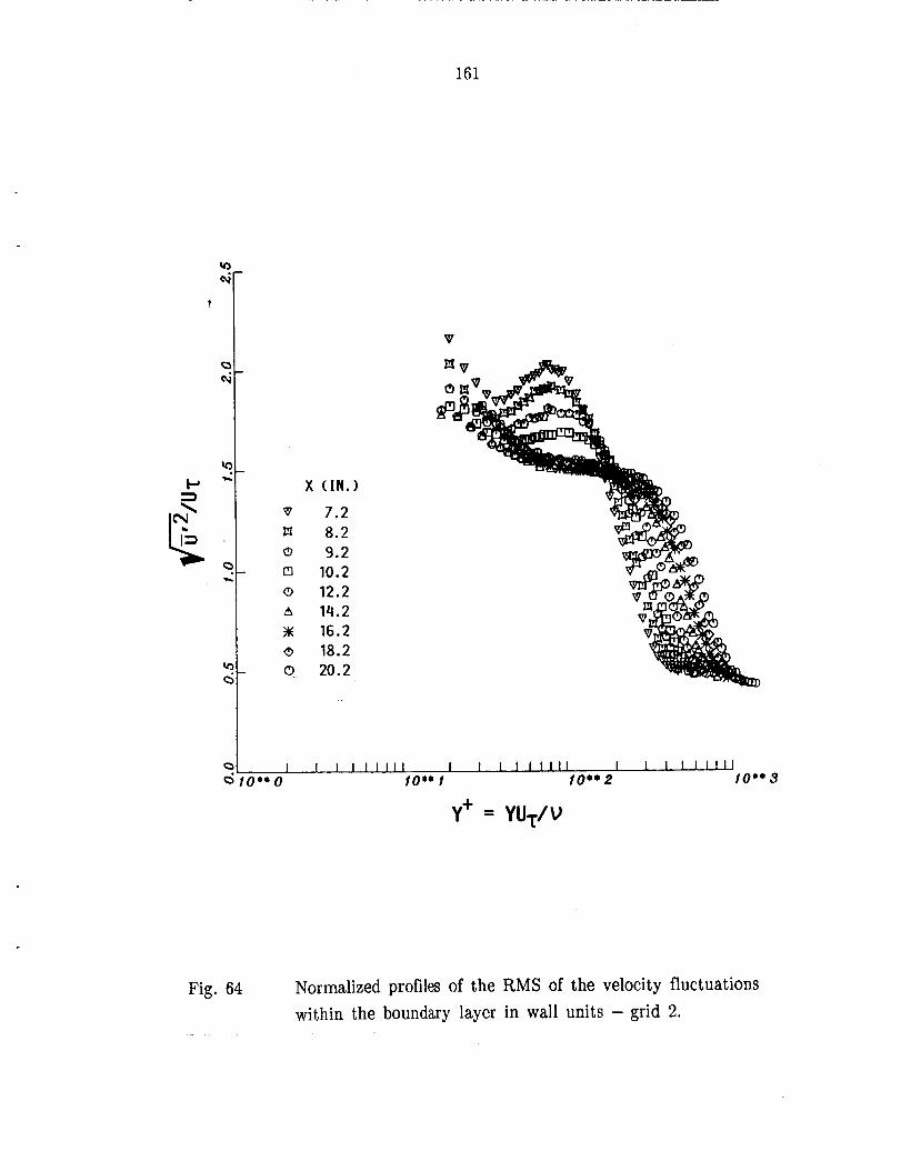
161
¢q
¢S
¢5
(9
[9
(9
A
- (D
X (IN.)
7.2
8.29.2
10.212.214.2
16.218.220.2
I I I I fill I I I I Illll I I I I J ItllI0"" f 10**2 I0"" 3
Y+= YU.[./V
Fig. 64 Normalized profiles of the RMS of the velocity fluctuations
within the boundary layer in wall units - grid 2.

162
H O_-
KLEDANOFF[ ];2 ]
¢_ 1 1 I I I0 2 4 6 8 10
Fig. 65 Comparison of the RMS measurements to the results of Klebanoff
for a fully turbulent boundary layer.

163
OJ
f_II
L00I.LOC.r4
EC_
C
!
>E
E©E
o°_o0°_
0

164
1.0
0.8
0.6
I
O.q
0.2
0.0 I0-- 5
F-i--]GRCD 31I.'IGRID_IGRID IIx I GRID.sl__L GRIDoI
r.Jr_P "'"/ /./m
/ l!/ /
id , /
II , /i,
I ¢,, /
i (
I[ (/"
/I
), ,/
/I!
I0-,, 6_
R_x
Oum 7
Fig. 67 Intermittency factor versus Reynolds number based on x distance.

IG5
o_
o<>_
I0
0
0000
_OL
x1S
0...I
_=
-_1
0I0
0
I
\\
\
I
0X
co
°_0I
°,,,_
00:>
00o

166
U
U
THREE- FULLY
SPANWISE DIMENSIONAL TURBULENT
VORTICITY VORTEX FLOWBREAKDOWN
T/S
WAVES\I--
IIII
STABLE ILAMINAR IFLOW
IiII
iRe
criti--_x W,EDGE
0 CONTAMINATION
LAMINAR I-_---TRANSITION LENGTH _: TURBULENT
Retr
Fig. 69 Transition via the T-S path - from White [1].

167
E0E
ueaw3/3
0
°'_'4
°_j0
_6

168
I.D0
400
360
320
280
24O
2OO
160
120
80
40
0 OBSERVED NATURAL OSCILLATIONS
(SCHUBAUER AND SKRAMSTAD)
MEASUREMENTS
r THEORYJ
0 800 1600 2400 3200
R - U_61
V
Fig. 71 Neul, ra.I sl, al)ilil,y curve - from Schlichting [5].

169
II
IIII
I
4Z)Z)
o.
0
U14,1
I--
00I
0_oooo_8oI
ID,--
0_

170
8
U
.4--
.3--
,2
0--
.20 --
,- Cr/Uoo/
/
104 105
Uoo81
V
106
Fig. 73 Neutral stability curve -from Schlichting [5].

171CC
II
II
II
XX
XX
XX
1|
-i_i-
_i-|i
-|l-|i-|i|_.|
E_
uEew
3/3

172
r_Q
do
0
0°_°_°_
°_
O
lrjt,.-do
ueaw3/3

17;I
0¢,,,,JX::I:1:
00
I.I.I
II
II
I
433
II
II
g.0
U1,1.1
I,--
0,g
ooo.-IIX
v)o°_©
¢.o
°_,,,q

174
(WII_-lOH)
NV3W3/3
II
II
aI
aN
=
LL
LFL
l-,,-a
__
O}"-
+
II
:.+
;-
+_
•.
._.
..
.0')
vID
I"'
I!
_,,I
=OJ
OJ
¢0
00
00
0
I--
--=
un
w
•.
,•
.o
,.................
(3_IM-IOH)
BA
/_
B,..--i
0,.c:t
+,.ct0_u<3.>
B=©(i>
B°,.-+
or]It+....
t-+...
o,..-_
p..,
(D>-+
n_=o,zno_0©
ORIGINAL
PAG
EIS
OF+PO
OR
QU
AI+
tT_

175
..J
>.
,.m
o
Q°,._0oO
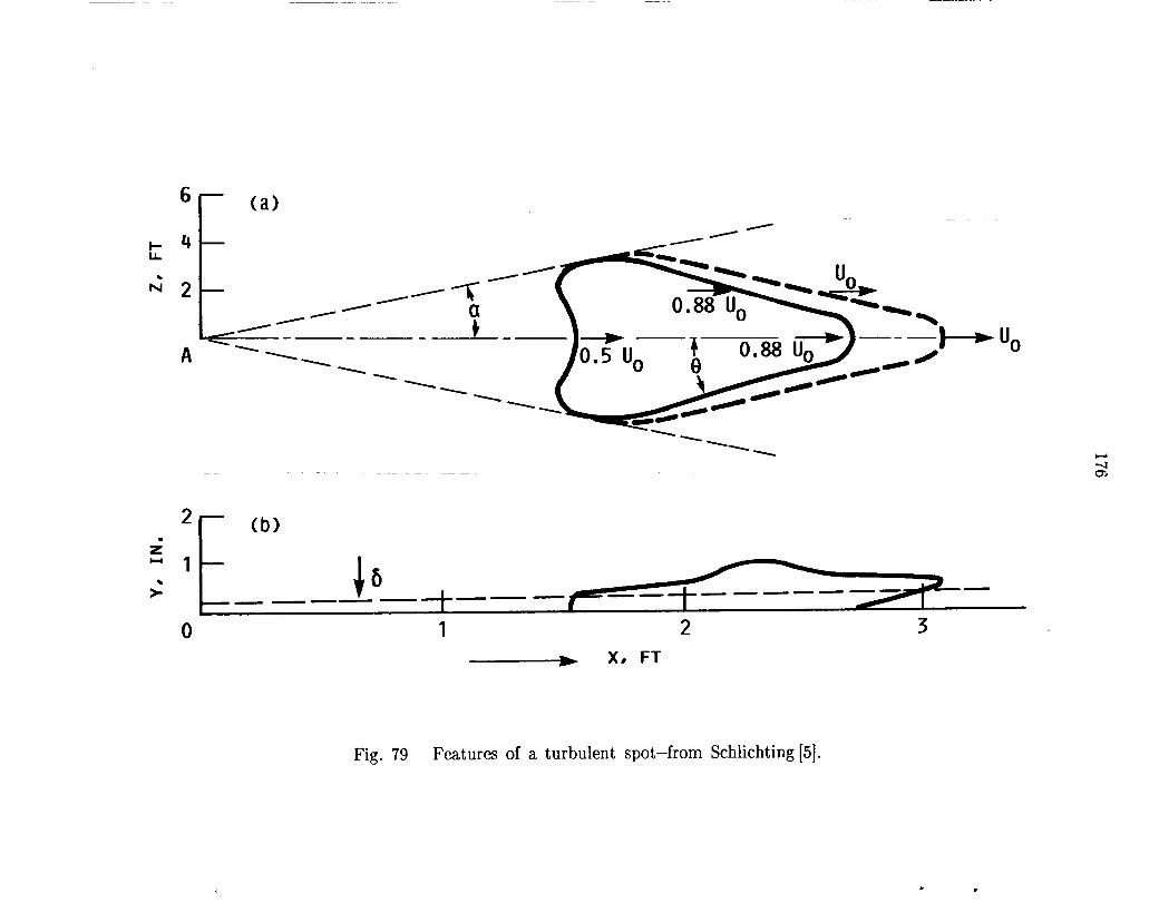
176
AV
\
\
II
I
i/\
I
_yo..///
\/
\/
\/
/////
AI
1-
I
¢",,,I
i-,I1X
,.o.
°,,-i
o,,,,,,,q
¢,)
000gr_
.I.-I"Z
'NI
"A

177
II
II
II
0'00000000
II
oo6
0-
oi=
I
ID0I
"7.ZiIqv{JZZG
9
O
ama_°a=
oo_b
("NI)
-"4DNY.I.Sl(I
"IYDIJ.H.';IA

178
u_
¢;,.!
"1r"_
_"1f-"l
r"_i
r"l_-I
f"_r"_
r"_lJ
L-_L
--JL
--II--.J
1_L._I
I__lL
_.jL.j
L-JL.
[][]
ODDOOD
[]00000
[]
O0000OO0001
000000000
[]
00000
nr_
I--I
NNNN.
PNNI"'
mcoomaoo.JQs_I0X0
0olo0EI0
r_0°_0e_
00_¢_)00I
0_
f
0
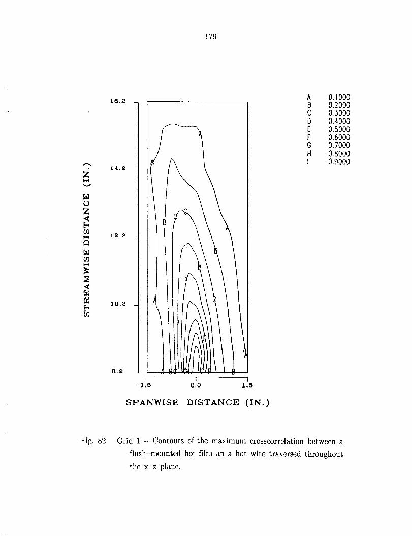
179
0Z<
.<
a;[..,
16.2
14.2
12.2
10.2
8.2
DISTANCE (IN.)
A O.lO00B 0.2000C 0.3000D 0.4000E 0.5000F 0.6000G 0.7000H 0.8000I 0.9000
Fig. 82 Grid 1 - Contours of the maximum crosscorrelation between a
flush-mounted hot film an a hot wire traversed throughout
the x-z plane.

180
AW0.C0CmN
I
]_n_nn_nnn_
]00000000000
]00000000000
]0000000000
]0000000
O0
][]
[]
[]
[]
[]
]0[]
OF7[][]
[]
[]
][]
[]
[]
[]
[]
N
[]]
NN
W0e-0mX
Wt-O00-J0L.
o_I0"1-
[]
0im00JEmI0Z
r_o°_k-io
bl
x:IX
,_.._°_o
°_
O

181
19.2
=_
Z
I,-,,,115.7
LIJ
LU
k--¢J3
12.2
\
(\
I l I
-1.5 0 1,5
SPANWISE DISTANCE, IN.
A 0.1000
B 0.2000C 0.3000D 0.4000E 0.5000F 0.6000(; 0.7000H 0.8000
Fig. 84 Grid 0.5 - Contours of the maximum cross---correlation between a
flush-mounted hot film and a hot wire traversed throughout
the x--z plane.

182
,I
II
t
if_vrr
II
N¢'_I
To_E
"T
I
w
II
Ie
•
II
o_
c_
.<09°_

183
I0
i
II
II
II
00
00
00
ZH
/EA
"GS
d
0
O0I0
N"I-
ZILl
ILl
IJ.
._o
o,..._
o

184
l.DL.
I0
ZHIEA
"flSd
(L)
(:L)
o__°
c_
c_
_{_°•,x_
0_°_
•,.__
t"-
O0fro

I0
L
iI
I
II
II
00
00
ZH/EA
"OS
d
ZU.I
0L
L
000CX
l
Io
I',.C
OI
I0
0
(L)
o
o
'-o
-_o
0"_
._
_),x::
o"_
r_oo_b

186
ORIGINA L r,_-
OF. POOR QUALITZ
U 9
0 M_ -1
0 _" -2
0 wN --3
(r)
O-- -_
ONM --_
ONN --_
0 m_ --7
10-- -8
.°
; /: /
/
5 1 0 0 2
• 25 H.
• 50 H=
• 1 O0 H.
X 200 H.
_( 500 H.
• 1000 H.
" 2000 H.
# 5000 HZ
×
Fig. 89 Grid 0.5 - Streamwise distribution of the boundary layer
disturbance amplitude at selected frequencies.
)

187
_'d/\
OX
<]
r"<
1X
e_tD<
]×
0<
IxII
..,iqx
[]
[]
<IX
[]×
[]
(-.o_b-h.-I!
_J
D
D
[]
E]
[]
E:b-----
]•
L]
[]
.q
,,,,,,,£na
fll_l_rlin
iltili
iltiltlit
71NIIIT
-I-qlIIHIT
-r-_IT[I--
tOC
OI'_
¢0O
)0
00
00
00
',-I
II
II
II
WI11
ILl
I.UILl
I.Ul,L
I0
00
00
00
ILl0,i,i,,
(ZH
/_A)
GS
d
....m'-
)-zILl
'lp"
0
0¢p¢_)
¢)or'
hi
o
°_bO0oI
o_
r_o._,,q
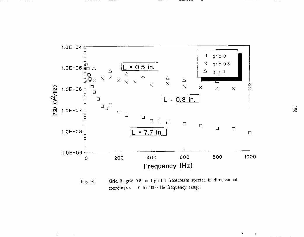
188
.IIV
....[]
X
<]
X
<IX
i--X
.I0×
II
_1<1
x
X
c-.mco0
II
_1
00
<1
X0
[]X
[][]
0[]
[]
[qD
D0
D
.nI!
._1
<]
XD
DF90
o.E_-
[1111I
I=
:allllllI
I"_IIIIII
II
IIIIIII1
II
IIIIIII
Il---
'_"tO
CO
I".-C
OO
_
00
00
00
II
II
II
UJ
UJ
LLI
LU
ILl
LU
00
00
00
(ZH
/_^)G
Sd
0000ocoo
1,4
g-r">.,
0(-.
(D
{D"
ga,
xl"
t..
U-
ooo
0°_g._0
(L)
rOt',l
°_g0ooo
"_,_0.
,..-i
°_

189....
<3
×
um
×
0U
X
c-:
Xam
0<3
×II
_.I
×
<3
X
n°oK
llllI
II
1B
IIIIII
II'_'I
00
II
l.Uiii
oo
0
[]o
IIIIII
II
l
0I
IJJo
a,
r-I
I"_,I
I"..I
III
[]
[]
E3
[]
[]
0
ItlllI
I'I
'I"'
oI
l.Uoql""
0£-J.....
01.0
0
0[]
-00
N
0o
"_0
0I
wo
0°p..._Q
'2go
•_._°_.._
°_._
(ZH
/_A)
OS
d

NationalAeronauticsandSpaceAdministration
1. Report NO.
NASA TM-I00913
4. Title and Subtitle
Report Documentation Page
2. Government Accession No. 3. Reciptent's Catalog No.
5. Report Date
Experimental Study of Bypass Transition in a Boundary Layer
7. Author(s)
Kenneth L. Suder, James E. O'Brien, and Eli Reshotko
9. Performing Organization Name and Address
National Aeronautics and Space Administration
Lewis Research Center
Cleveland, Ohio 44135-3191
12. Sponsoring Agency Name and Address
National Aeronautics and Space Administration
Washington, D.C. 20546-0001
May 1988
6. Performing Organization Code
8. Performing Organization Report No.
E-3953
10. Work Unit No.
505-62-21
11. Contract or Grant No.
13. Type of Report and Period Covered
Technical Memorandum
14. Sponsoring Agency Code
15. Supplementary Notes
Kenneth L. Suder and James E. O'Brien, NASA Lewis Research Center; Eli Reshotko, Case Western Reserve
University, Dept. of Mechanical and Aerospace Engineering, Cleveland, Ohio 44106. This report was a thesis
submitted by Kenneth L. Suder in partial fulfillment of the requirements for the degree of Master of Science to
Case Western Reserve University, Cleveland, Ohio in May 1988.
16. Abstract
A detailed investigation to compare the boundary layer transition process in a low intensity disturbance environment to that in anenvironment in which the disturbances are initially non-linear in amplitude has been conducted using a flat plate model. Testsection freestream turbulence values were varied from 0.3% to approximately 5% using rectangular-bar grids. The longitudinal
integral length scale, intensity, and frequency spectra were acquired to characterize the freestream turbulence. For each level offreestream turbulence, boundary layer surveys of the mean longitudinal velocity and rms of the velocity fluctuations wereobtained at several streamwise locations with a linearized hot-wire constant temperature anemometer system. From these surveys
the resulting boundary layer shape factor, inferred skin friction coefficients, and distribution of the velocity fluctuations throughthe boundary layer were used to indentify the transition region corresponding to each level of freestream turbulence. Both the
initially linear and initially non-linear transition cases were identified. Hereafter, the transition process initiated by the lineargrowth of Tollmien Schlichting (T-S) waves will be referred to as the T-S path to transition; whereas, the transition processinitiated by finite non-linear disturbances will be referred to as the bypass transition process. The transition mechanism based onlinear growth of T-S waves was associated with a freestream turbulence level of 0.3%; however, for a freestream turbulenceintensity of 0.65% and higher, the bypass transition mechanism prevailed. The following detailed measurements were acquired tostudy and compare the two transition mechanisms: 1) simultaneous time traces of a flush-mounted hot film and a hot wire forthe hot wire located at different depths within the boundary layer, 2) crosscorrelations between flush-mounted hot films, 3) two-
point correlations between a flush-mounted hot film and a hot wire positioned at various locations throughout the flowfield, and4) boundary layer spectra at various streamwise distances through the transition region. The results of these measurementsindicate that there exists a critical value for the peak rms of the velocity fluctuations within the boundary layer of approximately3 to 3.5% of the freestream velocity. Once the unsteadiness within the boundary layer reached this critical value, turbulentbursting initiated, regardless of the transition mechanism. The two point correlations and simultaneous time traces within the
transition region illustrate the features of a turbulent burst and its effect on the surrounding flowfield.
17. Key Words (Suggested by Author(s))
Boundary layer transition; Bypass; Freestream turbulence
Flat plate; Hot-wire anemometry; Hot films
18. Distribution Statement
Unclassified- Unlimited
Subject Category 34
19. Security Classif. (of this report) 20. Security Classif. (of this page) 21. No of pages
Unclassified Unclassified 198
NASAFORMlSZ6oct a8 *For sale by the National Technical Information Service, Springfield, Virginia 22161
22. Price*
A09