Original Article

Exploiting signal processing approaches forbroadband echosounders

Andone C. Lavery1*, Christopher Bassett1‡, Gareth L. Lawson2, and J. Michael Jech3

1Department of Applied Ocean Physics and Engineering, Woods Hole Oceanographic Institution, Woods Hole, MA 02543, USA2Biology Department, Woods Hole Oceanographic Institution, Woods Hole, MA 02543, USA3NOAA Northeast Fisheries Science Center, Woods Hole, MA 02543, USA

*Corresponding author: tel: þ1 508 289 2345; fax: þ1 508 457 2194; e-mail: alavery@whoi.edu.‡Present address: NOAA Alaska Fisheries Science Center, Seattle, WA 98115, USA.

Lavery, A. C., Bassett, C., Lawson, G. L. and Jech, J.M. Exploiting signal processing approaches for broadband echosounders. – ICES Journal ofMarine Science, 74: 2262–2275.

Received 12 August 2016; revised 19 June 2017; accepted 22 June 2017; advance access publication 28 August 2017.

Broadband echosounders, which transmit frequency-modulated pulses, increase the spectral characterization of targets relative to narrow-band echosounders, which typically transmit single-frequency pulses, and also increase the range resolution through broadband matched-filter signal processing approaches. However, the increased range resolution does not necessarily lead to improved detection and characteriza-tion of targets close to boundaries due to the presence of undesirable signal processing side lobes. The standard approach to mitigating theimpact of processing side lobes is to transmit tapered signals, which has the consequence of also reducing spectral information. To addressthis, different broadband signal processing approaches are explored using data collected in a large tank with both a Kongsberg–Simrad EK80scientific echosounder with a combination of single- and split-beam transducers with nominal centre frequencies of 18, 38, 70, 120, 200, and333 kHz, and with a single-beam custom-built echosounder spanning the frequency band from 130 to 195 kHz. It is shown that improved de-tection and characterization of targets close to boundaries can be achieved by using modified replica signals in the matched filter processing.An additional benefit to using broadband echosounders involves exploiting the frequency dependence of the beam pattern to calibratesingle-beam broadband echosounders using an off-axis calibration sphere.

Keywords: broadband acoustic backscattering, matched-filter signal processing, Simrad EK80 echosounder, WBT, wideband.

IntroductionNarrowband echosounders, transmitting single-frequency sinu-

soidal pulses, also referred to as continuous wave (CW) tones,

have been extensively used for fisheries research and studies of

zooplankton ecology for over two and a half decades (Holliday

et al., 1989; Foote et al., 1991; Andersen, 2001; Korneliussen and

Ona, 2002; Wiebe et al., 2002; Fielding et al., 2012; Scoulding

et al., 2015). However, there has been a recent emergence of

broadband acoustic backscattering systems transmitting fre-

quency modulated (FM) signals, typically linearly-frequency-

modulated signals, or chirps, for characterizing fish and other

marine organisms (Foote et al., 2005a,b; Stanton et al., 2010,

2012; Lavery et al., 2010). The success of these broadband systems

is built upon a long history of laboratory-based and in situ broad-

band measurements (Holliday, 1972; Simmonds and Armstrong,

1990; Stanton et al., 1998; Thompson and Love, 1996; Zakharia

et al., 1996; Stanton, 2009; and references there in). Broadband

systems allow acoustic backscattering to be measured continu-

ously over a range of frequencies, thereby increasing the amount

of information available for spectral characterization of targets, as

compared with narrowband techniques, which measure acoustic

backscattering at discrete frequencies.

Here, the term “broadband” refers to a system that uses FM

transmit signals and hardware capable of transmitting and

VC International Council for the Exploration of the Sea 2017.This is an Open Access article distributed under the terms of the Creative Commons Attribution License (http://creativecommons.org/licenses/by/4.0/), which permits unrestricted reuse, distribution, and reproduction in any medium, provided the original work isproperly cited.

ICES Journal of Marine Science (2017), 74(8), 2262–2275. doi:10.1093/icesjms/fsx155

receiving over a range of frequencies. A single broadband trans-

ducer can typically transmit sound efficiently over an octave

bandwidth, where the upper band frequency is twice the lower

band frequency. Transducer bandwidth typically increases with

frequency. The term “wideband” refers to a system that combines

multiple transducers, each with different broadband or narrow-

band signals and capabilities, to span a range of frequencies larger

than can be achieved with a single transducer. Though multi-

frequency narrowband echosounders are wideband, the improve-

ments associated to broadband signal processing techniques can-

not be achieved from a collection of narrowband signals.

In addition to improved spectral characterization, broadband

matched-filter (MF) processing techniques (Turin, 1960), also re-

ferred to as compressed pulse processing (Chu and Stanton, 1998;

Ehrenberg and Torkelson, 2000; Stanton and Chu, 2008), can im-

prove the temporal, and thus range, resolution. Although the range

resolution of narrowband systems, Dr ¼ cw s2

(m), where cw is the

sound speed (m/s), is determined by the duration of the transmitted

signal, s (s), the Dr of broadband systems, after MF processing, is in-

dependent of s, and is instead determined by the inverse signal band-

width, 1=B. For example, a narrowband signal of duration

s ¼1.024 ms has Dr ¼ 76 cm, while a broadband pulse with a

bandwidth of 100 kHz has Dr � 0.75 cm, regardless of s.

Furthermore, the signal-to-noise ratio (SNR) increases in proportion

to Bs as a result of broadband signal processing gains (Ehrenberg

and Torkelson, 2000; Stanton and Chu, 2008; and references

therein).

Despite the many benefits of broadband approaches, the use of

FM transmit signals can increase the complexity of the calibra-

tion, processing, and interpretation of the data. Calibration of

broadband systems must account for frequency-dependent ab-

sorption, transducer response, and beam pattern. Although there

is a rich literature on the calibration of narrowband echosounders

(e.g. Foote et al., 1987; Demer et al., 2015; and references therein)

there has been less published research focused on calibration of

broadband echosounders. There are various calibration methods

for broadband systems that can be used (Dragonette et al., 1981;

Foote, 2006; Atkins et al., 2008; Stanton and Chu, 2008; Eastland

and Chu, 2014), including using multiple calibration spheres in

the far- or near-field, or a single calibration sphere with process-

ing of the frequency-independent scattering from the front face

of the sphere.

A practical approach to broadband calibration, similar to nar-

rowband calibration approaches, uses multiple calibration

spheres of different sizes (Foote, 2000, 2006; Lavery et al., 2010)

spanning the ka range from �0.5 to 35, where k ¼ 2p=k is the

wavenumber of the transmitted sound, k (m) is the wavelength,

and a (m) is the sphere radius. Depending on the sphere size and

material properties in relation to the frequency band of interest,

the frequency-dependent scattering response may have at least

one null due to constructive and destructive interference of the

scattered sound (Figure 1). Calibration at frequencies close to

these nulls tends not to be accurate, as the target strength (TS; dB

re 1 m2) of the sphere is highly sensitive to small variations in ma-

terial properties (Foote, 2006, 2007). To avoid these uncertainties,

narrowband calibrations are generally performed at frequencies

distant from the null locations. By using multiple spheres with

different sizes, materials, or both, the nulls will occur at different

frequencies, allowing calibration across the entire measurement

bandwidth for a broadband system (Foote, 2006; Lavery et al.,

2010).

Though calibration of broadband echosounders is generally more

challenging than narrowband echosounders, there are some potential

advantages. Most calibrations rely on the position of the calibration

sphere in the acoustic beam being known. This may be easily

achieved with a split-beam system, in which the transducer is split

into four quadrants, allowing the location of a target in the beam to

be determined by measuring the phase difference in the signals arriv-

ing in each quadrant. However, this can be more challenging with

single-beam systems, whether broadband or narrowband. Typical

single-beam systems rely on painstakingly maximizing the returns

and assuming that the calibration sphere is centered in the beam

when the peak return is largest. However, with a broadband system,

either single- or split-beam, it is possible to use the frequency depen-

dence of the beam pattern and known spectral response of the

sphere to estimate the angle between the sphere and the beam axis.

Thus a single-beam broadband echosounder can be calibrated even

if the target is not centered in the beam. This approach complements

the approach of maximizing the returns to position the target as

close as possible to the centre of the beam.

The optimal broadband signals and signal processing approaches

for exploiting the increased range resolution of broadband systems

for the detection and characterization of targets near boundaries are

not well understood. In principle, broadband systems should im-

prove the detection and characterization of targets near boundaries,

such as fish near the seabed. These broadband techniques may re-

duce the volume associated to the acoustic dead zone (Ona and

Mitson, 1996; Lawson and Rose, 1999), in the absence of excessive

seafloor roughness or slope (Demer et al., 2009; Patel et al., 2009).

This could improve acoustic monitoring of some demersal and

semi-demersal fish stocks (Hylen et al., 1986; Godø, 1998; Karp and

Walters, 1994) and provide information that complements bottom-

trawl surveys. However, side lobes resulting from MF processing

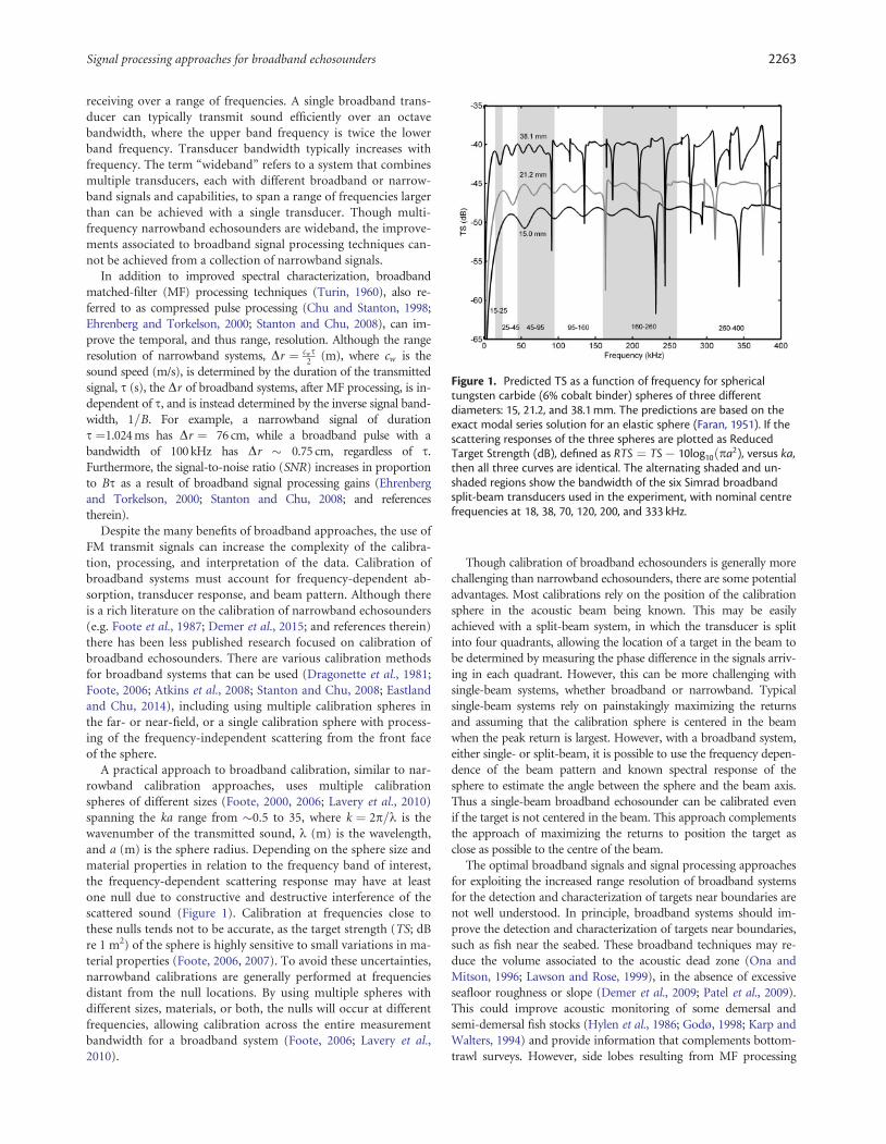
Figure 1. Predicted TS as a function of frequency for sphericaltungsten carbide (6% cobalt binder) spheres of three differentdiameters: 15, 21.2, and 38.1 mm. The predictions are based on theexact modal series solution for an elastic sphere (Faran, 1951). If thescattering responses of the three spheres are plotted as ReducedTarget Strength (dB), defined as RTS ¼ TS� 10log10ðpa2), versus ka,then all three curves are identical. The alternating shaded and un-shaded regions show the bandwidth of the six Simrad broadbandsplit-beam transducers used in the experiment, with nominal centrefrequencies at 18, 38, 70, 120, 200, and 333 kHz.

Signal processing approaches for broadband echosounders 2263

may be problematic when the seabed echoes are much stronger

than those from nearby fish.

Here, we present results from a series of measurements in a

controlled laboratory environment aimed at exploring signal pro-

cessing techniques to exploit the frequency dependence of the

transducer beam pattern to facilitate single-beam broadband cali-

brations when the position of the target is not known a priori,

concurrently achieve full spectral characterization of targets in

the free-field and detection and spectral characterization of tar-

gets close to boundaries, and evaluate the multiple calibration

spheres approach to calibrate an EK80 wideband echosounder

across the frequency band from 15 to 400 kHz.

MethodsTwo sets of experiments were performed to (i) investigate the use

of the frequency-dependent spectrum of a calibration sphere off

the central beam axis to locate the sphere in the beam, thus re-

sulting in the possibility of an off-axis calibration for single-beam

echosounder, and (ii) better understand the signal processing

approaches and limitations for detecting targets close to bound-

aries. These measurements were performed with a wideband,

split-beam, Simrad–Kongsberg (Simrad) EK80 scientific

echosounder and with a custom-built echosounder, described in

more detail below. Simrad officially released the EK80 broadband

scientific echosounder in June 2015. However, the experiments

performed here were performed prior to the official release, using

earlier versions of the EK80 firmware. The available firmware at

the time did not incorporate the built-in calibration function

available with the official release; however, all other functionali-

ties were equivalent.

The first experiment, in October 2013, was aimed at calibrating

the EK80 in support of field work performed in January 2014

(a companion paper by Jech et al., this issue). These measure-

ments allowed the utility of the frequency-dependent spectrum of

a calibration sphere off the central beam axis to locate the sphere

in the beam to be investigated.

The second experiment, in April 2015, was aimed at under-

standing the signal processing approaches and limitations for

broadband detection of targets close to boundaries. Approaches

to reduce the impact of the processing side lobes were explored,

including (i) transmitting different tapered broadband signals,

and (ii) implementing a modified MF approach in which the

transmit signal is unmodified, but the signal used to perform the

MF, also known as the “replica” signal, is strongly tapered. A cus-

tom echosounder was also used to explore broadband signals and

processing techniques not available in the EK80, such as arbitrary

waveforms and a higher sampling frequency of 4 MHz.

Experimental setupTank descriptionAll measurements were performed in a large fresh water tank

(12-m width, 18-m length, 6-m depth) located in the Jere A.

Chase Ocean Engineering facility at the University of New

Hampshire, USA (Figure 2). The transducers were aimed hori-

zontally and mounted on a pole connected to an automated,

computer-controlled, mobile mounting platform that allowed the

depth of the transducer to be set as well as enabling the

transducer to be swept angularly through 360� with 0.1� resolu-

tion. The platform could be positioned horizontally at any loca-

tion. Because of limited cable lengths, the distance from the

transducers to the wall was slightly different between the EK80

system and the custom echosounder.

Description of EK80 scientific echosounderCalibration measurements for the companion paper by Jech et al.

(this issue) were obtained using multiple wideband transceivers

(WBTs), and multiple Simrad split-beam transducers with nomi-

nal centre frequencies, fnom, at 18, 38, 70, 120, 200, and 333 kHz

(Table 1) operated by the EK80 software. Each WBT has four

channels that can either work independently with a single-beam

transducer, or together with a four-quadrant split-beam trans-

ducer. The calibration measurements in October 2013 were per-

formed in split-beam configuration. The WBT is designed for

applications where power consumption (12–15 VDC, 5 A) and

physical size (84 � 213 � 438 mm) are not limiting factors, such

as on board a research vessel with GB-Ethernet communications

and a data-acquisition computer. The EK80 software controls the

WBTs, which can be operated over frequencies ranging from 10

to 500 kHz.

A modified Simrad WBT-Tube system was used for the April

2015 measurements involving calibration spheres close to the

tank wall boundary. This system is fundamentally similar to the

WBT; however, it has been modified to allow towed operation.

All measurements with the WBT-Tube were performed in single-

beam configuration. Three depth-rated Simrad transducers were

used for these measurements with nominal centre frequencies at

70, 200, and 333 kHz.

The WBTs and WBT-Tube digitized the received signals at

1.5 MHz, which is above the Nyquist sampling criterion for the

maximum frequency of 500 kHz. The data from each split-beam

transducer were decimated by an amount pre-determined in the

EK80 software, which was not user controlled, and was related to

the bandwidth of the transmitted signal. There were two stages of

decimation and filtering applied in hardware and software in this

version of the EK80 echosounder, with a decimation associated

with each filter. The filtered and decimated values were saved as

complex samples in binary files with a “.raw” extension. All post-

processing of EK80 data was performed in MATLAB.

Figure 2. Schematic of the fresh water tank (12 m width, 18 mlength, 6 m depth) at the University of New Hampshire. Thetransducers were pole-mounted and aimed horizontally, withcontrol of the depth, angle, and x-y position in the tank. The insetshows a photograph of the tank and transducer mount.

2264 A. C. Lavery et al.

EK80 transmit signalsThe EK80 software (version released on 10 October 2013) allowed

either linear FM signals, with control of the initial and final fre-

quencies within a system-determined range, or CW signals at the

nominal centre frequency of the transducers. The transmitted

power and s were also programmable within system-defined

ranges. All results presented here used s ¼ 1.024 ms. The signals

from the different transducers could be transmitted either sequen-

tially or simultaneously. In sequential mode, the transmit interval,

which was user programmable, corresponded to the amount of

time between the signal transmissions on each transducer. The

measurements discussed here were collected either in sequential

mode or with only one transducer installed. The “slope,” or taper,

of the transmitted signal was either “fast” or “slow” (Figure 3a).

The fast taper involves smoothly tapering the first two and last

two wavelengths with a half cosine wave, equivalent to a Hann

window that is not applied to entire signal. The slow taper in-

volves a Hann window applied to the entire signal (Oppenheim

and Schafer, 1989). The calibration measurements performed in

October 2013 were performed using the fast taper. The measure-

ments of targets close to boundaries with the WBT-Tube in

January 2014 were performed with both fast and slow tapers.

Description of the custom echosounderData were also collected with a custom echosounder (Lavery and

Ross, 2007; Bassett et al., 2015). The transducers used were single-

beam (6� full beam width), custom-built, octave-bandwidth trans-

ducers (Airmar Technology Corp.) with nominal centre frequency

at 160 kHz. The transducers and calibration spheres were set up

the same way as for the measurements performed with the EK80

system. The custom echosounder can transmit arbitrary wave-

forms. The transmit signals used involved 1.024-ms, 130–195 kHz

FM pulses. The Airmar transducer frequency band did not fully

overlap with the Simrad transducer frequency bands. The 65-kHz

bandwidth of the Airmar signal, however, was chosen to be equal

to that of the EK80 with the ES120-7C transducer transmitting

over the frequency band from 95 to 160 kHz. Two types of tapers

were used: (i) an un-tapered FM signal, which resembled the EK80

“fast” taper, and (ii) Gaussian-tapered FM signal with different

standard deviations, described below. The transmitted and received

signals were sampled at 4 MHz. This high-sampling frequency and

Table 1. Transducer and signal parameters used for the calibration measurements with the Simrad WBTs.

Modelfnom

(kHz)FrequencyRange (kHz)

BandwidthB (kHz)

Full BeamWidth

RangeResolutioncw/2B (cm)

ka rangefor WC 15 mm

ka rangefor WC 21.2 mm

ka rangefor WC 38.1 mm

ES18-11 18 15–25 10 11� 7.5 0.48–0.79 0.67–1.12 1.21–2.02ES38DD 38 25–45 20 7� 3.75 0.79–1.43 1.12–2.02 2.02–3.63ES70-7C 70 45–95 50 7� 1.5 1.43–3.02 2.02–4.26 3.63–7.66ES120-7C 120 95–160 65 7� 1.15 3.02–5.08 4.26–7.18 7.66–12.91ES200-7C 200 160–260 100 7� 0.75 5.08–8.26 7.18–11.67 12.91–20.97ES333-7C 333 260–400 140 7� 0.54 8.26–12.70 11.67–17.95 20.97–32.26

Other signal configurations and parameters were also tested, but the results presented in this paper are based on the parameters in this table. These parameterswere chosen for use in the field work performed in January 2014 as part of a companion study (Jech et al., this issue). With the three WC spheres used, of diam-eters 15, 21.2, and 38.1 mm, the ka range from 0.5 to 33 is entirely spanned with no gaps.

Figure 3. (a) Normalized amplitude for the 200 kHz broadbandchirps (160–260 kHz), of 1.024 ms duration, as a function of time forthe two EK80 taper options: “fast” taper (black line) and “slow” taper(grey line). (b) 10log10ECPðtÞ calculated from the autocorrelation ofthe two signals in (a). The “fast” taper has significant sidelobescompared with the “slow” tapered signal, whereas the main peak ofthe “fast” tapered signal is significantly narrower than the main peakof the “slow” tapered signal. (c) Spectral amplitude, 20log10 YT fð Þj j,of the two signals in (a). The “slow” taper has approximately half thespectral content of the “fast” tapered signal. The ringing and ripplesin the spectral response can be clearly seen with the fast taper,known as the Gibbs effect, which is significantly reduced with theslow taper.

Signal processing approaches for broadband echosounders 2265

the lack of additional filtering and decimation allowed for addi-

tional post-processing approaches that are outlined below. The re-

ceived signals were pre-amplified and saved in binary format as

raw voltage versus time, with no decimation applied. All data pro-

cessing was performed in MATLAB.

Calibration spheresThe calibration measurements involved spheres made from tung-

sten carbide (WC) with 6% cobalt binder, with diameters of 15,

21.2, and 38.1 mm, commonly used to calibrate narrowband

echosounders of similar nominal centre frequencies. Given the

frequency bands available and these calibration sphere sizes, ka

ranged from 0.5 to 33 with no gaps. Calibrations with WC

spheres are most reliable with ka from �5 to 16.5, where there

are fewer nulls (Lavery et al., 2007, 2010). At higher ka, the cali-

bration is more sensitive to rapid changes in the scattering spec-

trum, target roughness, and knots in the monofilament tether;

and at smaller ka values, TS is smaller and SNR is lower.

For the WC spheres, the longitudinal sound speed, cL, used in

the TS calculations was 6864 m/s, the transverse sound speed, cT ,

was 4161 m/s, and the density, q, was 14.9 g/cm3 (Foote and

MacLennan, 1984). The tank contained freshwater and the tem-

perature was measured to accurately calculate cw ¼1484 m/s (us-

ing Fofonoff and Millard, 1983).

Experimental procedureProcedure for multiple sphere calibrationDuring the October 2013 measurements, the calibration spheres

were suspended using 2-lb test monofilament line, with a diame-

ter of � 150 lm, at ranges spanning 5–7 m from the transducers

and at a depth of �2–3 m. The depth of the sphere was controlled

to sub-centimetre precision by a motorized pulley system. The

height and angle of the transducer under test were adjusted until

the target was in the centre of the beam. This was accomplished

by maximizing the amplitude of the return from the sphere and

by ascertaining that it was located in the centre of the beam ac-

cording to the split-beam software with no measurable differences

in the phases of the signals arriving at the four different split-

beam quadrants. For the beam widths and ranges used, the

spheres were in the far field of the transducers, conservatively

given by a2T=k, where aT is the transducer radius, and within the

first Fresnel zone. Acoustic scattering data were collected with: (i)

the spheres located in the centre of the beam at various ranges,

and (ii) the transducers rotated so that the sphere moved off the

centre of the beam axis in pre-determined angular steps.

Procedure for calibration spheres close to the tank boundaryThe single-beam WBT-Tube system was used to measure broad-

band acoustic backscattering from the WC 38.1 mm sphere lo-

cated close to the boundary provided by the tank wall. The WC

38.1 mm sphere was chosen for these measurements as it had the

highest TS away from the nulls. The WC 38.1 mm sphere was sus-

pended with its centre 10 cm from the tank wall and in the centre

of the beam. The target was then moved 10, 20, 30, 50, 75, and

150 cm from the wall. These measurements were performed with

the Simrad fnom ¼ 120 kHz channel with both fast and slow ta-

pers. These measurements were then repeated for the custom

echosounder for various signal tapers.

Signal processingSignal processing for on-axis targetsThe broadband capabilities of the EK80 echosounder were ex-

ploited through the use of MF processing techniques. The re-

ceived voltage time-series from each of the four split-beam

transducer quadrants were filtered, decimated, and saved as com-

plex values by the EK80 data acquisition software. The initial step

in the processing involved cross-correlating these received echo-

voltage time-series, vR;i tð Þ; on each of the four split-beam quad-

rants i ¼ 1� 4ð Þ; with the transmitted signal time-series, vT tð Þ,also referred to as the replica signal. The replica signal time-series

was generated at the full sampling frequency (1.5 MHz) and then

the same tapers, decimations, and filters were applied as were ap-

plied to the received signals. The normalized autocorrelation

function of the transmit signal is given by:

yT tð Þ ¼ vT tð Þ � v�T ðtÞvT ðtÞj j2

; (1)

where � represents complex conjugate, jj represents absolute

value, and � represents cross-correlation. The MF output for

each of the four split-beam quadrants is given by:

yR;i tð Þ ¼ vR;i tð Þ � v�T ðtÞvT ðtÞj j2

: (2)

When a target is located in the centre of the beam, the averaged

pulse-compression signal from all four quadrants is given by

yRðtÞ. The envelope of yR tð Þ, ECP tð Þ; or its logarithmic form,

10log10ECPðtÞ, is often used to visualize the output of the MF

processing (Lavery et al., 2010). However, ECP does not incorpo-

rate the calibration measurements, so ECP for different channels

cannot be directly compared.The measured, un-compensated, frequency-dependent, target

strength (TS) is given by (modified from Lavery et al., 2010;

Stanton et al., 2010; L. Anderson, Simrad, pers. comm.):

TSmeas fð Þ ¼ 10log10

YR fð Þj j2

YT fð Þj j2� 10log10LTLðf Þ2

� 10log10 KT PTð Þ: (3)

where f is the acoustic frequency, YR fð Þj j is the absolute value of

the Fourier transform of yR tð Þ, and YT fð Þj j is the absolute value

of the Fourier transform of yT tð Þ. The N-point MATLAB fast

Fourier transform algorithm was used for these calculations, pad-

ded with zeros if the chosen window had fewer than N points

(Press et al., 1992). The value of N was chosen to be the next

power of 2 larger than the window size in order to optimize the

algorithm performance. If a larger power of 2 is chosen, then fre-

quency smoothing results.The frequency-dependent transmission loss on a linear scale,

LTL fð Þ; attributable to spherical spreading and absorption, is

LTL fð Þ ¼ 10�2a fð Þr=20

r2 , where a fð Þ is the frequency-dependent ab-

sorption factor (dB m�1). PT accounts for the transmit power

and is a parameter that can be varied in the EK80 software. KT is

a parameter to correct for the received power of a matched load:

KT ¼ 2Z knom2

16p2 , where knom is the wavelength at the nominal centre

frequency and Z accounts for the system hardware impedance

(according to the manufacturer Z � 75 X). This parameter is

2266 A. C. Lavery et al.

likely a function of frequency, but is not critical to the calcula-

tions, as it is accounted for in the system calibration.

The frequency-dependent system calibration for each trans-

ducer, Gðf Þ, is the difference between the TSmeas and the theoret-

ically predicted TS based on the exact modal series solution for a

solid elastic sphere, TSmodel fð Þ, using the exact size and material

properties of the sphere:

G fð Þ ¼ 0:5 TSmeas fð Þ � TSmodel fð Þ� �

: (4)

The factor 0.5 is retained to be consistent with Simrad’s ap-

proach for narrowband and broadband systems (Andersen, 2001;

Lunde et al., 2013).

Frequency-dependent beam pattern for off-axis targetsFor a constant-radius transducer, the transducer beamwidth de-

creases with increasing frequency. Thus, a target located off-axis

is closer to the “edge” (�3 dB points) of the main lobe at higher

frequencies than at lower frequencies. A consequence of this is

that the measured TS fð Þ of a target located off-axis (uncorrected

for position) appears to decrease with increasing frequency rela-

tive to the spectrum of a target located in the centre of the main

lobe. It is possible to use this frequency-dependent “droop” in

the frequency response of the sphere to infer the angular position

of the target in the beam. The one-way beam pattern is given by

Medwin and Clay (1998):

DT f ; hð Þ ¼ 2J1ðkaT sinhÞ

kaT sinh

� �2

; (5)

where J1is the first order cylindrical Bessel function, and h is the

angle. The predicted TS is given by

TSmodel; off�axis f ; hð Þ ¼ TSmodel fð Þ � 10log10D2T f ; hð Þ: (6)

The angular position, htarget, of a target can be determined by

comparing the measured TS fð Þ for an off-axis target,

TSmeas; off�axis f ; htarget

� �, to TSmodel; off�axis f ; hð Þ over a range of

values of h (for example, by calculating least squares differences).

It is then possible to also determine the frequency-dependent cali-

bration curve. This analysis was performed for various spheres

and frequency bands.

MF processing: side lobes and signal tapersA less welcome feature associated with MF signal processing is

the presence of processing side lobes (Figure 3). When an un-

tapered signal is transmitted, the MF processing results in side

lobes that emerge from the cross-correlation operation. The side

lobes of the MF can be suppressed by tapering the transmitted

signal (Figure 3). However, tapering the transmit signal is also as-

sociated with a corresponding loss in bandwidth, as well as a loss

of range resolution associated with the widening of the main lobe

of the MF. The two signal tapering options provided by the EK80,

the “fast” and the “slow” tapers, corresponded to transmitting ei-

ther very slightly tapered chirps, with good spectral bandwidth

but high side lobes, or a very strongly tapered signal with less

spectral bandwidth and lower side lobes. These two tapers are im-

plemented by using the appropriate “replica” transmit signal in

Equation (2), i.e. by replacing vT ðtÞ with either vslowT ðtÞ or

vfastT ðtÞ.

Suppression of processing side lobes can also be accomplished

by transmitting an un-tapered signal and then using a tapered

“replica” signal to perform the MF in post-processing. This ap-

proach was only implemented for the data collected with the cus-

tom echosounder. Similar post-processing steps were also applied

to the EK80 data but the results are not presented. This is because

the stage-2 (software) filter in the EK80 software produced arte-

facts that could not be suppressed by tapering in post-processing.

Future changes to the EK80 software could, in theory, permit

similar processing to be applied to EK80 data with comparable

results. For the custom echosounder, Gaussian tapers were used

to perform this “post-processing” as, theoretically, Gaussian ta-

pered signals have no side lobes (Priestley, 1981). The Gaussian

taper can be applied in the frequency or time domain. In the time

domain [modified from Equation (8) in Chu and Stanton, 1998],

the Gaussian taper is described by

GT tð Þ ¼ e� t�tcð Þ2

2r2t ; (7)

where tc is the centre of the transmit signal in time and rt is the

standard deviation, which controls the degree of tapering. For a

given bandwidth and signal duration, the larger the time-domain

standard deviation (rt ), the faster the taper and the closer the sig-

nal becomes to an un-tapered, or “square” FM pulse. It is also

possible to implement the Gaussian taper in the frequency do-

main, where the frequency-domain taper is a Gaussian shaped

function. The frequency- and time-domain standard deviations,

for a given signal duration and bandwidth, are related by

rf ¼ Bs r�1

t . In the time domain, the Gaussian post-processing ta-

per is implemented by replacing vT ðtÞ in Equation (2) with

vGTT tð Þ ¼ GTðtÞ vT tð Þ, where vT tð Þ is the actual transmitted sig-

nal. Thus, Equation (2) becomes:

yR;i tð Þ ¼ vR;i tð Þ � vGTT tð Þ�

vGTT tð Þ�� ��2 : (8)

Three primary Gaussian tapers were implemented for the custom

echosounder: (i) rf ¼ 6 kHz, equivalent to rt ¼ 0:095 ms for a

s ¼ 1:024 ms duration signal, (ii) rf ¼ 15 kHz, equivalent to

rt ¼ 0:236 ms for a s ¼ 1:024 ms duration signal, and (iii)

rf ¼ 30 kHz, equivalent to rt ¼ 0:472 ms for a

s ¼ 1:024 ms duration signal.

ResultsCalibration curves based on multiple on-axis calibrationspheresThe frequency-dependent calibration curves [Equation (4)] using

multiple WC spheres of different sizes for the Simrad transducers

are shown in Figures 4 and 5. These measurements were per-

formed with the WC 38.1, 21.2, and/or 15.0-mm targets on-axis,

as determined by the positioning of the automated tank calibra-

tion set-up as well as by the EK80 split-beam processing.

For the 18-, 38-, and 70-kHz channels, the calibration curves

are based on the 21.2-mm target (Figure 4a–c, blue curves).

A single calibration was used and there was no need for interpola-

tion. It was found that the usable bandwidth was between 16 and

Signal processing approaches for broadband echosounders 2267

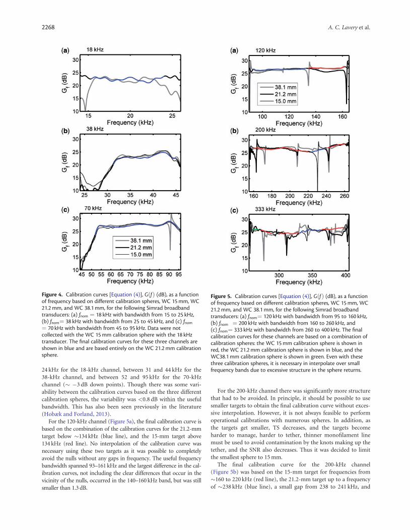
24 kHz for the 18-kHz channel, between 31 and 44 kHz for the

38-kHz channel, and between 52 and 95 kHz for the 70-kHz

channel (� �3 dB down points). Though there was some vari-

ability between the calibration curves based on the three different

calibration spheres, the variability was <0.8 dB within the useful

bandwidth. This has also been seen previously in the literature

(Hobæk and Forland, 2013).

For the 120-kHz channel (Figure 5a), the final calibration curve is

based on the combination of the calibration curves for the 21.2-mm

target below �134 kHz (blue line), and the 15-mm target above

134 kHz (red line). No interpolation of the calibration curve was

necessary using these two targets as it was possible to completely

avoid the nulls without any gaps in frequency. The useful frequency

bandwidth spanned 93–161 kHz and the largest difference in the cal-

ibration curves, not including the clear differences that occur in the

vicinity of the nulls, occurred in the 140–160 kHz band, but was still

smaller than 1.3 dB.

For the 200-kHz channel there was significantly more structure

that had to be avoided. In principle, it should be possible to use

smaller targets to obtain the final calibration curve without exces-

sive interpolation. However, it is not always feasible to perform

operational calibrations with numerous spheres. In addition, as

the targets get smaller, TS decreases, and the targets become

harder to manage, harder to tether, thinner monofilament line

must be used to avoid contamination by the knots making up the

tether, and the SNR also decreases. Thus it was decided to limit

the smallest sphere to 15 mm.

The final calibration curve for the 200-kHz channel

(Figure 5b) was based on the 15-mm target for frequencies from

�160 to 220 kHz (red line), the 21.2-mm target up to a frequency

of �238 kHz (blue line), a small gap from 238 to 241 kHz, and

Figure 4. Calibration curves [Equation (4)], GðfÞ (dB), as a functionof frequency based on different calibration spheres, WC 15 mm, WC21.2 mm, and WC 38.1 mm, for the following Simrad broadbandtransducers: (a) fnom ¼ 18 kHz with bandwidth from 15 to 25 kHz,(b) fnom¼ 38 kHz with bandwidth from 25 to 45 kHz, and (c) fnom

¼ 70 kHz with bandwidth from 45 to 95 kHz. Data were notcollected with the WC 15 mm calibration sphere with the 18 kHztransducer. The final calibration curves for these three channels areshown in blue and are based entirely on the WC 21.2 mm calibrationsphere.

Figure 5. Calibration curves [Equation (4)], GðfÞ (dB), as a functionof frequency based on different calibration spheres, WC 15 mm, WC21.2 mm, and WC 38.1 mm, for the following Simrad broadbandtransducers: (a) fnom¼ 120 kHz with bandwidth from 95 to 160 kHz,(b) fnom ¼ 200 kHz with bandwidth from 160 to 260 kHz, and(c) fnom¼ 333 kHz with bandwidth from 260 to 400 kHz. The finalcalibration curves for these channels are based on a combination ofcalibration spheres: the WC 15 mm calibration sphere is shown inred, the WC 21.2 mm calibration sphere is shown in blue, and theWC38.1 mm calibration sphere is shown in green. Even with thesethree calibration spheres, it is necessary in interpolate over smallfrequency bands due to excessive structure in the sphere returns.

2268 A. C. Lavery et al.

finally the 15-mm target up to the upper end of the band at

260 kHz. The small gap between 238 and 241 kHz is a result of ex-

cessive structure in all the target responses, and is filled by linear

interpolation between the last value of the 21.2-mm target below

the gap and the first value of the calibration curve for the 15-mm

target above the gap. For the 200-kHz channel, it was only

necessary to interpolate 3% of the total bandwidth. This interpo-

lation is reasonable as all three targets show that there was no sig-

nificant frequency dependent change in the transducer response

in this frequency band. The useful frequency bandwidth spanned

160–260 kHz (��3 dB points) and the largest difference in the

calibration curves, not including the clear differences that occur

in the vicinity of the nulls, occurred in the 200–230 kHz band,

but was still smaller than 1.2 dB.

As with the 200-kHz channel, there was significantly more

structure to be avoided for the 333-kHz channel (Figure 5c). The

final calibration curve for the 333-kHz channel was based on the

38.1-mm target for frequencies from 260 to 270 kHz (green line),

the 15-mm target for frequencies from 270 to 289 kHz (red line),

a gap from 289 to 299 kHz, the 15-mm target for frequencies

from 299 to 330 kHz (red line), the 21.2-mm target from 330 to

362 kHz (blue line), and finally the 15-mm target from 262 to

397 kHz (red line). It was necessary to linearly interpolate from

289 to 299 kHz, representing �14% of the total bandwidth. The

useful frequency bandwidth spanned 260–397 kHz (� �3 dB

points) and the largest difference in the calibration curves, not in-

cluding the clear differences that occur in the vicinity of the nulls,

occurred in the 380–400 kHz, and was up to 2.5 dB in this high

end of the frequency band.

Off-axis calibrationFigure 6a shows the position of the WC 38.1 mm sphere, as deter-

mined from the EK80 split-beam processing (grey line), as it was

slowly moved horizontally through the 200-kHz transducer

beam. Figure 6b shows TSmodel; off�axis f ; hð Þ for the WC 38.1 mm

target over the frequency band of the 200-kHz transducer for

h ¼1, 2, 3, and 4 degrees (corresponding to the locations of the

coloured dots in Figure 6a). It is important to note that the posi-

tion of the nulls does not change. The black curve corresponds to

the TS model predictions with the target in the centre of the

beam (h ¼ 0). Figure 6c shows TSmeas; off�axis for the target at

the positions indicated by the coloured dots in Figure 6a, with

the black curve corresponding to measurements with the target in

the centre of the beam. These TS spectra have not been corrected

for the location of the target in the beam; in other words, the pro-

cessing of the data to arrive at Figure 6c follows the same process-

ing as a target located in the centre of the beam, and the

Figure 6. Off-axis calibration: (a) Angular position of the WC 38.1 mm target in the beam as determined by the split-beam processing of the200 kHz broadband transducer as the transducer is mechanically rotated in 0.1 degree steps through the main beam of the transducer (greyline). Large coloured dots represent the on-axis (black), 1 (green), 2 (red), 3 (pink), and 4 (yellow) degree positions of the target in the beam.(b) Predicted TS as a function of frequency and degrees off-axis. (c) Measured TS as a function of frequency [Equation (3)] for the 200 kHzSimrad broadband channel, when the WC 38.1 mm target is at the angular positions shown by the coloured dots in (a). For the purposes ofillustration, the measured TS has been arbitrarily shifted vertically to align with the predicted TS. This vertical offset is accounted for in thefinal calibration curves [Equation (4)]. (d) Measured TS as a function of frequency for the 200-kHz Simrad broadband channel when the WC38.1 mm target is at the angular positions shown by the coloured dots in (a) and corrected for the frequency-dependent beam pattern. Theoff-axis measured TS spectra, shown in (c), collapse onto the on-axis TS spectrum once their angular position in the beam has beenaccounted for.

Signal processing approaches for broadband echosounders 2269

measured signals on all four split-beam quadrants are averaged

together, simulating a single-beam system. Thus, when the target

is off-axis, the spectra decrease with increasing frequency.

Figure 6d shows the measured TS spectra in Figure 6c corrected

for the position of the target in the beam [Equation (6)]. It can

be seen that the corrected TS spectra are in close agreement with

the spectrum for the target at the centre of the beam. Once the

target is sufficiently outside the main lobe (e.g. at h ¼ 4�), there

are larger errors in the corrected TS, particularly at higher fre-

quencies where the beamwidth is narrower. This illustrates that

the shape of the spectrum for an off-axis target can be used to de-

termine how far off-axis the target is, though not precisely where

in the beam the target is located. For the purposes of calibration,

this allows a system to be accurately calibrated even if the target is

off-axis by an unknown amount during calibration, so long as it

is still within the main beam for some significant portion of the

frequency band.

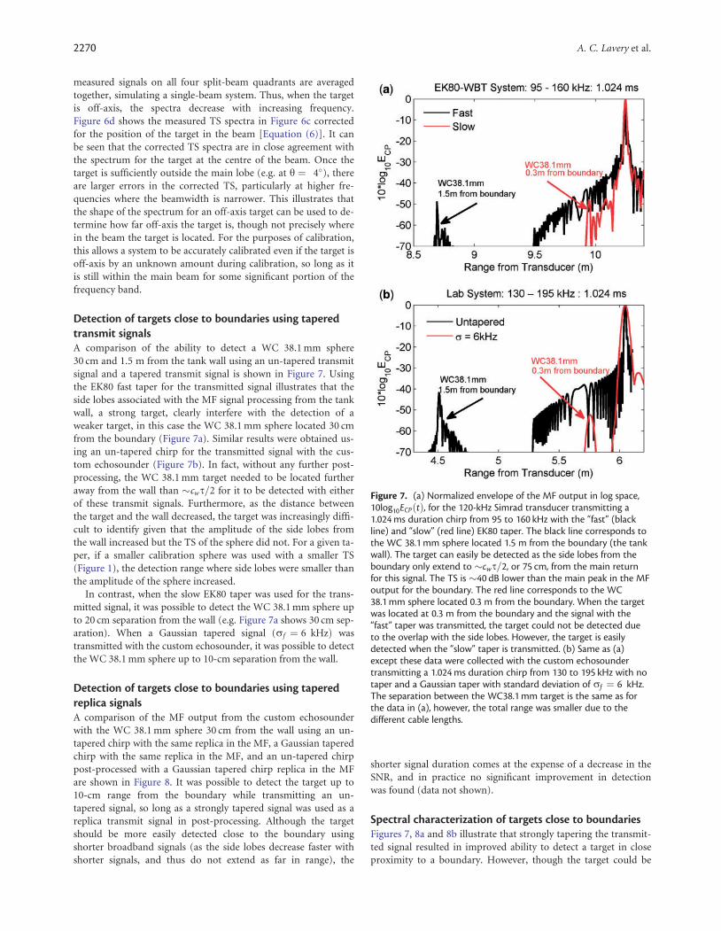
Detection of targets close to boundaries using taperedtransmit signalsA comparison of the ability to detect a WC 38.1 mm sphere

30 cm and 1.5 m from the tank wall using an un-tapered transmit

signal and a tapered transmit signal is shown in Figure 7. Using

the EK80 fast taper for the transmitted signal illustrates that the

side lobes associated with the MF signal processing from the tank

wall, a strong target, clearly interfere with the detection of a

weaker target, in this case the WC 38.1 mm sphere located 30 cm

from the boundary (Figure 7a). Similar results were obtained us-

ing an un-tapered chirp for the transmitted signal with the cus-

tom echosounder (Figure 7b). In fact, without any further post-

processing, the WC 38.1 mm target needed to be located further

away from the wall than �cws=2 for it to be detected with either

of these transmit signals. Furthermore, as the distance between

the target and the wall decreased, the target was increasingly diffi-

cult to identify given that the amplitude of the side lobes from

the wall increased but the TS of the sphere did not. For a given ta-

per, if a smaller calibration sphere was used with a smaller TS

(Figure 1), the detection range where side lobes were smaller than

the amplitude of the sphere increased.

In contrast, when the slow EK80 taper was used for the trans-

mitted signal, it was possible to detect the WC 38.1 mm sphere up

to 20 cm separation from the wall (e.g. Figure 7a shows 30 cm sep-

aration). When a Gaussian tapered signal (rf ¼ 6 kHzÞ was

transmitted with the custom echosounder, it was possible to detect

the WC 38.1 mm sphere up to 10-cm separation from the wall.

Detection of targets close to boundaries using taperedreplica signalsA comparison of the MF output from the custom echosounder

with the WC 38.1 mm sphere 30 cm from the wall using an un-

tapered chirp with the same replica in the MF, a Gaussian tapered

chirp with the same replica in the MF, and an un-tapered chirp

post-processed with a Gaussian tapered chirp replica in the MF

are shown in Figure 8. It was possible to detect the target up to

10-cm range from the boundary while transmitting an un-

tapered signal, so long as a strongly tapered signal was used as a

replica transmit signal in post-processing. Although the target

should be more easily detected close to the boundary using

shorter broadband signals (as the side lobes decrease faster with

shorter signals, and thus do not extend as far in range), the

shorter signal duration comes at the expense of a decrease in the

SNR, and in practice no significant improvement in detection

was found (data not shown).

Spectral characterization of targets close to boundariesFigures 7, 8a and 8b illustrate that strongly tapering the transmit-

ted signal resulted in improved ability to detect a target in close

proximity to a boundary. However, though the target could be

Figure 7. (a) Normalized envelope of the MF output in log space,10log10ECPðtÞ, for the 120-kHz Simrad transducer transmitting a1.024 ms duration chirp from 95 to 160 kHz with the “fast” (blackline) and “slow” (red line) EK80 taper. The black line corresponds tothe WC 38.1 mm sphere located 1.5 m from the boundary (the tankwall). The target can easily be detected as the side lobes from theboundary only extend to �cws=2, or 75 cm, from the main returnfor this signal. The TS is �40 dB lower than the main peak in the MFoutput for the boundary. The red line corresponds to the WC38.1 mm sphere located 0.3 m from the boundary. When the targetwas located at 0.3 m from the boundary and the signal with the“fast” taper was transmitted, the target could not be detected dueto the overlap with the side lobes. However, the target is easilydetected when the “slow” taper is transmitted. (b) Same as (a)except these data were collected with the custom echosoundertransmitting a 1.024 ms duration chirp from 130 to 195 kHz with notaper and a Gaussian taper with standard deviation of rf ¼ 6 kHz.The separation between the WC38.1 mm target is the same as forthe data in (a), however, the total range was smaller due to thedifferent cable lengths.

2270 A. C. Lavery et al.

detected to small target-boundary separations, the strongly ta-

pered transmit signals also resulted in a decrease in the effective

bandwidth available to spectrally characterize the target (Figure

8c and d). In addition, some of the energy in the side lobe of the

boundary echo “leaked” into the signal from the target and re-

sulted in errors in the TS spectra (i.e. differences in measured ver-

sus theoretical).

Data collected with the custom echosounder demonstrated

that similar characterization of the target was possible when a

Gaussian tapered signal was transmitted as when an un-tapered

signal was transmitted (Figure 8c and d). However, in order to

obtain this same level of detection and characterization when an

un-tapering signal was transmitted, it was necessary to post-

process the data with a tapered replica signal.

Figure 9 shows a comparison of the un-tapered transmitted

chirp and the MF output post-processed using three Gaussian ta-

per widths (r ¼ 6, 15, 30 kHz) with the target 30 cm from the

tank wall. In all cases, the taper suppresses the side lobes, making

the target easily identifiable, at the expense of increased width of

the main lobe (associated with loss in spatial resolution). There is

a clear loss in spectral information of the target as the taper be-

comes more aggressive (Figure 9b). This highlights the need to

balance target detection with the desire to adequately characterize

the target.

DiscussionMeasurements of acoustic scattering over a wide frequency band

offer the potential for improved target discrimination and charac-

terization relative to traditional narrowband methods, while si-

multaneously increasing range resolution and improving signal-

to-noise. However, there are also calibration and signal processing

challenges that need to be addressed to optimize the capabilities of

broadband systems. Till recently, the limited availability of com-

mercial broadband echosounders geared towards fisheries acous-

tics has not required these issues to be addressed as systematically

as they have been for narrowband echosounders. The Simrad

EK80 wideband, split-beam, scientific echosounder, released in

June 2015, is a welcome arrival, which, however, deserves the same

careful scrutiny that was afforded to its earlier narrowband coun-

terparts, the EK60 and EK500 (e.g. Jech et al., 2005).

A Simrad EK80, which combined WBTs with split-beam,

transducers with nominal centre frequencies of 18, 38, 70, 120,

200, and 333 kHz, was calibrated in a controlled laboratory envi-

ronment using multiple calibration spheres of different sizes.

Figure 8. (a, b): Normalized envelope of the MF output in log space, 10log10ECPðtÞ, for the custom echosounder transmitting a 1.024 msduration chirp from 130 to 195 kHz with no taper (grey line), a Gaussian taper with standard deviation of rf ¼ 6 kHz (blue line), and withno taper but post-processed with a Gaussian taper with standard deviation of rf ¼ 6 kHz (red line). (a) The WC 38.1 mm target is 1.5 mfrom the boundary (the tank wall), and (b) the WC 38.1 mm target is 0.3 m from the boundary. (c) Measured TS spectrum of the WC38.1 mm target 1.5 m from the boundary. For the purposes of illustration, the measured spectra have been arbitrarily shifted to match thepredicted TS at fnom. (d) Measured TS spectrum of the WC 38.1 mm target 0.3 m from the boundary. For the purposes of illustration, themeasured spectra have been arbitrarily shifted to match the predicted TS at fnom. With either the pre- or post-processed signals there issignificant loss in the spectral content of the signal, but that the ability to detect the target is similar for either the pre- or post-processedsignals. In fact, while the detectability is similar, there is more spectral content with the post-processed signal.

Signal processing approaches for broadband echosounders 2271

Though the Simrad EK80 currently markets the 18- and 38-kHz

channels as narrowband, this study addressed the possibility of

using these transducers in broadband mode. For this study, three

tungsten carbide calibration spheres of diameters 15, 21.2, and

38.1 mm were used for the routine calibration. With these

spheres, the ka range spanned �0.5–33, resulting in a calibration

without the need for excessive (< approximately 15% bandwidth

in this study) interpolation across the nulls in the frequency re-

sponse of the spheres. By using more than one sphere with nulls

positioned at different frequencies it was possible to minimize

calibration error in the vicinity of the nulls. Three spheres of dif-

ferent sizes were used to provide piecewise calibration coverage

across the full band of interest while avoiding nulls, and to ensure

that the transducer response did not change rapidly in the fre-

quency band of interest, as it is possible that rapid changes in the

vicinity of a null could mask significant changes in the transducer

response. Although the general applicability of these three spheres

to EK80 broadband calibration in different environments remains

to be confirmed, results presented here suggest that the three

spheres used here are sufficient for adequate calibration of the

EK80 across the available bandwidth. These calibrations have

been used in a field study published in a companion paper (Jech

et al., this issue).

During this calibration exercise, performed in a large tank with

the ability to precisely control the position of the calibration

spheres in the beam, the potential to calibrate the EK80 with a

broadband single-beam transducer with an off-axis target was in-

vestigated. Though the split-beam capabilities of the EK80 make

it relatively straightforward to locate the target in the centre of

the beam, thus facilitating the calibration of the system, the

WBTs and WBT-Tube can be operated in single-beam configura-

tion. One of the advantages of operating the EK80 in single-beam

configuration is the increase in the number of broadband chan-

nels available. Each split-beam transducer requires four channels

to independently digitize the information from each split-beam

quadrant. Using each of these channels for a single-beam trans-

ducer effectively quadruples the bandwidth of the system, at the

expense of target positioning and tracking. Although a split-beam

Figure 9. (a) Normalized envelope of the MF output in log space, 10log10ECPðtÞ, for the custom echosounder with the WC 38.1 mm targetlocated 0.3 m away from the boundary and transmitting a 1.024 ms duration un-tapered chirp from 130 to 195 kHz but with post-processingusing either no tapering (black line), a Gaussian taper with standard deviation of rf ¼ 30 kHz (grey line), a Gaussian taper with standarddeviation of rf ¼ 15 kHz (red line), and a Gaussian taper with standard deviation of rf ¼ 6 kHz (blue line). (b) The measured and scaled TSas a function of frequency for the WC 38.1 mm sphere for the different post-processed signals shown in (a). The black curve in (b)corresponds to the predicted TS as the target could not be detected with an un-tapered signal and no post-processing taper applied. As thetaper becomes more aggressive, more frequency bandwidth, and hence spectral information content, is lost, thus reducing the ability toperform characterization as well as detection. Furthermore, as the taper becomes more aggressive, and the effective bandwidth decreases, thewidth of the main lobe increases, and thus the range resolution decreases.

2272 A. C. Lavery et al.

system is preferable for single target detection and characteriza-

tion, there are many applications when this is either of no partic-

ular advantage (e.g. high density of targets in the sampling

volume, particularly a concern at large ranges when the sampling

volume is large) or simply not available. Yet it is notoriously chal-

lenging to position a sphere in the centre of a single acoustic

beam in dynamic calibration environments.

For a narrowband system, the only way to position a sphere in

the centre of a single-beam in the field is to carefully move the

target to optimize the amplitude of the return. We have shown

that an advantage of a broadband system is that it is possible to

both optimize the amplitude of the return and determine the an-

gular position of a known calibration sphere by exploiting the

strong frequency dependence of the beam width, effectively illus-

trating that it is not necessary to locate the target in the centre of

the beam to calibrate the system. In fact, the latter method may

be more effective because the TS spectrum shape is more sensitive

than the amplitude of the peak in the MF output to the position

of the target in the beam. This calibration approach relies on the

spherical symmetry of the sphere and the fact that the position of

the nulls in scattering response do not depend on the angular po-

sition of the spherical target in the beam. Once the angular posi-

tion of the sphere in the beam is known, the calibration curve can

be determined by correcting for the angular position of the target

in the beam. This may be of particular utility in highly dynamic

calibration environments where it is not always straightforward

to place the sphere reliably in the centre of the beam, and of even

higher utility for single-beam systems where there is otherwise no

highly effective method for localizing the angular position of the

target in the beam, other than using a supplementary split-beam

transducer (Wurtzell et al. 2016). However, these measurements

have been performed in a controlled laboratory environment

with high SNR, and the applicability of the methodology in oper-

ational conditions still remains to be determined.

Though the increased spectral coverage for improved target

classification was the initial motivation that stimulated the devel-

opment of wideband scientific echosounders, the increased spatial

resolution associated to broadband MF signal processing has also

triggered substantial excitement within the fisheries community,

particularly in light of the potential for increased detection and

classification of demersal fish close to the sea floor (Ona and

Mitson, 1996; Lawson and Rose, 1999; MacLennan et al., 2004).

A less welcome feature associated with MF techniques is the

presence of processing side lobes. The location of these side lobes

is dependent on the duration of the transmit signal. When dis-

crete targets are of comparable amplitude and relatively closely

spaced (more closely spaced than the transmit signal but further

apart than the broadband range resolution determined by the

bandwidth), the processing side lobes may overlap but generally

have only a limited impact on target detection and/or characteri-

zation. On the other hand, when a relatively weak target is located

near a strong target or boundary (e.g. demersal fish near the sea

floor), the side lobes from the stronger target can entirely mask

the presence of the weaker target. As the spatial extent of the side

lobes is determined by the signal duration, for a weak target close

to a strong boundary, the range at which a weak target can be de-

tected is not significantly better than the detection range of a nar-

rowband system, with the precise improvement depending on

SNR and TS.

There are a number of options for side lobe suppression for

applications in which the goal is the detection and/or

characterization of a target near a boundary. These options in-

clude tapering the transmitted signal, transmitting an un-tapered

signal or weakly tapered signal and applying a taper signal in

post-processing, or transmitting a sufficiently short narrowband

CW pulse. This latter option does not involve MF processing and

so there are no complications involving side-lobe masking of the

target, but also does not allow spectral characterization of the tar-

get: It simply represents an option that can improve range resolu-

tion. There are benefits and disadvantages to each of these

approaches that must be weighed for particular applications.

The first, and most straightforward, option for side lobe sup-

pression is to transmit a tapered chirp, thus reducing the need for

additional processing steps. To date, for the EK80, the options for

pre-tapered signals are restricted to the “slow” taper option.

Limitations associated with transmitting a tapered transmit signal

are that some frequency content available for target characteriza-

tion is lost and the range resolution and SNR decrease. The loss

of frequency content can be particularly important if the SNR is

low and the tapered portions of the signal are under the noise

floor. Furthermore, the frequency content, and associated infor-

mation, lost by transmitting a tapered signal cannot be recovered,

which means that tapered transmit signals also reduce the ability

to characterize the frequency response of targets located away

from boundaries (e.g. fish up in the water column).

It is also possible to transmit an un-tapered signal and post-

process the data using a tapered signal as a replica in the cross-

correlations to identify and characterize targets located near

boundaries while retaining full spectral coverage of targets far

(i.e. more than the pulse duration) from the boundary. The pri-

mary benefit of this post-processing approach is that no informa-

tion is permanently lost. It is possible to process the data in the

water column (far from the boundary) using the traditional ap-

proach with the un-tapered replica signal and resulting in full

spectral coverage for the detection and classification of targets in

the water column, with little adverse effects from the side lobes of

the MF. The data close to the boundary (closer than the broad-

band pulse duration) can be independently post-processed using

the tapered replica signal, which reduces the adverse effects of the

processing side lobes and thus results in improved detection in

situations where there is a boundary (or strong target) in the vi-

cinity of a weak target. This technique has been shown to be effec-

tive in the laboratory, however, how well this approach works in

operational scenarios still remains to be determined.

Finally, the range resolution for detection purposes can also be

improved by transmitting a short, narrowband CW signal.

For high-frequency transducers (e.g., f > 70 kHz), relatively short

(s < 100 ls) CW signals are required to improve upon the range

resolution of tapered broadband chirps. However, by transmit-

ting a short, narrowband, CW signal, significant frequency con-

tent is sacrificed. Thus detection may be achieved, but there is

limited information for the basis of characterization, including

for targets far from the boundary. Furthermore, even when apply-

ing a taper, MF processing results in higher SNRs. Therefore,

even aggressively tapered broadband signals have benefits over

CW signals.

SummaryThis study demonstrated that the calibration of the EK80 wide-

band, split-beam scientific echosounder across the full range of

available Simrad transducers, including the 18 and 38 kHz trans-

ducers, is possible using three WC calibration spheres.

Signal processing approaches for broadband echosounders 2273

Recommendations for the best ka range to perform the calibra-

tions, and which calibration spheres to use for each frequency

band are given. It has been shown that, at least in the laboratory,

the EK80 can be calibrated in split-beam or single-beam mode,

without the need for the calibration sphere to be located in the

centre of the beam (and without a priori knowledge of the loca-

tion of the target in the beam) as the locations of the nulls do not

depend on the location of the target in the beam. Finally, signal

processing approaches have been explored that identify the sig-

nals and parameters that can improve the detection and classifica-

tion of targets close to boundaries, without sacrificing spectral

content for the classification of targets in the water column far

from the boundary. Although the current version of the EK80

does not provide full control of some of these parameters, the

ability to detect targets close to boundaries with the EK80 is sig-

nificantly improved through the use of the “slow” tapered trans-

mit signal. Additional flexibility in determining the exact shape of

the transmit signal, as well as more control over the signal deci-

mation, could lead to even better system performance.

AcknowledgementsThe authors gratefully acknowledge Tom Weber for kindly allow-

ing the acoustic scattering measurements to be performed at the

Jere A. Chase Ocean Engineering Facility at the University of New

Hampshire, and to Carlo Lanzoni for technical support during

the measurements. The authors benefited from many informative

discussions with Dezhang Chu, at Northwest Fisheries Science

Centre, and the authors would also like to thank Simrad for al-

lowing the authors to test the newly developed EK80 and loaning

multiple WBTs for use on this project. The thoughtful and con-

sistent support of Lars Nonboe Andersen is particularly noted.

MATLAB code developed for post-processing of the broadband

acoustic data will be made available upon request.

FundingThis research was supported by the NOAA Office of Science and

Technology, Advanced Sampling Technology Working Group.

G.L.L. was partially supported by NOAA Cooperative

Agreements NA09OAR4320129 and NA14OAR4320158 through

the NOAA Fisheries Quantitative Ecology and Socieconomics

Training (QUEST) program. A.C.L. was partially supported

through the Office of Naval Research Ocean Acoustics Program.

ReferencesAndersen, L. N. 2001. The new Simrad EK60 scientific echosounder

system. Journal of the Acoustical Society of America, 109: 2336.

Atkins, P., Francis, D. T., and Foote, K. G. 2008. Calibration ofbroadband sonars using multiple standard targets. Journal of theAcoustical Society of America, 123: 3436. Also Proceedings of theNinth European Conference on Underwater Acoustics, 1, pp.261–266. Ed. by M. E. Zakharia, D. Cassereau, and F. Luppe.French Acoustical Society, Paris.

Bassett, C., Lavery, A. C., Maksym, T., and Wilkinson, J. P. 2015.Laboratory measurements of high-frequency, acoustic broadbandbackscattering from sea ice and crude oil. Journal of theAcoustical Society of America, 137: EL32–EL38.

Chu, D., and Stanton, T. K. 1998. Application of pulse compressiontechniques to broadband acoustic scattering by live individualzooplankton. Journal of the Acoustical Society of America, 104:39–55.

Demer, D. A., Cutter, G. R., Renfree, J. S., and Butler, J. L. 2009. Astatistical-spectral method for echo classification. ICES Journal ofMarine Science: Journal du Conseil, 66: 1081–1090.

Demer, D. A., Berger, L., Bernasconi, M., Bethke, E., Boswell, K.,Chu, D., Domokos, R. et al. 2015. Calibration of acoustic instru-ments. ICES Cooperative Research Report No. 326, 136. p.

Dragonette, L. R., Numrich, S. K., and Frank, L. J. 1981. Calibrationtechnique for acoustic scattering measurements. Journal of theAcoustical Society of America, 69: 1186–1189.

Eastland, G., and Chu, D. 2014. Calibration of a broadband acousticsystem in near-field. Journal of the Acoustical Society of America,135: 2176–2176.

Ehrenberg, J. E., and Torkelson, T. C. 2000. FM slide (chirp) signals:a technique for significantly improving the signal-to-noise perfor-mance in hydroacoustic assessment systems. Fisheries Research,47: 193–199.

Faran, J. J. 1951. Sound scattering by solid cylinders and spheres.Journal of the Acoustical Society of America, 23: 405–418.

Fielding, S., Watkins, J. L., Collins, M. A., Enderlein, P., andVenables, H. J. 2012. Acoustic determination of the distributionof fish and krill across the Scotia Sea in spring 2006, summer 2008and autumn 2009. Deep-Sea Research II, 59-60: 173–188.

Fofonoff, N. P., and Millard Jr, R. C. 1983. Algorithms forComputation of Fundamental Properties of Seawater. Endorsedby Unesco/SCOR/ICES/IAPSO Joint Panel on OceanographicTables and Standards and SCOR Working Group 51. UnescoTechnical Papers in Marine Science, No. 44.

Foote, K. G. 2000. Standard-target calibration of broadband sonars.Journal of the Acoustical Society of America, 108: 2484–2484.

Foote, K. G. 2006. Optimizing two targets for calibrating a broadbandmultibeam sonar. In OCEANS 2006, pp. 1–4. IEEE, 2006.

Foote, K. G. 2007. Acoustic robustness of two standard spheres forcalibrating a broadband multibeam sonar. In OCEANS2007-Europe (pp. 1–4). IEEE, 2007.

Foote, K. G., Atkins, P. R., Francis, D. T. I., and Knutsen, T. 2005b.Measuring echo spectra of marine organisms over a wide band-width. In Proceedings of the International Conference onUnderwater Acoustic Measurements: Technologies and Results,II, Heraklion, Greece, 28 June–1 July 2005, pp. 501–508. Ed. By J.S. Papadakis, and L. Bjørnø. Institute of Applied andComputational Mathematics (IACM) at the Foundation forResearch and Technology (FORTH), Hellas.

Foote, K. G., Chu, D., Hammar, T. R., Baldwin, K. C., Mayer, L. A.,Hufnagle, Jr, L. C., ., and Jech, J. M. 2005a. Protocols for calibrat-ing multibeam sonar. Journal of the Acoustical Society ofAmerica, 117: 2013–2027.

Foote, K. G., Knudsen, H. P., Korneliussen, R. J., Nordbø, P. E., andRøang, K. 1991. Postprocessing system for echo sounder data.Journal of the Acoustical Society of America, 90: 37–47.

Foote, K. G., Knudsen, H. P., Vestnes, G., MacLennan, D. N., andSimmonds, E. J. 1987. Calibration of acoustic instruments forfish-density estimation: a practical guide. ICES CooperativeResearch Report, No. 144. 63 p.

Foote, K. G., and MacLennan, D. N. 1984. Comparison of copperand tungsten carbide spheres. Journal of the Acoustical Society ofAmerica, 75: 612–616.

Godø, O. R. 1998. What can technology offer the future fisheries sci-entist- possibilities for obtaining better estimates of stock abun-dance by direct observations. Journal of Northwest AtlanticFishery Science, 23: 105–132.

Hobæk, H., and Forland, T. N. 2013. Characterization of targetspheres for broad-band calibration of acoustic systems. ActaAcustica United with Acustica, 99: 465–476.

Hylen, A., Nakken, O., and., and Sunnana, K. 1986. The use of acous-tic and bottom trawl surveys in the assessment of North-EastArctic cod and haddock stocks. A workshop on comparative biol-ogy assessment, and management of gadoids from the North

2274 A. C. Lavery et al.

Pacific and Atlantic Oceans. Northeast and Alaska FisheriesScience Centre, Seattle, USA. 1986.

Holliday, D. V., Pieper, R. E., and Kleppel, G. S. 1989. Determinationof zooplankton size and distribution with multifrequency acoustictechnology. ICES Journal of Marine Science, 46: 52–61.

Holliday, D. V. 1972. Resonance structure in echoes from schooledpelagic fish. Journal of the Acoustical Society of America, 51:1322–1332.

Jech, J. M., Foote, K. G., Chu, D., and Hufnagle, L. C. Jr., 2005.Comparing two 38-kHz scientific echosounders. ICES Journal ofMarine Science, 62: 1168–1179.

Jech, J. M., Lawson, G. L., and Lavery, A. C. Wideband acoustic volumebackscattering (15-260 kHz) of Northern krill (Meganyctiphanesnorvegica) and butterfish (Peprilus triacanthus). ICES Journal ofMarine Science, 74: 2249–2261.

Karp, W. A., and Walters, G. E. 1994. Survey assessment ofsemi-pelagic gadoids: the example of walleye pollock, Theragrachalcogramma, in the eastern Bering Sea. Marine FisheriesReview, 56: 8–22.

Korneliussen, R. J., and Ona, E. 2002. An operational system for pro-cessing and visualizing multi-frequency acoustic data. ICESJournal of Marine Science, 59: 293–313.

Lunde, P., Pedersen, A. O., Korneliussen, R. J., Tichy, F. E., and Ness,H. 2013. Power-Budget and Echo-Integrator equations for FishAbundance Estimation, Fisken og Havet no 10/2013, Institute ofMarine Research, Bergen, Norway, 39 p.

Lavery, A. C., and Ross, T. 2007. Acoustic scattering fromdouble-diffusive microstructure. Journal of the Acoustical Societyof America, 122: 1449–1462.

Lavery, A. C., Chu, D., and Moum, J. N. 2010. Measurements ofacoustic scattering from zooplankton and oceanic microstructureusing a broadband echosounder. ICES Journal of Marine Science,67: 379–394.

Lawson, G. C., and Rose, G. A. 1999. The importance of detectabilityto acoustic surveys of semi-demersal fish. ICES Journal of MarineScience, 56: 370–380.

Medwin, H., and Clay, C. S. 1998. Fundamentals of AcousticalOceanography. Academic Press, Boston, MA, USA. ISBN-13:978-0124875708.

MacLennan, D. N., Copland, P. J., Armstrong, E., and Simmonds, E.J. 2004. Experiments on the discrimination of fish and seabed ech-oes. ICES Journal of Marine Science, 61: 201–210.

Ona, E., and Mitson, R. B. 1996. Acoustic sampling and signal pro-cessing near the seabed: the deadzone revisited. ICES Journal ofMarine Science, 53: 677–690.

Oppenheim, A. V., and Schafer, R. W. 1989. Discrete-Time SignalProcessing. Englewood Cliffs, NJ, USA, pp. 447–448.

Patel, R., Pedersen, G., and Ona, E. 2009. Inferring the acousticdead-zone volume by split-beam echo sounder with narrow-beam

transducer on a nonintertial platform. Journal of the AcousticalSociety of America, 125: 698–705.

Press, W. H., Teukolsky, S. A., Vetterling, W. T., and Flannery, B. P.1992. Numerical Recipes in C: The Art of Scientific Computing,Ch. 12, 2nd edn. Cambridge University Press, Cambridge, UK.

Priestley, M. B. 1981. Spectral Analysis and Time Series. AcademicPress, London, UK. ISBN-13: 978 0125649223.

Scoulding, B., Chu, D., Ona, E., and Fernandes, P. G. 2015. Targetstrengths of two abundant mesopelagics fish species. Journal ofthe Acoustical Society of America, 137: 989–1000.

Simmonds, E. J., and Armstrong, F. 1990. A wideband echo sounder:measurements on cod, saithe and herring, and mackerel from 27to 54 kHz. Rapports et Proces-verbaux des Reunions. ConseilInternational pour l’�Exploration de la Mer, 189: 381–387.

Stanton, T. K., Chu, D., Wiebe, P. H., Martin, L., and Eastwood, R. L.1998. Sound scattering by several zooplankton groups I:Experimental determination of dominant scattering mechanisms.Journal of the Acoustical Society of America, 103: 225–235.

Stanton, T. K., and Chu, D. 2008. Calibration of broadband activeacoustic systems using a single standard spherical target. Journalof the Acoustical Society of America, 124: 128–136.

Stanton, T. K. 2009. Broadband acoustic sensing of the ocean.Journal of the Marine Acoustic Society of Japan, 36: 95–107.

Stanton, T. K., Chu, D., Jech, J. M., and Irish, J. D. 2010. New broad-band methods for resonance classification and high-resolutionimagery of fish with swimbladders using a modified commercialbroadband echosounder. ICES Journal of Marine Science, 67:365–378.

Stanton, T. K., Sellers, C., and Jech, J. 2012. Resonance classificationof mixed assemblages of fish with swimbladders using a modifiedcommercial broadband acoustic echosounder at 1–6 kHz.Canadian Journal of Fisheries and Aquatic Sciences, 69: 854–868.

Thompson, C. H., and Love, R. H. 1996. Determination of fish sizedistributions and areal densities using broadband low-frequencymeasurements. ICES Journal of Marine Science, 53: 197–201.

Turin, G. L. 1960. An introduction to matched filters. Institute ofRadio Engineers Transactions on Information Theory, IT, 6:311–329.

Wiebe, P. H., Stanton, T. K., Greene, C. H., Benfield, M. C., Sosik, H.M., Austin, T. C., Warren, J. D., and Hammar, T. 2002.BIOMAPER-II: an integrated instrument platform for coupled bi-ological and physical measurements in coastal and oceanic re-gimes. IEEE Journal of Oceanic Engineering, 27: 700–716.

Wurtzell, K. V., Baukus, A., Brown, C., Jech, J. M., Pershing, A., andSherwood, G. D. 2016. Industry-based acoustic survey of Atlanticherring distribution and spawning dynamics in coastal Maine wa-ters. Fisheries Research, 178: 71–81.

Zakharia, M. E., Megand, F., Hetroit, F., and Diner, N. 1996.Wideband sounder for fish species identification at sea. ICESJournal of Marine Science, 53: 203–208.

Handling editor: David Demer

Signal processing approaches for broadband echosounders 2275