exploringvisualizationmethodsforcomplex variables...

Exploring Visualization Methods for ComplexVariablesAndrew J. Hanson1 and Ji-Ping Sha1

1 Computer Science Department and Mathematics DepartmentIndiana UniversityBloomington, IN 47405 USA{hansona,jsha}@indiana.edu

AbstractApplications of complex variables and related manifolds appear throughout mathematics andscience. Here we review a family of basic methods for applying visualization concepts to thestudy of complex variables and the properties of specific complex manifolds. We begin withan outline of the methods we can employ to directly visualize poles and branch cuts as complexfunctions of one complex variable. CP2 polynomial methods and their higher analogs can then beexploited to produce visualizations of Calabi-Yau spaces such as those modeling the hypothesizedhidden dimensions of string theory. Finally, we show how the study of N-boson scattering in dualmodel/string theory leads to novel cross-ratio-space methods for the treatment of analysis in twoor more complex variables.

1998 ACM Subject Classification I.3.5 Computational Geometry and Object Modeling,J.2 Physical Sciences and Engineering

Keywords and phrases Visualization, Complex Manifolds, High Dimensions

Digital Object Identifier 10.4230/DFU.SciViz.2010.90

1 Introduction

Mathematical visualization of issues involving complex variables is a fundamental problemthat, sooner or later, is related to almost any problem in science. Our goal here is to reviewsome general methods that can be used to make the abstract features of complex variablesmore concrete by exploiting computer graphics technology, and to illustrate these methodswith some interesting applications. We begin with a number of general concepts, and concludewith some examples related to problems of mathematical physics motivated by string theory.

The basic methods for the representation of the shapes of homogeneous polynomialequations in CP2 were explored in detail in ([3]), and this will be the starting point formany of our basic visualizations. We will also briefly summarize some more recent results of([4]) treating some geometric objects arising naturally in the complex analysis of integralsappearing in the N-boson scattering amplitudes of the dual models of early string theory.

2 Visualizing Complex Analysis

Complex Numbers

We may think of a complex number in several ways. The most traditional form comes fromthe observation that, while the trivial equation x2 = 1 can be solved in the domain of realnumbers, the closely related equation x2 = −1 cannot: one must introduce an “imaginary

© A.J. Hanson and J.-P. Sha;licensed under Creative Commons License NC-ND

Scientific Visualization: Advanced Concepts.Editor: Hans Hagen; pp. 90–109

Dagstuhl PublishingSchloss Dagstuhl – Leibniz Center for Informatics (Germany)

http://dx.doi.org/10.4230/DFU.SciViz.2010.90

http://creativecommons.org/licenses/by-nc-nd/3.0/

A.J. Hansen and J.-P. Sha 91

number” obeying i2 = −1 in order to be able to represent the solutions to all algebraicequations of a single variable.

The most general form of the solution to an algebraic equation in one variable thus hastwo parts, a real part and an imaginary part, which can be written in terms of two realnumbers x and y as

z = x+ iy . (1)

We also introduce the complex conjugation operation,

z = x− iy , (2)

which in turn leads to the concept of the modulus-squared,

zz ≡ |z|2 = x2 + y2 . (3)

The essential properties of products of complex numbers follow directly from the propertiesof the symbol i, yielding

z1z2 = (x1 + iy1) (x2 + iy2) = (x1x2 − y1y2) + i (x1y2 + x2y1) . (4)

A more formal way of writing this would be to consider Eq. (4) as a realization of an abstractalgebra relating pairs of numbers, where the corresponding (commutative, associative) algebrais defined as

(x1, y1) ? (x2, y2) = (x1x2 − y1y2, x1y2 + x2y1) . (5)

Equations (4) and (5) are indistinguishable in any mathematical sense, though some practi-tioners may feel strongly about being more comfortable with one or the other.

For completeness, we note that another unique property of complex numbers is that,besides the trivial case of real multiplication, only complex multiplication is both commutativeand preserves the value of the modulus under multiplication,

|z1z2| = |z1| |z2| . (6)

2.0.0.1 Visualizing a Complex Point

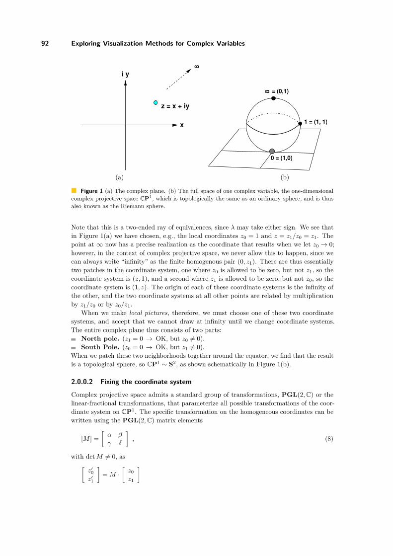
Once we have Eq. (1), we may ask immediately how we visualize a complex point. Oneapproach is that of Figure 1(a), which simply treats x and y as Cartesian variables, and soevery complex number is depicted as a point in the 2D plane. However, this does not allowus to easily treat infinity, which is a critical element in the mathematical analysis of functionsof a complex variable. Thus Figure 1(a) is only a local view of the actual manifold thatmathematicians refer to as “the complex line” because of its one-dimensional complex nature,and that physicists and engineers, for example, would refer to as the “complex plane” becauseof its two-dimensional real nature. In order to treat the space of one complex variable in away that infinity is no longer a special point, and can be included naturally in all the tasksof complex analysis, we must find a way to express coordinates on the space in a way that ismore general than simple Cartesian coordinates. The solution to this problem is to treat therepresentation of one complex variable using one-dimensional complex projective space orCP1, which is the space of pairs of complex numbers (z0, z1) that are taken to be equivalentunder multiplication by any nonvanishing complex number λ, which is to say

(z0, z1) ∼ (λz0, λz1) . (7)

Chapte r 7

92 Exploring Visualization Methods for Complex Variables

x

i y

z = x + iy

8

1 = (1, 1)

0 = (1,0)

= (0,1)8

(a) (b)

Figure 1 (a) The complex plane. (b) The full space of one complex variable, the one-dimensionalcomplex projective space CP1, which is topologically the same as an ordinary sphere, and is thusalso known as the Riemann sphere.

Note that this is a two-ended ray of equivalences, since λ may take either sign. We see thatin Figure 1(a) we have chosen, e.g., the local coordinates z0 = 1 and z = z1/z0 = z1. Thepoint at ∞ now has a precise realization as the coordinate that results when we let z0 → 0;however, in the context of complex projective space, we never allow this to happen, since wecan always write “infinity” as the finite homogenous pair (0, z1). There are thus essentiallytwo patches in the coordinate system, one where z0 is allowed to be zero, but not z1, so thecoordinate system is (z, 1), and a second where z1 is allowed to be zero, but not z0, so thecoordinate system is (1, z). The origin of each of these coordinate systems is the infinity ofthe other, and the two coordinate systems at all other points are related by multiplicationby z1/z0 or by z0/z1.

When we make local pictures, therefore, we must choose one of these two coordinatesystems, and accept that we cannot draw at infinity until we change coordinate systems.The entire complex plane thus consists of two parts:

North pole. (z1 = 0 → OK, but z0 6= 0).South Pole. (z0 = 0 → OK, but z1 6= 0).

When we patch these two neighborhoods together around the equator, we find that the resultis a topological sphere, so CP1 ∼ S2, as shown schematically in Figure 1(b).

2.0.0.2 Fixing the coordinate system

Complex projective space admits a standard group of transformations, PGL(2,C) or thelinear-fractional transformations, that parameterize all possible transformations of the coor-dinate system on CP1. The specific transformation on the homogeneous coordinates can bewritten using the PGL(2,C) matrix elements

[M ] =[α β

γ δ

], (8)

with detM 6= 0, as[z′0z′1

]= M ·

[z0z1

]


or

(z′0, z′1) = (αz0 + βz1, γz0 + δz1) , (9)

in the homogeneous, ray-equivalent coordinates, or as

z′ = αz0 + βz1

γz0 + δz1(10)

in the γz0 + δz1 6= 0 set of inhomogeneous coordinates.The group of linear fractional transformations thus has three free complex parameters

that can be used to map any three complex points in the complex plane to any chosenpoints to fix the degrees of freedom under the map. As illustrated in Figure 1(b), these areconventionally chosen in the following way:

“0” is projective (1, 0),“1” is projective (1, 1), and“∞” is projective (0, 1).

2.1 Cross Ratios and Cross-Ratio CoordinatesAn important feature of complex projective space is that there is a family of invariants underthe linear fractional transformations (9) known as the cross ratios, defined as follows:

u(w, x, y, z) = (w − y)(w − z)

/(x− y)(x− z) = (w − y)(x− z)

(w − z)(x− y) . (11)

In particular, one can verify that there are two distinct cross ratios of four variables,

u1 = u(z, z1, z0, z2) = (z − z0)(z1 − z2)(z − z2)(z1 − z0) (12)

u2 = u(z1, z2, z, z0) = (z1 − z)(z2 − z0)(z1 − z0)(z2 − z)

(13)

that are related by the constraint

1 = u1 + u2 . (14)

Since there are three remaining complex degrees of freedom in the PGL(2,C) matrix[M ] after accounting for projective equivalence, we can exhaust those degrees of freedomby choosing a coordinate system on CP1 that fixes three complex points. This fact ties inwith the definition of the group-invariant cross ratios because it allows us to fix three of thevariables in the cross ratio to be, for example, 0, 1, and ∞, thus fixing

u1 = u(z, 1, 0,∞) = z (15)u2 = u(1,∞, z, 0) = 1− z . (16)

2.1.0.3 Cross-ratio space

However, even this is not the whole story. As pointed out in ([4]), from Eq. (14) we candeduce the existence of yet another projective space, the cross-ratio space, which results fromcreating a new set of homogeneous coordinates, this time in CP2, by realizing that we mustadd a third variable, u0, to Eq. (14) to make it homogenous:

u0 = u1 + u2 . (17)

Chapte r 7


This equation can be solved projectively in three different sets of variables, corresponding tochoosing the local coordinates u0 = 1, u1 = 1, or u2 = 1, and three intervals in inhomogeneouscoordinates as A = [0, 1], B = [1,∞], and C = [−∞, 0]. The triples of variables solving theconstraint equation (17) can then be written

A(t) : [1, t, (1− t)]B(t) : [(1− t), 1, −t] (18)C(t) : [−t, (1− t), −1] .

The variables of region A solve 1 = u1 + u2 with u1 = t, B solves 1 = u1 + u2 withu1 = 1/(1− t) when all is multiplied by (1− t), and C solves 1 = u1 + u2 with u1 = (t− 1)/twhen all is multiplied by t. We note that C(1) = −A(0), so that in fact we have a doublecovering of the constraint space: the constraint equation solutions must be adjoined to theirnegatives to form a piecewise continuous curve in CP2.

This concludes our introduction to the basic concepts we need to build various visual-izations related to a single complex variable. Next we work out some examples in complexanalysis.

2.2 Visualizing a Simple PoleThe simplest example of a complex function is a constant function,

z = a+ ib.

Choosing a particular local CP1 coordinate system allows us to plot this as a point in aplane as in Figure 1(a). However, even this is not quite as simple as it looks. First we recallthat ordinary real graphs of functions are written as

y = f(x) ,

so that we use one space dimension to graph the value of the independent variable and asecond one to graph the result. Thus the correct complex analog would involve two complexvariables: z describing the value of the independent variable, and, say,

w = f(z) = Re f(z) + i Im f(z)

to describe the (complex) result of evaluating the function. Thus, we might consider thegraphing process to be described more clearly using two variables, z1 = x1 + iy1 andz2 = x2 + iy2, where

z2 = f(z1) . (19)

We can easily see how this works with the classic example of a simple pole at the origin,

1z

= x− iyx2 + y2 .

Using the two-variable form, we find that the result involves four variables, (x1, y1, x2, y2),and one complex or two real equations, so the shape described is a surface with componentsgiven by the real and imaginary parts of the following:

z2 = x2 + iy2 = 1z1

= x1 − iy1

x21 + y2

1. (20)


z0

z0

z1−

_____

x

i y = pole

(a) (b)

Figure 2 (a) Conventional picture of a complex pole f(z) = 1/(z − z0) at z0, indicating thepositive sense of a contour to pick up the residue. (b) Visualizing the geometric shape of a complexpole w = 1/z showing Re w as a function of z. The imaginary part looks basically the same.

The result must be projected from 4D to 3D to be rendered using standard graphics methods.In Figure 2, we show the location of a general pole f(z) = 1/(z − z0) using a textbook 2Dcomplex analysis plot, and then show the visualization of the complex surface correspondingto the pole using Re z2 = x2 as the third axis.

Remark: The analysis of a pole typically involves one more step, namely the descriptionof a circular contour integral surrounding the pole. From the classic theorems of complexanalysis, this integral∫

closed circle

dz

z

vanishes if the contour does not enclose the pole, and has the constant value 2πi as long asthe contour encloses the pole. The proof is trivial in polar coordinates with z = r exp(iθ):∫

circle with radius r

dz

z=∫ 2π

0

ireiθdθ

reiθ= 2πi .

2.3 Integrating with Branch CutsMoving on from simple poles, we next examine functions with multiple roots, and hencemultiple branches of the Riemann surfaces that are needed to precisely define the functions.The square root already has ample complexity to challenge our visualization technology.If we consider the contour integral of the function w =

√1− z2 along a path that passes

around z = +1, we find the standard textbook drawing in Figure 3 describing the integral∫a+b

dz√

1− z2 .

The main characteristic distinguishing a branch cut in analysis is that, while, e.g., thephase of the function changes by a full (2π) along a path going around a pole, it changes by aprecise fraction, namely 2π/n, along a path going from one side of an n-th root branch pointto the other. Thus, for example, the relative phase between the integrand on the path of the

Chapte r 7


i y

Square Root Riemann Surface

z=−1 z=+1

a

xb

Figure 3 Complex contour integral around the square-root branch point of√

1− z2 at z = +1.

a branch and the path of the b branch for the square root branch cut shown in Figure 3 is

e2πi/2 = −1 .

Here, once again, we need to go beyond conventional diagrams such as Figure 3 to createa useful visualization. One approach to functions with multiple branch points is to realizethat the Riemann surface to be displayed should not just represent a single branch, e.g.,

w = +√

1− z2 (21)

or

w = −√

1− z2 , (22)

but should represent all branches. With a little thought we can see that everything issummarized nicely in the equation

w2 + z2 = 1 . (23)

There are many different ways to plot this surface (remember, 4 real variables, with 2 realequations means it is a surface), including just using the separate pieces from Eqs. (21) and(22) directly. We typically prefer the methods introduced in ([3]), which will be describedshortly, and which recreate the entire surface from a very simple fundamental domain viacomplex phase transformations around the fixed points of the surface. The basic problemgoes back once again to the difference between homogeneous and inhomogeneous coordinates:we should really be looking at Eq. (23) as a homogeneous equation in CP2 of the form

z 20 + z 2

1 + z 22 = 0 . (24)

Choosing any one of the CP2 variables (z0, z1, z2) to be a constant (z0 = i is just as goodas z0 = 1) gives a partial shape that does not include infinity (where the constant variablevanishes, e.g., z0 → 0). Thus we are left with holes in the surface that are represented asrings that go off to infinity when we plot the surface using a local pair of inhomogeneousvariables as in Figure 4. The square root branch points and cuts can be explicitly seen inthe projection of Figure 4 as the ending points of the X-shaped crossings.

2.4 Visualizations of Homogeneous Polynomials in CP2

The square root Riemann surface is a special case of a general family of polynomials thatare of interest. Here we review the properties and visualization methods for the simplest


Figure 4 Assorted views of the full square-root Riemann surface with Re w projected to the 3rdaxis. The surface is a topological sphere, but the local inhomogeneous coordinates obscure thatfact since there are two rings going off to the surface at infinity. The inner ends of the X-shapedcrossings are the branch points.

homogeneous polynomials that arise in the study of CP2. Starting from the n-th root of apolynomial of one complex variable with zeros at the n roots of unity, that is

w = (1− zn)1/n (25)

and following the same procedure as for the square root, we arrive at the correspondinghomogeneous polynomial in CP2:

z n0 + z n

1 + z n2 = 0 . (26)

As we have noted, there are a variety ways to solve this equation, including:n roots: Set z n

0 = −1 and solve for the n roots of (1 − zn)1/n (which are found bymultiplying by a phase exp(2πik/n), k = 0, . . . , n− 1).Spinor variables: Parameterize the solution using the variables typically used to definenull spinors, w 2

0 + w 21 + w 2

2 = 0 ([1]):z0 =

(i(x2 + y2)

)2/n

z1 =(x2 − y2)2/n

z2 = (2xy)2/n.

Because of the projective equivalence, only n2 of the n3 phase choices available here aremeaningful.n2 roots: In the method of ([3]), the relative phases of n2 different congruent patchestie together to create the full topological surface, where the obvious locations of thefixed points of the z1 and z2 phase transformations expose many key features of thesurface. The method starts as before by setting z n

0 = −1. Then we exploit the complextrigonometric identity

cos(θ + iξ)2 + sin(θ + iξ)2 = 1

to define one patch, the fundamental domain, as the quadrant where θ gives a positivereal part for cos and sin, namely 0 ≤ θ ≤ π/2 and −ξmax ≤ ξ ≤ +ξmax. Thus the firstand most elementary of the n2 patches is

w1 = (cos(θ + iξ))2/n

w2 = (sin(θ + iξ))2/n.

The remaining patches are found by making phase transformations on both z1 and z2until the entire surface is covered; all the patches are then labeled by the n2 integer pairs

Chapte r 7


Figure 5 n = 3 in CP2: The cubic is atorus.

Figure 6 n = 4 in CP2: The quartic is asection of the K3 surface, a 4-manifold.

(k1, k2), where k1 = 0, . . . , n− 1, k2 = 0, . . . , n− 1, and the parametric solutions of theequations become

z1 = exp(2πik1/n)w1

z2 = exp(2πik2/n)w2 .

Typical results are shown in the Figures as follows:Cubic Torus. The cubic is topologically a torus (genus 1), though it is hard to see dueto the infinities in local coordinates. It is also technically the standard polynomial inCP2 that is a Calabi-Yau space. See Figure 5.Slice of K3 Quartic. K3 is described by the quartic polynomial of complex dimension2 (4 real dimensions) in CP3. This is the unique simply-connected Calabi-Yau 4-manifold,and we can write the equation locally as

(z1)4 + (z2)4 + (z3)4 = 1 . (27)

This is one complex constraint in 3D complex space, and thus is a manifold with 2complex, 4 real, dimensions. Setting, e.g., z3 = 0, gives a slice that is a surface in CP2

with genus 3. See Figure 6.Slice of Calabi-Yau Quintic. It is hypothesized that 10-dimensional string theoryincludes 4 dimensions of space-time and 6 dimensions that are curled up into a Calabi-Yauspace at the scale of the Planck length. A popular (but by no means unique) candidatefor this space is the quintic in CP4 given locally by the equation

(z1)5 + (z2)5 + (z3)5 + (z4)5 = 1 . (28)

This is one complex constraint in 4D complex space, and thus is a manifold with 3complex, 6 real, dimensions. Setting, e.g., z3 = z4 = 0, gives a slice that is a surface inCP2 with genus 6. See Figure 7.

In general, it can be shown that every homogeneous polynomial of degree N + 1 in CPN

is in fact a Calabi-Yau space and therefore admits a Ricci-Flat metric. Calabi conjecturedand Yau proved the existence of these metrics ([8]), but, except for trivial cases such as theCP2 cubic torus, none are explicitly known. In Table 1, we summarize this family of spaces.


Figure 7 n = 5 in CP2: The quintic is a section of the Calabi-Yau quintic, the 6-manifoldproposed for the hidden dimensions of string theory.

Table 1 Road map of the simple homogeneous polynomial Calabi-Yau spaces.

N CP deg(f) C dim R dim Remarks

1 CP1 2 0 0 z = ±1, the 0-sphere S0

2 CP2 3 1 2 flat torus T2

3 CP3 4 2 4 K3 surface4 CP4 5 3 6 CY String Theory quinticN CPN N+1 N-1 2(N-1) Solution of

N∑i=1

(zi)N+1 = 1

Chapte r 7


0

u + v

10

u

vr

Figure 8 The Euler Beta Function has this remarkable unshrinkable contour representation dueto Pochhammer.

Figure 9 When u + v = 0,−1, . . ., deformation through ∞ has no obstruction: one can simplyunloop the contour and pass through the [0, 1] branch line, resulting in a contour that shrinks tozero.

2.5 Visualizing Infinite Riemann Surfaces: the Pochhammer ContourThe next challenge is to consider the problems of visualizing complex functions that, unlikethe square root and its analogs, may have infinite Riemann surfaces. There is a classicexample from the 19th century that provides all the features relevant to this problem. TheEuler Beta Function can be represented as the improper integral

B(u, v) =∫ 1

0xu−1(1− x)v−1 dx (29)

with the analytic continuation

B(u, v) = Γ(u)Γ(v)Γ(u+ v) . (30)

Now, if one considers the integrand of Eq. (29) as a branched complex function zu−1(1−z)v−1

defining a Riemann surface, one finds branch points at z = 0 and at z = 1 with possiblyinfinite branchings if u or v should be irrational. However, in 1890 Pochhammer was cleverenough to see this not as a problem but as an opportunity to define a new kind of contourintegral that was not sensitive to infinite branchings ([5]). In Figure 8 we show the usualplanar sketch of Pochhammer’s Contour, from which a little analysis allows us to computeits value as

ε(u, v) = (1− e2πiu)(1− e2πiv)∫ 1

0xu−1(1− x)v−1 dx (31)

= (1− e2πiu)(1− e2πiv)B(u, v) . (32)


-0.50

0.51

1.5

x

-0.5-0.25

00.25

0.5i y

-1

-0.5

0

0.5

1

Re@wD

-0.5-0.25

00.25

0.5

-1

-0.5

0

0.5

Figure 10 Sample Riemann surface forthe B4 integrand – multiple branch cover-ings spiral to infinity.

-0.50

0.51

1.5

x

-0.4-0.2

00.20.4i y

-1

-0.5

0

0.5

1

Re@wD

-0.50

0.51

1.5

Figure 11 The corresponding embeddedPochhammer contour is a commutator , en-circling each branch point twice.

Through an interesting trick of complex analysis, one can determine the zeroes of thefunction directly to occur when u+ v = 0,−1, . . .: at these values, the contour can be “pulledover” the point at infinity as shown in Figure 9 and deformed to an equivalent vanishingloop. These zeroes can be confirmed explicitly from the analytic continuation Eq. (30).

Finally, we can explicitly create a function representing the Riemann surface of the EulerBeta function integrand.

β(z; u, v) = zu−1(1− z)v−1 (33)

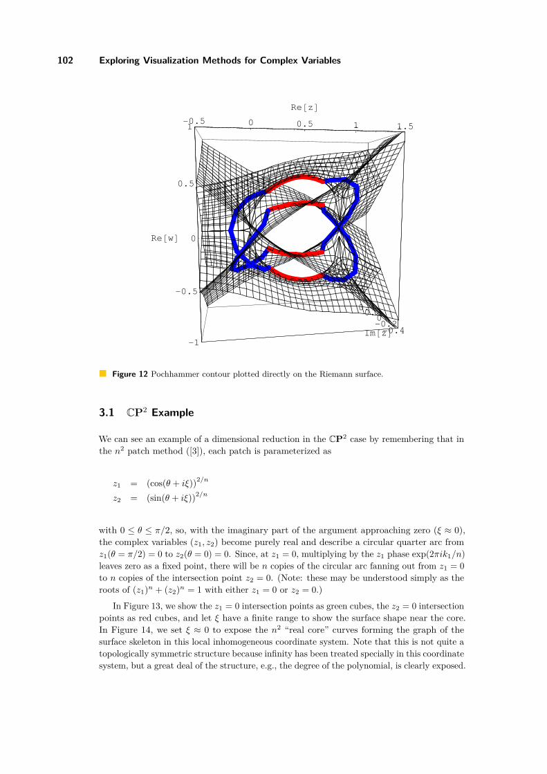
and create a 3D projection with, e.g., the vertical axis given by Reβ(z; u, v). Figures 10 and11 show a section of a branched covering that could in principle spiral indefinitely, alongwith the closed Pochhammer loop that can be traced on the Riemann surface, no matterhow complex. Figure 12 superimposes these on the same space to illustrate the context.

3 Extending CP2 Visualization Methods to CP3

Our next objective is to see how we can create some basic images of the K3 surface that givemore global information than the 2D slice representation that we saw in Figure 6. We recallthat K3 can be represented in general as a homogeneous quartic polynomial in CP3 in theform

z 40 + z 4

1 + z 42 + +z 4

3 = 0 , (34)

which reduces after division by z0 6= 0 (or equivalently, after division by z1, z2, or z3) to Eq.(27). Even though this is a 4-manifold (after division, 6 real variables and two real constraintequations), we can pick out some of its global, non-slicing, properties by considering whatamounts to the “real subspace” of the parameterization.

Chapte r 7


-0.5 0 0.5 1 1.5

Re@zD

-0.4-0.20

0.20.4

Im@zD

-1

-0.5

0

0.5

1

Re@wD

0 0.5 1 1.5

@ D

Figure 12 Pochhammer contour plotted directly on the Riemann surface.

3.1 CP2 Example

We can see an example of a dimensional reduction in the CP2 case by remembering that inthe n2 patch method ([3]), each patch is parameterized as

z1 = (cos(θ + iξ))2/n

z2 = (sin(θ + iξ))2/n

with 0 ≤ θ ≤ π/2, so, with the imaginary part of the argument approaching zero (ξ ≈ 0),the complex variables (z1, z2) become purely real and describe a circular quarter arc fromz1(θ = π/2) = 0 to z2(θ = 0) = 0. Since, at z1 = 0, multiplying by the z1 phase exp(2πik1/n)leaves zero as a fixed point, there will be n copies of the circular arc fanning out from z1 = 0to n copies of the intersection point z2 = 0. (Note: these may be understood simply as theroots of (z1)n + (z2)n = 1 with either z1 = 0 or z2 = 0.)

In Figure 13, we show the z1 = 0 intersection points as green cubes, the z2 = 0 intersectionpoints as red cubes, and let ξ have a finite range to show the surface shape near the core.In Figure 14, we set ξ ≈ 0 to expose the n2 “real core” curves forming the graph of thesurface skeleton in this local inhomogeneous coordinate system. Note that this is not quite atopologically symmetric structure because infinity has been treated specially in this coordinatesystem, but a great deal of the structure, e.g., the degree of the polynomial, is clearly exposed.


Figure 13 Left: n = 3 cubic. Right: n = 4 quartic. Red and Green points represented as smallcubes indicate where the zeros of z1 and z2 pass through the surface; each of z2 = 0 Red points isconnected to all n copies of the z1 = 0 Green points, and vice versa, through the “real” central lineof each of the n2 patches.

Figure 14 Shrinking the complex extent of the surface parameterization so that only the “realcore” curves remain shows a connected graph of n2 arcs connecting the 2n nodes.

3.2 The K3 “Real Core”The representation of the K3 surface as a fourth-degree homogeneous polynomial in CP3,like the general case of the CP2 polynomials described earlier, can be solved in a variety ofways. Here we will focus on generalizing the n2 patch method ([3]) to CP3, which turns outto lead naturally to n3 patches of dimension 4 (and for CPN , to nN patches of dimension2(N − 1)). Thus the basic equation for which we seek a 4-parameter parametric form is

(z1)4 + (z2)4 + (z3)4 = 1 . (35)

Following the complexified circle ( S1) method used for CP2, we arrive at a 4-manifoldparameterization based on the complexified sphere S2, namely

(cos θ sinφ, sin θ sinφ, cosφ) (36)

with 0 ≤ φ ≤ π, 0 ≤ θ < 2π. For the full 4D patch, we would complexify the angularvariables as θ → θ + iξ, φ → φ + iρ to get exponential growth towards infinity. To retainthe “real skeleton” surface analogous to the network of edges shown in Figure 14 for CP2

polynomials, all we need to do is recast the real equation (36) in the form

w1 = (cos θ sinφ)2/n

w2 = (sin θ sinφ)2/n

w3 = (cosφ)2/n,

Chapte r 7


-1

-0.5

0

-1

-0.5

0

-1

-0.5

0

0.5

1

-1

-0.5

0

-1

-0.5

0

0.5

Figure 15 The “real core” of the quartic K3 Calabi-Yau space, delimited by 43 = 64 sphericaltriangles. Each spherical triangle is bounded by the intersections of the zeros of the three localcomplex variables with the K3 surface (a 4-manifold).

with n = 4 selecting the K3 fundamental domain (2/n = 2/4 = 1/2 so each term is a squareroot). The remaining patches are found by making phase transformations on (z1, z2, z3)until the entire surface is covered; all the patches are then labeled by the n3 = 64 integers(k1, k2, k3), where ki = 0, 1, 2, 3 and the parametric solutions of the equations become

z1 = exp(2πik1/4)w1

z2 = exp(2πik2/4)w2

z3 = exp(2πik3/4)w3 .

The result is a collection of octants of the sphere, spherical triangles that fan out four at atime from the curves where z1 = 0, z2 = 0, and z3 = 0 intersect the manifold. The resultis depicted in Figure 15, where part of the shape is cut away so that the interior “fanningout” is made visible. We remark that just as Figure 14 appears to have non-manifold tripleor quadruple intersections, but in fact, when complexified, yields the smoothed continuoussurface of Figure 13, we need to imagine that in 4D, Figure 15 also extends completelysmoothly away from the 4-way fan-out junctions.

3.2.0.4 Regular global tessellations

The representations shown here are local and are limited in their effectiveness for exposingthe overall topology of the polynomials in CP2 and CP3, etc. Extending these limitedlocal representations to global tessellations with maximal symmetries is a subject of ongoingresearch.


4 Two Complex Variables and the Dodecahedron

Finally, we review our approach to creating visualizations for problems arising in many-complex-variable analysis, outlining the two-complex-variable case as our main example ([4]).We begin with the N -particle bosonic scattering amplitude of the original dual model, theprecursor to string theory, which is given by the integral

BN =∫· · ·∫

vol

∏ij

uαij−1

ij

∏k

du1k

(1− u14) · · · (1− u1,N−1)

The N -point cross-ratios uij obey a set of constraints that is non-linear except for the4-particle case B4, which in fact is the Euler Beta function treated earlier:

uij = 1−j−1∏

m=i+1

i−1∏n=j+1

umn .

These constraints define manifolds in CPN(N−3)/2 that provide new insight into the natureof the analytic continuation of these integrals.

The N = 5 case is the simplest non-trivial example that we can work out explicitly; thecorresponding improper integral is two-dimensional,

B5(α1, α2, α3, α4, α5) =

=∫ 1

0

∫ 1

0sα1−1tα2−1(1− s)α3−1(1− st)α4−α3−α5(1− t)α5−1 ds dt

=∫ ∫

(z1)α1−1(z2)α2−1(z3)α3−1(z4)α4−1(z5)α5−1 ds dt/(1− st) , (37)

and thus must eventually be treated using two complex variables.The B5 cross-ratio constraints are quadratic,

1− z1 − z3z4 = 01− z2 − z4z5 = 01− z3 − z5z1 = 0 (38)1− z4 − z1z2 = 01− z5 − z2z3 = 0 ,

and, in these variables, there are twelve different possible integration domains of Eq. (37)that we can initially represent as in Figure 16. Using CP5 cross-ratio variables, we wouldproperly represent these equations as z 2

0 − z0z1 − z3z4 = 0, etc., but we will omit the detailshere.

Each individual region, when plotted using Eq. (38), is not simply a square or triangle asone might guess from the Cartesian variable plot in Figure 16, but is actually a pentagon, asshown in Figure 17

The resulting figure is a “blown-up” dodecahedral manifold formed from twelve pentagons,but this dodecahedron, shown in Figure 18, is quite different topologically from the familiarPlatonic dodecahedron, and in fact has Euler characteristic χ = −3, so it is a surface

Chapte r 7


1

4

1112

5 10

92

6

7

3

8

s =

t

s = 0 s = 1

s =

t

t = 1

t = 0

Figure 16 The 12 connected components of the domain of parameters for the set of 5-pointcross-ratios.

0

0.25

0.5

0.75

1

x

0

0.25

0.5

0.75

1

y

0

0.25

0.5

0.75

1

u

0

0.25

0.5

0.75

1

x

0

0.25

0.5

0.75

Figure 17 A direct plot of the solu-tions (e.g., (x, (1 − x)/(1 − xy), y)) shows“stretched” limits turning squares or trian-gles in (s, t) coordinates into pentagons in[z1, z2, z3, z4, z5]-space.

15

15

12

1

14 14

1414

13 6

613

2

2

3

3

7

7

4

49

9

5

5

10 10

11

15

15

11

8

8

6

7

2 9

101

5

12 11

8

3

4

Figure 18 The 12 B5 connected compo-nents without singularities.


15

15

12

1

14 14

1414

13 6

613

2

2

3

3

7

7

4

49

9

5

5

10 10

11

15

15

11

8

8

6

7

2 9

101

5

12 11

8

3

4

α4 α3

’α3’α4

α2

’α2

’α1

’α5

α5

α1

1

2

3

4

5

6

7

8

9

10

1

2

3

4

5

6

7

8

9

10

11

12

15

13

11

12

13

15

12

12

1414

11

1313

15

15

11

14

14

(a) (b)

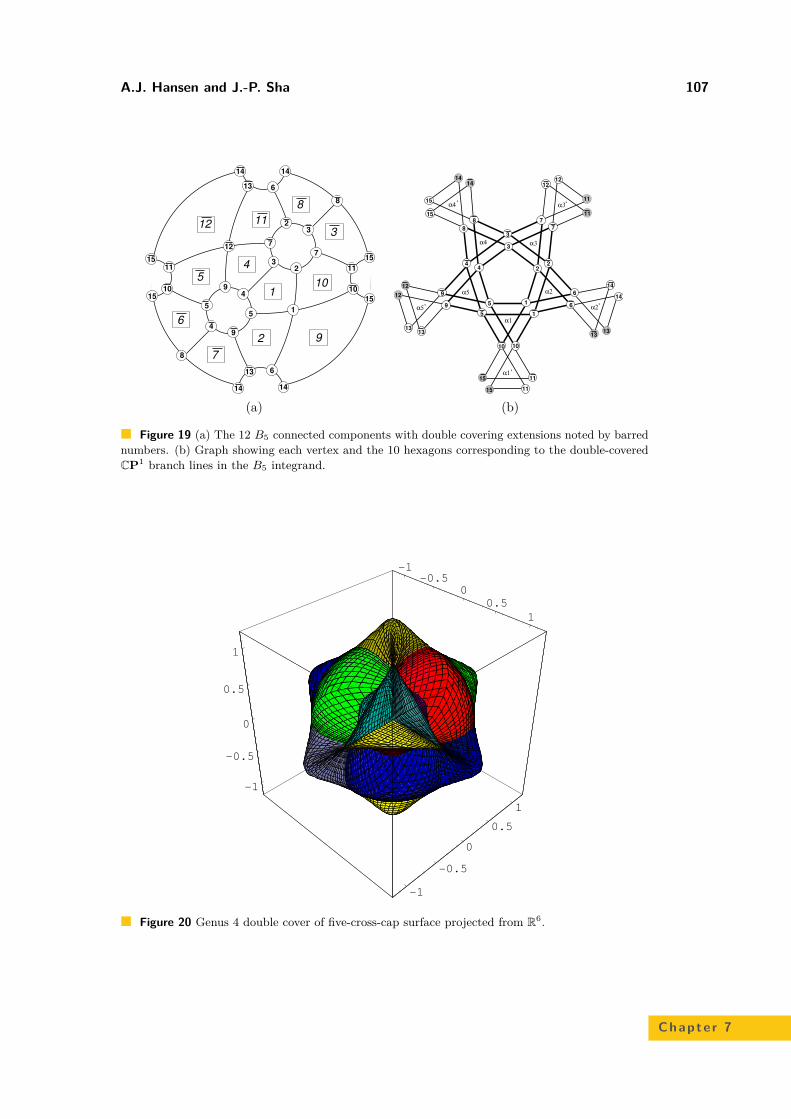
Figure 19 (a) The 12 B5 connected components with double covering extensions noted by barrednumbers. (b) Graph showing each vertex and the 10 hexagons corresponding to the double-coveredCP1 branch lines in the B5 integrand.

-1

-0.5

0

0.5

1

-1

-0.5

0

0.5

1

-1

-0.5

0

0.5

1

Figure 20 Genus 4 double cover of five-cross-cap surface projected from R6.

Chapte r 7


Figure 21 Projected embedding of the five-cross-cap surface itself.

corresponding to a sphere with five cross-caps. Figure 19 shows the solutions of the cross-ratio constraints, which double cover the five-cross-cap surface, and Figure 20 finally showsthe visualization of the full double-covered surface embedded in R6. Creating an identifiedembedding of the five cross-cap surface itself (the single cover, not the double cover) employingthe methods of ([4]) leads to the example image in Figure 21.

Much remains to be done to create further informative visualizations of these families ofsurfaces.

5 Discussion and Remarks

We have reviewed a family of basic problems in the complex analysis of one and manyvariables, and presented visualizations of a number of the manifolds that naturally arise. Anew method, the use of cross-ratio variables instead of the expected CPN variables for theanalysis of N complex variables, shows promise and is essential for the treatment of certainN -dimensional integrals. Among the surprising and unexpected aspects of this investigationwas the discovery of a relationship to a family of objects known as the Stasheff associahedra([7, 6, 2]). The explicit geometric embeddings that we discovered as part of our explicitgraphics-oriented approach are in fact new geometric realizations of these topological objects.

Complex analysis is a fertile proving ground for developing and testing mathematicalvisualization methods. Here we have reviewed a variety of basic approaches that can beused for visualization in complex analysis, focusing on several families of complex algebraicequations and their geometry. Much remains to be done.

Acknowledgments

This research was supported in part by NSF grant numbers CCR-0204112 and IIS-0430730.Our thanks to Philip Chi-Wing Fu and Sidharth Thakur for assistance with graphics tools.


References

1 Élie Cartan. The Theory of Spinors. Dover, New York, 1981.2 Satyan L. Devadoss. Tessellations of moduli spaces and the mosaic operad. In Homotopy in-

variant algebraic structures. (Baltimore, MD, 1998), volume 239, pages 91–114, Providence,RI, 1999. Amer. Math. Soc.

3 A.J. Hanson. A construction for computer visualization of certain complex curves. Noticesof the Amer.Math.Soc., 41(9):1156–1163, November/December 1994.

4 Andrew J. Hanson and Ji-Ping Sha. A contour integral representation for the dual five-pointfunction and a symmetry of the genus four surface in R6. Journal of Physics A: Mathematicsand General, 39:2509–2537, 2006. Web version at http://www.iop.org/EJ/abstract/0305-4470/39/10/017/ or on the arXiv at http://arxiv.org/abs/math-ph/0510064.

5 L.A. Pochhammer. Zur theorie der Euler’schen integrale. Math. Ann., 35:495–526, 1890.6 James Stasheff. Homotopy associativity of H-spaces. Trans. Amer. Math. Soc., 108:275–292,

1963.7 James Stasheff. H-spaces from a Homotopy Point of View. Lecture Notes in Mathematics

161. Springer Verlag, New York, 1970.8 S.-T. Yau. On the Ricci curvature of a compact Kähler manifold and the complex Monge-

Ampere equation. Commun. Pure and Appl. Math., 31:339–411, 1978.

Chapte r 7

exploringvisualizationmethodsforcomplex variables...

Documents