Improving and Extending the Testing ofDistributions for Shape-Restricted PropertiesEldar Fischer1, Oded Lachish2, and Yadu Vasudev∗3

1 Faculty of Computer Science, Israel Institute of Technology (Technion), Haifa,Israeleldar@cs.technion.ac.il

2 Birkbeck, University of London, London, UKoded@dcs.bbk.ac.uk

3 Fakultät für Informatik, TU Dortmund, Dortmund, Germanyyaduvasudev@gmail.com

AbstractDistribution testing deals with what information can be deduced about an unknown distributionover 1, . . . , n, where the algorithm is only allowed to obtain a relatively small number ofindependent samples from the distribution. In the extended conditional sampling model, thealgorithm is also allowed to obtain samples from the restriction of the original distribution onsubsets of 1, . . . , n.

In 2015, Canonne, Diakonikolas, Gouleakis and Rubinfeld unified several previous results,and showed that for any property of distributions satisfying a “decomposability” criterion, thereexists an algorithm (in the basic model) that can distinguish with high probability distributionssatisfying the property from distributions that are far from it in variation distance.

We present here a more efficient yet simpler algorithm for the basic model, as well as veryefficient algorithms for the conditional model, which until now was not investigated under theumbrella of decomposable properties. Additionally, we provide an algorithm for the conditionalmodel that handles a much larger class of properties.

Our core mechanism is a way of efficiently producing an interval-partition of 1, . . . , n thatsatisfies a “fine-grain” quality. We show that with such a partition at hand we can directly moveforward with testing individual intervals, instead of first searching for the “correct” partition of1, . . . , n.

1998 ACM Subject Classification F.2.2 Nonnumerical Algorithms and Problems, G.3 Probabil-ity and Statistics

Keywords and phrases conditional sampling, distribution testing, property testing, statistics

Digital Object Identifier 10.4230/LIPIcs.STACS.2017.31

1 Introduction

1.1 Historical backgroundIn most computational problems that arise from modeling real-world situations, we arerequired to analyze large amounts of data to decide if it satisfies a fixed property. Theamount of data involved is usually too large for reading it in its entirety, both with respectto time and storage. In such situations, it is natural to ask for algorithms that can sample

∗ This work was done when the author was a postdoctoral fellow at Israel Institute of Technology(Technion), Haifa, Israel.

© Eldar Fischer, Oded Lachish, and Yadu Vasudev;licensed under Creative Commons License CC-BY

34th Symposium on Theoretical Aspects of Computer Science (STACS 2017).Editors: Heribert Vollmer and Brigitte Vallée; Article No. 31; pp. 31:1–31:14

Leibniz International Proceedings in InformaticsSchloss Dagstuhl – Leibniz-Zentrum für Informatik, Dagstuhl Publishing, Germany

31:2 Improving and Extending the Testing of Distributions for Shape-Restricted Properties

points from the data and obtain a significant estimate for the property of interest. The areaof property testing addresses this issue by studying algorithms that look at a small part ofthe data, and then decide if the object that generated the data has the property or is far(according to some metric) from having the property.

There has been a long line of research, especially in statistics, where the underlying objectfrom which we obtain the data is modeled as a probability distribution. Here the algorithmis only allowed to ask for independent samples from the distribution, and has to base itsdecision on them. If the support of the underlying probability distribution is large, it is notpractical to approximate the entire distribution. Thus, it is natural to study this problem inthe context of property testing.

The specific sub-area of property testing that is dedicated to the study of distributions iscalled distribution testing. There, the input is a probability distribution (in this paper thedomain is the set 1, 2, . . . , n) and the objective is to distinguish whether the distributionhas a certain property, such as uniformity or monotonicity, or is far in `1 distance from it.See [7] for a survey about the realm of distribution testing.

Testing properties of distributions was studied by Batu et al. in [5], where they gavea sublinear query algorithm for testing closeness of distributions supported over the set1, 2, . . . , n. They extended the idea of collision counting, which was implicitly used foruniformity testing in the work of Goldreich and Ron ([15]). Consequently, various propertiesof probability distributions were studied, like testing identity with a known distribution([4, 19, 2, 12]), testing independence of a distribution over a product space ([4, 2]), andtesting k-wise independence ([3]).

In recent years, distribution testing has been extended beyond the classical model. A newmodel called the conditional sampling model was introduced. It first appeared independentlyin [9] and [10]. In the conditional sampling model, the algorithm queries the input distributionµ with a set S ⊆ 1, 2, . . . , n, and gets an index sampled according to µ conditioned on theset S. Notice that if S = 1, 2, . . . , n, then this is exactly like in the standard model. Theconditional sampling model allows adaptive querying of µ, since we can choose the set Sbased on the indexes sampled until now. Chakraborty et al. ([10]) and Canonne et al. ([9])showed that testing uniformity can be done with a number of queries not depending onn (the latter presenting an optimal test), and investigated the testing of other propertiesof distributions. In [10], it is also shown that uniformity can be tested with poly(logn)conditional samples by a non-adaptive algorithm. In this work, we study distribution testingin the standard (unconditional) sampling model, as well as in the conditional model.

A line of work which is central to our paper, is the testing of distributions for structure.The objective is to test whether a given distribution has some structural properties likebeing monotone ([6]), being a k-histogram ([16, 12]), or being log-concave ([2]). Canonne etal. ([8]) unified these results to show that if a property of distributions has certain structuralcharacteristics, then membership in the property can be tested efficiently using samples fromthe distribution. More precisely, they introduced the notion of L-decomposable distributionsas a way to unify various algorithms for testing distributions for structure. Informally,an L-decomposable distribution µ supported over 1, 2, . . . , n is one that has an intervalpartition I of 1, 2, . . . , n of size bounded by L, such that for every interval I, either theweight of µ on it is small or the distribution over the interval is close to uniform. A propertyC of distributions is L-decomposable if every distribution µ ∈ C is L-decomposable (L isallowed to depend on n). This generalizes various properties of distributions like beingmonotone, unimodal, log-concave etc. In this setting, their result for a set of distributionsC supported over 1, 2, . . . , n translates to the following: if every distribution µ from C is

E. Fischer, O. Lachish, and Y. Vasudev 31:3

L-decomposable, then there is an efficient algorithm for testing whether a given distributionbelongs to the property C.

To achieve their results, Canonne et al. ([8]) show that if a distribution µ supportedover [n] is L-decomposable, then it is O(L logn)-decomposable where the intervals are ofthe form [j2i + 1, (j + 1)2i]. This presents a natural approach of computing the intervalpartition in a recursive manner, by bisecting an interval if it has a large probability weightand is not close to uniform. Once they get an interval partition, they learn the “flattening”of the distribution over this partition, and check if this distribution is close to the propertyC. The term “flattening” refers to the distribution resulting from making µ conditionedon any interval of the partition to be uniform. When applied to a partition correspondingto a decomposition of the distribution, the learned flattening is also close to the originaldistribution. Because of this, in the case where there is a promise that µ is L-decomposable,the above can be viewed as a learning algorithm, where they obtain an explicit distributionthat is close to µ. Without the promise it can be viewed as an agnostic learning algorithm.For further elaboration of this connection see [11].

1.2 Results and techniquesIn this paper, we extend the body of knowledge about testing L-decomposable properties. Weimprove upon the previously known bound on the sample complexity, and give much betterbounds when conditional samples are allowed. Additionally, for the conditional model, weprovide a test for a broader family of properties, that we call atlas-characterizable properties.Atlas-characterizable properties include the family of symmetric properties, of which a subsetis studied in [20] in the unconditional context, and [10] studies them in the conditional model.

Our approach differs from that of [8] in the manner in which we obtain the intervalpartition. We show that a partition where most intervals that are not singletons havesmall probability weight is sufficient to learn the distribution µ, even though it is not theoriginal L-decomposition of µ. We show that if a distribution µ is L-decomposable, then the“flattening” of µ with respect to this partition is close to µ. It turns out that such a partitioncan be obtained in “one shot” without resorting to a recursive search procedure.

We obtain a partition as above using a method of partition pulling that we develophere. Informally, a pulled partition is obtained by sampling indexes from µ, and taking thepartition induced by the samples in the following way: each sampled index is a singletoninterval, and the rest of the partition is composed of the maximal intervals between sampledindexes. Apart from the obvious simplicity of this procedure, it also has the advantage ofproviding a partition with a significantly smaller number of intervals, linear in L for a fixedε, and with no dependency on n unless L itself depends on it. This makes our algorithmmore efficient in query complexity than the one of [8] in the unconditional sampling model,and leads to a dramatically small sampling complexity in the (adaptive) conditional model.

Another feature of the partition pulling method is that it provides a partition with smallweight intervals also when the distribution is not L-decomposable. This allows us to use thepartition in a different manner later on, in the algorithm for testing atlas-characterizableproperties using conditional samples.

The main common ground between our approach for L-decomposable properties andthat of [8] is the method of testing by implicit learning, as defined formally in [13] (see[18]). In particular, the results also provide a means to learn a distribution close to µ if µsatisfies the tested property. We also provide a test under the conditional query model for theextended class of atlas-characterizable properties that we define below, which generalizes bothdecomposable and symmetric properties. A learning algorithm for this class is not provided;only an “atlas” of the input distribution rather than the distribution itself is learned.

STACS 2017

31:4 Improving and Extending the Testing of Distributions for Shape-Restricted Properties

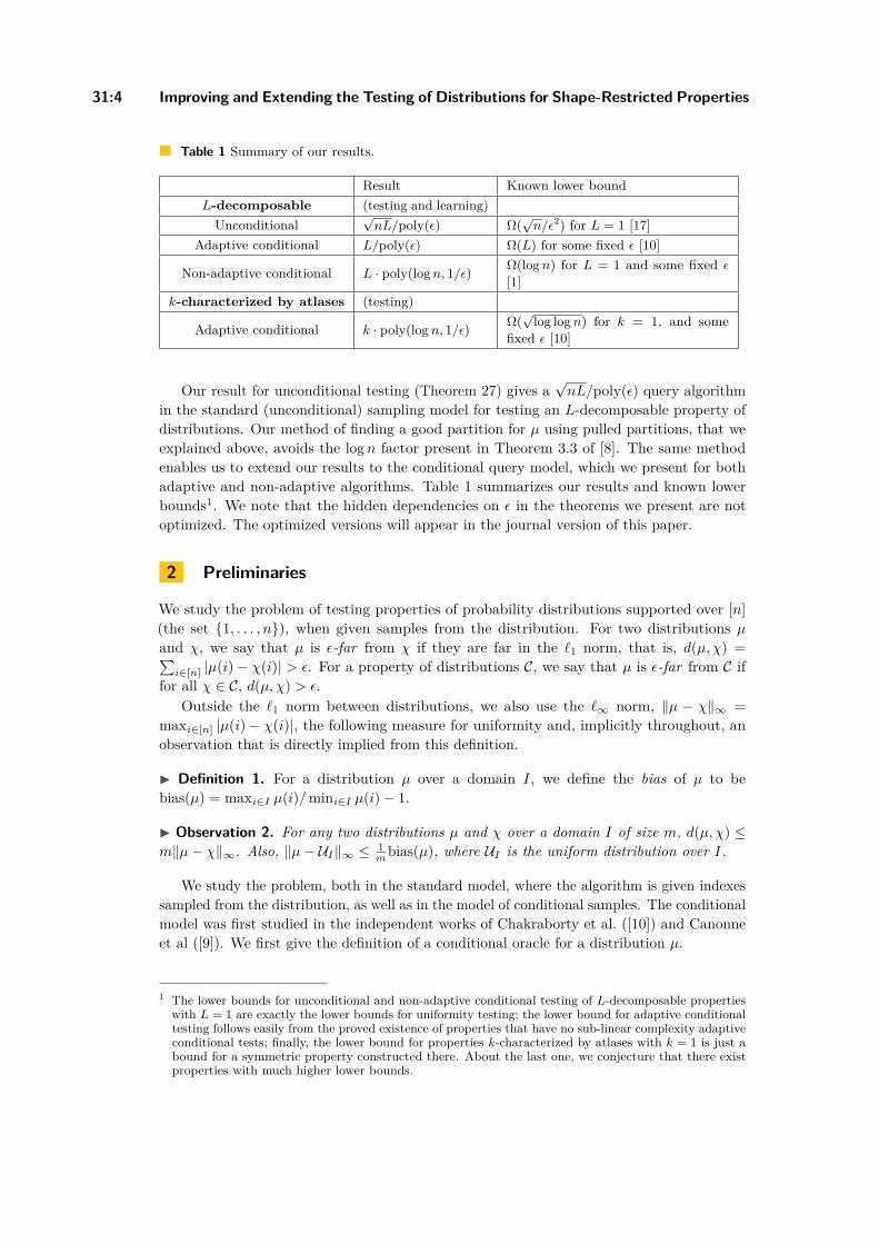
Table 1 Summary of our results.

Result Known lower boundL-decomposable (testing and learning)Unconditional

√nL/poly(ε) Ω(

√n/ε2) for L = 1 [17]

Adaptive conditional L/poly(ε) Ω(L) for some fixed ε [10]

Non-adaptive conditional L · poly(logn, 1/ε) Ω(logn) for L = 1 and some fixed ε

[1]k-characterized by atlases (testing)

Adaptive conditional k · poly(logn, 1/ε) Ω(√

log logn) for k = 1, and somefixed ε [10]

Our result for unconditional testing (Theorem 27) gives a√nL/poly(ε) query algorithm

in the standard (unconditional) sampling model for testing an L-decomposable property ofdistributions. Our method of finding a good partition for µ using pulled partitions, that weexplained above, avoids the logn factor present in Theorem 3.3 of [8]. The same methodenables us to extend our results to the conditional query model, which we present for bothadaptive and non-adaptive algorithms. Table 1 summarizes our results and known lowerbounds1. We note that the hidden dependencies on ε in the theorems we present are notoptimized. The optimized versions will appear in the journal version of this paper.

2 Preliminaries

We study the problem of testing properties of probability distributions supported over [n](the set 1, . . . , n), when given samples from the distribution. For two distributions µand χ, we say that µ is ε-far from χ if they are far in the `1 norm, that is, d(µ, χ) =∑i∈[n] |µ(i)− χ(i)| > ε. For a property of distributions C, we say that µ is ε-far from C if

for all χ ∈ C, d(µ, χ) > ε.Outside the `1 norm between distributions, we also use the `∞ norm, ‖µ − χ‖∞ =

maxi∈[n] |µ(i)− χ(i)|, the following measure for uniformity and, implicitly throughout, anobservation that is directly implied from this definition.

I Definition 1. For a distribution µ over a domain I, we define the bias of µ to bebias(µ) = maxi∈I µ(i)/mini∈I µ(i)− 1.

I Observation 2. For any two distributions µ and χ over a domain I of size m, d(µ, χ) ≤m‖µ− χ‖∞. Also, ‖µ− UI‖∞ ≤ 1

mbias(µ), where UI is the uniform distribution over I.

We study the problem, both in the standard model, where the algorithm is given indexessampled from the distribution, as well as in the model of conditional samples. The conditionalmodel was first studied in the independent works of Chakraborty et al. ([10]) and Canonneet al ([9]). We first give the definition of a conditional oracle for a distribution µ.

1 The lower bounds for unconditional and non-adaptive conditional testing of L-decomposable propertieswith L = 1 are exactly the lower bounds for uniformity testing; the lower bound for adaptive conditionaltesting follows easily from the proved existence of properties that have no sub-linear complexity adaptiveconditional tests; finally, the lower bound for properties k-characterized by atlases with k = 1 is just abound for a symmetric property constructed there. About the last one, we conjecture that there existproperties with much higher lower bounds.

E. Fischer, O. Lachish, and Y. Vasudev 31:5

Input: Distribution µ supported over [n], parameters η > 0 (fineness) and δ > 0 (errorprobability)

1 Take m = 3η log

(3ηδ

)unconditional samples from µ

2 Arrange the indices sampled in increasing order i1 < i2 < · · · < ir without repetitionand set i0 = 0

3 for each j ∈ [r] do4 if ij > ij−1 + 1 then add the interval ij−1 + 1, . . . , ij − 1 to I;5 Add the singleton interval ij to I6 if ir < n then add the interval ir + 1, . . . , n to I;7 return I

Algorithm 1: Pulling an η-fine partition.

I Definition 3 (conditional oracle). A conditional oracle to a distribution µ supported over[n] is a black-box that takes as input a set A ⊆ [n], samples a point i ∈ A with probabilityµ(i)/

∑j∈A µ(j), and returns i. If

∑j∈A µ(j) = 0, then it chooses i ∈ A uniformly at random.

I Remark. The behaviour of the conditional oracle on sets A with µ(A) = 0 is as per themodel of Chakraborty et al. [10]. However, upper bounds in this model also hold in themodel of Canonne et al. [9], and most lower bounds can be easily converted to it.

Now we define adaptive conditional distribution testing algorithms. The definition oftheir non-adaptive version, which we will also analyze, appears in [14].

I Definition 4. An adaptive conditional distribution testing algorithm for a property ofdistributions C, with parameters ε, δ > 0, and n ∈ N, with query complexity q(ε, δ, n), isa randomized algorithm with access to a conditional oracle of a distribution µ with thefollowing properties:

For each i ∈ [q], at the ith phase, the algorithm generates a set Ai ⊆ [n], based onj1, j2, · · · , ji−1 and its internal coin tosses, and calls the conditional oracle with Ai toreceive an element ji, drawn independently of j1, j2, · · · , ji−1.Based on the received elements j1, j2, · · · , jq and its internal coin tosses, the algorithmaccepts or rejects the distribution µ.

If µ ∈ C, then the algorithm accepts with probability at least 1− δ, and if µ is ε-far from C,then the algorithm rejects with probability at least 1− δ.

3 Fine partitions and how to pull them

We define the notion of η-fine partitions of a distribution µ supported over [n], which arecentral to all our algorithms.

I Definition 5 (η-fine interval partition). Given a distribution µ over [n], an η-fine intervalpartition of µ is an interval-partition I = (I1, I2, . . . , Ir) of [n] such that for all j ∈ [r],µ(Ij) ≤ η, excepting the case |Ij | = 1. The length |I| of an interval partition I is the numberof intervals in it.

Algorithm 1 is the pulling mechanism. The idea is to take independent unconditionalsamples from µ, make them into singleton intervals in our interval-partition I, and then takethe intervals between these samples as the remaining intervals in I.

STACS 2017

31:6 Improving and Extending the Testing of Distributions for Shape-Restricted Properties

Input: Distribution µ supported over [n], parameters η, γ > 0 (fineness) and δ > 0(error probability)

1 Take m = 3η log

(5γδ

)unconditional samples from µ

2 Perform Step 2 through Step 6 of Algorithm 1.3 return I

Algorithm 2: Pulling an (η, γ)-fine partition.

I Lemma 6. Let µ be a distribution that is supported over [n], and η, δ > 0, and supposethat these are fed to Algorithm 1. Then, with probability at least 1− δ, the set of intervals Ireturned by Algorithm 1 is an η-fine interval partition of µ of length O

(1η log

(1ηδ

)).

Proof. Let I the set of intervals returned by Algorithm 1. The guarantee on the length of Ifollows from the number of samples taken in Step 1, noting that |I| ≤ 2r − 1 = O(m).

Let J be a maximal set of pairwise disjoint minimal intervals I in [n], such that µ(I) ≥ η/3for every interval I ∈ J . Note that every i for which µ(i) ≥ η/3 necessarily appears as asingleton interval i ∈ J . Also clearly |J | ≤ 3/η.

We shall first show that if an interval I ′ is such that µ(I ′) ≥ η, then it fully containssome interval I ∈ J . Then, we shall show that, with probability at least 1− δ, the samplestaken in Step 1 include an index from every interval I ∈ J . By Steps 2 to 6 of the algorithmand the above, this implies the statement of the lemma.

Let I ′ be an interval such that µ(I ′) ≥ η, and assume on the contrary that it contains nointerval from J . Clearly it may intersect without containing at most two intervals Il, Ir ∈ J .Also, µ(I ′ ∩ Il) < η/3 because otherwise we could have replaced Il with I ′ ∩ Il in J , and thesame holds for µ(I ′ ∩ Ir). But this means that µ(I \ (Il ∪ Ir)) > η/3, and so we could haveadded I \ (Il ∪ Ir) to J , again a contradiction.

Let I ∈ J . The probability that an index from I is not sampled is at most (1 −η/3)3 log(3/ηδ)/η ≤ δη/3. By a union bound over all I ∈ J , with probability at least 1 − δ,the samples taken in Step 1 include an index from every interval in J . J

The following is a definition of a variation of a fine partition, where we allow someintervals of small total weight to violate the original requirements.

I Definition 7 ((η, γ)-fine partitions). Given a distribution µ over [n], an (η, γ)-fine intervalpartition is an interval partition I = (I1, I2, . . . , Ir) such that

∑I∈HI

µ(I) ≤ γ, where HI isthe set of violating intervals I ∈ I : µ(I) > η, |I| > 1.

In our applications, γ will be larger than η by a factor of L, which would allow us throughAlgorithm 2 to avoid having additional logL factors in our expressions for the unconditionaland the adaptive tests.

I Lemma 8. Let µ be a distribution that is supported over [n], and γ, η, δ > 0, and supposethat these are fed to Algorithm 2. Then, with probability at least 1− δ, the set of intervals Ireturned by Algorithm 2 is an (η, γ)-fine interval partition of µ of length O

(1η log

(1γδ

)).

The proof of this lemma is based on Lemma 6 and appears in [14].

4 Handling decomposable distributions

The notion of L-decomposable distributions was defined and studied in [8]. They showedthat a large class of properties, such as monotonicity and log-concavity, are L-decomposable.We now formally define L-decomposable distributions and properties, as given in [8].

E. Fischer, O. Lachish, and Y. Vasudev 31:7

I Definition 9 ((γ, L)-decomposable distributions [8]). For an integer L, a distribution µ sup-ported over [n] is (γ, L)-decomposable, if there exists an interval partition I = (I1, I2, . . . , I`)of [n], where ` ≤ L, such that for all j ∈ [`], at least one of the following holds.1. µ(Ij) ≤ γ

L .2. maxi∈Ij

µ(i) ≤ (1 + γ) mini∈Ijµ(i).

The second condition in the definition of a (γ, L)-decomposable distribution is identicalto saying that bias(µ Ij

) ≤ γ. An L-decomposable property is now defined in terms of allits members being decomposable distributions.

I Definition 10 (L-decomposable properties, [8]). For a function L : (0, 1]× N→ N, we saythat a property of distributions C is L-decomposable, if for every γ > 0, and µ ∈ C supportedover [n], µ is (γ, L(γ, n))-decomposable.

Recall that part of the algorithm for learning such distributions is finding (throughpulling) what we referred to as a fine partition. Such a partition may still have intervalswhere the conditional distribution over them is far from uniform. However, we shall showthat for L-decomposable distributions, the total weight of such “bad” intervals is not high.

The next lemma shows that every fine partition of an (γ, L)-decomposable distributionhas only a small weight concentrated on “non-uniform” intervals, and thus it will be sufficientto deal with the “uniform” intervals.

I Lemma 11. Let µ be a distribution supported over [n] which is (γ, L)-decomposable. Forevery γ/L-fine interval partition I ′ = (I ′1, I ′2, . . . , I ′r) of µ, the following holds:∑

j∈[r]:bias(µI′j

)>γ µ(I ′j) ≤ 2γ.

Proof. Let I = (I1, I2, . . . , I`) be the L-decomposition of µ, where ` ≤ L. Let I ′ =(I ′1, I ′2, . . . , I ′r) be an interval partition of [n] such that for all j ∈ [r], µ(I ′j) ≤ γ/L or |I ′j | = 1.

Any interval I ′j for which bias(µ I′j) > γ, is either completely inside an interval Ik such

that µ(Ik) ≤ γ/L, or intersects more than one interval (and in particular |I ′j | > 1). Thereare at most L− 1 intervals in I ′ that intersect more than one interval in I. The sum of theweights of all such intervals is at most γ.

For any interval Ik of I such that µ(Ik) ≤ γ/L, the sum of the weights of intervals fromI ′ that lie completely inside Ik is at most γ/L. Thus, the total weight of all such intervals isbounded by γ. Therefore, the sum of the weights of intervals I ′j such that bias(µ I′

j) > γ is

at most 2γ. J

In order to get better bounds, we will use the counterpart of this lemma for the moregeneral (two-parameter) notion of a fine partition.

I Lemma 12. Let µ be a distribution supported over [n] which is (γ, L)-decomposable.For every (γ/L, γ)-fine interval partition I ′ = (I ′1, I ′2, . . . , I ′r) of µ, the following holds:∑

j∈[r]:bias(µI′j

)>γ µ(I ′j) ≤ 3γ.

Proof. Let I = (I1, I2, . . . , I`) be the L-decomposition of µ, where ` ≤ L. Let I ′ =(I ′1, I ′2, . . . , I ′r) be an interval partition of [n] such that for a set HI of total weight at most γ,for all I ′j ∈ I \ HI , µ(I ′j) ≤ γ/L or |I ′j | = 1.

Exactly as in the proof of Lemma 11, the total weight of intervals I ′j ∈ I \ HI for whichbias(µ I′

j) > γ is at most 2γ. In the worst case, all intervals in HI are also such that

bias(µ I′j) > γ, adding at most γ to the total weight of such intervals. J

STACS 2017

31:8 Improving and Extending the Testing of Distributions for Shape-Restricted Properties

As previously mentioned, we are not learning the actual distribution but a “flattening”thereof. We next formally define the flattening of a distribution µ with respect to an intervalpartition I. Afterwards we shall describe its advantages and how it can be learned.

I Definition 13. Given a distribution µ supported over [n] and a partition I = (I1, I2, . . . , I`),of [n] to intervals, the flattening of µ with respect to I is a distribution µI , supported over[n], such that for i ∈ Ij , µI(i) = µ(Ij)/|Ij |.

The following lemma shows that the flattening of any distribution µ, with respect to anyinterval partition that has only small weight on intervals far from uniform, is close to µ.

I Lemma 14. Let µ be a distribution supported on [n], and let I = (I1, I2, . . . , Ir) be aninterval partition of µ such that

∑j∈[r]:d(µIj

,UIj)≥γ µ(Ij) ≤ η. Then d(µ, µI) ≤ γ + 2η.

The proof of this lemma appears in [14]. The good thing about a flattening (for an intervalpartition of small length) is that it can be efficiently learned. For this we first make atechnical definition and note a trivial observation, whose proof follows immediately from thedefinition:

I Definition 15 (Coarsening). Given µ and I, where |I| = `, we define the coarsening of µaccording to I the distribution µI over [`] as by µI(j) = µ(Ij) for all j ∈ [`].

I Observation 16. Given a distribution µI over [`], define µI over [n] by µ(i) = µI(ji)/|Iji |,where ji is the index satisfying i ∈ Iji

. This is a distribution, and for any two distributionsµI and χI we have d(µI , χI) = d(µI , χI). Moreover, if µI is a coarsening of a distributionµ over [n], then µI is the respective flattening of µ.

The following lemma, which is proved in [14], shows how learning can be achieved. We willultimately use this in conjunction with Lemma 14 as a means to learn a whole distributionthrough its flattening.

I Lemma 17. Given a distribution µ supported over [n] and an interval partition I =(I1, I2, . . . , I`), using 2(`+log(2/δ))

ε2 samples, we can obtain an explicit distribution µ′I , supportedover [n], such that, with probability at least 1− δ, d(µI , µ′I) ≤ ε.

5 Weakly tolerant interval uniformity tests

To unify our treatment of learning and testing with respect to L-decomposable properties toall three models (unconditional, adaptive-conditional and non-adaptive-conditional), we firstdefine what it means to test a distribution µ for uniformity over an interval I ⊆ [n]. Thefollowing definition is technical in nature, but it is what we need to be used as a buildingblock for our learning and testing algorithms.

I Definition 18 (Weakly tolerant interval tester). A weakly tolerant interval tester is analgorithm T that takes as input a distribution µ over [n], an interval I ⊆ [n], a maximumsize parameter m, a minimum weight parameter γ, an approximation parameter ε and anerror parameter δ, and satisfies the following.1. If |I| ≤ m, µ(I) ≥ γ, and bias(µ I) ≤ ε/100, then the algorithm accepts with probability

at least 1− δ.2. If |I| ≤ m, µ(I) ≥ γ, and d(µ I ,UI) > ε, then the algorithm rejects with probability at

least 1− δ.In all other cases, the algorithm may accept or reject with arbitrary probability.

E. Fischer, O. Lachish, and Y. Vasudev 31:9

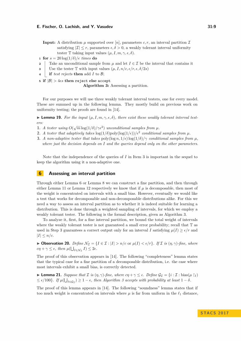
Input: A distribution µ supported over [n], parameters c, r, an interval partition Isatisfying |I| ≤ r, parameters ε, δ > 0, a weakly tolerant interval uniformitytester T taking input values (µ, I,m, γ, ε, δ).

1 for s = 20 log(1/δ)/ε times do2 Take an unconditional sample from µ and let I ∈ I be the interval that contains it3 Use the tester T with input values (µ, I, n/c, ε/r, ε, δ/2s)4 if test rejects then add I to B;5 if |B| > 4εs then reject else accept

Algorithm 3: Assessing a partition.

For our purposes we will use three weakly tolerant interval testers, one for every model.These are summed up in the following lemma. They mostly build on previous work onuniformity testing; the proofs are found in [14].

I Lemma 19. For the input (µ, I,m, γ, ε, δ), there exist these weakly tolerant interval test-ers:1. A tester using O(

√m log(1/δ)/γε2) unconditional samples from µ.

2. A tester that adaptively takes log(1/δ)poly(log(1/ε))/ε2 conditional samples from µ.3. A non-adaptive tester that takes poly(logn, 1/ε) log(1/δ)/γ conditional samples from µ,

where just the decision depends on I and the queries depend only on the other parameters.

Note that the independence of the queries of I in Item 3 is important in the sequel tokeep the algorithm using it a non-adaptive one.

6 Assessing an interval partition

Through either Lemma 6 or Lemma 8 we can construct a fine partition, and then througheither Lemma 11 or Lemma 12 respectively we know that if µ is decomposable, then most ofthe weight is concentrated on intervals with a small bias. However, eventually we would likea test that works for decomposable and non-decomposable distributions alike. For this weneed a way to assess an interval partition as to whether it is indeed suitable for learning adistribution. This is done through a weighted sampling of intervals, for which we employ aweakly tolerant tester. The following is the formal description, given as Algorithm 3.

To analyze it, first, for a fine interval partition, we bound the total weight of intervalswhere the weakly tolerant tester is not guaranteed a small error probability; recall that T asused in Step 3 guarantees a correct output only for an interval I satisfying µ(I) ≥ ε/r and|I| ≤ n/c.

I Observation 20. Define NI = I ∈ I : |I| > n/c or µ(I) < ε/r. If I is (η, γ)-fine, wherecη + γ ≤ ε, then µ(

⋃I∈NI

I) ≤ 2ε.

The proof of this observation appears in [14]. The following “completeness” lemma statesthat the typical case for a fine partition of a decomposable distribution, i.e. the case wheremost intervals exhibit a small bias, is correctly detected.

I Lemma 21. Suppose that I is (η, γ)-fine, where cη+ γ ≤ ε. Define GI = i : I : bias(µ I)≤ ε/100. If µ(

⋃I∈GI

) ≥ 1− ε, then Algorithm 3 accepts with probability at least 1− δ.

The proof of this lemma appears in [14]. The following “soundness” lemma states that iftoo much weight is concentrated on intervals where µ is far from uniform in the `1 distance,

STACS 2017

31:10 Improving and Extending the Testing of Distributions for Shape-Restricted Properties

Input: Distribution µ supported over [n], parameters L (decomposability), ε > 0(accuracy), a weakly tolerant interval uniformity tester T taking input values(µ, I,m, γ, ε, δ)

1 Use Algorithm 2 with input values (µ, ε/2000L, ε/2000, 1/9) to obtain a partition Iwith |I| ≤ r = 105L log(1/ε)/ε

2 Use Algorithm 3 with input values (µ,L, r, I, ε/20, 1/9,T)3 if Algorithm 3 rejected then reject;4 Use Lemma 17 with values (µ, I, ε/10, 1/9) to obtain µ′I5 return µ′I

Algorithm 4: Learning an L-decomposable distribution.

then the algorithm rejects. Later we will show that this is the only situation where µ cannotbe easily learned through its flattening according to I.

I Lemma 22. Suppose that I is (η, γ)-fine, where cη + γ ≤ ε. Define FI = i : I : d(µ I ,UI) > ε. If µ(

⋃I∈FI

) ≥ 7ε, then Algorithm 3 rejects with probability at least 1− δ.

The proof of this lemma appears in [14]. Finally, we present the query complexity of thealgorithm. It is presented as generally quadratic in log(1/δ), but this can be made lineareasily by first using the algorithm with δ = 1/3, and then repeating it O(log(1/δ)) times andtaking the majority vote. When we use this lemma later on, both r and c will be linear inthe decomposability parameter L for a fixed ε, and δ will be a fixed constant.

I Lemma 23. Algorithm 3 requires O(q log(1/δ)/ε) many samples, where q is a function ofn/c, ε/r, ε and δ/2s that is the number of samples that the invocation of T in Step 3 requires.

In particular, Algorithm 3 can be implemented either as an unconditional samplingalgorithm taking r

√n/c log2(1/δ)/poly(ε) many samples, an adaptive conditional sampling

algorithm taking r log2(1/δ)/poly(ε) many samples, or a non-adaptive conditional samplingalgorithm taking r log2(1/δ)poly(logn, 1/ε) many samples.

Proof. A single (unconditional) sample is taken each time Step 2 is reached, and all othersamples are taken by the invocation of T in Step 3. This makes the total number of samplesto be s(q + 1) = O(q log(1/δ)/ε).

The bound for each individual sampling model follows by plugging in Items 1, 2 and 3of Lemma 19 respectively. For the last one it is important that the tester makes itsqueries completely independently of I, as otherwise the algorithm would not have beennon-adaptive. J

7 Learning and testing decomposable distributions and properties

Here we finally put things together to produce a learning algorithm for L-decomposabledistributions. This algorithm is not only guaranteed to learn with high probability adistribution that is decomposable, but is also guaranteed with high probability to notproduce a wrong output for any distribution (though it may plainly reject a distributionthat is not decomposable). This is presented in Algorithm 4. We present it with a fixederror probability 2/3 because this is what we use later on, but it is not hard to move to ageneral δ.

First we show completeness, that the algorithm succeeds for decomposable distributions.

I Lemma 24. If µ is (ε/2000, L)-decomposable, then with probability at least 2/3, Algorithm4 produces a distribution µ′ so that d(µ, µ′) ≤ ε.

E. Fischer, O. Lachish, and Y. Vasudev 31:11

Proof. By Lemma 8, with probability at least 8/9, the partition I is (ε/2000L, ε/2000)-fine,which means by Lemma 12 that

∑j∈[r]:bias(µI′

j)>ε/2000 µ(I ′j) ≤ 3ε/2000. When this occurs,

by Lemma 21 with probability at least 8/9, Algorithm 3 will accept and so the algorithm willmove past Step 3. In this situation, in particular by Lemma 14 we have that d(µI , µ) ≤ 15ε/20(in fact this can be bounded much smaller here), and with probability at least 8/9 (by Lemma17) Step 4 provides a distribution that is ε/10-close to µI and hence ε-close to µ. J

Next we show that the algorithm will, with high probability, not mislead about thedistribution, whether it is decomposable or not.

I Lemma 25. For any µ, the probability that Algorithm 4 produces (without rejecting) adistribution µ′ for which d(µ, µ′) > ε is bounded by 2/9.

Proof. Consider the interval partition I. By Lemma 8, with probability at least 8/9, it is(ε/2000L, ε/2000)-fine. When this happens, if I is such that

∑j:d(µIj

,UIj) µ(Ij) > 7ε/20,

then by Lemma 22 with probability at least 8/9, the algorithm will reject in Step 3, and weare done (recall that here a rejection is an allowable outcome).

On the other hand, if I is such that∑j:d(µIj

,UIj) µ(Ij) ≤ 7ε/20, then by Lemma 14

we have that d(µI , µ) ≤ 15ε/20, and with probability at least 8/9 (by Lemma 17), Step4 provides a distribution that is ε/10-close to µI and hence ε-close to µ, which is also anallowable outcome. J

We now plug in the sample complexity bounds and afterwards summarize all as a theorem.

I Lemma 26. Algorithm 4 requires O(L log(1/ε)/ε + q/ε + L log(1/ε)/ε3) many samples,where the value q = q(n/L, ε2/105L log(1/ε), ε/20, ε/2000) is a bound on the number ofsamples that each invocation of T inside Algorithm 3 requires.

In particular, Algorithm 4 can be implemented either as an unconditional samplingalgorithm taking

√nL/poly(ε) many samples, an adaptive conditional sampling algorithm

taking L/poly(ε) many samples, or a non-adaptive conditional sampling algorithm takingLpoly(logn, 1/ε) many samples.

Proof. The three summands in the general expression follow respectively from the samplecomplexity calculations of Lemma 8 for Step 1, Lemma 23 for Step 2, and Lemma 17 for Step4 respectively. Also note that all samples outside Step 2 are unconditional. The bound foreach individual sampling model follows from the respective bound stated in Lemma 23. J

I Theorem 27. Algorithm 4 is capable of learning an (ε/2000, L)-decomposable distribution,giving with probability at least 2/3, a distribution that is ε-close to it, such that for nodistribution will it give as output a distribution ε-far from it with probability more than 1/3.

It can be implemented either as an unconditional sampling algorithm taking√nL/poly(ε)

many samples, an adaptive conditional sampling algorithm taking L/poly(ε) many samples,or a non-adaptive conditional sampling algorithm taking Lpoly(logn, 1/ε) many samples.

Proof. This follows from Lemmas 24, 25 and 26 respectively. J

Algorithm 5, next, is a direct application of the above to testing decomposable properties.

I Theorem 28. Algorithm 5 is a test (with error probability 1/3) for the L-decomposableproperty C. For L = L(ε/4000, n), It can be implemented either as an unconditional samplingalgorithm taking

√nL/poly(ε) many samples, an adaptive conditional sampling algorithm

taking L/poly(ε) many samples, or a non-adaptive conditional sampling algorithm takingLpoly(logn, 1/ε) many samples.

STACS 2017

31:12 Improving and Extending the Testing of Distributions for Shape-Restricted Properties

Input: Distribution µ supported over [n], function L : (0, 1]× N→ N(decomposability), parameter ε > 0 (accuracy), an L-decomposable property Cof distributions, a weakly tolerant interval uniformity tester T taking inputvalues (µ, I,m, γ, ε, δ).

1 Use Algorithm 4 with input values (µ,L(ε/4000, n), ε/2,T) to obtain µ′2 if Algorithm 4 accepted and µ′ is ε/2-close to C then accept else reject

Algorithm 5: Testing L-decomposable properties.

Proof. The number and the nature of the samples are determined fully by the applicationof Algorithm 4 in Step 1, and are thus the same as in Theorem 27. Also by this theorem,for a distribution µ ∈ C, with probability at least 2/3, an ε/2-close distribution µ′ will beproduced, and so it will be accepted in Step 2.

Finally, if µ is ε-far from C, then with probability at least 2/3, Step 1 will either producea rejection, or again produce µ′ that is ε/2-close to µ. In the latter case, µ′ will be ε/2-farfrom C by the triangle inequality, and so Step 2 will reject in either case. J

8 Introducing properties characterized by atlases

In this section, we formally define properties characterized by atlases. It is shown in [14,Section 9], that distributions that are L-decomposable are, in particular, characterized byatlases. First we start with the definition of an inventory.

I Definition 29 (Inventory). Given an interval I = [a, b] ⊆ [n] and a real-valued function ν :[a, b]→ [0, 1], the inventory of ν over [a, b] is the multisetM corresponding to (ν(a), . . . , ν(b)).

That is, we keep count of the function values over the interval including repetitions, butignore their order.

I Definition 30 (Atlas). Given a distribution µ over [n], and an interval partition I =(I1, . . . , Ik) of [n], the atlas A of µ over I is the ordered pair (I,M), where M is thesequence of multisets (M1, . . . ,Mk) so that Mj is the inventory of µ (considered as a real-valued function) over Ij for every j ∈ [k]. In this setting, we also say that µ conformsto A.

There can be many distributions over [n] with the same atlas. We also denote by an atlasA any ordered pair (I,M) where I is an interval partition of [n] andM is a sequence ofmultisets of the same length, so that the total sum of all members of all multisets is 1. It is asimple observation that for every such A there exists at least one distribution that conformsto it. The length of an atlas |A| is defined as the shared length of its interval partition andsequence of multisets. Next we define when a property is characterized by atlases.

I Definition 31. For a function k : (0, 1]×N→ N, we say that a property of distributions Cis k-characterized by atlases if for every n ∈ N and every ε > 0 we have a set A of atlases oflengths bounded by k(ε, n), so that every distribution µ over [n] satisfying C conforms tosome A ∈ A, while on the other hand no distribution µ that conforms to any A ∈ A is ε-farfrom satisfying C.

In [14, Section 9], we give some examples of such properties, and show that characteriz-ability is preserved also when switching to a tolerant testing scheme. The following is themain result, whose proof is given in [14, Section 9].

E. Fischer, O. Lachish, and Y. Vasudev 31:13

I Theorem 32. If C is a property of distributions that is k-characterized by atlases, thenfor any ε > 0 there is an adaptive conditional testing algorithm for C with query complexityk(ε/5, n) · poly(logn, 1/ε) (and error probability bound 1/3).

References1 Jayadev Acharya, Clément L. Canonne, and Gautam Kamath. A chasm between iden-

tity and equivalence testing with conditional queries. In Approximation, Randomization,and Combinatorial Optimization. Algorithms and Techniques, APPROX/RANDOM 2015,August 24-26, 2015, Princeton, NJ, USA, pages 449–466, 2015. doi:10.4230/LIPIcs.APPROX-RANDOM.2015.449.

2 Jayadev Acharya, Constantinos Daskalakis, and Gautam Kamath. Optimal testing forproperties of distributions. In Corinna Cortes, Neil D. Lawrence, Daniel D. Lee, MasashiSugiyama, and Roman Garnett, editors, Advances in Neural Information Processing Sys-tems 28: Annual Conference on Neural Information Processing Systems 2015, December7-12, 2015, Montreal, Quebec, Canada, pages 3591–3599, 2015.

3 Noga Alon, Alexandr Andoni, Tali Kaufman, Kevin Matulef, Ronitt Rubinfeld, and NingXie. Testing k-wise and almost k-wise independence. In Proceedings of the Thirty-ninthAnnual ACM Symposium on Theory of Computing, STOC’07, pages 496–505. ACM, 2007.doi:10.1145/1250790.1250863.

4 Tugkan Batu, Lance Fortnow, Eldar Fischer, Ravi Kumar, Ronitt Rubinfeld, and PatrickWhite. Testing random variables for independence and identity. In 42nd Annual Symposiumon Foundations of Computer Science, FOCS 2001, 14-17 October 2001, Las Vegas, Nevada,USA, pages 442–451, 2001. doi:10.1109/SFCS.2001.959920.

5 Tugkan Batu, Lance Fortnow, Ronitt Rubinfeld, Warren D. Smith, and Patrick White.Testing that distributions are close. In 41st Annual Symposium on Foundations of ComputerScience, FOCS 2000, 12-14 November 2000, Redondo Beach, California, USA, pages 259–269. IEEE Computer Society, 2000. doi:10.1109/SFCS.2000.892113.

6 Tugkan Batu, Ravi Kumar, and Ronitt Rubinfeld. Sublinear algorithms for testing mono-tone and unimodal distributions. In László Babai, editor, Proceedings of the 36th AnnualACM Symposium on Theory of Computing, Chicago, IL, USA, June 13-16, 2004, pages381–390. ACM, 2004. doi:10.1145/1007352.1007414.

7 Clément L. Canonne. A survey on distribution testing: Your data is big. but is it blue?Electronic Colloquium on Computational Complexity (ECCC), 22:63, 2015.

8 Clément L. Canonne, Ilias Diakonikolas, Themis Gouleakis, and Ronitt Rubinfeld. Testingshape restrictions of discrete distributions. CoRR, abs/1507.03558, 2015.

9 Clément L. Canonne, Dana Ron, and Rocco A. Servedio. Testing probability distribu-tions using conditional samples. SIAM J. Comput., 44(3):540–616, 2015. doi:10.1137/130945508.

10 Sourav Chakraborty, Eldar Fischer, Yonatan Goldhirsh, and Arie Matsliah. On the powerof conditional samples in distribution testing. In Innovations in Theoretical ComputerScience, ITCS’13, Berkeley, CA, USA, January 9-12, 2013, pages 561–580, 2013. doi:10.1145/2422436.2422497.

11 Ilias Diakonikolas. Learning structured distributions. Handbook of Big Data, page 267,2016.

12 Ilias Diakonikolas and Daniel M. Kane. A new approach for testing properties of discretedistributions. CoRR, abs/1601.05557, 2016.

13 Ilias Diakonikolas, Homin K. Lee, Kevin Matulef, Krzysztof Onak, Ronitt Rubinfeld,Rocco A. Servedio, and Andrew Wan. Testing for concise representations. In 48th AnnualIEEE Symposium on Foundations of Computer Science (FOCS 2007), October 20-23, 2007,Providence, RI, USA, Proceedings, pages 549–558, 2007. doi:10.1109/FOCS.2007.70.

STACS 2017

31:14 Improving and Extending the Testing of Distributions for Shape-Restricted Properties

14 Eldar Fischer, Oded Lachish, and Yadu Vasudev. Improving and extending the testing ofdistributions for shape-restricted properties. CoRR, abs/1609.06736, 2016. URL: http://arxiv.org/abs/1609.06736.

15 Oded Goldreich and Dana Ron. On testing expansion in bounded-degree graphs. ElectronicColloquium on Computational Complexity (ECCC), 7(20), 2000.

16 Piotr Indyk, Reut Levi, and Ronitt Rubinfeld. Approximating and testing k-histogram dis-tributions in sub-linear time. In Proceedings of the 31st ACM SIGMOD-SIGACT-SIGARTSymposium on Principles of Database Systems, PODS 2012, Scottsdale, AZ, USA, May20-24, 2012, pages 15–22, 2012. doi:10.1145/2213556.2213561.

17 Liam Paninski. A coincidence-based test for uniformity given very sparsely sampled discretedata. IEEE Transactions on Information Theory, 54(10):4750–4755, 2008.

18 Rocco A. Servedio. Testing by implicit learning: A brief survey. In Property Testing– Current Research and Surveys [outgrow of a workshop at the Institute for ComputerScience (ITCS) at Tsinghua University, January 2010], pages 197–210, 2010. doi:10.1007/978-3-642-16367-8_11.

19 Gregory Valiant and Paul Valiant. An automatic inequality prover and instance optimalidentity testing. In 55th IEEE Annual Symposium on Foundations of Computer Science,FOCS 2014, Philadelphia, PA, USA, October 18-21, 2014, pages 51–60, 2014. doi:10.1109/FOCS.2014.14.

20 Paul Valiant. Testing symmetric properties of distributions. SIAM J. Comput., 40(6):1927–1968, 2011. doi:10.1137/080734066.