extended abstractsweb.mst.edu/~yyqkc/ref/indochina-ref/proceeding_digital_small.pdf · extended...
TRANSCRIPT


Extended Abstracts
APPLIED GEOPHYSICS 1
1 Revealing a leakage model using dipole-dipole investigation and field mapping; A case study at HuaiYai
Reservoir, Petchabun Province, Thailand
Benjamas Sawatdipong, Anchalee Kongsuk
7 High Resolution Automatic 3D Off-set Pole-Dipole Resistivity Measurements for Deep Groundwater In-
vestigation
Desell Suanburi, Natthee Rongkhapimonpong, Channarong Thangkanasup
10 Landslide Risk Status of Road High Cutting Sandstone Slope by 2D Resistivity Imaging and Seismic
Refraction Technique
Songkiert Tansamrit, Desell Suanburi
14 The Integration of Ground and Underwater Resistivity Measuring for the Leakage of Internal Structure
at Gypsum Mine Boundary
Desell Suanburi, Wimonsiri Methaweranon, Monkon Ponchunchoovong, Boonyoung Tepsut
17 An Investigation of The Flood-Affected Concrete Structures Using Resistivity Measurements
Narongchai Wiwattanachang, Pham Huy Giao
23 Possibility of chemical contamination from waste-dumping area to irrigation canal-interpretation based
on geophysical data of an area in Mae Jo, Chiang Mai Provinces, Thailand
Noppadol Poomvises, Sarawute Chantraprasert
31 Application of geophysical methods for characterizing a selected solid waste disposal site in Songkhla
province
Thirat Sommai, Kamhaeng Wattanasen, Sawasdee Yodkayhun
36 Detection Leakage Reservoir located on Fault zone and Karst Topography by Dipole-Dipole Resistiv-
ity and Seismic refraction survey : A case study at Ban Phra Jaedee Sam Ong reservoir, Karnjanaburi
Province Thailand
Tirawut Na Lampang, Anchalee Kongsuk, Benjamart Sawaddipong, Noppadol Poomvises, Narucha Sangtong
CRUSTAL STUDIES 42
42 Fault Delineation Using Magnetic Data in the Eastern Part of Chiang Mai Basin
Chawanun Ninsom, Siripon Chaisri, Sarawute Chantraprasert
48 Geophysical Surveys to Detect Potential Active Faults in San Sai District, Chiang Mai Province
Tanapon Suklim, Suwimon Udphuay, Siriporn Chaisri, Sarawute Chantrapraserta
53 Thailand Crustal Thickness Estimation Using Joint Inversion of Surface Wave Dispersion and Receiver
Functions
Tira Tadapansawut, Siriporn Chaisri, Paiboon Nuannin
EARTHQUAKE STUDIES 62
62 Evaluation of TMD Seismograph Network Detection Capabilities
Chatupond Munkong, Paiboon Nuannin
68 Microtremor measurements in Chiang Mai city, northern Thailand for seismic microzonation
Narin Kluntong, Passakorn Pananont
71 Resistivity imaging to detect the liquefaction induced by the Mw 6.8 earthquake in Myanmar on March
24, 2011 in Chiang Rai province, northern Thailand
Rapeeporn Sakulnee, Passakorn Pananont
The 6th International Conference on Applied Geophysics, Nov 15-17, 2012, Kanchanburi, Thailand i

75 Micro-tremor in Bangkok and its comparison with amplified shear waves and H/V spectrum of Rayleigh
waves
Satoshi Morio, Yoshinori Kato, Akira Kitazumi, Suwith Kosuwan, Sitirag Limpisawad, Tirawat Boonyatee
GEOPHYSICAL MODELING AND INVERSION 82
82 Inversion of Magnetic Data from Remanent and Induced Sources
Robert Ellis, Barry de Wet, Ian Macleod
87 Extracting shear wave velocity from seismic reflection data: Case studies in near surface characterization
using Multichannel Analysis of Surface Wave (MASW)
Sawasdee Yordkayhun, Aksara Mayamae, Preeya Srisuwan
94 Quality Improvement Comparison Between Time-Space Window Varying Median Filter and Time Win-
dow Varying Median Filter
Siriphon Somsri, Pisanu Wongpornchai
GEOPHYSICAL FOR PETROLEUM EXPLORATION 100
100 Gas reservoir detection using three dimensional seismic attribute analysis, Gulf of Moattama, Offshore
Myanmar
Soe Linn Htike, Pisanu Wongpornchai
108 Porosity and Permeability Estimation from Seismic Attributes by Multi-layer Feedforward Neural Net-
work Technique in an Area of Gulf of Thailand
Theerachai Norkhamboot, Pisanu Wongpornchai
GEOTHERMAL EXPLORATION 112
112 Model-based Inversion of Magnetotelluric (MT) Data in the Fang Basin
Khin Moh Moh Latt, Pham Huy Giao
117 Geological Structures related to Hot Springs in Krabi, Southern Thailand
Usa Nilsuwan, Helmut Durrast
LABORATORY GEOPHYSICS 129
129 Geomechanical Simulation of Deformation by CO2 Injection into Homogeneous Sandstone
Avirut Puttiwongrak, Toshifumi Matsuoka
138 Dating Geological Events using Thermoluminescence Technique
Prakrit Noppradit, Sommai Changkian, Helmut Durrast
Index of Authors 143
The 6th International Conference on Applied Geophysics, Nov 15-17, 2012, Kanchanburi, Thailand ii
Revealing a leakage model using dipole-dipoleinvestigation and field mapping; A case study at HuaiYaiReservoir, Petchabun Province, Thailand
Benjamas Sawatdiponga,∗, Anchalee Kongsuka
a Geophysics group, Geology section, Office of Topographical and Geotechnical Survey, Royal Irrigation Department, Dusit,
Bangkok, Thailand∗, E-mail: [email protected]
ABSTRACT
The geophysical investigation of HuaiYai Reservoir, Petchabun Province aims to investigate critical area, delineate the leak path, and
analyze causes of leakage. The leakage at HuaiYai was taken place near outlet of saddle dam and the vicinity area. Field mapping was
initially mapped the geological structure and condition of joints in the area. Dipole-dipole imaging had later been used to map 2-D profiling.
Three survey lines were designed covering an area of problem in three levels. Line A, at +221.7 metres above mean sea level and total length
of 560 meters was located at a center line of saddle dam crest. Line B, at +204.4 m msl and total length of 340 meters, was at downstream
toe-drain and approximately 3 metres higher than control outlet. Line C was at front of control outlet building at +201.3 m msl, and the
total length of 365 meters. As the results of line A, 2-D profile shows three dominant anomalous zones of low resistivity range, station
235.5 m spheroid in shape, 235.5-355 m slightly dipping along the contact of saddle and spur, and 350-440 m, approximately 10 meters
thick, laying horizontal continuous on top of the spur. The 2-D resistivity profile of line B and C demonstrates seven anomalies between
station 0 to 340 with several shape, geometry, dimension, elevation, and resistivity range. The most anomalous zones likely appear beneath
the river outlet. Combine resistivity imaging and geological mapping, it can be interpreted cause of the leakage into three assumptions.
First, the seepage flow and leak through main fracture inside tuffaceous sandstone foundation which is aligned in the northeast-southwest
direction by mechanism of gravity. Second, seepage from water run-off along downstream slope and under rip-rap layer. Apart of the water
seeped down under the gutter, which was designed to protect control outlet building, and leak out to cut slope which is located behind the
outlet building. Last, the ground surface behind control outlet building is approximately 30 centimeter lower than a shallow ground water
table of the area that make water flow out on cut-slope face as a slope seepage. A little while after, a maintenance team had treated the area
of problem with several methods to be safe until the present day.
KEYWORDS: Dipole-dipole electrical resistivity, Revealing leakage model, Leakage, HuaiYai Reservoir, geophysical investigation,
resistivity imaging
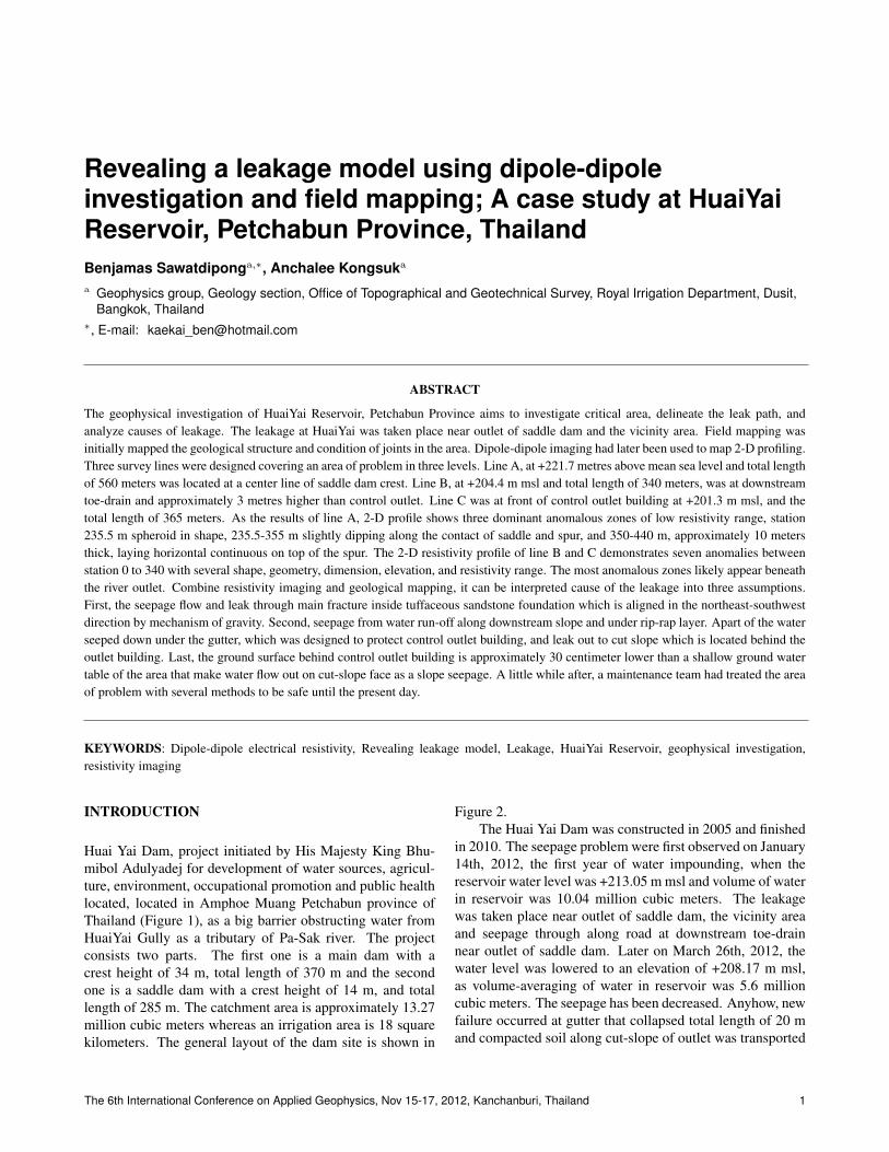
INTRODUCTION
Huai Yai Dam, project initiated by His Majesty King Bhu-
mibol Adulyadej for development of water sources, agricul-
ture, environment, occupational promotion and public health
located, located in Amphoe Muang Petchabun province of
Thailand (Figure 1), as a big barrier obstructing water from
HuaiYai Gully as a tributary of Pa-Sak river. The project
consists two parts. The first one is a main dam with a
crest height of 34 m, total length of 370 m and the second
one is a saddle dam with a crest height of 14 m, and total
length of 285 m. The catchment area is approximately 13.27
million cubic meters whereas an irrigation area is 18 square
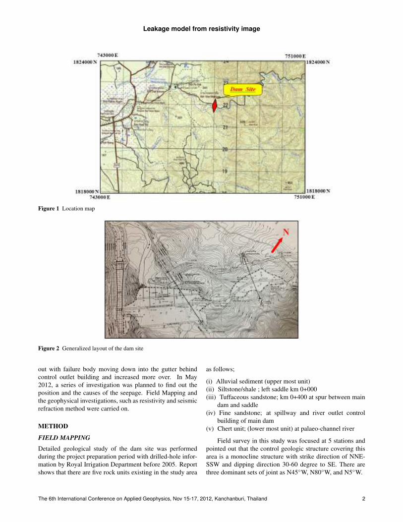
kilometers. The general layout of the dam site is shown in
Figure 2.
The Huai Yai Dam was constructed in 2005 and finished
in 2010. The seepage problem were first observed on January
14th, 2012, the first year of water impounding, when the
reservoir water level was +213.05 m msl and volume of water
in reservoir was 10.04 million cubic meters. The leakage
was taken place near outlet of saddle dam, the vicinity area
and seepage through along road at downstream toe-drain
near outlet of saddle dam. Later on March 26th, 2012, the
water level was lowered to an elevation of +208.17 m msl,
as volume-averaging of water in reservoir was 5.6 million
cubic meters. The seepage has been decreased. Anyhow, new
failure occurred at gutter that collapsed total length of 20 m
and compacted soil along cut-slope of outlet was transported
The 6th International Conference on Applied Geophysics, Nov 15-17, 2012, Kanchanburi, Thailand 1
Leakage model from resistivity image
Figure 1 Location map
Figure 2 Generalized layout of the dam site
out with failure body moving down into the gutter behind
control outlet building and increased more over. In May
2012, a series of investigation was planned to find out the
position and the causes of the seepage. Field Mapping and
the geophysical investigations, such as resistivity and seismic
refraction method were carried on.
METHOD
FIELD MAPPING
Detailed geological study of the dam site was performed
during the project preparation period with drilled-hole infor-
mation by Royal Irrigation Department before 2005. Report
shows that there are five rock units existing in the study area
as follows;
(i) Alluvial sediment (upper most unit)
(ii) Siltstone/shale ; left saddle km 0+000
(iii) Tuffaceous sandstone; km 0+400 at spur between main
dam and saddle
(iv) Fine sandstone; at spillway and river outlet control
building of main dam
(v) Chert unit; (lower most unit) at palaeo-channel river
Field survey in this study was focused at 5 stations and
pointed out that the control geologic structure covering this
area is a monocline structure with strike direction of NNE-
SSW and dipping direction 30-60 degree to SE. There are
three dominant sets of joint as N45W, N80W, and N5W.
The 6th International Conference on Applied Geophysics, Nov 15-17, 2012, Kanchanburi, Thailand 2
Sawatdipong and Kongsuk
DIPOLE-DIPOLE ELECTRICAL RESISTIVITY
METHOD
The electrical resistivity method has been used in geotech-
nical and environmental investigation for about a century.
Fresh rock in general has a significantly higher resistivity
than clayey soil because it has much smaller primary porosity
and fewer interconnected pore spaces. clayey materials tend
to hold more moisture and have a higher concentration of ion
to conduct electrical, therefore, have resistivity values less
than 100 ohm-m (Telford and others 1990).
Figure 3 is shown the data collection sequence for the
dipole-dipole array in an investigation. The symbol ‘a’ de-
notes the unit spacing of electrodes, which is selected based
on the desired depth of penetration, the required resolution,
and the type of array. The electrode spacing and dipole
separation are constant for each traverse (n) and increase with
each successive traverse. Larger electrode spacing provides
data from greater depths, but with lower resolution.
Figure 3 The data collection sequence for the dipole-dipole array
in the investigation
Dipole-dipole electrical resistivity is one of geophysical
technique method has been used in data collection and used
for revealing leakage model. Electrical resistivity data was
collected from three survey lines. The lines were designed
covering an area of problem in 2 spacing system 5- and 2.5-
metre system.
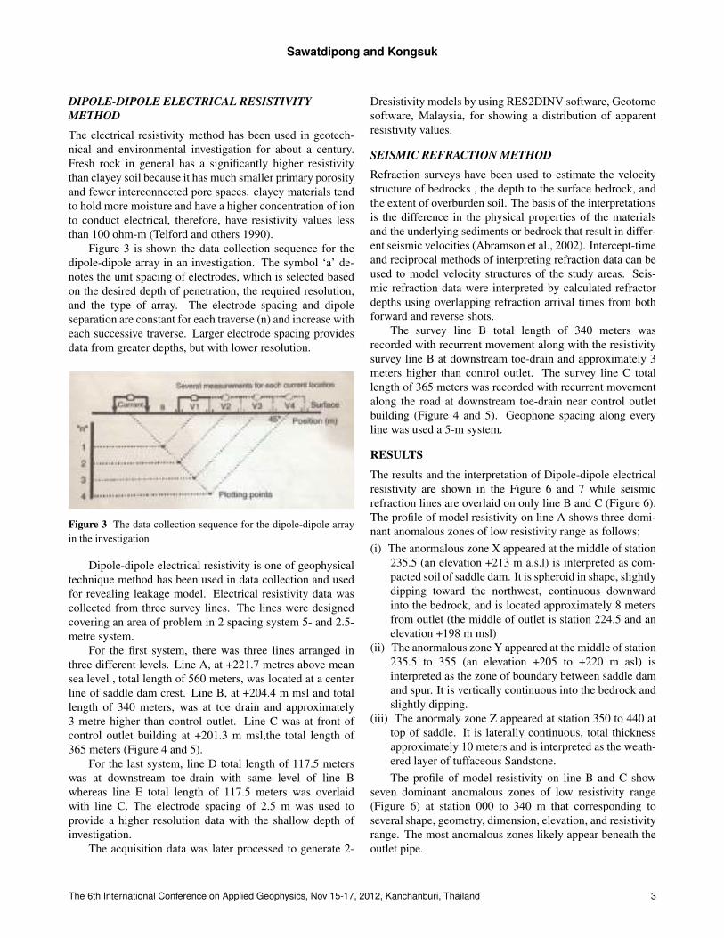
For the first system, there was three lines arranged in
three different levels. Line A, at +221.7 metres above mean
sea level , total length of 560 meters, was located at a center
line of saddle dam crest. Line B, at +204.4 m msl and total
length of 340 meters, was at toe drain and approximately
3 metre higher than control outlet. Line C was at front of
control outlet building at +201.3 m msl,the total length of
365 meters (Figure 4 and 5).
For the last system, line D total length of 117.5 meters
was at downstream toe-drain with same level of line B
whereas line E total length of 117.5 meters was overlaid
with line C. The electrode spacing of 2.5 m was used to
provide a higher resolution data with the shallow depth of
investigation.
The acquisition data was later processed to generate 2-
Dresistivity models by using RES2DINV software, Geotomo
software, Malaysia, for showing a distribution of apparent
resistivity values.
SEISMIC REFRACTION METHOD
Refraction surveys have been used to estimate the velocity
structure of bedrocks , the depth to the surface bedrock, and
the extent of overburden soil. The basis of the interpretations
is the difference in the physical properties of the materials
and the underlying sediments or bedrock that result in differ-
ent seismic velocities (Abramson et al., 2002). Intercept-time
and reciprocal methods of interpreting refraction data can be
used to model velocity structures of the study areas. Seis-
mic refraction data were interpreted by calculated refractor
depths using overlapping refraction arrival times from both
forward and reverse shots.
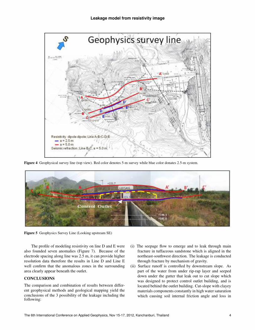
The survey line B total length of 340 meters was
recorded with recurrent movement along with the resistivity
survey line B at downstream toe-drain and approximately 3
meters higher than control outlet. The survey line C total
length of 365 meters was recorded with recurrent movement
along the road at downstream toe-drain near control outlet
building (Figure 4 and 5). Geophone spacing along every
line was used a 5-m system.
RESULTS
The results and the interpretation of Dipole-dipole electrical
resistivity are shown in the Figure 6 and 7 while seismic
refraction lines are overlaid on only line B and C (Figure 6).
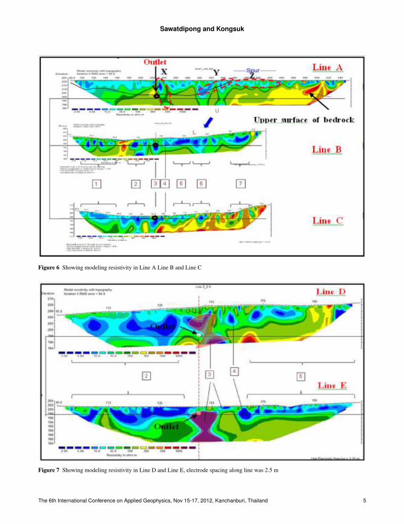
The profile of model resistivity on line A shows three domi-
nant anomalous zones of low resistivity range as follows;
(i) The anormalous zone X appeared at the middle of station
235.5 (an elevation +213 m a.s.l) is interpreted as com-
pacted soil of saddle dam. It is spheroid in shape, slightly
dipping toward the northwest, continuous downward
into the bedrock, and is located approximately 8 meters
from outlet (the middle of outlet is station 224.5 and an
elevation +198 m msl)
(ii) The anormalous zone Y appeared at the middle of station
235.5 to 355 (an elevation +205 to +220 m asl) is
interpreted as the zone of boundary between saddle dam
and spur. It is vertically continuous into the bedrock and
slightly dipping.
(iii) The anormaly zone Z appeared at station 350 to 440 at
top of saddle. It is laterally continuous, total thickness
approximately 10 meters and is interpreted as the weath-
ered layer of tuffaceous Sandstone.
The profile of model resistivity on line B and C show
seven dominant anomalous zones of low resistivity range
(Figure 6) at station 000 to 340 m that corresponding to
several shape, geometry, dimension, elevation, and resistivity
range. The most anomalous zones likely appear beneath the
outlet pipe.
The 6th International Conference on Applied Geophysics, Nov 15-17, 2012, Kanchanburi, Thailand 3
Leakage model from resistivity image
Figure 4 Geophysical survey line (top view). Red color denotes 5-m survey while blue color donates 2.5-m system.
Figure 5 Geophysics Survey Line (Looking upstream SE)
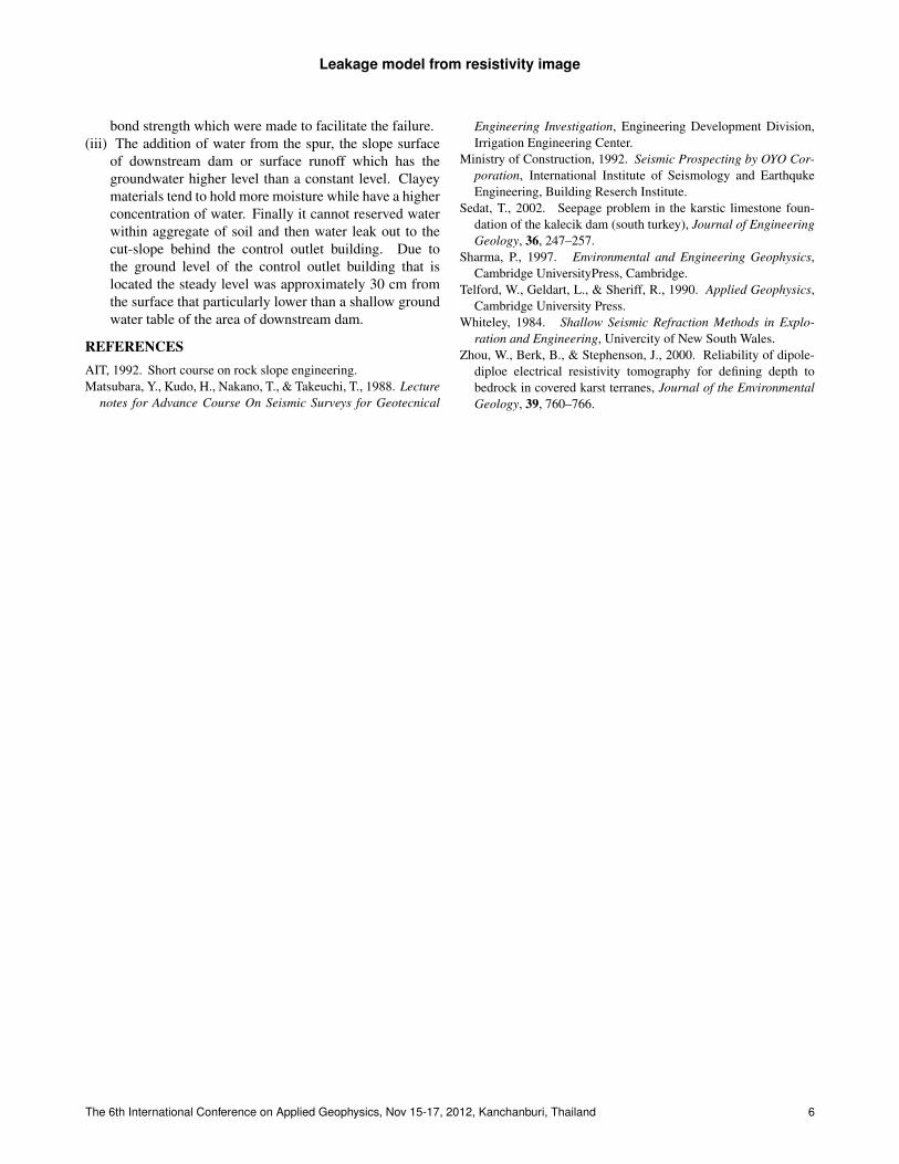
The profile of modeling resistivity on line D and E were
also founded seven anomalies (Figure 7). Because of the
electrode spacing along line was 2.5 m, it can provide higher
resolution data therefore the results in Line D and Line E
well confirm that the anomalous zones in the surrounding
area clearly appear beneath the outlet.
CONCLUSIONS
The comparison and combination of results between differ-
ent geophysical methods and geological mapping yield the
conclusions of the 3 possibility of the leakage including thefollowing:
(i) The seepage flow to emerge and to leak through main
fracture in tuffaceous sandstone which is aligned in the
northeast-southwest direction. The leakage is conducted
through fracture by mechanism of gravity.
(ii) Surface runoff is controlled by downstream slope. As
part of the water from under rip-rap layer and seeped
down under the gutter that leak out to cut slope which
was designed to protect control outlet building, and is
located behind the outlet building. Cut-slope with clayey
materials components constantly in high water saturation
which causing soil internal friction angle and loss in
The 6th International Conference on Applied Geophysics, Nov 15-17, 2012, Kanchanburi, Thailand 4
Sawatdipong and Kongsuk
Figure 6 Showing modeling resistivity in Line A Line B and Line C
Figure 7 Showing modeling resistivity in Line D and Line E, electrode spacing along line was 2.5 m
The 6th International Conference on Applied Geophysics, Nov 15-17, 2012, Kanchanburi, Thailand 5
Leakage model from resistivity image
bond strength which were made to facilitate the failure.
(iii) The addition of water from the spur, the slope surface
of downstream dam or surface runoff which has the
groundwater higher level than a constant level. Clayey
materials tend to hold more moisture while have a higher
concentration of water. Finally it cannot reserved water
within aggregate of soil and then water leak out to the
cut-slope behind the control outlet building. Due to
the ground level of the control outlet building that is
located the steady level was approximately 30 cm from
the surface that particularly lower than a shallow ground
water table of the area of downstream dam.
REFERENCES
AIT, 1992. Short course on rock slope engineering.
Matsubara, Y., Kudo, H., Nakano, T., & Takeuchi, T., 1988. Lecture
notes for Advance Course On Seismic Surveys for Geotecnical
Engineering Investigation, Engineering Development Division,
Irrigation Engineering Center.
Ministry of Construction, 1992. Seismic Prospecting by OYO Cor-
poration, International Institute of Seismology and Earthquke
Engineering, Building Reserch Institute.
Sedat, T., 2002. Seepage problem in the karstic limestone foun-
dation of the kalecik dam (south turkey), Journal of Engineering
Geology, 36, 247–257.
Sharma, P., 1997. Environmental and Engineering Geophysics,
Cambridge UniversityPress, Cambridge.
Telford, W., Geldart, L., & Sheriff, R., 1990. Applied Geophysics,
Cambridge University Press.
Whiteley, 1984. Shallow Seismic Refraction Methods in Explo-
ration and Engineering, Univercity of New South Wales.
Zhou, W., Berk, B., & Stephenson, J., 2000. Reliability of dipole-
diploe electrical resistivity tomography for defining depth to
bedrock in covered karst terranes, Journal of the Environmental
Geology, 39, 760–766.
The 6th International Conference on Applied Geophysics, Nov 15-17, 2012, Kanchanburi, Thailand 6
High Resolution Automatic 3D Off-set Pole-DipoleResistivity Measurements for Deep GroundwaterInvestigation
Desell Suanburia,∗, Natthee Rongkhapimonpongb, Channarong Thangkanasupc
a Department of Earth Sciences, Faculty of Science, Kasetsart Universityb Issara Mining Limited, Thailandc Suwanwajokkasikit Field Corp Research Station, Kasetsart University
∗, E-mail: [email protected], [email protected]
ABSTRACT
Due to a large amount of groundwater use for agricultural purpose, high yields and deep resources are needed to investigate effectively. An
application of a modified technique from an off-set pole-dipole array approach was performed at Suwanwajokkasikit Field Corp Research
Station, Kasetsart University, Nakhonratchasima province, where local hydro-geology aspects presented as limestone aquifer regions.
Objectives of true 3D resistivity measurement are to explore deep groundwater resource concisely with more than 160 m deep covering
an area of 300 m x 460 m by allowing for fast data acquisition with 48 electrode automatic reading of large quantity of data. Location
of 3D measurement was selected from previous 2D resistivity imaging. For survey specification, one set of measurement contains two
reading survey lines with electrode spacing of 20 m and line separation of 100 m while 17 current points are located at the middle between
reading survey lines with spacing of 40 m. Remote current electrode was positioned away 1000 m perpendicular to survey line direction.
Three measuring set were done in east-west direction. 3D inversion geo-electrical models were created by RES3DINV software package.
The result displays clearly that concise low resistivity zones appears within major high resistivity region which may infers to groundwater
zones in fracture or cavity in limestone at depth of 150 m to 180 m. Both shallow and deep groundwater zones can be classified and
located for future groundwater management in agriculture use. This approach can be proved as a new tool for effective deep groundwater
investigation.
KEYWORDS: Off-set pole-dipole, Deep groundwater, 3D Resistivity imaging
INTRODUCTION
Groundwater resources play as a significant rule for water
supply in agricultural uses during summer time in Thailand.
Groundwater system and it’s potential zones at agricultural
land are necessary to identify high yield of groundwater
boundary.
2D resistivity imaging were applied for groundwater
investigation successfully. (Suanburi, et. al., 2007) To
improved more effective achievement, a modified proce-
dure called “scanning technique” was introduced (Suanburi,
2010).
3D resistivity measurement have been attempted to in-
vestigate subsurface geological aspects with higher resolu-
tion and deeper position than previous 2D resistivity imaging
results.
Aims
The purpose of 3D resistivity measuring offset Pole-Dipole
configuration are to investigate for deep groundwater re-
sources concisely with more than 160 m deep covering an
area of 300 m × 460 m by allowing for fast data acquisition
with 48 multi-electrode automatic readings.
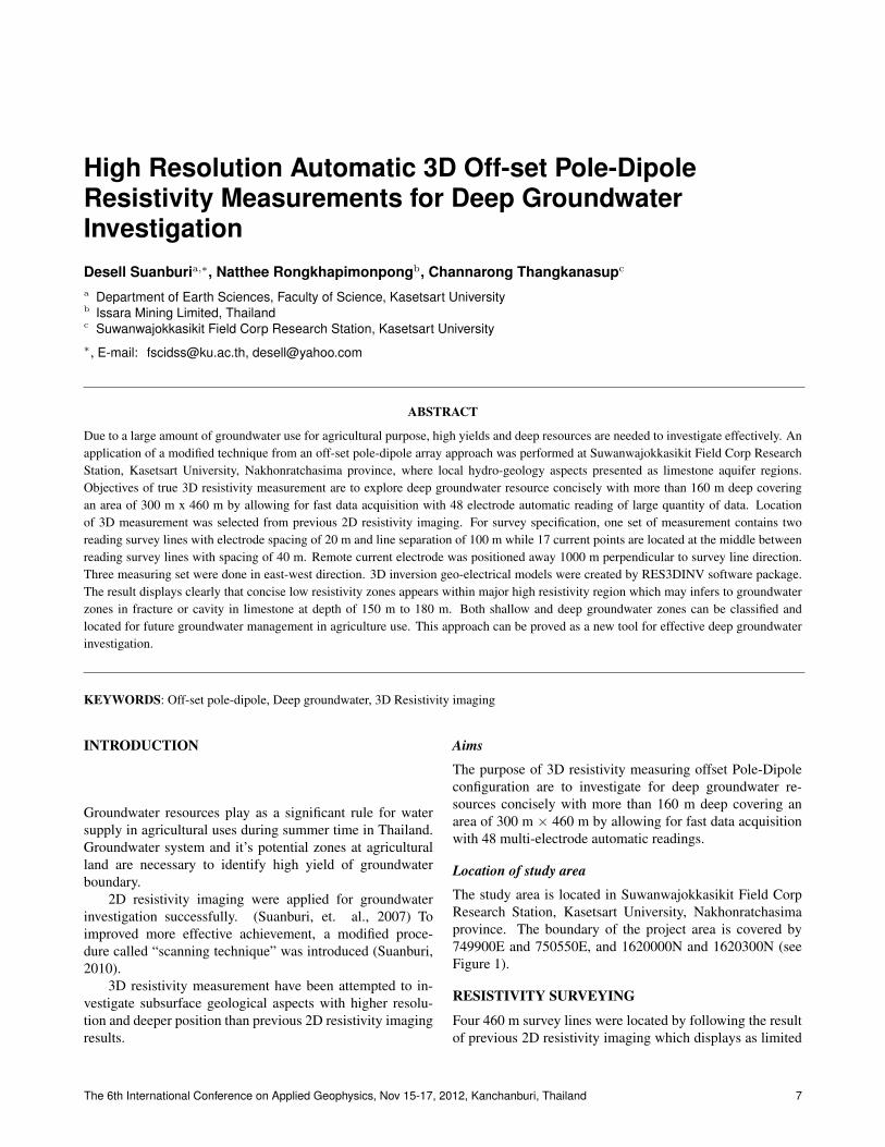
Location of study area
The study area is located in Suwanwajokkasikit Field Corp
Research Station, Kasetsart University, Nakhonratchasima
province. The boundary of the project area is covered by
749900E and 750550E, and 1620000N and 1620300N (see
Figure 1).
RESISTIVITY SURVEYING
Four 460 m survey lines were located by following the result
of previous 2D resistivity imaging which displays as limited
The 6th International Conference on Applied Geophysics, Nov 15-17, 2012, Kanchanburi, Thailand 7
3D off-set pole-dipole for groundwater investigation
Figure 1 Location map and electrode configuration
depth and less detailed measuring points. Then three 3D
Offset Pole-Dipole set up were designed in E-W direction
covering an area of partly Suwanwajokkasikit Field Corp
Research Station. (See the position of survey lines in Figure
1).
Remote current electrode was positioned away 1000 m
perpendicular to survey line direction. The measuring sys-
tem, Offset Pole-Dipole electrode configuration, was used for
continuous and detailed subsurface investigation (explained
in the Figure 2). Measurements of data display as apparent
resistivity value by section and plan view form were carefully
interpreted in term of hydro-geological aspects. Then the
data were further compiled by RES3DINV software package
which created 3D inversion geo-electrical models.
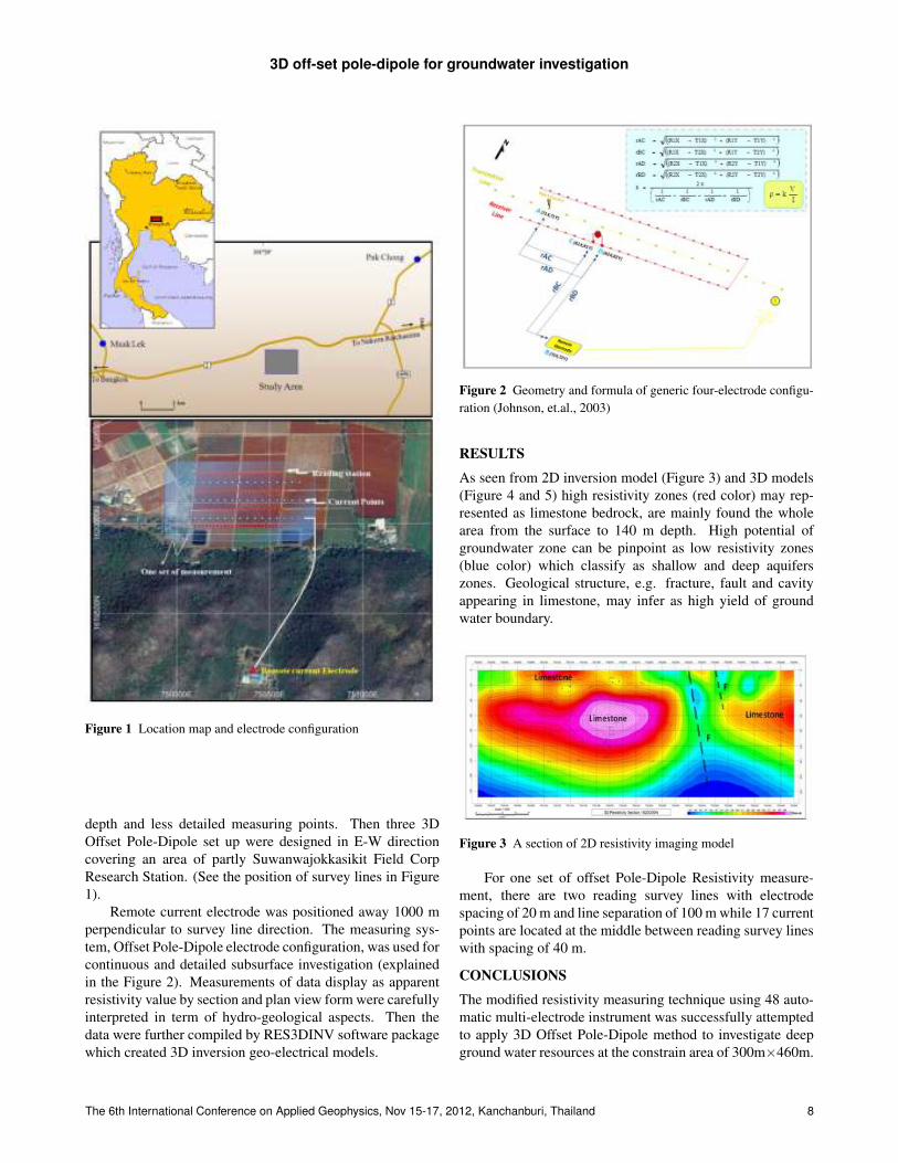
Figure 2 Geometry and formula of generic four-electrode configu-
ration (Johnson, et.al., 2003)
RESULTS
As seen from 2D inversion model (Figure 3) and 3D models
(Figure 4 and 5) high resistivity zones (red color) may rep-
resented as limestone bedrock, are mainly found the whole
area from the surface to 140 m depth. High potential of
groundwater zone can be pinpoint as low resistivity zones
(blue color) which classify as shallow and deep aquifers
zones. Geological structure, e.g. fracture, fault and cavity
appearing in limestone, may infer as high yield of ground
water boundary.
Figure 3 A section of 2D resistivity imaging model
For one set of offset Pole-Dipole Resistivity measure-
ment, there are two reading survey lines with electrode
spacing of 20 m and line separation of 100 m while 17 current
points are located at the middle between reading survey lines
with spacing of 40 m.
CONCLUSIONS
The modified resistivity measuring technique using 48 auto-
matic multi-electrode instrument was successfully attempted
to apply 3D Offset Pole-Dipole method to investigate deep
ground water resources at the constrain area of 300m×460m.
The 6th International Conference on Applied Geophysics, Nov 15-17, 2012, Kanchanburi, Thailand 8
Suanburi et al.
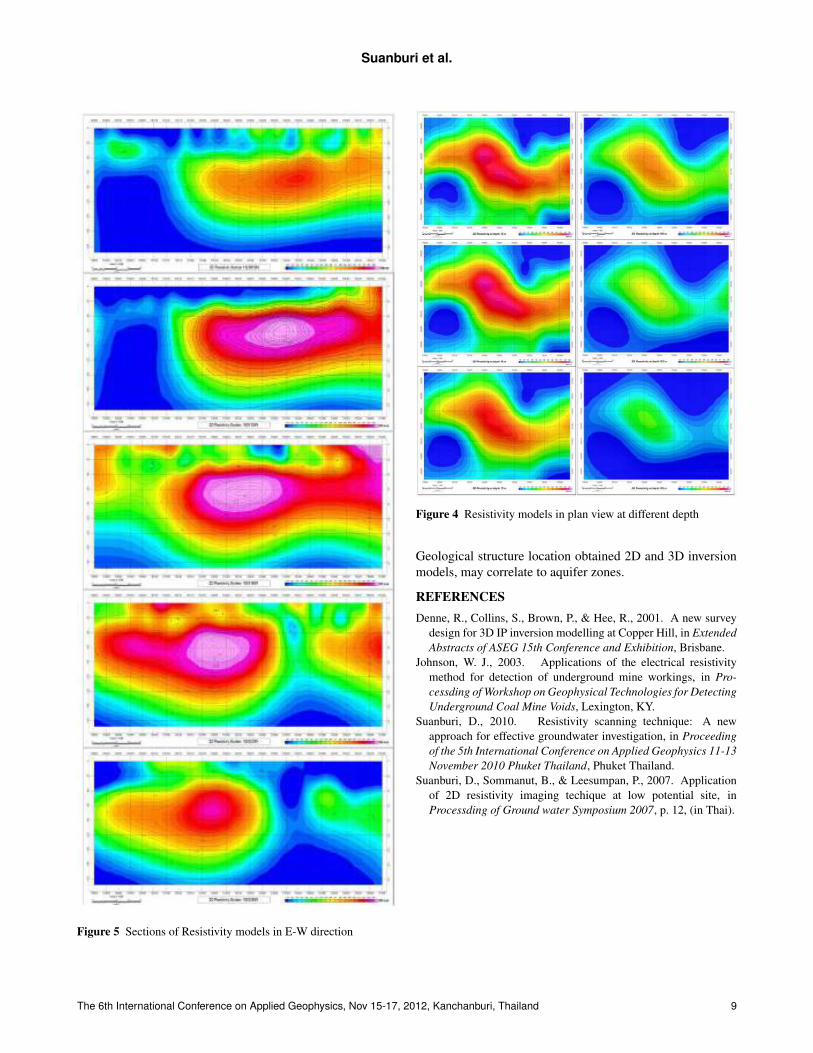
Figure 5 Sections of Resistivity models in E-W direction
Figure 4 Resistivity models in plan view at different depth
Geological structure location obtained 2D and 3D inversion
models, may correlate to aquifer zones.
REFERENCES
Denne, R., Collins, S., Brown, P., & Hee, R., 2001. A new survey
design for 3D IP inversion modelling at Copper Hill, in Extended
Abstracts of ASEG 15th Conference and Exhibition, Brisbane.
Johnson, W. J., 2003. Applications of the electrical resistivity
method for detection of underground mine workings, in Pro-
cessding of Workshop on Geophysical Technologies for Detecting
Underground Coal Mine Voids, Lexington, KY.
Suanburi, D., 2010. Resistivity scanning technique: A new
approach for effective groundwater investigation, in Proceeding
of the 5th International Conference on Applied Geophysics 11-13
November 2010 Phuket Thailand, Phuket Thailand.
Suanburi, D., Sommanut, B., & Leesumpan, P., 2007. Application
of 2D resistivity imaging techique at low potential site, in
Processding of Ground water Symposium 2007, p. 12, (in Thai).
The 6th International Conference on Applied Geophysics, Nov 15-17, 2012, Kanchanburi, Thailand 9
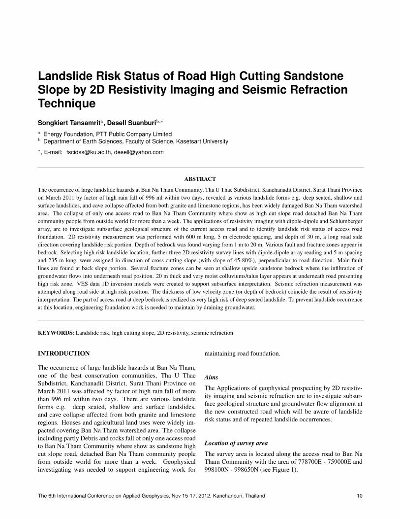
Landslide Risk Status of Road High Cutting SandstoneSlope by 2D Resistivity Imaging and Seismic RefractionTechnique
Songkiert Tansamrita, Desell Suanburib,∗
a Energy Foundation, PTT Public Company Limitedb Department of Earth Sciences, Faculty of Science, Kasetsart University
∗, E-mail: [email protected], [email protected]
ABSTRACT
The occurrence of large landslide hazards at Ban Na Tham Community, Tha U Thae Subdistrict, Kanchanadit District, Surat Thani Province
on March 2011 by factor of high rain fall of 996 ml within two days, revealed as various landslide forms e.g. deep seated, shallow and
surface landslides, and cave collapse affected from both granite and limestone regions, has been widely damaged Ban Na Tham watershed
area. The collapse of only one access road to Ban Na Tham Community where show as high cut slope road detached Ban Na Tham
community people from outside world for more than a week. The applications of resistivity imaging with dipole-dipole and Schlumberger
array, are to investigate subsurface geological structure of the current access road and to identify landslide risk status of access road
foundation. 2D resistivity measurement was performed with 600 m long, 5 m electrode spacing, and depth of 30 m, a long road side
direction covering landslide risk portion. Depth of bedrock was found varying from 1 m to 20 m. Various fault and fracture zones appear in
bedrock. Selecting high risk landslide location, further three 2D resistivity survey lines with dipole-dipole array reading and 5 m spacing
and 235 m long, were assigned in direction of cross cutting slope (with slope of 45-80%), perpendicular to road direction. Main fault
lines are found at back slope portion. Several fracture zones can be seen at shallow upside sandstone bedrock where the infiltration of
groundwater flows into underneath road position. 20 m thick and very moist colluviums/talus layer appears at underneath road presenting
high risk zone. VES data 1D inversion models were created to support subsurface interpretation. Seismic refraction measurement was
attempted along road side at high risk position. The thickness of low velocity zone (or depth of bedrock) coincide the result of resistivity
interpretation. The part of access road at deep bedrock is realized as very high risk of deep seated landslide. To prevent landslide occurrence
at this location, engineering foundation work is needed to maintain by draining groundwater.
KEYWORDS: Landslide risk, high cutting slope, 2D resistivity, seismic refraction
INTRODUCTION
The occurrence of large landslide hazards at Ban Na Tham,
one of the best conservation communities, Tha U Thae
Subdistrict, Kanchanadit District, Surat Thani Province on
March 2011 was affected by factor of high rain fall of more
than 996 ml within two days. There are various landslide
forms e.g. deep seated, shallow and surface landslides,
and cave collapse affected from both granite and limestone
regions. Houses and agricultural land uses were widely im-
pacted covering Ban Na Tham watershed area. The collapse
including partly Debris and rocks fall of only one access road
to Ban Na Tham Community where show as sandstone high
cut slope road, detached Ban Na Tham community people
from outside world for more than a week. Geophysical
investigating was needed to support engineering work for
maintaining road foundation.
Aims
The Applications of geophysical prospecting by 2D resistiv-
ity imaging and seismic refraction are to investigate subsur-
face geological structure and groundwater flow alignment at
the new constructed road which will be aware of landslide
risk status and of repeated landslide occurrences.
Location of survey area
The survey area is located along the access road to Ban Na
Tham Community with the area of 778700E - 759000E and
998100N - 998650N (see Figure 1).
The 6th International Conference on Applied Geophysics, Nov 15-17, 2012, Kanchanburi, Thailand 10

Landslide risk status by 2D resistivity and seismic refraction
Figure 1 Location map of survey area
Figure 2 Location of survey lines
RESULTS
GEOPHYSICAL SURVEYING
Line A is located along road side (see in figure 2) covering
landslide risk portion. with 600 m long where conducting 2D
Figure 3 Interpretation of Line A along the road, found 3 locations
of high risk of landslide
Figure 4 (a) Interpreted geological section of Line 1 from resistiv-
ity and (b) from chargeability showing high risk of landslide beneath
road cutting.
resistivity multi-electrode measurement with 5 m electrode
spacing, and depth of 30 m. From initial data interpretation
along the road, it is found that there are three zones to be
high risk of landslide condition i.e. deep bedrock filled with
groundwater, and weathered zone at fracture or fault zone.
Then 3 survey lines (Line 1, 2 and 3) were positioned with
the direction of up-down slop (of 30 - 70%), crossing the
road. Both Dipole-Dipole and Schlumberger array reading
with 235 m long and electrode spacing of 5 m, were applied
for 2D section and 1D inversion model. Seismic refraction
measurements were conducted along the road side following
the result of Line A, with geophone spacing of 5 m.
The result of 2D inversion model of Line A displays
that depth of bedrock varies from 1 m to 20 m and various
fault and fracture zones appear in bedrock. (Figure 3) 2D
resistivity section of Line 1 (Figure 4(a)) presents low re-
sistivity zones (moisture/groundwater content) beneath road
position with bedrock depth of about 20 m. Main fault line
clearly found at cutting slope side. Chargeability anomalies
(Figure 4(b)) appear at between geological structure zones
may strengthen moist rock fragments/debris deposits (may
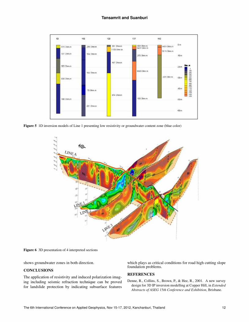
fill with clay enrichment). 1D inversion models (Figure
5) of Line 1 verify moisture portion (blue color) at differ-
ent depth from ground surface due to the discontinuity of
rock/groundwater layer affected from fault lines. 3D visual
presentation in Figure 6 for 4 Lines of resistivity imagings
The 6th International Conference on Applied Geophysics, Nov 15-17, 2012, Kanchanburi, Thailand 11
Tansamrit and Suanburi
Figure 5 1D inversion models of Line 1 presenting low resistivity or groundwater content zone (blue color)
Figure 6 3D presentation of 4 interpreted sections
shows groundwater zones in both direction.
CONCLUSIONS
The application of resistivity and induced polarization imag-
ing including seismic refraction technique can be proved
for landslide protection by indicating subsurface features
which plays as critical conditions for road high cutting slopefoundation problems.
REFERENCES
Denne, R., Collins, S., Brown, P., & Hee, R., 2001. A new survey
design for 3D IP inversion modelling at Copper Hill, in Extended
Abstracts of ASEG 15th Conference and Exhibition, Brisbane.
The 6th International Conference on Applied Geophysics, Nov 15-17, 2012, Kanchanburi, Thailand 12

Landslide risk status by 2D resistivity and seismic refraction
Johnson, W. J., 2003. Applications of the electrical resistivity
method for detection of underground mine workings, in Pro-
cessding of Workshop on Geophysical Technologies for Detecting
Underground Coal Mine Voids, Lexington, KY.
Suanburi, D., 2010. Resistivity scanning technique: A new
approach for effective groundwater investigation, in Proceeding
of the 5th International Conference on Applied Geophysics 11-13
November 2010 Phuket Thailand, Phuket Thailand.
Suanburi, D., Sommanut, B., & Leesumpan, P., 2007. Application
of 2D resistivity imaging techique at low potential site, in
Processding of Ground water Symposium 2007, p. 12, (in Thai).
The 6th International Conference on Applied Geophysics, Nov 15-17, 2012, Kanchanburi, Thailand 13
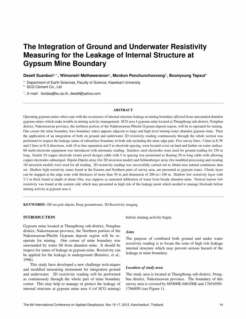
The Integration of Ground and Underwater ResistivityMeasuring for the Leakage of Internal Structure atGypsum Mine Boundary
Desell Suanburia,∗, Wimonsiri Methaweranona, Monkon Ponchunchoovongb, Boonyoung Tepsutb
a Department of Earth Sciences, Faculty of Science, Kasetsart Universityb SCG Cement Co., Ltd
∗, E-mail: [email protected], [email protected]
ABSTRACT
Operating gypsum mines often cope with the occurrence of internal structure leakage at mining boundary affected from surrounded abandon
gypsum mines which make trouble in mining activity management. SCG area 4 gypsum mine located at Thungthong sub-district, Nongbua
district, Nakornsawan province, the northern portion of the Nakhonsawan-Phichit Gypsum deposit region, will be re-operated for mining.
One corner the mine boundary (two boundary sides) appears adjacent to large and high level mining-water abandon gypsum mine. Then
the application of an integration of both on ground and underwater 2D resistivity reading continuously through the whole section was
performed to inspect the leakage status of subsurface boundary in both side including the mine edge part. Five survey lines, 3 lines in E-W
and 2 lines in N-S directions, with 10 m line separation and 5 m electrode spacing, were located cover on land and further on water surface.
60 multi-electrode equipment was introduced with automatic reading. Stainless steel electrodes were used for ground reading for 250 m
long. Sealed 10 copper electrode (water proof design) cable with 5 m spacing was positioned as floating 50 m long cable with allowing
copper electrodes submerged. Dipole-Dipole array (for 2D inversion model) and Schlumberger array (for modified processing and creating
1D inversion model) were used for all reading. 2D resistivity reading was successfully carried out to obtain nice natural continuous data
set. Shallow high resistivity zones found at the Eastern and Northern parts of survey area, are presented as gypsum zones. Clastic layer
can be mapped at the edge zone with thickness of more than 30 m and dimension of 200 m×100 m. Shallow low resistivity layer with
2-3 m thick found at depth of about 10m, was suppose as saturated infiltration of water from beside abandon-mine. Vertical narrow low
resistivity was found at the eastern side which may presented as high risk of the leakage point which needed to manage blockade before
mining activity at gypsum area 4.
KEYWORDS: Off-set pole-dipole, Deep groundwater, 3D Resistivity imaging
INTRODUCTION
Gypsum mine located at Thungthong sub-district, Nongbua
district, Nakornsawan province, the Northern portion of the
Nakornsawan-Phichit Gypsum deposit region will be re-
operate for mining. One corner of mine boundary was
surrounded by water fill from abandon mine. It should be
inspect for status of leakage at gypsum mine. Resistivity can
be applied for the leakage in underground (Ramirez, et al.,
1996).
This study have developed a new challenge tech-niques
and modified measuring instrument for integration ground
and underwater. 2D resistivity reading will be performed
as continuously through the whole part of mine boundary
corner. This may help to manage or protect the leakage of
internal structure at gypsum mine area 4 (of SCG mining)
before mining activity begin.
Aims
The purpose of combined both ground and under water
resistivity reading is to locate the zone of high risk leakage
internal structure which may prevent serious hazard of the
leakage at mine boundary.
Location of study area
The study area is located at Thungthong sub-district, Nong-
bua district, Nakornsawan province. The boundary of this
survey area is covered by 685800E-686300E and 1765450N-
176600N (see Figure 1).
The 6th International Conference on Applied Geophysics, Nov 15-17, 2012, Kanchanburi, Thailand 14
Leakage boundary from ground and underwater resistivity
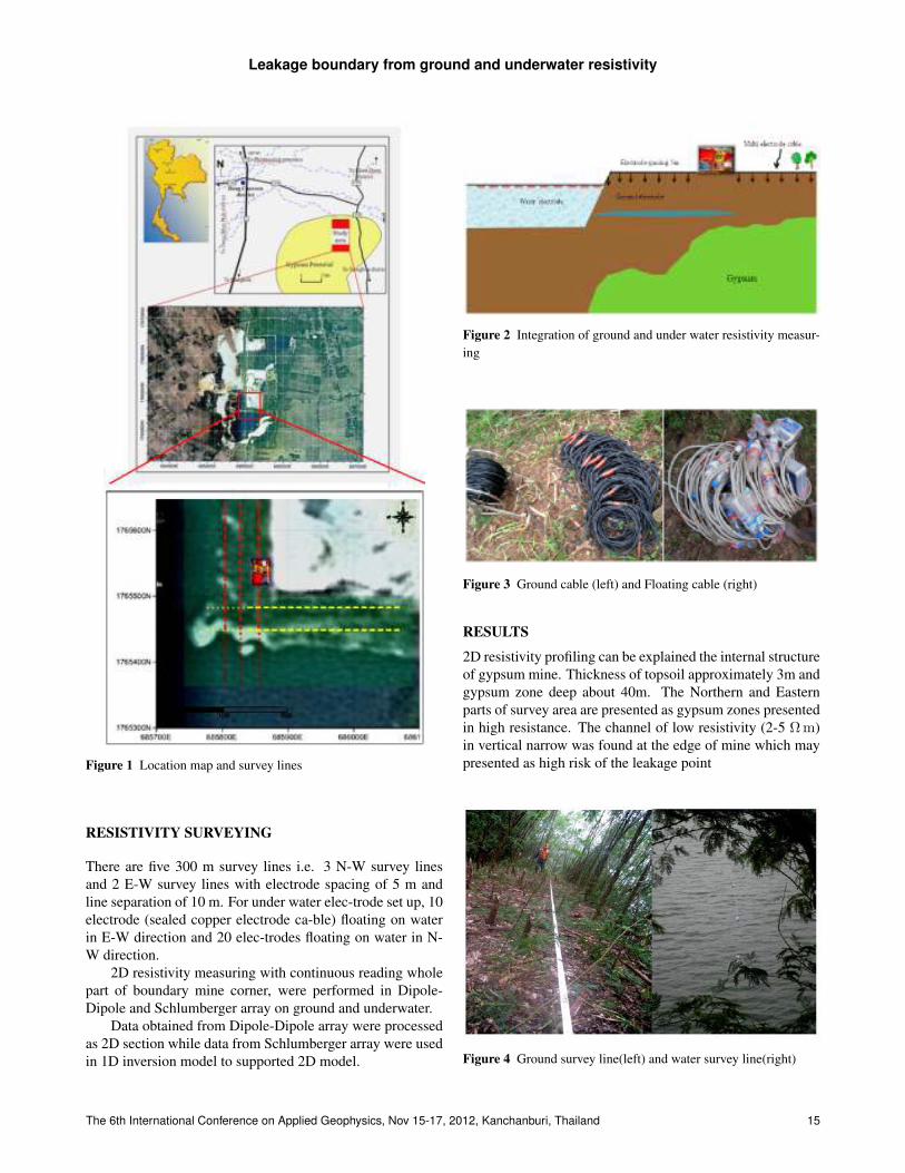
Figure 1 Location map and survey lines
RESISTIVITY SURVEYING
There are five 300 m survey lines i.e. 3 N-W survey lines
and 2 E-W survey lines with electrode spacing of 5 m and
line separation of 10 m. For under water elec-trode set up, 10
electrode (sealed copper electrode ca-ble) floating on water
in E-W direction and 20 elec-trodes floating on water in N-
W direction.
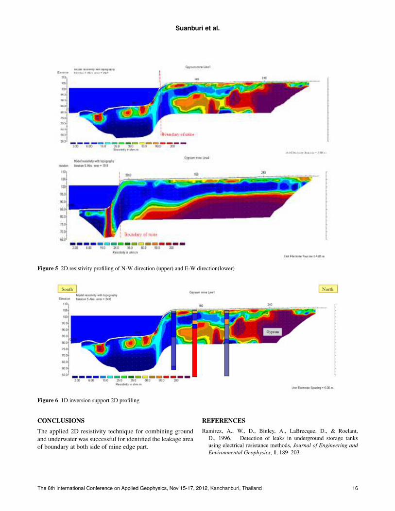
2D resistivity measuring with continuous reading whole
part of boundary mine corner, were performed in Dipole-
Dipole and Schlumberger array on ground and underwater.
Data obtained from Dipole-Dipole array were processed
as 2D section while data from Schlumberger array were used
in 1D inversion model to supported 2D model.
Figure 2 Integration of ground and under water resistivity measur-
ing
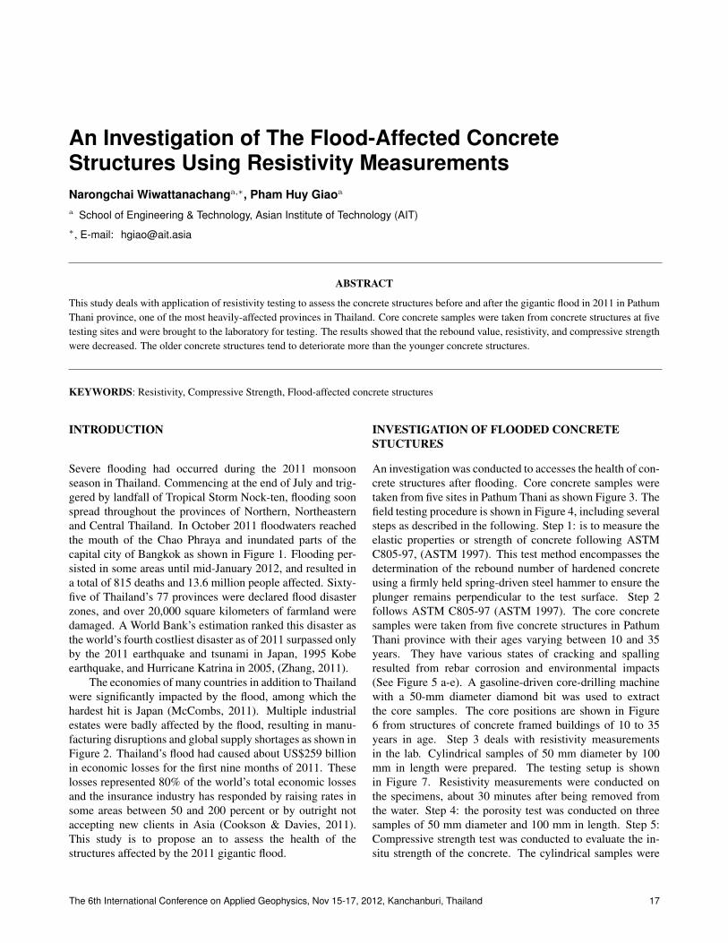
Figure 3 Ground cable (left) and Floating cable (right)
RESULTS
2D resistivity profiling can be explained the internal structure
of gypsum mine. Thickness of topsoil approximately 3m and
gypsum zone deep about 40m. The Northern and Eastern
parts of survey area are presented as gypsum zones presented
in high resistance. The channel of low resistivity (2-5 Ωm)
in vertical narrow was found at the edge of mine which may
presented as high risk of the leakage point
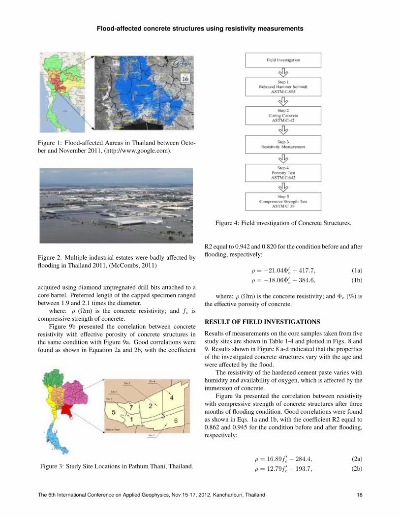
Figure 4 Ground survey line(left) and water survey line(right)
The 6th International Conference on Applied Geophysics, Nov 15-17, 2012, Kanchanburi, Thailand 15
Suanburi et al.
Figure 5 2D resistivity profiling of N-W direction (upper) and E-W direction(lower)
Figure 6 1D inversion support 2D profiling
CONCLUSIONS
The applied 2D resistivity technique for combining ground
and underwater was successful for identified the leakage area
of boundary at both side of mine edge part.
REFERENCES
Ramirez, A., W., D., Binley, A., LaBrecque, D., & Roelant,
D., 1996. Detection of leaks in underground storage tanks
using electrical resistance methods, Journal of Engineering and
Environmental Geophysics, 1, 189–203.
The 6th International Conference on Applied Geophysics, Nov 15-17, 2012, Kanchanburi, Thailand 16
An Investigation of The Flood-Affected ConcreteStructures Using Resistivity Measurements
Narongchai Wiwattanachanga,∗, Pham Huy Giaoa
a School of Engineering & Technology, Asian Institute of Technology (AIT)
∗, E-mail: [email protected]
ABSTRACT
This study deals with application of resistivity testing to assess the concrete structures before and after the gigantic flood in 2011 in Pathum
Thani province, one of the most heavily-affected provinces in Thailand. Core concrete samples were taken from concrete structures at five
testing sites and were brought to the laboratory for testing. The results showed that the rebound value, resistivity, and compressive strength
were decreased. The older concrete structures tend to deteriorate more than the younger concrete structures.
KEYWORDS: Resistivity, Compressive Strength, Flood-affected concrete structures
INTRODUCTION
Severe flooding had occurred during the 2011 monsoon
season in Thailand. Commencing at the end of July and trig-
gered by landfall of Tropical Storm Nock-ten, flooding soon
spread throughout the provinces of Northern, Northeastern
and Central Thailand. In October 2011 floodwaters reached
the mouth of the Chao Phraya and inundated parts of the
capital city of Bangkok as shown in Figure 1. Flooding per-
sisted in some areas until mid-January 2012, and resulted in
a total of 815 deaths and 13.6 million people affected. Sixty-
five of Thailand’s 77 provinces were declared flood disaster
zones, and over 20,000 square kilometers of farmland were
damaged. A World Bank’s estimation ranked this disaster as
the world’s fourth costliest disaster as of 2011 surpassed only
by the 2011 earthquake and tsunami in Japan, 1995 Kobe
earthquake, and Hurricane Katrina in 2005, (Zhang, 2011).
The economies of many countries in addition to Thailand
were significantly impacted by the flood, among which the
hardest hit is Japan (McCombs, 2011). Multiple industrial
estates were badly affected by the flood, resulting in manu-
facturing disruptions and global supply shortages as shown in
Figure 2. Thailand’s flood had caused about US$259 billion
in economic losses for the first nine months of 2011. These
losses represented 80% of the world’s total economic losses
and the insurance industry has responded by raising rates in
some areas between 50 and 200 percent or by outright not
accepting new clients in Asia (Cookson & Davies, 2011).
This study is to propose an to assess the health of the
structures affected by the 2011 gigantic flood.
INVESTIGATION OF FLOODED CONCRETE
STUCTURES
An investigation was conducted to accesses the health of con-
crete structures after flooding. Core concrete samples were
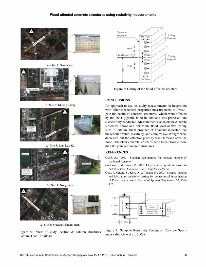
taken from five sites in Pathum Thani as shown Figure 3. The
field testing procedure is shown in Figure 4, including several
steps as described in the following. Step 1: is to measure the
elastic properties or strength of concrete following ASTM
C805-97, (ASTM 1997). This test method encompasses the
determination of the rebound number of hardened concrete
using a firmly held spring-driven steel hammer to ensure the
plunger remains perpendicular to the test surface. Step 2
follows ASTM C805-97 (ASTM 1997). The core concrete
samples were taken from five concrete structures in Pathum
Thani province with their ages varying between 10 and 35
years. They have various states of cracking and spalling
resulted from rebar corrosion and environmental impacts
(See Figure 5 a-e). A gasoline-driven core-drilling machine
with a 50-mm diameter diamond bit was used to extract
the core samples. The core positions are shown in Figure
6 from structures of concrete framed buildings of 10 to 35
years in age. Step 3 deals with resistivity measurements
in the lab. Cylindrical samples of 50 mm diameter by 100
mm in length were prepared. The testing setup is shown
in Figure 7. Resistivity measurements were conducted on
the specimens, about 30 minutes after being removed from
the water. Step 4: the porosity test was conducted on three
samples of 50 mm diameter and 100 mm in length. Step 5:
Compressive strength test was conducted to evaluate the in-
situ strength of the concrete. The cylindrical samples were
The 6th International Conference on Applied Geophysics, Nov 15-17, 2012, Kanchanburi, Thailand 17
Flood-affected concrete structures using resistivity measurements
Figure 1: Flood-affected Aareas in Thailand between Octo-
ber and November 2011, (http://www.google.com).
Figure 2: Multiple industrial estates were badly affected by
flooding in Thailand 2011, (McCombs, 2011)
acquired using diamond impregnated drill bits attached to a
core barrel. Preferred length of the capped specimen ranged
between 1.9 and 2.1 times the diameter.
where: ρ (Ωm) is the concrete resistivity; and fc is
compressive strength of concrete.
Figure 9b presented the correlation between concrete
resistivity with effective porosity of concrete structures in
the same condition with Figure 9a. Good correlations were
found as shown in Equation 2a and 2b, with the coefficient
Figure 3: Study Site Locations in Pathum Thani, Thailand.
Figure 4: Field investigation of Concrete Structures.
R2 equal to 0.942 and 0.820 for the condition before and after
flooding, respectively:
ρ = −21.04Φ′c + 417.7, (1a)
ρ = −18.06Φ′c + 384.6, (1b)
where: ρ (Ωm) is the concrete resistivity; and Φe (%) is
the effective porosity of concrete.
RESULT OF FIELD INVESTIGATIONS
Results of measurements on the core samples taken from five
study sites are shown in Table 1-4 and plotted in Figs. 8 and
9. Results shown in Figure 8 a-d indicated that the properties
of the investigated concrete structures vary with the age and
were affected by the flood.
The resistivity of the hardened cement paste varies with
humidity and availability of oxygen, which is affected by the
immersion of concrete.
Figure 9a presented the correlation between resistivity
with compressive strength of concrete structures after three
months of flooding condition. Good correlations were found
as shown in Eqs. 1a and 1b, with the coefficient R2 equal to
0.862 and 0.945 for the condition before and after flooding,
respectively:
ρ = 16.89f ′c − 284.4, (2a)
ρ = 12.79f ′c − 193.7, (2b)
The 6th International Conference on Applied Geophysics, Nov 15-17, 2012, Kanchanburi, Thailand 18

Wiwattanachang and Giao
Site Age Rebound Value, R
Location (year) Above the Flood Level Below the Flood Level
1 10 36 34
2 15 39 36
3 20 33 31
4 30 42 37
5 35 41 36
Table 1: Rebound Value Results in the Flood Zone
Difference in Potential, (mV) Current Intensity, I (mA) Concrete Resistivity, ρ (Ωm)
Site Above Below Above Below Above Below
Location Flood Level Flood Level Flood Level Flood Level Flood Level Flood Level
1 3677 3606 0.48 0.48 145.5 142.7
2 3815 3793 0.46 0.47 157.6 153.3
3 3624 3608 0.55 0.58 125.2 118.2
4 4006 3877 0.40 0.41 190.3 179.7
5 3857 3523 0.44 0.46 166.6 145.5
Table 2: Results of resistivity test.
Max. Load, F (kN) Compressive Strength, f ′c (MPa)
Site Age Above Below Above Below
Location (year) Flood Level Flood Level Flood Level Flood Level
1 10 5201 4993 26.5 25.4
2 15 5436 5164 27.7 26.3
3 20 4867 4632 24.8 23.6
4 30 5770 5240 29.4 26.7
5 35 5632 5069 28.7 25.8
Table 3: Result of compressive strength test.
Bulk Density, g1 (Mg/m3) Apparent Density, g2 (Mg/m3) Effective Porosity, Φc, (%)
Site Age Above Below Above Below Above Below
Location (year) Flood Level Flood Level Flood Level Flood Level Flood Level Flood Level
1 10 2.12 2.28 2.45 2.64 13.2 13.74
2 15 2.27 2.07 2.59 2.38 12.4 12.94
3 20 2.30 2.08 2.67 2.44 13.7 14.73
4 30 2.15 2.11 2.42 2.39 11.1 11.90
5 35 2.39 2.35 2.70 2.69 11.5 12.45
Table 4: Results of resistivity test.
The 6th International Conference on Applied Geophysics, Nov 15-17, 2012, Kanchanburi, Thailand 19
Flood-affected concrete structures using resistivity measurements
(a) Site 1: Sam Khok
(b) Site 2: Khlong Luang
(c) Site 3: Lam Luk Ka
(d) Site 4: Nong Suea
(e) Site 5: Mueang Pathum Thani
Figure 5: View of study location & column structures
Pathum Thani Thailand
Figure 6: Coring of the flood-affected structure.
CONCLUSIONS
An approach to use resistivity measurements in integration
with other mechanical properties measurements to investi-
gate the health of concrete structures, which were affected
by the 2011 gigantic flood in Thailand was proposed and
successfully conducted. Measurements taken on the concrete
structures above and below the flood level at five testing
sites in Pathum Thani province of Thailand indicated that
the rebound value, resistivity, and compressive strength were
decreased but the effective porosity was increased after the
flood. The older concrete structures tend to deteriorate more
than the younger concrete structures.
REFERENCES
C805, A., 1997. Standard test method for rebound number of
hardened concrete.
Cookson, R. & Davies, P., 2011. Lloyd’s Asian syndicate closes to
new business., Financial Times. http://www.ft.com..
Giao, P., Chung, S., Kim, D., & Tanaka, H., 2003. Electric imaging
and laboratory resistivity testing for geotechnical investigation
of Pusan clay deposits, Journal of Applied Geophysics, 52, 157–
175.
Figure 7: Setup of Resistivity Testing on Concrete Speci-
mens (after Giao et al., 2003).
The 6th International Conference on Applied Geophysics, Nov 15-17, 2012, Kanchanburi, Thailand 20

Wiwattanachang and Giao
(a) (b)
(c) (d)
Figure 8: Comparison of Concrete Structure Properties before and after Flood: a) Rebound Value; b) Concrete Resistivity; c)
Compressive Strength; and d) Effective Porosity
(a) (b)
Figure 9: Correlation between Concrete Resistivity and (a) Compressive Strength as well as (b) Effective Porosity for the
samples of the flooded.
The 6th International Conference on Applied Geophysics, Nov 15-17, 2012, Kanchanburi, Thailand 21

Flood-affected concrete structures using resistivity measurements
McCombs, D., 2011. Thailand investments put japan inc. directly
in flood’s path, bloomberg, http://www.businessweek.com..
Neville, A., 1998. Properties of concrete, Longman House, Harlow.
Sidney, M., Francis, Y., , & David, D., 2002. Concrete, Prentice
Hall.
Zhang, B., 2011. Top 5 most expensive natural disasters in history.,
http://www.accuweather.com..
The 6th International Conference on Applied Geophysics, Nov 15-17, 2012, Kanchanburi, Thailand 22
Possibility of chemical contamination fromwaste-dumping area to irrigation canal-interpretationbased on geophysical data of an area in Mae Jo, ChiangMai Provinces, Thailand
Noppadol Poomvisesa,∗, Sarawute Chantraprasertb
a Office of Topographical and Geotechnical survey, Royal Irrigation Departmentb Department of Geological Science, Faculty of Science,Chiang Mai Universityc Suwanwajokkasikit Field Corp Research Station, Kasetsart University
∗, E-mail: [email protected]
ABSTRACT
Geophysical surveys were carried out during an international workshop in a Mae Jo area of Chiang Mai province, as part of the Geoscientists
Without Borders 2011 project, organized by Boise State University and Chiang Mai University. The project was supported by the Society of
Exploration Geophysicists Foundation’s program. The aim of the surveys was to study subsurface structures in the eastern part of the Chiang
Mai basin and to provide the workshop participants with training and work experience on modern geophysical acquisition, processing and
preliminary interpretation. The survey methods include gravity, seismic, magnetic, resistivity and electromagnetic measurements. A survey
line of 2,750 m in length was laid in a southwest-northeast direction. The southwestern part of the line was conducted to pass through an
active waste-dumping area while the middle part was intersected by a main irrigation canal. The northeastern part of the line ran along
the boundary of a large sediment quarry and next to the quarry, the survey line was placed parallel to a sub-irrigation canal. The results of
all geophysical methods correspond to each other and confirm two sets of steeply-dipping normal faults, one fault possibly surfaced near
the canal. The ground water table in this area is rather shallow, approximately 30-40 m deep, with flow directions by gradient towards
the lower level of the irrigation canal. It can be noted that the existence of such subsurface structures associate with shallow ground water
table could result in the area beneath or close to the canal having a high possibility of chemical contamination seeping from the dump area
and the quarry. Importantly, the quarry is still active and it contains a large volume of water at a higher elevation than the irrigation canal.
Also, there is a conceivable tendency of the quarry being adopted as a landfill site of Chiang Mai province in the near future. For these
reasons, a hydrogeology study program should be planned to evaluate the possibility of chemical contamination to the canal. The resultant
information could facilitate in a future program to prevent the possible contamination scenario from occurring.
KEYWORDS: Contamination, geophysical measurement, dump area, landfill, Chiang Mai basin
INTRODUCTION
In January 2011, an international workshop was established
at Chiang Mai province, Thailand. It is as part of the Geo-
scientists Without Borders (GWB) 2011 project, organized
by Boise State University (BSU) and Chiang Mai University
(CMU). Main purpose of this project is to help connect
universities and industry with communities in need using
applied geophysics to benefit people and environmental
around the world. Participants from fifteen institutions from
seven countries, who submitted their application to GWB
homepage, were selected. Conceptually, main method in the
workshop is student-direct training to address social problem
that include engineering and environmental problems and
solutions. Practically, the workshop separated the training
into two main parts, in-field and in-house training.
The in-field training was carried out at two field sites
around Chiang Mai, Mae Jo and Wiang Kum Kam. Mae
Jo is an engineering site while Wiang Kun Kam is a paleo-
archaeology site. The first one will be mentioned in this
paper while the last will be not. Mae Jo site is located
at the eastern part of the Chiang Mai basin (Figure 1). It
is very interesting to survey here as the site of a M5.1
earthquake in 2006. Geophysical surveys were conducted
along rural roads and adjacent farm fields to identify geo-
logic structures and faults related to the seismically active
region. A combination of several geophysical methods can
The 6th International Conference on Applied Geophysics, Nov 15-17, 2012, Kanchanburi, Thailand 23
Chemical contamination based on geophysical data
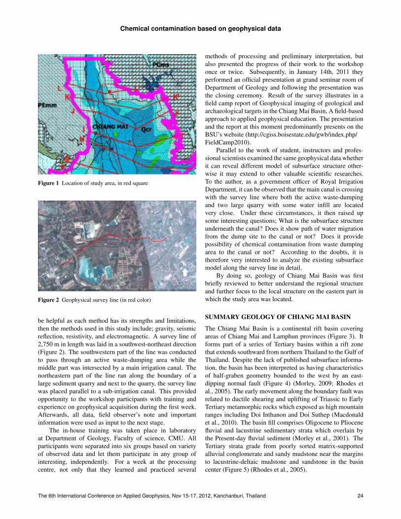
Figure 1 Location of study area, in red square
Figure 2 Geophysical survey line (in red color)
be helpful as each method has its strengths and limitations,
then the methods used in this study include; gravity, seismic
reflection, resistivity, and electromagnetic. A survey line of
2,750 m in length was laid in a southwest-northeast direction
(Figure 2). The southwestern part of the line was conducted
to pass through an active waste-dumping area while the
middle part was intersected by a main irrigation canal. The
northeastern part of the line ran along the boundary of a
large sediment quarry and next to the quarry, the survey line
was placed parallel to a sub-irrigation canal. This provided
opportunity to the workshop participants with training and
experience on geophysical acquisition during the first week.
Afterwards, all data, field observer’s note and important
information were used as input to the next stage.
The in-house training was taken place in laboratory
at Department of Geology, Faculty of science, CMU. All
participants were separated into six groups based on variety
of observed data and let them participate in any group of
interesting, independently. For a week at the processing
centre, not only that they learned and practiced several
methods of processing and preliminary interpretation, but
also presented the progress of their work to the workshop
once or twice. Subsequently, in January 14th, 2011 they
performed an official presentation at grand seminar room of
Department of Geology and following the presentation was
the closing ceremony. Result of the survey illustrates in a
field camp report of Geophysical imaging of geological and
archaeological targets in the Chiang Mai Basin, A field-based
approach to applied geophysical education. The presentation
and the report at this moment predominantly presents on the
BSU’s website (http://cgiss.boisestate.edu/gwb/index.php/
FieldCamp2010).
Parallel to the work of student, instructors and profes-
sional scientists examined the same geophysical data whether
it can reveal different model of subsurface structure other-
wise it may extend to other valuable scientific researches.
To the author, as a government officer of Royal Irrigation
Department, it can be observed that the main canal is crossing
with the survey line where both the active waste-dumping
and two large quarry with some water infill are located
very close. Under these circumstances, it then raised up
some interesting questions; What is the subsurface structure
underneath the canal? Does it show path of water migration
from the dump site to the canal or not? Does it provide
possibility of chemical contamination from waste dumping
area to the canal or not? According to the doubts, it is
therefore very interested to analyze the existing subsurface
model along the survey line in detail.
By doing so, geology of Chiang Mai Basin was first
briefly reviewed to better understand the regional structure
and further focus to the local structure on the eastern part in
which the study area was located.
SUMMARY GEOLOGY OF CHIANG MAI BASIN
The Chiang Mai Basin is a continental rift basin covering
areas of Chiang Mai and Lamphun provinces (Figure 3). It
forms part of a series of Tertiary basins within a rift zone
that extends southward from northern Thailand to the Gulf of
Thailand. Despite the lack of published subsurface informa-
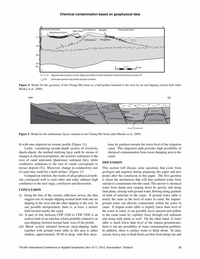
tion, the basin has been interpreted as having characteristics
of half-graben geometry bounded to the west by an east-
dipping normal fault (Figure 4) (Morley, 2009; Rhodes et
al., 2005). The early movement along the boundary fault was
related to ductile shearing and uplifting of Triassic to Early
Tertiary metamorphic rocks which exposed as high mountain
ranges including Doi Inthanon and Doi Suthep (Macdonald
et al., 2010). The basin fill comprises Oligocene to Pliocene
fluvial and lacustrine sedimentary strata which overlain by
the Present-day fluvial sediment (Morley et al., 2001). The
Tertiary strata grade from poorly sorted matrix-supported
alluvial conglomerate and sandy mudstone near the margins
to lacustrine-deltaic mudstone and sandstone in the basin
center (Figure 5) (Rhodes et al., 2005).
The 6th International Conference on Applied Geophysics, Nov 15-17, 2012, Kanchanburi, Thailand 24
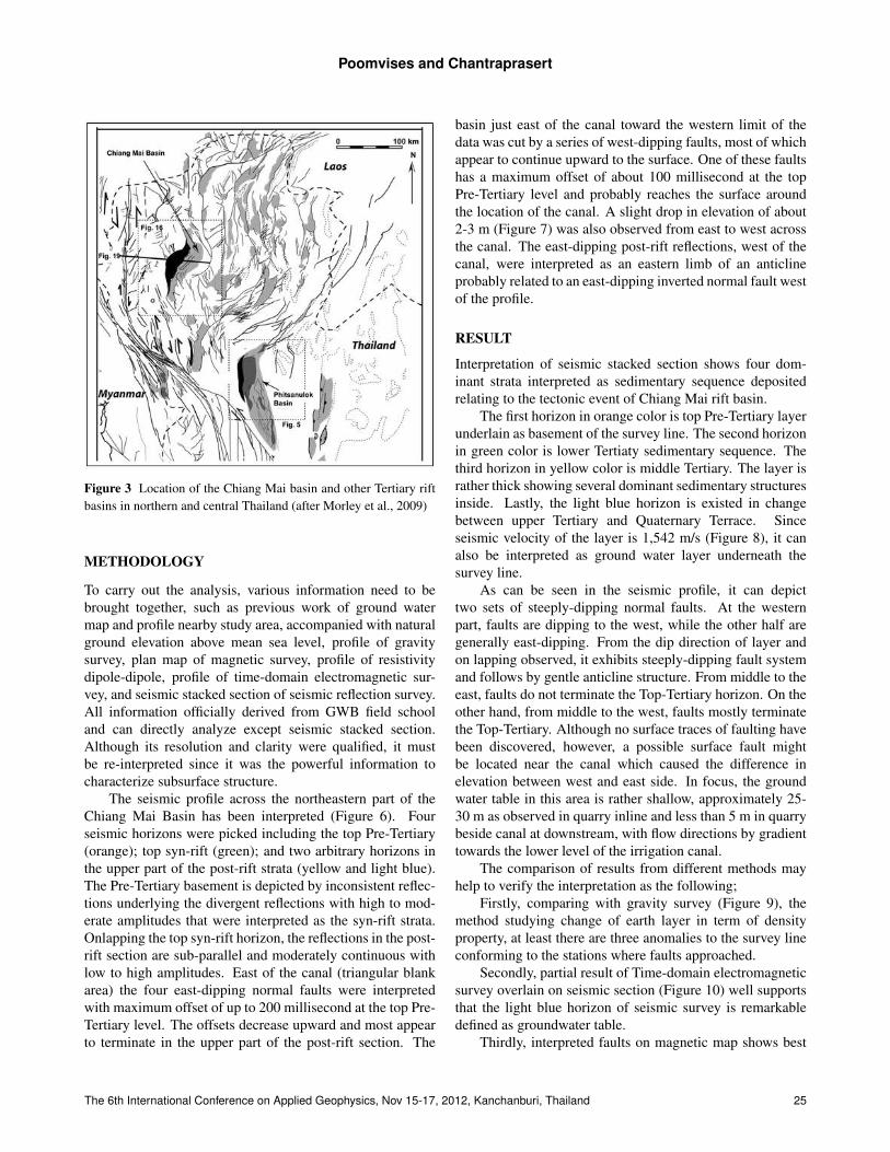
Poomvises and Chantraprasert
Figure 3 Location of the Chiang Mai basin and other Tertiary rift
basins in northern and central Thailand (after Morley et al., 2009)
METHODOLOGY
To carry out the analysis, various information need to be
brought together, such as previous work of ground water
map and profile nearby study area, accompanied with natural
ground elevation above mean sea level, profile of gravity
survey, plan map of magnetic survey, profile of resistivity
dipole-dipole, profile of time-domain electromagnetic sur-
vey, and seismic stacked section of seismic reflection survey.
All information officially derived from GWB field school
and can directly analyze except seismic stacked section.
Although its resolution and clarity were qualified, it must
be re-interpreted since it was the powerful information to
characterize subsurface structure.
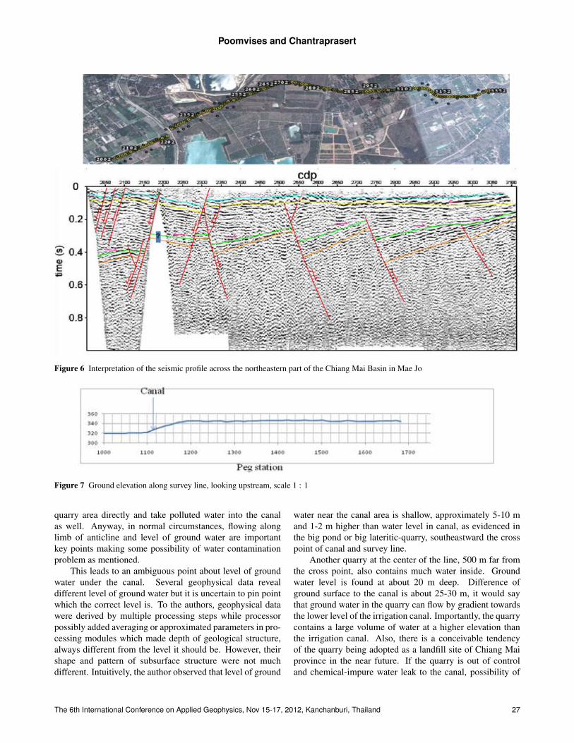
The seismic profile across the northeastern part of the
Chiang Mai Basin has been interpreted (Figure 6). Four
seismic horizons were picked including the top Pre-Tertiary
(orange); top syn-rift (green); and two arbitrary horizons in
the upper part of the post-rift strata (yellow and light blue).
The Pre-Tertiary basement is depicted by inconsistent reflec-
tions underlying the divergent reflections with high to mod-
erate amplitudes that were interpreted as the syn-rift strata.
Onlapping the top syn-rift horizon, the reflections in the post-
rift section are sub-parallel and moderately continuous with
low to high amplitudes. East of the canal (triangular blank
area) the four east-dipping normal faults were interpreted
with maximum offset of up to 200 millisecond at the top Pre-
Tertiary level. The offsets decrease upward and most appear
to terminate in the upper part of the post-rift section. The
basin just east of the canal toward the western limit of the
data was cut by a series of west-dipping faults, most of which
appear to continue upward to the surface. One of these faults
has a maximum offset of about 100 millisecond at the top
Pre-Tertiary level and probably reaches the surface around
the location of the canal. A slight drop in elevation of about
2-3 m (Figure 7) was also observed from east to west across
the canal. The east-dipping post-rift reflections, west of the
canal, were interpreted as an eastern limb of an anticline
probably related to an east-dipping inverted normal fault west
of the profile.
RESULT
Interpretation of seismic stacked section shows four dom-
inant strata interpreted as sedimentary sequence deposited
relating to the tectonic event of Chiang Mai rift basin.
The first horizon in orange color is top Pre-Tertiary layer
underlain as basement of the survey line. The second horizon
in green color is lower Tertiaty sedimentary sequence. The
third horizon in yellow color is middle Tertiary. The layer is
rather thick showing several dominant sedimentary structures
inside. Lastly, the light blue horizon is existed in change
between upper Tertiary and Quaternary Terrace. Since
seismic velocity of the layer is 1,542 m/s (Figure 8), it can
also be interpreted as ground water layer underneath the
survey line.
As can be seen in the seismic profile, it can depict
two sets of steeply-dipping normal faults. At the western
part, faults are dipping to the west, while the other half are
generally east-dipping. From the dip direction of layer and
on lapping observed, it exhibits steeply-dipping fault system
and follows by gentle anticline structure. From middle to the
east, faults do not terminate the Top-Tertiary horizon. On the
other hand, from middle to the west, faults mostly terminate
the Top-Tertiary. Although no surface traces of faulting have
been discovered, however, a possible surface fault might
be located near the canal which caused the difference in
elevation between west and east side. In focus, the ground
water table in this area is rather shallow, approximately 25-
30 m as observed in quarry inline and less than 5 m in quarry
beside canal at downstream, with flow directions by gradient
towards the lower level of the irrigation canal.
The comparison of results from different methods may
help to verify the interpretation as the following;
Firstly, comparing with gravity survey (Figure 9), the
method studying change of earth layer in term of density
property, at least there are three anomalies to the survey line
conforming to the stations where faults approached.
Secondly, partial result of Time-domain electromagnetic
survey overlain on seismic section (Figure 10) well supports
that the light blue horizon of seismic survey is remarkable
defined as groundwater table.
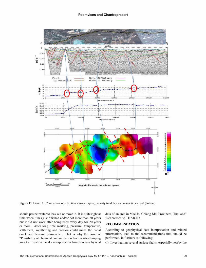
Thirdly, interpreted faults on magnetic map shows best
The 6th International Conference on Applied Geophysics, Nov 15-17, 2012, Kanchanburi, Thailand 25
Chemical contamination based on geophysical data
Figure 4 Model for the geometry of the Chiang Mai basin as a half-graben bounded to the west by an east-dipping normal fault (after
Morley et al., 2009).
Figure 5 Model for the sedimentary facies variation in the Chiang Mai basin (after Rhodes et al., 2005)
fit with ones depicted on seismic profile (Figure 11).
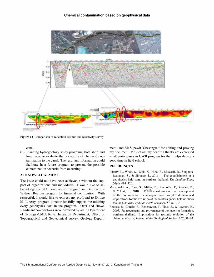
Lastly, considering pseudo-depth section of resistivity
dipole-dipole, the method studying layer earth by means of
changes in electrical properties, the resistive sediments to the
west of canal represents Quaternary sediment (Qs), while
conductive sediments to the east of canals corresponds to
terrace deposit (Ts). Moreover, change in conductivity east
of canal may stand for a fault surface. (Figure 12)
Comparison solution, the results of all geophysical meth-
ods correspond well to each other and make enhance high
confidence to the next stage, conclusion and discussion.
CONCLUSION
(i) Along the line of the seismic reflection survey, the data
suggest sets of steeply-dipping normal fault with one set
dipping to the west and the other dipping to the east. In
one possible interpretation, there is, at least, a surface
fault located nearby the canal.
(ii) A part of line between CDP 2100 to CDP 2300 is an
eastern limb of an anticline which probably related to an
east-dipping inverted normal fault, west of the profile.
(iii) Block system initiated between steep-dipping faults
together with ground water table in this area is rather
shallow, approximately 30-40 m deep, with flow direc-
tions by gradient towards the lower level of the irrigation
canal. This migration path provides high possibility of
chemical contamination from waste dumping area to the
canal.
DISCUSSION
This section will discuss some questions that come from
geologist and engineer during preparing this paper and also
points after the conclusion in this paper. The first question
is about the mechanism that will take polluted water from
outside to contaminate into the canal. The answer is chemical
water from dump area seeping down by gravity and along
fault plane, mixing with ground water, flowing along gradient
of limb of anticline to the canal. If ground water table is
nearly the same as the level of water in canal, the impure-
ground water can directly contaminate within the water in
canal. If impure-water table is slightly lower than level of
the water in canal, it can possibly move upward and pollute
to the canal water by capillary force through soil sediment
and along fault plane as well. On the other hand, if water
table is much lower than level of the impure-groundwater,
there is not any possibility of water contamination problem.
In addition, there is surface water to think about. In rainy
season, heavy rain or flash flood can flow from dump site and
The 6th International Conference on Applied Geophysics, Nov 15-17, 2012, Kanchanburi, Thailand 26
Poomvises and Chantraprasert
Figure 6 Interpretation of the seismic profile across the northeastern part of the Chiang Mai Basin in Mae Jo
Figure 7 Ground elevation along survey line, looking upstream, scale 1 : 1
quarry area directly and take polluted water into the canal
as well. Anyway, in normal circumstances, flowing along
limb of anticline and level of ground water are important
key points making some possibility of water contamination
problem as mentioned.
This leads to an ambiguous point about level of ground
water under the canal. Several geophysical data reveal
different level of ground water but it is uncertain to pin point
which the correct level is. To the authors, geophysical data
were derived by multiple processing steps while processor
possibly added averaging or approximated parameters in pro-
cessing modules which made depth of geological structure,
always different from the level it should be. However, their
shape and pattern of subsurface structure were not much
different. Intuitively, the author observed that level of ground
water near the canal area is shallow, approximately 5-10 m
and 1-2 m higher than water level in canal, as evidenced in
the big pond or big lateritic-quarry, southeastward the cross
point of canal and survey line.
Another quarry at the center of the line, 500 m far from
the cross point, also contains much water inside. Ground
water level is found at about 20 m deep. Difference of
ground surface to the canal is about 25-30 m, it would say
that ground water in the quarry can flow by gradient towards
the lower level of the irrigation canal. Importantly, the quarry
contains a large volume of water at a higher elevation than
the irrigation canal. Also, there is a conceivable tendency
of the quarry being adopted as a landfill site of Chiang Mai
province in the near future. If the quarry is out of control
and chemical-impure water leak to the canal, possibility of
The 6th International Conference on Applied Geophysics, Nov 15-17, 2012, Kanchanburi, Thailand 27

Chemical contamination based on geophysical data
Figure 8 Picking velocity of 1,542 m/s on semblance, interpreted as groundwater table
Figure 9 Interpretation result of gravity method
chemical contamination will shift to environmental impact
or risk, in consequence various problems must be followed
without stay away from.
Next question is about the risk or effect of water con-
tamination. The canal daily conveys much water to irri-
gation area downstream whereas many crops were planted.
Some of them need much water and absorb many nutrient
elements. If contaminated water from canal, which contains
heavy element and toxic chemical substance, is fed to the
crops continuously until much than safety level, agricultural
products will be infected and spread out to the people by
accident.
Somebody informed that irrigation canal fundamentally
constructed follow through the standard safety design which
Figure 10 Reflection seismic versus time domain electromagnetic result. Determine groundwater table at 60 meter below surface.
The 6th International Conference on Applied Geophysics, Nov 15-17, 2012, Kanchanburi, Thailand 28
Poomvises and Chantraprasert
Figure 11 Figure 11 Comparison of reflection seismic (upper), gravity (middle), and magnetic method (bottom).
should protect water to leak out or move in. It is quite right at
time when it has just finished and/or not more than 20 years
but it did not work after being used every day for 20 years
or more. After long time working, pressure, temperature,
settlement, weathering and erosion could make the canal
crack and become permeable. That is why the issue of
“Possibility of chemical contamination from waste-dumping
area to irrigation canal - interpretation based on geophysical
data of an area in Mae Jo, Chiang Mai Provinces, Thailand”
is expressed to THAICID.
RECOMMENDATION
According to geophysical data interpretation and related
information, lead to the recommendations that should be
performed, in furthers as following;
(i) Investigating several surface faults, especially nearby the
The 6th International Conference on Applied Geophysics, Nov 15-17, 2012, Kanchanburi, Thailand 29
Chemical contamination based on geophysical data
Figure 12 Comparison of reflection seismic and resistivity survey
canal.
(ii) Planning hydrogeology study programs, both short and
long term, to evaluate the possibility of chemical con-
tamination to the canal. The resultant information could
facilitate in a future program to prevent the possible
contamination scenario from occurring.
ACKNOWLEDGEMENT
The issue could not have been achievable without the sup-
port of organizations and individuals. I would like to ac-
knowledge the SEG Foundation’s program and Geoscientist
Without Boarder program for financial contribution. With
respectful, I would like to express my profound to Dr.Lee
M. Liberty, program director for fully support me utilizing
every geophysics data in the program. Over and above,
significant contributions were provided by all in Department
of Geology-CMU, Royal Irrigation Department, Office of
Topographical and Geotechnical survey, Geology Depart-
ment, and Mr.Supawit Yawsangratt for editing and proving
my document. Most of all, my heartfelt thanks are expressed
to all participants in GWB program for their helps during a
good time in field school.
REFERENCES
Liberty, L., Wood, S., Wijk, K., Hinz, E., Mikesell, D., Singhara-
jwarapan, S., & Shragge, J., 2011. The establishment of a
geophysics field camp in northern thailand, The Leading Edge,
30(4), 414–420.
Macdonald, A., Barr, S., Miller, B., Reynolds, P., Rhodes, B.,
& Yokart, B., 2010. PUtUt constraints on the development
of the doi inthanon metamorphic core complex domain and
implications for the evolution of the western gneiss belt, northern
thailand, Journal of Asian Earth Sciences, 37, 82–104.
Rhodes, B., Conejo, R., Benchawan, T., Titus, S., & Lawson, R.,
2005. Palaeocurrents and provenance of the mae rim formation,
northern thailand: Implications for tectonic evolution of the
chiang mai basin, Journal of the Geological Society, 162, 51–63.
The 6th International Conference on Applied Geophysics, Nov 15-17, 2012, Kanchanburi, Thailand 30
Application of geophysical methods for characterizing aselected solid waste disposal site in Songkhla province
Thirat Sommaia,b,∗, Kamhaeng Wattanasena,b, Sawasdee Yodkayhuna,b
a Department of Physics, Faculty of Science, Prince of Songkla University, Hat Yai ,90112, THAILANDb Geophysics Research Center, Department of Physics, Faculty of Science, Prince of Songkla University, Hat Yai ,90112,
THAILAND∗, E-mail: [email protected]
ABSTRACT
Songkhla province mainly uses a landfill method for the solid waste disposal. It is thus possible that the subsurface groundwater or/and soil
can be contaminated by the contaminant, if the waste can leak from the landfill site. This work has applied the geophysics methods
to characterize the subsurface structure in a selected solid waste disposal site in the Songkhla province, which has been previously
recommended by GIS study and to characterize the subsurface structure around an active landfill site of Hat Yai municipality. 2D - IP
& resistivity imaging, Vertical Electrical Sounding (VES), Self-potential (SP), and Seismic refraction surveys have been conducted in those
two sites. The subsurface geological barrier can be obtained by 2D - IP & resistivity imaging and seismic refraction data. The image
of low resistivity clay layer can be mapped and it underlines the higher resistivity top soil layer. In the active landfill site of Hat Yai
municipality, the lateral resistivity variation in the clay layer and the position of discontinuous clay layer are possible the leakage channel
of the contaminant that spread further to the surrounding area. Low chargeability data from IP indicate the present of clay layer which
corresponds to the positive SP data and the low resistivity layer. The study results can suggest the appropriate site with according to the
standard criteria for the subsurface geological structure of landfill site and can probably provide the area of contamination in the ground.
Geophysics method therefore shows that it is a promising tool for site selection study of landfill.
KEYWORDS: Geophysical methods, waste disposal site, contamination
INTRODUCTION
Waste is one of the major problems of the world that
affect to environment. There are many methods for solid
waste disposal such as Open Dumps, Sanitary Landfills,
Incineration, and Ocean Dumping. The advantages and
disadvantages of each method are different and the selecting
method for the solid waste disposal is based on the economy,
society, organization, and landscape. For Thailand, the
suitable method of solid waste disposal is the sanitary landfill
(Pollution Control Department, 2009). However, the leakage
waste from the landfill site will greatly affect to environment
if the subsurface structure of the landfill site has a defect of
no natural barrier e.g. clay layer etc.
There are many ground geophysics methods can em-
ploy to map the subsurface geological structure. The inte-
grated interpretation data from various method can reduce
an ambiguous of the subsurface model and it has been
used in conjunction with other methods such as the seismic
method, the induced polarization (IP) method, and/or the
self-potential (SP) method for the environmental investiga-
tion (Aristodemou E. and Thomas-Betts A., 2000). The
resistivity method has been widely used for landfill and waste
disposal investigation (e.g. Mota, R. et al., 2004; Class, A.,
et al., 2008; Ehirim, C.N., et al., 2009; UGWU,S.A., et al.,
2009; Gemail,Kh.S., et al. 2011; Nwankwo et al.,2012).
Songkhla province locates in the southern part of Thai-
land where mainly uses a landfill method for the solid waste
disposal. It is thus possible that the subsurface groundwater
or/and soil can be contaminated by the contaminant, if
the waste can leak from the landfill site. A GIS study
of Songkhla province for selecting the landfill site was
performed by Rottana (2002) and the appropriate area was
recommended. Two sites from Rottana’s reccomment have
been choosen for geophysical study (Figure 1). The first site
locates in Khuan Lang sub district, Hat Yai district where
the landfill in this site has been actived. The second site is
in Ban Na Wat Pho School, Klong Hoi Khong sub district,
Klong Hoi Khong district.
The aims of this study are: (i) to characterize the
subsurface structure in a selected solid waste disposal site
The 6th International Conference on Applied Geophysics, Nov 15-17, 2012, Kanchanburi, Thailand 31
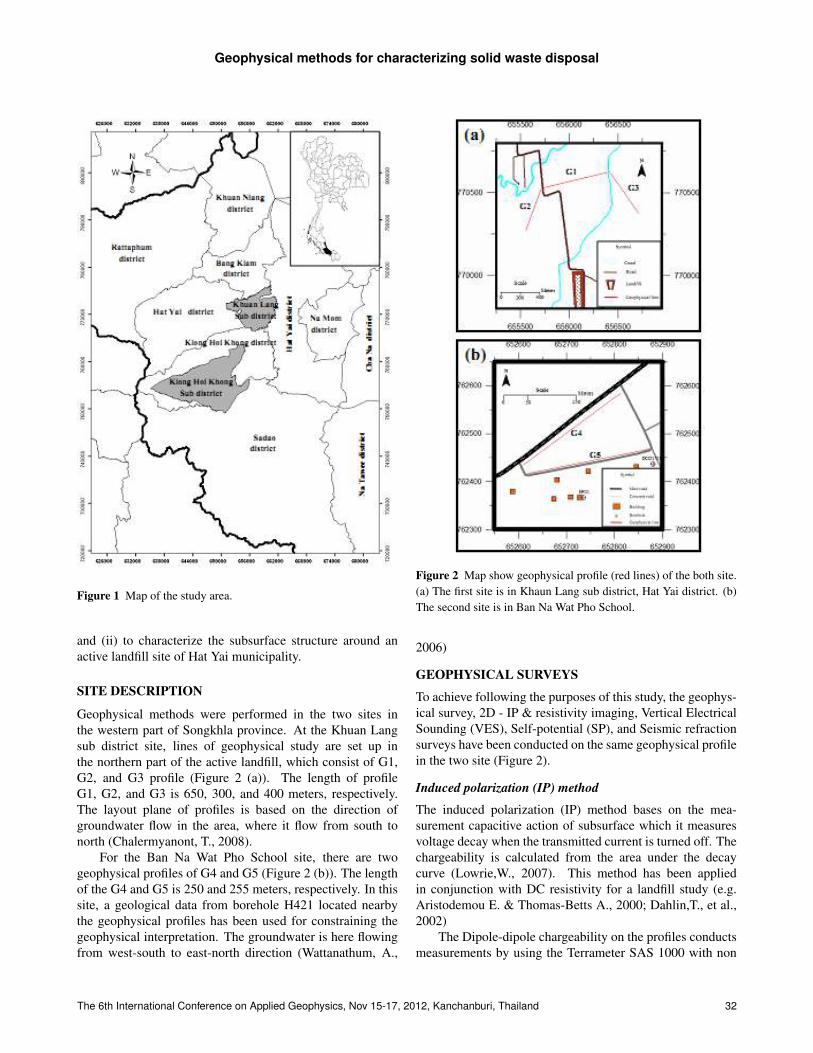
Geophysical methods for characterizing solid waste disposal
Figure 1 Map of the study area.
and (ii) to characterize the subsurface structure around an
active landfill site of Hat Yai municipality.
SITE DESCRIPTION
Geophysical methods were performed in the two sites in
the western part of Songkhla province. At the Khuan Lang
sub district site, lines of geophysical study are set up in
the northern part of the active landfill, which consist of G1,
G2, and G3 profile (Figure 2 (a)). The length of profile
G1, G2, and G3 is 650, 300, and 400 meters, respectively.
The layout plane of profiles is based on the direction of
groundwater flow in the area, where it flow from south to
north (Chalermyanont, T., 2008).
For the Ban Na Wat Pho School site, there are two
geophysical profiles of G4 and G5 (Figure 2 (b)). The length
of the G4 and G5 is 250 and 255 meters, respectively. In this
site, a geological data from borehole H421 located nearby
the geophysical profiles has been used for constraining the
geophysical interpretation. The groundwater is here flowing
from west-south to east-north direction (Wattanathum, A.,
Figure 2 Map show geophysical profile (red lines) of the both site.
(a) The first site is in Khaun Lang sub district, Hat Yai district. (b)
The second site is in Ban Na Wat Pho School.
2006)
GEOPHYSICAL SURVEYS
To achieve following the purposes of this study, the geophys-
ical survey, 2D - IP & resistivity imaging, Vertical Electrical
Sounding (VES), Self-potential (SP), and Seismic refraction
surveys have been conducted on the same geophysical profile
in the two site (Figure 2).
Induced polarization (IP) method
The induced polarization (IP) method bases on the mea-
surement capacitive action of subsurface which it measures
voltage decay when the transmitted current is turned off. The
chargeability is calculated from the area under the decay
curve (Lowrie,W., 2007). This method has been applied
in conjunction with DC resistivity for a landfill study (e.g.
Aristodemou E. & Thomas-Betts A., 2000; Dahlin,T., et al.,
2002)
The Dipole-dipole chargeability on the profiles conducts
measurements by using the Terrameter SAS 1000 with non
The 6th International Conference on Applied Geophysics, Nov 15-17, 2012, Kanchanburi, Thailand 32
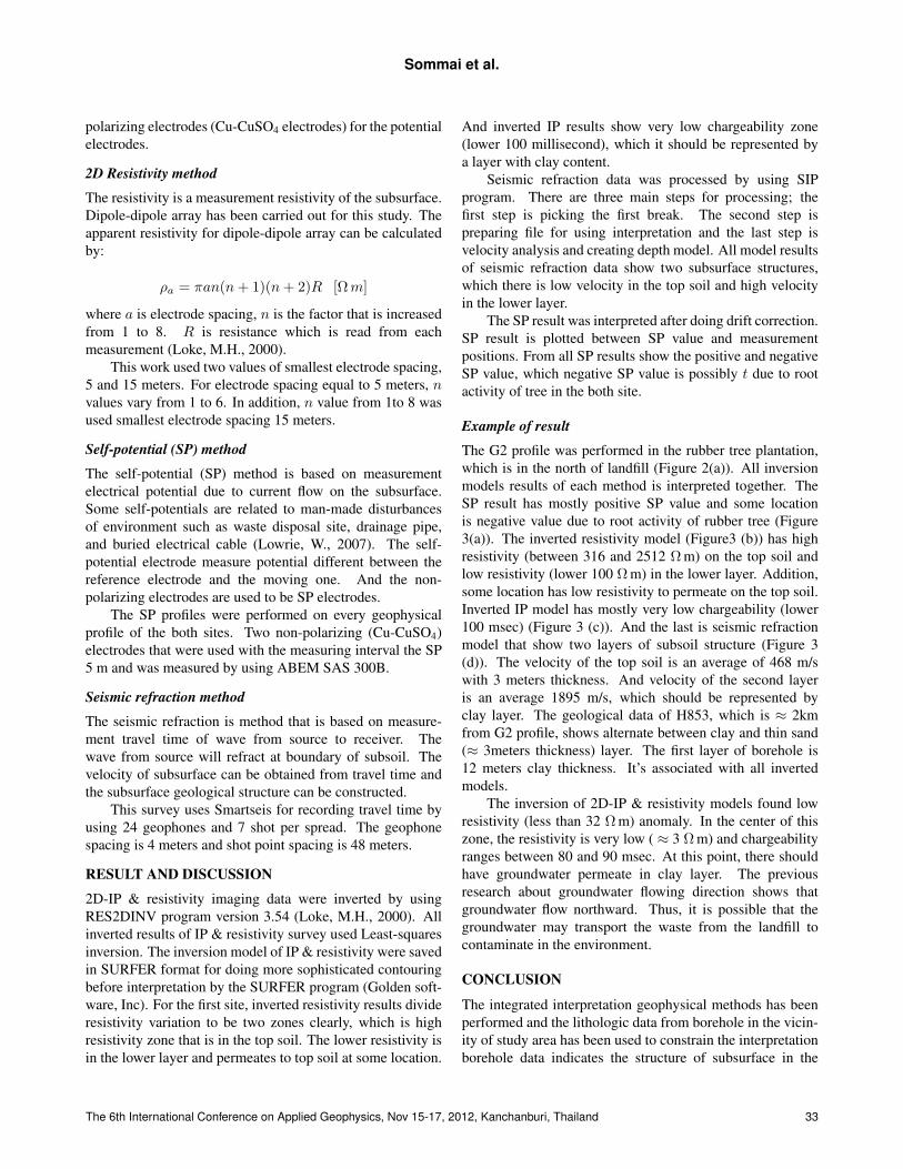
Sommai et al.
polarizing electrodes (Cu-CuSO4 electrodes) for the potential
electrodes.
2D Resistivity method
The resistivity is a measurement resistivity of the subsurface.
Dipole-dipole array has been carried out for this study. The
apparent resistivity for dipole-dipole array can be calculated
by:
ρa = πan(n+ 1)(n+ 2)R [Ωm]
where a is electrode spacing, n is the factor that is increased
from 1 to 8. R is resistance which is read from each
measurement (Loke, M.H., 2000).
This work used two values of smallest electrode spacing,
5 and 15 meters. For electrode spacing equal to 5 meters, nvalues vary from 1 to 6. In addition, n value from 1to 8 was
used smallest electrode spacing 15 meters.
Self-potential (SP) method
The self-potential (SP) method is based on measurement
electrical potential due to current flow on the subsurface.
Some self-potentials are related to man-made disturbances
of environment such as waste disposal site, drainage pipe,
and buried electrical cable (Lowrie, W., 2007). The self-
potential electrode measure potential different between the
reference electrode and the moving one. And the non-
polarizing electrodes are used to be SP electrodes.
The SP profiles were performed on every geophysical
profile of the both sites. Two non-polarizing (Cu-CuSO4)
electrodes that were used with the measuring interval the SP
5 m and was measured by using ABEM SAS 300B.
Seismic refraction method
The seismic refraction is method that is based on measure-
ment travel time of wave from source to receiver. The
wave from source will refract at boundary of subsoil. The
velocity of subsurface can be obtained from travel time and
the subsurface geological structure can be constructed.
This survey uses Smartseis for recording travel time by
using 24 geophones and 7 shot per spread. The geophone
spacing is 4 meters and shot point spacing is 48 meters.
RESULT AND DISCUSSION
2D-IP & resistivity imaging data were inverted by using
RES2DINV program version 3.54 (Loke, M.H., 2000). All
inverted results of IP & resistivity survey used Least-squares
inversion. The inversion model of IP & resistivity were saved
in SURFER format for doing more sophisticated contouring
before interpretation by the SURFER program (Golden soft-
ware, Inc). For the first site, inverted resistivity results divide
resistivity variation to be two zones clearly, which is high
resistivity zone that is in the top soil. The lower resistivity is
in the lower layer and permeates to top soil at some location.
And inverted IP results show very low chargeability zone
(lower 100 millisecond), which it should be represented by
a layer with clay content.
Seismic refraction data was processed by using SIP
program. There are three main steps for processing; the
first step is picking the first break. The second step is
preparing file for using interpretation and the last step is
velocity analysis and creating depth model. All model results
of seismic refraction data show two subsurface structures,
which there is low velocity in the top soil and high velocity
in the lower layer.
The SP result was interpreted after doing drift correction.
SP result is plotted between SP value and measurement
positions. From all SP results show the positive and negative
SP value, which negative SP value is possibly t due to root
activity of tree in the both site.
Example of result
The G2 profile was performed in the rubber tree plantation,
which is in the north of landfill (Figure 2(a)). All inversion
models results of each method is interpreted together. The
SP result has mostly positive SP value and some location
is negative value due to root activity of rubber tree (Figure
3(a)). The inverted resistivity model (Figure3 (b)) has high
resistivity (between 316 and 2512 Ωm) on the top soil and
low resistivity (lower 100 Ωm) in the lower layer. Addition,
some location has low resistivity to permeate on the top soil.
Inverted IP model has mostly very low chargeability (lower
100 msec) (Figure 3 (c)). And the last is seismic refraction
model that show two layers of subsoil structure (Figure 3
(d)). The velocity of the top soil is an average of 468 m/s
with 3 meters thickness. And velocity of the second layer
is an average 1895 m/s, which should be represented by
clay layer. The geological data of H853, which is ≈ 2km
from G2 profile, shows alternate between clay and thin sand
(≈ 3meters thickness) layer. The first layer of borehole is
12 meters clay thickness. It’s associated with all inverted
models.
The inversion of 2D-IP & resistivity models found low
resistivity (less than 32 Ωm) anomaly. In the center of this
zone, the resistivity is very low ( ≈ 3 Ωm) and chargeability
ranges between 80 and 90 msec. At this point, there should
have groundwater permeate in clay layer. The previous
research about groundwater flowing direction shows that
groundwater flow northward. Thus, it is possible that the
groundwater may transport the waste from the landfill to
contaminate in the environment.
CONCLUSION
The integrated interpretation geophysical methods has been
performed and the lithologic data from borehole in the vicin-
ity of study area has been used to constrain the interpretation
borehole data indicates the structure of subsurface in the
The 6th International Conference on Applied Geophysics, Nov 15-17, 2012, Kanchanburi, Thailand 33
Geophysical methods for characterizing solid waste disposal
Figure 3 A geophysical results of G2 profile.(a) the SP result(rubber tree is represented with green point), (b) the inverted resistivity model
, (c) the inverted induced polarization (IP) model, and (d) the seismic refraction model.
northern part of the active Hat Yai landfill is mostly clay
layer, which is good natural barrier and agree well with
geophysical methods. Geophysical method can applied to
motoring for the environmental problem. The combined
geophysical methods make interpretation greatly. Resistivity
measurement is suitable method for monitoring contamina-
tion and/or environmental problem. Using IP measurement
combine with resistivity method clearly make interpretation
of clay content layer. SP method is not good method for
this study area due to amount of root activity of the trees.
The 6th International Conference on Applied Geophysics, Nov 15-17, 2012, Kanchanburi, Thailand 34
Sommai et al.
And seismic refraction method provides a very good shallow
subsurface structure that the natural barrier (clay) layer can
be clearly mapped.
ACKNOWLEDGMENT
This work is supported by research grants from the Gradu-
ate studies and department of Physics, Faculty of Science.
Furthermore, we wish to thank my friends for helping in
geophysical field work.
REFERENCES
Aristodemou, E. & Thomas-Betts, A., 2000. DC resistivity and
induced polarization investigations at a waste disposal site and
its environments, Journal of Applied Geophysics, 44, 275–302.
Arora, T. et al., 2007. Non-intrusive characterization of the redox
potential of landfill leachate plumes from self- potential data,
Journal of Applied Geophysics, 92, 274–292.
Chalermyanont, T. et al., 2008. Aquifer characteristic and quality
of groundwater in the vicinity area of the Songkhla lake, Hat Yai
basin, Tech. rep., Prince of Songkla University.
Chandra, S. et al., 2010. Geophysical model of geological dis-
continuities in a granite aquifer:analyzing small scale variability
of electrical resistivity for groundwater occurrences, Journal of
Applied Geophysics, 71, 137–148.
Class, A. et al., 2008. Assessing aquifer vulnerability to pollutants
by electrical resistivity tomography (ERT) at a nitrate vulnerable
zone in NE spain, Journal of Environmental Geology, 54, 515–
520.
C.N., N. et al., 2012. Geophysical method of investigating
groundwater and sub-soil contamination-A case study, American
Journal of Environmental Engineering, 2(3), 49–53.
Dahlin, T., Leroux, V., & Nissen, J., 2002. Measuring techniques
in induced polarization imaging, Journal of applied geophysics,
50, 279–298.
Department, P. C., 2009. Sanitary landfill, Tech. rep., Pollution
Control Department.
Edet, A. et al., 2002. Delineation of shallow groundwater aquifers
in the coastal plain sands of Calabar area using surface resistivity
and hydrogeological data, Journal of Applied Geophysics, 35,
433–443.
Ehlrim, C. & Ofor, W., 2011. Assessing aquifer vulnerability
to contaminants near solid waste landfill sites in a coastal
environment,Port Harcourt, Nigeria, Trends in Applied Sciences
Research, 6, 165–173.
Frohlich, R. K. et al., 2008. Investigating changes of electrical char-
acteristics of the saturated zone affected by hazardous organic
waste, Journal of Applied Geophysics, 64, 25–36.
Gemail, K. S. et al., 2011. Assessment of aquifer vulnerability
to industrial waste water using resistivity measurements. A case
study, along El-Gharbyia main drain, Nile Delta, Egypt, Journal
of Applied Geophysics, 75, 140–150.
Genelle, F. et al., 2012. Monitoring landfill cover by electrical
resistivity tomography on an experimental site, Journal of Engi-
neering Geology, 145-146, 18–29.
Georgaki, I. et al., 2008. Evaluating the use of electrical resistivity
imaging technique for improving CH4 and CO2 emission rateestimations in landfills, Journal of Science of the Total Environ-
ment, 389, 522–531.
Ladachart, R., 2002. Area University selection for solid waste
disposal at changwat Songkhla, Master’s thesis, Faculty of
Science, Chulalongkorn.
Loke, M., 2000. Electrical imaging surveys for environmental and
engineering studies.
Lowrie, W., 2007. Fundamentals of geophysics, Cambridge
University Press, 2nd edn.
Meesin, W., 1996. The contamination of some pollutants in
groundwater, Amphoe Hat Yai, Changwat Songkhla, Master’s
thesis, Prince of Songkhla University.
Milsom, J., 2003. Field Geophysics, Chichester, 3rd edn.
Mota, R. et al., 2004. Granite fracturing and incipient pollution
beneath a recent landfill facility as detected by geoelectrical
surveys, Journal of Applied Geophysics, 57, 11–22.
Parasnis, D., 1997. Principles of Applied Geophysics, Methuen
Co.Ltd, 5th edn.
Robinson, E. S., 1988. Basic Exploration Geophysics, Canada.
Schmutz, M. et al., 2006. Azimuthal resistivity soundings over a
steeply dipping anisotropic formation: A case history in central
Tunisia, Journal of Applied Geophysics, 60, 213–224.
Software, G., 2009. RES2DINV version 3.58 Rapid 2-D Resis-
tivity& IP inversion using the least-squares method., Geotomo
Software.
Telford, W. et al., 1990. Applied Geophysics, Cambridge University
Press, 2nd edn.
Thongnark, K., 1998. Solid waste management of municipalities
and sanitary districts in Southern Thailand, Master’s thesis,
Prince of Songkla University.
Ugwu, S. et al., 2009. Effect of waste dumps on groundwater in
Choba using geophysical method, Journal of Applied Sciences
Environmental Manage, 13(1), 85–89.
Wattanathum, A., 2006. Numerical Simulation of Groundwater
Flow in Hat Yai Basin, Changwat Songkhla, Master’s thesis,
Prince of Songkhla University.
The 6th International Conference on Applied Geophysics, Nov 15-17, 2012, Kanchanburi, Thailand 35
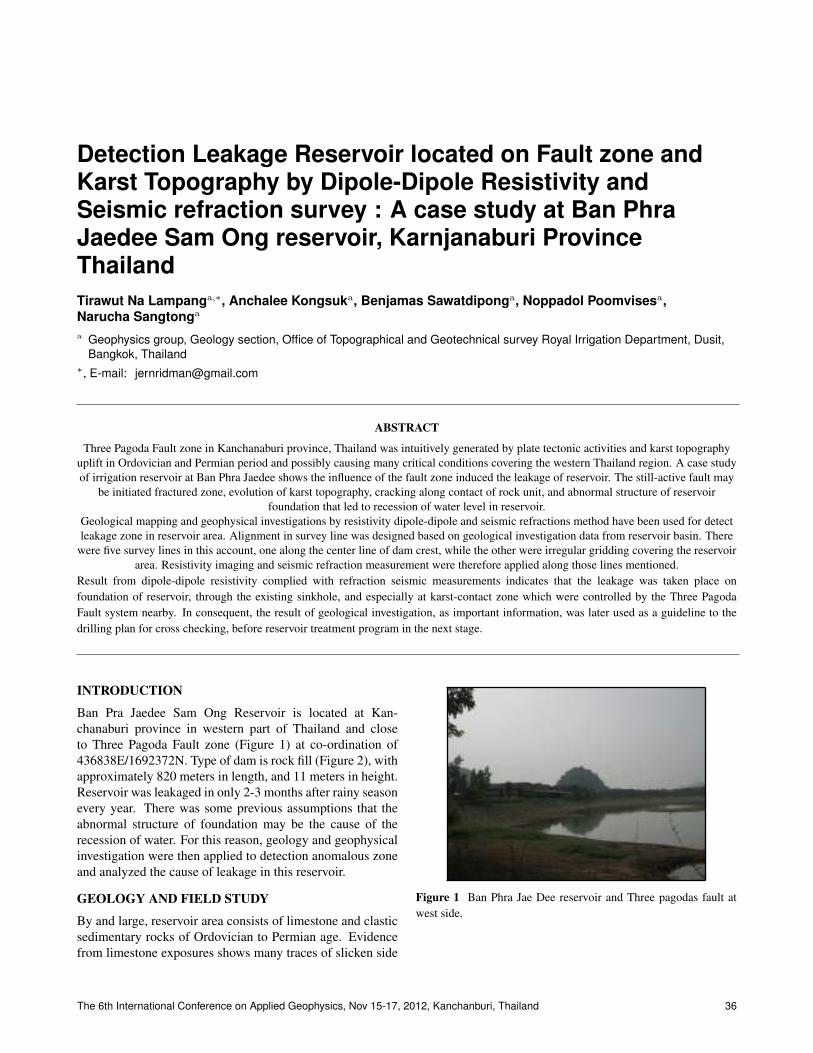
Detection Leakage Reservoir located on Fault zone andKarst Topography by Dipole-Dipole Resistivity andSeismic refraction survey : A case study at Ban PhraJaedee Sam Ong reservoir, Karnjanaburi ProvinceThailand
Tirawut Na Lampanga,∗, Anchalee Kongsuka, Benjamas Sawatdiponga, Noppadol Poomvisesa,
Narucha Sangtonga
a Geophysics group, Geology section, Office of Topographical and Geotechnical survey Royal Irrigation Department, Dusit,
Bangkok, Thailand∗, E-mail: [email protected]
ABSTRACT
Three Pagoda Fault zone in Kanchanaburi province, Thailand was intuitively generated by plate tectonic activities and karst topography
uplift in Ordovician and Permian period and possibly causing many critical conditions covering the western Thailand region. A case study
of irrigation reservoir at Ban Phra Jaedee shows the influence of the fault zone induced the leakage of reservoir. The still-active fault may
be initiated fractured zone, evolution of karst topography, cracking along contact of rock unit, and abnormal structure of reservoir
foundation that led to recession of water level in reservoir.
Geological mapping and geophysical investigations by resistivity dipole-dipole and seismic refractions method have been used for detect
leakage zone in reservoir area. Alignment in survey line was designed based on geological investigation data from reservoir basin. There
were five survey lines in this account, one along the center line of dam crest, while the other were irregular gridding covering the reservoir
area. Resistivity imaging and seismic refraction measurement were therefore applied along those lines mentioned.
Result from dipole-dipole resistivity complied with refraction seismic measurements indicates that the leakage was taken place on
foundation of reservoir, through the existing sinkhole, and especially at karst-contact zone which were controlled by the Three Pagoda
Fault system nearby. In consequent, the result of geological investigation, as important information, was later used as a guideline to the
drilling plan for cross checking, before reservoir treatment program in the next stage.
INTRODUCTION
Ban Pra Jaedee Sam Ong Reservoir is located at Kan-
chanaburi province in western part of Thailand and close
to Three Pagoda Fault zone (Figure 1) at co-ordination of
436838E/1692372N. Type of dam is rock fill (Figure 2), with
approximately 820 meters in length, and 11 meters in height.
Reservoir was leakaged in only 2-3 months after rainy season
every year. There was some previous assumptions that the
abnormal structure of foundation may be the cause of the
recession of water. For this reason, geology and geophysical
investigation were then applied to detection anomalous zone
and analyzed the cause of leakage in this reservoir.
GEOLOGY AND FIELD STUDY
By and large, reservoir area consists of limestone and clastic
sedimentary rocks of Ordovician to Permian age. Evidence
from limestone exposures shows many traces of slicken side
Figure 1 Ban Phra Jae Dee reservoir and Three pagodas fault at
west side.
The 6th International Conference on Applied Geophysics, Nov 15-17, 2012, Kanchanburi, Thailand 36
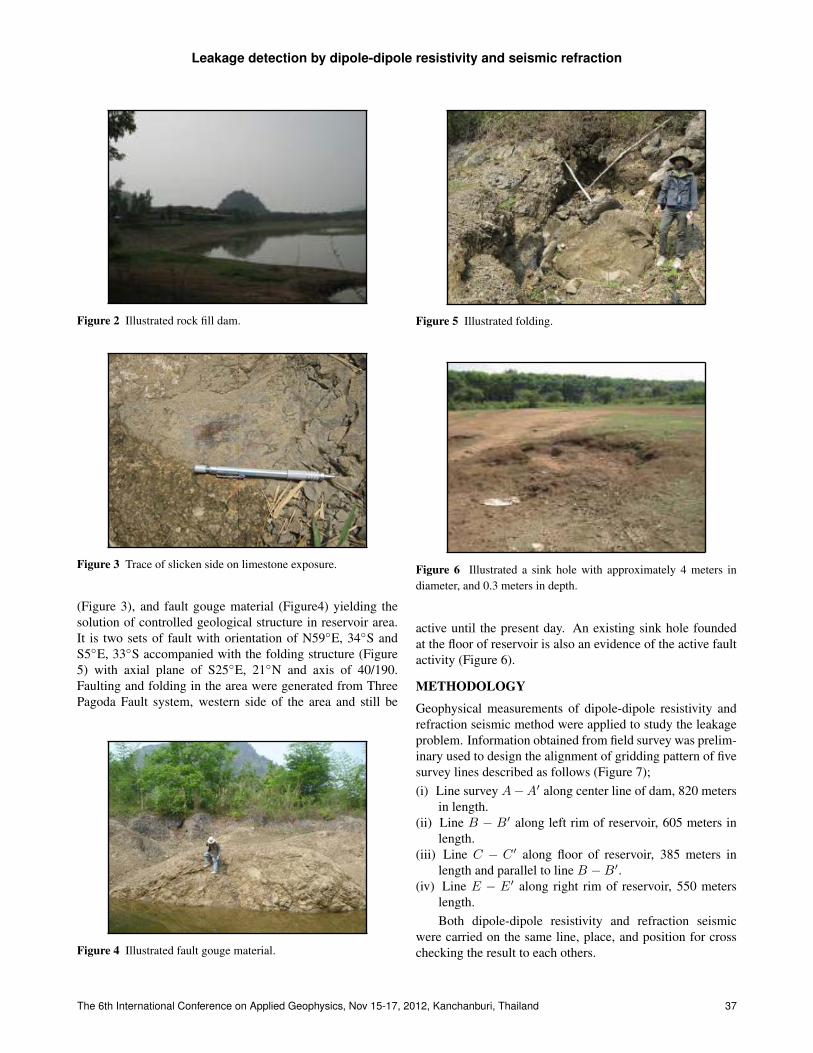
Leakage detection by dipole-dipole resistivity and seismic refraction
Figure 2 Illustrated rock fill dam.
Figure 3 Trace of slicken side on limestone exposure.
(Figure 3), and fault gouge material (Figure4) yielding the
solution of controlled geological structure in reservoir area.
It is two sets of fault with orientation of N59E, 34S and
S5E, 33S accompanied with the folding structure (Figure
5) with axial plane of S25E, 21N and axis of 40/190.
Faulting and folding in the area were generated from Three
Pagoda Fault system, western side of the area and still be
Figure 4 Illustrated fault gouge material.
Figure 5 Illustrated folding.
Figure 6 Illustrated a sink hole with approximately 4 meters in
diameter, and 0.3 meters in depth.
active until the present day. An existing sink hole founded
at the floor of reservoir is also an evidence of the active fault
activity (Figure 6).
METHODOLOGY
Geophysical measurements of dipole-dipole resistivity and
refraction seismic method were applied to study the leakage
problem. Information obtained from field survey was prelim-
inary used to design the alignment of gridding pattern of five
survey lines described as follows (Figure 7);
(i) Line survey A−A′ along center line of dam, 820 meters
in length.
(ii) Line B − B′ along left rim of reservoir, 605 meters in
length.
(iii) Line C − C ′ along floor of reservoir, 385 meters in
length and parallel to line B −B′.
(iv) Line E − E′ along right rim of reservoir, 550 meters
length.
Both dipole-dipole resistivity and refraction seismic
were carried on the same line, place, and position for cross
checking the result to each others.
The 6th International Conference on Applied Geophysics, Nov 15-17, 2012, Kanchanburi, Thailand 37
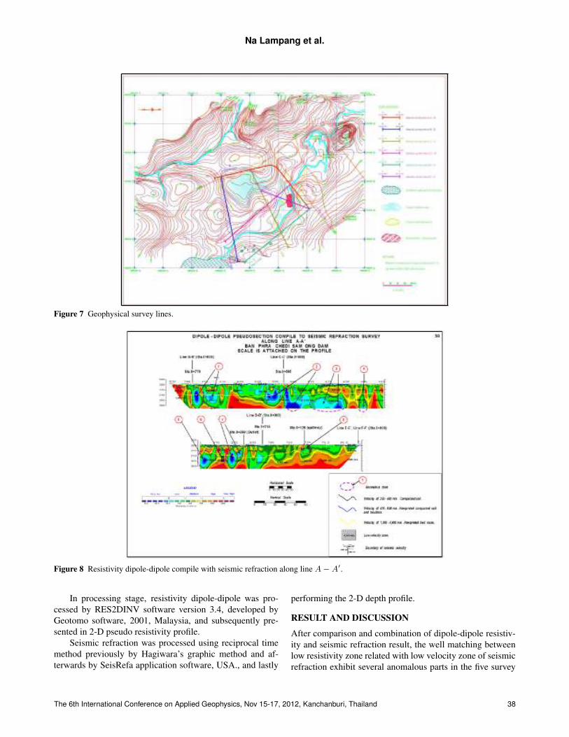
Na Lampang et al.
Figure 7 Geophysical survey lines.
Figure 8 Resistivity dipole-dipole compile with seismic refraction along line A−A′.
In processing stage, resistivity dipole-dipole was pro-
cessed by RES2DINV software version 3.4, developed by
Geotomo software, 2001, Malaysia, and subsequently pre-
sented in 2-D pseudo resistivity profile.
Seismic refraction was processed using reciprocal time
method previously by Hagiwara’s graphic method and af-
terwards by SeisRefa application software, USA., and lastly
performing the 2-D depth profile.
RESULT AND DISCUSSION
After comparison and combination of dipole-dipole resistiv-
ity and seismic refraction result, the well matching between
low resistivity zone related with low velocity zone of seismic
refraction exhibit several anomalous parts in the five survey
The 6th International Conference on Applied Geophysics, Nov 15-17, 2012, Kanchanburi, Thailand 38
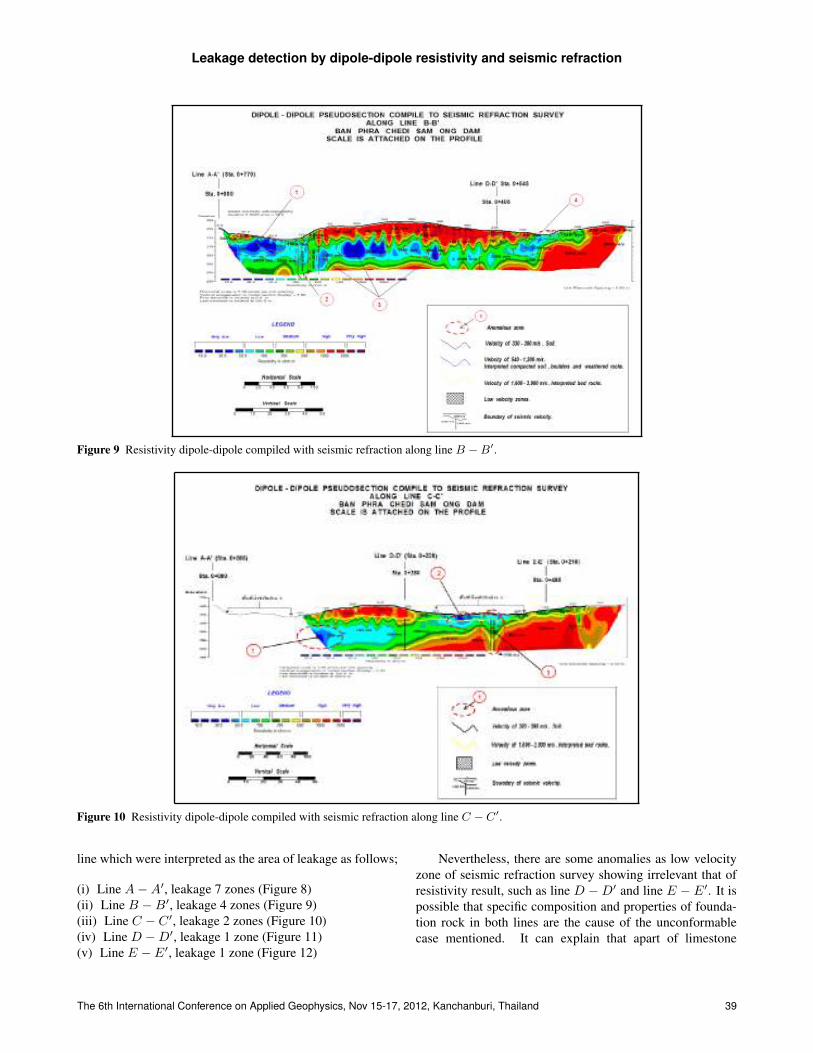
Leakage detection by dipole-dipole resistivity and seismic refraction
Figure 9 Resistivity dipole-dipole compiled with seismic refraction along line B −B′.
Figure 10 Resistivity dipole-dipole compiled with seismic refraction along line C − C′.
line which were interpreted as the area of leakage as follows;
(i) Line A−A′, leakage 7 zones (Figure 8)
(ii) Line B −B′, leakage 4 zones (Figure 9)
(iii) Line C − C ′, leakage 2 zones (Figure 10)
(iv) Line D −D′, leakage 1 zone (Figure 11)
(v) Line E − E′, leakage 1 zone (Figure 12)
Nevertheless, there are some anomalies as low velocity
zone of seismic refraction survey showing irrelevant that of
resistivity result, such as line D −D′ and line E − E′. It is
possible that specific composition and properties of founda-
tion rock in both lines are the cause of the unconformable
case mentioned. It can explain that apart of limestone
The 6th International Conference on Applied Geophysics, Nov 15-17, 2012, Kanchanburi, Thailand 39
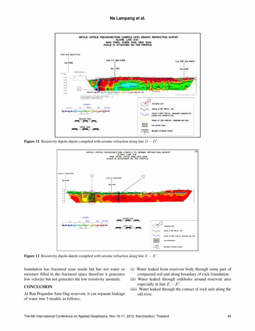
Na Lampang et al.
Figure 11 Resistivity dipole-dipole compiled with seismic refraction along line D −D′.
Figure 12 Resistivity dipole-dipole compiled with seismic refraction along line E − E′.
foundation has fractured zone inside but has not water or
moisture filled in the fractured space therefore it generates
low velocity but not generates the low resistivity anomaly.
CONCLUSION
At Ban Prajaedee Sam Ong reservoir, it can separate leakage
of water into 3 models as follows;
(i) Water leaked from reservoir body through some part of
compacted soil and along boundary of rock foundation.
(ii) Water leaked through sinkholes around reservoir area
especially in line E − E′.
(iii) Water leaked through the contact of rock unit along the
old river.
The 6th International Conference on Applied Geophysics, Nov 15-17, 2012, Kanchanburi, Thailand 40
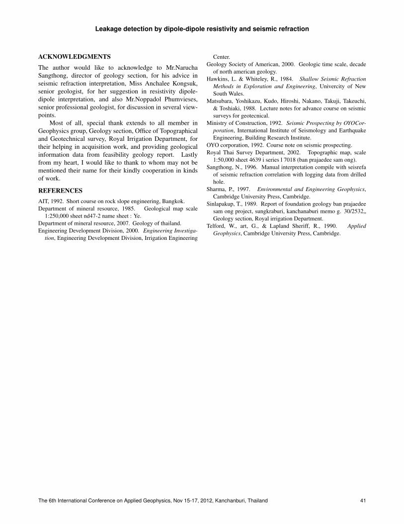
Leakage detection by dipole-dipole resistivity and seismic refraction
ACKNOWLEDGMENTS
The author would like to acknowledge to Mr.Narucha
Sangthong, director of geology section, for his advice in
seismic refraction interpretation, Miss Anchalee Kongsuk,
senior geologist, for her suggestion in resistivity dipole-
dipole interpretation, and also Mr.Noppadol Phumvieses,
senior professional geologist, for discussion in several view-
points.
Most of all, special thank extends to all member in
Geophysics group, Geology section, Office of Topographical
and Geotechnical survey, Royal Irrigation Department, for
their helping in acquisition work, and providing geological
information data from feasibility geology report. Lastly
from my heart, I would like to thank to whom may not be
mentioned their name for their kindly cooperation in kinds
of work.
REFERENCES
AIT, 1992. Short course on rock slope engineering, Bangkok.
Department of mineral resource, 1985. Geological map scale
1:250,000 sheet nd47-2 name sheet : Ye.
Department of mineral resource, 2007. Geology of thailand.
Engineering Development Division, 2000. Engineering Investiga-
tion, Engineering Development Division, Irrigation Engineering
Center.
Geology Society of American, 2000. Geologic time scale, decade
of north american geology.
Hawkins, L. & Whiteley, R., 1984. Shallow Seismic Refraction
Methods in Exploration and Engineering, Univercity of New
South Wales.
Matsubara, Yoshikazu, Kudo, Hiroshi, Nakano, Takuji, Takeuchi,
& Toshiaki, 1988. Lecture notes for advance course on seismic
surveys for geotecnical.
Ministry of Construction, 1992. Seismic Prospecting by OYOCor-
poration, International Institute of Seismology and Earthquake
Engineering, Building Research Institute.
OYO corporation, 1992. Course note on seismic prospecting.
Royal Thai Survey Department, 2002. Topographic map, scale
1:50,000 sheet 4639 i series l 7018 (ban prajaedee sam ong).
Sangthong, N., 1996. Manual interpretation compile with seisrefa
of seismic refraction correlation with logging data from drilled
hole.
Sharma, P., 1997. Environmental and Engineering Geophysics,
Cambridge University Press, Cambridge.
Sinlapakup, T., 1989. Report of foundation geology ban prajaedee
sam ong project, sungkraburi, kanchanaburi memo g. 30/2532„
Geology section, Royal irrigation Department.
Telford, W., art, G., & Lapland Sheriff, R., 1990. Applied
Geophysics, Cambridge University Press, Cambridge.
The 6th International Conference on Applied Geophysics, Nov 15-17, 2012, Kanchanburi, Thailand 41
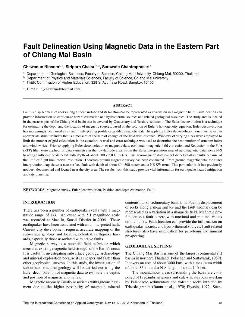
Fault Delineation Using Magnetic Data in the Eastern Partof Chiang Mai Basin
Chawanun Ninsoma,∗, Siriporn Chaisrib,c, Sarawute Chantrapraserta
a Department of Geological Sciences, Faculty of Science, Chiang Mai University, Chiang Mai, 50200, Thailandb Department of Physics and Materials Sciences, Faculty of Science, Chiang Mai universityc ThEP, Commission of Higher Education, 328 Si Ayuthaya Road, Bangkok 10400
∗, E-mail: [email protected]
ABSTRACT
Fault is displacement of rocks along a shear surface and its location can be represented as a variation in a magnetic field. Fault location can
provide information on earthquake hazard estimation and hydrothermal sources and related geological resources. The study area is located
in the eastern part of the Chiang Mai basin that is covered by Quaternary and Tertiary sediment. The Euler deconvolution is a technique
for estimating the depth and the location of magnetic sources, based on the solution of Euler’s homogeneity equation. Euler deconvolution
has increasingly been used as an aid in interpreting profile or gridded magnetic data. In applying Euler deconvolution, one must select an
appropriate structure index that is a measure of the rate of change of the field with distance. Windows of varying sizes were employed to
limit the number of grid calculation in the equation. A trial and error technique was used to determine the best number of structure index
and window size. Prior to applying Euler deconvolution to magnetic data, earth main magnetic field correction and Reduction to the Pole
(RTP) filter were applied for data symmetry in the low-latitude area. From the Euler interpretation map of aeromagnetic data, some N-S
trending faults can be detected with depth of about 500 - 2,000 meters. The aeromagnetic data cannot detect shallow faults because of
the limit of flight line interval resolution. Therefore ground magnetic survey has been conducted. From ground magnetic data, the Euler
interpretation map shows a near surface fault with depth of about 60 - 500 meters and a NE-SW trend. This particular fault has previously
not been documented and located near the city area. The results from this study provide vital information for earthquake hazard mitigation
and city planning.
KEYWORDS: Magnetic survey, Euler deconvolution, Position and depth estimation, Fault
INTRODUCTION
There has been a number of earthquake events with a mag-
nitude range of 1-3. An event with 5.1 magnitude scale
was recorded at Mae Jo, Sansai District in 2006. These
earthquakes have been associated with an uninterpreted fault.
Current city development requires accurate mapping of the
subsurface geology and locating potential earthquake haz-
ards, especially those associated with active faults.
Magnetic survey is a potential field technique which
measures existing magnetic field strength of the Earth’s crust.
It is useful in investigating subsurface geology, archaeology
and mineral exploration because it is cheaper and faster than
other geophysical surveys. In this study, the investigation of
subsurface structural geology will be carried out using the
Euler deconvolution of magnetic data to estimate the depths
and position of magnetic anomalies.
Magnetic anomaly usually associates with igneous base-
ment due to the higher possibility of magnetic mineral
contents that of sedimentary basin fills. Fault is displacement
of rocks along a shear surface and the fault anomaly can be
represented as a variation in a magnetic field. Magnetic pro-
file across a fault is zero with maximal and minimal values
on the flanks. Fault location can provide the information on
earthquake hazards, and hydro-thermal sources. Fault related
structures also have implication for petroleum and mineral
prospecting.
GEOLOGICAL SETTING
The Chiang Mai Basin is one of the largest continental rift
basins in northern Thailand (Polachan and Sattayarak, 1989).
It covers an area of about 3000 km2, with a maximum width
of about 35 km and a N-S length of about 140 km.
The mountainous areas surrounding the basin are com-
posed of Precambrian gneiss and calc-silicate rocks overlain
by Palaeozoic sedimentary and volcanic rocks intruded by
Triassic granite (Baum et al., 1970; Piyasin, 1972; Suen-
The 6th International Conference on Applied Geophysics, Nov 15-17, 2012, Kanchanburi, Thailand 42

Fault delineation using magnetic data
Figure 1 Location map of study area, Chiang Mai basin from
Google Earth software, with earthquake events in circles, possibly
unknown faults in blue and green lines, Mae Tha fault a red line,
and ground magnetic survey area outlined by red dashed line.
silpong et al., 1977)
The study area is located in the eastern part of the Chiang
Mai Basin that is covered by Quaternary to Tertiary gravel,
sand, silt, clay and laterite. The underlying basement is
mostly Carboniferous sedimentary rocks. These rocks were
compressed into N-S trending folds and reverse faults that
were cross-cut by N-S trending normal faults and NE-SW,
NW-SE trending strike-slip faults. The Mae Tha Fault is
one of the important faults east of the Chiang Mai Basin
and has been mapped as an active fault by the Department of
Mineral Resource (DMR, 2011). Ban Thi District is located
in the northern part of the Lamphun Province where there
has been frequent earthquake events. Ban Thi is covered
by Quaternary alluvial sediment. In satellite images, the
sediment cover in the study area corresponds to two different
shades divided by the Kuang River, where an unknown fault
is possibly located.
Based on information from satellite images, GIS data,
groundwater, earthquake locations, and total-count radioac-
tivity map, Chantraprasert (pers. comm.) interpreted un-
known faults (blue and green lines in Figure 1) in the vicinity
of the Chiang Mai and Lamphun city areas. These faults were
not previously mapped by Department of Mineral Resource
(DMR).
MAGNETIC DATA
The aeromagnetic data in northern Thailand was obtained
from the Department of Mineral Resources with gridded
spacing of about 100 meters at 1,000 feet elevation covering
the Chiang Mai Basin area. Ground magnetic surveys in
the Ban Thi area, Lamphun Province, have been conducted
where the prospective fault is located. The survey cover an
area of about 16 km2 using cesium magnetometer reading at
0.5 second interval and were recorded using a base station for
diurnal correction. The geomagnetic field parameters for the
study area are 0.46 Declination and 25.27 Inclination from
National Oceanic and Atmopheric Administration (NOAA).
The Earth main magnetic field removal was applied to both
aeromagnetic and ground magnetic data as shown in Figures
2 and 3, respectively.
DATA PROCESSING
Both ground and air-borne magnetic data contain some high-
frequency noise such as the effect from near surface struc-
tures and that from high-voltage power lines with 50 to 150
meter electromagnetic effects (Mizoue et al., 2004). Also,
the edges of magnetic anomalies are not resolved because
in the low-latitude areas (the magnetic field inclination in
this area is 25), the magnetic signals are dipolar over
causative bodies (Figures 2 and 3). Processes such as upward
continuation, reduction to the pole, Euler deconvolution were
implemented in the gridded magnetic data.
Upward continuation
The magnetic data contain various minor anomalies that are
not related to regional structures. An upward continuation
method was calculated and applied to eliminate or minimize
such noise and the effects of shallow sources (Henderson &
Zietz, 1949).
Reduction to the pole
Reduction to the pole (RTP) is the method that transform
dipolar magnetic to monopolar anomalies (inclination = 90°)
for data symmetry in the low-latitude area and can simplify
the interpretation of the data (Al-Garni, 2010).
After upward continuation and RTP were applied to
aeromagnetic and ground magnetic gridded data , the output
maps have smoother and symmetrical magnetic anomalies
(Figures 4 and 5).
After 1,000m upward continuation and reduction to
the pole, the aeromagnetic data show the location of the
causative bodies from residual magnetic anomaly (Figure 4)
and NW-SE trending magnetic lineations in the northern part
of the basin and NE-SW trending lineations in the south.
High magnetic anomalies west of the basin are probably
related to granitic rocks.
After 200 m upward continuation and reduction to the
pole, ground magnetic data have high magnetic anomalies in
the central area and low anomalies in the eastern and western
parts of the study area (Figure 5). Magnetic lineations trend
N-S and NE-SW.
Euler deconvolution
Euler deconvolution has been widely used as an aid for
interpreting profile or gridded magnetic data to provide
The 6th International Conference on Applied Geophysics, Nov 15-17, 2012, Kanchanburi, Thailand 43
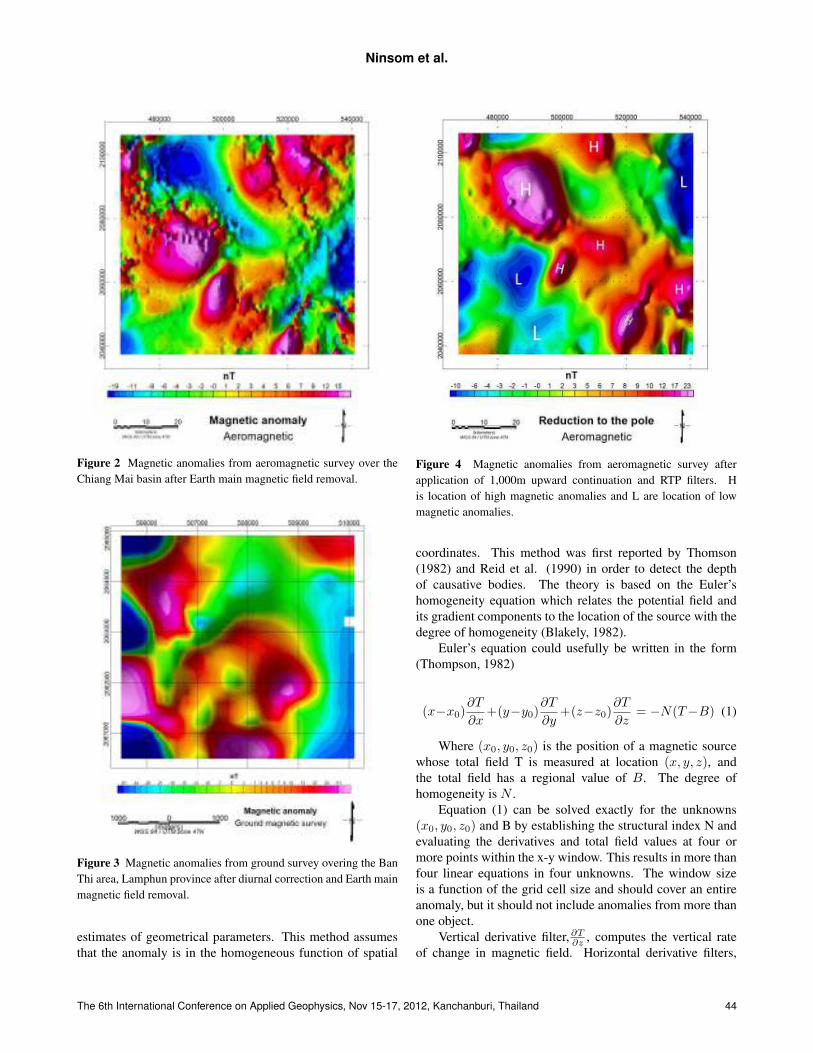
Ninsom et al.
Figure 2 Magnetic anomalies from aeromagnetic survey over the
Chiang Mai basin after Earth main magnetic field removal.
Figure 3 Magnetic anomalies from ground survey overing the Ban
Thi area, Lamphun province after diurnal correction and Earth main
magnetic field removal.
estimates of geometrical parameters. This method assumes
that the anomaly is in the homogeneous function of spatial
Figure 4 Magnetic anomalies from aeromagnetic survey after
application of 1,000m upward continuation and RTP filters. H
is location of high magnetic anomalies and L are location of low
magnetic anomalies.
coordinates. This method was first reported by Thomson
(1982) and Reid et al. (1990) in order to detect the depth
of causative bodies. The theory is based on the Euler’s
homogeneity equation which relates the potential field and
its gradient components to the location of the source with the
degree of homogeneity (Blakely, 1982).
Euler’s equation could usefully be written in the form
(Thompson, 1982)
(x−x0)∂T
∂x+(y−y0)
∂T
∂y+(z−z0)
∂T
∂z= −N(T−B) (1)
Where (x0, y0, z0) is the position of a magnetic source
whose total field T is measured at location (x, y, z), and
the total field has a regional value of B. The degree of
homogeneity is N .
Equation (1) can be solved exactly for the unknowns
(x0, y0, z0) and B by establishing the structural index N and
evaluating the derivatives and total field values at four or
more points within the x-y window. This results in more than
four linear equations in four unknowns. The window size
is a function of the grid cell size and should cover an entire
anomaly, but it should not include anomalies from more than
one object.
Vertical derivative filter,∂T∂z
, computes the vertical rate
of change in magnetic field. Horizontal derivative filters,
The 6th International Conference on Applied Geophysics, Nov 15-17, 2012, Kanchanburi, Thailand 44
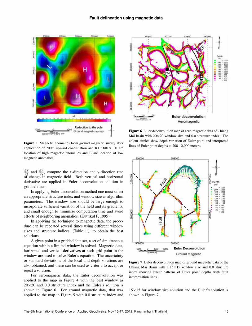
Fault delineation using magnetic data
Figure 5 Magnetic anomalies from ground magnetic survey after
application of 200m upward continuation and RTP filters. H are
location of high magnetic anomalies and L are location of low
magnetic anomalies.
∂T∂x
and ∂T∂y
, compute the x-direction and y-direction rate
of change in magnetic field. Both vertical and horizontal
derivative are applied in Euler deconvolution solution in
gridded data.
In applying Euler deconvolution method one must select
an appropriate structure index and window size as algorithm
parameters. The window size should be large enough to
incorporate sufficient variation of the field and its gradients,
and small enough to minimize computation time and avoid
effects of neighboring anomalies. (Kuttikul P, 1995).
In applying the technique to magnetic data, the proce-
dure can be repeated several times using different window
sizes and structure indices, (Table 1.), to obtain the best
solutions.
A given point in a gridded data set, a set of simultaneous
equation within a limited window is solved. Magnetic data,
horizontal and vertical derivatives at each grid point in the
window are used to solve Euler’s equation. The uncertainty
or standard deviations of the local and depth solutions are
also obtained, and these can be used as criteria to accept or
reject a solution.
For aeromagnetic data, the Euler deconvolution was
applied to the map in Figure 4 with the best window as
20×20 and 0.0 structure index and the Euler’s solution is
shown in Figure 6. For ground magnetic data, that was
applied to the map in Figure 5 with 0.0 structure index and
Figure 6 Euler deconvolution map of aero-magnetic data of Chiang
Mai basin with 20×20 window size and 0.0 structure index. The
colour circles show depth variation of Euler point and interpreted
lines of Euler point depths at 200 - 2,000 meters.
Figure 7 Euler deconvolution map of ground magnetic data of the
Chiang Mai Basin with a 15×15 window size and 0.0 structure
index showing linear patterns of Euler point depths with fault
interpretation lines.
15×15 for window size solution and the Euler’s solution is
shown in Figure 7.
The 6th International Conference on Applied Geophysics, Nov 15-17, 2012, Kanchanburi, Thailand 45
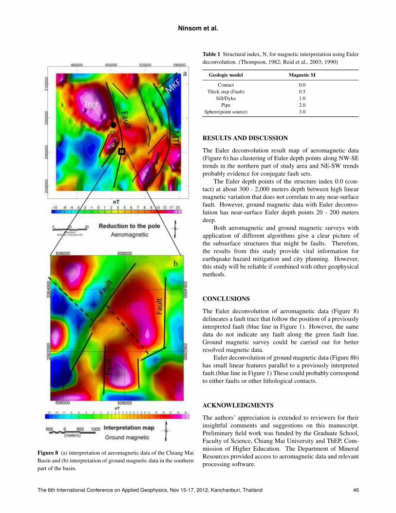
Ninsom et al.
Figure 8 (a) interpretation of aeromagnetic data of the Chiang Mai
Basin and (b) interpretation of ground magnetic data in the southern
part of the basin.
Table 1 Structural index, N, for magnetic interpretation using Euler
deconvolution. (Thompson, 1982; Reid et al., 2003; 1990)
Geologic model Magnetic SI
Contact 0.0
Thick step (Fault) 0.5
Sill/Dyke 1.0
Pipe 2.0
Sphere(point source) 3.0
RESULTS AND DISCUSSION
The Euler deconvolution result map of aeromagnetic data
(Figure 6) has clustering of Euler depth points along NW-SE
trends in the northern part of study area and NE-SW trends
probably evidence for conjugate fault sets.
The Euler depth points of the structure index 0.0 (con-
tact) at about 300 - 2,000 meters depth between high linear
magnetic variation that does not correlate to any near-surface
fault. However, ground magnetic data with Euler deconvo-
lution has near-surface Euler depth points 20 - 200 meters
deep.
Both aeromagnetic and ground magnetic surveys with
application of different algorithms give a clear picture of
the subsurface structures that might be faults. Therefore,
the results from this study provide vital information for
earthquake hazard mitigation and city planning. However,
this study will be reliable if combined with other geophysical
methods.
CONCLUSIONS
The Euler deconvolution of aeromagnetic data (Figure 8)
delineates a fault trace that follow the position of a previously
interpreted fault (blue line in Figure 1). However, the same
data do not indicate any fault along the green fault line.
Ground magnetic survey could be carried out for better
resolved magnetic data.
Euler deconvolution of ground magnetic data (Figure 8b)
has small linear features parallel to a previously interpreted
fault.(blue line in Figure 1) These could probably correspond
to either faults or other lithological contacts.
ACKNOWLEDGMENTS
The authors’ appreciation is extended to reviewers for their
insightful comments and suggestions on this manuscript.
Preliminary field work was funded by the Graduate School,
Faculty of Science, Chiang Mai University and ThEP, Com-
mission of Higher Education. The Department of Mineral
Resources provided access to aeromagnetic data and relevant
processing software.
The 6th International Conference on Applied Geophysics, Nov 15-17, 2012, Kanchanburi, Thailand 46
Fault delineation using magnetic data
REFERENCES
Al-Garni, M., 2010. Magnetic survey for delineating subsurface
structures and estimating magnetic sources depth, wadi fatima,
ksa, Journal of King Saud university, 22, 87–96.
Bournas, N., Galdeano, A., Hamoudi, M., & Baker, 2003. Interpre-
tation of the aeromagnetic map of eastern hoggar (algeria) using
the euler deconvolution, analytic signal and local wavenumber
methods, Journal of African Earth Sciences, 37, 191–205.
Chuamthaisong, C., 1971. Geology and groundwater of Chiang
Mai basin, Thailand., Master’s thesis, University of Alabama.
Gerovska, D. & Bravo, M., 2003. Automatic interpretation of
magnetic data basedon euler deconvolution with unprescribed
structural index, Computer and Geosciences, 29, 949–960.
Henderson, R. G. & Zietz, I., 1949. The upward continuation
of anomalies in total magnetic intensity fields, Geophysics, 14,
517–534.
Kuttikul, P., 1995. Optimization of 3D Euler deconvolution
for the interpretation of potential field data, Master’s thesis,
International Institute for Aerospace Survey and Earth Sciences.
Mizoue, T., Onoe, Y., Moritake, H., Okamura, J., Sokejima, S.,
& Nitta, H., 2004. Residential proximity to high-voltage
power lines and risk of childhood hematological malignancies,
Epidemiol, 14(4), 118–123.
NOAA, 2011. Geomagnetism, online, Tech. rep., National Oceanic
and Atmopheric Administration.
Piyasin, S., 1972. Geology of Changwat Lampang Sheet, scale
1:250,000. Rept. of Invest. no. 14, Dept. Min. Res., Bangkok,
Thailand.
Polachan, S. & Sattayarak, N., 1989. Strike-slip tectonics and
the development of tertiary basins in thailand, International
Symposium on Intermontane Basin, Geology and Resources,
Chiang Mai, Thailand, ,, 243–253.
Reid, A., Allsop, J., Granser, H., M. A., & Somerton, I., 1990.
Magnetic interpretation in three dimensions using euler decon-
volution, Geophysics, 55(1), 80–91.
Suensilpong, S., Meesook, A., Nakapadungrat, N., & P., P., 1977.
The granitic rocks and mineralization at the khuntan batholith,
lampang, Geol. Sot. Malaysia Bull, 9, 159–173.
Thompson, D., 1982. Euldph: A new technique for making
computer-assisted depth estimates from magnetic data, Geo-
physics, 47(1), 31–37.
The 6th International Conference on Applied Geophysics, Nov 15-17, 2012, Kanchanburi, Thailand 47

Geophysical Surveys to Detect Potential Active Faults inSan Sai District, Chiang Mai Province
Tanapon Suklima, Suwimon Udphuaya,b,∗, Siriporn Chaisria,b, Sarawute Chantrapraserta
a Department of Geological Sciences, Faculty of Science, Chiang Mai University, Chiang Mai, 50200, Thailandb ThEP, Commission of Higher Education, 328 Si Ayutthaya Road, Bangkok 10400, Thailandc Department of Physics and Materials Sciences, Faculty of Science, Chiang Mai University, Chiang Mai, 50200, Thailand
∗, E-mail: [email protected]
ABSTRACT
The earthquake with a magnitude of 5.1 Mw occurred in San Sai District, Chiang Mai Province on 13 December 2006 was considered
an uncommon event. This is because there was no statistical record of such significant earthquakes in the area, although several minor
earthquake events have been documented by the Department of Mineral Resources and the United States Geological Survey catalogues.
Therefore, the earthquake might have been associated with a potential active fault zone within the Chiang Mai Basin. San Sai District
is located in the eastern part of the Chiang Mai Basin. Exposed in the area are mostly fluvial Quaternary and Tertiary sediment and
sedimentary rocks. The underlying basement exposed at the nearest basin margin includes Carboniferous to Permian clastic and carbonate
sedimentary rocks and Permian volcanic rocks. The objective of this study is to investigate the existence of potential active faults that might
have been related to the earthquake in San Sai District. An integrated geophysical investigation, including gravity, 2D electrical resistivity
and seismic reflection techniques, was carried out along two profiles across the prospective north-south trending fault interpret, previously
interpreted based on satellite images and low-resolution air-borne geophysical data. Although structural imaging using geophysical surveys
in poorly stratified semi-consolidated sediments underlain by a strongly deformed sedimentary and volcanic basement is very challenging,
the reflection seismic and 2D electrical resistivity data reveal two sets of normal faults: the first cutting the lower part of the section and
the second the upper part. A few faults have offsets across an inferred water table and appear to continue upward to the surface. These
particular faults are appropriate candidates for being the active faults related to recent earthquake activities in the area. This potential active
fault system should be studied in more details to confirm its geometry, orientation and lateral extent.
KEYWORDS: Resistivity, Compressive Strength, Flood-affected concrete structures
INTRODUCTION
The earthquake magnitude of 5.1 occurred in the San Sai
District area on December, 13, 2006 was considered uncom-
mon. This is due to the fact that there was no statistical
record of such significant earthquake in the area although
several earthquake events have been recorded (epicenter
locations shown in Figure 1, according to the Department of
Mineral Resources (DMR), Thailand and the U.S. Geological
Survey (USGS) catalogues, DMR, 2011 and Petersen et al.,
2007). The epicenter of the 2006 San Sai earthquake was
located at roughly 18.93N, 99.00E which was not on the
Mae Tha fault zone. Therefore the earthquake might have
been associated with a potential active fault zone within the
Chiang Mai Basin. Interpretation of subtle river and stream
patterns on satellite images indicated a possible fault trending
approximately north-south from San Sai and Mueang Chiang
Mai Districts of Chiang Mai Province to Mueang Lamphun
District of Lamphun Province (Figure 1) However, there is
insufficient geological evidence at the surface to explain the
existence of such fault because it is probably covered by
the recent fluvial sediment during a long quiescence period.
Therefore, this paper presents results from an integrated
geophysical investigation of the potentially active Fault in
San Sai district where located 20 km northeast of Mueang
Chiang Mai district (Figure. 2). The main aim of the
investigation was used geophysical data to image this subsur-
face fault in order to understand its geometry, location, and
orientation. The results from various geophysical surveys
conducted in this report including resistivity, gravity and
seismic methods. The geophysical survey will be very useful
for future preparation of possible earthquake hazard that may
be related to the movement of this potential active fault.
The 6th International Conference on Applied Geophysics, Nov 15-17, 2012, Kanchanburi, Thailand 48

Geophysical surveys to detect potential active faults
Figure 1 Location of the possible unknown faults shown in blue
and green lines, and the field survey area in red dash rectangle. Red
line is Mae Tha Fault.
GEOLOGICAL SETITNG
San Sai District area is located in the eastern side of Chiang
Mai Basin, covered by Quaternary and Tertiary sediments
including gravels, sands, silts, clays, and laterites. The
underlying basement is Carboniferous sedimentary bedrock
(Liberty L. M., 2011). Structural geology of areas is mainly
north-south trending extensional faults. The Mae Tha fault
zone appears as a curved line (Figure 1) along the eastern
margin of the Chiang Mai Basin from Doi Saket and San
Kampang Districts to Lamphun Province, is one of the main
faults that located by the DMR.
GEOPHYSICAL SURVEYS
Geologic faults have specific physical characteristics, so they
are susceptible to detection and mapping by geophysical
methods. In this study gravity, resistivity and seismic
methods of geophysical surveys were applied to model the
shallow geological structure, locating and constructing a
2D subsurface geometry for the subsurface faults associated
with the earthquake occurrences in San Sai District, Chiang
Mai Province. The surveys were carried out on east-west
direction of 1km long for San Sai-01 (SS-01) and 1.2 km for
San Sai-02 (SS-02) across the prospecting fault trend (Figure
2).
GRAVITY METHOD
Gravity measurements investigate the subsurface geology by
measuring horizontal variations in the earth ’s gravitational
field generated by density difference between subsurface
rocks (Kearey and Brooks, 1991). The aim of the gravity
surveys for this research was to determine the location of the
fault plane.
The gravity value of each point was measured with a
SCINTREX Autograv gravimeter, model CG-3.Thirty-four
and Thirty-nine measuring points were place along profile
Figure 2 Location map showing survey SS-01 (AA’) and SS-02
(BB’) across the prospecting fault line.
Figure 3 Bouguer anomaly of, a) survey SS-01, b) survey SS-02.
SS-01 and SS-02, respectively. The spacing measuring point
was generally 30 m. The location and elevation of measuring
point was determined with a GPS for base station (reference
point) and used the total station to correct the position and
elevation of another measuring point for both survey lines.
The measured gravity values were corrected for effect of
instrumental drift and tides, latitude, elevation, and free air
with a density is 2.67 kg cm3 (Average earth ’s crust density).
A Bouguer anomaly value was drawn and used for interpre-
tation in order to determine the geological structure. The
resulting bouguer anomaly profiles were shown in Figure. 3.
The bouguer value of profile SS-01 and profile SS-02 were
increase with offset from South-West (SW) to North-East
direction (NE). The trend of bouguer anomaly was present
the direction of basement laying down from NE to SW.
The 6th International Conference on Applied Geophysics, Nov 15-17, 2012, Kanchanburi, Thailand 49

Suklim et al.
Figure 4 Interpreted resistivity profile (top) and seismic section (bottom) of survey line SS-01
Figure 5 Interpreted resistivity profile (top) and seismic section (bottom) of survey line SS-02.
RESISTIVITY SURVEY
The objective of the electrical surveys is to determine the
subsurface resistivity distribution from measurements taken
at the ground surface. Ground resistivity is related to various
geological parameters such as the mineral and fluid content,
porosity and degree of water saturation. Resistivity surveys
can provide data for subsurface geological and structural
interpretation, which can be used to detect and map fault
systems.
Resistivity measurements are acquired by injecting cur-
rent into the ground through two current electrodes and
measuring the resulting voltage difference at two potential
electrodes. The apparent resistivity distribution, ρa, is then
calculated from the input current, I , and output voltages, V .
The apparent resistivity can be written as (Telford, 1990):
ρa = kV
I(1)
where k is the geometric factor which depends on the
electrode arrangement.
In this study, the resistivity surveys were performed with
ABEM TERRAMETER SAS 4000 resistivity meter. The
dipole-dipole array was chosen based on previous work that
showed quite good resolution of fractures and fault with this
configuration (Liberty L. M., 2011, Adepelumi, 2008, and
Wise, 2003). The survey employed a dipole spacing of 10
m for SS-01 and SS-02 surveys lines. The raw apparent
resistivity dipole-dipole data were inverted and interpreted
using the rapid two-dimensional (2D) resistivity inversion
least squares method which developed by Loke, (1998), was
used to acquire a 2D ’true ’ earth resistivity inversion solution
in a color grid. The results of the resistivity survey can
be displayed as apparent vertical resistivity cross-sections
along the survey lines. The results indicate the existence of
fault anomalies, as illustrated in Figure 4 and 5 (top). The
faults appear as low-resistivity features in higher resistivity
environments and elevation changed of high resistivity value.
SS-01 and SS-02 profiles shown the low resistivity zones (red
dash lines) are considered as faults. A resistive layer (higher
The 6th International Conference on Applied Geophysics, Nov 15-17, 2012, Kanchanburi, Thailand 50
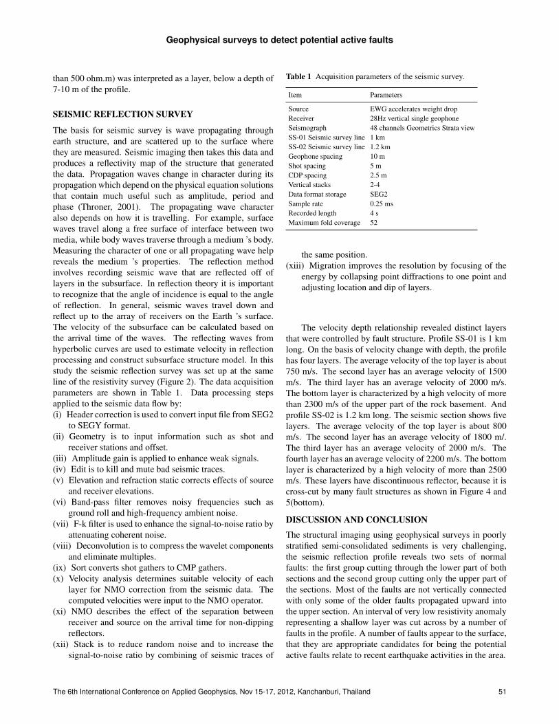
Geophysical surveys to detect potential active faults
than 500 ohm.m) was interpreted as a layer, below a depth of
7-10 m of the profile.
SEISMIC REFLECTION SURVEY
The basis for seismic survey is wave propagating through
earth structure, and are scattered up to the surface where
they are measured. Seismic imaging then takes this data and
produces a reflectivity map of the structure that generated
the data. Propagation waves change in character during its
propagation which depend on the physical equation solutions
that contain much useful such as amplitude, period and
phase (Throner, 2001). The propagating wave character
also depends on how it is travelling. For example, surface
waves travel along a free surface of interface between two
media, while body waves traverse through a medium ’s body.
Measuring the character of one or all propagating wave help
reveals the medium ’s properties. The reflection method
involves recording seismic wave that are reflected off of
layers in the subsurface. In reflection theory it is important
to recognize that the angle of incidence is equal to the angle
of reflection. In general, seismic waves travel down and
reflect up to the array of receivers on the Earth ’s surface.
The velocity of the subsurface can be calculated based on
the arrival time of the waves. The reflecting waves from
hyperbolic curves are used to estimate velocity in reflection
processing and construct subsurface structure model. In this
study the seismic reflection survey was set up at the same
line of the resistivity survey (Figure 2). The data acquisition
parameters are shown in Table 1. Data processing steps
applied to the seismic data flow by:
(i) Header correction is used to convert input file from SEG2
to SEGY format.
(ii) Geometry is to input information such as shot and
receiver stations and offset.
(iii) Amplitude gain is applied to enhance weak signals.
(iv) Edit is to kill and mute bad seismic traces.
(v) Elevation and refraction static corrects effects of source
and receiver elevations.
(vi) Band-pass filter removes noisy frequencies such as
ground roll and high-frequency ambient noise.
(vii) F-k filter is used to enhance the signal-to-noise ratio by
attenuating coherent noise.
(viii) Deconvolution is to compress the wavelet components
and eliminate multiples.
(ix) Sort converts shot gathers to CMP gathers.
(x) Velocity analysis determines suitable velocity of each
layer for NMO correction from the seismic data. The
computed velocities were input to the NMO operator.
(xi) NMO describes the effect of the separation between
receiver and source on the arrival time for non-dipping
reflectors.
(xii) Stack is to reduce random noise and to increase the
signal-to-noise ratio by combining of seismic traces of
Table 1 Acquisition parameters of the seismic survey.
Item Parameters
Source EWG accelerates weight drop
Receiver 28Hz vertical single geophone
Seismograph 48 channels Geometrics Strata view
SS-01 Seismic survey line 1 km
SS-02 Seismic survey line 1.2 km
Geophone spacing 10 m
Shot spacing 5 m
CDP spacing 2.5 m
Vertical stacks 2-4
Data format storage SEG2
Sample rate 0.25 ms
Recorded length 4 s
Maximum fold coverage 52
the same position.
(xiii) Migration improves the resolution by focusing of the
energy by collapsing point diffractions to one point and
adjusting location and dip of layers.
The velocity depth relationship revealed distinct layers
that were controlled by fault structure. Profile SS-01 is 1 km
long. On the basis of velocity change with depth, the profile
has four layers. The average velocity of the top layer is about
750 m/s. The second layer has an average velocity of 1500
m/s. The third layer has an average velocity of 2000 m/s.
The bottom layer is characterized by a high velocity of more
than 2300 m/s of the upper part of the rock basement. And
profile SS-02 is 1.2 km long. The seismic section shows five
layers. The average velocity of the top layer is about 800
m/s. The second layer has an average velocity of 1800 m/.
The third layer has an average velocity of 2000 m/s. The
fourth layer has an average velocity of 2200 m/s. The bottom
layer is characterized by a high velocity of more than 2500
m/s. These layers have discontinuous reflector, because it is
cross-cut by many fault structures as shown in Figure 4 and
5(bottom).
DISCUSSION AND CONCLUSION
The structural imaging using geophysical surveys in poorly
stratified semi-consolidated sediments is very challenging,
the seismic reflection profile reveals two sets of normal
faults: the first group cutting through the lower part of both
sections and the second group cutting only the upper part of
the sections. Most of the faults are not vertically connected
with only some of the older faults propagated upward into
the upper section. An interval of very low resistivity anomaly
representing a shallow layer was cut across by a number of
faults in the profile. A number of faults appear to the surface,
that they are appropriate candidates for being the potential
active faults relate to recent earthquake activities in the area.
The 6th International Conference on Applied Geophysics, Nov 15-17, 2012, Kanchanburi, Thailand 51
Suklim et al.
This potential active fault system should be studied
in more details to confirm its geometry, orientation and
lateral extent. More seismic survey lines across the possible
unexposed faults in the Chiang Mai Basin should be acquired
along with other geophysical methods (e.g. ground penetrat-
ing radar, resistivity, gravity, magnetic, electromagnetic, soil
gas radon). Integration of such data will be very useful for
city planning and mitigation of possible earthquake hazard
related to the movement of this fault system
ACKNOWLEDGEMENTS
We thank the PTTEP, Thai Center of Excellence in Physics
(ThEP), and the Graduate School, Chiang Mai University for
research funding supports.
REFERENCES
Adepelumi, A. A., Ako, B. D., Ajayi, T. R., Olorunfemi, A. O.,
Awoyemi, M. O., & Falebita, D. E., 2008. Integrated geophys-
ical mapping of the ifewara transcurrent fault system, nigeria,
Journal of African Earth Sciences, 52, 161–166.
Kearey, P., Brooks, M., & Hill, I., 1991. An introduction to
geophysical exploration, Blackwell Science, London, UK.
Liberty, L. M., Wood, S., van Wijk, K., Hinz, E., Mikesell, T. D.,
Singharajawarapan, F., & Shragge, J., 2011. The establishment
of a geophysics field camp in northern thailand, The Leading
Edge, 30, 414.
Loke, M. H., 1998. RES2DINV version 3.3: Rapid 2D resistivity
and IP inversion using the least-squares method: Computer disk
and manual, Penang, Malaysia, Applied Geophysics.
Petersen, M., Harmsen, S., Mueller, C., Haller, K., Dewey, J., Luco,
N., Crone, A., Lidke, D., & Rukstales, K., 2007. Documentation
for the southeast asia seismic hazard maps, U.S. Geological
Survey Administrative Report September 30, 30, 65.
Telford, W. M., 1990. Applied Geophysics, Cambridge University
Press, Cambridge.
Throner, R. H., 2001. Engineering geology field manual, U.S.
Department of the Interior Bureau of Reclamation (USDIBR).
Wise, D. J., Cassidy, J., & Locka, C. A., 2003. Geophysical imaging
of the quaternary wairoa north fault, new zealand: a case study,
Journal of Applied Geophysics, 53, 1–16.
The 6th International Conference on Applied Geophysics, Nov 15-17, 2012, Kanchanburi, Thailand 52
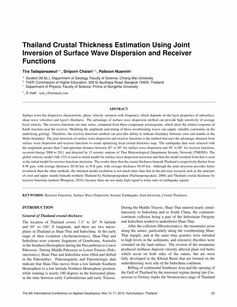
Thailand Crustal Thickness Estimation Using JointInversion of Surface Wave Dispersion and ReceiverFunctions
Tira Tadapansawuta,∗, Siriporn Chaisria,b, Paiboon Nuanninc
a Student (M.Sc.), Department of Geology, Faculty of Science, Chiang Mai Universityb ThEP, Commission of Higher Education, 328 Si Ayuthaya Road, Bangkok 10400, Thailandc Department of Physics, Faculty of Science, Prince of Songkhla University
∗, E-mail: [email protected]
ABSTRACT
Surface wave has dispersive characteristic, phase velocity variation with frequency, which depends on the layer properties of subsurface,
shear wave velocities and layer’s thickness. The advantage of surface wave dispersion method can provide high sensitivity of average
local velocity. The receiver functions are time series, computed from three-component seismograms, which show the relative response of
Earth structure near the receiver. Modeling the amplitude and timing of those reverberating waves can supply valuable constraints on the
underlying geology. Therefore, the receiver functions method can provides ability to indicate boundary between crust and mantle or the
Moho boundary. The joint inversion of surface wave dispersion and receiver functions is the method that uses the advantage obtained from
surface wave dispersion and receiver functions to create optimizing local crustal thickness map. The earthquake data were selected with
the magnitude greater than 5 and epicenter distance between 20 to 40 for surface wave dispersion and 30 to 90 for receiver functions,
occurred during 2008 to 2011 and detected by 15 seismic stations of Thai Meteorological Department Seismic Network (TMDSN). The
global velocity model (AK-135) is used as initial model for surface wave dispersion inversion and then the model resulted from that is used
as the initial model for receiver functions inversion. The results show that the crustal thickness beneath Thailand is respectively thicker from
S-W part, with average thickness 20-30 km, to N-E part, with average thickness 30-45 km. Although the joint inversion provides better
resolution than the other methods, the obtained model resolution is not much more than that in the previous research such as the structure
of crust and upper mantle beneath northern Thailand by Pacharapongsakun (Pacharapongsakun, 2006) and Thailand crustal thickness by
receiver functions method (Wongwai, 2010), because there are not many high signal to noise ratio of earthquake signals.
KEYWORDS: Receiver Functions, Surface Wave Dispersion, Seismic Earthquake, Joint Inversion, Crustal Thickness
INTRODUCTION
General of Thailand crustal thickness
The location of Thailand covers 7.5 to 20 N latitude
and 98 to 106 E longitude, and there are two micro-
plates in Thailand as Shan-Thai and Indochina. In the early
stage of their evolution (Archeotectonics), Shan-Thai and
Indochina were cratonic fragments of Gondwana, Australia
in the Southern Hemisphere during the Precambrian to Lower
Paleozoic. During Middle Paleozoic to Lower Triassic (Pale-
otectonics), Shan-Thai and Indochina were rifted and drifted
in the Paleotethys. Paleomagnetic and Paleontologic data
indicate that Shan-Thai moves from a low latitude Southern
Hemisphere to a low latitude Northern Hemisphere position,
while rotating is nearly 180 degrees in the horizontal plane,
in the time between early Carboniferous and early Triassic.
During the Middle Triassic, Shan-Thai sutured nearly simul-
taneously to Indochina and to South China, the continent-
continent collision being a part of the Indosinian Orogeny
and Indochina tended to underthrust Shan-Thai.
After the collision (Mesotectonics), the mountains arose
along the suture, particularly along the overthrusting Shan-
Thai margin, and at the same time granites were intruded
to high levels in the sediments, and extensive rhyolites were
extruded on the land surface. The erosion of the mountains
produced mollasse deposits (mostly alluvial plain red-beds)
which occur on both sides of the suture, but are most
fully developed in the Khorat Basin that are formed on the
underthrusting west side of the Indochina continent.
Rifting of continental Southeast Asia and the opening of
the Gulf of Thailand by the tensional regime during late Cre-
taceous to Tertiary marks the Neotectonics stage of Thailand
The 6th International Conference on Applied Geophysics, Nov 15-17, 2012, Kanchanburi, Thailand 53
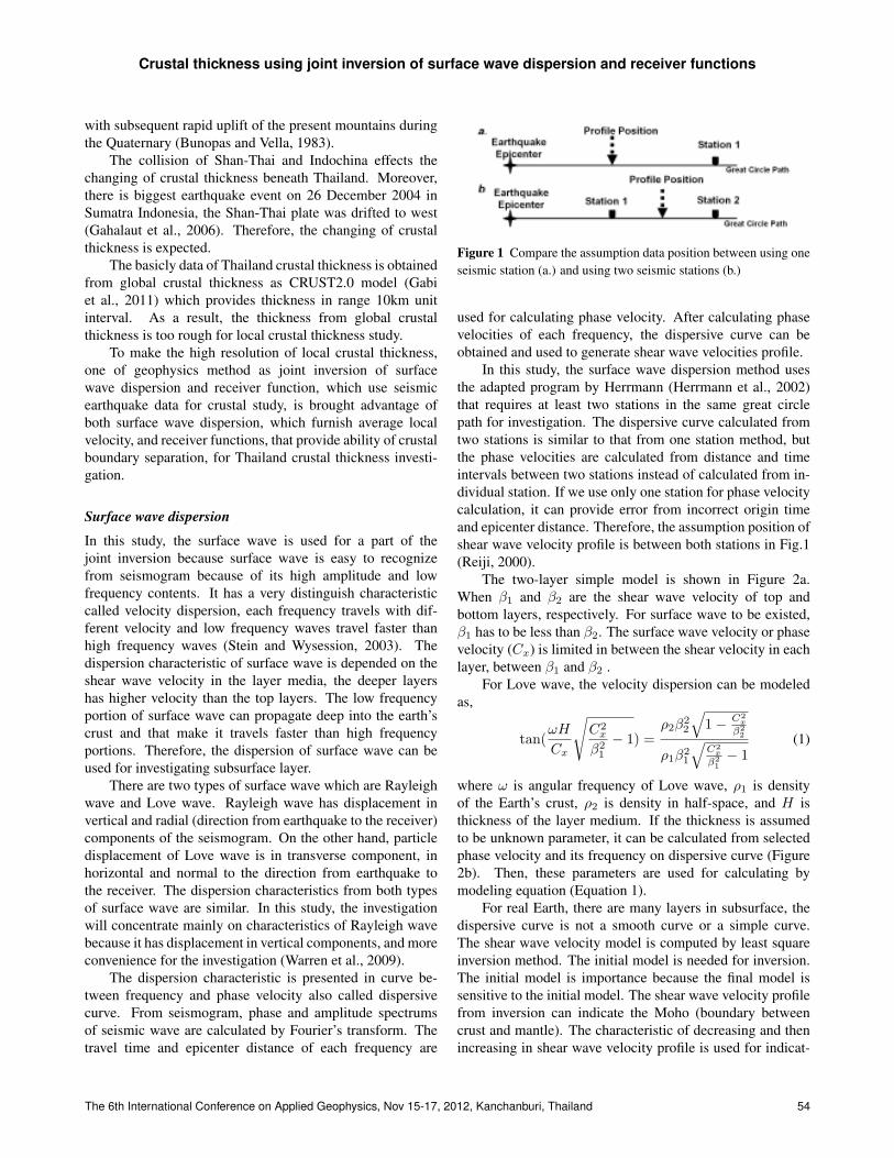
Crustal thickness using joint inversion of surface wave dispersion and receiver functions
with subsequent rapid uplift of the present mountains during
the Quaternary (Bunopas and Vella, 1983).
The collision of Shan-Thai and Indochina effects the
changing of crustal thickness beneath Thailand. Moreover,
there is biggest earthquake event on 26 December 2004 in
Sumatra Indonesia, the Shan-Thai plate was drifted to west
(Gahalaut et al., 2006). Therefore, the changing of crustal
thickness is expected.
The basicly data of Thailand crustal thickness is obtained
from global crustal thickness as CRUST2.0 model (Gabi
et al., 2011) which provides thickness in range 10km unit
interval. As a result, the thickness from global crustal
thickness is too rough for local crustal thickness study.
To make the high resolution of local crustal thickness,
one of geophysics method as joint inversion of surface
wave dispersion and receiver function, which use seismic
earthquake data for crustal study, is brought advantage of
both surface wave dispersion, which furnish average local
velocity, and receiver functions, that provide ability of crustal
boundary separation, for Thailand crustal thickness investi-
gation.
Surface wave dispersion
In this study, the surface wave is used for a part of the
joint inversion because surface wave is easy to recognize
from seismogram because of its high amplitude and low
frequency contents. It has a very distinguish characteristic
called velocity dispersion, each frequency travels with dif-
ferent velocity and low frequency waves travel faster than
high frequency waves (Stein and Wysession, 2003). The
dispersion characteristic of surface wave is depended on the
shear wave velocity in the layer media, the deeper layers
has higher velocity than the top layers. The low frequency
portion of surface wave can propagate deep into the earth’s
crust and that make it travels faster than high frequency
portions. Therefore, the dispersion of surface wave can be
used for investigating subsurface layer.
There are two types of surface wave which are Rayleigh
wave and Love wave. Rayleigh wave has displacement in
vertical and radial (direction from earthquake to the receiver)
components of the seismogram. On the other hand, particle
displacement of Love wave is in transverse component, in
horizontal and normal to the direction from earthquake to
the receiver. The dispersion characteristics from both types
of surface wave are similar. In this study, the investigation
will concentrate mainly on characteristics of Rayleigh wave
because it has displacement in vertical components, and more
convenience for the investigation (Warren et al., 2009).
The dispersion characteristic is presented in curve be-
tween frequency and phase velocity also called dispersive
curve. From seismogram, phase and amplitude spectrums
of seismic wave are calculated by Fourier’s transform. The
travel time and epicenter distance of each frequency are
Figure 1 Compare the assumption data position between using one
seismic station (a.) and using two seismic stations (b.)
used for calculating phase velocity. After calculating phase
velocities of each frequency, the dispersive curve can be
obtained and used to generate shear wave velocities profile.
In this study, the surface wave dispersion method uses
the adapted program by Herrmann (Herrmann et al., 2002)
that requires at least two stations in the same great circle
path for investigation. The dispersive curve calculated from
two stations is similar to that from one station method, but
the phase velocities are calculated from distance and time
intervals between two stations instead of calculated from in-
dividual station. If we use only one station for phase velocity
calculation, it can provide error from incorrect origin time
and epicenter distance. Therefore, the assumption position of
shear wave velocity profile is between both stations in Fig.1
(Reiji, 2000).
The two-layer simple model is shown in Figure 2a.
When β1 and β2 are the shear wave velocity of top and
bottom layers, respectively. For surface wave to be existed,
β1 has to be less than β2. The surface wave velocity or phase
velocity (Cx) is limited in between the shear velocity in each
layer, between β1 and β2 .
For Love wave, the velocity dispersion can be modeled
as,
tan(ωH
Cx
√
C2x
β21
− 1) =ρ2β
22
√
1− C2x
β2
2
ρ1β21
√
C2x
β2
1
− 1(1)
where ω is angular frequency of Love wave, ρ1 is density
of the Earth’s crust, ρ2 is density in half-space, and H is
thickness of the layer medium. If the thickness is assumed
to be unknown parameter, it can be calculated from selected
phase velocity and its frequency on dispersive curve (Figure
2b). Then, these parameters are used for calculating by
modeling equation (Equation 1).
For real Earth, there are many layers in subsurface, the
dispersive curve is not a smooth curve or a simple curve.
The shear wave velocity model is computed by least square
inversion method. The initial model is needed for inversion.
The initial model is importance because the final model is
sensitive to the initial model. The shear wave velocity profile
from inversion can indicate the Moho (boundary between
crust and mantle). The characteristic of decreasing and then
increasing in shear wave velocity profile is used for indicat-
The 6th International Conference on Applied Geophysics, Nov 15-17, 2012, Kanchanburi, Thailand 54
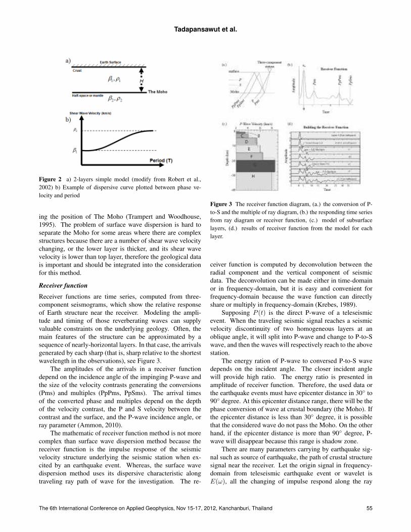
Tadapansawut et al.
Figure 2 a) 2-layers simple model (modify from Robert et al.,
2002) b) Example of dispersive curve plotted between phase ve-
locity and period
ing the position of The Moho (Trampert and Woodhouse,
1995). The problem of surface wave dispersion is hard to
separate the Moho for some areas where there are complex
structures because there are a number of shear wave velocity
changing, or the lower layer is thicker, and its shear wave
velocity is lower than top layer, therefore the geological data
is important and should be integrated into the consideration
for this method.
Receiver function
Receiver functions are time series, computed from three-
component seismograms, which show the relative response
of Earth structure near the receiver. Modeling the ampli-
tude and timing of those reverberating waves can supply
valuable constraints on the underlying geology. Often, the
main features of the structure can be approximated by a
sequence of nearly-horizontal layers. In that case, the arrivals
generated by each sharp (that is, sharp relative to the shortest
wavelength in the observations), see Figure 3.
The amplitudes of the arrivals in a receiver function
depend on the incidence angle of the impinging P-wave and
the size of the velocity contrasts generating the conversions
(Pms) and multiples (PpPms, PpSms). The arrival times
of the converted phase and multiples depend on the depth
of the velocity contrast, the P and S velocity between the
contrast and the surface, and the P-wave incidence angle, or
ray parameter (Ammon, 2010).
The mathematic of receiver function method is not more
complex than surface wave dispersion method because the
receiver function is the impulse response of the seismic
velocity structure underlying the seismic station when ex-
cited by an earthquake event. Whereas, the surface wave
dispersion method uses its dispersive characteristic along
traveling ray path of wave for the investigation. The re-
Figure 3 The receiver function diagram, (a.) the conversion of P-
to-S and the multiple of ray diagram, (b.) the responding time series
from ray diagram or receiver function, (c.) model of subsurface
layers, (d.) results of receiver function from the model for each
layer.
ceiver function is computed by deconvolution between the
radial component and the vertical component of seismic
data. The deconvolution can be made either in time-domain
or in frequency-domain, but it is easy and convenient for
frequency-domain because the wave function can directly
share or multiply in frequency-domain (Krebes, 1989).
Supposing P (t) is the direct P-wave of a teleseismic
event. When the traveling seismic signal reaches a seismic
velocity discontinuity of two homogeneous layers at an
oblique angle, it will split into P-wave and change to P-to-S
wave, and then the waves will respectively reach to the above
station.
The energy ration of P-wave to conversed P-to-S wave
depends on the incident angle. The closer incident angle
will provide high ratio. The energy ratio is presented in
amplitude of receiver function. Therefore, the used data or
the earthquake events must have epicenter distance in 30 to
90 degree. At this epicenter distance range, there will be the
phase conversion of wave at crustal boundary (the Moho). If
the epicenter distance is less than 30 degree, it is possible
that the considered wave do not pass the Moho. On the other
hand, if the epicenter distance is more than 90 degree, P-
wave will disappear because this range is shadow zone.
There are many parameters carrying by earthquake sig-
nal such as source of earthquake, the path of crustal structure
signal near the receiver. Let the origin signal in frequency-
domain from teleseismic earthquake event or wavelet is
E(ω), all the changing of impulse respond along the ray
The 6th International Conference on Applied Geophysics, Nov 15-17, 2012, Kanchanburi, Thailand 55

Crustal thickness using joint inversion of surface wave dispersion and receiver functions
path of earthquake wave is T (ω), the instrument respond is
I(ω), and response to local velocity contrast near the receiver
is H(ω), (Clayton and Wiggins, 1976). The approximated
recorded signal in vertical component is results of signal
deconvolution as
Z(ω) = E(ω)T (ω)I(ω). (2)
The signal of Z(ω) does not contain the changing local
velocity respond H(ω) because the teleseismic wave will not
perpendicularly pass crustal boundary beneath the station in
vertical direction.
Whereas the approximated signal in radial component at
the receiver which relate to the events location will be
R(ω) = E(ω)T (ω)I(ω)H(ω). (3)
In order to find the function which represents the local
velocity contrast, we must divide the radial component of the
seismogram (equation 3) by the vertical component (equation
2) which gives
H(ω) =R(ω)
Z(ω)(4)
The result in equation 4 is still frequency-domain, so the
inverse Fourier transform is applied to calculate the function
of h(t) and also called“the receiver function” which indicates
the velocity contrast on the ray path of the incoming seismic
data (see Figure 3b.).
If there is the 2-layer simple crustal model as Figure 2a,
the depth of crust can be calculated from equation as
tpms − tp = H
(
√
1
β2− p2 −
√
1
α2− p2
)
(5)
Where p is ray parameter, tpms is time of P-to-S phase
conversion wave, and tp is time of first arrival P phase
wave. Although the equation 5 can be used for calculated the
thickness layer, it is just simple model. In the real earth, there
are many layers under subsurface. Therefore, the least square
inversion is brought for calculated for crustal model. The
initial model of both surface wave dispersion and receiver
functions methods is very important because the calculated
final model will relate to the initial model.
In this study, the global velocity model as AK-135 is
used to be an initial model for both surface wave dispersion
and receiver functions processing.
Joint inversion of surface wave dispersion and receiver
functions
In2003, R.B. Herrmann and C.J. Ammon (Herrmenn and
Ammon, 2003) adapted and combined surface wave dis-
persion with receiver function for joint inversion to find
crustal thickness. The joint inversion between both methods
provides higher resolution in deep structure because they
bring the advantages from each method together for signal
analyzing. For surface wave, it provides high sensitivity of
average S-wave velocity in vertical direction. Whereas, the
receiver function provides position of phase conversion and
has ability to identify high velocity contrast position as the
Moho interface (Julia et al., 2003). The procedure of joint
inversion is same as receiver functions method, but the model
resulted from surface wave dispersion inversion is used as
initial model for receiver function inversion (see Figure 4).
We expect that an initial model from surface wave dispersion
provides S-wave velocity model better than using an initial
model from global crustal thickness because the calculated
initial model are nearly the local subsurface layers beneath
Thailand. Therefore, the final model of S-wave velocity from
joint inversion will provide better results than using either
receiver functions or surface wave dispersion.
METHODOLOGY
The earthquake data were selected with the magnitude
greater than 5 and epicenter distance between 20 to 40
for surface wave dispersion and 30 to 90 for receiver
functions, occurred during 2008 to 2011 and detected by
15 seismic stations of Thai Meteorological Department Seis-
mic Network (TMDSN). This study is separated for three
parts. First, the surface wave dispersion is set for 14 lines
processing which shown in Figure 5. Whereas, the receiver
functions use 13 seismic stations which presented in Figure
5 except MHMT and TRTT stations. For surface wave
dispersion, we used band-pass filter with frequency 0.02-0.1
Hz for dispersive curve calculation because the dispersive
curve looks clear and has high signal to noise ratio. Only the
fundamental mode or zero mode is selected for the inversion
because the fundamental model is easy and clear for mode
selection.
Second, the receiver function is calculated from de-
convolution of radial and vertical components. The raw
data are filter for frequency range 1-10 Hz. Then, the
receiver function is used for least square inversion for crustal
thickness investigation. The global velocity model as AK-
135 is used for both surface wave dispersion and receiver
functions inversions.
Finally, the joint inversion is done for the Thailand
crustal thickness investigation by using the calculated model
from surface wave inversion to be as an initial model for the
receiver function in the joint inversion method (see Figure
4). After getting the final model from all method, then the
velocity of S-wave velocity in range 4-5 km/s is decided
to be and the Moho boundary or crustal thickness. The
contour map of Thailand crustal thickness is created from
the thickness at its position.
The 6th International Conference on Applied Geophysics, Nov 15-17, 2012, Kanchanburi, Thailand 56
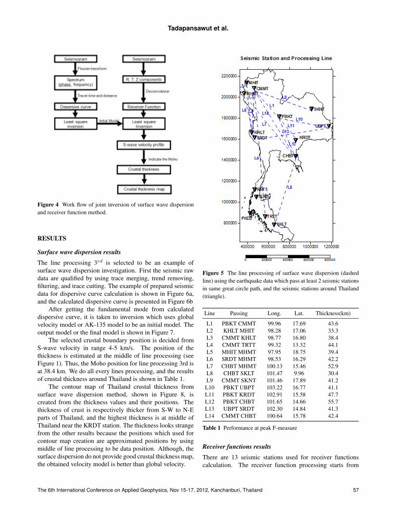
Tadapansawut et al.
Figure 4 Work flow of joint inversion of surface wave dispersion
and receiver function method.
RESULTS
Surface wave dispersion results
The line processing 3rd is selected to be an example of
surface wave dispersion investigation. First the seismic raw
data are qualified by using trace merging, trend removing,
filtering, and trace cutting. The example of prepared seismic
data for dispersive curve calculation is shown in Figure 6a,
and the calculated dispersive curve is presented in Figure 6b
After getting the fundamental mode from calculated
dispersive curve, it is taken to inversion which uses global
velocity model or AK-135 model to be an initial model. The
output model or the final model is shown in Figure 7.
The selected crustal boundary position is decided from
S-wave velocity in range 4-5 km/s. The position of the
thickness is estimated at the middle of line processing (see
Figure 1). Thus, the Moho position for line processing 3rd is
at 38.4 km. We do all every lines processing, and the results
of crustal thickness around Thailand is shown in Table 1.
The contour map of Thailand crustal thickness from
surface wave dispersion method, shown in Figure 8, is
created from the thickness values and their positions. The
thickness of crust is respectively thicker from S-W to N-E
parts of Thailand, and the highest thickness is at middle of
Thailand near the KRDT station. The thickness looks strange
from the other results because the positions which used for
contour map creation are approximated positions by using
middle of line processing to be data position. Although, the
surface dispersion do not provide good crustal thickness map,
the obtained velocity model is better than global velocity.
Figure 5 The line processing of surface wave dispersion (dashed
line) using the earthquake data which pass at least 2 seismic stations
in same great circle path, and the seismic stations around Thailand
(triangle).
Line Passing Long. Lat. Thickness(km)
L1 PBKT CMMT 99.96 17.69 43.6
L2 KHLT MHIT 98.28 17.06 33.3
L3 CMMT KHLT 98.77 16.80 38.4
L4 CMMT TRTT 99.32 13.32 44.1
L5 MHIT MHMT 97.95 18.75 39.4
L6 SRDT MHMT 98.53 16.29 42.2
L7 CHBT MHMT 100.13 15.46 52.9
L8 CHBT SKLT 101.47 9.96 30.4
L9 CMMT SKNT 101.46 17.89 41.2
L10 PBKT UBPT 103.22 16.77 41.1
L11 PBKT KRDT 102.91 15.58 47.7
L12 PBKT CHBT 101.65 14.66 55.7
L13 UBPT SRDT 102.30 14.84 41.3
L14 CMMT CHBT 100.64 15.78 42.4
Table 1 Performance at peak F-measure
Receiver functions results
There are 13 seismic stations used for receiver functions
calculation. The receiver function processing starts from
The 6th International Conference on Applied Geophysics, Nov 15-17, 2012, Kanchanburi, Thailand 57
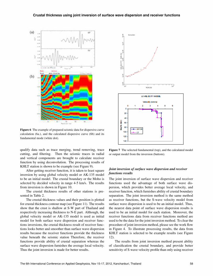
Crustal thickness using joint inversion of surface wave dispersion and receiver functions
Figure 6 The example of prepared seismic data for dispersive curve
calculation (6a.), and the calculated dispersive curve (6b) and its
fundamental mode (white dot).
qualify data such as trace merging, trend removing, trace
cutting, and filtering. Then the seismic traces in radial
and vertical components are brought to calculate receiver
function by using deconvolution. The processing results of
KHLT station is shown to be example (see Figure 9).
After getting receiver function, it is taken to least square
inversion by using global velocity model or AK-135 model
to be an initial model. The crustal boundary or the Moho is
selected by decided velocity in range 4-5 km/s. The results
from inversion is shown in Figure 10.
The crustal thickness results of other stations is pre-
sented in Table 2.
The crustal thickness values and their position is plotted
for crustal thickness contour map (see Figure 11). The results
show that the crust is shallow at S-W part of Thailand and
respectively increasing thickness to N-E part. Although, the
global velocity model or AK-135 model is used as initial
model for both surface wave dispersion and receiver func-
tions inversions, the crustal thickness result of receiver func-
tions looks better and smoother than surface wave dispersion
results because the receiver functions provide the thickness
value beneath the seismic station Therefore, the receiver
functions provide ability of crustal separation whereas the
surface wave dispersion furnishes the average local velocity.
Thus the joint inversion is made for better results.
Figure 7 The selected fundamental (top), and the calculated model
or output model from the inversion (buttom).
Joint inversion of surface wave dispersion and receiver
functions results
The joint inversion of surface wave dispersion and receiver
functions used the advantage of both surface wave dis-
persion, which provides better average local velocity, and
receiver function, which furnishes ability of crustal boundary
separation. The joint inversion method is the same method
as receiver functions, but the S-wave velocity model from
surface wave dispersion is used to be an initial model. Thus,
the nearest data point of surface wave dispersion results is
used to be an initial model for each station. Moreover, the
receiver functions data from receiver functions method are
used to be the data for the joint inversion method. To clear the
procedure of joint inversion method, please see the work flow
in Figure 4. To illustrate processing results, the data from
KHLT station is selected to be example results (see Figure
12).
The results from joint inversion method present ability
of classification the crustal boundary, and provide better
sensitivity of S-wave velocity profile than only using receiver
The 6th International Conference on Applied Geophysics, Nov 15-17, 2012, Kanchanburi, Thailand 58
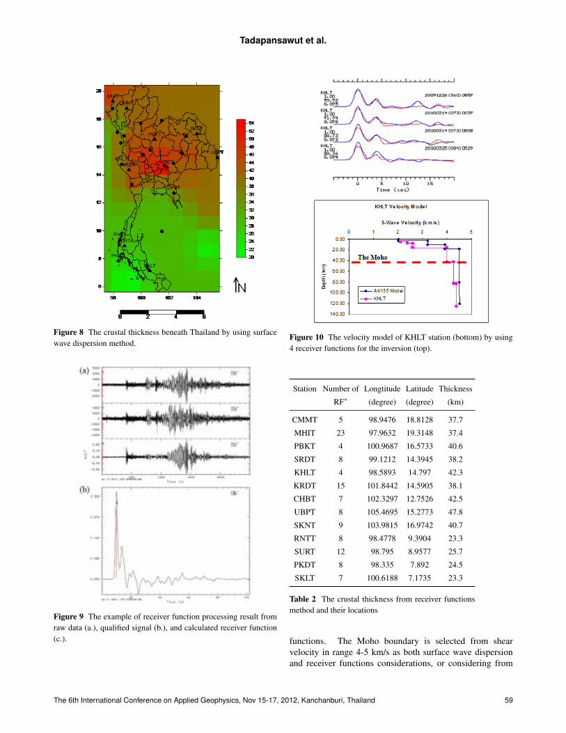
Tadapansawut et al.
Figure 8 The crustal thickness beneath Thailand by using surface
wave dispersion method.
Figure 9 The example of receiver function processing result from
raw data (a.), qualified signal (b.), and calculated receiver function
(c.).
Figure 10 The velocity model of KHLT station (bottom) by using
4 receiver functions for the inversion (top).
Station Number of Longtitude Latitude Thickness
RF∗ (degree) (degree) (km)
CMMT 5 98.9476 18.8128 37.7
MHIT 23 97.9632 19.3148 37.4
PBKT 4 100.9687 16.5733 40.6
SRDT 8 99.1212 14.3945 38.2
KHLT 4 98.5893 14.797 42.3
KRDT 15 101.8442 14.5905 38.1
CHBT 7 102.3297 12.7526 42.5
UBPT 8 105.4695 15.2773 47.8
SKNT 9 103.9815 16.9742 40.7
RNTT 8 98.4778 9.3904 23.3
SURT 12 98.795 8.9577 25.7
PKDT 8 98.335 7.892 24.5
SKLT 7 100.6188 7.1735 23.3
Table 2 The crustal thickness from receiver functions
method and their locations
functions. The Moho boundary is selected from shear
velocity in range 4-5 km/s as both surface wave dispersion
and receiver functions considerations, or considering from
The 6th International Conference on Applied Geophysics, Nov 15-17, 2012, Kanchanburi, Thailand 59
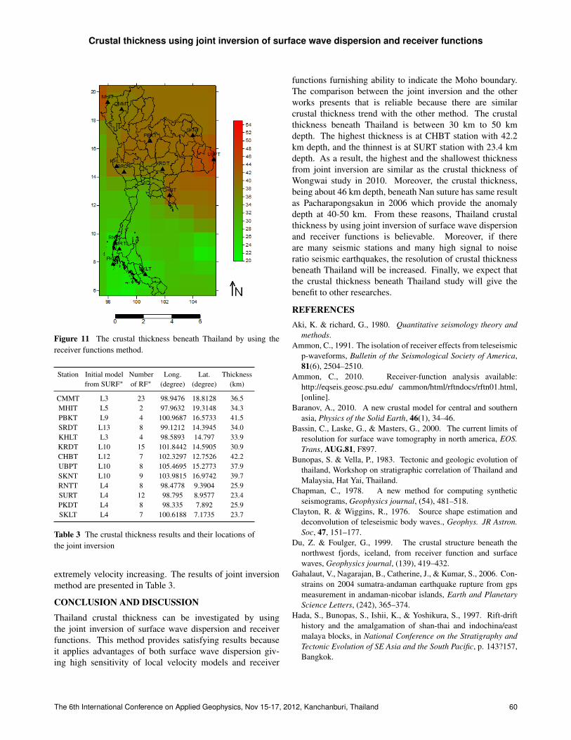
Crustal thickness using joint inversion of surface wave dispersion and receiver functions
Figure 11 The crustal thickness beneath Thailand by using the
receiver functions method.
Station Initial model Number Long. Lat. Thickness
from SURF∗ of RF∗ (degree) (degree) (km)
CMMT L3 23 98.9476 18.8128 36.5
MHIT L5 2 97.9632 19.3148 34.3
PBKT L9 4 100.9687 16.5733 41.5
SRDT L13 8 99.1212 14.3945 34.0
KHLT L3 4 98.5893 14.797 33.9
KRDT L10 15 101.8442 14.5905 30.9
CHBT L12 7 102.3297 12.7526 42.2
UBPT L10 8 105.4695 15.2773 37.9
SKNT L10 9 103.9815 16.9742 39.7
RNTT L4 8 98.4778 9.3904 25.9
SURT L4 12 98.795 8.9577 23.4
PKDT L4 8 98.335 7.892 25.9
SKLT L4 7 100.6188 7.1735 23.7
Table 3 The crustal thickness results and their locations of
the joint inversion
extremely velocity increasing. The results of joint inversion
method are presented in Table 3.
CONCLUSION AND DISCUSSION
Thailand crustal thickness can be investigated by using
the joint inversion of surface wave dispersion and receiver
functions. This method provides satisfying results because
it applies advantages of both surface wave dispersion giv-
ing high sensitivity of local velocity models and receiver
functions furnishing ability to indicate the Moho boundary.
The comparison between the joint inversion and the other
works presents that is reliable because there are similar
crustal thickness trend with the other method. The crustal
thickness beneath Thailand is between 30 km to 50 km
depth. The highest thickness is at CHBT station with 42.2
km depth, and the thinnest is at SURT station with 23.4 km
depth. As a result, the highest and the shallowest thickness
from joint inversion are similar as the crustal thickness of
Wongwai study in 2010. Moreover, the crustal thickness,
being about 46 km depth, beneath Nan suture has same result
as Pacharapongsakun in 2006 which provide the anomaly
depth at 40-50 km. From these reasons, Thailand crustal
thickness by using joint inversion of surface wave dispersion
and receiver functions is believable. Moreover, if there
are many seismic stations and many high signal to noise
ratio seismic earthquakes, the resolution of crustal thickness
beneath Thailand will be increased. Finally, we expect that
the crustal thickness beneath Thailand study will give the
benefit to other researches.
REFERENCES
Aki, K. & richard, G., 1980. Quantitative seismology theory and
methods.
Ammon, C., 1991. The isolation of receiver effects from teleseismic
p-waveforms, Bulletin of the Seismological Society of America,
81(6), 2504–2510.
Ammon, C., 2010. Receiver-function analysis available:
http://eqseis.geosc.psu.edu/ cammon/html/rftndocs/rftn01.html,
[online].
Baranov, A., 2010. A new crustal model for central and southern
asia, Physics of the Solid Earth, 46(1), 34–46.
Bassin, C., Laske, G., & Masters, G., 2000. The current limits of
resolution for surface wave tomography in north america, EOS.
Trans, AUG.81, F897.
Bunopas, S. & Vella, P., 1983. Tectonic and geologic evolution of
thailand, Workshop on stratigraphic correlation of Thailand and
Malaysia, Hat Yai, Thailand.
Chapman, C., 1978. A new method for computing synthetic
seismograms, Geophysics journal, (54), 481–518.
Clayton, R. & Wiggins, R., 1976. Source shape estimation and
deconvolution of teleseismic body waves., Geophys. JR Astron.
Soc, 47, 151–177.
Du, Z. & Foulger, G., 1999. The crustal structure beneath the
northwest fjords, iceland, from receiver function and surface
waves, Geophysics journal, (139), 419–432.
Gahalaut, V., Nagarajan, B., Catherine, J., & Kumar, S., 2006. Con-
strains on 2004 sumatra-andaman earthquake rupture from gps
measurement in andaman-nicobar islands, Earth and Planetary
Science Letters, (242), 365–374.
Hada, S., Bunopas, S., Ishii, K., & Yoshikura, S., 1997. Rift-drift
history and the amalgamation of shan-thai and indochina/east
malaya blocks, in National Conference on the Stratigraphy and
Tectonic Evolution of SE Asia and the South Pacific, p. 143?157,
Bangkok.
The 6th International Conference on Applied Geophysics, Nov 15-17, 2012, Kanchanburi, Thailand 60

Tadapansawut et al.
Harris, P., 1972. “The composition of the earth”. In Gass, I.
G. et al. (eds). Understanding the earth: a reader in the
earth sciences., Horsham: Artemis Press for the Open University
Press.
Herrmann, R. & Ammon, C., 2002. Computer program in seismol-
ogy : Surface wave receiver function and crustal structure, St.
Louis University, St. Louis, MO.
Herrmann, R. & Ammon, C., 2003. Surface waves receiver
functions and crustal structure program, Department of Earth and
Atmospheric Sciences, Saint Louis University.
Herrmann, R., Ammon, C., Julia, & Mokhtar, 2002. Joint inversion
of receiver functions and surface wave dispersion for crustal
structure, Saint Louis University.
Julia, J., Ammon, C., & Herrmann, R., 2003. Lithospheric structure
of the arabian shield from the joint inversion of receiver function
and surface wave group velocity, Tectonophysics, (371), 1–21.
Kennett, B., Engdahl, E., & Buland, R., 1995. Constraints on
seismic velocities in the earth from travel times, Geophys. J.,
122, 108–124.
Kosarev, G., Makeyeva, L., & Vinnik, L., 1984. Anisotropy of
the mantle inferred from observations of p to s converted waves.,
Geophys. J. Roy. Astro. Soc., 76, 209–220.
Laske, G., Masters, G., & Reif, C., 2010. A new global
crustal model at 2 × 2 degrees., [online]. Available from
http://igppweb.ucsd.edu/ gabi/crust2.html.
Ligorria, J. & Ammon, C., 1999. Iterative deconvolutionand
receiver-function estimation, Bulletin of the Seismological Soci-
ety of America, (89), 1395–1400.
Mohsen, A., 2004. A receiver function study of the crust and upper
mantle across the dead sea transform, Ph.D. thesis, Department
of Geosciences, Freie University of Berlin, Germany.
Mooney, W., Laske, G., & Masters, G., 1998. Crust5.1: A global
crustal model at 5 × 5, J. Geophys. Res., 103, 727–747.
Mooney, W. D., McDonald, S., & Detweiler, S., 2006. An
updated eurasian crustal model using multiple seismic methods,
Geophysical Union, Fall Meeting, S53A-1305.
Reiji, K., 2000. Crust and upper mantle structure in east antarctica
from phase velocity of rayleigh wave, Polar Geoscience, (13),
158–164.
Stein, S. & Wysession, M., 2003. An introduction to seismology
earthquake and earth structure.
Thai Meteorological Department (TMD), 2010.
Seismic monitoring system, [online]. Available:
http://www.seismology.tmd.go.th/en/index.php [2010, June
01].
Trampert, J. & Woodhouse, J., 1995. Global phase velocity maps
of love and rayleigh waves between 40 and 150 s, Geophysics
journal, (122), 675–690.
Warren, B., Simon, L., Shyam, S., & Jesse, F., 2009. Partial melt
in the upper-middle crust of the northwest himalaya revealed by
rayleigh wave dispersion, Tectonophysics, (477), 58–65.
Wikipedia The Free Encyclopedia, 2010. Receiver function, Avail-
able: http://en.wikipedia.org/wiki/Receiver_function (2010, Au-
gust 20).
Wongwai, W., 2011. The crustal thickness of Thailand by
teleseismic receiver function, Master’s thesis, Prince of Songkhla
University.
The 6th International Conference on Applied Geophysics, Nov 15-17, 2012, Kanchanburi, Thailand 61
Evaluation of TMD Seismograph Network DetectionCapabilities
Chatupond Munkonga,∗, Paiboon Nuannina
a Geophysics Research Center, Department of Physics, Faculty of Science, Prince of Songkla University, Hatyai , Songkhla ,
THAILAND∗, E-mail: [email protected]
ABSTRACT
The background seismic noise characteristics of 40 stations of Thai Meteorology Department Seismograph Network (TMDSN) were
analyzed by using power spectral density (PSD) estimation and their corresponding probability density functions (PDFs). The results
were directly evaluated with the new Peterson’s low and high noise model. The stations that closely located to a reservoirs reveal high
cultural noise level with periods < 1 s. The microseism noise (1 - 16 s) among the inland stations was very similar and uniform trend
and high noise level observed for the stations situated near sea shore. Variations of background noise for long period (> 20 s) varied from
-160 dB to -110 dB and higher than upper limited of the noise model from some stations due to poor quality of seismometer installation.
Sensitivity of the network, i.e. magnitude of completeness (Mc) was investigated by using TMD earthquake data from 1998 to 2010.
The data were separated to three periods following historical upgrading of the network. The analysis result gives Mc 5.3, 5.4 and 4.7,
respectively. Epicenter locations reported in TMD catalog were compared with the reference events from ISC catalog to estimate the
accuracy of epicenter location. The distributions of mis-location distance for each period are 25, 30 and 10 km. respectively.
KEYWORDS: Background seismic noise, TMD seismograph network, Magnitude of completeness, epicenter
INTRODUCTION
Thailand Seismograph Network is operated by the Seismo-
logical Bureau, Thai Meteorological Department (TMD) for
earthquake monitoring in Thailand and surrounding area.
The area of responsibility is cover within latitudes 0° -
25° N and longitudes 90° - 110° E. The earthquake ob-
servation in Thailand has started in 1963, the first World-
Wide Standardized Seismograph Network (WWSSN) was
deployed at Chiangmai province, and two years later at
Songkhla province. In 1997, one SRO station (Seismic
Research Observatories) was also installed at Chiang-mai by
the USGS (Nuannin, 1995). In the following years, short
period seismographs were installed in nationwide in Thailand
by Thai Meteorological Department (TMD) and Electricity
Generating Authority of Thailand (EGAT). There were 14
analog stations (SPZ 1 Hz), later added to 11 digital stations
(L-4-C3D and CMG -40 T) and begin reported earthquakes
in TMD catalogue in 1998.
After the great earthquake M = 9.1 on December 26,
Thai Meteorological Department has received funds to up-
grade and improve new weak motion and strong motion
stations throughout the country. The improvement of the
seismograph network project was divided into two phases.
The 1st phase started in 2004 and finished in 2006, 15 new
digital stations were deployed; consist of 8 short period sta-
tions (Trillium 40 SP) and 7 broadband stations (Trillium 120
SP). And the second phase was implemented during 2006-
2009; amount of 25 stations were installed; consist of 15
short period stations (S-13J, 1Hz) and 10 broadband stations
(KS-2000, 120sec). Altogether, The TMDSN consists of 40
seismograph stations throughout the country. Figure 1 show
the location of the stations.
NOISE ANALYSIS
The background seismic noise of year 2010 of each individ-
ual among 40 seismograph stations in TMDSN were esti-
mated by using PDF-SA solfware by McNamara and Boaz,
(2005). Upon processing, the time domain are converted into
frequencies domain and calculated Power Spectral Density
(PSD) via direct Fourier transform or Cooley-Tukey method
(Cooley and Tukey, 1965) For the entire available dataset,
which is divided into 1 hr time segments overlapping by
50 percentages. The instrument response was removed and
the PSD estimate to obtain accelerations. Details on this
calculation can be obtained from McNamara and Buland
(2004). The estimated PSD results were directly compared
to the high and low noise models (NHNM, NLNM) of
The 6th International Conference on Applied Geophysics, Nov 15-17, 2012, Kanchanburi, Thailand 62

Evaluation of seismograph network detection
Figure 1 Distribution of seismograph stations in TMDSN.
Peterson (1993), that powers expressed in decibels referred
to 1(m/sec2)2/Hz.
To achieve a better analysis the background seismic
noise at individual stations, the Probability Density Func-
tions (PDFs) is calculated. For each period, a histogram rep-
resents the number of occurrences of each power bin. PDF in
percentile over a period versus power graph is represented by
color palette. More details of PSDs calculation can be found
in McNamara and Buland (2004).
Statistical analysis (max, mode, min, PDFs) also
displyed for each station. Mode curves is considered better to
represent the majority noise level and correspond to highest
probability density function at each frequency bin (Diaz et
al., 2010).
CHARACTERIZATION
The seismic background noise of all stations in the TMDSN
were displayed by PSD mode line curve in Figure 2. The
PSD extends from -165 dB to -100 dB to covering about
65 dB of power in high frequencies. At short periods (0.1
- 1 sec) the most major sources of noise are the human
activities (road traffic, machinery) that couple energy into
the Earth. This so-called cultural noise propagates mainly as
high-frequency surface waves that attenuate within several
kilometers from the source (Havskov and Alguacil, 2004).
The PDF histogram revealed high seismic background noise
level in many cases of the stations have been located nearly
reservoir i.e. CHBT, PKDT, SKNT, SRDT, CRAI, NONG,
PHIT, SURI, SRAK and KRAB shown high noise level
at high frequency band (1-15 Hz) (see Figure 3a). In
addition, among 4 stations have been situated closely to
local meteorological building i.e. CMAI, KHON, PATY and
UMPA displayed critical high background noise at frequency
around 10 Hz (see Figure 3b). However, all of the PSD curve
still below the High Noise Model.
Figure 2 PSD mode curve of seismic background noise levels of
all stations in TMDSN.
In microseisms (1-16 sec), the background seismic noise
has been relationship with the energy released by oceanic
waves in this interval (Diaz et al., 2010). Therefore, the sea
shore stations in TMDSN i.e. PKDT, KRAB, SKLT, TRTT,
RNTT, SURT, SURA and SRIT were specially considered.
The PDF histogram indicated the highest seismic background
noise level in case of PKDT station (see Figure 3c). It
reaches to -120 dB (at 4-8 sec), However, It still lower to the
High Noise Model. These more effected by oceanic noise
because the station is located on island. However, the PSD
of all stations lie within -170 dB to -120 dB to cover 50
dB of power and just above 20 - 30 dB to the Low Noise
Model. Therefore, all stations can be considered as good
performance for noise period 1 - 16 sec.
In case of long period (T > 16 sec), the PDS show
extremely different between high and low of seismic back-
ground noise levels. The low PSD lie about -170 dB to -
180 dB caused by data from short period stations in TMD
The 6th International Conference on Applied Geophysics, Nov 15-17, 2012, Kanchanburi, Thailand 63
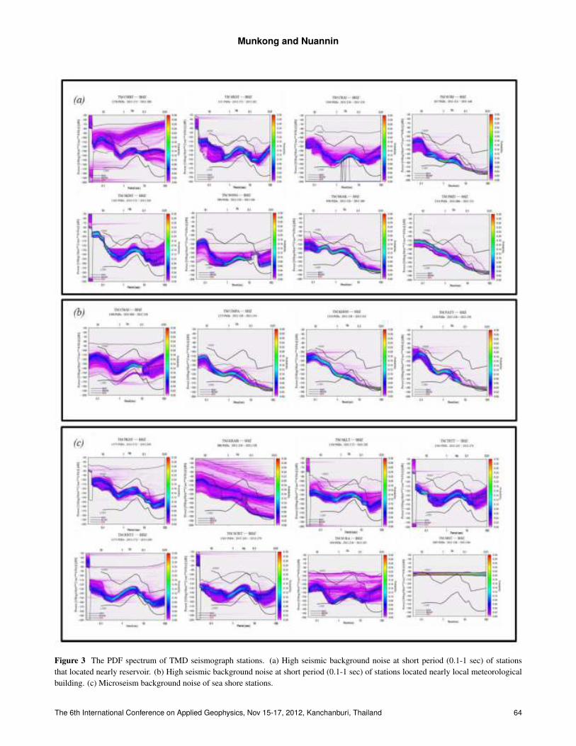
Munkong and Nuannin
Figure 3 The PDF spectrum of TMD seismograph stations. (a) High seismic background noise at short period (0.1-1 sec) of stations
that located nearly reservoir. (b) High seismic background noise at short period (0.1-1 sec) of stations located nearly local meteorological
building. (c) Microseism background noise of sea shore stations.
The 6th International Conference on Applied Geophysics, Nov 15-17, 2012, Kanchanburi, Thailand 64
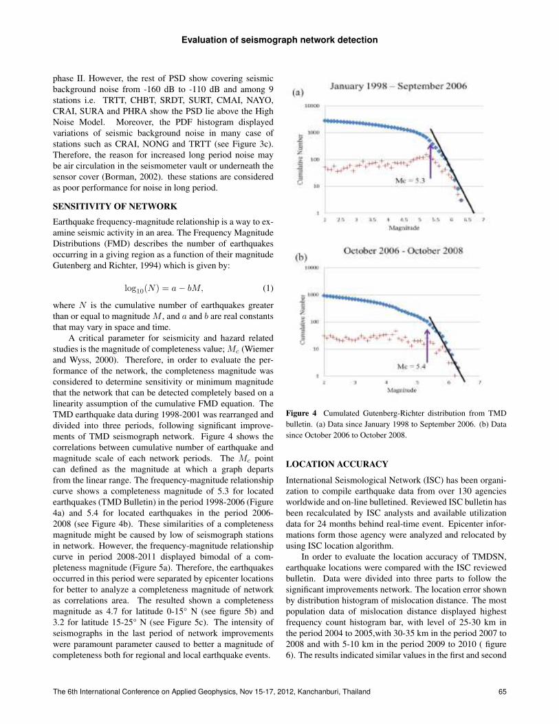
Evaluation of seismograph network detection
phase II. However, the rest of PSD show covering seismic
background noise from -160 dB to -110 dB and among 9
stations i.e. TRTT, CHBT, SRDT, SURT, CMAI, NAYO,
CRAI, SURA and PHRA show the PSD lie above the High
Noise Model. Moreover, the PDF histogram displayed
variations of seismic background noise in many case of
stations such as CRAI, NONG and TRTT (see Figure 3c).
Therefore, the reason for increased long period noise may
be air circulation in the seismometer vault or underneath the
sensor cover (Borman, 2002). these stations are considered
as poor performance for noise in long period.
SENSITIVITY OF NETWORK
Earthquake frequency-magnitude relationship is a way to ex-
amine seismic activity in an area. The Frequency Magnitude
Distributions (FMD) describes the number of earthquakes
occurring in a giving region as a function of their magnitude
Gutenberg and Richter, 1994) which is given by:
log10(N) = a− bM, (1)
where N is the cumulative number of earthquakes greater
than or equal to magnitude M , and a and b are real constants
that may vary in space and time.
A critical parameter for seismicity and hazard related
studies is the magnitude of completeness value; Mc (Wiemer
and Wyss, 2000). Therefore, in order to evaluate the per-
formance of the network, the completeness magnitude was
considered to determine sensitivity or minimum magnitude
that the network that can be detected completely based on a
linearity assumption of the cumulative FMD equation. The
TMD earthquake data during 1998-2001 was rearranged and
divided into three periods, following significant improve-
ments of TMD seismograph network. Figure 4 shows the
correlations between cumulative number of earthquake and
magnitude scale of each network periods. The Mc point
can defined as the magnitude at which a graph departs
from the linear range. The frequency-magnitude relationship
curve shows a completeness magnitude of 5.3 for located
earthquakes (TMD Bulletin) in the period 1998-2006 (Figure
4a) and 5.4 for located earthquakes in the period 2006-
2008 (see Figure 4b). These similarities of a completeness
magnitude might be caused by low of seismograph stations
in network. However, the frequency-magnitude relationship
curve in period 2008-2011 displayed bimodal of a com-
pleteness magnitude (Figure 5a). Therefore, the earthquakes
occurred in this period were separated by epicenter locations
for better to analyze a completeness magnitude of network
as correlations area. The resulted shown a completeness
magnitude as 4.7 for latitude 0-15° N (see figure 5b) and
3.2 for latitude 15-25° N (see Figure 5c). The intensity of
seismographs in the last period of network improvements
were paramount parameter caused to better a magnitude of
completeness both for regional and local earthquake events.
Figure 4 Cumulated Gutenberg-Richter distribution from TMD
bulletin. (a) Data since January 1998 to September 2006. (b) Data
since October 2006 to October 2008.
LOCATION ACCURACY
International Seismological Network (ISC) has been organi-
zation to compile earthquake data from over 130 agencies
worldwide and on-line bulletined. Reviewed ISC bulletin has
been recalculated by ISC analysts and available utilization
data for 24 months behind real-time event. Epicenter infor-
mations form those agency were analyzed and relocated by
using ISC location algorithm.
In order to evaluate the location accuracy of TMDSN,
earthquake locations were compared with the ISC reviewed
bulletin. Data were divided into three parts to follow the
significant improvements network. The location error shown
by distribution histogram of mislocation distance. The most
population data of mislocation distance displayed highest
frequency count histogram bar, with level of 25-30 km in
the period 2004 to 2005,with 30-35 km in the period 2007 to
2008 and with 5-10 km in the period 2009 to 2010 ( figure
6). The results indicated similar values in the first and second
The 6th International Conference on Applied Geophysics, Nov 15-17, 2012, Kanchanburi, Thailand 65
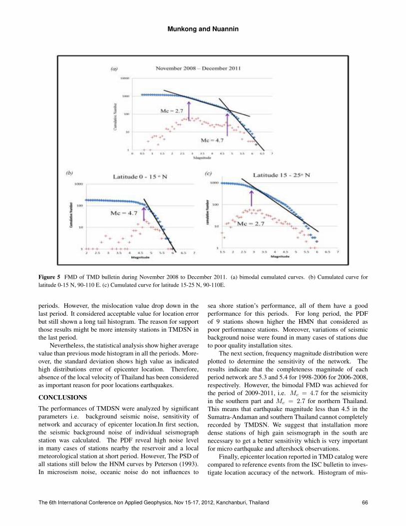
Munkong and Nuannin
Figure 5 FMD of TMD bulletin during November 2008 to December 2011. (a) bimodal cumulated curves. (b) Cumulated curve for
latitude 0-15 N, 90-110 E. (c) Cumulated curve for latitude 15-25 N, 90-110E.
periods. However, the mislocation value drop down in the
last period. It considered acceptable value for location error
but still shown a long tail histogram. The reason for support
those results might be more intensity stations in TMDSN in
the last period.
Nevertheless, the statistical analysis show higher average
value than previous mode histogram in all the periods. More-
over, the standard deviation shows high value as indicated
high distributions error of epicenter location. Therefore,
absence of the local velocity of Thailand has been considered
as important reason for poor locations earthquakes.
CONCLUSIONS
The performances of TMDSN were analyzed by significant
parameters i.e. background seismic noise, sensitivity of
network and accuracy of epicenter location.In first section,
the seismic background noise of individual seismograph
station was calculated. The PDF reveal high noise level
in many cases of stations nearby the reservoir and a local
meteorological station at short period. However, The PSD of
all stations still below the HNM curves by Peterson (1993).
In microseism noise, oceanic noise do not influences to
sea shore station’s performance, all of them have a good
performance for this periods. For long period, the PDF
of 9 stations shown higher the HMN that considered as
poor performance stations. Moreover, variations of seismic
background noise were found in many cases of stations due
to poor quality installation sites.
The next section, frequency magnitude distribution were
plotted to determine the sensitivity of the network. The
results indicate that the completeness magnitude of each
period network are 5.3 and 5.4 for 1998-2006 for 2006-2008,
respectively. However, the bimodal FMD was achieved for
the period of 2009-2011, i.e. Mc = 4.7 for the seismicity
in the southern part and Mc = 2.7 for northern Thailand.
This means that earthquake magnitude less than 4.5 in the
Sumatra-Andaman and southern Thailand cannot completely
recorded by TMDSN. We suggest that installation more
dense stations of high gain seismograph in the south are
necessary to get a better sensitivity which is very important
for micro earthquake and aftershock observations.
Finally, epicenter location reported in TMD catalog were
compared to reference events from the ISC bulletin to inves-
tigate location accuracy of the network. Histogram of mis-
The 6th International Conference on Applied Geophysics, Nov 15-17, 2012, Kanchanburi, Thailand 66
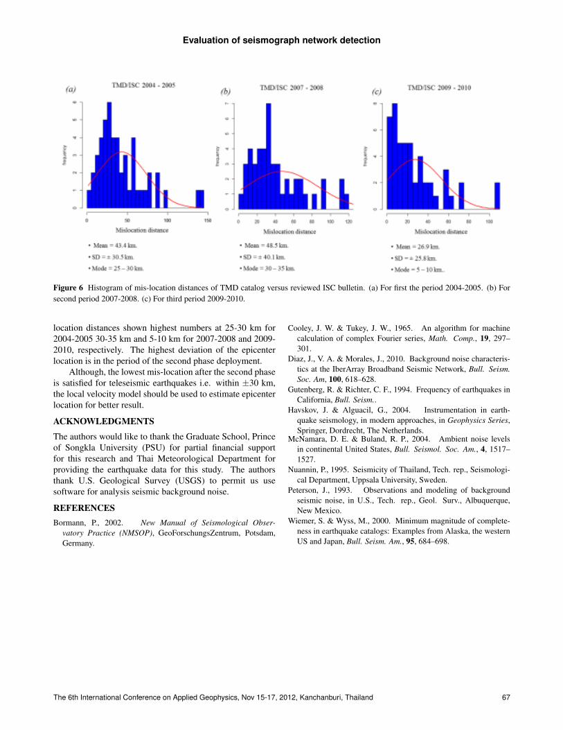
Evaluation of seismograph network detection
Figure 6 Histogram of mis-location distances of TMD catalog versus reviewed ISC bulletin. (a) For first the period 2004-2005. (b) For
second period 2007-2008. (c) For third period 2009-2010.
location distances shown highest numbers at 25-30 km for
2004-2005 30-35 km and 5-10 km for 2007-2008 and 2009-
2010, respectively. The highest deviation of the epicenter
location is in the period of the second phase deployment.
Although, the lowest mis-location after the second phase
is satisfied for teleseismic earthquakes i.e. within ±30 km,
the local velocity model should be used to estimate epicenter
location for better result.
ACKNOWLEDGMENTS
The authors would like to thank the Graduate School, Prince
of Songkla University (PSU) for partial financial support
for this research and Thai Meteorological Department for
providing the earthquake data for this study. The authors
thank U.S. Geological Survey (USGS) to permit us use
software for analysis seismic background noise.
REFERENCES
Bormann, P., 2002. New Manual of Seismological Obser-
vatory Practice (NMSOP), GeoForschungsZentrum, Potsdam,
Germany.
Cooley, J. W. & Tukey, J. W., 1965. An algorithm for machine
calculation of complex Fourier series, Math. Comp., 19, 297–
301.
Diaz, J., V. A. & Morales, J., 2010. Background noise characteris-
tics at the IberArray Broadband Seismic Network, Bull. Seism.
Soc. Am, 100, 618–628.
Gutenberg, R. & Richter, C. F., 1994. Frequency of earthquakes in
California, Bull. Seism..
Havskov, J. & Alguacil, G., 2004. Instrumentation in earth-
quake seismology, in modern approaches, in Geophysics Series,
Springer, Dordrecht, The Netherlands.McNamara, D. E. & Buland, R. P., 2004. Ambient noise levels
in continental United States, Bull. Seismol. Soc. Am., 4, 1517–
1527.
Nuannin, P., 1995. Seismicity of Thailand, Tech. rep., Seismologi-
cal Department, Uppsala University, Sweden.
Peterson, J., 1993. Observations and modeling of background
seismic noise, in U.S., Tech. rep., Geol. Surv., Albuquerque,
New Mexico.
Wiemer, S. & Wyss, M., 2000. Minimum magnitude of complete-
ness in earthquake catalogs: Examples from Alaska, the western
US and Japan, Bull. Seism. Am., 95, 684–698.
The 6th International Conference on Applied Geophysics, Nov 15-17, 2012, Kanchanburi, Thailand 67
Microtremor measurements in Chiang Mai city, northernThailand for seismic microzonation
Narin Kluntonga, Passakorn Pananonta,∗
a Department of Earth Sciences, Faculty of Science, Kasetsart University, Bangkok, THAILAND
∗, E-mail: [email protected], [email protected]
ABSTRACT
The Chiang Mai City is one of the biggest cities in the northern Thailand. The city is a part of the Chiang Mai Basin that is covert by fluvial
sediments. This soft sediment can both introduce its own natural frequency and can amplify the ground shaking from the earthquake.
The phenomena can lead to potential damages of the buildings and infrastructures in the city due to stronger shaking in the event of
the earthquake. The microtremor observation measures the vibration of the ground from the ambient noise and can be used to identify
the natural frequency of the ground shaking. The horizontal to vertical spectral analysis (H/V) is used to approximate both predominant
frequency and possible amplification of ground motion. The effect of soft sediment on seismic wave in the Chiang Mai city was studied
by measuring predominant frequency of the ground at 36 sites by microtremor observations. The predominant frequencies of the Chiang
Mai city range from 0.23 Hz to 4.95 Hz. The fundament frequency of the ground trends to be lower (longer period) towards the Ping River
which could be due to variations in sediment thickness. The result of this study can be applied for the seismic microzonation of the city in
the future.
KEYWORDS: Seismic Microzonation, Microtremor Observation, Chiang Mai, Seismic Hazard
INTRODUCTION
It is well known that the behavior of the ground motion
during an earthquake is generally well explained by the
lower velocity and density in the geological subsurface. In
1989, it was the first time that Nakamura used the single
site Horizontal to Vertical Spectral Ratio (HVSR) method to
study a site responses using ambient seismic noise sources.
The Chiang Mai city, one of the biggest city in the
northern Thailand, is covert by fluvial sediments that can
both create a specific natural ground response and can also
amplify the amplitude of the seismic wave. This phenomena
are important factors that can introduce potential damages of
the buildings and infrastructures in the city due to stronger
shaking in the event of the earthquake. There are numerous
examples of the damages to the city that was a result of
natural response of the ground and a soil amplifications such
as several damages from moderate earthquakes occurring in
California and the infamous Mexico city incident in 1985.
The natural ground shaking of a certain site can be obtained
with a microtremor method that measures ambient noise on
the ground surface. The main sources of these noises are
human activities, traffic and nature (such as ocean wave
and wind). Investigation of these microtremors can be used
to approximate both predominant frequency and possible
amplification of ground motion at a specific site.
The microtremor can be calculated with the empirical
formula using the measured ambient noise data of both
vertical and horizontal ground movement at the site of
interest. The results can be used in constructing a seismic
microzonation of the city. The proposed H/V spectral ratio
method, in which the predominant period of the ground
vibration is determined by the ratio of horizontal and vertical
Fourier spectra of microtremors observation at a site.
This study focuses on constructing a seismic micro-
zonation map of the Chiang Mai city using microtremor
observations. The study area (Figure 1) is located in the
urban area in the center of the city of Chiang Mai.
GEOLOGICAL SETTING
The surface geology of Chiang Mai city consists mainly of
fluvial sediments, with bedrocks cropping out at the western
part of the city (Doi Suthep mountain) The sediments are
Quaternary alluvium deposits of thin clay and sand along the
Ping river which flows through the northern and southern part
of Chiang Mai city. The measurement sites is located in the
center of the Chiang Mai city, which is a valley and fluvial
flood plain. Therefore this urban area can amplify the seismic
wave from the earthquake (Figure 2).
The 6th International Conference on Applied Geophysics, Nov 15-17, 2012, Kanchanburi, Thailand 68

Microtremor for seismic microzonation
Figure 1: Study area of this work.
Figure 2: Locations of HVSR sites in the Chiang Mai city.
EQUIPMENT AND DATA ACQUISITION
Equipment
The ambient noise are recorded with a 3-component seis-
mometer with natural response from 40 second to 50 Hz
and a 24 bits digitizer. A sampling rate of 100 samples
per second were used. At each site, we record ambient
noise continuously for at least 90 minutes with GPS for the
accuracy control of the timing.
(a) A sample of spectrums of the microtremor measurement. Z, N
and E are vertical, N-S and E-W component respectively.
(b) H/V spectrum of recorded microtremor data.
Figure 3
Data acquisition
The microtremor data were recorded at 36 sites during
October through December 2009. Measuring locations was
selected to represent spatial distribution and to avoid direct
traffic, heavy machine, other underground structures and
strong wind or rain. The data processing was done with the
GEOPSY software.
RESULTS OF H/V MEASUREMENTS
The result of the H/V calculation suggest that the sites
in the central area of Chiang Mai city has low frequency
(long period) response, ranging from 0.23 - 0.99 Hz and the
amplification of ground motion are 2 - 6.4 times compared
to the rock surface, especially near Ping River. The result of
this study shown in Figure 4.
DISCUSSION AND CONCLUSION
This study presents a result of predominant frequency and the
amplification factor from the microtremor measurement in
Chiang Mai city. It can be seen that sites with lower predomi-
nant frequency appear to locate towards the Ping River which
could contribute more soft sediment on the ground. The
result can suggest that the tall buildings near the Ping River
The 6th International Conference on Applied Geophysics, Nov 15-17, 2012, Kanchanburi, Thailand 69
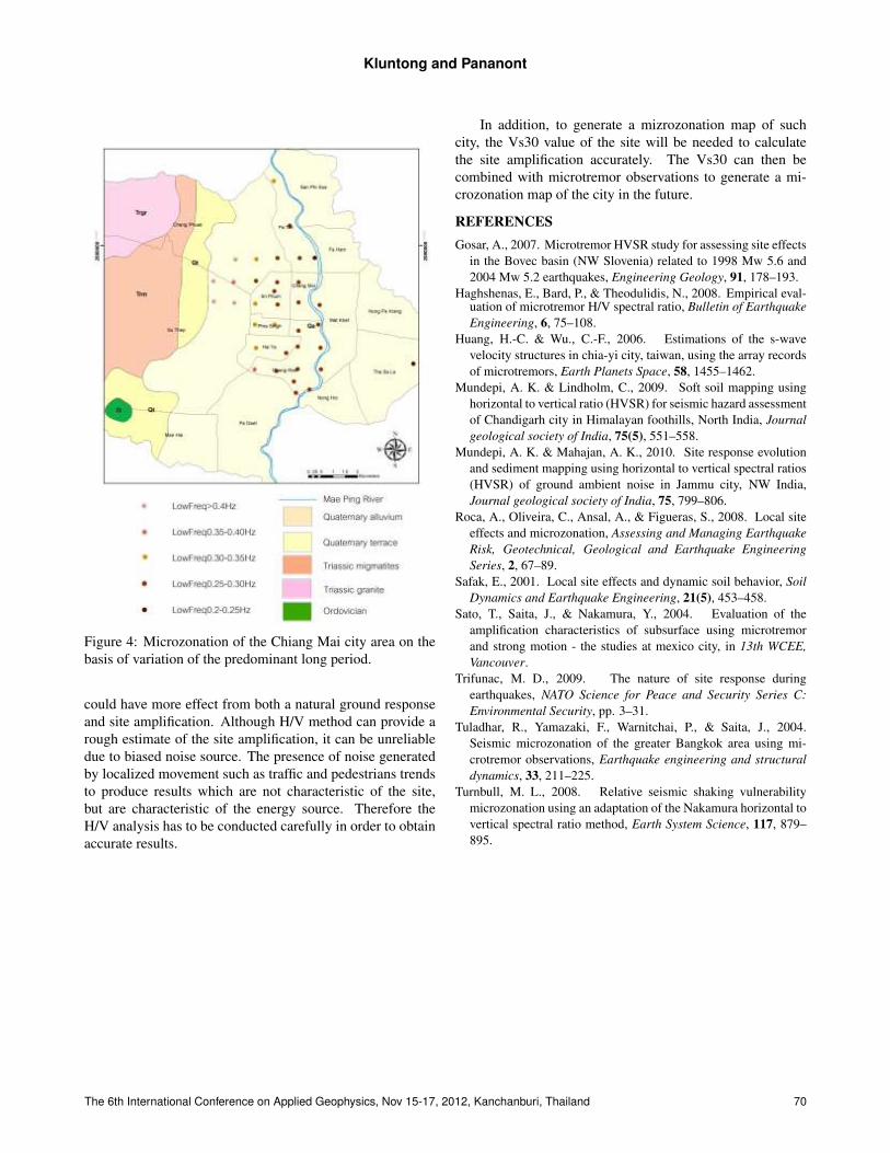
Kluntong and Pananont
Figure 4: Microzonation of the Chiang Mai city area on the
basis of variation of the predominant long period.
could have more effect from both a natural ground response
and site amplification. Although H/V method can provide a
rough estimate of the site amplification, it can be unreliable
due to biased noise source. The presence of noise generated
by localized movement such as traffic and pedestrians trends
to produce results which are not characteristic of the site,
but are characteristic of the energy source. Therefore the
H/V analysis has to be conducted carefully in order to obtain
accurate results.
In addition, to generate a mizrozonation map of such
city, the Vs30 value of the site will be needed to calculate
the site amplification accurately. The Vs30 can then be
combined with microtremor observations to generate a mi-
crozonation map of the city in the future.
REFERENCES
Gosar, A., 2007. Microtremor HVSR study for assessing site effects
in the Bovec basin (NW Slovenia) related to 1998 Mw 5.6 and
2004 Mw 5.2 earthquakes, Engineering Geology, 91, 178–193.
Haghshenas, E., Bard, P., & Theodulidis, N., 2008. Empirical eval-uation of microtremor H/V spectral ratio, Bulletin of Earthquake
Engineering, 6, 75–108.
Huang, H.-C. & Wu., C.-F., 2006. Estimations of the s-wave
velocity structures in chia-yi city, taiwan, using the array records
of microtremors, Earth Planets Space, 58, 1455–1462.
Mundepi, A. K. & Lindholm, C., 2009. Soft soil mapping using
horizontal to vertical ratio (HVSR) for seismic hazard assessment
of Chandigarh city in Himalayan foothills, North India, Journal
geological society of India, 75(5), 551–558.
Mundepi, A. K. & Mahajan, A. K., 2010. Site response evolution
and sediment mapping using horizontal to vertical spectral ratios
(HVSR) of ground ambient noise in Jammu city, NW India,
Journal geological society of India, 75, 799–806.
Roca, A., Oliveira, C., Ansal, A., & Figueras, S., 2008. Local site
effects and microzonation, Assessing and Managing Earthquake
Risk, Geotechnical, Geological and Earthquake Engineering
Series, 2, 67–89.
Safak, E., 2001. Local site effects and dynamic soil behavior, Soil
Dynamics and Earthquake Engineering, 21(5), 453–458.
Sato, T., Saita, J., & Nakamura, Y., 2004. Evaluation of the
amplification characteristics of subsurface using microtremor
and strong motion - the studies at mexico city, in 13th WCEE,
Vancouver.
Trifunac, M. D., 2009. The nature of site response during
earthquakes, NATO Science for Peace and Security Series C:
Environmental Security, pp. 3–31.
Tuladhar, R., Yamazaki, F., Warnitchai, P., & Saita, J., 2004.
Seismic microzonation of the greater Bangkok area using mi-
crotremor observations, Earthquake engineering and structural
dynamics, 33, 211–225.
Turnbull, M. L., 2008. Relative seismic shaking vulnerability
microzonation using an adaptation of the Nakamura horizontal to
vertical spectral ratio method, Earth System Science, 117, 879–
895.
The 6th International Conference on Applied Geophysics, Nov 15-17, 2012, Kanchanburi, Thailand 70

Resistivity imaging to detect the liquefaction induced bythe Mw 6.8 earthquake in Myanmar on March 24, 2011 inChiang Rai province, northern Thailand
Rapeeporn Sakulneea, Passakorn Pananonta,∗
a Department of Earth Sciences, Faculty of Science, Kasetsart University, Bangkok, THAILAND
∗, E-mail: [email protected], [email protected]
ABSTRACT
On March 24th, 2011, an Mw 6.8 earthquake occurred in the Shan state, Myanmar. The epicenter was located at about 30 km north
of Amphoe Mae Sai, Chiang Rai province near the Thailand-Myanmar border. This earthquake generated the ground shaking that can
be felt throughout the northern Thailand and induced liquefaction along the northern border of Thailand. Eighteen lines of resistivity
imaging surveys (Dipole-Dipole and Wenner-Schlumberger arrays) were conducted in 5 study areas in Amphoe Mae Sai and Chiang Saen,
Chiang Rai province in order to evaluate the ability of the geophysical method to detect the liquefaction and to study the characteristic
of the liquefaction such as the depth that the liquefaction originally occurred. The results of resistivity imaging surveys indicate that the
liquefaction zones are represented by the high resistivity regions (∼100 - 200 Ωm) embedded in the low resistivity zone (less than 100
Ωm). These high resistivity anomaly could be the liquefied clean sands that are ejected along the subsurface ruptures upwards to the
ground due to the strong shaking. The low resistivity zone may be clay layers as the saturated clay has rather low resistivity values.
KEYWORDS: liquefaction, earthquake, resistivity imaging, Chiang Rai, northern Thailand
INTRODUCTION
The earthquake of moment magnitude (Mw) 6.8 occurred in
Myanmar on 24th March 2011. The epicenter was located to
the east of Shan State in Myanmar with a hypocenter depth
of 10 km (Figure 1). This earthquake occurred on an active
fault that is part of a broad zone of deformation resulting
from the collision of the Indian plate with the Eurasian plate.
The earthquake killed at least 74 people, injured 111 locals,
damaged 413 buildings and caused one bridge to collapse in
Shan state, Myanmar. It was felt widely in Myanmar, Laos,
southern China, Vietnam and northern Thailand. In Thailand,
one person was killed in Amphoe Mae Sai, Thailand.
The ground shaking from this earthquake was felt
throughout the northern Thailand, including Mae Hong Son,
Chiang Rai, Chiang Mai, Lamphun, Lampang, Nan, Phayao,
an as far as Nonthaburi and Bangkok.
This earthquake caused damage along the Thailand-
Myanmar border (Figure 2). We choose Amphoe Mae Sai
and Chiang Saen, Chiang Rai province as our study areas
as it is the first time that the liquefaction was evident.
We conducted several geophysical methods including the
resistivity imaging surveys in order to detect the liquefaction
and to study the characteristic of the liquefaction.
Figure 1 Showing a location of earthquake epicenter occurred in
Myanmar near the Thailand-Myanmar border. (Source: USGS,
2011)
Four sites of the resistivity imaging surveys were con-
ducted in Amphoe Mae Sai and one site were conducted in
Amphoe Chiang Saen (Figure 3). Near study areas is the
Sai river in Amphoe Mae Sai and the Ruak river in Amphoe
Chiang Saen which influence the local geology in these areas
including Quaternary floodplain deposits and river terraces,
The 6th International Conference on Applied Geophysics, Nov 15-17, 2012, Kanchanburi, Thailand 71
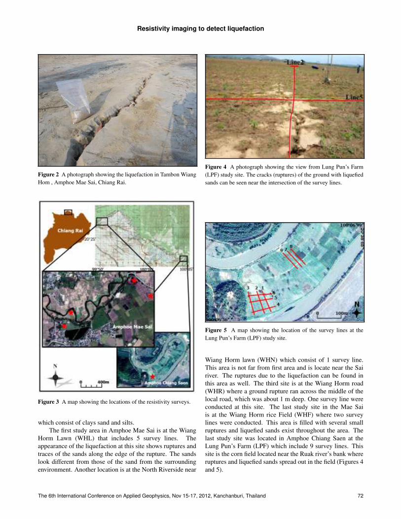
Resistivity imaging to detect liquefaction
Figure 2 A photograph showing the liquefaction in Tambon Wiang
Hom , Amphoe Mae Sai, Chiang Rai.
Figure 3 A map showing the locations of the resistivity surveys.
which consist of clays sand and silts.
The first study area in Amphoe Mae Sai is at the Wiang
Horm Lawn (WHL) that includes 5 survey lines. The
appearance of the liquefaction at this site shows ruptures and
traces of the sands along the edge of the rupture. The sands
look different from those of the sand from the surrounding
environment. Another location is at the North Riverside near
Figure 4 A photograph showing the view from Lung Pun’s Farm
(LPF) study site. The cracks (ruptures) of the ground with liquefied
sands can be seen near the intersection of the survey lines.
Figure 5 A map showing the location of the survey lines at the
Lung Pun’s Farm (LPF) study site.
Wiang Horm lawn (WHN) which consist of 1 survey line.
This area is not far from first area and is locate near the Sai
river. The ruptures due to the liquefaction can be found in
this area as well. The third site is at the Wiang Horm road
(WHR) where a ground rupture ran across the middle of the
local road, which was about 1 m deep. One survey line were
conducted at this site. The last study site in the Mae Sai
is at the Wiang Horm rice Field (WHF) where two survey
lines were conducted. This area is filled with several small
ruptures and liquefied sands exist throughout the area. The
last study site was located in Amphoe Chiang Saen at the
Lung Pun’s Farm (LPF) which include 9 survey lines. This
site is the corn field located near the Ruak river’s bank where
ruptures and liquefied sands spread out in the field (Figures 4
and 5).
The 6th International Conference on Applied Geophysics, Nov 15-17, 2012, Kanchanburi, Thailand 72
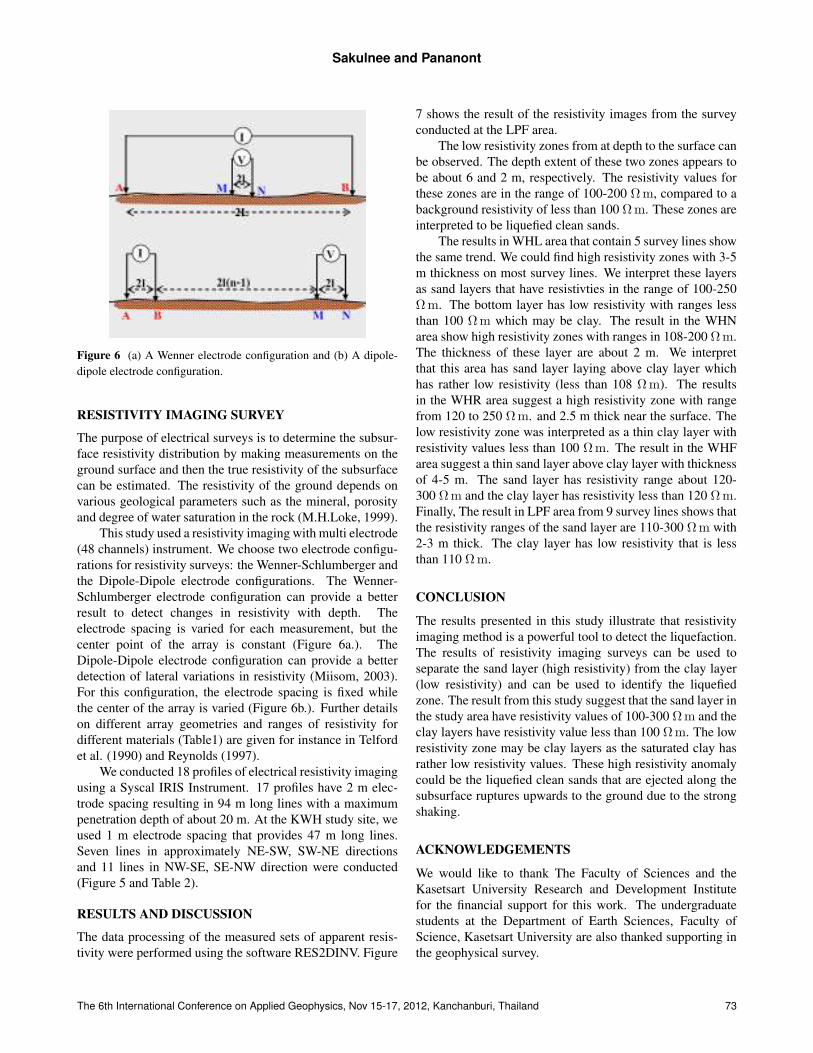
Sakulnee and Pananont
Figure 6 (a) A Wenner electrode configuration and (b) A dipole-
dipole electrode configuration.
RESISTIVITY IMAGING SURVEY
The purpose of electrical surveys is to determine the subsur-
face resistivity distribution by making measurements on the
ground surface and then the true resistivity of the subsurface
can be estimated. The resistivity of the ground depends on
various geological parameters such as the mineral, porosity
and degree of water saturation in the rock (M.H.Loke, 1999).
This study used a resistivity imaging with multi electrode
(48 channels) instrument. We choose two electrode configu-
rations for resistivity surveys: the Wenner-Schlumberger and
the Dipole-Dipole electrode configurations. The Wenner-
Schlumberger electrode configuration can provide a better
result to detect changes in resistivity with depth. The
electrode spacing is varied for each measurement, but the
center point of the array is constant (Figure 6a.). The
Dipole-Dipole electrode configuration can provide a better
detection of lateral variations in resistivity (Miisom, 2003).
For this configuration, the electrode spacing is fixed while
the center of the array is varied (Figure 6b.). Further details
on different array geometries and ranges of resistivity for
different materials (Table1) are given for instance in Telford
et al. (1990) and Reynolds (1997).
We conducted 18 profiles of electrical resistivity imaging
using a Syscal IRIS Instrument. 17 profiles have 2 m elec-
trode spacing resulting in 94 m long lines with a maximum
penetration depth of about 20 m. At the KWH study site, we
used 1 m electrode spacing that provides 47 m long lines.
Seven lines in approximately NE-SW, SW-NE directions
and 11 lines in NW-SE, SE-NW direction were conducted
(Figure 5 and Table 2).
RESULTS AND DISCUSSION
The data processing of the measured sets of apparent resis-
tivity were performed using the software RES2DINV. Figure
7 shows the result of the resistivity images from the survey
conducted at the LPF area.
The low resistivity zones from at depth to the surface can
be observed. The depth extent of these two zones appears to
be about 6 and 2 m, respectively. The resistivity values for
these zones are in the range of 100-200 Ωm, compared to a
background resistivity of less than 100 Ωm. These zones are
interpreted to be liquefied clean sands.
The results in WHL area that contain 5 survey lines show
the same trend. We could find high resistivity zones with 3-5
m thickness on most survey lines. We interpret these layers
as sand layers that have resistivties in the range of 100-250
Ωm. The bottom layer has low resistivity with ranges less
than 100 Ωm which may be clay. The result in the WHN
area show high resistivity zones with ranges in 108-200 Ωm.
The thickness of these layer are about 2 m. We interpret
that this area has sand layer laying above clay layer which
has rather low resistivity (less than 108 Ωm). The results
in the WHR area suggest a high resistivity zone with range
from 120 to 250 Ωm. and 2.5 m thick near the surface. The
low resistivity zone was interpreted as a thin clay layer with
resistivity values less than 100 Ωm. The result in the WHF
area suggest a thin sand layer above clay layer with thickness
of 4-5 m. The sand layer has resistivity range about 120-
300 Ωm and the clay layer has resistivity less than 120 Ωm.
Finally, The result in LPF area from 9 survey lines shows that
the resistivity ranges of the sand layer are 110-300 Ωm with
2-3 m thick. The clay layer has low resistivity that is less
than 110 Ωm.
CONCLUSION
The results presented in this study illustrate that resistivity
imaging method is a powerful tool to detect the liquefaction.
The results of resistivity imaging surveys can be used to
separate the sand layer (high resistivity) from the clay layer
(low resistivity) and can be used to identify the liquefied
zone. The result from this study suggest that the sand layer in
the study area have resistivity values of 100-300 Ωm and the
clay layers have resistivity value less than 100 Ωm. The low
resistivity zone may be clay layers as the saturated clay has
rather low resistivity values. These high resistivity anomaly
could be the liquefied clean sands that are ejected along the
subsurface ruptures upwards to the ground due to the strong
shaking.
ACKNOWLEDGEMENTS
We would like to thank The Faculty of Sciences and the
Kasetsart University Research and Development Institute
for the financial support for this work. The undergraduate
students at the Department of Earth Sciences, Faculty of
Science, Kasetsart University are also thanked supporting in
the geophysical survey.
The 6th International Conference on Applied Geophysics, Nov 15-17, 2012, Kanchanburi, Thailand 73
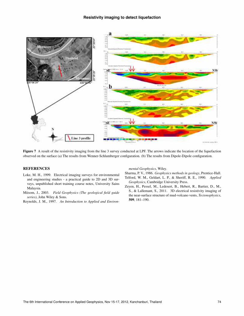
Resistivity imaging to detect liquefaction
Figure 7 A result of the resistivity imaging from the line 3 survey conducted at LPF. The arrows indicate the location of the liquefaction
observed on the surface (a) The results from Wenner-Schlumberger configuration. (b) The results from Dipole-Dipole configuration.
REFERENCES
Loke, M. H., 1999. Electrical imaging surveys for environmental
and engineering studies - a practical guide to 2D and 3D sur-
veys, unpublished short training course notes, University Sains
Malaysia.
Miisom, J., 2003. Field Geophysics (The geological field guide
series), John Wiley & Sons.
Reynolds, J. M., 1997. An Introduction to Applied and Environ-
mental Geophysics, Wiley.
Sharma, P. V., 1986. Geophysics methods in geology, Prentice-Hall.
Telford, W. M., Geldart, L. P., & Sheriff, R. E., 1990. Applied
Geophysics, Cambridge University Press.
Zeyen, H., Pessel, M., Ledesert, B., Hebert, R., Bartier, D., M.,
S., & Lallemant, S., 2011. 3D electrical resistivity imaging of
the near-surface structure of mud-volcano vents, Tectonophysics,
509, 181–190.
The 6th International Conference on Applied Geophysics, Nov 15-17, 2012, Kanchanburi, Thailand 74
Micro-tremor in Bangkok and its comparison withamplified shear waves and H/V spectrum of Rayleighwaves
Satoshi Morioa,∗, Yoshinori Katoa,, Akira Kitazumib,, Suwith Kosuwanc,, Sitirag Limpisawadc,,
Tirawat Boonyateed,
a Maizuru National College of Technology, Kyoto 625-8511, Japanb Ex JICA SV (Senior Volunteer), Osaka 592-0002, Japanc DMR (Department of Mineral Resources), Ratchatewee, Bangkok 10400, Thailandd Chulalongkorn University, Phayathai, Bangkok 10330, Thailand
∗, E-mail: [email protected]
ABSTRACT
Bangkok, the capital of Thailand, is located at a remote distance from seismic sources. However, it has a substantial risk from these distance
earthquakes due to the ability of the underling soft soil deposits to amplify ground motions. A wide range micro-tremor observation was
conducted in Bangkok metropolitan area to estimate the deep underground soil structure, velocity profile down to the seismic bedrock,
which is essential to predict long-period ground motion caused by the strong earthquakes. The long period velocity-type seismometer,
Trillium 40, was used. Micro-tremor observation was carried out at 89 sites in the greater Bangkok area during the winter season to detect
the long period micro-seisms caused by the high waves in the Gulf of Thailand. The horizontal-to-vertical (H/V) spectrum ratio of micro-
tremor was calculated and the subsurface velocity profile down to seismic bedrock was estimated. And these H/V spectrums were compared
with the SH wave amplification function and also with the theoretical Rayleigh wave amplification ratio H/V at the ground surface. It was
clarified that there was a deep basin at the southern part of Bangkok metropolitan area near the Gulf of Thailand. And it was also proved
that H/V spectrums of micro-tremor coincided with SH wave amplification function and also with theoretical Rayleigh wave amplification
ratio H/V at the ground surface very well.
KEYWORDS: Bangkok, Micro-tremor, H/V spectrum, Amplification function, Rayleigh Wave
INTRODUCTION
Recently, earthquake activities around Thailand were more
common. For instance, three M6 earthquakes occurred at
an active fault near to the western border with Myanmar
during last 50 years. M9.1 earthquake occurred at Sumatra in
December 26, 2004. Two M6 occurred near to the northern
border with Myanmar and Laos on May 16, 2007 and March
24, 2011. Although building failures or loss of life did not
occurred in Bangkok, people in high-rises could feel the
movement of buildings during these earthquakes. Bangkok
metropolitan is a big city with population of more than 6
million people. Besides high-rises in the city, a number of
large infrastructures have been constructed, for instance, the
Bangkok Transportation System (BTS), Mass Rapid Transit
(MRT), Suvarnnabhumi airport, Airport link line, etc. Since
earthquake activities were rarely observed in the past, few
structures were designed to resist earthquake motion. Since
Bangkok is situated on thick soil deposits, it is possible that
the magnitude of long distance earthquake motion can be am-
plified when it goes up to the ground surface. Unfortunately,
the influence of such layers to the amplification of waves
has not been fully understood. Therefore, even the seismic
design was carried out, the magnitude of ground motion used
in the design might be underestimated. Studies by the authors
(Kitazumi 2005; Morio et al, 2007) showed that thick soil
layers under the city would amplify long period earthquake
motion so that a number of structures will be damaged if an
M7 earthquake (an earthquake with magnitude more than 7)
occurs at an active fault in the vicinity of Bangkok.
MICROTREMOR MEASUREMENT
The measurements were carried out during winter season,
between 14 December 2009 and 20 January 2010, because
the height of ocean waves will be the highest across the year.
The measurements were made at 89 locations over an area of
The 6th International Conference on Applied Geophysics, Nov 15-17, 2012, Kanchanburi, Thailand 75
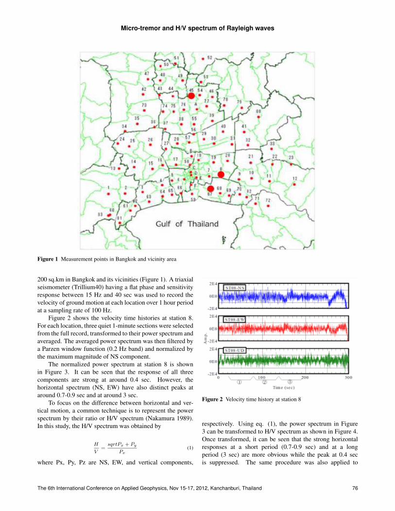
Micro-tremor and H/V spectrum of Rayleigh waves
Figure 1 Measurement points in Bangkok and vicinity area
200 sq.km in Bangkok and its vicinities (Figure 1). A triaxial
seismometer (Trillium40) having a flat phase and sensitivity
response between 15 Hz and 40 sec was used to record the
velocity of ground motion at each location over 1 hour period
at a sampling rate of 100 Hz.
Figure 2 shows the velocity time histories at station 8.
For each location, three quiet 1-minute sections were selected
from the full record, transformed to their power spectrum and
averaged. The averaged power spectrum was then filtered by
a Parzen window function (0.2 Hz band) and normalized by
the maximum magnitude of NS component.
The normalized power spectrum at station 8 is shown
in Figure 3. It can be seen that the response of all three
components are strong at around 0.4 sec. However, the
horizontal spectrum (NS, EW) have also distinct peaks at
around 0.7-0.9 sec and at around 3 sec.
To focus on the difference between horizontal and ver-
tical motion, a common technique is to represent the power
spectrum by their ratio or H/V spectrum (Nakamura 1989).
In this study, the H/V spectrum was obtained by
H
V=
sqrtPx + Py
Px
(1)
where Px, Py, Pz are NS, EW, and vertical components,
Figure 2 Velocity time history at station 8
respectively. Using eq. (1), the power spectrum in Figure
3 can be transformed to H/V spectrum as shown in Figure 4.
Once transformed, it can be seen that the strong horizontal
responses at a short period (0.7-0.9 sec) and at a long
period (3 sec) are more obvious while the peak at 0.4 sec
is suppressed. The same procedure was also applied to
The 6th International Conference on Applied Geophysics, Nov 15-17, 2012, Kanchanburi, Thailand 76
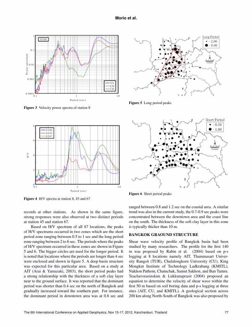
Morio et al.
Figure 3 Velocity power spectra of station 8
Figure 4 H/V spectra at station 8, 45 and 67
records at other stations. As shown in the same figure,
strong responses were also observed at two distinct periods
at station 45 and station 67.
Based on H/V spectrum of all 87 locations, the peaks
of H/V spectrums occurred in two zones which are the short
period zone ranging between 0.5 to 1 sec and the long period
zone ranging between 2 to 6 sec. The periods where the peaks
of H/V spectrum occurred in these zones are shown in Figure
5 and 6. The bigger circles are used for the longer period. It
is noted that locations where the periods are longer than 4 sec
were enclosed and shown in figure 5. A deep basin structure
was expected for this particular area. Based on a study at
AIT (Arai & Yamazaki, 2003), the short period peaks had
a strong relationship with the thickness of a soft clay layer
near to the ground surface. It was reported that the dominant
period was shorter than 0.4 sec on the north of Bangkok and
gradually increased toward the southern part. For instance,
the dominant period in downtown area was at 0.8 sec and
Figure 5 Long period peaks
Figure 6 Short period peaks
ranged between 0.8 and 1.2 sec on the coastal area. A similar
trend was also in the current study, the 0.7-0.9 sec peaks were
concentrated between the downtown area and the coast line
on the south. The thickness of the soft clay layer in this zone
is typically thicker than 10 m.
BANGKOK GRAOUND STRUCTURE
Shear wave velocity profile of Bangkok basin had been
studied by many researchers. The profile for the first 140
m was proposed by Rabin et al. (2004) based on p-s
logging at 8 locations namely AIT, Thammasart Univer-
sity Rangsit (TUR), Chulalongkorn University (CU), King
Mongkut Institute of Technology Ladkrabang (KMITL),
Nakhon Pathom, Chatuchak, Samut Sakhon, and Ban Tamru.
Teachavorasinskun & Lukkunaprasit (2004) proposed an
equation to determine the velocity of shear wave within the
first 50 m based on soil boring data and p-s logging at three
sites (AIT, CU, and KMITL). A geological section across
200 km along North-South of Bangkok was also proposed by
The 6th International Conference on Applied Geophysics, Nov 15-17, 2012, Kanchanburi, Thailand 77
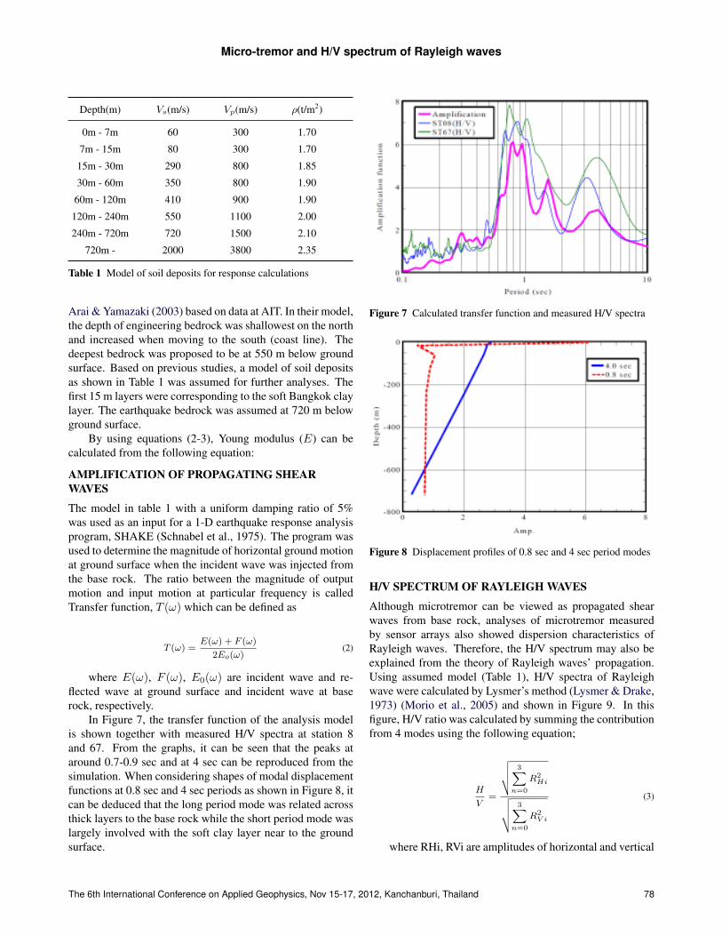
Micro-tremor and H/V spectrum of Rayleigh waves
Depth(m) Vs(m/s) Vp(m/s) ρ(t/m2)
0m - 7m 60 300 1.70
7m - 15m 80 300 1.70
15m - 30m 290 800 1.85
30m - 60m 350 800 1.90
60m - 120m 410 900 1.90
120m - 240m 550 1100 2.00
240m - 720m 720 1500 2.10
720m - 2000 3800 2.35
Table 1 Model of soil deposits for response calculations
Arai & Yamazaki (2003) based on data at AIT. In their model,
the depth of engineering bedrock was shallowest on the north
and increased when moving to the south (coast line). The
deepest bedrock was proposed to be at 550 m below ground
surface. Based on previous studies, a model of soil deposits
as shown in Table 1 was assumed for further analyses. The
first 15 m layers were corresponding to the soft Bangkok clay
layer. The earthquake bedrock was assumed at 720 m below
ground surface.
By using equations (2-3), Young modulus (E) can be
calculated from the following equation:
AMPLIFICATION OF PROPAGATING SHEAR
WAVES
The model in table 1 with a uniform damping ratio of 5%
was used as an input for a 1-D earthquake response analysis
program, SHAKE (Schnabel et al., 1975). The program was
used to determine the magnitude of horizontal ground motion
at ground surface when the incident wave was injected from
the base rock. The ratio between the magnitude of output
motion and input motion at particular frequency is called
Transfer function, T (ω) which can be defined as
T (ω) =E(ω) + F (ω)
2Eo(ω)(2)
where E(ω), F (ω), E0(ω) are incident wave and re-
flected wave at ground surface and incident wave at base
rock, respectively.
In Figure 7, the transfer function of the analysis model
is shown together with measured H/V spectra at station 8
and 67. From the graphs, it can be seen that the peaks at
around 0.7-0.9 sec and at 4 sec can be reproduced from the
simulation. When considering shapes of modal displacement
functions at 0.8 sec and 4 sec periods as shown in Figure 8, it
can be deduced that the long period mode was related across
thick layers to the base rock while the short period mode was
largely involved with the soft clay layer near to the ground
surface.
Figure 7 Calculated transfer function and measured H/V spectra
Figure 8 Displacement profiles of 0.8 sec and 4 sec period modes
H/V SPECTRUM OF RAYLEIGH WAVES
Although microtremor can be viewed as propagated shear
waves from base rock, analyses of microtremor measured
by sensor arrays also showed dispersion characteristics of
Rayleigh waves. Therefore, the H/V spectrum may also be
explained from the theory of Rayleigh waves’ propagation.
Using assumed model (Table 1), H/V spectra of Rayleigh
wave were calculated by Lysmer’s method (Lysmer & Drake,
1973) (Morio et al., 2005) and shown in Figure 9. In this
figure, H/V ratio was calculated by summing the contribution
from 4 modes using the following equation;
H
V=
√
√
√
√
3∑
n=0
R2Hi
√
√
√
√
3∑
n=0
R2V i
(3)
where RHi, RVi are amplitudes of horizontal and vertical
The 6th International Conference on Applied Geophysics, Nov 15-17, 2012, Kanchanburi, Thailand 78
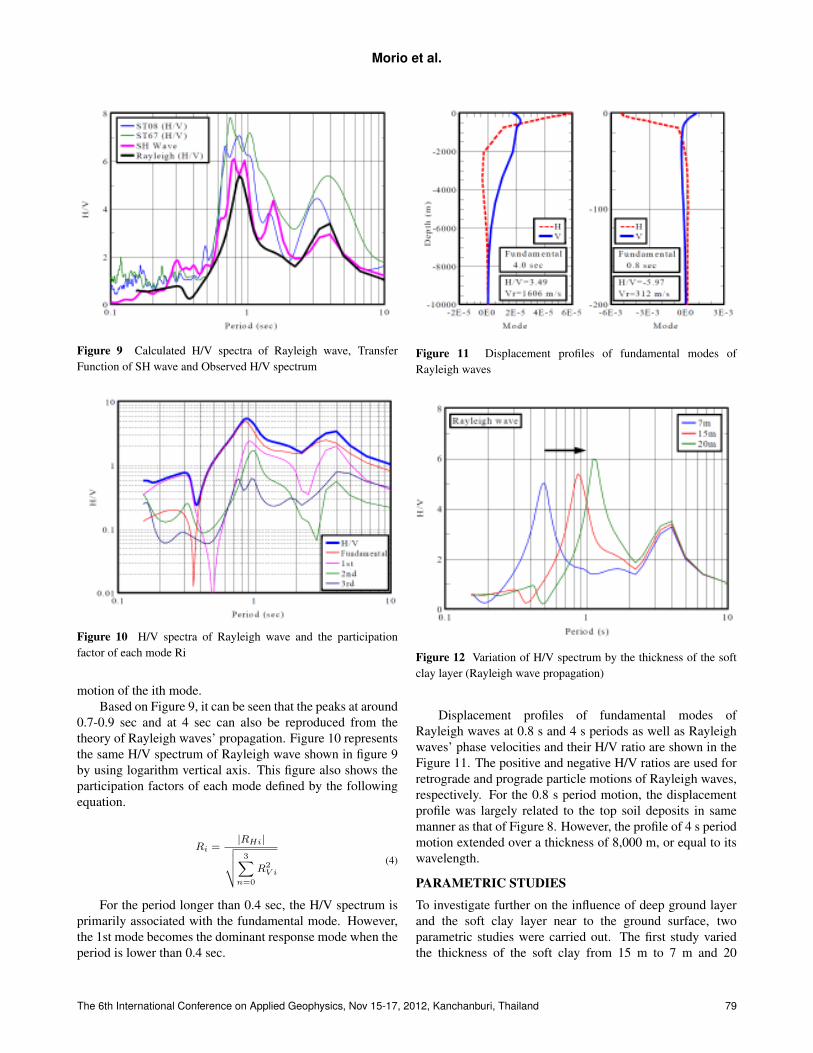
Morio et al.
Figure 9 Calculated H/V spectra of Rayleigh wave, Transfer
Function of SH wave and Observed H/V spectrum
Figure 10 H/V spectra of Rayleigh wave and the participation
factor of each mode Ri
motion of the ith mode.
Based on Figure 9, it can be seen that the peaks at around
0.7-0.9 sec and at 4 sec can also be reproduced from the
theory of Rayleigh waves’ propagation. Figure 10 represents
the same H/V spectrum of Rayleigh wave shown in figure 9
by using logarithm vertical axis. This figure also shows the
participation factors of each mode defined by the following
equation.
Ri =|RHi|
√
√
√
√
3∑
n=0
R2V i
(4)
For the period longer than 0.4 sec, the H/V spectrum is
primarily associated with the fundamental mode. However,
the 1st mode becomes the dominant response mode when the
period is lower than 0.4 sec.
Figure 11 Displacement profiles of fundamental modes of
Rayleigh waves
Figure 12 Variation of H/V spectrum by the thickness of the soft
clay layer (Rayleigh wave propagation)
Displacement profiles of fundamental modes of
Rayleigh waves at 0.8 s and 4 s periods as well as Rayleigh
waves’ phase velocities and their H/V ratio are shown in the
Figure 11. The positive and negative H/V ratios are used for
retrograde and prograde particle motions of Rayleigh waves,
respectively. For the 0.8 s period motion, the displacement
profile was largely related to the top soil deposits in same
manner as that of Figure 8. However, the profile of 4 s period
motion extended over a thickness of 8,000 m, or equal to its
wavelength.
PARAMETRIC STUDIES
To investigate further on the influence of deep ground layer
and the soft clay layer near to the ground surface, two
parametric studies were carried out. The first study varied
the thickness of the soft clay from 15 m to 7 m and 20
The 6th International Conference on Applied Geophysics, Nov 15-17, 2012, Kanchanburi, Thailand 79
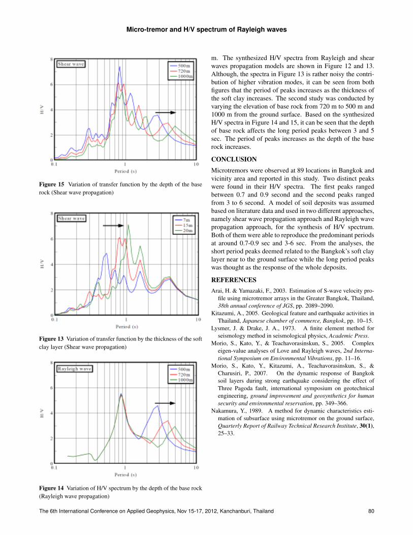
Micro-tremor and H/V spectrum of Rayleigh waves
Figure 15 Variation of transfer function by the depth of the base
rock (Shear wave propagation)
Figure 13 Variation of transfer function by the thickness of the soft
clay layer (Shear wave propagation)
Figure 14 Variation of H/V spectrum by the depth of the base rock
(Rayleigh wave propagation)
m. The synthesized H/V spectra from Rayleigh and shear
waves propagation models are shown in Figure 12 and 13.
Although, the spectra in Figure 13 is rather noisy the contri-
bution of higher vibration modes, it can be seen from both
figures that the period of peaks increases as the thickness of
the soft clay increases. The second study was conducted by
varying the elevation of base rock from 720 m to 500 m and
1000 m from the ground surface. Based on the synthesized
H/V spectra in Figure 14 and 15, it can be seen that the depth
of base rock affects the long period peaks between 3 and 5
sec. The period of peaks increases as the depth of the base
rock increases.
CONCLUSION
Microtremors were observed at 89 locations in Bangkok and
vicinity area and reported in this study. Two distinct peaks
were found in their H/V spectra. The first peaks ranged
between 0.7 and 0.9 second and the second peaks ranged
from 3 to 6 second. A model of soil deposits was assumed
based on literature data and used in two different approaches,
namely shear wave propagation approach and Rayleigh wave
propagation approach, for the synthesis of H/V spectrum.
Both of them were able to reproduce the predominant periods
at around 0.7-0.9 sec and 3-6 sec. From the analyses, the
short period peaks deemed related to the Bangkok’s soft clay
layer near to the ground surface while the long period peaks
was thought as the response of the whole deposits.
REFERENCES
Arai, H. & Yamazaki, F., 2003. Estimation of S-wave velocity pro-
file using microtremor arrays in the Greater Bangkok, Thailand,
38th annual conference of JGS, pp. 2089–2090.
Kitazumi, A., 2005. Geological feature and earthquake activities in
Thailand, Japanese chamber of commerce, Bangkok, pp. 10–15.
Lysmer, J. & Drake, J. A., 1973. A finite element method for
seismology method in seismological physics, Academic Press.
Morio, S., Kato, Y., & Teachavorasinskun, S., 2005. Complex
eigen-value analyses of Love and Rayleigh waves, 2nd Interna-
tional Symposium on Environmental Vibrations, pp. 11–16.
Morio, S., Kato, Y., Kitazumi, A., Teachavorasinskun, S., &
Charusiri, P., 2007. On the dynamic response of Bangkok
soil layers during strong earthquake considering the effect of
Three Pagoda fault, international symposium on geotechnical
engineering, ground improvement and geosynthetics for human
security and environmental reservation, pp. 349–366.
Nakamura, Y., 1989. A method for dynamic characteristics esti-
mation of subsurface using microtremor on the ground surface,
Quarterly Report of Railway Technical Research Institute, 30(1),
25–33.
The 6th International Conference on Applied Geophysics, Nov 15-17, 2012, Kanchanburi, Thailand 80

Morio et al.
Schnabel, P. B., Lysmer, J., & Seed, H. B., 1975. SHAKE a com-
puter program for earthquake response analysis of horizontally
layered sites, Report No. EERC75-30, University of California,
Berkeley.
Teachavorasinskun, S. & Lukkunaprasit, P., 2004. A simple
correlation for shear wave velocity of soft Bangkok clays,
Geotechnique, 54, 323–326.
Tuladhar, R., Yamazaki, F., Warnitchai, P., & Saita, J., 2004.
Seismic microzonation of the greater Bangkok area using micro-
tremor observations, Earthquake Engineering and Structural
Dynamics, 33, 211–225.
Yordkayhun, S., 2011. Detecting near surface objects using
seismic traveltime tomography: Experimentation at a test site,
Songklanakarin Journal of Science and Technology, 33, 477–
485.
The 6th International Conference on Applied Geophysics, Nov 15-17, 2012, Kanchanburi, Thailand 81
Inversion of Magnetic Data from Remanent and InducedSources
Robert Ellisa,∗, Barry de Wetb, Ian Macleoda
a Geosoft Inc. Suite 810, 207 Queens Quay West, Toronto, ON, Canadab Ivanhoe Australia Ltd. Level 13, 484 St Kilda Road Melbourne, VIC, 3004, Australia
∗, E-mail: [email protected]
ABSTRACT
Magnetic field data are of fundamental importance in many areas of geophysical exploration with 3D voxel inversion being a common aid
to their interpretation. In the majority of voxel based inversions it is assumed that the magnetic response arises entirely from magnetic
induction. However, in the last decade, several studies have found that remanent magnetization is far more prevalent than previously
thought. Our experience with numerous minerals exploration projects confirms that the presence of non-induced magnetization is the rule
rather than the exception in base metals exploration. In this work we show that failure to accommodate for remanent magnetization in 3D
voxel-based inversion can lead to misleading interpretations. We present a technique we call Magnetization Vector Inversion (MVI), which
incorporates both remanent and induced magnetization without prior knowledge of the direction or strength of remanent magnetization. We
demonstrate our inversion using model studies and field data. Successful application to numerous minerals exploration surveys confirms
that incorporating remanent magnetization is essential for the correct interpretation of magnetic field data.
INTRODUCTION
The utility of magnetic field data in many areas of geophys-
ical exploration is well-known as is the application of 3D
voxel inversion to aid in magnetic data interpretation (for
example, Li and Oldenburg 1996, Pilkington, M., 1997, Silva
et al. 2000, Zhdanov and Portniaguine 2002, to cite just a
few). In the majority of voxel based inversions it is assumed
that the magnetic response arises entirely from magnetic
induction.
However, in the last decade, studies have found that
remanent magnetization is far more prevalent than previously
thought (McEnroe et al. 2009) and affects crustal rocks as
well as zones of mineralization. Unfortunately, remanent
magnetization can seriously distort inversion based on the
assumption that the source is only induced magnetization.
The severity of the distortion is due to the highly non-unique
nature of potential field inversion making it extraordinarily
easy for a potential field inversion to produce a seemingly
plausible model which agrees satisfactorily with the observed
data, even when a fundamental assumption in the inversion is
flawed.
Several authors have reported progress toward magnetic
data inversions including remanent effects (for example,
Shearer and Li 2004, Kubota and Uchiyama 2005, Lelievre
and Oldenburg 2009). In this work we report further progress
in this direction with a technique we call Magnetization
Vector Inversion (MVI), which incorporates both remanent
and induced magnetization without prior knowledge of the
direction or strength of remanent magnetization. In the fol-
lowing sections, we extend conventional scalar susceptibility
inversion to a magnetization vector inversion, that is, we
allow the inversion to solve for the source magnetization
amplitude and direction. While this increases the number
of variables in the inversion we will show by example that
the same regularization principles that allow compact targets
to be resolved in highly unconstrained scalar susceptibility
inversion also apply in vector inversion.
Perhaps our most significant finding is that MVI, or more
generally, inversion including all forms of magnetization,
significantly improves the interpretation of the majority of
minerals based magnetic field inversions. Unfortunately, the
surprising degree of improvement in interpretability cannot
be adequately presented in a paper and can only be verified
by direct experience. Consequently, while we have applied
MVI to a large number of magnetic field surveys and find
the results to be significantly superior to conventional scalar
based inversion, in this paper we are forced to limit our
attention to a synthetic case and field data from the Cu-Au
Osborne deposit located approximately 195km SE of Mount
Isa, in Western Queensland, Australia.
The 6th International Conference on Applied Geophysics, Nov 15-17, 2012, Kanchanburi, Thailand 82

Magnetic inversion from remanent and induced sources
MATHOD AND RESULTS
Let us begin with the very general assumption that the
magnetic properties of the earth can be represented by a
volume magnetization, M(r) (Telford et al. 1990). We make
no assumptions about whether source of the magnetization is
induced, remanent, or otherwise.
From magnetostatics, the magnetic field b at point rjresulting from a volume V containing magnetization, M(r),is given by
B(ri) = ∇∫
v
M)r) · ∇ 1
|r− rj|dr3 (1)
This expression shows directly that the magnetization
vector M(r) is the natural parameter for inversion. This is
a crucial observation.
If the volume V consists of a collection of N sub-
volumes vk each of constant magnetization mk then
Bβ(rj) =
N,3∑
k,α
mk,α
∫
vk
∂α∂β1
|r− rj|dr3 (2)
This defines the forward problem: given a set of sources
mk(k = 1, ..., N) then Bj is the predicted magnetic field
anomaly at points, rj(j = 1, ...,M). Note that the coordinate
index α is summed over indicating that we are free to choose
the most computationally convenient internal coordinate sys-
tem. It also suggests that a coordinate invariant quantity, such
as the amplitude, M(r) = |M(r)|, will be most robustly
determined from the data.
For conciseness, we will represent Eq (2) simply as
B = Gm (3)
The vector magnetization inverse problem is defined as
solving for m given B subject to an appropriate regular-
ization condition. Although there are many choices for the
regularization (see for example, Zhdanov 2002), we choose
without loss of generality, the familiar Tikohonov minimum
gradient regularizer. The inverse problem becomes solving
for m in,
minφ(m) = φD(m) + λφM (m)
φD(m) =M∑
i
∣
∣
∣
∣
Gjm−Bj
ej
∣
∣
∣
∣
2
φM (m) =3∑
γ
|wγ∂γm|2 + |w0m|2
λ : φD(m) = χ2T
(4)
where in the first line, the total objective function φ is the sum
of a data term φD and a model term φM with a Tikohonov
regularization parameter, λ. The second line defines the data
Figure 1 The buried prism model with magnetization vector
orientation (Easterly) shown by the green cones. Side=100m
objective function in terms of the data equation (3) and the
error associated with each data point ej . The third line gives
the model objective function in terms of the gradient of the
model ∂γm and the amplitude of the model, with weighting
terms as required, wγ , w0. The fourth line indicates that the
Tikhonov regularization parameter λ is chosen based on a
satisfactory fit to the data in a chi-squared sense, χ2T . In
addition, other constraints, such as upper and lower bounds,
can be placed on m as appropriate to the specific exploration
problem.
Example - Buried Prism
Although the buried prism model is far too simplistic to
have exploration significance, it does make an excellent
pedagogical example, so we follow tradition and begin by
considering the inversion of simulated TMI data over a buried
prism with magnetization vector M perpendicular to the
earth field. The model consists a cube with side length 40
m buried with a depth to top of 20 m and a magnetization
vector in the EW direction, (My = 0, Mz = 0) as shown in
Figure 1.
Simulated TMI data are shown in Figure 2 for Earth
field with inclination 90° and amplitude 24000 nT. Cardinal
directions have been chosen only for simplicity of explana-
tion; any directions could be chosen with equivalent results.
Also for simplicity, the data were simulated at 20 m constant
clearance and on a regular 8m grid.
Inverting the TMI data in Figure 2 yields the model
shown in Figure 3 which should be compared to the true
model shown in Figure 1. There is some variability in
the magnetization direction but the predominant direction is
clearly EW, in agreement with the true model.
Vector magnetization models in 3D are difficult to inter-
pret directly in all the but the simplest cases. In real-world
The 6th International Conference on Applied Geophysics, Nov 15-17, 2012, Kanchanburi, Thailand 83

Ellis et al.
Figure 2 The TMI data simulated over the magnetization vector
model shown in Figure 1. The axes are in metres.
Figure 3 The MVI recovered model for comparison with Figure 1.
The magnetization vector orientation is shown by the green cones.
exploration we need some simpler derived scalars which
highlight the important information in the vector model. As
suggested by Eq (1), the most robust and meaningful scalar is
the amplitude of the vector magnetization and this should be
the primary quantity used in interpretation. However, since
the magnetization vector direction is the earth field direction
for induced sources, it is tempting to attempt to use the
directional information recovered in MVI to generate scalars
related to the earth field direction.
There are many possibilities but we have found that three
useful derived scalars for exploration are: the amplitude of
the magnetization, the earth field projection of the magneti-
zation, and the amplitude of the perpendicular-to-earth-field
components of the magnetization. In exploration problems,
the amplitude is robust by being independent on of any
assumptions regarding the earth field, while the amplitude
Figure 4 (a) A cross section through the true model, (b) the recov-
ered amplitude of the magnetization vector, (c) the amplitude of the
perpendicular-to-earth-field components of the magnetization, (d)
the projection of the magnetization on to the earth field direction.
The colour scales indicate the MVI magnetization in normalized to
SI (see text).
perpendicular is an approximate indicator of non-induced
magnetization. To support our findings, these three derived
scalars are shown in Figure 4b, c, d for an East-West slice
through the model volume bisecting the target in the true
model.
In exploration situations it is convenient to present MVI
output M normalized by the amplitude of the earth’s mag-
netic intensity in the area of interest. That is, our results
are displayed as M/HE where HE is the amplitude of
the earth’s magnetic intensity in the area of interest. By
using this normalization in an area of purely induced mag-
netization, the numerical values returned by MVI inversion
will be directly comparable to those of scalar susceptibility
inversion, in our case in SI.
For completeness, and to show the contrast between
MVI and conventional scalar inversion, Figure 5b shows the
equivalent section through a model produced by an inversion
which assumes only induced magnetization. As should be
expected, the recovered model using scalar inversion is a
very poor representation of the true model, which in real-
world exploration ultimately adds significant confusion to the
interpretation process.
This simple prism example demonstrates the power of
magnetization vector inversion and its advantage over scalar
susceptibility inversion in cases where the magnetization
vector direction deviates from the earth field direction. We
argue that this situation predominates in real-world explo-
ration environments based on experience from many mag-
netic surveys, however this cannot be shown here.
The 6th International Conference on Applied Geophysics, Nov 15-17, 2012, Kanchanburi, Thailand 84
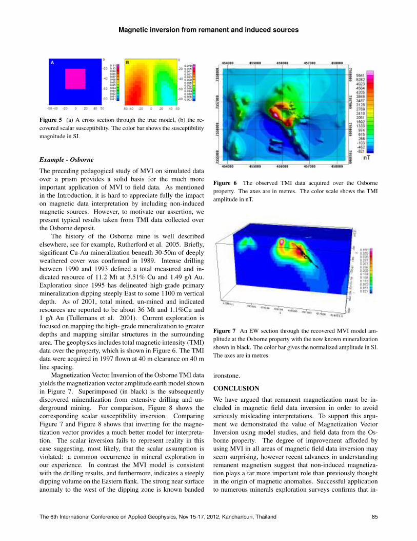
Magnetic inversion from remanent and induced sources
Figure 5 (a) A cross section through the true model, (b) the re-
covered scalar susceptibility. The color bar shows the susceptibility
magnitude in SI.
Example - Osborne
The preceding pedagogical study of MVI on simulated data
over a prism provides a solid basis for the much more
important application of MVI to field data. As mentioned
in the Introduction, it is hard to appreciate fully the impact
on magnetic data interpretation by including non-induced
magnetic sources. However, to motivate our assertion, we
present typical results taken from TMI data collected over
the Osborne deposit.
The history of the Osborne mine is well described
elsewhere, see for example, Rutherford et al. 2005. Briefly,
significant Cu-Au mineralization beneath 30-50m of deeply
weathered cover was confirmed in 1989. Intense drilling
between 1990 and 1993 defined a total measured and in-
dicated resource of 11.2 Mt at 3.51% Cu and 1.49 g/t Au.
Exploration since 1995 has delineated high-grade primary
mineralization dipping steeply East to some 1100 m vertical
depth. As of 2001, total mined, un-mined and indicated
resources are reported to be about 36 Mt and 1.1%Cu and
1 g/t Au (Tullemans et al. 2001). Current exploration is
focused on mapping the high- grade mineralization to greater
depths and mapping similar structures in the surrounding
area. The geophysics includes total magnetic intensity (TMI)
data over the property, which is shown in Figure 6. The TMI
data were acquired in 1997 flown at 40 m clearance on 40 m
line spacing.
Magnetization Vector Inversion of the Osborne TMI data
yields the magnetization vector amplitude earth model shown
in Figure 7. Superimposed (in black) is the subsequently
discovered mineralization from extensive drilling and un-
derground mining. For comparison, Figure 8 shows the
corresponding scalar susceptibility inversion. Comparing
Figure 7 and Figure 8 shows that inverting for the magne-
tization vector provides a much better model for interpreta-
tion. The scalar inversion fails to represent reality in this
case suggesting, most likely, that the scalar assumption is
violated: a common occurrence in mineral exploration in
our experience. In contrast the MVI model is consistent
with the drilling results, and furthermore, indicates a steeply
dipping volume on the Eastern flank. The strong near surface
anomaly to the west of the dipping zone is known banded
Figure 6 The observed TMI data acquired over the Osborne
property. The axes are in metres. The color scale shows the TMI
amplitude in nT.
Figure 7 An EW section through the recovered MVI model am-
plitude at the Osborne property with the now known mineralization
shown in black. The color bar gives the normalized amplitude in SI.
The axes are in metres.
ironstone.
CONCLUSION
We have argued that remanent magnetization must be in-
cluded in magnetic field data inversion in order to avoid
seriously misleading interpretations. To support this argu-
ment we demonstrated the value of Magnetization Vector
Inversion using model studies, and field data from the Os-
borne property. The degree of improvement afforded by
using MVI in all areas of magnetic field data inversion may
seem surprising, however recent advances in understanding
remanent magnetism suggest that non-induced magnetiza-
tion plays a far more important role than previously thought
in the origin of magnetic anomalies. Successful application
to numerous minerals exploration surveys confirms that in-
The 6th International Conference on Applied Geophysics, Nov 15-17, 2012, Kanchanburi, Thailand 85

Ellis et al.
Figure 8 The same section as in Figure 7 for the scalar model
with drilling and mineralization in black. The color bar gives the
susceptibility in SI. The axes are in metres.
corporating remanent magnetization is recommended for the
correct interpretation of the majority of magnetic field data.
REFERENCES
Butler, R. F., 1992. Paleomagnetism: magnetic domains to geologic
terranes, Blackwell Scientific Publications.
Geophysics, A., 1990. Telford, W. M. and Geldart, L. P. and
Sherriff, R. E. and Keys, D. A., Cambridge University Press.
Kubota, R. & Uchiyama, A., 2005. Three-dimensional magneti-
zation vector inversion of a seamount, Earth Planets Space, 57,
691–699.
Lelievre, P. G. & Oldenburg, D. W., 2009. A 3D total magnetization
inversion applicable when significant complicated remanence is
present, Geophysics, 74, 21–30.
Li, Y. & Oldenburg, D. W., 1996. 3-D inversion of magnetic data,
Geophysics, 61, 394–408.
McEnroe, S. A., Fabian, K., Robinson, P., Gaina, C., & Brown, L.,
2009. Crustal magnetism, Lamellar magnetism and rocks that
remember, Elements, 5, Elements.
Pilkington, M., 1997. 3-D magnetic imaging using conjugate
gradients, Geophysics, 62, 1132–1142.
Rutherford, N. F., Lawrance, L. M., & Sparks, G., 2005. Osborne
cu-au deposit, clonclurry, north west queensland, Tech. rep.,
CRC LEME Report.
Shearer, S., , & Li, Y., 2004. 3D inversion of magnetic total gradient
data in the presence of remanent magnetization, in 74th Annual
Meeting, SEG, Technical Program, Expanded Abstracts.
Silva, J. B. C., Medeiros, W. E., & Barbosa, V. C. F., 2001.
Potential-field inversion: Choosing the appropriate technique to
solve a geologic problem, Geophysics, 66, 511–520.
Tullemans, F. J., P., A., & Voulgaris, P., 2001. The role of geology
and exploration within the mining cycle at the Osborne mine,
NW Queensland, in monograph 23 - mineral resource and ore
reserve estimation - the AusIMM guide to good practice, Tech.
rep., Australian Institute of Mining and Metallurgy.
Zhdanov, M. S., 2002. Geophysical inverse theory and regulariza-tion problems, in Method in Geochemistry and Geophysics 36,
Elsevier Science.
Zhdanov, M. S. & Portniaguine, O., 2002. 3-D magnetic inversion
with data compression and image focusing, Geophysics, 67,
1532–1541.
The 6th International Conference on Applied Geophysics, Nov 15-17, 2012, Kanchanburi, Thailand 86
Extracting shear wave velocity from seismic reflectiondata: Case studies in near surface characterization usingMultichannel Analysis of Surface Wave (MASW)
Sawasdee Yordkayhuna,b,∗, Aksara Mayamaea,, Preeya Srisuwana,
a Department of Physics, Faculty of Science, Prince of Songkla University, Hat Yai ,90112, THAILANDb Geophysics Research Center, Department of Physics, Faculty of Science, Prince of Songkla University, Hat Yai ,90112,
THAILAND∗, E-mail: [email protected]
ABSTRACT
Understanding elastic properties of near-surface material are importance in geotechnical, earthquake engineering and environmental studies.
Using compressional (P) wave seismic reflection for detecting shallow buried objects is difficult when the data are lack of high frequency
contents and the near surface is of highly heterogeneity. In addition, the difficulty in data processing may be due to the presence of P-waves
interfering with noises of shear (S) wave and surface wave. For seismic refraction, it is based on the assumption of velocity increase with
depth whereas velocity inversions in the real earth layers can lead to the pitfalls in the interpretation. To show that near surface layers
can be characterized by shear wave velocity obtained from seismic reflection data, some case studies were demonstrated. By applying
Multichannel Analysis of Surface Wave (MASW) technique, we take advantage of surface wave from the three seismic dataset, testing
across a buried drainpipe area, a sinkhole area and a fault detection area. MASW is implemented as an iterative inversion technique for
reconstructing shear wave velocity model from dispersion curves of the surface wave. In the buried drainpipe area and the fault detection
area, although the location of targets was not clearly resolved, the evidence of lateral and vertical velocity variation has potential to evaluate
the soil stress changing due to the disturbed ground and increased load. In the sinkhole area, a suspected void was observed as indicated
by the anomaly pattern of a low velocity feature underlying a high velocity due to the induced stress on the wall and roof of cavern. The
results revealed that elastic properties of the shallow subsurface can be obtained from joint interpretation of P-wave and S-wave, without
significant increase in acquisition and testing time.
KEYWORDS: surface wave, shear wave, MASW, near-surface object, seismic reflection
INTRODUCTION
Understanding elastic properties of the near surface mate-
rial, especially shear (S) wave velocity (Vs) are importance
in geotechnical, earthquake engineering and environmental
studies. Generally, the determinations of S-wave data can
be done either in direct way (using downhole or cross-
hole and surface seismic methods) or indirect ways (using
empirical relation with N value from Standard Penetration
Test, SPT). In case of downhole or crosshole (e.g., VSP),
the measurements are expensive because several boreholes
need to be drilled, and it is difficult to conduct in urban
areas. For surface seismic methods, compressional (P) and
S-wave reflection/refraction data is considered to be standard
technique for P and S-wave velocity determination. How-
ever, it is generally accepted that refraction methods cannot
handle velocity inversions and hidden layers problems. For
deep investigations, long profile is necessary which make it
difficult to run measurements in urban areas. In addition,
the pitfalls in data processing might be due to the presence
of P-waves interfering with S-wave arrivals. For indirect
way of shear wave velocity determination, several empirical
relationships exist for different lithology and tend to be site
dependent (Akin et al., 2011).
In recent years, a new technique for shear wave veloc-
ity determination, Multichannel Analysis of Surface Waves
(MASW), was developed and increasingly used in earth-
quake and geotechnical engineering because it is non-
intrusive, fast and cost-effectively geophysical method (Park
et al., 1999). Surface waves (e.g., Rayleigh wave or ground
roll) are typically considered as noise for seismic reflection
and refraction surveys. On the other hand, it becomes
signal and contain useful information in the MASW method.
The advantages of analyzing surface wave are: 1) it is
The 6th International Conference on Applied Geophysics, Nov 15-17, 2012, Kanchanburi, Thailand 87
Multichannel analysis of surface wave
coherent event in the shot records because more than two-
thirds of total seismic energy generated is contributed into
Rayleigh waves (Richart et al., 1970). 2) Even in the case of
velocity inversion, Rayleigh wave dispersive characteristics
can be used to estimate S-wave velocities of the near-surface
(Doyle, 1995; Xia et al., 2002).
Numerous studies have shown that S-wave velocity as
derived from MASW method can be used in a range of
applications. For example, estimating the amplification of
earthquake-induced ground motion for quantitative earth-
quake hazard assessment and site response studies (Ergina
et al., 2004; Anbazhagan & Sitharam, 2008; Maheswari et
al., 2010), Liquefaction potential analysis (Kayabali, 1996;
Andrus & Stokoe, 2000; Karastathis et al., 2010), the control
of soil compaction (Kanli et al., 2006), the detection of
underground cavities, tunnels and sinkholes (Leparoux et al.,
2000).
The purpose of this study is to determine S-wave velocity
at the sites by using MASW method with regard to a wide
range of applications. Although the data were recorded for
reflection and tomography analysis (Mayamae & Durrast,
2010; Yordkayhun, 2011), here we take advantage of using
the same dataset for MASW method based on the fact
that the data are contaminated by strong ground roll and
our natural frequency of geophone is slightly low (14 Hz).
Interpretation of S-wave velocity results attempt to test the
potential of the method in detecting near-surface velocity
anomalies associated with the known target location.
THEORETICAL BACKGROUND OF SURFACE
WAVE METHODS
Rayleigh and S-wave velocities
Rayleigh wave (or ground roll) is a surface wave which
its particle motion is a combination of an elliptical and
retrograde motion and its amplitude decay is exponentially
with depth from the free surface (Lin et al., 2007). In seismic
survey, it is majority part of seismic energy propagating
which can be characterized by strong amplitude and low
frequencies. In case of inhomogeneous media, it is disper-
sive, different frequencies travel at the different velocities
(velocity is dependent on frequency) with multiple modes.
Dispersion characteristic of Rayleigh waves is the crucial
property to estimate the S-wave velocities for the MASW
method.
In an elastic half space, relationship between the S-waves
and Rayleigh wave velocities is expressed as follows (Richart
el al., 1970).(
VR
VS
)6
+ 8
(
VR
VS
)4
+
(
24− 161− 2σ
2− 2σ
)(
VR
VS
)2
+16
(
1− 2σ
2− 2σ− 1
)
= 0
(1)
Where VR is Rayleigh wave velocity and σ is Poisson
ratio. Normally, Poisson’s ratio range from 0 to 0.5 for
very stiff solids to fluids (Sheriff, 1991). Therefore, the
Rayleigh wave velocity ranges from 0.87 to 0.96 of S-wave
velocity. As mentioned earlier and based on this equation,
the Rayleigh wave phase velocity of a layered earth is a
function of frequency and subsurface properties including
P-wave velocity, S-wave velocity, density, and thickness of
layers.
In geotechnical engineering, the dynamic elastic proper-
ties of soil are importance for site investigation and construc-
tion purposes. These properties can be derived from seismic
velocities and density. In an elastic medium, the propagation
velocity of S-waves is given by (Dobrin & Savit, 1988):
VS =
√
µ
ρ(2)
Where µ is the shear modulus and ρ is the density. Based on
this relationship, shear modulus can be calculated. Given the
relationship between P and S wave velocity, Poisson’s ratio
can be derived from equation:
σ =V 2P − 2V 2
S
2(V 2P − V 2
S )(3)
By using equations (2-3), Young modulus (E) can be calcu-
lated from the following equation:
V 2P =
E
ρ
1− σ
(1 + σ)(1− 2σ)(4)
MASW METHOD
The MASW technique relies on the principles of the dis-
persion analysis and inverse theory (Menke, 1989). The
method of determining subsurface S-wave velocities consists
of following steps:
(i) Data acquisition. Data are recorded in the same way as
the conventional seismic reflection/refraction acquisition
except the low natural frequency geophones (∼4.5 Hz)
are typically used (Figure 1a). Some rules of thumb for
optimum data acquisition are given by Xia et al. (1999).
(ii) Dispersion analysis and pick. Dispersion energy is
constructed using the 2D transformation discussed by
Park et al. (1998) to maps a shot gather in time-
space (t-x) domain into the phase velocity-frequency (f-
v) domain (Figure 1b). Then dispersion curve can be
extracted by picking the peaks of dispersion energy over
different frequency values.
(iii) Dispersion curves inversion. Inversion of dispersion
curve is non-linear and has non-unique solutions. The
iterative least-squares inverse routine is a standard tech-
nique for dealing with this matter. By setting up a suit-
able initial model and adjusting the model parameter val-
ues (the S-wave velocity) with the object of minimizing
the error between the calculated and picked dispersion
curve, a 1D velocity profile is obtained (Figure 1b).
The 6th International Conference on Applied Geophysics, Nov 15-17, 2012, Kanchanburi, Thailand 88
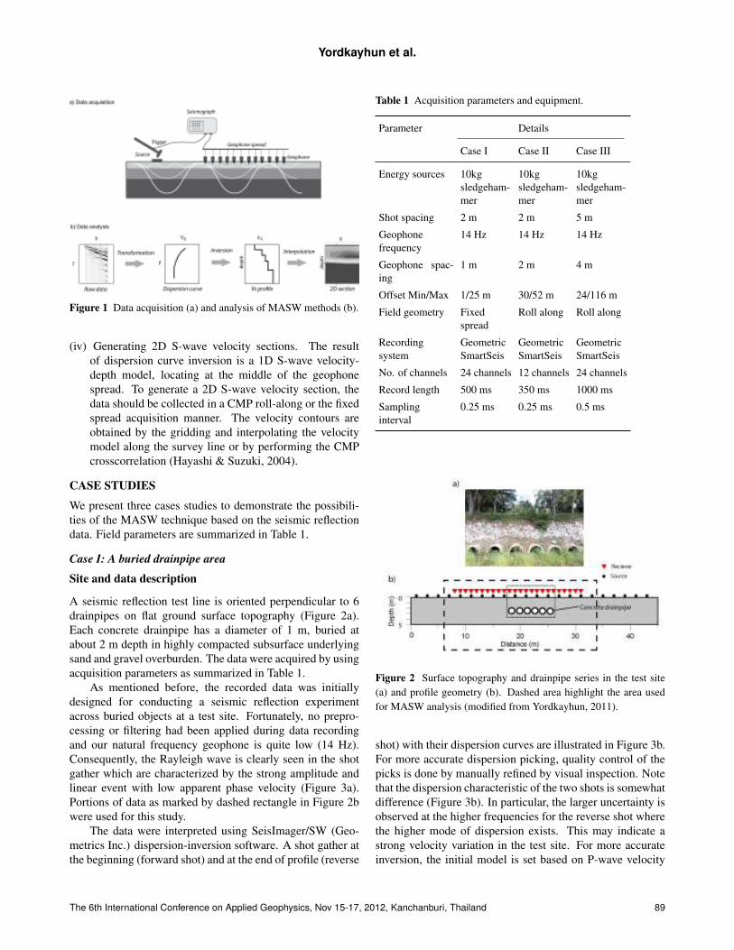
Yordkayhun et al.
Figure 1 Data acquisition (a) and analysis of MASW methods (b).
(iv) Generating 2D S-wave velocity sections. The result
of dispersion curve inversion is a 1D S-wave velocity-
depth model, locating at the middle of the geophone
spread. To generate a 2D S-wave velocity section, the
data should be collected in a CMP roll-along or the fixed
spread acquisition manner. The velocity contours are
obtained by the gridding and interpolating the velocity
model along the survey line or by performing the CMP
crosscorrelation (Hayashi & Suzuki, 2004).
CASE STUDIES
We present three cases studies to demonstrate the possibili-
ties of the MASW technique based on the seismic reflection
data. Field parameters are summarized in Table 1.
Case I: A buried drainpipe area
Site and data description
A seismic reflection test line is oriented perpendicular to 6
drainpipes on flat ground surface topography (Figure 2a).
Each concrete drainpipe has a diameter of 1 m, buried at
about 2 m depth in highly compacted subsurface underlying
sand and gravel overburden. The data were acquired by using
acquisition parameters as summarized in Table 1.
As mentioned before, the recorded data was initially
designed for conducting a seismic reflection experiment
across buried objects at a test site. Fortunately, no prepro-
cessing or filtering had been applied during data recording
and our natural frequency geophone is quite low (14 Hz).
Consequently, the Rayleigh wave is clearly seen in the shot
gather which are characterized by the strong amplitude and
linear event with low apparent phase velocity (Figure 3a).
Portions of data as marked by dashed rectangle in Figure 2b
were used for this study.
The data were interpreted using SeisImager/SW (Geo-
metrics Inc.) dispersion-inversion software. A shot gather at
the beginning (forward shot) and at the end of profile (reverse
Table 1 Acquisition parameters and equipment.
Parameter Details
Case I Case II Case III
Energy sources 10kg
sledgeham-
mer
10kg
sledgeham-
mer
10kg
sledgeham-
mer
Shot spacing 2 m 2 m 5 m
Geophone
frequency
14 Hz 14 Hz 14 Hz
Geophone spac-
ing
1 m 2 m 4 m
Offset Min/Max 1/25 m 30/52 m 24/116 m
Field geometry Fixed
spread
Roll along Roll along
Recording
system
Geometric
SmartSeis
Geometric
SmartSeis
Geometric
SmartSeis
No. of channels 24 channels 12 channels 24 channels
Record length 500 ms 350 ms 1000 ms
Sampling
interval
0.25 ms 0.25 ms 0.5 ms
Figure 2 Surface topography and drainpipe series in the test site
(a) and profile geometry (b). Dashed area highlight the area used
for MASW analysis (modified from Yordkayhun, 2011).
shot) with their dispersion curves are illustrated in Figure 3b.
For more accurate dispersion picking, quality control of the
picks is done by manually refined by visual inspection. Note
that the dispersion characteristic of the two shots is somewhat
difference (Figure 3b). In particular, the larger uncertainty is
observed at the higher frequencies for the reverse shot where
the higher mode of dispersion exists. This may indicate a
strong velocity variation in the test site. For more accurate
inversion, the initial model is set based on P-wave velocity
The 6th International Conference on Applied Geophysics, Nov 15-17, 2012, Kanchanburi, Thailand 89
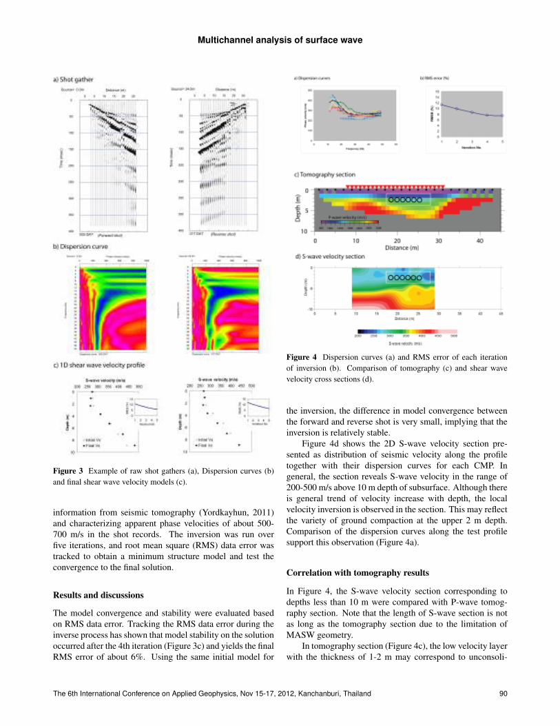
Multichannel analysis of surface wave
Figure 3 Example of raw shot gathers (a), Dispersion curves (b)
and final shear wave velocity models (c).
information from seismic tomography (Yordkayhun, 2011)
and characterizing apparent phase velocities of about 500-
700 m/s in the shot records. The inversion was run over
five iterations, and root mean square (RMS) data error was
tracked to obtain a minimum structure model and test the
convergence to the final solution.
Results and discussions
The model convergence and stability were evaluated based
on RMS data error. Tracking the RMS data error during the
inverse process has shown that model stability on the solution
occurred after the 4th iteration (Figure 3c) and yields the final
RMS error of about 6%. Using the same initial model for
Figure 4 Dispersion curves (a) and RMS error of each iteration
of inversion (b). Comparison of tomography (c) and shear wave
velocity cross sections (d).
the inversion, the difference in model convergence between
the forward and reverse shot is very small, implying that the
inversion is relatively stable.
Figure 4d shows the 2D S-wave velocity section pre-
sented as distribution of seismic velocity along the profile
together with their dispersion curves for each CMP. In
general, the section reveals S-wave velocity in the range of
200-500 m/s above 10 m depth of subsurface. Although there
is general trend of velocity increase with depth, the local
velocity inversion is observed in the section. This may reflect
the variety of ground compaction at the upper 2 m depth.
Comparison of the dispersion curves along the test profile
support this observation (Figure 4a).
Correlation with tomography results
In Figure 4, the S-wave velocity section corresponding to
depths less than 10 m were compared with P-wave tomog-
raphy section. Note that the length of S-wave section is not
as long as the tomography section due to the limitation of
MASW geometry.
In tomography section (Figure 4c), the low velocity layer
with the thickness of 1-2 m may correspond to unconsoli-
The 6th International Conference on Applied Geophysics, Nov 15-17, 2012, Kanchanburi, Thailand 90
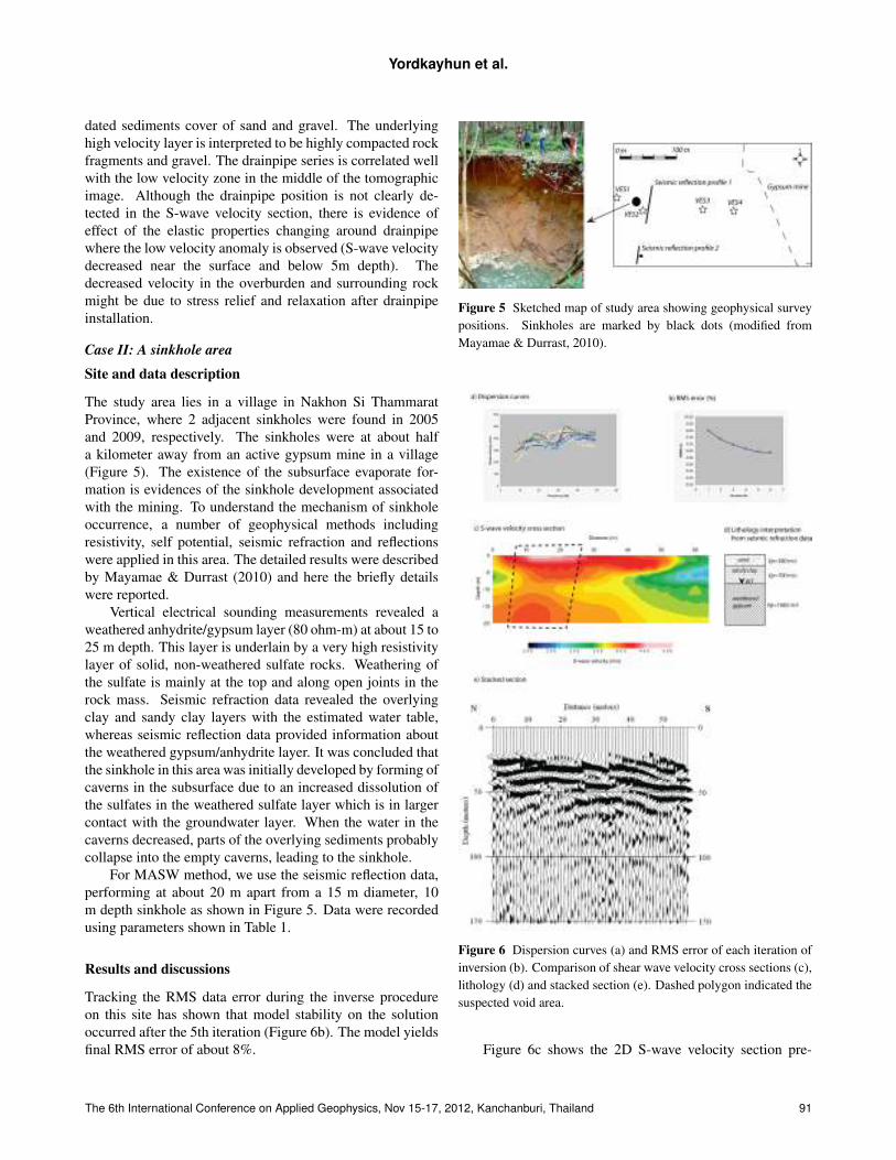
Yordkayhun et al.
dated sediments cover of sand and gravel. The underlying
high velocity layer is interpreted to be highly compacted rock
fragments and gravel. The drainpipe series is correlated well
with the low velocity zone in the middle of the tomographic
image. Although the drainpipe position is not clearly de-
tected in the S-wave velocity section, there is evidence of
effect of the elastic properties changing around drainpipe
where the low velocity anomaly is observed (S-wave velocity
decreased near the surface and below 5m depth). The
decreased velocity in the overburden and surrounding rock
might be due to stress relief and relaxation after drainpipe
installation.
Case II: A sinkhole area
Site and data description
The study area lies in a village in Nakhon Si Thammarat
Province, where 2 adjacent sinkholes were found in 2005
and 2009, respectively. The sinkholes were at about half
a kilometer away from an active gypsum mine in a village
(Figure 5). The existence of the subsurface evaporate for-
mation is evidences of the sinkhole development associated
with the mining. To understand the mechanism of sinkhole
occurrence, a number of geophysical methods including
resistivity, self potential, seismic refraction and reflections
were applied in this area. The detailed results were described
by Mayamae & Durrast (2010) and here the briefly details
were reported.
Vertical electrical sounding measurements revealed a
weathered anhydrite/gypsum layer (80 ohm-m) at about 15 to
25 m depth. This layer is underlain by a very high resistivity
layer of solid, non-weathered sulfate rocks. Weathering of
the sulfate is mainly at the top and along open joints in the
rock mass. Seismic refraction data revealed the overlying
clay and sandy clay layers with the estimated water table,
whereas seismic reflection data provided information about
the weathered gypsum/anhydrite layer. It was concluded that
the sinkhole in this area was initially developed by forming of
caverns in the subsurface due to an increased dissolution of
the sulfates in the weathered sulfate layer which is in larger
contact with the groundwater layer. When the water in the
caverns decreased, parts of the overlying sediments probably
collapse into the empty caverns, leading to the sinkhole.
For MASW method, we use the seismic reflection data,
performing at about 20 m apart from a 15 m diameter, 10
m depth sinkhole as shown in Figure 5. Data were recorded
using parameters shown in Table 1.
Results and discussions
Tracking the RMS data error during the inverse procedure
on this site has shown that model stability on the solution
occurred after the 5th iteration (Figure 6b). The model yields
final RMS error of about 8%.
Figure 5 Sketched map of study area showing geophysical survey
positions. Sinkholes are marked by black dots (modified from
Mayamae & Durrast, 2010).
Figure 6 Dispersion curves (a) and RMS error of each iteration of
inversion (b). Comparison of shear wave velocity cross sections (c),
lithology (d) and stacked section (e). Dashed polygon indicated the
suspected void area.
Figure 6c shows the 2D S-wave velocity section pre-
The 6th International Conference on Applied Geophysics, Nov 15-17, 2012, Kanchanburi, Thailand 91
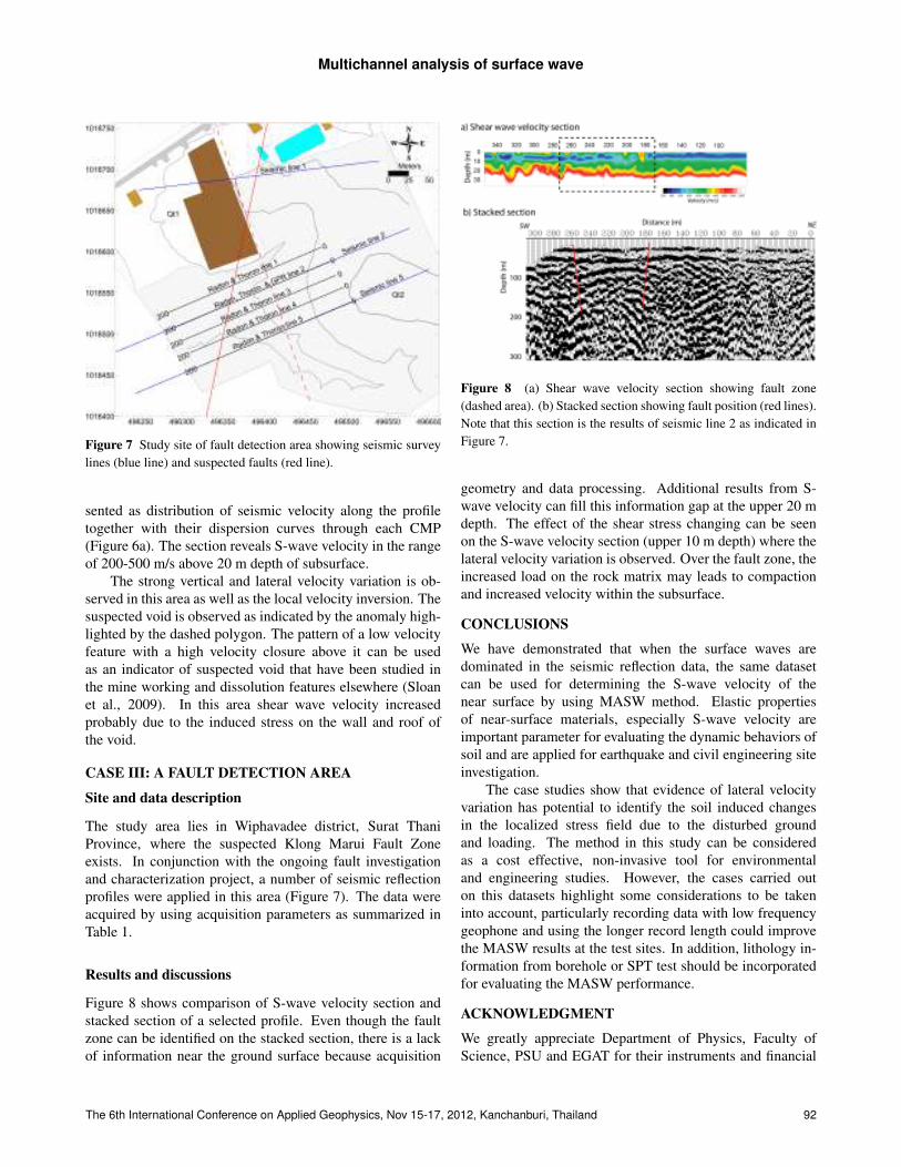
Multichannel analysis of surface wave
Figure 7 Study site of fault detection area showing seismic survey
lines (blue line) and suspected faults (red line).
sented as distribution of seismic velocity along the profile
together with their dispersion curves through each CMP
(Figure 6a). The section reveals S-wave velocity in the range
of 200-500 m/s above 20 m depth of subsurface.
The strong vertical and lateral velocity variation is ob-
served in this area as well as the local velocity inversion. The
suspected void is observed as indicated by the anomaly high-
lighted by the dashed polygon. The pattern of a low velocity
feature with a high velocity closure above it can be used
as an indicator of suspected void that have been studied in
the mine working and dissolution features elsewhere (Sloan
et al., 2009). In this area shear wave velocity increased
probably due to the induced stress on the wall and roof of
the void.
CASE III: A FAULT DETECTION AREA
Site and data description
The study area lies in Wiphavadee district, Surat Thani
Province, where the suspected Klong Marui Fault Zone
exists. In conjunction with the ongoing fault investigation
and characterization project, a number of seismic reflection
profiles were applied in this area (Figure 7). The data were
acquired by using acquisition parameters as summarized in
Table 1.
Results and discussions
Figure 8 shows comparison of S-wave velocity section and
stacked section of a selected profile. Even though the fault
zone can be identified on the stacked section, there is a lack
of information near the ground surface because acquisition
Figure 8 (a) Shear wave velocity section showing fault zone
(dashed area). (b) Stacked section showing fault position (red lines).
Note that this section is the results of seismic line 2 as indicated in
Figure 7.
geometry and data processing. Additional results from S-
wave velocity can fill this information gap at the upper 20 m
depth. The effect of the shear stress changing can be seen
on the S-wave velocity section (upper 10 m depth) where the
lateral velocity variation is observed. Over the fault zone, the
increased load on the rock matrix may leads to compaction
and increased velocity within the subsurface.
CONCLUSIONS
We have demonstrated that when the surface waves are
dominated in the seismic reflection data, the same dataset
can be used for determining the S-wave velocity of the
near surface by using MASW method. Elastic properties
of near-surface materials, especially S-wave velocity are
important parameter for evaluating the dynamic behaviors of
soil and are applied for earthquake and civil engineering site
investigation.
The case studies show that evidence of lateral velocity
variation has potential to identify the soil induced changes
in the localized stress field due to the disturbed ground
and loading. The method in this study can be considered
as a cost effective, non-invasive tool for environmental
and engineering studies. However, the cases carried out
on this datasets highlight some considerations to be taken
into account, particularly recording data with low frequency
geophone and using the longer record length could improve
the MASW results at the test sites. In addition, lithology in-
formation from borehole or SPT test should be incorporated
for evaluating the MASW performance.
ACKNOWLEDGMENT
We greatly appreciate Department of Physics, Faculty of
Science, PSU and EGAT for their instruments and financial
The 6th International Conference on Applied Geophysics, Nov 15-17, 2012, Kanchanburi, Thailand 92
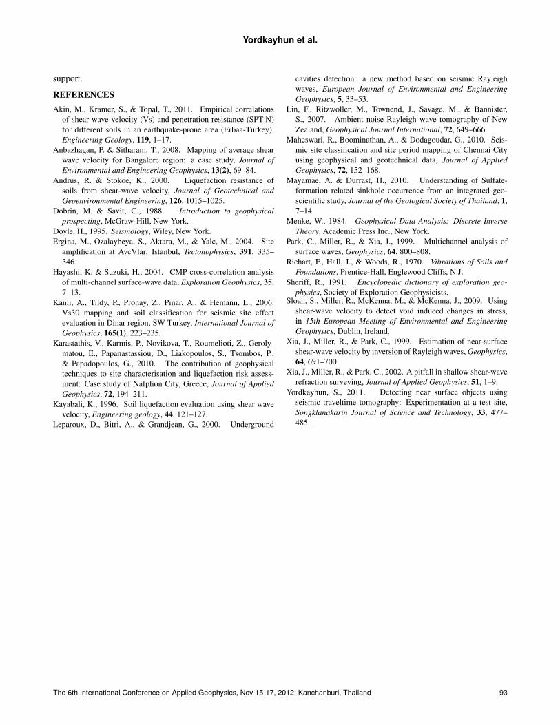
Yordkayhun et al.
support.
REFERENCES
Akin, M., Kramer, S., & Topal, T., 2011. Empirical correlations
of shear wave velocity (Vs) and penetration resistance (SPT-N)
for different soils in an earthquake-prone area (Erbaa-Turkey),
Engineering Geology, 119, 1–17.
Anbazhagan, P. & Sitharam, T., 2008. Mapping of average shear
wave velocity for Bangalore region: a case study, Journal of
Environmental and Engineering Geophysics, 13(2), 69–84.
Andrus, R. & Stokoe, K., 2000. Liquefaction resistance of
soils from shear-wave velocity, Journal of Geotechnical and
Geoenvironmental Engineering, 126, 1015–1025.
Dobrin, M. & Savit, C., 1988. Introduction to geophysical
prospecting, McGraw-Hill, New York.
Doyle, H., 1995. Seismology, Wiley, New York.
Ergina, M., Ozalaybeya, S., Aktara, M., & Yalc, M., 2004. Site
amplification at AvcVlar, Istanbul, Tectonophysics, 391, 335–
346.
Hayashi, K. & Suzuki, H., 2004. CMP cross-correlation analysis
of multi-channel surface-wave data, Exploration Geophysics, 35,
7–13.
Kanli, A., Tildy, P., Pronay, Z., Pinar, A., & Hemann, L., 2006.
Vs30 mapping and soil classification for seismic site effect
evaluation in Dinar region, SW Turkey, International Journal of
Geophysics, 165(1), 223–235.
Karastathis, V., Karmis, P., Novikova, T., Roumelioti, Z., Geroly-
matou, E., Papanastassiou, D., Liakopoulos, S., Tsombos, P.,
& Papadopoulos, G., 2010. The contribution of geophysical
techniques to site characterisation and liquefaction risk assess-
ment: Case study of Nafplion City, Greece, Journal of Applied
Geophysics, 72, 194–211.
Kayabali, K., 1996. Soil liquefaction evaluation using shear wave
velocity, Engineering geology, 44, 121–127.
Leparoux, D., Bitri, A., & Grandjean, G., 2000. Underground
cavities detection: a new method based on seismic Rayleigh
waves, European Journal of Environmental and Engineering
Geophysics, 5, 33–53.
Lin, F., Ritzwoller, M., Townend, J., Savage, M., & Bannister,
S., 2007. Ambient noise Rayleigh wave tomography of New
Zealand, Geophysical Journal International, 72, 649–666.
Maheswari, R., Boominathan, A., & Dodagoudar, G., 2010. Seis-
mic site classification and site period mapping of Chennai City
using geophysical and geotechnical data, Journal of Applied
Geophysics, 72, 152–168.
Mayamae, A. & Durrast, H., 2010. Understanding of Sulfate-
formation related sinkhole occurrence from an integrated geo-
scientific study, Journal of the Geological Society of Thailand, 1,
7–14.
Menke, W., 1984. Geophysical Data Analysis: Discrete Inverse
Theory, Academic Press Inc., New York.
Park, C., Miller, R., & Xia, J., 1999. Multichannel analysis of
surface waves, Geophysics, 64, 800–808.
Richart, F., Hall, J., & Woods, R., 1970. Vibrations of Soils and
Foundations, Prentice-Hall, Englewood Cliffs, N.J.
Sheriff, R., 1991. Encyclopedic dictionary of exploration geo-
physics, Society of Exploration Geophysicists.Sloan, S., Miller, R., McKenna, M., & McKenna, J., 2009. Using
shear-wave velocity to detect void induced changes in stress,
in 15th European Meeting of Environmental and Engineering
Geophysics, Dublin, Ireland.
Xia, J., Miller, R., & Park, C., 1999. Estimation of near-surface
shear-wave velocity by inversion of Rayleigh waves, Geophysics,
64, 691–700.
Xia, J., Miller, R., & Park, C., 2002. A pitfall in shallow shear-wave
refraction surveying, Journal of Applied Geophysics, 51, 1–9.
Yordkayhun, S., 2011. Detecting near surface objects using
seismic traveltime tomography: Experimentation at a test site,
Songklanakarin Journal of Science and Technology, 33, 477–
485.
The 6th International Conference on Applied Geophysics, Nov 15-17, 2012, Kanchanburi, Thailand 93

Quality Improvement Comparison Between Time-SpaceWindow Varying Median Filter and Time Window VaryingMedian Filter
Siriphon Somsria,∗, Pisanu Wongpornchaia,b
a Applied Geophysics Program, Faculty of Science, Chiang Mai Universityb Thailand Center of Excellent in Physics (ThEP), Commission on Higher Education, Bangkok 10400, Thailand
∗, E-mail: [email protected]
ABSTRACT
Noise in seismic data affects the signal to noise ratio, obscures details, and complicates identification of useful information. The random
and coherent noises in seismic data cannot be avoided during the recording. However, non-linear filters can eliminate these noises. A
non-linear filter is any filter that does not meet the criteria of linearity such as one-dimensional time varying median filter. The principle
of these filters is based on median filter but there were developed to enhance efficiency. These experiments present the abilities of filters
to improve signal of un-stack, deconvolved and stacked noisy seismic data. Signal to noise ratio, the subtracted value between filtered
and non-filter data and the result after applying AGC can be used to compare the filters competence. For three data types, the time-space
varying median filter (TSVMF) can more reduce the random noise, ground roll and refracted wave than time varying median (TVMF).
However, both filters can preserve the signal.
KEYWORDS: Time-space varying median filter, time varying median filter
INTRODUCTION
The seismic method is the most important geophysical tech-
nique in terms of expenditures and number of geophysicists
involved. It is predominantly due to high accuracy, high
resolution, and great penetration. However, the reliability of
seismic method is strongly depended on the quality of data
recording. Noise such as ground roll can drop the data quality
and cannot be avoided in explorations.
Random noise is a non-predictable noise but also certain
statistical properties (Telford et al, 1990). Some of this
seismic random noise exhibits spike-like characteristics and
neither continuous nor correlative (Liu et al, 2009). The
random noise can be produced from many sources such as
wind, tree shaking, and human activities.
Ground roll is the Rayleigh wave but it is often called the
ground roll in seismic exploration. Ground roll is a coherent
noise which propagates at the surface of the earth, at low
frequency and low velocity which are below 10 Hz and 100
to 1000 m/s, respectively (Olhovich, 1964). The ground roll
energy is high so it often obscures reflected seismic data.
(Saatcilar and Canitez, 1988).
Noise eliminating can be achieved in processing steps
by filters. Two of non-linear filters, time window varying
median filter and time-space window varying median filter,
were tested with noisy seismic data. The most useful of these
filters is denoising most of spiky noise or random noise and a
few of ground roll. The abilities of the filters are considered
from keeping signal and denoising.
The time window varying median filter (TVMF) was
presented by Liu et al. (2009). TVMF is one-dimensional
median filter which window size is designed from threshold
value. The threshold value is calculated from the average
of the signal amplitude. The prestack data from Texas was
applied by TVMF. The TVMF can eliminate random noise
enough to enhance the continuity of events. This method is
more powerful to eliminate random noise than the stationary
window median filter.
The two-dimensional median filter was developed for
enhanced efficiency. Vijaykumar et al. (2007) used an
adaptive window length recursive weighted median filter
(ARWMF) in an image processing and they considered the
size of window by using the density of noise
So from this idea, the time-space varying median filter
(TSVMF) was developed. This filter can adapt by using a
threshold value which different from ARWMF. And the filter
is also similar to TVMF but it is a two-dimensional filter.
Filter efficiency is determined by the signal to noise
The 6th International Conference on Applied Geophysics, Nov 15-17, 2012, Kanchanburi, Thailand 94

Time-space and time window varying median filter
Figure 1 Algorithm of TSVMF.
ratio (S/N) and the difference between filtered data and non-
filtered data by their subtraction. Good filters would provide
high S/N value which reduces only the high amplitude noise.
The window of S/N analysis can be represented by win-
dow D (Equation 1). S/N can be calculated using Equation 2
(Liu et al, 2009).
D = [xi,j ] (0 < M 6 Nx, 0 < N 6 Nt) (1)
S/N = 10 log10
N∑
j=1
(
M∑
i=1
xi,j
)2
MN∑
j=1
M∑
i=1
x2
i,j−N∑
j=1
(
M∑
i=1
xi,j
)2
(2)
where xi,j is amplitude signal in the window D, M and Nare size of window D which consist of trace number and sam-
ple number, respectively. Subtraction between filtered and
non-filtered data is an easy checking on noise elimination.
The appearance of interested noises in subtracted value is the
efficiency of filter that can reduce the noises.
Figure 2 a) Synthetic data b) Synthetic data with salt pepper
noise c) Synthetic data after filter by TSVMF d). Subtracted value
between filtered data and non-filtered data.
Developed TSVMF
TSVMF was developed based on TVMF. The size of refer-
ence window should be small such as 5×5 sizes (C1 × C2).
The threshold values (T ) are calculated using Equation 3.
T =1
NxNt
Nx∑
i=1
Nt∑
j=1
|YC1,C2| (3)
where |YC1,C2| is median value from reference window. Nx
is number of samples and Nt is number of traces.
The 6th International Conference on Applied Geophysics, Nov 15-17, 2012, Kanchanburi, Thailand 95
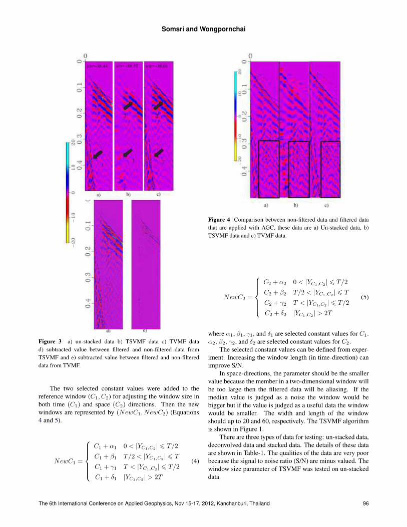
Somsri and Wongpornchai
Figure 3 a) un-stacked data b) TSVMF data c) TVMF data
d) subtracted value between filtered and non-filtered data from
TSVMF and e) subtracted value between filtered and non-filtered
data from TVMF.
The two selected constant values were added to the
reference window (C1, C2) for adjusting the window size in
both time (C1) and space (C2) directions. Then the new
windows are represented by (NewC1, NewC2) (Equations
4 and 5).
NewC1 =
C1 + α1 0 < |YC1,C2| 6 T/2
C1 + β1 T/2 < |YC1,C2| 6 T
C1 + γ1 T < |YC1,C2| 6 T/2
C1 + δ1 |YC1,C2| > 2T
(4)
Figure 4 Comparison between non-filtered data and filtered data
that are applied with AGC, these data are a) Un-stacked data, b)
TSVMF data and c) TVMF data.
NewC2 =
C2 + α2 0 < |YC1,C2| 6 T/2
C2 + β2 T/2 < |YC1,C2| 6 T
C2 + γ2 T < |YC1,C2| 6 T/2
C2 + δ2 |YC1,C2| > 2T
(5)
where α1, β1, γ1, and δ1 are selected constant values for C1.
α2, β2, γ2, and δ2 are selected constant values for C2.
The selected constant values can be defined from exper-
iment. Increasing the window length (in time-direction) can
improve S/N.
In space-directions, the parameter should be the smaller
value because the member in a two-dimensional window will
be too large then the filtered data will be aliasing. If the
median value is judged as a noise the window would be
bigger but if the value is judged as a useful data the window
would be smaller. The width and length of the window
should up to 20 and 60, respectively. The TSVMF algorithm
is shown in Figure 1.
There are three types of data for testing: un-stacked data,
deconvolved data and stacked data. The details of these data
are shown in Table-1. The qualities of the data are very poor
because the signal to noise ratio (S/N) are minus valued. The
window size parameter of TSVMF was tested on un-stacked
data.
The 6th International Conference on Applied Geophysics, Nov 15-17, 2012, Kanchanburi, Thailand 96
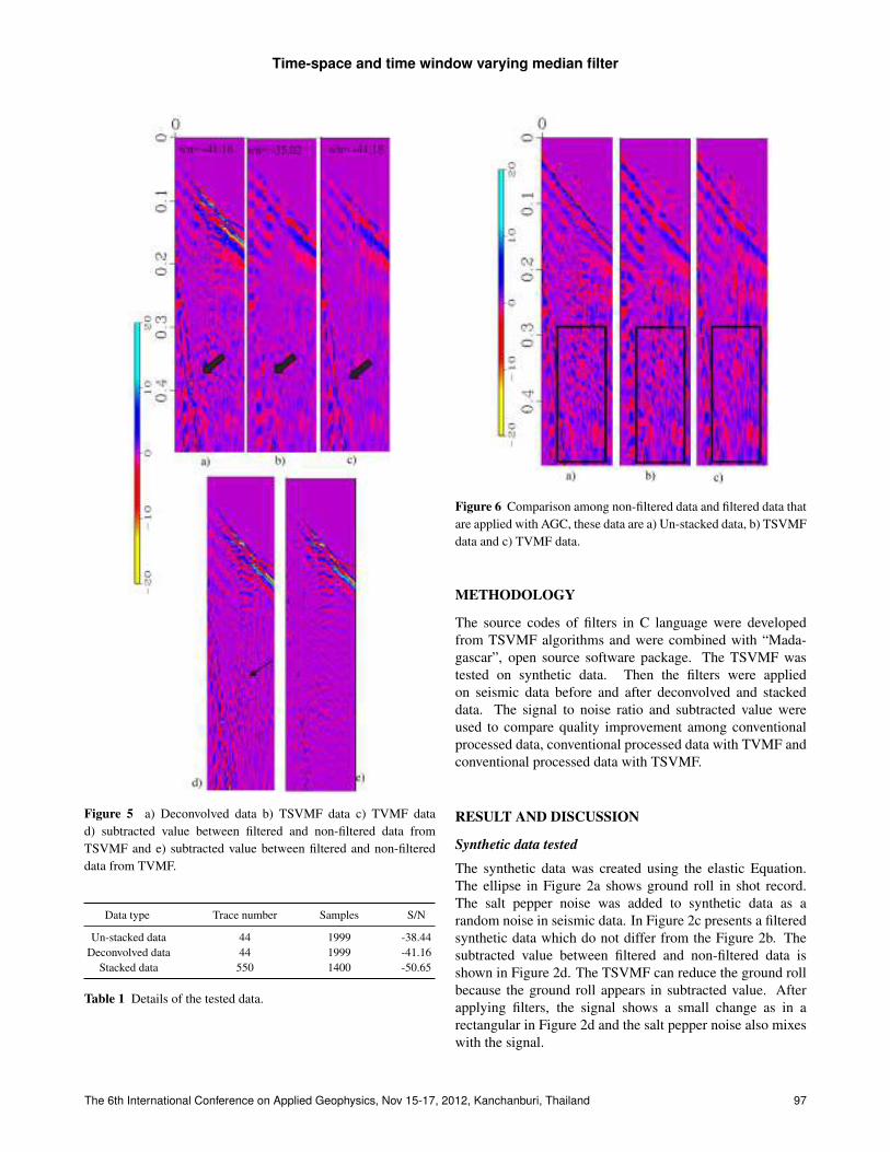
Time-space and time window varying median filter
Figure 5 a) Deconvolved data b) TSVMF data c) TVMF data
d) subtracted value between filtered and non-filtered data from
TSVMF and e) subtracted value between filtered and non-filtered
data from TVMF.
Data type Trace number Samples S/N
Un-stacked data 44 1999 -38.44
Deconvolved data 44 1999 -41.16
Stacked data 550 1400 -50.65
Table 1 Details of the tested data.
Figure 6 Comparison among non-filtered data and filtered data that
are applied with AGC, these data are a) Un-stacked data, b) TSVMF
data and c) TVMF data.
METHODOLOGY
The source codes of filters in C language were developed
from TSVMF algorithms and were combined with “Mada-
gascar”, open source software package. The TSVMF was
tested on synthetic data. Then the filters were applied
on seismic data before and after deconvolved and stacked
data. The signal to noise ratio and subtracted value were
used to compare quality improvement among conventional
processed data, conventional processed data with TVMF and
conventional processed data with TSVMF.
RESULT AND DISCUSSION
Synthetic data tested
The synthetic data was created using the elastic Equation.
The ellipse in Figure 2a shows ground roll in shot record.
The salt pepper noise was added to synthetic data as a
random noise in seismic data. In Figure 2c presents a filtered
synthetic data which do not differ from the Figure 2b. The
subtracted value between filtered and non-filtered data is
shown in Figure 2d. The TSVMF can reduce the ground roll
because the ground roll appears in subtracted value. After
applying filters, the signal shows a small change as in a
rectangular in Figure 2d and the salt pepper noise also mixes
with the signal.
The 6th International Conference on Applied Geophysics, Nov 15-17, 2012, Kanchanburi, Thailand 97

Somsri and Wongpornchai
Figure 7 Comparison of the filtered and non-filtered data
Un-stacked, deconvolved and stacked data tested
In Figure 3a, 3b, 3c show the filtered data using TSVMF
(Figure 3b) and TVMF (Figure 3c). The arrows in Figure
3a to 3c are pointing to the amplitude changing for refracted
wave and ground roll. The TSVMF can better reduce the
refracted wave and ground roll more than TVMF as shown
by arrows 1 and 2 in Figure 3a and Figure 3b. Even if, the
useful signals appear in subtracted values for TSVMF, but
after useful data was applied by AGC, it looks similar to non-
filtered data which represent by rectangle area in Figure 4a to
4c. Both filters can preserve the useful data.
In Figure 3a, 3b, 3c show the filtered data using TSVMF
(Figure 3b) and TVMF (Figure 3c). The arrows in Figure
3a to 3c are pointing to the amplitude changing for refracted
wave and ground roll. The TSVMF can better reduce the
refracted wave and ground roll more than TVMF as shown
by arrows 1 and 2 in Figure 3a and Figure 3b. Even if, the
useful signals appear in subtracted values for TSVMF, but
Figure 8 Comparison among the filtered and non-filtered data
which are applied by AGC.
after useful data was applied by AGC, it looks similar to non-
filtered data which represent by rectangle area in Figure 4a to
4c. Both filters can preserve the useful data.
The results from applying TSVMF and TVMF to stacked
data are shown in Figure 7. The difference between non-
filter, TSVMF and TVMF data are difficult to compare but
the subtracted values are easy to compare (Figure 9a and 9b).
The elliptical area in Figure 9a shows the presence of ground
roll but in Figure 9b the ground roll disappears. The other
noise, TSVMF and TVMF can reduce some refracted wave.
The random noise was decreased when data were stacked, so
it is difficult to compare with this case.
The S/N for all testing, TSVMF gives a highest S/N
value while TVMF gives a lower S/N value than TSVMF and
The 6th International Conference on Applied Geophysics, Nov 15-17, 2012, Kanchanburi, Thailand 98
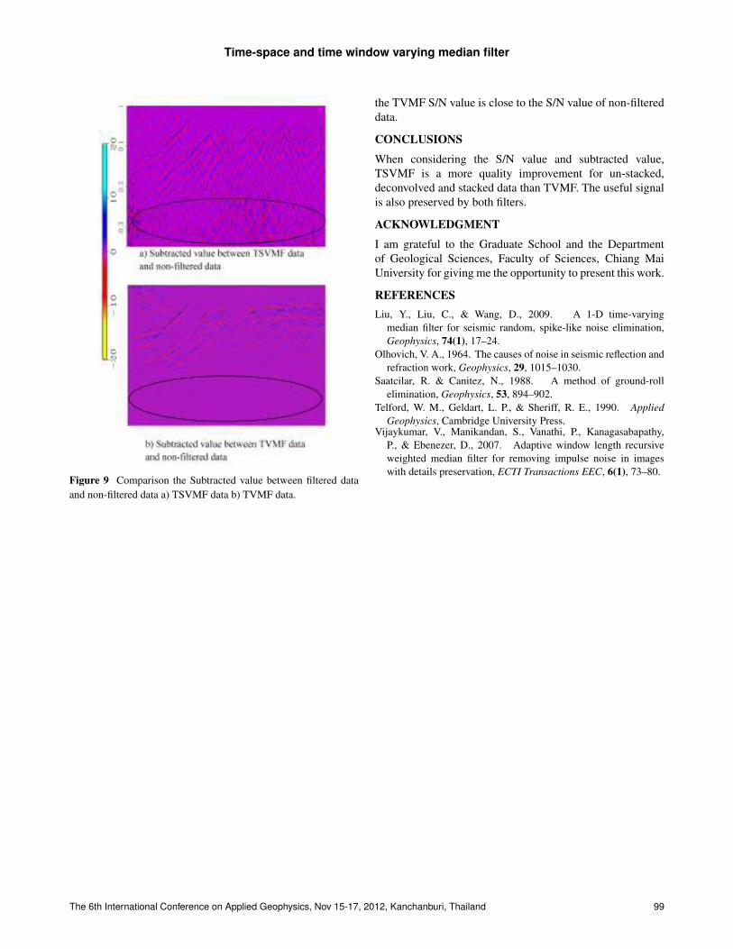
Time-space and time window varying median filter
Figure 9 Comparison the Subtracted value between filtered data
and non-filtered data a) TSVMF data b) TVMF data.
the TVMF S/N value is close to the S/N value of non-filtered
data.
CONCLUSIONS
When considering the S/N value and subtracted value,
TSVMF is a more quality improvement for un-stacked,
deconvolved and stacked data than TVMF. The useful signal
is also preserved by both filters.
ACKNOWLEDGMENT
I am grateful to the Graduate School and the Department
of Geological Sciences, Faculty of Sciences, Chiang Mai
University for giving me the opportunity to present this work.
REFERENCES
Liu, Y., Liu, C., & Wang, D., 2009. A 1-D time-varying
median filter for seismic random, spike-like noise elimination,
Geophysics, 74(1), 17–24.
Olhovich, V. A., 1964. The causes of noise in seismic reflection and
refraction work, Geophysics, 29, 1015–1030.
Saatcilar, R. & Canitez, N., 1988. A method of ground-roll
elimination, Geophysics, 53, 894–902.
Telford, W. M., Geldart, L. P., & Sheriff, R. E., 1990. Applied
Geophysics, Cambridge University Press.Vijaykumar, V., Manikandan, S., Vanathi, P., Kanagasabapathy,
P., & Ebenezer, D., 2007. Adaptive window length recursive
weighted median filter for removing impulse noise in images
with details preservation, ECTI Transactions EEC, 6(1), 73–80.
The 6th International Conference on Applied Geophysics, Nov 15-17, 2012, Kanchanburi, Thailand 99
Gas reservoir detection using three dimensional seismicattribute analysis, Gulf of Moattama, Offshore Myanmar
Soe Linn Htikea, Pisanu Wongpornchaia,∗
a Department of Geological Sciences, Faculty of Science, Chiang Mai University, Chiang Mai, 50200, THAILAND
∗, E-mail: [email protected]
ABSTRACT
Economic growth in Southeast Asian countries increases in energy demand. The Gulf of Moattama, offshore Myanmar, Andaman Sea,
is one of the petroleum production areas in the Southeast Asia. This research presents the detection of gas reservoirs by integration of
seismic attributes and well-log data in the Gulf of Moattama, offshore Myanmar, Andaman Sea. Three horizons were picked with reference
to the gamma ray and resistivity logs. These horizons were defined as the top of sand layers. Well tie to seismic data was performed
and three horizons picking in the three dimensional seismic cube were carried on. Nine seismic attributes were calculated from three
dimensional seismic data and seismic attribute maps of each horizon were generated. Well-log calibrated seismic attributes were used to
generate porosity maps. Anomalies for each attributes map were located for possible potential areas. Seismic attributes maps and porosity
maps were overlaid and four possible prospect areas were delineated. Comparing between some possible prospect areas with the proved
prospected areas indicates that integration of the seismic attributes analysis and well-log data has been proved to be an effective tool in
detection of gas reservoirs.
KEYWORDS: Seismic attribute analysis, Gas reservoir detection, Gulf of Moattama, Myanmar
INTRODUCTION
Seismic attributes were introduced in the early 1970s and
became an analytical tool for qualitative prediction of geom-
etry, lithology and reservoir characteristics. By combining
seismic attributes and well-log data, the result shows the
enhanced image for interpretation or analysis. As seis-
mic attributes have a various number and variety, many
researchers have attempted to classify seismic attributes.
For example, Taner et al. (1979) classified attributes into
two categories: geometrical and physical. The geometrical
attributes (e.g., dip, azimuth, and continuity) provide the
visibility of the geometrical characteristics of seismic data.
The physical attributes (e.g., amplitude, phase, and fre-
quency) deal with the physical parameters of the subsurface
and relate to lithology. Brown (1996) classified attributes
into time, amplitude, frequency. The time-derived attributes
provide structural information, whereas amplitude-derived
and frequency-derived attributes provide stratigraphic and
reservoir information. Some attributes can be used as the
hydrocarbon indicators (Sukmono, 2007).
The objective of this study is to detect gas reservoirs
using seismic attribute analysis and geophysical well log data
in an area of Gulf of Moattama, offshore Myanmar, Andaman
Sea (Figure 1).
GEOLOGY OF THE STUDY AREA
The Andaman Sea is an extensional structure. The tectonic
evolution has taken place since Eocene (45 ma) when the
India Plate was moving eastwards towards under the Sunda
Trench (Figure 2). According to the tectonism in this
area, two major sedimentary basins have developed in the
offshore Myanmar and one of them is Moattama Basin
(Figure 2). Davies et al (2003) described the Gulf of
Moattama Basin as being bounded by north-south trending
rifted Oligocene basement and as being filled by Pliocene-
Pleistocene sediments from the Ayeyarwaddy River to the
north and highlands to the east. This late Tertiary-Quaternary
basin-fill exceeds 10 kilometers in thickness. Ayeyarwady
formation is a thick sequence of deltaic sediments deposited
by the palaeo Ayeyarwady River, comprising interbedded
claystones, siltstones and sandstones. The formation com-
prises light to medium and locally dark grey, soft to firm and
sometimes silty claystones. The claystones are interbedded
with grey-white to light grey, unconsolidated to soft and
friable sandstones. These sandstones are composed of very
fine to medium grained. Hydrocarbon potential has been
established chiefly from Ayeyarwady formation. The clastic
reservoirs are shallow marine to deltaic sandstones. The
deltaic sandstones have been deposited from the north and
The 6th International Conference on Applied Geophysics, Nov 15-17, 2012, Kanchanburi, Thailand 100
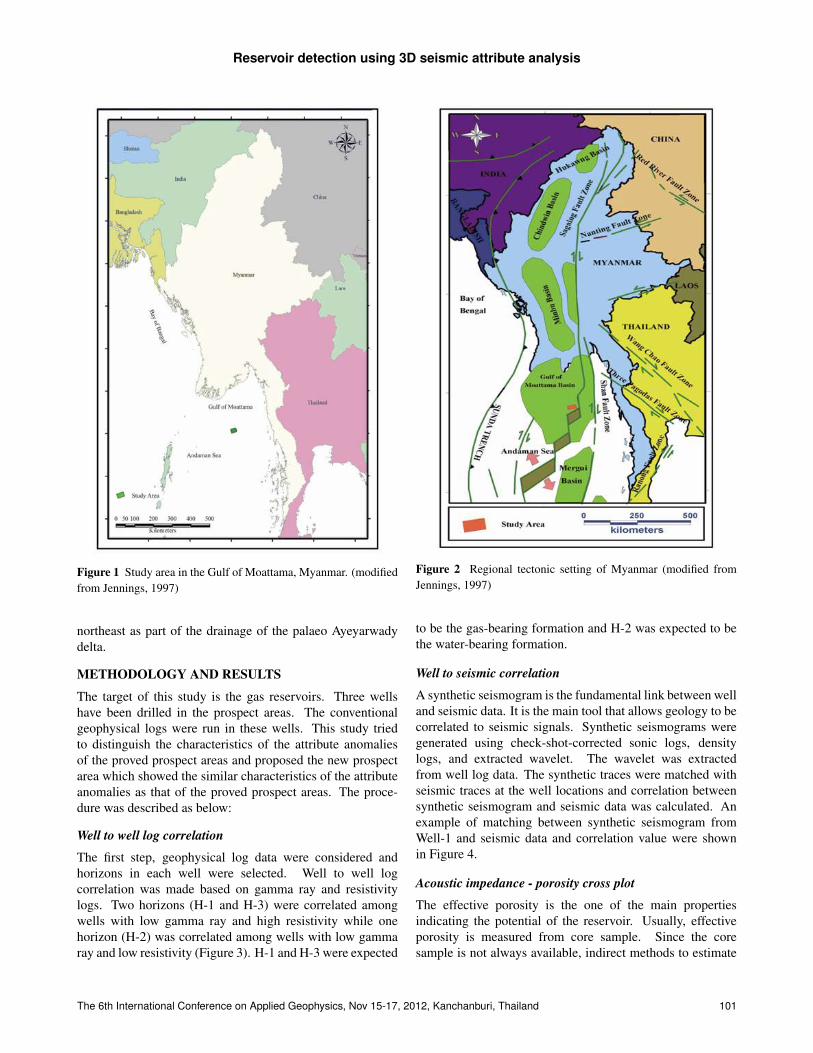
Reservoir detection using 3D seismic attribute analysis
Figure 1 Study area in the Gulf of Moattama, Myanmar. (modified
from Jennings, 1997)
northeast as part of the drainage of the palaeo Ayeyarwady
delta.
METHODOLOGY AND RESULTS
The target of this study is the gas reservoirs. Three wells
have been drilled in the prospect areas. The conventional
geophysical logs were run in these wells. This study tried
to distinguish the characteristics of the attribute anomalies
of the proved prospect areas and proposed the new prospect
area which showed the similar characteristics of the attribute
anomalies as that of the proved prospect areas. The proce-
dure was described as below:
Well to well log correlation
The first step, geophysical log data were considered and
horizons in each well were selected. Well to well log
correlation was made based on gamma ray and resistivity
logs. Two horizons (H-1 and H-3) were correlated among
wells with low gamma ray and high resistivity while one
horizon (H-2) was correlated among wells with low gamma
ray and low resistivity (Figure 3). H-1 and H-3 were expected
Figure 2 Regional tectonic setting of Myanmar (modified from
Jennings, 1997)
to be the gas-bearing formation and H-2 was expected to be
the water-bearing formation.
Well to seismic correlation
A synthetic seismogram is the fundamental link between well
and seismic data. It is the main tool that allows geology to be
correlated to seismic signals. Synthetic seismograms were
generated using check-shot-corrected sonic logs, density
logs, and extracted wavelet. The wavelet was extracted
from well log data. The synthetic traces were matched with
seismic traces at the well locations and correlation between
synthetic seismogram and seismic data was calculated. An
example of matching between synthetic seismogram from
Well-1 and seismic data and correlation value were shown
in Figure 4.
Acoustic impedance - porosity cross plot
The effective porosity is the one of the main properties
indicating the potential of the reservoir. Usually, effective
porosity is measured from core sample. Since the core
sample is not always available, indirect methods to estimate
The 6th International Conference on Applied Geophysics, Nov 15-17, 2012, Kanchanburi, Thailand 101
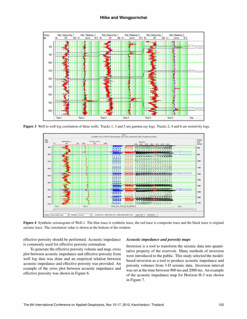
Htike and Wongpornchai
Figure 3 Well to well log correlation of three wells. Tracks 1, 3 and 5 are gamma ray logs. Tracks 2, 4 and 6 are resistivity logs.
Figure 4 Synthetic seismogram of Well-1. The blue trace is synthetic trace, the red trace is composite trace and the black trace is original
seismic trace. The correlation value is shown at the bottom of the window.
effective porosity should be performed. Acoustic impedance
is commonly used for effective porosity estimation.
To generate the effective porosity volume and map, cross
plot between acoustic impedance and effective porosity from
well log data was done and an empirical relation between
acoustic impedance and effective porosity was provided. An
example of the cross plot between acoustic impedance and
effective porosity was shown in Figure 6.
Acoustic impedance and porosity maps
Inversion is a tool to transform the seismic data into quanti-
tative property of the reservoir. Many methods of inversion
were introduced to the public. This study selected the model-
based inversion as a tool to produce acoustic impedance and
porosity volumes from 3-D seismic data. Inversion interval
was set at the time between 900 ms and 2000 ms. An example
of the acoustic impedance map for Horizon H-3 was shown
in Figure 7.
The 6th International Conference on Applied Geophysics, Nov 15-17, 2012, Kanchanburi, Thailand 102
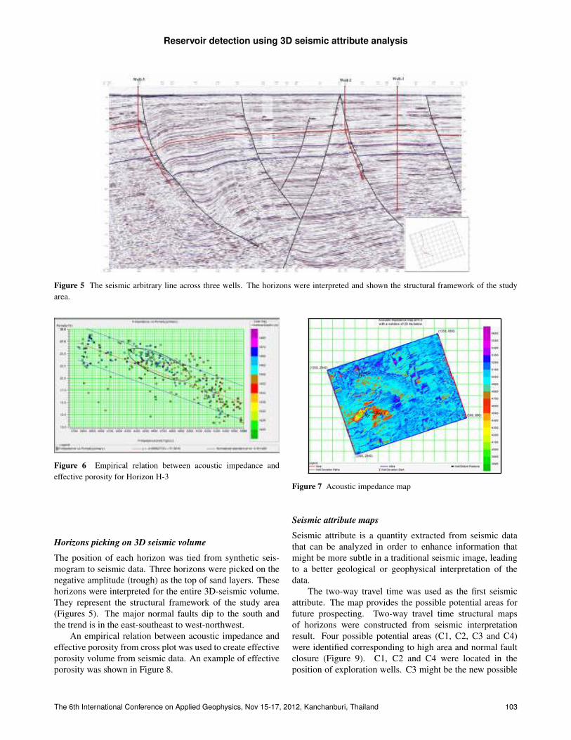
Reservoir detection using 3D seismic attribute analysis
Figure 5 The seismic arbitrary line across three wells. The horizons were interpreted and shown the structural framework of the study
area.
Figure 6 Empirical relation between acoustic impedance and
effective porosity for Horizon H-3
Horizons picking on 3D seismic volume
The position of each horizon was tied from synthetic seis-
mogram to seismic data. Three horizons were picked on the
negative amplitude (trough) as the top of sand layers. These
horizons were interpreted for the entire 3D-seismic volume.
They represent the structural framework of the study area
(Figures 5). The major normal faults dip to the south and
the trend is in the east-southeast to west-northwest.
An empirical relation between acoustic impedance and
effective porosity from cross plot was used to create effective
porosity volume from seismic data. An example of effective
porosity was shown in Figure 8.
Figure 7 Acoustic impedance map
Seismic attribute maps
Seismic attribute is a quantity extracted from seismic data
that can be analyzed in order to enhance information that
might be more subtle in a traditional seismic image, leading
to a better geological or geophysical interpretation of the
data.
The two-way travel time was used as the first seismic
attribute. The map provides the possible potential areas for
future prospecting. Two-way travel time structural maps
of horizons were constructed from seismic interpretation
result. Four possible potential areas (C1, C2, C3 and C4)
were identified corresponding to high area and normal fault
closure (Figure 9). C1, C2 and C4 were located in the
position of exploration wells. C3 might be the new possible
The 6th International Conference on Applied Geophysics, Nov 15-17, 2012, Kanchanburi, Thailand 103
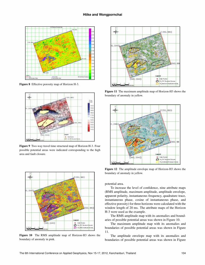
Htike and Wongpornchai
Figure 8 Effective porosity map of Horizon H-3.
Figure 9 Two-way travel time structural map of Horizon H-3. Four
possible potential areas were indicated corresponding to the high
area and fault closure.
Figure 10 The RMS amplitude map of Horizon-H3 shows the
boundary of anomaly in pink.
Figure 11 The maximum amplitude map of Horizon-H3 shows the
boundary of anomaly in yellow.
Figure 12 The amplitude envelope map of Horizon-H3 shows the
boundary of anomaly in yellow.
potential area.
To increase the level of confidence, nine attribute maps
(RMS amplitude, maximum amplitude, amplitude envelope,
apparent polarity, instantaneous frequency, quadrature trace,
instantaneous phase, cosine of instantaneous phase, and
effective porosity) for three horizons were calculated with the
window length of 20 ms. The attribute maps of the Horizon
H-3 were used as the example.
The RMS amplitude map with its anomalies and bound-
aries of possible potential areas was shown in Figure 10.
The maximum amplitude map with its anomalies and
boundaries of possible potential areas was shown in Figure
11.
The amplitude envelope map with its anomalies and
boundaries of possible potential areas was shown in Figure
The 6th International Conference on Applied Geophysics, Nov 15-17, 2012, Kanchanburi, Thailand 104
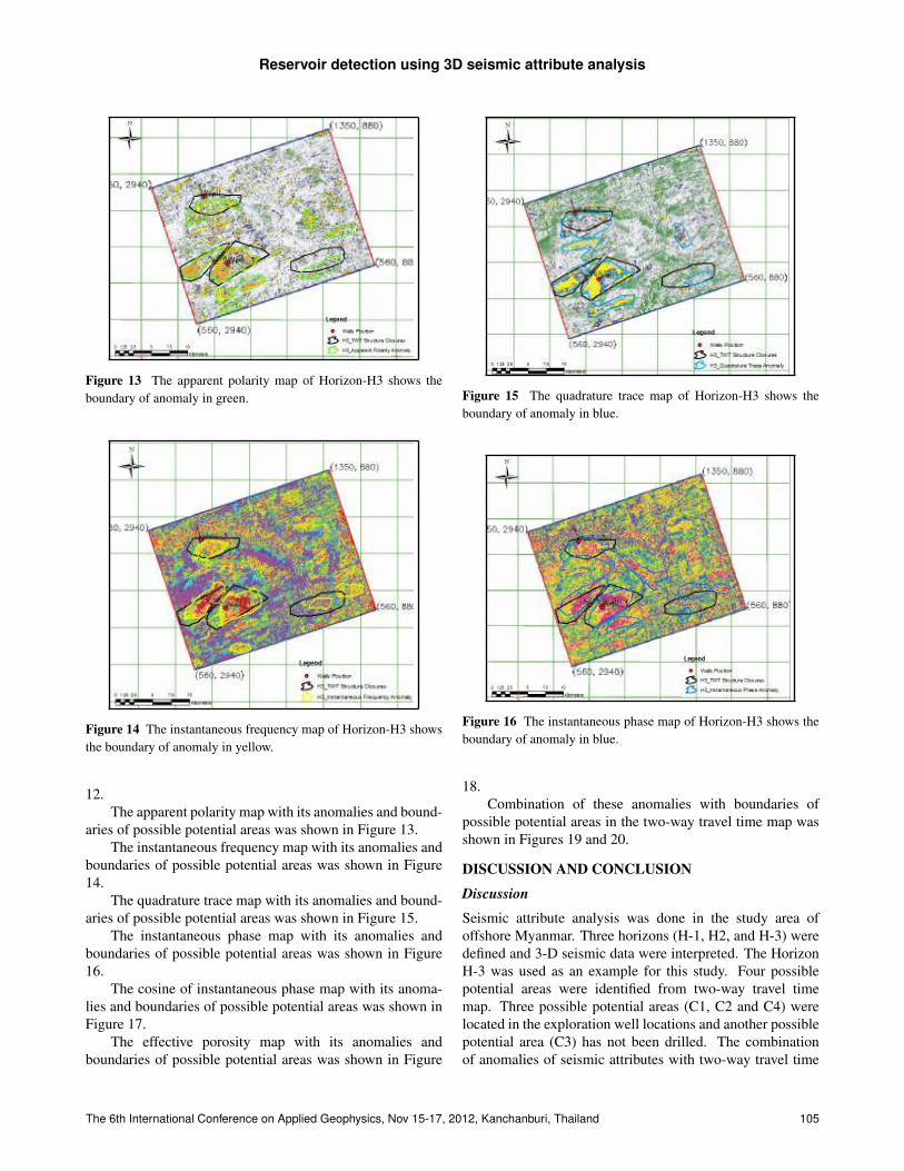
Reservoir detection using 3D seismic attribute analysis
Figure 13 The apparent polarity map of Horizon-H3 shows the
boundary of anomaly in green.
Figure 14 The instantaneous frequency map of Horizon-H3 shows
the boundary of anomaly in yellow.
12.
The apparent polarity map with its anomalies and bound-
aries of possible potential areas was shown in Figure 13.
The instantaneous frequency map with its anomalies and
boundaries of possible potential areas was shown in Figure
14.
The quadrature trace map with its anomalies and bound-
aries of possible potential areas was shown in Figure 15.
The instantaneous phase map with its anomalies and
boundaries of possible potential areas was shown in Figure
16.
The cosine of instantaneous phase map with its anoma-
lies and boundaries of possible potential areas was shown in
Figure 17.
The effective porosity map with its anomalies and
boundaries of possible potential areas was shown in Figure
Figure 15 The quadrature trace map of Horizon-H3 shows the
boundary of anomaly in blue.
Figure 16 The instantaneous phase map of Horizon-H3 shows the
boundary of anomaly in blue.
18.
Combination of these anomalies with boundaries of
possible potential areas in the two-way travel time map was
shown in Figures 19 and 20.
DISCUSSION AND CONCLUSION
Discussion
Seismic attribute analysis was done in the study area of
offshore Myanmar. Three horizons (H-1, H2, and H-3) were
defined and 3-D seismic data were interpreted. The Horizon
H-3 was used as an example for this study. Four possible
potential areas were identified from two-way travel time
map. Three possible potential areas (C1, C2 and C4) were
located in the exploration well locations and another possible
potential area (C3) has not been drilled. The combination
of anomalies of seismic attributes with two-way travel time
The 6th International Conference on Applied Geophysics, Nov 15-17, 2012, Kanchanburi, Thailand 105

Htike and Wongpornchai
Figure 17 The cosine of phase map of Horizon-H3 shows the
boundary of anomaly in green.
Figure 18 The effective porosity map of Horizon-H3 shows the
boundary of anomaly in red.
map shows that most of anomalies of seismic attributes were
located in the possible potential areas. Three wells were
drilled in three possible potential areas with the satisfied
result. This study indicates that another possible potential
area might be the next target of exploration.
Conclusion
Integration of well log data and seismic attribute analysis
is one of the powerful tools for indicating the gas-bearing
reservoir in seismic exploration. It can scope and show the
possible potential area for the future exploration. It can help
the reduction of the exploration cost and increasing the level
of confidence in seismic exploration.
ACKNOWLEDGMENT
Authors are grateful to the Graduate School and the Depart-
ment of Geological Sciences, Faculty of Sciences, ChiangMai University for giving us the opportunity to present this
work.
REFERENCES
Brown, A. R., 1996. Interpretation of three-dimensional seismic
data (Forth Edition), American Association of Petroleum Geolo-
gists, 42, 223–284.
Davies, R., Medwedeff, D., & Yarwood, D., 2003. Structural
trap and fault-seal analysis, offshore Myanmar: A case study,
AAPG/Datapages Discovery series, 7, 157–178.
Jennings, B., 1997. Final report Blocks M9 and M7 Gulf of
Martaban Myanmar.
Sukmono, S., 2007. Complex attributes for DHI & reservoir
analysis, Seismic Courses, pp. 1–131.
Taner, M., Koehler, F., & Sheriff, R., 1979. Complex seismic trace
analysis, Geophysics, 44, 1041–1063.
The 6th International Conference on Applied Geophysics, Nov 15-17, 2012, Kanchanburi, Thailand 106

Reservoir detection using 3D seismic attribute analysis
Figure 19 Combination of attribute anomalies of RMS amplitude, maximum amplitude, amplitude envelope, apparent polarity, and two-
way travel time map of Horizon H-3.
Figure 20 Combination of attribute anomalies of instantaneous frequency, instantaneous phase, cosine of instantaneous phase, quadrature
trace, and two-way travel time map of Horizon H-3.
The 6th International Conference on Applied Geophysics, Nov 15-17, 2012, Kanchanburi, Thailand 107
Porosity and Permeability Estimation from SeismicAttributes by Multi-layer Feedforward Neural NetworkTechnique in an Area of Gulf of Thailand
Theerachai Norkhamboota,∗, Pisanu Wongpornchaia
a Department of Geological Sciences, Faculty of Science, Chiang Mai University, Chiang Mai, THAILAND
∗, E-mail: [email protected]
ABSTRACT
In this study, seismic attribute analysis was used to estimate porosity and permeability of reservoir in an area of Gulf of Thailand. An
interesting sandstone layer was identified with the aid of well log data. Acoustic impedance volume was created as an external attribute
for seismic attribute analysis. To improve the ability of porosity and permeability estimation, the best attributes of multi-attribute analysis
results were computed using multi-layer feedforward neural network technique. To verify the multi-layer feedforward neural network
technique, the cross-plot analysis of multi-layer feedforward neural network results were performed and found that the correlation between
the predicted porosity and actual porosity gave a correlation value of about 0.95 with an average error value of 0.016. The multi-layer
feedforward neural network result of the correlation between the predicted permeability and actual permeability result gave correlation
value of about 0.99 with an average error value of 318.44 The analysis of results from multi-layer feedforward neural network technique
were shown that they are an effective technique to estimate porosity and permeability in a reservoir.
KEYWORDS: Seismic attribute analysis, Well log data, Multi-layer feedforward neural network, Gulf of Thailand
INTRODUCTION
Porosity is an important property of a reservoir because
hydrocarbon (oil and gas) can fill in voids of porous rocks.
Permeability is essential requirement information for reser-
voir evaluation because it is the ability of fluids to pass
through the pores in a material. The estimation of reser-
voir properties has been continuously developed for many
years. The prediction of physical properties such as porosity
from empirical correlations of multivariate linear regression
between seismic attributes and well log data was introduced
by numerous authors (Schultz et al., 1994; Schultz et al.,
1994a; Russell et al., 1997; Hampson et al., 2001). A seismic
attribute analysis to estimate physical properties such as
porosity, permeability and others in a reservoir were studied
(Brown, 1996; Leiphart and Hart, 2001; Tebo and Hart, 2003;
Calderon and Castagna, 2007). In this study, seismic attribute
analysis was applied to estimate porosity and permeability
in a gas sandstone layer. Acoustic impedance volume as
an external attribute was created and the internal attributes
were computed from seismic data. Step wise regression
method was used to find the best internal attributes. These
attributes were applied in multi-layer feedforward neural
network to estimate porosity and permeability. The attribute
map from multi-layer feedforward neural network result can
be used to interpret porosity and permeability related to
spatial distribution of a gas sandstone layer.
STUDY AREA
Cenozoic basins in the Gulf of Thailand consist of non-
marine to marginal marine Tertiary strata and the non-marine
sandstone reservoirs deposited in river system of fluvial and
lacustrine deltaic environments (Pradidtan and Dook, 1992).
The study area is one of the important petroleum production
fields in the Gulf of Thailand.
METHODOLOGY
A gas sandstone layer was selected from 2 well log data.
It was identified by low gamma ray (green curve), high
resistivity (red curve) in the first track, and crossover between
neutron porosity (blue curve) and density porosity (red curve)
in the second track (Figures 1 and 2). The interesting sand-
stone layer at well ZA was selected at the measured depth
of 1726.1 to 1741.64 m (black straight line) (Figure 1) and
at well ZB was selected at the measured depth of 1536.08 to
1545.29 m (black straight line) (Figure 2). The total porosity
was computed from neutron and density porosity logs. Since
clay minerals in sandstone closed the connection of pores in
The 6th International Conference on Applied Geophysics, Nov 15-17, 2012, Kanchanburi, Thailand 108

Porosity and permeability multi-layer feedforward neural network
Figure 1: The interesting sandstone layer was picked at well
ZA. The blue seismic trace is the synthetic seismic trace. The
red seismic trace is the composite seismic trace. Two yellow
lines are a window of analysis.
Figure 2: The interesting sandstone layer was picked at well
ZB. The blue seismic trace is the synthetic seismic trace. The
red seismic trace is the composite seismic trace. Two yellow
lines are a window of analysis.
sandstone, effective porosity was needed to calculate from
total porosity which shown in the third track (red curve)
(Figures 1 and 2). The irreducible water saturation defines
the maximum water saturation that a formation can retain
without producing water. The permeability was computed
from effective porosity and irreducible water saturation that
shown in the fourth track (magenta curve) (Figures 1 and 2).
Well to seismic correlation was done by synthetic seismo-
grams (Figures 1 and 2). Synthetic seismogram (blue line)
was generated by convolution between acoustic impedance
(product of check shot corrected sonic and density logs) and
extracted wavelet from seismic data. The synthetic seismic
traces were correlated with composite seismic traces (red
line) at the wells ZA and ZB. Acoustic impedance volume
was created by inversion between acoustic impedance log
Figure 3: The acoustic impedance inversion result of well
ZA and well ZB. The blue curve is original log (acoustic
impedance log). The red curve is inverted result. The
brown curve is initial model. The green curve is constraints.
The black and gray lines are top and base of horizons,
respectively.
(a) The attribute list for porosity prediction of the multi-
attributes analysis result
(b) The multi-attribute attribute analysis result shows the
average RMS error and validation error.
Figure 4
and seismic volume. The seismic attributes were computed
from seismic volume and compared with actual effective
porosity log and actual permeability log for the maximum
The 6th International Conference on Applied Geophysics, Nov 15-17, 2012, Kanchanburi, Thailand 109
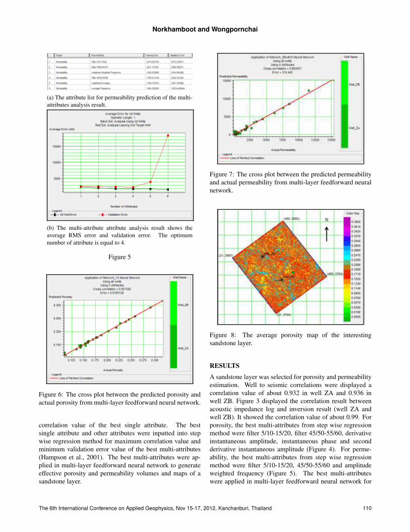
Norkhamboot and Wongpornchai
(a) The attribute list for permeability prediction of the multi-
attributes analysis result.
(b) The multi-attribute attribute analysis result shows the
average RMS error and validation error. The optimum
number of attribute is equal to 4.
Figure 5
Figure 6: The cross plot between the predicted porosity and
actual porosity from multi-layer feedforward neural network.
correlation value of the best single attribute. The best
single attribute and other attributes were inputted into step
wise regression method for maximum correlation value and
minimum validation error value of the best multi-attributes
(Hampson et al., 2001). The best multi-attributes were ap-
plied in multi-layer feedforward neural network to generate
effective porosity and permeability volumes and maps of a
sandstone layer.
Figure 7: The cross plot between the predicted permeability
and actual permeability from multi-layer feedforward neural
network.
Figure 8: The average porosity map of the interesting
sandstone layer.
RESULTS
A sandstone layer was selected for porosity and permeability
estimation. Well to seismic correlations were displayed a
correlation value of about 0.932 in well ZA and 0.936 in
well ZB. Figure 3 displayed the correlation result between
acoustic impedance log and inversion result (well ZA and
well ZB). It showed the correlation value of about 0.99. For
porosity, the best multi-attributes from step wise regression
method were filter 5/10-15/20, filter 45/50-55/60, derivative
instantaneous amplitude, instantaneous phase and second
derivative instantaneous amplitude (Figure 4). For perme-
ability, the best multi-attributes from step wise regression
method were filter 5/10-15/20, 45/50-55/60 and amplitude
weighted frequency (Figure 5). The best multi-attributes
were applied in multi-layer feedforward neural network for
The 6th International Conference on Applied Geophysics, Nov 15-17, 2012, Kanchanburi, Thailand 110
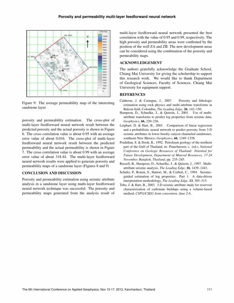
Porosity and permeability multi-layer feedforward neural network
Figure 9: The average permeability map of the interesting
sandstone layer.
porosity and permeability estimation. The cross-plot of
multi-layer feedforward neural network result between the
predicted porosity and the actual porosity is shown in Figure
6. The cross correlation value is about 0.95 with an average
error value of about 0.016. The cross-plot of multi-layer
feedforward neural network result between the predicted
permeability and the actual permeability is shown in Figure
7. The cross correlation value is about 0.99 with an average
error value of about 318.44. The multi-layer feedforward
neural network results were applied to generate porosity and
permeability maps of a sandstone layer (Figures 8 and 9)
CONCLUSION AND DISCUSSION
Porosity and permeability estimation using seismic attribute
analysis in a sandstone layer using multi-layer feedforward
neural network technique was successful. The porosity and
permeability maps generated from the analysis result of
multi-layer feedforward neural network presented the best
correlation with the value of 0.95 and 0.99, respectively. The
high porosity and permeability areas were confirmed by the
position of the well ZA and ZB. The new development areas
can be considered using the combination of the porosity and
permeability maps.
ACKNOWLEDGEMENT
The authors gratefully acknowledge the Graduate School,
Chiang Mai University for giving the scholarship to support
this research work. We would like to thank Department
of Geological Sciences, Faculty of Sciences, Chiang Mai
University for equipment support.
REFERENCES
Calderon, J. & Castagna, J., 2007. Porosity and lithologic
estimation using rock physics and multi-attribute transforms in
Balcon field, Colombia, The Leading Edge, 26, 142–150.Hampson, D., Schuelke, J., & Quirein, J., 2001. Use of multi-
attribute transforms to predict log properties from seismic data,
Geophysics, 66, 220–236.
Leiphart, D. & Hart, B., 2001. Comparison of linear regression
and a probabilistic neural network to predict porosity from 3-D
seismic attributes in lower brushy canyon channeled sandstones,
southeast New Mexico, Geophysics, 66, 1349–1358.
Pradidtan, S. & Dook, R., 1992. Petroleum geology of the northern
part of the Gulf of Thailand, in: Piancharoen, c. (ed.), National
Conference on Geologic Resources of Thailand: Potential for
Future Development, Department of Mineral Resources, 17-24
November, Bangkok, Thailand, pp. 235–245.
Russell, B., Hampson, D., Schuelke, J., & Quirein, J., 1997. Multi-
attribute seismic analysis, The Leading Edge, 16, 1439–1443.
Schultz, P., Ronen, S., Hattori, M., & Corbett, C., 1994. Seismic-
guided estimation of log properties: Part 1: A data-driven
interpretation methodology, The Leading Edge, 13, 305–315.
Tebo, J. & Hart, B., 2003. 3-D seismic attribute study for reservoir
characterization of carbonate buildups using a volume-based
method, CSPG/CSEG Joint convention, June 2-6..
The 6th International Conference on Applied Geophysics, Nov 15-17, 2012, Kanchanburi, Thailand 111
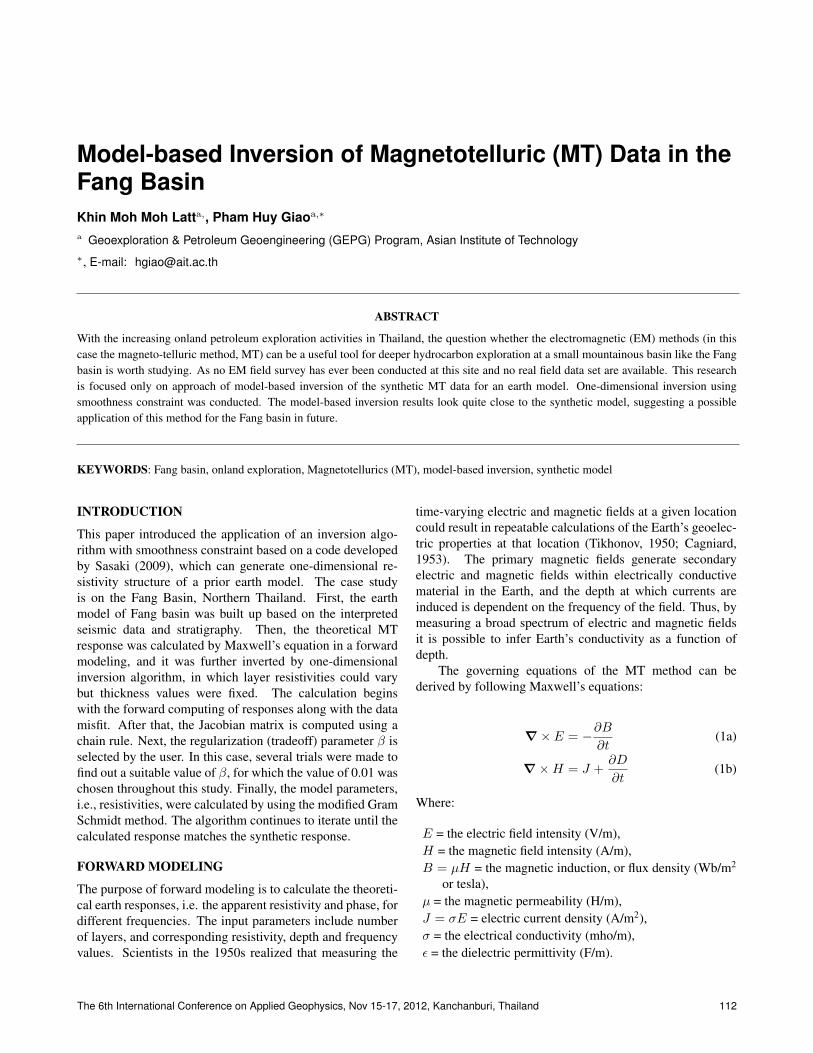
Model-based Inversion of Magnetotelluric (MT) Data in theFang Basin
Khin Moh Moh Latta,, Pham Huy Giaoa,∗
a Geoexploration & Petroleum Geoengineering (GEPG) Program, Asian Institute of Technology
∗, E-mail: [email protected]
ABSTRACT
With the increasing onland petroleum exploration activities in Thailand, the question whether the electromagnetic (EM) methods (in this
case the magneto-telluric method, MT) can be a useful tool for deeper hydrocarbon exploration at a small mountainous basin like the Fang
basin is worth studying. As no EM field survey has ever been conducted at this site and no real field data set are available. This research
is focused only on approach of model-based inversion of the synthetic MT data for an earth model. One-dimensional inversion using
smoothness constraint was conducted. The model-based inversion results look quite close to the synthetic model, suggesting a possible
application of this method for the Fang basin in future.
KEYWORDS: Fang basin, onland exploration, Magnetotellurics (MT), model-based inversion, synthetic model
INTRODUCTION
This paper introduced the application of an inversion algo-
rithm with smoothness constraint based on a code developed
by Sasaki (2009), which can generate one-dimensional re-
sistivity structure of a prior earth model. The case study
is on the Fang Basin, Northern Thailand. First, the earth
model of Fang basin was built up based on the interpreted
seismic data and stratigraphy. Then, the theoretical MT
response was calculated by Maxwell’s equation in a forward
modeling, and it was further inverted by one-dimensional
inversion algorithm, in which layer resistivities could vary
but thickness values were fixed. The calculation begins
with the forward computing of responses along with the data
misfit. After that, the Jacobian matrix is computed using a
chain rule. Next, the regularization (tradeoff) parameter β is
selected by the user. In this case, several trials were made to
find out a suitable value of β, for which the value of 0.01 was
chosen throughout this study. Finally, the model parameters,
i.e., resistivities, were calculated by using the modified Gram
Schmidt method. The algorithm continues to iterate until the
calculated response matches the synthetic response.
FORWARD MODELING
The purpose of forward modeling is to calculate the theoreti-
cal earth responses, i.e. the apparent resistivity and phase, for
different frequencies. The input parameters include number
of layers, and corresponding resistivity, depth and frequency
values. Scientists in the 1950s realized that measuring the
time-varying electric and magnetic fields at a given location
could result in repeatable calculations of the Earth’s geoelec-
tric properties at that location (Tikhonov, 1950; Cagniard,
1953). The primary magnetic fields generate secondary
electric and magnetic fields within electrically conductive
material in the Earth, and the depth at which currents are
induced is dependent on the frequency of the field. Thus, by
measuring a broad spectrum of electric and magnetic fields
it is possible to infer Earth’s conductivity as a function of
depth.
The governing equations of the MT method can be
derived by following Maxwell’s equations:
∇× E = −∂B
∂t(1a)
∇×H = J +∂D
∂t(1b)
Where:
E = the electric field intensity (V/m),
H = the magnetic field intensity (A/m),
B = µH = the magnetic induction, or flux density (Wb/m2
or tesla),
µ = the magnetic permeability (H/m),
J = σE = electric current density (A/m2),
σ = the electrical conductivity (mho/m),
ǫ = the dielectric permittivity (F/m).
The 6th International Conference on Applied Geophysics, Nov 15-17, 2012, Kanchanburi, Thailand 112
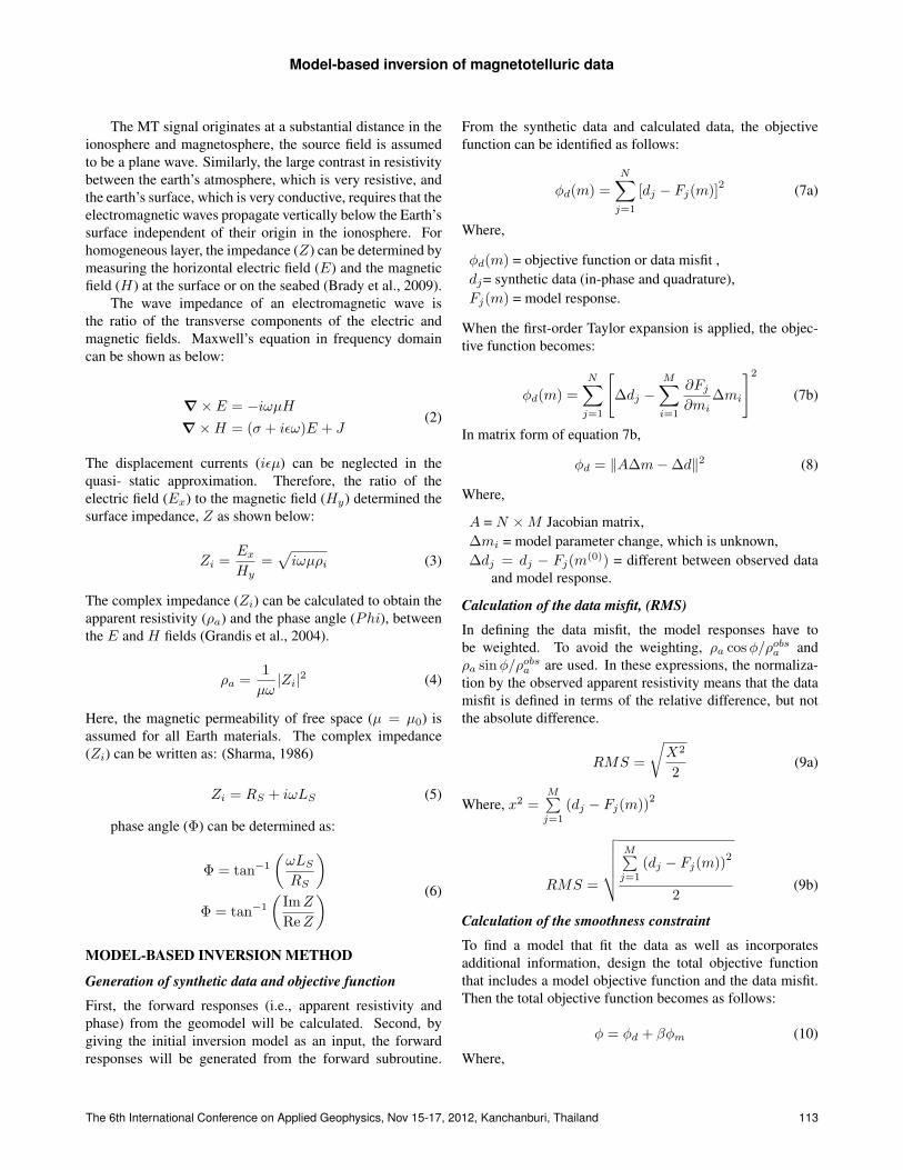
Model-based inversion of magnetotelluric data
The MT signal originates at a substantial distance in the
ionosphere and magnetosphere, the source field is assumed
to be a plane wave. Similarly, the large contrast in resistivity
between the earth’s atmosphere, which is very resistive, and
the earth’s surface, which is very conductive, requires that the
electromagnetic waves propagate vertically below the Earth’s
surface independent of their origin in the ionosphere. For
homogeneous layer, the impedance (Z) can be determined by
measuring the horizontal electric field (E) and the magnetic
field (H) at the surface or on the seabed (Brady et al., 2009).
The wave impedance of an electromagnetic wave is
the ratio of the transverse components of the electric and
magnetic fields. Maxwell’s equation in frequency domain
can be shown as below:
∇× E = −iωµH
∇×H = (σ + iǫω)E + J(2)
The displacement currents (iǫµ) can be neglected in the
quasi- static approximation. Therefore, the ratio of the
electric field (Ex) to the magnetic field (Hy) determined the
surface impedance, Z as shown below:
Zi =Ex
Hy
=√
iωµρi (3)
The complex impedance (Zi) can be calculated to obtain the
apparent resistivity (ρa) and the phase angle (Phi), between
the E and H fields (Grandis et al., 2004).
ρa =1
µω|Zi|2 (4)
Here, the magnetic permeability of free space (µ = µ0) is
assumed for all Earth materials. The complex impedance
(Zi) can be written as: (Sharma, 1986)
Zi = RS + iωLS (5)
phase angle (Φ) can be determined as:
Φ = tan−1
(
ωLS
RS
)
Φ = tan−1
(
ImZ
ReZ
) (6)
MODEL-BASED INVERSION METHOD
Generation of synthetic data and objective function
First, the forward responses (i.e., apparent resistivity and
phase) from the geomodel will be calculated. Second, by
giving the initial inversion model as an input, the forward
responses will be generated from the forward subroutine.
From the synthetic data and calculated data, the objective
function can be identified as follows:
φd(m) =
N∑
j=1
[dj − Fj(m)]2
(7a)
Where,
φd(m) = objective function or data misfit ,
dj= synthetic data (in-phase and quadrature),
Fj(m) = model response.
When the first-order Taylor expansion is applied, the objec-
tive function becomes:
φd(m) =
N∑
j=1
[
∆dj −M∑
i=1
∂Fj
∂mi
∆mi
]2
(7b)
In matrix form of equation 7b,
φd = ‖A∆m−∆d‖2 (8)
Where,
A = N ×M Jacobian matrix,
∆mi = model parameter change, which is unknown,
∆dj = dj − Fj(m(0)) = different between observed data
and model response.
Calculation of the data misfit, (RMS)
In defining the data misfit, the model responses have to
be weighted. To avoid the weighting, ρa cosφ/ρobsa and
ρa sinφ/ρobsa are used. In these expressions, the normaliza-
tion by the observed apparent resistivity means that the data
misfit is defined in terms of the relative difference, but not
the absolute difference.
RMS =
√
X2
2(9a)
Where, x2 =M∑
j=1
(dj − Fj(m))2
RMS =
√
√
√
√
√
M∑
j=1
(dj − Fj(m))2
2(9b)
Calculation of the smoothness constraint
To find a model that fit the data as well as incorporates
additional information, design the total objective function
that includes a model objective function and the data misfit.
Then the total objective function becomes as follows:
φ = φd + βφm (10)
Where,
The 6th International Conference on Applied Geophysics, Nov 15-17, 2012, Kanchanburi, Thailand 113
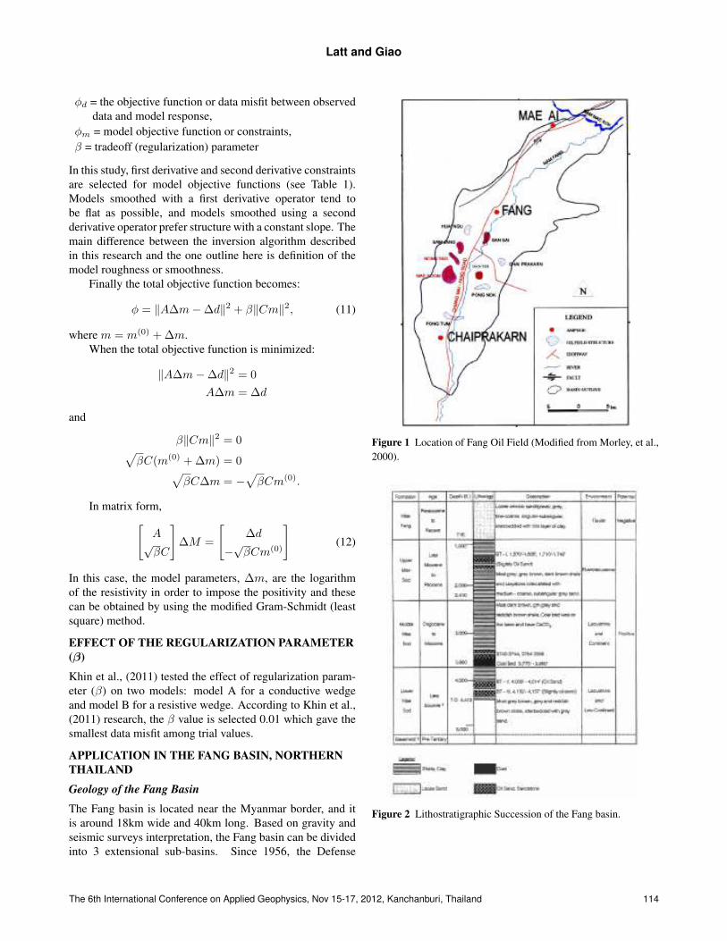
Latt and Giao
φd = the objective function or data misfit between observed
data and model response,
φm = model objective function or constraints,
β = tradeoff (regularization) parameter
In this study, first derivative and second derivative constraints
are selected for model objective functions (see Table 1).
Models smoothed with a first derivative operator tend to
be flat as possible, and models smoothed using a second
derivative operator prefer structure with a constant slope. The
main difference between the inversion algorithm described
in this research and the one outline here is definition of the
model roughness or smoothness.
Finally the total objective function becomes:
φ = ‖A∆m−∆d‖2 + β‖Cm‖2, (11)
where m = m(0) +∆m.
When the total objective function is minimized:
‖A∆m−∆d‖2 = 0
A∆m = ∆d
and
β‖Cm‖2 = 0√
βC(m(0) +∆m) = 0√
βC∆m = −√
βCm(0).
In matrix form,
[
A√βC
]
∆M =
[
∆d
−√βCm(0)
]
(12)
In this case, the model parameters, ∆m, are the logarithm
of the resistivity in order to impose the positivity and these
can be obtained by using the modified Gram-Schmidt (least
square) method.
EFFECT OF THE REGULARIZATION PARAMETER
(β)
Khin et al., (2011) tested the effect of regularization param-
eter (β) on two models: model A for a conductive wedge
and model B for a resistive wedge. According to Khin et al.,
(2011) research, the β value is selected 0.01 which gave the
smallest data misfit among trial values.
APPLICATION IN THE FANG BASIN, NORTHERN
THAILAND
Geology of the Fang Basin
The Fang basin is located near the Myanmar border, and it
is around 18km wide and 40km long. Based on gravity and
seismic surveys interpretation, the Fang basin can be divided
into 3 extensional sub-basins. Since 1956, the Defense
Figure 1 Location of Fang Oil Field (Modified from Morley, et al.,
2000).
Figure 2 Lithostratigraphic Succession of the Fang basin.
The 6th International Conference on Applied Geophysics, Nov 15-17, 2012, Kanchanburi, Thailand 114
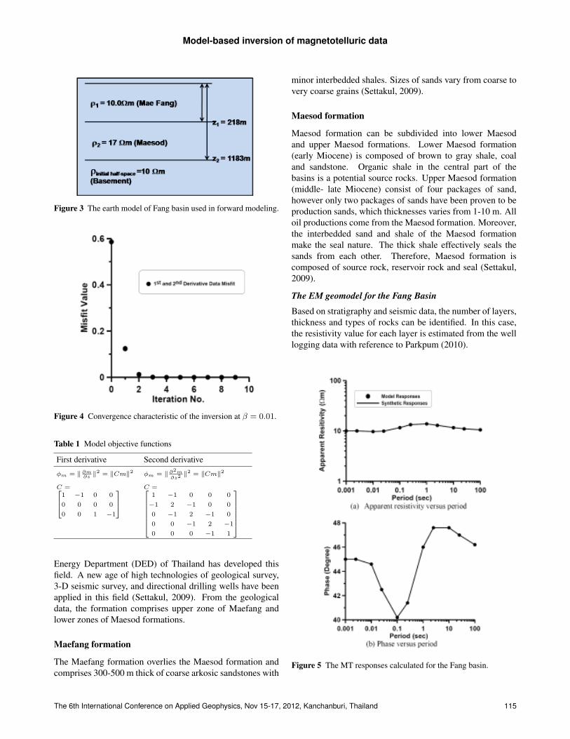
Model-based inversion of magnetotelluric data
Figure 3 The earth model of Fang basin used in forward modeling.
Figure 4 Convergence characteristic of the inversion at β = 0.01.
Table 1 Model objective functions
First derivative Second derivative
φm = ‖ ∂m∂z
‖2 = ‖Cm‖2 φm = ‖ ∂2m
∂z2‖2 = ‖Cm‖2
C =
1 −1 0 0
0 0 0 0
0 0 1 −1
C =
1 −1 0 0 0
−1 2 −1 0 0
0 −1 2 −1 0
0 0 −1 2 −1
0 0 0 −1 1
Energy Department (DED) of Thailand has developed this
field. A new age of high technologies of geological survey,
3-D seismic survey, and directional drilling wells have been
applied in this field (Settakul, 2009). From the geological
data, the formation comprises upper zone of Maefang and
lower zones of Maesod formations.
Maefang formation
The Maefang formation overlies the Maesod formation and
comprises 300-500 m thick of coarse arkosic sandstones with
minor interbedded shales. Sizes of sands vary from coarse to
very coarse grains (Settakul, 2009).
Maesod formation
Maesod formation can be subdivided into lower Maesod
and upper Maesod formations. Lower Maesod formation
(early Miocene) is composed of brown to gray shale, coal
and sandstone. Organic shale in the central part of the
basins is a potential source rocks. Upper Maesod formation
(middle- late Miocene) consist of four packages of sand,
however only two packages of sands have been proven to be
production sands, which thicknesses varies from 1-10 m. All
oil productions come from the Maesod formation. Moreover,
the interbedded sand and shale of the Maesod formation
make the seal nature. The thick shale effectively seals the
sands from each other. Therefore, Maesod formation is
composed of source rock, reservoir rock and seal (Settakul,
2009).
The EM geomodel for the Fang Basin
Based on stratigraphy and seismic data, the number of layers,
thickness and types of rocks can be identified. In this case,
the resistivity value for each layer is estimated from the well
logging data with reference to Parkpum (2010).
Figure 5 The MT responses calculated for the Fang basin.
The 6th International Conference on Applied Geophysics, Nov 15-17, 2012, Kanchanburi, Thailand 115
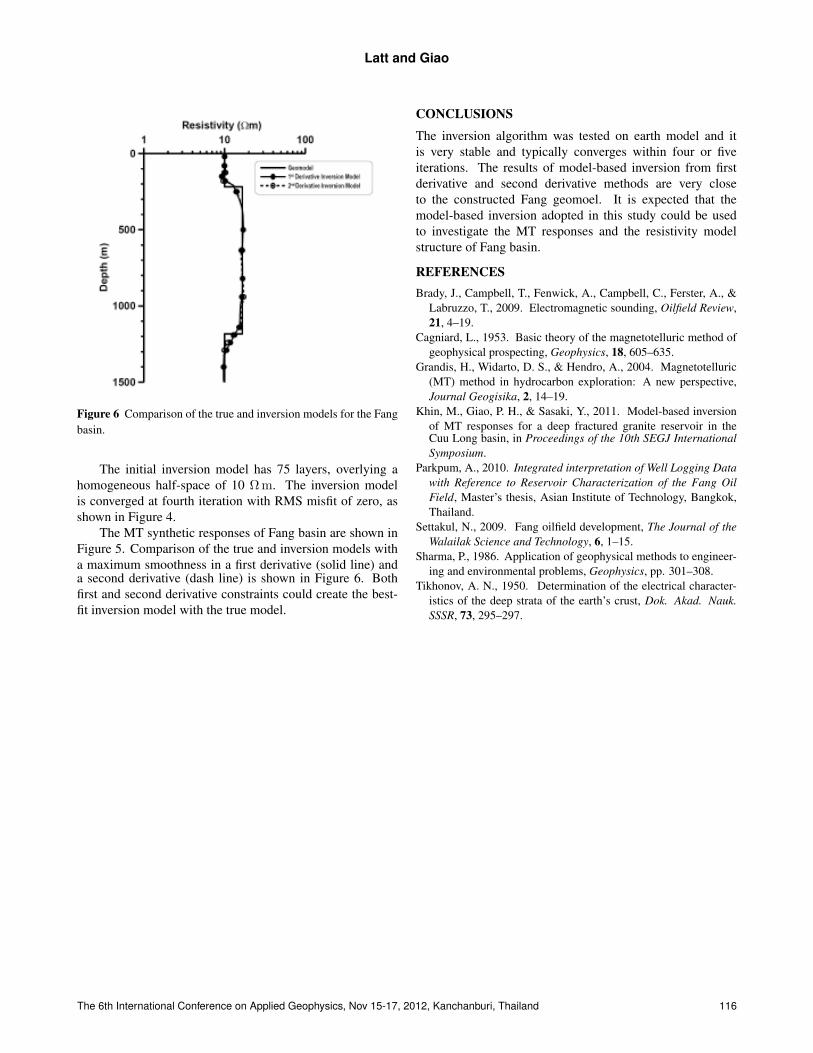
Latt and Giao
Figure 6 Comparison of the true and inversion models for the Fang
basin.
The initial inversion model has 75 layers, overlying a
homogeneous half-space of 10 Ωm. The inversion model
is converged at fourth iteration with RMS misfit of zero, as
shown in Figure 4.
The MT synthetic responses of Fang basin are shown in
Figure 5. Comparison of the true and inversion models with
a maximum smoothness in a first derivative (solid line) anda second derivative (dash line) is shown in Figure 6. Both
first and second derivative constraints could create the best-
fit inversion model with the true model.
CONCLUSIONS
The inversion algorithm was tested on earth model and it
is very stable and typically converges within four or five
iterations. The results of model-based inversion from first
derivative and second derivative methods are very close
to the constructed Fang geomoel. It is expected that the
model-based inversion adopted in this study could be used
to investigate the MT responses and the resistivity model
structure of Fang basin.
REFERENCES
Brady, J., Campbell, T., Fenwick, A., Campbell, C., Ferster, A., &
Labruzzo, T., 2009. Electromagnetic sounding, Oilfield Review,
21, 4–19.
Cagniard, L., 1953. Basic theory of the magnetotelluric method of
geophysical prospecting, Geophysics, 18, 605–635.
Grandis, H., Widarto, D. S., & Hendro, A., 2004. Magnetotelluric
(MT) method in hydrocarbon exploration: A new perspective,
Journal Geogisika, 2, 14–19.
Khin, M., Giao, P. H., & Sasaki, Y., 2011. Model-based inversion
of MT responses for a deep fractured granite reservoir in theCuu Long basin, in Proceedings of the 10th SEGJ International
Symposium.
Parkpum, A., 2010. Integrated interpretation of Well Logging Data
with Reference to Reservoir Characterization of the Fang Oil
Field, Master’s thesis, Asian Institute of Technology, Bangkok,
Thailand.
Settakul, N., 2009. Fang oilfield development, The Journal of the
Walailak Science and Technology, 6, 1–15.
Sharma, P., 1986. Application of geophysical methods to engineer-
ing and environmental problems, Geophysics, pp. 301–308.
Tikhonov, A. N., 1950. Determination of the electrical character-
istics of the deep strata of the earth’s crust, Dok. Akad. Nauk.
SSSR, 73, 295–297.
The 6th International Conference on Applied Geophysics, Nov 15-17, 2012, Kanchanburi, Thailand 116
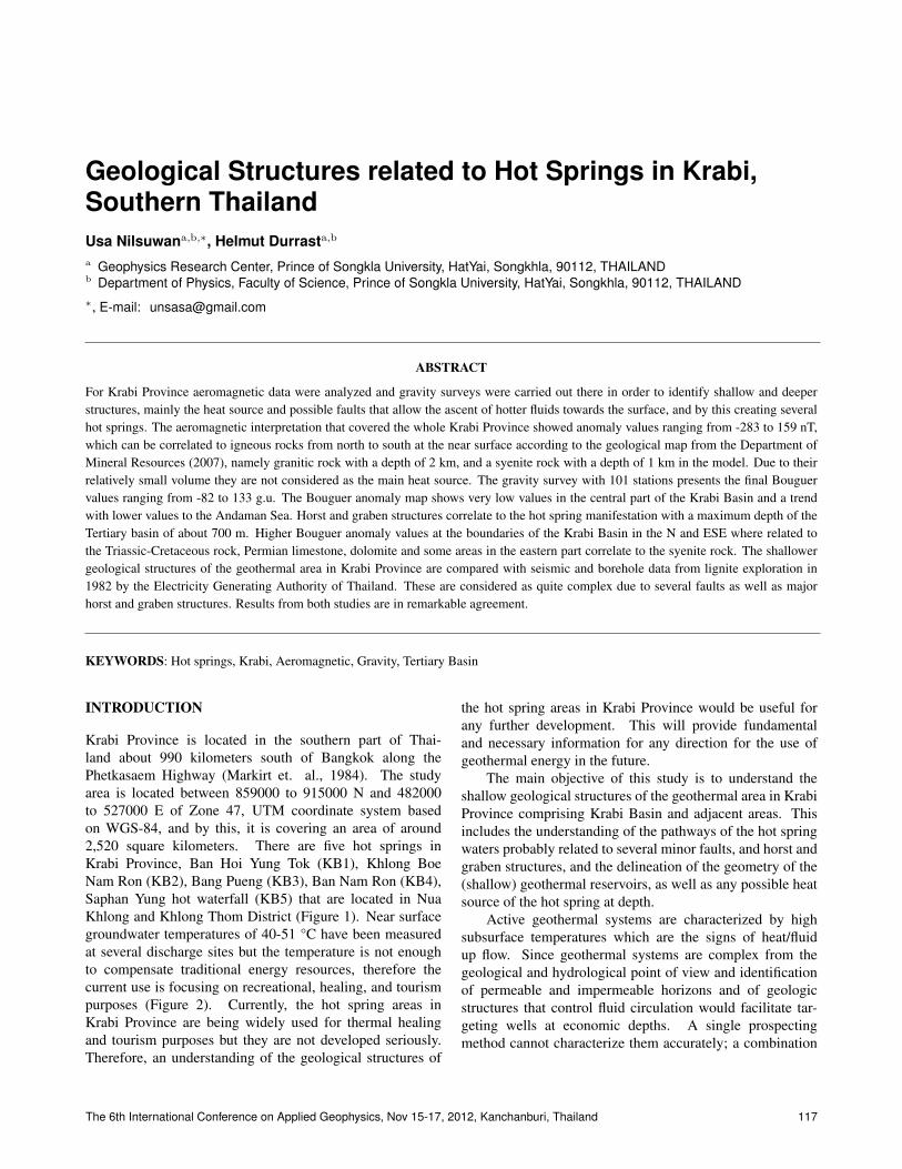
Geological Structures related to Hot Springs in Krabi,Southern Thailand
Usa Nilsuwana,b,∗, Helmut Durrasta,b
a Geophysics Research Center, Prince of Songkla University, HatYai, Songkhla, 90112, THAILANDb Department of Physics, Faculty of Science, Prince of Songkla University, HatYai, Songkhla, 90112, THAILAND
∗, E-mail: [email protected]
ABSTRACT
For Krabi Province aeromagnetic data were analyzed and gravity surveys were carried out there in order to identify shallow and deeper
structures, mainly the heat source and possible faults that allow the ascent of hotter fluids towards the surface, and by this creating several
hot springs. The aeromagnetic interpretation that covered the whole Krabi Province showed anomaly values ranging from -283 to 159 nT,
which can be correlated to igneous rocks from north to south at the near surface according to the geological map from the Department of
Mineral Resources (2007), namely granitic rock with a depth of 2 km, and a syenite rock with a depth of 1 km in the model. Due to their
relatively small volume they are not considered as the main heat source. The gravity survey with 101 stations presents the final Bouguer
values ranging from -82 to 133 g.u. The Bouguer anomaly map shows very low values in the central part of the Krabi Basin and a trend
with lower values to the Andaman Sea. Horst and graben structures correlate to the hot spring manifestation with a maximum depth of the
Tertiary basin of about 700 m. Higher Bouguer anomaly values at the boundaries of the Krabi Basin in the N and ESE where related to
the Triassic-Cretaceous rock, Permian limestone, dolomite and some areas in the eastern part correlate to the syenite rock. The shallower
geological structures of the geothermal area in Krabi Province are compared with seismic and borehole data from lignite exploration in
1982 by the Electricity Generating Authority of Thailand. These are considered as quite complex due to several faults as well as major
horst and graben structures. Results from both studies are in remarkable agreement.
KEYWORDS: Hot springs, Krabi, Aeromagnetic, Gravity, Tertiary Basin
INTRODUCTION
Krabi Province is located in the southern part of Thai-
land about 990 kilometers south of Bangkok along the
Phetkasaem Highway (Markirt et. al., 1984). The study
area is located between 859000 to 915000 N and 482000
to 527000 E of Zone 47, UTM coordinate system based
on WGS-84, and by this, it is covering an area of around
2,520 square kilometers. There are five hot springs in
Krabi Province, Ban Hoi Yung Tok (KB1), Khlong Boe
Nam Ron (KB2), Bang Pueng (KB3), Ban Nam Ron (KB4),
Saphan Yung hot waterfall (KB5) that are located in Nua
Khlong and Khlong Thom District (Figure 1). Near surface
groundwater temperatures of 40-51 °C have been measured
at several discharge sites but the temperature is not enough
to compensate traditional energy resources, therefore the
current use is focusing on recreational, healing, and tourism
purposes (Figure 2). Currently, the hot spring areas in
Krabi Province are being widely used for thermal healing
and tourism purposes but they are not developed seriously.
Therefore, an understanding of the geological structures of
the hot spring areas in Krabi Province would be useful for
any further development. This will provide fundamental
and necessary information for any direction for the use of
geothermal energy in the future.
The main objective of this study is to understand the
shallow geological structures of the geothermal area in Krabi
Province comprising Krabi Basin and adjacent areas. This
includes the understanding of the pathways of the hot spring
waters probably related to several minor faults, and horst and
graben structures, and the delineation of the geometry of the
(shallow) geothermal reservoirs, as well as any possible heat
source of the hot spring at depth.
Active geothermal systems are characterized by high
subsurface temperatures which are the signs of heat/fluid
up flow. Since geothermal systems are complex from the
geological and hydrological point of view and identification
of permeable and impermeable horizons and of geologic
structures that control fluid circulation would facilitate tar-
geting wells at economic depths. A single prospecting
method cannot characterize them accurately; a combination
The 6th International Conference on Applied Geophysics, Nov 15-17, 2012, Kanchanburi, Thailand 117
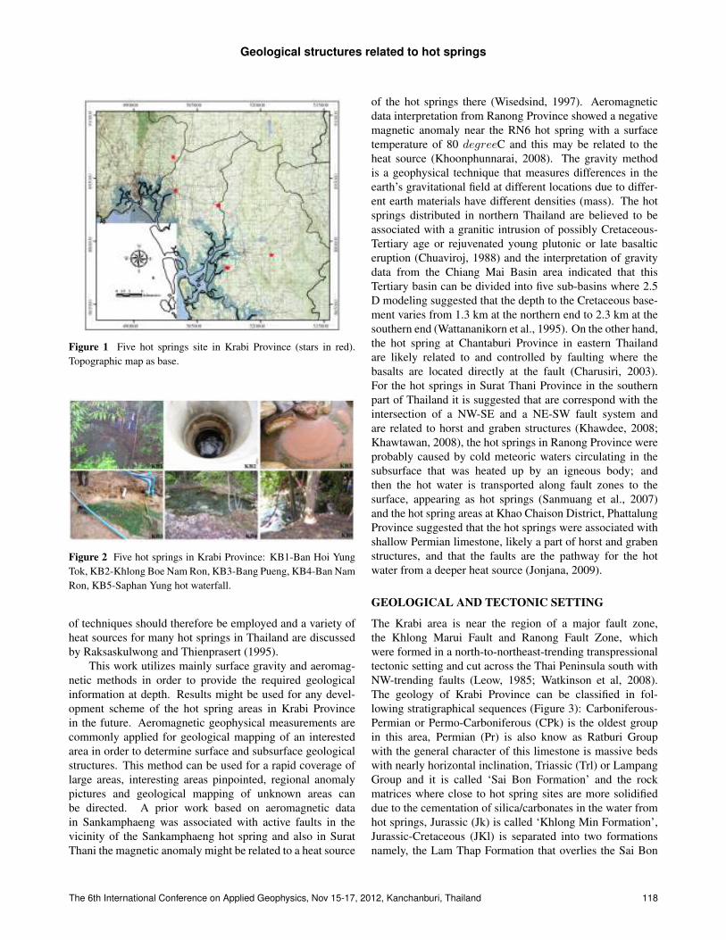
Geological structures related to hot springs
Figure 1 Five hot springs site in Krabi Province (stars in red).
Topographic map as base.
Figure 2 Five hot springs in Krabi Province: KB1-Ban Hoi Yung
Tok, KB2-Khlong Boe Nam Ron, KB3-Bang Pueng, KB4-Ban Nam
Ron, KB5-Saphan Yung hot waterfall.
of techniques should therefore be employed and a variety of
heat sources for many hot springs in Thailand are discussed
by Raksaskulwong and Thienprasert (1995).
This work utilizes mainly surface gravity and aeromag-
netic methods in order to provide the required geological
information at depth. Results might be used for any devel-
opment scheme of the hot spring areas in Krabi Province
in the future. Aeromagnetic geophysical measurements are
commonly applied for geological mapping of an interested
area in order to determine surface and subsurface geological
structures. This method can be used for a rapid coverage of
large areas, interesting areas pinpointed, regional anomaly
pictures and geological mapping of unknown areas can
be directed. A prior work based on aeromagnetic data
in Sankamphaeng was associated with active faults in the
vicinity of the Sankamphaeng hot spring and also in Surat
Thani the magnetic anomaly might be related to a heat source
of the hot springs there (Wisedsind, 1997). Aeromagnetic
data interpretation from Ranong Province showed a negative
magnetic anomaly near the RN6 hot spring with a surface
temperature of 80 degreeC and this may be related to the
heat source (Khoonphunnarai, 2008). The gravity method
is a geophysical technique that measures differences in the
earth’s gravitational field at different locations due to differ-
ent earth materials have different densities (mass). The hot
springs distributed in northern Thailand are believed to be
associated with a granitic intrusion of possibly Cretaceous-
Tertiary age or rejuvenated young plutonic or late basaltic
eruption (Chuaviroj, 1988) and the interpretation of gravity
data from the Chiang Mai Basin area indicated that this
Tertiary basin can be divided into five sub-basins where 2.5
D modeling suggested that the depth to the Cretaceous base-
ment varies from 1.3 km at the northern end to 2.3 km at the
southern end (Wattananikorn et al., 1995). On the other hand,
the hot spring at Chantaburi Province in eastern Thailand
are likely related to and controlled by faulting where the
basalts are located directly at the fault (Charusiri, 2003).
For the hot springs in Surat Thani Province in the southern
part of Thailand it is suggested that are correspond with the
intersection of a NW-SE and a NE-SW fault system and
are related to horst and graben structures (Khawdee, 2008;
Khawtawan, 2008), the hot springs in Ranong Province were
probably caused by cold meteoric waters circulating in the
subsurface that was heated up by an igneous body; and
then the hot water is transported along fault zones to the
surface, appearing as hot springs (Sanmuang et al., 2007)
and the hot spring areas at Khao Chaison District, Phattalung
Province suggested that the hot springs were associated with
shallow Permian limestone, likely a part of horst and graben
structures, and that the faults are the pathway for the hot
water from a deeper heat source (Jonjana, 2009).
GEOLOGICAL AND TECTONIC SETTING
The Krabi area is near the region of a major fault zone,
the Khlong Marui Fault and Ranong Fault Zone, which
were formed in a north-to-northeast-trending transpressional
tectonic setting and cut across the Thai Peninsula south with
NW-trending faults (Leow, 1985; Watkinson et al, 2008).
The geology of Krabi Province can be classified in fol-
lowing stratigraphical sequences (Figure 3): Carboniferous-
Permian or Permo-Carboniferous (CPk) is the oldest group
in this area, Permian (Pr) is also know as Ratburi Group
with the general character of this limestone is massive beds
with nearly horizontal inclination, Triassic (Trl) or Lampang
Group and it is called ‘Sai Bon Formation’ and the rock
matrices where close to hot spring sites are more solidified
due to the cementation of silica/carbonates in the water from
hot springs, Jurassic (Jk) is called ‘Khlong Min Formation’,
Jurassic-Cretaceous (JKl) is separated into two formations
namely, the Lam Thap Formation that overlies the Sai Bon
The 6th International Conference on Applied Geophysics, Nov 15-17, 2012, Kanchanburi, Thailand 118
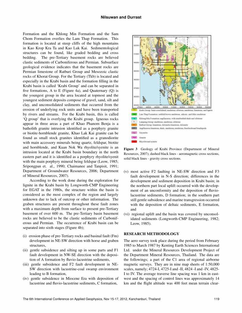
Nilsuwan and Durrast
Formation and the Khlong Min Formation and the Sam
Chom Formation overlies the Lam Thap Formation. This
formation is located at steep cliffs of the high mountains
in Kao Krop Kra Ta and Kao Luk Kai. Sedimentological
structures can be found, like graded bedding and cross
bedding. The pre-Tertiary basement rocks are believed
clastic sediments of Carboniferous and Permian. Subsurface
geological evidence indicates that the basement rocks are
Permian limestone of Ratburi Group and Mesozoic clastic
rocks of Khorat Group. For the Tertiary (Tkb) is located and
especially in the Krabi basin and the formation filling in the
Krabi basin is called ‘Krabi Group’ and can be separated in
five formations, A to E (Figure 4a), and Quaternary (Q) is
the youngest group in the area located at topmost and the
youngest sediment deposits compose of gravel, sand, silt and
clay, and unconsolidated sediments that occurred from the
erosion of underlying rock units and have been transported
by rivers and streams. For the Krabi basin, this is called
‘Q group’ that is overlying the Krabi group. Igneous rocks
appear in three areas a part of Khao Phanom Benja is a
batholith granite intrusion identified as a porphyry granite
or biotite-hornblende granite, Khao Lak Kai granite can be
found as small stock granites identified as a granodiorite
with main accessory minerals being quartz, feldspar, biotite
and hornblende, and Kuan Nok Wa rhyolite/syenite is an
intrusion located at the Krabi basin boundary in the north
eastern part and it is identified as a porphyry rhyolite/syenit
with the main porphyry mineral being feldspar (Leow, 1985;
Sripongpan et. al., 1990; Chaimanee and Tanpisit, 1991;
Department of Groundwater Resources, 2006; Department
of Mineral Resources, 2007).
According to the work done during the exploration for
lignite in the Krabi basin by Longworth-CMP Engineering
for EGAT in the 1980s, the structure within the basin is
considered as the most complex of the region and largely
unknown due to lack of outcrop or other information. The
graben structures are present throughout these fault zones
with a maximum depth from surface to present pre-Tertiary
basement of over 600 m. The pre-Tertiary basin basement
rocks are believed to be the clastic sediments of Carbonif-
erous and Permian. The occurrence of Krabi basin can be
separated into sixth stages (Figure 4b);
(i) erosion phase of pre-Tertiary rocks and basinal fault (Fm)
development in NE-SW direction with horse and graben
structures,
(ii) gentle subsidence and silting up in some parts and F1
fault development in NW-SE direction with the deposi-
tion of A formation by fluvio-lacustrine sediments,
(iii) gentle subsidence and F2 fault development in NE-
SW direction with lacustrine-coal swamp environment
leading to B formation,
(iv) gentle subsidence in Miocene Era with deposition of
lacustrine and fluvio-lacustrine sediments, C formation,
Figure 3 Geology of Krabi Province (Department of Mineral
Resources, 2007); dashed black lines - aeromagnetic cross sections,
solid black lines - gravity cross sections.
(v) most active F2 faulting in NE-SW direction and F3
fault development in N-S direction; differences in the
development and sediment deposition in Krabi basin; in
the northern part local uplift occurred with the develop-
ment of an unconformity and the deposition of fluvio-
lacustrine sediments, D formation; in the southern part
still gentle subsidence and marine transgression occurred
with the deposition of deltaic sediments, E formation,
and
(vi) regional uplift and the basin was covered by unconsol-
idated sediments (Longworth-CMP Engineering, 1982;
Leow, 1985).
RESEARCH METHODOLOGY
The aero survey took place during the period from February
1985 to March 1987 by Kenting Earth Sciences International
Ltd. under the Mineral Resources Development Project of
the Department Mineral Resources, Thailand. The data are
the followings; a part of the C1 area of regional airborne
magnetic surveys. They are in nine map sheets of 1:50,000
scales, namely; 4724-I, 4725-I and -II, 4824 -I and -IV, 4825-
I to IV. The average traverse line spacing was 1 km in east-
west and the spacing of control lines was approximately 14
km and the flight altitude was 400 feet mean terrain clear-
The 6th International Conference on Applied Geophysics, Nov 15-17, 2012, Kanchanburi, Thailand 119
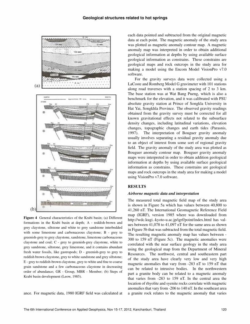
Geological structures related to hot springs
Figure 4 General characteristics of the Krabi basin; (a) Different
formations in the Krabi basin at depth; A - reddish-brown and
grey claystone, siltstone and white to grey sandstone interbedded
with some limestone and carbonaceous claystone; B - grey to
greenish-grey to grey claystone, sandstone, limestone carbonaceous
claystone and coal; C - grey to greenish-grey claystone, white to
grey sandstone, siltstone, grey limestone, and it contains abundant
fresh water fossils, like gastropods; D - greenish-grey to grey to
reddish brown claystone, grey to white sandstone and grey siltstone;
E - grey to reddish-brown claystone, grey to white and fine to coarse
grain sandstone and a few carbonaceous claystone in decreasing
order of abundance; GR - Group, MBR - Member; (b) Steps of
Krabi basin development (Leow, 1985).
ance. For magnetic data, 1980 IGRF field was calculated at
each data pointed and subtracted from the original magnetic
data at each point. The magnetic anomaly of the study area
was plotted as magnetic anomaly contour map. A magnetic
anomaly map was interpreted in order to obtain additional
geological information at depths by using available surface
geological information as constrains. These constrains are
geological maps and rock outcrops in the study area for
making a model using the Encom Model VisionPro v7.0
software.
For the gravity surveys data were collected using a
LaCoste and Romberg Model G gravimeter with 101 stations
along road traverses with a station spacing of 2 to 3 km.
The base station was at Wat Bang Pueng, which is also a
benchmark for the elevation, and it was calibrated with PSU
absolute gravity station at Prince of Songkla University in
Hat Yai, Songkhla Province. The observed gravity readings
obtained from the gravity survey must be corrected for all
known gravitational effects not related to the subsurface
density changes, including latitudinal variations, elevation
changes, topographic changes and earth tides (Parasnis,
1997). The interpretation of Bouguer gravity anomaly
usually involves separating a residual gravity anomaly due
to an object of interest from some sort of regional gravity
field. The gravity anomaly of the study area was plotted as
Bouguer anomaly contour map. Bouguer gravity anomaly
maps were interpreted in order to obtain addition geological
information at depths by using available surface geological
information as constrains. These constrains are geological
maps and rock outcrops in the study area for making a model
using VisionPro v7.0 software.
RESULTS
Airborne magnetic data and interpretation
The measured total magnetic field map of the study area
is shown in Figure 5a which has values between 40,800 to
41,260 nT. The International Geomagnetic Reference Field
map (IGRF), version 1985 where was downloaded from
http://wdc.kugi.-kyoto-u.ac.jp/igrf/point/index.html has val-
ues between 41,078 to 41,097 nT for the same area as shown
in Figure 5b that was subtracted from the total magnetic field.
The resulting magnetic anomaly map has values between -
300 to 159 nT (Figure 5c). The magnetic anomalies were
correlated with the near surface geology in the study area
using the geological map from the Department of Mineral
Resources. The northwest, central and southeastern part
of the study area have clearly very low and very high
magnetic anomalies that vary from -283 nT to 159 nT that
can be related to intrusive bodies. In the northwestern
part a granite body can be related to a magnetic anomaly
that varies from -283 to 159 nT. In the central area the
location of rhyolite and syenite rocks correlate with magnetic
anomalies that vary from -206 to 140 nT. In the southeast area
a granite rock relates to the magnetic anomaly that varies
The 6th International Conference on Applied Geophysics, Nov 15-17, 2012, Kanchanburi, Thailand 120
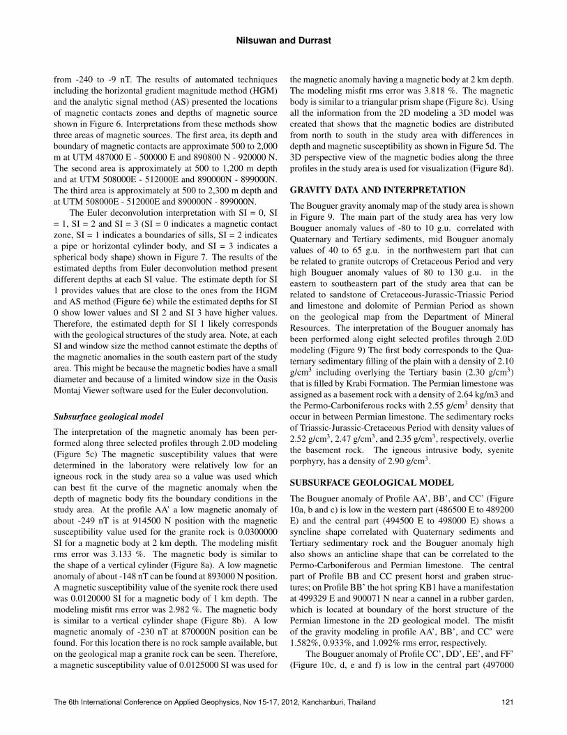
Nilsuwan and Durrast
from -240 to -9 nT. The results of automated techniques
including the horizontal gradient magnitude method (HGM)
and the analytic signal method (AS) presented the locations
of magnetic contacts zones and depths of magnetic source
shown in Figure 6. Interpretations from these methods show
three areas of magnetic sources. The first area, its depth and
boundary of magnetic contacts are approximate 500 to 2,000
m at UTM 487000 E - 500000 E and 890800 N - 920000 N.
The second area is approximately at 500 to 1,200 m depth
and at UTM 508000E - 512000E and 890000N - 899000N.
The third area is approximately at 500 to 2,300 m depth and
at UTM 508000E - 512000E and 890000N - 899000N.
The Euler deconvolution interpretation with SI = 0, SI
= 1, SI = 2 and SI = 3 (SI = 0 indicates a magnetic contact
zone, SI = 1 indicates a boundaries of sills, SI = 2 indicates
a pipe or horizontal cylinder body, and SI = 3 indicates a
spherical body shape) shown in Figure 7. The results of the
estimated depths from Euler deconvolution method present
different depths at each SI value. The estimate depth for SI
1 provides values that are close to the ones from the HGM
and AS method (Figure 6e) while the estimated depths for SI
0 show lower values and SI 2 and SI 3 have higher values.
Therefore, the estimated depth for SI 1 likely corresponds
with the geological structures of the study area. Note, at each
SI and window size the method cannot estimate the depths of
the magnetic anomalies in the south eastern part of the study
area. This might be because the magnetic bodies have a small
diameter and because of a limited window size in the Oasis
Montaj Viewer software used for the Euler deconvolution.
Subsurface geological model
The interpretation of the magnetic anomaly has been per-
formed along three selected profiles through 2.0D modeling
(Figure 5c) The magnetic susceptibility values that were
determined in the laboratory were relatively low for an
igneous rock in the study area so a value was used which
can best fit the curve of the magnetic anomaly when the
depth of magnetic body fits the boundary conditions in the
study area. At the profile AA’ a low magnetic anomaly of
about -249 nT is at 914500 N position with the magnetic
susceptibility value used for the granite rock is 0.0300000
SI for a magnetic body at 2 km depth. The modeling misfit
rms error was 3.133 %. The magnetic body is similar to
the shape of a vertical cylinder (Figure 8a). A low magnetic
anomaly of about -148 nT can be found at 893000 N position.
A magnetic susceptibility value of the syenite rock there used
was 0.0120000 SI for a magnetic body of 1 km depth. The
modeling misfit rms error was 2.982 %. The magnetic body
is similar to a vertical cylinder shape (Figure 8b). A low
magnetic anomaly of -230 nT at 870000N position can be
found. For this location there is no rock sample available, but
on the geological map a granite rock can be seen. Therefore,
a magnetic susceptibility value of 0.0125000 SI was used for
the magnetic anomaly having a magnetic body at 2 km depth.
The modeling misfit rms error was 3.818 %. The magnetic
body is similar to a triangular prism shape (Figure 8c). Using
all the information from the 2D modeling a 3D model was
created that shows that the magnetic bodies are distributed
from north to south in the study area with differences in
depth and magnetic susceptibility as shown in Figure 5d. The
3D perspective view of the magnetic bodies along the three
profiles in the study area is used for visualization (Figure 8d).
GRAVITY DATA AND INTERPRETATION
The Bouguer gravity anomaly map of the study area is shown
in Figure 9. The main part of the study area has very low
Bouguer anomaly values of -80 to 10 g.u. correlated with
Quaternary and Tertiary sediments, mid Bouguer anomaly
values of 40 to 65 g.u. in the northwestern part that can
be related to granite outcrops of Cretaceous Period and very
high Bouguer anomaly values of 80 to 130 g.u. in the
eastern to southeastern part of the study area that can be
related to sandstone of Cretaceous-Jurassic-Triassic Period
and limestone and dolomite of Permian Period as shown
on the geological map from the Department of Mineral
Resources. The interpretation of the Bouguer anomaly has
been performed along eight selected profiles through 2.0D
modeling (Figure 9) The first body corresponds to the Qua-
ternary sedimentary filling of the plain with a density of 2.10
g/cm3 including overlying the Tertiary basin (2.30 g/cm3)
that is filled by Krabi Formation. The Permian limestone was
assigned as a basement rock with a density of 2.64 kg/m3 and
the Permo-Carboniferous rocks with 2.55 g/cm3 density that
occur in between Permian limestone. The sedimentary rocks
of Triassic-Jurassic-Cretaceous Period with density values of
2.52 g/cm3, 2.47 g/cm3, and 2.35 g/cm3, respectively, overlie
the basement rock. The igneous intrusive body, syenite
porphyry, has a density of 2.90 g/cm3.
SUBSURFACE GEOLOGICAL MODEL
The Bouguer anomaly of Profile AA’, BB’, and CC’ (Figure
10a, b and c) is low in the western part (486500 E to 489200
E) and the central part (494500 E to 498000 E) shows a
syncline shape correlated with Quaternary sediments and
Tertiary sedimentary rock and the Bouguer anomaly high
also shows an anticline shape that can be correlated to the
Permo-Carboniferous and Permian limestone. The central
part of Profile BB and CC present horst and graben struc-
tures; on Profile BB’ the hot spring KB1 have a manifestation
at 499329 E and 900071 N near a cannel in a rubber garden,
which is located at boundary of the horst structure of the
Permian limestone in the 2D geological model. The misfit
of the gravity modeling in profile AA’, BB’, and CC’ were
1.582%, 0.933%, and 1.092% rms error, respectively.
The Bouguer anomaly of Profile CC’, DD’, EE’, and FF’
(Figure 10c, d, e and f) is low in the central part (497000
The 6th International Conference on Applied Geophysics, Nov 15-17, 2012, Kanchanburi, Thailand 121
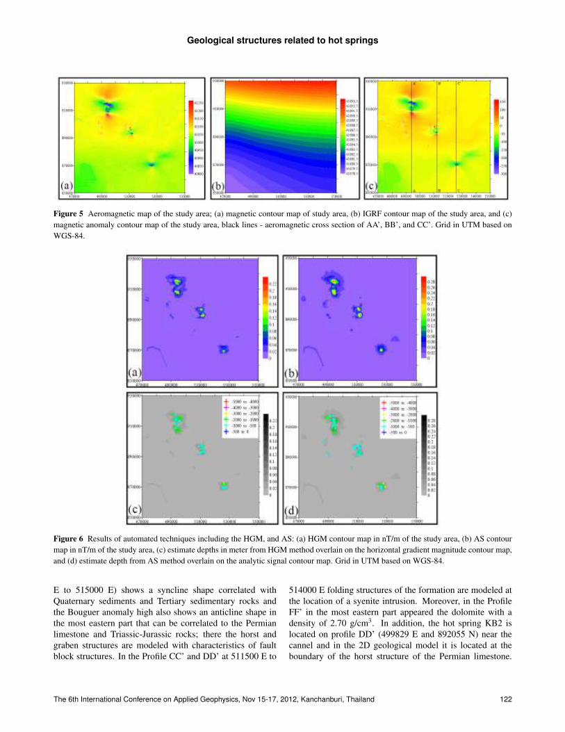
Geological structures related to hot springs
Figure 5 Aeromagnetic map of the study area; (a) magnetic contour map of study area, (b) IGRF contour map of the study area, and (c)
magnetic anomaly contour map of the study area, black lines - aeromagnetic cross section of AA’, BB’, and CC’. Grid in UTM based on
WGS-84.
Figure 6 Results of automated techniques including the HGM, and AS: (a) HGM contour map in nT/m of the study area, (b) AS contour
map in nT/m of the study area, (c) estimate depths in meter from HGM method overlain on the horizontal gradient magnitude contour map,
and (d) estimate depth from AS method overlain on the analytic signal contour map. Grid in UTM based on WGS-84.
E to 515000 E) shows a syncline shape correlated with
Quaternary sediments and Tertiary sedimentary rocks and
the Bouguer anomaly high also shows an anticline shape in
the most eastern part that can be correlated to the Permian
limestone and Triassic-Jurassic rocks; there the horst and
graben structures are modeled with characteristics of fault
block structures. In the Profile CC’ and DD’ at 511500 E to
514000 E folding structures of the formation are modeled at
the location of a syenite intrusion. Moreover, in the Profile
FF’ in the most eastern part appeared the dolomite with a
density of 2.70 g/cm3. In addition, the hot spring KB2 is
located on profile DD’ (499829 E and 892055 N) near the
cannel and in the 2D geological model it is located at the
boundary of the horst structure of the Permian limestone.
The 6th International Conference on Applied Geophysics, Nov 15-17, 2012, Kanchanburi, Thailand 122

Nilsuwan and Durrast
Figure 7 Results of the estimated depths from Euler deconvolution method where position and depth of magnetic overlain on the magnetic
anomaly contour map; (a) SI 0 and WS 15, (b) SI 1 and WS 17, (c) SI 2 and WS 17, (d) SI 3 and WS 25, (e) estimate depth from HGM,
AS, and Euler deconvolution method. Grid in UTM based on WGS-84; SI - structural index, WS - window size.
Figure 8 2.0D modeling of the magnetic anomaly interpretation has been performed along 3 selected profiles; (a) magnetic model along
profile AA’, (b) Magnetic model along profile BB’, (c) Magnetic model along profile CC’, and (d) 3D perspective of magnetic body of three
profile in the study area with azimuth 309 and inclination 20; Horizontal axis in UTM based on WGS-84, vertical scale in m. Top section
is a residual magnetic line which is the straight line when rms error is zero, Middle section shown three lines; black line is the magnetic
anomaly data, pink line is the regional magnetic and red line is the magnetic model.
The 6th International Conference on Applied Geophysics, Nov 15-17, 2012, Kanchanburi, Thailand 123

Geological structures related to hot springs
Figure 9 Bouguer gravity anomaly contour map of study area;
black lines - gravity cross sections of AA’, BB’, CC’, DD’, EE’,
FF’, GG’, and SS’.
The hot spring KB3 located on profile EE’ (509958 E
and 888525 N) is at the boundary of a horst and graben
structure of Jurassic-Cretaceous rocks in the 2D geological
model. The misfit of the gravity modeling in profile DD’,
EE’, and FF’ were 1.389%, 0.906%, and 0.697% rms error,
respectively.
The Bouguer anomaly values of Profile GG’ (Figure
10g) increase from the western part towards the eastern one.
In this section, hot spring KB5 is located in a hot cannel
at 522572 E and 876715 N, which is also well known as
Sapan Yung hot waterfall, located near a proposed fault line
in the 2D geological model. The misfit of gravity modeling
in Profile GG’ has an rms error of 1.297%.
The Bouguer anomaly of Profile SS’ (Figure 10h) is low
in the southern part (885000 N to 889000 N) and shows a
syncline shape correlated to the Tertiary sedimentary rock
and a Bouguer anomaly high (890000 N to 913000 N) also
shows an anticline shape that can be correlated to large folded
structures of Cretaceous-Jurassic rocks and Permian rocks
possibly from the syenite intrusion. In the central part of
profile a basin structure is present. The misfit of the gravity
modeling in profile SS’ has an rms error of 1.305%.
DISCUSSION AND CONCLUSION
According to aeromagnetic model the magnetic anomaly
changes from -100 nT to 50 nT in the middle of profile BB’
related to the occurrence of syenite rocks that are exposed
at the surface with an estimated depth of 1 km from HGM,
AS, and Euler deconvolution method. This is in agreement
with the gravity profile SS’ presenting the syenite rock at
near surface at the same location as in the magnetic model.
Moreover, the gravity profiles of this study were compared
with seismic sections from lignite exploration in 1982. The
two gravity models in Profile CC’ and EE’ were compared
with two cross sections from seismic survey nearby, Line 4
and Line 6, respectively (Leow, 1985). It has to be noted
that the absolute depth values of both section to be compared
as shown below are quite different as the gravity modeling
reaches down to larger depths. For the stratigraphic cross
section Line 4 of the seismic surveys was compared with the
gravity Profile CC’ (Figure 11a) where the depth estimates
for the Tertiary sediments are with 200 to 300 m similar
for both sections, while Profile EE’ was compared with the
stratigraphic cross section Line 6 from seismic survey and the
stratigraphic geological section from borehole (Figure 11b
and c). Both section profiles show a remarkable agreement,
especially in the western part with the horst and graben
structures and the Tertiary sediment thickness is about 300
to 600 m. In the eastern part the situation is more complex as
the graben boundary structure is not clearly reflected in the
stratigraphic cross section of the gravity model. However, the
resolution of the seismic section is better due to the spacing
of the data in the gravity survey and the gravity methods
itself.
The comparison of the stratigraphic cross section from
seismic surveys with the gravity models shows that the
main structures, here mainly horst and graben structures,
can be revealed by the gravity survey, especially that the
data spacing is sufficient enough. In the geological cross
section and seismic section Line 6, which were compared
with gravity section Profile EE’, show a changing of the basin
with dip from east to west. For the comparison shown here it
has to be noted that the seismic data are from the early 1980s
and that therefore the quality in acquisition, processing and
interpretation might differ from present data if available.
The Tertiary basin shows that the fault block structures
were related to several minor faults in NW-SE and NE-SW
direction (Figure 12). The location and strike of the main
subsurface faults drawn from the 2D gravity models present-
ing horst and graben structures reveal normal faults mainly
in the west and northwest and fault block structures in the
southeast with a remarkable agreement with the contour map
of minor faults in the Krabi basin from lignite exploration in
1982 (Leow, 1985). The hot springs are mainly located at
the border position of horst and graben structures with KB1
(499329 E 900071 N), KB2 (499829 E 892055 N) and KB3
(509958E 888525N). All of hot spring surface locations are
covered by 150 to 300 m thick layers of Tertiary sediments.
Hot spring KB3 is located at the Nattha Waree Hotspring
Resort and Spa, a private commercial area with some public
space. A borehole was drilling showing at around 20 m depth
hot water of 55 °C flowing. In the area near the well hot water
The 6th International Conference on Applied Geophysics, Nov 15-17, 2012, Kanchanburi, Thailand 124

Nilsuwan and Durrast
Figure 10 Models of Bouguer anomaly of eight profiles selected; (a) along profile AA, (b) along profile BB’, (c) along profile CC’, (d)
along profile DD’, (e) along profile EE’, (f) along profile FF’, (g) along profile GG’, and (h) gravity model along profile; Horizontal axis in
UTM based on WGS-84, vertical scale in m. Top section is a residual gravity line which is the straight line when rms error is zero. Middle
section shown three lines; black line is the gravity anomaly data, pink line is the regional gravity, and blue line is the gravity model.
was also seeping naturally at several places out from the
ground. However, another borehole about 30 meters further
to the east with drilling depth of about 20 m shows cool water.
This shows that hot water outflow can be quite localized. A
possible reason for that is that some faults might be extended
to shallower depth and by this either channeling the hot
water flow up to close to the surface, or these faults acting
as boundaries in the shallow groundwater system, dividing
areas of hot water and normal cooler groundwater.
A schematic geothermal system for Krabi Province is
shown in Figure 13, which shows that the system is clearly
associated with the horst and graben structures (KB3). The
normal faults are the pathways for the cold meteoric water
from the recharge area and also for the hot water to the
discharge areas, making it a circulating flow path of the
geothermal water. Hot spring KB4 (512317 E 873646 N)
is brine (saline) hot water which covers an area in the
mangroves in the western part, also shown schematically in
Figure 13.
The aeromagnetic interpretation and gravity surveys and
geological investigations were carried out in the geothermal
area in Krabi Province in order to understand the geological
structures related to the geothermal system and the possible
pathways of the hot spring waters as well as heat source
related to the geothermal system.
The gravity measurements and modeling results show
fault block structures, which are related to several minor
faults in mainly N-S strike direction (NW-SE, NE-SW, and
The 6th International Conference on Applied Geophysics, Nov 15-17, 2012, Kanchanburi, Thailand 125

Geological structures related to hot springs
Figure 11 Gravity models compared with the stratigraphic cross sections from the seismic survey; (a) gravity model in Profile CC’ (top)
with the cross section Line 4 from seismic survey (bottom), (b) gravity model in Profile EE’ (top) with geological cross section from
borehole (bottom), and (c) gravity model in Profile EE’ (top) with the cross section Line 6 from seismic survey (bottom); blue line -
boundary of basin and horst show a remarkable agreement. Red line - basin from the cross section Line 6 shows a narrow basin that cannot
be seen in the gravity model.
Figure 12 Contour map of Tertiary sediment depth in meters of Krabi basin from 2D gravity model. Pink star are the hot spring locations,
the white lines are the normal fault locations indicated from Tertiary sediment depths, and the red lines are the normal fault locations that
separated the sub basins drawn from the figure on the right from the lignite exploration in the 1980s (Leow, 1985).
N-S). These horst and graben structure are in agreement with
earlier investigations in the 1980s during lignite exploration
in this area, mainly based on reflection seismic and borehole
data. The structures are the result of extensional tectonics in
Tertiary time. The thickness of the Tertiary sediments from
this and the earlier study are also in good agreement.
The normal faults related to the horst and graben struc-
tures are likely the pathways of the geothermal water from
deeper subsurface to the surface, as well as for the colder
meteoric waters to recharge the hot water system. Higher
salinity of some of the hot spring water (e.g. KB4) in-
dicate that the geothermal system is actively connected,
likely through subsurface faults, to the Andaman Sea further
south and west concentrations (Na ≈428-2,783 mg/L and Cl
≈1,682 mg/L).
Igneous bodies were found partly with surface outcrop
and distributed from north to south with a depth of 2 km in
the south eastern part and the north western part, and at a
The 6th International Conference on Applied Geophysics, Nov 15-17, 2012, Kanchanburi, Thailand 126
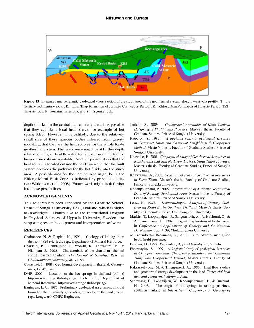
Nilsuwan and Durrast
Figure 13 Integrated and schematic geological cross-section of the study area of the geothermal system along a west-east profile. T - the
Tertiary sedimentary rock, JKl - Lam Thap Formation of Jurassic-Cretaceous Period, JK - Khlong Min Formation of Jurassic Period, TRl -
Triassic rock, P - Permian limestone, and Sy - Syenite rock.
depth of 1 km in the central part of study area. It is possible
that they act like a local heat source, for example of hot
spring KB3. However, it is unlikely, due to the relatively
small size of these igneous bodies inferred from gravity
modeling, that they are the heat sources for the whole Krabi
geothermal system. The heat source might be at further depth
related to a higher heat flow due to the extensional tectonics;
however no data are available. Another possibility is that the
heat source is located outside the study area and that the fault
system provides the pathway for the hot fluids into the study
area. A possible area for the heat sources might be in the
Khlong Marui Fault Zone as indicated by previous studies
(see Watkinson et al., 2008). Future work might look further
into these possibilities.
ACKNOWLEDGEMENTS
This research has been supported by the Graduate School,
Prince of Songkla University, PSU, Thailand, which is highly
acknowledged. Thanks also to the International Program
in Physical Sciences of Uppsala University, Sweden, for
supporting research equipment and interpretation software.
REFERENCES
Chaimanee, N. & Tanpisit, K., 1991. Geology of khlong thom
district (4824 iv), Tech. rep., Department of Mineral Resource.
Charusiri, P., Buenkhuntod, P., Won-In, K., Thayakupt, M., &
Niampan, J., 2003. Characteristic of the chantaburi thermal
spring, eastern thailand, The Journal of Scientific Research
Chulalongkorn University, 28, 71–95.
Chuaviroj, S., 1988. Geothermal development in thailand, Geother-
mics, 17, 421–428.
DMR, 2005. Location of the hot springs in thailand [online]
http://www.dmr.go.th/hotspring/, Tech. rep., Department of
Mineral Resources, http://www.dmr.go.th/hotspring/.
Engineers, L. C., 1982. Preliminary geological assessment of krabi
basin for the electricity generating authority of thailand., Tech.
rep., Longworth CMPS Engineers.
Jonjana, S., 2009. Geophysical Anomalies of Khao Chaison
Hotspring in Phatthalung Province, Master’s thesis, Faculty of
Graduate Studies, Prince of Songkla University.
Kaew-on, S., 1997. A Regional stady of geological Structure
in Changwat Satun and Changwat Songkhla with Geophysics
Method, Master’s thesis, Faculty of Graduate Studies, Prince of
Songkla University.
Khawdee, P., 2008. Geophysical study of Geothermal Resources in
Kanchanadit and Ban Na Doem District, Surat Thani Province,
Master’s thesis, Faculty of Graduate Studies, Prince of Songkla
University.
Khawtawan, A., 2008. Geophysical study of Geothermal Resources
in Surat Thani, Master’s thesis, Faculty of Graduate Studies,
Prince of Songkla University.
Khoonphunnarai, P., 2008. Interpretation of Airborne Geophysical
Data of Ranong Geothermal Area, Master’s thesis, Faculty of
Graduate Studies, Prince of Songkla University.
Leow, N., 1985. Sedimentological Analysis of Tertiary Coal-
Bearing Krabi Basin, Southern Thailand, Master’s thesis, Fac-
ulty of Graduate Studies, Chulalongkorn University.
Markirt, T., Laoprapaipan, P., Sanguanlosit, A., Jariyabhumi, O., &
Anupandhanant, P., 1984. Lignite exploration at krabi basin,
in Conference on Applications of Geology and the National
Development, pp. 9–39, Chulalongkorn University.
of Groundwater Resources, D., 2006. Groundwater map guide
book, krabi province.
Parasnis, D., 1997. Principle of Applied Geophysics, 5th edn.
Phethuayluk, S., 1997. A Regional Study of geological Structure
in Changwat Songkhla, Changwat Phatthalung and Changwat
Trang with Geophysical Method, Master’s thesis, Faculty of
Graduate Studies, Prince of Songkla University.
Raksaskulwong, M. & Thienprasert, A., 1995. Heat flow studies
and geothermal energy development in thailand, Terrestrial heat
flow and geothermal energy in Asia.
Sanmuang, E., Lohawijarn, W., Khoonphannarai, P., & Duerrast,
H., 2007. The origin of hot springs in ranong province,
southern thailand, in International Conference on Geology of
The 6th International Conference on Applied Geophysics, Nov 15-17, 2012, Kanchanburi, Thailand 127

Geological structures related to hot springs
Thailand: Towards Sustainable Development and Sufficiency
Economy (GEOTHAI 2007), pp. 355–357.
Sripongpan, P., Kijthaworn, T., & Phoeraksa, S., 1990. Geology
of ban mak (4725 i) and krabi province (4725 ii), Tech. rep.,
Department of Mineral Resource.
Wattananikorn, K., Beshirt, J., & Nochaiwong, A., 1995. Gravity
interpretation of chiang mai basin, northern thailand: concen-
trating on ban thung sieo area, Journal of Southeast Asia Earth
Sciences, 12, 53–64.
Wisedsind, W., 1997. Some airborne geophysical characteristic
of geothermal promising areas thailand, Tech. rep., Kyushu
University.
The 6th International Conference on Applied Geophysics, Nov 15-17, 2012, Kanchanburi, Thailand 128
Geomechanical Simulation of Deformation by CO2
Injection into Homogeneous Sandstone
Avirut Puttiwongraka,∗, Toshifumi Matsuokaa
a Environment and Resource System Engineering Laboratory, Department of Urban Management, Graduate School of
Engineering, Kyoto University-Katsura, Nishikyo-ku, Kyoto, 615-8540, JAPAN∗, E-mail: [email protected]
ABSTRACT
Geomechanics has become increasingly important because more and more new projects involve viscous or immobile oils, higher
temperatures, pressures and depths, and reservoir materials that are weak, intensely fractured, or highly compressible. Deformation
measurements are critically important for geomechanics. The geomechanical processes are due to injection of CO2 in CCS (Carbon
dioxide Capture and Storage) project, i.e. pressurization, causes expansion of reservoir that may result in a ground surface deformation.
In this study we analyzed and re-produced deformation results of Berea sandstone core sample, which is well known in testing to be
homogeneous and isotropic material, from laboratory experiment using geomechanical simulation. The experiment was setup to emulate a
surface uplift problem caused by CO2 injection in CCS site. Strain changing of core sample in laboratory testing can be implied to reservoir
deformation in field observation. The experiment was divided into three stages in order to measure the strain, i.e., (1) Confining pressure
change stage, (2) Water injection stage (Pore pressure changes) and (3) CO2 injection stage, with continuous tests, respectively. We used
FLAC3D simulator with coupled fluid-mechanic interaction process to simulate core sample deformation based on stages of laboratory
experiment. The simulation results are discussed and proposed that effective porosity changes (closing/opening effect of pore connection)
can explain strain changes during both caused by confining pressure increase (closing of pore connection) and water injection (opening
of pore connection). In addition, we applied this theory to simulate in the case of CO2 injection stage. The deformation of core sample
caused by CO2 injection can be also clarified by change of effective porosity relating to bulk modulus. Finally, the simulation can help us
to understand the deformations of Berea sandstone on three stages of laboratory testing, especially in the case of CO2 injection in which
relates to CCS project.
KEYWORDS: Geomechanical simulation, CO2 injection, FLAC3D, Rock deformation, Berea sandstone
INTRODUCTION
Nowadays, geomechanics has been extensively interested be-
cause of many hydrocarbon fields are geometrically complex
and irregular, and the rock properties are spatially variable,
such an assessment can be conveniently done on a numerical
model of the field understudy (Orlic, 2008). Petroleum
geomechanics has evolved differently from civil and mining
geomechanics. Petroleum geomechanics is far young and has
followed a direction based far more on physics, analysis and
field observations than on laboratory testing and empirical
models (Dusseault, 2011).
The geomechanics plays a prominent role in the assess-
ment of the impact of CO2 injection on the induced surface
deformation. Because CO2 injection changes the pressure
in the reservoir, it also affects the state of stress within the
reservoir and surrounding rocks, the pressurization causes
vertical expansion of the reservoir and changes in the stress
field. These changes are proportional to the magnitude
of the pressure increase and depend on the geometry and
geomechanical properties of the reservoir and surrounding
sediments. The vertical expansion of the reservoir may result
in a ground surface deformation (Rutqvist, 2012).
In this study we used geomechanical simulation to ana-
lyze and re-produce laboratory results of core sample in term
of deformations. Strain changes of core sample in laboratory
testing can be inferred to reservoir deformation relating to
a surface uplift in field observation. We used FLAC3D
simulator with a coupled fluid-mechanic interaction feature
to simulate core sample deformations based on stages of
laboratory experiments. We used a relationship of effective
porosity and effective bulk modulus changes proposed by
Russell and Smith (2007) and Gussmann’s equation (Guss-
mann, 1951) to apply for simulations. Consequently, the
simulation results can help to understand the deformations
of core sample in laboratory testing, especially a case of CO2
The 6th International Conference on Applied Geophysics, Nov 15-17, 2012, Kanchanburi, Thailand 129
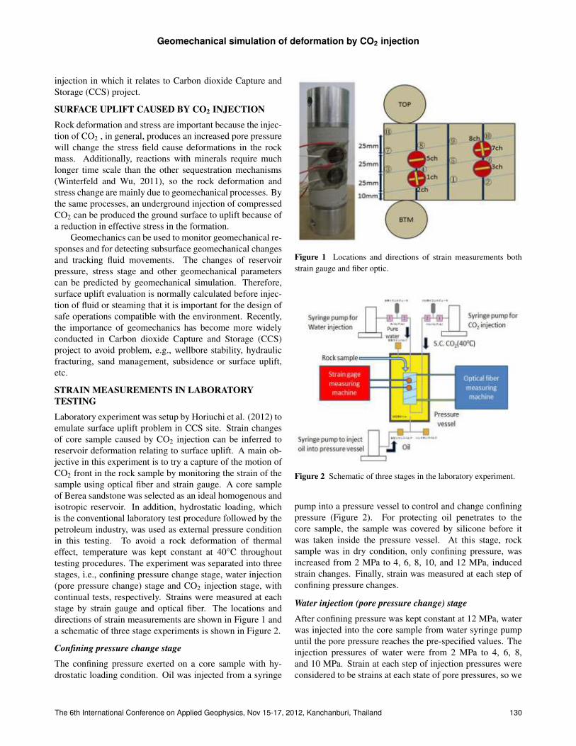
Geomechanical simulation of deformation by CO2 injection
injection in which it relates to Carbon dioxide Capture and
Storage (CCS) project.
SURFACE UPLIFT CAUSED BY CO2 INJECTION
Rock deformation and stress are important because the injec-
tion of CO2 , in general, produces an increased pore pressure
will change the stress field cause deformations in the rock
mass. Additionally, reactions with minerals require much
longer time scale than the other sequestration mechanisms
(Winterfeld and Wu, 2011), so the rock deformation and
stress change are mainly due to geomechanical processes. By
the same processes, an underground injection of compressed
CO2 can be produced the ground surface to uplift because of
a reduction in effective stress in the formation.
Geomechanics can be used to monitor geomechanical re-
sponses and for detecting subsurface geomechanical changes
and tracking fluid movements. The changes of reservoir
pressure, stress stage and other geomechanical parameters
can be predicted by geomechanical simulation. Therefore,
surface uplift evaluation is normally calculated before injec-
tion of fluid or steaming that it is important for the design of
safe operations compatible with the environment. Recently,
the importance of geomechanics has become more widely
conducted in Carbon dioxide Capture and Storage (CCS)
project to avoid problem, e.g., wellbore stability, hydraulic
fracturing, sand management, subsidence or surface uplift,
etc.
STRAIN MEASUREMENTS IN LABORATORY
TESTING
Laboratory experiment was setup by Horiuchi et al. (2012) to
emulate surface uplift problem in CCS site. Strain changes
of core sample caused by CO2 injection can be inferred to
reservoir deformation relating to surface uplift. A main ob-
jective in this experiment is to try a capture of the motion of
CO2 front in the rock sample by monitoring the strain of the
sample using optical fiber and strain gauge. A core sample
of Berea sandstone was selected as an ideal homogenous and
isotropic reservoir. In addition, hydrostatic loading, which
is the conventional laboratory test procedure followed by the
petroleum industry, was used as external pressure condition
in this testing. To avoid a rock deformation of thermal
effect, temperature was kept constant at 40°C throughout
testing procedures. The experiment was separated into three
stages, i.e., confining pressure change stage, water injection
(pore pressure change) stage and CO2 injection stage, with
continual tests, respectively. Strains were measured at each
stage by strain gauge and optical fiber. The locations and
directions of strain measurements are shown in Figure 1 and
a schematic of three stage experiments is shown in Figure 2.
Confining pressure change stage
The confining pressure exerted on a core sample with hy-
drostatic loading condition. Oil was injected from a syringe
Figure 1 Locations and directions of strain measurements both
strain gauge and fiber optic.
Figure 2 Schematic of three stages in the laboratory experiment.
pump into a pressure vessel to control and change confining
pressure (Figure 2). For protecting oil penetrates to the
core sample, the sample was covered by silicone before it
was taken inside the pressure vessel. At this stage, rock
sample was in dry condition, only confining pressure, was
increased from 2 MPa to 4, 6, 8, 10, and 12 MPa, induced
strain changes. Finally, strain was measured at each step of
confining pressure changes.
Water injection (pore pressure change) stage
After confining pressure was kept constant at 12 MPa, water
was injected into the core sample from water syringe pump
until the pore pressure reaches the pre-specified values. The
injection pressures of water were from 2 MPa to 4, 6, 8,
and 10 MPa. Strain at each step of injection pressures were
considered to be strains at each state of pore pressures, so we
The 6th International Conference on Applied Geophysics, Nov 15-17, 2012, Kanchanburi, Thailand 130
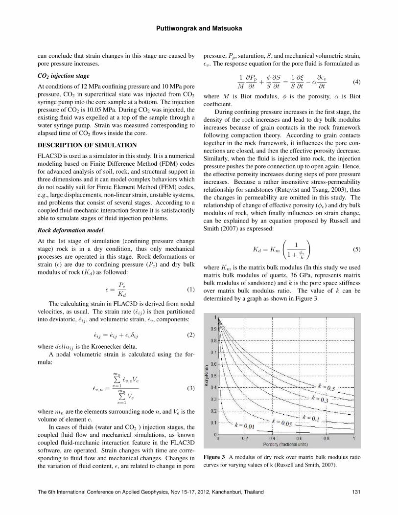
Puttiwongrak and Matsuoka
can conclude that strain changes in this stage are caused by
pore pressure increases.
CO2 injection stage
At conditions of 12 MPa confining pressure and 10 MPa pore
pressure, CO2 in supercritical state was injected from CO2
syringe pump into the core sample at a bottom. The injection
pressure of CO2 is 10.05 MPa. During CO2 was injected, the
existing fluid was expelled at a top of the sample through a
water syringe pump. Strain was measured corresponding to
elapsed time of CO2 flows inside the core.
DESCRIPTION OF SIMULATION
FLAC3D is used as a simulator in this study. It is a numerical
modeling based on Finite Difference Method (FDM) codes
for advanced analysis of soil, rock, and structural support in
three dimensions and it can model complex behaviors which
do not readily suit for Finite Element Method (FEM) codes,
e.g., large displacements, non-linear strain, unstable systems,
and problems that consist of several stages. According to a
coupled fluid-mechanic interaction feature it is satisfactorily
able to simulate stages of fluid injection problems.
Rock deformation model
At the 1st stage of simulation (confining pressure change
stage) rock is in a dry condition, thus only mechanical
processes are operated in this stage. Rock deformations or
strain (ǫ) are due to confining pressure (Pc) and dry bulk
modulus of rock (Kd) as followed:
ǫ =Pc
Kd
(1)
The calculating strain in FLAC3D is derived from nodal
velocities, as usual. The strain rate (ǫij) is then partitioned
into deviatoric, eij , and volumetric strain, ǫv , components:
ǫij = eij + ǫvδij (2)
where deltaij is the Kroenecker delta.
A nodal volumetric strain is calculated using the for-
mula:
ǫv,n =
mn∑
e=1ǫv,eVe
mn∑
e=1Ve
(3)
where mn are the elements surrounding node n, and Ve is the
volume of element e.
In cases of fluids (water and CO2 ) injection stages, the
coupled fluid flow and mechanical simulations, as known
coupled fluid-mechanic interaction feature in the FLAC3D
software, are operated. Strain changes with time are corre-
sponding to fluid flow and mechanical changes. Changes in
the variation of fluid content, ǫ, are related to change in pore
pressure, Pp, saturation, S, and mechanical volumetric strain,
ǫv . The response equation for the pore fluid is formulated as
1
M
∂Pp
∂t+
φ
S
∂S
∂t=
1
S
∂ξ
∂t− α
∂ǫv∂t
(4)
where M is Biot modulus, φ is the porosity, α is Biot
coefficient.
During confining pressure increases in the first stage, the
density of the rock increases and lead to dry bulk modulus
increases because of grain contacts in the rock framework
following compaction theory. According to grain contacts
together in the rock framework, it influences the pore con-
nections are closed, and then the effective porosity decrease.
Similarly, when the fluid is injected into rock, the injection
pressure pushes the pore connection up to open again. Hence,
the effective porosity increases during steps of pore pressure
increases. Because a rather insensitive stress-permeability
relationship for sandstones (Rutqvist and Tsang, 2003), thus
the changes in permeability are omitted in this study. The
relationship of change of effective porosity (φe) and dry bulk
modulus of rock, which finally influences on strain change,
can be explained by an equation proposed by Russell and
Smith (2007) as expressed:
Kd = Km
(
1
1 + φe
k
)
(5)
where Km is the matrix bulk modulus (In this study we used
matrix bulk modulus of quartz, 36 GPa, represents matrix
bulk modulus of sandstone) and k is the pore space stiffness
over matrix bulk modulus ratio. The value of k can be
determined by a graph as shown in Figure 3.
Figure 3 A modulus of dry rock over matrix bulk modulus ratio
curves for varying values of k (Russell and Smith, 2007).
The 6th International Conference on Applied Geophysics, Nov 15-17, 2012, Kanchanburi, Thailand 131

Geomechanical simulation of deformation by CO2 injection
Table 1 Physical properties of Berea sandstone.
Parameter Value
Dry bulk modulus (GPa) 8.3
Shear modulus (GPa) 7.0
Dry density (kg/m3) 2100
Permeability (mD) 100
(Initial) Porosity (%) 23
Furthermore, Gassmann’s equation was used to convert
the time-dependent pore pressure and saturations resulting
from the flow simulation into elastic rock parameter changes
(Gassmann, 1951). Gassman’s equation computes effective
bulk moduli of rock saturated (Ksat) with a given composi-
tion of pore fluid from the elastic moduli of the dry rock. The
equation is
Ksat
Km −Ksat
=Kd
Km −Kd
+Kf
φe(KM −Kf )(6)
where Kf is the total fluid bulk modulus which can be
calculated by
1
Kf
=Sw
Kw
+SCO2
KCO2
(7)
where Sw and SCO2are the saturation of water and CO2
and Kw and KCO2are the bulk modulus of water and CO2 ,
respectively.
Model setup
Model geometry was created corresponding to the core
sample in the laboratory. The size of core sample is 5 cm
of diameter and 10 cm of length. The simulation problem
was discretized into 3-dimensional mesh, the mesh size in x,
y, and z direction is 16×16×32 as shown in Figure 4. The
calculating volumetric strains are consistent with the same
location and direction of strain measurements of optical fiber
(Figure 1) in the laboratory. The problems of our simulations
are in nonsupport system, thus the confining pressure with
hydrostatic loading condition is performed as mechanical
boundary condition and elastic model was for simulations.
Rock properties of Berea sandstone that were used to be
input parameters are standard properties of Berea sandstone
as shown in Table 1.
After we setup model geometry, boundary condition,
and input parameters, the model was examined until a result
is satisfactory and then the three stages of experiments in
laboratory were simulated in order to calculate volumetric
strains, respectively. Fluid bulk modulus of water and CO2
in supercritical phase which were used in this simulation are
1 GPa and 0.05 GPa. For mixing fluid bulk modulus of water
and CO2 can be determined by (7) with assuming saturation
of water and CO2 are 0.3 and 0.7, respectively.
Figure 4 Setup of model geometry and the locations of simulation
strains.
DISCUSSIONS AND RESULTS OF SIMULATIONS
Here will be demonstrated simulation results of each stage,
i.e., (1) confining pressure change stage, (2) water injection
stage, and (3) CO2 injection stage, which are constrained by
experimental results in the laboratory testing. The simulation
results are discussed to explain suspicions of experimental
results and help to understand a mechanism of deformations
of porous material caused by fluid injection.
Simulation result vs. experimental result
In order to compare simulation and experimental results, we
need to convert a volumetric strain from simulation results
to experimental strain (ǫexpt.) in the direction which was
measured by optical fiber.
As we can determine an angle (θ) between optical fiber
direction and x-axis as shown in Figure 6, and then a
definition of volumetric strain of cylinder material can be
expressed by (8). Hence, we can convert volumetric strain
to experimental strain in the same direction of optical fiber
by using (9). Those equations which we used for conversion
are
ǫv = 2ǫd + ǫl (8)
ǫexpt. =ǫv
2 cos θ + sin θ(9)
The 6th International Conference on Applied Geophysics, Nov 15-17, 2012, Kanchanburi, Thailand 132

Puttiwongrak and Matsuoka
Figure 5 Workflow of simulations.
where ǫd and ǫl are the diametrical strain and longitudinal
strain, respectively.
Simulation of confining pressure change stage
Both simulation and experimental results of confining pres-
sure change stage demonstrated that the strain deceases
were due to confining pressure increases (Figure 7). The
simulation results seem to be consistent with experimental
results and almost straight line. We simulated deformations
of rock in this stage using dry bulk modulus of rock as input
parameters as shown in Table 1 for every confining pressure,
thus Figure 7 shows that during confining pressure increases
with hydrostatic loading condition, density of rock is in-
creased influencing the dry bulk modulus increase because
grain contacts, as followed compaction theory, or effective
porosity decrease because pore connection closing is less
sensitive, so the graph shows straight line and can be simu-
lated by only one value of Kd throughout confining pressure
changes. The rock behaved deformations as a shrinkage in
Figure 6 A schematic of volumetric strain-optical fiber conversion.
Figure 7 Comparison between simulation and experimental results
of confining pressure change stage.
this stage. In addition, variations of strain measurement of
each location in laboratory when confining pressure increases
can be explained by indirect confining pressure exerted on the
sample and the core (itself) is not completely homogeneous,
but the simulation model is perfect homogeneous model.
As the confining pressure is controlled by oil injection, the
silicone was used to cover the rock to protect oil penetration;
therefore, the sample is probably not equal at each location
because differences of silicone thickness.
The 6th International Conference on Applied Geophysics, Nov 15-17, 2012, Kanchanburi, Thailand 133
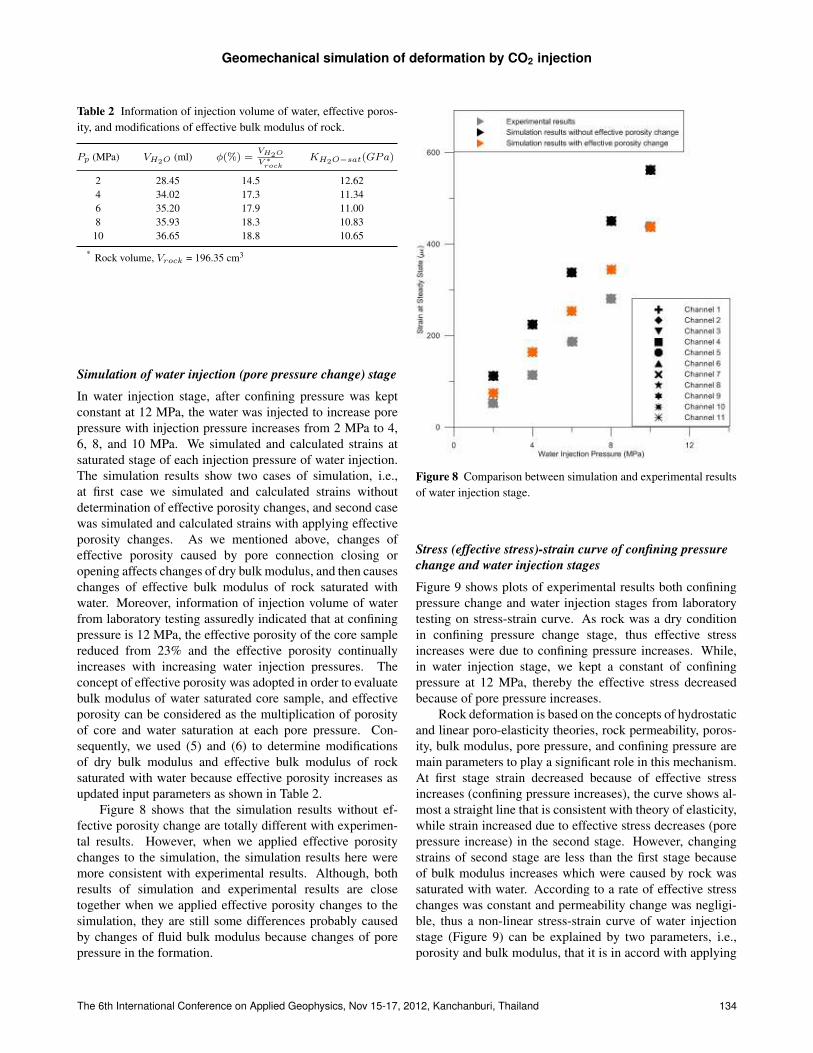
Geomechanical simulation of deformation by CO2 injection
Table 2 Information of injection volume of water, effective poros-
ity, and modifications of effective bulk modulus of rock.
Pp (MPa) VH2O (ml) φ(%) =VH2O
V ∗
rockKH2O−sat(GPa)
2 28.45 14.5 12.62
4 34.02 17.3 11.34
6 35.20 17.9 11.00
8 35.93 18.3 10.83
10 36.65 18.8 10.65
*Rock volume, Vrock = 196.35 cm3
Simulation of water injection (pore pressure change) stage
In water injection stage, after confining pressure was kept
constant at 12 MPa, the water was injected to increase pore
pressure with injection pressure increases from 2 MPa to 4,
6, 8, and 10 MPa. We simulated and calculated strains at
saturated stage of each injection pressure of water injection.
The simulation results show two cases of simulation, i.e.,
at first case we simulated and calculated strains without
determination of effective porosity changes, and second case
was simulated and calculated strains with applying effective
porosity changes. As we mentioned above, changes of
effective porosity caused by pore connection closing or
opening affects changes of dry bulk modulus, and then causes
changes of effective bulk modulus of rock saturated with
water. Moreover, information of injection volume of water
from laboratory testing assuredly indicated that at confining
pressure is 12 MPa, the effective porosity of the core sample
reduced from 23% and the effective porosity continually
increases with increasing water injection pressures. The
concept of effective porosity was adopted in order to evaluate
bulk modulus of water saturated core sample, and effective
porosity can be considered as the multiplication of porosity
of core and water saturation at each pore pressure. Con-
sequently, we used (5) and (6) to determine modifications
of dry bulk modulus and effective bulk modulus of rock
saturated with water because effective porosity increases as
updated input parameters as shown in Table 2.
Figure 8 shows that the simulation results without ef-
fective porosity change are totally different with experimen-
tal results. However, when we applied effective porosity
changes to the simulation, the simulation results here were
more consistent with experimental results. Although, both
results of simulation and experimental results are close
together when we applied effective porosity changes to the
simulation, they are still some differences probably caused
by changes of fluid bulk modulus because changes of pore
pressure in the formation.
Figure 8 Comparison between simulation and experimental results
of water injection stage.
Stress (effective stress)-strain curve of confining pressure
change and water injection stages
Figure 9 shows plots of experimental results both confining
pressure change and water injection stages from laboratory
testing on stress-strain curve. As rock was a dry condition
in confining pressure change stage, thus effective stress
increases were due to confining pressure increases. While,
in water injection stage, we kept a constant of confining
pressure at 12 MPa, thereby the effective stress decreased
because of pore pressure increases.
Rock deformation is based on the concepts of hydrostatic
and linear poro-elasticity theories, rock permeability, poros-
ity, bulk modulus, pore pressure, and confining pressure are
main parameters to play a significant role in this mechanism.
At first stage strain decreased because of effective stress
increases (confining pressure increases), the curve shows al-
most a straight line that is consistent with theory of elasticity,
while strain increased due to effective stress decreases (pore
pressure increase) in the second stage. However, changing
strains of second stage are less than the first stage because
of bulk modulus increases which were caused by rock was
saturated with water. According to a rate of effective stress
changes was constant and permeability change was negligi-
ble, thus a non-linear stress-strain curve of water injection
stage (Figure 9) can be explained by two parameters, i.e.,
porosity and bulk modulus, that it is in accord with applying
The 6th International Conference on Applied Geophysics, Nov 15-17, 2012, Kanchanburi, Thailand 134

Puttiwongrak and Matsuoka
Figure 9 Stress (effective stress) âAS strain curve of confining
pressure change and water injection stages.
Table 3 Input parameters for simulation of CO2 injection stage.
PCO2−inj(MPa) φCO2(%) KH2O+CO2−sat (GPa)
10.05 4.2 20.06
an effective stress change to simulations as we discussed in
previous section.
Simulation of CO2 injection stage
A suspicion of strain changes in this stage is a high strain
increment with elapsed time despite a small rate of pore
pressure increase (0.05 MPa). This increased strain seems
to be equal to an increase of strain at 7 MPa of pore pressure
in water injection stage.
A rate of pore pressure increase with 0.05 MPa is not
certainly possible to generate a rate of strain increment in the
laboratory testing for CO2 injection stage. Consequently, we
considered that the high rate of strain increment of this stage
is due CO2 migrates to the narrow and small pores where
water cannot reach these pores during water injection stage
because pore connections are closed together when confining
pressure increases.
As we know effective porosity at final stage of water
injection, i.e., the effective porosity at 10 MPa of pore pres-
sure is 18.8% as shown in Table 2, hence pores that will be
occupied by CO2 (φCO2) can be determined by a difference
of initial porosity and effective porosity at 10 MPa of pore
pressure (23 - 18.8 = 4.2%). Afterward, we created a rock
model in order to simulate a rock that has 4.2% of porosity
and effective bulk modulus of rock (KCO2+H2O−sat), which
saturated with mixing fluid (CO2 dissolved in water), is 20.06
GPa as shown in Table 3.
Equation (5) was used to determine a dry bulk modulus
of rock is due to porosity changes to 4.2%, and then the
effective bulk modulus of rock which saturated with mixing
fluid by using (6) and (7). Parameters, i.e., saturation of
water and CO2 is 0.3 and 0.7, were assumed in order to find
fluid bulk modulus of mixing fluid. Finally, input parameters
as shown in Table 3 using for simulation of this stage are
CO2 injection pressure (PCO2−inj), porosity which will be
occupied by CO2 (φCO2), and effective bulk modulus of
rock which saturated with mixing fluid (KCO2+H2O−sat).
Hence, in this stage strain changes were generated from pore
pressure change of 10.05 MPa.
Figure 10 represents volumetric strains changed corre-
sponding to pore pressure changes from simulation results.
This figure is used to confirm that strain change of rock is
in accord with changing pore pressure of rock. In addition,
motion of CO2 front inside rock, which is represented by No.
1-11 of strain increases with elapsed times, can be explained
by Figure 11.
CONCLUSIONS
Geomechanical simulation using FLAC3D simulator with
coupled fluid-mechanic interaction feature was used in this
study to explain rock deformations of laboratory experi-
ments. At the same effective stress, the differences of
strain changes because confining pressure and pore pressure
increases, as shown in Figure 9, were significantly controlled
by effective porosity and effective bulk modulus changes.
Furthermore, the high rate of strain increments in CO2
injection stage can also be explained by changes of effective
porosity and effective bulk modulus. We used information
of injection volume of water from laboratory testing and
equations (5), (6) and (7) to calculate effective porosity and
bulk modulus changes as input parameters as shown in Table
2 and 3 in cases of simulations. Furthermore, strain was
increased corresponding to a flow of CO2 front inside the
core sample during CO2 injection that can be monitored by
a strain of each location (No. 1-11) of measurements and
simulations.
The rock deformation, is due to injection or depletion
of fluid inferring surface uplift and subsidence, has not been
widely understood up-to-date. Geomechanics are used and
discussed for how monitoring of geomechanical responses
is used for detecting subsurface geomechanical changes and
tracking fluid movements. Therefore, in this study we
propose and hope that our simulation results can help to
understand the deformations of Berea sandstone, especially,
for CO2 injection in which it can be inferred on surface uplift
problem of CO2 storage in abandoned oil and gas fields,
where are normally clastic (sandstone) reservoir rock.
The 6th International Conference on Applied Geophysics, Nov 15-17, 2012, Kanchanburi, Thailand 135
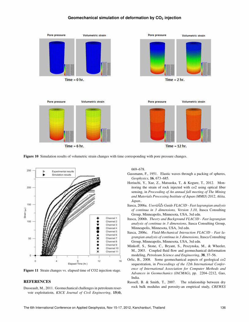
Geomechanical simulation of deformation by CO2 injection
Figure 10 Simulation results of volumetric strain changes with time corresponding with pore pressure changes.
Figure 11 Strain changes vs. elapsed time of CO2 injection stage.
REFERENCES
Dusseault, M., 2011. Geomechanical challenges in petroleum reser-
voir exploitatioin, KSCE Journal of Civil Engineering, 15(4),
669–678.
Gassmann, F., 1951. Elastic waves through a packing of spheres,
Geophysics, 16, 673–685.
Horiuchi, Y., Xue, Z., Matsuoka, T., & Kogure, T., 2012. Mon-
itoring the strain of rock injected with co2 using optical fiber
sensing, in Proceeding of An annual fall meeting of The Mining
and Materials Processing Institute of Japan (MMIJ) 2012, Akita,
Japan..
Itasca, 2006a. UserâAZs Guide FLAC3D - Fast lagrangian analysis
of continua in 3 dimensions, Version 3.10, Itasca Consulting
Group, Minneapolis, Minnesota, USA, 3rd edn.
Itasca, 2006b. Theory and Background FLAC3D - Fast lagrangian
analysis of continua in 3 dimensions, Itasca Consulting Group,
Minneapolis, Minnesota, USA, 3rd edn.
Itasca, 2006c. Fluid-Mechanical Interaction FLAC3D - Fast la-
grangian analysis of continua in 3 dimensions, Itasca Consulting
Group, Minneapolis, Minnesota, USA, 3rd edn.
Minkoff, S., Stone, C., Bryant, S., Peszynska, M., & Wheeler,
M., 2003. Coupled fluid flow and geomechanical deformation
modeling, Petroleum Science and Engineering, 38, 37–56.
Orlic, B., 2008. Some geomechanical aspects of geological co2
sequestration, in Proceedings of the 12th International Confer-
ence of International Association for Computer Methods and
Advances in Geomechanics (IACMAG), pp. 2204–2212, Gao,
India.
Russell, B. & Smith, T., 2007. The relationship between dry
rock bulk modulus and porosity-an empirical study, CREWES
The 6th International Conference on Applied Geophysics, Nov 15-17, 2012, Kanchanburi, Thailand 136

Puttiwongrak and Matsuoka
Research Report, 19, 1–14.
Rutqvist, J., 2012. The geomechanics of co2 storage in deep sedi-
mentary formations, Geotechnical and Geological Engineering,
30(3), 525–551.
Rutqvist, J. & Tsang, C., 2003. A numerical simulator for analysis
of coupled thermal-hydrologic-mechanical processes in fractured
and porous geological media under multi-phase flow conditions,
in Proceeding of TOUGH Symposium 2003, pp. 1–9, Berkeley,
California, USA.
Winterfeld, P. & Wu, Y., 2011. Parallel simulation of co2 seques-
tration with rock deformation in saline aquifers, in Proceeding
of SPE Reservoir Simulation Symposium, pp. 1–22, Woodlands,
Texas, USA.
The 6th International Conference on Applied Geophysics, Nov 15-17, 2012, Kanchanburi, Thailand 137

Dating Geological Events using ThermoluminescenceTechnique
Prakrit Noppradita,b,∗, Sommai Changkiana,c, Helmut Durrasta,b
a Geophysics Research Center, Prince of Songkla University, HatYai, Songkhla, 90112, THAILANDb Department of Physics, Faculty of Science, Prince of Songkla University, HatYai, Songkhla, 90112, THAILANDc Department of Science, Faculty of Science and Technology, Prince of Songkla University, Pattani, 94000, THAILAND
∗, E-mail: [email protected]
ABSTRACT
Thermoluminescence (TL) dating is a suitable approach for dating geological events by sampling quartz or feldspar rich sediments.
Generally, when minerals in sediments are irradiated by natural-ionizing radiation (from radioactive elements in its surrounding
environment), electrons are continuously accumulated in traps. However, these accumulated electrons can be bleached and reset by sunlight.
Therefore, the calculated age is the last time the sampled sediment was bleached by sunlight (not precisely the event time). Many minerals
in sediments are widely applied as a dosimeter to determine its signal, for example, quartz, which is used in this study. Sediment samples
were collected in Surat Thani Province, where different geological events were identified, for example, alluvial sedimentation processes
or fault movements. The accumulated dose (AD) was determined by the additive dose method where the dose from an artificial source is
added to the natural dose in quartz. The environmental ionizing radiation rate, or the dose rate (D), was determined from the activities of
natural radioactive elements using gamma ray spectrometry. The age of the event is calculated by AD proportional to D. In this study, the
calculated TL ages of alluvial sediment sequences were 122-1,900 ka. The upper sediment layer was formed about 122-225 ka ago. The
lower sediment layer was formed around 1,336-1,900 ka ago shown the evidence of moving of the subsurface because of the discontinuity
of a layer.
KEYWORDS: Thermoluminescence dating, Geological events, Sediments
INTRODUCTION
When studying geological events, it is necessary to carefully
analyze the events, for example, by mapping the detailed
structures. However, often it is also important to know
the timing of the geological event and by this to answer
questions, like, when did this happened or when was the fault
movement?
There are many dating techniques available; both relative
dating (compared with known ages) and absolute dating
methods. The thermoluminescence (TL) dating is a type
of absolute dating the commonly applied to date minerals
in the interesting material such as archeological materials
or sediments. Quartz and feldspar are often used in TL
dating, because both minerals have a high abundance in
sediments and can resist weathering better when compared
with other minerals, such as carbonate minerals (Preusser
et al., 2008). The TL dating has been widely applied in
many studies, such as landscape evolution, palaeoclimate,
geohazards, paleoseismology and many others (Preusser et
al., 2008; Fattahi, 2009).
TL is a technique, which is using the accumulated
signals, TL light, in a mineral. The intensity of the TL
signal depends on the environmental ionizing-radiation and
the duration the mineral has received that radiation.
Natural ionizing radiation
Preusser et al. (2008) described that the ionizing radiation
naturally occurs in form of alpha, beta and gamma radiation
and cosmic rays. Moreover, it can be separated into three
types of ionizing radiation; cosmic radiation, external radia-
tion, and internal radiation. The cosmic radiation is radiated
from space that decreased with depth from surface. The
external radiation is radiated from neighboring grains that
are naturally containing radioactive elements, like potassium,
uranium, and thorium. For the internal radiation, it can be
mainly related to beta radiation in potassium feldspar from
potassium-40.
The 6th International Conference on Applied Geophysics, Nov 15-17, 2012, Kanchanburi, Thailand 138
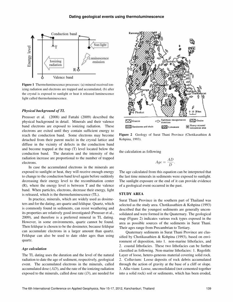
Dating geological events using thermoluminescence
Figure 1 Thermoluminescence processes: (a) mineral received ion-
izing radiation and electrons are trapped and accumulated, (b) after
the crystal is exposed to sunlight or heat it released luminescence
light called thermoluminescence.
Physical background of TL
Preusser et al. (2008) and Fattahi (2009) described the
physical background in detail. Minerals and their valence
band electrons are exposed to ionizing radiation. These
electrons are exited until they contain sufficient energy to
reach the conduction band. Some electrons may become
detached from their parent nuclei in the crystal lattice and
diffuse in the vicinity of defects in the conduction band
and become trapped at the trap (T) level located below the
conduction band. The duration and the intensity of the
radiation increase are proportional to the number of trapped
electrons.
In case the accumulated electrons in the minerals are
exposed to sunlight or heat, they will receive enough energy
to change to the conduction band level again before suddenly
decreasing their energy level to the recombination center
(R), where the energy level is between T and the valence
band. When particles, electrons, decrease their energy, light
is released, which is the thermoluminescence (TL).
In practice, minerals, which are widely used as dosime-
ters and for the dating, are quartz and feldspar. Quartz, which
is commonly found in sediments, can resist weathering and
its properties are relatively good investigated (Preusser et al.,
2009), and therefore is a preferred mineral in TL dating.
However, in some environments, quartz cannot be found.
Then feldspar is chosen to be the dosimeter, because feldspar
can accumulate electrons in a larger amount than quartz.
Feldspar can also be used to date older ages than using
quartz.
Age calculation
The TL dating uses the duration and the level of the natural
radiation to date the age of sediment, respectively, geological
event. The accumulated electrons in the minerals, called
accumulated dose (AD), and the rate of the ionizing radiation
exposed to the minerals, called dose rate (D), are needed for
Figure 2 Geology of Surat Thani Province (Chotikasathien &
Kohpina, 1993).
the calculation as following
Age =AD
D.
The age calculated from this equation can be interpreted that
the last time minerals in sediments were exposed to sunlight.
The sunlight exposure or the end of it can provide evidence
of a geological event occurred in the past.
STUDY AREA
Surat Thani Province in the southern part of Thailand was
selected as the study area. Chotikasathien & Kohpina (1993)
described that the youngest sediments are generally uncon-
solidated and were formed in the Quaternary. The geological
map (Figure 2) indicates various rock types exposed in the
area as possible sources of the sediments in Surat Thani.
Their ages range from Precambrian to Tertiary.
Quaternary sediments in Surat Thani Province are clas-
sified by Chotikasathien & Kohpina (1993), based on envi-
ronment of deposition, into 1. non-marine lithofacies, and
2. coastal lithofacies. These two lithofacies can be further
classified as following. Non-marine lithofacies: 1. Regolith:
Layer of loose, hetero-geneous material covering solid rock.
2. Colluvium: Loose deposits of rock debris accumulated
through the action of gravity at the base of a cliff or slope.
3. Allu-vium: Loose, unconsolidated (not cemented together
into a solid rock) soil or sediments, which has been eroded,
The 6th International Conference on Applied Geophysics, Nov 15-17, 2012, Kanchanburi, Thailand 139
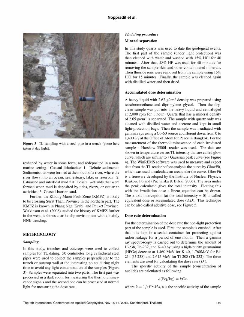
Noppradit et al.
Figure 3 TL sampling with a steel pipe in a trench (photo here
taken at day light).
reshaped by water in some form, and redeposited in a non-
marine setting. Coastal lithofacies: 1. Deltaic sediments:
Sediments that were formed at the mouth of a river, where the
river flows into an ocean, sea, estuary, lake, or reservoir. 2.
Estuarine and intertidal mud flat: Coastal wetlands that were
formed when mud is deposited by tides, rivers, or estuarine
activities. 3. Coastal-barrier sand.
Further, the Khlong Marui Fault Zone (KMFZ) is likely
to be crossing Surat Thani Province in the northern part. The
KMFZ is known in Phang Nga, Krabi, and Phuket Province.
Watkinson et al. (2008) studied the history of KMFZ further
in the west; it shows a strike-slip environment with a mainly
NNE-trending.
METHODOLOGY
Sampling
In this study, trenches and outcrops were used to collect
samples for TL dating. 50 centimeter long cylindrical steel
pipes were used to collect the samples perpendicular to the
trench or outcrop wall at the interesting points during night
time to avoid any light contamination of the samples (Figure
3). Samples were separated into two parts. The first part was
processed in a dark room for measuring the thermolumines-
cence signals and the second one can be processed at normal
light for measuring the dose rate.
TL dating procedure
Mineral separation
In this study quartz was used to date the geological events.
The first part of the sample (under light protection) was
then cleaned with water and washed with 15% HCl for 40
minutes. After that, 48% HF was used for 40 minutes for
removing the sample skin and other contaminated minerals.
Then fluoride ions were removed from the sample using 15%
HCl for 15 minutes. Finally, the sample was cleaned again
with distilled water and then dried.
Accumulated dose determination
A heavy liquid with 2.62 g/cm3 density was prepared using
tetrabromoethane and dipropylene glycol. Then the dry-
clean sample was put into the heavy liquid and centrifuged
at 2,000 rpm for 1 hour. Quartz that has a mineral density
of 2.65 g/cm3 is separated. The sample with quartz only was
cleaned with distilled water and acetone and kept in small
light-protection bags. Then the sample was irradiated with
gamma rays using a Co-60 source at different doses from 0 to
1,400 Gy at the Office of Atom for Peace in Bangkok. For the
measurement of the thermoluminescence of each irradiated
sample a Harshaw 3500L reader was used. The data are
shown in temperature versus TL intensity that are called glow
curve, which are similar to a Gaussian peak curve (see Figure
4). The WinREMS software was used to measure and export
data from the TL reader before analysis the curve by GlowFit,
which was used to calculate an area under the curve. GlowFit
is a freeware developed by the Institute of Nuclear Physics,
Krakow, Poland (Puchalska & Bilski, 2006). The area under
the peak calculated gives the total intensity. Plotting this
with the irradiation dose a linear equation can be drawn.
The x-axis interception (at the total intensity = 0) is called
equivalent dose or accumulated dose (AD). This technique
can be also called additive dose, see Figure 5.
Dose rate determination
For the determination of the dose rate the non-light protection
part of the sample is used. First, the sample is crushed. After
that it is kept in a sealed container for protecting against
radon leakage for a period of one month. Then a gamma
ray spectroscopy is carried out to determine the amount of
U-238, Th-232, and K-40 by using a high-purity germanium
(HPGe) detector at 1.460 MeV for K-40, 1.760MeV for Bi-
214 (U-238) and 2.615 MeV for Tl-208 (Th-232). The three
elements are used for calculating the dose rate (D ).
The specific activity of the sample (concentration of
nuclide) are calculated as following
a(Bq/kg) = kCn
where k = 1/ǫPγMs, a is the specific activity of the sample
The 6th International Conference on Applied Geophysics, Nov 15-17, 2012, Kanchanburi, Thailand 140

Dating geological events using thermoluminescence
Figure 4 Example of a glow curve (Sample TL08) from the TL
reader with temperature versus TL intensity for doses of 0, 200,
400, 800, 1,200, and 1,400 Gy from below to top.
Figure 5 Dose (Gy) versus TL intensity at 325 °C of Sample TL08.
Accumulated dose determination using the additive dose method
gives AD=194.1 Gy.
in Bq/kg, Cn is the count rate at a certain peak, ǫ is a detec-
tor efficiency, Pγ is a number of gammas per disintegration
of this nuclide for a transition at energy E, and Ms is the
mass in kg of the measured sample. The emission of gamma
ray, which is the ionizing radiation of the surrounding earth
material, affects directly the thermoluminescence dosimeter
(quartz or feldspar) over time. The dose rate is the ratio of an
increment dose in a time interval. The dose rate (D) can be
calculated as following:
D(nGy/h) = a(Bq/kg)× CF (nGy/h per Bq/kg),
where a is the concentration of nuclide, and CF is the
conversion factor that 0.429 for U, 0.666 for Th and 0.042
for K (Tsertos & Tzortzis, 2003).
Table 1 Dose rate, accumulated dose, and calculated ages.
Sample (no) Dose rate (Gy/ka) Accumulated dose (Gy) Age (ka)
TL08 0.864 194.1 225
TL09 0.863 1,074.1 1,240
TL10 0.763 1,445.3 1,900
TL11 0.450 55.0 122
TL12 0.437 583.3 1,336
RESULTS
The collected samples are alluvial sediments that have a sand
and clay composition (Figure 6). Several samples were taken
and the age based on the TL method determined. Five of the
samples, their location in a trench and their age are shown
in Figure 5. The TL peaks from the quartz samples mainly
appeared at 153 °C, 210 °C, 275 °C, and 325 °C. The 325 °C
peak is the suitable one for dating quartz minerals (Wintle,
1997); therefore this temperature peak was selected.
The measurement results of Sample TL08 are shown as
an example, with the TL intensity measured and analyzed
intensity for each temperature (see Figure 4 and 5). The
325 °C intensity peak was selected to find the relationship
between its intensity and dose. The x-axis-interception was
determined as its accumulated dose (194.1 Gy). Its dose
rate then can be calculated from the gamma ray spectrom-
etry, which is 0.864 Gy/ka. The age can be calculated to
194.1/0.864=225 ka. For the other samples the results with
dose rate, accumulated dose, and age are shown in Table 1
DISCUSSION
From Figure 6 it can be seen that the L6 layer was formed
about 1,336-1,900 ka ago. The L1 sediment layer on top
was deposited about 122-225 ka ago. The TL09 sample
with an age of 1,240 ka seemingly does not fit in the
other ages related to layer L1. This difference might be
related to various reasons. The sample, for example, might
represent a mixed layer and as a result the TL age might also
show a mixed age. Moreover, high age values often have
high uncertainty, which is related to the saturation of the
trapped electrons. However in this study, the graphs fitted
to determine the AD are looking linear for all samples (not
shown here). Further interpretations of the sedimentological
implications of the TL ages are currently being done.
ACKNOWLEDGMENTS
The authors would like to thank the Development and Pro-
motion of Science and Technology (DPST) Talent Project,
Thailand, and the Electricity Generating Authority of Thai-
land (EGAT) for financial support. Further thanks go to the
people and local government officers in the study area for
supporting this work.
The 6th International Conference on Applied Geophysics, Nov 15-17, 2012, Kanchanburi, Thailand 141
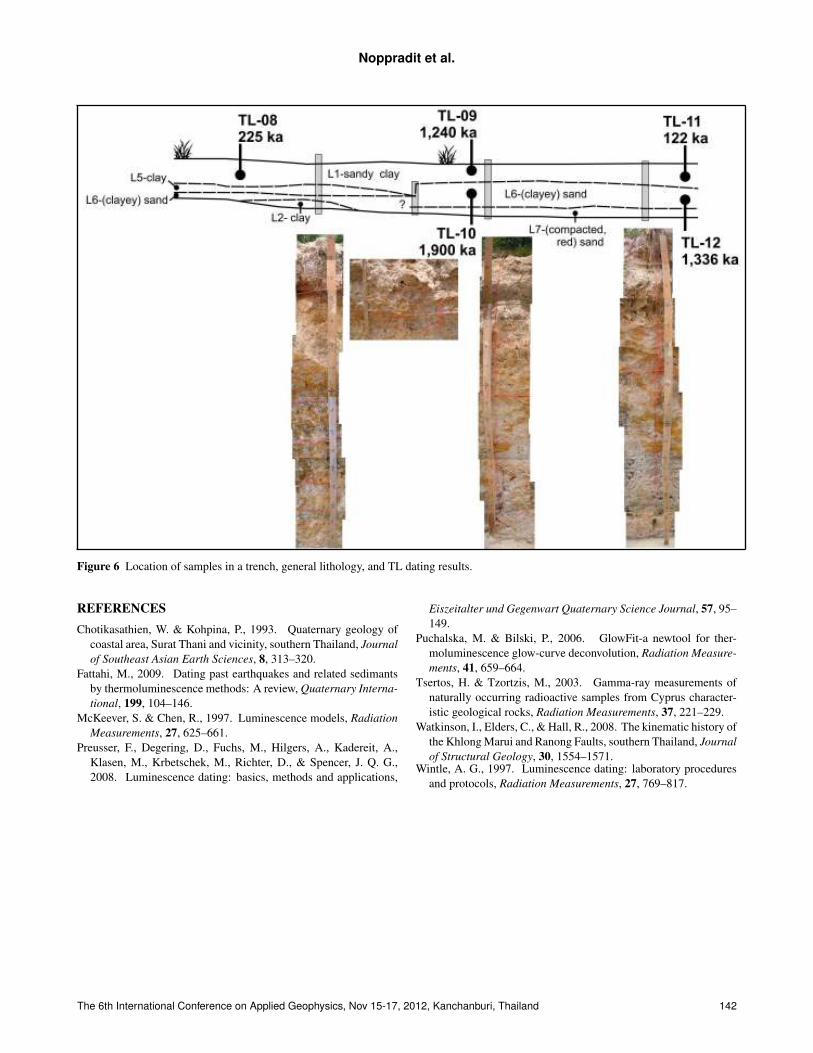
Noppradit et al.
Figure 6 Location of samples in a trench, general lithology, and TL dating results.
REFERENCES
Chotikasathien, W. & Kohpina, P., 1993. Quaternary geology of
coastal area, Surat Thani and vicinity, southern Thailand, Journal
of Southeast Asian Earth Sciences, 8, 313–320.
Fattahi, M., 2009. Dating past earthquakes and related sedimants
by thermoluminescence methods: A review, Quaternary Interna-
tional, 199, 104–146.
McKeever, S. & Chen, R., 1997. Luminescence models, Radiation
Measurements, 27, 625–661.
Preusser, F., Degering, D., Fuchs, M., Hilgers, A., Kadereit, A.,
Klasen, M., Krbetschek, M., Richter, D., & Spencer, J. Q. G.,
2008. Luminescence dating: basics, methods and applications,
Eiszeitalter und Gegenwart Quaternary Science Journal, 57, 95–
149.
Puchalska, M. & Bilski, P., 2006. GlowFit-a newtool for ther-
moluminescence glow-curve deconvolution, Radiation Measure-
ments, 41, 659–664.
Tsertos, H. & Tzortzis, M., 2003. Gamma-ray measurements of
naturally occurring radioactive samples from Cyprus character-
istic geological rocks, Radiation Measurements, 37, 221–229.
Watkinson, I., Elders, C., & Hall, R., 2008. The kinematic history of
the Khlong Marui and Ranong Faults, southern Thailand, Journal
of Structural Geology, 30, 1554–1571.Wintle, A. G., 1997. Luminescence dating: laboratory procedures
and protocols, Radiation Measurements, 27, 769–817.
The 6th International Conference on Applied Geophysics, Nov 15-17, 2012, Kanchanburi, Thailand 142

Index of Authors
Boonyatee, Tirawat, 75
Chaisri, Siriporn, 42, 48, 53
Changkian, Sommai, 138
Chantraprasert, Sarawute, 23, 42, 48
de Wet, Barry, 82
Durrast, Helmut, 117, 138
Ellis, Robert, 82
Giao, Pham Huy, 17, 112
Htike, Soe Linn, 100
Kato, Yoshinori, 75
Kitazumi, Akira, 75
Kluntong, Narin, 68
Kongsuk, Anchalee, 1, 36
Kosuwan, Suwith, 75
Latt, Khin Moh Moh, 112
Limpisawad, Sitirag, 75
Macleod, Ian, 82
Matsuoka, Toshifumi, 129
Mayamae, Aksara, 87
Methaweranon, Wimonsiri, 14
Morio, Satoshi, 75
Munkong, Chatupond, 62
Na Lampang, Tirawut, 36
Nilsuwan, Usa, 117
Ninsom, Chawanun, 42
Noppradit, Prakrit, 138
Norkhamboot, Theerachai, 108
Nuannin, Paiboon, 53, 62
Pananont, Passakorn, 68, 71
Ponchunchoovong, Monkon, 14
Poomvises, Noppadol, 23, 36
Puttiwongrak, Avirut, 129
Rongkhapimonpong, Natthee, 7
Sakulnee, Rapeeporn, 71
Sangtong, Narucha, 36
Sawatdipong, Benjamas, 1, 36
Sommai, Thirat, 31
Somsri, Siriphon, 94
Srisuwan, Preeya, 87
Suanburi, Desell, 7, 10, 14
Suklim, Tanapon, 48
Tadapansawut, Tira, 53
Tansamrit, Songkiert, 10
Tepsut, Boonyoung, 14
Thangkanasup, Channarong, 7
Udphuay, Suwimon, 48
Wattanasen, Kamhaeng, 31
Wiwattanachang, Narongchai, 17
Wongpornchai, Pisanu, 94, 100, 108
Yordkayhun, Sawasdee, 31, 87

The main focus of Austhai Geophysical Consultants Limited is on providing advice and guidance for
The main focus of Austhai Geophysical Consultants Limited is on providing advice and guidance for
Austhai Geophysical Consultants
The main focus of Austhai Geophysical Consultants Limited is on providing advice and guidance for
geophysical exploration programs as well as providing a wide range of geophysical services to the environmental
and engineering industries.
Our main area of operations is the Asia Pacific region with long term experience in Base metal, Gold and Copper
exploration. Austhai Geophysical Consultants Limited has provided Geophysical Data Processing and Modelling
services for various clients.
The main advantages that Austhai offer are:
Review and assessment of any pre-existing or archival geophysical data
Experienced staff providing expert survey planning and field supervision
Experienced in planning and conducting surveys in extreme terrain
Experienced in conducting, processing and interpreting Induced Polarization, Transient Electromagnetic,
Magnetic, Gravity, Radiometric and Seismic Data.
Infield data QC and 2D/3D preliminary inversion Modelling to determine survey effectiveness
Final 2D and 3D inversions carried out in the office using UBC-GIF Inversion Software
Detailed Interpretative Reports relating the 2D and 3D Geophysical Models to Geology and including:
Field checking and verification of anomalous zones or targets generated from the modeled data.
After action review of drill hole data as it relates to the Geophysical survey results.
Austhai Geophysics and Geotechnical Austhai Geophysical Consultants (Thailand) Co., Ltd.
AFP-RSBS industrial Park, KM-12, East service Road cor C-5 RM. 403, 4th Floor , S.N.P.Building,
Taguig City, 1630 Philippines No. 40 Soi Sukhumvit 62, Sukhumvit Road,
Tel: +63 2 866 1033 Fax: +63 2 866 1036 Bangjak, Prakanong, Bangkok 10260 Thailand Mobile 1:+63 9 17557 6310, Mobile 2: +66 (0) 85462 2662 Tel/Fax: +66 2 741 6403 Mobile 1: +66 (0) 85462 2662
Email: [email protected] Webpage: www.austhaigeophysics.com
ental
pper
ing
Ltd.


The next generation of Hampson-Russell’s software suite, HRS-9, was
created to ease the learning curve of reservoir characterization. With
increased speed and efficiency as well as new applications for lithology
prediction and seismic attribute computation, HRS-9 revolutionizes
the seismic interpretation experience with its workflow-driven design
so you can truly innovate. Evaluate more data with less effort and get
better results. Learn by doing.
Delivering SeisAble Benefitscggveritas.com/hampson-russell
HRS-9 Empowers The new generation of geoscientists need next-generation tools

Imitation broadband solutions don’t provide the bandwidth
of signal to accurately image and quantify reservoir
potential. Only BroadSeis™ delivers over 6 octaves of
recorded signal down to 2.5 Hz, using a proprietary
combination of equipment, acquisition geometry and
innovative deghosting. Using the quietest steerable solid
streamers, with a customized curved profile, BroadSeis
is the authentic broadband choice for accurate inversion
results for optimal well placement and field development.
Broaden your horizons with the widest recorded frequency
spectrum in the industry.
Delivering SeisAble Benefitscggveritas.com/broadseis
Authentic BroadbandBroadSeis integrated marine solution


Better Clarity, Accuracy and Resolution
ORION 3D is unique in
its ability to image
resistivity and chargeability
from surface to great depth
with high resolution and
accuracy. By acquiring
1000 times more data
per receiver than any
other system, and using
omni-directional acquisition,
ORION 3D provides clear
results for con!dent follow-up.
DCIP & MT
www.QuantecGeoscience.com
Leaders in Geophysical Resolution
PSEUDO-3D
TRADITIONAL IP
UNMATCHED RESOLUTION
TRUE 3D DATA FOR TRUE 3D INTERPRETATION
y
t depth
quisition,
p.
.com


SIRIPYRA Co.,Ltd.120/69 Soi Prukudom, Chaiyapruk Road
Talingchan, Bangkok 10170, Thailand
Tel: 66-2-435-5756, 66-2-882-0607
Fax: 66-2-882-0608
Siripyra
120/69
10170
0-2435-5756, 0-2882-0607
0-28820608
Representative of
OYO Corporation
IRIS Instruments
Delta Epsilon Instruments Inc.
LAVAL underground surveys
Geometrics
Geophysical Instruments
Supplier
www.KMSTechnologies.com
MT system for hydrocarbon & geothermal exploration
Array system-MESH with self healing nature
EM / microseismic array systems
Induction coil magnetometers
Fluxgate magnetometers
Electrodes
Microseismic sensors
EM transmitters
EM modeling
Borehole systems
KMS Technologies/KJT Enterprises, Inc. 6420 Richmond Ave., Suite 610
Houston, Texas 77057 Tel.: USA +1.713.532.8144 Fax:832.204.8418
email: [email protected]
A Clearer Image www.pgs.com
GeoStreamer + GeoSourceGeoStreamer GSTM
Ghost-free acquisition.
Solved!
Singapore
Tel: +65 6735 6411
Fax:+65 6735 6413
GeoStreamer GS is the first marine acquisition system to
eliminate both source and receiver ghosts.
6th International Conference on Applied Geophysics
Date: November 15, 2012
Time: 13.15-13.30 November 15, 2012
De-ghosting of towed marine seismic via wavefield separation,
and its impact on the seismic exploration life-cycle
international conference on
applied geophysicsNov 15-17, 2012, Kanchanaburi, Thailand6
The
MT
Co-organizer and main sponsor of the 6th International Conference on Applied Geophysics, Nov15-17, 2012, Kanchanaburi, Thailand
TSEG
TSEG website:
http://geophysics.sc.mahidol.ac.th/TSEG/
mailto:
“Bridging Geophysicists”
also exchanging and promoting new technologies, geophysical ideas, and concepts among the members.
We are increasing the visibility of the SEG/TSEG to the geoscience communities in Thailand
We organize ...
Empower four student chapters Co-organize evening lectures with SEAPEX and SPE
We also ...
Contact us ...
Contact info:
Natthawut Charoenthanwa, President of TSEG
Distinguished Lecture (DL) Honorary Lecture (HL) Distinguished Instructor Short Course (DISC)
SEG”

Field surveysfrom
to
integrating with
DC Resistivity Survey
Magnetotelluric Survey
Seismic Survey
We conduct...Modeling & Inversion
GeologyWe develop ...
2-D & 3-D magnetotelluric Inversion Codes(after Boonchaisuk et al., 2012)
Seismic Modeling/Inversion Codes
2-D & 3D DC Resitivity Inversion Codes (after Vachiratienchai and Siripunvaraporn, 2012)
Kanchanaburi
Our codes are recognized worldwide.
We interpret ...
http://[email protected], +662 201 5764
Geophysics Research Group, Department of Physics,Faculty of Science, Mahidol University,272, Rama VI Rd., Rachadhewee, Bangkok,10400, Thailand
Geophysics Research Group
Fluid in lower crust beneath Kanchanaburi province(after Boonchaisuk et al., 2012)
Cavities detection (after Satitpittakul et al., 2012)
We publish in ...
- Earth, Planets and Space
- Engineering Geology
- Geophysics
- Geophysical Research Letters
- Geophysical Journal International
- Gondwana Research
- Physics of the Earth and Planetary Interiors
- Surveys in Geophysics
- SEG Technical Program Expanded Abstracts

Siripyra
A T G