external risk measures and basel accords - …sk75/naturalriskstatistics.pdfexternal risk measures...
TRANSCRIPT
External Risk Measures and Basel Accords
Steven KouDepartment of IEOR, 312 Mudd Building, Columbia University, New York,
New York 10027, [email protected]
Xianhua PengDepartment of Mathematics, The Hong Kong University of Science and Technology,
Kowloon, Hong Kong, [email protected]
Chris C. HeydeDeceased
Choosing a proper external risk measure is of great regulatory importance, as exemplified in the Basel II andBasel III Accord which use Value-at-Risk (VaR) with scenario analysis as the risk measures for setting capitalrequirements. We argue a good external risk measure should be robust with respect to model misspecification andsmall changes in the data. A new class of data-based risk measures called natural risk statistics are proposed toincorporate robustness. Natural risk statistics are characterized by a new set of axioms; they include the Basel IIand III risk measures and a subclass of robust risk measures as special cases; therefore, they provide a theoreticalframework for understanding and, if necessary, extending the Basel accords.
Key words: financial regulation; capital requirements; risk measure; scenario analysis; robustness
MSC2000 Subject Classification: Primary: 91B30, 62P20; Secondary: 91B08
OR/MS subject classification: Primary: Risk, regulations
1. Introduction. Broadly speaking, a risk measure attempts to assign a single numerical value tothe random loss of a portfolio of assets. Mathematically, let Ω be the set of all the possible states ofnature at the end of an observation period, and X be the set of financial losses, which are randomvariables defined on Ω. Then a risk measure ρ is a mapping from X to the real line R. Obviously, it canbe problematic to use one number to summarize the whole statistical distribution of the potential loss.Therefore, one should avoid doing this if it is at all possible. In many cases, however, there is no otherchoice. Examples of such cases include margin requirements in financial trading, insurance premiums,and regulatory capital requirements. Consequently, choosing a good risk measure becomes a problem ofgreat practical importance.
The Basel accord risk measures are used for setting capital requirements for the banking books andtrading books of financial institutions. Since the Basel accord risk measures lead to important regula-tions, there are a lot of debates on what risk measures are good in the finance industry. In fact, onecan even question whether it is efficient to set up capital requirements using any risk measures. Forexample, in an interesting paper Keppo, Kofman, and Meng [31] analyze the effect of the Basel accordcapital requirements on the behavior of a bank and show surprisingly that imposing trading book capitalrequirements may in fact postpone recapitalization of the bank and hence increase its default probability.
One of the most widely used risk measures is Value-at-Risk (VaR), which is a quantile at some pre-defined probability level. More precisely, let F (·) be the distribution function of the random loss X , thenfor a given α ∈ (0, 1), VaR of X at level α is defined as VaRα(X) := infx | F (x) ≥ α = F−1(α). Inpractice, VaRα(X) is usually estimated from a sample of X , i.e., a data set x = (x1, . . . , xn) ∈ Rn.
Gordy [18] provides a theoretical foundation for the Basel accord banking book risk measure by demon-strating that under certain conditions the risk measure is asymptotically equivalent to the 99.9% VaR.The Basel II and Basel III risk measures for trading books [5, 7] are both special cases of VaR withscenario analysis, which is a class of risk measures involving calculation and comparison of VaR underdifferent scenarios; each scenario refers to a specific economic regime such as an economic boom and afinancial crisis. The loss distributions under different scenarios are substantially different and hence thevalues of VaR calculated under different scenarios are distinct from each other; for example, the VaRcalculated under the scenario of the 2008 financial crisis is much higher than the VaR calculated undera scenario corresponding to normal market conditions. The exact formulae of the Basel II and Basel IIIrisk measures are given in Section 4.
Although the Basel II and Basel III risk measures for trading books are of great regulatory importance,there has been no axiomatic justification for their use. The main motivation of this paper is to investigate
1
2 Kou, Peng, and Heyde: External Risk Measures and Basel Accords
Mathematics of Operations Research xx(x), pp. xxx–xxx, c©200x INFORMS
whether VaR, in combination with scenario analysis, is a good risk measure for external regulation. Byusing the notion of comonotonic random variables studied in the actuarial literature such as Wang, Young,and Panjer [48], we shall define a new class of risk measures that satisfy a new set of axioms. The newclass of risk measures include VaR with scenario analysis, and particularly the Basel II and Basel III riskmeasures, as special cases. Thus, we provide a theoretical framework for understanding and extending theBasel accords when needed. Indeed, the framework includes as special cases some proposals to addressthe procyclicality problem in Basel II such as the counter-cyclical indexing risk measure suggested byGordy and Howells [19].
The objective of a risk measure is an important issue that has not been well addressed in the existingliterature. In terms of objectives, risk measures can be classified into two categories: internal riskmeasures used for internal risk management at individual institutions, and external risk measures usedfor external regulation and imposed for all the relevant institutions. The differences between internaland external risk measures mirror the differences between internal standards (such as morality) andexternal standards (such as law and regulation). Internal risk measures are applied in the interest ofan institution’s shareholders or managers, while external risk measures are used by regulatory agenciesto maintain safety and soundness of the financial system. A risk measure may be suitable for internalmanagement but not for external regulation, or vice versa.
In this paper, we shall focus on external risk measures from the viewpoint of regulatory agencies. Inparticular, we emphasize that an external risk measure should be robust (see Section 5).
The main results of the paper are as follows: (i) We postulate a new set of axioms and define a newclass of risk measures called natural risk statistics; furthermore, we give two complete characterizationsof natural risk statistics (Section 3.2). (ii) We show that natural risk statistics include the Basel IIand Basel III risk measures as special cases and thus provide an axiomatic framework for understandingand, if necessary, extending them (Section 4). (iii) We completely characterize data-based coherent riskmeasures and show that no coherent risk measure is robust with respect to small changes in the data(Section 3.3 and 5.6). (iv) We completely characterize data-based insurance risk measures and show thatno insurance risk measure is robust with respect to model misspecification (Section 3.4 and 5.6). (v)We argue that an external risk measure should be robust, motivated by philosophy of law and issues inexternal regulations (Section 5). (vi) We show that tail conditional median, a special case of natural riskstatistics, is more robust than tail conditional expectation suggested by coherent risk measures (Section5.4). (vii) We show that natural risk statistics include a subclass of robust risk measures that are suitablefor external regulation (Section 5.5). (viii) We provide other critiques of the subadditivity axiom ofcoherent risk measures from the viewpoints of diversification and bankruptcy protection (Section 6). (ix)We derive the Euler capital allocation rule under a subclass of natural risk statistics including the BaselII and III risk measure (Section 7).
2. Review of Existing Risk Measures.
2.1 Coherent and Convex Risk Measures. Artzner, Delbaen, Eber, and Heath [4] propose thecoherent risk measures that satisfy the following three axioms:
Axiom A1. Translation invariance and positive homogeneity: ρ(aX + b) = aρ(X) + b, ∀a ≥ 0, ∀b ∈R, ∀X ∈ X .
Axiom A2. Monotonicity: ρ(X) ≤ ρ(Y ), if X ≤ Y .
Axiom A3. Subadditivity: ρ(X + Y ) ≤ ρ(X) + ρ(Y ), ∀X,Y ∈ X .
Axiom A1 states that the risk of a financial position is proportional to its size, and a sure loss ofamount b simply increases the risk by b. Axiom A1 is proposed from the accounting viewpoint. Forexternal risk measures such as those used for setting margin deposits and capital requirements, theaccounting-based axiom seems to be reasonable. Axiom A2 is a minimum requirement for a reasonablerisk measure. What is questionable lies in Axiom A3, which basically means that “a merger does notcreate extra risk” (see Artzner et al. [4, p. 209]). We will discuss the controversies related to this axiom inSection 6. Artzner et al. [4] and Delbaen [9] also present an equivalent approach for defining coherent riskmeasures via acceptance sets. Follmer and Schied [13] and Frittelli and Gianin [14] propose the convexrisk measures that relax Axiom A1 and Axiom A3 to a single convexity axiom: ρ(λX + (1 − λ)Y ) ≤
Kou, Peng, and Heyde: External Risk Measures and Basel Accords
Mathematics of Operations Research xx(x), pp. xxx–xxx, c©200x INFORMS 3
λρ(X) + (1− λ)ρ(Y ), ∀X,Y ∈ X , ∀λ ∈ [0, 1].
A risk measure ρ is coherent if and only if there exists a family Q of probability measures such thatρ(X) = supQ∈QE
Q[X ], ∀X ∈ X , where EQ[X ] is the expectation of X under the probability measureQ (see Huber [24], Artzner et al. [4], and Delbane [9]). Each Q ∈ Q can be viewed as a prior probability,so measuring risk by a coherent risk measure amounts to computing the maximal expectation under a setof prior probabilities. Coherent and convex risk measures are closely connected to the good deal boundsof asset prices in incomplete markets (see, e.g., Jaschke and Kuchler [29], Staum [45]).
Artzner et al. [4] suggest using a specific coherent risk measure called tail conditional expectation(TCE). For a random loss X with a continuous distribution, TCE of X at level α is defined as
TCEα(X) := E[X |X ≥ VaRα(X)]. (1)
For X with a general probability distribution, TCEα(X) is defined as a regularized version of E[X |X ≥VaRα(X)] (Rockafellar and Uryasev [38]). Tail conditional expectation is also called expected shortfall(Acerbi and Tasche [1]) or conditional value-at-risk (Rockafellar and Uryasev [38]).
A risk measure is called a law-invariant coherent risk measure (Kusuoka [33]) if it satisfies AxiomA1-A3 and the following Axiom A4:
Axiom A4. Law invariance: ρ(X) = ρ(Y ), if X and Y have the same distribution.
Insisting on a coherent or convex risk measure rules out the use of VaR, for VaR does not universallysatisfy subadditivity or convexity. The exclusion of VaR gives rise to a serious inconsistency betweenacademic theories and governmental practices. By requiring subadditivity only for comonotonic randomvariables, we will define a new class of risk measures that include VaR and, more importantly, VaR withscenario analysis, thus eliminating the inconsistency (see Section 3).
2.2 Insurance Risk Measures. Wang, Young, and Panjer [48] propose the insurance risk measuresthat satisfy the following axioms:
Axiom B1. Law invariance: the same as Axiom A4.
Axiom B2. Monotonicity: ρ(X) ≤ ρ(Y ), if X ≤ Y almost surely.
Axiom B3. Comonotonic additivity: ρ(X + Y ) = ρ(X) + ρ(Y ), if X and Y are comonotonic. (X andY are comonotonic if (X(ω1)−X(ω2))(Y (ω1)− Y (ω2)) ≥ 0 holds almost surely for ω1 and ω2 in Ω.)
Axiom B4. Continuity: limd→0 ρ((X − d)+) = ρ(X+), limd→−∞ ρ(max(X, d)) = ρ(X), andlimd→∞ ρ(min(X, d)) = ρ(X), ∀X , where x+ := max(x, 0), ∀x ∈ R.
Axiom B5. Scale normalization: ρ(1) = 1.
Comonotonic random variables are studied by Yaari [49], Schmeidler [40], Denneberg [10], and others.If two random variables X and Y are comonotonic, X(ω) and Y (ω) always move in the same directionhowever the state ω changes. For example, the payoffs of a call option and its underlying asset arecomonotonic.
Wang et al. [48] show that ρ is an insurance risk measure if and only if ρ has a Choquet integralrepresentation with respect to a distorted probability:
ρ(X) =
∫Xd(g P ) =
∫ 0
−∞
(g(P (X > t))− 1)dt+
∫ ∞
0
g(P (X > t))dt, (2)
where g(·) is called the distortion function which is nondecreasing and satisfies g(0) = 0 and g(1) = 1.g P is called the distorted probability and defined by g P (A) := g(P (A)) for any event A. In general,an insurance risk measure does not satisfy subadditivity unless g(·) is concave (Denneberg [10]). Unlikecoherent risk measures, an insurance risk measure corresponds to a fixed distortion function g and a fixedprobability measure P , so it does not allow one to compare different distortion functions or differentpriors.
VaR with scenario analysis, such as the Basel II and Basel III risk measures (see Section 4 for theirdefinition), are not insurance risk measures, although VaR itself is an insurance risk measure. The mainreason that insurance risk measures cannot incorporate scenario analysis or multiple priors is that they
4 Kou, Peng, and Heyde: External Risk Measures and Basel Accords
Mathematics of Operations Research xx(x), pp. xxx–xxx, c©200x INFORMS
require comonotonic additivity. Wang et al. [48] impose comonotonic additivity based on the argumentthat comonotonic random variables do not hedge against each other. However, comonotonic additivityholds only if a single prior is considered. If multiple priors are considered, one can get strict subadditivityrather than additivity for comonotonic random variables. Hence, Axiom B3 may be too restrictive. Toincorporate multiple priors, we shall relax the comonotonic additivity to comonotonic subadditivity (seeSection 3).
The mathematical concept of comonotonic subadditivity is also studied independently by Song andYan [42], who give a representation of the functionals satisfying comonotonic subadditivity or comonotonicconvexity from a mathematical perspective. Song and Yan [43] give a representation of risk measuresthat respect stochastic orders and are comonotonically subadditive or convex. There are several majordifferences between their work and this paper: (i) The new risk measures proposed in this paper aredifferent from those considered in Song and Yan [42, 43]. In particular, the new risk measures include VaRwith scenario analysis, such as the Basel II and Basel III risk measures, as special cases. However, VaRwith scenario analysis are not included in the class of risk measures considered by Song and Yan [42, 43].(ii) The framework of Song and Yan [42, 43] is based on subjective probability models, but the frameworkof the new risk measures is explicitly based on data and scenario analysis (Section 3.1). (iii) We providelegal and economic reasons for postulating the comonotonic subadditivity axiom (Section 5 and 6). (iv)We provide two complete characterizations of the new risk measures (Section 3.2). (v) We completelycharacterize the data-based coherent and insurance risk measures so that we can compare them with thenew risk measures (Section 3.3 and 3.4).
3. Natural Risk Statistics.
3.1 Risk Statistics: Data-based Risk Measures. In external regulation, the behavior of therandom loss X under different scenarios is preferably represented by different sets of data observed orgenerated under those scenarios because specifying accurate models for X (under different scenarios) isusually very difficult. More precisely, suppose the behavior of X is represented by a collection of datax = (x1, x2, . . . , xm) ∈ Rn, where xi = (xi1, . . . , x
ini) ∈ Rni is the data subset that corresponds to the
i-th scenario and ni is the sample size of xi; n1 + n2 + · · · + nm = n. For each i = 1, . . . ,m, xi can bea data set based on historical observations, hypothetical samples simulated according to a model, or amixture of observations and simulated samples. X can be either discrete or continuous. For example,the data used in the calculation of the Basel III risk measure comprise 120 data subsets correspondingto 120 different scenarios (m = 120); see Section 4 for the details of the Basel III risk measures.
A risk statistic ρ is simply a mapping from Rn to R. It is a data-based risk measure that mapsx, the data representation of the random loss X , to ρ(x), the risk measurement of X . In this paper,we will define a new set of axioms for risk statistics instead of risk measures because (i) risk statisticscan directly measure risk from observations without specifying subjective models, which greatly reducesmodel misspecification error; (ii) risk statistics can incorporate forward-looking views or prior knowledgeby including data subsets generated by models based on such views or knowledge; and (iii) risk statisticscan incorporate multiple prior probabilities on the set of scenarios which reflect multiple beliefs aboutthe probabilities of occurrence of different scenarios.
3.2 Axioms and a Representation of Natural Risk Statistics. First, we define the notion ofscenario-wise comonotonicity for two sets of data, which is the counterpart of the notion of comonotonicityfor two random variables. x = (x1, x2, . . . , xm) ∈ Rn and y = (y1, y2, . . . , ym) ∈ Rn are scenario-wisecomonotonic if for ∀i, ∀1 ≤ j, k ≤ ni, it holds that (xij − xik)(y
ij − yik) ≥ 0. Let x and y represent the
observations of random losses X and Y respectively, then x and y are scenario-wise comonotonic meansthat X and Y move in the same direction under each scenario i, i = 1, . . . ,m, which is consistent withthe notion that X and Y are comonotonic.
Next, we postulate the following axioms for a risk statistic ρ.
Axiom C1. Positive homogeneity and translation scaling: ρ(ax + b1) = aρ(x) + sb, ∀x ∈ Rn, ∀a ≥0, ∀b ∈ R, where s > 0 is a scaling constant, 1 = (1, 1, ..., 1) ∈ Rn.
Axiom C2. Monotonicity: ρ(x) ≤ ρ(y), if x ≤ y, where x ≤ y means xij ≤ yij , j = 1, . . . , ni; i = 1, . . . ,m.
These two axioms (with s = 1 in Axiom C1) are the counterparts of Axiom A1 and A2 for coherent
Kou, Peng, and Heyde: External Risk Measures and Basel Accords
Mathematics of Operations Research xx(x), pp. xxx–xxx, c©200x INFORMS 5
risk measures. Axiom C1 clearly yields ρ(0 · 1) = 0 and ρ(b1) = sb, for any b ∈ R, and Axioms C1 andC2 imply that ρ is continuous. Indeed, suppose ρ satisfies Axiom C1 and C2. Then for any x ∈ Rn,ε > 0, and y ∈ Rn satisfying x− ε1 < y < x + ε1, by Axiom C2 we have ρ(x − ε1) ≤ ρ(y) ≤ ρ(x + ε1).Applying Axiom C1, the inequality further becomes ρ(x)− sε ≤ ρ(y) ≤ ρ(x) + sε, which establishes thecontinuity of ρ.
Axiom C3. Scenario-wise comonotonic subadditivity: ρ(x+ y) ≤ ρ(x) + ρ(y), for any x and y that arescenario-wise comonotonic.
Axiom C3 relaxes the subadditivity requirement, Axiom A3, in coherent risk measures so that sub-additivity is only required for comonotonic random variables. It also relaxes the comonotonic additivityrequirement, Axiom B3, in insurance risk measures. In other words, if one believes either Axiom A3 orAxiom B3, then one has to believe the new Axiom C3.
Axiom C4. Empirical law invariance:
ρ((x1, x2 . . . , xm)) = ρ((x1p1,1 , . . . , x1p1,n1
, x2p2,1 , . . . , x2p2,n2
, . . . , xmpm,1, . . . , xmpm,nm
))
for any permutation (pi,1, . . . , pi,ni) of (1, 2, . . . , ni), i = 1, . . . ,m.
This axiom is the counterpart of the law invariance Axiom A4. It means that if two data x and y havethe same empirical distributions under each scenario, i.e., the same order statistics under each scenario,then x and y should give the same measurement of risk.
A risk statistic ρ : Rn → R is called a natural risk statistic if it satisfies Axiom C1-C4. The followingtheorem completely characterizes natural risk statistics.
Theorem 3.1 (i) For a given constant s > 0 and an arbitrarily given set of weights W = w ⊂ Rn witheach w = (w1
1 , . . . , w1n1, . . . , wm1 , . . . , w
mnm
) ∈ W satisfying the following conditions
n1∑
j=1
w1j +
n2∑
j=1
w2j + · · ·+
nm∑
j=1
wmj = 1, (3)
wij ≥ 0, j = 1, . . . , ni; i = 1, . . . ,m, (4)
define a risk statistic ρ : Rn → R as follows:
ρ(x) := s · supw∈W
n1∑
j=1
w1jx
1(j) +
n2∑
j=1
w2jx
2(j) + · · ·+
nm∑
j=1
wmj xm(j)
, ∀x = (x1, . . . , xm) ∈ Rn, (5)
where (xi(1), . . . , xi(ni)
) is the order statistics of xi = (xi1, . . . , xini) with xi(ni)
being the largest, i = 1, . . . ,m.
Then the ρ defined in (5) is a natural risk statistic.
(ii) If ρ is a natural risk statistic, then there exists a set of weights W = w ⊂ Rn such that eachw = (w1
1 , . . . , w1n1, . . . , wm1 , . . . , w
mnm
) ∈ W satisfies condition (3) and (4), and
ρ(x) = s · supw∈W
n1∑
j=1
w1jx
1(j) +
n2∑
j=1
w2jx
2(j) + · · ·+
nm∑
j=1
wmj xm(j)
, ∀x = (x1, . . . , xm) ∈ Rn. (6)
Proof. See Appendix A.
The main difficulty in proving Theorem 3.1 lies in part (ii). Axiom C3 implies that ρ satisfies subaddi-tivity on scenario-wise comonotonic sets of Rn, such as the set B := y = (y1, . . . , ym) ∈ Rn | y11 ≤ y12 ≤· · · ≤ y1n1
; . . . ; ym1 ≤ ym2 ≤ · · · ≤ ymnm. However, unlike the case of coherent risk measures, the existence
of a set of weights W that satisfies (6) does not follow easily from the proof developed by Huber [24].The main difference here is that the set B is not an open set in Rn. The boundary points do not haveas nice properties as the interior points do and treating them involves greater effort. In particular, oneshould be very cautious when using the results of separating hyperplanes. For the case of m = 1 (onescenario), Ahmed, Filipovic, and Svindland [3] provide alternative shorter proofs for Theorem 3.1 andTheorem 3.3 using convex duality theory after seeing the first version of this paper.
Natural risk statistics can also be characterized via acceptance sets, as in the case of coherent riskmeasures. We show in Appendix B that for a natural risk statistic ρ, the risk measurement ρ(x) is equal
6 Kou, Peng, and Heyde: External Risk Measures and Basel Accords
Mathematics of Operations Research xx(x), pp. xxx–xxx, c©200x INFORMS
to the minimum amount of cash that has to be added to the position corresponding to x to make themodified position acceptable.
3.3 Comparison with Coherent Risk Measures. To formally compare natural risk statisticswith coherent risk measures, we first define the coherent risk statistics, the data-based versions of coherentrisk measures. A risk statistic ρ : Rn → R is called a coherent risk statistic if it satisfies Axiom C1, C2,and the following Axiom E3.
Axiom E3. Subadditivity: ρ(x+ y) ≤ ρ(x) + ρ(y), ∀x, y ∈ Rn.
Theorem 3.2 A risk statistic ρ is a coherent risk statistic if and only if there exists a set of weightsW = w ⊂ Rn such that each w ∈ W satisfies (3) and (4), and
ρ(x) = s · supw∈W
n1∑
j=1
w1jx
1j +
n2∑
j=1
w2jx
2j + · · ·+
nm∑
j=1
wmj xmj
, ∀x = (x1, . . . , xm) ∈ Rn. (7)
Proof. The proof for the “if” part is trivial. To prove the “only if” part, suppose ρ is a coherentrisk statistic. Let Θ = θ1, . . . , θn be a set with n elements and Z be the set of all real-valued functionsdefined on Θ. Define the functional E∗(Z) := 1
s ρ(Z(θ1), Z(θ2), . . . , Z(θn)), ∀Z ∈ Z. By Axiom C1, C2,and E3, E∗(·) satisfies the conditions in Proposition 10.1 on p. 252 of Huber and Ronchetti [25], so theresult follows by applying that proposition.
Natural risk statistics satisfy empirical law invariance, which coherent risk statistics do not. To bettercompare natural risk statistics and coherent risk measures, we define empirical-law-invariant coherent riskstatistics, which are the counterparts of law-invariant coherent risk measures. A risk statistic ρ : Rn → Ris called an empirical-law-invariant coherent risk statistic if it satisfies Axiom C1, C2, E3, and C4. Thefollowing theorem completely characterizes empirical-law-invariant coherent risk statistics.
Theorem 3.3 (i) For a given constant s > 0 and an arbitrarily given set of weights W = w ⊂ Rn witheach w = (w1
1 , . . . , w1n1, . . . , wm1 , . . . , w
mnm
) ∈ W satisfying the following conditions
n1∑
j=1
w1j +
n2∑
j=1
w2j + · · ·+
nm∑
j=1
wmj = 1, (8)
wij ≥ 0, j = 1, . . . , ni; i = 1, . . . ,m, (9)
wi1 ≤ wi2 ≤ · · · ≤ wini, i = 1, . . . ,m, (10)
define a risk statistic
ρ(x) := s · supw∈W
n1∑
j=1
w1jx
1(j) +
n2∑
j=1
w2jx
2(j) + · · ·+
nm∑
j=1
wmj xm(j)
, ∀x = (x1, . . . , xm) ∈ Rn, (11)
where (xi(1), . . . , xi(ni)
) is the order statistics of xi = (xi1, . . . , xini) with xi(ni)
being the largest, i = 1, . . . ,m.
Then the ρ defined in (11) is an empirical-law-invariant coherent risk statistic.
(ii) If ρ is an empirical-law-invariant coherent risk statistic, then there exists a set of weights W =w ⊂ Rn such that each w ∈ W satisfies (8), (9), and (10), and
ρ(x) = s · supw∈W
n1∑
j=1
w1jx
1(j) +
n2∑
j=1
w2jx
2(j) + · · ·+
nm∑
j=1
wmj xm(j)
, ∀x = (x1, . . . , xm) ∈ Rn. (12)
Proof. See Appendix C.
Theorem 3.1 and 3.3 set out the main differences between natural risk statistics and coherent risk mea-sures: (i) Any empirical-law-invariant coherent risk statistic assigns larger weights to larger observationsbecause both xi(j) and w
ij increase when j increases; by contrast, natural risk statistics are more general
and can assign any weights to the observations. (ii) VaR and VaR with scenario analysis, such as theBasel II and Basel III risk measures (see their definition in Section 4), are not empirical-law-invariant
Kou, Peng, and Heyde: External Risk Measures and Basel Accords
Mathematics of Operations Research xx(x), pp. xxx–xxx, c©200x INFORMS 7
coherent risk statistics because VaR does not assign larger weights to larger observations when it is es-timated from data. However, VaR and VaR with scenario analysis are natural risk statistics, as will beshown in Section 4. (iii) Empirical-law-invariant coherent risk statistics are a subclass of natural riskstatistics.
3.4 Comparison with Insurance Risk Measures. Insurance risk statistics, the data-based ver-sions of insurance risk measures, can be defined similarly. A risk statistic ρ : Rn → R is called aninsurance risk statistic if it satisfies the following Axiom F1-F4.
Axiom F1. Empirical law invariance: the same as Axiom C4.
Axiom F2. Monotonicity: ρ(x) ≤ ρ(y) if x ≤ y.
Axiom F3. Scenario-wise comonotonic additivity: ρ(x + y) = ρ(x) + ρ(y), if x and y are scenario-wisecomonotonic.
Axiom F4. Scale normalization: ρ(1) = s, where s > 0 is a constant.
Theorem 3.4 ρ is an insurance risk statistic if and only if there exists a single weight w =(w1
1 , . . . , w1n1, . . . , wm1 , . . . , w
mnm
) ∈ Rn with wij ≥ 0 for j = 1, . . . , ni; i = 1, . . . ,m and∑m
i=1
∑ni
j=1 wij = 1,
such that
ρ(x) = s
n1∑
j=1
w1jx
1(j) +
n2∑
j=1
w2jx
2(j) + · · ·+
nm∑
j=1
wmj xm(j)
, ∀x = (x1, x2, . . . , xm) ∈ Rn, (13)
where (xi(1), . . . , xi(ni)
) is the order statistics of xi = (xi1, . . . , xini), i = 1, . . . ,m.
Proof. See Appendix D.
Comparing Theorem 3.1 and 3.4 highlights the major differences between natural risk statistics andinsurance risk measures: (i) An insurance risk statistic corresponds to a single weight vector w, but anatural risk statistic can incorporate multiple weights. (ii) VaR with scenario analysis, such as the BaselII and III risk measures, are not special cases of insurance risk statistics but special cases of natural riskstatistics. (iii) Insurance risk statistics are a subclass of natural risk statistics.
Example 3.1 Although natural risk statistics include both empirical-law-invariant coherent risk statisticsand insurance risk statistics, not all risk statistics are natural risk statistics. For example, the shortfallrisk statistic with order p > 1, which is the data-based version of the shortfall risk measure ρ(X) :=E[|X |p|X > VaRα(X)] (see, e.g., Tasche [46]), is not a natural risk statistic. Indeed, in the one-scenariocase, for a set of observations x = (x1, . . . , xn), the shortfall risk statistic with order p > 1 is defined by
ρ(x) :=1
n− ⌈nα⌉
n∑
k=⌈nα⌉+1
|x(k)|p.
Suppose that x and y = (y1, . . . , yn) are comonotonic, and x(k) > 0 and y(k) > 0 for all k > ⌈nα⌉, then
ρ(x+ y) =1
n− ⌈nα⌉
n∑
k=⌈nα⌉+1
(x(k) + y(k))p >
1
n− ⌈nα⌉
n∑
k=⌈nα⌉+1
(xp(k) + yp(k)) = ρ(x) + ρ(y).
4. Axiomatization of the Basel II and Basel III Risk Measures. The Basel II Accord [5]specifies that the capital charge for the trading book on any particular day t for banks using the internalmodels approach should be calculated by the formula
ct = max
VaRt−1, k ·
1
60
60∑
i=1
VaRt−i
, (14)
where k is a constant that is no less than 3; VaRt−i is the 10-day VaR at 99% confidence level calculatedon day t− i, i = 1, . . . , 60. VaRt−i is usually estimated from a data set xi = (xi1, x
i2, . . . , x
ini) ∈ Rni which
is generated by historical simulation or Monte Carlo simulation (Jorion [30]).
8 Kou, Peng, and Heyde: External Risk Measures and Basel Accords
Mathematics of Operations Research xx(x), pp. xxx–xxx, c©200x INFORMS
Adrian and Brunnermeier [2] point out that risk measures based on contemporaneous observations,such as the Basel II risk measure (14), are procyclical, i.e., risk measurement obtained by such riskmeasures tend to be low in booms and high in crises, which impedes effective regulation. Gordy andHowells [19] examine the procyclicality of Basel II from the perspective of market discipline. They showthat the marginal impact of introducing Basel II depends strongly on the extent to which market disciplineleads banks to vary lending standards procyclically in the absence of binding regulation. They alsoevaluate policy options not only in terms of their efficacy in dampening cyclicality in capital requirements,but also in terms of how well the information value of Basel II market disclosures is preserved.
Scenario analysis can help to reduce procyclicality by using not only contemporaneous observationsbut also data under distressed scenarios that capture rare tail events which could cause severe losses.Indeed, to respond to the financial crisis that started in late 2007, the Basel committee recently proposedthe Basel III risk measure for setting capital requirements for trading books [7], which is defined by
ct = max
VaRt−1, k ·
1
60
60∑
i=1
VaRt−i
+max
sVaRt−1, ℓ ·
1
60
60∑
i=1
sVaRt−i
, (15)
where VaRt−i is the same as in (14); k and ℓ are constants no less than 3; sVaRt−i is called the stressedVaR on day t − i, which is calculated under the scenario that the financial market is under significantstress as happened during the period from 2007 to 2008. The additional capital requirements based onstressed VaR help reduce the procyclicality of the original risk measure (14).
In addition to the capital charge specified in (15), the Basel III Accord requires banks to hold additionalincremental risk capital charge (IRC) against potential losses resulting from default risk, credit migrationrisk, credit spread risk, etc. in the trading book which are incremental to the risks captured by theformula (15) [6, 7]. The IRC capital charge on the t-th day is defined as
IRCt = max
VaRirt−1,
1
60
60∑
i=1
VaRirt−i
, (16)
where VaRirt−i is defined as the 99.9% VaR of the trading book loss due to the aforementioned risks
over a one-year horizon calculated on day t− i. The VaRirt−i should be calculated under the assumptionthat the portfolio is rebalanced to maintain a target level of risk and that less liquid assets have longliquidity horizons (see [6]). Glasserman [17] analyzes the features of the IRC risk measure, with particularemphasis on the impact of the liquidity horizons nested within the long risk horizon of one year on theportfolio’s loss distribution.
The Basel II and Basel III risk measures do not belong to any existing theoretical framework of riskmeasures proposed in the literature, but they are special cases of natural risk statistics, as is shown bythe following theorems.
Theorem 4.1 The Basel II risk measure defined in (14) and the Basel III risk measure defined in (15)are both special cases of natural risk statistics.
Proof. See Appendix E.
Theorem 4.2 The Basel III risk measure for incremental risk defined in (16) is a special case of naturalrisk statistics.
Proof. See Appendix E.
Natural risk statistics thus provide an axiomatic framework for understanding and, if necessary, ex-tending the Basel accords. Having such a general framework then facilitates searching for other externalrisk measures suitable for banking regulation.
Example 4.1 The regulators may have different objectives in choosing external risk measures. For ex-ample, as we shall explain in the next section, it is desirable to make them robust. Another objective is tochoose less pro-cyclical risk measures. Gordy and Howells [19] propose to mitigate the procyclicality of ct,the Basel II capital requirement, by a method called counter-cyclical indexing. This applies a time-varying
Kou, Peng, and Heyde: External Risk Measures and Basel Accords
Mathematics of Operations Research xx(x), pp. xxx–xxx, c©200x INFORMS 9
multiplier αt to ct and generates a smoothed capital requirement αtct, where αt increases during boomsand decreases during recessions to dampen the procyclicality of ct. In the static setting the multiplierαt corresponds to the scaling constant s in Axiom C1; thus, natural risk statistics provide an axiomaticfoundation in the static setting for the method of counter-cyclical indexing. Although the current paperfocuses on static risk measures, it would be of interest to study axioms for dynamic risk measures whichalso depend on business cycles.
5. Robustness of External Risk Measures.
5.1 The Meaning of Robustness. A risk measure is said to be robust if (i) it can accommodatemodel misspecification (possibly by incorporating multiple scenarios and models); and (ii) it is insensitiveto small changes in the data, i.e., small changes in all, or large changes in a few of the samples (possiblyby using robust statistics).
The first part of the meaning of robustness is related to ambiguity and model uncertainty in decisiontheory. To address these issues, multiple priors or multiple alternative models represented by a set ofprobability measures may be used; see, e.g., Gilboa and Schmeidler [16], Maccheroni, Marinacci, andRustichini [35], and Hansen and Sargent [20]. The second part of the meaning of robustness comes fromthe study of robust statistics, which is mainly concerned with the statistical distribution robustness; see,e.g., Huber and Ronchetti [25]. Appendix F presents a detailed mathematical discussion of robustness.
5.2 Legal Background. Legal realism, one of the basic concepts of law, motivates us to argue thatexternal risk measures should be robust because robustness is essential for law enforcement. Legal realismis the viewpoint that the legal decisions of a court are determined by the actual practices of the judgesrather than the law set forth in statutes and precedents. All the legal rules contained in statutes andprecedents are uncertain due to the uncertainty in human language and the fact that human beings areunable to anticipate all possible future circumstances (Hart [21, p. 128]). Hence, a law is only a guidelinefor judges and enforcement officers (Hart [21, pp. 204–205]), i.e., it is only intended to be the average ofwhat judges and officers will decide. This concerns the robustness of law, i.e., a law should be establishedin such a way that different judges will reach similar conclusions when they implement it. In particular,consistent enforcement of an external risk measure in banking regulation requires that it should be robustwith respect to underlying models and data.
An illuminating example manifesting the concept of legal realism is how to set up speed limits onroads, which is a crucial issue involving life and death decisions. Currently, American Association ofState Highway and Transportation Officials recommends setting speed limits near the 85th percentile ofthe free flowing traffic speed observed on the road with an adjustment taking into consideration thatpeople tend to drive 5 to 10 miles above the posted speed limit (Transportation Research Board of theNational Academies [47, p. 51]). This recommendation is adopted by all states and most local agencies.The 85th percentile rule appears to be a simple method, but studies have shown that crash rates arelowest at around the 85th percentile. The 85th percentile rule is robust in the sense that it is based ondata rather than on some subjective model and it can be implemented consistently.
5.3 Robustness Is Indispensable for External Risk Measures. In determining capital require-ments, regulators impose a risk measure and allow institutions to use their own internal risk models andprivate data in the calculation. For example, the internal model approach in Basel II and III allowsinstitutions to use their own internal models to calculate their capital requirements for trading booksdue to various legal, commercial, and proprietary trading considerations. However, there are two issuesarising from the use of internal models and private data in external regulation: (i) the data can be noisy,flawed, or unreliable; and (ii) there can be several statistically indistinguishable models for the same assetor portfolio due to limited availability of data. For example, the heaviness of tail distributions cannotbe identified in many cases. Heyde and Kou [22] show that it is very difficult to distinguish betweenexponential-type and power-type tails with 5,000 observations (about 20 years of daily observations)because the quantiles of exponential-type distributions and power-type distributions may overlap. Forexample, surprisingly, a Laplace distribution has a larger 99.9% quantile than the corresponding T distri-bution with degree of freedom (d.f.) 6 or 7. Hence, regardless of the sample size, the Laplace distributionmay appear to be more heavily tailed than the T distribution up to the 99.9% quantile. If the quantiles
10 Kou, Peng, and Heyde: External Risk Measures and Basel Accords
Mathematics of Operations Research xx(x), pp. xxx–xxx, c©200x INFORMS
have to be estimated from data, the situation is even worse. In fact, with a sample size of 5,000 it isdifficult to distinguish between the Laplace distribution and the T distributions with d.f. 3, 4, 5, 6, and 7because the asymptotic 95% confidence interval of the 99.9% quantile of the Laplace distribution overlapswith those of the T distributions. Therefore, the tail behavior may be a subjective issue depending onpeople’s modeling preferences.
To address the aforementioned two issues, external risk measures should demonstrate robustness withrespect to model misspecification and small changes in the data. From a regulator’s viewpoint, an externalrisk measure must be unambiguous, stable, and capable of being implemented consistently across all therelevant institutions, no matter what internal beliefs or internal models each may rely on. When thecorrect model cannot be identified, two institutions that have exactly the same portfolio can use differentinternal models, both of which can obtain the approval of the regulator; however, the two institutionsshould be required to hold the same or at least almost the same amount of regulatory capital becausethey have the same portfolio. Therefore, the external risk measure should be robust; otherwise, differentinstitutions can be required to hold very different regulatory capital for the same risk exposure, whichmakes the risk measure unacceptable to both the institutions and the regulators. In addition, if theexternal risk measure is not robust, institutions can take regulatory arbitrage by choosing a model thatsignificantly reduces the capital requirements or by manipulating the input data.
5.4 Tail Conditional Median: a Robust Risk Measure. We propose a robust risk measure,tail conditional median (TCM), which is a special case of natural risk statistics. TCM of the random lossX at level α is defined as
TCMα(X) := median[X |X ≥ VaRα(X)].
For X with a continuous distribution, it holds that
TCMα(X) = median[X |X ≥ VaRα(X)] = VaR 1+α2(X). (17)
For X with a general distribution having discontinuities, VaR 1+α2(X) may be slightly different from
TCMα(X) if either VaR 1+α2(X) or TCMα(X) happens to be equal to a discontinuity.
Eq. (17) shows that VaR at a higher level can incorporate tail information, which contradicts theclaims in some of the existing literature. For example, if one wants to measure the size of loss beyond the99% level, one can use VaR at 99.5%, or equivalently TCM at 99%, which gives the median of the size ofloss beyond 99%. It is also interesting to point out that TCMα(X + Y ) ≤ TCMα(X) + TCMα(Y ) mayhold for those X and Y that cause VaRα(X + Y ) > VaRα(X) +VaRα(Y ); in other words, subadditivitymay not be violated if one replaces VaRα by TCMα. Here are two such examples: (i) The example onpage 216 of Artzner et al. [4] shows that 99% VaR does not satisfy subadditivity for the two positionsof writing an option A and writing an option B. However, 99% TCM (or equivalently 99.5% VaR) doessatisfy subadditivity. Indeed, the 99% TCM of the three positions of writing an option A, writing anoption B, and writing options A+B are equal to 1000− u, 1000− l, and 1000− u− l, respectively. (ii)The example on page 217 of Artzner et al. [4] shows that the 90% VaR does not satisfy subadditivity forX1 and X2. However, the 90% TCM (or equivalently 95% VaR) does satisfy subadditivity. Actually, the90% TCM of X1 and X2 are both equal to 1. By simple calculation, P (X1 +X2 ≤ −2) = 0.005 < 0.05,which implies that the 90% TCM of X1 +X2 is strictly less than 2.
TCM can be shown to be more robust than TCE by at least four tools in robust statistics: (i) influencefunctions, (ii) asymptotic breakdown points, (iii) continuity of statistical functional, and (iv) finite samplebreakdown points. See Appendix F.
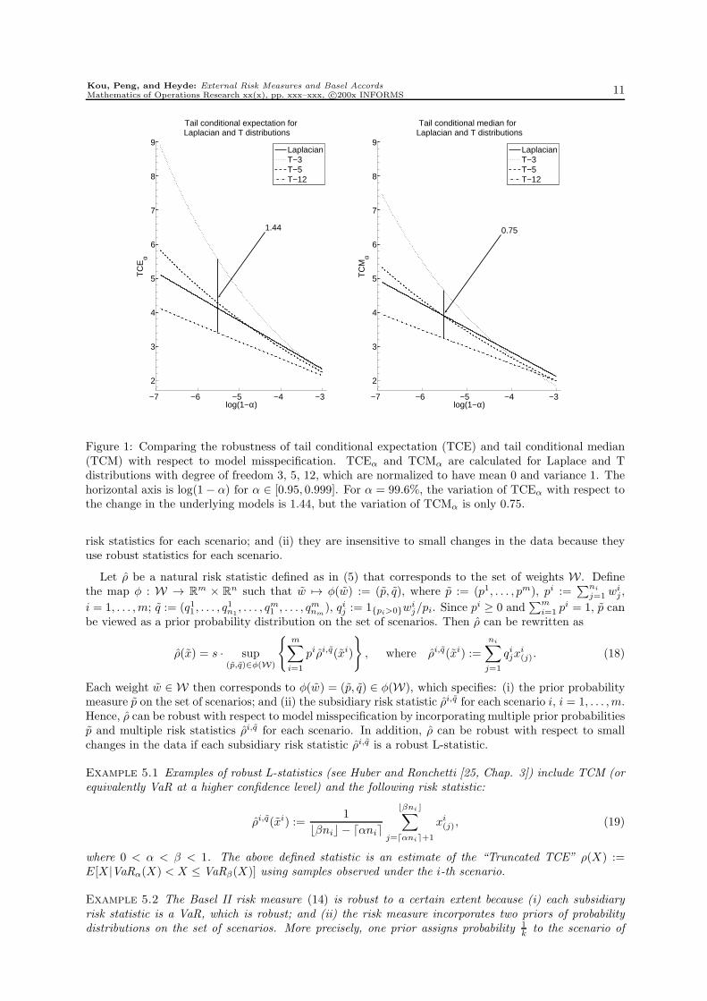
TCE is also highly model-dependent, and particularly sensitive to modeling assumptions on the ex-treme tails of loss distributions, because the computation of TCE relies on these extreme tails, as isshown by (66) in Appendix F. Figure 1 illustrates the sensitivity of TCE to modeling assumptions. TCMis clearly less sensitive to tail behavior than TCE, since the changes in TCM have narrower ranges thanthose in TCE.
5.5 Robust Natural Risk Statistics. Natural risk statistics include a subclass of risk statisticsthat are robust in two respects: (i) they are insensitive to model misspecification because they incorporatemultiple scenarios, multiple prior probability measures on the set of scenarios, and multiple subsidiary
Kou, Peng, and Heyde: External Risk Measures and Basel Accords
Mathematics of Operations Research xx(x), pp. xxx–xxx, c©200x INFORMS 11
−7 −6 −5 −4 −3
2
3
4
5
6
7
8
9
Tail conditional expectation for Laplacian and T distributions
log(1−α)
TC
Eα
LaplacianT−3T−5T−12
−7 −6 −5 −4 −3
2
3
4
5
6
7
8
9
Tail conditional median for Laplacian and T distributions
log(1−α)
TC
Mα
LaplacianT−3T−5T−12
1.44 0.75
Figure 1: Comparing the robustness of tail conditional expectation (TCE) and tail conditional median(TCM) with respect to model misspecification. TCEα and TCMα are calculated for Laplace and Tdistributions with degree of freedom 3, 5, 12, which are normalized to have mean 0 and variance 1. Thehorizontal axis is log(1 − α) for α ∈ [0.95, 0.999]. For α = 99.6%, the variation of TCEα with respect tothe change in the underlying models is 1.44, but the variation of TCMα is only 0.75.
risk statistics for each scenario; and (ii) they are insensitive to small changes in the data because theyuse robust statistics for each scenario.
Let ρ be a natural risk statistic defined as in (5) that corresponds to the set of weights W . Definethe map φ : W → Rm × Rn such that w 7→ φ(w) := (p, q), where p := (p1, . . . , pm), pi :=
∑ni
j=1 wij ,
i = 1, . . . ,m; q := (q11 , . . . , q1n1, . . . , qm1 , . . . , q
mnm
), qij := 1pi>0wij/pi. Since p
i ≥ 0 and∑m
i=1 pi = 1, p can
be viewed as a prior probability distribution on the set of scenarios. Then ρ can be rewritten as
ρ(x) = s · sup(p,q)∈φ(W)
m∑
i=1
piρi,q(xi)
, where ρi,q(xi) :=
ni∑
j=1
qijxi(j). (18)
Each weight w ∈ W then corresponds to φ(w) = (p, q) ∈ φ(W), which specifies: (i) the prior probabilitymeasure p on the set of scenarios; and (ii) the subsidiary risk statistic ρi,q for each scenario i, i = 1, . . . ,m.Hence, ρ can be robust with respect to model misspecification by incorporating multiple prior probabilitiesp and multiple risk statistics ρi,q for each scenario. In addition, ρ can be robust with respect to smallchanges in the data if each subsidiary risk statistic ρi,q is a robust L-statistic.
Example 5.1 Examples of robust L-statistics (see Huber and Ronchetti [25, Chap. 3]) include TCM (orequivalently VaR at a higher confidence level) and the following risk statistic:
ρi,q(xi) :=1
⌊βni⌋ − ⌈αni⌉
⌊βni⌋∑
j=⌈αni⌉+1
xi(j), (19)
where 0 < α < β < 1. The above defined statistic is an estimate of the “Truncated TCE” ρ(X) :=E[X |VaRα(X) < X ≤ VaRβ(X)] using samples observed under the i-th scenario.
Example 5.2 The Basel II risk measure (14) is robust to a certain extent because (i) each subsidiaryrisk statistic is a VaR, which is robust; and (ii) the risk measure incorporates two priors of probabilitydistributions on the set of scenarios. More precisely, one prior assigns probability 1
k to the scenario of
12 Kou, Peng, and Heyde: External Risk Measures and Basel Accords
Mathematics of Operations Research xx(x), pp. xxx–xxx, c©200x INFORMS
day t− 1 and 1− 1k to an imaginary scenario under which losses are identically 0; the other prior assigns
probability 160 to each of the scenarios corresponding to day t− i, i = 1, . . . , 60.
Example 5.3 The Basel III risk measure (15) is more robust than the Basel II risk measure (14) becauseit incorporates 60 more scenarios and it essentially incorporates two more priors of probability measureson the set of scenarios.
Example 5.4 Similar to the Basel II risk measure (14), the Basel III IRC risk measure (16) is robust
in the sense that each subsidiary risk statistic VaRirt−i is robust, and the risk measure incorporates twopriors of probability distributions on the set of scenarios.
5.6 Neither Coherent Risk Measures Nor Insurance Risk Measures Are Robust. Nocoherent risk measure is robust with respect to small changes in the data because coherent risk measuresexclude the use of robust statistics. Indeed, by Theorem 3.3, an empirical-law-invariant coherent riskstatistic ρ can be represented by (12), where for each weight w, wij is a nondecreasing function of j.Hence, any empirical-law-invariant coherent risk statistic assigns larger weights to larger observations,but assigning larger weights to larger observations is clearly sensitive to small changes in the data. Anextreme case is the maximum loss maxxi(ni)
: i = 1, . . . ,m, which is not robust at all. In general, the
finite sample breakdown point (see Huber and Ronchetti [25, Chap. 11] for definition) of any empirical-law-invariant coherent risk statistic is equal to 1/(1 + n), which implies that one single contaminationsample can cause unbounded bias. In particular, TCE is sensitive to modeling assumptions of heavinessof tail distributions and to outliers in the data, as is shown in Section 5.4.
No insurance risk measure is robust to model misspecification. An insurance risk measure can incor-porate neither multiple priors of probability distributions on the set of scenarios nor multiple subsidiaryrisk statistics for each scenario because it is defined by a single weight vector w, as is shown in Theorem3.4.
5.7 Conservative and Robust Risk Measures. One risk measure is said to be more conservativethan another if it generates higher risk measurement than the other for the same risk exposure. Theuse of more conservative risk measures in external regulation is desirable from a regulator’s viewpoint,since it generally increases the safety of the financial system. Of course, risk measures which are tooconservative may retard economic growth.
There is no contradiction between the robustness and the conservativeness of external risk measures.Robustness addresses the issue of whether a risk measure can be implemented consistently, so it is arequisite property of a good external risk measure. Conservativeness addresses the issue of how stringentlyan external risk measure should be implemented, given that it can be implemented consistently. In otherwords, an external risk measure should be robust in the first place before one can consider the issue ofhow to implement it in a conservative way. In addition, it is not true that TCE is more conservative thanTCM because the median can be bigger than the mean for some distributions. Eling and Tibiletti [12]compare TCE and TCM for a set of capital market data, including the returns of S&P 500 stocks, 1347mutual funds, and 205 hedge funds. They find that although TCE is on average about 10% higher thanTCM at standard confidence levels, TCM is higher than TCE in about 10% of the cases. So TCE is notnecessarily more conservative than TCM.
A natural risk statistic can be constructed by (5) in the following way so that it is both conservativeand robust: (i) more data subsets that correspond to stressed scenarios can be included in (5); and (ii)a larger constant s in (5) can be used. For example, adding 60 stressed scenarios makes (15) much moreconservative than (14), and a larger k or ℓ in (15) can be used by regulators to increase the capitalrequirements.
6. Other Reasons to Relax Subadditivity.
6.1 Diversification and Tail Subadditivity of VaR. The subadditivity axiom is related to theidea that diversification does not increase risk; the convexity axiom for convex risk measures also comesfrom the idea of diversification. There are two main justifications for diversification. One is based onthe simple observation that σ(X + Y ) ≤ σ(X) + σ(Y ), for any two random variables X and Y with
Kou, Peng, and Heyde: External Risk Measures and Basel Accords
Mathematics of Operations Research xx(x), pp. xxx–xxx, c©200x INFORMS 13
finite second moments, where σ(·) denotes standard deviation. The other is based on expected utilitytheory. Samuelson [39] shows that any investor with a strictly concave utility function will uniformlydiversify among independently and identically distributed (i.i.d.) risks with finite second moments; see,e.g., McMinn [36], Hong and Herk [23], and Kijima [32] for the discussion on whether diversification isbeneficial when the asset returns are dependent. Both justifications require that the risks have finitesecond moments.
Is diversification still preferable for risks with infinite second moments? The answer can be no. I-bragimov [26, 27] and Ibragimov and Walden [28] show that diversification is not preferable for riskswith extremely heavy tailed distributions (with tail index less than 1) in the sense that: (i) the loss ofthe diversified portfolio stochastically dominates that of the undiversified portfolio at the first order andsecond order; (ii) the expected utility of the (truncated) payoff of the diversified portfolio is smaller thanthat of the undiversified portfolio. They also show that investors with certain S-shaped utility functionswould prefer non-diversification, even for bounded risks.
In addition, the conclusion that VaR prohibits diversification, drawn from simple examples in theliterature, may not be solid. For instance, Artzner et al. [4] show that VaR prohibits diversification bya simple example (see pp. 217–218) in which 95% VaR of the diversified portfolio is higher than that ofthe undiversified portfolio. However, in the same example 99% VaR encourages diversification becausethe 99% VaR of the diversified portfolio is equal to 20,800, which is much lower than 1,000,000, the 99%VaR of the undiversified portfolio.
Ibragimov [26, 27] and Ibragimov and Walden [28] also show that although VaR does not satisfysubadditivity for risks with extremely heavy tailed distributions (with tail index less than 1), VaR satisfiessubadditivity for wide classes of independent and dependent risks with tail indices greater than 1. Inaddition, Danıelsson, Jorgensen, Samorodnitsky, Sarma, and de Vries [8] show that VaR is subadditive inthe tail region provided that the tail index of the joint distribution is larger than 1. Asset returns withtail indices less than 1 have extremely heavy tails; they are hard to find but easy to identify. Danıelssonet al. [8] argue that they can be treated as special cases in financial modeling. Even if one encountersan extremely fat tail and insists on tail subadditivity, Garcia, Renault, and Tsafack [15] show that whentail thickness causes violation of subadditivity, a decentralized risk management team may restore thesubadditivity for VaR by using proper conditional information. The simulations carried out in Danıelssonet al. [8] also show that VaRα is indeed subadditive for most practical applications when α ∈ [95%, 99%].
To summarize, there seems to be no conflict between the use of VaR and diversification. When therisks do not have extremely heavy tails, diversification seems to be preferred and VaR seems to satisfysubadditivity; when the risks have extremely heavy tails, diversification may not be preferable and VaRmay fail to satisfy subadditivity.
6.2 Does A Merger Always Reduce Risk? Subadditivity basically means that “a merger doesnot create extra risk” (see Artzner et al. [4, p. 209]). However, Dhaene, Goovaerts, and Kaas [11] pointout that a merger may increase risk, particularly when there is bankruptcy protection for institutions.For example, an institution can split a risky trading business into a separate subsidiary so that it has theoption to let the subsidiary go bankrupt when the subsidiary suffers enormous losses, confining losses tothat subsidiary. Therefore, creating subsidiaries may incur less risk and a merger may increase risk. HadBarings Bank set up a separate institution for its Singapore unit, the bankruptcy of that unit would nothave sunk the entire bank in 1995.
In addition, there is little empirical evidence supporting the argument that “a merger does not createextra risk.” In practice, credit rating agencies do not upgrade an institution’s credit rating because of amerger; on the contrary, the credit rating of the joint institution may be lowered shortly after the merger.The merger of Bank of America and Merrill Lynch in 2008 is an example.
7. Capital Allocation under the Natural Risk Statistics. In this section, we derive the capitalallocation rule for a subclass of natural risk statistics which include the Basel II and Basel III riskmeasures. The purpose of capital allocation for the whole portfolio is to decompose the overall capitalinto a sum of risk contributions for such purposes as identification of concentration, risk-sensitive pricing,and portfolio optimization (see, e.g., Litterman [34]).
First, as an illustration, we compute the Euler capital allocation under the Basel III risk measure.
14 Kou, Peng, and Heyde: External Risk Measures and Basel Accords
Mathematics of Operations Research xx(x), pp. xxx–xxx, c©200x INFORMS
The Euler rule is one of the most widely used methodologies for capital allocation under positive ho-mogeneous risk measures (see, e.g., Tasche [46]; McNeil, Frey, and Embrechts [37]). Consider a port-folio comprised of ui units of asset i, i = 1, . . . , d, and denote u = (u1, u2, . . . , ud). Suppose thatthere are m scenarios. Let x(i) = (x(i)1, x(i)2, . . . , x(i)m) be the observed loss of the i-th asset, wherex(i)s = (x(i)s1, x(i)
s2, . . . , x(i)
sns) ∈ Rns are the observations under the s-th scenario, s = 1, . . . ,m. Then
the observations of the portfolio loss are given by l(u) =∑d
i=1 uix(i) = (l(u)1, l(u)2, . . . , l(u)m), where
l(u)s = (l(u)s1, l(u)s2, . . . , l(u)
sns) ∈ Rns and l(u)sk :=
∑di=1 uix(i)
sk. The required capital measured by a
natural risk statistic ρ is denoted by Cρ(u) := ρ(l(u)). Let m = 120 and α = 99%, then the requiredcapital calculated by the Basel III risk measure is
Cρ(u) := max
l(u)1(⌈αn1⌉)
,k
60
60∑
s=1
l(u)s(⌈αns⌉)
+max
l(u)61(⌈αn61⌉)
,ℓ
60
120∑
s=61
l(u)s(⌈αns⌉)
.
We have the following proposition on the Euler capital allocation under the Basel III risk statistic:
Proposition 7.1 Suppose x is a sample of the random vector (X(1), X(2), . . . , X(d)), where X(i) =(X(i)1, X(i)2, . . . , X(i)m) and X(i)s = (X(i)s1, X(i)s2, . . . , X(i)sns
) ∈ Rns . Suppose that the joint distri-bution of (X(1), X(2), . . . , X(d)) has a probability density on Rdn. Then for any given u 6= 0, it holdswith probability 1 that
Cρ(u) =
d∑
i=1
ui∂Cρ(u)
∂ui, (20)
and the capital allocation for the i-th asset under the Euler’s rule is ui∂Cρ(u)∂ui
.
Proof. For any given u 6= 0, let Xu be the set of samples (x(1), x(2), . . . , x(d)) ∈ Rdn that satisfythe following conditions: (i) l(u)1(⌈αn1⌉)
6= k60
∑60s=1 l(u)
s(⌈αns⌉)
; (ii) l(u)61(⌈αn61⌉)6= ℓ
60
∑120s=61 l(u)
s(⌈αns⌉)
;
(iii) l(u)si 6= l(u)sj for any s and i 6= j. Then it follows from the condition of the proposition thatP ((X(1), X(2), . . . , X(d)) ∈ Xu) = 1. Fix any (x(1), x(2), . . . , x(d)) ∈ Xu. By the definition of Xu, thereexists δ > 0, such that Cρ(·) is a linear function on the open set V := v ∈ Rd : ‖v − u‖ < δ. Hence,Cρ(·) is differentiable at u and Eq. (20) holds.
Let Xu be defined in the above proof and x ∈ Xu. To compute ui∂Cρ(u)∂ui
, one only needs to compute∂l(u)s(⌈αns⌉)
∂ui. Let (p1, . . . , pns
) be the permutation of (1, 2, . . . , ns) such that l(u)sp1 < l(u)sp2 < · · · <
l(u)spns. Then there exists a neighborhood V := v ∈ Rd : ‖v − u‖ < δ of u such that l(v)sp1 <
l(v)sp2 < · · · < l(v)spnsfor ∀v ∈ V . Hence, for ∀v ∈ V , l(v)s(⌈αns⌉)
= l(v)sp⌈αns⌉=∑d
i=1 vix(i)sp⌈αns⌉
, and∂l(u)s(⌈αns⌉)
∂ui= x(i)sp⌈αns⌉
.
In general, let Υ1 be the set of natural risk statistic ρ that can be represented in Eq. (6) by a finite
set W . Let Υ2 be the set of natural risk statistic ρ that can be written as ρ =∑K
k=1 akρk, where ak ≥ 0and ρk ∈ Υ1, k = 1, . . . ,K. Both the Basel II risk measure and Basel III risk measure belong to the setΥ2. For any ρ ∈ Υ2, it can be shown in the same way as in Proposition 7.1 that Cρ(u) is a piece-wiselinear function of u and the Euler capital allocation rule can be computed similarly.
8. Conclusion. We propose a class of data-based risk measures called natural risk statistics that arecharacterized by a new set of axioms. The new axioms only require subadditivity for comonotonic randomvariables, thus relaxing the subadditivity for all random variables required by coherent risk measures,and relaxing the comonotonic additivity required by insurance risk measures.
Natural risk statistics include VaR with scenario analysis, and particularly the Basel II and BaselIII risk measures, as special cases. Thus, natural risk statistics provide a theoretical framework forunderstanding and, if necessary, extending the Basel accords. Indeed, the framework is general enoughto include the counter-cyclical indexing risk measure suggested by Gordy and Howells [19] to address theprocyclicality problem in Basel II.
We emphasize that an external risk measure should be robust to model misspecification and smallchanges in the data in order for its consistent implementation across different institutions. We show that
Kou, Peng, and Heyde: External Risk Measures and Basel Accords
Mathematics of Operations Research xx(x), pp. xxx–xxx, c©200x INFORMS 15
coherent risk measures are generally not robust with respect to small changes in the data and insurancerisk measures are generally not robust with respect to model misspecification.
Natural risk statistics include a subclass of robust risk measures that are suitable for external regula-tion. In particular, natural risk statistics include tail conditional median (with scenario analysis), whichis more robust than tail conditional expectation suggested by the theory of coherent risk measures. TheEuler capital allocation can also be easily calculated under the natural risk statistics.
Appendix A. Proof of Theorem 3.1. A simple observation is that ρ is a natural risk statisticcorresponding to a constant s in Axiom C1 if and only if 1
s ρ is a natural risk statistic corresponding to theconstant s = 1 in Axiom C1. Therefore, in this section, we assume without loss of generality that s = 1in Axiom C1. The proof relies on the following two lemmas, which depend heavily on the properties ofthe interior points of the set
B := y = (y1, . . . , ym) ∈ Rn | y11 ≤ y12 ≤ · · · ≤ y1n1; . . . ; ym1 ≤ ym2 ≤ · · · ≤ ymnm
. (21)
The results for boundary points will be obtained by approximating the boundary points by the interiorpoints, and by employing continuity and uniform convergence.
Lemma A.1 Let B be defined in (21) and Bo be the interior of B. For any fixed z ∈ Bo and any ρsatisfying Axiom C1-C4 and ρ(z) = 1, there exists a weight w = (w1, . . . , wm) ∈ Rn such that the linearfunctional λ(x) :=
∑n1
j=1 w1jx
1j +
∑n2
j=1 w2jx
2j + · · ·+
∑nm
j=1 wmj x
mj satisfies
λ(z) = 1, (22)
λ(x) < 1 for any x such that x ∈ B and ρ(x) < 1. (23)
Proof. Let U = x = (x1, . . . , xm) | ρ(x) < 1 ∩ B. For any x = (x1, . . . , xm) ∈ B and y =(y1, . . . , ym) ∈ B, x and y are scenario-wise comonotonic. Then Axiom C1 and C3 imply that U is convex,and, hence, the closure U of U is also convex. For any ε > 0, since ρ(z − ε1) = ρ(z) − ε = 1 − ε < 1, itfollows that z−ε1 ∈ U . Since z−ε1 tends to z as ε ↓ 0, we know that z is a boundary point of U becauseρ(z) = 1. Therefore, there exists a supporting hyperplane for U at z, i.e., there exists a nonzero vectorw = (w1, . . . , wm) = (w1
1 , . . . , w1n1, . . . , wm1 , . . . , w
mnm
) ∈ Rn such that λ(x) :=∑n1
j=1 w1jx
1j +
∑n2
j=1 w2jx
2j +
· · ·+∑nm
j=1 wmj x
mj satisfies λ(x) ≤ λ(z) for any x ∈ U . In particular, we have
λ(x) ≤ λ(z), ∀x ∈ U. (24)
We shall show that the strict inequality holds in (24). Suppose, by contradiction, that there existsr ∈ U such that λ(r) = λ(z). For any α ∈ (0, 1), we have
λ(αz + (1− α)r) = αλ(z) + (1 − α)λ(r) = λ(z). (25)
In addition, since z and r are scenario-wise comonotonic, we have
ρ(αz + (1− α)r) ≤ αρ(z) + (1− α)ρ(r) < α+ (1 − α) = 1, ∀α ∈ (0, 1). (26)
Since z ∈ Bo, it follows that there exists α0 ∈ (0, 1) such that α0z+(1−α0)r ∈ Bo. Hence, for any smallenough ε > 0,
α0z + (1 − α0)r + εw ∈ B. (27)
With wmax := maxw11, w
12 , . . . , w
1n1;w2
1 , w22 , . . . , w
2n2; . . . ;wm1 , w
m2 , . . . , w
mnm
, we have α0z + (1 − α0)r +εw ≤ α0z + (1− α0)r + εwmax1. Thus, the monotonicity in Axiom C2 and translation scaling in AxiomC1 yield
ρ(α0z + (1− α0)r + εw) ≤ ρ(α0z + (1− α0)r + εwmax1) = ρ(α0z + (1− α0)r) + εwmax. (28)
Since ρ(α0z + (1 − α0)r) < 1 via (26), we have by (28) and (27) that for any small enough ε > 0,ρ(α0z+(1−α0)r+εw) < 1, α0z+(1−α0)r+εw ∈ U . Hence, (24) implies λ(α0z+(1−α0)r+εw) ≤ λ(z).However, we have, by (25), an opposite inequality λ(α0z+(1−α0)r+εw) = λ(α0z+(1−α0)r)+ε|w|
2 >λ(α0z + (1− α0)r) = λ(z), leading to a contradiction. In summary, we have shown that
λ(x) < λ(z), ∀x ∈ U. (29)
Since ρ(0) = 0, we have 0 ∈ U . Letting x = 0 in (29) yields λ(z) > 0, so we can re-scale w such thatλ(z) = 1 = ρ(z). Thus, (29) becomes λ(x) < 1 for any x such that x ∈ B and ρ(x) < 1, from which (23)holds.
16 Kou, Peng, and Heyde: External Risk Measures and Basel Accords
Mathematics of Operations Research xx(x), pp. xxx–xxx, c©200x INFORMS
Lemma A.2 Let B be defined in (21) and Bo be the interior of B. For any fixed z ∈ Bo and any ρsatisfying Axiom C1-C4, there exists a weight w = (w1, . . . , wm) ∈ Rn such that w satisfies (3) and (4),and
ρ(x) ≥
m∑
i=1
ni∑
j=1
wijxij for any x ∈ B, and ρ(z) =
m∑
i=1
ni∑
j=1
wijzij . (30)
Proof. We will show this by considering three cases.
Case 1: ρ(z) = 1. From Lemma A.1, there exists a weight w = (w1, . . . , wm) ∈ Rn such that the linearfunctional λ(x) :=
∑mi=1
∑ni
j=1 wijxij satisfies (22) and (23).
Firstly, we prove that w satisfies (3), which is equivalent to λ(1) = 1. To this end, first note that for anyc < 1, Axiom C1 implies ρ(c1) = c < 1. Thus, (23) implies λ(c1) < 1, and, by continuity of λ(·), we obtainthat λ(1) ≤ 1. On the other hand, for any c > 1, Axiom C1 implies ρ(2z − c1) = 2ρ(z)− c = 2− c < 1.Then it follows from (23) and (22) that 1 > λ(2z − c1) = 2λ(z)− cλ(1) = 2 − cλ(1), i.e. λ(1) > 1/c forany c > 1. So λ(1) ≥ 1, and w satisfies (3).
Secondly, we prove that w satisfies (4). For any fixed i and 1 ≤ j ≤ ni, let k = n1+n2+ · · ·+ni−1+ jand e = (0, . . . , 0, 1, 0, . . . , 0) be the k-th standard basis of Rn. Then wij = λ(e). Since z ∈ Bo, thereexists δ > 0 such that z−δe ∈ B. For any ε > 0, Axiom C1 and C2 imply ρ(z−δe−ε1) = ρ(z−δe)−ε ≤ρ(z)− ε = 1− ε < 1. Then (23) and (22) imply 1 > λ(z− δe− ε1) = λ(z)− δλ(e)− ελ(1) = 1− ε− δλ(e).Hence, wij = λ(e) > −ε/δ, and the conclusion follows by letting ε go to 0.
Thirdly, we prove that w satisfies (30). It follows from Axiom C1 and (23) that
∀c > 0, λ(x) < c for any x such that x ∈ B and ρ(x) < c. (31)
For any c ≤ 0, we choose b > 0 such that b + c > 0. Then by (31), we have λ(x + b1) < c+ b for any xsuch that x ∈ B and ρ(x+b1) < c+b. Since λ(x+b1) = λ(x)+bλ(1) = λ(x)+b and ρ(x+b1) = ρ(x)+b,we have
∀c ≤ 0, λ(x) < c for any x such that x ∈ B and ρ(x) < c. (32)
It follows from (31) and (32) that ρ(x) ≥ λ(x) for any x ∈ B, which in combination with ρ(z) = 1 = λ(z)completes the proof of (30).
Case 2: ρ(z) 6= 1 and ρ(z) > 0. Since ρ(
1ρ(z) z
)= 1 and 1
ρ(z) z ∈ Bo, it follows from the result proved
in Case 1 that there exists a weight w = (w1, . . . , wm) ∈ Rn such that w satisfies (3), (4), and the linear
functional λ(x) :=∑mi=1
∑ni
j=1 wijxij satisfies ρ(x) ≥ λ(x) for ∀x ∈ B and ρ
(1
ρ(z) z)
= λ(
1ρ(z) z
), or
equivalently ρ(z) = λ(z). Thus, w also satisfies (30).
Case 3: ρ(z) ≤ 0. Choose b > 0 such that ρ(z + b1) > 0. Since z + b1 ∈ Bo, it follows from theresults proved in Case 1 and Case 2 that there exists a weight w = (w1, . . . , wm) ∈ Rn such that wsatisfies (3), (4), and the linear functional λ(x) :=
∑mi=1
∑ni
j=1 wijxij satisfies ρ(x) ≥ λ(x) for ∀x ∈ B, and
ρ(z + b1) = λ(z + b1), or equivalently ρ(z) = λ(z). Thus, w also satisfies (30).
Proof of Theorem 3.1. Firstly, we prove part (i). Suppose ρ is defined by (5), then obviously ρsatisfies Axiom C1 and C4. To check Axiom C2, suppose x ≤ y. For each i = 1, . . . ,m, let (pi,1, . . . , pi,ni
)be the permutation of (1, . . . , ni) such that (yi(1), y
i(2), . . . , y
i(ni)
) = (yipi,1 , yipi,2 , . . . , y
ipi,ni
). Then for any
1 ≤ j ≤ ni and 1 ≤ i ≤ m, yi(j) = yipi,j = maxyipi,k ; k = 1, . . . , j ≥ maxxipi,k ; k = 1, . . . , j ≥ xi(j),which implies that ρ satisfies Axiom C2 because
ρ(y) = supw∈W
m∑
i=1
ni∑
j=1
wijyi(j)
≥ sup
w∈W
m∑
i=1
ni∑
j=1
wijxi(j)
= ρ(x).
To check Axiom C3, note that if x and y are scenario-wise comonotonic, then for each i = 1, . . . ,m,there exists a permutation (pi,1, . . . , pi,ni
) of (1, . . . , ni) such that xipi,1 ≤ xipi,2 ≤ · · · ≤ xipi,niand yipi,1 ≤
yipi,2 ≤ · · · ≤ yipi,ni. Hence, we have (xi + yi)(j) = xipi,j + yipi,j = xi(j) + yi(j), j = 1, . . . , ni; i = 1, . . . ,m.
Kou, Peng, and Heyde: External Risk Measures and Basel Accords
Mathematics of Operations Research xx(x), pp. xxx–xxx, c©200x INFORMS 17
Therefore,
ρ(x+ y) = ρ((x1 + y1, . . . , xm + ym))
= supw∈W
m∑
i=1
ni∑
j=1
wij(xi + yi)(j)
= sup
w∈W
m∑
i=1
ni∑
j=1
wij(xi(j) + yi(j))
≤ supw∈W
m∑
i=1
ni∑
j=1
wijxi(j)
+ sup
w∈W
m∑
i=1
ni∑
j=1
wijyi(j)
= ρ(x) + ρ(y),
which implies that ρ satisfies Axiom C3.
Secondly, we prove part (ii). Let B be defined in (21). By Axiom C4, we only need to show thatthere exists a set of weights W = w ⊂ Rn such that each w ∈ W satisfies condition (3) and (4), andρ(x) = supw∈W
∑mi=1
∑ni
j=1 wijxij for ∀x ∈ B.
By Lemma A.2, for any point y ∈ Bo, there exists a weight w(y) = (w(y)11, . . . ,w(y)1n1
; . . . ;w(y)m1 , . . . , w(y)mnm
) ∈ Rn such that (3) and (4) hold, and that
ρ(x) ≥
m∑
i=1
ni∑
j=1
w(y)ijxij for ∀x ∈ B, and ρ(y) =
m∑
i=1
ni∑
j=1
w(y)ijyij . (33)
Define W as the collection of such weights, i.e., W := w(y) | y ∈ Bo, then each w ∈ W satisfies (3) and(4). From (33), for any fixed x ∈ Bo, we have
ρ(x) ≥
m∑
i=1
ni∑
j=1
w(y)ijxij for ∀y ∈ Bo, and ρ(x) =
m∑
i=1
ni∑
j=1
w(x)ijxij .
Therefore,
ρ(x) = supy∈Bo
m∑
i=1
ni∑
j=1
w(y)ijxij
= sup
w∈W
m∑
i=1
ni∑
j=1
wijxij
, ∀x ∈ Bo. (34)
Next, we prove that the above equality is also true for any boundary points of B, i.e.,
ρ(x) = supw∈W
m∑
i=1
ni∑
j=1
wijxij
, ∀x ∈ ∂B. (35)
Let b = (b11, . . . , b1n1, . . . , bm1 , . . . , b
mnm
) be any boundary point of B. Then there exists a sequence
b(k)∞k=1 ⊂ Bo such that b(k) → b as k → ∞. By the continuity of ρ and (34), we have
ρ(b) = limk→∞
ρ(b(k)) = limk→∞
supw∈W
m∑
i=1
ni∑
j=1
wijb(k)ij
. (36)
If we can interchange sup and limit in (36), i.e. if
limk→∞
supw∈W
m∑
i=1
ni∑
j=1
wijb(k)ij
= sup
w∈W
limk→∞
m∑
i=1
ni∑
j=1
wijb(k)ij
= sup
w∈W
m∑
i=1
ni∑
j=1
wijbij
, (37)
then (35) holds and the proof is completed. To show (37), note by Cauchy-Schwarz inequality∣∣∣∣∣∣
m∑
i=1
ni∑
j=1
wijb(k)ij −
m∑
i=1
ni∑
j=1
wijbij
∣∣∣∣∣∣
≤
m∑
i=1
ni∑
j=1
(wij)2
12
m∑
i=1
ni∑
j=1
(b(k)ij − bij)2
12
≤
m∑
i=1
ni∑
j=1
(b(k)ij − bij)2
12
, ∀w ∈ W ,
because wij ≥ 0 and∑m
i=1
∑ni
j=1 wij = 1, ∀w ∈ W . Hence,
∑mi=1
∑ni
j=1 wijb(k)
ij →
∑mi=1
∑ni
j=1 wijbij uni-
formly for all w ∈ W as k → ∞. Therefore, (37) follows.
18 Kou, Peng, and Heyde: External Risk Measures and Basel Accords
Mathematics of Operations Research xx(x), pp. xxx–xxx, c©200x INFORMS
Appendix B. The Second Representation via Acceptance Sets. A statistical acceptance setis a subset of Rn that includes all the data considered acceptable by a regulator in terms of the riskmeasured from them. Given a statistical acceptance set A, the risk statistic ρA associated with A isdefined to be
ρA(x) := infh | x− h1 ∈ A, ∀x ∈ Rn. (38)
ρA(x) is the minimum amount of cash that has to be added to the original position corresponding to xin order for the resulting position to be acceptable.
On the other hand, given a risk statistic ρ, one can define the statistical acceptance set associated withρ by
Aρ := x ∈ Rn | ρ(x) ≤ 0. (39)
We shall postulate the following axioms for the statistical acceptance set A:
Axiom D1. A contains Rn−, where Rn− := x ∈ Rn | xij ≤ 0, j = 1, . . . , ni; i = 1, . . . ,m.
Axiom D2. A does not intersect the set Rn++, where Rn++ := x ∈ Rn | xij > 0, j = 1, . . . , ni; i =1, . . . ,m.
Axiom D3. If x and y are scenario-wise comonotonic and x ∈ A, y ∈ A, then λx + (1 − λ)y ∈ A, for∀λ ∈ [0, 1].
Axiom D4. A is positively homogeneous, i.e., if x ∈ A, then λx ∈ A for any λ ≥ 0.
Axiom D5. If x ≤ y and y ∈ A, then x ∈ A.
Axiom D6. A is empirical-law-invariant, i.e., if x = (x11, x12, . . . , x
1n1, . . . , xm1 , x
m2 , . . . ,
xmnm) ∈ A, then for any permutation (pi,1, pi,2, . . . , pi,ni
) of (1, 2, . . . , ni), i = 1, . . . ,m, it holds that(x1p1,1 , x
1p1,2 , . . . , x
1p1,n1
, . . . , xmpm,1, xmpm,2
, . . . , xmpm,nm) ∈ A.
The following theorem shows that a natural risk statistic and a statistical acceptance set satisfyingAxiom D1-D6 are mutually representable.
Theorem B.1 (i) If ρ is a natural risk statistic, then the statistical acceptance set Aρ is closed andsatisfies Axiom D1-D6.
(ii) If a statistical acceptance set A satisfies Axiom D1-D6, then the risk statistic ρA is a natural riskstatistic (with s = 1 in Axiom C1).
(iii) If ρ is a natural risk statistic, then ρ = sρAρ.
(iv) If a statistical acceptance set D satisfies Axiom D1-D6, then AρD = D, the closure of D.
Proof. (i) (1) For ∀x ≤ 0, Axiom C2 implies ρ(x) ≤ ρ(0) = 0. Hence, x ∈ Aρ by definition.Thus, D1 holds. (2) For any x ∈ Rn++, there exists α > 0 such that 0 ≤ x − α1. Axiom C2 and C1imply that ρ(0) ≤ ρ(x − α1) = ρ(x) − sα. So ρ(x) ≥ sα > 0 and hence x /∈ Aρ, i.e., D2 holds. (3)If x and y are scenario-wise comonotonic and x ∈ Aρ, y ∈ Aρ, then ρ(x) ≤ 0, ρ(y) ≤ 0, and λx and(1 − λ)y are scenario-wise comonotonic for any λ ∈ [0, 1]. Thus, Axiom C3 implies ρ(λx + (1 − λ)y) ≤ρ(λx) + ρ((1 − λ)y) = λρ(x) + (1 − λ)ρ(y) ≤ 0. Hence, λx + (1 − λ)y ∈ Aρ, i.e., D3 holds. (4) For anyx ∈ Aρ and a > 0, we have ρ(x) ≤ 0 and Axiom C1 implies ρ(ax) = aρ(x) ≤ 0. Thus, ax ∈ Aρ, i.e., D4holds. (5) For any x ≤ y and y ∈ Aρ, we have ρ(y) ≤ 0. By Axiom C2, ρ(x) ≤ ρ(y) ≤ 0. Hence, x ∈ Aρ,i.e., D5 holds. (6) If x ∈ Aρ, then ρ(x) ≤ 0. For any permutation (pi,1, pi,2, . . . , pi,ni
) of (1, 2, . . . , ni),i = 1, . . . ,m, Axiom C4 implies ρ((x1p1,1 , x
1p1,2 , . . . , x
1p1,n1
, . . . , xmpm,1, xmpm,2
. . . , xmpm,nm)) = ρ(x) ≤ 0. So
(x1p1,1 , x1p1,2 , . . . , x
1p1,n1
, . . . , xmpm,1, xmpm,2
. . . , xmpm,nm) ∈ Aρ, i.e., D6 holds. (7) Suppose x(k)∞k=1 ⊂ Aρ,
and x(k) → x as k → ∞. Then ρ(x(k)) ≤ 0, ∀k. The continuity of ρ (see the comment following the
definition of Axiom C2) implies ρ(x) = limk→∞ ρ(x(k)) ≤ 0. So x ∈ Aρ, i.e., Aρ is closed.
(ii) (1) For ∀x ∈ Rn, ∀b ∈ R, we have
ρA(x+ b1) = infh | x+ b1− h1 ∈ A = b+ infh− b | x− (h− b)1 ∈ A
=b+ infh | x− h1 ∈ A = b+ ρA(x).
Kou, Peng, and Heyde: External Risk Measures and Basel Accords
Mathematics of Operations Research xx(x), pp. xxx–xxx, c©200x INFORMS 19
For ∀x ∈ Rn, ∀a ≥ 0, if a = 0, then ρA(ax) = infh | 0 − h1 ∈ A = 0 = aρA(x), where the secondequality follows from Axiom D1 and D2. If a > 0, then
ρA(ax) = infh | ax− h1 ∈ A = a · infu | a(x− u1) ∈ A
= a · infu | x− u1 ∈ A = aρA(x),
by Axiom D4. Therefore, C1 holds (with s = 1). (2) Suppose x ≤ y. For any h ∈ R, if y − h1 ∈ A, thenAxiom D5 and x − h1 ≤ y − h1 imply that x − h1 ∈ A. Hence, h | y − h1 ∈ A ⊆ h | x − h1 ∈ A.By taking infimum on both sides, we obtain ρA(y) ≥ ρA(x), i.e., C2 holds. (3) Suppose x and y arescenario-wise comonotonic. For any g and h such that x − g1 ∈ A and y − h1 ∈ A, since x − g1 andy − h1 are scenario-wise comonotonic, it follows from Axiom D3 that 1
2 (x − g1) + 12 (y − h1) ∈ A. By
Axiom D4, the previous formula implies x + y − (g + h)1 ∈ A. Therefore, ρA(x + y) ≤ g + h. Takinginfimum of all g and h satisfying x − g1 ∈ A, y − h1 ∈ A, on both sides of the above inequality yieldsρA(x + y) ≤ ρA(x) + ρA(y). So C3 holds. (4) Fix any x ∈ Rn and any permutation (pi,1, pi,2, . . . , pi,ni
)of (1, 2, . . . , ni), i = 1, . . . ,m. Then for any h ∈ R, Axiom D6 implies that x − h1 ∈ A if and onlyif (x1p1,1 , x
1p1,2 , . . . , x
1p1,n1
, . . . , xmpm,1, xmpm,2
, . . . , xmpm,nm) − h1 ∈ A. Hence, h | x − h1 ∈ A = h |
(x1p1,1 , x1p1,2 , . . . , x
1p1,n1
, . . . , xmpm,1, xmpm,2
, . . . , xmpm,nm) − h1 ∈ A. Taking infimum, we obtain ρA(x) =
ρA((x1p1,1 , x
1p1,2 , . . . , x
1p1,n1
, . . . , xmpm,1, xmpm,2
, . . . , xmpm,nm)), i.e., C4 holds.
(iii) For ∀x ∈ Rn, we have ρAρ(x) = infh | x − h1 ∈ Aρ = infh | ρ(x − h1) ≤ 0 = infh | ρ(x) ≤
sh = 1s ρ(x), where the third equality follows from Axiom C1.
(iv) For any x ∈ D, we have ρD(x) ≤ 0. Hence, x ∈ AρD . Therefore, D ⊆ AρD . By the results (i)and (ii), AρD is closed. So D ⊆ AρD . On the other hand, for any x ∈ AρD , we have by definition thatρD(x) ≤ 0, i.e., infh | x − h1 ∈ D ≤ 0. If infh | x − h1 ∈ D < 0, then there exists h < 0 such thatx−h1 ∈ D. Then since x < x−h1, by D5 x ∈ D. Otherwise, infh | x−h1 ∈ D = 0. Then there existshk such that hk ↓ 0 as k → ∞ and x− hk1 ∈ D. Hence, x ∈ D. In either case we obtain x ∈ D. Hence,AρD ⊆ D. Therefore, we conclude that AρD = D.
Appendix C. Proof of Theorem 3.3. In this section, we assume without loss of generality thats = 1 in Axiom C1. The proof for Theorem 3.3 follows the same line as that for Theorem 3.1. We firstprove two lemmas that are similar to Lemma A.1 and A.2.
Lemma C.1 Let B be defined in (21). For any fixed z ∈ B and any ρ satisfying Axiom C1, C2, E3, C4and ρ(z) = 1, there exists a weight w = (w1, . . . , wm) ∈ Rn satisfying (10) such that the linear functionalλ(x) :=
∑n1
j=1 w1jx
1j +
∑n2
j=1 w2jx
2j + · · ·+
∑nm
j=1 wmj x
mj satisfies
λ(z) = 1, (40)
λ(x) < 1 for any x such that ρ(x) < 1. (41)
Proof. Let U = x | ρ(x) < 1. Axiom C1 and E3 imply that U is convex, and, hence, the closureU of U is also convex.
For any ε > 0, since ρ(z − ε1) = ρ(z) − ε = 1 − ε < 1, it follows that z − ε1 ∈ U . Since z − ε1converges to z as ε ↓ 0, z is a boundary point of U because ρ(z) = 1. Therefore, there exists a supportinghyperplane for U at z, i.e., there exists a nonzero vector u = (u11, . . . , u
1n1, . . . , um1 , . . . , u
mnm
) ∈ Rn suchthat µ(x) :=
∑mi=1
∑ni
j=1 uijxij satisfies µ(x) ≤ µ(z) for any x ∈ U . In particular, we have
µ(x) ≤ µ(z), ∀x ∈ U. (42)
For each i = 1, . . . ,m, let φi : 1, 2, . . . , ni → 1, 2, . . . , ni be a bijection such that uiφi(1)≤ uiφi(2)
≤
· · · ≤ uiφi(ni), and ψi(·) be the inverse of φi(·). Define a new weight w and a new linear functional λ(·) as
follows:
wij :=uiφi(j)
, j = 1, . . . , ni; i = 1, . . . ,m, (43)
w :=(w11 , . . . , w
1n1, . . . , wm1 , . . . , w
mnm
), (44)
λ(x) :=
m∑
i=1
ni∑
j=1
wijxij , (45)
20 Kou, Peng, and Heyde: External Risk Measures and Basel Accords
Mathematics of Operations Research xx(x), pp. xxx–xxx, c©200x INFORMS
then by definition w satisfies condition (10). For any fixed x ∈ U , by AxiomC4, ρ((x1ψ1(1)
, . . . , x1ψ1(n1), . . . , xmψm(1), . . . , x
mψm(nm))) = ρ(x) < 1, so (x1ψ1(1)
, . . . , x1ψ1(n1), . . . ,
xmψm(1), . . . , xmψm(nm)) ∈ U . Then, we have
λ(x) =
m∑
i=1
ni∑
j=1
wijxij =
m∑
i=1
ni∑
j=1
uiφi(j)xij =
m∑
i=1
ni∑
j=1
uiφi(ψi(j))xiψi(j)
=
m∑
i=1
ni∑
j=1
uijxiψi(j)
=µ((x1ψ1(1), . . . , x1ψ1(n1)
, . . . , xmψm(1), . . . , xmψm(nm))) ≤ µ(z) (by (42)). (46)
Noting that zi1 ≤ zi2 ≤ · · · ≤ zini, i = 1, 2, . . . ,m, we obtain
µ(z) =
m∑
i=1
ni∑
j=1
uijzij ≤
m∑
i=1
ni∑
j=1
uiφi(j)zij = λ(z). (47)
By (46) and (47), we haveλ(x) ≤ λ(z), ∀x ∈ U. (48)
We shall show that the strict inequality holds in (48). Suppose, by contradiction, thatthere exists r ∈ U such that λ(r) = λ(z). With wmax := maxw1
1, . . . , w1n1, . . . , wm1 ,
. . . , wmnm, we have r + εw ≤ r + εwmax1 for any ε > 0. Thus, Axiom C1 and C2 yield
ρ(r + εw) ≤ ρ(r + εwmax1) = ρ(r) + εwmax, ∀ε > 0. (49)
Since ρ(r) < 1, we have by (49) that for small enough ε > 0, ρ(r + εw) < 1. Hence, r+ εw ∈ U and (48)implies λ(r + εw) ≤ λ(z). However, λ(r + εw) = λ(r) + ε|w|2 > λ(r) = λ(z), leading to a contradiction.In summary, we have shown that
λ(x) < λ(z), ∀x ∈ U. (50)
Since ρ(0) = 0, we have 0 ∈ U . Letting x = 0 in (50) yields λ(z) > 0, so we can re-scale w such thatλ(z) = 1 = ρ(z). Thus, (50) becomes λ(x) < 1 for any x such that ρ(x) < 1, from which (41) holds.
Lemma C.2 Let B be defined in (21). For any fixed z ∈ B and any ρ satisfying Axiom C1, C2, E3 andC4, there exists a weight w = (w1, . . . , wm) ∈ Rn satisfying (8), (9), and (10), such that
ρ(x) ≥
m∑
i=1
ni∑
j=1
wijxij for any x ∈ Rn, and ρ(z) =
m∑
i=1
ni∑
j=1
wijzij. (51)
Proof. We will show this by considering two cases.
Case 1: ρ(z) = 1. From Lemma C.1, there exists a weight w = (w1, . . . , wm) ∈ Rn satisfying (10) suchthat the linear functional λ(x) :=
∑mi=1
∑ni
j=1 wijxij satisfies (40) and (41).
Firstly, we prove that w satisfies (8), which is equivalent to λ(1) = 1. To this end, first note that for anyc < 1, Axiom C1 implies ρ(c1) = c < 1. Thus, (41) implies λ(c1) < 1, and, by continuity of λ(·), we obtainthat λ(1) ≤ 1. On the other hand, for any c > 1, Axiom C1 implies ρ(2z − c1) = 2ρ(z)− c = 2− c < 1.Then it follows from (40) and (41) that 1 > λ(2z − c1) = 2λ(z)− cλ(1) = 2 − cλ(1), i.e. λ(1) > 1/c forany c > 1. So λ(1) ≥ 1, and w satisfies (8). Secondly, we prove that w satisfies (9). For any fixed i and1 ≤ j ≤ ni, let k = n1+n2+ · · ·+ni−1+ j and e = (0, . . . , 0, 1, 0, . . . , 0) be the k-th standard basis of Rn.Then wij = λ(e). For any ε > 0, Axiom C1 and C2 imply ρ(z− e−ε1) = ρ(z− e)−ε ≤ ρ(z)−ε = 1−ε < 1.
Then (40) and (41) imply 1 > λ(z− e−ε1) = λ(z)−λ(e)−ελ(1) = 1−ε−λ(e). Hence, wij = λ(e) > −ε,and the conclusion follows by letting ε go to 0. Thirdly, we prove that w satisfies (51). It follows fromAxiom C1 and (41) that
∀c > 0, λ(x) < c for any x such that ρ(x) < c. (52)
For any c ≤ 0, we choose b > 0 such that b+ c > 0. Then it follows from (52) that λ(x+ b1) < c+ b forany x such that ρ(x + b1) < c+ b. Since λ(x+ b1) = λ(x) + bλ(1) = λ(x) + b and ρ(x+ b1) = ρ(x) + b,we have
∀c ≤ 0, λ(x) < c for any x such that ρ(x) < c. (53)
It follows from (52) and (53) that ρ(x) ≥ λ(x) for any x ∈ Rn, which in combination with ρ(z) = 1 = λ(z)completes the proof of (51).
Kou, Peng, and Heyde: External Risk Measures and Basel Accords
Mathematics of Operations Research xx(x), pp. xxx–xxx, c©200x INFORMS 21
Case 2: ρ(z) 6= 1. The argument is the same as that in case 2 and case 3 of the proof for Lemma A.2.
Proof of Theorem 3.3. Without loss of generality, we assume s = 1 in Axiom C1.
Firstly, we prove part (i). We only need to show that under condition (10), the risk statistic (11)satisfies subadditivity for any x and y ∈ Rn. Let (pi,1, pi,2, . . . , pi,ni
) be the permutation of (1, . . . , ni)such that (xi + yi)pi,1 ≤ (xi + yi)pi,2 ≤ · · · ≤ (xi + yi)pi,ni
. Then for k = 1, . . . , ni − 1, the partial sumup to k satisfies
k∑
j=1
(xi + yi)(j) =
k∑
j=1
(xi + yi)pi,j =
k∑
j=1
(xipi,j + yipi,j ) ≥
k∑
j=1
(xi(j) + yi(j)). (54)
In addition, we have for the total sum
ni∑
j=1
(xi + yi)(j) =
ni∑
j=1
(xi + yi)j =
ni∑
j=1
(xij + yij) =
ni∑
j=1
(xi(j) + yi(j)). (55)
Re-arranging the summation terms yields
ρ(x + y) = ρ((x1 + y1, x2 + y2, . . . , xm + ym)) = supw∈W
m∑
i=1
ni∑
j=1
wij(xi + yi)(j)
= supw∈W
m∑
i=1
ni−1∑
j=1
(wij − wij+1)
j∑
k=1
(xi + yi)(k) + wini
ni∑
k=1
(xi + yi)(k)
,
which, along with (54), (55), and the fact wij − wij+1 ≤ 0, shows that
ρ(x+ y) ≤ supw∈W
m∑
i=1
ni−1∑
j=1
(wij − wij+1)
j∑
k=1
(xi(k) + yi(k)) + wini
ni∑
k=1
(xi(k) + yi(k))
= supw∈W
m∑
i=1
ni∑
j=1
wijxi(j) +
m∑
i=1
ni∑
j=1
wijyi(j)
≤ supw∈W
m∑
i=1
ni∑
j=1
wijxi(j)
+ sup
w∈W
m∑
i=1
ni∑
j=1
wijyi(j)
= ρ(x) + ρ(y).
Secondly, we prove part (ii). Let B be defined in (21). By Axiom C4, we only need to show thatthere exists a set of weights W = w ⊂ Rn such that each w ∈ W satisfies (8), (9), and (10), andρ(x) = supw∈W
∑mi=1
∑ni
j=1 wijxij for ∀x ∈ B.
By Lemma C.2, for any y ∈ B, there exists a weight w(y) = (w(y)11, . . . , w(y)1n1;
. . . ;w(y)m1 , . . . , w(y)mnm
) satisfying (8), (9), and (10), such that
ρ(x) ≥
m∑
i=1
ni∑
j=1
w(y)ijxij for any x ∈ Rn, and ρ(y) =
m∑
i=1
ni∑
j=1
w(y)ijyij . (56)
Define W as the collection of such weights, i.e., W := w(y) | y ∈ B. Then each w ∈ W satisfies (8),(9), and (10). From (56), for any fixed x ∈ B, we have ρ(x) ≥
∑mi=1
∑ni
j=1 w(y)ijxij for ∀y ∈ B, and
ρ(x) =∑mi=1
∑ni
j=1 w(x)ijxij . Therefore,
ρ(x) = supy∈B
m∑
i=1
ni∑
j=1
w(y)ijxij
= sup
w∈W
m∑
i=1
ni∑
j=1
wijxij
, ∀x ∈ B,
which completes the proof.
22 Kou, Peng, and Heyde: External Risk Measures and Basel Accords
Mathematics of Operations Research xx(x), pp. xxx–xxx, c©200x INFORMS
Appendix D. Proof of Theorem 3.4. Proof. We assume, without loss of generality, that s = 1in Axiom F4. The “if” part can be proved by using the same argument as that in the proof for part (i)of Theorem 3.1. To prove the “only if” part, we shall first prove
ρ(cx) = cρ(x), ∀c ≥ 0, ∀x ≥ 0. (57)
By Axiom F3, we have ρ(0) = ρ(0) + ρ(0), so ρ(0) = 0. Axiom F3 also implies ρ(mx) = mρ(x), ∀m ∈N, x ∈ Rn, and ρ( km x) =
1m ρ(kx) =
km ρ(x), for ∀m ∈ N, k ∈ N ∪ 0, x ∈ Rn, or equivalently, for the set
of nonnegative rational numbers Q+,
ρ(qx) = qρ(x), ∀q ∈ Q+, x ∈ Rn. (58)
In general, for any c ≥ 0 there exist two sequences dn∞n=1 ⊂ Q+ and en
∞n=1 ⊂ Q+, such that dn ↑ c
and en ↓ c as n→ ∞. Then for ∀x ≥ 0, ∀n, we have dnx ≤ cx ≤ enx. It follows from Axiom F2 and (58)that dnρ(x) = ρ(dnx) ≤ ρ(cx) ≤ ρ(enx) = enρ(x), ∀n, ∀x ≥ 0. Letting n→ ∞, we obtain (57).
Now we are ready to prove the “only if” part. Let ej := (0, . . . , 0, 1, 0, . . . , 0) be the j-th standard
basis of Rn, and ℓ1 := 0, ℓi :=∑i−1j=1 nj , i = 2, . . . ,m. By Axiom F1 and F3,
ρ(x) = ρ((x1(1), x1(2), . . . , x
1(n1)
, . . . , xm(1), xm(2), . . . , x
m(nm)))
= ρ
(m∑
i=1
(0, 0, . . . , 0, xi(1), xi(2), . . . , x
i(ni)
, 0, 0, . . . , 0)
)
=
m∑
i=1
ρ((0, 0, . . . , 0, xi(1), xi(2), . . . , x
i(ni)
, 0, 0, . . . , 0)). (59)
Further, by Axiom F3,
ρ((0, . . . , 0, xi(1), xi(2), . . . , x
i(ni)
, 0, . . . , 0))
=ρ((0, . . . , 0, 0, xi(2) − xi(1), . . . , xi(ni)
− xi(1), 0, . . . , 0)) + ρ
xi(1)
ℓi+ni∑
j=ℓi+1
ej
=ρ((0, . . . , 0, 0, 0, xi(3) − xi(2), . . . , xi(ni)
− xi(2), 0, . . . , 0)) + ρ
(xi(2) − xi(1))
ℓi+ni∑
j=ℓi+2
ej
+ ρ
xi(1)
ℓi+ni∑
j=ℓi+1
ej
= · · ·
=ρ
(xi(ni)
− xi(ni−1))
ℓi+ni∑
j=ℓi+ni
ej
+ · · ·+ ρ
(xi(2) − xi(1))
ℓi+ni∑
j=ℓi+2
ej
+ ρ
xi(1)
ℓi+ni∑
j=ℓi+1
ej
=(xi(ni)− xi(ni−1))ρ
ℓi+ni∑
j=ℓi+ni
ej
+ · · ·+ (xi(2) − xi(1))ρ
ℓi+ni∑
j=ℓi+2
ej
+ ρ
xi(1)
ℓi+ni∑
j=ℓi+1
ej
, (60)
where the last equality follows from (57). If xi(1) ≥ 0, then by (57) we have
ρ
xi(1)
ℓi+ni∑
j=ℓi+1
ej
= xi(1)ρ
ℓi+ni∑
j=ℓi+1
ej
. (61)
If xi(1) < 0, then since xi(1)∑ℓi+ni
j=ℓi+1 ej and −xi(1)∑ℓi+ni
j=ℓi+1 ej are scenario-wise comonotonic, we have by
Axiom F3 that ρ(xi(1)
∑ℓi+ni
j=ℓi+1 ej
)+ ρ
(−xi(1)
∑ℓi+ni
j=ℓi+1 ej
)= ρ(0) = 0, which implies
ρ
xi(1)
ℓi+ni∑
j=ℓi+1
ej
= −ρ
−xi(1)
ℓi+ni∑
j=ℓi+1
ej
= xi(1)ρ
ℓi+ni∑
j=ℓi+1
ej
, (62)
where the last equality follows from (57). Then by (59), (60), (61), and (62), we obtain ρ(x) =∑mi=1
∑ni
j=1 wijxi(j), where wij := ρ(
∑ℓi+ni
k=ℓi+jek) − ρ(
∑ℓi+ni
k=ℓi+j+1 ek). Since by Axiom F2 wij ≥ 0 and∑mi=1
∑ni
j=1 wij = ρ(1) = 1, the proof is completed.
Kou, Peng, and Heyde: External Risk Measures and Basel Accords
Mathematics of Operations Research xx(x), pp. xxx–xxx, c©200x INFORMS 23
Appendix E. Proof of Theorem 4.1 and Theorem 4.2. Proof of Theorem 4.1. Letxi = (xi1, . . . , x
ini) ∈ Rni be the data subset that is used to calculate VaRt−i, i = 1, . . . , 60, and xi+60 =
(xi+601 , . . . , xi+60
ni+60) ∈ Rni+60 be the data subset used to calculate sVaRt−i, i = 1, . . . , 60. In addition, define
the 121-th scenario x121 := 0 ∈ R and n121 := 1. Let n :=∑121
i=1 ni. We will show that (14) and (15) arenatural risk statistics defined onRn. Define w = (w1, . . . , w121) = (w1
1 , . . . , w1n1, . . . , w121
1 , . . . , w121n121
) ∈ Rn
such that wij := 1j=⌈0.99ni⌉, 1 ≤ j ≤ ni, i = 1, . . . , 121. Then we have
VaRt−i =
ni∑
j=1
wijxi(j), sVaRt−i =
ni+60∑
j=1
wi+60j xi+60
(j) ; i = 1, . . . , 60. (63)
By (63), the Basel II risk measure (14) is equal to
k ·max
121∑
i=1
ni∑
j=1
uijxi(j),
121∑
i=1
ni∑
j=1
vijxi(j)
, (64)
where the two weights u = (u1, . . . , u121) and v = (v1, . . . , v121) are defined by
u1 :=1
kw1; ui := 0, i = 2, . . . , 120; u121 :=
k − 1
kw121,
vi :=1
60wi, i = 1, . . . , 60; vi := 0, i = 61, . . . , 121.
Hence, by Theorem 3.1, (14) is a natural risk statistic that corresponds to s = k in Axiom C1. Again,by (63), the Basel III risk measure (15) is equal to
k ·max
121∑
i=1
ni∑
j=1
uijxi(j),
121∑
i=1
ni∑
j=1
vijxi(j)
+ ℓ ·max
121∑
i=1
ni∑
j=1
gijxi(j),
121∑
i=1
ni∑
j=1
hijxi(j)
, (65)
where the two weights g = (g1, . . . , g121) and h = (h1, . . . , h121) are defined by
gi := 0, ∀i 6= 61 and i 6= 121; g61 :=1
ℓw61; g121 =
ℓ− 1
ℓw121,
hi := 0, i = 1, . . . , 60; hi :=1
60wi, i = 61, . . . , 120; h121 = 0.
It is straightforward to verify that (65) satisfies Axiom C1-C4, with s = k + ℓ in Axiom C1. Hence, (15)is also a natural risk statistic.
Proof of Theorem 4.2. The IRC risk measure (16) corresponds to a natural risk statistic withs = 1, which can be shown by following the same argument as that for proving Theorem 4.1.
Appendix F. Analysis of the Robustness of TCM and TCE. The following tools in robuststatistics show that TCM is more robust than TCE.
(i) The influence function is an important tool for assessing the robustness of statistics. Let F be thedistribution function of X , x = (x1, . . . , xn) be a sample of X , and Fn(·) be the empirical distributionfunction. Let M be the space of distribution functions on R. Consider estimating T (F ) from x for somestatistical functional T (·) : M → R. TCM and TCE are both such functionals, since
TCMα(F ) = F−1(1 + α
2), TCEα(F ) =
1
1− α
∫ 1
α
F−1(s)ds. (66)
A natural estimator for T (F ) is T (Fn), e.g.,
TCMα(Fn) = x(⌈n(1+α)/2⌉), (67)
TCEα(Fn) =1
1− α
(kn− α)x(k) +
1
n
n−1∑
j=k
x(j+1)
, k = ⌈nα⌉. (68)
The robustness of the statistic T (Fn) can be asymptotically characterized by its influence functionIF (y, T, F ) := limε↓0
1ε [T ((1− ε)F + εδy)− T (F )] , y ∈ R, where δy is the point mass 1 at y which
represents a contamination point to the distribution F . If the influence function is bounded, i.e.,supy∈R
|IF (y, T, F )| < ∞, then T (Fn) is robust; otherwise, T (Fn) is not robust and outliers in thedata may cause large changes to T (Fn) (Huber and Ronchetti [25]). The following proposition showsthat TCE has an unbounded influence function but TCM has a bounded one.
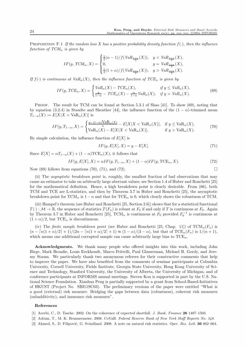
24 Kou, Peng, and Heyde: External Risk Measures and Basel Accords
Mathematics of Operations Research xx(x), pp. xxx–xxx, c©200x INFORMS
Proposition F.1 If the random loss X has a positive probability density function f(·), then the influencefunction of TCMα is given by
IF (y,TCMα, X) =
12 (α− 1)/f(VaR 1+α
2(X)), y < VaR 1+α
2(X),
0, y = VaR 1+α2(X),
12 (1 + α)/f(VaR 1+α
2(X)), y > VaR 1+α
2(X).
If f(·) is continuous at VaRα(X), then the influence function of TCEα is given by
IF (y,TCEα, X) =
VaRα(X)− TCEα(X), if y ≤ VaRα(X),y
1−α − TCEα(X)− α1−αVaRα(X), if y > VaRα(X).
(69)
Proof. The result for TCM can be found at Section 5.3.1 of Shao [41]. To show (69), noting thatby equation (3.2.4) in Staudte and Sheather [44], the influence function of the (1 − α)-trimmed meanT1−α(X) := E[X |X < VaRα(X)] is
IF (y, T1−α, X) =
y−(1−α)VaRα(X)
α − E[X |X < VaRα(X)], if y ≤ VaRα(X),
VaRα(X)− E[X |X < VaRα(X)], if y > VaRα(X).(70)
By simple calculation, the influence function of E[X ] is
IF (y, E[X ], X) = y − E[X ]. (71)
Since E[X ] = αT1−α(X) + (1− α)TCEα(X), it follows that
IF (y, E[X ], X) = αIF (y, T1−α, X) + (1− α)IF (y,TCEα, X). (72)
Now (69) follows from equations (70), (71), and (72).
(ii) The asymptotic breakdown point is, roughly, the smallest fraction of bad observations that maycause an estimator to take on arbitrarily large aberrant values; see Section 1.4 of Huber and Ronchetti [25]for the mathematical definition. Hence, a high breakdown point is clearly desirable. From (66), bothTCM and TCE are L-statistics, and then by Theorem 3.7 in Huber and Ronchetti [25], the asymptoticbreakdown point for TCMα is 1−α and that for TCEα is 0, which clearly shows the robustness of TCM.
(iii) Hampel’s theorem (see Huber and Ronchetti [25, Section 2.6]) shows that for a statistical functionalT (·) : M → R, the sequence of statistics T (Fn) is robust at F0 if and only if T is continuous at F0. Againby Theorem 3.7 in Huber and Ronchetti [25], TCMα is continuous at F0 provided F−1
0 is continuous at(1 + α)/2, but TCEα is discontinuous.
(iv) The finite sample breakdown point (see Huber and Ronchetti [25, Chap. 11]) of TCMα(Fn) is(n − ⌈n(1 + α)/2⌉+ 1)/(2n− ⌈n(1 + α)/2⌉+ 1) ≈ (1 − α)/(3 − α), but that of TCEα(Fn) is 1/(n+ 1),which means one additional corrupted sample can cause arbitrarily large bias to TCEα.
Acknowledgments. We thank many people who offered insights into this work, including JohnBirge, Mark Broadie, Louis Eeckhoudt, Marco Frittelli, Paul Glasserman, Michael B. Gordy, and Jere-my Staum. We particularly thank two anonymous referees for their constructive comments that helpto improve the paper. We have also benefited from the comments of seminar participants at ColumbiaUniversity, Cornell University, Fields Institute, Georgia State University, Hong Kong University of Sci-ence and Technology, Stanford University, the University of Alberta, the University of Michigan, and ofconference participants at INFORMS annual meetings. Steven Kou is supported in part by the U.S. Na-tional Science Foundation. Xianhua Peng is partially supported by a grant from School-Based-Initiativesof HKUST (Project No. SBI11SC03). The preliminary versions of the paper were entitled “What isa good (external) risk measure: Bridging the gaps between data (robustness), coherent risk measures(subadditivity), and insurance risk measures”.
References
[1] Acerbi, C., D. Tasche. 2002. On the coherence of expected shortfall. J. Bank. Finance 26 1487–1503.
[2] Adrian, T., M. K. Brunnermeier. 2008. CoVaR. Federal Reserve Bank of New York Staff Reports No. 348.
[3] Ahmed, S., D. Filipovic, G. Svindland. 2008. A note on natural risk statistics. Oper. Res. Lett. 36 662–664.
Kou, Peng, and Heyde: External Risk Measures and Basel Accords
Mathematics of Operations Research xx(x), pp. xxx–xxx, c©200x INFORMS 25
[4] Artzner, P., F. Delbaen, J.-M. Eber, D. Heath. 1999. Coherent measures of risk. Math. Finance 9 203–228.
[5] Basel Committee on Banking Supervision. 2006. International Convergence of Capital Measurement andCapital Standards: A Revised Framework (Comprehensive Version).
[6] Basel Committee on Banking Supervision. July 2009. Guidelines for Computing Capital for Incremental Riskin the Trading Book.
[7] Basel Committee on Banking Supervision. February 2011. Revisions to the Basel II Market Risk Framework.
[8] Danıelsson, J., B. N. Jorgensen, G. Samorodnitsky, M. Sarma, C. G. de Vries. 2005. Subadditivity re-examined: the case for Value-at-Risk. Working paper, London School of Economics.
[9] Delbaen, F. 2002. Coherent risk measures on general probability spaces. In: Sandmann, K., Schonbucher,P. J. (Eds.), Advances in Finance and Stochastics–Essays in Honour of Dieter Sondermann. Springer, NewYork.
[10] Denneberg, D. 1994. Non-Additive Measure and Integral. Kluwer Academic Publishers, Boston.
[11] Dhaene, J., M. J. Goovaerts, R. Kaas. 2003. Economic capital allocation derived from risk measures. N. Am.Actuar. J. 7 44–59.
[12] Eling, M., L. Tibiletti. 2010. Internal vs. external risk measures: how capital requirements differ in practice.Oper. Res. Lett. 38 482–488.
[13] Follmer, H., A. Schied. 2002. Convex measures of risk and trading constraints. Finance Stoch. 6 429-447.
[14] Frittelli, M., E. R. Gianin. 2002. Putting order in risk measures. J. Bank. Finance 26 1473–1486.
[15] Garcia, R., E. Renault, G. Tsafack. 2007. Proper conditioning for coherent VaR in portfolio management.Management Sci. 53 483–494.
[16] Gilboa, I., D. Schmeidler. 1989. Maxmin expected utility with non-unique prior. J. Math. Econom. 18 141–153.
[17] Glasserman, P. 2009. Risk horizon and rebalancing horizon in portfolio risk measurement. Math. Finance,forthcoming.
[18] Gordy, M. B. 2003. A risk-factor model foundation for ratings-based bank capital rules. J. Financial Intermed.12 199–232.
[19] Gordy, M. B., B. Howells. 2006. Procyclicality in Basel II: can we treat the disease without killing the patient?J. Financial Intermed. 15 395–417.
[20] Hansen, L. P., T. J. Sargent. 2007. Robustness. Princeton University Press.
[21] Hart, H. L. A. 1994. The Concept of Law. 2nd ed. Clarendon Press, Oxford.
[22] Heyde, C. C., S. G. Kou. 2004. On the controversy over tailweight of distributions. Oper. Res. Lett. 32
399–408.
[23] Hong, C.-S., L. F. Herk. 1996. Increasing risk aversion and diversification preference. J. Econom. Theory 70
180–200.
[24] Huber, P. J. 1981. Robust Statistics. Wiley, New York.
[25] Huber, P. J., E. M. Ronchetti. 2009. Robust Statistics. 2nd ed. Wiley, New York.
[26] Ibragimov, R., 2004a. On the robustness of economic models to heavy-tailedness assumptions. Mimeo, YaleUniversity.
[27] Ibragimov, R., 2004b. Portfolio diversification and value at risk under thick-tailedness. Harvard Institute ofEconomic Research Discussion Paper #2086.
[28] Ibragimov, R., J. Walden. 2007. The limits of diversification when losses may be large. J. Bank. Finance 31
2551–2569.
[29] Jaschke, S., U. Kuchler. 2001. Coherent risk measures and good deal bounds. Finance Stoch. 5 181–200.
[30] Jorion, P. 2007. Value at Risk: The New Benchmark for Managing Financial Risk. 3rd ed. McGraw-Hill,Boston.
[31] Keppo, J., L. Kofman, X. Meng. 2010. Unintended consequences of the market risk requirement in bankingregulation. Working paper, University of Michigan.
[32] Kijima, M. 1997. The generalized harmonic mean and a portfolio problem with dependent assets. Theoryand Decision 43 71–87.
[33] Kusuoka, S. 2001. On law invariant coherent risk measures. Adv. Math. Econom. 3 83–95.
[34] Litterman, R. 1996. Hot spotsTM and hedges. J. Portfolio Management 22 52–75.
[35] Maccheroni, F., M. Marinacci, A. Rustichini. 2006. Ambiguity aversion, robustness, and the variationalrepresentation of preferences. Econometrica 74 1447–1498.
[36] McMinn, R. D. 1984. A general diversification theorem: a note. J. Finance 39 541–550.
[37] McNeil, A., R. Frey, P. Embrechts. 2005. Quantitative Risk Management. Princeton University Press.
[38] Rockafellar, R. T., S. Uryasev. 2002. Conditional Value-at-Risk for general loss distributions. J. Bank. Finance26 1443–1471.
[39] Samuelson, P. A. 1967. General proof that diversification pays. J. Financial Quant. Anal. 2 1–13.
26 Kou, Peng, and Heyde: External Risk Measures and Basel Accords
Mathematics of Operations Research xx(x), pp. xxx–xxx, c©200x INFORMS
[40] Schmeidler, D. 1989. Subjective probability and expected utility without additivity. Econometrica 57 571–587.
[41] Shao, J. 2003. Mathemtical Statistics. 2nd ed. Springer-Verlag.
[42] Song, Y., J.-A. Yan. 2006. The representations of two types of functionals on L∞(Ω,F) and L∞(Ω,F ,P).Sci. China Ser. A: Math. 49 1376–1382.
[43] Song, Y., J.-A. Yan. 2006. Risk measures with comonotonic subadditivity or convexity and respecting s-tochastic orders. Working paper, Chinese Academy of Sciences.
[44] Staudte, R. G., S. J. Sheather. 1990. Robust Estimation and Testing. Wiley, New York.
[45] Staum, J. 2004. Fundamental theorems of asset pricing for good deal bounds. Math. Finance 14 141–161.
[46] Tasche, D. 1999. Risk contributions and performance measurement. Preprint. Technische UniversitatMunchen.
[47] Transportation Research Board of the National Academies. 2003. Design Speed, Operating Speed, and PostedSpeed Practices.
[48] Wang, S. S., V. R. Young, H. H. Panjer. 1997. Axiomatic characterization of insurance prices. InsuranceMath. Econom. 21 173–183.
[49] Yaari, M. E. 1987. The dual theory of choice under risk. Econometrica 55 95–115.