the basel i and basel ii accords: comparison of the models and

Vrije Universiteit AmsterdamDepartment of Mathematics

Master’s Thesis

The Basel I and Basel II Accords.

Comparison of the models andeconomical conclusions.

Paulina Rymanowska

Supervisor:

Dr Sandjai Bhulai

Amsterdam 2006

Contents

1 Introduction 1

2 Structure of the contract 52.1 Periodical Installments . . . . . . . . . . . . . . . . . . . . . . 52.2 Default . . . . . . . . . . . . . . . . . . . . . . . . . . . . . . . 62.3 Probability of Default . . . . . . . . . . . . . . . . . . . . . . 72.4 Exposure . . . . . . . . . . . . . . . . . . . . . . . . . . . . . . 72.5 Costs . . . . . . . . . . . . . . . . . . . . . . . . . . . . . . . . 82.6 Cash Flow . . . . . . . . . . . . . . . . . . . . . . . . . . . . . 92.7 Regulatory and Economic Capital . . . . . . . . . . . . . . . . 9

3 The Basel I Capital Accord 103.1 Introduction . . . . . . . . . . . . . . . . . . . . . . . . . . . . 103.2 The Basel I approach on the contract level . . . . . . . . . . . 10

3.2.1 The Merton model . . . . . . . . . . . . . . . . . . . . 123.3 The Basel I approach on the portfolio level . . . . . . . . . . . 15

3.3.1 Probability of default . . . . . . . . . . . . . . . . . . . 173.3.2 Default threshold . . . . . . . . . . . . . . . . . . . . . 203.3.3 Joint probability of default . . . . . . . . . . . . . . . . 21

4 The Basel II Capital Accord 254.1 Introduction . . . . . . . . . . . . . . . . . . . . . . . . . . . . 254.2 The Basel II approach on the contract level . . . . . . . . . . 26

4.2.1 The Asymptotic Risk Factor . . . . . . . . . . . . . . . 264.3 The Basel II approach on the portfolio level . . . . . . . . . . 28

4.3.1 Heterogenous portfolio . . . . . . . . . . . . . . . . . . 294.3.2 Homogeneous portfolio . . . . . . . . . . . . . . . . . . 37

5 Internal Return Capacity – IRCRisk adjusted Return on Capital – RaRoC 415.1 The Realized IRC and RaRoC . . . . . . . . . . . . . . . . . . 42

2

5.2 The Expected IRC and RaRoC . . . . . . . . . . . . . . . . . 43

6 Comparison of Model Performance between Basel I and BaselII 45

7 Conclusions 48

Bibliography 50

3

List of Figures

4

Abstract

In this thesis we will compare the Basel I (1988) and the Basel II accord(2004), including the rules regulating operations of the present banks and fi-nancial companies. We will present these documents giving a general overviewand mention some details. But our concentration will be mostly focusedon measures, which give information about the contract, are exploited tocompare contracts, and enable to make a decision whether the contract isattractive or not.

We will start from the contract analysis. We are going to bring closerthe contract’s structure by introducing the special notations, for instance,PD, LGD, EAD, etc, and explain their meaning. We will present also thecomputational methods based on the Merton model and designed to deter-mine capital requirements, called Regulatory or Economic Capital. Behindthe mathematical approach we will outline economical background concern-ing the problems, which we are going to study. For illustrative purposes, wewill apply the theory to real example.

At the end of thesis, we will draw conclusions and give an explanationwhy Basel II is better.

Chapter 1

Introduction

In the light of permanent development of financial markets and continu-ously changing market situation, banks and other financial companies needrules which will regulate financial agreements between them and their clients.Usually, conditions of such agreements are formalized in the form of contract.The bank and the customer, accepting the contract, commit themselves toobeying the contract’s conditions. It means that bank lends the customermoney and the customer is obliged to pay them back. However, sometimesthe customer losses financial liquidity, and then the contract goes to default.Hence, for all financial institutions it is very difficult to quote whether thecustomer is ‘good’ or ‘bad’, whether he will be solvent at the contract dura-tion. Seeing that, banks and financial companies would like to have a verygood measure that will give them an unambiguous answer to their questions.

On the other hand, banks will only be able to generate new transactionsif the customers do not doubt their ability to remain solvent. For the sake ofcomplexity of the financial market and interactions between all components,it is difficult to consider all possible events which can occur in the future.The market volatility renders that each move or investment is related to risk.

Unfortunately, models which are usually used to measure the risk level donot give exact results. The reason is that, it is very difficult to calculate therisk, because of unforeseen events, like customer’s default. Hence, the modelsonly include tools to identify concentrations of risk and give opportunities fordiversification within a disciplined and objective framework. Regardless ofthe shortcomings, these methods are commonly used because all companiesare under an obligation to have some fixed frame of calculating risk anddecision making whether to take this risk or not.

One of the tools used by banks is the determination of a capital require-ment. The definition of the capital requirement says that this is an amount ofmoney required to cover monetary losses due to the unexpected bad events,

1

in other words, to hedge the contract. Each company should keep reservesof money to hedge contracts. Furthermore, it seems to be obvious that theamount of money is not the same for each company, but the question is:how should we calculate this amount? Are there some methods which let usdetermine the capital requirements? Unfortunately, the problem is not easysolvable.

During recent years, almost the whole banking and financial world hasbeen concentrated on research concerning capital allocation. Everybodywould like to find the method which gives the most precise results or thebest estimation.The most involved in this research is the Basel Committee on Banking Super-vision. This committee, established by the Bank of International Settlements,has played a leading role in formalizing the relationship between credit risk,different forms of market risk, and the capital requirements. It undertook adetailed study of methods to set the regulatory capital. During a long time ofconsiderations, the Basel Committee found some solutions which were pub-lished as the Basel I and Basel II accords. In general, the Basel documentsare sets of rules for banking regulation and supervisory. In particular, theyset the global capital adequacy standards. They are international agreementsthat describe the risk sensitive framework for the assessment of regulatorycapital and oblige financial companies to take adequate hedging actions.

The Basel I accord was introduced in 1988. The main aims of this agree-ment were ‘leveling the playing field’ for the competition in terms of costsbetween internationally active banks and reduction of the probability thatsuch competition would lead to bidding down of capital ratios to extremelylow levels. It wanted to eliminate unfair advantages of banks in countrieswithout a minimum of capital requirements. Hence, the Basel Committeeset this minimum according to a given measure of the total credit risk out-standing amount.At the beginning, it introduced calculation of the required capital using amathematical model based on the Merton model and the properties of theBeta distribution. This model will be described in detail in Chapter 3. Un-fortunately, methodology of this model was too advanced to apply in realityand caused a lot of problems in computations. Hence, the Basel Committeeapplied an approach that relied on historical data. It determined, requiredto hedge contract, amount of money as 8% of the capital contribution, re-gardless of the customer’s credibility. In practice it looked as if the financialinstitutions had to keep 8% of outstanding amount of money as the capitalrequirement.

Application of this approach showed that it is not correct. The basicproblem of the Basel I was that it focused on costs, overlooking the consid-

2

erations of risk and financial stability. It took into consideration the risk,which is conected with given contract. Regardless of the customer’s risklevel, it requires 8% to secure the contract, whereas the capital requirementsshould depend on the customer’s risk that one takes. Moreover, Basel I ex-hibited a fundamental weakness – it based on a model that was becomingobsolete quickly. During a very short time, it was recognized that the riskand unexpected events should have a significant impact on the investments.Namely, every company has different vulnerability to risk and every contractis related with a different risk level, so standardization of the requirementsfor all companies and contracts is a naive approach. On account of necessarycorrections of the shortcomings, they prepared the New Capital Accord.

The Basel II accord was presented in 2004. In contrast to Basel I, thenew agreement is mostly an instrument of prudential regulations. It puts apressure on things, which are specific to each institution and defines instru-ments to deal with this diversity and idiosyncrasy.The New Capital Accord extended the old method of calculating the capitalrequirements based on the Merton model and introduced a new method basedon the Asymptotic Risk Factor Model. It takes into account the company’ssituation on the market, expressed by the rating and the probability of de-fault, describing the risk level. Basel II makes financial institutions obligor tohedging all their contracts by different amounts of capital contributions de-pending on the customer’s credibility. We will present the details in Chapter4.

Talking about Basel I and Basel II we have to pay particular attentionto the Internal Return Capacity, called the IRC and Risk-adjusted Return onCapital, called the RaRoC. These measures are strictly linked with the Baselenvironment.Generally, both of them express a fraction of amount of money earned by thecompany to the amount of money, which company has to keep for hedgingthe contract. The IRC is provided by the Basel I accord and the RaRoC bythe Basel II accord. Hence, the methods of computing the IRC are imposedby the Basel Committee. However, in the Basel II approach the choice ofthe method of the RaRoC computations is to the financial company to spec-ify. Because the capital requirements can be computed in different way byeach company, the same contract can be described by different values of theRaRoC, depending on the financial company.

The IRC and the RaRoC are used by banks to making the decision about arejection or an acceptance of a given contract. Each financial institution setsits own IRC or RaRoC threshold, called in the RaRoC case target RaRoC, andaccording to that they make a decision about the contract. If the thresholdis equal to for instance 20%, then it means that all contracts with the IRC

3

and the RaRoC above this amount are accepted and below this amount arerejected. Hence the IRC and the RaRoC frameworks are very useful andcommonly applicable by banks. The details and the application in practicewill be seen in Chapter 5.

4

Chapter 2

Structure of the contract

Let us consider a hypothetical situation in which we have a contract betweenthe bank and the customer. The contract is characterized by components.Some of them, such as the amount of money, which the bank is going tolend the customer or an interest rate are set by the bank or the customerin the beginning of the contract. But some of them, such as the probabilityof default or the funding rate are fixed and are usually dependent on thequality of the bank and the customer. Because we are interested in gettingan economical overview, we will consider a very easy contract, without anyadditional components, such as taxes, and any other events, such as auto-matical lease extension. All components which we are going to consider arepresented below, along with explanation of their meaning.

2.1 Periodical Installments

Let us assume that the financial company lends the customer some amountof money (a principal amount) for some time (a contract’s term). In thissituation, the customer becomes obliged to pay a fixed amount of moneyevery month (year). This fixed payment is the sum of principal payments(the part of borrowed money which equals the principal amount divided bythe number of periods) and interest payment (the amount of money paid tothe bank for a service). The interest payment is determined by a monthly(yearly) percentage rate called active rate, which can be split into fundingrate and margin rate.

The funding rate reflects the cost of funds and the margin rate determinesthe company’s profit received as a result of giving a loan. In other words, thefunding rate is the monthly (yearly) cost of getting money for the customerby the financial company. The basis rule is that the better company, the

5

cheaper they can get money, therefore the funding rate is lower.The margin rate is a percentage rate reflecting the amount of the company’sincome. According to the definition, the income is the amount of moneyearned by the company as a result of normal business activities.

If we denote the contract’s term as T , the principal amount as PA, thefixed monthly active rate as rma , then the total monthly payment P is ex-pressed by formula:

P :=rma

1− (1 + rma )−12T· PA

Because the monthly active rate is constant, hence the total monthly paymentis constant in each month as well.

2.2 Default

When a financial company decides to accept a contract, it does not knowwhat will happen in the future. There are a lot of internal and externalfactors which have a vast influence. We already know that all investmentsare related to risk. The company does not know if the customer will besolvent during the whole contract’s duration or if he will default.

According to the Basel Committee on Bank Supervision:

“A default is considered to have occurred with regard to a particular obligorwhen either or both of the two following events has taken place.

The bank considers that the obligor is unlikely to pay its credit obligationsto the banking group in full, without recourse by the bank to actions such asrealizing security (if held).

The obligor is past due more than 90 days on any material credit oblig-ation to the banking group. Overdrafts will be considered pas due once thecustomer has breached an advised limit or been advised of a limit smallerthan current outstanding.” (Basel Committee on Banking Supervision, 2003)

Hence we can conclude that a default does not mean that a bank willloose its money. It means that the customer has temporary problems withsolvency, but after paying all arrears back, the contract finishes normally. Byarrears we understand the amount of money, which the customer has to payextra in case of not refunding at the fixed time.

6

The default, which occurs with a probability of default is not typical fora normal course of the contract. It entails the consequences for the clientand its potential occurrence causes an uncertainty for the bank.

2.3 Probability of Default

Given a specific contract, we are not able to predict whether a lessee will de-fault. However, experience teaches us how often a similar lessee has defaulted.Basing on historical data we can adjust the frequency of going default fora specific contract. This frequency is expressed by the probability of defaultand it depends on the customer and the vintage of the contract.The “quality of the lessee” is usually asserted by ratings in the Standard &Poor’s ranking. They change from R1 till R21, and each of them denotes adifferent financial situation and the ability to default for the company. Thebest is the R1 rating, and the R21 means a default.

2.4 Exposure

During the contract time the customer pays money back in periodical pay-ments, causing reduction of the outstanding amount of money. Accordingto Basel II, the outstanding amount of money is called an Exposure and isdenoted by EXP.Usually, the exposure is computed annually and at the start of the contract,is equal to the principal amount. As long as the customer pays the moneyback, the exposure equals to the principal amount at time t subtracted by theamount of money paid by the customer back and at the end of the contractit is equal to 0. For the sake of a time value of money, the principal amountat time t is equal the principal amount at time 0 multiplied by the annualinterest factor.

We mentioned above that the exposure is computed yearly. Because anactive rate is a monthly rate, hence we have to change it into a yearly rate.We can do this using follow expression:

(1 + rma )12 = (1 + rya)

Therefore, the formula expressing the exposure of the nth contract at timet, where t means the t’th year of the contract term, is as follows:

EXPn,t :=

PA, t = 0

PA · (1 + rma )12t − P · (1+rma )12t−1rma

for t = 1, . . . , T − 1

0 t = T.

7

With respect to the contract, we use an Exposure at Default, denotedby EAD. By analogy, it means the amount of money, which the customerowes the bank at default time. In accordance with the definition of defaultintroduced by the Basel Committee, this money includes the exposure atthis time and arrears, accumulated during 90 days. Only the first year of thecontract constitutes an exception.At the start of the contract, arrears are unavailable, so the EAD is equalto the exposure. For future points, the assumption is made that in case ofdefault three monthly payments of arrears have been added. This results inthe following EAD equation:

EADn,t :=

EXPn,t, for t = 0,

EXPn,t + P · (1+rma )3

rma

, for t = 1, . . . , T − 1,

and finally:

EADn,t :=

EXPn,t, for t = 0,

PA · (1 + rma )12t − P · (1+rma )12t−(1+rm

a )3

rma

, for t = 1, . . . , T − 1.

2.5 Costs

Each contract is strictly related to different kinds of costs, which the companyhas to incur. Based upon Activity Based Costing, cost allocations occur inthe Front Office Costs and the Back Office Costs. A further distinction ismade between fixed and variable costs.

The fixed costs are represented by a constant value and are incurred atthe start of the contract. Similarly, the variable Front Office Costs occurat the start of the contract, but they are computed as a percentage of theprincipal amount. The variable Back Office Costs are a percentage of theaverage exposure over the periods. Hence:

Cn,t :=

CFOCn,t + CBOC

n,t + (cFOCn,t + cBOCn,t ) · 12(EXPn,t + EXPn,t+1), t = 0,

cBOCn,t · 12· (EXPn,t + EXPn,t+1), t = 1, . . . , T − 1.

where CFOCn,t , CBOC

n,t denote fixed Front and Back Office Costs, and cFOCn,t ,cBOCn,t denote variable Front and Back Office Costs for nth contract at timet, respectively.

8

2.6 Cash Flow

The term Cash Flow is used to describe all flows of money. It is defined asthe difference between the income and the expenses of the company. If weassume that the contract does not go into default, then the expenses includeonly costs, but when the customer defaults then the expenses include thecosts till default time and the loss caused by default.

The loss for nth contract is expressed as the fraction of the remaining ex-posure at default moment, and this fraction is determined by the percentagecalled Loss Given Default.

Ln,t = LGDn · EADn,t.

The loss given default (LGD) is given in advance and it is the contract’s andcustomer’s specification.

2.7 Regulatory and Economic Capital

In general, Regulatory and Economic Capital are the amount of capital al-located and held by the financial company in order to protect it from theunexpected losses with a reasonable degree of confidence. In other words,they are the sorts of capital requirements, which were provided in the intro-duction. Hence, they are determined by the confidence interval from the LossDistribution. We will explain it in greater detail in the next chapter, but fornow we would like to mention that the confidence level specifies how muchof the unexpected losses should be covered by the economical or regulatorycapital. Usually, this amount depends on the rating of the bank, for instancethe banks with rating R1 should cover 99, 99% of the unexpected losses.

The difference between regulatory and economic capital concerns choicesof the confidence level and the time horizon. For economic capital bankschoose it, whereas for regulatory capital supervisors set it. Hence, usuallythe capital requirements provided by Basel I are called regulatory capital,whereas provided by Basel II are called economic capital. We will keep thisterminology, and additionally we will denote regulatory capital by RECAPand economic capital by ECAP .

The idea of using the confidence level in the computations of the capitalrequirements appears in the Basel I document, and it was extended in theBasel II document. The documents include some settlements concerning theconfidence level and according to them the banks are asked to calculate theirregulatory capital requirements to an αth confidence interval. This issue iselaborated in Chapter 4.

9

Chapter 3

The Basel I Capital Accord

3.1 Introduction

The Basel I accord was revolutionary in that it sought to develop the sin-gle risk-adjusted capital standard that would be applied by internationalbanks. The heart of the Basel Accord was the establishment of similar cap-ital requirements for the banks to eliminate unfair advantages of banks inthe countries, where a minimum of capital was not required. Hence, Basel Idefines a standard methodology for calculating the capital requirements.

3.2 The Basel I approach on the contract level

In the previous chapter, we gave a definition of the capital requirements andwe affirmed also that they are determined by the confidence level of the lossdistribution. Now we will explain it in greater detail.

The default and, linked with it, loss appear to be unforeseen. Because ofthat, we do not know whether it will occur and how much the loss will be.Hence, the idea is to consider the default and the loss, as a random variables.In aftermath of this, we can talk about the probability of an event and thedistribution.The definition of the probability of default was given in the previous chapter.Now, we will introduce the formula expressing this probability. Furthermore,we will use this formula to determine the loss distribution and, in the end,the αth percentile of this distribution.

Without loss of generality, we can consider discrete random variables Dn,t,

10

given as follows:

Dn,t =

1, when default occurs at time t,

0, otherwise,

where n denotes the n’th contract and t = 0, . . . , T − 1 – t’th year of thecontract term.

This variable has two-point distribution and values, which are taken bythis variable, depend on the default occurrence. Because the default occursat time t with the probability of default PDn,t, we have

Dn,t =

1, with PDn,t

0, with 1− PDn,t

Furthermore, using properties of the two-point distribution, we can directlyconclude that the expected value of Dn,t is expressed by a formula:

E(Dn,t) = PDn,t (3.1)

and the standard deviation is given as follows:

σ(Dn,t) =√

PDn,t(1− PDn,t). (3.2)

In that case, it is also possible to change the loss formula, which is in accor-dance to the formula presented in the previous chapter, as follows:

Ln,t = LGDn · EADn,t. (3.3)

Because the random variable Dn,t takes only two values 0 or 1, and LGDn

and EADn,t for all contracts and t = 0, . . . , T − 1 are the constants given inadvance, we can write that:

Ln,t = Dn,t · LGDn · EADn,t. (3.4)

In the aftermath of this, we can consider the loss as a random variable anddetermine the distribution called the loss distribution.

With respect to the loss distribution we can talk about expected valuecalled Expected Loss and standard deviation called Unexpected Loss.The expected loss is a part of the loss, which is expected by banks to incur itin the future. For the sake of that, it is not related to the risk, so usually it isnot covered by the economic capital. Because mathematically it is expressedby the expected value of the loss distribution, hence

E(Ln,t) = E(Dn,t) · LGDn · EADn,t = PDn,t · LGDn · EADn,t.

11

The unexpected loss, causing by unforseen events, is used to reflects uncer-tainty. Because it is the result of the risk taking, hence the Basel Committeerequires keeping regulatory capital to cover it. Mathematically, the unex-pected loss is understanding as the standard deviation of loss, so we canwrite directly that

σ(Ln,t) =√

PDn,t(1− PDn,t) · LGDn · EADn,t.

Usually, the expected loss at time t is denoted by ELn,t, the unexpected lossat time t by ULn,t and we will keep this notation.

The construction of random variable for the loss guarantees existence ofthe loss distribution, which in this case is estimated by a Beta distributionwith the mean that equals to the expected loss, and the standard deviationequals the unexpected loss.

Moreover, if we denote the confidence level by α, then in accordance withthe model the capital requirements are represented by the αth percentile ofthe Beta distribution, which is approximated with eight multiplied by theunexpected loss.

Economic Capitaln,t ≈ 8 · ULn,t. (3.5)

Both the above approximation and the estimation of the loss distribution arethe results of plenty tests and numerical simulations that have been carriedout by the Basel Committee. We refer interested readers to more advanceddocuments.

However, let us mention one issue, which is related to the computationof the capital requirements.Namely, if we look at Formula (3.5), we see that only LGD, EAD, and theprobability of default are necessary to compute the regulatory capital. As westated above, LGD and EAD are given in advance, so only the probabilityof default is needed to get the value of capital requirements. Basel I admitsseveral methods of computations, but the most widely used is based on theMerton model.

3.2.1 The Merton model

In 1974, Merton introduced Black and Scholes (1973) option pricing modelto evaluate corporate liabilities, focusing mostly on the computations of theprobability of default. Assuming that the firm’s structure of capital can beexpressed as the sum of equities and values of debt, he proposed to considerthe firm’s assets in the option framework. More precisely, he showed thatthe equity is equivalent to a call option. Using some examples, he explainedlegitimacy of his idea.

12

To present of Merton’s methodology we will start from introducing thefollowing notation: An,t – the firm’s asset value at time t, En,t – the equityat time t, Bn,t – the debt at time t and n – the number of the company.In accordance with the Merton model assumptions, we have

An,t = En,t +Bn,t for t = 0, . . . , T − 1. (3.6)

Further, let us assume that we have the contract between the bank and theclient, which says that if the client does not repay his debt, then the bankholds the assets. In this situation, the assets exemplify a guarantee, that theclient will give the money back. Therefore, we can consider two situations:

• An,t > Bn,t

In this situation En,t = An,t − Bn,t is positive when the client repaidhis debt (because the asset’s value, which he will get, is greater thanthe amount of repaid to bank money) or equal zero otherwise (becauseof insolvency of the client the bank kept the assets, so the customer donot earn anything).

• An,t < Bn,t

In this situation En,t is negative if the client repaid his debts (becausethe asset’s value, which he will get, is smaller than the amount of repaidto bank money) or equal zero otherwise.

As a conclusion, we get that a repayment of the debt in the first case , howeverkeeping the debt in the second situation is the most profitable action for thecustomer. In the first situation he will earn money. In the second he doesnot earn anything, but at least he does not loss anything. Let us place ourresults in a figure.

Now, if we look at the graph of payments, we will see that it is the sameas the graph of call option payments. Hence, we state that the equity can beexpressed as the call option on the asset with strike price equal to Bn,t andmaturity T .It is also very easily noticeable that the threshold is determined by equalitybetween the equity and the debts, and moreover it denotes the moment ofdefault occurrence. Namely, it was showed above that the default occurswhen the value of the firm’s assets is less than the amount of debts. Seeingthat, the frequency of the default’s occurrence is expressed by the probabilityof default, we can express the probability of default as follows:

PDn,tD = P(An,tD < Bn,tD), (3.7)

where tD denotes the default time.

13

Above we also concluded that the equity is represented by the call option.We already know that the tool which lets us price the call option is the Black-Scholes model. The simple conclusion is that we can directly use the samemodel to the firm’s asset pricing and indirectly to compute the probabilityof default.Assume that we can express the dynamics of the firm’s assets as

dAn,t = µndt+ σndWn,t, (3.8)

where µn is the total expected return on the asset, σn is the asset volatility,and Wn,t is a Brownian motion. Using Ito’s formula, we can give a solutionto the differential equation (3.8), which is as follows:

An,tD = An,t · exp

((µn −

σ2n

2

)· (tD − t) + σn ·

√tD − t ·Xn,t,tD

), (3.9)

where

Xn,t,tD =Wn,tD −Wn,t√

tD − t,

and in accordance with the properties of a Brownian motion it is standardnormally distributed. Let us make also a remark that An,t denotes the currentasset value of nth company.In reference of Formula (3.7):

P(An,tD < Bn,tD) ⇔ P(An,t·exp

((µn −

σ2n

2

)· (tD − t) + σn ·

√tD − t ·Xn,t,tD

)

< Bn,tD) ⇔ P(((

µn −σ2n

2

)· (tD − t) + σn ·

√tD − tXn,t,tD

)< ln

Bn,tD

An,t

)

⇔ P

Xn,t,tD <ln Bn,tD

An,t− (µn − σ2

n

2) · (tD − t)

σn ·√tD − t

.

Using assumption about the standard normal distribution ofXn,t,tD we finallyget:

PDn,tD = Φ

(lnBn,tD − lnAn,t − (µn − σ2

n

2)(tD − t)

σn√tD − t

). (3.10)

Now, if we come back to Formula (3.5), and we insert all computed valuesthen the regulatory capital on the contract level is expressed by

14

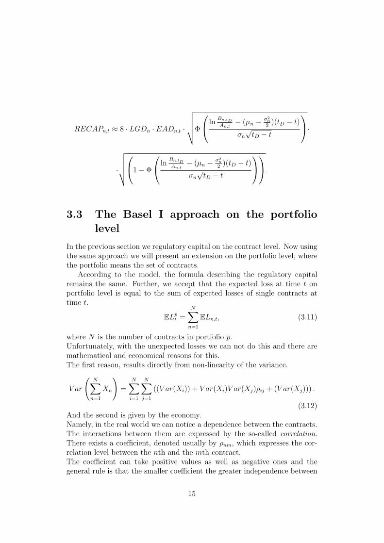
RECAPn,t ≈ 8 · LGDn · EADn,t ·

√√√√√Φ

lnBn,tD


n

2)(tD − t)

σn√tD − t

·

·

√√√√√1− Φ

lnBn,tD


n

2)(tD − t)

σn√tD − t

.

3.3 The Basel I approach on the portfolio

level

In the previous section we regulatory capital on the contract level. Now usingthe same approach we will present an extension on the portfolio level, wherethe portfolio means the set of contracts.

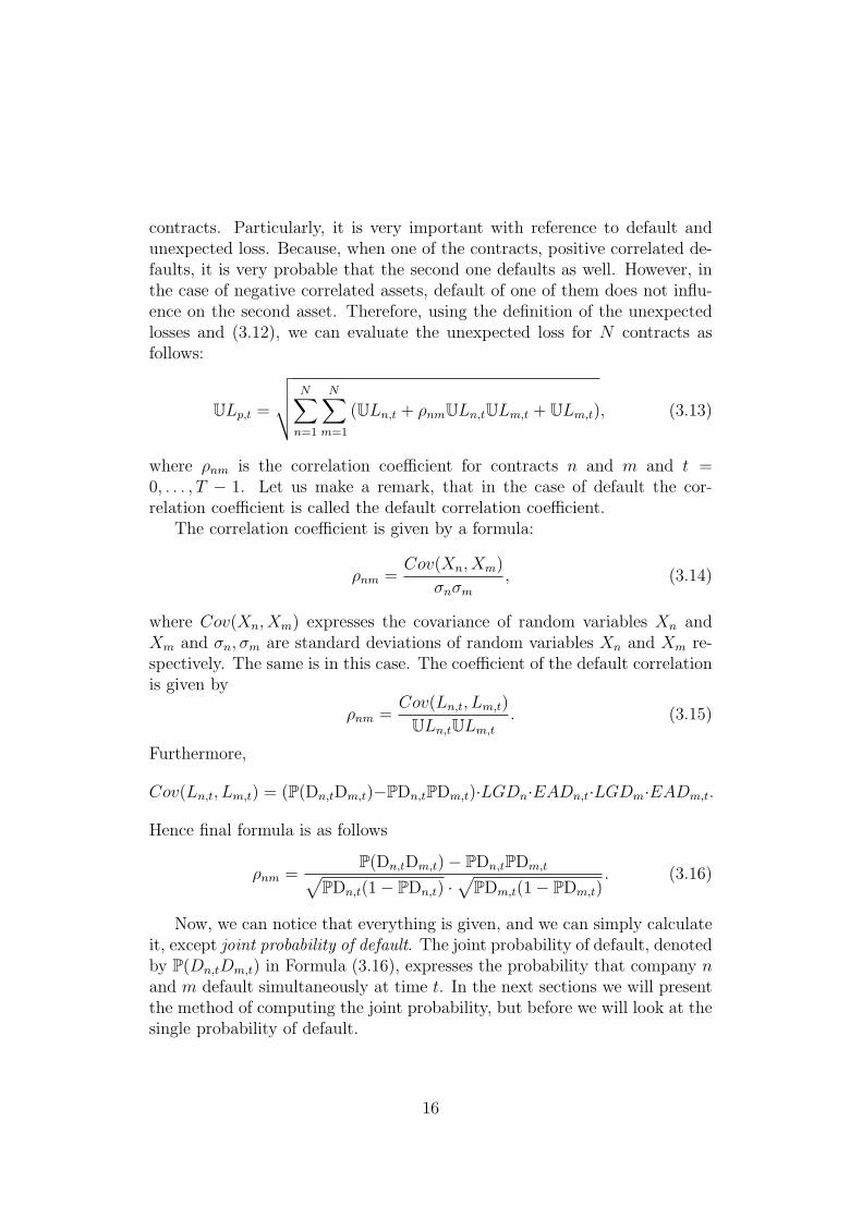
According to the model, the formula describing the regulatory capitalremains the same. Further, we accept that the expected loss at time t onportfolio level is equal to the sum of expected losses of single contracts attime t.

ELpt =N∑n=1

ELn,t, (3.11)

where N is the number of contracts in portfolio p.Unfortunately, with the unexpected losses we can not do this and there aremathematical and economical reasons for this.The first reason, results directly from non-linearity of the variance.

V ar

(N∑n=1

Xn

)=

N∑i=1

N∑j=1

((V ar(Xi)) + V ar(Xi)V ar(Xj)ρij + (V ar(Xj))) .

(3.12)And the second is given by the economy.Namely, in the real world we can notice a dependence between the contracts.The interactions between them are expressed by the so-called correlation.There exists a coefficient, denoted usually by ρnm, which expresses the cor-relation level between the nth and the mth contract.The coefficient can take positive values as well as negative ones and thegeneral rule is that the smaller coefficient the greater independence between

15

contracts. Particularly, it is very important with reference to default andunexpected loss. Because, when one of the contracts, positive correlated de-faults, it is very probable that the second one defaults as well. However, inthe case of negative correlated assets, default of one of them does not influ-ence on the second asset. Therefore, using the definition of the unexpectedlosses and (3.12), we can evaluate the unexpected loss for N contracts asfollows:

ULp,t =

√√√√ N∑n=1

N∑m=1

(ULn,t + ρnmULn,tULm,t + ULm,t), (3.13)

where ρnm is the correlation coefficient for contracts n and m and t =0, . . . , T − 1. Let us make a remark, that in the case of default the cor-relation coefficient is called the default correlation coefficient.

The correlation coefficient is given by a formula:

ρnm =Cov(Xn, Xm)

σnσm, (3.14)

where Cov(Xn, Xm) expresses the covariance of random variables Xn andXm and σn, σm are standard deviations of random variables Xn and Xm re-spectively. The same is in this case. The coefficient of the default correlationis given by

ρnm =Cov(Ln,t, Lm,t)

ULn,tULm,t. (3.15)

Furthermore,

Cov(Ln,t, Lm,t) = (P(Dn,tDm,t)−PDn,tPDm,t)·LGDn·EADn,t·LGDm·EADm,t.

Hence final formula is as follows

ρnm =P(Dn,tDm,t)− PDn,tPDm,t√

PDn,t(1− PDn,t) ·√

PDm,t(1− PDm,t). (3.16)

Now, we can notice that everything is given, and we can simply calculateit, except joint probability of default. The joint probability of default, denotedby P(Dn,tDm,t) in Formula (3.16), expresses the probability that company nand m default simultaneously at time t. In the next sections we will presentthe method of computing the joint probability, but before we will look at thesingle probability of default.

16

3.3.1 Probability of default

To determine the probability of default we will come back to the Mertonmodel, which was presented in Section 3.2.1. According to this model, thedefault occurs at time t when the firm’s asset value is smaller than the value ofdebts at this time. It means that the asset value of the company and its debtchange in time. The changes caused mainly by various market factors, canbe expected and unexpected. And accordingly we can consider the expectedand the unexpected part of value of assets.

Usually, the expected changes are deterministic. They can occur only incases when we have some new information about the market. Otherwise, theexpected changes do not occur. This has a direct bearing on the expectedmarket value of assets, because if we do not have the expected changes thenthe expected value of assets remains the same.A different situation is with the unexpected changes in the risk factor. Theyoccur very often and they cause an uncertainty in the asset value. Becauseof them, everything that can happen with assets is not predictable.

In addition to the market factors, we consider also the risk coefficientswhich are reserved separately for each asset. Those coefficients are in chargeof level risk of investment in this asset and they enable distinction betweenmore and less risky assets. In comparison to the market risk factors, whichshow us the general tendency of risk for all assets, they determine the risklevel specify for each single asset.Hence, the chances are that we can express the market asset value of firm nat time t as follows:

An,t = δn +K∑k=1

(φknθk,t) + ψnεn,t, (3.17)

for n = 1, . . . , N , where n denotes the firm’s number, δn,t expresses the ex-pected part of market risk factor at time t, θk,t expresses the unexpectedpart of market risk factor at time t, εn,t express the firm’s risk factor at timet. Because the influence of the risk factors on each asset is different, weconsider the coefficient of the firm’s sensitivity to the risk factor. Hence φkndenotes the firm’s sensitivity to the kth market risk factor and ψn denotesthe firm’s sensitivity to the firm’s risk factor. Moreover we assume that themarket risk factors are normally distributed with expectation 0 and covari-ance matrix Ω and the firm’s risk factor has the standard normal distribution.

Usually it is like this, that one portfolio consists of a lot of contracts.Because we have to know the correlation between each two contracts, the

17

number of computations grows large very fast. This lengthens the calcu-lation time. To simplify calculations, and to make them more efficient wewill introduce selection. The idea is to select contracts according to country,industry, etc. It gives us sufficient granularity and enables making our com-putations easier.In the aftermath of this, we will introduce structures which we call the riskbuckets. Each risk bucket includes contracts, which are similar in the senseof some feature. We assume that contracts which are in the same risk buckethave the same expected risk and sensitivity to the unexpected risk. Thisgives us instead of consideration of each two contracts opportunity to con-sider risk buckets.

Let G denote the set of the risk buckets. A bucket g will be one of themconsisting of some firms. Then in accordance to the above assumptions wecan write:

An,t = δg +K∑k=1

(φkgθk,t) + ψnεn,t n ∈ g (3.18)

Let us remind that the main aim of these considerations is getting thejoint probability of default for two companies. To this end, we will keep theassumption that the company defaults when the asset value of company issmaller than the amount of debts. Hence in our case

P(Dn,t = 1) = P(An,t < Bn,t), (3.19)

where An,t is expressed by (3.18), and Bn,t denotes the amount of liabilitiesat time t. Further

An,t < Bn,t ⇔ δg+K∑k=1

(φkgθk,t)+ψnεn,t < Bn,t ⇔K∑k=1

(φkgθk,t)+ψn,tεn,t < Bn,t−δg

According to our above assumption we know that δg denotes the expectedvalue of the risk so it is deterministic. Thus, without loss of generality, we canintroduce a constant Cn,t = Bn,t − δg and it automatically gives conclusionthat default occurs when

K∑k=1

(φkgθk,t) + ψnεn,t < Cn,t (3.20)

Determination of the default probability is a rather difficult issue. Dueto that, we will define a new random variable denoted by Zg,t and expressedby formula

Zg,t =K∑k=1

(φkgθk,t), (3.21)

18

where t = 0, . . . , T − 1. Let us notice that this notation is very efficientfor us. First, Zg,t expresses the market risk factor for bucket g and is thesame for all contracts in the bucket g. Second, Zg,t is the sum of standardnormally distributed random variables, so it has a normal distribution withexpectation 0 and a variance given by a formula:

V ar(Zg,t) = V ar(K∑k=1

(φkgθk,t)) =K∑k=1

K′∑k′=1

(V ar(φkgθk,t) + σkk′V ar(φkgθk,t)·

·V ar(φk′g θk′,t) + V ar(φk′

g θk′,t)) =K∑k=1

K′∑k′=1

((φkg)2V ar(θk,t) + σkk′φ

kgφ

k′

g ·

·V ar(θk,t)V ar(θk′,t) + (φk′

g )2V ar(θk′,t)).

Shortly,

Zg,t ∼ N

(0,√V ar(Zg,t)

). (3.22)

We know that dividing normally distributed random variable minus its ex-pectation value by its standard deviation we will result in a random variablewhich has a standard normal distribution. Hence:

Zg,t√V ar(Zg,t)

∼ N(0, 1). (3.23)

Let us denote this fraction by Xg,t.We can also denote

√V ar(Zg,t) by wg. Then we will get:

Zg,t = wgXg,t =K∑k=1

φkgθk,t,

and coming back to formula (3.18):

An,t = δg + wgXg,t + ψnεn,t. (3.24)

Because of that the probability of default is given by

P(Dn,t = 1) = P(wgXg,t + ψnεn,t < Cn,t). (3.25)

For facilitation of the notation and computations we will denote wgXg,t +ψnεn,t by un,t. Knowing that Xg,t ∼ N(0, 1) we can designate distribution ofun,t. Seeing that un,t is the sum of normally distributed random variables,we can conclude that it is normally distributed as well. Moreover, we assume

19

that the firm risk factor and the market risk factor are independent, whatmeans also that the covariance between them is equal 0. Hence un,t has anormal distribution with expected value equal to 0 and a variance given by

V ar(un,t) = V ar(δg+wgXg,t+ψnεn,t) = w2gV ar(Xg,t)+ψ

2nV ar(εn,t) = w2

g+ψ2n,

and finally

un,t ∼ N(0,√w2g + ψ2

n

)(3.26)

where un,t is the random variable expressing the market risk and the firmrisk.

Using basic knowledge from probability theory and particularly fromproperties of the normal distribution we will write

φ(un,t) =1√

2π(w2g + ψ2

n)exp

(−1

2

u2n,t

(w2g + ψ2

n)

), (3.27)

Φ(un,t) =

∫ Cn,t

−∞

1√2π(w2

g + ψ2n)

exp

(−1

2

u2n,t

(w2g + ψ2

n)

)(3.28)

and in the next section we will use these formulas for further considerations.

3.3.2 Default threshold

In the previous section, we considered the market asset value of a firm. Weexpressed this as a sum of corresponding risk factors and we obtained the dis-tribution of this random variable. This means that we are ready to considerthe joint probability of default for two companies.

We know already that the probability of default for one company is ex-pressed by formula:

P(Dn,t = 1) = P(An,t < Bn,t) = P(wgXg,t + ψnεn,t < Cn,t) = P(un,t < Cn,t),

where un,t, t = 0, . . . , T − 1 has a normal distribution. Knowledge whichwe have so far gives us the opportunity to say something about Cn,t as well.Let us notice that till now this value was unknown. Unfortunately, we cannot give an exact value of Cn,t, but we can express the threshold value by adifferent variable which is already known. Thanks to the normal distributionof un,t and standardization of the random variable, we get that

un,t√w2g + ψ2

n

∼ N(0, 1),

20

and directly

P(un,t < Cn,t) = P

(un,t√w2g + ψ2

n

<Cn,t√w2g + ψ2

n

)= Φ

(Cn,t√w2g + ψ2

n

),

where Φ is the cumulative function of the standard normal distribution.Existence of an inverse cumulative function to a cumulative function of

a continuous distribution guarantees us opportunity to consider inversion ofcumulative function of standard normal distribution. Therefore we can writethat

Cn,t = Φ−1(PDn,t)√w2g + ψ2

n,

and this is an expression of the default threshold which will be using fromnow. It gives us directly a new default probability formula

P(Dn,t = 1) = P(un,t < Φ−1(PDn,t)

√w2g + ψ2

n

).

In the future, the above two formulas will be a basis to construct joint defaultprobabilities.

3.3.3 Joint probability of default

In the beginning of this section let make a remark about the probability ofdefault for two firms. We know that every company is going to default withcertain probability and it is obvious that probability can be the same forboth companies or totally different for each of them.

If probability is the same for companies then situation is very easy, be-cause the joint probability is equal probability of default for one company.We will consider the second situation, when the probabilities are different.For us this situation is more interesting, because situation when companiesare going to default with the same probability are rather rare on the realmarket.

Let us take company n and m with probability of default at time t =0, . . . , T − 1 PDn,t and PDm,t respectively. Moreover for simplicity compu-tations we will keep the assumption that these two firms default on theircontract in the same time interval.

In the previous section we showed that probability of default for onecompany is equal probability of event that Di is equal 1 and is expressed byformula

PDn,t = P(Dn,t = 1) = P(un,t < Φ−1(PDn,t)

√w2g1

+ ψ2n

),

21

where g1 denotes the bucket which contains nth company. The same we canwrite for company m

PDm,t = P(Dm,t = 1) = P(um,t < Φ−1(PDm,t)

√w2g2

+ ψ2m

)where g2 denotes the bucket which contains mth company. This approachlets us consider joint probability of default as probability of event that Dn,t

is equal 1 and Dm,t as well. According to this we have:

P(Dn,tDm,t) = P(Dn,t = 1,Dm,t = 1) =

= P(un,t < Φ−1(PDn,t)

√w2g1

+ ψ2n, um,t < Φ−1(PDm,t)

√w2g2

+ ψ2m,t

)Now consider two random variable X1 and X2 - both of them normal dis-tributed with the expected values µ1, µ2 and the standard deviations σ1, σ2

respectively. We know that in general case the density function of bivariatenormal distribution is expressed by formula

f(x1, x2) =1

2π|Σ|−

12 exp

(−1

2(XTΣ−1X)

)where

X =

[x1 − µ1

x2 − µ2

]and covariance matrix Σ as follow

Σ =

[σ2

1 σ1σ2ρ12

σ1σ2ρ12 σ22

]Try to use this to solve our problem.

Generally it is not true that if we have two random variables with thenormal distribution then the distribution of random vector is normal distrib-uted as well. But in this case it will be like this and it is a result of followlemma:

Lemma 3.1 The vector X = (X1, X2, . . . , Xk) is Nk(µ,Σ)-distributed if andonly if aTX is N1(a

Tµ, aTΣa)-distributed for every a ∈ Rk.

We know that random variables un,t and um,t are dependent (because marketrisk factors Xg1 and Xg2 are dependent). But on the other hand they arelinear combination of random variables, which are independent. And thisguarantees fact that every time we can find the vector a, which satisfies the

22

condition of above lemma.Thus, the vector (Dn,t, Dm,t) has bivariate normal distribution.

We see that applying above formula requires the computation of somevalues. We know already that un,t and um,t are standard normal distributedwith expected values 0 and variations w2

g1+ψ2

n and w2g2

+ψ2m respectively. It

gives us directly a vector

U =

[un,tum,t

]To get a covariance matrix we need variation of random variables and covari-ation. The variation we already have, so look at covariance.

The covariance represents the co-movement of the two variables and isdefined as

Cov(un,t, um,t) = E(un,t − E(un,t))(um,t − E(um,t))

The expectation values of variables equal 0 and independence between cor-responding risk factors lead us to

Cov(un,t, um,t) = E(un,tum,t) = E((wg1Xg1,t+εn,tψn)(wg2Xg2,t+εn,tψn)) = wg1wg2E(Xg1,tXg2,t)

As we assumed in the beginning of our consideration the firm risk factors arenot related each other and they are not related with market risk factors aswell. Hence, the correlation coefficient, which expressed relationship betweenthem will depend only on market risk factors and will be defined by ρg1g2 =E(Xg1,tXg2,t). So finally the covariance matrix is as follow

Σ =

[w2g1

+ ψ2n wg1wg2ρg1g2

wg1wg2ρg1g2 w2g2

+ ψ2m

]As we see we got a ’values’ which characterizes bivariate normal distrib-

ution. Now we make some computation which let us to get final formula ofdensity function. Using mostly properties of matrix in the computations wewill get

|Σ| = (w2g1

+ ψ2n)(w

2g2

+ ψ2m)− w2

g1w2g2ρ2g1g2

where |Σ| denotes determinant of the covariance matrix Σ.

|Σ|−12 =

1√(w2

g1+ ψ2

n)(w2g2

+ ψ2m)− w2

g1w2g2ρ2g1g2

Σ−1 =

w2g2

+ψ2m√

(w2g1

+ψ2n)(w2

g2+ψ2

m)−w2g1w2

g2ρ2g1g2

− wg1wg2ρg1g2√(w2

g1+ψ2

n)(w2g2

+ψ2m)−w2

g1w2

g2ρ2g1g2

− wg1wg2ρg1g2√(w2

g1+ψ2

n)(w2g2

+ψ2m)−w2

g1w2

g2ρ2g1g2

w2g1

+ψ2n√

(w2g1

+ψ2n)(w2

g2+ψ2

m)−w2g1w2

g2ρ2g1g2

23

Getting a nice formula of the density function is not easily solvable problemin this case. In theory it should be possible by deriving an integral of thisfunction, but in practice it will be very difficult and not necessary. Presently,a lot of corresponding programs is available (for instance SPSS, Matlab, etc),which enable getting the results without manual computations.

24

Chapter 4

The Basel II Capital Accord

4.1 Introduction

In June 2004 the Basel Committee introduced a New Accord called Basel II.Similarly to the Basel I accord, the Basel II settles regulations concerningbanking. The document includes methods of measuring risk and calculatingcapital requirements. However, the Basel Committee does not force banksto use exactly these methods. Contrary to Basel I, the New Accord givesbanks freedom of choice. They can adapt analytical methods of computingthe amount of required capital and the advancement level of it to their ownneeds. Hence, the banks have an opportunity to reduce their economic capi-tal and regulatory capital through efficient data management and reporting.

The Basel II is based on a “three pillars” concept:

• minimum capital requirements – introduces methods and rules of com-puting required capital,

• supervisory review – determines rights and duties of banking supervi-sors,

• market discipline – sets the rules of reporting the information concern-ing risk taken by the bank.

As we mentioned in the previous chapters, the required capital is strictlyrelated to risk, in particular, to credit risk. With respect to the risk, BaselII extended old methods presented by the Basel I, and introduced new one.Hence, according to the Basel Committee directives, banks can apply two ap-proaches to calculate credit risk: the standardized approach and the InternalRating Based approach (IRB).

25

The first one, based largely on the current accord, is its slight modifi-cation, what still means that capital requirements are equal 8% of the out-standing amount of money. Banks use this method because application ofmethods of determine the PD′s based on ratings is rather impossible in manycountries. The reason is that only few borrowers possess ratings which areconvenient for local markets and give banks favorable risk weights.

The Internal Rating Based approach gives banks more possibilities. Ingeneral, banks are ought to calculate borrowers’ probability of default usinginternal measures. In particular, banks can also estimate the loss given de-fault and the exposure at default using theirs own methods. Then, we speakabout the Advanced Internal Ratings Based model. Anyway, both approacheslead banks to the same – to get an estimate of the capital requirements, withthe exception that the Advanced IRB is more adapted to the bank. In thiscase the LGD and the EAD are based on the historical data, which gives abetter estimate. However, in accordance with the basic IRB, the LGD andthe EAD are given by Basel Committee. Hence, they are constant and theydo not depend on the bank.

According to the Basel II, one of the tool which can be used by thefinancial institutions to determine the probability of default and the capitalrequirements is an Asymptotic Risk Factor Model. The ASRFM is based onthe Merton model and by acceptance of certain assumptions, it gives theestimate of above components.

4.2 The Basel II approach on the contract

level

4.2.1 The Asymptotic Risk Factor

The Asymptotic Risk Factor Model gives the opportunity to calculate eco-nomic capital requirements using risk weight formulas. Similar to Basel I,we distinguish two risk types: the market risk and the risk which is speci-fied for the company. The idea behind the ASRFM is that the market riskis completely diversified and the portfolio becomes more fine-grained whichmeans that large individual exposures have smaller shares in the exposureof the whole portfolio. Hence, we assume that the bank’s portfolio consistsof a large number of contracts with small exposure. Moreover, because oftotal diversification of the market risk, we assume that the economic capitaldepends only on the contract and the company, not on the portfolio whichincludes this contract.

For the sake of expressing the market asset value as the sum of normally

26

distributed market risk factor and firm’s risk factor multiplied by correspond-ing sensitivities, the market asset value has also the normal distribution.However, in comparison to the model presented by Basel I, the ASFRM re-quires something more than only the normal distribution of the market assetvalue. According to the model it should be a standard normal distributed.Because of that, the model introduced new formula, which is as follows:

An,t =√ρnXt +

√1− ρnεn,t, (4.1)

where Xt denotes the market risk factor at time t, εn,t denotes the firm’srisk factor for company n at time t, and t as previously, means the tth yearduring the contract time t = 0, . . . , T − 1.Directly, it follows from this equation that the assets of firms n and m aremultivariate Gaussian distributed (a similar proof is presented in Chapter3) and the assets of two firms are correlated, with the linear correlationcoefficient

E(An,tAm,t) =√ρnρm.

Moreover, the correlation between the asset’s return An,t and the market riskfactor Xt is equal to

√ρn, therefore

√ρn is interpreted as the sensitivity to

the systematic risk.

The same as in the Basel I approach, the ASRFM is based on the singleasset model of Merton. Hence, the firm’s asset value is expressed as the sumof liability and the amount of debt, and the probability of default is equal tothe probability that the firm’s asset value is less than the amount of debts.We remember from Chapter 3 that

Dn,t =

1 if An,t ≤ Φ−1(PDn,t),

0 if An,t ≥ Φ−1(PDn,t).(4.2)

where Dn,t denotes the default at time t and PDn,t the probability of de-fault. According to the definition, PDn,t is an unconditional probability. Itis specify for the customer and based on ’the quality of the customer’. Theunconditional probability is used mainly to obtain the loss distribution. Inthe case of small number of contracts it it possible, however using the un-conditional probability and unconditional loss distribution when we have alot of contracts is not efficient for the sake of difficulty of computations.Therefore, along with the unconditional probability, the ASRFM introducesa conditional probability. This probability is characterized by dependence onthe market risk factor. We calculate it knowing the outcome of the system-atic risk factor at time t. Further, it will enable determination of expected

27

distribution.

P(Dn,t = 1|Xt = x) = P(An,t ≤ Φ−1(PDn,t)|Xt = x)

= P(√ρnXt +

√1− ρnεn,t ≤ Φ−1(PDn,t)|Xt = x)

= P(εn,t ≤

Φ−1(PDn,t)−√ρnXt√

1− ρn

∣∣∣Xt = x

)= Φ

(Φ−1(PDn,t)−

√ρnx√

1− ρn

) (4.3)

Usually this probability is called The Stress Probability and expresses theprobability of the total loss. Moreover, the conditional probability can beinterpreted as assuming various scenarios for the economy, determining theprobability of a given portfolio loss under each scenario, and then weightingeach scenario by its likelihood.

We already know that the economic capital is kept to cover only theunexpected losses. Hence, if we would like to have the probability of theunexpected loss we have to subtract the probability of the expected loss,which is expressed by the unconditional probability of default. Hence:

PDthe unexpected loss = PDthe stress − PDthe expected loss.

Because we know that the unexpected losses are strictly linked with the lossgiven default and the exposure at default, hence, to hedge the contract withα’s certainty the nth bank has to keep at time t the economic capital asfollows:

ECAPn,t = LGDn · EADn,t · PDthe unexpected loss

= LGDn · EADn,t ·(

Φ

(Φ−1(PDn,t)−

√ρnx√

1− ρn

)− PDn,t

). (4.4)

This formula holds for all x – realizations of Xt.

4.3 The Basel II approach on the portfolio

level

The idea of the Basel II for portfolios, similar to the individual contract islargely based on the Merton model.Similarly, as in the previous sections, we will consider the portfolio loss andlater we will introduce the formula expressing the required capital. We willpresent the computations separately for two types of the portfolio.

28

4.3.1 Heterogenous portfolio

A heterogenous portfolio includes contracts with all different characteristicsfor each of them: the exposures EXPn,t, the probabilities of default PDn,t,the asset correlations ρn, and the loss given defaults LGDn.Assume that we have this kind of portfolio with N contracts. Each of thesecontracts has its share in the whole portfolio. This means that when acontract goes into default, then its default will trigger the loss proportionalto the share. The most convenient tool to express the share of each contractloss in the loss of whole portfolio is using the weight. But what is the smartestway of determining these weights?

We already know that the loss is related to the exposure. The exposuredenotes the remaining outstanding amount, hence the greater exposure, thegreater loss. Because of that, taking the share of the contract’s exposure inthe exposure of portfolio as the weights seems to be logical. So let us definethe exposure weight at time t as

wn,t =EXPn,t∑Nn=1EXPn,t

n = 1, . . . , N t = 0, . . . , T − 1 (4.5)

Considering the Basel I approach, we said that the capital requirementsare expressed by αth percentile of the loss distribution. The same approachis applied in the ASFRM and now we will discuss the details.

Let us take into consideration the heterogenous portfolio with N con-tracts, with the exposures EXPn,t, the asset correlations ρn, the probabilitiesof default PDn,t, the losses given default LGDn and the weights wn,t. Thenthe portfolio loss per monetary unit of exposure (for instance dollars, euros)at time t is given by a formula

Lpt :=N∑n=1

EXPn,t · LGDn ·Dn,t.

If we denote LGDn,t ·Dn,t as a random variable Zn,t then

Zn,t =

0, when the default does not occur at time t,

LGDn,t, otherwise.(4.6)

For the sake of the construction of Zn,t and properties of the LGD, we canassume:

(A.1) Zn,t to belong to the interval [0, 1] and conditionally on Xt,to be inde-pendent for all n = 1, . . . , N .

29

With respect to this portfolio we can also consider the portfolio loss ratioRpt expressing the ratio of the total portfolio loss to total portfolio exposure

Rpt =

Lpt∑Nn=1EXPn,t

=

∑Nn=1EXPn,t · LGDn ·Dn,t∑N

n=1EXPn,t=

∑Nn=1EXPn,t · Zn,t∑N

n=1EXPn,t,

for Zn,t given by Formula (4.6). We provide it, because as we will see further,the ASFRM proposes to determine a distribution of the portfolio loss ratio,instead of the loss distribution.

In accordance with the ASFRM, we consider the portfolio only with con-tracts characterized by small amount of exposure. However, the sequence ofexposure amounts should not converge to zero too quickly. Because of that,we will pose some restrictions concerning the exposure. This is necessaryto guarantee that the market risk will be completely diversified. Thus, weassume:

(A.2) EXPn,t forms a sequence of positive numbers such that∑N

n=1EXPn,t ↑∞ for N →∞ and for τ > 0

EADN,t∑Nn=1EXPn,t

= O(N−( 1

2+τ)). (4.7)

Assumptions (A.1) and (A.2) are weak; they hold in the real world and forus are very important. Due to these assumptions, we are sure that the shareof the greatest exposures shrinks to 0, as the number of exposures in theportfolio increases. In that case, it can be shown that

Proposition 4.1 If we assume (A.1) and (A.2), then for N →∞

Rpt − E[Rp

t |Xt = x] → 0, almost surely. (4.8)

Proof: To prove Proposition 4.1 we will use the special version of the StrongLaw of Large Numbers presented in the “Oxford Studies in Probability” byValentin V. Petrov in 1995 (Theorem 6.7):

Theorem 4.1 If aN ↑ ∞ and∑∞

N=1V ar(YN )

a2N

<∞ then

1

aN

(N∑n=1

Yn − E

(N∑n=1

Yn

))→ 0, almost surely. (4.9)

30

Let Yn,t ≡ Zn,t · EXPn,t and aN,t ≡∑N

n=1EXPn,t for t = 0, . . . , T − 1 andn = 1, . . . , N . Hence:

∞∑N=1

V ar(YN,t)

a2N,t

=∞∑N=1

V ar(ZN,t · EXPN,t)(∑Nn=1EXPn,t

)2 (4.10)

Because EXPn,t at time t is given for each contract n, we have:

∞∑N=1

V ar(YN,t)

a2N,t

=∞∑N=1

(EXPN,t∑Nn=1EXPn,t

)2

· V ar(ZN,t). (4.11)

For all realization of Xt x, a conditional independence implies that

∞∑N=1

V ar(YN,t|Xt = x)

a2N,t

=∞∑N=1

(EXPN,t∑Nn=1EXPn,t

)2

· V ar(ZN,t|Xt = x).

To apply Theorem (4.1) we have to show that this sum is finite. In accordanceto assumption about Zn,t, we know that for t = 0, . . . , T−1 and n = 1, . . . , Nit belongs to [0, 1]. Thus, V ar(ZN,t|Xt = x) is finite for any Xt = x. In thatcase, for t = 0, . . . , T − 1 there exists the constant Mt such that

V ar(ZN,t|Xt = x) < Mt.

Moreover, using Assumption (A.2) we have that

EXPN,t∑Nn=1EXPn,t

= O(N−( 1

2+τ))

for τ > 0,

and directly(EXPN,t∑Nn=1EXPn,t

)2

=(O(N (− 1

2+τ)))2

=(O(1) ·N (− 1

2+τ))2

=

= O(1) ·N (1+2τ) = O(N (1+2τ)

).

The lemma presented below and fact that

Rpt =

∑Nn=1 YnaN

, for t = 0, . . . , T − 1

finishes the explanation why the assumption of theorem holds, what meansthat Rp

t − E[Rpt |Xt = x] → 0 for t = 0, . . . , T − 1.

31

Lemma 4.1 If bN is a sequence of positive real numbers such that bNis O(N−ς) for some ς > 1, then

∑∞N=1 bN <∞.1

Intuitively, this proposition says that shrinking the exposure sizes of thesingle contracts cause total diversification of the market risk. In the limit,the loss ratio converges to the function depending on the market risk factor.This is very useful, because we would like to know the distribution of portfolioloss ratio.

According to Proposition (4.1) we can consider the conditional distrib-ution of E[Rp

t |Xt = x], and then automatically we have the unconditionaldistribution. Now it is natural, that we would like to know something aboutthe variance. It is reasonable that we may expect getting the variance of Rp

t

by computing the variance of E[Rpt |Xt = x]. But for us it is more important

to obtain knowledge about the percentiles of the unconditional distribution,because it expressed the capital requirements. We said that the capital re-quirements, enabling covering α of the unexpected losses, are expressed bythe αth percentile. The ASRFM is using definition of percentile as follows:

qα(Y ) = infy : P(Y ≤ y) ≥ α (4.12)

The first step to show that the α percentile of Rpt can be turn into the α

percentile of E[Rpt |Xt = x] for t = 0, . . . , T , is to prove a proposition below.

Proposition 4.2 If (A.1) and (A.2) hold, then for t = 0, . . . , T

limN→∞

(V ar(Rp

t )− V ar(E[Rpt |Xt])

)= 0.

Proof: Similar like the proof of Proposition (4.1), this proof will be basedon Theorem (4.1). Moreover we will use the lemma below:

Lemma 4.2 Let bN and cN be sequences of real numbers such thataN =

∑Nn=1 bn ↑ ∞ and cN → 0. Then 1

aN

∑Nn=1 bncn → 0.2

Let us take bn,t ≡ EXPn,t and cn,t ≡ EXPn,tPni=1 EXPi,t

for t = 0, . . . , T − 1 . Then,

similar as in the previous proof, Assumption (A.2) gives us that aN,t ↑ ∞and cN,t → 0 if N →∞. Hence, according to the lemma

1∑Nn=1EXPn,t

N∑n=1

(EXPn,t)2∑n

i=1EXPi,t−→ 0. (4.13)

1Knopp, Konrad, Infinite Sequences and Series, New York: Dover Publications, 1956(a corollary of Theorem 3.5.2)

2Petrov, Valentin V., Limit Theorems of Probability Theory , n.4‘Oxford Studies in Probability’, Oxford University Press (1995), Lemma 6.10

32

Using the standard property of the conditional variance we get

V ar(Rpt )− V ar(E[Rp

t |Xt]) = E(V ar[Rpt |Xt]) =∑N

n=1(EXPn,t)2 · E(V ar[Zn,t|Xt])(∑N

n=1EXPn,t

)2

Under Assumption (A.1) it exists for t = 0, . . . , T − 1 the constant Mt suchas

E(V ar[Zn,t|Xt]) < Mt

and then

V ar(Rpt )− V ar(E[Rp

t |Xt]) < Mt ·∑N

n=1(EXPn,t)2(∑N

n=1EXPn,t

)2 =

=Mt∑N

n=1EXPn,t·∑N

n=1(EXPn,t)2∑n

i=1EXPi,t<

Mt∑Nn=1EXPn,t

·∑N

n=1(EXPn,t)2∑n

i=1EXPi,t−→ 0

based on (4.13). Therefore, we see that we can approximate the unconditional distribution ofthe loss by the conditional distribution. This is very convenient for us becauseit is easier to get the conditional distribution than the unconditional.

In particular, we will be interested in the approximation of the α per-centile from the unconditional distribution by the percentile from the con-ditional distribution. If this is possible then we can easily get the capitalrequirements for the heterogenous portfolio.We will start from the proposition below:

Proposition 4.3 If assumptions (A.1) and (A.2) hold then for any δ > 0and

limN→∞

FN(qα(E[Rpt |Xt])− δ) ∈ [0, α]

limN→∞

FN(qα(E[Rpt |Xt]) + δ) ∈ [α, 1]

FN denotes the sequence of the cumulative distribution functions of the dis-tribution of the Rp

t . The literal interpretation of this proposition is that theαth percentile of E[Rp,t|X] covers almost whole distribution of the loss.

Proof: Due to the previous proposition and the fact that almost sure con-vergence implies convergence in probability we have that for all x and ε > 0

limN→∞

P(|Rpt − E(Rp

t |Xt)| ≤ ε |Xt = x) = 1. (4.14)

33

The above proposition has a very important advantage. Due to this, we

can substitute the percentile of Rpt by the percentile of E[Rp

t |Xt]. Moreover,if we assume some additional restrictions, then the percentile of E[Rp

t |Xt] forall t = 0, . . . , T is expressed in a simple and desirable form. So, let us assumethat:

(A.3) the market risk factor Xt is one-dimensional for t = 0, . . . , T − 1

(A.4) there exists an open interval I containing qα(Xt) and the number ofcontracts in the portfolio p N0 ∈ R such that for all N > N0:

(a) E[Rpt |Xt = x] is nondecreasing on I,

(b) infx∈I E[Rpt |Xt = x] ≥ supx≤inf I E[Rp

t |Xt = x],

(c) supx∈I E[Rpt |Xt = x] ≤ infx≥inf I E[Rp

t |Xt = x].

To give an explanation: the first assumption guarantees that qα(Xt) is deter-mined uniquely, the assumptions (b) and (c) are needed to ensure that theneighborhood of qα is associated with the neighborhood of the percentile ofE[Rp

t |Xt].

Proposition 4.4 If (A.3) and (A.4) hold, then for N > N0

qα(E[Rpt |Xt]) = E[Rp

t | qα(Xt)]. (4.16)

Proof: To prove the proposition we will use Assumption (A.3). Let N > N0

be fixed.Xt ≤ qα(Xt) −→ E[Rp

t |Xt] ≤ E[Rpt |qα(Xt)] (4.17)

Hence,P(E[Rp

t |Xt] ≤ E[Rpt |qα(Xt)]) ≥ P(Xt ≤ qα(Xt)) ≥ α.

Similarly we can consider reverse implication in Equation (4.17) and then wewill get finally

infy : P(E[Rpt |Xt] ≤ y) ≥ α = E[Rp

t |qα(Xt)].

Note, that the left side of this equation is exactly the definition of the αthpercentile so the proposition is proved.

To get the final formula we have to consider the continuity. We haveto avoid the discontinuity at the percentile, hence, for the certainty we willprovide additional constraints:

35

(A.5) There is an open interval I containing qα(Xt) and for this intervalthe following conditions hold:

(a) the cumulative distribution function of the market risk factor Xt

is increasing and continuous

(b) there exist κ, κ ∈ R such that

0 < κ < E[Rpt |Xt = x] < κ <∞, for N > N0.

Due to this assumptions and previous ones as well we can use proposition:

Proposition 4.5 If (A.1) to (A.5) hold then for N →∞

P(Rpt ≤ E[Rp

t |qα(Xt)]) −→ α, (4.18)

|qα(Rpt )− E[Rp

t |qα(Xt)]| −→ 0.3 (4.19)

Using the above proposition and Formula (4.16) we can write that

limN→∞

qα(Rpt ) = qα(E[Rp

t |Xt]).

It gives us an opportunity to use the expected distribution of the loss ratioinstead of the unexpected distribution in the computations.

Continuing, we can write based on Proposition (4.4) and the definition ofthe loss fraction that:

limN→∞

qα(Rpt ) = E[Rp

t |qα(Xt)] =

∑Nn=1EXPn,t · E[Zn,t|Xt = Φ−1(α)]∑n=1

N EXPn,t.

Further, since the LGD’s are assumed to be known in the advance and de-terministic

limN→∞

qα(Rpt ) =

∑Nn=1EXPn,t · LGDn · P(Dn,t = 1|Xt = Φ−1(α))∑N

n=1EXPn,t.

Inserting Formulas (4.3) and (4.5) we will get finally

limN→∞

qα(Rpt ) =

N∑n=1

wn,t · LGDn · Φ(

Φ−1(PDn,t)−√ρnΦ

−1(α)√

1− ρn

).

3 the proposition and proof we can find in M.Gordy. A risk-factor foundation forrisk-based capital rules. Journal of Banking and Finance, 24:119-142,2000

36

Let us remark that we considered everything provided that the customersdepend on the same unique risk factor and any exposure has not the signif-icant share in the portfolio. Hence as the number of the customers in theportfolio N →∞, the α-percentile of the resulting portfolio loss distributionapproaches the asymptotic value

qα(Rp,t) =N∑n=1

wn,t · LGDn · Φ(

Φ−1(PDn,t)−√ρnΦ

−1(α)√

1− ρn

),

and similarly like in the approach on the contract level (Formula (4.4)) theeconomic capital for nth company at time t is expressed by formula

ECAPn,t =N∑n=1

wn,t · LGDn ·(

Φ

(Φ−1(PDn,t)−

√ρnΦ

−1(α)√

1− ρn

)− PDn,t

).

4.3.2 Homogeneous portfolio

The portfolios of financial institutions have different sizes and the size ofportfolio has significant influence on the efficiency of computations. Let usimagine a portfolio with 1 million contracts. Then, the consideration ofeach contract separately is time-consuming. To increase the efficiency wecan apply the same approach as Basel I proposed. We can split the wholeportfolio into smaller parts so-called subportfolios.

Each subportfolio contains some number of the contracts characterizedby the same exposure, the asset correlation, the probability of default, andthe loss given default. If we assume that in the range of one portfolio wehave S subportfolios, then the loss of each subportfolio is expressed by theformula

Lst = LGDs · ws,t ·Ns∑n=1

Dn,t,

where s denotes one of the subportfolios, Ns denotes the number of contractsin the sth subportfolio, and

Dn,t =

1, when An,t ≤ Φ−1(PDn,t),

0, otherwise

Because at time t = 0, . . . , T − 1 all contracts depend on the same marketrisk Xt, the total loss of the portfolio is equal to

Lpt =S∑s=1

Lst =S∑s=1

LGDs · ws,t ·Ns∑n=1

Dn,t.

37

In the case of one subportfolio,∑Ns

n=1Dn,t denotes exactly the number ofcontracts included in this subportfolio which defaulted at time t.

Assume like above that nth customer goes into default at time t withthe probability PDn,t and that we have k defaults for k ≤ Ns. Then, theprobability of having exactly k defaults is the average of the conditionalprobabilities of k defaults, averaged over the possible realizations of Xt andweighted with the probability density function φ(x).

P

(Ns∑n=1

Dn,t = k

)=

∫ ∞

−∞P

[Ns∑n=1

Dn,t = k|Xt = x

]φ(x)dx. (4.20)

We mentioned before that the number of defaults is a binomially distributedrandom variable, so the conditional probability is expressed as follows:

P

[Ns∑n=1

Dn,t = k|Xt = x

]=

=

(Ns

k

)(P[Dn,t = 1|Xt = x])k(1− P[Dn,t = 1|Xt = x])Ns−k

We already know that according to the ASFRM model the individual condi-tional default probability P[Dn,t = 1|Xt = x] is given by the formula

P [Dn,t = 1|Xt = x] = Φ

(Φ−1(PDn,t)−

√ρnx√

1− ρn

)Therefore substituting this into Equation (4.20) yields

P

(Ns∑n=1

Dn,t = k

)=

∫ ∞

−∞

(Ns

k

)(Φ

(Φ−1(PDn,t)−

√ρnx√

1− ρn

))k

·(

1− Φ

(Φ−1(PDn,t)−

√ρnx√

1− ρn

))Ns−k

φ(x)dx,

and finally the distribution of the number of defaults is as follows

P

(Ns∑n=1

Dn,t ≤ l

)=

l∑k=0

∫ ∞

−∞

(Ns

k

)(Φ

(Φ−1(PDn,t)−

√ρnx√

1− ρn

))k

·(

1− Φ

(Φ−1(PDn,t)−

√ρnx√

1− ρn

))Ns−k

φ(x)dx

38

Above formula and everything which we said till this time works for sub-portfolios with finite number of contracts. Of course, the subportfolios withinfinite number of contracts never occur. However, for completeness of themodel we will consider this case as well.

Let us assume that we have a subportfolio with very large Ns. Unfor-tunately, we are not able to compute exact values, hence we will make theapproximation for large subportfolio. Because of that we will consider thefraction of customers who defaulted.Conditional on the realization x of Xt for t = 0, . . . , T the individual defaultsoccur independently from each other. Hence, in a very large subportfolio, theLaw of Large Numbers ensures that the fraction is equal to the individualdefault probability:

P

[∑Ns

n=1Dn,t

Ns

= PDn,t

∣∣∣Xt = x

]= 1. (4.21)

Applying the same approach as above we have:

P

[∑Ns

n=1Dn,t

Ns

≤ l

]= E

(P

[∑Ns

n=1Dn,t

Ns

≤ l∣∣Xt = x

])=

=

∫ ∞

−∞P

[∑Ns

n=1Dn,t

Ns

≤ l∣∣Xt = x

]φ(x)dx.

Knowing (4.21) we can write

P

[∑Ns

n=1Dn,t

Ns

≤ l

]=

∫ ∞

−∞P[PDn,t ≤ l|Xt = x]φ(x)dx

=

∫ ∞

−∞IPDn,t≤lφ(x)dx =

∫ ∞

−xφ(x)dx = Φ(x), (4.22)

where x is taken such that

PDn,t(−x) = l for x = x,

PDn,t(x) ≤ l for x > x.

The above formula and the application of the formula of the probability ofdefault given by the ASFRM, enables the computation of the value of x.Hence:

x =

√1− ρnΦ

−1(l)− Φ−1(PDn,t)√ρn

.

39

Inserting to Formula (4.22) we have that:

P

[∑Ns

n=1Dn,t

Ns

≤ l

]= Φ

(√1− ρnΦ

−1(l)− Φ−1(PDn,t)√ρn

)

If now the αth percentile of the loss distribution is denoted by lα, then:

α = Φ

(√1− ρnΦ

−1(lα)− Φ−1(PDn,t)√ρn

),

and directly

lα = Φ

(Φ−1(PDn,t) +

√ρnΦ

−1(α)√

1− ρn

).

Hence if we assume that the number of the customers in each subportfolioN1, . . . , NS →∞, then the αth percentile of the portfolio loss distribution isgiven by

qα(Lpt ) =

N∑n=1

EXPn,t · LGDn · Φ(

Φ−1(PDn,t) +√ρnΦ

−1(α)√

1− ρn

),

and the economic capital at time t:

ECAPn,t =N∑n=1

EXPn,t ·LGDn ·(

Φ

(Φ−1(PDn,t) +

√ρnΦ

−1(α)√

1− ρn

)− PDn,t

).

40

Chapter 5

Internal Return Capacity – IRCRisk adjusted Return onCapital – RaRoC

The measure which is used in the quantification of risk is the Risk-adjustedReturn on Capital denoted by RaRoC. According to definition presentedby the Basel Committee, the RaRoC is a risk-adjusted profitability mea-surement and management framework for measuring risk-adjusted financialperformance for providing a consistent view of profitability across business.

Development of the RaRoC methodology began in the late 1970s. Thefirst steps in this field were made by a group at Bankers Trust. Their originalinterest was to measure the risk of the bank’s credit portfolio, as well asthe number of the bank’s depositors and other debt holders to a specifiedprobability of loss. Since then, a number of other large banks have developedthe RaRoC with the aim, in most cases, of quantifying the amount of equitycapital necessary to support all of their operating activities.

The key principle of the RaRoC is adjusting for risk so that the rate ofreturn reflects the risk on a given facility. Hence, the RaRoC percentage is therisk adjusted return as a percentage of the capital requirements. Generallywe can write:

RaRoCn,t =Cash F lown,t

Capital Requirementsn,t=

CFn,tECAPn,t

(5.1)

We already know that the Basel Committee provided two main methodsof computing the capital requirements. In the accordance to Basel I, the cap-ital requirements are defined as 8% of the outstanding amount of money andaccording to Basel II, they are expressed by the economic capital (the formu-las using in the computations were presented in the previous chapters). In

41

aftermath to this, we can also distinguish next to the RaRoC, measure whichwas introduced by Basel I and is called Internal Return Capacity (IRC). Be-cause of the model specification and its assumption, IRC is less risk-adjusted,but the method of computations remains the same like in the RaRoC case.Hence generally:

IRCn,t =Cash F lown,t

Capital Requirementsn,t=

CFn,tRECAPn,t

(5.2)

In relation to the Cash Flow, Basel II does not propose any changes inthe computation, so the definition from Chapter 2 holds in both cases. Asa reminder, by Cash Flow we understand the net income diminished by allcosts, and the losses in case of default occurrences. We gave the specificationof the above components in the second chapter as well.

The IRC as well as the RaRoC give a information about contracts. Mainly,they are the measures introduced to determine the risk. In that case, theIRC and the RaRoC should give the information about the risk which wasrelated with the realized contract, and which will be taken by bank in connec-tion with the acceptance of new contract. When considering the distinctionbetween the realized risk and the expected risk, this naturally leads to therealized RaRoC and the expected RaRoC. In the case of IRC we rather donot distinguish realized IRC and expected IRC. However, for purposes of thisthesis we will be consider both of them.

5.1 The Realized IRC and RaRoC

The realized RaRoC and realized IRC are the measures reflected the past.More precisely, we use them to describe the contracts from the past. Becausethese contracts are realized, we know everything about them. We have theknowledge about all parameters, such as the costs, the net income, etc, andabout the course of contract. To put it differently, we know whether itdefaulted or not. Hence, the computations of the IRC and the RaRoC aremainly based on summing up all discounted components and dividing by sumof the capital requirements over the years.If we denote the income by I, the costs by C and the loss by L then theRaRoC for ith contract:

RaRoCn =

∑Tt=1

CFn,t

(1+rD)t∑T−1t=0

ECAPn,t

(1+rD)t

=

∑Tt=1

(In,t

(1+rD)t − Cn,t−1

(1+rD)t−1 − Ln,t−1

(1+rD)t−1 ·Dn,t−1

)∑T−1

t=0ECAPn,t

(1+rD)t

,

42

and the IRC for ith contract:

IRCn =

∑Tt=1

CFn,t

(1+rD)t∑T−1t=0

RECAPn,t

(1+rD)t

=

∑Tt=1

(In,t

(1+rD)t − Cn,t−1

(1+rD)t−1 − Ln,t−1

(1+rD)t−1 ·Dn,t−1

)∑T−1

t=0CRn,t

(1+rD)t

,

where T denotes the contract time in years and rD is an annual discountedrate.

Let us remark that value of the income, the costs, etc. discounted totime 0 are called a present value of the income, the costs, etc.. Usually, thepresent value is denote by prefix PV. Hence, to simplify the notation we canwrite:

RaRoCn =

∑Tt=1 PV (CFn,t)∑T−1t=0 PV (CRn,t)

IRCn =

∑Tt=1 PV (CFn,t)∑T−1t=0 PV (CRn,t)

.

5.2 The Expected IRC and RaRoC

The state of the financial market changes very often. Because of that itis very difficult to predict the economy and the future of contracts. Despitethat, financial companies would like to have some knowledge about a contractbefore making the decision about acceptance or rejection. As long as the IRCand the RaRoC are used, this knowledge is expressed by the expected IRCand the expected RaRoC.

Distinct from the realized IRC, RaRoC, the expected IRC, RaRoC giveus information about future contracts. We do not know parameters whichdescribe the contract. Hence, we try to estimate them in some way. To thisend, we compute the IRC and the RaRoC over the years and we get theexcepted value of IRC , RaRoC multiplied by probability of default and asurvival probability. The survival probability for the nth contract in the tthyear is defined as 1− PDn,t.More precisely, we assume a certain number of scenarios for the contract.Because the contract can default in each year within the contract term orfinish normally without default, the number of possible scenarios is equalto the contract term plus one. In connection with this, we can provide asurvived probability, which expresses probability that the customer survivestill tth year and then defaults in the tth year, or survives till the end of thecontract term. Hence, the survived probability is expressed by formula:

(1− PDn,1) · (1− PDn,2) · . . . · (1− PDn,t−1) · PDn,t.

As long as we would keep the assumption that the probability of default forsingle contract is the same in each year, we can write:

(1− PDn)t−1 · PDn.

43

We mentioned above that the expected IRC, RaRoC are indeed the ex-pected value of IRC, RaRoC. Hence, summarizing this section we can providethe corresponding formulas, which are as follows:

E(RaRoCn) =T∑t=0

RaRoCn,t · (1− PDn,0) · . . . · (1− PDn,t−1) · PDn,t.

E(IRCn) =T∑t=0

IRCn,t · (1− PDn,0) · . . . · (1− PDn,t−1) · PDn,t.

The formulas presented above enable to consider the IRC and RaRoC onthe single contract level, but it also enables computations on the portfoliolevel. The idea is to take as the nominator the sum of the cash flows overthe contracts included in this portfolio. Hence, for the realized IRC, RaRoCas well as for the expected IRC, RaRoC, we aggregate the cash flows of allcontracts within each year into total cash flow for the portfolio within eachyear and apply the same approach as in the case of one contract. To getthe total cash flow of the portfolio within the portfolio term, we sum up thepresent values of the cash flows over years.The methodology of computing of the capital requirements was presented indetails in Chapters 3 and 4. Therefore, we can directly conclude that:

RaRoCp =

∑Tt=1 PV (

∑Nn=1CFn,t)∑T−1

t=0 PV (ECAPp,t)IRCp =

∑Tt=1 PV (

∑Nn=1CFn,t)∑T−1

t=0 PV (RECAPp,t),

where in accordance to our notation p means the portfolio with N contracts.

44

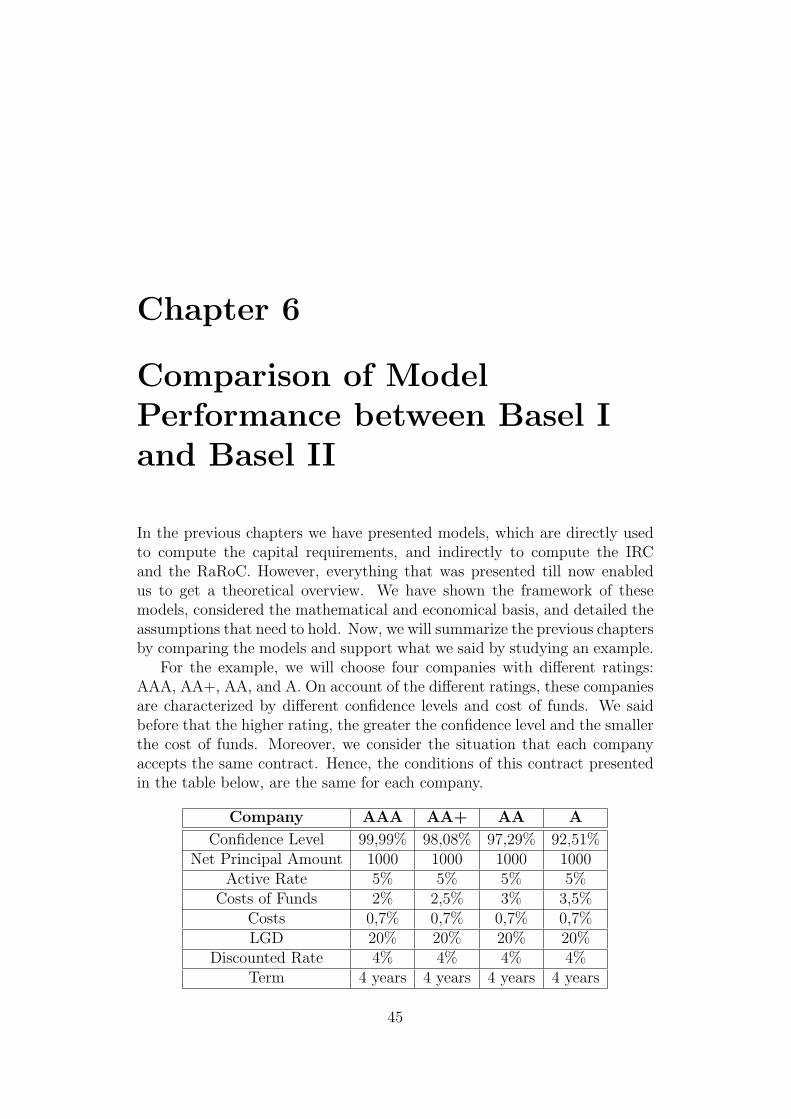
Chapter 6

Comparison of ModelPerformance between Basel Iand Basel II

In the previous chapters we have presented models, which are directly usedto compute the capital requirements, and indirectly to compute the IRCand the RaRoC. However, everything that was presented till now enabledus to get a theoretical overview. We have shown the framework of thesemodels, considered the mathematical and economical basis, and detailed theassumptions that need to hold. Now, we will summarize the previous chaptersby comparing the models and support what we said by studying an example.

For the example, we will choose four companies with different ratings:AAA, AA+, AA, and A. On account of the different ratings, these companiesare characterized by different confidence levels and cost of funds. We saidbefore that the higher rating, the greater the confidence level and the smallerthe cost of funds. Moreover, we consider the situation that each companyaccepts the same contract. Hence, the conditions of this contract presentedin the table below, are the same for each company.

Company AAA AA+ AA A

Confidence Level 99,99% 98,08% 97,29% 92,51%Net Principal Amount 1000 1000 1000 1000

Active Rate 5% 5% 5% 5%Costs of Funds 2% 2,5% 3% 3,5%

Costs 0,7% 0,7% 0,7% 0,7%LGD 20% 20% 20% 20%

Discounted Rate 4% 4% 4% 4%Term 4 years 4 years 4 years 4 years

45

Further, for each company we consider the variable PD to be in the range(0%, 25%).

According to definitions, the IRC and the RaRoC reflect the risk level.They are generally determined as the fraction of the cash flow and the capitalrequirements. Let us emphasize, that the IRC is less-risk adjusted.We said that both accords, the Basel I and the Basel II accord, provide thesame method of calculating the cash flow. Thus, it is obvious that as longas the input data are the same, the results are the same for all companies aswell.

Therefore, the difference between the IRC and the RaRoC is the after-math of the differences between the methods of computing the capital re-quirements.

The models, which are presented in this thesis, are commonly used toderive the capital requirements. For Basel I as well as Basel II, we showedhow to compute the amount of the required capital on the contract level andon the portfolio level as well. The approach for both accords is mainly thesame. The models consider the default and the loss as the random variables,determine the loss distribution and express the capital requirements as theαth percentile of this distribution. However, they do this in a different way,in particular, on the portfolio level.

Both models distinguish two types of risk: the market risk and the firm-specific risk, and they express the market asset value as the weighted averageof the market risk factor and the firm’s risk factor. By the assumption thatthese factors are normally distributed, it is guaranteed that the market assetvalue is normally distributed. But the ASRFM (provided by Basel II) re-quires, additionally, that the market asset value should have standard normaldistribution.Next, they model the probability of default based on the Merton model, whichassumes that the default occurs when the market asset value is smaller thanthe total debts. However, in the further computations, the model providedby Basel I uses the unconditional probability, whereas the ASFRM uses theconditional probability. Remember that the conditional probability is com-puted provided that we know the value of the market risk factor. In otherwords, when we know the situation of economy.

We said repeatedly that the capital requirements are kept to cover theunexpected loss. Depending on the ratings of the financial institutions, com-panies are obliged to hedge the contract to some extent, determined by theconfidence level. The general rule is that the lower rating, the smaller theconfidence level (but this is observed only in the Basel II accord). Accordingto the ASFRM model, the capital requirements depend on the quality of thefinancial institution, and this is reflected in the ECAP’s formula.

46

In comparison to Basel II, Basel I presents a poor assessment of the riskincurred. Due to lack of granularity within risk levels, the same contractsfrom different customers are treated the same. Hence, the model makes thecapital requirements on the contract level conditional only on the contract’scondition. On the portfolio level, Basel I continues with the same approach.Hence, on the portfolio level as well as on the contract level, Basel I requireshedging the contract with 8% of the outstanding amount of money.

Distinct from Basel I, Basel II proposed some changes on the portfoliolevel. First of all, it distinguishes between heterogenous and homogeneousportfolios. The methods of computations are adjusted to these two types ofportfolios. Moreover, instead of the loss distribution, for the heterogenousportfolio it considers the portfolio loss fraction distribution. However, for thehomogeneous portfolio the loss distribution is defined as the Bernoulli dis-tribution with k successes (k contracts went to default) with the conditionalprobability of default. The interpretation of the ECAP’s formula remainswithout changes.

In relation to the IRC and the RaRoC, Basel I and Basel II keep thesame methods of computation. Thus, the difference is caused only by thedifference in calculating the capital requirements.

Summarizing, we can conclude that the Basel Committee rightly made adecision about substituting the Basel I accord with the Basel II accord. Firstof all, Basel I almost did not take the risk into account, even though it is verysubstantial. Second, no distinction was made between the customers, despitethe fact that their risk profiles were significantly different. Besides, risk wasviewed on the contract level and not on the portfolio level. The risk-reducingeffects were only taken very marginally into account. Third, with referenceto the portfolio, Basel I did not take the correlation between the assets intoconsideration. Due to all these shortcomings, the results given by the BaselI model are not fully correct. Mainly, an accuracy of estimation depends onthe single contract and its characteristics.

In comparison to Basel I, Basel II presents a slightly different approach.It takes into account everything that was omitted in the Basel I Accord. Dueto that, the ASFRM and all models recommended by Basel II give betterestimate. It is very important for correctness of model, that the accuracy ofthe estimation depends on the model, not only on the single contract.By more possibilities for banks, they can adopt models to their needs. Itguarantees better results. Looking at that from the economic point of view,it is more profitable for banks. Banks can save more money, but from theother side they keep enough to cover unexpected losses.

47

Chapter 7

Conclusions

The Basel I and the Basel II are international agreements regulating gen-eral rules in the banking. In this thesis we have compared both of thesedocuments, more precisely, the models which were or are commonly used.Generally, these models give us the opportunity to compute the IRC andthe RaRoC, which are the tools to verify the decision about acceptation orrejection the contract.

Models were built up from the most simple case provided by the Basel Ito the complex case of a heterogenous portfolio with different exposure sizes.The last one was consistent with the Basel II convention and recommendedby the Basel Committee. As we said, the Basel II does not require frombanks using the same model. The banks can choose the model, which is themost adjusted to their needs.

For the sake of taken assumptions these models are not the most generalones. Namely, all models are one-factor models, what means that the marketrisk factor, which is taken into account is only one. However, it is alsopossible to consider the multi-factor models. The idea behind them is toreplace the random variable expressing the market risk factor by the randomvector. Then the dimension of the vector is equal to the number of themarket risk factors, and they are the coordinates of this vector. This ideahas very important advantage - it enables the application of the slightlymodified approach applied in the one-factor model. Therefore, we considerthe default and the loss as random variables, determine the loss distributionand express the capital requirements as the α percentile of this distribution.The method of computing the IRC and the RaRoC remains the same as well.

Due to comparison of the Basel I and the Basel II accord we could drawthe conclusions. Among them, the most important conclusion says thatindeed the Basel II presents the better approach. But even though it does notmake Basel II perfect. Basel II is better than Basel I, but still it bares several

48

disadvantages. The assumptions taken by the models are more restrictive,and because of that the models are less general. Hence, it will be developingby Basel Committee. But as long as correctness of Basel II is sufficient forall financial institutions, it will be commonly using by them.

49

Bibliography

[1] K. Aas, “The Basel II IRB approach for credit portfoilos: A survey”,Samba/33/05 , 2005.

[2] D. Bams, “Large Deal Pricing Tool”, Methodology document, De LageLanden International B.V., 2005.

[3] Basel Committee on Banking Supervision, “The new Basel Capital Ac-cord”, Consultative Document, 2001.

[4] Basel Committee on Banking Supervision, “An Explanatory Note on theBasel II IRB Risk Weight Functions”, Consultative Document, 2004a.

[5] Basel Committee on Banking Supervision, “International Convergence ofCapital Measurement and Capital Standards. A Revised Framework.”,Consultative Document, 2004b.

[6] P. Billingsley, “Probability and Measure”, third edition, New York: JohnWilley & Sons, 1995.

[7] L. Cathcart, L. El-Janel, “Multiple defaults and Merton’s model”, TanakaBusiness School Discussion Paper: TBS/DP04/12, London: Tanaka Busi-ness School, 2004.

[8] S. Emmer and D. Tasche, “Calculating credit risk capital charges withone-factor model”, Journal of Risk 6(1):59-92, 2003.

[9] C.C. Finger, “Conditional Approaches for CreditMetrics Portfolio Distri-butions”, CreditMetrics Monitor pp. 14-33, 1999.

[10] J.C. Garcia Cespedes, “Credit Risk Modelling and Basel II”, Algo Re-search Quarterly 5(1):57-66, 2002.

[11] M. Gordy, “A comparative anatomy of credit risk models”, Journal ofBanking and Finance 24:119-142, 2000.

50

[12] M. Gordy, “A risk-factor foundation for risk-based capital rules”, Jour-nal of Financial Intermediation 12:199-232, 2003.

[13] M. Gordy, “Granularity adjustment in portfolio credit risk measure-ment”, Risk Measures for the 21th Century edited by G. Szego, Wiley,2004.

[14] A. Hamerle, T.Liebig and D. Rosch “Credit Risk Factor Modelling andthe Basel II IRB Approach”, Discussion Paper Series 2: Banking andFinancial Supervision, No 02/2003, 2003.

[15] N.J.M. Honings, “Estimating Default Correlation for a Retail LeasePortfoilo”, Final Thesis, University of Maastricht, Faculty of Economicsand Business Administartion, 2004.

[16] K. Knopp, “Infinite Sequences and Series”, New York: Dover Publica-tions, 1956.

[17] R.C. Merton, “On the pricing of corporate debt: The risk structure ofinterest rates”, Journal of Finance 29:449-470, 1974.

[18] V.V. Petrov, “Limit Theorems of Probability Theory”, number 4, OxfordStudies in Probability Oxford University Press, 1995.

[19] M. Pykhtin and A. Dev, “Analytical approach to credit risk modelling”,RISK 15:26-32, 2002.

[20] P.J. Schonbucher, Factor Models for Portfolio Credit Risk , Working pa-per, University of Bonn, 2002a.

[21] P.J. Schonbucher, Taken to the limit: Simple and not-so-simple LoanLoss Distributions , Working paper, University of Bonn, 2002b.

[22] A.W. van der Vaart, “Financial Stochastics”, Lecture Notes, VU Ams-terdam, 2005.

[23] O.A. Vasicek, “The distribution of loan portfolio value”, RISK 15:160-162, 2002.

51

the basel i and basel ii accords: comparison of the models and

Documents